THE ALGEBRAIC EIGENVALUE
PROBLEM
BY
J. H. WILKINSON
M.A. (Cantab.), Sc.D., D.Tech., F.R.S.
CLARENDON PRESS • OXFORD
THE ALGEBRAIC EIGENVALUE
PROBLEM
BY
J. H. WILKINSON
M.A. (Cantab.), Sc.D., D.Tech., F.R.S.
CLARENDON PRESS • OXFORD
Oxford University Press, Walton Street, Oxford 0X2 6DP
Oxford New York Toronto
Delhi Bombay Calcutta Madras Karachi
Petaling Jaya Singapore Hong Kong Tokyo
Nairobi Dar es Salaam Cape Town
Melbourne Auckland
and associated companies in
Beirut Berlin Ibadan Nicosia
Oxford is a trade mark of Oxford University Press
Published in the United States
by Oxford University Press, New York
© Oxford University Press, 1965
First published 1965
Reprinted (with corrections) 1967, 1969, 1972, 1977, 1978
First published in paperback 1988
All rights reserved. No part of this publication may be reproduced,
stored in a retrieval system, or transmitted, in any form or by any
means, electronic, mechanical, photocopying, recording, or otherwise,
without the prior permission of Oxford University Press
This book is sold subject to the condition that it shall not, by way of
trade or otherwise, be lent, re-sold, hired out, or otherwise circulated
without the publisher’s prior consent in any form of binding or cover
other than that in which it is published and without a similar condition
including this condition being imposed on the subsequent purchaser
British Library Cataloguing in Publication Data
Wilkinson, J. H.
The algebraic eigenvalue problem.—
(Monographs on numerical analysis)
I. Matrices 2. Eigenvalues
I. Title II. Series
512.9'434 QAI93
ISBN 0-19-853418-3
Library of Congress Cataloging in Publication Data
Wilkinson, J. H. (James Hardy)
The algebraic eigenvalue problem.
(Monographs on numerical analysis)
Bibliography: p.
Includes index.
I. Equations—Numerical solutions. 2. Matrices.
3. Algebras, Linear. I. Title. II. Series.
QA218.W51988 512.9'4 87-2874
ISBN 0-19-853418-3
Printed in Great Britain
at the University Printing House, Oxford
by David Stanford
Printer to the University
Preface
The solution of the algebraic eigenvalue problem has for long had a
particular fascination for me because it illustrates so well the difference
between what might be termed classical mathematics and practical
numerical analysis. The eigenvalue problem has a deceptively simple
formulation and the background theory has been known for many
years; yet the determination of accurate solutions presents a wide
variety of challenging problems.
The suggestion that I might write a book on this topic in the series
of Monographs on Numerical Analysis was made by Professor L. Fox
and Dr. E. T. Goodwin after my early experience with automatic
digital computers. It is possible that its preparation would have
remained a pious aspiration had it not been for an invitation from
Professor J. W. Givens to attend a Matrix Symposium at Detroit in
1957 which led to successive invitations to lecture on ‘Practical
techniques for solving linear equations and computing eigenvalues
and eigenvectors’ at Summer Schools held in the University of
Michigan. The discipline of providing a set of notes each year for these
lectures has proved particularly valuable and much of the material
in this book has been presented during its formative stage in this way.
It was originally my intention to present a description of most of
the known techniques for solving the problem, together with a
critical assessment of their merits, supported wherever possible by the
relevant error analysis, and by 1961 a manuscript based on these lines
was almost complete. However, substantial progress had been made
with the eigenvalue problem and error analysis during the period in
which this manuscript was prepared and I became increasingly
dissatisfied with the earlier chapters. In 1962 I took the decision to
redraft the whole book with a modified objective. I felt that it was no
longer practical to cover almost all known methods and to give error
analyses of them and decided to include mainly those methods of
which I had extensive practical experience. I also inserted an
additional chapter giving fairly general error analyses which apply
to almost all the methods given subsequently. Experience over the
years had convinced me that it is by no means easy to give a
reliable assessment of a method without using it, and that often
comparatively minor changes in the details of a practical process have
a disproportionate influence on its effectiveness.
vi
PREFACE
The writer of a book on numerical analysis faces one particularly
difficult problem, that of deciding to whom it should be addressed.
A practical treatment of the eigenvalue problem is potentially of
interest to a wide variety of people, including among others, design
engineers, theoretical physicists, classical applied mathematicians
and numerical analysts who wish to do research in the matrix field.
A book which was primarily addressed to the last class of readers
might prove rather inaccessible to those in the first. I have not
omitted anything purely on the grounds that some readers might find
it too difficult, but have tried to present everything in as elementary
terms as the subject matter warrants. The dilemma was at its most
acute in the first chapter. I hope the elementary presentation used
there will not offend the serious mathematician and that he will treat
this merely as a rough indication of the classical material with which
he must be familiar if he is to benefit fully from the rest of the book.
I have assumed from the start that the reader is familiar with the
basic concepts of vector spaces, linear dependence and rank. An
admirable introduction to the material in this book is provided by
L. Fox’s ‘An introduction to numerical linear algebra’ (Oxford, this
series). Research workers in the field will find A. S. Householder’s
‘The theory of matrices in numerical analysis’ (Blaisdell, 1964) an
invaluable source of information.
My decision mentioned earlier to treat only those methods of which
I have extensive experience has inevitably resulted in the omission of
a number of important algorithms. Their omission is perhaps less
serious than it might have been, since the treatises by Durand,
‘Solutions num£riques des equations algebriques’ (Masson, 1960,1961)
and by D. K. Faddeev and V. N. Faddeeva, ‘Vycislitel’nye metody
lineinoi algebry’ (Moscow, 1963) give fairly extensive coverage.
However, two omissions call for special mention. The first is the
Jacobi-type method developed by P. J. Eberlein and various modi-
fications of this method developed independently by H. Rutishauser.
These seem to me to show exceptional promise and may well provide
the most satisfactory solution to the general eigenvalue problem.
I was reluctant to include them without first giving them the detailed
study which they deserve. My decision was reinforced by the reali-
zation that they are not directly covered by the general error analyses
I have given. The second omission is a general treatment of Rutis-
hauser’s QD algorithm. This is of very wide application and I did not
feel I could do full justice to this work within the restricted field of the
PREFACE
vii
eigenvalue problem. The reader is referred to papers by Rutishauser
and Henrici. The literature in the eigenvalue field is very extensive
and I have restricted the bibliography mainly to those papers to
which explicit reference is made in the text. Very detailed bibliog-
raphies are available in the books by Faddeev and Faddeeva and
Householder mentioned earlier.
When redrafting the book I was tempted to present the algorithms
in ALGOL, but decided that the difficulties of providing procedures
which were correct in every detail were prohibitive at this stage.
Accordingly I have used the language of classical mathematics but
have adopted a form of words which facilitates translation into
ALGOL and related computer languages.
The material for this book is drawn from many sources but I have
been particularly influenced by the work of colleagues at the Univer-
sity of Michigan Summer Schools, especially that of F. L. Bauer,
G. E. Forsythe, J. W. Givens, P. Henrici, A. S. Householder, 0.
Taussky, J. Todd and R. S. Varga. Apart from this it is the algo-
rithmic genius of H. Rutishauser which has been my main source of
inspiration.
It is a pleasure to acknowledge the assistance I have received from
numerous friends in this enterprise. I would like to thank Professors
J. W. Carr and R. C. F. Bartels for successive invitations to lecture at
the Summer Schools in Ann Arbor, thereby providing me with an
annual stimulus for completing the manuscript. I am particularly
indebted to Professors G. E. Forsythe and J. W. Givens who gen-
erously provided duplicating facilities for the two main drafts of
the manuscript. This has enabled me to benefit from the opinions of
a much wider circle of readers than would otherwise have been possible.
Many valuable comments were received from Professor G. E. For-
sythe, Dr. J. M. Varah and Mr. E. A. Albasiny. The whole of the
final manuscript was read by Dr. D. W. Martin and Professor L. Fox
and the first proofs by Dr. E. T. Goodwin. Their comments and sugges-
tions rescued me from numerous blunders and infelicities of style.
I am a notoriously poor proof reader and I was fortunate indeed to
have the expert guidance of Mrs. I. Goode in seeing the book through
the press. Finally sincere thanks are due to my wife who typed successive
versions of the manuscript. Without her patience and pertinacity the
project would almost certainly have foundered.
J. H. Wilkinson
Teddington, March, 1965

)
Contents
1. THEORETICAL BACKGROUND	Page
Introduction	1
Definitions	2
Eigenvalues and eigenvectors of the transposed matrix	3
Distinct eigenvalues	4
Similarity transformations	6
Multiple eigenvalues and canonical forms for general matrices	7
Defective system of eigenvectors	9
The Jordan (classical) canonical form	10
The elementary divisors	12
Companion matrix of the characteristic polynomial of A	12
Non-derogatory matrices	13
The Frobenius (rational) canonical form	15
Relationship between the Jordan and Frobenius canonical forms	16
Equivalence transformations	17
Lambda matrices	18
Elementary operations	19
Smith’s canonical form	19
The highest common factor of fc-rowed minors of а Л-matrix	22
Invariant factors of (A —XI)	22
The triangular canonical form	24
Hermitian and symmetric matrices	24
Elementary properties of Hermitian matrices	25
Complex symmetric matrices	26
Reduction to triangular form by unitary transformations	27
Quadratic forms	27
Necessary and sufficient conditions for positive definiteness	28
Differential equations with constant coefficients	30
Solutions corresponding to non-linear elementary divisors	31
Differential equations of higher order	32
Second-order equations of special form	34
Explicit solution of By — —Ay	35
Equations of the form (AB — XI )x = 0	35
The minimum polynomial of a vector	36
The minimum polynomial of a matrix	37
Cayley-Hamilton theorem	38
Relation between minimum polynomial and canonical forms	39
Principal vectors	42
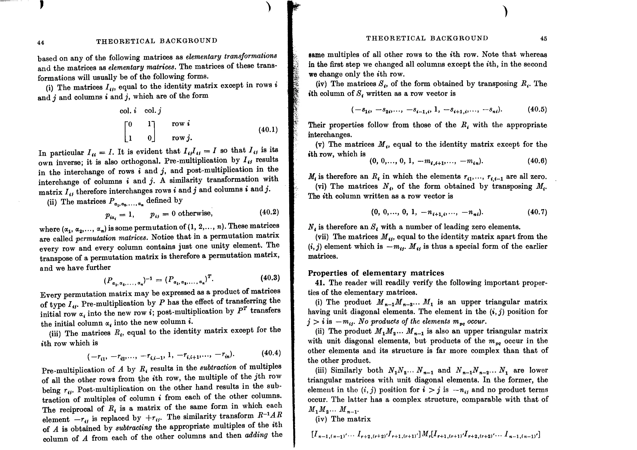
Elementary similarity transformations	43
Properties of elementary matrices	45
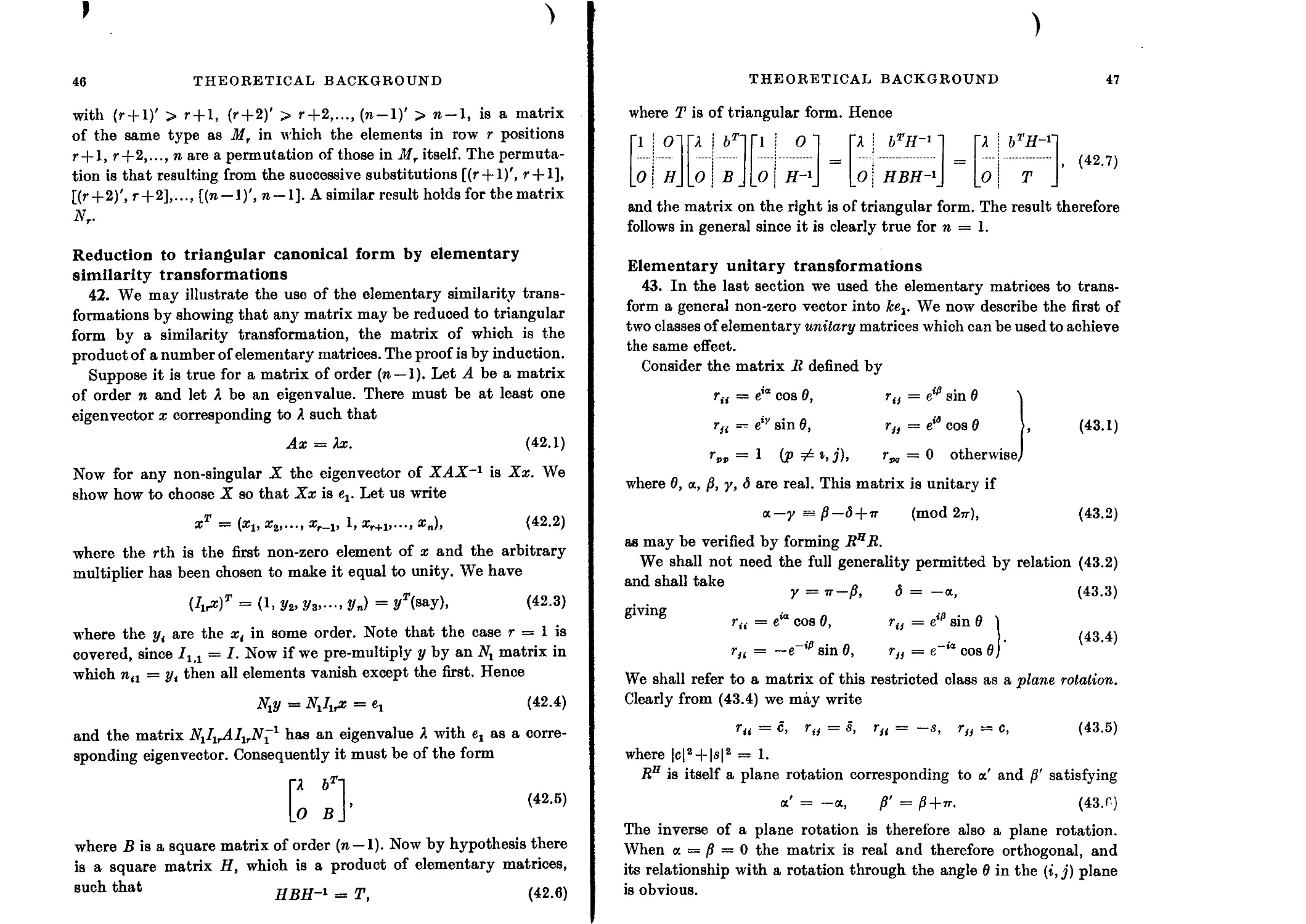
Reduction to triangular canonical form by elementary similarity
transformations	46
Elementary unitary transformations	47
Elementary unitary Hermitian matrices	48
Reduction to triangular form by elementary unitary transformations	50
Normal matrices	51
Commuting matrices	52
X
CONTENTS
Eigenvalues of AB	54
Vector and matrix norms	55
Subordinate matrix norms	56
The Euclidean and spectral norms	57
Norms and limits	58
Avoiding use of infinite matrix series	60
2.	PERTURBATION THEORY
Introduction	62
Ostrowski’s theorem on continuity of the eigenvalues	63
Algebraic functions	64
Numerical examples	65
Perturbation theory for simple eigenvalues	66
Perturbation of corresponding eigenvectors	67
Matrix with linear elementary divisors	68
First-order perturbations of eigenvalues	68
First-order perturbations of eigenvectors	69
Higher-order perturbations	70
Multiple eigenvalues	70
Gerschgorin’s theorems	71
Perturbation theory based on Gerschgorin’s theorems	72
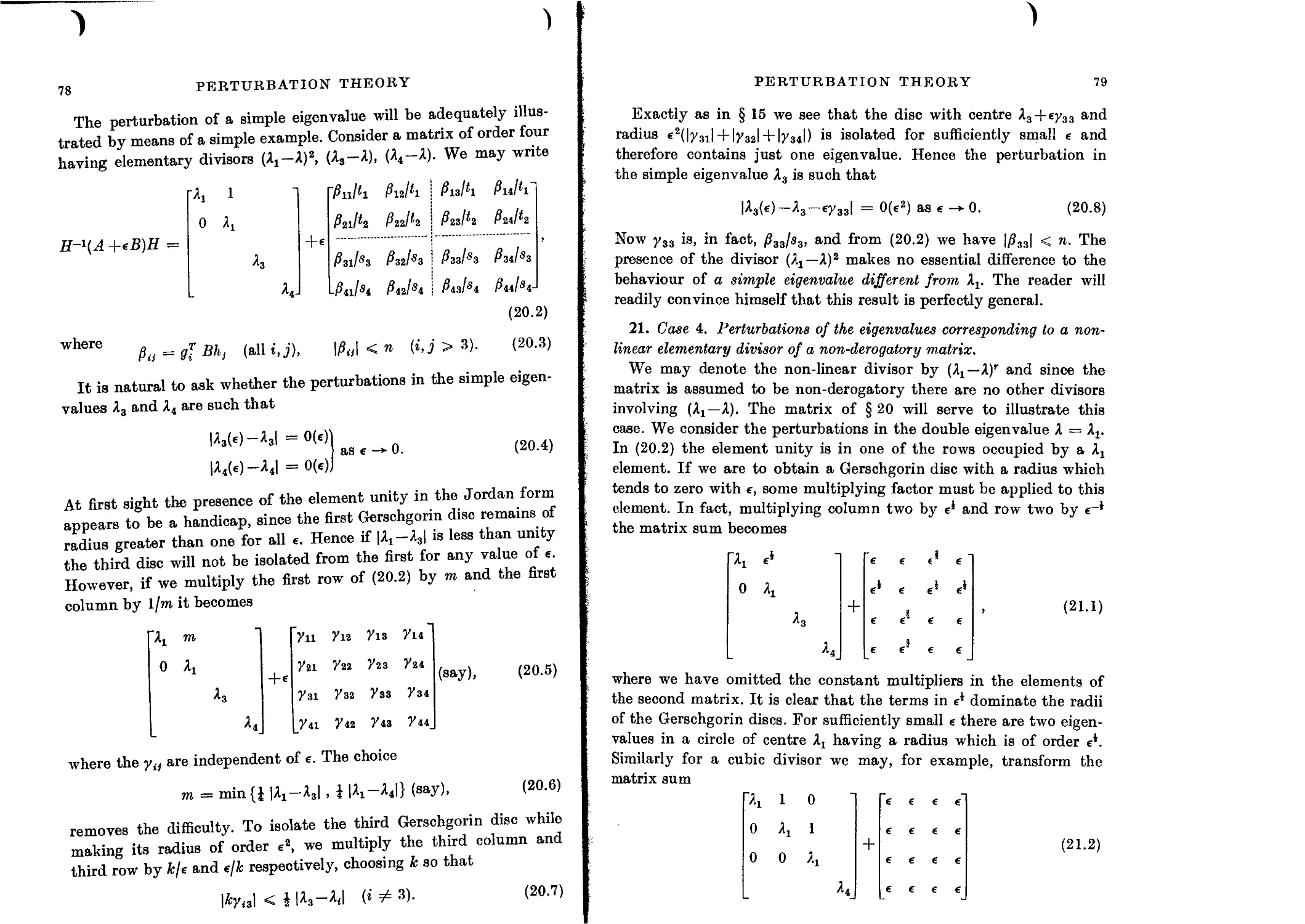
Case 1.	Perturbation of a simple eigenvalue of a matrix having linear
elementary divisors.	72
Case 2.	Perturbation of a multiple eigenvalue of a matrix having
linear elementary divisors.	75
Case 3.	Perturbation of a simple eigenvalue of a matrix having one or
more non-linear elementary divisors.	77
Case 4.	Perturbations of the eigenvalues corresponding to a non-linear
elementary divisor of a non-derogatory matrix.	79
Case 5.	Perturbations of eigenvalues Л,- when there is more than one
divisor involving (Л,- — Л) and at least one of them is non-linear.	80
Perturbations corresponding to the general distribution of non-linear
divisors	81
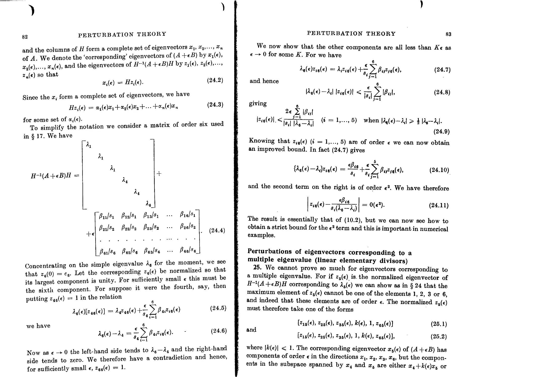
Perturbation theory for the eigenvectors from Jordan canonical form 81
Perturbations of eigenvectors corresponding to a multiple eigenvalue
(linear elementary divisors)	83
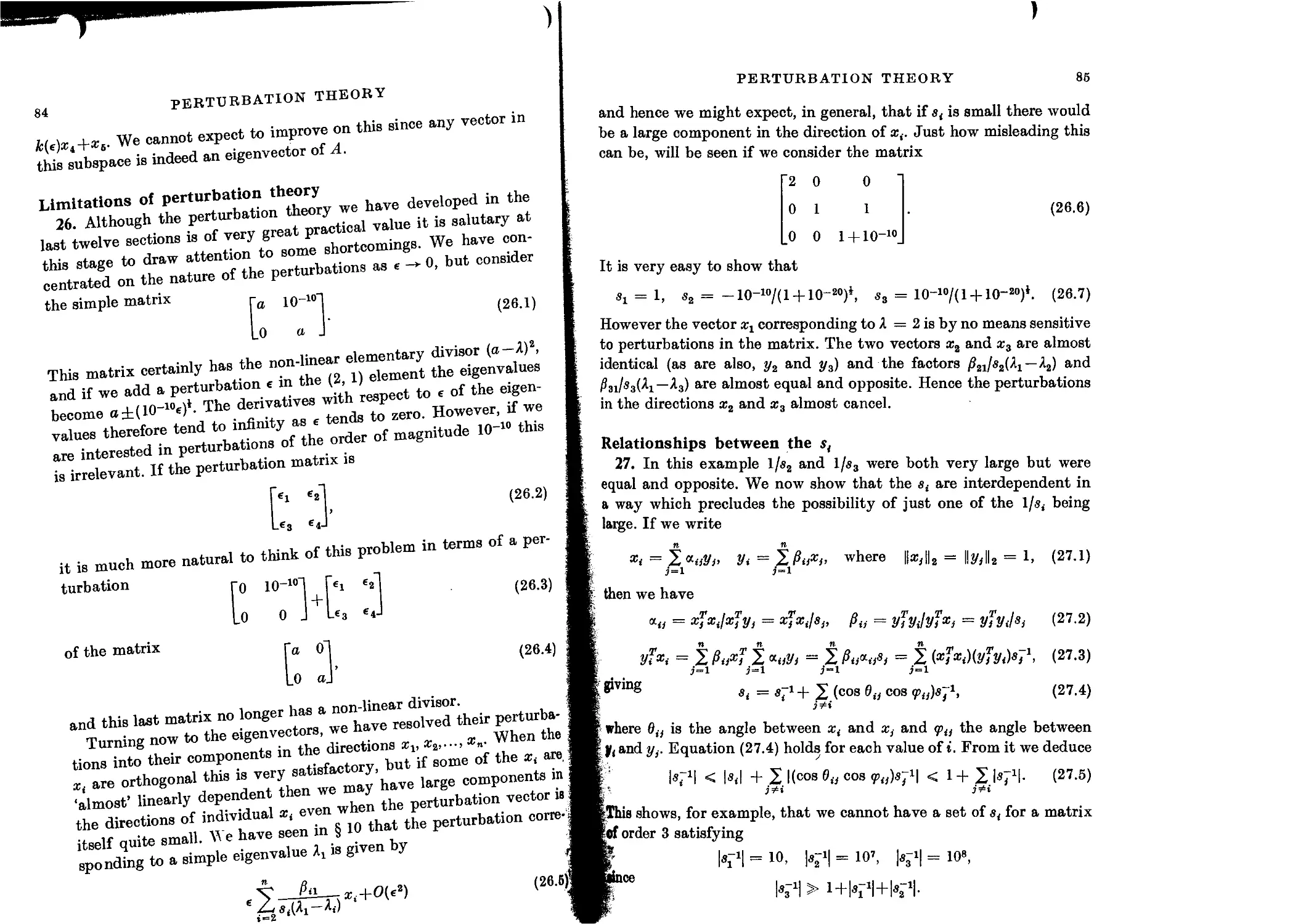
Limitations of perturbation theory	84
Relationships between the e(	85
The condition of a computing problem	86
Condition numbers	86
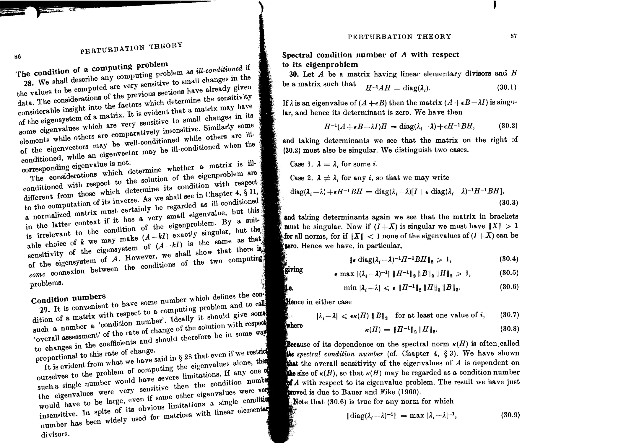
Spectral condition number of A with respect to its eigenproblem	87
Properties of spectral condition number	88
Invariant properties of condition numbers	89
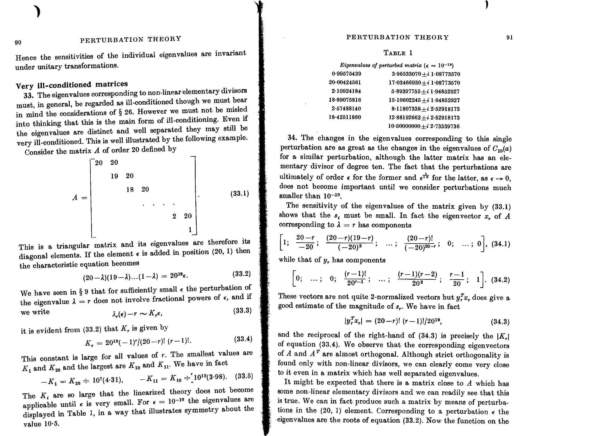
Very ill-conditioned matrices	90
Perturbation theory for real symmetric matrices	93
Unsymmetric perturbations	93
Symmetric perturbations	94
Classical techniques	94
Symmetric matrix of rank unity	97
Extremal properties of eigenvalues	98
Minimax characterization of eigenvalues	99
Eigenvalues of the sum of two symmetric matrices	101
CONTENTS	xi
Practical applications	102
Further applications of minimax principle	103
Separation theorem	103
The Wielandt-Hoffman theorem	104
3.	ERROR ANALYSIS
Introduction	110
Fixed-point operations	110
Accumulation of inner-products	111
Floating-point operations	112
Simplified expressions for error bounds	113
Error bounds for some basic floating-point computations	114
Bounds for norms of the error matrices	115
Accumulation of inner-products in floating-point arithmetic	116
Error bounds for some basic/Z2( ) computations	117
Computation of square roots	118
Block-floating vectors and matrices	119
Fundamental limitations of 2-digit computation	120
Eigenvalue techniques based on reduction by similarity transformations 123
Error analysis of methode based on elementary non-unitary trans-
formations	124
Error analysis of methods based on elementary unitary transformations 126
Superiority of the unitary transformation	128
Real symmetric matrices	129
Limitations of unitary transformations	129
Error analysis of floating-point computation of plane rotations	131
Multiplication by a plane rotation	133
Multiplication by a sequence of plane rotations	134
Error in product of approximate plane rotations	139
Errors in similarity transforms	140
Symmetric matrices	141
Plane rotations in fixed-point arithmetic	143
Alternative computation of sin в and cos 0	145
Pre-multiplication by an approximate fixed-point rotation	145
Multiplication by a sequence of plane rotations (fixed-point)	147
The computed product of an approximate set of plane rotations	148
Errors in similarity transformations	148
General comments on the error bounds	151
Elementary Hermitian matrices in floating-point	152
Error analysis of the computation of an elementary Hermitian matrix 153
Numerical example	156
Pre-multiplication by an approximate elementary Hermitian matrix	157
Multiplication by a sequence of approximate elementary Hermitians 160
Non-unitary elementary matrices analogous to plane rotations	162
Non-unitary elementary matrices analogous to elementary Hermitian
matrices	163
Pre-multiplication by a sequence of non-unitary matrices	165
A priori error bounds	166
Departure from normality	167
Simple examples	169
A posteriori bounds	170
A posteriori bounds for normal matrices	170
XU	CONTENTS
Rayleigh quotient	172
Error in Rayleigh quotient	173
Hermitian matrices	174
Pathologically close eigenvalues	176
Non-normal matrices	178
Error analysis for a complete eigensystem	180
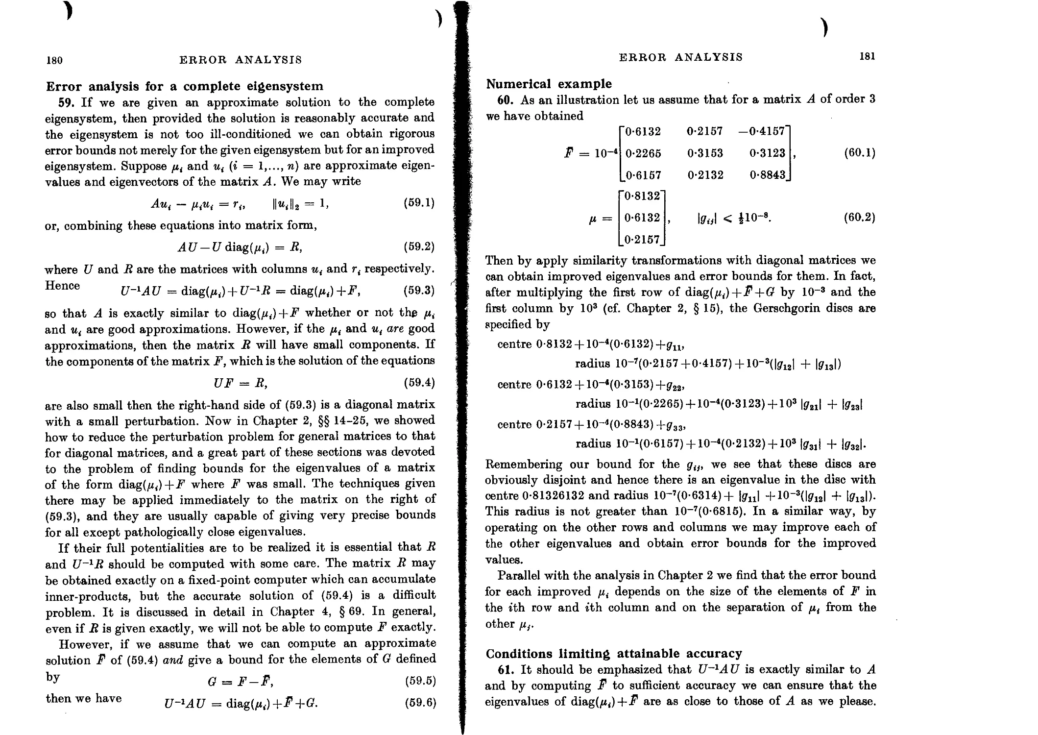
Numerical example	181
Conditions limiting attainable accuracy	181
Non-linear elementary divisors	182
Approximate invariant subspaces	184
Almost normal matrices	187
4.	SOLUTION OF LINEAR ALGEBRAIC EQUATIONS
Introduction	189
Perturbation theory	189
Condition numbers	191
Equilibrated matrices	192
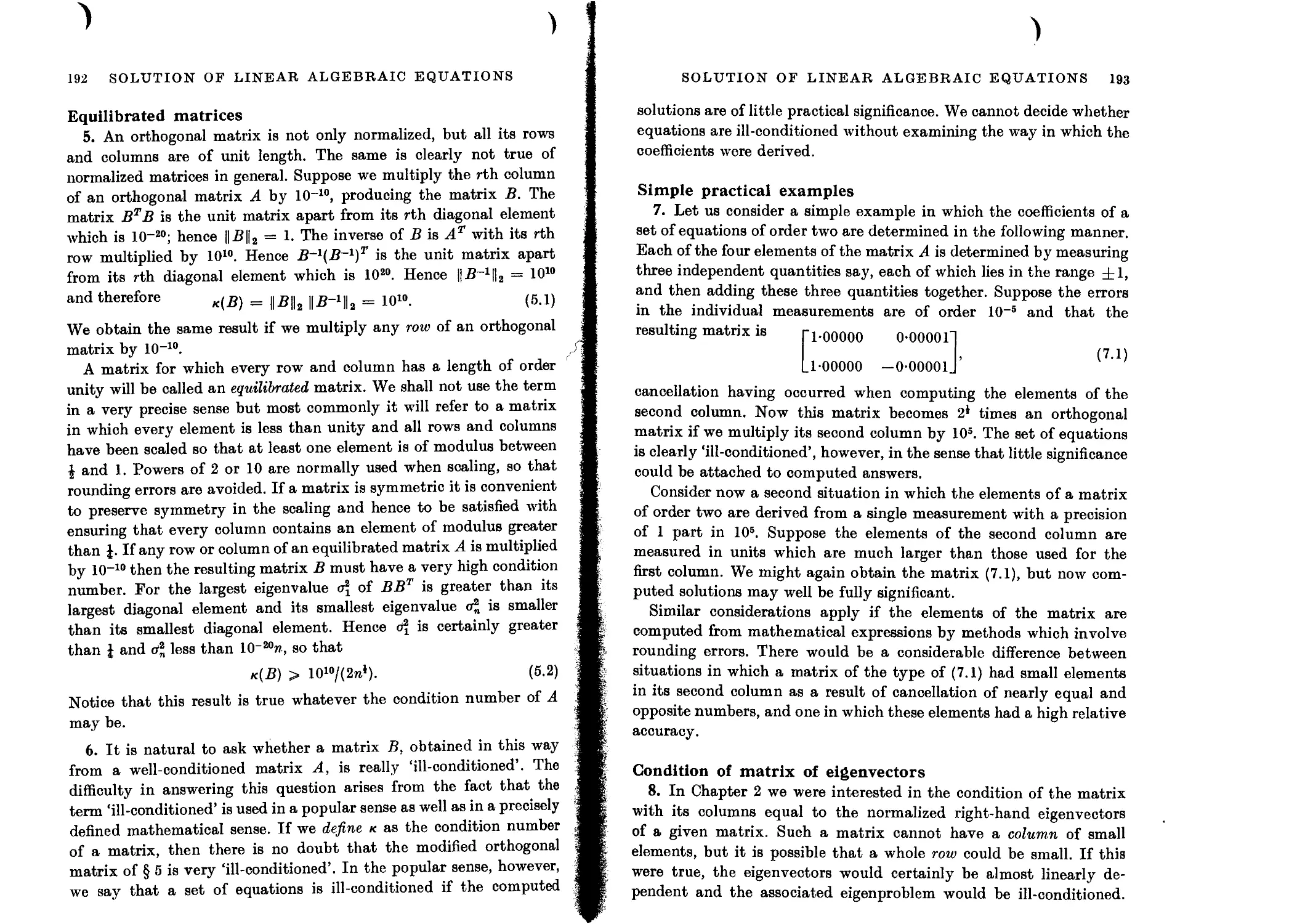
Simple practical examples	193
Condition of matrix of eigenvectors	193
Explicit solution	194
General comments on condition of matrices	195
Relation of ill-conditioning to near-singularity	196
Limitations imposed by /-digit arithmetic	197
Algorithms for solving linear equations	198
Gaussian elimination	200
Triangular decomposition	201
Structure of triangular decomposition matrices	201
Explicit expressions for elements of the triangles	202
Breakdown of Gaussian elimination	204
Numerical stability	205
Significance of the interchanges	206
Numerical example	207
Error analysis of Gaussian elimination	209
Upper bounds for the perturbation matrices using fixed-point arithmetic 211
Upper bound for elements of reduced matrices	212
Complete pivoting	212
Practical procedure with partial pivoting	214
Floating-point error analysis	214
Floating-point decomposition without pivoting	215
Loss of significant figures	217
A popular fallacy	217
Matrices of special form	218
Gaussian elimination on a high-speed computer	220
Solutions corresponding to different right-hand sides	221
Direct triangular decomposition	221
Relations between Gaussian elimination and direct triangular decom-
position	223
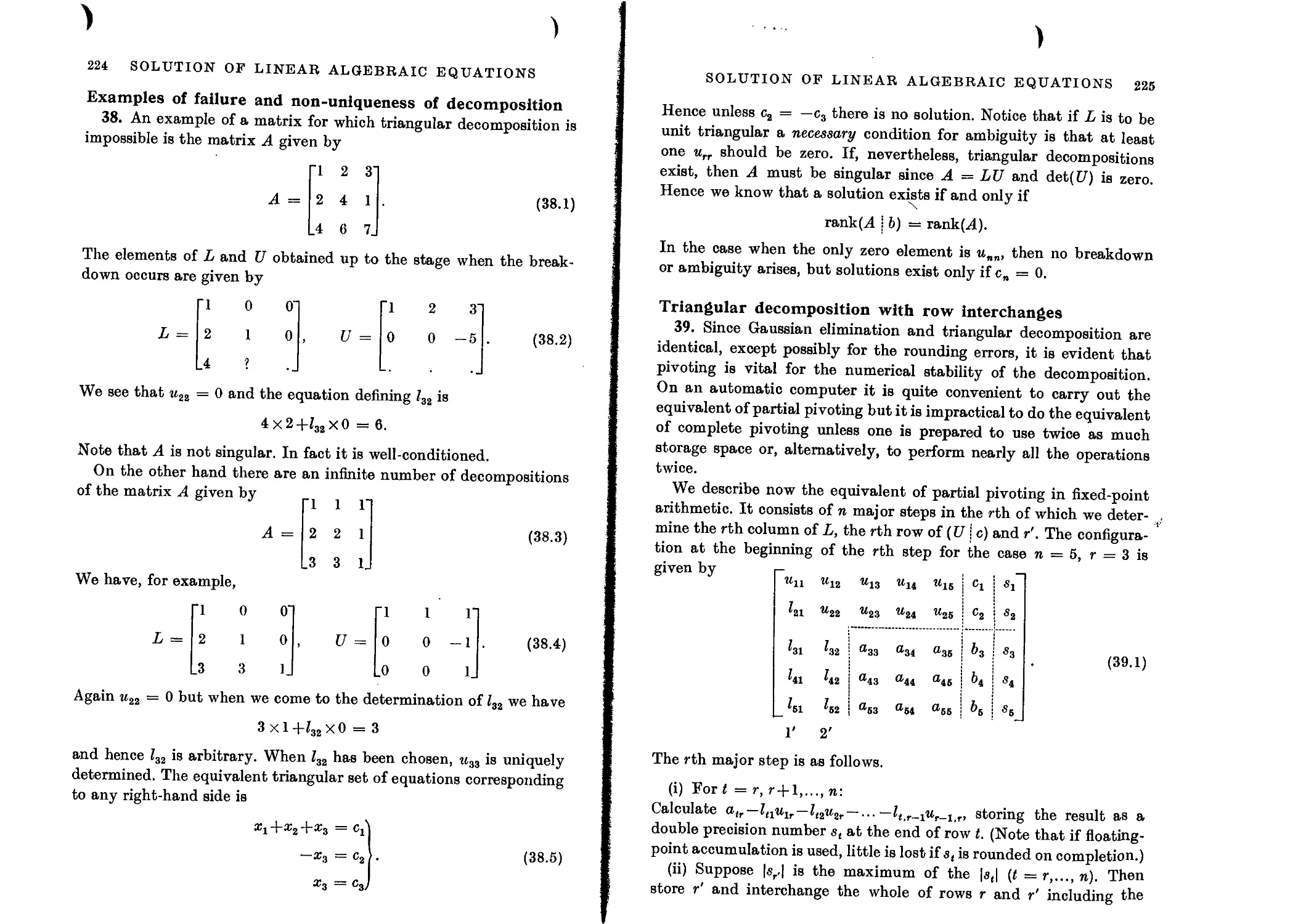
Examples of failure and non-uniqueness of decomposition	224
Triangular decomposition with row interchanges	225
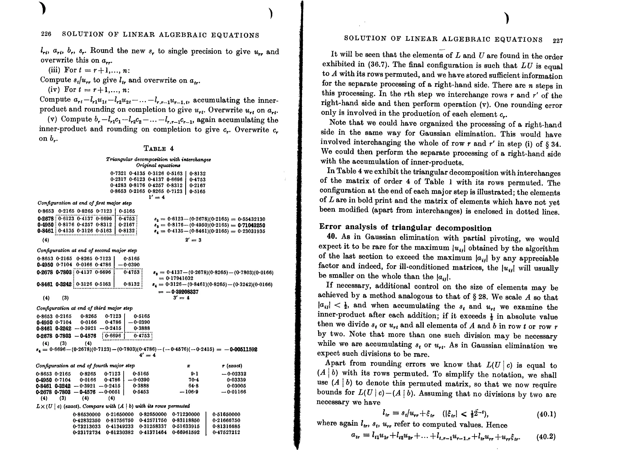
Error analysis of triangular decomposition	227
Evaluation of determinants	228
Cholesky decomposition	229
CONTENTS	xiii
Symmetric matrices which are not positive definite	230
Error analysis of Cholesky decomposition in fixed-point arithmetic	231
An ill-conditioned matrix	233
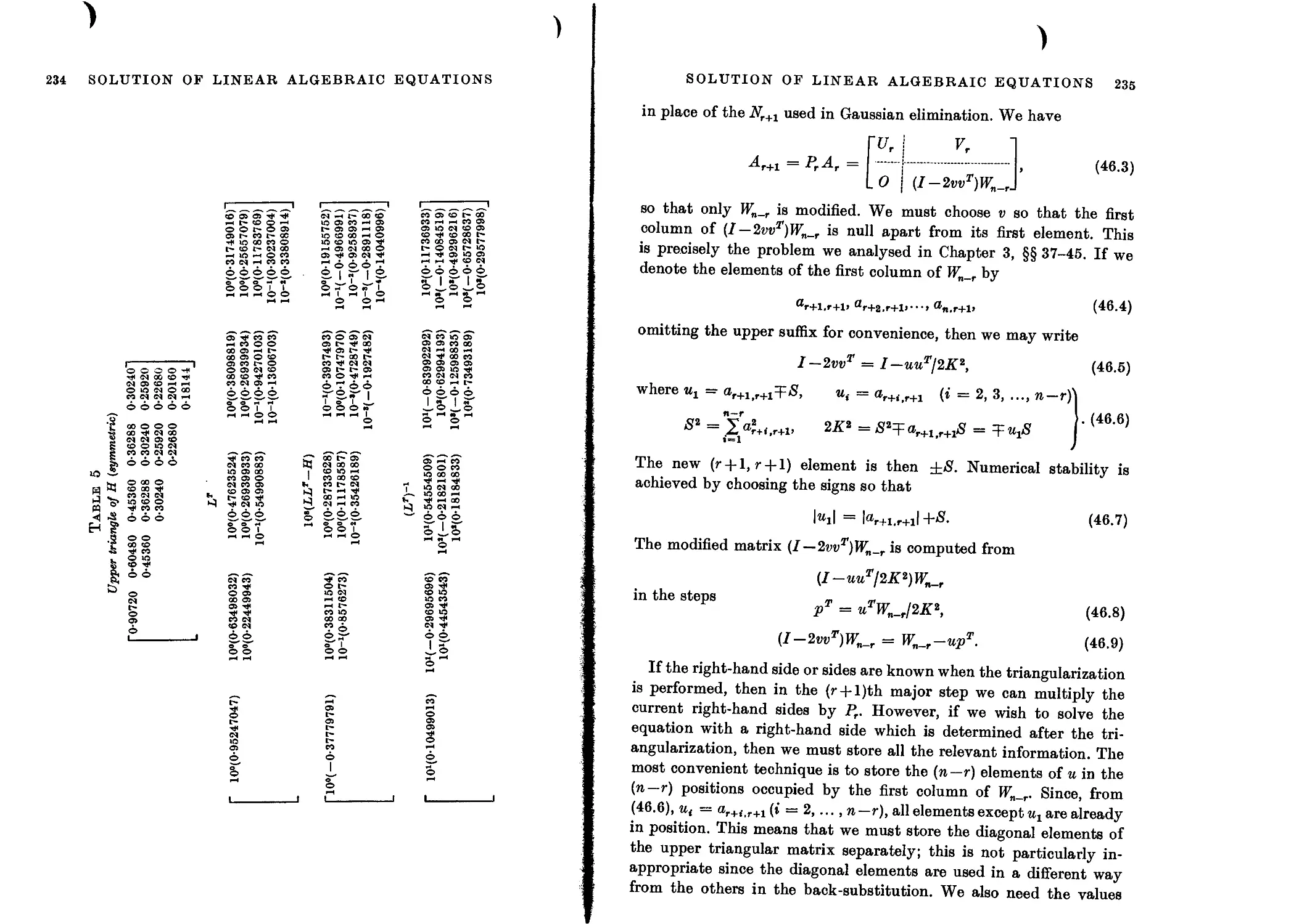
Triangularization using elementary Hermitian matrices	233
Error analysis of Householder triangularization	236
Triangularization by elementary stabilized matrices of the type M'u 236
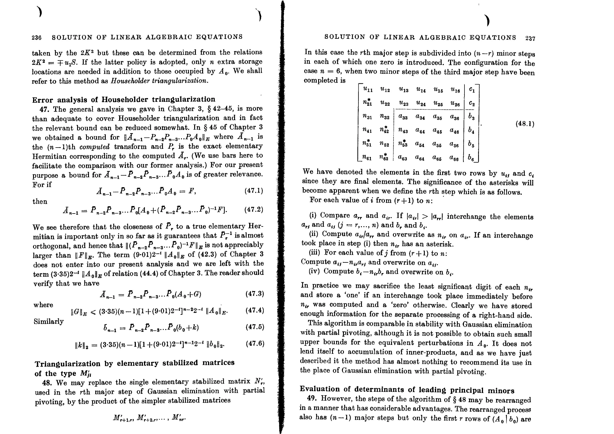
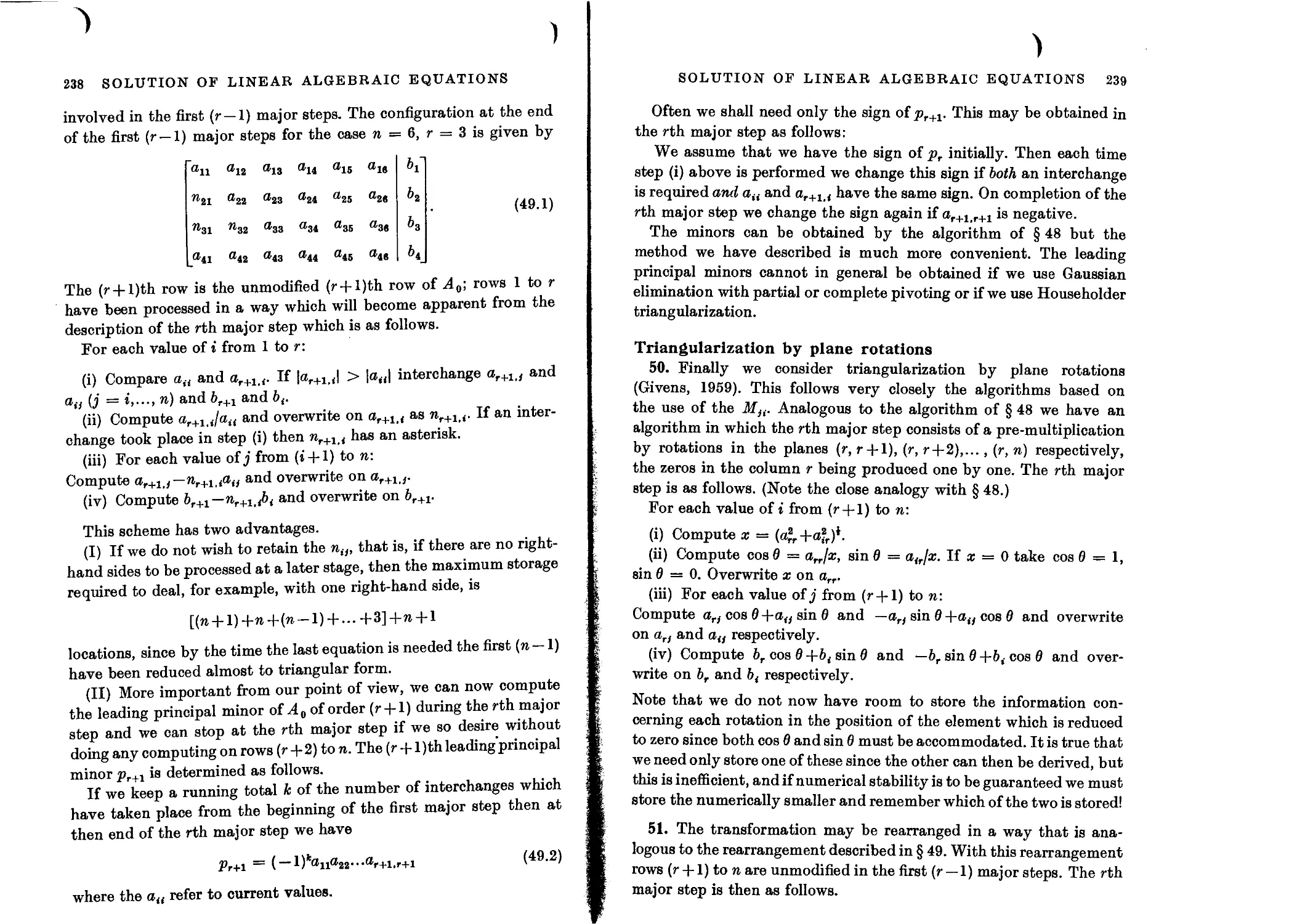
Evaluation of determinants of leading principal minors	237
Triangularization by plane rotations	239
Error analysis of Givens reduction	240
Uniqueness of orthogonal triangularization	241
Schmidt orthogonalization	242
Comparison of the methods of triangularization	244
Back-substitution	247
High accuracy of computed solutions of triangular sets of equations 249
Solution of a general spt of equations	251
Computation of the inverse of a general matrix	252
Accuracy of.computed solutions	253
Ill-conditioned matrices which give no small pivots	254
Iterative improvements of approximate solution	255
Effect of rounding errors on the iterative process	256
The iterative procedure in fixed-point computation	257
Simple example of iterative procedure	258
General comments on the iterative procedure	260
Related iterative procedures	261
Limitations of the iterative procedure	261
Rigorous justification of the iterative method	262
5.	HERMITIAN MATRICES
Introduction	265
The classical Jacobi method for real symmetric matrices	266
Rate of convergence	267
Convergence to fixed diagonal matrix	268
Serial Jacobi method	269
The Gerschgorin discs	269
Ultimate quadratic convergence of Jacobi methods	270
Close and multiple eigenvalues	271
Numerical examples	273
Calculation of cos 0 and sin 0	274
Simpler determination of the angles of rotation	276
The threshold Jacobi method	277
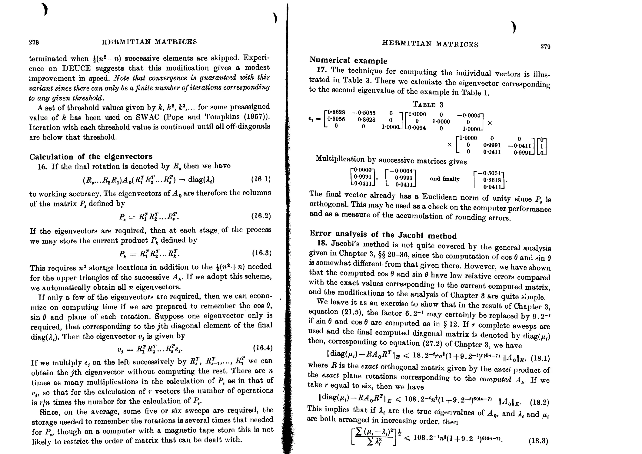
Calculation of the eigenvectors	278
Numerical example	279
Error analysis of the Jacobi method	279
Accuracy of the computed eigenvectors	280
Error bounds for fixed-point computation	281
Organizational problems	282
Givens’ method	282
Givens’ process on a computer with a two-level store	284
Floating-point error analysis of Givens’ process	286
Fixed-point error analysis	287
Numerical example	288
Householder’s method	290
xiv	CONTENTS
Taking advantage of symmetry	292
Storage considerations	293
Householder’s process on a computer with a two-level store	294
Householder’s method in fixed-point arithmetic	294
Numerical example	296
Error analyses of Householder’s method	297
Eigenvalues of a symmetric tri-diagonal matrix	299
Sturm sequence property	300
Method of bisection	302
Numerical stability of the bisection method	302
Numerical example	305
General comments on the bisection method	306
Small eigenvalues	307
Close eigenvalues and small	308
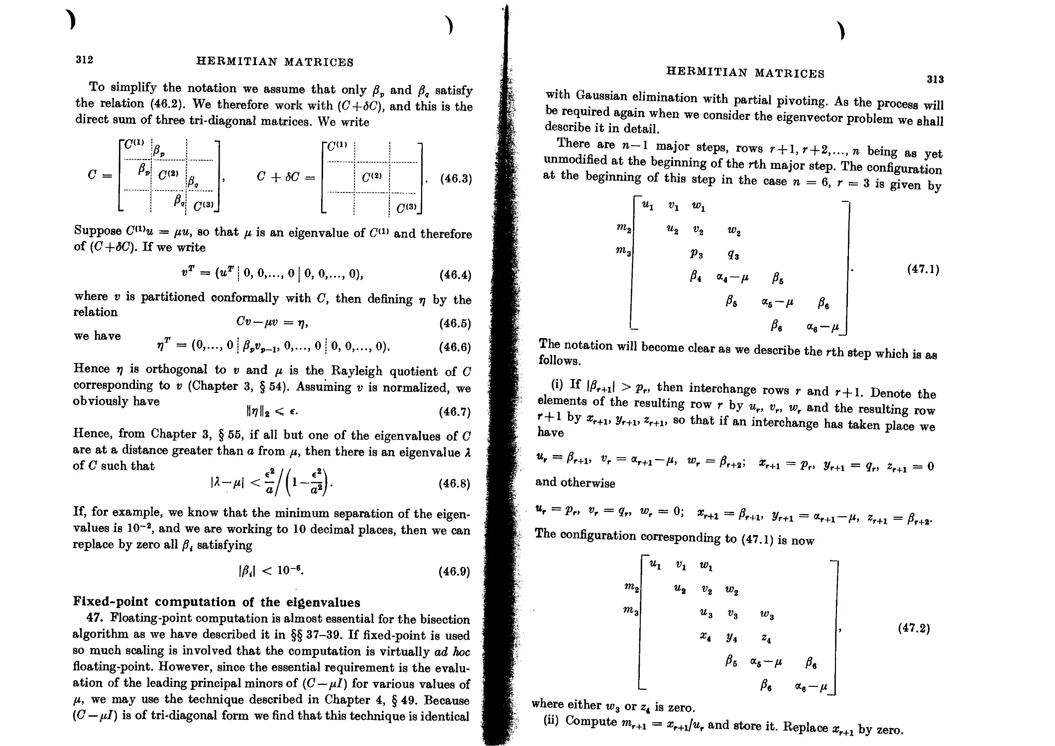
Fixed-point computation of the eigenvalues	312
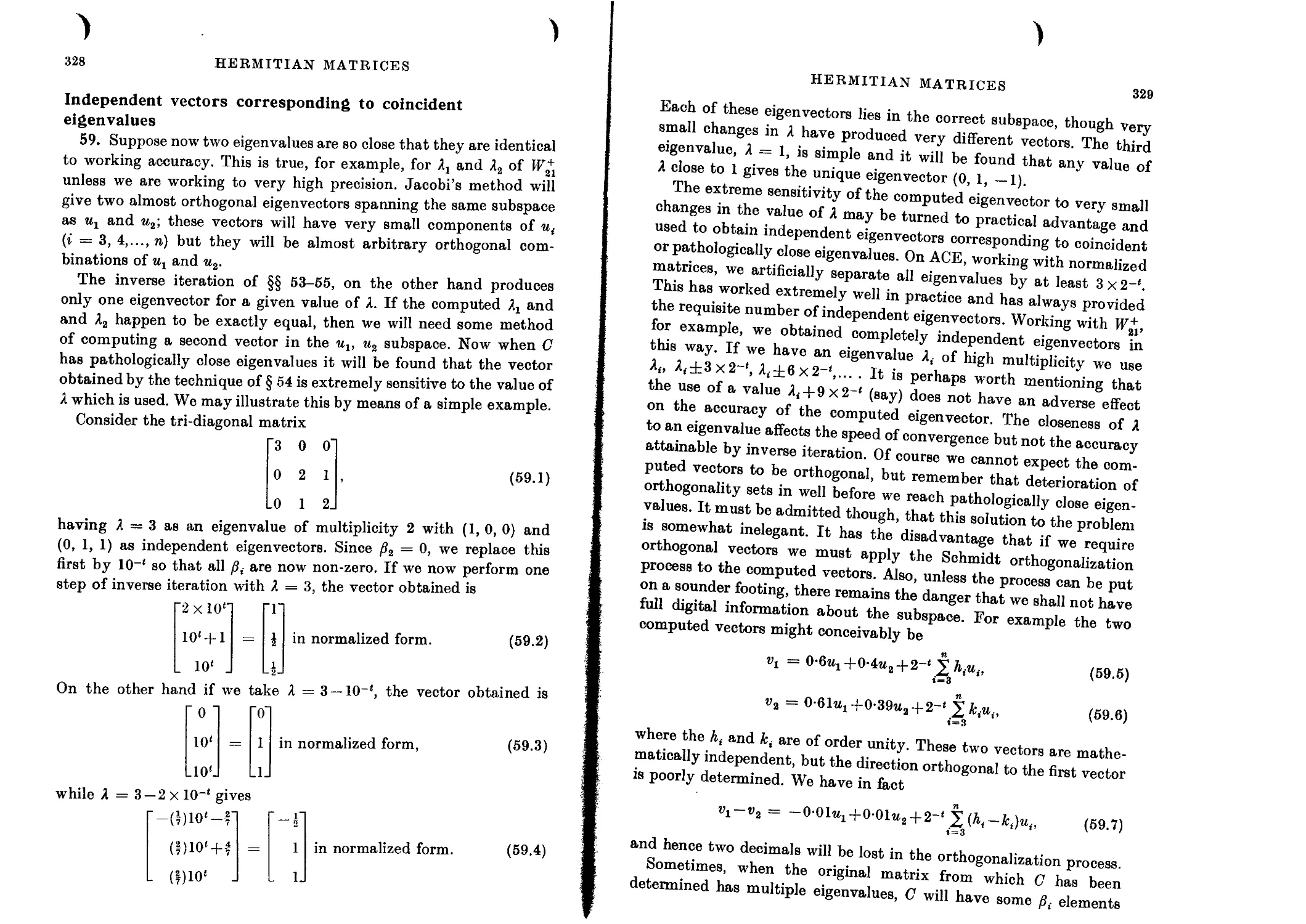
Computation of the eigenvectors of a tri-diagonal form	315
Instability of the explicit expression for the eigenvector	316
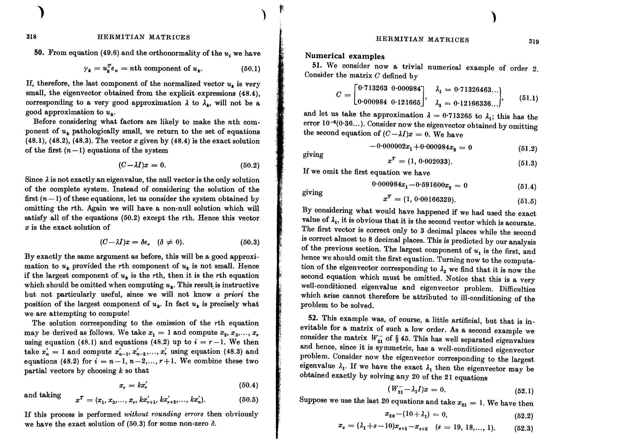
Numerical examples	319
Inverse iteration	321
Choice of initial vector b	322
Error analysis	323
Numerical example	325
Close eigenvalues and small	327
Independent vectors corresponding to coincident eigenvalues	328
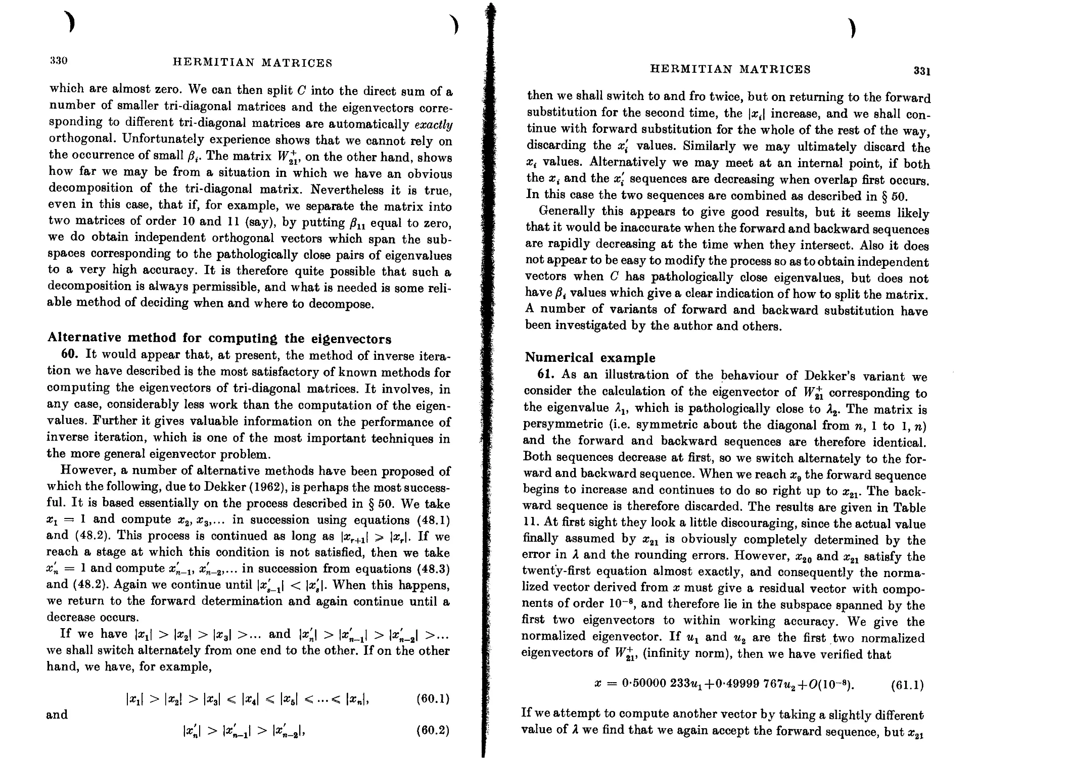
Alternative method for computing the eigenvectors	330
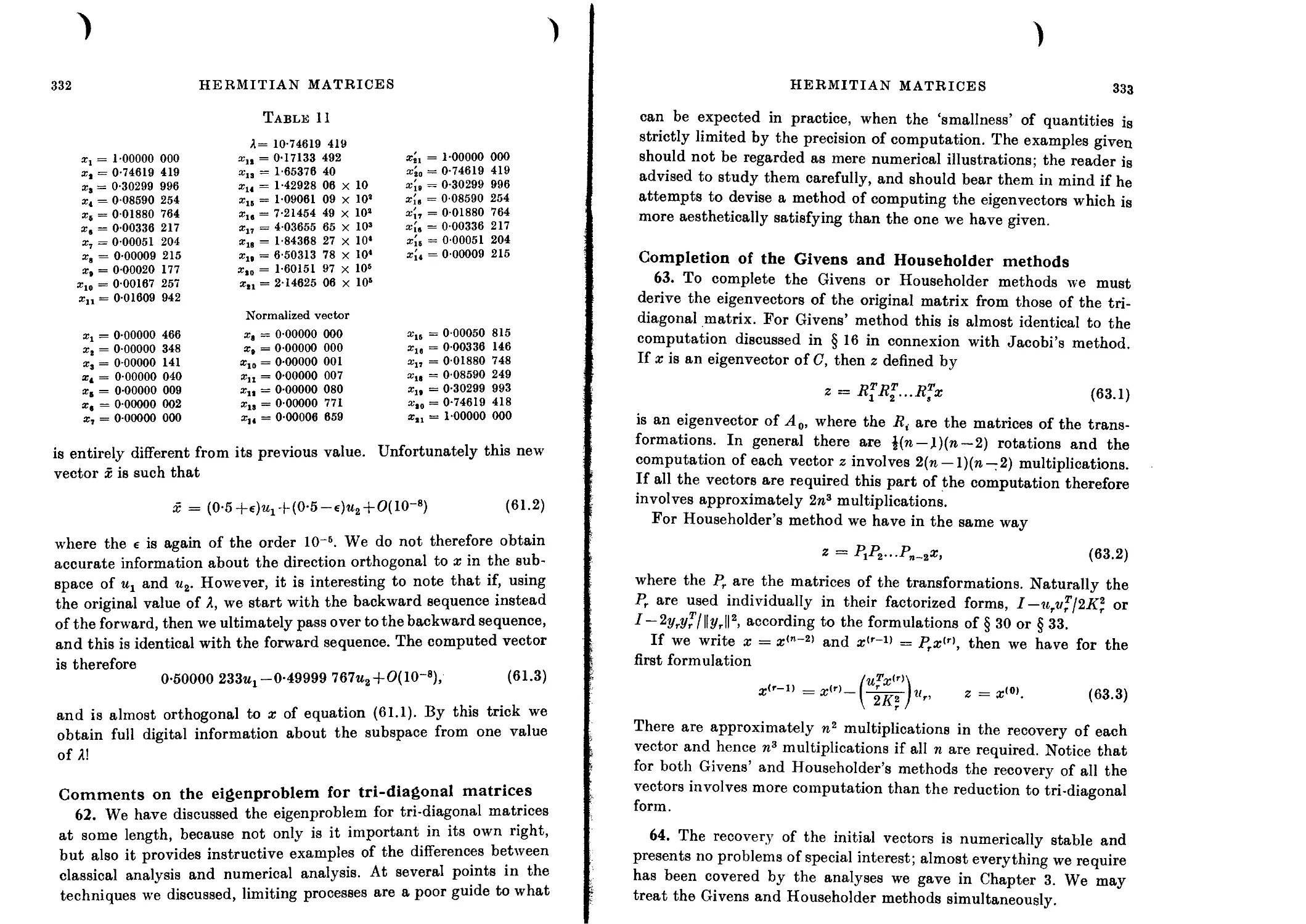
Numerical example	331
Comments on the eigenproblem for tri-diagonal matrices	332
Completion of the Givens and Householder methods	333
Comparison of methods	334
Quasi-symmetric tri-diagonal matrices	335
Calculation of the eigenvectors	336
Equations of the form Ax — S.Bx and ABx = Ле	337
Numerical example	339
Simultaneous reduction of A and В to diagonal form	340
Tri-diagonal A and В	340
Complex Hermitian matrices	342
6.	REDUCTION OF A GENERAL MATRIX TO CONDENSED
FORM
Introduction	345
Givens’ method	345
Householder’s method	347
Storage considerations	350
Error analysis	350
Relationship between the Givens and Householder methods	351
Elementary stabilized transformations	353
Significance of the permutations	355
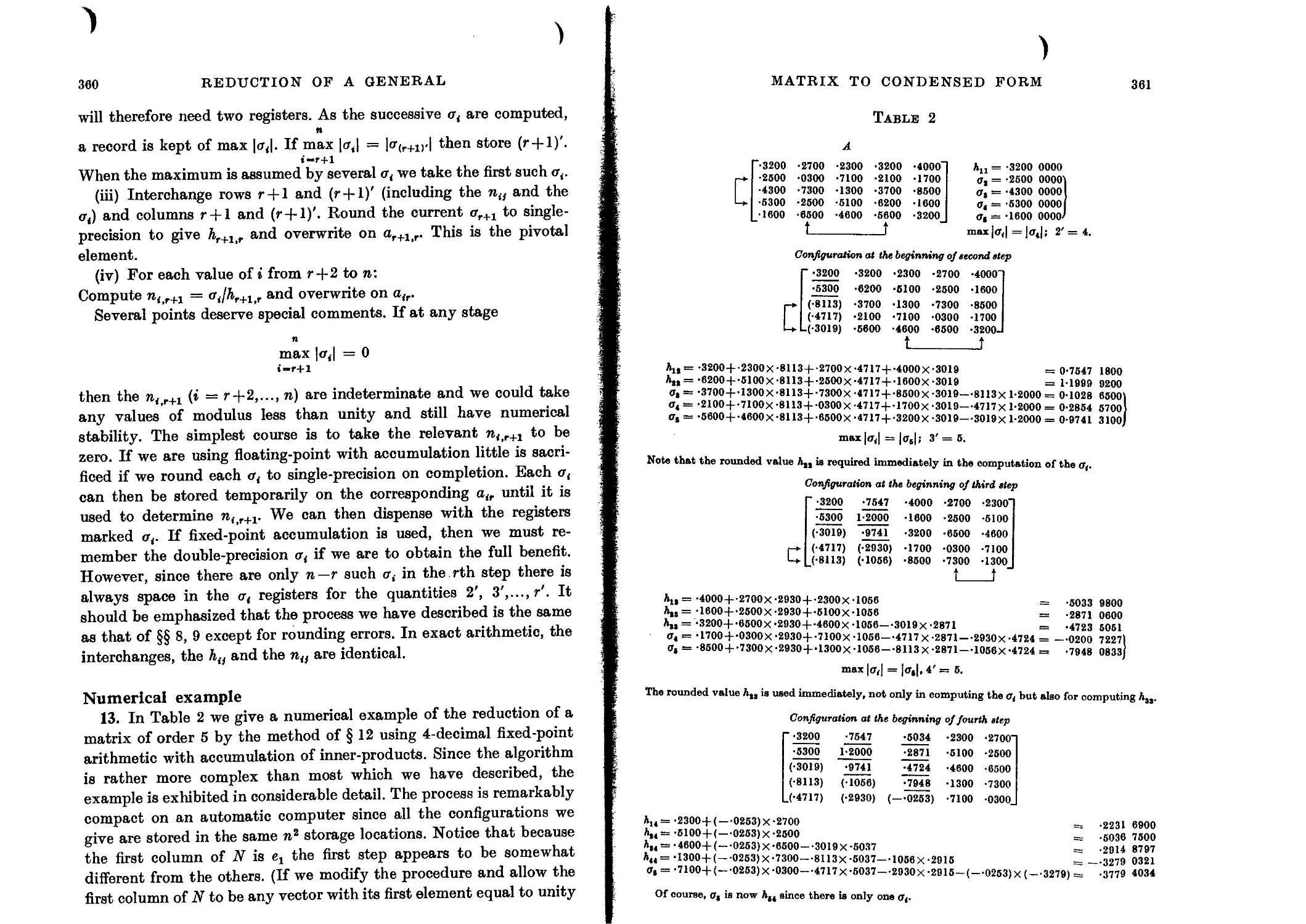
Direct reduction to Hessenberg form	357
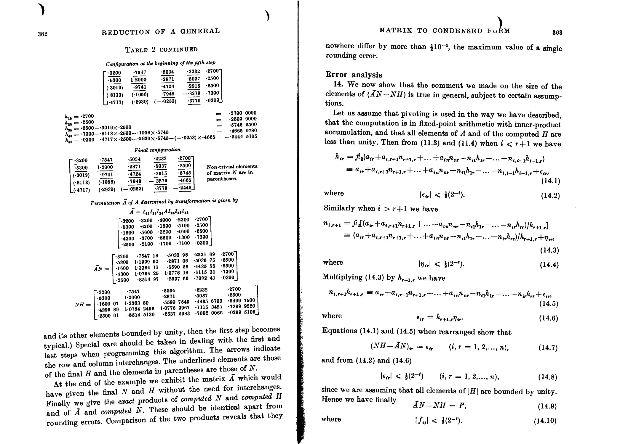
Incorporation of interchanges	359
Numerical example	360
Error analysis	363
Related error analyses	365
CONTENTS	xv
Poor determination of the Hessenberg matrix	368
Reduction to Hessenberg form using stabilized matrices of the type M'jt 368
The method of Krylov	369
Gaussian elimination by columns	370
Practical difficulties	371
Condition of C for some standard distributions of eigenvalues	372
Initial vectors of grade less than n	374
Practical experience	376
Generalized Hessenberg processes	377
Failure of the generalized Hessenberg process	378
The Hessenberg method	379
Practical procedure	380
Relation between the Hessenberg method and earlier methods	381
The method of Amoldi	382
Practical considerations	383
Significance of re-orthogonalization	385
The method of Lanczos	388
Failure of procedure	389
Numerical example	390
The practical Lanczos process	391
Numerical example	392
General comments on the unsymmetric Lanczos process	394
The symmetric Lanczos process	394
Reduction of a Hessenberg matrix to a more compact form	395
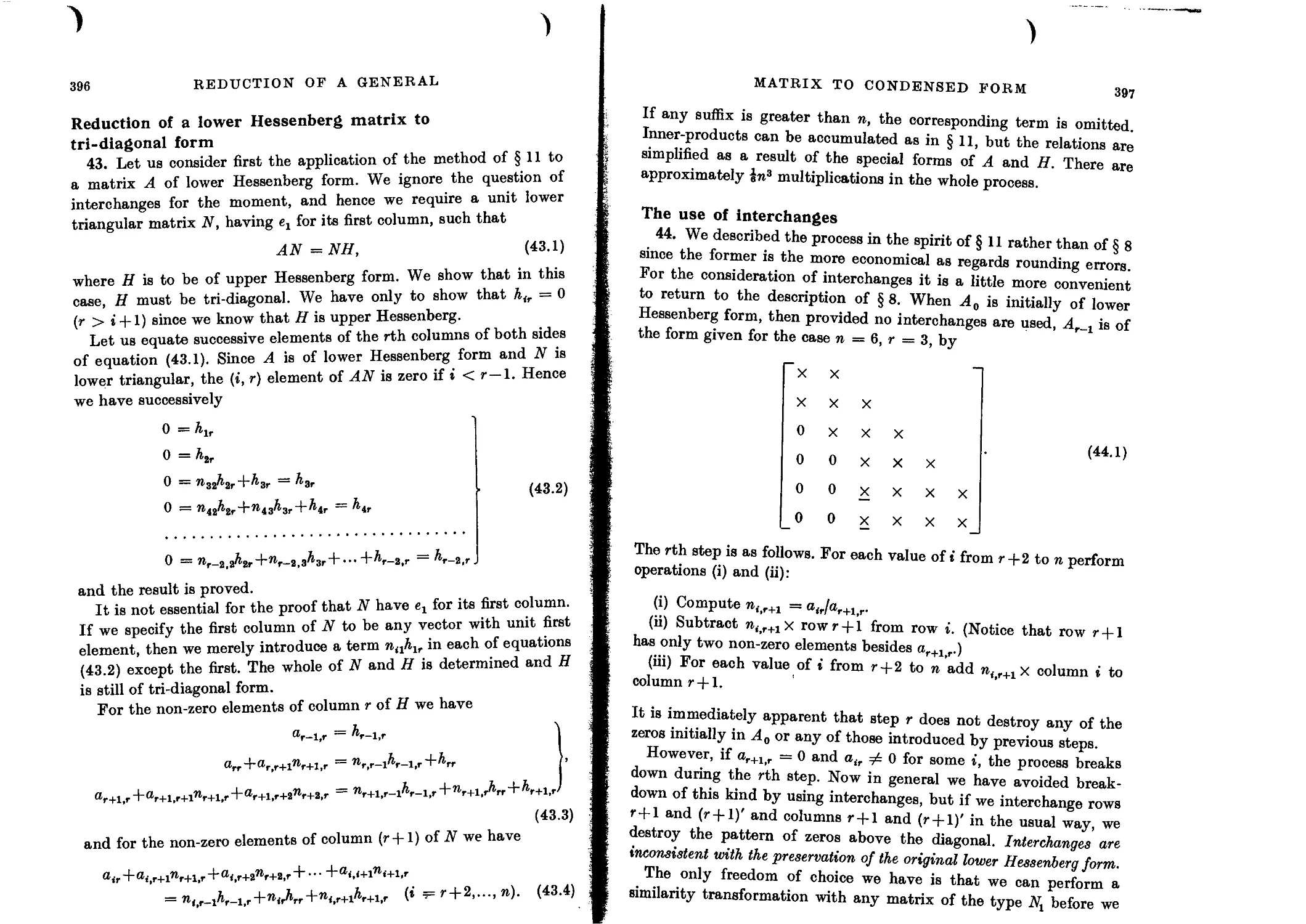
Reduction of a lower Hessenberg matrix to tri-diagonal form	396
The use of interchanges	397
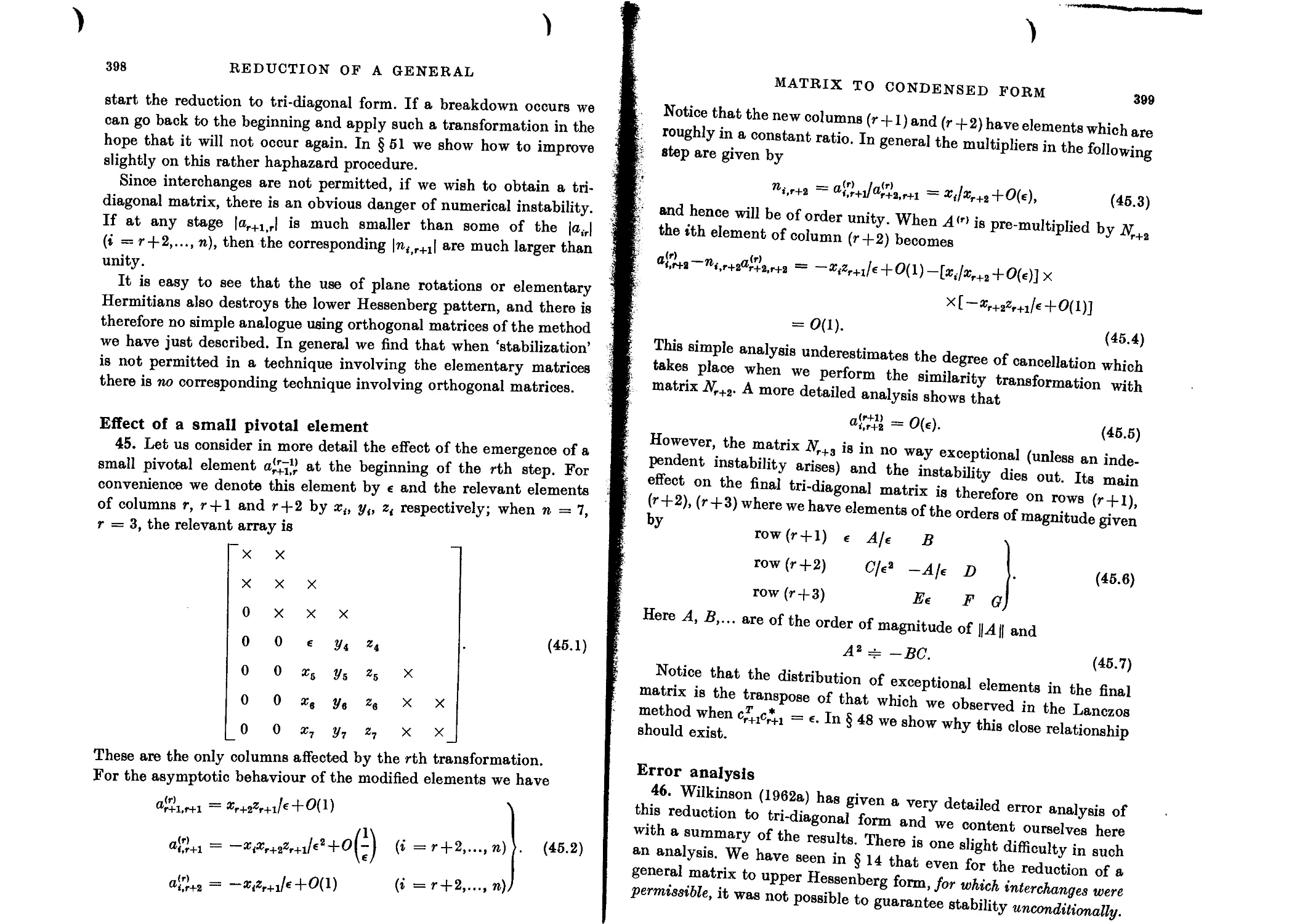
Effect of a small pivotal element	398
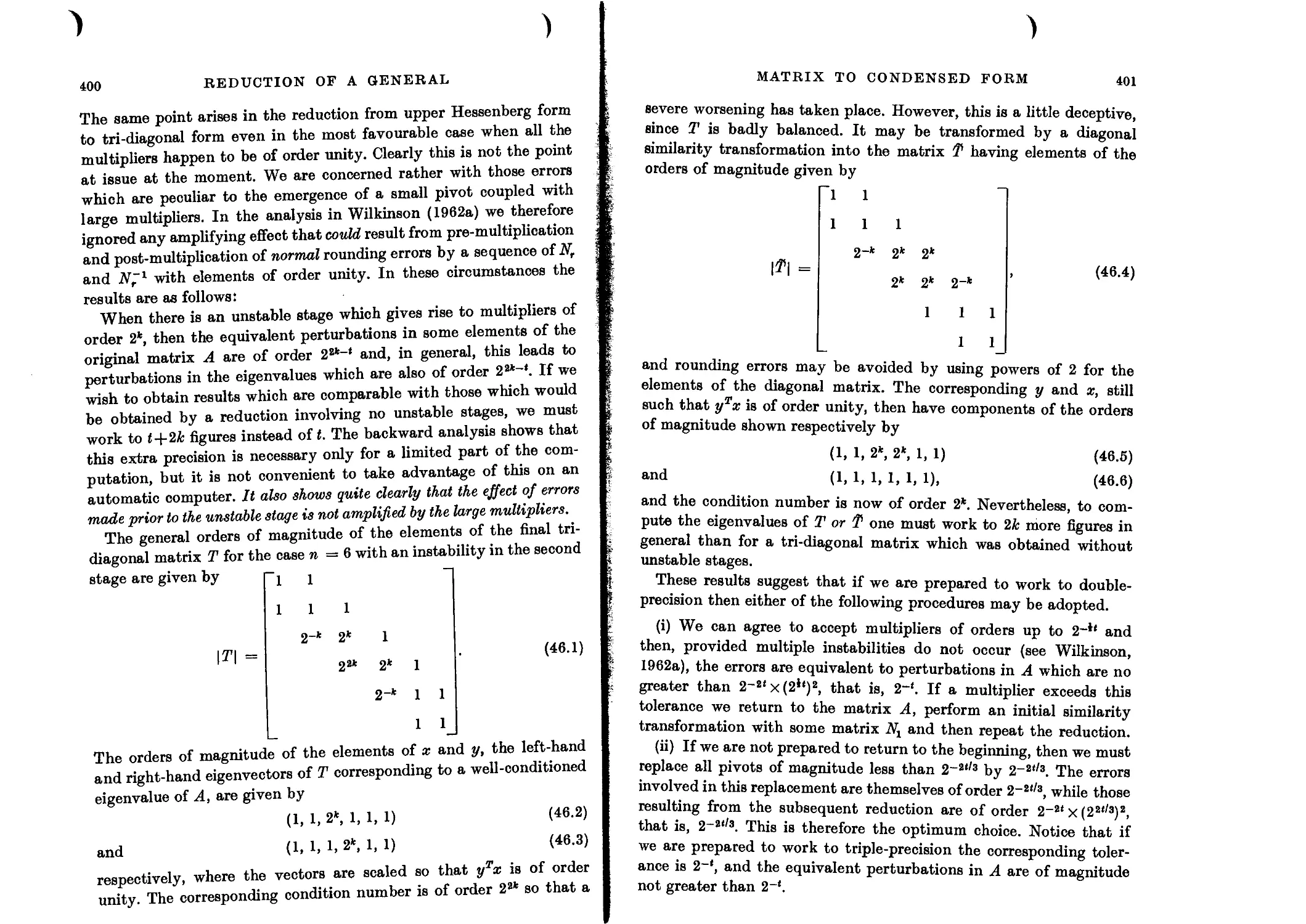
Error analysis	399
The Hessenberg process applied to a lower Hessenberg matrix	402
Relationship between the Hessenberg process and the Lanczos process 402
Reduction of a general matrix to tri-diagonal	form	403
Comparison with Lanczos method	404
Re-examination of reduction to tri-diagonal form	404
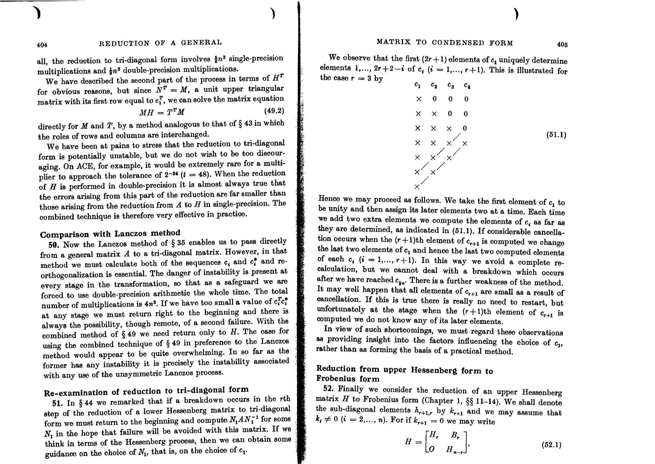
Reduction from upper Hessenberg form to Frobenius form	405
Effect of small pivot	407
Numerical example	408
General comments on the stability	408
Specialized upper Hessenberg form	409
Direct determination of the characteristic polynomial	410
7.	EIGENVALUES OF MATRICES OF CONDENSED FORMS
Introduction	413
Explicit polynomial form	413
Condition numbers of explicit polynomials	416
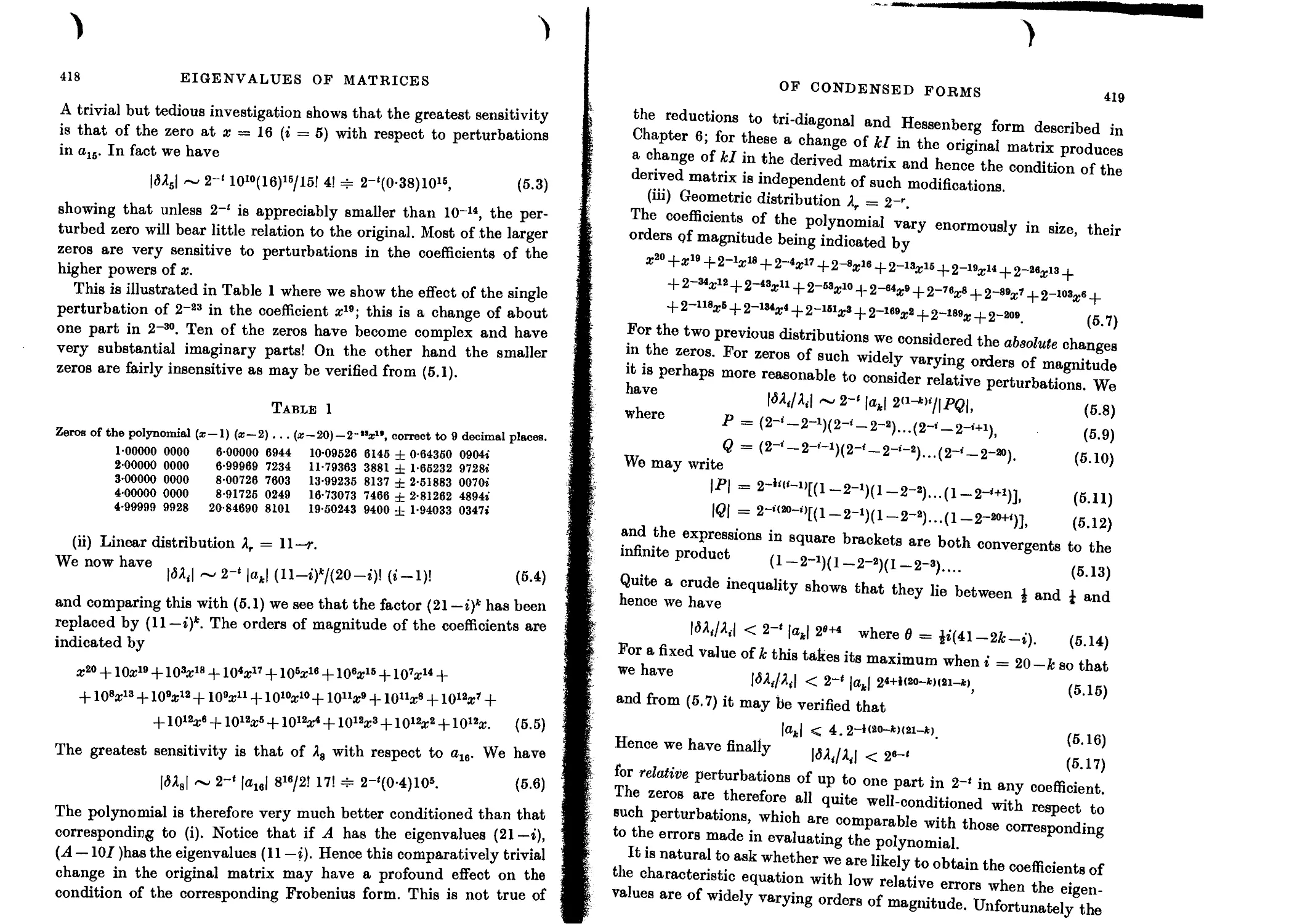
Some typical distributions of zeros	417
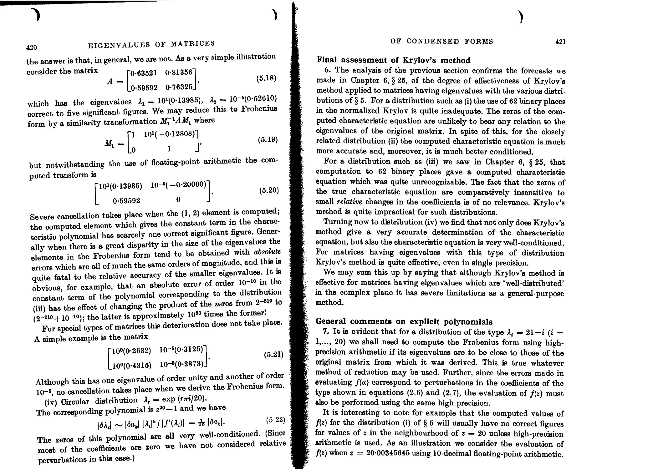
Final assessment of Krylov’s method	421
General comments on explicit polynomials	421
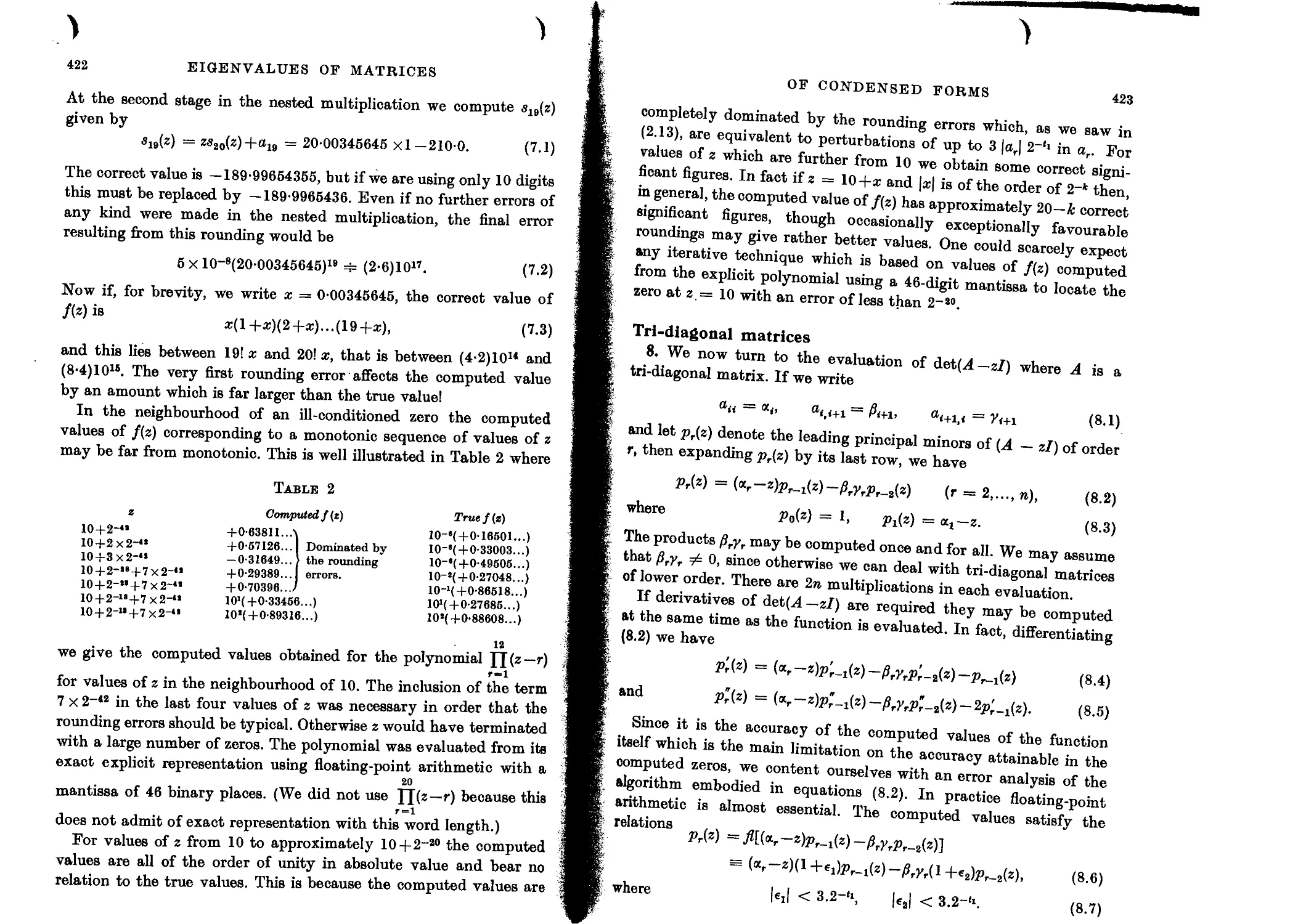
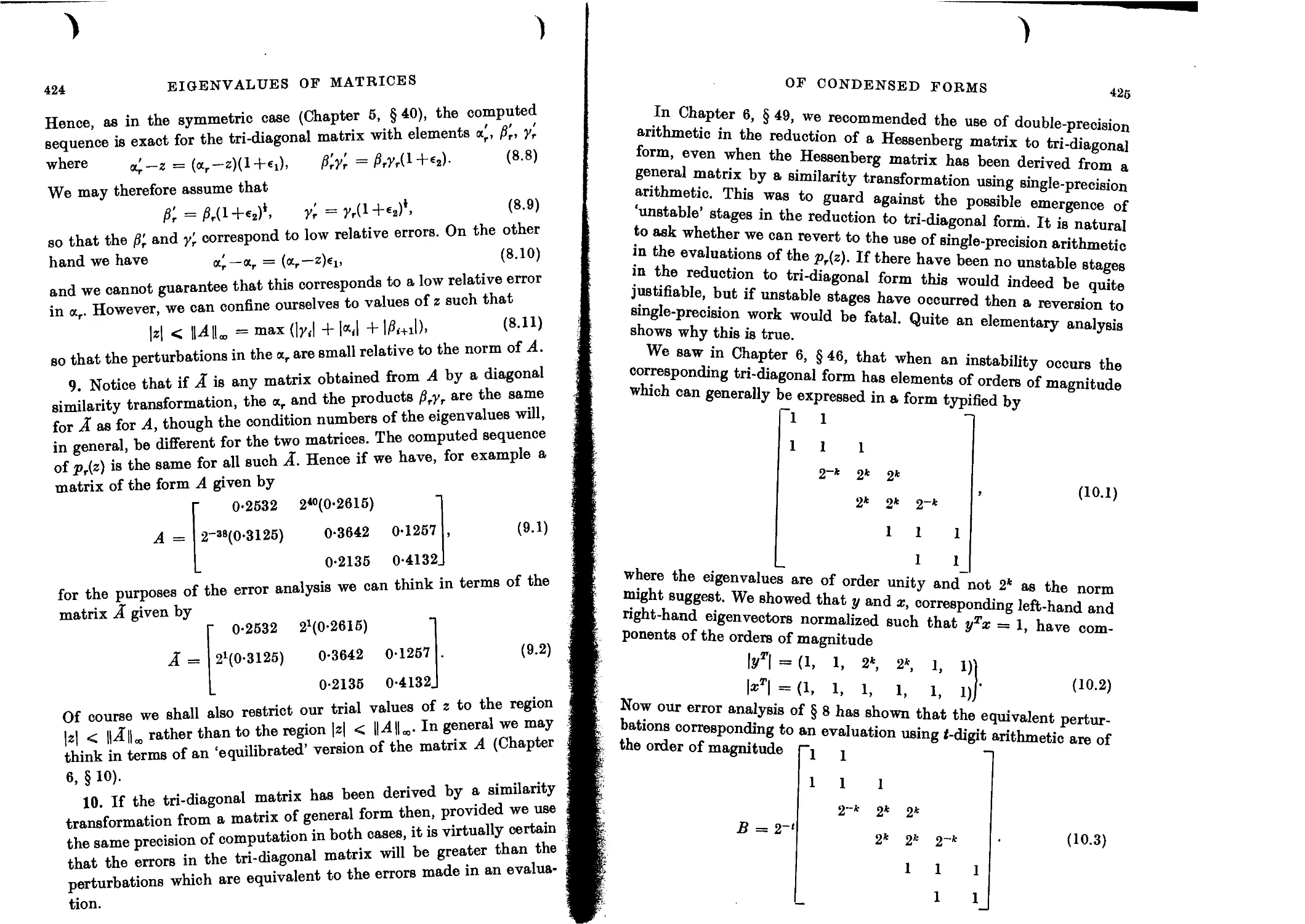
Tri-diagonal matrices	423
Determinants of Hessenberg matrices	426
Effect of rounding errors	427
Floating-point accumulation	428
Evaluation by orthogonal transformations	429
xvi	CONTENTS
Evaluation of determinants of general matrices	431
The generalized eigenvalue problem	432
Indirect determinations of the characteristic polynomial	432
Le Verrier’s method	434
Iterative methods based on interpolation	435
Asymptotic rate of convergence	436
Multiple zeros	437
Inversion of the functional relationship	439
The method of bisection	440
Newton’s method	441
Comparison of Newton’s method with interpolation	442
Methods giving cubic convergence	443
Laguerre’s method	443
Complex zeros	446
Complex conjugate zeros	447
Bairstow’s method	449
The generalized Bairstow method	450
Practical considerations	452
Effect of rounding errors on asymptotic convergence	453
The method of bisection	453
Successive linear interpolation	455
Multiple and pathologically close eigenvalues	457
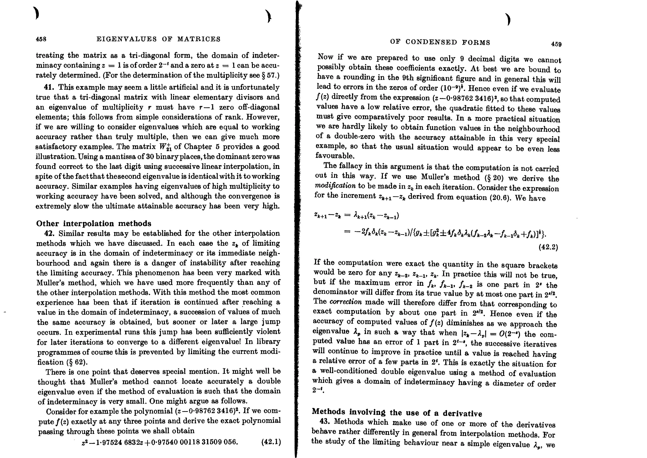
Other interpolation methods	458
Methods involving the use of a derivative	459
Criterion for acceptance of a zero	461
Effect of rounding errors	462
Suppression of computed zeros	464
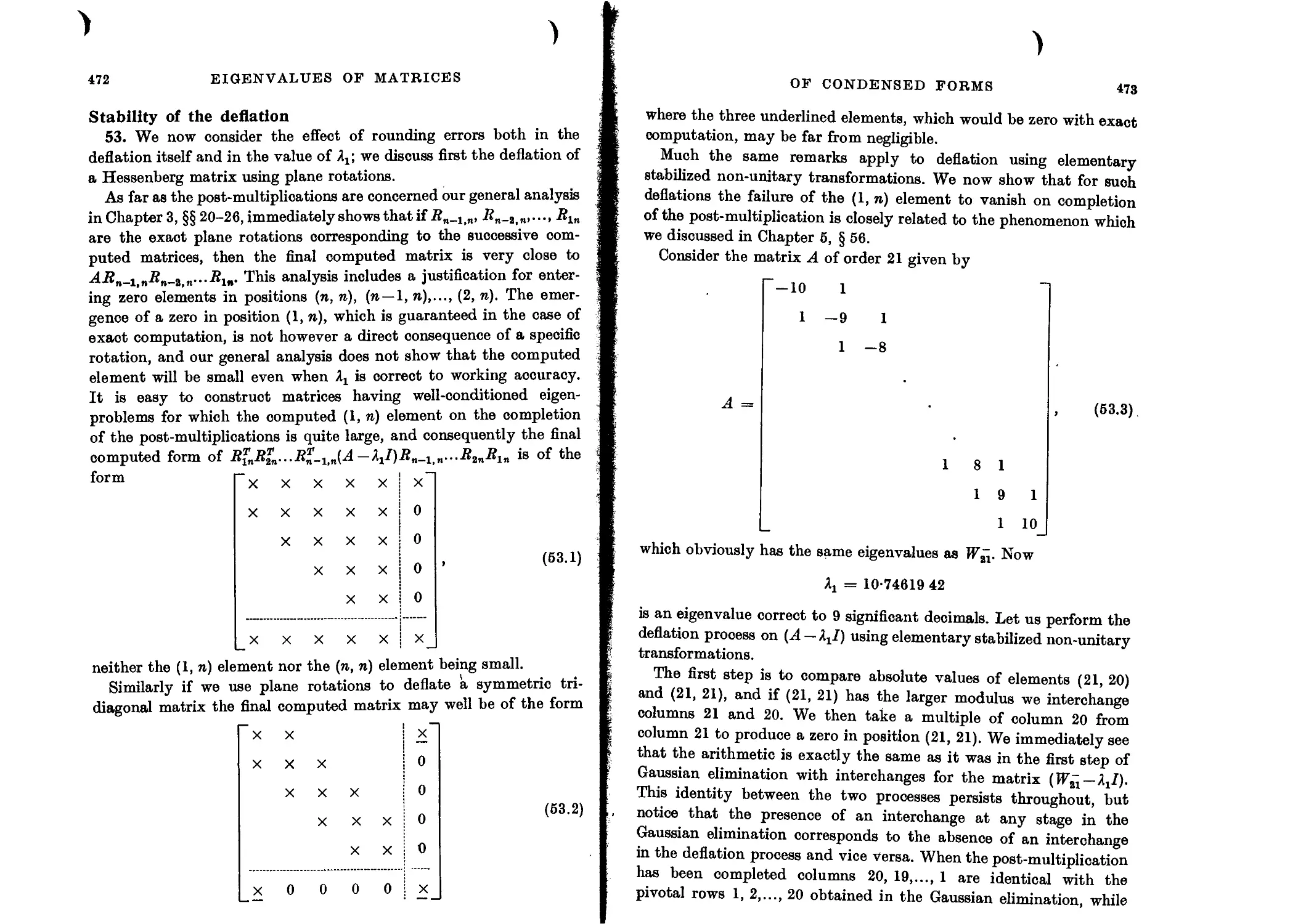
Deflation for Hessenberg matrices	465
Deflation of tri-diagonal matrices	468
Deflation by rotations or stabilized elementary transformations	469
Stability of the deflation	472
General comments on deflation	474
Suppression of computed zeros	474
Suppression of computed quadratic factors	475
General comments on the methods of suppression	476
Asymptotic rates of convergence	478
Convergence in the large	478
Complex zeros	481
Recommendations	482
Complex matrices	483
Matrices containing an independent parameter	483
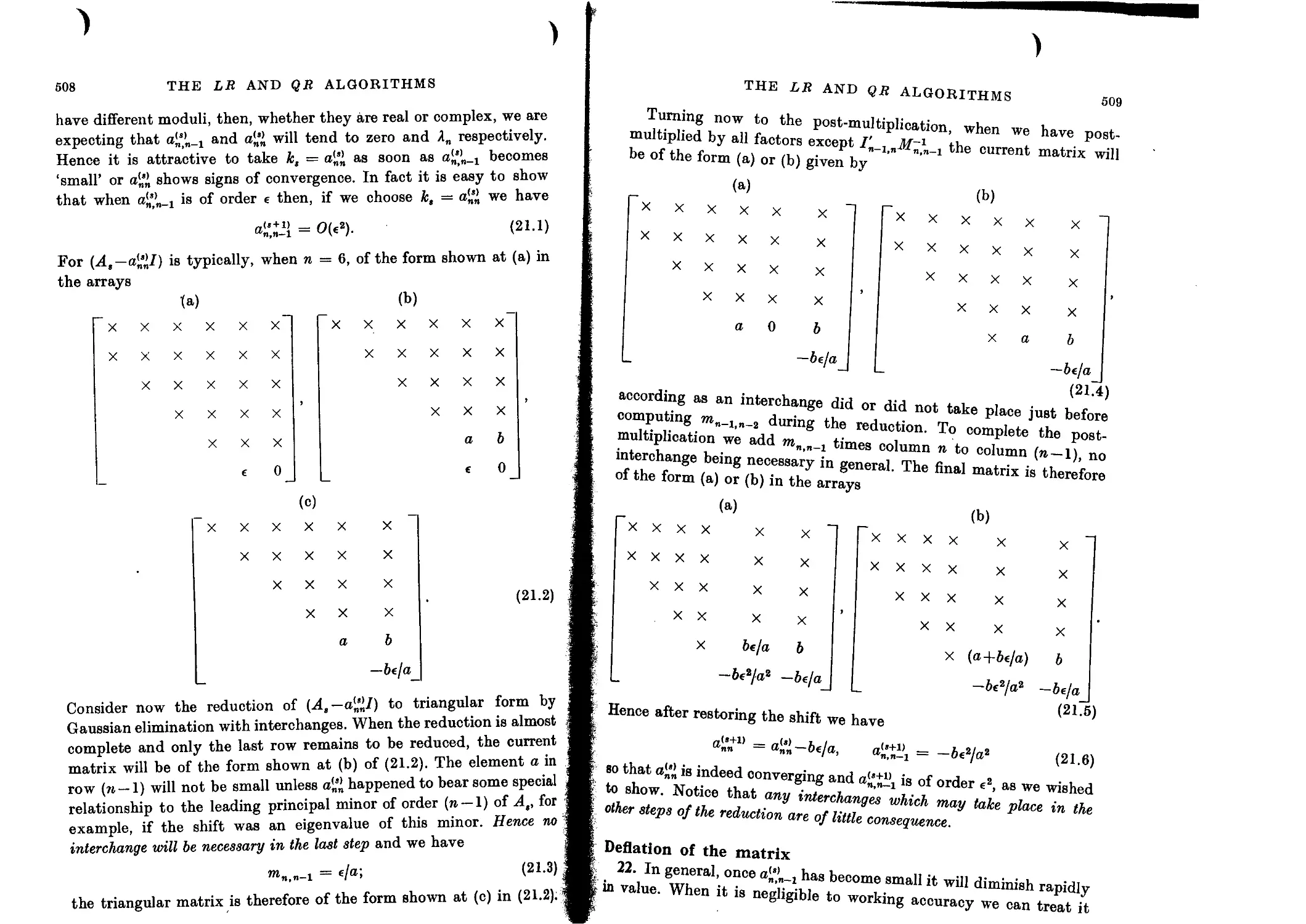
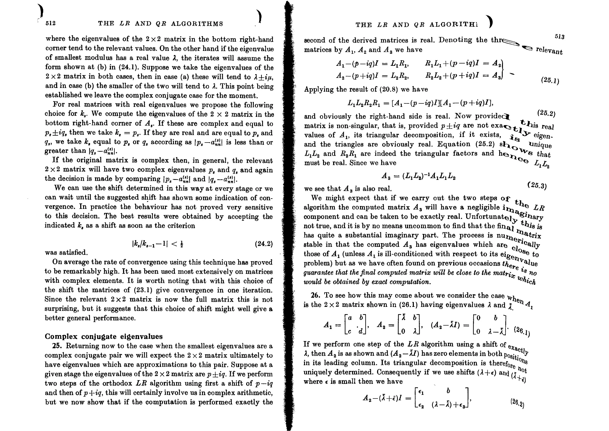
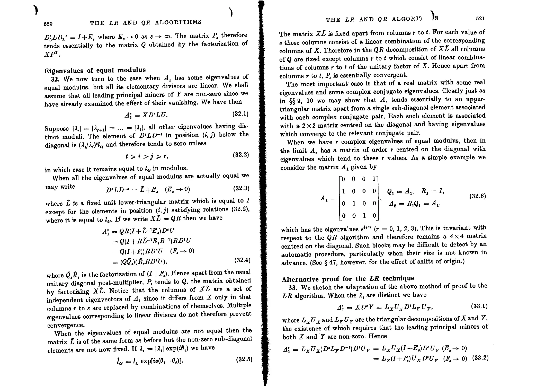
8.	THE LR AND QR ALGORITHMS
Introduction	485
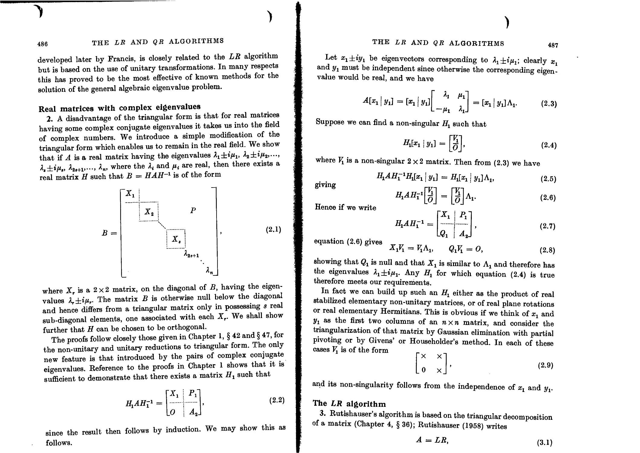
Real matrices with complex eigenvalues	486
The LR algorithm	487
Proof of the convergence of the A,	489
Positive definite Hermitian matrices	493
Complex conjugate eigenvalues	494
Introduction of interchanges	498
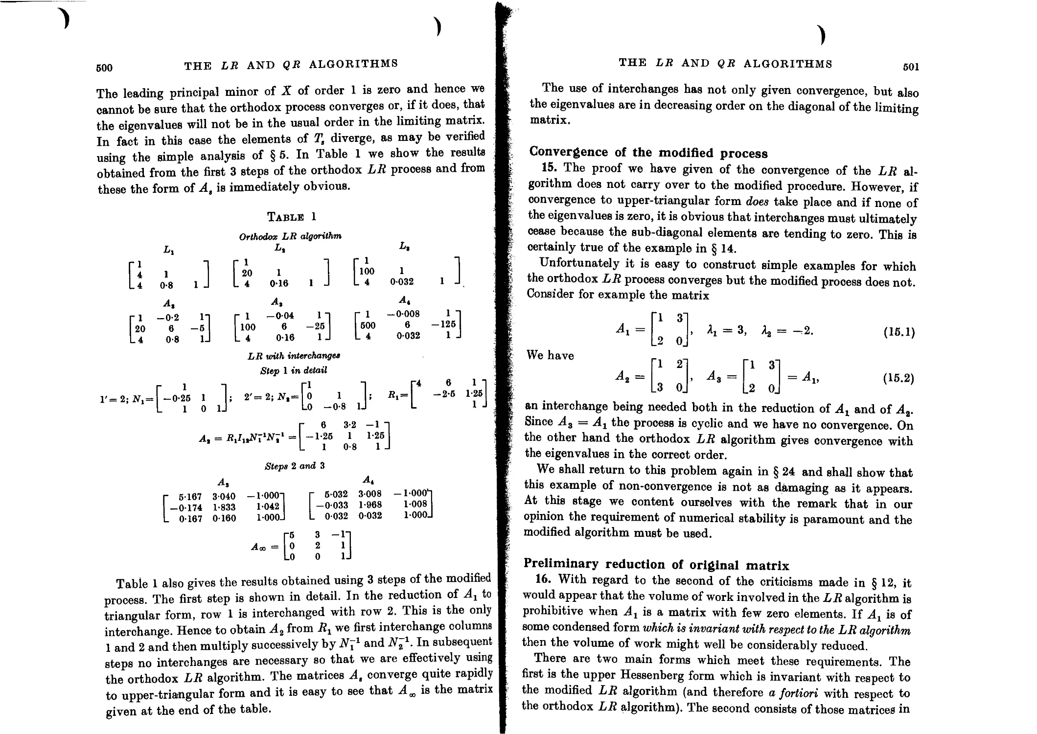
Numerical example	499
Convergence of the modified process	501
CONTENTS	xvu
Preliminary reduction of original matrix	501
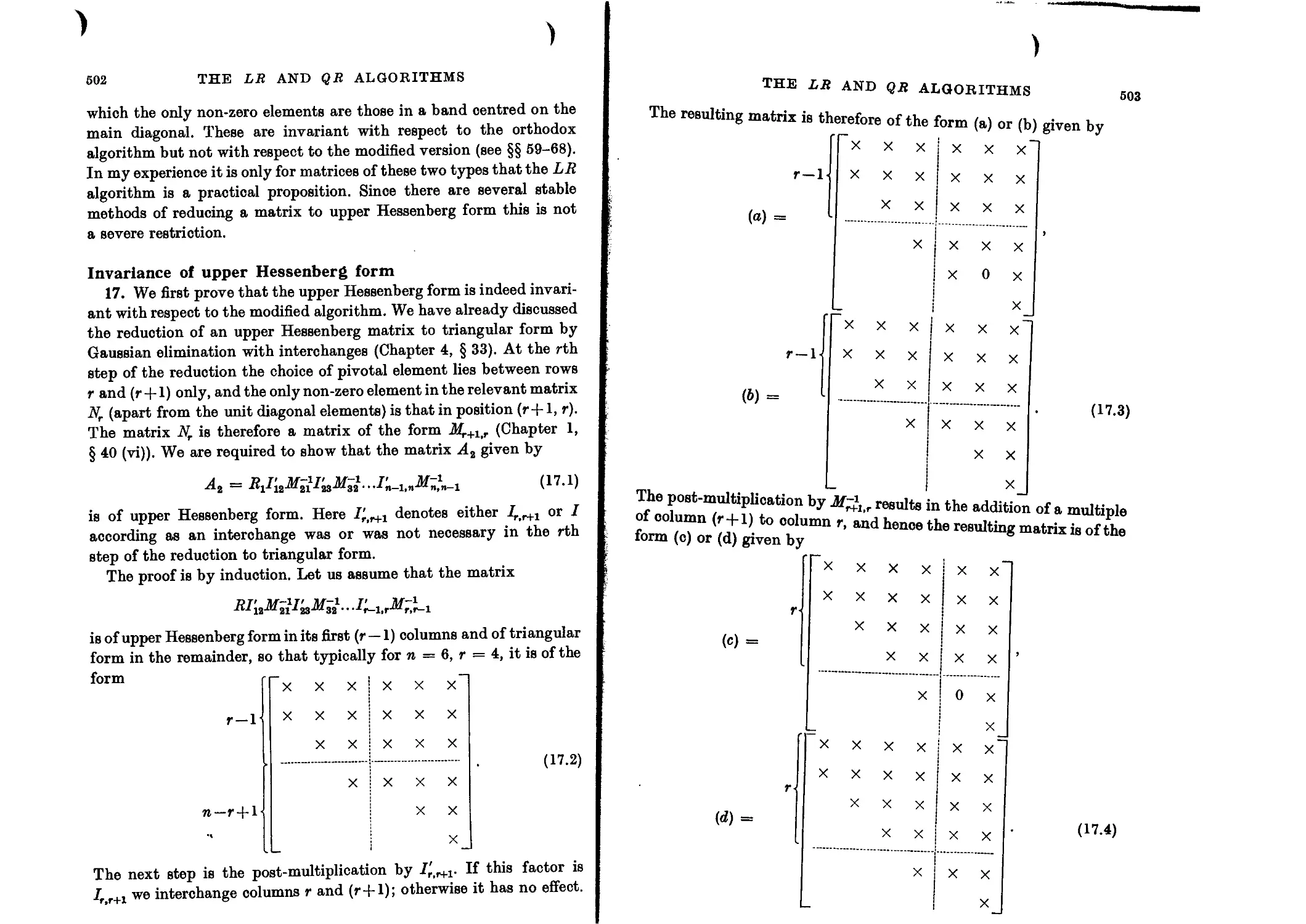
Invariance of upper Hessenberg form	502
Simultaneous row and column operations	504
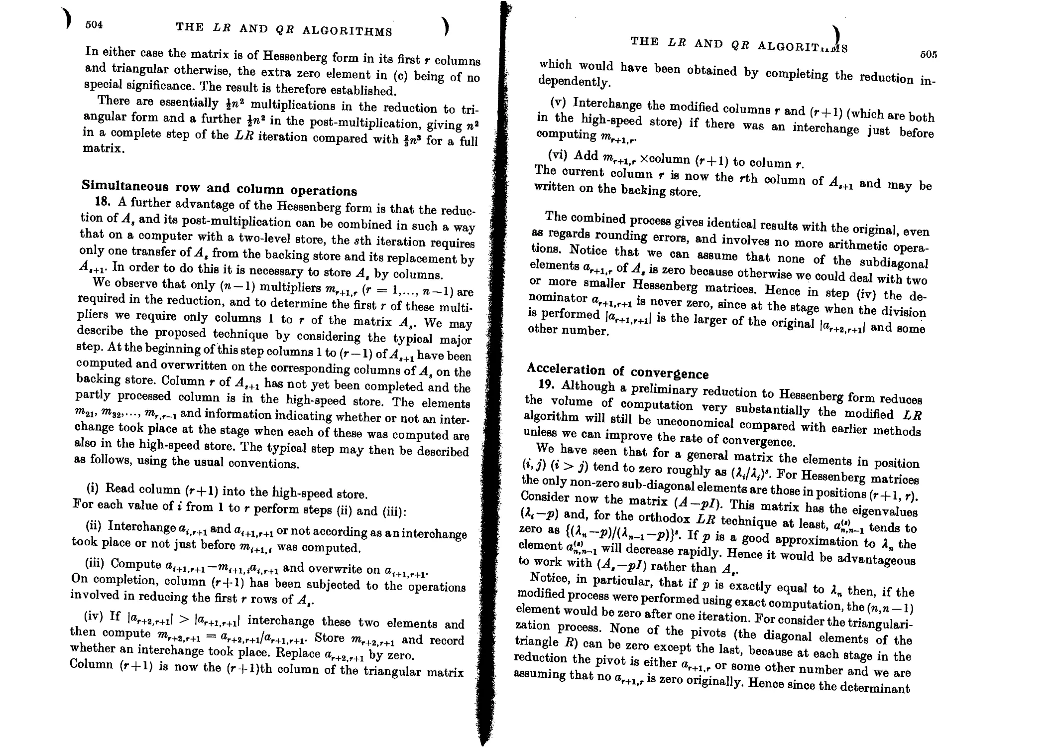
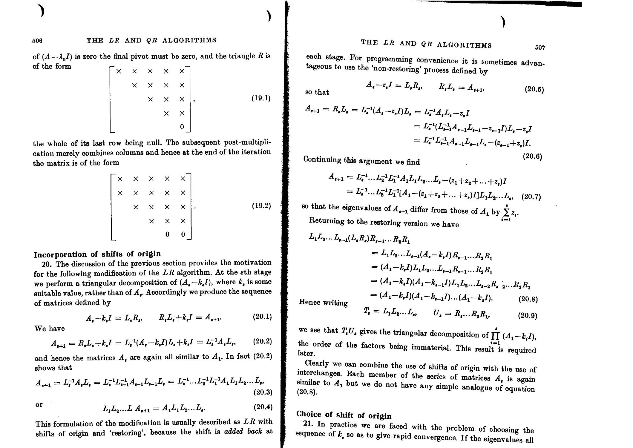
Acceleration of convergence	505
Incorporation of shifts of origin	506
Choice of shift of origin	507
Deflation of the matrix	509
Practical experience of convergence	510
Improved shift strategy	511
Complex conjugate eigenvalues	512
Criticisms of the modified LR algorithm	515
The QR algorithm	515
Convergence of the QR algorithm	516
Formal proof of convergence	517
Disorder of the eigenvalues	519
Eigenvalues of equal modulus	520
Alternative proof for the LR technique	521
Practical application of the QR algorithm	523
Shifts of origin	524
Decomposition of A,	525
Numerical example	527
Practical procedure	527
Avoiding complex conjugate shifts	528
Double QR step using elementary Hermitians	532
Computational details	534
Decomposition of As	535
Double-shift technique for LR	537
Assessment of LR and QR algorithms	538
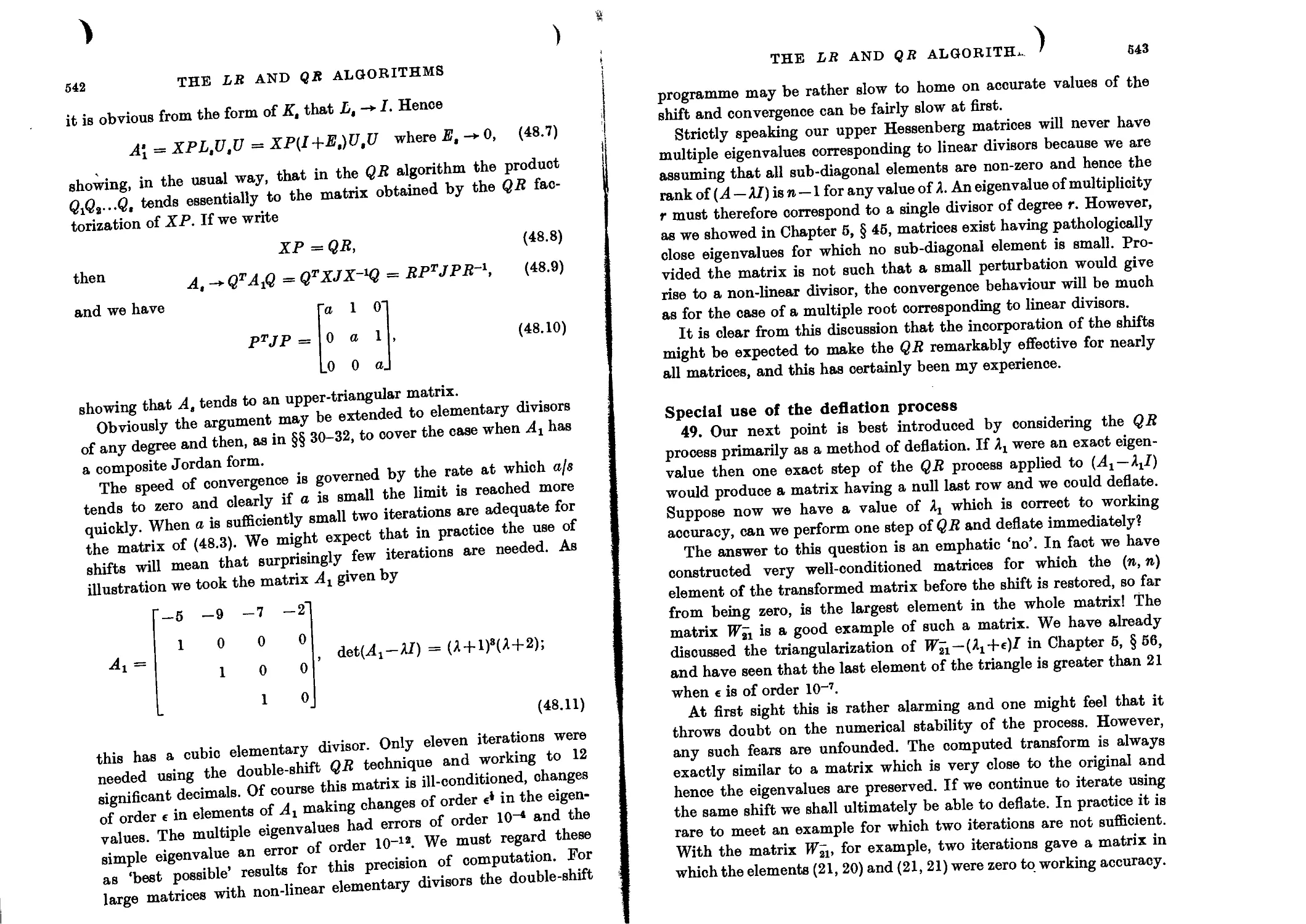
Multiple eigenvalues	540
Special use of the deflation process	543
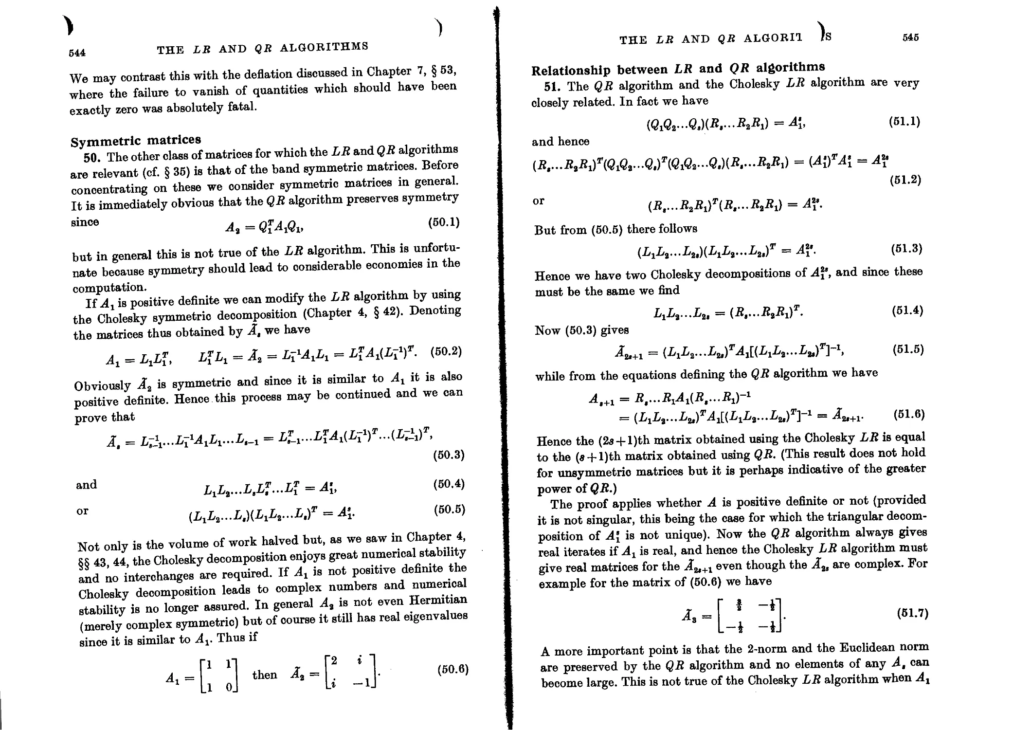
Symmetric matrices	544
Relationship between LR and QR algorithms	545
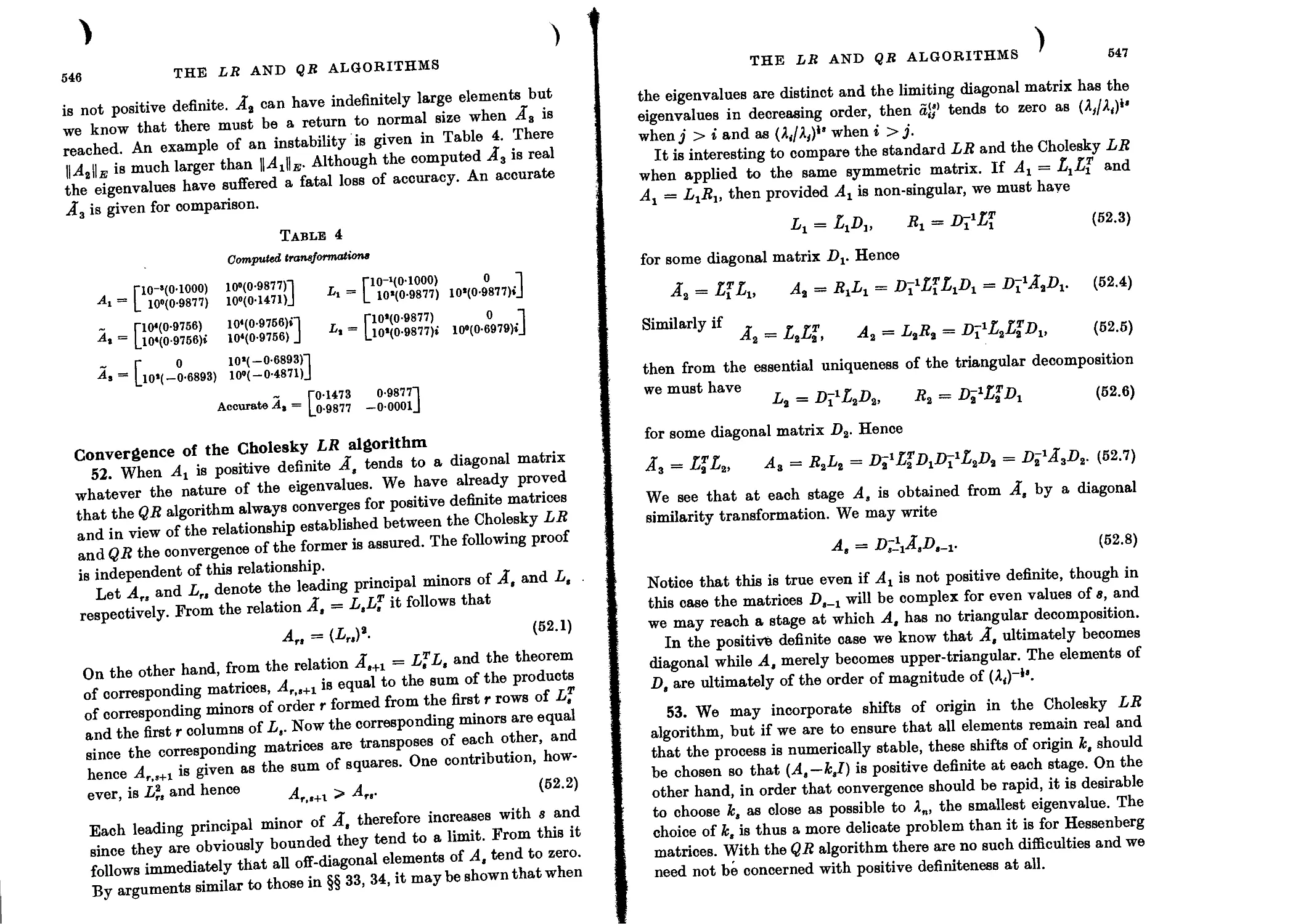
Convergence of the Cholesky LR algorithm	546
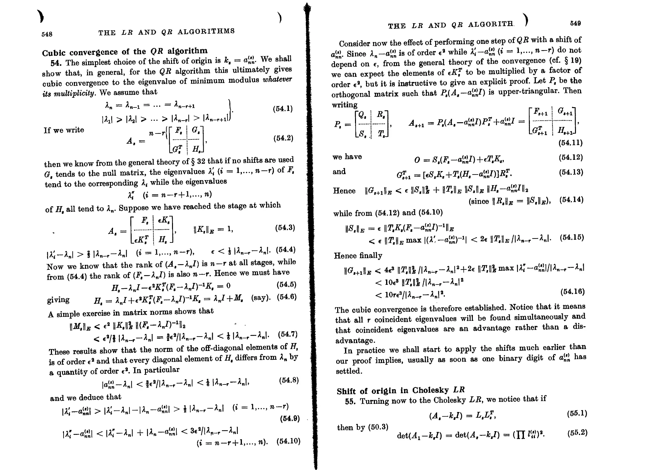
Cubic convergence of the QR algorithm	548
Shift of origin in Cholesky LR	549
Failure of the Cholesky decomposition	550
Cubically convergent LR process	551
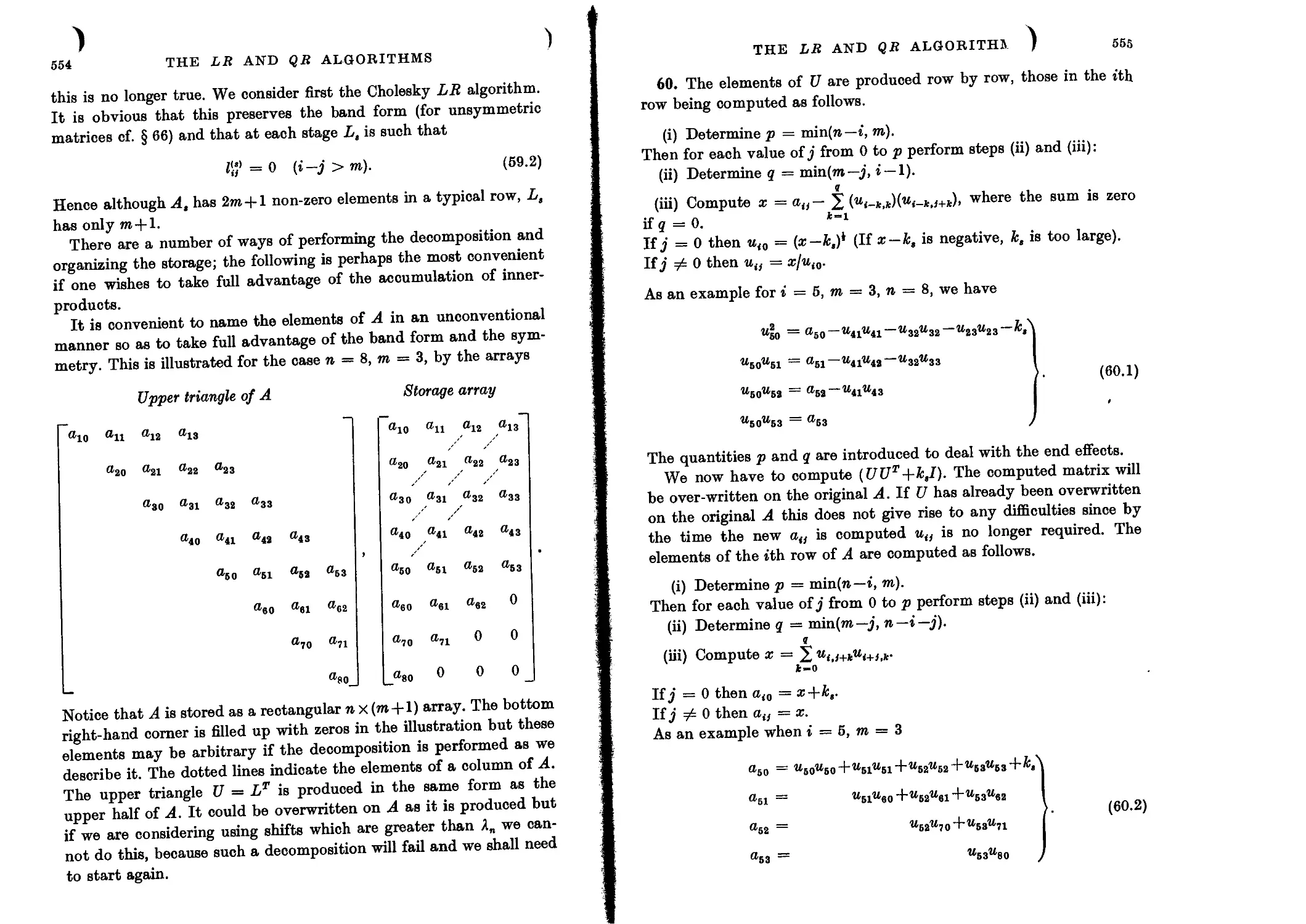
Band matrices	553
QR decomposition of a band matrix	557
Error analysis	561
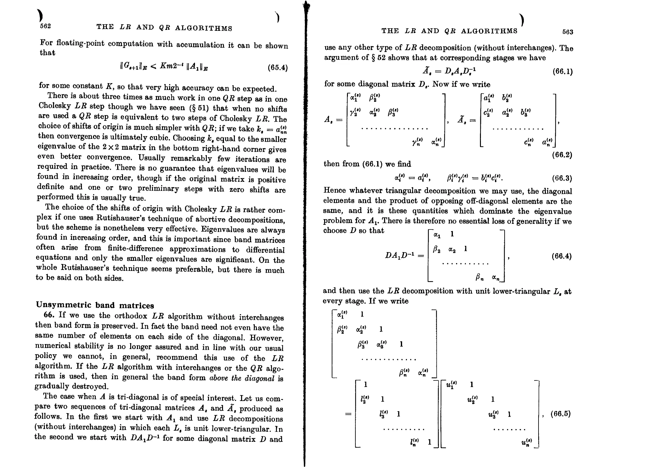
Unsymmetric band matrices	562
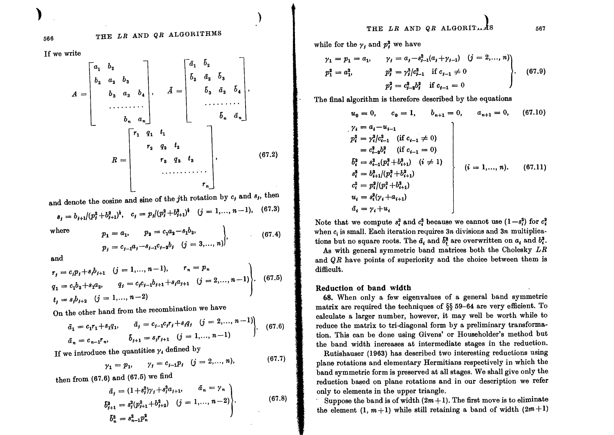
Simultaneous decomposition and recombination in QR algorithm	565
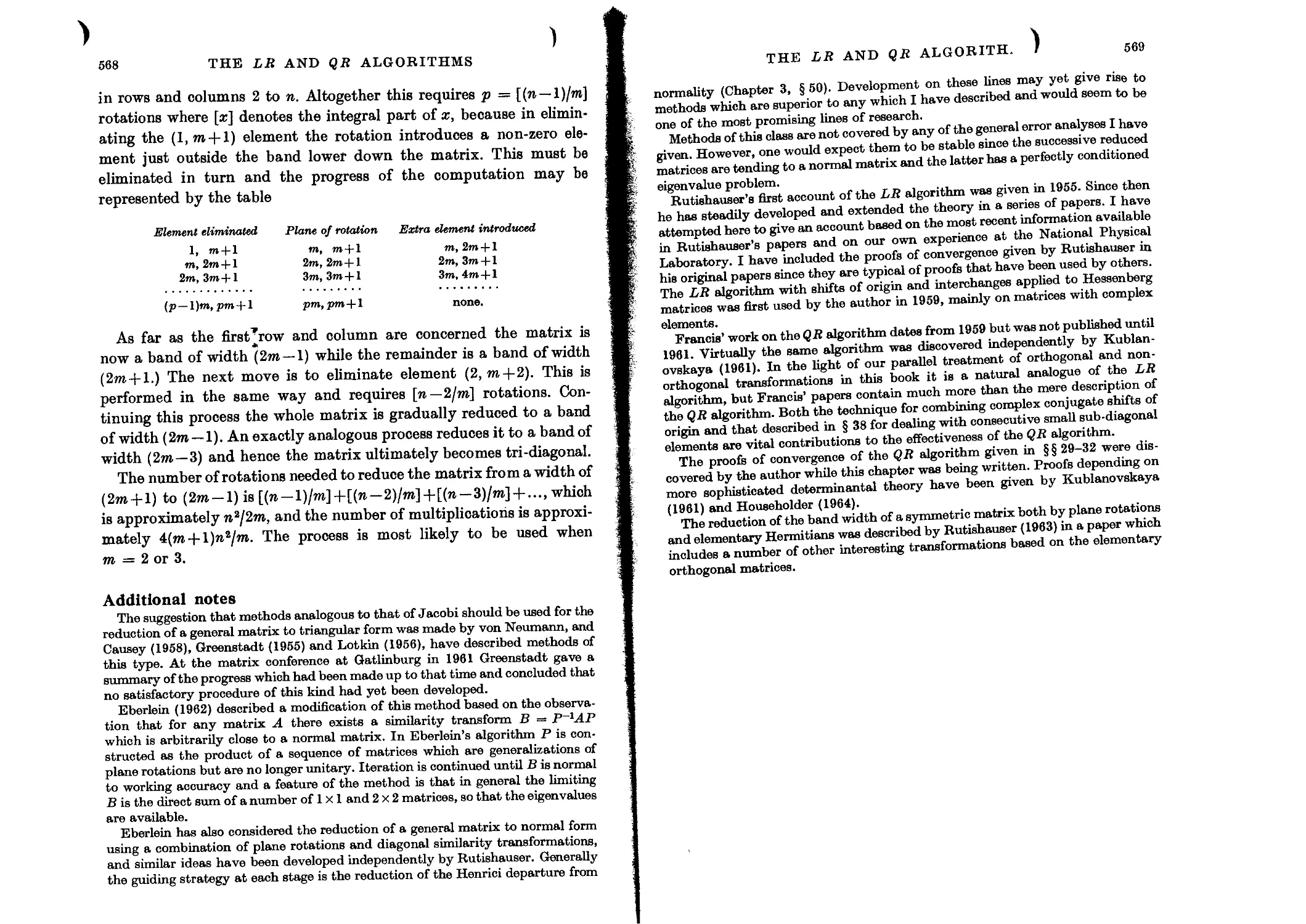
Reduction of band width	567
9.	ITERATIVE METHODS
Introduction	570
The power method	570
Direct iteration with a single vector	571
Shift of origin	572
Effect of rounding errors	573
Variation of p	576
Ad hoc choice of p	577
xviii
CONTENTS
Aitken’s acceleration technique	578
Complex conjugate eigenvalues	579
Calculation of the complex eigenvector	581
Shift of origin	582
Non-linear divisors	582
Simultaneous determination of several eigenvalues	583
Complex matrices	584
Deflation	584
Deflation based on similarity transformations	585
Deflation using invariant subspaces	587
Deflation using stabilized elementary transformations	587
Deflation using unitary transformations	589
Numerical stability	590
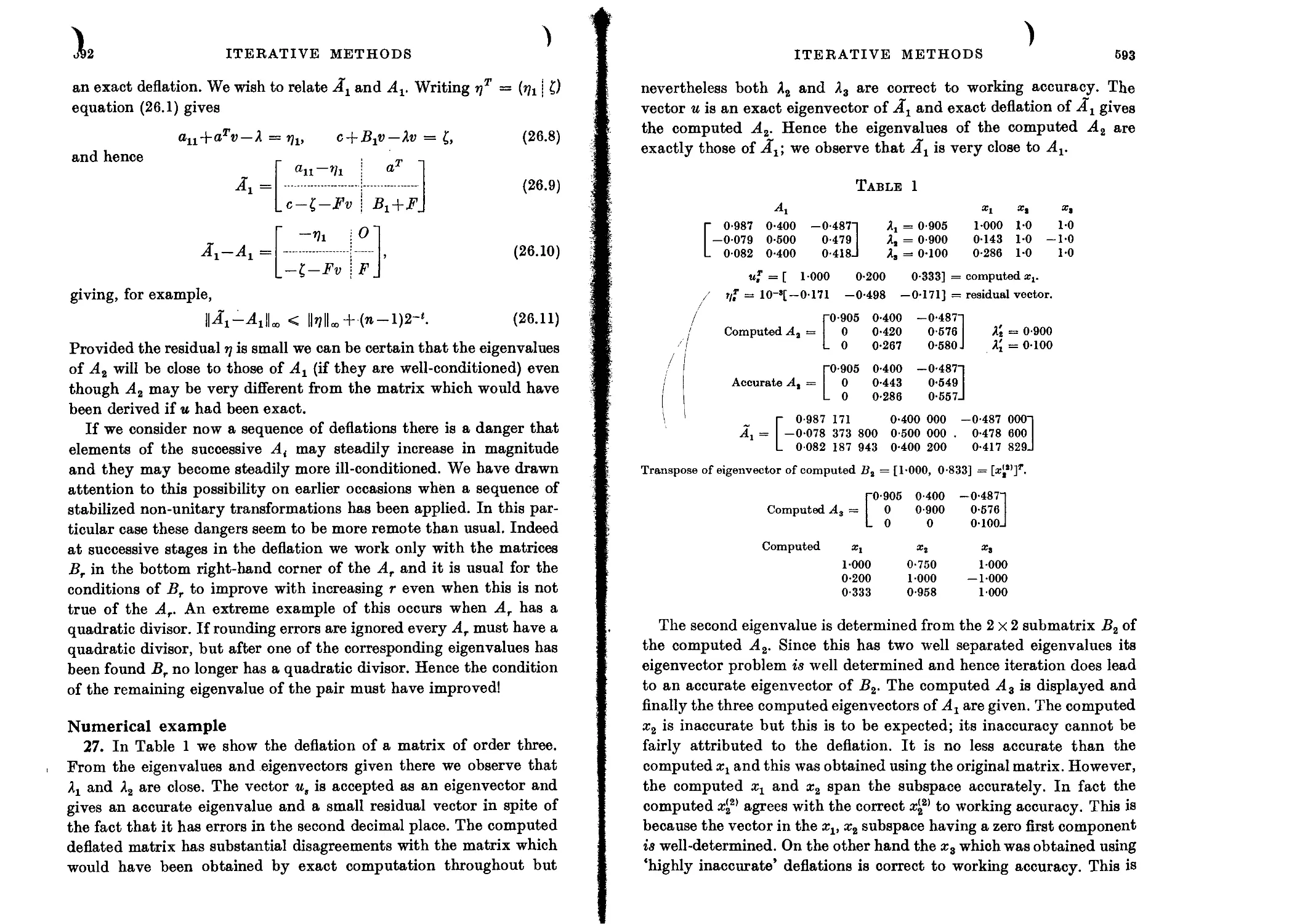
Numerical example	592
Stability of unitary transformations	594
Deflation by non-similarity transformations	596
Genera] reduction using invariant subspaces	599
Practical application	601
Treppen-iteration	602
Accurate determination of complex conjugate eigenvalues	604
Very close eigenvalues	606
Orthogonalization techniques	606
Analogue of treppen-iteration using orthogonalization	607
Bi-iteration	609
Numerical example	610
Richardson’s purification process	614
Matrix squaring	615
Numerical stability	616
Use of Chebyshev polynomials	617
General assessment of methods based on direct iteration	618
Inverse iteration	619
Error analysis of inverse iteration	620
General comments on the analysis	621
Further refinement of eigenvectors	622
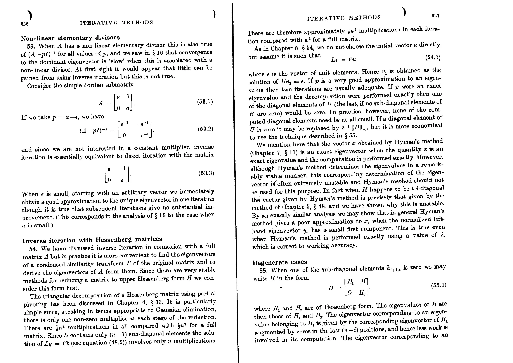
Non-linear elementary divisors	626
Inverse iteration with Hessenberg matrices	626
Degenerate cases	627
Inverse iteration with band matrices	628
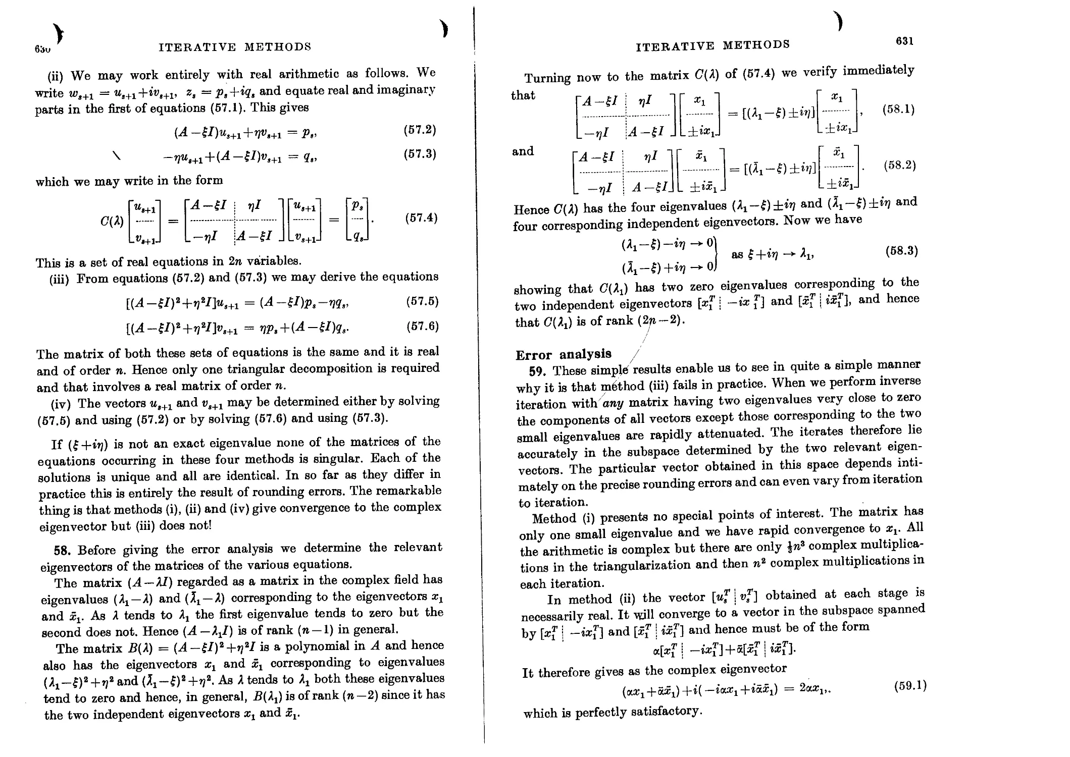
Complex conjugate eigenvectors	629
Error analysis	631
Numerical example	633
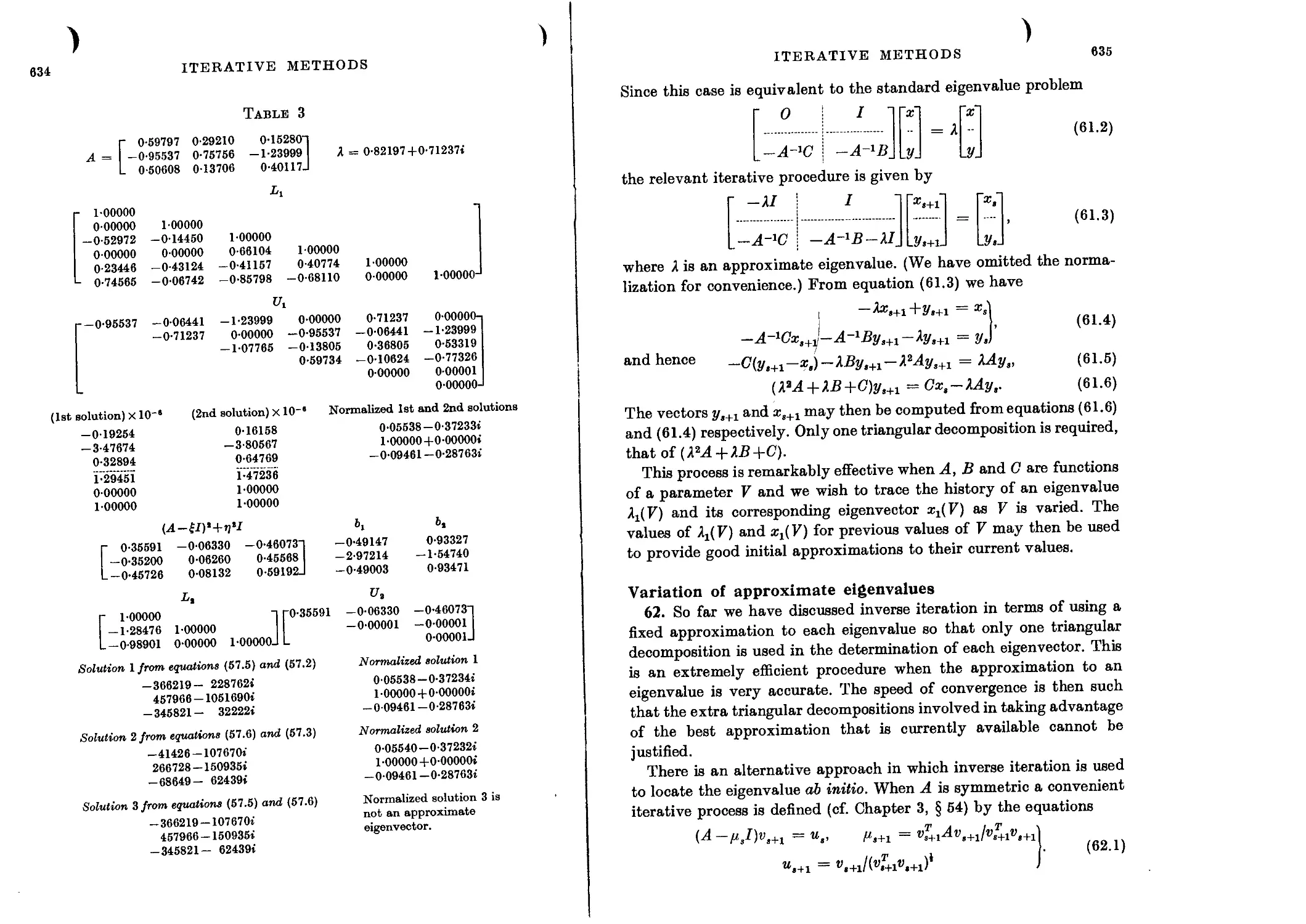
The generalized eigenvalue problem	633
Variation of approximate eigenvalues	635
Refinement of eigensystems	637
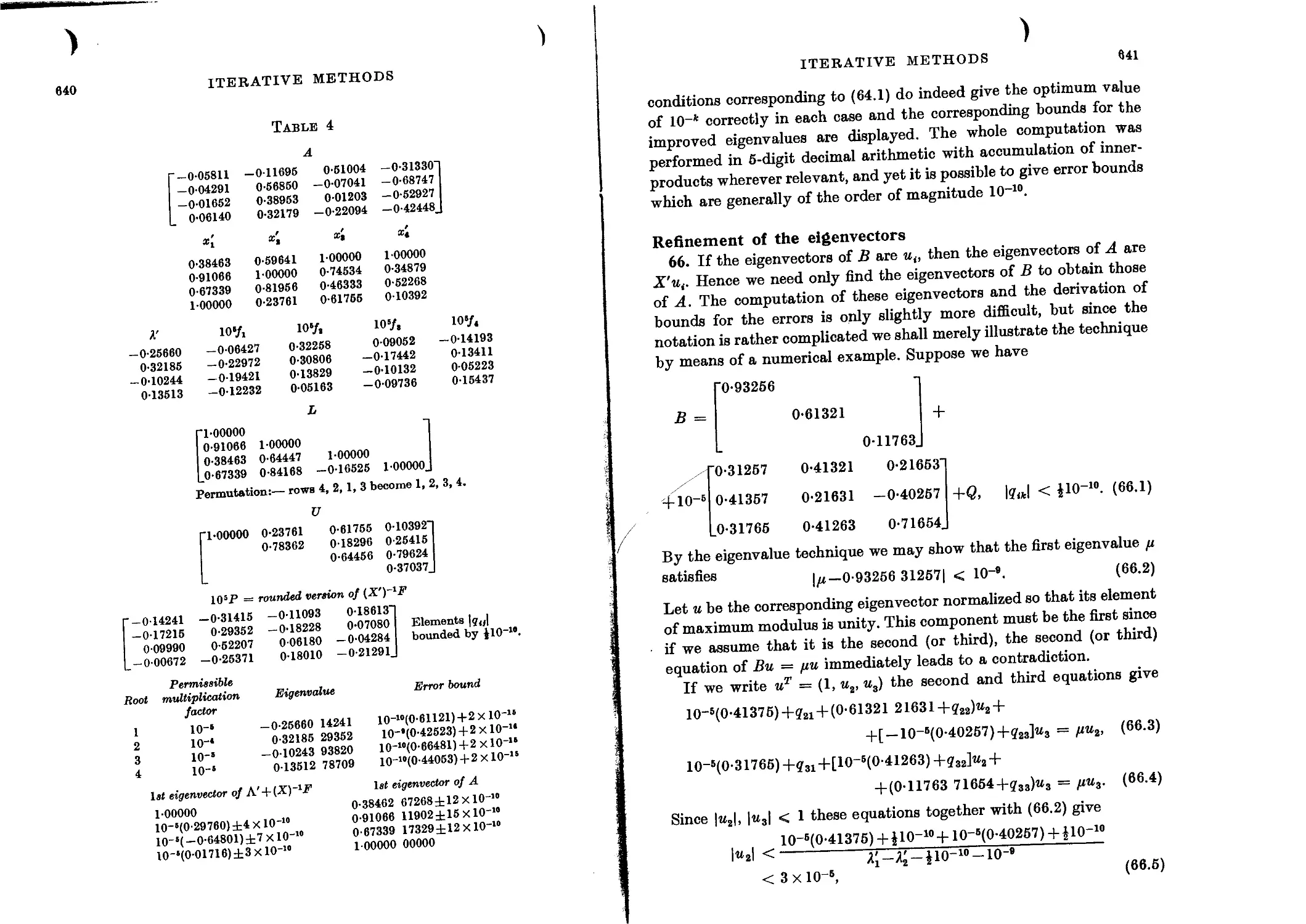
Numerical example	639
Refinement of the eigenvectors	641
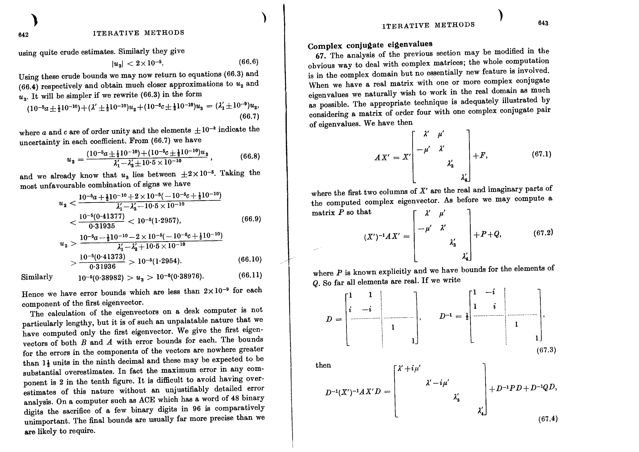
Complex conjugate eigenvalues	643
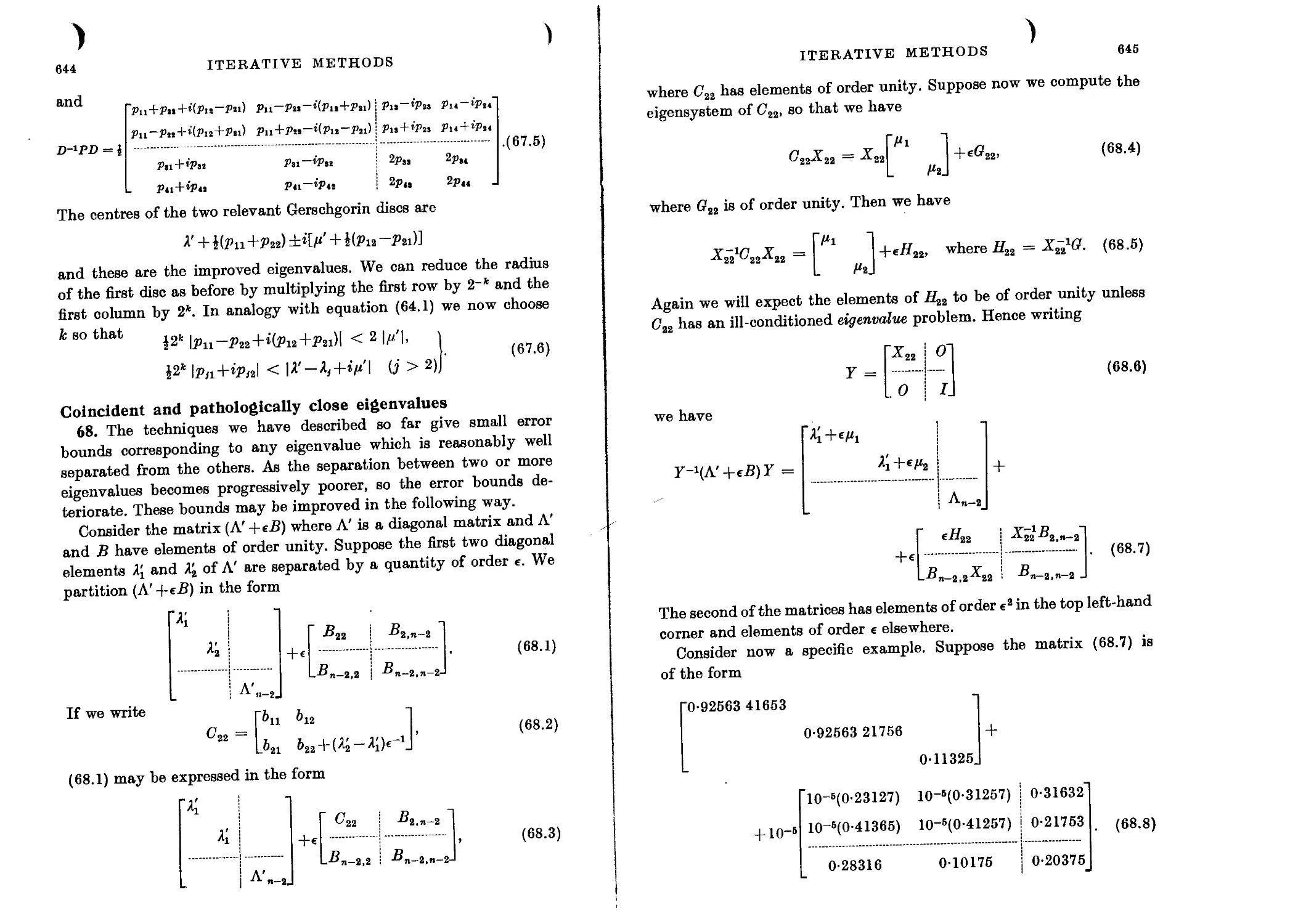
Coincident and pathologically close eigenvalues	644
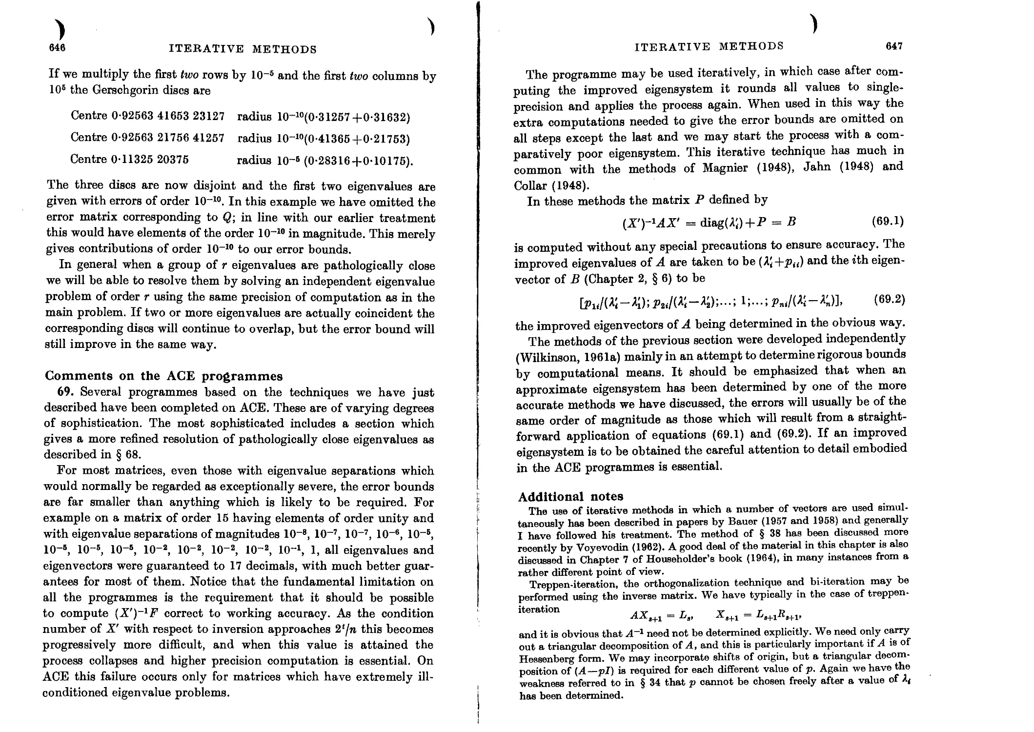
Comments on the ACE programmes	646
BIBLIOGRAPHY	649
INDEX	657
1
Theoretical Background
Introduction
1.	In this introductory chapter we shall give a brief account of the
classical theory of canonical forms and of several other theoretical
topics which will be required in the remainder of the book.
Since a complete treatment is beyond the scope of this chapter
we have concentrated on showing how the eigensystem of a matrix
is related to its various canonical forms. The emphasis is therefore
somewhat different from that which would be found in a standard
treatise. No attempt has been made to give rigorous proofs of all the
fundamental theorems; instead we have contented ourselves, in gen-
eral, with the statement of the results and have given proofs only
when they are particularly closely related to practical techniques
which are used subsequently.
In order to avoid repeated explanation we refer here to some con-
ventions of notation to which we have adhered throughout the book.
We denote matrices by capital letters and, unless there is an
indication to the contrary, matrices may be assumed to be square
and of order n. The (i,J) element of a matrix A will be denoted by
atj. Vectors will be denoted by lower case letters and will generally
be assumed to be of order n. The ith component of a vector x will
be denoted by xf.
The identity matrix will be denoted by I and its (i,j) element
by <5tJ, the Kronecker symbol, rather than iif. We have then
<5„ = 0	<5H = 1.	(1.1)
The ith column of I will be denoted by e, and e will be used to denote
the vector e1+e2 + --> +en, having all its components equal to unity.
We shall frequently be concerned with systems of n vectors which
will be denoted by aq, x2,..., xn. When this is done we shall refer to
the jth element of xt as aqf and to the matrix having x( as its ith
column as X, without always making specific reference to this fact.
The notation |Л| will be reserved for the matrix which has |a„|
for its (i,j) element and the notation
•n • i +	И < 1*1	<L2)
will imply that	, ,	„ . .
Iaob< I&J for all г, j.	(1.3)
2
THEORETICAL BACKGROUND
As a result of this decision and the use of ЦАЦ for the norm of A
(of. § 52) the determinant of A will be denoted by det (A). In line
with this, an (n x n) diagonal matrix with (i, i) element equal to
А,- will be denoted by diag (AJ.
The transpose of a matrix will be denoted by AT and is such that
its (i, j) element is equal to aSi. Similarly xT will denote a row vector
having its ith component equal to x(. Since it is more convenient to
print a row vector than a column vector, we shall frequently intro-
duce a column vector x and then define it by giving the explicit
expression for xT.
We assume throughout that we are working in the field of complex
numbers, though in computational procedures there is much to be
gained from remaining in the real field whenever possible.
Definitions
2.	The fundamental algebraic eigenproblem is the determination
of those values of A for which the set of n homogeneous linear equa-
tions in n unknowns
Ax — Ax	(2.1)
has a non-trivial solution. Equation (2.1) may be written in the form
(A-AZ)x = 0,	(2.2)
and for arbitrary A this set of equations has only the solution x = 0.
The general theory of simultaneous linear algebraic equations shows
that there is a non-trivial solution if, and only if, the matrix (A —AZ)
is singular, that is
det(A —AZ) = 0.	(2.3)
The determinant on the left hand side of equation (2.3) may be
expanded to give the explicit polynomial equation
a0+a1A + ...+an_1A’-1 + (-l)"An = 0.	(2.4)
Equation (2.4) is called the characteristic equation of the matrix A
and the polynomial on the left-hand side of the equation is called
the characteristic polynomial. Since the coefficient of An is not zero
and we are assuming throughout that we are working in the complex
number field, the equation always has n roots. In general the roots
may be complex, even if the matrix A is real, and there may be roots
of any multiplicities up to n. The n roots are called the eigenvalues,
latent roots, characteristic values or proper values of the matrix A.
THEORETICAL BACKGROUND
3
Corresponding to any eigenvalue Л, the set of equations (2.2) has
at least one non-trivial solution x. Such a solution is called an eigen-
vector, latent vector, characteristic vector or proper vector corresponding
to that eigenvalue. If the matrix (А— Л1) is of rank less than (n — 1)
then there will be more than one independent vector satisfying
equation (2.2). We discuss this point in detail in §§ 6-9. It is evident
that if a; is a solution of (2.2), then kx is also a solution for any value
of k, so that even when (Л — Л1) is of rank (n — 1), the eigenvector
corresponding to Л is arbitrary to the extent of a constant multiplier.
It is convenient to choose this multiplier so that the eigenvector has
some desirable numerical property, and such vectors are called
normalized vectors. The most convenient forms of normalization are
those for which
(i)	the sum of the squares of the moduli of the components is
equal to unity,
(ii)	a component of the vector which has the largest modulus is
equal to unity, and
(iii)	the sum of the moduli of the components is equal to unity.
The normalizations (i) and (iii) have the disadvantage of being
arbitrary to the extent of a complex multiplier of modulus unity.
Many of the processes we describe in this book lead, in the first
instance, to eigenvectors which are not in normalized form. It is
often convenient to multiply such vectors by a power of 10 (or 2) so
that the largest element lies between 01 and 1-0 (or | and 1) in
modulus. We shall refer to vectors which have been treated in this
way as standardized vectors.
Eigenvalues and eigenvectors of the transposed matrix
3.	The eigenvalues and eigenvectors of the transpose of a matrix
are of considerable importance in the general theory. The eigenvalues
of AT are, by definition, those values of Л for which the set of equations
= Лу	(3.1)
has a non-trivial solution. These are the values for which
det(^r—Л1) = 0,	(3.2)
and since the determinant of a matrix is equal to that of its transpose,
the eigenvalues of AT are the same as those of A. The eigenvectors
are, in general, different. We shall usually denote the eigenvector
of AT corresponding to 2,- by yit so that we have
A^Vi = ^iVi-	(3.3)
4
THEORETICAL BACKGROUND
Equation (3.3) may be written in the form
= A.yf,
(3-4)
so that yf is sometimes called a left-hand eigenvector of A correspond-
ing to 2j; while the vector x( such that
Ax( = ZjXf	(3.5)
is called a right-hand eigenvector of A corresponding to 2(. The
importance of the eigenvectors of the transposed matrix springs
mainly from the following result.
If xt is an eigenvector of A corresponding to the eigenvalue 2(,
and y, is an eigenvector of AT corresponding to 2,, then
= 0 (#2,^2,).
For we may write (3.5) in the form
xf AT = 2ЛТ
= 2,yr
and we have
(3-6)
(3-7)
(3-8)
Post-multiplying (3.7) by ys and pre-multiplying (3.8) by xf and
subtracting we have „ , T , T
6	0=2Лг^-2,а^„	(3.9)
leading to equation (3.6).
Note that since xf and/or yf may be complex vectors, xfyt is not an
inner-product as usually understood. We have in fact
= У?*»
xfy} =
When x is complex we can have
xTx = 0
whereas a true inner-product is positive for all non-zero x.
and not
(3.10)
(3.11)
(3-12)
Distinct eigenvalues
4. The general theory of the eigensystem is simplest when the
n eigenvalues are distinct, and we consider this case first. We denote
the eigenvalues by 21; 22,..., 2n. Equation (2.2) certainly has at least
one solution for each value of 2( and we can therefore assume the
existence of a set of eigenvectors which we denote by xlt xs,..., xn.
We shall show that each of these vectors is unique, apart from an
arbitrary multiplier.
THEORETICAL BACKGROUND
5
We first show that the vectors must be linearly independent. For,
if not, let r be the smallest number of linearly dependent vectors.
We may number the vectors so that these are xlt xz,..., xr and, from
our assumption, there is a relation between them of the form
5 afxt = 0	(4.1)
i
in which none of the a4 is zero. Clearly r > 2 because, by definition,
none of the xt is the null vector. Pre-multiplying equation (4.1) by
A, we have	r
2 а4ЛЛ = 0.	(4.2)
1
Multiplying equation (4.1) by and subtracting (4.2) gives
(4.3)
i
and none of the coefficients in this relation is zero. Now equation (4.3)
implies that xlt x2,..., хг_г are linearly dependent, which is contrary
to hypothesis. The n eigenvectors are therefore independent and span
the whole n space. Consequently they may be used as a base in which
to express an arbitrary vector.
From the last result the uniqueness of the eigenvectors follows
immediately. For if there is a second eigenvector zT corresponding
to we may write	n
zi — 2 aA>	(4.4)
where at least one of the a, is non-zero. Multiplying (4.4) by A gives
^izi = 2 Ma-	(4-5)
i
Multiplying (4.4) by and subtracting from (4.5) we have
0 = 2^-^,	(4.6)
2
and hence from the independence of the a;4
а4(Л4 — Ях) = 0 (t = 2, 3,..., n),
glV1Ilg	<tt = 0 (» = 2, 3,..., n).	(4.7)
The non-zero a4 must therefore be a1; showing that zx is a multiple
of
Similarly we may show that the eigenvectors of AT are unique
and linearly independent. We have proved earlier that
=0 (Я, * Ы	(4.8)
6
THEORETICAL BACKGROUND
so that the two sets of vectors form a bi-orthogonal system. We have
further	т
xfy( =#= 0 (* = 1, 2,..., n).	(4.9)
For if x{ were orthogonal to yt it would be orthogonal to yx, уг,...,уп
and hence to the whole n-space. This is impossible, since xx is not the
null vector.
Equations (4.8) and (4.9) enable us to obtain an explicit expression
for an arbitrary vector v in terms of the xt or the y(. For if we write
® = Ja<a:<,	(4.10)
4—1
then	n
yfv =£л<у?х{ = ^yfxf.	(4.11)
Hence	т , r
«,= yfv/yfxi,	(4-12)
the division being permissible because the denominator is non-zero.
Similarity transformations
5. If we choose the arbitrary multipliers in the x( and yt so that
yfxf = 1 (» = 1, 2,...,n),	(5.1)
the relations (4.8) and (5.1) imply that the matrix YT, which has
yf as its tth row, is the inverse of the matrix, X, which has x( as its
ith column. The n sets of equations
Axt — Xixi	(5.2)
may be written in matrix form
AX = X diag(Ai).	(5.3)
Now we have seen that the inverse of the matrix X exists and is
equal to YT. Equation (5.3) therefore gives
X-'AX = YTAX = diag^J.	(5.4)
Transforms, H~lAH, of the matrix A, where H is non-singular,
are of fundamental importance from both the theoretical and the
practical standpoints and are known as similarity transforms while A
and H~lAH are said to be similar. Obviously HAH-1 is also a
similarity transform of A. We have shown that when the eigenvalues
of A are distinct then there is a similarity transformation which
reduces A to diagonal form and that the matrix of the transformation
THEORETICAL BACKGROUND
7
has its columns equal to the eigenvectors of A. Conversely if we
haVe	H~rAH = diagf/zj	(5.5)
^ien	ЛЯ — // diagf/z,).	(5.6)
This last equation implies that the /z( are the eigenvalues of A in
some order, and that the tth column of H is an eigenvector corre-
sponding to Hf.
The eigenvalues of a matrix are invariant under a similarity trans-
formation. For if	,	,
Ax = Xx	(5.7)
then	,T , .	, ,T ,
H~rAx — XH^x,
giving
Н-ЧЦНН-^х = ЛЯ"1», (H^AHjH-h: = Ш^х. (5.8)
The eigenvalues are therefore preserved and the eigenvectors are
multiplied by Я-1.
Many of the numerical methods for finding the eigensystem of
a matrix consist essentially of the determination of a similarity trans-
formation which reduces a matrix A of general form to a matrix В
of special form, for which the eigenproblem may be more simply
solved.
Similarity is a transitive property, for if
В = Hi'AHi and C = H?BH2	(5.9)
then	C = H^H^AHJb = (HMr'AtHiHJ. (5.10)
In general the reduction of a general matrix to one of special
form will be effected by a sequence of simple similarity transforma-
tions.
Multiple eigenvalues and canonical forms for general
matrices
6. The structure of the system of eigenvectors for a matrix which
has one or more multiple eigenvalues may be far less simple than that
described above. It may still be true that there is a similarity trans-
formation which reduces A to diagonal form. When this is true, we
have, for some non-singular H,
H-'AH = diagUJ.
(6.1)
8
THEORETICAL BACKGROUND
The Я( must then be the eigenvalues of A and each 2, must occur
with the appropriate multiplicity. For
Я~1(Л-27)Я = Н^АН-Ш-ЧН = diag^-2),	(6.2)
and taking determinants of both sides we have
det(H“1) det (A -U) det(tf) = ПМ.-Д	(6.3)
glVmg	det(^-lf) = №.—Д	(6.4)
The 2, are therefore the roots of the characteristic equation of A.
Writing (6.1) in the form . ,T „
6 v '	AH = H diag(2(),	(6.5)
we see that the columns of H are eigenvectors of A. Since H is non-
singular, its columns are independent. If, for example, is a double
root, then, denoting the first two columns of H by xr and x2 we have
AX} = 2jXlt Ax2 = 2ха;2,	(6.6)
where xr and ж2 are independent. From equations (6.6), any vector
in the subspace spanned by xx and x2 is also an eigenvector. For we
A (eq#! + <х2ж2) = a.jA^Xi~}-ct.2XjX2 = 2х(осхя;х-|-а2й;2).	(6.7)
Coincident roots for a matrix which can be reduced to diagonal
form by a similarity transformation are associated with an indeter-
minacy in the eigenvectors corresponding to the multiple root. We
can still select a set of eigenvectors which span the whole n-space and
can therefore be used as a base in which to express an arbitrary
vector.
Thus the diagonal matrix Л defined by
(6-8)
has the 5 independent eigenvectors ex, e2, e3, e4 and e6. Any combina-
tion of ex and e2 is an eigenvector corresponding to 2. = I and any
combination of e3 and e4 is an eigenvector corresponding to 2 = 2.
For any matrix similar to Л there is a non-singular H such that
H-^AH = A
(6.9)
THEORETICAL BACKGROUND
9
and the eigenvectors of A are Нег, He2, He3, Het and HeB, any
combination of the first two being an eigenvector corresponding to
2 = 1 and any combination of the third and fourth an eigenvector
corresponding to 2 = 2.
Defective system of eigenvectors
7. The properties of a matrix which is similar to a diagonal matrix
but has multiple eigenvalues are in most respects like those of a
matrix with distinct eigenvalues. However, not all matrices with
multiple eigenvalues are of this type.
The matrix C2(a) defined by
t72(a) —
Г
a
(7.1)
has the double eigenvalue 2 = a. If x is an eigenvector of C2(a) with
components aq and a:2, then we must have
(te1+ x2 = 0
0aq+0a;2 = 0
(7.2)
These equations imply that ж2 = 0. There is thus only one eigen-
vector corresponding to 2 = a, the vector ev We may regard C2(a)
as the limit as b —> a of a matrix B2 defined by
В
2 —
a
0
1
b
(7-3)
For Ъ Ф a this matrix has two eigenvalues a and b, and the corre-
sponding vectors are
1'
0
and
1 '
b — a
As b -► a the two eigenvalues and eigenvectors become coincident.
More generally if we define matrices Cr(a) by the relations
^(a) = [a], Cr(a) =	a 1 a 1 a 1	,	(7-4)
	a 1 _ a	
10
THEORETICAL BACKGROUND
then Cr(a) has an eigenvalue, a, of multiplicity r, but it has only one
eigenvector, x = ev We may prove this as we proved the correspond-
ing result for Cs(a). Alternatively it follows from the fact that the
rank of [C,(a)-aZ] is (r — 1). (The matrix of order (r — 1) in the top
right-hand corner has determinant 1.) The transposed matrix [<7r(a)]r
also has only one eigenvector, у = er. We have immediately
xTy = eier ~ °	(7.5)
which contrasts with the result obtained for the eigenvectors of
matrices with distinct eigenvalues.
The matrix Cr(a), (r > 1), cannot be reduced to diagonal form by a
similarity transformation. For if there exists an H for which
= diag(2j),	(7.6)
that 18’	С.Н diag(2,),	(7.7)
then, as shown in § 6, the 2, must be equal to the eigenvalues of CT(a)
and must therefore all have the value a. Equation (7.7) then shows
that the columns of H are all eigenvectors of Cr(a). These columns
are independent, since H is non-singular. The assumption that such
an H exists must therefore be false.
The matrix (7r(a) is called a simple Jordan submatrix of order r,
or sometimes a simple classical submatrix of order r. Matrices of this
form are of special importance in the theory, as will be seen in the
next section.
The Jordan (classical) canonical form
8.	We see then that a matrix with multiple eigenvalues is not
necessarily similar to a diagonal matrix. It is natural to ask what is
the most compact form to which a matrix A may be reduced by means
of a similarity transformation. The answer is contained in the following
theorem.
Let A be a matrix of order n with r distinct eigenvalues 21, 22,..., 2r
of multiplicities mt, m2,..., mr so that
m1+m2+... +mr = n.	(8.1)
Then there is a similarity transformation with matrix Я such that
the matrix H~XAH consists of simple Jordan submatrices isolated
along the diagonal with all other elements equal to zero. The sum of
the orders of the submatrices associated with Л( is equal to mt. Apart
THEORETICAL BACKGROUND
11
from the ordering of the submatrices along the diagonal, the trans-
formed matrix is unique. We say that H^AH is the direct sum of
the simple Jordan submatrices.
Thus a matrix of order six with five eigenvalues equal to and one
equal to A2, which is similar to C defined by
cannot also be similar to a matrix of the form
^2(^1)	>
L
(8.3)
although this too has five roots equal to and one equal to 22. The
matrix of simple Jordan submatrices is called the Jordan canonical
form or the classical canonical form of the matrix A.
In the special case when all the Jordan submatrices in the Jordan
canonical form are of order unity, this form becomes diagonal. We
have already seen that if the eigenvalues of a matrix are distinct
then the Jordan canonical form is necessarily the matrix diag(2i).
The total number of independent eigenvectors is equal to the
number of submatrices in the Jordan canonical form. Thus a matrix A
which can be reduced to G, defined by equation (8.2), has four in-
dependent eigenvectors. The eigenvectors of C are elt e3, e5 and.ee and
those of A are Helt He3, He6 and Hea. There are only three eigen-
vectors corresponding to the eigenvalue which is of multiplicity
five.
We shall not prove the existence and the uniqueness of the Jordan
canonical form since the method of proof has little relevance to the
methods we describe in later chapters. In the simple Jordan submatrix
of order r we have taken the elements equal to unity to lie on the
super-diagonal line. There is a corresponding form in which these
elements are taken on the sub-diagonal. We may refer to the form of
equation (7.4) as the upper Jordan form and the alternative form as
the lower Jordan form. The choice of the value unity for these elements
is of no special significance. Clearly by a suitable similarity trans-
formation with a diagonal matrix these elements could be given arbitrary
non-zero values.
12
THEORETICAL BACKGROUND
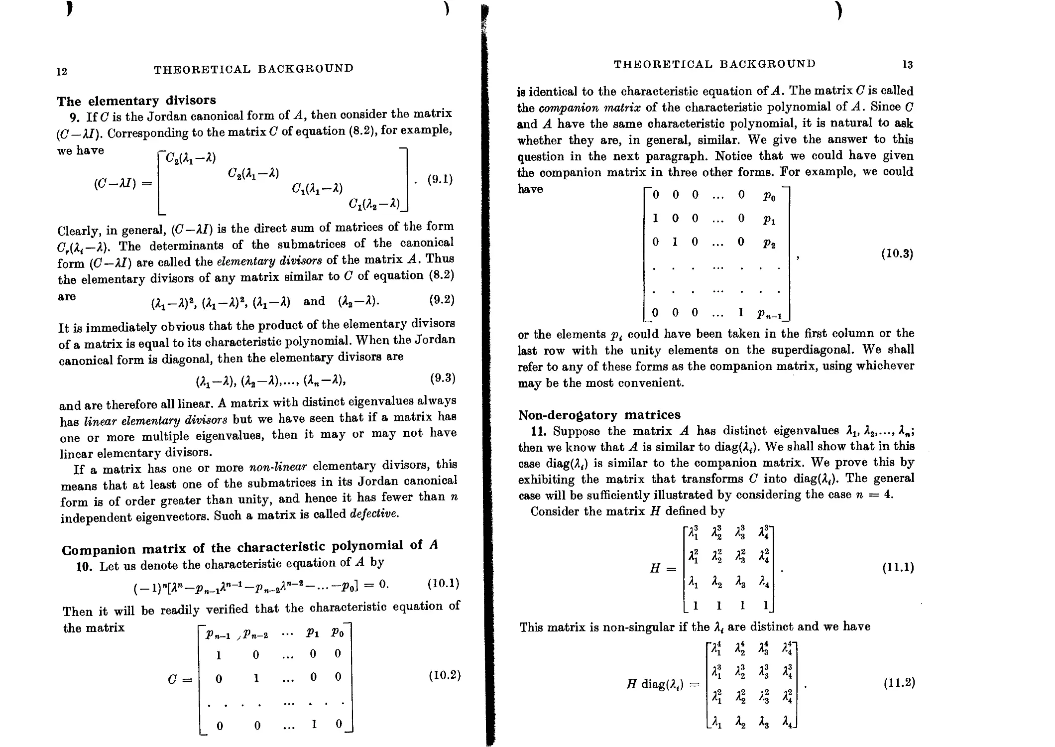
The elementary divisors
9.	If C is the Jordan canonical form of A, then consider the matrix
(С—21). Corresponding to the matrix C of equation (8.2), for example,
we have
(7^-2)
(<7—2Z) =
ед-2)
C'1(21-2)
• (9.1)
C'i(22-2)_
Clearly, in general, (<7—21) is the direct sum of matrices of the form
Cr(2(—2). The determinants of the submatrices of the canonical
form (C—21) are called the elementary divisors of the matrix A. Thus
the elementary divisors of any matrix similar to C of equation (8.2)
аГе	(2i— 2)2, (2x-2)2, (2X—2) and (22—2).	(9.2)
It is immediately obvious that the product of the elementary divisors
of a matrix is equal to its characteristic polynomial. When the Jordan
canonical form is diagonal, then the elementary divisors are
(2x-2), (2a—2),..., (2n—2),	(9.3)
and are therefore all linear. A matrix with distinct eigenvalues always
has linear elementary divisors but we have seen that if a matrix has
one or more multiple eigenvalues, then it may or may not have
linear elementary divisors.
If a matrix has one or more non-linear elementary divisors, this
means that at least one of the submatrices in its Jordan canonical
form is of order greater than unity, and hence it has fewer than n
independent eigenvectors. Such a matrix is called defective.
Companion matrix of the characteristic polynomial of A
10.	Let us denote the characteristic equation of A by
( —l)n[2”—pn_22n~2 —... —p0] = 0.	(10.1)
Then it will be readily verified that the characteristic equation of
the matrix	— —	
	Pn-1 jPn-2	Pl Po	
	1	0	... 0	0	
C =	0	1	... 0	0	(Ю.2)
	0	0	...	1	0	
THEORETICAL BACKGROUND
13
is identical to the characteristic equation of A. The matrix G is called
the companion matrix of the characteristic polynomial of A. Since G
and A have the same characteristic polynomial, it is natural to ask
whether they are, in general, similar. We give the answer to this
question in the next paragraph. Notice that we could have given
the companion matrix in three other forms. For example, we could
have	“0	0	0
	1	0	0
	0	1	0
0	Po	
0	Pl	
0	P2	,	(10.3)
1	Pn-1	
0 0 0
or the elements p( could have been taken in the first column or the
last row with the unity elements on the superdiagonal. We shall
refer to any of these forms as the companion matrix, using whichever
may be the most convenient.
Non-derogatory matrices
11.	Suppose the matrix A has distinct eigenvalues Я1; Я2,..., An;
then we know that A is similar to diag(A,). We shall show that in this
case diag(A4) is similar to the companion matrix. We prove this by
exhibiting the matrix that transforms G into diag(2<). The general
case will be sufficiently illustrated by considering the case n = 4.
Consider the matrix H defined by
j3 j3
Л1 Л2
J2 I2
H = 1 2
Aj A2
1 1
This matrix is non-singular if the A< are distinct and we have
	X	*2	^3	%
	я!			%
H diag(A() =				
	%			%
	Л	^2	^8	^4-
(П.2)
14
THEORETICAL BACKGROUND
Further, the relation
>з Рг Pl Po		"14 14 14 14“ Л1 л2 л3 л4	
10	0	0		13	13	13	13 Л1	Л2	Л3 Л4	
	H =		(11.3)
0	10 0		12	12	12	12 Л1 Л2 Л3 Л4	
0 0	1	0		^3	^4.	
follows immediately from the fact that
AJ = P3A?+/M?+M+Po-	(П.4)
Hence
CH = H diag(A(),	(11.5)
so that C is similar to diag(^J and hence to any matrix with eigen-
values
Turning now to the case when there are some multiple eigenvalues,
we see immediately that if A has more than one independent eigen-
vector corresponding to then it cannot be similar to C. For (C—AI)
is of rank (n — 1) for any value of Я, since the determinant of the matrix
of order (n —1) in the bottom left-hand corner is obviously 1. The
eigenvector x{ corresponding to the eigenvalue At is given by
x? =[ЛГ\ЯГ2,...,Я,., 1],	(11.6)
as can be seen by solving
(C-AJX = 0 .	(11.7)
For a matrix to be similar to the companion matrix of its charac-
teristic polynomial then, it is necessary that its Jordan canonical
form should have only one Jordan submatrix associated with each
distinct eigenvalue. We now prove that this condition is also sufficient
and again it will suffice to demonstrate it for a simple case.
12.	Consider a matrix of order 4 having (Лх —Я)2, (Я3—Я), (Я4 — Я) for
its elementary divisors. Such a matrix is similar to At given by
'A 1
О Я4
^4-
(12.1)
THEORETICAL BACKGROUND
16
Now the matrix H defined by
"i8	012	o3“
Aj OAj Ag A^
% ч Л32 22
н =
2i 1	23 Я4
1	0	11
(12.2)
is clearly non-singular if 21( 23, 24 are distinct, and we have
	ЯА4 =	X 42? 23 2?"	•	(12.3)
		}3	q12	08 j3 A^ OAj Ag A^		
				
		2? 22i A2 2?		
		_2i	1	23 24		
Since 2i is a double root of the characteristic equation/(2)				= 0, we have
/'(Ai) = 0, giving and hence	42i — 32>32i+2pg2i4-Pi, CH = HA 4.			(12.4) (12.5)
In an exactly similar way we can deal with a Jordan submatrix
of order r associated with a matrix of order n. If 2j is the relevant
eigenvalue then the corresponding matrix H, has the r columns
2”-1	In — 1' \ 1 ,	л;-2 ..	In —1\ 1 i A?“r yr—1/ 1	
2»-2	In— 2' \ 1 >	2«-3 ..	1 T r-i 1 1	(12.6)
Ai	1	-•	0	
1	0	..	°	
b Hence, provided there is only one Jordan matrix associated with each
Ц distinct 2,., and therefore only one eigenvector associated with each
К distinct 2O the matrix is similar to the companion matrix of its
ж characteristic polynomial. Such a matrix is called non-derogatory.
К The Frobenius (rational) canonical form
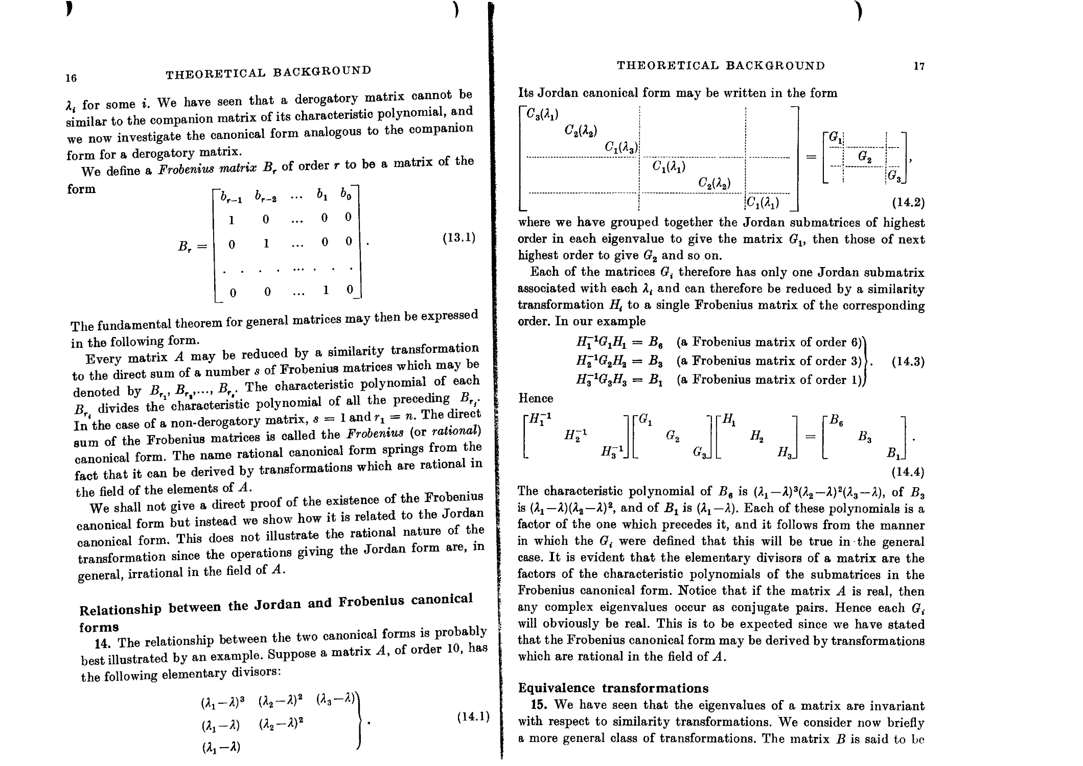
В 13. A matrix is called derogatory if there is more than one Jordan
К wbmatrix (and therefore more than one eigenvector) associated with
16
THEORETICAL BACKGROUND
for some i. We have seen that a derogatory matrix cannot be
similar to the companion matrix of its characteristic polynomial, and
we now investigate the canonical form analogous to the companion
form for a derogatory matrix.
We define a Frobenius matrix Br of order r to		be a matrix of the
form		
	^r-l ^r-2	*0	
	1	0	...	0 0	
Br =	0	1	...	0 0	(13.1)
	_ 0	0	...	1 0_	
The fundamental theorem for general matrices may then be expressed
in the following form.
Every matrix A may be reduced by a similarity transformation
to the direct sum of a number s of Frobenius matrices which may be
denoted by Bfj, Вг>,..., Br . The characteristic polynomial of each
ВГ( divides the characteristic polynomial of all the preceding ВГ).
In the case of a non-derogatory matrix, s = 1 and rt = n. The direct
sum of the Frobenius matrices is called the Frobenius (or rational)
canonical form. The name rational canonical form springs from the
fact that it can be derived by transformations which are rational in
the field of the elements of A.
We shall not give a direct proof of the existence of the Frobenius
canonical form but instead we show how it is related to the Jordan
canonical form. This does not illustrate the rational nature of the
transformation since the operations giving the Jordan form are, in
general, irrational in the field of A.
Relationship between the Jordan and Frobenius canonical
forms
14.	The relationship between the two canonical forms is probably
best illustrated by an example. Suppose a matrix A, of order 10, has
the following elementary divisors:
Л-Я)3
(Л1-Л)
Л-Я)
(Л2-Я)2
(Л-D2
U3-A)'
(14.1)
THEORETICAL BACKGROUND
17
Its Jordan canonical form may be written in the form
4(A)
GM
CM
rGi
cm
G3J
I	1ВД
where we have grouped together the Jordan submatrices of highest
order in each eigenvalue to give the matrix Gv then those of next
highest order to give G2 and so on.
Each of the matrices Gt therefore has only one Jordan submatrix
associated with each and can therefore be reduced by a similarity
transformation Ht to a single Frobenius matrix of the corresponding
order. In our example
H^G.H. = Be
H?G3H3 = B3
H3lG3H3 = Br
(14-2)
Hence
ГЯГ1
(a Frobenius matrix of order 6)'
(a Frobenius matrix of order 3) .
(a Frobenius matrix of order 1),
(14-3)
6r2
G3.
r^i 1
h,
L	h3]
Ba

з J
Г&

(14.4)
The characteristic polynomial of Be is (Aj—Л)3(Л2—A)2(A3—A), of B3
is (AJ—A)(A2—A)2, and of Br is (Ax—A). Each of these polynomials is a
factor of the one which precedes it, and it follows from the manner
in which the G( were defined that this will be true in the general
case. It is evident that the elementary divisors of a matrix are the
factors of the characteristic polynomials of the submatrices in the
Frobenius canonical form. Notice that if the matrix A is real, then
any complex eigenvalues occur as conjugate pairs. Hence each G(
will obviously be real. This is to be expected since we have stated
that the Frobenius canonical form may be derived by transformations
which are rational in the field of A.
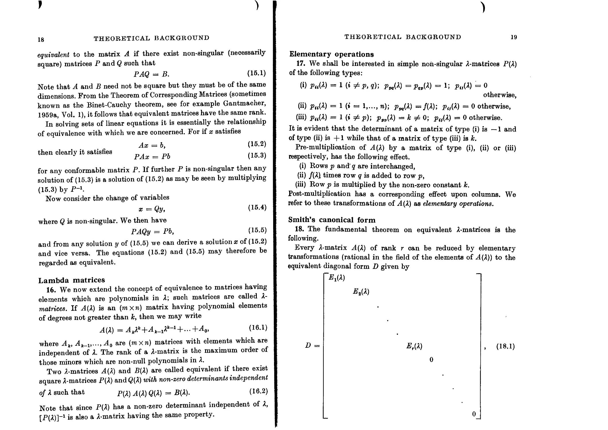
Equivalence transformations
15.	We have seen that the eigenvalues of a matrix are invariant
with respect to similarity transformations. We consider now briefly
a more general class of transformations. The matrix В is said to be
18
THEORETICAL BACKGROUND
equivalent to the matrix A if there exist non-singular (necessarily
square) matrices P and Q such that
PAQ = B.	(15.1)
Note that A and В need not be square but they must be of the same
dimensions. From the Theorem of Corresponding Matrices (sometimes
known as the Binet-Cauchy theorem, see for example Gantmacher,
1959a, Vol. 1), it follows that equivalent matrices have the same rank.
In solving sets of linear equations it is essentially the relationship
of equivalence with which we are concerned. For if x satisfies
Ax = b,	(15.2)
then clearly it satisfies
PAx = Pb	(15.3)
for any conformable matrix P. If further P is non-singular then any
solution of (15.3) is a solution of (15.2) as may be seen by multiplying
(15.3) by P-\
Now consider the change of variables
a: = Qy,	(15.4)
where Q is non-singular. We then have
PAQy = Pb,	(15.5)
and from any solution у of (15.5) we can derive a solution x of (15.2)
and vice versa. The equations (15.2) and (15.5) may therefore be
regarded as equivalent.
Lambda matrices
16.	We now extend the concept of equivalence to matrices having
elements which are polynomials in 2; such matrices are called 2-
matrices. If Л (2) is an (mxn) matrix having polynomial elements
of degrees not greater than k, then we may write
Л(2) = Л^*+А_12*-1+...+Л0,	(16.1)
where Ak, Ak_r....Ao are (mxn) matrices with elements which are
independent of 2. The rank of a 2-matrix is the maximum order of
those minors which are non-null polynomials in 2.
Two 2-matrices Л(2) and B(2) are called equivalent if there exist
square 2-matrices F(2) and 0(2) with non-zero determinants independent
of к such that	л(2) Q(A) = B(2).	(16.2)
Note that since F(2) has a non-zero determinant independent of 2,
[jP(2)]“1 is also a 2-matrix having the same property.
THEORETICAL BACKGROUND
19
Elementary operations
17.	We shall be interested in simple noh-singular 2-matrices P(2)
of the following types:
(i)	рц(Х) =	<?); pM(2) = ^>„(2) = 1; pit(X) = 0
otherwise,
(ii)	PhW = 1 (i = 1,..., n); pM(2) ==/(2); po(2) = 0 otherwise,
(iii)	p{i(k) = 1 (i ^p)-, р„„(2) = к =£ 0; po(2) = 0 otherwise.
It is evident that the determinant of a matrix of type (i) is — 1 and
of type (ii) is +1 while that of a matrix of type (iii) is k.
Pre-multiplication of Л(2) by a matrix of type (i), (ii) or (iii)
respectively, has the following effect.
(i)	Rows p and’ q are interchanged,
(ii)	/(2) times row q is added to row p,
(iii)	Row p is multiplied by the non-zero constant k.
Post-multiplication has a corresponding effect upon columns. We
refer to these transformations of Л(2) as elementary operations.
Smith’s canonical form
18.	The fundamental theorem on equivalent 2-matrices is the
following.
Every 2-matrix Л (2) of rank r can be reduced by elementary
transformations (rational in the field of the elements of Л(2)) to the
equivalent diagonal form D given by
"Ei(2)
ErW
0
(18.1)
0
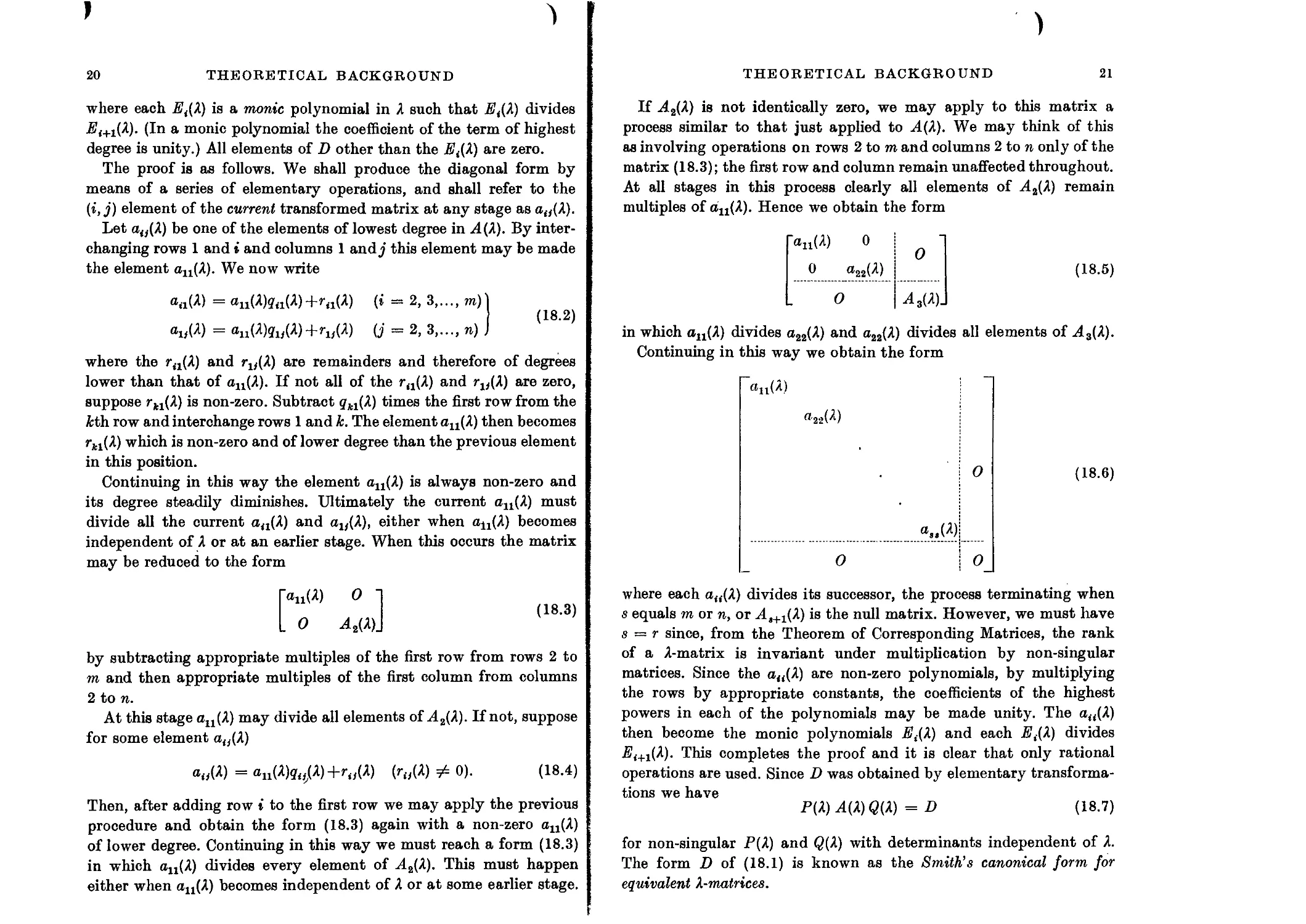
20
THEORETICAL BACKGROUND
where each Et(X) is a monic polynomial in 2 such that Е<(Л) divides
A'<+i(2). (In a monic polynomial the coefficient of the term of highest
degree is unity.) All elements of D other than the E{(X) are zero.
The proof is as follows. We shall produce the diagonal form by
means of a series of elementary operations, and shall refer to the
(i, j) element of the current transformed matrix at any stage as aiy(2).
Let ao(2) be one of the elements of lowest degree in А(2). By inter-
changing rows 1 and i and columns 1 and J this element may be made
the element an(2). We now write
an(2) — anW<hiW(* — 2, 3,..., wi)l
(18-2)
au(2) = au(2)?u(2)+rw(2) (j = 2, 3,..., n) J
where the rn(2) and rjy(2) are remainders and therefore of degrees
lower than that of au(2). If not all of the rn(2) and rH(2) are zero,
suppose rH(2) is non-zero. Subtract g'il(2) times the first row from the
Mh row and interchange rows 1 and k. The element au(2) then becomes
ги(2) which is non-zero and of lower degree than the previous element
in this position.
Continuing in this way the element au(2) is always non-zero and
its degree steadily diminishes. Ultimately the current au(2) must
divide all the current aa(2) and au(2.), either when ац(2) becomes
independent of 2 or at an earlier stage. When this occurs the matrix
may be reduced to the form
«nW 0
. О A2(2).
(18.3)
by subtracting appropriate multiples of the first row from rows 2 to
m and then appropriate multiples of the first column from columns
2 to n.
At this stage au(2) may divide all elements of A2(2). If not, suppose
for some element a(J(2)
a„(2) =au(2)g4(2)+ro(2) (r„(2) ф 0).	(18.4)
Then, after adding row i to the first row we may apply the previous
procedure and obtain the form (18.3) again with a non-zero au(2)
of lower degree. Continuing in this way we must reach a form (18.3)
in which au(2) divides every element of A2(2). This must happen
either when au(2) becomes independent of 2 or at some earlier stage.
THEORETICAL BACKGROUND
21
If AZ(A) is not identically zero, we may apply to this matrix a
process similar to that just applied to A (2). We may think of this
as involving operations on rows 2 to m and columns 2 to n only of the
matrix (18.3); the first row and column remain unaffected throughout.
At all stages in this process clearly all elements of A2(2) remain
multiples of an(2). Hence we obtain the form
«и(А) о
0
О
(18.5)
in which an(2) divides агг(Х) and a22(2) divides all elements of A3(2).
Continuing in this way we obtain the form
«11(A)
«22(A)	>
| 0
«,,(A)|
О	O_
(18.6)
where each af((2) divides its successor, the process terminating when
s equals m or n, or ri.3+1(2) is the null matrix. However, we must have
s = r since, from the Theorem of Corresponding Matrices, the rank
of a 2-matrix is invariant under multiplication by non-singular
matrices. Since the a4<(2) are non-zero polynomials, by multiplying
the rows by appropriate constants, the coefficients of the highest
powers in each of the polynomials may be made unity. The ««(A)
then become the monic polynomials P,(2) and each P,(2) divides
2?<+i(2). This completes the proof and it is clear that only rational
operations are used. Since D was obtained by elementary transforma-
tions we have
P(2) A(2) QW = D	(18.7)
for non-singular P(2) and Q(2) with determinants independent of A.
The form D of (18.1) is known as the Smith’s canonical form for
equivalent ^.-matrices.
22
THEORETICAL BACKGROUND
The highest common factor of Л-rowed minors
of a A-matrix
19.	Consider now the Л-rowed minors of the Smith’s canonical
form. If к > т then all Л-rowed minors are zero. Otherwise the only
non-zero Л-rowed minors are products of Л of the Et(A). Since each
Et(A) is a factor of EM(A), the highest common factor (H.C.F.) Gk(A)
of Л-rowed minors is Ek(A) E2(A)...Ek(A). Hence if we write С0(Л) = 1
(i = 1, 2,..., r).	(19.1)
We now show that the H.C.F. of Л-rowed minors of a matrix (we
take the coefficient of the highest power of Л to be unity) is invariant
under equivalence transformations. For if
Р(Л)А(Л)(?(Л) = В(Л),	(19.2)
then any Л-rowed minor of В(Л) may be expressed as the sum of
terms of the form PaApQy where Pa, Ap, Q? denote a Л-rowed minor
of Р(Л), А(Л), Q(A) respectively. Hence the H.C.F. of the Л-rowed
minors of A(A) divides any Л-rowed minor of В (A). Since, however,
Л(Л) = [Р(Л)]-»В(Л)[(?(Л)]-»
and [Р(Л)]-1 and [ф(Л)]_1 are also Л-matrices, the H.C.F. of Л-rowed
minors of B(A) divides any Л-rowed minor of А(Л). The two H.C.F.’s
must therefore be equal.
All equivalent Л-matrices therefore have the same Smith’s canonical
form. The polynomials E{(A) are called the invariant factors or invariant
polynomials of А(Л).
Invariant factors of (A—XI)
20.	If A is a square matrix, then (A —Al) is a Л-matrix of rank n,
and hence has n invariant factors, Ег(А), E2(A),..., E„(A), each of
which divides its successor. We now relate the invariant factors of
(A— Al) with the determinants of the Frobenius matrices in the
Frobenius canonical forms. Suppose В is the Frobenius canonical
form of A, so that there exists an H such that
and therefore
H^AH = B,	(20.1)
H~l(A-AI)H = B—AI.	(20.2)
Since the matrices H-1 and H are non-singular and independent of Л,
(B—AI) is equivalent to (A —Al).
THEORETICAL BACKGROUND
23
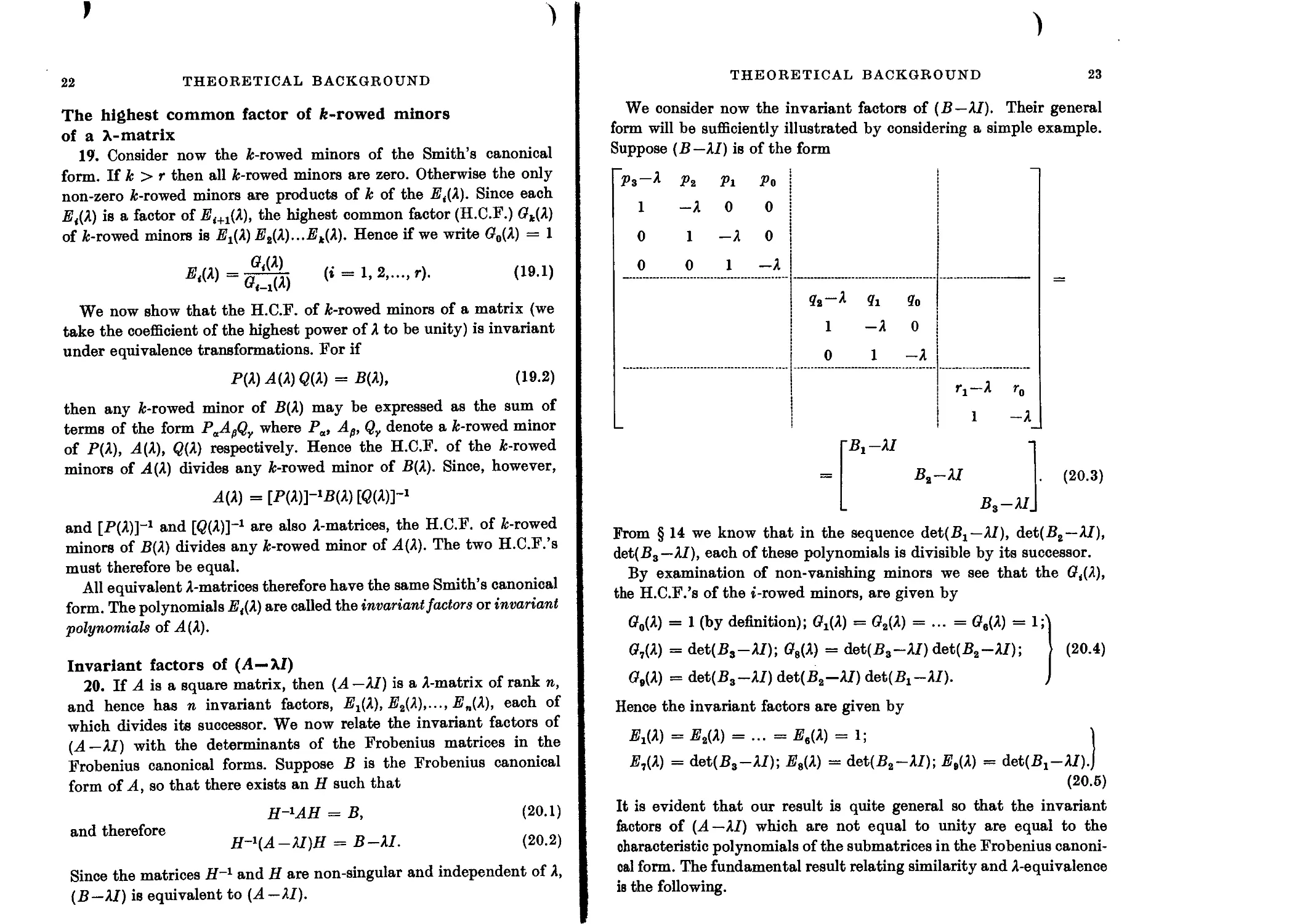
We consider now the invariant factors of (В—Al). Their general
form will be sufficiently illustrated by considering a simple example.
Suppose (B—AI) is of the form
р3-Л	p2	P1	p0
1	-Л	0	0
0	1	-A	0
0	0	1	-A
q0
1 -A 0
0 ~A
ri-Л r0
1 -A
ГВ1-Л/
Ba—AI
BS-AI
(20.3)
From § 14 we know that in the sequence de^Bj — Al), det(B2 —Al),
&eh(B3—AI), each of these polynomials is divisible by its successor.
By examination of non-vanishing minors we see that the Gt(A),
the H.C.F.’s of the i-rowed minors, are given by
G0(A) = 1 (by definition); G±(A) = G2(A) = ... = (?в(Л) = 1Л
(77(A) = det(B3—AI); G8(A) = det(B3-lT) det(B2-W); I (20.4)
Gt(A) = det(B3 —Al) &Л(В3-А1) АеЦВ^-AI).	J
Hence the invariant factors are given by
EX(A) = ВД = ... = E3(A) = 1;	1
E2(A) = det(B3-Al)-, E3(A) = det(B2-Af); E3(A) = det(B1-lir).j
(20.5)
It is evident that our result is quite general so that the invariant
factors of (A—Al) which are not equal to unity are equal to the
characteristic polynomials of the submatrices in the Frobenius canoni-
cal form. The fundamental result relating similarity and A-equivalence
is the following.
24
THEORETICAL BACKGROUND
A necessary and sufficient condition for A to be similar to В is that
(А — 27) and {B—AI) are equivalent. For this reason the invariant
factors of (A—Ad) are sometimes called the similarity invariants of A.
Again from § 14 we see that if we write
E^A) = (Лх—ЛУЧЛа—Л)Ч	(20.6)
where Лх, Л2,..., Л, are the distinct eigenvalues of A, then the factors
on the right of (20.6) are the elementary divisors of A.
The triangular canonical form
21.	Reduction to Jordan canonical form provides complete informa-
tion on both the eigenvalues and the eigenvectors. This form is a
special case of the triangular canonical form. The latter is very much
simpler from the theoretical standpoint and also for practical com-
putation. Its importance is a consequence of the following theorem
and that of § 25.
Every matrix is similar to a matrix of triangular form, that is, a
matrix in which all the elements above the diagonal are zero. We
refer to such a matrix as a lower triangular matrix. As with the
Jordan form there is an alternative transformation leading to a
matrix with zeros below the diagonal {upper triangular). The proof is
comparatively elementary but is deferred until § 42 when the appro-
priate transformation matrices have been introduced.
Clearly the diagonal elements are the eigenvalues with the appro-
priate multiplicities. For if these elements are pt then the characteristic
polynomial of the triangular matrix is JJ {pt —A) and we have seen
that the characteristic polynomial is invariant under similarity trans-
formations.
Hermitian and symmetric matrices
22.	Matrices which are real and symmetric are of special importance
in practice as we shall see in § 31. We could extend this class of
matrices by including all matrices which are symmetric and have
complex elements. However, such an extension proves to be of little
value because matrices of this extended class do not have many of
the more important properties of real symmetric matrices. The most
useful extension is to the class of matrices of the form (P+iQ) where
P is real and symmetric and Q is real and skew symmetric, that is
QT = -Q.	(22.1)
THEORETICAL BACKGROUND
25
Matrices of this class are called Hermitian matrices. If A is Her-
mitian we have from the definition
AT = A,	(22.2)
where A denotes the matrix whose elements are the complex con-
jugates of those of A. The matrix AT is frequently denoted by AB
and is referred to as the Hermitian transposed matrix. Similarly xB
is the row vector with components equal to the complex conjugates
of those of the column vector x. The notation is a convenient one and
has the advantage that results proved for Hermitian matrices may
be converted to the corresponding results for real symmetric matrices
by replacing AH by AT and ж® by xT. If a is a scalar, aH is defined to
be the complex conjugate of a. It follows immediately from the
definitions that
(AB)B = A
(хл)н = X
= CbBbAh
AB — A
(22.3)
(ABC)H
while
(22.4)
if A is Hermitian.
Note that ^x is the inner-product of у and x as normally under-
stood and	г.	n J! tt	.лл —
У x = (у x)B = xBy.	(22.5)
The inner-product xBx is real and positive for all x other than the
null vector since it is equal to the sum of the squares of the moduli
of the elements of x.
Elementary properties of Hermitian matrices
23.	The eigenvalues of a Hermitian matrix are all real. For if
then
Ax = Ax
xBAx = AxBx.
(23.1)
(23.2)
Now we have remarked that xBx is real and positive for a non-null x.
Further we have
(xBAx)B == xBABx?B — Xя Ax,
(23.3)
and since Xя Ax is a scalar this means that it is real. Hence A is real.
For real symmetric matrices, real eigenvalues imply real eigenvectors,
but the eigenvectors of a complex Hermitian matrix are in general
complex.
If Ax — Ax we have for a Hermitian matrix
ABx ~ Ax
(23.4)
26
THEORETICAL BACKGROUND
and taking the complex conjugate of both sides
ATx = }.£.	(23.5)
The eigenvectors of the transpose of a Hermitian matrix are therefore
the complex conjugates of those of the matrix itself. In the notation
°f § 3	yt = xt.	(23.6)
The quantities yfx{ which are of great importance in the theory
therefore become x?x( for Hermitian matrices. It follows immediately
from the general theory of § 3 that if a Hermitian matrix has
distinct eigenvalues then its eigenvectors satisfy
A = 0 (i^j).	(23.7)
If we normalize the x{ so that
x*x{ = 1,	(23.8)
equations (23.7) and (23.8) imply that the matrix X formed by the
eigenvectors satisfies	. e _^h =	^3 9)
A matrix which satisfies equations (23.9) is called a unitary matrix.
A real unitary matrix is called an orthogonal matrix.
We have therefore proved the following for Hermitian and real
symmetric matrices with distinct eigenvalues.
(I) If A is Hermitian there exists a unitary matrix U such that
UBAU = diag(Ai) (real Л<).
(II) If A is real and symmetric, there exists an orthogonal matrix
U such that _	, .
UTAU = diag(^) (real AJ.
Perhaps the most important property of Hermitian (real symmetric)
matrices is that I (II), which we have so far proved only in the case
of distinct eigenvalues, is true whatever multiplicities there may be.
The proof is deferred until § 47.
Immediate consequences of this fundamental result are.
(i)	The elementary divisors of a Hermitian matrix are all linear.
(ii)	If a Hermitian matrix has any multiple eigenvalues then it is
derogatory.
(iii)	A Hermitian matrix cannot be defective.
Complex symmetric matrices
24.	That none of the important properties of real symmetric
matrices is shared by complex symmetric matrices may be seen by
THEORETICAL BACKGROUND
27
considering the matrix A defined by
Г2» 11
(24.1)
The characteristic equation is Л2 —2iA—1 = 0, so that Я = i is an
eigenvalue of multiplicity 2. The components xlt x2 of a corresponding
eigenvector satisfy	= „	=	(24.2)
so that there is only one eigenvector, and that has components
(1, -»')•
We conclude that there is a quadratic divisor associated with A = i.
In fact the Jordan canonical form is
		Гг П		
and we have		.0 ».	J	(24.3)
	"2г 11Г 1 C . 1 OJL— i 1	1	1	01 Гг	Г i 1_ .0	i_	(24.4)
Reduction to triangular form by unitary transformations
25.	Since a Hermitian matrix may always be reduced to diagonal
form by a unitary similarity transformation, it is interesting to con-
sider what reduction of a general matrix may be achieved by such a
transformation. It can be shown that any matrix may be reduced
by a unitary similarity transformation to triangular form. Since the
triangular form provides us immediately with the eigenvalues, and
the eigenvectors may be found comparatively simply, this result is
of practical importance because unitary transformations have desir-
able numerical properties. We defer the proof until § 47 when the
appropriate transformation matrices have been introduced.
Quadratic forms
26.	We may associate with a real symmetric matrix A, a, quadratic
form xTAx in the n variables xv x2,..., x„ defined by
xvAx = £ a^XiXj,	(26.1)
where x is the vector with components xt. Corresponding to each
quadratic form we may define a bilinear form xTAy defined by
xTAy = 2	= УтАх-	(26.2)
M-i
Hence writing
we have
28	THEORETICAL BACKGROUND
Certain types of quadratic form are of particular interest. A quad-
ratic form with matrix A is defined to be
positive definite	7 > 0
•negative definite I	I < 0
> according as xrAx Z for all real x 0.
non-negative definite j	| > 0
non-positive definite )	\ < 0
The matrix of a positive definite quadratic form is called a positive
definite matrix.
A necessary and sufficient condition for жгЛа; to be positive definite
is that all the eigenvalues of A should be positive. For we know that
there exists an orthogonal matrix R such that
RTAR = diag(24).	(26.3)
x — Rz i.e. z = RTx,	(26.4)
xTAx = zTRTARz — J	.	(26.5)
»=i
n
A necessary and sufficient condition for J A,z? to be positive for all
non-null z is that all should be positive. From (26.4) we see that
non-null z correspond to non-null x and conversely; hence the result
is established. Since the determinant of a matrix is equal to the prod-
uct of its eigenvalues the determinant of a positive definite matrix
must be positive.
From equations (26.4) and (26.5) we deduce that the problem of
determining the orthogonal matrix R, and hence the eigenvectors of
A, is identical with that of determining the principal axes of the
quadratic	g а„х{х} = 1	(26.6)
and that the are the reciprocals of the squares of the principal
axes. A multiple eigenvalue is associated with an indeterminacy of
the principal axes. As a typical example we may take an ellipsoid
in three dimensions with two equal principal axes. One of its principal
sections is then a circle and we may take any two perpendicular
diameters of the circle as principal axes.
Necessary and sufficient conditions for positive
definiteness
27.	We denote by xTArx the quadratic form derived from xTAx
by setting хг+1, xr+2,   , xn equal to zero. xrAr x is therefore a quadratic
THEORETICAL BACKGROUND
29
form in the r variables xv x2,..., xr, and the matrix Ar of this
form is the leading principal submatrix of order r of A. Clearly if
xTAx is positive definite, xTArx must be positive definite. For if
there exists a non-null set of values xlf x2,..., xr for which xTArx is
non-positive, then xTAx is non-positive for the vector x given by
xT = (x1)J1,...,a:r, 0.....0).	(27.1)
Hence all leading principal minors of a positive definite matrix must
be positive.
Note that an exactly similar method of proof shows that any
principal submatrix of a positive definite matrix is positive definite
and hence has positive determinant. However, the possession of n
positive leading principal minors is also a sufficient condition for
positive definiteness. The proof is by induction.
Suppose it is true for matrices of order (n —1). We then show that
it is true for matrices of order n. For suppose on the contrary that A
is a matrix of order n for which the n leading principal minors are
positive and that A is not positive definite. If R is the orthogonal
matrix for which RT A R — diag(AJ then writing x = Rz we have
= zTRTARz — 2 Afz$.	(27.2)
Now by hypothesis A is not positive definite and therefore, since
n
IT (Л() = det(^) > 0, there must be an even number r of negative
i=i
Suppose the first r are negative. Then consider the set of equations
zr+l = Zr+2 = •• = zn =	= 0-	(27.3)
Since the z{ are linear functions of the x< we have (n — r + 1) linear
homogeneous equations in the n unknowns aq, x2,..., x„. There is
therefore at least one non-null solution x which we may denote
by (aCj, a52,..., xn_lt 0). The corresponding z is also non-null and we
may denote this by (z1( z2,..., zr, 0, 0,..., 0). For this x and z we have
xTAx = J Л,г? = 2 2,z? < 0.	(27.4)
1 1
Now since xn = 0, this implies that xTAn_1x is negative for the
vector («и x2,..., ж„_1). This contradicts our inductive hypothesis.
The result is obviously true for matrices of order one and is therefore
true for matrices of any order.
In the same way as we have associated a quadratic form with a
30
THEORETICAL BACKGROUND
real symmetric matrix, we may associate with a Hermitian matrix A,
a Hermitian form defined by
n
xHAx = £ atjxtxt.	(27.6)
We have	=	=	(27,6)
and hence XsAx is real. The concepts of positive definiteness etc.
carry over immediately to Hermitian forms and there are results
analogous to those we have just proved for real quadratic forms.
Differential equations with constant coefficients
28.	The solution of the algebraic eigenvalue problem is closely
related to the solution of a set of linear simultaneous ordinary differ-
ential equations with constant coefficients. The general set of first-
order homogeneous equations in n unknowns ylt у2,..-,уп may be
written in the form	л
BIt{y)=Gy,	(28.1)
where t is the independent variable, у is the vector with components
yit and В and C are n X n matrices. If В is singular the n left-hand
sides of the system of equations satisfy a linear relation. The right-
hand side must satisfy the same linear relation and hence the yt are
not independent. The set of equations may therefore be reduced to
a system of lower order. We shall not pursue this further and shall
assume that В is non-singular.
Equation (28.1) may then be written in the form
(У) = Ay,	(28.2)
where	Я = в~Ю.	(28.3)
Let us assume that (28.2) has a solution of the form
у — xeu,	(28.4)
where ж is a vector independent of t. Then we must have
Лжел = Axeu,
and therefore	= Ax	(28,5)
Equation (28.4) will give a solution of (28.2) if A is an eigenvalue of
A and x is the corresponding eigenvector. If there are r independent
eigenvectors of A then we obtain r independent solutions of A, this
being true regardless of whether all the corresponding eigenvalues
are distinct. However, there must be n independent solutions of
)
THEORETICAL BACKGROUND	31
(28.2), so that if r < n, that is if some of the elementary divisors of
A are non-linear, equation (28.2) must have some solutions which are
not of pure exponential type.
Solutions corresponding to non-linear elementary
divisors
29.	The nature of the solution when there are non-linear elementary
divisors can be examined in terms of the Jordan canonical form. Let
X be the matrix of the similarity transformation which reduces A to
the Jordan form. If we now define new variables z by the relation
У = Xz,	(29.1)
then (28.2) becomes	A
XT.(z)=AXz	(29.2)
(Lv
i.e.	^-(z)=X~lAXz.	(29.3)
etc
Note that the matrix of the equations undergoes a similarity trans-
formation. The matrix of the system of equations is now the Jordan
canonical form of A.
Suppose, for example, A is a matrix of order 6 with the lower
Jordan canonical form
Сз(Ях)
G(A2).
Then equations (29.3) are
dzl , d?~A1Z1 dF “ Z1+A1Z2 dz,	. , dF =	гг+Л12з			(29.4)
dt ~ dz5 = dt dze dt ~	us	: +	! i	^2Z6	
32
THEORETICAL BACKGROUND
The solutions of the first, fourth, and sixth of these equations are
zx = axeA1‘, z4 = а4еД1/, zB — aee*‘l,	(29.5)
of the third is
and of the fifth,
where a4, a4 and ae are arbitrary constants. The general solution of
the second equation is	,, ,	,	..
1	z2 = а2еЛ1>+a1te*1*,	(29.6)
z3 = а/1' +а2«еЛ1<+(29.7)
zB = aBeAli +а4/еЛ1‘,	(29.8)
where a2, a3 and aB are arbitrary constants. The general solution
of the system is therefore given by
zi
Z2
= axe 1
= ajieilt+а2е‘
Z3
+a3eA,(
z4 =
z6 —
a4el‘
a4<eA1‘ +aBeA1‘
(29.9)
ze =	«ee ’ .
Note that there are only three independent solutions which are pure
exponentials. These are
z = a3e*l‘e3, z = авеД1<ев, z = авед,<ев, (29.10)
as we would expect, since e3, eB and ee are the only eigenvectors of
the Jordan canonical form.
The general solution of the original equations is now obtained by
substituting for z in equation (29.1). If the columns of X are denoted
by xt, ж2,..., xB then the general solution of (28.2) is
у = a1eilt(x1+tx3 + lt2x3)+a2e^t(x2+tx3)+a3elltx3 +
+а4еД1\я4+<яв)+авеД1(яв+авед<гв. (29.11)
The result in the general case is immediately obvious from this.
Differential equations of higher order
30.	We consider now the system of n simultaneous homogenous
differential equations of order r by
dr	d'"1
Л^-,(Уо)+^г-1^Т1 (Уо) + ---+^оУо = °-
(30.1)
THEORETICAL BACKGROUND
33
where Ar, Ar_v..., Ao are (nxn) matrices with constant elements
and det(Ar) 0, and we use y0 to denote the vector of order n formed
by the n dependent variables. (We use y9 instead of у for reasons
which will soon become apparent.) The system (30.1) may be reduced
to a system of first-order equations by introducing r(n — 1) new vari-
ables defined by
d
y* = d№
(30.2)
~~ dt
If Ar is non-singular we may write equations (30.1) in the form
d
B^/0-\-B1y1-\-...JrBr_1yr-i = dj(yr-i)> (30.3)
here	B, = -Ar~%.	(30.4)
Equations (30.2) and (30.3) may be regarded as a single set of
nr equations in the nr variables which are the components of
Уо> Уг-i- We may write them in the form
" 0 0 0	I 0 0	0 I 0	0 . 0 . I	0 0 0	~ У 0 ~ Уг	43 II	~ У о ~ У1 Уг	. (30.5)
0 _So	to о	0	0 . S3 .	. I  Br^_	чг ч	ч 1	1 to 1				Ут-2 _Уг-1_	
This system may now be solved by the methods of the previous
section and requires the determination of the Jordan canonical form
of the matrix В of order nr on the left-hand side of (30.5). Although
this matrix is of high order it is of a particularly simple form and has
a high percentage of zero elements. If л is an eigenvalue of B, and x
is an eigenvector which is partitioned into the r vectors a;0, x1,..., xr_v
then	,	,.
x( = лх^ (i = 1,..., r — 1) I
(30.6)
‘	-®oa;o~h ByX^-^-... + Br_1xr_l = Ла;г_1)
and hence (B0+BJ+... +Br_^)x9 = Л%.	(30.7)
34	THEORETICAL BACKGROUND
These equations have a non-zero solution if
det (Bo + ВХЛ +... + B^-1 —1ЛГ) = 0.	(30.8)
In practical work we have a choice of working with the matrix В of
order rn and solving the standard eigenproblem, or alternatively of
working with the determinantal equation (30.8) which is no longer
standard, but in which the matrix is of order n only.
Second-order equations of special form
31.	The equations of motion for small vibrations about a position
of stable equilibrium of a mechanical system operated upon by a
conservative system of forces are of the form
By = -Ay,	(31.1)
where A and В are symmetric and positive definite. If we assume
that the solutions are of the form у = xe'^ then we must have
pPBx = Ax.	(31.2)
Writing p2 = Я this becomes
ЛВх = Ax.	(31.3)
We shall now show that when A and В are symmetric and В is
positive definite, then the roots of det(A — ЛВ) = 0 are all real.
Since В is positive definite there exists an orthogonal R such that
RTBR = diag($),	(31.4)
where the /9? are the eigenvalues, necessarily positive, of B. We may
write	diag(ft) = D, diag(0?) = D2.	(31.5)
Then we have
(А—ЛВ) = RD(D-lRTARD-1-tT)DRT, (31.6)
and hence det(J = (det Д)2 (det D)i det(P-A/), (31.7)
where	P = D~1RTARD~1.	(31.8)
Since (det R)2 = 1 and (det D)2 = П^> ^e zeros °f det(A— ЛВ)
are those of det(P—Я7). The latter are the eigenvalues Ях, Л2,..., Л„
of P, a symmetric matrix, and are therefore real.
The matrix P has a complete set of eigenvectors zt which may be
taken to be orthogonal. We have therefore
Pzt = Л^, D~1RTARD~1zi =	(31.9)
giving
AtRD-'zJ =	= AtRD(DRT RD~l)zt = Л,В(РВ~\). (31.10)
THEORETICAL BACKGROUND
35
Hence xt = RD~1z( is an ‘eigenvector’ corresponding to A( of the
generalized eigenproblem represented by equation (31.3). Note that
since the z( are orthogonal and RD~V is real and non-singular, the x(
form a complete set of real eigenvectors of equation (31.3). Further
we have
0 = zfz, = (DRTxi)TDRTxi = x^RDDRTxj = xfBxjt (31.11)
showing that the vectors xt are orthogonal with respect to B.
If A is also positive definite, then the A( are positive. For we have
Ax{ = АчВх(, x?Axt = 2ptfBxt,	(31.12)
and both x^AXf and x^Bxt are positive.
Explicit solution of By = —Ay
32.	We can now derive an explicit expression for the solution of
equations (31.1) when A and В are positive definite. Let xv x2,...,xn
be n independent solutions of (31.3) corresponding to the eigenvalues
A1( A2,..., An. The latter must be positive but are not necessarily
distinct. Writing	2 = pl	(32 1)
where the pf are taken to be positive, the set of equations (31.1) has
the general solution n
у = J (а<е,/,‘/+6je_,7'*/)a:o	(32.2)
i
where the and bt are the 2n arbitrary constants. Assuming the
solution to be real, we may write it in the form
У = J ct СО8(/*^+«<)«<>	(32.3)
i
where the cf and are now the arbitrary constants.
Equations of the form (AB—M)x = 0
33.	In theoretical physics the problem we have just considered
often arises in the form (AB_U)x = Q>	(33Д)
where A and В are symmetric and one (or both) is positive definite.
If A is positive definite, then (33.1) is equivalent to
(B-AA-1)» = 0	(33.2)
since a positive definite matrix has a positive determinant and is
therefore non-singular. If В is positive definite, (33.1) may be written
in the form	(Д -ЛВ-1)(Ва;) = 0.	(33.3)
36	THEORETICAL BACKGROUND
Now the inverse of a positive definite matrix is itself positive definite.
F°r lf	A = RT diag(a2)B	(33.4)
then	A-1 = RT diag«2)B.	(33.5)
Hence equation (33.1) is not essentially different from equation (31.3).
The importance of the positive definiteness of one of the matrices
should not be underestimated. If A and В are real symmetric matrices,
but neither is positive definite, then the eigenvalues of AB need not
be real and the same applies to the roots of det(A — ЛВ) = 0. A
simple example will illustrate this. Let
A =	"a O' .0 ь.	>	в =	'0 Г .1 o.	(33.6)
Then	AB		'0 a b o_	•	(33.7)
The eigenvalues of AB satisfy the equation
Л2 = ab	(33.8)
and are complex if a and b have different signs.
If neither A nor В is positive definite and (a+i/9) is a complex root
of det(A —ЛВ) = 0 then we have
Ax = (ct+iftyBx	(33.9)
for some non-null x. Hence
Л1ж = (а-Н^аЛ&г.	(33.10)
Since XsAx and хиВх are real, equation (33.10) implies that
Xе Ax = xBBx = 0.	(33.11)
The minimum polynomial of a vector
34.	The eigenvectors x of a matrix are characterized by the fact
that there exists a linear relation between x and Ax. For an arbitrary
vector b no such relation exists, but if we form the sequence b, Ab,
A2b,..., Arb, then there must be a minimum value m of r for which
these vectors are dependent, and clearly m < n. We may write the
corresponding relation in the form
(A™+cm_1A’»-1+...+c()f)6 = °-	(34.1)
THEORETICAL BACKGROUND
37
From the definition of m there is no relation of the form
(Ar-j-dr_1Ar~1 + .-+<V)b = 0 (r < m).	(34.2)
The monic polynomial c(2) corresponding to the left-hand side of
(34.1) is called the minimum polynomial of b with respect to A. If s(4)
is any other polynomial in A for which s(A)b — 0 then c(A) must
divide s(A). For if not, then by the Euclidean algorithm there exist
polynomials p(A), q(A), r(A), such that
p(A)e(A)-g(A)c(A) = r(A)	(34.3)
where г(Л) is of lower degree than с(Л). But from (34.3) it follows
that r(A)b = 0 and this contradicts the hypothesis that c(A) is the
polynomial of lowest degree for which this is true.
The minimum polynomial is unique, for if d(A)b = 0 for a second
monic polynomial of degree wi, then [c(A) — d(A)]b = 0 and c(A) —d(A)
is of degree less than m. The degree of c(A) is called the grade of b with
respect to A.
The minimum polynomial of a matrix
35. In a similar way we may consider the sequence of matrices
I, A, A2,..., Ar. Again there is a smallest value s of r for which this
set of matrices is linearly dependent. We may write the relation in
the form	...	, T л
А*+т,_1А,~1 + -..	= 0.	(35.1)
For example if	A =	~Pi Po' . 1 0.	(35.2)
then	A2 =	'pI+p0	PiPo'
and hence		. Pi	Po -
Лг-Р1Л—p07 =	Pi+Po PiPo'		pl
L Pi Po J UPi
PiT’o'l po
0	0
(35.3)
0 '
Po.
'0 0‘
0 0
(35.4)
There is no relation of lower order because
>i +«0
_ 1
Po'
co_
A -\-c0I =
(35.5)
38	THEORETICAL BACKGROUND
and this is not null for any c0. This example is of significance in later
sections.
The polynomial т(Л) corresponding to the left-hand side of equation
(35.1) is called the minimum polynomial of the matrix A. Exactly as
in § 34 we may show that it is unique and divides any other poly-
nomial р(Л) for which p(A) = 0.
The minimum polynomial с(Л) of any vector b with respect to A
divides m(X} since we obviously have m(A)b = 0. Let с^Л), с2(Я),...,
cn(A) be the minimum polynomials of ev e2,..., en with respect to A
and let р(Л) be the least common multiple (L.C.M.) of the сДЛ). Then
we have	g(4)e, = 0 (j = x> n)	(35.6)
and hence g(A) = 0. This implies that g(A)b ~ 0 for any vector and
therefore д(Л) is the L.C.M. of the minimum polynomials of all vectors.
In fact we must have p(A) = тп(Л). For by definition m(A) = 0 and
hence m(A)e{ = 0. The L.C.M. of the minimum polynomials of the e{
must therefore divide m(X) and hence д(Я) divides ш(Л). But, by
definition, m(X) is the polynomial of lowest degree for which m(A) == 0.
We have developed this theory from the system of column vectors
b, Ab, A2b... In a similar way, by considering the system of row
vectors bT, bTA, bTA2,... we can determine a minimum polynomial of
bT with respect to A. Clearly the minimum polynomial of bT with
respect to A is the same as the minimum polynomial of b with
respect to AT.
If we denote the L.C.M. of the minimum polynomials of ef, ef*,..., e„
by h(X), then we may show as before, that h(A) is the null matrix and
hence that Л(Л) is also identical with да(Я). We arrive at the same
minimum polynomial of A whether we consider row or column vectors.
It will be more convenient later (§ 37) to work with row vectors.
Cayley-Hamilton theorem
36. Since there are n2 elements in each power of A it is evident
that the minimum polynomial of A cannot be of degree greater than
n2. We shall now show that if the characteristic equation of A is
givenby	Ля+сп_1Л»-1+...+с0 = 0	(36.1)
then	A”+Cn_lA*-i + ...+c0I = 0.	(36.2)
This means that the minimum polynomial of a matrix cannot be of
degree greater than n.
To prove this, we introduce the adjoint В of a matrix A. This is

THEORETICAL BACKGROUND
39
the matrix having for its (г, j) element the co-factor of aH, that is
the coefficient of ajt in the expansion of det(A) by its Jth row. We
have therefore	- det^)/.	<36.3)
Now this result is true for any matrix and is therefore true in par-
ticular for the matrix (AJ —A). The adjoint B(A) of (XI—A) is a
А-matrix, each element of which is a polynomial of degree (n— 1) or
less in A, since it is a minor of order (n — 1) of (XI—A). We may write
B(X) = Bn_1A’-i+Bn_2A"-2 + ...+B0,	(36.4)
where the Bt are (n x n) matrices with constant elements. Applying
the result (36.3) to (XI—A) we have
(AZ-A)(Bn_1An-1 + ...+B0) = det(Aj —A)I
= (A"+c„_ xA"-1 +... +c0)J. (36.5)
[.This relation is an identity in A and equating coefficients of powers of
A we have
I
-®n-l
-®n-2—-^^n-1 = Cn-1^
-®n-3	-^-®n-2 = Cn-2^
(36.6)
(36.7)
characteristic
A -Bq	— Cof
Multiplying these equations by An, Л"-1,..., I gives
0 = An+cn_1An-1 + ...+c0Z.
Every square matrix therefore satisfies its own
[equation. This result is known as the Cayley-Hamilton theorem. We
immediately conclude that the minimum polynomial divides the
’ characteristic polynomial and hence the former is of degree not
greater than n.
Relation between minimum polynomial and canonical
forms
г 37. The considerations of § 34 are sometimes used in order to
derive the Frobenius canonical form. (See Turnbull and Aitken, 1932).
We shall not do this, but it is important from the point of view of
later work to understand the relationship between the minimum
polynomial of a matrix and its Frobenius and Jordan canonical forms.
40
THEORETICAL BACKGROUND
We observe first that all similar matrices have the same minimum
polynomial. For if H^AH — В we have
Я-МгЯ = H-1 АНН-1 AH = B2	(37.1)
and similarly	H~1ArH =
gmng	(37.2)
where f(A) is any polynomial in A. If f(A) = 0 we have f(B) — 0
and vice versa. Hence the minimum polynomial of A divides that of
В and vice versa. These polynomials must therefore be identical.
Consider now a Frobenius matrix Br of order r given by equation
(13.1). We have
£ Br = ef (s = 1, 2,..., r —1)1
(37.3)
bo)	J
giving	(k = O,l,...,r-l).	(37.4)
We have therefore
ef(afc5® + ...+a0/) = (0,..., 0, afc, .......a0)	fork < r—1, (37.5)
and the vector on the right-hand side cannot be null unless all a, are
zero. The minimum polynomial of ejf with respect to Br is therefore
not of degree less than r. We have in fact
Л = e^'(br_1Brr~l+br_2Brr~2 +... +M),	(37.6)
and hence the minimum polynomial of is the characteristic poly-
nomial of Br. The minimum polynomial of Br is therefore also its
characteristic polynomial. The example of § 35 provides an illustra-
tion of this for the case r = 2.
Turning now to the general Frobenius canonical form B, we may
denote this by
(37.7)
THEORETICAL BACKGROUND
41
where the characteristic polynomial of each Br is divisible by that
of its successor. For any polynomial f(B) in В we have
Ж)
f(B) =
(37.8)
If/(B) is the null matrix then each of the matrices f(Br) must be
null. Now f(BT() is the null matrix if and only if /(Л) is a multiple of
/ДЛ), the characteristic polynomial of ВГ(, and since every /ДЛ)
divides /Х(Л) it follows that Д(Л) is the minimum polynomial of B.
Hence Д(Л) is the minimum polynomial of any matrix similar to B.
Our proof shows that the minimum polynomial of a matrix is
equal to its characteristic polynomial if and only if there is only one
Frobenius matrix in its Frobenius canonical form, that is if it is
non-derogatory. This is true in particular when the eigenvalues are
distinct.
38.	Turning now to the Jordan canonical form we consider first a
simple Jordan matrix, for example C3(a) given by
~a 0 O'
Cs(a) = 1 a 0
(38.1)
0 1 a
Denoting the matrix by G for brevity we have
	- a2	0	0 1	Г a3		0	0 '	
C2 =	2a	a2	0	C3 =	3a2	a3	0	(38.2)
	1	2a	a2.		_3a	3a2	a3.	
(Here for definiteness we have assumed the lower Jordan canonical
form.) It is evident that C2 is not a linear combination of C
and I, and hence the degree of the minimum polynomial of (73(a) is
greater than 2. The minimum polynomial is therefore the character-
istic polynomial (а - Л/)3. Now if G is a Jordan canonical form it is
42
THEORETICAL BACKGROUND
the direct sum of Jordan submatrices. We denote the general sub-
matrix in this form by Ct where there may, of course, be several
submatrices associated with a particular value of A4. As with the
Frobenius form we see that f(C), a polynomial in C, is the direct
sum of the matrices/[(74(A4)]. Hence/(C) is null if and only if every
/[C'j/AJ] is null. If we denote by C\ (A,) the Jordan matrix of highest
order associated with A4 then the minimum polynomial of C must
therefore be JJ (A—A4)**. Reference to the relationship established
i
between the Jordan and Frobenius canonical forms in § 14 shows
that we have confirmed that similar Jordan and Frobenius canonical
forms all have the same minimum polynomials.
It should be verified that the vector having unit elements in each
of the leading positions corresponding to the Jordan submatrices of
highest order in each A,-, and zeros elsewhere, has for its minimum
polynomial the minimum polynomial of the Jordan form itself.
Principal vectors
39.	For a matrix A with linear elementary divisors there exist n
eigenvectors spanning the whole n-space. If A has a non-linear
divisor, however, this is not true since there are then fewer than n
independent eigenvectors. It is convenient nevertheless to have a set
of vectors which span the whole n-space and to choose these in such
a way that they reduce to the n eigenvectors when A has linear
divisors. Now we have seen that in the latter case the eigenvectors
may be taken as the columns of a matrix X, such that
X-'AX = diag(A4).	(39.1)
A natural extension when the matrix has non-linear divisors is to
take, as base vectors the n columns of a matrix X which reduces A
to the Jordan canonical form.
These vectors satisfy important relations. It will suffice to demon-
strate them for a simple example of order 8. Suppose the matrix A
is such that
	'Сз(А)	
AX =X		,	(39.2)
	CM L	CM.	
THEORETICAL BACKGROUND
43
then if xv x2,..., xa are the columns of X, we have on equating
columns
Ax±	Ax^ =	= ^zrg-J-x?, Ax3 =
-4*^2	Л|Я?2“|“Жз, 4.Xg = ^1*^5)	Ax7 = ^2*^7	,
4x3 = AjX3	t
(39.3)
from which we deduce
(A	= 0, (A —^I^Xt = 0, (A —22I)2xe — 0, (A —A3Z)x8 = 0\
(A — AjZ)2^ = 0, (A — A^jxg = 0, (A —J.2I)x7 = 0	L
(A — 21I)x3 = 0	J
(39.4)
Each of the vectors therefore satisfies a relation of the form
(А-Ц)>хк=0.	(39.5)
A vector which satisfies equation (39.5) but does not satisfy a
relation of lower degree in (A—2,J) is called a principal vector of
grade j corresponding to Я,. Note that (Л —Xi)i is the minimum poly-
nomial of xk with respect to A. Any eigenvector is therefore a princi-
pal vector of grade one, and columns of the matrix X are all principal
vectors of A. Since the columns of X are independent, there exists a
set of principal vectors which span the whole n-space. In general the
principal vectors are not unique, since if x is a principal vector of
grade r corresponding to the eigenvalue then the same is true of
any vector obtained by adding multiples of any vectors of grades not
greater than r corresponding to the same eigenvalue. For a matrix in
Jordan canonical form the vectors elt e2,..., en form a complete set of
principal vectors.
Elementary similarity transformations
40.	The reduction of a matrix of general form to one of canonical
form, or indeed to any condensed form, will usually be achieved pro-
gressively by performing a sequence of simple similarity transfor-
mations. We have already discussed some elementary transformation
matrices in § 17, but it is convenient to generalize these somewhat,
and to introduce a standard notation for each type to which we shall
adhere in the remainder of the book. We shall refer to transformations
44	THEORETICAL BACKGROUND
based on any of the following matrices as elementary transformations
and the matrices as elementary matrices. The matrices of these trans-
formations will usually be of the following forms.
(i)	The matrices Iit, equal to the identity matrix except in rows i
and j and columns i and j, which are of the form
col. i col. j
‘0	1"|	row i
(40.1)
.1	0J	row j.
In particular I(t = I. It is evident that = I so that I{) is its
own inverse; it is also orthogonal. Pre-multiplication by Iif results
in the interchange of rows i and j, and post-multiplication in the
interchange of columns i and j. A similarity transformation with
matrix I(l therefore interchanges rows i and J and columns i and y.
(ii)	The matrices P„ „	„ defined by
Piat — Pa = 0 otherwise,	(40.2)
where (04, a2,..., a„) is some permutation of (1, 2,..., n). These matrices
are called permutation matrices. Notice that in a permutation matrix
every row and every column contains just one unity element. The
transpose of a permutation matrix is therefore a permutation matrix,
and we have further
...J-1 =	...®Z (40-3)
Every permutation matrix may be expressed as a product of matrices
of type Itj. Pre-multiplication by P has the effect of transferring the
initial row cqinto the new row i; post-multiplication by PT transfers
the initial column a, into the new column i.
(iii)	The matrices Rit equal to the identity matrix except for the
ith row which is
(-Лр	~r.»)-	(40-4)
Pre-multiplication of A by Rt results in the subtraction of multiples
of all the other rows from the ith row, the multiple of the jth row
being r4J. Post-multiplication on the other hand results in the sub-
traction of multiples of column i from each of the other columns.
The reciprocal of R{ is a matrix of the same form in which each
element — ru is replaced by +г(1. The similarity transform R~rAR
of A is obtained by subtracting the appropriate multiples of the ith
column of A from each of the other columns and then adding the
THEORETICAL BACKGROUND
45
same multiples of all other rows to the ith row. Note that whereas
in the first step we changed all columns except the ith, in the second
we change only the ith row.
(iv)	The matrices St, of the form obtained by transposing Rt. The
ith column of St written as a row vector is
(— SH’ s2«,--4 —— 5»+l,«............. ~~Sni)‘	(40.5)
Their properties follow from those of the R( with the appropriate
interchanges.
(v)	The matrices equal to the identity matrix except for the
ith row, which is
(0, 0,..., 0, 1,	(40.6)
Mt is therefore an R( in which the elements ra,..., rt{_t are all zero.
(vi)	The matrices N{, of the form obtained by transposing Mt.
The ith column written as a row vector is
(0, 0,..., 0, 1,	... ~nni).	(40.7)
N( is therefore an 8( with a number of leading zero elements.
(vii)	The matrices Jftj, equal to the identity matrix apart from the
(i, j) element which is —Mit is thus a special form of the earlier
matrices.
Properties of elementary matrices
41.	The reader will readily verify the following important proper-
ties of the elementary matrices.
(i)	The product Jfn_tJif n_2... Jfi is an upper triangular matrix
having unit diagonal elements. The element in the (i, j) position for
j > iis — mi}. No products of the elements m^ occur.
(ii)	The product	is also an upper triangular matrix
with unit diagonal elements, but products of the occur in the
other elements and its structure is far more complex than that of
the other product.
(iii)	Similarly both NrN2... Nn_t and Arn_1Nn_2... Nj are lower
triangular matrices with unit diagonal elements. In the former, the
element in the (i, j) position for i > j is — niS and no product terms
occur. The latter has a complex structure, comparable with that of
(iv)	The matrix
- fr+2.(r+2)'^r+l,(r+l)']^fr[fr+l,(r+l>'fr+2,(r+2)'- •• I n-l.(n-l)']
46
THEORETICAL BACKGROUND
with (r + 1)' > r+1, (r-4-2)' > r+2,..., (n —1)' > n — 1, is a matrix
of the same type as Mr in which the elements in row r positions
r + 1, n are a permutation of those in Mr itself. The permuta-
tion is that resulting from the successive substitutions [(r + 1)', r + 1],
[(r+2)', r+2],..., [(n —1)', n — 1]. A similar result holds for the matrix
Ar.
Reduction to triangular canonical form by elementary
similarity transformations
42.	We may illustrate the use of the elementary similarity trans-
formations by showing that any matrix may be reduced to triangular
form by a similarity transformation, the matrix of which is the
product of a number of elementary matrices. The proof is by induction.
Suppose it is true for a matrix of order (n —1). Let A be a matrix
of order n and let Л be an eigenvalue. There must be at least one
eigenvector x corresponding to Я such that
Ax = Az.	(42.1)
Now for any non-singular X the eigenvector of ХАХ~г is Xx. We
show how to choose X so that Xx is e,x. Let us write
xT = (sq, ж2,..., xr_x, 1, xr+t,..., xn),	(42.2)
where the rth is the first non-zero element of x and the arbitrary
multiplier has been chosen to make it equal to unity. We have
(4+)Г = (1,	Уз,--, Уп) = УГ(8аУ),	(42.3)
where the yt are the x( in some order. Note that the case r = 1 is
covered, since 11л = I. Now if we pre-multiply у by an matrix in
which na — yt then all elements vanish except the first. Hence
Xxy =	= ex	(42.4)
and the matrix Хг1ГгА1ХгХ^ has an eigenvalue A with ег as a corre-
sponding eigenvector. Consequently it must be of the form
~A bT'
О В
(42.5)
where В is a square matrix of order (n — 1). Now by hypothesis there
is a square matrix H, which is a product of elementary matrices,
such that
HBH-1 = T,
(42.6)
THEORETICAL BACKGROUND
47
where T is of triangular form. Hence
7 i brH-r
o i т
’i l oip i ьт'
0 I H] [o I в _
Г1 i 0 1
0 I H-1
7 I bTH-i 
_o| HBH-1
(42.7)
and the matrix on the right is of triangular form. The result therefore
follows in general since it is clearly true for n = 1.
Elementary unitary transformations
43.	In the last section we used the elementary matrices to trans-
form a general non-zero vector into fcex. We now describe the first of
two classes of elementary unitary matrices which can be used to achieve
the same effect.
Consider the matrix В defined by
rit — eta cos 0,	ri} = elP sin 0	'	
rj{ — ety sin 0,	ги = eli cos 0	(43.1)
= 1 (P *, 3)>	= 0 otherwise,	
where 0, a, ft, y, <5 are real. This matrix is unitary if
a— у = /?— <5-|-7t (mod 2tt),	(43.2)
as may be verified by forming RHR.
We shall not need the full generality permitted by relation (43.2)
and shall take	„
у = n—p,
gMng	r<t-= e’a cos 0,
rj( = — e sin 0,
<5 = —a,
r(i = sin 0
r}j = e-ia cos 0
(43.3)
(43.4)
We shall refer to a matrix of this restricted class as a plane rotation.
Clearly from (43.4) we may write
r<< = c, r(j = s, rH = ~s, r„ = c,	(43.5)
where lc|2-4~|sl2 = !•
RH is itself a plane rotation corresponding to a' and ft1 satisfying
a' = -a, ft' = ft+ir.	(43.C)
The inverse of a plane rotation is therefore also a plane rotation.
When a = /J = 0 the matrix is real and therefore orthogonal, and
its relationship with a rotation through the angle 0 in the (t, j) plane
is obvious.
48	THEORETICAL BACKGROUND
44.	If x is any vector, then given i and j we can choose a plane
rotation such that (Rx)( is real and non-negative and (Rx)j is zero.
Clearly (Rx), — x, for all s i,j. We have
(Rx)t = — sxt+cxj.	(44.1)
If we write r2 = ]ж(|2 + 1^12 then, provided r is not zero, we may take
where r is chosen to be positive. Then clearly (Rx){ = 0 and we have
(Rx){ = cx(+sxi = --+^- = r > 0.	(44.3)
If r = 0, then we may take c = 1 and s = 0. If we do not require
(Rx)t to be real then we can drop the parameter a in equations (43.1).
Notice that if x{ is real, equations (44.2) give a real value for c in any
case.
The vector x may be transformed into ket by successive pre-
multiplication with (n — 1) plane rotations in the planes (1, 2),
(1, 3),..., (1, n). The rotation in the (1, i) plane is chosen so as to
reduce the ith element to zero. It is evident from what we have just
proved that the rotations may be chosen so that к is real and non-
negative. Clearly
= (laql2 + |«2|2+... + |X„|2)1 = (A)».	(44.4)
An immediate consequence of this is that if x and у are such that
(xHx) = (t^y) then there exists a product 5 of rotation matrices
such that	Sx^y.	(44.5)
This follows because both x and у may be transformed into ket by a
product of plane rotation matrices and the inverse of a plane rotation
is a plane rotation.
Elementary unitary Hermitian matrices
45.	The second class of elementary unitary matrices consists of
matrices P defined by
P — I—^wuP, vFw = 1.	(45.1)
The matrices are unitary because we have
PP11 = (I-2wtZ)(I-2wwH)
= I—iww3 +4w(wBw)wH = I.	(45.2)
THEORETICAL BACKGROUND
49
They are also obviously Hermitian. We shall refer to matrices of this
type as elementary Hermitian matrices. When w is a real vector, P is
orthogonal and symmetric.
If у and x satisfy the relation
у = Px = x —2w(w®x),
уИу = з^рИРх = xHx,
Xяу = xaPx,
then we have
and
(45.3)
(45.4)
(45.5)
and the right-hand side of (45.5) is real since P is Hermitian. Hence
given an x and у we cannot expect to be able to find a P such that
у — Px unless ж®» = yRy and хя у is real. When these conditions
are satisfied we can indeed find a suitable P as we now show.
If x = y, then any w such that w®» = 0 will give an appropriate
P. Otherwise we see from (45.3) that any suitable w must lie in the
direction of y—x and hence we need consider only the w given by
w = eia(y—®)®(y-«)]*.	(45.6)
It is obvious that the factor e” does not affect the corresponding P.
That any such w is satisfactory may be immediately demonstrated.
We have in fact	2(y-x){y ~x)Bx
2(y —x)Bx = 2(yBx—xBx)
= ^x-\-xHy—a^x~^y
= -(y-x)H{y-x),
since xFy is real and ж®ж = y®y from our assumptions. Hence
(45.7)
and
(45.8)
(I— 2wwB)x = x-\-(y—x) = y.	(45.9)
46.	It is not, in general, possible to convert x into fcej with к real
by pre-multiplying with a suitable P. If we denote the components
of x by г(е'в‘ we can however convert x into у defined by
У = ±(Л)1е*%1	(46.1)
since Xя у is then obviously real. For the appropriate P we may take
w = {х-у)!\{х-у)н{х-у)^.	(46.2)
If rt = 0 then may be regarded as arbitrary, and if we take вг = 0
the corresponding P converts x into a real multiple of ev We shall
often be interested in P for which the corresponding w has zero
50
THEORETICAL BACKGROUND
components in the first r positions for some value of r from 0 to
n — 1. Pre-multiplication of a vector x by such a P leaves the first r
components of x unchanged.
If x is real, у and w of (46.1) and (46.2) are real and hence P is
real. Note that with unitary matrices of the form e’sP we can reduce
an arbitrary vector to the form kcv with к real.
Reduction to triangular form by elementary
unitary transformations
47.	We now prove the two results mentioned earlier on the re-
duction to canonical form by orthogonal (unitary) transformations
(§§ 23, 25). We show first that any matrix may be reduced to tri-
angular form by a unitary transformation. The proof is by induction.
Suppose it is true for matrices of order (n — 1). Let A be a matrix of
order n, and 2 and x be an eigenvalue and eigenvector of A, so that
Ax = 2x.	(47.1)
We know from § 44 and § 46 that there is a unitary matrix P such
that	Px = kev	(47.2)
P may be taken to be either the product of (n— 1) plane rotation
matrices or one of the elementary Hermitian matrices. From (47.1)
PAx = Pl-x, PA(PbP)x = IPx,
{PAPH)kex = 2^, (PAPB)e1 = Ae1 since к ф 0.	(47.3)
The matrix PAPH must therefore be of the form Л*1’ given by
7 bT '
0 A n_j
Л'1» =
(47.4)
where Ап_г is of order (n —1). Now by hypothesis there is a unitary			
matrix R, such that	RAn_xRH =	= Tn_x,	(47.5)
where Tn_r is triangular ’1 1 °’ O\ R.	. Hence Г1 •: O' л<1> - : ....... [_6H Ra	17 i bTRn~	(47.6) Г11
and the matrix on the right of (47.6) is triangular. Since			......... p 0 i R
is a unitary matrix, the result is now established. Note that if A is
THEORETICAL BACKGROUND	51
real and its eigenvalues are real, then its eigenvectors are also real,
and consequently the matrix P is orthogonal and the whole trans-
formation can be completed using orthogonal matrices.
If A is Hermitian, the triangular matrix is diagonal. For we have
seen that there is a unitary matrix R such that
RAR3 = T,	(47.7)
where T is triangular. The matrix on the left is Hermitian and hence
T is Hermitian and therefore diagonal.
Normal matrices
48.	We have just proved that for any Hermitian matrix there
exists a unitary matrix R such that
RAR3 = D,	(48.1)
where D is diagonal and real. We now consider the extension of this
class of matrices which is obtained by permitting D to be complex.
In other words we consider matrices A which may be expressed in
the form R3DR where R is unitary and D is diagonal. If
A = R3DR,	(48.2)
then	AAll = дн^дднрнд = дЯ(ррН)В>	(48.3)
A3 A = R3DFRR3DR = R3(DBD)R.	(48.4)
Hence A A3 — A3A since DD3 is clearly equal to DUD.
We now show conversely that if
A A3 = A3 A,	(48.5)
then A may be factorized as in (48.2). For any matrix A may be
expressed in the form R3TR where R is unitary and T upper tri-
angular. Hence we have
R3TRR3T3R = R3THRRHTR,
glvmg	R3TT3R = R3T3TR.	(48.6)
Hence pre-multiplying by R and post-multiplying by R3 we have
TT3 = THT.	(48.7)
52
THEORETICAL BACKGROUND
Equating the diagonal elements, we find that all off-diagonal elements
of T are zero, so that T is diagonal. Hence the class of matrices which
can be factorized in the form RHDR is the same as the class of
matrices for which AAB = ABA. Such matrices are called normal
matrices. From the relation (48.5) it is evident that included among
normal matrices are those for which
(i)	AB = A
(ii)	AB = —A
(iii)	AB = A-1
(Hermitian matrices),
(Skew-Hermitian matrices)
(Unitary matrices).
In practice we have found that it is comparatively uncommon for
the eigenvalues of skew-Hermitian matrices or of unitary matrices to
be required.
we have
and similarly
Commuting matrices
49.	Normal matrices have the property that A and AB commute.
A = RBDR,	(49.1)
ARB = RBD	(49.2)
ABRB = RB1)B.	(49.3)
The matrices A and AB therefore have a common complete system
of eigenvectors, namely that formed by the columns of RB.
We now show that if any two matrices A and В have a common
complete system of eigenvectors then AB = BA. For if this system
of eigenvectors forms the columns of the matrix H, then we have
Hence
and
A = HDiH-1, В = HD2H~\
AB =
BA = HDJI-41DJI-1 =
(49.4)
(49.5)
(49.6)
so that AB = BA, since diagonal matrices commute.
50.	Conversely if A and B, commute and have linear elementary
divisors then they share a common system of eigenvectors. For
suppose the eigenvectors of A are hlt h2,...,hn and that these form
the matrix H. Then
H~\AH = diag(^)	(50.1)
where the A{ may or may not be distinct. The nature of the proof is
obvious if we consider a matrix of order eight for which = A2 = Л3,
THEORETICAL BACKGROUND
63
= Лв and Лв, Л7 and Л8 are isolated. Equation (50.1) may then be
written
H^AH =
(50.2)
Now since Ah( = A(h(, we have
BAh{ = XiBht,
(50.3)
giving
A(Bh{) = WBhJ.
(50.4)
This shows that if h{ is an eigenvector of A corresponding to then
Bht lies in the subspace of eigenvectors corresponding to A(. Hence
Bhi =pu^i+jp2A+jP3A> Bh^ — Pi2^i "bjP22^2 “ЬРаг^З)	Bh3 — Pghg	
Bh3 = Pi3^i “bjp23^2 “НРззЛз,	Bh>] —— p/^htj	(50.5)
Bht = <711^4+?21^B>	Bhs = |UgAg	
Bh5 =	+722^s>		
These equations are equivalent to the single matrix equation
H-'BH
(50.6)
Now since В has linear elementary divisors the same must be true of
the matrix on the right of equation (50.6) and hence of P and Q.
Matrices К and L of orders three and two therefore exist such that
r^i
K-'PK =
Л*2
and L^QL =
(50.7)
64
THEORETICAL BACKGROUND
Tf we write
(50.8)
G =

L
then
L j i 4J
G-UJ^BHG = diag(/q).
On the other hand from (50.2) we see that
(50.9)
G-Ui-'AIIG = diag(2,).
(50.10)
Hence В and A share a common system of eigenvectors, namely the
vectors which are the columns of HG.
Eigenvalues of AB
51.	Notice, however, that the eigenvalues of AB and of BA are
identical for all square A and B. The proof is as follows. We have
and	' 1	i o~	'pl	A '	=		A '	(51.1)
	-B	\ p1-	В	P1.		0 p2I — BA		
	iw I	—A'	'pl	A ‘		p2I—AB i O'		(51.2)
	-°	I	В		—	в	i	
Taking determinants of both sides of (51.1) and (51.2) and writing
			A'	= x,	(51.3)
we have	pn det (J	_B 0 =	P'1. pnd	et(p2I — BA)	(51-4)
and	pn det(X) =		pn det(p2I —AB).		(51.5)
Equations (51.4) and (51.5) are identities in p2 and writing p2 = Л
we have	det(M - BA) = det(M —AB),	(51.6)
showing that AB and BA have the same eigenvalues.
The same proof shows that if A is an m x n matrix and В is an
nxm matrix, then AB and BA have the same eigenvalues except
that the product which is of higher order has |m—»| extra zero
eigenvalues.
THEORETICAL BACKGROUND
56
Vector and matrix norms
52.	It is useful to have a single number which gives an overall
assessment of the size of a vector or of a matrix and plays the same
role as the modulus in the case of a complex number. For this purpose
we shall use certain functions of the elements of a vector and a
matrix which are called norms.
The norm of a vector will be denoted by ||a?|| and the norms we use
all satisfy the relations
(i)	||a;|| > 0 unless x = 0
(ii)	||fc«|| = |fc| ||я|| for any complex scalar к
(iii)	||®+зИ1 < IWI + M
(52.1)
From (iii) we have
ll®-yll > I kll-IMI I-
We use only three simple vector norms. They are defined by
1И, = (l*ilP + k2lP + •  • +l*nlP)’ (p = 1, 2, oo) (52.2)
where НжЦ^ is interpreted as max |a\|. The norm ||я?||а is the Euclidean
length of the vector x as normally understood. We have also
Л = lk|||	(52.3)
ftnd	1*^1 < 21®<1 Ы
< № hila	(52.4)
by Cauchy’s theorem. We may therefore write
— ll®||2	IIУIIze’71 008 0	|O<0<^|.	(52.5)
When x and у are real, 0 is the angle between the two vectors; in
the complex case we may regard 0, defined by (52.5) as the generaliza-
tion of the angle between the two vectors.
Similarly the norm of a matrix A will be denoted by ||A || and the
norms we use all satisfy the relations
(i)	||Л|| > 0 unless A = 0	\
(ii)	ЦЛЛ || = |fc| ||Л|| for any complex scalar к I
>.	(52.6)
(iii)	М + ВЦ < ||Л|| + ||Б||
(iv)	MBH < Mil ||B||	J
66
THEORETICAL BACKGROUND
Subordinate matrix norms
53.	Corresponding to any vector norm a non-negative quantity,
defined by sup |M®||/IWI, may be associated with any matrix A.
X*0
From relation (ii) of (52.1) we see that this is equivalent to sup ||Ax ||.
1Ы1-1
This quantity is obviously a function of the matrix A and it may
readily be verified that it satisfies the conditions required of a matrix
norm. It is called the matrix norm subordinate, to the vector norm.
SinCe	Mil = sup M®II/IM	(53.1)
x*0
wehave	Mali < Mil IM	(53.2)
for all non-zero x, and the relation is obviously true when x = 0.
Matrix and vector norms for which (53.2) is true for all A and x
are said to be compatible. A vector norm and its subordinate matrix
norm are therefore always compatible.
For any subordinate norm we have, from the definition, ]|f|| = 1.
Further there always exists a non-zero vector such that
IM® II = IMII IM-
This follows because from (52.1) a vector norm is a continuous func-
tion of the components of its argument and the domain ||M = 1
is closed. Hence instead of sup \\Ax Ц/||x|| we may write max |М®11/II® II •
The matrix norm subordinate to ||a;||„ is denoted by Mil»- These
norms satisfy the relations
IMIIi = maxjlaj,	(53.3)
} i
IM II® = max 2 |a«l,	(53.4)
i 3
|M Ila — (maximum eigenvalue of АаА)*. (53.5)
The first two results are trivial, and clearly Mill = IMff||«>. The
third may be proved as follows.
The matrix AHA is Hermitian and its eigenvalues are all non-
negative because xHAHAx = (Ax)B(Ax) > 0. We denote its eigen-
values by «г? where aj >	>... > a* > 0. Now from its definition,
[M||2 = maxH^b,	(53.6)
X*0 Il®ll2
IM lit = max = max x ^B^X.	(53.7)
11*112	* *
THEORETICAL BACKGROUND
57
(53.9)
Now if Up u2,...,un is an orthonormal system of eigenvectors of
ABA, we may write	v	/кч я\
’ J	X — 2, °4ui-	(53.8)
Hence	xBABAx 2WM 2
xBx ~ 2|a,p <
The value al is attained when x = ut. The non-negative quantities
at are called the singular values of A. The 2-norm is often called the
spectral norm.
The Euclidean and spectral norms
54.	There is a second important norm which is compatible with
the vector norm ||ж||2. This is the so-called Euclidean or Schur norm
which we denote by || A || E. It is defined by
Mil® = (llej8)*	(54.1)
It is obvious that it cannot be subordinate to any vector norm
because we have	||/||я = n1.	(54.2)
The Euclidean norm is a very useful norm for practical purposes
since it may readily be computed. Further, we have from the defini-
tion	11И1Ь = ||Л||Я.	(54.3)
The 1 and oo matrix norms satisfy similar relations but in general
ИИ1112^ Mk	(54-4)
In fact since ||Л||я is equal to the trace of ABA which is itself equal
to 2 o? we have	c ni	(54.5)
where both bounds may be attained. Hence we have
IIMIh < IIMIIh = iMlh < n* Mils- (54.6)
An inconvenient feature of the Euclidean norm is that
lldiag^)!^ = (2W2)*	(54.7)
whereas Udiag^)!!, = max |AJ (p = 1, 2, 00).	(54.8)
Both the Euclidean matrix norm and the 2-vector and 2-matrix
norms have important invariant properties under unitary trans-
formations. For arbitrary x and A and unitary R we have
l|2M2 = ||x||2	(54.9)
since	= (Rx)HRx = xBRBRx = Л = j|»||2.	(54.10)
58	THEORETICAL BACKGROUND
Similarly, it follows directly from the definition that
||БЛ||2 = Mila and ||ВЛВв||2 = MIL (54.11)
1|ВЛ||Е=||Л||в.	(54.12)
This follows because the Euclidean length of each column of RA
is equal to that of the corresponding column of A.
Suppose now that A — RH diag^JI? is a normal matrix, then we
have
||ЛВ||Е = ||RB diag(A,.)BB||E = ||diag(a,)BjB||E < max |Л,| ||ЛВ||Е
= max JAJ ||В||Я. (54.13)
In future, whenever we refer to a norm, one of the specific norms
we have introduced is implied, and we shall not generalize the concept
any further. It is convenient to have a uniform treatment of norms
even with this restricted definition and it is surprising how much is
gained from a facility in their use.
Norms and limits
55.	It will be convenient to establish a number of simple criteria
for the convergence of sequences of matrices. Where the results
follow immediately from the definitions, the proofs have been omitted.
(A)	Lim A<r) = A if, and only if, M — A(r,|| -» 0. If
r-*oo
A^ -+A then M(r)ll -> ЦАЦ.
(B)	Lim Ar = 0 if Mil < 1- For
r->CO
IM'll = M^MI < Mil Mr-1ll < Mil2 IMr~2ll <...< Mir.
(C)	If A is an eigenvalue of A, then А < MII- For we have Ax = Ax
for some non-null x. Hence for any of the consistent pairs of matrix
and vector norms
|Л| И = ||b|| = M*ll < Mil И,
|Л| < Mil-	(55.1)
From this result we have
IM II2 = max eigenvalue of ABA
< MMlli < Mfflli Mill = MIL Mill. (55.2)
g	THEORETICAL BACKGROUND	59
£	(D) Lim Ar = 0 if, and only if, |AJ < 1 for all eigenvalues. This
r-*co
£ follows by considering the Jordan canonical form. For a typical
Jordan submatrix we have
and clearly this tends to zero if, and only if, |a| <1. It is common
to prove result (C) from (D), though since we are interested only in
consistent pairs of matrix and vector norms, the proof we have given
seems more natural. The quantity p(A) defined by
p(A) = max |AJ	(55.4)
is called the spectral radius of A. We have seen that
p(A) < ЦЛЦ.	(55.5)
(E)	The series I+A +A2+... converges if, and only if, Ar -* 0.
The sufficiency of the condition follows from (D). For if it is satisfied
the eigenvalues of A all lie inside the unit circle and hence (I—A)
is non-singular. Now the relation
(/-Л)(/+Л+Я2 + ...+Лг) =/-Лг+1	(55.6)
is satisfied identically and hence
I+A+A2 + ...+Ar = (I-A)-1-(I-A)-1Ar+1.	(55.7)
The second term on the right tends to zero and therefore
I+A+A2+... ->(!—A)-1.
The necessity of the condition is self-evident.
(F)	A sufficient criterion for the convergence of the series
I-J-A A2is that any of the norms of A should be less than
unity. For if this is true we have from (C)
Rd < i
for all eigenvalues. Hence from (Z>) Ar -> 0 and therefore from (E)
the series is convergent.
Note that the existence of a norm such that ||A|| > 1 does not
preclude the convergence of the series. For example if
0-9
A =
.0-3
(55.8)
0 '
0-8.
60
THEORETICAL BACKGROUND
then ||Л||Ю = 1-1, ||AL ||x = 1-2, and ||А||Я = (1-54)*, yet Ar -> 0 since
its eigenvalues are 0-9 and 0-8.
When attempting to establish the convergence of a series in practice
we shall be free to choose whichever of the norms is the smallest.
(G)	A sufficient criterion for the convergence of the series in (E)
is that any norm of any similarity transform of A is less than unity.
For if A = HBH-^then
I+A+...+Ar =	+	(55.9)
The series on the right converges if ||B|| <1.
We may use a similarity transformation to produce a matrix for
which one of our standard norms is smaller than that of the original
matrix. For the matrix given in (F) we may take
"0-9	0 "
.0-1 o-sj’
(55.10)
and we have Ц-ВИд, = 0-9.
As a more convincing example consider
we see that || jB|| = 0-9, so that the series in A converges. Similarity
transformations with diagonal matrices are frequently of great value
in error analysis.
Avoiding use of infinite matrix series
56. We may often avoid the use of infinite series of matrices by
making use of the elementary properties of norms. For example, we
may obtain a bound for ||(Z+A)~1|| if ||A|| < 1 as follows.
г	)
I
I	THEORETICAL BACKGROUND	61
Since || A || <1 all eigenvalues of A are numerically less than unity.
(Z+-4) is therefore non-singular and (I+Л)-1 exists. We have
I = (7-M)-V+-4)
= (Ш)-1-НШ)-Ч.	(56.1)
Hence mil > ||(/+Л)-1||- ikz+лилц
> ||(Z+4LH||-||(/+Л)-1|| Mil	(56.2)
|	ll(Z+^)-1ll < l|Z||/(l-Mil) = (1 — мII)-1 if mil = 1- (56.3)
The alternative is to write
|	(I+A)-1 =1-А+А*-..„	(56.4)
| convergence being assured if MII < 1- From (56.4) we conclude
I	ll(Z+^)-1u < ||Z||+MIH-MII2+...
= (1 —Mil)-1 if l|Z|| = 1.	(56.5)
Additional notes
In this chapter I have attempted merely to give a sketch of the background
material that will be needed in the remainder of the book. The serious research
worker in this field will need to supplement this chapter with further reading.
A very complete coverage of the classical theory is contained in Volume 1 of
Gantmacher’s The theory of matrices (1959a). In the bibliography I have included
a number of standard text books in this field. Householder’s The theory of
matrices in numerical analysis (1964) deserves special mention since it covers
virtually the whole of the theoretical material discussed in later chapters, in
addition to much of that discussed in this chapter.
2
Perturbation Theory
Introduction
1. In the first chapter we were concerned with the mathematical
background to the algebraic eigenproblem. The remainder of the book
is devoted to a consideration of the practical problems involved in
computing eigenvalues and eigenvectors on a digital computer and
in determining the accuracy of the computed eigensystems. A major
preoccupation will be that of estimating the effect of the various
errors which are inherent in the formulation of the problem and its
solution. There are three main considerations.
(i)	The elements of the given matrix may be determined directly
from physical measurements, and therefore be subject to the errors
inherent in all observations. In this case the matrix A with which
we are presented is an approximation to the matrix which corresponds
to exact measurements. If it can be asserted that the error in every
element of A is bounded by <5, then we can say that the true matrix
is (A-j-E), where E is some matrix for which
|ey| < <5.	(1.1)
A complete solution of the practical problem involves not only the
determination of the eigenvalues of A, but also an assessment of the
range of variation of the eigenvalues of all matrices of the class
(A +E), where E satisfies equation (1.1). We are thus led immediately
to the consideration of the perturbations of the eigenvalues of a
matrix corresponding to perturbations in its elements.
(ii)	The elements of the matrix may be defined exactly by mathe-
matical formulae but we may still be prevented by practical considera-
tions from presenting a digital computer with this exact matrix. If
the elements of the matrix are irrational this will almost inevitably
be true. Even if they are not irrational their exact representation
may require more digits than we are prepared to use. The matrix A,
for instance, may be defined as the product of several matrices each
of which has elements with the full number of digits normally used
on the computer. It is evident that we are faced with much the same
PERTURBATION THEORY	63
problem as in (i). The given matrix will be (A-f-E) where E is the
error matrix.
(iii)	Even if we can regard the matrix presented to the digital
computer as exact, the same will not be true, in general, of the com-
puted solution. Most commonly the procedure by which the solution
is computed will involve the calculation of a sequence of similarity
transforms Alt A2, A3>..., of the original matrix A, and rounding
errors will be made in carrying out each of the transformations. At
first sight the errors arising from these transformations are of a
different nature from those discussed in (i) and (ii). However, this is
not, in general, true. Frequently we shall be able to show that the
computed matrices Af are exactly similar to matrices (A-]-E() where
the E{ have small elements which are functions of the rounding errors.
Often we will be able to find strict bounds for the E{. The eigenvalues
of Hie At will therefore be exactly those of (A +EJ and again we are
led to consider the perturbations of the eigenvalues and eigenvectors
of a matrix corresponding to perturbations in its elements.
Ostrowski’s theorem on continuity of the eigenvalues
2. Upper bounds for the perturbations in the eigenvalues have been
given by Ostrowski (1957). His results may be expressed as follows.
Let A and В be matrices with elements which satisfy the relations
K,l < 1, 1^1 < 1-
(2.1)
Then if A' is an eigenvalue of (Л-|-еБ), there is an eigenvalue A of A
such that
|A'-A| < (n+2)(n2e)”.
(2.2)
Further the eigenvalues A and A' of A and (A+eH) can be put in one-to-
one correspondence so that
|A'-A| < 2(n + l)2(n2e)n.
(2.3)
Although these results are of great theoretical importance they are
of little practical value. Suppose we have a matrix A of order 20
with irrational elements satisfying the relation
K,l < I-	(2.4)
Consider now the matrix (Л Ц-E) obtained by rounding the elements
of A to 10 decimal places, so that
|e„| < |10-10,	(2.5)
64
PERTURBATION THEORY
where the upper bounds are attainable. From Ostrowski’s second
result we have
|Л'-Л| < 2 x212 x (400 x JlO-1°)2o.
(2.6)
This bound is far poorer than could be obtained by simple norm
theory. For we have
UK ML <20	;
|Л'| < М+Яоо < 20 + 10x 10~10,
(2.7)
and hence	]Л—Л'| < |A|+|A'| < 40 + 10-8.	(2.8)
Ostrowski’s result is an improvement on that obtained by simple
norm theory only when	,
2(n + l)2(n2e)« < 2n,
giving	n”-2	1 6 < (n+l)2n eW+2 	(2,9)
For n = 20 this means that e must be less than 10~27. To obtain a
useful bound from Ostrowski’s result e must be far smaller even than
this.
It is evident that the factor Д is the main weakness of Ostrowski’s
result. Unfortunately, as an example due to Forsythe shows, its
presence is inevitable in any general result. Consider for example
C'n(a), the Jordan submatrix of order n, which has its n eigenvalues
equal to a. If we change the (1, n) element from 0 to e, then the
characteristic equation becomes
(a-A)n + (-l)n-1e = 0,	(2.10)
giving	,
A=a+wren (r = 0.......n —1)	(2.11)
for the n eigenvalues, where co is any primitive nth root of unity.
Algebraic functions
3. In the analysis which follows we shall need two results from the
theory of algebraic functions (see for example Goursat, 1933). These
we now state without proof.
Let f(x, y) be defined by
f(x, y) = yn+pn-i(x)yn-1+pn_2(x)yn-i+... +Pi(x)y+p0(x), (3.1)
where the p<(x) are polynomials in x. Corresponding to any value of
x the equation f(x, y) = 0 has n roots ух(х), y2(x),..., yn(x), each root
f	)
!;	PERTURBATION THEORY	66
s
being given its appropriate multiplicity. The roots of f(O,y) =0
' are therefore denoted by y/0), y2(0),..., yn(0). The two theorems are
as follows.
Theorem 1. Suppose yff>) is a simple root of /(0, y) — 0. Then
there exists a positive <5, such that there is a simple root yfx) of f(x,y) =0
defined by	y,(x) = y,(0)+pa®+pi2a:2 +...,	(3.2)
where the series on the right of (3.2) is convergent for |x| <
Note: (i) We require only that the root y,(0) under consideration
j be simple. No assumption is made about the nature of the other
roots of/(0, y) = 0. (ii) The series on the right of (3.2) may terminate,
(iii) yfx) -> y,(0) as x -> 0.
i Theorem 2. If yj(O) — y2(0) =•• = ymW a ro°i °f multiplicity
;	m of f(0, у) = 0 then there exists a positive 8 such that there are exactly
m zeros of f(x, у) = 0 when |x| < 8 having the following properties.
j The m roots fall into r groups of mlt m2,..., mr roots respectively
	where	—
;	У m( = m,	(3.3)
I and those roots in the group of mt are the mt values of a series
I	2/1(0) +pnz+p,.az2 + ...	(3.4)
fe
I corresponding to the mt different values of z defined by
I	z =	(3.5)
S
( Note: (i) Again any of the series (3.4) may terminate, (ii) We may
have r = 1, in which case mt = m and all m roots are given by the
f same fractional power series, (iii) We may have m( = 1 for some i,
1. in which case the corresponding power series (3.4) does not involve
L fractional powers, (iv) All m of the roots tend to yx(0) as x tends to
	zero.
►
;	Numerical examples
	4. (i) f(x, y) == y2(l+®)—3y(l+®2)+(2+®). We have
'	/(0, y) = y2-3y+2.
Hence, for example, yt(0) = 1 is a simple root. The corresponding
root y^x) is given by
yx(x) = [3(l+®2)-(l-12® + 14x2 + 9®4)1]/2(l+a:).
i This may obviously be expanded as a convergent power series in x
j provided 12 |x| +14 |x|2+9 |x|4 < 1.
66	PERTURBATION THEORY
(ii) /(ж, У) = У3— У2— ®(1 +#)2. We have /(0, y) — y3—y2, so that
2/](0) = 1 is a simple root and y2(0) = 0 is a double root. Clearly we
have
yi(x) = 1+a;,
so that the convergent series in x terminates. Note that the presence
of the double root has not led to fractional powers in y1(a:).
The roots corresponding to y2(0) = 0 are the solutions of
уг+ух+х(1+х) = 0,
and are therefore given by the two values of
У = i[-x + (-4o;-3a:2)1]
= f[—х+2га;*(1 H-fa)1].
The power series therefore contains only the odd powers of it is
convergent if |x| < 3.
(iii) f(x, y) — yi— у2a(l+a)2 +#3(l+a)2. The equation/(0, y) = 0
has the quadruple root у = 0. The roots of /(«, y) = 0 are given
by
у = а?(1+я)1, у = a(l+a)1, у = —«(!+«)*.
In the notation of Theorem 2 we have = 2, m2 = 1, m3 = 1.
Note that although the third polynomial has a quadruple zero,
the perturbations in the coefficients of the powers of у are so related
that none of the perturbations in the roots is of order xl. Related
perturbations of this kind are common in the eigenvalue theory.
Perturbation theory for simple eigenvalues
5.	Consider now two matrices A and В satisfying relations (2.1),
and let Aj be a simple eigenvalue of A. We wish to examine the
corresponding eigenvalue of (A 4-eB). Let us denote the characteristic
equation of A by
det(AZ—Л) = An+cn_1An-1+cn_2An-2 + ...+c0 = 0.	(5.1)
Then the characteristic equation of (A +eB) is given by
det(Af —A —eB) ^An+cn_1(6)An-1+cn_2(6)An-2 + ...+c0(e) = 0,
(6.2)
where cr(e) is a polynomial of degree (n—r) in e such that
cr(0) = cr.
(5-3)
PERTURBATION THEORY
67
This is immediately obvious if we examine the explicit expression for
det(A7—A—eB). We may write
cr(e) = cr+crle+cr2€2 + ---+crn_r€”_r.	(5-4)
Now since Ax is a simple root of (5.1) we know from Theorem 1 of
§ 3 that for sufficiently small e there is a simple root Ax(e) of (5.2),
given by a convergent power series
Ai(e) = Aq-J-Ajjt+&2C2(5.5)
Clearly Ax(e) -> Aj as e -> 0. Note that
lA^-AJ = 0(e)	(5.6)
independent of the multiplicities of other eigenvalues.
Perturbation of corresponding eigenvectors
6.	Turning now to the perturbation in the corresponding eigen-
vector, we first develop explicit expressions for the components of
an eigenvector xt corresponding to a simple eigenvalue Ax of A.
Since Ax is a simple eigenvalue, (A — Ax7) has at least one non-vanishing
minor of order (n —1). Suppose, without loss of generality, that this
lies in the first (n — 1) rows of (A—AXZ). Then from the theory of linear
equations the components of x may be taken to be
(Anl, Ani,..., Ann),	(6.1)
where Ani denotes the cofactor of the (n, i) element of (A —A^), and
hence is a polynomial in Ax of degree not greater than (n — 1).
We now apply this result to the simple eigenvalue Ax(e) of (A -\-eB).
We denote the eigenvector of A by хг and the eigenvector of (A +eB)
by »i(e). Clearly the elements of x^e) are polynomials in and e,
and since the power series for Аг(е) is convergent for all sufficiently
small e we see that each element of x1(e) is represented by a convergent
power series in e, the constant term in which is the corresponding
element of xt. We may write
^i(e) = a;1+€Zj-|-e2z2 + .-.,	(6.2)
where each component of the vector series on the right is a convergent
power series in e. Corresponding to the result of (5.6) for the eigen-
value, we have for the eigenvector the result
= 0(e),	(6.3)
and again there are no fractional powers of e.
68
PERTURBATION THEORY
Matrix with linear elementary divisors
7.	If the matrix A has linear elementary divisors, then we may
assume the existence of complete sets of right-hand and left-hand
eigenvectors xv x2,..., xn and yt, y2,..., yn respectively, such that
yiX^O	(7.1)
though these vectors are unique only if all the eigenvalues are simple.
Expressing each of the vectors zt of (6.2) in terms of the xt in the
form	n
zi = 2 shxp	(7-2)
J-i
we have	n	n
«1(e) = x1 + ^8jlxj + ^^8iixj + ...,	(7.3)
5=1	1=1
and collecting together the terms in the vector xt
Ж1(6) = (1+e«ll+e2S12 + ---)a:l+(es21+e2s22 + -")a:2 +
+ ...+(е5п1+6Чг + -К- (7-4)
The convergence of the n power series in the brackets is a simple
consequence of the absolute convergence of the series in (6.2).
We are not interested in a multiplying factor in xt(e) and we may
divide by (1+е5ц4-ег512-{-...) since this is non-zero for sufficiently
small e. We may then redefine the new vector as aq(e). This gives
aq(6) = o:1+(d21+e2«22 + ...)a:2 + ... +(etnl+62fn2 + ...)x„, (7.5)
where the expressions in brackets are still convergent power series
for sufficiently small e.
This relation has been obtained under the assumption that the
components of the x( were obtained directly from their determinantal
expressions. However, if we replace these x{ by new x{ which are
normalized so that	..
Mi = Ъ	(7.6)
this merely introduces a constant factor into each of the expressions
in brackets and this may be absorbed into the ttj. Equation (7.5)
then holds for normalized x( though xf(e) will not, of course, be
normalized for e 0.
First-order perturbations of eigenvalues
8.	We now derive explicit expressions for the first-order perturba-
tions in terms of the xt and yt. We first introduce quantities sf which
will be used repeatedly in subsequent analysis; they are defined by
the relations 5,. =	(» = 1,2,..., n),	(8.1)
PERTURBATION THEORY
69
where the y( and xt are normalized left-hand and right-hand vectors.
If yt and xt are real, then is the cosine of the angle between these
vectors.
If there are any multiple eigenvalues the corresponding xt and yt
will not be uniquely determined; in this case we assume that the s,
we are using correspond to some particular choice of the xt and y{.
Even when x( and y{ correspond to a simple Л, they are arbitrary to
the extent of a complex multiplier of modulus unity, but in this case
|e{| is fully determined.
We have in any case
N = №i\ <	= i.	(8.2)
We define also quantities by the relations
= y^Bx,	(8.3)
and, since || B||2 < n, we have
\0{j\ = \у*(Вх,)\ < Ilydkll-BarJU < ||B||2||yJ|2||a:,||2 < n. (8.4)
9.	From their definitions we have
(Л+еВ)Ж1(е) =Л1(е)®1(е),	(9.1)
and since Ax(e) and all components of ж1(е) are represented by con-
vergent power series we may equate terms in the same power of e
on each side of this equation. Equating terms in e gives, from (5.5)
and (7.5)	/ »	\	/ n \
л I X +-B®i == M 2 г<1®<) +&i®i>	(9-2)
Л«=2	/	\i = 2	/
or	У (Л4— X1)tilxi+Bx1 = kjX^	(9.3)
!«=2
Pre-multiplying this by yf and remembering that y^x( = 0, (i 1),
we obtain	= уТ^уТ^ =	(9.4)
and hence	from (8 4)	(9.5)
For sufficiently small e the main term in the perturbation of
is kjg, so we see that the sensitivity of this eigenvalue is primarily
dependent on Unfortunately an s( may be arbitrarily small.
First-order perturbations of eigenvectors
10.	Pre-multiplying (9.3) by yf we have
=0 (» = 2, 3,..., n),	(10.1)
70
PERTURBATION THEORY
and hence from (7.5) the first order term in the perturbation of xt
is given by
€
1^21Х2	,	031X3	.	, flnlXn
(Aj—Я2)«2	(Ax A3).s3 (Лх A„)s„
(Ю.2)
Notice now that all the s, other than sx are involved and we also have
the factors (Ax—A<) in the denominators. The presence of the s( is a
little misleading as we shall show in § 26. However, we expect the
eigenvector corresponding to the simple eigenvalue Ax to be very
sensitive to perturbations in A if is close to any of the other eigen-
values, and this is indeed true.
When Ax is well separated from the other eigenvalues and none of
the s{ (i — 2, 3,..., n) is small we can certainly say that the eigen-
vector «j is comparatively insensitive to perturbations in A.
Higher-order perturbations
11.	We may obtain expressions for higher-order perturbations by
equating coefficients of the higher powers of e in equation (9.1).
Equating the coefficients of e2, for example, we have
A |	2 lilXi ) —’ ^2X1~^~^1\ 2 ^ilXi )	2 ^i2Xi ) ’
\i=2 J \i=2	/	\i=2	/	\i=2 J
or 2	= к^+кЛ 2^) .	(11.1)
i=2	\i=2	/	\i»2	/
Pre-multiplication by yf gives
and hence from (10.1)
2	— k2Slt
i = 2
к = — У —
2 ’
(П-2)
(Н.З)
In the same way we may obtain the second-order terms in the per-
turbation of хг and so on, but these higher-order terms are of little
practical value.
Multiple eigenvalues
12.	Turning to the perturbation of an eigenvalue Ax of multiplicity
m, an analysis similar to that of § 5 now requires the use of Theorem 2
of § 3. This shows that, corresponding to such an eigenvalue, there
will be a set of m eigenvalues which, in general, will fall into groups
which can be expanded in terms of fractional power series of e. If
there is only one group, then each eigenvalue will be representable
PERTURBATION THEORY
71
by a power series in em, but if there are several groups, other fractional
powers will be involved. In particular we could have m groups, in
which case no fractional powers would be involved and for each of the
m perturbed eigenvalues A<(e), a relation of the form
Й<(е)—AJ = 0(e)	(12.1)
would hold.
Analysis in terms of the characteristic polynomial is very clumsy
for multiple zeros because it is too remote from the original matrix
form. In the next few sections we reconsider the perturbation theory
using a much more powerful tool which is also of great practical
value.
Gerschgorin’s theorems
13.	For this alternative approach we require two theorems which
are due to Gerschgorin (1931).
Theorem 3.	Every eigenvalue of the matrix A lies in at least one of
the circular discs with centres ati and radii J |ao|.
The proof is quite simple. Let A be any eigenvalue of A. Then there
is certainly at least one non-null x such that
Ax = Лх.	(13.1)
Suppose the rth component of x has the largest modulus; we may
normalize x so that
®Г = (®i, ®2>--> ®r-i> L ®,+!,•••, ®„),	(13.2)
where	, .	,
|®<| <1 (i r).	(13.3)
Equating the rth element on each side of (13.1) we have
2 arjxj = Azr = A.	(13.4)
j=i
|A—arr\ < 2	< 2 l®rJ l®jl < 2 larjl> (13.5)
and A lies in one of the circular discs.
The second theorem gives more detailed information concerning
the distribution of the eigenvalues among the discs.
Theorem 4.	If s of the circular discs of Theorem 3 form a connected
domain which is isolated from the other discs, then there are precisely
s eigenvalues of A within this connected domain.
The proof is dependent on the notion of continuity. We write
A = diag(a<<)+<7 = Z>+<7 (say),	(13.6)
72
PERTURBATION THEORY
where C is the matrix of off-diagonal elements, and define quantities
r< by the relations	r( = £ |a„|.	(13.7)
Consider now the matrices (Z>+eC) for values of e satisfying
0 < e < 1.	(13.8)
For e = 0 this is the matrix D, while for e = 1 it is the matrix A.
The coefficients of the characteristic polynomial of (ZJ-f-eC') are poly-
nomials in e, and by the theory of algebraic functions the roots of
the characteristic equation are continuous functions of e. By Theorem
3, for any value of e the eigenvalues all lie in the circular discs with
centres al( and radii er(, and if we let e vary steadily from 0 to 1 the
eigenvalues all traverse continuous paths.
Without loss of generality we may assume that it is the first s
discs which form the connected domain. Then, since the (n—s) discs
with radii r,+1, r>+2,..., rn are isolated from those with radii rt, r2,..., rs,
the same is true for corresponding discs with radii er, for all e in the
range (13.8). Now when e = 0 the eigenvalues are au, a22,..., ann,
and of these the first s lie in the domain corresponding to the first
,9 discs and the remaining (n—s) lie outside this domain. It follows
that this is true for all e up to and including e = 1.
In particular, if any of the Gerschgorin discs is isolated, it contains
precisely one eigenvalue. Note that corresponding results may be
obtained by working with AT instead of with A.
Perturbation theory based on Gerschgorin’s theorems
14.	We now investigate the eigenvalues of (A +«B) by making use
of the Jordan canonical form. We distinguish five main cases.
Case 1. Perturbation of a simple eigenvalue of a matrix having
linear elementary divisors.
The Jordan canonical form is then of diagonal form. There is a
matrix H such that	,
Н~гАН = diag(Af),
(14-1)
having its columns parallel to a complete set of right-hand eigen-
vectors xit and such that H~l has its rows parallel to a complete set
of left-hand eigenvectors yf. If we normalize the vectors so that
IIM2 = IW8 = 1.	(14.2)
then we may take the ith column of H to be x{ and the ith row of
H~l to be yllst in the notation of § 8. (Note that since is simple
PERTURBATION THEORY
73
хг and yx are unique within a factor of modulus unity.) With H in
this form we see immediately that
H-1(A	= diag^J+e	Pulsi	PlzlSl • • • ^гг/82 •••	Plnlsl 02nls2	.	(14.3)
	fnllsn	PnJsn •••	0П.Х	
An application of Theorem 3 shows that the eigenvalues lie in
circular discs with centres	and radii e J |/?у/в4|. Using
relation (8.4) we see that if |6И| < 1, the tth disc is of radius less than
n(n — l)tl\s(\, and since has been assumed to be simple, for sufficiently
small e the first disc is isolated and therefore contains precisely one
eigenvalue.
15.	The result we have just obtained is a little disappointing
because we would expect from our previous analysis that the eigen-
value corresponding to could be located in a circle centre (Лг +«^11/'?1)
but having a radius which is 0(e2) as e -» 0. We can reduce the radius
of the Gerschgorin circular discs by the following simple device.
If we multiply the ith column of any matrix by m and its ith row
by 1/m, then its eigenvalues are unaltered. Let us apply this for
i = 1 to the matrix on the right-hand side of (14.3), taking m = k/e.
This then becomes
diag(AJ +	^ai/s2	2	е^2з/52	e^2n/S2	. (15.1)
	kfinllsn	ePnilsn	6£яз/8»	••		
The elements in the first row other than (1, 1) now contain the factor
e2 while those in the first column other than (1, 1) are independent
of e. All other elements are unchanged. We wish to choose к so as to
make the first Gerschgorin disc as small as possible while keeping the
other discs sufficiently small to avoid overlapping the first.
Clearly this will be true for all sufficiently small e if we choose
к to have the largest value consistent with the inequalities
< i ^<1 (* — 2, 3,..., n).
(15.2)
74
PERTURBATION THEORY
(The factor | in relation (15.2) has no special significance; it may be
replaced by any other number independent of e and less than unity.)
This requirement will be met if
к = min	(i = 2, 3,..., n).	(15.3)
(If all the are zero, A-i+e/Jn^ is an exact eigenvalue and we need
not pursue the matter further.) With this definition of к we have for
the radius of the first Gerschgorin disc
n
= 2	< n(n-l)e2lk IsJ.	(15.4)
We have also
к~г = max	A,)s,| < max |2n/(Aj—AJeJ.	(15.5)
At this stage we remind the reader that these bounds are based on
the assumption that В is normalized so that \b(j| < 1.
16.	The explicit expressions for the bounds tend, on the whole,
to conceal the simplicity of the basic technique. This simplicity
becomes immediately apparent if we consider a numerical example.
By way of illustration we consider first the matrix X defined by
	"0-9		' 0-1234	0-4132	— 0-2167"	
X =	0-4	+ 10~6	-0-1342	0-4631	0-1276	. (16.1)
	0-4.		0-1567	0-1432	0-3125.	
The first matrix on the right has one double eigenvalue but has
linear divisors.
On multiplying the first row by 10-5 and the first column by 108
we see that the eigenvalues of X are those of
"0-9	n		"IO-8 (0-1234) 10~10 (0-4132) IO"10 (-0-2167)"
0-4	+	-0-1342 IO-6 (0-4631) 10-8	(0-1276)
0-4.		0-1567	10-8 (0-1432) 10~8	(0-3125).
(16.2)
The corresponding Gerschgorin discs have
centre 0-9+IO-6 (0-1234)
centre 0-4+ 10-8 (0-4631)
radius 10~10 (0-4132 + 0-2167) = 10-10
(0-6299),
radius 0-1342 +IO-5 (0-1276),
centre 0-4 +IO-8 (0-3125)
radius 0-1567 +IO-5 (0-1432).
PERTURBATION THEORY
75
The first disc is obviously isolated and hence contains just one
eigenvalue; the radius of this disc is of order IO-10. The fact that the
other two diagonal elements are identical does not affect the result
at all.
However if we make one of the other two eigenvalues approach
the first, then the location of this eigenvalue is adversely affected.
Consider the matrix Y defined by
	’0-9		’ 0-1234	0-4132	—0-2167*
Y =	0-89	+ Ю-8	-0-1342	0-4631	0-1276
	0'4.		0-1567	0-1432	0-3125.
(16.3)
We can no longer use the multiplying factor 10-8 because the first
two Gerschgorin discs would then overlap. Using the multiplier 10-3
the matrix Y becomes
*0-9		IO-8 (0-1234) IO-8 (0-4132) 10~8 (-0-2167)"
0-89	+	10-2 (-0-1342) 10-8 (0-4631) IO-8 (0-1276)
0-4.		.IO-2	(0-1567) 10-® (0-1432) 10~8	(0-3125).
(16.4)
and the first Gerschgorin disc is isolated. There is therefore an eigen-
value in the disc with centre 0-9 +IO-8 (0-1234) and radius 10-8
(0-6299).
17.	Case 2. Perturbation of a multiple eigenvalue of a matrix
having linear elementary divisors.
This case is sufficiently illustrated by considering a simple example
of order 6 having = A2 = A3 and = Л6. Since the matrix A has
linear divisors, {A -f-eB) is similar to
^•1
Pul 5i	Pulsi	•••	Pielsi
PzllS2	PmIS2	•••	^ae/S2
P«11sв	Pe2lse	•••	Peelse_
(17-1)
76
PERTURBATION THEORY
We have already dealt with Лв under case 1. By multiplying column
six by k/e and row six by e/k we can locate a simple eigenvalue in a
disc with centre Ae+e/?ee/5e an<^ having a radius which is 0(e2) as
e —> 0. Consider now the other five Gerschgorin discs. There are three
with centres ^i+ePuls( (i = 1, 2, 3) and two with centres
(i = 4, 6), and the corresponding radii are all of order e. Obviously
for sufficiently small e the group of three will be isolated from the
group of two, but we cannot, in general, claim that the individual
discs in a group are isolated. The perturbations in the triple eigenvalue
are all of order e as e —>- 0 but it is not in general true that there is
one eigenvalue in each of three discs with centres	(i = 1,2,3)
and radii of order e2.
18. We can however reduce the radii of these circular discs to some
extent. Let us concentrate our attention on the triple eigenvalue and
denote (17.1) by
'P j <?'
-P | P
where P, Q, R, S are (3 x 3) matrices. Multiplying the first three rows
by e)k and the first three columns by fc/e we obtain
k-WQ'
diag^lj+e
ГеР
diag(2J +
(18.1)
(18.2)
kR j eS
We may choose a value of k, independent of e, so that the first three
discs are isolated from the others. Hence for some suitable к there are
three eigenvalues in the union of the three discs:
centre
radius е(|Д12| + |^3|)/|^| +e2(l/?14l + I1M +
centre A1+e/?22/s2
radius е(|Д21| + )/?23|)/|e2| +e2(l£24| + I026l + l&el)/* l^l,
centre Aj +e/?33/s3
radius e(I/?31| + |^32|)/|s2| + e2(|/?34| + |/?35| + \fi2<i\)lk |s3|.
For a matrix of order six the reduction in the radius is not impressive
but for matrices of higher order it is more substantial. We shall see
later (Chapter 9, §68) that by reducing the matrix P of (18.1) to
canonical form we can obtain sharper results, but this does not con-
cern us here.
Note that we have demonstrated that when A has a multiple
eigenvalue but has linear divisors, the coefficients in the characteristic
PERTURBATION THEORY
77
polynomial must be specially related in such a way that no proper
fractional powers of e occur in the perturbations.
19.	Case 3. Perturbation of a simple eigenvalue of a matrix having
one or more non-linear elementary divisors.
Since A has some non-linear elementary divisors there is no longer
a complete set of eigenvectors. We first investigate the values that
can be attributed to the «, for such
matrix A given by
a matrix. Consider the simple
11
a
A =
Lo
The eigenvalues are = a and A2 =
hand and left-hand vectors are given by
т
ax2
т
Уг
(19.1)
bj
b and the corresponding right-
= (1, 0),
<*У1 = (a—b, 1),
We have therefore
si = Уixi = (a-b)/a,
= (1, b -a)'
= (0, 1) .
where a — [1+(a—h)2]1.
(19.2)
s2 = yfx2 = (h—a)/a,	(19.3)
and as b -► a both Sj and s2 tend to zero. We have seen that the sensi-
tivity to perturbations of a simple eigenvalue is proportional to sf1 and
hence as b tends to a both eigenvalues become more and more sensitive.
Note however that we have	= 0 for any value of b, so that
although and s21 both tend to infinity they are not independent.
20.	For matrices with non-linear elementary divisors, an analysis
similar to that of the previous sections may be carried out using the
Jordan canonical form of A. There is a non-singular matrix H such
that	H-\AH = C	(20.1)
where C is the upper Jordan canonical form. We are no longer free
to assume that all columns of H are normalized since the scaling
factors of those columns associated with non-linear elementary
divisors are restricted by the requirement that the relevant super-
diagonal elements in C are unity (Chapter 1, § 8). Nevertheless, it is
still convenient to assume that the columns associated with linear
divisors are normalized. We shall denote by G the matrix which
consists of normalized rows of and shall write
gfhi = st if g( and Л, correspond to a linear divisor,
gfh{ = t{ if g{ and h( are part of the system corresponding to a
non-linear divisor.
78
PERTURBATION THEORY
The perturbation of a simple eigenvalue will be adequately illus-
trated by means of a simple example. Consider a matrix of order four
having elementary divisors (2X—2)2, (23—2), (24—2). We may write
Л 1	-I 0 2j H~\A +eB)H =	+e ^3 24. where	r	. Pn = 9lBhl (all i,j),	Puhi Puhi Pzihz РггЬз	Puhi Puhr РгзЬз Pzihz	
	Рз118з Рзг18з -PillSi Pizlst 1/M < n (i,j	Рзз18з PsJS3 Pul8! Pul8!- (20.1 > 3).	(20.	0 3)
It is natural to ask whether the perturbations in the simple eigen-
values 23 and 24 are such that
IW- M =0(6»
} as e -> 0.	(20.4)
|24(e)-24| = 0(e))
At first sight the presence of the element unity in the Jordan form
appears to be a handicap, since the first Gerschgorin disc remains of
radius greater than one for all e. Hence if |2г—23| is less than unity
the third disc will not be isolated from the first for any value of e.
However, if we multiply the first row of (20.2) by m and the first
column by ijm it becomes
"2X wi		>11	У12	У13	У14~	
0 2X	+e	У 21	У22	У23	У24	(say),
^3		У 31	У 32	Узз	У34	
^4		У«	У 42	У 43	У 44_	
(20.5)
where the are independent of e. The choice
m = min {J |2X—23| , } |2X-2J} (say),	(20.6)
removes the difficulty. To isolate the third Gerschgorin disc while
making its radius of order e2, we multiply the third column and
third row by k/e and e[k respectively, choosing к so that
IW <	(»^=3).
(20.7)
PERTURBATION THEORY
79
Exactly as in § 15 we see that the disc with centre A3+ey33 and
radius €2(|у31| + |у32| + |уз4|) is isolated for sufficiently small e and
therefore contains just one eigenvalue. Hence the perturbation in
the simple eigenvalue A3 is such that
|A3(e)—A3 —ey33| = 0(e2) as e -+ 0.	(20.8)
Now y33 is, in fact, /?33/s3, and from (20.2) we have |/?33| < n. The
presence of the divisor (Аг—A)2 makes no essential difference to the
behaviour of a simple eigenvalue different from AP The reader will
readily convince himself that this result is perfectly general.
21.	Case 4. Perturbations of the eigenvalues corresponding to a non-
linear elementary divisor of a non-derogatory matrix.
We may denote the non-linear divisor by (Ax —A)r and since the
matrix is assumed to be non-derogatory there are no other divisors
involving (Ax —A). The matrix of § 20 will serve to illustrate this
case. We consider the perturbations in the double eigenvalue A = Ax.
In (20.2) the element unity is in one of the rows occupied by a Ax
element. If we are to obtain a Gerschgorin disc with a radius which
tends to zero with e, some multiplying factor must be applied to this
element. In fact, multiplying column two by and row two by
the matrix sum becomes
where we have omitted the constant multipliers in the elements of
the second matrix. It is clear that the terms in dominate the radii
of the Gerschgorin discs. For sufficiently small e there are two eigen-
values in a circle of centre Ax having a radius which is of order e1.
Similarly for a cubic divisor we may, for example, transform the
matrix sum
80
PERTURBATION THEORY
to one of the form
by multiplying columns two and three by c* and and rows two and
three by and t The Gerschgorin theorems then show that for
sufficiently small e there are three eigenvalues in a disc centre
and radius proportional to e*.
The general result for a divisor of degree n is now obvious and the
example we gave in § 2 shows that we cannot avoid the factor en
if В is to be a general matrix. Of course there will be specific pertur-
bations of order e for which the perturbations in the eigenvalues are
of order e or even zero.
22.	Case 5. Perturbations of eigenvalues 2,- when there is more than
one divisor involving (2(—2) and at least one of them is non-linear.
Before giving general results for this case we consider the simple
example of a matrix having the Jordan canonical form
X 1 0 0 2X 1 0	0 2j	
	; "С О
(22.1)
It is natural to ask if there will always be two eigenvalues in a disc
with centre 2X and radius which is 0(el) as e -» 0. The answer to this
is clearly ‘no’, for if we place perturbations e in positions (3, 4) and
(5, 1) the characteristic equation is
(2X-2)B +e2 = 0,	(22.2)
so that all perturbations are proportional to el.
We can prove, however, that there is always at least one perturba-
tion which is not of an order of magnitude greater than e*. For con-
sider all possible perturbations of order e in the elements of the
matrix (22.1). We may expand the characteristic equation in powers
)

PERTURBATION THEORY	81
of (Ax—A) and from consideration of the determinants involved, it is
evident that the constant term is of the form
Л2б2+Лз63+Л4б«+Лбе5.	(22.3)
There can be no term in e or independent of e. Now if the roots of
this equation are given by
(А-А,.)=р_,	(22.4)
we have
if	TTp«	=	А2ег+А3е3+А^+А6е5.	(22.5)
|	‘-=1
I Hence it is not possible for all the p{ to be of greater order of magnitude
I than The addition of eigenvalues of any multiplicity but distinct
| from Ax clearly does not affect this result.
(Perturbations corresponding to the general distribution
of non-linear divisors
23.	The presence of elementary divisors of higher degree in (Aj —A)
therefore affects the sensitivity even of the eigenvalues corresponding
to linear divisors (A!—A), but not that of eigenvalues distinct from
i Aj. We leave it as an exercise to prove the following two results.
Let the elementary divisors corresponding to Ar be
;	(At -AA (Ax -AA,..., (Ar — A)r',	(23.1)
i where	„
;	rx > r2 >...> r„ Xri:=t-	(23.2)
Then for sufficiently small e the perturbations plt p2,..., pt satisfy
= Л,е'+Л,+1е'+1 + ...+Ле‘)	(23.3)
i=l
and hence at least one A lies in a disc centre Ar and radius Кге11 for
some value of Kx. On the other hand all the corresponding perturbed
eigenvalues lie in a disc centre Aj of radius -K’2c1/r‘ for some K2.
Perturbation theory for the eigenvectors
' from Jordan canonical form
24.	The perturbations in the eigenvectors may also be studied by
working with the Jordan canonical form. We shall not consider the
i problem in its full generality but shall restrict ourselves to the case
when A has linear elementary divisors. We have therefore
>	H~lAH = diag(A,)	(24.1)
82
PERTURBATION THEORY
and the columns of H form a complete set of eigenvectors xlt x2,..., xn
of A. We denote the ‘corresponding’ eigenvectors of (A +eB) by ^i(e),
x2(e),..., xn(e), and the eigenvectors of B~1(A by z^e), z2(e),...,
zn(e) so that
x£(e) = Hzfc).	(24.2)
Since the x, form a complete set of eigenvectors, we have
#z<(e) = oi1(e)x1 + <x.2(e)x2 + ...+xn(e)xn	(24.3)
for some set of at(e).
To simplify the notation we
in § 17. We have
consider a matrix of order six used
A
H-4A+eB)H =
X
p2ilS2 ^23lS2
PlelSl
p2els2
(24.4)
/^вз/5б Peelss_
Concentrating on the simple eigenvalue xe for the moment, we see
that z6(0) = e6. Let the corresponding z6(e) be normalized so that
its largest component is unity. For sufficiently small e this must be
the sixth component. For suppose it were the fourth, say, then
putting z46(e) = 1 in the relation
в
(24.5)
we have	в
Лв(е)-Я4 =^У/34Лв(6).	-	(24.6)
Now as e -* 0 the left-hand side tends to Яв—Я4 and the right-hand
side tends to zero. We therefore have a contradiction and hence,
for sufficiently small e, zee(e) = 1.
PERTURBATION THEORY
83
We now show that the other components are all less than Ke as
e -> 0 for some K. For we have
Ae(e)z<e(e) = A(z(e(6) +^^)6{е),	(24.7)
•jsal
and hence	e
|Ae(e)-Ad |z<e(e)| <	(24.8)
’4-1
giving	e
2< J Ш
|Яв~-А |	= 1’"’’ when	lAr-AJ-
(24.9)
Knowing that zi9(e) (i = 1,..., 5) are of order e we can now obtain
an improved bound. In fact (24.7) gives
p.«(6)—^}z<e(e) ~ ~7~	&Ae(e)>	(24.10)
and the second term on the right is of order e2. We have therefore
(24Л1)
The result is essentially that of (10.2), but we can now see how to
obtain a strict bound for the e2 term and this is important in numerical
examples.
Perturbations of eigenvectors corresponding to a
multiple eigenvalue (linear elementary divisors)
25.	We cannot prove so much for eigenvectors corresponding to
a multiple eigenvalue. For if z5(e) is. the normalized eigenvector of
H~1(A+eB)H corresponding to A5(e) we can show as in § 24 that the
maximum element of z6(c) cannot be one of the elements 1, 2, 3 or 6,
and indeed that these elements are of order e. The normalized z6(e)
must therefore take one of the forms
[zis(€)> z2s(€)> zse(€)> ^(e), 1, ze6(«)]	(25.1)
[zie(€)> z2b(6)> z3s(e)> 1> ^(6)> zes(6)]>	(25.2)
where |fc(e)| < 1. The corresponding eigenvector rr5(e) of (A +eB) has
components of order e in the directions xlt x2, x3, xa, but the compon-
ents in the subspace spanned by xi and xs are either xt+k(e)x6 or
84
PERTURBATION THEORY
k{e)xi +xs. We cannot expect to improve on this since any vector in
this subspace is indeed an eigenvector of A.
Limitations of perturbation theory
26.	Although the perturbation theory we have developed in the
last twelve sections is of very great practical value it is salutary at
this stage to draw attention to some shortcomings. We have con-
centrated on the nature of the perturbations as « -> 0, but consider
the simple matrix
a 10~w~
_0 a .
(26.1)
This matrix certainly has the non-linear elementary divisor (а—Л)2,
and if we add a perturbation e in the (2, 1) element the eigenvalues
become a±(10~10€)i. The derivatives with respect to e of the eigen-
values therefore tend to infinity as e tends to zero. However, if we
are interested in perturbations of the order of magnitude 10-10 this
is irrelevant. If the perturbation matrix is
*1 e2
-63	64-
(26.2)
it is much more natural to think of this problem in terms of a per-
turbation
of the matrix
"0 .0	lO-io- 0 .		+	ei -e3	4 64-
		'a	O’		
		.0	a.		
(26.3)
(26.4)
and this last matrix no longer has a non-linear divisor.
Turning now to the eigenvectors, we have resolved their perturba-
tions into their components in the directions xv xn. When the
x( are orthogonal this is very satisfactory, but if some of the xt are,
‘almost’ linearly dependent then we may have large components in
the directions of individual ж, even when the perturbation vector is
itself quite small. We have seen in § 10 that the perturbation corre-
sponding to a simple eigenvalue Aj is given by	j
£3	—
(26.5):
PERTURBATION THEORY
85
and hence we might expect, in general, that if is small there would
be a large component in the direction of x(. Just how misleading this
can be, will be seen if we consider the matrix
	’2 0	0	
	0 1	1	(26.6)
	.0 o i + io-10.	
It is very easy to show that		
51 = 1,	= -10-lo/(l + 10-20)*, s3 = 10-10/(1 + 10-20)< (26.7)
However the vector xx corresponding to A = 2 is by no means sensitive
to perturbations in the matrix. The two vectors ж2 and x3 are almost
identical (as are also, y2 and y3) and the factors /^/^(Ax—A2) and
f?3i/s3(A1 —A3) are almost equal and opposite. Hence the perturbations
in the directions x2 and x3 almost cancel.
Relationships between the s<
27.	In this example I/s2 and l[s3 were both very large but were
equal and opposite. We now show that the are interdependent in
a way which precludes the possibility of just one of the 1/.$4 being
large. If we write
xi = 2,<*нУ)> Vi = 2/V+ where IIMa = Ш1г =	(27+)
j	j=i
t then we have
j ao = x^x^y, = xfxjsj, = rfyilrfa, = yJyi/Sj (27.2)
I	=Д(а:га;<)(УгУ*)571> (27-3)
к giving	g< _	2 (cos cos	(27.4)
В where Qit is the angle between xt and Xj and <ptj the angle between
В and у,- Equation (27.4) holds for each value of i. From it we deduce
t Iv1! < l5<l + 2 Kcos cos <i+2	(27-5)
This shows, for example, that we cannot have a set of s{ for a matrix
of order 3 satisfying
В	|s-i| = 10, |e~i| = 107, |s-i| = IO»,
Квпсе
КГ	M>i+M+IVl-
86	PERTURBATION THEORY
The condition of a computing problem
28.	We shall describe any computing problem as ill-conditioned if
the values to be computed are very sensitive to small changes in the
data. The considerations of the previous sections have already given ‘
considerable insight into the factors which determine the sensitivity ;
of the eigensystem of a matrix. It is evident that a matrix may have ;
some eigenvalues which are very sensitive to small changes in its 1
elements while others are comparatively insensitive. Similarly some 3
of the eigenvectors may be well-conditioned while others are ill- |
conditioned, while an eigenvector may be ill-conditioned when the |
corresponding eigenvalue is not.	j
The considerations which determine whether a matrix is ill- j
conditioned with respect to the solution of the eigenproblem are 1
different from those which determine its condition with respect 1
to the computation of its inverse. As we shall see in Chapter 4, § 11, j
a normalized matrix must certainly be regarded as ill-conditioned Я
in the latter context if it has a very small eigenvalue, but this «
is irrelevant to the condition of the eigenproblem. By a suit- Я
able choice of к we may make (A —kl) exactly singular, but the 
sensitivity of the eigensystem of (A — kl) is the same as thatS
of the eigensystem of A. However, we shall show that there iell
some connexion between the conditions of the two computing»
problems.	Я
Condition numbers	>
29.	It is convenient to have some number which defines the соп«Я
dition of a matrix with respect to a computing problem and to callM
such a number a ‘condition number’. Ideally it should give some®
‘overall assessment’ of the rate of change of the solution with respect®
to changes in the coefficients and should therefore be in some way^B
proportional to this rate of change.	^B
It is evident from what we have said in § 28 that even if we restrict®
ourselves to the problem of computing the eigenvalues alone, thei®
such a single number would have severe limitations. If any one 0^1
the eigenvalues were very sensitive then the condition numba^H
would have to be large, even if some other eigenvalues were veq®
insensitive. In spite of its obvious limitations a single conditio^B
number has been widely used for matrices with linear elementaf^B
divisors.
PERTURBATION THEORY
87
Spectral condition number of A with respect
to its eigenproblem
30.	Let A be a matrix having linear elementary divisors and H
be a matrix such that „ , . r,	..
H~lAH = diag(A,).	(30.1)
If A is an eigenvalue of (A +«B) then the matrix (A +eB —XI) is singu-
: lar, and hence its determinant is zero. We have then
Н~\А+eB-)J)H = diag(A, -A)	(30.2)
s and taking determinants we see that the matrix on the right of
J (30.2) must also be singular. We distinguish two cases.
Case 1.	A — A( for some i.
Case 2.	A A4 for any i, so that we may write
diag(Ai-A)+eB“1BB = diag(A£-A)[Z+e diag(Al-A)-1H-1BH],
(30.3)
and taking determinants again we see that the matrix in brackets
must be singular. Now if (Z+X) is singular we must have ||X|| > 1
for all norms, for if ||ZC || < 1 none of the eigenvalues of (Z+-X) can be
lero. Hence we have, in particular,
||< diag(A£ —> 1,
e max |(A4—A)-1| ||ZM|2 ||B||2 ||H||2 > 1,
min |A,-~A| < e ||H-i||2 ||Я||а ll-ВЦ,.
(30.4)
(30.5)
(30.6)
giving
e.
Hence in either case
|А, —A| < ек(Н) ||B||2 for at least one value of i, (30.7)
ЬеГе	<H) = UH-1!!, ||Я||2.	(30.8)
lecause of its dependence on the spectral norm is often called
ie spectral condition number (cf. Chapter 4, § 3). We have shown
hat the overall sensitivity of the eigenvalues of A is dependent on
lie size of k(H), so that k(H) may be regarded as a condition number
tA with respect to its eigenvalue problem. The result we have just
roved is due to Bauer and Fike (1960).
.Note that (30.6) is true for any norm for which
I'	l|diag(A£ - A)-11| = max |A(-A|~1,	(30.9)
88
PERTURBATION THEORY
and hence it is also true for the 1-norm and oo-norm. Since it is true
of the 2-norm it is true a fortiori for the Euclidean norm.
Using the concept of continuity we may localize the roots more
accurately by the same method as we used to prove Gerschgorin’s
second theorem. This leads to the following result. If s of the circular
dlSCS	I^-AI < ек(Н) ||B||2	(30.10)
form a connected domain which is isolated from the remainder, then
there are precisely s eigenvalues in this domain. Note that we do not
require e to be small in these results.
Properties of spectral condition number
31.	Since the matrix H is not unique (even if the eigenvalues are
distinct, each column may be multiplied by an arbitrary factor),
we define the spectral condition number of A with respect to its
eigenvalue problem to be the smallest value of k(H) for all permissible
H. We have in any case
к(Н) = ]\Н~Цг ||H||2 > \]H-41\\2 = 1.	(31.1)
If A is normal (Chapter 1 § 48) and therefore if in particular it is
Hermitian or unitary, we may take H to be unitary and we then have
k(H) = 1.	(31.2)
The eigenvalue problem is therefore always well-conditioned for a
normal matrix, though this is not necessarily true of the eigenvector
problem.
We consider now the relationship of k(H) to the quantities jsf1!
which govern the sensitivity of the individual eigenvalues. Normalized
right-hand and left-hand eigenvectors corresponding to are given
by x, =	yt (Н-^е(1\\(Н^Ге(\\2.	(31.3)
Hence from its definition
. , . T , ______________________________________1
|s.-l - \yt	- цЯе<||2 ||(2Z-i)=re<(|2	||He,.||2 IKH-1)1^ ’	’
and we have )|ад < ((Я(|а	=	(31.5)
< ||(Н-1Л211М2 = II(Я-1)!2 = 11Я-1ц2, (31.6)
gIving	к1! < к{Н).	(31.7)
)
PERTURBATION THEORY	89
On the other hand we may take the columns of H to be and
the rows of H~l to be y^js}, and with this choice of H
к(Н) = цяц2 ||я-1||г < ця||Е ||я->цЕ = (i кчЖ IVI? = f К'Ч.
(31.8)
Гог a full knowledge of the sensitivity of the eigenvalues of A
with respect to perturbations in its elements we require the n3
quantities 5Z,/daw, since the sensitivity of the individual eigenvalues
with respect to changes in the individual elements of A may vary
very widely. Such a large aggregate is clearly impossible for practical
work. A reasonable compromise is provided by the n numbers |s,71|,
and we shall refer to these as the n condition numbers of A with
respect to the eigenvalue problem. It is perhaps worth mentioning
that in order to find an approximate value of k{H) in practice we are
usually obliged to compute a set of approximate eigenvectors. Having
obtained these it is simpler to obtain approximations to the individual
s( than to obtain an approximation to k(H).
Invariant properties of condition numbers
32.	Both к and the n condition numbers Isf1] have important
invariant properties with respect to unitary similarity transforma-
tions. For if R is unitary and
В = RARU,	(32.1)
then corresponding to „ , . ,
p s Я-MH = diag(A,)	(32.2)
we have
H-4tHBRH = diag(A<) or (7?Я)~1В(ВЯ) = diag(AJ.
(32.3)
Hence the spectral condition number к' of В is given by
к' = ||(2?ЯГ)-1||а \\RH\\2 = 1|Я-1||2 ||Я||2 = К. (32.4)
Similarly if xt and y{ are right-hand and left-hand eigenvectors
of A then those of В are given by
x't = Rx(, у\ = Ryif
and hence
st ~ (y'ifai = У?RTR%i = yfRBRxt = yfx( = st.	(32.5)
90
PERTURBATION THEORY
Hence the sensitivities of the individual eigenvalues are invariant
under unitary transformations.
Very ill-conditioned matrices
33.	The eigenvalues corresponding to non-linear elementary divisors
must, in general, be regarded as ill-conditioned though we must bear
in mind the considerations of § 26. However we must not be misled
into thinking that this is the main form of ill-conditioning. Even if
the eigenvalues are distinct and well separated they may still be
very ill-conditioned. This is well illustrated by the following example.
Consider the matrix A of order 20 defined by
20 20
19 20
A =
18 20
(33.1)
2 20
1
This is a triangular matrix and its eigenvalues are therefore its
diagonal elements. If the element e is added in position (20, 1) then
the characteristic equation becomes
(20—Я)(19—Я)...(1 —Л) = 2019e.	(33.2)
We have seen in § 9 that for sufficiently small e the perturbation of
the eigenvalue A = r does not involve fractional powers of e, and if
we 'write	i / \ v'	/« n о\
Ar(f)—r ~Ar6,	(33.3)
it is evident from (33.2) that KT is given by
Kr = 2019( —l)r/(20—r)! (r— 1)!.	(33.4)
This constant is large for all values of r. The smallest values are
Kx and K20 and the largest are Klo and Kn. We have in fact
= If20 Ф 107(4-31), -Ku == tf10 1012(3-98). (33.5)
The K< are so large that the linearized theory does not become
applicable until e is very small. For e = 10-1° the eigenvalues are
displayed in Table 1, in a way that illustrates symmetry about the
value 10-5.
PERTURBATION THEORY
91
Table 1
io-1»)
3-96533070±i 1 08773570
17-03466930±г 1-08773570
5-89397755±г 1-94852927
15-10602245±i 1-94852927
8-118O7338±i 2-52918173
12-88192662±i 2-52918173
10-50000000±i 2-73339736
Eigenvalues of perturbed matrix (e
0-99575439
20-00424561
2-10924184
18-89075816
2-57488140
18-42511860
34.	The changes in the eigenvalues corresponding to this single
perturbation are as great as the changes in the eigenvalues of C10(a)
for a similar perturbation, although the latter matrix has an ele-
mentary divisor of degree ten. The fact that the perturbations are
ultimately of order e for the former and e" for the latter, as e 0,
does not become important until we consider perturbations much
smaller than 10-10.
The sensitivity of the eigenvalues of the matrix given by (33.1)
shows that the must be small. In fact the eigenvector xr of A
corresponding to A — r has components
i;	20—r -20 ’	(20—r)(19—r) (-20)2	’ •’	(20—r)! ’ (- 20)2°-r’	0; ...	; о	, (34.1)
while that of		yr has components				
	0; •••;	0-	-	- ’	201-1 ’ •" ’	(r —l)(r—2) . 202	r— 1 ~20~ ’	i	. (34.2)
These vectors are not quite 2-normaIized vectors but y,xr does give a
good estimate of the magnitude of sr. We have in fact
= (20—r)! (r—1)!/2019,	(34.3)
and the reciprocal of the right-hand of (34.3) is precisely the |Ar|
of equation (33.4). We observe that the corresponding eigenvectors
of A and AT are almost orthogonal. Although strict orthogonality is
found only with non-linear divisors, we can clearly come very close
to it even in a matrix which has well separated eigenvalues.
It might be expected that there is a matrix close to A which has
some non-linear elementary divisors and we can readily see that this
is true. We can in fact produce such a matrix by means of perturba-
tions in the (20, 1) element. Corresponding to a perturbation e the
eigenvalues are the roots of equation (33.2). Now the function on the
92
PERTURBATION THEORY
left-hand side of this equation is symmetric about A = 10-5 and has 9
maxima and 10 minima. If we increase e starting from 0 then the roots
10 and 11 move together and ultimately coincide at 10-5 when
(i f-.-V)2 * * * * = 20i”6,
(34-4)
giving a value of e of approximately 7-8 x IO-14.
The corresponding divisor must be quadratic since the perturbed
matrix {A—XI) is of rank 19 for any X, the matrix of order 19 in
the upper right-hand comer having determinant 2019. If e is increased
further the roots 8 and 9 and 12 and 13 move together and from
symmetry they become coincident for the same value of e. The
matrix then has two double eigenvalues and both correspond to
quadratic divisors. Similarly increasing e further we may bring the
roots 6 and 7 and 14 and 15, respectively, together and so on.
35.	All the eigenvalues of the matrix we have just considered were
ill-conditioned though some were more ill-conditioned than others.
We now give an example of a set of matrices each of which has
eigenvalues of widely varying condition. The matrices are those of
the class Bn defined by
n	(’i —1)	(77 — 2)	...	3	2	1
(71-1)	(77-1)	(77-2)	...	3	2	1
(77-2)	(77-2)	...	3	2	1
2 2 1
1 1_
(35.1)
The largest eigenvalues of this matrix are very well-conditioned and
the smallest very ill-conditioned. For 77 — 12 the first few st are of
order unity while the last three are of order 10~7. With increasing
values of 77 the smallest eigenvalues become progressively worse
conditioned.
That some of the eigenvalues must be very sensitive to small
changes in some matrix elements is evident from the following con-
sideration. The determinant of the matrix is unity for all values of 77,
as can be shown by simple operations on the rows of the matrix.
If the (1,77) element is changed to (1 +e) the determinant becomes
1±(77-1)1 e.
(35.2)
PERTURBATION THEORY
93
If e = 10~10 and n = 20 the determinant is changed from 1 to
(1 — 19! 10-10), that is, approximately —1-216 xlO7. Now the deter-
minant of a matrix is equal to the product of its eigenvalues. At least
one eigenvalue of the perturbed matrix must be very different from
that of the original. Again, when n = 12 a perturbation of less than
10-® in the (1, 12) element produces a quadratic divisor.
Ill-conditioning of the type we have just discussed is, in our
experience, far more important than that associated directly with
non-linear elementary divisors. Matrices having exact non-linear
divisors are almost non-existent in practical work. Even in theoretical
work they are mainly associated with matrices of a very special form
usually with small integer coefficients. If the elements of such a
matrix are irrational or cannot be represented on the digital computer
which is being used, rounding errors will usually lead to a matrix
which no longer has non-linear elementary divisors. Matrices with
some small st, on the other hand, are quite common.
Perturbation theory for real symmetric matrices
36.	The next few sections are devoted to an examination of per-
turbation theory for real symmetric matrices. This theory is simpler
than for general matrices because the two sets of vectors x( and y{
may be taken to be identical (even if there are some multiple eigen-
values) and hence all the s{ are unity. As we have remarked already
in § 31, the eigenvalue problem for real symmetric matrices is always
well-conditioned. Some of the results we shall prove in the following
sections extend immediately in an obvious way to the whole class of
normal matrices, but others extend only to Hermitian matrices or
not at all. We have indicated the relevant extension in each case
without proof.
Unsymmetric perturbations
37.	We shall sometimes be interested in unsymmetric perturba-
tions of a symmetric matrix and accordingly we examine the eigen-
system of (A -|-€jB) where A is Symmetric but В is not. From equation
(30.6) we know that every eigenvalue of (A +eB) lies in at least one of
the circular discs given by
[Л.-Л1 < е||Н-1||2||Н||2||Б||2,	(37.1)
and since H may be taken to be orthogonal, these reduce to
|Л<-Л| < e ||Б||а < ne (if |i„| < 1).	(37.2)
94
PERTURBATION THEORY
We know further that if any s of these discs form a connected domain
isolated from the others, then there are precisely s eigenvalues in
this domain. These results are obviously true for all normal matrices.
In the case of real symmetric matrices, we shall usually be interested
in real В and hence any complex eigenvalues of (A +e.B) must occur
as conjugate pairs. If |Л,—Л,| > 2ne (j Ф i), then the ith circular
disc is isolated and contains only one eigenvalue. This eigenvalue
must therefore be real. Hence if all the eigenvalues of A are separated
by more than 2ne, random unsymmetric perturbations of up to e
in modulus in individual elements still leave the eigenvalues real
and simple and hence the eigenvectors are also real and form a com-
plete system.
Symmetric perturbations
38.	Most of the more accurate techniques for computing eigen-
systems of real symmetric matrices are based on the use of orthogonal
similarity transformations. Exact symmetry is preserved in the
successive transformed matrices by computing only their upper
triangles and completing the matrix by taking elements below the
diagonal to be equal to corresponding elements above the diagonal.
For this reason we shall most commonly be concerned with symmetric
perturbations of symmetric matrices.
When the perturbations are symmetric, the perturbed matrix
necessarily has a real eigensystem and the same is true of the matrix
of perturbations. It is natural to seek relations between the eigen-
values of the-original matrix, the perturbation matrix and the per-
turbed matrix. Most of the results we have obtained hitherto have
been weak unless the perturbations were small. We shall find on the
other hand that many of the results we are about to prove are not
subject to such limitations. We therefore dispense with the e and
write
C=A+B.	(38.1)
where A, В and hence C are real and symmetric.
Classical techniques
39.	There are extremely effective techniques, based on the mini-
max principle, for investigating the eigenvalues of the sum of two
symmetric, matrices. Partly in order to emphasize their power we
start with an analysis based on more classical lines.
I
PERTURBATION THEORY
95
We first derive a simple result for a bordered diagonal matrix.
Let the symmetric matrix X be defined by
:	T
a  a
X =
a ; diag(aj
(i = 1,..., n — 1),
(39.1)
where a is a vector of order (n — 1). We wish to relate the eigenvalues
of X with the a,-.
Suppose that only s of the components of a are non-zero; if
is zero, then <x,f is an eigenvalue of X. By a suitable choice of a permu-
tation matrix P involving the last (n— 1) rows only, we may derive
a matrix Y such that
Y = PTXP =	a	bT	0 •	,	(39.2)
	b	diag(&)	0	
	0	0	diag(y,)_	
where no component of b is zero, diag(/3t) is of order s, diag(y<) is of
order (n — 1 — s) and the and y( together are a rearrangement of the
a4. Note that included in the y( there may be some or all of the
multiple eigenvalues, if any, of diag(aj.
The eigenvalues of X are therefore the y, together with those of
the matrix Z defined by
bT
a
Z =
> i diag(ft)..
(39.3)
If 8 = 0, Z is the single element a and hence the eigenvalues of X
are those of diag(a,) and the value a. Otherwise let us examine the
characteristic polynomial of Z which is
(а-Л)П(^-А)-2^П(^-Я) =0.	(39.4)
t = l	j=l
Suppose there are only i distinct values among the /?,. which, without
loss of generality, we may take to be	and that these
are of multiplicities rv r2,..., rt respectively, so that
;	ri+r2 + ...+»•«== «•	(39.5)
(We may, of course, have t = s, all the being simple.) Then clearly
I the left-hand side of (39.4) has the factor
E	fl (Pi-W*-1,	(39.6)
I so that flf is an eigenvalue of Z of multiplicity (rf — 1).
8
96	PERTURBATION THEORY
t
Dividing (39.4) by JJ (&—Л)г< we see that the remaining eigenvalues
i =1
of Z are the roots of
0 = (ot-Л)- £ c^..-Л)-1 = а-/ (Л) say, (39.7)
i
where each c? is the sum of the rt values dj associated with /?< and is
therefore strictly positive. A graph of/(Л) against Л is given in Fig. 1,
where we have assumed that distinct p( are in decreasing order. It is
immediately evident that the Z + l roots of а =/(Л) which we denote
by dj, <52,..., <5t+i satisfy the relations
co > <?i > Pf, fii-i > d{ > pt (i = 2, 3,..., Z); pt > <5t+1 > — co.
(39.8)
The n eigenvalues of X therefore fall into three sets.
(i)	The eigenvalues yv y2....corresponding to the zero at.
These are equal to n — 1 — s of the a,-.
(ii)	s —t eigenvalues consisting of rt — 1 values equal to p( (i — 1,
2,..., Z). These are equal to a further s — Z of the a(.
(iii)	Z4-1 eigenvalues equal to <54 satisfying the relations (39.8). И
Z = 0 then <5j = a.
Note that either or both of the sets (i) and (ii) may be empty. In any
case the members of these two sets are independent of a. If the eigenvalues
of X be denoted by A4 (i = 1, 2,..., n) where the arrangement is in
non-increasing order, then it is an immediate consequence of our
enumeration of the A4 above that if the a( are also arranged in non-
increasing order then
Aj > ax > A2 > cc2 > •  • > an—1 >	(39.9)
In other words the a4 separate the A( at least in the weak sense.
s
PERTURBATION THEORY
97
40.	Consider now the eigenvalues of X' derived from X by replacing
a by a'. The eigenvalues of X' will be equal to those of X as far as
sets (i) and (ii) are concerned. Let us denote those in set (iii) by
dj, dp..., dj+1. Now for A > 0 we have
= 1+ 2сЖ-А)2 > 1 (all A),	(40.1)
(LA.	1
and hence each d{—df lies between 0 and a' —a (see Fig. 1). We may
therefore write
where
dj— d4 = m{(a'— a),
0 < mf < 1 and 2 m< — !•
(40.2)
(40.3)
If t = 0 then di = a' and dr = a and
dj—d1=a'—a.	(40.4)
Hence we may write in all cases
where
d' — dj = пгДа'—a),
0 < ini < 1, J m, = 1.
(40.5)
(40.6)
Since the other eigenvalues of X and X' are equal, we may say that
we have established a correspondence between the n eigenvalues of
X and X', which we rename Ax, Ap..., An and A2......Xn such that
where
A'(—A, = m,(a'- a)
0 < т( < 1, J m{ = 1
(40.7)
where we obviously have mt = 0 for the eigenvalues from sets (i)
and (ii).
Moreover if the relations (40.7) are satisfied by the A, and 7't with
some ordering, they are satisfied a fortiori when the At and AJ are
each arranged in non-increasing order.
Symmetric matrix of rank unity
41.	The result of the previous paragraph may be applied to assess
the eigenvalues of C defined by
C=A+B,	(41.1)
where A and В are symmetric and В is of rank unity. In this case
there exists an orthogonal matrix R such that
RTBR
-P O'
0 °.
(41.2)
98
PERTURBATION THEORY
where p is the unique non-zero eigenvalue of B. If we write
RT AB =	a	aT -	(41.3)
	a	^n-l_	
then there is an orthogonal matrix & of order (n — 1) such that
STAn_1S = diag(a,),	(41.4)
and if we define Q by the relation
	'1 ! O~	
Q = R	—• —	(41.5)
	0 i s_	
then Q is orthogonal and
	Га i bT 1			
QT(A+B)Q =	b i diag(af)	+	0 I 0	(41.6)
where b = STa. The eigenvalues of A and of (A + B) are therefore
those of
a	bT -	and	a+p	bT -	-	(41.7)
_b	diag(a()_		b L	diag(aj_	
and if we denote these eigenvalues by A4 and X't in decreasing order,
then they satisfy the relations
where
AJ-A,. = miP
0 < mi < 1, J т( = 1.
(41.8)
Hence when В is added to A, all eigenvalues of the latter are shifted
by an amount which lies between zero and the eigenvalue p of B.
Incidentally, from the remark at the end of § 40 and the transform
of A given in (41.7) it is evident that the eigenvalues of the principal
minor An_r of A separate those of A at least in the weak sense. If A
has an eigenvalue A, of multiplicity k, then Лп_г must have an
eigenvalue А,- of multiplicity k — 1, k, or i-}-l.
Extremal properties of eigenvalues
42.	Before presenting the minimax characterization of the eigen-
values we consider the problem of determining the maximum value
M of the function xTAx subject to the restriction xTx = 1. Clearly
M also satisfies the relation
M = ma.x(xTAxlxTx).	(42.1)
x^Q
PERTURBATION THEORY
99
Since A is a symmetric matrix there is an orthogonal matrix R such
that
RTAR = diag(A,).	(42.2)
If we introduce new variables у defined by
x — Ry i.e. у — RTx	(42.3)
then xTAx = yTRTARy = yr diagfiljy = J^y?,	(42.4)
i
a;7® = yTRTRy = J y?.	(42.5)
i
Now since (42.3) establishes a one-to-one correspondence between x
and y, the original problem is equivalent to finding the maximum
n	n
value of J У* subject to the condition J y? = 1. If we assume that
i	i
the Л, are in non-increasing order, then clearly the maximum value
is this being attained when у = ег. The corresponding vector x
is r1( the first column of R which is, in. fact, an eigenvector of A
corresponding to (Note that if At = Л2 =••• = Ar Лг+1, then any
unit vector у in the subspace spanned by en e2,..., er gives the value
Ap) Similarly An is the minimum value of xTAx under the same
condition.
Let us now consider the same maximization problem subject to
the extra restriction that x is orthogonal to rv From the relations
0 = r^x = rfRy = e^RTRy = efy,	(42.6)
we see that the corresponding restriction on у is that it should have
a zero first component. Hence the maximum value of xTAx subject
to this restriction is Л2, and this is attained for у — e2 and hence for
x = r2. Similarly we find that the maximum value of xTAx subject
to the additional restrictions r^x = r%x = ... = rf® is A,+1 and this
is attained when x = r,+1.
The weakness of this characterization of the eigenvalues is that the
determination of each Л, is dependent on a knowledge of r1; r2,..., г,_г,
which are eigenvectors of A corresponding to Лх, Л2,..., A,_v
Minimax characterization of eigenvalues
43.	We now turn to a characterization of the eigenvalues (see,
for example, Courant and Hilbert, 1953) which does not have the
100
PERTURBATION THEORY
disadvantage we have just mentioned. Let us consider the maximum
value of xTAx subject to the conditions
xTx = 1,	1
r	,	(43.1)
Pi x = 0, Pi Ф 0 (t = 1, 2,..., s; s < n)j
where the pt are any s non-null vectors. In other words, we consider
only values of x satisfying s linear relations. For all values of x we
have	,	«,
An < xTAx < Лх,	(43.2)
so that xTAx is bounded, and its maximum is clearly a function of
the ns components of the p(. We now ask ourselves ‘what is the
minimum value assumed by this maximum for all possible choices of
the 8 vectors p(V
As before we may work with у defined by (42.3). The relations
(43.1) become r	.
у у = 1,	I
„	_	„	(43.3)
rfy = 0.	= p< o)
Now consider any particular choice of the plt p2,...,p,. This gives us
a corresponding set of q{. The n variables y, therefore satisfy s linear
homogeneous equations. If we add the further relations
У,+2 = У,+з =••• = Уп = 0,	(43.4)
then we have altogether n — 1 homogeneous equations in the n un-
knowns ylt y2,...,yn and hence there is at least one non-zero solution
(У1, УУ,+1, 0, 0,..., 0)	(43.5)
which may be normalized so that Jy? = 1. With this choice of у
we have	1=1
e+1
yT diagUJy =	> A.+1-	(43.6)
i=l
This shows that whatever the choice of the there will always be a
y, and therefore an x, for which
xTAx = yT diag(A()y > Л,+1,
and hence	, r . „	,
max(x Ax) > A3+1
for any choice of the pt. This means that
min max xTAx > A,+x.
(43.7)
(43.8)
(43.9)
PERTURBATION THEORY	101
However, if we take p( = Reit then qf = ef and the relations (43.3)
become	= 0 (i = 1, 2,..., s),	(43.10)
and hence for any у subject to these particular relations we have
xTAx = yT diag(AJy = 2 У? < A«+i>	(43.1x)
»+i
giving	max (xTAx) < A,+1.	(43.12)
Relations (43.8) and (43.12) together imply that with this choice
ofthe^<	тах(жгЛж) == A,+1	(43.13)
and indeed this value is attained by the permissible у defined by
3/.+i=l> У< = 0 (i^s + 1).	(43.14)
Hence min m&x(xTAx), when x is subject to s linear relations, is
AM+1. This result is known as the Cour ant-Fischer theorem. We emphasize
that we have shown that there is at least one set of pt and one corre-
sponding x for which the minimax value is attained.
In an exactly similar way we may prove that
A, = max т1п(жгЛа;)
_	r	•	(43.15)
for	xTx = 1, p^x = 0 (i = 1, 2,..., n — s)J
Notice that in both characterizations the sets of pt include those
in which some of the pt are equal, although, of course, in general the
actual minimization of the maximum will occur for a set of distinct
pt. If then we have any s vectors pt, we may assert that
A„,, < max(xrAx)	1
Г	7	1 Г П Г 1 9 J (43Л6)
for	x x = 1, P(X =0 (* = 1,2,...,s)J
whether or not all the are distinct.
Eigenvalues of the sum of two symmetric matrices
44.	The minimax characterization of the eigenvalues may be used
to establish a relation between the eigenvalues of symmetric matrices
A, В and C where	_	, „
’	С = Л+Б.	(44.1)
We denote the eigenvalues of A,, В and C by a.(, and y, respectively
where all three sets are arranged in non-increasing order. By the
minimax theorem we have
ys = min тах(хТС'ж)	)
r	. r „	..	, „	,.}•	(44.2)
xTx =	1,	plx	=0	(*	— 1, 2,...,	s — 1)J
102
PERTURBATION THEORY
Hence, if we take any particular set of pit we have for all corresponding
ж
y3 < тах(жгСж) = max(xTAx-\-xTBx).	(44.3)
If R is the orthogonal matrix such that
RTAR — diag(a£)	(44.4)
then if we take p{ = Re, the relations to be satisfied are
0 — p^x = efy (i — 1, 2,..., s — 1).
With this choice of the p( then, the first (s — 1) components of у are
zero, and from (44.3) we have
y, < max (xTAx+xTBx) = max f 2 a« 2/1 +жг/?ж^.	(44.6)
\t~s	J
However,	«
(44.7)
i—tf
while
xTBx <	(44.8)
for any x. Hence the expression in brackets is not greater than a,
for any x corresponding to this choice of the pt. Therefore its maximum
is not greater than and we have
y, < a3+^.	(44.9)
Since A = G + (— B) and the eigenvalues of (— B) in non-increasing
order are —fin,	an application of the result we have
just proved give§
a, < У« + (-/?п) or 7» > «»+/?«•	(44.10)
Relations (44.9) and (44.10) imply that when В is added to A all
of its eigenvalues are changed by an amount which lies between the
smallest and greatest of the eigenvalues of B. This agrees with the
result we proved in § 41 by analytic methods for a В of rank unity.
Note that we are not concerned here specifically with small perturba-
tions and the results are not affected by multiplicities in the eigen-
values of A, B, or C.
Practical applications
45.	The result of the last section is one of the most useful in practice.
Frequently В will be small and the only information we shall have is
F
PERTURBATION THEORY
юз
some upper bound for its elements, or perhaps for some norm. If
for example we have	। <	^g
then
and hence
—ne < /3n <	< ne,
1Гг-«г1 < ne.
(45.2)
(45.3)
This is stronger than our earlier result of § 37 for unsymmetric
perturbations, since there are now no restrictions on the separations
of the a„ р( and y,-. Previously we were able to prove the relation
(45.3) only when the eigenvalues ar were all separated by more than
2ne.
Further applications of minimax principle
46.	The result obtained in § 44 may be generalized to give
7,+,-i < cr.r+ps (r+s-1 < n).	(46.1)
The proof is as follows.
There is at least one set of p( for which
тах(жтЛя;) = <xr subject to pfx =0 (» = 1, 2,..., r — 1), (46.2)
and a set of q( for which
max(xTBx) = ps subject to q?x =0 (i = 1, 2,..., s —1). (46.3)
Consider now the set of x satisfying both p^x = 0 and qfx = 0.
Such non-zero x exist because the total number of equations is
r+s—2 which from (46.1) is not greater than n — 1. For any such x
we have	xTCx = xTAx-\-xTBx < ar+/?,.	(46.4)
Hence	max(xTCx) < ar+(9s	(46.5)
for all x satisfying the particular set of r-fs—2 linear equations of
(46.2) and (46.3). Therefore
Уг+s-i = min max(xTCx) < <*r+ps,	(46.6)
since the minimization is taken over all sets of r+s—2 relations.
Separation theorem
47.	As a further illustration of the minimax theorem we prove
that the eigenvalues A*,	of the leading principal minor А„_г
of the matrix An separate the eigenvalues Лц, Л2,..., Л„ of A„. (This
result was proved in § 41 by analytical methods for the lowest
104
PERTURBATION THEORY
principal minor of order (n —1); clearly if true at all, it is true for all
principal minors of order (n —1) as may be seen immediately by
applying similarity transformations with permutation matrices.)
The set of values assumed by ж2,Лп_1« for all unit vectors x of
order (n — 1) is the same as the set of values assumed by xTAnx for
unit vectors of order n subject to the condition xn = 0. Hence
2' = min max(xTA„x), xTx = 1
x„ = 0, pfx — 0 (i = 1, 2,..., s—1)	(
Now this maximum value will be attained for some set of p(. For
this set of p^ Xs is the maximum value of xTAnx subject to the s linear
relations in the second line of (47.1). However, 2,+1 is the minimum
value taken by the maximum subject to any s relations. Hence
AJ+1 < 4	(47.2)
Now consider any particular set of s — 1 vectors pt. Denote the
maximum value of xTAnx, for unit x subject to the corresponding
set of linear relations, by fn(p{). Let the maximum subject to the
extra restriction xn — 0 be denoted by /n_i(p,), then obviously
/n-i(2>.) < /«(?.)	(47.3)
min/„_i(p,) < min/„(p4),	(47.4)
X < Я,.	(47.5)
The whole of the theory of the last six sections extends immediately
to Hermitian matrices in general; the results and the proofs are
obtained by replacing the superscript T by H wherever it occurs.
The Wielandt-Hoffman theorem
48.	There is a theorem of a rather different type from those we
have just considered, which relates the perturbations in the eigen-
values to the Euclidean norm of the perturbation matrix. This
theorem, which is due to Hoffman and Wielandt (1953), is as follows.
If C = A 4-2?, where A, В and C are symmetric matrices having the
eigenvalues a„ yt- respectively arranged in non-increasing order, then
i(y4_a<)2< m =	(48.i)
i==l	i = l
Hoffman and Wielandt gave a very elegant proof which was dependent
on the theory of linear programming. The proof that follows is less
and hence
giving
J
PERTURBATION THEORY	105
elegant but more elementary. It is essentially due to Givens (1964).
We shall require two simple lemmas.
(i)	If a symmetric matrix X has eigenvalues then
n
Hill = 2^-	(48.2)
i
For there is an orthogonal matrix R such that
RTXR — diag(Aj)	(48.3)
and taking the Euclidean norm of both sides, the result follows from
the invariance of the Euclidean norm with respect to orthogonal
transformations.
(ii)	If Rlt R2,... is an infinite sequence of orthogonal matrices, then
there exists a subsequence R,, R,t,... such that
lim RSi = R.	(48.4)
i—*oo
This follows from the n2-dimensional version of the Bolzano-Weier-
strass theorem, since all elements of all Rt lie in the range ( — 1, 1).
The matrix R must be orthogonal since
= I,	(48.6)
and hence taking limits we have
RTR = I.	(48.6)
49.	Now let R± and R2 be orthogonal matrices such that
R^BR1 = diag(/9(), R%CR2 = diag(y4). (49.1)
Then diag(&) = R?BR1 =
= Ri[R2 diag^^f-^]!?!
= R2 [diag(yj—R2AR2]R2R1; (49.2)
and taking norms of both sides
2/3? = ||diag {yf)-R^AR2^.	(49.3)
Consider now the set of values taken by ||diag(y4) —= f(R)
n
say, for all orthogonal matrices R. Equation (49.3) shows that 2 Pl
»=i
belongs to this set. The set is obviously bounded and therefore has
finite upper and lower bounds, и and I. These bounds must be attained
for some R, since f(R) is a continuous function on the compact set
of orthogonal matrices.
PERTURBATION THEORY
106
50.	We now show that I must be achieved for an R such that RTA R
is diagonal. For suppose that there are r distinct values of yt which
we denote by d{ (i = 1, 2,..., r) ordered so that
We may write
diag(y<) ==
(50.1)
(50.2)

where the identity matrices are of appropriate orders. If RT AR
be partitioned to conform with (50.2) we may write
RTAR =
^21	-^22
xr2
= X (say).
(50.3)
We show first that I can only be achieved for an R for which all off-
diagonal blocks in (50.3) are null. For suppose there is a non-zero
element x in row p and column q of RrAR, and that this is in the
block X(j (i Then the elements at the intersection of rows and
columns p and q of diag(yj and RTAR are of the forms
diag(y<)
col. p col. q
X = RTAR
col. p col. q
----<5, --------------0-------------row p -a-------x-	row p
:	!.| i.(50.4)
....0........<5,......row q - ...........x.........b-.....row <7
where for simplicity we have avoided using suffices in the relevant
elements of X. We show that we can choose an elementary orthogonal
matrix iS corresponding to a rotation in the (p, q) plane such that
q(S) = ||diag(y<) ~STRTARS№- ||diag(y<)-RrAR^ < 0. (50.5)
F
PERTURBATION THEORY	107
Let us denote by a', x', b' the corresponding elements of STRTARS
at the intersections of rows and columns p and q. Since
= || RTAR\\%,	(50.6)
it is easy to see directly from the definition of the Euclidean norm
that
g(S) = -2a' 6,-26' 6, + 2a 6,-+ 26 6,
= 2(a —a') ё( +2(6 -6')	(50.7)
all other terms cancelling. If the angle of the rotation is в then
a' = a cos20 —2« cos 0 sin 0+6 sin20)
(50.8)
6' = a sin20 + 2ж cos 0 sin 0 +6 cos20;
This gives
6(0) =	= 2 6,[(a —6) sin20+« sin 20] + 2 6,[(6—a)sin20—»sin20]
= P sin20+Q sin 20 (say),	(50.9)
where Q / 0 because x is non-zero by hypothesis, and <5,—<5, is non-
zero because <5, and <5, are in different diagonal blocks. Now we have
d
6(0) = P sin 20 + 2Q cos 20,	(50.10)
du
and hence the derivative is 2Q when 0 = 0, showing that we can
make g(S) > 0 and g(S) < 0 for appropriate choices of 0.
51.	We have therefore shown that/(.7?) cannot be a maximum or
minimum for any R for which X has any non-zero elements in any
(i + j)- Suppose now that R is an orthogonal matrix for which
f(R) achieves its minimum value, then we must have

diag(yj — RTAR —
If Qi are the orthogonal matrices such that
(61.1)

(51.2)
108	PERTURBATION THEORY
where the Dt are diagonal, then denoting the direct sum of the Q{
by Q we have
^diagfrJQ-Q^2^
= diag(yj — QTRTARQ.	(51.3)
Hence	f(RQ) =	(51.4)
and the minimum must always be attained for a matrix RQ which
reduces A to diagonal form. Clearly the elements of the Dt are the
a, in some order. We have therefore, remembering that the <5,- with
the appropriate multiplicities are the yt,
minf(R) = 2 (^-aj2	(51.5)
R
where pv p2,..., Pn is a permutation of 1, 2,..., n.
We show now that the minimum occurs when pt = i. Let us write
* = 2	(51-6)
for some particular permutation. If pr 1 then suppose thatp, = 1,
so that y, is paired with ax. Let us interchange px and p, in the
permutation. The change in x is given by
(7i - «i)2 + (7. -	)2 - (7i -«pj 2 “ (7. - ai)2
= -2(7,-7i)(«₽1-«i) < 0, (51.7)
and hence the sum is diminished. Similarly, keeping 04 in the first
position and aligning y2 and a2, we see again that the sum is not
increased. Hence finally when each a.t is aligned with the corresponding
y( the sum is not greater than its initial value.
Our final result then, is that the minimum value of f(R) is
2 (7< —a<)2. However in (49.3) we showed that 2 is one
values attained by f(R) and hence
1ТО = 2Д?> 2(7i-a*)2.	(5L8)
i=l i=l
This completes the proof.
PERTURBATION THEORY
109
52.	The proof extends trivially to Hermitian matrices, but the
result is also true for any normal matrix. A similar method of proof
can be used in the general case, though now the elements in the (p, q)
and (q, p) positions in (50.4) will not be complex conjugates. Using
the plane-rotation matrix of equations (43.4) of Chapter 1 we can
show that the relevant minimum is attained when RHAR is diagonal.
The details are left as an exercise.
Additional notes
Although the material of §§ 6-12 is essentially classical perturbation theory, a
simple but rigorous treatment does not appear to be readily available in the
literature.
Gerschgorin’s theorem has been widely recommended for the location of
eigenvalues, Taussky having been a particularly ardent advocate; an interesting
discussion of this theorem and its extensions is given by Taussky (1949). The use
of diagonal similarity transforms to improve the location of the eigenvalues was
discussed in Gerschgorin’s original paper (1931) but the extension of this device
to give the results of classical perturbation theory together with rigorous error
bounds appears to be new.
A comprehensive account of those inclusion and exclusion domains for eigen-
values which can he derived by the application of norms is given in Chapter 3 of
Householder’s The theory of matrices in numerical analysis (1964). This chapter
also gives a discussion of results obtained from extensions of the minimax
principle.
The Wielandt-Hoffman theorem does not seem to have attracted as much
attention as those arising from the direct application of norms. In my experience
it is the most useful result for the error analysis of techniques based on orthogonal
transformations in floating-point arithmetic.
3
Error Analysis
Introduction
1.	Since the main object of this book is to give a comparative
assessment of the various techniques for solving the algebraic eigen-
value problem, we have included error analyses of a number of the
more important methods. Such analyses naturally require an under-
standing of the fundamental arithmetic operations as performed on
a digital computer. In Wilkinson (1963b) Chapter 1, I have given a
fairly detailed account of the rounding errors in these operations
and have discussed the main variations which are to be found in
current computers.
I shall assume that the reader is familiar with this work and will
give only a brief гезшпё of the results which we shall need here. It
will be simpler if we restrict ourselves to a specific set of rounding
procedures, since the bounds we obtain are not very sensitive to the
variations which exist. We shall be concerned with both fixed-point
and floating-point computation and shall assume throughout that
binary arithmetic is used. However, it is useful to exhibit simple
examples from time to time, and in nearly all cases these have been
carried out on a desk computer in the decimal scale. It is rather
unsatisfactory to perform such computations on an automatic com-
puter since rounding errors may be involved in the conversion from
binary to decimal representation.
Fixed-point operations
2.	In fixed-point computation we shall assume that scaling factors
are introduced if necessary, so that every number x lies in the standard
range
-1 < x < 1,	(2.1)
and shall not bother to exclude either end-point since this often
complicates error analysis in an inessential manner. We shall assume
that there are t digits after the binary point and shall say that the
computer has ‘a «-digit word’ even though «4-1 digits may be needed
for its representation.
ERROR ANALYSIS
III
An equation of the form / x \
z=fi{xty)	(2.2)
will imply that x, у and z are standard fixed-point numbers and that
z is obtained by performing the appropriate fixed-point operation
on x and y. In the case of addition, subtraction and division we assume
that the computed z does not lie outside of the permitted range.
No rounding errors are involved in addition or subtraction so that
we have	z = fi(x^y) = x±y,	(2-3)
where the last term in (2.3) represents the exact sum or difference.
We use the equivalence sign to emphasize that rounding errors have
been taken into account. This helps to distinguish the computational
equations from the mathematical equations which may be used to
describe an algorithm. Multiplication and division in general involve
rounding errors. We assume that the rounding procedure is such
that	z — fi(x*y) = x*y+e,	(2.4)
where	|e| < 2-‘"i.	(2.5)
We emphasize that in (2.4) the terms x^y on the right-hand side
represent the exact product or quotient, so that the signs ‘ x ’ and
‘ 4-’ have their normal arithmetic significance.
Accumulation of inner-products
3.	On many computers it is possible without special programming
to calculate the inner-product
x1xy1+x2xy2 + ...+xnxyn	(3.1)
exactly in fixed-point arithmetic (provided no overspill occurs). In
general the exact representation of the sum in (3.1) requires 2t digits
after the binary place. If z is the number obtained by accumulating
the inner-product (3.1) exactly and then rounding the result to give
a standard fixed-point number, we write
where
while
where
z =fi2(x1xy1+x2xy2 + ...+xnxyn),	(3.2)
where the suffix ‘2’ denotes that exact accumulation was used. With
our rounding procedure we have
z =fi2(x1xy1+x2xy2 + ...+xnxyn) =^xiyi + e,	(3.3)
|e| < 2-‘-i,	‘ *	(3.4)
fi(xi^yi+x2^yi + --+xnxyn'} =2«,y, + €,	(3.5)
i=i
|e| < П2-'-1.	(3.6)
112
ERROR ANALYSIS
A computer possessing the facility for accumulating inner-products
is usually designed to accept a dividend with 2t digits after the binary
place and to divide this by a standard fixed-point number to give a
rounded fixed-point quotient. We shall write
w = fii[(x1xy1+xixy2 +... +xnxyn)/z]
where
Hence
n
wz—
i=l
kl <
(3.7)
(3.8)
s |ze| < 2-‘-i |z|.
(3-9)
We shall use the notation fi( ) andji2( ) very freely. For example
if we write
C = fi2(AxB),
(3.10)
where А, В, C are matrices, we imply that all elements of А, В, 0
are standard fixed-point numbers and that each co is defined by
Cii —b2j -f- ... -f-UjnX ^ni)-	(3.11)
Provided C is representable without overflow we have
C — fi2(AxB) =;AB+F
\fo\ < 2-'-1
(3.12)
where A В denotes, of course, the exact matrix product.	j
It should be noted that if the expression inside the parentheses in |
fi( ) is very complex, the result may depend on the order in which the 1
operations are carried out and this will then need to be specified. 1
Floating-point operations
4.	In floating-point computation each standard number x is repre-
sented by an ordered pair a and b such that x = 2ba. Here b is an ;
integer, positive or negative, and a is a number satisfying	|
— j > a > — 1 or J < a < 1.	(4.1)|
We refer to b as the exponent and to a as the mantissa. We shall ]
assume that a has t figures after the binary place and say that the!
computer has ‘a /-digit mantissa’. We shall use the same symbol 7’1
as in fixed-point computation, though in practice, on some computers!
which can work in both modes, the number of digits in a and b together!
is the same as in a fixed-point number. It is important to bear thisj
in mind when comparing error bounds obtained for fixed-point and!
ERROR ANALYSIS
ИЗ
floating-point computation. We shall assume that the number zero
has a non-standard representation in which a = b = 0.
An equation of the form
+
г = fl(x^y)	(4.2)

will imply that x, у and z are standard floating-point numbers and
that z is obtained from x and у by performing the appropriate floating-
point operation. We assume that the rounding errors in these opera-
tions are such that
( + \ / \
«x«/l = Ux3/I(l +e),	(4.3)
where
kl < 2-‘,	(4.4)
so that each of the individual arithmetic operations gives a result
having a low rounding error. As pointed out in Wilkinson (1963b),
p. 11, some computers have rounding procedures such that addition
and subtraction do not necessarily give results having low relative
errors, but this makes very little difference to bounds obtained for
extended computations.
Simplified expressions for error bounds
5.	A number of results will be required repeatedly throughout this
book and we assemble them here for convenience. They are direct
consequences of the relations (4.3) and (4.4). However, the application
of these relations frequently leads in the first instance to bounds of
• the form
$	(l-2-‘)r < 1+e < (1+2-%	(5-1)
£ and these are somewhat inconvenient. In order to simplify such
i bounds we make the assumption that in all practical applications in
I which we shall be interested, r will be subject to the restriction
I'f	r2~‘ < 0-1.	(5.2)
11
[ Tor any reasonable value of t this is unlikely to involve any restriction
| on r which would not in any case have been forced on us by con-
r ^derations of storage capacity. With the restriction (5.2) we have
(1 +2-‘)r < 1+(1-O6)r2-(1
(1-2'7 > l-(l-06)r2-‘.
(5.3)
114
ERROR ANALYSIS
In order to simplify these expressions still further we introduce tx
defined by	2~“ = (l-06)2~‘,	(5.4)
Le-	tt = t — log2(l-06) = t-0-08406,	(5.5)
so that is only marginally different from t. In all future bounds then,
we shall replace the relations (5.1) by
|e| < r2““,	(5.6)
whenever this is advantageous, the restriction (5.2) being tacitly under-
stood.
Error bounds for some basic floating-point
computations
6.	We state now the following results without proof.
(i)	>jXa:2x... xxn) == (1+-®)	(6-l)
where	\E\ < (и-1)2-“.	(6.2)
(ii)	fl(x1~l-x2 + ...+«„) = «1(1+^)+«2(1 +«2) + ... +«„(l+en), (6.3)
where
kil < (n-l)2-“ |er| < (n + l-r)2-“ (r = 2,..., n). (6.4)
It is assumed that the operations take place in the order
s2 = fl(x1+x2), Sr =fi(8r_t+xr) (r = 3,..., n).
(iii)	fl{xTy) = fl(x1yl+x2y2 + ...+xnyn) = 3^(1 +e2) +
+«2y2(l+e2) + ...+a:ny„(l+e„), (6.5)
|er| < (n+2-r)2-“ (r = 2,..., n).	(6.6)
fl(xTy) —xTy = »rz,	(6.7)
z = diag(€{)y.	(6.8)
Useful consequences of this basic result are
LAfc1^) ~xTy\ < 2 kJ	ly.l leJ	(6-9)
<n2-,*|a;|r|y|	(6.10)
< n2-fl ||ж||2 ||y||2.	(6.11)
(iv)	C = fl(A + В) =	A + В + F (say),	(6.12)
where	c,7 = (ao+b,7)(l+ej,	k„|<2-‘.	(6.13)
where . .
kJ <
We may write
where
Hence
)
ERROR ANALYSIS	115
l/J = e., K+&J-	(614)
We have therefore
|ДЛ+Б)-(Л + В)| < 2~‘IA +BI-	(6.15)
This result is true only for the particular rounding procedure we have
chosen and is far from true for other rounding procedures. We shall
make little use of it. However (6.15) certainly implies that
1Л(Л+В)-(Л+5)| < 2-*(|А|+|Б|),	(6.16)
and this extends immediately to all rounding procedures I have
examined if an extra factor of four (say) is included in the bound.
>	(v)	fl(AB) s AB + F,	(6.17)
where fti = ааЪ„е™ +ai2bi}$” +... +ainbniJf’>	(6.18)
and |€<o,| < n2-\	|e'w| < (n+2-r)2-'i (r = 2,...,n). (6.19)
j Hence	|J| < |Л| |P| |Б| < n2-‘> |Л| |5|,	(6.20)
i where D is a diagonal matrix having the elements
;	[n2-% и2-%(п-1)2-‘>, ..., 3.2-'1, 2.2-'1].	(6.21)
j (vi)	fl(aA) ^aA+F,	(6.22)
? where	f„ = aao€„ and |e„| < 2~‘.	(6.23)
 Hence	^(аЛ)— аЛ| < 2~‘ |а| |Л|.	(6.24)
 (vii)	fl(xyT) = xyT+F,	(6.25)
В where	fa =	and |ej < 2~‘.	(6.26)
В Hence	\fl(xyT)-xyT\ < 2~‘|ж|	(6.27)
Bounds for norms of the error matrices
7.	Often in applications of the results we have just obtained we
shall need bounds for some norm of the error matrix. If we take for
example the bound (6.20) for the error in matrix multiplication we
have	ИИ < II |Г| II < n2~‘l II |Л| II II |B| II,	(7.1)
and hence for the Euclidean, 1-norm or co-norm we have
И11 < n2~(1 ||Л|| ||5||,	(7.2)
but for the 2-norm we have only
iuii2 < ^2-'* mu, mii2.
(7.3)
116
ERROR ANALYSIS
The bound in (7.3) is in fact weak compared with
И||я < n2-(l ||Л||В ||В||Я	(7.4)
®mCe ИЛа<11ЛД and ||Л||в||В||в < n ЦЛ ||2 ||B||2.	(7.5)
We shall often find that the bounds obtained using the 2-norm are
weaker than those obtained by using the Euclidean norm. Note,
however, that if A and В have non-negative elements then we have
IIл2 < п2-'Ч|Л||2||В||2,	(7.6)
and this result is stronger than that of (7.4).
Accumulation of inner-products in floating-point
arithmetic
8.	On some computers which are now under construction special
facilities are provided for the addition and subtraction of numbers
having a mantissa of 2/ binary digits. On such computers the extended
sum	+ + ж„) may be accumulated with a 2/-digit mantissa,
as may also the scalar product^(«1y14-«2y2 + ... +жяу„). In the latter
it is assumed that the x( and are standard numbers with /-digit
mantissae. Similarly a dividend with a 2/-digit mantissa may be
accepted and divided by a standard number with a /-digit mantissa.
On ACE, one of the computers at the National Physical Laboratory, ;
subroutines exist which perform these operations in much the same 
times as the corresponding standard floating-point operations. We i
use the notation fl2( ) to denote these operations in analogy with |
our use offi2{ )• Note however that fl2(x1Ax2 + --- +#n) does not, in 1
general, give the exact sum.	|
The rounding errors in the basic fl2( ) operations were analysed!
in Wilkinson (1963b), pp. 23-25, and we shall not repeat the analysis !
here, but again we summarise the most useful results. A direct!
application of the error bounds for the basic arithmetic operations!
gives rise to bounds of the form	Д
(l-f2-2t)r < 14-6 < (14-f2-2‘)L	(8.1j|
and these are rather	inconvenient. We shall always assume that	Л
fr2-2« <0-1,	(8.2)1
and with this restriction (8.1) implies that	3
|e| < f(l-06)r2-«‘.	(8.3)1
ERROR ANALYSIS
117
)
Corresponding to the definition of in § 5 we define t2 so that
2~2** == (l-06)2~2t,	2t2 = 21- 0-08406.	(8.4)
The resulting t2 is only marginally different from t and (8.1) now
impliea that	w <	(8,6)
If bothy?( ) and A( ) are used in the same computation, the assump-
tion (5.2) renders (8.2) superfluous.
Error bounds for some basic fl2( ) computations
9.	We now state without proof the following basic results.
(i)	=
’	= [ж1(1 +€l)+a:2(l + ег) + --- +жп(1+еп)](1 +e) (9-1)
|e| < 2~', |ej < f(ra —1)2-2<>1
(9.2)
f	|er| < l(n + l-r)2-^ (r = 2,...,n))
к In (9.1) the sum is accumulated using a 2t-digit mantissa and is
| rounded on completion. We have further
It А(ж1 + ••• d-^n) —(^1+^2"!"••• +#«)(!+e) s
I	s= a;^ +x2e2 +... +xnen, (9.3)
I.	where the bounds (9.2) are still adequate.
К (ii) fl2(x1y1+x2y2 + ... +xnyn) s
В	s +€i)+#2^2(1+ea)+•••+^«261(1+eJ](l+€)> (9.4)
В	и < 2~‘, |ei| < <п2-2‘«)
В	(9.5)
В	к| < l(n + 2~r)2~^ (г = 2,..., n)J
В We have further
В.. Аг{хту)-хту{1+е) == X1y1€1+xsy2e2 + ...+x„y„e„,	(9.6)
[where the bounds (9.5) are still adequate. It is important to realise
B|the full significance of (9.6). It does not enable us to assert that
ВА(жГУ) ^а8 a low relative error because severe cancellation may take
Bplace among the terms of xTy. However (9.6) implies that
B*	\fi2^Ty)-xTy\ < |e| k^l+2 l^il lyj kl
К	< 2^‘\xTy\+jn2~2t4xlT ly[	(9.7)
	< 2~l 1хгу1+^п2-2‘> И, ||уЦ2.	(9.8)
118
ERROR ANALYSIS
Unless exceptionally severe cancellation takes place among the terms
of xTy the second term on the right-hand side of (9.7) is negligible
compared with the first.
(iii)	Taking у equal to x in the results in (ii) we have
xTx = |«|r|x|,	(9.9)
and hence
\fl2(xTx) — xrx| < 2~{(хтх)+%п2~2**(хтх) =
= (2-<+fn2-2ti)(xI’x). (9.10)
If fn2-< < 0-1 we have
2-‘+tn2-2,« < 2-‘[l + (0-l)22‘-2<i] < 2-*(l ll) (say), (9.11)
so that fl2(xTx) always has a low relative error.
(iv)	If x and у are vectors and z is a scalar then
lxFy\ _ ж1У1(1+е1) + ...+хпуп(1 + еп)
z ) “	z/(l + e)	’	( J
where the e and e, satisfy the relations (9.5). We may express this
in the form:
The computed value of xTy/z is the exact value of xTylz where the
elements of x and у differ from those of x and у by relative errors
of order 2~2t* while z differs from z by a relative error of order 2-t.
(V)	fl2(AB) =AB + F,	(9.13)
Where	|F| < 2~l \AB\+ln2~2t' |A| |B|.	(9.14)
Computation of square roots
10.	Square roots are usually unavoidable at some stage or other
in techniques involving the use of elementary unitary transformations.
The bound for the error made in extracting a square root naturally
depends to some extent on the algorithm which is used. We do not
wish to enter into a detailed discussion of such algorithms. We shall
assume that
fi{x') =х‘+е,	where |e| < (l-OOOOl^-*-1,	(10.1)
= x*(l +e), where |e| < (l-00001)2-(,	(10.2)
since these are true on ACE. In most matrix algorithms the number
of square roots is small compared with the number of other operations,
and even appreciably larger errors than those of (10.1) and (10.2)
would make little significant difference to the overall error bounds.
ERROR ANALYSIS
119
Block-floating vectors and matrices
11.	In fixed-point arithmetic it is common to use a method of
representation of vectors and matrices which to some extent combines
the virtues of fixed and floating-point.
In this scheme a single scale factor in the form of a power of 2 is
associated with all components of a vector or a matrix. This factor
is chosen so that the modulus of the largest component lies between
j and 1. Such a vector is called a standardized block-floating vector.
Thus, for example in (11.1), a is a standardized block-floating vector
and A is a standardized block-floating matrix. (We have naturally used
the decimal scale for our illustration.)
	’ 0-0013'		0-0067	0-2175	0-4132“
a = 10-»	-0-2763	, A = 10B	— 0-1352	0-3145	-0-5173
	0-0002		_-0-0167	-0-0004	0-5432_
	0-0013				(П-1)
Sometimes the columns of a matrix differ so much in magnitude that
each column is represented as a block-floating vector. Similarly we
may represent each row by a block-floating vector. Finally we could
have a scale factor associated with each row and each column.
The advantage of this scheme is that only one word is allocated to
the exponent and each individual element is allowed a full word
for its storage, no digits being wasted on the exponent as they would
be in floating-point computation.
Often at intermediate stages in a computation a block-floating
vector is computed which does not have any component of modulus
as large as j. Such a vector is called a non-standardized block-floating
vector and illustrated by a in (11.2).
'- 0-0023
00123
a = 103	0-0003	(И-2)
-0-0021
In some situations the scale factor associated with a vector is of no
importance; this is usually true, for example, for an eigenvector.
We define a normalized block-floating vector to be a standardized
block-floating vector having the scale factor 2°. The scale factor is
usually omitted in such a vector.
120
ERROR ANALYSIS
Fundamental limitations of /-digit computation
12.	We have already remarked in Chapter 2 that when a matrix A
requires more than t digits for its representation then we cannot
present a computer using a /-digit word with the exact matrix. We
must ab initio restrict ourselves to a ‘/-digit approximation’ to the
matrix.
Suppose we agree for the moment to regard the original matrix
stored in the computer as exact, then we might well ask ourselves
what is the optimum accuracy that we can reasonably expect from
any technique when we employ, say, floating-point arithmetic with a
/-digit mantissa. (In future we shall refer to this as t-digit floating-
point arithmetic.) We can shed some light on this question if we
consider a very simple operation on A, the calculation of the trans-
form	where D = diag(d<). If we write
B=Jl(D-MD),	(12.1)
we see that
where
Ьц — di +e«)>
ko| <2.2-\
(12.2)
(12.3)
The relations (12.2) show that В is an exact similarity transformation
of the matrix with elements ao(l-(-€o), and hence the eigenvalues
of В are those of (Л + F) (say), where
|F| < 2.2-‘> щ	(12.4)
It is not difficult to construct examples for which this bound is
almost attained.
The eigenvalues of В will therefore have departed to some extent
from the eigenvalues of A. For an isolated eigenvalue we know
from Chapter 2, § 9, that as t -* oo
(12.5)
where yt and x( are normalized left-hand and right-hand eigenvectors
of A. From (12.4) we have
\yTFxls(\ < 2.2-0 ЦЛ ||B/|SJ < 2.2-ои* ||Л ||2/|sJ.	(12.6)
We deduce that even the simplest of similarity transformations
introduces an error in the eigenvalue which may be expected to
be proportional to 2~‘ and l/|s,|. If l/|sj is large it is likely that the
eigenvalue Я,- will to a corresponding extent suffer from rounding
errors made in a transformation. Note, however, that if the original
ERROR ANALYSIS
121
matrix were not given exactly, errors of this type have already been
introduced.
Now most eigenvalue techniques involve the computation of a
considerable number of similarity transformations, each of which is
rather more complex than the simple transformation we have just
considered. Suppose к such transformations are involved. It seems
inherently improbable that we would be able to obtain an a priori
bound for the error which was less than к times the size of that we
have just given. Indeed, if the transformation were in any way
‘unstable’ we might expect that a much larger bound would be
relevant.
If then a technique involves к similarity transformations, and we
can prove that the final matrix is exactly similar to (Л+^) and can
obtain a bound of the form
|F|<2fc.2-‘im	(12.7)
which holds for all A, then we take the view that such a technique
must be regarded as extraordinarily numerically stable. It should be
emphasized that even such a technique as this might well give in-
accurate results for eigenvalues for which the corresponding values
of l/|sj are large. We regard any inaccuracy which arises from this
factor as inevitable and in no way to be regarded as attributable
to shortcomings of the technique under consideration.
The reader may well feel that we have little justification at this
stage for the comments of the last paragraph. We shall not attempt
to defend them here but we hope that the analyses given in the
remaining chapters will convince the reader of their validity. However
to avoid a fundamental misunderstanding of our view point we add
a few comments.
13.	(i) We do not imply that if any matrix has a large value for
any of its n-condition numbers then the corresponding eigenvalue
is certain to suffer a loss of accuracy of the order of magnitude
suggested by the bounds in (12.5) and (12.6) when any technique is
used. Consider, for example, the ill-conditioned matrix defined in
§ 33 of Chapter 2; this belongs to the class of matrices which are
known as tri-diagonal matrices. A matrix A is tri-diagonal if
ait = 0 unless j = i, i + 1, or i — 1.	(13.1)
Now we shall develop techniques for dealing specifically with tri-
diagonal matrices and we shall be able to show that the rounding
122
ERROR ANALYSIS
errors made in these techniques are equivalent to perturbatinos in
the non-zero elements of A. Now although the matrix of § 33 has ill-
conditioned eigenvalues, they are not at all sensitive to perturbations
in the elements in the three lines centred on the diagonal and hence
we may well obtain very accurate results with this matrix, using
these techniques, notwithstanding the large values of l/|sj.
(ii) If we accumulate inner-products or use any of the operations
of the^2( ) or ) type, then although we may think of this as /-digit
arithmetic, we are effectively obtaining some results which have 2t
correct figures. If extensive use is made of such operations we may
well obtain appreciably better results than we have indicated.
(iii) In our discussion of the previous section we have referred
to the possibility that some of the transformations might be ‘unstable’
and implied that the errors could then be much larger. We may
illustrate this concept of instability in a very simple manner. Consider
the matrix Ло defined by
Ao
10~3 (0-3000) 0-4537"
0-3563	0-5499. ’
(13.2)
Using 4-digit floating-point arithmetic, let us multiply Ло on the
right by a matrix of the type (Chapter 1, § 40), chosen so as to
reduce the (1, 2) element to zero. We have

’1
.0
104 (-0-1512)"
1

IO-3 (0-3000)	0
0-3563	103 (-0-5382).
(13.3)
(where we have entered zero for the (1, 2) element of AgAfJ followed
by
"1 104 (0-1512)"

"IO3 (0-5387)
0-3563
10е (-0-8138)"
103 (-0-5382).
= A (say).
(13.4)
Since the trace of the computed transform is 0-5000 while that of
the original matrix is 0-5502, At cannot be exactly similar to any
(Л + Л for which	(13.5)
)
ERROR ANALYSIS
123
The very large element in has resulted in an having much
larger elements than Ло, and the rounding errors are not equivalent
to ‘small’ perturbations in the elements of Ao. In fact the harmful
effects of the transformation are more severe than may be appreciated
merely from examining the error in the trace. The eigenvalues of
Ao are 0-7621 and —0-2119 to four decimal places, while those of Аг
are 0-2500±i(5-342). In general we shall find that when we use a
transformation matrix with large elements, the rounding errors made
in the transformation are equivalent to large perturbations in the
original matrix.
Eigenvalue techniques based on reduction by similarity
transformations
14.	Bearing in mind the considerations of the previous section,
we now give a general analysis of eigenvalue techniques based on
similarity transformations. Let us consider an algorithm which,
starting from a matrix Ao, defines a sequence of matrices At, A2,..., A,
defined by
A,	= H-'A^H, (p = 1,..., s).	(14.1)
Usually, but not always, each A„ is simpler than its predecessor in
that H„ is defined in such a way that A „ retains all the zero elements
introduced by previous steps and has some additional zero elements.
There are some techniques of an iterative character, however, for
which the sequence is essentially infinite and the zero elements occur
only in the limiting matrix of the sequence. Techniques of this type
must be sufficiently rapidly convergent in practice for elements to
become ‘zero to working accuracy’ in a reasonable number of steps.
The analysis which follows applies in any case; if the technique is of
this iterative type then the sets of zero elements to which we refer
from time to time may be empty.
The set of matrices A„ defined by (14.1) corresponds, of course,
to exact computation. In practice rounding errors are made, and as a
result a set of matrices is obtained which we may denote by Ao,
Alt Л2,..., A„. The Av have one particular feature which deserves
comment. The exact algorithm is designed so as to produce a certain
set of zero elements in each A„; in the practical procedure the matrices
A„ are also given the same set of zero elements. In other words no attempt
is made to compute these elements; they are automatically set equal
to zero at each stage of the process.
124
ERROR ANALYSIS
Consider now the typical stage in the practical procedure at which
we have derived the matrix AP_1. There exists a matrix H’v (say)
which is obtained by applying the algorithm exactly to Ар_г and this
matrix is not, of course, the same as /7Р. Moreover, in practice we
obtain a matrix йр which will not, in general, be the same as H'p
because we shall make rounding errors in applying the algorithm to
Ар_г. There are thus three sets of matrices.
(i)	The matrices and Av satisfying (14.1) which correspond to
exact execution of the algorithm throughout.
(ii)	The matrices H' and Ap satisfying
4; =	(14.2)
where H'p is the matrix corresponding to the exact application of the
pth step of the algorithm to Ap-1.
(iii	) The matrices Й„ and A„ which are obtained in practice.
We shall find that the first set of matrices plays no part in any
of the error analyses which we give. It might be expected that algorithms
which are numerically stable would lead to matrices A„ which are close
to Av, and that it would be fruitful to attempt to find a bound for
AP — Ap, but this proves to be untrue. At first sight this may seem
scarcely credible since one might feel that unless A„ were close to Ap
there would be no reason to suppose that the eigenvalues of A„
were close to those of Ap. However we must remember that we do
not really care if A„ is close to A„ provided it is exactly similar to
some matrix which is close to Ao. If this is true, then the error in
each eigenvalue will depend primarily on its sensitivity to perturbations
in the original matrix and we have already remarked that we cannot
expect to avoid the adverse effect of ill-condition of the original matrix.
Error analysis of methods based on elementary non-
unitary transformations
15.	The considerations involved in the general analysis are different
according as the matrices Hv are unitary or non-unitary elementary
matrices. We consider the non-unitary case first.
At the pth stage we calculate the computed matrix Йр and from it
and Ар_г we derive the matrix AP. The elementary non-unitary
matrices are all of such a nature that having obtained Йр, the inverse
Й~х is immediately available without rounding errors as will be seen
from Chapter 1, § 40. In general the elements of AP fall into three
main classes.
ERROR ANALYSIS
125
(i)	Elements which have already been eliminated by previous
steps and remain zero. Even if the pth step were performed exactly
starting with these elements would remain zero since the new
elements are usually defined to be linear combinations of zero elements
of
(ii)	Elements which the algorithm is designed to eliminate in the
pth step. These are given the value zero automatically even though
the corresponding elements of Й^А^Й^ are not exactly zero, be-
cause of the rounding errors made in computing Й„. Note that the
elements of (^)-1^Ip_1£T' in these positions are exactly zero because
by definition H'p is the matrix corresponding to the exact application
of the pth step of the algorithm to A^.
(iii)	Elements which are derived by computation of Й~гАр_гЙр.
We define F„ by the relation
A = Й^А^Йг+Р, (p = 1,..., s),
so that it denotes the difference between the matrix which we
as Ap and the exact product Й^А^Й,.
The equations (15.1) can be combined to give
As s Fs+G;1F„_1Gt + G;\F,_2G,_1 + ...+G;1F1G2+G:1A0G1,
where
(15.1)
accept
(15.2)
(15.3)
G, = й,йр+1...й,.
If we define F by the equation
F = F,+G;1F,_1G,+G;\F,_2G,+G;1F1Gi,
then (15.2) becomes
A, == F+G^AoG,, or A.—F = G^A^.
(15.4)
(15.5)
This implies that At differs from an exact similarity transformation
of Ao by the matrix F. If on the other hand we define К by the
relation	„	„____,
К = GXFG^,	(15.6)
then (15.2) becomes T „ ,	„
(15.7)
This shows that As is exactly similar to (Ло+Х) and hence we have
obtained an expression for the perturbation in Ao which is equivalent
to the errors made in the computation. From (15.3), (15.4) and (15.6)
we have K = L	+ £	£-_i+... +	(15.8)
Where	L, _ Й,Й,...Й,.	(15.9)
126
ERROR ANALYSIS
Now, from what we have said earlier we may regard ||A'||/||A0||
as providing a measure of the effectiveness of the algorithm under
examination. The smaller the a priori bound we can find for this
ratio the more effective we must regard the algorithm.
We shall find that it is extremely difficult to find really useful
a priori bounds for the perturbation matrix К for methods based
upon non-unitary elementary transformations. However equation
(15.8) gives a strong indication that it is desirable to use elementary
matrices which do not have large norms. We shall most commonly
use matrices of the type Mp or Np of Chapter 1, § 40, and in the
interests of numerical stability shall usually arrange our algorithms
so that the elements of the MP and NP are bounded in modulus by
unity if this is possible.
This conclusion is reinforced if we observe that a transformation
with a matrix Йр having large elements is likely to lead to an Ap
with much larger elements than Ap_lt and the rounding errors in
this stage are therefore likely to be comparatively large, leading to
an Fp with a large norm (cf. the example of § 13).
We have given expressions for F and K, the equivalent perturba-
tions in the final computed matrix A, and the initial matrix Ao
respectively. Bounds for F are likely to be useful a posteriori when
we have computed the eigensystem of A, (at least approximately)
and have estimates for the conditions of its eigenvalues. A priori
bounds for K, on the other hand, enable us to assess the algorithm.
Turning now to the individual equations (15.1) we see that if we
wish to follow the history of an eigenvalue we need to have estimates
of at each stage. In general will be different for each value of
p. If we could guarantee that the conditions of the eigenvalues were
not deteriorating then we would know that the effect of the various
Fp was no more than additive.
Error analysis of methods based on elementary
unitary transformations
16.	In general we can obtainjnuch better error bounds for methods
based on elementary unitary transformations but there is one diffi-
culty which did not arise in the case of non-unitary transformations.
At the pth stage we compute a matrix Йр which, if we made no
errors at this stage, would be the exact unitary transformation H'p
defined by the algorithm for the matrix Ap_v Having computed
Йр we assume that it is indeed unitary and we take ffp as its inverse.
ERROR ANALYSIS
127
It is desirable that we should do this in all cases, but when the initial
Ao is Hermitian it is almost mandatory, since we will naturally wish
to preserve the Hermitian nature of the Ap. However in using the
formula ЙРАР_1ЙР we are not even attempting to compute a similarity
transformation of
It is important that the method of computing ЙР should be such
that it gives a matrix which is close to an exact unitary matrix.
Usually we shall ensure that ЙР is very close to H'p, the exact unitary
matrix defined by the pth step of the algorithm for AP_lt but this is
not the only course as we show in § 19.
Suppose we have shown that
Hp = h;+xp,	(16.1)
and can find a satisfactorily small bound for Then we define
Fp as in (16.1) by the relation
AP = 5я A^H^+F,,	(16.2)
so that Fp is again the difference between the accepted AP and the
exact product Й^А^Й^ We have then
AP = (H'p+xp}bAp^h'paxpufp = (н;)я^р_1н;+кр,
(16.3)
where	= (Д;)яЛ>А + (X^A^H',+XfAp_1Xp+FP,
(16.4)
and (н;)д2р_1н; is an exact unitary similarity transformation of
Combining the equations (16.3) for values ofp from 1 to s we have
A, s Y,+GfY,_1G,+GB_1Ys_2G^1 + ...+GBY1G2+GBA0Gv (16.5)
where
a, = h;h;+1...h;.	(ie.6)
Comparing this with (15.2) and (15.3) we see that H'P has taken the
place of and Yp has taken the place of Fp. We may write
A, = Y+G?AaGv
+ ...+G2hFx(72,
where
or alternatively	j, = gh{Z +Aq)Gi,
where z _ LJ)Lh +	+... + l&L*
ftnd.	T	Tit TJ! 11!
(16.7)
(16.8)
(16.9)
(16.10)
(16.11)
io
128
ERROR ANALYSIS
Superiority of the unitary transformation
17.	Now in spite of the greater complexity of the definition of
Y„ compared with that of F„ in § 15, the equations (16.5) to (16.11)
are much more informative than the corresponding equations of
§15. All the matrices G„ and L„ are exactly unitary and hence we
have	II K||2 < ||Тв||г + 1|Гв_х||2+...+ 115^112	(17.1)
from the invariance of the 2-norm under unitary transformations.
Similarly, since Z = GrYG^, we have
ll^lla = IIП2-	(17.2)
Equation (16.7) shows that (At—Y) is an exact unitary similarity
transform of 40, while (16.9) shows that A, is an exact unitary
similarity transform of (Ao + Z).
In practice we shall use either plane rotations or the elementary
Hermitian transformations, and we shall find that in all cases we
shall be able to obtain a most satisfactory bound for the norm of
X„ defined by (16.1). If we can prove, for example, that
< a2-‘,	(17.3)
then (16.4) gives
||Г„112< ||Л_1||2(2«2-‘+а22-ге) + И^11г-	(17.4)
and from (16.3)
ЦЛР||2 < Up-ills+IOz < (1+а2-‘)2 ||Л_1||г + ИЛ- (17.5)
Now F„ is the matrix of errors made in attempting to calculate
Й^А^^Й^, and because Йр is almost a unitary matrix the general
order of magnitude of the elements of Ap will be much the same as
that of the elements of AP_V Hence it is usually not difficult in
practice to find a bound for ||/’„||2 of the form
ИЛ <f(p, n)2-‘ НЛ-xh,	(17.6)
where/(p, n) is some simple function of p and n. From (17.4), (17.5),
(17.6) we have
|| J„||2 < [(1 +а2-‘)г+/(7>. »)2-‘] к (17-7)
and HKplla < [2a+a22-'+/(p, n)]2~‘ || Jj)_1||2,	(17.8)
and thence we can obtain an a priori bound for the norm of the
equivalent perturbation Z in Ao of the form
||Z||2 < 2-‘ ||Ao||2 f xP,	(17.9)
p=i
ERROR ANALYSIS
129
where	=[2а+а22-'+Жп)]ур_1	(17.10)
p
У, = Ш(На2-‘)!+/(‘Ж]-	(iTH)
•=i
The analysis of any algorithm based on unitary transformations
reduces then to the problem of finding values for a and/(p, n).
Real symmetric matrices
18.	When Ao is real the algorithms we shall use will give real (and
therefore orthogonal) matrices When in addition Ao is symmetric
we shall maintain exact symmetry in all the A„ by computing only
their upper triangles and completing the matrices by symmetry.
Note that in this case the matrices F„ and У„ in (16.3) are exactly
symmetric, since they represent the differences between A„ and
+ and (H'J))TAJ>_1H’P respectively, and each of
the last two matrices is exactly symmetric. The relation (17.9) now
implies that Z, which is exactly symmetric, satisfies
||Z||2 < 2-‘ max |AJ 2 xv-	U8-1)
i>-i
If the computed eigenvalues are Aj+dAj, Я2+<ЗЛ2,..., ЯП+5АП then from
Chapter 2, § 44,
sSn < 2~‘ А (18-2)
Ill cl A |/lt-1	J?=sl
so that our analysis gives us a bound for the relative error in any Л,
in terms of the eigenvalue of maximum modulus.
We have given the analysis throughout in terms of the 2-norm;
a similar analysis may be carried out using the Euclidean norm. An
application of the Wielandt-Hoffman theorem (Chapter 2, § 48) then
glves	[Ж)2]* < ll^k-	(18.3)
We would like to emphasize that the error analysis for unsymmetric
matrices is not, in general, more difficult than that for symmetric
matrices. It is the implications of the bound for Z which are so
different in the two cases.
Limitations of unitary transformations
19.	The discussion of the previous section may well have given
the impression that any algorithm based on unitary transformations
is necessarily stable, but this is far from true. We have discussed only
130
ERROR ANALYSIS
techniques in which each matrix Ap is obtained by a single elementary
unitary transformation of AP_± and have assumed that the extra
zero elements (if any) that were introduced in Ap came as a result of
that single transformation. We showed that provided we can prove
that in practice RP is close to H'P then stability is guaranteed. There
were only two sources of error.
(i) Those made in attempting to compute elements of A P from
(ii) Those corresponding to the insertion of certain new zero ele-
ments in AP.
In practice it is always easy to show that the first set of errors
causes no trouble. As far as the second set is concerned the situation
is even more satisfactory. Our analysis was based on finding a small
bound for Yp—Ap — (H’jA^H',,. For the special zero elements the
corresponding elements of Yp are exactly zero, from the definition
of H'p. However, this particular way of conducting the analysis does
not always give the sharpest bound. If we can prove that RP is close
to any exact unitary matrix R», can obtain a good bound for (Rp -~RP)
and, moreover, can show that the elements of (ВрАр_гВр) in the posi-
tions corresponding to the zero elements of AP are small, then we
can carry out an analysis similar to that of §§ 16, 17.
However, there are some algorithms based on elementary unitary
transformations in which strategic zero elements are produced only as
the end product of several successive transformations; the emergence of
these zeros usually depends in a highly implicit manner on the defini-
tion of the HP matrices contained in the algorithm.
Suppose, starting from /l0, that these zeros ought first to arise in
the matrix Aq, that is after q transformations. If we could prove
that the product R1R2...Rq is close to	then the method
would be stable. However, even if we can show that each Rp is close
to the corresponding H'p (as we usually can), this is of little value
since the H'P may well be arbitrarily different from the IIP. As we
implied in § 14 the matrices Ap and AP may diverge completely from
each other and it was an essential feature of our analysis that no
comparisons are made between Ap and AP or IIP and Rp.
If the success of such an algorithm depends critically on our being
able to accept zeros in those elements of Aq corresponding to the
zero elements in Aq, then it may be quite useless for practical
purposes. We shall give examples of the catastrophic failure of such
algorithms.
ERROR ANALYSIS
131
Error analysis of floating-point computation of plane
rotations
20. Although there exists a considerable number of techniques
based on unitary transformations, there are a few basic computations
which occur repeatedly, and in the next few sections we give error
analyses of these computations for future use. We start with plane
rotations in standard floating-point arithmetic since these are prob-
ably the simplest; we restrict ourselves to the real case, so that the
matrices involved are orthogonal.
In many algorithms the transformation at a typical stage is defined
in the following manner.
We have a vector x (usually a column or row of the current trans-
formed matrix) and we wish to determine a rotation R in the (i,j)
plane so that (Rx)j = 0.
If we write	„
xT = (z1; x2,..., xn),	(20.1)
then the components xv are standard floating-point numbers. Re-
ferring to Chapter 1, § 43, we see that the exact rotation defined by
the algorithm for the vector x is such that
where
rlt. = cos 0,
= —sin fl,
= cos fl = c,
riS = sin 0’
rSj = cos fl.
(20.2)
+ •£/)* = sin fl = s.
If x} = 0 we take c = 1, s = 0 whether or not x, = 0.
We shall refer to the matrix which is defined exactly by equations
(20.2) as R, although strictly in accordance with our previous sections
it should be called R', since it is the exact matrix defined by the
algorithm for the current values of computed elements. However,
since the matrix which would have been obtained by exact computa-
tion throughout never enters into our considerations we can now
drop the prime in the interests of a simpler notation.
In practice we obtain a matrix R with elements c and s in place of
c and s where _	в	(20 3)
The computation of c and s takes place in the steps
a = flffi+xfy, Ь=А(а*), c = flixjb), s=fl{xj/b). (20.4)
If Xj = 0 we take c — 1, s = 0, so that in this case R = R.
У
132
ERROR ANALYSIS
In order to illustrate the application of our method of floating-
point analysis we analyse (20.4) in detail. In later applications which
are as simple as this we shall give only the final results. In order
to obtain as sharp a bound as possible we revert to bounds of the
fOTm	(1-2-T < 1+e < (l+2~‘r,	(20.5)
rather than using the simpler bound in terms of 2_<I. We have
(i)	a =fl(x2i+x^) =^(l+e1)+«J(I+e2) = (xf+xf)(l -H3),
where (i-2-<)2 < 1-Ht. < (1 -f-2-')2 (i = 1, 2, 3).
(ii)	b =^(ai) = ®*(l+€4) where |e4| < (1-00001)2“' from (10.2).
(iii)	c = flixjb) = ж,.(1+е5)/&, в =fl(xtlb) = f,(l-|-ee)/&,
|e.| < 2-‘ (i = 5, 6).
Combining (i), (ii), and (iii) we have
е' = с(1+б5)/(1+б3)‘(1+е4), s =в(1+€в)/(1+е3)*(1+б4),	(20.6)
and simple computation shows that certainly
c = c(l-j-e7), s = s(14-€s),	(20.7)
|e,.| < (3-003)2“' (i = 7, 8),	(20.8)
where the factor 3-003 is extremely generous. The computed c and s
therefore have low relative errors. It must be emphasized, however,
that the use of floating-point computation does not always guarantee
that we obtain results having low relative errors even when the
computations are as simple as those we have just analysed (Chapter 5,
§12).
We may write
c = c-^-bc, s = s+<5s, R =	(20.9)
where bR is null except at the intersections of the ith and jth rows
and columns where it has elements
be bs
<5s be.
in this pattern. Hence we have
||<5Я||2 = (<5с2+(58г)* < (3-003)2-',
||дЛ||я = [2(<5с2+<5з2)]‘ < (3-003)2*2-',
(20.10)
(20.11)
(20.12)
ERROR ANALYSIS
133
showing that the computed R is close to the exact R corresponding
to the given and x}-. If we are given any two floating-point numbers
x( and x} we shall call R the corresponding approximate rotation in
the (i, j) plane.
Multiplication by a plane rotation
21.	Consider now a composite operation which we define as follows:
Given two floating-point numbers xt and x;. and a matrix A having
standard floating-point components, compute the approximate rota-
tion R in the (i, j) plane and then compute fl(RA).
For simplicity of notation we first consider the computation of
fl(Ra) where a is a vector. Only two elements of a are modified,
those in positions i and j. If we write
b = fl(Ra)
then
b„ =a„ (p^i,j)
bt =fl(cai+saj) cat(l-lre1)Asai{l+^
bi = fl{-sai+ca}) = _sa,.(l+€3)+ca>(l-|-€4)
(1 -2~')2 < 1+e,. < (1+2-')2 (i = 1, 2, 3, 4)
We may express this in the form
'bt
-bi.
(21-1)
(21.2)
(21-3)
ds~
dc_
+
Using the bounds for 5c, 5s and the ef, and writing
fl(Ra)—Ra = /(say),	(21.4)
we have
ll/lla < (5с2+552)1(а?+а?)1 + (2-0002)2-([2(с2+в-2)]1(а?+^)1
< 6.2-^+0?)*,	(21.5)
and again the factor 6 is quite generous. Notice that this means that
if a{ and are particularly small relative to some of the other com-
ponents, then II/1|2/II®IIг particularly small. We shall find that this
is not true for fixed-point computation. From (21.3) and the relation
k+H+zlla < Мг + ИИг + Мг we have
(b*+b*)* < (а,?+а2)1 + 6.2-г(а2+а?)1 = (1+6.2-‘)(a«+a2)‘. (21.6)
This relation is important in the subsequent analysis.
134
ERROR ANALYSIS
An examination of (20.11) and (21.5) shows that half the error comes
from the errors made in computing R and the other half from the errors
made in multiplying by the computed R.
When the vector a is the vector x from which the elements x{ and
x} were obtained, then in practice one does not usually compute
fl{Rx) but instead takes the ith component to be fl[(x2 +«;)*] and the
jtli component to be zero. This expression defining the ith component
will already have been computed when determining R. The two
elements off are therefore J?[(«?+#?)*]—(^2+^2)* and zero, and it
may readily be verified that the bound (21.5) is more than adequate
in this case. The special treatment of the vector x cannot therefore
cause any trouble.
Our result extends immediately to the computation offl{RA) where
A is an (n x m) matrix. The m vectors of RA are treated independently
and we have	fl{RA) — RA = F,	(21.7)
where F is null except in rows i and j, and
ИПя < б.г-^+^+а^+а^ + .-.+а^+а^. (21.8)
Notice that the bound is for || F\\E and not for ||/T||2. The squares of the
norms of rows i and j replace a® and a2 in our analysis of the vector
case. The bound (21.8) is adequate even if one of the columns of A
is our vector x and is treated specially.
Multiplication by a sequence of plane rotations
22.	Suppose we are given a set of s pairs of floating-point numbers
x( ,xs (p = 1,..., s) and a matrix AQ. Corresponding to each pair we
may compute an approximate plane rotation Rp in the (iB, j„) plane
and thence we may compute the s matrices defined by
(22.1)
А =	s R^-i+F» (p = 2,..., s) J
Combining equations (22.1) for a sequence of values of p
Л = <Мо+ел+№+••• +<?Л1+^	(22-2)
where	Qk = RpR Rk.
Since, by definition, the Rk are exactly orthogonal, the Qk are also
exactly orthogonal. Hence
+ 11Л11 ++ (p =	*)>
(22.3)
for either the 2-norm or the Euclidean norm.
ERROR ANALYSIS
135
Now in practice we shall often be concerned with a set of jn(n —1)
rotations in the successive planes (1, 2) (1, 3)...(1, n); (2, 3) (2, 4)..,
(2, n);... ; (n— 1, n). We show that for a special set of rotations of
this kind we can obtain a very satisfactory bound for
11-‘^№-Вдг-йлг-1”--ВМ011я (N = |n(n —1)).	(22.4)
23.	The main difficulty associated with the analysis is that of
notation, so we shall start first with a single vector in place of the
matrix Ao and for further simplicity we shall take n — 5 (and hence
N = 10), the proof in the general case being sufficiently evident
from this. We denote the initial vector by t>0 and the successive
derived vectors by vlt t?2,..., vN. In Table 1 we display the elements
of the vectors and to avoid a confusing multiplicity of suffices we
have used a different letter for the elements in each position. We
have changed the suffix only when the corresponding element is
altered. In general the first element is changed in each of the first
(n—1) transformations and then undergoes no further change. Simi-
larly the second element is changed in each of the next (n—2) trans-
formations and then undergoes no further change, and so on. We have
Table 1
«0		«0		®4	«0		0,	«0		®10
«0	a.		a,	a,	3.	a.		3.	3.	3.
bo	5i	bi	К	bi	5.	5.	5.	5*	ь.	5.
co	Co	Cl	«,	cx	C.	c,		ё»	c.	ё<
do	do	do	<1,	<1,	<*1	d,	d,	do	d.	do
eo	«0	eo	«0	Cl	Cl	«1	ё,	ё.	ё.	ё.
indicated this grouping in Table 1. Every element is changed n — 1
times in all, so that the final suffix is n — 1 for every element.
If we write =	s +fj>>	(23.
then our previous analysis shows that
< II/1II2 + IIУгНгН---- + ll/wh- (23.2)
Now the analysis of § 21 applies immediately to each transformation,
since each is a vector with floating-point components, and writing
6.2-t = x we have
ИЛИ < x(<4 + f>;)i; II/,II <x(a;+4)i; ||/,|| <	+«#)*; ||/.|| < x(a\ + ej)i\
ИЛ II <^(5!+с?И; II/. || < ^(5’+d’)h II/, И < I
ИЛИ <	II/,||	’
IIAoll <	/
(23.3)
136
ERROR ANALYSIS
where the grouping is designed to emphasize the general form. If
we write
/= II/1II2 + - + ll/лгИз	(23.4)
then applying the inequality
(?i+9'2 + ---+?w)2 < H(ql+ql + ...+q2N),
which holds for any positive qit we have from (23.3)
(®o+&o) +(®1+Со) + (®2+^о) + (®з+ео)
+ (6i4-Ci) +(5|+<?1) + (5з+ё1)
S2 < 10
+(ёз+ё|)
+ (<?з+ёз)
(23.5)
(23.6)
where the factor 10 is TV in the general case.
Writing к = (1 4-ж)2 for brevity, the relations corresponding to
(21.6) for each of the N transformations are
dJ+6; < fc(a;+b$);	\
a\ +C? < fcfaJ+cS); fij+cj < к(Ь\+с\У,	I
aj +<?? < k(al +d0’);5 +d!j < k(b} +<??); cj +Jj < fc(cj +$);	I
dj+ё? <fc(aj+ej); Sj+ej < fc(6j+e|); cj-f-ej < k(c\ +ej); Jj-f-ej <fc(^+e|)/
(23.7)
We wish to establish a relation between S and ИМг- From the
relations in the first column of (23.7) we have
d2<&(«o+bo)	“5®	)
a2 < k2(a2+b2)+kc2 -kb2 -c2	,	(23.8)
a2 < k3(a^-j-b^)+k2c2-j-kd2— k2bf — kef —
and hence, defining Sr by the relation
Sr = l+fc + fc2 + ...+fcr-\	(23.9)
the sum in the first row of the right-hand side of (23.6) is bounded
ад+ед+м+ад+ад-^-ад-М-	(23.Ю)
In exactly the same way the remaining three sums in (23.6) are
bounded by
S^+S^l+Syg2	-M ,	(23.П)
ERROR ANALYSIS
137
where our alignment indicates the corresponding result for the general
case. Summing the equations in (23.10) and (23.11) we see that (23.6)
is equivalent to	Л«о	+83c2 +82d2 +84<	
82 < 10	+fc2c2+H2 -Hi +A;J2 +ё2	,	(23.12)
	+e32	
considerable cancellation taking place between the negative terms in
each row and the positive terms in the succeeding row. The first
row is expressed entirely in terms of the elements of v0. To reduce
the second row to a comparable form we multiply the inequalities
in the first column of (23.7) by fc3, k2, k, and 1 respectively and add.
This gives
4-fc2cJ+W1+e3 < fc4(a3+6o)+fc3Co + fc2do+fceo,	(23.13)
and hence a fortiori
&362+(fc2c?+fcJ2+e2) < fc4(a2+62)+&3c2 + ^o+*4	(23.14)
Similarly from the second column of (23.7)
k2cl+(ktil+el) < k3(f>l+cf) +k2<%+kej
< jfes(a2+b2) + fc4c2 + fc3d2 + fc2e§,	(23.15)
where the last line follows a fortiori on multiplying (23.14) by k.
Similarly from the third column of (23.7) and using (23.15)
^з + (ёз) < &2(с|+52)+&ё|
< fce(ag + 6§)+jb5c2 + ^o+*3eo-	(23.16)
The expressions in parentheses on the left-hand sides of (23.14),
(23.15) and (23.16) are the second, third and fourth rows of (23.13)
and hence we have a fortiori
S2 < Юад+ад+ад+ад+ад), (23.17)
and from the method of proof it is clear that in the general case the
coefficients are 82n_3, <S2n_3, 82n_4,..., Sn_t. Replacing each of the co-
efficients in (23.17) by the largest, S7, we have certainly
S2 < lOS7(a2+52-|-c§-|-d2-|-eo),	(23.18)
and hence in the general case
S2 < in(n-i)S2„_3 h0||2
< jn(n — l)(2n — 3)(1 +«)4n-8 ||v0||| (since 8, < r (l-j-x)2r~2)
< n8(l Ч-ж)4”-8 hX	(23.19)
138
ERROR ANALYSIS
Referring to (23.2) and (23.4), we see finally that this means that
11^-< жп8(1 +ж)2п-* ||v0||2.	(23.20)
24.	The analysis extends immediately to the pre-multiplication of
an (n x tn) matrix by the same N approximate rotations. We have
only to replace the square of the *th element of the current vector
by the sum of the squares of the elements in the ith row of the current
transformed matrices at every stage in the argument. The expression
corresponding to (23.6) still has only jn(n — 1) terms in parenthesis
within the large bracket. We have then
IMv~-^v-^'V-i----^'+4oII.e < жп4(1+®)2п 4 Molls
= 6.2-W(l+6.2-()2"-4 Molls- (24.1)
The term (l+6.2-t)2n-4 tends to infinity exponentially with n but
fortunately this is unimportant, since the computed AN is likely to
be of value only as long as the ratio || error ||B/Mo Ils is small. Suppose
we wish, for example, to keep this ratio below 10-e. Then we must
have	б.г-'иМ+б.г-')2"-4 < IO"6.	(24.2)
If we regard t as fixed then this gives us the largest value of n for
which we can guarantee an acceptable result. Clearly we must have
6.2~*п* < 10~e and hence
(1+6.2-()2”-4 < (1 + 10-en_,)2n < exp(2.10-«n-4) < (1+2.10-®).
(24.3)
This factor is therefore quite insignificant in its effect on the range
of applicability.
The right-hand side of (24.1) represents an extreme upper bound
and there are several points in the analysis at which inequalities
were used which are quite weak for some distributions of the matrix
elements. The statistical distribution of the rounding errors can also
be expected to reduce the error well below the level of our bound,
and for this reason alone a factor of the order of n* in place of the n*
might well be more realistic for large n.
Notice that in obtaining this bound we assumed no relationship
between the x< and x, determining the rotations and the matrices
Ao and A„. Our result holds whatever the origin of these pairs of
floating-point numbers. Each pair could be derived from the current
A„ or it might be derived from some completely independent source.
Our comparison, though, is between the exact transform corresponding
ERROR ANALYSIS
139
to the given pairs of numbers and the computed transform. If each
pair is drawn from the current A„, no comparison is made between
the final computed AN and the matrix that would have been obtained
if exact computation had been performed throughout, including the
selection of the pairs of numbers from the exact transforms.
Error in product of approximate plane rotations
25.	So far we have considered only pre-multiplication and not
similarity transformations. Before extending our result, we remark
that these one-sided transformations are of interest in themselves.
In the next chapter we shall consider the reduction of a square matrix
to triangular form by pre-multiplication with elementary orthogonal
matrices. The result of § 24 is immediately applicable to this com-
putation.
In the eigenvector problem we shall need to compute the product
of sets of approximate plane rotations and we shall be interested in
the departure of the computed product from orthogonality. Taking
Ao = I in (24.1) we have
||Рлг-ВлгВдг_1...В1||в < xn‘(l+x)2"-4 \\I\\E = xn2(14-x)2”-\
(25.1)
where PN is the computed product; the matrix RNRN_l...R1 is, of
course, exactly orthogonal. If we denote the ith columns of PN and
by p( and p( respectively, then since each column of
the matrix I is treated independently, an application of (23.20) shows
that ||p,_p.||2 < хпц j+ж)2п^ ||e.||2 =	1+ж)2п^,
and hence } —Xnl(l -|-x)2n~4 < ||jp*|la < 1+xn*(l+x)2n-4.
Also if we write
then
(25.2)
(25.3)
(25.4)
(25.5)
Pi = Pi+gt,
$Pi = (.pf+gf)(Pi+gi) = gfPi+pfgi+gfgi
\P?Pi\ < IM2 + 1Ыг + IlS'JIa IlS'illa
< «п8(1+«)2п-4[2+я:п’(1+я:)2п-4].
(25.6)
This inequality gives bounds for the departure of the columns of
PN from orthonormality. As an example, if t = 40 and n = 100 we
have	xn* = 6 X 2-40 x 1000 < 6.10-9,
and hence the computed product of 100 approximate rotations will
certainly be an orthogonal matrix to about eight decimal places.
140
ERROR ANALYSIS
Statistical considerations indicate that it will probably be an or-
thogonal matrix to about ten decimal places.
Errors in similarity transforms
26.	If BQ is an (m x n) matrix, then there is clearly an exactly
similar error analysis for the post-multiplication of Bg by the trans-
poses of a set of N approximate rotations. In fact if BN is the final
matrix we have, as in (24.1),
< xAl-H)2"-4 ll-Bolb- (26.1)
Now suppose we start with Ao and perform the N pre-multiplications
to obtain AN. This matrix has floating-point elements and hence
may be used as Bg in (26.1) giving
\\Bn-AnRTRT.--Rn\\E < ams(l+«)2”~4 |Мл11Е = у || JE|(E
(say). (26.2)
Also from (24.1) we have, with the same abbreviated notation,
ll-^v —	*» У II^oIIe»	(26.3)
and hence	MeHe < (1+y)	(26.4)
Combining these results we have
< У 11-^"л'11в+ 11^
< y(i +?/) MoU+y II^-oIIe
= y(2+y) Molls.	(26-5)
showing that the final'matrix differs from the exact similarity trans-
form of Ag by a matrix with its norm bounded by
6.2~‘n}(l +6.2-()2n-4[2 +6.2-(n’(l4-6.2-‘)2я-4] Moll®-
(26.6)
Since the computed matrix BN will be of interest only if у is small,
the presence of the у term in the parentheses in (26.5) is of no impor-
tance and the relative error is only twice as big as for the one-sided
transformation, as we would expect.
27.	There are some algorithms in which the pre-multiplications are
completed before performing any of the right-hand transformations,
but frequently this is not possible because the pth pair of floating-
point numbers which determines the pth rotation is taken from the
ERROR ANALYSIS
141
(27.1)
matrix obtained by performing the first (p — 1) similarity transforma-
tions.
Starting with Ao the sequence may then be defined by
X-i —	)
A„=fl(X^)	(p= 2,..., N)
At first sight it appears possible that the insertion of a post-
multiplication between two pre-multiplications might disturb the
rather special relationship between the norms of the rows of the A„
which were essential in deriving the bound. However, consider the
effect of inserting an exact post-multiplication by an exact rotation
between two pre-multiplications. The post-multiplication operates on
two columns, leaving the norm of each row undisturbed; now the
contribution to the error made by any pre-multiplication depends
only on the norms of the two rows which it modifies, and hence the
insertion of any number of exact post-multiplications has no effect
on the bound obtained for the error. This shows immediately that the
order in which the multiplications takes place has only a second-
order effect. An argument of a similar nature to that of § 23 shows
that
|идг-2?дг...В1Ао<...<||в < 12.2-W(l+6.2-‘)<"-7 ||Л0||Е.
(27.2)
As far as the factor (1+6.2-1)4"”7 is concerned the argument is a
little weak and could possibly be improved, but since the computation
is only of value if 12.2-(n* is appreciably less than unity this factor
can never be of practical importance.
This final result justifies for plane rotations our remark in § 17 that
the rounding errors made in the actual multiplications do not lead to
numerical instability. We have given an analysis of considerable
generality in order to cover a wide range of possible applications.
In most algorithms the successive transforms will have more and more
zero elements and hence a somewhat better bound is usually obtain-
able in any specific application. However, such improvements usually
do not affect the main factor пг2~* in the bound, but only the constant
multiplier.
Symmetric matrices
28.	When the original matrix is symmetric we shall take all Af
to be exactly symmetric. Our analysis does not therefore apply
142
ERROR ANALYSIS
immediately since when a rotation is performed in the (i,j) plane
the elements below the diagonal in each transform are not actually
computed but are automatically assigned the same values as the
elements above the diagonal. If we assume that А„_1 is symmetric,
then even if the computation were actually performed using an
approximate plane rotation, exact symmetry would be preserved
except possibly in the (i, j) and (j, i) elements.
It does not seem to be possible to show in any simple manner that
the error bound we have obtained in the unsymmetric case is adequate
to cover the symmetric case, but it is comparatively simple to show
that an extra factor of 21 is adequate. The main point is as follows:
If we perform the complete (1, 2) transformation using either the
pre-multiplication or the post-multiplication first, the matrix of errors
will be null except in rows and columns 1 and 2 and will be symmetric
except for the elements at the intersections of these rows and columns.
We may denote the errors in these positions by
'p S']	\P r
and
.r sj	L?	8.
(28.1)
respectively. The two error matrices will be the same elsewhere in
these rows and columns. Now if we assume complete symmetry the
errors in the positions corresponding to (28.1) will be
P	?"l	[~P r~
or
,q	sj	Lr	s_
(28.2)
The sum of the squares of the errors corresponding to each of the
four cases is
(i)	7>2+32+r2+s2+S2 —
(ii)	,р2+32+г2+з2+22 = fci 1 , }	(28.3)
(iii)	,P2+?2+?2+s2+S2 = k3 I
(iv)	2>2+r2+r2+s2+22 = kt)
respectively, where S2 is the sum of the squares of the other errors
and is the same in all four cases. We have therefore certainly
fc3, < 2fcv	(28.4)
and this gives the factor 2* in the Euclidean norm. It is obvious that
this result is quite weak. Indeed a factor of 2~* rather than 2* might
ERROR ANALYSIS
143
well be more realistic because the error matrix corresponding to both
pre-multiplication and post-multiplication combined is of the form
In the bound of § 27 we have taken the Euclidean norms of the row
and column contributions separately. If it were not for the elements
p, q, r, s we could gain a factor of by considering the contributions
together.
Plane rotations in fixed-point arithmetic
29.	We now turn our attention to fixed-point computation; since
every element of an orthogonal matrix lies in the range —1 to +1
and the norms of the transformed matrices remain constant (except
for the small drift resulting from rounding errors), the use of fixed-
point arithmetic does not present any severe scaling problems.
We consider first the problem of § 20. We are given a vector x
with fixed-point components and we wish to determine a rotation
in the (i, j) plane such that (2?x),- = 0. We shall assume that
< 1.	(29.1)
Now in floating-point computation an almost orthogonal matrix is
obtained using equations (20.2) without any special computational
tricks. This is no longer true in fixed-point arithmetic. Suppose,
for example, we have
x( = 0-000002, x, = 0-000003,	(29.2)
and we use 6-decimal digit arithmetic. We have then
fi(x% +xj)1 = 0-000004 (correct to 6 decimal places),
glving cos 0 = 0-500000, sin 0 = 0-750000.	(29.3)
It is immediately apparent that the corresponding approximate plane
rotation is far from orthogonal.
144
ERROR ANALYSIS
We shall describe two methods of overcoming this, the first of
which is very convenient on a computer on which inner-products
may be accumulated exactly. In either method we take cos 0 = 1 and
sin 0 = 0 if — 0. We write
S2 = x2+x2,	(29.4)
and 82 is computed exactly; from (29.1) it cannot exceed capacity.
We then determine 22 where X2 = 2si82 and к is the smallest integer
for which
| < S2 = 22*S2 < 1.	(29.5)
Finally the required s and c are computed using the relations
S=X(S8)*L	с=Л(2Ч/2).	5=Л2Ч/2).	(29.6)
The quantities 2*^ and 2ltxJ may be computed without rounding
error and we have
S =2 + ^1, (eif	< (l-00001)2-'-i,	(29.7)
2kx( C =-^-+€2,	2% 3 — -^“ + e3>	(29.8)
kl < 2-'-1	(i = 2, 3).	(29.9)
Combining these results		
c = c+e4,	e = s-l-eg,	(29.10)
where	_ = elc/2 + f2>	e6 = epS/2-Нз-	(29.11)
The scaling of 8, x( and x} ensure that c and s have small absolute
errors, though one or other may have a high relative error. If we
write R ~ R+bR then dR is null except at the intersections of rows
and columns i and j where it has the pattern of values
ei e5
,	(29.12)
-~e5 6 J
and from this and the additive property of norms we have
||dfl||2 < |е1|/Ё + (е2 + е2)^ < (1-71)2-* (say)	(29.13)
for any reasonable t. Similarly
< (1-71)2*2-* < (2-42)2-'.	(29.14)
ERROR ANALYSIS
145
Alternative computation of sin 0 and cos 0
30.	On some computers the technique we have just described may
not be very convenient. The following scheme is satisfactory on almost
any computer. Since
if we write
we have
cos в = х(/{х2+х2^, sin в = х^+х2?,
xfxf = m and xfixt = n,
cos 0 = m/(wi2 + l)* = l/(n2 + l)\
(30.1)
(30.2)
(30.3)
sind = l/(m2 + l)* = n/(n2 + l)1.	(30.4)
We may use the expressions involving m or n according as |иг| is
or is not less than unity. In order to keep all numbers within range,
(30.3) and (30.4) may be written in the form
cos 0 = im/(lm2 + l)* = i/(Jn2 + J)\	(30.5)
sin 0 = i/(jm2+i)i = W(i«2 + i)*.	(30.6)
The application of this technique again gives values of c and s having
small absolute errors.
Pre-multiplication by an approximate fixed-point rotation
31.	The operation considered in § 21 is somewhat simpler in fixed-
point computation and we pass immediately to the estimate of
fi(RA)-RA = F (say) without considering a vector multiplication
first. We have
F =fi(RA)—RA = fi(RA)-RA+RA-RA = fi(RA)— RA +&RA.
(31.1)
We shall need to make some assumption about the size of the elements
of A if fixed-point work is to be practicable. We shall assume that the
2-norms of A and all derived matrices are bounded by unity and shall
examine the significance of this assumption only when the analysis is
complete (cf. § 32).
Only rows i and j are modified by the pre-multiplication so that
fi(RA)— RA is null everywhere except in these rows. If we assume
that we use fi2( ) operations then we have
[J?2(^)].t = А(са«*+ва«) = an*+*b*+e,*>	(3L2)
— fizt ^aik'^^aSk) == $aik ^^ik 4" ejk’	(31.3)
Ы,	(i = !,...,«).	(31.4)
198 SOLUTION OF LINEAR ALGEBRAIC EQUATIONS
for its representation, using fixed-point arithmetic. If we round-off
the resulting numbers, the transformed set of equations is
(cA +F)x = cb+k )
(14.1)
I/«I < 12-*,	< >2-0
This transformed set is exactly equivalent to
{A + F/cjx — b+kfc,	(14.2)
so that the rounding errors are equivalent to perturbations Fjc and
к/с in A and b respectively, having bounds which are 1/c times those
for the initial roundings. Now a typical step in most direct methods
of solving equations consists of adding a multiple of one equation
to another. Since even for a matrix of modest order there are many
such steps, we might well expect that the sum total of the rounding
errors made in these steps would impair the accuracy of the solution
much more seriously than the single operation of equation (14.1).
It is a matter for some surprise that one of the simplest methods of
solution generally leads to an error, the expected value of which is
precisely that resulting from random perturbations F and к satisfying
equations (13.3). This means that when the original elements are not
exactly representable by numbers of t binary digits the errors resulting
from any initial rounding that may be necessary are as serious as
those arising from all the steps in the solution. Even more surprising
is the fact that for some very ill-conditioned matrices the initial
roundings have by far the more serious effect. (See § 40 and § 45
respectively.)
Algorithms for solving linear equations
15.	We shall be interested only in direct methods of solving linear
equations and all the algorithms we use are based on the same basic
stratagem. If a; is a solution of
Ax — b,	(15.1)
where A is an (n x n) matrix, then it is also a solution of
PAx = Pb,	(15.2)
where P is any (m x n) matrix. However, if P is square and non-
singular, then any solution of (15.2) is a solution of (15.1) and vice
versa. Further, if Q is also non-singular and у is a solution of
PAQy = Pb,	(15.3)
SOLUTION OF LINEAR ALGEBRAIC EQUATIONS 199
then Qy is a solution of (15.1) (cf. Chapter 1, § 15). Some of our
algorithms will make use of this last result, taking Q to be a permuta-
tion matrix (Chapter 1, § 40 (ii)).
The basic stratagem is the determination of a simple non-singular
matrix P such that PA is upper triangular. The set of equations
(15.2) may then be solved immediately, since the nth equation in-
volves only xn, the (n —l)th involves only xn and x„_lf and so on.
The variables may therefore be determined one by one in the order
xn, xn-i> • • • > xi- This method of solving a set of equations with an
upper triangular matrix of coefficients is usually referred to as a
back-substitution.
The reduction of A to triangular form is also of fundamental
importance in contexts in which the back-substitution is not required,
so we concentrate for the moment on the triangularization.
The algorithms we shall discuss generally consist of (n— 1) major
steps, and have the following features in common. We denote the
initial set of equations by x _	(15 4)
Each step leads to the production of a new set of equations which
is equivalent to the original set. We denote the pth equivalent set by
Л,® =6,,	(15.5)
and an essential feature of the algorithms is that Av is already upper
triangular as far as its first p columns are concerned, so that typically
for n — Д p = 3, the equations A„ x = b„ have the form
Here the crosses denote elements which are, in general, non-zero.
It is conventional to omit the column of x( and the equality signs
and to present only the matrix (Av ! Ьр).
The rth major step consists of the determination of an elementary
matrix PT such that Ar, defined by Pr Ar_t, is upper triangular in its
200 SOLUTION OF LINEAR ALGEBRAIC EQUATIONS
first r columns and is identical with ЛГ1 in its first (r — 1) rows and
columns. This step therefore leaves the first (r — 1) equations completely
unaltered. The equations defining the rth transformation are
Ar — Pr A,-!, br = Pr Ьг_г
(15.7)
Clearly the rth column of Pr Ar_r is
(15.8)
and Pr is to be chosen so that a{fr“1) to a(r^}r are unaltered, while
ar+i!r>-"> an,rV are 1° be reduced to zero. This is precisely the problem
we have considered in connexion with our fundamental error analyses
in Chapter 3. Most of the rest of this chapter is devoted to a discussion
of the relevant algorithms.
Gaussian elimination
16.	The simplest algorithm is obtained if we take for the matrix Pr
the elementary matrix Nr (Chapter 1, § 40 (vi)) with
(16-1)
The divisor a£-1> is called the r-th pivotal element or the r-th pivot.
Pre-multiplication by Nr results in the subtraction of a multiple
ntT of the rth row from the ith row for each of the values of i from
(r-]-l) to n, the multiples being chosen so as to eliminate the last
(n—r) elements in column r. The same operations are performed on
the right-hand side br_t. Clearly rows 1 to (r — 1) are unaltered, and
moreover none of the zeros in the first (r — 1) columns is affected since
each is replaced by a linear combination of zero elements. With this
algorithm row r is also unaltered. The reader will recognize this as a
systematized version of the method of elimination taught in school
algebra. In effect the rth equation is used to eliminate xr from
equations (r +1) to n of Ar_rx = br^. This algorithm is usually referred
to as Gaussian elimination.
SOLUTION OF LINEAR ALGEBRAIC EQUATIONS 201
Triangular decomposition
17.	Combining equations (15.7) with Pr = Nr for r = 1 to n — 1 we
have
= А,.»	= b„_v (17.1)
The first of these gives
A = Ny1N~1...N~11A„_1 =	(Chapter 1, §§ 40, 41),
(17-2)
where N is the lower triangular matrix with unit diagonal elements
and sub-diagonal elements equal to the n{j defined in (16.1). No
products of the nfj occur in the product of the Nf1. Gaussian elimina-
tion therefore produces a unit lower triangular matrix N and an
upper triangular matrix Ап_г such that their product is equal to Ao.
If Ao is representable as such a product (cf. § 20) and is non-singular,
then the representation is unique. For if
Ao = LJJr = L2U2,	(17.3)
where the L, are unit lower triangular and the U( are upper tri-
angular, then since ,	,	, r ,
det(ri.o) = det(Z4) det(J7f),	(17.4)
the Ut cannot be singular. Hence (17.3) gives
L21Ll = U2U^.	(17.5)
The left-hand matrix is the product of two unit lower triangular
matrices and is therefore unit lower triangular, while the right-hand
matrix is upper triangular. Hence both sides must be the identity
matrix and Lx = L2, Ux = U2.
Structure of triangular decomposition matrices
18.	For later applications the relations between various sub-
matrices of Ao, N, А„_г and the intermediate Ar are of considerable
importance. We denote conformal partitions of these matrices by
^0 ~	-Arr		лг.п-г -	, N =			0 ’		, (18.1)
	n—r,r		A П—Т.П — r-J		-^n-T.T		;	Т.П—Г-		
^n-l		~Urr	Ur.n-r '	, A =		'U„ I	Ur.n_r 		(18.2)
		. 0	Un^r.			-° 1	Wn-r.n-r-		
202 SOLUTION OF LINEAR ALGEBRAIC EQUATIONS
Here a matrix with suffices i,j has i rows and j columns. We shall
refer to N and An_t as L and U respectively when we do not wish to
emphasize their association with the execution of the algorithm.
The notation in (18.2) reflects the fact that the first r rows of Ar are
unaltered in later steps; however, we have seen that row (r + 1) of Ar
is also unaltered in these steps so that the first rows of Un_r n_r and
Wn-r.n-r are also identical.
From the first r major steps we have
ВД-г-ДДЛ = Ar,
giving
Ao = N;lN;\..Nr~iAr =
(18.3)
from the properties of the N( with respect to multiplication (Chapter
1, § 41). Equating partitions in (17.2) we have
Arr = LrTUrr, Arn^. = L„Uri„_T
Ап_Г'Т ~~ ^п—г.т^гт* An_r n~r •^n—r,r^r,n—r'^~-^n—r,n—r^n—r.n—r'
(18.4)
while from the last partitions in (18.3) we find
An~ r,n~ r	^n—r.r^r.n—r^^n—T.n—r'
(18.5)
These last five equations give us a considerable amount of informa-
tion. The first shows that L„U„ is the triangular decomposition of
A„, the leading principal submatrix of order r of Ao. In performing
Gaussian elimination we therefore obtain the triangular decomposition
of each of the leading principal matrices of AQ in turn. Further, the
triangles corresponding to the rth leading principal submatrix of Ao
are the leading principal submatrices of the final triangles N and
The last equation of (18.4) and (18.5) show that
Ln_r,„_rUn-rin_r = Wn_r.n_r,	(18.6)
so that Zn_r B_rZ7n_r,„_r is the triangular decomposition of the square
matrix of order (n — r) in the bottom right-hand comer of Ar.
Explicit expressions for elements of the triangles
19.	Equations (18.4) enable us to obtain explicit expressions for
the elements of N and A^ in terms of minors of Ao and these too
SOLUTION OF LINEAR ALGEBRAIC EQUATIONS 203
will be required later. If we combine the first and third of the equa-
tions we obtain
(19.1)
Equating rows 1 to r — 1 and row i on both sides of this equation,
we have	. T TT ..	.	,
Air — LirUrr (г — l,...,n),	(19.2)
where Л1г denotes the matrix formed by the first (r—1) rows and the
ith row of the first r columns of Ao, and Lir has a similar definition.
Now since Lir is equal to L„ in its first (r—1) rows, it is necessarily
triangular, so that
Hence
When i — r,
and hence
(19.7)
giving
det(Z<r) = liT.	(19.3)
det(4<r) = det( Urr).	(19.4)
det(dL„) = det(Urr)	(19.5)
nir = lir = det(4jr)/det(^rr) (i — 1.....n).	(19.6)
Notice that det(4,r) = 0 for i < r (since Air then has two identical
rows) agreeing with the triangular nature of N.
Similarly [yU:	= j
and with a corresponding notation
dr* = ^rr^rit
det(ylrJ = det(Ur<) (i = 1,..., n).
(19.8)
(19.9)
Now Uri is equal to Urr in its first (r—1) columns and is therefore
necessarily triangular. Hence
det(^ri) = det( f7r_ir_j)wr<.	(19.10)
Combining (19.10) and (19.5) with r — r—1
uri — det(^ri)/det(y4r_1.r_1) (» = l,...,n).	(19.11)
Inpartiouisr „„ =	(r > !))
(19.12)
We have seen before (18.3) that wr+i,r+1 is the (1, 1) element of
Wn_r n_r and equation (19.12) shows that it is equal to
det(4r+1>r+1)/det(4r,).
204 SOLUTION OF LINEAR ALGEBRAIC EQUATIONS
We can obtain similar expressions for other elements of the square
matrix Wn_r.r. For brevity we denote the (i, j) element of Ar by
wit when i,j > r so that the matrix И^_Г1Я_Г is comprised of such
elements. Now in deriving AT from Ao, multiples of rows 1 to r only
are added to other rows. Hence any minor which includes every row
from 1 to r is unaltered. Consider then the minor Лгг>,л drawn from
rows I to r and i and columns 1 to r and j. This minor is unaltered
in value and from the structure of Ar it is equal to det( Hence
We have	detMmi?) = det(tl„)w<p	(19.13)
and from (19.5)	, ,, .	...
wi} = det(yfrrJJ)/det(^rr).	(19.14)
The value we obtained for wr+1.r+1 is merely a special case of (19.14);
this is not surprising since, up to the stage when wr+Er+1 is used as a
pivot, all elements of J7„_r n_r are on the same footing. We now have
explicit expressions for all elements of N and of the Ar.
Breakdown of Gaussian elimination
20.	The expressions we have obtained for the elements of N and Ar
are based on the assumption that Gaussian elimination can actually
be carried out. However, the algorithm cannot fail if all the pivots
are non-zero and from (19.13) this will be true if the leading principal
minors of orders 1 to (n —1) are all non-zero. Note that we do not
require that det(Ann) (that is, det(A0)) shall be zero.
Suppose that the first pivot to vanish is the (r-f-l)th, so that the
first r leading principal minors are non-zero while det(j4r+1 r+1) is
zero. From (19.6), if det(4i r+1) Ф 0 for some i greater than r-|-l
the algorithm will fail because n(>r+1 is then infinite. However, if
det(A<>r+1) = 0 (i = r+ 1,..., n), then all the nitr+1 are indeterminate.
In this case we can take arbitrary values for the n,.r+1 and if, in
particular, we take them to be zero we have jVr+J = I and the (r + l)th
major step leaves Ar unchanged.
In fact in this case the first column of Wn_r„_r is already null as
may be seen from (19.14) if we observe that
-^rr.i.r+l ~ -d«.r+l-	(20.1)
Further, the rank of the first (r-f-1) columns of Ar is obviously r,
showing that they are linearly dependent. However, the (r +1) columns
are obtained from the same columns of Ao by pre-multiplication
with non-singular matrices and hence these columns of Ao must
SOLUTION OF LINEAR ALGEBRAIC EQUATIONS 205
also be linearly dependent. Ao is therefore singular and a solution
of Ax — b exists only for b such that rank (Ло) = rank (Ло i 6).
If the equations are not consistent this is revealed in the back-
substitution at the stage when we attempt to compute xr+1 by dividing
by the zero pivot. If they are consistent then xr+j will be indetermin-
ate.
Notice that breakdowns in the elimination process are not, in
general, associated with singularity or ill-condition of the matrix.
For example, if Ao is	i-^
-1 0.
then the Gaussian elimination fails at the first step, though 40 is
orthogonal and therefore very well-conditioned.
Numerical stability
21.	So far we have considered only the possibility of a breakdown
in the elimination process. However, if we now think in terms of
computation, the process is likely to be numerically unstable if any
of the multipliers nir is large. To overcome this we may replace the
Nr by the stabilized elementary matrices N'T described in Chapter 3,
§ 47. In the rth major step we multiply by NTIrу where r' is defined
by
= max |a£~ 1)|.	(21.1)
If the r' defined in this way is not unique we take the smallest of its
possible values.
The pre-multiplication by Irу results in the interchange, of rows r
and r' (where r' > r) and the subsequent pre-multiplication by Nr
results in the subtraction of a multiple of the new rth row from each
of rows (r +1) to n in turn, all the multipliers being bounded in modulus
by unity. Note that rows 1 to (r — 1) remain unaltered in the rth major
step and the zeros introduced by previous steps still persist. For the
modified procedure we have
Лг = NrIr T' •••N272,2'-do>	(21-2)
where Ar is still of the form (18.2)
This stabilized procedure is uniquely determined at each stage
unless at the beginning of the rth major step a£-1’ = 0 (i = r,..., n).
Our rule then gives r' = r, but the multipliers are indeterminate.
We may take N'r — I, in which case the rth step is effectively skipped,
204 SOLUTION OF LINEAR ALGEBRAIC EQUATIONS
We can obtain similar expressions for other elements of the square
matrix W„_rn_.r. For brevity we denote the (i,j) element of Ar by
wiS when i, j > r so that the matrix TFn_r n_r is comprised of such
elements. Now in deriving Ar from Ao, multiples of rows 1 to r only
are added to other rows. Hence any minor which includes every row
from 1 to r is unaltered. Consider then the minor Arr ( f drawn from
rows 1 to r and i and columns 1 to r and j. This minor is unaltered
in value and from the structure of Ar it is equal to det(Urr)wtj. Hence
we have	det(Arr,fJ) = det( Grr)	(19.13)
and from (19.5)	....	.	.......
= det(4rr,f,))/det(4rr).	(19.14)
The value we obtained for ur+1>r+1 is merely a special case of (19.14);
this is not surprising since, up to the stage when ur+l r+1 is used as a
pivot, all elements of W„_r n_r are on the same footing. We now have
explicit expressions for all elements of N and of the Ar.
Breakdown of Gaussian elimination
20.	The expressions we have obtained for the elements of N and Ar
are based on the assumption that Gaussian elimination can actually
be carried out. However, the algorithm cannot fail if all the pivots
are non-zero and from (19.13) this will be true if the leading principal
minors of orders 1 to (n — 1) are all non-zero. Note that we do not
require that det(4nn) (that is, det(A0)) shall be zero.
Suppose that the first pivot to vanish is the (r + l)th, so that the
first r leading principal minors are non-zero while det(4r+lr+1) is
zero. From (19.6), if det(4,- r+1) Ф 0 for some i greater than r 4-1
the algorithm will fail because n< r+1 is then infinite. However, if
det(4/>r+i) = 0 (£ = r 4-1...n),	then all the »(>r+1 are indeterminate.
In this case we can take arbitrary values for the n,- r+1 and if, in
particular, we take them to be zero we have Nr+1 = I and the (r + l)th
major step leaves Ar unchanged.
In fact in this case the first column of	is already null as
may be seen from (19.14) if we observe that
Лм.Ж = -^£.r+l-	(20.1)
Further, the rank of the first (r + 1) columns of Ar is obviously r,
showing that they are linearly dependent. However, the (r + 1) columns
are obtained from the same columns of Ao by pre-multiplication
with non-singular matrices and hence these columns of Ao must
)
SOLUTION OF LINEAR ALGEBRAIC EQUATIONS 206
also be linearly dependent. Ao is therefore singular and a solution
of Ax = b exists only for b such that rank (+0) = rank (Ло i 6).
If the equations are not consistent this is revealed in the back-
substitution at the stage when we attempt to compute xr+1 by dividing
by the zero pivot. If they are consistent then a?r+1 will be indetermin-
ate.
Notice that breakdowns in the elimination process are not, in
general, associated with singularity or ill-condition of the matrix.
For example, if Ao is
-1 0.
then the Gaussian elimination fails at the first step, though Ao is
orthogonal and therefore very well-conditioned.
Numerical stability
21.	So far we have considered only the possibility of a breakdown
in the elimination process. However, if we now think in terms of
computation, the process is likely to be numerically unstable if any
of the multipliers nir is large. To overcome this we may replace the
Nr by the stabilized elementary matrices N'r described in Chapter 3,
§ 47. In the rth major step we multiply by NrIry where r' is defined
by	,-
№>1’l = max |a'r~ 1,|-	(21-1)
t—
If the r' defined in this way is not unique we take the smallest of its
possible values.
The pre-multiplication by Irr- results in the interchange of rows r
and r' (where r' > r) and the subsequent pre-multiplication by Nr
results in the subtraction of a multiple of the new rth row from each
of rows (r + 1) ton in turn, all the multipliers being bounded in modulus
by unity. Note that rows 1 to (r — 1) remain unaltered in the rth major
step and the zeros introduced by previous steps still persist. For the
modified procedure we have
= NrIrT- ...N2I2 2> л- Ao,	(21.2)
where Ar is still of the form (18.2)
This stabilized procedure is uniquely determined at each stage
unless at the beginning of the rth major step = 0 (i = r,..., n).
Our rule then gives r' = r, but the multipliers are indeterminate.
We may take N'r — I, in which case the rth step is effectively skipped,
206 SOLUTION OF LINEAR ALGEBRAIC EQUATIONS
this being permissible since Аг_г is already triangular in its first r
columns. As in the unstabilized procedure, this can happen only if
the first r columns of Ao are linearly dependent. The stabilized
elimination process is usually called Gaussian elimination with inter-
changes or with pivoting for size. Note that it cannot break down in any
circumstances and with the conventions we have described it is unique.
If the equations are inconsistent this becomes evident during the
back-substitution.
Significance of the interchanges
22.	The description of the modified process is simpler if we think
in terms of actually performing the row interchanges since the final
matrix A„_i is then truly upper triangular and the intermediate
matrices are of the form exhibited in (15.6). On some computers it
may be more convenient to leave the equations in their original
places and to keep a record of the positions of the pivotal rows. The
final matrix is then given typically for the case и = 5 by
“0	0	0	X	X	
0	X	X	X	X	
X	X	X	X	X	(22.1)
0	0	X	X	X	
_0	0	0	0	X	
where the successive pivotal rows were in the third, second, fourth,
first and fifth positions. The final matrix is then a triangular matrix
with its rows permuted.
If we actually make the interchanges then we have
bn_^ =	...NtIi i’NlIltl-(Aox—b(f). (22.2)
We now show that pivoting effectively determines a permutation of
the rows of Ao such that, with this permutation, Gaussian elimination
may be performed without pivoting, using only multipliers w hich are
bounded in modulus by unity.
In order to avoid obscuring the essential simplicity of the proof
we use the case n = 4 for illustration. From (22.2)
A3 = A3Z3i3W2^2,2'Ai^i>i'A0
— А’з/з>уА2(Л,3'^8,3')А1Я'-^1(А,2'Д,3''^3,8''4,2')А,1'-^0,	(22.3)
)
SOLUTION OF LINEAR ALGEBRAIC EQUATIONS 207
since the products in parentheses are equal to the identity matrix.
Regrouping the factors we have
(22.4)
where from Chapter 1, § 41 (iv), $2 and are derived from N2 and Nr
merely by permuting sub-diagonal elements, while Ao is Ло with its
rows permuted. Suppose now we were to perform Gaussian elimination
on A0 without pivoting. We would obtain
A* = N*N2N*A0,	(22.5)
where A* is upper triangular and N*, N2, W* are elementary matrices
of the usual type. Equations (22.4) and (22.5) give two triangular
! decompositions of Ao (with unit lower triangular factors) and hence
they are identical. This means that N3 — N£, $2 = N2,	= Nf
and hence the Gaussian elimination of A0 without interchanges leads
to multipliers which are bounded in modulus by unity.
Numerical example
23.	In Table 1 we show the use of Gaussian elimination with
interchanges to solve a set of equations of order 4 using fixed-point
arithmetic with 4 decimals. When working with pencil and paper
it is inconvenient to carry out the interchanges since this involves
rewriting the equations in the correct order. Instead we have under-
lined the pivotal equation. We have included the equations which
: have been used as pivots in each of the reduced sets, so that all
reduced sets are the equivalents of the original set. The solution has
been computed to one decimal place, so that its largest component
has 4 figures; in other words we have produced a 4-digit block-
floating solution.
We can see immediately that the solution is unlikely to have more
than 2 correct significant figures in the largest component, for this
i is obtained by dividing 0-5453 by —0-0052. Now the presence of
only one rounding error in the divisor would mean that even without
any ‘accumulation’ of rounding errors we would be prepared for an
error of 1 part in 100 in the computed xt. In general when there is a
loss of к significant figures in any pivot we would expect at least a
corresponding loss of к significant figures in some components of the
solution.
208 SOLUTION OF LINEAR ALGEBRAIC EQUATIONS
N(A, i 63) (exact) (Compare with (A„ j b„) with its rows permuted)
’0-8653	0000	0-2165	0000	0-8265	0000	0-7123	0000	i	0-5165	0000’
0-4283	2350	0-8175	6750	0-4257	1750	0-8311	8850	i	0-2166	6750
0-7321	3033	0-4134	9233	0-3125	8337	0-5162	3915	I	0-8131	6685
-0-2317	2734	0-6123	0382	0-4136	7543	0-6695	3752	j	0-4753	1100-1

)
SOLUTION OF LINEAR ALGEBRAIC EQUATIONS 209
In Table 1 we give the rounding errors made in each stage of the
reduction. The significance of these errors is discussed in §§ 24, 25.
We also give N and A3 permuted so as to give the true triangular
matrices, and the exact product of N(A3 I b3) similarly permuted.
For exact computation in the triangularization this should have been
equal to (ri0 | b0) with rows 4, 2, 3, 1 in the order 1, 2, 3, 4. Note that
N(A3 j b3) is indeed remarkably close to this, the greatest divergence
being 0-00006248 in element (1, 4).
Finally we give the exact values of A 0 x for the computed x, and
of the vector r defined by r = b0 —Aox. This vector is called the
residual vector corresponding to x and its components are called the
residuals. It will be seen that the maximum residual is 0-03296.
This is surprisingly small since we are expecting an error of order
unity in x4 alone and such an error might be expected to give residuals
of order unity. We shall see later that the solutions computed by
Gaussian elimination and back-substitution always have errors which
are related in such a way as to give residuals which are quite mis-
leadingly small with respect to the errors in the solution. The errors
in the components of x are in fact —0-1, -1-0, —0-9, 1-4 to one
decimal place.
Error analysis of Gaussian elimination
24.	The steps involved in Gaussian elimination with interchanges
are covered by our general analysis of Chapter 3, § 48, except that
we have to justify entering the zeros in appropriate positions in the
reduced matrices. However, this is the first detailed analysis we have
given, and since it is formally the simplest, we propose to give a
fairly detailed account so that the reader can fully grasp the essential
features.
We give first a rather general analysis which applies to fixed-point
or floating-point computation. We assume for the purposes of the
analysis that the original matrix has been permuted as described in
§ 22 so that no interchanges are required. Our analysis will refer only
to elements of the computed N and the computed AT and hence no con-
fusion will arise if the usual ‘bars' are omitted throughout.
Consider now the history of the elements in the (j, j) position of
the successive matrices Ar.
(i) HJ > i, then this element is modified in steps 1, 2,..., i — 1; it
then becomes an element of a pivotal row and is subsequently un-
altered. We may write
210 SOLUTION OF LINEAR ALGEBRAIC EQUATIONS
4" =	-naa*>	+<« \
<%> =	-W“>	+4a)
>,	(24.1)
а'Г1’ =<2’-»м-1«+<Г17
where e'*’ is the error made in computing a)*’ from computed a’*-1’,
computed nik and computed In general we will determine only
a bound for the e'*1 and this will depend on the type of arithmetic
used. .
(ii) If i > j, then this element is modified in steps 1,2,..., J — 1
and finally, in step j, it is reduced to zero and at the same time used
to calculate n^. The equations are therefore the same as (24.1) except
that they terminate with the equation
„(1-1) = „(1-2)	„(1-2) I (1-1)
We have further	_ <i-»i„(i-п ,t
nii — aij laii
(24.2)
(24.3)
Expressing this last equation in the same form as those of (24.1)
it becomes 0	^-d _n,.a(i-i) +e(i> (e(i> = a(i-i)f j.	(24.4)
Note that the zero on the left-hand side of this equation corresponds
to the zero which is inserted in this (i, j) position after the jth reduc-
tion. Adding equations (24.1), cancelling common members and re-
arranging, we have for j > i
паа^+ni2a'^ +... +n(	= at? +««’+eii’ + • •• +€1Г1)
(24.5)
while for i > j, if we include equation (24.4) we have
n^+n^ + ...+п^ =	+	(24.6)
Similarly for the right-hand side we have
b<*>	(k =	(24.7)
giving
п^+п^Ч.-.+п^Ь^+Ъ^ = bJ0»+e(<1’ + ...+4<-1’. (24.8)
Equations (24.5), (24.6), and (24.8) express the fact that
	^M„-ii^-i) = (Ae+Fib0+k),	
where	fti =ea> + ...+^-1’ U>i)" Л1 = + •••+«« fc< = e<i)+...+eri>	(24.9)
SOLUTION OF LINEAR ALGEBRAIC EQUATIONS 211
In other words, the computed matrices N and Ап_г are the matrices
which would have been obtained by exact decomposition of (A-}-F).
This result is exact; there is no multiplication or neglect of second-order
quantities. This is in agreement with our analysis of Chapter 3 but
now we are in a better position to obtain upper bounds for the
rounding errors.
We draw two main conclusions from these results.
I. The exact determinant of rin_1, that is ац<4а is the
exact determinant of (ri0 + F).
II. The exact solution of An_tx = Z>n_1 is the exact solution of
(A+F)x =b0+k.
Upper bounds for the perturbation matrices using
fixed-point arithmetic
25.	Let us assume that the original equations were normalized
and equilibrated, at least approximately, and that interchanges have
been used. We make the further assumption (at the moment com-
pletely unwarranted) that all aW and are bounded in modulus
by unity. Now in general is the error made in computing а{$
from the computed values of nik and a**-1’. Only one error
is made in this process, and that at the stage when the 2i-digit
product nika%~1} is rounded to t digits. Hence
I4k)l < >2-‘.	(25.1)
This holds for all except those of the form which arise from
the rounding errors in the divisions when the n^ are computed. From
(24.3), satisfies	it i 12-»	(25.2)
since it is the error in a simple division; we are certain that |no| < 1
because |a,(/-1,| > and the round-off cannot therefore lead to
a value which is greater in modulus than unity. Hence from (24.4)
and our assumption about the elements of the reduced matrices we
have	k»’| = |а)Г%1 < |2-‘.	(25.3)
Similarly, under our assumption about the elements 5}**
|e<*’| < 42-*.
(25.4)
Combining relations (25.1), (25.3), and (25.4) for all relevant к we
have
l/«l <
i(i-l)2-‘
(i < j)'
(» >Л
(25.5)
1**1 < Hi —1)2~*,
these results being extreme upper bounds.
212 SOLUTION OF LINEAR ALGEBRAIC EQUATIONS
The errors in each step of the elimination of our previous example
are exhibited in Table 1. At the foot of the table the exact value of
A(A3 J b3) is displayed. It should be compared with (Ao ! 60) with its
rows suitably permuted. Note that the difference Ar(A3 i b3) — (Ao i b0)
permuted is the exact sum of the error matrices at each stage.
Upper bound for elements of reduced matrices
26.	So far the assumption that |a$’| < 1 for all i,j, к would appear
to be quite unjustified. Even with pivoting we can guarantee only
that la’J’l < 2*. This follows from the inequalities
|a<*>| = la!)-11 -п.ХГ1’! < |аГ1’1 + 14Г1,1-	(26.1)
Unfortunately we can construct matrices (admittedly highly artificial)
for which this bound is achieved. Examples are matrices of the form
1 О О О Г
-11001
-1-1	1	0	1
-1 -1-1	1	1
-1 -1 -I	-1	1
(26.2)
Complete pivoting
27.	Our analysis has already shown the vital importance of pre-
venting the elements of the successive a'*’ from increasing rapidly.
We now consider an alternative method of pivoting for which we
can give appreciably smaller bounds for |а’*’ |.
In the algorithm described in § 21 the variables are eliminated in
the natural order and at the rth stage the pivot is selected from the
elements in the first column of the square matrix of order (n—r-f-1)
in the bottom right-hand corner of Аг_г.
Suppose now we choose the rth pivot to be the element of maximum
modulus in the whole of this square array. If this element is in the
(r', r") position (r', r" > r) then, thinking in terms of interchanges,
we may write
Ar =NrIr,r.Ar_Jr.r..
(27-1)
In general both row and column interchanges are now required, and
the variables are no longer eliminated in the natural order; however,
SOLUTION OF LINEAR ALGEBRAIC EQUATIONS 213
the final An^ is still upper triangular. We have, typically, when
n = 4
(^3^3.3’^г4,2'^1Л.1"^оЛ,1'^2,2'А,3’)(Д.З'4.2'А,1”®) =
— ^Уз.з'-^2-4.2'-^1Л,1'^(» (27.2)
since the product of the factors inserted between Ao and x is I. The
solution of ATy = br is therefore 1гг..,.12Л.11лл. We are now using
two-sided equivalence transformations of Ao, but the right-hand
multipliers are the simple permutation matrices.
We refer to this modification as complete pivoting in contrast
to the earlier form which we call partial pivoting. Wilkinson (1961b)
has shown that with complete pivoting
la'r11 | < rJ[2131/241/3...r1/!r-1’]*a = /(r)a,	(27.3)
where a — max [a'®1!. In Table 2 we give-values of f(r) for representa-
tive values of r.
Table /2
r	10	20	60	100
/(r)	19	67	530	3300
The function f (r) is much smaller than 2r for large r and the method
of proof of (27.3) indicates that the true upper bound is much smaller
still. In fact no matrix has yet been discovered for which/(r) > r.
For matrices of the form (26.2) and of any order, the maximum
element with complete pivoting is 2.
One might be tempted to conclude that it would be advisable to
use complete pivoting in all cases, but partial pivoting does have
considerable advantages. The most important of these are the following.
(I) On a computer with a two-level store it may be easier to
organize than complete pivoting.
(II) For matrices having a considerable number of zero elements
arranged in a special pattern, this pattern may be preserved by
partial pivoting but destroyed by complete pivoting. This is a particu-
larly cogent argument from the point of view of our own applications.
In spite of the existence of matrices of the form shown in (26.2)
it is our experience that any substantial increase in size of elements
of successive Ar is extremely uncommon even with partial pivoting.
If the matrix A 0 is at all ill-conditioned it is common for the elements
of successive Ar to show a steady downward trend, especially if the
214 SOLUTION OF LINEAR ALGEBRAIC EQUATIONS
(i, j) element is a smooth function of i and j, in which case the
elimination process gives results which are closely akin to differencing.
No example which has arisen naturally has in my experience given
an increase by a factor as large as 16.
Practical procedure with partial pivoting
28.	A recommended procedure with partial pivoting in fixed-point
is the following. We scale the matrix initially so that all elements lie
in the range — f to |. We can therefore perform one step without
any danger of elements exceeding unity. As this step is performed
we examine each element as it is computed to see if its modulus
exceeds j. If any element exceeds j, then on completion the corre-
sponding row is divided through by 2. We therefore start the next
step with a matrix having elements lying in the range — | to |.
The corresponding error analysis requires only trivial modifications.
At the stage when we divide a row by 2 an extra rounding error,
bounded by 2_(, is made in each element. Subsequent rounding errors
made in this row are equivalent to perturbations in the original
matrix which are bounded by 2_* rather than |2~‘. The rounding
errors reflected back into the original matrix are still strictly additive.
Similar comments apply if a row is divided on more than one occasion.
Floating-point error analysis
29.	The fixed-point procedure described in § 28 is in some respects
rather like ad hoc floating-point, though, as we pointed out, we expect
divisions of rows to be infrequent in practice. The error analysis of
true floating-point computation follows much the same lines. We
now have
=ЖГ -ne^-v)
=	+«!)](!+e2) (hl < 2-‘),	(29.1)
n., = MW = «rW” +f« (If J < >2-'), (29.2)
where we can use an absolute bound for since pivoting ensures
that |no| < 1. If we assume that
|aj*’| < ak (say),	(29.3)
then using the same notation as in the fixed-point analysis we have
|е‘Л’| = Чг%1 < 2-(~4-i (* >J)>	(29-4>
SOLUTION OF LINEAR ALGEBRAIC EQUATIONS 216
while for all other relevant (i, j) and fc a simple manipulation shows
that certainly
MJ’I =
g2
1 +e2
-ni1ca^ei
< 2 *[ак[(1—2 *)+ак-1] < 2	(29.5)
These bounds show that the computed N and An_x are such that
where
NAn^^Ao + F,
(29.6)
(2-'[ao+(2-Ol)a1+... +(2-01)a<_2 + (l-01)ai_1] (j > i)'
l/o1 < (2-<[ao + (2-Ol)a1 + ... +(2-01)a<_2+(l-51)a/_1] (i >j).
. (29.7)
The bounds (29.7) could be sharpened somewhat, but it would not
serve much purpose. They show that if < a for all relevant
i, j, к then certainly
l/J <
(2-01)2-‘a(i-1)
.(2.01)2-^.
(29.8)
Equations (29.7) show that when the decrease progressively with
increasing k, then the bound for F may be far better for floating-point
than fixed-point. If, for example,
< 2-*,	(29.9)
so that roughly one binary figure is lost per stage, then
|/J < 2-‘[l +(2-01)(2-1-|-2-2 + ...)] < (3-01)2-*.	(29.10)
A progressive loss of significant figures is quite common with certain
types of ill-conditioned equations and our result shows that floating-
point computation should then be superior; this has been borne out
in practice. (A comparable effect can be obtained in fixed-point if,
after each reduction, we multiply each row by the largest power of 2
for which the elements remain in the range ±1-)
We may obtain results of a similar nature for the rounding errors
made in the right-hand sides.
Floating-point decomposition without pivoting
30.	In Table 3 we give a simple example which illustrates the
catastrophic loss of accuracy which may result from the failure to
pivot for size. The matrix involved is very well-conditioned but the
failure to pivot is fatal to the accuracy. Floating-point computation
has been used because the numbers involved in the Ar span a very
wide range.
216 SOLUTION OF LINEAR ALGEBRAIC EQUATIONS
Table 3
n	0-000003	ло 0-213472	0-332147	be 0-235262
71837-3) 67762-3)	0-215512 0-173257	0-375623 0-663257	0-476625 0-625675	0-127653 0-285321
		Ai		bi
	0-000003 0-000000	0-213472 — 15334-9	0-332147 — 23860-0	0-235262 -16900-5
0-803905)	0-000000	— 12327-8	-19181-7	-13586-6
		A»		bt
	0-000003 0-000000 0-000000	0-213472 — 15334-9 0-000000	0-332147 — 23860-0 -0-500000	0-235262 -16900-5 -0-200000
	Exact equivalent, Bx = c,		of Atx =	
	0-000003 0-2155119 0-1732569	0-213472 0-3521056 0-6989856	0-332147 0-5436831 0-5531881	0-235262 0-0868726 0-3216026
The first pivot is very small and as a result, n2i and «31 are of order
108. The computed elements of Аг and are accordingly also very
large. If we consider the computation of we have
«и =Л«и“и21«1з) = Ж<76625-71837-Зх 0-332147)
=~ 72(0-476625-23860-5) = -23860-0.
The exact value of a^’ — пг1а$ is given by
0-476625—23860-5436831 = -23860-0670581
and the quantity e^’ is the difference between the two values. Observe
that in computing a$, nearly all the figures in are ignored; we
would obtain the same computed value for any element a^’ lying
in the range 0-45 to 0-549999. In Table 3 we show the equations
obtained by reflecting back the errors into the original equations.
It will be seen that the perturbed second and third equations bear
no relation to the originals. It may readily be verified that the solution
of the computed set of equations is very inaccurate.
We have also exhibited the second major step in the computation.
Notice that the large elements which arise in the third equation as a
result of the first step disappear in the second step. However, it is
obvious that nearly all the figures given in the computed are
spurious. The value of the determinant given by a^a^’a^ is also
highly inaccurate. This is obvious since a$ clearly has at most one
correct significant figure.
SOLUTION OF LINEAR ALGEBRAIC EQUATIONS 217
Loss of significant figures
31.	So far we have focused attention on the dangers of techniques
which lead to an increase in the size of elements of the successive
Ar. It might well be objected that the more serious loss of accuracy
occurs in the examples where there is a progressive diminution in
the size of the elements. This is indeed true, but there is an important
difference between the two phenomena. When, as a result of not
pivoting, or of using partial instead of complete pivoting, the elements
of a reduced matrix are very large, we suffer a loss of accuracy which is
quite unnecessary and could have been avoided by a superior strategy.
On the other hand, the progressive loss of significant figures is a
consequence of ill-conditioning, and the loss of accuracy that ensues
is more or less inevitable. Thezargument of § 29 shows that if floating-
point is used, then when there is a loss of significant figures during
the elimination process, the equivalent perturbations in the original
equations are actually smaller than when this loss does not occur.
A popular fallacy
32.	There is a widely held belief that the selection of large pivots
is, in some respects, harmful. The argument is as follows: ‘The product
of the pivots is equal to the determinant of Ao and is therefore
independent of pivoting. If we select large pivots initially, then
inevitably the later pivots must be smaller and therefore have higher
relative errors.’
Now there are matrices for which the last pivot is small with
complete pivoting but not with partial pivoting. However, the last
pivot is the reciprocal of some element of the inverse matrix whatever
strategy may have been used, and hence it cannot be as small as
2~* (say) unless the norm of the inverse is at least as large as 2k.
If the matrix really does have an inverse as large as this the accuracy
is bound to suffer accordingly. The emergence of a small pivot is
merely one way in which ill-conditioning may make itself felt. In our
example of § 30 we saw that the use of an ‘unnecessarily’ small pivot
may not make the last pivot any larger; it merely leads to a very large
pivot in the next stage and a return to ‘normal’ in the next stage but one.
We do not claim that selecting the largest elements as pivots is
the best strategy and indeed this will often be far from true. We do
claim that no alternative practical procedure has yet been proposed.
Typical of the alternative proposals is that the pivot should be chosen
to be the element nearest in modulus to the nth root of the absolute
218 SOLUTION OF LINEAR ALGEBRAIC EQUATIONS
value of the determinant. There are three objections to this and to
related proposals.
(i)	The value of the determinant is not usually known until
Gaussian elimination is complete.
(ii)	There may be no elements near to the prescribed values.
(iii)	Even if (i) and (ii) were not true, it is not difficult to invent
examples for which it is an extremely poor strategy. Complete pivot-
ing, on the other hand, is never a very poor strategy.
Matrices of special form
33. There are three special classes of matrices which will be of
great importance in the eigenproblem, and for which the pivotal
strategy is much simpler. The proofs of the following results are only
briefly sketched since they are fairly simple and have been given in
detail by Wilkinson (1961b).
Class I. Hessenberg matrices. We define a matrix A to be upper
Hessenberg if	= 0 (* > J4-2).	(33.1)
Similarly A is said to be lower Hessenberg if
a,j = 0 (j > *4-2),
(33.2)
so that if A is upper Hessenberg then AT is lower Hessenberg. If
we perform Gaussian elimination with partial pivoting on an upper
Hessenberg matrix, then at the beginning of the rth major step Лг_1
is of the form given typically when n = 6, r = 3 by
~X	X	X	X	X	X
0	X	X	X	X	X
0	X	X	X	X
X	X	X	X
XXX
X X
(33.3)
where we have entered the zeros produced by previous steps. The
matrix in the bottom right-hand comer is itself upper Hessenberg.
The elements in rows (r +1) to n are the same as those in A 0. There are
only two rows in the relevant matrix involving xr so that r' is either
r or r-+-l. We may say that there is, or is not, an interchange at the
rth step according as r' = r4-l, or r' — r. From this we can show
that if	|a<®> | < 1 then |a<;’| < r-H,	(33.4)
SOLUTION OF LINEAR ALGEBRAIC EQUATIONS 219
and each column of (the permuted N) has only one sub-diagonal
element. If interchanges take place at steps 1, 3, 4, for a matrix of
order 6, for example, then is of the form
-1				
X	i			
0	0	1		(33.5)
0	0	0	1	
0	X	X	X 1	
_o	0	0	о x i_	
If Gaussian elimination of a lower Hessenberg matrix is required,
then the variables should be eliminated in the order x„, xn_v..., хг
so that the final matrix is lower triangular. In either case the use
of complete pivoting destroys the simple form of the matrix, and
since we now have a much better bound for the ajj’, complete pivoting
has no special merit.
Glass II. Tri-diagonal matrices. We have defined tri-diagonal
matrices in Chapter 3, § 13; from this definition we now see that
tri-diagonal matrices are both upper and lower Hessenberg. The
results we obtained for upper Hessenberg matrices therefore hold for
tri-diagonal matrices but they admit of further simplification, is
of the same form as before, while Ao and Ar are given typically for
the case n = 6, r = 3 by
	al Pl		ui vi wi
	7г “а Рг		u2 v2 wz
Ao —	7з «з Рз	, A3 —	u3 v3 w3
	7i a4 Pi		Pi <li
	П as Рз		7s as Рз
	7e ae_		7e ae_
			(33.6)
The element wf is zero unless there was an interchange in the ith step.
It follows by a simple inductive proof that if
1«<1, 1Л1> 1У<1 < 1 (i = l,...,n)	(33.7)
then < 2, |?<| < 1, |Mj| < 2, |vj < 1, |W<| < 1.	(33.8)
220 SOLUTION OF LINEAR ALGEBRAIC EQUATIONS
Glass III. Positive definite symmetric matrices. For matrices of this
type Gaussian elimination is quite stable without any pivotal strategy.
We can show that if, as in § 18, we write
	i uT,n_T J	
л =		,	(33.9)
	.0 wn_r.n_r.	
then Wn_Tin_r is itself positive definite and symmetric at each stage,
and if < 1 then |a^’| < 1. See for example, Wilkinson (1961b).
We omit the proof because, although the triangularization of
positive definite matrices is of fundamental importance in our appli-
cations, we shall not use Gaussian elimination to achieve it.
Note that we do not claim that all elements of N are bounded by
unity and indeed this may not be true. This is illustrated by the:
matrix
0-000064 0-006873'
.0-006873 1-000000.
(33.10)
for which nzl = 107-391. This means we must use floating-point
arithmetic, but a large multiplier cannot lead to an increase in the
maximum of the elements of the reduced matrix; in this example
4V = 0-261902.
Our error analysis has shown that the errors at each stage are
reflected back without amplification into the original matrix. Since
all elements of all reduced matrices are bounded by unity, the round-
ing errors cannot be large.
Gaussian elimination on a high-speed computer
34. We now describe a method of organizing Gaussian elimination
with partial pivoting on a computer. At the beginning of the rth
major step the configuration in the store is given typically for the
case n = 5, r = 3 by
«n	«12	«13	«14	«15	bi	
П21	«22	«23	«24	«25		
W31	n32	a33	«34	«35	Ьз	(34.1)
n4i	n42	ai3	«44	«45	4	
Л1	n62	a33	«54	«55	&5_	
r	2'	3'				
)
SOLUTION OF LINEAR ALGEBRAIC EQUATIONS 221
The elements Г, 2',... in the last row describe the positions of the
pivotal rows, r' having been determined in the (r— l)th step. The
method of description is quite close to that used in many automatic
programming languages, in that, for example, atj refers to the current
element in the (г, j) position after all operations up to the current stage
have been performed. We omit the upper suffix which was used in
the mathematical discussion. The rth major step is as follows.
(i)	Interchange arj (j = r,...,n) and br with ar't (j = r,...,n) and
br’. Note that if r' = r there is no interchange. For each value of s
from (r + 1) to n in succession perform (ii), (iii), (iv).
(ii)	Compute n,T = a„la„ !and overwrite on a„.
(iii)	For each value of t from (r + 1) to n, compute a,t—n„ari and
overwrite on a,t.
(iv)	Compute b,—n„br and overwrite on b,.
As the rth major step progresses, we keep a record of the largest
of the quantities |a,.r+i|. If, on completion, this is a(r+1)-ir+1, then
(r+1)' is entered in the (r + l)th position of the last line.
Obviously a preliminary step is required in which we locate the
element of maximum modulus in the first column of Ao.
Solutions corresponding to different right-hand sides
35.	We shall often be interested in the solutions of sets of equations
Ax — b, all having the same matrix A but with a number of different
right-hand sides. If the right-hand sides are known ah initio, then
clearly we may process them all as the elimination proceeds. Note
that if we take the n right-hand sides en the n solutions are the
columns of the inverse of A.
Often though, we shall be using techniques in which each right-
hand side is determined from the solution obtained with the previous
right-hand side. The separate processing of a right-hand side has
(n—1) major steps of which the rth is as follows.
(i)	Interchange br and br..
(ii)	For each value of s from (r + 1) to n compute bs—n,rbr and
overwrite on b„.
Direct triangular decomposition
36.	We return now for the moment to the elimination process
without interchanges. It is evident that the intermediate reduced
matrices Ar are of little value in themselves and that the main
222 SOLUTION OF LINEAR ALGEBRAIC EQUATIONS
purpose of the process is to produce the matrices N and An-1 such
that
NAn_, = Ao.
(36.1)
If we are given N and An_lt the solution of Ax = b with any right-
hand side b can be reduced to the solution of the two triangular
sets of equations
Ny = b, A„_tx = y.	(36.2)
This suggests that we consider the possibility of producing the
matrices N and directly from Ao without going through the
intermediate stages.
Since the Ar are to be discarded, there is no point in using our old
notation. We therefore consider the problem of determining a unit
lower triangular matrix L, an upper triangular matrix U and a vector
c such that
L(U I с) = (Л | b).
<
(36.3)
Let us assume that the first (r — 1) rows of L, U and c can be determined
by equating the elements in the first (r — 1) rows of both sides of
equation (36.3). Then, equating the elements in the rth row, we have
hiuu	— ariy
^rlM12*l_^2M22	~ агг
^rlMlr + ^2M2r + --- +hrurr ~ arrJ
^-lMl,r+ld'^r2M2.r+l + "-+^rrMr.r+l = ar,r+l
hlUln + ^r2M2n	+•••-HrrMrn	= arn
hlCl	+ ^r2C2	+---+^rrCr	= Ьг
(36.4)
(36.5)
From equations 1 to (r — 1) of (36.4) lrl, lr2,..., lr.r-i are determined
necessarily and uniquely. If l„ is chosen arbitrarily, the rth equation
determines urr. The remaining equations then determine urr+1 to urn
and cr uniquely. Since the result is obviously true for the elements
of the first row, it is therefore true in general.
We see that the product lrrurT is uniquely determined, but either
lrT or urr may be chosen arbitrarily. If we require L to be unit lower
triangular then l„ = 1. In this case the only divisions involved are
those in which lr{ (i = l,...,r —1) are determined, and the divisors
)
SOLUTION OF LINEAR ALGEBRAIC EQUATIONS 223
are the wtj. The decomposition cannot fail if u„ ф 0, and indeed it is
then unique. In the above process the elements were determined in
the order
first row of U, c: second row of L; second row of U, c: etc.
(36.6)
It will readily be verified that they also can be determined in the
order
first row of U, c; first column of L: second row of U, c;
second column of L: etc. (36.7)
Relations between Gaussian elimination
and direct triangular decomposition
37.	We have already shown that if A is non-singular then the
triangular decomposition with a unit triangular factor is unique if
it exists, and hence L and U must be identical with the N and An_r
of Gaussian elimination. Failure and non-uniqueness of the decom-
position occur therefore in just the same circumstances as in Gaussian
elimination without pivoting.
Consider now the determination of lri, for example, from the
relation	,	.	,	,	,	,.
hi — (ari hluU ЬгиМ~Ьз'и,зИ1‘иЫ‘	(37.1)
A comparison with Gaussian elimination shows that
(i) «н = ar4,	(ii) <41’ =ari-lrluu,	j
(iii)	= ar4—Zrlit14—^«24, (iv)	= art—hiuu~42m24~^-3mmJ
(37.2)
and hence in determining the numerator of (37.1) we obtain in turn
each of the elements in the (r, 4) positions of Av A2, A3. Similar
remarks apply to the computation of elements of U.
However, if we think in terms of triangular decomposition we do
not write down these intermediate results. Even more important,
if we have facilities for fi2( ) or fl2{ ) computation, we do not need
to round to single-precision after each addition. The numerator may
be accumulated and w44 divided into the accumulated value. If,
however, we use standard floating-point arithmetic or fixed-point arith-
metic without accumulation, even the rounding errors are the same in the
two processes.
224 SOLUTION OF LINEAR ALGEBRAIC EQUATIONS
Examples of failure and non-uniqueness of decomposition
38. An example of a matrix for which triangular decomposition is
impossible is the matrix A given by
4x2+l32x0 = 6.
Note that A is not singular. In fact it is well-conditioned.
On the other hand there are an infinite number of decompositions		
of the matrix A given by	Г1 1 T A = 2 2 1 .3 3 1. We have, for example, '1	0 O'	'1	1	Г	(38.3)
L = 2	1	0 , U = .3	3	1.	0	0-1 .0	0	1.	(38.4)
Again u22 = 0 but when
we come to the determination of Z32 we have
3 xl-H32xO = 3
and hence l32 is arbitrary. When Z32 has been chosen, u33 is uniquely
determined. The equivalent triangular set of equations corresponding
to any right-hand side is
aq+a;2+a;3 = с/
x3 — c2
(38.5)
x3 — C3.
SOLUTION OF LINEAR ALGEBRAIC EQUATIONS 225
Hence unless c2 = —c3 there is no solution. Notice that if L is to be
unit triangular a necessary condition for ambiguity is that at least
one uTT should be zero. If, nevertheless, triangular decompositions
exist, then A must be singular since A == LU and det(t7) is zero.
Hence we know that a solution exists if and only if
rank(H : b) = гапк(Л).
In the case when the only zero element is u„n, then no breakdown
or ambiguity arises, but solutions exist only if cn — 0.
Triangular decomposition with row interchanges
39. Since Gaussian elimination and triangular decomposition are
identical, except possibly for the rounding errors, it is evident that
pivoting is vital for the numerical stability of the decomposition.
On an automatic computer it is quite convenient to carry out the
equivalent of partial pivoting but it is impractical to do the equivalent
of complete pivoting unless one is prepared to use twice as much
storage space or, alternatively, to perform nearly all the operations
twice.
We describe now the equivalent of partial pivoting in fixed-point
arithmetic. It consists of n major steps in the rth of which we deter-
mine the rth column of L, the rth row of (U i c) and r'. The configura-
tion at the beginning of the rth step for the case n = 5, r = 3 is
given by	«11 ki	«12 U22	«13 «23	«14 «24	«16 «26	Cl C2	< S2	
	^31	^32	a33	«34	«36	b3	S3	(39.1)
	^41	^42	аиз	«44	«46	*4	«4	
	^51	^62	«63	«64	«66		«6	
								
	1'	2'						
The rth major step is as follows.
(i)	For t = r, r + 1,..., n:
Calculate atr—ltiu2r —... —	storing the result as a
double precision number st at the end of row t. (Note that if floating-
point accumulation is used, little is lost if st is rounded on completion.)
(ii)	Suppose |sr,| is the maximum of the |s(| (t = r,..., n). Then
store r' and interchange the whole of rows r and r' including the
226 SOLUTION OF LINEAR ALGEBRAIC EQUATIONS
lfi, ari, br, sr. Round the new sr to single precision to give urr and
overwrite this on arr.
(iii)	For t — r + 1,..., n:
Compute st[urr to give ltr and overwrite on atr.
(iv)	For t — r + 1,..., n:
Compute art— 1лии—1г2и2( —  — h,r-iur-i,t> accumulating the inner-
product and rounding on completion to give urt. Overwrite wrl on arf.
(v)	Compute 6r — Zrlcx—Zr2c2 —... — Zr.r_iCr_1( again accumulating the
inner-product and rounding on completion to give cr. Overwrite cr
on br.
Table 4
Triangular decomposition with interchanges
Original equations
0-7321 0-4135 0-3126 0-5163
0-2317 0-6123 0-4137 0-6696
0-4283 0-8176 0-4257 0-8312
0-8653 0-2165 0-8265 0-7123
1' = 4
0-8132
0-4753
0-2167
0-5165
Configuration at end of first major step
0-8653 0-2165 0-8265 0-7123
0-2878 ; 0-6123 0-4137 0-6696
0-4980 I 0-8176 0-4257 0-8312
0-8461 i 0-4135 0-3126 0-5163
(4)
0-5165
6-4753 [
0-2167 i
0-8132 •
«2 = 0-6123 — (0-2678)(0-2165) = 0-55432130
я, = 0-8176-(0-4950)(0-2165) = 0-71043250
= 0-4135 —(0-8461)(0-2165) = 0-23031935
2' == 3
Configuration at end of second major step
0-8653 0-2165 0-8265 0-7123 0-4950 0-7104 0-0166 0-4786	0-5165 — 0-0390	
0-2878 0-7803  0-4137 0-6696 0-8461 0-32421 0-3126 0-5163	0-4753 0-8132	«, = 0-4137 —(0-2678)(0-8265) — (0-7803)(0-0166) = 0-17941032 «4 = 0-3126—(0-8461)(0-8265) — (0-3242)(0-0166)
= — 0-39208337
(4)	(3)	3' = 4
Configuration at end of third major step				
0-8653	0-2165	0-8265	0-7123	0-5165
0-4950	0-7104	0-0166	0-4786	— 0-0390
0-8461	0-3242	— 0-3921	-0-2415	0-3888
0-2678	0-7803	-0-4576	| 0-6696	0-4753!
(4)	(3)	(4)		
s< = 0-6696 —(0-2678)(0-7123) — (0-7803)(0-4786) — ( — 0-4576)( —0-2415) = -0-00811592
4' = 4
Configuration at end of fourth major step	X	r (exact)
0-8653 0-2165	0-8265	0-7123	0-5165	9-1	— 0-02332
0-4950 0-7104	0-0166	0-4786	- 0-0390	70-4	0-03339
0-8461 0-3242 — 0-3921 -0-2415	0-3888	64-8	0-03005
0-2678 0-7803 -0-4576 -0-0051	0-5453	-106-9	-0-01166
(4)	(3)	(4)	(4)		
LX (U 1 c) (exact). Compare with (A i 5) with its rows permuted		
0-86530000 0-21650000 0-82650000	0-71230000	0-51650000
0-42832350 0-81756750 0-42571750	0-83118850	0-21666750
0-73213033 0-41349233 0-31258337	0-51633915	0-81316685
0-23172734 0-61230382 0-41371464	0-66961592	0-47527212
)
SOLUTION OF LINEAR ALGEBRAIC EQUATIONS 227
It will be seen that the elements of L and U are found in the order
exhibited in (36.7). The final configuration is such that LU is equal
to A with its rows permuted, and we have stored sufficient information
for the separate processing of a right-hand side. There are n steps in
this processing. In the rth step we interchange rows r and r' of the
right-hand side and then perform operation (v). One rounding error
only is involved in the production of each element cr.
Note that we could have organized the processing of a right-hand
side in the same way for Gaussian elimination. This would have
involved interchanging the whole of row r and r' in step (i) of § 34.
We could then perform the separate processing of a right-hand side
with the accumulation of inner-products.
In Table 4 we exhibit the triangular decomposition with interchanges
of the matrix of order 4 of Table 1 with its rows permuted. The
configuration at the end of each major step is illustrated; the elements
of L are in bold print and the matrix of elements which have not yet
been modified (apart from interchanges) is enclosed in dotted lines.
Error analysis of triangular decomposition
40.	As in Gaussian elimination with partial pivoting, we would
expect it to be rare for the maximum |wo| obtained by the algorithm
of the last section to exceed the maximum |ao| by any appreciable
factor and indeed, for ill-conditioned matrices, the |wo| will usually
be smaller on the whole than the |аи|.
If necessary, additional control on the size of elements may be
achieved by a method analogous to that of § 28. We scale A so that
la.jl < i, and when accumulating the st and urt we examine the
inner-product after each addition; if it exceeds J in absolute value
then we divide st or wr( and all elements of A and b in row t or row r
by two. Note that more than one such division may be necessary
while we are accumulating st or uTt. As in Gaussian elimination we
expect such divisions to be rare.
Apart from rounding errors we know that L( U I c) is equal to
(A | b) with its rows permuted. To simplify the notation, we shall
use (A i b) to denote this permuted matrix, so that we now require
bounds for L(U I c) — (A ; b). Assuming that no divisions by two are
necessary we have
lir = 8tlurr+^r (IfJ < |2-‘),	(40.1)
where again lir, st, urr refer to computed values. Hence
atr s ^lMlr + ^2M2r + ---+^.r-lMr-l.r + ^rMrr+urr?lr	(40.2)
228 SOLUTION OF LINEAR ALGEBRAIC EQUATIONS
Similarly for the computed urt and cr we have
urt = art~hlult ^r2u2t	h,r-lUr-l.i^~etr (l6irl <	(40.3)
cr = 6r-lriC1-Zr2c2-...-^r_1cr_1 + er ((er( < |2-‘).	(40.4)
Collecting terms in L, U and c to one side, relations (40.2), (40.3),
(40.4) show that	c) _ (Д+р, b+k),	(40.5)
fi2-‘
IZ"‘ *= U l«„l 2-
(* < J)'
(i >j) -
(40.6)
IkJ < i2~‘
Since we are assuming that |ад^| < 1, we see that all /tJ satisfy
I/«I < i2-<> but if some |wn| are much smaller than unity then many
of the elements |/o| will be much smaller than |2~<.
The relations (40.6) show triangular decomposition with inter-
changes to be a remarkably accurate process if we can accumulate
inner-products. In the case when the elements of A are not exactly
representable by i-digit numbers the errors made in rounding the
numbers initially to t digits usually have as much effect as all the
rounding errors in the triangularization. Note that we are forced to
say ‘usually’, in order to cover those rare cases where, even when
using interchanges, some elements of U are appreciably larger than
those of A,
At the foot of Table 4 we give the exact products of L and (U
c)
for comparison with (A i b). It will be seen that the maximum differ-
ence is 0'00003915, in the (1, 4) element. This is less than the maximum
value of one rounding error.
Evaluation of determinants
41.	From the relation LU = A+F, where A is now the permuted
form of the original matrix we deduce that
det(A+F) = wuw22...wnn.	(41.1)
For the original ordering we must multiply by (— 1)* where к is the
number of values of r for which r' r. In practice determinants are
invariably evaluated using floating-point arithmetic. The computed
value D is therefore given by
D = (1+е)П«гг (И < (n-l)2-‘*).	(41.2)
SOLUTION OF LINEAR ALGEBRAIC EQUATIONS 229
For any reasonable value of n the factor (1 +«) corresponds to a very
low relative error. Apart from this D is the exact determinant of
(A + .F). If the eigenvalues of (A +F) are Л- and those of A are Я,- we
have	det(jl) = JU, D — (1 +6)ПХ-	(41-3)
There results are of great importance in connexion with the practical
eigenvalue problem.
Cholesky decomposition
42.	When the matrix A is symmetric and positive definite the
diagonal elements of L can be chosen in such a way that L is real
and U — LT. The proof is by induction. Let us assume that it is
true for matrices of orders up to (n — 1). Now if A „ is a positive definite
matrix of order n we may write
A
	b
. bT	®nn
(42.1)
where A„_t is the leading principal submatrix of order (n —1) and is
therefore positive definite (Chapter 1, § 27). Hence by hypothesis
there exists a matrix Ln-i such that
— ^n-i-	(42.2)
Clearly Ln_x is non-singular, since [det(Z„_1)]2 = det(A„_1); hence
there exists a c such that £	_ j
(42.3)
Now for any	value 'Д.-1	of X O'	w	e have Г^-г	c		^n-l	b '
	. cT	x_		_ 0	x.		. bT	стс-\-х2_
so that if we define x by the relation
cTc-\-xz = a
(42.4)
(42.5)
we have a triangular decomposition of An. To show that x is real, we
take determinants of both sides of (42.4), giving
[detfZ^j)]2 x2 = det(A„).	(42.6)
The right-hand side is positive because An is positive definite, and
hence x is real and may be taken to be positive. The result is now
established since it is obviously true when n = 1. Notice that
cl+cl + ...+c^+х2 =ann.	(42.7)
Hence if |ao| < 1 then |!<у| < 1 and further
+ -	= aa < 1,
(42.8)
230 SOLUTION OF LINEAR ALGEBRAIC EQUATIONS
showing that the symmetric decomposition may be carried out in
fixed-point arithmetic. It is evident that no interchanges are required.
This symmetric decomposition is due to Cholesky.
Symmetric matrices which are not positive definite
43.	If A is symmetric but not positive definite there may be no
triangular decomposition without interchanges. A simple example is
provided by the matrix
’0 Г
.1 0.
(43.1)
Even if triangular decompositions exist, there will be none of the
form LLT with real non-singular L because LLT is necessarily positive
definite for such an L. However, if triangular decompositions do
exist, there will be decompositions of the form LLT if we are prepared
to use complex arithmetic. The interesting thing is that each column
of L is either entirely real or entirely imaginary, so that we may
write	Ln = MnDnf	(43.2)
where Mn is real and Dn is a diagonal matrix having elements each
of which is equal to 1 or i. The proof is again by induction and is
almost identical with that of § 42. The value of x2 given by the
equivalent of (42.7) is again real, but can be negative.
We may avoid the use of imaginary quantities if we observe that
An = LnLTn = MnDnDnMTn.	(43.3)
Now the matrix D2n is a diagonal matrix having elements which are
all equal to ±1, and if we write
An = (MnDnDn)n M = NnMTn,	(43.4)
this gives us a triangular decomposition of A „ in which every column
of Nn is equal either to the corresponding row of AfJ or to this row
with the sign of each element changed. Alternatively we may associate
the signs in Dn with the Nn and the Mn in such a way that the
diagonal elements of Mn are all positive. Both matrices are then
specified by Nn only. If, for example,
	'1	0	0	O’		‘1	2	1	Г
	2	-1	0	0		0	1	-2	-1
Nn =	1	2	-1	0	then	—	0	0	1	-1
	1	1	1	1		0	0	0	1
(43.5)
SOLUTION OF LINEAR ALGEBRAIC EQUATIONS 231
However, it cannot be emphasized too strongly that the symmetric
decomposition of a matrix which is not positive definite enjoys none of
the numerical stability of the positive definite case. To be sure of stability
we must use interchanges and this destroys symmetry. Although selecting
the largest diagonal element at each stage (this corresponds to identical
row and column interchanges) preserves symmetry, it does not
guarantee stability.
Error analysis of Cholesky decomposition
in fixed-point arithmetic
44.	We now restrict ourselves to the positive definite case and we
show that if
(i) |a„| < 1-(1-00001)2-* and (ii) Л„ = l/M"1!! > i(n + 2)2~‘,
(44.1)
then the computed Cholesky decomposition using fixed-point arith-
metic with accumulation of inner-products gives an L satisfying
(44.2)
LLT = A + F, |Z„| < 1,
pirr2-‘ < |2~*	(r > s)'
|/„| < b„2-‘< |2~‘	(r<3)
k(l-00001)Zrr2_* < (1-00001)2-* (r = s),
(44.3)
The proof is by induction. Suppose we have computed the elements
of L as far as lr.t_i (s —1 < r) and that these elements correspond
to those of the exact decomposition of (A+I^,^) where is
symmetric, has elements in the (i, j) positions given by
i, j < r — 1; i = r, j < s — 1; j = r, i < s — 1
which satisfy relations (44.2) and (44.3) and is null elsewhere. Then
we have Amin(A +ГГ,^) > Amin(A) + Amln(Fr.s_1)
> Л„-|(г+2)2-*
> 0 from (ii),	(44.4)
and |(A+J’r,^_i)t7| < 1. Hence (A +Fr,„-i) is positive definite and has
elements bounded in modulus by unity. It therefore has an exact
triangular decomposition of which we already have the elements up
to Now consider the expression
ar»~lrihi~•••—Ir.s-ih.s-i ~	.
------------------------------ = x (say),
(44.5)
232 SOLUTION OF LINEAR ALGEBRAIC EQUATIONS
where the li} are the elements which have already been computed.
This expression is the (r, s) element of the triangular decomposition
of (Л 4-^,»-!) and hence it is bounded in modulus by unity. Now by
definition fi2{x) is the correctly rounded value of x and hence it, too,
cannot exceed unity in modulus. For the computed we then have
l„ -	+£rs (|^s| c |2_t) (44 6)
\	"ss	J
Thisimpii»	(«.,)
Where	1Л.1 < il.fi-1 < i2-‘.	(«•»>
and we have established the requisite inequalities up to the lrs element.
To complete the inductive proof we must consider the computation
of the diagonal element lTr. If we write
y2 =arr_/2i_/22_..._^_i.	(44.9)
then у is the (r, r) element of the exact triangular decomposition
of (A +Fr.r_1) and therefore lies in the range 0 to 1. Hence
== y+e (|e| < (l-00001)2~i-1 from Chapter 3, § 10), (44.10)
where we assume that the square root routine always gives an answer
which is not greater than unity. Hence
& = У2 + 2«/4-€г
*ri+& + ---+& = a„+2ey+e2 < arr+2ey+2e2 = arr+2e?fr,
(44.11)
lg (LLT)rr ^arr+frr (|/rr| < (l-OOOOl)UH). (44.12)
The result is now fully established.
A similar result can be established if JZ2( ) is used. Ignoring elements
of order 2~2t the corresponding bounds are essentially
1Л.1 <
'\Ш 2-‘
\Ш 2-‘
Л2,2-‘
(r > s)'
(r < s)
(r = <s)
(44.13)
)
SOLUTION OF LINEAR ALGEBRAIC EQUATIONS 233
An ill-conditioned matrix
45.	If most of the lTS are much smaller than unity, these bounds
imply that LLT differs from A by much less than |2~( in most of its
elements and it is quite possible for the errors made in the triangulariza-
tion to be far less important than those made in the initial roundings
of the elements of the matrix if these were necessary for t-digit repre-
sentation.
In Table 5 we exhibit the triangularization of a very ill-conditioned
matrix, H, derived from a submatrix of order five of the Hilbert
matrix by multiplying by the factor 1-8144 so as to avoid rounding
errors in the original representation. The computation has been
performed using ) and 8 decimal digits. The difference between
LLT and H is given; note that most of its elements are far smaller
than |10~8 in magnitude. An interesting feature of this example is
that the elements of {LLT—H) are smallest in those positions in
which perturbations have the greatest effect on the solutions. The
results may be compared with those obtained by Wilkinson (1961b)
using fixed-point arithmetic with accumulation.
It will be seen that the elements of (LLT—H) are even smaller for
the floating-point computation than they are for the fixed. (For
discussion of the condition of the Hilbert matrix and related topics
see Todd (1950, 1961).)
Triangularization using elementary Hermitian matrices
46.	We now turn to the other methods of triangularization, the
existence of which was implied in § 15. We describe first a method
due to Householder (1958b) based on the use of the elementary
Hermitians, and to facilitate comparison with our general analysis
in Chapter 3, §§ 37-45, we concentrate on the (r + l)th transformation.
There are (n — 1) major steps and on the completion of the rth step
Ar is already upper triangular in its first r columns. We may write
rr,
VT lr
(46.1)
where Ur is an upper triangular matrix of order r. In the (r + l)th
step we use a matrix Pr of the form
P, =
{I ' О
M2 = i,
(46.2)
О i I — 2vvT.
234 SOLUTION OF LINEAR ALGEBRAIC EQUATIONS
SOLUTION OF LINEAR ALGEBRAIC EQUATIONS 235
in place of the Wr+1 used in Gaussian elimination. We have
Лг+1 — PrAr
~ur\ vT -
.0 I (f-2wr)Wn_r.
(46.3)
so that only Wn_r is modified. We must choose « so that the first
column of (I—2vvT)Wn_r is null apart from its first element. This
is precisely the problem we analysed in Chapter 3, §§ 37-45. If we
denote the elements of the first column of JF„_r by
ar+l.r+l» ar+2.r+l>"-> ®n,r+l>
(46.4)
omitting the upper suffix for convenience, then we may write
I—2vvT — I—иит[2Кг,
(46.5)
where ur = «r+i.r+iT'S',
w,-= ar+f,r+i (i = 2, 3, ..., n—r)

2X2 = S4ar+lir+1S =
. (46.6)
The new (r + 1, r + 1) element is then ±S. Numerical
achieved by choosing the signs so that
l«ll = lar+l.r+ll +&
The modified matrix (I—2vvT)W„_r is computed from
(I—uuTl2K2)Wn_r
pT = WrIFn_r/2X2,
(7-2wr)IFn_r = Wn_r-upT.
in the steps
stability is
(46.7)
(46.8)
(46.9)
If the right-hand side or sides are known when the triangularization
is performed, then in the (r + l)th major step we can multiply the
current right-hand sides by PT. However, if we wish to solve the
equation with a right-hand side which is determined after the tri-
angularization, then we must store all the relevant information. The
most convenient technique is to store the (n—r) elements of и in the
(n— r) positions occupied by the first column of W„_T. Since, from
(46.6), ut — ar+i,r+i (i = 2,..., n—r), all elements except are already
in position. This means that we must store the diagonal elements of
the upper triangular matrix separately; this is not particularly in-
appropriate since the diagonal elements are used in a different way
from the others in the back-substitution. We also need the values
236 SOLUTION OF LINEAR ALGEBRAIC EQUATIONS
taken by the 2K2 but these can be determined from the relations
2№ = ±^8. If the latter policy is adopted, only n extra storage
locations are needed in addition to those occupied by Ao. We shall
refer to this method as Householder triangularization.
Error analysis of Householder triangularization
47.	The general analysis we gave in Chapter 3, § 42-45, is more
than adequate to cover Householder triangularization and in fact
the relevant bound can be reduced somewhat. In § 45 of Chapter 3
we obtained a bound for Рп_2Рп_3...Р0Л0||в where An_x is
the (n — l)th computed transform and Pr is the exact elementary
Hermitian corresponding to the computed Ar. (We use bars here to
facilitate the comparison with our former analysis.) For our present
purpose a bound for Рп_2Рп_3...Р0Л0 is greater relevance.
For if
A„-1-Pn~sP„_3...P0A0 = F,	(47.1)
then
Л-i =	(47.2)
We see therefore that the closeness of Pr to a true elementary Her-
mitian is important only in so far as it guarantees that P,1 is almost
orthogonal, and hence that ||(Pn_2Pn_3...P0)“'1F||s is not appreciably
larger than ||F||B. The term (9'01)2_‘ Molls of (42.3) of Chapter 3
does not enter into our present analysis and we are left with the
term (3-35)2~* Molls of relation (44.4) of Chapter 3. The reader should
verify that we have
where
Similarly
Л-i — P п-гР п-з---Р AAo-\-G)
||(?||B < (3-35)(n- 1)[1 + (9-01)2-']«~г2-‘ Molls-
5Я-1 — P n-3P п-З-'-Р
(47.3)
(47.4)
(47.5)
||*||2 = (3-35)(n-l)[l+(9-01)2-‘]"-i2-‘ ||60||2.	(47.6)
Triangularization by elementary stabilized matrices
of the type
48.	We may replace the single elementary stabilized matrix N'T,
used in the rth major step of Gaussian elimination with partial
pivoting, by the product of the simpler stabilized matrices
-^r+2,r> • • • >
SOLUTION OF LINEAR ALGEBRAIC EQUATIONS 237
In this case the rth major step is subdivided into (n—r) minor steps
in each of which one zero is introduced. The configuration for the
case n = 6, when two minor steps of the third major step have been
completed is	«и «21	«12 «22	«13 «23	«14 «24	«15 «25	«16 «26	1 - «, О	О 1	
	«31	«32	«33	«34	«35	«36	^3	(48.1)
	«41	«4*2	«43	«44	«45	«46	bi	
	«51	«52	«53	«54	«55	«56	Ь$	
	_«61	n* n62	«63	«64	«65	«66	b._	
We have denoted the elements in the first two rows by uif and ct
since they are final elements. The significance of the asterisks will
become apparent when we define the rth step which is as follows.
For each value of i from (r + 1) to n:
(i)	Compare arr and air. If |a<r| > |arr| interchange the elements
arj and atj (j — r,...,n) and br and bt.
(ii)	Compute air/arr and overwrite as nir on air. If an interchange
took place in step (i) then nir has an asterisk.
(iii)	For each value of J from (r + 1) to n :
Compute ai}—nirar} and overwrite on atj.
(iv)	Compute Ь(—п(гЬг and overwrite on b(.
In practice we may sacrifice the least significant digit of each nir
and store a ‘one’ if an interchange took place immediately before
nir was computed and a ‘zero’ otherwise. Clearly we have stored
enough information for the separate processing of a right-hand side.
This algorithm is comparable in stability with Gaussian elimination
with partial pivoting, although it is not possible to obtain such small
upper bounds for the equivalent perturbations in Ao. It does not
lend itself to accumulation of inner-products, and as we have just
described it the method has almost nothing to recommend its use in
the place of Gaussian elimination with partial pivoting.
Evaluation of determinants of leading principal minors
49.	However, the steps of the algorithm of § 48 may be rearranged
in a manner that has considerable advantages. The rearranged process
also has (w —1) major steps but only the first r rows of (Ло I &0) are
238 SOLUTION OF LINEAR ALGEBRAIC EQUATIONS
involved in the first (r — 1) major steps. The configuration at the end
of the first (r — 1) major steps for the case n = 6, r = 3 is given by
®11	®12	®13	®14	®15	®W	ЪС	
И21	®22	®23	®24	®25	®26	h	
							(49.1)
W31	W32	®33	®34	®35	®33	bg	
®41	®42	®43	®44	®45	®46	bt	
The (r + l)th row is the unmodified (r + l)th row of Ao; rows 1 to r
have been processed in a way which will become apparent from the
description of the rth major step which is as follows.
For each value of i from 1 to r:
(i)	Compare a(t and ar+1J. If |ar+1>(| > (««1 interchange ar+li# and
a,7 (j = i,...,n) and br+1 and b{.
(ii)	Compute	and overwrite on ar+lt as nr+li. If an inter-
change took place in step (i) then иг+1>< has an asterisk.
(iii)	For each value of j from (г 4-1) to n:
Compute ar+i.j~nr+i.iaif and overwrite on af+1J.
(iv)	Compute Z>r+1 — nr+lifi{ and overwrite on br+1.
This scheme has two advantages.
(I) If we do not wish to retain the ni}, that is, if there are no right-
hand sides to be processed at a later stage, then the maximum storage
required to deal, for example, with one right-hand side, is
[(n 4-1) 4-n +(n -1) 4-... 4-3] 4- n 4-1
locations, since by the time the last equation is needed the first (a — 1)
have been reduced almost to triangular form.
(II) More important from our point of view, we can now compute
the leading principal minor of Ao of order (r 4-1) during the rth major
step and we can stop at the rth major step if we so desire without
doing any computing on rows (r 4-2) to n. The (r 4- l)th leading principal
minor pr+1 is determined as follows.
If we keep a running total к of the number of interchanges which
have taken place from the beginning of the first major step then at
then end of the rth major step we have
Pr+i ~ ( l)*®ii®aa..‘®r+i,r+i	(49.2)
where the ai{ refer to current values.
SOLUTION OF LINEAR ALGEBRAIC EQUATIONS 239
Often we shall need only the sign of pr+1. This may be obtained in
the rth major step as follows:
We assume that we have the sign of pT initially. Then each time
step (i) above is performed we change this sign if both an interchange
is required and ait and ar+lii have the same sign. On completion of the
rth major step we change the sign again if ar+i,r+i is negative.
The minors can be obtained by the algorithm of § 48 but the
method we have described is much more convenient. The leading
principal minors cannot in general be obtained if we use Gaussian
elimination with partial or complete pivoting or if we use Householder
triangularization.
Triangularization by plane rotations
50.	Finally we consider triangularization by plane rotations
(Givens, 1959). This follows very closely the algorithms based on
the use of the Analogous to the algorithm of § 48 we have an
algorithm in which the rth major step consists of a pre-multiplication
by rotations in the planes (r, r + 1), (r, r+2),..., (r, n) respectively,
the zeros in the column r being produced one by one. The rth major
step is as follows. (Note the close analogy with § 48.)
For each value of i from (r + 1) to n:
(i)	Compute x — (a^+a?.)1.
(ii)	Compute cos 0 = a„/x, sin 9 = a(r/x. If x = 0 take cos 0 = 1,
sin 0 = 0. Overwrite x on a„.
(iii)	For each value of j from (r + 1) to n:
Compute arj cos 0+ao sin 0 and — ari sin 0 +at) cos 0 and overwrite
on arj and aiS respectively.
(iv)	Compute br cos 0 +&f sin 0 and — br sin 0 +6,- cos 0 and over-
write on br and b( respectively.
Note that we do not now have room to store the information con-
cerning each rotation in the position of the element which is reduced
to zero since both cos 0 and sin 0 must be accommodated. It is true that
we need only store one of these since the other can then be derived, but
this is inefficient, and if numerical stability is to be guaranteed we must
store the numerically smaller and remember which of the two is stored!
51.	The transformation may be rearranged in a way that is ana-
logous to the rearrangement described in § 49. With this rearrangement
rows (r +1) to n are unmodified in the first (r — 1) major steps. The rth
major step is then as follows.
240 SOLUTION OF LINEAR ALGEBRAIC EQUATIONS
For each value of i from 1 to r:
(i)	Compute»2 = («<,+«,+1.,)-
(ii)	Compute cos 0 = aH/«, sin 0 = ат+1л1х. Overwrite x on ait.
(iii)	For each value of j from (i + I) to n:
Compute ai} cos 0+ar+1>/ sin 0 and — ati sin 0+ar+1J cos 0 and over-
write on ai} and ar+1J respectively.
(iv)	Compute b( cos 0 +&r+1 sin 0 and — bt sin 0 +&r+1 cos 0 and over-
write on b( and br+1 respectively.
Since each of the rotation matrices has the determinant +1, the
determinant pr+1 of the leading principal minor of order (r + 1) is
given on completion of the rth major step by
Pr+l ~ alla22---ar+l,r+V	(51.1)
We shall refer to triangularization by means of plane rotations as
Givens triangularization whether it is organized as in § 50 or as we
have just described.
Error analysis of Givens reduction
52.	Again the error analysis we gave in Chapter 3, § 20-36, is more
than adequate to cover Givens triangularization and, as with the
Householder triangularization, the bounds can be reduced somewhat.
For standard floating-point computation we can show that if the
final computed set of equations is ANx = bN then
		(52.1)
	= RN...R2R1(b0+g)	(52.2)
where	||G||B < а М||я, Ш2 < a ||h0||2	(52.3)
” 14-6 2~* "I2"-*
< Зм*2< 1—(4-3)2-‘J	’	(52-4)
The last factor in a is of no importance for any value of n for which
a is appreciably less than unity and the Euclidean norm of the
equivalent perturbation is effectively bounded by knl2~* ||A0)|B.
For fixed-point computation the results of Chapter 3 may be
improved somewhat by taking advantage of the fact that the zeros
introduced at the successive stages persist throughout. Further, it is
a simple deduction from the analysis of Chapter 3 that if every
column is scaled initially so that its 2-norm is less than 1—fn22~‘
SOLUTION OF LINEAR ALGEBRAIC EQUATIONS 241
(say), then no element can exceed capacity during the course of the
reduction. Hence, even if we permit scaling only by powers of 2,
we can ensure that
< M0||E <	(52.5)
without any danger of exceeding capacity during the computation.
In fact with this scaling, the 2-norm of each column will remain less
than unity at every stage. The bounds for the equivalent perturbation
in 40 may be expressed in many ways but with this scaling we
certainly have
HG||B < t«l2-‘ < 3w22-‘ |M0|Ь/(1 -fn22~').	(52.6)
Similarly if b0 is scaled in the same way we have certainly
l|fi-||2 < 0-4n22~‘ < 0-8n22_l ||b0||2.	(52.7)
Uniqueness of orthogonal triangularization
53.	If we denote by QT the product of the orthogonal transforma-
tion matrices derived by either the Givens or the Householder tri-
angularization we have T
Q = U,	(53.1)
where QT is orthogonal and V is upper triangular. We may write
this in the form	A,=QU.	(53.2)
We now show that if A 0 is non-singular and is expressed in the form
(53.2), then Q and U are essentially unique. For if
QiUi —Q2U2	(53.3)
then	= U2U^ = V,	(53.4)
so that V is also upper triangular. The non-singularity of U1 follows
from that of Ao. Now is orthogonal and hence
VTV = I.	(53.5)
Equating elements on both sides we find that V must be of the form
7 = Z? = diag(dj(), di( = ±1.	(53.6)
Hence apart from the signs associated with the columns of Q and the
rows of U, the decomposition (53.2) is unique. Similarly if Ao is
complex and non-singular we may show that the unitary triangulariza-
tion is unique apart from a diagonal multiplier having elements of
modulus unity.
146
ERROR ANALYSIS
For fi( ) operations the error bounds are twice as big. Relations
(31.2) to (31.4) show that we may write
fi2(RA) — RA = G,	(31.5)
where G is null except in rows i and j where it has elements which
are bounded in modulus by 2-t-1. Hence we have
IIG'lla < II W Ha < 2’M(2»)‘>	(31.6)
||G||e < 2-‘-i(2n)\	(31.7)
and (31.1) and (29.13) give
||F||2 = КЛ(ЛЛ)-ЛЛ||а < 11(711,+ im, Mil,
< 2-‘-1(2n)‘ + (b71)2-t.	(31.8)
Notice that the bound for the contribution to the error coming from
the actual multiplication contains the factor n* whereas the contribu-
tion arising from the departure of R from R is independent of n.
In floating-point computation the two contributions were almost
exactly equal and both were independent of n. Notice also that even
if rows i and j consist entirely of elements which are small compared
with || A || 2 we do not obtain a more favourable bound. This contrasts
with the result which we obtained for floating-point computation.
If the x( and xf which determine a rotation are elements in some
column of rows i and j respectively of then one does not usually
compute the new values of these two elements as in (31.2) and (31.3).
Instead the values fi(2~k'Ei) (cf. § 29) and zero are inserted. It is not
difficult to see that this is not serious. The two corresponding elements
in RA are 2~*S and zero respectively and hence the errors in these
positions are fi(2-^)-2-^ and zero,
and we have
fi(2-kZ)-2-kZ = 2-kZ + e-2~*S (|e| < 2-'-1),
giving
| fi(2-kl)-2-*S| < 2-k |S-S| + |e| < г-'-^+г-*) < 2~‘.
(31.9)
It is clear that we need change only the factor in (31.8) from 1-71
to 2-21. If then we take
||F||2 < 2-‘-1(2w)‘ + (2-21)2-‘	(31.10)
the special case is covered.
ERROR ANALYSIS
147
Multiplication by a sequence of plane rotations
(fixed-point)
32.	We now consider the fixed-point version of the problem of
§22. Analogous to equations (22.1) and (22.2) we have

and	AP = А(ДМр-1) = RpAp^+Fp (p = 2,..., s)	(32.1)
	Ap = ФМо+Фг^х-Ь... +Qpfj1p-1+-^1p,	(32.2)
where	Qk = RpRp-i---Rk-	(32.3)
Hence	Mp	< М111г + --- + МрИг-	(32.4)
If we assume Mj|2 < 1 for all of the transforms, then the analysis
of the last section shows that
and hence
giving
ИЛИ2 < [(2n)i + 4-42]2-‘-1 = x (say),
iMp RpRp—р-.-йрЛ-оИг < Pxf
ИЛ < IM0||2+px.
(32.5)
(32.6)
(32.7)
We can now verify that if s transformations are contemplated, then
M0II2 < 1-ar,	(32.8)
Ю2 < 1 (P = 0, !,...,«).	(32.9)
For a set of N transformations such as were considered in § 22 our
final result is
||Ллг-ЛлгБлг_1...Л1А0||2 < Nx ~ 1п12*2~1,	(32.10)
provided Ao is scaled so that
M0II2 < 1-Nx.	(32.11)
33.	Since we are interested in the result only when Nx is small,
the initial scaling requirement is scarcely more severe in practice
than that which would be necessary even if no rounding errors were
involved. However the requirement of (32.11) is impractical since
the computation of Moll2 is about as difficult a problem as the
computation of the eigenvalues of Ao. On the other hand we have
so that if
M0II2 < Molls-
Molls <
(33.1)
(33.2)
148
ERROR ANALYSIS
the same is true a fortiori of ||Л0||2, and ||ЛО||Я is easily computed.
If the initial scaling is such that (33.2) is satisfied then we can show
in much the same way that
11^л —--^1-40||E < Ny,	(33.3)
where
у = [(2n)i+5-84]2-‘-1.	(33.4)
Since x and у are almost equal when n is large, if Ao has been scaled
so as to satisfy (33.2), then (33.3) is the sharper result.
The computed product of an approximate
set of plane rotations
34.	We may apply these results to the computation of the product
of a sequence of approximate plane rotations as in § 25. However, we
cannot take Ao = I in (32.10) because this violates (32.11). If we take
Ao — |Z then (32.11) will be satisfied for any value of n for which the
product is of any value. If P is the final computed matrix we have
||P-iZ?N^_1...Z?1||2 < Nx,	(34.1)
||2P-Z?NPN_1...I?1||2 < 2Nx	(34.2)
and the error is again of order n*.
Errors in similarity transformations
35.	Our analysis immediately provides bounds for the errors made
in a sequence of N similarity transformations. In fact if we compute
fi2{RNRN^1...R1Al)Rf...R^_1Rfl) whatever the order of the multipli-
cations, we have
HJjv-RN...R1A0R^...R%\\2 < 2Nx,	(35.1)
provided
Mo||2 < l-2tf®.	(35.2)
However, the pair of numbers which determines RP will often be
elements of and in this case the computations will be performed
in the order
X, = A(M,-i)-	(p = 2,...,N)
(35.3)
ERROR ANALYSIS
149
In this case it is advantageous to consider the pre-multiplications
and post-multiplications in pairs. We define Hp by the relation
HP = AP-RPAP_1RTP = fii{RpAp^RTp)-RpAp^RTp, (35.4)
so that
A.-R^A^R* = H.+R.A^RT-R.A^rI
^H^R^A^RlA-R^A^Rl+bR^A^Rl.
(35.5)
Hence
\\AP-RPAP_XRTP\\2 < ||Я„||2+(2 ЦйЯр||2+||дЯр||2) ИЛ-ill,
< ||Яр||г + (3-43)2-‘ 114,-JI, (say), (35.6)
where we have replaced [2(1-71)2—*+(1’71)22~2<] by (3-43)2_*. Pro-
vided ||Лр_г||2 < 1 for all relevant p we have then
||Jjv-^...7?1A0<...^||2 < f ||Яр||2+Я(3-43)2-‘.	(35.7)
i
Now ЯР is the matrix of errors actually made in computing AP
from RP AP_1RP. If the rotation is in the (i, j) plane then the trans-
formation affects only the elements in rows and columns i and j
and hence Hp is null elsewhere. Apart from the four elements at the
intersections, only rows i and J are affected by the pre-multiplication
and only columns i and j by the post-multiplication. We have
therefore
— fii{aikc+aiks)—<iikc—ajks = eik (|ea| < 2~J) (35.8)
for all к Ф i, j. Similarly
|(Яр)п|, |(Hp)J, |(Яр)„| < 2-‘-i.	(35.9)
The elements at the four intersections are altered both by the pre-
multiplication and the post-multiplication and we now consider them
in detail. We assume the pre-multiplication is performed first. The
errors made in the pre-multiplication in these four positions are on
the same footing as those made in the remainder of rows i and j.
We may therefore denote the values obtained by
.C+tji
_ (say),
L<7 Я
(35.10)
150
ERROR ANALYSIS
where А, В, C, D correspond to exact pre-multiplication by Rv.
The values obtained after post-multiplication may therefore be ex-
pressed in the form
Ac-\-Bs — As+Bc+r](j
_Cc + Ds+t]j{ —Cs+I)c+r)jf_
where every i]lt satisfies
< 2 •
(35.11)
(35.12)
If we denote the errors in these positions in the combined operation
(relative to R„	by
2-t-i
(35.13)
we have
2-<-1a =	+
"a /3"
_y <5.
2-‘-i |a| < |ej |c| + |ew| |s| + |^|
< (е?<4-в?у)*(с®+ва)*4- |т?„| < (2-42)2-'-i. (35.14)
The same bound is obviously adequate for /3, y, <5, and hence typically
when n = 6, i = 2, j = 4 we have
	~o	1	0	1	0	0~	
	1	2-42	1	2-42	1	1	
|N„| < 2-«	0	1	0	1	0	0	(35.15)
	1	2-42	1	2-42	1	1	
	0	1	0	1	0	0	
	_0	1	0	1	0	0_	
Now the symmetric matrix formed from the unit elements has the
characteristic equation	, „
4	Лп-2(и-2)Л"-г = 0	(35.16)
and hence its 2-norm is (2n—4)}. The 2-norm of the remaining matrix
of four elements is not greater than (4-84)2~‘-1. Combining these
results we have
ЦЯЛ < [(2n-4)»+4-84]2-‘-\
(35.17)
and therefore from (35.7)
||JX-^...^X...^||2 < 2-'-4(2n-4)* + U-70]N. (35.18)
ERROR ANALYSIS
151
The corresponding initial scaling requirement is, of course,
Moh <	(35.19)
General comments on the error bounds
36.	The fixed-point bounds we have just obtained appear not to
have an exponential factor of the type which we had in the floating-
point bounds. However, this difference is illusory since we must
remember that our bound holds only under the assumption that
(35.19) is satisfied. If n is too large this condition cannot be met
since it implies that ||A0||2 must be negative. Over their useful ranges
the results are essentially of the forms
< К1П*2~* ||A0||B (floating-point), (36.1)
< К2п12-* ||Ao||2 (fixed-point), (36.2)
< •Кз'И^2_( ||АО||Я (fixed-point). (36.3)
There is no doubt that the floating-point result is appreciably stronger
for large n.
It is perhaps worth mentioning that it is unlikely that the fixed-
point result for a general matrix Ao could be improved as far as the
factor п*2~‘ is concerned. For consider the following hypothetical
experiment in which we compute the matrices Av (p = 1,..., N) as
follows:
At the pth stage the matrices Rv and R^A^R? are computed
exactly using an infinite number of figures and, after this exact
computation, the elements of R„ A^R^ are rounded to give standard
fixed-point numbers, the resulting matrix being defined as A„. Clearly
we have	T „ T
A j, = RpAy-iRp-^-Hf,,	(36.4)
where |H„| is bounded for n = 6, i = 2, j = 4 by the array
	~0 1 0 1 0 0"	
	111111	
	0 10 10 0	
2-e-i		(36.5)
	111111	
	0 10 10 0	
0 10 10 0
152
ERROR ANALYSIS
(We are assuming the general case here, so that there are no zero
elements introduced in the A„ by the transformations.) It follows
now as in § 35 that even for this experiment the bound obtained for s’
ll^№has the factor п*2~*.
The use ofji2( ) rather than_/i( ) from time to time has little effect
on the final bound; an additonal factor of 2 is all that is required if
fi( ) is used throughout. In the floating-point analysis we used fl( )
throughout but the use of fl2( ) would have made no essential differ-
ence since no high-order inner-products occur anywhere in the whole ,
computation.	j
Elementary Hermitian matrices in floating-point
37.	We now turn our attention to the use of the elementary
Hermitian matrices (Chapter 1, §§ 45, 46). It is not practical to give
analyses of each of the fi( ),fi2( ),fl( ) and fl2( ) modes and we have
selected the fl2( ) mode because it is particularly effective and we
have given analyses of alternative modes elsewhere. See for example
Wilkinson (1961b) and (1962b). The most common situation arising
in the relevant algorithms is the following.
We are given a vector x of order n with floating-point components,
and we wish to determine an elementary Hermitian matrix P so that
pre-multiplication by P leaves the first r components of x unchanged
and eliminates elements r+2, r+3,..., n. We shall assume that x is
real and give the relevant mathematical analysis first without regard
for rounding errors.
If we write w2* = (0..........0, wr+1,..., w„)	(37.1)
= (O\vT),
where v is a vector with (n—r) components, then we have
(37.2)
(37.3)
P = I —2wwT =	'I	0 ‘
	_O	I —2wT_
(I—2vvT) is an elementary Hermitian matrix of order (n—r) since
	T V V = W	Tw = 1.	(37.4)
Partitioning xT to conform with P		, so that	
	XT = (	yT\zT),	(37.5)
vie have	[I i ОП	Гy\	Г у ”1	
Px=	0 1 I — 2vvT.	Ld - L(/-2^k	(37.6)
ERROR ANALYSIS
153
Hence we have only to choose v so that (I—2vvT)z has zeros every-
where except in its first component.
38.	It is evident that our original problem, which had the param-
eters r and n, is essentially equivalent to a simpler problem with
parameters 0 and n —r. It will therefore be quite general if we con-
sider for the moment the following problem.
Given a vector x of order n, to construct an elementary Hermitian matrix
Since the 2-norm is invariant, if we write		
		(38.2)
then к = ±8.		(38.3)
Equation (38.1) therefore gives		
x1—2w1(wTx) = ±8,		(38.4)
x(—2wi(wTx) = 0 (i = 2,..., n),		(38.5)
and hence 2.KWJ =	2Kwf = xt (i = 2,..	., n),	(38.6)
where	_ К = wTx.		(38.7)
Squaring the equations (38.6), adding, and dividing by two		we have
2X2 =82T«i8.		(38.8)
If we write	„ « = М8,х2,х31...,гп),		(38.9)
then w = u/2K,		(38.10)
and	m P =I-uuT/2K2.		(38.11)
Only one square root is involved in the whole process, that of S2
to give 8.
Error analysis of the computation of an elementary
Hermitian matrix
39.	Suppose now that x has floating-point components and we use
) computation to derive a matrix P. We wish to find a bound for
|| P—P||, where P is the exact matrix corresponding to the given x.
Since x is to be regarded as exact for the purposes of this comparison
we omit bars from its components.
154
ERROR ANALYSIS
There is a choice of signs in the equations of § 38. We shall find that
the correct choice for numerical stability is such that
2K2 =	= S2+ («J S,	(39.1)
so that no cancellation takes place in forming 2K2. Hence if xt is
positive we take	2R2	(39.2)
w1' = (ajj+iS, x2,..., x„).	(39.3)
No generality is lost in taking хг to be positive; provided we take the
stable choice, the error bounds are not dependent on the sign of xx.
The steps in the computation are as follows.
(i)	Calculate the quantity a defined by
«=	+«2+•••+««),	(39.4)
where we retain the 2t-digit mantissa in a since it is required in steps
(ii) and (iii). Hence
a =^(1+^) + ...+«*(!+€„),	(39.5)
where a fortiori from (9.4) and (9.5) we have
|ej < ln2~2t*.	(39.6)
Therefore
a = (x2+x* + ... +^)(l + e) =S2(l+e) (|e| < Ы’2*’).	(39.7)
(ii)	Calculate S from a, where
8	= aM+’l) (I’ll < (1-00001)2-*)	(39.8)
from (10.2). Hence
8 s=S(l+<)»(!+»?) sS(l + $),	(39.9)
where certainly from (39.7) and (39.8)
f < (1-00002)2-*.	(39.10)
(iii)	Calculate 2 J? 2 where
2X2 =fi2(x2+x2 + ...+x2+x1S)
= [^(i +»?i) +^(i +*7г) + ••• +a:n(1 +»?«) +*i^(1 +»?n+i)](l +«)
(39.11)
where a fortiori from (9.4) and (9.5)
<f(n + l)2-2*.,	|e| < 2-*.	(39.12)
In this computation of 2R2 most of the accumulation has already
been done in (i).
ERROR ANALYSIS
155
Combining these results and remembering that xt is positive we
have
2R2	(^1+x2 + ...+x2n+x1S)(l + a(l+e) (Ш < t(n + l)2-2'.)
^[S’+a^l + £)](! 44)(l+e)-
Now if we write
^+ar^(l+f) = (S’+xjSXI+k)
K ~ \S2+xtSr-
Since XjS and 82 are positive and xr < 8 this gives
И < ilfl-
(39.13)
(39.14)
we have
(39.15)
(39.16)
Again our choice of sign is significant; if xt is negative we must take
S2—x1S to be sure of a low relative error. We have therefore certainly
2R2=2K2(l+6) (|0| < (1-501)2-').	(39.17)
(iv) Finally we compute й. Only one element of й, the first, involves
computation and we have
u. =fl(x1+S) = (^+^(1+^) (|fl < 2-')
= [ж14-8(14-{)](14-^).
(39.18)
(39.19)
Here again our choice of sign ensures a low relative error and we
obtain certainly
«1 = (Ж1+Я)(1+г) (M < (1-501)2-')
=
We may write -r =
where	ЦМ* = l«il M < (1-501)2-' |<
and hence |(-|(g = ||w+dtt||2 < [14.(1.501)2-'] ||«||2.
(39.20)
(39.21)
(39.22)
(39.23)
(39.24)
40. The matrix P is now available if we are content to leave it in
the factorized form p =	(40< x)
and this is often the most convenient thing to do. No further rounding
errors are made until we attempt to use P as a multiplier and this
involves a separate analysis. From (40.1)
P-Р = иит/2К2-ййт12К2
— (иит—ййт)/2К2+ййт(1/2К2 — 112К2).
(40.2)
156
ERROR ANALYSIS
with Р and to compute the vector v defined by
tf7’ =^(йг/2£г),
so that	P=7-wCr.
From (40.4)	(йг/2£2)(1 +e<) (|e.| < 2-<),
and hence	v^uj2K2+bv,
where	||<M2 < 2-‘ ||й||2/2£8.
For P computed in this way we have certainly
IIP-Ph < (11-02)2-'.
Since ||uuT/2K21|2 = 2, a simple computation using (39.17), (39.23)
and (39.24) shows that certainly
||P-P||2 < (9-01)2-‘.	(40.3)
Note that the bound is independent of n which, since P is as effective
as (n —1) plane rotations, is highly satisfactory.
For some applications it is convenient to procede a little further
(40.4)
(40.5)
(40.6)
(40.7)
(40.8)
(40.9)
Since ||а6г||2 = Ца6!Г|| E for any vectors a and b, we may replace the
2-norms by Euclidean norms in the above bounds.
Returning to the case when we wish to alter only the last (n — r)
components, we produce a matrix of the form
7 i O'
О | Л
where the P is of order (n—r). Remember, however, that our error
bound was independent of n.
Numerical example
41.	The vital importance of the correct choice of sign may be
illustrated by the following simple numerical example. Suppose the
vector x is given by
x = [10°(0-5123); 10~8(0-6147); 10-8(0-5135)].
Using fl2( ) corresponding to 4-digit decimal arithmetic we have
а = Д(^+^+х|) = Ю°(0-26245193), S =	= 10°(0-5123),
and with the stable choice of sign
2K2 = fl^+xl+xl+x^) = 10°(0-5249),
«1 =A(®i+^) = 1040-1025),
йт = [10x(0-1025); 10-3(0-6147); 10-8(0-5135)].
>	ERROR ANALYSIS	157
The ‘correct’ values with this choice of sign are
8 = 10°(0-5123006261...), 2Г = 10°(0-5249035...),
'	uT = [101(0-10246006...); 10"3(0-6147); 10~3(0-5135)].
f It may be verified that the barred values satisfy the inequalities of
§ 39 where we replace 2~* by |10-3, the corresponding value for 4-
digit decimal computation.
f Using the unstable choice of signs we have
i	2£3 - fl2(x2 +x$ +a% -XiS) s 10-e(0-6400),
«j = fl2(xl-S) = 10°(0-0000),
йт = [10°(0-0000); 10“3(0-6147); 10~3(0-5135)].
The ‘correct’ values with this choice of sign are
2Л:3 = 10~e(0-3207...),
uT = [10-®(-0-6261); 10~3(0-6147); 10“3(0-5136)].
It will readily be verified that P = I—ййт/2Кг is not even approxi-
mately orthogonal in this case and therefore is not close to P. The
computed value 2J?2 has a very large relative error.
Pre-multiplication by an approximate elementary
Hermitian matrix
42.	In analogy with our investigation of plane rotations we now
require a bound for
01
P
(42.1)
Clearly the pre-multiplications leave the first r rows of A unaltered
and the last (n—r) rows are pre-multiplied by P (or by P with rounding
errors). The error matrix of (42.1) is therefore null in its first r rows
and it is perfectly general to consider the pre-multiplication of a
matrix A of m rows and n columns by a P having for its corresponding
w a vector of order m with no zero components.
We take P in the factorized form (I —ййт/2К2) so that the in-
equalities of § 39 and (40.3) are satisfied. We write
fl2(PA)-PA =flz(PA)-PA+PA-PA,	(42.2)
ШРА)-РАЦЕ < IMPA)-PAIIS+ Ц(Р-Р)АЦЕ
< Ufl2(PA)-PAIIE+(9-01)2-‘ ||Л||К. (42.3)
158
ERROR ANALYSIS
We therefore require a bound for fl2(PA) —PA which is the matrix
of errors actually occurring in the pre-multiplication. Notice that the
error bound which we gave in (9.14) does not apply to the calculation
offl2(PA) since P is used in factorized form in order to economize on
the volume of computation.
In order to emphasize the fact that we are now concerned only with
the errors made in the pre-multiplication we introduce у and M
defined by	_	,,
J	у = и, M = 2A2,	(42.4)
SOthat	P=I-yyTIM	(42.5)
and \\y\\*/M = \\й\\*/2К*
< ||u||2[l + (l-501)2-‘]2/2№[l — (1 -501)2~e]
< 2[l + (4-51)2-'].	(42.6)
43.	We may express the steps in the exact derivation of PA and
in the computation of fl2{PA) as follows:
Exact	Computed
pT=yTA/M;	pT =fl2(yTAIM).	(43.1)
В = PA = A -урт-, В = fl2(PA) = fl2(A -ypT). (43.2)
The ith component pt is therefore given by
Pi = [2/1ан(1+е1)+2/2а2<(1+ег)+--- +Утат«(1+ет)](1+е)/^>
(43.3)
where a fortiori from (9.2) and (9.5) we have
|e<| <f(m + l)2-««,	|e| < 2"«.	(43.4)
НеПСе	Pi = P<(1 +*)+?.->	(43.5)
where
|д<1 < 1(7п + 1)2-^“(1+2-‘Ж1 Ы + |у2| |a2il + - +1?т| КЛЖ
(43.6)
giving
|p4-p<| < 2~‘ |pJ+t(m4-l)2-««(l+2-‘)[H|r \y\](/M.	(43.7)
We have therefore
IIP-p||2 < 2-‘ ||p||2+l(m+1)2-20(1+2-') ||y||2 \\А\\е/М, (43.8)
and invoking the assumption of (5.2) that n2~‘ < 0-1, we may write
lip-pll2 < 2~‘ ||p||2 + (0-16)2-‘ ||y||2 \\A\\E/M.	(43.9)
ERROR ANALYSIS
159
For the (г, j) component of Ё we have
=Аг(А-урТ)н
= [«o(l+»?i)-^(l+»?a)](1 + f)>
1^1, foal < <2-2',	|f| < 2-'.
If we define dp by the relation
p = p+dp,
(43.10)
(43.11)
(43.12)
then
=	«W1 +%)](!+£)•
Hence
|5„—d„| < 2~* |b„| +
+[|2-2‘ Ы+<2~2* |yj |p,| + |3/J |dp,| (l+f2-2‘)](l+2-e),
giving
IS-BI < 2-* |B| +
+[|2-« |4| +t2-2‘ |y| |p|r + |y| |<5p|r(l +t2-«)](l4-2-*),
from which we deduce
(43.13)
(43.14)
(43.15)
||Л-В||в < 24 ||B||e +
+[f2-« M||B+f2-« hila lli’lla + hila ||<5р||г(1+I2-2*)](1+2~‘).
(43.16)
44.	We now require bounds for each term on the right-hand side
in terms of ||Л||Е. From (43.1) and (40.3) we have
l|B||E = ||РЛ||Я < ||PA||E + \\{P-P)4||B < ||4||e+(9-01)2-‘ ||4||e.
(44.1)
From (43.1) and (42.6)
hila ИЯ2 < Il2/lla \\AWJM < 2 ||Л||E[1 +(4-51)2-*].	(44.2)
From (43.9) and (42.6)
hila ll^lla < 113/lla[2~* ||p||2 +(0-16)2~‘ ||y||2 ||4||E/Jf]
< 2~‘{2 ||4||e[1+(4-51)2-‘]+(0-32) ||4llE[1 +(4-51)2-*]}
< (2-33)2-* ||Л||Е.	(44.3)
Combining these results we have certainly
||Л-В||Я < (3-35)2-* M||E>	(44.4)
160
ERROR ANALYSIS
and remembering that B—B = fl2(PA) — PA, (42.3) becomes
Мг(РА)-РАЦв < (3-35)2-* М||в+(9-01)2-< Ц||E
= (12-36)2-' Mlb	(44.5)
Returning to the general case we have immediately
(Г1
flz
0
01
-- A < (12-36)2-' M„_rh
P] e
< (12-36)2-' M lb
(44.6)
where An_r is the matrix consisting of the last (n—r) rows of A. In
the particular case when one of the columns of A is the vector x by
means of which P was defined, then we do not actually compute
the elements of Px but automatically assign the appropriate number
of zero elements and give the remaining element the value The
corresponding values in PA are zero and T®, so that from (39.9) the
contribution to the error matrix is the single element The
special treatment of such a column is therefore covered by our
general analysis.
Multiplication by a sequence of approximate elementary
Hermitians
45.	In a number of algorithms we shall be concerned with a sequence
of (n —1) elementary Hermitians Po, Plt..., P„_2 where the vector wr
corresponding to Pr has zero elements in the first r positions. We
consider pre-multiplications first and denote the computed PT by Pr
and computed transforms by Ar. We have then
Л~Р0А = Po,	ИЛЬ < (12-36)2-' Molls»	(45.1)
Л+1-РЛ = Pr,	||Pr||s < (12-36)2-' ||Л|b	(45.2)
and hence if we write (12-36)2-* = x,
Ып-1-Рп-2Рп-3-Р0А0\\Е < х[1+(1+х)+(1+Я:)2 + - +
+(i 4-®)"-»] Mob
< (n-l)(l+z)"-2a; Molb (45.3)
We shall be interested in the results only if nx is appreciably less
than unity, so that although the factor (1+я)п~2 is exponentially
increasing, it has little effect on the range of applicability. Our bound
then, is essentially (12-36)n2“' Molls» which is remarkably satis-
factory, particularly if we remember that we have not taken the
)
ERROR ANALYSIS	161
statistical distribution of the errors into account. In our experience,
computation in the ) mode has proved to be even more accurate
than statistical considerations suggest. Note that our argument is
weak in some respects since, as in (44.6), we replace the norm of the
matrix formed by the modified rows at each stage by the norm of the
whole matrix.
If we take Ao = 1 we obtain a bound for the error in the computed
product of (n — 1) approximate elementary Hermitians. This gives
= (12-36)n,2-/[l +(12-36)n2-‘]"-«. (45.4)
For similarity transformations we have immediately from (45.3),
with an obvious notation, the result
11^я-1-Л-2Л-з-Р<3<Л--Рп-211В < 2(п-1)(1+Я;)г"-^ М0||я.
(45.5)
There are no special difficulties of the type discussed in connexion
with plane rotations, since our analysis makes no attempt to establish
special relationships between sections of the successive transformed
matrices. Clearly the multiplications could take place in any order
without affecting the bound.
It is unlikely that the factor n2~* could be improved upon for a
general matrix, as we may see by considering the following hypotheti-
cal experiment. Suppose we produce a sequence of matrices in the
following way. We are given n exact elementary Hermitians Pr
(r = 1,..., n) and starting from Ло we produce n matrices Ar
(r = l,...,n) as follows. The matrix Лг+1 is derived from Ar by
computing Pr+1^Ir Pr+1 exactly and then rounding the elements of the
resulting matrix to give Z-digit floating-point numbers. If we write
Л+1 МЛЛ- fr+l-^r fr+l =	(45.6)
then clearly the optimum bounds for the elements of 6?r+1 are
(45.7)
and hence	||£r+1||B < 2~‘ ||5г+1||я.	(45.8)
Our optimum bound for the error in the final An is given by
||An-PnPn-V. .PtA„Г,.. .P^P*||E <
< 2-‘[l+(l+2-‘) + ... +(l+2-‘)"-i] M0||B, (45.9)
and hence is essentially п2~* ||Л01|E.
162
ERROR ANALYSIS
If Ao is symmetric then we may retain symmetry throughout, but
it is convenient to reorganize the computation so as to minimize the
amount of work. We shall discuss this in Chapter 5 when we describe
the relevant transformations.
Non-unitary elementary matrices analogous to plane
rotations
46.	The great numerical stability of algorithms involving unitary
transformations springs from the fact that, apart from rounding
errors, the 2-norm and Euclidean norm are invariant, so that there
can be no progressive increase in the general size of the elements in
the successive transformed matrices. This is important because the
current rounding errors at any stage are essentially proportional to
the size of the elements of the transformed matrices.
The non-unitary elementary matrices have no natural stability
properties of this kind, but we can organize the computation so as to
give them a limited form of stability. Let us consider first the problem
of § 20. There we had a vector x, and we reduced its jth element to
zero by pre-multiplication with a matrix which affected only the ith
and Jth elements, both being replaced by linear combinations of
their initial values. Now pre-multiplication by the matrix Mfi
(Chapter 1, § 40, vii) has a similar effect. This leaves all components
unaffected except the jth which becomes x'} defined by
x'j = — т1(х(+х^	(46.1)
We can reduce x, to zero by taking = х,/х^ However, if we do
this the value of mjt may be arbitrarily large, possibly infinite. Hence
||ЛГЯ|| may be arbitrarily large and any matrix A which is pre-
multiplied by Mjt may have elements in its jth row arbitrarily aug-
mented. It is obvious from the analysis that we have given that this
is unsatisfactory.
We may introduce a measure of stability in the following way.
(i)	If |f,| < |£,|, then we proceed as above and we have mjt < 1.
(ii)	If |«,| > |«J, then we first pre-multiply by Ii} (Chapter 1,
§ 40, i), thus interchanging the ith and jth elements, and then multiply
by the appropriate Mi(.
The matrix by which we pre-multiply may therefore be expressed
in the form МцГи, where is either or I according as an
interchange was necessary or not. We have not covered the case
ERROR ANALYSIS
163
when x< = x} = 0. This presents no difficulties; we have only to
take	1ц = I, mfi = 0,	(46.2)
so that M}i Гц = I in this case.
The matrix product Mj( I'ti is comparable in effect with a rotation
in the (t, j] plane and we might expect it to be reasonably stable.
We shall denote this product by Mj( and a simple calculation shows
that	l«l2 < [i(3+6*)]*.	(46.3)
Corresponding to algorithms in which we use a sequence of rotations
in the (1, 2), (1, 3),..., (1, n); (2, 3),..., (2, n);...; (n —1, n) planes we
have algorithms in which we use a set of matrices
-^31> •••> ^nl>	^41—l -^n,n-r
We shall not be able to give any general error analyses leading to
bounds of the form nl2~l || A ||; usually bounds of the form 2ппк2~* || A ||
will be the best attainable for general transformations of general
matrices. We shall therefore give only specific analyses at the appro-
priate point in the later chapters.
There are some algorithms involving sequences of elementary trans-
formations in which interchanges are not permissible because they
would destroy an essential pattern of zeros introduced by previous
steps. To execute these algorithms we are forced to rely on the Mjt
matrices rather than the M'}i, and hence situations can occur in which
the algorithms are arbitrarily unstable. Such algorithms have no
counterparts involving plane rotations since their use, like that of
the М'л, would inevitably destroy the patterns of zeros.
Non-unitary elementary matrices analogous to elementary
Hermitian matrices
47.	In a similar way, by considering the problem of § 37 we can
introduce non-unitary matrices which are analogous to the elementary
Hermitian matrices. The problem is, given a vector x, to determine
a matrix M such that Mx has zeros in components (r + 1) to n while
components 1 to r are unaltered. Let us consider the pre-multiplica-
tion of x by Nr (Chapter 1, § 40, vi). If we write
	x' = NTx	(47.1)
then	x'i = +•	(i = l,...,r)	1 х\ = х{— nirxr	(i, = r+1,..., n))’	(47.2)
and taking	nir = xjxr (i = r + 1,..., n),	(47.3)
164
ERROR ANALYSIS
we see that the conditions are satisfied, but the elements of Nr m&y
be arbitrarily large or even infinite and this will lead to numerical
instability. Stability is achieved as follows: Suppose the maximum
value of [Xjl (i = r,..., n) is attained for i = r' > r. Then the vector
« defined by
(47.4)
is derived from x by interchanging the elements xr and я>. Hence
(yr| > (yj (» =r+l,...,n),	(47.5)
and if we now choose Nr so that NT у has zero components in positions
(r + 1) to n, we have
k '	niT = yjy,	(47.6)
and
|n.rl < 1-	(47.7)
The matrix Nr therefore has elements which are bounded in modulus
by unity and we have achieved some measure of numerical stability.
We have in fact
ll^rlla < №-r+2) + (n-r)‘(n-r+4)‘]}‘.	(47.8)
We denote the matrix product NrIr r, by N'r. If x( = 0 (i = r,..., n)
then we take N'r = I. Clearly N'r can be used to achieve the same
effect as the product Af'+1>r М'т+21Г...М'пт though starting from the
same vector x we will not in general have
N'r =K+1,rX+2,r...Kr.	(47.9)
Equation (47.9) will be satisfied, however, if no interchanges are
required. The process of selecting the largest element from a given
set in this context is usually referred to as ‘pivoting for size’.
Corresponding to algorithms in which we use a set of elementary
Hermitian matrices (I—2wrwf) with wr having zero components in
positions 1 to (r — 1), we have algorithms in which we use matrices
Again we shall not usually be able to give general
error analyses leading to bounds comparable with those we gave
for transformations based on the Hermitians. We shall refer to M'}i
and N'r as stabilized elementary matrices.
As before, we shall find that there are some algorithms based on
elementary similarity transformations in which the use of inter-
changes at each stage is not permissible because it would destroy
an essential pattern of zeros produced by preceding transformations.
Some algorithms are potentially unstable and always need careful
consideration. They have no counterparts based on elementary
ERROR ANALYSIS
165
Hermitian matrices since their use would inevitably destroy the
patterns of zeros in much the same way as the use of interchanges.
Throughout this book we shall be faced repeatedly with a choice
between the use of elementary unitary matrices and elementary
stabilized matrices. In general the elementary stabilized transforma-
tions will be somewhat simpler, but on the other hand we shall not
be able to give such good guarantees of numerical stability.
Pre-multiplication by a sequence of non-unitary
matrices
48.	There is one transformation using matrices of the N’r type for
which we can give a reasonably satisfactory error analysis. This is
the pre-multiplication of a matrix Ao by the sequence of matrices
N'v ^n-i- We write
Ar = fl(N'r JU) = N'r +Hr,	(48.1)
so that Hr is the matrix of errors made in the actual multiplication.
The pre-multiplication by IT r. merely interchanges rows r and r'
and therefore involves no rounding errors. In the subsequent pre-
multiplication by rows 1 to r are unaltered, so the Hr is null in
these rows. Combining relations (48.1) for r = 1 to n — 1 we have
by an argument similar to that of § 15
л„_1 = ^_л;-г---^Ио+(^;)-1я1-1-(^)-1(^)-1н2+...+
+	(48.2)
The matrix An-1 is therefore exactly equivalent to the paatrix in
square brackets on the right-hand side of (48.2).
We now show that
(j7;)-i(^H...(^)-iHr = 11Л.12Л....1гУнг.	(48.3)
We have (N'r)-41r = (NrIry)~^Hr = 4,r^r-1#r-	(48.4)
Now fl,1 is the same as the matrix but with the signs of the
elements below the diagonal changed. Hence
R~'Hr = Hr,	(48.5)
since pre-multiplication by merely results in the addition of
multiples of the null rth row to rows (r-f-1) to n. We have therefore
(^;)-% = Irr.Hr,	(48.6)
and since r' > r the matrix 41Г>НГ *3 null in rows 1 to (r — 1). Continuing
this argument we obtain (48.3). The matrix on the right of (48.3)
)
166	ERROR ANALYSIS
is merely Hr with its rows permuted. Equation (48.2) therefore shows
that is exactly equivalent to Ao with the perturbation
A.1A +Л,1'-4,2’^2 + •  • +Л,1'-4,2'-• Л|-1,(п-1)'^4-1-	(48.7)
Hence each set of errors Hr is equivalent in its effect to a perturbation
of the original matrix consisting merely of Hr with its rows permuted.
No amplification of these errors occurs when they are reflected back into
the original matrix. (Note that this result is true, of course, even if
no interchanges are used.) There is, naturally, a similar result for
post-multiplication by matrices of the form M' where
M'r = IryMr,	(48.8)
and post-multiplication by Ir , now gives column interchanges.
It is immediately apparent from this remarkable result that the
danger from instability comes only from the possibility that the
Hr may themselves be large. Since the errors made at any stage are,
in general, proportional to the size of the current elements of the
transformed matrix, we see the vital importance of ensuring that the
elements of the Ar are kept as small as possible. It is for this reason
that interchanges are essential.
The reader should verify that the corresponding analysis for trans-
formations with matrices Jfdoes not give such satisfactory results.
The equivalent perturbations in the original matrix have a much
more complex structure.
A priori error bounds
49.	We have seen that for some algorithms based on unitary trans-
formations we can expect to be able to find an a priori bound for
perturbations in the original matrix which are equivalent to the
errors made in the computations. This will not, in general, give us
a priori bounds for the errors in the quantities which we wish to
calculate, though the theme of Chapter 2 is that this will be true in
the case of similarity transformations of symmetric matrices when
the required quantities are the eigenvalues. Even in this very favour-
able case we cannot obtain a priori bounds for the errors in the
eigenvectors. However, a priori bounds for the equivalent perturba-
tions in the original matrix are of great value in assessing the relative
performance of algorithms.
ERROR ANALYSIS
167
We shall find that the most effective bounds which we can obtain
for the equivalent perturbation F are of the form
ИН < n‘2-‘||Л||	(49.1)
in some norm, where к is some constant usually less than three.
Such bounds are usually attainable only for algorithms based on
unitary transformations. For stabilized elementary non-unitary trans-
formations it is usually quite difficult to obtain bounds even of the
f°rm	||F|| < w‘2"2-‘ЩИ,	(49.2)
though often for specific methods grounds exist for believing that the
factor 2" is attainable only in extremely adverse circumstances. For
non-stabilized non-unitary transformations even a bound of the form
(49.2) is usually unobtainable. Indeed there will usually be circum-
stances, not at all related to ill-conditioning of the original problem,
for which such transformations will break down completely through
the occurrence of divisions by zero.
Departure from normality
50.	In order to obtain bounds for the errors resulting from the use
of a given algorithm, we need not only bounds for the equivalent
perturbations in the original matrix but also bounds for the sensi-
tivities of the required quantities. It is natural to ask whether there
is any simple way of estimating this sensitivity factor in the case
of the eigenvalue problem. Now we know from Chapter 2, (31.2)
that if A is normal then the eigenvalues of (A+F) lie in the discs
|Я—Л1 < nils < Ик-	(50.1)
We might therefore expect that if A is ‘almost a normal matrix’ then
its eigenvalues would be comparatively insensitive. If A is normal
then (Chapter 1, § 48) there is a unitary matrix R such that
RHAR = diag(2<),	(50.2)
while (Chapter 1, § 47) for any matrix there is a unitary R such that
RHAR = diag(2j) + T = D-\-T,	(50.3)
where T is strictly upper-triangular, that is
= 0 (i > j)-	(50.4)
We might reasonably regard || T || /1| A || as a measure of the ‘departure
of A from normality.’
168
ERROR ANALYSIS
Hence
giving
Henrici (1962) has used the relation (50.3) to obtain estimates
of the effect of perturbations in A on its eigenvalues in the following
manner.
Let G be defined by
RH(A+F)R = D + T+G,	(50.5)
so that „ zr
G = RHFR, ||6Ъ = И112, IIGb = ИЬ (50.6)
If 2 is any eigenvalue of (A + F) then (D—XI)+ T-]-G is singular. We
distinguish two cases:
(i) X = X, for some i.
(ii) for any i, in which case (D — XI) and (D + T—XI) are
non-singular.
0 = detCD + T-lf+Gq
= det[D + 7,-27]det[7+(D + T-2f)-1(7])	(50.7)
0 = det[Z + (D + 7’-2Z)-1G<].	(50.8)
Equation (50.8) implies that
1 < \\{В + Т-Х1)-Ю\\2
< \\(D + T-XI)-42 ||(7||2
= ||(7 +KT)~1K\\2 ||(?||2 where К = (D-XI)-1 = diag[(2i-A)~i]
(50.9)
= \\[I-KT+(KT)^-...+(-l)”-^KT)”-l]K\\2 ||(7||2,	(50.10)
since (KT)r = 0 (r > n) because KT is strictly upper-triangular.
Writing ||Я||2=а, ||T||2=&, ||2Ъ=с,	(50.11)
we have j c (1 +a6+a8ft2+... +a"-i6"-i)a ||(7||2	(50.12)
< (1+ас+агс2 + ... +an~1cn~1)a ||(7||я.	(50.13)
Notice that the result is still true if we replace c by any larger quantity.
Now	a = И||2 = 1/min IX,-XI,	(50.14)
and hence (50.13) shows that there is a X, so that
the same result holding when c is replaced by b.
Since in case (i) the relation (50.15) is obviously true, it is true in
all cases. When A is normal, c = 0 and our result reduces to (50.1).
ERROR ANALYSIS
169
Simple examples
51.	This result is not subject to the limitations which we discussed
in Chapter 2, § 26. If we take for example
Ик = Г),	(51.1)
then b = e and writing |1—2| = f we have
l+(e/f) + ...+(e/f)"-1 <	{5L2)
If n = 10, e = 10~10, r) = 10~8, then the maximum value of f is the
solution of
f = 10~8[l+(10“10/£)+(10~10/$)г-|-...+(10-10/£)8],	(51.3)
and this obviously lies between 10-8 and 10~8(l+ Ю-2).
To make any use of (50.15) we require an upper bound for c which
can be computed reasonably easily. Now a necessary and sufficient
condition for A to be normal is that (AHA —AAH) should be zero. We
might reasonably expect therefore that c is related to (AHA—AAH).
Henrici (1962) has shown, in fact, that

(51.4)
determination of which requires two matrix multiplications. Since
there are ns multiplications in a matrix multiplication the volume
of work is far from negligible.
Unfortunately a matrix may exhibit considerable departure from
normality without its eigenvalues being at all ill-conditioned. Consider
for example the matrix
Г1 21
(51.5)
170
ERROR ANALYSIS
Here we have Ь = c = 2, and hence if A is an eigenvalue of (A + J)
then our result shows that either
or	1 +2/jA —1|	= rh |A—3|	(51.6)
That is, either	1+2/Ц-3| <	= ’?• 1Л —1| < f[»?+(J?2+8J?)*]j	(51.7)
or	|A—3| < |[??+(??2 + 8J/)1]j’	(51.8)
and the radii of these circles are greater than (2??)*. The left-hand
and right-hand eigenvectors of this matrix are given in (51.9),
= 3;	У1=	[0,	1] and zf = [1, 1]1
^2 = 1;	3/Г = [1, — 1] and x£ = [1, 0]J	(51.9)
Hence (Chapter 2, § 8) |eJ = |5г| = 24 If K is the spectral condition
number then from Chapter 2, relation (31.8), к <	< 2*;
and by (30.7) of Chapter 2, the eigenvalues of (A +F) certainly lie in
thecirdes	|A-1|<2*^
|Л-3| < 2»J'	<б1Л°)
Clearly when r) is small the results (51.8) are very weak.
A posteriori bounds
52.	At present there do not appear to be any useful a priori
bounds for the perturbations of the eigenvalues of non-normal
matrices of general form. Even the result of the previous section,
weak though it is, requires 2n3 multiplications in order to obtain an
estimate for the departure from normality. Now some of the algorithms
we shall describe require only a small multiple of n3 multiplications
for the determination of the complete eigensystem. It is not surprising
to find that from the approximate computed eigensystem we can
obtain much more precise estimates of the eigenvalues. Error bounds
determined from a computed eigensystem or partial eigensystem are
called a posteriori bounds. The case for relying on a posteriori bounds
for non-normal matrices would appear to be overwhelming.
A posteriori bounds for normal matrices
53.	Suppose we have an approximate eigenvalue p and correspond-
ing eigenvector v of a matrix A. Then consider the vector r) defined
by	(A—pI)v = Av—pv = ip	(53.1)
ERROR ANALYSIS
171
This is usually called the residual vector corresponding to /z and v.
If p and v were exact, у would be zero. Hence if у is ‘small’ we might
expect that p would be a good approximation to an eigenvalue.
If A has linear divisors then there exists an H such that
H diag(2,)H-1 = A.
Hence from (53.1)
H diag(A,—p)H~1v = r).	(53.2)
Two cases arise
(i) Л4 = ft for some i,
(ii) Ф p, for any i, in which case (53.2) gives
v — H diag[(At — /z)-1]#-1^,	(53.3)
and hence M < |(jy(| ||jy_1(| ||diag [(Л<_я)-1]|( h)|
= “ax|^A_ ||H||	h||,	(53.4)
for any norm for which the norm of a diagonal matrix is the modulus
of its largest element. Hence using the 2-norm
min |/z Л,| if Ip/IU/Mn	(rtR.rt)
where if Is as In ft 51, The rein,lion (53,5) Im iiIivlonely miiLIhIIciI In пней
(1) and hence we deduce I,hat there Is alwaye at least one eigen value
of A in a disc with centre /z and radius к ||?j || 2/ ||v || 2. Clearly there is no
loss of generality in assuming that ||t>||2 = 1 and we shall do this from
now on. Since, in general, we have no a priori estimate of к this result
is not usually of much practical value unless we have more informa-
tion about the eigensystem. If A is normal, however, we know that
к = 1 and our result then shows that there is at least one eigenvalue
in the disc with centre p and radius ]|г? ||2.
There is another way of looking at equation (53.1) which relates
this result to that of Chapter 2. Equation (53.1) implies that
(A— yt^jv =Av—rf(vHv) =Av—T) — pv, (53.6)
and hence p and v are an exact eigenvalue and eigenvector of the
matrix (A —r)vB). From Chapter 2, § 30, we know that all the eigen-
values of (A -yvH) lie in the discs
|Л —Л*| < к h«fl||2 = к hila (* = b •••> n),	(53.7)
and this leads to the same result as we have just obtained.
172
ERROR ANALYSIS
Rayleigh quotient
54. If we are given any vector v then we may choose a value of
p so that ||Лг>—pv\\2 is a minimum. Writing к = vBAv and assuming
that M2 = 1 we have
||Л«— pvfll = (Av—pv)H(Av—pv)
= vHAHAv—kkB+(pB—kB)(p—k).	(54.1)
Clearly the minimum is achieved for p = к = vBAv. This quantity is
known as the Rayleigh quotient corresponding to v. We denote it
by pR. The term ‘quotient’ is used because, if v is not normalized, the ;
appropriate value is vBAv/vBv. Clearly if
Av-pRv = yR,
then	н n
v Vr = 0.
If for any p we have
Av—pv=y (hila = «)
then	.	... „	.
Av-pRv=yR (hB||2 < e).
(54.2)
(54.3)
(54.4)
(54.5)
The circular disc with centre pR has a radius which is at least as small
as that corresponding to any other p.
The Rayleigh quotient is defined for any matrix but it is of special
importance for normal matrices as we shall now show. Suppose we
have	Av—pRv = у (hh = 1; hila = e)	(54.6)
and we know that n — 1 of the eigenvalues satisfy the relation
l^-^l > a,	(54.7)
where a is some constant. We may take the relevant eigenvalues to
be A2, A3,..., An. Now if A is normal it certainly has an orthonormal
system of eigenvectors xt (i = 1,..., n) and we may write
v = 2 oqa:,-, 1=2 la<l2-	(54.8)
1	i
Equation (54.6) therefore gives
1
and hence
e2 = 2 l«*l2	'“«I2 > 1 l^l2 Pli-^l2	(54.9)
1	2
> a2 2 |aj2 from (54.7).	(54.10)
2
ERROR ANALYSIS
173
From this we deduce that
I«1I2 = 1-2	> l-e2/«2-	(54.11)
2
If we define 0 by the relation
«г = [aj e",	(54.12)
then	ve~a = (aj ®i+2 a,e-<<k,	(54.13)
2
and hence	„	»
= (|a1|-l)2+2l«d2
2
€4/a4	€2 e4 €2
< (l+|«il)2+a2<a4+a2’	(54-14)
From (54.14) we see that if a > e, then ve~ie is a good approximation
to xt. The constant factor e~№ is of little importance. As a diminishes
the result becomes progressively weaker until, when a is of the order
of magnitude of e, it no longer gives a useful result. Notice, that the
results obtained so far hold whether or not p.R is a Rayleigh quotient.
Error in Rayleigh quotient
55. Turning now to p,R we have from its definition
= vB^v = 2 Л{ [aj2.	(55.1)
1
Hence	n	n
<“«2 kl2 = 2 At
1 1
giving (/Ог--*1) l«il2 = 2 (Ъ-Рв) kl2
2
= 2 lk~^)l2 kl2/k~(55.2)
2
From (54.11), (54.7) and (54.9) we find
(1—Тг)	< 2 R« — /*в1г kl2/k~
<	2к~/Ъг12 kl2/®
<	e2/a,
^il < "т/(1— 7г)-	(55.3)
Relation (55.3) shows that if a > e, the Rayleigh quotient has an
error which is of order e2. As a is diminished the result becomes
progressively weaker until, when a is of the same order of magnitude
174
ERROR ANALYSIS
as e, it is no stronger than that which we have for an arbitrary p
such that ||.Av—/zv||2 = e.
That deterioration in the bounds for the errors in the Rayleigh
quotient and the vector is inevitable, when a is of order e, is illustrated
by the following example. Consider the matrix A and the alleged
eigenvalue and eigenvector given by
We have
Ал —
Av—pBv =
(55.4)
(55.5)
and hence ||г?||2 = e for the normalized vector v. The eigenvalues are
so that pB has an error of order e. The eigenvectors are
(55.6)
showing that v is in no sense an approximate eigenvector.
Hermitian matrices
56.	The only normal matrices with which we shall be much con-
cerned will be Hermitian, usually real and symmetric. The solution
of the eigenproblem for a complex Hermitian matrix may be reduced
to that of a real symmetric matrix by the following device. Suppose
A = B+iC (B and C real)
BT = B, CT = -C
(56.1)
Then if is an eigenvalue of A (necessarily real) and («,+»»,) is the
corresponding eigenvector we have
i.e.
(B+iC)(ut 4-tvJ = Цщ+iVf),
Buf—Cvi — Л4«А
Cut+Bvt = A4vJ
Hence
-Bj Lv,-.
(56.2)
(56.3)
(56.4)
and since
"а4"	V,-
and
ERROR ANALYSIS
175
are orthogonal, the augmented real matrix has as a double eigen-
value. The augmented matrix is obviously real and symmetric and
its eigenvalues are Лх, Л2, Я2,..., Лп, Лп.
Most of the better algorithms for finding the eigensystems of real
symmetric matrices lead to real approximations to the eigenvalues
and eigenvectors. The circular discs we have mentioned therefore
become intervals on the real axis.
Notice that if /j,R is the Rayleigh quotient corresponding to v and
Av — /aRv = r),	(56.5)
then since r]Tv = 0 we have
(A — rjvT—vr)T)v = /aRv	(56.6)
so that v and pR are exact for the matrix (Л — rjvT—vr]T). This matrix
is symmetric if A is symmetric and we are now concerned with a
symmetric perturbation of a symmetric matrix. It is easy to verify
that
h*r Wil = hiL	(56.7)
if Ms = 1 and yTv = 0.
If we obtain n approximate eigenvalues and eigenvectors and the
intervals are disjoint, then we know that there is precisely one eigen-
value in each. The result of the last section will enable us to locate
the eigenvalues very precisely unless they are poorly separated. Thus
if for a matrix of order four we have the Rayleigh quotients д,- and
residuals r)t specified by
£	i	2	3	4
	0-1	0-1001	0-2	0-3	(56.8)
hi II2	10-8	2.IO-8	2.10-8	ЗЛО-8
then we know immediately that there is at least one eigenvalue in
each of the intervals
|A-0-l| < IO-8,	|Я-0-10011 < 2.10-8)
(56.9)
|Л-0-2| < 2.10-8,	|Л-0-3| < ЗЛО-8)
These intervals are clearly disjoint and hence each contains precisely
one eigenvalue.
176
ERROR ANALYSIS
We now illustrate the use of the result of § 55 by obtaining a very
precise bound for the eigenvalue A2 in the second interval. Clearly
we have
Л1) > |01001 — 0-1 —10~8| = 10~4(0-9999) 'i
A3( > (04001-0-2+2.10~8| > 0-0998 (say)).	(56.10)
|/za-A4| > 104001-0-3 + 3.10~8| > 0-1998 (say)J
Hence we may take a = 10~4(0-9999) and (55.3) gives
4.10~ie II Г 2.10-8 1a|	,
C 10-*(0-9999)/ I1 ~ |_10“*(0-9999)J /	j
= (4-0004)10~12.	j
In spite of the fact that Ax and Л2 might well be regarded as quite
close, the Rayleigh quotient is very accurate. The quotients /z3 and j
/z4 are even more accurate. In practice we shall find that the Rayleigh 1
quotient is so accurate (except for pathologically close eigenvalues) |
that it must be computed with great care if its full potentialities are I
to be realized.	|
Pathologically close eigenvalues	1
57.	When the intervals surrounding the Rayleigh quotients are not |
disjoint the situation is much more obscure and we cannot be sure -1
without further investigation that all the eigenvalues are contained I
in the union of the intervals. We may illustrate the difficulty by I
considering an extreme case. Suppose the eigenproblem of a matrix 1
of order 4 with well separated eigenvalues is solved using 4 different J
algorithms. We denote the approximations to the eigenvalue A4 and !
eigenvector хг obtained by the four methods by //, and v({i = 1,..., 4). 1
Although these are all approximations to the same eigenvalue and!
eigenvector, they will not, in general, be identical; in fact the vt wills
usually be strictly linearly independent. If we are presented withe
these four pairs of and v( we shall obtain four overlapping intervale, 
assuming the algorithms were stable, yet there will be only one eigen-fl
value in their union. Clearly we shall need a good deal more than sfl
mere mathematical independence of vectors if we are to make usefulfl
and rigorous claims.	fl
The following considerations shed light on this problem. Supposefl
(i = 1....r) are orthogonal normalized vectors and /z,- (i = 1,..., r)fl
are such that
Аг(-^ = T)(,	||»?*||2 =	(57.1Я
ERROR ANALYSIS
177
There exists a set of normalized vectors ur+1,..., vn such that the
matrix V having the vt- (г = l,...,n) as its columns is orthogonal.
Consider now the matrix В defined by
В = VTAV.
В is clearly symmetric and from (57.1) we have
bi} — vfАц	(all i, j),
=	(j = 1> •••>*)•
From the symmetry we may write
(57.2)
(57.3)
(57.4)
where X is symmetric, and
= Vi*!/ (» = r; j = 1,..., n).	(57.5)
Now В has the eigenvalues Л1( Я2,..., Л„ of A and if /zr+1, /zr+2,...,
are the eigenvalues of X we have, by the Hoffman-Wielandt theorem
(Chapter 2, § 48), for some ordering of the A,
i (Af-M<)2 < 2	< IIPIII + 110111 + II01’II1
< 2()|+ IIQII1)
= 2 2117, J|2
1
= 2 e? = F.	(57.6)
Hence there are certainly r eigenvalues in the union of the r intervals
ц{—к < A < PiA-k. Notice that the were not necessarily Rayleigh
quotients.
As an example we cohsider the diagonal matrix D of order n with
f	da — a (i — 1, 2,..., n— 1), dnn = a+nh. (57.7)
178
ERROR ANALYSIS
If we take
we have
v = (±ил, in-1,..., in-1),
f] = (0, 0,..., ±e)
(57.8)
(57.9)
ц ~ a,
and hence, whatever the distribution of signs, ||r/||2 = e. It is well
known that if n is a power of 2, there are n orthogonal vectors of the
type (57.8). All the corresponding intervals have the same centre a,
and it is evident that the smallest interval which will cover all n
eigenvalues is (а—п*е) to (a-J-n'e). The Rayleigh quotient corre-
sponding to each of the v is (a in_'e), so that we do not get an appre-
ciably better result.
Suppose then, we are given
Av1—fi,1v1 =	(57.10)
Av2-fi2v2 = r]2,	(57.11)
where И^Иг, ||»;2||2, 1л*1—Ла! are small and where
viv2 — cos 0-	(57.12)
We may write	„ ,	. „
J	v2	=	«j cos 0+w* sm 0,	(57.13)
where is a unit vector in the subspace of and v2 and orthogonal
to vt. Multiplying (57.10) by cos 6 and subtracting from (57.11) we
obtain
Awt sin 0—(/z2—/zjvj cos 0—/z2wi sin ® ~ Vz-7)! cos
giving	Awt~ n2w1 = t)3>	(57.14)
Where	Vi—Hi COS 0 +(//2-//!^! COS 6
% =	-Г0	’	(57Дб)
и и + ((’Villa + l/hi —/*11
Ы12 <-----------------------------•	(57Л6)
Provided sin 0 is not small, (57.14) and (57.16) now show that the
orthogonal vectors and have small residuals and we can use our
previous result. As 0 becomes smaller this result grows progressively 
weaker.	;
Non-normal matrices
58.	For normal matrices we can often obtain very precise and
rigorous bounds for eigenvalues from relatively imprecise information
relating to only a part of the eigensystem. For non-normal matrices
this is seldom possible. The relation (53.5) is of value only if we have
ERROR ANALYSIS
179
an estimate for к and this is not obtainable from the relation (53.1).
Even if we have a sound estimate for к the bound (53.5) may be very
pessimistic if p happens to be an approximation to a well-conditioned
eigenvalue but A has some ill-conditioned eigenvalues.
However let us consider ‘close’ approximations ur and vr to the
right-hand and left-hand vectors corresponding to For such a
and vY we may write
«1 = ^(^+/1),	«1 = ЦУ1+Л),	(58.1)
where A is in the subspace spanned by x2 to xn, gt is in the subspace
spanned by y2 to yn and both are small. Hence we have
vfAuJv^U! = (у? 4-fiF1r)(A1a:]L4-^/1)/(y17’+fiF1I’)(a:1+/i)
= (^i«i +9iAfi)l(si +9i fi), where	= yfx1;
1+ «.+9.7. ’
giving
(58.2)
< (IMII+I^I) llfibh II AI|2/(KI - llfi-illa II Alla). (58.3)
Provided is not too small we might therefore expect that the
quotient (v^AuJv^Uj) would give a good approximation to
For normal matrices the Rayleigh quotient (UyAuJu^Uy) was of
particular importance. Since for such matrices we have
У1 = af,	(58.4)
we see that the quotient (v^AuJvluj) is a natural extension for non-
normal matrices of the Rayleigh quotient for normal matrices. We
shall refer to it as the generalized Rayleigh quotient corresponding to
Vj and ur.
Suppose then, using a stable algorithm, we have found alleged
normalized left-hand and right-hand eigenvectors and uY corre-
sponding to the same eigenvalue, and we verify that for p defined by
p = Vy Au1/vfu1	(58.5)
both (Au1—puy) and (ATv1—pv1) are small, then there is a strong pre-
sumption that VyUv is a close approximation to and p is an even
better approximation to However, without some further informa-
tion we cannot obtain a rigorous bound for the error in p or even be
absolutely certain that ux and are approximations corresponding
to the same eigenvalue.
180
ERROR ANALYSIS
Error analysis for a complete eigensystem
59.	If we are given an approximate solution to the complete
eigensystem, then provided the solution is reasonably accurate and
the eigensystem is not too ill-conditioned we can obtain rigorous
error bounds not merely for the given eigensystem but for an improved
eigensystem. Suppose and u( (i = 1,..., n) are approximate eigen-
values and eigenvectors of the matrix A. We may write
Aut —	= г,-,	||м,-1| 2 = 1,	(59.1)
or, combining these equations into matrix form,
AU — U diag(/zt) = R,	(59.2)
where U and R are the matrices with columns u{ and r, respectively.
Hence u~xAU = diag(/z,.) + U^R = diag^J+P, (59.3)
so that A is exactly similar to diag(/z,)+ F whether or not the /z,
and ut are good approximations. However, if the /zf and ut are good
approximations, then the matrix R will have small components. If
the components of the matrix F, which is the solution of the equations
UF = R,	(59.4)
are also small then the right-hand side of (59.3) is a diagonal matrix
with a small perturbation. Now in Chapter 2, §§ 14-25, we showed
how to reduce the perturbation problem for general matrices to that
for diagonal matrices, and a great part of these sections was devoted
to the problem of finding bounds for the eigenvalues of a matrix
of the form diagf/zJ+J1 where F was small. The techniques given
there may be applied immediately to the matrix on the right of
(59.3), and they are usually capable of giving very precise bounds
for all except pathologically close eigenvalues.
If their full potentialities are to be realized it is essential that R
and U-1R should be computed with some care. The matrix R may
be obtained exactly on a fixed-point computer which can accumulate
inner-products, but the accurate solution of (59.4) is a difficult
problem. It is discussed in detail in Chapter 4, § 69. In general,
even if R is given exactly, we will not be able to compute F exactly.
However, if we assume that we can compute an approximate
solution F of (59.4) and give a bound for the elements of G defined
ЪУ	G = F-P,	(59.5)
then we have	v = diag(jUj +	(59.6)
ERROR ANALYSIS
181
Numerical example			
60. As an illustration we have obtained	let us assume that for a matr ’0-6132	0-2157 -0-4157’		ix A of order 3
F = 10~4	0-2265 .0-6157 ’0-8132'	0-3153	0-3123 0-2132	0-8843.	(60.1)
/z =	0-6132 .0-2157.	, I(7OI < HO-8.	(60.2)
Then by apply similarity transformations with diagonal matrices we
can obtain improved eigenvalues and error bounds for them. In fact,
after multiplying the first row of diag(/zf)+/’+<? by 10-3 and the
first column by 103 (cf. Chapter 2, § 15), the Gerschgorin discs are
specified by
centre 0-8132+ 10-4(0-6132)+<7u,
radius 10~7(0-2157+0-4157)+ 10-3(|g12| + |913|)
centre 0-6132+ 10-4(0-3153)+jf22,
radius 10-1(0-2265) + 10-4(0-3123) + 103 |fir21| + |gr23|
centre 0-2157 +10~4(0-8843)+<733,
radius 10-1(0-6157) + 10-4(0-2132) + 103 |g3J| + |gr32|.
Remembering our bound for the g{j, we see that these discs are
obviously disjoint and hence there is an eigenvalue in the disc with
centre 0-81326132 and radius 10~’(0-6314) + |<7U| +10-3(|jf12| + |<713|).
This radius is not greater than 10-7(0-6815). In a similar way, by
operating on the other rows and columns we may improve each of
the other eigenvalues and obtain error bounds for the improved
values.
Parallel with the analysis in Chapter 2 we find that the error bound
for each improved /z4 depends on the size of the elements of F in
the ith row and ith column and on the separation of from the
other Hj.
Conditions limiting attainable accuracy
61. It should be emphasized that U^AU is exactly similar to A
and by computing F to sufficient accuracy we can ensure that the
eigenvalues of diag(/zi)+/’ are as close to those of A as we please.
182
ERROR ANALYSIS
In Chapter 4 we describe a method of solving equations (59.4) using
t-digit fixed-point arithmetic which normally ensures that F is a
correctly rounded result so that |go| < 2_* max | fkl\. If we use such
k,l
a technique, then the bound for gtj will depend directly on the size
of F. We do not need a priori estimates for this because dll the information
will come from the a posteriori computation itself, but it is instructive
to consider what are the factors governing the size of F.
If U were the matrix of exact normalized eigenvectors, then the
rows of would be given by yf/s( (Chapter 2, § 14). Hence we
might well expect that, in general, the ith row of U-1, wf say, is
an approximation to yffsc Now the (i, i) element of U-1A U is wf Auit
and since wf is a row of J7-1 we have
wfut = 1.	(61.1)
This (i, i) element may therefore be expressed in the form wf Aufwfuit
and hence from § 58 it is the generalized Rayleigh quotient corre-
sponding to w{ and ut. It is the computed value of wfAuJwfut
which is the improved eigenvalue obtained by the technique of
§§ 59, 60. It follows that the basic device involved in that technique
then, is equivalent to the determination of a set of approximate
left-hand eigenvectors from the given set of approximate right-hand
eigenvectors, followed by the calculation of the n generalized Ray-
leigh quotients. By organizing the work as in §§ 59, 60 we obtain
in addition rigorous error bounds.
Since the ith row of U~l will be approximately yf jst the ith row
of F will be approximately yfH/Sf and we might expect these elements
to be large if is small. This in turn will lead to poorer bounds for
the g{j. Hence, not surprisingly, small s( will limit our attainable
accuracy for a given precision of computation as will also close
eigenvalues.
Notice that when we have the matrix U of approximate eigen-
vectors the computation of Z7-1 gives us estimates of the immediately
and of к somewhat less directly, from the determination of
However at this stage we need attach little importance to an estimate
for к since the technique we have given in § 59 involves less work
and gives far more detailed information.
Non-linear elementary divisors
62. So far we have tacitly
assumed that the matrix A has linear

divisors. When the matrix has non-linear divisors one difficulty
ERROR ANALYSIS
183
immediately presents itself if we use an algorithm which is based
on the reduction of the original matrix to one of simpler form. Even
if the algorithm is quite stable the computed transform will be
exactly similar to (A +F) where, at best, the elements of F will be of
order 2~‘ times those of A. Now we have seen (Chapter 2, § 19) that
the eigenvalues corresponding to non-linear divisors may well be very
sensitive to perturbations in the matrix elements, and hence the
eigenvalues of the transformed matrix might well have quite reason-
able separations and independent eigenvectors.
Suppose for example our original matrix A and its Jordan canonical
form В are given by
	1	1	-Г		“1	1 o’	
A =	-2	2	1	, в =	0	1	0	i
	— 2	I	2_		0	0 3_	
	J.							
							
						1	1	0
				В’ =		10-ю	1	0 . (62.1)
						_ 0	0 3_
The matrix A obviously has the divisors (2—3) and (2 —I)2. Using
10-digit decimal computation, even a very stable algorithm might
transform A into a matrix which is exactly similar to B' rather than
B. The matrix B’ has the simple eigenvalues I^IO-5 and 3, which
are reasonably well separated from the point of view of 10-digit
computation, and has three independent eigenvectors. As a result of
such a computation we could obtain alleged eigenvalues 1 + IO-5,
1 — IO-5, 3 + 10~10 (say) and corresponding eigenvectors given by
	~1	1	Ю-io	
[«1 иг ы3] =	14-ю-5	l-io-6	1 + io-10	(62.2)
	1 — IO-10	1-10-10	1	
(We expect errors of order IO-10 in the third eigenvalue and eigen-
vector because these are well-conditioned.)
The corresponding residual matrix is given by
10-i°
io-10
-10-10-IO"20
kl Г3] =
-2.1O-10
—io~10+io-18
-2.10-10	-4.10-lo-10-2°
—10~10 —10~18 —2. IO-10
(62.3)
184
ERROR ANALYSIS
Notice that although the computed eigensystem has errors of order
10~s the residual matrix has components which are of order IO-10.
This will generally be true of eigensystems computed by stable
methods. Indeed if A and и are exact for (A + F) the residual vector
corresponding to A is — Fu, and hence will be dependent on the
size of F.
However when we attempt to compute U~XR the inadequacy of
the solution reveals itself. We have in fact
14-10-5
U~lAU =
+ F, (62.4)
3 + Ю-10
where, writing 10~5 = x,
— |x+a;2 —|z3
jx	+ }x3
— 2x2—x3
-x-ix3~
x — jx2
-X2 .
(Ы < ilO-15). (62.5)
We see that some of the elements of F are of order 10~5. The technique
described in Chapter 4, § 69, gives a solution with error bounds of
the order of IO-15 in such a case; accordingly we have assumed that
the elements of |G| are bounded by |10~15.
Gerschgorin’s theorem immediately gives us a very precise bound
for the third eigenvalue. Corresponding to multiplication of row 3
by 10-5 and column 3 by 105, the Gerschgorin discs are disjoint and
the third has
centre (3 + Ю-10—10~104-(7зз),
radius 10-s(2.10~lo-10-15 + 2.10-lo + 10-15 + |g31| + lfir32l)-
We have therefore located it in a disc of centre 3 and radius less
then 6.10~15 in spite of the fact that our eigensystem was largely spurious.
We obviously cannot obtain such precise bounds for the other two
eigenvalues without further computation.
Approximate invariant subspaces
63. It is scarcely surprising that the solution of the equation
UF — R was much larger than R itself, since two of the columns
ERROR ANALYSIS
185
of U were in effect approximations to the unique eigenvector corre-
sponding to Я = 1. The higher the precision to which we work the
more nearly singular does U become, but we obtain better and better
approximations to the third eigenvalue.
If we knew in advance that the matrix had a quadratic divisor
it would be more satisfactory to attempt to compute an invariant
subspace corresponding to the double eigenvalue. The vectors
v2,..., vr
are said to span an invariant subspace of A of order r if Avt (i = 1,..., r)
lie in the same subspace. The simplest form of invariant subspace
is that spanned by the single eigenvector corresponding to a simple
eigenvalue. Obviously the principal vectors corresponding to a non-
linear elementary divisor span an invariant subspace. Although the
eigenvector corresponding to Л = 1 is sensitive to perturbations, the
invariant subspace of order two is not. This subspace is spanned by
e and e2 since	_ e_|-e2.	(63.1)
Each of the vectors иг and u2 of § 62 may be expressed in the form
ae+be2+O(10-10) and hence lies in the subspace to working accuracy.
However, the departure of иг and u2 from linear dependence is
registered by a vector whose elements are O(10-5) only. Since in
general we must regard the components of these vectors as being in
error in the tenth decimal, ux and u2 do not really determine the
subspace to working accuracy.
We digress to mention that the analysis of § 59 may easily be
extended to cover the case when we have determined approximate
subspaces of orders greater than unity. For example, if for a matrix A
of order 4 we have
Aur — a11u1+a21u24-r1,
Aw3 = p3u3+r3,
then we have	n
an
a21
А[иг u2 u3 w4] = [wj w2 w3 w4] -.
Au2 = a^Wj+a^Ug+rg)
, (63.2)
Aut =	J
a12
a22
+ [' l Г2 Г3 Г4]> (63‘3)
/*4_
and with an obvious notation
U~'AU = D + U-^R.
(63.4)
186
ERROR ANALYSIS
giving
Apart from the case of non-linear elementary divisors we shall fre-
quently be interested in the subspace of order two spanned by a
complex conjugate pair of eigenvectors corresponding to a real matrix.
If the vectors are w±w where и and v are real, then и and v span the
subspace. If are the corresponding eigenvalues we have
A{u-}-iv) = (2+i/z)(w+w)'|
Au = Xu — /w
Av = pu + Xv
Returning now to the simple problem of § 62, if we attempt to
compute an invariant subspace to replace ы1( u2 of § 62 we might
obtain, for example,
(63.5)
1—IO-10'
'14-10-10
[«i
w2] =
-IO-10
i-io-10
2 + 10-10
(63.6)
and we have
I-IO-10.
0
2. IO10'
-4.1O-10
2. IO"10
. (63.7)
-5.10-10
зло-10
A[Wj мг] ~ twi
2
The residuals are therefore of the same order of magnitude as in
(62.3). If we complete U by adding the same u3 as before we have
u2 Wg] ------ [it| U2 Ug]
+
-4 4
— 4.1O~10
„-5.10-10
i 3 + 1O-10
2.10-10
_ 10-ю-IQ-20
2.10~10
ЗЛО'10
— 4.10~10—10~20
— 2.10~10
, (63.8)
0
giving
4
U~'AU =
-4 14
jlO-104-Ю-20
|10~lo+5.10~20
.-5.10-10-6. IO-20
3 + io-1»
1|.1O~10
1Ю-1О-2.1О-20
10-Ю4-4. io-20
|10-i0-2J.10-20
-1|. io-10 + iio~20
- 10-lo4-10-2°
+<?,
(63.9)
ERROR ANALYSIS
187
where
(|(7OI < НО’20).
We are now able to place the third eigenvalue in a disc with a radius
of order IO-20 and are in a better position to obtain more accurate
estimates of the other eigenvalues.
Almost normal matrices
64. In Chapter 2, § 26, we showed that the error analysis based
on the n-condition numbers is unsatisfactory for a matrix which is
similar, for example, to A given by
Г1 io-10 O’
A = 0	1	0
(64.1)
.0	0	2.
This matrix has a non-linear divisor but the eigenvalues are com-
paratively insensitive. It is natural to ask whether we shall expect
any special difficulties if we attempt to solve the eigenproblem for
such a matrix. In fact such a matrix is surprisingly innocuous in
practice. The transformed matrix will be similar to (A+jT) and in
general this will not have a non-linear divisor, it will have two
eigenvalues (l+«10-10) and (1+610-10) and two fully independent
corresponding eigenvectors. Of course it will be extremely difficult to
prove by computation involving rounding errors that the original
matrix has a non-linear divisor. However, it should be appreciated
that it is virtually impossible to establish by such methods that a
matrix has a multiple eigenvalue as long as rounding errors are made,
though often when multiple eigenvalues are exact integers or the
roots of factors of the type (x2+p%+q), where p and q are integers,
this will be made apparent by numerical methods.
Additional notes
The first detailed analysis of the rounding errors made in the fixed-point
arithmetic operations was given by von Neumann and Goldstine (1947) in their
fundamental paper on the inversion of matrices. Their notation and general lines
of treatment were adopted by several subsequent writers.
The corresponding analysis for the floating-point operations was first given by
Wilkinson in 1957 and after a period of development was published in 1960. The
choice of the form in which the results were expressed was influenced by the
conviction that the effect of the rounding errors made in the course of the solution
of matrix problems is best expressed in terms of equivalent perturbations of the
original matrix.
188
ERROR ANALYSIS
The result of § 55 can be sharpened somewhat as follows. For any ц we have
Av-fiv = Аъ-цяк + (цл-р.)к = »7л + (/хя-д)и,	(1)
giving
||At>-/w||* = e‘+|дя-д|* = y* (say)	(2)
from the orthogonality of yR and v. Hence there is at least one eigenvalue in the
disc with centre y. and radius y. Consider now the values of у such that
У+	= a.	(3)
For such у the corresponding discs and the disc with centre yR and radius a
touch internally. Hence the unique eigenvalue in the latter disc lies in each of
the relevant discs with centre у satisfying (3), and therefore in their union. The
union is obviously a disc with centre yR and radius у — |yR —and we have
у -	-д| = (У* - \/*х-1*\*Шу+ |^я~i“|) = e*la.	(4)
The unique eigenvalue is therefore in a disc with centre yR and radius e2/a. This
result is implicit in the paper by Bauer and Householder (1960). The sharper
result for Hermitian matrices has been given by Kato (1949) and Temple (1952).
In practice the presence of the extra factor (1 —e2/a2) in (55.3) is of no importance
since the result is of value only when a is appreciably larger than e.
4
Solution of Linear Algebraic Equations
Introduction
1.	A detailed comparison of numerical methods for solving systems
of linear equations, inverting matrices and evaluating determinants
has been given in a companion volume in this series (Fox, 1964).
However, since we shall be concerned with these problems from time
to time we shall need to give some consideration to them. Many of
the systems we shall have to solve will be very ill-conditioned and
it is vital that the significance of this should be fully appreciated.
The study of systems of linear equations will also enable us to gain
experience of error analyses and stability considerations in the simpler
context of one-sided equivalence transformations before passing to
the similarity transformations. We therefore consider first the factors
which determine the sensitivity of the solution of a system of equations
Ax = b	(1-1)
with respect to changes in the matrix A and the right-hand side b.
We shall be concerned only with systems for which the matrix A is
square.
Perturbation theory
2.	We consider first the sensitivity of the solution of (1.1) to
perturbations in b. If b is changed to b-\-k and
A(x+h) = b+k,	(2.1)
then subtracting (1.1) we have
that is	Ah = k,	(2.2)
	h = А-Чс	(2.3)
and hence	IIM/IIM < IM-1!!-	(2.4)
We shall usually be interested in the relative error, and for this we
have IIM/kll < M-1II Ull/IM||-I||b|| = ||A|| ЦА-Ц1 ЦИ/ЦЫ1, (2.5)
showing that ||A|| ||A~1|| may be regarded as a condition number for
this problem.
190 SOLUTION OF LINEAR ALGEBRAIC EQUATIONS
When M || M~1II is very large this result will be very pessimistic
for most right-hand sides b and perturbations k. Most b will then be
OUVI1	и > Mil-111И,	(2.6)
but there are always some b and к for which (2.5) is realistic.
3.	Turning to the effect of perturbations in A we may write
(A+F}(x+h) = 6,	(3.1)
SivinS	(A +F)h = - Fx.	(3.2)
Even if A is not singular (and we naturally assume this), (A+F)
may be singular if F is not restricted. Writing
A+F = Л(/+Л-1Г),	(3.3)
we see that (А+Л is certainly non-singular if
M^ll < 1.	(3.4)
Assuming this condition to be satisfied we have
h = -(I+A-V^A-'Fx,	(3.5)
and hence by (56.3) of Ch. 1
IIA-^II hn M-1II Mil hll
11 11 <	< 1—ЦА-1!! MU’ ( ’
provided	M-1II Ml! < 1-	(3.7)
For the relative error we are interested in some bound for ||Л||/||а:||
in terms of Mll/llA||. We may write (3.6) in the form
IIM/WI < Mil IM^II |5|/(1- Mil IM-1II pl), (3.8)
and again the quantity MII M-1ll18 the decisive factor. The condition
number in most common use is Mil2 M-1ll2’> this is usually denoted
by k(A) and is called the spectral condition number of A with respect
to inversion. We see now from Chapter 2, §§ 30, 31, that the spectral
condition number of a matrix A with respect to its eigenvalue problem
is the spectral condition number of its matrix of eigenvectors with
respect to inversion.
In deriving the relations (3.6) and (3.8) we have replaced ||A~ M||
by |M-11| M||. There will always be some perturbations for which
this is pessimistic. If, for example, F = a.A then from (3.6)
IIM <	(3-9)
1—	|a|
and the condition number is obviously not involved.
SOLUTION OF LINEAR ALGEBRAIC EQUATIONS 191
Condition numbers
4.	The spectral condition number к is invariant with respect to
unitary equivalence transformations. For if R is unitary and
В = RA	(4.1)
"WA llAiVA
Il-Blla imi2 = 1|ЛЛ||2 ||Л-Ч?Я||2 = MIla IM^IIa- (<-2)
Also if c is any scalar we have obviously
к(сА) = K(A).	(4.3)
This is a reasonable result since we would not expect to affect the
condition of a system of equations by multiplying both sides by a
constant. From its definition
K(A) = MH2 M-1||2 > ||ЛЛ-Ч|2 = 1	(4.4)
for any matrix, equality being achieved if A is a multiple of a unitary
matrix.
If and <r„ are the largest and smallest singular values of A
(Chapter 1, § 53) then	,
к(Л) = oi/tf,,,	(4.5)
while if A is symmetric we have
Ф0 = lAJ/IAJ,	(4.6)
where and are the eigenvalues of largest and smallest modulus.
The emergence of the ratios in equations (4.5) and (4.6) is often found
puzzling and it is important to realize that the numerators are merely
normalizing factors.
If we take ||A||2 = 1, which can always be achieved by multiplying
the set of equations Ax = ft by a suitable constant, then
k(A) = || A ||2 ||J-i||a = l/a„	(4.7)
— 1/|Л„| if A is symmetric. (4.8)
A normalized matrix A is therefore ill-conditioned if and only if
|| A-11| 2 is large, that is, if <rn is small or, in the case of a symmetric
matrix, if is small. In using к as a condition number we are merely
implying that a normalized matrix is ill-conditioned if its inverse is
‘large’, which is in accordance with the popular concept of ill-
conditioning since it implies that a small change in the right-hand
side can make a large change in the solution.
192 SOLUTION OF LINEAR ALGEBRAIC EQUATIONS
Equilibrated matrices
5.	An orthogonal matrix is not only normalized, but all its rows
and columns are of unit length. The same is clearly not true of
normalized matrices in general. Suppose we multiply the rth column
of an orthogonal matrix A by 10~10, producing the matrix B. The
matrix BTB is the unit matrix apart from its rth diagonal element
which is 10_20; hence ||B||2 = 1. The inverse of В is AT with its rth
row multiplied by 1010. Hence	is the unit matrix apart
from its rth diagonal element which is 1020. Hence	= 10w
and therefore	= цВц2 цВ-1ца = 10io	(5.1)
We obtain the same result if we multiply any row of an orthogonal
matrix by IO-10.
A matrix for which every row and column has a length of order
unity will be called an equilibrated matrix. We shall not use the term
in a very precise sense but most commonly it will refer to a matrix
in which every element is less than unity and all rows and columns
have been scaled so that at least one element is of modulus between
f and 1. Powers of 2 or 10 are normally used when scaling, so that
rounding errors are avoided. If a matrix is symmetric it is convenient
to preserve symmetry in the scaling and hence to be satisfied with
ensuring that every column contains an element of modulus greater
than J. If any row or column of an equilibrated matrix A is multiplied
by IO-10 then the resulting matrix В must have a very high condition
number. For the largest eigenvalue a2 of BBT is greater than its
largest diagonal element and its smallest eigenvalue <r2 is smaller
than its smallest diagonal element. Hence <4 is certainly greater
than | and tf2 less than 10-20и, so that
k(B) > 1010/(2nl).	(5.2)
Notice that this result is true whatever the condition number of A
may be.
6.	It is natural to ask whether a matrix В, obtained in this way
from a well-conditioned matrix A, is really ‘ill-conditioned’. The
difficulty in answering this question arises from the fact that the
term ‘ill-conditioned’ is used in a popular sense as well as in a precisely
defined mathematical sense. If we define к as the condition number
of a matrix, then there is no doubt that the modified orthogonal
matrix of § 5 is very ‘ill-conditioned’. In the popular sense, however,
we say that a set of equations is ill-conditioned if the computed
SOLUTION OF LINEAR ALGEBRAIC EQUATIONS 193
solutions are of little practical significance. We cannot decide whether
equations are ill-conditioned without examining the way in which the
coefficients were derived.
Simple practical examples
7.	Let us consider a simple example in which the coefficients of a
set of equations of order two are determined in the following manner.
Each of the four elements of the matrix A is determined by measuring
three independent quantities say, each of which lies in the range ±1,
and then adding these three quantities together. Suppose the errors
in the individual measurements are of order 10-5 and that the
resulting matrix is n.00000	0-0000iq
(7.1)
Ll-00000 -0-00001J
cancellation having occurred when computing the elements of the
second column. Now this matrix becomes 2i times an orthogonal
matrix if we multiply its second column by 105. The set of equations
is clearly ‘ill-conditioned’, however, in the sense that little significance
could be attached to computed answers.
Consider now a second situation in which the elements of a matrix
of order two are derived from a single measurement with a precision
of 1 part in 105. Suppose the elements of the second column are
measured in units which are much larger than those used for the
first column. We might again obtain the matrix (7.1), but now com-
puted solutions may well be fully significant.
Similar considerations apply if the elements of the matrix are
computed from mathematical expressions by methods which involve
rounding errors. There would be a considerable difference between
situations in which a matrix of the type of (7.1) had small elements
in its second column as a result of cancellation of nearly equal and
opposite numbers, and one in which these elements had a high relative
accuracy.
Condition of matrix of eigenvectors
8.	In Chapter 2 we were interested in the condition of the matrix
with its columns equal to the normalized right-hand eigenvectors
of a given matrix. Such a matrix cannot have a column of small
elements, but it is possible that a whole row could be small. If this
were true, the eigenvectors would certainly be almost linearly de-
pendent and the associated eigenproblem would be ill-conditioned.
194 SOLUTION OF LINEAR ALGEBRAIC EQUATIONS
It is evidently ‘correct’ to regard such a matrix of eigenvectors as
ill-conditioned. Even in this case there is much to be said for equili-
brating this matrix by multiplying the offending row by a power of 2
(or 10) before inverting it to find the left-hand system of eigenvectors.
The computed inverse would then need its corresponding column
multiplied by the same power of 2 (or 10) to give the true inverse.
9.	We see then that the condition of a system of linear equations
in the popular sense is a highly subjective matter. What is important
in practice is the condition of the computing problem associated
with the solution of the system.
Some of the techniques discussed in this chapter are most appro-
priate for equilibrated matrices in that decisions are taken from time
to time which depend on the relative size of elements of the matrix. '
Since we almost invariably decrease the condition number of a matrix
by equilibration, the case for it would appear very strong. If we are
using floating-point arithmetic, normalization, as distinct from equi-
libration, does not play any essential part. Even so the assumption
of normalization simplifies the discussion without really sacrificing
generality.
If a matrix is equilibrated and normalized in the strict sense, then,
even if we include symmetric equilibration, ||Л||2 lies between j and
n and will usually be of the order of n*. Except for very large matrices
therefore, ||Л-1||2 (or even the element of A-1 of maximum modulus)
will be a reasonable condition number. Since the rth column of Л-1
is the solution of Ax = er, it is evident that a normalized equilibrated
matrix is ill-conditioned if and only if there is a normalized b for
which the solution of Ax — b has a large norm.
Explicit solution
10.	If A has linear elementary divisors, we can obtain a simple
explicit solution of the equation Ax = b. For if we write
a; = ^,a(xit	(Ю.1)
where the x{ form a complete set of normalized eigenvectors of A,
then	_
I Ллх{ = b.	(10.2)
Hence, if are the corresponding eigenvectors of AT, we have
a« =	= уТьц&г1.	(10.3)
SOLUTION OF LINEAR ALGEBRAIC EQUATIONS 195
From (10.1) and (10.3) we have
M < 2 l«.-l W = 2 lad < 11И 2 l^h1-	(10.4)
IFe cannot have a large solution unless at least one or s4 (or both) is
small. If A is symmetric then all the s( are unity so that A cannot
be ill-conditioned unless it has a small eigenvalue, agreeing with the
result obtained previously.
General comments on condition of matrices
11.	It is important to appreciate that a normalized unsymmetric
matrix may be very ill-conditioned without possessing any small
eigenvalues. For example, the set of equations of order 100 given by
has for the first component of its solution
X1 = 1/(0-600 X 0-599 X... x 0-501) > (O-6)“100 > 1022.	(11.2)
Hence the norm of the inverse of the matrix of coefficients is certainly
greater than 1022. In spite of this, its smallest eigenvalue is 0-501.
This matrix must have a singular value of the order of magnitude
of 10“22.
On the other hand the possession of a small eigenvalue by a
normalized matrix necessarily implies ill-conditioning. For we have
|| A-11|2 > (maximum eigenvalue of Л-1| — 1/min |Л4|.	(11.3)
Finally the possession of a small s( does not necessarily imply ill-
conditioning. This is illustrated by the matrix in Chapter 2, § 26.6.
This matrix has an sf of order 10-10 but its inverse is
1 0	0
0 1 -l/(l+x)
.0 0	1/(1 +«).
(x = 10-10).
(H.4)
196 SOLUTION OF LINEAR ALGEBRAIC EQUATIONS
Turning to matrices with non-linear divisors we see from the
matrix
1
1
1
(H-5)
that their possession does not necessarily imply ill-conditioning. On
the other hand if we replace all the diagonal elements of the matrix
in (11.1) by 0-500, it is even more ill-conditioned and it now has an
elementary divisor of degree 100.
These considerations show that although the condition of a matrix
with respect to its eigenvalue problem and with respect to inversion
are entirely different matters they are not completely unrelated.
Relation of ill-conditioning to near-singularity
12.	If a matrix is singular it must have at least one zero eigenvalue,
since the product of its eigenvalues is equal to its determinant. It is
natural to think of singularity as an extreme form of ill-conditioning
and therefore tempting to conclude that an ill-conditioned normalized
matrix must have a small eigenvalue. We have just seen that this is
not true, but it is instructive to see why thinking in terms of the
limiting process is so misleading.
We now show that if n is fixed and ЦЛ||2 = I, then Лп, the eigen-
value of A of smallest modulus, does indeed tend to zero as
tends to infinity but we can guarantee only a very slow rate of
convergence. For any matrix A there is a unitary R such that
RBAR = diag(A,.) + T = D + T,	(12.1)
where T is strictly upper triangular (cf. Chapter 3, §47). Hence we
have
RBA~1R = (D + T)-1
where К = D^T, (12.2)
since Kr = 0 (r > n) because К is strictly upper triangular. Quite
crude bounds will be adequate for our purpose. We have
||T||a < \\T\\B < \\D + T\\e = Mils < Mil, = n»,	(12.3)
and	.
||X||2 < ||Л-1||2 ||T||2 < п}/|Л|,	(12.4)
SOLUTION OF LINEAR ALGEBRAIC EQUATIONS 197
where A is the eigenvalue of smallest modulus. Hence from (12.2)
= !1Ян-4-1Яз < [1 +nVRI + И|Я|)2 + - +(ni/|A|)”-1]/R|
< п*(’1+1>/|Л|п,	(12.5)
8ivinS	|Л| < (п^+^А-Ц^п.	(12.6)
This certainly shows that, keeping n fixed, Л tends to zero as ||Л"'1||2
tends to infinity, but the 1/nth power is involved. The examples
we have discussed show that this bound is quite realistic as far as
the factor ||Л-1||| is concerned and we can construct a normalized
matrix of order 100 having a condition number of the order of 2100
but with no eigenvalue smaller than 0-5.
Limitations imposed by t-digit arithmetic
13.	If the A and ft of
Ax = ft	(13.1)
require more than t digits for their representation then we must
content ourselves with i-digit approximations A' and ft'. We have
A' = A+F,	ft' =	ft+&,	(13.2)
where for fixed-point computation			
l/«l < i2-‘,	l*.l <	; i2-‘,	(13.3)
so that ИII2 < i«2-‘,	IIM2 «	C 1^2-'.	(13.4)
It is obviously possible for the upper bounds to be attained. Unless
|| Л-11|2 2~* < 1 the matrix (X+F) could be singular from (3.7).
If this condition is satisfied a simple manipulation shows that the
exact solution x' of A'x' = ft' satisfies
h'-x||2 < (M-4|2 m2 klla + M-1^ WI2)/(1-M-4I2 ||F||2).
(13.5)
It is evident that unless п2~* is appreciably smaller than
unity the initial errors may well completely destroy the accuracy
of the solution. For floating-point computation we have, similarly,
l/J < 2-4«J,	| < 2~* |ftj,	(13.6)
11Л2 < ||ЛЕ < 2-‘ MUE < 2-‘n* ||Л||2,	||fc||2 < 2-* ||ft||2. (13.7)
14.	We turn now to the rounding errors made during the course of
computation. Consider the effect of multiplying the system of equa-
tions by a constant c lying between 4 and 1 and requiring t digits
242 SOLUTION OF LINEAR ALGEBRAIC EQUATIONS
The reader may possibly wonder whether the product of the
rotation matrices which produce the zeros in the rth column in the
Givens triangularization is equal to the elementary Hermitian which
produces these zeros in the Householder reduction. That it is not,
we can see immediately if we consider the rotations which introduce
the zeros in the first column. These are rotations in the
(1, 2), (1, 3),... ,(1, n)
planes. Multiplying the corresponding matrices together we see that
the product is of the form illustrated for n = 6 by
X	X	X	X	X	X	
X	X	0	0	0	0	
X	X	X	0	0	0	(53.7)
X	X	X	X	0	0	
X	X	X	X	X	0	
_x	X	X	X	X	x_	
There is always a triangle of zero elements in the position shown.
On the other hand, the first matrix in the Householder transformation
has, in general, no zero elements in any of these positions and, in any
case, is symmetric.
Schmidt orthogonalization
54. If we equate corresponding columns in equations (53.2) then
we have	ai = uugx	\ a2 ~ U12.91Jt'U22(12	1 ),	(54.1) = u1/q1+u2rq2 +... +urrqj
where ar and ur denote the rth columns of A and U respectively. We
may use these equations and the orthonormality condition to deter-
mine both the qt and the utj. The process consists of n steps in the
rth of which we determine ulr, u2r>... , wrr and qr from the previously
computed quantities. We have in fact
uir=qfar (i = I,-,r-l),	(54.2)

(54.3)
SOLUTION OF LINEAR ALGEBRAIC EQUATIONS 243
the second equation showing the degree of arbitrariness. In the
complex case we can take an arbitrary complex multiplier of modulus
unity in place of the multiplier ±1. The determination of the ortho-
normal set of qt from the at is usually known as the Schmidt orthogonali-
zation process.
55.	With exact computation the Schmidt process gives matrices
Q and U which are identical (apart possibly from the signs) with
those given by either the Givens or the Householder process. However,
the matrix Q derived in practice using equations (54.1) to (54.3), and
those which would be obtained by multiplying together the trans-
posed transformation matrices of the Givens or Householder process
may differ almost completely from each other. Incidentally the two
product matrices may themselves differ completely. From the error
analyses of Chapter 3 we know that the latter matrices must be very
close to orthogonal matrices for any reasonable value of n, though we
seldom need to form this product in practice. However, the vectors
q{ obtained from applying (54.1) to (54.3) may depart from ortho-
gonality to an almost arbitrary extent.
This may at first sight seem very surprising since it would appear
that the Schmidt process is specifically designed to produce orthogonal
vectors. However, consider the matrix of order 2 given by
A =
’0-63257
0-31256
0-56154’
0-27740
(55.1)
The first step in the Schmidt process gives
Mu = 0-70558, ql = (0-89652, 0-44298),	(55.2)
and the second step gives w12 = 0-62631. We have therefore
u22gf = az ~u12qi = (0-00004, -0-00004).	(55.3)
In the computation of the right-hand side of (55.3), extensive cancella-
tion takes place, and the resulting components have a high relative
error. (This is true whether fixed-point or floating-point is used.)
Consequently, when the vector on the right is normalized to give
q2 it is not even approximately orthogonal to g1! This shows quite
convincingly that this is not a phenomenon which is associated with
high order matrices and it cannot be attributed to the ‘cumulative
effect of a large number of rounding errors’.
244 SOLUTION OF LINEAR ALGEBRAIC EQUATIONS
It is natural to ask whether the computed orthogonal matrix
obtained from either the Givens or the Householder process is actually
‘close’ to that unique orthogonal matrix which corresponds to exact
computation with all three methods. The answer is that, in general,
we cannot guarantee that this will be so. Our error analysis of Chapter
3 guarantees that the matrices will be ‘almost orthogonal’ but not
that they will be ‘close’ to the matrix corresponding to exact com-
putation. (In Chapter 5, § 28, we give illustrations of this in connexion
with orthogonal similarity transformations.) In some computations
the orthogonality of Q is vital. For example, in the QB algorithm for
symmetric matrices (Chapter 8), after deriving the QU decomposition
of A, the matrix UQ is computed. Since we have UQ — Q~\QU)Q =
Q~XAQ, this derived matrix is a similarity transform of A, but it
will be symmetric only if Q is orthogonal. The phenomenon we have
just discussed in connexion with the Schmidt process will occupy us
again when we consider Arnoldi’s method for solving the eigenvalue
problem (Chapter 6, § 32).
The number of multiplications involved in the Schmidt process is
n3, while the Householder and Givens triangularizations require fn3
and fn3 respectively. It is true that the Householder and Givens
processes give the orthogonal matrix only in factorized form, but
this is often more convenient in practice. The computation of the
product of the Householder transformation requires jw3 further multi-
plications, so that even if the orthogonal matrix is required explicitly,
Householder’s method is quite economical. Moreover if we wish to
obtain a matrix of ‘comparable orthogonality’ using the Schmidt
process, the vectors must be re-orthogonalized at each stage and
this requires a further n3 multiplications (see Chapter 6).
Comparison of the methods of triangularization
56.	We now come for the first time to a comparison of methods
based on stabilized elementary transformations and on the elementary
orthogonal transformations.
There is one case for which the choice is quite definite and that is
the triangularization of a positive definite symmetric matrix. Here
the symmetric Cholesky decomposition has all the virtues. No inter-
changes are needed and the work may conveniently be performed in
fixed-point. If accumulation of inner-products is possible the bound
for the error, using a given precision of computation, is about as
small as can reasonably be expected for any method. It takes full
SOLUTION OF LINEAR ALGEBRAIC EQUATIONS 245
advantage of symmetry and requires only n8/6 multiplications. Note
that, ignoring rounding errors, we have
A = LLr and Л"1 =	(56.1)
giving
Mila = ||L||| and IM"1!!, = HL-1!!8,	(56.2)
and again this is a most satisfactory state of affairs in that the spectral
condition number of L is equal to the square root of that of A. If
A is a band matrix, i.e. if aif = 0 (|i —J| > k), then lif = 0 (|» —J| > k),
so that full advantage is taken of this form. Perhaps the only adverse
comment we might make is that n—1 square roots are required
whereas none is needed in ordinary Gaussian elimination.
57.	Turning now to the more general case the decisions are not so
clear cut. If the matrix is perfectly general then the volume of
computation in the four methods we have discussed is approximately
as follows.
(I)	Gaussian elimination with partial or complete pivoting: |n8
multiplications.
(II)	Triangularization with matrices of the form MJ,: |n3 multipli-
cations.
(Ill)	Householder triangularization: $n3 multiplications, n square
roots.
(IV)	Givens triangularization: fn3 multiplications, jn2 square roots.
On grounds of speed then, methods I and II are superior to III
and IV and they are, moreover, somewhat simpler. On many com-
puters, I and II may be performed in double-precision in much the
same time as IV can be performed in single-precision. Unfortunately,
as far as numerical stability is concerned I and II are, from a strictly
theoretical point of view, rather unsatisfactory. We have seen that
if we use partial pivoting, the final pivot can be 2"-"1 times as large
as the maximum element in the original matrix and hence the only
rigorous a priori upper bound we can obtain for the equivalent
perturbation of the original matrix contains this factor 2”-1. However,
experience suggests that though such a bound is attainable it is quite
irrelevant for practical purposes. In fact it is unusual for any growth
to take place at all, and if inner-products can be accumulated then
the equivalent perturbations in the original matrix are exceptionally
small.
246 SOLUTION OF LINEAR ALGEBRAIC EQUATIONS
For Gaussian elimination with complete pivoting we have a far
smaller bound for the maximum growth of the pivotal elements and
strong reasons for believing that this bound cannot be approached.
Unfortunately it would appear to be impossible to use the accumula-
tion of inner-products to advantage with this method, and hence on a
computer with this facility partial pivoting must be considered prefer-
able in spite of the potential dangers. Fortunately for several types
of matrix which are important in the eigenproblem, the bound for
the pivotal growth with partial pivoting is much lower than for
general matrices.
As far as orthogonal triangularization is concerned, Householder’s
method is superior to Givens’ method in speed and also, in general,
in accuracy, except possibly for standard floating-point computation.
The numerical stability of both methods is guaranteed unconditionally
in that we have most satisfactory a priori bounds for the equivalent
perturbations of the original matrix. Apart from rounding errors,
the 2-norm of each column remains constant, so we cannot possibly
have any dangerous growth in size of elements during the reduction.
58.	If one is of a cautious disposition and has a very fast computer
one might feel inclined to use Householder’s method for general
purpose triangularization. In practice I have preferred to use Gaussian
elimination with partial pivoting, risking the remote possibility of
extensive pivotal growth; the temptation to do this has been the
greater because the computers I have used have had facilities for
accumulating inner-products; the results obtained in this way have
probably been more accurate generally than results which would have
been obtained by Householder’s method. For Hessenberg matrices,
even the most cautious computer might well prefer Gaussian elimina-
tion with partial pivoting; while for tri-diagonal matrices there is no
longer any reason for preferring Householder’s method.
If the object of triangularization is to evaluate the n leading
principal minors then I and III are excluded. We are faced with a
choice between Givens’ method and the use of matrices of the form
ATj,-. The former has a guaranteed stability but requires four times
as many multiplications as the second. Again I have preferred the
second in practice since the chances of instability are really rather
slight. Note that one cannot take advantage of the facility to accumu-
late inner-products with either of these methods. The cautious might
still prefer Givens’ method except possibly for Hessenberg and
SOLUTION OF LINEAR ALGEBRAIC EQUATIONS 247
tri-diagonal matrices, but it is worth mentioning that method II may
be performed in double-precision in about the same time as the Givens’
in single-precision and would then almost certainly give far higher
accuracy.
From time to time throughout this book we shall be faced with a
choice of the nature we have just described. It is probably true to
say that orthogonal transformations compare rather less favourably
with the other elementary transformations for the current problems
than in any that arise later.
Back-substitution
59.	The reader may have felt surprised that we compared the
methods of triangularization before considering the errors made in the
back-substitution. We did this for two reasons. The first is that if
we are interested in determinant evaluation then there is, in any case,
no back-substitution. The second is that the errors made in the back-
substitution tend to be rather less important than might be expected.
We shall content ourselves with a fairly brief analysis since we
have discussed this problem in considerable detail in Wilkinson
(1963b), pp. 99-107. We consider the solution of a set of equations
Lx = b	(59.1)
having a lower triangular matrix L of coefficients (not necessarily a
unit lower triangular matrix). The solution of an upper triangular
set is exactly analogous. Suppose xlt ж2,... , xr_t have been computed
from the first (r— 1) of the equations (59.1) using floating-point with
accumulation. Then xr is given by
Xr ~	^r2x2~~ ••• ~~K.r-lXr-l'^'W^rrl
— Нг&П +е1)~^гл:г(1 +e4) —... —+er-i)+Ml +er)] x
where from Chapter 3, § 9, we have certainly x(^+e)Mrr> (59.2)
|e,| < f(r-i + 2)2-2(», |€r| <t2-2t, |e| < 2~‘.	(59.3)
If we divide the numerator and denominator by (l+-er) we may
write
xr = HA(H»h) -^(l 4-»h) -	+M/M1 +»?)
к	,	(59.4)
where certainly
I»/,I < f(r-»+3)2-2<>,	< 2-‘(l-00001) (say). (59.5)
248 SOLUTION OF LINEAR ALGEBRAIC EQUATIONS
Multiplying equation (59.4) by lrr( 1-H?) and rearranging we have
W1 +’il)a:l + W1 +^2)^2 + • • • + ^,r-l( 1 +’?r-l)a:r-l +M1 +4)Xr = &r,
(59.6)
showing that the computed xt satisfy exactly an equation with co-
efficients £„(14-1/,) (i — 1,... , r — 1) and 1ГГ(1+?]). The relative per-
turbations are of order 2~2'« in all coefficients except l„ which has a
relative perturbation which may be of order 2~*. The computed vector
x therefore satisfies
(L+bL}x = b,	(59.7)
where bL is a function of b but in any case is uniformly bounded as
shown in (59.8) for the case n = 5.
|<LL| < 2~‘( 1-00001)
Нзз1
HmI
0
+t2-2‘>
4 l^ail	0
5 H31I	4 H32I 0
6 IM	5 |Z„| 4 |U 0
7 l*«l	6 |1ю| 5 |ZB8| 4 |ZM| 0_
. (59.8)
60.	This is one of the most satisfactory error bounds obtained in
matrix analysis. Just how remarkable it is will become apparent if
we consider the residual vector. We have
b~Lx — bLx
(60.1)
giving
||b-Jzr|| < ||<5L|| ||x||.	(60.2)
If the elements of L are bounded by unity then we have certainly
||(5b|| < 2-‘(l-0000I)-H2-2/2(n+3)2	(60.3)
for the 1, 2 or oo norms. If w22~' < 1 the second term is negligible.
SOLUTION OF LINEAR ALGEBRAIC EQUATIONS 249
Consider now the vector x obtained by rounding the exact solution
xt to t figures in floating-point arithmetic. We may write
Clearly
and hence
x = x,+d.
к IL < 2"‘ ||a;, IL
b—Lx = b—L(xt+d) = —Ld,
||Ь—Lx|L « l|b*IL < II^IL IldlL < ^2-‘ kIL-
(60.4)
(60.5)
(60.6)
(60.7)
It would not be difficult to devise examples for which this bound is
achieved. This means that we can expect the residuals corresponding
to the computed solution of a triangular set of equations to be smaller
than those corresponding to the correctly rounded solution.
High accuracy of computed solutions of triangular
sets of equations
61.	In the last paragraph we gave a bound for the residual of the
computed solution. Remarkable though this is, it still gives an under-
estimate of the accuracy of the solution itself when L is very ill-
conditioned. We have shown that the computed x satisfies (59.7)
and have given the bound (59.8) for dL. All we can deduce from this
18 that x = (L+SLj-'b = (I+L-1 &L)-lL~lb	(61.1)
and hence that
\\x-L~^l\\L-4>\\ < ||L-4L||/(1- HL-MLII), (61.2)
provided ||L~1 6L|| < 1. Hithertfi when we have had an estimate of
this kind we have replaced ||L~13L|| by ||L~ 1|| ||<5L|| and this is
usually by no means a severe overestimate. However for our particular
computation this is not so. In fact ignoring the terms in 2-2t‘ we
haVe	|L-i 5L| < |L~i| |3L| < 2-‘[|L-i| diag(|Z„|)].	(61.3)
Now the diagonal elements in L-1 are 1/Z<4 and hence the matrix
in square brackets on the right of (61.3) is unit lower triangular.
Suppose the elements of L~x satisfy the relations
|(L-%| < К |(L-%| (i>j)	(61.4)
for some K. Then (61.3) gives
IL-1 <5L| < 2-‘KT,	(61.5)
where T is a lower triangular matrix every element of which is unity-
250 SOLUTION OF LINEAR ALGEBRAIC EQUATIONS
where, ignoring
that
Again if
then we have
||2/-ЧЛ||/< 2~*пК.	(61.6)
Similarly if we solve the upper triangular set of equations
Ux = b	(61.7)
the computed solution satisfies
(U+dU)x = b,	(61.8)
terms of order 2~2t‘, dU is a diagonal matrix such
|(6U)J < 2~‘(l-00001)| u,J.	(61.9)
|(17~%|	|(t7~i)„| (icj),	(61.10)
<2-4^.	(61.11)
For many very ill-conditioned triangular matrices К is of the
order of unity. An example of such a matrix is LT of § 45. For this
upper triangular matrix we may certainly take К = 2-5, so the
computed inverse of LT can be expected to be close to its true inverse
in spite of the fact that LT is quite ill-conditioned. In fact the maxi-
mum error in any component is less than one in the least significant
figure of the largest element. It is interesting to note that for the
corresponding lower triangular matrix L the value of К is considerably
larger.
62.	In order to emphasize that this rather unexpectedly high
accuracy is not restricted to matrices having the property (61.4),
we now consider matrices having almost the opposite property.
Suppose L is lower triangular and has positive diagonal elements and
negative off-diagonal elements. We show that if b is a right-hand side
having non-negative elements, then the computed solution has a low
relative error however ill-conditioned L may be.
Let us denote the exact solution by у and the computed solution by
x and define E by the relations
xr ~yr(l+Er).	(62.1)
We shall show that
(l-l2-2t)r(r+1,lz < 1+Яг < (1 +2-,)r (1 +|2-2<)r(r+1)/2,
(62.2)
it being convenient to retain this form for the error bounds for the
time being. The proof is by induction. Suppose it is true up to xr_v
SOLUTION OF LINEAR ALGEBRAIC EQUATIONS 251
Now xr is given by (59.2) where from Chapter 3, § 8, we may replace the
bounds (59.3) by the stricter bounds
(1—f2-2<)r	(l+12-2<)r 'j
(l-f2-2<)’-*+« < l+e, < (14-t2-2,)r-<+2[.	(62.3)
1—2~‘ < 1+e < l+2-‘ J
Remembering that the lri (i < r) are negative and that the xt and
yt are obviously non-negative, the expression for xr is a weighted
mean of non-negative terms, and from our inductive hypothesis we
see that Er satisfies the bounds (62.2).
It is easy to prescribe matrices of this kind having arbitrarily
high condition numbers. Notice that to invert L we take the n right-
hand sides q to e„ and each of these consists entirely of non-negative
elements. Hence the elements of the computed inverse all have low
relative errors. The reader may well feel that the arguments we have
just given are rather tendentious. While admitting that this is true,
it is worth stressing that computed solutions of triangular matrices
are, in general, much more accurate than can be deduced from the
bound obtained from the residual vector, and this high accuracy is
often important in practice.
We have analysed only the case when floating-point accumulation
is used. For other forms of computation the upper bounds obtained
are somewhat poorer but the same broad features persist. Detailed
analyses have been given by Wilkinson (1961b) and in Wilkinson
(1963b), pp. 99-107.
Solution of a general set of equations
63.	We return now to the solution of the general set of equations
Ax = b.	(63.1)
Suppose A has been triangularized by some method and we have
matrices L and U such that
LU = A+F,	(63.2)
where the bound for F depends on the details of the triangularization.
If some form of pivoting has been used, then A denotes the original
matrix with its rows suitably permuted. To complete the solution
we must solve the two sets of triangular equations
Ly — b and Ux — y.	(63.3)
252 SOLUTION OF LINEAR ALGEBRAIC EQUATIONS
If we use x and у to denote the computed solutions, then for floating-
point arithmetic with accumulation we have
{L-\-8L)y~b and (U+8U)x = y,	(63.4)	?
with bounds for 8L as given in (59.8) and corresponding hounds for
8 U. Hence the computed x satisfies	-
(L+8L)(U+8U)x = b,	(63.5)
ie-	(A +G)x= b,	(63.6)
where	G = F-\-8LU+L 8U+8L 8U.	(63.7)
If we assume that ]a(J\ < 1, that partial pivoting has been used and
that all elements of 17 have remained less than unity in modulus,
then for computation in floating-point with accumulation we have
for example,
ll<?U < n2-f+(l-00001)2-<n + (l-00001)2-‘n+O(n32-2<). (63.8) ’
Hence provided n22~‘ is appreciably smaller than unity, the bound
for (|G||„ is approximately 3.2~!n. Notice that one third of this |
bound comes from the error in the triangularization and the other ,
two thirds from the solution of the triangular sets of equations. j
From (63.6) we have
r = b—Ax = Gx, ||г||да < \\G\\„ ||х||да < (3-l)2-'n kU, (63.9) ’
the last bound certainly holding when na2-t < 0-01 (say). We there-
fore have a bound for the residual which is dependent only on the
size of the computed solution and not on its accuracy. If A is very ill-
conditioned, then usually the computed solution will be very in-
accurate, but if nevertheless ЦжЦ^ is of order unity, the residual will
be of order n2~* at most. This means that the computed x will be
the exact solution of Ax = b +<56 for some 8b having a norm of order
not greater than п2~*. Again, as in § 60, it is instructive to compare
the residual with that corresponding to the correctly rounded solu-
tion. The upper bound for the norm of this residual is n2~* ЦжЦ^ so
that the bound of (63.9) corresponding to the computed solution is
only three times as large.	5
Computation of the inverse of a general matrix
64.	By taking b to be ev e2>... , e„ in succession we obtain the n
computed columns of the inverse of A. For the rth column xr we have
(L+8LT)(U+8Ur)xT = er,	(64.1) '
SOLUTION OF LINEAR ALGEBRAIC EQUATIONS 263
where we have written 6Lr and dUr to emphasize that the equivalent
perturbations are different for each right-hand side, though they
are uniformly bounded as shown typically in (59.8). Writing
AX-I = К	(64.2)
and using the uniform bounds for bLT and d Ur we find that certainly
HIL < (3-l)n2-‘ HIL if n22~‘ < 0-01.	(64.3)
If И-йГИад is less than unity, (64.2) implies that neither A nor X is
singular.’ In this case we have
X-A-1 = A~lK,	(64.4)
g^ng IIJr-4-Х < (3-l)n2~‘ M'X HL (64.5)
and HL < M-i||e,/[i-(3-i)n2-‘M-1L]-	(64.6)
From (64.5) we then have
их-л-чи/ил-чи < (3-l)n2-‘ ||Л-Ч|л/[1-(3-1)п2-‘ M-4IJ.
(64.7)
From these results we deduce the following;
If we compute the inverse of A in floating-point arithmetic with
accumulation using triangular decomposition with interchanges, and
if no element of U exceeds unity, then provided the computed X is
such that (3'l)n2_‘ HL is less than unity, the relations (64.6) and
(64.7) are satisfied. If, in particular, this quantity is small, then (64.5)
shows that the computed X has a low relative error. Conversely any
normalized matrix for which (3-l)n2~‘ ЦЛ-11)m < 1 must give a com-
puted X satisfying (64.7) provided pivotal growth does not occur.
It is unfortunate that the remark concerning pivotal growth must
be inserted, but since such growth is very uncommon this condition
is not very restrictive in practice.
For other less accurate modes of computation we have correspond-
ing bounds which are, of course, somewhat weaker, but because of
the statistical effect the upper bounds we have just given are not
usually exceeded in practice.
Accuracy of computed solutions
65.	We notice that for matrix inversion we have obtained much
more satisfactory results than were obtained for the solution of a set
of linear equations. This is because a small residual matrix (AX —I)
necessarily implies that X is a good inverse, whereas a small residual
254 SOLUTION OF LINEAR ALGEBRAIC EQUATIONS
vector (Ax—b) does not necessarily imply that a; is a good solution. In
practice when we have computed an alleged inverse -S’ by any technique,
we may compute (AX —I) and therefore obtain a reliable bound for
the error in X.
It is natural to ask whether there is any analogous method for
estimating the accuracy of a computed solution of Ax = b. If we
wr^e	b—Ax — т	(65.1)
then the error in x is А~гг, and hence if we have a bound for ||Л-1||
in some norm we can obtain a bound for the error. However this
bound can be very disappointing even when our bound for is
very precise. Suppose, for example, that A is a normalized matrix
such that ]| A~l1| „ = 10® and that b is a normalized right-hand side
such that ||Л_Ч>||00 = 1. If ж is the vector obtained by rounding
A-1b to ten significant decimal places, then we have
IHL = ||ft-Ax\\„ < IMO-™	(65.2)
and this bound might well be quite realistic. Hence if we were given
such an x and a correct bound 10® for || A~ 1||<o, we would be able to
demonstrate only that the norm of the error in x is bounded by
£п10~г, a most disappointing result. In order to be able to recognize
the accuracy of such a solution we require quite an accurate approxi-
mate inverse X of A and a reasonably sharp bound for ||Л —4-1||.
Ill-conditioned matrices which give no small pivpts
66.	It might be thought that if a normalized matrix A were very
ill-conditioned, then this must reveal itself in triangular decomposition
with pivoting by the emergence of a very small pivot. One might
argue that if A were actually singular and if the decomposition were
carried out exactly, then one of the pivots would necessarily be zero
and hence if A is ill-conditioned one of the pivots should be small.
Unfortunately this is by no means true even when A is symmetric.
(This should be a favourable case since all the are then unity.)
For consider a matrix having for eigenvalues
1-00, 0-95, 0-90,... , 0-05 and 10~10.
Such a matrix is almost singular in the sense that (A — 10-10Z) is
exactly singular. Now the product p of the pivots is equal to the
product of the eigenvalues and is therefore given by
p = lO-lo(O-O5)2o2O!.

SOLUTION OF LINEAR ALGEBRAIC EQUATIONS 255
If all the pivotal values were equal, then each of them, would be
approximately 0-1 and we certainly cannot regard this as pathologi-
cally small. It might be felt that this is an artificial argument, but
we shall see in Chapter 5, § 56, that such examples can actually arise.
This phenomenon can occur not only in Gaussian elimination with
partial pivoting but also in the Givens and Householder triangulariza-
tions.
There are a number of symptoms which might be exhibited during
the solution by Gaussian elimination with partial pivoting of the set
of equations Ax — b (with normalized A and b) which would immedi-
ately indicate their ill-conditioned nature. They are the emergence of
(i) a ‘small’ pivotal element,
h (ii) a ‘large’ computed solution,
(iii)	a ‘large’ residual vector.
Unfortunately one can invent pathologically ill-conditioned sets of
* equations which display none of these symptoms. Working with t-
digit arithmetic we might well obtain a solution having elements of
order unity, and therefore necessarily having residuals of order 2_<,
which nevertheless was incorrect even in its most significant figures.
Iterative improvements of approximate solution
67.	The considerations of the previous sections show that a reliable
bound for the error in a computed solution, which is not pessimistic
for accurate solutions of ill-conditioned equations, is by no means a
simple requirement. We now show how to improve an approximate
solution and at the same time to gain reliable information on the
accuracy of the original and the improved solution.
Suppose we have obtained approximate triangular factors L and
U °fA such that	LU = A + F.	(67.1)
We may use these triangular factors to obtain a sequence of approxi-
mate solutions ж(г’ to the true solution x of Ax = b, by the iterative
process defined by the relations
x<0’ = 0.
r(0) = b
. (67.2)
LU = r”5-1’, x™ =	r<*> = b-Ax<*\
If this process could be performed without rounding errors then we
would have xW =	+p)-i(&_^a;<*-i))
= д.п-1) -у(Л -|-F)~]A(x— х1*-1'),
(67.3)
256 SOLUTION OF LINEAR ALGEBRAIC EQUATIONS
giving	=
= [/-(Л+Г)-М]*я:.	(67.4)
A sufficient condition for the convergence of the exact iterative process
is therefore	||I-(A+^)-M|| < 1,	(67.5)
which is certainly satisfied if
IM-41 IIЛ < i-	(67.6)
Similarly we have = A[/_(A	(67.7)
and again this certainly tends to zero if (67.6) is satisfied.
If A has been triangularized by Gaussian elimination with partial
pivoting using floating-point with accumulation we have in general
И IL < n2-‘,	(67.8)
and hence the exact iterative process will converge if
M-4L < 2‘-i/n.	(67.9)
If n2_< || A~1 IL < 2-p, then x(ky will gain at least p binary figures per
iteration and r**’ will diminish by a factor at least as small as 2~p.
If n2~f || A-1 IL is appreciably greater than | we cannot expect the
process, in general, to converge.
Effect of rounding errors on the iterative process
68.	In fact we are not able to perform the iterative process exactly,
and at first sight it looks as though the effect of rounding errors
could be disastrous. If the iteration is performed using «-digit arith-
metic of any kind, the accuracy of cannot increase indefinitely
with к since we are using only t digits to represent the components.
This, of course, is to be expected, but when we turn to the residuals
we find a rather disturbing situation. We showed in § 63 that if, for
example, we use floating-point arithmetic with accumulation, then
the residual corresponding to the first solution is almost certain to be
of the same order of magnitude as that corresponding to the correctly
rounded solution. We can therefore scarcely expect the residual to
diminish by the factor 2~p with each iteration and it appears a priori
improbable that the accuracy of the successive solutions could steadily
improve if the residuals remain roughly constant. Nevertheless this
is precisely what does happen, and the performance of the practical
process using any mode of arithmetic does not fall far short of that
SOLUTION OF LINEAR ALGEBRAIC EQUATIONS 257
corresponding to exact iteration provided only that inner-products
are accumulated in the computation of the residuals.
In Wilkinson (1963b), pp. 121-126, I gave a detailed error analysis
of the iterative process in fixed-point arithmetic using accumulation
at all relevant stages and computing each xw and as block-
floating vectors. We shall not repeat the analysis here, but since the
technique is of great importance in later chapters we describe it in
detail. The relevant changes if floating-point accumulation is used
are obvious, and indeed the process is somewhat simpler in this mode.
The iterative procedure in fixed-point computation
69.	We assume that A is given with single-precision fixed-point
elements and L and U have been computed by triangular decomposi-
tion with interchanges, using accumulation of inner-products. We
assume further that no element of U is greater than unity in modulus.
The right-hand side b also has fixed-point elements, but these may be
either single-precision or double-precision numbers.
We express the &th computed solution x(*’ in the form 2nyik) where
is a normalized block-floating vector. In general, pk will be con-
stant for all iterations. (At least this is true if A is not too ill-
conditioned for the process to work; however, if there is a very close
round-off in the largest component, pk may vary by ±1 from one
iteration to the next.) The general step of the iteration is then as
follows.
(i) Compute the exact residual r{k} defined by
r(*> == b—2Pt Ay
obtaining this vector in the first instance as a non-normalized double-
precision block-floating vector. Clearly we may use a double-precision
vector b at this stage without requiring any double-precision multi-
plication.
(ii) Normalize the residual vector rm and then round it to give the
single-precision block-floating vector which we may denote by 2Qkslk).
(iii) Solve the equations LUx — sm, obtaining the solution in the
form of a block-floating single-precision vector. Adjust the scale
factor to give the computed solution dm of LUx = 2’*s(i) (ii) (iii) (iv).
(iv) Compute the next approximation from the relation
=b.f.(x<fc>+d<fc)),
obtaining x,lc+1) as a single-precision block-floating vector.
258 SOLUTION OF LINEAR ALGEBRAIC EQUATIONS
Simple example of iterative procedure
70.	In Table 6 we give an example of the application of this method
to a matrix of order 3, the computation being performed using six-
digit fixed-point decimal arithmetic with accumulation of inner-
products. The matrix has a condition number between 10* and 105.
Table 6
Iterative solution of set of equations with 3 different right-hand sides
-0-876543 0-617341 0-589973-		-0-863257-		-0-8632572136-		-0-4135762133-
0-612314 0-784461 0-827742		0-820647		0-8206474986		0-3712631241
.0-317321 0-446779 0-476349.		.0-450098.		.0-4500984014.		-0-5163213142.
-1-000000
0-698556 1-000000
.0-362014 0-632175 1-000000.
-0-876543 0-617341 0-589973"
0-353214 0-415613
0-000030.
Iterations corresponding to first right-hand side
x”'	ж<«|	x<”	x<‘>	x<’'
0-639129	0-636280	0-636330	0-636329	0-636329
-0-050678	— 0-029140	-0-029513	-0-029507	-0-029507
0-566667	0-548363	0-548680	0-548674	0-548674
10’ r‘”	10’ r'!>	10’ r<”	10’ r“>	
0-326160	0-172501	-0-407897	0-304438	
0-204138	—0-044726	-0-450687	0-421313	
-0-446030	—0-032507	— 0-252623	0-242118	
Iterations corresponding to second right-hand side
x'”	x<‘>	x>”	x<”	x<‘t
0-639129	0-636815	0-636855	0-636855	0-636855
—0-050678	-0-033187	-0-033490	-0-033484	— 0-033485
0-566667	0-551803	0-552060	0-552056	0-552056
10’ r<l>	10‘r<”	10’ r'*>	10’r<”	
0-539760	0-307503	0-677045	-0-667109	
0-702738	0-147071	0-616500	-0-779298	
-0-044630	0-076211	0-335715	-0-439563	
Iterations corresponding to third righi-hand side
x‘”	x“>	x<”	x'4'	x<”
1632-2	1603-9	1604-4	1604-4	1604-4
— 12336-6	— 12123-1	-12126-8	-12126-8	-12126-8
10484-6	10303-2	10306-4	10306-3	10306-3
10i r(i)	10i r<«>	10’ r<”	10’	
-0-218436	0-031220	-0-389014	0-200959	
—0-098483	—0-113868	-0-638125	0-189617	
-0-099289	—0-073525	-0-372475	0-103874	
SOLUTION OF LINEAR ALGEBRAIC EQUATIONS 259
The equations have been solved with three different right-hand sides
which illustrate a number of features of special interest.
The first right-hand side has been chosen so that, in spite of the
ill-condition of A, the true solution is of order unity. Since the
matrix is not too ill-conditioned for the process to succeed, the first
solution is also of order unity. Accordingly, the first residual vector
has components of order 10-e in spite of the fact that the solution
has errors in the second decimal place. The inaccuracy of the first
solution is immediately revealed when the second is computed. The
changes in the first components of the solution in successive iterations
are —0-002849, 0-000050, —0-000001, 0-000000 and the other com-
ponents behave similarly. The large relative change made by the
first correction demonstrates conclusively that the matrix A is ill-
conditioned and, in fact, shows that the condition number is probably
of the order of 104.
In this example this is obvious because the last element of U is
0-000030, showing that the (3,3) element of the inverse is of the order
of 30000. It is not possible to construct a matrix of order 3 which
does not reveal its ill-condition in this way, but for high order
matrices the ill-conditioning need not be at all obvious. The behaviour
of the iterates however, still gives a reliable indication in such cases.
We note that all the residual vectors are of much the same size and
indeed the final residual corresponding to the correctly rounded solu-
tion is one of the largest.
The second right-hand side disagrees with the first only in figures
beyond the sixth and the first solution is therefore identical with that
for the first right-hand side. However, we may use all the figures of
b2 in forming the residual vector and hence the extra figures make
themselves felt after the first iteration. Although the difference be-
tween the two right-hand sides is of order 10~e, the two solutions
may differ by a vector of order 10-a since ||A-1|| is of order 104.
This indeed proves to be true and the use of the full right-hand side
is therefore of great importance.
The third right-hand side gives a solution having components of
the order of 104. The emergence of such a solution immediately
reveals the ill-condition of the matrix and we are in no danger of
being misled. Since the solutions are obtained as block-floating vectors
we have only one figure after the decimal place, and even the final
correctly rounded solutions may have errors of up to ±0-05. The
residuals are now of order 0-01 at all stages in spite of the fact that
260 SOLUTION OF LINEAR ALGEBRAIC EQUATIONS
components of the first solution have errors which are greater than
100. Random errors of this order of magnitude would give residuals
of order 100.
General comments on the iterative procedure
71.	The behaviour exhibited in our example is typical of that for
a matrix with a condition number of order 10* and the reader is
advised to study it very carefully. For a matrix of order 3 one would
scarcely think of speaking of ‘the cumulative effect’ of rounding
errors and it is important to appreciate that this accumulation plays a
comparatively minor role in general. We illustrate this by giving rough
bounds for the various errors which arise when we solve a normalized
set of equations with a normalized right-hand side by this technique.
In these bounds the statistical effect has been included. We assume
that the condition number is of order 2“, the maximum component
of the true solution is of order 26 and that n2a2~‘ is appreciably
smaller than J.
(a)	The maximum component of the first and all subsequent solu-
tions is of order 2b.
(b)	The general level of components of the residual corresponding
to the first solution is of order (2n)i2i>_‘.
(c)	The general level of errors in components of first solution is of
order ni2’’_,2a.
(d)	The general level of components of the residual corresponding
to the second solution (and ail subsequent solutions!) is of order
(e)	The general level of errors in second solution is of order n2b~2t22a.
Note that the bounds for the residuals contain the factor 2", and
hence at all stages are proportional to the size of the computed
solution and are independent of the condition number, 2“. However,
we know that 26 cannot be greater than 2a, so that the condition of
the matrix controls the maximum size attainable by the solution and
hence by the residuals.
Although we have spoken of the process as ‘iterative’, we expect
to use very few iterations in general. Suppose, for example, we have a
matrix for which n = 212 and a = 220. This corresponds to quite
serious ill-conditioning. Nevertheless, on ACE we would expect to
gain 48—(|. 12)—20 binary digits per stage, so that after the second
correction the answer should be correct to full working accuracy. If
only a few right-hand sides are involved, then the iterative process
SOLUTION OF LINEAR ALGEBRAIC EQUATIONS 261
is far more economical than carrying out the whole solution in double-
precision arithmetic, besides giving us a virtual guarantee that the
final vector is a correctly rounded solution. However if n2~* M-1|| > J,
then the iterative process will not in general converge at all and none
of the computed solutions will have any correct figures. The precision
obtained working in double-precision will have some correct figures
provided n2~2<	< 1.
Related iterative procedures
72.	The procedure we have just described will work using other
less accurate modes of arithmetic provided inner-products are accumu-
lated when computing the residuals. If this is not practical, then the
residuals must be computed in true double-precision arithmetic.
Accumulation of inner-products' is not essential at any other stage
of the process. In general, if the norm of the equivalent perturbation
in A corresponding to the errors made in, the solution is bounded by
nk2~‘, then the process will work provided nk2~‘ ||A-11| is less than j.
In practice, because of the statistical distribution of errors, the process
will usually work provided пк,22~1 is less than unity. (We are
assuming here that the pivotal growth is negligible.)
Similarly if we use the Givens or Householder triangularization and
store details of the orthogonal transformation we can perform an
analogous iterative procedure. Again -the only stage at which it is
important to accumulate inner-products is when computing the
residuals. For the orthogonal methods of triangularization we may
leave out the proviso concerning the pivotal growth since this is now
precluded. However, I do not think that this justifies the use of the
orthogonal transformations.
If inner-products are not accumulated when forming the residuals,
the iterative process will not in general converge. In fact the errors
made in computing the residuals will then be of the same order of
magnitude as the true residuals (except possibly at the first stage,
when the true residuals may be somewhat larger for high-order
matrices because of the factor nk). In general, the successive iterates
will show no tendency to converge; a succession of vectors will be
obtained all having errors comparable with that of the first solution.
Limitations of the iterative procedure
73.	Analyses similar to that in Wilkinson (1963b), pp. 121-126,
show that, provided no pivotal growth occurs, any of the iterative
262 SOLUTION OF LINEAR ALGEBRAIC EQUATIONS
procedures must converge for all matrices satisfying some criterion
of the form
2-‘/(n) ЦЛ-Ч1 < 1,
(73.1)
where/(n) depends on the method of triangularization and the mode
of arithmetic used. If the process does not converge and no pivotal
growth has occurred in the triangularization, then we can be abso-
lutely certain that A does not satisfy (73.1). We can say that the
matrix is ‘too ill-conditioned to be solved by the technique in question’
unless higher precision arithmetic is used.
There remains the possibility, however, that in spite of the fact
that (73.1) is not satisfied, the process apparently converges and yet
gives the wrong answer. Attempts to construct such examples im-
mediately reveal how very improbable this is even for one right-hand
side; if we are interested in several different right-hand sides it seems
almost inconceivable that we could be misled in this way. Even in
the case of the ill-conditioned matrices which were mentioned in § 66,
for which no pivot is small, the solution is of order unity and the first
residual is of order 2-*, this ill-condition is immediately exposed in
full when the first correction is computed.
In any automatic programme based on the iterative technique,
one could easily incorporate additional safeguards; pivots of the order
of magnitude of n2~l or solutions of the order of magnitude of 2~e/n
are a sure sign that the condition of the matrix is such that conver-
gence of the iterates, in the unlikely event of its occurring, is not to
be taken as guaranteeing a correct solution. Even the failure of two
successive corrections to decrease is unmistakable evidence that (73.1)
is not satisfied.
Rigorous justification of the iterative method
74.	We have always taken the view that if we include the additional
safeguards we have mentioned (probably even if we do not), then
convergence of the iterates may safely be taken at its face value and
that it is pedantic to require further proof.
If we are not prepared to do this, however, we must obtain an
upper bound for ||A-1||. Sometimes such a bound is obtainable a
priori from theoretical considerations. Otherwise we can use the
triangular matrices to obtain a computed inverse X and then obtain
a bound for ||A-1|| as *n § 64 by computing (AX—I). If the bound for
|| A'11| ensures that (73.1) is satisfied then we know that the iterative
process must converge and give the correct solution. Otherwise we
SOLUTION OF LINEAR ALGEBRAIC EQUATIONS 263
conclude that A is too ill-conditioned for the precision of computation
which is being used.
Notice that having computed X we may use an alternative iterative
process in which we compute the correction dm from Xrm rather
than by solving LUx = r{k\ I analysed this process in Wilkinson
(1963b), pp. 128-131, and showed that it is rather less satisfactory than
the process of § 67 and both iterations involve roughly the same
number of multiplications. We see that quite a heavy price is paid
merely in order to obtain an upper bound for ||A-1 j|.
75.	There is a comparatively economical way of computing an
upper bound ||A~11| though it may be very pessimistic. We write
L = Dl-\-Ls, U = Dz-\-U,,	(75.1)
where and Z>2 are diagonal and Ls and U, are strictly lower-
triangular and upper-triangular respectively. Then if x is the solution
£
°	(|P1|-|Z,|)(|P2|-|tr,|)x = e,	(75.2)
where e is the vector with unit components, then
Halloo >	(75.3)
From § 62 we know that the computed solution of (75.2) has com-
ponents with low relative errors and hence gives us a reliable bound
for M-X.
Additional notes
In this chapter we have covered only those aspects of linear equations with
which we shall be directly concerned in this book, so that no reference has been
made to the solution by iterative methods. For more general discussions the
reader is referred to the books by Fox (1964) and Householder (1964) for both
direct and iterative methods and to those by Forsythe and Wasow (1960) and
Varga (1962) for iterative methods.
The problem of equilibration has been discussed in papers by Forsythe and
Straus (1955) and more recently by Bauer (1963). These papers give a good deal
of insight into the factors involved but the problem of how to carry out equil-
ibration in practice before computing the inverse remains intractable. Equil-
ibration is often discussed in connexion with the pivotal strategy in Gaussian
elimination and this may give the impression that it is irrelevant when orthogonal
triangularization is used. That this is not so becomes apparent if we consider a
matrix with elements of the orders of magnitude given by
"1	1010 10W
1	1	1
1	1	1
264 SOLUTION OF LINEAR ALGEBRAIC EQUATIONS
The first row should be scaled before orthogonal triangularization or the informa-
tion in the other rows will be lost.
The first published error analyses of techniques based on Gaussian elimination
were those of von Neumann and Goldstine (1947) and Turing (1948). The former
may be said to have laid the foundation of modern error analysis, in its rigorous
treatment of the inversion of a positive definite matrix. The analyses given in
this chapter are based on work done by the author between 1957 and 1962 and
are framed everywhere in terms of backward error analysis. Somewhat similar
analyses of some of the processes have been given by Gastinel (1960) in his thesis.
5
Hermitian Matrices
Introduction
1.	In this chapter we describe techniques for solving the eigen-
problem for Hermitian matrices. We shall assume that the matrices
are not sparse or special in any other respect; the techniques which
are appropriate for sparse matrices will be discussed in later chapters.
We have seen in Chapters 1, 2 and 3 that the eigenproblem is
simpler for Hermitian matrices than for matrices in general. A
Hermitian matrix A always has linear elementary divisors and there
is always a unitary matrix R such that
RHAR = diag(^).	(1.1)
Further, the eigenvalues are real and, as we showed in Chapter 2,
§ 31, small perturbations in the elements of A necessarily give rise to
small perturbations in the eigenvalues. If the matrix of perturbations
is Hermitian, then the eigenvalues remain real (Chapter 2, § 38).
Although the eigenvectors are not necessarily well-determined, poor
determination must be associated with close eigenvalues since s4 = 1
• in (10.2) of Chapter 2.
2.	For the greater part of this chapter we shall confine ourselves
to real symmetric matrices. For such matrices the matrix R of equa-
tion (1.1) can be taken to be real and is therefore an orthogonal
matrix. It should be remembered that complex symmetric matrices
possess none of the important properties of real symmetric matrices
(Chapter 1, § 24).
Most of the methods for solving the eigenproblem for a matrix A
of general form depend on the application of a series of similarity
transformations which converts A into a matrix of special form. For
Hermitian matrices the use of unitary matrices has much to recom-
mend it, since the Hermitian property, with all its attendant advan-
tages, is thereby preserved. In the methods described in this chapter
we use the elementary unitary transformations introduced in Chapter
1, §§ 43-46.
266
HERMITIAN MATRICES
The classical Jacobi method for real symmetric matrices
3.	In the method of Jacobi (1846) the original matrix is trans-
formed to diagonal form by a sequence of plane rotations. Strictly
speaking the number of plane rotations necessary to produce the
diagonal form is infinite; this is to be expected since we cannot, in
general, solve a polynomial equation in a finite number of steps. In
practice the process is terminated when the off-diagonal elements are
negligible to working accuracy. For a real symmetric matrix we use
real plane rotations.
If we denote the original matrix by Ao then we may describe
Jacobi’s process as follows. A sequence of matrices Ak is produced
satiafying the relation»	(3.1)
where the matrix Rk is determined by the following rules. (Note
that we have used the notation Rk Ak_rRk and not RkAk_xRk in
order to conform with our general analysis in Chapter 3.)
Suppose the off-diagonal element of Ак_г of maximum modulus is
in the (p, q) position, then Rk corresponds to a rotation in the (p, q)
plane and the angle в of the rotation is chosen so as to reduce the
(p, q) element of Ak_r to zero. We have
-В,, =	= cos в, Rm = -Rw = sin 0)
l>
R.. =1 (i ф p, q), Ri} = 0 otherwise )
where we assume that p is less than q. Ak differs from Ак_г only in
rows and columns p and q and all Ak are symmetric. The modified
values are defined by
= a'*-1’ cos 0-ha^-1’ sin 0 = 4**1
I, (* P> ?)	(3.3)
a(4’ = — a}*-1’ sin 0 +a^-11 cos 0 = a$’J
a',*’ = a'*~1} cosa0+2a',*-1’ cos 0 sin 0+4V1’ sin20 A
a<*> = 4V1’ sin^-a^1’ cos 0 sin 0+a‘V1’ °os20	. (3.4)
4« = (a'V1’-4V1,)cos 0 sin 04-a^’(cos20-sin20) = a™ J
Since a™ is to be zero we have
tan 20 = 2a<ri7(4V1’ -4Г ”)•	(3-5)
We shall always take в to lie in the range
|0| < In,	(3.6)
HERMITIAN MATRICES
267
and if a^-1) = a**-1’, we take Q to be ±|tt according to the sign of
We assume that 0, since otherwise the diagonalization
is complete. The process is essentially iterative since an element which
is reduced to zero by one rotation is, in general, made non-zero by
subsequent rotations.
Rate of convergence
4.	We now prove that if each angle 0 is taken in the range defined
by (3.6), then .	,, ,	,
Ak -> diag(AJ as к -* co,	(4.1)
where the X{ are the eigenvalues of Ao, and hence of all Ak, in some
order.
We write
Л = diag(a|?’)+^,
(4.2)
where Ek is the symmetric matrix of off-diagonal elements, and we
first prove that „ „ „	,
1	\\Ek\\s -*0 as -* co.	(4.3)
For from equations (3.3) we have
2 [(a^)2+(^’)2] = 2 [«-1,)2+(a^1’)2],	(4.4)
i ^p,t	•' ¥=p,q
and hence the sum of the squares of the off-diagonal elements exclud-
ing the (p, q) and (q, p) elements remains constant. However, these
last two elements become zero, and hence
над = ll^_1lll-2(a'V1,)2>	(4.5)
and since a*,*-1’ is the element of Ек_г of maximum modulus,
над < [i-2/(n®-n)j надш < [i-2/(^-n)r над. (4.6)
The inequality (4.6) provides a rather crude bound for the rate of
convergence. If we write _T ,, „	,
6	N	= |(n2-n)	(4.7)
then пади < (i-i/ад над <	е-цад.	(4.8)
We shall see that this gives a considerable	underestimate of the rate
of convergence. However, it shows certainly that
< «2H^oH2 when r > 21n(l/e),	(4.9)
so that for e = 2-t, for example, this gives
r > 2 In 2* = 1-3W.	(4.10)
268
HERMITIAN MATRICES
Convergence to fixed diagonal matrix
5.	We have still to show that Ak tends to a fixed diagonal matrix.
Suppose we have continued the iteration until
II^IL < e-	(5-1)
Then from (4.2) we see that if the eigenvalues of Ak (and hence of
Ло) and the a)*’ are arranged in increasing order, corresponding
eigenvalues in the two sequences differ by less than e (Chapter 2,
§ 44). Hence the dfi* arranged in some order lie in intervals of width
2e centred on the Since e may be made arbitrarily small, we can
locate the eigenvalues to any required accuracy.
We now show that each a’*’ does indeed converge to a specific
We assume first that the At are distinct and we define e by the
relation	0 < 4e = min	(5.2)
Let к be chosen so that (5.1) is satisfied; from (4.6) it will be satisfied
by all subsequent Er. With this choice of e the intervals centred on
the A, are obviously disjoint and there is therefore just one aff in
each interval. We may assume that the At have been numbered so
that each a'*’ lies in the At interval. We show that it must remain in
the same interval at all subsequent stages.
For suppose the next iteration is in the (p, q) plane; then the
(p, p) and (q, q) elements are the only diagonal elements to change.
Hence and a^+n must still be the two diagonal elements in the
Ap and A, intervals. We show that it must be which lies in the
A„ interval. For we have
а<и+1) —	= “pp sin20—2a*,*’ cos 0 sin в+a™ cos2© —A„
= (4p-~^)sin20+(a^-Ая+Аа-A„)cos20-2a£’cos в sin 0,
(6.3)
giving
|а£+1,-Я„1 > |Лв-Я„|со820-|а'«-Яр|8т20-|а'«-Лв| cos20-|<’|
> 4e cos2©—e sin2©—e cos2©—e
= 2e cos 20.	(5.4)
However, we have
|tan 20| = |2а^/(а^-а<‘>)| < 2e/2e = 1.	(5.5)
Hence for 0 in the range given by (3.6) we have |20| < and hence
|a‘*+1’ "Л1 > 24	<5-6)
showing that a^+1> is not in the Ap interval.
HERMITIAN MATRICES
269
6.	The introduction of multiple eigenvalues does not present much
difficulty. We now define e so that (5.2) is true for all distinct Л4
and We know that if is a zero of multiplicity s, then precisely
s of the a)*’ lie in the interval (Chapter 2, § 17). The proof that no
a*,*’ and lying in different intervals can change allegiance
remains unaltered. Hence, in all cases, after a certain stage each
diagonal element of Ak remains in a fixed Л,- interval as к is increased,
and the width of the interval tends to zero as к tends to infinity.
Serial Jacobi method
7.	Searching for the largest off-diagonal element is time consuming
on an automatic computer and it is usual to select the elements to
be eliminated in some simpler manner. Perhaps the simplest scheme
is to take them sequentially in the order (1, 2), (1, 3),..., (1, n);
(2, 3), (2, 4),..., (2, n);...; (я —1, n) and then return to the (1, 2) ele-
ment again. This is sometimes referred to as the special serial Jacobi
method to distinguish it from a generalization of the method in which
all off-diagonal elements are eliminated just once in any sequence
of N rotations, but not necessarily in the above order. In the serial
method (special or general) we shall refer to each sequence of N
rotations as a single sweep.
Forsythe and Henrici (1960) have shown that the special serial
Jacobi method does indeed converge if the angles of rotation are suit-
ably restricted, but the proof is quite sophisticated. In § 15 we shall
describe a variant of the serial method for which convergence is
obviously guaranteed.
The Gerschgorin discs
8.	Suppose the eigenvalues Xt of Ao are distinct, that
min |Л, — Я,| = 2d,	(8.1)
and we have reached a matrix Ak for which
1®й’-Л1 < i<5, max |ao| = e,	(8.2)
Whete	(»-!).< ii.	(8.3)
At this stage the Gerschgorin discs are definitely disjoint, since
l<’-a’J’l > lAy-Ayl-|a‘« — AJ — }«<*>> Id. (8.4)
We have therefore .	,	,.	,o _.
I»« -41 < (n-l)e.	(8.5)
270
HERMITIAN MATRICES
Now if we multiply row i by «=/<5 and column i by <5/e, the ith Gersch-
gorin disc is certainly contained in the disc
|а|«-Л| <(n-l)e*/d,	(8.6)
while the remainder are contained in the discs
< (n-2)e+<3 (j ф i).	(8.7)
The ith disc is certainly isolated from the others, so from (8.6) we
see that when the absolute values of the off-diagonal elements have
become less than e, then for sufficiently small e the diagonal elements
differ from the eigenvalues by quantities of order e2. Note that if A
had some multiple eigenvalues we could still obtain the same result
for any of the simple eigenvalues.
Ultimate quadratic convergence of Jacobi methods
9.	We have just shown that we can obtain very good estimates of
the eigenvalues when the off-diagonal elements have become small.
It is important therefore that the convergence of any Jacobi method
should become more rapid in the later stages. It has been shown that
for several variants of the Jacobi method convergence does indeed
ultimately become quadratic when the eigenvalues are distinct. The
first result of this type was obtained by Henrici (1958a). The sharpest
results obtained so far, expressed in the notation of §§ 4 and 8,
are the following.
(i) For the classical Jacobi method, Schonhage (1961	) has shown
that if	.	.	.	
|Я(-Л,| > 2<5 («	(9.1)
and we have reached the stage at which	
ll^rk <	(9.2)
ШеП	ПЯ+vlh < (in-1)* ИЗД/д.	(9.3)
Schonhage has shown further that if (9.1) holds except for p pairs
of coincident eigenvalues, then
\\Er+r-\\E < In \\Er\\2s[6,	(9.4)
Whele	r' = N+p(«-2).	(9.5)
(ii) For the general serial Jacobi method Wilkinson (1962c) has
shown that, subject to the conditions (9.1) and (9.2),
II^+nIIe < 400 — 1)]*	(9.6)
HERMITIAN MATRICES
271
Schonhage has remarked that the same result is true even if A has
any number of pairs of coincident eigenvalues, provided that the
rotations corresponding to these pairs are performed first.
(iii) For the special serial Jacobi method Wilkinson (1962c) has
shown that	||^+2V||E < ||^г||2,/(2М).	(9.7)
We mention that the proofs of these results show only that if the
processes are convergent, then they are ultimately quadratically con-
vergent. It has never been proved that the general cyclic Jacobi
method is convergent. (See, however, § 15.)
Close and multiple eigenvalues
10.	The bounds for the convergence rates all contain the factor
1/5 and this would seem to suggest that when 5 is small the onset
of quadratic convergence is delayed. If 5 is zero the proofs break
down, though it has been shown that when there are no eigenvalues
of multiplicities greater than two, quadratic convergence can be
guaranteed if the order in which the elements are eliminated is
modified slightly. (See, for example, Schonhage (1961).) Little pro-
gress has been made in the investigation of the rate of convergence
when there are eigenvalues of multiplicity greater than two.
Our experience with the special serial Jacobi method has suggested
that, in practice, very close and multiple eigenvalues usually affect
the number of iterations required to reduce the off-diagonal elements
below a prescribed level rather less than might be expected in our
present state of knowledge. For matrices of orders up to 50 and for
word lengths of 32 to 48 binary digits the total number of sweeps has
averaged about 5 to 6, and the number of iterations required on
matrices having multiple eigenvalues has often proved to be some-
what lower than the average. The following considerations indicate
how this may come about.
In the first place if all eigenvalues are equal to then the matrix
is Яг1 and no iterations are needed! Suppose, to take a less extreme
case, that all the eigenvalues are very close so that
Ъ = a+Sit	(10.1)
where the d( are small compared with a. Then we have
A = RT diag(a-|-3,)I?	(10.2)
for some orthogonal matrix R, and hence
A = al 4-RT diag(5JI?.	(10.3)
272
HERMITIAN MATRICES
Now we have
||7?rdiag(<5,.)7?||B = (2<5?)t>
(Ю.4)
showing that the off-diagonal elements must be small initially. Com-
putation with A is identical with computation with (A —al), and this
matrix is no longer special in the original sense. However, since all
elements of (A—al) are small to start with we may expect that the
reduction of the off-diagonal elements below a prescribed level will
take less time for A than for a general symmetric matrix. In fact if
max |<3J = 0(10~r), then we would expect to reduce the off-diagonal
elements of A below 10~*~г in the time usually taken to reduce them
below 10-'.
For example, for the symmetric matrix В defined by
’0-2512 0-0014 0-0017'
В =	0-2511 0-0026
(10.5)
0-2507
(we give only the upper triangle), the angles of rotation are clearly
the same as for the matrix C defined by
’0-1200 0-1400 0-1700’
C = 1005-257 =	0-1100 0-2600
(10.6)
0-0700.
However, if we think in terms of the matrix C, we must remember
that we have only to reduce off-diagonal elements below 10~2 in
order to give off-diagonal elements of В which are of order 10-4.
Next we may show that if the matrix A has an eigenvalue a of
multiplicity (n — 1), then it will be reduced to diagonal form in less
than one sweep. For denoting the other eigenvalue by b, we know
that A may be expressed in the form
HERMITIAN MATRICES
273
The matrix al does not affect the Jacobi process and the (i,j) element
of the second matrix on the right-hand side of (10.7) is given by
(b— a)rnirnj. From this we deduce immediately that the n — 1 rotations
required to eliminate the elements of the first row of A do, in fact,
eliminate dll off-diagonal elements.
Numerical examples
11.	Tables 1 and 2 illustrate both the process itself and the quad-
ratic convergence of the final stages. Note that we do not need to do
both the row and the column transformations except for the four
elements which are situated at the intersections of the relevant rows
and columns, and two of these become zero. Exact symmetry is
preserved by storing and computing only the elements in the upper
triangle and assuming the corresponding elements in the lower tri-
angle to be identical with them. There are therefore approximately
4n multiplications in each rotation and 2n3 multiplications in a
complete sweep. The elements which are modified in a matrix of
order 6 by a rotation in the (3, 5) plane are indicated by
X X	X	X	X	X
X	x	X	X	X
X-----XX---X
XXX
X X
X
(111)
The example of Table 1 has been chosen so that, after the first
rotation, all off-diagonal elements are small compared with the differ-
ence between the diagonal elements. Subsequent rotations are through
small angles, and off-diagonal elements which are not currently being
reduced to zero are changed so little that they are unaffected to the
working accuracy of four decimals.
The example of Table 2 has been chosen to illustrate the fact that
the presence of a pair of close diagonal elements does not delay the
onset of quadratic convergence. We have taken the first two diagonal
elements to be equal and all off-diagonal elements to be small. The
first rotation, (in the (1, 2) plane), is through an angle of |тт. It
reduces the (1, 2) element to zero and leaves the other off-diagonal
elements of the same order of magnitude. The angle of the second
274
HERMITIAN MATRICES
rotation, (in the (1, 3) plane), is small since the first and third elements
are not close. The same applies to the (2, 3) rotation, and at the end
of the sweep all off-diagonal elements are zero to working accuracy.
Table 1
Ло —	-0-6532	0-2165 0-4105	0-0031- 0-0052 0-2132.	Rotation in (1, 2) plane, tan 20 = 2 x0-2165/(0-6532~0-4105) cos 0 = 0-8628, sin 0 = 0-5055
	-0-7800	0-0000	0-0053-	Rotation in (1, 3) plane.
At =		0-2836	0-0029	tan 20 = 2 x 0-0053/(0-7800 — 0-2123)
L	0-2132J cos 0 = 1 0000, sin 0 = 0 0094
Note that because a”1 is small, в is small.
	-0-7801 0-0000	0-0000-	Rotation in (2, 3) plane.
A« —	0-2836	0-0029	tan 20 = 2x0-0029/(0-2836—0-2132)
	L	0-2132.	cos 0 = 0-9991, sin 0 = 0-0411
The (1, 2) element has remained zero to working accuracy. Similarly the (2, 3) element
has remained small; in fact it is unchanged to working accuracy.
-0-7801 0-0000 0-00001
0-2837
0-0000
0-2131.
The matrix is now diagonalized to working accuracy.
Table 2
Ao —	-0-2500	0-0012 0-2500	0-0014- 0-0037 0-6123.	Rotation in (1, 2) plane. tan 20 = 2 x 0-0012/(0-2500-0-2500) cos 0 = sin 0 = 0-7071
	-0-2512	0-0000	0-0036-	Rotation in (1, 3) plane.
A, =		0-2488	0-0016	tan 20 = 2x0-0036/(0-2512—0-6123)
			0-6123.	cos 0 = 1-0000, sin 0 = —0-0099
The next two rotations are both through small angles and the proximity of the (1, 1)
and (2, 2) elements is of no consequence.
A, -	-0-2512	0-0000 0-2488	o-oooo- 0-0016 0-6124.	Rotation in (2, 3) plane. tan 20 = 2 X 0-0016/(0-2488-0-6124) cos 0 = 1-0000, sin 0 = —0-0044
	-0-2512	0-0000	o-oooo-	
A, =		0-2488	0-0000	
			0-6124.	
It is obvious that the same argument applies if any number of
pairs of diagonal elements are close (or coincident), but not if there
is a group of three or more elements.
Calculation of cos 9 and sin 9
12.	So far the calculation of the angles of rotation has been taken
for granted, but it should be noticed that it is not covered by the
HERMITIAN MATRICES
276
analysis given in Chapter 3, § 20. In practice considerable attention
to detail is necessary if we are to ensure that:
(i)	cos2© + sin2© is very close to unity, so that the transformation
matrix really is almost orthogonal, and the transformed matrix is
almost similar to the original.
(ii)	(a*,** —a^)cos 0 sin ©4-a^(cos2© — sin2©) is very small, so that
we are justified in replacing aj,*+1) by zero.
We omit the superfix к and write
tan 2© =	= x/y,	(12.1)
where
x = ±2аот, у = lapp-aj.	(12.2)
Then for 0 lying in the range |0| < Jv, we have formally
2 cos2© = [(x2 +y2)* +y]/(x2-}-y2)‘l
2 sin2© = [(x2 4-y2)1 -y]/(x2 +y2)* ’	<12’3)
where cos 0 is to be taken to be positive and sin © has the same sign
as tan 2©.
Now if x is small compared with y, equations (12.3) give a most
unsatisfactory determination of sin 0. For ten-decimal computation
with both fixed-point and floating-point, (12.3) gives sin© — 0 and
cos 0 = 1 for all values of x and у for which |x| < 10~8 |y|. Hence,
although condition (i) is satisfied, condition (ii) is not.
On the other hand, if floating-point is used, the determination of
cos в from (12.3) is quite satisfactory. In fact from Chapter 3, §§ 6, 10,
we have
« =fi(xz+y2) = (x2+y®)(l-f-€i)
v	= «*(l+et)
w =fl(v+y) s (v+y)(l+€3)
z = fl(w/2v) = ад(1-|-€4)/2г;
c Sz‘(l+«»)
(|q| < (2-00002)2"*)	
(|et| < (1-00001)2-*)	
(|e8l < 2~‘)		(12.4)
(Ы < 2-*)	
(|€e| < (1-00001)2-*)	
Combining these results we have certainly
c == cos 0(1+ee) (|ee| < (3-0003)2-*),	(12.5)
where cos 0 is the true value corresponding to x and y. Here and
subsequently the bounds we give are quite loose; often it will be
276
HERMITIAN MATRICES
possible to improve them by detailed analyses. A value s for sin 0 may
be obtained from the relation
2 sin 0 cos 0 = ж/(х2+у2)*.	(12.6)
Using floating-point arithmetic and the computed value c we have
5 = /(ж/2ст) = a:(l -)-e7)/2cv (|c7] < (2-00002)2-*),	(12.7)
and from this, (12.4) and (12.5) we may deduce that
s == sin 0(1 -J-eg) (]eg| < (6-0006)2-‘).	(12.8)
Hence both s and c have low relative errors compared with the exact
values corresponding to the given x and y. It is now obvious that
condition (ii) is satisfied by the computed values.
13.	To obtain comparable results in fixed-point the following tech-
nique is very satisfactory if inner-products can be accumulated. We
compute x2+y2 exactly and then choose к to be the largest integer
for which	22*(ж2-|-у2) < 1.	(13.1)
The computation is then performed using 2kx and 2ky in place of x
and у in equation (12.3) for cos20 and again in equation (12.6) for
sin 0.
Alternatively, if inner-products cannot be accumulated, we may
[1+(»/»)]*
2 cos 0 sin 0 = 1/[1 +(у/ж)2]*	(13.3)
if |a:| > y, and corresponding expressions if у > |x| (cf. Chapter 3,
§30).
(13.2)
Simpler determination of the angles of rotation
14.	On some computers the determination of the trigonometric
functions by the methods of §§ 12-13 makes heavier demands on
time or on storage than is desirable, and alternative simpler methods
of determining the angles of rotation have been developed.
Since any orthogonal transformation leaves the eigenvalues un-
altered, we need not determine the angle of rotation so as to reduce
the current element to zero. Provided we reduce its1 value substan-
tially, we can expect convergence since ||l?ft||s is diminished by
2(a^’)2—2(<4*+1))2. However, in order to retain quadratic convergence
HERMITIAN MATRICES
277
in the final stages, it is important that the angles of rotation should
tend to those computed by the orthodox method when the off-diagonal
elements become small.
In one such alternative method, the angle of rotation <f> is defined by
T = tan Ц = a„/2(a„-a„)	(14.1)
provided this gives an angle </> lying in the range (—	, Jtt) , and
Ф = otherwise, the sign being that of the right-hand side of
(14.1). Comparing (14.1) and (12.1) we see that
and hence
tan 26 = 4 tan |</>
as 0 —> 0.
(14.2)
(14.3)
We may calculate sin <j> and cos <f> from the relation
sin </> = 2T/(1-|-T2), cos</> = (1-T2)/(14-T2),	(14.4)
and since |37 < 1 the computation is quite simple in either fixed-
point or floating-point. It will readily be verified that with this choice
of the angle, the rotation has the effect of replacing a™ by where
a satisfies	„	,.
0 < a < |(14-2*)	(14.5)
and lies near to zero for quite a large range of the angles defined by
(14.1). The speed of convergence with this determination of the
angles of rotation has proved to be comparable with that correspond-
ing to the orthodox choice.
The threshold Jacobi method
15.	The maximum reduction in the value of that can be
achieved by a rotation in the (p, q) plane is 2(а(Р*’)2. If is much
smaller than the general level of off-diagonal elements then little
purpose is served by a (p, q) rotation. This has led to the development
of a variant known as the threshold serial Jacobi method.
We associate with each sweep a threshold value, and when making
the transformations of that sweep, we omit any rotation based on an
off-diagonal element which is below the threshold value. On DEUCE,
working in fixed-point, the set of threshold values 2-3, 2-e, 2~10, 2-18,
2~30 has been used. All subsequent sweeps have the threshold value
2-30, and since this is the smallest permissible number on DEUCE,
only zeros are skipped in the fifth and later sweeps. The process is
278
HERMITIAN MATRICES
terminated when J(n2~n) successive elements are skipped. Experi-
ence on DEUCE suggests that this modification gives a modest
improvement in speed. Note that convergence is guaranteed with this
variant since there can only be a finite number of iterations corresponding
to any given threshold.
A set of threshold values given by к, к3, к3,... for some preassigned
value of к has been used on SWAC (Pope and Tompkins (1957)).
Iteration with each threshold value is continued until all off-diagonals
are below that threshold.
Calculation of the eigenvectors
16.	If the final rotation is denoted by R, then we have
(Л,...ад)Ло(«...Д2’) = diag(l<) (16.1)
to working accuracy. The eigenvectors of Ao are therefore the columns
of the matrix P, defined by
P, = RfRf. ..Rf.	(16.2)
If the eigenvectors are required, then at each stage of the process
we may store the current product Pk defined by
Pk = R*R*...R*.	(16.3)
This requires n2 storage locations in addition to the |(n2+n) needed
for the upper triangles of the successive Ak. If we adopt this scheme,
we automatically obtain all n eigenvectors.
If only a few of the eigenvectors are required, then we can econo-
mize on computing time if we are prepared to remember the cos 0,
sin в and plane of each rotation. Suppose one eigenvector only is
required, that corresponding to the Jth diagonal element of the final
diag(Aj). Then the eigenvector vf is given by
v, = R[R^...Rfes.	(16.4)
If we multiply es on the left successively by Rf, R^-r,..., R? we can
obtain the jth eigenvector without computing the rest. There are n
times as many multiplications in the calculation of P, as in that of
Vj, so that for the calculation of r vectors the number of operations
is r/n times the number for the calculation of P,.
Since, on the average, some five or six sweeps are required, the
storage needed to remember the rotations is several times that needed
for P„ though on a computer with a magnetic tape store this is not
likely to restrict the order of matrix that can be dealt with.
HERMITIAN MATRICES
279
Numerical example
17.	The technique for computing the individual vectors is illus-
trated in Table 3. There we calculate the eigenvector corresponding
to the second eigenvalue of the example in Table 1.
Table 3
	0-8628	-0-5055	0 1	-1-0000	0	—0-0094П	
®, =	0-5055	0-8628	0	0	1-0000	0	X
	. 0	0	i-ooooJ	.0-0094	0	1-0000-1	
ti-oooo о о n ro-
0	0-9991 —0-0411	1
0	0-0411	0-9991J LO.
Multiplication by successive matrices gives
0-0000-1 Г -0-0004-1
0-99911,	0-9991 1 and finally
.0-0411J L 0-0411J
--0-5054-1
0-8618
. 0-0411-1
The final vector already has a Euclidean norm of unity since P, is
orthogonal. This may be used as a check on the computer performance
and as a measure of the accumulation of rounding errors.
Error analysis of the Jacobi method
18.	Jacobi’s method is not quite covered by the general analysis
given in Chapter 3, §§ 20-36, since the computation of cos в and sin в
is somewhat different from that given there. However, we have shown
that the computed cos в and sin в have low relative errors compared
with the exact values corresponding to the current computed matrix,
and the modifications to the analysis of Chapter 3 are quite simple.
We leave it as an exercise to show that in the result of Chapter 3,
equation (21.5), the factor 6.2~‘ may certainly be replaced by 9.2-t
if sin Q and cos в are computed as in § 12. If r complete sweeps are
used and the final computed diagonal matrix is denoted by diag(^J
then, corresponding to equation (27.2) of Chapter 3, we have
lldiagf/z,)-Л4ОЯТ||В < 18.2-W(l+9.2-‘)'<4"-7) Mob (18.1)
where R is the exact orthogonal matrix given by the exact product of
the exact plane rotations corresponding to the computed Ak. If we
take r equal to six, then we have
||diag(/x<)—ЕЛОЕГ||В < 108.2-‘n’(l+9.2-()в<4""” ||ЛО||Я. (18.2)
This implies that if X( are the true eigenvalues of Ao, and Л, and pt
are both arranged in increasing order, then
108.2-W(l-h9.2-')e<4”-’>.	(18.3)
“A? J
280
HERMITIAN MATRICES
As usual, the final factor is of little importance in practice, since if
the right-hand side is to be reasonably small this factor is almost
unity. The right-hand side of (18.3) is an extreme upper bound, and
we might expect that the statistical distribution of the rounding
errors will ensure a bound of order
ГК^-Vli
L 2??
11.2-W.
(18.4)
If we take t = 40 and n = 104, for example, the right-hand side is
approximately 10~8. This shows that, in practice, time or storage
capacity are more likely to be limiting factors than the accuracy
of the computed eigenvalues.
then
where
Accuracy of the computed eigenvectors
19.	We have been able to obtain satisfactory rigorous a priori
bounds for the errors in the eigenvalues, but we cannot hope to
obtain comparable bounds for the eigenvectors. Inevitably their
accuracy will depend, in general, on the separation of the eigenvalues.
diag(^)-7?A0I?1’ = F,	(19.1)
diag(/z,.) = R(A0+G)RT,	(19.2)
G = RTFR, ||G||e = ||#||B.	(19.3)
Even if we could compute RT exactly, it would give only the eigen-
vectors of (Ao+G).
In fact we shall fall somewhat short of this. We shall have only the
computed rotations and we shall make errors in multiplying the
corresponding matrices together. If we denote the computed product
by RT, then as in Chapter 3, § 25 with 9.2~‘ for x we have
||Л7’||я < 9.2-/rn2(l-|-9.2_,)г<г"~4> >	(19.4)
and again taking r = 6 and assuming a reasonable distribution of
the errors we might expect something like
< 8n2-‘.	(19.5)
The computed matrix RT will therefore be very close to the exact
orthogonal matrix RT.
We have therefore obtained a bound for the departure of RT from
RT, the exact matrix of eigenvectors of (A 0+G), and we already have
a bound for G. The bounds (19.4) and (19.5) are independent of the
)
HERMITIAN MATRICES
281
separation of the eigenvalues. Even when Ao has some pathologically
close eigenvalues the corresponding eigenvectors are almost exactly
orthogonal, though they may be very inaccurate; it is evident that
they span the correct subspace and give full digital information. This
is perhaps the most satisfactory feature of Jacobi’s method. The
other techniques we describe in this chapter are superior to Jacobi’s
method in speed and accuracy, but it is comparatively tiresome to
obtain orthogonal eigenvectors corresponding to pathologically close
or coincident eigenvalues.
Error bounds for fixed-point computation
20.	In a similar way, by methods analogous to those described in
Chapter 3, § 29, we can obtain bounds for the errors in the eigenvalues
obtained using fixed-point computation. The precise bounds depend
on the particular method used to determine cos в and sin в but they
are all of the form
or
||diag(/i,) -ЛЛО1?Г||2 < Kjrn1^-*,	(20.1)
||diag(/z,)—ЛЛО1?Г||Е < K2rni2~t,	(20.2)
depending on whether we work with the 2-norm or the Euclidean
norm. Here again r is the number of sweeps. As in Chapter 3, §§ 32, 33,
the inequality (20.1) is obtained under the assumption that Ao is
scaled initially so that < j _^rnl2_f	(20.3)

This is a difficult requirement to meet since we usually have no
reliable estimate for ||Л0||2 until the process is complete. On the other
hand (20.2) is derived under the assumption that Ao is scaled initially
80 that	М0||я < 1 -A2rn52-‘,	(20.4)
which is easily met since ||ЛО||Я may be computed quite simply. These
scalings guarantee that no elements of any Ak will exceed capacity.
Again by a method similar to that described in Chapter 3, § 34,
we find that RT, the computed product of the computed rotations,
satisfies	\\RT-J?r||2 < X3rn!2-(,	(20.5)
where RT is the exact matrix of eigenvectors of (Ao-|-6?) and we have
either	c Kirnl2-t or ||G||e < #2ГО12-«	(20.6)
As with floating-point computation, RT will be almost orthogonal
for any reasonable value of n, independently of how close its columns
may be to the true eigenvectors of Ao.
282
HERMITIAN MATRICES
Organizational problems
21.	An inconvenient feature of Jacobi’s method is that each trans-
formation requires access to rows and columns of the current matrix.
If the matrix can be held in the high-speed store this presents no
difficulties, but if the high-speed store is inadequate there seems to
be no very satisfactory way of organizing Jacobi’s method. However,
Chartres (1962) has described modified forms of the Jacobi method
which are well adapted for use on a computer with magnetic-tape
backing store. For details of these techniques we refer the reader to
Chartres’ paper.
Givens’ method
22.	The method of Jacobi is essentially iterative in character. The
next two methods we shall describe aim at a less complete reduction
of the original matrix, producing, by orthogonal similarity trans-
formations, a symmetric tri-diagonal matrix (Chapter 3, § 13). Such
a reduction may be achieved by methods which are not of an iterative
nature and consequently require very much less computation. Since
the computation of the eigenvalues of a symmetric tri-diagonal matrix
is comparatively simple, these methods are very effective.
The first such method, which was developed by Givens (1964) is
also based on the use of plane rotations. It consists of (n—2) major
steps, in the rth of which zeros are introduced in the rth row and
rth column without destroying the zeros introduced in the previous
(r —1) steps. At the beginning of the rth major step the matrix is
tri-diagonal as far as its first (r — 1) rows and columns are concerned;
for the case n — 6, r = 3 the configuration is given by
X X	X X	0 X	0 0	0 0	0 0	
0	X	X	X	X	X	(22.1)
0	0	X	X	X	X	•<—
0	0	X	X	X	X	•<—
0	0	X	X t	X t	X t	•<—
The rth major step consists of (n—r —1) minor steps in which zeros
are introduced successively in positions r+2, r+3,..., n of the rth
row and rth column; the zero in the ith position is produced by
HERMITIAN MATRICES
283
rotation in the (r + l,t) plane. In (22.1) we have underlined the
elements which are eliminated in the rth major step, and have indi-
cated by arrows the rows and columns which are affected. It is
immediately obvious that the first (r — 1) rows and columns are entirely
unchanged; in so far as elements in these rows and columns are
involved at all, some zero elements are replaced by linear combina-
tions of zeros. In the rth major step we are therefore effectively
concerned only with the matrix of order (n—r-f-1) in the bottom right-
hand corner of the current matrix.
In order to facilitate comparison with triangularization by plane
rotations (Chapter 4, § 50) we shall first give an algorithmic description
of the process, assuming that the full matrix is stored at all stages.
The current values of cos 6 and sin в are stored in the positions
occupied by the two symmetrically placed elements which are elimin-
ated. The rth major step is then as follows.
For each value of i from r+2 to n perform steps (i) to (iv): '
(i)	Compute» = (a?,r+i+<$)*.
(ii)	Compute cos в — ar r+1/x, sin в = ari[x. (If x — 0 we take
cos 6 = 1 and sin 6 = 0 and we may omit (iii) and (iv).) Overwrite
cos в on ar{, sin в on air and x on ar>r+1 and ar+liT, x being the correct
new value in those positions.
(iii)	For each value of J from r+1 to nt
Compute ahr+1 cos &+afi sin 6 and — ajfT+1 sin 6+aH cos в and over-
write on aj>r+1 and aSi respectively.
(iv)	For each value of j from r+1 to nt
Compute ar+l j cos 0+ao sin 0 and —ar+1>, sin 6+af, cos в and over-
write on ar+1'} and a(i respectively.
In practice we do not need to do the whole of steps (iii) and (iv)
since, because of symmetry, (iv) mainly repeats for the rows the
computation which (iii) has performed on the columns. Usually one
works only with the upper triangle, and the positions of the elements
which are involved in a typical rotation are as shown in (11.1).
However, note that if we wish to store the values of cos в and sin в
we shall need the full n® storage locations.
23. The number of multiplications in the rth step, when full ad-
vantage is taken of symmetry, is approximately 4(n—r)2 and hence
there are approximately fn3 multiplications in the complete reduction
to tri-diagonal form. We may compare this with 2n3 multiplications
in one sweep of the Jacobi process. In addition there are approximately
284	HERMITIAN MATRICES
Jn2 square roots in both the Givens reduction and in one sweep of the
Jacobi process. Finally, the calculation of the angles of rotation is
much simpler for Givens’ method. If we assume that there are six
sweeps in the Jacobi process then, certainly for large n, the Jacobi
reduction involves about nine times as much computation as the
Givens reduction. Provided we can find the eigenvalues of the tri-
diagonal form reasonably quickly, the Givens process is much faster
than the Jacobi.
Givens’ process on a computer with a two-level store
24. If we think of Givens’ process in the terms used in § 22, then
it is comparatively inefficient on a computer using a two-level store.
Even if we take advantage of symmetry we find that both row and
column transfers are involved in each minor step. If, for example,
the upper triangle is stored by rows on the backing store, then in the
rth major step rows r to n must be transferred from and to the backing
store for each minor step, although only two elements are altered in
each row except for the two on which the current rotation is based.
We now describe a modified procedure due to Rollett and Wilkinson
(1961) and Johansen (1961) in which only one transfer to the com-
puting store and back is made for each of rows r to n for the whole
of the rth major step.
The first (r —1) rows and columns play no part in the rth major
step, which is formally similar to the first but operates on the matrix
of reduced order (n —r-J-1) in the bottom right-hand corner. There is
thus no loss of generality in describing the first major step and this
will be done for the sake of simplicity. Four groups of n registers
each are required in the high-speed store. The first major step has five
main stages. (Since elements are stored partly on the backing store
and partly in the high-speed store, we have departed somewhat from
the algorithmic language used previously.)
(1)	Transfer the first row of A to the group 1 registers.
(2)	For each value of j from 3 to n compute:
Xf =	C0S2,/ = al.2VlXi’ sin e2,/== al,llXi>
Where	»L2 = “1,2 and a1.2 ~ Xi-
Overwrite cos в23 on a13 and store sin 02>/ in the group 2 registers.
(3)	Transfer the second row to the group 3 registers. (Only those
elements on and above the diagonal are used in this and all succeeding
rows.)
HERMITIAN MATRICES
286
I
For each value of к from 3 to n perform steps (4) and (5):
(4a) Transfer the feth row to the group 4 registers.
(4b) Perform the row and column operations which involve cos 021
and sin 62ii. on the current elements a2i2, a2ik and akk.
(4c) For each value of I from to n, perform the part of the
row transformation involving cos e2tJfc and sin 02k on а2Л and akl.
(4d) For each value of I from fe + 1 to n, perform the part of the
column transformation involving cos 02>I and sin 02j! on a2tk and aM,
taking advantage of the fact that a2tk = ak<2, by symmetry. When
(4a), (4b), (4c) and (4d) have been completed for a given k, all the
transformations involved in the first major step have been performed
on all the elements of row к and on elements 3, 4,..., к of row 2.
Elements 2,	fc-|-2,..., n of row 2 have been subjected only to
the transformations involving в2_3, 02Л,..., 02tk.
(5) Transfer the completed feth row to the backing store and return
to (4a) with the next value of k.
25.	When stages (4) and (5) have been completed for all appropriate
values of k, the whole of the computation on row 2 has also been
completed. The cos 02iit and sin в2 к (к = 3 to n) and the modified
elements of the first row (i.e. the first two elements of the tri-diagonal
matrix) may be written on the backing store and row 2 transferred
to the group 1 registers. Since the second row plays the same role in
the second major step as did the first row in the first major step,
everything is ready for stage (2) in the second major step. Stage (1)
is not needed in any of the later major steps because the appropriate
row is already in the high-speed store.
It should be emphasized that the process we have just described
is merely a rearrangement of the Givens process. Although some
parts of the later transformations in a major step are done before the
earlier transformations have been completed, the elements affected
by these later transformations are not subsequently involved in the
completion of the earlier transformations. The two schemes are
identical as far as the number of arithmetic operations and the round-
ing errors are concerned but the number of transfers from and to the
backing store is substantially reduced.
It is convenient to allocate n2 locations for the matrix on the
backing store, storing each row in full, in spite of the fact that the
elements below the diagonal are not used, since the full number of
locations is needed for the storage of the sines and cosines. The latter
286
HERMITIAN MATRICES
must be stored if the eigenvectors are required. A convenient method
of storing the final configuration is shown in (25.1). With this method
of storage the ‘address’ arithmetic is particularly simple.
al,l	al,2	COS 02>3	cos 02>4	COS 02>5	
X	®2,2	a2,3	cos 03>4	COS 03,5	
sin 04,6	X	a3,3	a3,4	COS 04,s	(25.1)
sin 03,4	sin 03,s	X	a4,4	a4,5	
_sin 02,3	sin 02,4	sin 02,5	X	a5,5	
Johansen (1961) has pointed out that if transfers from the backing
store take place in units of к words at a time, the high-speed storage
requirement may be reduced from 4n registers to 3n+7c registers, since
we do not need to have the whole of the current row of A in the
high-speed store at one time.
Floating-point error analysis of Givens’ process
26.	To complete the solution of the original eigenproblem we must
solve the eigenproblem for the tri-diagonal matrix. Since our next
method also leads to a symmetric tri-diagonal matrix we leave this
point for the moment and give error analyses of the reduction to
tri-diagonal form.
It is immediately apparent that Givens’ reduction is completely
covered by the general analyses given in Chapter 3, §§ 20-36, even
the computation of the angles of rotation being as described there.
If we denote the computed tri-diagonal matrix by C and the exact
product of the |(ra —l)(n—2) exact rotations corresponding to the
computed Ak by R, then we have from Chapter 3, equation (27.2), the
result
11(7-< 12.2-W(H-6.2-‘)4"-7 Mob (26.1)
for standard floating-point computation.
Note that the rotations involved in the Givens’ reduction do not
quite constitute a complete set in the sense described in Chapter 3,
§ 22, since no rotations involving the first plane are required. The
bound given there is obviously adequate a fortiori for the reduced
set of rotations.
The bound (26.1) takes no advantage of the fact that the successive
reduced matrices have an increasing number of zero elements, and
HERMITIAN MATRICES
287
indeed it is by no means simple to do this. However, the most that
can be expected from such an analysis is that the factor 12 in (26.1)
might be reduced somewhat. In any case we have certainly
Г2
L m J
12.2-'n*(l +6.2-‘)4n-7,
(26.2)
where the fi( are the eigenvalues of the computed tri-diagonal matrix.
This may be compared with the bound (18.3) for the Jacobi method.
We show in §§ 40-41 that the errors made in computing the eigen-
values of a tri-diagonal matrix are negligible compared with the
bound of (26.2).
Fixed-point error analysis
27.	The genetai fixed-point analysis of Chapter 3, §§ 29-35, also
applies directly to the Givens reduction, but now it is quite easy to
take advantage of the zeros which are introduced progressively during
the course of the reduction. During the rth major step we are dealing
with a matrix of order (n—r-|-l) rather than n. Hence in the bound of
Chapter 3, (35.17), we must replace (2n—4)* by (2n—2r—2)1. In-
corporating this modification we have certainly
||(7-БЛоЛ2'||2 < г-*-1 2[(2n-2r-2)»+9-0](n-r-l)
r
/2*	\
<	n5+4-5n2)	= x (say),	(27.1)
у V	J
provided Ao is scaled so that
Мо||2<1-«.	(27.2)
Similarly we can show that
||C—RA0RT\\E < г-^^+б»2) = у (say), (27.3)
provided Ao is scaled so that
И0||я<1-у.	(27.4)
The factors associated with the n2 terms in (27.1) and (27.2) are quite
generous and could probably be reduced considerably by a careful
analysis, but for sufficiently large n the bound is, in any case, domi-
nated by the term in n*.
288
HERMITIAN MATRICES
Numerical example
28.	We now give a simple numerical example of Givens’ method
which has been specially designed to illustrate the nature of the
numerical stability of the process. We have always been at great
pains to emphasize that the final tri-diagonal matrix is very close
to the matrix which would have been obtained by applying to ri0 the
exact orthogonal transformations corresponding to the successive
computed Ar. We do not claim that the tri-diagonal matrix is close to
the matrix which would have been obtained by exact computation
throughout, but this fact is immaterial provided the eigenvalues and
eigenvectors we finally obtain are close to those of Ao.
In Table 4 we give first the reduction of a matrix of order 5 to
tri-diagonal form using fixed-point computation and working to 5
decimal places. When the zero is introduced in position (1,5) the
elements in positions (2, 3), (2, 4), (2, 5) all become very small as a
result of cancellation. These elements accordingly have a high relative
error compared with those which would have been obtained by exact
computation. Consequently when we determine the rotations in the
(3, 4) and (3, 5) planes, the angles are very different from those
corresponding to exact computation.
We have emphasized this by repeating the calculation using six
decimal places. The (2, 3), (2, 4), (2, 5) elements are now
0000012, 0-000007, 0-000008 respectively
compared with
0-00002,	0-00001,	0-00001 respectively
for 5-decimal computation. For the rotation in the (3, 4) plane, for
example, we have tan 0 — 7/12 and tan в = | respectively in the two
cases. As a result, the two final tri-diagonal matrices differ almost
completely as far as later rows and columns are concerned. Our error
analysis shows, however, that both tri-diagonal matrices must have
eigenvalues which are close to those of Ao.
In Table 4 we have given the eigenvalues of these two tri-diagonal
matrices and of Ao correct to 8 decimals and they confirm our claim.
Note that in both cases the effect on each eigenvalue of the rounding
errors made in the whole reduction is less than one unit in the last
figure retained in the computation. In practice we have found that
the actual errors are always well below the upper bounds we have
HERMITIAN MATRICES
289
Table 4
	*0-71235 0-33973 1-18585	0-28615 — 0-21846	0-30388 -0-06685	0-2940П — 0-37360
Ло —		0-18159	0-27955	0-38898
			0-23195	0-20496
				0-46004-
Reduction using 5 decimals
Matrix As obtained after introducing zeros in first row.
	*0-71235 0-61325	0	0	0 *
	0-61874	0-00002	0-00001	0-00001
A, =		0-81366	0-51237	0-61325
			0-21436	0-21537
				0-41267.
Matrix As obtained after introducing zeros in second row.
	*0-71235	0-61325	0	0	0 "I
At = Final tri-diagonal m	atrix At.	0-61874	0-00002 1-48135	0 0-02405 —0-07568	0 0-11049 -0-10328 0-03502-
A, =	-0-71235	0-61325 0-61874	0 0-00002 1-48135	0 0 0-11308 -001292	o 1 0 0 0-11694 -0-02774-
Reduction using 6 decimals
Matrix A, obtained after introducing zeros in first row.
	*0-712350 0-613256 0-618749	0 0-000012	0 0-000007	0	- 0-000008
A, =		0-813654	0-512374 0-214360	0-613255 0-215375
L	0-412665J
Matrix At obtained after introducing zeros in second row.
	-0-712350 0-613256	0	0	0
	0-618749	0-000016	0	0
At —		1-486335	-0-068499	0-024712
			-0-079492	-0-102483
				0-033837-
Final tri-diagonal matrix A,.
	"0-712350 0-613256	0	0	0
	0-618749	0-000016	0	0
At -		1-486335	0-072820	0
			—0-001012	-0-115055
	-			-0-044643-
Eigenvalues to eight decimal places
A,	At (5 decimal computation)	A, (6 decimal computation)
1-48991 259	1-48991 000	1-48991 239
1-28058 937	1-28057 855	1-28058 869
-0-14126 880	-0-14126 174	-0-14126 895
0-09203 628	0-09204 175	0-09203 657
0-05051 055	0-05051 145	0-05051 030
290
HERMITIAN MATRICES
obtained and indeed usually much smaller than are indicated by
crude estimates of the statistical effect.
Observe that we really have a considerable freedom of choice in
the angles of rotation in the (3, 4) and (3, 5) planes. When making
the rotation in the (3, 6) plane, for example, we have only to choose
cos 0 and sin 0 so that they are a true pair to working accuracy and
so that, in the six-decimal case for example,
| — (0-000012) sin 0 + (O-OOOOO7)cos 0| < |10-e.
The techniques we have described are such that 0 corresponds very
,	0-000007
accurately to that given by tan 0 = qqqqqj^ an(^	simP^es^
x
thing to do. However, any value - for tan 0 such that
У
0-0000065 < x < 0-0000075,	0-0000115 < у < 0-0000125
would have worked equally well, though such values correspond to
a wide range of final tri-diagonal matrices.
In case this should seem surprising, let us return to exact compu-
tation and suppose that complete cancellation occurs so that the
(2, 3), (2, 4), (2, 5) elements become zero when a18 is eliminated.
Now any exact plane rotations in the (3, 4) and (3, 5) planes would
leave these three zero elements unaltered and could be regarded as
appropriate Givens’ transformations. Different rotations would give
different final tri-diagonal matrices but all such matrices would be
exactly similar to Ao. When complete cancellation occurs in the exact
process we may choose ‘all figures’ in the corresponding angles of
rotation arbitrarily.
Householder’s method
29.	For a number of years it seemed that the Givens’ process was
likely to prove the most efficient method of reducing a matrix to
tri-diagonal form, but in 1958 Householder suggested that this re-
duction could be performed more efficiently using the elementary
Hermitian orthogonal matrices rather than plane rotations. In Chapter
6, § 7, we show that the Givens and Householder transformations
are essentially the same.
There are (n—2) steps in this reduction, in the rth of which the zeros
are introduced in the rth row and rth column without destroying
HERMITIAN MATRICES
281
the zeros introduced in the previous steps. The configuration im-
mediately before the rth step is illustrated in (29.1) for the case n == 7,
r = 4. We write
(29.1)
where br_x is a vector having (n~ r) components, Cr_r a tri-diagonal
matrix of order r, and BT_V a square matrix of order (n —r). The matrix
Pr of the rth transformation may be expressed in the form
where vf is a unit vector having (n—r) components. Hence we have
Ar = РГЛГ_ХРГ =
(29.3)
where
(29.4)
c, = QA
If we choose vr so that cr is null except for its first component, then
Ar is tri-diagonal as far as its first (r 1) rows and columns are con-
cerned. We have therefore expressed the condition determining Pr in
the standard form considered in Chapter 3, §§ 37, 38, but it is con-
venient to reformulate the results given there in terms of the quantities
now involved. We denote the current (i, j) element of Аг_г by aiS
omitting reference to the suffix r. We shall assume that only the upper
triangle of elements is stored and express all formulae in terms of
these elements.
292
HERMITIAN MATRICES
where
Wr+l,r =
Sr =
(29.6)
The formulae are simplest if we think in terms of the matrix
Pr = I—2wrWr, where wr is a unit vector having n components of
which the first r are zero. We have then
Pr = I-2wrwTr = I-uru^2K2r,	(29.5)
uiT = 0	{»==!, 2,..., r)
“f,rA uir = ari (i = r + 2,..., n)
( X afX, 2Kf =Sr2Tar,r+A
\i=r+l /
In the equation defining wr+1T, the sign associated with Sr is taken
to be that of ar>r+1, so that cancellation cannot take place in the
addition. The new value of аГ1Г+1 is ±»Sr. (We contrast this with
Givens’ method for which, with our formulation, the super-diagonal
elements in the tri-diagonal form are non-negative.) Notice that if
all the elements which are to be eliminated in a given step are
already zero, the transformation matrix is not the identity matrix
as might be expected. (In fact I is not an elementary Hermitian
according to our definition.) The transformation matrix differs from
the identity matrix in that the (r-f-l)th diagonal element is — 1
instead of +1. We could arrange to detect this case and omit the
corresponding transformation.
Taking advantage of symmetry
30.	It is important to take full advantage of symmetry, and to do
this the calculation of Ar from
Лг — Pr AT_iPr
requires careful formulation. We have in fact
Ar = (I-u^lZK^A^I-u^m,
and if we write	.	.„
Л-1«г/2-К* = Pr>
equation (30.2) may be written in the form
AT = Ar_1—urp^—pru'^ + ur(u^pr)u^l2Kl.
Hence if we introduce qr defined by
we have
Ar = Ar_t-urq^-qru^,
(30.1)
(30.2)
(30.3)
(30.4)
(30.5)
(30.6)
HERMITIAN MATRICES
293
and the right-hand side is in convenient form for taking advantage
of symmetry. In fact we are interested only in the matrix of order
(n—r) in the bottom right-hand corner of Ar since the elements in
the first (r—1) rows and columns are the same as the corresponding
elements of Ar_t and the transformation Pr is designed to eliminate
ari (» = r+2,..., n) and to convert ar>r+1 to ±fi>.
The vector pr has its first (r — 1) components equal to zero and we
do not require the rth element. Hence (n—r)2 multiplications are
involved in its computation. The number of operations involved in
the computation of qr is of order (n—r) and is relatively negligible.
Finally the computation of the relevant elements of Ar from (30.6)
involves approximately (n—r)2 multiplications, since we have only
to compute the upper triangle of elements. The total number of
multiplications in the whole reduction is therefore essentially Jn3,
compared with fn3 in Givens’ reduction. In the formulation we have
given there are essentially n square roots compared with Jn2 in the
Givens process.
Storage considerations
31.	If we require the vectors, then details of the transformation
matrices must be stored. It is clearly adequate to store the non-zero
elements of the ur and sufficient information for the 2jf2 to be recover-
able. Now the vector wr has (n—r) non-zero elements, while it elimi-
nates only (n—r —1) elements of Лг-1. The (r, r-}-l) element does not
become zero and is in fact a super-diagonal element of the final
tri-diagonal matrix. However, it is quite convenient to store these
super-diagonal elements separately and hence we may overwrite all
the non-zero elements of ur in the space occupied by the original
matrix. This is particularly convenient since uir = ari (i = r-|-2,..., n)
and hence all elements of ur except wr+1>r are already in position.
The successive pr may all be stored in the same set of n registers
and we can overwrite each qr onpr. Since there are only (n —r) elements
in qr and pr which are of interest, we can store the super-diagonal
elements as they are derived, in the same set of n registers. From
±Sr and the «r+1,r we can recover the 2K, when required, using the
relation
2K2r = ar,r+A = ВДТ ar,r+1) = -(±Sr)ur+v . (31.1)
Hence the whole process requires only |(n2+3n) registers, whereas
n2 are necessary for the Givens process if the details of the trans-
formations are stored.
294
HERMITIAN MATRICES
Householder’s process on a computer with a two-level store
32.	If Householder’s method is performed in this way on a com-
puter having a two-level store then in the rth major step it is necessary
to make two transfers of the upper triangle of elements of jBr_x
(cf. equation (29.1)) to the high-speed store, once in order to compute
pr and then a second time in order to derive the elements of Ar.
In the modified form of Givens’ method described in § 24 only one
such transfer was necessary in each major step, and the same economy
can be effected here as follows.
During the computation of Ar, which involves the reading of Аг_г
from the backing store and its replacement by Ar, ur+1 and pr+1
might also be computed. Ar differs from Ar_t only in rows and columns
т to n, and as soon as the (r-bl)th row of Ar is known ur+1 can be
computed. As each element of AT is determined it can be used to
compute the corresponding contributions to Arwr+1. Since we assume
we are working with the upper triangles only, the computed (i,j)
element of Ar must be used to determine the relevant contribution
both to (Агит+1)( and (Arur+1)j. When the calculation of Ar and its
entry on the backing store is complete, ur+l and Arttr+1 will be deter-
mined and hence 2A^+1, pr+1 and ?r+1 may be computed without
further reference to the backing store. This technique halves the
number of references to the backing store and makes Householder as
efficient as Givens in this respect.
If we are to realize the full accuracy attainable by accumulating
the inner-products involved in Arur+1, then each of its elements must
be held in double-precision while it is being built up piecemeal as
Ar is computed. The working store must therefore be able to accom-
modate the five vectors ur, qr, ur+1, Arur+1 and the current row of
Ar_1 which is being transformed into a row of Ar. Since Arur+l is
temporarily in double-precision form, 6n registers are required. If
transfers to and from the backing store take place in units of к words
at a time this may be reduced to 5n+k registers since we do not need
the whole of the current row of Ar_T to be in the store at the same time.
Householder’s method in fixed-point arithmetic
33.	The technique we described in §§ 29, 30 does not carry over
immediately to fixed-point work. In floating-point work the term
(wrw^)2X^ is effectively factorized in the form ur(u,/2,K?). If those
elements which determine the current transformation are very small,
then the components of wr/2A® will be much greater than unity.
HERMITIAN MATRICES
295
Wilkinson (1960) has described an alternative formulation in which
one effectively works with 2(ur[2Kr)(u, [2Kr) which involves one
additional square root in each transformation. For high-order matrices
the time involved in the additional square roots is negligible com-
pared with the total time taken by the reduction, and moreover the
scaling requirements are very easily met in this formulation. There
are, however, alternatives in which the extra square roots are avoided,
and we now describe one such formulation, partly because it will
be required in a later chapter and partly because the error analysis
has some instructive features.
Instead of working directly with the vector ur we use a scaled
version defined by	,	,
J	Уг = +/++i.r-	(33.1)
From (29.5) and (29.6) we have
y.r = 0 (i = 1, 2,...,r)	1
(33.2)
2/,+i.r = 1» yir = ari{(artT+^ST) (i = r + 2,..., n)J
and Pr = /-Mr<W -	(33.3)
Now if all ari (i = r + 1,..., n) are small, the computed Sr will usually
have a comparatively high relative error. Nevertheless, all computed
elements of yr will obviously be bounded in modulus by unity, though
the computed yr may differ substantially from that corresponding
exactly to the given ari. In order to make certain that the trans-
formation matrix is accurately orthogonal we should therefore use
Pr = I-2yry?l\\yr\\*	(33.4)
instead of the right-hand side of (33.3).
AT can now be computed from the sequence
Pr = АГ-1УГ1\\УГ\\*>	(33.5)
<ir = Рг-(уГрг)Уг/11Уг112»	(зз.б)
Ar = Ar_x-2yrq^~2qryIr.	(33.7)
Since 1 < IIУ, II2 < 2, it will be necessary to introduce factor of J
at various points in this formulation, but the most convenient way
of doing this depends to some extent on the fixed-point facilities which
are available and we shall not pursue this further.
296
HERMITIAN MATRICES
We now have a different situation from the one to which we have
been accustomed in our error analysis. The, computed transformation
matrix may be substantially different from that corresponding to exact
computation for the computed Ar_v However, this proves to be quite
unimportant. Because yr+1>r = 1, the computed ||yr||2 has a low
relative error, and hence the matrix computed from (33.4) is almost
exactly orthogonal; further, the elements of РГЛГ-1РГ in the appro-
priate positions are zero to working accuracy. These are the only
requirements we have to meet.
Numerical example
34.	These points are well illustrated in the example of Table 5
which has been computed using the formulation of § 33. The elements
of Ao which determine the first transformation are all very small.
Table 5
A
о
'0-23157
0-00002
0-00003
0-00004
0-00002
0-31457
0-21321
0-31256
0-00003
0-21321
0-18175
0-21532
0-00004"
0-31256
0-21532
0-41653
Si = 0-00005
IfyJI» = 1-51020
У&М2 = 0-49519
VT = (0-00000,	1-00000,	0-42857, 0-57143)
pr = (0-00004,	0-38707,	0-27423,	0-42568}
9f = (0-00004, -0-10812, 0 06201, 0-14271)
Ai
" 0-23157	-0-00005	0-00000	0-00000"
-0-00005	0-74705	0-18186	0-15071	S,	=	0-23619
0-00000	0-18186	0-07545	0-02213	||y,||«	=	1-12997
0-00000	0-15071	0-02213	0-09033J yJpj/UM*	=	0-08078
y* = (0-00000, 0-00000,
pj = (0-00000, 0-20903,
qf = (0-00000, 0-20903,
1-00000, 0-36051)
0-07383, 0-04840)
-0-00695, 0-01928)
A,
" 0-23157	-0-00005	0-00000	0-00000"
— 0-00005	0-74705	-0-23619	0-00000
0-00000	-0-23619	0-10325	—0-01142
0-00000	0-00000	—0-01142	0-06253
Accurate computation of first step
= 0-000053852,	(|^ ||« = 1-45837, уТа/ИМ ’ = 0-50464
y[ =	(0-00000,	1-00000,	0-40622,	0-54162)
pl =	(0-00004,	0-39117,	0-27679,	0-42899)
9J* =	(0-00004,	-0-11347,	0-07180,	0-15567)
A,
"0-23157 -0-00005 0-00000 0-00000"
0-76845 0-16180 0-12414
0-06508 0-01107
0-07927
HERMITIAN MATRICES
297
As no scaling is used, the computed value of has a high relative
error. In fact the computed value is 0 00005 while the true value is
0-000053852... . If we were to associate the factor (StA-a^lSi with
yry^ as in (33.3), the transformation matrix would not be even
approximately orthogonal. Using the formulation (33.4), almost exact
orthogonality is assured and we are still fully justified in taking the
relevant elements of to be zeros. However is quite different
from the matrix which would have been obtained using floating-point
and the formulation of § 30. That formulation gives an orthogonal
matrix which is close to the exact matrix corresponding to Ao.
At the end of the table we give the vector yx corresponding to
accurate computation, and the corresponding matrix Av It will be
seen that both the yr and the Аг are substantially different.
Error analyses of Householder’s method
35.	Quite a number of detailed error analyses of Householder’s
method have been given. Our general analysis of Chapter 3, § 45,
needs only minor modifications to cover the symmetric case. Equation
(45.5) there shows that if C is the computed tri-diagonal matrix
obtained using floating-point with accumulation, and R is the exact
product of the orthogonal matrices corresponding to the computed
Ar, then certainly
||C-ЯА01?т||я < 2К1п2-'(1+К12~*)** ||АО||Я,	(35.1)
for some constant Kv For the floating-point operations used on ACE
we have shown that 2Kt is certainly less than 40. Hence in the nota-
tion of § 26 we have
Г5
L tv J
< 40n2-'(l+20.2~()2"
(35.2)
and as usual, the final factor on the right of (35.2) is unimportant
in the useful range of this bound. The first result of this kind was
obtained by Ortega (1963) by an argument which was not essentially
different from ours. As we pointed out in Chapter 3, § 45, the factor
n2~* is scarcely likely to be improved upon, since such a factor is
obtained even if we assume that each transformation is performed
exactly and the resultant Ar then rounded to t binary places before
passing to the next step.
298	HERMITIAN MATRICES
Ortega also obtained a bound corresponding to standard floating-
point computation. His bound when expressed in our notation is
essentially of the form
* < 2X2n22-‘(l+X2n2~‘)2n.	(35.3)
The constants and K2 depend rather critically on the details of
the arithmetic, and careful attention to detail in the analysis may
reduce somewhat the values which have been obtained, but comparing
(26.2) and (35.3) we see that over the useful range we have bounds
of order n*2_‘ and n22~* respectively for Givens and Householder
performed in standard floating-point. For large n, the bound for
the Givens process is therefore the better. There seems no doubt that
the bound (35.3) is rather weaker than most which we have obtained,
but there is as yet no conclusive evidence as to which gives the
more accurate results in practice. The difficulty is that, because of
the statistical distribution of rounding errors, the eigenvalues ob-
tained in practice are very accurate, and significant information on
the relative accuracy of the two methods would require the solution
of a very large number of high-order matrices.
Although the upper bound (35.2) for Householder’s method per-
formed in floating-point with accumulation is, in any case, very
encouraging, experience seems to suggest that this is a severe over-
estimate and even a value of п*2~* has not usually been attained for
matrices which I have investigated in detail. If we accept the value
n*2-‘ as a guide, then it is obvious that the effect of rounding errors
is not likely to be a limiting factor in the foreseeable future. If we
take t = 40 and n = 104, for example, then п*2~* is approximately
10~10. Hence we might well expect that
|~£ 'fa--!* < 10-10,	(35.4)
2. J
a most satisfactory result. However, a full matrix of order 104 has
108 elements and its reduction involves some jlO12 multiplications.
Even with a l/zs multiplication time the reduction would take about
200 hours.
A detailed error analysis of Householder’s method in fixed-point
with accumulation has been given by Wilkinson (1962b). This analysis
showed that	max < К2п22~*	(35.5)
provided Ao was scaled so that
IM0||2 < |-A3n22<	(35.6)
HERMITIAN MATRICES
289
This was for the formulation involving two square roots per major
step, but provided inner-products are accumulated, several other
formulations give results of the same type as (35.5) with varying
values of K3. Again experience has suggested that even n2_‘ is a
considerable over-estimate in general.
For fixed-point computation without accumulation a bound of the
form	,
max 1^—/z,| < KjntZ-*	(35.7)
is the best that has so far been obtained.
Eigenvalues of a symmetric tri-diagonal matrix
36.	In order to complete the Givens or Householder method we
must solve the eigenproblem for a symmetric tri-diagonal matrix.
Tri-diagonal matrices commonly arise as primary data in many
physical problems and hence are important in their own right. Since
there are only (2n — 1) independent elements in such a matrix we might
expect this problem to be considerably simpler than that for the
original matrix.
We consider then a symmetric tri-diagonal matrix C and for con-
venience we write
cii — °4> Ci,i+1 — C«+l,i _ Pi+1‘	(36.1)
If r of the are zero, then C is the direct sum of (r +1) tri-diagonal
matrices of lower order. We may write
"O'11
<7<2>
(36.2)
C‘r+1>
where C(,> is of order m, and = n- The eigenvalues of the C(<)
together comprise those of C, and if x is an eigenvector of C4’1 the
corresponding eigenvector у of C is given by
= (0, 0......0,	xT, 0, ..., 0).	(36.3)
mj	m, mt+1 mr+1
Hence, without loss of generality, we may assume that none of the
p{ is zero and this we do from now on.
300
HERMITIAN MATRICES
Sturm sequence property
37.	If we denote the leading principal minor of order r of (C—kl)
bypr(A) then, defining 7>0(Я) to be 1, we have
Рх(Л) = oq-Л,	(37.1)
р4(Л) =	(i = 2,..., п).	(37.2)
The zeros of pr(A) are the eigenvalues of the leading principal sub-
matrix of order r of C and hence are all real. We denote this sub-
matrix by Cr.
Now we know that eigenvalues of each Cr separate those of Cr+1,
at least in the weak sense (Chapter 2, § 47). We show that if none of
the p{ is zero, then we must have strict separation. For if ,/z is a zero
of pT(h) and Pr-rW, then from (37.2) for i = r and the fact that
is non-zero, p is also a zero of рг_2(Л). Hence from (37.2) for г = r — 1,
it is also a zero of рг_3(Я). Continuing in this way we find that p is a
zero of p0{X), and since p0(k) = 1 we have a contradiction.
From this we deduce that if a symmetric matrix has an eigenvalue
of multiplicity k, then the tri-diagonal matrix obtained by performing
the Givens method or Householder method exactly must have at
least (к — 1) zero super-diagonal elements. On the other hand the
presence of a zero super-diagonal element in the Givens or Householder
tri-diagonal form need not imply the presence of any multiple roots.
38.	The strict separation of the zeros for symmetric tri-diagonal
matrices with non-zero super-diagonal elements forms the basis of
one of the most effective methods of determining the eigenvalues
(Givens, 1954). We first prove the following result:
Let the quantities pQ(p), p^p),..., pn(p) be evaluated for some value
of p. Then s(p), the number of agreements in sign of consecutive members
of this sequence, is the number of eigenvalues of C which are strictly
greater than p.
In order that the above statement should be meaningful for all
values of p, we must associate a sign with zero values of pr(p). If
pr(p) — 0 then pr(p) is taken to have the opposite sign to that of
pT~i(p). (Note that no two consecutive pt(p) can be zero.)
The proof is by induction. Assume that the number of agreements
s in the sequence pQ(p), Pi(p),---, pr(p) is the number of eigenvalues
of CT (i.e. the number of zeros of prW) which are greater than p.
Then we may denote the eigenvalues of Cr by х1г xa.....xr where
ajj >	> ... > x, > p > xl+1 > x,+2 > ... > xr, (38.1)
HERMITIAN MATRICES
301
and there are no coincident eigenvalues since no /?,• is zero. Now the
eigenvalues yx, y2, --, yr+1 of Cr+1 separate those of Cr in the strict
sense, and hence
У1 > xi > Уг > хг
У» > x> > У>+1 > x>+i
... > Уг > xr > Уг+1, (38.2)
showing that either s or s4-l eigenvalues of Cr+1 are greater than y.
Clearly we have
T	r+1
P№ = П (*,-/*) and Pr+1(/*) = IT(y<-/*)-	(38.3)
t=l	t=l
_ у - _ y_ _ у	У	zeros ofpr_t(X)
—X-----X----;---X-----*- zeros of p, (A)
—X—'—X------X----X-----X-----X— «ros °f Pr.i <*>
Fig. 1.
If none of the xi or y< is у then our result is immediately established.
For in this case, if y>+1 > y, then pr(y) and pr+1(/z) have the same
sign and hence there is one more agreement in the augmented series,
while if y,+1 < у then pr(y) and pr+1{y) have different signs, so that
the augmented sequence has the same number of agreements. In
either case we have the appropriate correspondence with the number
of eigenvalues greater than y.
If Vs+i ~ P then we are to take the sign of pr+1[y) to be different
from that of pr(y) (which cannot be zero in this case) so that the
augmented series has the same number of agreements, corresponding
correctly with the same number of eigenvalues strictly greater than y.
If xt = у then the situation must be as illustrated typically in
Fig. 1 for the case r == 5, s = 2. The sign associated with the zero pr(y)
is to be taken to be the opposite of that associated with pT^t(y).
It follows from the strict separation of the zeros ofT>r_1(A), pr(l.) and
pr+i(A) that рг+1(Л) must have exactly one extra zero greater than
у and one extra zero less than у when compared with pr-iW- Hence
pr+1(/x) must be of opposite sign to pr_i(/x) and therefore of the same
302
HERMITIAN MATRICES
sign as we have assumed for pr(p). There is thus one more agreement,
corresponding correctly to one more zero greater than p.
The reader should satisfy himself that if we are interested only in
the eigenvalues of C itself, then the signs associated with zero values
of pr(p) (r =	1) are of no importance. We have only to
apply the strict rule to pn(p).
We may say that the polynomials р0(Л), р^Л),..., р„(Л) have the
Sturm sequence property.
Method of bisection
39.	This Sturm sequence property may be used to locate any
individual eigenvalue, the £th in order of decreasing value say, with-
out reference to any of the others. For suppose we have two values
a0 and b0 such that
bg ctQf	#(bg) < к	(39.1)
so that we know that Л* lies in the interval (a0, b0). Then we can
locate in an interval (ap, b„) of width (b0—a0)/2p in p steps of the
iterative process of which the rth step is as follows. Let
cr = l(ar-1 +br_i)
be the mid-point of (ar_lt Ьг-1). Then compute the sequence
^o(Cr),7’l(Cr),---,7’n(Cr)
and hence determine s(cr).
If s(cr) > k, then take ar = cr and br = Ьг-1.
If s(cr) < k, then take aT = ar_x and br = cT.
In either case we have
s(ar) > к and s(br) < k,	(39.2)
so that Л* is in the interval (ar, br). Suitable values for a0 and b0
are ± IlCU, and we have ||C|| ю = max {|ft| 4- |a,-| + |ft+1|}.
Numerical stability of the bisection method
40.	With exact computation the method of § 39 could be used to
determine any eigenvalue to any prescribed accuracy. In practice
rounding errors will limit the attainable accuracy but the method
is nevertheless exceptionally stable, as we now show. We give an
error analysis corresponding to the use of standard floating-point
arithmetic.
HERMITIAN MATRICES	303
We show first that for any value of p the computed values of the
sequence pQ(p), p^p),..., pn(p) are the exact values corresponding to
a modified tri-diagonal matrix having elements cq-M»,, where
<5a( and satisfy
l<5«il < (3-01)2~*(|а<( + |/z|)l
(40.1)
|<5/?J < (1-51)2~*(|/?J) J
The proof is by induction. We assume that the computed
are exact for a matrix having modified elements up to
/?f_x +dpr_lt and then show that the computed pr(/z) is the exact value
for a matrix having these same modified elements in rows 1, 2,..., r—1
and modified elements ar+<5ar and 0r+&Pr. We have for the computed
Pr(p),
PM = fi[ («г - P)Pr-i(p} -^Pr-MA
{ctr-p)pT_1(p)(1^l}-pirpr_M{l+^,	(40.2)
where, from the usual inequalities,
(1-2~*)3 < 1+e, < (1+2-*)3 (i = 1, 2).	(40.3)
Hence we can justify the computed pT(p) without modifying previous
а;+ба,- and if we take
аг+<5аг—p = (ar—/z)(l 4-Cj),	(40.4)
(/?,+<>&)’ =$(l+e8),	(40.5)
giving certainly
]<5ar| < (3-01)2-'(|ar| + |/z|),	(40.6)
!<W < (1-51)2-* |/?,|.	(40.7)
Our result is now established, since it is obviously true when r = 1.
Notice that (40.7) implies that if is non-zero then /3r-\-dflr is also
non-zero and hence the perturbed matrix also has distinct eigen-
values.
We may denote the perturbed tri-diagonal matrix by (C+dCj, where
we use the suffix /z to emphasize that 8СЦ is a function of p. The
number of agreements in sign between consecutive members of the
304
HERMITIAN MATRICES
computed sequence is therefore the number of zeros of (C+dCJ which
are greater than ц.
41.	Let us suppose for convenience that and p{ satisfy the
relations
lad, 1Л1 < 1-	(41.1)
Then as in § 39 all the values of ц which are used in the bisection
process lie in the interval (—3, 3). Hence we have
IdaJ < (12-04)2-*,	< (1-51)2-*	(41.2)
for any value of p. The matrices dC^ are therefore uniformly bounded
and, using the infinity norm, we see that the eigenvalues of always
lie in the intervals of width
2[12-04 + 2(l-51)]2-* = (30-12)2-* = 2d (say), (41.3)
centred on the eigenvalues of C (Chapter 2, § 44).
Now the vital question that has to be answered in each step of the
bisection process when computing the ith eigenvalue is, ‘Are there
fewer than к eigenvalues of C which are greater than cr, the mid-point
of the current interval?’ If the answer to this question is given
correctly every time, then is always located in a correct interval.
This is true whether or not the actual number is determined correctly!
We now show that we must obtain the correct answer in practice
if cr is outside the interval (41.3) centred on however close the
eigenvalues may be and even if some of the other eigenvalues of C lie
inside the Лк interval. For if cr is less than — d, then certainly the
first к eigenvalues of (674-dC*M) must be greater than cr and possibly
some others. The computed sequence gives the correct number of
agreements corresponding to (Сand hence it mustgive the correct
answer, ‘no’, to our question even if it gets the actual number wrong.
Similarly if cr is greater than then certainly the ith eigenvalue
and all smaller eigenvalues of (C'+6C'/<) must be less than cr. Hence
we must obtain the correct answer, ‘yes’, to our question.
The history of the process is therefore as follows:
Either (i) the correct answer is obtained every time in which case
%k lies in each of the intervals (ar, br) or (ii) there is a first step at
which the process gives an incorrect answer. This cannot happen
unless cr is inside the interval. (Note that there may have been
previous correct decisions corresponding to a cr inside the Ak interval.)
HERMITIAN MATRICES
306
We now show that in this case all subsequent intervals (a{, b() have
either one or both of their end-points inside the interval.
By hypothesis this is true for (ar+1, 5r+1). Now if both are inside
the Лд. interval then obviously all subsequent at and b( are inside.
If only one, 6r+1 say, is inside, then 6r+1 must be the point at which
the incorrect decision was made. The situation is therefore as shown
in Fig. 2.
If cr+2, the mid-point of (ar+1, 6r+1), is inside the interval, then what-
ever the decision, cr+2 is an end-point of (ar+2, br+i). If cr+2 is outside
the interval then the correct decision is made with respect to cr+2
Fig. 2.
and we have 6r+2 = 5r+1. Hence in any case at least one end-point
of (ar+2, 6r+2) is inside the interval. Continuing the argument, our
result follows.
Hence, if we stop at the pth stage, the centre cP+1 of the final
interval (a,, b„) is such that
K+i-^l < (15-06)2-‘+(6e-ae)2-’-1 < (15-06)2-'+3.2-’.	(41.4)
Numerical example
42.	In Table 6 we show the application of the Sturm sequence
property to the location of the third eigenvalue of a tri-diagonal
matrix of order 5 using 4-decimal floating-point arithmetic. The in-
finity norm of the matrix is certainly less than 1-7 so that all eigen-
values lie in the interval ( — 1-7, 1-7). The first bisection point is
Table 6
<	0	1	2	3	4	5
at	—	0-2105	0-3123	0-4175	0-4431	0-0124
fif	—	—	0-7163	0-3125	0-2014	0-5010
p((0 0000)	+1-0000	+10°(0-2165)	—10°(0-6487)	-10’(0-3385)	-10-1(0-1934)	+ 10°(0-1579)	» = 3
p/0-8500)	+1-0000	-10»(0 0335)	-10»(0-3757)	+10°(0-3605)	-10-,(0-7102)	-10°(0-1640)	«-2
p/0-4250)	+1-0000	-10’(0-2085)	-10’(0-6928)	+10-1(0-7035)	+10»(0-1408)	-10-*(0-8902)	« - 2
therefore zero, at which there are 3 agreements, showing that A3 is in
the interval (0, 1-7). The second bisection point is 0-85, and here the
Sturm sequence has 2 agreements showing that A3 is in the interval
(0, 0-85). The third bisection point is therefore 0-425 and gives 2
306
HERMITIAN MATRICES
agreements. Hence A3 is between 0 and 0-425. Notice that we have
also obtained the following information:
and As lie between —1-7 and 0.
Zj and A3 lie between 0-85 and 1-7.
General comments on the bisection method
43.	If we use t stages of bisection then, from (41.4), the bound for
the error in the Hh computed eigenvalue is (18-06)2-t, and from
the analysis it is evident that this will usually be an overestimate.
The most remarkable thing about this result is that it is independent
of n.
There are essentially 2n multiplications and 2n subtractions in each
computation of the sequence p0, plt..., pn (the /?2 may be computed
once and for all), so that if all n eigenvalues are found independently
using t bisection steps, then 2n2t multiplications and subtractions
are involved. For large n then, the time is of order n2 while the time
taken to perform either a Givens or Householder reduction is of
order n3. For sufficiently large n the computation of the eigenvalues
is therefore small compared with either reduction, but because of
the factor 2t associated with n this is not usually true until n is of
order 100 or more. In practice it is uncommon for all the eigenvalues
of a large matrix to be required.
The time taken by the bisection method is independent of the
separation of the eigenvalues and, as we have shown, the accuracy
is quite unaffected even by dense clusters. We are not obliged to
use bisection all the time and once an eigenvalue has been isolated
in an interval one can switch to an iterative technique which has
ultimate quadratic or cubic convergence. We shall discuss such
methods in Chapter 7. However, if there are many close eigenvalues,
the gain from switching over may be quite slight. Methods which are
quadratic or cubic for simple eigenvalues are usually only linearly
convergent for multiple eigenvalues. If therefore the matrix has
pathologically close eigenvalues (it cannot have true multiple eigen-
values since no pt is zero) the quadratic or cubic convergence may
not come into evidence and the alternative technique may even be
slower than bisection.
The bisection method has very great flexibility. We may use it to-
find specifically selected eigenvalues Arj, Я,,,..., the eigenvalues in
a given interval (x, y) or a prescribed number of eigenvalues to the
HERMITIAN MATRICES
307
left or right of a given value. We are not obliged to determine all
required eigenvalues to the same precision and can vary the precision
very simply by altering the number of steps of bisection. If we are
interested only in the general distribution of the eigenvalues and not
in their accurate determination then it is particularly effective. It
has been used by Dean (1960) to give the distribution of the eigen-
values of tri-diagonal matrices of orders up to 32000.
We have discussed the location of each of the eigenvalues individu-
ally. However, since each evaluation of the Sturm sequence tells us
how many of the eigenvalues are to the right of the point of evaluation,
we can search for all of the eigenvalues simultaneously. If there are
several clusters of eigenvalues the gain thereby is quite appreciable.
This particular application of the Sturm sequence property was
described by Givens (1954) in his original paper.
Small eigenvalues
44.	Notice that we have not claimed that small eigenvalues will
be determined with low relative errors, and a simple example will
serve to illustrate why this cannot be so in general. Consider the
matrix of order n such that
a,. = 2 (» = !,...,»), fii+l = 1 (i = l,...,n-l). (44.1)
nr
_2(n + l)
(r = 1, 2,..., n)
The eigenvalues of this matrix are 4 sin2
and if n is large the smallest eigenvalues are much smaller than unity.
Now in computing the Sturm sequence for any value of p we have
Pr(P) = («T-p)Pr-l(p)~PrPr-2(P)
(44.2)
and the factor v.T —p is 2—p. Suppose, for example, we were working
in 6-digit decimal floating-point arithmetic, and p = 10-3(0-213456).
Then for 2—p we obtain 101(0-199979), the last 4 figures of p being
completely ignored. Hence the computed Sturm sequence is identical
for all values of p between 10-3(0-205) and 10~3(0-215), and we cannot
possibly obtain many correct significant figures in eigenvalues which
are as small as this.
In spite of this warning one does frequently obtain small eigen-
values with surprisingly small relative errors, but a special error
analysis is usually required in order to explain this accuracy.
308
HERMITIAN MATRICES
Close eigenvalues and small p(
45.	We have seen (§37) that a tri-diagonal matrix necessarily has
simple eigenvalues if the ff( are non-zero. It might be thought that a
matrix having some pathologically close eigenvalues must have at
least one ‘very small’ but this is not true. It can be shown that if
C is a normalized tri-diagonal matrix and if the minimum separation
of any two eigenvalues of C is d, then keeping n fixed, max -*• 0
as 6 -> 0, but we can construct matrices of quite modest order having
pathologically close eigenvalues, but in which the are by no means
small.
In this connexion we introduce two classes of tri-diagonal matrices
W£,+1 and W^,+1 which will also be of interest in later sections. We
define W2„+1 by the relations
a.t = n + 1 — i (* = 1,..., n +1),	— i— n — 1 (t = n+2,..., 2n + l)l
ft = 1 (f = 2,..., 2n + l)	Г
(45.1)
and W2„+1 by the relations
a< = n + 1— i (i = 1,..., n + 1), cq = n + 1— i (i = n+2..........2n + l)l
ft = l (i = 2,..., 2n + l)	J’
(45.2)
so that we have for example
1
0	1
1 -1 1
1 -2_
(45.3)
HERMITIAN MATRICES
309
In Table 7 we give the eigenvalues of an(^ ^21	? decimal
places. The matrix has a number of pairs of eigenvalues which
are quite remarkably close. In fact Ax and Л2 agree to 15 significant
decimals and A3 and Л4 agree to 11 significant decimals; thereafter
the pairs gradually separate. For larger values of n this phenomenon
becomes even more marked and it can be shown that is roughly
of the order of (n!)-2. Admittedly the matrix is not normalized,
but || Л Wji || „ = 1, so that even after normalization we have =1/11
Table 7
Eigenvalues of	Eigenvalues of IFf,
10-74619 42	5-00024 44	±10-74619 42
10-74619 42	4-99978 25	±9-21067 86
9-21067 86	4-00435 40	±8-03894 11
9-21067 86	3-99604 82	±7-00395 20
8-03894 11	3-04309 93	±6-00022 57
8-03894 11	2-96105 89	±5-00000 82
7-00395 22	2-13020 92	±4-00000 02
7-00395 18	1-78932 14	±3-00000 00
6-00023 40	0-94753 44	±2-00000 00
6-00021 75	0-25380 58	±1-00000 00
	-1-12544 15	0-00000 00
and no can be regarded as pathologically small. Note that a number
of the dominant eigenvalues of W%i are remarkably close to some of
the eigenvalues of PF^; this too becomes even more marked for
larger n. The eigenvalues of are equal and opposite in pairs and
it is trivial to show that this is true in general of the IK^n+i-
The eigenvectors of the matrix PF^n+1 can be determined indirectly
by working with two matrices Un+1 and Vn having well-separated
eigenvalues. For simplicity we illustrate the reduction for the case
n = 3, the general case being obvious from this. We write
ut =	3 1 1 2 1 1 1 1 2 0.	, V3 =	1	1 h-	1— 1	1
(45.4)
Now if и is an eigenvector of Ut corresponding to the eigenvalue A,
it is immediately apparent that A is an eigenvalue of Wf and the
corresponding eigenvector w± is given by
wf = («j, u2, u3, uit Us, иг, uj,	(45.5)
310
HERMITIAN MATRICES
and is symmetric about the middle element. On the other hand if v
is an eigenvector of 73 corresponding to the eigenvalue ц, then ц is
an eigenvalue of Wj and the corresponding eigenvector w2 is given by
ws =	v3, 0, -«’a. -V2>	(45.6)
and is antisymmetric with respect to the middle element.
The eigenvalues of JF3n+1 are therefore those of and Vn and
each of these last two has well separated eigenvalues. Corresponding
to n = 10, the largest eigenvalues of Uu and Vlo are
10-74619 41829 0339... and 10-74619 41829 0332...
respectively! The corresponding eigenvectors и and v of Un and
are given in Table 8.
Table 8
u
1-00000 00000
0-74619 41829
0-30299 99415
0-08590 24939
0-01880 74813
0-00336 14646
0-00050 81471
0-00006 65944
0-00000 77063
0-00000 08061
0-00000 01500
v
1-00000 00000
0-74619 41829
0-30299 99415
0-08590 24939
0-01880 74813
0-00336 14646
0-00050 81471
0-00006 65942
0-00000 77045
0-00000 07905
The corresponding eigenvectors and w2 of W2l are constructed as
we have just described. Notice that (w1+w2) is almost null in its lower
half and (w^ — w2) is almost null in its upper half. The components of
the vectors and w2 have very pronounced minima.
It is worth remarking that whenever an eigenvector of a tri-
diagonal matrix C has a very pronounced minimum at an internal
point, then C must have some very close eigenvalues. Suppose, for
example, that a normalized matrix of order 17 has an eigenvalue Я
corresponding to an eigenvector и with components having logarithms
which are approximately as follows:
(0,-1,-4,-8, -12,-12, -8,-3,0,-2,-8, -11,-12, -8,-3,-1,0).
HERMITIAN MATRICES	311
Consider now the vectors wlt w2, w3 defined by
— (ult u2, u3, uit 0,..., 0),	(45.7)
wf = (О,-., 0, u7, u8, u9, u10, u11( 0,..., 0),	(45.8)
u18, u19, u17).	(45.9)
The residual vectors (Cwt~AwJ all have components which are either
zero or of order 10-11; this follows immediately from the tri-diagonal
nature of C. Hence the three orthogonal vectors wlt w2, w3 all give
very small residuals corresponding to the value Л, and the latter is
therefore almost a triple eigenvalue (Chapter 3, § 57).
46. When the original tri-diagonal matrix has some zero we
have suggested that it be regarded as the direct sum of a number of
smaller tri-diagonal matrices. Suppose, however, we replace all zero
(3{ by e (a small quantity) and work with the resulting matrix (С +6C)
instead of C. The matrix 5C is symmetric and all eigenvalues Л of 8C
|A| < HdCL < 2e. 	(40.1)
The eigenvalues of (C'+^C) are therefore all distinct and lie in the
intervals of width 4« centred on the eigenvalues of C. If C has com-
ponents bounded in modulus by unity, and we take e .= 2~‘~2 (say),
then the errors resulting from the addition of the e elements are
clearly quite negligible.
We need no longer split (С+йС) into smaller submatrices since it
has no zero off-diagonal elements. This modification makes for ad-
ministrative simplicity in the programme but it is obviously somewhat
uneconomic in terms of computing time. It has, however, the advan-
tage of dealing with C as a whole, and hence we can find a specific
eigenvalue, the rth (say), without dealing separately with the smaller
matrices.
If economy of computing time is our main concern we can take
a step in the opposite direction and replace any small in the
original matrix C by zero, thereby giving a matrix (C+<5C) which splits
into a number of submatrices. If we liquidate all satisfying
l&l < e,	(46.2)
then by the same argument as that used in the last paragraph the
maximum error thereby made in any eigenvalue is 2e. For any eigen-
value which is reasonably well separated from the others the error
introduced is much smaller than this, as we now show.
312
HERMITIAN MATRICES
To simplify the notation we assume that only and satisfy
the relation (46.2). We therefore work with (C-f-<5C), and this is the
direct stun of three tri-diagonal matrices. We write
c -	-C<i)			,	С + дС =	-С»)			. (46.3)
	Д,	(7(2)	д«			(7(2)		
		д.	(7<3>.				(7<з)_	
Suppose Ca)u = ци, so that ц is an eigenvalue of C’1’ and therefore
of (C-f-^C). If we write
vT = (uT\ 0, 0,..., 0 | 0, 0,..., 0),	(46.4)
where v is partitioned conformally with C, then defining by the
relation	„
Cv—fiv=ri,	(46.5)
we have	= (0,..., 0 i 0,..., 0 i 0, 0,..., 0).	(46.6)
Hence T) is orthogonal to v and ц is the Rayleigh quotient of C
corresponding to v (Chapter 3, § 54). Assuming v is normalized, we
obviously have	„ „
J	h Ik < «•
(46.7)
Hence, from Chapter 3, § 55, if all but one of the eigenvalues of C
are at a distance greater than a from /z, then there is an eigenvalue Л
of C such that	2 , . a,
(4e-8)
If, for example, we know that the minimum separation of the eigen-
values is 10~2, and we are working to 10 decimal places, then we can
replace by zero all fft satisfying
1Д*1
(46.9)
Fixed-point computation of the eigenvalues
47. Floating-point computation is almost essential for the bisection
algorithm as we have described it in §§ 37-39. If fixed-point is used
so much scaling is involved that the computation is virtually ad hoc
floating-point. However, since the essential requirement is the evalu-
ation of the leading principal minors of (C—fil) for various values of
fi, we may use the technique described in Chapter 4, § 49. Because
(C—p.1) is of tri-diagonal form we find that this technique is identical
HEBMITIAN MATRICES
313
with Gaussian elimination with partial pivoting. As the process will
be required again when we consider the eigenvector problem we shall
describe it in detail.
There are n— 1 major steps, rows r4-1, r+2,..., n being as yet
unmodified at the beginning of the rth major step. The configuration
at the beginning of this step in the case n = 6, r = 3 is given by

Uj vt
m2 u2 v2 w2
Рз Зз
Pt P&
P& a5 ~ Р Рв
_	P«	ae ~ p_
(47.1)
The notation will become clear as we describe the rth step which is as
follows.
(i)	If |)8r+1| > pr, then interchange rows r and r-f-1. Denote the
elements of the resulting row r by uT, vr, wr and the resulting row
r 4-1 by xr+1, yr+1, zr+1, so that if an interchange has taken place we
have
«Г = Pr+i, «r =	= Pr+2', ®r+i = Pr, Уг+1 = 9r, zr+1 = о
and otherwise
«r = Pr, vr = qr, wr = 0; a:r+1 = £+1, yr+l = аг+1-^, zr+1 = fiT+2.
The configuration corresponding to (47.1) is now
Uj	Vt	W}
m2	u2	v2	w2
m2	u3	v3	w3
Vi
Ps Рл
Рв
(47.2)
where either w3 or z4 is zero.
(ii)	Compute mr+1 = жг+1/иг and store it. Replace xr+1 by zero.
314
HERMITIAN MATRICES
(iii)	Compute pr+1 = yT+1-mr+1vr,
write on yr+1 and zr+1 respectively.
yr+i = zr+1 —mr+1wr, and over-
The configuration is now
wi vi wi
m2
m3
m4
Notice that px = cq —p,
if C is scaled so that
u2 v2 w2
u3 v3 ws
Pt it
05 Л5~~Р	05
05	<^5-P_
3i = @2. A simple inductive proof shows that
l«<b 1Л1 < i
then, for any permissible value of p, all elements derived during the
reduction are bounded by unity so that fixed-point computation is
quite convenient. In order to emphasize that the process really is
Gaussian elimination we have displayed (C—yl) and the successive
reduced matrices in full, but in practice we will, of course, take
advantage of the tri-diagonal form and merely store the uit vu as
linear arrays. If we store the mt, uit vit w( and remember whether
or not an interchange took place just before wt, was computed, we
can subsequently process a right-hand side of the equations
(С-ц1)х = b.
The rth principal minor dr is (— l)*'-w1M2...wr_1pr where kr is the
total number of interchanges which have taken place up to the end of
the (r — 1 )th major step. Of course we do not need to form this product;
we merely keep a record of its sign. Since we have
dr+l^r = {~^if+1u1u2...UrPr+1l(-^u1u2...ur_1pr\
we see that dr+1 and dr are of the same sign, that is we have a sign
agreement if the right-hand side of (47.4) is positive.
It is not possible to carry out an error analysis similar to that
which we gave in § 41. As a result of interchanges the equivalent
perturbation of the original matrix can be unsymmetric. If, for
example, interchanges take place at every stage, then the matrix
HERMITIAN MATRICES
316
which gives precisely the computed multipliers and pivotal rows is,
typically, of the form	
al+el &+e2 e3 e4 e5 Pt	«2 Рв	
Рз *3 Pi Pi a4 Pi _	Рз a5_	,	(47.5)
all perturbations being in the first row. Further, the equivalent
perturbation corresponding to the rth step then modifies some of
the equivalent perturbations corresponding to the earlier steps. Be-
cause the perturbations are unsymmetric, some of the perturbed
principal submatrices could even have some complex conjugate zeros.
However it is trivial to show that the 2-norms of all the perturba-
tion matrices are bounded by Кп*2~‘ for some K, and hence the
signs of all leading principal minors must be obtained correctly except
possibly for values of p which lie in narrow intervals centred on the
|n(n + l) eigenvalues of all the leading principal submatrices. Con-
sequently it is not very surprising to find that the bisection process
based on this method is very effective. In practice we have found that,
for a matrix scaled in the way we have described, the error in a com-
puted eigenvalue seldom attains 2.2~* even for matrices with patho-
logically close eigenvalues. There is a strong incentive to use this
process rather than that of §§ 37-39 since the method we shall
recommend for computing the eigenvectors also requires the tri-
angularization of (С—pl). On computers on which the number of
digits in the mantissa of a floating-point number is appreciably less
than that in a fixed-point number the technique we have just described
will almost certainly give more accurate results. All that is lacking
is a rigorous a priori estimate of the error bounds!
Computation of the eigenvectors of a tri-diagonal form
48.	We now turn to the computation of the eigenvectors of a
symmetric tri-diagonal matrix C. Again we can assume that C has no
zero elements since otherwise, as pointed out in § 36, the eigen-
vector problem for C reduces to the eigenvector problem for a number
of smaller tri-diagonal matrices. We assume that very accurate eigen-
values have already been obtained by the bisection technique or some
other technique of comparable accuracy.
316
HERMITIAN MATRICES
At first sight the problem appears to be very simple. We know that
components of the eigenvector x corresponding to Я satisfy the
equations
(cq — A)x1+/^2x2 = 0,
(48.1)
Pixi-i+(Ki-№i+Pi+ix<+i = 0 (i = 2....n — 1),	(48.2)
^na'n-l“h(an — 0-
(48.3)
Clearly Xi cannot be zero, since from equations (48.1) and (48.2), all
other x( would then be zero. Since we are not interested in a normaliz-
ing factor we may take xv = 1. A simple inductive proof shows that
(r = 2,..., n).	(48.4)
To derive this result we require only equations (48.1) and (48.2),
but the resulting a:n_x and o:n automatically satisfy (48.3) since we
have
=	= 0,	(48.5)
the last equality following because pn(A) is zero when Л is an eigen-
value.
We therefore have explicit expressions for the components of the
eigenvector in terms of the pr(A). Now we saw that the pr(A) deter-
mined the eigenvalues in an extraordinarily stable manner, and we
might therefore imagine that if A were a very good approximation
to an eigenvalue the use of these explicit expressions for the com-
ponents would give a good approximation to the eigenvector. In
fact this is not the case. We shall show that the vector obtained in
this way from a very good approximation to an eigenvalue may be
catastrophically in error.
Instability of the explicit expression for the eigenvector
49.	Let A be very close to an eigenvalue but not exactly equal to
it, and let a:r be the exact values obtained from the relations (48.4)
corresponding to this value of A. By definition then, the xr satisfy
equations (48.1) and (48.2). The components a?n_x and xn cannot
satisfy equation (48.3) exactly because, if they did, x would be a
non-null vector satisfying (A—AI)x = 0, and hence A would be an
exact eigenvalue, contrary to our assumption. We have therefore
=<5^0,
(49.1)

HERMITIAN MATRICES	317
and the vector x satisfies exactly the equations
?	(C—M)x = <5e„,	(49.2)
where e„ is the nth column of the identity matrix. Since we are not
interested in arbitrary non-zero multipliers, x is effectively the solu-
• tion of the equations (C_iZ)l = e„.	(49.3)
The matrix {C—2J) is, by asstunption, non-singular and hence x is
gi™ Ьу	a = (C(49.4)
Now in order to emphasize that the phenomenon we are about to
exhibit is not associated with ill-conditioning of the eigenvector
problem for C, we assume that C has very well separated eigenvalues
so that, since C is symmetric, the eigenvectors are not sensitive to
perturbations in its elements. We assume that the eigenvalues are
ordered so that
i > «2 >... > An,
(49.5)
and that A is very close to A*. Hence A —A* is ‘small’ but A—(i Ф fc)
is ‘not small’.
Let u1; u2,..., un be the orthonormal system of eigenvectors of C.
Then we may express en in the form
= Уу^, £y? = L	(49.6)
1
Equation (49.4) therefore gives
® = 2у*«</(а,-Л)
1
= У*«*/(А*-Л) + 2	—Л).	(49.7)
• If a; is to be a good approximation to uk then it is important that
I	should be very large compared with y^A,—A) (i Ф k).
|	Now we know that A* — A is very small, but if уk is also very small x
|	will not be particularly ‘rich’ in the vector uk. Suppose for example
we are working with ten decimals and A* — A = 10~10. If yk happens
t to be 10-18 (say), then x will be almost completely deficient in uk
and therefore almost orthogonal to it.
i The reader may feel that this is rather an extravagant argument
> and that there is no reason for expecting that e„ will ever be so
i	catastrophically deficient in any of the eigenvectors. It is our conten-
I	tion that such a deficiency is extremely common and the main aim
E of the next few sections is to show how easily this may come about.
318
HERMITIAN MATRICES
50.	From equation (49.6) and the orthonormality of the ut we have
yk — u^en = nth component of uk.	(50.1)
If, therefore, the last component of the normalized vector uk is very
small, the eigenvector obtained from the explicit expressions (48.4),
corresponding to a very good approximation Л to lk, will not be a
good approximation to uk.
Before considering what factors are likely to make the nth com-
ponent of uk pathologically small, we return to the set of equations
(48.1), (48.2), (48.3). The vector x given by (48.4) is the exact solution
of the first (n —1) equations of the system
(C-H)x = 0.	(50.2)
Since Я is not exactly an eigenvalue, the null vector is the only solution
of the complete system. Instead of considering the solution of the
first (n — 1) of these equations, let us consider the system obtained by
omitting the rth. Again we will have a non-null solution which will
satisfy all of the equations (50.2) except the rth. Hence this vector
x is the exact solution of
(C-U)x = <5er (<5	0).	(50.3)
By exactly the same argument as before, this will be a good approxi-
mation to uk provided the rth component of uk is not small. Hence
if the largest component of uk is the rth, then it is the rth equation
which should be omitted when computing uk. This result is instructive
but not particularly useful, since we will not know a priori the
position of the largest component of uk. In fact uk is precisely what
we are attempting to compute!
The solution corresponding to the omission of the rth equation
may be derived as follows. We take xk = 1 and compute x2, x3,..., xr
using equation (48.1) and equations (48.2) up to i = r — 1. We then
take x'n = 1 and compute х'п_1г x'n_2,..., x'r using equation (48.3) and
equations (48.2) for i = n — 1, n~2,..., r + 1. We combine these two
partial vectors by choosing к so that
xr = kx'T	(50.4)
and taking =	...HJ.	(50.5)
If this process is performed without rounding errors then obviously
we have the exact solution of (50.3) for some non-zero 5.
HERMITIAN MATRICES
319
Numerical examples
51.	We consider now a trivial numerical example of order 2.
Consider the matrix C defined by
0-713263 0-000984'
0-000984 0-121665.
0 =
= 0-71326463.. Л
(51-1)
Я2 = 0-12166336..J
and let us take the approximation A = 0-713265 to Aj; this has the
error 10~e(0-36...). Consider now the eigenvector obtained by omitting
the second equation of (C—AI)x = 0. We have		
	- 0-000002a;1-|-0-000984;r2 = 0	(51.2)
giving	xT = (1, 0-002033).	(51.3)
If we omit the first equation we have		
	0-000984ZJ-0-591600Z2 = 0	(51.4)
giving	xT = (1, 0-00166329).	(51.5)
By considering what would have happened if we had used the exact
value of Ax, it is obvious that it is the second vector which is accurate.
The first vector is correct only to 3 decimal places while the second
is correct almost to 8 decimal places. This is predicted by our analysis
of the previous section. The largest component of is the first, and
hence we should omit the first equation. Turning now to the computa-
tion of the eigenvector corresponding to Я2 we find that it is now the
second equation which must be omitted. Notice that this is a very
well-conditioned eigenvalue and eigenvector problem. Difficulties
which arise cannot therefore be attributed to ill-conditioning of the
problem to be solved.
52.	This example was, of course, a little artificial, but that is in-
evitable for a matrix of such a low order. As a second example we
consider the matrix W~ of § 45. This has well separated eigenvalues
and hence, since it is symmetric, has a well-conditioned eigenvector
problem. Consider now the eigenvector corresponding to the largest
eigenvalue Яг If we have the exact Ях then the eigenvector may be
obtained exactly by solving any 20 of the 21 equations
(IF--V)a; = 0.	(52.1)
Suppose we use the last 20 equations and take x21 = 1. We have then
«^-(lO+Aj) = 0,	(52.2)
x, = (Я1+в-Ю)а:,+1-ж,+2 (« =	18,..., !)•	(52.3)
320
HERMITIAN MATRICES
Now Aj is certainly greater than 10 and hence if we assume that
®.+i > *>+2 > 0 we have
x> > sxs+i~xs+2 > (5 — l)^s+i-	(52.4)
Since z20 is obviously greater than x21 this shows that the z, certainly
do increase with decreasing i at least as far as x2, and
x2> x3> 2! x4 > 3! x5 >...> 19! x21 = 19! > 1017	(52.5)
In fact we have also xr > x2 since
(^-10)3?! = x2	(52.6)
and Aj certainly lies between 10 and 11. Hence the last component
of the normalized eigenvector is less than 10~17 and therefore, in the
notation of § 49, we have < 10-17. The explicit solution (48.4)
corresponding to an approximation to A which is in error by only
10~10 is therefore almost completely deficient in иг.
This is illustrated in Table 9. There is the true eigenvector
correct to 8 decimal places, while x is the vector obtained by solving
correctly the first 20 equations of (A —AI)x = 0 with A = 10-74619420.
Since this vector is somewhat difficult to compute, we have not given
the same number of figures throughout. All figures quoted are correct,
however, and they illustrate the behaviour of x. Note that x is the
vector corresponding to the correct use of the explicit formulae (48.4).
The vector у is the vector we actually obtained from the first 20
equations with this same value of A, using fixed-point computation
with 8 decimal places. Because of the rounding errors (and only
because of them) у differs from x, though it shows the same general
behaviour in that their components diminish rapidly to a minimum
and then increase again. It is evident that this is an unstable process;
rounding errors made in the early components are amplified dis-
astrously in the later ones. This has led some to conclude that the
divergence of у from the true eigenvector Uj is a result of these round-
ing errors and that for a value of A of the accuracy specified, a good
eigenvector would be obtained if the first 20 equations were solved
using high-precision arithmetic. The vector x has been given to show
the falsity of this assumption.
The fourth vector z in Table 9 is the accurate solution of the first
20 equations with A = 10-74619418 and again all figures quoted are
correct. Like x this diminishes rapidly at first and then increases,
though the later components are now negative. From x and z we see
HERMITIAN MATRICES
321
Table 9
“1	X	У	z	W
1-00000 000	1-00000 000	1-00000 000	1-00000 000	1-41440 4161 X 10”
0-74619 418	0-74619 420	0-74619 420	0-74619 418	1-05542 0141 X 10”
0-30299 994	0-30299 998	0-30299 998	0-30299 993	4-28564 3680x10”
0-08590 249	0-08590 260	0-08590 259	0-08590 248	1-21500 8414x10”
0-01880 748	0-01880 783	0-01880 780	0-01880 742	2.66013 790x10”
0-00336 146	0-00336 303	0-00336 288	0-00336 120	4-75446 937 x 10”
0-00050 815	0-00051 681	0-00051 596	0-00050 668	7-18725 327x 10”
0-00006 659	0-00012 346	0-00011 789	0-00005 694	9-41912 640x10”
0-00000 771	0-00043 95.	0-00039 724	-0 00006 562	1-08984 9597x10”
0-00000 080	0-00372 1. .	0-00335 645	-0-00063 09.	1-12909 8198x10”
0-00000 007	0-03582 . . .	0-03231 537	—0-00608 3. .	1-05914 3420x10”
0-00000 001	0-3812 .. .	0-34391 079	-0-06600 1. .	9-07788 963x10”
0-00000 000	0-4442 x 10’	4-00732 756	— 0-76917 . . .	7-16312 559x10’
0-00000 000	0-5624 X 10’	50-73426 451	-9-738 . . .	5-23693 576x10’
0-00000 000	0-7686x10’	The components now increase		3-56680 106x10’
0-00000 000 0-00000 000 0-00000 000 0-00000 000 0-00000 000 0-00000 000	0-1128x10’ 0-1768x10’ 0-2950 X 10’ 0-5217x10’ 0-9751X10’ 0-1920 X 10“	rapidly in magnitude like those of X.		2-27383 533x10’ 1-36242 037x10’ 7-70028 174x10’ 4-08658 380x10’ 2-07461 942x10’ 1-00000 000 x 10’
that there is no ten-figure value of Л for which the exact solution of the
first 20 equations is anything like w/.
Finally we give the vector w obtained by solving the last 20 re-
cursions. As our analysis showed the components increase rapidly.
When normalized this vector agrees with и to within 1 unit in the
eighth decimal place.
Inverse iteration
53.	Let us consider now the solution of the inhomogeneous set of
equations
(A-M)x = b,	(53.1)
where b, for the moment, is an arbitrary normalized vector. If b is
expressed in the form	n
(53.2)
i=l
then the exact solution of (53.1) is
* =	(53.3)
i=l
Assuming for the moment that we can solve sets of equations such as
(53.1) without rounding error, we see that if Я is close to but not
to any other Л,, then x is much richer in uk than is b. All that is necessary
322
HERMITIAN MATRICES
for x to be a good approximation to uk is that yk should not be
small. If we now solve the set of equations
(A-M)y-x	(53.4)
without rounding error we obtain
=	(53.5)
>=i
and у is even richer than x in the vector uk.
We could obviously repeat this process indefinitely, thereby obtain-
ing vectors which were dominated more and more by uk, but
provided we had some method of choosing b so that it was not
pathologically deficient in uk the second vector у would usually be a
very good approximation to uk. Suppose, for example, that
Л-4 = IO-10,	|Л —л,| > 10-3 (i k), yk = IO"4. (53.6)
In such a case we could reasonably say that b was fairly deficient in
uk and that Ak was not particularly well separated from the other
eigenvalues. Yet we have
у =	Ьа/(^-а)2
i^k
= io16Mt+ Sw/UH)2-
i^k
10-iey = +	(53.7)
i^k
and [|10-1в	< 10~le.10« Г	10~10. (53.8)
i±k	L< Я J
Hence even in such an unfavourable case the normalized vector у is
almost exactly uk.
Choice of initial vector b
54.	There remains the problem of how to choose b. Notice that
we are not requiring b to be chosen particularly well, that is, so that
uk is one of the largest components, but only that it should not be
pathologically deficient in uk. No solution to this problem has been
found which can be demonstrated rigorously to be satisfactory in all
cases, but the following technique has proved to be extremely effective
in practice and there are good reasons for believing that it cannot
fail.
HERMITIAN MATRICES
323
Corresponding to the good approximation Л, Gaussian elimination
with interchanges is performed on (C—ZI) as described in § 47. (It
is not relevant now whether fixed-point or floating-point computation
is performed.) The pivotal rows v(, and the multiplier mi are
stored, together with the information concerning interchanges. Our
final stored matrix U (say), is therefore given typically for the case
n = 5 by	•Ui	
	v2 w2	
U =	«3 V3 W3	(54.1)
		
		
Note that none of the can be zero, because at each stage of the
teduction the pivot is chosen from /?r+1 and pr and we are still assuming
that no is zero. The final element pn can, of course be zero, and
indeed would always be so if Л were an exact eigenvalue and exact
computation were performed. (See, however, § 56.)
We now choose our right-hand side b to be such that when the
elimination process is performed it gives as the reduced right-hand
side the vector e consisting entirely of unit elements. We do not need
to determine the b itself. Notice that b is a function of Л, so that we
are effectively using a different right-hand side for each Л. If we now
soIve	Ux = e	(54.2)
by a back-substitution, we have performed one step of inverse itera-
tion. If pn is zero we may replace it by a suitably small number
2~( Halloo (say). As many steps of inverse iteration as are required
may be performed, using the multipliers m( to achieve the reduction
and the matrix U for the back-substitution. No further triangulariza-
tibns are required until we wish to compute the next eigenvector,
that is with a different Z.
In practice we have usually found this choice of b to be so effective
that after the first iteration, x is already a good approximation to the
required eigenvector and a third iteration has never really been
essential.
Error analysis
55.	In Chapter 9 we shall discuss inverse iteration in a more
general context and moreover we have already examined the
324	HERMITIAN MATRICES
symmetric tri-diagonal case in detail in Wilkinson (1963b) pp.
143-147. For this reason we content ourselves here with a less
formal examination.
Notice first that for a given approximate eigenvalue we always
use the same triangular decomposition of (C — AI), and this will be an
exact triangular decomposition of (C —Af-f-F) for some small error
matrix F. From this it is obvious that the best we can hope to obtain,
however many iterations we may use, is an eigenvector of (C + F).
We cannot expect to obtain correctly any figures in an eigenvector
of C which are modified by small perturbations in C. However, this
is true, in general, of any method, and if C has been obtained pre-
viously by Givens’ or Householder’s method, errors of this kind will
already be present.
Let us assume, for convenience, that C has been normalized and
that we perform the iteration defined by
(C-U)xM = yr, y,+i =^+1/11^+11100,	(55.1)
so that xT is normalized after each iteration. We wish to be able to
detect in practice when the iteration should be stopped. Taking
advantage of the tri-diagonal nature of C we can apply the argument
of Chapter 4, § 63 to show that the computed solution satisfies
(C-kI+G)xr+1^yT,	(55.2)
where	||G||2 < fcn‘2~f.	(55.3)
If we write	Я =	+	(55.4)
then (55.2) can be written in the form
(C-V)y,+1 = ^Уг+1-°Уг+1+Уг1\\^г+1\\т-	(55.5)
Of the terms on the right, the first is small since Я is assumed to be
very close to an eigenvalue, and the second is small from (55.3).
The third will be small if ||a;r+i|| „ is large. Hence the larger the value
we obtain for ||o;r+1|| x the smaller will be our bound for the right-hand
side of (55.5), and this is the residual vector corresponding to yr+1
and Xk. In Wilkinson (1963b), pp. 139-147, we showed that ||^r+x||
must be large if yT is not too deficient in uk.
From these considerations we have derived the following empirical
rule for use on ACE, for computation in floating-point with t = 46:
Continue, iteration until the condition
ll^rL > 27Ю0П	(55.6)
is satisfied and then perform one more step.
HERMITIAN MATRICES
325
In practice this has never involved doing more than three iterations
and usually only two iterations are necessary. (Note that the first
iteration involves only a back-substitution.) The factor l/100n has
no deep significance and merely ensures that we will seldom perform
an unnecessary extra iteration. It might be thought that the nor-
malized yT would tend to a limit, within rounding error, and that some
condition based on this, rather than (55.6), would be a more natural
terminating criterion. However, this is not so; if C has more than one
eigenvalue pathologically close to Я, then ultimately yr will lie in the
subspace spanned by the corresponding eigenvectors, but it some-
times happens that we obtain an entirely different vector lying in this
subspace in successive iterations. Successive yr do not then ‘converge’
at all.
Numerical example
56.	In Table 10 we show the application of this method to the
calculation of the dominant eigenvector of W~r We have taken
Table 10
u	V	w	X	Normalized x
1 00000 00	— 1'74619 42	1'00000 00	-2-35922 2x10’	1 00000 00
1 00000 00	-2.74619 42	1'00000 00	— 1-76043 8x10’	0-74619 43
1-00000 00	-3-74619 42	1'00000 00	— 7-14844 2x10'	0-30300 00
100000 00	—4-74619 42	1'00000 00	— 2 02663 1X10’	0 08590 25
1-00000 00	—5-74619 42	1'00000 00	— 4-43710 5xl05	0 01880 75
1-00000 00	— 6-74619 42	1'00000 00	— 7'93046 7x10*	000336 15
1-00000 00	— 7'74619 42	1-00000 00	-1-19885 3X10*	0 00050 82
1-00000 00	— 8-74619 42	1'00000 00	-1-57128 3X10’	0-00006 66
1-00000 00	— 9-74619 42	1'00000 00	-1-81935 8X10’	0 00000 77
1-00000 00	-10-74619 42	1'00000 00	-1-89629 9X10	0 00000 08
1 00000 00	— 11'74619 42	1'00000 00	— 1-88118 0	0 00000 01
-4 07784 23	0-34996 24	Interchanges	-0-25253 85 '	0-00000 00
— 12-66037 37	1 00000 00	cease at	-0-08518 65	0'00000 00
— 13-66720 76	1 00000 00	12 th step	— 0-07849 27	0'00000 00
— 14-67302 64	1 00000 00		— 0-07277 54	0'00000 00
— 15-67804 19	1-00000 00		— 0-06783 52	0'00000 00
— 16-68241 07	1'00000 00		— 0-06352 36	0'00000 00
— 17-68625 08	1'00000 00		-0-05972 74	0'00000 00
— 18-68965 31	1'00000 00		— 0-05635 39	0'00000 00
-19-69268 87	1'00000 00		— 0-05323 40	0'00000 00
—20-69541 39	=P11		— 0-04831 99	0'00000 00
Я = 10-7461942 (correct to 9 significant decimals) and we exhibit
the matrix of pivotal rows. For ease of presentation we have not
given this matrix in the extended form of (54.1) but have written
the u,, Vf and wt in columns. Interchanges take place at each of the
first 11 stages, so the first 11 pivotal rows have three non-zero
326
HERMITIAN MATRICES
elements. Thereafter there are no interchanges. Notice that the column
и gives the pivotal elements and none of these is at all small (cf.
Chapter 4, § 66). For an exact eigenvalue exact computation would
give a zero value for pn, the last pivot. However, even if exact com-
putation had been carried out with X — 10'7461942, the pivots
would have been almost exactly as shown (the first 11 would still
be unity!) except for the twelfth which would be entirely different.
We must have a value of A of much higher accuracy than the one we
have used before the last pivot becomes ‘small’. (For a more extended
discussion of this example see Wilkinson 1958a.)
The fourth column of Table 10 gives the vector obtained by carrying
out a back-substitution with e as the right-hand side. It will be seen
that some components of x are very large and, from our remarks
of the previous section, this implies that the normalized x and Л
give a small residual vector. Hence, since At is well separated from
A2, normalized ж is a good eigenvector. In fact it is correct almost to
7 decimal places, the working accuracy.
Notice that not all the components of e were of equal importance
in the back-substitution; the last 11 components were quite irrelevant
and the values they give become negligible when normalization is
performed. In fact if the corresponding computation is carried out
for each of the eigenvalues of in turn, we find that for the different
eigenvectors it is different components of e which play the vital role.
It is a measure of the effectiveness of the technique that working
with 46 binary digit arithmetic every eigenvector of was correct
to 40 or more binary places after the first iteration, and the limiting
accuracy was obtained in the second iteration.
57.	It is natural to ask whether the process can ever fail and a
sequence of values be obtained for which (55.6) is never satisfied.
This would seem to be almost impossible. It could only occur if the
vector b, which is implicit in the use of the technique, contained a
component of the required vector which was of order 2~* or less and
the rounding errors were such that this component was not enriched.
This technique throws an interesting light on the meaning of the
term ‘ill-conditioned’. The matrices (С—XI) which we use are almost
singular, since X is almost an eigenvalue. The computed solutions we
obtain for the sets of equations (C — XI)xr+l = yr are therefore gener-
ally incorrect even in their most significant figures. Yet the process
is well-conditioned as far as the normalized xr is concerned unless C
has more than one eigenvalue close to X. Even in this case the errors
HERMITIAN MATRICES
327
(58.2)
(58.3)
= «i+/(»)2-‘
v2 = u2+/(»)2-‘
in the eigenvectors are merely the inevitable errors corresponding to
the effect of small perturbations in the elements of C.
Close eigenvalues and small p,
58.	From the arguments of the previous sections we see that the
eigenvector of limiting accuracy will be an exact eigenvector of some
matrix (C + F) where F is a small perturbation matrix such that
||F|| </(n)2-1 (say),	(58.1)
f(n) being some quite mild function of n dependent on the type of
arithmetic used. The matrix F will, in general, be different for each
eigenvalue. Suppose now C has two eigenvalues and Л2 separated
by 2~p, while — (i 1, 2) is not small. Then we can expect to
obtain approximations and v2 such that
2pA2m2 + ^h{ut
2p£1uJ + J kiui
i=3
where all h( and kf are of order unity. In other words and v2 will
be contaminated by substantial components of u2 and ux respectively,
but by negligible components of the other ut-. We have
^2 = (fci +Л2)/(п)2р-‘ +2-2'(/(w))2 2 М,-	(58.4)
t=3
In general h2 and kr will not be related, and hence as p tends to t
and the two eigenvalues move very close together, vx and v2 will,
in general, depart further and further from strict orthogonality.
We may contrast this with the situation which arises when the
eigenvectors of the tri-diagonal matrix are found by Jacobi’s method.
We would then have
vi = м1+2-‘^(п)|2рЛ2м2+	(58.5)
\	t=3	/
v2 = u2 + 2-/g'(n)(2p£1w1+	(58.6)
\	«=з	/
where g(ri) is again some mild function of n, but rather larger than
/ (n), since the effect of rounding errors is somewhat greater. However,
we know from § 19 that vr and v2 will be ‘almost orthogonal’ and
hence that h2 and кг will be almost equal and opposite. Although, as
p tends to t, vr and v2 inevitably become more contaminated with
u2 and иг respectively, the near orthogonality is not in any way
affected.
328
HERMITIAN MATRICES
Independent vectors corresponding to coincident
eigenvalues
59.	Suppose now two eigenvalues are so close that they are identical
to working accuracy. This is true, for example, for Ai and A2 of IF*
unless we are working to very high precision. Jacobi’s method will
give two almost orthogonal eigenvectors spanning the same subspace
as ur and w2; these vectors will have very small components of
(i = 3, 4,..., n) but they will be almost arbitrary orthogonal com-
binations of Ui and w2.
The inverse iteration of §§ 53-55, on the other hand produces
only one eigenvector for a given value of A. If the computed Ax and
and A2 happen to be exactly equal, then we will need some method
of computing a second vector in the ux, иъ subspace. Now when C
has pathologically close eigenvalues it will be found that the vector
obtained by the technique of § 54 is extremely sensitive to the value of
A which is used. We may illustrate this by means of a simple example.
Consider the tri-diagonal matrix
"3 0 O’
0 2 1
.0 1 2.
(59.1)
having A = 3 as an eigenvalue of multiplicity 2 with (1, 0, 0) and
(0, 1, 1) as independent eigenvectors. Since /?2 = 0, we replace this
first by 10~' so that all /?,• are now non-zero. If we now perform one
step of inverse iteration with A = 3, the vector obtained is
	"2 x 10'" 1041	==	’Г i	in normalized form.	(59.2)
	10' .		-i-	
On the other hand if we take				A — 3 —10-', the vector obtained is
’ 0 ’
10'
_10'_
(59.3)
1 in normalized form,
.1.
while A = 3 — 2 x 10~‘ gives
’-(l)io'-r
(l)io'-H =
L (|)10'
in normalized form.
(59.4)
HERMITIAN MATRICES
329
Each of these eigenvectors lies in the correct subspace, though very
small changes in A have produced very different vectors. The third
eigenvalue, A = 1, is simple and it will be found that any value of
A close to 1 gives the unique eigenvector (0, 1, —1).
The extreme sensitivity of the computed eigenvector to very small
changes in the value of A may be turned to practical advantage and
used to obtain independent eigenvectors corresponding to coincident
or pathologically close eigenvalues. On ACE, working with normalized
matrices, we artificially separate all eigenvalues by at least 3 x 2-'.
This has worked extremely well in practice and has always provided
the requisite number of independent eigenvectors. Working with
for example, we obtained completely independent eigenvectors in
this way. If we have an eigenvalue A, of high multiplicity we use
A<( A,±3x2"', Aj±6 x2_<,... . It is perhaps worth mentioning that
the use of a value Ai + 9x2~< (say) does not have an adverse effect
on the accuracy of the computed eigenvector. The closeness of A
to an eigenvalue affects the speed of convergence but not the accuracy
attainable by inverse iteration. Of course we cannot expect the com-
puted vectors to be orthogonal, but remember that deterioration of
orthogonality sets in well before we reach pathologically close eigen-
values. It must be admitted though, that this solution to the problem
is somewhat inelegant. It has the disadvantage that if we require
orthogonal vectors we must apply the Schmidt orthogonalization
process to the computed vectors. Also, unless the process can be put
on a sounder footing, there remains the danger that we shall not have
full digital information about the subspace. For example the two
computed vectors might conceivably be
v1 = O-eUj+O-iUj+Z-4 J Л,и,.,	(59.5)
i=3
= 0-61u14-0-39u2+2"‘ у	(59.6)
t=3
where the Л, and ki are of order unity. These two vectors are mathe-
matically independent, but the direction orthogonal to the first vector
is poorly determined. We have in fact
V1-v2 = -0-01w1+0-01w2 + 2-( J (^-k^,	(59.7)
1=3
and hence two decimals will be lost in the orthogonalization process.
Sometimes, when the original matrix from which C has been
determined has multiple eigenvalues, G will have some fj( elements
330
HERMITIAN MATRICES
which are almost zero. We can then split C into the direct sum of a
number of smaller tri-diagonal matrices and the eigenvectors corre-
sponding to different tri-diagonal matrices are automatically exactly
orthogonal. Unfortunately experience shows that we cannot rely on
the occurrence of small The matrix W£v on the other hand, shows
how far we may be from a situation in which we have an obvious
decomposition of the tri-diagonal matrix. Nevertheless it is true,
even in this case, that if, for example, we separate the matrix into
two matrices of order 10 and 11 (say), by putting /?u equal to zero,
we do obtain independent orthogonal vectors which span the sub-
spaces corresponding to the pathologically close pairs of eigenvalues
to a very high accuracy. It is therefore quite possible that such a
decomposition is always permissible, and what is needed is some reli-
able method of deciding when and where to decompose.
Alternative method for computing the eigenvectors
60.	It would appear that, at present, the method of inverse itera-
tion we have described is the most satisfactory of known methods for
computing the eigenvectors of tri-diagonal matrices. It involves, in
any case, considerably less work than the computation of the eigen-
values. Further it gives valuable information on the performance of
inverse iteration, which is one of the most important techniques in
the more general eigenvector problem.
However, a number of alternative methods have been proposed of
which the following, due to Dekker (1962), is perhaps the most success-
ful. It is based essentially on the process described in § 50. We take
a?! = 1 and compute x2, x3>... in succession using equations (48.1)
and (48.2). This process is continued as long as |a;r+1| > ]^r|- If we
reach a stage at which this condition is not satisfied, then we take
x'n = 1 and compute x’^, x’n_2,... in succession from equations (48.3)
and (48.2). Again we continue until |x' J < |x'|. When this happens,
we return to the forward determination and again continue until a
decrease occurs.
If we have (xj > |x2| > |x3| >... and |a£| >	> |ж'_2| >...
we shall switch alternately from one end to the other. If on the other
hand, we have, for example,
kil > кг1 > кз1 < kJ < ksl <•••< kJ. (eo.i)
and
kJ > KJ > K2I,	(60.2)
HERMITIAN MATRICES
331
then we shall switch to and fro twice, but on returning to the forward
substitution for the second time, the IojJ increase, and we shall con-
tinue with forward substitution for the whole of the rest of the way,
discarding the х'{ values. Similarly we may ultimately discard the
x( values. Alternatively we may meet at an internal point, if both
the Xf and the х< sequences are decreasing when overlap first occurs.
In this case the two sequences are combined as described in § 50.
Generally this appears to give good results, but it seems likely
that it would be inaccurate when the forward and backward sequences
are rapidly decreasing at the time when they intersect. Also it does
not appear to be easy to modify the process so as to obtain independent
vectors when C has pathologically close eigenvalues, but does not
have values which give a clear indication of how to split the matrix.
A number of variants of forward and backward substitution have
been investigated by the author and others.
Numerical example
61.	As an illustration of the behaviour of Dekker’s variant we
consider the calculation of the eigenvector of corresponding to
the eigenvalue which is pathologically close to A2. The matrix is
persymmetric (i.e. symmetric about the diagonal from n, 1 to 1, n)
and the forward and backward sequences are therefore identical.
Both sequences decrease at first, so we switch alternately to the for-
ward and backward sequence. When we reach x9 the forward sequence
begins to increase and continues to do so right up to z21. The back-
ward sequence is therefore discarded. The results are given in Table
11. At first sight they look a little discouraging, since the actual value
finally assumed by x21 is obviously completely determined by the
error in Л and the rounding errors. However, x20 and x21 satisfy the
twenty-first equation almost exactly, and consequently the norma-
lized vector derived from x must give a residual vector with compo-
nents of order 10~8, and therefore lie in the subspace spanned by the
first two eigenvectors to within working accuracy. We give the
normalized eigenvector. If иг and u2 are the first two normalized
eigenvectors of W21, (infinity norm), then we have verified that
x = 0-50000 233«x +0-49999 767m2 + 0(10~8).	(61.1)
If we attempt to compute another vector by taking a slightly different
value of Л we find that we again accept the forward sequence, but x2l
332
HERMITIAN MATRICES
Table 11
Л= 10-74619 419
Xl =	1-00000	000	*11	= 0-17133	492	x'tl	= 1-00000	000
x, =	0-74619	419	*13	= 1-65376	40	X20	= 0-74619	419
=	0-30299	996	*u	= 1-42928	06 x 10	*19	= 0-30299	996
=	0-08590	254	*15	= 1-09061	09 x 102	*18	= 0-08590	254
=	0-01880	764	*16	= 7-21454	49 X 102	*17	= 0-01880	764
x, =	0-00336	217	*17	= 4-03655	65 X 10s	*10	= 0-00336	217
x, =	0-00051	204	*18	= 1-84368	27 x 10*	*15	= 0-00051	204
x, =	0-00009	215	*1»	= 6-50313	78 x 10*	*u	= 0-00009	215
ж, =>	0-00020	177	*20	= 1-60151	97 X 105			
^10 —	0-00167	257	*21	= 2-14625	06 x 10s			
xn —	0-01609	942						
			Normalized vector					
Xi =	0-00000	466	*•	= 0-00000	000	*15	= 0-00050	815
хг =	0-00000	348	*»	= 0-00000	000	*16	= 0-00336	146
X3 =	0-00000	141	X10	= 0-00000	001	*17	= 0-01880	748
=	0-00000	040	*11	= 0-00000	007	*18	= 0-08590	249
Ж, =	0-00000	009	*11	= 0-00000	080	*1»	= 0-30299	993
x, =	0-00000	002	*13	= 0-00000	771	*20	= 0-74619	418
X, =	0-00000	000	*H	= 0-00006	659	*11	= 1-00000	000
is entirely different from its previous value. Unfortunately this new
vector x is such that
x = (0-5+e)w1+(0-5—е)м2 + 0(10~8)
(61.2)
where the e is again of the order IO-6. We do not therefore obtain
accurate information about the direction orthogonal to x in the sub-
space of w2 and u2. However, it is interesting to note that if, using
the original value of 2, we start with the backward sequence instead
of the forward, then we ultimately pass over to the backward sequence,
and this is identical with the forward sequence. The computed vector
is therefore
0-50000 233uj -0-49999 767u2 + O( 10~8),	(61.3)
and is almost orthogonal to я; of equation (61.1). By this trick we
obtain full digital information about the subspace from one value
of Я!
Comments on the eigenproblem for tri-diagonal matrices
62.	We have discussed the eigenproblem for tri-diagonal matrices
at some length, because not only is it important in its own right,
but also it provides instructive examples of the differences between
classical analysis and numerical analysis. At several points in the
techniques we discussed, limiting processes are a poor guide to what
HERMITIAN MATRICES
333
can be expected in practice, when the ‘smallness’ of quantities is
strictly limited by the precision of computation. The examples given
should not be regarded as mere numerical illustrations; the reader is
advised to study them carefully, and should bear them in mind if he
attempts to devise a method of computing the eigenvectors which is
more aesthetically satisfying than the one we have given.
Completion of the Givens and Householder methods
63.	To complete the Givens or Householder methods we must
derive the eigenvectors of the original matrix from those of the tri-
diagonal matrix. For Givens’ method this is almost identical to the
computation discussed in § 16 in connexion with Jacobi’s method.
If x is an eigenvector of C, then z defined by
z = RTtRl...RTsx	(63.1)
is an eigenvector of Ao, where the R( are the matrices of the trans-
formations. In general there are |(n —l)(n—2) rotations and the
computation of each vector z involves 2(n —l)(n—2) multiplications.
If all the vectors are required this part of the computation therefore
involves approximately 2n3 multiplications.
For Householder’s method we have in the same way
z = P1J>2...Pn_2a;,	(63.2)
where the Pr are the matrices of the transformations. Naturally the
Pr are used individually in their factorized forms, I —urv^/2K2 or
I — 2yry^/||yr||2, according to the formulations of § 30 or § 33.
If we write x = а?<п-2) and a?<r~1) = /’ra;(r), then we have for the
first formulation
/ и Tx r) \
ж(г-1) =x(r)_(_z_^Wr>	Z=x(o>.	(63.3)
There are approximately n2 multiplications in the recovery of each
vector and hence n3 multiplications if all n are required. Notice that
for both Givens’ and Householder’s methods the recovery of all the
vectors involves more computation than the reduction to tri-diagonal
form.
64.	The recovery of the initial vectors is numerically stable and
presents no problems of special interest; almost everything we require
has been covered by the analyses we gave in Chapter 3. We may
treat the Givens and Householder methods simultaneously.
334
HERMITIAN MATRICES
Let R denote the exact product of the exact orthogonal matrices
corresponding to the computed Ar. Then we have
0 = RA0RT+F,	(64.1)
where bounds for F have been found for the various methods. If
a; is a computed normalized eigenvector of C, then we have
Cx — kx = t],	(64.2)
where the error analysis gives a bound for ||»7 ||a. Hence
(C+G)x = Я®,	(64.3)
where G can be taken to be symmetric if Л is the Rayleigh value
corresponding to x, and from Chapter 3, § 56, we have
IIGIIa = hll2-	(64.4)
Finally the analyses of Chapter 3, §§ 23, 34 and 45, give a bound for f,
defined in terms of the computed z by
z = RTx+f.	(64.5)
Combining (64.1) and (64.3) we have
(A0+RTFR+RTGR)RTx = ARTx.	(64.6)
Hence RTx is an exact eigenvector of a symmetric matrix differing
from Ao by a perturbation which is bounded in norm by ||F|| + ||(J||,
while z differs from RTx by f. The bound for f is not dependent on the
condition of the eigenvector problem.
The main threat to ill-conditioned vectors comes from the possible
effect of the symmetric perturbations ofA0. Note that G is dependent
only on the technique we used for finding the eigenvector of C while
F is dependent on the method of tri-diagonalization, as is also f.
Except possibly for Householder’s method performed in floating-
point with accumulation, the bound for the error in the vector is
dominated by the bound for F. For Householder’s method, the
bound for F is so good that the error introduced by G becomes
comparable.
Comparison of methods
65.	If we are interested only in eigenvalues, then Jacobi’s method
has practically nothing to recommend it compared with either Givens’
or Householder’s method. Assuming 6 sweeps are used, the Jacobi
)
HERMITIAN MATRICES	335
reduction to diagonal form takes about 9 times as long as the Givens
tri-diagonalization and about 18 times as long as the Householder
tri-diagonalization. If only a few selected eigenvalues are wanted
Jacobi compares particularly unfavourably. Since Householder’s re-
duction is about twice as fast as Qivens’ and information concerning
the transformations can be stored in half the space, the case for
Householder would appear to be overwhelming.
All three methods are so accurate in practice that accuracy is
unlikely to be a decisive point, but in any case the balance is in favour
of Householder and Givens. If inner-products can be accumulated
Householder’s method is extraordinarily accurate.
There is one small point in favour of Givens’ method. If an element
which is to be eliminated is already zero, then the corresponding
rotation is easily omitted; it is true that in this case an element of w(
is zero in the Householder method, but it is not quite so convenient
to take advantage of this. If the original matrix is very sparse the
number of rotations required is substantially reduced, and although
the zeros tend gradually to ‘fill up’ as the process proceeds, later
rotations require less computation than the earlier ones.
If the vectors are required then there is a little more to be said
for Jacobi’s method. Although it is true that an eigenvector computed
by Jacobi’s method will, in general, have a larger component orthog-
onal to the relevant subspace than will the corresponding vector
computed by Givens or Householder and the method of §§ 53-55,
Jacobi’s method has the advantage of giving vectors which are
almost orthogonal. The extreme simplicity of Jacobi’s method from
the programming point of view might also commend its use to some.
On the whole though, I have felt that, even when the vectors are
required, Householder’s method seems preferable and the aesthetic
shortcomings of the method of determination of independent vectors
corresponding to close eigenvalues are not such as to justify the use of
a method which is slower and less accurate.
Quasi-symmetric tri-diagonal matrices
66.	The elements of a general tri-diagonal matrix C may be defined
by the equations
cn =	= Pi+i> c.+i,i = Vi+i, ca = 0 otherwise.
(66.1)
336
HERMITIAN MATRICES
In general the eigenvalues of such a matrix may be complex even if
the elements are real. However if the a( are real and
> 0 (i = 2,...,n),	(66.2)
then C may be transformed into a real symmetric matrix by means of
a similarity transformation with diagonal matrix D. If we define D
by the relations
di,i = 1, dit- =	(66.3)
then
D^CD = T	(66.4)
where T is tri-diagonal and
hi — at> h,i+i ~ h+i,i =	(66.5)
If a or y{ is zero the eigenvalues of C are the eigenvalues of a
number of smaller tri-diagonal matrices, so that this case does not
cause any difficulties.
We can use the Sturm sequence property to compute the eigen-
values as in §§ 37-39; we merely replace by Tri-diagonal
matrices having real a< and with and yt satisfying equation (66.2)
are sometimes called quasi-symmetric tri-diagonal matrices.
Calculation of the eigenvectors
67.	The method of calculating the eigenvectors described in §§ 53-55
takes no account of symmetry, and indeed symmetry is usually
destroyed in Gaussian elimination with interchanges. It can therefore
be applied immediately to quasi-symmetric matrices. However, in
later stages in this book where we are concerned with the eigen-
vectors of tri-diagonal matrices, these will sometimes have been
produced by similarity transformations from more general matrices.
Thus we shall have
X^AX—C,	(67.1)
for some non-singular matrix X. Corresponding to an eigenvector у
of C we shall be interested in the vector x defined by
x = Xy,	(67.2)
since this will be an eigenvector of A. Now usually when the elements
fif and y, are of widely varying orders of magnitude this springs from
HERMITIAN MATRICES
337
an X having columns which vary considerably in order of magnitude.
If X is replaced by Y defined by
Y = XD,	(67.3)
where D is any non-singular diagonal matrix, then we have
Y-'AY = D-4JD = T,	(67.4)
where T is also tri-diagonal. Variations in the matrix D will cause
variations in the interchanges which are used in the Gaussian elimina-
tion of (T — Al), and will also influence the effectiveness of the vector e
which we used as right-hand side for the back-substitution in § 54.
In general it seems advisable to choose D so that the columns of Y
are of the same order of magnitude and then to apply the technique
of §§ 53-55 to the resulting matrix T.
Equations of the form Ax = AB* and ABx = A*
68.	In Chapter 1, §§ 31-33, we considered equations of the forms
Ax = лВх	(68.1)
and	ABx = to,	(68.2)
where A and В are real and symmetric and at least one of them is
positive definite.
We showed that if, for example, В is positive definite and we have
solved its eigenproblem, so that we have
RTBR = diag(£?) = D2,	(68.3)
for some orthogonal R, then (68.1) is equivalent to the standard
eigenproblem	Pz =	(68,4)
where	p = jy-iRTARD-\ and z = drtx	(68.5)
If we have solved the eigenproblem for В by the method of Jacobi,
Givens, or Householder, we shall have R in factorized form, and the
real symmetric matrix P may be computed from the factors. Such
techniques have in fact been used to solve (68.1) and the correspond-
ing technique to solve (68.2). They are numerically stable and have
the advantage that the same programme is used twice for solving the
eigenvalue problem for В and P respectively. However, the volume
of work is considerable.
69.	The following is even more stable numerically and involves
considerably less work. By way of contrast we consider the form
338
HERMITIAN MATRICES
(68.2). If В is positive definite then by the Cholesky decomposition
we have
В = LLT,
(69.1)
with a real non-singular lower triangular L. Hence (68.2) may be
written in the form	, , _ T
ALLTx = Ax,
(LTAL)LTx = ALTx.
(69.2)
giving
(69.3)
Therefore if Я and у are an eigenvalue and eigenvector of LTAL, A
and (LT)~1y are solutions of (68.2).
Now we know that the Cholesky decomposition of В is extremely
stable, particularly if we can accumulate inner-products. Further it
requires only |n3 multiplications. In computing LTAL from L we
can take full advantage of symmetry. For if we write
F = AL,	(69.4)
G = LTF,	(69.5)
then G is the symmetric matrix LTAL, and hence we require only its
lower triangle. Now L? is upper triangular, so that only the lower
triangular elements of F are used in computing the lower triangle
of G. Hence we need compute only the lower triangle of F from (69.4).
There are Jn3 multiplications in the determination of this lower
triangle and |n3 in the determination of the lower triangle of G.
Hence G is obtained from A and В in jn3 multiplications! If inner-
products are accumulated at all relevant stages the total effect of
rounding errors is kept to a very low level.
Turning to the form (68.1) we find that we now require the cal-
culation of (L~1)A(L~1)T', and the solution of triangular sets of
equations is now involved. Again we may accumulate inner-products
at all relevant stages and take advantage of the symmetry of the
final matrix. Here we benefit considerably from the high accuracy
of solutions of triangular sets of equations.
When В is ill-conditioned with respect to inversion this process for
(Л — AB) will itself be ill-conditioned. If we assume (without essential
loss of generality) that ||B||2 = 1, then in the ill-conditioned case
||L_M(A-1)I’||2 will be much larger than ЦЛ ||2. In general the original
eigenproblem will have some ‘large’ eigenvalues and others of ‘normal
size’; the latter will be inaccurately determined by this process. In
the limit when В has a zero eigenvalue of multiplicity r, det(^ — AB)
will be a polynomial of degree (n—r); (A —AB) therefore has r ‘infinite’
HERMITIAN MATRICES
339
eigenvalues. Nevertheless the finite eigenvalues of (A — AB) will not
in general be sensitive to perturbations in A and В and their ill-
determination must be regarded as a weakness of the method. A
similar difficulty arises if В is diagonalized since D then has r zero
elements. (For further comments see p. 344.)
Numerical example
70.	In Table 12 we show the calculation of both LTAL and of
Lr1A(L~1)T corresponding to the same pair of matrices A and B.
Six-digit decimal arithmetic with accumulation of inner-products was
used throughout. To find the zeros of det(^R—AI) and det(A— AB),
Table 12
A (symmetric)
'0-935 0-613 0-217 0-413"
0-216 0-317 0-323
0-514 0-441
0-315
В (symmetric and positive definite)
'0-983 0-165 0-213 0-122"
0-897 0-214 0-132
0-903 0-213
0-977.
LT (where В — LLT)
F = AL (lower triangle only)
'0-991464 0-166421 0-214834
0-932365 0-191177
0-905703
0-123050"
0-119612
0-180741
0-956496.
'1-126474
0-751562
0-432593
0-596731
0-300629
0-446574
0-423141
0-545238
0-456348
0-301296.
G = LTF = LTAL (symmetric)
'1-408298
0-854808 0-416283
0-499655 0-480942 0-576304
.0-570771 0-404733 0-436495 0-288188
W = L~'Z = L-lA(L-l)T (symmetric)
ZT = L~XA (upper triangle only)
"0-943050 0-618278 0-218868 0-416556'
0-121310 0-300929 0-272078
0-452079 0-330676
0-179229.
0-951169	0-493351	-0-088100	0-268090'
0-493351	0-042050	0-206361	0-176732
-0-088100	0-206361	0-476486	0-241206
0-268090	0-176732	0-241206	0-085213.
the eigenvalues of the symmetric matrices LTAL and L~lA(L~l)T
are required. In general we have given only one triangle of symmetric
matrices; the exception is the matrix W = L~1A(L~1)T. This matrix
is obtained by solving LW = Z and when computing the rth column
of W we use the previously computed values wrl, wr2,..., wr r-1 as the
values wlr, w2r,..., wr_l r. Remarkably little work is involved in the
two calculations. For comparison, the matrices LTAL and L~1A(L~1)T
were computed using much higher precision. The maximum error in
any element of the presented LT AL is 10~e(2-04), and this occurs in
only one element and even there as a result of exceptionally unfor-
tunate roundings; all other elements have errors of less than 10~e.
340
HERMITIAN MATRICES
The maximum error in any element of the computed
is 10_®(0-98). These results confirm the remarkable numerical stability
of the two processes.
Simultaneous reduction of A and В to diagonal form
71.	From the solutions of the eigenproblem
Ax = XBx	(71.1)
we can derive the non-singular matrix X which is such that XTAX = diag(A<), XTBX = I.	(71.2)
For consider the equivalent symmetric eigenproblem L-'A(L~ify = Xy,	(71-3)
and let У1,Уг,---,У„ be an orthogonal system of eigenvectors. Then	
we have	=	(71.4)
аЫ	L-iAtL-'fY = Y diag(A<).	(71.5)
If we define X by the relation Y = LTX	(71.6)
then X is non-singular and (71.4) becomes XTLLTX = I, i.e. XTBX = I.	(71-7)
On the other hand, pre-multiplying (71.5) by YT we have XTAX = diag(^).	(71.8)
Tri-diagonal A and В
72.	When A and В are both tri-diagonal the method we have
discussed for the solution of Ax — XBx is unattractive because
L~rA (L-1)1, is, in general, a full matrix. This problem may be solved
by a method analogous to that used in § 39. We first prove the follow-
ing simple lemma.
If A and В are symmetric and В is positive definite the zeros of
det(Ar—XBr) separate those of det(Ar+1—ABr+I), where A{ and B{
denote the leading principal submatrices of order i.
HERMITIAN MATRICES
341
This follows if we observe that if
then
у = LTx
(72.1)
yTL-1A(L^1)Ty _ xTAx _ xTAx
yTy ~ xTLLTx ~ xTBx ’
(72.2)
and equation (72.1) gives a one-to-one correspondence between non-
null x and y. Hence the zeros of det(A — AB) are given by the min.
max. definition applied to the ratio xTAx/xTBx for non-null x (cf.
Chapter 2, § 43). We can now prove a separation theorem for the
zeros of the det(-4r — ABr) in exactly the same way as in Chapter 2,
§47. Hence if we write
aH — ai> ai+l,i — ai,i+l ~ fli+l! ~ ai>	~ 4,4+1 — fli+l’
(72.3)
then the polynomials defined by
7>oU) = h jPiU) = 04-Ла;.-
рг(Л) = (аг-Л<)рг_1(Л)-(Дг-Л^рг_2(Л)]
(72.4)
form a Sturm sequence, and we can find the zeros of р„(Л) by bisection
as in § 39. Alternatively we can find the signs of det(Ar—ABr)
(r = l,...,n) as in §47, by performing Gaussian elimination with
interchanges on the tri-diagonal matrix (A — ЛВ). As with the simpler
problem we do not need to pursue bisection all the time, but can
switch to some quadratically convergent process for finding the
zeros of р„(Л) = det(A — AB), when a zero has been isolated,
To compute the eigenvector from a good value of A, the inverse
iteration now requires the solution of
(A-AB)xr+1 = yr,	(72.5)
Уг+i =	(72.6)
since these equations imply that
[А-М(А-1)г-Л/]Ага;г+г =	LTxr.	(72.7)
Again we shall expect two iterations to be adequate in general.
These techniques take full advantage of the tri-diagonal form of
A and B.
342
HERMITIAN MATRICES
Complex Hermitian matrices
73.	The techniques we have described for real symmetric matrices
have exact analogues for complex Hermitian matrices. For the
methods of Jacobi and Givens on the one hand, and of Householder
on the other hand, we require the complex unitary matrices of
Chapter 1, §§ 43-44 and §§ 45-46 respectively. The most natural
extension of the formulation used in § 29 gives a method in which
two square roots are needed to determine each elementary Hermitian.
A slight modification reduces this requirement to one square root.
In the notation of § 29 we now have
PT =
«r+l.r = «г,г+1(1+^/Уг)>
&r = i i«rj2,
t=r+l
2K* =S® + Tr
uir = 0 (i = 1, 2,..., r) \
uir=an (i = r+2,..., n)
J, (73.1)
Tr =	I
where we have chosen the stable signs.
The matrices remain Hermitian at all stages, whichever of the
three methods we use. Jacobi’s method gives a real diagonal matrix
as the limiting form, while from Chapter 1, § 44, it can be shown that
Givens’ method gives a real tri-diagonal matrix. Householder’s
method gives a tri-diagonal Hermitian matrix C which will, in
general, have complex off-diagonal elements. This follows from the
remark at the beginning of § 46 of Chapter 1. We have
and hence
= a,- (real), c{ i+1 = 0i+v c<+1_,. = /?<+1
Ci,i+ici+i,i = Ift+il2 (rea1)-
(73.2)
(73.3)
The fact that the are complex is therefore not of much importance.
Rather surprisingly, in view of their importance in theoretical
physics, we have encountered few examples of complex Hermitian
matrices and complex versions of our programmes have not been made.
As pointed out in Chapter 3, § 56, the eigenvalue problem for a complex
Hermitian matrix (В+г'С) may be reduced to that of the real sym-
metric matrix A given by
A =
~B
_C
-C
B.
(73.4)
and on ACE and DEUCE we have done this. We know that the
eigenvalues of A are A1;	Л2, Л2,..., *n respectively, so that we
need find only eigenvalues 1, 3,..., In — 1 of the tri-diagonal matrix
HERMITIAN MATRICES
343
derived from A. The presence of coincident eigenvalues does not
affect the accuracy with which they are determined, and only one
vector is needed in the subspace of the eigenvectors corresponding
to each double eigenvalue. All vectors in this subspace correspond to
the same complex eigenvector of A. The tri-diagonal matrix derived
by Givens’ or Householder’s method should split into two equal
matrices, but this may not always happen in practice.
However, the matrix A requires twice as much storage as (B-\-iC)
and since the number of multiplications in both the Givens and House-
holder reductions varies as the cube of the order, there are eight
times as many real multiplications in the reduction of A as there are
complex multiplications in the reduction of (B +iC). Since one complex
multiplication involves four real multiplications the reduction of
(B+iC) involves only half as much computation as that of A by the
same method. In the Givens reduction two of the four special elements
of every plane rotation are real except those in planes (i, and
if we take advantage of this, the number of multiplications in the
reduction of (B +iC) is diminished further by the factor |. If a very
large number of such computations were required and if the matrices
involved were so large that storage problems became important,
then the case for making the more complicated complex versions
would become very strong.
Additional notes
The present interest in Jacobi’s method dates mainly from its rediscovery in
1949 by Goldstine, Murray, and von Neumann, though it was used on desk
computers at the National Physical Laboratory in 1947. The ability to overwrite
one number on another makes Jacobi’s method much more attractive on high-
speed computers. Since 1949 the method has received extensive coverage in the
literature; we mention papers by Goldstine, Murray and von Neumann (1969),
Gregory (1953), Henrici (1958a), Pope and Tompkins (1957), Schonhage (1961)
and Wilkinson (1962c). The paper by Goldstine et al. gives an error analysis of
the process; although not published until 1959 much of the work was completed
by 1951.
The general superiority of the method of Givens to that of Jacobi for the
determination of the eigenvalues gained recognition comparatively slowly in spite
of the fact that Givens (1954) gave a rigorous a priori error analysis which, in my
opinion, is one of the landmarks in the history of the subject. Probably the fact
that the methods proposed for computing the eigenvectors were found to be
unreliable gave rise to unjustified suspicions concerning the accuracy of the
eigenvalues.
Householder first suggested the use of the elementary Hermitian matrices for
the reduction to tri-diagonal form in a lecture given at Urbana in 1958 and
referred again to it briefly in a joint paper with Bauer (1959). Its general superior-
ity to Givens’ method both in speed and accuracy was first recognized by
344
HERMITIAN MATRICES
Wilkinson (1960a). Error analyses were given for the fixed-point reduction by
Wilkinson (1962b) and for the floating-point reduction by Ortega (1963).
The calculation of the eigenvalues of a tri-diagonal matrix using the Sturm
sequence property was described and an error analysis given by Givens (loc. cit.).
This analysis applied to fixed-point computation with ad hoc scaling and was the
first in which explicit reference was made to what is now known as a ‘backward
error analysis’, though this idea was implicit in the papers by von Neumann and
Goldstine (1947) and Turing (1948).
The problem of computing eigenvectors of a tri-diagonal matrix when accurate
eigenvalues are known has been considered by Brooker and Sumner (1956),
Forsythe (1958), Wilkinson (1958a), and by Lanczos in the paper by Rosser et al.
(1951). Inverse iteration gives a very satisfactory solution to the problem as far
as reasonably well-separated eigenvalues are concerned. The problem of determin-
ing reliably full digital information in the subspace spanned by eigenvectors
corresponding to coincident or pathologically close eigenvalues has never been
satisfactorily solved. The analogous problem is important also in connexion with
the determination of eigenvectors of Hessenberg matrices and is discussed in
Chapter 9.
The solution of the eigenproblem for (A —AB) is rather unsatisfactory when В
is ill-conditioned with respect to inversion. That the finite eigenvalues may be
well-determined even when В is singular is illustrated for example by the
matrices
A =
'2
1
1 Г
1 1
Г
2
В =
We have det(A — AB) = 3— 2A so that the eigenvalues are 1| and oo. Small
changes in A and В make small changes in the finite eigenvalue but the infinite
eigenvalue becomes finite, though very large.
If A is well-conditioned and positive or negative definite we can work with
(В — AA) or (— В —A( —A)) respectively. Unfortunately we will not always know
in advance whether A or В is ill-conditioned, though in some problems in statistics
and theoretical physics a well-conditioned В is almost guaranteed.
In the ill-conditioned case the method of § 68 has certain advantages in that
‘all the ill-condition of B’ is concentrated in the small elements of D. The matrix
P of (68.5) has a certain number of rows and columns with large elements
(corresponding to the small d(<) and eigenvalues of (A — AB) of normal size are
more likely to be preserved.
6
Reduction of a General Matrix to
Condensed Form
Introduction
1. We now turn to the more difficult problem of computing the
eigensystem of a general matrix Ao. We cannot now expect to have
a priori guarantees of accurate results, but we expect stable trans-
formations to produce matrices which are exactly similar to some
matrix (Ao+J®), and to be able to establish satisfactory bounds for E.
In the first half of this chapter we shall consider the reduction of
Ao to Hessenberg form (Chapter 4, § 33) by elementary similarity
transformations. Although, in general, a Hessenberg matrix has
|n(n+l) non-zero elements, a reduction of only one half compared
with a full matrix, this reduction effects a remarkable simplification
in the eigenproblem. There are two versions of each of the techniques
we shall discuss, leading respectively to upper and lower Hessenberg
matrices. It is a little more convenient from the point of view of later
applications to have upper Hessenberg matrices and accordingly we
have described methods appropriate to this form.
This has one slightly unfortunate consequence; it is conventional
to describe techniques for symmetric matrices in terms of the upper
triangle of elements and therefore in terms of introducing zeros in
this upper triangle, and in Chapter 5 we adhered to this convention.
(Of course, by symmetry, zeros are simultaneously introduced in the
lower triangle.) Our decision therefore makes comparison of techniques
for symmetric matrices with corresponding techniques for unsymmetric
matrices rather less direct than it might otherwise be, though the modi-
fications required to give lower Hessenberg matrices are quite trivial.
In the second half of the chapter we consider the further reductions
from Hessenberg form to tri-diagonal form and to Frobenius form. The
solution of the eigenvalue problem for these condensed forms is
discussed in Chapter 7.
Givens’ method
2. We consider first the analogues of the Givens and Householder
methods discussed in Chapter 5. The Givens reduction has (n—2)
346
REDUCTION OF A GENERAL
major steps, and immediately before the rth step Ao has already
been reduced to upper Hessenberg form as far as its first (r — 1)
columns are concerned, so that typically for n = 6, r = 3, it has the
form	X	X	X	X	X	X		
	X	X	X	X	X	X		
-	0 0	X 0	X X	X X	X X	X X	«—	(2.1)
	0	0	X	X	X	X	< -	
	0	0	X	X t	X t	x_ t	Ч1 '	
In fact, we could say that its leading principal minor of order r is
already of Hessenberg form, and this part is unaltered in later steps.
The rth major step consists of (n —r — 1) minor steps in which zeros
are introduced successively in positions r+2, r+3,...,n of the rth
column; the zero in the ith position is introduced by a rotation in
the (r + 1, i) plane. In (2.1) we have underlined the elements which
are eliminated and indicated by arrows the rows and columns which
are affected. The rth major step may be described in the usual
algorithmic language as follows.
For each value of i from r+2 to n perform steps (i) to (iv):
(i)	Compute x = (c£h,,+»?,.)*•
(ii)	Compute cos 0 = ar+i.r/«, sin 0 = air/x. (If x = 0 take cos 0 = 1
and sin 0 = 0 and omit (iii) and (iv).) Overwrite x on ar+1>r and zero
on air.
(iii)	For each value of J from r + 1 to n:
Compute ar+l i cos 0+at7 sin 0 and —ar+1J sin 0+a,7 cos 0 and over-
write on ar+ij and atj respectively.
(iv)	For each value of j from 1 to n:
Compute a,r+1 cos 0+ая sin 0 and —a, r+1 sin 0+a„ cos 0 and over-
write on +,r+1 and aj( respectively.
Of these, (iii) represents the effect of the pre-multiplication and (iv)
the effect of the post-multiplication by the rotation in the (r + 1, i)
plane. This transformation should be compared with the correspond-
ing symmetric version described in Chapter 5, § 22. Since there is
MATRIX TO CONDENSED FORM
347
no symmetry, both row and column transfers are now required. The
total number of multiplications is essentially
У 4n(n —r —1) + 2 4(n — r —I)2 = 2n3+fn3 = Vn3- (2.2)
This compares with the fn3 in the symmetric version of Givens’
method. Notice that there is not room to store the values of cos в
and sin 0 in the positions in which the zeros are introduced, since the
introduction of a zero in position (i, r) is not now associated with
that of a zero in position (r, i). An economical method of storage,
consistent with numerical stability, is the following. Of the cos 0 and
sin 0 we store the one which has the smaller modulus, and we use the
two least significant digits to indicate whether or not cos 0 was
stored and the sign of the other one.
Householder’s method
3.	Similarly we have a natural analogue of the Householder method
discussed in Chapter 5. Again there are (n—2) major steps and immedi-
ately before the rth step Ao has been reduced to a form which for
n = 6, r = 3, is given by
XXX
XXX
XXX
XXX
XXX
XXX
(3.1)
The matrix Hr_v is of upper Hessenberg form. This is identical with
the form at the beginning of the rth major step of the Givens method,
but we have partitioned Аг_г in a way which illustrates the effect of
the rth transformation. The matrix Pr of this transformation may be
expressed in the form
o
r(7 | O'
n~ r(Lo I Qr.
_O I 1—2vrv^ _
(3.2)
348
REDUCTION OF A GENERAL
where vr is a unit vector with (n—r) components. Hence we have
Ar — -Pr Ar^Pr —
Cr-iQr '
QrBr^Qr-
(3.3)
where cr = QTbT_t. If we choose vr so that cr is null except for its first
element, then the leading principal submatrix of of order (r + 1) is
of Hessenberg form.
Again, as in Chapter 5, § 29, the formulae are simplest if we think
in terms of the matrix Pr — I—2wrw^, where wr is a unit vector
having n components of which the first r are zero. We have then
,	Pr — I — 2wrw, — I— и	(3.4)
where
uir = 0 (* = r)	\
«,+i.r = «r+i.rT-8, ulr = air (i = r+2,...,n)l
Sr = ( 2 аЛ 2K* = S^ar+1>rSr
\r+l /	/
In (3.5) aif denotes the (i,j) element of AT_X. The new (r + 1, r)
element is +«Sr. The sign is chosen in the usual way.
4.	We no longer have symmetry and therefore the pre-multiplica-
tion and post-multiplication by Pr are considered separately. For the
pre-multiplication we have
PTAT^ = (I-urfftK^A^ = A^-uAufA^fiK* = Fr, (4.1)
and for the post-multiplication
Ar = PrAr_tPT = FTPr = Fr(I—urUr/2Kf) = Fr-(Frur)u?l2K*. (4.2)
Since ur is null in its first r elements, it is clear from these equations
that pre-multiplication by Pr leaves the first r rows of ^4г_г unchanged
while post-multiplication of the resulting Fr by Pr leaves its first r
columns unchanged.
We may write	=	(4.3)
where p, has its first (r—1) elements equal to zero because of the
zeros in ur and Ar__l. We have then
Fr = Ar_1-(«r/2^)pr1’.	(4.4)
We need not compute the rth element of pr because this influences
only the rth column of Fr, and we know already that the first r
elements of this column are those of Ar_! and the remainder form
MATRIX TO CONDENSED FORM
349
the vector cr; the transformation has been specifically designed so
that cr is null except in its first element which is ±$r. There are
therefore only (n—r)2 multiplications in the calculation of the
relevant (n—r) elements of pr and a further (n—r)2 multiplications in
the calculation of Fr from (4.4).
For the post-multiplication, we write
Frur = qr,	(4.5)
and the vector qr has no zero components. Because the first r com-
ponents. of uT are zero, there are n(n—r) multiplications in the com-
putation of qr. Finally we have
Ar = Fr-qr(ur/2K2Tf,	(4.6)
and this requires a further n(n—r) multiplications. Notice that both
in (4.4) and (4.6) it is the vector ur/2Kf which is required though ur
itself is still required while Fr is being computed, since we have
subsequently to derive FTur. This difficulty is avoided if we work
with wr but at the expense of taking the square root of 2K2.
If the matrix is held on the backing store and economy of transfers
is the main requirement, then the following formulation is probably
the most convenient. We define the vectors p,, qr, vr and the scalar
ar by the relations
prr = ыггЛг_1, qr = Лг_1Мг, vr = ur/2K2, p?vr = ar. (4.7)
Then we compute Ar from the equation
Ar = 4г-1— vrp,~ qrvf+{p^vr)urv^
= Ar_1-vrp^-(qr-ccrur)v^.	(4.8)
This has more in common with the symmetric formulation in Chapter
5, §§ 29-30, but the term ur(u, А^и^и?[(2K2)2 cannot now be
shared between the other two terms to such advantage.
The total number of multiplications in the complete reduction,
using any of these variants, is essentially
2 2(n — r)2 + J 2n(n—r) = fn3+n3 = fn3.	(4.9)
«
This compares with In3 in the symmetric version of Householder.
Again we find that Householder’s method requires half as many
multiplications as Givens’ method.
350
REDUCTION OF A GENERAL
Storage considerations
5.	The storage of the details of the Householder transformation is
quite convenient. There are (n—r) non-zero elements in ur and the
corresponding transformation produces only (n—r —1) zero elements;
we cannot therefore store quite all the information in the space
occupied by the original matrix. However, we shall find that the
sub-diagonal elements of the Hessenberg form play a special role in
all subsequent operations on the Hessenberg matrix so that it is
quite convenient to store these separately as a linear array of (n — 1)
elements. Notice that w<r = air (i = r+2,..., n), and hence all non-
zero elements of uiT except wr+1>r are already stored in the appropriate
positions! The allocation of storage at the end of the rth major step
for the case n = 6,	r = 3, is given	by
The hif are elemei	S- 1	1 и 8	8	8	8 S 93	9i	CO	tO	M 2,	 S	tS	to	M	*0	to a e e E a	9>	co	to	ь* 8° CO	0»	CO	CO	co	9» b--I	a15 ale Л24 a25 a2e ^34 a35 азв	._	,. (5-1) A44 a45 aM a54	a55	a56 a34 ав5 авв_ Hessenberg form and the aif are
current elements of Ar. In addition to this we use n storage registers
to hold the vector
[Л21, Л32,..., Лу+11Г; (wr+l r, wr+2r,..., unT)/2Kf]. (5-2)
On a computer with a two-level store a further set of n registers is
required to hold the vector pT followed by the vector qr- these vectors
are not required simultaneously. There is no need to store either of
these vectors if we have a one-level store since each element of pr
and qr may be used immediately it is computed, working with the
formulations of equations (4.4) and (4.6). Inner-products may be
accumulated when computing 8%, p, and qr.
Error analysis
6.	The general analyses of Chapter 3 enable us to show that for
both the Givens and Householder reductions the final computed
Hessenberg matrix H is exactly similar to (Л +E), and to give bounds
for E. These analyses are no more difficult in the unsymmetric case
MATRIX TO CONDENSED FORM
351
than the symmetric; indeed they are often a little simpler. We
summarize the results that have been obtained in Table 1. In each
case the matrix of the similarity transformation which reduces {A -\-Е)
to H is the exact product of the exact orthogonal matrices correspond-
ing to the computed AT.
Table 1
Method
Givens
Givens
Householder
Householder
Householder
Givens
Householder
Householder
Mode of computation
fixed-point (fit)
fixed-point
fixed-point (ft)
fixed-point (fi)
fixed-point (flt)
floating-point [fl)
floating-point (fi)
floating-point (fl,)
Initial scaling of A
Moll, < 1-К,2-М
M.ll,< 1-K,2~‘ni
Moll, < i-K»2-'nt
Moll, < l-Kt2-<nl
Moll, < i-K,2-‘n‘
Unnecessary
Bound for E
Mil, <
Mll,< K,2-'nl
Mil. < K,2-’nl
Mll,< Kt2~‘nt
Mil, < K,2-‘n‘
Mil, < K,2-‘nl ||A,||,
IMII,< K,2-‘n« Moll,
Mil, <K,2~>n Moll,
The Kr are quantities of order unity. As far as the first two bounds
are concerned the use of fi in place of fi2 affects only the constants
Kt and K2.
In the fixed-point computations some preliminary scaling is re-
quired in order to ensure that all intermediate numbers lie within
the permitted range. We have given bounds for ||B||2 and ]|£J||B where
these have been determined. Corresponding to bounds on ||£?||B we
have given bounds on the permissible size of ||A0||B, though of course
the less restrictive bound on ||A0||2 would have been adequate to
avoid numbers exceeding capacity. However, the bound on М0||я
can easily be met in practice, while that on || A0||a is rather unrealistic.
All the bounds for ||7?||B corresponding to the use of floating-point
arithmetic should contain an extra factor of the form (14-/(n)2_()p(n>
which tends to infinity with n, but since this factor is always close to
unity in the useful range of application of the method its omission is
not serious.
These results show that when A is reasonably well conditioned the
limitation on any of the methods of Table 1 is more likely to be
storage capacity or time than accuracy. Of course we can construct
an A which is so ill-conditioned that even very small bounds for E
are inadequate to ensure the required accuracy in the eigenvalues.
Relationship between the Givens and Householder
methods
7.	Both the Givens and Householder methods give a reduction
of Ao to an upper Hessenberg matrix by an orthogonal similarity
352
REDUCTION OF A GENERAL
transformation. We now show that the matrices of the two transfor-
mations are identical to within multipliers ± 1 of each column. We first
prove the following somewhat more general theorem which will be
required subsequently.
If AQr = Qi-Hj and AQ2 = Q2H2, where the Q( are unitary and the
H( are upper Hessenberg, and if and Q2 have the same first column,
then, in general,
Q2=Q1D,	H.-D^D,	(7.1)
where D is a diagonal matrix with elements of modulus unity. We
have only to show that if
and the first column of Q is given, then Q and H are essentially
uniquely determined. The proof is as follows.
Equating the first columns of (7.2) we have
^31 — ^пЗг+^ггЗг-	(7-3)
Hence, since Q is unitary,
Ьц —	h21q2 = Aqr —h^q^	(7.4)
The first equation gives hlt and the second gives
l^ail = 1М31-Ли3111г,	(7-5)
so that q2 is determined to within a factor e*®1 (say).
Equating the second columns of (7.2) we have
^Зг ~ ^'ггЗг'Ь^'ггЗг'Ь^'заЗз»	(7-6)
and hence
^12 = 3?-^32> ^22 = Зг^Зг» ^заЗз = -^За ^ггЗг ^ггЗг-
The first two equations give h12 and h22 and the third then gives
1^321 = 1МЗг ^ia3i ^ггЗгИг-
It may readily be verified that |Л32| is independent of the factor e,e’,
so that q3 is determined to within a factor e‘®« (say). Continuing in
this way, Q is determined to within a post-multiplying factor D
given by diag(e*9') and the corresponding indeterminacy of H is
obviously as shown in (7.1).
Notice that if we insist that hi+1( be real and positive, then both
Q and H are uniquely determined by the first column of Q. The
MATRIX TO CONDENSED FORM
353
proof breaks down if any of the hi+lii is zero, since gi+1 is then an
arbitrary unit vector orthogonal to g1; q2,..., qt.
The effective equivalence of the Givens and Householder methods
now follows if we observe that the matrix of each of the transfor-
mations has er for its first column. This is because there are no
rotations involving the first plane in the Givens method, and all the
vectors u>r in that of Householder have their first elements equal to
zero. The equivalence of the symmetric Givens and Householder
methods is, of course, a special case of the result we have just proved.
The argument should be compared with that of Chapter 4, § 53.
Again we emphasize that although the matrices of the complete
Givens and Householder transformations are essentially the same,
the matrix which produces the rth column of zeros is not the same
for the two methods. The proof is almost identical with the corre-
sponding proof given in Chapter 4, § 53.
In spite of the formal equivalence of the two transformations and
the fact that they are both ‘stable’, rounding errors may cause them
to differ completely in practice. This is not surprising, since we saw
in Chapter 5, § 28, that even two applications of Givens’ transforma-
tion to the same matrix, working to slightly different precisions, may
give very different tri-diagonal matrices. We saw there that such a
divergence of the two computations would take place if, in any major
step, all elements which were to be eliminated were small. Notice
that from (7.5) and (7.8) the element A,+li< is the square root of the
sum of the squares of such elements, and we remarked above that the
relation AQ = QH does not define Q uniquely when an Ai+1>i is zero.
The non-uniqueness of the exact transformation when an hi+lti is
zero is matched by a poor determination of the transformation in
practice when an hi+lti is small. We emphasize once again that the
accuracy of the final results is in no way influenced by the poor
determination of the transformation.
Elementary stabilized transformations
8.	For symmetric matrices the advantages of using orthogonal
transformations are so great that we did not consider the use of the
simpler elementary stabilized matrices, but the position is now very
different.
We consider the reduction of A 0 to upper Hessenberg form using
stabilized elementary matrices of the type N, (Chapter 3, § 47). There
are (n—2) major steps and at the beginning of the rth step the matrix
354
REDUCTION OF A GENERAL
Ao has already been reduced to which for the case n = 6, r = 3,
is of the form
Ли	Л12	^13	«14	«15	«13	
Л21	^22	^23	«24	«25	«23	
0	A32	^33	«34	«35	«33	(8.1)
0	0	«43	«44	«45	«43	
0	0	«53	«54	«55	«56	
_ 0	0	«63	«34	«65	®63_	
We shall see that subsequent steps do not affect the elements which
are entered as AtJ. The rth major step is then as follows.
(i)	Determine the maximum of the quantities |air| (i = r + 1,..., n).
(When this is not unique, we take the first of these maximum values.)
If this element is a(r+i)',r> then interchange rows r + 1 and (r + 1)', i.e.
pre-multiply by 4+i,(r+i)'- (The element a(r+1)->r may be regarded as
the ‘pivotal element’ with respect to this transformation.)
(ii)	For each value of i from r+2 to n:
Compute niiT+1 = a,r/ar+i,r so that |w,,r+1| < 1.
Subtract nf r+1 xrow r + 1 from row i.
The operations in (ii) comprise a pre-multiplication by a matrix of
the type Nr+l. They produce zeros in positions (i, r) (i = r+2,..., n).
(iii)	Interchange columns r + 1 and (r + 1)', i.e. post-multiply by
Л+1,(г+1Н
(iv)	For each value of i from r+2 to n:
Add n, r+1 x column i to column r + 1.
The operations in (iv) comprise a post-multiplication by N~+v If the
pivotal element is zero, the ni>r+1 are arbitrary, and it is simplest to
take A^.+1/r+1(r+l). = I.
Notice that columns 1 to r —1 are unaltered by the rth transfor-
mation which is itself determined by the elements in column r in
positions r + 1 to n. The interchange is included in order to avoid
numerical instability. Elements 1 to r of column r are also unaltered.
There are (n— r — 1) quantities n<>r+1, and these may be written in the
positions previously occupied by the eliminated aiT.
9.	The description we gave in § 8 seems the most natural way to
introduce the algorithm, but we now describe two different refor-
mulations of the rth major step which make it possible to take
MATRIX TO CONDENSED FORM
355
advantage of inner-product accumulation. We revert to the use of
the superfix r, because this notation will be required in the error
analysis of these reformulations. The interchanges and the multipliers
ni,r+i are determined as before and the modified elements are then
determined from the following relations.
Reformulation I
aft+i = <r+i+ 1	(i = 1,..., r + 1/
j—r+2
n
a£r+l “ C+V + 2 aiI"1)nM+l~ni(r+lar+ltr+l
>=r+2
aU — aii nitT+lar+i,i
(i,j = r+2,..., n)J
Reformulation II
«'P =	(M = r+2,..., n)\
«&+1 = «Лг+l —«'i.r+l^r+l + 1 4r4,r+i (» = r +2,..., n) I
>=r+2	/	\V-*)
= <Cm’+ 2 4r-14.r+l	(» = 1,..., r + 1) I
j’=r+2	/
A single rounding error is made when the relevant inner-product has
been completed. The two processes are identical mathematically, but
not in practice. Since the pivotal element in the next step is chosen
from the elements a$+1 (i = r+2,..., ri), we may determine (r+2)'
as these elements are computed.
The approximate number of multiplications in the rth step is
(n—r)2 in the pre-multiplication and n(n—r) in the post-multiplica-
tion whether we use the original formulation or either of the refor-
mulations. The total number of multiplications in the complete
reduction is therefore essentially
J (n —r)2 + J n(n—r) == fn3,	(9.3)
just half the number in Householder’s reduction and one quarter the
number in Givens’ reduction.
Significance of the permutations
10.	We may express the complete transformation in the form
^n-lAi-l,(n-l)'"--^3^3,3'^2-4,2'-^0^2,2'-^2 1 A, 3'^3	n-1 =
(10.1)
356
REDUCTION OF A GENERAL
where H is the final Hessenberg form. We now show that the inter-
changes effectively determine a similarity permutation transforma-
tion of Ao such that, with this permutation, pivotal elements arise
naturally in the pivotal position. We exhibit the proof for a matrix
of order 5, the general case being obvious from this (cf. Chapter 4,
§ 22). When n = 5, equation (10.1) may be written in the form
Х^2,2'(^3,3'^4Л'^4.4'-^3,3')-^2 ^З.З'^Л'^М')^3 ^Л'^ 1 — -И,	(10.2)
since each of the products in parenthesis is equal to the identity
matrix. Regrouping the factors, we have
З'Л,4')(Лл'^3,3'-^2,г'-^оЛ,2'^3,З'Ал') Х
х(АХз,Л ^з.гА.гКА.Л 1 — Н' (Ю-З)
The central matrix is a similarity permutation transformation of Ao,
which we may call Ao, and if we denote the pre-multiplying factors
in each pair of parentheses by ^4, fi3, ^2> then (10.3) becomes
МЛЛМ'Ч'1 = H.
(Ю.4)
Now since r’ > r (r — 2,..., n — 1), each fir is a matrix of exactly the
same form as Nr', it merely has the sub-diagonal elements in the rth
column re-ordered (Chapter 1, § 41(iv)). Hence Ao, a version of Ao
with its rows and columns similarly permuted, may be reduced to H
without pivoting, the multipliers being automatically bounded in
modulus by unity. Now we know from Chapter 1, § 41 (iii), that in
the matrix	1 no products of the ntj arise. We may denote
this product by fi, where fi is a unit triangular matrix having its
first column equal to ex since there is no factor 1 in the product.
The elements below the diagonal in the rth column of fi are equal to
the elements nir suitably permuted. We have therefore
Aofi = fiH,
(10.5)
and if no interchanges were necessary when transforming Ao, this
would become	A,N = Nil.	(10.6)
In Chapter 4, § 5, we referred to the need for equilibration of a
matrix before performing Gaussian elimination with pivoting. Sim-
ilarly here it is difficult to justify pivoting unless some analogous
equilibration is performed. In the case of the eigenvalue problem this
may be achieved for example by replacing Ao by DA0D-1 where D
)
MATRIX TO CONDENSED FORM	357
is a diagonal matrix chosen so that the elements of maximum
modulus in each row and column of the transformed matrix are of
comparable magnitude. No completely satisfactory analysis of this
problem has yet been given. On ACE we have tried various forms of
equilibration and there is no doubt that it is of considerable im-
portance to avoid working with a badly balanced matrix. (For
discussions of this problem see Bauer (1963) and Osborne (I960).)
Direct reduction to Hessenberg form
11.	In Chapter 4, § 17, we observed that Gaussian elimination
without pivoting produced triangular matrices N and An_r such that
NAn^ = Ao>
(U.l)
and then showed in § 36 that the elements of N and An_t could be
determined directly by equating elements on both sides of equation
(11.1). Subsequently we showed that pivoting could be incorporated.
In a similar way, ignoring pivoting for the moment, we show that
equation (10.6) can be used to find the elements of N and H directly,
without going through the intermediate stages of determining each of
the transforms Ar. Accordingly we drop the zero suffix in Ao, since
this is now irrelevant.
Typically when n = 5 equation (10.6) is of the form
X
X
X
X
X
X
X
X
X
X
X
X
X
X
(11.2)
0	X	X	1
0	X	X	X	1
358
REDUCTION OF A GENERAL
and from the structure of the matrices we show that by equating
successive columns on both sides we can determine the elements of
N and H column by column. In fact by equating the rth columns we
determine column r of H and column (r + 1) of N. Column 1 of N is,
of course, known a priori to be et.
The proof is by induction. Suppose that by equating the first (r — 1)
columns of equation (10.6) we have determined the first (r—1) columns
of H and the first r columns of N. Let us now equate the elements of
the rth column. The (i, r) elements of the left-hand side are
,г+1тег+1,г ~^а(,г+2пг+2,г + ...+а<Лг (alii), (U.3)
while the (i, r) elements of the right-hand side are
и1Лг+га<2А2г+...+«'<,«-Л-1,г+^г (* < г + 1)1
(11.4)
n(1hlr+ni2h2r + ...+niir+1hr+lir	(» >r + l)J
where we have included terms in niV although these are zero, in order
that the first contributions should not be special. Now since the rth
column of N is known, the expression (11.3) can be computed for all
i. Equating elements we obtain successively hlr, h2r,...,	пг+21Г+1,
nr+3>r+i..nn,r+i- These are the non-zero elements in column r of H
and column (r +1) of N. The process is concluded when we find the nth
column of H. There is no difficulty in starting, since the first column
of N is known.
This formulation of the reduction enables us to take full advantage
of inner-product accumulation. Thus we have from (H.3) and (11.4)
the formulae
A<r = a<rxl+ 2 а.Л,-	(i = 1,..., r + 1)
Ki,r+1 = kxl+ 2 aiknkr— t,nikhkr\ hr+1>r (i = r+2,...,n)
\	й=г+1	Л = 1	//	'
(П.5)
so that hir is given as an inner-product and n( r+1 as an inner-product
divided by hr+lfT.
Notice that it is because the first column of N is known a priori
that we can determine the whole of N and H in this way. It is not
particularly relevant that this column is er If we take the first
column to be any vector with a unit first element, then again we can
determine the whole of N and of H and the equations are unchanged.
(The result we have just proved is closely analogous to that of § 7.)
MATRIX TO CONDENSED FORM
369
It was partly for this reason that we included the terms in ntl (i 1).
If we think in terms of the formulation of § 8, then taking the first
column of N to be other than ex is equivalent to computing N^AqNi 1
before starting the usual process. This remark will be important
later.
Incorporation of interchanges
12.	The process of § 11 is formally identical to that of § 8 but
without the provision of interchanges. Their incorporation is quite
simple and is probably best described in algorithmic language. There
are n major steps, in the rth of which we determine the rth column
of H and the (r + l)th column of N. The configuration immediately
before the beginning of the rth step is illustrated for the case n = 6,
r = 3, by the array
	^12	«13	«14	«16	«13	«1	
Л21	^22	«23	«24	«25	«23	«2	
П32	^32	«зз	«34	«36	«33	«3	
							(12.1)
И42	те43	«43	«44	«46	«43	«4	
n62	те53	«63	«54	«66	«63	«6	
_n32	тезз	«зз	«34	«35	«33_	«3	
r' = 2'	3'
The a{i are elements of the original matrix A though interchanges
may have taken place; these interchanges and the significance of the
registers at and r' will become apparent when we describe the rth
step which is as follows.
(i)	For each value of i from 1 to r:
n	i—1
Compute hir = air+ 2 an<nkr— 2 паЛкг> accumulating inner-pro-
*=r+l	t=2
ducts if possible. Round the final value to single-precision and over-
write on air. (If the upper limit of any sum is smaller than the lower,
the sum is ignored; remember that nn = 0 (t = 2,...,n).) If r = n
the reduction is now complete.
(ii)	For each value of i from r + 1 to n:
n	r
Compute (ajT + 2 ai*nkr~ 'S,nnftkr) and store in the register
*=r+l	k=2
Each sum should be accumulated in double-precision if possible and
360
REDUCTION OF A GENERAL
will therefore need two registers. As the successive at are computed,
n
a record is kept of max |<rj. If max [<7*1 = |cT(r+i)-| then store (r + 1)'.
t «r+l
When the maximum is assumed by several a( we take the first such a(.
(iii)	Interchange rows r + 1 and (r + 1)' (including the no and the
crj and columns r + 1 and (r+1)'. Round the current <rr+1 to single-
precision to give hr+ltr and overwrite on ar+1>r. This is the pivotal
element.
(iv)	For each value of i from r+2 to n:
Compute n4,r+1 = и4/Аг+1,г and overwrite on air.
Several points deserve special comments. If at any stage
n
max |aj = 0
«-r+1
then the n{>r+1 (i = r+2,..., n) are indeterminate and we could take
any values of modulus less than unity and still have numerical
stability. The simplest course is to take the relevant n(>r+1 to be
zero. If we are using floating-point with accumulation little is sacri-
ficed if we round each a{ to single-precision on completion. Each at
can then be stored temporarily on the corresponding air until it is
used to determine nf r+1. We can then dispense with the registers
marked at. If fixed-point accumulation is used, then we must re-
member the double-precision a{ if we are to obtain the full benefit.
However, since there are only n—r such a, in the rth step there is
always space in the a( registers for the quantities 2', 3',...,r'. It
should be emphasized that the process we have described is the same
as that of §§ 8, 9 except for rounding errors. In exact arithmetic, the
interchanges, the h(i and the n{j are identical.
Numerical example
13.	In Table 2 we give a numerical example of the reduction of a
matrix of order 5 by the method of § 12 using 4-decimal fixed-point
arithmetic with accumulation of inner-products. Since the algorithm
is rather more complex than most which we have described, the
example is exhibited in considerable detail. The process is remarkably
compact on an automatic computer since all the configurations we
give are stored in the same n2 storage locations. Notice that because
the first column of N is the first step appears to be somewhat
different from the others. (If we modify the procedure and allow the
first column of N to be any vector with its first element equal to unity
MATRIX TO CONDENSED FORM
361
Table 2
A
*3200	-2700	-2300	-3200	-4000*
2500	-0300	-7100	-2100	-1700
•4300	-7300	-1300	*3700	-8500
5300	-2500	-5100	-6200	-1600
1600	-6500	-4600	-5600	-3200
t______________t
Au = -3200 0000
<T, = -2500 0000)
a,= -4300 ooooI
a4 = -5300 ooooI
0, = -1600 0000/
max |crj = |<t4| ; 2Z = 4.
Configuration at the beginning of second step
~-3200	•3200	•2300	•2700	•4000“
•5300	•6200	•5100	2500	1600
(-8113)	•3700	•1300	•7300	8500
(-4717)	•2100	•7100	0300	•1700
-(3019)	•5600	4600	•6500	3200-
t
J
hj,= -3200 + -2300X-8113 + -2700X-4717 + -4000X-3019	= 0-7547 1800
A„= •62004-5100X-8113-(--2500x-4717 + -1600X-3019	= 1-1999 9200
О, = -3700+-1300Х-8113-|--7300х-4717+-8600Х-3019—8113x1-2000= 0-1028 6500)
0,= -2100 + -7100x-8113+-0300x-4717+-n00x-3019—4717X1-2000 = 0-2854 5700}
ff, = -5600 + -4600X-8113-I--6600X-4717 + -3200X -3019—3019x1-2000= 0-9741 3100}
max|04| = |0(|; 3'= 5.
Note that the rounded value Atl ie required immediately in the computation of the u<>
Configuration at the beginning of third step
~-3200	•7547	•4000	•2700	•2300*
5300	1-2000	•1600	•2500	•5100
(-3019)	•9741	•3200	•6500	•4600
(-4717)	(2930)	•1700	0300	•7100
.(8113)	(-1056)	•8500	•7300	•1300_
t_______t
Л„=-4000+-2700X-2930+-2300X-1056	=	-5033	9800
A„= 1600-|--2б00Х-2930-|--5100Х-105в	=	-2871	0600
A,, =-3200+-6500X-2930 + -4600X-1056—3019X-2871	=	-4723	5051
04= -1700 + -0300X-29304-7I00X-1056—4717X-2871—2930X-4724	=	—0200	7227)
0, = •8500-|--7300X-2930 + -1300X-1056—8113 X -2871 — 1056X -4724	=	-7948	0833/
max |0,| = (0,|, 4' = 5.
The rounded value AM is used immediately, not only in computing the 0( hut also for computing AM.
Configuration at the beginning of /ourih step
Г -3200	•7547	•5034	•2300	•2700П
5300	1-2000	•2871	5100	•2500
(3019)	•9741	•4724	•4600	6500
(8113)	(1056)	•7948	•1300	•7300
L(-4717)	(•2930)	(—0253)	7100	•0300.
A„= -2300+(—0253) X-2700	= -2231	6900
A„= -5100-H—0253)X‘2500	=	-5036	7500
A,4 = • 4600-1- (—0253) X -6500—ЗО19Х -5037	=	-2914	8797
A44= -1300-1-(— 0253) X-7300—8113Х-5037—1056 X-2915	= —3279	0321
0, = -71004-(—0253)X-0300--4717X-5037—2930X’2915-(--0253)X(-	•3279) = -3779	4034
Of course, 04 is now AH since there is only one 0(.
382
REDUCTION OF A GENERAL
Table 2 continued
Configuration at the beginning of the fifth step
~ -3200	•7547	•5034	•2232	•2700"
•5300	1*2000	•2871	•5037	•2500
(•3019)	9741	•4724	•2915	6500
(•8113)	(•1056)	7948	— 3279	7300
.(•4717)	(•2930)	(—0253)	•3779	0300.
hu = -2700	—	-2700	0000
hn = -2500	=	.2500	0000
Л35 = -6500 —3019X-2500	=	-51452500
ha = -1300—8113X-2500—1066X-5745	=	-4665	0780
Л„ = 0300—4717X-2500—2930X-5745-(—0253)X-4665 = —2444 5105
Final configuration
•3200	7547	5034	•2232	•2700"	
•5300	1-2000	2871	5037	•2500	Non-trivial elements
(3019)	•9741	4724	•2915	5745	of matrix N are in
(•8113)	(-1056)	•7948	—3279	•4665	parentheses.
(-4717)	(•2930)	(—0253)	•3779	—2445.	
Permutation A of A determined by transformation is given by
NH =
AN =
'•3200	•3200	4000
•5300	•6200	•1600
1600	•5600	•3200
•4300	3700	8500
2500	•2100	1700
2300
5100
4600
•1300
7100
•2700"
•2500
6500
7300
0300
3200	•7547 18	5033 98	•2231 89	•2700"
5300	1-1999 92	•2871 06	5036 75	•2500
1600	1-3364 11	5590 26	4435 55	•6500
4300	1-0764 25	1 0776 18	1115 31	•7300
2500	8514 97	•2537 66	7092 41	•0300
3200		7547		5034		•2232		2700	-
5300		1-2000		•2871		•5037		•2500	
1600	07	1-3363	80	5590	7549	-4435	6703	•6499	7500
4299	89	1-0764	2496	1-0776	0967	•1115	3421	•7299	9220
2500	01	8514	5130	•2537	2983	•7092	0066	•0299	5105
and its other elements bounded by unity, then the first step becomes
typical.) Special care should be taken in dealing with the first and
last steps when programming this algorithm. The arrows indicate
the row and column interchanges. The underlined elements are those
of the final H and the elements in parentheses are those of N.
At the end of the example we exhibit the matrix A which would
have given the final N and H without the need for interchanges.
Finally we give the exact products of computed N and computed H
and of A and computed N. These should be identical apart from
rounding errors. Comparison of the two products reveals that they
MATRIX TO CONDENSED bwRM	363
nowhere differ by more than |10~4, the maximum value of a single
rounding error.
Error analysis
14.	We now show that the comment we made on the size of the
elements of (AN—NH) is true in general, subject to certain assump-
tions.
Let us assume that pivoting is used in the way we have described,
that the computation is in fixed-point arithmetic with inner-product
accumulation, and that all elements of A and of the computed H are
less than unity. Then from (11.3) and (11.4) when i < r + 1 we have
A,-r = fid&ir 4~ai,r+lnr+l,r + ••• +®<пипг	•••
s «ir+ai,«4-inr+i,r+”- +ainwnr	... — w<r<_1A<_1>r+e<r,
(14.1)
where	|eir| < i(2~‘).	(14.2)
Similarly when i > r +1 we have
ni,r+l = fi^.(air~i~ai,r+lnr+l,r^'-“ H~®innnr nil^lr ••• nir^lrr)l^'r+l,r]
— (air+a4,r+lnr+l,r +    +atnnnr~ ntlhlr~... — n,rArr)/^r+l,r+,?tr>
(14.3)
where	|»?tr| < |(2-‘).	(14.4)
Multiplying (14.3) by Лг+1,г we have
ni,r+l\+l,r s a»r+ai,r+lnr+l,r + --- '^~ainnnr~niJllr~ •••
(14.5)
where	€<r = hr+ltrqir.	(14.6)
Equations (14.1) and (14.5) when rearranged show that
{NH—AN)ir = eir (i, r = 1, 2..........n),	(14.7)
and from (14.2) and (14.6)
Ы < i(2-‘) (i.r = 1,2,..., n),	(14.8)
since we are assuming that all elements of \H\ are bounded by unity.
Неме »e have finally J}/_NH _	(14,9)
where	| ftj\ < i(2~‘).	(14.10)
364
REDUCTION OF A GENERAL
This is a most satisfactory result in that we could scarcely have
expected (AN—NH) to be smaller! However, it is perhaps not quite
so good as it looks. Equation (14.9) implies that
H = N-^A-FN-^N,	(14.11)
and that	N~1AN = H+N^1F.	(14.12)
Hence the computed H is an exact similarity transformation of
(A—FN"1) with the computed N as the matrix of the transformation.
Alternatively we may say that H differs from an exact similarity
transformation of A by the matrix N~rF. The fact that A is involved,
rather than A, is unimportant since the eigenvalues of A and their
individual condition numbers are the same as those of A.
Now we have	(14.13)
but although the elements ni} are bounded by unity may be
quite large. In fact if all the relevant non-zero niS were equal to — 1
then we have, typically for n	= 5,	
	~1 0 1	
N-1 =	0 1 1 0 2 11 _0 4 2 1 1_	,	(14.14)
and in general nn2 is 2"-3. Certainly without some deeper analysis we
cannot obtain a bound for ||N~1F||2 which does not contain the
factor 2”. We may contrast this with the situation which would
have existed if N were unitary. We then have immediately
= ||F||2.
15.	There are then two sources of danger in this process. First the
elements of H may be very much larger than those of A which
invalidates the assumption on which our bound for F was based. If
the largest element of H is of order 2* then the bound we have for F
will contain the additional factor 2*. Secondly, even when we have
used pivoting, the norm of W-1 can be. quite large. The situation is
not unlike that which we had in Gaussian elimination (or triangular
decomposition) with partial pivoting, though now we have the
additional danger from the norm of N-1. No analysis of the pivotal
growth factor appears to have been made.
MATRIX TO CONDENSED FORM
385
In practice little pivotal growth seems to occur and the matrices
N"1 have norms of order unity. Consequently ||7V-1F'||a has usually
been less than £п2~‘, which is the bound we found for ||F||2 itself.
Again the situation is strongly reminiscent of the situation which we
described in connexion with Gaussian elimination.
The net result is that the transformation using stabilized elementary
matrices usually proves to be even more accurate than Householder’s
method. However, there remains the potential danger from pivotal
growth and from an N-1 of large norm, and anyone of a cautious
disposition might well prefer to use Householder’s method. On
balance there seems now to be slightly more justification for the
cautious point of view than there was in the case of triangularization.
If one has a computer on which inner-products cannot conveniently
be accumulated, then the stabilized elementary matrices in any case
are rather less attractive.
Related error analyses
16.	We have given the error analysis corresponding to fixed-point
accumulation. If we use floating-point accumulation ignoring terms
of order 2~2t, we find the bound for F is given typically for the case
n = 5 by
		0	1^12!	1^13!		0	
		|ЛИ1	1^22!	1^2з1	1^24!	0	
|F| <	- 2-<	1^211	1^32!	1^зз1	1^34!		(16.1)
		1^211	1^32!	1^4з1	|Л*41	^4а(	
			1^32!	1^4з1	|Л54|	1^5б1_	
As usual, we gain a little more when there are small elements in the
transformed matrix than we do in the case of fixed-point computa-
tion, besides dealing automatically with any pivotal growth without
the need for scaling.
The analyses of the methods of §§ 8-9 have much in common with
that of the direct reduction to Hessenberg form. For the methods of
§ 9, for example, for reformulation I with fixed-point accumulation
of inner-products we have
(4+l,(r+l)'^r-14+l,(r+l)’)-№r+i—— Fj.	(16.2)
366
REDUCTION OF A GENERAL
where from equations (9.1) and the equations determining the п<1Г+1
we have, typically when n = 6, r — 2, the result
	-0 0 1 0 0 0~	
	0 0 1 0 0 0	
	0 0 1 0 0 0	
|Er| < 2-‘-i		(16.3)
	0 11111	
	0 11111	
	° 1 1 1 1 1_	
Again we are assuming that all elements of Ar_t and Ar are bounded
by unity.
Equation (16.2) may be expressed in the form
= ^r+-^r+l-^r ~	(1в.4)
and we have								
	0	0	1	0	0	0~	
	0	0	1	0	0	0	
	0	0	1	0	0	0	
|Gr| < 2-‘-i	0	1	2	1	1	1	(16.5)
	0	1	2	1	1	1	
	_0	1	2	1	1	1	
Similarly, we can show for reformulation II that
Д-+1(Л+1,(г+1)'-4г-1Л+1,(г+1)' + W+\ =	(16.6)
and can obtain the same bound for J£r as for Gr. Equation (16.6)
gives a perturbation of AT._r which is equivalent to the errors in the
rth step.
Unfortunately, with either reformulation, the final bound for the
perturbation of Ao which is equivalent to the rounding errors made
in the whole process contains the factor 2” and, as might be expected,
is somewhat poorer than the bound which we obtained for the direct
reduction.
17.	It is instructive to follow the history of a specific eigenvalue Л
of Ao as we progress from Ao to A„_2. In general, the condition
MATRIX TO CONDENSED FORM
367
number (Chapter 2, § 31) of this eigenvalue will change, and if we
denote the relevant values by l/|s<<)| (i = 0, 1,..., n—2), then rough
upper bounds for the final errors in Я are given respectively by
n—2	Я—2
1 1КШ1*(И1 and 2	(17.1)
r-=l	r=l
according as we use reformulation I or II. If we write
a = max |s<0)/s<r,|,	(17.2)
then the final errors in Я are no greater than those resulting from
perturbations in Ao bounded respectively by
n-2	n-2
a^ll^L and «211^,118.	(17-3)
r=l	r—1
and hence, from (16.5) using the Euclidean norm as an estimate,
certainly by	n_2
a2-«-i 2[r(r+4)+n]*.	(17.4)
r=l
The sum tends asymptotically to |n2.
If the condition numbers of each eigenvalue did not vary too
widely, then a would be of the order unity and the result we have
obtained would be very satisfactory. Now if у and x are normalized
left-handed and right-handed eigenvectors corresponding to Я the
eigenvectors of Ar are N%y andN2 1x, but these are no longer normal-
ized. We have therefore
Hence the ratio of s0 to sx is dependent upon the lengths of the
vectors N3y and N3*x and these have components
(У1> У2+п3гУз +«42^4 + • • • +nn2y„, y3,..., y„)l
(17.6)
and	(Жр %2> X3 Wj2^2> ®4 ^42^"2> • • • > %п ^пг^з) '
respectively. The length of the transformed eigenvectors can there-
fore increase progressively even when, as a result of pivoting, we
have |n(,| < 1.
We have tested this variation for a random selection of matrices, and
found that there was surprisingly little variation in the condition
numbers. However, since the work involved is substantial, the sample
was necessarily small.
368
REDUCTION OF A GENERAL
We emphasize that if pivoting is not used and we have an ni>r+1 of
order 2*, then in general there are elements of Ar which are larger
than those of by a factor of order 22k. The equivalent pertur-
bations in the original matrix are also larger by this factor 22k.
Failure to pivot can therefore be even more serious than in the case
of Gaussian elimination. Our discussion of the variation of the con-
dition numbers of individual eigenvalues shows further that when an
n<if+1 is large there is likely to be a sharp deterioration in the condition
number as a result of the rth transformation.
Poor determination of the Hessenberg matrix
18.	If at any stage in the reduction described in § 12 all the elements
a( are small as a result of cancellation, then the pivotal element,
which is max |o-J, will itself be small. This pivotal element must be
rounded before it is divided into the other to give the multipliers
ni>r+1, and hence all these multipliers will be poorly determined. In
such a case we find that the final computed Hessenberg matrix is
very dependent on the precision of computation which is used. It is
important to realise that this poor determination of H is in no way
associated with a poor determination of the eigenvalues. The situa-
tion is exactly analogous to that discussed in Chapter 5, § 28, in
connexion with the poor determination of the final tri-diagonal
matrix in the symmetric Givens reduction. It is helpful to consider
what happens in the exact computation if all the are zero. The
corresponding nf>r+1 are then indeterminate and we can give them
arbitrary values. Corresponding to this complete arbitrariness in
the case of exact computation we have poor determination in
practice when the at are small. These considerations will be important
later.
Reduction to Hessenberg form using stabilized
matrices of the type M}{
19.	In Chapter 4, § 48, we described a method for reducing a
matrix to triangular form by pre-multiplication with matrices of
the form М’я. There is a corresponding method for the similarity
reduction to Hessenberg form. As in the triangularization, this
is closely analogous to the method based on plane rotations; the
— zeros in column r are introduced one by one, using
(n_r—1) stabilized matrices instead of one stabilized matrix
N'r+1.
MATRIX TO CONDENSED FORM
369
In the case of triangularization this technique had much to recom-
mend it because it enabled us to find all the leading principal minors
of the original matrix. There appear to be no corresponding advan-
tages associated with the similarity reduction, and since it involves
as many multiplications as the direct reduction of § 11 we shall not
discuss it in detail.
The method of Krylov
20.	We now describe an algorithm (normally used for computing
the explicit characteristic polynomial) which will lead us naturally
to a second class of methods which are closely related to those we
have already presented. This method is due to Krylov (1931).
If b0 is a vector of grade n, then the vectors br defined by
br = Arb0	(20.1)
satisfy the equation
b« +Pn-ib«-i + • • • +Pobo = 0,	(20.2)
where X"4-pn_iA"-1 + ... +p0 is the characteristic polynomial of A
(Chapter 1, §§ 34-39). Equation (20.2) may be written in the form
-Bp = ~b„, В = (b0 i i ... ’ bn_j), (20.3)
to provide us with a non-singular set of linear equations for determin-
ing p and hence for computing the characteristic equation of A. If b0
is a vector of grade less than n, then the minimum polynomial of 60
with respect to A will he of degree less than n. We then have
bm+cm-ibm-i + ... +c0&0 = 0 (m < n),	(20.4)
and from equation (20.4) we may determine the minimum polynomial
Am+cm_1Am~1 + ... +c0; this will be a factor of the characteristic
polynomial. If A is derogatory every vector will be of grade less
than n.
In practice we shall not know in advance whether or not b0 is of
grade less than n. It is desirable that we should use some technique
which automatically provides this information. The process we are
about to describe is based on the following reorganised version of
Gaussian elimination.
370
REDUCTION OF A GENERAL
Gaussian elimination by columns
21.	We denote the matrix on which elimination is to be performed
by X and its columns by x{. The matrix X is reduced to upper
triangular form U in n major steps, one for each column separately,
columns xr, zr+1,..., xn being unaffected by the first (r — 1) steps, at the
end of which the matrix X has been reduced to the form given
typically for the case n = 5, r = 3, by
«11	«12	*13	*14	*16	ffl
«21	«22	*23	*24	*26	ff2
«31	«32	*33	*34	*35	<r3.	(21.1)
«41	«42	*43	*44	*45	<*4
__«61 1'	«62 2'	*63	*64	*65_	<4
The rth step is then as follows.
(i)	For each value of i from 1 to n multiply xiT by 1 and store the
product in the double-precision register a,.
For each value of i from 1 to r —1 perform steps (ii) and (iii);
(ii)	Interchange o, and o>, round the new to single-precision to
give uir and overwrite on xir.
(iii)	For each value of J from i-f-1 to n replace a, by as— nifu(r.
n
(iv)	Select aT, such that |ar,| = max |а4|. If there is more than
i=r
one such maximum, take the first. Store r' at the foot of the rth
column.
(v)	Interchange <rr and ar., round the new or to single-precision
to give urr and overwrite on xrT.
(vi)	For each value of £ from r + 1 to n compute nir = а([игт and
overwrite on xtr.
It should be emphasized that this process is identical with tri-
angular decomposition using partial pivoting and accumulation of
inner-products (Chapter 4, § 39); even the rounding errors are the
same. However, if the rth column of X is linearly dependent on the
preceding columns, this is revealed during the rth major step of the,
modified process by the emergence of a set of zero <r{ (£ = r,...,ri)
at minor step (iv). At this point no computation has been performed
on later columns.
MATRIX TO CONDENSED FORM
371
We may apply this process to the matrix В formed by the vectors
60, 61,..., 6n_v If, when bm is processed, we discover that it is linearly
dependent on 60, bp..., bm_lt then we do not compute the later vectors.
We may write
Um =	U11	«12 «22	••• ulm —	«2m	>	«m =	Ul,m+1 «2,m+l	,	(21.2)
			«mm_		_«m,m+l_	
so that the solution of the equations
C7mc = -um	(21.3)
gives the coefficients of c0, Cp..., cm_x of the minimum polynomial
of 60 with respect to A.
Practical difficulties
22.	It is not difficult to show that if A is non-derogatory, then
almost all vectors are of grade n and therefore yield the full character-
istic equation.
In practice this distinction between linear dependence and in-
dependence is blurred as the result of rounding errors. Even if 60
is of grade less than n it will be unusual for the relevant set of ai to
vanish exactly. Moreover if the matrix В is ill-conditioned this might
well reveal itself by the emergence of a set of small and this will
be indistinguishable from true linear dependence. Unfortunately there
are a number of factors which contribute to the possibility of В being
ill-conditioned, and these we now discuss.
In order to gain insight into these factors let us assume for sim-
plicity that A is the matrix diag(A,) and that
1-41 > |Л2| >...> |ЛП|.	(22.1)
И the initial vector 60 has components /?р/3a,...,then we know
that if any is zero, the vector 60 is of grade less than n and hence
В is singular. We might therefore expect that a small element
372
REDUCTION OF A GENERAL
would give an ill-conditioned matrix В but that the choice = 1
(i = 1,..., n) would be reasonably favourable. The matrix В is then
given by		1 A	Й® ...	*rr	
		1 л2	л| ...	Я?"1	
	В =				,	(22.2)
		J	л: ...	1 		
and the equations giving the coefficients of the characteristic poly-
nomial are
Bp = -ьп, Ьтп = (Л?, Л?,..., %).
(22.3)
From the explicit form, В is obviously singular if = Л, (as we
already knew) and will be ill-conditioned if any two eigenvalues are
very close. We may equilibrate В to give the matrix C defined by
"1 Pi pl - PV
i	...
_i £ ...
(22.4)
where /j,t — A J 2^
and a reasonable estimate of the condition number of C is provided
by the largest element of its inverse. The matrix C is a matrix of
Vandermonde form and it may be shown that if Z is its inverse, then
z.r = (Pr-Pt)
where the pr, are defined by
n-1
II (P-Pi) = 2Pr,,+iP*-
(22.5)
(22.6)
Condition of C for some standard distributions of
eigenvalues
23.	We now estimate the condition numbers of C for a few standard
distributions of eigenvalues of matrices of order 20.
(i)	Linear distribution Лг = 21— r.
We have I l/П {pf-Pi) I = 20«/(r-1)! (20—r)l
I >Vr	I
and this has its greatest value, approximately 4.1012, when r = 10 or
11. Since some of the coefficients p10e are of order 10®, we see that
Z has some elements which are greater than 1016.
(23.1)
MATRIX TO CONDENSED FORM	373
(ii)	Linear distribution = 11— r.
We now have
| !/П	| = Ю19/(г —1)! (20—r)!	(23.2)
This is smaller by the factor 2~18 than the value obtained for distri-
bution (i) and corresponding quantities |prj| are also smaller. The
condition number is smaller by a factor of at least 10~*.
(iii)	Geometric distribution Лг = 2~r.
For r = 20 we have
| уП | = 2~le/(2~1 —2-20)(2~2—2~20)...(2~19 —2~20)
= 2П1.	(23.3)
Now jO2oд is almost equal to 1, so that the condition number of C is
certainly as great as 2171.
(iv)	Circular distribution Ar = ехр(гттг/10).
For this distribution
= 1/20 (all r).	(23.4)
Further all pr, are of modulus unity. The matrix is therefore very
well conditioned and we may expect to determine the coefficients of
the characteristic polynomial to the full working accuracy. (Note
that the are complex and complex arithmetic is therefore needed
if we assume that A is in diagonal form.)
If A is not diagonal but
A = H'1 diag(A,)H	(23.5)
then	br = Arb0 = Я-1 diagW)(Hb0).	(23.6)
The sequence corresponding to the matrix A with initial vector
&0 = H-1c0 is H~i times the sequence corresponding to diag(A() with
the initial vector c0. We cannot reasonably expect the matrix corre-
sponding to A to be any better conditioned, in general, than that
corresponding to diag(A<). Hence, turning to the significance of the
use of e as the initial vector, we restrict ourselves again to the use
of diag(A,).
Now it is evident that when there is a considerable variation in
the sizes of the eigenvalues, then the later vectors in the sequence
have very small components in the later positions. The following
374
REDUCTION OF A GENERAL
example suggests that the difficulty is fundamental and that any
quest for a b9 which provides a well-conditioned В is doomed to
failure.
For the distribution (i) we might accordingly consider the effect
of starting with = (2^„ 19-,................j),	(23.7)
in which the components corresponding to the small eigenvalues are
well represented, then we have
6f0 = (1, 1, 1,..., 1)
b? = 2Olo[l, (19/20)10, (18/2O)10,..., (1/20)10].	(23.9)
in which the components corresponding to large eigenvalues are well
represented. The corresponding equilibrated matrix C is given by
(23.8)
and
2O-10	20"»	... 1	1	1
19-io	19~®	... 1	19/20	... (19/20)»
2-io	2-o	... 1	2/20	(2/20)»
_ 1	1	... 1	1/20	...	(l/20)»_
= C" (say). (23.10)
It is evident that if and Z>2 are the diagonal matrices defined by 1
= [1, (19/20)10, (18/20)10,..., (1/2O)10],	(23.11)	1
P2 = (2O10, 20*..... 201, 1, 1,..., 1),	(23.12)	1
then DtCDz is the same as the matrix which we obtained correspond- 1
ing to Ьо = e. Hence the new inverse Y is given in terms of the old 1
inverse by the relation y =	(23,13) I
and Y is still very ill-conditioned.	Я
Initial vectors of grade less than n	J
24.	It is instructive to consider what will happen in practice when |
the initial vector is of grade m, less than n. We consider the theoretical |
position first. We have	j
= 0 (m < n),	(24.1)1
<-o	 •!
and therefore, pre-multiplying (24.1) by А’,	ii
"S ctbi+,+bm+, = 0	(* = 0,..., n -m),	(24.2)1
i-0	'1

1
MATRIX ТО CONDENSED FORM	375
showing that any m 4-1 consecutive br satisfy the same linear relations.
Clearly the equations _
Bp == -bn	(24.3)
are compatible, since rank(B) = rank(B | b„) = m from relations
(24.2). Hence we may choose pm, рп_г arbitrarily and
jp0,..., pm-i are then determined. The general form of the solution
may be derived from equations (24.2). For if we take arbitrary values
q, (s = 0,..., n— m — 1) and qn_m = 1, multiply corresponding equa-
tions of (24.2) by q, and add, we obtain
n2Pibi + bn = 0,	(24.4)
uo
where is the coefficient of x* in the expansion of
(Co-Hix +... +cm_1a:’n-1 4- »m) (g0 +q& +...
Since we have n —m arbitrary constants, thejp, represent the general
solution of (24.3). The corresponding polynomial
Р0+2>1Л + ...+рп_1Ля-1+Ля
is therefore given by
(c0+M+...	+Am)(g0+д1Л+...	4- Л»—),
(24.5)
and has the minimum polynomial of 60 as a factor, the other factor
being arbitrary.
In practice if we do not recognize premature linear dependence
= and continue the process as far as the vector bn, then, when Gaussian
f elimination is performed as described in § 21, the triangle of order
I {n—m) in the bottom right-hand comer of U„ will consist entirely of
I 'small’ elements rather than zeros; the last {n—m) elements of un will
I likewise be small. We therefore obtain more or less random values
I fotPn-i, Pn-2<---<Pm- However, the corresponding variables
J*	PvPl,-,P-i
 will be determined correctly from the first m of the triangular equa-
E lions. Hence the computed polynomial will have the factor
I ‘	с04-с1Л4-...+ст_1Лм-1+Л™,
В- the other factor of degree {n—m) being quite arbitrary.
376
REDUCTION OE A GENERAL
Practical experience
25.	The results described in the last few sections have been con-
firmed in practice using a programme written for DEUCE. In order to
compensate for the expected ill-condition of the matrix В the process
is coded using double-precision fixed-point arithmetic.
The two sequences b0, bn and c0, tq,..., cn are calculated from
the relations
= C0> ^r+l = -^Cr> cr+l ~ "'r+l^r+l>
where &r+1 is chosen so that ||cr+1|| e = 1. The original matrix A has
single-precision elements only, and in forming Acr inner-products
are accumulated exactly and then rounded on completion; this re-
quires only the multiplication of single-precision numbers by double-
precision numbers (62 binary digits). Since we work with the original
A throughout we can take full advantage of any zero elements it
may contain. The equations
(Co ; ci ... ; cn_])q = c„	(25.2)
are then solved using true double-precision fixed-point arithmetic,
and finally the coefficients pr of the characteristic polynomial are
computed from the relations
Pt ^r+l^r+2“'^n = 9r>	(25.3)
using double-precision floating-point arithmetic.
Attempts were made as described in § 21 to recognize linear depend-
ence at the earliest stage at which it occurred by treating as zero all
elements which were below a prescribed tolerance in absolute magni-
tude. (For this it is convenient to normalize the br to give the cr even
if double-precision floating-point is used throughout.) I also at-
tempted to make the initial vector defective in the eigenvectors
corresponding to smaller eigenvalues by a few preliminary multipli-
cations by A, so as to force premature linear dependence. On the
whole my experience with these techniques was not very happy and
I abandoned their use in favour of the computation of the full set of
vectors in all cases. Results obtained in practice were the following.
(i)	Using a diagonal matrix diag(A,) with = 21 — r and the initial
vector e, the characteristic equation had 13 correct binary figures
in its most accurate coefficient and 10 in its least. This is roughly
what we might expect since the condition number of c is of order
10ls. Using the initial vector of equation (23.7) the most accurate
MATRIX TO CONDENSED FORM	377
coefficient had 15 correct binary figures and the least had 11. Both
of the derived equations are quite useless for the determination of the
eigenvalues. (See Chapter 7, § 6.)
(ii)	For a diagonal matrix of order 21 with 2.r = 11— r and initial
vector e, the computed characteristic polynomial had all coefficients
correct to at least 30 binary places, some being appreciably more
accurate. This was adequate to determine the eigenvalues to about
20 binary places.
(iii)	For the distribution Лг = 2~r the computed characteristic
equations corresponding to a number of different initial vectors bore
no relation to the true equation.
(iv)	To experiment with the distribution Лг = exp(rvi/10) without
using complex arithmetic, we used the tri-diagonal matrix having
10 blocks of the form
cos 0r sin 0/
—sin 0r cos 0r
0r = rv/10.
(25.4)
With initial vector e this gave the characteristic equation correct to
60 binary places and eigenvalues which were correct to the same
accuracy.	»
For simple distributions with some coincident or very close eigen-
values it was common to obtain some correct eigenvalues and some
which were quite arbitrary, thus confirming the analysis of § 24.
Generalized Hessenberg processes
26.	Our discussion of Krylov’s method shows that it is likely to
give good results only when the distribution of eigenvalues is favour-
able, but perhaps we should mention that favourable distributions
are not uncommon for matrices which arise in connexion with damped
mechanical and electrical oscillations, for which the eigenvalues are,
in general, complex conjugate pairs.
In order to widen the range of satisfactory operation, methods
have been sought which ‘stabilize’ the sequence of Krylov vectors.
These may be grouped together under the title ‘generalized Hessen-
berg methods’. The basis of all such methods is the following.
We are given a set of n independent vectors z,- which are the
columns of the matrix X. Starting with an arbitrary vector bx we
form a set of modified Krylov vectors 62, 63,..., 6n+1 defined by the
relations	r
kr+ibf+i — Abr— 2 b'tfb^	(26.1)
>=1
378
REDUCTION OF A GENERAL
(Now that we are no longer concerned with the direct determination
of the characteristic equations there are advantages in naming the
initial vector rather than b0.) The /q.+1 are scalars, inserted for
numerical convenience, and are commonly normalizing factors. The
hir are determined so that 6r+1 is orthogonal to aq,..., xr. The vector
in+1 must be null, if not some earlier br, because it is orthogonal to n
independent vectors. Equations ( single matrix equation		26.1)	may &12	be assembled ^13	••• ^ln		into the
		^2	^22	Л2з	^3n	
WiMM =[6х!бг!	...K]	0	Aq	A33	^3n	, (26.2)
i.e.	AB =	0 = BH	0	- kn	^nn_	(26.3)
where the matrix H is of upper Hessenberg form.
That equation (26.2) includes the condition that 6„+1 is null can
be seen by equating column n of both sides and comparing with
(26.1). The orthogonality condition may be written in the form
XTB = L,	(26.4)
where L is a lower triangular matrix. Provided В is non-singular,
equation (26.3) may be written in the form
B~AAB = H.	(26.5)
For convenience we have assumed that the vectors x( are given in
advance. There is nothing in the above description that requires
this, and we may in fact derive them at the same time as the bt by
any process that may prove expedient.
Failure of the generalized Hessenberg process
27.	The process we have just described may break down for two
different reasons.
(i)	A vector 6r+1 (r < n) may be null. If this is so, then we may
replace the null br+1 by any vector cr+1 which is orthogonal to aq.xr.
MATRIX TO CONDENSED FORM	379
We may preserve a consistent notation by defining new sets of vectors
satisfying the following relations.
C1 ~ &V &r+l = Acr S	&r+lCr+l = ^r+1 (^r+1 7^ О/)
i=l	I
)	(27 1)
cr+i is an arbitrary non-null vector orthogonal to aq,..., жгГ
(&r+1 = 0)2
If we take kr+1 = 0 when br+1 is null, then the relation fcr+1cr+1 = br+1
is still true.
With these definitions we have
AC = CH, XTC = L.	(27.2)
For every null br there is a corresponding zero kr in H. We now see
that we should scarcely regard the emergence of a null br as a ‘break-
down’ in the procedure, but rather as providing some choice in the
method of continuing. In fact the calculation of the eigenvalues of
H is simpler in this case, since when a kr is zero the eigenvalues of H
are those of two smaller matrices. We discuss the process in terms of
the c( from now on.
(ii)	The elements of the matrix H are derived from the relation
hir — х^Ас^х^с^	(27.3)
If an a;fc,. is zero, then we cannot determine hir. It is evident that
the vanishing of an х<с( is a more serious matter than premature
vanishing of a bt. Now if the xt are not given in advance, we may be
able to choose xt so that aifc, is not zero. When the x( are given in
advance the vanishing of xfc( would certainly appear to be fatal and
the only solution appears to be to restart with a different vector bv
An interesting consideration is how to choose bt so that this break-
down does not occur.
Notice that from (27.2) we have lit = xfct. If no zfc, is zero, then
L is non-singular and hence C is non-singular.
The Hessenberg method
28.	An obvious choice for X is the identity matrix and we then
have x{ = et. This gives the method of Hessenberg (1941). The second
of equations (27.2) now becomes
L = XTC = C,
(28.1)
380
REDUCTION OF A GENERAL
so that C itself is lower triangular, that is the first (r— 1) components
of cr are zero. We may choose the kr so that the rth component of cr
is unity, and we write
crr = (0,..., 0, 1, nr+1 „..., n„r)	(28.2)
for reasons which will later become apparent. The rth step in the
process is as follows.
Compute Acr which will, in general, have no zero elements. Then
subtract successively a multiple of cx to annihilate the first element,
a multiple of c2 to annihilate the second element,..., and finally a
multiple of cr to annihilate the rth element. This gives the vector
6r+1. We then take fcr+1 to be the (r+l)th element of 6r+1, so that
cr+1 is of the form corresponding to equation (28.2). If 6r+1 is null
then we may take cr+1 to be an arbitrary vector of the form
(0,..., 0, 1, «r+a r+v• •> wn,r+i)	(28.3)
since this is automatically orthogonal to elt e2,..., er. The correspond-
ing value of £r+1 is zero. This corresponds to case (i) of § 27.
If 6r+1 is not null but its (r-f-l)th element is zero, we cannot
normalize 6r+1 to obtain cr+1 in the way we described. Whatever
normalizing factor we use we have e^+1cr+1 = 0 and hence the process
will break down in the next step. This corresponds to case (ii) of §. 27.
Practical procedure
29.	We can avoid the break-down and also ensure numerical
stability if we take the x( to be the columns of I but not necessarily
in the natural order. We take xT = er, where Г, 2',...,n' is some
permutation of 1, 2,..., n.
The way in which the r' are determined is probably best explained
by describing the rth step. The vectors Ci,...,cr and 1have
already been determined, and c, has zero elements in positions
1',..., (i —1)'. The rth step is then as follows.
Compute Acr and subtract multiples of c1( c2,..., cr so as to annihi-
late elements Г, 2',..., r' respectively. The resulting vector is br+1.
If the maximum element of 6r+1 is in position (r+1)', then we take
this element to be kr+l and xr+1 to be e(r+1)- It is clear that elements
1r' of cr+1 are zero and all non-zero elements are bounded by
unity. If br+1 is null we may take xr+1 to be any column e(r+1). of I
orthogonal to et. (i = 1,..., r) and cr+1 to be any vector with unity for
its (r + l)th component which is also orthogonal to the ee (i — 1,..., r).
MATRIX TO CONDENSED FORM
381
Clearly the e(. form the columns of a permutation matrix P
(Chapter 1, § 40 (ii)). Equations (27.2) therefore become
AC = CH, PTC = L,	(29.1)
where L is not merely lower triangular, but unit lower triangular.
Hence we have PrA(Ppr)C = prCHt	(29.2)
(PTAP)(PTC) = (PTC)H,
AL = LH,	(29.4)
where A is some similarity permutation transform of A and L is C
with its rows suitably permuted.
or
(29.3)
that is
Relation between the Hessenberg method and
earlier methods
30.	If the e< are used in the natural order, then we have
AC = CH,	(30.1)
and with the cr given by equation (28.2) we may write
AN = NH,	(30.2)
where TV is a unit triangular matrix. Now if we take the initial vector
q to be e1; then from § 11 we see that the matrices N and H are
identical with those which are derived by the direct reduction to
Hessenberg form. Taking cr in the Hessenberg process to be any other
vector with unit first component is equivalent to including the pre-
liminary transformation N^AN^ if we think in terms of similarity
transformations of A.
The practical procedure described in § 29 is the exact equivalent
of the direct reduction to Hessenberg form with the inclusion of
interchanges. Notice that the r' of § 29 are not the r' of § 12, but the
r' of § 12 are such that	= P- to fa<>f is еа8У to
reframe the description of § 29 so that we perform similar row and
column interchanges on A and a row interchange of the current
matrix of c{ at each stage instead of using the e, in some permuted
order. The two methods are not only mathematically equivalent
but, if inner-products are accumulated whenever possible, then even
the rounding errors are the same.
We do not therefore need to carry out a separate error analysis
for the Hessenberg method. However, we shall describe the results
382
REDUCTION OF A GENERAL
obtained earlier in terms appropriate to the present method. We
assume for convenience of description that A and the vectors are
actually permuted at each stage.
(i)	The use of interchanges is essential in the sense that otherwise
we may obtain indefinitely large elements njt of the vector ct and this
can lead to a great loss of accuracy.
(ii)	If at any stage a vector 6t has small elements in all positions
from i to n, then no loss of accuracy results from this in spite of the
fact that the n}i are calculated as the ratio of small numbers. We
merely have a poor determination of the final matrix H. We do not
apologize for emphasizing this again; it has been suggested that
when this occurs we should start again with a different initial vector
in the hope that this situation will be avoided. There is absolutely
no justification for such a precaution.
(iii)	If a computed 6r+1 is zero then we may take cr+1 — er+l. This
corresponds to the fact that when = 0 (i = r+1,..., w) then
the matrix Wr+1 of § 8 can be taken to be the identity matrix, though
of course any Ar+1 could be used.
The method of Arnold!
31.	Another natural choice for the set of vectors x{ in the gener-
alized Hessenberg process is the set c( itself. This leads to the method
of Arnoldi (1951). The second of equations (27.2) now becomes
CTC = D,	(31.1)
where D is diagonal, since it is both lower triangular and symmetric.
We may choose the normalizing factor so that CTC = I and the pro-
cess then gives an orthogonal matrix. (The advantage of doing this is
quite slight as compared with normalizing so that the maximum
element of each |ct| lies between | and 1 and the latter is more
economical; however, we shall see that the normalization CTC = I
reveals an interesting relationship with earlier methods.) We shall
assume for the moment that C is not symmetric since the symmetric
case is discussed in a different context in § 40.
If we take cx to be e± then we have
AC = CH	(31.2)
for an orthogonal matrix C having et for its first column. Hence from
§ 7 we see that C and H are essentially the matrices produced by the
Givens and Householder transformations.
MATRIX TO CONDENSED FORM
383
Practical considerations
32.	Although Amoldi’s process with the normalization CTC= I
is so closely related to Givens’ and Householder’s methods, the
computational process has little in common with either. We now
consider the practical process in more detail. We need not assume
that Сл is «j but shall take it to be an arbitrary normalized vector.
We first consider the vector 6f+1 defined by
^r+1 = Acr	^2+2	(32.1)
where the hir are chosen so that 6r+1 is orthogonal to c{ (i = 1,..., r).
Now it may well happen that when br+1 is computed extensive can-
cellation takes place so that the components of 6r+1 are all very small
compared with ||Acr||a. In this case 6r+1 will not even be approxi-
mately orthogonal to the cP (Compare the similar phenomenon discussed
in Chapter 4, § 55, in connexion with Schmidt orthogonalization.)
Now it is essential that the c< should remain strictly orthogonal
to working accuracy or there will be no guarantee that cn+1 is null
to working accuracy. The difficulty which arises should not be attributed
to the cumulative effect of rounding errors. It can happen in the first
step of the computation with a matrix of order two! This is illustrated
in Table 3. Almost complete cancellation takes place when
i>2 = Acj—^1101
is computed. Consequently 62 is by no means orthogonal to q. If we
ignore this, normalize b2 and continue, we find that b3 is not almost
null as it would have been if сг and c2 were almost exactly orthogonal.
The matrix H is by no means similar to A. (The computation has
been performed using block-floating arithmetic but this is not of
any real significance. The same difficulty arises whatever mode of
arithmetic is used.) The trace is 0-62888 instead of 0-62697 and ||b3||2
is of order 2 x 10"2 instead of 10~6.
Suppose now we re-orthogonalize the computed vector b2 with
respect to cv We may write
b2 = 62 — бцСи	(32.2)
and for orthogonality we have
en — cib2.	(32.3)
Now because b2 has already been orthogonalized once with respect to
cx, we can be quite sure that eu is of order 10~6. Hence we have
h' =b2+0(10-6).
(32.4)
384
REDUCTION OF A GENERAL
Table 3
A
Г0-41323	0614521
|_0-54651	0-21374J
Amoldi’a process without re-orthogonalization
	c,	Act	Ъ,
	0-78289	0-70584	0-00004
	0-62216	0-56084	-0-00006
	= 0-90153	fc, = 10-‘(0-72111)
e,	Ac,	Ас^—Л,,с,	hf — Ac,—h,,c,—h,,c,
0-55470	—0-28209	— 0-17023	-001899
0-83205	0-12531	0-21420	-001266
	Л,, = -0-14288	h,t = —0-27265	
H
Г 0-90153	-0-142881
[_10-4(0-721П)	-0-27205 J
Arnoldi’e proses» with re-orthogonalization
Cl	Ac,,		5, — 5, — СцС,
0-78289	0-70584	0-00004	10-‘{ 0-44708)
0-62216	0-56084	-0-00006	10-‘( -0-56258)
Ли	= 0-90153	fc, = 10’	‘ (0-71859)
с»	Ac,	Ac,—Л„с,	6, = Ac,—Л„сх—^,,0,
0-62216	— 0-22401	—0-17082	0-00000
0-78289	0-17268	0-21495	0-00000
Ли	= —0-06794	л„ =	— 0-27456
H
0-90153	-0-067941
,10-‘(0-71859)	- 0-27456J
However, the original orthogonalization ensured that b2 satisfied the
relation
b2 = Ac1-hllc1+0(10-b),	(32.5)
and hence
b's = Л^-Ьц^+ОСЮ-»).	(32.6)
The re-orthogonalization therefore will not make the relation between
b2, Ac± and cx any less satisfactory, but it will make b'2 orthogonal
to cx to working accuracy, in the sense that the angle between them
7Г
will differ from - by an angle of order IO-6.
This is illustrated in Table 3. The normalized vector is computed
from b2 and we have
= ^2-
(32.7)
MATRIX TO CONDENSED FORM
386
Since cx and c2 are now almost orthogonal, b3 really does vanish to
working accuracy. Notice that the computed quantities now satisfy
k2c2 = Лс1-А11с1+0(10-5),	(32.8)
so that
b3 = 0(10-®) =	A22c2+O(10-®),
h12
^22-
+ 0(10-®),
(32.9)
(32.10)
^tci t сг] — tci i csl

which is the best result we can expect. This shows that the computed
H is now almost exactly similar to A. Note that the trace is preserved
to working accuracy and it may be verified that this is true of the
eigenvalues and also of the eigenvectors found via the transformation.
Significance of re-orthogonalization
33.	To obtain a vector b2 which is truly orthogonal to cx we applied
the Schmidt orthogonalization process to b2. It is important to realize
that the correction to b2 which is obtained in this way is not the only
correction which will give satisfactory results. All that is needed is
that we should make a correction which is of the order of 10_® or less
in magnitude, and which makes b'2 almost exactly orthogonal to ct.
For example the vector b2 given by
b2 = 10_*(0-43814, -0-65133)	(33.1)
gives just as good results as the b'2 obtained by re-orthogonalization.
On normalization it gives a c2 such that (32.8) is satisfied. The effect
of cancellation is to give us some degree of choice in the vector b2.
In Wilkinson (1963b), pp. 86-91, I have shown that even if we use
re-orthogonalization, the final matrices C and H are very dependent
on the precision of computation when cancellation takes place.
The simplest procedure, in general, is to compute br+1 given by
— Acr—A2rC2 •••—^rr^r’	(33.2)
and then to compute b'r+1 such that	
^r+l : ^r+l~elrCl~e2rC2~---~errCr>	(33.3)
^r+lCr+l = ^r+1»	И+ц-Лг =	(33.4)
where	
e,r = с?Ьг+1[ст.с< = c?br+1.	(33.5)
386
REDUCTION OF A GENERAL
We shall then have
4(C1 i ca |...i c„) « (q | q :...> cB)H+O(2-‘),	(33.6)
if A is a normalized matrix and we are using /-digit computation.
The precise meaning of has been left deliberately vague. In
general it will be a matrix which is bounded in norm by
where /(n) will depend on the type of arithmetic used. The factor
f (n) can reasonably be attributed to the cumulative effect of rounding
errors; for floating-point computation with accumulation of inner-
products a rough estimate shows that f(ri) < Кпг, but this result
can probably be improved upon.
The need for re-orthogonalization springs from cancellation and
not from the accumulation of rounding errors. We have used a matrix
of order two for purposes of illustration because it emphasizes this
point. If no cancellation takes place at any stage, re-orthogonalization
can be safely omitted, but unfortunately this is rare. The inclusion
of re-orthogonalization makes the method of Arnoldi far less economi-
cal than that of Householder; there are 2и3 multiplications without
re-orthogonalization and 3n3 with it. (In this connexion see our
comparison of the Schmidt orthogonalization process and House-
holder’s triangularization in Chapter 4, § 55.) Without re-orthogonal-
ization Amoldi’s method may give arbitrarily poor results even for a
well-conditioned matrix. When re-orthogonalization is included how-
ever, Arnoldi’s method is quite comparable in accuracy with that
of Householder; this accuracy is not in any way impaired if we happen
to choose Ьг so that it is deficient or even completely defective in some
of the eigenvectors.
Again we have the situation that, in exact computation, when a
br vanishes we have complete freedom of choice in ‘all figures’ of cr
provided only that it is orthogonal to the preceding ct, while for
computation of a restricted precision, when k figures vanish as a
result of cancellation we can effectively choose t—k figures arbitrarily.
Note that in Amoldi’s method we cannot have the second type of
failure described in § 27 because xfc( — cfct ~ 1.
34.	Two questions arise quite naturally in connexion with the
re-orthogonalization.
(i)	Why was there nothing corresponding to this re-orthogonaliza-
tion in the method of Hessenberg?
MATRIX TO CONDENSED FORM
387
(ii)	What takes the place of re-orthogonalization in Givens’ and
Householder’s reductions which we know to be mathematically equiv-
alent to that of Arnoldi?
It is imperative that the reader should be quite clear on both of
these points, and we now discuss them in some detail. On the first
point we notice that if we define cr+1 by the equations
kr+icr+i — Acr	... h„cr,	(34.1)
then provided only that cn+1 = 0 we have
AC = CH,	(34.2)
however the hir may have been chosen. Choosing the hir so that cr+1
is orthogonal with respect to the independent vectors x, is important
only because it ensures that the c{ are independent and that cn+1 is
null. Now when the xt are the vectors et exact orthogonality is
maintained merely by taking the appropriate components of c{ to be
exactly zero. We therefore achieve exact orthogonality almost without
being aware of it. With most choices of the xt accurate orthogonality
cannot be achieved in such a simple manner, and will normally involve
substantial computation. However, when X is any non-singular upper
triangular matrix the vectors ct are exactly the same as those corre-
sponding to X = I. For if, in this case, cr+1 is to be orthogonal to
xlt..., xr, its first r components must be exactly zero. When computing
fer+1 from the relations
6r+i = Acr hlrcr h2rc2 •••—hrrcr	(34.3)
we need therefore make no reference to the actual components of the
x(. We first subtract a multiple hXr of cx from Acr so as to annihilate
its first component. We then have orthogonality with respect to xv
We next subtract a multiple h2r of c2 so as to annihilate the second
component; this leaves the first component still equal to zero. Con-
tinuing in this way we obtain a 5r+1 which is zero in its first r com-
ponents and is therefore orthogonal to xlt..., xr.
The second point is a little more subtle. The vectors c4 obtained
by the method of Arnoldi are the equivalent of the columns of the
matrix obtained by multiplying together the orthogonal transforma-
tion matrices in the Givens or Householder methods. We saw in
Chapter 3 that comparatively simple devices ensure that these factors
are orthogonal to working accuracy. In Amoldi’s method the trans-
formation matrix is not factorized and we determine it directly,
388
REDUCTION OF A GENERAL
column by column. Ifc so happens that the numerical processes used
to give orthogonality in this case are much less efficient.
The method of Lanczos
35.	There is one further choice of the xt which is of great practical
importance. In this the xf are determined simultaneously with the
bt and c( and are derived from AT in the same way as the c( are
derived from A. We discuss the exact mathematical process first.
Since the ct and x{ play such closely related roles, it is convenient
to use a notation which reflects this. Following Lanczos (I960), we
refer to the vectors derived from AT as b* and c?; we wish to emphasize
that the asterisk does not denote the conjugate transpose, here or
later in this section. The relevant equations are
^r+lCr+l ~ ^r+l = -^Cr	(35.1)
=1
= b*+1 = ЛЧ* - 1 Л*с*,	(35.2)
i=l
where the hir and Л*г are chosen so that br+1 is orthogonal to c* ,..., c*
and b*+l is orthogonal to cr respectively.
We may apply the general analysis to both sequences, and hence
we have	= Cff	(C*)TC = L
ATC* =	(7T(7* = L*J’
(35.3)
where H and H* are of upper Hessenberg form and L and L* are
lower triangular. From the second and fourth of equations (35.3)
we find	L = (L*)r,	(35.4)
and hence both are diagonal and may be denoted hy D. The first and
third equations then give
H = C-'AC = Z>-1(H*)I’P.	(35.5)
The left-hand side of (35.5) is upper Hessenberg and the right-hand
side is lower Hessenberg. Hence, both are tri-diagonal and
h* = hir = Q (i = 1,..., r-2),	(35.6)
showing that if Acr is orthogonalized with respect to с*_г and c* it
is automatically orthogonal with respect to all earlier c* and similarly
for Arc*. We have further, from (35.5), the equations
h„ = h^, hrr+xlcr+x = Лг*,+Л*н.	(35.7)
MATRIX TO CONDENSED FORM	389
so that if the multiplying factors kr+1 and k*+1 are taken to be unity,
Лг>г+1 = h *r+1 and H and H* are identical. Since the matrices H and
H* are tri-diagonal it is simpler to use the notation
Уг+1^+1 = br+1 = Асг-<хгсг~/Згсг_1г	(35.8)
7?+Л*+1 = 6r*+1 = 44* -«A* -^r4*-i	(36.9)
where from (35.7)	л
Уг+ifir+i — Уг+iflr+f	(35.10)
It is convenient to give explicit equations for the ar, /3r, (}*. We have
ar = (c*)r4cr/(c*)rcr = c?ATc*tfc*	(35.11)
(ir = (c^Ac^fc^.
= ^A^Kc^fc^
= crT(y*c* +ar_1c;_1+^r*_1cr*_2)/(c?_i)I’cr_1
= yr^r^l^r-i)T^r-i	(35.12)
from the orthogonality and (35.9). Similarly
£* = y^fc^c^c^.	(35.13)
Failure of procedure
36.	Before turning to the practical process we must deal with the
case when either 6r+1 or b*+1 (or both) is null. These events are quite
independent. If 6r+1 is null, we take cr+1 to be any vector orthogonal
to c*,..., c* and (35.8) is then satisfied if we take yr+1 = 0. Similarly
if 6*+1 is null, we take c*+1 to be any vector orthogonal to cv..., cr
and y*+1 = 0. Notice from (35.10) that if br+l is null and b*+1 is not,
then /?*+1 is zero, while if b*+l is null and 6r+1 is not, then fir+l is
zero.
The use of the multiplying factors yr+1, y*+1 makes it quite obvious
that the vanishing of a Z>r+1 or a b*+1 should not really be regarded
as a ‘failure’ of the process. It merely gives us freedom of choice. If
we take the multiplying factors equal to unity, then the vanishing
of a br+1 or 6*+1 appears to be more exceptional than it really is.
On the other hand if crTc* is zero at any stage the process breaks
down completely and we must start again with a fresh vector cx or c*
(or both) in the hope that this will not happen again. Unfortunately
the breakdown does not seem to indicate any reliable method for
re-selecting cr or c*.
390
REDUCTION OF A GENERAL
Let us assume now that cx and c* are such that cfc* 0 for any
value of i relevant to our discussion. We show that, in this case, if cx
is of grade p with respect to A, then the first й, to vanish is
For, combining equations (35.8) for r = 1,..., s, we may write
6<+l =	Л-24-...-К'*>2)С1 = f,(A)c1 (36.1)
where/,(4) is a monic polynomial (Chapter 1, § 18) of degree s in A.
Hence 6,+1 cannot vanish if s < p. Now since cx is of grade p, 4®cx
may be expressed as a linear combination of 4*cx (i = 1,..., p — 1) so
that
— 9v-i(A)Ci	(36.2)
where fiTp_i(4) is a polynomial of degree (p — 1) in A. From equations
(36.1) for s — l,...,p —1 we see that ffi)-i(A)c1 may be expressed as a
linear combination of bbt and therefore of ^...,cx. We may
write
p .
^®+i = 2 tfii,	(36.3)
i-1
and since bp+1 is orthogonal to cj,..., c*, we have
0 == ^(c*)Tc( i.e. tf = 0 (i = l,...,p)	(36.4)
and the proof is complete.
We deduce that if A is derogatory, then we must have premature
vanishing of the bt and also, similarly, of the b*.
Numerical example
37.	We wish to emphasize that the vanishing of a cfc* is not
associated with any shortcoming in the matrix A. It can happen even
when the eigenproblem of A is very well conditioned. We are forced
Table 4
to regard it as a specific weakness of the Lanczos method itself. In
Table 4 we give an example of such a breakdown. Since the use of a
normalizing factor introduces rounding errors we have taken all y(
and y* to be unity, so that c, = b{ and c* = b* at all stages. The
quantity с%с* is exactly zero; obviously this would still be true
MATRIX TO CONDENSED FORM
391
whatever scaling factors were used, provided no rounding errors were
made. For a matrix which does not have small integer coefficients
and if we take initial vectors with random components, the exact
vanishing of a cfc* is extremely improbable.
The practical Lanczos process
38.	If the Lanczos process is carried out in practice using equations
(35.8) to (35.13), then the strict bi-orthogonality of the two sequences
cf and c* is usually soon lost. Whenever considerable cancellation
takes place on forming a vector 5, or b*, a catastrophic deterioration
in the orthogonality ensues immediately. To avoid this it is essential
that re-orthogonalization is performed at each stage. A convenient
practical procedure is the following:
At each stage we first compute br+1 and b*+l defined by
5T+1 = Acr-arcr-j9rcr_v ar = (с*)гЯсг/(с*)гсг, \
Pr =	I
<*r = cfATctl(c*)Tcr,	|	(381)
ft = (cr-i)TATc*l(c*_1')Tcr_1J
It is instructive to determine the two values of ar independently, as a
check on the computation. We then compute cr+1 and c*+1 from the
relations
7r+lCr+l = &Г+1 == ^r+i~erlcl~er2cz~  ~errcr 1
_	,	(38.2)
У?+А*+1 = 5r*+1 = Ь*+1-еЖ-^С*-...-е?гС^
Whele eri = (c*)r6r+1/(c*)rc<( e* = cfb^cT. (38.3)
In other words, 6r+1 is re-orthogonalized with respect to c*,..., c*
and b%.j with respect to q,..., cr. Naturally this is performed progres-
sively, each correction being subtracted immediately it is computed.
It cannot be too strongly emphasized that re-orthogonalization does
not produce the vectors which would have been obtained by more
accurate computation and that this has no deleterious effect.
Notice that it is just as important to re-orthogonalize 5r+1 with
respect to c*_x and c* as with respect to c*,..., c*_2. This is because
the need to re-orthogonalize springs from cancellation and not from
the accumulation of rounding errors. The factors yr+1 and y*+1 may
conveniently be chosen to be powers of two such that the maximum
392
REDUCTION OF A GENERAL
elements of |cr+1| and |c*+1| lie in the range (J, 1), since this involves
no rounding errors. If floating-point computation is used, these
normalizing factors would appear to be of no significance, but they
become important when finding the eigenvectors of the resulting
tri-diagonal matrix (cf. Chapter 5, § 67).
Now we know that if cfc* = 0 at any stage, then the theoretical
process breaks down. We might therefore expect the numerical proc-
ess to be unstable if cfc* is small. (We are assuming here that c, and
c* are normalized). If all cfc* are of order unity then we may show
that, for normalized A, (35.6) produces
AC = CT+0(2-*)	(38.4)
where T is the tri-diagonal matrix with
^ii — ai> ^t.i+l — Pi+l’	= 7i+V	(38.5)
It might be felt that we should replace T by (T +F), where F is the
matrix formed by the eit and where (T-pF) is of upper Hessenberg
form with small elements outside its tri-diagonal section. There is
no point in doing this since the contribution of F is already covered
by the term 0(2-*). The precise bound for 0(2~‘) depends on the type
of arithmetic which is used.
However, when
cfc* =5= 2~p (p, a positive integer)	(38.6)
for some i, then we find that, in general,
AC = CT+O(22p-‘),	(38.7)
so that we usually lose 2p more figures of accuracy in such a case than
when A is transformed using a stable procedure.
Numerical example
39.	The nature of the instability is well illustrated by the example
in Table 5, in which for simplicity we have taken сг and c* to be
almost orthogonal. (We can avoid a breakdown at the first step in
practice by taking ct = c*.) The computation was carried out to
high precision, so that the values given are correct in all figures. In
order to illustrate our point we have taken the y( and y* to be unity.
The and fl* are therefore equal.
Notice that if we denote cfcj by e, oq and a2 are of order e-1 and are
almost equal and opposite, while /?2 is of order e-2. By a rather tedious
analysis it can be shown that, in general, if cfc* = e, ar and ar+1
MATRIX TO CONDENSED FORM
393
Table 5
*1026-5005
1000
A
*4 13 2*
2 12 5
13 3 4
4 12 1
*1026-5005
1
Ci
"1 *
2~io
0
.0 .
c’
-2-ю-
1
0
0
cfcf = 2-’
— 1037297-7
-1010-3982
1
-1-1047112
-8-7263879
1
1-0358765
1-6241315.
-1037-2977
-1010-3982
1
-1-1047112
-8-7263879
1
1-0358765
1-6241315
are of order ||4||/«, pr+1 is of order ЦЛ || 2/e2 and 0r+2is of orderЩЦ2 e.
(The last result does not become obvious with the example of Table 5
until we take a much smaller value of e than 2-9.) The upheaval caused
by the small value of c^c* then dies out unless some later cfc* is
small, but this, if it occurs, is an independent event.
We can now see immediately why a value of c^c* of order 2_® has
the effect indicated by equation (38.7). Suppose, for example, we
are dealing with a matrix of order 2 only, and correctly rounded
values are obtained for eq, a2 and /S2. The computed matrix may then
be represented by
ai(l+6i) ^2(1+c2)
1	«а^+ез)-
l6il < 2 *,
(39.1)
where the a, and are the values corresponding to exact computation.
The characteristic polynomial of the matrix in (39.1) is
^2 —^[ai(l +e1) + «2(l +e3)]+a1a2(l+e1)(l +e3) — /?a(l +e2). (39.2)
Hence the error in the constant term is
aiaa(ei+e3 +е1ез) -^2«a>	(39-3)
and we have seen that and a2 are of order 2® and 02 of order 22p.
There is no reason for expecting the terms to cancel in (39.3) and in
general they do not. Incidentally this example shows that the trouble
does not arise from the amplification of errors in previous steps.
If we use the customary scaling factors in the example of Table 6
we obtain the matrix T instead of T, but our argument is not affected
by this. The ‘damage’ is still proportional to 22p and not 2®.
304
REDUCTION OF A GENERAL
The same matrix was solved using the initial vectors
cf = (1, 2~p, 0, 0),	(с?)г = (2_J>, 1, 0, 0)
with different values of p, using a double-precision version (60 binary
places) of the Lanczos process. As p was increased the eigenvalues
of the computed T departed further from those of A, until for p = 30
they had no figures in common, thus confirming our analysis. The
orders of magnitude of eq, a2, Д2, Рз varied in the manner indicated
earlier in this section.
General comments on the unsymmetric Lanczos
process
40.	Although the Lanczos process has provided us with a tri-
diagonal matrix, a very satisfactory compression of the original data,
we may well pay a heavy price in terms of numerical stability.
Because of this potential instability the Lanczos process has been
coded in double-precision arithmetic and with a tolerance set on the
acceptable size of ]cfc*| for normalized c{ and c*. If this inner-product
has a modulus less than 2-li, then the process is restarted with different
initial vectors. Although restarting is quite rare, moderately small
values of ofc* are quite common, showing that the accuracy attain-
able with single-precision computation is often inadequate.
The total number of multiplications when re-orthogonalization is
included is approximately 4и3, and since double-precision work is
involved throughout, the volume of computation is substantial.
Notice, however, that the original matrix need not be represented to
double-precision and hence when forming the Act and ATc*, (involving
soiqe 2n3 multiplications in all), we require only the multiplication of
single-precision elements of A by double-precision elements of the
c, and c*. We show in § 49 that there is an alternative process which
is fully the equivalent of the Lanczos process as regards stability,
and which involves much less work. In view of this we shall not discuss
further the unsymmetric Lanczos process.
The symmetric Lanczos process
41.	When A is real and symmetric, and we take = c*, then the
two sequences of vectors are identical. If, further, at each stage we
choose yr+1 so that ]| cr+1]|2 = 1, we see that the symmetric Lanczos
process and the symmetric Arnoldi process are the same. Re-orthogo-
nalization is just as important for the symmetric Lanczos process
MATRIX TO CONDENSED FORM
395
as for the unsymmetric, but only half the computation is required.
However, as we pointed out in connexion with Arnoldi’s method in
the general case, we cannot now have cfc* = 0 since c^c* = ||c,||£ = 1,
from the normalization.
If we include re-orthogonalization, the numerical stability of the
symmetric Lanczos method is comparable with that of the symmetric
Givens and Householder reductions to tri-diagonal form, but of course
Householder’s reduction is far more economical. No loss of accuracy
ensues if the initial vector is completely or almost completely de-
ficient in some eigenvectors, but the re-orthogonalization is particu-
larly important in the latter case. If we take c2 = ev then apart
from signs, the Lanczos process gives the same tri-diagonal matrix
as Givens’ and Householder’s methods with exact computation. It is
difficult to think of any reason why we should use Lanczos’ method
in preference to Householder’s.
We have assumed that the normalizing factors yT are chosen so
that Hcr|j| = 1 at each stage since this makes the relationship with
other methods particularly close. However, it serves no other useful
purpose and necessitates the use of square roots. In practice it is
simpler to choose yr to be a power of two such that the maximum
element of |cr| lies between J and 1. For exact computation, all the
are non-negative, since we have, from (35.12)
= Vr IIM2/IlCr-JI2-	(41-1)
However, the /3r are not computed in this way and it is possible for
a computed (3r to be a small negative number, in which case T is not
quasi-symmetric (Chapter 5, § 66). Such a (ir should be replaced by
zero when computing the eigenvalues of T.
Reduction of a Hessenberg matrix to a more
compact form
42.	We have seen that there are a number of very stable methods of
reducing a general matrix to Hessenberg form. The remainder of the
chapter is concerned with the further reduction of a Hessenberg
matrix to some more compact form. We shall discuss two such forms,
the tri-diagonal and the Frobenius. We have already mentioned
the production of a tri-diagonal matrix in connexion with Lanczos’
unsymmetric process and we saw that it was attained only at the risk
of numerical instability. We shall find that this is true, in general,
of all the methods which we discuss in the remainder of this chapter.
396
REDUCTION OF A GENERAL
Reduction of a lower Hessenberg matrix to
tri-diagonal form
43.	Let us consider first the application of the method of § 11 to
a matrix A of lower Hessenberg form. We ignore the question of
interchanges for the moment, and hence we require a unit lower
triangular matrix N, having e4 for its first column, such that
AN = NH,	(43.1)
where H is to be of upper Hessenberg form. We show that in this
case, H must be tri-diagonal. We have only to show that hir = 0
(r > i-f-l) since we know that H is upper Hessenberg.
Let us equate successive elements of the rth columns of both sides
of equation (43.1). Since A is of lower Hessenberg form and N is
lower triangular, the (i, r) element of AN is zero if i < r—1. Hence
we have successively
0 — hlr
0 = h%r
О == MonAo-===
32 2r 3r 3r	(43.2)
0 = И42^’2г4~Я'4зЛ3г + Л.4г — hir
0 —Иг_212^2г4~Иг_21зА3,.-|-...+Лг-2>r — ^r-2,r .
and the result is proved.
It is not essential for the proof that N have for its first column.
If we specify the first column of N to be any vector with unit first
element, then we merely introduce a term in each of equations
(43.2) except the first. The whole of N and H is determined and H
is still of tri-diagonal form.
For the non-zero elements of column r of H we have
ат-l,r = Ь,-1'Г
®rr + аг,г+1Иг+1,г	^r,r—l^r—l,r ~h^rr	P
®r+l,r + ar+l,r+lnr+l,r + аг+1,г+2Иг+2,г =	“h^r+l.r^rr "b^r+l.r'
(43.3)
and for the non-zero elements of column (r-|-1) of N we have
,r+lnr+l,r "Ь ai,r+2nr+2,r + ••• + ®t ,<+ln«+l,r
= и<,г-1Лг_1гГ-f-n(rArr4-n<tr+iAr+itf. (i ?=	n). (43.4)
MATRIX TO CONDENSED FORM
397
If any suffix is greater than n, the corresponding term is omitted.
Inner-products can be accumulated as in § 11, but the relations are
simplified as a result of the special forms of A and H. There are
approximately in3 multiplications in the whole process.
The use of interchanges
44.	We described the process in the spirit of § 11 rather than of § 8
since the former is the more economical as regards rounding errors.
For the consideration of interchanges it is a little more convenient
to return to the description of § 8. When +0 is initially of lower
Hessenberg form, then provided no interchanges are used, is of
the form given for the case n = 6, r = 3, by
XX
XXX
о	x	x	x
(44.1)
0	0	X	X	X
0	0	X	X	X	X
_0	0	X	X	X	x_
The rth step is as follows. For each value of i from r+2 to n perform
operations (i) and (ii):
(i)	Compute wi>r+1 = air/ar+1.r.
(ii)	Subtract wi>r+1 X row r + 1 from row i. (Notice that row r + 1
has only two non-zero elements besides ar+1>r.)
(iii)	For each value of i from r+2 to n add n(i,+iX column i to
column r + 1.
It is immediately apparent that step r does not destroy any of the
zeros initially in Ao or any of those introduced by previous steps.
However, if ar+1>r = 0 and air Ф 0 for some i, the process breaks
down during the rth step. Now in general we have avoided break-
down of this kind by using interchanges, but if we interchange rows
r+1 and (r + 1)' and columns r + 1 and (r + 1)' in the usual way, we
destroy the pattern of zeros above the diagonal. Interchanges are
inconsistent with the preservation of the original lower Hessenberg form.
The only freedom of choice we have is that we can perform a
similarity transformation with any matrix of the type Nt before we
398
REDUCTION OF A GENERAL
start the reduction to tri-diagonal form. If a breakdown occurs we
can go back to the beginning and apply such a transformation in the
hope that it will not occur again. In § 51 we show how to improve
slightly on this rather haphazard procedure.
Since interchanges are not permitted, if we wish to obtain a tri-
diagonal matrix, there is an obvious danger of numerical instability.
If at any stage |ar+i,r| is much smaller than some of the |a,r|
(i = r-f-2,..., n), then the corresponding |n4 r+1| are much larger than
unity.
It is easy to see that the use of plane rotations or elementary
Hermitians also destroys the lower Hessenberg pattern, and there is
therefore no simple analogue using orthogonal matrices of the method
we have just described. In general we find that when 'stabilization’
is not permitted in a technique involving the elementary matrices
there is no corresponding technique involving orthogonal matrices.
Effect of a small pivotal element
45.	Let us consider in more detail the effect of the emergence of a
small pivotal element a(r^ at the beginning of the rth step. For
convenience we denote this element by e and the relevant elements
of columns r, r + 1 and r+2 by x{, y(, z( respectively; when n — 7,
r = 3, the relevant array is
X X
X	X	X				
0	X	X	X			
0	0	e	yt	Z4		
0	0	X5	Уь	Z5	X	
0	0	Хв	y«	Z6	X	X
0	0	x7	У-г	Z7	X	X
(45.1)
These are the only columns affected by the rth transformation.
For the asymptotic behaviour of the modified elements we have
ar+l,r+l — Xr+2Zr+lle "fi 1)	'i
<’+1 = ~^хг+2гг+11^+0^ (i = r + 2,..., n) V	(45.2)
а%+2 = -ж4гг+1/е+0(1)	(г = r + 2,..., n)J
MATRIX TO CONDENSED FORM
309
Notice that the new columns (r +1) and (r + 2) have elements which are
roughly in a constant ratio. In general the multipliers in the following
step are given by
ni,r+2 = ai\r+l/ar+2,r+l ~ a'i/iCr+2~b^(6)>	(45.3)
and hence will be of order unity. When A,r> is pre-multiplied by Nr+2
the ith element of column (r+2) becomes
а<д+а W»,r+2ar+2.r+2 =	XiZr+ll£ + Oft) [a't/a'r+2~b^(e)] X
X [ Хг+2?т+11е +	1)]
= 0(1)-
(45.4)
This simple analysis underestimates the degree of cancellation which
takes place when we perform the similarity transformation with
matrix Nr+2. A more detailed analysis shows that
= 0(e).
(45.5)
However, the matrix Nr+3 is in no way exceptional (unless an inde-
pendent instability arises) and the instability dies out. Its main
effect on the final tri-diagonal matrix is therefore on rows (r + 1),
(r+2), (r+3) where we have elements of the orders of magnitude given
by	row (r + 1) €	Al.	В	1	
	row (r+2) row (r + 3)	С}.*	-Afe D Ее F G.	(45.6)
Here A, B,... are of the order of magnitude of ||Л|| and
A* = -BC.
(45.7)
Notice that the distribution of exceptional elements in the final
matrix is the transpose of that which we observed in the Lanczos
method when c^c^j — e. In § 48 we show why this close relationship
should exist.
Error analysis
46.	Wilkinson (1962a) has given a very detailed error analysis of
this reduction to tri-diagonal form and we content ourselves here
with a summary of the results. There is one slight difficulty in such
an analysis. We have seen in § 14 that even for the reduction of a
general matrix to upper Hessenberg form, for which interchanges were
permissible, it was not possible to guarantee stability unconditionally.
400
REDUCTION OF A GENERAL
The same point arises in the reduction from upper Hessenberg form
to tri-diagonal form even in the most favourable case when all the
multipliers happen to be of order unity. Clearly this is not the point
at issue at the moment. We are concerned rather with those errors
which are peculiar to the emergence of a small pivot coupled with
large multipliers. In the analysis in Wilkinson (1962a) we therefore
ignored any amplifying effect that could result from pre-multiplication
and post-multiplication of normal rounding errors by a sequence of Nr
and N~l with elements of order unity. In these circumstances the
results are as follows:
When there is an unstable stage which gives rise to multipliers of
order 2*, then the equivalent perturbations in some elements of the
original matrix A are of order 22*-* and, in general, this leads to
perturbations in the eigenvalues which are also of order 22*~‘. If we
wish to obtain results which are comparable with those which would
be obtained by a reduction involving no unstable stages, we must
work to t-|-2Jk figures instead of t. The backward analysis shows that
this extra precision is necessary only for a limited part of the com-
putation, but it is not convenient to take advantage of this on an
automatic computer. It also shows quite clearly that the effect of errors
made prior to the unstable stage is not amplified by the large multipliers.
The general orders of magnitude of the elements of the final tri-
diagonal matrix T for the case n = 6 with an instability in the second
stage are given by	“1 1
	1 1 1
|T| =	2~* 2*	1 22*	2*	1
	2~* 1 1
(46.1)
The orders of magnitude of the elements of x and y, the left-hand
and right-hand eigenvectors of T corresponding to a well-conditioned
eigenvalue of A, are given by
(1, 1, 2*, 1, 1, 1)	(46.2)
and	(1, 1, 1, 2*, 1, 1)	(46.3)
respectively, where the vectors are scaled so that yTx is of order
unity. The corresponding condition number is of order 22* so that a
MATRIX TO CONDENSED FORM
401
severe worsening has taken place. However, this is a little deceptive,
since T is badly balanced. It may be transformed by a diagonal
similarity transformation into the matrix T having elements of the
orders of magnitude given by
1 1 1
1^1 =
2-* 2* 2*
2* 2* 2“*
(46.4)
1 1
1 1
and rounding errors may be avoided by using powers of 2 for the
elements of the diagonal matrix. The corresponding у and x, still
such that yTx is of order unity, then have components of the orders
of magnitude shown respectively by
(1, 1, 2*, 2*, 1, 1)	(46.6)
and	(1, 1, 1, 1, 1, 1),	(46.6)
and the condition number is now of order 2*. Nevertheless, to com-
pute the eigenvalues of T or T one must work to 2k more figures in
general than for a tri-diagonal matrix which was obtained without
unstable stages.
These results suggest that if we are prepared to work to double-
precision then either of the following procedures may be adopted.
(i) We can agree to accept multipliers of orders up to 2_*‘ and
then, provided multiple instabilities do not occur (see Wilkinson,
1962a), the errors are equivalent to perturbations in A which are no
greater than 2~2‘x(2l<)2, that is, 2~‘. If a multiplier exceeds this
tolerance we return to the matrix A, perform an initial similarity
transformation with some matrix Nt and then repeat the reduction.
(ii) If we are not prepared to return to the beginning, then we must
replace all pivots of magnitude less than 2~2‘/з by 2-2t/3. The errors
involved in this replacement are themselves of order 2-2</з, while those
resulting from the subsequent reduction are of order 2~2i X (22,/3)2,
that is, 2*2l/3. This is therefore the optimum choice. Notice that if
we are prepared to work to triple-precision the corresponding toler-
ance is 2~*, and the equivalent perturbations in A are of magnitude
not greater than 2~‘.
402
REDUCTION OF A GENERAL
The Hessenberg process applied to a lower
Hessenberg matrix
47.	In § 30 we established that if we take X ~ I in § 26, the
Hessenberg process is identical, even as regards rounding errors, with
the direct reduction without interchanges. Since this is true in the
general case, it is true in particular when the initial matrix is of lower
Hessenberg form. In spite of this relationship it is instructive to
describe the reduction again in terms of the Hessenberg process.
At the beginning of the rth step clt c2,..., cr have been computed,
c, having its first (i — 1) elements equal to zero and its ith element
equal to unity. In the rth step we compute cr+x from the relation
^r+lCr+l — Acr	^2rC2	••• hrrCT>	(47.1)
where the hir are determined so that cr+1 is orthogonal to ex,..., er.
Now when A is of lower Hessenberg form Acr has its first (r—2)
elements equal to zero, and is therefore already orthogonal to
cx,..., er_2; hence hiT = 0 (i = 1,..., r—2). Apart from the factor
kr+1, cr+x is determined from Acr by subtracting multiples kr_l r and
hrr of cr_t and cr so as to annihilate the (r —l)th and rth elements
respectively. The factor I:r+X is chosen so that the (r-|-l)th element
of cr+x is unity. Clearly the matrix H is tri-diagonal. When the vector
on the right-hand side of (47.1) is not null, but its (r-(-l)th element
is zero, the process breaks down. If the whole vector is null cr+x can
be taken to be any vector orthogonal to et....er with its (r+l)th
element equal to unity.
If Cj = ex, the vectors c{ are identical with the columns of the
matrix N in the processes of §§ 43, 44. Taking cx to be any other
vector with a unit first component is equivalent, in terms of § 44, to
including the initial transformation NjANi1, where N^1 has cx as its
first column.
Relationship between the Hessenberg process and the
Lanczos process
48.	We now show further that when A is of lower Hessenberg form
there is a close relationship between the Hessenberg process and the
Lanczos unsymmetric process.
We first prove that if we take c* = ex in the Lanczos process then
the vectors c? form the columns of an upper triangular matrix,
independent of the choice of cx. For suppose this is true up to c*.
We have	= Arc? _(48.1)
)
MATRIX TO CONDENSED FORM	403
But since AT is of upper Hessenberg form, ATc* has zero com-
ponents in positions r + 2,..., n from our inductive hypothesis for c*.
Hence the vector c*+1 also has zero components in these positions
whatever values ar and /?* may take. This is the required result for
We may use this result to show that the vectors c, are the columns
of a lower triangular matrix. This follows from the remark made in
§ 34 that orthogonalization with respect to the columns of any upper
triangular matrix produces the same result as orthogonalization with
respect to the columns of I. Further, as we remarked there, this
orthogonalization does not require the use of the elements of the
upper triangular matrix.
Hence the vectors c( and the a,- and of the Lanczos process can be
obtained without actually computing the c*; since they are the same as
the quantities obtained by taking X — I instead of X = (7*, we have
established the identity of the Lanczos vectors with the Hessenberg
vectors. Notice that in this particular use of the Lanczos process no
re-orthogonalization is required because exact orthogonality is auto-
matically achieved when X is upper triangular. If, further, Cj = ex both
the Hessenberg process and the Lanczos process give the same results
as the method of § 43.
We now see that it is not at all surprising that the emergence of a
small pivot in the process of § 43 led to the same behaviour in the
tri-diagonal matrix as we had observed in § 39 for the Lanczos pro-
cess when cfc* was small. The former is a particular case of the
general phenomenon associated with the Lanczos process.
Reduction of a general matrix to tri-diagonal form
49.	The methods of § 12 and § 43 may be combined to give a
reduction of a general matrix A to tri-diagonal form. We first use
the method of § 12 to reduce A to the upper Hessenberg matrix H,
using interchanges. This is stable except in very special cases and
we might expect to use single-precision arithmetic. Since HT is of
lower Hessenberg form, we can now use the method of § 43 (or the
equivalent method of § 47) to obtain a tri-diagonal matrix T, such
that	HTN~NT or NtH = TtNt.	(49.1)
Hence the matrix TT, which is also tri-diagonal, is similar to A. This
second transformation is appreciably less stable and we should use
double-precision arithmetic and the precautions described in § 46. In
404
REDUCTION OF A GENERAL
all, the reduction to tri-diagonal form involves fyi3 single-precision
multiplications and $n3 double-precision multiplications.
We have described the second part of the process in terms of HT
for obvious reasons, but since NT = M, a unit upper triangular
matrix with its first row equal to ef, we can solve the matrix equation
MH = TTM	(49.2)
directly for M and T, by a method analogous to that of § 43 in which
the roles of rows and columns are interchanged.
We have been at pains to stress that the reduction to tri-diagonal
form is potentially unstable, but we do not wish to be too discour-
aging. On ACE, for example, it would be extremely rare for a multi-
plier to approach the tolerance of 2~21 (t = 48). When the reduction
of H is performed in double-precision it is almost always true that
the errors arising from this part of the reduction are far smaller than
those arising from the reduction from A to Я in single-precision. The
combined technique is therefore very effective in practice.
Comparison with Lanczos method
50.	Now the Lanczos method of § 35 enables us to pass directly
from a general matrix A to a tri-diagonal matrix. However, in that
method we must calculate both of the sequences c< and c* and re-
orthogonalization is essential. The danger of instability is present at
every stage in the transformation, so that as a safeguard we are
forced to use double-precision arithmetic the whole time. The total
number of multiplications is 4ns. If we have too small a value of cfc*
at any stage we must return right to the beginning and there is
always the possibility, though remote, of a second failure. With the
combined method of § 49 we need return only to H. The case for
using the combined technique of § 49 in preference to the Lanczos
method would appear to be quite overwhelming. In so far as the
former has any instability it is precisely the instability associated
with any use of the unsymmetric Lanczos process.
Re-examination of reduction to tri-diagonal form
51.	In § 44 we remarked that if a breakdown occurs in the rth
step of the reduction of a lower Hessenberg matrix to tri-diagonal
form we must return to the beginning and compute NjANf1 for some
Nr in the hope that failure will be avoided with this matrix. If we
think in terms of the Hessenberg process, then we can obtain some
guidance on the choice of Nj, that is, on the choice of cv
MATRIX TO CONDENSED FORM	405
We observe that the first (2r + 1) elements of q uniquely determine
elements 1,..., 2r-f-2 — i of c( (i = 1 r + 1). This is illustrated for
the case r = 3 by
C1	C2	C3	^4
X	0	0	0
X	X	0	0
x x x z.°	(61.1)
X	X	xz	X
x	xz	xz
ХХУ
xz
Hence we may proceed as follows. We take the first element of Cj to
be unity and then assign its later elements two at a time. Each time
we add two extra elements we compute the elements of c{ as far as
they are determined, as indicated in (61.1). If considerable cancella-
tion occurs when the (r + l)th element of cr+1 is computed we change
the last two elements of cx and hence the last two computed elements
of each c, (i = l,...,r + l). In this way we avoid a complete re-
calculation, but we cannot deal with a breakdown which occurs
after we have reached cin. There is a further weakness of the method.
It may well happen that all elements of cr+1 are small as a result of
cancellation. If this is true there is really no need to restart, but
unfortunately at the stage when the (r + l)th element of cr+1 is
computed we do not know any of its later elements.
In view of such shortcomings, we must regard these observations
as providing insight into the factors influencing the choice of cx,
rather than as forming the basis of a practical method.
Reduction from upper Hessenberg form to
Frobenius form
52. Finally we consider the reduction of an upper Hessenberg
matrix H to Frobenius form (Chapter 1, §§ 11-14). We shall denote
the sub-diagonal elements ftr+1>r by fcr+1 and we may assume that
kt Ф 0 (i = 2,..., n). For if &r+1 = 0 we may write
'H, Br '
406
REDUCTION OF A GENERAL
where HT and Hn_r are both of upper Hessenberg form, and hence
det(H—Л1) =det(H;-A/)det(^„_r-iW).	(62.2)
Notice that if k( Ф 0 (i = 2,...,n), H cannot be derogatory since
(H—2.1) is then of rank (и —1) for any value of Л. On the other hand
an arbitrary number of the kf may be zero even if H is non-derogatory.
In the latter case we shall compute only the Frobenius forms of each
of the relevant smaller Hessenberg matrices; this is in any case an
advantage since it gives us a factorization of the characteristic
polynomial.
We assume first that, apart from being non-zero, the kt are not
otherwise special. The reduction consists of (n — 1) major steps; at the
beginning of the rth step the
r = 4, is given by ,r-0	0
. ) k2 0
r—1\	2
I &3
current matrix for the case n = 6,
0	XXX-	
0	XXX	
0	XXX	
		(52.3)
^4	XXX	
ks X X
Лв x
The sub-diagonal elements are unaltered throughout. The rth step is
as follows.
For each value of i from 1 to r perform steps (i) and (ii):
(i)	Compute w( r+l = h{r/kr+1.
(ii)	Subtract и^гИх row (r-f-1) from row i.
(iii)	For each value of i from 1 to r add ki+1n{>r+1 to A,->r+1.
This completes the similarity transformation.
The final matrix X and its diagonal similarity transformation
F = D~*XD are given by
	0	0	0 ... x0		1 О © О © 1		
	k2 0	0 ... X!		1 0 0 ... Pi	
X =	k2 0 ... x2	, F =	1 0 ... p2	, (52.4)
	kn xn_j_		1	
MATRIX TO CONDENSED FORM	407
where D has the elements
1, ^2> ^'2^'3>”4 ^'2^'3”,^'n	(52.6)
and the pt are given by
Pi = kJc3...kn_tXi.	(52.6)
There are approximately |w3 multiplications in this reduction.
Effect of small pivot
53. If in the typical step |fcr+1| is much smaller than the |AjT| the
multipliers n(>r+1 will be large and we can expect instability. Un-
fortunately we cannot use interchanges because this destroys the
pattern of zeros. Hence there are no related transformations based
on orthogonal matrices. In fact we cannot, in general, obtain the
Frobenius canonical form by an orthogonal transformation.
At first sight the effect of a small pivotal value appears to be
somewhat less serious than it was in the case of the reduction to
tri-diagonal form. For suppose at the rth step kr+1 is e and all other
elements are of order unity. We see immediately that at the end of
this step orders of magnitude of the elements are given typically for
the case n = 5, r = 3, by
1 о о о 1 1	
1 0 0 e-1 e-1	
1 0 e-1 e-1	(53.1)
e 1	1	
1 1	

There are no elements of order e~2. In fact even the elements of order
Г would not appear to be harmful. If we carry out the next step
for the matrix of (53.1) we see that the final matrix X and the
corresponding F have elements of the orders of magnitude given by
	1 о о о ф 1 _J		"0 0 0 оГ	
	1 0 0 0 e-1		1 0 0 0 1	
X =	1 0 0 «Н	, F =	10 0 1	. (53.2)
	e 0	1		1 0 1	
	1 1 _		1 1_	
All elements of order e~x have vanished in F\
408
REDUCTION OF A GENERAL
Numerical example
54. The discussion of the last section would seem to indicate that
the use of a small pivot is not harmful, in that the computed Frobenius
form might not differ much from the matrix which would have been
obtained by exact computation. Consider the simple example ex-
hibited in Table 6.
Table 6
Г 10°(0-99995)
|_io-4o-23125)
10~’(0-4132бП
0
,10-40-23125)
- 10’(0'43245)"j
1040-20000)J
104 -0-10000)1
10»( 0-20000)J
Correct# =
104-0 1000049 . ..)'
104 0-200005)
We see that the computed F is indeed almost correct to working
accuracy, in spite of the use of multipliers of order 10s in the com-
putation of X. Nevertheless, the eigenvalues of the computed F do
not agree closely with those of the correct F which are, of course,
those of H. The cause of the trouble is that the matrix F is very
much more ill-conditioned than H, and hence the small ‘errors’ in
the elements of F lead to quite serious errors in the eigenvalues. If
we estimate the equivalent perturbations in the original matrix H
the harmful effect of the transformation is immediately revealed. In
fact if N is the computed matrix of the transformation it may be
verified that
N-1XN
' 10°(0-999948125) 10a(-0-1756873125)'
_10-5(0-23125)	10\ 0-1000051875).
(54.1)
The (1, 2) element has a very large perturbation. In this example it
is much better to regard k2 — h21 as zero to working accuracy, so
that the eigenvalues of H are obtained from the two smaller Hessen-
berg matrices of order (1X1).
General comments on the stability
55. In passing to the Frobenius canonical form we find that it is
quite common for a serious deterioration in the condition number to
take place. In fact all non-derogatory matrices with the same set of
eigenvalues, whatever their condition numbers, have the same
Frobenius canonical form. Consider for example the symmetric tri-
diagonal matrix of Chapter 5, § 45. Since it is symmetric and has
* )
I	MATRIX TO CONDENSED FORM	40»
I well separated eigenvalues, its eigenvalue and eigenvector problem
 are well-conditioned. Nevertheless, its corresponding Frobenius form
E. is very ill-conditioned, as we shall see in Chapter 7.
В We have described a two-stage reduction of a general matrix A to
В Frobenius form.
E Stage 1. A is reduced to upper Hessenberg form H by stabilized
К elementary transformations.
E Stage 2. H is reduced to Frobenius form F by non-stabilized ele-
B mentary transformations.
E The stability considerations involved in these two stages are very
E different. In practice we would generally need to work to higher
К precision in stage 2 to ensure that the errors resulting from this stage
E were as small as those resulting from stage 1.
 In the method of Danilewski (1937) these two stages are combined,
к This method consists of (n — 1) steps, in the rth of which zeros are
 introduced in positions 1,..., r, r+2,..., n of column r by a similarity
к transformation with a matrix of type Sr+1 (Chapter 1, § 40(iv)). It
E is possible by means of interchanges to ensure that the |s<r+1|
E (i = r + 2,..., n) are bounded by unity but not the remaining |s<>r+1|.
E The usual description of Danilewski’s method pays no attention to
И the difference in the numerical stability of the two halves of the
 process.
К Specialized upper Hessenberg form
E 56. The reduction to Frobenius form described in § 51 is consider-
E ably simplified if the original Hessenberg form has k( = 1 (i = 2,...,n).
E No divisions are then needed in the reduction and the matrix X is
E already in the required form F.
E' If at the time the Hessenberg form H is derived from the general
К matrix A it is intended that H should subsequently be reduced to
№' Frobenius form, then it is much more convenient to arrange that H
E should have unit sub-diagonal elements, except where these elements
E are necessarily zero. This can be arranged in the Hessenberg process
E of § 29 by taking kr+1 to be unity except when 6r+1 is null, when we
E- must take ^r+i to be zero.
E Similarly if we think in terms of § 11 we solve the matrix equation
AN =NH
(56.1)
410
REDUCTION OF A GENERAL
for H and N, but now under the assumption that N is lower tri-
angular (with q as its first column) but not otherwise unit triangular,
and that H has unit sub-diagonal elements. Just as in § 11 the ele-
ments of N and H may be found column by column. Each element
of N is now given as an inner-product and each of the elements htj
of H, other than the hi+1>i, is given as an inner-product divided by
niit the reverse of the situation in § 11. We have the same economy
of rounding errors as before and interchanges may be incorporated
as in § 12. Moreover, the presence of unity sub-diagonal elements
considerably reduces the number of rounding errors made in the
further reduction to Frobenius form.
The Hessenberg matrix of the present formulation can be obtained
from that of §§ 11, 12 by a diagonal similarity transformation.
Whereas in the latter case the elements of H are linear in those of
A, since the elements of N are homogeneous and of order zero in the
ai}, in the present formulation hi} is of degree (j — i +1). This is obviously
a disadvantage on a fixed-point computer. Assuming then that we
are using floating-point, we shall find that if A is equilibrated and
|| A || is very different from unity, then H will usually be very far from
equilibrated. Whereas with the formulation of §§ 11, 12 we regard a
sub-diagonal element of H as zero when it is smaller than 2~‘ ЦАЦ
say, and so split H into two smaller Hessenberg matrices, with the
present formulation we do not have such a specific criterion to help
us.
Direct determination of the characteristic polynominal
57. We have described the determination of the Frobenius form
in terms of similarity transformations for the sake of consistency and
in order to demonstrate its relation to Danilewski’s method. How-
ever, since we will usually use higher precision arithmetic in the
reduction to Frobenius form than in the reduction to Hessenberg
form, the reduced matrices arising in the derivation of the former
cannot be overwritten in the registers occupied by the Hessenberg
matrix.
It is more straightforward to think in terms of a direct derivation
of the characteristic polynomial of H. This polynomial may be
obtained by recurrence relations in which we determine successively
the characteristic polynomial of each of the leading principal sub-
matrices Hr (r — 1,..., n) of H. If we denote by pr(7) the characteristic
polynomial of the submatrix of order r, then expanding det(Hr—Я7)
MATRIX TO CONDENSED FORM	4Ц
in terms of its rth column we have
Po(A) — 1, PiW = ^n —\
рг(Л) ={hrr—A)j>r_1(A) — hr-i,rkfPr^2,(X)-\-hT_2rkrkr_ipr_3{P) —... >. (57.1)
••• +( 1	 -^zPo^))
To derive the coefficients of pT(X) we must store those of рДЛ)
(i = 1,..., r —1). There are essentially |r2 multiplications in the com-
putation of pT(X) and hence %n3 in the complete computation of the
characteristic polynomial of H. This is the same as when similarity
transformations are used. If we decide to compute р„(Я) to double-
precision, each of the pr(X) must be obtained to double-precision.
However, if we assume that the elements of H are given only to
single-precision, the multiplications involved are of double-precision
numbers by single-precision numbers.
No special difficulties arise if some of the kT are small or even zero,
though in the latter case it would be better to deal with the appropri-
ate Hessenberg matrices of lower order. Again the process is simplified
somewhat if the kr are unity.
In general, the reduction to Frobenius form (or the computation
of the characteristic equation) is much less satisfactory than the
reduction to tri-diagonal form. For many quite harmless looking
distributions of eigenvalues the Frobenius form is extremely ill-
conditioned, and it is common for double-precision arithmetic to be
quite inadequate. We shall cover this point more fully in Chapter 7.
Additional notes
Although pivoting has been widely discussed in connexion with Gaussian
elimination its role in similarity transformations has by comparison been
neglected; in fact it is even more important here. If A has linear divisors we have
AX ~ XX for some X and hence
(D1ADj'1)D1XDa = DpXDjA
for any diagonal matrices Dj and D2. (The matrix D2 gives only a scaling of the
eigenvectors.) We wish to choose Dt so that kID-^XD^} is as small as possible;
this problem corresponds to that of equilibration in the case of matrix inversion.
Bauer (1963) has given a penetrating discussion of this problem. The difficulty
in practice is that one must choose Dj before X is determined; the problem is
therefore in some respects more severe than that of the equilibration of A for
matrix inversion. Osborne (1960) has discussed the problem from a more empirical
standpoint. Again, as in the matrix inversion problem, it should be stressed that
the need for equilibration is not specially related to the use of pivoting; its role
can be just as important when orthogonal transformations are used.
412	REDUCTION OF A GENERAL MATRIX
Although compact methods of triangular decomposition have long been used,
the direct reduction to Hessenberg form discussed in §§ 11-12 seems to be new.
It was first used on ACE in 1959 (including the incorporation of interchanges);
the computation was performed in double-precision arithmetic with quadruple
accumulation of inner-products.
The discussion of the formal aspects of the generalized Hessenberg processes of
§§ 26-35 is based on the paper by Householder and Bauer (1959). The method of
Lanczos (1950) has been discussed in numerous papers including those by
Brooker and Sumner (1956), Causey and Gregory (1961), Gregory (1958), Rosser
et al. (1951), Rutishauser (1953) and Wilkinson (1958b). A reliable automatic
procedure for determining the eigenvalues and eigenvectors has slowly emerged
from these successive approaches and the history of the algorithm is particularly
instructive for numerical analysts. It is ironic that by the time the practical
process was fully understood it should have been superseded by the method of
§43.
A general discussion of methods for reducing a general matrix to tri-diagonal
form has been given by Bauer (1959) and the methods described in that paper may
well lead to algorithms which are superior to the one we have described.
7
Eigenvalues of Matrices of Condensed Forms
Introduction
1. This chapter is concerned with the solution of the eigenvalue
problem for matrices of the special forms discussed in the previous
chapter. If for the moment we let A denote a matrix of any of these
forms, we require the zeros of the function /(z) defined by
f(z) =det(ri— zl}.	(1.1)
; Since we are computing the zeros of a polynomial, all relevant methods
t must be essentially iterative in character.
| The methods discussed in this chapter depend effectively on the
I evaluation of/ (z), and possibly of some of its derivatives, for sequences
I of values tending to its zeros. The distinguishing features of the
I various methods are
i (i) The algorithm used for evaluating/(z) and its derivatives;
к (ii) the process used for deriving the successive members of the
В sequence;
 (iii) the techniques used to avoid converging to the same zero more
К than once.
К Of these, the first is directly dependent on the form of the matrix A,
К while the second and third are almost independent of this form.
• < In all the methods the ultimate location of the zeros is dependent
R on the computed values obtained in the neighbourhoods of these
Bxeros. Clearly the accuracy to which we can evaluate f(z) in these
В neighbourhoods is of fundamental importance. We therefore consider
BLthe evaluations first.
Explicit polynomial form
B| 2. The Frobenius form is the simplest of those considered in Chapter
This gives us either the characteristic polynomial in explicit form
tor its factorization into two or more explicit polynomials. The co-
efficient of the highest power of z is unity so we consider the evaluation
Bpf/(z) defined by
b’	/(z) =z"+a„_1z"-1 + ...+a0.	(2.1)
414
EIGENVALUES OF MATRICES
The simplest method of evaluation is that usually known as ‘nested
multiplication’. Corresponding to the value z = a we compute sr(a)
(r = n,..., 0) defined by
sn(a) = 1> sr(a) = <wr+1(a)+a, (r=n-l.........0).	(2.2)
Clearly we have/(a) = s0(a). Since s0(a) satisfies the equation
Зо(«)=П («-*<)	(2-3)
»=i
the required values may cover a very wide range and floating-point
computation is almost mandatory.
The computed values satisfy the relations
e„(a) = 1	\
*r(a) = Я«*г+1(а)+<1	)	(2-4)
= aSr+iJaXH-eJ+a^l+ej) (r = n —l,...,0)j
Where	|С1|<2.2-\	|e2| < 2~**.	(2.5)
Combining these results we have
«„(«)	+	(2-»>
where certainly	,EJ < (2, + l)2-..	(2.7)
The computed value of s0(a) is therefore the exact value for z — a
of the polynomial with coefficients ar(l-b£'r). Hence, however much
cancellation may take place in the computation of 50(a), the errors
may be accounted for by small relative perturbations in the co-
efficients.
Notice, however, that the polynomial with coefficients a,(l-(-2?f)
does not give the remaining computed sr(a) (r = 1,..., n — 1). In fact
from (2.4) we have
5r(a) = asr+1(a)(l-)-e1)+ar(l-|-e2)
= asr+1(a) +t«r(1 +ez) +a5r+i(a)eil>	<2-8)
showing that the polynomial which gives all the computed sr(a) has
coefficients ar given by
a'r = ar(l+e2),+asr+1(a)e1.	(2.9)
If the change from ar to a'r is to correspond to a small relative pertur-
bation, asr+i(a) must be of the same order of magnitude as ar, or
less, for all r; for many polynomials this is far from true. However,
OF CONDENSED FORMS
416
(2.Ю)
if all the zeros (i = 1,..., n) are real and of the same sign, these
conditions are always satisfied for an a in the neighbourhood of any of
the zeros. To prove this we observe that
/(z) = (z—a) 2*r(a)zr-1 +«0(a).
1
From (2.1) we have	_ , „
«г = ±2ЛА-А_,>	(2.Ц)
while taking a = A* in (2.10) and observing that в0(Ль) = 0 we have
*,(**) = ±Ш-к, A *	(2-12)
This shows that зг(Лк) is of the same sign as ar and not greater in
absolute magnitude, and from (2.2) this implies that |AJt<sr+1(AJfc)| < (ar|.
Hence from (2.9)
I®, ar[ < |®гегИ“1^*®г+1(^*)е11 < l®rl 2~J* +2 |ar| 2~(1 = 3 |ar| 2_<1.
(2-13)
In general we cannot gain very much from the accumulation of
inner-products when evaluating a polynomial. If we are to avoid
multiplicands having progressively increasing numbers of digits, it is
necessary to round each sr(a) before computing the next. We have,
in fact,
«,(«) =A[asr+i(«)+®rl = [<«r+i(a)(l+ei)+ar(l+ea)](l+6). (2.14)
Where |61| <3.2'««,	|e8| < (l-5)2-2“,	|€| < 2~‘.	(2.15)
Hence the equivalent perturbation in ar is of order 2~* unless
K(*)l < |arl,	(2.16)
that is, unless severe cancellation takes place when sr is computed.
The derivatives of f(z) may be computed by recurrence relations
similar to those in (2.2). In fact by differentiating these equations we
have
«Да) = ae^aj+s^a), <(a) = as^aj+^^a), (2.17)
and the first and second derivatives may conveniently be computed at
the same time as the function itself.
3. We have shown then that in all cases the computed value s0(a)
of /(a) satisfies the relation
s0(«) = 2 ®r(l +Er)ar, |£r| < (2r+l)2-‘1	(3.1)
416
EIGENVALUES OF MATRICES
and have indicated that for certain distributions of zeros the upper
bound for |Ff| may be much smaller. In any case, taking the statistical
effect into account we can expect the Er to satisfy some such bound
as
1Я1 < (2r + l)*2-(1.	(3.2)
If the explicit polynomial has been derived by the reduction of a
general matrix to Frobenius form, then the errors in the coefficients
which arise from this reduction will often be much larger than those
corresponding to (3.2) and the actual evaluations of the polynomial
are hardly likely to be the weak link in the chain.
Notice that the perturbations Er are functions of a. If we denote
the zeros of +Er)zr by Я)®’ (i = 1,..., n) then we have
*о(*)=П(*-«	(3.3)
while the true value /(a) is given by
/(a) =П (а-Я,).	(3.4)
Condition numbers of explicit polynomials
4. The weakness of eigenvalue techniques which are based on the
reduction to Frobenius form arises almost entirely from the extra-
ordinary sensitivities of the zeros of many polynomials with respect
to small relative perturbations in their coefficients. This is true not
only for polynomials having multiple or pathologically close zeros
but also of many having zero distributions which, at first sight,
appear to be quite innocuous. This was discussed by Wilkinson
(1959a) and also forms the main topic of Wilkinson (1963b), Chapter
2; we content ourselves here with a brief summary of the results.
Let us consider the zeros of the polynomial g(z) defined by
fif(z) =f(z)+6akzk = ^arzr+dakzk.	(4.1)
Then we have the following simple results.
(i) If Я, is a simple zero of f(z) then the corresponding zero (Я4+<5Я,)
of g(z) satisfies the relation
~	= -дак%/ Д (Я,—Я,).	(4.2)
(ii) If Я, is a zero of/(z) of degree m, then there are m corresponding
zeros	of g(z), where the <5Я{ are the m values satisfying
Я ~[-т!да*Я^//<т>(Я,)]" = [-<ЧЯ?
/д (А<--М]м. <4-3)'
OF CONDENSED FORMS
417
In the case of a simple zero we see that |A*/J~[ (24 —A,) is effectively
a condition number for the zero at 2(. We may relate this result to
the usual matrix perturbation theory applied to the Frobenius form.
In Chapter 1, § 11, we saw that the right-hand vector x( corresponding
to one version of the Frobenius form is given by
xf = (A?-1, A?-’,..., 1).	(4.4)
With the substitution of ar for the pr of Chapter 1, the corresponding
left-hand vector yt is given by
yf — (i;	^?+ап-1^ч+ап-г; •••;	+
(4-5)
Clearly we have yfx, and hence the change dX{ in 2( corre-
sponding to a perturbation tB in the Frobenius matrix satisfies the
relation	,, Tz , T	„v
~ У{(еВ)х{ j yfxt.	(4.6)
If we take eB to be the matrix corresponding to the single perturba-
tion da, in the element ak, the relation (4.6) immediately reduces to
(4.2).
Some typical distributions of zeros
5. The relation (4.3) shows immediately that multiple zeros are
very sensitive to small perturbations in the coefficients and this is
well known. It is perhaps not so widely realized that extreme sen-
sitivity is often associated with zero distributions which appear to
be quite innocent. We therefore consider this problem for each of the
distributions discussed in Chapter 6, § 23, in connexion with Krylov’s
method. For purposes of illustration we shall consider the effect of a
perturbation %~lak in the coefficient ak.
(i) Linear distribution 2r = 21— r.
We have
|<524| ~ 2-‘ |at| (21—i)*/(20—i)l (i-1)!	(5.1)
and the coefficients are of the orders of magnitude given by
x20+103xw + 105x18 + 107x17 + 10Ve +1010xls+IO11»14 +
+ 1012x13 + 1013x12 + 101Bzu + 10lez10 + 1017ж9+1017x8 4- 1018x7 +
,	+ 1019xe + 1019zB + 1019r4 + 1020x3 + 1020x2+1019x-|-1019. (5.2)
418
EIGENVALUES OF MATRICES
A trivial but tedious investigation shows that the greatest sensitivity
is that of the zero at x = 16 (i = 5) with respect to perturbations
in a15. In fact we have
|<U5| ~ 2~‘ 1010(16)1B/15! 4! == 2-‘(0-38)101B,	(5.3)
showing that unless 2~‘ is appreciably smaller than 10~14, the per-
turbed zero will bear little relation to the original. Most of the larger
zeros are very sensitive to perturbations in the coefficients of the
higher powers of x.
This is illustrated in Table 1 where we show the effect of the single
perturbation of 2-23 in the coefficient ж19; this is a change of about
one part in 2-30. Ten of the zeros have become complex and have
very substantial imaginary parts! On the other hand the smaller
zeros are fairly insensitive as may be verified from (5.1).
Table 1
Zeros of the polynomial (« — 1) (»—2) . . . (я—20) — 2'”»1*, correct to 9 decimal places.
1-00000 0000	6-00000	6944	10-09526 6145 ± 0-64350 0904»
2 00000 0000	6-99969	7234	11-79363 3881 ± 1-65232 9728»
3 00000 0000	8-00726	7603	13-99235 8137 ± 2-51883 0070»
4 00000 0000	8-91725	0249	16-73073 7466 ± 2-81262 4894»
4-99999 9928	20-84690	8101	19-50243 9400 ± 1-94033 0347»
(ii) Linear distribution Xr = 11—r.
We now have
~ 2-‘ |at| (11—i)fc/(20 —z)l (i-1)!
(5.4)
and comparing this with (5.1) we see that the factor (21 — i)k has been
replaced by (11— i)k. The orders of magnitude of the coefficients are
indicated by
Xго + 10x19 + 103x18 +10 V7 + 10Bxle 4-IO6#15 + 107z14 +
4- 108z13 4- 10 V2 4- 109zu 4-1010*10 4- 10uz9 4- IO11*8 4- Ю1 V 4-
4-	1012a;e 4- 1012a;5 4- Ю12х4 4- 1012a:3 -|- 1012z2 4- 1012x.	(5.5)
The greatest sensitivity is that of A8 with respect to a16. We have
|M8| ~ 2-‘ |ale| 8«/2! 17! == 2-‘(0-4)105.	(5.6)
The polynomial is therefore very much better conditioned than that
corresponding to (i). Notice that if A has the eigenvalues (21— i),
(A —101 )has the eigenvalues (11 — i). Hence this comparatively trivial
change in the original matrix may have a profound effect on the
condition of the corresponding Frobenius form. This is not true of
OF CONDENSED FORMS
419
J the reductions to tri-diagonal and Hessenberg form described in
Chapter 6; for these a change of kl in the original matrix produces
:	a change of kl in the derived matrix and hence the condition of the
derived matrix is independent of such modifications.
(iii) Geometric distribution = 2~r.
The coefficients of the polynomial vary enormously in size, their
j orders of magnitude being indicated by
к	x20 4-я19 +2~1x18 + 2~4a;17 +2~8a;le +2“13x15 + 2'19z14 + 2-28a:13 +
I	+ 2~^х12+2~43a;u + 2~53a;10 + 2~Mx9 + 2~’ex8 + 2-'89;r7 + 2~10 V +
I	+2-n8a;6 + 2-134a:44-2-161x3 + 2-ieex3+2-18ex+2-i!oe.	(5.7)
В For the two previous distributions we considered the absolute changes
к in the zeros. For zeros of such widely varying orders of magnitude
 it is perhaps more reasonable to consider relative perturbations. We
have	ВД1 ~ 2~‘ |afc| 2^I\PQ\,	(5.8)
where p = (2-<-2~1)(2-i-2--2)...(2-,-2-<+1),	(5.9)
Q = (2-’-2-’-1)(2-'-2—2)...(2~' —2-20).	(5.10)
We may write
|P| = 2-‘<<<-i>[(l-2-i)(l-2-2)...(l-2-<+1)],	(5.11)
|@| = 2“‘t20~‘>[(l — 2-1)(l — 2~2)...(1 — 2-20+<)],	(6.12)
and the expressions in square brackets are both convergents to the
infinite product	(1 —2“4)(1 —2'2)(1 — 2~3)....	(5.13)
Quite a crude inequality shows that they lie between j and j and
hence we have
< 2~‘ |at| 2«+4 where в = |i(41-2i-i).	(5.14)
For a fixed value of к this takes its maximum when i = 20—к so that
we have	< 2~‘ ]а*| 24+*‘2°-*><21-*>,	(5.15)
and from (5.7) it may be verified that
|afc| < 4.2-*<2°-*’<21-*’.	(5.16)
Hence we have finally	< 2«-f	(5.17)
for relative perturbations of up to one part in 2~* in any coefficient.
The zeros are therefore all quite well-conditioned with respect to
such perturbations, which are comparable with those corresponding
to the errors made in evaluating the polynomial.
It is natural to ask whether we are likely to obtain the coefficients of
the characteristic equation with low relative errors when the eigen-
values are of widely varying orders of magnitude. Unfortunately the
EIGENVALUES OF MATRICES
420
the answer is that, in general, we are not. As a very simple illustration
consider the matrix
0-63521
.0-59592
0-81356
0-76325.
(5.18)
A =
which has the eigenvalues Ax = 10*(0-13985), A2 = 10-6(0-52610)
correct to five significant figures. We may reduce this to Frobenius
form by a similarity transformation M^AMi where
< =
'1 104-0-12808)'
.0	1
(5.19)
but notwithstanding the use of floating-point arithmetic the com-
puted transform is
101(0-13985) 10-«(-0-20000)’
0-59592	0
(5.20)


Severe cancellation takes place when the (1, 2) element is computed;
the computed element which gives the constant term in the charac-
teristic polynomial has scarcely one correct significant figure. Gener-
ally when there is a great disparity in the size of the eigenvalues the
elements in the Frobenius form tend to be obtained with absolute
errors which are all of much the same orders of magnitude, and this is


quite fatal to the relative accuracy of the smaller eigenvalues. It is
obvious, for example, that an absolute error of order 10-10 in the
constant term of the polynomial corresponding to the distribution
(iii) has the effect of changing the product of the zeros from 2~Z1° to
(2~210+10~10); the latter is approximately 10й times the former!
For special types of matrices this deterioration does not take place.



A simple example is the matrix
10°(0-2632) 10-5(0-3125)'
.10°(0-4315) 10-5(0-2873).
Although this has one eigenvalue of order unity and another of order
10-5, no cancellation takes place when we derive the Frobenius form.
(iv) Circular distribution Лг = exp (r tri/20).
The corresponding polynomial is z20—1 and we have

The zeros of this polynomial are all very well-conditioned. (Since
most of the coefficients are zero we have not considered relative
perturbations in this case.)
OF CONDENSED FORMS
421
Final assessment of Krylov’s method
6. The analysis of the previous section confirms the forecasts we
made in Chapter 6, § 25, of the degree of effectiveness of Krylov’s
method applied to matrices having eigenvalues with the various distri-
butions of § 5. For a distribution such as (i) the use of 62 binary places
in the normalized Krylov is quite inadequate. The zeros of the com-
puted characteristic equation are unlikely to bear any relation to the
eigenvalues of the original matrix. In spite of this, for the closely
related distribution (ii) the computed characteristic equation is much
more accurate and, moreover, it is much better conditioned.
For a distribution such as (iii) we saw in Chapter 6, § 25, that
computation to 62 binary places gave a computed characteristic
equation which was quite unrecognizable. The fact that the zeros of
the true characteristic equation are comparatively insensitive to
small relative changes in the coefficients is of no relevance. Krylov’s
method is quite impractical for such distributions.
t Turning now to distribution (iv) we find that not only does Krylov’s
; method give a very accurate determination of the characteristic
j' equation, but also the characteristic equation is very well-conditioned,
t For matrices having eigenvalues with this type of distribution
I Krylov’s method is quite effective, even in single precision.
t We may sum this up by saying that although Krylov’s method is
R effective for matrices having eigenvalues which are ‘well-distributed’
| in the complex plane it has severe limitations as a general-purpose
method.
Ц General comments on explicit polynomials
В 7. It is evident that for a distribution of the type A, — 21—i (i =
В !>•••, 20) we shall need to compute the Frobenius form using high-
к precision arithmetic if its eigenvalues are to be close to those of the
g original matrix from which it was derived. This is true whatever
К method of reduction may be used. Further, since the errors made in
К evaluating /(a) correspond to perturbations in the coefficients of the
Ц type shown in equations (2.6) and (2.7), the evaluation of /(z) must
R also be performed using the same high precision.
К It is interesting to note for example that the computed values of
g /(z) for the distribution (i) of § 5 will usually have no correct figures
К for values of z in the neighbourhood of z = 20 unless high-precision
K- arithmetic is used. As an illustration we consider the evaluation of
fc- /(z) when z = 20-00345645 using 10-decimal floating-point arithmetic.
422
EIGENVALUES OF MATRICES
At the second stage in the nested multiplication we compute s18(z)
given by
s18(z) = zs20(z)+a18 = 20-00346645 xl-210-0.	(7.1)
The correct value is —189-99654355, but if we are using only 10 digits
this must be replaced by —189-9965436. Even if no further errors of
any kind were made in the nested multiplication, the final error
resulting from this rounding would be
5 X 10~8(20-00345645)19 = (2-6)1017.	(7.2)
Now if, for brevity, we write x — 0-00345645, the correct value of
^,18	ж(1+й;)(2+«)...(19+«),	(7.3)
and this lies between 19! x and 20! sc, that is between (4-2)1012 * 14 and
(8-4)1015 * * * *. The very first rounding error affects the computed value
by an amount which is far larger than the true value!
In the neighbourhood of an ill-conditioned zero the computed
values of /(z) corresponding to a monotonic sequence of values of z
may be far from monotonic. This is well illustrated in Table 2 where
Table 2
z	Computed f(z)	True f (z)
10+2-“	+0-63811. .Л	10-»(+0-16501...)
10+2x2-“	+0-57126... Dominated by	10-«( + 0-33003...)
10+3x2-“	— 0-31649... the rounding	10-’(+0-49505...)
10+2-“+7x2-“	+0-29389... errors.	10-’(+0-27048...)
10+2-*’+7x2-“	+0-70396..J	lo-’f+o-eesie...)
10+2-“+7x2-“	10*(+0-33456...)	10l(+0-27685...)
10+2-“+7x2-“	10*(+0-89316...)	10’(+0-88608...)
12
we give the computed values obtained for the polynomial JJ(z— r)
r«=l
for values of z in the neighbourhood of 10. The inclusion of the term
7 x 2-4a in the last four values of z was necessary in order that the
rounding errors should be typical. Otherwise z would have terminated
with a large number of zeros. The polynomial was evaluated from its
exact explicit representation using floating-point arithmetic with a
20
mantissa of 46 binary places. (We did not use JJ(z—r) because this
r=l
does not admit of exact representation with this word length.)
For values of z from 10 to approximately 10+2~20 the computed
values are all of the order of unity in absolute value and bear no
relation to the true values. This is because the computed values are
OF CONDENSED FORMS
423
completely dominated by the rounding errors which, as we saw in
(2.13), are equivalent to perturbations of up to 3 |ar| 2-*1 in ar. For
values of z which are further from 10 we obtain some correct signi-
ficant figures. In fact if z = 10 -\-x and |ж| is of the order of 2~k then,
in general, the computed value of /(z) has approximately 20—к correct
significant figures, though occasionally exceptionally favourable
roundings may give rather better values. One could scarcely expect
any iterative technique which is based on values of /(z) computed
from the explicit polynomial using a 46-digit mantissa to locate the
zero at z.= 10 with an error of less than 2-ao.
Tri-diagonal matrices
8. We now turn to the evaluation of det(4— zl) where A is a
tri-diagonal matrix. If we write
an — °4,	a<,«+i ~ &i+i>	a<+i,< —	(8.1)
and let pr(z) denote the leading principal minors of (A — zl) of order
r, then expanding pr(z) by its last row, we have
Prfc) = («-r-^Pr-l^-PrVrPr-i^) (r = 2,..., n),	(8.2)
where	p0(z) = 1, pv(z) = at—z.	(8.3)




5 and
The products ftTyT may be computed once and for all. We may assume
that fiTyT 0, since otherwise we can deal with tri-diagonal matrices
of lower order. There are 2ra multiplications in each evaluation.
If derivatives of det(j< — zl) are required they may be computed
at the same time as the function is evaluated. In fact, differentiating
(8.2) we have
Pr(2) = (ar-2)Pr-i(»)-j8ryr^r-2(z)-^r_1(z)
^(z) = (ar-z)^_1(z)-/?ryrp;_2(z)-2^;_1(z).
Since it is the accuracy of the computed values of the
itself which is the main limitation on the accuracy attainable in the
computed zeros, we content ourselves with an error analysis of the
algorithm embodied in equations (8.2). In practice floating-point
arithmetic is almost essential. The computed values satisfy the
: relations . . лг/ .	, , o . „
I	P,(«) =^[(»r-2)Pr-l(2)-^r7r2>r-2(2)]
I	® (аг-2)(1+«1К1(«)Чд(Нс2)Мз),
(8-4)
(8.5)
function





(8.6)
where
(8.7)
424
EIGENVALUES OF MATRICES
Hence, as in the symmetric case (Chapter 5, § 40), the computed
sequence is exact for the tri-diagonal matrix with elements a', /?', у,
where a;_2 = (ar-Z)(l+ei),	= &yr(l +e2).	(8.8)
We may therefore assume that
д; =дг(1+е2)\ y;=yr(lW.	(8.9)
so that the and y' correspond to low relative errors. On the other
hand we have	a;-«r = (ar-z)€1,	(8.10)
and we cannot guarantee that this corresponds to a low relative error
in ar. However, we can confine ourselves to values of z such that
H < MIL = max (|yj + k| + |/?<+1|),	(8.11)
so that the perturbations in the ar are small relative to the norm of A.
9. Notice that if A is any matrix obtained from A by a diagonal
similarity transformation, the ar and the products /5ryr are the same
for A as for A, though the condition numbers of the eigenvalues will,
in general, be different for the two matrices. The computed sequence
of pr(z) is the same for all such A. Hence if we have, for example a 10
matrix of the form A given by			
	0-2532	24°(0-2615)	
A =	2~38(0-3125)	0-3642	0-1257	,	(9.1)
		0-2135	0-4132.	
for the purposes of the error analysis we can think in terms of the		
matrix A given by	’ 0-2532	21(0-2615)	
A =	2г(0-3125)	0-3642	0-1257 0-2135	0-4132.	(9.2)
Of course we shall also restrict our trial values of z to the region
|z| < MlL rather than to the region |z| < MIL- general we may
think in terms of an ‘equilibrated’ version of the matrix A (Chapter
6, § 10).
10. If the tri-diagonal matrix has been derived by a similarity
transformation from a matrix of general form then, provided we use
the same precision of computation in both cases, it is virtually certain
that the errors in the tri-diagonal matrix will be greater than the
perturbations which are equivalent to the errors made in an evalua-
tion.
OF CONDENSED FORMS
425
In Chapter 6, § 49, we recommended the use of double-precision
arithmetic in the reduction of a Hessenberg matrix to tri-diagonal
form, even when the Hessenberg matrix has been derived from a
general matrix by a similarity transformation using single-precision
arithmetic. This was to guard against the possible emergence of
‘unstable’ stages in the reduction to tri-diagonal form. It is natural
to ask whether we can revert to the use of single-precision arithmetic
in the evaluations of the pr(z). If there have been no unstable stages
in the reduction to tri-diagonal form this would indeed be quite
justifiable, but if unstable stages have occurred then a reversion to
single-precision work would be fatal. Quite an elementary analysis
shows why this is true.
We saw in Chapter 6, § 46, that when an instability occurs the
corresponding tri-diagonal form has elements of orders of magnitude
which can generally be expressed in a form typified by
1	1				
1	1	1			
	2“*	2*	2*		,	(Ю.1)
		2*	2*	2~*	
			1	1 1	
				1 1_	
where the eigenvalues are of order unity and not 2* as the norm
might suggest. We showed that у and x, corresponding left-hand and
right-hand eigenvectors normalized such that yTx = 1, have com-
ponents of the orders of magnitude
|yr| = (1,	1,	2*,	2*,	1,	1)]
|жт| = (1,	1,	1,	1,	1,	1)]*	(10’2)
Now our error analysis of § 8 has shown that the equivalent pertur-
bations corresponding to an evaluation using t-digit arithmetic are of
the order of magnitude	“11	
	1 1 1	
	2-fc 2* 2*	
В = 2~'	2k 2k 2~k	(10.3)
	1 1 1	
	1 L	
426
EIGENVALUES OF MATRICES
Hence from Chapter 2, § 9, the order of magnitude of the pertur-
bation in the eigenvalue will in general be that of yTBxjyTx and we
have	yTBxlyTx = О(22к~*).	(Ю.4)
This shows that we should use the same precision in the evaluations
as in the reduction, but as we showed in Chapter 6, § 49, we can
generally expect double-precision arithmetic to be quite adequate
unless the original matrix is itself too ill-conditioned. This is a far
more satisfactory situation than we found in connexion with the
Frobenius form.
Determinants of Hessenberg matrices
11.	Finally we consider the evaluation of det(A —zl) for assigned
values of z when A is an upper Hessenberg matrix. Again we find
that this can be achieved using simple recurrence relations which are
derived as follows (Hyman, 1957). Let us write
P = A-zI,
(11.1)
and denote the columns of P by plt p2,...,pn. Suppose we can find
scalars x„_v x„_2,..., жх such that
®J’i+:«2?2 + -+a:n-il’n-i+pn = A(2)ex,	(11.2)
that is, such that the left-hand side has zero components in all
positions except the first. Then the matrix Q derived from P by
replacing its last column by kex clearly has the same determinant as
P. Hence, expanding the determinant of Q by its last column, we
haVe det(A— zl) = detP = detQ = ±k(z)a2la22...antn._2. (H-3)
The elements ai+l i play a special role; we emphasize this with the
notation
(11.4)
= 6
From equation (11.2) we may compute x„_lt x„_2,..., xx in succes-
sion by equating elements n, n—1,..., 2 on both sides. We have then
brxr^1+(arr-z)xr+arr+1xr+1+...+aTnxn = 0 (r = n,..., 2) (11.5)
where xn = 1. Finally, equating the first components we find
(a11-z)x1+al2x2+...+a1„x„ = k(z).	(11.6)
The determinant of (A — zl) differs from k(z) only by a constant
multiplier and hence we may concentrate on finding the zeros of
k(z\. There are effectively jn2 multiplications in each evaluation. If
OF CONDENSED FORMS
427
the sub-diagonal elements br are all unity then the xr_t may be com-
puted without using divisions. We have seen in Chapter 6, § 56, that
it is quite convenient to produce upper Hessenberg matrices which
are specialized in this way provided we work in floating-point arith-
metic. However, we shall make no assumptions about the br except
that they are non-zero. If any bT is zero we may work with Hessenberg
matrices of lower order.
We may obtain the derivatives of /(z) by similar recurrence
relations. Differentiating (11.5) and (11.6) with respect to z we obtain
+(«гг-2)ж;+«Г1Т+1х^1 4-... +arnx’n-xr = 0,	(11.7)
(«и~я)х[+а12х'2 + ...+а1пх'п—xx — k'(z),	(11.8)
and since xn = 1 we have x'n = 0. There are similar relations for the
second derivatives. The derivatives of the x( and k(z) are therefore
conveniently evaluated at the same time as the functions themselves.
Effect of rounding errors
12.	For the evaluation of the xf defined by (11.5), floating-point
computation is almost essential. The computed хг_г is given in terms
of the computed xt (i ~ r,..., n) by the relation
~®r-l = A{®rn®«+- +®r,r+l®r+l+(®rr-S')a:r}/M
s {“rn^rX1 +er») + • • • +®r,r+l®r+l(1 +er,r+l) +
+ (a„~z)xr(l +е„)}(1 +er)/b„	(12.1)
where |«r<| < (i—r + 2)2-‘* (i > r), jerr| < 3.2-*1, |er| < 2“‘.
(12.2)
We therefore have an exact evaluation for a matrix with elements
and b'r given by
^ri
&тг “ ^rr(l ”b^rr) 2€Pr,
b'r = Ml 4-^),
k.l <(»-r 4-2)2-^ (i > r)\
IM < 3.2-“	. (12.3)
l*7r| < 2-“	J
These elements all have low relative errors except possibly the a'„\
however, we are interested only in values of z satisfying
|z| < ||A||	(12.4)
and hence	< {|arr| 4- IIA11}	(12.5)
showing that this perturbation is small compared with any norm
of A.
428
EIGENVALUES OF MATRICES
As an illustration we consider the case when all elements of A are
bounded in modulus by unity, so that we have
l*l< M||E <[|(n2+3n-2)]t	(12.6)
The equivalent perturbation matrix, which is a function of z, is then
uniformly bounded by a matrix F of the form typified for n = 5 by
	“3 3 4 5 6"	
	1 3 3 4 5	
F ~ 2~‘l	13 3 4	+3 ||A||B2_,1f,	(12.7)
	1 3 3	
	1 3_	
		
and since ||A||B = O(n) we have		
Ill’ll	E ~ 2~<l(n2/12) as n -> oo.	(12.8)	
Once again we find that the errors made in an evaluation can
scarcely be serious unless the eigenvalues are extremely sensitive to
end-figure perturbations in the elements of the Hessenberg form
itself. We have shown in Chapter 6 that there are several very stable
methods of reducing a matrix to Hessenberg form. Single-precision
computation is therefore normally adequate both for the reduction
and subsequent evaluations unless the original matrix is too ill-
conditioned.
Floating-point accumulation
13.	Although the result of the previous section is by no means
unsatisfactory, very much smaller error bounds may be obtained
for evaluations of the determinants of Hessenberg matrices using
floating-point accumulation. To take full advantage of the accumu-
lation a:f_1 should be computed from the x( (i = r,..., n) using the
relation	a _	\ii п /то
=fis[{ar„x„ + ...+arir+1xr+1+artxr-zxr)lbr]. (13.1)
Notice that we have written a„xr—zxr and not (a„~z)xT since a
single-precision rounding error may be involved in computing a„—z.
Equation (13.1) gives
—«r_x = [arn«n(l+€rn) + -”+arra:r(l+en-)—2a:r(l+’7r)](l+er)/^r
(13.2)
where
|er,| < b5(i-r+3)2-2(>,	1^1 < 3.2-*«, |er| < 2~'. (13.3)
OF CONDENSED FORMS
429
The evaluation is therefore exact for a matrix with elements a'H and
b’r given by
ari = ан(! + «+)>
< = a-rrU+err)-«»?,>
b'r = 6r(l+fr),
|erJ < l-5(f—r + 3)2-2‘* (i = n,
|err| < (4-5)2-«“	|,r| < 3.2-2“
|fr| < 2-“
,r + l)
(13.4)
Again, for illustration, we consider the case when all elements of
A are bounded in modulus by unity. The equivalent perturbations
are now bounded by a matrix F of the form typified for w = 5 by
3 4 5 6 7
3 4 5 6
F = (l-5)2~2“
3 4 5 +
3 4
3_
Го 0 0
10 0
о 0
о 0
о 0
+3 ||A|lx2-2“Z + 2-“
(13.5)
1 0
1
1 0
In the general case the three matrices on the right have 2-norms
which are bounded respectively by
l-5(n+2)22-2<«/12‘,	3-0(n+2)2-2“/2l and 2-‘>.
Hence, provided пг2~‘ is appreciably less than unity, ||.F||2 is effect-
ively 2~“, a most satisfactory result.
Evaluation by orthogonal transformations
14.	Hyman’s method of evaluation is based on a post-multiplica-
tion of the Hessenberg matrix by an elementary matrix of the type
Sn (Chapter 1, § 40(iv)), the strategic elements of Sn being chosen
so as to reduce the last column to a multiple of er In previous
situations we have found that pivoting was essential for numerical
stability, but the error analysis of §§ 12, 13 has shown that it is
irrelevant in this case, and the use of large multipliers xf has no
430
EIGENVALUES OF MATRICES
adverse effect. In the same way we can see that although we divide
by the br elements no harm results from this, however small they may
be. Interchanges can be incorporated but they serve no useful pur-
pose in this case. The way in which they can be introduced will
become apparent in the next paragraph when we consider the use of
plane rotations.
Fear of numerical instability is therefore misplaced but it has led
to the suggestion that plane rotations should be used. (See, for
example, White (1958).) The method of evaluation consists of (n — 1)
major steps, in the rth of which a zero is introduced in position
(n— r+1) of the last column. The configuration at the beginning of
the rth step is given for the case n — 5, r = 3 by
X	X	X	X	x~	
X	X	X	X	X	
	X	X	X	X	(14.1)
		X	X	0	
			X	0_	
The rth step consists of a post-multiplication by a rotation in the
{n—r, n) plane, the angle of the rotation being chosen so that
an-r+i,n is reduced to zero. The steps are:
(i)	Compute a: = (b®_+1 +a*_r+i,n)-
(ii)	Compute cos в = bn_r+1/x and sin в — an_r+1 n[x.
(iii)	For each value of i from 1 to n—r:
Compute ayn_r cos 6 +a,n sin 9 and — a} n_r sin 9 +aJn cos 9 and over-
write on aj n_r and ajn respectively.
(iv)	Replace 6n_r+1 by x and «n_r n by zero.
Clearly we have replaced columns n —r and n by linear combinations
of themselves so that zeros produced by the earlier steps are un-
disturbed.
The final matrix is of the same form as that corresponding to
Hyman’s method, and the determinant A is given by
А=±«1.Пи	(14.2)
Now it is easy to show in the usual way that the computed deter-
minant is the exact determinant of some matrix (A +<34) where, for
standard floating-point computation for example,
||M||E < Kn* ||Л||В.	(14.3)
)
OF CONDENSED FORMS	431
The method is therefore stable, but the bound is poorer than for
Hyman’s method in standard floating-point computation. From
relations (12.3) to (12.5) we have certainly
11Ш® < Kn M||B,	(14.4)
but for Hyman’s method using floating-point accumulation we had
an even better result.
15.	Since there are four times as many multiplications in the
method using plane rotations, we can state without any reservations
that for this computation the use of elementary transformations
without interchanges is superior in every respect. Indeed Hyman’s
method has one further advantage which is not immediately apparent
from our analysis. We have shown that the computed determinant is
the exact determinant of (A +SA), and for each non-zero element of A
we have obtained a bound of the form
I<5a„| < 2-'/(i,j) |a„|.	(15.1)
Now consider any diagonal similarity transformation of (Л+5Л); we
may express such a transform in the form D~1(A-)-dA)D — A+SA,
and clearly we have the same relationship between the elements of
<5A and A as we had between those of <5A and A. In assessing the
effect of the perturbation SA on the eigenvalues of A we can think
in terms of the best-conditioned of all diagonal similarity transforms
of A. Clearly, therefore, there is no need to equilibrate A before
carrying out Hyman’s method. None of these comments applies to
the use of orthogonal transformations or of the elementary similarity
transformations with interchanges.
Evaluation of determinants of general matrices
16.	Before taking up the consideration of iterative methods for
locating the zeros, we deal with three topics which are related
to those we have been discussing. The first is the evaluation of
det(4— zl) when A is of general form. As we showed in Chapter 4,
a stable determination is afforded by any of the reductions to
triangular form based on stabilized elementary transformations or
orthogonal transformations. If we can accumulate inner-products,
then direct triangular decomposition with interchanges is particularly
favourable. The weakness of such methods lies in the volume of work
required and not in their stability. A single evaluation requires at
432
EIGENVALUES OF MATRICES
least jn3 multiplications, whereas if we reduce first to Hessenberg
form an evaluation requires only jw2 multiplications.
The generalized eigenvalue problem
17.	The second topic concerns the solution of n simultaneous
differential equations of order r and in Chapter 1, § 30, we showed that
it led to a generalized eigenvalue problem in which we require the
zeros of
det[H0+j512+... +...Br_1z'-1-lzr] = det[C(z)]. (17.1)
Although this may be reduced to the standard eigenvalue problem
the corresponding matrix is of order nr. There are therefore advan-
tages in dealing directly with the form (17.1) in the following manner.
Corresponding to each value of z the elements of the matrix C(z)
are evaluated; this involves approximately n2r multiplications. The
determinant of C(z) may then be evaluated by any of the stable
methods of triangularization described in Chapter 4. The most
economical of these methods involved |w3 multiplications. Since
each element of C(z) is obtained by evaluating an explicit polynomial
there is a potential danger here, but in practice the order of the
original differential equation is usually quite low, orders two and
three being by far the most common. Quite a common situation is
for the matrices Bt to be functions of a parameter and for the history
of specific zeros for a sequence of values of the parameter to be
required. We return to this point in § 63.
Indirect determinations of the characteristic polynomial
18.	The third point is that because of the compact nature of the
explicit polynomial form it is tempting to determine the coefficients
of the polynomial from computed values of det( A —zl). If det(A —zl),
or some constant multiple of it, is evaluated at zv z2,..., zn+1, then
the coefficients of the polynomial are the solutions of the set of
equations
Cnz"+Cn-12"-1+•••+ci2i+co = (t = 1.........n + 1),	(18.1)
where v( are the computed values. Similarly, if the zeros of the
expression (17.1) are required we may make (nr + 1) evaluations.
The fact that so much effort has been devoted to the solution of
polynomial equations has provided a further incentive to reduce the
problem to this form.
OF CONDENSED FORMS	433
Our main object here is to show that such methods have severe inherent
limitations. To illustrate this, we describe one method of determining
the characteristic polynomial and assess its accuracy for one specific
distribution of zeros. This method is based on the fact that we can
obtain an explicit solution of equations (18.1). In fact we have
n+1
c„_, = 2	(18.2)
where = (-l)r 2	(г*“г>)*	(18.3)
The choice of the z4 is at our disposal. If we form some estimate of
the norm N of the matrix then a reasonable set of values is provided
by the (n+1) equidistant points between ±W. With this choice the Pf*
may be determined once and for all for a given value of n, apart from
the simple factor Nr.
Suppose now the matrix A has the eigenvalues 1, 2,..., 20 and our
estimate of the norm happens to be 10. The corresponding values of
zt are then —10, —9,..., +9, +10. For the purpose of illustration we
consider only the determination of the coefficient of z18 and we make
the very favourable assumption that all the values v( are computed
with a maximum error of one part in 2‘. In Table 3 we give the orders
Table 3											0
	-10	-9	-8	-7	-6	-5	-4	-3	-2	-1	
|P"’|	2-58	2-5*	2-51	2~48	2~*e	2-45	2-«	2-“	2~“	2-**	0
	2’«	285	2 88	281	2’*	2”	2»»	2”	2”	2”	2»»
	22e	231	2a«	2”	2aa	2s*	2“	2”	2««	2“	0
of magnitude of the factors PJ1’ and of the values v(. Since vt = 0
(i = 11,..., 21) we have omitted the corresponding P*/’ though it is
evident from symmetry that P'11 = P^4. The true value of c19 is,
of course, 210 and is therefore of order 2®, but we see from Table 3
that some of the contributions to the sum 2 P\1}v, axe of order 233.
Considerable cancellation therefore takes place when c19 is computed.
The error in c19 arising from the error in det(+ +71) alone will be of
order 233~*. Hence, even with our very favourable assumption, the
error in c19 can scarcely be less than one part in 2‘—25, and we have
seen in § 5 that this is fatal to the accuracy of the computed eigen-
values unless t is very large.
The reader will find it an instructive exercise to investigate the
errors in other coefficients, and to study the effect of varying the
434	EIGENVALUES OF MATRICES
estimate of the norm both for this distribution of eigenvalues and
for the other distributions discussed in § 5. In general, the results
obtainable with this method are most unsatisfactory. Various modi-
fications have been investigated including, in particular, the fitting
of an expansion in terms of Chebyshev polynomials, but the results
have been unimpressive. Our analysis shows that even when the
computed values have errors of only one part in 2‘, the exact zeros
of the exact polynomial taking the computed values may well be
quite different from the true eigenvalues.
Le Verrier’s method
19.	An independent method of determining the characteristic
equation is based on the observation that the eigenvalues of Ar are
Я, and hence the trace of Ar is equal to ar where
n
=	%.	(19.1)
t-i
If we compute ar(r = 1....n) by this means, then the coefficients cr
may be derived using Newton’s equations
cn-i =	~°i>	1
=	-(ur+cn_1ur_1+...+cn_r+1ff1)	1	(19.2)
(r =	2,...,n). (19.2)	J
Again we find that it	is common for severe cancellation to take place
when the cr are computed, as can be verified by estimating the orders
of magnitude of the various contributions to cr. Consider for example
the calculation of c0 for the matrix having the eigenvalues 1, 2,..., 20.
We have c0 = -(a20+c19u19+...+0^/20.	(19.3)
Now we know that c0 is 20! while the first contribution on the right-
hand side is —a2o/2O which is approximately —2020/21. The first
contribution is therefore of opposite sign to c0 and larger by a factor
of approximately 2 xlOe; some of the later contributions are even
larger, so that an error of one part in 2‘ in any of the <rt or cf produces
a much larger relative error in the c0 computed from it.
An even more striking illustration is provided by the distribution
21-* (i = 1,..., 20). It is clear that all the <r{ satisfy the relation
1 < at < 2,	(19.4)
and the first contribution to cB_r is —aTlr. Now the later c{ are very
small, so that cancellation must be very severe; we cannot even
OF CONDENSED FORMS
436
guarantee to obtain the correct sign in these coefficients unless we
use a very high precision in the computation.
Iterative methods based on interpolation
20.	We now turn to the methods used to locate the zeros. We
consider first those which are based on computed values of/(z) and
not on values of any of the derivatives. These are essentially methods
of successive interpolation. (We do not distinguish here between
‘interpolation’ and ‘extrapolation’.) In the most important group of
methods in this class the next approximation zk+1 to a zero is deter-
mined from the r + 1 previous approximations zt, z^,..., zk_r as a
zero of the polynomial of degree r passing through the points
(z*>/(2»))>---, (z*-r>/(2fc-r))- Of the r such zeros zt+1 is taken to be
that one which lies closest to zk. If we take r to be 1 or 2 then the
corresponding polynomials are linear and quadratic and the deter-
mination of the zeros is trivial. It is convenient to write
f(zi)	(20.1)
For the case r = 1 we have
„	„  A(Z* — Z*-1)	zhfk-l~~zk-lfk	/ОЛ
z*+i = 2t+	/-----f---•	(20.2)
Jk-l ~Jk	Jk-l ~Jk
For the case r = 2, Muller (1956) has suggested a very convenient
formulation of the computation. We write
= z4	= 1+^<>	(20.3)
and with this notation it may readily be verified that the required
A+i satisfies the quadratic equation
*9к^~/к ~ 0	(20.4)
where	gk = A-2^-A-i^+A(A+^).	(20.5)
From this we obtain
^k+l —	^fk^k^k(fk-Z^k~fk-l^k+fk)]*}-	(20.6)
The sign in the denominator of (20.6) is chosen so as to give the
corresponding At+1 (and hence hk+1) the smaller absolute magnitude.
Clearly successive linear interpolation has the advantage of sim-
plicity, but it suffers from the weakness that if zk and zk_x are real,
and f (z) is a real function, then all subsequent values are real. With
successive quadratic interpolation we can move out into the complex
plane even if we start with real values.
436	EIGENVALUES OF MATRICES
If we take r to be greater than two, each step of the iteration
requires the solution of a polynomial equation of degree three or
higher. Hence the use of cubic or higher interpolation could scarcely
be justified unless it had superior convergence properties (cf. the end
of §21).
Asymptotic rate of convergence
21.	We consider now the ultimate rate of convergence in the
neighbourhood of a zero at z — «. If we write
z—a = w,	г{ — а. = wt,	(21.1)
then we have
fi = /<(»+«’<) = /'w1 +	+	(21.2)
41	ol
where/',/',... denote the derivatives at z = a. For the purposes of
this investigation we may express the interpolation polynomial in
terms of w. Now the polynomial of order r through the points (wt, f()
(i = к, к—1....k—r) is given by
	0	wr	w'-1 .	. Г	
	A	w*		. i	
det	Л-i	4-1	•	. i	= 0.
(21.3)
_/*_r wr^r w;jr ... i_
Substituting from (21.2) for the /( and expanding (21.3) by its first
row we have	j
-Ц	^/<r)wr+(7Zij!/<r~1’wr~1 + "- + ||/'w+	’
+	= 0, (21.4) 1
where in the coefficient of each w* we have included only the dominant j
term. If the wt are sufficiently small the required solution wk+1 is j
such that ~ (-l)’-+y<'+i)wA_1...wfc_r/[(r+l)!/'].	(21.5)
The nature of this solution justifies a posteriori our omission of all I
but the dominant terms in (21.4).	1
In order to assess the asymptotic behaviour we express (21.5) ini
the form	(w*+i| = K |Wa) |Wjt_1|...|w*_r|,	(21.6)1
OF CONDENSED FORMS
437
that is (K> |wt+1|) = (K* |wt|)(^	|w*_r|),	(21.7)
giving
%+! ~ W)t+M*-1+ ••• +W*-r>
= log(X* |WJ).
(21.8)
From the theory of linear difference equations the solution of (21.8) is
uk = 5 4$
(21-9)
where the p( are the roots of
дг+1 = мг+дг-1+.>.+1.	(21.10)
This equation has one root between 1 and 2 which is such that
Ux -> 2 as t -> oo.	(21.11)
The other r roots satisfy zr+2—2zr+14-l = 0 and are all inside the
unit circle, as can be seen by applying Rouche’s theorem to the
functions	zr+2 + l and 2zr+1.	(21.12)
Hence	uk ~ c^, K' |wk| ~ eC1"1
giving	(A"+ |w*+1|) ~ (A"* |wfc|)"\	(21.13)
K+il	(21.14)
When r = 1 we have
К = |/72/'|,	= t(l+6*) Ф 1-62 |
K+il ~ К |wj ,	|w*+1| ~ K™	(2L16)
and when r = 2 we have
к = i-r/e/'i,
kt+il ~ к |w*|	|wt_2|,
Hr = 1-84	]
(21.16)
The asymptotic rate of convergence is quite satisfactory in either
case, but notice that a large value of К delays the onset of the
limiting rate of convergence. Since fik is less than 2 for all values of r,
there would appear to be little justification for using interpolating
polynomials of higher degree as far as the asymptotic convergence
rate is concerned.
Multiple zeros
22.	In the analysis of the previous paragraph we have assumed
that /' Ф 0, so that a is a simple zero. We give the corresponding
analysis for the cases r = 1 and 2 when a is a double zero. In this
• case we have	j
fi = 57/'w?+-rw? + ... .	(22.1)
4'	O’
438
EIGENVALUES OF MATRICES
When r = 1 the linear equation for wk+1 is
	(22.2)
giving	wfc+1 ~ wkwk_J(wk +wk_k). Writing — l/Wf, (22.3) becomes	(22.3)
M*+i =	(22.4)
The general solution is	.	. w* = a1(u*+a2/4,	(22.5)
where and /z2 satisfy the equation	
= /z+1. Hence we have finally	(22.6)
w* = l/uk ~ l/^*) == l/a1(I 62)*,	(22.7)
so that ultimately the error is divided by approximately each step. When r = 2 the quadratic equation for wk+1 is	1’62 in
-(«’*-wt_1)(wt-wifc_2)(wt_1-wifc_2) X	
x[i/'w2 - V"/(tt’*wt_1 +wkwk_2 +wk_1wk_i)w +ifmwkwk_jwk	-8] = o,
	(22.8)
where we have again included only the dominant term	in each
coefficient. In the limit the solution is given by
^t+i)wkwk_}Wk_2,	(22.9)
i.e. |wt+1|2 = К |w*| |wt_J |wfc_2| where К = \ —Г/зу\.	(22.10)
We justify this at the end of the section. Writing u( = log К |wj we
haVe	2wfc+1 = м*+и*-г+«*-2-	(22.11)
The general solution is щ =	+c^	(22.12)
where р.г, are the roots of	
2дз = ^ + /* + 1.	(22.13)
As in the previous paragraph we may show that two roots of this
equation are inside the unit circle. The other, plt is approximately
1-23. Hence we have finally
- Я"1"1 |w*n = | -Г/3/Т-23 lw*l1’23-	(22.14)
This result justifies a posteriori our neglect of the term in w in
equation (22.8).
OF CONDENSED FORMS
439
Inversion of the functional relationship
23.	If/(z) has a simple zero at z — x then z may be expressed as a
convergent power series in f for all sufficiently small f. We write
z = ff(f) where z = x when f = 0.	(23.1)
Instead of approximating to / by means of polynomials in z we may
approximate to z by means of polynomials in f (see, for example,
Ostrowski (I960)). The general case will be sufficiently illustrated by
considering the use of polynomials of the second degree in f. For the
approximation polynomial L(f) through the points (zb Д), (zk_t, fk^k),
(zt_2, А-г) expressed in Lagrangian form we have
T(л _ ? (/-A-!)(/-A-2) , ,	(/-AX/-A-2) ,
k	+ 2‘-1 (A-x-AXA-x-A-2)+
, 2	(/—AX/—A-x)	/23 2x
+ ‘-2(A-2-A)(A-2-A-x)’	( 3-2)
The standard theory of Lagrangian interpolation polynomials gives
for the error
ff(f)-Uf) =	(/-А)(/-А-х)(/-А-г)>	(23.3)
where is some point in the interval containing/, fk, fk_lt fk_2. Taking
/ = 0 we have	m .
а —Д0) = - ^AA-xA-2-	(23.4)
Hence if we take zk+1 to be Д0), the right-hand side of (23.3) gives
us an expression for the error. From (23.2) we have
2*+x = ДО) = АА-хА-2[Л(Л_л_1)(/л_л_2) +
A-x(A-x—A)(A-x—А-г) A-2(A-2~A)(A-2—A-x)_
It is obvious that whatever the degree of the interpolation poly-
nomial may be, zk+1 is unique. Moreover, if / is a real function and
we start the iteration with real values of z{, all iterates are real. This
contrasts with our previous technique which involved the solution of
a polynomial equation and thus enabled us to move out into the
complex plane.
Now we have
Л =/(2<) ~(2<-«)/'(«) as z<-+x.	(23.6)
440
EIGENVALUES OF MATBICES
Hence (23.4) gives
(zfc+1-a) ~W(V^-i-«)(*m-«).	(23.7)
and writing z,-—a = wt we have
w*+i ~	where К = -/"(»7)[/'(«)]3/3!. (23.8)
This is a relation of the same form as (21.16) and shows that
ultimately	|wt+1| ~	|Wt|i-84.	(23.9)
In the general case, when we use an interpolation polynomial of
degree r, we have
where К = -/+1(>7)[Ла)]г+1/(г + 1)1-
(23.10)
Notice that if r = 1 this method is identical with the successive linear
interpolation discussed in § 20. There is little advantage in taking r
greater than two, since as we saw in § 21, corresponding to the
relation (23.10), the ultimate rate of convergence is never quite
quadratic however large r rosy be.
If a is a zero of multiplicity m then we have
/ = cm(z—a)m+cm+1(z —a)m+14-... ,	(23.11)
and z—a is expressible as a power series in /1/m. It is obvious that
interpolation is far less satisfactory in this case.
In our experience the methods described in this section are less
satisfactory in connexion with the eigenvalue problem than those of
the previous section. (On the other hand, they have proved very
satisfactory for the accurate determination of zeros of Bessel func-
tions starting from good approximations.) Hence in the comparisons
made in § 26 we do not discuss the methods of this section.
The method of bisection
24.	To complete our account of methods which depend on function
values alone we mention the method of bisection. We have already
discussed this in Chapter 6 in connexion with the eigenvalues of
symmetric tri-diagonal matrices, but it is obvious that it can be
used in a more general context to find real zeros of a real function.
Before we can apply it we must determine by independent means
values a and b such that/(a) and f(b) are of opposite signs. Once this
has been done a zero is located in an interval of width (&—a)/2* in к
steps. The problem of convergence does not arise.	1
OF CONDENSED FORMS
441
Newton’s method
25.	The analysis of §§ 21-23 is concerned only with the ultimate
rate of convergence, and we have considered this in detail only for
zeros of multiplicities one and two. Furthermore it ignores the effect
of rounding errors. In general we shall not be able to start the
iterative process with close approximations to the zeros, and the
computed values will in any case be subject to rounding errors. We
discuss these topics in §§ 59-60 and §§ 35-47 respectively when we
have considered other iterative methods.
We turn now to those methods in which values of derivatives are
used in addition to functional values. The best known of these is
Newton’s method, in which the (&4-l)th approximation is related to
the fcth by the equation
2*+i — 2*—/(2*)// (zt)-	(25.1)
In the neighbourhood of a simple zero at z = a we may write
w=z — a,	f(z) =f(w + «.) =/'w+... ,	(25.2)
where the derivatives are evaluated at z = a. Hence we have
giving
/X+t/4+i/"4+-
№№-
-/'+/”4+>«+•••’
wfc+1 ~ (/72/')w?	(/' =# 0)-
(25.3)
(25.4)
(25.5)
For a double zero we have/' = 0J*	0 and hence from .(25.3)
1 ftHyP |
= Jw*+ 7:--,	(25.6)
giving	wk+1 ~	(25.7)
Similarly for a zero of multiplicity r we may show that
wk+i ~ (l-l/r)wt,	(25.8)
so that convergence becomes progressively slower as the multiplicity
increases. It is evident that for a zero of multiplicity r the correction
_ made at each stage is too small by a factor 1/r. This suggests that
(25.1) be replaced by = Zk-rf(zk)/f(zk)	(25.9)
for such a zero, and in fact (25.9) gives
/<r+i)
~ r-(f+1)7(7) wk-	(25.10)
Unfortunately we do not usually have a priori information on the
; multiplicity of zeros.
442
EIGENVALUES OF MATRICES
Comparison of Newton’s method with interpolation
26.	For each of the condensed matrix forms the computation of
the first derivative involves about the same amount of work as the
computation of the function itself. Moreover if the matrix is of
reasonably high order we may assume that the work involved in a
single application of linear or quadratic interpolation or of Newton’s
method is negligible compared with the evaluation of a functional
value or a derivative.
On this basis a reasonable comparison is between two steps of
either linear or quadratic interpolation, and one step of Newton’s
method. For two steps of linear interpolation in the neighbourhood
of a simple zero we have from (21.15)
wt+2 ^Z° e2(K0'eXe2)1’62 - where #=/72/', (26-!)
while for Newton’s method we have
wk+x = Kwl	(26.2)
with the same value of K. Clearly linear interpolation gives the
higher asymptotic rate of convergence.
In the neighbourhood of a double zero we have for two steps of
linear interpolation
~ Wfe/(1 -в2)« Ф ^/2-62	(26.3)
and once more this compares favourably with Newton’s method.
Newton’s method shares one disadvantage with linear interpolation;
if f(z) is a real function and we start with a real value of zlt then all z
are real and we cannot determine a complex zero.
Successive quadratic interpolation emerges even more favourably
from such a comparison. For a simple zero, two steps of quadratic
interpolation give
where К = |-Г/6/'|,	(26.4)
while for a double zero, two steps give
|w*+2| ~PW5 where JC =	(26.5)
These comparisons were based on the assumption that the com-
putation of a derivative was strictly comparable with the computa-
tion of the function itself. For a matrix A of general form this is
certainly not true of the function det(ri— zl); the evaluation of a
derivative involves far more work than that of a function value.
)
OF CONDENSED FORMS	443
The contrast is even more marked for the generalized eigenvalue
problem for which the relevant function is of the form
•	det(Arzr+Ar_1zr-1 * * * * * * В + ... +Л0).
? For such problems the balance is tipped even further in the favour
[ of interpolation methods.
| Methods giving cubic convergence
|	27. Methods can be derived having asymptotic convergence of any
I required order provided we are prepared to evaluate the appropriate
К number of derivatives. A simple method of deriving such formulae
К is by reversion of the Taylor-series expansion. We have
lr	/(2fc4-A) =/(zk)W(2*) + ^TO+W. (27.1)
|: Hence if h is to be chosen so that/(zt+A) = о we have
I	= * = -/(2»)//'(2*) -Ay'(z»)/2f'(z*) +0(A’)
I	"-WMWWW]’ (27.2)
К and it may readily be verified that this gives cubic convergence.
Ц This formula seems to have been little used.
I Laguerre’s method
|	28. A more interesting formula which also gives cubic convergence
В in the neighbourhood of a simple zero is that due to Laguerre, who
| developed his method in connexion with polynomials having only
Ц real zeros. The motivation is as follows:
Ц Let/(x) have the real zeros < Л2 <... < and let x lie between
Ц Дж and Am+1. When x lies outside the (21, 2n) interval we may regard
к the real axis as joined from —co to +oo and say that x lies between
E A,, and Лр Consider now the quadratic g(X) in X defined for any
B|real и by
I	g(X) = (x-X)»[ J	-(u-X)«.	(28.1)
Clearly if и Ф x we have
I	g(^) > 0	g(x) < 0.	(28.2)
L Hence for any real и Ф x, the function g(X) has two zeros X'(u) and
В X*(u) such that
jr :	Am < X < x < X < Am+1.	(28.3)
444
EIGENVALUES OF MATRICES
„ л nn / . dA dB dC
2Au +2B = 0 I since	= 3-
\ du du du
(In the case when x lies outside the (Я1; Л„) interval, we have an X'
lying ‘between’ An and x and an Xя lying ‘between’ x and Av) We
may regard X' and Xя as better approximations to the two zeros
neighbouring x than was x itself. Consider now the minimum value
of X' and the maximum value of Xя attainable for any real u. In
general these maxima and minima will be attained for different
dX'	dX"
values of «. For the extreme values we have -r— = 0 = ——. If we
du	du
write g(X) s Au2+2Bu+C where А, В, C are functions of X, then
for extreme values of the roots we have
n	dX л
= 0 because -x— = 0
du
(28.4)
giving B2 = AC. We may readily verify by an algebraic argument
that the vanishing of the discriminant does indeed give the extreme
values.
Observing that
(/'//) - 2 l/(^-A) = Sn	(28-5)
= s i/(*--u2 =	(28.6)
so that	2А/(Ж~~^)2 — x ^2 ~
we see after a little algebraic manipulation that the relation B2 = AC
reduces to
n-2 2х(ж-Х)4-[2? -(n-1) 22](«-X)2 = 0.	(28.7)
Accordingly Laguerre gives the two values
ТГ	n
X=x~
nf	lctQ ox
= x ~ /'±[(n-W')2-n(n-l)jTI* ’	(28’8)
one of which is nearer to Am and the other to Ят+1. Although the
motivation applied only to polynomials with real zeros we may
immediately extend the results to the complex plane giving the
iterative process
z*+1 = «*-»Л/(Л±Я1) where Hk = (»-l)U)‘-s(»-l)/X
(28.9)
OF CONDENSED FORMS
445
In the neighbourhood of a simple zero at Am (28.9) implies that if we
choose the sign so that the denominator has the larger absolute value then
z*+i	—1) Sg — (Sj)2]/(n — 1),	(28.10)
where S' = 2 1/(Ят-Л.)г, S{ = J 1/(Ят-Я4).	(28.11)
i&m
The convergence is therefore cubic in the neighbourhood of a simple
zero. It is interesting that in the verification of the cubic nature of
the convergence no use is made of the fact that the n occurring in
the formulae (28.9) is the degree of f and the process has cubic
convergence for any other value of n.
On the other hand if is a zero of multiplicity r it may be verified
that (28.9) implies that
~ (r-l)(zt-2m)/{r+[(«-l)r/(n-r)]*}	(28.12)
so that the convergence is merely linear.
It is easy to modify (28.9) so as to obtain cubic convergence in the
neighbourhood of a zero of multiplicity r. The appropriate formula is
/Ift _____ f	11“
A' +(—[(n-i)(A)a-W*"]] ], (28.13)
which reduces to (28.9) when r = 1. Unfortunately we must be able
to recognize the multiplicity of the zero which is being approached in
order to take advantage of this formula.
It is clear that in the case when all the zeros are real the selection
of a fixed sign in the formula (28.9) gives a monotonic sequence
tending to one or other of the zeros neighbouring the initial approxi-
mation. There appears to be no analogous result for polynomials
having complex zeros.
Again if we assume that the computation of/' is comparable with
that of / and /', two steps of either of these cubically convergent
processes should be compared with three steps of Newton’s process.
For two steps of the cubically convergent processes we have
wt+2~44	(28.14)
while for three steps of Newton’s process we have
w*+3 ~ Bwl-	(28.15)
Newton’s process is therefore inferior as far as the asymptotic
behaviour is concerned.
446
EIGENVALUES OF MATRICES
Complex zeros
29.	Up to the present we have made only passing references to
complex zeros. Most of the techniques we have discussed, both for
the evaluation of/(z) and its derivatives and for the computation of
the zeros, carry over immediately to the computation of complex
eigenvalues of complex matrices. We merely replace real arithmetic
by complex arithmetic; since a complex multiplication involves four
real multiplications there is usually about four times as much
computation in the complex case.
However, complex matrices are comparatively rare in practice. A
more common situation is for the matrix to be real but for some of
the eigenvalues to consist of complex conjugate pairs. Naturally we
could deal with this situation by treating all quantities as complex,
but we would expect to be able to take some advantage of the special
circumstances to reduce the volume of computation.
Notice first that if we locate a complex zero we know immediately
that the complex conjugate is a zero. Hence, provided the volume of
work in one complex iteration is not greater than twice that in a real
iteration, we can find a pair of complex conjugate zeros in the same
time as two real zeros.
If we evaluate an explicit polynomial for a complex value of z by
nested multiplication (cf. § 2) then every value of sr except 8„ is
complex, and true complex multiplication is involved at each stage.
A single evaluation therefore takes four times as long, and the fact
that the ar are real is of little advantage. We show how to overcome
this in the next section.
For real tri-diagonal matrices (cf. § 8) writing
2 = X +iy, pT(z) = sr(z) 4-itr(z),
equation (8.2) becomes
s,(«) = (аг-^)5г-1(2)+^г-1(2)-^гУА-г(2)'
= (a,-^)tr_i(2)-ysr_1(z)-^7rtr-2(2Z
Thus six multiplications are required compared with two in the real
case.
Finally for Hessenberg matrices (cf. § 11), writing
xr = ur+ivT, z = x+iy,
equation (11.5) is replaced by
brur_1+(a„-x)ur+arr+1ur+1 + ...+arnun+yvr = O'
br®r_i+(a„-®)»r+«r,r+i®r+i + ...+aTnv„-yur = 0,
(29.1)
(29.2)
(29.3)
(29.4)
г
OF CONDENSED FORMS	447
Apart from the presence of the additional terms yvr and — yur there
is exactly twice the volume of computation. The same comment
applies to the differentiated equation (11.7). Hence in this case we
can find complex conjugate pairs of zeros with about the same
efficiency as two real zeros without effectively modifying our
procedure.
30.	It might be thought that the error analysis which we gave in
§§12, 13 does not carry over to the complex case, since it would
appear that each of the equations in (29.4) determines independently
an equivalent perturbation in each of the art, and that these will not
in general be the same. However, this difficulty proves to be illusory
and is met by permitting a complex perturbation in each a„. To
avoid a multiplicity of suffices we concentrate our attention on a
specific element ar„ and we assume that the equivalent perturbations
corresponding to the rounding errors are respectively ап*г and a„e2
in the first and second of equations (29.4). We wish to show that
there exist satisfactory and q2 so that

Clearly we have
giving
(’?i+’?2)(lt?+4) ==
fi+nl < 4+4-
(30.1)
(30.2)
(30.3)
It can be shown that the error bounds which we gave for floating-
point operations with real numbers carry over to complex work
without any essential modifications. The corresponding results are
J?(Z]iz2) = (z1+z2)(l +«1), -|«il < 2~(
Л(2122) = ZjZ2(l +e2),	|e2| < 2.212-“
fl(zi[zt) s 2i(l+ез)/22>	Кз1 < 5.212-“
(30.4)
where the e( are now, in general, complex. In these results we have
assumed that the rounding errors in the real arithmetic which these
complex computations involve are of the type discussed in Chapter
3. The proof of these results is left as an exercise.
Complex conjugate zeros
31.	We now show that we can evaluate a polynomial with real
coefficients for a complex value of the argument in approximately
2n multiplications. We observe first that/(«) is the remainder when
448
EIGENVALUES OF MATRICES
f(z) is divided by z—a. This suggests that/(a+ij9) may be obtained
from the remainder when/(z) is divided by z2 — pz —I where
[z — (a+i/?)][z— (a— i/9)] = z2—pz— I.
(31.1)
In fact if
then
If we write
/(z) = (z2 — pz-l)q(z)+rz+s
= (ra+e)+i(rfi).
f(z) = anzn+an_1zn-1 + ...+aQ '
q(z) = qnzn~z +7n_1zB-3 +... +q2.
(31-2)
(31.3)
(31.4)
then, equating powers of z on both sides of (31.2) and rearranging, we
have	,	.
= ®n>	?П-1 = «Л-1Ж
4, = ®.+P?,+i+??.+2 (s = П-2,..., 2) .
r = aj^+pq^+lq^ s = a0+lq2 J
These equations may be used to determine successively q„, qn_!.
q2, r, s. Notice that if we continue the recurrence relation to give
?i = ar+pq2+lq3
?o = ao+Wi+^2
r = qlt and s = q0-pqi = q3 (say).
It is then convenient to write (31.2) in the form
(31.5)
(31.6)
then
(31-7)
(31.8)
(31.9)
/(z) = (z2-pz-l)g'(z)+71z+?o.
By means of the recurrence relations and equations (31.3) we may
evaluate /(a +ifl) in approximately 2n real multiplications.
32. A similar device may be used to evaluate /'(a+h^). To do this
we first divide q(z) by z2 —pz—I. If we write
q(z) = (zi-pz-l)T(z)+T1z + T'o,
T(z) = Tn_2zn-^Tn_zzn^ + ...-YT2,
then we have by a similar argument
^n-2 = ?n>	^n-3 = ?n-l "hjP^n-2
T, =	+pT,+1 +lTe+2 (s = n - 4,..., 0) J.
(32.1)
(32.2)
(32.3)
OF CONDENSED FORMS
449
If the two sets of recurrence relations are carried out pari passu then
we do not need to store the intermediate q,. Differentiating (31.9)
/'(z) = (z2-f>z-Z)/(z)+(2z-f>)g'(z)+S'i,	(32.4)
f'(a+i0) = (2a+2i/?-p)g(a+»/?)+g1>	(32.5)
and from (32.1) we find
q(<* +ip) = T& + T'o +iTJ.	(32.6)
Hence remembering that 2a = p we have
/'(«+»£) = 2^(Т1Я + ^+ад+г1.	(32.7)
Similarly we may obtain /"(a+i(t) if we divide T(z) by z2 — pz— I and
so on.
Bairstow’s method
33. In the last section we introduced division by z2 — pz—I as a
means of evaluating /(z) for a complex value of the argument.
Notice though, that the recurrence relations for the qr enable us to
evaluate /(z) at Zj and z2, the zeros of z2 — pz— I, independently of
whether they are a complex conjugate pair or real.
In Bairstow’s method (1914) we iterate directly for real quadratic
factors of f(z). Differentiating (31.9) with respect to I and p respec-
tively we have
0 = -9'(z)+(z2-T>z-Z)-|g-(z)+^z+(33.1)
0= -xq(z)+(z*-pz-l) ^-q(z)+^z+^	(33.2)
which may be written in the form
^z+^=5(z)	mod(z2— pz—I),	(33.3)
mod(z2-pz-Z).	(33.4)
Hence from (32.1) we obtain
llz+l[ +	(33.5)
^Z№Z + T'J	(33.6)
450
EIGENVALUES OF MATRICES
Using Newton’s method to improve an approximate zero of
we choose dp and 81 so that
д	d
(?i2+?o) +	(?i2+?o) %> + jjj (ftz+tfo) = 0	(33.7)
for all z, and hence
qi+(pTi + To) <5?+^ M = 0,	(33.8)
gi+ll\ dp + Todl = 0.	(33.9)
The solution may be expressed in the form
Ddp =	D 81 = Mq^-T^
where	M = ITt+pTv D =	)
Since terms in dp2, dp 81, and 8l2 and higher have been omitted in
(33.7) this method gives quadratic convergence to a quadratic factor.
Even when it converges to a quadratic factor with complex zeros,
Bairstow’s method is not identical with that of Newton. In particular
if we apply it to a polynomial of degree two, then it converges to the
correct factor from an arbitrary start in one iteration. Newton’s
method merely gives quadratic convergence.
The generalized Bairstow method
34. Bairstow’s method is usually discussed in connexion with
explicit polynomials. However, we can apply it to a polynomial
expressed in any form provided we can compute the remainders
corresponding to two successive divisions by z2 — pz—I.
For a tri-diagonal matrix we can obtain simple recurrence relations
for the remainders obtained when the leading principal minors of
(A—zI) are divided by z2—pz—l. If we write
pr(z) = (z2 -pz-l)qr(z)+Arz+BJ
qr(z) = (z2—pz—l)Tr(z)+Crz+I)r)’
then from the relation
pr(z) = (ar-z)jpr_1(z)-^ryrpr_2(z)	(34.2)
we have on substituting for the p((z) from (34.1) and equating co-
efficients of z2 — pz—I
qr(z) = (<f-r—z)qr_1(z)—^ryrqr_i{z)—Ar_1	(34.3)
and similarly
(34.4)
Tr(z) = («r-z)Tr_1(z)-/?ryr7;_2(z)-C'r_1.
OF CONDENSED FORMS
451
These equations give
Л = («г-рИмЧпЛ-»7^-1 A
-Br = ЛгВг_1-~^гУг^г~2~^г-1 I
>.	(34.5)
Cr = ^T~p)Cr^-firYtGT^-Dr^ |
-Or = ar^r-l РгУг-^г-2 ^r-1 -^r-1/
Since p0(z) = 1, q0(z) — 0, p1(z) = ax—z, ^(z) = 0 we have
Ao = 0, Bo = 1, Ai = -1, Bx = oq; Ga = Dg = Gr = Dx = 0.
(34.6)
Notice that the first two of equations (34.5) enable us to determine
7>n(a-|-i/0 in 5n multiplications as compared with the 6n required if
we used equations (29.2). The quantities An, Bn, Cn, Dn are respec-
tively the qlt qjj, Tlt T'o of the previous section.
We may obtain corresponding relations for the leading principal
minors of (A— zl) when A is upper Hessenberg. To simplify the
notation we assume that the sub-diagonal elements are unity. We
have then
pr(z) = (arr-z)pr_1(2)-ar_lrrpr_a(z) +
-ba,-2.rJPr-3(2) + ... +(-1Г1а1гРо(г)> (34.7)
where p0(z) = 1.
Defining qr(z), Ar, Br, Cr, Dr as in (34.1), the qr{z) satisfy the relations
5r(z) = (arr-2)gr_1(z)-ar_1>rgr_2(z) +
+ar_2>rgr_3(z) + ... + (- l)’-1alr70(z)	(34.8)
and the Ar, BT, Or, Dr satisfy the relations
Л = («гг-7’Мг-1-аг-1,г^г-2+аг-2,г-4г-з + --+(-1)’'_Чг^0-^г-?
-Br — a„BT_x—ar-1 >rBr_2+ar_2 rBr_8-f--.. +(— l)r-1alrB0— 1Аг-1
Dr = arrDr_1 —ar_1>rDr_2 +nr-a>rDr_3 +...	I
(34.9)
where
Ло = 0, Bo = 1, Ai =	1, Вг — u13l; Co = Do ~ C\ = Dx — 0.
(34.10)
There are approximately 2n2 multiplications in an iteration.
452
EIGENVALUES OF MATRICES
Handscomb (1962) has given a slightly different formulation of the
recurrence relations.
4
Practical considerations
35.	Up to the present our discussion of the iterative methods has
made no concessions to the exigencies of numerical computation. Our
discussion of the asymptotic behaviour of the convergence would be
realistic only if it were customary to compute eigenvalues to some
prodigious number of significant figures. In practice we are seldom
interested in more than 10 correct significant decimals, though we
may have to work to much higher precision in order to attain them.
A common way of expressing the behaviour of methods having
quadratic or cubic convergence is to say that ‘ultimately the number
of figures is doubled or trebled with each iteration’. Such a comment
might well be made by a ‘classical’ analyst but is inappropriate in
the field of practical numerical analysis. Suppose, for example, that
using a cubically convergent process the ultimate behaviour of the
error w{ is described by the relation
wt+1 ~ 10<<	(35.1)
If we take wk = 10~3 then we have
w*+i == Ю-®, wt+2 == 10-«, wt+3 = 10-*’,	(35.2)
assuming that the asymptotic relation is substantially true when
wk = 10~3. Now in practice we cannot expect to have wt+3 = 10~3’
unless we are using more than 29 decimal places in our function
values; the iteration is quite likely to be stopped at wt+2, and if we
proceed to wt+3 the accuracy will probably be limited by the precision
of the computation. This is true even if the computed values of f(z)
and the derivatives are correct to working accuracy. Almost as soon
as we reach a value of wk which is small enough for the asymptotic
behaviour to come into force we find that the precision of the com-
putation limits our ability to take advantage of it.
The attainable accuracy is further limited by our ability to evaluate
f(z) itself in the neighbourhood of a zero. An examination of the
formulae we have given reveals that in every case the ‘correction’,
zt+1— zk, is directly proportional to the current computed value of
/(zt). The computed correction will therefore not bear any relation
to the true correction unless f(zk) has some correct significant figures.
OF CONDENSED FORMS
463
Effect of rounding errors on asymptotic convergence
36.	For each of the special matrix forms we have found bounds for
the perturbation SA in A which is equivalent to the errors made in
evaluating деЦА—zI). In each case the bound for ||54||E is propor-
tional to 2~* and hence the perturbations may be made as small as
possible by working to a sufficiently high precision. It must be
emphasized that dA is a function of z and of the algorithm used to
evaluate det(4 — zl).
If the eigenvalues of A are denoted by and those of (А +54) by
h'it then from the continuity of the eigenvalues we know that the A,
can be arranged so that
A'- -* If as t —> co.
However, unless t is sufficiently large, the eigenvalues of (A +54) may
not have much in common with those of A. The Frobenius form with
eigenvalues 1, 2,..., 20 provides a good example of this; we have seen
(equation (5.3)) that unless 2~* is smaller than 10-14, the eigenvalues
of the perturbed matrix can scarcely be regarded as approximations
to those of the original matrix.
The method of bisection
37.	We consider first the limitations of the method of bisection
when used to locate a simple real eigenvalue A„ of a real matrix. We
assume that we have located two points a and b at which the com-
puted values of det(A-zI) are of opposite signs. Corresponding to
our evaluation of det(4 —zl) for a specific real value of z we obtain
det(4 +54— zl), where SA is real and
det(4+54 —zl) = TJ (A<—z).	(37.1)
•-i
For each of the compact forms we have given bounds for 54, and for
any permissible 54 each corresponding A'- will lie in a connected
domain containing Ac We may call this domain the domain of inde-
terminacy associated with A,. Notice that this domain is dependent
on t and the algorithm used for evaluating det(A—zI). We assume that
t is sufficiently large for the domain containing A„ to be isolated from
the other domains. In this case all A' must, of course, be real and
the domain containing A„ is an interval on the real axis.
A typical situation is illustrated in Fig. 1. The eigenvalue in question
is АБ, and this remains real for all perturbations 54 satisfying the
relevant bounds. The other eigenvalues behave as follows.
454
EIGENVALUES OF MATRICES
is a double eigenvalue which becomes a complex conjugate pair
for some SA.
A3 and are close eigenvalues which become a complex conjugate
pair for some SA.
2e and Л7 are real eigenvalues which remain real.
Я8 and A, are a complex conjugate pair which remain a complex
conjugate pair. The diameter of the domain containing Л( is a measure
of its condition.
Now if det(.4 —zl) is evaluated at the points marked a and b we
obtain a positive and a negative value respectively, irrespective of
the positions of the Л'{ in their domains. If we now bisect the interval
(a, b) repeatedly we must obtain the correct sign of det(J. — zl) for
any bisection point which is not in the domain containing Л6. Hence,
exactly as in Chapter 5, § 41, we may show that either all the bisection
intervals really do contain Л5, or from some stage onwards at least
one of the end points of the bisection intervals lies in the domain
containing Л5. If this domain is the interval (Л5— x, Л6+у), then
clearly after 1c steps of bisection the centre of the final bisection
interval lies in the interval
. [Л„-х-^-\Ь-а), ^+y+2-*-i(6-a)].	(37.2)
Since we can use as many steps as we please, the ultimate limitation
on the method is that imposed by the size of the interval (Я5 —x, Л6+y).
Notice that in general we cannot expect computed values of small
eigenvalues to have a low relative error. There is no reason to expect
that the domain containing a small zero will be any smaller than those
containing the larger zeros. In general the best we can expect is that
the domain will be of the order of magnitude of 2_* ||Л ||E when the
eigenvalue is well-conditioned.
OF CONDENSED FORMS
466
Successive linear interpolation
38.	With the method of bisection there are no convergence prob-
lems and it might be felt that the success of the method is strictly
dependent on the fact that we make no quantitative use of the
function values. For example, if a bisection point z lies just outside
the domain containing some eigenvalue 2„, then the sign of the com-
puted det(z4 — zl) will certainly be correct, but its relative error may
be arbitrarily large as can be seen from (37.1) and the fact that 2J,
may be anywhere in the 2P domain.
On the other hand if we are using successive linear interpolation
we have	zt+1 = zt4-/t(zt z*-i)/(/t-i~fk),	(38.1)
and at first sight a high relative error in fk appears to be very serious.
However, this is illusory. If the precision of computation is such that
the possibility of locating the eigenvalue at 2„ with reasonable
precision may be seriously considered, then at the stage when we
reach a zk which is close to the 2„ domain, zk and zk_k will be on the same
side of 2„, and, from § 21, \zk — 2„| will be much smaller than |г4_г —2„|.
If and 2" be the eigenvalues of the perturbed matrix (А +<5Л) corre-
sponding to the evaluations at zk and zk_1 respectively, we have
z*+i — z*+(z*~z*-i) IT (^»—z*)I	— zt-i)—	~~zk)
=5= 2* + (2t — 2*-1)(^1>~2*)/[(^1> — Zk-1) ~Up-z*)]>	(38.2)
since	2'{-zk = 2--zk	(i^p).	(38.3)
The relation (38.2) may be expressed in the form
/Г
2*+1Ф2*+(л;-2,)/ i+ttt'
IL zk zk-
(38.4)
showing that zk+1 is very close to 2'. In general, zk+1 will be a con-
siderably less accurate value than that which would have been
obtained by exact computation; the latter is such that zk+1—2„ is
of the order of magnitude of (zt—2,,)(zt_1—2„), as we have shown in
(21.15). Nevertheless, our argument shows that we can expect the
iterates to improve until we have obtained a value which is inside
the domain of indeterminacy, and even with the method of bisection
we cannot do better than this.
Having reached the domain of indeterminacy, the situation is less
satisfactory. The computed values of f are almost exactly propor-
tional to zk—2* and 2' will vary with zk. Hence for zk inside the
domain of indeterminacy the computed values of det(z4— zkI) will
456
EIGENVALUES OF MATRICES
fluctuate according to the vagaries of the rounding errors, the
‘expected’ value being more or less constant for any such zk. This is
well illustrated in Table 2 of § 7 where each of the first five values of
zk lies in the domain of indeterminacy surrounding = 10. In spite
of the fact that the distance of the fifth value from the zero is 219
times as great as that of the first value, all computed function values
are of the same order of magnitude. Now from equation (38.1) we
see that the modification resulting from an iteration is
(zt—zk_t)[fkl (/t_i —/*)].
For values of zk and zk_t inside the domain of indeterminacy the
quantity in the square brackets is entirely dependent on the rounding
errors. In general its value will be of order unity (this is true, for
example, for any pair of zf taken from the first five entries in Table 2),
but if it happens that Jk_1 and fk are exceptionally close, then its value
will be very large.
39.	Accordingly the behaviour of iterates may be described as
follows. At a sufficient distance from an eigenvalue the computed
function values have a low relative error, and the correction made in
a typical step is much the same as that corresponding to exact
computation. As we approach the domain of indeterminacy the
relative error in the computed values increases, though as long as
the current value is outside the domain of indeterminacy the move
is in the correct direction. The ordered progress ceases when we reach
a point inside the domain of indeterminacy. Thereafter the successive
approximations tend to remain inside or near the domain of indeter-
minacy, though an unfortunate combination of rounding errors in
two successive evaluations may produce a value which is well outside
this domain.
It is instructive to carry out the relevant computation for pairs of
values of zk taken from Table 2 using both the computed values and
the ‘true’ values. Remember that even these so-called true values are
not exact, since they are subject to a single rounding error inherent
in their representation to a small number of significant decimal
places. It is important to realize that if, say, the eigenvalue at 2 = 10
is required correct to s binaiy places then when ]zk —10| is of the
order of 2-’, it is adequate to compute f(zk) correct to s—p binary
places. The correction made at each stage will then agree with the
correction corresponding to the exact computation in all s —p figures
which are relevant.
OF CONDENSED FORMS	457
Thus in Table 2 the value at z = 10+2-28 + 7 x2-42 is given to
about 15 significant binary figures. If we take this value and perform
one step of linear interpolation using z = 10 4-2~18 4-7 x2~42 as our
other interpolation point, the interpolated value has 43 correct
binary places, that is 284-15.
Multiple and pathologically close eigenvalues
40.	The method of bisection cannot be used to locate a multiple
zero of even order, but we can still use successive linear interpolation.
It may be thought that the accuracy attainable in a multiple zero by
such means is necessarily severely limited but this is not so. Although
convergence is slow the ultimate attainable accuracy is still depend-
ent only on the size of the domain of indeterminacy. The situation
is rather less favourable now than it was for a simple zero. For a
double eigenvalue, for example, the relation (38.2) becomes
ф 2*+(2*-^-i)(A;-zt)2/[(A;-zt_1)2-(A;-zt)2]	(4o.i)
but we cannot claim that zt—is much smaller than zle_1 —Л„ since,
even with exact computation, the error is reduced only by the factor
1-62 in each iteration (cf. (22.7)). Instability can therefore set in
when zk —is several times the diameter of the domain of indeter-
minacy if and Я" happen to be on opposite sides of
It is true, though, that if the multiple eigenvalue is ill-conditioned,
or even if it is well-conditioned but the method of evaluation is
ill-conditioned, the domain of indeterminacy will be comparatively
large. For example, if we use the explicit form of the function
z3—3z24-3z —1 and evaluate /(z) by nested multiplication, then we
know that each evaluation gives the exact value for some polynomial
(14-€3)z3—3(1 4-€2)z2 4-3(14-e3)z—(14-e4),	(40.2)
where the bounds on the are of the order of 2_*. Such perturbations
in the coefficients may cause perturbations of order 2-‘/3 in the zeros
(Chapter 2, § 3). The domain of indeterminacy is therefore of width
i2-^3 for some 4 of order unity. Accordingly, linear interpolation
ceases to give a steady improvement once we reach a z having an
error of the order of magnitude of 2_</3. However if we evaluate the
-zl,	(40.3)
1J
458
EIGENVALUES OF MATBICES
treating the matrix as a tri-diagonal form, the domain of indeter-
minacy containing z = 1 is of order 2~‘ and a zero at z = 1 can be accu-
rately determined. (For the determination of the multiplicity see § 57.)
41.	This example may seem a little artificial and it is unfortunately
true that a tri-diagonal matrix with linear elementary divisors and
an eigenvalue of multiplicity r must have r—1 zero off-diagonal
elements; this follows from simple considerations of rank. However,
if we are willing to consider eigenvalues which are equal to working
accuracy rather than truly multiple, then we can give much more
satisfactory examples. The matrix of Chapter 5 provides a good
illustration. Using a mantissa of 30 binary places, the dominant zero was
found correct to the last digit using successive linear interpolation, in
spite of the fact that thesecond eigenvalue is identical with it to working
accuracy. Similar examples having eigenvalues of high multiplicity to
working accuracy have been solved, and although the convergence is
extremely slow the ultimate attainable accuracy has been very high.
Other interpolation methods
42.	Similar results may be established for the other interpolation
methods which we have discussed. In each case the zt of limiting
accuracy is in the domain of indeterminacy or its immediate neigh-
bourhood and again there is a danger of instability after reaching
the limiting accuracy. This phenomenon has been very marked with
Muller’s method, which we have used more frequently than any of
the other interpolation methods. With this method the most common
experience has been that if iteration is continued after reaching a
value in the domain of indeterminacy, a succession of values of much
the same accuracy is obtained, but sooner or later a large jump
occurs. In experimental runs this jump has been sufficiently violent
for later iterations to converge to a different eigenvalue! In library
programmes of course this is prevented by limiting the current modi-
fication (§ 62).
There is one point that deserves special mention. It might well be
thought that Muller’s method cannot locate accurately a double
eigenvalue even if the method of evaluation is such that the domain
of indeterminacy is very small. One might argue as follows.
Consider for example the polynomial (z—0-98762 3416)2. If we com-
pute/(z) exactly at any three points and derive the exact polynomial
passing through these points we shall obtain
z2-1-97524 6832z+0-97540 00118 31509 056.	(42.1)
OF CONDENSED FORMS
459
Now if we are prepared to use only 9 decimal digits we cannot
possibly obtain these coefficients exactly. At best we are bound to
have a rounding in the 9th significant figure and in general this will
lead to errors in the zeros of order (IO-9)*. Hence even if we evaluate
/(z) directly from the expression (z—0-98762 3416)2, so that computed
values have a low relative error, the quadratic fitted to these values
must give comparatively poor results. In a more practical situation
we are hardly likely to obtain function values in the neighbourhood
of a double-zero with the accuracy attainable in this very special
example, so that the usual situation would appear to be even less
favourable.
The fallacy in this argument is that the computation is not carried
out in this way. If we use Muller’s method (§ 20) we derive the
modification to be made in zt in each iteration. Consider the expression
for the increment zk+1—zk derived from equation (20.6). We have
2fc+l zk = ^*+l(2* “'2*-l)
(42.2)
If the computation were exact the quantity in the square brackets
would be zero for any z*_2, zk_lt zk. In practice this will not be true,
but if the maximum error in fk, fk_lt fk_2 is one part in 2’ the
denominator will differ from its true value by at most one part in 2’/2.
The correction made will therefore differ from that corresponding to
exact computation by about one part in 2,/г. Hence even if the
accuracy of computed values of /(z) diminishes as we approach the
eigenvalue in such a way that when |zt —Я„| = O(2~*) the com-
puted value has an error of 1 part in 2<_*, the successive iteratives
will continue to improve in practice until a value is reached having
a relative error of a few parts in 2‘. This is exactly the situation for
a well-conditioned double eigenvalue using a method of evaluation
which gives a domain of indeterminacy having a diameter of order
2-».
Methods involving the use of a derivative
43.	Methods which make use of one or more of the derivatives
behave rather differently in general from interpolation methods. For
the study of the limiting behaviour near a simple eigenvalue we
460	EIGENVALUES OF MATRICES
first make the very reasonable assumption that in the neighbourhood
of a zero the relative error in the computed derivatives is smaller than
in the function values.
For the purpose of illustration we may consider Newton’s method
(§ 25), since the effect of rounding errors on the limiting behaviour
is much the same for all such methods. If we denote the computed
values of f(zk) and f'(zk) hyfk and Д respectively, then the correction
obtained in a typical step is —fk/fk instead of —fk[fk. We may write
7»=A(l+e*),	A=A(l+»?fc),	(43.1)
and our assumption is that in the neighbourhood of we have
< 1ч|-	(43.2)
The ratio between the computed correction and the true correction
is therefore essentially that between fk and fk, and in the notation of
§ 38 we find
fklfk — П (^i~Zk) I t^i~Zk)
iBl	/ i®»!
= (^-zk)l(^-zk).	(43.3)
As long as |Я„ —zk\ is appreciably greater than |Л„—2J,|, that is as
long as zk is well outside the domain of indeterminacy, the computed
correction has a low relative error, but when these two quantities
approach the same order of magnitude this is no longer true. If at
this stage zk is +0(9) where 0 is small, the true correction would
produce a zk+1 given by 2„+O(02) where we are assuming that the
precision of computation is such that the domain of indeterminacy
is small compared with the distance of from neighbouring eigen-
values. Hence the computed correction will be zk+0(6z)]/fk so
that the computed zk+l is approximately A'p. Again we find that the
computed iterates improve right up to the stage when the domain of
indeterminacy is reached.
Thereafter the behaviour differs from that exhibited by interpola-
tion methods. For points zk inside the domain of indeterminacy the
computed values of /' will still have a comparatively low relative
error. Hence the ratio of the computed correction to the true correc-
tion will be given almost exactly by the right-hand side of (43.3),
and since the true correction will give zfc+1 = almost exactly, the
OF CONDENSED FORMS
461
computed correction gives almost exactly. The iterates will there-
fore move about, more or less at random inside the domain of
indeterminacy.
44.	Our argument has been based on the assumption that the
relative error in the computed derivative is much lower than that in
the function value. This will generally be true, even for multiple or
very close eigenvalues, for values of 2 outside the domain of indeter-
minacy, but inside this domain it will, in general, no longer hold for
such eigenvalues. Indeed the computed value of/'(z) may even turn
out to be zero and /(z) non-zero.
However, the comments we made in § 40 apply with equal force
to iterative methods in which the derivative is used. Even when a
matrix has a multiple zero or a very severe cluster of zeros, provided
the corresponding domains of indeterminacy are small the limiting
accuracy attainable in the zero will be high; only the rate of con-
vergence will be affected. Furthermore, in the unlikely event of our
knowing the multiplicity of a zero, then the use of formula (25.9) or
(28.12) will give a high rate of convergence.
Criterion for acceptance of a zero
45.	The practical problem of determining when a value attained
by an iterative procedure should be accepted as a zero presents
considerable difficulties. We consider first the simplified problem in
which it is assumed that no rounding errors are made in the com-
putation, so that any prescribed accuracy may be attained in a zero
a by continuing the iteration for a sufficient number of steps.
Now in all the methods we have described we have ultimately
lz<+i-«l = O(|z,.+1-zJ),	(45.1)
and indeed for simple zeros we have the stronger result
lz.+i~al = °(lz.+i~zil)-	(45.2)
Hence an obvious criterion to use for stopping the iteration is
|zi+1-Z<|<e,	(45.3)
where e is some pre-assigned ‘small’ quantity. Notice, however, that
if this criterion is to be adequate to cover multiple zeros it is necessary
to take e to be appreciably smaller than the maximum error that is
462
EIGENVALUES OF MATRICES
regarded as acceptable in a zero. For example if a is a zero of multi-
plicity r and we are using Newton’s method, then we have ultimately
*~2{+1+(г-1)(г{+1-г<),	(45.4)
and we must take e to be smaller than our required tolerance by the
factor (r—I)-1 at least.
It is tempting to use some criterion based on the relative change
made by the current iteration, for example,
I(z<+1-«*)/«*! < e.	(45.5)
For convergence to a zero at z = а Ф 0 such a criterion is indeed
satisfactory, but if a = 0 we have
Kzm-zJ/zJ 1	(45.6)
for a simple zero. If we are dealing with the explicit polynomial
form, then zero eigenvalues can be detected quite simply and dis-
carded. Hence in this case if all the non-zero eigenvalues are simple,
the relative criterion can be used.
Effect of rounding errors
46.	There is little point in pursuing the analysis of the previous
section any further since in practice the effect of rounding errors
entirely dominates the practical problem. In practice the attainable
accuracy in any zero with a given precision of computation is limited
by the domain of indeterminacy associated with that zero and, in
general, we shall have no a priori information on the size of these
domains. If we rely on the criterion (45.3), then if we choose too
small a value of e the criterion may never be satisfied however long
the iteration is continued. On the other hand if we take e to be too
large then we may accept a much less accurate value than may
ultimately be attainable. This will be true, for example, in the case
of well-determined multiple zeros since for these the passage to the
limit is slow but persistent.
If the domain of indeterminacy surrounding a zero is comparatively
large then we may not be able to meet even the most modest demands.
For example, if we use the Frobenius form and our matrix has the
eigenvalues 1, 2,..., 20, then working to single-precision on ACE
(almost 14 decimals) a value of e of 10~2 will not be met when con-
verging to the zeros 10, 11,..., 19. In fact these eigenvalues have such
large domains of indeterminacy that it is impossible to detect when
OF CONDENSED FORMS
463
iterates are in their neighbourhoods unless we work to an appreciably
higher precision than 14 decimals.
An ideal programme would be able to detect when higher-precision
computation is essential and to distinguish this from the disordered
progress which precedes ‘homing’ on a zero. Further it should be
designed to move progressively to the precision of computation which
is required in order to determine the eigenvalues to the prescribed
accuracy. In practice the aim is usually rather more modest and the
criterion (45.3) with some compromise value for e is used.
47.	Garwick has proposed a simple device which reduces the risk
of iterating indefinitely for ill-conditioned zeros without sacrificing
the accuracy attainable in well-conditioned zeros. This is based on
the observation that when we are moving towards a zero, then from
a certain stage onwards the differences |zi+1—zj progressively de-
crease until we effectively reach the domain of indeterminacy. There-
after the differences may behave erratically in the way we have
described. Garwick suggested that a relatively modest criterion of
the form
Izm-Zil < e	(47.1)
should be used, and when this criterion has been satisfied iteration
should continue as long as the differences between consecutive z( are
diminishing. When finally we reach values for which
lzr+2 Zr+ll > lzr+l zrl>	(47.2)
then the value zr+1 is accepted.
As an example of its application Newton’s method was used on the
explicit polynomial with zeros 1, 2.20, working to double-precision
on ACE (about 28 decimals) and with e = 10~®. It was found that
for each of the zeros iteration continued until a value inside the
corresponding domain of indeterminacy was reached. Thus the error
in the accepted approximation to the zero at z = 1 was about 10~27
while that in the accepted approximation to the ill-conditioned zero
at z = 15 was about 10~14, so that optimum efficiency was effectively
achieved.
Little seems to have been done in the direction of designing
programmes which detect automatically when the limiting precision
has been reached. On a computer employing non-normalized floating-
point arithmetic this should not be too difficult, since it is obvious
464
EIGENVALUES OF MATRICES
from our earlier discussion that iteration should continue as long as
the current computed value of the function has some correct signifi-
cant figures. As soon as we reach a value of zt for which this is not
true, z{ is indistinguishable from a zero of the function with the
precision of computation and the algorithm which is being used.
Suppression of computed zeros
48.	When a zero of/(z) has been accepted we wish to avoid con-
verging to this zero on subsequent occasions. If we are working with
the explicit characteristic polynomial, then when a has been accepted
we can compute explicitly the quotient polynomial /(z)/(z—a).
Similarly if z2— pz— I has been accepted as a quadratic factor we
can compute the quotient polynomial /(z)/(z2—pz—Z). This process
is usually referred to as deflation. Notice from (2.10) that
/(z)/(z-a) = ier(a)zr-1	(48.1)
r=l
where the sr(a) are the values obtained using nested multiplication
with z = a, while in the notation of § 31
n
f(z)l(z2-pz-l) = £?rzr-2.	(48.2)
r-2
In practice, an accepted zero or quadratic factor will usually be in
error and further errors will occur in the deflation process itself.
There is thus a danger that successive computed zeros may suffer a
progressive loss of accuracy and, indeed, the deflation process is
generally regarded as being extremely dangerous in this respect.
In Wilkinson (1963b), Chapter 2, I gave a very detailed analysis of
this problem and I shall content myself here with a summary of the
main results:
If before each deflation iteration is continued until the limiting
accuracy for the precision of computation is attained, then provided
the zeros are found roughly in order of increasing absolute magnitude,
little progressive deterioration takes place. In general the limiting
accuracy attainable in a zero by iterating in a computed deflated
polynomial falls only a little short of that attainable by iteration in
the original polynomial. On the other hand if a polynomial has zeros
which vary considerably in order of magnitude, an approximation
OF CONDENSED FORMS
466
to one of the larger zeros is accepted and deflation carried out before
finding a much smaller zero, then a catastrophic loss of accuracy may
take place. This is likely to be true even when all the zeros of the original
polynomial are very well-conditioned in that they are insensitive to small
relative changes in the coefficients.
Although deflation is somewhat less dangerous than is commonly
supposed, there seems to be no reliable method of ensuring in general
that zeros are found roughly in order of increasing absolute magni-
tude, and in § 55 we describe techniques for suppressing computed
zeros without explicit deflation.
Deflation for Hessenberg matrices
49.	For the explicit polynomial form, after accepting a zero we
are able to derive an explicit polynomial having the remaining (n — 1)
zeros. It is natural to ask whether there is an analogous process for
each of the other condensed forms, and if so whether it is stable. The
problem can be posed explicitly as follows:
If we are given an eigenvalue of a Hessenberg (tri-diagonal) matrix
of order n, can we produce a Hessenberg (tri-diagonal) matrix of
order (n—1) having the remaining (n— 1) eigenvalues?
We consider the Hessenberg case first. Let 11 be an eigenvalue of
the upper Hessenberg matrix A. As always we may assume without
loss of generality that the sub-diagonal elements of A are non-zero.
Now taking z = in Hyman’s method as described in § 11, we find
that this method effectively determines a matrix Af of the form
—#2
M =
(49.1)
such that В — (A	has all elements in its last column equal
to zero except the first which is proportional to det(A— 1-J). Now
since is an eigenvalue of A, det(A—^7) is zero and hence the
whole of the last column is zero. Notice that apart from its last
466
EIGENVALUES OF MATBICES
column, В is the same as (Л — ^1), so that when n = 5, В is typically
of the form	X	X	X	X	0~	
	X	X	X	X	0	
В =		X	X	X	0	(49.2)
			X	X	0	
				X	0	
We may complete a similarity transformation by pre-multiplying
В by M-1, and this has the effect of adding xt times row n to row
i for each value of i from 1 to n—1. This clearly does not disturb the
Hessenberg form or the zeros in the last column, so that M-1(A — 2j7)2lf
is also of the form shown in (49.2). Hence Л7-1(Л — Ajl) J7+is of the
form
X	X	X	X	“6“
X	X	X	X	0
	X	X	X	0
		X	X	0
X				
(49.3)
Clearly the remaining eigenvalues are those of the Hessenberg matrix
of order (n— 1) in the top left-hand comer.
50.	Since the tri-diagonal form is a special case of the Hessenberg
form we may apply this process to it. The post-multiplication by Jf
leaves the first (n—1) columns unaltered and the form (49.2) now
becomes	X	X	O"	
	X	X X	0	
		X X	x 0	(50.1)
		X	x 0	
			X 0_	
Pre-multiplication by Af-1 merely alters column (n— 1) so that the
OF CONDENSED FORMS	467
final matrix is of the form
XX	X	0
X	X	X	X	0
X	X	X	0
X	X	0
X 0
(50.2)
The matrix of order (n— 1) in the top left-hand corner is no longer
tri-diagonal; it has additional non-zero elements in the whole of its
last column. The tri-diagonal form is therefore not invariant with
respect to our deflation process.
It is convenient to refer to a matrix obtained from a tri-diagonal
matrix by the addition of non-zero elements in its last column as an
augmented tri-dia^ondl matrix. It is immediately obvious that the
augmented tri-diagonal matrix is invariant under our deflation pro-
cess. More specifically the deflation of a matrix An leads to a matrix
Cn where An and On are of the forms
A
XX	X
XXX	X
XXX	X
XXX	X
X	X	X	X
XXX
X	X
(50.3)
468
EIGENVALUES OF MATRICES
Hence although the tri-diagonal form is not preserved the deflated
matrices do not become progressively more complex in structure.
Deflation of tri-diagonal matrices
51.	We have introduced the deflation of tri-diagonal matrices as a
special case of that of upper Hessenberg matrices, but the process
has a closer relationship with that of § 8 if we introduce the non-zero
elements in the first column of the deflated matrix rather than the
last. We illustrate the process for a matrix of order five. Suppose we
take our original tri-diagonal matrix to be of the form An given by
	«1	1			
	02	«2	1		
=		03	a3	1	(51.1)
			0<	«4	1	
				05 a5_	
If Ях is an eigenvalue of A„ we define рг(Ях) by the relations
= !>	= «1—pr(Ax) = (аг-Лх)рг_х(Л1)-Дгрг_г(Лх)
(r = 2,...,n). (51.2)
Then if we take M to be the matrix
	M =	1 -Pi(h) 1 Рз(^ -Рз<М PM	1 1 1	(51.3)	
we have	"0	1 0 (a2-	-Ях)	1		—	
(Л„-Лх7)> =	•P 0 0 0	3	(«3—^1) 0,	1 («4 “Л) 05	1	, (51.4)
OF CONDENSED FORMS
469
the (n, 1) element being zero because 2>n(Ax) = 0. Hence we have
	Л,	1	
	0	a2+p1(A1)	1	
	0	03~P2(^l) a3 1	. (51.5)
	0	Рз(Л1) 04 a4 1	
	_0	—^4(^1)	05 a6_	
The deflated matrix of order (n—1) in the bottom right-hand
corner therefore has the extra elements ±рг(Л1) in its first column.
Let us denote the leading principal minor of order r of (4n4-zl)
by qr+1(z). We then have
?i(z) = 1,	?2(z) = (<4-z)?i(z)+:Pi(*i)
, (51.6)
gr(z) = (<*r-z)gr-i(z)-^rgr_2(z)+pr_1(A1) (r = 3,..., n)J
and we see that the column of elements pf(AL) has scarcely added to
the complexity of the recurrence relations.
To carry out a second deflation after finding an eigenvalue of
.4„_i we post-multiply by a matrix of the form
1	
—82(^2)	1 Зз(^г)	(51.7)
_-?4<A2)	1_	
and the final deflated matrix of order (n—2) is of the form
a3"b?2(^2)	1
Зз(^г) a4 1
^4(^2) Ps a5-
(51.8)
Hence the recurrence relations connecting the principal minors of the
deflated matrices never become more complex than those of (51.6)
Deflation by rotations or stabilized elementary transformations
52.	The deflation process for Hessenberg matrices has a close
formal relationship with Hyman’s method, and we have seen that
the latter has remarkable numerical stability. Similarly the deflation
of tri-diagonal matrices is associated with the simple recurrence
relations used in § 8 and these too are very stable.
470	EIGENVALUES OF MATRICES
Nevertheless the deflation processes do not enjoy the same numeri-
cal stability. It might be felt that this is because we have abandoned
the use of interchanges, and that if they were incorporated or
alternatively if plane rotations were used, we might obtain a stable
form of deflation. We now consider this.
We have already shown in § 14 how to reduce the last (n — 1)
elements of the last column of the Hessenberg matrix (A — zl) to zero
by post-multiplying successively by rotations in the planes (n~ 1, n),
(n—2, n),..., (1, n). In the particular case when z = an eigenvalue
of A, the first element of the last column of the transformed matrix
will also be zero (if the computation is exact) and hence the trans-
formed matrix will be as in (49.2). We complete the similarity trans-
formation by pre-multiplying successively by the rotations in planes
(n — 1, n), (n —2, n),..., (1, n). Clearly each pre-multiplication pre-
serves the zeros in the last column and the Hessenberg nature of
the matrix of order (n — 1) in the top left-hand corner, but the rotation
in the (r, n) plane (r = n—1,..., 2) introduces a non-zero element into
position (n, r — 1). The final matrix obtained after adding back is
therefore of the form	X	X	X	X	0 ~	
	X	X	X	X	0	
		X	X	X	0	(52.1)
			X	X	0	
	_x	X	X	X	Al_	
The presence of the non-zero elements in the last row is of no
importance and the Hessenberg matrix of order (n~ 1) in the top
left-hand corner again has the remaining (n—1) eigenvalues. The
Hessenberg form is therefore invariant with respect to our deflation
technique even when rotations are used. An exactly equivalent
deflation may be performed using stabilized non-unitary elementary
transformations, and again it leads to a matrix of the form (52.1).
Before discussing the effect of rounding errors we consider the
same reductions applied to a tri-diagonal matrix. At the end of the
post-multiplications the transformed matrix is clearly of the form
(50.1). We shall show that the pre-multiplication leads to a matrix
of the form (52.1), that is the tri-diagonal matrix is replaced, in
general, by a full Hessenberg matrix. The proof is by induction.
Suppose that after the pre-multiplication by a rotation in the (r, n)
OF CONDENSED FORMS
471
plane the matrix is of the form given typically for the case n = 7,
r = 4, by
0	0 x X X x i 0
The next rotation is in the (r—1, n) plane and replaces rows r—1 and
n by linear combinations of themselves. Hence in general row r — 1
gains non-zero elements in positions r + 1 to n — 1 and row n gains a
non-zero element in position r — 2, Again elementary stabilized non-
unitary transformations have a similar effect, though the Hessenberg
matrix will have quite a high percentage of zero elements. However,
if the original tri-diagonal matrix is symmetric, symmetry is preserved
by the orthogonal deflation and knowing this we can show that the
tri-diagonal form is also preserved. The argument is as follows.
Since the final deflated matrix has a null last column it must also
have a null last row. This in turn implies that after the pre-multipli-
cation by the rotation in the (r, n) plane the elements in positions
(n, r+1), (n, r+2),..., (n, n — 1) must already be zero. For the only
operations which have still to be carried out are the successive
replacements of row n by
(row n)cos 0,—(row t)sin	(i = r —1,..., 1),	(52.3)
(using an obvious notation), and from the non-vanishing nature of
the subdiagonal elements of the original matrix we cannot have
cos 0,- = 0. Since from (52.2) the elements in positions r+1, ..., (n —1)
of each of rows r —1,..., 1 are zero, it is clear that the specified
elements of row n must already be zero. From this it now follows
that we do not introduce non-zero elements in positions above the
diagonal, so that the final matrix is tri-diagonal. Deflation using
elementary stabilized non-unitary matrices does not preserve sym-
metry or the tri-diagonal form.
472
EIGENVALUES OF MATRICES
Stability of the deflation
53.	We now consider the effect of rounding errors both in the
deflation itself and in the value of we discuss first the deflation of
a Hessenberg matrix using plane rotations.
As far as the post-multiplications are concerned our general analysis
in Chapter 3, §§ 20-26, immediately shows that if -К„_11П,	...Й1П
are the exact plane rotations corresponding to the successive com-
puted matrices, then the final computed matrix is very close to
This analysis includes a justification for enter-
ing zero elements in positions (n, n), (те —1, те),..., (2, те). The emer-
gence of a zero in position (1, те), which is guaranteed in the case of
exact computation, is not however a direct consequence of a specific
rotation, and our general analysis does not show that the computed
element will be small even when is correct to working accuracy.
It is easy to construct matrices having well-conditioned eigen-
problems for which the computed (1, те) element on the completion
of the post-multiplications is quite large, and consequently the final
computed form of RinRln...R^_ln{A — ^iI)Rn-itn---^n^m is of the
form	X	X	X	X	X	X	
	X	X	X	X	X	0	
		X	X	X	X	0	
							,	(63.1)
			X	X	X	0	
				X	X	0	
	X	X	X	X	X	x_	
neither the (1, те) element nor the (те, n) element being small.
Similarly if we use plane rotations to deflate a symmetric tri-
diagonal matrix the final computed matrix may well be of the form
X X
xxx
xxx
x x
x
X	X 0 0 0	(53.2)
X	0	
X 0	0	0	0 : X
OF CONDENSED FORMS
473
where the three underlined elements, which would be zero with exact
computation, may be far from negligible.
Much the same remarks apply to deflation using elementary
stabilized non-unitary transformations. We now show that for such
deflations the failure of the (1, n) element to vanish on completion
of the post-multiplication is closely related to the phenomenon which
we discussed in Chapter 5, § 56.
Consider the matrix A of order 21 given by
-10	1
1 -9	1
1 -8
A =	•	,	(53.3)
1	8 1
1 9	1
1 10_
which obviously has the same eigenvalues as 17^. Now
Aj = 10-74619 42
is an eigenvalue correct to 9 significant decimals. Let us perform the
deflation process on (A — Лх7) using elementary stabilized non-unitary
transformations.
The first step is to compare absolute values of elements (21, 20)
and (21, 21), and if (21, 21) has the larger modulus we interchange
columns 21 and 20. We then take a multiple of column 20 from
column 21 to produce a zero in position (21, 21). We immediately see
that the arithmetic is exactly the same as it was in the first step of
Gaussian elimination with interchanges for the matrix (W7^ —Axf).
This identity between the two processes persists throughout, but
notice that the presence of an interchange at any stage in the
Gaussian elimination corresponds to the absence of an interchange
in the deflation process and vice versa. When the post-multiplication
has been completed columns 20, 19,..., 1 are identical with the
pivotal rows 1, 2,..., 20 obtained in the Gaussian elimination, while
474
EIGENVALUES OF MATRICES
the twenty-first column of the reduced (A — Л^) is equal to the final
pivotal row obtained in Gaussian elimination, so that the element
(1, 21) which should have been zero is in fact — 2069541 39. The
elements in column (21 — i) are the wt, vt and u{ of Table 10, Chapter 5.
General comments on deflation
54.	In Chapter 8 we describe some methods of deflation which are '
both economical and stable, but since they are rather intimately
connected with the topics which are presented there we defer the
discussion of them.
Each of the techniques of deflation which we have described in
this chapter is unsatisfactory in some respect or other. In general we
are forced to compute eigenvalues to an unnecessarily high accuracy
and to use arithmetic of high precision in the deflation process, in
order to preserve the eigenvalues in the deflated matrices. This can
be avoided in the case of the explicit polynomial only if we can find
the zeros in order of increasing absolute magnitude and in general
there appears to be no simple method of guaranteeing this. It is
natural to ask whether there are alternative methods of suppressing
computed zeros without an explicit deflation.
Suppression of computed zeros
55.	Let J(z) be a polynoihial defined in some manner, not neces-
sarily explicitly, and let Л2..Лп be its zeros. If approximations
Лр Aj,..., Л, to the first r zeros have been accepted then we may
define a function gr(z) by the relation
<?,(*) ^/(z)/f[(*-^)-	(55.1)
I M
If each 2' were exactly equal to the corresponding Л{ then gr(z) would
be a polynomial of degree (n —r) having the zeros 2r+1.2n.	However,
even if the 2J are not exact the function gT{z) will, in general, have
zeros at 2r+1,..., 2n. Indeed gr(z) has these zeros whatever the values
of the Л{ unless some of these quantities happen to coincide with
some of the 2r+1,..., 2„. Provided we can evaluate/(z) for an assigned
value of z we can obviously evaluate gr(z) merely by dividing the
computed /(z) by the computed value of JJ(z — 2(). Hence we can
immediately apply any of the methods depending on function values
alone to find the zeros of gr(z).
OF CONDENSED FORMS
476
To apply Newton’s method to the function gr(z) we require the
function gr(z)/^r(z), but since we have
?;(z)/?,(z) = /'(z)//(z) - i V(z -Ai)	(55.2)
»=1
we can evaluate this function provided we can evaluate/(z) and/'(z).
Finally for methods requiring <?*(z) we have
= [/'(z)//(z)]2-/'(z)//(z)- i 1/(Z-A')2.
i-i
(55.3)
Hence we can compute everything that is required by the iterative
methods.
Suppression of computed quadratic factors
56.	There is an analogous technique for suppressing accepted
quadratic factors which can be used in connexion with methods of
the Bairstow type. Suppose we have accepted the quadratic factor
z2 —Pz—L. If this were an exact factor and we could compute
exactly the explicit polynomial g(z) = /(z)/(z2 —Pz—L), then the
essential requirement in a Bairstow step is the computation of the
remainders when g(z) is divided twice in succession by a trial factor
z2 — pz— I. Formulae are required therefore which obtain these
remainders by working directly with/(z) itself. Suppose that
/(z) = T(z)(z2—pz—/)2+(cz+d)(z2—pz—l)+az+d,	(56.1)
so that a, b, c and d are the quantities qt, q'^, Тх, Т'й of §§ 31, 32. Now
if
g(z) = P(z)(z2 — pz— Z)a+(c''z+<r')(z2— pz—l)+a"z+b",	(56.2)
then
(z2 - Pz—L)[ V(z)(z2—pz-l)2+(c'z +d")(z*-pz-l) +a"z +У]
= T(z)(zi—pz—l)2 + (cz+d)(z2—pz—l)-[-az+b. (56.3)
This identity enables us to express a", b", c", d” in terms of a, b, c, d
and hence to obtain the remainders corresponding to g(z) from those
corresponding to /(z).
EIGENVALUES OF MATRICES
476
Following Handsoomb (1962), but with a slight change in notation,
we may express the solution in the form
p' =P-P,	I' = l-L		
f = pp’+l,	e =fl'—lp'z		
a' = al'—bp',	b’ = bf—alp'		
			(56.4)
c' = ce—a',	d' = de—b'—a’p'		
a"e = a',	b"e = b'		
c"e3 — c’l' —d'p',	d"e3 = d'f—c'lp'		
Notice that as a and 6 tend to zero the same is true of a’ and b";
moreover since the convergence of a and b is ultimately quadratic the
same is true of a* and 6'. We therefore get true convergence to the
zeros of/(z) even if the accepted factor z3 —Pz—L is quite poor.
Since we are not concerned with an arbitrary constant multiplier of a,
b, c and d we may take
a" = a'e,
c" = c’l' —d'p',
b” = b'e
d" — d'f—c'lp'
(56.5)




Obviously starting with a", b", c", d" we can suppress a second
quadratic factor in the same way, and so on.
General comments on the methods of suppression
57.	At first sight these processes appear to be rather dangerous,
since for example the function gr(z) will, in general, still have all the
zeros of /(z) together with a number of poles at the points
(i = 1,..., r), these poles being very close to the corresponding zeros.
However, in practice we work with computed values of gr(z) and
these in turn are obtained from computed values of f(z). An essential
feature of the practical application of the process is that the same
precision of computation should be used throughout.
Consider then the computation of a typical value of gr(z). The
n
computed value of /(z) is	(z—A,), where the A, are values inside
the domain of indeterminacy of the corresponding each being, of
course, a function of z. The accepted zeros P{ will also be in the
domains of indeterminacy, or very close to them, and hence the
computed gr{z) is given by jfj (z—A() / Ц (z—Я')' For values of z which
t=l	/ is»!
OF CONDENSED FORMS
477
are not too close to any of the A4 (i = 1,..., r) the computed value of
Я
g(z) is therefore essentially JJ (z—Xt). Hence we can expect to obtain
t «r + 1
any of the remaining zeros just as accurately using values of gr(z) as
values of J(z). If z is in the neighbourhood of any of the A, (i = 1,..., r)
the computed values will be so erratic that the question of converging
again to one of these zeros can scarcely arise. Naturally we must
avoid attempting an evaluation at any of the points z = AJ, but this
can easily be arranged.
In this argument we have assumed that the A, are simple zeros.
However, multiple or pathologically close zeros do not give rise to
any special difficulties. They are determined to lower accuracy only
if the domains of indeterminacy are large, as indeed they will be, for
example, for the explicit polynomial form. Thus if /(z) has a double
zero at z = Ar = Aa, and we have accepted a zero at AJ, then the
computed values of/(z)/(z—AJ) behave as though the function has a
simple zero in the neighbourhood of z = Av provided z is appreciably
outside the domain of indeterminacy. Zeros of multiplicities as high
as five have been computed on ACE using this method of suppression,
and all of them were obtained with errors which were no greater than
were to be expected having regard to the size of the domains of
indeterminacy.
We notice that the accidental acceptance of a zero which is
seriously in error does not affect the accuracy of the later computed
zeros, but if a A, is accepted which is not of the limiting accuracy we
are likely to converge again to a true limiting approximation to A4.
Since programmes will normally be designed to find precisely n zeros
of a polynomial of degree n, the acceptance of a spurious zero will
naturally imply that a true zero is missed.
An important feature of the method of suppression is that each
zero is in effect determined independently. The agreement of the sum
of the computed zeros with the trace of the original matrix therefore
constitutes quite a good check on their accuracy. This is not true of
many methods of deflation. These are often of such a nature that the
sum of the computed zeros is correct even if the zeros have little
relation to the eigenvalues. With explicit polynomial deflation, for
example, even if we accept random values as zeros at each stage
except the last (at this stage the polynomial is of degree unity and
hence the root is given without iteration!) it is easy to see that the
sum is correct.
478
EIGENVALUES OF MATRICES
Asymptotic rates of convergence
58.	It is not immediately obvious that Newton’s method (§ 25)
and Laguerre’s method (§ 28) remain quadratically and cubically
convergent when applied to gr(z). We now show that this is indeed
true. Consider first the use of Newton’s method and suppose that
z = Яг+1+Л; then we have
0r(z)/0r(z) =	1 V(z“^)
»=i	t=i
= Щ + t' l/(z-A,)- 2 1/(г—AJ), (58.1)
where 2' denotes that i = r +1 is omitted from the sum. Hence
?;(z)/^(z) = llh+A+O(h),	(58.2)
where	A = £, 1/(Яг+1 _Л<) _ £ i/(2r+1 -ЛЭ,	(58.3)
t S31	•' ₽ ]
giving	z-0r(z)/£(z) =Яг+1+ЛЛ’+О(Л’).	(58.4)
With Laguerre’s method we use the formula
_ _______(n-r)gr(zk)
(58.5)
and again taking zk = Vn+^ aud using (55.2) and (55.3) it can be
verified that
zt+i~^r+i ~ yi\(n-r-l)B-A*]l(n-r~V),	(58.6)
where A is as defined in (58.3) and В is defined by
в = t 1/(Яг+1-Л,-)2- i 1/(яг+1-я;)2.	(58.7)
»=1 «=1
Convergence in the large
59.	So far we have avoided any reference to the problem of obtain-
ing initial approximations to the eigenvalues. Naturally if we have
approximations from some independent source the methods of this
chapter are very satisfactory, but in practice they are most frequently
used as the sole means of locating eigenvalues.
When it is known that all the eigenvalues are real then the situation
is quite satisfactory. As far as Laguerre’s method is concerned we
know that convergence to neighbouring zeros is guaranteed starting
from any initial approximation. A simple procedure is to use ||A || x
as the starting value for each zero and the method of suppression
OF CONDENSED FORMS
479
described in § 55. The convergence in the large is so remarkable that
this simple procedure is perfectly satisfactory unless A has some
multiple or pathologically close zeros. For such zeros (28.12) implies
that	Zk+1	C(zk-Xm),	(59.1)
and	Zk+2	~	^(zfc+l ^m)>	(59.2)
giving	(zt+2	2*+l)	C(zfc+1— zk)-	(59.3)
Writing zt+1-zk	= Azfc we have		
	Дг*+1/Дг*	~G.	(59.4)
Parlett (1964) suggested that convergence to a simple zero was
usually so rapid that if from a certain point on
|Дг*+1/Дг*1 4-	> 0-8,	(59.5)
then it could be assumed that the zero which was being approached
was at least of multiplicity two and (28-13) could be used with r = 2.
Parlett found that it was reasonably safe to use this criterion after
three iterations. This process could be continued in an attempt to
recognize zeros of higher multiplicity.
If we use Newton’s method and ЦЛЦ^ as the starting value for
each zero with the method of suppression described in § 55, obviously
we obtain the eigenvalues in monotonically decreasing order. Finally
if we use successive linear interpolation and, say, (1-1) ЦЛЦ*, and ЦЛЦ^
as the starting values we again obtain the eigenvalues in decreasing
order. The convergence in the large of these last two methods is not
as satisfactory as that of Laguerre’s method, and it seems worth
while to try to obtain somewhat better starting values. Since the
eigenvalues are found in decreasing order the last computed zero
is an upper bound of the remaining zeros but the method of suppres-
sion precludes its use. Instead we could use |(Ат+Лт_1) at all
stages after the second for Newton’s method and i(Am_1+2Am) and
t(2Am_i+Am) for successive interpolation. When is equal to
it should be replaced by the first of Ят_2,...,	which is greater than
Am_i or, if none such exists, by MIL- Notice that instead of
we may use any known upper bound for the eigenvalues. If A has
been obtained from an original matrix Ao by a similarity transfor-
mation it may well happen that Mll«, > Moll® in which case it is
much better to use IMolL- With each of the last two methods not
only are the zeros found in monotonic decreasing order but the
convergence to each zero is monotonic.
480
EIGENVALUES OF MATRICES
When the starting value is much larger than any of the eigenvalues,
both Newton’s method and successive linear interpolation give rather
slow convergence. The use of the following (unpublished) result
(discovered independently by Kahan and Maehly) can lead to a
considerable reduction in the required number of iterations. Suppose
first that we have
® > Ях > Я2 > j > • • • > An,
(59.6)
and that we apply twice the Newton correction to give as our next
approximation the value f defined by
f = x-2f(x)/f'(x).
(59.7)
Let the zeros off'(x) be denoted by fi( (i — 1,..., n — 1) so that
Я? > Ai	Ag ^ ... ^ ^n—1 > P'n—1 >
(59.8)
Then we shall show that f Since f'(x) — (x —it is clear
that all derivatives of / are non-negative for x > p.v Hence we may
write
n
/(«) =/(л)+ 2br^-^Y (*, > 0),	(59.9)
2
and we have
= (^-j»i)-2/(x)//'(x)
= (*-/<i)-2 fM+^b^x-n^/^rb^x-fi^
2	J/ 2
" n	*1 ] n
2 (r~2A(a:-^i)r~2/(jU1) / j rb^x-fi^-1.
-2	J/ 2
(59.10)
Since/(^j) < 0 and br > 0, both the numerator and the denominator
consist entirely of non-negative terms, showing that f > Notice
that we required only that and were real and that all derivatives
of / were non-negative for x > цг. The proof therefore applies for
example to /(ж) = x10—1.
Similarly with successive linear interpolation starting with an xx
and x2 both greater than Лх we can apply double the shift given by
linear interpolation without obtaining a value less than This
follows since if x1 > x2 the correction corresponding to linear inter-
polation is smaller than that corresponding to Newton’s method
applied at the point x2.
Hence we may safely apply the double-shift technique and if it is a
simple eigenvalue we shall not progress beyond /zt. The iterates will
be monotonically decreasing until a value is obtained which is less
' ’— 1 rr"----twHI ь T»Asitive and at this point the double
OF CONDENSED FORMS
481
shift can be abandoned. Notice that the proof continues to be valid
for eigenvalues of any multiplicity. If in particular is a multiple
eigenvalue the double-shift technique never gives a value below
and convergence is monotonic throughout until rounding errors
dominate the computation. Kahan has extended these ideas con-
siderably and has further results in connexion with Muller’s method.
When A is a symmetric or quasi-symmetric tri-diagonal matrix we
can obtain information on the distribution of the zeros from the
Sturm sequence property and bisection (Chapter 6, § 39). We may
therefore combine the methods of this chapter with the method of
bisection. A particularly elegant combination of the methods of
bisection and of successive linear interpolation has been made by
Dekker (1962). This may be used to locate a real zero of any real
function once an interval has been found containing such a zero.
Complex zeros
60.	When we turn to complex eigenvalues of either real or complex
matrices we no longer have any satisfactory methods of ensuring
convergence. In general Laguerre’s method appears to have by far
the best general convergence properties, but Parlett (1964) has
shown that there exist simple polynomials for which some starting
values give a repeated cycle of iterates. He considered the function
z(za+b2) with b > 0, for which
W = ^-3zfc(za+b2)/[3z2+b2±2b(62-3z2)*].	(60.1)
If = 3~*6 then z2 = —zx and z3 = zv Cycling is also possible with
each of the other methods, and in particular only the methods of
Muller and Laguerre are capable of producing complex iterates start-
ing from a real value for a real function. There is the additional com-
plication that cycling may result from ill-conditioning and not from
a fundamental failure of the method which is being used. In such a
case the use of sufficiently high precision in the computation would
remove the apparent cycling.
It is idle to deny that these comments constitute a serious criticism
of the methods of this chapter. The purist may feel disinclined to use
methods the success of which would appear to be largely fortuitous,
but it is salutary to remember that there are as yet no alternative
methods for the general eigenvalue problem which can be guaranteed
to give results in an acceptable time. Our experience has been that
programmes based on the methods of this chapter are very powerful
as well as being among the most accurate.
482
EIGENVALUES OF MATRICES
Recommendations
61.	Of the methods I have used for real matrices the most effective
has been that based on the following combination of the methods of
Laguerre and Bairstow. For each eigenvalue Laguerre’s method is
tried first, but if convergence is not obtained in a prescribed number,
k, of iterations I switch to Bairstow’s method. In practice the value 32
has been used for k, though most commonly Laguerre’s method gives
convergence in from 4 to 10 iterations. The methods of suppression
described in §§ 65-56 are used and not deflation.
If the original matrix is of general form then my preferred method
has been to reduce it to Hessenberg form and to use this form for
evaluating the function and its derivatives. Single-precision com-
putation has almost invariably given correctly all those figures which
are unaltered by perturbations of up to a few parts in 2* in the
elements of the original matrix. For general purposes this method
has proved superior to all others I have used except the method of
Francis described in the next chapter.
I have also experimented with the further reduction to tri-diagonal
form, but recommend that in this case both the reduction to tri-
diagonal form and the evaluations of the function and its derivatives
should be performed in double-precision in order to guard against
the possible deterioration in the condition of the eigenvalues. For
matrices of orders greater than about sixteen this has proved faster
than the use of the Hessenberg matrix in single-precision, and except
in rare cases where the deterioration in condition has been exception-
ally severe the tri-diagonal matrix has given the more accurate
results. My preference for the Hessenberg form might therefore be
regarded by some as rather too cautious.
Although we have made it clear that we regard the use of the
Frobenius form as dangerous, in that it may well be catastrophically
worse-conditioned than the original matrix, we have found the
programme based on its use surprisingly satisfactory in general for
matrices arising from damped mechanical or electrical systems. It is
common for the corresponding characteristic polynomial to be well-
conditioned. When this is true methods based on the use of the
explicit characteristic polynomial are both fast and accurate.
Complex matrices
62.	Surprisingly few general matrices with complex elements
appear to have been solved. For almost all those solved at the
)
OF CONDENSED FORMS	483
National Physical Laboratory by the methods of this chapter,
Muller’s method has been used. Where the original matrix was of
general form the evaluations were again performed in single-precision
using the reduced Hessenberg form. However a number of examples
have been encountered in which the original matrix was itself of
tri-diagonal form and for these a single-precision evaluation based
on the method of § 8 has been used. As an indication of the accuracy
attained we may mention that for a group of 8 such complex tri-
diagonal matrices of order 105 (the highest order of complex matrix
with which we have dealt) subsequent analysis showed that the
maximum error in any eigenvalue was less than 2~43 this
accuracy being achieved using a 46 binary digit mantissa. The
average number of iterations per eigenvalue was 10.
In all the iterative eigenvalue programmes an upper bound for the
eigenvalues is computed before starting the iterations. Where the
original matrix was of a different form from that used for the evalua-
tion, the smaller of the infinity norms of the original matrix and of
the reduced matrix is used. This norm gives an upper bound for the
modulus of all eigenvalues; when an iterate exceeds this norm it is
replaced by some suitable value. The way in which this is done is
not critical, but unless some such device is used an excessive number
of iterations may be required when an iterate is accepted which is far
outside the domain containing the eigenvalues. An example of such
an excursion arises if we take z = | for the polynomial z20—1 and
use Newton’s method. The next approximation is roughly 219/20,
and a return to the relevant domain would take place very slowly.
Matrices containing an independent parameter
63.	As we have remarked, iterative methods appear to best
advantage when approximations to the eigenvalues are available
from an independent source. There is one important situation when
such approximations are indeed available. This is when the matrix
elements are functions of an independent parameter v, and the
history of some or all of the eigenvalues is required as v varies.
This situation is quite common in connexion with the generalized
eigenvalue problem
det[B0(v) + AB1(v) + ...4-ArBr(v)] =0.	(63.1)
An important example is provided by the ‘flutter’ problem in aero-
dynamics; for this problem we have r = 2 and v is the velocity of the
484
EIGENVALUES OF MATRICES
aircraft. The flutter velocity is the value of v for which an eigenvalue
has a zero real part.
The eigenvalue problem is solved completely for an initial velocity
v0, and the history of some or all of these eigenvalues is traced for a
series of values v0, If the difference between successive values
of vt is kept sufficiently small each eigenvalue at v{ will serve as a
good approximation to the corresponding eigenvalue at v<+1. The
programme on ACE based on Muller’s method in which the function
values are obtained directly from -B0(w)+A.B1(v) + ... +XTBT(v) by
Gaussian elimination with interchanges, has proved particularly
successful. Even better initial approximations could have been
obtained by differencing Ae(vt), but since convergence is usually
immediate for the intervals in v which are required in practice, there
has been little incentive to use such a refinement. No doubt successive
linear interpolation would have been equally satisfactory but we
have no experience of its use in this connexion. The ACE programme
has been used very successfully to deal with the generalized problem
in which the Bt were complex matrices of order 6 and r was equal to
5, so that there were 30 eigenvalues for each value of v.
Additional notes
The current interest in Laguerre’s method was stimulated by Maehly (1954).
Probably the most careful analysis of its effectiveness in practice is that given by
Parlett (1964) and the reader is strongly advised to study this paper carefully.
Practical experience of iterative methods soon reveals that attention to detail,
particularly as regards the determination of the attainment of limiting accuracy
and the recognition of multiple roots and of ill-conditioning, is vital to the success
of any automatic procedure.
Since going to press Traub (1964) has published an excellent treatise on
iterative methods which includes an improved formulation of Muller’s method
based on Newtonian interpolation polynomials instead of Lagrangian. For a
quadratic we have in the usual notation for divided differences
/(») =/(WJ) + (W-«i)/[w<,	W(_v
= f(Wi) + (w	wi-1] + (w<wf_2]} +
+(а>-м<)а/[и>{, u>t_v w4_2]
= f («'<) +	+	(say),
giving	w = w( —2f	±[p2—4/(w4)g]i}.
Since f[Wi, wt_v м(_2] = {/[w<,w4_1]-/[w4_1,w1_J}/(w4-w4_2) we have only
to compute /[w4, w4_il at each stage.
8
The LR and QR Algorithms
Introduction
1. In Chapter 1, § 42, we showed that any matrix may be reduced to
triangular form by a similarity transformation and in § 47 we showed
further that the matrix of the transformation may be chosen to be
unitary. Obviously any algorithm which gives such a reduction must
be essentially iterative since it gives the zeros of a polynomial.
As we showed in Chapter 1, § 48, a unitary transformation which
reduces a normal matrix to triangular form must, in fact, reduce it
to diagonal form. The method of Jacobi (Chapter 5, § 3) gives such a
reduction in the case of real symmetric matrices. The basic stratagem
in that method is the successive reduction of the norm of the matrix
of super-diagonal elements by a sequence of elementary orthogonal
transformations. Since symmetry is retained this automatically en-
sures a simultaneous reduction in the norm of the matrix of sub-
diagonal elements.
Jacobi’s method may be extended in a fairly simple way to cover
normal matrices in general (Goldstine and Horwitz, 1959), but it is
natural to attempt to develop a method based on a similar stratagem
for the reduction of a general matrix to triangular form. Unfortu-
nately, although a number of attempts have been made, no algorithm
has yet emerged which is comparable in practice with the more
successful of those described in Chapters 6 and 7.
The methods of deflation described in Chapter 7, §§ 49-54, effec-
tively lead to a reduction of a matrix of Hessenberg form to one of
triangular form, but these were numerically unstable. In Chapter 9
we describe stable methods of deflation which provide a similarity
reduction of a general matrix to triangular form.
In this chapter we shall be concerned with two algorithms known
respectively as the LR and QR algorithms. The first of these, which
was developed by Rutishauser (1958), gives a reduction of a general
matrix to triangular form by means of non-unitary transformations.
In my opinion its development is the most significant advance which
has been made in connexion with the eigenvalue problem since the
advent of automatic computers. The QR algorithm, which was
486	THE LR AND QR ALGORITHMS
developed later by Francis, is closely related to the LR algorithm
but is based on the use of unitary transformations. In many respects
this has proved to be the most effective of known methods for the
solution of the general algebraic eigenvalue problem.
Real matrices with complex eigenvalues
2. A disadvantage of the triangular form is that for real matrices
having some complex conjugate eigenvalues it takes us into the field
of complex numbers. We introduce a simple modification of the
triangular form which enables us to remain in the real field. We show
that if A is a real matrix having the eigenvalues
4, where the Л( and ц{ are real, then there exists a
real matrix H such that В = HAH~l is of the form
(2.1)
where XT is a 2 x 2 matrix, on the diagonal of B, having the eigen-
values Ar±ifiT. The matrix В is otherwise null below the diagonal
and hence differs from a triangular matrix only in possessing s real
sub-diagonal elements, one associated with each Xr. We shall show
further that H can be chosen to be orthogonal.
The proofs follow closely those given in Chapter 1, § 42 and § 47, for
the non-unitary and unitary reductions to triangular form. The only
new feature is that introduced by the pairs of complex conjugate
eigenvalues. Reference to the proofs in Chapter 1 shows that it is
sufficient to demonstrate that there exists a matrix such that

p:
7J'
(2.2)
since the result then follows by induction. We may show this as
follows.
THE LR AND QR ALGORITHMS
487
Let	be eigenvectors corresponding to	clearly xx
and г/j must be independent since otherwise the corresponding eigen-
value would be real, and we have
-“Mi
Mi
At-
(2.3)
Suppose we can find a non-singular such that
#il>i | Mi] =
(2.4)
where 1^ is a non-singular 2x2 matrix. Then from (2.3) we have
ЪАН^Н^! yj gi^ng	rp-. Hence if we write	—	i =[> *11 Pl'	У11&1,	(2.5) г	(2.6) (2.7)
	-Qi i ^2-	
equation (2.6) gives =	_ g
showing that is null and that Xx is similar to Aj and therefore has
the eigenvalues	Any Hj for which equation (2.4) is true
therefore meets our requirements.
In fact we can build up such an either as the product of real
stabilized elementary non-unitary matrices, or of real plane rotations
or real elementary Hermitians. This is obvious if we think of xr and
yr as the first two columns of an wxn matrix, and consider the
triangularization of that matrix by Gaussian elimination with partial
pivoting or by Givens’ or Householder’s method. In each of these
cases is of the form
'x x
0 x
(2.9)
and its non-singularity follows from the independence of xt and yv
The LR algorithm
3. Rutishauser’s algorithm is based on the triangular decomposition
of a matrix (Chapter 4, § 36); Rutishauser (1958) writes
A&i! У1] = ki j Ух]
= [®i|?/i]Ai-
A = LR,
(3-1)
488
THE LR AND QR ALGORITHMS
where L is unit lower-triangular and R is upper-triangular. In order
to facilitate comparison with Rutishauser’s work we shall use R
instead of U in this chapter.
Suppose now we form the similarity transform L^AL of the matrix
A. We have L^AL = L-^LRjL = RL.	(3.2)
Hence if we decompose A and then multiply the factors in the reverse
order we obtain a matrix similar to A. In the LR algorithm this
process is repeated indefinitely. If we rename the original matrix At
then the algorithm is defined by the equations
— Li-iR,-!,	— As.	(3.3)
Clearly A, is similar to A,_x and hence by induction to At. Rutishauser
showed that under certain restrictions
Lt-+ I and R, -* A,
as в —► oo. (3.4)
4. Before proving this result we establish relations between the
successive iterates which will be required repeatedly. From (3.3) we
have	A, =	(4-1)
and repeated application of this result gives
A, = L~\L~l2...L2rL^xA-iLrL2...Lt_1,	(4.2)
or	LXL2...L,_XA, = AXLXL2...L,_X.	(4.3)
Now the matrices Ts and U, defined by
T.-L^.L, and U, = R,R,_1...R1	(4A)
are unit lower-triangular and upper-triangular respectively. Consider
the product Ts U,. We have
T,U, = L-iL2...L,_x{LsR,')Rt^...R2R1
= A1L1L2...L,_1R,_1...R2Rl (from (4.3))

(4.5)
THE LR AND QR ALGORITHMS
489
Repeated application of this result shows that
T,U, = A{,
so that T,U, gives the triangular decomposition of A{.
(4-6)
Proof of the convergence of the At
5. Equation (4.6) is the fundamental result on which the analysis
depends. We shall use it to prove that if the eigenvalues of Ax
satisfy the relations >	> )AJ	(бл)
then, in general, the results (3.4) are true. Before giving the formal^
proof we consider the simple case of a matrix of order three. If for
simplicity we express the matrix X of right-hand eigenvectors in the
form
X1
У1
Z1
x2
Уг
(6.2)
and its inverse У by
-хг
У2
z.
X-1 =
az
then we have
Pl
La3
bi
b2
b3
ci'
C2
C3-
(5.3)
X =
4
z2
F = Л! = X
4
4
Ala'i®i4" Ajj/jCt! Л AjZjOj
A{*«°i 4- A’,yta, 4- A',z,a,
_ Alx.a, 4-AJy.a, 4-AJz,a,
(5.4)
А1ж,Ь, 4-	4- AjZjbj
AJ®>b j Ц- AJj/a 6a 4- AJzjb,
A	+AJt/abs+A{za6.
Мх>с14_^яУас1"Ь^1гас» •
ЛiXscA+Л jJ/jCj 4~	_
(5.5)
Ai and hence the
Now T, U, is the triangular decomposition of
elements of the first column of Tt are given by
= 1
^21 = (M®2°1 ^Уга2 'Ь^Зг2°з)/(^'1а'1а1 + ^2?/1а2 ~Ь ^3Zlas) !•	(5.6)
Clearly if x1a1 Ф 0 then
^21 ~ X2lXl^~^(^2l^lY an(^ ^31 = гСз/а'14'0(^гД1),>
(5.7)
490	THE LR AND QR ALGORITHMS
and elements of T, tend, in general, to the corresponding elements
obtained in the triangular decomposition of X.
For the elements of the second column of Tt we have similarly
4V = i
*32* = (/11/з2—/12/з1)/(/11/22_/12J21)
= (W(xiy3~хзУ1)(аЛ -a2&i) + • • • .	{5 8)
(А1Я2)’(«1У2 -Х2У1)(« A -a2Ji)+•••[’	'
_ х1Уз~хзУ1 , ^/^з\* j
х1У2~хгУ1 W
provided	(«1^2—а2^1)(ж1У2—хгУ1) Ф 0-	(5.9)
From (5.8) we see that the limiting value of is equal to the corre-
sponding element obtained in the triangular decomposition of X.
We have therefore established that if
X = TU	(5.10)
then provided x1a1 Ф 0 and (Я1У2—ЯгУ1)(аА—°2&i) т6 9 then
T, -* T.	(5.11)
6. We have shown in this simple case that the matrix Ts tends to
the unit lower-triangular matrix obtained from the triangular de-
composition of the matrix X of eigenvectors, provided the leading
principal minors of X and Y are non-zero. We now show that this
result is true in general for a matrix with distinct eigenvalues. If
we write
TtU, = A’ — B,	(6.1)

then from the explicit expressions obtained in Chapter 4, § 19, for the
elements of the triangular factors of a matrix, we have
= det(Bit)ldet(Bti).	(6.2)
Here Bi( denotes the leading principal submatrix of В and Bj{ the
matrix obtained from Bit by replacing its ith row by the corresponding
elements of the Jth row of B. From the relation
В = A> = X diag(^) r	(6.3)

THE LR AND QR ALGORITHMS	491
we have	Z11	X12	•	Xln
	Z21	X22	••	X2n
Bti =			
		Xi-1,2	
	_ Xil	Xf2	•	Xin
X	^1Уп ^2^21	^13/12 А^Угг	...	*1Уи
		^пУп2	...	^•пУт_
(6Л)
By the Theorem of Corresponding Matrices (Chapter 1, § 15) det(Bj4)
is equal to the sum of the products of corresponding г-rowed minors
of the two matrices on the right of (6.4). Hence we may write
(6.5)
VrrW	7/(0	(2. 2.	Ip
" V	w<0	Tk~2.	A~P ’
where i0 4he i-rowed minor consisting of rows 1, 2,..., i—1
and j and columns p1( p2......p< of X, and	is the i-rowed
minor consisting of rows plt pit-..,pt and columns 1, 2,..., i of Y.
The dominant terms in the numerator and denominator of (6.5)
are those associated with (A^.-A,)* provided the corresponding
coefficients are non-zero. The appropriate term in the denominator is
det(XH)det(yji)( A^... AJ*,	(6.6)
where Xti and У,, are the leading principal submatrices of order i.
Provided det(XH)det(yf<) is non-zero, we have
det(yH)det(yj _ det(X„)
il det(Xi,.)det(yi<) ~ det(XH) ’
showing that T. -► T where rrirr
6	’	X = TU.	(6.8)
From (4.3) and (4.4) we have
A, = Т^1А1Тг_1 — T-^T = UX-^AXU-1 = t7 diag(Aj)Z7-1,
(6.9)
showing that the limiting A, is upper-triangular with diagonal ele-
ments Af.
From the relation L, = T~\T, and equation (6.5) it can be proved
by an elementary but rather tedious argument that
= O(AJA,)« (s - co).	(6.10)
492
THE LR AND QR ALGORITHMS
From this we may deduce, using the relation A, = L,R, and the fact
that R, tends to a limit, that
ai;’ = o(w («-*“) (*’>;)•	(«-и)
Hence if the separation of some of the eigenvalues is poor, the con-
vergence of A, to triangular form may be slow. An alternative (and
simpler) proof is given in § 33 but the method of proof used here is
instructive.
7.	In establishing these results the following assumptions have
been made either explicitly or implicitly.
(i)	The eigenvalues are all of different absolute magnitude. Note
that A may be complex, but not a real matrix having some complex
conjugate eigenvalues (the latter case is discussed in § 9).
(ii)	The triangular decomposition exists at every stage. It is easy
to construct matrices, which are not otherwise exceptional, for which
this condition is not satisfied, for example
О П
(7.1)
This matrix has eigenvalues 1 and 3 but it has no triangular decom-
position. Notice though, that (A -}-I), for example, has a triangular
decomposition and we could equally well work with this modified
matrix.
(iii)	The leading principal minors of X and Y are all non-zero. There
are quite simple matrices for which this requirement is .not met. The
most obvious examples are provided by matrices of the form
'At О '
.0 A2.
(7.2).
which clearly retain this form at each stage. The matrices A1 and A2
are effectively treated independently and the limiting matrix has the
eigenvalues of A1 in the upper left-hand corner and those of A2 in the
lower right-hand corner independent of their relative magnitudes. It
is instructive to consider the 2x2 matrix
a
(7-3)
THE LR AND QR ALGORITHMS
493
where |b| > )a). If the e( are zero the matrix remains unchanged by
the LR algorithm and the limiting matrix does not have the eigen-
values a and b in the correct order. The matrix of eigenvectors is
'0
.1
0J
and its first principal minor is zero. If the et are non-zero
1
but small, then the eigenvalues are very close to a and b; the limiting
matrix now has the eigenvalues in the correct order but, not sur-
prisingly, the convergence may be slow even when a and b are not
particularly close together.
In this example it is obvious that the two halves of the matrix
are completely ‘decoupled’ when ex = e2 = 0, and the introduction of
small and e2 effects a ‘weak coupling’. In more complicated ex-
amples we may have complete decoupling initially, that is for some
i we have
det(Xi4)det(T/i) — 0,
(7.4)
but rounding errors made in the LR process may have the effect of
introducing weak coupling.
Positive definite Hermitian matrices
8.	When Ar is a positive definite Hermitian matrix we can remove
the restrictions discussed in § 7. We now have
Аг = X diag(Z4)Xff,
(8.1)
where X is unitary and the A( are real and positive. Hence equation
(6.5) becomes
V	,=(<)	/11 i u
fit) _	/g 2)
Now consider the class of aggregates p^Pz---Pi for which	0;
let	be a member of this class such that	takes a
value which is not exceeded for any other member. The denominator
is clearly dominated by the term (or terms) in	As
far as the numerator is concerned we know from our definition of
qv q2,-.-, q{ that there cannot be a term which is of greater order of
magnitude than (Л„ Л .Л )* and indeed this term may have a zero
coefficient. Hence t$ tends to a limit which can be zero.
We wish here to make no assumptions about the principal minors
of X and so we cannot assert that the limiting T, is the matrix obtained
494	THE LR AND QR ALGORITHMS
from the triangular decomposition of X. Accordingly we do not
proceed as in equation (6.9), but we write
		(8.3)
so that	L3 = T^T, ->	= I.	(8.4)
Further we have	A 	 /7Т-1 Am	m-1 a m 8——1	oo ^1-^00,	(8.5)
so that A, tends to	a limit, Ax say. Now	
		(8.6)
and hence R, tends to the same limit as A,. Since R, is triangular
for all s this limit is necessarily triangular. It must have the eigen-
values of Ar in some order on its diagonal since from (8.5) it is similar
to Av
Notice that the proof is unaffected by the presence of multiple
eigenvalues or by the vanishing of some of the leading principal
minors of X, though the may not necessarily be in order of de-
creasing magnitude on the diagonal of A. Again there is the danger
that in the case when exact computation would lead to a limiting
matrix with ‘disordered’ eigenvalues, the incidence of rounding errors
will destroy this condition and may result in a very slow convergence
to a triangular matrix with the eigenvalues correctly ordered.
Complex conjugate eigenvalues
9.	When A j is real but has one or more pairs of complex conjugate
eigenvalues it is obvious that A, cannot tend to an upper triangular
matrix having these eigenvalues on the diagonal since all A, are real.
We consider first the case when there is one pair of complex conjugate
eigenvalues and 2m_1 but otherwise |Л,-| > if i < j. Since
this is to be an extension of § 6 we shall also assume that none of the
leading principal minors of X or Y is zero. From (6.5) we see that
-> det X/Jdet Xi( (i Ф m — 1)	(9.1)
just as in the previous case. For i = m — 1 however, there are terms in
both (Л1Л2---^т-г^т-1)’ ancl (^Л-•	2^m-1)’ in the numerator and
denominator. In order to study the asymptotic behaviour of these
THE LR AND QR ALGORITHMS
495
elements it is convenient to introduce a simplified notation for the
minors of order (m — 1) of X and Y. We write
n, = det		Х11	x12	•••	Xl,m-1 Z21	^22	•••	^g.m-l	
?m-l =	det	Xm-2,1	Xm-2,2	••• Xm-2,m Xil	Xi2	•••	Xi,m- У11	У12	•••	У1,т— Уг1	Угг	Уг,т-	-1 1 (9-2)
so that, rememberir conjugates as are ah Pj — det <Zm-i = det	ig t JO r< X X	У m—ltl У m—lt2	Ут—l,m— tiat columns (яг—1) and яг of X are complex jws (яг—1) and яг of Y, we have 11	x12	•••	xl,m-2	Xlm 81	x22	•••	X2,m-2	x2m	
	Xm-2,1	xm-2,2	••• xm-2,m-2 XH	XJ2	•••	XJ,m-2 У11	У12	•••	У1. m-1 Угг	Угг	•••	Уг.т-i		xm-2,m xim _ (9.3)
	Ут—2,1 2/tn—2,2	Ут—2,m— 1 _ У ml	У m2	”•	У m.tn—1 _		
Equation (6.5) now gives
which does not converge as s -»• co. We may express (9.4) in the form
/(«)
*7,m—1
a>Pi+d,Pi
««Pm-l+^Pm-l
(9.5)
496	THE LR AND QR ALGORITHMS
and from this we see that
fC+lJ _f(.) _ ~	~Pm-lPj) («,+!«. -«,+!«,)
= PAPm-lPi-Pm-iPi)-	(9.6)
The difference between the (m — l)th column of 7’,+1 and Ta is therefore
parallel to the fixed vector with components рт_\Р] — pm-tPf From
the determinantal expressions for p,, p}, pm_x and рт_г, Sylvester’s
theorem (see for example Gantmacher, 1959a, Vol. 1) gives
Pm-lPi-Pm-lPi = (®12	(9.7)
The first factor is independent of j and since we have
Hm	(9.8)
we may write
(9-9)
10.	We have now proved that all columns of Ta tend to a limit
except column (m — 1); ultimately columns (m— 1) of Ta+1 and Ta differ
by a multiple of column m of Ta. Hence since Ta+1 = TaLa+1 we have
1
Q, 1
(Ю.1)
where the element Qa is in position (m, m — 1). From the relation
T~^ = L^T,1 we see that all rows of T,1 tend to a limit except
row m; ultimately row m of differs from row m of T,1 by a
THE LR AND QR ALGORITHMS
497
multiple — Q, of row {m — 1). Hence A<+1 =	tends to a limit
except in row m and column (m — 1). Now L,+1 is obtained from the
triangular decomposition of As+1, and from the limiting form of Ls+l
we see that either all sub-diagonal elements of Л,+1 except that in
position (m, m — 1) tend to zero, or some of the diagonal elements of
A,+1 tend to infinity. Now from (9.4) may be expressed in the
form tj’m-1 ~ cos(s0 +a, +/?m-i)/cos(s0 +am_!	(10-2)
Unless 0 is expressible in the form dn/e, where d and e are integers,
the expression on the right will take arbitrarily large values; however
it will also take values of order S for an infinite number of values of
a. Hence we can exclude the possibility of elements of A,+l tending
to infinity.
11.	Our analysis can be extended in an obvious manner to give the
following result.
Let A be a real matrix and let the eigenvalues he arranged so
that lAJ > |A2| >...> |ЛП|. Let us denote a typical real eigenvalue
by Лг and a typical complex pair by and so that ).c = ^е_г. If
(i)	|Л*| > |Л<+1| except for the conjugate pairs,
(ii)	det^Jdet^,) 0 (i = 1,..., n),
(iii)	at each stage Ar has a triangular decomposition,
then
(i)	a’J* —> 0 (i > j) except for the
(ii)	a,™ -►
(iii)	all elements a’J’ (j > i) tend to a limit except for those in
rows c and columns (c —1),
(iv) the 2x2 matrices
„to
(») -i
c—l,c
a
Л
(«)
c,c— 1
a(’>
do not converge but their eigenvalues converge to the corresponding
Ac_! and Ac,
(v) the elements t-f tend to the limits given in (6.7) except for
those in the columns (c —1).
Notice that the LR transformation effectively gives a reduction of a
real matrix to the form discussed in § 2.
12.	We can now attempt to assess the value of the LR algorithm
as a practical technique. At first sight it does not appear to be very
promising for the following reasons.
498
THE LR AND QR ALGORITHMS
(i)	Matrices exist which have no triangular decomposition, in spite
of the fact that their eigenproblem is well-conditioned. Without some
modification of the process such matrices cannot be treated by the
LR algorithm. Further there is a much larger class of matrices for
which triangular decomposition is numerically unstable: numerical
instability can arise at any step in the iterative process and may lead
to a severe loss in accuracy in the computed eigenvalues.
(ii)	The volume of computation is very high. There are fa3 multi-
plications in each step of the iteration, half of these being in the
triangularization and the remainder in the post-multiplication.
(iii)	The convergence of the sub-diagonal elements to zero depends
on the ratios (Лг+1/Лг) and will be very slow if separation of the eigen-
values is poor.
Clearly if the LR algorithm is to compete with the better of the
methods described in Chapters 6 and 7 it must be modified to meet
these criticisms.
Introduction of interchanges
13.	In triangular decomposition numerical stability was main-
tained by the introduction of interchanges where necessary, and the
same device was used in the similarity reduction to Hessenberg form.
We now consider the analogous modification for the LR algorithm.
If A is any matrix, we saw in Chapter 4, § 21, that there exist
matrices Ir r- and Nr such that
=	(13.1)
where all elements of |jVr| are bounded by unity. We can complete a
similarity transformation of A by post-multiplying R by
Il.l'Ni1! 2,2'-^2 1 • • • Al-l.(n-l)
and we have
=	(13.2)
In the particular case when no interchanges are required so that
Ir r, = I (r = 1,..., n—1), the matrix product preceding A in (13.1) is
the matrix L~r for which L~lA = R or, equivalently, such that
A = LR-, in this case the matrix on the right of equation (13.2) is
the matrix RL. Accordingly we propose the following modification
to the LR algorithm.
THE LR AND QR ALGORITHMS	499
At each stage we reduce the matrix A, to an upper-triangular
matrix R, using Gaussian elimination with interchanges. We then
post-multiply R, by the inverses of the factors used in the reduction.
This gives us the matrix A,+1. The volume of computation is the same
as in the orthodox LR process.
To avoid a tedious complexity we analyse the relationship between
and A2 a little more closely for the case when n = 4. The analysis
extends immediately to the general case. We have
=	3'4,3')Л,2-^1(Л,2'^3.3'Л,3'^2,2')Л,1'}^1 X
х{4,1'(-4,2'-4,з'-4,з'-4,2')-^11-4,2'(4,з'-4,з')-^г21-4,з'-^з1}> (1з.з)
where the terms in parenthesis are each equal to I. Hence remembering
that -4,8'-4,8"^14,2'А,3' ~	A,3'-^2-4,3' — ^2	(13.4)
where and S2 are of the same form as and N2 but with sub-
diagonal elements reordered, (13.3) gives on regrouping the factors
Я2 =	Lx —	\	= I33.	/1(Г
(13.5)
Clearly Д is a unit lower-triangular matrix and is Ax with its
rows and columns suitably permuted. If we write
4,3’4,2’4,i' =	(13.6)
where is a permutation matrix then
A = p^p*. ЛА = a2 = r1p^L1 = L^ap^.
(13.7)
Numerical example
14.	As a simple numerical example of the modified process we have
taken a 3 x 3 matrix which was used by Rutishauser (1958) to illustrate
the non-convergence of the orthodox LR process. The matrix Av the
corresponding Я,-, and the X and У matrices are given by
		’1	-1 r	Л1 = 5,	
л =		4	6 -1	, к = 2,	
		.4	4	1.	h = 1,	
	'0-1 -	-1'		’ 1	1 O’	
x =	1 1	1	, Y =	0	1 -1	(14.1)
	.1	0	1.		.-1 -1 1.	
500
THE LR AND QR ALGORITHMS
The leading principal minor of X of order 1 is zero and hence we
cannot be sure that the orthodox process converges or, if it does, that
the eigenvalues will not be in the usual order in the limiting matrix.
In fact in this case the elements of 71, diverge, as may be verified
using the simple analysis of § 5. In Table 1 we show the results
obtained from the first 3 steps of the orthodox LU process and from
these the form of A, is immediately obvious.
Li
-1
4	1
-4	0-8	1 -
A,
- 1	-0-2	1-
20	6	-6
.4	0-8	1-
Table 1
Orthodox LR algorithm
Ь»
1		-
20	1	
4	0-16	1 -
	A,	
1	-0-04	1 -
100	6	-25
4	0-16	1 .
LR with interchanges
Step 1 in detail
L.		
- 1		-i
100	1	
_ 4	0-032	1 .
	A,	
- 1	-0-008	1 -
500	6	-125
. 4	0-032	1 .
Г4 6	11
l'=2; N,=
1
-0-26
1
7?!=	-2-6 1-25
A, = RJ^NT'N?
-	6	3-2	-1 -
— 1-25	1	1-26
-	1	0-8	1 -
Steps 2 and 3
A,
6 167 3040 -1 000-
0 174 1-833	1-042
0-167 0-160	1-000-
A4
- 5-032 3-008 -1-0001-
-0033 1-968	1-008
. 0-032 0-032	1-000.
A
3 -Г
2	1
0	1-
Table 1 also gives the results obtained using 3 steps of the modified
process. The first step is shown in detail. In the reduction of Ar to
triangular form, row 1 is interchanged with row 2. This is the only
interchange. Hence to obtain A2 from Rr we first interchange columns
1 and 2 and then multiply successively by N^1 and N2 x. In subsequent
steps no interchanges are necessary so that we are effectively using
the orthodox LR algorithm. The matrices A, converge quite rapidly
to upper-triangular form and it is easy to see that A ю is the matrix
given at the end of the table.
THE LR AND QR ALGORITHMS
601
The use of interchanges has not only given convergence, hut also
the eigenvalues are in decreasing order on the diagonal of the limiting
matrix.
Convergence of the modified process
15.	The proof we have given of the convergence of the LR al-
gorithm does not carry over to the modified procedure. However, if
convergence to upper-triangular form does take place and if none of
the eigenvalues is zero, it is obvious that interchanges must ultimately
cease because the sub-diagonal elements are tending to zero. This is
certainly true of the example in § 14.
Unfortunately it is easy to construct simple examples for which
the orthodox LR process converges but the modified process does not.
Consider for example the matrix
	Aj —	’1 2	3' 0.	,	= 3, Я2 = -2.			(15.1)
We have							
	=	’1	2’	, A3 —	'1 3"	— Av	(15.2)
							
		.3	0.		_2 0.		
an interchange being needed both in the reduction of At and of A3.
Since A3 = At the process is cyclic and we have no convergence. On
the other hand the orthodox LR algorithm gives convergence with
the eigenvalues in the correct order.
We shall return to this problem again in § 24 and shall show that
this example of non-convergence is not as damaging as it appears.
At this stage we content ourselves with the remark that in our
opinion the requirement of numerical stability is paramount and the
modified algorithm must be used.
Preliminary reduction of original matrix
16.	With regard to the second of the criticisms made in § 12, it
would appear that the volume of work involved in the LR algorithm is
prohibitive when Аг is a matrix with few zero elements. If Аг is of
some condensed form which is invariant with respect to the LR algorithm
then the volume of work might well be considerably reduced.
There are two main forms which meet these requirements. The
first is the upper Hessenberg form which is invariant with respect to
the modified LR algorithm (and therefore a fortiori with respect to
the orthodox LR algorithm). The second consists of those matrices in
502
THE LR AND QR ALGORITHMS
which the only non-zero elements are those in a band centred on the
main diagonal. These are invariant with respect to the orthodox
algorithm but not with respect to the modified version (see §§ 59-68).
In my experience it is only for matrices of these two types that the LR
algorithm is a practical proposition. Since there are several stable
methods of reducing a matrix to upper Hessenberg form this is not
a severe restriction.
Invariance of upper Hessenberg form
17.	We first prove that the upper Hessenberg form is indeed invari-
ant with respect to the modified algorithm. We have already discussed
the reduction of an upper Hessenberg matrix to triangular form by
Gaussian elimination with interchanges (Chapter 4, § 33). At the rth
step of the reduction the choice of pivotal element lies between rows
r and (r+1) only, and the only non-zero element in the relevant matrix
Nr (apart from the unit diagonal elements) is that in position (r+1, r).
The matrix Nr is therefore a matrix of the form Д.+1>г (Chapter 1,
§ 40 (vi)). We are required to show that the matrix As given by
A2 =	(17-1)
is of upper Hessenberg form. Here 1'^ denotes either Ir>r+1 or I
according as an interchange was or was not necessary in the rth
step of the reduction to triangular form.
The proof is by induction. Let us assume that the matrix

is of upper Hessenberg form in its first (r—1) columns and of triangular
form in the remainder, so that typically for n = 6, r = 4, it is of the
form
The next step is the post-multiplication by ^r.r+i- If this factor is
Лг+i we interchange columns r and (r+1); otherwise it has no effect.
THE LR AND QR ALGORITHMS
603
The resulting matrix is therefore of the form (a) or (b) given by
(17.3)
The post-multiplication by results in the addition of a multiple
of column (r +1) to column r, and hence the resulting matrix is of the
form (c) or (d) given by
(17.4)
XXX
X
504
THE LR AND QR ALGORITHMS
In either case the matrix is of Hessenberg form in its first r columns
and triangular otherwise, the extra zero element in (c) being of no
special significance. The result is therefore established.
There are essentially |na multiplications in the reduction to tri-
angular form and a further |n2 in the post-multiplication, giving n2
in a complete step of the LR iteration compared with fn3 for a full
matrix.
Simultaneous row and column operations
18.	A further advantage of the Hessenberg form is that the reduc-
tion of A, and its post-multiplication can be combined in such a way
that on a computer with a two-level store, the sth iteration requires
only one transfer of A, from the backing store and its replacement by
Aj+1. In order to do this it is necessary to store Aa by columns.
We observe that only (n — 1) multipliers mT+1 r (r — 1,..., n —1) are
required in the reduction, and to determine the first r of these multi-
pliers we require only columns 1 to r of the matrix Aa. We may
describe the proposed technique by considering the typical major
step. At the beginning of this step columns 1 to (r — 1) of Aa+1 have been
computed and overwritten on the corresponding columns of Aa on the
backing store. Column r of Aa+1 has not yet been completed and the
partly processed column is in the high-speed store. The elements
m21, m32,..., mr>r_! and information indicating whether or not an inter-
change took place at the stage when each of these was computed are
also in the high-speed store. The typical step may then be described
as follows, using the usual conventions.
(i)	Read column (r+1) into the high-speed store.
For each value of i from 1 to r perform steps (ii) and (iii) :
(ii)	Interchange a( r+1 and a<+1>r+i or not according as an interchange
took place or not just before was computed.
(iii)	Compute ai+l r+1—wi<+l iaj r+1 and overwrite on a<+1>r+i.
On completion, column (r+1) has been subjected to the operations
involved in reducing the first r rows of Aa.
(iv)	If |ar+2 r+i( > |ar+i,r+1| interchange these two elements and
then compute wir+2>r+1 = ar+2,r+ilar+i,r+i- Store mr+2 r+1 and record
whether an interchange took place. Replace ®r+2>r+1 by zero.
Column (r + 1) is now the (r + l)th column of the triangular matrix
THE LR AND QR ALGORITHMS	505
which would have been obtained by completing the reduction in-
dependently.
(v)	Interchange the modified columns r and (r + 1) (which are both
in the high-speed store) if there was an interchange just before
computing mr+1 r.
(vi)	Add wir+1>r xcolumn (r + 1) to column r.
The current column r is now the rth column of A,+1 and may be
written on the backing store.
The combined process gives identical results with the original, even
as regards rounding errors, and involves no more arithmetic opera-
tions. Notice that we can assume that none of the subdiagonal
elements ar+1>r of A, is zero because otherwise we could deal with two
or more smaller Hessenberg matrices. Hence in step (iv) the de-
nominator ar+1>r+i is never zero, since at the stage when the division
is performed |ar+i>r+1| is the larger of the original |ar+2(.+1) and some
other number.
Acceleration of convergence
19.	Although a preliminary reduction to Hessenberg form reduces
the volume of computation very substantially the modified LR
algorithm will still be uneconomical compared with earlier methods
unless we can improve the rate of convergence.
We have seen that for a general matrix the elements in position
(i, j) (i > j) tend to zero roughly as (A,/AJ*. For Hessenberg matrices
the only non-zero sub-diagonal elements are those in positions (r+1, r).
Consider now the matrix (A—pl). This matrix has the eigenvalues
(Л(—p) and, for the orthodox LR technique at least, tends to
zero as {(t‘n~P')l^n-i~P')}‘- If p is a good approximation to An the
element will decrease rapidly. Hence it would be advantageous
to work with (A,—pl) rather than At.
Notice, in particular, that if p is exactly equal to then, if the
modified process were performed using exact computation, the (n,n — 1)
element would be zero after one iteration. For consider the triangulari-
zation process. None of the pivots (the diagonal elements of the
triangle R) can be zero except the last, because at each stage in the
reduction the pivot is either ar+1>r or some other number and we are
assuming that no ar+1>r is zero originally. Hence since the determinant
506	THE LR AND QR ALGORITHMS
of (A—AnI) is zero the final pivot must be zero, and the triangle -Ris
of the form	X	X	X	X	x~	
		X	X	X	X	
			X	X	X	(19.1)
				X	X	
					0_	
the whole of its last row being null. The subsequent post-multipli-
cation merely combines columns and hence at the end of the iteration
the matrix is of the form	
X X X X x~	
X X X X X	
X X X X xxx °	0_ Incorporation of shifts of origin	(19.2)
20.	The discussion of the previous section provides the motivation
for the following modification of the LR algorithm. At the sth stage
we perform a triangular decomposition of (A,~k,I), where k, is some
suitable value, rather than of A,. Accordingly we produce the sequence
of matrices defined by
A,-k,I = L,R„ R,L,+kJ = A,+1.	(20.1)
We have
A,+1 = R,L, + k,I = L~\At - k,I)L, +k,I = L^A,L„ (20.2)
and hence the matrices A, are again all similar to Av In fact (20.2)
shows that
A,+1 = L, 1A,L, — L,1L^1A,_lL^1Lt - L,t...Li1L-ilA1LiLi...L„
(20.3)
°Г	LlLi...LA,+1 = A1LlLi...L,.	(20.4)
This formulation of the modification is usually described as LR with
shifts of origin and ‘restoring’, because the shift is added back at
THE LR AND QR ALGORITHMS
507
each stage. For programming convenience it is sometimes advan-
tageous to use the ‘non-restoring’ process defined by
A,—z,I = L,R,, R,L, = A,+1,	(20.5)
so that
Л+1 = R.L. = L-\A,-z,I)L, = L?A,L,-z,I
= L^L^A^L^L.-iz^+z,)!.
(20.6)
Continuing this argument we find
1...L^L-ilA-iL-iL2...Lt (z^-f-Zj-b ••• 4~z,).I
= L71...bg1£j1[j41—(z1-}-z2-}-... +z,)l]I/1Z2...Z„ (20.7)
f
so that the eigenvalues of 4,+1 differ from those of At by J£z,.
(1
Returning to the restoring version we have
— Ъ}Ъ2.. .Lt—i(At—k^R.^.-.R^
— (-dj ]c,l)Lib2...L,_lR,_i...R2Rl
= (A k,I)(At—kt_^I}LxL2.. ,Lt_2Rt_2... RtRx
=	(20.8)
Hence writing
T, = LxL2... L„ U, = R,... R2Rx,	(20.9)
»
we see that T,U, gives the triangular decomposition of	(Лх—kJ),
<-l
the order of the factors being immaterial. This result is required
later.
Clearly we can combine the use of shifts of origin with the use of
interchanges. Each member of the series of matrices A, is again
similar to Аг but we do not have any simple analogue of equation
(20.8).
Choice of shift of origin
21.	In practice we are faced with the problem of choosing the
sequence of kt so as to give rapid convergence. If the eigenvalues all
508
THE LR AND QR ALGORITHMS
have different moduli, then, whether they are real or complex, we are
expecting that «’.“’„-j and will tend to zero and respectively.
Hence it is attractive to take k, — as soon as , becomes
‘small’ or a{’\ shows signs of convergence. In fact it is easy to show
that when is of order e then, if we choose к, = we have
= O(e2).
(21.1)
For (A, —a{’}nI) is typically, when n = 6, of the form shown at (a) in
the arrays
(a)
X	X	X	X	X	X
X	X	X	X	X	X
X	X	X	X	X
X	X	X	X
XXX
e 0
XXX
X X
X
(b)
X X	X	X	X
X	X	X	X
XXX
X X
a
€
(c)
XX	X
XX	X
XX	X
XX	X
a	b
X
X
X
X
b
0
(21.2)
Consider now the reduction of (A„ — a^Z) to triangular form by
Gaussian elimination with interchanges. When the reduction is almost
complete and only the last row remains to be reduced, the current
matrix will be of the form shown at (b) of (21.2). The element a in
row (74. — 1) will not be small unless a1^ happened to bear some special
relationship to the leading principal minor of order (n—1) of At, for
example, if the shift was an eigenvalue of this minor. Hence no
interchange will be necessary in the last step and we have
= «/a;	(21-3):
the triangular matrix is therefore of the form shown at (c) in (21.2).'
THE LR AND QR ALGORITHMS
509
Turning now to the post-multiplication, when we have post-
multiplied by all factors except	the current matrix will
be of the form (a) or (b) given by
		(a)		(b)					
X	X X	X	X	X		XXX	X	X	X
X	X X	X	X	X		XXX	X	X	X
	X X	X	X	X		X X	X	X	X
	X	X	X	X	i	X	X	X	X
		a	0	b			X	a	b
-				—beja					—bt/a (21.4)
according as an interchange did or did not take place just before
computing ?пя_11П_2 during the reduction. To complete the post-
multiplication we add шл я_1 times column n to column (n—1), no
interchange being necessary in general. The final matrix is therefore
of the form (a) or (b) in the arrays
(a)
X	X	X X	X	X
X	X	X X	X	X
XXX	X	X
XX	X	X
X	beja	b
—be2]a2 —befa
Hence after restoring the shift
= 4'i-be/
(b)
X	X	X	X	X	X
X	X	X	X	X	X
XXX	X	X
XXX X
x (а+бс/а) b
—be2/a2 —be]a
(21.5)
have
an.n-i = -b^/a2	(21.6)
so that a(„*’ is indeed converging and is of order e2, as we wished
to show. Notice that any interchanges which may take place in the
other steps of the reduction are of little consequence.
Deflation of the matrix
22. In general, once has become small it will diminish rapidly
in value. When it is negligible to working accuracy we can treat it
510
THE LR AND QR ALGORITHMS
as zero and the current value of a(n’^ is then an eigenvalue. The
remaining eigenvalues are those of the leading principal submatrix of
order (n — 1); this matrix is itself of Hessenberg form so that we can
continue with the same method, working with a matrix of order one
less than the original. Since we are expecting all sub-diagonal elements
to tend to zero may already be fairly small, and in this case
we can immediately use «„-i.n-i the next value of k,.
Continuing in this way we may find the eigenvalues one by one,
working with matrices of progressively decreasing order. The later
stages of the convergence to each eigenvalue will generally be quad-
ratic, and moreover we can expect that when finding the later eigen-
values in the sequence we shall have a good start.
This method of deflation is very stable; in fact eigenvalues can
only be seriously affected if they are sensitive to the sub-diagonal
values. Since we are assuming that in general the original Hessenberg
matrix Ax has been obtained by the reduction of a full matrix A,
if the eigenvalues are sensitive to small errors in the sub-diagonal
elements of At we shall already have lost accuracy before starting on
the LU process. The only additional danger is that the condition of
the A, may degenerate progressively. We comment on this in § 47
when we compare the LR and QR algorithms.
Practical experience of convergence
23. We have experimented with the LR algorithm (with inter-
changes) on Hessenberg matrices using shifts of origin determined by
the current value of a^. Naturally it was used only on real matrices
which were known to have real eigenvalues or on matrices with
complex elements. It is not at all obvious when we should start using
this value of the shift and we have investigated the effects of the
following procedures.
(i)	using the shift a{’}„ at every stage,
(ii)	using the shift only when |1 —«„’n/0™11 I < e> where e is some
tolerance (i.e. the shift is used when has begun to ‘settle down’),
(iii)	using the shift only when < r) MjU^, where is again
some tolerance.
In general, convergence using (i) has been remarkably satisfactory,
and this suggests that when using (ii) and (iii) the tolerances should
not be too stringent. On the whole, method (ii) with e = | has been
marginally the most effective. For the majority of the matrices which
THE LR AND QR ALGORITHMS
511
have been tried (of orders between 5 and 32) the average number of
iterations per eigenvalue has been of the order of 5, and usually
several of the later eigenvalues have been obtained after only 1 or 2
iterations. However, matrices were encountered which did not give
convergence using (i), (ii) or (iii). This is obviously true, for example,
of the 2 X 2 matrices t-
/ a b
n > Ibl. |c| > |a|,
OJ
(23.1)
c
an example of which was discussed in § 15. These become
a c’l	Га b~
and
Lb oj	Lc o.
(23.2)
successively if we use LR with interchanges. Clearly = 0 for all
s and the choice k, — has no effect.
Since, if we have convergence, «„.L-i tends to zero, shifts given by
= K’n-i+41.	(23.3)
for which k, -* a(^ were also tried. This simple empirical device gave
convergence in nearly all cases when the choice k, = a(„’> had failed.
Nevertheless, there were some matrices with distinct eigenvalues
which did not give convergence even with this modified shift. In the
next section we describe a strategy for choosing the shift which has
proved much more effective.
Improved shift strategy
24. The motivation for the improved shift strategy is provided by
considering the case when the matrix is real but has some complex
conjugate eigenvalues. We know that in this case the limiting matrix
will not be strictly upper-triangular. If the eigenvalues of smallest
modulus are a complex conjugate pair then the iterates will
ultimately become of the form shown at (a), in the arrays
612
THE LR AND QR ALGORITHMS
where the eigenvalues of the 2x2 matrix in the bottom right-hand
comer tend to the relevant values. On the other hand if the eigenvalue
of smallest modulus has a real value A, the iterates will assume the
form shown at (b) in (24.1). Suppose we take the eigenvalues of the
2x2 matrix in both cases, then in case (a) these will tend to A±i/z,
and in case (b) the smaller of the two will tend to A. This point being
established we leave the complex conjugate case for the moment.
For real matrices with real eigenvalues we propose the following
choice for ka. We compute the eigenvalues of the 2x2 matrix in the
bottom right-hand comer of A,. If these are complex and equal to
P, then we take k, — pa. If they are real and are equal to p, and
q„, we take k, equal to p, or qa according as !p„ — a„„| is less than or
greater than \qa -<’>].
If the original matrix is complex then, in general, the relevant
2x2 matrix will have two complex eigenvalues pa and q, and again
the decision is made by comparing \pa— a^| and	a$,nl-
We can use the shift determined in this way at every stage or we
can wait until the suggested shift has shown some indication of con-
vergence. In practice the behaviour has not proved very sensitive
to this decision. The best results were obtained by accepting the
indicated k, as a shift as soon as the criterion
< 1	(24.2)
was satisfied.
On average the rate of convergence using this technique has proved
to be remarkably high. It has been used most extensively on matrices
with complex elements. It is worth noting that with this choice of
the shift the matrices of (23.1) give convergence in one iteration.
Since the relevant 2x2 matrix is now the full matrix this is not
surprising, but it suggests that this choice of shift might well give a
better general performance.
Complex conjugate eigenvalues
25. Returning now to the case when the smallest eigenvalues are a
complex conjugate pair we will expect the 2x2 matrix ultimately to
have eigenvalues which are approximations to this pair. Suppose at a
given stage the eigenvalues of the 2x2 matrix are p ^iq. If we perform
two steps of the orthodox LR algorithm using first a shift of p—iq
and then of p+iq, this will certainly involve us in complex arithmetic,
but we now show that if the computation is performed exactly the
THE LR AND QR ALGORITH1
513
relevant
(25.1)
RiLx + {p—iq)I = Л2
R2L2 + (P +*?)! — -A,
second of the derived matrices is real. Denoting the thr<
matrices by A2 and A3 we have
At-(p-iq)I = LiRv
A2-[p+iq)I = LzRz>
Applying the result of (20.8) we have
LXL2R2RY =	(p+ig)/],
and obviously the right-hand side is real. Now provided^
matrix is non-singular, that is, provided p±iq are not exa<^^^Ais real
values of Alt its triangular decomposition, if it exists, 3^ eigen-
and the triangles are obviously real. Equation (25.2)	Unique
AA and R2R± are indeed the triangular factors and h^^ that
must be real. Since we have	A A
-A = (AA) XAAA
we see that A3 is also real.	(25.3)
We might expect that if we carry out the two steps of .
algorithm the computed matrix A3 will have a negligible	LR
component and can be taken to be exactly real. Unfortunately ®J*iary
not true, and it is by no means uncommon to find that the Апщ is
has quite a substantial imaginary part. The process is nu^ **^trix
stable in that the computed A3 has eigenvalues which are
those of Al (unless At is ill-conditioned with respect to its eige °Se to
problem) but as we have often found on previous occasions there.^Ue
guarantee that the final computed matrix will be close to the matrix n°
would be obtained by exact computation.	bJ^ich
(25.2)
26. To see how this may come about we consider the case
is the 2x2 matrix shown in (26.1) having eigenvalues A and 6,1 A
'0 b '
.0 A —A_ ‘ (2e.j)
7 b~
~ Lo d’
(A3-1I) =
2
a b
A ~	•, >
_c d_
If we perform one step of the LR algorithm using a shift of e*a
A, then A 2 is as shown and (A 2—Al) has zero elements in both
in its leading column. Its triangular decomposition is therefOre 101,8
uniquely determined. Consequently if we use shifts (Я-J-e) and п*10*'
where e is small then we have
'ei	b
_e2 (A—I)+eJ
j42 — (J-j-e)/ —
(26.2,
514
THE LR AND QR ALGORITHMS
where ex, e2 and e3 are of the same order of magnitude as e. If the
computation is performed exactly then A3 will be real, but quite small
errors in «j and e2 will alter A3 substantially. In general, using /-digit
computation, A3 will have imaginary components as large as 2~‘/e
and these cannot be neglected, though provided we retain the imagi-
nary components the eigenvalues are fully preserved. Here again
the use of the exact A and A is instructive. In the triangular de-
composition of (Л2—If) of (26.1) the matrix L3 may be taken to be
"1 O'
m 1.
where the m is arbitrary. The final matrix A3 is given by
Z-j-mb b
(26.3)
(26.4)
m[( A—A) — mb] A — mb.
which is exactly similar to At for all values of m, but it is not a real
matrix unless m is chosen so that A— mb is real. The indeterminacy
in the exact computation with exact eigenvalue shifts is matched by
the poor determination of m in the practical process. This is illustrated
in Table 2.
Table 2
Г 0-31257	0-61425“|	Eigenvalues 0-36444 ± 0-56154i
L-0-51773	0-41631J	Shifts A, A = 0-36442 ±0-56156»

Г 0-00000 + 0-00004»
0-00003 - 0-00004»
Г—0-24983 —0-10083»
1-11108—0-20167»
0-61425
0-00004 + 1-12308»
0-61425
0-97871+0-10083»’
The eigenvalues of A± are 0-36444 ±0-56154i, and shifts of 0-36442
±0-56156i were used. The elements of (A3—Xl) in the first column are
both very small and have very high relative errors. The matrix ^i3,
which would have been real with exact computation, has an imaginary
part of the same order of magnitude as the real part. Nevertheless its
eigenvalues are the same as those of Аг to working accuracy. Further
if we compute the eigenvectors of A3, and use them to determine
the eigenvectors of At making use of the computed transformation,
the vectors obtained are accurate vectors of Av
515
)
THE LR AND QR ALGORITHMS
Criticisms of the modified LR algorithm
27.	In discussing the use of complex conjugate shifts we have
ignored the question of interchanges. Exact computation does not
guarantee, in general, that A3 is real if we include interchanges. How-
ever if we use interchanges only in passing from to Ait then in
the notation of §13 we have
P^-AI) = L^, R^L^XI = A3, A2 =
A3 Xi = L3R3,	R3L3-\-Xl = A3, A3 = L3^A3L3 J
(27.1)
giving
Z^R^ = ^1(A2^XI)R1 = (P^P^-XljliRi
= (P1A1P^-Xl)P1(A1-XI),	(27.2)
and post-multiplication on the right of PT shows that this last product
is real. Unfortunately we cannot guarantee that interchanges are not
required in passing from A3 to A3.
Even if we restrict ourselves to cases where there are no complex
conjugate zeros (and the situations in which one can guarantee this
a priori are rare), the modified algorithm is still open to criticism on
the grounds of numerical stability. As we pointed out in Chapter 4,
even when interchanges are used the stability of triangular decom-
position cannot be guaranteed unconditionally. Even assuming that
no more than four iterations per eigenvalue are required, this implies
some 200 iterations in dealing with a matrix of order 50. The danger
of a progressive growth in size of super-diagonal elements cannot be
ignored. (The diagonal elements are tending to the eigenvalues and
the sub-diagonal elements to zero.) Experience suggests that loss of
accuracy from this cause is not too uncommon.
The QR algorithm
28.	In line with the general treatment in this book it seems natural
to attempt to replace the stabilized elementary transformations used
in the modified LR algorithm by elementary unitary transformations.
This leads directly to the QR algorithm of Francis (1961). In place of
triangular decomposition Francis uses a factorization into the product
of a unitary matrix Q and an upper-triangular matrix R.
The algorithm is defined by the relations
A, = Q,R„ A,+1 = Q?A,Q, = Q”Q,R,Q. = P.Q., (28.1)
I	)
516	THE LR AND QR ALGORITHMS
so that at each stage we now use a unitary similarity transformation.
The required factorization has already been discussed in Chapter 4,
§§ 46-56, and we have shown that if A, is non-singular this factoriza-
tion is essentially unique and indeed is unique if we take the diagonal
elements of R, to be real and positive. If A, is real both Q, and R,
are real. This factorization has the advantage that the vanishing of
a leading principal minor of A, does not cause a breakdown as it does
in the orthodox LR decomposition.
The successive iterates satisfy relations similar to those derived
for the LR transformation. We have
Л+1 = Q?A.Qt - QTQ^A,= (Q? ...Q^A^-.Q,),
(28.2)
giving	Mr-QA» =	(28.3)
All A, are therefore unitarily similar to Av and if we write
QiQz-Qt — RtRt-i---Ri = U „	(28.4)
then PtU, = Qi- ••Ql~i(QlRt)Rl~i---Ri
— Qi'--Q»-iA,Rt_1...R1 = A1Q1...QI_1R>_1...R1 from (28.3)
= A.P^U,^.	(28.5)
Hence	P,U, — A{,	(28.6)
and we have shown that P, and U, give the corresponding factoriza-
tion of A‘v This factorization is unique if the diagonal elements of
the upper triangle are positive, and this will be true of Ut if it is true
of the R,.
Convergence of the QR algorithm
29.	In general the matrix A, tends to upper-triangular form under
somewhat less stringent conditions than were necessary for the con-
vergence of the LR algorithm. Before discussing the convergence in
detail we mention one minor difference between the convergence of
the two techniques.
If is an upper-triangular matrix then with the LR algorithm
we have Lt = I, Rr = A1 and hence A, = Ax for all s. This is not
true of the QR algorithm if we insist that Rg have positive diagonal
elements. In fact writing
«<, = 1“>>1 ехр(гО(), D = diag[exp(i0,)], (29.1)
we have	=	= D~'ArD. (29.2)
THE LR AND QR ALGORITHMS
517
)
Hence although A2 has the same diagonal elements as Alt the super-
diagonal elements are multiplied by complex factors of modulus unity.
Obviously therefore we cannot expect A, to tend to a strict limit
unless all are real and positive. The factors of modulus unity are of
little importance and we shall say that A, is ‘essentially’ convergent if
asymptotically As+1 ~ В~\А,В for some unitary diagonal matrix B.
As in § 5 we consider first the case of a 3 x 3 matrix with
Ц11 > |Яа| > |A3|
so that A{ has the form of (5.5). It is convenient to think of the
factorization in terms of the Schmidt orthogonalization process with
normalization (Chapter 4, § 54). The first column of P„ is therefore
that of A* scaled so that its Euclidean norm is unity so that its com-
ponents are in the ratios
+^y1a2+^z1a3 : P1x2a1+^iy2a2+P3z2a3 :
 ^за1 + ^Узаг + ^з2заз-	(29.3)
Provided аг is not zero these elements are ultimately in the ratios
a:1:a:2:«3. If we insist that all diagonal elements of all R{ be positive
then the first column of P, assumes asymptotically the form
(ai/l«il)(AJIAJ)’^!, Ух, *i)/(l*il8 + l2/il2 + l*il8)*>	(29.4)
and is therefore ‘essentially’ convergent to the first column of the
unitary matrix obtained by the factorization of X. If at is zero but
a2 is not, then the components of the first column of P, are ultimately
in the ratios У1'.уг'.у3. A similar phenomenon occurs in connexion
with the LR technique.
Notice that the vanishing of xt is irrelevant for the QR algorithm
though in general it causes divergence in the LR algorithm. The
‘accidental’ failure of the LR process for a specific value of s, as a
result of the vanishing of А|а:1а1+Я|у1а2+Л|21аз, has no counterpart
in the QR technique.
We can continue this elementary analysis to find the asymptotic
behaviour of the second and third columns of P„ but this is rather
more tedious than it was for the LR algorithm. Clearly we can expect
that P, will converge essentially to the unitary factor of X.
Formal proof of convergence
30.	We now give a formal proof of the essential convergence of Ps
and in the first instance we assume that the eigenvalues of A satisfy
1AJ > |Л2| >...> |Л„|.	(30.1)
618	THE LR AND QR ALGORITHMS
Since such an At necessarily has linear divisors we may write
A{ = X diag(AJ)X-1 = XD‘Y.	(30.2)
We define matrices Q, R, L, U by the relations
X = QR, Y = LU,	(30.3)
where R and U are upper-triangular, L is unit lower-triangular and
Q is unitary. All four matrices are independent of s. The non-singu-
larity of R follows from that of X. Note that the QR decomposition
always exists, but a triangular decomposition of Y exists only if all
its leading principal minors are non-zero. We have
AJ = QRD'LU = QR{D,LD~*)D'U,	(30.4)
and clearly D,LD~* is a unit lower-triangular matrix. Its (i,j)
element is given by 1«(Л*/Л#)* when i > j, and hence we may write
D,LD~* = I+E, where E, ->0 as s —► oo. (30.5)
Equation (30.4) therefore gives
A; = QR(I+E,)D>U
= Qtl+RE.R-ijRDW
= Q(I +F,)RD‘U where F, —> 0 as s —> co. (30.6)
Now (14-F,) may be factorized into the product of a unitary matrix
Q, and an upper-triangular matrix Ё, and since Ft -»• 0, Q, and Ё,
both tend to I. Hence we have finally
A{ = (QQ,)(R,RD>U).	(30.7)
The first factor in parenthesis is unitary and the second is upper-
triangular. Provided AJ is non-singular its factorization into such a
product is essentially unique and therefore P, is equal to Q@, apart
possibly from a post-multiplying diagonal unitary matrix. Hence P,
converges essentially to Q. If we insist that all R, have positive di-
agonal elements we can find the unitary diagonal factor from (30.7).
Wntmg	D = |2)(2^ v =	(30.8)
where Dr and Z>2 are unitary diagonal matrices and D%lU has
positive diagonal elements (Ё, and R already have positive diagonal
elements), we obtain from (30.7)
AJ =	\D\\D?U)\.	(30.9)
THE LR AND QR ALGORITHMS Г	519
The matrix in braces is upper-triangular with positive diagonal
elements and hence Pt ~ showing that ultimately Qt becomes
Л-
Disorder of the eigenvalues
31.	The proof shows that provided all leading principal minors of
Y are non-zero we not only have essential convergence but the Л,
are correctly ordered on the diagonal. No corresponding restriction is
placed on the matrix X. It is obvious from the 3x3 matrix that if ar
(i.e. the first leading principal minor of Y) is zero, P, still tends to a
limit. We now establish this formally for the general case when a
number of the principal minors of Y vanish.
Although Y will not have a triangular decomposition when a
principal minor of Y vanishes, there always exists a permutation
matrix P such that P Y has a triangular decomposition. In Chapter 4,
§ 21, we showed how to determine such a P by using a pivotal strategy.
In terms of Gaussian elimination, at each stage we took as pivot the
element of largest modulus in the leading column. Suppose instead
at the rth stage we choose as pivot the first non-zero element of those
in positions (r, r), (r+1, r).(n, r), and if this is the (r', r) element
we rearrange the rows in the order r', r, r + 1,..., r' —1, r' + l,..., n.
Then we have finally PY = LU	(311)
where L has a number of zero elements below the diagonal in positions
which are related to the permutation matrix P. Since Y is non-
singular there will certainly be a non-zero pivot at each stage. We
may therefore write
A{ = XD*Y = XD‘PTLU = XPT(PD’PT)LU. (31.2)
The matrix PD‘PT is a diagonal matrix with the elements in a
different order, while XPT is obtained from X by permuting its
columns. If we write
XPT = QR, PD*PT = D3	(31.3)
then	A[ = QRD’3LU — QR(D‘3LD^’)D3U.	(31.4)
Since the elements 2$ are not in the natural order in D3 it appears
at first sight that D3LD3 * no longer tends to I. However, if we denote
the diagonal elements of D3 by Л(1, Я^,..., Л{я, then the (p, q) element
(p >q) of D3LD3‘ is given by (2^/2^)*!^ and the pivotal strategy
for Y assures that = 0 whenever i„ < iq. Hence we may write
)
520	THE LR AND QR ALGORITHMS
D’3LD3' = I+E, where E, -> 0 as s -> oo. The matrix P, therefore
tends essentially to the matrix Q obtained by the factorization of
XPT.
Eigenvalues of equal modulus
32.	We now turn to the case when Ar has some eigenvalues of
equal modulus, but all its elementary divisors are linear. We shall
assume that all leading principal minors of Y are non-zero since we
have already examined the effect of their vanishing. We have then
= XD’LU.	(32.1)
Suppose |A,| = |Ar+1| = ... — |AJ, all other eigenvalues having dis-
tinct moduli. The element of D’LD~‘ in position (i,j) below the
diagonal is (Л4/2У)*1Н and therefore tends to zero unless
t > i >j > r,	(32.2)
in which case it remains equal to ltj in modulus.
When all the eigenvalues of equal modulus are actually equal we
may write	D’LD-* = L+E, (Я, — 0)	(32.3)
where L is a fixed unit lower-triangular matrix which is equal to I
except for the elements in position (i,j) satisfying relations (32.2),
where it is equal to li}. If we write XL = QR then we have
Л’х = QR(I+L~'E,)D'V
= Q(I+RL-lEaR-l)RD4J
= Q(I+F,)RD>U (Л^О)
= (QQs)(RsRD>U),	(32.4)
where is the factorization of (I +F„). Hence apart from the usual
unitary diagonal post-multiplier, P, tends to Q, the matrix obtained
by factorizing XL. Notice that the columns of XL are a set of
independent eigenvectors of since it differs from X only in that
columns r to 8 are replaced by combinations of themselves. Multiple
eigenvalues corresponding to linear divisors do not therefore prevent
convergence.
When the eigenvalues of equal modulus are not equal then the
matrix L is of the same form as before but the non-zero sub-diagonal
elements are not now fixed. If = |Л,| expliflj we have
k = /oexp[is(0<-0,)].	(32.5)
THE LR AND QR ALG0RI1 FS
521
The matrix XL is fixed apart from columns r to t. For each value of
s these columns consist of a linear combination of the corresponding
columns of X. Therefore in the QR decomposition of XL all columns
of Q are fixed except columns r to t which consist of linear combina-
tions of columns r to t of the unitary factor of X. Hence apart from
columns r to t, P, is essentially convergent.
The most important case is that of a real matrix with some real
eigenvalues and some complex conjugate eigenvalues. Clearly just as
in §§ 9, 10 we may show that A, tends essentially to an upper-
triangular matrix apart from a single sub-diagonal element associated
with each complex conjugate pair. Each such element is associated
with a 2 x 2 matrix centred on the diagonal and having eigenvalues
which converge to the relevant conjugate pair.
When we have r complex eigenvalues of equal modulus, then in
the limit A, has a matrix of order r centred on the diagonal with
eigenvalues which tend to these r values. As a simple example we
consider the matrix At given by
	"0	0	0	г
	1	0	0	0
II	0	1	0	0
	0	0	1	0
Qi — Ri —
- RiQi — Alt
(32.6)
which has the eigenvalues eiinr (r = 0, 1, 2, 3). This is invariant with
respect to the QR algorithm and therefore remains a 4 x 4 matrix
centred on the diagonal. Such blocks may be difficult to detect by an
automatic procedure, particularly when their size is not known in
advance. (See § 47, however, for the effect of shifts of origin.)
Alternative proof for the LR technique
33.	We sketch the adaptation of the above method of proof to the
LR algorithm. When the are distinct we have
A{ = XD'Y = LxUxD’LyUy,	(33.1)
where LXU x and L7UT are the triangular decompositions of X and Y,
the existence of which requires that the leading principal minors of
both X and Y are non-zero. Hence
A^ = LXU x(D,LyD~’)D,U у — LxUx(I-\-E,)D‘Uy (Es—> 0)
= Lx(I+F,)UxD’Uy (Fs—>0). (33.2)
522
THE LR AND QR ALGORITHMS
The matrix (I+FJ certainly has a triangular decomposition for all
sufficiently large s, each of the factors tending to I, but for early
values of s this decomposition may not exist. This corresponds to
the case of ‘accidental’ failure which arises when a principal minor
of some A, is zero. It has no counterpart in the QR algorithm.
Ignoring this possibility we see that in the notation of § 4, T, -► Lx.
From this it follows that A, tends to upper-triangular form with the
in the correct order on the diagonal.
If one (or more) of the leading principal minors of Y vanishes there
will nevertheless be a permutation matrix such that PY has a tri-
angular decomposition. Denoting this again by LTUT we have
A{ = XD’PTLrUy = (XPT)(PD*PT)LrUr. (33.3)
If XPT has a triangular decomposition LXUX, that is if all its leading
principal minors are non-zero, then we can show in the usual way
that T, -*• Lx and A, tends to a triangular matrix with DPT as its
diagonal.
34.	The treatment of multiple eigenvalues (corresponding to linear
divisors) and eigenvalues of the same modulus is analogous to that
we have just given for the QR algorithm. In the former case we have
convergence if XPTL has a triangular decomposition, where L is a
fixed matrix derived from the lower triangle of the factorization of Y
in the way we have described. However, the case when Ar is sym-
metric is of special interest. We now have X — YT, and if P is
chosen so that PY has a triangular decomposition, XPT also has a
decomposition because its leading principal minors have the same
values as those of PY and are therefore non-zero.
If there are no eigenvalues of equal modulus then it is precisely
the matrix XPT which is required to have a triangular decomposition,
and at first sight it looks as though the LR process must always
converge. However we must not forget that (I may fail to have
a decomposition for some specific value of s even though we know
that it must have such a decomposition for all sufficiently large s.
Hence for a symmetric matrix having eigenvalues with distinct
moduli, exact computation must certainly give convergence apart
from the possibility of an accidental failure at an early stage.
If At is symmetric and positive definite we can show that conver-
gence must take place even when there are multiple eigenvalues.
(Since all eigenvalues are positive, eigenvalues of equal modulus are
THE LR AND QR ALGORITH	523
necessarily equal.) It is easy to show that in this case accidental
breakdown cannot occur at any stage. If we write
PY = LJJ» XPT = t/fbf,	(34.1)
then, as in § 32, for convergence of the LR algorithm we require
that XPTL should have a triangular decomposition, where L is
derived from L by deleting all elements below the diagonal except
those in rows and columns corresponding to the equal diagonal
elements in PD*PT. Now we have
(XPT)L = C/fZfZ,	(34.2)
and hence all that is necessary is that ZfZ should have a triangular
decomposition, that is, all its leading principal minors should be
non-zero. From the relationship of L to L, it follows, using the theorem
of corresponding matrices, that every leading principal minor of ZfZ
is greater than or equal to unity. The result is therefore established.
Practical application of the QR algorithm
35.	The typical step of the QR algorithm requires the factorization
of A, into Q,Rt. For theoretical purposes it was convenient to think
of this in terms of the Schmidt orthonormalization of the columns
of A, but as we have remarked in Chapter 4, § 55, in practice this
commonly gives rise to a Qt which is by no means orthogonal. In
such a case the numerical stability normally associated with orthogonal
similarity transformations is likely to be lost. In practice we usually
determine the matrix Qf such that
Q?A, = R„	(35.1)
rather than Qs itself. The matrix Qf is not determined explicitly but
rather in factorized form, either as the product of plane rotations or
of elementary Hermitians using the Givens or Householder triangu-
larization respectively. The matrix R,Q, is then computed by succes-
sive post-multiplication of R, with the transposes of the factors of
Q?. We have shown in Chapter 3, §§ 26, 35, 45, that the product of
the computed factors of Qf will then be almost exactly orthogonal
and that the computed RtQ„ will be close to the matrix obtained by
multiplying exactly by the computed factors. Hence we can show
that the computed Л>+1 is close to an exact orthogonal transformation
of the computed As. (We cannot show that the computed As+J is
close to that transform of the computed A, which would be obtained by
performing the 5th step exactly, and indeed this is not true in general.)
524
THE LR AND QR ALGORITHMS
Clearly the volume of work is even greater than that for the LR
transformation. The QR algorithm is of practical value only when
is of upper Hessenberg form or symmetric and of band form. We deal
with the upper Hessenberg form first, and we assume that none of
the sub-diagonal elements is zero since otherwise we can work with
Hessenberg matrices of lower order.
The Hessenberg form is invariant with respect to the QR trans-
formation, as we now show. Consider first the triangularization of
the Hessenberg matrix using Givens’ process. It is easy to see that
this is achieved by rotations in planes (1,2), (2, 3),..., (n —1, n)
respectively, and that only 2n2 multiplications are required. No
advantage is gained by using Householder’s reduction instead of
Givens’, since in each major step of the triangularization there is
only one element to be reduced to zero. On post-multiplying the
upper triangle by the transposes of the rotations, the Hessenberg
form is regained just as in the LR algorithm with interchanges.
There are 4n2 multiplications in one complete step of the QR
algorithm compared with n2 in LR with interchanges, but the con-
vergence properties are on a much sounder footing with the QR
algorithm.
Just as with the LR algorithm with interchanges, we find that if
we store each A, by columns then the decomposition and post-
multiplication can be combined in such a way that in each step A,
is read once from the backing store and replaced by Al+1. Accom-
modation in the high-speed store is required for two columns of A,
and for the cosines and sines of the (n — 1) angles of rotation, amounting
to approximately 4n words at the stage requiring maximum storage.
Shifts of origin
36.	Shifts of origin with or without restoring may be introduced in
the QR algorithm just as in the LR algorithm. The process with
restoring is defined by
A,-ktI = Q,R„ R,Q,+k.I = A,+1,	(36.1)
and we may show as before that
A, = (^1Q2...Q<_i)i’A1Q1Q2...Q,_1,	(36.2)
and
(&&...<2,)(!?,... ад) =	(36.3)
These shifts of origin are essential in practice. When At is real and is
known to have real eigenvalues or if Ax is complex we can choose k,
THE LR AND QR ALGORITHM
525
exactly as in § 24. In the former case all the arithmetic is real. In
general the number of iterations has proved to be considerably less
for the QR transformation than with the modified LR process using
shifts determined on the same basis in each case.
When is real but has some complex conjugate eigenvalues then,
in general, the 2x2 matrix in the bottom right-hand comer will have
complex conjugate eigenvalues A, A at some stage in the iteration.
If we perform two steps of QI? using shifts A and A, then exact com-
putation would give a real matrix on completion though the inter-
mediate matrix would be complex. Although we do not now have the
difficulty that was noticed in § 27 in connexion with interchanges we
may still find in practice that the final matrix has a substantial
imaginary part although the eigenvalues have been accurately pre-
served. Francis has described an elegant method of combining the
two steps in such a way that complex arithmetic is avoided. The final
matrix is necessarily real and the process is as stable as the standard
QR algorithm. Before discussing this technique however, we shall
describe two other stratagems which give a considerable economy in
the volume of computation. They can be used in connexion with
both the QR and the modified LR algorithm and are most simply
considered in connexion with the latter.
Decomposition of A,
37.	The first point is that although we have assumed that Аг has
non-zero sub-diagonal elements, we know that, in general, some of
the sub-diagonal elements of A, are tending to zero. It may well
happen during the course of the iteration that a matrix A, has one
or more very small sub-diagonal elements. If any such element is
sufficiently small we may regard it as zero and deal with the smaller
Hessenberg matrices. Thus in the matrix
(37.1)
626
THE LR AND QR ALGORITHMS
if < is sufficiently small we may find the eigenvalues of D and then
of B. Note that the elements G then serve no further purpose. Remem-
ber that in general the original Hessenberg matrix will itself have
been obtained by a previous computation, and hence when e is smaller
than the errors in the original elements of Alt little can be lost by
replacing e by zero. A number of the order of magnitude of 2~,||A||e(
is a suitable tolerance.
Hence at each stage of the iteration we can examine the sub-diagonal
elements and if the latest of the sub-diagonal elements which are
negligible is in position (r+1, r) we can continue iterating with the
matrix of order (n—r) in the bottom right-hand comer, returning to
the upper matrix when all the eigenvalues of the lower matrix are
found. If r = n — 1 the lower matrix is of order unity and its eigen-
value is known. At this stage we can deflate by omitting the last row
and column. If r = n—2 the lower matrix is of order 2 and we can
find its two eigenvalues by solving a quadratic. Again we can deflate
by omitting the last two rows and columns.
38.	The second point concerns an extension of this idea by Francis
(1961). Consider a Hessenberg matrix A having small elements
and e2 in positions (r + 1, r) and (r+2, r+1). This is illustrated for
the case n = 6, r = 2 by the matrix given by
'X | F"
(38.1)
Let A be partitioned with respect to these elements in the manner
illustrated in (38.1), where E is null apart from the element clt We
show that any eigenvalue p of W is also an eigenvalue of a matrix
A' which differs from A only by an element ^е2/(ar+l r+1—p) in
position (r+2, r).
For since (W—pl) is singular there exists a non-null vector x such
that
xT(W—pI) = 0.	(38.2)
THE LR AND QR ALGORITHMS
527
The first two components of x satisfy the relations
giving
(ar+l,r+l	— 0
ela:l"b[ele2/(ar+l,r+l	/Z)]’C2 = 0.
(38.3)
(38.4)
Equations (38.2) and (38.4) together imply that the last (n—r) rows
of the modified matrix (A' —pl) are linearly dependent and hence
that p is an eigenvalue of A'. If «i€2/(ar+lir+1 —p) is negligible then p
is effectively an eigenvalue of A. Provided ar+ltT+l—p is not small, the
small terms cx and e2 serve to decouple W from the rest of the matrix.
Numerical example
39.	This effect is illustrated in Table 3. The matrix of order 6 has
elements 10-6 in positions (3, 2) and (4, 3). The eigenvalues plt p3,
p3, pt of the matrix of order 4 in the bottom right-hand comer are
given, and only /z4 is close to a33. Hence we can expect that the full
matrix has eigenvalues Лх, Л2, Я3 differing from plt p3, p3 by quantities
of order IO-10. The eigenvalue Л4 differs from pt by a quantity of
order 10-B approximately. Eigenvalues Л5 and Л3 have no counter-
parts though of course they are very close to eigenvalues of the leading
principal matrix of order 3.
Table 3
Eigenvalues of A,
Aj = —0-46410 31621
Л, = -0-99999 85712
Л, = 6-46412 31631
=	600011	84534
= —0-85410 48844
Л, = 5-85396 50012
I 5 e
2 17
2 6 7
1 2 3
4 1
Eigenvalues of W
Pi = —0-46410 31621
p, = -0-99999 85714
p, = 6-46412 31611
pt = 5-99997 85724
Practical procedure
40.	To take advantage of this phenomenon in the use of the LR
algorithm we proceed as follows. At the end of each iteration we
determine the shift of origin k, to be used in the next stage. We
then test whether the condition
ar+l,rar+2,r+l/(ar+l,r+l &») <	*11-^111
(40.1)
628
THE LR AND QR ALGORITHMS
is satisfied for r = 1, 2,..., n—1 and denote by p the largest value of
r for which this is true. We next perform triangularization with inter-
changes of (A,—kJ) starting at row (p +1) instead of the first row. This
introduces an element a(f}.lit,	Positi°n (p+2, p),
no interchange being required in the first step, and under our assump-
tion this element is negligible. At the end of the partial triangulariza-
tion the matrix is of the form given for the case n = 6, p = 2 by
The first p rows are unmodified; the bar denotes the negligible element
introduced by the reductions. We now complete the similarity trans-
formation. Obviously this involves only operations on columns (p + 1)
to n including the elements in the matrix in the upper right-hand
corner. Usually if the condition (40.1) has been satisfied in the sth
step it will be satisfied in subsequent steps.
We have described the process in terms of the LR technique with
interchanges but it carries over immediately to the QR algorithm. In
fact the same criterion is adequate, since when it is satisfied we can
start the unitary triangularization at row (p+1); the angle of the first
rotation is small and the negligible element introduced in position
(p +2, p) is «1ч/[|ай1,р+1-	+<|]*-
Clearly we can combine the two techniques we have described,
taking advantage both of individually negligible a(£l tl and of negligible
аг^-2,гН-1/(а^-1,г>+1 ~*^«)>
Avoiding complex conjugate shifts
41.	We are now in a position to deal with the case when the matrix
is real but may have some complex conjugate eigenvalues. For the
moment we consider the QR algorithm only. Suppose at the sth
stage the eigenvalues of the 2x2 matrix in the bottom right-hand
comer are k± and k2; these may be real or a complex conjugate pair.
In either case let us consider the effect of performing two steps of QR
THE LR AND QR ALGORITHk '	529
with shifts kt and k2 respectively. It is convenient to rename the sth
matrix for the purpose of this investigation. We have then
A^kJ = Q^,	R&i+kJ = A2	(41.1)
A2—k2I = Q2R2,	R2Q2+k2I = A3	(41.2)
= (Ai-kJ^-kJ)	(41.3)
A = (MM&	(41.4)
Provided kt and k2 are not exactly eigenvalues, the QR decompositions
are unique if we insist that the upper triangular matrices have positive
diagonal elements.
Now the matrix on the right of (41.3) is real in any case, and hence
QiQ2 is real and is obtained by the orthogonal triangularization of
(A1—k1I)(A1—k2I). We shall write
Q1Q2 = Q, R^Rt = R, QR = (Ai-kiI)(Al-kJ). (41.5)
Equation (41.4) implies that the real matrix Q is such that
A& = QA3.	(41.6)
Now assume that by any other method we can determine an orthog-
onal matrix Q having the same first column as Q and such that
A& = QB,	(41.7)
where В is a Hessenberg matrix with positive sub-diagonal elements.
From Chapter 6, § 7, we know that such a Q must indeed be Q and В
must be A3. We propose to determine such Q and В without using
complex arithmetic at any stage. In effect we shall do this by com-
puting a having the same first row as QT and such that
dTAi = B$T.	(41.8)
Now from (41.5) we have
Q^-kJj^-kJ) = R	(41.9)
and hence QT is the orthogonal matrix that reduces (A1—klI)(A1—k2I)
to upper triangular form. In terms of Givens’ method for the tri-
angularization, QT is determined as the product of |и(п—1) plane
rotations R(J. Hence we may write
QT — -^n—l,n* *" ^2,n* * •-^2,3-^l,n’•‘^1,3-^1,2*	(41.10)
630	THE LR AND QR ALGORITHMS
If we build up the product on the right starting with _Z?12 we find that
the first row of QT is the first row of 2?ln... Rx,zR\,4, the subsequent
multiplication by the other rotations leaving this row unaltered. Now
I?ii2, Rlt3.R1<n are determined entirely by the first column of
and hence can be computed without knowing the
rest of this matrix. This first column consists of three elements only
and if we denote these by xlt ylt zr then
®1 = (®11	4~®12®21 = ®h4~®12®21 ®n(l'l“kl'2) "k^'1^'2
t/1 — ®21(®11 I'2)4'(®22 ^1)®21 = ®21(®114~®22	^2)
Z1 = ®32®21	>
(41.11)
Consequently R1A, Rls,..., Rlt„ are each the identity matrix, while
,Rlt2 and R13 are determined by xv ylt zx which are obviously real.
Suppose I?1>2 and 2?1>3 are computed from xlt yt and zv and we then
form the matrix C\ defined by
Ri,s^1,2^1 Ri.zRi.3 “	(41.12)
In Chapter 6, § 7, we showed that corresponding to any real matrix
there is an orthogonal matrix 8 (say) having its first column equal
to e, and such that
SfCA = B,	(41.13)
where В is an upper Hessenberg matrix. This matrix 8t can be
determined either by Givens’ or Householder’s process. Hence
(S^R^Rx^R^R^Sx) =. B,	(41.14)
and if we write (SxRx,3Ri,3) — QT> then from (41.14)
QTAx = BQT.	(41.15)
Since the first row of 8? is ef, the first row of QT is the same as the
first row of 7?i>3I?ii2 which we have already shown to be the same as
the first row of QT. Hence В must be the matrix A3 which would be
obtained by performing two steps of QI? with shifts of kt and k2.
We therefore have a method of deriving A3 without using complex
arithmetic even when and k3 are complex.
42.	This derivation is remarkably efficient, as we now show. The
number of multiplications involved in computing the rotations I?12
THE LR AND QR ALGORITHM
631
and 7?13 is independent of n. Having obtained them, Сг can be com-
puted from equation (41.12) and again the number of multiplications
is independent of n. For the case n = 8, Gx has the form
xxxxxxxx
xxxxxxxx
xxxxxxxx
XOXXXXXX
X	X	X	X	X
X	X	X	X
X	X	X
X X
xxxxxxxx
xxxxxxxx
X X X X X X X
x	x	x	x	x	x	«-
X	X	X	X	X	x	<-
X	0	X	X	X	X	<-
xxx
X X
t t t
(42.1)
No advantage results from the vanishing of the element denoted
by zero. C\ is not quite of Hessenberg form, extra non-zero elements
having been introduced in columns 1 and 2 by the pre-multiplications
and post-multiplications. We now consider the similarity reduction
of Gr to Hessenberg form using Givens’ method. Because Gr is already
almost of Hessenberg form the work involved in this is much less
than if Cx had been a full matrix.
As in the general case (Chapter 6, § 2), there are (n—2) major steps,
in the rth of which the zeros are produced in the rth column. We
now show that at the beginning of the rth step Cr is of Hessenberg
form apart from non-zero elements in positions (r+2, r) and (r+3, r).
532	THE LR AND QR ALGORITHMS
The element (r+3, r+1) is zero but this is of no advantage. This ii
illustrated for the case n = 8, r — 3, in (42.1). Assuming such a
configuration in the rth step we pre-multiply by rotations in the
planes (r+1, r+2) and (r + 1, r+3) to eliminate those two elements
underlined in (42.1). The pre-multiplication destroys the zero in
position (r+3, r+1) but otherwise introduces no new non-zero ele-
ments. We next post-multiply by the transposes of these two rotations.
This replaces columns (r+1) and (r+2) by linear combinations of them-
selves, and then columns (r+1) and (r+3) by linear combinations of
themselves. In (42.1) we have indicated by arrows the rows and
columns of Gr which are modified in the rth step. It is now obvious
that the form of Gr+1 is exactly analogous to that of Gr.
We have described the preliminary transformation of A x to give
Cj as though it were distinct from the operations required to reduce
Oj. In fact if we augment the matrix Аг by adding at the front an
extra column consisting of the elements xlr yt, zx as illustrated by the
array
and denote the augmented matrix by G3, then Gx is derived from Co
by steps which are exactly analogous to those used to derive CrJrl
from (7r. There are essentially 8n2 multiplications involved in passing
from At to A3, the same number as in two real steps of the QB
algorithm. If we actually perform two steps using complex shifts
lcx and k3, two steps of QR in complex arithmetic are required, in-
volving 16n2 multiplications.
Double QR step using elementary Hermitians
43.	We have described the double QR step in terms of Givens’
transformation since it is conceptually simpler. For the single-shift
THE LR AND QR ALGOKITHMS f 533
technique Householder’s method is in no way superior, but for the
double-shift technique it is appreciably more economical.
We shall use the notation Pr = I—2wrv^, where
w? = (0, 0,..., 0, x, X, X. x).	(43.1)
r-1
We show that A 3 can be derived in the following way. We first produce
an elementary Hermitian such that
Ptx = kex where xT = (xlf ylt zv 0,..., 0).	(43.2)
Clearly only the first three components of the corresponding wx are
non-zero.
We then compute the matrix Cx = РХЛХРХ, which is of the form
illustrated by
xxxxxxxx
xxxxxxxx
xxxxxxxx
xxxxxxxx
X X	X	X X
X	X	X X
XXX
X x_
c3
xxxxxxxx
xxxxxxxx
X X X X X X X
X X X X X X
634	THE LR A.KD QR ALGORITHMS
It is of almost the same form as the matrix O1 obtained using plane
rotations (cf. (42.1)); the only difference is that there is no longer
a zero in the (4, 2) position and this is of no particular significance.
The matrix Gr is next reduced to Hessenberg form using House-
holder’s method (Chapter 6, § 3). This involves successive pre-
multiplication and post-multiplication by matrices P2, P3.Pn-z-
The resulting Hessenberg matrix В is such that
Pn_2.. .PJW\P3.. ,Pn_2 = B,	(43.4)
and Pn_i...P1 has the same first row as Pr which itself has the same
first row as the orthogonal matrix which triangularizes
(A— kjI)(A — k2I).
Hence В is A3.
We now show that just before the pre-multiplication by Pr, the
current matrix Сг-1 has the form illustrated in (43.3) for the case
n = 8, r = 4. For, assuming this is true of Сг_х, then there are only
two elements in column (r—1) to be eliminated by Pr and hence the
corresponding wr has non-zero components only in positions r, r + 1,
r+2. Pre-multiplication and post-multiplication by Pr therefore re-
place rows and columns r, r+1, r+2 by linear combinations of them-
selves and thereby eliminate elements (r, r + 1) and (r, r+2). The
matrix Gr is of the same form as Gr_t and since is of the required
form the result is established. As in § 42 we can include the initial
transformation in the general scheme, by augmenting the matrix Аг
with an extra first column consisting of the elements xv ylt zx.
Computational details
44.	The non-zero elements of Pr are determined by the elements
cn7-l> cr+i^i an<^ cJ+2?r-i- We shall denote these elements by xr, yr, zr,
which is consistent with our previous use of xv ylt zv The most
economical representation of Pr is that described in Chapter 5, § 33.
This gives
Pr = I-2prp^\\prfz	\
Pr = (0,..., 0, 1, ur, vr, 0,..., 0)	I
/> (44.1)
= x®+^+z®, ur = yrl(xr^ST), vr = zr/(xr^Sr)
2/IIPrlla = 2/(1 +«*+«*) = ar (say)	)
where the sign is chosen so that
^+^1=1^1+^.	(44.2)
THE LR AND QR ALGORITHMS	536
This method of computation ensures that PT is orthogonal to working
accuracy. We use Pr in the form
Pr~I-pr(«rP*),	(44.3)
since this takes advantage of the fact that one of the three components
of pr is unity. There are only fin 2 multiplications involved in passing
from Aj to A3 in this way.
Decomposition of At
45.	We can still take advantage of the two stratagems described in
§§ 37, 38 while using the double-step technique. If a sub-diagonal
element is zero to working accuracy at any stage this is obvious. In
the case when two consecutive sub-diagonal elements of an A, are
'small’, the modification is not quite trivial. If <4+11Г and <4+2,r+i are
both sufficiently small we hope to start the transformation with
Pr+1 rather than Pt. Accordingly by analogy with (41.11) we calculate
elements жг+1, yr+1, zr+1 defined by
жг+1 = ar+l,r+l+ar+l,r+2®r+2,r+l_ar+l,r+l(^l+^'2)'b^l^2'j
Ут+l = ®r+2,r+l(®r+l,r+l+ar+2,r+2—^1—^2)	/’	(45.1)
zr+l — ar+3,r+2ar+2,r+l	'
and from them we determine Pr+1 in the usual way. In the case when
n = 7, r = 2, the matrices Pr+1and A, are given by
7-2w3wf.
xxx
x
x
x
(45.2)
xxx
where we have denoted ar+1 r and ar+2 r+1 by and e2 to emphasize
that they are small..Pre-multiplication by Pr+1 leaves the first r rows
536
THE LR AND QR ALGORITHMS
unaffected. The part marked E in (45.2) has only one non-zero element
and in general after pre-multiplication it will have three non-zero
elements as illustrated by
X X	X	X	X	X	X	
X X	X	X	X	X	X	
’ll	X	X	X	X	X	
%	X	X	X	X	X	,	(45.3)
V3	X	X	X	X	X	
			X	X	X	
				X	x_	
Z having been modified in rows r+1, r+2, r+3 in the usual way.
We require that rj2 and r}3 should be negligible. In the notation of
§ 44 we have
Vi = ei-WtH-^+i+^+i)
т]г=
(45.4)
»7з = ~2e?V+1/(l+«?+!+«?+!)/
From (45.1) we see that yr+1 and zr+1 have the factor ar+2r+i = e2,
but жг+1 is not, in general, small. Hence Mr+1 and vr+1 have the factor
e2, and i)2 and rj3 have the factor e^, while will be — if e2 is small
enough. There is no need to compute »y2 and r)3 exactly and an adequate
criterion for starting at row (r + 1) is
1«1(|Уг+11 + |zr+1l)/«r+il < 2-‘Mi||e.	(45.5)
Notice that the sign of must be changed to give
The total saving resulting from taking advantage of small sub-
diagonal elements in the two ways we have described is often very
substantial. However, it is worth pointing out that we should not
think of these devices merely in terms of the saving of computation
in those iterations in which they are used. The reduction to Hessen-
berg form is unique only if sub-diagonal elements are non-zero and
therefore it is important to use only the lower sub matrix when a
sub-diagonal element is negligible. When they are relevant it means
that the top and bottom halves of the matrix are weakly coupled. If
the upper half has some eigenvalues which are smaller than any
corresponding to the lower half, then certainly if we iterate for long
537
)
THE LR AND QR ALGORITHMS
enough with a zero shift of origin the small eigenvalue in the top half
will be ‘fed down’ to the bottom right-hand comer, but because of
the weak coupling this will be a slow process. Applying the stratagems
we have described avoids the waste of time but unfortunately makes
it less likely that eigenvalues will be found in order of increasing
absolute magnitude.
Double-shift technique for LR
46.	Ignoring interchanges we have an analogous double-shift tech-
nique for the LR algorithm. The equations analogous to those of
(41.1) to (41.4) now give
L-^L2R2R^ = (A^ ^i-f)(-^i	AjZjZg = L-^L2A3,
(46.1)
and writing LXL2 = L, R2Rt — R, we have
LR = (Aj—	k2I), ArL = LA3. (46.2)
We now make use of the fact that if L is a unit lower-triangular
matrix having the same first coluinn as L, and such that
AjZ = LB,	(46.3)
where В is upper Hessenberg, then L is L and В is A3 (Chapter 6,
§ 11). Analogously with the QR case we effectively find the factors
of Z-1 rather than L itself.
We calculate the first column of (A^k^IjiA^—k^I) and, as before,
it has only the three non-zero elements xv ylt zr given in (41.11). We
then determine an elementary matrix of type Nr which reduces this
first column to a multiple of ex. The first column of Wf1 is obviously
the first column of L. Finally we compute given by Сг =
and reduce it to Hessenberg form В using elementary non-unitary
matrices of types N2, N3,..., Nn-z (Chapter 6, § 8). Hence
Nn_3..	= B,	(46.4)
and the matrix N^1N21...N^_2 is a unit lower-triangular matrix
having the same first column as N^1, which itself has the same first
column as L. В is therefore the matrix A3. At the rth stage of the
reduction the current matrix is of exactly the same form as in the
corresponding stage of the Givens reduction illustrated in (42.1).
Hence each Nr except the last has only two non-zero elements below
638
THE LR AND QR ALGORITHMS
the diagonal, those in positions (r + 1, r) and (r+2, r). As with QR
the initial step can be combined with the others. The total number
of multiplications is of the order of 2n2.
We can introduce interchanges at all stages by replacing each Nit
including Ny, by but the process is now on a rather shaky
theoretical basis. In general interchanges continue to take place in
earlier rows and columns even when some of the other eigenvalues
are almost determined. Nevertheless we have found in practice that
the double-shift technique works quite satisfactorily though it is
absolutely essential that negligible sub-diagonal elements and small
consecutive sub-diagonal elements be detected in the way we have
described.
Assessment of LR and QR algorithms
47.	We are now in a position to compare the relative merits of the
LR and QR algorithms as applied to Hessenberg matrices. In my
opinion the case for preferring the unitary transformations is very
much stronger than it has been on previous occasions when faced
with such a choice. The convergence properties of the LR technique
with interchanges are far from satisfactory, and there is the further
point that a considerable number of transformations are required
so that there may well be a progressive deterioration of the condition
of the matrix and a steady increase in the size of off-diagonal elements.
For the QR algorithm on the other hand, it is easy to prove by the
methods of Chapter 3, § 45, that A, is exactly unitarily similar to a
matrix (Л1+^,), where E, is small. For example it can be shown,
using floating-point with accumulation of inner-products wherever
possible, that ||^,||я < -Ksn2-‘||.41||£.. Moreover the number of itera-
tions required using QR has proved to be consistently less than with
LR.
The procedure based on the double-shift QR technique, with shifts
determined by the bottom 2x2 matrix and including the detection
of small sub-diagonal elements, has proved to be the most powerful
general-purpose programme of any I have used. In view of its import-
ance it seems worth while to deal with one or two common mis-
conceptions concerning its convergence.
In § 32 we pointed out that when the matrix has r eigenvalues
of equal modulus then, if no shifts are used, there may be a corre-
sponding square block of order r centred on the diagonal at every
stage in the iteration. This may give the impression that the detection
THE LR AND QR ALGORITHM ’	539
of such a group always gives difficulties. In fact when shifts of origin
are incorporated this is rarely true. For example, each of the matrices
(i)
(И)
-1	-1	-1	-1	-Г		0	-1	-1	0	-Г
1	0	0	0	0		1	0	0	0	0
	1	0	0	0			1	0	0	0
		1	0	0				1	0	0
			1	0					1	0_
0
1
0	0
0	0
1	0
1
0 -1
0 — i
u 2
0 -1
0 -1
1 -1
and
~i	-1	-1	-l	-Г
1	0	0	0	0
10	0	0
1	о	0
1
(47.1)
was solved using the standard double-shift QU procedure. Although
the modulus of every eigenvalue of matrices (i), (ii) and (iii) is unity
the average number of iterations per eigenvalue was less than three.
The shifts of origin determined by the standard process are such that
the modified matrices do not have eigenvalues of equal modulus and
the difficulty disappears. This was not true of the matrix (32.6) which
has the characteristic equation A4 + l =0. This matrix is invariant
with respect to QU and the shifts of origin determined by the usual
process are both zero. However, if we perform one iteration on this
matrix with an arbitrary shift of origin then convergence takes place.
540
THE LR AND QR ALGORITHMS
Further if (Ar+1) is a factor of the characteristic equation of a matrix,
this does not mean that the zeros of this factor will not be isolated
by the QR algorithm. Provided the other factor is such that non-zero
shifts are used, convergence will take place. The second matrix pro-
vides an example of this. The characteristic equation is (A3 + 1)(A2 + 1)
but after the first iteration the usual process determines non-zero
shifts. All five eigenvalues were determined to 12 decimals in a total
of 12 iterations.
Multiple eigenvalues
48.	We now turn to multiple eigenvalues. The argument of § 32
shows that multiple eigenvalues corresponding to linear elementary
divisors do not adversely affect the speed of convergence. This is
sometimes found puzzling and gives rise to the following type of
argument.
Let the matrix have the elementary divisors (A—a), (A—a) and
(A—b) where a and b are approximately 1 and 3, and suppose that
at some stage Ar is given by
ГЗ 1 21
1 2
(48.1)
-e2 e8 1-
It may be verified that one step of LR produces a matrix Ar+1 given
by
-	3	12'
iq + Ь 1	2
- ic3 сз+1е2 1-
(48.2)
(The QR algorithm gives much the same results.) Clearly the (3, 2)
element will not converge satisfactorily.
The fallacy in this argument is that if A± has linear divisors it
cannot give rise to such an Ar. The rank of (A — al) must be unity and
hence, for example, the (2, 3) element must satisfy the relation
(3—a)a23—2^ = 0, so that a23 must be approximately equal to
If one allows for the relations that must exist between the elements
of Ar, then one finds that sub-diagonal elements are indeed diminished
by a factor of about J in each iteration. The use of shifts gives a much
higher rate of convergence (cf. § 64 for symmetric matrices).
THE LR AND QR ALGORITHMS
541
If Аг has non-linear divisors then the LR algorithm does not in
general give convergence to upper-triangular form. Thus the matrix
(48.3)
is invariant with respect to the orthodox LR technique, and when
|a| > 1 this is true even if interchanges are used. (The fact that it is
of lower-triangular form is of no value with a procedure which is
designed to detect the emergence of upper-triangular form.)
The QR algorithm nevertheless gives convergence. In fact we may
prove that convergence takes place for any matrix having the Jordan
form At of (48.3). For we have
(48.4)
and hence if У = LU we have
a*
0
— XPKSU (say).
0_
(48.5)
Now if we write
K, = L,U„
(48.6)
542
THE LR AND QR ALGORITHMS
it is obvious from the form of K, that L, -+ I. Hence
= XPL,U,U = XP(I+E,)U,U where E, -> 0, (48.7)
showing, in the usual way, that in the QR algorithm the product
QiQi -'Q, tends essentially to the matrix obtained by the QR fac-
torization of XP. If we write
then	At~	XP = QR, -^ТА& = QTXJX~lQ		= RPTJPR~\	(48.8) (48.9)
and we have			~a 1 O'		
		PTJP =	0 a 1	>	(48.10)
			.0 0 a.		
showing that A, tends to an upper-triangular matrix.
Obviously the argument may be extended to elementary divisors
of any degree and then, as in §§ 30-32, to cover the case when Ax has
a composite Jordan form.
The speed of convergence is governed by the rate at which a/s
tends to zero and clearly if a is small the limit is reached more
quickly. When a is sufficiently small two iterations are adequate for
the matrix of (48.3). We might expect that in practice the use of
shifts will mean that surprisingly few iterations are needed. As
illustration we took the matrix given by
	-5	-9	-7	-2"	
	1	0	0	0	
		1	0	0	, det(Ax-Af) = (Л+1)»(А+2);
			1	0	
					(48.11)
this has a cubic elementary divisor. Only eleven iterations were
needed using the double-shift QR technique and working to 12
significant decimals. Of course this matrix is ill-conditioned, changes
of order e in elements of Аг making changes of order in the eigen-
values. The multiple eigenvalues had errors of order 10~4 and the
simple eigenvalue an error of order 10~13. We must regard these
as 'best possible’ results for this precision of computation. For
large matrices with non-linear elementary divisors the double-shift
THE LR AND QR ALGORITHM '	543
programme may be rather slow to home on accurate values of the
shift and convergence can be fairly slow at first.
Strictly speaking our upper Hessenberg matrices will never have
multiple eigenvalues corresponding to linear divisors because we are
assuming that all sub-diagonal elements are non-zero and hence the
rank of (А —Л1) is n—1 for any value of Я. An eigenvalue of multiplicity
r must therefore correspond to a single divisor of degree r. However,
as we showed in Chapter 5, § 45, matrices exist having pathologically
close eigenvalues for which no sub-diagonal element is small. Pro-
vided the matrix is not such that a small perturbation would give
rise to a non-linear divisor, the convergence behaviour will be much
as for the case of a multiple root corresponding to linear divisors.
It is clear from this discussion that the incorporation of the shifts
might be expected to make the QR remarkably effective for nearly
all matrices, and this has certainly been my experience.
Special use of the deflation process
49.	Our next point is best introduced by considering the QR
process primarily as a method of deflation. If were an exact eigen-
value then one exact step of the QR process applied to (Лх—Лх7)
would produce a matrix having a null last row and we could deflate.
Suppose now we have a value of which is correct to working
accuracy, can we perform one step of QR and deflate immediately?
The answer to this question is an emphatic ‘no’. In fact we have
constructed very well-conditioned matrices for which the (n, n)
element of the transformed matrix before the shift is restored, so far
from being zero, is the largest element in the whole matrix! The
matrix JTj! is a good example of such a matrix. We have already
discussed the triangularization of ИГ21~(^1+е)^ *n Chapter 5, §56,
and have seen that the last element of the triangle is greater than 21
when e is of order 10-7.
At first sight this is rather alarming and one might feel that it
throws doubt on the numerical stability of the process. However,
any such fears are unfounded. The computed transform is always
exactly similar to a matrix which is very close to the original and
hence the eigenvalues are preserved. If we continue to iterate using
the same shift we shall ultimately be able to deflate. In practice it is
rare to meet an example for which two iterations are not sufficient.
With the matrix for example, two iterations gave a matrix in
which the elements (21, 20) and (21, 21) were zero to working accuracy.
644
THE LR AND QR ALGORITHMS
We may contrast this with the deflation discussed in Chapter 7, § 53,
where the failure to vanish of quantities which should have been
exactly zero was absolutely fatal.
Symmetric matrices
50.	The other class of matrices for which the LR and QR algorithms
are relevant (cf. § 35) is that of the band symmetric matrices. Before
concentrating on these we consider symmetric matrices in general.
It is immediately obvious that the QR algorithm preserves symmetry
SinCe	A^QIA'Q,,	(50.1)
but in general this is not true of the LR algorithm. This is unfortu-
nate because symmetry should lead to considerable economies in the
computation.
If Аг is positive definite we can modify the LR algorithm by using
the Cholesky symmetric decomposition (Chapter 4, § 42). Denoting
the matrices thus obtained by A, we have
=	= A2 = L^A^ = L^A1(L^1)T. (50.2)
Obviously A2 is symmetric and since it is similar to Аг it is also
positive definite. Hence this process may be continued and we can
prove that
Л = LT^.L-^L^.L,^ = L^.L^A^f-^-l^,
(50.3)
and	L1L2...LsL?...Li =	(50.4)
°Г	(L1Z2...L,)(Z1Z2...L,)T = A{.	(50.5)
Not only is the volume of work halved but, as we saw in Chapter 4,
§§ 43, 44, the Cholesky decomposition enjoys great numerical stability
and no interchanges are required. If At is not positive definite the
Cholesky decomposition leads to complex numbers and numerical
stability is no longer assured. In general A2 is not even Hermitian
(merely complex symmetric) but of course it still has real eigenvalues
since it is similar to Av Thus if
Ai
‘1 Г]	Г2	i '
then A~ =
Ll Oj	Li -1J
(50.6)
THE LR AND QR ALG0RI1 fS
546
Relationship between LR and QR algorithms
51.	The QR algorithm and the Cholesky LR algorithm are very
closely related. In fact we have
=(51.1)
and hence
(В,...ад)г((?1(22...(2,)т((2х(22...(?,)(л,...ад) = (л;)гл; = a*
(51.2)
or	(R,... ад)т(Я,... RaRJ = Al’.
But from (50.5) there follows
(Z1Z2...Z2,)(Z1Z(2...Z2,)1' = Al*.	(51.3)
Hence we have two Cholesky decompositions of Al’, and since these
must be the same we find
LiLi-.-Lz, = (R,...RaR1)T.	(51.4)
Now (50.3) gives
Л.+1 = (L1La...La,)t'A1[(L1La...La,)1']-\	(51.5)
while from the equations defining the QR algorithm we have
A,+i = R,...R1A1(Rt...R1)~1
= (L1La...La,)I'A1[(L1La...Lat)1']-1 = Az,+1.	(51.6)
Hence the (2s+l)th matrix obtained using the Cholesky LR is equal
to the (e + l)th matrix obtained using QR. (This result does not hold
for unsymmetric matrices but it is perhaps indicative of the greater
power of QR.)
The proof applies whether A is positive definite or not (provided
it is not singular, this being the case for which the triangular decom-
position of A{ is not unique). Now the QR algorithm always gives
real iterates if Ax is real, and hence the Cholesky LR algorithm must
give real matrices for the A^.^ even though the Aas are complex. For
example for the matrix of (50.6) we have

 I -F
.-I -k
(51.7)
A more important point is that the 2-norm and the Euclidean norm
are preserved by the QR algorithm and no elements of any A, can
become large. This is not true of the Cholesky LR algorithm when Aa
546
THE LR AND QR ALGORITHMS
is not positive definite. can have indefinitely large elements but
we know that there must be a return to normal size when A3 is
reached. An example of an instability is given in Table 4. There
||Аг||я is much larger than Mills- Although the computed JT3 is real
the eigenvalues have suffered a fatal loss of accuracy. An accurate
A3 is given for comparison.
Table 4
Computed transformations
_	riO-’(O-lOOO)	1О’(О-9877П	_	[TO-’fO-lOOO)	0 I
“ j. 10°(0-9877) 10°(0-1471)J	X0’(0-9877) 1O‘(O-9877)»J
~	_	Г10«(0-9756)	1O‘(O-9756)»"1	_	Г10’(0-9877)	0	"1
“	LI°‘(0-9756)i	10‘(0-9756) J	~	(_Ю*(0-9877)»	10»(0-6979)»J
~ _ Г О 1O’(-0-6893)-]
~ Ll0‘(-0-6893) 1O’(-O-4871)J
. x ~	Г0-1473	0-98771
Accurate A, - [0.9877 _0.0001J
Convergence of the Cholesky LR algorithm
52.	When is positive definite As tends to a diagonal matrix
whatever the nature of the eigenvalues. We have already proved
that the QR algorithm always converges for positive definite matrices
and in view of the relationship established between the Cholesky LR
and QR the convergence of the former is assured. The following proof
is independent of this relationship.
Let Ars and Lrt denote the leading principal minors of A, and L, .
respectively. From the relation A, = LtL^ it follows that
A, =	(52.1)
On the other hand, from the relation A,+1 = L?L, and the theorem
of corresponding matrices, Ar>,+1 is equal to the sum of the products
of corresponding minors of order r formed from the first r rows of L?
and the first r columns of L,. Now the corresponding minors are equal
since the corresponding matrices are transposes of each other, and
hence Ar<3+1 is given as the sum of squares. One contribution, how-
ever, is L*„ and hence	(62,2)
Each leading principal minor of A, therefore increases with s and
since they are obviously bounded they tend to a limit. From this it
follows immediately that all off-diagonal elements of A, tend to zero.
By arguments similar to those in §§ 33, 34, it may be shown that when
THE LR AND QR ALGORITHMS
647
the eigenvalues are distinct and the limiting diagonal matrix has the
eigenvalues in decreasing order, then а-p tends to zero as (A^/A,)**
when J > i and as (A,/A,)1* when i > j.
It is interesting to compare the standard LR and the Cholesky LR
when applied to the same symmetric matrix. If	and
Ay — LyRy, then provided Ay is non-singular, we must have
Ly = LyDy, Ry = Dy1^	(62.3)
for some diagonal matrix Dv Hence
J, = LfLy, A2 = RyLy = Dy^LyDy = D?AtDy. (52.4)
Similarly if A L lr Л LR D^L^Dy, (52.5)
then from the essential uniqueness of the triangular decomposition
we must have	, _	.
= L^L2D2, Ii2 = D^Dy	(52.6)
for some diagonal matrix D2. Hence
~	A2 = R2L2 = D2iL2DyDy1L2D2 = D2^A2D2. (52.7)
We see that at each stage As is obtained from A, by a diagonal
similarity transformation. We may write
A, = D;lyA,Da_y.	(52.8)
Notice that this is true even if Ay is not positive definite, though in
this case the matrices D,_y will be complex for even values of e, and
we may reach a stage at which A, has no triangular decomposition.
In the positive definite case we know that A, ultimately becomes
diagonal while A, merely becomes upper-triangular. The elements of
D, are ultimately of the order of magnitude of (A()-i’.
53.	We may incorporate shifts of origin in the Cholesky LR
algorithm, but if we are to ensure that all elements remain real and
that the process is numerically stable, these shifts of origin k, should
be chosen so that (A,—kJ) is positive definite at each stage. On the
other hand, in order that convergence should be rapid, it is desirable
to choose k, as close as possible to A„, the smallest eigenvalue. The
choice of k, is thus a more delicate problem than it is for Hessenberg
matrices. With the QR algorithm there are no such difficulties and we
need not be concerned with positive definiteness at all.
548
THE LR AND QR ALGORITHMS
Cubic convergence of the QR algorithm
54.	The simplest choice of the shift of origin is k, = aB^. We shall
show that, in general, for the QR algorithm this ultimately gives
cubic convergence to the eigenvalue of minimum modulus whatever
its multiplicity. We assume that
If we write
An— 1	••• Яп_г+1
|2X| > |Л2| > ••• > l^n-rl > l^n-r+ll
n~rl F, 'i
Л. =	1 ....i--- ,
j9,T i H_
(54.1)
(54.2)
then we know from the general theory of § 32 that if no shifts are used
G, tends to the null matrix, the eigenvalues (i = 1...n—r) of F,
tend to the corresponding At while the eigenvalues
Л* (i = n —r+1,..., n)
of H, all tend to Дв. Suppose we have reached the stage at which
’ F.
И.к = 1.
H,.
(54.3)
|Л;-Л„| > J |Я„_Г-Яп| (i = 1,..., П-r), e < i |Л„_Г-Л„|. (54.4)
Now we know that the rank of (А,—AnI) is n—r at all stages, while
from (54.4) the rank of (F,—AnI) is also n—r. Hence we must have
= 0	(54.5)
giving я, = V+^.V.-V)-1^. = V+< (say). (54.6)
A simple exercise in matrix norms shows that
IWIIx < e2 ||А,||я ||(J’,—Лв7)-1||2	.
< <a/J	= f<a/|A„_—AB| < f |ЯВ_Г-ЛВ|. (54.7)
These results show that the norm of the off-diagonal elements of H,
is of order e2 and that every diagonal element of H, differs from A„ by
a quantity of order e2. In particular
K’-A„l < fea/IV,-Л„| < | |ЯВ_Г —Яв|, (54.8)
and we deduce that
|л;— a%\ > |Л;-Лв|-|Лв-<‘’| > l IVr-лв| (i = 1,..., n-r}
(54.9)
|Л;-<1 < |л;-л„1 + |Л»-<1 < Зе2/|ЛВ_Г-Лв|
(i = п— r + 1,..., n). (54.10)
THE LR AND QR ALGORITH
649
Consider now the effect of performing one step of QR with a shift of
Since Л„ —	is of order e2 while A'—(i = 1,..., n—r) do not
depend on e, from the general theory of the convergence (cf. § 19)
we can expect the elements of tK? to be multiplied by a factor of
order ea, but it is instructive to give an explicit proof. Let P, be the
orthogonal matrix such that P,(A,—al^I) is upper-triangular. Then
writing
А,+1=РАА,-а%1)Р?+а%1 =	’Vi	G.+l'
	-Ci	Я,+1-Г
(54.11)
we have
and
0 = S,(F,-<•»/)+fT,K„	(54.12)
G.r+i = [e«+T.(H,-a^)]Bf.	(54.13)
Hence ||(?,+1||я < e ||S,|& + ||Т,||Е ||Я,||я \\Н,-а%1\\2
while from (54.12) and (54.10)
(since ||Я,||я = ||Я,||я), (54.14)

< e ||T,||B max |(A' -a’’’)-1! < 2€ ||T,||E /|An_r -A„|. (54.15)
Hence finally
11<?.+1Ия < 4еЗ ||TM /IV,-Л„|*+2е ||Т,|Ц max |Л7 —а^]/|Л„_г—Л„|
< Ю*3 Иад/IVr-Anl2
< 10г€з/|Лл_г —Л„|«	(54.16)
The cubic convergence is therefore established. Notice that it means
that all r coincident eigenvalues will be found simultaneously and
that coincident eigenvalues are an advantage rather than a dis-
advantage.
In practice we shall start to apply the shifts much earlier than
our proof implies, usually as soon as one binary digit of a^n has
settled.
Shift of origin in Cholesky LR
55.	Turning now to the Cholesky LR, we notice that if
(A,-kJ) = Ljf,	(55.1)
then by (50.3)
det(Jx-V) = det(J,-V) == (П *«)’•	(55.2)
> )
660	THE LR AND QR ALGORITHMS
Hence each time a decomposition is performed we can compute
detf-dj—A/) for the value A = k,. If both k, and k,_t are less than A„
then since det(^x-AZ) «/(A) = П(А,-А),	(55.3)
it is evident that if
*,+i = [/(*,) Vi -/(*.-1) W(*.) -/(*,-1)],	(55.4)
then &,+1 < An and A„ —A,+1 < (An —k,) and (An — k,^). (55.6)
Once we have succeeded in choosing kx and k2 both less than A„, then
we can produce a sequence of such values all less than An and con-
verging to it. If is positive definite we may take lct — —
k2 — 0. All subsequent k( will be positive. Notice that we do not
need to continue iterating until k, = An to working accuracy. We can
stop as soon as the off-diagonal elements in row n and column n are
negligible and then deflate. If we keep a record of the last two values
П — 1
of П at all stages we can compute a good initial value for the
4=1
shift immediately on deflation.
This technique is quite simple and is very effective provided there
are no multiple or pathologically close eigenvalues.

Failure of the Cholesky decomposition
56.	Rutishauser (1960) has suggested a method of choosing the
shifts of origin which ultimately gives cubic convergence. It is based
on an analysis of the breakdown which occurs when a k, is taken which
is greater than A„. We dispense irfth the suffix 8 for the purpose of
this investigation. If we write
'M i O'
L =	4
A -kl = LLT,
_G
,N
(56.1)
Hj
then
MMT = F—kl, MNT = G, NNT+PPT = H-kI. (56.2)
Suppose the decomposition has proceeded up to the stage where M
and N have been determined, but that when we attempt to determine
the first element of P the square root of a negative number is re-
quired. From (56.2) we have
PPT — H—kI—GT(F—kiy^G = X (say), (56.3)
and our assumption is that is negative. Suppose т is the algebrai-
cally smallest eigenvalue of X; from our assumption about X this is
THE LR AND QR ALGORITHMS '	551
obviously negative. We assert that (A—kl—rl) is positive definite;
in other words if we start again using the shift (fc+т) instead of к we
shall be able to complete the reduction.
Obviously since r is negative we can proceed at least as far as
before and the relevant matrix P now satisfies the relation
PPr = H-kl-rl-G^F-kl-rl)-^
= (X—rI)-\-GT(F—kI)~1G—GT(F—kI—Tl)~1G = Y (say).
(66.4)
We must show that Y is positive definite. Now since r is the smallest
eigenvalue of X, (X —rl) is non-negative definite. Let Q be an orthog-
onal matrix such that
F = QT diag(Aj)Q.	(56.5)
Since we have assumed that (F—kl) has a decomposition, Л4' — к > О
(i = 1,..., p). Hence we have
GT(F-kI)-1G-GT(F-kI-rI)-1G
= Gr<2r[diag( Л' - k)-1 —diag(2' - к -т)-1]^
= 8T diag[ -т/(Л; -k)( Л; - к -t)]S.	(56.6)
The elements of the diagonal matrix are all positive and hence the
matrix on the right of (56.6) is certainly non-negative definite, and
is positive definite unless 8, and therefore G, has linearly dependent
rows. Y is therefore always non-negative definite and in general is
positive definite.
To turn this result to advantage it is essential first to ensure that
the breakdown occurs at a very late stage so that X is a matrix of
low order (preferably 1 or 2) and its eigenvalues can be readily com-
puted, and secondly that fc-f-т is very close to Л„. We consider this
problem in the next section.
Cubically convergent LR process
57.	Let At be a matrix of the type discussed in § 54 except that
we now assume that it is positive definite, and suppose we have
iterated using the Cholesky LR algorithm until A, satisfies the con-
ditions of (54.3), (54.4). We know from (54.6) that at this stage all
diagonal elements of Hs differ from by a quantity of order e2.
552	THE LR AND QR ALGORITHMS
Suppose we use ==	as our shift of origin. The decom-
position must then fail since any diagonal element of a symmetric
matrix exceeds its smallest eigenvalue. However, from (54.9) the
failure will not occur until stage (ra—r-j-1). The relevant matrix X at
this stage is given by
from (54.6)
=	(57.1)
and it is a matrix of order r. If r is the smallest eigenvalue of X
the argument of § 56 shows that a**’+r is a safe shift. We now show
that it is remarkably close to Я„. Writing X — —m^I + Y we have
IIЛВ < В(Л-АJ)-1-(J’,-<V)-I||j.	(57.2)
Since the two matrices on the right have the same system of eigen-
vectors we have
II уцЕ < г max |1/(л; _лп)_ 1/(л; _о<«>)|
=	max |(а'в’> —ЛВ)/(Л1 — ЛВ)(Л; -а(в‘>)|
< еа[|€а/(Лв_г-Лв)][3/(Лв_г-Лв)8] by (54.8), (54.9) and (54.4)
- feV(^-r-A»)8.	(57.3)
Непсе since т =	4- smallest eigenvalue of Y
we have
апп+т = А»+Отп»~w»BB-(-smallest eigenvalue of Y, (57.4)
gIVmg Й+т-Яв| < || П|р < |е‘/(Яв_г-Лв)\	(57.5)
We could now carry out a direct analysis similar to that of § 54 to
show that if we perform one iteration on J,—(а^+т)7, then
ll<?.+illE is of order e8. We leave this as an exercise. The general theory
shows that G, will be diminished by a factor of order
|[Ав-(а’'»+т)]/[Лв_г-(а’’>+т)]|^
that is, of order ea. Since G, is of order e the result is established.
THE LR AND QR ALGORITI )	563
58.	We have treated the case when the minimum eigenvalue is of
arbitrary multiplicity, but in practice the method is most satisfactory
when r is 1 or 2 since only then is the smallest eigenvalue т readily
available.
It is not easy to be certain when we have reached the stage at
which it is advantageous to apply this procedure and in practice the
decision must be taken on empirical grounds. The broad strategy for
a simple eigenvalue is as follows.
We determine positive shifts in any appropriate manner, such as
the method of § 55, until (a^ —&,_x) is considerably smaller than all
the other diagonal elements of A, and the off-diagonal elements in
the last row and column are small. We then take as the next
shift and the decomposition fails. If the remaining matrix at the
failure point is of order greater than two, we have changed methods
too early (notice that if the eigenvalue is really of multiplicity greater
than two the breakdown will always occur too early). Rutishauser and
Schwarz (1963) have developed very ingenious stratagems for applying
this process and the reader is strongly advised to refer to their paper.
It is perhaps worth remarking that it is conceptually simpler to
use the ‘non-restoring* method with the Cholesky LR. The element
a™ then gives us important information on the stage of convergence.
Since A, is formed by computing Lf^L,^ it is always at least non-
negative definite. If a,™ < c then deflation at this stage gives an
error of less than e in every eigenvalue. For if the eigenvalues of the
leading principal submatrix of order (n—1) are A'{, then
Ях > Ях > ... > Лп_х >Л„_Х	\
Л1+... +Я„_х+е = Лх + ... 4-Я„	I, (58.1)
(^i~я')+... +Un-i~V-i) —	> oj
from which the result follows. Notice though that if the off-diagonal
elements of the last row and column are small enough we may deflate
whether or not is small; the latter will, in fact, be small only if
the shifts have been well chosen.
Band matrices
59.	For general symmetric matrices the volume of work is pro-
hibitive but for band matrices such that
an — 0 (|i—> m), 2m4-1 < n
(59.1)
554
THE LR AND QR ALGORITHMS
this is no longer true. We consider first the Cholesky LR algorithm.
It is obvious that this preserves the band form (for unsymmetric
matrices cf. § 66) and that at each stage L, is such that
4? =0	(59.2)
Hence although A, has 2m+1 non-zero elements in a typical row, L,
has only m-J-l.
There are a number of ways of performing the decomposition and
organizing the storage; the following is perhaps the most convenient
if one wishes to take full advantage of the accumulation of inner-
products.
It is convenient to name the elements of A in an unconventional
manner so as to take full advantage of the band form and the sym-
metry. This is illustrated for the case n = 8, m = 3, by the arrays
Upper triangle of A
«10	«11	«12	«13
«20	«21	«22	«23
«30	«31	«32	«33
«40	ail	ai1	«43
«50	«51	«52
«50	«51
«70
array
«53
«52
«71
«80
«10
«20
«30
«40
«50
«60
«70
«80
«и
«12
«13
«21
«22
«23
«31
«41
«51
«51
«71
0
«32
«33
«42
«52
«62
0
0
«43
«53
0
0
0
Notice that A is stored as a rectangular n x (wi + 1) array. The bottom
right-hand comer is filled up with zeros in the illustration but these
elements may be arbitrary if the decomposition is performed as we
describe it. The dotted lines indicate the elements of a column of A.
The upper triangle U = LT is produced in the same form as the
upper half of A. It could be overwritten on A as it is produced but
if we are considering using shifts which are greater than Лп we can-
not do this, because such a decomposition will fail and we shall need
to start again.
THE LR AND QR ALGORITHM J	555
60.	The elements of U are produced row by row, those in the ith
row being computed as follows.
(i)	Determine p = min(n—i, m).
Then for each value of j from 0 to p perform steps (ii) and (iii):
(ii)	Determine q —	i — 1).
(iii)	Compute ж = ao — 2 (“«-л,л)(м<-*,у+л)> where the sum is zero
if q = 0.	*=1
If j =0 then u(Q = (x—k,)* (If x—k, is negative, k, is too large).
If J	0 then utj = x/«j0.
As an example for i = 5, m = 3, n = 8, we have
MS0 = ®50	U41U41	U32U32	M23M23—
M50M51 = ®51	M41M42	U32M33	I
}.	(60.1)
M50M52 — a52~M41M43	I
U50U53 = a53	J
The quantities p and q are introduced to deal with the end effects.
We now have to compute (UUT+k,I). The computed matrix will
be over-written on the original A. If U has already been overwritten
on the original A this does not give rise to any difficulties since by
the time the new ait is computed uif is no longer required. The
elements of the ith row of A are computed as follows.
(i)	Determine p = min(ra—i, m).
Then for each value of j from 0 to p perform steps (ii) and (iii):
(ii)	Determine q = min(m—j, n—i—j).
в
(iii)	Compute x = J u(J+kui+jik.
t-o
If J = 0 then ai0 = x+ks.
If у	0 then a{j = x.
As an example when i = 5, m = 3
a50 ~ W5OW5o+U51W51d~U52M62~l“U53W53 + &Л
®51 ==	И51МвО~ЬИб2И61-ЬИ53Мв2	I
>.	(60.2)
®S2 ~	иъ2и"13~^'иЪзУ‘71	I
a53 ==	M53M80	J
) )
556	THE LR AND QR ALGORITHMS
On a computer with a two-level store the decomposition and the
recombination can be combined. When computing row i of U„ rows
i — 1, i—2,...,i — m of U, and row i of A, must be in the high-
speed store; as soon as row i of U, is complete we can compute row
i—m of A,+1. Again we cannot do this if we are considering using
values of k, which will cause a breakdown.
61. If we are using Rutishauser’s technique of § 56 then we must
examine each breakdown. If a breakdown occurs when i = n, then
the current value of x is the next shift. If the breakdown occurs when
i = n — 1 we must calculate the 2x2 matrix X of equation (56.3).
We have
жп = current x	A
®12 = an-l,l~Un-2,lun-2.2~Mn-3,2Mn-8,8 — ••• — Un-m,m-lUn-m,m />
X22 = an,0~Un-2,2~un-3,3~"- ~Un-m,m	/
(61.1)
and we require the smaller eigenvalue of this 2x2 matrix. If the
breakdown occurs at any earlier stage then it is not convenient to
take advantage of the remaining matrix.
There are approximately jnm2 multiplications in the decomposition
and the same number in the recombination; if m < n this is far less
than is required for a full matrix. We have seen in Chapter 4, § 40,
that the error in the Cholesky decomposition is very small. For
example, using fixed-point arithmetic with accumulation of inner-
products we have
L,L* = Л,+Я„	|e<;>| < >2-‘,	(61.2)
where E, is of the same band form.
Similarly
A,+1 = L*L,+F„	|Л7>| < i2-<,	(61.3)
where F, is again of band form. From these results it is easy to see
that the maximum error introduced in any eigenvalue by a complete
transformation is (2m + l)2“‘. If A± is scaled so that || Aj||ю < 1, then
all elements of all |A,| are bounded by unity. Notice that if we com-
pare the computed A, with the exact A, we might be misled into
thinking that the eigenvalues will be of much lower accuracy (see for
example Rutishauser, 1958, p. 80).
THE LR AND QR ALGORITHM
657
QR decomposition of a band matrix
62. It is not quite so obvious that the QR algorithm preserves the
band form. The matrix R produced by the QR decomposition is of
width 2m + 1 and not m 4-1 as was the case with the Cholesky LR
decomposition. If we use Householder’s method for the triangulari-
zation (Chapter 4, § 46), n—1 elementary Hermitians Pv Pn^
are required, and the vector w* corresponding to P{ has non-zero
elements only in positions i, »4-l.i+m, (except of course for the
later wj. The matrices PaPx.4, and R, for the case n = 8, m = 2, are
given by
PJ\A,
X	X	X	X	X
0	X	X	X	X	X
0	0	X	X	X	X
0	X	X	X	X
X	X	X	X	X
X	X	X	X	X
X	X	X	X
xxx
P-P-M = P.
X X	X	X	X
X	X	X	X	X
X	X	X	X	X
X	X	X	X	X
X	X	X	X
xxx
X X
X
(62.1)
In the former the zeros introduced by Pt and P2 are indicated. Con-
sider now the post-multiplication by Pv This replaces columns 1 to
658
THE LR AND QR ALGORITHMS
m-j-1 by combinations of themselves. Hence R,^ is given typically
ЪУ	ВД
X X	X	X	X
X	X	X	X
xxx
X X
X
X	X	X	X	X
X	X	X	X	X	X
X	X	X	X	X	X	X
X	X	X	X	X	X	X
X	X	X	X	X	X
xxx
X X
(62.2)
Subsequent post-multiplications by P2,..., P„_1 leave the first column
unaltered and hence Л,+1 has m-f-1 elements in this column. Con-
tinuing in this way we see that Л,+1 has only m elements below the
diagonal in each column (except of course for the last m columns).
However, we know that the final matrix is symmetric and hence
those elements in i, j positions for which J > i-f-m must vanish.
It is evident that to compute the lower triangle of Al+1 we use only
those elements in R, in positions (i, j) satisfying J = i, i + !,•••, i+m.
Hence when computing R, we need produce only the first wi-|-l
non-zero elements in each row.
63.	To take advantage of this and of symmetry we require some
auxiliary storage. For simplicity we shall assume first that the com-
putation of R, is completed before we start to compute At+1. The
triangularization is probably most simply described by considering a
THE LR AND QR ALGORITHMS
659
W,
'W10 wil w12~
^20	^21	^22
w30 w31 w32_
specific step. We therefore concentrate on the fourth major step in
the triangularization of a matrix A, for which n = 8, m = 2. The
configuration at the beginning of this step is illustrated by the arrays
A, and R,
rio rn ru
r20	r21	r22
r30	r31	r32
a40 ail a42
a50	a51	a52
ав0 ®6J	®62
®70	®71	X
_®80 X X
(63.1)
Auxiliary store
'Ум	У 4i	Ум	Ум	О'
Z50	Z51	Z52	Z63	0	.
_®42	a51	(®«0	^«)	®«1	®62_
The matrix W, consists of the vectors w< of the matrices Pv The
auxiliary store in the general case holds m-f-l vectors of 2m + 1
elements each. In our case, at the beginning of the fourth major
step it already contains the row vectors denoted by yw,-.., yi3 and
z50,..., z83 which are the partially processed rows 4 and 5. The arrange-
ment displayed in (63.1) is that which would obtain in the non-
triangularized bottom right-hand comer of the complete matrix.
Thus the suffices of the у and z vectors signify different locations
relative to the diagonal. The fourth step is as follows.
(i)	Transfer the complete row 6 of A, to the auxiliary store and
incorporate the shift as shown. (Note that all relevant rows of A,
are still available.)
(ii)	Compute the vector wt from the elements y40, z60, a42. (In the
general case w4 has m + l non-zero elements.) Store w4 as the fourth
row of W„.
(iii)	Pre-multiply by Pt. The only elements affected by this
transformation are those in the auxiliary store. The effect of this
560
THE LR AND QR ALGORITHMS
pre-multiplication (but not the storage) is indicated in (63.2). Only
the first 3 elements of row 4 of R, need be computed.
	T/40	Ум	У 42	У43	0 -		’r40	Г41	Г42	—	— '
P4X	Z50	Z51	Z52	263	0	=	0	УвО	У 51	У 52	У53
	_®42	«51	(ав0—	«61	«62.		_ 0	260	261	Z62	263 _
(63.2)
As the fourth row of R, is produced it is overwritten on the fourth
row of A„ (note that only the first 3 components are produced), and
as the elements y6i and zei are produced they are written in the у and
z positions of the auxiliary store. Hence on the completion of (iii)
the stage is set for the fifth major step. Of course, there are the
usual end effects. Since we do not contemplate using abortive decom-
positions with the QR algorithm we can always overwrite R, on At.
64.	Turning now to the recombination, As+1 is produced row by
row and overwritten on R,. Actually we produce the elements below
the diagonal of each column of A,+1 and then enter them as the ele-
ments above the diagonal of the corresponding row of AJ+1, thereby
taking advantage of the known symmetry of AJ+1 and economizing
considerably on the computation.
We describe the typical step in which the fourth row of A,+l
is computed. The auxiliary store in the general case holds an
(m4-l)x(m+l) array. In our case, at the beginning of the fourth
major step the column vectors denoted by yi0, yti and z50, z5] (the
tildes indicate that these quantities are unrelated to those of (63.1))
are already in the auxiliary store as represented by the arrays
	$40	z50	Г42		«40	~—	
	$41	261	Г51	X‘P4’ =	«41	$50	260	(64.1)
	- 0	0 r6o-		-«42	$51	261-	
The fourth major step is as		follows.		
(i)	Transfer the elements r42, r61, re0 of the sixth column of R„ to
the auxiliary store as shown.
(ii)	Post-multiply the 3x3 matrix in the auxiliary store by ‘P4’,
the submatrix of P4 which is a function of wt. The first column of
the resulting matrix gives the relevant elements of the fourth row of
A,+1. The other two columns provide the у and z vectors for the next
major step. Notice that only part of the computation involved in the
post-multiplication by P4 is actually performed.
THE LR AND QR ALGORITHMS
661
)
It is now evident that the decomposition and the recombination
can be combined. In our example as soon as the first three rows of Rt
are computed we have sufficient information to determine the first
row of A,+1. In general the recombination can be pursued m rows
behind the decomposition and if we do this we do not need to store
the whole of Ws but merely the last m vectors w4. Since we recommend
the use of QR (and LR) techniques only on narrow bands, the auxiliary
storage requirement is slight compared with that for At. It is interest-
ing that if we combine the decomposition and recombination the
storage required for QR is actually less than in the Cholesky LR in
which abortive decompositions are used!
Error analysis
65.	In taking advantage of symmetry we are effectively assuming
that the elements a(j (m <j—i < 2m), which would have been zero
if exact computation had been used, will in fact be negligible. It is
important to justify this assumption and fortunately it is almost
covered by our general analysis of Chapter 3, § 45. If R, is the com-
puted matrix (with exact zeros below the diagonal) and Pv P2,..., Pn_1
are the exact elementary Hermitians corresponding to the successive
computed reduced matrices, then we have
Д =	(65.1)
where E, is small. In fact we compute only part of R, but we use
exactly the same arithmetic operations as would have been used if
we were computing the whole of it.
We now multiply the computed R, successively by the computed
elementary Hermitians Pt. In spite of any rounding errors which
might be made the resulting matrix A,+1 certainly has only m sub-
diagonal elements in each column. If we were to do the whole com-
putation our general analysis shows that the computed At+l would
satisfy the relation
— ^«Pi"-PB-i*hPs
— Рв-1--Р1-^«Р1-Рв-1+Р«Р1'-Рв-1+Рв,	(65.2)
where F, is small. In fact we compute only the lower half of At+1 in
this way and complete our matrix As+1 by symmetry. Clearly we have
IIG'.+ilk = Mt+1-PB_1...P1JsP1-PB-ilk
< 2*[цад-рв-111в+ iip.iib]
= 2*[||^к+ ||P,||B].	(65.3)
562
THE LR AND QB ALGORITHMS
For floating-point computation with accumulation it can be shown
that
1|в,+1Ия < Km2~* MJIs	(65.4)
for some constant K, so that very high accuracy can be expected.
There is about three times as much work in one QR step as in one
Cholesky LR step though we have seen (§ 51) that when no shifts
are used a QR step is equivalent to two steps of Cholesky LR. The
choice of shifts of origin is much simpler with Q R; if we take k, =
then convergence is ultimately cubic. Choosing k, equal to the smaller
eigenvalue of the 2x2 matrix in the bottom right-hand corner gives
even better convergence. Usually remarkably few iterations are
required in practice. There is no guarantee that eigenvalues will be
found in increasing order, though if the original matrix is positive
definite and one or two preliminary steps with zero shifts are
performed this is usually true.
The choice of the shifts of origin with Cholesky LR is rather com-
plex if one uses Rutishauser’s technique of abortive decompositions,
but the scheme is nonetheless very effective. Eigenvalues are always
found in increasing order, and this is important since band matrices
often arise from finite-difference approximations to differential
equations and only the smaller eigenvalues are significant. On the
whole Rutishauser’s technique seems preferable, but there is much
to be said on both sides.
Unsymmetric band matrices
66.	If we use the orthodox LR algorithm without interchanges
then band form is preserved. In fact the band need not even have the
same number of elements on each side of the diagonal. However,
numerical stability is no longer assured and in line with our usual
policy we cannot, in general, recommend this use of the LR
algorithm. If the LR algorithm with interchanges or the QR algo-
rithm is used, then in general the band form above the diagonal is
gradually destroyed.
The case when A is tri-diagonal is of special interest. Let us com-
pare two sequences of tri-diagonal matrices A, and A, produced as
follows. In the first we start with Ax and use LR decompositions
(without interchanges) in which each L, is unit lower-triangular. In
the second we start with DAjI)-1 for some diagonal matrix D and
THE LR AND QR ALGORITHMS
503
use any other type of LR decomposition (without interchanges). The
argument of § 52 shows that at corresponding stages we have
2, = D,^1	(66.1)
for some diagonal matrix D,. Now if we write
A
a?’ №
7<” a<‘>
У»’
then from (66.1) we find
a<” = a<*>,	= b<”c<”.	(66.3)
Hence whatever triangular decomposition we may use, the diagonal
elements and the product of opposing off-diagonal elements are the
same, and it is these quantities which dominate the eigenvalue
problem for There is therefore no essential loss of generality if we
choose D so that DAJ)-1 =	«1 1 ^2 a2 1	,	(66.4)
	__	Pn	
and then use the LR decomposition with unit lower-triangular L, at
every stage. If we write
"a'”	1
№ 4” 1
«s’	1
(66.5)
>64
THE LR AND QR ALGORITHMS
then we have
w<’> =
u<t’> +Z& = aj*+1* (i = 1,..., n),
and hence
Z<” +«<•> = a<«> (i = 2.....n)|
= Z<’>u<”	(» = 2,...,п)Г
(66.6)
«(»+/<£ = a’,+1> = Z'’+1>+m's+1>,
Z^m'** = ^*+1> = /'’+1)u£+1).
(66.7)
These equations show that after computing the mJ1*, ZJ1’ all later u’”
and Z|’’ may be determined without computing the aj’’ and /?’’*. In
fact if we regard Z{” as zero for all s then we have the scheme
0
Ц1’
0
0
4”
(66.8)
Ц3>
in which each sloping line with the upper suffix s can be derived from
the sloping line above it using equations (66.7), the related elements
being those situated at the vertices of the rhombi of the type we have
indicated. Readers who are familiar with the QD algorithm will
recognize the Z’’* and «•’* arrays as Rutishauser’s gj” and e'” arrays.
The QD algorithm is of much wider significance in the general
problem of computing the zeros of meromorphic functions and a
full discussion of it is beyond the scope of this book.
From the point of view of our present problem the QD algorithm
is seen to be a little unsatisfactory since it corresponds to elimination
without interchanges. However when is positive definite we know
THE LR AND QR ALGORITHMS
665
that if we use Cholesky decompositions throughout then numerical
stability is guaranteed. If we write
(66.9)
then in this case our analysis shows that the al” and the (6)”)2 are
exactly the same quantities as the a'” and the obtained using
the form (66.3). It seems more appropriate to work in terms of the
al” and /31”. This means effectively that we can obtain the full
advantages of the Cholesky LR without computing any square roots.
It is probably simplest to think of passing directly from the aj”, /81”
to the al’+1), /?l’+n, and if we incorporate a shift k, at each stage and
use the non-restoring method the equations become
Zl” = /З!”/^.”!,
те'” = al”-*s-Z<”,
«)” = a’”-A:,
(66.10)
Provided the total shift at all stages is less than the smallest eigen-
values, all al” and /31” will be positive and the process will be stable.
Only те —1 divisions and те —1 multiplications are involved in each
step.
Simultaneous decomposition and recombination in
QR algorithm
67.	Ortega and Kaiser (1963) have pointed out that a similar
process may be used to pass from A, to Л„+1 by the QR technique
without using square roots. With this transformation symmetry is
required but not positive definiteness.
To avoid the upper suffix s we consider the passage from A to A
via the relations
A=QlR1, RXQX=A,	(67.1)
and omit the use of a shift. The reduction of Я to J? is achieved by pre-
multiplication by те—1 rotations in planes (i, i +1) (i = 1,..., те—1).
566
THE LR AND QR ALGORITHMS
If we write
r2 9г ^г
гз 9a *8
(67.2)
and denote the cosine and sine of the Jth rotation by c} and s}, then
ai=bi+i/(Pi+V+i)1, с,=Р,/(Р?+&1)* (j = l,...,n-l), (67.3)
where
and
Pi — ai> Pa — ci®a Sjb2i
Pi = ci-iai~si-ici~abi U ==3,...,n).
(67.4)
»> = CiPi+*A+i 0’ = 1.....n-1), rn=pn	>
Ji = с162+з1а2> 9t ~ cici-i^i+i +s/a/+i 0 = 2,...,n —1) >. (67.6)
ty = spj+2 (j — I,..., n 2)	)
On the other hand from the recombination we have
«1 = ciri +si9i> = ci-iciri +si9i O’ = 2,..., n -1)]
|. (67.6)
®n — cn-lrn> ^i+1 = 3iri+i 0 = !>•••> n~~ 1)	'
If we introduce the quantities y{ defined by
7i = Pi> Vi = ci-iPi (j = 2.......re)> (67-7)
then from (67.6) and (67.5) we find
а, = (1+8?)у,+зХ+Р	««=?»')
5?+i = «+х+Ь?+2) O’ = 1,-, n~2) •	(67.8)
= «LiPn	)
THE LR AND QR ALGORIT
567
while for the y, and p* we have
7i = Pi = ai> Vi = a,~s*-i(ay+7,-i) O' = 2>--> n)
Pi = ®i>	P* = 7?/cti if ci-i 0
P2i — c?-2b? ci-i = 0
(67.9)
The final algorithm is therefore described by the equations
w0 — 0> co — 1» bB+i — ®n+i — 0>	(67.10)
Vi =
Pt = Vtlct-i ct-i 0)
= (if = 0)
5?=«?_i(P?+b?+1) (i^l)
= b?+i/(P?+b?+1)
с? =Р?/(Р?+Ь?+1)
«« = *?(7i+«<+i)
= 7t+u<
(i = !,...,«).
(67.11)
Note that we compute sf and cj because we cannot use (1 — s?) for c|
when c( is small. Each iteration requires 3n divisions and 3n multiplica-
tions but no square roots. The a{ and 5® are overwritten on at and b*.
As with general symmetric band matrices both the Cholesky LR
and QR have points of superiority and the choice between them is
difficult.
Reduction of band width
68.	When only a few eigenvalues of a general band symmetric
matrix are required the techniques of §§ 59-64 are very efficient. To
calculate a larger number, however, it may well be worth while to
reduce the matrix to tri-diagonal form by a preliminary transforma-
tion. This can be done using Givens’ or Householder’s method but
the band width increases at intermediate stages in the reduction.
Rutishauser (1963) has described two interesting reductions using
plane rotations and elementary Hermitians respectively in which the
band symmetric form is preserved at all stages. We shall give only the
reduction based on plane rotations and in our description we refer
only to elements in the upper triangle.
Suppose the band is of width {2m + 1). The first move is to eliminate
the element (1, wi-j-l) while still retaining a band of width {2m + 1)
)
568	THE LR AND QR ALGORITHMS
in rows and columns 2 to n. Altogether this requires p = [(n — l)/m]
rotations where [ж] denotes the integral part of x, because in elimin-
ating the (1, m-f-1) element the rotation introduces a non-zero ele-
ment just outside the band lower down the matrix. This must be
eliminated in turn and the progress of the computation may be
represented by the table
Element eliminated Plane of rotation Extra element introduced
1, m-f-1	m, m-f-1	m, 2m-)-l
m,2m-t-l	2т,2т+1	2m,3m-f-l
2m,3m-l-l	3m, Зт-f-l	3m, 4m4-1
(p — l)m, pm-j-1	pm,pm+l	none.
As far as the first’row and column are concerned the matrix is
now a band of width (2m—1) while the remainder is a band of width
(2ш+1.) The next move is to eliminate element (2,m-]-2). This is
performed in the same way and requires [п—2/т] rotations. Con-
tinuing this process the whole matrix is gradually reduced to a band
of width (2m — 1). An exactly analogous process reduces it to a band of
width (2m—3) and hence the matrix ultimately becomes tri-diagonal.
The number of rotations needed to reduce the matrix from a width of
(2t»+1) to (2m — 1) is [(n —1)/тп]+[(п—2)/m]+[(n—3)/m] + ..., which
is approximately »2/2m, and the number of multiplications is approxi-
mately 4(ти + 1)п2/ш. The process is most likely to be used when
m = 2 or 3.
Additional notes
The suggestion that methods analogous to that of Jacobi should be used for the
reduction of a general matrix to triangular form was made by von Neumann, and
Causey (1958), Greenstadt (1955) and Lotkin (1956), have described methods of
this type. At the matrix conference at Gatlinburg in 1961 Greenstadt gave a
summary of the progress which had been made up to that time and concluded that
no satisfactory procedure of this kind had yet been developed.
Eberlein (1962) described a modification of this method based on the observa-
tion that for any matrix A there exists a similarity transform В = P~\AP
which is arbitrarily close to a normal matrix. In Eberlein’s algorithm P is con-
structed as the product of a sequence of matrices which are generalizations of
plane rotations but are no longer unitary. Iteration is continued until В is normal
to working accuracy and a feature of the method is that in general the limiting
В is the direct sum of a number of 1 x I and 2x2 matrices, so that the eigenvalues
are available.
Eberlein has also considered the reduction of a general matrix to normal form
using a combination of plane rotations and diagonal similarity transformations,
and similar ideas have been developed independently by Rutishauser. Generally
the guiding strategy at each stage is the reduction of the Henrici departure from
THE LR AND QR ALGORITH. f	569
normality (Chapter 3, § 50). Development on these lines may yet give rise to
methods which are superior to any which I have described and would seem to be
one of the most promising lines of research.
Methods of this class are not covered by any of the general error analyses I have
given. However, one would expect them to be stable since the successive reduced
matrices are tending to a normal matrix and the latter has a perfectly conditioned
eigenvalue problem.
Rutishauser’s first account of the LR algorithm was given in 1955. Since then
he has steadily developed and extended the theory in a series of papers. I have
attempted here to give an account based on the most recent information available
in Rutishauser’s papers and on our own experience at the National Physical
Laboratory. I have included the proofs of convergence given by Rutishauser in
his original papers since they are typical of proofs that have been used by others.
The LR algorithm with shifts of origin and interchanges applied to Hessenberg
matrices was first used by the author in 1959, mainly on matrices with complex
elements.
Francis’ work on the QR algorithm dates from 1959 but was not published until
1961. Virtually the same algorithm was discovered independently by Kublan-
ovskaya (1961). In the light of our parallel treatment of orthogonal and non-
orthogonal transformations in this book it is a natural analogue of the LR
algorithm, but Francis’ papers contain much more than the mere description of
the QR algorithm. Both the technique for combining complex conjugate shifts of
origin and that described in § 38 for dealing with consecutive small sub-diagonal
elements are vital contributions to the effectiveness of the QR algorithm.
The proofs of convergence of the QR algorithm given in § § 29-32 were dis-
covered by the author while this chapter was being written. Proofs depending on
more sophisticated determinantal theory have been given by Kublanovskaya
(1961) and Householder (1964).
The reduction of the band width of a symmetric matrix both by plane rotations
and elementary Hermitians was described by Rutishauser (1963) in a paper which
includes a number of other interesting transformations based on the elementary
orthogonal matrices.
9
Iterative Methods
Introduction
1.	In this final chapter we shall be concerned with what are usually
called iterative methods for solving the eigenvalue problem. This is
something of a misnomer since all eigenvalue techniques are essenti-
ally iterative. A distinguishing feature of the methods of this chapter
is that the eigenvalues are found by a technique which is primarily
concerned with the determination of an eigenvector or, possibly, of
several eigenvectors. The reader may have noticed that so far we
have said little about the computation of eigenvectors of non-
Hermitian matrices; this is because most of the stable techniques for
computing eigenvectors are of the ‘iterative’ type. It is interesting
that stable methods for computing eigenvalues do not necessarily
lead to stable methods for the eigenvectors. We have already drawn
attention to this in connexion with the computation of eigenvectors
of tri-diagonal matrices (Chapter 5, §§ 48-52).
The methods described in this chapter are rather less precisely
defined than the methods of previous chapters. Although they are
mostly quite simple conceptually they do not readily lend themselves
to the design of automatic procedures. This is particularly true of
those techniques which are designed to recognize the presence of
non-linear elementary divisors and to determine the corresponding
invariant subspaces. In practice it is much easier to deal with non-
linear divisors if they are known in advance to be present.
An exception to this general criticism is the method of inverse
iteration described in §§ 47-60. This is by far the most useful method
for computing eigenvectors.
The power method
2.	Until specific reference is made to the contrary we shall confine
ourselves to matrices having linear elementary divisors. For any such
matrix A we have
A = X diag(A,)A-1 = X diag(AJ YT = f A, xt rf,	(2.1)
i
ITERATIVE METHODS	671
where the columns x( of X and rows yf of YT are the right-hand and
left-hand eigenvectors of A normalized so that
yfx( = 1.	(2.2)
Hence	A, = x diag(A?) yT = jr д.х. ут	(2.3)
1
and if (Ail = |A2| = ... = |Ar| > |Ar+1| > ... > |A„|	(2.4)
the expression on the right of (2.3) is ultimately dominated by the
T
terms	AJ xt yf. This is the fundamental result on which the methods
i
of this chapter are based. (We have already seen that it is also the
basis of the LR and QR algorithms of Chapter 8.)
We shall refer to the eigenvalues Av..., Ar as the dominant eigen-
values and to the corresponding eigenvectors as the dominant eigen-
vectors. Most commonly r = 1 and in this case A* is ultimately
dominated by AJ xx yf.
Most of the practical techniques based on this so-called power
method incorporate some device for increasing the dominance of the
eigenvalue of maximum modulus. They make use of the fact that
if p(A) and q(A) are polynomials in A then
p(A){g(A)}-i = X	(2.5)
provided g(A) is non-singular. If we write
=l»(A<)/g(Ai)	(2.6)
the object is to choose the polynomials p(A) and q(A) if possible so
that one of the |/*J is much larger than the others.
Direct iteration with a single vector
3.	The simplest application of the power method is the following.
Let u0 be an arbitrary vector and let the sequences v, and ut be defined
by the equations
v,+1 = Au„ u,+1 = D,+1/max(i!,+1),	(3.1)
where here and later we use the notation max(x) to denote the element
of maximum modulus of the vector x. Clearly we have
иа = Л*'и0/тах(Я’и0)	(3.2)
and if we write	„
uo = Sa.a:<>	(3-3)
i
672
ITERATIVE METHODS
then apart from the normalizing factor, u, is given by
2 a,- A’ xt =	«^4- У	
1	L 2
(3.4)
If |AX| > |Л2| > |A3| >	> |Л„|, then provided oq ^Owe have
u, ~*a:i /maxf^i) and maxfi’J ->	(3.5)
Hence this process provides simultaneously the dominant eigenvalue
and the corresponding eigenvector. If is close to unity the
convergence is very slow.
If there are a number of independent eigenvectors corresponding
to the dominant eigenvalue this does not affect the convergence.
Thus lf Aj = 22 = ... = A, and |ЯХ] > |Ar+1| > ... > |Л„|,	(3.6)
we have	r r „
A‘UO = ?! X <XtX{+ 2
.1	f+i
~ AJ £ к,х(.	(3.7)
The iterates therefore tend to some vector lying in the subspace
spanned by the eigenvectors xlt..., xr, the limit depending upon the
initial vector u0.
Shift of origin
4.	The simplest polynomials in A are those of the form (A —pl). The
corresponding eigenvalues are Л, — p, and if p is chosen appropriately
convergence to an eigenvector may be accelerated. We consider first
the case when A and all are real. Clearly if > Ла > ... > Лв_х > A„
then however we choose p, either At— p or An— p is the dominant
eigenvalue. For convergence to xt the optimum value of p is |(Ла+Яв)
and the convergence is determined by the speed at which
{(Ла — ЛП)/(2Л1 — A2—AB)}'
tends to zero. Similarly the optimum choice for convergence to xn
is p = i(A1+A„_1), the convergence being governed by the quantity
{(Лх —ЛВ_1)/(Л1+Л„_1—2ЛВ)}’. We shall analyse first the effect of using
specific values of p and leave until later the problem of determining
such values.
For some distributions of eigenvalues this simple device can be
quite effective. For example, for a matrix of order 6 with A{ = 21 —i,
iteration without shift of origin gives convergence to хг at a rate
ITERATIVE METHODS
573
governed by (19/20)’. If we take p = 17 then the eigenvalues become
3, ±2, ±1, 0 and we still have convergence to aq but at a rate
governed by (2/3)'. To obtain a prescribed precision in xt the un-
accelerated iteration requires about eight times as many iterations
as the accelerated version. Similarly if we take p = 18 the eigenvalues
become ±2, ±1, 0, —3 and we have convergence to xe at a speed
governed by (2/3)’.
Unfortunately distributions quite commonly arise for which the
maximum attainable rate of convergence with this device is not very
satisfactory. Suppose for example
X( = 1/i (i = 1,..., 20)	(4.1)
and we wish to choose p so as to obtain ж20. The optimum choice of p
is |(1 +1/19) and the rate of convergence is governed by (180/181)’.
Approximately 181 iterations are required to reduce the relative
error in the vector by a factor e-1. It is quite common to encounter
distributions for which ^B_x—Л„|< |ЛХ—Л„| and with such distribu-
tions convergence to is slow even with the optimum choice of p.
Effect of rounding errors
5.	It is important before considering more complicated acceleration
techniques to assess the effect of rounding errors. It might well be
felt that since we are working directly with A itself the attainable
accuracy will always be high even when A has an ill-conditioned
eigenvector problem but this is not so. If we include the effect of
rounding errors in the process of § 3, then denoting max(rj+1) by
£,+1 we have	k,+1u,+1 = Au,+f„	(5.1)
where in general/, will be a ‘small’ non-null vector. It is quite possible
for ul+1 to be equal to u, when it is still far from an accurate eigen-
vector.
Consider, for example, the matrix
	0-9901	10~3(0-2000)’ A =	(5.2) Ю-з(-0-1000)	0-9904 J
for which	Я = 0-9903, x* = (1, 1) 1 (6.3) Л2 = 0-9902, x% = (1, 0-5)1
If we take и? = (1, 0-9), exact computation gives
= (0-99028, 0-89126), uf+1 = (1 0, 0-900008...), k,+1 = 0-99028.
(5.4)
) )
574	ITERATIVE METHODS
The differences between the components of u,+1 and of u, are less than
5xl0-s and hence if we are working with 4-decimal floating-point
arithmetic it is quite likely that the computed u>+1 will be exactly
equal to u, and the process will become stationary. It may be verified
that widely different vectors u, show this behaviour.
6.	If the component of u, of maximum modulus is the ith, then (5.1)
may be written in the form
— (A+fteT)ui>	(6.1)
and hence we have effectively performed an exact iteration with
A +f,ef rather than with A. As far as this step is concerned we are
progressing towards an eigenvector of A +f,e^. (There are of course
many other perturbations F of A such that (A+J’Jm, = k,+1u,+1.)
Corresponding to a given technique for evaluating Au, there will, in
effect, be a domain of indeterminacy associated with each eigenvector,
and ordered progress towards the true vector will, in general, cease
once a vector is attained which lies in this domain.
If, for example, Au, is computed using standard floating-point
arithmetic we have from Chapter 3, § 6(v),
fl(Au,) = (A +F,)u„ |FJ < 2-‘. |A| diag(»4-l-*).	(6.2)
We cannot guarantee that progress will continue after we have reached
a vector u, which is an exact eigenvector of some matrix (A +<?) with
[6?| < 2~‘i |A| diag(» + l — г),	(6.3)
though usually the error in the u, of limiting accuracy is much less
than that corresponding to the maximum that can be caused by
perturbations satisfying (6.2). Notice that the bound for each |/o|
in (6.2) is given by 2_‘>(n + l—j) |ajy| and since this is directly pro-
portional to |a,J it is clear as in Chapter 7, § 15, that the accuracy
attainable in the dominant eigenvalue by iterating with D~\AD
(where D is any diagonal matrix) is the same as that attainable by
iterating with A.
In the example of § 5 the k,+1 of limiting accuracy was a very good
approximation to in spite of the inaccuracy of the vector from
which it was determined. This is because the relevant matrix has
well-conditioned eigenvalues but ill-conditioned eigenvectors because
the eigenvalues are close. When is an ill-conditioned eigenvalue,
that is when sx is small (Chapter 2, § 31), the limiting accuracy
attainable in the eigenvalue is also low.
ITERATIVE METHODS
575
Consider for example the matrix
	1	1	O’ - I + IO-8	3	0 0	1	1.	(6.4)
which has the eigenvalues 2+10-4 and 1. If we take uf = (1, 1, 1)		
then	(Au,)T = (2, 2 + 10-8, 2)	(6.5)	
so that using floating-point arithmetic with an 8-digit mantissa the
process is stationary and gives Л = 2 as an eigenvalue.
7.	We see then that the effect of rounding errors made in the
iterative process is not essentially of a different nature from that
corresponding to errors made in successive similarity transformations.
Indeed it is our experience that if, for example, we iterate for the
dominant eigenvector using standard floating-point arithmetic the
error introduced is usually greater than that corresponding to errors
made in the reduction to Hessenberg form using elementary Her-
mitians with floating-point accumulation.
With the matrix of (5.2) it is possible to obtain the eigenvectors
accurately by using suitable shifts of origin. We have, for example,
A—0-991 =
’10-3(0 1000)
.10-3(0 1000)
10-3(0-2000)’
10-3(0-4000).
(7.1)
and this matrix has the eigenvalues 10~3(0-3) and 10-8(0-2). This is
rather a special case. In general when 1^ —Я2| < |AX—An| the difficulty
involved in computing xt and x3 accurately is quite fundamental and
cannot be overcome by such a simple device.
8.	There is one other respect in which rounding errors have a
profound influence. Suppose, for example, we have a matrix A of order
3 with eigenvalues of the orders of magnitude of 1-0, 0-9 and IO-4.
If we iterate directly with A then with exact computation the com-
ponent of x3 will be reduced by a factor of IO-4’ in s iterations.
However, the effect of rounding each element of u, to t binary places
will be to introduce a component of x3 which will, in general, be of
the order of magnitude 2~fx3. In fact there will not normally be any
i-digit approximation to xt which contains a component of x3 which is
appreciably smaller than this. The importance of this comment will
become apparent in the next section.
676
ITERATIVE METHODS
Variation of p
9.	The value of p may be varied in successive iterations to con-
siderable advantage. If we denote the current vector by xi then
after one iteration the vector becomes 2ai(^~P)a:i apart from the
normalizing factor. If p = Xk the component of xk is completely
eliminated, while if p is close to Afc the relative size of the component
xk is considerably reduced. Suppose we have reached a stage at which
и, = л1х1+лгхг+ 2 e(xit |ej << |ax|, |a2|,	(9.1)
i=3
and we have some estimate A2 of Taking jj = A' we have
(A—pI)u, = axCAj—Aa)a;a+ 'Slei(Ai—tyx(. (9.2)
з
If IAjj —Aa| < lAj—A2| the component of x2 is greatly reduced relative
to that of xlt though if |A,. —A2| > |A1 — A2| for some i > 2 the corre-
sponding components will increase relative to that of xt. If the e,
are very small we may perform a number of iterations with p = A2,
but we must not continue to do so indefinitely or ultimately the
component of xn will dominate.
By way of illustration suppose a matrix of order 4 has the eigen-
values 10, 0-9, 0-2, 01. If we iterate without shift of origin, the
components of x3 and xt will rapidly die out but rounding errors
will prevent their being diminished indefinitely. Suppose, working
to 10 decimal places, we have reached a us given by
Xi + lO-^ + lO-^j + lO-10^	(9.3)
and that at this stage we have an estimate 0-901 for A2. If we perform
r iterations with p = 0-901 then we have
(A-pI)rus = (0-099)%+10~«(-0-001)% +
+ (-0-701)'10-10a;3 +(-0-801)r10-wx4. (9.4)
The offending component of x2 is rapidly attenuated, but we must
remember that in the normalized ut, rounding errors will always
maintain a component of x2 of the order of magnitude of IO-10.
Taking r = 4 we see that u,+4 is roughly proportional to
Ю-^О-Эб)»! + 10-иа;2 + 10-10(0-24)a;3 + 10-lo(0-41%,
that is to а.1 + 10-10(1.04)а.2 + 10-б(0.2б)а.з + 10-в(0.4з)а.4	(9.5)
Further iteration with p — 0-901 would not reduce the component
of x2 and the components of xa and x4 are rapidly increasing. If we
ITERATIVE METHODS
577
return now to p = 0 the components of x3 and xt will rapidly die out
again and in 5 or 6 iterations the vector will be essentially
xr + 10-10a:2 + 10-10z3 + 10-10a:4.	(9.6)
It would take about 200 iterations to achieve this result starting
from (9.3) and using p = 0 throughout. When and Я2 are even
closer the advantages to be gained from such a technique are even
greater but in order to reap the benefit a more accurate approximation
to Л2 is required.
Ad hoc choice of p
10.	On the computers at the National Physical Laboratory ad hoc
versions of this technique have been developed in which the choice
of the value of p is made by the operator. This value of p is set up
on hand switches and read by the computer at the beginning of each
iteration, the value of the current estimate [max(»,) +p] of the eigen-
value is displayed on output lights at the end of each iteration and
the successive vectors us are displayed in binary form on a cathode
ray tube.
The use of these programmes is probably best illustrated by dis-
cussing a specific field of application. Consider the determination of
the dominant eigenvalue and eigenvector of a matrix known to have
all its eigenvalues real and positive. Iteration is begun using the
value p = 0. If convergence is very rapid then there is no need to
use any other value of p, but if not, an estimate can be made of the
speed at which u, is converging. Since the programme uses fixed-
point arithmetic this can quite easily be done by observing how
many iterations are needed for the digits in each binary place of u,
to become stationary. Suppose it takes к iterations per digit then
we may assume that	/, »» . ,	..
1Л2/Л11 — i
and taking the current value of [max(»,) +p] as we have
*2 = [max^+pKi)1'*.	(10.2)
This approximation to Я2 is set up on the input switches. Normally
the vectors ut will then show a much higher rate of convergence for
the next few iterations but gradually the components of xn, x„_v...
assume greater importance and digits in the ut which have settled
down begin to be disturbed.
In practice it is usually safe to continue until almost all digits
of uf are changing; at this stage the component of xn will probably
578	ITERATIVE METHODS
be somewhat larger than that of xv We then revert to the value p — 0
and the components of xn and x„_t are rapidly reduced again. If
and A2 are very close it is sometimes necessary to repeat this
process several times in order to obtain xx to the required accuracy.
This technique has proved remarkably successful on matrices of
quite high order provided Ax and A2 are not pathologically close. In
practice it is advisable to use a value of p which is somewhat smaller
than that given by (10.2) since it is safer to have p less than A2
rather than greater.
Aitken’s acceleration technique
11.	Aitken (1937) has described a method for speeding the converg-
ence of the vectors which is sometimes of great value. Suppose
u„ u«+i> w«+2 are three successive iterates and that we have reached
the stage at which u, is essentially of the form (а^+еЯг) where e is
small. If X} and x2 are both normalized so that max («J = 1, then for
sufficiently small e the largest element of u, will usually be in the
same position as that of xt. Suppose the element of x2 in this position
is k, so that we have |&| < 1, then u„ w,+1 and u,+2 are given by
(0?!+еж2)/(14-еЛ:),	(^х1+б^2){(^+ек^).
Consider now the vector a with components defined by
a{ = [u'” ^’+2,-(u;’+1))2]/[^”-2wJ’+1)+«?+2)]
=	-[«’»> -u<,+1)]2/[m‘,) -2u’,+1)	(11.2)
where uf denotes the ith component of w*’1. Substituting from (11.1)
and writing A2/Ax = r we have after some simplification
e(l — r)2(xj2) — fco:|1,)(a:d) — t2r2kx{2})
e(l-r)2(a:|2>-b<1>)(l-eW)	(1L3)
= [ajJ11 — €2r2fcr{2,]/[l —e2i2r2],	(11-4)
fiiving	a=a:1+O(e2).	(11.5)
It might well be thought that since the denominator and numerator
of both have the factor c the process will be seriously affected by
rounding errors, but this is not so. If u„ u,+1 and u,+2 have errors
which are denoted by 2~*a, and 2~*y then ignoring 2~*e etc.
equation (11.3) becomes
e(l —г)2(ат(2) —fcr’1’)^’1’ — e2r2kx{2)) +a;d,2-<(at- +у,- — 2(Ц)
a< = e(l -r)2(a;<2' -Ь<1()(1 -eW) +2-‘(а< +y, - 2ft) ‘
(H-6)
ITERATIVE METHODS
579
(П.7)
We may write this in the form
_	~gag^8)
a< ~	р—*г<1
showing that the rounding errors are comparatively unimportant.
Hence when we have reached the stage at which all eigenvectors
other than xt and x2 have been eliminated, the vector given by
Aitken’s process is much closer to x2 than those from which it is
derived. However, if A3 and Л2 are not well separated it may require
many iterations before the component of xa is negligible compared
with that of x2.
It is surprisingly difficult to design an automatic programme which
uses Aitken’s process efficiently. In the ad hoc programme designed
at the National Physical Laboratory the use of Aitken’s process was
controlled by the operator. By setting an input switch he could
request the use of the process at the end of the current iteration and
by observing the behaviour of the vector iterates he could assess
whether the process had been beneficial. When no gain was observed
the use of Aitken’s process was usually abandoned as far as the
determination of the current vector was concerned. In spite of the
difficulty of designing an automatic procedure, the use of Aitken’s
process in this way was found to be of very considerable value.
Complex conjugate eigenvalues
12.	If the dominant eigenvalues of a real matrix are a complex
conjugate pair Лх and the iterated vectors will not converge. In
fact if xt and хг are the corresponding eigenvectors an arbitrary real
vector ug will be expressible in the form
n
u0 — «1х1+я1х1+ £ aixi-	(12.1)
3
Hence we have
(12-2)
3
where	Лх = r/®, ax = P1eie.	(12.3)
The components of xn ultimately die out, but if we write
v,+i = Au„, max(v,+1) = k,+1,	u,+1 = v,+1/k,+1, (12.4)
it is clear from (12.2) that neither k,+1 nor u,+1 tend to a limit. If we
denote the Jth component of xx by ^е№>, equation (12.2) gives
(Л»м0), ~ 2P1rff, cos(a+<ft+sfl)	(12.5)
and hence the components of u, oscillate in sign.
580
ITERATIVE METHODS
If and are the roots of Л2 — pX— q = 0 we have
(Л’+2— рЛ’+1 — qAs)u0 -> 0 (s —> oo)	(12.6)
or
&s+1^s+2Wj+2 ~P^s+1U»+1 QUl 0
(12Л)
and hence ultimately any three successive iterates are linearly de-
pendent. By the method of least squares we can determine successive
approximations p, and q, to p and q. We have
^s+l^s+2
МЯ-1Мз+2
- «.*4+2 -
uI+lUs Pt^t+l
b,t«,JL q.
(12.8)
-
When p, and qt have tended to limits p and q, Ai and Aj may be
computed from the relations
W = ip, У(ЛХ) = 1(р2+4^.	(12.9)
13.	Since they are obtained from an explicit polynomial equation,
and Ax will be poorly determined from the coefficients p and q
when the roots are close, that is, when ^(AJ is small. It might be
felt that the loss of accuracy in the eigenvalues is attributable to
ill-condition of the original problem but this is not necessarily true.
Consider for example the matrix A given by
' 0-4812 0-0023"
0-0024 0-4810. ’
(13-1)
The eigenvalues are 0-4811 ±0-00231 and it may readily be verified
that they are relatively insensitive to small perturbations in the ele-
ments of A. However, the characteristic equation is
А2-0-9622A±0-23146272 = 0
and the roots of this equation are very sensitive to independent
changes in the coefficients. Hence even a comparatively accurate
determination of p and q by the method of § 12 will give a poor
determination of the imaginary parts of the eigenvalue. Unfortunately
it is precisely in this case that the equations (12.8) are ill-conditioned.
This is well illustrated by the matrix of (13.1). Since this is of
order two we can take any vector as ut. If we take = (1, 1) then
we have
(Лм1)г = (0-4835, 0-4786),	(А*и,)т = (0-2338, 0-2290), (13.2)
581
ITERATIVE METHODS
working to 4 decimals. Since there are only two components, p and q
are uniquely determined and we have
0-2338 = 0-4835p+g
0-2290 = 0-4786p+7
glYmg	p = 0-9796, q = —0-2398.	(13.3)
Exact computation, of course, gives p and q exactly. The values of p
and q in (13.3) are quite useless for the determination of Лх.
Calculation of the complex eigenvector
14.	/When the components of x3,...,xn have been eliminated we
?u, = a^+a^,	v,+1 = Au, =	(14.1)
«А = Zi+Wr, Ai =	(14.2)
= 2z1;	v,+1 = 2^1z1—2t]1w1,	(14.3)
Zi+iw1 = l[«,+i(f Л-я.+Ж]-	(!4.4)
Apart from a normalizing factor we have therefore
(14.5)
When is small, u, and vs+1 may well be almost parallel and hence
the vector «x is poorly determined. This point also is well illustrated
by the example of § 13. Notice that (zx i wt) is an invariant subspace
(Chapter 3, § 63) since the equation
A(z1+iw1) = (|1+^1)(z1+iw1)	(14.6)
implies 4^ =	Awt =	(14.7)
Since a real eigenvalue has a real eigenvector, that is, a vector
with zero imaginary part, it might be thought that if is small the
eigenvector when normalized so that тах(хх) = 1-f-iO will have
a comparatively small imaginary part. However, this will not be true
unless there is a matrix close to A having a real quadratic divisor
close to (Я—Ях)2. For example, the normalized eigenvector хг corre-
sponding to the matrix of (13.1) is given by
xf = (-0-0417-10-9782, 1 -f-iO).	(14.8)
The poor results we obtained with this matrix are not caused by our
choice (1, 1) for «,T- Almost any vector would have given equally
poor results.
I	)
582	ITERATIVE METHODS
This becomes clear if we consider the case of a real matrix having
a real dominant eigenvalue with two corresponding eigenvectors. It
is clear that we cannot obtain both of these eigenvectors from one
simple sequence u0, uv u2,...; we can only obtain one vector in the
appropriate subspace. This is the limiting situation corresponding
to a complex pair of eigenvalues (£x	as t]1 -> 0 and the elementary
divisors remain linear.
Shift of origin
15.	It is evident that if we iterate with (Л —pl) using any real value
of p we cannot ‘separate’ a complex conjugate pair of eigenvectors.
If, however, we take complex values of p and use complex vector
iterates, (Ях— p) and (Aj— p) are of different modulus and it is possible
to obtain convergence to xt. There is now about twice as much work
in one iteration but this is quite reasonable since when x2 and
are found we immediately have x± and In this connexion it is
worth remarking that in the method of § 12 we are attempting to
determine a complex conjugate pair of eigenvectors with little more
computation than is involved in computing one real eigenvector.
My experience with using complex shifts has not been a very
happy one and suggests that it would be better to use the method of
§12 incorporating only real shifts but retaining double-precision
vectors Since A has only single-precision elements this involves
only twice as much arithmetic as the use of single-precision vectors,
quite a reasonable ratio in view of the fact that we obtain two eigen-
values. It may be verified that provided |?h| > 2“li ||Л|| the double-
precision vectors give full protection against the ill-conditioning we
have discussed, though to gain the full benefit we must continue
iteration until the components of the remaining eigenvectors are of
order 2-2< rather than 2_<.
Non-linear divisors
16.	The behaviour of the simple power method when A has non-
linear elementary divisors is illustrated by considering the case when
A is a simple Jordan submatrix Cr(a) (Chapter 1, § 7). We have
[Cr(a)]’e< = (. * (а-'+Ч + С %)a’-<+se2 + - + (ja’-1e<_1+a’ei.
—-“1/	\t> —' £i/	\1/
(16.1)
ITERATIVE METHODS
583
Clearly as 8 -> oo the term in ex becomes predominant but convergence
is slow since the right-hand side of (16.1) may be written in the form
(s \	.,,Г i — 1
—_ae2+...J,
and the term in brackets is asymptotic to
t-1
6i+ — ae2.
и
(16.2)
(16.3)
Starting with any vector u0 we do ultimately have convergence to the
unique eigenvector elt but the asymptotic convergence is slower than
that corresponding to distinct eigenvalues however poorly they may
be separated. The asymptotic rate of convergence, however, may be a
little misleading; if a is small we see that the term in e2 in (16.3) is
small. Tnis apparently trivial comment is important in connexion
with inverse iteration (§ 53).
Returning now to the general case we have
A’ = XC’X-1,	(16.4)
where C is the Jordan canonical form. If the dominant eigenvalue of
A is and this corresponds to a single divisor of degree r, then if
(7r(Ai) is the first submatrix in the Jordan form C, C'X^Uq ~ k,et
for an arbitrary u0 provided not all of the first r components of
are zero. Hence	.
~ k, xv	(16.5)
The convergence is usually too slow to be of practical value but we
notice that the components of invariant subspaces corresponding
to the eigenvalues of smaller modulus are diminished by the factor
after s iterations. We are therefore left with a vector lying in
the subspace corresponding to at a comparatively early stage. We
return to non-linear divisors in §§ 32, 41, 53.
Simultaneous determination of several eigenvalues
17.	An essential feature of the method of § 12 is the determination
of two eigenvalues from a single sequence of iterates. The fact that
the eigenvalues were complex conjugates is really quite incidental
and the method may be extended to cover the determination of
several real or complex eigenvalues. Suppose for example
|AX| > |Л2| > Ц81 > |Я4| > - > IU
(17.1)
684
ITERATIVE METHODS
The components of xt to xn will die out rapidly in the iterated vectors
and we shall soon reach a stage at which u, is effectively given by
а.1х1+а.2хз+лзхз- И we define quantities p2, pv p0 by the equation
then
giving
(Я ——Л2)(Л—Л3) = Л3+р2Л24-р1Л+р0,
(A3+piA2+p1A+p0I)us = О,
(17.2)
(17.3)
~Рз
= [A*u, I Aus i «,] Pi
(17-4)
L-Po-J
The coefficients p,- may therefore be obtained by least squares from
any four consecutive iterates following u,.
The use of such a technique would have most to recommend it
when |Я1|, | Л2|, | Л31 were close, since it is in such circumstances that the
iterates are slow to converge to the dominant eigenvector. Unfor-
tunately if Ли Я2, Я3 are of the same sign and close together, not only
is the relevant polynomial ill-conditioned but the equations determin-
ing the pt are also ill-conditioned. For these reasons the method is of
little practical value. The method of Krylov (Chapter 6, § 20) is
precisely this method carried to the full limit. In general to determine
r eigenvalues in a well-conditioned manner we require r independent
sets of iterated vectors. Such methods are discussed in §§ 36-39.
Complex matrices
18.	If the matrix A is complex then we may use the simple iterative
procedure working in complex arithmetic throughout, but there is
now four times as much work in each iteration. Complex shifts of
origin may be used but in general the choice of such values presents
considerable difficulties. In general to obtain the dominant eigenvector
of a complex matrix it is unsatisfactory to rely entirely on iteration
with matrices of the type (A— pl), and the procedure described at
the end of § 62 is recommended.
Deflation
19.	We have seen that when A is real and has real eigenvalues we
can employ real shifts of origin to give convergence either to or
to In. In the case of complex matrices by using appropriate shifts of
origin we could in principle make quite a number of the eigenvalues
dominant in turn but this would usually be prohibitively difficult to
do.
ITERATIVE METHODS
685
It is natural to ask whether we can use our knowledge of and xt
in such a way that another eigenvector may be found without danger
of converging again to One class of such methods depends essen-
tially on replacing A by a matrix which possesses only the remaining
eigenvalues. We shall refer to such methods as methods of deflation.
Probably the simplest is that due to Hotelling (1933) which can be
applied when an eigenvalue and vector aq of a symmetric matrix
are known. If we define A2 by the relation
= 1, A2 = Aj^—Л^х^	(19.1)
then from the orthogonality of the x< we have
/ A2xt = AjXi — XjXjX^Xf = 0 (i = 1)1
|	(» ^ 1)1
Hence'the eigenvalues of A2 are 0, Я2...An corresponding to eigen-
vector^ xv x2,..., x„, and the dominant eigenvalue has been reduced
to zero.
When Аг is unsymmetric there is a corresponding deflation tech-
nique, also due to Hotelling (1933), but it requires the determination
of the left-hand eigenvector as well as xv If both are determined
and normalized so that yfaq = 1 then defining A2 by
A2 =	(19.3)
we have from the bi-orthogonality of the x( and yt
A^Xf = A1xi — 21x]yiXi = 0 (i = 1)1
(19-4)
= Л(Х( (i Ф 1))
These two methods of deflation have rather poor numerical stability
and I do not recommend their use.
Deflation based on similarity transformations
20.	We consider now deflations which depend on similarity trans-
formations of At. Suppose Нг is any non-singular matrix such that
Hlxl = kyCi,	(20.1)
where clearly kr Ф 0. We have
Axxt = 21x1 giving Jf1A1(di^1I/1)x1 =	(20.2)
586
ITERATIVE METHODS
Equations (20.1) and (20.2) give
(20.3)
and hence the first column of Я1Л1Я11 must be Л1е1. We may write
= =
-^2
'A i
.0 j
(20.4)
where B2 is a matrix of order (n—1) which obviously has the eigen-
values Л2...To find the next eigenvalue Л2 we can work with the
matrix B3. If the corresponding eigenvector of B3 is denoted by x£\
then writing
(say)
(20.5)
we have
(^-^a+bf^2’ = 0,
(20.6)
and hence finally from (20.4)
x2 = Я,
(20.7)
From an eigenvector of B3 the corresponding eigenvector of Ar may
therefore readily be determined.
In a similar way after finding an eigenvector x22’ of B2, if we
determine H3 so that	=	(20.8)
we have
(20.9)
where B3 is of order (n—2) and has eigenvalues Я3,..., Я„. From an
eigenvector x(331 of B3 we may determine an eigenvector x3a) of B3,
then a vector x{3} of	and hence finally a vector x3 of Ar
Continuing this process we may find all eigenvalues and eigenvectors
of Ar If we write
(20.10)
then we have
Kr...K3K1A1K^1K31...K-1 =
Or'
Br+1.
(20.11)
ITERATIVE METHODS
687
)
where Tr is an upper-triangular matrix with diagonal elements
Яр..., Яг and Br+l has the eigenvalues Ar+1,..., Л„. Successive deflation
therefore gives a similarity reduction to triangular form (Chapter 1,
§§ 42, 47).
Deflation using invariant subspaces
21. Before considering details of the deflation process we discuss
the case when we have determined an invariant subspace of A
(Chapter 3, § 63) but not necessarily individual eigenvectors. Suppose
we have a matrix X having m independent columns and anmxm
matrix M such that
AX = XM.
(21.1)
Suppose further that H is a non-singular matrix such that
rn
HX =
LoJ
(21.2)
where T is a non-singular m x m matrix
practice). If we write
(usually upper-triangular in
HAH-1 =
(21-3)
then from the relation
НАН-Ч1Х = HXM
we have
giving
ВТ = TM and DT = 0.
(21.4)
(21-5)
(21-6)
From the second of these relations D = 0 and hence the eigenvalues
of A are those of В and E. From the first of equations (21.6) the
eigenvalues of В are those of M.
Deflation using stabilized elementary transformations
22.	Returning now to the case when we have a single eigenvector
ajj we require a matrix Ht satisfying (20.1). We can determine Hx
in a stable manner as a product of the form	where the element
of xt of maximum modulus is in position 1'. Assuming xt is normalized
so that max(jji) = 1 the deflation takes the following form.
588
ITERATIVE METHODS
(i)	Interchange rows 1 and 1' and columns 1 and 1' of
(ii)	Interchange elements 1 and 1' of xr calling the resulting vector
У1-
(iii)	For each value of i from 2 to n compute
row i = row i — {yt x row 1).
(iv)	For each value of i from 2 to n compute
column 1 = column 1X column i).
In fact step (iv) need not be performed since we know that column 1
must become (Лх, 0,..., 0). There are therefore only (n —I)2 multiplica-
tions in the deflation. Notice that with this deflation, bf of equation
(20.4) consists of the elements of row 1' of At other than ari- permuted
in the obvious way. Even when is symmetric this will not in general
be true of A2.
23.	When we have an invariant subspace X as in § 21 we wish to
determine an H satisfying (21.2). Again this can be performed quite
conveniently using stabilized elementary transformations. A suitable
H may be determined as the product
(23.i)
where these matrices are precisely those which would be obtained by
performing Gaussian elimination with interchanges on the matrix X.
(The fact that it has only m columns instead of n is irrelevant.)
Obviously we have
-^m^m,m'--"^2^2,2'-^lA,l"^ —
(23.2)
where T is upper-triangular. When interchanges are unnecessary H
has the form	~L	0 •	and if XT is [U i У], (23.2) is equivalent to
		Л- m-	
LU = T and HfU+V = 0.	(23.3)
The computation of HAIH takes place in m steps in the rth of which
we perform a similarity transformation using the matrix NrIr>r..
Notice that we need not compute that part of the deflated matrix
denoted by D in (21.5) because we know that this should be null.
Since we have full information on the interchanges before starting
the deflation we know which rows and columns of A will give rise to
г
ITERATIVE METHODS
589
the submatrix D. It is quite easy to organize the computation so
that inner-products are accumulated both in determining H (as in
triangular decomposition with interchanges) and in computing the
deflated matrix.
24.	The most common example of the use of invariant subspaces
arises in association with a complex pair of eigenvalues. If we are
using the method of § 12, then after convergence has taken place
any two consecutive u, and u,+1 constitute an invariant subspace.
When the complex eigenvector (zi+tWj) itself has been determined
the deflation process has a particularly interesting feature. Let us
assume that (2^+iwJ has been normalized so that max(xx) = l-|-0i.
We thenhave typically when n = 5 and 1' — 3 the
array
zf = a3
wi = \ ьг
«4
bt
«5
bs.
(24.1)
The first interchange gives
1 Gtg
_0 b3 bt bi
^5-
Г1
a2
bz
a3
b3 bi
(24.2)
1
0

«6
&
and in Nx we have nsl = a't. The reduction of the first column of x
leaves the second unaffected; this is then reduced independently by
the pre-multiplication by N2I2<2-- The net effect is that we first treat
zx as a real eigenvector and perform one deflation; we then treat
(with its zero element omitted) as though it were a real eigenvector
of the deflated matrix and perform the next deflation accordingly.
Deflation using unitary transformations
25.	In a similar way we can use unitary transformations to effect a
deflation. In the case of a single vector the matrix Нг of equation
(20.1) can be chosen either to be a single elementary Hermitian
(I—2wwT), where in general w has no zero components, or the product
of rotations in planes (1, 2), (1, 3),..., (1, n). If xt is real the matrices
are orthogonal.
There are approximately 8n2 multiplications in the deflation if we
use plane rotations, and 4ra2 if we use elementary Hermitians. This
gives the usual two to one ratio and there is little to be said for the
plane rotations. However, we notice that with elementary Hermitians
there are four times as many multiplications as with stabilized non-
unitary transformations; in previous situations the ratio has been
ITERATIVE METHODS
690
two to one. This is because in the case of deflation by stabilized
non-unitary transformations we do not actually have to perform the
post-multiplication by It leaves the last (n— 1) columns unaltered
in any case, and we set the first column equal to without com-
putation. Although with the unitary transformations we can take
the final first column to be this does not save much computation
since all other columns are modified in the post-multiplication.
If the original matrix is Hermitian the deflated matrix is also
Hermitian and is therefore of the form
i О'
(25.1)
Lo i Д
where B2 is Hermitian. The deflation can be carried out in almost
the same way as the first step of Householder’s method (except that w
no longer has a zero first element) including the device described in
Chapter 5, § 30, for simplifying the symmetric case. It is interesting
that this method of deflation using elementary Hermitians was first
described by Feller and Forsythe (1951) though in rather different
terms. It is unfortunate that it did not attract more attention (prob-
ably because it was only one of a very large number of deflation tech-
niques described in the paper) since otherwise it might have led to
the general use of the elementary Hermitians at a much earlier stage
in the history of matrix work in numerical analysis.
Similarly we can deal with an invariant subspace consisting of m
columns by treating them in the same manner as the first m columns
of a square matrix are treated in orthogonal triangularization (Chapter
4, § 46). This requires m elementary Hermitians with vectors w(
having respectively 0, 1, 2,..., m—1 zero elements. The corresponding
matrix T is again upper-triangular. Corresponding to a complex
eigenvector (zt+iwj) of a real matrix we use the real invariant subspace
(zx ! wt) so that real (orthogonal) matrices are adequate and no com-
plex arithmetic is involved.
Numerical stability
26.	The methods of deflation of § 22 and § 25 are remarkably
stable. Suppose the vector u, has been accepted as an eigenvector
and 2 = max(A«,) as an eigenvalue. We may drop the suffix s for
the purpose of this investigation and it will simplify the notation
ITERATIVE METHODS
691
without any real loss of generality if we assume that the element of
u, of maximum modulus is in the first position. We write
Atu —Au = у	(26.1)
and we assume that ||^|| is small compared with ||Я|[. However,
(53.6) of Chapter 3 and § 10 of Chapter 2 show that this does not
mean that и is necessarily accurate. Indeed if there is more than one
eigenvalue close to A our и might well be a very inaccurate eigenvec-
tor. If we write
fl'll I fl
A
c j В
uT — (1 j vT) where |vf| < 1,	(26.2)
then
 1
H, =
i 01
(26.3)
/J
L— v
Using A2 now to denote the computed deflated matrix we have
(26.4)
where only the elements of are actually computed. In fixed-point
computation for example we have
ao2) =	-«<««’ 4-et, |e«l < <2-*	(1 <i,j < n), (26.5)
glVmg	B2 = B^vaT + F,	(26.6)
where F is the matrix formed by the etj. Consider now the matrix
Av defined in terms of the computed As by the relation
Ar = H^AJ^ =	A—aTv	: aT		
	Av — B2v—vaTv A —aTv i	i B2 +t>< aT -		
	AAI-B^-Fjv i			
The computed A2 has exactly the same eigenvalues as Аг and it is
obvious that Ax has A and и as exact eigenvalue and eigenvector.
We may therefore say that the computed A2 is the matrix obtained by
finding an exact eigenvalue and eigenvector of At and then performing
1
ITERATIVE METHODS
an exact deflation. We wish to relate and Av Writing r]T = (t]1 i £)
equation (26.1) gives
ац4-агг>—A =
and hence
a =
t]v c + BjV—Av = £,
аг 1
ац— ’/i
-Vi
(26.8)
(26.9)
(26.10)
_ c — £ —Fv
I
01
_-t,-Fv IF_
(26.11)
giving, for example,
IIA-All
Provided the residual t] is small we can be certain that the eigenvalues
of Л2 will be close to those of (if they are well-conditioned) even
though A2 may be very different from the matrix which would have
been derived if и had been exact.
If we consider now a sequence of deflations there is a danger that
elements of the successive At may steadily increase in magnitude
and they may become steadily more ill-conditioned. We have drawn
attention to this possibility on earlier occasions when a sequence of
stabilized non-unitary transformations has been applied. In this par-
ticular case these dangers seem to be more remote than usual. Indeed
at successive stages in the deflation we work only with the matrices
Br in the bottom right-hand corner of the Ar and it is usual for the
conditions of Br to improve with increasing r even when this is not
true of the AT. An extreme example of this occurs when Ar has a
quadratic divisor. If rounding errors are ignored every Ar must have a
quadratic divisor, but after one of the corresponding eigenvalues has
been found Br no longer has a quadratic divisor. Hence the condition
of the remaining eigenvalue of the pair must have improved!
Numerical example
27.	In Table 1 we show the deflation of a matrix of order three.
From the eigenvalues and eigenvectors given there we observe that
and A2 are close. The vector us is accepted as an eigenvector and
gives an accurate eigenvalue and a small residual vector in spite of
the fact that it has errors in the second decimal place. The computed
deflated matrix has substantial disagreements with the matrix which
would have been obtained by exact computation throughout but
ITERATIVE METHODS
593
nevertheless both Л2 and A3 are correct to working accuracy. The
vector и is an exact eigenvector of Аг and exact deflation of Ar gives
the computed A2. Hence the eigenvalues of the computed A2 are
exactly those of A^; we observe that is very close to At.
Table 1
A					a:,	
0-987	0-400	—0-487"	Aj = 0-905	1-000	1-0	1-0
—0-079	0-600	0-479	A, = 0-900	0-143	1-0	-1-0
0-082	0-400	0-418-	A. = 0-100	0-286	1-0	1-0
	и, = [ 1-000	0-200	0-333] = computed ajj.
/ / /	r/f — 10_’[—0-171 -0-498 —0-171] = residual vector. "0-905 0-400 —0-487"!
/	Computed A2 =	0	0-420	0-676	Л'г	=	0-900 L	0	0-267	0-580	A,	=	0-100 "0-905 0-400 —0-487" Accurate A, =	0	0-443	0-549 L	0	0-286	0-657. Г 0-987	171	0-400	000	-0-487	000" At =	-0-078	373	800	0-500	000	.	0-478	600 L 0-082	187	943	0-400	200	0-417	829.
Transpose of eigenvector of computed jB2 = [1-000, 0-833] = [a^”]’’.
Computed Aa —		"0-906 0 . 0	0-400 0-900 0	—0-487" 0-676 0-100.
Computed				
	1-000		0-750	1-000
	0-200		1-000	-1-000
	0-333		0-958	1-000
The second eigenvalue is determined from the 2x2 submatrix B2 of
the computed A2. Since this has two well separated eigenvalues its
eigenvector problem is well determined and hence iteration does lead
to an accurate eigenvector of B2. The computed Aa is displayed and
finally the three computed eigenvectors of Ar are given. The computed
x2 is inaccurate but this is to be expected; its inaccuracy cannot be
fairly attributed to the deflation. It is no less accurate than the
computed and this was obtained using the original matrix. However,
the computed хг and x2 span the subspace accurately. In fact the
computed x(2} agrees with the correct x^ to working accuracy. This is
because the vector in the xlt x2 subspace having a zero first component
is well-determined. On the other hand the xa which was obtained using
‘highly inaccurate’ deflations is correct to working accuracy. This is
594
ITERATIVE METHODS
to be expected since x3 is a well-conditioned eigenvector and the
errors made in the first deflation are merely equivalent to working
with Ai instead of Av
In recovering x2 from the eigenvector of B2 we have
*2 =
(27-1)
where a is to be determined by equating the first elements of Ax2
and ?.2x2. This gives
A2 = Лх+а(-0 005 671), or -0 005 = а(-0005 671).
Observe that a is determined as the ratio of two small quantities.
This is invariably the case when At has close eigenvalues but is not
close to a matrix having a non-linear divisor. In the limiting case
when Ях and Я2 are equal but Аг has linear divisors, the coefficient
of a (that is aTx'2}~) is exactly zero, showing that a is arbitrary as we
might expect. When Аг has a quadratic divisor, aTx22> is non-zero
and hence effectively x2 = xx and we obtain only one eigenvector.
The vector x22> gives an independent vector in the subspace of A±
corresponding to the quadratic divisor.
Stability of unitary transformations
28.	As might be expected the unitary deflation of § 25 is also very
stable and does not even suffer from the dangers that the elements of
the successive deflated matrices might progressively increase in size
and the matrices themselves become more ill-conditioned. There are
no new points in the analysis. We again observe that Л and и are an
exact eigenvalue and eigenvector of (A1—ijuT), and the general analy-
ses of Chapter 3 then apply immediately. The analysis in the case
of fixed-point computation with accumulation of inner-products has
been given in detail by Wilkinson (1962b).
For deflation using elementary Hermitians with floating-point
accumulation the analysis of Chapter 3, § 45, shows that the computed
AT is exactly similar to (Лх-|-^г) where
ИКЯ < Ы12 + ы8 +...+ l|7?r_ill24-2(r-l)(l+x)2--4xMill£.
(28.1)
Here x = (12-36)2_< and is the residual vector at the ith stage.
ITERATIVE METHODS
696
Hence provided we iterate until the residuals are small the eigen-
values are preserved (in so far as they are well-conditioned) even if
the accepted eigenvectors are poor.
Obviously symmetry in Ak is preserved. An apparent difficulty in
the analysis arises from the fact that (A1—t/uT)> of which uT is an
exact eigenvector, will not in general be symmetric. However, if
we take Я to be the Rayleigh quotient (Chapter 3, § 54) corresponding
to и we have tfu = 0 and hence
(Аг—t]UT — ит]т)и = Я«.	(28.2)
The matrix in parenthesis is exactly symmetric.
Ignoring rounding errors we know that the individual condition
numbers^'of the eigenvalues of the A< are invariant under the unitary
deflations, but this is a little misleading. At each stage we do not
work with the full matrix A( but only with its submatrix B{ where
0
b,_
(28.3)
and Tt_, is an upper-triangular matrix having the computed eigen-
values for its diagonal elements. If Xk is an eigenvalue of B, it is easy
to show that the individual condition number sk of Xk with respect to
Bi is not less in modulus than the condition number sk of Я4 with
respect to А,- and therefore with respect to Av For if
then
BfV — Akv,
'TL,	0 '	O'
cl,	bl	_w_
B,w = Xkw,
= Л* —
_w_
Г 01
(28.4)
(28.5)
showing that |st| > |вл|. Hence in general the eigenvalues of Bt are
less sensitive than those of At; the extra sensitivity of those of At
arises because of possible perturbations in the remaining three sub-
matrices. We did not have quite such a good result in the case of
non-unitary deflations, though experiments on ACE have shown that
the condition numbers do usually show a progressive improvement.
The number of multiplications in the non-unitary deflation is
approximately n2 compared with 4n2 in the unitary deflation, while
if A x is a full matrix there are approximately n2 multiplications in one
iteration. If a considerable number of iterations are used to find
each eigenvector the work involved in the deflations may well be
quite a small fraction of the total. In this case the argument for using
•X
ITERATIVE METHODS
the unitary transformations with their unconditional guarantee of
stability is very strong.
Deflation by non-similarity transformations
29.	For the case when we have determined a single eigenvector
xlt Wielandt (1944b) has described a general form of deflation which
is not a similarity transformation. Suppose Wj is any vector such that
wfxi = Aj.	(29.1)
Consider the matrix Л2 defined by
A2 = A—	(29.2)
We have	_ Ax1~x1v^x1 — A^—A^ = 0,	(29.3)
and hence x± is still an eigenvector but the corresponding eigenvalue
has become zero. On the other hand
А2(х( — aix1) = Axi—a.iAx1—x1UiXi-\-a.ix1UiX1
= A,®,—Xjwfx,
= A^^—(wfx./AJXi] (i = 2,..., n).	(29.4)
Hence taking a, = (u[x{[2.() we see that A, has remained an eigenvalue
and the corresponding eigenvector is given by
x^ —	(29.5)
Notice that the n vectors xlt x^} (i > 2) are independent. For if
fiixi + 2&&-(и1хМх1] = 0	(29-6)
i=2
we must have /?,• = 0 (i = 2,..., n) because the х{ аге independent,
and hence is also zero.
Hotelling’s deflation (§ 19) is a special case of this in which
is taken to be A1y1, where is the left-hand eigenvector normalized
so that yfxj = 1. Since yfz,- = 0 (i 1) the eigenvectors are invari-
ant in this case.
30.	In the general process we have tacitly assumed that Atf 0
and, although this can always be assured by a shift of origin, it is an
unsatisfactory feature of the method. Consider the matrix given by
An appropriate vector и is given by uT — [4, 0] and we have
'2 11 Г11	Г-2 Г
(30.2)
ITERATIVE METHODS
597
)
The matrix A2 has the quadratic divisor Я2 and is much more ill-
conditioned than A.
Suppose now that v2 is any vector such that
vixi = 1-	(30.3)
We have v^AxY = v^A1x1 = Alt and v2A is an acceptable vector for
the ref in relation (29.1). Taking this vector, Wielandt’s process gives
A2 — A—XjV^A.	(30.4)
The eigenvectors are now
/ xt —(v[Axt/Ai)x1 = Xf~{уТх^Хг (i = 2,..., n),	(30.5)
and zero values of are no longer of special significance. It may be
verified directly that xt—(v^xi)x1 (i = 2,..., n) are indeed eigen-
vectors of A2. This is clearly not a similarity transformation since
in general is changed.
If a:| is normalized so that тах(ж1) = 1 and if the unit element is
in position 1' an obvious choice for is the vector er. We then have
A2 = A-x^A.	(30.6)
Clearly row 1' of A2 is null and row i of A2 is obtained from row i of
A by subtracting x'( times row Г. Hence IliV A2I1V has the same
elements in the matrix of order (n—1) in the bottom right-hanfd
corner as the matrix given by the deflation of § 22. Since A2 has a
null row Г the eigenvectors corresponding to (i = 2,..., re) all have
zero components in position T. This is otherwise evident since the
relevant eigenvectors of A3 are given by xi~(e^.xi)xl. We can clearly
omit column 1' and row 1' when iterating with A2 and deal only with
a matrix of order (re —1).
It will simplify the subsequent discussion if we assume that Г = 1;
the appropriate modifications when Г =£ 1 are trivial. The deflated
matrix A3 is then given by
A2 = A-x^A = (I-x^A.	(30.7)
We denote the eigenvectors of A2 by xv x23>, x32>,..., x'n2>, where
х$2> (i > 2) has a zero first component. When x{22} has been found we
may perform a second deflation and again we assume for simplicity
of notation that 2' = 2. Hence we have
A3 = A2—x{2ye2A2 = (I -х{2}е1)(1—х^)А,	(30.8)
and A3 has null rows 1 and 2.
598
ITERATIVE METHODS
In general it is convenient to perform the deflations explicitly to
obtain A3, A3,... or at least the relevant submatrices of respective
orders n~ 1, n—2,... which are used in later iterations. If A is very
sparse it may be uneconomic to do this since A3 and subsequent
matrices will not in general be so sparse. If just a few eigenvectors of
a large sparse matrix are required it will usually be better to work
with the deflated matrices in the factorized form of which (30.8) is
typical. When iterating with A3 for example we know that every
relevant eigenvector has its first two components equal to zero.
Hence we may take our initial vector «0 to be of this form and u,
will remain of this form throughout. If we write Au, = p,+1 then we
compute first grs+1 defined by
?«+i =	=P.+i~ (eiP,+1)xv	/	(30.9)
Clearly qIJrl is obtained from p,+1 by subtracting the appropriate
multiple of xt so as to eliminate the first element. We then have
(Z-42’e2’)?,+1 = ?,+i-(<?,+1)^ = ®,+i (say), (30.10)
so that v,+1 is the unnormalized vector obtained from q,+1 by sub-
tracting a multiple of a^2’ so as to eliminate the second element.
This process may be used at the general stage when we have Ar.
When n = 6 and r = 4 for example, we have
[®i i
0
Au,
«,+i
(30.11)
0
ITERATIVE METHODS
699
and Au, must be reduced to the form i\+1 by an elimination process
; which operates column-wise rather than row-wise. The vector t?J+1 is
then normalized to give u,+1. We shall see in § 34 that this is almost
exactly the process of treppen-iteration introduced by F. L. Bauer.
General reduction using invariant subspaces
31.	If X is an invariant subspace with m columns such that
AX = XM,	(31.1)
= where M is an mxm matrix and if P is any nxm matrix such that
	:	PTX = M,	(31.2)
then We have a generalized form of Wielandt’s deflation in which
iA2 — A—XPT.	(31.3)
A2X = AX—XPTX = XM-XM = 0,	(31.4)
; the m independent columns of X are all eigenvectors of Аг
ending to the eigenvalue zero. (This is true even if X corre-
sponds to an elementary divisor of degree m.) The eigenvalues of A2
are otherwise the same as those of A, as we now show. The proof
depends on the simple identity
det(/n-2?S) = det (Im—SR)	(31.5)
which is true when R and S are arbitrary nxm and mxn matrices
respectively. Equation (31.5) is an immediate consequence of the fact
that the non-zero eigenvalues of RS are the same as those of SR
(Chapter 1, § 51). We see further from (31.1) that
IX-AX = IX-XM,	(31.6)
giving
(Mn—A)X = X(Mm~M), or X(XIm-M)~i = (Mn-A)~iX.
(31-7)
We now have
det(;/n-4a) = det( AI„-A+XPT)
= det(^Zn—Л) det[7n+U7„-^)-iXP2']
= det(Un-A) det[Zn+Jf(ylZm->)-1PT] from (31.7)
= det(AI„—A) det[Zmd-PTX(Um-Jf)-1} from (31.5)
= det(^7n— A) det[Zm+>(27m->)-1] from (31.2)
= det(3Zn-J);i’"det(;iZm--Jf)-1,	(31.8)
showing that Аг has the eigenvalues of A except that those belonging
to ЛГ are replaced by zeros.
ITERATIVE METHODS
32.	Householder (1961) discusses the relations between the in-
variant subspaces of A2 and A. These are the generalizations of
equation (29.5) and they suffer defects comparable with the presence
of the divisor Л,- in that equation. We shall consider only the case
which is used in practice, for which somewhat stronger results may be
obtained more simply than in the general case.
As a natural extension of equation (30.3) let Q be any matrix such
fchat	QTX = Im.	(32.1)
Then from (31.1) we have
QTAX = QTXM = M,	(32.2)
and hence QTA is an appropriate matrix PT in equation (31.2).
Accordingly we have in this case
A2 = A—XQTA = (I—XQT)A, A2X = 0. 7	(32.3)
Now suppose that Y consists of a set of p vectors independent of
those of X but such that
A Y = [X ! У]
= [Xj Y]W
(say).
(32.4)
(Notice that Y need not itself be an invariant subspace of A but
(31.1) and (32.4) imply that [X I F] is an invariant subspace.) Con-
sider now A2(Y — XZ) where Z is any matrix such that (Y—XZ)
exists. Since A2X = 0 we have
A2(Y-XZ) = A2Y = AY —XQTAY
= [X! Y]W—XQT[X\ Y]W
= [X i F]P7-[X^ XQTY]W
= (Y—XQTY)N.	(32.5)
If we take Z — QTY, equation (32.5) shows that Y—X{QTY) is an
invariant subspace of A2. The independence of X and Y—X(QTY)
follows immediately from that of X and Y. The significance of this
result becomes more apparent if we consider a particular application.
Suppose A has a quartic elementary divisor (Л —Ят)4 and that we
have found vectors x1 and x2 of grades one and two but not x3 and
xt. If we deflate, by (31.4) the matrix A2 now has two linear divisors
A and A corresponding to xr and x2, and a quadratic divisor (Л—2J2
having vectors of grades one and two respectively corresponding to
the reduced forms of x3 and xt. In practice, however, iteration with
A is more likely to provide the whole space spanned by xv x2, x3, xi
than the subspace spanned by xt and x2 only.
ITERATIVE METHODS
601
Practical application
33.	The only restriction on the matrix Q is that it should satisfy
equation (32.1), In theory this gives considerable freedom of choice
but in practice one chooses Q in such a way as to minimize the
computation. If we write QT = [J { K] and XT — [UT i VT] where J
and U are mxm matrices, then probably the simplest choice of Q is
given by	j __	к = 0	(зз j)
If we write
A =
giving
then A2
(33.2)
(33.3)
so that A2 is, null in rows 1 to m. The remaining eigenvalues are those
of {E-VU-Ю).
In practice we would not take the first m rows of X but would use
pivoting to select the relevant m rows. When this is done it may be
verified that the matrix (E — V U~4J) (which is the part of A2 which is
actually used in subsequent iteration) is the same as the correspond-
ing part of the deflated matrix obtained by the technique of § 23.
However, it is more convenient to reduce the invariant subspace X
to standard trapezoidal form before carrying out the deflation. This
form is obtained by performing the relevant part of a triangular
decomposition with partial pivoting. Thus if we ignore the pivoting
for convenience of notation, we may write
(33.4)
(33.6)
ITERATIVE METHODS
>
602
T is a unit lower trapezoidal nxm matrix and R is an upper-triangular
mxm matrix. Obviously if X is an invariant subspace the same is
true of T, so that T may be used in place of X throughout. Since the
sub matrix of T corresponding to U is now a unit lower-triangular
mxm matrix the computation of (E — VU~lC) is particularly simple.
Again if A is sparse we may use (33.2) in the form
I

A
2
A,
vu-1
(33.6)

if it is more economical. We know from (33.3) that relevant invariant
subspaces Y of A2 have their first m rows null and hence when
iterating with A2 we may start with our initial Yo in this form and all
Y, will retain this form. If we write
'k;

L<J
(33.7)
then А2У9 is obtained from AY, by subtracting multiples of the
column of T so as to eliminate the first m rows. This is particularly
easy to do because T is of unit trapezoidal form.
Treppen-itera tion
34.	One difficulty in the use of iteration and deflation is that in
general we shall not know at each stage whether the current dominant
eigenvalue is real or complex or whether it corresponds to a non-
linear divisor. We can overcome this difficulty by working with a
complete set of n vectors simultaneously and can ensure that they
are independent by taking the n vectors to be the columns of a unit
lower-triangular matrix. If at each stage we denote the matrix
formed by the set of n vectors by L„ the process becomes
X,+1 = AL„	(34.1)
where each L, is unit lower-triangular and each R, is upper-triangular.
If we take Lo to be I then we have
L,R, = X, = AL,^,	(34.2)
LJtJl,-, = AL,_-,R,, = AAL,_2 = A2L,_2,	(34.3)
= А'Ьй = A*.	(34.4)
ITERATIVE METHODS
603
Hence L, and R,Ra_1...R1 are the matrices obtained by the triangular
decomposition of A* so that from Chapter 8, § 4, L, is equal to the
product of the first a lower-triangular matrices obtained in the LR
algorithm while the R, are identical with the individual upper-
triangular matrices in the same algorithm. We know therefore
(Chapter 8, § 6) that if, for example, all eigenvalues are of distinct
moduli, then L, —► L, the matrix obtained by the triangular decom-
position of the matrix of right-hand eigenvectors of A. One should
not assume that this formal relationship with LR implies that this
technique will be as useful in practice as the LR algorithm.
The practical LR technique depends critically for its success on a
number of factors. Of these the invariance of the upper Hessenberg
form (even when interchanges are used), the effectiveness of the shifts
of origin and the stability of the deflation process are the most impor-
tant. If in treppen-iteration we take A to be upper Hessenberg and
Lo to be I, then although Lr has only (n — 1) non-zero sub-diagonal
elements, the number of such elements in successive L( progressively
increases until with Zn_x we have a full lower-triangular matrix, and
from then on ALi is a full matrix.
If on the other hand we take A to be lower Hessenberg, ALt is also
of lower Hessenberg form at each stage, but although there are only
jn2 multiplications in the triangular decomposition of AL(, the com-
putation of AL( requires |n3 multiplications. The introduction of
row interchanges in the decomposition of A L( destroys the advantages
of the Hessenberg form but column interchanges do not, though as
with the LR algorithm the introduction of interchanges destroys the
theoretical justification of the process. Acceleration of convergence
may be achieved by operating with (A —pl) instead of A, andp may
be varied from iteration to iteration, but the absence of a really
effective deflation process makes this much less satisfactory than in
the LR technique. When a small eigenvalue Я, of A has been deter-
mined we cannot choose p freely since this may make (Л4— p) a
dominant eigenvalue of A.
Obviously we need not use a complete set of n vectors. We can
work with a block of m vectors in unit lower-trapezoidal form.
Denoting these by T, the process becomes
AT, = X,+1, X,+x = T,+1R,+1,	(34.5)
where R,+1 is an mxm upper-triangular matrix. If the dominant m
eigenvalues of A have distinct moduli, T, -> T where T is obtained
604
ITERATIVE METHODS
by trapezoidal decomposition of the m dominant eigenvectors. More
generally if
RJ > |Л2| > ... > |Лга| > |Лт+1|,	(34.6)
Ts does not necessarily tend to a limit but it does tend to an invariant
subspace (Chapter 8, §§ 32, 34). This process was first described by
F. L. Bauer (1957) and was called treppen-iteration or staircase
iteration.
If |ЯХ| > |Я2| the first column of T, will converge to xr in a few
iterations and at this stage there is little point in including хг in the
matrix T, when computing X9+1. In general if the first к vectors of
T, have converged we need not multiply these vectors by A in sub-
sequent steps. We may write
Ts = [T'1’ j 7T>],	(34.7)
where T*1’ consists of the first к vectors, which have converged, and
Tm consists of the remaining (m—k) which have not. We now define
-X\+i by the relation
*,+i = № ’ ^<2>],	(34.8)
of which T*11 is already in trapezoidal form but AT(S2> in general
consists of (m—k) full vectors. X9+1 is then reduced to trapezoidal
form in the obvious way. It is immediately apparent that the process
we are using is identical with that discussed in § 30.
It should be emphasized that it is not necessarily the earlier
columns which converge first. For example if the four dominant
eigenvalues of A are 1, 0-99, 10~2, 10-3 the first two columns will
soon span the subspace corresponding to aq and x2 and hence columns
3 and 4 will converge. The separation of columns 1 and 2 into the
appropriate eigenvectors will take place more slowly. If the dominant
eigenvalue corresponds to a non-linear divisor this effect may be even
more marked. A numerical example is given in § 41.
Accurate determination of complex conjugate eigenvalues
35.	The discussion of the last few sections suggests a method for
the determination of complex conjugate eigenvalues of a real matrix
A which does not suffer from any loss of accuracy when the corre-
sponding eigenvalues have small imaginary parts (except, of course,
when A is close to a matrix having a quadratic elementary divisor).
We describe the process first without the inclusion of a pivotal
ITERATIVE METHODS
605
strategy. At each stage we iterate with a pair of real vectors a, and
b, which are in standard trapezoidal form, so that
a? = (1, a„ X,..., X, X)'
= (0, 1, X,..., X, X),
We compute cs+1 and d,+1 given by
and write
cs+i = Aat, d,+1 = Ab„
C3+l =	7»+i> X,..., X, X )1
df+i ~ (<5s+i, es+i> x,..., x, x)j
(35.1)
(35.2)
(35.3)
The next vectors a,+1, bt+1 are obtained by reducing (cs+1, ds+1) to
standard trapezbidal form.
If the dominant eigenvalues of A are a complex conjugate pair
(£х±«7х>) then ultimately
।	[c»+i i ^»+i] = ta«:	(35.4)
where M, is a 2\x 2 matrix which varies with s but has fixed eigen-
values (fiii^x). At each stage we determine the matrix M, such that
_as 1.
Рг+l ^»+l
-7s+i	e«+i-
(35.5)
and obtain the current approximations to fxzti’Jx from the eigen-
values of Ms.
It might be thought that if is small we shall still lose accuracy
when we compute the eigenvalues of but this will not happen if
(fi±wh) are well-conditioned eigenvalues of A. In this case it will be
found that and will be close to and and will be
small. In fact in the limit when tends to zero both and
become zero provided A does not have the quadratic divisor (Я—fj2.
The vectors as and b, or cs+1 and ds+1 ultimately determine the invari-
ant subspace accurately but we have seen in § 14 that the determina-
tion of the two individual eigenvectors is an ill-conditioned problem.
If the eigenvector u„ oi M, corresponding to +ir/i is given by
«F = (?>,> yA	(35-6)
then the corresponding eigenvector of A is given by {<psas+y>,b,)-
Naturally us should be normalized so that the larger of |y>„| and |^,|
is unity.
For numerical stability pivoting is essential in the reduction of
[cs+11 ds+1] to trapezoidal form. The unit elements in a, and b, will
606	ITERATIVE METHODS
not in general be in the first two positions and moreover the positions
will vary with s. Notice, however, that the matrix Jf, is determined
from the four elements of ca+1 and d,+l which are in the same positions
as the unit elements in a, and b,.
This technique involves about twice as much computation as that
of § 12 in which we were attempting to determine (fi±«?i) from a
single sequence of iterated vectors.
Very close eigenvalues
36.	An exactly analogous technique may be used to determine
accurately a group of poorly separated dominant eigenvalues pro-
vided, of course, they are well-conditioned. Suppose, for example, a
real matrix A has dominant eigenvalues Aj—ex, Aj—e2, where the
e( are small. If we iterate using a trapezoidal set of vectors a„ b„ c,
and write	= A i 6,| c,],	(36.1)
then as in the treatment in § 35 we can determine a 3x3 matrix
from the appropriate elements of a„ b„ c, and d,+1, e,+1, f,+1. The
eigenvalues of Jf, will tend to elt e2 respectively. If the
eigenvalues of A are not ill-conditioned the eigenvalues of Jfs will be
determined accurately. In fact ultimately the diagonal elements of
JU will be close to and all off-diagonal elements will be of the same
order of magnitude as the et.
Orthogonalization techniques
37.	We now turn to an alternative technique for suppressing the
dominant eigenvector (or eigenvectors). The simplest example of its
use is in connexion with real symmetric matrices. Suppose and xx
have been determined so that Ax± — l1x1. We know that the remain-
ing eigenvectors are orthogonal to xt and hence we may suppress the
component of x2 in any vector by orthogonalizing it with respect to
xr This gives us the iterative procedure defined by the relations
»t+l = Au>’ W>+1 =	U'+l = w.+il™,x{w,+1),
(37.1)
where it is assumed that ||x1|f2 = 1. Obviously u, tends to the sub-
dominant eigenvector or, if A has a second eigenvalue equal to it
tends to an eigenvector corresponding to which is orthogonal to xv
Obviously unless |Я11>|Я21 it will not strictly be necessary to
orthogonalize with respect to xt in every iteration but if A is of high
order the work involved in the orthogonalization is in any case slight.
ITERATIVE METHODS
607
)
We may generalize this process to find xr+1 when х1г x2,---,xr have
been determined. The corresponding iteration is defined by
t>J+i = Au,, w,+l = v,+1- 2	M«+i = «’,+>»(’»«)
(37.2)
Note that apart from rounding errors this method gives results
identical with those of Hotelling (§ 19) since from (37.1) we have
w,+i =	= Au,-*^ AxJ
= Au.-^x-^Xy)
= Au.-^x^u,)
/	= (4-^fK.	(37.3)
There is an ^analogous process which may be used when A is
unsymmetric, but this requires the computation of both the left-
hand eigenvector and the right-hand eigenvector xv If these are
normalized so that x^yl = 1 we may use the iterative procedure
v,+i = Au„ w,+1 = 9,+1-^+1У1)х1г u,+1 = w,+1/max(w,+1). (37.4)
Because of the bi-orthogonality of the left-hand and right-hand
eigenvectors the component of xt in w,+1 is suppressed. Again we
have the obvious generalization when r eigenvectors have been
determined.
Analogue of treppen-iteration using orthogonalization
38.	In treppen-iteration we iterate simultaneously on a number of
vectors and their independence is maintained by reducing them to
standard trapezoidal form at each stage. There is an analogous
procedure in which independence of the vectors is maintained by
using the Schmidt orthogonalization procedure (Chapter 4, § 54) or
its equivalent. We consider first the case when we iterate with n
vectors simultaneously. If we denote the matrix formed by these
vectors at each stage by Q, then the process becomes
AQ, — K+i> K+i ~ Qs+1Rs+1,	(38.1)
where the columns of @J+1 are orthogonal and R,+1 is upper-triangular.
НеПСе	AQ, = Q,+1R,+1,	(38.2)
and if we take Qo = I we have
А’=(2,(ад_1-й1)-	(38.3)
608
ITERATIVE METHODS
Equation (38.3) implies that Q, and	are the matrices
obtained by the orthogonal triangularization of A’. Comparison with
the QR algorithm (Chapter 8, § 28) shows that Q, is equal to the
product of the first s orthogonal matrices determined by the QR
algorithm. Hence, for example, if the | A J are all different, Qs essentially
tends to a limit, this being the matrix obtained from the triangular
orthogonalization of X, the matrix of eigenvectors. The diagonal
elements of Rs tend to |A,|. In the more general case, where some of
the eigenvalues are of the same modulus, the corresponding columns
of Qs may not tend to a limit but they will ultimately span the
appropriate subspaces. As in § 34 we warn the reader that the formal
equivalence of the method of this section with the QR algorithm does
not imply that it leads to an equally valuable practical procedure.
The invariance of the upper Hessenberg form and an automatic
and stable method of deflation were essential to the success of the
QR algorithm and we do not have anything of comparable con-
venience in the orthogonalization technique. (Compare the corre-
ponding discussion of treppen-iteration at the end of § 34.)
39.	We can use Householder’s process for the orthogonal tri-
angularization (Chapter 4, § 46) in which case the transpose Q? rather
than Qs itself is obtained at each stage as the product P^P^-.-P^
of (n — 1) elementary Hermitians. In these terms the process becomes
= H+i. P^-P^+1)Pi+1V>+1 = Б,+1. (39.1)
If all the |Л,| are distinct the diagonal elements of |I?,| converge and
at this stage we can compute the current Q, from the Pj”; we do not
need to compute Qs at the earlier stages. When some of the |Л,| are
equal the corresponding elements of |2?s| may not converge and it
will not be possible to recognize when the ‘limit’ has been reached in
the sense that groups of columns of Q, span the appropriate subspaces.
We have described the case when Qs has the full number of columns
in order to emphasize the relationship with the QR algorithm. In
fact there is no reason why we should not work with a smaller number
of columns. If Qs has r columns the process is still described by
equation (37.1) but R, is now an upper-triangular rxr matrix. A
case of special interest arises when r — 2 and the dominant eigen-
values are a complex conjugate pair (^ ±z*Jx). The columns of Q, then
ultimately consist of two orthogonal vectors spanning the relevant
subspace. The method can be used to determine accurately both
609
)
ITERATIVE METHODS
(fi+*’?i) and the invariant subspace even when is small. At each
stage we write	E+1 =«	(39.2)
where M, is a 2x 2 matrix. From the orthogonality of the columns of
Q, we have	д =	(39,3)
The eigenvalues of Д, tend to (fxii^) and when is small but the
eigenvalues are well-conditioned it will be found that rn$ and
are of order ifa so that (^±^1) will be accurately determined.
Bi-iteration
40.	Bauer (1958) has suggested a generalization of the method of
§ 36 which he has called bi-iteration-, in this all the ж, and y< may be
found, simultaneously. At each stage two systems of n vectors are
retained comprising the columns of two matrices X, and Y, respec-
tively. The two matrices Ps+1 and Q,+1 defined by
x Ps+1 = AX„ Qs+1 = ATY,	(40.1)
are formed, and from them two matrices X,+1 and TJ+1 are derived;
the columns of these matrices are chosen so as to be bi-orthogonal.
The equations defining the ith columns of X,+1 and Yt+1 are therefore
~ ™(s+D	_ ~(s+l)___	__r ~(s+l) 1
*i ~ Pi rliXl ~ r2ix2	'i-l.i xi-l
,	(40.2)
-uu y‘s+1)-u2i y's+1) -...г/Й1’ )
where the rki and uki are chosen so as to make
(yV+1,)’X’+1) = 0,	(4,+1’)тз4*+1’ =o (к = 1,..., г-1). (40.3)
Clearly we have
P.+i = *s+A+i> Q,+i = Yt+1Us+1,	(40.4)
where J?,+1 and U,+1 are the unit upper-triangular matrices formed
from the rki and uki. From the bi-orthogonality we have
= Ds+1,	(40.5)
where D,+1 is a diagonal matrix. If we take Xo = Fo = I we have
giving
A — XkRk, AX, — X,+iR,+1
AT =Y1U1, ATY,—Y,+1U,+l)
A> = ад...ад, (AT)* = fsczs...cz2czv
(40.6)
(40.7)
610
Hence
)
ITERATIVE METHODS
= (Y,U,...UiU1)TX,R,...R2R1
=	(40.8)
showing that the unit lower-triangular matrix C7fC7f...C7^ is that
corresponding to the triangular decomposition of A2’. Now we have
seen that in the LR algorithm, L1L2...L2, is the matrix obtained by
the triangular decomposition of A2’ (Chapter 8, § 4) and hence
= L^L*.	(40.9)
Results from the LR algorithm therefore carry over immediately
to bi-iteration. In particular if the |AJ are distinct U^U2 ...Uf tends
to the matrix given by the triangular decomposition of X and hence
U, -► I. Similarly R, -► I. In practice the columns of X and Y are
normalized at each stage, usually so that max(ijJ|) = max(y|’>) = 1.
Hence in the case of distinct | AJ, Хг -> X and Y, -► Y. In one step of
bi-iteration convergence proceeds as far as in two steps of LR. When
some of the are equal the corresponding columns of X, and Y,
tend to the relevant invariant subspaces. If A is symmetric the two
systems X, and Y, are identical and the method becomes essentially
that of § 37, since the columns of X, itself are made orthogonal at
each stage. This corresponds to the fact that two steps of the LR
algorithm become equivalent to one of the QR algorithm for sym-
metric matrices.
We have dealt with the case when the X, and Y, consist of complete
systems of n vectors in order to show the relationship with the LR
and QR algorithms, but the process can obviously be used when X,
and Z, have any number r of columns from 1 to n. The same equations
apply but now R, and U, are rxr matrices. In general the process
will provide the r dominant left-hand and right-hand eigenvectors
(or invariant subspaces).
Numerical example
41.	In order to draw attention to some of the problems which arise
in the use of the methods of the previous section we give a simple
numerical example. In Table 2 we show the application of treppen-
iteration (§ 34) and of the orthogonalization technique of § 38. We
have taken A to be a 3x3 matrix having the elementary divisors
(2 + l)2and (Л+0-1).
ITERATIVE METHOL
611
Table 2
A
' —2-1
1
- 0
—1>2	—0-1"]	A, = Л2 = —1	Elementary divisors (Л + 1)*,	(Л-|-0-1)
О	О	Л, = -01
1	0	J
xl		x,	У1	Уг	Уг
1	— 2	0-01	1-0	1	1
-1	1	-0-1	1-1	0'1	. 2
1	0	1	01	0	1
x, and x, form an invariant subspace of A. x, is the eigenvector,
j/i and y, form an invariant subspace of AT. j/t is the eigenvector.
Treppen-iteration
	AI	Lt						B,	
"—2-1	-1-2	-o-i-		- 1		-I	"—2-1	-1-2	-01 -
1	0	0	—>	-0-476	—0-571	1			-0-048
- 0	1	0 .		-	0	1			1	0 -
Note that pivotal rows are in positions 1, 3, 2 respectively and remain so.
AL,				L,			B,			
- — 1-529 1000 -—0-476	0-585 0 —0-571	-1-200" 0 1-000.	—►	- 1 -0-654 . 0-311	-0-509 1	1	"—1-529		0-585 -0-753	—1'200" -0-086 1-373-
	AL,				L,				B.	
--1-346 1-000 .-0-654	0'511 0 —0-509	-1-200" 0 1 000-	->	' 1 -0-743 _ 0-486	-0-502 1	1	" — 1-346		 0-511 -0-757	-1-200" —0097 1'583-
	AL,									
-—1-257 1-000 --0-743	0-502 0 -0-502	— 1-200" 0 1'000-	-*	" 1 —0-796 _ 0-591	— 0'500 1	1	" — 1'257		0-502 -0-799	-1-200- -0101 1-709-
			Orthogonalization process							
	AI				Q,					
* -21 1 - 0	-1-2 0 1	-0-1 " 0 0 -		"-O-9O3 0-430 .	0	-0-196 — 0'414 -0-889	—	0-395" 0789 0-474-	-0	326 1 084 1-125	0090-] 0 020 0038.
	AQ,				Qz				B2	
- 1-380 —0-903 . 0-430	0-820 —0-196 -0-414	1-824" -0-395 — 0-789-		" 0-810 —0-530 _ 0-252	0-425 0-235 —0-875	0-402 " 0-816 0-425 -		"1-704 0-664 0-664 - .	0		1-488" 1-373 0-087.
	AQ,				Q,				B,	
- — 1090 0-810 - — 0-530	— 1087 0-425 0-235	-1-866" 0-402 0-816.	==	--0-748 0 556 - — 0-364	-0-523 —0-159 0-837	—0-439" —0-806 —0-388-		"1	458 0-964 0-700	1-322" 1-595 0098-
AQ,
г 0-940	1-205	1-928"
-0-748 —0-523 —0-439
_ 0-556 —0-159 —0806-
12
ITERATIVE METHODS
In the application of treppen-iteration pivoting has been used in
the triangularizations. The pivotal positions remain constant in each
step. This will invariably be true when A has real eigenvalues except
possibly for the first few stages. It will be observed that the second
column of the Ls is tending rapidly to a limit. This limit is the vector
having a zero first component and lying in the subspace correspond-
ing to the quadratic divisor. The first column is tending to the unique
eigenvector corresponding to A = —1, but of course convergence is
slow (§ 16). Since A is of order three the last column is fixed in any
case as soon as the pivotal positions become constant, but r$ tends
rapidly to A3. The fact that r33 converges and the second column of
L, soon tends to a true limit, while the first column does not, gives a
strong indication that we have a non-linear elementary divisor. (If
we had two equal linear elementary divisors both columns would
tend to a limit, while if we had complex conjugate eigenvalues neither
would tend to a limit.) It can be verified that columns 1 and 2 of L,
form an invariant subspace by showing that the first two columns
of AL3 and the first two columns of L3 are almost linearly dependent.
In fact by the method of least squares we have
'—1-257	0-502*		 1	0	
					Г-1-257	0-502*
1-000	0	—	-0-743	-0-502	
					L-0-132 -0-743.
.-0-743	-0-502.		. 0-486	1-000.	
					*	0	0 *
				<= io-3	-0-215	0	. (41.1)
					.-0-098 -2-972.
The eigenvalues are found from the 2x2 matrix in equation (41.1).
The characteristic equation is
A2 + 2-000A + l-000215 = 0,	(41.2)
but the determination of the eigenvalues is of course an ill-conditioned
problem. We recall that the same was true of the example of § 13.
Turning now to the orthogonalization technique we find that the
third column of the Q, tends to a limit, the vector orthogonal to the
subspace corresponding to the quadratic divisor. This vector should
be [6~ 1, 2.6~1, 6“1], and it is not as accurate in our example as might
be expected. This is because we used the Schmidt orthogonalization
instead of orthogonalization by elementary Hermitians. In this
)
ITERATIVE METHODS
613
example an accurate third column may easily be obtained by com-
puting the (unique) vector orthogonal to the first two columns.
Neither of the first two columns tends rapidly to a limit. The first
column is tending slowly to the unique eigenvector corresponding to
Л = — 1. In fact, apart from the normalizing factor, the first column
of Qs is the same as the first column of Ls. The second column is
tending equally slowly to the vector in the 2-space which is orthogonal
to the eigenvector. The element r$ tends rapidly to |Л3|. The sign
may be inferred from the fact that the third column of Qs is changing
sign with each iteration.
We do not have such a clear indication of the presence of a non-
linear divisor as in the case of treppen-iteration, but the convergence
of the third vector shows that the other two vectors are already
spanning a 2-space. The corresponding eigenvalues are determined
from the first two columns of Q3 and AQa which are almost linearly
dependent. From the method of least squares we have
0-940 -0-748 0-556	1-205' -0-523 -0-159.	—	'-0-748 0-556 .-0-364	-0-523' -0-159 0-837.		— 1-320 . 0-090 -0-290	-1-134 -0-683 -0-44Г
				= io-3		0-230	-1-093
						0-190	-0-105.
(41-3)
and the characteristic equation of the 2x2 matrix is
А2 + 2-003Л+ 1-003620.	(41.4)
Again we have an ill-conditioned determination of the eigenvalues.
When we have a complex conjugate pair of eigenvalues instead of
a non-linear divisor, treppen-iteration has the unsatisfactory feature
that the pivotal positions will change throughout the course of the
iteration. A vector corresponding to a real eigenvalue of smaller
modulus than the complex pair will therefore not tend to a limit
since its zero elements will not be in a fixed position, while if we do
not use a pivotal strategy we may have severe numerical instability
from time to time. There is no corresponding weakness with the
orthogonalization technique.
The method of bi-iteration is rather unsatisfactory in the case of
a non-linear divisor. The first columns of Xt and У, tend slowly to
> )
614	ITERATIVE METHODS
xt and respectively and these are orthogonal (Chapter 1, § 7);
hence from the definitions of the rki and of § 40 the bi-orthog-
onalization of later columns becomes increasingly numerically
unstable.
Richardson’s purification process
42.	Richardson (1950) has described a process which can be used
to find the eigenvectors when good approximations to the eigenvalues
are known. The result is based on the following observation. If the
eigenvalues were known exactly and if
U == 2	(42.1)
is an arbitrary vector, then
П M -V)« = «* П (4 "Л)®*,	(42.2)
iVt	ilk
all other components being eliminated. Hence we may obtain each
of the eigenvectors in turn. If we have accurate approximations %
rather than the exact values then pre-multiplication by (А —А'(1)
severely attenuates the component of xt.
Although this appears to be quite a powerful tool its straight-
forward use in the manner we have described is very disappointing
with some distributions. Consider the determination of x20 for a
matrix having the eigenvalues Лг = 1/r (r = 1,..., 20). Let us assume
that A) = 1 —10-10, Л2 = l/r(r = 2,..., 20) and that computation may
be performed exactly. If we pre-multiply an arbitrary vector и by
JJ (A— A-I) all components are eliminated except those of x1 and
4*20
z20 which become
ai10-10(l- i)(l-»...(!-A)xx = ax( lO-io/l 9)^,	(42.3)
and
«20(20 —1 +Ю_10)(Л —1)(г'о —4).-.(г1о —fe)a:2o =?=	a2o(2O)-19;c2O>
(42.4)
respectively. The xt component is actually increased in magnitude
relative to that of z2o by a factor which is greater than 104. If we
were to perform three initial iterations with (A — A[I) this would
decrease the component of xk by a factor of IO-30 if exact arithmetic
were performed, but rounding errors prevent the reduction of any
component much below 2~‘a;,. When the eigenvalues are known
accurately one can often determine integers r such that JJ(A — Я'1)г'м
i*k
ITERATIVE METHODS
615
)
gives an accurate xk, but in general we have found the useful range of
application of Richardson’s process to be a little disappointing.
Matrix squaring
43.	Instead of forming the sequence A’u0 for an arbitrary u0 we
may construct the sequence of matrix powers directly. This has the
advantage that when A* is computed we may obtain A2* in one
matrix multiplication. Hence we may build up the sequence A, A2,
A*,..., A2* and we have
Л2* = 2 Wwf = arkyf + i (W^yft (43.1)
l	2	)
When the are distinct the matrix powers are dominated by the
term so that all rows become parallel to y± and all columns
to xv The speed of convergence is determined by the rate at which
U2M1)2' tends to zero; hence a comparatively small number of itera-
tions is required even when |Лх| and |Я2| are fairly poorly separated.
Generally the successive matrices A2' will either increase or
decrease rapidly in size and even in floating-point arithmetic over-
spill or underspill will occur. This can easily be avoided by scaling
each matrix by a power of two, chosen so that the element of maxi-
mum modulus has index zero. This introduces no additional rounding
errors. The numbers of iterations required to eliminate the com-
ponent of xzy% to working accuracy by matrix squaring and the
simple power method are determined respectively by
|Я2/Я1|2' < 2~‘ and №1» < 2-'.	(43.2)
If A does not contain any appreciable number of zero elements there
is about n times as much work in one step of matrix squaring as in
the simpler process. Hence matrix squaring is the more efficient if
t log 2/log IAj/AjI > n log2{t log 2/log .	(43.3)
For a given separation matrix squaring will always be the less
efficient for sufficiently large n. Alternatively, keeping n fixed, matrix
squaring is the more efficient if the separation of Я2 and is suffi-
ciently small. When A is symmetric all matrix powers are symmetric;
we therefore gain from symmetry in matrix squaring but not in the
simple iterative process.
As an example, if 1A2/AjJ = 1—2“10 and t — 40, 15 steps of matrix
squaring or about 28000 steps of the simpler process are required to
eliminate the component of x2 to working accuracy. Hence matrix
616
ITERATIVE METHODS
squaring is the more efficient for matrices of orders up to about
2000, while for matrices of order 100 matrix squaring is almost 20
times as efficient.
However, such a comparison is a little misleading for two reasons.
(i) It is unlikely that we would carry out 28000 steps of the simple
process without applying some method of accelerating convergence
and it is not so convenient to apply analogous techniques in the matrix
squaring process.
(ii) Most matrices of orders greater than 50 encountered in practice
are quite sparse. Sparseness is usually destroyed by matrix squaring
and hence our simple estimate of the amount of work involved in the
two processes is unrealistic.
Numerical stability
44.	As far as the dominant eigenvalue and eigenvector is concerned,
matrix squaring is a very accurate method, particularly if inner-
products can be accumulated. It is interesting to consider what
happens if there is more than one eigenvector corresponding to the
eigenvalue Or eigenvalues of maximum modulus. If we write
A = [aq j a2! ... : an] then A2' = A2’-1^ i a2 j ... I an], (44.1)
Now each of the vectors ak is expressible in terms of the xt. Hence if,
for example, we have a real dominant eigenvalue with r independent
eigenvectors, all r of these will be represented in the columns of A2.
If, on the other hand, A has and — as its dominant eigenvalues,
each column of A2’ will ultimately consist of a vector in the sub-
space spanned by the two corresponding eigenvectors. In any case
the eigenvalues of A are best obtained by using the simple power
method on the independent column vectors of A2'.
Since the separation of the eigenvalues steadily improves as we
form higher powers of A it is at first sight attractive to combine the
matrix squaring method with the simple power method and deflation.
In this combination we would compute A2 == Br for some com-
paratively modest value of r and then perform simple iteration using
BT. The weakness of this is that the eigenvalues of smaller mod-
ulus are comparatively poorly represented in BT. In fact we have
A2’ =	+ 2 (W2,x( y? +O(2-‘)|,	(44.2)
ITERATIVE METHODS
617
where O(2~() is used to denote the effect of rounding errors. If
1^*1 < i l^il the term in xkyk is already smaller than the rounding
errors when s = 6, and no significant figures of xk and Лк can be obtained
from Be. However, a combination of r steps of matrix squaring
followed by simple iteration will often be the most economical method
for finding the dominant eigenvalue. In the case when several of the
other eigenvalues are close to the dominant eigenvalue these may be
found quite accurately from Br using simple iteration and deflation.
Thus if, for example, the eigenvalues of a matrix are given in decreas-
ing order by
6 J 1-00, 0-99, 0-98, 0-50, ..., 0-00,
then in six steps of matrix squaring all eigenvalues except the first
three are virtually eliminated. These become 1, (0-99)64, (0-98)64,
respectively. The three corresponding eigenvectors are fully repre-
sented in Br and can be obtained accurately by simple iteration and
deflation; since they are now comparatively well separated few
iterations are needed.
LJSe of Chebyshev polynomials
/ 45. Suppose we know that all the eigenvalues A2 to lie in some
interval (a, b) and that lies outside this interval. For an effective
iterative scheme we wish to determine a function f(A) of the matrix
A, such that |/(is as large as possible relative to the maximum
value assumed by |/(Я)| in the interval (a, b). If we restrict ourselves
to polynomial functions then the solution to this problem is provided
by the Chebyshev polynomials.
Applying the transformation
x = [2Л—(a+b)]j(b— a),	(45.1)
the interval {a, b) becomes ( — 1, 1), and the polynomial/П(Л) of degree
n satisfying our requirement is given by
/„(A) = Tn(x) = cos(n cos^’x).	(45.2)
Hence if we define В by the relation
В =\2A-(a+b)I]l(b-a),	(45.3)
the most effective polynomial of degree s is T„(B). Now the Chebyshev
polynomials satisfy the recurrence relation
TS+1(B) = 2BTS(B)-TS^B),	(45.4)
ITERATIVE METHODS
and hence starting with an arbitrary vector v0 we may form the
vectors v, = T,(B)v0 for s = 1, 2,... from the relations
^.+1(^0 = ЪВТАВ^-Т'-ЛВ^,	(45.5)
v,+1 = 2Bv,(45.6)
Only one multiplication is required for each vector, no more than in
the simple iterative procedure. Obviously the eigenvector corre-
sponding to An may be found in a similar manner.
There is an extensive literature on the use of orthogonal poly-
nomials for the computation of eigenvectors. Such methods have
been widely used for computing the smaller eigenvalues of large
sparse matrices derived from finite-difference approximations to
partial differential equations. In general, success depends rather
critically on the details of the practical procedure. The reader is
referred to papers by Stiefel (1958) and Engeli et al. (1959).
General assessment of^methods based on direct iteration
46.	We are now in a position to assess the methods we have dis-
cussed which are based on iteration with A itself or with (A —pl). The
outstanding weakness of all such methods is the limitation on the
rate of convergence. Their main advantages are their simplicity and
the fact that they enable one to take full advantage of sparseness in
the matrix provided one does not perform explicit deflations.
I have found their most useful field of application the determination
of a small number of the algebraically largest or smallest eigenvalues
and the corresponding eigenvectors of large sparse matrices. Indeed
for very large sparse matrices they are usually the only methods that
can be used, since methods involving the reduction of the matrix to
some condensed form usually destroy sparseness and take a pro-
hibitively long time. If the matrix is sparse and the non-zero elements
are defined in some systematic manner it is often possible to avoid
storage of the matrix altogether by constructing the elements as
required during each iteration. If more than one eigenvector is re-
quired the deflation must not be performed explicitly but rather as
in § 30.
The methods in which several vectors (or even a complete set of n
vectors) are used are of great theoretical interest because of their
relationship with the LB and QB algorithms. In practice there do
not appear to be many situations in which their use can be strongly
)
ITERATIVE METHODS	619
recommended, though when it is known (or suspected) that there
are non-linear divisors they are useful for computing the relevant
invariant subspaces with reasonable accuracy.
It has been suggested that they should be used for refining eigen-
systems determined by techniques which rely on similarity trans-
formations of A and which therefore introduce rounding errors.
However, as we have pointed out, the more stable of the methods
using similarity transformations are remarkably good and the
superior stability of methods which work directly with A is not as
marked as might be expected. I consider the method which we shall
discuss in § 54 to be much superior for the refinement of complete
eigensystems than treppen-iteration and related techniques. Never-
theless it is my experience that minor modifications of an algorithm
sometimes improve its effectiveness to quite a remarkable extent and
this could well prove to be true of treppen-iteration, the orthogonali-
zation technique and bi-iteration.
Inverse Iteration
47.	We have already remarked that the LR and QR algorithms
depend effectively on the power method. It might therefore seem
strange that whereas a very high rate of convergence is attainable
with these algorithms the main weakness of the methods based
directly on the power method is their slow rate of convergence.
When converging to An using a shift of origin p, the speed of
convergence of the LR and QR techniques is determined by the speed
at which [(Лп— p)K^n-i~P)]’ tends to zero. In this process p is chosen
as an approximation to An. We can obtain a similar high rate of
convergence with the power method if we iterate with (A—pl)-1
rather than {A—pl). Apart from rounding errors the process is
defined by = (A _pI)-iUit U)+i = г>,+1/тах(»,+1).	(47.1)
If we write	Во = 2«л	(47 2)
then apart from a normalizing factor we have
u, =	(47.3)
Hence if — p\ •< |Я4— p\ (i k) the components of xt (i^k) in u,
decrease rapidly as s increases. We have already described this process
in connexion with the computation of eigenvectors of symmetric tri-
diagonal matrices, but because of its great practical value we shall
now analyse it further in this more general context.
) )
620	ITERATIVE METHODS
Error analysis of inverse iteration
48.	The argument of the previous section shows that, in general,
the nearer p is to the eigenvalue ).k the faster u, tends to xk. However,
as p tends to Ak the matrix (A—pl) becomes more and more ill-
conditioned until when p = Xk it is singular. It is important to
understand the effect of this on the iteration process.
In practice the matrix (A —pl) is triangularly decomposed into the
product LU using partial pivoting and a record is kept of the elements
of L and U and of the pivotal positions (Chapter 4, § 39). This means
that apart from rounding errors we have
P(A-pI)=LU	(48.1)
where P is some permutation matrix. With the stored information
we may solve the equations (A —pl)x = b effectively by solving the
two triangular sets of Equations
Ly — Pb and Ux = y.	(48.2)
Apart from giving numerical stability the interchanges play little
part. The effect of rounding errors is that we have
P(A-pI+F) = LU,	(48.3)
and the computed x satisfies
P(A—pI+F+Gb)x = Pb or (A — pI+F+Gb)x = b,
(48.4)
where F and Gb are matrices of small elements depending on the
rounding procedure (Chapter 4, § 63). Obviously the matrix F is
independent of b but Gb is not.
Hence having obtained the triangular decomposition we can com-
pute the sequences u, and v, defined by
(A-pI+F+Gu)v,+1 = «„	u,+1 = rj+1/||v,+1||2,	(48.5)
where we have normalized uJ+1 according to the 2-norm for conveni-
ence in the analysis. If the matrices Gu were null then we would be
iterating exactly with (A ~pl+F)~\ and hence u, would tend to the
eigenvector of (Я+/') corresponding to the eigenvalue nearest top.
The accuracy of the computed vector would be high if ||.F||/||.4|| were
small unless the eigenvector were ill-conditioned. Now as we have
pointed out, the computed solutions of triangular sets of equations
are usually exceptionally accurate (Chapter 4, §§ 61, 62), so that in
practice i>,+1 is usually remarkably close to the solution of
(A —pl+F)x = u,
ITERATIVE METHODS
621
)
at each stage and the iterated vectors do indeed converge eventually
to the eigenvectors of (A + F).
49.	However, if we ignore this rather special feature of triangular
matrices we can still show that inverse iteration gives good results
even when p is very close to kk, or actually equal to it, unless xk is
ill-conditioned. We write
p =	F+GU' = H,	|| H||2 = e2,	(49.1)
and assume without essential loss of generality that ||Л ||2 = 1. Hence
we may write	(A _pI+H)v>+i =	(49.2)
We now show that in order to establish our result it is sufficient to
prove that v,+1 is large. From (49.2) we have
(^ e-jl +^)^,+1/||^,+1112 = Mj/llw»+ill2> (49.3)
(Л - V)«J+1 = (e1/-H)uJ+1+«J/h.+1||2 = 7),	(49.4)
Where	1Ы12 <(Ы+е2) + 1/К+111г-	(49.5)
This shows that if ||i>,+1||2 is large and and e2 are small, w,+1 and Ak
give a small residual and hence u,+l is a good eigenvector except in
so far ай xk is ill-conditioned. In fact, writing
= lLa-ixi> v.+i = lPixt’	(49.6)
and assuming ||«(||2 = ||у4||2 = 1, we obtain from equation (49.2), on
pre-multiplication by yk on both sides,
^i^k+ykHv,+Jsk = afc.	(49.7)
НеПСе	|a*l < kil 1Д*1+е8 lb+ill2/W
< l4l lh,+ill2/kl+e2h.+1ll2/|sj,	(49.8)
giving	h.+1H2> 1*Л1Ж1+*2)-	(49.9)
Substitution in (49.5) gives
IM < (|Ч|+е2)(1 + 1/|аЛ|).	(49.Ю)
Hence provided neither a.k nor sk is small the residual vector r] is
small.
General comments on the analysis
50.	Inverse iteration has the following potential weaknesses.
(i)	Since L and U are obtained using partial pivoting there is a
slight danger that elements of U may be considerably larger than
) )
622	ITERATIVE METHODS
those of A, in which case e2 would not be small. As we remarked in
Chapter 4, § 57, this is a comparatively remote danger. It could be
reduced still further by using complete pivoting or removed altogether
by performing an orthogonal triangularization of (A —pl) using ele-
mentary Hermitians. I take the view that this danger is negligible.
(See also §§ 54, 56.)
(ii)	Our analysis did not actually show that the component flkxk
is large but only that is large if u, is not deficient in xk. It should
be appreciated that we cannot show that /?* is large unless we make
some further assumptions about the distribution of eigenvalues. If
there are several eigenvalues very close to p the ‘largeness’ of ||v,+1||
may well result from large components of any of the corresponding
vectors. This weakness is inevitable; if there are other eigenvalues
very close to p this means that xk is ill-conditioned and we must
expect to suffer to^some extent from this. What we can prove is
that wa+1 cannot contain a large component of any xt for which (A4— p)
is not small. For equating the components of ж,- on both sides of
(49.2) we have ^-p^+y^Hv^s, =	(50.1)
1Л1 < Ь	Pb	(50.2)
If Лк is the only eigenvalue near to p then a large i>,+1 must imply
that the xk component is large.
(iii)	If the initial u0 has a very small component of all xt corre-
sponding to those which are close to p then rounding errors may
prevent these components from being enriched and we may never
reach a u, in which they are substantial. This does indeed appear to
be possible but experience suggests that it is extremely unlikely. If
p is very close to Ak then in my experience initial vectors which are
extraordinarily deficient in the xk component usually have a sub-
stantial component after one iteration.
Further refinement of eigenvectors
51.	I have found inverse iteration to be by far the most powerful
and accurate of methods I have used for computing eigenvectors.
By way of illustration of its power we describe how it may be used
to give results which are correct to working accuracy. It is clear
from our analysis that working with a fixed triangular decomposition
of (A —pl) we cannot expect to do better than to obtain an accurate
eigenvector of the matrix (A+F) of equation (48.3). Now we know
that the matrix F corresponding to triangular decomposition is
623
)
ITERATIVE METHODS
usually remarkably small, but if there are other eigenvalues moder-
ately close to the computed eigenvector of (A +F) will inevitably
contain components of the corresponding eigenvectors which are far
from negligible. As an example, if ЦАЦ = 0(1),	= 1, A2 = 1—2~m
and all other eigenvalues are well separated from these two, the
computed eigenvector и will be essentially of the form
3
where e may be of the order of magnitude 2m	and the ef
are of order Ц (Chapter 2, § 10).
It is interesting to discuss whether we can obtain a more accurate
eigenvector than и while still using the same triangular decomposition
and the same precision of computation. Consider now the exact
solution of the equation . . r,
n	(A — pl)x — u.	(51.1)
Clearly we have
Х1	eX2 XT
/ x =—Цч--------------Г А-^ + > —Н-	51.2
p-l p-l-2-m
and hence if p is much closer to 1 than to 1 — 2-m, the normalized x
vVill have a much smaller component of x2 than had u. Now in Chapter
4, §§ 68, 69, we discussed the problem of solving a set of equations
accurately and showed that (51.1) could be solved correct to working
accuracy, provided inner-products can be accumulated and (A —pl)
is not too ill-conditioned.
Accordingly we propose a scheme consisting of two essentially
different stages. In the first stage we compute the sequence u, defined
by	(A -pl)v,+1 = u„ u,+1 = ®,+1/max(t>,+1).	(51.3)
We continue with this iteration until u, shows no further improve-
ment. Renaming the last iterate u, we now solve accurately the
equation (A —pl)x = и using the same triangular decomposition.
This too is an iterative process and has much in common with the
iteration of the first stage. It has, however, an entirely different
objective.
52.	An interesting consideration is how to choose p so as to achieve
maximum overall efficiency. The nearer p is taken to the more
rapidly does the first stage reach the u, of limiting accuracy. In fact
if we take p = Я1+<?(2_<) then the limiting accuracy will almost
(24
ITERATIVE METHODS
invariably be attained in two iterations. The ill-condition of (A — pl)
is irrelevant at this stage. Turning now to the second stage we find
that if we can indeed solve (Л —pl)x — и accurately there is again an
advantage in having p as close as possible to since this ensures that
the relative size of the components of a:2 in x is as small as possible.
On the other hand the closer p is taken to the more ill-conditioned
(Л —pl) becomes and the slower the convergence of x to the correct
solution of (A —pl)x = uY until ultimately (Л —pl) becomes too ill-
conditioned for the correct solution to be obtained at all without
working to higher precision.
In order to avoid the complication caused by having ill-conditioned
eigenvalues let us tkke A to be symmetric so that all eigenvalues are
perfectly conditioned. We assume that ||Л || = 1 for convenience and
by way of illustration we take = 1,12 — 1—2~10, |AJ < 0-5 (i > 2),
t = 48. The size of the error matrix F will depend on the rounding
procedure; we shall assume that ||JF||2 = п*2~*8. If we denote the
eigenvalues and eigenvectors of (Л+J1) by A' and x'( then we have
< n‘2^, x{ =	(52.i)
2
Where Ы < п‘2-48/2-10 = п*2-з8,	|e,.| < n*2~48/0-5 = ni (ii)2~*'>
(i > 2). (52.2)
Provided p is appreciably closer to than Л2 the first stage will
give convergence to x'^, only the speed of convergence is affected,
not the ultimate accuracy. The component of x2 will diminish relative
to that of x[ by a factor (AJ— p)/(^—p) per iteration and the other
components will diminish even faster. We now assess the effectiveness
of the combined process for two different values of p.
(i) p = 1—2~48. In the first stage the component of a:2 diminishes
relative to that of x{ by a factor which is smaller than
(и‘ -1 )2-“8/[2-10 - (n* -1 )2-«].
Unless n is very large, 2 iterations will almost certainly be adequate.
In the second stage (A —pl) is so ill-conditioned that we cannot solve
(Л —pl)x = u at all.
(ii) p = 1—2-30. In the first stage x2 diminishes relative to x[ by
a factor which is smaller than
(2-30 +п*2-48)/(2-10 -2-3° -n‘2-48).
)
ITERATIVE METHODS
626
Hence we gain about 20 binary digits per iteration and three iterations
are almost certainly adequate. In the second stage the relative error
in the successive solution of (A—pI)x = и diminishes by a factor
of approximately n*2302~48 = nl2-18 per step. With n = 64 for ex-
ample we certainly obtain the correctly rounded solution of these
equations in four iterations. The exact solution is given by
Л1 P	P
and hence after normalization
x = a:i+	|»?2| < n^-^-20,	|^| < n^-4^"30 (i > 2).
(52.4)
This shows that the computed x will almost certainly be a correctly
rounded version of aq and the ill-condition of the eigenvector and the
errors in the triangular decomposition have been completely overcome.
If and Л2 are even closer than in this example the vector x
obtained in this way may not be xt to working accuracy. In this case
thezSecond stage of the process can then be repeated to obtain the
accurate solution у of (A — pl)y = x, and so on. If |AX —Л2| < 2nl2_‘
the eigenvector xr cannot be isolated without working to higher
precision.
On DEUCE a number of programmes have been developed based
on this technique. The most sophisticated was designed to find double-
precision eigenvectors of complex matrices starting with approximate
eigenvalues. Only one single-precision triangular decomposition was
used in computing each eigenvector! It is possible to determine double-
precision vectors using the technique described in Chapter 4, § 69,
because, as pointed out in section (i) of that paragraph, we may use
a double-precision right-hand side in the equations (Л —pl)x = b
without performing any double-precision arithmetic. The DEUCE
programme was something of a tour-de-force and on a computer with
a large high-speed store it would probably have been a little more
economical to use true double-precision computation. However, the
programme gives considerable insight into the nature of inverse itera-
tion. It also provides extremely reliable indications of the accuracy
of the computed vectors. It is interesting that this reliable estimate
may be obtained for and xt without having anything more than
crude estimates of the other eigenvalues.
626
ITERATIVE METHODS
Non-linear elementary divisors
53.	When A has a non-linear elementary divisor this is also true
of (A —pl)-1 for all values of p, and we saw in § 16 that convergence
to the dominant eigenvector is ‘slow’ when this is associated with a
non-linear divisor. At first sight it would appear that little can be
gained from using inverse iteration but this is not true.
Consider the simple Jordan submatrix
If we take p = a— <•, we have
(A-pf)-1
0
(53.1)
(53.2)
and since we are not interested in a constant multiplier, inverse
iteration is essentially equivalent to direct iteration with the matrix
"e -1
.0 e .
(53.3)
When e is small, starting with an arbitrary vector we immediately
obtain a good approximation to the unique eigenvector in one iteration
though it is true that subsequent iterations give no substantial im-
provement. (This corresponds in the analysis of § 16 to the case when
a is small.)
Inverse iteration with Hessenberg matrices
54.	We have discussed inverse iteration in connexion with a full
matrix A but in practice it is more convenient to find the eigenvectors
of a condensed similarity transform В of the original matrix and to
derive the eigenvectors of A from them. Since there are very stable
methods for reducing a matrix to upper Hessenberg form H we con-
sider this form first.
The triangular decomposition of a Hessenberg matrix using partial
pivoting has been discussed in Chapter 4, § 33. It is particularly
simple since, speaking in terms appropriate to Gaussian elimination,
there is only one non-zero multiplier at each stage of the reduction.
There are |n2 multiplications in all compared with Jn3 for a full
matrix. Since L contains only (n —1) sub-diagonal elements the solu-
tion of Ly = Pb (see equation (48.2)) involves only n multiplications.
ITERATIVE METHODS '	627
There are therefore approximately |n2 multiplications in each itera-
tion compared with n2 for a full matrix.
As in Chapter 5, § 54, we do not choose the initial vector и directly
but assume it is such that
Le = Pu,	(54.1)
where e is the vector of unit elements. Hence is obtained as the
solution of Uvx = e. If p is a very good approximation to an eigen-
value then two iterations are usually adequate. If p were an exact
eigenvalue and the decomposition were performed exactly then one
of the diagonal elements of U (the last, if no sub-diagonal elements of
H are zero) would be zero. In practice, however, none of the com-
puted diagonal elements need be at all small. If a diagonal element of
U is zero it may be replaced by 2_( ЦНЦа,, but it is more economical
to use the technique described in § 55.
We mention here that the vector x obtained by Hyman’s method
(Chapter 7, § 11) is an exact eigenvector when the quantity г is an
exact eigenvalue and the computation is performed exactly. However,
although Hynlan’s method determines the eigenvalues in a remark-
ably stable manner, this corresponding determination of the eigen-
vector is often extremely unstable and Hyman’s method should not
be used for this purpose. In fact when H happens to be tri-diagonal
the vector given by Hyman’s method is precisely that given by the
method of Chapter 5, § 48, and we have shown why this is unstable.
By an exactly similar analysis we may show that in general Hyman’s
method gives a poor approximation to xr when the normalized left-
hand eigenvector yr has a small first component. This is true even
when Hyman’s method is performed exactly using a value of
which is correct to working accuracy.
Degenerate cases
55.	When one of the sub-diagonal elements hi+l t is
write H in the form
Нг В'
H =
Lo h2J
zero we may
(55.1)
where Нг and H2 are of Hessenberg form. The eigenvalues of H are
then those of Нг and H2. The eigenvector corresponding to an eigen-
value belonging to Нг is given by the corresponding eigenvector of
augmented by zeros in the last (n—г) positions, and hence less work is
involved in its computation. The eigenvector corresponding to an
628	ITERATIVE METHODS
eigenvalue of H2 will not in general be specialized and the usual
method of inverse iteration is the most economical method of deter-
mining it.
If H has an eigenvalue of multiplicity r with r independent eigen-
vectors it must have at least (r— 1) zero sub-diagonal elements (cf.
Chapter 1,^ 41). Nevertheless H may have eigenvalues which are
equal to working accuracy without any of these elements being at all
small. Independent eigenvectors of H may be obtained in this case
by performing inverse iteration with slightly different values of p,
the considerations being the same as those in Chapter 5, § 59.
When H has a non-linear elementary divisor (Я—22)r the vectors
obtained using different values of p close to will themselves be
quite close to one another. Inverse iteration will not display the
characteristic ‘instability’ associated with a repeated linear divisor
which enables us to obtain independent eigenvectors. Commonly
when H has a quadratic divisor the computed eigenvalues are not
equal but differ by a quantity of the order of magnitude of 2~,/2 ||2Z||
(cf. Chapter 2, § 23). The eigenvectors aq and oq determined by inverse
iteration using these two different eigenvalues differ by quantities
of order 2~t/2, and (x± — x2) gives a principal vector of grade two, but
naturally it has at best only correct figures (cf. Chapter 3, § 63).
Inverse iteration with band matrices
56.	Inverse iteration is even more economical in the case of tri-
diagonal matrices. We have already discussed this in Chapter 5 in
connexion with symmetric matrices but since no advantage was taken
of the symmetry the comments apply immediately to the unsymmetric
case except that it is now possible for some eigenvalues to be complex
even when the matrix is real.
As we saw in Chapter 6 none of the usual methods for reducing
a general matrix to tri-diagonal form is unconditionally guaranteed
to be numerically stable. For this reason, when the tri-diagonal
matrix has been derived from a general matrix via an inter-
mediate Hessenberg matrix, we recommend that the eigenvectors
be found from the Hessenberg matrix rather than the tri-diagonal
matrix. Moreover when an eigenvector of the Hessenberg matrix
has been computed it should be used in direct iteration to improve
the eigenvalue, since this may be comparatively inaccurate if the
reduction from Hessenberg form to tri-diagonal form has been moder-
ately unstable. We emphasize that if we find the eigenvector of the
ITERATIVE METHODS
629
)
tri-diagonal matrix we have in any case to compute from it the eigen-
vector of the Hessenberg matrix in order to obtain the eigenvector
of the original matrix. It is therefore not so inefficient to find the
eigenvector of the Hessenberg matrix as it might appear.
In eigenvalue problems associated with partial differential equa-
tions band matrices of width greater than three are involved. Usually
such matrices are symmetric and positive definite but since we must
work with (A —pl) positive definiteness is inevitably lost unless p is
an approximation to the smallest eigenvalue. Interchanges must
therefore be used in the triangular decomposition so that one obtains
the decomposition of P(A —pl), where P is a permutation matrix. If
we write
P(A-pI) = LU,	(56.1)
then it may readily be verified that if A is a band of width (2m +1)
the matrix L has only m non-zero sub-diagonal elements in each column
(except of course the last m columns), while U has up to (2wi-f-l)
non-zero elements in each row. It is tempting but unwise to omit
the interchanges, particularly if a number of intermediate eigenvalues
are required. We notice that these remarks are true whether or not
A is symmetric/
This method has been used on ACE to find several eigenvectors of
symmetric matrices of order 1500 and band width 31, starting from
moderately good eigenvalues. The use of the Rayleigh quotient
enabled eigenvalues of very high accuracy to be obtained with very
little additional labour.
Complex conjugate eigenvectors
57.	The calculation of a complex eigenvector of a real matrix is
particularly interesting from the point of view of the error analysis.
Suppose (fi+i^j) is a complex eigenvalue, is the corresponding
complex eigenvector and we have an approximation Л = tt+ir) to
(£i+i»h). Inverse iteration may be carried out in a number of different
ways.
(i)	We may compute the sequence of complex vectors z, and w,
given by
(A-l-iri)w,+x = z„ z,+1 = w,Jmax(w,+1),	(57.1)
where the whole computation is performed using complex numbers
where necessary. In general w, tends to a complex eigenvector.
63v
ITERATIVE METHODS
(ii)	We may work entirely with real arithmetic as follows. We
write wj+1 = «a+i+w,+1, z, = p„+iq, and equate real and imaginary
parts in the first of equations (57.1). This gives
(A+l+qv,+1 = p„
-Vu,+i+(A~^)v>+i = ?«>
(57.2)
(57.3)
(57.4)
which we may write in the form
This is a set of real equations in 2n variables.
(iii)	From equations (57.2) and (57.3) we may derive the equations
[(A-a)2+r)2I]us+1 = (A-^p.-^q,,	(57.5)
UA-tr)*+V4]v,+1 = т1ра+(А-£1)Яз.	(57.6)
The matrix of both these sets of equations is the same and it is real
and of order n. Hence only one triangular decomposition is required
and that involves a real matrix of order n.
(iv)	The vectors u,+1 and ws+1 may be determined either by solving
(57.5) and using (57.2) or by solving (57.6) and using (57.3).
If (f+Й?) is not an exact eigenvalue none of the matrices of the
equations occurring in these four methods is singular. Each of the
solutions is unique and all are identical. In so far as they differ in
practice this is entirely the result of rounding errors. The remarkable
thing is that methods (i), (ii) and (iv) give convergence to the complex
eigenvector but (iii) does not!
58.	Before giving the error analysis we determine the relevant
eigenvectors of the matrices of the various equations.
The matrix (А —Л1) regarded as a matrix in the complex field has
eigenvalues (Лх —Л) and (Ix —Л) corresponding to the eigenvectors xt
and xv As Л tends to the first eigenvalue tends to zero but the
second does not. Hence (A — Лх/) is of rank (и —1) in general.
The matrix В(Л) = (A~gl)2 +tj2I is a polynomial in A and hence
also has the eigenvectors x± and x± corresponding to eigenvalues
(Лх—f)a+»72 and (Jj—f)2+?}2. Ав Л tends to both these eigenvalues
tend to zero and hence, in general, is of rank (n —2) since it has
the two independent eigenvectors xt and xv
ITERATIVE METHODS
631
Turning now to the matrix С(Л) of (57.4) we verify immediately
that		i yl	Г xi 1			
							= [(Ax-f)±ir/]			,	(58.1)
		\A-fI J	Liizi-		-	
and	'A-fl	ril	«1		Xi	
					= [(А1-|)±Й;]		.	(58.2)
	-ril	A—fl\	- ±»«1-		-±^1-	
Hence С(Я) has the four eigenvalues (Л1—^)±г»? and (Лх—and
four corresponding independent eigenvectors. Now we have
} as £ 4-in -> L,	(58.3)
(^-f)+^->0j
showing that C(^1) has two zero eigenvalues corresponding to the
two independent eigenvectors [xf j —ix f] and [xf ; ix?], and hence
that GUJ is of rank (2^ — 2).
Error analysis /
59.	These simple results enable us to see in quite a simple manner
why it is that method (iii) fails in practice. When we perform inverse
iteration with any matrix having two eigenvalues very close to zero
the components of all vectors except those corresponding to the two
small eigenvalues are rapidly attenuated. The iterates therefore lie
accurately in the subspace determined by the two relevant eigen-
vectors. The particular vector obtained in this space depends inti-
mately on the precise rounding errors and can even vary from iteration
to iteration.
Method (i) presents no special points of interest. The matrix has
only one small eigenvalue and we have rapid convergence to xr. All
the arithmetic is complex but there are only |n3 complex multiplica-
tions in the triangularization and then n2 complex multiplications in
each iteration.
In method (ii) the vector [uf j vf] obtained at each stage is
necessarily real. It will converge to a vector in the subspace spanned
by [xf i — ixf] and [xf ! ixx] and hence must be of the form
a[x^ —ixT]+a[xi ! ix?].
It therefore gives as the complex eigenvector
(aXj-J-axJ+if — iax1+iax1) = 2aXi„	(59.1)
which is perfectly satisfactory.
632
ITERATIVE METHODS
In method (iii) the vectors ua and v, will obviously be real and will
rapidly tend to vectors spanned by xt and xv Hence when components
of other vectors have been eliminated (which should be almost
immediately when Л is very close to 2X) we have
u, = aXi+aXj, v, =	(59.2)
but we have no reason to expect that a and /? will be related in any
way. The complex eigenvector given by this method is
u,+iv, = («+»/?)»!+(«+»Д)жх	(59.3)
and this is not a multiple of xv Although u, and v„ are real vectors
spanning the same subspace as xx and xr the vector (us4-iv4) is not a
multiple of x± and to obtain the latter further computation is required.
In method (iv) we really do obtain the correct real vector vs+1 to
accompany u,+1 by making use of equation (57.2). In the limiting
case when 2 is equal to 2X to working accuracy we find that the solution
u,+1 to equation (57.5) is larger than the p, and q, from which it is
derived by a factor of the order 1/ЦРЦ, where F is the error matrix
arising from the decomposition of (A — £I)2+t}2I. Hencep, is negligible
in equation (57.2) and the computed v,+1 essentially satisfies
^.+i =
= —(A—^I)(ax1+vx1)
= «(f—21)a;1+a(f —(59.4)
and (59.2) then provides
»/(wJ+1+we+i) = аг}Х1+аг/х1-)-л^х1 — o.-qx1 = 2a^x1;	(59.5)
showing that (ws+i+ws+i) is indeed a true multiple of xx.
The fact that (iii) will give an incorrectly related «s+1 and vs+1
is fairly obvious in the case of a 2x2 matrix. In fact it is easy to
see that even if tp,4-ig,s) is a correct eigenvector, («>+i+wa+1) will be
arbitrarily poor. This follows because in the 2x2 case, = 0.
Hence if we compute B(A) for a value of A which is correct to working
accuracy this matrix will consist only of rounding errors. It may
therefore be expressed in the form 2~‘P where P is an arbitrary
matrix of the same order of magnitude as A2. Now if (p,+iqs) is an
eigenvector the right-hand sides of (57.5) and (57.6) are — 2?^, and
2?^, respectively. Apart from a constant factor we have
“.+i =	«,+i = P-%,	(59.6)
and since the matrix P is arbitrary we cannot expect wa+1 and v,+l
to be correctly related.
ITERATIVE METHODS	633
We have discussed the extreme case when A is correct to working
accuracy. When ||Л|| = 1 and |A—AJ == 2-*, then even in the most
favourable circumstances method (iii) will give an eigenvector of the
form (x1+ex1) where e is of the order of As к approaches t the
component of xt becomes of the same order of magnitude as that
of xv
Numerical example
60.	In Table 3 we show the application of methods (ii), (iii) and
(iv) of § 57 to the calculation of a complex eigenvector of a real
matrix of order three. Inverse iteration has been performed using
A = 0-82197 4-O-71237i, which is correct to working accuracy. We
first give the triangular decomposition with interchanges of the 6x6
real matrix (7(A) of (57.4); the triangular matrices are denoted by
and Uv The fact that C(A) has two eigenvalues very close to zero
is revealed in the most obvious way, the last two diagonal elements
of U1 being zero. Iff the first iteration we may start with the back-
substitution and Лаке e as the right-hand side. Clearly we may take
the last two components of the solution to be arbitrarily large and
in any ratio. The components of the right-hand side are virtually
ignored. We have computed two solutions, taking the last two com-
ponents to be 0 and 10® in one case and 10® and 10® in the other.
Although the two real solutions are entirely different, the correspond-
ing normalized complex eigenvectors are both equal to the true eigen-
vector to working accuracy.
Next we give the triangular decomposition of the 3x3 real matrix
A(A); the triangles are denoted by Z2 and U2. Again the fact that it
has two eigenvalues very close to zero is revealed by the emergence
of two almost zero diagonal elements in U2. We have performed one
step taking (e+ei) as the initial complex vector. In method (iii) the
right-hand sides (A—^Ije—ye and (A — are labelled and b2
respectively. The vectors obtained by method (iv) are both correct
to within two units in the last figure retained. That obtained using
method (iii) is completely inaccurate; it is a combination of xt and x2.
The generalized eigenvalue problem
61.	The method of inverse iteration extends immediately to the
generalized eigenvalue problem (Chapter 1, § 30). It will suffice to
consider the most common case, the determination of A and x such
that	(A A2+BA +C)x = 0.	(61.1)
634
ITERATIVE METHODS
A =
Table 3
0-59797
0-95537
0-50608
0-29210
0-75756
0-13706
0-15280"
— 1-23999
0-40117.
A = 0-82197+0-71237»
bi
r 1-00000 0-00000	I-00000				
—0-52972 0-00000 0-23446 L 0-74565	—0-14450 0-00000 —0-43124 -0-06742	1-00000 0-66104 —0-41157 -0-85798	1-00000 0-40774 —0-68110	1-00000 0-00000	1-00000-
—0-95537	— 0-06441	u. — 1-23999	0-00000	0-71237	0-00000-,
	-0-71237	0-00000 -1-07765	-0-95537 -013805 0-59734	-0-06441 0-36805 -0-10624 0-00000	— 1-23999 0-53319 -0-77326 0-00001 o-ooooo-l
(1st solution) X 10"* —0-19254 -3-47674 0-32894 1-29451 0-00000 1-00000	(2nd solution) X10"’ Normalized 1st and 2nd solutions 0-16158	0-05538 - 0-37233» -3-80567	1-00000 +0-00000» 0-64769	-0-09461-0-28763» 1-47236 1-00000 1-00000
(А-Ц)* + ,]Ч	bt	b,
" 0-35591	-006330	—0-46073"	-0-49147	0-93327
-0-35200	0-06260	0-45568	— 2-97214	-1-54740
.-0-45726	0-08132 L.	0-59192.	-0-49003	0-93471
" 1-00000 -1-28476 .-0-98901	- Г0-35591 -0-06330 1-00000	-0-00001 0-00000 1-00000.1 -			-0-46073" -0-00001 0-00001.
Solution 1 from equations (57.5) and (57.2) Normalized solution 1
-366219- 228762»	0-05538 - 0-37234»
457966 — 1051690»	1-00000+0-00000»
-345821- 32222»	-0-09461-0-28763»
Solution 2 from equations (57.6) and (57.3) Normalized solution 2
-41426-107670»	0-05540—0-37232»
266728-150935»	1-00000+0-00000»
-68649- 62439»	—0-09461—0-28763»
Solution 3 from equations (57.5) and (57.6)	Normalized solution 3 is
- 366219 -107670»	not an approximate
457966-150935»	eigenvector.
-345821- 62439»
ITERATIVE METHODS
635
Since this case is equivalent to the standard eigenvalue problem
 0 !	I '	~x
-А~Ю	-A~lB_	.У.
(61.2)
the relevant iterative procedure is given by
-zZ s	I
-А-Ю	-AAB--).I
xs+l
Ly.+d
(61.3)
where Л is an approximate eigenvalue. (We have omitted the norma-
lization for convenience.) From equation (61.3) we have
and hence
।	-K+i+y.+i = <
-А-Юх,+^-А-1Ву,+х-Ку,+г = y,J
-G(y,+i-^.)-^By,+l-).2Ay,+l = XAy„
(X2A-\-lB+G)yt+1~Gxt — kAy,.
(61.4)
(61.5)
(61.6)
The vectors y,+1 and xs+1 may then be computed from equations (61.6)
and (61.4) respectively. Only one triangular decomposition is required,
that of (№A + IB+C).
This process is remarkably effective when A, В and G are functions
of a parameter V and we wish to trace the history of an eigenvalue
A1(F) and its corresponding eigenvector a:1(F) as V is varied. The
values of Лх( V) and ж1( V) for previous values of V may then be used
to provide good initial approximations to their current values.
Variation of approximate eigenvalues
62.	So far we have discussed inverse iteration in terms of using a
fixed approximation to each eigenvalue so that only one triangular
decomposition is used in the determination of each eigenvector. This
is an extremely efficient procedure when the approximation to an
eigenvalue is very accurate. The speed of convergence is then such
that the extra triangular decompositions involved in taking advantage
of the best approximation that is currently available cannot be
justified.
There is an alternative approach in which inverse iteration is used
to locate the eigenvalue ab initio. When A is symmetric a convenient
iterative process is defined (cf. Chapter 3, § 54) by the equations
(4-^,Z)t»,+1 = u„ y)+l = vf+1Avs+1/vf+1vt+1}
„	!	•	(62.1)
= r«+l/(v«+ll;»+l)
ITERATIVE METHODS
)
636
At each stage the new approximation p,+1 to the eigenvalue is given
by the Rayleigh quotient corresponding to the current vector. It is
easy to show that the process is cubically convergent in the neigh-
bourhood of each eigenvector. Suppose we have
“» =Ж*+Х4Ж<»	(62.2)
where 2' denotes that the suffix к is omitted in the summation.
Then	p. = (4+X44)/(i +5'4).	(62.3)
and hence	= х^к-^+^ x^^-p,).	(62.4)
Apart from a normalizing factor we have
“.+i = ®*+(4- я») Х^^Ж-я.)
= ж*+р'1+%У} 24 *Ж-Ж (62.5)
and all coefficients other than that of xk are cubic in the
There is an analogous process for unsymmetric matrices in which
approximate left-hand and right-hand eigenvectors are found at each
stage. The process is defined by the equations
М-ЖК+1 = м»> M -Ж)Г?,+1 =
Iй r+1 —	а+1/ч‘з+1г>s+1	?•	(62.6)
u,+i = u,+i/max(«,+1), Th+i = ?,+i/max(ye+1)J
The triangular decomposition of (A—pj) enables us to determine both
г>,+1 and q,+1. The current value of p,+1 is now the generalized Rayleigh
quotient corresponding to q>+1 and w„+1 (Chapter 3, § 58).
The process is again ultimately cubically convergent. Suppose we
have	U> ^Xb+^'tiXi, P, = Ук + 2'ъУ(-	(62.7)
Then /zt = (2.kykxk + '^,'^ir)(yiXi)l(ykxk + 'X,eit]i^xi), (62.8)
and hence apart from normalizing factors
w«+i =	(62.9)
P,+i = Ук + (Лк-Р,№ч<У{11Л-Рз)-	(62.10)
All coefficients other than those of xk and yk are cubic in the and
If the condition number ykxk of Xk is small the onset of cubic
convergence is delayed.
The limiting rate of convergence is obviously very satisfactory,
though quite often by the time the domain of cubic convergence has
been reached the precision of computation will be limiting the possible
gain in accuracy. If accurate eigenvalues are required they may be
ITERATIVE METHODS
637
)
obtained by careful computation of the final Rayleigh quotient or
generalized Rayleigh quotient. Usually the exact Rayleigh quotients
at this stage will be correct to more than single-precision. The
quotients can be found accurately without using double-precision if
we compute the quantities
1*>+1 = ’ Ah +	— ^г^)ив+11и»+1иг+1> (62.11)
or in the unsymmetric case
(A-/i/)w,+1,	/<,+1 = i«s+^+i(^+i/A+i«,+r (62.12)
The vector {A—pj')us+1 should be computed using accumulation of
inner-products. Considerable cancellation will normally occur and the
single-precision version of (А +1 may then be used in the
determination of u,+1.
Ostrowski (1958, 1959) has given a very detailed analysis of these
techniques in a series of papers to which the reader is referred for
further information.
The determination of both the left-hand and right-hand eigen-
vectors is time consuming. If a fairly good approximation p, to an
eigenvalue is known then convergence of the simple inverse iteration
process is in any case more than adequate. Direct iteration, inverse
iteration and deflation can be used in combination in the following
way. Direct iteration is used until a reasonably good value of /z, is
obtained and incidentally quite a good approximate eigenvector.
Direct iteration is then replaced by inverse iteration with (А— pj),
the pt being kept fixed, starting with the final vector obtained from
direct iteration. Finally, when the eigenvector has been determined, de-
flation is carried out. This is a particularly effective technique when A is
a complex matrix. For an excellent account of its use see Osborne (1958).
Refinement of eigensystems
63.	As our final topic we consider the refinement of a computed
eigensystem. In § 51 we have already shown that we can normally
determine the eigenvector corresponding to the eigenvalue nearest
to an assigned value p to any desired accuracy by inverse iteration.
Although in practice this method gives convincing evidence of the
accuracy of the computed eigenvector, it is not possible to use it to
obtain rigorous bounds.
In Chapter 3, §§ 59-64, we discussed the problem of the refinement
of a complete eigensystem from a theoretical standpoint. We now
describe in detail a practical procedure which makes use of the ideas
638	ITERATIVE METHODS
described there. On ACE the procedure has been programmed in fixed-
point arithmetic and we shall describe it in this form; the modifications
appropriate to floating-point computation are quite straightforward.
Suppose an approximate eigensystem has been determined by some
means. We denote the computed eigenvalues and eigenvectors by
A' and x'f and the matrix of eigenvectors by X’, and define the residual
matrix F by the equation
AX' = X'diag(A;)+J’, (X'j-'AX' = diag(A;)+(X')-1/7. (63.1)
We assume that < ЦЯ ||, otherwise the Л' and x'. can scarcely be
regarded as an approximate eigensystem. On ACE each column
of F is computed exactly by accumulating inner-products; the ele-
ments of fi are therefore double-precision numbers, though from our
assumption about F most of the digits in the first word of each
component are zeros. Each vector f( is then expressed in the form
2-k,gt where is chosen so that the maximum element of fgrj is
between | and 1; in other words, each f( is converted to a normalized
double-precision block-floated vector.
So far no rounding errors have been incurred. We next wish to
compute (X')-1 F as accurately as is convenient. On ACE this is done
using the iterative method described in Chapter 4, § 69. The matrix X’
is first triangularly decomposed using interchanges and then each of
the equations X'hi = gt is solved by iteration. Notice that the method
described in Chapter 4 uses single-precision computation with accumu-
lation of inner-products but, as we pointed out, double-precision
right-hand sides can be used. Provided n2_f ||(A )-1|| < j the process
converges and gives solutions h{ of the equations X'h( — gf which
are correct to working accuracy. If we write pt = we have
(X’y-KAX' ~ diag(Aj)+P+Q = В (say), (63.2)
where each column pi of P is known and is in the form of a single-
precision block-floated vector; the matrix Q is not known explicitly
but we have	(63.3)
from our assumption that the iterative procedure gave the correctly
rounded solutions. The eigenvalues of A are exactly those of B.
64.	We can now use Gerschgorin’s theorem (Chapter 2, § 13) to
locate the eigenvalues of B. Since В is scaled by columns it is con-
venient on ACE to apply the usual Gerschgorin result to BT rather
than В itself, but we have used the customary discs here so that
direct reference can be made to earlier work. A straightforward
ITERATIVE METHODS
639
application of Gerschgorin’s theorem shows that the eigenvalues of
A lie in circular discs with centres	and radii J |po+g,<J,
but in general this gives quite a weak result. On ACE improved
localization of the eigenvalues is obtained as follows.
Suppose the disc associated with is isolated. Let us multiply
row 1 of В by 2~k and column 1 by 2\ where к is the largest integer
such that the first Gerschgorin disc is still isolated. From our assump-
tion, к > 0. With this value of к Gerschgorin’s theorem states that
there is one eigenvalue in the disc with centre +pu +<7n and radius
2_* 2 IPu +?ul and therefore a fortiori in the disc with centre
and radius |?ц|+2_* £ (|ply| + |?nl). We can replace the |gu| by
jVl
their upper bounds since they are in any case smaller than the general
level of the |p1,| by a factor 2_f.
The following observations make it possible to choose the appro-
priate A: in a very simple manner. The radius of the first Gerschgorin
disc is approximately 2~* J |pu| while the dominant parts of the
radii of the other discs are approximately 2k |ptl| if к is appreciably
larger than unity. Hence on АСЕ к is chosen in the first instance to
be the largest integer such that
2k i^,ii <	(i = 2,..., n),	(64.i)
a very simple requirement. A check is then made that the first disc
is indeed isolated; this is almost invariably true, but if not, к is
decreased until the first disc is isolated. A similar process can be used
to localize each eigenvalue in turn provided the corresponding
Gerschgorin disc of В is isolated.
Numerical example
65.	Before describing the analogous process for the eigenvectors
we illustrate the eigenvalue technique by a simple numerical example.
In Table 4 the approximate eigensystem consisting of the Л, and x\
gives exactly the displayed residual vectors these have been
expressed in block-floating decimal form. The matrix A' has been
triangularly decomposed using interchanges to give the matrices L
and U and the row permutation has been recorded. The matrix P is
the correctly rounded version of (A')^1#; as often happens, the same
scale factor is appropriate for each of the columns of P. The elements
of the unknown matrix Q are bounded by |1O*10. For the isolation
of each eigenvalue factors of the form 10~* have been used. The
640
ITERATIVE METHODS
Table 4
A
'-0-05811
-0 04291
—0-01652
0-06140
0-38463
0-91066
0-67339
1-00000
-0-11695
0-56850
0-38953
0-32179
0-59641
1-00000
0-81956
0-23761
0-51004
-0-07041
0-01203
-0-22094
1-00000
0-74534
0-46333
0-61755
-0-31330"
-0-68747
—0-52927
-0-42448.
xj
1-00000
0-34879
0-52268
0-10392
Л'	Ю‘Л 10V,	105/,	Ю»Л
—0-25660	-0-06427	0-32258	0-09052	-0-14193
0-32185	-0-22972	0-30806	-0-17442	0-13411
-0-10244	- 0 19421	0-13829	- 0-10132	0-05223
0-13513	—0-12232	0-05163	- 0-09736	0-15437
L
'1-00000
0-91066 1-00000
0-38463 0-64447	1-00000
.0-67339 0-84168 -0-16525 1-00000.
Permutation:— rows 4, 2, 1, 3 become 1, 2, 3, 4.
				V			
		1-00000	0-23761 0-78362		0-61755 0-10392" 0-18296 0-25415 0-64456 0-79624 0-37037		
		105P =	rounded version of				
	0-14241 - 0-17215 0-09990 000672 -	-0-31415 0-29352 0-52207 -0-25371	—0-11093 -0-18228 0-06180 0-18010		0-18613" 0-07080 -0-04284 — 0-21291	Elements |gw| bounded by |10"”.	
Permissible Boot multiplication factor 1	IO"6 2	10~‘ 3	io-» 4	10-*			Eigenvalue	Error bound — 0-25660 14241	10"”(0-61121)±2x 10"“ 0-32185 29352	10"’(0-42523)±2xl0-“ —0-10243 93820	10-“(0-6648I)±2 x!0"“ 0-13512 78709	10"”(0-44053)±2 x 10"“				
	1st eigenvector of A'±(X)"*P 1-00000 10~‘(0-29760)±4 x 10"” 10-»(-0-64801) ±7x10-” 10~‘(0-01716)±3 X10"”				1st eigenvector of A 0-38462 67268±12 x 10"” 0-91066 11902 ±15X10"” 0-67339 17329±12x 10"” 1-00000 00000		
)
ITERATIVE METHODS	Ml
conditions corresponding to (64.1) do indeed give the optimum value
of IO-* correctly in each case and the corresponding bounds for the
improved eigenvalues are displayed. The whole computation was
performed in б-digit decimal arithmetic with accumulation of inner-
products wherever relevant, and yet it is possible to give error bounds
which are generally of the order of magnitude 1O~10.
Refinement of the eigenvectors
66.	If the eigenvectors of В are u<( then the eigenvectors of A are
X'Uf. Hence we need only find the eigenvectors of В to obtain those
of A. The computation of these eigenvectors and the derivation of
bounds for the errors is only slightly more difficult, but since the
notation is rather complicated we shall merely illustrate the technique
by means of a numerical example. Suppose we have
В =		'0-93256	0-61321	0-11763.	+	
	'0-31257		0-41321	0-21653’		
+ 10-6	0-41357		0-21631	-0-40257		+<2,
	.0-31765		0-41263	0-71654.		
l?al < 110-1». (66.1)
By the eigenvalue technique we may show that the first eigenvalue ц
satisfies	1^-0-93256 31257| < 10-e.	(66.2)
Let и be the corresponding eigenvector normalized so that its element
of maximum modulus is unity. This component must be the first since
if we assume that it is the second (or third), the second (or third)
equation of Bu = pu immediately leads to a contradiction.
If we write uT — (1, w2, w3) the second and third equations give
10-5(0-41375)+y2l + (0-61321 21631 +?22)«2 +
+[- 10-s(0-40257)+?23]u3 = /iu2!
10-»(0-31765) +?31+[10-6(0-41263)+?32]w2 +
+ (0-11763 71654+?33)ы3 = /zu3.
(66.3)
(66.4)
(66.5)
Since |u2|, |w3| < 1 these equations together with (66.2) give
l«al
10-6(0-41375)+ jl0-10+10-6(0-40257)+ |10-10
<	A;-^-iio-io-io-e
< 3 X IO-5,
642
ITERATIVE METHODS
using quite crude estimates. Similarly they give
|u3| <2x10-6.	(66.6)
Using these crude bounds we may now return to equations (66.3) and
(66.4) respectively and obtain much closer approximations to u2 and
u3. It will be simpler if we rewrite (66.3) in the form
(io-Ba±iio-lo)+(A' ±iio-lo)M2+(io-6C±iio-i(’)u3 = (;;±io-9)u2,
(66.7)
where a and c are of order unity and the elements ±10-t indicate the
uncertainty in each coefficient. From (66.7) we have
(10-®a±fl0-10) + (10-sc±|10-10)w3
u2 =----------------------------------
(66.8)
Я1-^±10-5 xlO-10
and we already know that u3 lies between ±2xl0-5. Taking the
most unfavourable combination of signs we have
10-®a + |1O~10 + 2 x 10-6( - 10-5c +110-10)
M2
Similarly
л£—л2—10-5 x io~10
10-5(0-41377)
~ 0-31935	< 10-S(b2957),
10-sa -110-10 - 2 x 10-5( - 10-Bc +110-10)
л;-л;+Ю-5 xio-10
10-5(0-41373)
-таЭзН > 10-SU-2954).
10-5(0-38982) > u3 > 10-6(0-38976).
(66.9)
(66.10)
(66.11)
^2
Hence we have error bounds which are less than 2x IO-9 for each
component of the first eigenvector.
The calculation of the eigenvectors on a desk computer is not
particularly lengthy, but it is of such an unpalatable nature that we
have computed only the first eigenvector. We give the first eigen-
vectors of both В and A with error bounds for each. The bounds
for the errors in the components of the vectors are nowhere greater
than 1 j units in the ninth decimal and these may be expected to be
substantial overestimates. In fact the maximum error in any com-
ponent is 2 in the tenth figure. It is difficult to avoid having over-
estimates of this nature without an unjustifiably detailed error
analysis. On a computer such as ACE which has a word of 48 binary
digits the sacrifice of a few binary digits in 96 is comparatively
unimportant. The final bounds are usually far more precise than we
are likely to require.
ITERATIVE METHODS
643
Complex conjugate eigenvalues
67.	The analysis of the previous section may be modified in the
obvious way to deal with complex matrices; the whole computation
is in the complex domain but no essentially new feature is involved.
When we have a real matrix with one or more complex conjugate
eigenvalues we naturally wish to work in the real domain as much
as possible. The appropriate technique is adequately illustrated by
considering a matrix of order four with one complex conjugate pair
of eigenvalues. We have then
(67.1)
where the first two columns of X' are the real and imaginary parts of
the computed complex eigenvector. As before we may compute a
matrix P so that
(X')-'AX' =
(67.2)
where P is known explicitly and we have bounds for the elements of
Q. So far all elements are real. If we write
D =
A -pifi
then
D~1(X')~1AX'D =
А' —г/л
+D-lPD + D-'QD,
(67.4)
ITERATIVE METHODS
)
644
and
D-lPD
	'Pll+ptt+t(ptt-pil)	Pn Pu Црц~^Рп)	Pif—iPn	Pn~iPt<~	
= i	Р11-Р„+ИР1г+Рп)	Р11+Ри-»(Рц-РИ)	Pls + »P2S	Pn + iPt»	.(67.5)
	Pn+iPai	Psi ^Pa	2p„	2pst	
					
	Pti+iPu	Рч~ip <2	2p«	2p<4	.	
The centres of the two relevant Gerschgorin discs are
X + liPll+Pzz)	+ l(P12 ~.P21)]
and these are the improved eigenvalues. We can reduce the radius
of the first disc as before by multiplying the first row by 2~k and the
first column by 2*. In analogy with equation (64.1) we now choose
к so that
i2* 1^11-A2+«(P12 +Ai)I < 2 Ip'l’
>2* 1Рн+*Рп1 <	(j > 2)
(67.6)
Coincident and pathologically close eigenvalues
68.	The techniques we have described so far give small error
bounds corresponding to any eigenvalue which is reasonably well
separated from the others. As the separation between two or more
eigenvalues becomes progressively poorer, so the error bounds de-
teriorate. These bounds may be improved in the following way.
Consider the matrix (Л' +e5) where Л' is a diagonal matrix and Л'
and jB have elements of order unity. Suppose the first two diagonal
elements Aj and Л’2 Л' are separated by a quantity of order e. We
partition (A'4-eJ3) in the form
(68.1)
If we write
^11 ^12
_^21 ^22 4" (^2 ^i)e
(68.2)
(68.1) may be expressed in the form
C22	^2,n-2
-®n-2,2	-®n-2,n-2
(68.3)
ITERATIVE METHODS
645
)
where C22 has elements of order unity. Suppose now we compute the
eigensystem of C22, so that we have

^22-^22 — -^22
/*2.
+ e<?22>
(68.4)
where G22 is of order unity. Then we have
A-22 ^22^22
l«2.
4-eZ722,
where H22 = Xz^G. (68.5)
Again we will expect the elements of H22 to be of order unity unless
C22 has an ill-conditioned eigenvalue problem. Hence writing
we have
Г-1(А'+еВ)У =
^l+e/l2
(68.6)
The second of the matrices has elements of order e2 in the top left-hand
corner and elements of order e elsewhere.
Consider now a specific example. Suppose the matrix (68.7) is
of the form
Г0-92563 41653
0-92563 21756
0-11325.
10-8(0-23127)
+ 10-B 10-6(0-41365)
0-28316
10-6(0-31257) j 0-31632"
10-6(0-41257) ! 0-21753
0-20375
0-10175
(68.8)
i

ITERATIVE METHODS
If we multiply the first two rows by 10~5 and the first two columns by
105 the Gerschgorin discs are
Centre 0-92563 41653 23127
radius 10-10(0-31257+0-31632)
Centre 0-92563 21756 41257
radius 1О-1о(О-41365+0-21753)
Centre 0-11325 20375
radius 10~5 (0-28316+0-10175).
The three discs are now disjoint and the first two eigenvalues are
given with errors of order 10"10. In this example we have omitted the
error matrix corresponding to Q; in line with our earlier treatment
this would have elements of the order 10~10 in magnitude. This merely
gives contributions of order IO-10 to our error bounds.
In general when a group of r eigenvalues are pathologically close
we will be able to resolve them by solving an independent eigenvalue
problem of order r using the same precision of computation as in the
main problem. If two or more eigenvalues are actually coincident the
corresponding discs will continue to overlap, but the error bound will
still improve in the same way.
Comments on the ACE programmes
69.	Several programmes based on the techniques we have just
described have been completed on ACE. These are of varying degrees
of sophistication. The most sophisticated includes a section which
gives a more refined resolution of pathologically close eigenvalues as
described in § 68.
For most matrices, even those with eigenvalue separations which
would normally be regarded as exceptionally severe, the error bounds
are far smaller than anything which is likely to be required. For
example on a matrix of order 15 having elements of order unity and
with eigenvalue separations of magnitudes 10-8, 10-7,10-7, 10-6, 10-6,
10~8, 10~5, 10-e, 10-2, 10-2, 10-2, IO-2, 10“x, 1, all eigenvalues and
eigenvectors were guaranteed to 17 decimals, with much better guar-
antees for most of them. Notice that the fundamental limitation on
all the programmes is the requirement that it should be possible
to compute (X'y^F correct to working accuracy. As the condition
number of X' with respect to inversion approaches 2‘/n this becomes
progressively more difficult, and when this value is attained the
process collapses and higher precision computation is essential. On
ACE this failure occurs only for matrices which have extremely ill-
conditioned eigenvalue problems.
ITERATIVE METHODS
647
The programme may be used iteratively, in which case after com-
puting the improved eigensystem it rounds all values to single-
precision and applies the process again. When used in this way the
extra computations needed to give the error bounds are omitted on
all steps except the last and we may start the process with a com-
paratively poor eigensystem. This iterative technique has much in
common with the methods of Magnier (1948), Jahn (1948) and
Collar (1948).
In these methods the matrix P defined by
(X'^AX' = diag(^)4-P = В	(69.1)
is computed without any special precautions to ensure accuracy. The
improved eigenvalues of A are taken to be (Я'-bp,,) and the г th eigen-
vector of В (Chapter 2, § 6) to be
Ш-ЫМ-Ы--.;	(69.2)
the improved eigenvectors of A being determined in the obvious way.
The methods of the previous section were developed independently
(Wilkinson, 1961a) mainly in an attempt to determine rigorous bounds
by computational means. It should be emphasized that when an
approximate eigensystem has been determined by one of the more
accurate methods we have discussed, the errors will usually be of the
same order of magnitude as those which will result from a straight-
forward application of equations (69.1) and (69.2). If an improved
eigensystem is to be obtained the careful attention to detail embodied
in the ACE programmes is essential.
Additional notes
The use of iterative methods in which a number of vectors are used simul-
taneously has been described in papers by Bauer (1957 and 1958) and generally
I have followed his treatment. The method of § 38 has been discussed more
recently by Voyevodin (1962). A good deal of the material in this chapter is also
discussed in Chapter 7 of Householder’s book (1964), in many instances from a
rather different point of view.
Treppen-iteration, the orthogonalization technique and bi-iteration may be
performed using the inverse matrix. We have typically in the case of treppen-
iteration	_rp
— ^s’	л«+1 — •L'«+l'Ks+l>
and it is obvious that A-1 need not be determined explicitly. We need only carry
out a triangular decomposition of A, and this is particularly important if A is of
Hessenberg form. We may incorporate shifts of origin, but a triangular decom-
position of (A—pl) is required for each different value of p. Again we have the
weakness referred to in § 34 that p cannot be chosen freely after a value of
has been determined.

Bibliography
Aitken, A. C., 1937, The evaluation of the latent roots and latent vectors of a
matrix. Proc. roy. Soc. Edinb. 57, 269-304.
Arnoldi, W. E., 1951, The principle of minimized iterations in the solution of the
matrix eigenvalue problem. Quart, appl. Math. 9, 17-29.
Bairstow, L., 1914, The solution of algebraic equations with numerical co-
efficients. Rep. Memor. Adv. Comm. Aero., Land., No. 154, 51-64.
Baueb, F. L., 1957, Das Verfahren der Treppeniteration und verwandte Ver-
fahren zur Losung algebraischer Eigenwertprobleme. Z. angew. Math. Phys.
8, 214-235.
Baueb, F. L., 1958, On modern matrix iteration processes of Bernoulli and
Graeffe type. J. Ass. comp. Mach. 5, 246-257.
Baueb, F. L., 1959, Sequential reduction to tridiagonal form. J. Soc. industr.
appl. Math. 7, 107-113.
Baueb, F. L., 1963, Optimally scaled matrices. Numerische Math. 5, 73-87.
Baueb, F. L. and Fike, С. T., 1960, Norms and exclusion theorems. Numerische
Math. 2, 137-141.
Baueb, F. L. and Householder, A. S., 1960, Moments and characteristic roots.
Numerische Math. 2, 42-53.
Bellman, R., 1960, Introduction to Matrix Analysis. McGraw-Hill, New York.
Birkhoit, G. and MacLane, S., 1953, A Survey of Modern Algebra (revised
edition). Macmillan, New York.
Bodbwig, E., 1959, Matrix Calculus (second edition). Interscience Publishers,
New York; North-Holland Publishing Company, Amsterdam.
Bbookeb, R. A. and Sumneb, F. H., 1956, The method of Lanczos for calculating
the characteristic roots and vectors of a real symmetric matrix. Proc. Instn
elect. Engrs B.103 Suppl. 114—119.
Causey, R. L., 1958, Computing eigenvalues of non-Hermitian matrices by
methods of Jacobi type. J. Soc. industr. appl. Math. 6, 172-181.
Causey, R. L. and Gregory, R. T., 1961, On Lanczos’ algorithm for tridiagon-
alizing matrices. SIAM Rev. 3, 322-328.
Chartres, B. A., 1962, Adaptation of the Jacobi method for a computer with
magnetic-tape backing store. Computer J. 5, 51-60.
Collar, A.R., 1948,Some notes on Jahn’s method for the improvement of approx-
imate latent roots and vectors of a square matrix. Quart. J. Meeh. 1, 145-148.
Collatz, L., 1948, Eigenwertprobleme und Ihre Numerische Behandlung. Chelsea,
New York.
Courant, R. and Hilbert, D., 1953, Methods of Mathematical Physics, Vol. 1.
Interscience Publishers, New York.
Danilbwski, A., 1937, О cislennom resenii vekovogo uravnenija, Mat. Sb. 2(44),
169-171.
Dean, P., I960, Vibrational spectra of diatomic chains. Proc. roy. Soc. A. 254,
507-521.
Dekker, T. J., 1962, Series AP 200 Algorithms. Mathematisch Centrum,
Amsterdam.
650
BIBLIOGRAPHY
Durand, E., 1960, Solutions Numeriques des Equations Algibriques. Tome 1.
Masson, Paris.
Durand, E., 1961, Solutions Numeriques des Squations Algibriques. Tome 2.
Masson, Paris.
Eberlein, P. J., 1962, A Jacobi-like method for the automatic computation of
eigenvalues and eigenvectors of an arbitrary matrix. J. Soc. industr. appl. Math.
10, 74-88.
Engeli, M., Ginsburg, T., Rutishauser, H. and Stiefel, E., 1959, Refined
Iterative Methods for Computation of the Solution and the Eigenvalues of Self-
Adjoint Boundary Value Problems. Birkhauser, Basel/Stuttgart.
Faddeev, D. K. and Faddeeva, V. N., 1963, Vycislitel’nye Metody Lineinoi
Algebry, Gos. Izdat. Fiz. Mat. Lit., Moskow.
Faddeeva, V. N., 1959, Computational Methods of Linear Algebra. Dover,
New York.
Feller, W. and Forsythe, G. E., 1951, New matrix transformations for obtain-
ing characteristic vectors. Quart, appl. Math. 8, 325-331.
Forsythe, G. E., 1958, Singularity and near singularity in numerical analysis.
Amer. math. Mon. 65, 229-240.
Forsythe, G. E., 1960, Crout with pivoting. Commun. Ass. comp. Mach. 3,
507-508.
Forsythe, G. E. and Henrici, P., 1960, The cyclic Jacobi method for computing
the principal values of a complex matrix. Trans. Amer. math. Soc. 94, 1-23.
Fobsythe, G. E. and Straus, E. G., 1955, On best conditioned matrices. Proc.
Amer. math. Soc. 6, 340-345.
Forsythe, G. E. and Straus, L. W., 1955, The Souriau-Frame characteristic
equation algorithm on a digital computer. J. Maths Phys. 34, 152-156.
Forsythe, G. E. and Wasow, W. R., 1960, Finite-Difference Methods for Partial
Differential Equations. Wiley, New York, London.
Fox, L., 1954, Practical solution of linear equations and inversion of matrices.
Appl. Math. Ser. nat. Bur. Stand. 39, 1-54.
Fox, L., 1964, An Introduction to Numerical Linear Algebra. Oxford University
Press, London.
Fox, L., Huskey, H. D. and Wilkinson, J. H., 1948, Notes on the solution of
algebraic linear simultaneous equations. Quart. J. Meeh. 1, 149-173.
Francis, J. G. F., 1961, 1962, The QR transformation, Parts I and II. Computer
J. 4, 265-271, 332-345.
Frank, W. L., 1958, Computing eigenvalues of complex matrices by determinant
evaluation and by methods of Danilewski and Wielandt. J. Soc. industr. appl.
Math. 6, 378-392.
Frazer, R. A., Duncan, W. J. and Collar, A. R., 1947, Elementary Matrices
and Some Applications to Dynamics and Differential Equations. Macmillan,
New York.
Gantmacher, F. R., 1959a, The Theory of Matrices, translated from the Russian
with revisions by the author. Vols. 1 and 2. Chelsea, New York.
Gantmacheb, F. R., 1959b. Applications of the Theory of Matrices, translated
from the Russian and revised by J. L. Brenner. Interscience, New York.
Gastinel, N., 1960, Matrices du second degr5 et normes g6n£rales en analyse
numdrique lin6aire. Thesis, University of Grenoble.
Gerschgorin, 8., 1931, Uber die Abgrenzung der Eigenwerte einer Matrix. Izv.
Akad. Nauk SSSR, Ser. fiz.-mat. 6, 749-754.
Givens, J. W., 1953, A method of computing eigenvalues and eigenvectors sug-
gested by classical results on symmetric matrices. Appl. Math. Ser. nat. Bur.
Stand. 29, 117-122.
BIBLIOGRAPHY
651
)
Givens, J. W., 1954, Numerical computation of the characteristic values of a real
symmetric matrix. Oak Ridge National Laboratory, ORNL-1574.
Givens, J. W., 1957, The characteristic value-vector problem. J. Ass. comp. Mach.
4, 298-307.
Givens, J. W., 1958, Computation of plane unitary rotations transforming a
general matrix to triangular form. J. Soc. industr. appl. Math. 6, 26-50.
Givens, J. W., 1959. The linear equations problem. Applied Mathematics and
Statistics Laboratories, Stanford University, Tech. Rep. No. 3.
Goldstine, H. H. and Horwitz, L. P., 1959, A procedure for the diagonalization
of normal matrices. J. Ass. comp. Mach. 6, 176-195.
Goldstine, H. H., Murray, F. J. and von Neumann, J., 1959, The Jacobi
method for real symmetric matrices. J. Ass. comp. Mach. 6, 59-96.
Goldstine, H. H. and von Neumann, J., 1951, Numerical inverting of matrices
of high order, II. Proc. Amer. math. Soc. 2, 188-202.
Goursat, E., 1933, Cours d'Ancdyse Mathimatique, Tome II (fifth edition).
Gauthier Villars, Paris.
Greenstadt, J., 1955, A method for finding roots of arbitrary matrices. Math.
Tab., Wash. 9, 47-52.
Greenstadt, J., 1960, The determination of the characteristic roots of a matrix
by the Jacobi method. Mathematical Methods for Digital Computers (edited by
Ralston and Wilf), 84-91. Wiley, New York.
Gregory, R. T., 1953, Computing eigenvalues and eigenvectors of a symmetric
matrix on the ILLIAC. Math. Tab., Wash. 7, 215-220.
Gregory, R. T., 1958, Results using Lanczos’ method for finding eigenvalues of
arbitrary matrices. J. Soc. industr. appl. Math. 6, 182-188.
Handscomb, D. C., 1962, Computation of the latent roots of a Hessenberg
matrix by Bairstow’s method. Computer J. 5, 139-141.
Henrici, P., 1958a, On the speed of convergence of cyclic and quasicyclic
Jacobi methods for computing eigenvalues of Hermitian matrices. J. Soc.
industr. appl. Math. 6, 144-162.
Henrici, P., 1958b, The quotient-difference algorithm. Appl. Math. Ser. nat.
Bur. Stand. 49, 23-46.
Henrici, P., 1962, Bounds for iterates, inverses, spectral variation and fields of
values of non-normal matrices. Numerische Math. 4, 24-40.
Hessenberg, K., 1941, Auflosung linearer Eigenwertaufgaben mit Hilfe der
Hamilton-Cayleyschen Gleichung, Dissertation, Technische Hochschule,
Darmstadt.
Hoffman, A. J. and Wielandt, H. W., 1953, The variation of the spectrum of a
normal matrix. Duke Math. J. 20, 37-39.
Hotelling, H., 1933, Analysis of a complex of statistical variables into principal
components. J. educ. Psychol. 24, 417-441, 498-520.
Householder, A. 8., 1958a, The approximate solution of matrix problems.
J. Ass. comp. Mach. 5, 205-243.
Householder, A. 8., 1958b, Unitary triangularization of a nonsymmetric matrix.
J. Ass. comp. Mach. 5, 339-342.
Householder, A. 8., 1958c, Generated error in rotational tridiagonalization.
J. Ass. comp. Mach. 5, 335-338.
Householder, A. 8., 1961, On deflating matrices. J. Soc. industr. appl. Math. 9,
89-93.
Householder, A. 8., 1964, The Theory of Matrices in Numerical Analysis.
Blaisdell, New York.
Householder, A. 8. and Bauer, F. L., 1959, On certain methods for expanding
the characteristic polynomial. Numerische Math. 1, 29-37.
652
BIBLIOGRAPHY
Hyman, M. A., 1957, Eigenvalues and eigenvectors of general matrices. Twelfth
National meeting A.C.M., Houston, Texas.
Jacobi. C. G. J., 1846, Uber ein leichtes Verfahren die in der Theorie der
Sacularstonmgen vorkommenden Gleichungen numerisch aufzuldsen. Crelle's
J. 30, 51-94.
Jahn, H. A., 1948, Improvement of an approximate set of latent roots and modal
columns of a matrix by methode akin to those of classical perturbation theory.
Quart. J. Meeh. 1, 131-144.
Johansen, D. E., 1961, A modified Givens method for the eigenvalue evaluation
of large matrices. J. Ass. comp. Mach. 8, 331-335.
Kato, T., 1949, On the upper and lower bounds of eigenvalues. J. phys. Soc.
Japan 4, 334-339.
Kincaid, W. M., 1947, Numerical methods for finding characteristic roots and
vectors of matrices. Quart, appl. Math. 5, 320-345.
Krylov, A. N., 1931, О cislennom resenii uravnenija, kotorym v techniceskih
voprasah opredeljajutsja castoty malyh kolebanii material’nyh sistem, Izv.
Akad. Nauk SSSR. Ser. fiz.-mat. 4, 491-539.
Kublanovskaya, V. N., 1961, On some algorithms for the solution of the com-
plete eigenvalue problem. Zh. vych. mat. 1, 555-570.
Lanczos, C., 1950, An iteration method for the solution of the eigenvalue
problem of linear differential and integral operators. J. Res. nat. Bur. Stand.
45, 255-282.
Lotkin, M., 1956, Characteristic values of arbitrary matrices. Quart, appl. Math.
14, 267-275.
Magnier, A., 1948, Sur le calcul num^rique des matrices. C.R. Acad. Sci., Paris
226, 464-465.
Maehly, H. J., 1954, Zur iterativen Auflosung algebraischer Gleichungen.
Z. angew. Math, Phys. 5, 260-263.
Marcus, M., 1960, Basic theorems in matrix theory. Appl. Math. Ser. nat. Bur.
Stand. 57.
McKeeman, W. M., 1962, Crout with equilibration and iteration. Commun. Ass.
comp. Mach. 5, 553-555.
Muller, D. E., 1956, A method for solving algebraic equations using an auto-
matic computer. Math. Tab., Wash. 10, 208-215.
von Neumann, J. and Goldstine, H. H., 1947, Numerical inverting of matrices
of high order. Bull. Amer. math. Soc. 53, 1021-1099.
Newman, M., 1962, Matrix computations. A Survey of Numerical Analysis
(edited by Todd), 222-254. McGraw-Hill, New York.
Olver, F. W. J., 1952, The evaluation of zeros of high-degree polynomials.
Phil. Trans, roy. Soc. A, 244, 385-415.
Ortega, J. M., 1963, An error analysis of Householder’s method for the sym-
metric eigenvalue problem. Numerische Math. 5, 211-225.
Ortega, J. M. and Kaiser, H. F., 1963. The LLT and QR methods for symmetric
tridiagonal matrices. Computer J. 6, 99-101.
Osborne, E. E., 1958, On acceleration and matrix deflation processes used with
the power method. J. Soc. industr. appl. Math. 6, 279-287.
Osborne, E. E., 1960, On pre-conditioning of matrices. J. Ass. comp. Mach.
7, 338-345.
Ostrowski, A. M., 1957, Uber die Stetigkeit von charakteristischen Wurzeln
in Abhangigkeit von den Matrizenelementen. Jber. Deutsch. Math. Verein.
60, Abt. 1, 40-42.
BIBLIOGRAPHY
653
)
Ostrowski, A. M., 1958-59, On the convergence of the Rayleigh quotient itera-
tion for the computation of characteristic roots and vectors. I, II, III, IV, V,
VI, Arch. rat. Meeh. Anal. 1, 233-241; 2, 423-428; 3, 325-340; 3, 341-347;
3, 472-481; 4, 153-165.
Ostbowski, A. M., 1960, Solution of Equations and Systems of Equations.
Academic Press, New York and London.
Parlett, B., 1964, Laguerre’s method applied to the matrix eigenvalue problem.
Maths Computation 18, 464-485.
Pope, D. A. and Tompkins, C., 1957, Maximizing functions of rotations—experi-
ments concerning speed of diagonalization of symmetric matrices using
Jacobi’s method. J. Ass. comp. Mach. 4, 459-466.
Richardson, L. F., 1950, A purification method for computing the latent columns
of numerical matrices and some integrals of differential equations. Phil. Trans,
roy. Soc. A, 242, 439-491.
Rollett, J. S. and Wilkinson, J. H., 1961, An efficient scheme for the co-
diagonalization of a symmetric matrix by Givens’ method in a computer with
a two-level store. Computer J. 4, 177-180.
Rossbb, J. B., Lanczos, C., Hestenbs, M. R. and Karush, W. 1951, The
separation of elose eigenvalues of a real symmetric matrix. J. Res. nat. Bur.
Stand. 41, 291-297.
Rutishauseb, H., 1953, Beitrage zur Kenntnis des Biorthogonalisierungs-
Algorithmus von Lanczos, Z. angew. Math. Phys. 4, 35-56.
Rutishauseb, H., 1955, Bestimmung der Eigenwerte und Eigenvektoren einer
Matrix mit Hilfe des Quotienten-Differenzen-Algorithmus. Z. angew. Math.
Phys. 6, 387-401.
Rutishauseb, H., 1957, Der Quotietden-Differenzen-Algorithmus. Birkhkuser,
Basel/Stuttgart.
Rutishauseb, H., 1958, Solution of eigenvalue problems with the LB-trans-
formation. Appl. Math. Ser. nat. Bur. Stand. 49, 47-81.
Rutishauseb, H., 1959, Deflation bei Bandmatrizen. Z. angew. Math. Phys.
10, 314-319.
Rutishauseb, H., 1960, Uber eine kubisch konvergente Variants der LR-
Transformation. Z. angew. Math. Meeh. 40, 49-54.
Rutishauseb, H., 1963, On Jacobi rotation patterns. Proceedings A.M.S.
Symposium in Applied Mathematics. 15, 219-239.
Rutishauseb, H. and Schwarz, H. R., 1963 Handbook Series Linear Algebra.
The LR transformation method for symmetric matrices. Numerische Math.
5, 273-289.
Schonhage, A., 1961, Zur Konvergenz des Jacobi-Verfahrens. Numerische
Math. 3, 374-380.
Stiefel, E. L., 1958, Kernel polynomials in linear algebra and their numerical
applications. Appl. Math. Ser. nat. Bur. Stand. 49, 1-22.
Strachey, C. and Francis, J. G. F., 1961, The reduction of a matrix to co-
diagonal form by eliminations. Computer J. 4, 168-176.
Tabnove, I., 1958, Determination of eigenvalues of matrices having polynomial
elements. J. Soc. industr. appl. Math. 6, 163-171.
Taussky, O., 1949, A recurring theorem on determinants. Amer. math. Mon. 56,
672-676.
Taussky, O., 1954, Contributions to the solution of systems of linear equations
and the determination of eigenvalues. Appl. Math. Ser. nat. Bur. Stand. 39.
Taussky, O. and Marcus, M., 1962, Eigenvalues of finite matrices. A Survey of
Numerical Analysis (edited by Todd), 279-313. McGraw-Hill, New York.
) )
654	BIBLIOGRAPHY
Temple, G., 1952, The accuracy of Rayleigh’s method of calculating the natural
frequencies of vibrating systems. Proc. roy. Soc. A. 211, 204-224.
Todd, J., 1949, The condition of certain matrices. I. Quart. J. Meeh. 2, 469-472.
Todd, J., 1950, The condition of a certain matrix. Proc. Camb. phil. Soc. 46,
116-118.
Todd, J., 1954a, The condition of certain matrices. Arch. Math. 5, 249-257.
Todd, J., 1954b, The condition of the finite segments of the Hilbert matrix.
Appl. Ser. Math. nat. Bur. Stand. 39, 109-116.
Todd, J., 1961, Computational problems concerning the Hilbert matrix. J. Res.
nat. Bur. Stand. 65, 19-22.
Traub, J. F., 1964, Iterative Methods for the Solution of Equations. Prentice-Hall,
New Jersey.
Turing, A. M., 1948, Rounding-off errors in matrix processes. Quart. J. Meeh.
1, 287-308.
Turnbull, H. W., 1950, The Theory of Determinants, Matrices, and Invariants.
Blackie, London and Glasgow.
Turnbull, H. W. and Aitken, A. C., 1932, An Introduction to the Theory of
Canonical Matrices. Blackie, London and Glasgow.
Varga, R. S., 1962, Matrix Iterative Analysis. Prentice-Hall, New Jersey.
Lb Vebrier, U. J. J., 1840, Sur les variations sdculaires des Elements elliptiques
des sept planetes principales. Lionville J. Maths 5, 220-254.
Voyevodin, V. V., 1962, A method for the solution of the complete eigenvalue
problem. Zh. vych. Mat. 2, 15-24.
White, P. A., 1958, The computation of eigenvalues and eigenvectors of a
matrix. J. Soc. industr. appl. Math. 6, 393-437.
Wielandt, H., 1944a, Bestimmung hoherer Eigenwerte durch gebrochene
Iteration. Ber, BiA/J/Vl der Aerodynamischen Versuchsansta.lt Gottingen.
Wielandt, H., 1944b, Das Iterationsverfahren bei nicht selbstadjungierten
linearen Eigenwertaufgaben. Math. Z. 50, 93-143.
Wilkinson, J. H., 1954, The calculation of the latent roots and vectors of matrices
on the pilot model of the ACE. Proc. Camb. phil. Soc. 50, 536-566.
Wilkinson, J. H., 1958a, The calculation of the eigenvectors of codiagonal
matrices. Computer J. 1, 90-96.
Wilkinson, J. H., 1958b, The calculation of eigenvectors by the method of
Lanczos. Computer J. 1, 148-152.
Wilkinson, J. H., 1959a, The evaluation of the zeros of ill-conditioned poly-
nomials, Parts I and II. Numerische Math. 1, 150-180.
Wilkinson, J. H., 1959b, Stability of the reduction of a matrix to almost tri-
angular and triangular forms by elementary similarity transformations. J.
Ass. comp. Mach. 6, 336-359.
Wilkinson, J. H., 1960a, Householder’s method for the solution of the algebraic
eigenproblem. Computer J. 3, 23-27.
Wilkinson,	1960b, Error analysis of floating-point computation.
Numerische Math. 2, 319-340.
Wilkinson, J. H., 1960c, Rounding errors in algebraic processes. Information
Processing, 44-53. UNESCO, Paris; Butterworths, London.
Wilkinson, J. H., 1961a, Rigorous error bounds for computed eigensystems.
Computer J. 4, 230-241.
Wilkinson, J. H., 1961b, Error analysis of direct methods of matrix inversion.
J. Ass. comp. Mach. 8, 281-330.
Wilkinson, J. H., 1962a, Instability of the elimination method of reducing a
matrix to tri-diagonal form. Computer J. 5, 61-70.
BIBLIOGRAPHY
655
Wilkinson, J. H., 1962b, Error analysis of eigenvalue techniques based on
orthogonal transformations. J. Soc. industr. appl. Math. 10, 162-195.
Wilkinson, J. H., 1962c, Note on the quadratic convergence of the cyclic
Jacobi process. Numerische Math. 4, 296-300.
Wilkinson, J. H., 1963a, Plane-rotations in floating-point arithmetic. Pro-
ceedings A.M.S. Symposium in Applied Mathematics 15, 185-198.
Wilkinson, J. H., 1963b, Rounding Errors in Algebraic Processes, Notes on
Applied Science No. 32, Her Majesty’s Stationery Office, London; Prentice-Hall,
New Jersey.
Zttbmuhl, R., 1961, Matrizen und ihre technischen Anwendungen, Dritte,
neubearbeitete Auflage. Springer-Verlag, Berlin; Gottingen; Heidelberg.

Index
Accumulation of inner-products, in fixed-
point, 111-112, floating-point, 116-
118.
ACE, 116, 118, 260, 324, 329, 342, 357,
404, 412, 462, 477, 484, 595, 629, 638,
642, 646.
Adjoint matrix, 38.
AITKEN, A. C., on acceleration of con-
vergence of eigenvectors, 578-579.
(See also TURNBULL, H. W.)
Arithmetic, block-floating, 119; fixed-
point, 110-112; floating-point, 112-118,
complex, 447, t-digit, 120.
ARNOLDI.W. E., on reduction to Hessen-
berg form, 382.
Amoldi’s method, 244, 382-388.
Back-substitution, 199; error analysis of,
247-251.
BAIRSTOW, L., on solution of algebraic
equations, 449.
Bairstow’s method, 449-450, 482, gener-
alized, 450-452, 475-476.
Band matrices, LB and QB algorithms
for, symmetric, 553-562, unsymmetric,
562-565; reduction of band width of,
567-568.
BAUER, F. L., on bi-iteration, 609-610,
647, equilibration, 263, 357, 411, reduc-
tion to tri-diagonal form, 412, treppen-
iteration, 599, 602-604, 647.
and FIKE, С. T., on the spectral con-
dition number, 87.
and HOUSEHOLDER, A. S., on error
in Rayleigh quotient, 188.
(See also HOUSEHOLDER, A. S.)
Bessel functions, zeros of, 440.
Bi-iteration, 609-610, 613-614, 647.
Bilinear form, 27.
Binet-Cauchy theorem, 18.
Bi-orthogonal system, of eigenvectors, 6,
Lanczos vectors, 391.
Bisection method, 302, 440; error analysis
of, 302-306, 453-455.
Block-floating arithmetic, 119.
Bolzano-Weierstrass theorem, 105.
BROOKER, R. A., and SUMNER, F. H.,
on eigenvectors of tri-diagonal form,
344; Lanczos* method, 412.
Canonical form, classical, 10-11, Fro-
benius, 15-17, Jordan, 10-12, ration-
al, 15-18, Smith’s, 19-24, triangular,
24.
CAUSEY, R., on methods of Jacobi
type for non-Hermitian matrices,
568.
and GREGORY, R. T., on Lanczos’
method, 412.
Cayley-Hamilton theorem, 38-39.
Characteristic equation, 2.
polynomial, 2, direct determination of,
410-411.
value, 2.
vector, 3.
CHARTRES, B. A., on a modification of
the Jacobi method, 282.
Chebyshev polynomials, 617-618.
Cholesky decomposition, 229-230; error
analysis of, 231-232.
LB algorithm, 544—547, for band
matrices, 553-556.
Classical canonical form, 10-11.
submatrix, 10.
COLLAR, A. R., on improving approxi-
mate eigensystem, 647.
Commuting matrices, 52-54.
Companion matrix, 12-13.
Complete pivoting, 212-213.
Complex conjugate eigenvalues, 579-581,
604—606; eigenvectors, 581-582, 604—
606, inverse iteration for, 629-633;
shifts of origin in LB, 512-515, QB,
528-532; zeros, 447-449.
Hermitian matrices, Householder’s
method for, 342.
non-Hermitian matrices, 482-483.
symmetric matrices, 26-27, 265.
zeros, 446-447.
Condition number, 86, n, 89-90; of explicit
polynomials, 416-420; spectral, with
respect to, eigenproblem, 87-89, inver-
sion, 191.
Corresponding Matrices, Theorem of, 18,
21, 491, 523.
COURANT, R., and HILBERT, D., on
minimax characterization of eigen-
values, 99-100.
Courant-Fischer theorem, 101.
658
INDEX
DANILEWSKI, A., on reduction of a
general matrix to Frobenius form, 409.
DEAN, J?., on eigenvalues of large tri-
diagonal matrices, 307.
Defective, system of eigenvectors, 9-10,
matrix, 12.
Deflation, by plane rotations, 469-471;
for explicit polynomials, 464-465, for
Hessenberg matrices, 465-468, for
tri diagonal matrices, 468-469; in con-
nexion with, LB, 509-510, matrix
iteration, 584-602; stability of, 472-474,
477; using, similarity transformations,
585-596, non-similarity transforma-
tions, 596—602.
DEKKER, T. J., on eigenvectors of tri-
diagonal matrices, 330-332, successive
linear interpolation and bisection,
481.
Departure from normality, 167-170, 568-
569.
Derogatory matrix, 15-16, 41.
Determinants, evaluation of, 228-229; of
general matrices, 431-432, of Hessen-
berg matrices, 426-431, of lambda-
matrices, 34, 432, of leading principal
matrices, 237-239, of tri-diagonal mat-
rices, 423-426.
DEUCE, 278, 342, 376, 625.
Differential equations with constant coeffi-
cients, 30-35, 443, 483-484, 633-635.
Direct sum of matrices, 10-11.
Disorder of eigenvalues, 494, 519, 522.
Dominant eigenvalue, 571, eigenvector,
571.
Double shift techniques, LB, 537-538,
QB, 528-537.
EBERLEIN, P. J., on a Jacobi-like
method, 568.
Eigenvalues, 2, distinct, 4, multiple, 7-11;
of AB, 54-55; of transposed matrix, 3.
Eigenvectors, 3, left-hand, 4, right-hand,
4; of transposed matrix, 3; defective
system of, 9-10; independence of, 5.
Elementary divisors, 12.
Elementary Hermitian matrices, 48-50,
in fixed-point, 152, in floating-point,
152-162; triangularization by, 233—236;
use of for, deflation, 589-590, 594-596,
similarity reduction, to tri-diagonal
form, 290-299, to Hessenberg form,
347-353.
Elementary matrices, 44-45; properties of,
45-46; stabilized, 164.
Elementary operations, 19.
ENGELI, M., GINSBURG, T., RUTIS-
HAUSER, H., and STIEFEL, E., on
iteration using orthogonal polynomials,
618.
Equilibration, in linear equations, 192-
194, 263, in eigenvalue problem, 357-
411.
Equivalence transformation, 17-24.
Error analysis, 110-187, fixed-point, 110-
112, floating-point, 112-118; for com-
plete eigensystem, 180; of Amoldi’s
method, 382-388, back-substitution,
247-251, bisection method, 302-306,
453-455, Cholesky’s decomposition,
231-232, deflation techniques, 590-596,
direct reduction to Hessenberg form,
363-365, elementary Hermitians in
fixed-point, 152, floating-point, 152-
162; Gaussian elimination, 209-212,
214-215, Givens’ method, 286-288,
Givens’ triangularization, 240, House-
holder’s method, symmetric, 297, un-
symmetric, 350; Householder’s triangu-
larization, 236, interpolation methods,
435-440; inverse iteration for, complex
conjugate eigenvectors, 631-633, eigen-
vectors of, general matrices, 620-621,
tri-diagonal matrices, 323-325; Lanczos’
method, 391-395, matrix squaring, 616;
plane rotations in fixed-point, 143-151,
floating-point, 131-143; QB algorithm,
538, for band matrices, 561; reduction
of Hessenberg matrix to, Frobenius
form, 405, tri-diagonal form, 399; tri-
angular decomposition, 227.
Euclidean norm, 57.
Exponent of floating-point number, 112.
Extremal properties of eigenvalues, 98-99.
FELLER, W., and FORSYTHE, G. E.,
on deflation using elementary Hermitian
matrices, 590.
Fixed-point arithmetic, 110-112.
Floating-point arithmetic, 112-118, com-
plex, 447, t-digit, 120.
FORSYTHE, G. E., on eigenvectors of
tri-diagonal matrices, 344.
and STRAUS., E. G., on equilibration,
263.
and WASOW, W. R., on iterative meth-
ods for solving equations, 263.
(See also FELLER, W.)
FOX, L., on numerical linear algebra, 189,
263.
FRANCIS, J. G. F., on QB algorithm, 486,
515, 525, 526, 569.
Frobenius canonical form, 15-17, reduc-
tion to, 405—411; relation to, Jordan
form, 16-17, minimal polynomial, 39-
42; roots of, 413-423.
INDEX
639
GANTMACHER, F. R., on the theory of
matrices, 61, 496; Theorem of Corre-
sponding Matrices, 18.
GARWICK, J., on termination of itera-
tive processes, 463.
GASTINEL, N., on error analysis, 264.
Gaussian elimination, 200, 484; break-
down of 204-205, 224; by columns,
370-371; error analysis of, 209-212,
214-215; on high-speed computer, 220-
221; relation with triangular decompo-
sition, 221-223.
Gerschgorin’s theorems, 71-72, 109; appli-
cation to perturbation theory, 72-81;
638-646.
GINSBURG, T., (See ENGELI, M.)
GIVENS, J. W., on error analysis, 343,
reduction to tri-diagonal form, 282,
Sturm sequences, 300, 307, 344, trian-
gularization, 240-241, Wielandt-Hoff-
man theorem, 105.
Givens’ method, symmetric, 282-290,
error analysis of, 286-290; unsymmetric,
345-347, error analysis of, 350-351;
relationship with Householder’s method,
351-353.
GOLDSTINE, H. H., and HORWITZ,
L. P., on the Jacobi method for normal
matrices, 486.
and MURRAY, F. J., and VON NEU-
MANN, J., on the Jacobi method, 343.
(See also VON NEUMANN, J.)
GOURSAT, E., on algebraic functions, 64.
Grade of vector, 37.
GREENSTADT, J., on Jacobi-type meth-
ods, 568.
GREGORY, R. T., on the Jacobi method,
343, Lanczos’ method, 412.
(See also CAUSEY, R.)
HANDSCOMB, D. C., on Bairstow’s
method for Hessenberg matrices, 452,
476.
HENRICI, P., on departure from normal-
ity, 168, 568, serial Jacobi method, 269,
270.
Hermitian, matrix, 24-26, elementary, 48-
50; eigenvalue problem for, 265-344.
transposed matrix, 25.
(See also Elementary Hermitian mat-
rices.)
HESSENBERG, K., on reduction to
Hessenberg form, 379-382.
Hessenberg matrix, 218, determinants of,
426-431, direct reduction to, 357-365,
invariance with respect to LR algo-
rithm, 502-504, QR algorithm, 524;
reduction to, 345-395; further reduction
)
of, to tri-diagonal form, 396-403, Fro-
benius form, 405-411.
method, 379-382, generalized, 377-395;
applied to Hessenberg matrix, 492-
505; relation to Lanczos’ method,
402-403.
HESTENES, M. R., (See ROSSER, J. B.)
HILBERT, D., (See COURANT, R.)
Hilbert matrix, 233-234.
HOFFMAN, A. J., and WIELANDT,
H. W., on the Wielandt-Hoffman
theorem, 104.
HOTELLING, H., on matrix deflation,
585, 607.
HOUSEHOLDER, A. S., on the theory
of matrices in numerical analysis, 61,
109, 569, 647, unitary triangularization,
233, use of elementary Hermitian mat-
rices, 343.
and BAUER, F. L., on Householder’s
method, 343.
Householder’s method, symmetric, 290-
299, error analysis of, 297, unsymmetric,
347-353, error analysis of, 350; relation-
ship with Givens’ method, 351-353.
HYMAN, M. A., on Hyman’s method,
426-431, 469, 627.
Inner-product, 4, 25; accumulation of,
in fixed-point, 111-112, floating-point,
116-118.
Interchanges, 162, 205-207, 399-401, 498-
501.
Interpolation methods, 435-440, error
analysis of, 455—459.
Invariant factors, 22-24.
subspaces, 185, deflation using, 587,
599-602.
Inverse iteration, for complex conjugate
eigenvectors, 629-633, for eigenvectors
of band matrices, 628-629, of general
matrices, 619-633, of generalized eigen-
value problem, 633-635, of Hessenberg
matrices, 626-627, of symmetric tri-
diagonal matrices, 321-330.
Inversion of matrices, 252-254.
Iterative method for the solution of the
eigenvalue problem, 570-576.
refinement of, solution of linear equa-
tions, 255-263, eigensystem, 637-646.
JACOBI, C. G. J., on the Jacobi method,
266.
Jacobi’s method, 270-282, 486, 568, classi-
cal, 266-269, serial, 269, threshold, 277-
278; convergence of, 270-273; error
analysis of, 279-281; for normal mat-
rices, 486.
660
INDEX
JAHN, H. A., on improvement of an
eigensystem, 647.
JOHANSEN, D. E., on Givens' method
for large matrices, 284-286.
Jordan canonical form, 10-12; perturba-
tion theory based on, 77-81; relation to
Frobenius form, 16-17, minimum poly-
nomial, 41-42.
KAHAN, W., on acceleration of conver-
gence of Newton’s method, 480, Muller’s
method, 481.
KAISER, H. F., (See ORTEGA, J. M.)
KARUSH, W., (See ROSSER, J. B.)
KATO, T., on inclusion theorems for
eigenvalues of Hermitian matrices, 188.
KRYLOV, A. N., on Krylov’s method,
369.
Krylov’s method, 369-377, 417, 421, 584.
KUBLANOVSKAYA, V. N., on QR algo-
rithm, 569.
Laguerre’s method, 443-445, 478, 479,
482, 484; failure of convergence of, 481.
Lambda matrices, 18-24, determinants of,
34, 432.
LANCZOS, C., on Lanczos’ method, 388.
(See also ROSSER, J. B.)
Lanczos’ method, 388-394, symmetric,
394-395; error analysis of, 391-395;
need for re-orthogonalization in, 391-
392; relation to Hessenberg’s method,
402-403.
Latent root, 2, vector, 3.
LOTKIN, M., on Jacobi-type method, 568.
Bower-triangular matrix, 24.
Ай algorithm, for band matrices, sym-
irietric, 553-556, unsymmetric, 562;
complex conjugate eigenvalues, 494-
497; positive definite matrices, 493-494;
tri-diagonal matrices, 562-565; conver-
gence of, 489-493, 521-523, acceleration
of, 505-509, 511; cubically convergent
version, 551-553; deflation technique
associated with, 509-510; relation of
symmetric, with QR, 545-546; sym-
metric Cholesky, 544-547.
MAEHLY, H. J., on acceleration of
Newton’s method, 480, Laguerre’s meth-
od, 484.
MAGNIER, A., on improvement of an
eigensystem, 647.
Mantissa of floating-point number, 112.
Matrix squaring, 615-617.
Minimax theorem, 99-104.
Minimum polynomial, of a matrix, 37-38,
of a vector, 36-37.
Monic polynomial, 20.
MULLER, D. E., on quadratic interpola-
tion, 435.
Muller’s method, 435—438; accuracy of, for
double zeros, 458-459, for complex
zeros, 481, 483; improved formulation
of, 484.
MURRAY, F. J., (See GOLDSTINE,
H. H.)
VON NEUMANN, J., and GOLDSTINE,
H. H., on inversion of matrices, 187,
264, 344.
(See also GOLDSTINE, H. H.)
Newton’s method, 441-443; comparison
with, interpolation methods, 442-443,
Laguerre’s method, 445; limitation of
root- variation with, 483; limiting be-
haviour of, 459-461; use in connexion
with suppression of zeros, 475, 478.
Non-derogatory matrices, 13-15.
Non-unitary elementary matrices, 162-
166.
Norm, of vector, 55, matrix, 55-61; com-
patible, 56, subordinate, 56; Euclidean,
57, spectral, 57, Schur, 57.
Normalized vector, 3.
Normal matrices, 51-52, a posteriori
bounds for, 170-174; Jacobi’s method
for, 486.
ORTEGA, J. M., on error analysis of
Householder’s method, 297-298, 344.
and KAISER, H. F., LLT and QR
algorithms for symmetric tri-diagonal
matrices.
Orthogonalization, (See Schmidt orthog-
onalization.)
Orthogonal matrix, 26.
OSBORNE, E. E., on equilibration, 357,
411, iteration for eigenvectors, 637.
OSTROWSKI, A. M., on continuity of
eigenvalues, 63-64, inverse interpola-
tion, 439, inverse iteration, 637.
PARLETT, B., on use of Laguerre’s
method for eigenvalues, 479, 481, 484.
Permutation matrices, 44.
Perturbation theory, 62-109; for linear
equations, 189-190, multiple eigen-
values and linear divisors, 75-77, non-
linear divisors, 77-81, real symmetric
matrices, 93-109, simple eigenvalues,
66-70, 72-75.
Pivot, 200.
Pivoting, 206, complete, 212-213, partial,
212-213; necessity for, 215-216.
Plane rotations, 47-48; fixed-point error
INDEX
analysis, 143-151, floating-point error
analysis, 131-143; triangularization by,
239-241; use of in Jacobi’s method,
266-269.
POPE, D. A., and TOMPKINS, C„ on
the threshold Jacobi method, 277-278,
343.
Positive definite form, 28-30.
matrix, 28-30; Cholesky decomposition
of, 229-233; LB algorithm for, 493-
494, 544.
Power method, 570-571.
Principal vector, 42-43; grade of, 43.
Proper value, 3, vector, 3.
Purification process, Richardson’s, 614-
615.
QD algorithm, 564.
QB algorithm, 515, convergence of, 516-
521, cubically convergent form of, 548-
549; for symmetric band matrix, 557-
562; relation with symmetric LB algo-
rithm, 545—546.
Quadratic form, 27-28.
Quasi-symmetric tri-diagonal matrices,
335-337.
Rational canonical form, 15-18.
Rayleigh quotient, 172-178, 595, 629;
generalized, 179, 182; inverse iteration
using, 636.
Refinement of, eigenvalues, 637-641, eig-
envectors, 641-642, coincident and
pathologically close eigenvalues, 644-
646, complex conjugate eigensystem,
643-644; solution of linear equations,
255-263.
Re-orthogonalization in Amoldi’s method,
383-388, Lanczos’ method, 391-395.
Residual vector, in eigenvalue problem,
171, 639, linear equations problem, 248-
249, 252, 255; use in iterative refine-
ment, of eigensystem, 637-646, of solu-
tion of linear system, 257-261.
Richardson’s purification process, 614-
616.
ROLLETT, J. S„ and WILKINSON,
J. H., on Givens’ method on machine
with two-level store, 284-286.
ROSSER, J. B„ LANCZOS, C., HES-
TENES, M. R., and KARUSH, W., on
. eigenvectors of tri-diagonal matrices,
344, method of Lanczos, 412.
Rotations, (See Plane rotations.)
RUTISHAUSER, H., on accuracy of
eigenvalues in LB algorithm, 556, cubic
convergence of version of symmetric
LB algorithm, 550, 556, 562, LB algo-
rithm, 485, 487, 569,	)
of LB algorithm, 499-wO,
of width of band matrix, 567-5Ct>,
and SCHWARZ, H. R., on stratagei.
for cubic convergence of symmetric
LB algorithm, 553.
Schmidt orthogonalization, 243-244, 383,
386, 517, 607, 612.
SCHONHAGE, A., on convergence of
Jacobi’s method, 270-271, 343.
Schur norm, 57.
SCHWARZ, H. R., (See RUTISHAUSER,
H.)
Separation theorem, 103-104.
Similarity transformation, 6, elementary,
43-47.
Singular values, 57.
Smith’s canonical form, 19-24.
Spectral norm, 57, radius, 59.
Square roots, rounding errors in, 118.
Stabilized elementary matrices, 164, trans-
formations, 469, 587.
Standardized vector, 3.
STIEFEL, E., on orthogonal polynomials,
618.
(See afeo ENGELI, M.)
Sturm sequence property, 300, 307, 344.
SUMNER, F. H., (See BROOKER, R. A.)
Suppression of zeros, 474-475, quadratic
factors, 475-476; stability of, 476-477.
SWAC, 278.
Sylvester’s theorem, 496.
TAUSSKY, O., on Gerschgorin’s theo-
rems, 109.
TEMPLE, G., on the Rayleigh quotient,
188.
TODD, J., on finite segments of the
Hilbert matrix, 233-234.
TOMPKINS, C., (See POPE, D. A.)
Trapezoidal form, 601, 602, 619.
TRAUB, J. F., on formulation of Muller’s
method, 484.
Treppeniteration, 599, 602-604, example
of, 610-612; using inverse matrix, 647.
Triangular canonical form, 24; reduction
to, 46-47, 50-51, 485.
Triangular decomposition, 201-204, direct,
222-223, error analysis of, 227; ex-
amples of failure and non-uniqueness of,
224; relation with Gaussian elimination,
223; with row interchanges, 225-228.
Triangularization by elementary Hermi-
tians, 233-236, elementary stabilized
matrices, 236, plane rotations, 239-241.
Tri-diagonal matrix, 121; symmetric,
eigenvalues of, 299-315, eigenvectors of,
662
INDEX
315-332; quasi-symmetric, 335-337; de-
flation of, 468; determinants of, 423-
426; Gaussian elimination of, 312-315;
inverse iteration with, 628; LB algo-
rithm for, 562-565; QB algorithm for,
565-567; reduction of Hessenberg mat-
rix to, 388-404.
TURING, A. M., on rounding errors in
matrix processes, 264, 344.
TURNBULL, H. W., and AITKEN,
A. C., on Frobenius canonical form, 39.
Unitary matrix, 26, elementary, 47-48.
Upper triangular matrix, 24.
VARGA, R. S., on iterative methods for
solving equations, 263.
Le Verrier’s method, 434-435.
VOYEVODIN, V. V., on an orthogonali-
zation method for the general eigenvalue
problem, 647.
WASOW, W. R., [See FORSYTHE, G. E.)
WHITE, P. A., on determinants of
Hessenberg matrices, 430.
WIELANDT, H. W., on deflation, 596,
599.
(See also HOFFMAN, A. J.)
Wielandt iteration, (See inverse iteration)
WILKINSON, J. H., on eigenvectors of
tri-diagonal matrices, 326; error analysis
of direct methods of matrix inversion,
213, 218, 233, 251, floating-point com-
putation, 187, orthogonal similarity
transformations, 298, 344, 594; House-
holder’s method, 344, Lanczos’ method,
412, LB algorithm for Hessenberg ma-
trices, 569, quadratic convergence of
Jacobi’s method, 270, 271, 343, reduc-
tion of a general matrix to tri-diagonal
form, 399-402.
(See also ROLLETT, J. S.)