v«SSfh-
1
Nonlinear
VlBftATlONS
AND
Stability
of Shells
and Plates
M COAMA
Cambridge www. -ambndge g/47&(H21£&32 "Q

This page intentionally left blank

NONLINEAR VIBRATIONS AND STABILITY OF
SHELLS AND PLATES
This unique book explores both theoretical and experimental aspects
of nonlinear vibrations and stability of shells and plates. It is ideal for
researchers, professionals, students and instructors. Expert researchers
will find the most recent progresses in nonlinear vibrations and stability
of shells and plates, including advanced problems of shells with fluid-
structure interaction. Professionals will find many practical concepts,
diagrams and numerical results, useful for the design of shells and plates
made of traditional and advanced materials. They will be able to
understand complex phenomena such as dynamic instability, bifurcations and
chaos, without needing an extensive mathematical background.
Graduate students will find (i) a complete text on nonlinear mechanics of
shells and plates, collecting almost all the available theories in a simple
form, (ii) an introduction to nonlinear dynamics and (iii) the state of
the art on the nonlinear vibrations and stability of shells and plates,
including fluid-structure interaction problems.
Marco Amabili is a professor and Director of the Laboratories in
the Department of Industrial Engineering at the University of Parma.
His main research is in vibrations of thin-walled structures and fluid-
structure interaction. Professor Amabili is the winner of numerous
awards in Italy and around the world, including the Bourse quebecoise
d'excellence from the Ministry of Education of Quebec in 1999. He is
the associate editor of the Journal of Fluids and Structures, a member
of the editorial board of the Journal of Sound and Vibration and the
editor of a special issue of the Journal of Computers and Structures.
He is a co-organizer of 14 conferences or symposia, the secretary of
the ASME Technical Committee on Dynamics and Control of
Structures and Systems (AMD Division) and a member of the ASME
Technical Committees on Vibration and Sound (DE Division) and Fluid-
Structure Interaction (PVP Division). Professor Amabili is the author
of more than 180 papers in vibrations and dynamics.

Nonlinear Vibrations and Stability
of Shells and Plates
Marco Amabili
University of Parma, Italy
Cambridge
UNIVERSITY PRESS

CAMBRIDGE UNIVERSITY PRESS
Cambridge, New York, Melbourne, Madrid, Cape Town, Singapore, Sao Paulo
Cambridge University Press
The Edinburgh Building, Cambridge CB2 8RU, UK
Published in the United States of America by Cambridge University Press, New York
www.cambridge.org
Information on this title: www.cambridge.org/9780521883290
© Marco Amabili 2008
This publication is in copyright. Subject to statutory exception and to the provision of
relevant collective licensing agreements, no reproduction of any part may take place
without the written permission of Cambridge University Press.
First published in print format 2008
ISBN-13 978-0-511 -37749-5 eBook (EBL)
ISBN-13 978-0-521-88329-0 hardback
Cambridge University Press has no responsibility for the persistence or accuracy of urls
for external or third-party internet websites referred to in this publication, and does not
guarantee that any content on such websites is, or will remain, accurate or appropriate.

To my wonderful wife Olga
To my parents Vito and Antonietta

Contents
Preface page xv
Introduction 1
1 Nonlinear Theories of Elasticity of Plates and Shells 6
1.1 Introduction 6
1.1.1 Literature Review 6
1.2 Large Deflection of Rectangular Plates 8
1.2.1 Green's and Almansi Strain Tensors for Finite Deformation 8
1.2.2 Strains for Finite Deflection of Rectangular Plates: Von
Karman Theory 11
1.2.3 Geometric Imperfections 14
1.2.4 Eulerian, Lagrangian and Kirchhoff Stress Tensors 14
1.2.5 Equations of Motion in Lagrangian Description 18
1.2.6 Elastic Strain Energy 18
1.2.7 Von Karman Equation of Motion 19
1.2.8 Von Karman Equation of Motion Including Geometric
Imperfections 23
1.3 Large Deflection of Circular Cylindrical Shells 24
1.3.1 Euclidean Metric Tensor 24
1.3.1.1 Example: Cylindrical Coordinates 25
1.3.1.2 Example: Spherical Coordinates 25
1.3.2 Green's Strain Tensor in a Generic Coordinate System 26
1.3.3 Green's Strain Tensor in Cylindrical Coordinates 27
1.3.4 Strains for Finite Deflection of Circular Cylindrical Shells:
Donnell's Nonlinear Theory 29
1.3.5 Geometric Imperfections in Donnell's Nonlinear Shell
Theory 32
1.3.6 The Flugge-Lur'e-Byrne Nonlinear Shell Theory 32
1.3.7 The Novozhilov Nonlinear Shell Theory 34
1.3.8 The Sanders-Koiter Nonlinear Shell Theory 36
1.3.9 Elastic Strain Energy 36
1.3.10 Donnell's Nonlinear Shallow-Shell Theory 37
VII

Contents
1.3.11 Donnell's Nonlinear Shallow-Shell Theory Including
Geometric Imperfections 43
1.4 Large Deflection of Circular Plates 43
1.4.1 Green's Strain Tensor for Circular Plates 43
1.4.2 Strains for Finite Deflection of Circular Plates: Von Karman
Theory 44
1.4.3 Von Karman Equation of Motion for Circular Plates 45
1.5 Large Deflection of Spherical Caps 46
1.5.1 Green's Strain Tensor in Spherical Coordinates 47
1.5.2 Strains for Finite Deflection of Spherical Caps: Donnell's
Nonlinear Theory 47
1.5.3 Donnell's Equation of Motion for Shallow Spherical Caps 48
1.5.4 The Fliigge-Lur'e-Byrne Nonlinear Shell Theory 49
References 50
2 Nonlinear Theories of Doubly Curved Shells for Conventional
and Advanced Materials 52
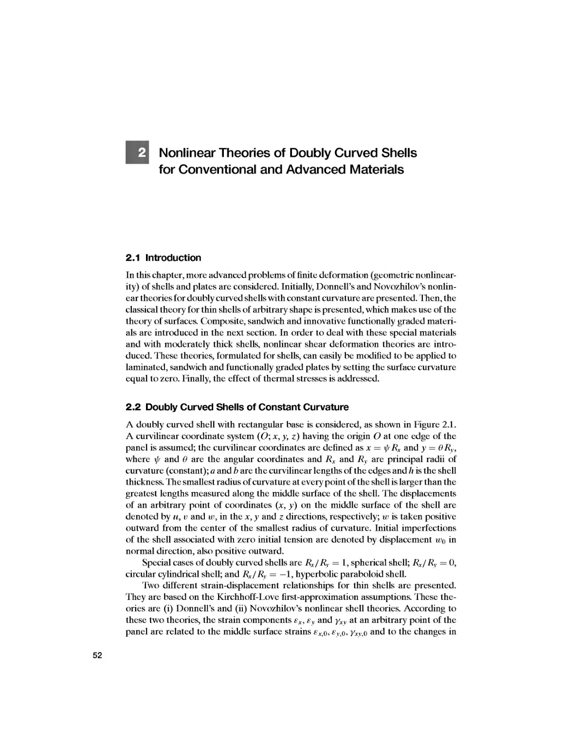
2.1 Introduction 52
2.2 Doubly Curved Shells of Constant Curvature 52
2.2.1 Elastic Strain Energy 55
2.3 General Theory of Doubly Curved Shells 56
2.3.1 Theory of Surfaces 56
2.3.2 Green's Strain Tensor for a Shell in Curvilinear Coordinates 62
2.3.3 Strain-Displacement Relationships for Novozhilov's
Nonlinear Shell Theory 65
2.3.4 Strain-Displacement Relationships for an Improved Version
of the Novozhilov Shell Theory 67
2.3.5 Simplified Strain-Displacement Relationships 68
2.3.6 Elastic Strain Energy 69
2.3.7 Kinetic Energy 69
2.4 Composite and Functionally Graded Materials 70
2.4.1 Stress-Strain Relations for a Thin Lamina 71
2.4.2 Stress-Strain Relations for a Layer within a Laminate 73
2.4.3 Elastic Strain Energy for Laminated Shells 73
2.4.4 Elastic Strain Energy for Orthotropic and Cross-Ply Shells 74
2.4.5 Sandwich Plates and Shells 75
2.4.6 Functionally Graded Materials and Thermal Effects 76
2.5 Nonlinear Shear Deformation Theories for Moderately Thick,
Laminated and Functionally Graded, Doubly Curved Shells 78
2.5.1 Nonlinear First-Order Shear Deformation Theory for
Doubly Curved Shells of Constant Curvature 78
2.5.2 Elastic Strain Energy for Laminated Shells 80
2.5.3 Kinetic Energy with Rotary Inertia for Laminated Shells 81
2.5.4 Nonlinear Higher-Order Shear Deformation Theory for
Laminated, Doubly Curved Shells 81
2.5.5 Elastic Strain and Kinetic Energies, Including Rotary
Inertia, for Laminated Shells According with Higher-Order
Shear Deformation Theory 85
2.5.6 Elastic Strain Energy for Heated, Functionally Graded Shells 86

2.5.7 Kinetic Energy with Rotary Inertia tor Functionally Graded
Shells 87
2.6 Thermal Effects on Plates and Shells 88
References 89
Introduction to Nonlinear Dynamics 90
3.1 Introduction 90
3.2 Periodic Nonlinear Vibrations: Softening and Hardening Systems 90
3.3 Numerical Integration of the Equations of Motion 93
3.4 Local Geometric Theory 94
3.5 Bifurcations of Equilibrium 96
3.5.1 Saddle-Node Bifurcation 97
3.5.2 Pitchfork Bifurcation 97
3.5.3 Transcritical Bifurcation 99
3.5.4 Hopf Bifurcation 99
3.6 Poincare Maps 101
3.7 Bifurcations of Periodic Solutions 103
3.7.1 Floquet Theory 103
3.7.2 Period-Doubling Bifurcation 106
3.7.3 Neimark-Sacker Bifurcation 107
3.8 Numerical Continuation Methods 107
3.8.1 Arclength Continuation of Fixed Points 107
3.8.2 Pseudo-Arclength Continuation of Fixed Points 109
3.8.3 Pseudo-Arclength Continuation of Periodic Solutions 110
3.9 Nonlinear and Internal Resonances 112
3.10 Chaotic Vibrations 113
3.11 Lyapunov Exponents 114
3.11.1 Maximum Lyapunov Exponent 114
3.11.2 Lyapunov Spectrum 115
3.12 Lyapunov Dimension 117
3.13 Discretization of the System: Galerkin Method and
Lagrange Equations 118
References 119
Vibrations of Rectangular Plates 120
4.1 Introduction 120
4.1.1 Literature Review 120
4.2 Linear Vibrations with Classical Plate Theory 121
4.2.1 Theoretical and Experimental Results 122
4.3 Nonlinear Vibrations with Von Karman Plate Theory 123
4.3.1 Boundary Conditions, Kinetic Energy, External Loads
and Mode Expansion 124
4.3.2 Satisfaction of Boundary Conditions 127
4.3.2.1 Case (a) 127
4.3.2.2 Case(b) 128
4.3.2.3 Case(c) 128
4.3.2.4 Case(d) 129
4.3.3 Lagrange Equations of Motion 130
4.4 Numerical Results for Nonlinear Vibrations 131
4.5 Comparison of Numerical and Experimental Results 132

Contents
4.6 Inertial Coupling in the Equations of Motion 137
4.7 Effect of Added Masses 139
References 139
Vibrations of Empty and Fluid-Filled Circular Cylindrical Shells .... 141
5.1 Introduction 141
5.1.1 Literature Review 142
5.2 Linear Vibrations of Simply Supported, Circular Cylindrical Shells 145
5.2.1 Donnell's Theory of Shells 145
5.2.2 Fliigge-Lur'e-Byrne Theory of Shells 148
5.3 Circular Cylindrical Shells Containing or Immersed in Still Fluid 150
5.4 Rayleigh-Ritz Method for Linear Vibrations 154
5.5 Nonlinear Vibrations of Empty and Fluid-Filled, Simply
Supported, Circular Cylindrical Shells with Donnell's Nonlinear
Shallow-Shell Theory 156
5.5.1 Fluid-Structure Interaction 159
5.5.2 Stress Function and Galerkin Method 160
5.5.3 Traveling-Wave Response 164
5.5.4 Proof of the Continuity of the Circumferential Displacement 164
5.6 Numerical Results for Nonlinear Vibrations of Simply
Supported Shells 165
5.6.1 Empty Shell 165
5.6.2 Water-Filled Shell 171
5.7 Effect of Geometric Imperfections 171
5.7.1 Empty Shell 172
5.7.2 Water-Filled Shell 174
5.8 Comparison of Numerical and Experimental Results 176
5.8.1 Empty Shell 180
5.8.2 Water-Filled Shell 182
5.9 Chaotic Vibrations of a Water-Filled Shell 187
References 191
Reduced-Order Models: Proper Orthogonal Decomposition
and Nonlinear Normal Modes 193
6.1 Introduction 193
6.2 Reference Solution 194
6.3 Proper Orthogonal Decomposition (POD) Method 194
6.4 Asymptotic Nonlinear Normal Modes
(NNMs) Method 197
6.5 Discussion on POD and NNMs 199
6.6 Numerical Results 201
6.6.1 Results for POD and NNMs Methods 202
6.6.2 Geometrical Interpretation 207
References 209
Comparison of Different Shell Theories for Nonlinear Vibrations
and Stability of Circular Cylindrical Shells 212
7.1 Introduction 212
7.2 Energy Approach 212
7.2.1 Additional Terms to Satisfy the Boundary Conditions 215

7.2.2 Fluid-Structure Interaction 216
7.2.3 Lagrange Equations of Motion 217
7.3 Numerical Results for Nonlinear Vibrations 219
7.3.1 Empty Shell 219
7.3.1.1 Comparison with Results Available in the Literature 223
7.3.2 Water-Filled Shell 224
7.3.2.1 Water-Filled Shell with Imperfections 228
7.3.3 Discussion 230
7.4 Effect of Axial Load and Presssure on the Nonlinear Stability
and Response of the Empty Shell 230
References 233
8 Effect of Boundary Conditions on Large-Amplitude Vibrations
of Circular Cylindrical Shells 234
8.1 Introduction 234
8.1.1 Literature Review 234
8.2 Theory 235
8.3 Numerical Results 237
8.3.1 Comparison with Numerical and Experimental Results
Available for Empty Shells 239
References 240
9 Vibrations of Circular Cylindrical Panels with Different
Boundary Conditions 242
9.1 Introduction 242
9.1.1 Literature Review 242
9.2 Linear Vibrations 244
9.3 Nonlinear Vibrations 245
9.3.1 Mode Expansion 247
9.3.2 Satisfaction of Boundary Conditions 248
9.3.2.1 Model A 248
9.3.2.2 Model B 250
9.3.2.3 Model C 251
9.3.3 Solution 251
9.4 Numerical Results 252
9.4.1 Nonperiodic Response 256
9.5 Comparison of Experimental and Numerical Results 262
9.5.1 Experimental Results 262
9.5.2 Comparison of Numerical and Experimental Results 265
References 270
10 Nonlinear Vibrations and Stability of Doubly Curved Shallow-
Shells: Isotropic and Laminated Materials 272
10.1 Introduction 272
10.1.1 Literature Review 272
10.2 Theoretical Approach for Simply Supported, Isotropic Shells 274
10.2.1 Boundary Conditions 275
10.2.2 Lagrange Equations of Motion 277
10.3 Numerical Results for Simply Supported, Isotropic Shells 279
10.3.1 Case with Rx/Ry = 1, Spherical Shell 279

XII
Contents
10.3.2 Case with Rx/Ry = -1, Hyperbolic Paraboloidal Shell 283
10.3.3 Effect of Different Curvature 285
10.4 Buckling of Simply Supported Shells under Static Load 286
10.5 Theoretical Approach for Clamped Laminated Shells 286
10.6 Numerical Results for Vibrations of Clamped Laminated Shells 289
10.7 Buckling of the Space Shuttle Liquid-Oxygen Tank 291
References 296
11 Meshless Discretizatization of Plates and Shells of Complex Shape
by Using the R-Functions 298
11.1 Introduction 298
11.1.1 Literature Review 298
11.2 The R-Functions Method 299
11.2.1 Boundary Value Problems with Homogeneous Dirichlet
Boundary Conditions 299
11.2.1.1 Example: Shell with Complex Shape 301
11.2.2 Boundary Value Problems with Inhomogeneous Dirichlet
Boundary Conditions 303
11.2.3 Boundary Value Problems with Neumann and Mixed
Boundary Conditions 303
11.2.4 Admissible Functions for Shells and Plates with Different
Boundary Conditions 304
11.3 Numerical Results for a Shallow-Shell with Complex Shape 306
11.4 Experimental Results and Comparison 308
References 309
12 Vibrations of Circular Plates and Rotating Disks 311
12.1 Introduction 311
12.1.1 Literature Review 311
12.2 Linear Vibrations of Circular and Annular Plates 313
12.3 Nonlinear Vibrations of Circular Plates 314
12.3.1 Numerical Results 317
12.4 Nonlinear Vibrations of Disks Spinning Near a Critical Speed 317
12.4.1 Numerical Results 320
References 323
13 Nonlinear Stability of Circular Cylindrical Shells under Static
and Dynamic Axial Loads 325
13.1 Inroduction 325
13.1.1 Literature Review 325
13.2 Theoretical Approach 328
13.3 Numerical Results 329
13.3.1 Static Bifurcations 329
13.3.2 Dynamic Loads 332
References 336
14 Nonlinear Stability and Vibration of Circular Shells
Conveying Fluid 338
14.1 Introduction 338
14.1.1 Literature Review 338

Contents
14.2 Fluid-Structure Interaction for Flowing Fluid 339
14.2.1 Fluid Model 339
14.2.2 Shell Expansion 340
14.2.3 Fluid-Structure Interaction 341
14.2.4 Nonlinear Equations of Motion with Galerkin Method 342
14.2.5 Energy Associated with Flow and Lagrange Equations 342
14.2.6 Solution of the Associated Eigenvalue Problem 345
14.3 Numerical Results for Stability 346
14.4 Comparison of Numerical and Experimental Stability Results 348
14.5 Numerical Results for Nonlinear Forced Vibrations 350
14.5.1 Periodic Response 350
14.5.2 Unsteady and Chaotic Motion 351
References 353
15 Nonlinear Supersonic Flutter of Circular Cylindrical Shells
with Imperfections 355
15.1 Introduction 355
15.1.1 Literature Review 356
15.2 Theoretical Approach 358
15.2.1 Linear and Third-Order Piston Theory 358
15.2.2 Structural Model 359
15.3 Numerical Results 361
15.3.1 Linear Results 361
15.3.2 Nonlinear Results without Geometric Imperfections 363
15.3.3 Nonlinear Results with Geometric Imperfections 367
References 371
Index
373

Preface
The present book is intended for (i) graduate students in engineering, (ii) researchers
working on vibrations or on shell mechanics and (iii) engineers working on
aircraft, missiles, launchers, cars, computer hard and optical disks, storage tanks, heat
exchangers, nuclear plants, biomechanics, nano-resonators or thin-walled roofs and
other structures in civil engineering. This book contains both theoretical and
practical methods that could be of interest for a variety of readers. Expert researchers will
find the most recent progress in nonlinear vibrations and the stability of shells and
plates, including advanced problems in shells with fluid-structure interaction.
Professionals will find many practical concepts, diagrams and numerical results, useful
for the design of shells and plates made of traditional and advanced materials. They
will be able to understand complex phenomena such as dynamic instability,
bifurcations and chaos, without needing an extensive mathematical background. Graduate
students will find (i) a complete text on the nonlinear mechanics of shells and plates,
collecting almost all the available theories in a simple form, (ii) an introduction to
nonlinear dynamics and (iii) the state of art on nonlinear vibrations and the stability
of shells and plates, including fluid-structure interaction problems.
My interest in vibrations of shells and plates started with my Master's thesis, more
than 16 years ago. However, the turning of my research toward nonlinear vibrations
is due to the lucky meeting of two friends: Michael P. Paidoussis and Francesco
Pellicano. The three of us have worked together as a team since 1997 on challenging
problems of nonlinear vibrations and the stability of circular cylindrical shells with
fluid-structure interaction. This book would have never been written without their
precious contribution during all these years.
Several other eminent researchers worked with me on nonlinear vibration
problems (in chronological order): Alexander Vakakis, Arun K. Misra, Konstantinos
Karagiozis, Eugeni Grinevitch, Rinaldo Garziera, Abijit Sarkar, Cyril Touze, Olivier
Thomas, Roger Ohayon, Jean-Sebastien Schotte, Yuri Mikhlin, Konstantin Avramov,
Yevgeniy Kurilov, Lidia Kurpa, Galina Pilgun, Silvia Carra and Korosh Khorshidi.
My thanks go to all of them.
Among my coauthors of other studies on shells and plates, I cannot forget
Giovanni Frosali, Moon K. Kwak and Kyeong-Hoon Jeong.
During the writing of the present book, I had many helpers. In particular, I would
like to thank Michael P. Paidoussis, who fully corrected the first three chapters of the
book; my colleague Rinaldo Garziera, who reviewed Chapter 3; Michael P. Nemeth

XVI
Preface
who authorized the use of six figures used in Chapter 10; Arvind Raman, Olivier
Thomas and Cyril Touze, who corrected Chapter 12, which is based on their work,
and authorized the use of their figures; Francesco Pellicano, who obtained the results
presented in Chapter 13;Konstantinos Karagiozis, who drew Figure 14.6,merging my
calculations with his results; the students of my course Meccanica delle Vibrazioni B
at the University of Parma, year 2006, who helped to find errors and drew Figures 3.3
and 3.9(b); my editor Peter Gordon and his assistant Erin Fae of Cambridge
University Press, who have found the photographs that I needed; and finally, my wife Olga,
for her patience.
During the past ten years, many students of mechanical engineering at the Dipar-
timento di Ingegneria Industriale of the University of Parma helped me perform
experiments under my supervision. In particular, the Ph.D. students: Silvia Carra,
Michele Pellegrini, Carlo Augenti and Fabrizio Pagnanelli; the Master's students:
Angelo Negri, Dario Rabotti, Andrea Bellingeri, Salvatore Falanga, Marco Tomme-
sani, Valentina Pinelli, Carlotta Truzzi, Paolo Evangelista, Simone Varesi, Antonio
Segalini, Paolo Campioli, Margherita Mangia, Francesco Boccia, Simone Sabaini,
Fabio Magnani, Marco Venturini, Francesca Righi, Federico CoUa, Filippo Vinci,
Marco Codeghini, Innocente Granelli, Giovanni Zannoni, Giangiacomo Clausi,
Filippo Huller and Pier Paolo Lanzi.
Thanks go to my friend Yaroslav Bysaga for his warm hospitality during the
proofreading and to Giovanna Magazzu for preparing the multimedia presentation
of the book.
Warm encouragemenl to complete this book was given to me during the 2006
ASME winter annual meeting by Isaac Elishakoff, Roger Ohayon and Liviu Librescu.
On April 16, 2007, Liviu Librescu was murdered as a hero during the terrible
massacre at Virginia Tech, so I take this opportunity to celebrate this extraordinary and
indefatigable researcher who helped colleagues and students up to the end.
I had the privilege to be at McGill University when Michael P. Paidoussis
was writing the second volume of his fundamental monograph Fluid-Structure
Interactions: Slender Structures and Axial Flow, this has been an extraordinary school.
Marco Amabili

Introduction
Plates are structural elements given by a flat surface with a given thickness h. The flat
surface is the middle surface of the plate; the upper and lower surfaces delimiting the
plate are at distance h/2 from the middle surface. The thickness is small compared
with the in-plane dimensions and can be either constant or variable. Thin plates are
very stiff for in-plane loads, but they are quite flexible in bending. Many applications
of plates, made of extremely different materials, can be found in engineering. For
example, very thin circular plates are used in computer hard-disk drives; rectangular
and trapezoidal plates can be found in the wing skin, horizontal tail surfaces, flaps
and vertical fins of aircraft; cantilever rectangular plates are used as nano-resonators
for drug detection; and flat rectangular panels are largely used in civil buildings.
If the middle surface describing the structural elements is folded, shells are
obtained. Such structures are abundantly present in nature. In fact, because of the
curvature of the middle surface, shells are very stiff for both in-plane and bending loads;
therefore, they can span over large areas by using a minimum amount of material.
Shells are largely used in engineering; some shell structures are impressive and
beautiful. In automotive engineering, the bodies of cars are shells; in biomechanics,
arteries are shells conveying flow. Shell structural elements are largely present in the
NASA space shuttle in Figure 1, where the solid rocket boosters and the big orange
tank for liquid fuels are large shell bodies. Actually, the super lightweight orange
tank is composed of a smaller top tank of ogival shape containing liquid oxygen and
a bigger bottom tank of circular cylindrical shape containing liquid hydrogen joined
by an intertank element. Shells are: the hull of the Queen Mary 2 transatlantic boat
shown in Figure 2 and of the Los Angeles-class fast attack submarine in Figure 3; the
roof of L'Hemisferic designed by Santiago Calatrava in the Ciutat del les Arts i les
Ciencies, Valencia, Spain (Figure 4); and the fuselage and wing panels of the huge
Airbus A380 civil aircraft in Figure 5.
One of the main targets in the design of shell structural elements is to make
the thickness as small as possible to spare material and to make the structure light.
The analysis of shells has difficulty related to the curvature, which is also the reason
for the carrying load capacity of these structures. In fact, a change of the curvature
can give a totally different strength (Chapelle and Bathe 2003). Moreover, because
of the optimal distribution of material, shells collapse for buckling much before the
failure strength of the material is reached. For their thin nature, they can present
large displacements, with respect to the shell thickness, associated to small strains

Introduction
r
Figure 1. NASA space shuttle: orbiter Discovery
with the two solid rocket boosters and the large
orange external tank. Courtesy of NASA.
.^■fS^
before collapse. This is the rationale for using a nonlinear shell and plate theory for
studying shell stability.
Shells are often subjected to dynamic loads that cause vibrations; vibration
amplitudes of the order of the shell thickness can be easily reached in many applications.
Therefore, a nonlinear shell theory should be applied.
"'*"" I
mi umi %\\l V
t fill II14«\ IV>\ V
'•1. -I4JLI .win
Figure 2. The Queen Mary 2 transatlantic boat. Courtesy of Carnival Corporation & PLC.

Introduction
< *
>.
■*i
*r*
£
4 /'V
.)
,. f
'#'.
Figure 3. The Los Angeles-class fast attack submarine USS Asheville. Courtesy of the U.S.
Navy.
The book is organized into 15 chapters. Chapter 1 obtains classical nonlinear
theories for rectangular and circular plates, circular cylindrical and spherical shells.
Classical shell theories for doubly curved shallow shells and for shells of arbitrary shape
are obtained in Chapter 2. Composite and innovative functionally graded materials
_ mo • "
"■I m i.lii ■' 'J .
M ■■■■■(nr"rB
Figure 4. L 'Hemisferic designed by Santiago Calatrava in the Ciutat del les Arts i les Ciencies,
Valencia, Spain. Alan Copson/age fotostock.

Introduction
'3:,
Figure 5. Airbus A380 aircraft. Plath/age fotostock.
are introduced and nonclassical nonlinear theories, including shear deformation and
rotary inertia, for laminated and functionally graded shells are developed; thermal
stresses are also introduced. The first two chapters are self-contained with the full
development of the theories under clear hypotheses and limitations. They present
material that is usually spread in several articles and books with different approaches
and symbols. The shell theories are expressed in lines-of-curvature coordinates, which
is the form suitable for applications and computer implementation. In some cases,
slightly improved formulations, suitable for moderately thick shells and large
rotations, have been developed.
The nonlinear dynamics, stability, bifurcation analysis and modern
computational tools are introduced in Chapter 3. The Galerkin method and the energy
approach that leads to the Lagrange equations of motion are introduced here.
Linear and nonlinear vibrations of rectangular plates and simply supported
circular cylindrical shells (closed around the circumference) are throughly studied in
Chapters 4 and 5, respectively. In particular, the Lagrange equations are used for dis-
cretizing plates and the Galerkin method is used for discretizing circular shells to show
both methods. Numerical and experimental results are presented and compared. The
effect of geometric imperfections is also addressed in both chapters. The problem
of inertial coupling in the equations of motion is analyzed in Chapter 4. Fluid-filled
circular shells are investigated with great care in Chapter 5 for their important
applications. Chaotic vibrations are analyzed for large harmonic excitation.
Modern numerical techniques, specifically proper orthogonal decomposition
(POD) and nonlinear normal modes (NNM) methods, that reduce the number
of degrees of freedom in nonlinear shell models are presented in Chapter 6. The
comparison of different classical nonlinear shell theories to study large-amplitude
vibrations of simply supported circular cylindrical shells is performed in Chapter 7,
where the Lagrange equations are used; the nonlinear stability of pressurized shells
is also investigated. Nonlinear vibrations of circular cylindrical shells with different
St

Reference
5
boundary conditions are addressed in Chapter 8. Linear and nonlinear vibrations of
circular cylindrical panels (open shells) with different boundary conditions are
studied in Chapter 9. Also in this case numerical and experimental results are presented
and successfully compared. Chaotic vibrations are detected for large harmonic
excitations. Nonlinear vibrations of doubly curved shallow (i.e. with small rise) shells
with rectangular base, including spherical and hyperbolic paraboloidal shells, are
investigated in Chapter 10. Both classical and first-order shear deformation theories
are used to study nonlinear vibrations of laminated composite shells. Static
buckling, including the example of the external tank of the NASA space shuttle, is also
addressed.
The R-function method for meshless discretization of shells and plates of
complex shape is introduced in Chapter 11. This is a method with great potential to
develop commercial software, but very little is still known about it outside of the
Ukraine and Russia. Linear and nonlinear vibrations of circular plates and
rotating disks are investigated in Chapter 12. They have an important application in
engineering; for example, in hard-disk, CD and DVD drives of computers.
Nonlinear stability of circular cylindrical shells under static and periodic axial
loads are studied in Chapter 13. The fundamental effects of geometric imperfections
on the buckling load are investigated, and the period-doubling bifurcation giving
dynamic instability in periodic loads is deeply analyzed. The problem of stability of
circular cylindrical shells conveying a subsonic flow is addressed in Chapter 14, where
a strongly subcritical divergence is detected. The fluid-structure interaction problem
for inviscid and incompressible flow is fully studied and the numerical and
experimental results obtained in a water tunnel are compared. Nonlinear forced vibrations
of circular cylindrical shells conveying water flow are studied for both moderate and
large excitations, giving periodic response and complex dynamics, respectively.
Flutter instability of circular cylindrical shells inserted in axial supersonic airflow is finally
investigated in Chapter 15 by using either linear or nonlinear piston theory to model
the aerodynamic loads, and a nonlinear shell model taking into account
geometric imperfections. Numerical results are compared with the results of experiments
performed by the National Aeronautics and Space Administration (NASA).
REFERENCE
D. Chapelle and K. J. Bathe 2003 The Finite Element Analysis of Shells — Fundamentals.
Springer, Berlin, Germany.

^Q Nonlinear Theories of Elasticity of Plates
and Shells
1.1 Introduction
It is well known that certain elastic bodies may undergo large displacements while
the strain at each point remains small. The classical theory of elasticity treats only
problems in which displacements and their derivatives are small. Therefore, to treat
such cases, it is necessary to introduce a theory of nonlinear elasticity with small
strains. If the strains are small, the deformation in the neighborhood of each point can
be identified with a deformation to which the linear theory is applicable. This gives a
rationale for adopting Hooke's stress-strain relations, and in the resulting nonlinear
theory large parts of the classical theory are preserved (Stoker 1968). However,
the original and deformed configuration of a solid now cannot be assumed to be
coincident, and the strains and stresses can be evaluated in the original undeformed
configuration by using Lagrangian description, or in the deformed configuration by
using Eulerian description (Fung 1965).
In this chapter, the classical geometrically nonlinear theories for rectangular
plates, circular cylindrical shells, circular plates and spherical shells are derived,
classical theories being those that neglect the shear deformation. Results are obtained in
Lagrangian description, the effect of geometric imperfections is considered and the
formulation of the elastic strain energy is also given. Classical theories for shells of any
shape, as well as theories including shear deformation, are addressed in Chapter 2.
1.1.1 Literature Review
A short overview of some theories for geometrically nonlinear shells and plates will
now be given. Some information is taken from the review by Amabili and Paidoussis
(2003).
In the classical linear theory of plates, there are two fundamental methods for the
solution of the problem. The first method was proposed by Cauchy (1828) and Pois-
son (1829) and the second by Kirchhoff (1850). The method of Cauchy and Poisson is
based on the expansion of displacements and stresses in the plate in power series of
the distance z from the middle surface. Disputes concerning the convergence of these
series and about the necessary boundary conditions made this method unpopular.
Moreover, the method proposed by Kirchhoff has the advantage of introducing
physical meaning into the theory of plates. Von Karman (1910) extended this method to
6

1.1 Introduction
study finite deformation of plates, taking into account nonlinear terms. The nonlinear
dynamic case was studied by Chu and Herrmann (1956), who were the pioneers in
studying nonlinear vibrations of rectangular plates. In order to deal with thicker and
laminated composite plates, the Reissner-Mindlin theory of plates (first-order shear
deformation theory) was introduced to take into account transverse shear strains.
Five variables are used in this theory to describe the deformation: three
displacements of the middle surface and two rotations. The Reissner-Mindlin approach does
not satisfy the transverse shear boundary conditions at the top and bottom surfaces
of the plate, because a constant shear angle through the thickness is assumed, and
plane sections remain plane after deformation. As a consequence of this
approximation, the Reissner-Mindlin theory of plates requires shear correction factors for
equilibrium considerations. For this reason, Reddy (1990) has developed a nonlinear
plate theory that includes cubic terms (in the distance from the middle surface of
the plate) in the in-plane displacement kinematics. This higher-order shear
deformation theory satisfies zero transverse shear stresses at the top and bottom surfaces
of the plate; up to cubic terms are retained in the expression of the shear, giving
a parabolic shear strain distribution through the thickness, resembling with good
approximation the results of three-dimensional elasticity. The same five variables of
the Reissner-Mindlin theory are used to describe the kinematics in this higher-order
shear deformation theory, but shear correction factors are not required.
Donnell (1934) established the nonlinear theory of circular cylindrical shells
under the simplifying shallow-shell hypothesis. Because of its relative simplicity and
practical accuracy, this theory has been widely used. The most frequently used form
of DonnelFs nonlinear shallow-shell theory (also referred to as Donnell-Mushtari-
Vlasov theory) introduces a stress function in order to combine the three equations
of equilibrium involving the shell displacements in the radial, circumferential and
axial directions into two equations involving only the radial displacement w and
the stress function F. This theory is accurate only for modes with circumferential
wavenumber n that are not small: specifically, 1/n2 <& 1 must be satisfied, so that
n > 4 or 5 is required in order to have fairly good accuracy. DonnelFs nonlinear
shallow-shell equations are obtained by neglecting the in-plane inertia, transverse
shear deformation and rotary inertia, giving accurate results only for very thin shells.
The predominant nonlinear terms are retained, but other secondary effects, such
as the nonlinearities in curvature strains, are neglected; specifically, the curvature
changes are expressed by linear functions of w only.
Von Karman and Tsien (1941) performed a seminal study on the stability of
axially loaded circular cylindrical shells, based on Donnell's nonlinear shallow-shell
theory. In their book, Mushtari and Galimov (1957) presented nonlinear theories
for moderate and large deformations of thin elastic shells. The nonlinear theory of
shallow-shells is also discussed in the book by Vorovich (1999), where the classical
Russian studies, for example, due to Mushtari and Vlasov, are presented.
Sanders (1963) developed a more refined nonlinear theory of shells, expressed in
tensorial form. The same equations were obtained by Koiter (1966) around the same
period, leading to the designation of these equations as the Sanders-Koiter
equations. Later, this theory was reformulated in lines-of-curvature coordinates, that is,
in a form that can be more suitable for applications; see, for example, Budiansky
(1968), where only linear terms are given. According to the Sanders-Koiter theory,
all three displacements are used in the equations of motion. Changes in curvature and
torsion are linear according to both the Donnell and the Sanders-Koiter nonlinear

8
Nonlinear Theories of Elasticity of Plates and Shells
theories (Yamaki 1984). The Sanders-Koiter theory gives accurate results for
vibration amplitudes significantly larger than the shell thickness for thin shells (Amabili
2003).
Details on the above-mentioned nonlinear shell theories may be found in Yamaki
(1984) and Amabili (2003), with an introduction to another accurate theory called
the modified Fliigge nonlinear theory of shells, also referred to as the Fliigge-Lur'e-
Byrne nonlinear shell theory (Ginsberg 1973). The Fliigge-Lur'e-Byrne theory is
close to the general large deflection theory of thin shells developed by Novozhilov
(1953) and differs only in terms for change in curvature and torsion.
Additional nonlinear shell theories were formulated by Naghdi and Nordgren
(1963), using the Kirchhoff hypotheses, and by Libai and Simmonds (1988).
In order to treat moderately thick laminated shells, the nonlinear first-order
shear deformation theory of shells was introduced by Reddy and Chandrashekhara
(1985), which is based on the linear first-order shear deformation theory introduced
by Reddy (1984). Five independent variables, three displacements and two rotations,
are used to describe the shell deformation. This theory may be regarded as the thick-
shell version of the Sanders theory for linear terms and of the Donnell nonlinear
shell theory for nonlinear terms. A linear higher-order shear deformation theory of
shells has been introduced by Reddy and Liu (1985); see also Reddy (2003). Dennis
and Palazotto have extended this theory to nonlinear deformations (1990); see also
Soldatos (1992).
The nonlinear mechanics of composite laminated shells has also been
investigated by many authors. Librescu (1987) developed refined nonlinear theories for
anisotropic laminated shells. Other theories applied to the dynamics of laminated
shells have been developed, for example, by Tsai and Palazotto (1991), Kobayashi
and Leissa (1995), Sansour et al. (1997), Gummadi and Palazotto (1999) and Pai
and Nayfeh (1994). Nonlinear electromechanics of piezoelectric laminated shallow
spherical shells was developed by Zhou and Tzou (2000).
1.2 Large Deflection of Rectangular Plates
1.2.1 Green's and Almansi Strain Tensors for Finite Deformation
It is assumed that a continuous body changes its configuration under physical actions
and the change is continuous (no fractures are considered). A system of coordinates
x\, X2, x-i is chosen so that a point P of a body at a certain instant of time is described
by the coordinates X{ (i = 1, 2, 3). At a later instant of time, the body has moved
and deformed to a new configuration; the point P has moved to Q with coordinates
G;(/' = 1,2,3) with respect to a new coordinate system «i, «2, ^3 (see Figure 1.1). Both
coordinate systems are assumed to be the same rectangular Cartesian (rectilinear
and orthogonal) coordinates for simplicity. The point transformation from P to Q is
considered to be one-to-one, so that there is a unique inverse of the transformation.
The functions x, and a,, describing the coordinates, are assumed to be continuous and
differentiable, and the Jacobian determinant of the transformation is positive (i.e. a
right-hand set of coordinates is transformed into another right-hand set) and does
not vanish at any point. The displacement vector u is introduced having the following
components:
iii = ^ — x, for / = 1,..., 3. (1-1)

1.2 Large Deflection of Rectangular Plates
gtffll,«2,«3)
X2, «2
xi, ai
Figure 1.1. Body in the original configuration and after displacement u, which moves point
PtoQ.
In the present book, the Lagrangian description of the continuous systems is
used for convenience; therefore h,- are considered to be functions of xi in order to
evaluate the Lagrangian (or Green's) strain tensor, that is, the strains are referred to
the original undeformed configuration.
HP, P', P" are three neighboring points forming a triangle in the original
configuration, and if they are transformed to points Q, Q', Q" in the deformed
configuration, the change in the area and angles of the triangle is completely determined if the
change in the length of the sides is known. However, the location of the triangle in
space is not determined by the change of the sides. Similarly, if the change in length
between any two arbitrary points of the body is known, the new configuration of the
body is completely defined except for the location of the body in the space. Because
interest here is on strains, and these are related to stresses, attention is now focused
on the change in distance between any two points of the body.
An infinitesimal line connecting point P (x\,x2, x?) to a neighborhood point P'
(xi + dxi, X2 + dx2, *3 + dx$) is considered; the square of its length in the original
configuration is given by
PP' = ds£ = doc{ + doc\ + cbc|.
(1.2)
When, due to deformation, P and P' become Q(a\, a2, a3) and Q(a\ + da\,a2 + da2,
a3 + da3), respectively, the square of the distance is
QQ' = dsz = daf + da| + dai,.
(1.3)
in the coordinate system a,-. The differentials da, can be transformed in the original
coordinate system X{.
dai dai Sa,
daL = —— dxi + -—dx2 + -— dx3.
0X\ dx2 OXj,
Therefore, by using equation (1.4), equation (1.3) is transformed into
d,2 = yyy^^dx!dx7.
(1.4)
(1.5)

10
Nonlinear Theories of Elasticity of Plates and Shells
The difference between the squares of the length of the elements may be written in
the following form by using equations (1.2) and (1.5):
** - d,02 = E E E (^^ - *,-) ^ **,. (i.6)
k=\ i=l ;=1 V °Xl °Xi /
where S,-;- is the Kronecker delta, equal to 1 if i = j and otherwise equal to zero. By
definition, Green's strain tensor s,-;- is obtained as
3 3
6s2 - Asl = 2 E E £i' dx' dx'' (1-7)
i=l ;=1
and therefore is given by
*-£fc
3a/t 3fl/t
2 \ ^ 3x; 3x7-
(1.8)
By using equation (1.1), the following expression is obtained:
dak diik
dx; dx;
(1.9)
Finally, by substituting equation (1.9) into equation (1.8), Green's strain tensor is
expressed as
iMdM^
1 / 3//; dllj -^ dllk dllk
3v- £-~i
2 \ dx;
k=1 dXi dXj
(1.10)
In unabridged notation (x, y, z for x\, X2, x^), the typical formulations are obtained:
3»i 1
~3T + 2
f—\2 + (—\2 4- (—X
\dx ) \ dx ) \ dx )
(1.11a)
dll\ dll2 ( dll\ dn\ 3»2 3»2 3"3 3"3\
(
3y dx \ dx dy dx dy dx dy J
(1.11b)
where the usual symbol yxy has been used instead of sxy in equation (1.11b).
Equation (1.10) shows that Green's strain tensor is symmetric.
If the Eulerian description of the continuous systems is used, h,- are considered
functions of a, in order to evaluate the Eulerian (usually referred to as the Almansi)
strain tensor (i.e. the strains are referred to the deformed configuration). With
analogous mathematical development, the Almansi strain tensor is given by
n^
■E^+*«
k=\
da.
m+\
1 / 3//; dllj y—^ dllk dllk
2 \ da;
k=i dcii dai
(1.12)
which is also symmetric; the superscript denotes "Eulerian."

1.2 Large Deflection of Rectangular Plates
11
Middle surface
Figure 1.2. Rectangular plate, (a) Symbols used for
displacements of middle surface and generic point,
(b) Symbols used for dimensions and Kirchhoff
stresses.
(a)
(b)
1.2.2 Strains for Finite Deflection of Rectangular Plates: Von Karman Theory
The displacements of a generic point of the middle surface of the plate are indicated
by u, v and w in x, y and z direction, respectively; the corresponding displacements
of a generic point of the plate at distance z from the middle surface are denoted by
ui, "2 and »3, as shown in Figure 1.2(a).
When the plate deflection w is of the same order of magnitude as the plate
thickness h, results obtained by using linear theories become quite inaccurate. Here
a theory for large deflections (large refers to the fact that w is not small compared to h,
so that the original and deformed configurations are different) of plates is developed
in rectangular coordinates (suitable for rectangular plates of in-plane dimensions a
and b, see Figure 1.2[b]). In the theory, the following hypotheses are made (Fung
1965):
(HI) The plate is thin: h «; a, h «; b.
(H2) The magnitude of deflection w is of the same order as the thickness h of
the plate, therefore small compared to the plate dimensions a and b for (HI):
\w\ = 0(h).
(H3) The slope is small at each point: \dw/dx\ «; 1, \dw/dy\ <£ 1.

12
Nonlinear Theories of Elasticity of Plates and Shells
z
(a)
Figure 1.3. Cross-section of the rectangular
plate, (a) Initial configuration; ax is the normal
Kirchhoff stress, (b) Deformed configuration;
ai ' is the normal Eulerian stress.
tt»
(H4) All strain components are small so that linear elasticity can be applied.
(H5) Kirchhoff s hypotheses hold, that is, stresses in the direction normal to the
plate middle surface are negligible, and strains vary linearly within the plate
thickness. These hypotheses are a good approximation for thin plates.
However, in the presence of external loads orthogonal to the plate surface, stresses
in the normal direction arise, even if they are generally of some order of
magnitude smaller than other stresses.
(H6) For von Karman's hypothesis, the in-plane displacements u and v are
infinitesimal, and in the strain-displacement relations only those nonlinear terms
that depend on w need to be retained. All other nonlinear terms may be
neglected.
Hypothesis (H6) can be removed in order to get more accurate nonlinear plate
theories.
Figure 1.3 shows that the deformed configuration of the plate differs significantly
from the original one. The Lagrangian description of the plate is used, so that the plate
surfaces are always designated as z = ±/i/2; a right-handed rectangular Cartesian
reference system (O; x, y, z) is used, with the x, y plane coinciding with the middle
surface of the plate in its initial, undeformed configuration and the z axis normal
to it. In the Lagrangian description, Green's strain tensor, referred to in the initial
configuration, is used; it is given by equations (1.10) and (1.11). By using hypothesis
(H5), we have
it! = n(x, y) - z-
dw
dx "
dw
n2 = v(x,y)-z—,
dy
n3 = w(x, y).
(1.13)
(1.14)
(1.15)
Equations (1.13-1.15) are linear expressions. In particular, these equations are
obtained as follows: hypothesis (H5) requires that strains vary linearly within the

1.2 Large Deflection of Rectangular Plates
13
plate thickness and Kirchhoff stresses in the direction normal to the plate middle
surface are negligible (i.e. ozz = r^ = tzv = 0, where er!7 is the normal stress acting
on the surface normal to i in direction /, and t!; is the tangential stress as shown in
Figure 1.2fb]); therefore, by using linear elasticity,
Oxx = ai(x, y) + bi(x, y) z, (1-16)
o-.vv = a2(x, y) + b2(x, y) z, (1.17)
Bzz - ~^- = —p, (°xx + 0-vv) , (1.18)
dz E
where £ is Young's modulus and v is Poisson's ratio. In the last equation, the linearized
expression of szz is used (this is the reason for using ~ instead of =) as a consequence
of equations (1.13-1.15) being linear. Integration of equation (1.18) gives
2
V V Z
u3 = w(x, y) - — [at(x, y) + a2(x, y)\z-— [h(x, y) + b2(x, y)] —, (1.19)
where the term w is the integration constant. The last two terms on the right-hand
side are in general very small for thin plates, as a consequence of v/E being a very
small number, and they can be neglected; therefore, equation (1.15) is verified, and
ezz ~ 0. Also for hypothesis (H5), the following expressions are obtained:
Inserting 113 = w(x, y) from equation (1.15) into equations (1.20) and (1.21) and
integrating, equations (1.13) and (1.14) are obtained.
Equations (1.13-1.15) are inserted into Green's strain tensor, equations (1.10)
and (1.1 L), in order to obtain the strain-displacement relations for a plate in
rectangular coordinates. The strain components exx, £vv and yxx at an arbitrary point of the
plate are related to the middle surface strains £x$, £Vjo and j/xv,o and to the changes in
the curvature and torsion of the middle surface kx, kx and k„. by the following three
relations:
£xx = £x,o + zkx, (1.22)
£yr=£y,0 + Zky, (1.23)
Yxy = Yxy,0 + Zkxy, (1-24)
where z is, as usual, the distance of the arbitrary point of the plate from the middle
surface. If von Karman hypothesis (H6) is used, the following expressions for the
middle surface strains and the changes in the curvature and torsion of the middle
surface are obtained, namely
8-°=K + l\l*) ' (L25)
fi*° —+ 2Ur)' (L26)
3t;
3y ' 2

14
Nonlinear Theories of Elasticity of Plates and Shells
dn dv dw dw
Kxv.o =— + — + — — , (1-27)
dy dx dx dy
* - -S- <"">
fev = -2-—. 130
3x3_y
These expressions are in general accurate enough for moderately large vibrations of
plates. If more accurate expressions are needed, hypothesis (H6) can be removed
and equations (1.25-1.30) can be computed, retaining all the nonlinear terms.
1.2.3 Geometric Imperfections
Initial geometric imperfections of the rectangular plate associated with zero initial
stress are denoted by normal displacement wq; in-plane initial imperfections are
neglected. Therefore, equation (1.15) is replaced by
u3 = w(x, y) + w0(x, y). (1.31)
Substituting equation (1.31) into Green's strain tensor and neglecting all terms
that depend on wq only (as they are associated with initial deformation and
therefore with zero stress), the following expressions are obtained, replacing equations
(1.25-1.27):
3// 1 /dw\ dw dwo
dx 2 \ dx J dx dx
dv 1 /3uA dw dwo
fi*0 = ^ + 2Ur)+i»i»' (L33)
3// dv dw dw dw dwo dwo dw
y„.0 = 1 1 1 --\ . (1.34)
dy dx dx dy dx dy dx dy
Equations (1.28-1.30) are unchanged by the presence of the imperfection wq. It can
be observed that, in the presence of geometric imperfections, the plate is no longer
perfectly flat.
1.2.4 Eulerian, Lagrangian and Kirchhoff Stress Tensors
In the deformed configuration of a body, the equations of equilibrium of an
infinitesimal parallelepiped with surfaces parallel to the coordinate planes (see Figure 1.4)
are given by
J2 —^ + Xi: = 0 for i = 1,..., 3, (1.35)

1.2 Large Deflection of Rectangular Plates
15
> «2
davv
«1 "" ddi
Figure 1.4. Stresses on an infinitesimal parallelepiped of the plate.
where a- is the Eulerian stress tensor (for simplicity, the symbol a is used here also
for the tangential stresses instead of t), that is, the stresses referred to the deformed
configuration a} are the coordinates describing the deformed configuration and Xt
are the body forces, including inertia, per unit volume. The Eulerian stresses are
symmetric, that is, er-; = er . Equation (1.35) shows that in the Eulerian description
the dynamic equations are simple, but the kinematics is complex; for this reason it is
convenient to find the relationships to transform the Eulerian stresses in the original
undeformed configuration in order to use the Lagrangian description. True loading
and stresses in a body exist only in the deformed configuration; therefore, the loading
and stresses in the initial undeformed configuration are somehow fictitious.
In Figure 1.5, a solid body with initial configuration drawn on the left-hand side
(described in the coordinate system x,, with i = 1,..., 3) is transformed into the
parallelepiped shown on the right-hand side (described in the deformed coordinate
system at, with i = 1,..., 3). The force vector dT acting on the deformed surface PQRS
of area dS corresponds to the force dTo in the original configuration, which acts
*i, «i
Figure 1.5. Infinitesimal parallelepiped in deformed configuration and corresponding body in
the initial configuration.

16
Nonlinear Theories of Elasticity of Plates and Shells
on the surface P0Q0R0S0 having area dSo. The stress vectors in the deformed and
original configurations are defined as the limiting ratios dT/dS and dTo/dSo,
respectively. The assignment of a correspondence rule between dT and dTo is arbitrary, but
must be mathematically consistent; two alternative rules are used and are known as
Lagrangian and Kirchhoff rules, respectively:
dT^ = dTt, (1.36)
y=i °ai
where i = 1,2,3 indicates each component of the vector. Although equation (1.36)
shows that with the Lagrangian rule the two vectors coincide, equation (1.37) shows
that with the Kirchhoff formula the rule of transformation of forces is the same as that
obtained for da, in equation (1.4). Actually, one could think that only the Lagrangian
rule could be introduced; the reason for introducing the Kirchhoff rule is that it gives
useful properties to the related stress tensor, as will be shown soon.
By using the Cauchy formula, it is possible to relate the force dT to the Eulerian
stresses
d£= >>f'„,- dS. (138)
where iij are the components of the unit vector n normal to the surface dS. Similarly,
it is possible to write
d7o(;L) = £ SjtnotdSo = dTt. (1.39)
3 3
dC = E^dSo = £ f^dl), (1.40)
;'=1 ;'=1 1
where Sij and er!7 are the Lagrangian and Kirchhoff stresses, respectively, and ;»o; are
the components of the unit vector no normal to the surface dSo-
For the law of conservation of mass (pdV = podV0, where dV is the volume of
the solid element),
-=m^———. (i-4i)
p° h fe /b 9fli 9fl2 3«3
where po and p are the densities of the material in the original and deformed
configurations, respectively, and e,-;-/t is the permutation symbol, that is, e,-;-/t = 0 when any
two indices are equal, e,-;-/t= 1 when i, /, k permute like 1, 2, 3 and e,-;-/t = — 1 when
i,j, k permute like 1,3,2. The following transformation rule is also introduced:
■r-^ -r-^ ^-v dXi dXj dXk ^-v ^-> ^-\ dX[ dXj dXk
f=i f=i k~\ °aydaadafi ~l~l1~[ dai da2 3«3
Two lines da, with components (dai, dci2, da^), and 8a, with components (Sai,
8a2, Sai), are considered in the deformed body, which correspond to dx and 8x,

1.2 Large Deflection of Rectangular Plates
17
respectively, in the undeformed body. The area dS of the parallelogram with da and
8a as sides is given by the vector product da A 8a, which can be rewritten as
3 3
lit dS = \J 2_. e'jk dfly <5fl/t-
j=\ k=l
Similarly,
3 3 3 3 3 3 dx dx
Multiplying both the right-hand and left-hand sides by dxi/day, summing up on i
and substituting equation (1.41) in order to make the notation more compact, the
relationship involving the areas is obtained:
3 a 33
^ tt- "OidSo = — ^ ^ eYafs daa8afi = —nYdS. (1-42)
Hence, from equations (1.38), (1.39) and (1.42),
± S„„0,d5b = P-l ± aif ± gi n0jdS0, (1.43)
;=1 P a=\ ;=1 °Ua
which, eliminating the two sums on / on both the left-hand and right-hand sides and
identifying term to term, gives
Similarly, from equations (1.38), (1.40) and (1.42),
phhda«da?
Equation (1.44) shows that the Lagrangian stress tensor Sji is not symmetric; on
the other hand, the Kirchhoff stress tensor (1.45) is symmetric (er!7 = ery!) and is
more suitable for use in a stress-strain law where the strain tensor is symmetric. By
substituting equation (1.44) into (1.45), it is finally possible to obtain the relation
linking Kirchhoff to Lagrangian stresses
3 dx-
which makes the pair with the inverse transformation
«7=i>4?- (L46b)
fc=i °xk
For an elastic material, there is a one-to-one correspondence between the Eule-
rian stress tensor cr>- and the strain tensor in an Eulerian description (Almansi strain

18
Nonlinear Theories of Elasticity of Plates and Shells
tensor), which is given by the Hooke's stress-strain relations. Because the Eulerian
stress tensor and the Almansi strain tensor are related uniquely to the Kirchhoff
stress tensor and Green's strain tensor (which is the strain tensor in a Lagrangian
description), respectively, an elastic material has a single-valued correspondence
between stress and strain also in Lagrangian description and the Hooke's law still
applies.
1.2.5 Equations of Motion in Lagrangian Description
The equations of motion (1.35) can now be rewritten in the original configuration
as
£^i + ^A-=0, fori =1,...,3, (1.47)
;=1 "XJ P
where the Lagrangian description is used. However, in order to use the more useful
Kirchhoff stresses, it is necessary to transform equation (1.47) into
Transformation (1.46b) has been used in order to obtain equation (1.48). It is known
from equation (1.1) that aL = xt + iii, and substituting into equation (1.48), the final
equations of equilibrium in Lagrangian description with Kirchhoff stresses become
t-
;=1 °XI
t>^+£)
+ ^Xi=0, for/ = l, ...,3. (1.49)
P
1.2.6 Elastic Strain Energy
The elastic strain energy Up of a rectangular plate, under Kirchhoff's hypothesis
o-zz = Tzx = r„ = 0, is given by
a b h/2
Up = 2 / / / (a*x exx + o-_vv Eyy + Txy Yxy) dx dy Az, (1.50)
0 0 -h/2
where h is the plate thickness; a and b are the in-plane dimensions in x and y
directions, respectively; oxx, ervv and t„. are Kirchhoff stresses; and exx, sv> and y„. are
Green's strains. The simplicity of equation (1.50) is due to the Lagrangian description
of the plate, which allows integration over the plate in the original undeformed
configuration. The Kirchhoff stresses for a homogeneous and isotropic material (ozz = 0,
case of plane stress) are given by
E , E E
axx = j (exx + v £vv) , o-vv = (£vv + v exx) , t„. = ———-yxv.
1 — vL 1 — vL " 2(1 + v) •
(1.51)

1.2 Large Deflection of Rectangular Plates
19
Analogous expressions can be used in non-homogeneous or nonisotropic material.
By using equations (1.22-1.24, 1.50, 1.51), the following expression is obtained for
uniform thickness:
Up = 2Y~^ I I \slo + slo + 2vsx,osy,o + —^-Yi-,o) d*d>-
0 0
1 Eh3
+ -
a b
— J !(% + % + 2vkxky + ^p^,) cb dy, (1.52)
2 12(1
o o
where the first term, on the right-hand side, is the membrane (also referred to as
stretching) energy and the second one is the bending energy. Equation (1.52) can be
written as a function of the displacements n, v, w by using equations (1.25-1.30) in
the case of a perfect plate and equations (1.32-1.34) and (1.28-1.30) in the case of a
plate with initial geometric imperfections associated with zero stress.
1.2.7 Von Karman Equation of Motion
If the in-plane inertia of the plate is neglected, a simplified version of the equations
of motion can be obtained, in the form originally presented by von Karman, without
proof, in 1910. Here the elegant development in Lagrangian coordinates by Fung
(1965) is used.
The stress resultants, which are forces per unit length, and the stress moments,
which are moments per unit length (see Figure 1.6(a,b)) are defined as
h/2 h/2 h/2
Nx =
-h/2 -h/2 -h/2
njz, njz, njz.
/ axx dz, Ny = / oyv dz, Nxy = / axy dz, (1.53a-c)
h/2 h/2 h/2
Mx =
-h/2 -h/2 -h/2
rij z, rij z, rij z
/ axx zdz, My = I <jyy zdz, Mxy = I oxy zdz, (1.53d-f)
h/2 h/2
Q*= J OxzdZ. Qy= J OyZdZ. (L53g,h)
-h/2 -h/2
According to hypothesis (H5), the Kirchhoff stress in the direction normal to the
plate middle surface is negligible so that Qx and Qx should be zero; however, because
(H5) is only an approximation, for equilibrium, Qx and Qx are not zero and must be
introduced. The stress resultants and stress moments are based on Kirchhoff stresses
Oij and are referred to the initial, undeformed configuration of the plate.
By using the strain-displacement relations (1.24-1.30) and the stress-strain
relations (1.51), the stress and moment resultants can be written in the following form:
Eh
Nx = :
dll
dx
dv 1 /3u'\ v /3wV
V~dy 2\dx) 2\~dy)
(1.54a)

20
Nonlinear Theories of Elasticity of Plates and Shells
(a)
Figure 1.6. Forces and moments per unit length
acting on a plate element, (a) Stress resultants, (b) Stress
moments.
(b)
Ny
Eh
1-v2
Nxy =
dv du 1 /dw\ V /dw\
~dy V~dx 2 \dy) 2 \dx)
Eh
2(1 + v)
3// dv dw dw
dy dx dx dy
'
'
32w\ ( d2w d2U)\
(1.54b)
(1.54c)
-v)D ,
' dx dy
(1.54d-f)
where D = Eh3/[I2(l - v2)\.
The three-dimensional equations of equilibrium of an infinitesimal plate element
are given by equation (1.49) in Lagrangian description; in particular, the following
notation is introduced into equation (1.49): x\ = x,X2 = y,x$ = z,a\ = x + m,a2 =
y + ii2, a-i = z + ii3- Moreover, by using hypothesis (H6), the following
approximations are used: dii\/dxi = dii2/dxi = du^/dz = 0. Therefore, the three equations of
motion can be written as
9ctv
dx
+
3ayx
dy
+ ■
dz
+ X=0,
daxv 9ctvv 9ctzv
—— + —-- + Y = 0, (1.55a,b)
dy dz
dx
+

1.2 Large Deflection of Rectangular Plates
21
3 / dw dw \ 3 / dw dw \
— I CXX- 1" Cr„- h Oxz I + — I 0„~ h CTyy- h CTVZ I
dx \ dx dy J dy \ dx dy J
3 / dw dw \ „ , „.
+ yz [v^ + ^-v— + crzz) + Z=0. (1.56)
where it has been assumed that the density of the body before and after deformation
is the same, that is, p0 = p, and X, Y and Z are the body forces per unit volume,
including inertia.
Multiplying equations (1.55a,b) by dz and integrating from — h/2 to h/2, and by
using definitions (1.53a-c), the following expressions are obtained:
-r— + -r-^ + fx = 0. —- + —- + /,.= 0. (1.57a,b)
dx dy dx dy
where fx = a-r \h/2 - o^\-h/2 + jh'^2 Xdz and fy = ozy \h/2 - ozy \-h/2 + jh'2/2 Ydz are
the external loading tangential to the plate per unit area, usually equal to zero if in-
plane inertia is neglected.
Similarly, by multiplying equations (1.55a,b) by zdz and integrating from — h/2
to h/2,
dMx dM„. „ dM„. 3MV
-rJL + -^--Qx+mx = 0, —2. + —2.-C2v+iiiv = 0, 1.58a,b)
dx dy dx dy
where mx = §({T-rU/2 - o-^|_^/2) + fhll/2 Xzdz and my = j(crzy\h/2 - ozy\-h/2) +
f-h/2 Yz dz are the external moments per unit area, in general, equal to zero.
The integration of the third equation of motion (1.56) with respect to z gives
3 (^ dw dw\ 3 z' dw dw\ , „ .
- (Qx 4- NX- 4 NX,-) + - (Gv 4- Nxy- +Ny-)+q = 0. (1.59)
where q is the transverse load (including inertia) per unit area of the undeformed
middle plane, which is given by
h/2 h/2
( dw dw\ f „
Q= [vzz + ozx— 4-o-ct—J + / Zdz. (1.60)
-h/2
The transverse load can be rewritten as
q = f + p — phw — chw, (1-61)
where /is the external pressure load, p is the fluid pressure in case of fluid-structure
interaction, phw is the inertia force per unit area and chw is the viscous damping
force per unit area; expression (1.61) covers most applications.
By using equations (1.57a,b), equation (1.59) can be simplified into
dQx 3(2,- d2W d2W d2W „ dw „ dw , „ „
-^ + -IT +1 + ^7T + 2N"lTir + N*TT - f'lT ~ *-T- = °" <L62>
3x dy dxL dxdy dyL dx dy

Nonlinear Theories of Elasticity of Plates and Shells
Eliminating Qx and Qv by using (1.58a,b),
d2Mx d2Mx,
d2Mv
dltlr
dllh
dx dy dy2
-q-
-2Nr
dx
d2W
dxdy
dy
Nx
9 w
~dx2
d2W _ dw _ dw
9_yz 9x dy
(1.63)
Finally, substituting equations (1.54d-f), the third equation of equilibrium takes the
form
9' w
n(—
\dx4 + ~dx2dy2
94uA dmx dniy d2w
dyA J dx dy dx2
■2Nxr
9 w
dxdy
d2W dw dw
Nr-~j Jx~ J\~ -
dyL dx dy
(1.64)
Coming back to the other two equations of equilibrium, equations (1.57a,b), and
substituting in them equations (1.54a-c), the following two expressions are obtained:
9
dx
dll
dx
dv 1 /9uA v /dw\2
V'dy + 2\dx) +2\dy)
1-v 9
2 9j
du
dv
dx
dw dw
dx dy
Eh
■/x = 0.
(1.65)
9
9j
4-
dv dll
— + V —
dy dx
1-v 9
2 dx
1 Idw\ V Idw\
2\dy) + 2 \"9xJ
dll dv dw dw
dy dx dx dy
Eh
f, = 0.
(1.66)
Equations (1.64-1.66) are the equations of motion of the plate in the three
displacements u, v, w. However, it is possible to reduce these equations to a single
equation of motion in w and a compatibility equation by introducing a stress
function F(x, y) and neglecting in-plane inertia, that is, ii, v.
The in-plane stress function F is introduced in order to satisfy identically
equations (1.57a,b) by introducing the following expressions for the stress resultants:
Nx
$~ff*dx> ^ = 0"/^dy'
Nx-
d2F
dxdy'
(1.67a-c)
where the indefinite integrals give the potentials of tangential loadings. Subtracting
equation (1.54b) multiplied by v from equation (1.54a) yields
du _ Nx
dx
-VNy 1 fdwV
Eli 2 \dx) '
(1.68a)
similarly, subtracting equation (1.54a) multiplied by v from equation (1.54b) yields

1.2 Large Deflection of Rectangular Plates
The compatibility equation is obtained by applying the differential operator 32/3x 3 v
to equation (1.54c),
d2Nxy
dxdy
Eh
d6u
2(1 + v)
/ d2w \
\dxdy)
■ + ■
d*v
+
dx dy2 dx2 dy
d2W d2W
+
d W dw
+
d W dw
dx2 dy dy dx dy2 dx
+
dx2 dy2
(1.69)
substituting in it equations (1.68a,b) after applying operators d2/dy2 and 32/3x2,
respectively, and finally using equations (1.67a-c) in order to have an expressions
involving only F and w, the resulting equation is
V4F = Eh
+
d2W d2W
dx2 dy2
17 d2w \2
l\dx~dy~)
^(/fydy-vjfxdxj,
(jfxdx-vjfydy\
(1.70)
where the biharmonic operator is defined as V4 = [32/3x2 + 32/(3_y2)]2.
The compatibility equation makes a pair with the following equation of motion,
obtained by inserting equations (1.67a-c) into (1.64):
DSJAw
q +
f*
'd2Ed2w
d2F
dy2 dx2
dw
~dx
/v
dw
97
dx dy dx dy
d2W
"dx2
d2W d2F d2W
+
+ ■
dmr
/
fx^X
dx2 dy2
d2w f f A
dx
+
3/77,.
~dy~
(1.71)
In most of applications, 777x, my,fx,fy, ffx dx and ffy dy are negligible (including
tangential inertia and tangential dissipation, which appears in fx,fy) and the equation
of motion can be written in the classical form
DVAw + chw + phw = f + p +
'd2Fd2w
d2F
v dy2 dx2 dx dy dx dy
which makes a pair with the compatibility equation
d2W d2F d2W
+
dx2 dy2
)•
1
~Eh
-V4F =
/ d2w \2
\dxdy)
d2W d2W
dx2 dy2
(1.72)
(1.73)
1.2.8 Von Karman Equation of Motion Including Geometric Imperfections
In the presence of initial geometric imperfections of the rectangular plate associated
with zero initial stress, denoted by normal displacement wq (see equation [1.31]), the
von Karman equation of motion becomes
DVAw + chw + phw = f + p +
d2F d2(w + w0)
dy2
dx2
d2F d2(w + w0) d2Fd2(w + w0)'
dx dy dx dy
dx2 dy2
(1.74)

24
Nonlinear Theories of Elasticity of Plates and Shells
which makes a pair with the compatibility equation
2 q2„, o2.
— V4F
Eh
/ d w \ d w d u>o / d w 3 u>o\ 3 ">
\dxdyj dxdy dxdy \dx2 dx2 J dy2
d w d Wo
dx2 dy2
(1.75)
Equations (1.74) and (1.75) are obtained by substituting equation (1.31) into the von
Karman equation of motion and neglecting all terms that depend on wq only (as they
are associated with initial deformation and therefore with zero stress).
1.3 Large Deflection of Circular Cylindrical Shells
1.3.1 Euclidean Metric Tensor
The metric tensor gives information on how to measure length in a reference system
different from the rectangular Cartesian one, here denoted by (x\,x2, x?) in a three-
dimensional Euclidean space. A new coordinate system (&i, 62, 63) is introduced,
with the following one-to-one transformation of coordinates:
6i = 6i(*i, x2, x3), for / = 1,... 3. (1.76)
The inverse transformation,
xi=xi(p1,62,63), (1-77)
is assumed to exist with one-to-one correspondence. A line element given by
differentials dxj, dx2, dx3 has length given by Pythagoras' theorem in the rectangular
Cartesian coordinate system
3 33
ds2 = ^ (d*i)2 = X!X!Si' ^ ^J■ (L78)
1=1 i=\ ;=1
By using the transformation of coordinates (1.77), the following differentiation rule
is obtained:
3 o
By inserting equation (1.79) into (1.78), the following expression is obtained:
d°2 = ttfwkWd6kde- (L80)
k=l m=\ i=l °Vk °Vm
It is useful to define the function gkm(Oi, 62, #3) given by
V^ dXi dx' n ei\
gfc-!=S^^' (L81)
so that equation (1.80) can be rewritten as follows:
3 3
ds2 = J2J2 Skm dek dem. (1.82)
k=l m=\

1.3 Large Deflection of Circular Cylindrical Shells
25
Figure 1.7. Cylindrical coordinate system.
Xl,X
Equation (1.80) is only formally similar to (1.5), which gives the length of a deformed
line element in the new coordinate system. The functions gkm are symmetric so that
gkm = gmk and are the components of the Euclidean metric tensor in the coordinate
system (61,62,63). As a consequence, the line element of components (d#i, 0,0) has
length *Jgu \d6\ \. If the coordinate system (61,62,63) is orthogonal, then g!y = Sijgu.
1.3.1.1 Example: Cylindrical Coordinates
The transformation from the cylindrical coordinate system (x, 6, p) (see Figure 1.7)
to the rectangular Cartesian system (jq, x2, x3) is given by
x\ = x, x2 = psin6, x3=pcos6. (1.83)
The components of the Euclidean metric tensor in the cylindrical coordinate system
are
(dx\2 /9psin6>\2 /9pcos6>\2
*"=y +(^H+r^H=1' (L84a)
(dx\ /3psin0\ /3pcos0\ 99 99 9
fe=U) +{J^6-) +{J^6-) =P2™2° + P2™2° = P2> d-84b)
/9x\2 /9psin6>\2 /9pcos6>\2 99 ,
1.3.1.2 Example: Spherical Coordinates
The transformation from the spherical coordinate system (up, 6, p) (see Figure 1.8)
to the Cartesian system (x\,X2, X3) is given by
x\ = p sin cp cos 6, X2 = p sin cp sin 6, x$ = p cos cp,
(1.85)
where 0 < <p < it and 0 < 6 < 2tt.
The components of the Euclidean metric tensor in the spherical coordinate
system are
gu
/ 9/0 sin #> cos 0 \ / 9p sin #> sin 0 \ /9/ocos^A
V 9P ) +\ 9P ) +\ dp )
sin2 <p(cos 62 + sin 62) + cos2 <p = 1,
(1.86a)

26
Nonlinear Theories of Elasticity of Plates and Shells
>x2
Figure 1.8. Spherical coordinate system.
*i
g22
g33
/ dp sin q> cos 6 \ / dp sin q> sin 6 \ / 3p cos <p \
V 9^ / +\ 9^ ) +\ d<p )
p2 cos2 <p(cos #2 + sin 02) + p2 sin2 <p = p2.
/ 9p sin <p cos (A / 9p sin <p sin (A /9pcos<p\
" V 96 J + V SO ) + V d~6 )
p2 sin2 <p(sin 62 + cos 02) = p2 sin2 <p
(1.86b)
(1.86c)
1.3.2 Green's Strain Tensor in a Generic Coordinate System
In Section 1.2.1, the Green's strain tensor was obtained in rectangular Cartesian
coordinate systems. Here this limitation is removed and Section 1.2.1 is extended to
generic coordinate systems.
In the original generic coordinate system {x\, x2, x3), an infinitesimal line
connecting point P (x\,X2,x$) to a neighborhood point P' (x\ + dx\,x2 + dx2,-*3 + dx^)
is considered; the square of its length, in the original undeformed configuration, is
given by
3 3
i=l ;=1
(1.87a)
When the system is deformed so that points P, P' migrate to Q (a\, a2, a?,), Q
(a\ + dai, a2 + da2, a3 + da3) in the new generic coordinate system ai,a2,a3, the
square of the distance is
3 3
ds2 = ^ ^2 llkm dak dam.
k=\ tn=l
(1.87b)
In equations (1.87a,b), g!y and hkm are the Euclidean metric tensors in the coordinate
systems x, and %, respectively. By using a Lagrangian description,
2 x~* x~* x~* x~* 1 9fl/r dam
ds = > > > > hkm-— -—dxidxj.
Ti 1 ^ -> dxi dxi
k=l m=V i=l ]=1 ' >
(1.88)

1.3 Large Deflection of Circular Cylindrical Shells
27
The difference between the squares of the length of the elements may be written in
the following form by using equations (1.87a) and (1.88):
** - *„* =(±t±± /^f^ - S,-) d* dx,. (1.89)
\k=l m=\ i=\ j=\ ' 1 )
By definition, the Green's strain tensor £!y is obtained as
3 3
ds2 - ds2 = 2 J2 J2 euVg^dxi^gjjdxj, (1.90)
i=l ;=1
where the only difference with respect to equation (1.7), valid for the rectangular
Cartesian system, is the presence of the factor ^fgH dx, instead of dxt; in fact, ^fgH dxt
is the length of a line element in a generic coordinate system, as discussed in
Section 1.3.1. By using equations (1.89) and (1.90), the Green's strain tensor £!y in generic
coordinate systems is
s'i = 2 L L ~7^~^ \hkmJx~^x~ ~ 8ii)- (L91)
Equation (1.91) is the generalization of equation (1.8). If the coordinate system (xi,
x2, x-i) is orthogonal, g,-;- = a,-;-g,-,-; similarly, if (ai, a2, a3) is orthogonal, hkm = hkmhkk.
If (ai,a2, a3) is a rectangular Cartesian coordinate system, that is, hkm = &km, and (*i,
x2, X3) is orthogonal, the Green's strain tensor can be simplified into
1 ^hvsnvsu\dxidxi J
1.3.3 Green's Strain Tensor in Cylindrical Coordinates
A point P of coordinates (x, 6, p) in a cylindrical coordinate system is considered, as
shown in Figure 1.9(a,b). The coordinates of P in a rectangular Cartesian coordinate
system (a\,a2, a3) are given by equation (1.83). Now, three orthogonal displacements
ill, "2, "3, m the axial, circumferential and radial direction, respectively, are given
to the point P as shown in Figure 1.9(b), so that a new point P' is obtained. The
coordinates of P' in the rectangular Cartesian system (ai, a2,a3) are
ai=x + m, a2 = psinO+ ii3sin0+u2cos6, a3 = p cos 6 +113 cos 0 — u2 sin 6.
(1.93)
The Green's strain tensor in cylindrical coordinates is obtained by using
equations (1.92), in which (1.84) and (1.93) must be substituted. In particular,
2
/3_aA + /d_a2\ + /9^\ =(1 + ^\ + (___, Sln 0+ !__ cos 0)
\ dx J \dx J \dx J \ dx J \dx dx J
fdll3 dll2 . \2
+ ( cos 6 sin 6 I
\dx dx J
= l + 2^1 + (^ V + (^)2 + (^]2 ,
dx \ dx J \ dx J \ dx J

28
Nonlinear Theories of Elasticity of Plates and Shells
(a)
> «3
Figure 1.9. Point P in initial position and after
displacement in rectangular Cartesian and
cylindrical coordinate systems, (a) Initial position,
(b) Initial position P and position P' after
displacement.
(b)
which gives
dll\ 1
Bxx = ~3x~ + 2
f—\2 + (—\2 + f—\
\3x ) \ dx ) \ dx )
(1.94)
which is unchanged with respect to equation (1.11a) obtained in rectangular
Cartesian coordinates.
Similarly,
(^i\2 + (^l\2 + (^l\2 = (^!l\2
V 36* ) \36 ) \36 ) \36 )
( . 3"3 . 3"2 \
+ I p cos 6 + m cos 6 — u2 sin 6 -\ sin 6 -\ cos 6 \
V 36 36 J
( ■ . 3"3 3"2 . \
+ I — p sin 6 — u% sin 6 — m? cos 6 -\ cos 6 sin 6 )
V 36* 36 J
which, after some manipulation, gives
; (1-95)
this is a more complex expression than equation (1.94), as a consequence of the
curvature of the cylindrical coordinates in 6 direction. In equation (1.95), the quadratic
\2 •
term (3it2/36 +113) is neglected in some shell theories with respect to the analogous
linear term (3ii2/36 +113) for small displacements ii\, 112,113.

1.3 Large Deflection of Circular Cylindrical Shells
29
x
Finally,
\\ 3a\ 3^28^2 3^3 3^3 / 3"i\ 3»i /3»3 . 3»2 \
1 1 = I 1 H V sin 0 H cos 0
c 30 dx 30 dx 30 V 3x J 30 \ 3x 3x J
(3»3 . 3»2 \ /3»3 3»2 . \
p cos 0 + j/3 cos 0 — u2 sin 0 H sin 0 -\ cos 01 + I cos 0 sin 01
30 30 J \3x 3x J
( ■ . 3"3 3"2 . \
I — p sin 0 —113 sin 0 — 112 cos 0 H cos 0 sin 0 I,
V 36* 30 J
which, after some manipulation, gives
/ 3u\ 3»2\ 1 f 3u\ 3u\\ 3ll2 (3ll2 \ du^/dus \
Yx° ~ \p30+~3x) +~p l\l)x~d0~) + ~dx~ \30~+"3) + ~dx \30~~"2)_ '
(1.96)
This differs from the analogous equation (1.11b) obtained in rectangular Cartesian
coordinates; in equation (1.96), the symbol yx6 is traditionally used instead of ex6.
Equations (1.94-1.96) give the Green's strains in cylindrical coordinates.
1.3.4 Strains for Finite Deflection of Circular Cylindrical Shells:
Donnell's Nonlinear Theory
A shell is a body bounded by two curved surfaces, the distance between the surfaces
being small in comparison with other dimensions. The middle surface of the shell is
the locus of points that lie al equal distance from these two surfaces.
A circular cylindrical shell of mean radius R, thickness h and length L is
considered. A theory for large deflection w (in radial direction) of circular cylindrical shells
was developed in cylindrical coordinates. In the theory, the following hypotheses are
made (see Figure 1.10):
(HI) The shell is thin: h <£ R, h <£ L (in practical applications h/R < 1/20 in
order to have a thin shell).
(H2) The magnitude of deflection w is of the same order as the thickness h of the
shell, therefore small compared to the shell dimensions R and L for hypothesis
(HI): \w\ = 0(h).
(H3) The slope is small at each point: \3w/3x\ «; 1, \3w/(R30)\ «; 1.
(H4) All strain components are small, so that linear elasticity can be applied.
(H5) The Kirchhoff-Love hypotheses hold; that is, stresses in the direction
normal to the shell middle surface are negligible, and strains vary linearly within
the shell thickness. These hypotheses are a good approximation for thin shells.
However, in the presence of external loads normal to the shell surface, stresses
in the normal direction arise, even if they are generally of some order of
magnitude smaller than other stresses, except in proximity to a concentrated load.
(H6) In Donnell's hypothesis, the tangential displacements u and v are
infinitesimal, and in the strain-displacement relations only those nonlinear terms that
depend on w are to be retained. All other nonlinear terms are to be neglected.
Hypothesis (H6) will be removed in the next sections of this chapter in order to
get more accurate nonlinear shell theories.

30
Nonlinear Theories of Elasticity of Plates and Shells
Figure 1.10. Circular cylindrical shell, (a)
Symbols used for dimensions and displacements of a
generic point, (b) Cross-section of the shell with
close-up view.
(b)
In analogy with the formulation for plates, the Lagrangian description is used.
A cylindrical coordinate system (O; x, 6, p) is used, with the surface p = R
coinciding with the middle surface of the shell in its initial, undeformed configuration, and
the p axis normal to it; the shell external and internal surfaces are designated as
p=R± h/2.
The orthogonal displacements of a generic point of the shell at coordinates (x, 6,
p = R + z) are denoted by ii\, u2,113, in the axial, circumferential and radial directions,
respectively, whereas u, v, w are the displacements of points on the middle surface
of the shell (the middle surface is obtained for z = 0, where z is the coordinate
along the shell thickness; see Figure 1.10). Note that the radial displacements z/3 and
w are taken positive outward with respect to the shell surface. In the Lagrangian
description, Green's strain tensor, referred to the initial configuration, is used; it is
given in equations (1.94-1.96). By using hypothesis (H5), we obtain
u1=u{x,e)-z^, (1.97)
dx
u2 = v(x,0)-z-^, (1.98)
113 = w(x, 6). (1.99)
Equations (1.97-1.99) are linear expressions that are obtained exactly in the same
way as for rectangular plates in Section 1.2.2, via substitution of y by R6;
assuming that R+ z— R, Figures l.ll(a,b) give the geometrical interpretation of
equations (1.97) and (1.98), respectively. These equations are inserted into Green's strain
tensor, equations (1.94-1.96), in order to obtain the strain-displacement relations
for a circular cylindrical shell; moreover, spp = ezz ~ 0, yxp ~ 0, yep ~ 0. The strain
components exx, tee and yx6 at an arbitrary point of the shell are related to the middle
surface strains £x$, £eo and yx6jo and to the changes in the curvature and torsion of
(a)

1.3 Large Deflection of Circular Cylindrical Shells
31
~.~~./h dw/dx
Figure 1.11. Displacements of a middle surface
point P and of a generic point Q of a circular
cylindrical shell, (a) Longitudinal section, (b) Cross-section.
(a)
/v dw/Rde
'Q'
->
(b)
the middle surface kx, ke and kx6 by the following three relations, which are the same
as those used for plates:
Bxx = Bx,0 + ZKX,
See = £e,o + zke,
yxe = Yxe,o + zkX0.
(1.100)
(1.101)
(1.102)
where z is, as usual, the distance of the arbitrary point of the shell from the middle
surface. If Donnell's hypothesis (H6) is used, and z (—h/2 < z < h/2) is neglected
with respect to R, the following expressions for the middle surface strains and the
changes in the curvature and torsion of the middle surface are obtained:
£e,o
YxBfi ■
3n 1 /3uA
dx 2 \dx J
v W 1 / dw \
W +~R + 2 \Rde) '
^36*
3//
dv dw dw
Rd6 ~dx ~dx Rd0'
(1.103)
(1.104)
(1.105)

32
Nonlinear Theories of Elasticity of Plates and Shells
d2W
k° = -*n^< (L107)
d2W
kxB = -2 . (1.108)
RdxdO v '
These expressions are, in general, accurate enough for moderately large vibrations of
thin circular cylindrical shells, even if the linear terms can give rise to some inaccuracy;
if more accurate expressions are needed, equations (1.97-1.99) can be improved, and
equations (1.103-1.108) can be computed with more accurate linear parts and retain
all the nonlinear terms. For thick shells, more accurate expressions can be obtained
by retaining z in the expression z + R. The possibility of retaining or neglecting
terms at different stages of the derivation gives rise to several different nonlinear
shell theories; the theories that are applied most frequently will be discussed in the
next subsections.
Equations (1.103-1.108) are valid for both complete circular cylindrical shells (i.e.
closed around the circumference) and circular cylindrical panels (i.e. open circular
cylindrical shells).
1.3.5 Geometric Imperfections in Donnell's Nonlinear Shell Theory
Initial geometric imperfections of circular cylindrical shells associated with zero
initial stress are denoted by radial displacement wq: in-plane initial imperfections are
neglected. Therefore, equation (1.99) is replaced by
u3 = w(x, y) + w0(x, y). (1.109)
Substituting equation (1.109) into Green's strain tensor and neglecting all terms
that depend only on w0 (as they are associated with initial deformation and therefore
with zero stress), the following expressions are obtained, replacing equations (1.103-
1.105):
3// 1 /dw\ dw dwo
dx 2 \dx J dx dx
dv w 1 / dw \2 dw dv>0
£o 0 = I I H (1.111)
' Rde r 2\RdeJ Rde Rde v '
dll dv dw dw dw dWQ dWQ dw
YxB,o- Rge +^ + "g^ Rd0 +~^ Rd0 + dx Rw- (• )
Equations (1.106-1.108) are unchanged by the presence of the imperfection wq. It
can be observed that, in the presence of geometric imperfections, the shell is no
longer perfectly circular cylindrical.
1.3.6 The Flugge-Lur'e-Byrne Nonlinear Shell Theory
According to the Fliigge-Lur'e-Byrne nonlinear theory (Ginsberg 1973; Yamaki
1984; Amabili 2003), the thinness assumption is delayed in the derivations; moreover,

1.3 Large Deflection of Circular Cylindrical Shells
33
hypothesis (H6) is eliminated. For this reason, displacements u\, u2,113 of points at
distance z from the middle surface are related to displacements 11, v, w on the middle
surface by the relationships
"1
3 (w + wq)
dx
"2
z (d(w + w0) \
V I V ) ,
R V 36* /
"3
36*
W + Wq.
(1.113)
(1.114)
(1.115)
Equation (1.113) is easily explained by using equation (1.115) and observing
Figure 1.11(a), where the displacement of a generic point Q of the shell is related to the
displacements of the corresponding point P on the middle surface. Similarly,
equation (1.114) is justified by the diagram in Figure 1.11(b). The differences between
equations (1.113-1.115) and (1.97-1.99) are (i) the addition of the geometric
imperfection wo and (ii) the substitution of the term v in equation (1.98) with v(l + z/R)
as a consequence of the curvature of the shell in u2 direction, so that the middle
surface tangential displacement 1; gives a contribution linearly increasing with z (in
particular, with the distance from the center of curvature) to 112. This is a better
approximation than keeping the contribution of v constant as for a flat surface, as in
equation (1.98).
The strain-displacement relationships for a generic point of the shell are given
by equations (1.94-1.96), where p = R+ z- The following thinness approximations
are now introduced:
1
R + z R
*[>
R
+ 0
(z/R)2]
(R + z)2
_L[,_l£ + OWR);]
(1.116)
(1.117)
where 0(z/R) is a small quantity of order (z/R) , which is neglected. By introducing
equations (1.113-1.115) into equations (1.94-1.96) and using approximations (1.116)
and (1.117), the middle surface strain-displacement relationships, changes in the
curvature and torsion are obtained for the Fliigge-Lur'e-Byrne nonlinear shell theory
of circular cylindrical shells, as follows:
Bx.O
dll 1
dx 2
>3w\2 /3tA2 /3uA2
\dx) + \dx) + \dx)
dw dwo
dx dx
"-^, (1.118)
dv W 1
Eefi = lide + li + 2R^
1
dv
YxBfi
dx
/3wV fdv \ (dw \
Xw) +U + U'j +\-30-V)
dwo (dw \ ( dv\
d6 \d6 J V 96vJ
V /dv \
x \de J
(1.119)
3// 1
~Rd6+~R
dll dll 3l
dx d6 dx
dw
dx
&-)
dwo
dx
dw dwo dv
H 1 Wq
dx d6 dx
(1.120)

34
Nonlinear Theories of Elasticity of Plates and Shells
d2W dll d2(w + Wq) dv d2(w + Wq)
dx2 dx dx2 dx R dx 86
a2.„
k. = —
1 /9tA
~R \~dx)
+ -( — ) , (1.121)
d2w w (w + wq) ( d2w dv\ w f 32wo\
'Wdl2 ~~& & \W + 902" + 90) ~ ~& \w° + ~~d(p~)
du / du d2(w + w0)\ dv d2(w + w0) . .
~ R2d6 \Rd6 dxdO ) R3d6 dd2 \- )
(
+
d2W dv dll du f du 92(w + Wo)
'RdxdO + Rdx ~ R2d0 ~ Rdx \Rd6 H dxdO
dv /dv d2(w + Wq)\ d2(w + Wq) f dv\
R2dx \d~0 ge5 ) R2qxdo yw + 'oej
d2w d2(w + w0) du dvd2(w + w0)
:wo —7 -777^-7- „7 0/l7 - (1-123)
R2dxd0 dx2 RdO dx R2d02
It is important to note that in the present formulation, differently from Ginsberg
(1973) and Yamaki (1984), nonlinear terms in changes in curvature and torsion are
retained in equations (1.121-1.123). Equations (1.118-1.123) have been obtained by
neglecting higher-order terms in z, in order to reduce equations (1.94-1.96) to the
form given by equations (1.100-1.102).
1.3.7 The Novozhilov Nonlinear Shell Theory
According to the Novozhilov (1953) nonlinear shell theory, equations (1.113-1.115)
are replaced by the following more complex nonlinear kinematic relationships:
wher
0 =
Hi =11 + Z®.
u2 = v + z^>.
u3 = w + w0 + zx*
e
9 (W + Wq) f dv w\ fd(w + Wo) l'\ dll dw Wq
dx V ' Rde ' R) ' V Rde R) Rd6 dx R'
fd(w + Wo) V \ / dll\ 9 (w + Wq) dv
„ du dv W + Wq dll ( dv W + Wq\ dll dv
A dx ' RdO R ' dx \Rd6 R J RdOdx'
(1.124)
(1.125)
(1.126)
(1.127)
(1.128)
(1.129)
Equations (1.124-1.129) were obtained by Novozhilov (1953) by imposing
analytically that the straight fibers that are normal to the middle surface of the shell remain
straight and normal to the middle surface after deformation, and are not elongated.
This assumption replaces the second part of hypothesis (H5) in DonnelFs theory (i.e.

1.3 Large Deflection of Circular Cylindrical Shells
35
strains vary linearly within the shell thickness); hypothesis (H6) is removed. More
details on this theory and a complete derivation are given in Chapter 2.
Substituting equations (1.124—1.129) into equations (1.94-1.96) and using
approximations (1.116) and (1.117), the following expressions for changes in the
curvature and torsion are obtained:
d2W dv / 3// dv d2(w + Wq)\ 3 (w + Wq) d2U
x ~ ~~dx2 + Rdx \ Rd6 + 3x 3x30 / + dx Sx2
d2U / V d(w+Wo)\ d2(w + Wq) dll
Rdx 36 V R ~Rd6 ) Rdx 36 Rd6
d2(w + Wq) (w dv dll\ d2W Wq
3x2 \li + l^ + ~dx~)~~dx2~R' ^' '
d2W dll dv (w + Wq) ( d2W dv dll
+
■ + -^r- + "T^TT - ^ T^T^T " T^T " 2-
R2d62 Rdx R2d6 R \R2d62 R2d6 Rdx,
w 32u>o du / 3// dv 32(u; + wo)\ dv
~R R2 d62 ~ R2d6 \RW + ~dx + 3x30 ) + R2d6
/ dv dll d2(w + Wo)\ d2V /3(w + Wo) \
\Rd~e+ 3x Rde2 )+ R3de2 V d~e v)
/ V dw \
V ~r+ Rde)
d(w + Wo) / v dw \ 3 (w + Wo) dll dw dwo
+ R2d6 \R~+ Rde) R2 d62 3x + R2 30 R~d6
d(w + wq) d2v dv d2(w + w0)
dx RdxdO dx RdxdO ' K ■ )
d2W dll dv dll ( dll d2(w + Wq)
k*e = -2———- ~ —r— + —- + —r— -— +
RdxdO R2d0 Rdx R2d0\ dx RdO2 RdO
dv \
Rde)
3 (w + Wq) dv V / dll dv d(w + Wo)\
+ dx2 3x ~ R1 \Rd62 + 3x30 + dx )
3 (w + Wo) / d2ll dw d2V \ dw dwo dv
+ R2d6 \.R302 + ~dx + 3x30/ + R2d6 3x + R3x
/w + wo dv d2(w + wo) 3h\ 3 (w + wo) ( d2u d2v\
X V R + R~d~e R~d&2 + 3x) + 3x V^3x30 + Sx2/
-292(W + W0) (™ + -^- + dJ!) _ 2 fw Wo. (1.J32,
Rdxd6 \R Rd6 dx) R2dxd6 v '
The middle surface strain-displacement relationships are still given by
equations (1.118-1.120); therefore, the only difference resulting from using such complex
kinematic relationships as compared to the Fliigge-Lur'e-Byrne nonlinear theory is
in the changes in curvature and torsion. Equations (1.118-1.120) and (1.130-1.132)
together are an improved version of the classical Novozhilov nonlinear shell theory,
as approximations (1.116) and (1.117) have been used instead of neglecting terms in
(z/R)2 in the derivation, as originally done by Novozhilov (1953).

36
Nonlinear Theories of Elasticity of Plates and Shells
1.3.8 The Sanders-Koiter Nonlinear Shell Theory
Sanders (1963) developed a refined nonlinear theory of shells, originally expressed in
tensorial form; the same equations were obtained by Koiter (1966) around the same
period, leading to the designation of the equations as the Sanders-Koiter equations.
These equations were obtained by using consistent simplification in order to obtain
mathematical expressions that respect the mechanics of shells and keep only terms of
the same magnitude. They are suitable for finite deformations with small strains and
moderately small rotations; therefore, hypothesis (H6) is removed. Transverse shear
strains are neglected. The middle surface strain-displacement relationships, changes
in the curvature and torsion for circular cylindrical shells are (Yamaki 1984)
dll 1 /dw\ 1 / dv dll \ dw dwo
£-° = - + 2 (, ajj + 8 (& - me) + ^ 17' (L133)
dv W
dx
2
Se'°-Hd0+H + 2
1 / dw v\ Y ^ dll dv\ dwo / dw v\
2 \RdO ~ ~R~) + 8 \RW ~ ~dx) + ~Rd!) \RdO ~ ~R~) '
(1.134)
3// dv dw / dw v\ dwo ( dw v\ dw dwo
Yxe,o = -j^ + — + — \j^ - -^j + — \j^ - -^j + -j^-j^- ( • )
^ = ~% d-136)
dv d2W
" r2 de r2 de2
d2w
(1.137)
RdxdO
J_ / d_v Ju\
2R\ dx RdOj K '
Changes in curvature and torsion are linear according to the Sanders-Koiter
nonlinear shell theory.
1.3.9 Elastic Strain Energy
The elastic strain energy Us of a circular cylindrical shell, under Love's hypothesis
<?zz = *zx = *ze = 0, is given by
L 2jt h/2
Us=2 / (cr^s^ + creesee + Txeyxe)dxRd0dz, (1.139)
0 0 -h/2
where h is the shell thickness; L is the length; R the mean radius; oxx, ervv and
r„. are Kirchhoff stresses and exx, eee and yxf) are Green's strains. The simplicity
of equation (1.139) is due to the Lagrangian description of the shell, which allows
integration over the shell in the original undeformed configuration. The Kirchhoff
stresses for a homogeneous and isotropic material (crzz = 0, case of plane stress) are
given by
E E E
Oxx = J (Exx + V EW) , (7ee = (£00 + V Exx) , tX0 = ——— -yx0.
1 — vL 1 — vL 2(l + v)
(1.140)

1.3 Large Deflection of Circular Cylindrical Shells
37
Figure 1.12. Circular cylindrical shell and
notation in case of Donnell's nonlinear shallow-shell
theory, (a) Symbols used for dimensions and
displacements of a generic point, (b) Cross-section
of the shell with close-up view.
(a)
(b)
By using equations (1.100-1.102), (1.139) and (1.140), the following expression is
obtained in the case of uniform thickness:
2jr L
Us = 2 T^v1 J J V*'0 + £^°+ 2v Ex'° Ee'°+ ~T~Y^°) dx Rde
0 0
2n L
2 12(f^//(5 + ^+2l^ + V^) dxRd°
1
+ -■
+
1
Eh3
o o
2n L
^)//(£"0
2 6^(1
o o
x dx RdO + 0(/»4),
kx + £e,o ke + v Bxfi ke + v eefi kx +
—z— Yxe,oKxe I
(1.141)
where the first term, on the right-hand side, is the membrane (also referred to as
stretching) energy and the second one is the bending energy. If the last term is
retained, membrane and bending energies are coupled. Equation (1.141) can be
written as function of the middle-surface displacements n,v,w by using the appropriate
strain-displacement relationships according with the selected shell theory.
1.3.10 Donnell's Nonlinear Shallow-Shell Theory
Neglecting in-plane inertia, a simplified version of the shell equations of motion can
be obtained, in the form originally obtained by Donnell (1934). Here a development
similar to the one in Section 1.2.7 for rectangular plates is used. Note that, for this
theory only, the radial displacements 113 (of a generic point) and w (of points on the
middle surface) are taken positive inward of the shell surface (see Figure 1.12) in
order to conform with the commonly used notation.

38
Nonlinear Theories of Elasticity of Plates and Shells
The assumption of negligible in-plane inertia is well verified by shallow-shells
(shells with small rise compared to the radius of curvature), and this is the reason for
the name of the theory. However, the theory is also applicable to complete circular
cylindrical shells (i.e. closed around the circumference) to study vibration modes
with a large number n of circumferential waves; specifically, 1/n2 <£ 1 is required in
order to have fairly good accuracy (i.e. n > 4 or 5). Transverse shear deformation
and rotary inertia are also neglected.
The stress resultants, which are forces per unit length, and the stress moments,
which are moments per unit length, are defined in equation (1.53), where y is replaced
by R6. According to hypothesis (H5), the Kirchhoff stresses in the direction normal
to the shell middle surface is negligible, so that Qx and Qe should be zero. However,
because (H5) is only an approximation, Qx and Qe are not zero for equilibrium and
must be introduced. The stress resultants and stress moments are based on Kirchhoff
stresses er!7 and are referred to the initial, undeformed, configuration of the shell.
By using the strain-displacement relations for DonnelFs nonlinear shell theory
(1.100-1.108), after changing the sign to w in the equations, and the stress-strain
relations (1.140), the stress and moment resultants can be written in the following
form:
Nx
Ne
Eh
Eh
vw
~R+2
w
R + 2
1 /dw\ V / dw \
2 \~dx) + 2 \~Rde)
V /dw\ 1 / dw \
2 \dx) + 2 \~Rde) + V
dll v dv
dll 1 dv
lbc+~R"de
N,
Eh
1 dw dw 1 3// dv
~R~dx~d!) "R90 to
2(1 + v)
„/32W d2W \ „/ d2W d2w\
Mr,
-(l-v)D-
3 w
(1.142a)
(1.142b)
(1.142c)
(1.142d-f)
3x^36*
where D = Eh3/[l2(l - v2)].
The equations of motion (1.47) can now be rewritten for an infinitesimal
cylindrical element in cylindrical coordinates and in the original configuration (see
Figure 1.13):
dSxx dSex dS^
~~dx~ Rd6 ~dz R~ ~p ~
dSxe dSee dStf _ S^ ^£y_ n
dx Rd6 dz R p ~
SSXZ dSez dSzz See - $zz . A)
P
R
0,
where the Lagrangian description is used and Sij are the Lagrangian stresses.
However, in order to use Kirchhoff stresses, it is necessary to use the transformation
(1.46b)
Sij
k=\
7ik
dxk

1.3 Large Deflection of Circular Cylindrical Shells
Cee+^ifM
+ ^?de
de /
Figure 1.13. Stresses on an infinitesimal element of a circular cylindrical shell.
wherexj = x,x2 = R0,x3 = z,a\ = x + ii\,a2 = R6+ii2,a3 = z + u-s- Moreover, by
using hypothesis (H6), the following approximations are used: diii/dxi = dn2/dxi =
dii^/dz = 0. After manipulation, the transformations for the stresses are
Sij = Oij, for i = 1, 2, 3 and / = 1, 2 (i.e. excluding z axis for /)
dw
dw
dx Rd6
+ (7iZ, for i = 1, 2,3.
Therefore, the three equations of motion can be written as
daxx da0x da^ °zx v „
~r ~r — ~r -& — U,
dx Rd6 dz R
dcrxe dcree dcrze _ o^ _
dx Rd6 dz R ~ '
(1.143a)
(1.143b)
3 / dw dw \ 3 / 3w
to V7" a7 + ^e^3^ + (T"J + R3^ifffaar
3w
■)
+
3 / dw dw \ 1 / 3w 3w \
(1.144)
where it has been assumed that the density of the body before and after deformation
is the same, that is, p0 = p, and X, Y and Z are the body forces per unit volume,
including inertia.
Multiplying equations (1.143a,b) by dz and integrating from — h/2 to h/2, and
by using definitions (1.53a-c), the following expressions are obtained:
dNr , dNxe dNx0 dNe , , n
+ ^„„ + Jx —v, — \- „„_ + Je —v,
dx Rd6
dx Rd6
(1.145a,b)

Nonlinear Theories of Elasticity of Plates and Shells
where
h/2 h/2
fx=<*zx\h/2-<*zx\-hl2-0-/R) / Or»dz+ / Xdz
-h/2 -h/2
and
h/2 h/2
fe = <yze\h/2-aze\_h/2-{l/R) I az6dz + / Ydz
-h/2 -h/2
are the external loading tangential to the shell per unit area equal to zero if in-plane
inertia is neglected in most applications.
Similarly, by multiplying equations (1.143a,b) by z dz and integrating from — h/2
to h/2,
dMx dMx6 „ dMx6 dMg „ „ . .
—- + —— - Qx + mx = 0, —— + - Qg + me = 0, (1.146a,b)
dx Rd6 ^ dx Rd6 ^ v ' '
where
h/2 h/2
mx = -{ozx\h/2- fr-r|_V2)-(l/^) / crzxzdz+ / Xzdz
-h/2 -h/2
and
h/2 h/2
m0 = -(oz0\hl2-ozo\_h/2)-(l/R) / crzez.dz+ / Yz.dz
h/2 h/2
are the external moments per unit area, in general, equal to zero.
The integration with respect to z of the third equation of motion (1.144) gives
(1.147)
where q is the transverse load (including inertia) per unit area of the undeformed
middle surface, which is given by
h/2 h/2
(dw dw \ ' 1 f ( dw dw \ f
aa + a*— + „#—) - - ] (vzz + ozx- + „„—) dz + ] Zdz.
-h/2 -h/2
(1.148)
The transverse load can be rewritten as
q = f — p — phiv — chw, (1.149)
where/is the external pressure load (assumed positive with w),p is the internal fluid
pressure in fluid-structure interaction (positive with — w), phiv is the inertia force
per unit area and chw is the viscous damping force per unit area. Expression (1.149)
takes most of applications into account.

1.3 Large Deflection of Circular Cylindrical Shells
By using equations (1.145a,b), equation (1.147) can be simplified into
dQx dQe d2W d2W
+ Ne
d W
N„
r2 de2 + r
dw
dx
fe
dw
Rde
a
(1.150)
Eliminating Qx and Qe by using (1.146a,b),
i2n4 u2n/i u2n/i. Qnl
dzMx d2Mw d2Me
dx2 dxRdO R2d62
-q-
dx
d2w
R2de2
dllly
Rde
Nr
d W
~dx2
■2NX(
dw dw
R~ + fxJx~ + feltde
3 w
dxRde
(1.151)
Finally, substituting equations (1.142d-f), the third equation of equilibrium takes the
form
3 w
of—
\dx4 + dx2R2de2
+
3 w
R*de4 .
dnix dnig d2w d2w
" + ^x-+Rde + Nx^ + 2Nxe^Rde
„T d2w Ne „ dw „ dw ,„ __
+*WW* + li-f'te-f°lm- (L152)
Coming back to the other two equations of equilibrium, equations (1.145a,b), and
substituting equations (1.142a-c) into them, the following two expressions are
obtained:
3
dx
vw 1 /dw\ v / dw \ 3// v dv
~~R+2 \dx) + 2 \Rde) + 3x + ~R30
+ ■
1- v 3
2 Rd6
1 dw dw 1 3// dv
'Wdx~de+^'de+'dx
+ ■
Eh
-fx = 0, (1.153)
Rd6
w
R + 2
V /dw\ 1 / dw \
2V37/ +2\Rde) +V
dll 1 dv
3x ~R~d6
+ ■
1-v 3
~2~ 3x
1 3w 3w 1 3// 3w
^"3x"30" + ^30 + 3x
+
1
Eh
fe = 0.
(1.154)
Equations (1.152-1.154) are the equations of motion of the circular cylindrical
shell in the three displacements u, v, w. However, it is possible to reduce these
equations to a single equation of motion in w and a compatibility equation by introducing
a stress function F(x,0) and neglecting in-plane inertia, i.e. ii, v.
The in-plane stress function F is introduced in order to satisfy identically
equations (1.146a,b), by introducing the following expressions for the stress resultants:
Nx
d2F
R2de2
I
fx dx, No
d2F
3^2
/
feRde, Nxl
d2F
dx Rde'
(1.155a-c)
where the indefinite integrals give the potentials of tangential loadings. Subtracting
equation (1.142b) multiplied by v from equation (1.142a),

Nonlinear Theories of Elasticity of Plates and Shells
Similarly, subtracting equation (1.142a) multiplied by v from equation (1.142b),
dv
RdO
Ne - vNx
Eh
1 / dw \ W
2 \Rde) + ~R'
(1.156b)
The compatibility equation is obtained by applying the differential operator 32/
dxRdO to equation (1.142c),
d2Nxe
dxRde
Eh
2(1 + v)
d3w
d3u
+
dx R2 dO2
dw
+
d3V
dx2Rd6
2
+
dx R2 dO2 dx
+
/ d2w \ 3
V dxRdOJ +1
d3W dw
dx2Rdf) RdO
d2W d2W
dx2 r2 de2
(1.157)
substituting in it equations (1.156a,1.156b) after applying operators d2/R2 d62 and
32/3x2, respectively, and finally using equations (1.155a-c) in order to obtain an
expression involving only F and w; the resulting equation is
2
V4F = Eh
+
[ 132ui / d2w \2 d2w d2w 1
\_~~R~dx2 + \dx Rd6) ~ dx2 R2d62j
(ff-d'-"ff'RM) + &(j
3Z
R2de2
feRde
■v I fxdx).
(1.158)
where the biharmonic operator in cylindrical coordinates is defined as V4 =
[32/3x2 + 32/(^2 df)2)]2.
The compatibility equation makes a pair with the following equation of motion,
obtained by inserting equations (1.155a-c) into (1.152):
DV4w
1 d2F (
+
dme
Rd6
dw
dx
d2F d2w
r2 de2 dx2
dw
d2F d2w d2F d2w
+
fe
'dxRdOdxRdO ' dx2R2d02
a2- F d2w
+
'dmx
dx
RdO
dzw f
~dx^ J
fxdx
R2d62
t
feRd6. (1.159)
In most of applications, mx, nie,fx,fe,f fx dx and f feRd0 are negligible
(including tangential inertia and tangential dissipation, which appears in fx, fe) and the
equation of motion can be written in the classical form
^4 , , r \d2F ( d2F d2W
DV w + chw + phw = J — p +
ld2F / c
~R~dx2 + \R
R2 dO2 dx2
d2F d2w d2F d2w
RdxdO RdxdO
which makes a pair with the compatibility equation
+
dx2 R2dO2,
— V4F:
Eh
1 d2w
Ydx2
+
/ d2w Y
\Rdxde)
d2W d2W
dx2 r2 de2
(1.160)
(1.161)
DonnelFs nonlinear shallow-shell equations (1.160) and (1.161) can be compared
to the von Karman equation of motion for a rectangular plate (1.72) and (1.73). By
using the notation y = R0 and verifying that the different sign of the fluid pressure
p is only due to notation (the fluid pressure is here assumed to be opposite to/), it is
immediately verified that both the equation of motion and the compatibility equation
here involve an additional term due to the curvature of the shell in 0 direction.

1.4 Large Deflection of Circular Plates
Figure 1.14. Point P in initial position and P' after displacement in
rectangular Cartesian and polar coordinate systems.
1.3.11 Donnell's Nonlinear Shallow-Shell Theory Including
Geometric Imperfections
In the presence of initial geometric imperfections of circular cylindrical shells
associated with zero initial stress and denoted by the radial displacement w0 (assumed
positive inward) (see equation [1.109]), Donnell's nonlinear shallow-shell equation
of motion becomes
DV4w + chw + phib = f
1 d2F 1
P+R^x~2+W2
d2F
/ d2w d2w0 \ d2F /
\dxd6 dxdOJ 'dx2 ^
d2w
dxdO \dxd6 ' dxdOJ ' dx2
which makes a pair with the compatibility equation
36»2 + 36*2
32F /d2w
36*2 \ dx2
)
+
32w0N
dx2 ,
d2W0
(1.162)
1
~Eh
-V*F
1 d2w
1
R dx2 + R2
/ d2w \
\dxde)
+ 2-
d2w
d2W0
/d2w 32wo\
V 3X2 dx2 J
d2w
~de2'
dxde dxda
d2W 82Wq
dx2 36*2
(1.163)
Equations (1.162) and (1.163) are obtained by substituting equation (1.109) into
Donnell's nonlinear shallow-shell equation of motion and neglecting all terms which
depend on wq only (as they are associated with initial deformation and therefore
with zero stress).
1.4 Large Deflection of Circular Plates
Circular plates are a common structural element in engineering. By using the results
obtained in the previous sections, the strain-displacement relationships and the von
Karman equation of motion are presented for circular plates.
1.4.1 Green's Strain Tensor for Circular Plates
A point P of coordinates (r, 0, z) in a polar coordinate system, with the additional
z axis orthogonal to the plate plane, is considered, as shown in Figure 1.14. Three
orthogonal displacements »i, 112,113, in the radial, circumferential and z direction,
respectively, are given to the point P as shown in Figure 1.14, so that a new point
P' is obtained. The coordinates of P' in the rectangular Cartesian system (gi, 02, G3)
are
a\ = r cos0 + Micos# — ii2sin0, ^2 = rsinO + Misin# + 112COS6, aj, = z + ii3-
(1.164)

Nonlinear Theories of Elasticity of Plates and Shells
The components of the Euclidean metric tensor are
gll = 1, g22 = r2, g33 = 1-
(1.165)
Green's strain tensor in the (r, 6, z) coordinates is obtained by using equations (1.92),
in which (1.164) and (1.165) must be substituted. In particular,
-^ =1 + 2—!- +
or J or
(SH^H
3»2\ /3»3\
~dr~) \oV)
which gives
err=d^+VA(—S+(—}2+(—}
dr 2 \dr J \dr J \ dr J
Similarly,
+(^-*)1+(W-
which, after some manipulations, gives
Finally,
3ai 3ai 3^2 3^2 3^3 3^3 3»i 3»2
~~d~r~d~6 ~~dr~o~6 ~dr~~o~0 ~ ~~d~6 r~oT~"2
(1.166)
(1.167)
+
3 Hi /dll\
V 36* ) dr V d6 J
dll2 \ 3»3 3»3
h "1 H
36* I dr 86
dr \ 36
which, after some manipulations, gives
(diii 3»2 u2\ 1 r3»i /3»i \ 3»2 /3»2 \ /3»3 3»3\
(1.168)
where the traditional symbol yrH is used instead of £rH. Equations (1.166-1.168) give
the Green's strains in the coordinates system (r, 6, z).
1.4.2 Strains for Finite Deflection of Circular Plates: Von Karman Theory
The von Karman hypotheses, previously described, are assumed. By using hypothesis
(H5) in the von Karman nonlinear theory of plates,
dw
ill = n(r, 6) - z—,
dr
dw
»2=»M)-Z—,
u3 = w(r, 6).
(1.169)
(1.170)
(1.171)

1.4 Large Deflection of Circular Plates
Equations (1.169-1.171) are linear expressions that are obtained exactly in the same
way as for rectangular plates. These equations are inserted into Green's strain tensor,
equations (1.166-1.168), in order to obtain the strain-displacement relations;
moreover, ezz ~ 0, Yrz — 0> Yez — 0- The strain components srr, see and yre at an arbitrary
point of the circular plate are related to the middle surface strains ero, £e,o and Yru$
and to the changes in the curvature and torsion of the middle surface k,., ke and k-e
by the following three relations:
trff Cf Q | -C f\f ^
Bee = e0fi + zke,
Yre = yre,o + zkre.
(1.172)
(1.173)
(1.174)
where z is, as usual, the distance of the arbitrary point of the plate from the middle
surface. If the von Karman hypothesis (H6) is used, the following expressions for the
middle surface strains and the changes in the curvature and torsion of the middle
surface are obtained:
Be
du 1 fdw\
£-0=97 + 2^J '
dv U 1 / dw \
0 ~ 7d0 ~r 2 \rde)
Yrefi ■
du
kr =
dv
9r
= -
V
r
d2W
Or*
+
dw
dr
dw
rd6
dw
r dr
3 w
r2d62'
d2W dw
/ 3 w dw \
\r dr dO ~ r2de)
(1.175)
(1.176)
(1.177)
(1.178)
(1.179)
(1.180)
1.4.3 Von Karman Equation of Motion for Circular Plates
The full derivation is omitted in this case. It can be deduced from the derivations
for rectangular plates and circular cylindrical shells, neglecting in-plane inertia. By
introducing the in-plane stress function F, the von Karman equation of motion for
circular plates is
~d2w /dF d2F \
~dr2 \~rdr + r2d62)
d2W dw \ ( d2F dF
DV w + chw + phw = f + p +
/ dw d2w \d2F /
\r~dr + r2d62) ~dr2 ~ \i
dr2 \r dr d6 r2d6
which makes a pair with the compatibility equation
)(
r dr d6 r2d6
).
1
~Eh
-V«F-
d2w
dw
,rdrd6 r2d6
\ 3 w / dw 3 w \
) ~ ~dr2 \rdr + r2d62)
(1.181)
(1.182)

46
Nonlinear Theories of Elasticity of Plates and Shells
(a)
Figure 1.15. Spherical cap. (a) Fhree-dimensional
drawing, (b) Cross-section, (c) View from the top.
(b)
>«i
(c)
where the biharmonic operator in polar coordinates is in this case defined as
V4 = [d2/dr2 + (l/r)(9/9r) + 92/(r296>2)]2, Fis the in-plane stress function,/is the
external pressure load,/? is the fluid pressure in the case of fluid-structure interaction,
phib is the inertia force per unit area and chw is the viscous damping force per unit
area of the plate.
1.5 Large Deflection of Spherical Caps
Spherical caps are segments of spherical shells with a circular base, as shown in
Figure 1.15. Spherical shells are a special case of the doubly curved shell addressed
in Chapter 2; however, in Chapter 2, spherical shells are not described in spherical
coordinates.

1.5 Large Deflection of Spherical Caps
47
1.5.1 Green's Strain Tensor in Spherical Coordinates
Three orthogonal displacements ii\, u2,113, in <p, 6 and p direction, respectively, are
given to a point P of coordinates (<p, 6, p) in a spherical coordinate system, so that a
new point P' is obtained (see Figure 1.15). The coordinates of P' in the rectangular
Cartesian system (gi, «2,03) are
a\ = p sin <p cos 6 + m cos <p cos 6 — u2 sin 6 +113 sin <p cos 6, (1.183a)
a2 = p sin <p sin 6 + m cos <p sin 6 +u2 cos 0 +113 sin <p sin 6, (1.183b)
c3 = p cos <p — ii\ sin <p +113 cos <p. (1.183c)
The components of the Euclidean metric tensor are
gw = P2< gee = p2sinV gpp = 1- (1.184)
Green's strain tensor in the spherical coordinates Up, 6, p) is obtained by using
equations (1.92), in which (1.183) and (1.184) must be substituted. In particular,
^(p(p
1
/ 3//3 irA / diii H3V / 3»2 V
\p3<P p/ \p3<p p/ \pdcpj
dlli U3 1
p d(p p I
(1.185)
similarly,
1
see
2p2 sin2 cp
1 dll2
+
'3»i
,~3#~
(2) +Gf) +(£) -
/3»2
V 36*
+ »2 Sin ra
J \d6 V
2 • 2
z sin <p
"1 "3 l
+ COty? 1 1 5—
sin <p p 36 p p 2p2sin cp
+ lit cos <p + 113 sin v?
»2 COS q>
1
(1.186)
finally,
Ytpe =
1
pz sin cp
3ai 3ai 3^2 3^2 3^3 3^3
!hp~~dO + !hp~~d6 + !hp~~d6
p sin <p
ll2 1 dill
COt(p 1
p sin cp p 36
+
dll2
p dip
dll2 /3»2
+ ^—[^7r+"iCOS(P+ "3 sm <p
dip \ 06
pL sin <p
/dlli \ /3»1
)♦£-<■)(■
3»3
36*
— ll2 COS <p
u2 sin <p
(1.187)
1.5.2 Strains for Finite Deflection of Spherical Caps: Donnell's
Nonlinear Theory
Donnell's hypotheses, previously described, are assumed. By using hypothesis (H5),
dw
ill = u(<4>, 6) - Z
Rdq>'
(1.188)

48
Nonlinear Theories of Elasticity of Plates and Shells
Hz = v{<p, e) - z dw (1.189)
R sin <p 39
u3 = w(r, 6). (1.190)
Equations (1.188-1.190) are linear expressions that are obtained exactly in the same
way as for plates and circular cylindrical shells; these equations are inserted into
Green's strain tensor, equations (1.185-1.187) with p = R (R being the radius of
the middle surface of the spherical shell), in order to obtain the strain-displacement
relations; moreover, szz ~ 0, y(pz ~ 0, y6z ~ 0. The strain components ew, see and yve
at an arbitrary point of the spherical shell are related to the middle surface strains
£<p,o, £e,o and y^e.o and to the changes in the curvature and torsion of the middle
surface kv, ke and kve by the following three relations:
£<p<p = e<p,o + zky, (1.191)
see =ee,o + zke. (1.192)
Y<pe = Y<pe,o + zk^e- (1.193)
IfDonnell'shypothesis(H6)isused,andz(— h/2 < z < h/2) is neglected with respect
to R and Rsin<p, the following expressions for the middle surface strains and the
changes in the curvature and torsion of the middle surface are obtained:
2
ev0 = — +-+L(JaL) , (i.i94)
dll w
Rd^ + ~R ' 2
1 dv 11 W 1 / dw \
sin(p R39 R R 2\Rsm(pd6J
dv V 1 3// dw dw
ye0= COtw h — 1 : , (1.196)
3 w
Wdy2'
COt <p dw d2W
K = —^TT. (L197)
(1.198)
R Rd<p R2sm2(pd62'
^ = "2 {-R^rz^ ~ ^^^)" t1-1")
3 w cot^ dw
'smydipdO R Rsin<pd6/
In equations (1.189) and (1.195-1.199), the quantity 7? sin <p is the radius of the parallel
circle (parallel and meridian circles are the coordinates used to identify positions on
the heart globe).
1.5.3 Donnell's Equation of Motion for Shallow Spherical Caps
Shallow-shells are curved panels with small rise compared to the smallest radius of
curvature. In the case of shallow spherical caps, the quantities sin <p = <p, cos <p = 1
and the radius of the parallel circle is r = Rsin <p = R<p.
Donnell's nonlinear shallow-shell equation of motion for spherical shallow-shells
with circular base is discussed here. It is obtained similarly to equations for
rectangular plates and circular cylindrical shells; also in this case, in-plane inertia is neglected.

1.5 Large Deflection of Spherical Caps
49
With the assumption that the shell is shallow, any point of the middle surface of the
shell can be identified by the polar coordinates (r, 6) of the projection on its base.
The equation of motion is
d2W
DV*w + chw + phw = f - p- —VF +
R
d2W
/dF d2F \
\rdr+r2d62)
/ dw d2w \d2F / d2w dw \ / d2F dF V
\rdr r2d62) dr2 \r dr d6 r2do)\rdrd6 r2 36 )
which makes a pair with the compatibility equation
Eh
V4F-
R
V2w +
( 32w 3w \ 32w ( 3w 32w \
\rdr36 ~ r2 36) ~ ~3r2 \7dr +r2362)
(1.200)
(1.201)
where the Laplacian operator in polar coordinates is defined as V2 = [32/3r2+
(l/r)(3/3r) + 32/(r2 362)], R is the radius of curvature, F is the in-plane stress
function,/is the external pressure loading,/? is the internal pressure in the case of fluid-
structure interaction, phw is the inertia force per unit area and chw is the viscous
damping force per unit area of the shell.
1.5.4 The Flugge-Lur'e-Byrne Nonlinear Shell Theory
In order to give more accurate strain-displacement relations, the Fliigge-Lur'e-Byrne
nonlinear shell theory is presented. According with this theory, equations (1.188-
1.190) are replaced by
(7 \ dw
"2
(1 + -^—) <<P,
\ RsiTKpJ
6)
Rsin<p
u3 = w(r, 6)
Rd<p
dw
R^in^dd'
(1.203)
(1.204)
The strain-displacement relationships for a generic point of the shell are given by
equations (1.185-1.187), where p = R + z. By introducing equations (1.202-1.204)
into equations (1.185-1.187) and using approximations (1.116) and (1.117), the
middle surface strain-displacement relationships, changes in the curvature and torsion
are obtained for the Fliigge-Lur'e-Byrne nonlinear shell theory for spherical caps:
du
ev,o
£e,o
w 1
Rdcp + ~R + 2
dv
dw
II \ / dll w\ / dv \
Rd<p ~RJ +\Rd<p + ~R~) +\Rd<p)
1 /dv
h u c
\d6
(1.205)
u w
+ cot« 1 h ■
sinyRde *R R l&sm2^
i cos <p + w sin (p
)'
(du \2 (dw . \2
+ 1 V COS ml +| V Sin (0 I
\de J \de J
YipBfi
dv
Rdcp
9
V 1 dll
^R smcpRdd
dv ( dv
H \-u
dip \de
R2 sin <p
■ \ (dw \(
cos <p + w sin <p I + I u I I
(1.206)
(du \ (du \
I h W ) I V COS W I
\d<p J \de V
)
dw
~d~e
v$mq>
(1.207)

50
Nonlinear Theories of Elasticity of Plates and Shells
d W W
R2d<p2 ~ 7P'
K = —F^T-? " -S?. (I-208)
cot« 3w 32w w 1 —sin«3w
fce = n n + t*- — , (1.209)
R Rd(p FPsirfcpde2 R2 IP sin2 <p 30
\R2si
d w coXcp dw \ cot<p(2 — sin<p) 1—sin<p3u
*" ' D2sin<p dcpdO R RsincpdoJ ^sincp RPsincp dq>'
(1.210)
In the equation above, nonlinear terms in changes of curvature and torsion have
been neglected.
REFERENCES
M. Amabili 2003 Journal of Sound and Vibration 264,1091-1125. Comparison of shell theories
for large-amplitude vibrations of circular cylindrical shells: Lagrangian approach.
M. Amabili and M. P. Pa'idoussis 2003 Applied Mechanics Reviews 56. 349-381. Review of
studies on geometrically nonlinear vibrations and dynamics of circular cylindrical shells
and panels, with and without fluid-structure interaction.
B. Budiansky 1968 Journal of Applied Mechanics 35,393-401. Notes on nonlinear shell theory.
A. L. Cauchy 1828 Exercises de Mathematique 3, 328-355. Sur Pequilibre et le mouvement
d'une plaque solid.
H-N. Chu and G. Herrmann 1956 Journal of Applied Mechanics 23,532-540. Influence of large
amplitude on free flexural vibrations of rectangular elastic plates.
S. T. Dennis and A. N. Palazotto 1990 International Journal of Non-Linear Mechanics 25, 67-
85. Large displacement and rotation formulation for laminated shells including parabolic
transverse shear.
L. H. Donnell 1934 Transactions of the ASME 56, 795-806. A new theory for the buckling of
thin cylinders under axial compression and bending.
Y. C. Fung 1965 Foundations of Solid Mechanics. Prentice-Hall, Englewood Cliffs, NJ, USA.
J. H. Ginsberg 1973 ASME JournalofApplied Mechanics 40,471-477. Large-amplitude forced
vibrations of simply supported thin cylindrical shells.
L. N. B. Gummadi and A. N. Palazotto 1999 AIAA Journal 37,1489-1494. Nonlinear dynamic
finite element analysis of composite cylindrical shells considering large rotations.
T. von Karman 1910 Festigkeitsprobleme im Maschinenbau. Encyklopadie der Mathematis-
chen Wissenschaften. Vol. 4, Heft 4, 311-385.
T. von Karman and H.-S. Tsien 1941 Journal of the Aeronautical Sciences 8. 303-312. The
buckling of thin cylindrical shells under axial compression.
G. Kirchhoff 1850 Journal fiir die Reine und Angewandte Mathematik (Crelle's) 40, 51-88.
Uber das gleichgewicht und die bewegung einer elastischen scheibe.
Y. Kobayashi and A. W. Leissa 1995 International Journal of Non-Linear Mechanics 30,57-66.
Large-amplitude free vibration of thick shallow shells supported by shear diaphragms.
W. T. Koiter 1966 Proceedings Koninklijke Nederlandse Akademie van Wetenschappen B 69,
1-54. On the nonlinear theory of thin elastic shells. I. II. III.
A. Libai and J. G. Simmonds 1988 The Nonlinear Theory of Elastic Shells, 2nd edition 1998.
Academic Press, London, UK.
L. Librescu 1987 Quarterly of Applied Mathematics 45,1-22. Refined geometrically nonlinear
theories of anisotropic laminated shells.
Kh. M. Mushtari and K. Z. Galimov 1957 Non-Linear Theory of Thin Elastic Shells. Academy
of Sciences (Nauka), Kazan'; English version, NASA-TT-F62 in 1961.
P. M. Naghdi and R. P. Nordgren 1963 Quarterly of Applied Mathematics 21, 49-59. On the
nonlinear theory of elastic shells under the Kirchhoff hypothesis.

References
V. V. Novozhilov 1953 Foundations of the Nonlinear Theory of Elasticity. Graylock Press,
Rochester, NY, USA (now available from Dover, NY, USA).
P. F. Pai and A. H. Nayfeh 1994 Nonlinear Dynamics 6, 459-500. A unified nonlinear
formulation for plate and shell theories.
S. D. Poisson 1829 Memoires de VAcademie Royale des Sciences de Vlnstitul 8, 357-570.
Memoire sur l'eguilibre et le mouvement des corp elastique.
J. N Reddy 1984 Journal of Engineering Mechanics 110,794—809. Exact solutions of moderately
thick laminated shells.
J. N. Reddy 1990 International Journal of Non-Linear Mechanics 25, 677-686. A general
nonlinear third-order theory of plates with moderate thickness.
J. N Reddy 2003 Mechanics of Laminated Composite Plates and Shells: Theory and Analysis,
2nd edition. CRC Press, Boca Raton, FL, USA.
J. N. Reddy and K. Chandrashekhara 1985 International Journal of Non-Linear Mechanics 20.
79-90. Geometrically non-linear transient analysis of laminated, doubly curved shells.
J. N Reddy and C. F. Liu 1985 International Journal of Engineering Science 23, 319-330. A
higher-order shear deformation theory of laminated elastic shells.
J. L. Sanders Jr. 1963 Quarterly of Applied Mathematics 21,21-36. Nonlinear theories for thin
shells.
C. Sansour, P. Wriggers and J. Sansour 1997 Nonlinear Dynamics 13, 279-305. Nonlinear
dynamics of shells: theory, finite element formulation, and integration schemes.
K. P. Soldatos 1992 Journal of Pressure Vessel Technology 114, 105-109. Nonlinear analysis
of transverse shear deformable laminated composite cylindrical shells. Part I: derivation of
governing equations.
J. J. Stoker 1968 Nonlinear Elasticity. Gordon and Breach, New York, USA.
C. T. Tsai and A. N. Palazotto 1991 International Journal of Non-Linear Mechanics 26,379-388.
On the finite element analysis of non-linear vibration for cylindrical shells with high-order
shear deformation theory.
1.1. Vorovich 1999 Nonlinear Theory of Shallow Shells. Springer-Verlag, New York, USA.
N Yamaki 1984 Elastic Stability of Circular Cylindrical Shells. North-Holland, Amsterdam.
Y.-H. Zhou and H. S. Tzou 2000 International Journal of Solids and Structures 37, 1663-1677.
Active control of nonlinear piezoelectric circular shallow spherical shells.

^R Nonlinear Theories of Doubly Curved Shells
for Conventional and Advanced Materials
2.1 Introduction
In this chapter, more advanced problems of finite deformation (geometric nonlinear-
ity) of shells and plates are considered. Initially, DonnelFs and Novozhilov's
nonlinear theories for doubly curved shells with constant curvature are presented. Then, the
classical theory for thin shells of arbitrary shape is presented, which makes use of the
theory of surfaces. Composite, sandwich and innovative functionally graded
materials are introduced in the next section. In order to deal with these special materials
and with moderately thick shells, nonlinear shear deformation theories are
introduced. These theories, formulated for shells, can easily be modified to be applied to
laminated, sandwich and functionally graded plates by setting the surface curvature
equal to zero. Finally, the effect of thermal stresses is addressed.
2.2 Doubly Curved Shells of Constant Curvature
A doubly curved shell with rectangular base is considered, as shown in Figure 2.1.
A curvilinear coordinate system (O; x, y, z) having the origin O at one edge of the
panel is assumed; the curvilinear coordinates are defined as x = ^Rx and y = 6Rr,
where \jr and 0 are the angular coordinates and Rx and Rr are principal radii of
curvature (constant); a and b are the curvilinear lengths of the edges and h is the shell
thickness. The smallest radius of curvature at every point of the shell is larger than the
greatest lengths measured along the middle surface of the shell. The displacements
of an arbitrary point of coordinates (x, y) on the middle surface of the shell are
denoted by u, v and w, in the x, y and z directions, respectively; w is taken positive
outward from the center of the smallest radius of curvature. Initial imperfections
of the shell associated with zero initial tension are denoted by displacement wq in
normal direction, also positive outward.
Special cases of doubly curved shells are Rx/Rr = 1, spherical shell; Rx/ Rr = 0,
circular cylindrical shell; and Rx/Rr = —1, hyperbolic paraboloid shell.
Two different strain-displacement relationships for thin shells are presented.
They are based on the Kirchhoff-Love first-approximation assumptions. These
theories are (i) DonnelFs and (ii) Novozhilov's nonlinear shell theories. According to
these two theories, the strain components ex, £v and yxy at an arbitrary point of the
panel are related to the middle surface strains £x$, £Vjo, Kxv.o and to the changes in
52

2.2 Doubly Curved Shells of Constant Curvature
53
Figure 2.1. Doubly curved shell with rectan- x'
gular base.
Rr
w
R*
h
J!L—-—
the curvature and torsion of the middle surface kx, ky and kxy by the following three
relationships
Bx = Bx,0 + Zkx, By = Byfl + Zky, Yxy = Yxyfi + zkxy,
(2.1)
where z is the distance of the arbitrary point of the panel from the middle surface.
The middle surface strain-displacement relationships and changes in the curvature
and torsion have different expressions for Donnell's and Novozhilov's theories.
According to Donnell's nonlinear shell theory, the middle surface
strain-displacement relationships and changes in the curvature and torsion for a doubly curved
shallow-shell are
£x,0
£y,0
Yxxfi
du W
RXW+~RX
dv W
Rv d6+~R,
1 / dw \
2\Rxdf)
•) 1 / dw \
7y + 2 \Ryd6j
+
+
dw dwo
Rxdi/ Rxdf'
dw 8wq
■ + ■
dv
du
Ryd6 ' Rxd4f
dwo dw
+
dw
Ryd6 Ryd6
dw dw dwo
+
Rx df R,. dO Rx d-ip R,. dO
+
Rxd\!/ Ryde'
d2W
k,
R2xdf2'
d2W
R2de2'
d2W
rxrv df de
(2.2a)
(2.2b)
(2.2c)
(2.2d)
(2.2e)
(2.2f)
According to Novozhilov's nonlinear theory, already presented in Section 1.3.7
for circular cylindrical shells, displacements m, 112 and 113 of points at distance z from
the middle surface are introduced; they are related to displacements on the middle
surface by the relationships (Novozhilov 1953):
"1
"2
"3
11 + z&,
v + zV,
W + W0 + ZJ,
(2.3a)
(2.3b)
(2.3c)

54
Nonlinear Theories of Doubly Curved Shells
where
&=_ /d(w + w0) _ u_\ / dv w_\
V Rxd1> rJ\ Rydo Ry)
/d(w + Wq) V \ dll / dw 11 \ Wq
+ V Ry ae ~R.) Ry de ~ \Rxdf ~ R~x) ~Ry'
= _ /d(w + w0) _ v\ / du w_\
\ RydO Ry)\ Rxdf Rj
(2.3d)
+
Ry de
' d(w + wq)
/d{w + w0) _ j/\ dv _ / dw _ j)\ wo cyx \
\ Rxdf ~ Rx) Rxdf ~ \Ryd6 ~ Ry) Rx' { ■ &)
dll dv
+ ^ „„ +(w + w0)
\RX + Ry)
Kdv W \
~Ry~de+~R^.)
rx df Ry de
du w + wq
(
/dll w\ Wo
\Rxdf + ~RX)~R
(2.3f)
W \ Wo dll dv
Ry de rx df
The strain-displacement relationships for a generic point of the shell are (Novozhilov
1953)
R
+ Z \dir J
+ u3) +
1
2(Rx + zY
£,.
_l (dll2 \
R^-z{-dT + 1V
+
1
2(Ry + z)z
G?+"3) +(0) +(^-Hl)
(2.4a)
(2.4b)
1 dllj 1 dll\ 1
+ ^ TT- +
1
Rx + z 3V Ry + zde Rx + zRy + z
dlli /3»1
/dll\ \ 3»2 /3»2 \ /3»3 \ /3»3 \
36* ydf
The following thinness approximations are now introduced:
l/(R+ z) = {l/R){l - z/R+ 0{z/R)2},
1/{R+ zf = (l/R2){l - 2z/R+ 0(z/R)2},
1/[(1 + z/Ri)(l + z/Rz)] = {1 - z/Ri - z/R2 + 0(z/R)2}.
(2.4c)
(2.5a)
(2.5b)
(2.5c)
where 0(z/R) is a small quantity of order (z/ R) , which is neglected. By introducing
equations (2.3) into equations (2.4) and using approximations (2.5a-c), the middle

2.2 Doubly Curved Shells of Constant Curvature
55
surface strain-displacement relationships, changes in the curvature and torsion are
obtained for the Novozhilov theory of shells, as follows:
Bx,0
du W 1
Rx 3V + ~% + 2Rj
+
1
J?
dv
£y,0
Ry dO Ry 2R2.
+
1
R*.
du
3 wq
~d~e~
Kxv.O
Ry d6 RX dl}/ RXRy
/du y fdv\ /dw \
\df +WJ + \Jf) + \df ~"J
(dw \ (du X
\-df-") + WoW + w)_'
fduV /dv x (3w X'
[w) +{d-o + w)+{-w-v)
/dw \ / dv\
\d6 ) V 96vJ
du / du \ dv /dv
h W + Wq H
de \df J df \de
dwo
dip
w 1
(2.6a)
dv 1
+ ^ „, +
(2.6b)
■)
/dw \ / dw \ dWQ / dw \ dWQ / dw \
+ \df ~") \d~0 ~v) + ~Qf \~d~e ~ v) +~db~ \df ~")
3 w w
+
dv
+
du
R2xdf2 RxRy RxRyd0 R2xdf
+ w + w0
(2.6c)
(2.6d)
ky
d w w
du
■ +
dv
R2.d62 RxRy RxRydf R^dO'
d2W
■2
RXRy df d6
dv / 1 1 \ du / 1 1 \
+ Rxdxp \R~X + R^.) + ~Ry~d6 \R~X ~ R~.)
(2.6e)
(2.6f)
Equations (2.6a-f) are an improved version of the Novozhilov nonlinear shell theory
obtained by Amabili (2005); in fact, approximations (2.5) have been used instead of
neglecting terms in (z/R)2 in the derivation, as originally done by Novozhilov (1953).
Nonlinearities in changes of curvature and torsion have been neglected in this case
for simplicity. It is interesting to observe that the derived equations are valid both
for regular and shallow doubly curved shells (shallow-shells are curved panels with
small rise, compared to the smallest radius of curvature).
2.2.1 Elastic Strain Energy
The elastic strain energy Us of the shell, neglecting oz, xzx. tzv, as stated by the
Kirchhoff-Love first-approximation assumptions, is given by
a b h/2
Us = 2 f f f (fTx£" + CTy£v + TxvKxv)(1 + Z/R^1 + z/jR>) d* dJ <k- (2-7)
0 0 -h/2
where x = Rxxp and y = RyO; the stresses ax, erv and xxy are related to the strains for
homogeneous and isotropic material (az = 0, case of plane stress) by
E E
Ox = {£x + V£y) , cry = (£v + VEX) , Xx
1-V2
1-V2
2(1 + v)
Yxy, (2-8)

56
Nonlinear Theories of Doubly Curved Shells
where E is Young's modulus and v is Poisson's ratio. By using equations (2.1, 2.7,
2.8), the following expression is obtained for shells of uniform thickness:
1 Eh f f ( 2 2 „ 1 - v 2 \ , , 1 Eh3
Us = 21^ J J {*'■<>+ £'-° + 2w^-° + —>H ^ + 212(l-v2)
0 0
x//(^ + ^+2,«,. + ^„)dxd,+ I(± + i-)^
0 0
c b
x I I (Ex.o kx + £v.0 ky + v£x.0 ky + v£_v.o A* H — yx,,o kxy \dxdy+ 0(/i4),
o o
(2.9)
where 0(h4) is a higher-order term in /», and the last term in h3 disappears if z/R
is neglected with respect to unity in equation (2.7), as must be done for Donnell's
theory. If this term is neglected, the right-hand side of equation (2.9) can be easily
interpreted: the first term is the membrane (also referred to as stretching) energy
and the second one is the bending energy. If the last term is retained, membrane and
bending energies are coupled.
2.3 General Theory of Doubly Curved Shells
In this section, the classical results of the theory of surfaces are summarized initially,
following Novozhilov (1964). Then, the strain-displacement relationships in local
curvilinear coordinates are obtained for thin shells of arbitrary curvature.
2.3.1 Theory of Surfaces
Every smooth surface may be determined in a rectangular Cartesian coordinate
system by three equations:
x = /i(ai, a2), y = fziai, <x2), Z = fs(ai, a2), (2.10a-c)
where/j are definite, continuous, single-valued functions of the two parameters a \, a2.
The values of these parameters are assumed to be restricted, in order to have a one-
to-one correspondence between the surface points and a\, a2. These two parameters
are the curvilinear coordinates of the surface.
The coordinate lines a\ are obtained by setting a constant value for a2 and varying
a\\ similarly, the coordinate lines a2 are obtained by setting a constant value for a\
and varying a2. Hence, every point of the surface may be regarded as the intersection
of the two coordinate lines a\ and a2 (see Figure 2.2).
For each surface, there exist an infinite number of possible choices for the
functions fi,f2,f3, and, depending on their choice, the form of the coordinate lines on
the surface will change. However, it is convenient to choose the functions that give
the simplest form of the curvilinear coordinates. This simplest choice is the one that
gives the two families of coordinate lines, which are simultaneously lines of
principal curvature of the surface. Such a system is orthogonal, because the directions of

2.3 General Theory of Doubly Curved Shells
57
Figure 2.2. Coordinate lines on a surface.
principal curvature on a surface are mutually perpendicular. Therefore, this system
of curvilinear coordinates will be always used.
The three scalar equations (2.10a-c) can be rewritten in vectorial form
r = r(ai,a2),
(2-11)
which after projection on the rectangular Cartesian coordinate system gives
equations (2.10a-c).
The derivatives of r with respect to ol\ and a2 are indicated as
9r 9r
da\
9a2
(2.12)
where the vectors rai and r„2 are at each point of the surface tangent to the a\ and a2
coordinate lines, respectively. Therefore, an increase of one of the curvilinear
coordinates corresponds to a shift of the vector r on the surface in the direction
corresponding to this coordinate line. The vector ds joining the surface points of coordinates
(ofi, a2) and (a\ + dai, a2 + da2) is given by (see Figure 2.3)
9r j 9r j
ds = dai H da2.
da\ 3a2
The square of the length of this vector is given by
|ds|2 = |rai \2daj + 2 rai • r«2 dai da2 + |r«2 |2daf,
(2.13)
(2.14)
Figure 2.3. Vector ds joining the surface
points of coordinates (ai, az) and (ai + dai,
a2 + da2)-

58
Nonlinear Theories of Doubly Curved Shells
Ae^
M ie
m\s\^
\
\
\
\
\
\
\
\
\
Ax
<* e"+Ae"
^/M-,
&\ yl2
*«,
Figure 2.4. Variation of the vector e„ with a\.
O
where the dot indicates the scalar product. By using the introduced orthogonality of
the curvilinear coordinates, rai ■ r„2 = 0. Introducing the following notation:
M2
equation (2.14) can be rewritten as
ds2 = A2 da2 + A\ da\. (2.16)
In particular, when only one coordinate at the time is varied, it yields
ds\ = A\da\, d«2 = ^bdo!2- (2.17a,b)
The quantities A\ and A2 are called the Lame parameters and are directly related
to the more general Euclidean metric tensor introduced in Section 1.3.1. In fact,
A\ = *Jgu and A2 = +Jgzi in the case of a two-dimensional orthogonal coordinate
system.
It is convenient to describe all vectors that are functions of surface points in
terms of their components along the tangents to the coordinate lines a\, 012, and
on the normal to the surface at the point considered. Because these reference axes
change their direction for a passage from one point of the surface to another, it is
necessary to investigate the differentiation of vectors with respect to a\ and 0,2-
Each vector T, referred to a given orthogonal coordinate system, can be written
in the form
T = Taiei + Ta2e2 + Tanen, (2.18)
where Tai, Ta2 and Tan are the projections and ei, ^2 and en are right-handed
orthogonal unit vectors in the directions of a\, 0,2 and orthogonal to the surface
1 1
d = -j-'ai, e2 = -rro,-2, eK = ej a e2, (2.19a-c)
where A indicates the vectorial product. It is assumed that en is directed outward
on the surface (or directed to the side of the centers of negative curvature, if the
signs of the radii of curvature are different). The positive directions of d, e2 are
arranged accordingly. Therefore, the study of differentiation of T reduces to the
study of differentiation rules of unit vectors (2.19).
The normals e„ are constructed in Figure 2.4 for two neighboring points Mi and
M2 on the coordinate line a\. These normals intersect at point O; the corresponding

2.3 General Theory of Doubly Curved Shells
59
principal radius of curvature of the surface is denoted by R\. Figure 2.4 shows that
in the passage from point M\ to the infinitely close point M2, the increase of the
unit vector en is in good approximation parallel to the chord M1M2. At the limit it
is parallel to vector ei (the normals remain coplanar to small terms of second order
and rotate about the corresponding center of curvature, as a result of the property of
the lines of principal curvature known as the Rodrigues Theorem). By using similar
triangles, the magnitude of the increase of the unit vector cn is
(2.20)
By observing that |ej = 1 and M1M2 = A\ dai, equation (2.20) leads to the first of
the differentiation rules:
|Ae„|
|e„|
M\M2 =
den
dai
9e„
da2
M\M2
Ri
A\ dai, e
A2
(2.21)
aa\ is.\
Similarly,
3e„ A,
(2.22)
is obtained, where R2 is the second principal radius of curvature at the point
considered.
Next, the relationship
toe* = 9r^ (Z23)
3o!2 3«i
is introduced, which is equivalent to the identity
32r 32r
da2dai 3ai3a2
The following identity is obtained by introducing (2.19a,b) into equation (2.23):
34iei 3^fee2
(2.24)
3a2 3«i
(2.25)
The derivative 3ei/3ai is studied by considering its components along ei, e2 and
en. In the direction ei, this derivative has zero projection, because the unit vector
has constant length and its change is perpendicular to ej. The projection of 3ei/3ai
on C2 is given by
3ei 3(e2-ei) 3e2 3e2
e2 • — = — ei ■ -— = -ei ■ -—, (2.26)
because (e2 • ei) = 0 due to the orthogonality of the coordinate lines a\ and a2. By
using equation (2.25), one obtains
3e2 _ 1 a/faei 1 9^2c . (22J)
dai A2 d(X2 A2 dai
substituting (2.27) into the right-hand side of equation (2.26), the following
expression is found:
3d 1 dAia I dAi Ai 3ei 1 dA ln OQ,
e2 • = —— ei • h — ei • e2 = ——ei • ei • ei. (2.28)
3ai A2 da2 Ai dai Ai 3«2 Ai 3«2

Nonlinear Theories of Doubly Curved Shells
Obviously ei • ei = 1 and ei • 9ei/9a2 = 0, as discussed above, and it yields
e2- — = - — — (2 29)
9ai A2 9o!2
The remaining projection of 9ei/9ai on en is obtained as follows:
9et 3(e„-ei) den den .. „_,
en ■ — = — ei • — = -d • —, (2.30)
dai dai dai dai
because (en • ei) = 0. By using (2.21) the final expression,
dai Rl '
is found, which gives the projection of den/dai on ei. As previously discussed
(Theorem of Rodrigues), den/dai has zero projections on both e2 and en-
Similarly, it is possible to determinate the other derivatives of the vector ei.
Starting with 9ei/9a2, it is observed that its projection on ei will be equal to zero. By
using (2.25), one obtains
3ei 1 dAi 1 g^ez 1 dA2
e2 ■ = —. ei • e2 + -re2 • = -; (2.32)
9a2 A da2 A dai A dai
The remaining projection of 9ei/9a2 on en is calculated as follows:
9d 9(e„-ei) den den A „ ,_ __.
*n- — = — ei • -— = -ei • -— = -ei • e2— = 0, (2.33)
9a2 9a2 9a2 9a2 "2
where (2.22) has been used. Equation (2.33) clarifies that 9ei/9a2 has zero component
one„.
Similarly, other projections of derivatives 9e2/9ai, 9e2/9a2 and den/da2 can be
obtained. The final rules of differentiation are summarized as follows:
(2.34a)
(2.34b)
(2.34c)
(2.34d)
(2.34e)
(2.34f)
These formulae permit differentiation of any vector with given projections on the
local axes ei, e2, en of a curvilinear coordinate system. From these equations, it is
possible to formulate fundamental relations between the Lame parameters and the
principal radii of curvature. From the identity
^^ = -**-, (2.35)
daida2 da2dai
9ei
dai
9ei
da2
9e2
dai
9e2
da2
den _
dai
den _
da2
1 dAi
A da2
1 9^
Ai dai
1 dAi
A2 da2
1 9^
A dai
A
A
Rle2-
A
' Ri*n'
A
' R2*n'

2.3 General Theory of Doubly Curved Shells
61
it follows that
or
9
3ai
(fe2)=iGH'
3ai \R2/ R-2 3«i 3«2 \Ri J Ri 9^2
Replacing 3ei/3a2 and 3e2/3ai by using equations (2.34), it yields
3 (At\ 1 dA~\ [ 3 (A>\ 1 9^2
3a2 \Ri J Rz 3^2 3^1 xRzJ Ri 3«i
e2 = 0.
Because the vector equation (2.38) must be satisfied identically, the two
relations, known as the conditions of Codazzi, are obtained:
3
3ai
R\ dai
m
3 M\_ 1 dAt
da2 \RlJ Ri 3«2
Next, from the identity
32e!
32e!
3ai3a2 So^S^l'
and by using (2.34), it yields
^3/1 dA?\ 3
V^aai/ 3«2 \4
3^_\ ^_^
2 3a2/ Rl Rz
e2 +
3
3a2
m
L 3^!
7^2 3a2
(2.36)
(2.37)
(2.38)
following
(2.39a)
(2.39b)
(2.40)
en = 0.
(2.41)
In order to satisfy identically this equation, each of the expressions in square brackets
must vanish separately. This gives two additional differential equations, only one of
which is new; the other coincides with one of equations (2.39). From the first term in
square brackets in equation (2.41), the following Gauss condition is obtained:
3
/J_3^\ _3_ /J_34\
\Ai da\) da2\A2da2)
R1R2
(2.42)
Equations (2.39) and (2.42) give three differential equations linking the Lame
parameters and the principal radii of curvature. Therefore, the four functions A\,A2,
R\ and R2 of the curvilinear coordinates on, a2 are not arbitrary but must satisfy the
Codazzi and Gauss conditions in order to define a surface.
Finally, the Gaussian curvature K of a surface is introduced as
K=ik- (2A3)
Points of the surface can be classified into elliptic (K > 0), parabolic (K = 0) and
hyperbolic (K < 0). If all points of the surface are elliptic, the surface has positive
Gaussian curvature. Similarly, if all points are parabolic, the surface has zero Gaussian
curvature; if all points are hyperbolic, it has negative Gaussian curvature.

62
Nonlinear Theories of Doubly Curved Shells
Figure 2.5. Shell in the original and displaced
positions.
2.3.2 Green's Strain Tensor for a Shell in Curvilinear Coordinates
A point P on the middle surface of the shell is identified by the curvilinear coordinates
a\ and a2, which are assumed to be lines of principal curvature. After deformation
of the surface, the point P will undergo a displacement u; this vector u is a function
of a\ and a2- As usual, the projections of this vector on the directions of the local
axes ei, e2, en are denoted by u, v, w.
The point Pj is a point of the shell at distance z along the normal e„ from the
point P, which is on the middle surface. Pi will undergo a displacement u^z\ which
is a function of ol\, a 2 and z. As usual, the projections of this vector on the directions
of the local axes ei, e2, en are denoted by ii\, 112 and 113. Observing Figure 2.5, it
is clear that the following relationship can be written between the middle surface
displacement u and the displacement u^ of a point at distance z from the middle
surface:
ze„ + uw = ze'n + u, (2.44)
where e'n is the unit vector normal to the deformed middle surface. From equation
(2.44), it is possible to obtain the displacement u^z) of a generic point of the shell as
a function of the middle surface displacement u
u«=u + z(e;-e„), (2.45)
where e'n = e[ A e2, e[ and e2 being the unit vectors tangent to the lines ol\, 0,2 on the
deformed middle surface.
The vectorial equation of the deformed shell, considering points at distance z
from the middle surface, is
RW = r + zen + uto = r<-z> + h^i + H2e2 + »3eK, (2.46)
where r is the equation of the undeformed middle surface and r^ = r + zen is the
equation of the undeformed shell layer at distance z from the middle surface.
The principal radii of curvature of points on the shell layer at distance z from
the middle surface are
pW = Rl+z, P^ = R2 + z. (2.47a,b)
Equations (2.17a,b) define the Lame parameters referred to the middle
surface. Because the principal radii for points at distance z from the middle surface

2.3 General Theory of Doubly Curved Shells
are given by (2.47a,b), these equations are modified into
d^z) = a(i + ±\ dau dsf = aU + ^) da2, (2.48a,b)
which give the following expressions for the Lame parameters of the shell layer at
distance z from the middle surface:
4z) = A(l + -|), 4) = A(l+^j. (2.49a,b)
By using equations (2.34a-f), where the new expressions (2.48a,b) and (2.49a,b)
for the radii of curvature and the Lame parameters have been inserted, it is possible
to evaluate the following derivative of the equation of the deformed shell:
1 9RW I 9rW
+
A^l + z/Ri) dat At(l + z/Ri) dat A0- +
dn2 9e2 9»3 9e;
H C2+U2 1 C« + "3
da\ da\ da\ da\
1 (du\ 9ei
\-z/Ri) \9ai 9ai
'■n \
'1/
' l dm l l
At(l + z/Ri) 9«i At(l + z/Ri) A(l + z/R2)
- + z/Ri) »3 \ / 1 9»2
da2 "2 Ri+z)61 V^i(l + Z/Ki)9«i
1 1 9^(1 + z/Ri)
A(l + z/Ri)Ml + z/R2) da2
1 9»3 J/i
^l(l + z/^i) 9«i ~ Ri + Z,
-hi e2
+ (-TTT-hn^ ^r " tt^) e»< (Z5°)
where equation (2.19a) has been used to evaluate the first term after equality. It is
possible to simplify equation (2.50) by using the relationship
540±fW = a4+ . (£)_£ (2.51)
da2 da2 da2 \ K\ J da2
where the second of the Codazzi conditions (2.39b) has been used to obtain the
expression on the right-hand side. Equation (2.50) can be rewritten in the following
form:
1 9RW
(l + £1)e1+ft;1e2-0eK, (2.52)
Atil + z/Ri) 9«i
where
1 / 1 dnt 1 dA "3\
h = (-; - + -T-. -"2 + — I, (2.53a)
l + z/Ri \Atdat AAda2 R\) V ;
JJ1 l + z/Ri \Aidai AAda^'1)' {'
1/1 3»3 "1 \ ,~ ™ >
0= — - + —). (2.53c)
l + z/Ri \ Atoi RiJ

Nonlinear Theories of Doubly Curved Shells
The other derivative of the equation of the deformed shell is similarly obtained:
1 3RW
M^+z/Ri) 3«2
<w2ei + (1 + £2)e2 - *eK, (2.54)
where
_ 1 / 1 9»2 1 'dAu »s\ (255a^
( 1 dm 1 dA2 \
—a -a—a "2 < (2.55b)
V^So^ A1A28a1 J
l + Z/^2 \ ^3«2 /&/"
1
<«2
1 + Z/^2
1
The vector dR^z\ joining the points of coordinates (ai, a2, z) to the points of
coordinates (aj + dai, a2 + da2, z) of the deformed shell layer at distance z from the
middle surface, is given by
,, 1 3R(z) 1 9R(z)
^(l + z/Kl) dai A2(l + z/N2) da2
(2.56)
where equations (2.52-2.55) can be substituted into (2.56) in order to have the explicit
expression.
The vector drw joins the points of coordinates (aj, a2, z) to the points of
coordinates (ai + dai, a2 + da2, z) on the undeformed shell layer at distance z from the
middle surface; then, the following expression can be obtained as generalization of
equation (2.16) to points outside the middle surface
dr« • dr« = A\(l + z/Ri)2 da2 + A2(l + z/R2)2 da2. (2.57)
By using equations (2.56) and (2.57), it is possible to write the generalization of
equation (1.7), as follows:
2 2
dR<z> • dR^ - dr^ • dr^ = 2 J^ J2 BuMl + z/WM1 + Z/Ri) dai dai- (2-58)
By using equation (2.58), it is possible to write the expressions of the Green's strain
tensor £!y in the curvilinear coordinate system, namely
£11 =£i + -(e2 + (4 + ©2). (2-59a)
£22 = e2 + 2 H + ~El + *2) < (2-59b)
Kl2 = ft>l + ft>2 + (£lft>2 + £2ft>l + ®*&), (2.59c)
where in equation (2.59c) the symbol y has been used instead of £, as usual.
Equations (2.59a-c) show that £1, s2 and m\ + o^ are the linear components of the strains
£11, £22 and yi2, respectively.

2.3 General Theory of Doubly Curved Shells
2.3.3 Strain-Displacement Relationships for Novozhilov's Nonlinear
Shell Theory
Assuming for the moment that the shell is a fully three-dimensional solid, it is possible
to obtain the expressions of other Green's strains. In particular, the derivative of the
equation of the deformed shell in the z direction is given by
3rW ar(d 9
dz
T" + T" ("lel + "2e2 + "3e«)
dz dz
(2.60a)
By extending equations (2.56-2.58) to three dimensions and using (2.60a), the
following expressions of the additional Green's strains are obtained:
9R(z) 9RW
1
Bin
A^l + Z/Rl) dd! dz
dill
+
1
dz 1 + z/Ri
+
(i
dll2
ddi
/ 1 3//3 iii \ / 1 3»i
V^i 3q?i ~~R~i) \A~doii
)dll2 ( 1 3»3 H] \
1 9A
1
B2n
A2(l+z/R2) 3«2
9»2
+
1
9R(z) 9R(z)
3?"
9»3
1 9^!
AtA2 da2
dll3
dz
u2
»3_\ dui_
Ri) dz
(2.60b)
dz l + z/R2
\A2da2 R2) \A2
"3
+
/ l dm
\ A2 da2
1
"i2 da2
dA2
dll2 1 dA2
AiA2 dai R2
AtA2 dai
' 9RW 3RW
^2 9a2
)dll\ f 1 9//3 J/2 \ 3»3
~dz~ + \A2'd^2~^2) ~dz~
I dz
(2.60c)
dz
dz
1
9»3 1
"9F + 2
/9»i \2 /9»2 \2 /3»3V
V 3z / V 3^ / V 3^ /
(2.60d)
The assumption that the straight fibers, which are normal to the middle surface
of the shell before the deformation, remain straight and normal to the middle surface
after deformation can be formulated as
Sin = S2n = 0-
The assumption that these fibers are not elongated is expressed by
B =0
(2.61)
(2.62)
The displacement of a point Pj of the shell at distance z along the normal from
the middle surface is assumed to be related to the middle surface displacement
u, v, w by the following linear relationships in z:
hi
"2
"3
u + z®,
W + ZX-
(2.63)
(2.64)
(2.65)

66
Nonlinear Theories of Doubly Curved Shells
After substituting (2.63-2.65) into equations (2.60b-d) and satisfying
equations (2.61) and (2.62), the following relations are obtained for 0, xjr and x'-
© = 0(1 + b2) - $oi2, (2.66a)
y = 4>(1 + st) - ©&!, (2.66b)
X = £i + £2 + £l£2 - <J>1<J>2, (2.66c)
where the expressions below, obtained evaluating equations (2.53a-c) and (2.55a-c)
for z = 0, have been used:
1 3" 1 3Ai w _ „, „
h = — h-—. -v-\ , (2.67a)
A\ da\ A\Ai da2 Ri
&1 = J_iL _ -J_^„ (267b)
A\ da\ A1A2 d(X2
1 dw u
A\ da\ Ri
1 dv 1 S/^ w
e2 = + — -u + —, (2.67d)
A2 da2 A1A2 dai R2
1 du 1 dA2
™2 = -r- T^~~^~v> (2.67e)
A2 da2 A\A2 da\
1 dv) v
A2 da2 R2
Equations (2.66a-c) show that 0 and * are the linear components (in terms of
displacements) of the rotations 0 and *, respectively.
The strain components £11, £22 and yu at an arbitrary point of the shell are
related to the middle surface strains £^0, £2,0 and yi2,o and to the changes in the
curvature and torsion of the middle surface k\, fe and k\2 by the following three
relationships:
£11 = £'1,0 + zfa, £22 = £2,0 + zkz, yu = yi2,o + zk12. (2.68a-c)
By inserting equations (2.63-2.67) into (2.59a-c), using the approximations 1 +
z/R\ = 1 + z/R-2 = 1 and writing the results in the form given by equations (2.68a-c)
neglecting higher-order terms in z, the middle surface strains and the changes in the
curvature and torsion are obtained, as follows:
£1,0 = £1 + ■= (e? + a$ + 02)
_ 1 du 1 dA w 1
~ ~A~da~l + A1A2da2V + ^+2
'/ 1 3// 1 dA w'V
V~A ~da~\ + AAda2v + ~Rj
+
/l 3d 1 dAt V ( 1 dw 11 \2'
\Ai dat AAda2") \Atdai Rt)
(2.69a)

2.3 General Theory of Doubly Curved Shells
67
£2,0 = h + - (o% + e\ + *2)
L a» l 34 w l
4 3^ + 44 3«i" + ~R2 + 2
a
du
1 34
4 da2 44 dai
2"
')'
+
/ 1 dv 1 34 wy/ldw v\
\A>~d^, + 44 3a/' + ~R2) + \A~d^,~l$,)
(2.69b)
Ki2,o = oji + a>2+ (sioj2 + S2OJ1 + 0'p)
1 34
1 dAz
(2.69c)
1 3d 1 3//
A\ da\ A2 d(X2 44 d(X2 44 da\
/ 1 du 1 34 w \ / 1 3// 1 34 \
\4 3ai AAda2 RiJ \Ada2 44 3ai )
/ 1 dv I dAz ii'Ul 3d 1 34 \
V^2 3a2 AA2dal" R2)\Ada1 44 da2")
/ 1 3w h \ / 1 3w v \
„ .7130 1 34 x\ /L
v vV^i9«i 44 3«2 #1/ \^i3«i A1A2da2
V yV^3«2 44 3«i #2/ V^3«2 44 3«i J
] 3^
)
£12 = (1 + h)
+ C02
+ 9
( 1 30 1 34 \ /13* 1 34 \
I —* I + (1 + £2) I -0
V4 3a2 44 3«i ) J\Adai 44 3«2 /
/ 1 30 1 34 x \ /13* 1 34 X \
( 1 -* + —) + ^t ( 1 -0+ ±- \
V4 3ai 44 3«2 R\) \A?>°L2 44 3«i R2)
V4 3«i i?i/ V^2 3«2 Ri)
Geometric imperfections are not introduced in this case, because this theory is
developed for a shell of arbitrary shape, so that the actual shell geometry can be used in
the numerical calculations.
2.3.4 Strain-Displacement Relationships for an Improved Version
of the Novozhilov Shell Theory
The approximation 1 + z/Ri = 1 + z/R-2 = 1 is not very accurate. In fact, it is
conveniently replaced by the approximations (2.5a-c), which give consistent terms of

68
Nonlinear Theories of Doubly Curved Shells
order z. By inserting equations (2.63-2.67) into (2.59a-c), using approximations
(2.5a-c) and writing the results in the form given by equations (2.68a-c)
neglecting higher-order terms in z, the following results are obtained for the changes in the
curvature and torsion:
w 1 3^ 1 3Ai 1 du 1 dv
RiR2 AAR\ dcti AiA2Ri da2 AR\ dai A2Ri da2
1 dA dw 1 dA dw 1 d2W
+ ^^t---^-t- (2.70a)
A A2, da2 da2 A\ 3ai 3aj A\ da2
1 3^ 1 dAt 1 3// 1 dv
RiR2 AAR\ 3ai A\ARi da2 ARi dai ARi da2
I dA dw 1 3^ dw 1 d2w
+ ^fT—T- ^TT. (2-70b)
2 '
ai.
A\A 3«i 3«i A\ da2 da2 A\ 3
1 3h / 1 1\ 1 3d /l 1 \
12 " ^3^ V^ ~^/ + 4 9^ V^ ~ ~R\)
2 dA dw 2 dA dw 2 d2w
A A2, dai da2 A2A2 da2 da\ AiA daida2'
where only linear terms in the changes in the curvature and torsion have been
reported for the sake of brevity. The middle surface strains are still given by
equations (2.69a-c). It is interesting to observe that the use of the approximations (2.5a-c)
results in different linear and nonlinear terms in k\, k2, k\2.
2.3.5 Simplified Strain-Displacement Relationships
Equations obtained with the improved version of the Novozhilov nonlinear shell
theory can be simplified by retaining only the main nonlinear terms; this gives rise
to a version analogous to Donnell's nonlinear shell theory for doubly curved shells,
reported in equations (2.2), but valid for arbitrary shells and with the advantage of
having an extremely accurate linear part. These equations are the following:
1 3// 1 dAt
£1.° = ~1~ o •" A A n
A da,\ A\A da2
w 1 / 1 dw \ ,„ „., ^
v-\ + - , (2.71a)
Rt 2\A1da1J K '
1 3d 1 3A2 w 1 / 1 dw\2 /
£2'° = A^ + ^ W + * + 2 U^J (Z71b)
_ 1 dv 1 du 13^! L 3^ 1 dw dw
A da\ A da2 A\A da2 AiA dai A A dai da2
and the changes in the curvature and torsion are still given by the linear equations
(2.70a-c).

2.3 General Theory of Doubly Curved Shells
69
2.3.6 Elastic Strain Energy
The elastic strain energy Us of the shell, neglecting on, xn\, xn2 as stated by Kirchhoff-
Love first-approximation assumptions, is given by
a p h/2
Us= - I I I (pU£u + ^22£22 + tu Ki2)(l + z/Ri)(l + z/Rz)AAdai da2dz,
0 0 -h/2
(2.72)
where it is assumed that the shell is rectangular in the curvilinear coordinates and
is described by the coordinate intervals (0,a) and (0,/J), for a\ and a\, respectively;
the stresses an, a22 and xn are related to the strains for homogeneous and isotropic
material by
E E E
<J\\ = t (£11 + l>£22) , C22 = -, 9 (£22 + V£U) , T12 = — ~Yt2, (2.73)
1 — vL 1 — vL 2 (1 + v)
where E is the Young's modulus and v is the Poisson's ratio. By using equations
(2.68a-c), (2.72) and (2.73), the following expression is obtained in the case of uniform
thickness:
Us= 2 1 _ 2 / / ( £1.° + £2,0 + 2v£l,0£2,0 H ~~Yl2fi ) AlA> dal d«2
" 0
2 12 (1 -~tf) f f Vl+^+ 2vkk2 + ~~T~^2) AAz d<Xl d<X2
o o
Eh3
1 Eh3
+
2 Ui + Ri)
a P
/ / ( SU0k + £2,0^2 + VElfik2 + VE2fih H ^—Kl2,0^12 J
6(l-v2)
X
0 0
x AtA2 dc^ da2 + 0(h4), (2.1 A)
where 0(h4) is a higher-order term in h. If the last term is retained, membrane and
bending energies are coupled.
2.3.7 Kinetic Energy
The kinetic energy Ts of the shell, by neglecting rotary inertia, is simply given by
Ts = ^Psh f f (ii2 + v2 + w2)AAda1 da2, (2.75)
o o
where ps is the mass density of the shell and the overdot denotes time derivative.

70
Nonlinear Theories of Doubly Curved Shells
(a)
(b)
Figure 2.6. Military aircraft with large use of composite materials, (a) B-2 stealth bomber
made by Northrop Grumman, (b) F-117A stealth fighter made by Fockheed Martin. Courtesy
of NASA.
2.4 Composite and Functionally Graded Materials
Composite materials present high stiffness-to-weight and high strength-to-weight
ratios. For this reason, they are largely used in aircraft and spacecraft. The use of
these materials introduced innovative design. Typical examples are the B-2 stealth
bomber made by Northrop Grumman (Figure 2.6[a]) and the F-117A stealth fighter
made by Fockheed Martin (Figure 2.6[b]), where virtually all the external parts are
made of various composite materials that have radar-absorption characteristics and
make possible a design reducing the radar visibility of the plane.
A composite material consists of two or more phases on a microscopic scale
and is designed to have mechanical properties and performance superior to those
of the constituent materials acting independently. One of the phases is usually
discontinuous, stiffer and stronger, and is called reinforcement, whereas the less stiff

2.4 Composite and Functionally Graded Materials
71
Figure 2.7. Unidirectional lamina and material
coordinate axes.
and weaker phase is continuous and is called the matrix. Sometimes, an interphase
exists between reinforcement and matrix. One of the most important parameters
characterizing the mechanical properties of the composite is the volume fraction of
reinforcement. The distribution of the reinforcement determines the homogeneity
or the strong anisotropy of the material. In high-performance structural components,
the usually continuous fiber reinforcement determines the stiffness and strength in
the direction of the fibers. The matrix phase provides protection and support to the
fibers and local stress transfer from one fiber to another.
Composite materials can be classified according to type, geometry and
orientation of the reinforcement fibers. A particulate filler gives a particulate composite,
which is quasi-homogeneous and quasi-isotropic. Discontinuous (short) fibers give
(i) unidirectional discontinuous fiber composites and (ii) randomly oriented
discontinuous fiber composites. Continuous fibers give (i) unidirectional continuous fiber
composites (ii) cross-ply or fabric continuous fiber composites and (iii)
multidirectional continuous fiber composites. Continuous fiber composites are the most efficient
for stiffness and strength.
Fiber-reinforced composites can be classified according to the matrix (Daniel
and Ishai 1994): polymer, metal, ceramic and carbon. Polymer matrix composites
include thermoset (epoxy, polyimide, polyester) or thermoplastic resins reinforced
with glass, graphite, aramid (Kevlar) or boron fibers and are used mainly in low-
temperature applications. For higher temperatures, metal matrix composites
reinforced with boron, graphite or ceramic fibers can be applied. For very high
temperatures, ceramic matrix composites with ceramic fibers should be used. Carbon matrix
composites have a carbon or graphite matrix reinforced by graphite fabric,
presenting the advantage of high strength at high temperatures with low thermal expansion
and low weight.
Composites can consist of thin layers of different materials (or the same material
with different orientation of fibers) bonded together; these are laminated composites.
2.4.1 Stress-Strain Relations for a Thin Lamina
A lamina, or ply, is a plane or curved layer of unidirectional fibers (see Figure 2.7) or
woven fabric in a matrix. A laminate is made of two or more laminae (see Figure 2.8)
stacked together at various orientations. The laminae can be of various thicknesses
and different materials.

72
Nonlinear Theories of Doubly Curved Shells
—>y
k-th layer
middle surface
Figure 2.8. Laminate with definition of the k-th
layer.
A thin lamina is assumed to be under plane stress, that is, 03 = T13 = T23 = 0.
The stress-strain relations for a thin lamina in plane stress, in the material principal
coordinates, are given by (Daniel and Ishai 1994)
(2.76)
o\
02
t\2
■ =
C\\
C21
0
C12
C22
0
0
0
G12
'
£1
£2
Y12
where Gu is the shear modulus in 1-2 directions and
E\ E2V12
c\\
1 — V12V21
C12 = C21
1 — V12V21
C22 :
1 — V12V21
vijEj =VjiEi.
(2.77)
Usually, the lamina material axes (1,2) do not coincide with the plate (or shell)
reference axes (x,y), as shown in Figure 2.9. Then, the strains and stresses on
material axes can be related to the reference axes by using the following invertible
expressions:
(2.78a,b)
o\
<T2
T12
= T
<?x
°y
Txv
• ,
£1
£2
= T
ex
Sy
where
COS20
sin26»
2 sin 6 cos 6
cos2 6 —2 sin 6 cos 6
sin 6 cos 6 sin 6 cos 6 cos2 6 — sin2 6
sin26>
(2.79)
Therefore, equation (2.76) is transformed into the reference axes
<?x
°y
xy
\=[Q\
ex
Sy
. x*>.
(2.80)
Figure 2.9. Material and reference axes for a unidirectional lamina.
» x

2.4 Composite and Functionally Graded Materials
73
^Laminate
1
2
3
4
Young's
Strain ex Modulus E
fi
Stress <jx
&
WjJ—
t / *
Try *
V
Figure 2.10. Linear strain distribution giving discontinuous stress in multidirectional laminate.
where
and
[Q]
Gn Qu Q13
Q.21 Q.22 Q23
On Q32 Q33
Qll Q\2 2Qi3
Q21 Q22 2Q23
Q31 Q32 2Q33
T 1
c\\ c12 0
C21 C22 0
0 0 2G12
(2.81)
(2.82)
2.4.2 Stress-Strain Relations for a Layer within a Laminate
Equation (2.80) can be rewritten in the following vectorial notation for the k-th layer
(see Figure 2.8):
{a«} = [G«]{£},
(2.83)
#)
where Q\ ■' are the material properties of the /c-th layer in the plate or shell principal
coordinates.
As a consequence of the discontinuous variation of the stiffness matrix Q±- from
layer to layer, the stresses may be discontinuous layer to layer. This is shown for a
four-layer laminate in Figure 2.10 under a linear strain variation.
Equation (2.83) can be rewritten by using equation (2.1) in the following form:
k(fc)} = [G(fc)] «»o
Bx,0
Yxxfl
+ z[Q(fc)]
kx
k,
<^xy f
(2.84)
2.4.3 Elastic Strain Energy for Laminated Shells
The elastic strain energy Us of a doubly curved shell, by assuming the Kirchhoff-Love
hypothesis, is given by
Us=\H\\ f fa®8* + v?)e>- + 4vVx,)(l + z/Rx)(l + z/Ry)AxA. dax da, dz.
k=1 0 0 M*-1)
(2.85)
where equation (2.85) is the extension of (2.72) with the axes (x,y) used instead of
(1,2); K is the total number of layers in the laminated shell and (Mfc ^, h^) are the
z coordinates of the k-th layer, as shown in Figure 2.11.

Nonlinear Theories of Doubly Curved Shells
VAMVSSA ZMtWffl
7%ih..
hK
Figure 2.11. Multidirectional laminate with
coordinate notation of individual layers.
2.4.4 Elastic Strain Energy for Orthotropic and Cross-Ply Shells
By using a classical shell theory, such as Donnell's or Novozhilov's, the elastic strain
energy of an orthotropic and laminated shell of uniform thickness must be rewritten.
By using equations (2.7), (2.76) and (2.77), the following expression for the strain
energy of orthotropic shells is obtained:
vx£x,0£y,0
0 0
+ ^-{l-v].xEx/Ey)Y2xy^dxdy
a b
^! f f IV + ^v £2 + 2v,xkxk,
v^EJEy) J J I x Ex '
0 0
+ ^L(l-v2yxEx/E,)k2xyyxdy
1/1 1\ Exh3 f [[ , £v
+2 U + *) 6(l-v^/£v) J J [S*0k* + YXS^ + "**-***
1
+212(1
+ VyxEyfi kx + -j±- (1 - V*xEx/Ey) yxyfikxy
dxdy.
(2.86)
Now attention is focused on symmetric, laminated composite shells. A laminate
is called symmetric when, for each layer, on one side of the middle surface there is
a corresponding identical layer on the other side. It is assumed that each lamina is
orthotropic and that each lamina's orthotropic principal directions coincide with
the shell coordinates. This kind of laminate is referred to as a symmetric cross-ply
laminate. It is convenient to introduce the distance hj of the upper surface of the
/-th lamina from the middle surface of the shell (see Figure 2.12), where j =l,...H
and H is the total number of layers of the half-laminate (the central half-lamina in a
laminate with an odd number of layers counts for one). For a laminate with an even
number of laminae, the first surface of the half-laminate coincides with the middle

2.4 Composite and Functionally Graded Materials
75
z
A
1*1
z
A
2
1
^ x
1
i
t
t*l
Middle surface
(a)
(b)
Figure 2.12. Symmetric laminated composite shell: distance hj of the upper surface of they'-th
lamina from the middle surface of the shell and numeration of layers of half-laminate, (a) Shell
with odd number of laminae, (b) Shell with even number of laminae.
surface of the shell and is not considered. The expression of the strain energy for this
laminated composite shell is obtained as a generalization of equation (2.86):
_"EXi(hj-hj_1)
s fei-'iM
a b
//h°
0 0
E
+ TT^v.O + 2lV,£x.O By.O +
9el(\ -v2 E±\ v2
dxdy
+ " E*i($-hl)
i=i3{l-vlXjEXi/Ey)
a b
dxdy
o o
H 2^,^-/^) (1 ,x
i 3 (l-v2X/£x//£v/) V^ *
b
J J BX,0 kX + T^-^V.O ky + VyXjBXfi ky + VyXj £ yfi fe
;=
a b
0 0
G
+ iP (l ~ V^iExi/E>>) Yx>'°kx-
dxdy,
(2.87)
where h0 = 0 and the subscript / refers to the material properties of the j-th lamina.
2.4.5 Sandwich Plates and Shells
In order to obtain structural elements with high stiffness and low weight, sandwich
plates and shells have been developed. A typical sandwich is composed by external
layers made of high-strength materials (aluminium, steel or composite), bonded to
a thick core made of low-weight material (honeycomb metal, balsa wood, porous
rubber, corrugated metal sheet or plastic), as shown in Figure 2.13. As a consequence

76
Nonlinear Theories of Doubly Curved Shells
External layer
Honeycomb core
(a) Figure 2.13. Sandwich plate with honeycomb
core, (a) Schematic drawing, (b) Photo of a
symmetric sandwich plate with external
layers made of graphite/epoxy plain-weave fabric
composite and aluminium honeycomb core.
(b)
of their structure, sandwiches offer increased bending stiffness with low weight and
excellent thermal and sound insulation. Sandwich plates and shells can be classified in
two main classes: (i) weak-core sandwich, characterized by low weight, and (ii) strong-
core sandwich.
In a weak-core sandwich, the in-plane stresses are carried by the external layers
and are negligible in the core, which carries only transverse shear and transverse
normal stresses. Although the external layers can be treated with classical or shear
deformation shell theories, special formulations can be developed for the core (Fibrescu
1975).
For a strong-core sandwich, the in-plane stresses cannot be neglected in the core,
and theories for moderately thick shells or plates with shear deformation must be
used to model the core.
2.4.6 Functionally Graded Materials and Thermal Effects
Functionally graded materials are those in which the volume fractions of two or
more phases are varied continuously as a function of the position along certain
directions. Thermal barrier plates for high-temperature applications may be formed
from a mixture of ceramic and metal. The composition is varied from a ceramic-rich
surface to a metal-rich surface, with a desired variation of the volume fractions of the
two materials through the thickness. The gradual change of the material properties
avoids discontinuities of stresses that are associated with composite laminates and

2.4 Composite and Functionally Graded Materials
77
Table 2.1. Temperature-dependent coefficients of material properties
Property
E
P
V
Material
Si3N4
AISI304
S13N4
AISI 304
S13N4
AISI 304
P-i
0
0
0
0
0
0
Po
385 x L09 Pa
192 x L09 Pa
2370 kg/m3
7850 kg/m3
0.24
0.3
Pi
-3x
3x
0
0
0
0
10-4
10-4
P2
2.2
-6.5
0
0
0
0
X
X
10-7
10-7
P3
-8.9 x 10-"
0
0
0
0
0
are the origin of delamination, cracks and interface stresses due to different thermal
expansion of fiber and matrix. In functionally graded materials, these problems are
avoided or reduced by gradually varying the volume fraction of the constituents.
A material with property graduation through the panel thickness h is considered
(Reddy 2000)
P(z) = (Pt-Pb)V+Pb,
where the profile of volume fraction variation with z is expressed by
(2.88)
(2.89)
P is the generic material property (e.g. elastic moduli E and G, density p and thermal
coefficient of expansion a); Pt and Pb are the property at the top and bottom surface
of the panel, respectively; and n is a parameter that dictates the material variation
profile through the thickness. For n = 1, the material property varies linearly through
the thickness. For very small n, the property varies very quickly close to the bottom
surface; the opposite is obtained for a very large n value.
The generic material properties Pt, Pb and P are temperature dependent, and
this dependence may be formulated as
P = P0(P lT-1 + l + P1T+P2T2 + P3T3),
in which Po, P-i, Pi, P2 and P3 are the coefficients of the dependence form the
temperature T(K) and are specific for each material. Typical coefficients for silicon
nitride ceramic (S13N4) and AISI 304 stainless steel are reported in Table 2.1.
The stress-strain relations for a functionally graded material in plane stress are
given by (Reddy 2000)
<?x
Oy
0
0
0
0
E
2(1+v) J
(
\
£x
£,.
Yxx-
■ '
[11
1
0
aAT
(2.90)
where a is the thermal coefficient of expansion and AT is the temperature change
from a stress-free state. The Young's modulus E and the thermal coefficient of
expansion a vary through the panel thickness according to equation (2.88), also as a function

78
Nonlinear Theories of Doubly Curved Shells
of the nonuniform temperature distribution, but v can be assumed to be constant
in many applications. The temperature change AT usually is a function of z.
2.5 Nonlinear Shear Deformation Theories for Moderately Thick,
Laminated and Functionally Graded, Doubly Curved Shells
In the case of moderately thick laminated shells, the classical shell theories
presented in Chapter 1 and Sections 2.2 and 2.3 can become inaccurate. In fact, the
hypotheses of negligible shear deformation and rotary inertia for thick laminated
shells can be a rough approximation. For laminated composite shells, because of the
anisotropic material, there is a coupling between bending and stretching. The use
of the Kirchhoff-Love hypothesis, which assumes that the normals to the middle
surface after deformation remain straight and undergo no thickness stretching, gives
rise to an underprediction of the potential stress energy in laminated shells; this is
due to the neglect of the shear strains. For this reason, the nonlinear first-order shear
deformation theory and the nonlinear higher-order shear deformation theory are
introduced here. Analogous theories exist for plates; however, these can be obtained
as a special case of doubly curved shells setting to infinity the two principal radii of
curvature.
2.5.1 Nonlinear First-Order Shear Deformation Theory for Doubly Curved
Shells of Constant Curvature
The nonlinear first-order shear deformation theory of shells, introduced by Reddy
and Chandrashekhara (1985), is presented. Five independent variables, three
displacements ii, v, w and two rotations <pi and <p2, are used to describe the shell
deformation. This theory may be regarded as the thick-shell version of the Sanders shell
theory for linear terms and of the Donnell nonlinear shell theory for nonlinear terms.
A doubly curved (with constant curvature) laminated shell made of a finite
number of orthotropic layers, oriented arbitrarily with respect to the shell
curvilinear coordinate system (x, y, z), is considered. The coordinate system is chosen
such that x and y are principal lines of curvature of the middle surface, which is
obtained for z = 0, and the coordinate z is taken always perpendicular to the middle
surface.
The hypotheses are (i) the thickness of the shell is small compared with the
principal radii of curvature, so that only moderately thick shells can be considered;
(ii) the transverse normal stress oz is negligible; in general, it is verified that oz is
small compared to xxz and tvz, except near the shell edges, so that the hypothesis is
a good approximation of the actual behavior of moderately thick shells; and (iii) the
normal to the middle surface of the shell before deformation remains straight, but not
necessarily normal, after deformation; this is a relaxed version of the Kirchhoff-Love
hypothesis (H5) in Section 1.3.4.
The displacements of a generic point are related to the middle surface
displacements by
ii\ = (1 + z/Rx) u + z4>\, ii2 = (1 + z/Ry) v + z<p2, 113 = w + w0, (2.91a-c)
where <p\ and <p2 are the rotations of the transverse normals about the y and x
axes, respectively, and wq is the geometrical imperfection in z direction, as usual. A

2.5 Shear Deformation Theories of Laminated Shells
79
higher-order (in z) displacement field can be assumed in equations (2.91a-c);
however, a linear field in z is assumed for the first-order shear deformation theory; \jr and
6 are the angular coordinates and Rx and Ry are principal radii of curvature (assumed
to be constant). In equation (2.91c), it is assumed that the normal displacement is
constant through the thickness, which means that ez = 0 is assumed.
Keeping only the linear-displacement terms in equations (2.60b,c), the following
expressions are obtained for the transverse shear strains:
3"i , 1 / 3"3 "i\ ,0fV, .
Y" = ~Z~ + T,—TW ~5^T ~ "F" ' (2.92a)
dz l + z/Rx \Rxdf RxJ
9"2 , 1 ( 9"3 "2^ /omux
Y™ =^~+ 1 , /p T~~ZZ --5-) {2.91b)
dZ l + Z/Ry\Ryd0 Ry/
The strain-displacement equations for the first-order shear deformation theory,
obtained neglecting terms z/Rx and z/Rr, are given by
Sx = sx,o + zkx, (2.93a)
sy = £y,o + zky. (2.93b)
Yxy = Yxy,o + zkxy, (2.93c)
Yxz = Yxz.o, (2.93d)
Yyz = Yyzfi, (2.93e)
where
Bx,0
dll - 1 ' *- x2
Rxdf
W 1 / dw \ dw dWQ
+ ~Rx + 2\Rxdip) + Rxdip Rxd<p' ^' &'
2
dv W 1 / dw \ dw dwo
JJ 1/ dw \ „„ „„„
**° = Ry-W + R;. + 2 (j&o) + 7^0 7^0' (Z94b)
3// dv dw dw dw dwo dwo dw
Yxyfi - R^ ge + Rxd^ + Rx dlp R^ w + Rx g^ ^ w + Rx dxp Rv de' (• C)
Yxzfi = 4>i + t^- - |-, (2-94d)
Rx dip Rx
dw V
^ = ^ + R^e-^ (Z94e)
kx = -^r. (2.94f)
Rxdf
d<p2
rx de'
ky = ^ (2-94g)
_ 90! 902 1/1 1 \ / dv du \
xy ~ Ry d6 + Rxdf + 2 V^ ~ R~x) \Rxdf ~ Ryde) " ( • )
Equations (2.93d,e) show a uniform distribution of shear strains through the
shell thickness, which gives uniform shear stresses. The top and bottom surfaces of
the shell can clearly not support shear stresses; therefore, the result is only a first
approximation. The actual distribution of shear stresses is close to a parabolic
distribution through the thickness, taking zero value at the top and bottom surfaces. For

80
Nonlinear Theories of Doubly Curved Shells
this reason, for equilibrium considerations, it is necessary to introduce a shear
correction factor with the first-order shear deformation theory in order not to overestimate
the shear forces.
2.5.2 Elastic Strain Energy for Laminated Shells
The stress-strain relations for the /c-th orthotropic lamina of the shell, in the material
principal coordinates, are obtained by modifying equation (2.76) in order to take
into account shear strains and stresses, under the hypothesis 03 = 0,
o\
C2
X\2
?13
. r23 -
(k)
=
C\\
C21
0
0
0
C12
C22
0
0
0
0
0
G\2
0
0
0
0
0
Gl3
0
0 ~
0
0
0
G23_
(k)
■
£l
£2
Y12
Ytt
- Y23 .
(2.95)
where Gn, G13 and G23 are the shear moduli in 1-2, 1-3 and 2-3 directions and
the coefficients c!y are given in equation (2.77); T13 and T23 are the shear stresses.
Equation (2.95) is obtained (i) under the transverse isotropy assumption with respect
to planes parallel to the 2-3 plane, that is, assuming fibers in the direction parallel to
axis 1, so that E2 = £3, Gu = G13 and V12 = V13; and (ii) solving the constitutive
equations for £3 as function of £1 and £2 and then eliminating it, thus approximately
removing the inconsistency of 03 = £3 = 0 introduced in the shell theory.
Equation (2.95) can be transformed to the shell coordinates by using
equation (2.82) for the 3x3 submatrix obtained by taking the first three lines and rows and
leaving unchanged the other terms, and rewritten in the following vectorial notation:
|ffw) = [^]w,
(2.96)
where £}■ are the material properties of the /c-th layer in the shell principal
coordinates.
The elastic strain energy Us of the shell, introducing the variables x = Rx^fr and
y = Rr0, is given by
a b feW
fc~] 0 0 «*-d
x (1 + z/Rx){\ + z/Ry) dx dy dz.
(2.97)
where K is the total number of layers in the laminated shell, (h^kl\ h^) are the
z coordinates of the /c-th layer and Kx and Ky are the shear correction factors. A
typical value of the shear correction factor is K% = K^. = 3/4 or 5/6. For simplicity,
a shell of rectangular base has been considered.
If required, the shear force resultants per unit length Qi are given by
fcW
Qi = K\
k=\ J
M*-i)
r-^dz, i=x,y.
(2.98)

2.5 Shear Deformation Theories of Laminated Shells
81
2.5.3 Kinetic Energy with Rotary Inertia for Laminated Shells
The kinetic energy Ts of the shell, including rotary inertia, is given by
a b hm
Ts=\YJPf f f f ("I + 4 + »!)(! + */W + z/Rv)dx dy dz
k=1 0 0 M*-1)
= \HpT f f / tK1 + *W' + ^i]2 + K1 + Z/R>^ + z<^2 +
fc=1 0 0 fcf*-"
x (1 + z//^)(l + z/^v) dxdydz,
w2}
(2.99)
.«
where p^; is the mass density of the k-th layer of the shell and the overdot denotes
time derivative. After simple calculation, equation (2.99) becomes
b h&
1.9. . 9 . .9 .
■z
0 0 M*-1)
a b K--> ,
0 0 M*-1) l
x 2^, + 2*2, + rf (A + i-) + ^ (i- + ±) + ^ (i- + i-)
+<J+B(i+i)+
+ 0(zz)[dxdydz,
(2.1UU)
where 0(z2) are small terms compared with z2. The z term vanishes after integration
on z in the case of laminate with symmetric density with respect to the z axis. In
particular, for a laminate with the same density for all the layers and uniform thickness,
the following simplified expression is obtained:
a b
Ts=\Pshj j\ii2 + v
0 0
h2
<Pi + 4>i + 20i»
\RX + Ry)
+
\RX Ry) \RX Ry)\Rx Ry)
+
w
RXRy
+ 0(hA)\ dxdy.
(2.101)
2.5.4 Nonlinear Higher-Order Shear Deformation Theory for Laminated,
Doubly Curved Shells
A linear higher-order shear deformation theory of shells has been introduced by
Reddy (1984) and Reddy and Liu (1985). Dennis and Palazotto (1990) and Palazotto
and Dennis (1992) have extended this theory to nonlinear deformation. The reason
for introducing this theory is to overcome the limit of the uniform shear strain and
stress distribution through the thickness, obtained with the first-order shear
deformation theory.

82
Nonlinear Theories of Doubly Curved Shells
A laminated shell of arbitrary shape, made of a finite number of orthotropic
layers, oriented arbitrarily with respect to the shell curvilinear coordinate system
(ofi, a2, z), is considered; however, the theory is unchanged for isotropic, orthotropic
and functionally graded materials. The displacements of a generic point are related
to the middle surface displacements by
lit = (1 + z/Ri) u + z4>i + z*fi + zVi + z%, (2.102a)
u2 = (1 + Z/R2) v + z<p2 + z2f2 + z3y2 + z%, (2.102b)
n3 = w + w0, (2.102c)
where <p\ and <p2 are the rotations of the transverse normals at z = 0 about the e2
and ei axes, respectively. Keeping only the linear displacement terms in equations
(2.60b,c), the following expressions are obtained for the transverse shear strains:
3"i , 1 / 3"3 »i\ ,_ir._ .
m = if+i^m (^r - * J ' (2-103a)
dll2 1 / 3»3 »2
K23 „
dz
+ I-r^ —I - (2.103b)
l + z/R2 \A2da2 Ri) v '
where A\ and A2 are the Lame parameters of the middle surface and R\ and R2 are
the principal radii of curvature.
The expressions for the transverse shear strains are obtained by substituting
equations (2.102a-c) into (2.103a,b); the vanishing of the shear strains at the top and
the bottom surfaces of the shell requires
Ki3 \z=±h,2 = 0, K23 \z=±h/2 = 0- (2.104a,b)
Equations (2.104a,b) give
f1 = f2= 0, (2.105a,b)
-4 / dw \ -4 / dw \ „ , x
W = 37^r + ^' ^=3^(^ + ^' (2-106a'b)
* = %' 6^m- (2-107a'b)
In particular, in equations (2.107a,b), h/R2 has been neglected with respect to unity.
Also negligible are the fourth-order terms in 0\ and 62. Finally,
4 / dw \
hi = (1 + z/Ri) u + z<Pi - ^z3 U + -^- J , (2.108a)
112 = (1 + z/R2) v + z<p2- ^z3 U2 + ~£^A > (2-108b)
n3 = w + wo, (2.108c)
where the geometric imperfection w0 in the normal direction has been introduced.
Equations (2.108a,b) represent the parabolic distribution of shear effects through
the thickness and satisfy the zero shear boundary condition at both the top and
bottom surfaces of the shell. This is the justification for the use of a third-order shear
deformation theory.

2.5 Shear Deformation Theories of Laminated Shells
83
Figure 2.14. Shear strain and stress distribution through the shell thickness.
By substituting equations (2.108a-c) into (2.103a,b), and using approximation
(2.5a), the following strain-displacement relationships are obtained for the shear
strains:
u
(
3aj
dw
Aidai
+ 4>1
+ 01
z
z
24 ,4
z \- z
h2 3RJi2
J, (2.109a)
2_ , 3
h2 3R1h2/
(w^K1
z
72— 4- T3
h2 3R2h2
)
02
(2.109b)
Among the terms kept in equations (2.109a,b), those in z and z3 are at least one order
of magnitude smaller than the others (i.e. of the order h/R2 with respect to them).
These terms have been neglected by Reddy and Liu (1985), Dennis and Palazotto
(1990) and Palazotto and Dennis (1992). The strain and stress distribution through
the thickness is almost a parabolic distribution, as shown in Figure 2.14, and the shear
correction factor is no longer required.
The strain-displacement equations for the higher-order shear deformation
theory, keeping terms up to z3 and using approximation (2.5), can be written as
£2 = £2,0 + #f +41}+Z242)),
Ki2 = Ki2.o + z(l$ + zl$ + z2k<V),
vis = mo + *(*£? + d$ + ^flY
Y23 = K23.0 + *(£§ + Zk£ + Z2^).
where
£1,0
£2,0
1 dll
1 dv
Aq da2
+
+
1 dAj. w
v H h
AAda2 Rl 2
1
9/42 w
AAdai" ~Ri 2
1 / dw y
2 \Aidai)
1 / dw \2
2\Azda2)
+
+
dw dwo
A\ da\ A\ da\
dw dwo
Aq da2 Aq da2'
(2.110a)
(2.110b)
(2.110c)
(2.110d)
(2.110e)
(2.111a)
(2.111b)

Nonlinear Theories of Doubly Curved Shells
1 dv 1 du 1 dA 1 dA dw dw
yj2 0 = 1 " v H
A da\ A dct2 A\Ai dct2 A\Ai da\ A\ da\ A dct2
dw dwo dwo dw
Ai da,\ Ai d(X2 Ai da,\ A2 d(X2'
dw
mo = 0i + -r^- (2.111d)
A dai
dw
K23,o = 02 + . „ , (2.111e)
A2da2
,(0) = 901 _ _*^_ v dA ( 1_ J_\ 02 9^1 .2112 .
^ A 9ai tf2 Ai^aazV ^1 Ri) AiA>da2
^ ^lA V9«i Ridai) RiAA2da2\ R2J
(2) 4 / 301 d2W 02 3Ai dw dAi dw dAi\
^ ~ 3h2\Aidai A2 da2 AA>da2 A\ dai 9«i A\A\?)a2da2) *
(2.112c)
wo) = 902 _ J£_, " 9^ /J ]_\ 0i 9^2 (2112d.
^ ~ Ada2 i^ Ai^ao-i V-Ri Ri) AAdai'
& = —V- ( ** + -^-) **— L + SL) , (2.112c)
^ R2A\da2 R2da2J R2A1Ada1\F1 Rj7 K '
A2) _ 4/902 92w 01 dA 9w dA 9w 34z\
^ ~ 3/j2V^2 9a2 A^af AAdax A\da2da2 AlAidaidai)'
(2.112f)
,(0) _ 901 902 _ 01 dAi _ 02 dA du /J. 1\
^2 ~~ A9a2 + A dai ~ A A 9«2 ~ AAdai + A> da2 \Ri ~ ~~R2)
~fai V ~K + ~Ri) ' (2-112g)
9
+
4
Al 9ai
(1) 901 902 dll dv
R.2Ad&2 RlA\da\ RiRzAd&l R\R2Adoii
kA\
'(pi dAx 02 9A u dAi v dA\
A A \Rl da2 R2 dat R2 da2 R\ 9«i /
+ ^r [^^ + ^^+^^ + ^2^ < (2-112h)
% " 3/,2 ^
901 902 d2W dw dAi
+ . + 2—- 2-
A 9a2 A 9ai A A 9ai 9o!2 A A dai 9«2
dw 9/42 01 9A 02 9A\
AA| 9a2 9ai A A2 da2 AiA 9ai,
(2.112i)
;(°) * ;W 4 ;(2) ^ rt1„ -.
%=-^-Ki3,o- lq3' = —^Yi3,o. V = 3^mo. (2.113a-c)
4s} = -jj-mo, 4" = "^K23,o, k% = ^-^y23fi. (2.113d-f)

2.5 Shear Deformation Theories of Laminated Shells
Equations (2.111a-c) and (2.112a-i) have been obtained by substituting
equations (2.108a-c) into (2.59a-c) and retaining only nonlinear terms in 3w/3a;. It can
be observed that k\3, k\3, k\3 , k\3, k\', k\ ', k\2 are negligible for shells that are not
very thick.
If all the nonlinear terms are retained in the membrane strains, equations
(2.111a-c), in the case of zero geometric imperfections, are replaced by (2.69a-c)
obtained with the Novozhilov theory, neglecting shear deformation.
2.5.5 Elastic Strain and Kinetic Energies, Including Rotary Inertia, for
Laminated Shells According with Higher-Order Shear Deformation Theory
The elastic strain energy of the shell is still given by equation (2.97) with the shear
correction factors equal to one, but the stresses are now given by
£l,0
£2,0
|CTW} = [GW] j y12,0
Kl3,0
K23.0
Kl
kf
+z[ew]j/t«>)
/C12
0
0
+ z2[G()]
f o
0
0
*£>
4}
+?[&*]
.(2) 1
k\
42)
0
0
(2.114)
for the first-order shear deformation theory, the terms in z2 and z3 do not appear. In
equation (2.114), k\3 . k\3. k^ . k^3.k\ . k\ . k\2 have been neglected, supposing
a moderately thick shell.
The kinetic energy Ts of the shell, including rotary inertia, is given by
a b hW
Ts=\Y.pf jf / ("i + "2 + "3)(1 + z/Rx)(l + z/Ry) dx dy dz
0 0 £(*-!)
b hW
\-L#ff / [(! + «/*>* +
z<t>i
+
0 0 «*-l)
(1 + z/R2) v + z<p2- ^z3 i
4 _. / . dw
).
<Pl +
dw
A2da2
).
+ w2
x (1 + z/Rx){l + z/Ry) dx dy dz.
After simple manipulation, equation (2.115) becomes
(2.115)
b m
a b US-' .
0 0 «*-i) l
+, [*,* + ** + if (£ + £) + *2 (£ + £) + *2 (i + £)
*'+^+2*"'(l+i)+2*2i,(i:+i)

86
Nonlinear Theories of Doubly Curved Shells
+
/ii2 v2\ / 1 1 \ w2
\R~X + YJ \RX + ~WJ + ~RX~R
202i> / 2 1 \ it2 / 1 3 \ v2 / 3 1 \
4 /. dw \ 4 /. 9w \
+ o(z3) \ dx dy dz,
(2.116)
where o(z3) are small terms compared with z3. The z and z3 terms vanish after
integration on z in the case of a laminate with symmetric density with respect to
the z axis. In particular, for a laminate with the same density for all the layers and
uniform thickness, the following simplified expression is obtained:
a b
h2 r., ., „. / 2 i \
-^ + 01 + 2^- + -]
Ts = \psh I I U2 + ir
o o
:-2 + W2 +
(2.117)
where 0(h4) are small terms of the order of h4
2.5.6 Elastic Strain Energy for Heated, Functionally Graded Shells
The stress-strain relations for a functionally graded material, generalizing equation
(2.90) for shear strains and stresses, are given by
<?2
~C\2
?23
E(z)
0
0
0
0
0
0
0
0
1
2(l+y)
0
0
0
0
2(l+y)
0
0
0
0
0
1
2(l+y)
/
'
I
£l
S2
Yl2
K13
. K23 .
. .
1
1
0
0
[oj
\
a(z)AT(z)
(2.118)
where thermal effects are taken into account by the thermal expansion coefficient
a (z), and a nonuniform change of temperature A T is assumed through the thickness;
the Young's modulus of the functionally graded shell can be expressed as
E(z) = {Et - Eb)
(H)"
+ Eb
(2.119)
where Et and Eb are the Young's moduli at the top and bottom surface of the panel,
respectively, and n is a parameter that dictates the material variation profile through
the thickness. Similarly,
a(z) = (at - ab)
(H)"
+ ab.
(2.120)
Both E and a are also a function of the nonuniform temperature T, which varies
as function of z; for the sake of brevity, the full expression is not derived here.

2.5 Shear Deformation Theories of Laminated Shells
£l
£2
Y12
Ytt
Y23
■ '
£1,0
£2,0
Y12.0
Kl3,0
K23,0
■ +z
kf
£f
4*
0
0
■+z2
0
0
o
4
k}l
■+Z3
kf
42)
4
0
0
The strains of a generic point at distance z from the middle surface of the shell
are given by
(2.121)
where k\3\ k\3\ k23', k23', k\', k\ \ k\2 have been neglected. Equation (2.121) can be
rewritten in vectorial notation as
{e} = {fi<«»} + z{k^} + z2{^} + z3{k&}. (2.122)
By using (2.122), equation (2.118) can be rewritten in vectorial notation as
{a} = E(z) [G] ({fi<°>} + z{^} + z2^1)} + z3!^2)} - {X}a(z)AT(z)), (2.123a)
where
{\}T = {1,1,0, 0,0}r,
(2.123b)
and
[G]
1-v2 1-vi
0
0
0
0
0
0 J
U 2(l+y)
0 0
0
0
0
0
2(l+y)
0 0
0
0
0
0
1
2(l+y)
(2.123c)
The elastic strain energy Us of the functionally graded shell is given by
a b h/2
Us = - I I I [cri(ei - a AT) + a2(e2 - a AT) + T12yi2 + r13y13 + T23K23]
0 0 -h/2
x (1 + z/Ri){l + z/R2) dxdydz, (2.124)
where strains and stresses are given by equations (2.122) and (2.123a), respectively.
2.5.7 Kinetic Energy with Rotary Inertia for Functionally Graded Shells
The density of the functionally graded shell can be expressed by
Ps{z) = {pt - Pb)
(H)'
+ p^
(2.125)
where pt and pb are the density at the top and bottom surface of the panel,
respectively, and n is a parameter that dictates the material variation profile through the
thickness.

88
Nonlinear Theories of Doubly Curved Shells
The kinetic energy Ts of the shell, including rotary inertia, is given by
a b h/2
Ts=\j f f Ps («i + »2 + «f)(l + z/Rx)(l + z/Ry) dx dy dz
0 0 -h/2
a b h/2
kill
Ps-
0 0 -h/2 v
+ (1 + z/R2) v + z<p2
4 , /. dw
(1 + z/Ri) ii + z<pi - ^jz3 Ui +
3/j2
dw
A\ dai
).
4 j /. dw \
3h^y2+A^-2)
+ uf
x (1 + z/Rx)(l + z/Ry) dx dy dz.
After simple manipulations, equation (2.126) becomes
(2.126)
a b h/2
ii2 4- v2 + w2 + z
Iff i[^-pbiii+l)n+"
0 0 -h/2
\RX Ryj \RX Ryj \RX Ryj
+ Z2 <j>\ + <j>22 + 24>!U (yx+J^)+ 2<P2V (j£ + J-)
ni2 i)2\{1 1 \ w'2 "
\RX Ryj \RX Ryj RxRy_
KVl *2,\RX Ryj Rx \RX Ryj
2<p\ii + 2<p2i>
+ 3
+ Z3
, 202i>
tf>2i) / 2 1 \ ii2 / 1 3 \ v2 / 3 1 \ 4
* (* + ^) "23^0 + a^T2)] + <Kf)\***y** (2-127)
2.6 Thermal Effects on Plates and Shells
In Sections 2.4 and 2.5, the effect of nonuniform thermal expansion has been taken
into account for functionally graded materials, as they are used for thermal barriers.
However, shells and plates of traditional or composite materials can be subjected
to significant changes of temperature. Thermal expansion produces a strain growth
that gives rise to thermal stresses. Assuming a nonuniform change of temperature
A T from a stress-free state, the strain-stress relations for a plate or shell made of
isotropic material are given by
1
£n = -f(o-h - WT22) + a AT,
(2.128a)

References
89
1
£22
-{022 - van) + a AT.
(2.128b)
Y12
G
~c\2, Yn
G
^13, K23
G
*23,
(2.128c-e)
where a is the thermal expansion coefficient. Usually AT varies on the surface and
through the thickness, that is, it is a function of a\, 0,2 and z. Solving equations (2.128)
for the stresses, the following equation is obtained:
02
1\2
?13
?2i
E
1-v2
vE
1-v2
0
0
0
vE
1-v2
E
1-v2
0
0
0
0
0
E
2(l+y)
0
0
0
0
0
E
2(l+y)
0
0
0
0
0
2(l+y).
/
'
I
£1
£2
Y12
Yn
. K23 .
• — '
1
1
0
0
0
\
aAT
I
(2.129)
which is analogous to (2.118), and (2.90) in the case of plane stress, obtained for
functionally graded materials. In equation (2.129), E and a can be assumed to be a
function of the nonuniform temperature T. Extension to orthotropic and laminated
plates and shells is straightforward.
REFERENCES
M. Amabili 2005 International Journal of Non-Linear Mechanics 40,683-710. Non-linear
vibrations of doubly curved shallow shells.
I. M. Daniel and O. Ishai 1994 Engineering Mechanics of Composite Materials. Oxford
University Press. New York. USA.
S. T. Dennis and A. N. Palazotto 1990 International Journal of Non-Linear Mechanics 25, 67-
85. Large displacement and rotation formulation for laminated shells including parabolic
transverse shear.
L. Librescu 1975 Elastostatics and Kinetics of Anisotropic and Heterogeneous Shell-type
Structures. Noordhoff, Leyden, The Netherlands.
V. V. Novozhilov 1953 Foundations of the Nonlinear Theory of Elasticity. Graylock Press,
Rochester, NY, USA (now available from Dover, NY, USA).
V. V. Novozhilov 1964 Thin Shell Theory, 2nd edition. Noordhoff, Groningen, The Netherlands.
A. N. Palazotto and S. T. Dennis 1992 Nonlinear Analysis of Shell Structures. AIAA
Educational Series, Washington, DC, USA.
J. N Reddy 1984 Journal of 'Engineering Mechanics 110,794—809. Exact solutions of moderately
thick laminated shells.
J. N Reddy 2000 International Journal for Numerical Methods in Engineering 47. 663-684.
Analysis of functionally graded plates.
J. N. Reddy and K. Chandrashekhara 1985 International Journal of Non-Linear Mechanics 20,
79-90. Geometrically non-linear transient analysis of laminated, doubly curved shells.
J. N Reddy and C. F. Liu 1985 International Journal of Engineering Science 23, 319-330. A
higher-order shear deformation theory of laminated elastic shells.

^M Introduction to Nonlinear Dynamics
3.1 Introduction
Different from linear systems, where the superposition theorem holds true, vibrations
of nonlinear systems can give rise to multiple coexisting solutions, bifurcations and
very complex dynamics. This chapter introduces nonlinear dynamics, focusing on
the concepts and tools used in the following parts of the book to study nonlinear
vibrations of plates and shells.
The resonance frequency of a nonlinear system changes with the vibration
amplitude. For very small amplitudes, it coincides with the natural frequency of the linear
approximation. For larger amplitudes, the resonance frequency decreases with
amplitude for softening systems and increases with amplitude for hardening systems.
Static solutions and their bifurcations can be analyzed by using a local
geometric theory. For periodic solutions, the Floquet theory may be used to study the
stability and to classify the bifurcations. Numerical techniques are used to find
solutions and to follow solution branches, such as the arclength and pseudo-arclength
methods.
Hints are given on internal resonances, quasi-periodic and chaotic vibrations,
Poincare maps, Lyapunov exponents and the Lyapunov dimension, which are used
to identify complex dynamics.
At the end of this chapter, two different methods are introduced to discretize
partial differential equations, which govern vibrations of continuous systems, such as
plates and shells. These are the Galerkin method and the energy approach that leads
to the Lagrange equations of motion; they allow us to obtain a finite set of ordinary
differential equations from the original partial differential equations.
3.2 Periodic Nonlinear Vibrations: Softening and Hardening Systems
A classical example of nonlinear system, originally studied by Duffing (1918), is the
forced mass-spring system with viscous damping, where the restoring force of the
spring is nonlinear:
nix + cx + k\x + k2x2 + k3x3 = f(t), (3.1)
90

3.2 Periodic Nonlinear Vibrations: Softening and Hardening Systems
91
where m is the mass, c is the viscous damping coefficient, k\ is the linear spring
stiffness, &2 is the quadratic stiffness, k-$ is the cubic stiffness, x is the vibration amplitude, /
is the force excitation and t is time. In this case, there is a symmetric nonlinearity, that
is, with equal effects in tension and compression. Equation (3.1), which represents a
nonautonomous system for the explicit dependence on time, can be rewritten in the
form
x + 2t;conx + co2nx + (k2/m)x2 + (k3/m)x3 = f(t)/m, (3.2)
where t, is the damping ratio and con is the natural circular frequency of the linearized
system, that is, the resonance circular frequency for infinitesimal vibration amplitude
x. If the excitation is harmonic,
/(0=/ocos(Grf); (3.3)
the first expectation is that the response x is harmonic, by analogy to linear systems.
Harmonic vibration with the same frequency of the excitation is given by
x = x0 cos(w* + <p), (3.4)
where xq is the vibration amplitude, con is the excitation circular frequency and <p is
the phase. In this case, the frequency-response curve around the linear resonance con
is given in Figures 3.1(a,b). In particular, in Figure 3.1(a) the peak of the vibration
amplitude moves to the left of con, indicating a softening behavior of the system; this
behavior is given by (i) the quadratic nonlinearity in the stiffness, not depending on
the sign of k2, (ii) the cubic nonlinearity with negative sign of k-$ or (iii) a combination
of quadratic and cubic nonlinearities. Figure 3.1(b) shows the opposite behavior, with
prevalence of the cubic nonlinearity with positive sign of /c3 on the quadratic one.
This gives hardening behavior of the system and the peak of the response moves to
the right with respect to &>„. In Figure 3.1(a,b), the continuous line indicates stable
periodic response (showing the maximum of the oscillation amplitude in a period),
and the dashed line gives unstable response. It is interesting to note that the
nonlinear response in Figure 3.1 is not a single-valued function, and a hysteretic effect
arises for increasing and decreasing excitation frequency. This gives rise to a jump
phenomenon, indicated by arrows in Figures 3.1(a,b).
Other periodic solutions x can be found, such as subharmonic and super harmonic
vibrations. The subharmonic vibration has the form
x = xq cos(&rf/;i + <p), (3-5)
where n is an integer. In addition, there are higher harmonics. Similarly, it is possible
to define a superharmonic vibration.
If the external excitation is removed in equations (3.1) and (3.2), an autonomous
system is obtained. The chain-dotted curve in Figure 3.2 represents the free vibration
behavior of the nonlinear system, showing the dependence of the resonance on the
vibration amplitude; this curve is called the backbone curve. The forced response of
Figure 3.1(b) is superimposed on this curve to show that the backbone curve lies "in
the middle" of the forced response curve; that is, it is equidistant from the forced
response curve, where the distance is measured, as a first approximation, orthogonal
to the backbone curve. Therefore, an experimental technique to obtain the backbone

Introduction to Nonlinear Dynamics
1
0.8
0.6
0.4
0.2
0
^\
\\
\ V.
\ \
\ \
\
\
\
1
\
-„^—- ^^-^_
0.9
0.9
0.95
1
ft)/ft)n
(a;
1.05
l.l
1
0.8
0.6
0.4
0.2
0
//
//
/t
/1
J*
T l
/ l
/ 1
/
/
/
/
/
~4T^ ^. _^
'
;
Figure 3.1. Frequency-response curve of
the forced, damped Duffing equation; —,
stable solution; —. unstable solution: t or
J,, jump, (a) Softening nonlinear response,
(b) Hardening nonlinear response.
0.95
1.05
(b)
1.1 1.15 1.2
curve is to measure the system response to different excitation levels, and then to draw
the backbone curve. In practice, the backbone curve can be obtained by joining the
peaks of the measured responses at different excitation levels. The backbone curve
does not depend on damping. In contrast, damping changes the shape of the forced
response curve, which becomes wider and more rounded for increasing damping, up
to the point where jumps can disappear altogether.
Many other types of nonlinearities, different from those introduced in
equation (3.1), must be used to describe different vibration problems. For example,
stiffness terms kxa, with a different from two and three, piece wise stiffness and viscosity,
nonlinear viscosity and mass, nonlinear friction forces. However, equation (3.1) is
particularly important for shells and plates as a consequence that the nonlinear models
introduced in Chapters 1 and 2 give rise to nonlinear equations of motion with linear,
quadratic and cubic stiffness terms.

3.3 Numerical Integration of the Equations of Motion
93
1.2
Figure 3.2. Backbone curve and forced response curve; , backbone curve; —, stable forced
response; —, unstable forced response.
3.3 Numerical Integration of the Equations of Motion
It is assumed that a set of N second-order ordinary differential equations of motion
describe the system:
N N
xj + 2$j coj Xj + J2 ZjjXi + J2 J2 zi->
hXiXfc
i=\
i=\ k=\
N N N
for j = 1,..., N
(3.6)
+ EEEZw'-«'(l'ItI' = /;cos(w0'
1=1 k=l 1=1
where N is an integer representing the number of degrees of freedom used to dis-
cretize the original partial differential equations, zjj are the coefficients associated
with the linear stiffness terms (transformed in the elimination of the mass form the
equations), zhi.k are the coefficients associated with quadratic stiffness terms and
Zj,i,k,i are tne coefficients associated with cubic stiffness terms. In inertial coupling, a
linear transformation, described in Section 4.6, converts the equations of motion to
the form given in equation (3.6).
The generic j-th equation of motion can be recast into the following two first-
order equations by using the dummy variable yf.
Xj = yj
N N N
)>i = -2£; o>j yj - E Zj,iX, - E E Zj,i,kXiXk for; = l,...,N,
i=\ i=\ k=\ (3.7)
N N N
"EEE Zj,i,k,lXiXkX[ + fj COs(fttf)
i=lk=ll=\

94
Introduction to Nonlinear Dynamics
For computational convenience a nondimensionalization of variables is also
performed: the time is divided by the period of the resonant mode, and the vibration
amplitudes are divided by the plate (or shell) thickness h. The resulting 2 x N first-
order nonlinear differential equations can be studied by using (i) a software for
continuation and bifurcation analysis of nonlinear ordinary differential equations,
for example, AUTO (Doedel et al. 1998), or (ii) direct integration of the equations
of motion, for example, by using the DIVPAG routine of the IMSL library.
Continuation methods allow us to follow the solution path, with the advantage that unstable
solutions can also be obtained. These solutions are not ordinarily worked out by
using direct numerical integration. The software AUTO is capable of continuation
of the solution, bifurcation analysis and branch switching by using pseudo-arclength
continuation and collocation methods. In particular, the plate and shell response
under harmonic excitation can be studied by using an analysis in two steps: (i) first
the excitation frequency is fixed far enough from resonance and the magnitude of
the excitation is used as bifurcation parameter. The solution is started at zero force
where the solution is the trivial undisturbed configuration of the plate (or shell),
and then is incremented to reach the desired force magnitude, (ii) When the desired
magnitude of excitation is reached, the solution is continued by using the excitation
frequency as bifurcation parameter.
Direct integration of the equations of motion by using Gear BDF method (e.g.
routine DIVPAG of the IMSL library) can also be performed to verify the results and
obtain the time behavior. The Adams-Gear algorithm can be used in the case of a
relatively high dimension of the dynamical system. Indeed, when a high-dimensional
phase space is analyzed, the problem can exhibit stiff characteristics due to the
presence of different timescales in the response. In simulations with adaptive step-
size Runge-Kutta methods, spurious nonstationary and divergent motions can be
obtained. Therefore, the Adams-Gear method, designed for stiff equations, should be
preferred in this case.
3.4 Local Geometric Theory
Interpretation of nonlinear dynamics is often presented in geometric terms or
pictures (Moon 1992). For example, the undamped free vibrations of a single-degree-
of-freedom linear system are described by the following equation of motion:
x + co2nx = 0, (3.8)
which gives in the phase plane (x, x) an ellipse. In this picture, time is implicit, and the
time history runs clockwise around the ellipse; the size of the ellipse is determined
by the initial conditions for (x, x). If the time axis is added to the plot, a helix, with
elliptic projection on the phase plane, is obtained.
A more general procedure, applicable to nonlinear problems, is to find the
equilibrium points of the system and then to study the motion around each equilibrium
point. The local motion around equilibrium points is characterized by the nature of
the eigenvalues of the linearized system. It is assumed that the system is described
by the following set of first-order differential equations (for plate and shell
vibrations, the second-order differential equations can be recast in first-order form with
the technique shown in equation [3.7]):
i = F(x),
(3.9)

3.4 Local Geometric Theory
95
where the vectorial notation has been used and x is a vector whose 2N components
are the state variables Xj and Xj. The equilibrium points are those for x = 0 and are
given by
F(xe) = 0.
(3.10)
In the previous example of equation (3.8), there is only one equilibrium point:
xe = (xe = 0, xe = 0). In order to determine the dynamics around the equilibrium
point, the vectorial function F is expanded in a Taylor series about xe in order to
study the linearized problem. A point x adjacent to xP is obtained giving a small
perturbation x to the equilibrium point x^:
Xg + X.
(3.11)
Substituting (3.11) into equation (3.10) and expanding F in a Taylor series about x^,
the following expression is obtained:
Xe + X :
«*>*£
where the Jacobian matrix is given by
rdFt
9F
9x
x+Otx2),
dFi -i
(3.12)
dxi
dx2N
dF7
2N
dF7
2N
- 3xi
dx2N-
(3.13)
The nature of the motion about the equilibrium point is characterized by the
eigenvalues Xt of the Jacobian matrix. The sign of the real part of the eigenvalues
determines the stability of the solution. An equilibrium point for which the
eigenvalues of the corresponding Jacobian matrix do not possess vanishing real parts is
called a hyperbolic or nondegenerate fixed point. If there is at least one eigenvalue
with zero real part (i.e. with pure imaginary eigenvalues ± ico), the equilibrium point
is called a nonhyperbolic or degenerate fixed point and stability is determined by
the nonlinear terms. If the real part of one of the eigenvalues is positive, the motion
about the equilibrium point is unstable.
Figure 3.3 shows the classification of fixed points and corresponding phase plane
plotsfor iV= 1 (i.e. in the case of only two eigenvalues k\ andA2). If all the eigenvalues
of the Jacobian matrix have negative real part, the fixed point is asymptotically stable
and is called a sink, which is an attractor. A sink can be classified either as a stable focus
if the eigenvalues are complex conjugate, or as a stable node if all the eigenvalues
are real (this is the case in supercritical damping). If one or more eigenvalues have
positive real part, the fixed point is asymptotically unstable and is called source, which
is a repellor. A source can be classified as an unstable focus if the eigenvalues are
complex conjugate, or as an unstable node if all the eigenvalues are real. If some of
the eigenvalues have positive real part, but the others have negative real part, the
fixed point is called a saddle point, which is unstable. A nonhyperbolic fixed point is
unstable if one or more eigenvalues have positive real part. If some of the eigenvalues
have negative real part, but the others have zero real part, the point is neutrally
or marginally stable. Only if all the eigenvalues of the Jacobian matrix are purely
imaginary and different from zero is the nonhyperbolic fixed point called center.

96
Introduction to Nonlinear Dynamics
%\
/f(
L 3(X)/
ly h h
W
stable node
SRft)
,
3(X)i
stable node
SRft,)
.
^<\
J)-
center or
3(X)
vortex poir
*(*,)
t
^^
3(X)
unstable node
X2=^i
SRft,)
30.),
Mc
unstable focus
Figure 3.3. Classification of fixed points in a two-dimensional phase space.
3.5 Bifurcations of Equilibrium
The variation of one or more parameters in a nonlinear system can affect the stability,
as well as the number of equilibrium points. The study of these changes in nonlinear
systems, when system parameters are varied, is referred to as bifurcation theory. The
value of the parameters giving a qualitative or topological change in the nature of
motion or equilibrium is called the critical or bifurcation value. The local bifurcations
arise as a result of the variation of one or more control parameters. By applying a
linear stability analysis, it is possible to determine the bifurcation value [icr for which
the fixed points become nonhyperbolic (Argyris et al. 1994). As a consequence of the
variation of system parameters, global bifurcations can arise in nonlinear systems.
Global bifurcations give global qualitative changes in the dynamic characteristics
that cannot be deducted from local information. For example, a global bifurcation
arises in the nonforced Duffing equation when small damping is added.

3.5 Bifurcations of Equilibrium
97
Bifurcations can also be classified into continuous and discontinuous or
catastrophic, depending on whether the states of the system vary continuously or discon-
tinuously when the control parameter is varied gradually through its critical value.
Bifurcations of autonomous systems can be static or dynamic. Two different branches
of solution meet at bifurcation points. In the case of saddle-node, pitchfork and trans-
critical bifurcations, these solution branches are constituted by fixed points or static
solutions. In fact, saddle-node, pitchfork and transcritical bifurcations are static
bifurcations. In contrast, a branch of fixed points meets a branch of periodic solutions at
a Hopf bifurcation point, which is a dynamic bifurcation (Nayfeh and Balachandran
1995).
Discontinuous bifurcations can be divided into dangerous and explosive,
depending on whether the system response jumps to a remote disconnected attractor or
explodes into a larger attractor, where the new attractor includes the old one. Upon
reversal of the control parameter, the new strange attractor implodes into the old
one at the same critical bifurcation value without hysteresis. The new large attractor
may be chaotic or not (Nayfeh and Balachandran 1995), where chaos is introduced
in Sections 3.6 and 3.10 and indicates the loss of deterministic solutions. A dangerous
bifurcation, where the periodic response jumps to a remote chaotic attractor, which
may be bounded or unbounded, is also known as "blue sky catastrophe." Usually,
reversing the control parameter, a bounded response remains on the path of the new
attractor, resulting in hysteresis.
In the next sections, local continuous bifurcations of fixed points in autonomous
systems are presented.
3.5.1 Saddle-Node Bifurcation
A classical example of saddle-node bifurcating system is considered:
x = F(x. n) = ii- x2, (3.14)
where /x is the control parameter. The equilibrium points are
xe = ±y/Ji. (3.15)
The equilibrium points are plotted in Figure 3.4, which is a typical bifurcation
diagram. No equilibrium exists for /x < 0. The only eigenvalue X of the Jacobian matrix
is X = — 2x\x=Xe; it shows that the branch xe = ^fjl is stable, whereas the branch
xe = —yfJL is unstable. For /x approaching zero, the stable and unstable branches
approach each other until they merge at /x = 0. For x = 0 and /x = 0, there is a
particular situation: F(x, /x) = 0 and X = 0. Therefore, there is a nonhyperbolic fixed point
at /x = 0. Passing through /x = 0 there is a change in the number of fixed points. The
point at x = 0 and /xcr = 0 is a static bifurcation point, referred to as a saddle-node
bifurcation; the solution displays a fold at the saddle-node bifurcation.
3.5.2 Pitchfork Bifurcation
The pitchfork bifurcation can be illustrated by the following system:
x = F(x, /x) = /xx — x3. (3.16)

98
Introduction to Nonlinear Dynamics
2
1
* 0
-1
-2
Saddle-node
bifurcation
^^-~-
/^^^
A
*"* —■
1
Figure 3.4. Saddle-node (fold) bifurcation. —, stable solution; —, unstable solution.
Three equilibrium solutions are obtained:
Xefi = 0, XeX2 = ±a/M-
(3.17)
The three solutions are shown in the bifurcation diagram in Figure 3.5. For positive
values of /x, at /x = 0 two new solutions xex2 branch off from the solution xe,o =
0. The only eigenvalue X of the Jacobian matrix is X = (—3x2 + fi)\x=Xe, indicating
that the solution xe$ = 0 is stable for /x < 0 and unstable for /x > 0. The solution
pair xex2 = ±v^ *s stable for /x > 0 (i.e. in the whole range where they exist). The
bifurcation value is /xcr = 0, and for the typical shape this bifurcation is named a
pitchfork bifurcation. This type of bifurcation can be supercritical, as the one in
Figure 3.5, or subcritical, as shown in Figure 3.6. Moreover, at a pitchfork bifurcation
point, for an axisymmetric shell, instead of a bifurcating branch, a bifurcating surface
m o
Pitchfork
bifurcation
/-
••- \
^-\
■
■
-2-1012
fl
Figure 3.5. Supercritical pitchfork bifurcation.

3.5 Bifurcations of Equilibrium
99
* o
■*■ -^
******
*••
*»te
■>!»
■»•*
*•*
^
N*
X
\
k
•
•
S
-^
-^
•**■
^ «•■• ^
^ —• -"■
Pitchfork
bifurcation
-4 -3-2-1012
Figure 3.6. Subcritical pitchfork bifurcation.
can come out. This is the case for divergence of circular cylindrical shells conveying
liquid.
3.5.3 Transcritical Bifurcation
The following system is considered:
x = F(x, /i) = /ix — x .
The equilibrium solutions are the two straight lines:
Xe.O = 0, Xe_! = jl.
(3.18)
(3.19)
The only eigenvalue X of the Jacobian matrix is X = (—2x + \i)\x=Xe and indicates
that the solution xe$ = 0 is stable for /x < 0 and unstable for // > 0. The solution
xe i = n is stable for /x > 0; therefore, the equilibrium solutions interchange stability
at [icr = 0, where a so-called transcritical bifurcation occurs. Figure 3.7 shows the
corresponding bifurcation diagram.
3.5.4 Hopf Bifurcation
This classical bifurcation is named after the mathematician Eberhard Hopf. The
following two-dimensional system is considered in order to illustrate this dynamic
bifurcation:
x = -y + x[/i - (x2 + y2)].
y = x + y[/i - (x2 + y2)\.
The only equilibrium solution is xe = ye = 0. The Jacobian matrix is
9F
9x
x,=(0,0)
\I —1
1 \I
(3.20a)
(3.20b)
(3.21)
x=(0,0)

100 Introduction to Nonlinear Dynamics
4
2
« 0
-2
-4
-3-2-10 12 3
Figure 3.7. Transcritical bifurcation.
which has the complex conjugate eigenvalues \\_2 = ii±i. For u < 0, the
equilibrium solution is a stable focus as a consequence of the fact that Ke(Xi^) < 0, which
becomes an unstable focus for /x > 0; therefore, for /x = 0, there is a change in stability.
In order to show that the solution escapes from the focus and is attracted by a
limit cycle, which is a dynamic attractor similar to a simple oscillation with specific
frequency, equations (3.20) are transformed into polar coordinates. By using the
transformations
x = r cos <p, y = r sin <p, (3.22)
system (3.20) is transformed into
r cos<p — r<psmq> = — r sin<p + r(/x — r2)cos<p, (3.23a)
f sin <p + r<p cos <p = r cos <p + r (/x — r2) sin <p. (3.23b)
Multiplying the first equation by cos <p (or sin <p) and the second by sin <p (respectively,
— cos <p) and adding the results, the following uncoupled system is obtained in polar
coordinates:
f = -r3 + nr, <p = l. (3.24a,b)
In particular, equation (3.24a) resembles (3.16). The states of equilibrium are
refi = 0, re>1 = ^/JI, for any q>. (3.25)
The negative radius solution has been ignored because it is meaningless in polar
coordinates. The solution re>i gives a closed circle, a limit cycle, that is, a periodic orbit
with amplitude given by the radius JJL. By means of stability analysis for periodic
solutions, it is possible to observe that for r < ^JJZ, inside the limit cycle, r > 0; for
r > JJL, outside the limit cycle, r < 0; therefore, the periodic orbit is stable. The
Hopf bifurcation is therefore the bifurcation of a state of equilibrium, a focus, into
a dynamic state, a limit cycle, and is represented in Figure 3.8 for a supercritical
case. The frequency of oscillation in Hz l/(27r) is obtained by using equation (3.24b);
'
^
Transcritical
bifurcation

3.6 Poincare Maps
101
2
15 Oscillation^-"''^
Hopf s'
1 bifurcation ^r
* 0.5 X
Static ^ /
0 '
-0.5
_ll , , , , ,
-3-2-10 12 3
J"
Figure 3.8. Supercritical Hopf bifurcation.
in general, the oscillation frequency is given by Im(A)/(27r). A classical example
of Hopf bifurcation is given by plates and shells in axial airflow. By increasing the
flow velocity, a Hopf bifurcation can arise, giving rise to the phenomenon known as
nutter.
3.6 Poincare Maps
A map for dynamical systems refers to a time-sampled sequence of data {x(t{),
x(t2), - - -, x(tN)}; usually the notation xn = x(tn) is used. Instead of looking at the
motion of a particle in the phase plane (x(t), x(t)) continuously, the dynamics is
observed only at discrete times. The motion will appear as a sequence of dots in the
phase plane. Setting xn = x(tn) and yn = x(tn), this sequence of points in the phase
plane represents a two-dimensional map:
Xn+l = f(xn, yn), y>n+l = g(xn, )>«)- (3.26)
Equations (3.26) are difference equations. When there is a driving motion of period T
and the sampling rule is taken as tn = nT + to, with n an integer, the two-dimensional
map is called a Poincare map (Moon 1992). If a harmonic motion with the same
frequency of excitation is plotted in a Poincare map, a single point is obtained. If a
subharmonic motion, with circular frequency cot/n, co being the excitation circular
frequency, is plotted, n points are obtained in the Poincare map.
If the motion is obtained as superposition of two oscillations with
incommensurate frequencies,
x(t) = C\ sin(ft>]£ + <pi) + C2 sin(ft>2^ + <pz), (3.27)
where cd\/cd2 is an irrational number, sampling at either frequency, the Poincare map
will show a closed orbit (see Figure 3.9[a]). This motion is called almost-periodic or
quasi-periodic, or motion on a torus. The last name can easily be explained by looking
at Figure 3.9(b). Defining 0\ = o)\t + <pi and 62 = ayrf + <p2, the quasi-periodic motion

102
Introduction to Nonlinear Dynamics
x o
(a)
Figure 3.9. Quasi-periodic motion on a torus for
a tub-dimensional system, (a) Poincare map. (b)
Motion on a torus, (c) Plot in the (0\. 6>2) plane.
(b)
(c)
is described in Figure 3.9(c) in the {61,62) plane; with continuing time, the curve will
eventually completely fill the plane. In order to avoid discontinuities in Figure 3.9(c)
at 0 and 2n for both 6\ and 62, the plane is folded in both the 6\ and 62 directions
and opposite sides are joined. This operation gives the torus shown in Figure 3.9(b).
If the Poincare map does not display a finite number of points or a closed orbit,
the motion can be chaotic (see Figure 3.10), which means the loss of deterministic
solutions. In undamped or lightly damped systems, the points of chaotic motion
appear in the Poincare map as disorganized points; such motion is called stochastic.
In damped systems, the points in the Poincare map will appear as highly organized.
In particular, it is possible to observe particular substructures composed by parallel
curved lines. Zooming in on the map, if it is possible to observe a structured set of
points, the map is said to be fractal-like; the motion behaves as a strange attractor.

3.7 Bifurcations of Periodic Solutions
103
-0.2
-0.4
-0.6
-0.8
x -1
-1.2
-1.4
-1.6
-1
■ >vav»-.". ■ ..
■■t^,%r-'-'.:,;.V.^v^ '-? ^JjP
0.5
1 1.5
-1.5 -1 -0.5 0
X
Figure 3.10. Poincare map for damped forced vibrations of a circular cylindrical shell
conveying water flow.
The appearance of fractal-like patterns in Poincare maps is a strong indicator of
chaotic motion (Moon 1992).
3.7 Bifurcations of Periodic Solutions
Unlike equilibrium solutions studied in Sections 3.4 and 3.5, periodic solutions are
characterized by time-varying states. A periodic solution is characterized by a
fundamental frequency, a zero frequency component and superharmonics. The stability of
periodic solutions can be studied by using Floquet theory; in particular, the Floquet
multipliers replace the eigenvalues of the Jacobian matrix (3.13) obtained for
equilibrium solution. Bifurcations of the periodic solutions of dissipative systems can be
classified similarly to bifurcations of fixed points of autonomous systems. For local
bifurcations, saddle-node, transcritical and pitchfork bifurcations are analogous to
those obtained in Section 3.5 for the static case, but now they are related to periodic
solutions. No Hopf bifurcation arises from a periodic solution, but two additional
bifurcations appear: the period doubling (or flip) and the Neimark-Sacker (or
secondary Hopf or torus) bifurcations.
3.7.1 Floquet Theory
The Floquet theory represents a linear stability analysis of periodic processes
(Argyris et al. 1994). Assuming a solution xp(t) with periodic motion of period T, it
is observed that
xp(t) = xp(t + T),
(3.28)
where xp(t) is the solution of a periodic, externally excited system, described by an
inhomogeneous set of nonautonomous, nonlinear differential equations
x = F(x, t) = F(x, t + T),
(3.29)
where F(0, t) ± 0.

104
Introduction to Nonlinear Dynamics
The stability of the periodic solution, similarly to the study for equilibrium points,
can be investigated by giving a small perturbation x (t) to the solution xp(t):
x(t)=xp(t)+x{t). (3.30)
Substituting equation (3.30) into (3.29) yields
xp(t) + x(t) = F(xp +x,t) = F(xp, t) + x(t). (3.31)
From (3.31)
x(t) = F(xp + x,t)- F(xp, t) = F(x, t) = F(x, t + T), (3.32)
where F(0, t) = 0; that is, the perturbation is the solution of a homogeneous nonau-
tonomous system. For small perturbation, the function F is expanded into a Taylor
series:
x(0
3F(x, 0
9x
x= 0
i+<x*)-£
-* 9F
(x, + x)--
xp + Oix2). (3.33)
where the time-dependent coefficient matrix (3F(x, t)/dx) |s=0 is defined analogously
to equation (3.13). By using equation (3.33), it is possible to write
9F(x. t)
9x
9F(x. t)
5=0
9x
x^xp(t)
Moreover, this time-dependent coefficient matrix is periodic:
9F(x, t)
9x
9F(x, t + T)
X -Xp(t)
9x
(3.34)
(3.35)
x=xp(t)
The periodicity of the coefficient matrix (3.35) allows the reduction of the system
(3.33), neglecting the term 0(x2), to a system of differential equations with constant
coefficients in order to observe the behavior of x (t) only at discrete times t = 0,
T, 2T, The system of n differential equations (3.33) has n independent vector
solutions &t(t), which can be used to describe the space of the solutions. These
solutions can be assembled in the n x n matrix &(t), defined as
*(0 = {*i(0, *2(0 *„(0}-
(3.36)
For convenience, among the possible <&;(0, those having the following initial
conditions at time t = 0 are chosen:
&(t = 0) = I.
(3.37)
Then, the perturbation x(t) can be rewritten as a linear combination of the base
vectors
x(0 = *(/)c,
(3.38)
where c is a constant vector, cT = {ci, C2, cn\. Also x(t + T), which is different
from x(t), can be represented as a linear combination of the base vectors. Moreover,

3.7 Bifurcations of Periodic Solutions
105
it is possible to find a constant n x n matrix C mapping <&(£) onto <&{t + T), which
allows one to write
&(t + T) = *(0 C. (3.39)
By using (3.39) and (3.37), it is obvious that
$(T) = ®(t = 0) C = C. (3.40)
Equation (3.40) allows to determine the matrix C, which is called the monodromy
matrix. This matrix can be built up numerically.
The matrix C can be used to transform a generic vector x,
x'= Cx, (3.41)
which has the inverse transformation
x = (TV. (3.42)
In particular, it is interesting to study the transformation of the hypersphere S of unit
radius, where the initial conditions of the n independent vector solutions <&; (t = 0)
lie, after a period T. The transformation of S gives a hyperellipsoid with the
independent vector solutions <&, (t = T) as semiaxes. The equation of the hypersphere
Sis
xTx = 1, (3.43)
which, after substituting equation (3.42) into (3.43), is transformed into
x'TAx' = 1, (3.44)
where
A=(C-1)TC-1. (3.45)
The eigenvalues of A coincide with the reciprocal values of the square of the semiaxes
of the hyperellipsoid. Therefore, for equation (3.45), the semiaxes of the
hyperellipsoid agree with the eigenvalues Xj, called Floquet multipliers, of the monodromy
matrix C. Therefore, the Floquet multipliers provide all the necessary information
on the stability of the periodic solution xp(t). In fact, if
|A.;|<1 for ;' = 1, ...,;i, (3.46)
the hyperellipsoid is contained within the sphere. Because the same transformation
C operates at every period T, as established by equation (3.39), the perturbation
tends asymptotically to zero. Therefore, if equation (3.46) holds true, the periodic
solution xp(t) is stable. If for one of the eigenvalues it is verified that |A.;-| > 1, the
periodic solution xp(t) is unstable, as shown in Figure 3.11(a). A periodic solution
can lose stability in three different ways:
Case (a): Xj = 1 with Im(A.;-) = 0, (3.47a)
Case (b): Xj = -1 with Im(A.;-) = 0, (3.47b)
Case (c): \Xj | = 1 with Im(A.;-) + 0; (3.47c)

106
Introduction to Nonlinear Dynamics
>Re(l)
t nstiiblc
(a)
Im(l)
*->Re(/l)
Im(l)
A
Re(l)
->Re(l)
Pitchfork, Saddle-node,
or Transcritical
bifurcation
Period-doubling
bifurcation
Neimark-Sacker
bifurcation
(b)
Figure 3.11. (a) Unit circle representing the stability limit for Floquet multipliers, (b)
Classification of the bifurcation points of periodic solutions based on the Floquet multipliers.
in case (c) there is a pair of complex conjugate eigenvalues. In particular, case (a)
gives saddle-node or fold, transcritical and pitchfork bifurcations; case (b) gives a
period-doubling bifurcation; finally, case (c) gives the Neimark-Sacker bifurcation.
This classification is shown in Figure 3.11(b).
3.7.2 Period-Doubling Bifurcation
When a Floquet multiplier becomes equal to -1, case (b) above, as in equation (3.47b),
a period-doubling bifurcation takes place. The periodic solution with oscillation
frequency co, which exists before the bifurcation value [icr, continues as an
unstable solution after [icr. At the bifurcation, a new stable branch is created in the
case of supercritical bifurcation, with oscillation frequency co/2 (double period).
In this case, the bifurcation is continuous. In the case of a subcritical bifurcation, a
branch of unstable period-doubled solution is destroyed at the bifurcation point. In
this second case, the bifurcation is catastrophic and the behavior of the system for
[x >/xcr can be dangerous or explosive (Nayfeh and Balachandran 1995). An example
of supercritical period-doubling bifurcation is given by
x + OAx + x — x3 = F cos (cot),
(3.48)
which is a forced and damped Duffing equation with cubic nonlinearity; the
excitation frequency is kept constant, co = 0.4. Equation (3.48) can be recast into two

3.8 Numerical Continuation Methods
107
first-order differential equations, as usual, by using the dummy variable introduced in
equation (3.7). The bifurcation parameter is the excitation amplitude F. At around
F = 0.38, a period-doubling bifurcation appears. Before the bifurcation, equation
(3.48) presents a stable periodic solution with frequency co, giving one dot in the
Poincare map and a closed loop in the phase plane. After the bifurcation, the only
stable solution is the bifurcated branch with frequency co/2, giving two dots in the
Poincare map and a single close curved with two loops in the phase plane (Nayfeh
and Balachandran 1995).
Dynamical systems can present an infinite sequence of period-doubling
bifurcations under the variation of a single parameter, culminating in a chaotic motion.
3.7.3 Neimark-Sacker Bifurcation
A Hopf bifurcation of a periodic solution is called a secondary Hopf or Neimark-
Sacker bifurcation. This bifurcation happens when two complex conjugate Floquet
multipliers reach unit modulus. The bifurcating solution may be periodic or quasi-
periodic, depending on the ratio between the two new frequencies introduced after
the bifurcation and the frequency of the periodic oscillation existing before the
bifurcation. There are supercritical and subcritical Neimark-Sacker bifurcations. In both
cases, the stable solution existing before the bifurcation becomes unstable after. A
new branch of stable quasi-periodic solution appears in the case of a supercritical
bifurcation, giving a continuous bifurcation. A branch of unstable quasi-periodic
solution is destroyed in the case of a subcritical bifurcation, giving a catastrophic
bifurcation. As a consequence of a quasi-periodic solution being a motion on a torus,
as discussed in Section 3.6, the Neimark-Sacker bifurcation can be also called a torus
bifurcation.
An example of supercritical Neimark-Sacker bifurcation arises in
large-amplitude vibrations of circular cylindrical shells, which are studied in Chapter 5
(Section 5.6.1).
3.8 Numerical Continuation Methods
In the case of an autonomous system (e.g. representing nonlinear stability of plates
and shells under a static load), the pseudo-arclength continuation used in the software
AUTO (Doedel et al. 1998) can be successfully used for continuation of equilibrium
solutions (fixed points). Once a fixed point is found, for example, the point
corresponding to the trivial undef ormed configuration of the unloaded system, a parameter
can be varied (e.g. the load on the plate or shell) until a bifurcation occurs,
representing the instability point. After the bifurcation, the postcritical (e.g. post-buckling)
behavior can also be investigated by using the same technique; however, a specific
algorithm for branch switching must be used at the bifurcation point, which requires
the calculation of the second derivatives of F(x, /x).
A successful algorithm for continuation of periodic solutions is also presented.
3.8.1 Arclength Continuation of Fixed Points
In the arclength continuation, the arclength s along a branch of solutions is used as the
continuation parameter (Nayfeh and Balachandran 1995). The system of equations

108
Introduction to Nonlinear Dynamics
HI
Figure 3.12. Arclength continuation of static solution.
(xo>i"o)
>H
of motion is assumed to be written in the form x = F(x, /x). Both the n-dimensional
solution x and the parameter /x are considered as a function of s: x = x(s) and /x =
/x(s), as shown in Figure 3.12. The equilibrium positions are given by
F(x(s), /x(s)) = 0. (3.49)
The following expression is obtained by differentiation of (3.49) with respect to s:
3F, . dx 3F, . d/x , „ .
— (x./x)- + — (x./x)-f =0. (3.50)
3x as 3/x as
which is a system of n equations in the n + 1 unknown x and /x. By introducing the
symbols x' = dx/ds,/x' = d /x/ds, the Jacobian matrix Fx = SF/SxandF^ = 3F/3/x,
equation (3.50) can be rewritten as
{Fx, F^} {*',}= {Fx, F^}t = 0, (3.51)
where t is the (;i + 1 )-dimensional vector tangent to the (x, /x) curve. In order to solve
equation (3.50), or its equivalent, equation (3.51), it is necessary to add an equation.
The following non-homogeneous equation is chosen, giving the Euclidean arclength
normalization, that is, giving unit length to the tangent vector t:
x/Tx' + /x72 = xf + x? + ... + x% + /j'2 = 1. (3.52)
It is assumed that the initial equilibrium solution to be continued is
x = xo, /x = /xo ats = 0. (3.53)
If the Jacobian matrix Fx is nonsingular and F^ is a vector different from zero, it is
possible to solve the system given by (3.50) and (3.52) and to calculate the tangent
vector t. The system (3.50) gives
x' = -// Fx 1(x. /x)F/x(x. /x) = -/x'z. (3.54)
Substituting (3.54) into (3.52) yields
// = ±^=U=, (3.55)
VI + zxz
where the plus or minus sign determines the continuation direction. Equations (3.54)
and (3.55) identify the tangent vector t, which is used to predict the value of x and /x
at the next step s + As,
x = Xo + x'As, \ju = /xo + /x'As. (3.56)

3.8 Numerical Continuation Methods
109
INI
A
Figure 3.13. Pseudo-arclength continuation of static solution.
Equation (3.56) is called the tangent predictor, which is a first-order predictor. The
predicted values are corrected through a Newton-Raphson algorithm. Crucial is the
choice of the step-size As, which depends on the convergence of the predictor and
the curvature of the equilibrium solution curve. It is convenient that the step-size
is adaptively varied during the continuation; this may be done by algorithms for
step-size control.
In the arclength continuation method it is possible to overpass folding points and
to end up at a value of the parameter /x where there are no equilibrium solutions.
In order to overcome this problem, the pseudo-arclength continuation has been
introduced.
3.8.2 Pseudo-Arclength Continuation of Fixed Points
The pseudo-arclength continuation, which is the continuation technique
implemented in the software AUTO (Doedel et al. 1998), also uses the arclength s as
continuation parameter. The solution x* and /x* is obtained for s = s* near the folding
with the arclength continuation (3.54-3.56), as shown in Figure 3.13. By using the
tangent predictor (3.56) for prediction at s = s* + As, yields (Nayfeh and Balachandran
1995)
\ju\ = \i* + n*' As, xj = x* + x*' As. (3.57)
According to Figure 3.13, the point (xi, /xi) corresponds to a parameter value /xi for
which there are no equilibrium solutions. The correction of the predictor is left to the
Newton-Raphson algorithm, which would seek for the solution along the vertical
line /x = /xi through the point (xi, /xi). As a consequence of no solution existing
for /x = /xi, the correction would fail. To overcome this problem, the correction is
introduced on the normal to t at the point (xi, /xi), which is indicated by a dashed
line in Figure 3.13.
For a generic solution point (x, /x) close to folding, which satisfies F(x, /x) = 0,
the vector
x = ( X - Xl I
[ /X - /X! j
X*'
is normal to the tangent t = { „}; that is,
X • t = 0. (3.59)
Substituting equation (3.57) into (3.59)
(x - x*)Tx*' + (/x - /x*)/x*' - \y*a + (x*')Tx*'] As = 0, (3.60)
Normal to t

110
Introduction to Nonlinear Dynamics
which, for the normalization (3.52), is equivalent to
f(x, 11) = (x - x*)Tx*' + (fi- 11*)n*' - As = 0. (3.61)
The pseudo-arclength continuation consists in the solution of the (n +1)-dimensional
system given by F(x, /x) = 0 and by the additional scalar equation (3.61). A Newton-
Raphson algorithm is applied to find a solution to this system. At each iteration k+1
of the algorithm,
xfc+l =xk + rAxk+l^ ^k+1 = llk + rAflk+^ p_62)
where r is the relaxation parameter and Axfc+1 and A/xfc+1 are determined by
Fx(x*, //)Axfc+1 + F^(xfc, tik)AiJk+1 = -F(xk, ijk), (3.63)
(x*')TAxfc+1 + /j,*'A//+1 = - f(xk, iik). (3.64)
If the Jacobian matrix Fx is nonsingular, equation (3.63) can be solved by using
the following bordering algorithm, which is based on the superposition method. Two
vectors zi and z2 are found in order to satisfy the following equations:
Fx(xfc, tik)z2 = -F^(xfc, tik), (3.65)
and
Fx(xfc,//)Z1 =-F(x")- (3-66)
Then, substituting (3.65) and (3.66) into (3.63) yields
Axfc+1 = zj + z2 A//+1. (3.67)
Substituting (3.67) into (3.64) finally gives
M f(xk. ixk) + zJx*'
A/xfc+1 = -^ ^ ' x—. (3.68)
H*' + z^ x*'
Once A/xfc+1 is obtained from (3.68), the value of Axfc+1 is computed by using equation
(3.67).
3.8.3 Pseudo-Arclength Continuation of Periodic Solutions
The simplest numerical approach for constructing periodic solutions is the numerical
integration starting from an initial condition. Integrating over a long time, the solution
will converge to an attractor. However, even if the method is very general, there is
no guarantee of converging to the desired attractor. Moreover, (i) the convergence
can be very slow in lightly damped systems, (ii) only some unstable solutions can be
obtained by reversing the direction of integration, and (iii) achievement of steady-
state solutions may be difficult (Nayfeh and Balachandran 1995). Therefore, specific
methods have been introduced to determine periodic solutions of systems of n first-
order differential equations:
x = F(x, fj,). (3.69)
Frequency domain, as the harmonic balance, and time domain, as the finite difference,
shooting, Poincare map and collocation methods can be used.

3.8 Numerical Continuation Methods
111
A very effective continuation method of periodic solutions is the pseudo-
arclength continuation, which is implemented in the software program AUTO. Time-
domain methods allow finding an initial condition x(/ = 0, /x) = 77 and a periodic
solution x(/, 77, /x) with a minimal period T that satisfies
x(T,77,/x)=77, (3.70)
where /x is a system parameter, as usual. In the pseudo-arclength continuation, the
arclength s is the continuation parameter. Therefore, equation (3.70) can be rewritten
as (Nayfeh and Balachandran 1995)
x[T(s).V(s),v(s)] = r](s). (3.71)
The ^-dimensional equation (3.71) gives the n boundary conditions for equation
(3.69); however, there are n + 2 unknowns, which are 77, T and /x. Therefore, it is
necessary to add two equations. The first of these two additional equations gives a
phase condition in the form of an integral equation. In particular, two consecutive
points xo = x(7o, 770, /xo) and x are considered on the same branch of solution. For
any time shift a, x(t + a) is also a solution. The phase condition consists in the
minimization of the distance ||x — xo || with respect to a, that is, in the minimization of
T
D(a) = f \\x(t + a) - MOfdt. (3.72)
0
Setting dD/dcr = 0 yields
T
f ^-[\\x(t + a) _ x0(0l|2]cU = 0, (3.73)
0
which is satisfied for 0=0*. Equation (3.73) can be rewritten as
T T T
I [x(0 - xo(0]Tx(Od* = -xT(t)x(t) \l - I xl(t)x(t)dt = - xl(t)x(t)dt,
0 00
(3.74)
where x(/) = x(t + cr") and integration by parts has been used. By substituting (3.69)
into (3.74), the following integral equation is finally obtained:
T T
f xTx0 dt = f xTF [x(T0, %, /x0), /x„] dt = 0. (3.75)
0 0
The second additional equation is the pseudo-arclength constraint, which is an
extension of equation (3.61) to periodic solutions:
T
f, _
(x - x0)Xdf + (T - TG)% + (ji- /xoK - As = 0, (3.76)
0
where the prime denotes a derivative with respect to s and As is the step. In the
program AUTO, the integrals (3.75) and (3.76) are approximated by back-forward
difference formulas and the (;i + 2)-dimensional system of equations given by (3.69),

112
Introduction to Nonlinear Dynamics
(3.75) and (3.76) with the boundary conditions (3.71) is discretized by using a
collocation algorithm.
3.9 Nonlinear and Internal Resonances
Nonlinear systems under harmonic excitation can have superharmonic and subhar-
monic responses, as previously discussed. Moreover, more resonance peaks can be
expected with respect to those obtained from the linearized systems. In particular, if
co is the circular frequency of harmonic excitation, and Qj, j = 1,..., N, are the
natural circular frequencies of the system (in the case of a continuous system, it must be
discretized, so that it presents a finite number N of natural frequencies), the resonant
solutions for linearized system are
co = Qj, j = l,...,N. (3.77)
In the case of a nonlinear system, the resonant solutions can be expected near the
excitation circular frequencies co satisfying the following relations (Schmidt and Tondl
1986):
N
koj =^2iijQh ; = 1 N, k=l,2 iij = 0, ±1, ±2
(3.78)
Particular cases of equation (3.78) are (i) subharmonic resonance co = iijQj with
uj =2, 3,...; (ii) superharmonic resonance co = Qj/k with k=2, 3,...; (iii) sub-
superharmonic resonance co = iijQJk with iij/k^ 1, 2.... and k/iij ^ 1, 2 ;
(iv) combination resonances i2~2j=inj^j with j = 1, - --, N,k= 1,2,... ,iij■ =
0, ±1, ±2, Nonlinear resonances can similarly be obtained for periodic, but
nonharmonic, excitations.
Note that most of the systems that are studied in this book can have additional
resonance peaks only in the presence of particular conditions. Complex responses
with additional peaks are often observed for nonlinear systems in the presence of
internal resonances, which are obtained when the ratio of two or several natural
frequencies is close to a ratio of small integers:
£2i/i2j =n, ii = 1,2,..., i,j = l,...,N. (3.79)
Special cases are (i) one-to-one (1:1) internal resonance, which is characteristic of
doubly symmetric systems, such as circular cylindrical shells, circular and square
plates, which have pairs of modes with the same natural frequency; (ii) one-to-
two (1:2) internal resonance when Qt = 2£27; (iii) one-to-three (1:3) internal
resonance when Qt ~ 3£27; and (iv) multiple internal resonances involving more than
two modes. An example of 1:1:1:2 internal resonances for a water-filled circular
cylindrical shell is shown in Figure 3.14. Because of the high modal density (i.e. to the high
number of natural modes in a given frequency range), plates and shells are structural
systems that can easily exhibit internal resonances.
Internal resonances not only can give additional peaks in the vibration response,
but can also give additional branches in the solution through bifurcations when the
excitation circular frequency co approaches Qt. Classical examples are given by
circular cylindrical shells and circular plates (see Figures 5.11 and 12.3, respectively).

3.10 Chaotic Vibrations 113
J I I I I I I I I I I I I I I I I I I I I I I I I I I I I I I I L
0.9 0.925 0.95 0.975 1 1.025 1.05
Figure 3.14. Forced response .t of a simply supported, water-filled circular cylindrical shell in
the case of 1:1:1:2 internal resonance; see Amabili et al. (2000).
In these cases, because of the axial symmetry of the systems, there are two
orthogonal modes with the same frequency (1:1 internal resonance), angularly described by
sin(n#) and cos(n#), respectively, n being the circumferential wavenumber. Even if
an external excitation drives only one of these two modes, close to the resonance a
pitchfork bifurcation of the periodic solution arises, and a traveling wave periodic
solution appears, given by a combination of both the two modes with a specific phase
shift. In correspondence to this bifurcated branch, energy is transferred from the
driven mode to the so-called companion mode, which is not directly excited, because
of the internal resonance.
3.10 Chaotic Vibrations
In Section 3.6 on the Poincare maps, strange attractors and chaotic oscillation have
been introduced. Only nonlinear systems can exhibit chaos. Chaotic vibrations have
some peculiar characteristics, which are synthesized as follows (Moon 1992): (i) high
sensitivity to small changes in the initial conditions; (ii) broad frequency spectrum
of vibration, even if produced by a harmonic excitation; (iii) fractal properties of the
oscillation in the phase space, denoting a strange attractor, which can be observed in
the Poincare maps; (iv) increasing complexity of regular motion by varying one or
more parameters, following a particular route to chaos; for example, period-doubling
bifurcations; (v) and transient or intermittent chaotic motion, in particular, nonperi-
odic bursts of irregular motion can appear. All the indicated points are good
symptoms of chaos. However, in order to have a reliable identification of chaotic vibrations,
it is necessary to introduce sophisticated diagnostic tests, such as the calculation of
the maximum Lyapunov exponent.
0.2
x
0.15
0.1

114
Introduction to Nonlinear Dynamics
dt
3.11 Lyapunov Exponents
The Lyapunov exponents are a powerful tool for diagnosing whether or not an
oscillation is chaotic and to determine some characteristics of chaos. Chaos in deterministic
systems implies a sensitive dependence on initial conditions; therefore, if two
trajectories start close to each other in the phase space, they will move exponentially away
(Moon 1992). The idea was introduced by the Russian mathematician Alexander M.
Lyapunov around the turn of the nineteenth century.
3.11.1 Maximum Lyapunov Exponent
In order to evaluate the maximum Lyapunov exponent, it is necessary to assume a
reference trajectory xr(t) in the phase space and to observe a neighboring
trajectory originating at infinitesimal initial perturbation 8x(to) from the reference
trajectory (Argyris et al. 1994). The evolution of the perturbation with time, Sx(t), is
governed by the following variational equations, obtained by applying variations to
equations (3.7):
Syj = -2£7 coj 8y, - ^ Zj,i 8xL
N N N
- X! X! X!Zj,i,k8xn(8k,nXi + 8i,nXk) for/ = 1,..., N,
k=1 1=1 k=\
N N N N
~^Z^Z^Z^Z ZJ,i,k,l 8xn {8i,nXkXl + 8hnXiXl + 8hnXkXi)
k=1 1=1 k=\ 1=1
(3.80)
where 8^n is the Kronecker delta. Taking 8xj and Syj as new variables, the
simultaneous integration of the 4xJV first-order differential equations (3.7) plus (3.80)
(note that equations [3.7] are nonlinear and can be integrated by using the DIVPAG
IMSL routine; and equations [3.80] are linear, but with time-varying coefficients, and
can be integrated by using the adaptive step-size fourth- to fifth-order Runge-Kutta
method) gives the solution of the equations of motion and the variational equations.
As usual, equation (3.7) can be rewritten in the compact form (3.69).
Analogously, equation (3.80) can be rewritten as
!& = mX^hx. (3.81)
dt dx v '
where in (3.81) 8x = {Sxt,..., 8xN, 8yt,..., 8yN}T and x = {xt,..., xN, yt,..., yN}T.
A specific software has been developed by Amabili (2005) for calculation of
Lyapunov exponents of shells and plates. In a typical application, the excitation
period has been divided in 10,000 integration steps At in order to have accurate
evaluation of the time-varying coefficients in equations (3.80) that are obtained at
each step by integration of equations (3.7). To find a reference trajectory, 6 x 106
steps are skipped in order to eliminate the transient and 1 x 106 steps are skipped to
eliminate the transitory on the variational equations (3.80). Then 1 x 106 or 1 x 107
steps are used for evaluation of the maximum Lyapunov exponent o\ for the reference
trajectory x(t).

3.77 Lyapunov Exponents
115
For a suitably chosen initial perturbation 8x(t0), the rate of exponential expansion
or contraction in the direction of 8x(t0) on the traj ectory is measured by the maximum
Lyapunov exponent o\, which is defined as
8x(t) = 8x(t0) emt, (3.82)
or
eri = hm sup - In t—^. (3.83)
Assuming the initial perturbation of unitary amplitude, equation (3.83) is simplified
into
1
a\ = lim sup - In \Sx(t)\. (3.84)
Then, by restoring at each integration time step k the amplitude of 8x(t) to its original
unitary measure by the following re-normalization:
8x(t)k=&-^, (3.85)
dk
where \8x(t)\k = dk, the following formula for the maximum Lyapunov exponent,
evaluated at step k, is obtained:
1=1
In the numerical calculation of the maximum Lyapunov exponent, the nondimen-
sional time is obtained by dividing by the period of the resonant mode. A perturbation
vector/i is determined with the maximum Lyapunov exponent o\.
It can be observed that:
(i) for periodic forced vibrations, o\ < 0,
(ii) for quasi-periodic response, o\ = 0,
(iii) for chaotic response, o\ > 0.
Therefore, o\ can conveniently be used for identification of system dynamics. The
physical reason for o\ < 0 for periodic response of nonautonomous forced systems is
that any perturbation in displacement or velocity is damped; in fact, a perturbation in
the direction of the trajectory in the phase space will be canceled because it changes
the phase relationship between excitation and response. This is the difference with
respect to an autonomous system, for which a perturbation in the direction of the
periodic trajectory will remain, giving o\ = 0.
3.11.2 Lyapunov Spectrum
The 2N numbers designating the spectrum of the Lyapunov exponents (Argyris et al.
1994) can be ordered according to their magnitude
o\ > o2 > ... > o2n- (3.87)
It is clear that, for any perturbation, the largest Lyapunov exponent o\ will emerge
and the perturbation vector will orient as fi. In order to calculate all the Lyapunov

116
Introduction to Nonlinear Dynamics
Figure 3.15. The p-dimensional parallelepiped (p = 3 in this case)
included in the 27V-dimensional space.
exponents, giving the so-called Lyapunov spectrum, it is necessary to introduce the
Lyapunov exponent oip-th order, indicated as o^, which is the mean exponential
growth rate of the volume V-p) of a p-dimensional parallelepiped (p = 2,..., 2N)
included in the 2iV-dimensional space (see Figure 3.15):
1 V(pHt)
r^ = iim sup- in ..;;.
t^oo t VM(t0)
(3.88)
Thisp-dimensional parallelepiped is spanned by thep orthogonal perturbation
vectors fi,..., (p in which the generic perturbation can be decomposed. As the
volume V^ is obtained as the product of the lengths of these orthogonal perturbation
vectors, which are directly related to the Lyapunov exponents, the Lyapunov
exponent of p-th order is equal to the sum of the corresponding Lyapunov exponents;
that is,
Or(rf =0! + ...+Op.
Therefore, once o^ is obtained,
er2 = oW -o\,
(3.89)
(3.90)
ap = cr(p> — o\
o>-l
Consequently, in order to obtain all the Lyapunov exponents, the Lyapunov exponent
of p-th order must be computed up to p = 2N. The main computational problem is
to keep all the perturbation vectors orthogonal each other. The set of p orthogonal
perturbations is indicated with {t\, tp}. After choosing an initial set of unitary and
orthogonal perturbation vectors, the following Gram-Schmidt orthonormalization
procedure is applied at each integration time step k in order to restore the amplitude
of each vector to its original unitary measure and keeping all vectors orthogonal to
one another (Argyris et al. 1994):
(fi)*=(fi)*/|fil.
i-l
(?i)k= [ft + Yl Cj,mf,
m=l
(3.91a)
(3.91b)
fori =2,...,p.with(cUm)k = (-f,- • fm)k

3.12 Lyapunov Dimension
117
Figure 3.16. Lyapunov spectrum for a
forced, damped spherical panel with
rectangular base. Hyperchaos with
four positive Lyapunov exponents is
detected.
40
30 t'
20
10
0
-10
-20
-30
-40
-50
1 4 7 10 13 16 19 22 25 28 31 34 37 40 43
Number of Lyapunov exponent
The volume Vjf at step k is given by
Vf^lfll/cA.-.Alf^.
(3.92)
By using this computational procedure, the Lyapunov exponent of p-th order is given
by
»
— VlnV^.
kAt l
(3.93)
By using equations (3.92) and (3.90), all the Lyapunov exponents can be calculated.
The Lyapunov spectrum allows us to identify characteristics of chaotic solutions.
In particular, an attractor with two or more positive Lyapunov exponents is
associated with so-called hyperchaos. The phase space of a dynamic system is stretched
in two or more directions in the case of hyperchaos. The Lyapunov spectrum of
chaotic undamped systems is antisymmetric. This antisymmetry is almost conserved
for slightly damped systems, as shown in Figure 3.16 for large harmonic excitation of
a shell, where it is possible to observe a small translation of the antisymmetry axis in
the ordinate direction due to damping.
3.12 Lyapunov Dimension
The long-term behavior of dissipative systems is characterized by attractors of the
most varied types if the trajectories are not drawn toward infinity. After a transient
state, in which some modes of motion finally vanish due to damping, the state of the
system approaches an attractor where the number of independent variables, which
determine the dimension of the phase space, is, in general, reduced considerably
(Argyris et al. 1994). The fractal dimension is a measure of the strangeness of an
attractor (Moon 1992) and indicates the number of effective independent variables
determining the long-term behavior of a motion. There exist several measures of the

118
Introduction to Nonlinear Dynamics
fractal dimension, including the well-known Lyapunov dimension, which is defined
as (Argyris et al. 1994; Moon 1992)
S
dL = S + J2°r/Ws+ll (3.94)
r=l
where the Lyapunov exponents are ordered by their magnitude, and s is obtained by
satisfying the following conditions:
i S+l
J2^r>0 and ^]err<0. (3.95)
3.13 Discretization of the System: Galerkin Method
and Lagrange Equations
In this chapter, it has been assumed that the partial differential equations governing
the system dynamics are discretized into the N second-order ordinary differential
equations of motion in the form (3.6). Two different methods are used in the following
chapters in order to obtain the discretized equations (3.6) of continuous systems: the
Galerkin method and an energy approach leading to the Lagrange equations of
motion. In both methods, the displacements (and rotations for shear deformation
theories) are expanded by using a sum of trial functions that satisfy the boundary
conditions. For example, in the case of Donnell's nonlinear shallow-shell theory only
the displacement w is used and can be expanded with the following expression:
N
w = ^2 <ii (0 <Pj («i > «2), (3.96)
;=i
where <pj(ai, ai) are the iV trial functions of the curvilinear coodinates a\, 012, and
qj (t) are the corresponding generalized coordinates, that is, the only unknowns, which
are functions of time only. The choice of the number and shape of the trial functions
is crucial in order to obtain accurate solution.
The Galerkin method (see also Section 5.5.2) successively weighs the partial
differential equation of motion, for example, equation (1.162), with the trial functions
<Pj(ax, a2). The Galerkin projection (..., <pj) of equation (1.162) is defined as
{DV4w + chw + phw = <pj)
0 0
, _„4 . . ... . , . . . , , for /' = 1,..., N,
(D\ w + chw + pnw = .. .)<pj(ai, 012) Ajy^dai a<X2,
(3.97)
where A\ and A2 are the Lame parameters defined in equations (2.17a,b). The
Galerkin method gives N second-order ordinary differential equations of motion
in the form of equation (3.6), that is, a problem with N degrees of freedom, which
are the generalized coordinates.
A more versatile method to obtain the discretized equations is an energy
approach, called here the Lagrange equations. Instead of discretizing the partial
differential equations, the discretized equations of motion (see also Section 4.3.3) are

References
119
directly obtained by minimizing the energy of the system. The Lagrange equations
of motion are given by
dT dU
dt \dqj J dqj dqj
s(f)-^ + £-=&' 1 = U....N. (3.98)
where T is the kinetic energy of the system, 3 T/ dqj is zero in most of the applications
addressed in the present book, U is the potential energy of the system (e.g. the
elastic strain energy) and Q are the generalized forces obtained by differentiation of
Rayleigh's dissipation function F and of the virtual work W done by external forces:
dF 3W
Qj = -— + —■ (3-99)
Hi Hi
Rayleigh's dissipation function takes into account nonconservative damping forces
proportional to generalized velocities. For a doubly curved shell (neglecting shear
deformation and rotary inertia), if viscous damping is assumed, F is given by
a fi
F=-c I J (ii2 +vz + w2)A1A2 do-! da2, (3.100)
0 0
where c is the viscous damping coefficient. Therefore, all the terms in equation (3.98)
are computed after the choice of the appropriate expansions of all the displacements
(and eventually rotations) of the plate (or shell) middle surface.
REFERENCES
M. Amabili 2005 International]ournal of Non-Linear Mechanics 40,683-710. Non-linear
vibrations of doubly curved shallow shells.
M. Amabili, F. Pellicano and A. F. Vakakis 2000 ASME Journal of Vibration and Acoustics
122, 346-354. Nonlinear vibrations and multiple resonances of fluid-filled, circular shells.
Part 1: equations of motion and numerical results.
J. Argyris, G. Faust and M. Ffaase 1994 An Exploration of Chaos. North-Holland, Amsterdam,
The Netherlands.
E. J. Doedel, A. R. Champneys, T. F. Fairgrieve, Y. A. Kuznetsov, B. Sandstede and X. Wang
1998 AUTO 97: Continuation and Bifurcation Software for Ordinary Differential Equations
(with HomCont). Concordia University, Montreal, Canada.
G. Duffing 1918 Erzwungene Schwingungen bei veranderlicher Eigenfrequenz ihre technische
bedeutung. Vieweg, Braunschweig, Germany.
F. C. Moon 1992 Chaotic and Fractal Dynamics. Wiley, New York, USA.
A. Ff. Nayfeh and B. Balachandran 1995 Applied Nonlinear Dynamics. Wiley, New York,
USA.
G. Schmidt and A. Tondl 1986 Non-linear Vibrations. Cambridge University Press, Cambridge,
UK.

^Q Vibrations of Rectangular Plates
4.1 Introduction
Flat rectangular plates with restrained normal displacement at the four edges exhibit
a strong hardening-type nonlinearity for vibration amplitude of the order of the
plate thickness. In order to have a behavior correctly described by a linear theory,
the vibration amplitude of thin plates must be of the order of 1/10 of the thickness, or
smaller. In-plane constraints largely enhance the nonlinear behavior; consequently,
in-plane stretching is produced for large-amplitude deflection, differently from what
is stated for linear theory.
Rectangular plates with normal displacement that is not restrained at all the
edges can present a linear behavior for larger vibration amplitude. This is the case
of the cantilever plate (clamped at one edge and free on the other three edges). In
fact, quite large displacement w can be associated with very small rotations dw/dx
and dw/dy for these boundary conditions, so that nonlinear terms in the strains can
be neglected.
Geometric imperfections play an important role; they transform the flat plate
in a curved panel (even if very shallow), which exhibits an initial weak softening
behavior, turning to strong hardening nonlinearity for larger vibration amplitude.
In this chapter, the linear vibrations of simply supported rectangular plates are
first addressed; numerical and experimental results are presented. Then, nonlinear
forced vibrations of plates with different boundary conditions are studied by using the
Lagrange equations of motion and the von Karman theory. The effect of geometric
imperfections is investigated. Numerical and experimental results are presented and
satisfactorily compared. Finally, the problem of inertia coupling among the equations
of motion, arising in the case of added lumped or distributed masses, is addressed.
4.1.1 Literature Review
Linear vibration of plates of different forms and subj ected to several sets of boundary
conditions are studied in the book by Leissa (1969).
A literature review of work on the nonlinear vibrations of plates is given by Chia
(1980; 1988) and Sathyamoorthy (1987). The fundamental study in the analysis of
large-amplitude vibrations of rectangular plates is by Chu and Herrmann (1956), who
were the pioneers in the field. They studied simply supported rectangular plates with
120

4.2 Linear Vibrations with Classical Plate Theory
121
immovable edges and obtained the backbone curve for the fundamental mode. The
solution was obtained by using a perturbation procedure and shows strong hardening-
type nonlinearity.
A series of interesting papers (Ganapathi et al. 1991; Rao et al. 1993; Leung and
Mao 1995; Shi and Mei 1996) compared different results for the backbone curve of
the fundamental mode of isotropic plates with those of Chu and Herrmann (1956).
All of them are in good agreement with the original results of Chu and Herrmann. In
particular, Leung and Mao (1995) also studied simply supported rectangular plates
with movable edges, which present reduced hardening-type nonlinearity with respect
to simply supported plates with immovable edges. Different boundary conditions
have been studied by Amabili (2004,2006).
The effect of geometric imperfection was investigated by Hui (1984) and Amabili
(2006). Recent studies by Han and Petyt (1997a,b) and Ribeiro and Petyt (1999a,b;
2000) used the hierarchical finite-element method to deeply investigate the nonlinear
response of clamped rectangular plates. A similar approach was used by Ribeiro
(2001) to investigate the forced response of simply supported plates with immovable
edges. El Kadiri and Benamar (2003) developed a simplified analytical approach for
the case studied by Chu and Herrmann (1956).
Nonlinear vibrations of rectangular laminated plates were thoroughly
investigated, for example, by Noor et al. (1993), Abe et al. (1998) and Harras et al. (2002).
Internal resonances in nonlinear vibration of rectangular plates were studied by
Chang et al. (1993).
Even if a large number of theoretical studies on large-amplitude vibrations of
plates are available in the scientific literature, experimental results are very scarce.
Complete experimental results are given by Amabili (2004; 2006), and only
experimental mode shapes for vibration amplitude 0.5 and 0.8 h are given by Harras et al.
(2002) for the fundamental mode of a clamped laminated rectangular plate.
4.2 Linear Vibrations with Classical Plate Theory
In the case of small-amplitude vibrations, the von Karman equations of motion of
rectangular plates, given by equations (1.72) and (1.73), can be simplified by deleting
all the nonlinear terms. No geometric imperfections are considered here, so that
the plate is perfectly flat. In particular, equation (1.73) becomes V4F = 0, which is
independent from the normal deflection w. This states that no in-plane stretching
is produced for small-amplitude deflections and that statics and dynamics are only
governed by equation (1.72) where Fis set equal to zero. Therefore, the equation of
motion of rectangular plates becomes
DV4w + chw + phib = f + p, (4.1)
where V4 = [32/3x2 + 32/(3_y2)]2. Equation (4.1) is usually referred to as the
Kirchhoff plate theory or the classical plate theory. In linear vibrations, the main
interest is the calculation of natural frequencies and modes. In order to perform
this calculation, viscous damping c, external excitation/and pressure/? due to fluid-
structure interaction are all set to zero in equation (4.1), giving
DVAw + phib = 0. (4.2)
In order to solve equation (4.2), it is necessary to assign boundary conditions that
represent the constraints at the four edges of the plate; only boundary conditions on

122
Vibrations of Rectangular Plates
the deflection w must be assigned. This shows that in-plane boundary conditions
do not change natural frequencies and mode shapes of a plate, according with the
classical plate theory.
The simplest case is a simply supported rectangular plate, having the following
boundary conditions:
Eh3
w = 0, Mx = —- -(kx + vk,.) = 0, atx = 0,a, (4.3a,b)
12(1 — vL)
Eh3
w = 0 Mv = 7^7i 5T(*v + vfe) = 0, sty = 0,b, (4.4a,b)
12(1 — vL)
where M is the bending moment per unit length. Substituting the expressions for
kx and &,. given by equations (1.28) and (1.29), the boundary conditions (4.3b) and
(4.4b) can be rewritten as
/ d2W d2w\ , , „ „
[v— + — j=0, at, = 0,6. (4.5b)
The expression of w that exactly satisfies the boundary conditions is
w(x,y,t) = wmn sin (nmx/a) sm(iury/b)f(t), (4.6)
where m and n are integers representing the number of half-waves of the mode shape
in the x and y directions, respectively, and wm,n is the vibration amplitude. The time
function is, as usual in the study of natural vibrations,
f(t) = cos(ftwJ), (4.7)
where co„un are the natural circular frequencies.
Substituting equations (4.6) and (4.7) into (4.2), the following result is obtained
n2
'O'Hif
(4.8)
Equation (4.8) gives the natural circular frequencies and (4.6) gives the mode shapes
of natural vibrations. There is an infinite number of natural frequencies,
representing plate resonances, which are obtained setting m = 1,2,... and n = 1, 2,... in
equation (4.8).
The case of perfectly flat, simply supported rectangular plates is particularly
simple. For more complex boundary conditions and geometric imperfections, the
solution is more complex; for example, the technique presented in Section 4.3 for
nonlinear vibrations can be used, canceling all the nonlinear terms.
4.2.1 Theoretical and Experimental Results
Calculations and experiments have been performed for a simply supported,
rectangular aluminum plate, shown in Figure 4.1, with the following dimensions and
material properties: a = 0.515 m, b = 0.184 m, h = 0.0003 m, E = 69 GPa, p =
2700 kg/m3 and v = 0.33. The plate was subjected to a burst-random excitation to
identify the natural frequencies and perform a modal analysis by measuring the

4.3 Nonlinear Vibrations with Von Karman Plate Theory
123
h
1 \
.%
-*
•«■
\
Figure 4.1. Photograph of the experimental setup.
plate response on a grid of points. The excitation was provided by an electrodynam-
ical exciter (shaker). A piezoelectric miniature force transducer placed on the plate
and connected to the shaker with a stinger measured the force transmitted. The plate
response was measured by using a subminiature accelerometer.
The sum of the measured frequency-response functions (FRFs) is shown in
Figure 4.2 with identification of natural modes in correspondence to peaks in the
response. Comparison of experimental and theoretical natural frequencies,
computed by using formula (4.8), is given in Figure 4.3. The agreement of results is
satisfactory and assures that the experimental boundary conditions approximate simply
supported edges. The theoretical mode shapes for n = 1, 2, m = 1, 2 are shown in
Figure 4.4.
4.3 Nonlinear Vibrations with Von Karman Plate Theory
Geometrically nonlinear vibrations, that is, large-amplitude vibrations, are studied
in this section by using an energy approach. The elastic strain energy given in
equation (1.52) is used. It is important to remark that the solution can alternatively be
obtained by directly approaching the von Karman equation of motion (1.72) and
(1.73). The energy approach used here involves more degrees of freedom than the
von Karman equation of motion; in fact, the two in-plane displacements u and v are
used instead of the single in-plane stress function F and in-plane inertia is retained.
However, the energy approach allows to take into account complicating effects more
easily, resulting in a more flexible technique.

124
Vibrations of Rectangular Plates
92e |—i 1 1 r
Amp 1 i "t ucJe
~\ 1 1 r
n=2
m=5
n=3
m=3
n=1
m=5
m=1
m=3
L
"i 1 r
n=3
m=5
O kli I I L
1 I I L
J I I L_
Figure 4.2. Sum of the measured FRFs with identification of natural modes.
4.3.1 Boundary Conditions, Kinetic Energy, External Loads
and Mode Expansion
The kinetic energy Tp of a rectangular plate, by neglecting rotary inertia, is given by
a D
TP = -ph ff (ii2 + v2 + w2) dx dy,
(4.9)
0 0
3
in
Figure 4.3. Theoretical and experimental
natural frequencies of the plate. Theoretical results:
—. Experimental results: ♦, n = 1; ■, n = 2; A,
n = 3.

4.3 Nonlinear Vibrations with Von Karman Plate Theory 125
Figure 4.4. Theoretical mode shapes of the simply supported rectangular plate, (a) n = 1,
m = 1. (b) n = 1, »7 = 2. (c) n = 2, m = 1. (d) n = 2, m = 2.
where p is the mass density of the plate. In equation (4.9), the overdot denotes time
derivative.
The virtual work W done by the external forces is written as
a b
W= (qxu + qyv + qzw)dxdy, (4.10)
o o
where qx, qv and qz are the distributed forces per unit area acting in x, y and z
directions, respectively. Initially, only a single harmonic force orthogonal to the plate
is considered; therefore, qx = qr = 0. The external distributed load qz applied to
the plate, due to the out-of-plane concentrated force /, is given by
qz = fs(y - y) «(* - *) cos(a*). (All)
where co is the excitation frequency, t is the time, 8 is the Dirac delta function, /
gives the force magnitude positive in z direction and x and y give the position of the
point of application of the force. Here, the point excitation is located at the center of
plate, that is, x = a/2 and y = b/2. Equation (4.10) can be rewritten in the following
form:
W=f cos(^)(w)x=a/%y=b/2. (4.12)
In order to reduce the system to finite dimensions, the middle surface
displacements ii, v and w are expanded by using approximate functions.
Four different boundary conditions are analyzed in the present study: case (a),
simply supported plate with immovable edges; case (b), simply supported plate with
movable edges; case (c), simply supported plate with fully free in-plane edges; case
(d), clamped plate.

126
Vibrations of Rectangular Plates
The boundary conditions for the simply supported plate with immovable edges
(case a) are
u = v = w = w0 = Mx = d2w0/dx2 = 0, at x = 0, a, (4.13a-f)
u = v = w = wa = My = d2w0/dy2 = 0, at y = 0, b, (4.14a-f)
where M is the bending moment per unit length.
The boundary conditions for the simply supported plate with movable edges
(case b) are
v = w = v:0 = Nx = Mx = d2w0/dx2 = 0. at x = 0. a. (4.15a-f)
u = w = w0 = Ny = My = d2w0/dy2 = 0, at y = 0, b, (4.16a-f)
where N is the normal force per unit length.
The boundary conditions for the simply supported plate with fully free in-plane
displacements (case c) are
w = w0 = Nx = Nxy = Mx = d2w0/dx2 = 0, at x = 0, a, (4.17a-f)
w = w0 = Ny = Nyx = My = d2w0/dy2 = 0, at y = 0, b. (4.18a-f)
The boundary conditions for the clamped plate (case d) are
n = v = w = wq = dw/dx = dwo/dx = 0, at x = 0, a, (4.19a-f)
u=v = w = wq = dw/dy = dwo/dy = 0. at y = 0. b. (4.20a-f)
Three bases of panel displacements are used to discretize the system for different
boundary conditions. For cases (a) and (d), the displacements n, v and w are expanded
by using the following expressions, which satisfy identically the geometric boundary
conditions (4.13a-c) and (4.14a-c):
M N
n(x,y,t) = y^y^u2m,n(t) sm(2nmx/a) sm(nny/b), (4.21a)
m=\ n=\
M N
v(x, y, t) = Y^ Y^ vm2n{t) sm(mnx/a) sm(2nny/b), (4.21b)
id ft
w(x, y, t) = >J 2_. wm,n(t) sin (nmx/a) sin(imy/b), (4.21c)
where m and n are the numbers of half-waves in x and y directions, respectively, and
t is the time; u„hn(i), vm>n(t) and w„hn(i) are the generalized coordinates, which are
unknown functions of t. M and N indicate the terms necessary in the expansion of
the in-plane displacements and, in general, are larger than M and N, respectively,
which indicate the terms in the expansion of w.
For case (b), the displacements u, v and w are expanded by using the following
expressions, which satisfy identically the geometric boundary conditions (4.15a,b)
and (4.16a,b):
M N
n(x, y, t) = >J 2_. "m,«(0 cos(tmtx/a) sm(nny/b). (4.22a)

4.3 Nonlinear Vibrations with Von Karman Plate Theory
127
M N
v(x, y, t) = Y^ Y^ vmn(t) sm(mnx/a) cos(nny/b), (4.22b)
m=\ n=\
M N
w(x, y, t) = Y^ Y^ wm^n{t) sin(nmx/a) sm(nny/b). (4.22c)
Case (b) represents the classical case, and the expansions of the displacements take
a simple and intuitive form.
For case (c), the expansions of the displacements u, v and w, which satisfy
identically the geometric boundary conditions (4.17a) and (4.18a) are given by:
M N
u{x, y, t) = y^y^nm,n(t) cos(nmx/a) cos(nny/b), (4.23a)
m=l n=\
M N
v(x, y, t) = y^ 2_. vm,n(t) cos(mnx/a) cos(nny/b), (4.23b)
m=l n=\
M N
w(x, y, t) = 2_^ Tj ivmM(t) sm(mnx/a) sm(nny/b). (4.23c)
m=l n=\
By using a different number of terms in the expansions, it is possible to study
the convergence and the accuracy of the solution. It will be shown in the following
that a sufficiently accurate model for the fundamental mode of the plate (case b)
has 9 degrees of freedom. In particular, it is necessary to use the following terms:
in, n = 1,3 in equations (4.22a,b) and m,n = 1 in equation (4.22c). For the boundary
conditions of other cases, more terms are necessary in the expansion to achieve the
same accuracy.
Initial geometric imperfections of the rectangular plate are considered only in z
direction. They are assumed to be associated with zero initial stress. The imperfection
w0 is expanded in the same form of w, that is, in a double Fourier sine series satisfying
the boundary conditions (4.13d,f) and (4.14d,f) at the plate edges,
M N
wo(x, y) = y^ 2_. Am.n sva(innx/a) sm(tmy/b), (4.24)
where A^n are the modal amplitudes of imperfections; N and M are integers
indicating the number of terms in the expansion.
4.3.2 Satisfaction of Boundary Conditions
4.3.2.1 Case (a)
The geometric boundary conditions, equations (4.13a-d,f) and (4.14a-d,f), are exactly
satisfied by the expansions of//, v, w and w0. On the other hand, equations (4.13e) and
(4.14e) can be rewritten in the form (4.3b) and (4.4b), which are identically satisfied
for the expressions of kx and &,. given in equations (1.28) and (1.29). Therefore, all
the boundary conditions are exactly satisfied in this case.

128
Vibrations of Rectangular Plates
4.3.2.2 Case (b)
In addition to the geometric boundary conditions and constraints on bending
moment, the following constraints must be satisfied:
Eh
Ny
Ny
1-v2
Eh
1 -v
{£x,o + veyfi) = 0, at x = 0, a,
2 (ey,o + v exfi) = 0, at y = 0, b.
(4.25)
(4.26)
Equations (4.25) and (4.26) are not identically satisfied. Eliminating null terms
at the panel edges, equations (4.25) and (4.26) can be rewritten as
9ft
dx 2
9
3y
1 /dwY
2 \dx)
V 1 /dw\
y + 2 \dy~)
dw dwo dv
H h V —
dx dx dy
dw dwo dll
H h V
dy dy dx
0.
x=0,a
v=0,b
(4.27)
(4.28)
where ft and 0 are terms added to the expansion of// and v, given in equation (4.22a-
c), in order to satisfy exactly the boundary conditions Nx = 0 and iV, = 0. Because ft
and v are second-order terms in the panel displacement, they have not been inserted
in the second-order terms that involve // and v.
Nontrivial calculations (see Chapter 10, Section 10.2.1, for details on the
mathematics in the case of doubly curved shallow-shells) give
N M
N M
iV M I -1 iV M
u(t) = - JJ JJ ("/7r/fl) | ^wm.n(t) sw(nny/b) YJ JJ ^7T7 Wsk^ ^n(k7Ty/b)
2 " ' " '' ' f—i*—im + s
M
: sin [(/// + s) nx/a] + wm,n(t) sin(nny/b) Y~" Y~"
;=1 i=l
/// + /'
xAj sm(jny/b) sin [(/// + i)nx/a] i, (4.29)
fit M f i fit M i
v(t) = — y^ 2^ (im/b) I —wmn(t)sm(nmx/a) >^ 2, r ws,k(t) sin(s7rx/a)
n=\ m=l
k=\ s=\
fit M
: sin [(n + k) ny/b] + wm n(t) sm(mnx/a) Y^ Y^
r—fr—fn + j
7=1 i=l J
xAj sin(/7Tx/fl) sin [(// + j)ny/b]
(4.30)
4.3.2.3 Case (c)
In addition to boundary conditions (4.25) and (4.26), which give the terms (4.29) and
(4.30) to be added to the expansions, the boundary conditions (4.17d) and (4.18d)
must be also satisfied. They give
Nxy = Nn
Eh
2(1 + v)
Yxv = 0, at x = 0, a, and at y = 0, b.
(4.31)

4.3 Nonlinear Vibrations with Von Karman Plate Theory
129
Eliminating null terms at the plate edges, equation (4.31) can be rewritten as
0. (4.32)
dll dv
dy dx
X=0,G
or
v=0,fc
Equation (4.32) is a linear condition, which is satisfied by using minimization of
energy in the Lagrange equations of motion. Therefore, no additional terms in the
expansion are introduced. Actually, equations (4.25) and (4.26) can also be satisfied
by energy minimization by avoiding to introduce equations (4.29) and (4.30). But,
in this case, the choice of the expansions of u and v becomes very tricky, that is, all
the terms involved in equations (4.29) and (4.30) must be inserted in the expansion
in order to predict the system behavior with accuracy.
4.3.2.4 Case (d)
As discussed in Section 4.3.1, equations (4.19a-d,f) and (4.20a-f) are identically
satisfied by the expansions of u, v, w and w0. On the other hand, equations (4.19e)
and (4.20e) can be rewritten in the following form:
Mx
My
Eh3
12(1 - v2)
Eh3
12(1 - v2)
(kx + vkx) = kdw/dx at x = 0, a, (4.33)
(ky + vkx) = kdw/dy at y = 0, b, (4.34)
where k is the stiffness per unit length of the elastic, distributed rotational springs
placed at the four edges, x = 0, a and y = 0,b. Equations (4.33) and (4.34) represent
the case of an elastic rotational constraint at the shell edges. They give any rotational
constraint from zero bending moment (Mx = OandM,, = 0, unconstrained rotation,
obtained for k = 0) to perfectly clamped plate (dw/dx = 0 and dw/dy = 0, obtained
as limit for k—> oo), according to the value of k. If k is different from zero, an
additional potential energy stored by the elastic rotational springs at the plate edges
must be added. This potential energy Ur is given by
UR:
(4.35)
In equation (4.35) a nonuniform stiffness k (function of x or y, simulating a
nonuniform constraint) can be assumed. In order to simulate clamped edges in numerical
calculations, a very high value of the stiffness k must be assumed. This approach
is usually referred to as the artificial spring method (Yuan and Dickinson 1992;
Amabili and Garziera 1999), which can be regarded as a variant of the classical
penalty method. The values of the spring stiffness simulating a clamped plate can be
obtained by studying the convergence of the natural frequencies of the linearized
solution by increasing the value of k. In fact, it was found that the natural frequencies
of the system converge asymptotically with those of a clamped plate when k becomes
very large.

130
Vibrations of Rectangular Plates
4.3.3 Lagrange Equations of Motion
The nonconservative damping forces are assumed to be of viscous type and are taken
into account by using the Rayleigh dissipation function
a b
F=-c f f (u2 + v2 + w2) Ax Ay, (4.36)
0 0
where c has a different value for each term of the mode expansion. Simple calculations
give
F=l-(ab/4)
N M N M
J2 J2 Cm'n ('4» + *kn) + J2J2 C«^m,n
n=l m=\ n=l m=\
(4.37)
The damping coefficient c„hn is related to the modal damping ratio that can be
evaluated from experiments by t,m^n = cm^n/(2fim^n com,n), where com^n is the natural
circular frequency of mode (m, ;i) and [im,„ is the modal mass of this mode, given by
AW = ph (ab/4).
The following notation is introduced for brevity:
q = {umn, vmM, wm^n}T. m=l M oxM and ;i = 1 N or N. (4.38)
The generic element of the time-dependent vector q is referred to as qf, the
dimension of q is N, which is the number of degrees of freedom (dofs) used in the mode
expansion.
The generalized forces Q} are obtained by differentiation of the Rayleigh
dissipation function and of the virtual work done by external forces:
dF dW
dqj dqj
10 if qj = nm,n, vmy, or wm,n with m or n = 4, 8
_
amn f cos(fttf) if qj = w„un with in or n ^ 4, 8,...,
where amn is a coefficient taking the opportune numerical value (± 1, ± V2/2, ± 1/2)
according with the value of (m, n).
The Lagrange equations of motion are
A^_3JL+3U= j=li_K (4.40)
At \ dqj ) dqj dqj
where dTp/dqj = 0 and the potential energy is given by U = Up + Ur, where Up
is given by equation (1.52) and Ur by (4.35); Ur is different from zero only for
boundary conditions expressed in case (d). These second-order equations have very
long expressions containing quadratic and cubic nonlinear terms. In particular,
*(l£)=Phiabmi* (4-41)
which shows that no inertial coupling among the Lagrange equations exists for the
plate with the mode expansion used.

4.4 Numerical Results for Nonlinear Vibrations
131
Figure 4.5. Response of the plate with
different boundary conditions; mode (1, 1).
—, case (a), simply supported plate with
immovable edges, / = 0.007 N, £14 =
0.0147, 16 dofs; , case (b), simply
supported plate with movable edges. / =
0.007 N, £U = 0.0117, 12 dofs. —, case (c),
simply supported plate with fully free in-plane
displacements, / = 0.007 N, £u = 0.0117,
22 dofs. —, case (d), clamped plate, / =
0.0467 N,£U = 0.0147, 39 dofs.
1.5
.25
1
.75
0.5
.25
0
h
ll
"
■1
II
1 // s
// ***'
1 // s '
/ I ' '
/ / ' '
VL'7
\m>'' 1
fc'Xx
£' \*AI
A\
1.4
0>/W1 1
The complicated term, derived from the maximum potential energy of the
system, giving quadratic and cubic nonlinearities can be written in the form
dU
N
N
N
— = X! ft-1 qi + X! fi^k® * + X! fiM qi qkqu
qi i=\ i,k=l i,k,l=l
(4.42)
where the coefficients/have long expressions that include also geometric
imperfections. It is interesting to observe that in equation (4.42) there are quadratic and cubic
terms. In particular, quadratic terms appear in all the equations of motion as a
consequence of including in-plane generalized coordinates. If the simpler von Karman
equation of motion (1.72, 1.73) is used, which neglects in-plane inertia, only cubic
nonlinearities are obtained for perfectly flat plates. The presence of quadratic
nonlinearities in the discretized equations of motion lead to the appearance of second-order
harmonic components in the response to harmonic excitation in the neighborhood
of a plate resonance. Third-order harmonics are due to cubic nonlinearities and are
obtained both retaining and neglecting in-plane inertia. In the presence of
geometric imperfections, plates become shallow shells; due to the curvature of the middle
surface, stronger second-order harmonics appear.
4.4 Numerical Results for Nonlinear Vibrations
Calculations have been initially performed for the same rectangular aluminum plate
without imperfections studied in Section 4.2.1, having the following dimensions
and material properties: a = 0.515 m, b = 0.184 m, h = 0.0003 m, E = 69 GPa, p =
2700 kg/m3 and v = 0.33. This plate has fundamental mode (;i = 1, m = 1) with
radian frequency m\\ = 24.26 x 2n rad/s and is subjected to harmonic excitation
around the fundamental resonance, at the plate center. Calculations have been
performed by using the computer program AUTO 97 (Doedel et al. 1998) based on the
pseudo-arclength continuation method.
The maximum oscillation al the center of the plate (almost coincident with w^\
in this case) is presented in Figure 4.5 for the four boundary conditions studied. It is

132
Vibrations of Rectangular Plates
clearly shown that immovable edges largely enhance the hardening-type nonlinearity
of the plate. The effect of rotation constraints, case (d), reduces the hardening-type
nonlinearity and increases the natural frequency. It must be observed that the natural
radian frequency changes with the out-of-plane constraints, but is left unchanged for
cases (a) and (b). The radian frequency of the fundamental mode of the clamped
plate is ft>i4 = 51.1 x 2n rad/s. In particular, to simulate the clamped plate (i.e. zero
rotations at the boundaries), the stiffness of the rotational distributed springs has
been assumed k = 109 N/rad; this value has been determined by convergence analysis
of the linear natural frequency.
A different number of dofs has been used in order to reach convergence of the
solution; in particular, more terms are necessary to reach convergence for clamped
boundary conditions, whereas for simply supported plate with movable edges, the
convergence is faster. By performing calculations in order to choose the most suitable
expressions, the following expansions have been obtained:
Case (a), N = 16, with the following terms in equations (4.21a-c): w^i, w3^, w^3,
^3,3, "2,1, "4,1, H6,l, "8,1, "2,3, "4,3, "1,2, "1,4, "1,6, "1,8, "3,2, "3,4j
Case (b), N = 12, with the following terms in equations (4.22a-c): wn, mi.i, t>i.i,
"3,1, "1,3, "3,3, "1,3, "3,1,"3,3, Wl$, W3,i, ^3,35
Case (c), N = 22, with the following terms in equations (4.23a-c): w^i, w^, w^i,
t"3,3, "1,0, "1,2, "1,4, "3,0, "3,2, "3,4, "5,0, "5,2, "5,4, "0,1, "2,1, "4,1, "0,3, "2,3, "4,3, "0,5,
"2,5, "4,5;
Case (d), N = 39, with the following terms in equations (4.21a-c): w^, i, j = 1,
3, 5; iiij, Vji, i = 2, 4, 6 and j = 1, 3, 5; with in addition: wji, W73, wjj, W37,
"8.1, "8.3, "2.7, "4.7, "1.8, "3.8, "7.2, "7.4-
Symmetry considerations have been applied in the choice of the generalized
coordinates, and geometric imperfections have been assumed to be symmetric. Case (c)
shows that the expansions of the in-plane displacements present terms u„hn and v„hn
with exchanged indexes with respect to the expansions of cases (a, d). Moreover, the
terms with ;i = 0 appear for u, and those with m = 0 for v, as a consequence of the
free in-plane condition.
4.5 Comparison of Numerical and Experimental Results
Experimental tests have been conducted on an almost squared, stainless steel plate
with the following dimensions and material properties: a = 0.2085 m, b = 0.21 m,
h = 0.0003 m, E = 198 GPa, p = 7850 kg/m3 and v = 0.3. The plate was inserted
into a heavy rectangular steel frame (see Figure 4.6), with grooves designed with a
V shape to hold the plate and avoid out-of-plane displacements at the edges. Silicon
was placed into the grooves to better fill any possible gap between the grooves and
the plate. Almost all the in-plane displacements at the edges were allowed because
the constraint given by silicon on in-plane displacements is small. Therefore, the
experimental boundary conditions are close to case (c).
The plate has been subjected to (i) burst-random excitation to identify the
natural frequencies and perform a modal analysis by measuring the plate response on
a grid of points, (ii) harmonic excitation, increasing or decreasing by very small

4.5 Comparison of Numerical and Experimental Results
133
I
I
I
I
Figure 4.6. Photograph of the experimental plate, connected to the shaker by the stinger and
the load cell.
steps the excitation frequency in the spectral neighborhood of the lowest natural
frequencies to characterize nonlinear responses in the presence of large-amplitude
vibrations (step-sine excitation). The excitation has been provided by an electrody-
namical exciter (shaker), model B&K 4810, as shown in Figure 4.6. A piezoelectric
miniature force transducer B&K 8203 of the weight of 3.2 g, placed on the plate
at x = a/4 and y = b/4 and connected to the shaker with a stinger, measured the
force transmitted. The plate response has been measured by using a very accurate
laser Doppler vibrometer Polytec (sensor head OFV-505 and controller OFV-5000)
in order to have noncontact measurement with no introduction of inertia. The time
responses have been measured by using the Difa Scadas II front-end connected to a
workstation and the software CADA-X of LMS for signal processing, data analysis
and excitation control. The same front-end has been used to generate the excitation
signal. The CADA-X closed-loop control has been used to keep constant the value
of the excitation force for any excitation frequency, during the measurement of the
nonlinear response.
Geometric imperfections of the plate have been measured by using a three-
dimensional laser scanning system. The contour plot indicating the deviation from
the ideal flat surface is reported in Figure 4.7. This figure shows that the actual shape
of the plate is closer to a very shallow spherical shell; this is probably due to residual
stresses of lamination in the steel foil and laser cut. Geometric imperfections are
always present in actual plates.

134
Vibrations of Rectangular Plates
-100 -80 -60 -40 -20 0 20 40 60 80 100
x
Figure 4.7. Contour plot indicating measured geometric imperfections as deviations from the
flat surface. Deviations are in millimeters.
A comparison of theoretical (22 dofs model for case [c]) and experimental results
is shown in Figure 4.8(a) for two force levels (damping fu = 0.0105, forces 0.01 and
0.04 N) and in Figure 4.8(b) for a higher-force level (damping f y = 0.0105, force
0.08 N); the same damping ratio is assumed for all the generalized coordinates.
Comparison of numerical and experimental results is good for all three cases; calculations
0.85 0.9 0.95 1 1.05 1.1 1.15 0.8 1 1.2 1.4
ft)/ft>[ j ft)/ft>[ j
(a) (b)
Figure 4.8. Comparison of numerical, case (c), and experimental results for the fundamental
mode (1,1) at the center of the experimental plate; first harmonic only; yl^i = h, £11 = 0.0105;
22 dofs. o, experimental data; —, stable theoretical solutions; , unstable theoretical
solutions, (a) / = 0.01 and 0.04 N. (b) / = 0.08 N.

4.5 Comparison of Numerical and Experimental Results
135
Figure 4.9. Response of the plate, case (c); fundamental mode (1,1), Aiti = h,f = 0.08 N and
£i_i = 0.0105; 22 dofs. —, stable periodic response; , unstable periodic response, (a)
Maximum of the generalized coordinate w^i. (b) Maximum of the generalized coordinate w1?.
(c) Maximum of the generalized coordinate io3ji. (d) Maximum of the generalized
coordinate u>3.3. (e) Maximum of the generalized coordinate m10. (f) Maximum of the generalized
coordinate i>0,i-
have been obtained introducing the geometric imperfection Aii = h, having the
form of mode (1,1), which is in reasonable agreement with the measured actual
plate surface, as reported in Figure 4.7 (measured imperfection at the center, about
0.41 mm, which would give A^i = 1.37 h if the imperfection had the shape of mode
[1,1]). The model with the introduced imperfection is perfectly capable to reproduce
qualitatively and quantitatively the nonlinear behavior of the imperfect plate, with
the initial softening-type behavior, turning to hardening type for larger excitations
and vibration amplitudes. It must be observed that, in Figure 4.8, the first harmonic
of the oscillation amplitude of the generalized coordinate w\\ is reported (therefore
the mean value is eliminated), which is practically coincident with the first harmonic
of the vibration amplitude of the plate at the center.
The six main generalized coordinates associated with the plate response, given
in Figure 4.8(b), are reported in Figure 4.9. In particular, w\$ and w^i give a
significant quantitative contribution to the plate response. In-plane vibration is smaller;
however, even if small, the contribution of in-plane terms is fundamental in order to
build an accurate model.
The time responses of the generalized coordinates close to the response peak
(for excitation frequency « = 1.135 ft>i,i) are given in Figure 4.10 with their frequency
spectra to show the contribution of superharmonics. In particular, the generalized
coordinate wy shows a large asymmetric displacement of the plate inward and
outward from the curvature created by the imperfection (a flat plate has symmetric

136
Vibrations of Rectangular Plates
10.65 10.66 10.67 10.68
(e) Time (s)
10.65 10.66 10.6*7 10.68
(f) Time (s)
u. o.oi
(g)
10.65 10.66 10.67 10. 6B
Time (s)
50 100 150 200 250 300 350
Frequency [Hz]
(i)
50 100 150 200 250 300 350
Frequency [Hz]
0.06
7=; 0.05
~0.04
S 0.03
£ 0-02
^0.01
0
1 A A L. .1 .
0)
50 100 150 200 250 300 350
Frequency [Hz]
■,■—> °-01
Ho.ooe
-j* 0.006
H* 0.004
U. 0.002
0
(k)
0.005
•co.oo-a
u.
U. o.OOl
1
_L
i
1
50 100 ISO 200 250 300 350
Frequency [Hz]
(1)
00 200 300 400
Frea.uen.cy THzl
(m)
50 100 150 200 250 300 350
Frequency [Hz]
Figure 4.10. Computed time response and frequency spectrum of the generalized coordinates;
mode (1,1), co = 1.1350)1,1,711,1 = h,f = 0.08 N and-J y = 0.0105; 22 dofs. (a) Force excitation,
(b) Time response of 101,1. (c) Time response of 101,3. (d) Time response of io3,i. (e) Time
response of 103,3. (f) Time response of ulf). (g) Time response of jj0,i. (h) Frequency spectrum
of u>i,i. (i) Frequency spectrum of 101,3 • (j) Frequency spectrum of io3,i. (k) Frequency spectrum
of 103,3. (1) Frequency spectrum of wi,0. (m) Frequency spectrum of i>o,i.
displacement). This asymmetric displacement, resulting in a movement of the zero
with respect to that of a sinusoidal oscillation (see Figure 4.10[b]), balances the
imperfection around the resonance. In the frequency spectra, this zero frequency
component is shown, as well as the second harmonic; these are due to quadratic
nonlinearities in the equations of motion introduced by geometric imperfections.
The convergence of the solution, versus the number of generalized coordinates
retained in the expansion, is shown in Figure 4.11. Although the solution with 13 dofs
is isolated on the right-hand side, responses computed with 22 and 38 dofs are very
close, indicating convergence. The model with 13 dofs has wi,i, ii\$, "1,2, "1,4, 113,0,
"3,2, "3,4, i>o,i, i>2,i, i>4,i, i>o,3, i>2,3, i>4,3- The model with 38 dofs has w1;1, w13, uiy, w3,3,
^1,5, ^5,1, "1,0, "1,2, "1,4, "1,6, "3,0, "3,2, "3,4, "3,6, "5,0, "5,2, "5,4, "5,6, "7,0, "7,2, "7,4, "7,6,
1>0,1, V2,l, 1>4,1, 1>6,1, l>0,3, l>2,3, l>4,3, l>6,3, l>0,5, V2,5, l>4,5, l>6,5, l>0,7, «2,7, «4,7, V6j.
The effect of the amplitude A\\ of geometric imperfection having the form of
mode (1,1) on the nonlinear response is shown in Figure 4.12. Smaller amplitudes
of A\,\ with respect to h do not allow the peculiar softening-hardening behavior
found in the experiments. Figure 4.12 shows that, after a while, all the curves for

4.6 Inertia! Coupling in the Equations of Motion
137
Figure 4.11. Convergence of results; fundamental
mode (1,1), case (c), A1A = 1.25 h, f = 0.105 N
and §u = 0.0105. —, 38 dofs; - -, 22 dofs; ,
13 dofs.
different initial imperfection become parallel to each other. This asymptotic result is
of significant relevance in applications.
The effect of A\± on the natural frequency of the fundamental mode (1,1) is
shownin Figure4.13. It isclearly shown that with Aii = h the theoretical natural
frequency raises from 32.7 to 38.5 Hz, becoming almost coincident to the experimental
value of 38.7 Hz. Therefore, the imperfection introduced perfectly describes the
linear and nonlinear behavior of the experimental plate.
4.6 Inertial Coupling in the Equations of Motion
For plates with added lumped or distributed masses and plates coupled to liquid,
inertia coupling arises in the equations of motion, so that they have a different
form with respect to equations (3.6) and cannot be immediately transformed in the
Figure 4.12. Effect of geometric
imperfection A\t\ on the nonlinear response of
thefundamentalmode(l,l),case(c); / =
0.105 N and £u = 0.0105.— ,A1X = 1.25
h;—,AU = 0.75 h; ,AU = 0.

138
Vibrations of Rectangular Plates
0 0.2 0.4 0.6 0.8 1 1.2 1.4
Ai,i/h
Figure 4.13. Natural frequency of the fundamental mode (1,1) versus the geometric
imperfection An, case (c).
form (3.7), which is required for numerical integration. In particular, the equations
of motion take the following form:
Mq + Cq + [K + N2(q) + N3(q, q)] q = f0 cos(crf),
(4.43)
where M is the mass matrix of dimension N x N (N being the number of degrees of
freedom), C is the damping matrix, K is the linear stiffness matrix, which does not
present terms involving q, N2 is a matrix that involves linear terms in q, therefore
giving the quadratic nonlinear stiffness terms, N3 is a matrix that involves quadratic
terms in q, therefore giving the cubic nonlinear stiffness terms, fo is the vector of
excitation amplitudes and q is the vector of the //generalized coordinates, defined in
equation (4.38). In particular, by using equation (4.42), the generic elements kj_i,n2■i
and /J3.., of the matrices K, N2 and N3, respectively, are given by
N N
kj,i = /;,,-, «2;,;(q) = X! futile, "3;-i(q, q) = X! fiM Ikqi-
k=\
k,l=l
Equation (4.43) is reduced to (3.6) in case that M is diagonal. In the present case,
non-diagonal M is assumed.
Equation (4.43) is pre-multiplied by M 1 in order to diagonalize the mass matrix,
as a consequence that the matrix M is always invertible; the result is
I q + M lC q + [M lK + M-1N2(q) + M xN3(q, q)] q = M\ cos(crf), (4.44)
which can be rewritten in the following form
Iq + Cq+[K + M 4N2(q) + M 1N3(q, q)]q = f0cos(crf), (4.45)
where
C = M 1C, ^ = 1X1^ and £, = M"%. (4.46a-c)
Equation (4.45) is in the form suitable for transformation in (3.7) for numerical
integration.

References
139
4.7 Effect of Added Masses
A system of N lumped masses Mk at x = x\, y = y\ is considered. The reference
translational kinetic energy of the added masses is given by
Tm = \ £ M* I'"12***' & + ^' fk) + <»2{xl y*k)]. (4.47)
If a classical theory is used, so that only three variables u, v and w are used to
describe the deformation and the rotary inertia of the plate is neglected, the rotary
kinetic energy of the added masses is given by
1 N f
TmR =72_,{ J~r,k
L k=\ [
where Jx^ and /,. ^ are the moment of inertia of the A;-th mass with respect to an axis
parallel to x and to y, respectively, passing by the middle plate surface at the mass
location x = x|, y = y£.
Equations (4.47) and (4.48) must be added to (4.9) in order to have the kinetic
energy of the plate with attached masses. In general, it gives equations of motion
with inertia coupling that must be solved with the transformation of coordinates
introduced in (4.44).
REFERENCES
A. Abe, Y. Kobayashi and G. Yamada 1998 International Journal of Non-Linear Mechanics
33, 675-690. Two-mode response of simply supported, rectangular laminated plates.
M. Amabili 2004 Computers and Structures 82.2587-2605. Nonlinear vibrations of rectangular
plates with different boundary conditions: theory and experiments.
M. Amabili 2006 Journal of Sound and Vibration 291, 539-565. Theory and experiments for
large-amplitude vibrations of rectangular plates with geometric imperfections.
M. Amabili and R. Garziera 1999 Journal of Sound and Vibration 224, 519-539. A technique
for the systematic choice of admissible functions in the Rayleigh-Ritz method.
S. I. Chang, A. K. Bajaj and C. M. Krousgrill 1993 Nonlinear Dynamics 4,433—460. Non-linear
vibrations and chaos in harmonically excited rectangular plates with one-to-one internal
resonance.
C.-Y Chia 1980 Nonlinear Analysis of Plates. McGraw-Hill, New York, USA.
C.-Y. Chia 1988 Applied Mechanics Reviews 41, 439-451. Geometrically nonlinear behavior
of composite plates: a review.
H.-N. Chu and G. Herrmann 1956 Journal of Applied Mechanics 23, 532-540. Influence of
large amplitude on free flexural vibrations of rectangular elastic plates.
E. J. Doedel, A. R. Champneys. T. F. Fairgrieve. Y A. Kuznetsov. B. Sandstede and X. Wang
1998 AUTO 97: Continuation and Bifurcation Software for Ordinary Differential Equations
(with HomCont). Concordia University, Montreal, Canada.
M. El Kadiri and R. Benamar 2003 Journal of Sound and Vibration 264,1-35. Improvement
of the semi-analytical method, based on Hamilton's principle and spectral analysis, for
determination of the geometrically non-linear response of thin straight structures. Part III:
steady state periodic forced response of rectangular plates.
M. Ganapathi. T. K. Varadan and B. S. Sarma 1991 Computers and Structures 39. 685-688.
Nonlinear flexural vibrations of laminated orthotropic plates.
W. Han and M. Petyt 1997a Computers and Structures 63, 295-308. Geometrically nonlinear
vibration analysis of thin, rectangular plates using the hierarchical finite element method.
I: the fundamental mode of isotropic plates.
dw
dx
(4,fk)
+ Jx,k
dw
~dy~
(4,fk)
(4.48)

Vibrations of Rectangular Plates
W. Han and M. Petyt 1997b Computers and Structures 63, 309-318. Geometrically
nonlinear vibration analysis of thin, rectangular plates using the hierarchical finite element
method. II: 1st mode of laminated plates and higher modes of isotropic and laminated
plates.
B. Harras, R. Benamar and R. G. White 2002 Journal of Sound and Vibration 251, 579-619.
Geometically non-linear free vibration of fully clamped symmetrically laminated
rectangular composite plates.
D. Hui 1984 Journal of Applied Mechanics 51, 216-220. Effects of geometric imperfections on
large amplitude vibrations of rectangular plates with hysteresis damping.
A. W. Leissa 1969 Vibration of Plates. NASA SP-160, U.S. Government Printing Office,
Washington, DC, USA (1993 reprinted by the Acoustical Society of America).
A. Y. T. Leung and S. G Mao 1995 Journal of Sound and Vibration 183,475-491. A symplectic
Galerkin method for non-linear vibration of beams and plates.
A. K. Noor, C. Andersen and J. M. Peters 1993 Computer Methods in Applied Mechanics
and Engineering 103,175-186. Reduced basis technique for nonlinear vibration analysis of
composite panels.
S. R. Rao, A. H. Sheikh and M. Mukhopadhyay 1993 Journal of the Acoustical Society of
America 93,3250-3257. Large-amplitude finite element flexural vibration of plates/stiffened
plates.
P. Ribeiro 2001 Proceedings of the 42nd AIAA/ASME/ASCE/AHS/ASC Structures. Structural
Dynamics, and Material Conference and Exhibit, Seattle, WA, USA (paper A01-25098).
Periodic vibration of plates with large displacements.
P. Ribeiro and M. Petyt 1999a Journal of Sound and Vibration 226, 955-983. Geometrical
non-linear, steady-state, forced, periodic vibration of plate. Part I: model and convergence
study.
P. Ribeiro and M. Petyt 1999b Journal of Sound and Vibration 226,985-1010. Geometrical
nonlinear, steady-state, forced, periodic vibration of plate. Part II: stability study and analysis
of multi-modal response.
P. Ribeiro and M. Petyt 2000 International Journal of Non-Linear Mechanics 35, 263-278.
Non-linear free vibration of isotropic plates with internal resonance.
M. Sathyamoorthy 1987 Applied Mechanics Reviews 40,1553-1561. Nonlinear vibration
analysis of plates: a review and survey of current developments.
Y Shi and C. Mei 1996 Journal of Sound and Vibration 193. 453-464. A finite element time
domain modal formulation for large amplitude free vibrations of beams and plates.
J. Yuan and S. M. Dickinson 1992 Journal of Sound and Vibration 152, 203-216. On the use
of artificial springs in the study of the free vibrations of systems comprised of straight and
curved beams.

^g Vibrations of Empty and Fluid-Filled Circular
Cylindrical Shells
5.1 Introduction
This chapter addresses the linear (small amplitude) and nonlinear (large amplitude)
vibrations of circular cylindrical shells closed around the circumference (like a tube).
Circular cylindrical shells are widely applied in aeronautical and aerospace
engineering, in the petrol and chemical industry, in mechanical, civil, nuclear and naval
engineering and in biomechanics. In fact, circular cylindrical shells are stiff structural
elements that can be easily manufactured, for example, by folding and welding a
metal sheet.
The linear vibrations of simply supported shells are studied by using the Donnell
and the Fliigge-Lur'e-Byrne theories. Fluid-structure interaction with still fluid is
investigated. Numerical and experimental results are presented and compared.
The Rayleigh-Ritz method is introduced to study different boundary conditions
and complicating effects, such as added masses and elastic bed.
The nonlinear vibrations of simply supported circular cylindrical shells under
radial harmonic excitations are studied by using Donnell's nonlinear shallow-shell
theory and the Galerkin method. For a periodic excitation applied to the circular
cylindrical shell, a standing wave, symmetrical with respect to the point of
application, is expected in the case of linear vibrations. This symmetrical standing wave
is the driven mode. For large-amplitude vibrations, the response of the shell near
resonance is given by circumferentially traveling waves, which can be in both
directions (plus or minus 6). They can be described as the movement of the nodal lines of
the driven mode. The traveling wave appears when a second standing wave (mode),
the orientation of which is at it/{hi) (where n is the number of nodal diameters)
with respect to the previous one, is added to the driven mode. This second mode is
called the companion mode. It has the same modal shape and frequency of the driven
mode. The presence of this second mode arises because of the axial symmetry of the
shell and is due to nonlinear coupling. The presence of a traveling-wave response
near the resonance, which usually appears for vibration amplitudes smaller than
the shell thickness for thin shells, is a fundamental difference with respect to linear
vibrations.
The effect of geometric imperfections is investigated; they break the axial
symmetry of the shell and change the nonlinear behavior. Numerical and experimental
results are presented and satisfactorily compared.
141

Vibrations of Empty and Fluid-Filled Circular Cylindrical Shells
5.1.1 Literature Review
Linear vibrations of circular cylindrical shells are extensively studied in the books by
Leissa (1973) and Soedel (1993) for different boundary conditions. Among the
possible boundary conditions, simply supported ends represent a particularly important
case because this is achieved approximately in practical applications by connecting
the shell to thin end plates and rings. Moreover, this condition is simple to treat
mathematically.
Circular cylindrical shells containing or immersed in still and flowing fluid are
extensively studied by Pai'doussis (2003). Sloshing is deeply investigated by Ibrahim
(2005).
A full literature review of work on the nonlinear vibrations and stability of
shells in vacuo, filled with or surrounded by quiescent and flowing fluids, is given by
Amabili and Paidoussis (2003). However, it is necessary to refer to some fundamental
contributions.
The first study on nonlinear vibrations of circular cylindrical shells is attributed
to Reissner (1955), who isolated a single half-wave (lobe) of the vibration mode and
analyzed it for simply supported shells. By using DonnelFs nonlinear shallow-shell
theory for thin-walled shells, Reissner found that the nonlinearity could be either
the hardening or softening type, depending on the geometry of the lobe. Almost at
the same time, Grigolyuk (1955) studied large-amplitude free vibrations of circular
cylindrical panels simply supported at all four edges. He used the same shell theory
as Reissner (1955) and a two-mode expansion for the flexural displacement involving
the first and third longitudinal modes. He also developed a single-mode approach.
Results show a hardening-type nonlinearity. Chu (1961) continued with Reissner's
work, extending the analysis to closed cylindrical shells. He found that nonlinearity
in this case always leads to hardening-type characteristics, which, in some cases, can
become quite strong. Nowinski (1963) confirmed Chu's results for closed circular
shells. Evensen (1963) proved that Nowinski's analysis was not accurate, because it
did not maintain a zero transverse deflection at the ends of the shell. Furthermore,
Evensen found that Reissner's and Chu's theories did not satisfy the continuity of in-
plane circumferential displacement for closed circular shells. Evensen (1963) noted
in his experiments that the nonlinearity of closed shells is of the softening type and
weak, as also observed by Olson (1965). Indeed, Olson (1965) observed a slight
nonlinearity of the softening type in the experimental response of a thin seamless
shell made of copper; the measured change in resonance frequency was only about
0.75%, for a vibration amplitude equal to 2.5 times the shell thickness.
In brief, it is possible to attribute to Evensen (1967) and Dowell and Ventres
(1968) the original idea of mode expansions of the shell flexural displacement
involving the two asymmetric modes with the same shape (sine and cosine functions around
the shell circumference. One is directly driven by external excitation, the driven
mode; the other is referred as the companion mode) and an axisymmetric term.
Their intuition was supported by a few available experimental results.
The studies by Ginsberg (1973) and Chen and Babcock (1975) constitute
fundamental contributions to the study of the influence of the companion mode on the
nonlinear forced response of circular cylindrical shells.
Goncalves and Batista (1988) and Amabili et al. (1998) studied the response
of fluid-filled shells. In particular, Goncalves and Batista (1988) neglected
companion mode participation, the importance of which in the nonlinear response was

5.1 Introduction
143
investigated by Amabili et al. (1998). Ganapathi and Varadan (1996) developed a
finite-element model (FEM) to study free nonlinear vibrations. In a series of papers,
Amabili, Pellicano and Pai'doussis (1999a,b; 2000a,b) systematically studied the
nonlinear stability and large-amplitude forced vibrations of circular cylindrical shells with
and without quiescent or flowing fluid by using a base of seven natural modes. The
convergence of the solution was studied by Pellicano, Amabili and Paidoussis (2002)
by using additional modes; a parametric study was also performed to investigate
switches from softening-type to hardening-type nonlinearity.
A problem of one-to-one-to-one-to-two (1:1:1:2) internal resonances among
driven, companion and axisymmetric modes for a water-filled circular cylindrical
shell was studied by Amabili, Pellicano and Vakakis (2000c) and Pellicano, Amabili
and Vakakis (2000). The phenomenon of saturation, with the energy being
transferred from the mode directly excited to another mode, was observed. Extremely
complex responses were found in the neighborhood of the primary resonance.
Kubenko and Lakiza (2000) studied experimentally the nonlinear vibrations of
circular cylindrical shells made of transparent plastic, filled with (i) a liquid and (ii) a
liquid containing gas. Both radial and axial excitations were used.
Autoparametric resonances for free flexural vibrations of infinitely long,
circular cylindrical shells were investigated by Popov et al. (2001). A simple two-mode
expansion, derived from Evensen (1967) but excluding the companion mode, was
used. An energy approach was applied to obtain the equations of motion, which
were transformed into action-angle coordinates and studied by averaging.
Dynamics and stability were extensively investigated by using the methods of Hamiltonian
dynamics, and chaotic motion was detected.
Jansen (2002) studied forced vibrations of simply supported, circular cylindrical
shells under harmonic modal excitation and static axial load. DonnelFs nonlinear
shallow-shell theory was used, but the in-plane inertia of axisymmetric modes was
taken into account in an approximate way. In-plane boundary conditions were
satisfied on the average. A four-degree-of-freedom expansion of the radial
displacement was used with the Galerkin method. Numerical results display a softening-
type response with a traveling wave in the vicinity of resonance. The quasi-periodic
response close to the resonance was deeply investigated. Jansen (2004) developed a
further study by using various analytical-numerical models with different levels of
complexity. Another theoretical study is by Kubenko et al. (2003).
Geometric imperfections of the shell geometry (out-of-roundness) were
considered in buckling problems occurring since the end of the 1950s. However, there is
no trace of their inclusion in studies of large-amplitude vibrations of shells until the
beginning of the 1970s. Research on this topic was probably introduced by Vol'mir
(1972). Kubenko et al. (1982) used a two-mode traveling-wave expansion, taking into
account axisymmetric and asymmetric geometric imperfections. Only free
vibrations were studied, but the effect of the number of circumferential waves on the
nonlinearity was investigated. In particular, the results showed that the
nonlinearity is of softening type and that it increases with the number of circumferential
waves. The effect of axisymmetric and asymmetric imperfections was to increase the
value of the natural frequency; this is in contrast with the results of other studies.
Watawala and Nash (1983) studied the free and forced conservative vibrations of
closed circular cylindrical shells by using Donnell's nonlinear shallow-shell theory.
Empty and liquid-filled shells with a free surface and a rigid bottom were studied.
A mode expansion that may be considered as a simple generalization of Evensen's

Vibrations of Empty and Fluid-Filled Circular Cylindrical Shells
analysis (1967) was introduced; therefore, it is not moment free at the ends of the
shell.
A systematic analysis of geometric imperfections was carried out by Amabili
(2003a) by using Donnell's nonlinear shallow-shell theory. In this study, the
convergence of the solution was carefully verified and models of up to 16 degrees of
freedom were built. A successful comparison with available results was performed.
In particular, it was found that (i) axisymmetric imperfections do not split the
double natural frequencies associated with each couple of asymmetric modes; outward
(with respect to the center of curvature) axisymmetric imperfections increase
natural frequencies; small inward (with respect to the center of curvature) axisymmetric
imperfections decrease natural frequencies, (ii) Ovalization has a small effect on
natural frequencies of modes with several circumferential waves and it does not split
the double natural frequencies, (iii) Imperfections of the same shape as the resonant
mode decrease both frequencies, but they decrease the frequency of the mode with
the same angular orientation much more, (iv) Imperfections with twice the number
of circumferential waves of the resonant mode decrease the frequency of the mode
with the same angular orientation and increase the frequency of the other mode; they
have a greater effect on natural frequencies than the imperfections of the same shape
as the resonant mode. The split of the double natural frequencies, which is present
in almost all real shells due to manufacturing imperfections, changes the traveling-
wave response. Good agreement between theoretical and experimental results was
obtained. All the modes investigated show a softening-type nonlinearity, which is
much more accentuated for the water-filled shell, except in a case that presented a
one-to-one internal resonance among modes with a different number of
circumferential waves. Traveling-wave and amplitude-modulated responses were observed in
the experiments.
Amabili (2003b) computed the large-amplitude response of perfect and
imperfect, simply supported circular cylindrical shells subjected to harmonic excitation in
the spectral neighborhood of the lowest natural frequency by using five different
nonlinear shell theories: (i) Donnell's shallow-shell, (ii) Donnell's with in-plane inertia,
(iii) Sanders-Koiter, (iv) Fliigge-Lur'e-Byrne and (v) Novozhilov's theories. Except
for the first theory, the Lagrange equations of motion were obtained by an energy
approach, retaining damping through the Rayleigh dissipation function. Both empty
and fluid-filled shells were investigated by using a potential fluid model. The effect
of radial pressure and axial load was also studied. Results from the Sanders-Koiter,
Fliigge-Lur'e-Byrne and Novozhilov theories were practically coincident. A small
difference was observed between the previous three theories and Donnell's theory
with in-plane inertia. On the other hand, Donnell's nonlinear shallow-shell theory
turned out to be the least accurate among the five theories compared. It gives
excessive softening-type nonlinearity for empty shells. However, for water-filled shells, it
gives sufficiently precise results for a large vibration amplitude. The different
accuracies of Donnell's nonlinear shallow-shells theory for empty and water-filled shells
can easily be explained by the fact that the in-plane inertia, which is neglected in
Donnell's nonlinear shallow-shell theory, is much less important for a water-filled
shell, which has a large radial inertia due to the liquid, than for an empty shell.
Contained liquid, compressive axial loads and external pressure increase the softening-
type nonlinearity of the shell. A minimum mode expansion necessary to capture the
nonlinear response of the shell in the neighborhood of a resonance was determined
and convergence of the solution was numerically investigated.

5.2 Linear Vibrations of Simply Supported, Circular Cylindrical Shells
145
Experimental work is much less abundant than theoretical and numerical studies.
Chen and Babcock (1975) measured the softening-type response for the fundamental
mode of an empty shell with end rings (approximating simply supported boundary
conditions) and detected traveling waves around the shell at an excitation frequency
close to a resonance. A comparison of theoretical and experimental results is given
by Amabili et al. (2002). A full series of comparisons of theoretical and experimental
results has been conducted by Amabili (2003a).
5.2 Linear Vibrations of Simply Supported, Circular Cylindrical Shells
A thin circular cylindrical shell made of isotropic, homogeneous and linearly elastic
material is considered, so that classic theories of shells are applicable. Many
linear theories of shells have been developed. In this section, only the Donnell and
Fliigge-Lur'e-Byrne theories of shells are considered; these are obtained by
neglecting nonlinear terms in the Donnell and Fliigge-Lur'e-Byrne nonlinear shell theories.
In particular, the Fliigge-Lur'e-Byrne theory gives very accurate results for isotropic
thin shells.
The shell is constrained at both ends by very thin diaphragms resistant to shear
forces, but, at the same time, extremely flexible to loads orthogonal to their plane. This
constraint is called simply support or "shear diaphragm." The boundary conditions,
referring to Figure 1.12, are given as
Nx= Mx = v = w = 0 forx = 0 and x = L, (5.1)
where n, v, w are the displacements of a generic point in the longitudinal,
circumferential and radial direction, respectively; Nx is the normal force, Mx is the bending
moment per unit length, and L is the shell length.
5.2.1 Donnell's Theory of Shells
The equations of motion for linear vibrations of circular cylindrical shells are obtained
from the nonlinear ones canceling nonlinear terms. For Donnell's theory of shells,
equations (1.52-1.54) represent the nonlinear equations of motion. The equation
of motion in the radial direction is given by substituting equation (1.142a-c) into
(1.52) and canceling all the nonlinear terms. The in-plane equations are obtained
by substituting fx = —phii and fe = —ph'v, where p is the shell density and h is the
shell thickness, deleting nonlinear terms; damping and external forcing are
eliminated from the equations, as always in the study of natural vibrations. This gives the
following equations of motion:
932W 1 — V d2U 1 + V d2V dw 1—V2 932W
R2^ + ~+R— vR— = p R2^-, (5.2a)
dx2 2 d62 2 dxdO dx F E dt2 v '
d2V ,1~ V d2V 1 + V d2ll dw 1 — V2 nd2V
-^j + R2 t + R =p R^r, (5.2b)
d62 2 dx2 2 dx 36 36 F E dt2 V '
(AdAw 9 34w 34uA 1 — v2 -,d2w
R^ + 2R\xTW2 + W) = p—*W (5-2c)
du dv / a4*- a4*- »4
vR— + —
dx 36
\2
where k = (1/12) (h/R) ,x,r,6 are the cylindrical coordinates, R is the shell radius,
v is the Poisson's ratio and E is the Young's modulus.

146
Vibrations of Empty and Fluid-Filled Circular Cylindrical Shells
n=0 n=\ n=2 «=3 «=4
Figure 5.1. Number n of circumferential waves identifying mode shapes.
It is convenient to define the following differential operator:
1 + v 82
■ n 82 1 - v 82
R-
R
1+v
2 8.v '60
8
vR—
8.v
602
2+^-^i
vR-
'60
'60
+ ■£)
(8
3.v4 6x2602 604J.
(5.3)
The differential operator Ld given in equation (5.3) becomes symmetric by changing
the sign to the third column, which is equivalent to taking w positive outward. By
using (5.3), equations (5.2) can be rewritten as
Lr>
1 - V2 7d2
> R2—
E dt2
ii
v
w
(5.4)
The solution of equations (5.2a-c), exactly satisfying all the boundary conditions
(5.1), is given in the form:
ii =
v
w
C\ cos(Amx) cos(n0) cos(fttf).
= C2sin(Amx)sin(n0)cos(ft)?),
= C3 sin(Amx) cos(n0) cos(atf),
(5.5a)
(5.5b)
(5.5c)
where Xm = nm/L, m = 1, 2,.. . and n = 0,1, 2,. . . are the number of axial half-
waves and circumferential waves, respectively, as shown in Figures 5.1 and 5.2, co is
the circular frequency of natural vibration and t is time.
Equations (5.5a-c) describe the mode shape and Q,i = 1,2,3 are the amplitude
constants. However, for any asymmetric mode shape (i.e. for n > 0), there is a second
mode, similar to the previous one, but orthogonal to it, with an angular shift of n/2n
(i.e. exchanging sine and cosine functions in the angular coordinate 6), as shown in
Figure 5.3. This second mode presents the maximum vibration amplitude where the
first mode has a node.
m =1 m =2 m = 3
Figure 5.2. Number m of axial half-waves identifying mode shapes.

5.2 Linear Vibrations of Simply Supported, Circular Cylindrical Shells
147
Figure 5.3. Couple of identical asymmetric modes: —. cos(k6>) mode:
, sin(K6>) mode; —, undeformed shell.
A frequency parameter Q is defined as
Q2 = (p/E) (1 - v2)o?F^.
Substituting equations (5.5) into (5.2) yields
0,
where
Ar
Q2 - Ht ——n~X
2
l + v
-vX
-vX
fi2-ft
(5.6)
(5.7)
(5.8)
X = Xm R, Ht = X + i^n2, H2=iYL~X + n2 and H3 = 1 + k(~X + n2)2. Equation
(5.7) gives an eigenvalue problem, for which eigenvalues are given by the following
bicubic characteristic equation:
Q.6 - K2 £24 + Kt O2-K0 = 0,
where the coefficients K, are given by
3-v
K7
Kt
1 +
-(ii2 + X2) + k(n2 + X2)2.
3-v
2\3
X-^- \(3 + 2v)~X2 + n2 + (ii2 + X2)2 + ^—-k(nz + Y)
l-v
Ko=l-^[(l-v2)XA + k(n2 + ~X2?]
(5.9)
(5.10a)
(5.10b)
(5.10c)
Equation (5.9) gives three real roots for any couple of m and n values. The
corresponding eigenvectors give three different natural modes, one with a radial, one
with a longitudinal and one with a circumferential prevalent displacement, each one
having its own distinct natural frequency. The lowest natural frequency is usually
associated with a mode with predominant radial displacement. The radial
displacements of mode shapes with prevalent radial displacement are shown in Figure 5.4. In

148
Vibrations of Empty and Fluid-Filled Circular Cylindrical Shells
li*ili*i
n = 0,m= l
■1
n = \,m = \
K,
n = 2, m = 1
n = 3, m = 1
TBI ft If*
w = 4, »i = 1
till fiBI
'ItHF^f
*Wirljy
n = 0,m = 2 n=l,m = 2 n = 2,m = 2 n = 3,m = 2 n = 4,m = 2
Figure 5.4. Mode shapes with prevalent radial displacement identified by the wavenumbers
(n, m).
particular, mode shapes are obtained by the system of linear-dependent equations
(5.7). It gives
Q2 - Hx ——ul
1 2
-^-n~X Q2 - H7
G/C,
c2/c3
vX
—n
(5.11)
In equation (5.11), the ratios Q/C3 and C2/C3 describe the mode shape; the
remaining third coefficient, which cannot be determined by the linear-dependent equations
(5.7), is a scale factor giving the vibration amplitude; this is determined by the initial
conditions or by a normalization criterion.
5.2.2 Flugge-Lur'e-Byrne Theory of Shells
The equations of motion, according to the Fliigge-Fur'e-Byrne theory of shells, can
be obtained similarly to the Donnell equations of motion by using the stress-strain
relationship (1.118-1.123), canceling nonlinear terms. Also in this case w is taken
positive inward (see Figure 1.12). According to the Fliigge-Lur'e-Byrne theory of
shells (Leissa 1973),
where
^MOD
(LD + /cLMOd)
l-v d2
l-v2 7d2
E dt2
(5.12)
2 de2
0
, a3 1 - v 33
-R3 —T -\ R -
dx3 2 dx dO2
0
3(1 - v) & 92
3-v , 33
R-
R5
l-v 93
R
dx3
^Rr 93
dxde2
dx2de
-1-2
dx2de
d2
de2
(5.13)

5.2 Linear Vibrations of Simply Supported, Circular Cylindrical Shells
149
Substituting equations (5.5a-c) into (5.12), the eigenvalue problem can be written
as
/ r i-v
AD + k
2
0
-if
o i(-f + ^j
.K-i2+V-2)
1 — V ~?
-3—— k
3-V ~2
—-— ;ia
3 — v ~2
Ilk
2
-(1 - 2/I2)
c2
c3
J/
(5.14)
by
By neglecting second-order and third-order terms in k, the eigenvalues are given
Qb
(K2 + kAK2) Q4 + (K-i + kAKt) Q2 - (Kq + kAKo) = 0, (5.15)
where the coefficients Ki are given by equations (5.10a-c) and
AK2
1_3 + v||2 + 3(l-v).2j
AKt = (3 - 2v)~k + (2 - v) n2 +
3-7v
2„2
k — (5 — v)k ii
AK0 = -[(4 - 3v2)X4 + 2(2 - v) k2n2 + nA - Ivk6
- 6~k4n2 - 2 (4 - v) X2?*4 - 2/i6].
(5.16a)
(5.16b)
(5.16c)
By neglecting k with respect to unity in the coefficients K2 + kAK2, K\ + kAK\
and ^o + kAKo, Fliigge obtained the following simplified coefficients (Leissa 1973):
AK2 = AKt = 0,
l-v
(5.17a,b)
A^n
[2 (2 - v) kif + n* - 2vk - 6k if-2 (4 - v) k if - 2if\ (5.17c)
Mode shapes are given by
£2Z
Hi
l + v
L-v
-nk
2
vk — kk\
£22
l-v
l + v
nA
2
1 — v ~?
H2 - 3^—kk
| C1/C3
i C2/C3
3-v -2
—r—kllk
(5.18)
Figure 5.5 gives the natural frequencies, computed by using the Fliigge theory
with the coefficients given by equations (5.17a-c), of a simply supported circular
cylindrical shell having the following dimensions and material properties: L = 520 mm,
E = 149.4 mm, h = 0.519 mm, E = 1.95 x 1011 Pa, p = 7800 kg/m3 and v = 0.3.
Except for axisymmetric modes (n = 0), the first natural frequency for any 11 is
obtained for modes with predominant radial motion. For 11 = 0 and 111 = 1, the first
mode is torsional, the second is axial; the radial mode has the largest frequency in
this case. More specifically for (n = 0,111 = I), whereas the torsional mode is
completely uncoupled presenting zero radial and axial displacement, the axial and radial

150
Vibrations of Empty and Fluid-Filled Circular Cylindrical Shells
Figure 5.5. Natural frequencies of a
simply supported circular cylindrical shell
versus the number n of circumferential
waves, for different number m of axial
half-waves. , modes with prevalent
radial motion; —, modes with prevalent
axial motion; , modes with prevalent
torsional motion.
0 2 4 6 8 10 12 14
n
modes are largely coupled presenting large contribution of both displacements. The
contribution of axial and torsional motion to radial modes with m = 1 is shown in
Figure 5.6.
Experiments have been conducted on a commercial circular cylindrical shell
made of stainless steel with the same dimensions and material properties used for
calculation in Figures 5.5 and 5.6. Two stainless steel annular plates with external and
internal radii of 149.4 and 60 mm, respectively, and a thickness of 0.25 mm have been
welded to the shell ends to approximate the simply supported boundary condition
of the shell. A comparison of theoretical and experimental natural frequencies is
presented in Figure 5.7, showing a good agreement. For some modes, two distinct
experimental natural frequencies are reported for given n and m values. This is due
to small imperfections that separate the natural frequencies of the couple of identical
sine and cosine modes.
5.3 Circular Cylindrical Shells Containing or Immersed in Still Fluid
An inviscid, irrotational and compressible fluid coupled to a vibrating shell is
considered (Morand and Ohayon 1992). The fluid is driven into oscillation by the shell
and has no mean flow. The fluid can be internal or external to the shell and, in the
longitudinal direction, is confined in the shell length. In the case of external fluid, this
condition is equivalent to that of a shell of infinite length surrounded by fluid and
infinite supports, each one at distance L from the next one; therefore, for external
fluid, L is the shell length between two consecutive supports. The shell is completely
filled in the case of internal fluid; in the case of external fluid, the fluid domain is
assumed to be infinite in the radial direction. Therefore, the fluid does not present a

5.3 Circular Cylindrical Shells Containing or Immersed in Still Fluid
151
O.OOfr
-0.25
Figure 5.6. Contribution of axial (C1/C3) and cS1
torsional (C2/C3) vibration to radial modes $
versus n for m = 1. Jv
■0.50
-0.75
-1.00
free surface and sloshing is not present. The velocity potential $ of the fluid satisfies
the Helmholtz equation
V2<D
1 92<D
(5.19)
where the Laplacian operator V2 in cylindrical coordinates is given by
92 19 1 92 92
dr2 r dr r2 d62 dx2
(5.20)
Figure 5.7. Theoretical and
experimental natural frequencies of the shell.
Theoretical results: —, m = 1; • • •, m = 2.
Experimental results: □. m = 1; x,
m = 1, second mode; A, m = 2.
150
4 5 6 7 8 9
Number of circumferential waves, n
10

152
Vibrations of Empty and Fluid-Filled Circular Cylindrical Shells
r,6,x being the cylindrical coordinates and c the velocity of sound in the fluid. The
velocity of the fluid at any point is related to $ by v = — V$. No cavitation is assumed
at the fluid-shell interface at r = R:
V 3r )r=R
w,
(5.21)
where the positive sign is on the right-hand side if the w is assumed positive inward.
For a simply supported circular cylindrical shell, the radial displacement w is given
by equation (5.5c).
If both ends of the fluid volume (in correspondence of the shell edges) are
assumed to be open, so that a zero pressure is assumed there, the boundary conditions
are
(*)*=o = (*)*=/. = 0;
in the case of a closed end, the boundary condition becomes
d$>/dx = 0.
(5.22a)
(5.22b)
For particular boundary conditions at the ends of the fluid domain, it is possible
to separate the velocity potential with respect to x
4>(r,e,x,t) = <P(r,0)Q(x)f(t),
(5.23)
where f(t) = cos(cot) is the harmonic function describing the shell vibrations and co
is the circular frequency of free vibration.
The longitudinal mode shape Q(x), in the following special cases, is given by
Q(x) = sm(Xmx)
= ^2vmcos(Xmx)
(2/77 — 1) TtX
if both ends are open,
if both ends are closed,
(5.24a)
(5.24b)
n=\
X!0"
2L
if open at x = L and closed at x = 0,
(5.24c)
where Xm = nm/L, m is the number of axial half-waves, L is the shell length and om
is a coefficient depending on 777. For simplicity, both the fluid ends are assumed to be
open. Substituting equation (5.23) and (5.24a) into (5.19), yields
d2<p 190 1 d2<p 2 _ to2
"972 + 797 + 72 902 " ^m<P = ~'c2<P'
(5.25)
where f(t) and Q(x) have been eliminated. The general solution of equation (5.25)
in the case of axisymmetric boundary conditions is
<!>(r,6) = Fn(r)cos(ii6),
(5.26)
where Fn must satisfy the following ordinary differential equation, obtained by
substituting equation (5.26) into (5.25)
d2Fn(r) , ld/v(r)
dr2
+
dr
0+0
F„(r) = 0.
(5.27)

5.3 Circular Cylindrical Shells Containing or Immersed in Still Fluid
153
The function Fn takes one of the following expressions:
(kr) + BmnYn (kr) if co/c > Xm, (5.28)
where k2 = (co2/c2) — X2^, or
Fn(r) = Cmnln (ktr) + DmnKn (ktr) if co/c < Xm. (5.29)
where k2 = X2n — (co2/c2), in and Yn are the Bessel functions of the first and second
kind and ln and Kn are the modified Bessel function of the first and second kind,
respectively.
For internal fluid, the function Fn must be regular at r = 0. For external fluid,
the spatial velocity potential $ must satisfy the radiation condition
hm $ = hm — = hm — = hm — = 0.
Therefore, four different expressions of Fn(r) are possible; if co/c > Xm, they are
Fn(r) = AmnJn(kr) for internal fluid, (5.30a)
Fn(r) = BmnYn(kr) for external fluid. (5.30b)
If co/c < Xm, they are
Fn(r) = CmnIn(kir) for internal fluid, (5.31a)
Fn(r) = DmnKn(kir) for external fluid. (5.31b)
In the following discussion, it is assumed that co/c < Xm, which is the condition of low
compressibility of the fluid. The case co/c > Xm can be easily obtained substituting k\
with k and I and K with J and Y, respectively.
Substituting (5.5a), (5.31a), (5.26), (5.24a) and (5.23) into the boundary condition
(5.21) yields for a simply supported shell with internal fluid
C3
Cmn = hvn(hRy (5J2)
where the apex indicates the derivative of the Bessel function with respect to
its argument; in particular, ¥n(kiR) = [ln i(kiR) + In+i(kiR)]/2. Equations (5.32),
(5.31a), (5.26), (5.24a) and (5.23) finally give
<D(r, 6, x, t) = C3 y^JL sin(Amx) cos(ii0)/(O- (5.33a)
For externa] fluid, equation (5.33a) is transformed into
<D(r, 6, x, t) = C3-^f^- sin(Amx) cos(ii0)/(O, (5.33b)
where K^(/ci R) = — [Kn i (ki R) + K„+i (ki R)] /2. In the case of incompressible fluid,
k\ is replaced by Xm.
The unsteady pressure p, positive outward on the shell, exerted by the fluid on
the shell wall, is obtained by using Bernoulli's equation and simply yields
P = PF „, , (5-34)
at
where pf is the mass density of the fluid.

154
Vibrations of Empty and Fluid-Filled Circular Cylindrical Shells
400
300
3 200
cr
CD
100
V
\
\
\
\
\
\
\
\
\
\
^
o\
\
>
V
~K
\
K
X
~~A--
^
--+—
^-G--
--'
_-or"
X/
^
* A
• >F
i
4 5 6 7 8 9
Number of circumferential waves, n
10
Figure 5.8. Theoretical and
experimental natural frequencies of the water-filled
shell. Theoretical results: , m = 1;
---,»! = 2; , m = 3.
Experimental results: □, m = 1; x, m = 1,
second mode; A, m = 2; +, m = 2, second
mode; o, m = 3.
In the presence of an internal pressure/? (positive in direction — w) acting on the
shell surface, equation (5.12) is modified adding the term [(1 — v2)/(Eh)]R2p to the
third row of the equation on the right-hand side. Therefore, by adding the pressure
p, the following equation of motion is obtained:
(Ld + &Lmod)
1
vz 7d<
— R2^;
3!
dF1
i
+ Pv-
vz 7 9'
— R2^;
3!
aT5
(5.35)
where pv is the added virtual density factor, given by
Pv
Pv
pP ln{k\R)
hhVn{hRY
pF Kn(kjR)
khK'^kiRY
for internal fluid
for external fluid.
(5.36a)
(5.36b)
Figure 5.8 shows the theoretical and experimentally measured natural
frequencies of the simply supported, water-filled shell, previously studied in Figures 5.5-5.7;
the agreement is very good. In the calculations of natural frequencies of the water-
filled shell, it has been assumed that water is incompressible; therefore, k\ = Xm and
pF = 1000 kg/m3. The added mass effect due to the contained water is evident
comparing Figures 5.7 (for empty shell) and 5.8 (water-filled shell); a very large decrement
of natural frequencies is obtained. In the shell used in the experiments, the ends were
closed by flexible rubber circular plates in order to simulate open ends. A smaller
decrement of frequencies is obtained for thicker shells.
5.4 Rayleigh-Ritz Method for Linear Vibrations
The case of simply supported circular cylindrical shells is very special, because the
closed-form analytical solution of mode shapes (5.5a-c) is obtained. For different
boundary conditions, or by complicating the system by attaching lumped masses or
springs, a closed-form analytical solution cannot be obtained. In these cases, it is

5.4 Rayleigh-Ritz Method for Linear Vibrations
155
necessary to use an approximate method to discretize the system. For this purpose,
a powerful tool is the Rayleigh-Ritz method.
The equation of motion for free harmonic vibrations of an undamped structure
can be written in the following form:
L(u) = ft>2/xu, (5.37)
where L is a self-adjoint differential operator, u is the displacement vector of the
middle surface (for plates and shells) of the structure, co is the corresponding radian
frequency and /x is the mass per unit length or area (/x = ph for plates and shells).
For the system considered, it is possible to write the Rayleigh quotient
9 L u • L(u) dS
03 = ~r H^T' (5-38)
Jr /xu- udi
T being the middle surface of the structure. The numerator on the right-hand side of
equation (5.38) equals twice the maximum potential energy of the system
U=(l/2) /u-L(u)dS. (5.39)
and the denominator is twice the reference kinetic energy, that is, the maximum
kinetic energy divided by co2 of the system
(1/2) f ^u-u
dS. (5.40)
The Rayleigh-Ritz method is used to find natural frequencies and mode shapes.
In particular, u is expanded by using a sum of admissible vectorial functions x,- and
appropriate unknown coefficients c,
u = 22 ai xi - (5-41)
The infinite sum in equation (5.41) is truncated to N terms in the applications. The
choice of the admissible functions is very important to simplify the calculations and
to guarantee convergence to the actual solution. The choice of admissible functions,
which are all the eigenfunctions, eventually including rigid body modes, of the closest,
"less-constrained" problem extracted from the one considered is useful in many
cases. In particular, it is applicable in all the cases where it is possible to extract a
less-constrained problem having mode shapes expressed by analytical expression in
closed form.
In fact, the expansion theorem states that any function (or vectorial function) u,
defined in the structure, satisfying the homogeneous boundary conditions of the
system, and for which L(u) is continuous, can be represented by an absolutely and
convergent series of the eigenfunctions of the system (Meirovitch 1967, see pages 211-
233). This theorem can be applied to the present case where u is a mode of the
considered system and the eigenfunctions x,- are those of the less-constrained
system. In fact, u satisfies the same boundary conditions as the less-constrained system,
if all the additional constraints are replaced by translational and rotational springs.
The nature of the convergence of the method and its rate in the case of a beam are
discussed by Amabili and Garziera (1999).

156
Vibrations of Empty and Fluid-Filled Circular Cylindrical Shells
In the Rayleigh-Ritz method, the unknown coefficients a, are determined by
minimizing the quantity (U — co2T) with respect to each of the coefficients a,, for
/' = l,...,N. This operation leads to the following eigenvalue problem:
^-{U-co2T) = 0, ..., JL{U-co2T) = 0, (5.42)
3ai daw
which determines a set of N linear algebraic homogeneous equations in the N
unknowns a,. The nontrivial solution is obtained by solving the associated
eigenvalue problem, with eigenvalues ft>2 and eigenvectors that give the coefficients a,
of mode shapes. It can be proved that by increasing the number N of terms in the
expansion (5.41), the computed natural frequencies converge to the actual values
from above. In practical applications, not more than the lowest N/2 natural
frequencies can be estimated with sufficient accuracy by using an expansion with N,
accurately chosen, terms in equation (5.41). The most accurate estimation is for the
lowest natural frequency, usually referred to as the fundamental frequency.
The use of admissible functions x,, which are the natural modes of a
less-constrained problem, allows an interesting simplification, in fact, the maximum potential
energy of the system can be obtained as the multiplication of the reference kinetic
energy of natural mode in the less-constrained problem by the corresponding
eigenvalue a);2 (the squared radian frequency) of the same problem and by the coefficient
at, and then adding all the products. For each term of the expansion it is possible to
write
[ xt ■ L(x;) dS = ft-2 f ia xt ■ xt dS. (5.43)
Jn Jn
Equation (5.43) is obtained by equalizing the maximum potential and the maximum
kinetic energies of each natural mode of the less-constrained problem. Therefore,
twice the maximum potential energy of the system can be written as
f u • L(u)dS = Vajcof Lx,- *■ dS. (5.44)
Jn i=1 Jn
In equation (5.44), the orthogonality of the eigenfunctions of the less-constrained
problem has been used.
5.5 Nonlinear Vibrations of Empty and Fluid-Filled, Simply
Supported, Circular Cylindrical Shells with Donnell's Nonlinear
Shallow-Shell Theory
The problem is approached by using Donnell's nonlinear shallow-shell theory,
including geometric imperfections, given by equations (1.162) and (1.163). The Galerkin
method is used here, differently from the energy approach used in Chapter 4 for
nonlinear vibrations of rectangular plates, and is applied directly to the partial differential
equations describing the dynamics in order to discretize them, that is, to transform
them into a finite set of ordinary differential equations. The Galerkin method is less
flexible than the Lagrange equations of motion (energy approach) used in Chapter 4.
However, as a consequence of Donnell's nonlinear shallow-shell theory being used,
it allows us to obtain models of smaller size (i.e. with less degrees of freedom) with a
reduced effort to find the appropriate expansions of the shell displacements. In fact,

5.5 Nonlinear Vibrations of Empty and Fluid-Filled Shells
157
only w is explicitly used. The energy approach will be used in Chapter 7 to solve the
same problem by using different nonlinear shell theories.
An external modal excitation/of unspecified physical origin is considered, which
has the form:
/ = fln cos(n#) sin(7rx/L) cos(cot), (5.45)
where/i,«is a coefficient having the dimension of pressure. Excitations with frequency
close to the natural frequency of the lowest modes are considered; low-frequency
modes have a predominant radial motion and are identified by the pair (;i, in), where
n is the number of circumferential waves and m is the number of axial half-waves.
This kind of external excitation is unrealistic. In practice, one or more forces are
usually applied to the system. More realistic is the case of a harmonic point
excitation, modeling, for instance, the excitation by an electrodynamical exciter (shaker);
the considerations above are important in the analysis of the experimental results
presented in the following sections. The point force excitation / is the resultant of
the following pressure distribution:
/ = fs(R0 - R0) 8(x - x) cos(&rf)> (5-46)
where 8 is the Dirac delta function, / is the magnitude of the localized force, 0 and
x give the angular and axial coordinates of the point of application of the force,
respectively.
The viscous damping model introduced in equation (1.162) is unrealistic and
will be substituted by modal damping coefficients experimentally identified in the
equations of motion used to perform numerical calculations.
The forces per unit length in the axial and circumferential directions, as well
as the shear force, are given by equations (1.155a-c), where fx = fe = 0. The force-
displacement relations, inserting geometric imperfection wq into equations (1.142a-
c), are
2
2\ Nx VW 1 /dw\ dw dwo V / dw \
^ ~V'~EJi~ ~R+2\dx) +~dx~dx~ + 2\Rde)
dw dlVo dll V dv
+ v -H 1 , (5.47a)
Rd6 Rd6 dx Rd6 v '
2
2\ Ne w v /dw\ dw dwo 1 / dw \
*■ ~ V '~Eh = ~~R + 2 \~dx ) +V'dx~dx~ + 2\Rde)
dw dwn dll 1 3t,' „
+ - + v— + , (5.47b)
Rd6 Rd6 dx Rd6 K '
(l-v2)^=2(l-v)
1 3u' 3u' 1 dw dwo 1 dwo dw 1 dll dv
~Rdx~dO + ~Rdx~ ~dT + ~R~dx~~dO +^R90 + 9x
(5.47c)
In this study, attention is focused on a finite, simply supported, circumferentially
closed circular cylindrical shell of length L. The following out-of-plane boundary
conditions are imposed:
w = w0 = 0, (5.48a)
Mx = -D{(d2w/dx2) + v[d2w/(R2 d62)]} = 0, (5.48b)

158
Vibrations of Empty and Fluid-Filled Circular Cylindrical Shells
and
d2w0/dx2 = 0 at x = 0, L, (5.48c)
where Mx is the bending moment per unit length. The in-plane boundary conditions
are
Nx = 0 and v = 0 at x = 0. L. (5.49a,b)
Moreover, m, u and w must be continuous in 6.
Past studies show that a linear modal base is the simplest choice to discretize
the simply supported shell. In particular, in order to reduce the number of degrees
of freedom, it is importanl to use only the most significant modes. It is necessary to
consider, in addition to the asymmetric mode directly driven into vibration by the
excitation (driven mode): (i) the orthogonal mode having the same shape and
natural frequency but rotated by 7r/(2n) (companion mode), (ii) additional asymmetric
modes, and (iii) axisymmetric modes. In fact, it has been clearly established that,
for large-amplitude shell vibrations, the deformation of the shell involves significant
axisymmetric oscillations inward. In particular, the shell presents an inward
axisymmetric dynamic contraction with twice the excitation frequency to guarantee the
in-plane quasi-inextensibility of the shell. In fact, without this axisymmetric
contraction, the shell increases its length along the circumference during large-amplitude
radial vibrations (see Figure 5.1 for n > 2), which is against the shell mechanics: a
shell bends more easily than it stretches.
According to these considerations, the radial displacement w is expanded by
using the eigenmodes of the empty shell (which are unchanged for the completely
filled shell with open ends):
Mi N
w(x, e,t) = ^2^2[Am,n(t) cos(n0) + Bm,n(t) sin(n0)] sin(Amx)
m=\ n=\
M2
+ ^2 A"^fi(t) sin(Amx), (5.50)
where n is the number of circumferential waves, m is the number of longitudinal
half-waves, Xm = nm/L and t is the time; A„hn(t), B„hn(t) and Amfi(t) are the
generalized coordinates that are unknown functions of t. The integers N, Mj and M2
must be selected with care in order to obtain the required accuracy and acceptable
dimensions of the nonlinear problem. The number of degrees of freedom used in
the present numerical calculations is 16 or more. It is observed that, for symmetry
reasons, the nonlinear interaction among linear modes of the chosen base involves
(i) the asymmetric modes (;i > 0) having a given n value (the resonant mode), (ii) the
asymmetric modes having a multiple of this value of circumferential waves (k x n,
where k is an integer) and (iii) axisymmetric modes (;i = 0). Asymmetric modes with
a different number of circumferential waves that do not satisfy the relationship hn
have interaction only if their natural frequencies are very close to a relationship of
the type 1:1,1:2 or 1:3 with the frequency of the resonant mode (;i, in), that is, giving
rise to internal resonances. Only modes with an odd m value of longitudinal half-
waves can be considered for symmetry reasons in the study of resonance of modes
with m = 1 (if imperfections with an even m value are not introduced). In particular,
asymmetric modes having up to three longitudinal half-waves (Mi = 3, only odd
in values) and modes having n, 2 x n and 3 x n circumferential waves have been

5.5 Nonlinear Vibrations of Empty and Fluid-Filled Shells
159
considered in the numerical calculations. For axisymmetric modes, M2 = 1 has been
used (only odd m values). Actually, M\ = Mj = 3 is sufficient to guarantee good
accuracy. However, as it has been shown by Amabili et al. (2000a) and Pellicano
et al. (2002), additional axisymmetric modes give a small contribution to the shell
response, whereas additional asymmetric modes with more than three longitudinal
half-waves are practically negligible. This is the reason for having Mj larger than Mi.
The form of the radial displacement used in the numerical calculation is
3 3
w(x, e,t) = ^2 X! [A™,kn(t) cos(foi0) + BmM(t) sin(A7»0)] sin(Amx)
4
+ X! A2m-i),o(0 sin(A.(2m_i) x). (5.51)
However, expansions involving additional asymmetric modes that do not satisfy the
relationship k x n, but having frequency close to relationship 1:1,1:2 or 1:3 with the
driven mode, have to be introduced in the case of internal resonances. The expansion
in equation (5.51) has 22 degrees of freedom (dof), which are reduced to 16 if
resonances of modes with m =1 are studied and imperfections with m = 2 are neglected;
in fact, modes with m = 2 do not give contributions for reasons of symmetry.
The presence of couples of modes having the same shape but different angular
orientations, the first one described by cos(/»0) (driven mode for the excitation given
by equation [5.45]) and the other by sin(/»0) (companion mode), in the periodic
response of the shell leads to the appearance of traveling-wave vibration around the
shell in the angular direction. This phenomenon is related to the axial symmetry of
the system.
When the excitation has a frequency close to the resonance of mode (;i, m = 1),
results show that the generalized coordinates A\M(t) and Bin(t) have the same
frequency of the excitation. The coordinates A\^n(t), B\,2n(t), A^n(t), B^n(t) and all
the coordinates associated with axisymmetric modes have twice the frequency of the
excitation. The coordinates A3 n(i), B^tn{f),Ai^n{t), Bi^n(t),As^n(t) and B3^n(t) have
three times the frequency of the excitation.
The initial radial imperfection wq is expanded in the same form of w, that is, in a
double Fourier series satisfying the boundary conditions (5.48a,c) at the shell edges:
if?! N M2
w0(x, 6) = ^ X! [Am,n cos(;i0) + ZL,« sin(;i0)] sin(Amx) + ^ Amfi sin(Amx),
m=\ n=l m=\
(5.52)
where Am^n, Bm^n and Am$ are the modal amplitudes of imperfections; N, Mi and
M2 are integers indicating the number of terms in the expansion.
5.5.1 Fluid-Structure Interaction
The contained fluid is assumed to be incompressible and inviscid. Liquid-filled shells
vibrating in a low-frequency range satisfy the incompressible hypothesis very well.
The nonlinear effects in the dynamic pressure and in the boundary conditions at the
fluid-structure interface are neglected. These nonlinear effects are negligible because
displacements of the order of the shell thickness have significant nonlinear effects
on the shell, but the deformation of the flow remains small from the hydrodynamic

160
Vibrations of Empty and Fluid-Filled Circular Cylindrical Shells
and aerodynamic point of view since h/R is small. The shell prestress due to the fluid
weight is also neglected. By using an extension of equation (5.33a) for the expression
of w given by (5.51), and by using (5.34), the dynamic pressure p exerted by the
contained fluid on the shell is given by
p = pF(<&)r=R = 2_^2_^ PF\Amn{t) cos(;»6>) + Bmn(t) sin(»6>)l sin(>.mx),
m=\ n=0 km^n\kmK)
(5.53)
where pF is the mass density of the internal fluid. Equation (5.53) shows that the
inertial effects due to the fluid are different for the asymmetric and the axisymmetric
terms of the mode expansion. Hence, the fluid is expected to change the nonlinear
behavior of the fluid-filled shell. Usually the inertial effect of the fluid is larger for
axisymmetric modes, thus enhancing the nonlinear behavior of the shell.
5.5.2 Stress Function and Galerkin Method
Expansions (5.50) and (5.51) used for the radial displacement w satisfy identically the
boundary conditions given by equations (5.48a,b). Moreover, they satisfy exactly the
continuity of the circumferential displacement, which is a fundamental condition,
2jr
J (dv/d6)d6 = v\e=2jt - v\e=0 =0. (5.54)
o
Equation (5.54) is proved in Section 5.5.4.
The boundary conditions for the in-plane displacements, equations (5.49a,b),
give very complex expressions when transformed into equations involving w.
Therefore, they are modified into simpler integral expressions that satisfy equations
(5.49a,b) on the average, as originally introduced by Dowell and Ventres (1968).
Specifically, the following conditions are imposed:
2jr
J Nx R dO = 0, at x = 0, L, (5.55)
o
2jt L
Nx0dx Rd0=Q. (5.56)
o o
ZJT L
Equation (5.55) ensures a zero axial force Nx on the average at x = 0, L; equation
(5.56) is satisfied when v = 0 on the average at x = 0, L and u is continuous in 6
on the average. Substitution of equations (5.49a,b) by equations (5.55) and (5.56)
simplifies computations, although it introduces an approximation (boundary
conditions [5.49a,b] are exactly satisfied at n discrete points, where n is the number of
circumferential waves).
When the expansions of w and wq, equations (5.50) and (5.52), are substituted in
the right-hand side of equation (1.163), a partial differential equation for the stress
function F is obtained. The solution may be written as
F = Fh + Fp, (5.57)

5.5 Nonlinear Vibrations of Empty and Fluid-Filled Shells
161
where F/, is the homogeneous solution and Fp is the particular solution. The particular
solution is given by
2M 2N
FP = ^2^2 [Fnml sin(nir]) sin(n0) + Fmn2 sm(m?]) cos(n0)
m=\ n=\
+ Fmni cos,(mrj) sin(n#) + Fmn4 cos(mr]) cos(n6)]
2N 2M
+ X! [F°n3 sin("e) + F0n4 cos(n6»)] + ^ \FrM2 sin(mr]) + Fm04 cos(mr])],
n=\ m=\
(5.58)
where N is the same as in equation (5.50), M is the largest between Mi and M2,
rj = ttx/L and the functions of time Fmnj, j = 1,... ,4, have a long expression not
reported here. They have been identified by using the Mathematica computer
program (Wolfram 1999) for symbolic manipulations. If equation (5.50) is substituted
into the right-hand side of equation (1.163), after some algebra, the following
expressions are obtained:
Yd2w n2 d2w n2 ™ ^r„ , , „ ., „ , w ,
~R Hx2 = ITF2^? = 'lil2 2- 2^{AmnCOs{n6) + B^smineftnfsmimr)),
m=l fz=0
(5.59)
/l d2W \2 Tt2 M M N N
(^to9e) = ~WFJ ^ ^ ^ J]»/l»/2»l»2COs(»/1??)cOS(»/2??)
^ ' m\=\ mi=\ fzi=0 fZ2=0
x \-Amim sin(n!6») + Bmini cos^A)]
x \-Am2tl2 sin(n26>) + B„,2n2 cos(n26>)] , (5.60)
d2w q2w n2 M M N N
J^rT^I = 'WL2 ^ ^ ^ J]^^sin(;»1??)sin(;»2??)
mi=l r?i2=l tii=0ti2=0
x [Amjni cos(n!6») + Bmini sin^e)]
x [Am2n2 cos(n26>) + Bm2H2 sin(n26>) |, (5.61)
mi=l m2=i fzi=UfZ2=u
x [—A
mini
sin(n!0) + Bmini cos(n!0)]
x \-Am2tl2 sin(n26>) + Bm2tl2 cos(n26>)], (5.62)
2,„ a2„. p2„,„ a2„, \ 7 M M N N
'd W d Wq d Wq d W
dx2 R2 W2 dx2 R2 dO2
' mi=lm2=l ni=0ti2=0
x sin(HZ] ??) sm(m2r))[Amim cos^e) + Bmim
x sin(n!6»)][A„!2K2 cos(n26») + 5„!2„2 sin(n26»)],
(5.63)

162
Vibrations of Empty and Fluid-Filled Circular Cylindrical Shells
where M is the largest between M\ and M2; the time dependence has been
suppressed here for the sake of brevity. By substituting equations (5.58-5.63) into
equation (1.163), the unknown functions Fmni can be identified by using the Mathematica
computer program.
The homogeneous solution may be assumed to have the form:
Fh = ^NxR2e2+i-x2
Ne
1
2nRL
L In
//[
dzFp
dx2
RdOdx
o o
NxexRB, (5.64)
where Nx, Ne and Nxe are the average in-plane restraint stresses (forces per unit
length) generated at the shell ends, defined as
2n L
m
[l/(2nL)]f f
N#dxd6.
(5.65)
o o
where the symbol # must be replaced by x, 6 and x6. Boundary conditions (5.55,
5.56) allow us to express Nx, Ne and Nxe, see equations (5.47a-c), in terms of w,
wq and their derivatives. Equation (5.64) is chosen in order to satisfy the boundary
conditions imposed. Moreover, it satisfies equations (1.155a-c) on the average.
By using equations (5.47a-c) and (5.65) and taking into account that, from the
boundary conditions (5.48) and (5.49), Nx = constant (in particular, Nx = 0) and
Nxe = 0, after simple calculations it is obtained:
Ne = vNx +
Eh
2nRL.
2jT L r-
f f W 1 / dw V
I J ~~R + 2\Rde)
o o L
+
dw dwo
Rde Rde
dxRde. (5.66)
By inserting equations
is obtained:
Ne
Eh
2nR
(5.50) and (5.52) into equation (5.66), the following expression
IM2 a / -, N Mi
-2 E ^r1 [i - (-in + ^ E E »2 (^(o + BUo)
N M
+ 7TT. / l / l^ \AmnAmn(t) + Dmniimn{t)) i ,
(5.67)
n=\ m=l
where N is the smallest between N and N and M is the smallest between Mj and Mj.
By use of the Galerkin method, 16 (or more) second-order, ordinary, coupled
nonlinear differential equations are obtained for the variables Am^n(t), Bm^n (0
and Amfi(t), for m = l,...,M and k = 1,..., 3, by successively weighting the single
original equation (1.162) with the functions that describe the shape of the modes
retained in equation (5.51); the weighting functions <pj, for / = 1,..., 16, are defined
as
q>j{x,e)
cos(n6) sin(Amx) for / = 1
sin(n0) sin(Amx) for j =2
(5.68)

5.5 Nonlinear Vibrations of Empty and Fluid-Filled Shells
163
The Galerkin projection, in this case, can be defined as
2n L
(DV4w + chw + phib = <Pj) = I I (DV^w + chw + phib = ...)
o o
x.<Pj(x,6)dxR<30. (5.69)
The Galerkin projections of the equation of motion (1.162) have been performed
analytically by using the Mathematica computer software (Wolfram 1999) in order to
avoid numerical errors, which arise from numerical calculations of surface integrals
of trigonometric functions.
The Galerkin projection of the modal excitation/on the weighting functions Zj,
gives
2jt L
(f,Zj) = j j fZj dx R dtf = ^ fhn cos(crf) for j = 1
0 0
= 0 for j + 1.
(5.70)
Therefore, the modal excitation considered gives a nonzero contribution only to
mode A^n(t) cos(n6) sin(7rx/L), that is, on the driven mode. The mode having the
shape of the driven mode, but rotated by 7r/(2n), that is, with form B\^n(t) sin(n#)
sin(7rx/L), is referred to as the companion mode and is not directly excited in this
case.
If the point excitation is located at 6 = 0, x = L/2, the Galerkin projection of
the point excitation/on the weighing functions Zj gives
(/ Zj) = /cos (cot) for Zj axisymmetric or containingcos(n0),
= 0 for Zj containing sin(n0).
In this case, setting / = f^n nRL/2, the only difference between modal excitation
and point excitation is that the point excitation directly drives all modes described
by a cosine function in angular direction 0 as well as the axisymmetric modes.
The generic7-th equation of motion takes the form of equation (3.6) after
dividing it by the modal mass associated with Amn(t) or Bmn(t). The equations of motion
resulting after the Galerking projections have very long expressions, containing
quadratic and cubic nonlinear terms, and are studied by (i) use of the software AUTO
97 (Doedel et al. 1998) for continuation and bifurcation analysis of nonlinear
ordinary differential equations and (ii) direct integration of the equations of motion by
using the DIVPAG routine of the Fortran library IMSL. The software AUTO 97 is
capable of continuation of the solution, bifurcation analysis and branch switching
by using the pseudo-arclength continuation method. In particular, the shell response
under harmonic excitation has been studied by using an analysis in two steps: (i) the
excitation frequency has been fixed far enough from resonance and the magnitude of
the excitation has been used as bifurcation parameter. The solution has been started
at zero force, corresponding to the trivial undisturbed configuration of the shell, and
has been continued up to reach the desired force magnitude, (ii) When the desired
magnitude of excitation has been reached, the solution has been continued by using
the excitation frequency as bifurcation parameter.

164
Vibrations of Empty and Fluid-Filled Circular Cylindrical Shells
5.5.3 Traveling-Wave Response
Away from resonance, the companion mode solution disappears (B\_n(t) = 0 ) and
the generalized coordinates are nearly in phase or in opposite phase. The presence of
the companion mode in the shell response leads to the appearance of a traveling wave
and to more complex phase relationships among the generalized coordinates. The
flexural mode shapes are represented by equation (5.51). Supposing that the response
of the driven and companion modes have the same frequency of oscillation, that is,
A\ n(t) = a\n cos(atf +6\) and B^n(t) = b\n cos(atf + 62), and considering the other
coordinates having smaller amplitude, equation (5.51) can be rearranged as
w = {[ain cos(cot + 6\) + b\^n sin(ft>? + 62)] cos(n6) + b^n sin(n0 — cot — 62)}
x sin(7rx/L) + O (a2n, b\n, a^n alj0, 03,0 - - -)< (5-72)
where a^n and b\>K are the amplitudes of driven and companion modes, respectively,
0\ and 62 are the phases and O are negligible terms. Equation (5.72) gives a combined
solution consisting of a standing wave plus a traveling wave of amplitude b\,„ moving
in an angular direction around the shell with angular velocity co/n. The resulting
standing wave is given by the sum of the two standing waves, one of amplitude
a^n and one of amplitude b^n, having the same circular frequency co and the same
shape, but having a phase difference of 62 — 61— n/2 . When 62 — 61= n/2, as is
generally observed in calculations and experiments, the amplitude of the resulting
standing wave is almost a\n — b\n; therefore, it becomes zero for a\n = b\n and
62 — 6\ = n/2, when a pure traveling wave appears. The amplitude and frequency of
the traveling-wave solution are not affected by the phase relationship between driven
and companion modes. For reasons of symmetry, traveling waves can appear in one
direction or in the opposite angular direction; both are solutions of the equations of
motion.
It is important to observe that the companion mode arises as a consequence of
the symmetry of the system. This phenomenon represents a fundamental difference
vis-a-vis linear vibrations.
5.5.4 Proof of the Continuity of the Circumferential Displacement
The continuity condition of the circumferential displacement v, equation (5.54), is
satisfied exactly by the assumed mode expansion. For the assumed boundary
conditions considered at the shell ends, by using equations (1.142a-c) and (1.155a-c),
equation (5.54) is transformed into
2n
1 /H2F -r>2F \ 11, I / 'Am \z
de = 0. (5.73)
f T 1 /d2F d2F \ w 1 / dw V
I ~Eh \9^ ~ V R2 d62) + ~R ~ 2 \Rd6~)
For simplicity, only seven terms are considered in the expansion of w and the
geometric imperfection is set to zero; in particular, m = 1,2 and k = 1 for asymmetric
terms and 111 = 1,2,3 for axisymmetric terms in equation (5.51). The terms involved
in equation (5.73), after some calculations, are
1
Vl
lit
f d2F ,
/ —rd6> =
J dx2
2n — 4
= Ne + -
Eh ° R
(a.0(«) + ^ + ^)-|[4..(0

5.6 Numerical Results for Nonlinear Vibrations of Simply Supported Shells
165
sin(7rx/L) + A30(t) sin(37rx/L) + A50(t) sin(57rx/L)]
nn
COS(7TX/L) H COS(Z7TX/L)
+
AAt) AM) + BUOBzAt) ,, ,r, ,4W + C(0
cos(37rx/L) H : :
cos(47rx/L)
(5.74)
2jt
d2F 2jt —
Eh I ^d^de-EhNx'
Eh J
(5.75)
2jt
Eh / Rd°= ~EhR '^1o(^ sin(nx/L) + A.oQ) sin(37rx/L) + 4>.o(0 sin(57rx/L)],
o
(5.76)
2jt _
1 f / dw \ , 7171 \ , n , ^ i , x\
+ (4,(0+^(0)
1 — cos(27tx/L)
1 — cos(47rx/ L)"
+ (4i,„(0 4j,»(0
+ Bi,n(t) B2,n(t)) [cos(7rx/L) — cos(37rx/L)]
(5.77)
and
No - vNY = Eh
—5 {A.o(t) + A.o{t) + A.o(t))
+ 8R2 K»(0 + BU*) + 4»(0 + *&,('))
(5.78)
Substituting equations (5.74-5.78) into equation (5.73), it is found that the left-hand
part of this equation is identically zero for all x values. This proves that the continuity
condition is exactly satisfied and the extension to geometric imperfections and to the
16 terms in equation (5.51) can be easily obtained.
5.6 Numerical Results for Nonlinear Vibrations of Simply
Supported Shells
5.6.1 Empty Shell
A test case of a simply supported circular cylindrical shell is analyzed. The shell
characteristics are: L = 0.2m,R = 0.1 m,h = 0.247 x 10 3 m,E = 71.02 x 109 Pa,
p = 2796 kg/m3 and v = 0.31; the driven mode is n = 6 and in = 1, which
corresponds to a case studied by several authors (Chen and Babcock 1975; Ganapathi
and Varadan 1996; Amabili el al. 1998; Amabili el al. 2000b; Pellicano et al. 2002).
The software AUTO 97 (Doedel et al. 1998) has been used for continuation and
bifurcation analysis of the nonlinear equations of motion.

166
Vibrations of Empty and Fluid-Filled Circular Cylindrical Shells
0.99 0.995 1 1.005 1.01
W/C01,n
Figure 5.9. Frequency-response curve without companion modes participation. —, 16 dofs
model; —,4 dofs model; —, 3 dofs model (Amabili et al. 1998); —, Chen and Babkock
(1975); - o -, backbone curve only (Ganapathi and Varadan 1996).
Figure 5.9 shows the frequency-response curve (computed by using the model
with 16 degrees of freedom [dofs]) of the driven mode (Am = 1>K =6(0) without
companion mode participation (Bm(ml) = 0); this is an artificial constraint that is
introduced in order to simplify the nonlinear response, which becomes similar to that
studied in Section 3.2, and to identify the trend of nonlinearity, which is softening in
this case. The present results (continuous thick line) are compared to those obtained
analytically by Chen and Babcock (1975), Ganapathi and Varadan (1996) (only
backbone curve), Amabili et al. (1998) and the 4 dofs model including Ai$, B\£, A\$, A^p
(obtained by removing the artificial kinematic constraint between Ai$ and A^o
introduced by Amabili et al. [1998] in order to reduce to three the number of degrees of
freedom). The amplitude of the external modal excitation is /ig = 0.0012h2pco26
and the damping ratio is 2^6 = 0.001 (with t,}^ = ^gcoj^/coi^ for the additional
generalized coordinates). The linear circular frequency of the driven and
companion modes is coi^ = 2n x 564.2 rad/s. The backbone curves (pertaining to undamped
free vibrations) are also shown, with the exception of the present result (for clarity).
Figure 5.9 shows reasonably good agreement between the present results and those
obtained previously. However, the complete model used here shows that the actual
response is more strongly softening. In particular, the 3 dofs model (Amabili et al.
L998) gives a stiffer response with respect to the present system using a fuller mode
expansion. Note that, after removing the kinematic constraint of the 3 dofs model,
that is, using the 4 dofs model, the response approaches the complete model,
demonstrating a rapid convergence of the series expansion of the radial displacement w.
In order to better investigate the convergence of the expansion (5.50), the 16 dofs
response is compared with reduced models; only the solution branch with no
companion mode participation is shown in Figure 5.10, where various expansions are
compared. In all models, both Aus, Bus are used, plus: (case i), the pair A112, B\xi

5.6 Numerical Results for Nonlinear Vibrations of Simply Supported Shells 167
1.2
1
0.8
^0.6
0.4
0.2
0.99 0.995 1 1.005 1.01
Figure 5.10. Frequency-response curves without companion modes participation. —, case (i),
6 dofs model; —, case (ii|; —, case (iii), 4 dofs model; , case (iv); —, case (v), 16 dofs
model.
of modes having 2u circumferential waves plus axisymmetric modes Ai$, A^o with 1
and 3 longitudinal half-waves (continuous thick line); (case ii) axisymmetric modes
Aifi, A3fi, A$p having 1,3 and 5 longitudinal half-waves (continuous thin line); (case
iii) axisymmetric modes A10, ^3,0 having 1 and 3 longitudinal half-waves (dashed thin
line); (case iv) the first axisymmetric mode Aijq (dashed dotted line); (case v) the 16
dofs model (dashed thick line). Figure 5.10 proves that if only the first axisymmetric
mode, case (iv), is used in the expansion, a hardening nonlinearity is erroneously
obtained. However, the convergence of the series is still not completely reached
with the 4 dofs expansion, case (iii); the 16 dofs model, case (v), gives more strongly
softening results, even if the difference is not large.
Figure 5.11 shows the frequency-response relationship with companion mode
participation (i.e. the actual response of the shell) for the 6 dofs model including
modes with In circumferential waves. The main branch 1 in Figure 5.11 corresponds
to vibration with zero amplitude of the companion mode B\^(t). This branch has
pitchfork bifurcations (BP) at co/co\fi = 0.9953 and at 1.0011, where branch 2 appears.
This new branch corresponds to participation of both A,6(0 and B\fi(t), giving a
traveling-wave response. The companion mode presents a node at the location of the
excitation force and therefore it is not directly excited; its amplitude is different than
zero only for large-amplitude vibrations, due to nonlinear coupling. In the narrow
frequency region where both Ai^(t) and B\fi(t) are different from zero, they give
rise to a traveling wave around the shell; phase shift between the two coordinates
is almost n/2. The appearance of branch 2 is related to the 1:1 internal resonance
of A\.(,{t) and B\_^{t), which is due to the axial symmetry of the circular cylindrical
shell. This branch appears for sufficiently large excitation, and it can be observed for
vibration amplitude of the order of 1/10 of the shell thickness.
Branch 2 undergoes two Neimark-Sacker (torus) bifurcations (TR), at co/co\fi =
0. 99534 and 0.9998. Amplitude-modulated (quasi-periodic) response is indicated

0.05
I
^0.04
g 0.03
0.02
0.01
0.99 0.995
1
(a)
1.005 1.01
1
\
w
1 '• ■
> 1 ',
I\ \
2\\\
1 1 *•
■ 1 1
\ 1 '» /
111 /'
\ ': V?
ii./^^
0.99 0.995
1
tu/tuM
(C)
1.005 1.01
0.6
0.5
0.4
0.3
0.2
0.1
0
A/
| TR
2i
i
TR j
f\
'■
BP JBP
■5-0.02
0.99 0.995
1
(olwxt
(b)'
1.005 1.01
1
2
/ i
J \
i \
: i
\
\
\
r\ ^
3\J
Ifi
//»
In
JI
' 4
1
0.99 0.995
1.005 1.01
<w/<w1(
(d)
0.025
0.02
^
*"£ 0.015
X
£
% 0.01
0.005
I
*
$.
&
l\V\
V\
\'W
\v\
i ■ *
■ ■ I
\ W
1 '» >!2
i V\ /
1 'X
J V
0.99 0.995
1
tu/tuM
(e)
1.005 1.01
0
-0.0002
-0.0004
I
*"£ -0.0006
J -0.0008
-0.001
-0.0012
■
1
"\ i
\ i
1
i
\
\
0.99 0.995
1 1.005 1.01
w/wl6
(f)
Figure 5.11. Frequency-response curve with companion mode participation for the model
including modes with 2n circumferential waves (6 dofs). —, Stable periodic solution; ,
stable quasi-periodic solution; —, unstable solutions; BP, pitchfork bifurcation; TR, Neimark-
Sacker bifurcation, (a) Maximum of Ai$(t)/h. (b) Maximum of B\$(t)/h. (c) Maximum of
Ai£i(t)/h. (d) Maximum of B\xi(t)/h. (e) Maximum of Aifi(t)/h. (f) Maximum of Aifi(t)/h.
168

5.6 Numerical Results for Nonlinear Vibrations of Simply Supported Shells
169
0.75I
0.5
0.25
S o
^-0.25
-0.5
-0.75
«3
0.61
0.4
0.2
0
-0.2
-0.4
-0.6
2.5
3 3.5
Time (s)
(a)
4.5
3 3.5 4
Time (s)
(b)
H
P-
P-
558 560 562 564 566 568 570
Frequency (Hz)
(c)
Figure 5.12. Quasi-periodic response for oj/ojitb = 0.999 and /i_6 = 0.0012 h2poji6; 6 dofs
model, (a) Time history Aifi(t)/h. (b) Time history _Bij6(f)//i. (c) Frequency spectrum of v4ij6(f).
in Figure 5.11 on branch 2 for 0.99534 < aVwi,6 < 0.9998, that is, bracketed by the
two Neimark-Sacker bifurcations. A further complication is shown in Figure 5.11(d),
related to Binit), where a third branch appears. The amplitude of axisymmetric
modes in Figures 5.11(e,f) is small if compared with Ai^(t) and B\fi{t); however, the
presence of A\fi(t) and ^fe,o(0 in the model is fundamental to predicting the correct
nonlinearity of the shell.
It can been observed in Figure 5.11 that no stable periodic solutions exist for
0.9981 < ft>/ft>i,6 < 0.9998, for the 6 dofs model. Therefore, the response of the system
to harmonic excitation has been investigated further in this region. Figure 5.12(a,b)
shows the quasi-periodic time response of the generalized coordinates A\fi(t) and
B\fi(i), respectively. This figure also shows that the maximum oiAi/z,{t) at any time
is approximately indicated by points for co/co^e = 0.999 (i.e. on a vertical line) in the
region contained between the two branches 1 and 2. The response is not chaotic as
can be observed from the frequency spectrum given in Figure 5.12(c). It shows that
the single-frequency response obtained in the stable region is divided into several
closely spaced frequencies that give a beating phenomenon. The whole area where no
stable periodic solutions exist is associated with beating phenomena that give quasi-
periodic response with modulations in the oscillation amplitude. Note that the small
portion of the spectrum given in Figure 5.12(c) contains most of the energy in the time
signal, that is, no harmonic components are present at lower and higher frequencies.
In order to clarify definitively the role of the fundamental ratios h/R and L/R
on the characterization of nonlinearity (softening or hardening), a two-parameter
study has been performed on a simple model including A\$, A^o and A3;o, because
the trend of nonlinearity is not affected by the companion mode B\£. Note that

170
Vibrations of Empty and Fluid-Filled Circular Cylindrical Shells
0.04
■s:|csj 0.03
0.02
0.01
0
hardening
.*|B*
softening
0.05
0.04
0.03
0.02
0.01
0
0.05
0.04
^|l^0.03
0.02
0.01
0
0
i
0.04
■s:|cs; 0.03
0.02
0.01
0
1
t
X
0 1
0.04
,Sl|Csj 0.03
0.02
0.01
/
/
h
0
2
L
R
(a)
•^^^
2
L
R
(d)
V
3 4
3 4
0.05
0.04
^-1 C< 0.03
0.02
0.01
0
(Oifll 011,6=2
anfi/ 0)1,6=3
0*3,0/ w\g=i
1
OMolo>l fi=2
2
L
R
3 4
0
R
(b)
2
L_
R
(c)
(g)
Figure 5.13. Characterization of the nonlinearity for different nodal diameters n with m = 1.
White region, hardening nonlinearity; black region, softening nonlinearity. (a) n = 6. (b) n = 6
with enlarged L/R axis, (c) n = 5. (d) n = 1. (e) n = 8. (f) Internal resonances between modes
(1.6) and (1.0). (g) Internal resonances between modes (1.6) and (3.0).
the mode (in = 1, n = 6) is not generally the fundamental mode (lower natural
frequency) when ratios h/R and L/R vary; the fundamental mode can have a different
value n. In Figures 5.13(a-e) maps in the (h/R, L/.R)-plane are shown. The dark
region represents softening behavior, and the white region represents hardening-
type nonlinearity. Figures 5.13(a,b), which are for n = 6, show that, for small values
of L/R or large values of h/R, shells have hardening behavior, but the greater part
of the plane is dominated by softening behavior. However, for sufficiently long shells
having small h/R ratios, the system can behave in a hardening way. Some other,
irregularly shaped softening regions, are present within the hardening region. The
passage from hardening to softening is quite interesting. Indeed, it may be observed
that the main boundary in Figure 5.13(a) is due to the presence of an internal
resonance. This correspondence is analyzed in detail by following the presence of the

5.7 Effect of Geometric Imperfections
171
Figure 5.14. Theoretical frequency-response
curve for an empty and water-filled, simply
supported shell. —, water-filled shell, excitation
/ = 3N, damping £i>K = 0.0017: . empty
shell, excitation / = 1.5N, damping <!,„ =
0.0008.
0.97 0.98 0.99 1 1.01 1.02
1:2 and 1:3 internal resonances between (1,6) and (1,0) modes, Figure 5.13(f), and
between (1,6) and (3,0) modes, Figure 5.13(g), in the (h/R, L/R)-plane. Analysis of
these internal resonances suggests that the main boundary, between hardening and
softening nonlinearity, is due to a 1:2 internal resonance between modes (1,6) and
(1,0) (upper part of the main softening region). The additional irregular regions
present in Figure 5.13(a) are due to 1:3 and 1:2 internal resonances between modes
(1,6) and (3,0), as shown in Figure 5.13(g). The small hardening region in
Figure 5.13(b) for long shells (L/R > 5) with small h/R ratios does not seem to be due
to an internal resonance. The results presented in Figure 5.13 depend on the
considered mode (1, ;i); for this reason Figures 5.13(c,d,e) show the results for n = 5,7,8,
respectively. The softening region is reduced as n is increased; nevertheless, it must
be pointed out that the number of nodal diameters n characterizing the fundamental
mode increases as the ratio h/R decreases. Therefore, the present analysis confirms
that circular cylindrical shells present "generally" a softening-type nonlinearity.
5.6.2 Water-Filled Shell
The dimensions and material properties of a simply supported, water-filled shell are
L = 520 mm, R = 149.4 mm, h = 0.519 mm, E = 1.98 x 1011 Pa, p = 7800 kg/m3,
pF = 1000 kg/m3 and v = 0.3; the mode (m = 1, n = 5) is considered, with natural
frequency of 79.21 Hz. Figure 5.14 presents the frequency-response curve for forced
vibrations of the same empty and water-filled shell. A modal damping coefficient
£i,5 = 0.0008 is used here for the empty shell (natural frequency, 210.9 Hz), whereas
£ 1,5 = 0.0017 is used for the water-filled shell. Excitation of 1.5 N is used for the empty
shell and 3 N for the water-filled shell. Figure 5.14 shows that added mass due to the
water contained in the shell generates a much stronger softening-type nonlinearity
than for the same empty shell, which shows a weak nonlinearity. In Figure 5.14, the
empty and water-filled shells have a different linear frequency tui,s, which is used to
nondimensionalize the excitation frequency co.
5.7 Effect of Geometric Imperfections
Calculations have been performed for circular cylindrical shells made of
stainless steel with the following dimensions and material properties: L = 520 mm,
1.75
1.5
1.25
1
0.75
0.5
0.25
V\
X^\\
l \
■ i
/ /
^S/
V
\ v^
\v^

172
Vibrations of Empty and Fluid-Filled Circular Cylindrical Shells
R = 149.4mm,/; = 0.519mm,£ = 1.98 x 10uPa,p = 7800kg/m3,pF = 1000kg/m3
and v = 0.3. These data coincide with those used in Section 5.6.2 and with those of an
experimentally tested shell, as reported in Section 5.8. An harmonic point excitation
at x = 251 mm, that is, close to the middle of the shell, is applied in the spectral
neighborhood of the fundamental frequency.
5.7.1 Empty Shell
Numerical calculations have been performed for the fundamental mode (n = 5,
m = 1) of the empty shell tested in the experiments in order to investigate the effect
of geometric imperfections of a given shape on the natural frequency and nonlinear
response.
Figure 5.15 shows the natural frequency of the fundamental mode of the empty
shell versus the amplitude of three different geometric imperfections: (i) axisymmet-
ric imperfection A\0, (ii) asymmetric imperfection A\s having the same shape of the
fundamental mode and (iii) asymmetric imperfection ^140 having twice the number
of circumferential waves of the fundamental mode. It is important to observe that
modes with 3n circumferential waves must be included in equation (5.51) in order to
study the effect of imperfection A\^o. The axisymmetric imperfection does not divide
the double eigenvalue associated with the fundamental mode; this is only obtained by
asymmetric imperfections. Small positive axisymmetric imperfections (inward gaus-
sian curvature) decrease the natural frequency, negative axisymmetric imperfections
(outward gaussian curvature) increase it. Moreover, imperfections having twice the
number of circumferential waves with respect to the resonant mode have a very large
effect on its natural frequency, as indicated in Figure 5.15(c). Imperfections with the
same number of circumferential waves have a smaller effect, but still significant, as
shown in Figure 5.15(b). Imperfections with a number of circumferential waves that
is not a multiple of n play a very small role.
The frequency-response relationship of the perfect, empty shell under harmonic
point excitation of magnitude 1.5 N is given in Figure 5.16 assuming modal damping
on the fundamental mode t, \$ = 0.0008. Only the resonant generalized coordinates
Axs(t) and Bis(t) are plotted. The coordinate Axs(t) is the driven mode because it
has an antinode at the location of the excitation force and the coordinate Bis(t) is
the companion mode.
Asymmetric imperfections with the same shape of the resonant mode have a
large effecl on the nonlinear response. Figure 5.17 shows the shell response along
with responses of the imperfect shell with ^5 = 0.5/j and B15 = 0.5/j (positive or
negative asymmetric imperfections with n waves give the same result; this is not
true for axisymmetric imperfections). Results show that the trend of nonlinearity is
minimally affected in this case, but the traveling-wave response is largely modified,
because natural frequencies of the driven and companion modes do not coincide
anymore. It is important to observe that the linear frequency ft)j 5, which is used to nondi-
mensionalize the excitation frequency co, is changed by the geometric imperfection;
therefore, each curve represented in Figure 5.17 has been nondimensionalized by
using a different linear frequency co\^.
The effect of geometric imperfections with 10 circumferential waves, which are
the most important, on the nonlinear response are analyzed in Section 5.8.

5.7 Effect of Geometric Imperfections
173
Figure 5.15. Natural frequency of the fundamental
mode (n = 5, m = 1) of the empty shell versus the
amplitude of geometric imperfections, (a) Axisym-
metric imperfection /4ij0. (b) Asymmetric
imperfection Ai.s- (c) Asymmetric imperfection A.io-
213
cS212
fr
g211
o
S
C
g 210
£
209
B15/&--'
-~~~4u^
Ai,io/h
(c)
Figure 5.16. Maximum amplitude of vibration
of y4ij5(f), driven mode, and _Bij5(f), companion
mode, versus excitation frequency, empty shell,
excitation 1.5 N, damping £lj5 = 0.0008, 16 dofs.
—, stable periodic solutions; , stable quasi-
periodic solutions; —, unstable periodic solutions.
1.5
0.985 0.99 0.995
1.005 1.01

174
Vibrations of Empty and Fluid-Filled Circular Cylindrical Shells
1.75
1.5
1.25
1
0.75
0.5
0.25
v\
\ \\
\ \
Perfect' \
A^V
'•\^\
■
■
^■B15=0.5h
,Ax5 = 0.5h
0.6
0.4
0.2
0.985 0.99 0.995 l 1.005 l.oi Figure5.17. Frequency-response curve of the
resonant generalized coordinates for the
fundamental mode of the empty shell; perfect shell and
shell with geometric imperfections A\t5 and i?ij5.
(a) Driven mode A,s(t). (b) Companion mode
Perfect
R <=0.5h
-A^=0.5h
0.985 0.99 0.995 1 1.005 1.01
ft>/ft>15
(b)
5.7.2 Water-Filled Shell
Calculations have been performed for the fundamental mode (n = 5, m = 1) of the
water-filled shell tested in the experiments. Figure 5.18 shows the natural frequency
of the fundamental mode of the water-filled shell versus the amplitude of five
different geometric imperfections: (i) axisymmetric imperfection A\$, (ii) ovalization
imperfection A\^, (in) asymmetric imperfection A\^ having the same shape of the
fundamental mode, (iv) asymmetric imperfection A\^o having twice the number
of circumferential waves of the fundamental mode and (v) asymmetric
imperfections with 16 circumferential waves, which are not a multiple of n = 5. Results show
that ovalization imperfections and asymmetric imperfections with 16
circumferential waves have a very small effect on the natural frequency of the fundamental
mode; moreover, they do not split the double eigenvalue. Similar to the case of an
empty shell, the imperfection giving the larger effect on natural frequency is A\_io.
Axisymmetric imperfection does not split the double eigenvalue associated with
the fundamental mode; small positive imperfections (inward gaussian curvature)
decrease the natural frequency, negative (outward gaussian curvature) imperfections
increase it.

5.7 Effect of Geometric Imperfections
175
160
N
a 140
80
0
Ax,0/h
(a)
77.5
£" 77.25
■►> 77
u
B
§ 76.75
c
*> 76.5
76.25
~^^\^ Bi,;Jh
^\
N.
Ai,Jh\
\
0.2
0
.4 0
A!,s/h
(c)
77.
.6
825
77.8
K 77.775
S> 77
.75
§ 77.75
S
C
0.4 0.6
A^/h
(b)
78.5
^78.25
N
S ?8
|"77.75
5. 77-5
£ 77.25
77
76.75
^^■-\-4
-^IhJh
v/h
0.02
0.04 0.06
Ai,io/h
(d)
0.08 0.1
g 77.725
c
g 77.7
fa
77.675
77.65
0.4 0.
Ai,ie/h
(e)
Figure 5.18. Natural frequency of the fundamental mode (n = 5, m = I) of the water-filled
shell versus the amplitude of geometric imperfections, (a) Axisymmetric imperfection A\$.
(b) Ovalization imperfection v4ij2- (c) Asymmetric imperfection v4ij5. (d) Asymmetric
imperfection Ai.io- (e) Asymmetric imperfection v4i,i6-
The frequency-response relationship of the fundamental mode of the perfect,
water-filled shell under harmonic point excitation of magnitude 3 N is given in
Figure 5.19, assuming modal damping t, \$ = 0.0017. The frequency-response
relationship of the shell in Figure 5.19 shows a largely increased softening behavior, due to the
contained water, with respect to the response of the empty shell given in Figure 5.16.
Figure 5.19 presents a main branch 1 corresponding to zero amplitude of the
companion mode Bi^(t). This branch has pitchfork bifurcations (BP) at cd/cd^s = 0.9714
and 1.0018 where branch 2 appears. This new branch corresponds to participation
of both Ai^(t) and B^s(t) that gives the traveling-wave response. Branch 2
undergoes two Neimark-Sacker (torus) bifurcations (TR), at ft>/ft>i,s = 0.9716 and 0.9949.
The response of the shell on branch 2 for 0.9716 < co/coi^ < 0.9949 is modulated in
amplitude (quasi-periodic).

76
Vibrations of Empty and Fluid-Filled Circular Cylindrical Shells
0.97 0.98 0.99 1 1.01
ft)/ft)15
(a) '
0.8
0.6
0.4
0.2
0
/'
/
/
1
!
i
i
i
i
!
_
TR
BP 1
TR \
]
BP
Figure 5.19. Maximum amplitude of vibration
versus excitation frequency, water-filled shell,
excitation 3 N, damping £i_5 = 0.0017, 16 dofs. 1,
branch 1; 2, branch 2; BP, pitchfork bifurcation;
TR, Neimark-S acker (torus) bifurcations. —,
stable periodic solutions; , stable quasi-periodic
solutions; - -, unstable periodic solutions, (a)
Maximum amplitude of v4ij5(f), driven mode, (b)
Maximum amplitude of Bits(t), companion mode.
0.97 0.98 0.99 1 1.01
ft)/ft)15
(b) '
The effect of axisymmetric imperfection with magnitude equal to the shell
thickness on the nonlinear response is limited, as shown in Figure 5.20. The ovalizaton
of an amplitude twice as big as the shell thickness is even less important. However,
asymmetric imperfections with the same shape of the resonant mode have a large
effect on the nonlinear response, as shown in Figures 5.21 and 5.22. Similarly to what
is observed in Figure 5.17 for the empty shell, the trend of nonlinearity is minimally
affected in this case, but the traveling-wave response is completely modified. It is easy
to conclude that imperfections having the same shape as the mode excited and with
the same order of magnitude as the shell thickness (the magnitude 0.5/j has been
simulated here) are able to change the shell response around a resonance almost
completely.
5.8 Comparison of Numerical and Experimental Results
Tests have been conducted on a commercial circular cylindrical shell made of stainless
steel and having a longitudinal seam weld; dimensions and material properties are
those given at the beginning of Section 5.7. Two stainless steel annular plates with

1.5
1.25
■^ 0.75
0.5
0.25
V
Perfect
shell^
\\
^1,0
/Afi = h
= -h
1.01
0.97 0.98 0.99
eo/eo1;5
no
\
\
Perfect^^ \
shell \l
^J*
^1,0 =
^ '^1,0
= -/l
= A
1.01
0.97 0.98 0.99
cd/cd15
(a)
0.05
0.04
< 0.03
"^
0.02
0.01
0.97 0.98 0.99 1 1.01
(c)
Figure 5.20. Frequency-response curve of the main generalized coordinates for the
fundamental mode of the water-filled shell; perfect shell and shell with axisymmetric geometric
imperfections Aifi = ±h- (a) Driven mode v4ij5(/). (b) Companion mode Bis{t). (c) First
axisymmetric mode A^t0(t).
2
1.75
1.5
^ 1.25
•? 1
0.75
0.5
0.25
^-
x\.
^ x
\X.
\x.
\ \
\
\
1
J
^y
X ' \
n\
X
^-
0.96 0.97 0.98 0.99 1 1.011.02
(a)
1.2
1
0.8
0.6
0.4
0.2
0
\
A
\ \
\
\
\
! 1
0.96 0.97 0.98 0.99 1 1.011.02
(b)
Figure 5.21. Frequency-response curve of the resonant generalized coordinates for the
fundamental mode of the water-filled shell; shell with geometric imperfection v4ij5 = 0.5h. (a)
Driven mode At^(t). (b) Companion mode Bis(t).
177

178
Vibrations of Empty and Fluid-Filled Circular Cylindrical Shells
1
0.8
I* °-6
0.4
0.2
j\
! \
ni \
V// \
0.97 0.98 0.99 1 1.01
(a)
0
0
0
0
8
6
4
2
i \
i \
0.97 0.98 0.99 1 1.01
(b)
Figure 5.22. Frequency-response curve of the resonant generalized coordinates for the
fundamental mode of the water-filled shell; shell with geometric imperfection $1.5 = 0.5h. (a)
Driven mode Ai5(t). (b) Companion mode Bi5(t).
external and internal radii of 149.4 and 60 mm, respectively, and a thickness of
0.25 mm have been welded to the shell ends to approximate the simply supported
boundary condition of the shell. A L-mm-thick rubber disk has been glued to each
of these annular end plates (see Figure 5.23). The tank has been tested empty and
completely filled with water. The zero-pressure boundary condition for the liquid
is well approximated by the flexible rubber disks at the shell ends. Two small pipe
fittings were welded onto one of the end plates in a position such that they do not
affect shell vibrations; they are used for filling the specimen with water.
The shell surface of the tested shell has been measured on a lathe by using a dial
gauge on a grid of 100 points, that is, five equidistant circumferences and 20 positions
around each circumference. Moreover, a fine grid of additional 68 points has been
J
Figure 5.23. Photograph of the experimental setup.

5.8 Comparison of Numerical and Experimental Results 179
m/100)
6
©
S
is
10
s
0
-s
-10
-IS
0 10000 20000 30000 40000 50000
x (mm/100)
(a) (b)
Figure 5.24. Geometric imperfections of the shell surface, (a) Central circumference
(imperfections magnified 10 times), (b) Fine at 0 = 60°. o, measured point; —, Fourier interpolation;
—, perfect geometry.
measured around the longitudinal weld where small deformations of the shell are
present. Figure 5.24(a) shows the geometry of the measured central circumference
with the magnitude of detected imperfection magnified by a factor 10; in
particular, both measured points and their associated Fourier interpolation are given. Fhe
origin of the angular coordinate 6 is taken at the excitation point. The geometric
imperfections in the central circumference are mainly localized around the weld at
6 = 63°, as shown in Figure 5.24(a), with a protuberance of about 0.15 mm. The
Fourier series interpolating the measured points of Figure 5.24(a) have been
computed. Obviously, Fourier coefficients from measurements on other circumferences
are slightly different. Geometric imperfections in the longitudinal direction are
plotted in Figure 5.24(b) at 6 = 60°, that is, 3C ahead of the longitudinal welding. Results
show that deformations are mainly concentrated at the longitudinal weld and at the
shell ends, where the annular end plates have been welded to the shell.
The shell has been suspended horizontally with cables to a box-type frame and
has been subjected to (i) burst-random excitation to identify the natural frequencies
and perform a modal analysis by measuring the shell response on a grid of points,
and to (ii) harmonic excitation, increasing or decreasing by very small steps the
excitation frequency in the spectral neighborhood of the lowest natural frequencies
to characterize nonlinear responses in presence of large-amplitude vibrations. The
excitation has been provided by an electrodynamical exciter (shaker), model LDS
V406 with power amplifier LDS PAIOOE, connected to the shell by a stinger glued in
a position close to the middle of the shell, specifically at x = 251 mm. A piezoelectric
force transducer, model B&K 8200, of mass 21 g, placed on the shaker and connected
to the shell by a stinger, measured the force transmitted. The shell response has been
measured by using two accelerometers, model B&K 4393, of mass 2.4 g. For all
nonlinear tests, the two accelerometers have been glued close to the middle of the
shell length, specifically at x = 264 mm, at different angular positions corresponding
to an antinode and a node of the excited driven mode to measure the nonlinear
response. The specific locations of the accelerometers are given in Table 5.1 for the
different modes investigated. The time responses have been measured by using the
Difa Scadas II front-end connected to a workstation with the software CADA-X of
LMS for signal processing and data analysis; the same front-end has been used to

180
Vibrations of Empty and Fluid-Filled Circular Cylindrical Shells
Table 5.1. Location R6 of the two accelerometers in large-amplitude
vibration tests. Excitation at origin 0 = 0
Mode
n = 5
n = 5
n = W
Shell filling
Empty
Water-filled
Water-filled
First
accelerometer
—26.5 mm
30 mm
0 mm
Second
accelerometer
21 mm
—17 mm
24 mm
generate the excitation signal. The CADA-X closed-loop control has been used to
keep constant the value of the excitation force for any excitation frequency, during
the measurement of the nonlinear response.
5.8.1 Empty Shell
The fundamental mode of the empty shell has been measured to be divided to a couple
of orthogonal modes having the same shape (;i = 5, m = 1) but slightly different
frequency, 209.33 and 212.6 Hz. The small difference in the frequency of the two
modes is attributed to imperfections of the test specimen, previously reported, and to
the mass of the sensors glued to the shell. In addition, imperfections affect the position
of the mode shapes on the circumference with respect to the excitation point, making
it more difficult to find nodes. Without imperfections, the first of the couple of modes
presents an antinode at the excitation point; the second mode presents a node there.
The node closest to the excitation point has been experimentally determined for each
of these two modes, and an accelerometer has been placed there. Therefore, each one
of the two accelerometers is at a node of one mode, corresponding to an antinode of
the other, orthogonal mode. The location of the accelerometers is given in Table 5.1.
It can be immediately observed that both accelerometers are considerably far from
the excitation point. Therefore, both modes are directly driven by the excitation.
The projections of the excitation force on A^s(t) and Bi,s(0 give 0.64/and 0.768/,
respectively.
Figures 5.25(a,b) show the experimental accelerations measured by the two
accelerometers around the fundamental frequency versus the excitation frequency
for four different force levels: 0.025,0.25,0.5 and 0.75 N. The closed-loop control used
in the experiments keeps the excitation force constant after filtering the signal from
the load cell in order to use only the harmonic component with the given excitation
frequency. The measured accelerations reported in Figure 5.25 have been filtered
in order to eliminate any frequency except the excitation frequency. Experiments
have been performed both increasing and decreasing the excitation frequency; the
frequency resolution used in this case is 0.025 Hz. The hysteresis between the two
curves (up = increasing frequency; down = decreasing frequency) is clearly visible.
Sudden increments (jumps) of the vibration amplitude are observed increasing and
decreasing the excitation frequency. These are characteristic of a weak softening-type
nonlinearity. When the vibration amplitude is equal to 0.7 times the shell thickness,
the peak of the response appears for a frequency that is lower by about 0.37% with
respect to the linear one (i.e. the one measured with force 0.025 N). The traveling-
wave response around the shell, associated with significant acceleration measured
by both accelerometers at the same frequency, is not observed in this case because

5.8 Comparison of Numerical and Experimental Results
181
700
700
I
209.5
211.5
213.5
0
207.5
209.5 211.5
Frequency (Hz) Frequency (Hz)
(a) (b)
Figure 5.25. Experimentally measured acceleration versus excitation frequency for the
fundamental mode of the empty shell: (a) first accelerometer. (b) Second accelerometer. - + -.
force 0.025 N; -o-, force 0.25 N up (i.e. increasing the excitation frequency); —A—, force 0.25 N
down (i.e. decreasing the excitation frequency); -□-, force 0.5 N up; , force 0.5 N down;
-•-, force 0.75 N up; — x —, force 0.75 N down.
213.5
the separation of the two modes with the same shape is too large for the maximum
force level reached in the experiments.
The phase relationships between the two accelerations (measured positive
outward) and the force input (measured positive inward) are given in Figure 5.26 for
excitation of 0.75 N.
The measured accelerations have been converted to displacements, dividing by
the excitation circular frequency squared, and have been plotted in Figure 5.27
together with the theoretical responses for the case with a force level of 0.75 N;
normalization of frequency with respect to co\£ = 212.6 x 2n has been performed.
When comparing filtered experimental results to theoretical results, only
coordinates Ai$(t) and Bi5(t) must be considered, because the others, which have higher
Figure 5.26. Experimentally measured
response phase-frequency curves for the
fundamental mode of the empty shell; force 0.75
N. -•-, first accelerometer up; -■-. second
accelerometer up; -A-, first accelerometer
down; -<>-, second accelerometer down.
n
-0.7
2.7
3.2
208
210 212
Frequency(Hz)
214

182
Vibrations of Empty and Fluid-Filled Circular Cylindrical Shells
0.7
0.6
0.5
.0.4
"0.3
0.2
0.1
0.98 0.9850.99 0.995 1 1.0051.01
ft)/ft)15
(a)
0.98 0.985 0.99 0.995 1 1.005 1.01
(b)
Figure 5.27. Frequency-response curve for the fundamental mode of the empty shell; force
0.75 N. o, experimental data; —, stable theoretical solutions; , unstable theoretical
solutions, (a) Displacement/^ from the first accelerometer. (b) Displacement/^ from the second
accelerometer.
frequencies, are eliminated by the filter. The theoretical curves have been computed
by including the geometric imperfection A,io = 0.072/j, which is the value needed
to reproduce the frequency separation between the two modes (;i = 5, m = 1); this
value is not too far from the geometric imperfection with 10 circumferential waves
measured on the central circumference, which is 0.1 ih. The modal damping used to
calculate the theoretical curves is flj5 = 0.00077 (0.077%) for A,5 and flj5 = 0.00084
(0.084%) for Bis and have been identified by matching the maximum value of the
measured response. The agreement between the theoretical curves and the
experimental results is particularly good.
5.8.2 Water-Filled Shell
The fundamental mode (;i = 5, m = 1) of the water-filled shell has been measured to
be split in a couple of orthogonal modes having the same shape but slightly different
frequency, 74.9 and 76.28 Hz, whereas the theoretical value is 76.16 Hz, according to
Fliigge's theory of shells, and 77.64 Hz, according to Donnell's shallow-shell theory.
Of these two modes, the one with the lowest frequency will be referred as the first
mode; the other will be the second mode. The location of the shapes of these two
modes with respect to the excitation point has been experimentally determined and
an accelerometer has been placed at a node of each mode, corresponding to an
antinode of the second mode. The locations of the two accelerometers are given in
Table 5.1. The projections of the excitation force on Axs(t) and B^s(t) give 0.543/
and 0.84/, respectively. Therefore, both modes are directly excited.
Experiments show a softening-type nonlinearity that is much stronger than in
the corresponding case for the empty shell. When the vibration amplitude is equal
to the shell thickness, the peak of the response appears for a frequency lower by
more than 1% with respect to the linear one (i.e. the one measured with force 0.1 N).

5.8 Comparison of Numerical and Experimental Results
183
0.05
0.04
,0.03
0.02
0.01
0.99
ft)/ft)15
(a) (b)
Figure 5.28. Frequency-response curve for the fundamental mode of the water-filled shell;
force 0.1 N, which gives linear behavior, o, experimental data; —, stable theoretical
solutions, (a) Displacement/^ from the first accelerometer. (b) Displacement/^ from the second
accelerometer.
The traveling-wave response around the shell has been detected in a relatively large
frequency range around the resonance, especially for the excitation force of 6 N.
The measured accelerations have been converted to displacements, dividing by
the excitation circular frequency squared, and have been plotted in Figures 5.28-
5.30 together with the theoretical responses for the case with force levels of 0.1
(linear case), 3 and 6 N, respectively; normalization of frequency with respect to
1.01
0.8
0.6
0.4
0.2
0.8
S
^0.6
0.4
0.2
(a) (b)
Figure 5.29. Frequency-response curve for the fundamental mode of the water-filled shell;
force 3 N. o, experimental data; —, stable theoretical solutions; , unstable theoretical
solutions, (a) Displacement/^ from the first accelerometer. (b) Displacement/^ from the
second accelerometer.

184
Vibrations of Empty and Fluid-Filled Circular Cylindrical Shells
"5
1.75
1.5
1.25
1
0.75
0.5
0.25
^s.
\
A
)
11
\
<S5
s%b
t
r
1 <Sn
\\
^©w1 %L
0.97
0.98 0.99
ft)/ft)ls
(a)
1.01
1.5
<5
=0 1
0.5
0.97 0.98
0.99
ft)/ft)ls
(b)
1.01
Figure 5.30. Frequency-response curve for the fundamental mode of the water-filled shell;
force 6 N. o, experimental data; —, stable theoretical solutions; , unstable theoretical
solutions, (a) Displacement//? from the first accelerometer. (b) Displacement//? from the
second accelerometer.
ojin = 76.28 x 2tt has been performed. The coordinate A\$ has resonance for the
first mode; B\^ has resonance for the second mode. The theoretical curves have been
computed by including the geometric imperfection A.io= 0.0817/j, which is the
value needed to reproduce the frequency difference between the two modes (n = 5,
in = I). This value is close enough to the geometric imperfection with 10
circumferential waves measured on the central circumference, which is 0.117*. The modal
damping used to calculate the theoretical curves is £1,5 = 0.001 and 0.00091 for Ai^
and #lj5, respectively, for force of 0.1 N; £1,5 = 0.0017 (0.17%) for both Ah5 and
Bi,5 for force of 3 N; and £lj5 = 0.0029 and 0.00058 for AU5 and Blj5, respectively,
for force of 6 N. These values have been identified by matching the maximum value
of the measured response. The agreement between the theoretical curves and the
experimental results is good for all the force magnitudes analyzed (forces 1.5 N and
4.5 N are not reported here for the sake of brevity) for both first and second modes
(it is excellent for the second mode) and for both coordinates A15 and B15. Only the
coordinate Ai^ participates to the first resonance (B15 = 0); on the other hand, both
coordinates Ai^ and B\s participate to the second resonance and traveling-wave
response arises (A15 has almost the same value of B15 for force of 6 N). In fact,
the softening behavior of the water-filled shell helps the interaction between the two
modes for the second resonance. In fact, due to the softening behavior, the resonance
of coordinate B\s moves to smaller frequency, coming very close to the resonance
of A,5-
Figure 5.31 shows the change in the identified modal damping versus the
excitation force, which is related to the vibration amplitude. The damping of the coordinate
A\_s increases almost linearly with the force magnitude; this seems due to the fact
that no traveling-wave response is observed for the resonance of A\^. Damping
coefficients of coordinates A\ 5 and B\ 5 have similar values for forces of 0.1 and 1.5 N

5.8 Comparison of Numerical and Experimental Results
185
0.0035
0.003
0.0025
o
Figure 5.31. Damping ratio of the funda- oz 0002
mental mode of the water-filled shell ver- i1
sus the excitation force. -<>-, coordinate 2- 00015
\ 5(f); -■-, coordinate Bi 5(f). S.
0.001
0.0005
0
0 1 2 3 4 5 6
Excitation Force (N)
and have exactly the same value for the force of 3 N. For this force magnitude the
traveling-wave response becomes significant (the amplitude of A15 becomes about
one-half of B\s around resonance of the second mode) and damping on the
coordinate B1.5 largely decreases for larger forces.
Then, mode (n = 10, m = 1) is investigated; results for additional modes are
presented by Amabili (2003a). This case is interesting because the measured frequency
separation between the couple of modes is very small. Moreover, the positions of
nodes and antinodes where the two accelerometers have been placed (see Table 5.1)
show that Ax 5(t) is directly excited (driven mode) and B^s(t) is not excited
(companion mode). Therefore, instead of using small geometric imperfections to perfectly
reproduce the experimental results, calculations have been performed for a perfect
shell. The measured accelerations have been converted to displacements, dividing
by the excitation circular frequency squared, and have been plotted in Figure 5.32
together with the theoretical responses for the case with force level 1.5 N.
Normalization of frequency with respect to cnn^o = 246.8 x 2n has been performed. The modal
damping used to calculate the theoretical curves is £1,10 = 0.0023 for A^io and £1,10 =
0.0025 for .6140- The agreement between the theoretical and experimental results is
strong. Around the resonance the amplitudes of A\^{t) and B\^{t) are close, with
Bi,io(t) smaller than Aii0(t); in this frequency range, the shell response is a traveling
wave around the circumference. Before the appearance of the pitchfork bifurcation
giving rise to branch 2, the measured acceleration on the second accelerometer,
corresponding to Bi,io(0, should be zero. However, because of the finite diameter of
the sensor, a small contribution of Ai^o(t) is recorded so that the measured vibration
level is small but not exactly zero.
The measured response of the shell for force of 3 N is shown in Figure 5.33. It is
particularly interesting to note that amplitudes of A,io(0 and Bi,io(0 are coincident
in this case in a frequency range of almost 2 Hz around the resonance. The companion
mode participation grows with the vibration amplitude (and the magnitude of the
excitation) from zero to the driven mode curve. After this point, driven and
companion mode amplitudes increase simultaneously, giving rise to a pure traveling-wave
response. The measured accelerations, converted to displacements, have been plotted
J I I I I I I I I I I I I I I I I I I I I I L

186
Vibrations of Empty and Fluid-Filled Circular Cylindrical Shells
0.08
0.04
1
0.03
0.02
^0.02
0.01
0.98 0.99 1
ft>/ft>110
0.99 1
&>/ft>i1()
(a) (b)
Figure 5.32. Frequency-response curve for mode (n = 10, m = 1) of the water-filled shell;
force 1.5 N. o, experimental data: —. stable theoretical solutions: . unstable
theoretical solutions, (a) Displacement//; from the first accelerometer. (b) Displacement//; from the
second accelerometer.
in Figure 5.34 together with the theoretical responses for the case with a force level
of 3 N. The modal damping used to calculate the theoretical curves is £i,io = 0.003 for
both Alio and Bi,io- The agreement between the theoretical and experimental results
is good. The main branch 1 corresponds to zero vibration amplitude of the companion
mode Bi,io(0- This branch has pitchfork bifurcations at ft>/ft>i,io = 0.9791 and 1.0043
where branch 2 appears. Branch 2 loses stability through two Neimark-Sacker (torus)
bifurcations at oV^i.io = 0.9795 and 0.9944. No stable periodic response is indicated
120
100
U)
I,
c
at
o
o
<
239
241
243
249
251
245 247
Frequency(Hz)
Figure 5.33. Experimentally measured acceleration versus excitation frequency for modes
(n = 10, m = 1) of the water-filled shell; force 3 N. -•-, first accelerometer; -A-, second
accelerometer.

5.9 Chaotic Vibrations of a Water-Filled Shell 187
0.97 0.98 0.99 1 1.01 1.02 0.97 0.98 0.99 1 1.01 1.02
(a) (b)
Figure 5.34. Frequency-response curve for mode (n = 10, m = 1) of the water-filled shell;
force 3 N. o, experimental data; —, stable theoretical solutions; , unstable theoretical
solutions, (a) Displacement//! from the first accelerometer. (b) Displacement//! from the
second accelerometer.
in Figure 5.34 in the frequency range between the two Neimark-Saker bifurcations;
in fact, the response is quasi-periodic.
5.9 Chaotic Vibrations of a Water-Filled Shell
The same shell described at the beginning of Section 5.7 is considered. The shell is
assumed to be perfect, simply supported and water-filled with open ends. The 16 dofs
model has been used.
Poincare maps have been computed by direct integration of the equations of
motion. The excitation frequency co has been kept constant, co = 0.92 coi^ (the shell
displays softening-type response; therefore, for large excitation, the resonance is
obtained for co < coi^), and the excitation amplitude has been varied between 0 and
600 N. The force range has been divided into 500 steps, so that the force is varied in
steps of 1.2 N. Each time the force is changed by a step, 500 periods have been allowed
to elapse in order to eliminate the transient motion. The initial condition at the first
step is zero displacement and velocity for all the variables. In the following steps, the
solution at the previous step, with addition of a small perturbation in order to find
a stable solution, is used as the initial condition. The bifurcation diagrams obtained
by all these Poincare maps by using the conventional Galerkin model are shown in
Figures 5.35 and 5.36. In particular, in Figure 5.35 the load is increased from 0 to
600 N; in Figure 5.36 the load is decreased from 600 N to 0. Simple periodic motion,
a period-doubling bifurcation, subharmonic response, amplitude modulations and
chaotic response have been detected, as shown in Figures 5.35(a,b) and 5.36(a,b). This
indicates the existence of complex nonlinear dynamics for the circular cylindrical shell
subject to large harmonic excitation. Comparison of Figures 5.35 and 5.36, where only
stable solutions are reported, shows that only in some regions the shell exhibits the
same behavior when the load (bifurcation parameter) is increased or decreased. This

188
Vibrations of Empty and Fluid-Filled Circular Cylindrical Shells
200 300 400
Dynamic load (N)
(a)
C.
M
•* __■•%_ B.a^*a_ ,»••__•
^W."1
*%
200 300 400
Dynamic load (N)
(b)
200 300 400
Dynamic load (N)
(C)
Figure 5.35. Bifurcation diagram of
Poincare maps and maximum Lyapunov
exponent for the water-filled shell under
increasing harmonic load with frequency
ft) = 0.92ft)ij5; conventional Galerkin
model, 16 dofs. (a) Generalized
coordinate v4ij5(f), driven mode; T, response
period equal to excitation period: PD,
period-doubling bifurcation; 2T, periodic
response with two times the excitation
period; M, amplitude modulations; C,
chaos, (b) Generalized coordinate Bi^(t),
companion mode, (c) Maximum
Lyapunov exponent.

5.9 Chaotic Vibrations of a Water-Filled Shell
189
-5
-10
rV ^>- ^V ■ -_- J „
100 200 300 400
Dynamic load (N)
(a)
500
20
15
/ -
At_
T SI
0 100 200 300 400 500 600
Dynamic load (N)
(b)
100 200 300 400 500 600
Dynamic load (N)
(c)
200
Dynamic Load (N)
,sW-*
(d)
AiMyQito!*)
Figure 5.36. Bifurcation diagram of Poincare maps and maximum Lyapunov exponent for the
water-filled shell under decreasing harmonic load with frequency oj = 0.92 cu^; 16 dofs. (a)
Generalized coordinate 4s (?), driven mode; T, response period equal to excitation period; C,
chaos, (b) Generalized coordinate Bits(t), companion mode, (c) Maximum Lyapunov
exponent, (d) Three-dimensional representation of the bifurcation diagram: generalized coordinate
Atts(t), enlarged scale.

190
Vibrations of Empty and Fluid-Filled Circular Cylindrical Shells
100
50
0
-50
100
•
: ' "/'>.. -V1 ,
: •; *'.• -»v- v.*
."
100
'"S 50
^ 0
-50
-100
■ •
• \ . •
. •••••• Hj ; ■/ .*• • i
. ".■* ■* -:--^'-a'..
.ft -*-/V : .„..*. , -. ,;-w *.
• ». *A',r" -*,'■<-• ' * ."fr .* *
• •. * *
-40
-20
0 20
Ai,n(t)/h
(a)
40
-40 -20 0 20
Bi,n(t)/h
(b)
40
Figure 5.37. Poincare maps for the water-filled shell under harmonic load with frequency
a) = 0.92 ftii„ and magnitude 550 N; 16 dots, (a) Generalized coordinate A^5(t), driven mode,
(b) Generalized coordinate 5i,s(f), companion mode.
indicates that different stable solutions coexist for the same set of system parameters,
so that the solution is largely affected by initial conditions.
Figures 5.35(c) and 5.36(c) give the maximum Lyapunov exponent o\ associated
with the bifurcation diagram. It can be observed that (i) for periodic forced vibrations,
o\ < 0, (ii) for quasi-periodic response, o\ = 0 and (iii) for chaotic response, o\ > 0.
Therefore, o\ can conveniently be used for identification of the system dynamics.
Unfortunately, the scale in Figures 5.35(c) and 5.36(c) does not allow us to distinguish
o\ < 0 (around —0.13) from n\ = 0.
Poincare maps obtained from zero initial conditions for co/co\^n = 0.92 and
excitation of magnitude 550 N are shown in Figure 5.37; the shape of the chaotic attractor
200
-200
1 3 5 7 9 11 13 15 17 19 21 23 25 27 29 31
Number of Lyapunov exponent
Figure 5.38. All the Lyapunov exponents for the water-filled shell under harmonic load with
frequency oj = 0.92ft)i„ and magnitude 550 N; 16 dofs.

References
191
is clear. All the Lyapunov exponents have been computed for this case and are given
in Figure 5.38. It is evident that the response is associated with hyperchaos with 16
positive Lyapunov exponents, which is a very-high-dimensional chaos, as indicated
by the Lyapunov dimension, which is 31.8. Such a large number of positive Lyapunov
exponents for chaotic behavior of a structure (in the present model the fluid gives
only an added inertia) do not seem to have been reported in the literature before.
This indicates that the 16 dofs model is already at its limit for describing the chaotic
response.
REFERENCES
M. Amabili 2003a Journal of Sound and Vibration 262, 921-975. Theory and experiments for
large-amplitude vibrations of empty and fluid-filled circular cylindrical shells with
imperfections.
M. Amabili 2003b Journal of Sound and Vibration 264,1091-1125. Comparison of shell theories
for large-amplitude vibrations of circular cylindrical shells: Lagrangian approach.
M. Amabili and R. Garziera 1999 Journal of Sound and Vibration 224, 519-539. A technique
for the systematic choice of admissible functions in the Rayleigh-Ritz method.
M. Amabili, R. Garziera and A. Negri 2002 Journal of Fluids and Structures 16, 213-227.
Experimental study on large-amplitude vibrations of water-filled circular cylindrical shells.
M. Amabili and M. P. Pa'idoussis 2003 Applied Mechanics Reviews 56, 349-381. Review of
studies on geometrically nonlinear vibrations and dynamics of circular cylindrical shells
and panels, with and without fluid-structure interaction.
M. Amabili, F. Pellicano and M. P. Pa'idoussis 1998 Journal of Fluids and Structures 12,883-918.
Nonlinear vibrations of simply supported, circular cylindrical shells, coupled to quiescent
fluid.
M. Amabili, F. Pellicano and M. P. Pa'idoussis 1999a Journal of Sound and Vibration 225, 655-
699. Non-linear dynamics and stability of circular cylindrical shells containing flowing fluid.
Part I: stability.
M. Amabili. F. Pellicano and M. P. Pa'idoussis 1999b Journal of Sound and Vibration 228.1103-
1124. Non-linear dynamics and stability of circular cylindrical shells containing flowing fluid.
Part II: large-amplitude vibrations without flow.
M. Amabili, F. Pellicano and M. P. Pa'idoussis 2000a Journal of Sound and Vibration 237, 617-
640. Non-linear dynamics and stability of circular cylindrical shells containing flowing fluid.
Part III: truncation effect without flow and experiments.
M. Amabili, F. Pellicano and M. P. Pa'idoussis 2000b Journal of Sound and Vibration 237, 641-
666. Non-linear dynamics and stability of circular cylindrical shells containing flowing fluid.
Part IV: large-amplitude vibrations with flow.
M. Amabili, F. Pellicano and A. F. Vakakis 2000c ASME Journal of Vibration and Acoustics
122, 346-354. Nonlinear vibrations and multiple resonances of fluid-filled, circular shells.
Part I: equations of motion and numerical results.
J. C. Chen and C. D. Babcock 1975 AlA A Journal13, 868-876. Nonlinear vibration of cylindrical
shells.
H.-N Chu 1961 Journal of Aerospace Science 28. 602-609. Influence of large-amplitudes on
flexural vibrations of a thin circular cylindrical shell.
E. J. Doedel, A. R. Champneys, T. F. Fairgrieve, Y. A. Kuznetsov, B. Sandstede and X. Wang
1998 AUTO 97: Continuation and Bifurcation Software for Ordinary Differential Equations
(with HomCont). Concordia University, Montreal, Canada.
E. H. Dowell and C. S. Ventres 1968 International Journal of Solids and Structures 4, 975-991.
Modal equations for the nonlinear flexural vibrations of a cylindrical shell.
D. A. Evensen 1963 AIAA Journal 1,2857-2858. Some observations on the nonlinear vibration
of thin cylindrical shells.
D. A. Evensen 1967 Nonlinear Flexural Vibrations of Thin-Walled Circular Cylinders. NASA
TN D-4090. U.S. Government Printing Office, Washington, DC, USA.

Vibrations of Empty and Fluid-Filled Circular Cylindrical Shells
M. Ganapathi and T. K. Varadan 1996 Journal of Sound and Vibration 192, 1-14. Large
amplitude vibrations of circular cylindrical shells.
J. H. Ginsberg 1973 Journal of Applied Mechanics 40, 471-477. Large amplitude forced
vibrations of simply supported thin cylindrical shells.
P. B. Goncalves and R. C. Batista 1988 Journal of Sound and Vibration 127,133-143. Non-linear
vibration analysis of fluid-filled cylindrical shells.
E. 1. Grigolyuk 1955 Prikladnaya Matematika i Mekhanika 19, 376-382. Vibrations of circular
cylindrical panels subjected to finite deflections (in Russian).
R. A. Ibrahim 2005 Liquid Sloshing Dynamics. Theory and Applications. Cambridge
University Press, Cambridge, UK.
E. L. Jansen 2002 International Journal of Non-Linear Mechanics 37, 937-949. Non-stationary
flexural vibration behaviour of a cylindrical shell.
E. L. Jansen 2004 Computers and Structures 82. 2647-2658. A comparison of analytical-
numerical models for nonlinear vibrations of cylindrical shells.
V. D. Kubenko, P. S. Koval'chuk and T. S. Krasnopol'skaya 1982 Soviet Applied Mechanics 18,
34-39. Effect of initial camber on natural nonlinear vibrations of cylindrical shells.
V. D. Kubenko, P. S. Koval'chuk and L. A. Kruk 2003 Journal of Sound and Vibration 265,245-
268. Non-linear interaction of bending deformations of free-oscillating cylindrical shells.
V. D. Kubenko and V D. Lakiza 2000 International Applied Mechanics 36, 896-902. Vibration
effects of the dynamic interaction between a gas-liquid medium and elastic shells.
A. W. Leissa 1973 Vibrations of Shells. NASA SP-288, U.S. Government Printing Office,
Washington, DC, USA (1993 reprinted by the Acoustical Society of America).
L. Meirovitch 1967 Analytical Methods in Vibrations. Macmillan, New York, USA, 211-233.
H. J.-P Morand and R. Ohayon 1992 Interactions Fluides-Structures. Masson, Paris. (English
edition 1995 Fluid Structure Interaction. Wiley, New York, USA).
J. Nowinski 1963 AIAA Journal 1, 617-620. Nonlinear transverse vibrations of orthotropic
cylindrical shells.
M. D. Olson 1965 AIAA Journal 3, 1775-1777. Some experimental observations on the
nonlinear vibration of cylindrical shells.
M. P. Pa'idoussis 2003 Fluid-Structure Interactions: Slender Structures and Axial Flow, Vol. 2.
Elsevier, London, UK.
F. Pellicano, M. Amabili and M. P. Pa'idoussis 2002 International Journal of Non-Linear
Mechanics 37, 1181-1198. Effect of the geometry on the nonlinear vibrations analysis of
circular cylindrical shells.
F. Pellicano, M. Amabili and A. F. Vakakis 2000 ASME Journal of Vibration and Acoustics
122,355-364. Nonlinear vibrations and multiple resonances of fluid-filled, circular shells. 2:
perturbation analysis.
A. A. Popov, J. M. T. Thompson and F. A. McRobie 2001 Journal of Sound and Vibration 248,
395-411. Chaotic energy exchange through auto-parametric resonance in cylindrical shells.
E. Reissner 1955 Nonlinear effects in vibrations of cylindrical shells. Ramo-Wooldridge
Corporation Report AM5-6.
W Soedel 1993 Vibrations of Shells and Plates, 2nd edition. Marcel Dekker, New York, USA.
A. S. Vol'mir 1972 Nonlinear Dynamics of Plates and Shells (in Russian). Nauka, Moscow.
L. Watawala and W A. Nash 1983 Computers and Structures 16,125-130. Influence of initial
geometric imperfections on vibrations of thin circular cylindrical shells.
S. Wolfram 1999 The Mathematica Book, 4th edition. Cambridge University Press, Cambridge,
UK.

^Q Reduced-Order Models: Proper Orthogonal
Decomposition and Nonlinear Normal
Modes
6.1 Introduction
Reduced-order models are very useful to study nonlinear dynamics of fluid and solid
systems. In fact, the study of nonlinear vibrations and dynamics of systems described
by too many degrees of freedom, like those obtained by using commercial finite-
element programs, is practically impossible. In fact, not only is the computational time
needed to obtain a solution by changing a system parameter too long, as the excitation
frequency around a resonance, but also spurious solutions and lack of convergence
are easily obtained for large-dimension systems. For this reason, techniques to reduce
the number of degrees of freedom in nonlinear problems are an important and
challenging research area.
The two most popular methods used to build reduced-order models (ROMs)
are the proper orthogonal decomposition (POD) and the nonlinear normal modes
(NNMs) methods. The first method (POD, also referred to as the Karhunen-Loeve
method) uses a cloud of points in the phase space, obtained from simulations or
from experiments, in order to build the reduced subspace that will contain the most
information (Zahorian and Rothenberg 1981; Sirovich 1987; Aubry et al. 1988; Breuer
and Sirovich 1991; Georgiou et al. 1999; Azeez and Vakakis 2001; Amabili et al. 2003;
Kerschen et al. 2003,2005; Sarkar and Paidoussis 2003,2004; Georgiou 2005; Amabili
et al. 2006). This method is, in essence, linear, as it furnishes the best orthogonal basis,
which decorrelates the signal components and maximizes variance.
Amabili et al. (2003,2006) compared the Galerkin and POD models of a water-
filled circular cylindrical shell from moderate to extremely large vibration amplitudes.
Accurate POD models can be built by using only POD modes with significant energy.
In particular, Amabili et al. (2006) found that more proper orthogonal modes are
necessary to reach energy convergence using time series extracted from more
complex responses (chaotic or quasi-periodic) than from the periodic ones. Therefore,
by using complex responses it is possible to build models with larger dimensions,
suitable to accurately describe large variations of the system parameters.
The second method (NNMs) constructs and defines the researched subspaces
from specific properties of the dynamical systems, by adapting the reduction
theorems provided by the mathematics: center manifold theorem (Carr 1981; Gucken-
heimer and Holmes 1983) and normal form theory (Poincare 1892; Elphick et al.
1987; Iooss and Adelmeyer 1998). Their application to vibratory systems led to two
193

194
POD and Nonlinear Normal Modes
definitions of NNMs, which are equivalent in a conservative framework: either a
family of periodic orbits in the vicinity of the equilibrium point (Rosenberg 1966;
Mikhlin 1995; Vakakis et al. 1996) or an invariant manifold containing these periodic
orbits (Shaw and Pierre 1991). Numerous asymptotic methods have been proposed
for their computation: the application of the center manifold theorem (Shaw and
Pierre 1993), the normal form theory (Jezequel and Lamarque 1991; Touze et al.
2004; Touze and Amabili 2006; Amabili and Touze 2007), the conservation of energy
for conservative systems (King and Vakakis 1994) or the method of multiple scales
(Lacarbonara et al. 2003). Numerical procedures have also been proposed recently
by Jiang et al. (2005a,b), who extended the method proposed by Pesheck et al. (2002)
for conservative cases. Bellizzi and Bouc (2005) propose a numerical resolution of
an extended KBM (Krylov-Bogoliubov-Mitropolsky) method, whereas Slater (1996)
used continuation techniques to generate the NNMs.
Application of the POD and NNM methods to reduced-order modeling enabled
us to show that a few degrees of freedom in general are enough to catch the nonlinear
behavior of many structures, versus the several degrees of freedom necessary in the
corresponding Galerkin models. A comparison of these two reduction techniques
has been proposed by Amabili and Touze (2007).
6.2 Reference Solution
The Galerkin method, employing any set of basis functions <pi, approximates the
nonlinear partial differential equation (PDE) by transforming it into a finite set of
coupled ordinary differential equations (ODEs), with the solution being expressed
as:
N
«>(&0 = I>(0w(O> (6.1)
1=1
where t is time, £ is the vector of spatial coordinate (x, 6) describing the shell middle
surface Q, qt(t) are the generalized coordinates and N is the number of generalized
coordinates (degrees of freedom), that is, the number of basis functions assumed.
The linear modal base is the best choice for discretizing the shell, as these are the
eigenfunctions of the linear operator of the PDE. The orthogonality property of
the eigenmodes allows decoupling the ODEs at the linear stage. Other sets of basis
functions may be used, with the consequence that the ODEs are linearly coupled, and
more functions are needed to attain convergence. The key question in the Galerkin
method is the convergence of the solution.
6.3 Proper Orthogonal Decomposition (POD) Method
The proper orthogonal modes (also referred to as spatially coherent modes) obtained
by the POD method are used as a basis in conjunction with the Galerkin approach.
The POD method optimally extracts the spatial information necessary to
characterize the spatio-temporal complexity and inherent dimension of a system, from a set of
temporal snapshots of the response, gathered from either numerical simulations or
experimental data (Zahorian and Rothenberg 1981; Sirovich 1987; Aubry et al. 1988;
Breuer and Sirovich 1991; Azeez and Vakakis 2001; Sarkar and Paidoussis 2003). In
the present context, the temporal responses are obtained via conventional Galerkin

6.3 Proper Orthogonal Decomposition (POD) Method
195
simulations. It can be observed here that, for large-amplitude experimentally
measured vibration, responses can be highly noise polluted.
The solution can be expressed by using the base of the proper orthogonal modes
MO,
K
«>(&o = I>(Oimo> (6-2)
1=1
where a, are the proper orthogonal coordinates and K is the number of degrees of
freedom of the POD solution (in general, significantly lower than N).
The displacement field w is divided into its time-mean value uJ(0 and the zero-
mean response w(£, t) = (w(£, t) — uJ(0)- In the POD method, the proper
orthogonal modes are obtained by minimizing the objective function,
* = ((HO - HO t)f) \i € n, (6.3)
with () denoting the time-averaging operation. If the temporal snapshots of w
are denoted by {w„}, the time-averaging operation of a series of N snapshots
is {w(0 0) = d/N) J2n=i &>n(0- By assuming that w is a random field, imposing
the normalization fn H(0 d£ = 1 and developing the squared expression in
equation (6.3), the proper orthogonal modes are obtained by maximizing the quantity
{fn ir{£)w{£, t)d£) for any £ of Q. To ensure that this quantity is positive,
maximization of {fn (H0H01)) d£) is performed. Therefore, the minimization of the
objective function in equation (6.3) can be replaced by the maximization of the
objective function:
(/»«'«> *(€.'))2d«)
*- ;^«>* • (6'4)
with respect to ftiO- In equation (6.4), the denominator is equal to unity.
Maximization of the objective function (6.4) is obtained by solving the eigenvalue problem:
/
(w(t t) w(0, t))f(0)d0 = X f(0, (6.5)
where (u>(£, t) w(£', t)) is the time-averaged spatial autocorrelation function.
A Galerkin projection scheme for determining proper orthogonal modes semi-
analytically, and in parallel to approximate the solution of the PDE, is presented
next. The proper orthogonal modes are projected on the eigenmodes <p(£) of the
empty shell as
N
iK0 = I>«(0> (6-6)
1=1
where a, are unknown coefficients. By substituting equations (6.2) and (6.6) into
(6.5), the following expression is obtained:
N N N f N
£ «(0 £ £ <<Zi-(t)qj(0> <*k / <Pj(0)<Pk(0W = A £ «<■ «(0. (6-7)
1=1 ;=1 k=l Jn 1=1
where q"j = (qt — ~qt) is the zero-mean response of the /-th generalized coordinate,
with Tjj being its mean. Equation (6.7) is multiplied by <pm(0 and integrated over Q

196
POD and Nonlinear Normal Modes
for any m from 1 to N. By using the orthogonality relationships of the basis functions
<Pm(€), the following eigenvalue problem is finally obtained:
Aa = XBa, (6.8)
where
Aj=TiTj(qi{t)qj{t)), Bij = xibih ti= f <fi(£)d£, (6.9-6.11)
Jo.
and Sij is the Kronecker delta. The norm of the basis functions t, in the present case
is nRL/2 for asymmetric modes and nRLiox axisymmetric modes; without effect on
the results, they can be assumed to be 0.5 and 1, respectively. In equation (6.8), A
and B are symmetric and positive definite matrices of dimension N x N, and a is a
vector containing the N unknown coefficients of the proper orthogonal modes. The
eigenvectors a corresponding to the largest eigenvalues (known as dominant proper
orthogonal modes) in equation (6.8) can now be inserted in equation (6.6) that gives a
basis for the approximate solution of the PDE using the Galerkin approach. This will
be referred to as the POD-Galerkin scheme hereafter. The optimal number of terms
K to be retained can be estimated by ^2i=1 h/^Zi=i h > 0.999 in equation (6.8), but
for each problem this cut-off value can be different. It can be useful to check the
convergence of the solution by increasing the value K. Over a certain value, results
become less accurate, because the additional terms introduced in the expansion are
highly noise polluted. As mentioned previously, the order of the POD-Galerkin
model necessary to capture the salient dynamical features of the original PDE is
significantly lower than that of the conventional Gakerkin model.
In some applications, it may be better to use time responses obtained for different
system parameters in order to produce better proper orthogonal modes. For example,
in the case of two such responses, equation (6.8) is still used, but equation (6.9) is
replaced by
where ||A|| = y'Tr (A AT) is the Frobenius norm of A,Tr gives the trace of the matrix,
4? = *'■*> (^)«f(0), (6-13)
4f = riri(gf(t)gf(t)), (6.14)
and ^(0 and ^(0 are the zero-mean first and second responses, respectively. In
equation (6.12) p\ and p2 are two coefficients used to give a different weight to the
first and second response in the calculation of the proper orthogonal modes. The
Frobenius norm is introduced just to normalize the matrices, as the amplitude of the
generalized coordinates qi(i) can be very different for the two responses.
For simply supported, circular cylindrical shells, by using equations (6.2), (6.6)
and (5.50), the expansion used for the POD solution is given by
K N K M N
w(£> 0 = HG< W H ";'.<' <P;'(£) = HG'(0 J2 J2 [""w cosC"0)
z=l 7=1 z=l m=\ n=0
+ Pm,n,i sin(n0)] sin(Xmx), (6.15)

6.4 Asymptotic Nonlinear Normal Modes (NNMs) Method
197
where, on the right-hand side, two different symbols am>nii and j8„w- have been
introduced to differentiate the coefficients of the proper orthogonal modes for cosine and
sine terms in 6 and are given by the corresponding ay!. Equation (6.15) is used to
solve equations (1.160) and (1.161) with the Galerkin method to find the equations
of motion of the reduced-order model. Moreover equation (6.15) has still the same
shape over the shell surface of equation (5.50). Therefore, the fluid-structure
interaction can be treated with the same approach used for the Galerkin method. This is
not surprising, because the POD modes have been projected on the eigenmodes.
6.4 Asymptotic Nonlinear Normal Modes (NNMs) Method
Nonlinear normal modes are here defined as an invariant manifold of the state space.
They are moreover chosen tangent at the origin, which corresponds to the position of
the structure at rest. An asymptotic procedure, based on the normal form theory, is
used to compute the NNMs of the system. The method is here recalled in brief, and the
interested reader is referred to Touze and Amabili (2006) for a complete description.
In particular, the present formulation of the NNM method allows us to take modal
damping into account in the derivations, hence extending previous results obtained
for conservative systems (Touze et al. 2004). A third-order asymptotic development
is applied in order to perform a nonlinear change of coordinates for the system of
the damped unforced equation of motion, corresponding to equations (3.6) with the
right-hand side equal to zero. A real formulation is used, so that normal forms are
expressed with oscillators; the formulation is applicable to systems with diagonal-
ized linear matrices, for example, obtained by using the technique introduced in
Section 4.6. The dummy variable y>j = ±j for the nondimensional velocity permits
recasting of the system of equations into first order. The nonlinear change of coordinates is
K K K K
xi = n + J2J2 {aii)ri rp+b%sisp) + J2J2 c$risp
i=l p>i i=l p=\
JC JC JC JC JC JC
+ £ £ £ (4pinrPrk+e^i^i)+£ £ £ ('S&v*+"fyiSpSk)*
i=l p>i k>p i=\ p=\ k>p
(6.16a)
K K K K
y> =s/+LE (aiPr- rp+Pifap)+J2J2 Yipwp
i=l p>i i=\ p=l
~K ~K K ~K ~K ~K
+ £ £ £ (*$r'rPr* + V(ipkSiSpSk) + £ £ £ (vg^-iy* + £$r,-sPSfc),
i=l p>i h~>p i=l p=\ k>p
(6.16b)
for j = l,...,N, where N and K are the number of degrees of freedom in the original
and the reduced-order model, respectively, r, is the transformed nondimensional
displacement and s, is the transformed nondimensional velocity. Other symbols are
the transformation coefficients. After substitution of (6.16) into (3.6), the dynamics,
written with the newly introduced variables (ry, s,), is expressed in an invariant-based
span of the state space. As a result, proper truncations can now be realized, as all
invariant-breaking terms between oscillators in equation (3.6) have been canceled.
The reduction can now be applied by simply selecting the most important normal
coordinates for simulation (master coordinates) and canceling all the others.

198
POD and Nonlinear Normal Modes
The nonlinear change of coordinates given by equations (6.16) leads to the
cancelation of all the quadratic terms in the original nonlinear equations of motion,
because these terms are nonresonant as long as no low-order internal resonance
relationship exists. On the other hand, several of the cubic coefficients introduced
in the nonlinear transformation (6.16) vanish, because they correspond to cubic
resonant terms in the original equations of motion; these cubic resonant terms stay in
the normal forms. The dynamics in the normal coordinates is written as
(6.17a)
" K
E \hi'pp + Aipp + Alip) rl + B/ppsp + \Ci'pp + Cp'ip)'
.p>i
+ E [(*$ + 4!j + S) rf + B^sf + (C)>! + d$) rlSl]
E WIp^p + <%rf) + E (4?™ + <#'*)
'<]
i=\
i=l
(6.17b)
for j = 1,..., K, where h\'k = Zjipk are the coefficients of cubic terms in
equation (3.6), denoted here with a different symbol in order to avoid confusion with
coefficients of quadratic terms, A^\, B>]'k and C\]'k arise from the cancelation of the
(0
quadratic terms, and are expressed by
K
Ez>»flS+E
l>i 1=1
K l<i
J2ziilbfk + J2zilib%
Ai)
-^ipk
B
.(;)
l<i
ipk
<j)
K
1=1
ipk ~ 2—i ZJ'1 pk + 2—i ]l'' Pk'
(6.18a)
(6.18b)
(6.18c)
l>i
1=1
and zjh are the coefficients of quadratic terms in equation (3.6).
For the simply supported, fluid-filled, circular cylindrical shells considered here,
the minimum model must retain the NNMs corresponding to the driven mode
(ri, si, that are the transformations of A\$ and A,s) and the companion mode
(r2, S2, that are the transformations of Bis and Bi,s), as these two modes have the same
eigenfrequency (1:1 internal resonance). Finally, the reduced-order model (ROM)
built by selecting these two pairs of coordinates takes the form
h + <4ri + 2$i<»ih + (4ii + Mil) ri + Biii ri ri + (4*2 + 422 + /fm) ri r2
+ B£2r\ r\ + B£2r2 r\ f2 + C\{xr\ r\ + (cf2\ + Cf{2\ n r2 h + C^2\r2 h = f cos(orf),
(6.19a)
h + o?2r2 + 2i;2co2f2 + (41 + M22) A + ^22 r2 f\ + (41 + 4ii + M12) r2 A
+ flg>r2 r\ + B[%n h r2 + 62%r22 r2 + {cf2\ + cg>) rx r2 h + d$j\ r2 = 0.
(6.19b)

6.5 Discussion on POD and NNMs
199
A forcing term has been added at the end of the process and now appears in
equation (6.19a). This is the second approximation used for building this ROM, as a
time-invariant manifold is used. The most accurate solution would have consisted of
constructing a periodically forced invariant manifold; see, for example, Jiang et al.
(2005b). However, this results in a very complicated formulation and time-consuming
numerical calculations for constructing the ROM. The proposed method has the
advantage of simplicity and quickness of computation. It allows the derivation of a
differential model that could be used easily for parametric studies. However, it is
valid, strictly speaking, only for small values of /.
With the NNMs method, the original 16 degrees of freedom of the conventional
Galerkin model obtained in Chapter 5 have been reduced to two in equations (6.19).
However, differently than the POD method, the structure of the equations of motion
is changed. In fact, quadratic nonlinear terms have been canceled, but cubic terms
involve both the transformed nondimensional displacement and the transformed
nondimensional velocity.
6.5 Discussion on POD and NNMs
After presentation of the two reduction methods, a first discussion on their theoretical
settings is here provided in order to underline their abilities and limitations.
The POD method, which consists in finding the best orthogonal hyperplanes that
contain the most information, is essentially a linear method. This can be seen as an
advantage because few manipulations involving linear algebra only are needed to
construct the ROM. The key formula of the method, equation (6.8), is an eigenvalue
problem. On the other hand, the linear essence of the method may be a drawback,
as curved subspaces are generally more suitable to capture clouds of points with
complicated shapes. An NNM, being an invariant manifold in state space, is a curved
subspace, so that the NNM reduction method is essentially nonlinear. The invariance
property is the key that allows finding the lowest dimensional subspaces that
contain dynamical properties, because dynamical motions do not exist within any other
subspace that does not share this invariance property. This is the main advantage of
the NNM method as compared with the POD. It is expected that fewer NNMs are
necessary than POD modes.
The POD method is global in the sense that it is able to capture any motion in
state space and furnishes the adapted basis for decomposing it. This is an advantage
compared with the asymptotic NNM method used here, which relies on a local theory.
The third-order development, equation (6.16), is valid for small values of the modal
amplitudes. The use of a time-invariant manifold in NNMs can give unreliable results
for large values of the amplitude of the external forcing; in fact, the oscillations of the
manifold will be too large, and the time-independent transformation will become too
crude an approximation. When increasing the nonlinearities by feeding more energy
into the system, the results provided by the asymptotic NNM method are expected
to deteriorate. This is not the case for the POD, if one has taken care to construct
its POD-based ROM with clouds of points that are significant for a large range of
values of the nonlinearity. In this context, it has already been argued (Kerschen et al.
2003; Amabili et al. 2006) that a chaotic response is the best candidate for building
the POD.
Finally, the two methods differ radically in the way the ROM is built. For the
POD, it is mandatory to have a response of the system to build the ROM. In the

200
POD and Nonlinear Normal Modes
1.6
1.4
1.2
l
■a
"s 0.8
0.6
0.4
0.2
3PV
TR \\\
*, \ >»
\ \\
\ W
\ \ \
\ \ \
\ \ \
2\ \ N
\ •
\)
, \
\\
\bp
aJ "TR \
0.8
0.6
0.4
0.2
0
/
/
/
i
i
TR
BP
/'
1
TR \
a
BP
0.97 0.98 0.99
(1)1(1) i;s
(a)
1.01
0.97 0.98 0.99 1 1.01
(i)l(i)l£
(b)
0.04
0.03
-" 0.02
0.01
BP^TR
W
X
*i
Nvo
v^\
\\\
\'\N
\\\
V\\
\ \'">
V:
^
2
vA
rR *\bp
\-_
0.97 0.98 0.99 1 1.01
(i)l(i)l$
(C)
Figure 6.1. Maximum amplitude of vibration versus excitation frequency, excitation 3 N;
conventional Galerkin model, 16 dofs. (a) Maximum amplitude of A.si?), driven mode, (b)
Maximum amplitude of ^^(f), companion mode, (c) Maximum amplitude of v4io(f), first axisym-
metric mode. 1, branch 1: 2. branch 2: BP. pitchfork bifurcation: TR. Neimark-Sacker (torus)
bifurcations; a, response "a"; b, response "b." —, stable periodic solutions; , stable quasi-
periodic solutions; —, unstable periodic solutions.
present context of a completely theoretical model, this is a drawback, because one
must compute time responses to be in a position of reducing the order. Moreover,
it has been emphasized by Amabili et al. (2003, 2006) that the choice of these time
responses is not an easy task that could be done blindly. By comparison, the
asymptotic NNM method does not need any response of the system, but dynamical
properties only, which are the discretized equations of motion, that is, after projection of
the PDE with the Galerkin method. With the eigenvalues of the linear part (eigen-
frequencies o)j and damping coefficients £;-) in hand and the nonlinear coefficients
Zjh and Zjtki, the nonlinear change of coordinates, equation (6.16), can be applied
directly to obtain the ROM. As the coefficients in equation (6.16) are computed
once and for all, application of the method is easy and not too demanding in terms
of computation time. In Section 6.6, all these conclusions will be illustrated with the
numerical results.

6.6 Numerical Results
201
39.13 39.135 39.14 39.145 39.15
Timc(s)
(a)
39.13 39.135 39.14 39.145 39.15
Time(s)
(c)
39.13 39.135 39.14 39.145 39.15
Til I ii (s)
(b)
39.13 39.135 39.14 39.145 39.15
Time(s)
(d)
Figure 6.2. Periodic time response without companion mode participation at excitation
frequency <w/ft>i,5 = 0.99, excitation 3 N; conventional Galerkin model, 16 dofs. (a) Excitation,
(b) Modal coordinate A.sC?) associated to the driven mode, (c) Modal coordinate A±ti0(t).
(d) Modal coordinate A.oCO associated with the first axisymmetric mode.
6.6 Numerical Results
The simply supported, water-filled circular cylindrical shell (without imperfections)
investigated in Chapter 5 is considered, with the following dimensions and material
properties: L = 520 mm, R = 149.4 mm, h = 0.519 mm, E = 2.06 x 1011 Pa, p = 7800
kg/m3, pf = 1000 kg/m3 and v = 0.3. Numerical calculations have been performed
for the fundamental mode (m = 1, n = 5) of the water-filled shell. The natural
frequency co^ of this mode is 79.21 Hz, according to DonnelFs theory of shells, and
modal damping f is = 0.0017 is assumed in the Galerkin model for the fundamental
mode. For additional modes in the Galerkin model, the following modal damping has
been assumed: t,m^n = £1,5 com^n/<^i,5- The same values of modal damping have been
used in all the reduced-order models.
The response of the fundamental mode of the water-filled shell to harmonic
point excitation of 3 N at x = L/2 and 6 = 0 has been computed by using the
conventional Galerkin model with 16 degrees of freedom (dofs). The results were given
in Figure 5.19 and are also reported in Figure 6.1 with the indication of two particular
time responses: a on branch 1 for co = 0.99 co\^, and b on branch 2 for co = 0.991 twi^.
Time response in case a is shown in Figure 6.2; it has zero amplitude of the
companion mode B\^n(t). The quasi-periodic time response b is reported in Figure 6.3
for the most significant generalized coordinates. The Galerkin model is used as
reference solution, and the time responses a and b are used in the POD method. On

POD and Nonlinear Normal Modes
90 92 94 96
Time (s)
(a) (b)
Figure 6.3. Quasi-periodic time response b at excitation frequency oj/oj^ 5 = 0.991, excitation
3 N; conventional Galerkin model, L6 dofs. (a) Modal coordinate Au(t) associated with the
driven mode, (b) Modal coordinate -Bi,s(f ) associated with the companion mode.
the other hand, the NNMs model is built directly from the 16 second-order ordinary
differential equations obtained with the Galerkin method presented in Chapter 5.
6.6.1 Results for POD and NNMs Methods
The coefficients of the proper orthogonal modes are given in Table 6.1 (most
significant terms only) for the modes extracted for cases: a, and a combination of b and
—b with the same weight (see equation [6.12], p1 = p2 = 0.5); case —b is obtained
by changing in case "b'" the sign to the generalized coordinates associated to sin(n#)
terms in equation (5.50). In fact, associated with the response b there is always an
identical response — b traveling in the opposite angular direction around the shell.
By taking into account both responses and combining them with identical weights,
the symmetry of the system is recovered. For simplicity, the combination of cases b
and —b is indicated with case b hereafter.
The optimal number of proper orthogonal modes K to be retained can be
estimated by plotting 2^;=i ^i/12i=i ^ as a function of K, as has been done in
Figures 6.4(a,b) for cases a and b, respectively. For case a, the first mode has almost all
the energy of the system, which is completely attained with two modes. An additional
mode is necessary for case b.
The first results analyzed are those with proper orthogonal modes extracted from
time series a. The maximum amplitude of the shell response for all the frequency
range in the spectral neighborhood of the fundamental frequency is shown in
Figure 6.5(a), calculated by using two proper orthogonal modes. The reference Galerkin
Table 6.1. Coefficients of the main proper orthogonal modes (POMs)
Time
response
i-th
POM
«l,5,i
A,S,i
"l.io,;
A,10,i
«l,0,i
«3,0,i
a 1-1 0 -0.00163 0 -0.000391 -0.00006
2 0.001658 0 -0.5819 0 -0.7914 0.1490
0.5 b 1 1 0 0.000213 0 0.0000434 8.85 xl0~6
+0.5-b 2 0 L 0 -0.000291 0 0
3 0.000123 0 -0.1847 0 -0.9641 0.1855
11
0.5
S o
*1,5
^-0.5
-1
88
90
92
Time (s)
i,
94
96
1 1
0.75
0.5
< 0.25
S o
--0.25
63
-0.5
-0.75
88

Figure 6.4. Significance of POD eigenvalues versus the
number of proper orthogonal modes, (a) POD applied to
time response a. (b) POD applied to time response b
combined with —b.
C 0.99999
o
a.
0.99998
CO
0.99997
2 3 4 5
Number of POM
(a)
1
sponse
pg 0.995
System
0.99
2 3 4 5
Number of POM
(b)
0.97
Figure 6.5. Maximum amplitude of vibration versus excitation frequency; POD model versus
conventional Galerkin model, case a. Maximum amplitude of v4ij5(r), driven mode, (a) —, POD
model (two modes); —, stable conventional Galerkin solutions; , unstable conventional
Galerkin solutions, (b) —, POD model with three modes; —, POD model with two modes
(coincident with model with three modes); , POD model with one mode.
203

204
POD and Nonlinear Normal Modes
solution is also plotted for comparison. Results are converted from proper
orthogonal coordinates to the more intuitive modal coordinate. Results for branch 1 are
extremely close, even though the dimension of the system has been reduced from 16
to 2. In this case, the proper orthogonal modes are not able to detect the bifurcation
points and branch 2 because they have been computed by using a time response
with zero companion mode participation. The convergence of the solution is
investigated in Figure 6.5(b), where the response computed with one, two and three proper
orthogonal modes is shown. Results show that the additional third mode gives zero
contribution to the shell response and that only two modes are necessary; results
with only one mode are completely wrong. The first of the two necessary modes is
associated with the driven mode (m = l,n = 5), whereas the second is associated
mainly with axisymmetric oscillation involving contribution of modes with 2u
circumferential waves (see Table 6.1). The axisymmetric term is fundamental for correctly
predicting the nonlinearity of the shell, as discussed in Chapter 5.
For case b, the coefficients of the main proper orthogonal modes in Table 6.1
show that the first proper orthogonal mode is the driven mode, the second is the
companion mode and the third is the axisymmetric mode. Responses obtained by
using the conventional Galerkin method (16 dofs) and the POD method from time
response b (3 dofs) compare very well for excitation of 3 N, as shown in Figure 6.6
for both driven and companion modes. The main difference is a slight shift on the
right of the first bifurcation point of branch 1. It can also be observed that the natural
frequency computed with the POD model is practically identical to the one computed
with the Galerkin model. Figure 6.6 also shows the response computed with the NNM
method with only two degrees of freedom. It can be observed that also the response
computed with the NNM method compares very well with the original Galerkin
model, with the curves just very slightly shifted to the left and with exact qualitative
behavior. In this case, the maximum vibration amplitudes reach about 1.5/i for the
driven mode and 0.9/j for the companion mode.
In order to also compare results in the time domain, the quasi-periodic responses
(fc>A»i,5 = 0.991, excitation 3 N) computed with the POD (case b) and NNM models
are reported in Figures 6.7 and 6.8, respectively; it is more critical to reproduce
this response by reduced-order models than simple periodic responses. Whereas the
response computed with the POD is in reasonably good agreement with the reference
solution in Figure 6.3, the response calculated by using the NNM model is practically
coincident with this one.
Figure 6.9 has been obtained with the same three models (Galerkin, NNMs
and POD case b, for which the same equations as obtained with the time response
for excitation of 3 N was used), but for excitation of 8 N. In this case, the maximum-
vibration amplitudes reach about 3/j for the driven mode and 2.5/j for the companion
mode. Differences among the three models become much more significant than in
the previous case. In particular, the POD model is relatively close to the original
Galerkin model, the main difference being the first bifurcation point of branch 1,
which is now significantly shifted on the right, giving rise to a significant difference
in the qualitative behavior of the two models. The NNM model has qualitatively
the same behavior as the original Galerkin model, but the response is significantly
shifted to the left, giving rise to the model overestimating the softening nonlinearity
of the system.
It can be observed here that the POD model could be improved by using a time
response computed for an excitation of 8 N to find the proper orthogonal modes.

6.6 Numerical Results
205
Figure 6.6. Maximum amplitude of vibration
versus excitation frequency, excitation 3 N;
conventional Galerkin model, POD model
(Case b) with three modes and NNMs model
with two modes, (a) Maximum amplitude of
Atts(t), driven mode, (b) Maximum
amplitude of Bits(t). companion mode. —.
conventional Galerkin model (16 dofs); —, POD
model (3 dofs); —, NNM model (2 dofs).
0.97 0.98 0.99
ft)/ft)15
(a)'
1.01
BQ
0.8
0.6
0.4
0.2
0
f\
\
U
■>' I
'—- Galerkin
1'
0.5
""»>, 0
i
i
^ !'
-0.5
-1
86 88 90 92 94
Time (s)
(a)
Figure 6.7. Time response at excitation
0.75
0.5
§ 0.25
^-0.25
-0.5
-0.75
86
frequency coA'-'i.s =
from time response b, 3 dofs. (a) Modal coordinate A15(f)
(b) Modal
0.97 0.98 0.99 1
ft)/ft)15
(b)
A A A 1
88 90 92 94
Time (s)
(b)
0.991, excitation 3 N; POD model
associated with the driven mode.
coordinate -Bi.s(f) associated with the companion mode.
1.01

POD and Nonlinear Normal Modes
Ir
0.5
0
0.5
-1
84
86
88
Time (s)
(a)
1
90
i
92
F
0.75
0.5
"5 0.25
® 0
V)
^--0.25
-0.5
-0.75
1
84
ilk iii
1
| 1
86 88 90
Time (s)
(b)
A 1
ll
92
Figure 6.8. Time response at excitation frequency co/w^s = 0.991, excitation 3 N; NNM model,
2 dofs. (a) Modal coordinate v4is(f) associated with the driven mode, (b) Modal coordinate
Bi,s(t) associated with the companion mode.
However, it is interesting here to investigate the robustness of a reduced-order model
to changes in the system parameters, and it is therefore convenient to use the same
model. On the other hand, the NNM model is built once and for all and may not be
changed when varying the amplitude of the forcing. The observed differences with
0.85 0.9 0.95
oj/cu15
(a)'
/* /^**
/ f
I 1
1 \
1 I
1 1
1 I
■ ■ I
1 1
1 1
■ I
1
1 1
^\l
\U
\^s. Hil
ll
Figure 6.9. Maximum amplitude of vibration versus
excitation frequency, excitation 8 N; conventional
Galerkin model, POD model (case b) with three
modes and NNM model with two modes, (a)
Maximum amplitude of A^s(t), driven mode, (b)
Maximum amplitude of _Bij5 (t), companion mode. —,
conventional Galerkin model (16 dofs); —, POD model
(3 dofs); —, NNM model (2 dofs).
0.85
0.9 0.95
(b)

6.6 Numerical Results
x10
Figure 6.10. Projection of the 32-dimensional state space onto the three-dimensional subspace
spanned by (Al,s, v4i,5, ^1,0)- Closed orbit: forced motion for oj/ojits = 0.99 and excitation 3 N,
case a. Curved surface: invariant manifold corresponding to the first NNM (driven mode).
the reference solution are the consequences of the two approximations used to build
it: asymptotic development and time-invariant manifold.
It is well known that the contribution of the axisymmetric mode, even if it is small
compared with the oscillation of the fundamental mode, is fundamental to predicting
the correct nonlinear behavior of the shell. It can be interesting to observe that both
reduced-order models do not need this knowledge a priori, because they act on time
responses, in the case of POD, or on the equations of motion, in the case of NNMs,
where this information on the system dynamics is included.
6.6.2 Geometrical Interpretation
In order to get a geometrical interpretation of the frequency-response curves shown
in the previous section, projections and Poincare sections of the solutions are here
proposed. The state space of the reference solution is 32-dimensional (16 dofs selected
with displacement and velocity as independent variables for each degree of
freedom), plus one for the external forcing. Two different time responses are considered
for excitation of 3 N: case a, co/coi^ = 0.99 on branch 1 with no companion mode
participation; case b, co/coi^ =0.991 on branch 2 with companion mode participation
and quasi-periodic response with amplitude modulations.
First, a two-dimensional invariant manifold, corresponding to a single NNM, is
shown in Figure 6.10. This NNM, defined by the coordinates (ri, si), corresponds to
the continuation of the driven asymmetric mode: (A\$, A\^). The geometry of the
manifold is given by equations (6.19). Keeping K master coordinates (here K = 1)

208 POD and Nonlinear Normal Modes
-1 -0.5 0 0.5 1
A Al'5
1,5
Figure 6.11. Poincare section in (v4ij5, Alf)). Cloud of points: section of the orbits with the
Poincare plane, cases b and c. POD differs very little from the original axis, whereas the section
of the four-dimensional invariant manifold (curved hyperbolic line) goes right in-between the
points (NNMs).
and canceling the others, equations (6.19) define a 2/^-dimensional invariant
manifold in state space. The closed orbit is computed by time integration of the reference
solution and corresponds to case a, where the companion mode is not excited,
ensuring a two-dimensional motion. One can observe that the forced motion occurs in
the vicinity of the time-invariant manifold, illustrating the quality of the proposed
approximation. Once again, the small differences (the orbit goes before the manifold
for Ai$ > 0, and behind for A\$ < 0) are due to the asymptotic approximations used
for constructing the subspace.
The dynamics in the vicinity of the first eigenfrequency is essentially governed
by the 1:1 internal resonance and the coupling between driven and companion mode.
Hence, the dynamics is essentially four-dimensional, so that only Poincare sections
will allow illustration of the geometry of the subspaces used for reduction.
Figure 6.11 shows such a Poincare map, where the selected section is the plane
(Ai_s, Ala), chosen in order to show the important contribution of the first axisym-
metric mode on the asymmetric motion. Two clouds of points are represented,
corresponding to time series computed by the reference model at points b and a new
point c corresponding to a periodic motion on branch 2, whereas at point b the stable
solution is quasi-periodic, so that the cloud of points occupies a larger part of the state
space. This difference explains, in particular, why the POD constructed with point b
is better than the one built with point c (Amabili et al. 2003), because the problem
defined by equation (6.8) is numerically better posed when the cloud of points spans
a large portion of the state space. Continuous lines in Figure 6.11 are the sections of
the subspaces provided by POD and NNM methods, respectively. The new POD axes
are given by the a, defined in equation (6.6), whose numerical values are recalled in
Table 6.1. This figure clearly shows why three POD modes are necessary to recover
the dynamics correctly. The new POD axes are extremely close to the original ones,
and the cloud of points lies precisely in between them, with a significant contribution
on Aifi. Hence, the third POD mode, which corresponds to Ai$, must mandatorily

References
209
be kept in the reduced POD model, otherwise significant dynamical information is
discarded.
On the other hand, the section of the four-dimensional invariant manifold
(corresponding to two NNMs) is given by the parabolic curve, which goes exactly where
the computed points are located. This explains why only two NNMs are necessary
to recover the dynamics, as the four-dimensional manifold displays an important
curvature in the direction of Aifi.
Both the proper orthogonal decomposition (POD) and the nonlinear normal
mode (NNM) methods have been verified to be suitable for building reduced-order
models of a water-filled shell. In particular, a larger reduction of the model is possible
by using the NNM method. However, the asymptotic formulation used here in the
NNM method does not make it suitable for studying very large vibration amplitudes,
where the POD model performs better.
The nonlinear character of the invariant manifold that defines NNMs allows
better reduction than the POD method, which is a linear decomposition. On the
other hand, the global nature of the POD provides very robust results even for
complex dynamics, whereas the asymptotic NNMs has been found to fail in recovering
these motions. However, it has been found that, despite being an approximation, the
qualitative behavior of the NNMs compares very well with the original solution, until
the validity limits are attained. It has been found numerically that these limits are
not that small: amplitude of vibration up to 3h.
Construction of the NNM-based reduced-order model with the asymptotic
method is direct and does not need intensive computations, because a single
nonlinear change of coordinates, computed once and for all, is required. The method can
thus be blindly applied, provided the Galerkin projection has been performed on a
large number of modes. On the other hand, for the POD, particular care must be
taken in the choice of the time responses used to build it.
To conclude, the investigations conducted here show that for moderate
vibration amplitudes, the asymptotic NNM method provides more reduced equations
that always recover the qualitative behavior. However, the method must be
modified in order to bypass its main limitation, which is due to the asymptotic
development. Unfortunately, only numerical solutions are possible, thus leading to an intense
numerical effort in order to build the reduced-order model. Hence, for very large
vibration amplitude and a large range of parameter variations, the POD method still
performs better because of its global nature.
REFERENCES
M. Amabili, A. Sarkar and M. P. Pa'idoussis 2003 Journal of Fluids and Structures 18, 227-
250. Reduced-order models for nonlinear vibrations of cylindrical shells via the proper
orthogonal decomposition method.
M. Amabili, A. Sarkar and M. P. Pa'idoussis 2006 Journal of Sound and Vibration 290,736-762.
Chaotic vibrations of circular cylindrical shells: Galerkin versus reduced-order models via
the proper orthogonal decomposition method.
M. Amabili and C. Touze 2007 Journal of Fluids and Structures 23, 885-903. Reduced-order
models for nonlinear vibrations of fluid-filled circular cylindrical shells: comparison of POD
and asymptotic nonlinear normal modes methods.
N. Aubry, P. Holmes, J. L. Lumley and E. Stone 1988 Journal of Fluid Mechanics 192,115-173.
The dynamics of coherent structures in the wall region of a turbulent boundary layer.
M. F. Azeez and A. F. Vakakis 2001 Journal of Sound and Vibration 240, 859-889. Proper
orthogonal decomposition (POD) of a class of vibroimpact oscillations.

POD and Nonlinear Normal Modes
S. Bellizzi and R. Bouc 2005 Journal of Sound and Vibration 287,545-569. A new formulation
for the existence and calculation of nonlinear normal modes.
K. S. Breuer and L. Sirovich 1991 Journal of Computational Physics 96, 277-296. The use of
the Karhunen-Loeve procedure for the calculation of linear eigenfunctions.
J. Carr 1981 Applications of Centre Manifold Theory. Springer-Verlag, New York, USA.
C. Elphick. E. Tirapegui. M. Brachet. P. Coullet and G. Iooss 1987 Physica D 29. 95-127. A
simple global characterization for normal forms of singular vector fields.
I. T. Georgiou 2005 Nonlinear Dynamics 41, 69-110. Advanced proper orthogonal
decomposition tools: using reduced order models to identify normal modes of vibration of slow
invariant manifolds in the dynamics of planar nonlinear rods.
I. T. Georgiou, I. Schwartz, E. Emaci and A. Vakakis 1999 Journal of Applied Mechanics 66,
448^-59. Interaction between slow and fast oscillations in an infinite degree-of-freedom
linear system coupled to nonlinear subsystem: theory and experiment.
J. Guckenheimer and P. Holmes 1983 Non-linear Oscillations, Dynamical Systems and Bifiir-
cations of Vector Fields. Springer, New York, USA.
G. Iooss and M. Adelmeyer 1998 Topics in Bifiircation Theory, 2nd edition. World Scientific,
New York, USA.
L. Jezequel and C. H. Lamarque 1991 Journal of Sound and Vibration 149, 429-459. Analysis
of non-linear dynamical systems by the normal form theory.
D. Jiang. C. Pierre and S. Shaw 2005a International Journal of Non-linear Mechanics 40. 729-
746. The construction of non-linear normal modes for systems with internal resonance.
D. Jiang, C. Pierre and S. Shaw 2005b Journal of Sound and Vibration 288, 791-812. Nonlinear
normal modes for vibratory systems under harmonic excitation.
G. Kerschen, B. F. Feeny, J.-C. Golinval 2003. Computer Methods in Applied Mechanics and
Engineering 192, 1785-1795. On the exploitation of chaos to build reduced-order models.
G. Kerschen, J.-C. Golinval, A. F. Vakakis and L. A. Bergman 2005 Nonlinear Dynamics 41,
147-169. The method of proper orthogonal decomposition for dynamical characterization
and order reduction of mechanical systems: an overview.
M. E. King and A. F. Vakakis 1994 Journal of Vibration and Acoustics 116, 332-340.
Energy-based formulation for computing nonlinear normal modes in undamped continuous
systems.
W. Lacarbonara, G. Rega and A. H. Nayfeh 2003 International Journal of Non-linear Mechanics
38, 851-872. Resonant non-linear normal modes. Part I: analytical treatment for structural
one-dimensional systems.
Y. V. Mikhlin 1995 Journal of Sound and Vibration 182,577-588. Matching of local expansions
in the theory of non-linear vibrations.
E. Pesheck, C. Pierre and S. Shaw 2002 Journal of Sound and Vibration 249, 971-993. A
new Galerkin-based approach for accurate non-linear normal modes through invariant
manifolds.
H. Poincare 1892 Les Methodes Nouvelles de la Mecanique Celeste. Gauthiers-Villars. Paris.
France.
R. M. Rosenberg 1966 Advances in Applied Mechanics 9,155-242. On non-linear vibrations
of systems with many degrees of freedom.
A. Sarkar and M. P. Pa'idoussis 2003 Journal of Fluids and Structures Yl, 525-539. A compact
limit-cycle oscillation model of a cantilever conveying fluid.
A. Sarkar and M. P. Pa'idoussis 2004 International Journal of Non-Linear Mechanics 39, 467-
481. A cantilever conveying fluid: coherent modes versus beam modes.
S. Shaw and C. Pierre 1991 Journal of Sound and Vibration 150, 170-173. Non-linear normal
modes and invariant manifolds.
S. Shaw and C. Pierre 1993 Journal of Sound and Vibration 164, 85-124. Normal modes for
non-linear vibratory systems.
L. Sirovich 1987 Quarterly Journal of Applied Mathematics 45, 561-571. Turbulence and
dynamics of coherent structures. Part I: coherent structures.
J. C. Slater 1996 Nonlinear Dynamics 10.19-30. A numerical method for determining nonlinear
normal modes.

References
211
C. Touze and M. Amabili 2006 Journal of Sound and Vibration 298, 958-981. Non-linear
normal modes for damped geometrically non-linear systems: application to reduced-order
modeling of harmonically forced structures.
C. Touze, O. Thomas and A. Chaigne 2004 Journal of Sound and Vibration 273,77-101.
Hardening/softening behaviour in nonlinear oscillations of structural systems using non-linear
normal modes.
A. F. Vakakis, L. 1. Manevich, Y. V. Mikhlin, V. N. Pilipchuk and A. A. Zevin 1996 Normal
Modes and Localization in Non-linear Systems. Wiley, New York, USA.
S. A. Zahorian and M. Rothenberg 1981 Journal of the Acoustical Society of America 69,
519-524. Principal component analysis for low-redundancy encoding of speech spectra.

^Q Comparison of Different Shell Theories for
Nonlinear Vibrations and Stability of Circular
Cylindrical Shells
7.1 Introduction
Most of studies on large-amplitude (geometrically nonlinear) vibrations of circular
cylindrical shells used Donnell's nonlinear shallow-shell theory to obtain the
equations of motion, as shown in Chapter 5. Only a few used the more refined Sanders-
Koiter or Fliigge-Lur'e-Byrne nonlinear shell theories. The majority of these studies
do not include geometric imperfections, and some of them use a single-mode
approximation to describe the shell dynamics.
This chapter presents a comparison of shell responses to radial harmonic
excitation in the spectral neighborhood of the lowest natural frequency computed by using
five different nonlinear shell theories: (i) Donnell's shallow-shell, (ii) Donnell's with
in-plane inertia, (iii) Sanders-Koiter, (iv) Fliigge-Lur'e-Byrne and (v) Novozhilov
theories. These five shell theories are practically the only ones applied to
geometrically nonlinear problems among the theories that neglect shear deformation.
Donnell's shallow-shell theory has already been used in Chapter 5, and the numerical
results presented there are used for comparison. Shell theories including shear
deformation and rotary inertia are not considered in this chapter. The results presented
are based on the study by Amabili (2003).
7.2 Energy Approach
The elastic strain energy of the shell is given by equation (1.141), in which the
expressions of the middle surface strain-displacement relationships and changes in
curvature and torsion must be inserted according to the selected nonlinear shell theory.
The kinetic energy Ts of a circular cylindrical shell, by neglecting rotary inertia
but retaining in-plane inertia, is given by
2jt L
Ts = l-ph f f (ii2 + v2 + w2) dxRde, (7.1)
0 0
where p is the mass density of the shell. In equation (7.1), the overdot denotes time
derivative.
212

7.2 Energy Approach
213
The virtual work W done by the external forces is written as
2jt L
W= I I (qxu +qev+qrw)dxRd6. (7.2)
o o
where qx, qe and qr are the distributed forces per unit area acting in axial,
circumferential and radial directions, respectively. Initially, only a single harmonic radial
force is considered; therefore, qx=qe = 0. The external radial distributed load qr
applied to the shell, because of the radial concentrated force /, is given by equation
(5.46). Here, the point excitation is located at x = L/2, 6 = 0. Equation (7.2) can be
rewritten in the following form:
W = /cos(crf) {w)x=L/2 e=0. (7.3)
In order to reduce the system to finite dimensions, the middle surface
displacements u, v and w are expanded by using trial functions. The boundary conditions
imposed at the shell ends, x = 0, L, are given by equations (5.48) and (5.49).
The study in Chapter 5 shows that it is necessary to consider, in addition to
the asymmetric mode directly driven into vibration by the excitation given in
equation (5.46) (driven mode), (i) the orthogonal mode having the same shape and
natural frequency but rotated by 7r/(2n) (companion mode), (ii) additional asymmetric
modes and (iii) axisymmetric modes. According to these considerations, the
displacements u, v and w are expanded by using the eigenmodes of the simply supported,
empty shell:
Mi N
n(x, 6, t) = ^2^2l"»w,c(0cos(;0) + iimjA*)sinO'0)] cos(Amx)
m=\ 7=1
M2
+ ^2"m.o(t)cos(\mx), (7.4a)
m=l
Mi N
v(x, 6, t) = ^2 X! ^iS) sinO'0) + «V;>(0 cosO'0)] sin(Amx)
m=\ 7=1
M2
+ X! w»'.o(0 sin(Amx), (7.4b)
m=l
Mi N
w(x. 6. t) = ^ X! rwf",;',c(^) cos(;0) + wmj,s(t) sin(/0)] sin(Amx)
m=\ 7=1
M2
+ ^2 "V°(0 sin&mx), (7.4c)
m=l
where j is the number of circumferential waves, m is the number of longitudinal
half-waves, Xm = nm/L and t is time; umj(t), vmj(t) and wmj(t) are the generalized
coordinates that are unknown functions of t. The additional subscript c or s indicates
if the generalized coordinate is associated with cosine or sine function in 0, except for
v, for which the notation is reversed (no additional subscript is used for axisymmetric
terms). The integers N, Mi and M2 must be selected with care in order to obtain the
required accuracy and acceptable dimension of the nonlinear problem.

214 Comparison of Different Shell Theories for Nonlinear Vibrations and Stability
Excitation in the neighborhood of resonance of mode with m = 1 longitudinal
half-wave and n circumferential waves, indicated as resonant mode (m, ;i) for
simplicity, is considered. The minimum number of degrees of freedom that has been
found to be necessary to predict the nonlinear response with good accuracy is 14. In
particular, asymmetric modes having up to three longitudinal half-waves (Mi = 3,
only odd m values) and modes having n, 2 x n, 3 x n and 4 x ;i circumferential waves
have been considered in the numerical calculations. For axisymmetric modes, up to
M2 = 9 have been used (only odd m values).
The minimal expansion used in the numerical calculation for excitation in the
neighborhood of resonance of mode (m = 1, ;i) is
u(x, 0, t) = \iii.n.c(t) cos(«0) + iii.n.s(t) sin(«0)] cos(Aix)
2
+ ^2ii2m-i,o(t)co^2m-ix), (7.5a)
m=l
2
v(x, e,t) = ^2 [vi,kn,c(t)sin(toi0) + v1M,s(t)cos(bi0)] sin(A.i*)
k=l
+ [v3.2n.c(f) sin(2«0) + v3_2n.s(t) cos(2«0)] sin(A3x), (7.5b)
w(x, 0, t) = [wi^c(t) cos(n0) + wi^s(t) sin(n0)] sin(Aix)
2
+ Yl w2»;-i,o(^) sin(\2m-ix). (7.5c)
m=l
This expansion has 14 generalized coordinates (degrees of freedom) and guarantees
good accuracy for the calculation performed here. Accuracy and convergence of
the solution have been checked numerically. It has been verified that no terms can
be eliminated from the expansion given in equations (7.5) without introducing large
errors in the shell response. However, in most calculations, 16 or more (26,36 and 48)
generalized coordinates have been used. In the expansion with 16 coordinates, which
has been largely used, terms [mi,2«,c(0 cos(2/i0) +//ij2n,i(?)sin(2n0)] cos(Aix) have
been added to equation (7.5a); however, they do not give a significant improvement
to the accuracy of the solution with respect to equations (7.5). It can be observed that,
if a different choice for the mode expansion with respect to equation (7.4) is used, a
different number of generalized coordinates is necessary to obtain good accuracy.
The point excitation considered gives a direct excitation only to modes described
by a cosine function in an angular direction in equation (7.5c), referred to as the driven
modes, and to axisymmetric modes. The modes having the shape of the driven modes,
but rotated by n/(2n), that is, with the form described by the sine function in the
angular direction 0, are referred to as the companion modes.
It is extremely interesting to observe that in equations (7.5a) and (7.5c) only
the resonant driven and companion modes plus the first and third axisymmetric
modes are retained in the minimal expansion. This is in perfect agreement with the
result obtained in Chapter 5 for the expansion of the radial displacement w used
with Donnell's nonlinear shallow-shell theory. For the circumferential displacement
v, no axisymmetric modes are necessary. In fact, the first axisymmetric modes with
prevalent radial displacement have contribution of axial displacement but zero
contribution of circumferential displacement, as shown in Figure 5.6. However, it is
necessary to retain in the expansion of v terms with 2n circumferential waves and

7.2 Energy Approach
215
three longitudinal half-waves. It must be clarified that DonnelFs nonlinear shallow-
shell theory used in Chapter 5 takes into account in-plane displacements by using the
stress function, which has terms having twice the axial and angular wavenumbers of
radial terms.
Initial geometric imperfections of the circular cylindrical shell are considered
only in the radial direction. They are associated with zero initial stress. The radial
imperfection wq is expanded in the form given by equation (5.52).
7.2.1 Additional Terms to Satisfy the Boundary Conditions
Equations (5.48a,c) and (5.49b) are identically satisfied by the expansions of u, v, w
and wq. Moreover, the continuity in 6 of all the displacements is also satisfied. On the
other hand, equations (5.48b) and (5.49a) can be rewritten in the following form:
Eh3
Mx = 12(lv2)(fe + vh) = 0. (7.6)
Eh
1
Nx = - j(exfi + vb6,o) = 0. (7.7)
Equation (7.6) is identically satisfied for the expressions of kx and ke given in
equations (1.106,1.107) and (1.136,1.137) for DonnelFs and the Sanders-Koiter nonlinear
shell theories, respectively. For the Fliigge-Lur'e-Byrne, modified in order to retain
nonlinear terms in changes of curvature and torsion, and Novozhilov nonlinear shell
theories, equation (7.6) is not satisfied only by nonlinear terms that are extremely
small for thin shells. For this reason, equation (7.6) can be considered identically
satisfied also for these two shell theories.
Equation (7.7) is not identically satisfied by all the nonlinear shell theories.
According to the Sanders-Koiter theory (see equations [1.133] and [1.134]), and
eliminating null terms at the shell edges, equation (7.7) can be rewritten as
3ft 1 I' dv du \ 1 /3wA dw du>o
9x JT V' \dx ~ RdOJ 2\dx) ~dx~dx
= 0, (7.8)
X=0,L
where ft is a term added to the expansion of u, given in equation (7.4a) or (7.5a), in
order to satisfy exactly the axial boundary conditions Nx = 0 (note that dn/dx = 0
at x = 0, L according to equations [7.4a] and [7.5a]). Because ft is a second-order
term in the shell displacement, it has not been inserted in the second-order terms
that involve u in equation (7.8).
All the generalized coordinates, except the six coordinates associated with the
resonant mode (m, n), which are nm,n,c(t), tW,c(0> wm^c(t), n„w(t), v„w(t),
Wm,n,s(t), are neglected because they are an infinitesimal of higher order.
Calculations give
]
u(t) = -— [a(t) + b(t) cos(2n0) + c(t) sin(2n0)] sm(2imzx/E) - (nm/L)
x [wm^c(t)cos(n6») + w„w(t)sin{n6)]
N M
y-^2,^2, r [A; cos(76') + Btj sin(y'6>)] sin [(in + i)nx/E\, (7.9)
;'=0 i=l

216
Comparison of Different Shell Theories for Nonlinear Vibrations and Stability
where M is the largest between M\ and M2 and
a(0 = (4nm/L) (w2mnc + w2mns) + (1 + v)(nm/L) {v2mnc + v2mns)
+ (1 + v)[Ln2/{mnR2)\ (u2mnc + u2mns)
-2{l + v)(n/R)(vm ), (7.10)
b{t) = (4nm/L) (w2mnc - w2mns) + (1 + v)(nm/L) {v2mns - v2mnc)
+ (1 + v)[Ln2/{mnR2)\ (u2nw - u2mnc)
c(t) = {8nm/L)wm^cwm^s +2(1 + v)(nm / L)vm^cvm^s
-2(1 + v)[Ln2/(nmR2)]um^ciim^s
). (7.12)
For the Donnell, Fliigge-Lur'e-Byrne and Novozhilov nonlinear shell theories,
equation (7.9) is still correct, but equations (7.10-7.12) are simplified. For the Donnell
nonlinear shell theory,
a(0 = (4nm/L) (w2m^c + w2m^s) , (7.13)
b(t) = (4nm/L) «„>c - <„J , (7.14)
c(t) = (8nm/L) wBI.„,cio„.s. (7-15)
For the Fliigge-Lur'e-Byrne and Novozhilov theories,
a(0 = {4iim/L)(w2mnc + w2mns + v2mnc + v2mns)+4v[Ln2/(iimR2)](ii2mnc + u2m_nJ,
(7.16)
b(t) = {4nm/L)(w2mnc - w2mns + v2mns - v2mnc)+4v[Ln2/(iimR2)](ii2mns - u2m^c),
(7.17)
c(t) = (8nm/L) (wm^cwm,n,s + vm^cvm^s) - 8v [Ln2/ (mnR2)] um,n,cUm,n,s- (7.18)
7.2.2 Fluid-Structure Interaction
The shell is assumed to be fluid filled and to have open ends. In addition, in this
case, nonlinear mechanics in the fluid deformation can be neglected, and the stresses
due to the fluid weight in the shell are also neglected. Only the kinetic energy Tp is
associated with inviscid and incompressible fluid:
Tf = \pf, fff V<D-VO dV, (7.19)
where V is the fluid volume and the potential function $ is given in the form of
equation (5.33a) with the simplification k\ = Xm for incompressible fluid. As introduced
in Chapter 5, the velocity of the fluid at any point is related to <I> by v = V<I>. Here
the sign has been changed since w is positive outward.

7.2 Energy Approach
217
By using the Green's theorem (Amabili 2000),
ffl™.v*dv=fffy-±dS=ffy^ds+fiy^ds, <,*»
where 9 V is the boundary of the fluid volume, which is given by the shell internal
surface S and the two circular surfaces (globally indicated with Se) at the shell edges
where the condition $ = 0 is imposed for open ends; rj indicates the normal to 9 V
directed outward the fluid domain. The last term in equation (7.20) is identically zero
for open ends. By using equations (7.20) and (5.21), and considering that the normal
rj coincides with r on the surface S, equation (7.19) can be transformed into
2jt L
Tf = \pf f f (<t>)r=R w dxRdO. (7.21)
0 0
As proved by Amabili (2000) in the case of harmonic oscillation, equation (7.21)
is also valid in the case of compressible fluid.
7.2.3 Lagrange Equations of Motion
The nonconservative damping forces are assumed to be of viscous type and are taken
into account by using Rayleigh's dissipation function:
2jt L
F=-c f f (ii2 + v2 + u^dxRdO, (7.22)
0 0
where c has a different value for each term of the mode expansion. Simple calculations
give
1 N M
fz=0 m=\
+ W,5 ( U2m.n.s + ^m.n.s + W2mns ) ] , (7.23)
where
f 2tt if/i = 0 . .
^={n if„>0. (7-24)
The damping coefficient c„hn>c or s is related to the modal damping ratio, which can be
evaluated from experiments, by t;m^c or ^ = cm^c ors/(2Vm,nOm,n), where wm,n is the
natural circular frequency of mode (m, ;i) and [im,„ is the modal mass of this mode,
given by [im^n = ifrn(p + pv)h(L/2)R, and the virtual mass due to contained fluid is
Pf in(^mR) „w
Xmh Vn (XmR)
The total kinetic energy of the system is
T=TS + TF. (7.26)
The potential energy of the system is only the elastic strain energy of the shell:
U=US. (7.27)

218 Comparison of Different Shell Theories for Nonlinear Vibrations and Stability
The virtual work done by the concentrated radial force /, given by equation (7.3),
is specialized for the expression of w given in equation (7.4c):
W = /cos(fttf) (w)x=L/2 e=0 = /cos(fttf)
' Mi N M2
(7.28)
In the presence of axial loads and radial pressure acting on the shell, additional
virtual work is done by the external forces. Let us consider a time-dependent axial
load N(t) applied at both shell ends; N(t) is positive in the x direction. In particular,
—N(t) is applied at x = 0 and N(t) is applied at x = L. The axial distributed force qx
has the following expression:
qx = N{t) [-«(*) + 8(x - L)]. (7.29)
where 8 is the Dirac delta function. The virtual work done bv the axial load is
2n L .,
M2
w=
o o
/• /• m2
/ I N(t) [S(x) + S(x - L)] u dxRde = -4nRN(t) J^ "™,o(0- (7-30)
In the case of uniform internal time-varying pressure pr(t), the radial distributed
force qr is obviously
qr = p,(t). (7.31)
The virtual work done by radial pressure is
W= I pr(t)wdxRdB=4Rpr(t)L^2wm,0(t)/m. (7.32)
o o m=l
Equations (7.30) and (7.32) show that only axisvmmetric vibrations are directly
excited by uniform axial loads and radial pressure.
The following notation is introduced:
q — \Hm,n,c-> Hm,n,s-> Vm,n,c-> Vm,n,s-> ^m,n,c-> ^m,n,sl , '" — ^, - - - , M and 11 — U, . . . , YY.
(7.33)
The generic element of the time-dependent vector q is referred to as qj. The
dimension of q is N, which is the number of degrees of freedom (dofs) used in the mode
expansion.
The generalized forces Q} are obtained by differentiation of the Rayleigh
dissipation function and of the virtual work done by external forces:
dF dW 0 if
Qj = 1 = —cj4j + 1 ~
dqj dqj [ /cos(ftrf) ilqj = wm^c,
(7.34)
where the subscript c/s indicates c or s.
The Lagrange equations of motion for the fluid-filled shell are
d / dT \ dT dU
dt \dqjj dqj dqj
(|")-lE + ^ = ^ 7 = 1,...,*, (735)

7.3 Numerical Results for Nonlinear Vibrations
219
where dT/dqj = 0. These second-order equations have very long expressions
containing quadratic and cubic nonlinear terms. In particular,
d / 9T \ ph(L/2)ipnRqj if
— I ) = { (7.36)
dt V dqj) \(p + Pv)h(L/2)fnRqj if
which shows that no inertial coupling among the Lagrange equations exists for the
shell with simply supported edges with the mode expansion used.
The very long term containing quadratic and cubic nonlinearities can be written
in the form:
Ml N N N
^— = X! fhili + X! fhiMi'&+ X! fiMliWhi (7-37)
1i i=\ i,k=l i,k,l=l
where coefficients/have long expressions that also include geometric imperfections.
7.3 Numerical Results for Nonlinear Vibrations
All calculations, with the exception of those in Section 7.3.1.1, have been performed
for a shell having the following dimensions and material properties: L = 520 mm, R =
149.4 mm, h = 0.519 mm, E = 1.98 x 1011 Pa, p = 7800 kg/m3 and v = 0.3. The shell
has been considered empty or completely water filled with zero pressure on the fluid
at the shell ends (pf = 1000 kg/m3), and water filled with geometric imperfections
in Section 6.3. Comparison of present results with those available in the literature
for an empty shell is given in Section 7.3.1.1. More results are presented for the
water-filled shell than for the empty shell because the presence of a liquid largely
enhances the softening-type nonlinearity of the response, as observed theoretically
and experimentally. Therefore, a nonlinear study is much more important for the
water-filled shell than for the empty one.
7.3.1 Empty Shell
The response of the circular cylindrical shell subjected to a harmonic point
excitation of 2 N applied at the middle of the shell in the neighborhood of the lowest
(fundamental) resonance co^n =2n x 215.3 rad/s, corresponding to mode (m = 1,
n = 5), is given in Figure 7.1; only the principal (radial) coordinates, corresponding
to driven and companion modes, are shown for brevity. The Fliigge-Lur'e-Byrne
nonlinear theory of shells has been used in the calculation, with modal
damping t,\,n = 0.001(£ijK = t,\^n,c on)- All the calculations reported in this section, if not
diversely specified, have been performed by using an expansion involving 16
generalized coordinates, which are the ones given in equations (7.5) with the additional
term \iii,2n,c(t) cos(2«0) +//ij2n,i(?)sin(2n0)] cos(Aix) in equation (7.5a). The
solution initially presents a single branch 1 with a folding and a typical softening-type
behavior and corresponds to a driven mode vibration with zero amplitude of the
companion mode. Branch 1 presents a pitchfork bifurcation around the peak of
the response where branch 2 arises and where branch 1 loses stability. Branch 2 is
the solution with participation of both driven and companion modes, giving a
standing wave plus a traveling-wave response around the shell. Branch 2 loses stability at a
Neimark-Sacker bifurcation where amplitude modulations of the solution arise;
modulations end at a second Neimark-Sacker bifurcation. The response between the two

220
Comparison of Different Shell Theories for Nonlinear Vibrations and Stability
<V BP
x\x
*\ x-
\*TR\
**
>
\
\\
\\
1 t
l
1
t
1
-^
\
\
\
%TR
2
\BP
\
0.992 0.994 0.996 0.998
(a) '
1.002 1.004
0.6
Figure 7.1. Frequency-response curve for the
fundamental mode of the perfect, empty
shell; £i„ = 0.001; Fltlgge-Lur'e-Byrne
theory. Only resonant generalized coordinates
are reported, (a) Amplitude of iciin>c(f),
driven mode, (b) Amplitude of v\„tS (t),
companion mode. 1, branch 1; 2, branch 2; BP,
pitchfork bifurcation; TR, Neimark-Sacker
bifurcation.
0.2
0.992 0.994 0.996 0.998
(b)
1.002 1.004
Neimark-Sacker bifurcations is quasi-periodic. Branch 2 ends at a second pitchfork
bifurcation where it merges with branch 1 that regains stability. A similar behavior
was found in Chapter 5 based on Donnell's nonlinear shallow-shell theory and the
Galerkin method.
The response of the shell in the time domain is given in Figures 7.2 and 7.3 for
excitation frequency &>/&>ijK = 0.998 (periodic response on branch 2) and 0.9969
(quasi-periodic response), respectively. In Figures 7.2(a-c) the generalized
coordinates associated with driven, companion and first axisymmetric modes are reported.
It is clearly shown that the phase difference between driven and companion modes is
62 — 0\ = 7i/2, giving a traveling-wave response. The relative amplitudes among the
generalized coordinates ui,n,c/s, ^i,n,c/s and w\^CjS associated with driven and
companion modes are almost the same as the ones observed for linear free vibrations

7.3 Numerical Results for Nonlinear Vibrations
221
0.5
e-0.5
6.4 6.402 6.404 6.406
Time(s)
(a)
0.5
= 0.5
6.4 6.402 6.404 6.406
Time(s)
(b)
-0.03
6.4 6.402 6.404 6.406
Time(s)
fc)
Figure 7.2. Time response of the shell in the case of traveling-wave response; oj/oj\m = 0.998;
Fliigge-Lur'e-Byrne theory, (a) Generalized coordinates associated with the driven mode: —,
wi,n,c(f); , vi^c(t); , ui^c(t). (b) Generalized coordinates associated with the
companion mode: —, iciin>s(f); , i>i,„,s(f); , wi,„,s(f). (c) Generalized coordinates associated
with the first axisymmetric mode: —. v\0(t): . wi,o(f)-
(eigenvectors of the linear solution). Only very small variations of the relative
amplitudes are observed for these modes in the neighborhood of the resonance. However,
this is not true for all the other generalized coordinates. When the excitation has a
frequency close to the resonance of mode (m = 1, ;i), results show that the generalized
coordinates associated with driven and companion modes (m = 1, n) have the same
frequency as the excitation. The coordinates associated with modes (m = 1,2n) and
(m = 3,2n) and all the coordinates associated with axisymmetric modes, as shown in
Figure 7.2(c), have twice the frequency of the excitation; the coordinates associated
with modes (m = 3, n), (m = 1,3n) and (m = 3,3n) have three times the frequency of
the excitation. Figure 7.2(c) also shows a negative (inward) axisymmetric oscillation
of the shell associated with large-amplitude asymmetric vibration. This is a
characteristic of nonlinear vibrations of circular cylindrical shells. Figures 7.3(a,b) confirm

Comparison of Different Shell Theories for Nonlinear Vibrations and Stability
0.5
-0.5
10
Time (s) Time 00
(a) (b)
Figure 7.3. Time response of the shell in the case of amplitude modulations (quasi-periodic
motion); &>/&>!,„ = 0.9969; Fltlgge-Lur'e-Byrne theory, (a) Generalized coordinate w\^c(t)
associated with the driven mode, (b) Generalized coordinate w\^s(t) associated with the
companion mode.
that the response is quasi-periodic between the two Neimark-Sacker bifurcations,
where no stable periodic solutions are indicated in Figure 7.1.
It is interesting to compare results obtained by using the same approach and
different shell theories. In Figure 7.4, branch 1 of the solution has been computed
with the present Lagrangian approach by using the Donnell, Sanders-Koiter, Fliigge-
Lur'e-Byrne and Novozhilov nonlinear shell theories. Results obtained by using
DonnelFs nonlinear shallow-shell theory, computed by using the mode expansion
given in equation (7.5c) and the Galerkin method reported in Chapter 5, are also
presented for comparison. For this case, results from Novozhilov's nonlinear shell
theory are coincident with those of the Flugge-Lur'e-Byrne theory and therefore are
not reported in Figure 7.4. Moreover, differences between the Flugge-Lur'e-Byrne
and Sanders-Koiter theories are absolutely negligible. For practical applications, the
Figure 7.4. Frequency-response curve
for the fundamental mode of the
perfect, empty shell; branch 1 only; £ijK =
0.001. Only the generalized coordinate
wi,n,c(t) is reported. —, Donnell's
nonlinear shallow-shell theory; ,
Donnell's theory (Lagrangian approach);
, Sanders-Koiter theory; —, Flugge-
Lur'e-Byrne theory (coincident with
Novozhilov).
0.992 0.994 0.996 0.998

7.3 Numerical Results for Nonlinear Vibrations
223
Figure 7.5. Frequency-response curve for
the fundamental mode of the perfect,
empty shell studied by Chen and Bab-
cock (1975); branch 1 only. Only the
generalized coordinate v\„tC(t) is reported.
, present study with 36 dofs (Donnell's
theory, Lagrangian approach); —, shell
response from Pellicano et al. (2002), also
given in Figure 5.9 in Chapter 5, by using
the Donnell's nonlinear shallow-shell
theory with 16 dofs; —■—, backbone curve and
response from Chen and Babcock (1975);
, backbone curve from Varadan et al.
(1989); — • —, babckbone curve from
Ganapathi and Varadan (1996).
difference between the Fliigge-Lur'e-Byrne and Donnell (with an energy approach
that includes in-plane inertia) theories can be considered very small as well. However,
although all the results obtained by using the present Lagrangian approach are very
close to each other, differences from Donnell's nonlinear shallow-shell theory are
quite significant; in particular, an excessive softening nonlinearity is predicted by
Donnell's nonlinear shallow-shell theory. In fact, this theory neglects in-plane inertia,
which plays a relevant role in axisymmetric modes. In this case, Donnell's nonlinear
shallow-shell theory gives a wrong evaluation of the linear natural frequency of the
first axisymmetric mode, and it explains the difference with all the other theories. It
is interesting to observe that the mode investigated has n = 5 circumferential waves,
which is a number almost at the limit of applicability of Donnell's shallow-shell
theory.
7.3.1.1 Comparison with Results Available in the Literature
In this subsection only, numerical results for a different shell are carried out in order
to compare present results to those available in the literature. Calculations have
been performed for a simply supported, empty shell previously studied by Chen and
Babcock (1975), Pellicano, Amabili and Paidoussis (2002), Varadan et al. (1989) and
Ganapathi and Varadan (1996). Dimensions and material properties are: L = 0.2 m,
E = 0.1 m, h = 0.247 mm, E = 71.02 x 109 Pa, p = 2796 kg/m3 and v = 0.31. A
harmonic force excitation / = 0.0785 N and modal damping £ijK = 0.0005 are assumed.
Donnell's nonlinear theory, retaining in-plane inertia, has been used with 36 degrees
of freedom (dofs). In particular, the 36 generalized coordinates used are given
by equations (7.4a-c) by inserting j = kxn, n = 6 for the fundamental mode,
k = 1,... 4; Mi = 3 if k = 2, Mi = 1 otherwise (odd m only); M2 = 5 (odd m only).
Only the fundamental mode (;i = 6, m = 1) is investigated; it has a natural frequency
of 555.9 Hz.
The shell response is shown in Figure 7.5. It is compared to (i) the response
obtained in Chapter 5 and reported in Figure 5.9 by using Donnell's nonlinear
shallow-shell theory with a mode expansion involving 16 dofs, originally obtained
by Pellicano et al. (2002); (ii) the response calculated by Chen and Babcock (1975),
who used the perturbation method to solve the nonlinear equations obtained by
0.994 0.996 0.998 1 1.002 1.004

224
Comparison of Different Shell Theories for Nonlinear Vibrations and Stability
1.5
1.25
« 1
u
S
~ 0.75
3
0.5
0.25
BP \N
TR v>
\
1
*
\\ \
2\ \ \
\ \ \ / \
\ '' f * \
N / n\bp
J "tr \
■^ ^
0.97 0.98 0.99 1 1.01
(a)
0.8
0.6
0.4
0.2
0
TR
BP
TR 1
/
/
1
1
2
BP
Figure 7.6. Frequency-response curve for the
fundamental mode of the perfect, water-filled
shell; £i>n = 0.0017; / = 3 N; Sanders-Koiter
theory. Only the resonant generalized coordinates are
reported, (a) Amplitude of w\^c(t), driven mode,
(b) Amplitude of ici.n>s(f), companion mode. 1,
branch 1; 2, branch 2: BP, pitchfork bifurcation;
TR, Neimark-Sacker bifurcation.
0.97 0.98 0.99 1 1.01
(b)
Donnell's nonlinear shallow-shell theory; (iii) the backbone curve (indicating only
the resonance, i.e. the peak of the response) computed by Varadan et al. (1989),
who used a simple three-mode expansion and Donnell's nonlinear shallow-shell
theory and (iv) the backbone curve obtained by Ganapathi and Varadan (1996), who
used the finite-element method with the nonlinear terms of the Donnell shell theory.
Present results are intermediate between those obtained by Pellicano et al. (2002)
and those obtained by Ganapathi and Varadan (1996) and are close to those of Chen
and Babcock (1975). This can be considered a good validation of the present model.
7.3.2 Water-Filled Shell
The response of the water-filled, circular cylindrical shell subjected to a harmonic
point excitation of 3 N applied at the middle of the shell in the neighborhood of
the lowest (fundamental) resonance coi^n = 2n x 76.15 rad/s, corresponding to mode
(m = l,n = 5), is given in Figure 7.6. Only the principal coordinates, corresponding
to driven and companion modes, are shown for brevity. The Sanders-Koiter nonlinear

7.3 Numerical Results for Nonlinear Vibrations
225
0.97 0.98 0.99 1 1.01
(a)
0.97 0.98 0.99 1 1.01
(b)
-s:
1
1.5
1.25
1
0.75
0.5
0.25
V
' V: f\
1 \
_^ ^
0.97 0.98 0.99 1 1.01
(c)
Figure 7.7. Frequency-response curve for the fundamental mode of the perfect, water-filled
shell: branch 1 only: £ljK = 0.0017: / = 3 N. Only u\„tC(t) is reported, (a) , Donnell's
nonlinear shallow-shell theory; —, Donnell theory (Lagrangian approach), (b) —, Donnell's
nonlinear shallow-shell theory; , Sanders-Koiter theory, (c) , Sanders-Koiter theory;
—, Flilgge-Lur'e-Byrne theory (coincident with Novozhilov).
theory of shells has been used in the calculation, with modal damping £ijK = 0.0017.
All the calculations reported in this section, if not diversely specified, have been
performed by using the expansion involving the 16 generalized coordinates
previously specified. The response is qualitatively close to the response of the fundamental
mode of the empty shell (see Figure 7.1). The main difference is the peak on branch
2 close to the second pitchfork bifurcation in Figure 7.6. From the quantitative point
of view, the change is much more important because the frequency scale is greatly
enlarged; it means that the water-filled shell presents a greatly enhanced nonlinear
behavior of the softening type with respect to the same empty shell.
The comparison among different nonlinear shell theories is given in Figure 7.7,
where both branches 1 and 2 are reported for the main coordinate wi_n^c(t). In

226
Comparison of Different Shell Theories for Nonlinear Vibrations and Stability
X 4
BP
<C
; "^v--
I2
\\
■A
/ "^sk \\
V. 3 7"V
1 Z>*<-
"'TR
0.85 0.9 0.95 1 1.05
(a)
Figure 7.8. Frequency-response curve for the fundamental mode of the perfect, water-filled
shell; £ijK = 0.0017; / = 30 N; Donnell's theory (Lagrangian approach), (a) Amplitude of
w\,n,c(t), driven mode, (b) Amplitude of iciin>s(f), companion mode. 1, branch 1; 2, branch 2;
BP, pitchfork bifurcation; TR, Neimark-Sacker bifurcation.
particular, the results for the Lagrangian approach using the Donnell, Sanders-
Koiter, Flugge-Lur'e-Byrne and Novozhilov nonlinear shell theories and the
results obtained using Donnell's nonlinear shallow-shell theory are compared. The
Novozhilov, Fliigge-Lur'e-Byrne and Sanders-Koiter theories give practically
coincident results. (As previously, results for the Novozhilov theory are not reported in
Figure 7.7. Fliigge-Lur'e-Byrne and Sanders-Koiter theories are compared in
Figure 7.7[c], but the curves are practically superimposed.) Figure 7.7(a) shows that the
difference between Donnell's nonlinear shallow-shell theory and Donnell's theory
with the present Lagrangian approach (retaining in-plane inertia) is much smaller for
the water-filled shell than for the empty case. A significant, but not large, difference
between the Sanders-Koiter (therefore, also the Fliigge-Lur'e-Byrne and Novozhilov
theories) and Donnell theories is shown in Figure 7.7(b).
In order to investigate whether the difference among the shell theories becomes
larger by increasing the vibration amplitude, the same shell subjected to an excitation
of 30 N has been investigated. Figure 7.8 presents the response computed by using
Donnell's nonlinear theory with the present Lagrangian approach. Large qualitative
differences between Figures 7.6 and 7.8 are evident. In particular, the peak on branch
2 close to the second bifurcation is greatly increased with respect to the other part of
the response and the frequency range with quasi-periodic responses is enlarged. The
branch 1 of the response shows a softening-type nonlinearity and presents a second
folding for a vibration amplitude of about 5/j.
The comparison among the different shell theories is given in Figure 7.9. In
this case as well, differences among Donnell's nonlinear shallow-shell, the Donnell
with Lagrangian approach and the Sanders-Koiter theories are significant, but not
excessive.
It can be concluded from these results that Donnell's nonlinear shallow-shell
theory is much more accurate for water-filled than for empty shells. This can be easily
explained because the in-plane inertia, which is neglected by Donnell's nonlinear
shallow-shell theory, is much less important for a water-filled shell that has a large
radial inertia due to the liquid associated with radial deflection.

7.3 Numerical Results for Nonlinear Vibrations
227
Figure 7.9. Frequency-response curve for the
fundamental mode of the perfect, water-filled shell;
branch 1 only; &,„ = 0.0017; / = 30N. Only
w\,n,c(t) is reported. —, Donnell's nonlinear
shallow-shell theory; , Donnell's theory
(Lagrangian approach); —, Sanders-Koiter theory.
1.05
The effect of neglecting the additional term u, see equations (7.8-7.18), is
investigated in Figure 7.10 for Donnell's theory with Lagrangian approach. The difference
is small and the additional term ii can be neglected without a significant difference
in the computed response. A similar effect of ii has been found for the other shell
theories.
A crucial point of the present Lagrangian approach is the expansion of the
middle surface displacements. The expansion given by equations (7.5a-c) has been
compared with reduced and enlarged expansions in Figure 7.11 for Donnell's theory
with the Lagrangian approach. In particular, results show that the expansion given
by equations (7.5a-c) is the smallest one necessary to obtain correct results. The
expansion with 16 dofs used in all the previous calculations gives results very close to
this one. A largely increased expansion with 36 dofs, which can be considered close
to convergence, gives a shell response relatively close to the one computed with
14 dofs. In particular, the 36 generalized coordinates used in the largest model are
given by equations (7.4a-c) by inserting j = kx n,n = 5 for the fundamental mode,
k = 1,..., 4; Mj = 3 if k = 2, M\ = 1 otherwise (odd m only); M2 = 5 (odd m only).
On the other hand, as shown by the 12 dofs model, if the generalized coordinates
1.6
Figure 7.10. Frequency-response curve for the
fundamental mode of the perfect, water-filled
shell; £i>n = 0.0017; / = 3N; Donnell's theory
(Lagrangian approach). , solution with ft; ,
solution neglecting ft. 1, branch 1; 2, branch 2.

228 Comparison of Different Shell Theories for Nonlinear Vibrations and Stability
Figure 7.11. Convergence of the
frequency-response curve for the fundamental mode of the
perfect, water-filled shell; branch 1 only; £1-n =
0.0017; / = 3 N; Donnell's theory (Lagrangian
approach). —, 12 dofs model; , 14 dofs model,
equation (19a-c); —, 16 dofs model; , 36 dofs
model.
0.97 0.98 0.99 1 1.01
V3,2n,c and v^2n,s are removed from equations (7.5a-c), a completely wrong response
is obtained.
The convergence of the solution for other shell theories is very similar. In
particular, Figure 7.12 shows the shell response computed by using the Sanders-Koiter
shell theory and expansions with 16 and 26 dofs. The 26 generalized coordinates are
given by equations (7.4a-c) by inserting / = k x n, n = 5, k = 1,..., 3, Mi = 1 and
M2 = 5 with odd m only.
7.3.2.1 Water-Filled Shell with Imperfections
The effect of geometric imperfections on the natural frequency of the
fundamental mode of the water-filled shell is investigated in Figures 7.13(a-c) for both the
Donnell (Lagrangian approach) and Sanders-Koiter theories with expansion
involving 48 dofs. Natural frequencies are evaluated by eliminating all the nonlinear terms
in the generalized coordinates (but not nonlinear terms associated with
imperfections) from the Lagrange equations. The 48 generalized coordinates are given by
equations (7.4a-c) inserting j = k x n, n = 5, k = 1,..., 4; Mi = 1 if k = 4, Mi = 3
otherwise (odd m only); M2 = 5 (odd m only). In particular, three different geometric
Figure 7.12. Convergence of the frequency-
response curve for the fundamental mode of the
perfect water-filled shell; £1>n = 0.0017; / = 3 N;
Sanders-Koiter theory. , 16 dofs model; ,
26 dofs model. 1, branch 1; 2, branch 2.
0.97 0.98 0.99 1 1.01
co/cohn
^
**■ *,

7.3 Numerical Results for Nonlinear Vibrations
229
a 140
>. 120
u
S
g 100
C
2 80
eo
j>
/
S
jr
y
^r
(l,5,c), (l,5,s)V'^
^^-t^^^J^"^
-20
-10
(a)
10
82
iS 80
r- 78
s
» 76
c
g 74
fa
72
,'-
(\5&„-~-^^
~ — ^—"""""^
<C!!T — -
^- .. (lL5.s)
""-"■—
0.2
0 .Jk 0.6
(c)
0.8
Figure 7.13. Natural frequency of the fundamental mode (n = 5. m = 1) of the water-filled
shell versus the amplitude of geometric imperfections, (a) Axisymmetric imperfection A\q.
(b) Asymmetric imperfection A\t„. (c) Asymmetric imperfection A\^,. , Donnell's theory
(Lagrangian approach); —, Sanders-Koiter theory.
imperfections are considered (i) axisymmetric imperfection A\$, (ii) asymmetric
imperfection A\_n having the same shape of the fundamental mode and (iii)
asymmetric imperfection A\2n having twice the number of circumferential waves of the
fundamental mode. The axisymmetric imperfection does not split the double eigenvalue
associated with the fundamental mode; this is only obtained by asymmetric
imperfections. Positive axisymmetric imperfections (outward Gaussian curvature) increase
the natural frequency; small negative axisymmetric imperfections (inward Gaussian
curvature) decrease it, but the trend is inverted around A\$ = — 10/j. Imperfections
having twice the number of circumferential waves with respect to the resonant mode
have a very large effect on its natural frequency, as indicated in Figure 7.13(c) (note
that curves cross at zero imperfection in this case and that the position of modes
fl, 5, c] and fl, 5, s] is inverted for negative imperfections); imperfections with the
same number of circumferential waves of the fundamental mode have a smaller
effect, but still quite large. Imperfections with a number of circumferential waves
that is not a multiple of n play a very small role, as shown in Chapter 5. The main
difference between the Donnell and Sanders-Koiter results is related to the calculation
of the natural frequency of the fundamental mode for zero imperfection. The effect
of imperfections on the frequency is almost the same for both theories.
The response of a simply supported, water-filled stainless steel shell
experimentally tested by Amabili (2003), and studied in Chapter 5, is computed by using
Donnell's nonlinear shell theory (Lagrangian approach) with the 36 dofs model
previously specified. Results are compared to the experimental results reported by
Amabili (2003) for validation purposes. The fundamental mode (;;i = l, n = 5) is
investigated. The modal damping used in the calculation is i;^n = 0.0017 and the
excitation is given by a harmonic radial force of 3 N applied at x = L/2 and 0 = 0. A
geometric imperfection A\^2n = — 0.147/i has been used to reproduce the difference
between the natural frequency of driven and companion modes. The comparison is

230 Comparison of Different Shell Theories for Nonlinear Vibrations and Stability
0.8
^ 0.6
u
3 0.4
0.2
0.97 0.98 0.99 1 1.01 0.97 0.98 0.99 1 1.01
ft>/ft>l,n w/wl,n
(a) ' fb)
Figure 7.14. Frequency-response curve for the fundamental mode of the water-filled
imperfect shell; £i„ = 0.0017; / = 3 N. o, experimental data; —, stable theoretical solutions; —,
unstable theoretical solutions, (a) Vibration amplitude / h from the first sensor, (b) Vibration
amplitude / h from the second sensor.
shown in Figure 7.14, where a good agreement between theoretical and experimental
results is shown. In particular, the agreement is excellent for the second peak.
7.3.3 Discussion
Results from the Sanders-Koiter, Flugge-Lur'e-Byrne and Novozhilov theories are
extremely close, for both empty and water-filled shells. For the thin shell
numerically investigated in this study, for which h/R = 288, there is almost no difference
among them. Small difference has been observed between the previous three theories
and Donnell's theory with in-plane inertia. On the other hand, Donnell's nonlinear
shallow-shell theory is the least accurate among the five theories here compared. It
gives excessive softening-type nonlinearity for empty shells. However, for water-filled
shells, it gives sufficiently precise results, also for quite a large vibration amplitude.
The different accuracy of Donnell's nonlinear shallow-shell theory for empty and
water-filled shells can easily be explained by the fact that the in-plane inertia, which
is neglected in Donnell's nonlinear shallow-shell theory, is much less important for a
water-filled shell, which has a large radial inertia due to the liquid, than for an empty
shell. Contained liquid, compressive axial loads and external pressure increase the
softening-type nonlinearity of the shell.
The Lagrangian approach developed has the advantage of being suitable to be
applied to different nonlinear shell theories, of exactly satisfying the boundary
conditions and of being very flexible in structural modifications without complicating
the solution procedure.
7.4 Effect of Axial Load and Pressure on the Nonlinear Stability
and Response of the Empty Shell
The effects of a uniform axial load per unit length N on the stability and the response
to harmonic radial excitation of the fundamental mode (m = 1, n = 5) of the empty

7.4. Effect of Axial Load and Pressure on Nonlinear Stability and Response 231
1
17.5
15
12.5
10
7.5
5
2.5
0
0 50 100 150 200 250 300 0 50 100 150 200 250 300
-N(kN/m) -N(kN/m)
(a) (b)
Figure 7.15. Buckling and post-buckling of the empty shell under static axial load per unit
length N. (a) Generalized coordinate u>i,k,c- (b) Generalized coordinate w\p. 1, branch 1; 2,
branch 2; BP, pitchfork bifurcation.
shell have been investigated. The Sanders-Koiter nonlinear theory has been used.
The mode expansion involves 22 dofs; they are those used in the previous model
with 16 dofs but with M2 = 9 (odd m only). This addition of axisymmetric modes is
necessary in the case of pressurization or axial loads in order to predict with accuracy
the static deformation and prestress of the shell.
The stability of the shell under static axial compressive load N is shown in
Figure 7.15, where the post-buckling behavior of the shell (without companion mode
participation) corresponds to branch 2, which starts at a pitchfork bifurcation point,
indicating buckling, at N = —205 kN/m. The bifurcation of the equilibrium is slightly
subcritical; this behavior is characteristic of softening-type systems. The mode that
goes first in instability is the fundamental mode of vibration (m = 1, ;i = 5) in this
case. The simple formula Ncr = Eh2/(Ry/3(l — v2)) (Yamaki 1984) gives a buckling
load per unit length Ncr = 216 kN/m, which is very close to the bifurcation point
found in Figure 7.15.
The nonlinear response of the shell under a harmonic radial excitation of 2 N
(applied at L/2), damping fijK = 0.001 and compressive axial load N = —150 kN/m
is shown in Figure 7.16. The axial load decreases the natural frequency of the shell to
about 0.51 co^n. By comparing Figures 7.16 and 7.1, which has been obtained for the
same case without static axial load, it is evident that a compressive axial load largely
increases the softening-type nonlinearity of the shell.
The effect of external uniform pressure has been also investigated with the same
model. The stability of the shell under pressure pr is shown in Figure 7.17 for mode
(m = l,n = 5). Buckling is reached for pr = —49.9 kPa (external pressure).
Comparison of Figures 7.15(b) and 7.17(b) shows that a larger pre-buckling deformation
(specifically, in the opposite direction) is obtained under axial load than under
pressure. The mode that is first in instability is the mode (m = 1, ;i = 6) for pr of about
—38 kPa in this case; the fundamental mode of vibration (m = I, n = 5) reaches
instability just after this one.
The nonlinear response of the shell under a harmonic radial excitation of 2 N,
damping t,\n = 0.001 and pressurepr = —37 kPa is shown in Figure 7.18 for mode

Comparison of Different Shell Theories for Nonlinear Vibrations and Stability
bp \V
0.46 0.47 0.48 0.49 0.5 0.51 0.52 0.53 0.46 0.47 0.48 0.49 0.5 0.51 0.52 0.53
(a) (b)
Figure 7.16. Frequency-response curve for the fundamental mode of the perfect, empty shell
under axial load N = —150 kN/m; £ijK = 0.001; Sanders-Koiter theory, (a) Amplitude of
w\,n,c(t), driven mode, (b) Amplitude of w\^s(t), companion mode. 1. branch 1: 2. branch
2; BP, pitchfork bifurcation.
Figure 7.17
coordinate
bifurcation
20 40 60 80 o 20 40 60 80
pr(kPa) pr(kPa)
(a) (b)
Buckling and post-buckling of the empty shell under pressure pr. (a) Generalized
w\,n,c- (b) Generalized coordinate wlf). 1, branch 1; 2, branch 2; BP, pitchfork
(in = l,n = 5). The imposed external pressure decreases the natural frequency of
the shell to about 0.51 &>ijK, as in the previous case. By comparing Figures 7.18
and 7.1, it is evident that an external pressure largely increases the softening-
type nonlinearity of the shell, as observed in Figure 7.16 for the compressive axial
load.
Geometric imperfections are not considered here. As is very well known,
geometric imperfections have a large effect on the buckling of axially compressed
shells.

References
233
3.5
3
2.5
2
1 .5
i
0.5
0
BP
2 \ \\
■ » \
\ ^\
\ '* \
\ « ^
__^_j
kBP
1.5
BP
^\
M
l
BP
0.5
0.46 0.47 0.48 0.49 0.5 0.51 0.52 0.53 0.46 0.47 0.48 0.49 0.5 0.51 0.52 0.53
oj/oj1 n o)lo)lu
(a) (b)
Figure 7.18. Frequency-response curve for the fundamental mode of the perfect, empty shell
under pressure pr = —37 kPa; £ijK = 0.001; the Sanders-Koiter theory, (a) Amplitude of
vJi,n,c(t). driven mode, (b) Amplitude of ioi>n>s(f). companion mode. 1. branch 1: 2. branch
2; BP, pitchfork bifurcation.
REFERENCES
M. Amabili 2000 Journal ofSound and Vibration 231,79-97. Eigenvalue problems for vibrating
structures coupled with quiescent fluids with free surface.
M. Amabili 2003 Journal of Sound and Vibration 264,1091-1125. Comparison of shell theories
for large-amplitude vibrations of circular cylindrical shells: Lagrangian approach.
J. C. Chen and C. D. Babcock 1975 AIAA Journal13,868-876. Nonlinear vibration of cylindrical
shells.
M. Ganapathi and T. K. Varadan 1996 Journal of Sound and Vibration 192, 1-14. Large-
amplitude vibrations of circular cylindrical shells.
F. Pellicano, M. Amabili and M. P. Paidoussis 2002 International Journal of Non-Linear
Mechanics 37, 1181-1198. Effect of the geometry on the nonlinear vibrations analysis of
circular cylindrical shells.
T. K. Varadan, G. Prathap and H. V. Ramani 1989 AIAA Journal 27, 1303-1304. Nonlinear
free flexural vibration of thin circular cylindrical shells.
N Yamaki 1984 Elastic Stability of Circular Cylindrical Shells. North-Holland, Amsterdam,
The Netherlands.

^M Effect of Boundary Conditions on
Large-Amplitude Vibrations of Circular
Cylindrical Shells
8.1 Introduction
Nonlinear vibrations of simply supported circular cylindrical shells are studied in
Chapters 5 and 7. However, shells can have different boundary conditions in practical
applications.
In this chapter, the effect of boundary conditions on the nonlinear forced
vibrations of circular cylindrical shells is investigated. Numerical results show that, for the
case analyzed, the axial constraint largely increases the softening-type nonhnearity
of the shell with respect to the simply supported shell. On the other end, for the
studied thin shell, the effect of the rotational constraint is very small.
8.1.1 Literature Review
Studies comparing the results for nonlinear vibrations of circular cylindrical shells
with different constraints are very scarce. In fact, most of the literature deals with
simply supported shells. Not many studies on shells with different boundary
conditions are available. In particular, Matsuzaki and Kobayashi (1969) studied large-
amplitude vibrations of clamped circular cylindrical shells theoretically and
experimentally. They based their analysis on Donnell's nonlinear shallow-shell theory and
used a simple mode expansion with two degrees of freedom (dofs). The analysis
found a softening-type nonhnearity for clamped shells, in agreement with their own
experimental results. They also found quasi-periodic response close to resonance.
Iu and Chia (1988) used Donnell's nonlinear shallow-shell theory to study free
vibrations and post-buckling of clamped and simply supported, unsymmetrically
laminated, cross-ply circular cylindrical shells. A multimode expansion was used
without considering the companion mode, so that only free vibrations were investigated.
Radial geometric imperfections were taken into account. The homogeneous solution
of the stress function was retained, but the dependence on the axial coordinate was
neglected. The equations of motion were obtained by using the Galerkin method and
were studied by harmonic balance. Three asymmetric and three axisymmetric modes
were used in the numerical calculations. In a later paper, Fu and Chia (1993) included
in their model nonuniform boundary conditions around the edges. Softening-type
or hardening-type nonhnearity was found, depending on the radius-to-thickness
ratio. Only undamped free vibrations and buckling were investigated in this series of
studies.
234

8.2 Theory
235
Large-amplitude vibrations of two vertical clamped circular cylindrical shells,
partially filled with water to different levels, were experimentally studied by Chiba
(1993). In this case, the responses displayed a general softening nonlinearity. The
shells tested showed a larger nonlinearity when partially filled, compared with the
empty and completely filled cases. Large-amplitude vibrations of four axially loaded,
clamped circular cylindrical shells made of aluminum were experimentally studied
by Gunawan (1998).
Ganapathi and Varadan (1996) used the finite-element method to study large-
amplitude vibrations of doubly curved composite shells. Only free vibrations were
investigated in the paper, using Donnell's nonlinear kinematics for shell deformation.
A four-node finite element was developed with 5 dofs for each node. Ganapathi and
Varadan (1996) also pointed out problems in the finite-element analysis of closed
shells that are not present in open shells. The same approach was used to study
numerically laminated composite circular cylindrical shells (Ganapathi and Varadan
1995).
Circular cylindrical shells with different boundary conditions were thoroughly
investigated by Amabili (2003).
8.2 Theory
The following boundary conditions are imposed at the shell ends
n = v = w = wq = 0. at x = 0. L.
Mx = -k(dw/dx) atjc = 0, L,
and
d2w0/dx2 = 0 atjc = 0, L, (8.1f)
where Mx is the bending moment per unit length and k is the stiffness per unit
length of the elastic, distributed rotational springs at x = 0, L. Moreover, n, v and w
must be continuous in 6. The boundary conditions (8.1a-c) restrain all the shell
displacements at both edges. Equation (8.1e) represents an elastic rotational constraint
at the shell edges. It gives any rotational constraint from zero moment (Mx = 0,
unconstrained rotation) to perfectly clamped shell (dw/dx = 0, obtained as limit for
k —> oo), according to the value of k.
A base of shell displacements is used to discretize the system; the displacements
ii, v and w can be expanded by using the following expressions, which identically
satisfy boundary conditions (8.1a-c)
Mi N
ii{x,6,t) = ^2^2[um.j.c(t) cos(je)+umj.s(t) sin(yy)] sin(Amx)
m=\ 7=1
M2
+ ^2 UmAO sin(Amx), (8.2a)
m=\
Mi N
v(x. 6. t) = ^^[tv7\c(0 sin(/6>) + tv7>(0 cos(/6>)] srn(Xmx)
m=\ 7=1
M2
+ ^2 vmfi(t) sin(\mx), (8.2b)
(8.1a-d)
(8.1e)

236
Boundary Condition Effects on Large-Amplitude Vibrations
Ml N
w(x, 6, t) = ^2^2 [uV;,c(f) cos(;'6») + wmJAf) sin(70)] sin(Amx)
m=\ 7=1
M2
+ ^2 "Vo(0 sin(Amx), (8.2c)
m=i
where / is the number of circumferential waves, m is the number of longitudinal half-
waves, Xm = nm/L and t is the time; nmj(t), vmj(t) and wmj(t) are the generalized
coordinates, which are unknown functions of t; the additional subscript c or s indicates
if the generalized coordinate is associated with the cosine or sine function in 6,
except for v, for which the notation is reversed (no additional subscript is used for
axisymmetric terms). The integers N, Mx and M2 must be selected with care in order
to obtain the required accuracy and acceptable dimension of the nonlinear problem.
Imperfection is assumed to be given by equation (5.52).
Excitation in the spectral neighborhood of the resonance of the mode with
in = 1 longitudinal half-wave and n circumferential waves (mode with predominant
radial oscillations), indicated as mode (m, n), is considered. The number of degrees
of freedom that predicts the nonlinear response with good accuracy is 54. This result
is based on a convergence study similar to the one reported in Chapter 7 for simply
supported shells. In particular, only modes with an odd m value of longitudinal
half-waves can be considered for reasons of symmetry in the expansions of v and w (if
geometric imperfections with an even m value are not introduced); only even terms
are necessary for u. Asymmetric modes having up to 12 longitudinal half-waves
(Mi = M2 = 12) have been considered in the numerical calculations to achieve good
accuracy. In fact, linear and nonlinear interaction among terms with different
numbers of axial half-waves exists; these terms are not the linear modes of the shell with
boundary conditions given by equations (8.1a-d). More terms are necessary for in-
plane than for radial displacements. Torsional axisymmetric terms are not necessary.
The expansion used is
6
ii(x,e,t) = ^2[ii2m,nAt) cos(n6>) + H2«w(0 sin(n6>)] sin(X2mx)
m=\
6
+ ^2 l'2m,o(t) sin^^x)
m=\
+ [ii2,2nAt) cos(2n6) + ii2,2nAf) sin(2«0)] sin(A.2x), (8.3a)
6
v(x,6,t) = ^2[v2m-i.nAt) sin(iW) + V2„,-i.nAt) cos(;i0)] sin^^-i*)
m=\
+ [vi,2nAt) sin(2n0) + v^nAO cos(2n6)]sw(Xix)
+ [v3,2nAt) sin(2«0) + v^2n,s(t) cos(2z*6)] sin(>.3x), (8.3b)
6
U)(X, 6, t) = ^ [w2m-l,nAt) COS(«6») + W2m-l,n,S (0 SUl(n6>)] SUl^^-lx)
m=\
6
+ ^2 w2m-i.o(t) sin(X2m-ix). (8.3c)
m=l
This expansion has 54 generalized coordinates (degrees of freedom). The dimension
of the nonlinear dynamics is much smaller than the 54 dofs, and a reduced-order

8.3 Numerical Results
237
model can be built by using the techniques given in Chapter 6. However, this base
is very intuitive and allows calculations without loosing the physical significance of
each term.
Expansions (8.3a-c) are an extension of those developed for simply supported
shells. In particular, more terms are necessary in order to have a good evaluation
of the natural (linear) frequency because the functions used are different from the
mode shape of the shell with constrained axial displacement (n = 0) at the shell ends.
The addition of some extra term such, as iin2n,c{t) and "4,2^(0> has been checked
numerically and does not give any significant change in the shell response.
Equations (8.1) give the boundary conditions. In particular, equations (8.1a-d,f)
are identically satisfied by the expansions of//, v, w and wq. Moreover, the continuity
in 6 of all the displacements is also satisfied. On the other hand, equation (8.1e) can
be rewritten in the following form:
Eh3
M* = -^T\ ?T (^ + vke) = kdw/dx, aix = 0,L, (8.4)
tz(l — v^)
In the case of zero stiffness of the distributed rotational springs, k = 0, equation (8.4)
is identically satisfied for the assumed expansion, according to any shell theories with
linear expressions of kx and ke. In the case of k different from zero, an additional
potential energy stored by the elastic rotational springs at the shell ends must be
added. This potential energy Ur is given by
In equation (8.5), a nonuniform stiffness k (function of 6, simulating a nonuniform
constraint) can be assumed.
In order to simulate clamped edges, corresponding to
— = 0, at x = 0, L, (8.6)
dx
a very high value of the stiffness k must be assumed. In this case, equation (8.6) is
satisfied by applying a condition on Mx. This approach is usually referred to as the
artificial spring method, which can be regarded as a variant of the classical penalty
method. The values of the spring stiffness simulating a clamped shell can be obtained
(i) by studying the asymptotic convergence of natural frequencies by increasing the
value of k, or (ii) by evaluating the edge stiffness of the shell. In fact, the natural
frequencies of the system converge asymptotically from below to those of a clamped
shell when k becomes very large.
8.3 Numerical Results
Calculations have been performed for a shell having the following dimensions and
material properties: L = 520 mm, R = 149.4 mm, // = 0.519 mm, E = 198 GPa, p =
7800 kg/m3 and v = 0.3. This shell has the fundamental mode with six circumferential
waves and one longitudinal half-wave (;/ = 6, m = 1) for the boundary conditions
given by equations (8.1) for any value of the stiffness k. The same shell, with simply
supported edges (i.e. with k = 0 and condition [8.1a] replaced by Nx = 0, where Nx
is the axial force per unit length) has the fundamental mode (;/ = 5, m = 1).

238
Boundary Condition Effects on Large-Amplitude Vibrations
0.7
0.6
_ 0.5
c 0.4
§0.3
§ 0.2
0.1
0
2.
1
TR
BP
1
1
|
/tr\
/ \
'
1
1
|bp
0.99
1.005
0.995 1
0)/a)ln
(b)'
Figure 8.1. Amplitude-frequency relationship for the fundamental mode of the empty shell
with free-edge rotation; Cln = 0.001; / = 3N; Donnell's theory, (a) Amplitude of v\„tC(t),
driven mode, (b) Amplitude of v\ntS(t), companion mode. 1, branch 1; 2, branch 2; BP,
pitchfork bifurcation; TR, Neimark-Sacker bifurcation. , stable response; , unstable
periodic response.
The nonlinear response of the empty shell in the spectral neighborhood of the
fundamental frequency is shown in Figure 8.1 for the shell with free rotation {Mx =
0) and n = 0 at x = 0,L. The assumed modal damping is fijK = 0.001 (£ijK = t;i^covs).
The fundamental mode (;i = 6, m = 1) has a natural frequency of 313.7 Hz
according to the Fliigge theory of shells with an expansion at convergence of the solution
(60 longitudinal modes). By using the expansion (8.3a-c), the natural frequency is
316.9 Hz for Donnell's theory and 309.9 Hz for Novozhilov's theory. For the
fundamental mode, the radial displacement w is largely predominant and it is the only
one shown. Only the two most important generalized coordinates, associated with
driven and companion modes, are presented in Figure 8.1. However, the generalized
coordinates associated with terms with more longitudinal half-waves also give an
important contribution to the shell response. Qualitatively, the behavior is the same
as observed for simply supported shells. The generalized coordinate w^n>c, which is
directly excited by the a harmonic force / = 3 N, presents a branch 1 displaying a
softening-type nonlinearity; branch 1 corresponds to zero companion mode
participation (u)iAS = 0). Branch 1 loses stability through a pitchfork bifurcation around the
peak of the response. Through this bifurcation, branch 2 arises, which leads to
companion mode participation. Branch 2 presents two Neimark-Sacker bifurcations; in
between, the response is a stable quasi-periodic solution. Figure 8.1 has been obtained
by Donnell's nonlinear theory (retaining in-plane inertia).
The same shell, but with clamped boundary conditions, has the fundamental
mode (;i = 6, m = 1) with a natural frequency of 315.1 Hz, according to the Fliigge
theory of shells with an expansion at convergence of the solution (60 longitudinal
modes). By using the expansion (8.3a-c) and k = 1010 N/rad, the natural frequency
is 326.7 Hz for Donnell's theory. It can be easily observed that the natural frequency
of the fundamental mode is very slightly increased by the rotational constraint with
respect to the previous case. In fact, the shell is very thin and long enough to be little
affected by this constraint, except in the two small regions close to the edges.

8.3 Numerical Results
239
Figure 8.2. Amplitude-frequency relationship for
the fundamental mode of the empty shell with
different boundary conditions; branch 1 only; £i,„ =
0.001; Donnell's theory. The shell displacement at
the excitation point is reported. , simply
supported shell (n = 5, m = 1), / = 2 N; , clamped
shell (n = 6. m = 1). / = 3 N: . shell with u =
0 and free rotation (n = 6, m = 1), / = 3N.
1.005
A comparison of branch 1 of the responses for (i) the shell with free rotation
(Mx = 0) and u = 0 at x = 0, L, (ii) clamped shell and (iii) simply supported shell
(Nx = 0,MX =0), for which the fundamental mode is (;i = 5, m = 1) instead of (;i = 6,
m = 1), is provided in Figure 8.2. The model of the simply supported shell is the one
obtained in Chapter 7. It is clearly shown that the axial constraint u = 0 largely
increases the softening-type nonhnearity of the shell with respecl to the constraint
Nx = 0 (however, the nonhnearity also increases with the number of circumferential
waves ;i). On the other end, for the studied thin shell, the effect of the rotational
constraint is very small.
8.3.1 Comparison with Numerical and Experimental Results
Available for Empty Shells
A first comparison has been performed for a clamped polyester shell experimentally
tested by Chiba (1993) that has the following dimensions and material properties: L =
480 mm, R = 240 mm, h = 0.254 mm, E = 4.65 GPa, p = 1400 kg/m3 and v = 0.38. The
Figure 8.3. Amplitude-frequency relationship
for mode (n = 15, m = 1) of the empty shell
experimentally tested by Chiba (1993) for two
force levels: / = 0.008 N and / = 0.02 N; branch
1 only; &.„ = 0.0015; Donnell's theory. The shell
displacement at the excitation point .t = L/2 is
reported. , theoretical stable response; —,
theoretical unstable response; o, experimental
result from Chiba (1993); , backbone curve
fitting the experimental results.
1.2
0.8
0.6
0.4
0.2
0.96

240
Boundary Condition Effects on Large-Amplitude Vibrations
Figure 8.4. Amplitude-frequency relationship
for mode (n = 8, m = 1) of the empty shell
studied by Matsuzaki and Kobayashi (1969) and
Ganapathi and Varadan (1996) for two force
levels: / = 0.025 N and / = 0.048 N; branch 1
only; £1>n = 0.0015; DonnelPs theory. The shell
displacement at the excitation point x = L/2
is reported. , theoretical stable response;
, theoretical unstable response; —,
backbone curve from Matsuzaki and Kobayashi
(1969); , backbone curve from Ganapathi
and Varadan (1996).
0.985 0.99 0.995 1 1.005
circular cylindrical shell had a longitudinal lap-joint seam, so that the axial symmetry
of the shell was broken and the measured response of the vibration mode (n = 15,
m = 1) did not present a traveling wave. For this reason, the companion modes were
eliminated by the expansion of the shell displacements in the numerical calculation
of this case. The natural frequency of mode (n = 15, m = 1) is 95.7 Hz, according to
DonnelPs shell theory; k = 108 N/rad has been used, which is large enough to simulate
clamped ends in this case. The numerical responses, evaluated for two force levels
/ = 0.008, and 0.02 N and modal damping £1>B = 0.0015, are plotted in Figure 8.3
and are compared to the backbone curve (giving the free-vibration resonance; i.e.
practically the maximum of the response versus the vibration amplitude) obtained
by Chiba (1993). Figure 8.3 shows the same trend of softening-type nonlinearity
computed by using the present approach and the experimental results obtained by
Chiba (1993), but some quantitative difference is present for the largest excitation.
A second comparison has been performed with the numerical simulations of
Matsuzaki and Kobayashi (1969) and Ganapathi and Varadan (1996), both of them
for the fundamental mode (;i = 8, m = 1) of the following clamped shell made of
super-invar: L = 110 mm, R = 55 mm, h = 0.052 mm, E = 125.6 GPa, p = 7975.5 kg/m3
and v = 0.25. The natural frequency of the fundamental mode is 888.2 Hz, according to
DonnelPs shell theory; k = 106 N/rad has been used, which is large enough to simulate
clamped ends in this case. The numerical responses (branch 1 only), evaluated for two
force levels / = 0.025 and 0.048 N and modal damping £i.„ = 0.0015, are plotted in
Figure 8.4 and are compared with the backbone curves of Matsuzaki and Kobayashi
(1969) and Ganapathi and Varadan (1996). A large difference is observed between
the results of Matsuzaki and Kobayashi and Ganapathi and Varadan. Differences
among different studies justify the effort for new research on nonlinear dynamics of
shells. The present results lie between those of Matsuzaki and Kobayashi (1969) and
Ganapathi and Varadan (1996) but are closer to those of Ganapathi and Varadan
(1996).
REFERENCES
M. Amabili 2003 AIAA Journal 41, 1119-1130. Nonlinear vibrations of circular cylindrical
shells with different boundary conditions.
2.5
* 1 C
3 1-5
03
0.5

References
241
M. Chiba 1993 ASME Journal of Pressure Vessel Technology 115, 381-388. Experimental
studies on a nonlinear hydroelastic vibration of a clamped cylindrical tank partially filled
with liquid.
Y. M. Fu and C. Y Chia 1993 International Journal of Non-Linear Mechanics 28,313-327.
Nonlinear vibration and postbuckling of generally laminated circular cylindrical thick shells with
non-uniform boundary conditions.
M. Ganapathi and T. K. Varadan 1995 Composite Structures 30, 33-49. Nonlinear free flexural
vibrations of laminated circular cylindrical shells.
M. Ganapathi and T. K. Varadan 1996 Journal of Sound and Vibration 192, 1-14. Large-
amplitude vibrations of circular cylindrical shells.
L. Gunawan 1998 Ph.D. Thesis, Faculty of Aerospace Engineering, Technische Universiteit
Delft, The Netherlands. Experimental study of nonlinear vibrations of thin-walled
cylindrical shells.
V. P. Iu and C. Y Chia 1988 International Journal of Solid Structures 24, 195-210. Non-linear
vibration and postbuckling of unsymmetric cross-ply circular cylindrical shells.
Y. Matsuzaki and S. Kobayashi 1969 Transactions of the Japan Society for Aeronautical and
Space Sciences 12, 55-62. A theoretical and experimental study of the nonlinear flexural
vibration of thin circular cylindrical shells with clamped ends.

^H Vibrations of Circular Cylindrical Panels with
Different Boundary Conditions
9.1 Introduction
This chapter addresses the linear (small amplitude) and nonlinear (large
amplitude) vibrations of circular cylindrical panels. Simply and doubly curved panels are
structural elements largely used in engineering applications, such as aeronautics,
aerospace, cars, boats, buildings, trains and many others.
The linear vibrations of simply supported circular cylindrical panels are studied
by using the Fliigge-Lur'e-Byrne theory.
Nonlinear vibrations of circular cylindrical panels with different boundary
conditions (including flexible rotational constraints) under radial harmonic excitations
are studied by using Donnell's shell theory with in-plane inertia, as this gives
practically the same results as for other refined classical theories for very thin isotropic
shells (Amabili 2005). The solution is obtained by using the Lagrange equations of
motion and up to 39 degrees of freedom (dofs). Numerical results show that a simply
supported panel for mode (1,1) presents a significant softening nonlinearity, which
turns to the hardening type for vibration amplitude larger than the shell thickness;
a similar behavior is observed for the panel with fixed edges and free rotations; on
the other hand, the same panel with free in-plane edges or clamped edges presents
hardening nonlinearity.
A peculiar aspect of nonlinear vibrations of curved panels is the asymmetric
oscillation with respect to the initial undeformed middle surface. In fact, the
oscillation amplitude inward (i.e. in the direction of the center of curvature) is significantly
larger than the amplitude outward.
Complex nonlinear vibrations are observed for large excitations, including
period-doubling bifurcation, subharmonic, quasi-periodic, chaotic response and
hyperchaos; they have been studied by using bifurcation diagrams of Poincare maps,
Lyapunov exponents and Lyapunov dimension.
The effect of geometric imperfections is investigated. Numerical and
experimental results are presented and very satisfactorily compared.
9.1.1 Literature Review
The linear vibrations of curved panels are analyzed in the books of Leissa (1973) and
Soedel (1993).
242

9.1 Introduction
243
The first studies on geometrically nonlinear vibrations of classical simply
supported, circular cylindrical shallow-shells are due to Reissner (1955), Grigolyuk
(1955) and Cummings (1964). They used Donnell's nonlinear shallow-shell theory
with a single-degree-of-freedom model. Leissa and Kadi (1971) studied linear and
nonlinear free vibrations of doubly curved shallow panels, classical simply supported
at the four edges. Donnell's nonlinear shallow-shell theory was used in a slightly
modified version to take into account the meridional curvature. A single-mode
expansion of the transverse displacement was used. Amabili (2005) studied the large-
amplitude, forced vibrations of circular cylindrical panels with a rectangular base,
classical simply supported at the four edges and subjected to radial harmonic
excitation. The Donnell and the Novozhilov shell theories were used. In-plane inertia and
geometric imperfections were taken into account. Convergence of the solution was
shown and differences between the Donnell and the Novozhilov nonlinear shell
theories were fully negligible. A very satisfactory comparison with the results obtained
by Kobayashi and Leissa (1995) was given. Interaction of modes having integer
ratios among their natural frequencies, giving rise to internal resonances, are also
discussed.
Raouf (1993) studied the nonlinear free vibrations of simply supported, curved
orthotropic panels by using Donnell's nonlinear shallow-shell theory. A single-mode
analysis was carried out. Results show that thin circular cylindrical panels display
softening nonlinearity when the ratio between the radius and length (R/L) of the panel is
smaller than 1.25 or 1.5 for the orthotropic composite material used, but for R/Lnot
too close to zero. Otherwise they display a hardening nonlinearity. Elishakoff et al.
(1987) conducted a nonlinear analysis of small vibrations of an imperfect cylindrical
panel around a static equilibrium position.
Not many studies deal with nonlinear vibrations of circular cylindrical
panels with boundary conditions different from classical simply supported edges. In
particular, Chia (1987a,b) studied laminated shallow cylindrical panels with mixed
boundary conditions resting on an elastic foundation. Zero transverse
displacement is assumed at the edges where rotational springs are introduced. In-plane
boundary conditions are zero tangential force and given force orthogonal to the
edges. A single-mode analysis is carried out by using Donnell's nonlinear shallow-
shell theory. Fu and Chia (1989) extended this study by considering a multimode
solution.
Tsai and Palazotto (1991) investigated the dynamic responses of circular
cylindrical panels by developing a 36 dofs, curved, quadrilateral, thin-shell finite element,
incorporating large displacement/rotation and parabolic transverse shear strains
through the thickness.
Yamaguchi and Nagai (1997) studied vibrations of a shallow cylindrical panel
with a rectangular boundary, with zero transverse deflection and free rotation at
the boundaries and with in-plane elastic constraints orthogonal to the edges and
free in-plane edges in the direction tangential to the edges. Donnell's nonlinear
shallow-shell theory was used. The response of the panel was of the softening type
over the whole range of the possible stiffness values of the in-plane springs
(elastic support), becoming hardening for a vibration amplitude of the order of the shell
thickness. In-plane constraints reduce the softening nonlinearity, which turns to
hardening for smaller vibration amplitudes. The objective of the study was to investigate
regions of chaotic motion; these regions were identified by means of Poincare maps

244
Vibrations of Circular Cylindrical Panels
and Lyapunov exponents. It was found that, when approaching the static
instability point (due to the constant acceleration load), chaotic shell behavior might be
observed.
A finite-element approach to nonlinear dynamics of shells was developed by
Sansour et al. (1997; 2002). They implemented a finite shell element based on a
specifically developed nonlinear shell theory. In this shell theory, a linear distribution
of the transverse normal strains was assumed, giving rise to a quadratic distribution
of the displacement field over the shell thickness. They developed a time integration
scheme for large numbers of degrees of freedom. In fact, problems can arise in finite-
element formulations of nonlinear problems with a large number of degrees of
freedom due to the instability of integrators. Chaotic behavior was found for a circular
cylindrical panel simply supported on the straight edges, free on the curved edges
and loaded by a point excitation having a constant value plus a harmonic component.
The constant value of the load was assumed to give three equilibrium points (one
unstable) in the static case.
Free nonlinear vibrations of doubly curved, laminated, clamped shallow panels,
including circular cylindrical panels, were studied by Abe et al. (2000). Both the first-
order shear deformation theory and the Donnell theory were used. Results obtained
neglecting in-plane and rotary inertia are very close to those obtained retaining these
effects. Two modes were considered to interact in the nonlinear analysis of the second
mode (2,1) (two circumferential and one longitudinal half-waves), but a single mode
was used for the first mode (1,1).
Comparison of theoretical and experimental results are given by Amabili (2006)
for modes (1,1) and (2,1). Finally the effect of boundary conditions on the trend of
nonlinearity is studied by Amabili (2007), together with large excitation giving rise
to complex and chaotic responses.
9.2 Linear Vibrations
A thin circular cylindrical panel made of isotropic, homogeneous and linearly elastic
material is considered, so that classic theories of shells are applicable. A cylindrical
coordinate system (O; x, r, 6), having the origin O at the center of one end of the
panel, is considered. The displacements of an arbitrary point of coordinates (x, 6) on
the middle surface of the panel are denoted by u, v and w, in the axial, circumferential
and radial directions, respectively; w is taken positive inward and the Fliigge-Lur'e-
Byrne theory of shells is used.
The panel is assumed to have simply supported edges, which give the boundary
conditions
v = w = Nx = Mx = 0, atx = 0, L, (9.1a)
u = w = Ne = Me = 0, at6> = 0, a, (9.1b)
where N is the normal force per unit length, M is the bending moment per unit
length, L is the length of the panel in longitudinal direction and a is the
angular extension of the panel in circumferential direction. The equations of motion
are given in equations (5.12) and (5.13) and are the same as those of a
circular cylindrical shell complete around the circumference. The solution of equations

9.3 Nonlinear Vibrations
245
Figure 9.1. Natural frequencies of a
simply supported circular cylindrical panel
versus the number n of
circumferential half-waves, for different number m
of longitudinal half-waves. ♦, m = 1; ■.
m = 2; A, m = 3.
15000
12500
10000
N
I
>
o
c
o
3
o-
0)
7500
5000
2500
(5.12) and (5.13), satisfying exactly all the boundary conditions (9.1), is given in the
form:
n
v
w
C\ cos(Amx) sin(aK0) cos(atf ),
C2 sin(Amx) cos(an6) cos(cot),
C3 sin(Amx) sin(an6) cos(cot),
(9.1c)
(9.1d)
(9.1e)
where Xm = nm/L, an = nn/a, m = 1,2,... and n = 1,2,... are the number of
longitudinal and circumferential half-waves, respectively, co is the circular frequency of
natural vibration and t is time. The eigenvalue problem that gives the natural
frequencies and mode shapes of the simply supported circular cylindrical panel is given
by equation (5.14), that is, the same as the complete circular cylindrical shell, with
the substitution of n with an.
A simply supported circular cylindrical panel with L = 0.1 m, R = l m, h =
0.001 m, angular width between supports a = 0.1 rad (i.e. the panel has a length
equal to the circumferential width), Young's modulus £ = 206 GPa, mass density
p = 7800 kg/m3 and Poisson's ratio v = 0.3 is considered. The natural frequencies of
radial modes, which are those with the lowest natural frequencies, are given in
Figure 9.1. Mode shapes are given in Figure 9.2.
9.3 Nonlinear Vibrations
A circular cylindrical panel with the cylindrical coordinate system (O; x, r, 0), having
the origin O at the curvature center of one end of the panel, is considered, as shown
in Figure 9.3. The Donnell nonlinear shell theory is used with an energy approach by

246
Vibrations of Circular Cylindrical Panels
(a)
(b)
(c)
(d)
Figure 9.2. Mode shapes with prevalent radial displacement identified by the wavenumbers
(n, m). (a) n = l, m = 1; (b) n = 2, m = 1; (c) n = 3, m = 1; (d) n = 1, m = 2.
writing the Lagrange equations of motion. The displacements of an arbitrary point
of coordinates (x, 0) on the middle surface of the panel are denoted by u, v and w,
in the axial, circumferential and radial directions, respectively; w is taken positive
outward. Initial imperfections of the circular cylindrical panel associated with zero
initial tension are denoted by radial displacement wq, also positive outward. Only
radial initial imperfections are considered.
The following boundary conditions are introduced:
A
w =
w -
B
= w0 = Nx = Mx = d2w0/dx2 = 0, Nx,x =-kv, atx = 0, a,
= w0 = Nx = My = d2w0/dy2 = 0, Nx,x = -hi, at y = 0, b.
v = w = w0 = Nx = Mx = d2w0/dx2 = 0, atx = 0, a,
ii = w = w0 = Nx = My = d2w0/dy2 = 0. at v = 0. b.
(9.2a-f)
(9.3a-f)
(9.4a-f)
(9.5a-f)
Figure 9.3. Geometry of the panel,
coordinate system and symbols.

9.3 Nonlinear Vibrations
247
Model C
Eh3
u = v = w = wq = 0, Mx = — — (kx + vkx) = cdw/dx, at x = 0, a,
12(1 — vl)
(9.6a-e)
Eh3
u=v = w = Wo = 0, My = —— — (kx + vkx) = cdw/dy, at y = 0, b,
1Z(1 — vz)
(9.7a-e)
where y = R6, b = Ra, k is the distributed in-plane spring stiffness (N/m2) where
springs are distributed along the panel edges in the edge direction, Mx and Mv are
the bending moments per unit length on the edges orthogonal tox andy, respectively,
Nx and ^Vv are the normal forces per unit length and Nx>y is the shear force per unit
length, c is the stiffness per unit length of the elastic, distributed rotational springs
placed at the four edges, x = 0, a and y = 0, b. w is restrained at the four panel edges
for all three models.
In model A, equations (9.2a-f) and (9.3a-f) give fully free in-plane boundary
conditions for k=0 and classical simply supported conditions in the limit case k —>•
oo. This model was developed by Amabili (2006).
In model B, equations (9.4a-f) and (9.5a-f) give the classical simply supported
boundary conditions. The problem was studied by Amabili (2005).
Model C gives fixed edges in-plane with free rotation for c = 0 and a perfectly
clamped panel (dw/dx = 0 and dw/dy = 0) obtained as the limit for c -»• oo. The
problem has been studied by Amabili (2007).
9.3.1 Mode Expansion
In order to reduce the system to finite dimensions, the middle-surface displacements
ii, v and w are expanded by using the following approximate functions, which satisfy
identically the geometric boundary conditions:
Model A
Model B
Mi Nl
w(x, y, t) = Y^ Y^ wm,n(t) sm(mnx/a) sm(nny/b), (9.8a)
m=\ n=\
M2 Nz
n(x, y, t) = Y^ Y^ Um,n(t) cos(nmx/a) cos(nny/b), (9.8b)
m=\ n=0
M3 N3
v(x, y, t) = Y^ Y^ vm^n(t) cos(mnx/a) cos(nny/b); (9.8c)
m=0 n=\
Mi Ni
w(x, 6, t) = Y^ Y^ wmM(t) sm(mnx/a) sm(nny/b), (9.9a)
m=\ n=\
M2 N2
n(x, 6, t) = Y^ Y^ u„^n(t) cos(nmx/a) sm(nny/b), (9.9b)
m=\ n=\
Mi N3
v(x, 6, t) = Y^ Y^ vm,n(t) sm(mnx/a) cvs(nny/b); (9.9c)

248
Vibrations of Circular Cylindrical Panels
Model C
At, N,
w(x, y, t) = Y^ 2_. wm,n{t) sin(mnx/a) sm(nny/b), (9.10a)
m=\ n=\
M2 N2
n(x, y, t) = Y^ Y^ iim,n(t) sin(nmx/a) sm(nny/b), (9.10b)
m=\ n=\
Mi N3
v(x. y. t) = Y^ 2_. vm,n(t) sin(mnx/a) sin(nny/b). (9.10c)
where m and n are the numbers of half-waves in x and y directions, respectively,
and t is the time; n„hn{t), v„hn(t) and w„hn(t) are the generalized coordinates that are
unknown functions of t. M# and iV# indicate the terms necessary in the expansion of
the displacements, where #=1,2,3.
Only out-of-plane initial geometric imperfections of the panel are assumed; they
are associated with zero initial stress. The imperfection wq is expanded in the same
form of w, that is, in a double Fourier sine series satisfying the boundary conditions
(9.2b,e) and (9.3b,e) at the panel edges
fit N
wo(x, y) = Y^ 2_. Am.n sm(mnx/a) sin(nny/b), (9.11)
where Amn are the modal amplitudes of imperfections and N and M are integers
indicating the number of terms in the expansion.
9.3.2 Satisfaction of Boundary Conditions
9.3.2.1 Model A
The geometric boundary conditions, equations (9.2a,b,e) and (9.3a,b,e), are exactly
satisfied by the expansions of u, v, w and wq. On the other hand, equations (9.2d)
and (9.3d) can be rewritten in the following form:
Eh3
M* = 7^75 5T (** + vko) = °> atx = 0, a, (9.12a)
lz(l — vz)
Eh3
M* = 7^71 2T (*& + vk*) = °> aty = 0, b. (9.12b)
lz(l — vz)
Equations (9.12a,b) are identically satisfied for the expressions of kx and ke of the
Donnell nonlinear shell theory. Moreover, the following constraints, equations (9.2c)
and (9.3c), must be satisfied:
Eh
Nx = - (eXt0 + veefi) = 0, at x = 0, a, (9.13a)
1 — vz
Eh
N, = - j (ee,o + vexfi) = 0, at y = 0, b. (9.13b)
1 — vz

9.3 Nonlinear Vibrations
249
Equations (9.13a,b) are not identically satisfied. Eliminating zero terms at the
panel edges, equations (9.13a,b) can be rewritten as:
du 1 /3wV
dx 2 \dx J
dw dlVo d(v + v) ,
+ — —~ + v^- '-=0, &tx = 0,a, (9.14a)
dx OX dy
dv 1 /dw\ dw dwc\ d(ll + fl)
ir + ohH +ir^r + v a =0' aty = o,fo, (9.i4b)
dy 2 \ dy J dy dy dx
where ii and v are terms added to the expansion of m and v, given in equation (9.8b,c),
in order to satisfy exactly the boundary conditions Nx = 0 and Nx = 0. The term v
in equation (9.14a) is eliminated because it gives a linear relationship between u and
v, which is satisfied by using the minimization of energy in the process of building
the Lagrange equations of motion. In fact, this is equivalent to the Rayleigh-Ritz
method, and it therefore requires satisfying only the geometrical boundary
conditions. Similarly u is eliminated in equation (9.14b). Therefore, ii and v are reduced to
second-order terms in the panel displacement (assuming geometric imperfections of
the same order of w„hn). Nontrivial calculations for Donnell's nonlinear theory give
~ / N V~^ V~^ nl7t I / N • / , N
u(t) = ~2^2^ \ 2UV«(0 sw(tmy/b)
fz=l m=\ \
Ni M, s
x \J 2_. ws_k(t) sm(hty/b) sin [(m + s) nx/a] + wmM(t) sin(imy/b)
k=l s=l
N M
X
2_[. /_, tAj sm(jny/b) sin[(m + i)nx/a] \ . (9.15a)
y=i i=i m + l J
v(t) = - 2^ 2^ IT 1 ^wmtn(t)sm(iimx/a)
Jj yj ws,k(t) sin(snx/a) sin [(;i + /c) ny/b] + wmM(t) sin(nmx/a)
k=\ s=\ " +
N M - 1
x^^] .4j sin(/7Tx/a) sin [(« + j)ny/b\ \ (9.15b)
7=1 i=\ U+ J J
Actually, equations (9.14a,b) can be satisfied by energy minimization by avoiding
the introduction of equations (9.15a,b). But the choice of the expansions of u and
v becomes very tricky; that is, all the terms involved in equations (9.15a,b) must be
inserted in the expansion as additional degrees of freedom in order to predict the
system behavior with accuracy. This has been verified numerically.
The axial displacement u will be given by u + ii, where u is given by equation
(9.8b) and ii is given by equation (9.15a); similarly, for v that will be given by v + v.
Finally, boundary conditions (9.2f) and (9.3f) must also be satisfied. They give
Eh
N*,v = 7^-,—^*.v = ~kv> at x = 0, a, (9.16a)
2(1 + v)
Eh
N^ = on ■ ^v.* = -*". at y = 0. b. (9.16b)
2(1 + v)

250
Vibrations of Circular Cylindrical Panels
Eliminating zero terms at the panel edges, equations (9.16a,b) can be rewritten as
Eh
2(l + v)ldy dxjx=0a
Eh Vdn dv~
2{l + v)\_dy 3xJv=ofc
kv atx = 0.a. (9.17a)
kit aty = 0. b. (9.17b)
In the case of zero stiffness of the distributed springs, k = 0, equations (9.17a,b)
give a linear condition, which is satisfied by using the minimization of energy in the
Lagrange equations of motion. Therefore, no additional terms in the expansion are
introduced. In the case of k different from zero, an additional potential energy stored
by the elastic springs at the shell edges must be added. This potential energy Uk is
given by
b a
Uk = \J k{[(v)x=0]2 + [(v)x=a]2} &y+\j M[("Xv=o]2 + [{u)y=af} dx. (9.18)
0 0
In equation (9.18), a nonuniform stiffness k (simulating a nonuniform constraint) can
be assumed. In order to simulate classical simply supported edges, corresponding to
v = 0 at x = 0, a, and u = 0 at y = 0, b, a very high value of the stiffness k must be
assumed.
9.3.2.2 Model B
Boundary conditions (9.4a,b,c,e,f) and (9.4a,b,c,e,f) are identically satisfied by the
expansions (9.4a-c) and (9.11). Conditions (9.4d) and (9.5d) are not identically
satisfied. According to DonnelFs theory, and eliminating null terms at the panel edges,
equations (9.4d) and (9.5d) can be rewritten as:
3ft 1 /3uA dw dwo 3t)
Vx + 2-{-3x-) + ~—+ v^=0 at* = °'«' <9-19a)
3t) 1 /dw\
ty + 2\dy~)
dx dx dy
dw dwn dll
+ — —- + v— =0 atj = 0,fo, (9.19b)
dy dy dx
where u and v are terms that must be added to the expansion of u and v, given in
equation (9.9b,c), in order to satisfy exactly the in-plane boundary conditions Nx = 0
and iVv = 0. Because ft and v are second-order terms in the panel displacement as
shown by equations (9.19a,b), they have not been inserted in the second-order terms
that involve u and v in equations (9.19a,b).
Nontrivial calculations give
Nl Ml nm fl Nl Ml
fi(t) = - X! X! I I X! ^2swm,nWs,k[cos[(n - k)ny/b\ - cos[(n + k)ny/b\\
n=\ m=\ y k=\ s=\
x sin [(in + s) Ttx/a\/(in + s) + wmn(t) sin(iury/b)
N M 1
x Y^ Y^ ~Ai,j sin(jny/b) sin [(in + i)nx/a\ \, (9.20a)
i=i i=\ '" +1 J

9.3 Nonlinear Vibrations
251
N M [ | N M
v(t) = -^2^2 ~T 1 i X! X! ^wm,nWs,k[cos[{ni - s)nx/a] - cos[(h; + s)jtx/a]]
x sin [(;i + k) ny/b\/(n + k) + w„un(t) sin(nmx/a)
N M 1
x ^2 X! .4,; sin(/7rx/G) sin [(« + j)ny/b\ \ , (9.20b)
7=1 i=l J
where the time dependence of wm>n from t has been dropped for simplicity.
9.3.2.3 Model C
The boundary conditions (9.6e) and (9.7e) are not identically satisfied by the
expansions (9.10a-c), but they give a linear condition. In the case of zero stiffness c of
rotational distributed springs, equations (9.6e) and (9.7e) are identically satisfied. In
the case of c different from zero, an additional potential energy stored by the elastic
rotational springs at the panel edges must be added in the minimization of the system
energy. This potential energy Ur is given by
UK
i t ir/3w\ t r/3^\
2 J CU\9^A=oJ +L\dX~)x=a-
1 f [fduA 1 [/'dw\
>2JC (f)^ + fe),
d,.
dx.
(9.21)
In equation (9.21), a nonuniform stiffness c (function of x or y, simulating a
nonuniform constraint) can be assumed. In order to simulate clamped edges in numerical
calculations, a very high value of the stiffness c must be assumed. This approach is
usually referred to as the artificial spring method, which can be regarded as a
variant of the classical penalty method. The values of the spring stiffness simulating a
clamped panel can be obtained by studying the convergence of the linearized solution
by increasing the value of c. In fact, it has been found that the natural frequencies
of the system converge asymptotically to those of a clamped panel when c becomes
very large.
9.3.3 Solution
The Lagrange equations of motion are built exactly as in Chapter 7, taking into
account that, in the present case, there is no energy due to fluid-structure
interaction and that for models A and C it is necessary to add the energies Uk and Ur,
respectively, to the potential energy U of the system. In particular, the elastic strain
energy of the panel is given by equation (2.9), and the kinetic energy Ts of a circular
cylindrical panel, by neglecting rotary inertia, is given by
a o
W/(-2
+ v2 + w2) dx dy,
(9.22)
o o

252
Vibrations of Circular Cylindrical Panels
Table 9.1. Natural frequency of mode (1,1) for different boundary
conditions
Model
A
A
B
C
C
Boundary condition
k = 0
k = 4x 109N/m2
Simply supported
c = 0
c = 5xl04N
Natural frequency (Hz)
549.3 (19 dofs) 539.4 (50 dofs)
597.0 (19 dofs)
636.9 (9 dofs)
912.0 (39 dofs) 912.0 (79 dofs)
1211.2 (39 dofs) 1168.3 (79 dofs)
where p is the mass density of the panel. In equation (9.22), the overdot denotes the
time derivative.
9.4 Numerical Results
Numerical calculations have been performed for the harmonic response of a circular
cylindrical panel having the following dimensions and material properties: length
between supports a = 0.1m, radius of curvature R= lm, thickness h = 0.001 m, angular
width between supports a = 0.1 rad (i.e. the panel has length equal to the
circumferential width), Young's modulus E = 206 GPa, mass density p = 7800 kg/m3 and
Poisson's ratio v = 0.3. A panel with the same dimension ratios (R/a = 10, h/a =
0.01, b/a = 1, v = 0.3) was studied by Kobayashi and Leissa (1995) and Amabili
(2005; 2007).
The following generalized coordinates have been used for model A, giving a
19 dofs model: wu, w1?, w3;1, w3,3, nlfi, nia, u1A, u3fi, u3a, h3,4, v0,i, i>2,i, i>4,i, i>o,3, v2,3,
w4,3, u0;5,1^2,5, ^4,5- Convergence of this model was shown in Amabili (2006).
The following generalized coordinates have been used for model B, giving a
9 dofs model: wn, »i,i, 1*3,1, **i,3,1/3,3, wi,i, «i,3, «3,i, «3,3- Convergence of this model
was shown in Amabili (2005).
The following generalized coordinates have been used for model C, giving a 39
dofs model: w1;1, w3;1, w5,i, u>7,i, w1;3, w3,3, w53, w7;3, w1;5, w3;5, w5;5, w1;7, w3J, 1*2,1,
"4,1, "6,1, "8,1, l>23, "4,3, "6,3, "8,3, "2,5, "4,5, "6,5, "2,7, "4,7, 1>1,2, l>3,2, l>5,2, «7,2, t>l,4, l>3,4,
w5,4, ^7,4, ^1,6, ^3,6, «5,6, «i,8, «3,8- Convergence was studied by Amabili (2007).
Geometric imperfections are not considered.
The natural frequency of mode (m = 1, n = 1) for different boundary conditions
is given in Table 9.1. For model A, which has a slow convergence of linear frequency, a
model with 50 dofs has also been used for comparison. Model C has slow convergence
in the case of high stiffness of rotational springs (almost clamped edges); in this case,
a model with 79 dofs has been used for comparison.
The effect of the stiffness k (N/m2) of distributed in-plane springs parallel to the
panel edges on natural frequencies of mode (1,1) is shown in Figure 9.4, obtained
with model A with 19 dofs. Figure 9.4 shows that k of the order of 1011 N/m2 is
necessary to simulate the classical simply supported panel.
The effect of the stiffness c (N/rad) of distributed rotational springs at panel
edges on natural frequencies of mode (1,1) is shown in Figure 9.5, obtained with
model C with 39 dofs. Figure 9.5 shows that c equal to or larger than 2 x 104 N/rad is
necessary to simulate the clamped panel.

9.4 Numerical Results
253
Figure 9.4. Natural frequency of mode (1,1)
of supported panel computed with model A
versus k; 19 dofs.
12 3 4
k/1010(N/m2)
Large-amplitude forced vibrations are studied by using the software AUTO 97
(Doedel et al. 1998). The following nondimensional modal excitation on the
generalized coordinate wy is introduced, and its amplitude is immediately related to the
harmonic point force excitation fat(x = x,y = y):
f
fsin(nx/a) sm(ny/b)
h2pa%i(a/2)(b/2)
Harmonic excitation of nondimensional amplitude /= 0.021 (corresponding to f =
6.6 N for the simply supported panel) has been imposed at the center of the panel
in the frequency range around resonance of the fundamental mode (1,1). In all the
numerical simulations, a modal damping £14 = 0.004 has been assumed.
Figure 9.6 shows the effect of the boundary conditions on the nonlinear response
(only the generalized coordinate wj;1 is given, which is the most significant) of the
panel considering models A and B. In fact, three different boundary conditions
are compared: classical simply supported (model B) versus model A for k = 0 and
k = 4 x 109 N/m2. The simply supported panel for mode (1,1) presents a significant
softening nonlinearity, whereas model A with free in-plane edges (k = 0) presents
hardening nonlinearity. The case for k = 4 x 109 N/m2 obviously lies in between.
Comparison of Figures 9.6(a,b) also shows asymmetric behavior of the oscillation outward
(maximum) and inward (minimum) with respect to the center of the curvature of the
panel. In particular, this asymmetric behavior is enhanced for the simply supported
panel.
Figure 9.5. Natural frequency of mode
(1,1) of panel with fixed edges computed
with model C versus c; 39 dofs.
1150
0 0.5 1 1.5 2
c/104 (N/rad)

254
Vibrations of Circular Cylindrical Panels
1.5
?,
I
0.5
0
0.9
J//
'"' ■'//
''ill
! v'//
* V"i
* 7\'A
7 A
/O
3 1.5
1.1
(a)'
1.2
1.3
^
+r
*** y
*r S
" S
sr jff
ss /r
" r-* Jy
''' -''/V
" '///
" /"/ //
" ;■ //
11 // //
• 1 ! if
III-//
1 \ I J 1
1 v/ I
\ ■ V v 1
i i A ■ I
V A
' ^__
~
1.1
(b)'
Figure 9.6. Nondimensional response of the
panel for different boundary conditions versus
nondimensional excitation frequency; mode (1,1),
/= 0.021, £u =0.004 , classical simply
supported panel (model B), 9 dofs; , model A with
k = 4 x 109 N/m2,19 dofs; , model A with k = 0
(in-plane free edges), 19 dofs. (a) Maximum of
generalized coordinate w\tl. (b) Minimum of wltl.
Figure 9.7 shows the effect of the boundary conditions on the nonlinear response
(in this case, the transverse displacement w at the center of the panel is shown, due
to the significant contribution of several generalized coordinates for model C) of
the panel considering models B and C. The panel with fixed in-plane edges and free
rotation (model C, c = 0) initially presents an enhanced softening-type nonlinear-
ity with respect to the simply supported panel, turning to the hardening type for
the larger value of the vibration amplitude. However, the behavior of the panel with
clamped edges (model C, c = 5 x 104 N/rad) is completely different and always shows
a relatively strong hardening-type nonlinearity. Also for model C, asymmetric
behavior of the oscillation outward and inward is observed. Response for model C with
c = 0 presents a peculiar loop due to internal resonances.
The convergence of the solution for a clamped panel (model C, c = 5 x 104 N/rad)
versus a different number of generalized coordinates retained in the expansion is
shown in Figure 9.8. In particular, three models are compared: 24, 27, and 39 dofs.
The 27 dofsmodelhas wu, w3;1, w5;1, wu, w33, w5;3, w1;5, w3;5, w5;5, "2,i, "4,1, "6,1, "2,3,
"43, "6,3, "2,5, "4,5, "6,5, i>i,2, «3,2, i>5,2, v1A, «3,4, v5A, i>i,6, i>3,6, i>5,6- The 24 dofs model has

Figure 9.7. Nondimensional response
(displacement measured at the panel center
divided by h) of the panel for different
boundary conditions versus nondimensional
excitation frequency; mode (1,1), /= 0.021,
£i_i = 0.004. classical simply supported
panel (model B), 9 dofs; , model C with
c = 5 x 104 N/rad (practically clamped), 39
dofs; , model C with c = 0 (fixed edges),
39 dofs. (a) Maximum transverse
displacement at the center of the panel, (b) Minimum
transverse displacement al the center of the
panel.
Figure 9.8. Convergence of model C(c = 5 x
104 N/rad) for nonlinear forced vibrations of
the clamped panel; nondimensional response
of generalized coordinate u>ii versus
nondimensional excitation frequency:
fundamental mode (1,1),/= 0.021, £u = 0.004. —, 24
dofs; —, 27 dofs; , 39 dofs.

256
Vibrations of Circular Cylindrical Panels
Wl,l, W34, W54, W13, W33, Wi;5, H2,l, "4,1, "6,1, "2,3, "4,3, "6,3, "2,5, "4,5, "6,5, «1,2,
w3,2, «5,2, «i,4, "3,4, «5,4, «i,6, "3,6, «5,6- The three models give a very close trend of
hardening-type nonlinearity results but, especially for the 24 dofs model, the
amplitude of the response of the generalized coordinate tuij is different. In fact, for
the model with 24 dofs only 6 out-of-plane coordinates are included in the model,
instead of 13 (39 dofs) and 9 (27 dofs). This result indicates that, even if W53, w^s,
W55 do not give significant contributions to the trend of nonlinear response, they
absorb significant energy from the excitation. It can be observed that the 27 and
39 dofs models present a nonclassical response with a strange tip, due to internal
resonances.
The five main generalized coordinates associated with the panel response given
in Figure 9.7 for model C with c = 5 x 104 N/rad (practically clamped edges) are
reported in Figure 9.9; all the coordinates have significant amplitude in this case. An
internal resonance 3:1 between w^i and w^i is detected close to 1.04 coi^, giving a
secondary peak in Figure 9.9(b).
The time response computed for model C with c = 5 x 104 N has been plotted
in Figure 9.10 for excitation frequency co = 1.06 a>n, that is, close to the peak of
the response. These results were obtained by direct integration of the equations
of motion by using the DIVPAG routine of the Fortran library IMSL, whereas all
the previous ones had been obtained by using AUTO 97. Results show that the
generalized coordinate wn has a harmonic response almost without super harmonics,
but with significant translation inward. Other generalized coordinates present large
superharmonics. Figure 9.10 also indicates the phase relationship with respect to
the excitation. The presence of superharmonics and zero-frequency (mean value)
component is clarified in Figure 9.11 with the frequency spectra.
9.4.1 Nonperiodic Response
The same shell with free in-plane boundary conditions (model A with k = 0, £1,1 =
0.004) is considered here and the 19 dofs model is used. Poincare maps have been
computed by direct integration of the equations of motion. The excitation frequency
has been kept constant, co = co\^ (linear resonance condition), and the excitation
amplitude has been varied between 0 and about 5952 N. The force range has been
divided into 800 steps, 600 periods have been skipped each time the force is changed
of a step in order to eliminate the transient motion. The initial condition at the first
step is zero displacement and zero velocity for all the variables. At the following
steps, the solution at the previous step, with the addition of a small perturbation in
order to find a stable solution, is used as the initial condition.
The bifurcation diagram obtained by all these Poincare maps is shown in
Figure 9.12 where the load is decreased from 5952.4 N to 0. Simple periodic motion, sub-
harmonic response, amplitude modulations and chaotic response have been detected,
as indicated in Figures 9.12(a,c-e). This shows the very rich and complex nonlinear
dynamics of the circular cylindrical panel subject to large harmonic excitation. In
particular, for an excitation of 5952.4 N, a chaotic response is obtained, which is
transformed into a subharmonic response with a period nine times the excitation period
around 5200 N. Then the response becomes quasi-periodic (amplitude modulation),
returning to the a simply periodic response around 4850 N. Around 4500 N there is a
period-doubling bifurcation, clearly visible in Figure 9.12(c), after which the response

9.4 Numerical Results
257
r -
i
i
i
i
i
o
0.8
1
(a)
II
ll
1 \
1 1
1 1
' 1
1
0.9 1 1.1 1.2
(c)'
0.1
0.08
o.oe
0.04
0.02
0
/
;
/ 1
' 1
i /
i 1
i 1
i I
i 1
/ i
J V
—^ ^~~~ ;
0.25
0.2
0.15
0.1
0.05
0
i
f
\\
j \^
1 1.1
(b)
0.8 0.9 1 1.1 1.2
(e)'
Figure 9.9. Response of panel with fixed edges computed with model C for c = 5 x 104 N/rad
(practically clamped); fundamental mode (1,1),/= 0.021, t,xx = 0.004,39 dofs. , stable
periodic response; —, unstable periodic response, (a) Maximum of the generalized coordinate
u)i,i. (b) Maximum of the generalized coordinate io3ji. (c) Maximum of the generalized
coordinate w-12. (d) Maximum of the generalized coordinate w^. (e) Maximum of the generalized
coordinate 1015.

258
Vibrations of Circular Cylindrical Panels
20
/-n 10
Excitation
O O
-2 0
A A
/ \ / \
\ \
MM
J \J
0.334
Time (s)
(a)
=
s.
?
0.75
0.5
0.25
0
-0.25
-0.5
-0.75
-1
A A
/ \ / \
/ \ / \
1 \ 1 \
\ 1 \ 1
\J \J
Time (s)
0.3335 0.334 0.3345
Time (s)
(f)
Figure9.10. TimeresponseofthepanelwithfixededgescomputedwithmodelCforc = 5 x 104
N/rad (practically clamped) for excitation frequency <w = 1.06 oj\y, fundamental mode (1,1),
/= 0.021, f i_i = 0.004, 39 dofs. (a) Force excitation, (b) Generalized coordinate w\t\. (c)
Generalized coordinate io3ji. (d) Generalized coordinate w1?. (e) Generalized coordinate wj?.
(f) Generalized coordinate ii2,\.

9.4 Numerical Results
259
0.6
„ 0.5
^S °-4
t °-3
£ 0.2
0.1
0.15
„ 0.125
©
^ 0.1
E 0.075
£ 0.05
0.025
0
o.ooe
0.00E
*k 0.00^
£ °-00:
^ o.oo;
0.00]
(
__ L 1
0 1000 2000 3000 4000 5000
Frequency [Hz]
(a)
X 1
i
0 1000 2000 3000 4000 5000
Frequency [Hz]
(c)
3
I
i
:^_J
i i
3
, ,
s
0 1000 2000 3000 4000
Frequency [Hz]
(b)
1000 2000 3000 4000
Frequency [Hz]
(d)
0 1000 2000 3000 4000 5000
Frequency [Hz]
fe)
Figure 9.11. Frequency spectrum of the response of the panel with fixed edges computed
with model C for c = 5 x 104 N/rad (practically clamped) for excitation frequency <w = 1.06
ft>i_i; fundamental mode (1,1),/= 0.021, £14 =0.004, 39 dofs. (a) Generalized coordinate w^i.
(b) Generalized coordinate io3ji. (c) Generalized coordinate w1?. (d) Generalized coordinate
u>3j3. (e) Generalized coordinate W2,i-
again becomes simply periodic. In the range between 2500 and 800 N, several
regions of quasi-periodic response appear. A period-doubling bifurcation is detected
around 670 N, which ends in a chaotic region at 580 N. After that, a simply periodic
oscillation is detected, with a final jump to the undisturbed configuration at zero
excitation.
Figure 9.12(b) gives the maximum Lyapunov exponent o\ associated with the
bifurcation diagram. It can be easily observed that: (i) for periodic forced vibrations
o\ < 0, (ii) for amplitude-modulated response (quasi-periodic) o\ = 0 and (iii) for
chaotic response o\ > 0. Therefore, o\ can be conveniently used for identification of
the system dynamics. A three-dimensional representation of the bifurcation diagram
for the generalized coordinate w\\ in the displacement, velocity and load space is

Vibrations of Circular Cylindrical Panels
2T
il
Mm
T/ls^'T
|It
*PD
M
It
f\ M/
F
f
i
f
fM
y
"'M
>M
11
2T W
C
1.5
0.5
-0.5
1000 2000 3000 4000 5000 6000
Dynamic load (N)
(a)
0 1000 2000 3000 4000 5000 6000
Dynamic load (N)
(c)
6 2T
M
9T.
V
1000 2000 3000 4000 5000 6000
Dynamic load (N)
lb)
4500 4750 5000 5250 5500 5750 6000
Dynamic load (N)
(d)
Figure 9.12. Bifurcation diagram of Poincare maps and maximum Lyapunov exponent for
the panel with in-plane free edges (model A with k = 0) under decreasing harmonic load /
with frequency oj = w^i (linear resonance condition); $u = 0.004; 19 dofs model, (a)
Bifurcation diagram: generalized coordinate w\t\, T, response period equal to excitation period;
2T, periodic response with two times the excitation period; 9T, periodic response with nine
times the excitation period: PD. period-doubling bifurcation: M, amplitude modulations; C.
chaos, (b) Maximum Lyapunov exponent, (c) Bifurcation diagram: generalized coordinate w\ j3.
(d) Bifurcation diagram: generalized coordinate u^i, enlarged scale, (e) Three-dimensional
representation of the bifurcation diagram: generalized coordinate vj1a.
shown in Figure 9.12(e), whereas in Figures 9.12(a,c,d) the bifurcation diagrams have
been projected on a plane orthogonal to the velocity axis.
The study of the complete spectrum of the Lyapunov exponents is often reported
only for simple systems. In the present case, all 38 Lyapunov exponents have
been evaluated for the case with excitation / = 5952.4 N, corresponding to chaotic
response, and are given in Figure 9.13. In this case, four positive Lyapunov
exponents have been identified, allowing us to classify this response as hyperchaos. The
Lyapunov dimension in this case is d^ = 27.56. The shape of the curve joining the
exponents in Figure 9.13 is nearly antisymmetric. Moreover, most of the exponents
have a very similar value (slightly negative), which can be related to damping; they
form a characteristic, nearly horizontal segment.

9.4 Numerical Results
261
tij ,(t)/(h to1A)
l)yn.i iilie Load (N) 4 o 0 0
(e)
Figure 9.12. (continued)
1 5 9 13 17 21 25
Number of Lyapunov exponent
Figure 9.13. All 38 Lyapunov exponents for the panel with in-plane free edges (model A with
k = 0); excitation frequency to = coy,i (linear resonance condition); / = 5952.4 N; f i_i = 0.004;
19 dofs model.

Vibrations of Circular Cylindrical Panels
V
* \
1
\
\
(a)
Frame
1 nun
Silicon PSSi
(b)
Figure 9.14. (a) Photograph of the experimental panel, connected to the shaker by the stinger
and the load cell, (b) Drawing of the panel inserted into the V-groove in the supporting
frame.
9.5 Comparison of Experimental and Numerical Results
9.5.1 Experimental Results
Tests have been conducted on a stainless steel panel with the following
dimensions and material properties: a = 0.199 m, R = 2 m, a = 0.066 rad, h = 0.0003 m,
E = 195 GPa, p = 7800 kg/m3 and v = 0.3. The panel was inserted into a heavy,
rectangular steel frame made of several thick parts (see Figure 9.14[a,b]), having V-grooves
designed to hold the panel and to avoid transverse (radial) displacements at the edges.

9.5 Comparison of Experimental and Numerical Results
263
Silicon was placed into the grooves to fill any gap between the panel and the grooves.
Almost all the in-plane displacements normal to the edges were allowed because the
constraint given by silicon on these displacements was very small. In-plane
displacements parallel to the edges were elastically constrained by the silicon. Therefore,
the experimental boundary conditions are close to those given by model A, with k
assuming a relatively small value.
The panels have been subjected to (i) burst-random excitation to identify
the natural frequencies and perform a modal analysis by measuring the panel
response on a grid of points, (ii) harmonic excitation, increasing or decreasing
by very small steps the excitation frequency in the spectral neighborhood of the
lowest natural frequencies, to characterize nonlinear responses in the presence of
large-amplitude vibrations (step-sine excitation). The excitation has been provided
by an electrodynamical exciter (shaker), model B&K 4810. A piezoelectric
miniature force transducer B&K 8203 weighing 3.2 g, glued to the panel and connected to
the shaker with a stinger, measured the force transmitted. The panel response was
measured by using a very accurate laser Doppler vibrometer Polytec (sensor head
OFV-505 and controller OFV-5000) in order to have noncontact measurement
without introduction of inertia. The time responses were measured by using the
Difa Scadas II front-end, connected to a workstation, and the software CADA-X
3.5b of LMS for signal processing, data analysis, experimental modal analysis and
excitation control. The same front-end was used to generate the excitation signal.
The CADA-X closed-loop control was used to keep constant the value of the
excitation force for any excitation frequency during the measurement of the nonlinear
response.
Geometric imperfections of the panel have been detected by using a three-
dimesional laser scanning system VI-910 Minolta to measure the actual panel surface.
The contour plot indicating the deviation from the ideal panel surface is reported in
Figure 9.15. Geometric imperfections are always present in actual panels. Actually, in
the panels tested these imperfections are associated with initial stresses, which have
been minimized with accurate positioning in the frame. These initial stresses are not
measured and are not taken into account in the modeling.
Figure 9.16 shows the measured oscillation (displacement, directly measured
by using the Polytec laser Doppler vibrometer with displacement decoder DD-
200 in the OFV-5000 controller; measurement position at the center of the panel)
around the fundamental frequency, that is, mode (1, 1), versus the excitation
frequency for three different force levels: 0.01, 0.05, 0.1, 0.15 and 0.2 N. The
excitation point was at x = a/4 and y = b/3. The level of 0.01 N gives a good
evaluation of the natural (linear) frequency, identified at 96.2 Hz. The closed-
loop control used in the experiments keeps constant the amplitude of the
harmonic excitation force, after filtering the signal from the load cell in order to use
only the harmonic component with the given excitation frequency. The measured
oscillation reported in Figure 9.16 has been filtered in order to eliminate any
frequency except the excitation frequency (first harmonic of the response).
Experiments have been performed increasing and decreasing the excitation frequency
(up and down). The frequency step used in this case is 0.025 Hz; 16 periods have
been measured with 128 points per period and 200 periods have been waited
before data acquisition every time that the frequency is changed. The hysteresis
between the two curves (up = increasing frequency; down = decreasing frequency)

Figure 9.15. Contour plot indicating
measured geometric imperfections as
deviation from the ideal panel surface.
Deviations are in millimeters.
x10-4
CD
(/)
o
Q.
(/)
CD O
DC
0
84
0.2 N down
102
Frequency (Hz)
Figure 9.16. Experimental oscillatory displacement (first-harmonic) versus excitation
frequency for different excitation levels measured at the center of the panel; fundamental mode
(1,1). •, experimental point; —, connecting line (down);..., connecting line (up); —>•, direction
of movement along the line.

9.5 Comparison of Experimental and Numerical Results
G>1.1
100 I. . . . .
-1 -0.5 0 0.5 1
Au/h
(c)
Figure 9.17. Natural frequency of the panel versus geometric imperfections; k = 0. (a) Effect
of Au, 38 dofs model, (b) Effect of AX3, 38 dofs model, (c) Effect of At> 36 dofs
model.
is clearly visible for the three larger excitation levels (0.1, 0.15 and 0.2 N).
Sudden increments (jumps) of the vibration amplitude are observed when
increasing and decreasing the excitation frequency; these indicate softening-type
nonlinearity.
It must be observed that the force input around resonance was very distorted
with respect to the imposed pure sinusoidal excitation; this is probably the reason
for the lack of perfect superposition of part of the "up" and "down" responses.
9.5.2 Comparison of Numerical and Experimental Results
The effects of geometric imperfections A\A and A\?, on the natural frequency of
modes (1,1) and (1,3) are shown in Figures 9.17(a,b), respectively; results have
been obtained for k = 0 with a 38 dofs model including the following generalized
coordinates: wu, w13, w3;1, w3;3, w1;5, w5;1, nlfi, ula, u1A, nlfi, h1;8, "1,10, "1,12, "1,14,
"1,16, "1,18, "1,20, "3,0, "3,2, "3,4, "3,6, "3,8, U0,1, «2,1, «4,1, «6,1, «8,1, Vl0,l, «12,l, «14,1, «16,1,
wi8,i, ^20,1, wo,3, «2,3, U43, U6;3, U8,3- The effect of imperfection A^2 on the natural
frequencies of modes (1,1) and (1,2) is presented in Figure 9.17(c), obtained for k = 0
with a 36 dofs model including wu, wu, wu, w3;1, w33, w1A, h1;i, h1;3, i/1;5, i/3;1, h3;3,
"3,5, "1,0, "1,2, "1,4, "3,0, "3,2, "3,4, "5,0, "5,2, "5,4, l>0,2, «2,2, «4,2, ^0,4, «2,4, «4,4, %1, «2,1,
l>4.1, «0,3, V2.3, l>4.3, f0.5, V2J5, l>4.5-
The effect of the stiffness k (N/m2) of distributed springs parallel to the panel
edges on natural frequencies of modes (1,1) and (1,2) is shown in Figure 9.18, obtained

266
Vibrations of Circular Cylindrical Panels
0.5
1.5
k/109(N/m2)
Figure 9.18. Naturalfrequency ofmodes (1,1) and (1,2) ofthe perfect panel versus the stiffness
k (N/nr) of in-plane, tangential distributed springs; 36 dofs model.
for the perfect panel with the 36 dofs model described previously. Figure 9.18 shows
that k larger than 2 x 109 N/m2 is necessary to simulate a classical simply supported
panel.
A comparison of theoretical (36 dofs model with k = 3 x 108 N/m2) and
experimental results for excitation / = 0.15N at (x = a/4, y = b/3) is shown in Figure 9.19
(damping £1;1 = 0.012, assumed to be the same for all the generalized coordinates).
Comparison of numerical and experimental results is excellent for both the first
harmonic and the mean value. Calculations have been obtained introducing the
1.05
i.i
0.95
(b)'
Figure 9.19. Comparison of numerical and experimental results for the nondimensional
response of the panel versus nondimensional excitation frequency; mode (1,1), f = 0.15
N, £u =0.012, Au = 0.35/i; £ = 2xl08 N/m2, 36 dofs. o, experimental data; —, stable
theoretical solutions; , unstable theoretical solutions, (a) First harmonic, (b) Mean
value.

9.5 Comparison of Experimental and Numerical Results
267
1.25
i 0.75
0.5
0.85
1.1
0.3
0.1
Figure 9.20. Comparison of numerical and experimental results for the nondimensional
response of the panel versus nondimensional excitation frequency; mode (1,1), / = 0.2 N,
£U = 0.011. Au = 035h: & = 2 x 10 8 N/m2. 36 dofs. o, experimental data: —. stable
theoretical solutions; —, unstable theoretical solutions, (a) First harmonic, (b) Mean value.
geometric imperfection An =0.35 h, having the form of mode (1,1), which is of
the same order of magnitude as measured imperfections of the plate surface, as
reported in Figure 9.15. Although the first harmonic of the response is the most
significant one because it is directly excited, the mean value (constant value, at zero
frequency) of the response indicates an asymmetric oscillation of the panel inward
and outward. Additional harmonics of the response are much smaller. The assumed
value of k = 3 x 108 N/m2 is compatible with the experimental boundary condition;
the value of damping has been identified by using the nonlinear experimental
response.
A second comparison of theoretical and experimental results is shown in
Figure 9.20 for excitation /= 0.2 N (damping f ij =0.011). This comparison is also
excellent for both the first harmonic and the mean value. In Figures 9.19 and 9.20 the
indication of stability of the solution is also given; however, it is the classical one of
a system with softening-type nonlinearity. The value of damping has been identified
by using the nonlinear experimental response also in this case and shows a slightly
increased damping with the increased excitation. The presence of nonlinear damping,
in general increasing with the amplitude of oscillation, was observed previously and
discussed in Chapter 5.
The five main generalized coordinates associated with the panel response given
in Figure 9.19 are reported in Figure 9.21 for completeness. In particular, the
asymmetry of the response of w^\ shows large difference between maximum (outward)
and minimum (inward) oscillation, giving rise to the mean value of the response
previously shown. This behavior is investigated with more accuracy in Figure 9.22,
where the time response has been plotted for excitation frequency m = 0.95 co^i, that
is, close to the peak of the response. These results were obtained by direct
integration of the equations of motion by using the DIVPAG routine of the Fortran library

Vibrations of Circular Cylindrical Panels
0.5
-0.5
-1.5
0.05
0.04
>, 0.03
,3,
| 0.02
0.01
0
K
\\
\\
\\
J V
—^ ^--
0.85 0.9
0.95 1 1.05 1.1
(a)
0.85 0.9 0.95 1
(b)
1.05 1.1
0.25
0.85 0.9 0.95 1 1.05 1.1
(c)'
0.85 0.9 0.95 1
(d)'
1.05 1.1
0.002
0.85 0.9 0.95 1 1.05 1.1
(e)'
Figure 9.21. Response of the panel; fundamental mode (1,1), / = 0.15 N, £1.1 =0.012,
Altl =0.35h; k = 2 x 108 N/m2, 36 dofs. , stable periodic response —, unstable periodic
response, (a) Maximum and minimum of the generalized coordinate vjltl. (b) Maximum of the
generalized coordinate u>ij3. (c) Maximum of the generalized coordinate io3ji. (d) Maximum
of the generalized coordinate 1033. (e) Maximum of the generalized coordinate wlj0.

9.5 Comparison of Experimental and Numerical Results
269
4.155 4.16 4.165 4.17
Time (s)
(a)
4.155 4.16 4.165 4.17
Time (s)
(b)
4.155 4.16 4.165 4.17
Time (s)
(C)
4.155 4.16 4.165 4.17
Time (s)
(d)
4.155 4.16 4.165 4.17
Time (s)
(e)
4.155 4.16 4.165 4.17
Time (s)
(f)
Figure 9.22. Computed time response of the panel for excitation frequency w = 0.95 a^;
fundamental mode (1,1), / = 0.15N, £u = 0.012, Au = 035k k = 2xl(f N/nr, 36 dofs. (a) Force
excitation, (b) Generalized coordinate ion. (c) Generalized coordinate iu13. (d) Generalized
coordinate w3x- (e) Generalized coordinate 103,3. (f) Generalized coordinate wli0.
IMSL, whereas all the previous ones were obtained by using AUTO 97. Figure 9.22
also indicates the phase relationship with respect to the excitation. The presence
of superharmonics and the zero-frequency (mean value) component is clarified in
Figure 9.23 with the frequency spectra.

270
Vibrations of Circular Cylindrical Panels
H
Ph
Ph
1.2
1
0.8
0.6
0.4
0.2
0
■
■
■
■
■
■
i
0.03
^ 0.025
~ 0 . 02
9
^0.015
Ph
fe 0.01
0.005
0
■
\
, |;
100 200 300
Frequency (Hz)
(a)
400
500
100 200 300
Frequency (Hz)
(C)
500
0.0015
0.00125
0.001
0.00075
0.0005
0.00025
0
100 200 300
Frequency (Hz)
(b)
400
500
0.01
g 0.008
j[ 0.006
H
£ 0.004
0.002
0
:
1
1
;
;
;
100 200 300 400
Frequency (Hz)
(d)
500
0 100 200 300 400 500
Frequency (Hz)
(e)
Figure 9.23. Frequency spectrum of the response of the panel for excitation frequency oj = 0.95
oi,i; fundamental mode (1,1), / = 0.15 N, £u = 0.012, Au = 035h; k = 2 x 108 N/m2, 36 dofs.
(a) Generalized coordinate w^i. (b) Generalized coordinate w1?. (c) Generalized coordinate
io3ji. (d) Generalized coordinate w^. (e) Generalized coordinate wij0.
REFERENCES
A. Abe, Y. Kobayashi and G. Yamada 2000 Journal of Sound and Vibration 234, 405^-26.
Non-linear vibration characteristics of clamped laminated shallow shells.
M. Amabili 2005 Journal of Sound and Vibration 281.509-535. Nonlinear vibrations of circular
cylindrical panels.
M. Amabili 2006 Journal of Sound and Vibration 298, 43-72. Theory and experiments for
large-amplitude vibrations of circular cylindrical panels with geometric imperfections.
M. Amabili 2007 Journal of Applied Mechanics 74, 645-657. Effect of boundary conditions on
nonlinear vibrations of circular cylindrical panels.
C. Y. Chia 1987a International Journal of Solids and Structures 23, 1123-1132. Non-linear
free vibration and postbuckling of symmetrically laminated orthotropic imperfect shallow
cylindrical panels with two adjacent edges simply supported and the other edges clamped.

References
C. Y. Chia 1987b International Journal of Engineering Sciences 25,427—441. Nonlinear vibration
and postbuckling of unsymmetrically laminated imperfect shallow cylindrical panels with
mixed boundary conditions resting on elastic foundation.
B. E. Cummings 1964 AIAA Journal 2, 709-716. Large-amplitude vibration and response of
curved panels.
E. J. Doedel, A. R. Champneys. T. F. Fairgrieve. Y. A. Kuznetsov. B. Sandstede and X. Wang
1998 AUTO 97: Continuation and Bifurcation Software for Ordinary Differential Equations
(with HomCont). Concordia University, Montreal, Canada.
1. Elishakoff, V. Birman and J. Singer 1987 Journal of Sound and Vibration 114, 57-63. Small
vibrations of an imperfect panel in the vicinity of a non-linear static state.
Y. M. Fu and C. Y Chia 1989 International Journal of Non-Linear Mechanics 24, 365-381.
Multi-mode non-linear vibration and postbuckling of anti-symmetric imperfect angle-ply
cylindrical thick panels.
E. I. Grigolyuk 1955 Prikladnaya Matematika i Mekhanika 19, 376-382. Vibrations of circular
cylindrical panels subjected to finite deflections (in Russian).
Y. Kobayashi and A. W. Leissa 1995 International Journal of Non-Linear Mechanics 30,57-66.
Large amplitude free vibration of thick shallow shells supported by shear diaphragms.
A. W. Leissa 1973 Vibrations of Shells. NASA SP-288, U.S. Government Printing Office,
Washington, DC, USA (1993 reprinted by the Acoustical Society of America).
A. W. Leissa and A. S. Kadi 1971 Journal of Sound and Vibration 16. 173-187. Curvature
effects on shallow shell vibrations.
R. A. Raouf 1993 Composites Engineering^, 1101-1110. A qualitative analysis of the nonlinear
dynamic characteristics of curved orthotropic panels.
E. Reissner 1955 Nonlinear effects in vibrations of cylindrical shells. Ramo-Wooldridge
Corporation Report AM5-6, USA.
C. Sansour, W Wagner, P. Wriggers and J. Sansour 2002 International Journal of Non-Linear
Mechanics 37, 951-966. An energy-momentum integration scheme and enhanced strain
finite elements for the non-linear dynamics of shells.
C. Sansour, P. Wriggers and J. Sansour 1997 Nonlinear Dynamics 13, 279-305. Nonlinear
dynamics of shells: theory, finite element formulation, and integration schemes.
W Soedel 1993 Vibrations of Shells and Plates, 2nd edition. Marcel Dekker, New York, USA.
C. T. Tsai and A. N. Palazotto 1991 International Journal of Non-Linear Mechanics 26,379-388.
On the finite element analysis of non-linear vibration for cylindrical shells with high-order
shear deformation theory.
T. Yamaguchi and K. Nagai 1997 Nonlinear Dynamics 13, 259-277. Chaotic vibration of a
cylindrical shell-panel with an in-plane elastic-support at boundary.

^W Nonlinear Vibrations and Stability of Doubly
Curved Shallow-Shells: Isotropic and
Laminated Materials
10.1 Introduction
Doubly curved shells are largely used in aeronautics and aerospace and are subjected
to dynamic loads that can cause vibration amplitudes of the order of the shell
thickness, giving rise to significant nonlinear phenomena. In order to reduce the weight,
traditional materials are often substituted with laminated panels. This justifies the
study of nonlinear vibrations of isotropic and laminated curved panels.
Nonlinear (large amplitude) forced vibrations of doubly curved shallow-shells
are initially studied by using Donnell's theory retaining in-plane inertia and the
Lagrange equations. The effect of the geometry and curvature are investigated for
isotropic shells. Then, nonlinear free vibrations of laminated composite shells are
studied by using both the Donnell and the first-order shear deformation theories in
order to compare numerical results. It is observed that a shear deformation theory
should be adopted for moderately thick laminated shells for which the ratio between
the thickness and the largest of the in-plane curvilinear dimensions is equal or larger
than 0.04.
The stability of a spherical shell under static normal load is discussed. Finally, the
example of buckling analysis of the external tank of the NASA space shuttle, taking
into account the effect of initial geometric imperfections, is performed following the
study of Nemeth et al. (2002).
10.1.1 Literature Review
Leissa and Kadi (1971) studied linear and nonlinear free vibrations of doubly curved
shallow-shells with rectangular boundaries, simply supported at the four edges and
without in-plane constraints. Donnell's nonlinear shallow-shell theory was used. A
single-mode expansion of the transverse displacement was used.
Large-amplitude vibrations of shallow-shells such as elliptic paraboloids,
parabolic cylinders and hyperbolic paraboloids, with zero displacements and rotational
springs at the four boundaries, were studied by Bhattacharya (1976). Sinharay and
Banerjee (1985) studied nonlinear vibrations of shallow spherical and noncircu-
lar cylindrical shells. Furthermore, the same elliptic paraboloid, parabolic cylinder
and hyperbolic paraboloid previously studied by Bhattacharya (1976) were
analyzed and results were compared. In the case of cylindrical panels, the edges were
272

70.7 Introduction
273
immovable and elastically restrained against rotation. The authors used a simple
mode expansion and an energy approach. Sinharay and Banerjee (1986) also studied
shallow spherical and circular cylindrical shells of nonuniform thickness with a single-
mode approach.
Chia (1988) investigated doubly curved panels with rectangular base by using
DonnelFs nonlinear shallow-shell theory and a single-mode expansion in all the
numerical calculations, for both vibration shape and initial imperfection. Only the
backbone curves, relative to free vibrations, were obtained.
Hui (1990) studied free nonlinear vibrations of rectangular plates and axisym-
metric shallow spherical shells with geometric imperfections. Backbone curves,
indicating an initial softening-type nonlinearity, turning to hardening for larger
amplitudes, were obtained. A single-mode approach was used. Response to initial
condition in the presence of viscous damping was also investigated.
Librescu and Chang (1993) investigated geometrically imperfect, doubly curved,
undamped, laminated composite shallow-shells. The nonlinear third-order shear
deformation theory was used. The nonlinearity was attributed to finite
deformations of the panel due to in-plane loads and imperfections. Only small-amplitude
free vibrations superimposed on this finite initial deformation were studied. A single
mode was used to describe the free vibrations and the initial imperfections.
Geometric imperfections of the panels with the same shape as the mode investigated
significantly lowered the natural frequency. Librescu and Chang (1993) also studied
the post-buckling stability. In fact, curved panels are characterized by an unstable
post-buckling behavior, in the sense that they are subject to a snap-through instability.
Kobayashi and Leissa (1995) studied nonlinear free vibrations of doubly curved,
thick shallow-shells. They used the nonlinear first-order shear deformation theory
of shells in order to study thick shells. The rectangular boundaries of the panel were
assumed to be simply supported at the four edges. A single-mode expansion was
used for each of the three displacements and two rotations involved in the theory;
in-plane and rotary inertia were neglected. The problem was reduced to a single
degree of freedom describing the out-of-plane displacement. Numerical results were
obtained for circular cylindrical, spherical and paraboloidal shallow-shells. Except
for hyperbolic paraboloids, a softening behavior was found, becoming hardening
for vibration amplitudes of the order of the shell thickness. However, increasing
the radius of curvature, that is, approaching a flat plate, the behavior changed and
became hardening. The effect of the shell thickness was also investigated.
Free vibrations of doubly curved, laminated, clamped shallow-shells with a
rectangular boundary were studied by Abe et al. (2000). Both first-order shear
deformation theory and classical shell theory (analogous to DonnelFs theory) were used.
Results obtained neglecting in-plane and rotary inertia are very close to those
obtained retaining these effects. Two modes were considered to interact in the
nonlinear analysis for higher modes, whereas a single mode was used for the mode with
one circumferential and one longitudinal half-wave.
Soliman and Goncalves (2003) studied large-amplitude, forced vibrations and
stability of axisymmetric shallow spherical shells (spherical cups, i.e. with circular
boundary). Transition to chaos for large harmonic loads, approaching the static
stability limit, was investigated. Thomas et al. (2005) and Touze and Thomas (2006)
investigated nonlinear vibrations and 1:1:2 internal resonance of free-edge thin
spherical caps by using a reduced-order model based on nonlinear normal modes.

274 Doubly Curved Shallow-Shells: Isotropic and Laminated Panels
Amabili (2005) studied large-amplitude vibrations of doubly curved shallow-
shells with a rectangular base, simply supported at the four edges and subjected
to harmonic excitation normal to the surface in the spectral neighborhood of the
fundamental mode. Two different nonlinear strain-displacement relationships, from
DonnelFs and Novozhilov's shell theories, were used to calculate the elastic strain
energy. In-plane inertia and geometric imperfections were taken into account. The
solution was obtained by using the Lagrangian approach. Numerical results were
compared with those available in the literature, and convergence of the solution
was shown. Interaction of modes having integer ratio among their natural
frequencies, giving rise to internal resonances, was discussed. Shell stability under static and
dynamic loads was also investigated by using the continuation method, the
bifurcation diagram from direct time integration and the calculation of the Lyapunov
exponents and Lyapunov dimension.
10.2 Theoretical Approach for Simply Supported, Isotropic Shells
A doubly curved shallow (i.e. having a small rise compared with the smallest radius
of curvature) shell with rectangular base is considered (as shown in Figure 2.1). A
curvilinear coordinate system (0;x,y, z), having the origin O at one edge of the panel
is assumed; x = ^rRx and y = 6Ry, where \jr and 6 are the angular coordinates and
Rx and Rr are the principal radii of curvature (constant); a and b are the curvilinear
lengths of the edges and h is the shell thickness. The smallest radius of curvature at
every point of the shell is larger than the greatest lengths measured along the middle
surface of the shell. The displacements of an arbitrary point of coordinates (x, y) on
the middle surface of the shell are denoted by u, v and w, in the x, y and z directions,
respectively, w is taken positive outward from the center of the smallest radius of
curvature. Initial imperfections of the shell associated with zero initial tension are
denoted by out-of-plane displacement w0, also positive outward. Only out-of-plane
initial imperfections are considered.
Two different strain-displacement relationships for thin shells are used in the
present study in order to compare results. These theories are: (i) Donnell's and
(ii) Novozhilov's nonlinear shell theories.
The elastic strain energy Us of the shell is given by equation (2.9). The kinetic
energy Ts of the shell, by neglecting rotary inertia, is given by equation (9.22).
The virtual work W done by the external forces is written as
a b
W= / / (qxii + qyv + qzw)dxdy, (10.1)
o o
where qx, qr and qz are the distributed forces per unit area acting in x, y and normal
directions, respectively. Initially, only a single harmonic normal force is considered;
therefore, qx = qr = 0. The external, normal, distributed load qz applied to the shell,
because of the radial concentrated force /, is given by
qz = f8(x — x)8(y — y) cos(atf), (10.2)
where co is the excitation frequency, t is the time, 8 is the Dirac delta function, /gives
the normal force amplitude positive in w direction and x and y give the position of

70.2 Theoretical Approach for Simply Supported, Isotropic Shells 275
the point of application of the force. Here, the point excitation is located at x = a/2,
y = b/2. Equation (10.2) can be rewritten in the following form:
W=fc0s(cot)(w)x=a/2y=b/2. (10.3)
The classical simply supported boundary conditions at the four edges of the shell
are
v = w = w0 = Nx = Mx = 32w0/3x2 = 0, at x = 0, a, (10.4a-f)
u = w = w0 = Ny = My = d2w0/dy2 = 0, at y = 0, b, (10.5a-f)
where N is the normal force and M is the bending moment per unit length.
In order to reduce the system to finite dimensions, the middle surface
displacements u, v and w are expanded by using approximate functions. A base of panel
displacements is used to discretize the system. The displacements u, v and w can
be expanded by using equations (9.9a-c), which satisfy identically the geometric
boundary conditions (10.4a,b) and (10.5a,b). A sufficiently accurate model for the
mode (m = 1, n = 1) in the absence of internal resonances has been shown to have
9 degrees of freedom (dofs). In particular, the following terms in equation (9.9)
have been used: m = 1,3 and n = 1,3 in equations (9.9b,c) and m = 1 and n = 1 in
equation (9.9a).
The normal imperfection w0 is expanded by using equation (9.11).
10.2.1 Boundary Conditions
Equations (10.4) and (10.5) give the boundary conditions for a simply supported shell.
Equations (10.4a,b,c,f) and (10.5a,b,c,f) are identically satisfied by the expansions of
u,v,w and wq. Equations (10.4e) and (10.5e) are satisfied by any classical shell theory
without nonlinear terms in the changes of curvature kx and /cv. On the other hand,
equations (10.4d) and (10.5d) are not identically satisfied for all the nonlinear shell
theories. According to DonnelFs nonlinear theory and eliminating null terms at the
panel edges, equations (10.4d) and (10.5d) can be rewritten as
3m 1 / dw \ dw dwn 3t)
Rxdf 2\RxdfJ Rxdf Rxdf Ry36
3t) 1 / dw \ dw dwn dll
Ry 86 2 V Ry 30 ) Ry 36 Ry 36 Rx3^
where ii and v are terms that must be added to the expansion of u and v, given in
equations (9.9b,c), in order to satisfy exactly the in-plane boundary conditions Nx = 0
and Ny = 0. Because ii and v are second-order terms in the panel displacement, they
have not been inserted in the second-order terms that involve u and v in equations
(10.6) and (10.7).
Nontrivial calculations give three contributions, related to the second, third and
fourth term, respectively, in equation (10.6),
ii(0 = fti(0 + "2(0 + ft3(0. (1°-8)
0, (10.6)
*=0. a/R,
0, (10.7)
6=0.h/R.,

276 Doubly Curved Shallow-Shells: Isotropic and Laminated Panels
where
dx
c=0,a
1 N M f N M
= ~2 ^ ^ ("m/a) 1 "V"(0 sin(?»7ry/fo) J] J] ^T+7^'^^
fz=l m=l t ^=1 5=1
x sin(for_y/fc) sin [(/?; + s)nx/a] \, (10.9)
112(0=-/ [
dx
X=0,G
3x 3x
JV M I fit M
I
- JJ JJ ("/7r/fl) | "W(0 sin(;i7T)7fe) YJ YJ ~~[rAi^
x sin(/7T_y/Z?) sin [(/?/ + i)nx/a] \, (10.10)
-v /■ M
li3(0 = -V / — dx. (10.11)
It can be observed that solution (10.9) is not unique, but the one proposed satisfies
boundary conditions and deformation energy considerations. Then, in order to satisfy
boundary conditions (10.4a), yields [3w/3.yL=o a = 0. Therefore, equation (10.11)
gives
ii3(0 = -v I T^l dx = 0. (10.12)
Similar expressions are obtained by integration of equation (10.7). Finally, the
following equations are obtained, which satisfy conditions (10.6) and (10.7):
N M [ i N M
u(t) = - J] X! (nm/a) \ -jwm,n(t) sin(nny/b) YJ YJ ws,k(t) sm(lazy/b)
n=\ m=l [ h=\ s=l
x sin [{in + s)nx/a\ + w„^n(t) sm{imy/b)
fit M 1
x 7 7 Ai j sin( jny/b) sin Um + i)nx/a] \, (10.13)
U^im+i ' J
N M f i N M i
v(t) = — Y~" Y~" (im/b) < -wmM(t) sm(nmx/a) Y~" Y~" jws,k(t) sin(s7rx/a)
n=\ m=\ y h=\ s=l
x sin [(/» + k)jty/b] + wm_n(t) sm(nmx/a)
fit M
^ ^ —^Aij sin(inx/a) sin [(« + j)ny/b] I . (10.14)
j=i i=i " + i J

70.2 Theoretical Approach for Simply Supported, Isotropic Shells
277
A simplified version of equations (lO.f 3) and (lO.f 4) that can be used in the case
of small interaction among mode (m, ;i) and other modes is
u(t) = —- [amn(t) + bmn(t)cos(2nny/b)]sm(2nmx/a) — (nm/a)wmn(t)sm(nny/b)
8
N M
y^ y^ rAij sin(jny/b) sin [(m + i)nx/a]. (10.f5)
-■ t ; t "' * '
X
J=l i=\
v(t) = — — \cmji{t) + dnhn(t)cos(2nmx/a)]sm(2imy/b) — (im/b)wmn{t)sm(iimx/a)
N M
X
y^ y^ ,Atj sin(/7Tx/a) sin [(« + j)ny/b\, (lO.f 6)
i=\ i=\ " + J
where
am,n(t) = {iim/a)w2mn{t), (10.17)
bmj.it) = -{nm/a)w2mn{t) (10.18)
cm,„(0 = (n7t/b)w2mJt), (10.19)
4n,„(0 = -{i^/b)w2mn(t). (10.20)
The simplified expressions (10.15) and (10.16) are obtained by assuming that
all the generalized coordinates, except the three coordinates associated with the
resonant mode (m, n), which are n„un(t), vmn(t), wmn(t), are negligible because
they are an infinitesimal of higher order.
For Novozhilov's nonlinear shell theory, the approximate equations (10.15) and
(10.16) are still correct, but equations (10.17-10.20) are substituted by (boundary
conditions are satisfied only approximately in this case)
U\ m7Z ( 2 , 2 \ , a "m,n 2wm,nllm,n V Q /«7T\2
am,n(t) = — K,, + O + — -^ ^— " g — (T) "m,n (10-21)
v a /nn\2 o 1HZ7T o
+ 8^(T)^+47<"- (1°-22)
/A 'I7r / 2 , 2 \ , b Vm,n 2Wm,nVm,n V b /HI7T\2
W(0 = T K,„ + «0 + -^ ^ g- (—) V- (10-23)
„2
/77,fZ ^fn,^
j /.\ "■" / 2 2 \ nun .
Um,n\l) — ~j~ \wm.n ~ llm.n) ~ ~~ j-,2 """ ft
v b /nm\2 9 1 nn o „
+-8^(-)<»+4ir<- (ia24)
10.2.2 Lagrange Equations of Motion
The nonconservative damping forces are assumed to be of the viscous type and are
taken into account by using Rayleigh's dissipation function
a b
F =-c f f (ii2 + v2 + w2)Ax Ay, (10.25)
0 0

278
Doubly Curved Shallow-Shells: Isotropic and Laminated Panels
where c has a different value for each term of the mode expansion. Simple calculations
give
1 ah N M
F=2^:T,Y,c^ ««+ <n + <n)- (io.26)
n=\ m=l
The damping coefficient cm_n is related to the modal damping ratio t,mjK that can be
evaluated from experiments by t,m_n = cm_n/(2iim_ncom,n), where com,n is the natural
circular frequency of mode (m, n) and /x„,_„ is the modal mass of this mode, given by
AW = ph(ab/4).
The virtual work done by the concentrated normal force /, given by
equation (10.2) specialized for the expression of w given in equation (9.9a), is
W = /cos(crf) (w)x=fl/2, y=b,2 = fcos(cot)
M N
EE(-1)i+1(-1)7+1^ 1.27-1(0
.'=1 ;=l
(10.27)
where M = Integer Part(l + M/2) and N = Integer Part(l + N/2).
In the presence of in-plane loads and pressure acting on the panel, additional
virtual work is done by the external forces. Let us consider a time-dependent load
N(t) per unit length, applied at both the shell edges x = 0, a; N(t) is positive in the
x direction. In particular, —N(t) is applied at x = 0 and N(t) is applied at x = a. The
distributed force qx has the following expression:
qx = N(t) [S(x) + S(x - L)], (10.28)
where 8 is the Dirac delta function. The virtual work done by the load is
f f Ah . . . .
W = / / N(t) [S(x) + 8(x - a)] udxdy = N(t) J2J2"2i »• 2y-i(0/(2j - 1)-
o o "" ;=1 i=*
(10.29)
In the case of uniform internal time-varying pressure pz (t), the normal distributed
force qz is obviously
qz = pz(t). (10.30)
The virtual work done by pressure is
W.l/^d,.^,^^). 0031,
0 0
Equations (10.29) and (10.31) show that only modes with an odd number of half-
waves in the x and y directions are directly excited by uniform in-plane loads and
pressure.
Then, the Lagrange equations are obtained as in Chapter 4 with equations similar
to (4.38-4.42).

70.3 Numerical Results for Simply Supported, Isotropic Shells
279
(a) (b)
Figure 10.1. Amplitude of the response of the shell (generalized coordinate u>i,i) versus the
excitation frequency; Rx/Ry = 1 (spherical shallow-shell); fundamental mode (»7 = 1, n = 1),
/ = 31.2 N and £i_i = 0.004; model with 9 dofs; Donnell's theory. , present stable results;
—, present unstable results; , backbone curve from Kobayashi and Leissa (1995). (a)
Maximum of the generalized coordinate u>ii (in a vibration period). (b) Minimum of the generalized
coordinate w\t\.
10.3 Numerical Results for Simply Supported, Isotropic Shells
Numerical calculations have been initially performed for doubly curved shallow-
shells, simply supported at the four edges, having the following dimensions and
material properties: curvilinear dimensions a = b = 0.1m, radius of curvature i?x = 1 m,
thickness h = 0.001 m, Young's modulus E = 206 x 109 Pa, mass density p =
7800 kg/m3 and Poisson's ratio v = 0.3. Shallow-shells with the same dimension
ratios (Rx/a = 10, h/a = 0.01, a/b = 1, v = 0.3) were studied by Kobayashi and
Leissa (1995) and Amabili (2005). In all the numerical simulations, a modal damping
t;lt = 0.004 and harmonic force excitation at the center of the shell in z direction
are assumed. If not explicitly specified, all calculations have been performed using
Donnell's shell theory.
10.3.1 Case with Rx/Ry = 1, Spherical Shell
A spherical shallow-shell (/?,. = 1 m) is considered. The frequency range around
the fundamental frequency (mode [m = 1, n = 1] in this case, where m and n are
the numbers of half-waves in x and y directions, respectively) is investigated. The
fundamental frequency toy is 952.31 Hz according to Donnell's shell theory and
952.26 Hz according to Novozhilov's shell theory, that is, almost the same results for
both theories. Other natural frequencies useful in the present study are (according
to Donnell's theory): tw^ = co3^ = 2575.9 Hz, co3^ = 4472.3 Hz. The amplitude of
the harmonic force is / = 31.2 N.
Figure 10.1 shows the maximum (in the time period; this is positive, i.e.
outward) and the minimum (negative, i.e. inward) of the shell response in z direction
in the spectral neighborhood of the fundamental mode (m = 1, n = 1) versus the

280
Doubly Curved Shallow-Shells: Isotropic and Laminated Panels
Figure 10.2. Amplitude of the response
of the shell versus the excitation
frequency; Rx/Ry = 1 (spherical shell);
fundamental mode (»7 = 1, n = 1), / =
31.2 N and £u = 0.004; model with 9
dofs. —. Donnell's theory: . Novo-
zhilov's theory.
excitation frequency. Calculations have been performed with the 9 dofs model. This
model includes the following terms in equations (9.9a-c): wy, My, ui,i, »3,i, «3,i, "1,3,
V1.3, "3.3, V33, that is, the same used for the simply supported rectangular plate (see
Chapter 4) and the simply supported circular cylindrical panel in Chapter 9. Results
are compared to those obtained by Kobayashi and Leissa (1995), where only the
backbone curve is given. The present results with 9 dofs are quite close to those of
Kobayashi and Leissa (considering that the backbone curve, indicating the maximum
of the response for different force excitations, approximately passes through the
middle of the forced response curve computed in the present calculation) and shows a
softening-type nonlinearity, turning to hardening for vibration amplitudes about two
times larger than the shell thickness. Comparing Figures 10.1(a) and 10.1(b) it is
evident that displacement inward is about two times larger than displacement outward
during a vibration period.
Comparison of results obtained by using Novozhilov's and Donnell's nonlinear
shell theories is given in Figure 10.2. Results are practically coincident in this case
(in = 1, ;i = 1) and have been computed by using 9 dofs. Results indicate that, at
least for the thin shallow-shell studied here, there is no advantage in using the more
refined Novozhilov shell theory, which is much more time consuming in numerical
computations.
In order to check the convergence of the solution, the response has been
calculated with a larger model, including 22 dofs. This model has the following additional
generalized coordinates with respect to the 9 dofs model: W13, W34, W33, "1,5, "3,5, "5,1,
"5,3, "5,5, «i,5, «3,5, ^5,1, U53, «5,5 • Comparison of the response computed with the 22 dofs
and the 9 dofs models is given in Figure 10.3, where the backbone curve of Kobayashi
and Leissa (1995) is also shown. The results of the 22 dofs model are moved slightly
to the left with respect to the smaller 9 dofs model and present a more complex curve,
specially in the frequency region around 0.9coi^. In fact, for excitation frequency
a) = 0.9 <«i.i, there is a 3:1 internal resonance with modes (m = 3, n = 1) and (in = 1,
11 = 3), giving 3&> = 0)3,1 = «i,3- A second relationship between natural frequencies
that leads to internal resonances is for co = 0.77 tw^i, where 6co = 0J33. This more
complex response, due to internal resonances, can be observed in Figure 10.4(a-c)

70.3 Numerical Results for Simply Supported, Isotropic Shells
281
Figure 10.3. Amplitude of the response of
the shell versus the excitation frequency;
Rx/Rv = 1 (spherical shell); fundamental
mode (m = 1, n = 1), / = 31.2 N and
£U = 0.004; Donnell's theory. , 22 dofs
model; —,9 dofs model; , backbone
curve from Kobayashi and Leissa (1995).
Figurel0.4. Amplitude of the response of theshell versus the excitation frequency; Rx/Ry = 1
(spherical shell); fundamental mode (»7 = 1, n = 1), / = 31.2 N and ^ = 0.004; 22 dofs
model; Donnell's theory. , stable solutions; —, unstable solutions, (a) Maximum of w\t\
(b) Maximum of io3ji. (c) Maximum of 1U33.

282
Doubly Curved Shallow-Shells: Isotropic and Laminated Panels
X
2.957 2.959
Time (s)
(a)
2.957 2.959
Time (s)
(c)
0.02
^3
^ 0.01
0
-0.01
A A
11 I 1
JUL
2.957
.959
2.
Time (s)
(e)
Figure 10.5. Time-domain response of the spherical shallow-shell: excitation frequency oj =
0.8(01,!. / = 31.2 N and t;u = 0.004; 22 dofs model; Donnell's theory, (a) Excitation, (b)
Generalized coordinate wltl. (c) Generalized coordinate io3ji. (d) Generalized coordinate u>3j3.
(e) Generalized coordinate wu.
where the generalized coordinates involved are shown (for the symmetry of the
spherical shell, w3^ = wy). In synthesis, the main difference between the 9 dofs
model and the 22 dofs model is related the internal resonances that cannot be studied
with the 9 dofs model because wi$, w^i, w^ are not included. Otherwise, the trend
of nonlinearity does not change much if investigated with the 9 or 22 dofs model.
It is of great importance to analyze the results in the time domain by using
direct integration of the equations of motion. Figure 10.5 shows the most significant

70.3 Numerical Results for Simply Supported, Isotropic Shells
283
1000 2000 3000 4000 5000
Frequency [Hz]
(a)
1000 2000 3000 4000 5000
Frequency [Hz]
(b)
0.8
(^
3, 0.4
^0.2
0
-A /
H 0
Ph o
0.6
0.5
0.4
3
. . A K.
1000 2000 3000 4000
Frequency [Hz]
(c)
5000
1000
2000 3000
Frequency [Hz]
(d)
4000 5000
Figure 10.6. Spectrum of the response of the spherical shallow-shell; excitation frequency o> —
0.8foi,i, / = 31.2 N and £u = 0.004; 22 dofs. (a) Generalized coordinate wu. (b) Generalized
coordinate w3yl. (c) Generalized coordinate w3?. (d) Generalized coordinate w^i.
(i.e. those with larger amplitude) generalized coordinates for excitation frequency
co = 0.8wi4 (with the 22 dofs model and initial conditions to catch the higher-
amplitude stable solution, which is in the softening-type region). The generalized
coordinates related to normal displacement w clearly indicate that there is a strong
asymmetry between vibration inward and outward. In fact, the vibration is much
larger inward (negative) than outward (positive), as previously observed for circular
cylindrical panels; this is related to the curvature of the shell. In particular, for the
generalized coordinate wi,i, which has the largest amplitude, the inward
displacement is about 1.8 times bigger than the outward displacement. Moreover, there is a
large contribution of higher harmonics, as clearly indicated by the frequency spectra
in Figure 10.6. The generalized coordinate w^i (associated with the resonant mode,
with Mi4 and v^) is less affected by these higher harmonics. Phase plane diagrams
in Figure 10.7 are also provided to better understand the asymmetry of inward and
outward vibration; the loops are related to higher harmonics.
10.3.2 Case with Rx/Ry = —1, Hyperbolic Paraboloidal Shell
A shallow hyperbolic paraboloidal shell with Rx/ Rx = -l(Ry = -lm) is considered.
The fundamental frequency tu1;1 is 488.1 Hz according to Donnell's shell theory. Other
natural frequencies useful in the present study are (according to Donnell's theory):
co13 = o>s.\ = 2528.7 Hz, 0J3.3 = 4396.6 Hz. The amplitude of the harmonic force is
/=4.37N.
Figure 10.8 shows the maximum of the shell response in z direction in the
spectral neighborhood of the fundamental mode (m = 1, n = 1) versus the excitation
frequency. Calculations have been obtained with the 9 and 22 dofs models. Results

-1.5-1-0.5 0 0.5 1
wu(t)/h
(a)
0.2
0.1
^^^
■—i
3
* o
+^
^-i
•3
-0.1
-0.2
.-•■ ^-'""
^
&
/
/
/
\
V
%
V——
"**••—..\
^\
v^-sA
^r ■ ^^
/ ': \
I J
\ /
X- ." jf
[/
.--^..-•"'
-0.05
0 0.05
0.1
(b)
0.06
0.04
3
0.01
w3 3(t)/h
(c)
Figure 10.7. Phase plane diagram of the response of the spherical shallow-shell; excitation
frequency to = 0.801,1. / = 31.2 N and £11 = 0.004; 22 dofs. (a) Generalized coordinate ujij .
(b) Generalized coordinate 103,1. (c) Generalized coordinate 103,3.
Figure 10.8. Amplitude of the response
of the shell versus the excitation
frequency; Rx/Ry = —1 (hyperbolic
paraboloidal shallow-shell); fundamental
mode (m = 1, n = 1), / = 4.37 N and
£11 = 0.004; Donnell's theory. , 22
dofs model; - -, 9 dofs model; ,
backbone curve from Kobayashi and
Leissa (1995).

70.3 Numerical Results for Simply Supported, Isotropic Shells
285
Figure 10.9. Effect of the curvature aspect
ratio Rx/Ry on the shell response (maximum
of the generalized coordinate u>i,i) versus
the excitation frequency; fundamental mode
(m = 1, n = 1); £u = 0.004; 9 dofs model;
Donnell's theory.
0.8 1 1.2 1.4
are compared with those obtained by Kobayashi and Feissa (1995), where only the
backbone curve is given. The present results with 9 dofs are very close to those
obtained by Kobayashi and Feissa and show a hardening-type nonlinearity. It is
observed that the displacement in z and -z direction is perfectly symmetric during a
vibration period. The results of the 22 dofs model are moved slightly to the left with
respect to the smaller 9 dofs model, showing good accuracy of the 9 dofs model in
this case, where internal resonances do not appear.
10.3.3 Effect of Different Curvature
Figure 10.9 synthesizes the maximum responses for the 9 dofs models for different
shell curvature aspect ratios Rx/Ry. It is clearly shown that for Rx/Ry = 1
(spherical), 0.5 and 0 (circular cylindrical), the shallow-shells considered exhibit softening-
type behavior turning to hardening type for vibration amplitude of the order of the
shell thickness. The softening behavior becomes weaker with the decrement of the
curvature aspect ratio Rx/Ry. In particular, the softening behavior of the spherical
shallow-shell for vibration amplitude at about 1.3 times the shell thickness is very
strong. On the other hand, for Rx/Ry = —0.5, —1 (hyperbolic paraboloid), the shell
has a strong hardening-type behavior without the presence of the softening region.
The effect of the curvature on the maximum response of spherical shallow-shells
is investigated in Figure 10.10, obtained with the 9 dofs model and Donnell's nonlinear
shell theory. Here, the radius of curvature Rx = Ry is varied with respect to the value
1 m used previously, whereas all the other geometric and material characteristics are
kept constant. In particular, three responses for Rx/a = 10, 20, 100 are presented
(solid line) and compared with the response of a flat square plate (dashed line) of the
same dimension and material, computed with the same theory presented in Chapter 4
and the 9 dofs model. It must be observed that the flat plate is the limiting case for a
spherical shallow-shell when Rx/a —> oo. Figure 10.10 shows that, by increasing the
curvature ratio Rx/a the shell response changes gradually from (i) strongly softening
turning to hardening for a vibration amplitude of about two times the shell thickness,
to (ii) fully hardening, which is the typical behavior of flat plates. It is curious that

Doubly Curved Shallow-Shells: Isotropic and Laminated Panels
Figure 10.10. Effect of the curvature ratio
Rx/a on the response (maximum of the
generalized coordinate ujij.) of spherical shallow-
shells versus the excitation frequency;
fundamental mode (»7 = 1, n = 1); ?i_i = 0.004; 9
dofs model; Donnell's theory. For Rx/a = 10,
coul = 952.3 Hz and / = 31.2 N: for RJa =
20! w1A = 637.1 Hz and / = 11.16 N; for
RJa = 100, 01,1 = 495.4 Hz and / = 5.56 N;
for Rx/a = oo (square plate), <«i.i = 488.6 Hz
and / = 5.4 N.
0.8 1 1.2 1.4 1.6
&)/&>! x
a flat plate (Rx/a —>- do) presents a slightly weaker hardening-type behavior than
the spherical shallow-shell with Rx/a = 100. However, the difference is practically
negligible.
10.4 Buckling of Simply Supported Shells under Static Load
The same spherical shallow-shell studied in Section 10.3.1 is investigated here with the
22 dofs model. A static load is applied at the center of the shell in — z direction and the
shell deformations are reported in Figures lO.ll(a-c). A buckling instability is clearly
identified at about 350 N, where the load-displacement curve in Figures 10.11(a,d)
presents an unstable region, and the shell deformation jumps from a relatively small
value to a significantly larger one without any load increment.
This type of instability is usually referred as snap-through instability. The region
of jumps from small to large deformations is delimited by two foldings (saddle-
node bifurcations) of the equilibrium solution. In this region, three static equilibrium
configurations of the shell are possible for any load: two of them are stable solutions
and one is unstable. This kind of instability is characteristic of shells under normal
loads. The shell deformations just before and after the snap-through are shown in
Figures 10.11(e,f). Note the enlarged scale of the vertical axis.
In practical applications, the snap-through instability under static load is
associated with a transient dynamic solution, as a consequence of the sudden jump from
a configuration of small deformation, before the buckling, to a large post-buckling
deformation. The buckling load of shells is highly sensitive to geometric
imperfections.
10.5 Theoretical Approach for Clamped Laminated Shells
The theoretical approach used here is taken from Abe et al. (2000). The first-order
shear deformation theory is used to study large-amplitude free vibrations of
laminated shallow-shells. In particular, the displacements of a generic point of the shell are
related to the middle-plane displacements by using equations (2.91a-c), where the
2.5
1.5
0.5

70.5 Theoretical Approach for Clamped Laminated Shells
287
0 100 200 300 400 500 600 700
Load (N)
(a)
0 100 200 300 400 500 600 700
Load(N)
(c)
0 100 200 300 400 500 600 700
Load (N)
(b)
342 344 346 348 350 352 354
Load(N)
(e) (f)
Figure 10.11. Deformation of the spherical shallow-shell under static concentrated load at the
shell center in -z direction; 22 dofs model, (a) Generalized coordinate 101,1. (b) Generalized
coordinate u)3ji. (c) Generalized coordinate u)3j3. (d) Zoom of (a) with indication of the jump
in the deformation amplitude occurring at snap-through instability, (e) Deformed shell shape
for load of 348.9 N (just before the snap-through instability), (f) Deformed shell shape for
load of 350 N (just after the snap-through instability).

288
Doubly Curved Shallow-Shells: Isotropic and Laminated Panels
terms z/R\ and z/Rz are neglected. The strain-displacement relationships are given
by equations (2.94a-h). The strain energy of the shell is given by equation (2.97) and
the kinetic energy by equation (2.101). For comparison purposes, Donnell's nonlinear
theory is also used.
The shell is assumed to be perfectly clamped at the four edges:
u = v = w = <pi = <p2 = 0, at x = 0, a, (10.32a-e)
u = v = w=(pi=(j)2=0, aty = 0,b. (10.33a-e)
Geometric imperfections are not considered.
The first step of the study is a linear analysis in order to determine the natural
modes. The shell displacements are approximated using power functions that satisfy
the boundary conditions
M N M N
n(x, y) = ^2^2am.nUx.m(x)Uy.n(y) = 'Y^2ianunxm~l(l - x2)/^1^ - y2),
m=\ fz=l m=\ fz=l
(10.34a)
M N M N
v(x. y) = J2J2 bm,nVx,m{x)VyAy) = J2J2 h™xm-\\ - x2)y-\l - y2).
m=\ fz=l m=\ fz=l
(10.34b)
M N
w(x> y) = X! X! c™,nw*,™(x)wyAy)
m=\ fz=l
M N
= J2J2 cm,nxm-\\ + xf(l - xff-\\ + yf(l - yf, (10.34c)
m=l n=l
M N M N
01 (x, y) = J2J2 d^xA^yAy) = J2J2 dm,nXm-\l - x2)y-\l - y2),
(10.34d)
M N M N
4>2(x. y) = J2J2 e^xA^yAy) = J2J2 em,nXm-\l - x2)y"-\l - j2).
(10.34e)
where f) in equation (10.34c) takes the value 1 for the first-order shear deformation
theory and 2 for Donnell's nonlinear theory. The coefficients a„hn, b„hn, c„hn, d„hn
and e„hn are obtained by solving a linear eigenvalue problem obtained by using the
Rayleigh-Ritz method. In this calculation, M = N = 8 have been used in order to
achieve good accuracy in the evaluation of the first and second mode.
The expansion in the nonlinear analysis is
K M N
u(x. y.t) = J2 "i(t) £ £ a%Ux,m(x)Uy,n(y), (10.35a)
i=\ m=\ n=\
K M N
v(x, y,t) = J2 vi(0 E E €]nVx.M)VyAy), (10.35b)
i=\ m=\ fz=l
K M N
w(x, y,t) = J2 M0 E E $L W*,m(x)Wy,n(y), (10.35c)
i=\ m=\ n=l

70.6 Numerical Results for Vibrations of Clamped Laminated Shells 289
ct)/ct)11 Max(iu1 Y)lh
(a) (b)
Figure 10.12. Effect of lamination sequence on nonlinear free vibration of mode (1, 1). (a)
Frequency-response curve (backbone curve), (b) |Min(u;iji)| — Max(ioii) versus Max(ioii).
, 6 = 45°/ -45°/45°; - -, 6 = 0790°/0°; , 6 = 45°/- 45°; 6 = 0790°. Adapted
from Abe et al. (2000).
K M N
<h(x, y> 0 = £>(0 E E^"**-"W*'-^), (10.35d)
i=l m=\ n=l
K M N
<h{x, y, 0 = E ** ^ E E e%»**.»>(x)%,n(y), (1035e)
i=\ m=l n=\
where iit(t), vt(t), wt(t), 4>i(t) and V^KO are ine generalized coordinates and the
coefficients amM, b„hn, cm>n, 4,n and e„hn have the superscript i, which indicates the i-th
natural modes. In the calculation of the nonlinear free vibration of the first mode
(l,l),K = 1 is used for simplicity; therefore, only a single mode is used. Moreover, in
order to reduce the number of degrees of freedom to a single one, in-plane and rotary
inertia are neglected so that iii(t), vt(t), <pi(t) and VKO are expressed as functions of
wt(t) by solving the equilibrium equations.
10.6 Numerical Results for Vibrations of Clamped Laminated Shells
Calculations have been performed for laminated shallow-shells with graphite-epoxy
layers. Each layer has the same thickness and material properties: E\ = 138 GPa,
£2 = 8.96 GPa, Gu = 7.1 GPa, G13 = E2/2, vu = 0.3. The shear correction factor
Kf = 5/6 has been used.
The effect of the lamination sequence on large-amplitude free vibrations of
spherical shells is investigated in Figure 10.12 for mode (1, 1) by using the first-
order shear deformation theory. All the shells have the following geometry: a/b = 1,
Rx = 10a, Rx = Rr, h = a/100. In particular, Figure 10.12(a) shows the trend of
the nonlinearity for the maximum of the generalized coordinate wn, which is
outward. Figure 10.12(b) gives the difference between the absolute value of the
minimum (inward) and the maximum (outward) displacements. For all the
lamination sequences studied, the shells initially present softening nonlinearity, which

290 Doubly Curved Shallow-Shells: Isotropic and Laminated Panels
Q| 1 1 1 1 1 QQQl rfg-S 1 1
0.91.0 1.2 1.5 1.8 2.1 u- o 1 2
fti/ftij j Max(u)j j)/ft
(a) ' (b)'
Figure 10.13. Effect of radius of curvature on nonlinear free vibration of mode (1,1).
Symmetric laminated (0 = 45°/ — 45°/45°) spherical shells, (a) Frequency-response curve (backbone
curve), (b) |Min(i«iii)| — Max(ioii) versus Max(ioii). , Rx = 100a; —, Rx = 50a; ,
Rx = 25a; , Rx = 10a. Adapted from Abe et al. (2000).
turns to hardening for vibration amplitude at about the shell thickness. In
particular, the nonhnearity is stronger for the lamination sequences that induce strong
bending-stretching coupling (6 = 0°/90°, 45°/ — 45°) than for symmetric lamination
sequences that do not induce this effect (0 = 45°/ - 45°/45°, 0°/9070°); here, 6 is
the angle defined in Figure 2.9.
Symmetric angle-ply (6 = 45°/ — 45°/45 ) laminated spherical shells of different
curvature are investigated in Figure 10.13. Mode (1,1) is considered by using the first-
order shear deformation theory. The shells have the following geometric parameters:
a/b =l,Rx = Rv,h = a/lOO.For^ = 10g, the shell has an initial softening behavior,
whereas by increasing the radius of curvature, the nonhnearity gradually becomes
the strong hardening type.
The effects of the curvature ratio Rx/Rr and aspect ratio a/b of symmetric angle-
ply laminated shallow-shells are studied in Figure 10.14. Mode (1,1) is considered
by using the first-order shear deformation theory. Among the cases studied, only
the spherical shell with square base (a/b = 1) presents an initial softening behavior.
As previously observed, for the hyperbolic paraboloid (Rx/Ry = —1), the vibration
amplitude inward and outward is the same.
Finally, Figure 10.15 shows the nonlinear vibration characteristics of symmetric
angle-ply laminated spherical shells with different thickness ratio (h/a). Mode (1,1)
is considered by using both the first-order shear deformation theory (thick line)
and Donnell's nonlinear theory (thin line) in order to compare them. The natural
frequency eo^i, used to normalize the curves in Figure 10.15(a), has been obtained
by using the first-order shear deformation theory; m\± is overpredicted by using
Donnell's theory for h/a = 0.04 and 0.1, as shown in Figure 10.15(a). Results show
that the hardening nonhnearity becomes stronger by increasing the shell thickness;
on the other hand, the asymmetry of the vibration amplitude inward and outward
decreases with the thickness. Further, when increasing the thickness, results obtained
by using the Donnell theory deviate from those obtained by using the first-order shear
deformation theory. It can be observed that, in the present case, the first-order shear

70.7 Buckling of the Space Shuttle Liquid-Oxygen Tank
291
1 -
/
1
/ /0''
/ Ay
/ *//
/ j'/s
/ -J/'
/ zf ••
/ S/9''
/ /A'
' '//
#
//•■'
'■ h
r
1.00
0.9 1.0 1.2 1.5 1.8 0 1 2
(a)' (b)'
Figure 10.14. Effects of curvature and aspect ratios on nonlinear free vibration of mode (1,1).
Symmetric laminated (0 = 45°/ — 45°/45' ) spherical shells, (a) Frequency-response curve
(backbone curve), (b) |Min(u;iii)| — Max(iuiji) versus Max(iuiji). , Rx/Ry = 1, a/b = 1;
,RJRy =0,fl/fc = l;—,RX'/Ry = -l.a/b = l: .RJRy'=l.a/b =1.5; RJRy =
1, a/b = 2. Adapted from Abe et al. (2000).
deformation theory should be used for thickness ratio h/a > 0.04 in order to achieve
good accuracy.
10.7 Buckling of the Space Shuttle Liquid-Oxygen Tank
In this section, the buckling analysis of the NASA space shuttle's liquid-oxygen tank is
discussed by following the study of Nemeth et al. (1996; 2002). Figure 10.16 shows the
o
/
1
1
/ If .'■' .■■■'
/ " S ■ s
/ * / .■■ s
/ ^ .• .■ ./•
/ ,f ■■ ■'s
/ e .-' y S /
/ " .' ■■■' /
/ / /a
/ /// /
/ .•• >■ /
/ ■•' ^
* //~ /
»//■■ /
Wi /
i
i
: ■ f ■
0.91.0 1.2
1.5
(a)
2.1
1.00
"- 0.75
0.50
.S
0.25
0.00.
Max(u)j ^/h
(b)
Figure 10.15. Effect of thickness radius on nonlinear free vibration of mode (1. 1).
Symmetric laminated (0 = 45°/ — 45°/45°) spherical shells, (a) Frequency-response curve
(backbone curve), (b) IMin^!.!)! — Max(iuljl) versus Max(iu1.1). , h/a = 0.01; —, h/a = 0.02;
, h/a = 0.04; , h/a = 0.1. Thick line, first-order shear deformation theory; thin line,
Donnefl's nonlinear theory. Adapted from Abe et al. (2000).

292
Doubly Curved Shallow-Shells: Isotropic and Laminated Panels
External tank
'S Solid rocket booster (SRB)
•*
r-
4=^
Forward
ogive
section
Aft ogive
section
Forward orbiter
attachment fitting
LH2 tank
Intertankj
Aft orbiter
attachment
fitting
\-
Cylindrical
barrel
section
Aft elliptical
dome
\ section
1 Thrust panel
SRB Beam
Aft SRB
attachment
point
Figure 10.16. NASA space shuttle with detail of the external tank components. LO:. liquid
oxygen; LH2, liquid hydrogen. From Nemeth et al. (2002). Courtesy of Dr. M. P. Nemeth of
NASA Langley.
NASA space shuttle with details of the external tank component, which is composed
by three main parts: the liquid-oxygen (LO2) tank at the top and the liquid-hydrogen
(LH2) tank at the bottom, joined by the intertank element. Here, attention is mainly
focused on the liquid-oxygen tank. Prior to launch, the weights of the liquid-oxygen
tank, the liquid-hydrogen tank and the fuels are balanced by forces at the solid-
rocket-booster (SRB) attachment points, which cause circumferential compressive
stresses and shear stresses that extend into the nose of the tank. Similar compressive
and shear forces are experienced during ascent, before the two solid rocket boosters
are jettisoned. The geometry and dimensions of the liquid-oxygen tank are given
in Figure 10.17; it is approximately 14.9 m long with a maximum diameter of about
8.4 m. The coordinate XT in Figure 10.17 is expressed in inches and is referred to as
the global coordinate system of the external tank; for example, the junction between
the forward ogive and the aft ogive is at coordinate XT = 536.74 in, and the portion
comprised between XT = 747.35 in and XT = 843 in is a circular cylindrical shell
(barrel in Figure 10.17). The liquid-oxygen tank has a forward T-ring and an aft Y-
ring that support a slosh baffle in order to prevent fuel sloshing during ascent. The
tank is made of gore and barrel panels that are stretch formed, chemically milled and
then welded together. The panels have tapered thickness to reduce structural mass.

70.7 Buckling of the Space Shuttle Liquid-Oxygen Tank
293
Forward ogive fitting
and cover plate
Forward
ogive
XT = 371
XT = 375
?m
■■ 536.74
XT = 742.35
<
XT = 747.35
XT = 843
J
~XT = 854.05
Aft
dome
-XT = 963.425
Spherical
dome cap
L02
suction
fitting
xY
(a)
■ L02 suction
fitting
331.0 in.
(b)
Figure 10.17. Liquid-oxygen (L02) tank components; values of the XT coordinates are given
in inches, (a) Side view, (b) Aft view. From Nemeth et al. (2002). Courtesy of Dr. M. P. Nemeth
of NASA Langley.
The external tank was originally made of 2219 aluminum alloy and was coated
with a thermal protection system given by a sprayed-on foam insulation; this is
referred to as the standard-weight external tank and has a structural mass of 30,000 kg.
Two full-scale experimental tests were conducted on the standard-weight liquid-
oxygen tank at the end of the 1970s at the NASA Marshall Spaceflight Center during
the design development program of the space shuttle. Both test specimens exhibited
unexpected buckling. Local and global buckling can cause the thermal protection
system to separate from the tank, with a consequent catastrophic failure of the
vehicle. Therefore, great care must be taken in design to prevent buckling. Calculations
show that buckling is highly sensitive to initial geometric imperfections. For this
reason, imperfections were measured on the test specimens, but not everywhere. In
particular, relatively large welding-induced imperfections were detected next to the
circumferential welds in the barrel section. The maximum outward amplitude of the
initial imperfection was 6.8 mm, and the maximum inward amplitude was 5.2 mm;
these amplitudes correspond to approximately twice the minimum skin thickness in
the region of the barrel.
A new super lightweight external tank was introduced in order to save 3600 kg
of weight, increasing the payload. This tank is made of 2195 aluminum-lithium alloy
and is thinner than the previous one and has a less-uniform thickness distribution in
order to optimize the material. The new tank flew for the first time in L998. New
buckling experiments have not been performed and design was based on finite-element
calculation based on the STAGS nonlinear structural analysis code for general shells.
Four critical loads configuration were individuated: two prelaunch conditions
(full liquid-hydrogen tank and empty liquid-oxygen tank, and both full tanks
without ullage pressure) and two flight conditions (early booster ascent and a 3g axial
acceleration at end-of-flight condition). The loading characteristics are given in
Figure 10.18. Loads consist of wind or aerodynamic pressure, structural weight or inertia,

294
Doubly Curved Shallow-Shells: Isotropic and Laminated Panels
Cryogenic
temperatures
SRB beam
LOz
pressure
Wind or
aerodynamic
pressure
Structural
weight or
inertia
x^j^
SRB
Interface
force,
Ri
LH2 tank
interface
moment, M
LH2 tank
interface
force, F
Figure 10.18. Loading on the liquid-oxygen tank.
From Nemeth et al. (2002). Courtesy of Dr. M. P.
Nemeth of NASA Langley.
pressure exerted on the shell wall by the liquid oxygen (including fluid weight or
inertia), ullage pressure inside the tank, interface forces exerted by each SRB, interface
force and moment between the intertank and the liquid-hydrogen tank and thermally
induced loads due to the cryogenic fuel temperatures and the aerodynamic heating.
The following results are relative to the standard-weight liquid-oxygen tank
experimentally tested at the NASA Marshall Spaceflight Center to simulate the
flight conditions corresponding to early booster ascent. The liquid-oxygen tank and
the intertank were mounted vertically to a liquid-hydrogen tank simulator giving a
self-equilibrated line load applied to the bottom of the intertank and to two rigid
vertical posts at the SRB attachment points. A uniformly distributed circumferential
line load of 6.2 x 106 N was applied to the tank at XT = 852.8 in. The tank was filled
with water at room temperature to XT = 455 in (corresponding to a depth of about
12.9 m) maintaining an ullage pressure in the tank. Decreasing the ullage pressure
at 3927 Pa, the tank unexpectedly buckled in the forward ogive between XT = 455
and 475 in and between 6 = 253° and 277°. Under these conditions, the reactions at
the SRB attachments were 5.76 x 106 N. The loading conditions during the test are
synthesized in Figure 10.19.
The forward ogive has a minimum thickness of 2 mm. The finite-element mesh
used in the STAGS nonlinear structural analysis code is shown in Figure 10.20(a)
and corresponds to 159,993 dofs. It is capable of modeling short-wavelength buckling
modes. The shape of the buckling mode in the present case is shown in Figure 10.20(b).
Numerical results are presented in Figure 10.21, where the effect of geometric
imperfections on the buckling load of the forward ogive is shown. Geometric
imperfections of amplitude A and the same mode shape shown in Figure 10.20(b) are
introduced; they are normalized with respect to the minimum thickness of the shell
t = 2 mm. In Figure 10.21, the experimental buckling load is at pa = 1, where pa is
the load factor that multiplies all the loads acting on the shell. Linear calculations find

70.7 Buckling of the Space Shuttle Liquid-Oxygen Tank
295
3927 Pa ullage pressure
Tank filled to XT = 455 with
room temperature water
5760 kN
XT=U29
116 kN structural weight
6200 kN uniformly
distributed line load
at XT= 852.8
5760 kN
Self-equilibrated sinusoidal
LH2 tank simulator load
Figure 10.19. Loading on the liquid-oxygen tank during experimental test. Adapted from
Nemeth et al. (1996). Courtesy of Dr. M. P. Nemeth of NASA Langley.
buckling aXpa = 1.14 for the perfect shell. Nonlinear calculations indicate buckling
load at pa = 1.18 for the perfect shell; this value is largely decreased by introducing
geometric imperfections, giving pa = 0.53 for geometric imperfection A/t = 1. All
curves in Figure 10.21, giving the load factor versus the maximum normal
displacement at the buckle crest, approach a horizontal tangent as the load factor increases,
which is characteristic of an incipient snap-through instability. In fact, with the finite-
element program utilized, the unstable part of the equilibrium solution cannot be
followed (see Figure lO.llfd] where the snap-through instability is shown) and the
3s
#*
■***
h>
**?-:^
■"JJi'rr
■f **& •
=-=_i. =
Forward ogive mesh
|e = 253 deg| |e = 277 deg|
(a) (b)
Figure 10.20. (a) Finite-element mesh of the forward ogive, (b) Buckling mode shape. From
Nemeth et al. (2002). Courtesy of Dr. M. P. Nemeth of NASA Langley

296 Doubly Curved Shallow-Shells: Isotropic and Laminated Panels
ilmperfection-amplitude-to- wall-thickness
| ratio A/t = 0 (XT = 457.6 in.) |
1.4
1.2
1
Load
factor, 08
Pa
0.6
0.4
0.2
0._
0 -0.1 -0.2 -0.3 -0.4 -0.5 -0.6
Normal displacement at buckle crest, in.
Figure 10.21. Effect of imperfection amplitude on the buckling load of the forward ogive.
A, imperfection amplitude; t. minimum thickness. Linear buckling pa = 1.14; experimental
buckling pa = 1. From Nemeth et al. (2002). Courtesy of Dr. M. P. Nemeth of NASA Langley.
calculations had to be stopped because of numerical difficulties. For the forward
ogive, a small geometric imperfection A/t = 0.064 gives exactly the buckling load
measured during experiments. Unfortunately, geometric imperfections on this area
of the forward ogive were not measured.
As a general rule, it is convenient to introduce geometric imperfections of the
order of the shell thickness in the numerical model if actual geometric imperfections
are not measured. This gives a reasonable guarantee of a safe design.
REFERENCES
A. Abe, Y. Kobayashi and G. Yamada 2000 Journal of Sound and Vibration 234, 405^-26.
Non-linear vibration characteristics of clamped laminated shallow shells.
M. Amabili 2005 International Journal of Non-Linear Mechanics 40,683-710. Non-linear
vibrations of doubly curved shallow shells.
A. P. Bhattacharya 1976 Journal of Applied Mechanics 43. 180-181. Nonlinear flexural
vibrations of thin shallow translational shells.
C. Y Chia 1988 Ingenieur-Archiv 58, 252-264. Nonlinear analysis of doubly curved
symmetrically laminated shallow shells with rectangular platform.
D. Hui 1990 Journal of Vibration and Acoustics 112, 304-311. Accurate backbone curves for a
modifled-Dufflng equation for vibrations of imperfect structures with viscous damping.
Y Kobayashi and A. W. Leissa 1995 International Journal of Non-Linear Mechanics 30,57-66.
Large amplitude free vibration of thick shallow shells supported by shear diaphragms.
A. W. Leissa and A. S. Kadi 1971 Journal of Sound and Vibration 16, 173-187. Curvature
effects on shallow shell vibrations.
L. Librescu and M.-Y Chang 1993 Acta Mechanica 96, 203-224. Effects of geometric
imperfections on vibration of compressed shear def ormable laminated composite curved panels.
M. P. Nemeth, V O. Britt, T. J. Collins and J. H. Starnes Jr. 1996 NASA Technical Paper 3616.
Nonlinear analysis of the Space Shuttle superlightweight external fuel tank.
1 1 >! 1 1
1 1 i\ 1 1
1 ! l\ ' '
_*-_.
Linear bifurcation
buckling load value,
Pa -1-14
~" Jy ••"
car*.
i
r ■
_ Ljr -~i -A/t = 0.1
/^ I
fr+ A/t _ n -jc
/* • Sf\ NX = 0.5
.i-ti:-
*]"S«.«
t = 0.080 in. i

References
297
M. P. Nemeth, R. D. Young, T. J. Collins and J. H. Starnes Jr. 2002 International Journal of Non-
Linear Mechanics 37, 723-744. Effects of initial imperfections on the non-linear response
of the space shuttle superlightweight liquid-oxygen tank.
G. C. Sinharay and B. Banerjee 1985 International Journal of Non-Linear Mechanics 20, 69-
78. Large-amplitude free vibrations of shallow spherical shell and cylindrical shell - a new
approach.
G. C. Sinharay and B. Banerjee 1986 AIAA Journal 24, 998-1004. Large-amplitude free
vibrations of shells of variable thickness - a new approach.
M. S. Soliman and P. B. Goncalves 2003 Journal of Sound and Vibration 259,497-512. Chaotic
behaviour resulting in transient and steady state instabilities of pressure-loaded shallow
spherical shells.
O. Thomas, C. Touze and A. Chaigne 2005 International Journal of Solids and Structures 42,
3339-3373. Non-linear vibrations of free-edge thin spherical caps: modal interaction rules
and 1:1:2 internal resonance.
C. Touze and O. Thomas 2006 International Journal of Non-linear Mechanics 41, 678-692.
Non-linear behaviour of free-edge shallow spherical shells: effect of the geometry.

^Q Meshless Discretization of Plates and Shells
of Complex Shape by Using the R-Functions
11.1 Introduction
In order to solve the system of nonlinear partial differential equations governing
the nonlinear dynamics of shells and plates, it is necessary to discretize the problem,
for example, by using admissible functions. The construction of the basis functions,
satisfying the boundary conditions, is a very difficult task in the case of domains with
complex shape. In fact, a very small number of studies address the nonlinear dynamics
of structural elements of complicated geometry. The R-functions theory, developed
by the Ukrainian mathematician V. L. Rvachev, is one of the possible approaches to
solving the problem. It allows us to build the basis functions in analytical form for
an arbitrary domain and different boundary conditions, including mixed boundary
conditions. However, the R-functions are still little known in the Western scientific
community.
The R-functions are a powerful tool to obtain meshless discretization of bidi-
mensional and three-dimensional domains of complex shape, and they can be applied
to moving boundaries. This approach is particularly convenient to study nonlinear
vibration compared with the finite-element method. In fact, it allows us to discretize
shells and plates of complex shape with a very small number of degrees of freedom.
The method has a great potential to develop commercial computer codes.
In this chapter, the R-functions are introduced and then applied to obtain series
expansions of displacements that satisfy exactly the boundary conditions in the case
of complex shape of shells and plates.
11.1.1 Literature Review
The Ukrainian mathematician Rvachev (1963; 1982) proposed the R-functions
theory and applied it to solve many engineering problems (Rvachev and Sheiko 1995;
Rvachev et al. 2000). Rvachev and his school in Kharkov developed a specific
computer program to discretize partial differential equations in complicated domains
by using the R-functions method (Rvachev and Shevchenko 1988). Many
applications to statics and dynamics of plates have been addressed (Rvachev and Kurpa
1987,1998; Kurpa et al. 2003). Nonlinear vibrations of plates of complex geometry
have been studied by Kurpa et al. (2005b). Vibrations of shallow-shells have been
298

11.2 The R-Functions Method
299
investigated by Kurpa et al. (2005a) with a linear theory, and by Kurpa et al. (2007)
with a geometrically nonlinear theory.
11.2 The R-Functions Method
The R-functions method (RFM) allows us to search for a solution of boundary value
problems in a form that satisfies exactly all the boundary conditions and contains
functions to be determined in order to satisfy the differential equations governing
the problem in approximate way.
11.2.1 Boundary Value Problems with Homogeneous Dirichlet
Boundary Conditions
Kantorovich (Kantorovich and Krylov 1958) introduced a solution u to homogeneous
Dirichlet conditions:
"Ian = 0, (11.1)
where 8Q is the boundary of the domain. This solution has the form:
u = coP, (11.2a)
where the function co vanishes at the boundary (co\dn =0) and is positive in the
interior of Q, and P is an unknown function that allows us to satisfy the differential
equations governing the problem. Because co is identically zero at the boundary 8Q,
then no matter what the indefinite component P (differentiable up to the required
order) is, the function u given by equation (11.2a) will satisfy the boundary
condition (11.1) exactly. The function P is determined in order to satisfy the differential
equations; therefore, in general, it can be expressed in approximate way by using a
series expansion of basis functions ^,-
N
P = YJCifi- (ll-2b)
1=1
where C,- are scalar coefficients. Thus, the solution takes the form:
N
u = co \^ Q \J/i. (11.2c)
1=1
The undetermined coefficients Q can be found numerically, for example, by using
variational (e.g. Lagrange equations) or Galerkin methods.
Kantorovich's idea did not have particular success because (i) no available
technique existed to construct such real functions co for domains of complex shape, and
(ii) the same solution was not applicable to other types of boundary value problems.
Rvachev found the way to overcome both of the obstacles by creating the R-
functions theory. R-functions are elementary functions /whose sign is completely
defined by the sign of their arguments; that is, for any R-function/exists a Boolean
function F (X\, X2,..., Xn) of Boolean variables Xn which satisfies the equality
F{S2(*i), S2(x2),...,&(xn)) = S2(f(x1,x2,...,xn)).

300
Meshless Discretization of Plates and Shells by Using R-Functions
The two-valued predicate S2 {x), which returns 0 or 1 according to the sign of the
argument, is defined by
JO V x<0,
*W= 1 v *>o. (1L3)
Functions that satisfy these properties are, for example, xyz, x + y + y/xy + x2 + y2
and xy + z+ \z — xy\. R-functions behave as continuous analogs of logical Boolean
functions. Every Boolean function has infinity analog R-functions. The best-known
system of R-functions is given by the R-conjunction (x Aa y) and the R-disjunction
(x Vq, y), which are defined as
xAay= (x + y- y/x2 + y2- 2axy), (11.4)
1 + a
1
x v« y = n (* + y + \/x2 + y2 - 2axy), (11.5)
1 +a
where a is a continuous function satisfying the condition — 1 < a(x, y) < 1; the denial
function, simply given by a minus, must be added to complete this system of R-
functions. The R-conjunction (11.4) is an R-function whose companion Boolean
function is logical "and" (a), whereas equation (11.5) has companion Boolean
function logical "or" (v). Note that the precise value of a is not important in many
applications, and it is often set to a constant. If a = 1 is taken, equations (11.4) and
(11.5) become the functions Min(x, y) and Max(x, y), respectively. Setting a = 0 in
equations (11.4) and (11.5), the following simpler functions are obtained:
xA0y = x + y- y/x2 + y2, (11.6)
xv0y = x + y + >/x2 + y2- (11.7)
R-functions are closed under composition. Therefore, the function co can be
obtained for domains of complicate shape (eventually time-varying), which can be
represented by using primitive geometric regions, for example, defined by systems of
inequalities. Using R-operations, such as R-disjunctions (x va y), which has analog
Boolean union U, R-conjunction (x Aa y), with analog Boolean intersection n, and
R-denial (— x), with analog Boolean absolute complement (indicated with an
overline), it is possible to construct the analytical expression of co for almost any
domain Q.
The first step in order to build co for the domain Q = Q (Q), where Q is a point
in the plane (x, y) or in the three-dimensional space, it is necessary to construct the
so-called characteristic function (also named two-valued predicate) of domain Q,
which is defined as
The domain and its characteristic function are usually denoted with the same symbol.
In general, the characteristic function of domain Q is obtained by applying simple
operations A, v, , that correspond to the Boolean operations intersection n, union
U, and absolute complement , respectively, to subdomains Qt. A characteristic
function Qt can be defined for each subdomain £2,:

11.2 The R-Functions Method
301
Because £2, € B2 {0,1}, that is, to the space of Boolean functions, then £2, may be
used as an argument of the Boolean function F
n = F(n1,n2,---,"»), (ii-io)
which is the characteristic function of domain Q. It is obvious that domain Q is
determined not only by the shape of subdomains Qt but also by the type of Boolean
functions involved in F (union, intersection and absolute complement).
As next step in the determination of co, the function m is introduced as the
continuous analog of the characteristic function Qt and is defined as
m(Q)>0 VQeVi,
TH(Q)<0VQt£2i, (11.11)
Let us assume that domain Q is defined by the characteristic function (two-
valued predicate) represented in equation (11.10), where F (£2i,..., i2n) is a known
Boolean function. Then, the inequality f (r}\ v]n) > 0 describes domain Q,
where co = f(jn,..., v]n) is an R-function that corresponds to the Boolean
function F(Qi,..., Qn). To construct the function co(x, y), it is sufficient to perform a
formal substitution of the characteristic function Qt with the continuous function m
and the Boolean operations Qt n Qj, Qt U Qj, Qt (intersection, union, absolute
complement) with the corresponding symbols of R-operations, rj, Aa vjj, m va rjj, —rji.
Following this substitution, the continuous function co of the domain Q is given
by
<»= f(m,i2, ••-,»?«)• (11.12)
11.2.1.1 Example: Shell with Complex Shape
In order to better understand the method, the function co is built for the shallow-shell
shown in Figure 11.1. The domain Q representing the shell surface is given by the
following Boolean operations on subdomains £2,:
S2 = S2i A S22 A (U3 v £24) .
(11.13)

302
Meshless Discretization of Plates and Shells by Using R-Functions
X
A
*
b/2
-b/2
X
A
a/2
v <—
. . ... . ., . y _._ ..
". - -I -"- ."
-■-w-"-
■J. ■■
'"*■!' ""
*■-*..
■*-*
.-..■■._■■ {>■■._-■■■/■■■
?^:::JS:
-a/2
a,/2
fa)
A
rrtr
.-l
,£Y
(c)
-a,/2
(b)
x
.£...
■■■■■..■■■■■■■J ■■■'■■■'■■■
"."--. ■": :-" ""--. -■".■ - .-"- -■". - :-". "-■" ■
• ■•.-■-■•-:■ v.- .•-••. ■•.■•J.-■-• •,■•■
■•..•..■.-.■:■.:•.■.■ .■.-.■:■*...■ ■
v <-
I-'.::'.:'.-:.-:'
...,...
■■■■-•■ ^-. ■-■■■•■■
:,.,^:...r.,
■\V:'.l>\K-;
-bx/2
"."-". V ." . -". /- . ■-". .-". -. .-".
:■. ■;.:■.:.■
... . . . . ,. ,.
■ ; ■■■'■■. ■: : .:..•..■•.■■.•■.-.-
■:■:■
(d)
Figure 11.2. Subdomains used to build the function oj. (a) Subdomain fii. (b) Subdomain i22
(c) Subdomain S23. (d) Subdomain £24.
By using (11.13), the equation of the domain for the shell in Figure 11.] may be
written as
oj(x, y) = r]i a0 m A0 {m vo m),
where the functions m,i= 1,... 4, are given by
(11.14)
m
(G)2
■ x2 J / b > 0 in &!. t]2
((I)2
y ) / a > 0 in £22-
(11.15a,b)
which are associated with horizontal (£2i) and vertical (^2) strips in the plane
confined between the straight lines x = ±b/2 and y = ±a/2, respectively (as shown in
Figure 11.2), and
m
w
y ) I ax > 0 in £23, r]4
HW™
in £24.
(11.15c,d)
In particular, Q3 is a vertical strip between y = ±ai/2 and Q4 is the region of the
plane exterior to the horizontal strip delimited by x = ±&i/2, as shown in Figure 11.2.

11.2 The R-Functions Method
303
Equation (11.14) is normalized up to the first order, that is, it satisfies the
following conditions:
(o{x, y) = 0, V(x, y) e 8Q, (11.16a)
-^ = -1, V(x,y)€3J2, (11.16b)
on
where n is the normal to the boundary 8Q contained in the plane tangent to the
panel al the boundary and directed outward the domain Q. Inside the domain Q, the
inequality co(x, y) > 0 is verified.
11.2.2 Boundary Value Problems with Inhomogeneous Dirichlet
Boundary Conditions
It is possible to extend the solution procedure of equation (11.2) to the case of
inhomogeneous Dirichlet conditions given by
"\an = <Po, (11.17)
where <po is a function defined at the boundary 8Q and <p is its extension defined in
all the domain Q. The solution structure can be written in the following form:
u = coP + <p. (11.18)
The general case of inhomogeneous Dirichlet conditions, in which the function
<Po in equation (11.17) is specified as a piecewise function at the boundary 8Q, can be
solved by using the generalized Lagrange formula obtained by Rvachev (1982). The
function <po on section 8Qt of the boundary 8Q of domain Q is indicated as
<Po(x,y)\ani =<Pi- (11.19)
Then, the solution may be represented by using the generalized Lagrange formula:
En
«=1 <P>
Q),
h
cokP+ fc , with As >1 and A: = max (A;-). (11.20)
En
1=1
ft);
-h
Solution (11.20) is given by a set of functions taking the prescribed value <pi on section
8Qt of the boundary 8Q. A possible choice is A = A; = 1, which makes the solution
defined everywhere except at corner points. If k, > 1 is chosen, the partial derivatives
of the function u coincide on section 8Qt with the corresponding partial derivatives
of the function <pi up to the k,■■ — 1 order. Equation (11.20) may be considered as the
general solution structure for inhomogeneous Dirichlet problems.
11.2.3 Boundary Value Problems with Neumann and Mixed
Boundary Conditions
Differential operators have been introduced by Rvachev to take into account
boundary conditions of differential type. For example, for two-dimensional problems, these
operators have the following form:

304
Meshless Discretization of Plates and Shells by Using R-Functions
where C'k = k(k —l)...(k—i + l)/i! and k > 1; co(x. y) = 0 is, as usual, the
normalized equation of 8Q (or of section dQt). Any function n(x, y) € Cn (Q) satisfies the
following expressions:
Dk(u) = ^, Tk(u) = ^, V(x,y)ean, (11.21c,d)
(Tk-mDm) (u) = (DmTk_m) (u) = dJ"rk-m- V(*' y) e dQ- (1L21e)
where n and x are the normal and the tangent to the boundary, respectively; both
of them are contained in the plane tangent to the panel at the boundary, with the
normal directed outward the shell domain.
In the case of Neumann boundary conditions in the form
? = vo, (11-22)
the solution structure can be written in the following form:
u = P + „xp - mDx (P) + o>2P, (11.23a)
where P and <p have been previously defined and D\ is given by (11.21) for k=l.
Equation (11.23a) is based on the generalized Taylor series (Rvachev and Sheiko
1995). Similar procedures can be used for almost any boundary condition,
including mixed boundary conditions. In particular, for boundary conditions of the type
u\gn = dit/dn\dQ = 0, which are those with clamped edges, the solution structure can
be written in the following simple form:
it = o)2P. (11.23b)
11.2.4 Admissible Functions for Shells and Plates with Different
Boundary Conditions
According to classical shell and plate theories, four boundary conditions are given
at each edge. The boundary conditions considered in this section are
Clamped edge
un = 0, vn = 0, w = — = 0, (11.24)
where un = id + vm, vn = —um + vl and /, m are the direction cosines of the
edge with respect to the in-plane coordinates it and v (in the case of a curved
edge, / and m are functions of the position).
In-plane immovable simply supported edge
/d2W d2w\
n„ = 0, v„ = 0, 117 = 0, Mn = -Dl — + v—\=0, (11.25)
where Mn is the bending moment.
Classical simply supported edge
vn = 0, w=0, Nn = 0, Mn = 0. (11.26)

11.2 The R-Functions Method
305
In-plane free simply supported edge
Nn = 0. Nm =0. w = 0. Mn = 0. (11.27)
where Nn = NJ2 + Nym2 + 2Nxylm, Nm = Nxy(l2 - hi2) + (Ny - Nx)lm.
In-plane free simply supported edge with elastic distributed springs tangent to the edge
Nn = 0, Nm = -ksvn, w = 0, Mn = 0, (11.28)
where ks is the spring stiffness per unit length.
For nonlinear vibrations of shells and plates (classical theories), the
displacements can written as
Ni
u(x, y,t) = YJ «« (0 Ut (x,y) + u, (11.29a)
1=1
N2
v(x. y.t) = J2 w«(0 Vi(x, y) + v, (11.29b)
1=1
N3
w(x,y,t) = Yj wi (0 Wi {x,y), (11.29c)
i=i
where iit(t), vi(t) and wi(t) are the generalized coordinates; Ut(x,y), Vt(x,y) and
Wt(x,y) are the admissible functions and u and D are nonlinear terms in wfa) that
must be added to the expansions of u and v in order to satisfy exactly the boundary
conditions (e.g. see Section 10.2.1).
The structure of admissible functions corresponding to clamped edges, equations
(11.24), and in-plane immovable simply supported edges, equations (11.25), is
Ui{x,y) = coP1, Vi{x,y) = coP2, Wt{x, y) = o/P3, (11.30a-c)
where co = 0 is the normalized equation of the domain boundary. The parameter k
in equations (11.30) depends on the type of boundary condition: k = 1 for in-plane
immovable simply supported edges and k = 2 for clamped edges.
The following structure of the solution satisfies the classical simply supported
edges, equations (11.26):
Ui(x,y) = ^P2+ojP3, Vi(x,y) = ^P2+ojP4, Wi(x, y) = coPt. (11.31a-c)
ox ay
If the edges of the shell base are parallel to the coordinates axes, equations (11.31a-c)
can be rewritten in a simpler form. As a consequence that dco/dx = 0 on the sides
parallel to the axis x, and that dco/dy = 0 on the sides parallel to y, equations (11.31a-c)
take the simplified form:
Ut(x. y) = a^P}. Vi{x.y) = co2Pi. Wt(x. y) = coPv. (H.32a-c)
where cot = 0, for i = 1, 2, are the equations of the domain edges on which the
boundary conditions u = 0 or v = 0, respectively, should be satisfied.

306
Meshless Discretization of Plates and Shells by Using R-Functions
If the panel has in-plane free simply supported edges, equations (11.27), the
structure of the solution satisfying the kinematic boundary conditions is
Ui(x, y) = Pi, Vi(x, y) = P2, Wi(x, y) = coP3.
(11.33a-c)
In the case of boundary conditions represented by equation (11.28), the structure
of the solution satisfying all the boundary conditions is
Ui(x, y) = Pt(l - nt*Cpro>) - a[DiPi - lm(l + v)TiPi
+ (vl2 - ni1)T1P2 - ImGpr ft],
Vi{x, y) = P2{1 - l2Qpr(o) - co\DiP2 + lm(l + v)TxP2
+ (l2-vm1)T1P1-lmCsprP1l
Wi{x, y) = P3 U + -&\ +G, Ui—1 + h2-l\,
(11.34a)
(11.34b)
(11.34c)
where D\ and T\ are obtained by equations (11.21), Cspr = 2(1 + v)ks/E,
co(x, y) as usual, & = co(x + hi, y + h2) and
hi
h2
1 ,
x + -o)(x, y), y
x,y+ -zO){x, y)
+ (X)
+ CO
x - -co(x, y), y
x,y- -zO){x, y)
In equations (11.30-11.34) the functions Pi, i = 1, . . . , 4, are the unknown
functions that are represented by
Mi M2
Pi = ^aiq>i(x,y), P2= ^2 hVi{x,y), (11.35a,b)
i'=l i=Mi+l
M3 Mi
p3= ^ *M*>y)> p4= J2 dM^y)- (ii.35c,d)
i=M2+l i=M3+l
In equations (11.35) a,, bt, c, and dj are the coefficients defined in equation (11.2b)
as d, to be determined by solving the corresponding eigenvalue (linear) problem,
and<p;(x, y), m(x,y), -fi(x,y), al (x, y) are elements of a complete function system
{(Pi(x, y)\, {t]i(x, y)\, {iffi(x, y)\, {cri(x, y)}; for example, power polynomials, Cheby-
shev polynomials, Legendre polynomials, trigonometric polynomials and functions
or finite functions (e.g. splines) can be used in equations (11.35).
11.3 Numerical Results for a Shallow-Shell with Complex Shape
A circular cylindrical panel with a complex base, shown in Figure 11.1, is investigated.
The dimension and material properties of the panel are: overall length b = 0.199 m,
curvilinear width a = 0.132 m, length of the cut bi = 0.041m, curvilinear width at the
cut gi = 0.092 m, radius of curvature fi, = 2m, thickness h = 0.00028 m, Young's
modulus E = 195 GPa, mass density p = 7800 kg/m3 and Poisson's ratio v = 0.3.

77.3 Numerical Results for a Shallow-Shell with Complex Shape
307
2,4
a- 1,6-
§
I
0,8
1,4
0,8-
0,0
*—■ 1—
■'"'*- /
- N
A
.
-
-
.
-
.
-
i
/■ ■;
f /
/
.. >
vx
\\'"'..
X
I 1 I 1
*V 1 ■ 1 ' 1 ' J
1-
\ i
\ i -
\ i ■
\ i -
\ i
\ i -
\ i
S>- x '■ -
\\ \ 1
V\. \ i
V:-. \i
\V
.....I..'
0,80
0,90
(b)'
1.0 1,2 i,* o,70
(a) '
Figure 11.3. Effect of boundary conditions on amplitude-frequency curves for the panel with
complex shape; RFM solution; —, clamped edges; —, in-plane immovable simply supported
edges; • • • •, classical simply supported panel; - • - •, in-plane free simply supported edges;
- • — •, in-plane free simply supported edges with additional distributed elastic tangential
spring of stiffness per unit length ks = 75 x 1011 N/m2. (a) Maximum of the coordinate w in a
vibration period, (b) Minus minimum of coordinate w.
0,10
In the present study, the power polynomials have been used in equations (11.35)
to obtain numerical results. For the panel in Figure 11.1, assuming simply supported
edges, because of the symmetry of the problem in x and y, the following polynomials
have been used:
y:l,/j2,/,xV,/...:
{r]j} :x,y,xy,x3y,xy3...,
{\pi}: y, x2y, y3, x4y, x2y3, y5 .
{er;} : x, x3, xy2, x5, x3y2, xy4 .
(11.36a)
(11.36b)
(11.36c)
(11.36d)
In numerical calculations, globally 63 coefficients a,, bt, c, and di have been used in
the linear analysis. This number of terms corresponds to the eleventh power in the
polynomials approximating u and v, and to the tenth power in the polynomial
approximating w in equations (11.36a-d) and give convergence of the linear eigenfunctions
and eigenvectors. In the nonlinear analysis, only mode (1, 1) has been considered
and the model has been reduced to a single degree of freedom neglecting in-plane
inertia; u and v are obtained as functions of w from the in-plane equilibrium
equations. Obviously, this is a rough model, but it can be easily improved by using the
same approach.
Figure 11.3 shows the backbone curve of the panel calculated in the present study
by using the RFM for each of the five types of boundary conditions given in equations
(11.24-11.28); the maximum, Figure 11.3(a), and the minimum, Figure 11.3(b), of the
response at the center of the panel, in radial direction, are shown. It is interesting to
note that, in the case of in-plane free simply supported edges of the panel, results
indicate a very weak hardening-type nonlinearity. The backbone curves for the other
types of boundary conditions indicate a softening-type nonlinearity.

308 Meshless Discretization of Plates and Shells by Using R-Functions
\
a
•3
(a)
P 'I
pru
\
(b)
Figure 11.4. Experimental setup, (a) Curved panel with complex base, (b) Panel excited by
the shaker at x = 40 mm and y = a/2.
11.4 Experimental Results and Comparison
Tests have been conducted on an aluminium circular cylindrical panel with the same
geometry (but different material) used for calculation in Section LI.3: b = 0.199 m,
a = 0.132 m, foj = 0.041 m, at = 0.092 m, Rx = 2 m, h = 0.00028 m, E = 70 GPa,

References
309
Figure 11.5. Comparison of numerical (for
different stiffness values ks) and
experimental amplitude-frequency curves (first
harmonic) of the panel with complex shape;
fundamental mode (1,1). o, Experimental
value; - • -, line interpolating the
experimental data; , simply supported panel
(ks -* oo); —, h = 197 x 1011 N/nr; ,
h = 52.6 x 1011 N/nr.
s-
a
E
\
0.8 0.85 0.9 0.95 1 1.05
u>/u>i i
p = 2700 kg/m3, v = 0.33. The panel was inserted into a heavy rectangular steel
frame (see Figure 11.4), having V-grooves designed to hold the panel and to avoid
transverse (radial) displacements at the edges; silicon was placed into the grooves to
fill any gap between the panel and the grooves. In-plane displacements normal to the
edges were allowed on the convex part of the domain because the constraint given by
silicon on these displacements was very small. This may be not true for the concave
part of the domain; in-plane displacements parallel to the edges were elastically
constrained by the silicon. Therefore, the experimental boundary conditions are
close to those given for in-plane free, simply supported boundary conditions with
distributed springs parallel to the edges, as expressed by equations (11.28), at least
for the convex part of the panel. For the two concave parts, the same boundary
conditions are imposed on the model, but the actual constraints in the tested plate
are probably more complex.
The experimental backbone curve is plotted in Figure 11.5 versus the theoretical
calculations for aluminium panels with simply supported edges and in-plane free
simply supported edges with additional elastic tangential spring of stiffness ks. The
theoretical first-harmonic component is plotted, which is approximately the average
value between the oscillation amplitude outside and inside the shell. In particular,
the theoretical curve for ks = 52.6 x 1011 N/m2 is extremely close to the
experimental results, giving both a qualitative and quantitative validation of the theoretical
approach. However, the natural frequency computed for ks = 52.6 x 1011 N/m2 is
significantly larger than the measured one (156 Hz). But for ks = 0.63 x 1011 N/m2,
a computed natural frequency of 160 Hz is obtained, which is extremely close to the
experimental value. The indetermination of the experimental boundary conditions as
well as a significant effect of geometric imperfections on both natural frequency and
the trend of nonhnearity are the probable reason for differences between numerical
and experimental results; geometric imperfections are not taken into account in the
present study.
REFERENCES
L. V. Kantorovich and V. I. Krylov 1958 Approximate Methods of Higher Analysis. Interscience
Publisher, New York, USA.
L. V. Kurpa, K. I. Lyubitska and A. V. Shmatko 2005a Journal of Sound and Vibration 279,
1071-1084. Solution of vibration problems for shallow shells of arbitrary form by the
R-function method.

310
Meshless Discretization of Plates and Shells by Using R-Functions
L. Kurpa, G. Pilgun and M. Amabili 2007 Journal of Sound and Vibration 306, 580-600.
Nonlinear vibrations of shallow shells with complex boundary: R-functions method and
experiments.
L. V. Kurpa, G. Pilgun and E. Ventsel 2005b Journal of Sound and Vibration 284, 379-392.
Application of the R-function method to nonlinear vibrations of thin plates of arbitrary
shape.
L. V. Kurpa, V. L. Rvachev and E. Ventsel 2003 Journal of Sound and Vibration 261,109-122.
The R-function method for the free vibration analysis of thin orthotropic plates of arbitrary
shape.
V. L. Rvachev 1963 Doklady AS USSR 153, 765-768. Analytical description of some geometric
objects (in Russian).
V. L. Rvachev 1982 Theory ofR-Functions and Some of Its Applications. Nauka Dumka, Kiev,
Ukraine (in Russian).
V. L. Rvachev and L. V. Kurpa 1987 The R-fimctions in Problems of Plate Theory. Nauka
Dumka, Kiev, Ukraine (in Russian).
V. L. Rvachev and L. V. Kurpa 1998 Problems of Machine-Building 1, 33-53. The application
of the R-functions theory for the investigation of plates and shells of arbitrary shape (in
Russian).
V. L. Rvachev and T. I. Sheiko 1995 Applied Mechanics Reviews 48,151-188. R-functions in
boundary value problems in mechanics.
V. L. Rvachev, T. I. Sheiko, V. Shapiro and I. Tsukanov 2000 Computational Mechanics 25,
305-316. On completeness of RFM solution structures.
V. L. Rvachev and A. N Shevchenko 1988 Problem-Oriented Languages and Systems for
Engineering Approaches. Tekhnika, Kiev, Ukraine (in Russian).

^M Vibrations of Circular Plates
and Rotating Disks
12.1 Introduction
Rotating disks are the principal components of many engineering systems, such as
hard-disk drives for computers (see Figure 12.1), optical memory disks (CD and
DVD), circular saws and turbines. They can be conveniently modeled as circular
and annular plates by using the nonlinear equations developed in Section 1.4 of
this book. When a spinning disk is subjected to a transverse load, as in the case of
a reading/writing head flying over a memory disk, the disk can experience a
critical speed resonance with catastrophically large vibration amplitudes whenever the
rotating speed is close to a certain multiple of a natural frequency of the disk. This
explains the reason for the choice of operating disks at subcritical speeds. However,
the necessity of faster data access rates in disk drives is increasing the speed of such
devices; this justifies the nonlinear study developed here.
In this chapter, the linear vibrations of fixed circular and annular plates is
addressed first. Then, the nonlinear vibrations of free-edge circular plates is
studied by using the von Karman equations of motion for circular plates. Finally, the
problem of rotating clamped-free disks is solved.
12.1.1 Literature Review
Linear vibrations of circular and annular plates are discussed in the book by Leissa
(1969).
Tobias (1957) and Williams and Tobias (1963) were among the first to study
nonlinear undamped vibrations of imperfect and perfect circular plates. Wah (1963)
studied large-amplitude vibrations of circular plates by using the Berger equations,
which are based on a simplification of the von Karman theory; this approximation
can lead to inaccurate results for some boundary conditions. Nonlinear vibrations of
imperfect circular plates were also investigated by Efstathiades (1971). An excellent
agreement between theoretical and experimental results for nonlinear vibrations
of a clamped circular plate were obtained by Kung and Pao (1972). The effect of
elastic constraints was addressed by Ramachandran (1974). Perfectly axisymmetric
nonlinear circular plates were studied by Sridhar et al. (1975; 1978). A very
interesting theoretical and experimental study on nonlinear vibrations of clamped circular
311

312
Vibrations of Circular Plates and Rotating Disks
•
Q
Figure 12.1. Hard-disk drive for computer. Fuis Alonso Ocana/age fotostock.
plates with geometric imperfections was developed by Yamaki et al. (1981a,b).
Circular plates on elastic foundation were analyzed by Dumir (1986). Subharmonic
forced excitation of nonlinear circular plates were studied by Nayfeh and Vakakis
(1994).
Touze et al. (2002) studied nonlinear vibrations of free-edge circular plates by
using a perturbation approach; perfect and imperfect plates were considered.
Experimental results for this case were obtained by Thomas et al. (2003).
Tobias and Arnold (1957) were the first to discuss the effect of imperfections
on the vibrations of spinning circular plates; they also performed experiments. Von
Karman-type nonlinear plate equations for axisymmetric rotating circular plates
were derived by Nowinski (1964). The nonlinear vibrations of spinning disks near
critical speed were also studied by Dugdale (1979). The seminal studies on nonlinear
vibrations of perfect and imperfect spinning disks near critical speed are due to
Raman and Mote (1999; 2001a,b).
The case of a disk spinning in air, giving rise to nonlinear aeroelastic nutter,
was thoroughly investigated by Jana and Raman (2005). Flutter is an instability
phenomenon; it arises when the equilibrium solution presents an Hopf bifurcation.
D'Angelo and Mote (1993) obtained direct evidence that the nutter of spinning disks
in air is due to the instability of a single reflected traveling wave. At preflutter speed,
they observed the characteristic behavior of spinning disks: a backward traveling-
wave frequency vanished al the disk critical speed, and the backward traveling wave
became a single reflected traveling wave with increasing frequency at
supercritical speeds. The vibration amplitude remained small at preflutter speeds. However,
beyond the nutter speed, the amplitude of the unstable single reflected traveling
wave grew rapidly.

72.2 Linear Vibrations of Circular and Annular Plates
313
12.2 Linear Vibrations of Circular and Annular Plates
An isotropic annular plate of constant thickness h, inner radius ai and outer radius
a2 is considered. In the case of linear vibrations, the equations of motion (1.181) and
(1.182) are reduced to
3 u)
DV4w + p h—- = 0. (12.1)
dtz
where the biharmonic operator in polar coordinates is V4 = [32/3r2+ (l/r)(3/3r) +
32/(r2 d62)]2. In the case of axisymmetric boundary conditions, by using the
separation of variables, the solution takes the following form:
w(r, 0,t) = J2J2 W™Ar) cos{ney -»', (12.2)
m=0 fz=0
where
JJ/ / \ y / kmn T \ / km^n T\ / km^n T \ / kmn T \
V a2 ) \ a2 J \ a2 ) \ a2 )
(12.3)
in which n and m represent the number of nodal diameters and circles, respectively;
cm,n, dm>n, e„hn and gm>n are the mode shape coefficients, which are determined by the
boundary conditions; Jn and Yn are the Bessel functions of first and second kind, ln
and Kn are the modified Bessel functions of first and second kind, respectively, and
k„hn is the frequency parameter, which is also determined by the boundary conditions.
As in Chapter 5 for circular cylindrical shells, for any asymmetric mode shape (i.e.
for n > 0), there is a second mode, similar to the previous one, but orthogonal to
it, with an angular shift of n/2n (i.e. exchanging cosine and sine functions in the
angular coordinate 6). The frequency parameter k„hn is related to the circular natural
frequency a>„hn by
i2 / n
(12.4)
ai.
In the case of circular plates, there is no central hole and the coefficients d„hn and
g„hn are zero.
Table 12.1 gives the frequency parameters for annular plates for different ratios
a = a2/a\ in the case of the clamped inner edge
w = dw/dr =0 at r = a\, (12.5)
and the free outer edge
„ /32w v dw v d2w\ , „ v
r d0
2 1 — v 32 /dw w\
W r2 dO2 \dr r)
0 at r = a2, (12.6b)
where Mr and Mr9 are the bending and twisting moments and Qr is the transverse
shear force. In-plane boundary conditions are not applied and have no effect on

314 Vibrations of Circular Plates and Rotating Disks
Table 12.1. Frequency parameters X„„, for annular plates clamped at the inner edge and free at
the outer edge for v = 0.3
n
0
0
0
1
1
1
2
2
2
m
0
1
2
0
1
2
0
1
2
a = 0.1
2.0583
1.8648
2.3711
5.0260
5.2603
6.0777
8.5965
8.8026
9.4963
a = 0.3
2.5806
2.5596
2.8206
6.5278
6.6805
7.1376
11.111
11.217
11.536
a = 0.5
3.6088
3.6454
3.8344
9.2212
9.3114
9.5779
15.610
15.666
15.832
a = 0.7
6.0787
6.1234
6.2670
15.486
15.533
15.671
26.089
26.116
26.196
a = 0.9
18.557
18.578
18.640
46.784
46.798
46.839
78.457
78.464
78.489
natural vibrations by using classical plate linear theory. Disks in the hard-disk drives
of computers can be modeled as clamped-free annular plates. Figure 12.2 shows the
mode shape (m = 0, n = 4) of a clamped-free annular plate.
12.3 Nonlinear Vibrations of Circular Plates
The equations of motion (1.181) and (1.182) must be satisfied with the
appropriate boundary conditions. In particular, free-edge circular plates are considered
here («i = 0). The boundary conditions are given by equations (12.6a,b), by a non-
divergence condition at the center and by the following in-plane boundary conditions,
which play a fundamental role in the nonlinear theory:
IdF 1 d2F
r or rL o6L
IdF 1 d2F
Nr e = -^ =0 at r = a2,
' r2 36 r dr 36
where F is the in-plane potential stress function.
(a)
(12.7a)
(12.7b)

72.3 Nonlinear Vibrations of Circular Plates
315
The displacement w is expanded by using the base of linear modes
M N
w{r. e.t) = J2J2 L'WO cos(" e) + B^n(t) sin(n G)\ Wm,n(r). (12.8)
n=0 n=0
where Amn(t) and Bmn(t) are the generalized coordinates and W„hn(r) is defined in
equation (12.3) with dmn = gmn = 0. Equation (12.8) can be written in the compact
form:
iv
w(r,6,t) = J2 1i W wi (r> 0)' (12-9)
1=1
where qi(i) are the generalized coordinates and //is the number of degrees of freedom
retained in the expansion (12.8). By introducing the functional
~d2w /dF d2F \ / dw d2w \d2F
\rdr r2d62) \r dr r2d62)
L(w, F)
/ d2w dw \ / d2F dF \
\r dr d6 ~ r2d6J \rdrd0 ~ r2d6J
equation (1.182) can be written as
(12.10)
Fh
V4F=- — L(w,w). (12.11)
Substituting equation (12.9) into (12.11) leads to
iv W
y4p = YsY.^)^) £<>'0)' (12-12)
where
Eh
E^r, 6) = - — L{Wi, Wj). (12.13)
The solution of equation (12.12) is given as F = Fh + Fp, where Fy, is the
homogeneous solution, which is zero in the present case for free-edge boundary conditions
(in fact, zero in-plane forces are imposed at the edges), and Fp is the particular
solution. Similarly to equation (12.9), the expansion of the particular solution can be
written as (Touze et al. 2002):
M
Fp(r, e,t) = J2 m(t) <pk{r, 6), (12.14)
k=l
so that
M
V4FP = J2 %(0 vV*(r, 6), (12.15)
k=\
where rjk(t) are unknown time functions and <pu are chosen in order to satisfy the
following equation
VV* = Hi4>k, (12-16)

316
Vibrations of Circular Plates and Rotating Disks
where %^ is a real number. Boundary conditions (12.7a,b) are rewritten in terms of
(pit by using equation (12.14)
d(j)k , 1320fc „ 130/c d2(pk „ t /nn-v
= 0, = 0, at r=a2. (12.17)
dr r d62 r d6 drdO v '
For axisymmetric boundary conditions, it is possible to use the separation of the
variables r and 6 to represent <pk in terms of <pt(r) [cos(j0) + sin(/#)]. Substituting
this expression in equations (12.17) leads to
d<P' J2 n d(fii 1 n /-mo \
<Pi = 0. <pi =0. at r = a2. (12.18a)
dr r dr r
which, for / ^ 1 as in the present case, is equivalent to
cj)k = 0, — = 0, at r = a2. (12.18b)
dr
The problem given by equation (12.16) with boundary conditions (12.18b) is
equivalent to equation (12.1) with clamped boundary conditions (12.5).
By substituting equation (12.15) into (12.12), considering equation (12.16),
multiplying the result by <pi and integrating over the plate surface S, the following result
is obtained by taking into account the orthogonality of the eigenmodes <pi:
N N
%(0 = 1212 GvMdO 9y (0. (12-19)
i=l ;=1
where
«"-infer <12'20)
Finally, the particular solution is given by
M I N N \
Fp{r, 0^) = J2(J2J2 Gi.i.*adO<lj(t) Mr, 6). (12.21)
It can be observed that the non-zero terms in equation (12.21) correspond to
axisymmetric and asymmetric shapes with 2u nodal diameters. Substituting equation
(12.21) into (1.181) and applying the Galerkin method (i.e. multiplying by wi and
integrating over the plate surface S), the discretized equations of motion take the
following form:
N N N
qi(t)+2£icoiqi(t) + cofqi(t) = fi + J2J2J2ri,ULpqi(t)qj(t)qp(t), (l222)
i=\ ;'=1 p=l ^ ' '
for / = 1,..., N,
where
2 DfsV4wiwidS
ph fs wf dS
fs(f + p)wldS
(12.23)
ph Js wf ab

72.4 Nonlinear Vibrations of Disks Spinning Near a Critical Speed
317
r E srfsL(w'' wi)4>k dSfsl(wp>4>k)m dS n??M
UJ-P~ 2pU $fstidsfsutds ■ (1Z25)
Here, it is assumed to have zero aerodynamic pressure p = 0 and external
harmonic point force excitation / = fS(R6 — R6) 8(r —r) cos(cot) applied at (f,6).
12.3.1 Numerical Results
A simplified analysis is developed by using only 2 degrees of freedom (dofs) in
equation (12.8), A^n(t) and B^n(t), for a given mode with n nodal diameters. The
equations of motion take the following nondimensional form (Touze et al. 2002):
qi + njqi = [12(1 - v2)/j2/a|] [Fift3 + Ciqiql - 2/x qx + Qx cos(fi„f„)] , (12.26a)
q2 + Qjq2 = [12(1 - v2)/»2/fl|] [Y2ql + C2q2q\ ~ 2/j, q2] , (12.26b)
where qi(t) = A\_n(t)a2/h2, q2(t) = B\_n(t)a2/h2, tn = t/'(g|Vph/D) is the
nondimensional time and the dot denotes the derivative with respect to nondimensional
time; Ti, r2, C\, C2, Q\ and /x are appropriate coefficients; Q\ and Q2 are the dimen-
sionless natural frequencies and Qn is the dimensionless excitation frequency. In the
case of a plate without geometric imperfections, T\ = T2 = C\ = C2 and Qi = Q2.
The numerical results presented here were obtained by Touze et al. (2002) by
using a perturbation approach instead of a numerical solution of the equations of
motion, as done in previous chapters.
Figure 12.3 shows the response to harmonic excitation of a free-edge circular
plate with small imperfection modeled only as difference between Qi and ^ in
particular, Q2 = Q\ + 0.05 with Q\ = 2n. The amplitude of vibration, normalized with
respect to h2/a2, is represented versus the detuning parameter a which is related to the
nondimensional excitation frequency by Qn = Qi + e a, where e = 12(1 — u2)/j2/g|
is the small perturbation parameter, which is taken equal to 0.1 in Figure 12.3. The
detuning parameter measures the closeness of the excitation frequency to the linear
frequency of cosine mode (m, n). Both the vibration amplitudes A\ and A2 of the
first harmonic of q\ and q2 (i.e. cosine and sine modes) are plotted in Figure 12.3(a).
It is shown that branch 1 corresponds to a single-mode vibration, which shows a
hardening-type nonlinearity that was previously observed in Chapter 4 for
rectangular plates. However, because of the one-to-one internal resonance between cosine
and sine modes, even in the presence of a small imperfection that breaks the perfect
axisymmetry of the problem, branch 1 solution bifurcates, and branch 2 with a
participation of both cosine and sine modes appears. The phases y\ and y2 of the first
harmonic of q\ and q2 are plotted in Figure 12.3(b). Coupled-mode solution, branch
2, exhibits a phase difference between y\ and y2 nearly equal to n/2, giving rise to
a wave traveling around the plate.
12.4 Nonlinear Vibrations of Disks Spinning Near a Critical Speed
The nonlinear model used here is for large-amplitude transverse vibrations of
clamped-free disks under a space-fixed point force, rotating near a critical speed.
The model falls in the category of the nongyroscopic systems because the equations
of motion are nongyroscopic in the corotating coordinates (that is, reference system
rotating with the disk).

318
Vibrations of Circular Plates and Rotating Disks
coupled solutions for Aj
(stable and unstable)
Cm— coupled solutions for A~
(unstable and stable)
(a)
o
4.5
4
3.5
3
x 2.5
>r 2
1.5
1
0.5
coupled solutions for y'
(unstable and stable)
coupled solutions for y n
(unstable and stable)
(b)
Figure 12.3. Response to harmonic excitation of a free-edge circular plate with small
imperfection; fii = 2n, fi2 = ^i + 0.05, e = 0.1, \jl = 2 and gi = 10; r1 = r2 = C1 = C2 = -5.
(a) Amplitude of the first harmonic of the response versus the detuning parameter, (b) Phase
of the first harmonic of the response versus the detuning parameter. From Touze et al. (2002).
Courtesy of Dr. C. Touze.
It must be observed that the fiexural natural frequencies mm^n of the disk increase
with the rotation speed Q, so that they are indicated as ojm^(£i); mode shapes also
change with Q. The critical speed of mode (m, n) is the rotation speed Q that gives
(»m,n(Q) = «£2- At this speed, a lateral excitation/given to the disk causes unbounded
response in the absence of damping; this is the critical speed resonance.
By introducing the in-plane stress function F, the von Karman equation of motion
for spinning circular and annular plates at speed Q in the corotating reference system
are
DV4w + chw + phw = f+ p+ L(w, F) - phQ;2r
which makes a pair with the compatibility equation
VAF =--Eh L{w, w) - 2,0/1(1 - v)Q2.
(12.27)
(12.28)

72.4 Nonlinear Vibrations of Disks Spinning Near a Critical Speed
319
Equations (12.27) and (12.28) reduce to equations (1.181) and (1.182) for £2 = 0. The
function Fis obtained as F = F^ + Fp + Fn, where Fh and Fp are obtained for Q = 0
and Fq is the particular solution of the equation
V4^
-2ph(l - v)Q2
(12.29)
The boundary conditions for a clamped-free disk are given by equations (12.5-
12.7) and by
nr
ue
1
~Eh
1
E~h
d2F /IdF 1 d2F\
~dr2 ~ V \~r~dr + T2"^2)
d3F 1 d2F
dr3 r dr2
1 dF 2+ v d2F
0, at r = a\,
3 + vd2F'
dr
drdO
d62
(12.30a)
0, atr = a\,
(12.30b)
where ur and ue are the in-plane radial and circumferential displacements,
respectively.
The external transverse load of constant amplitude, which is fixed in a fixed
reference system, is a rotating point force in the corotating reference system. It is
given by
/= f8(R6-R£lt)8(r-r),
(12.31)
where f is the radius of force application; a\<f< «2-
The displacement w is expanded by using equation (12.8). Following Raman and
Mote (2001a), it is assumed that at the critical speed resonance of mode (m, ;i) the
contribution of modes with different radial and circumferential wavenumber is
negligible, therefore excluding internal resonances different form the one-to-one between
sine and cosine modes. With the further assumption of harmonic oscillations,
Am,n(t) = A\ sin(z*£2r + <p{),
Bm,n(t) = A\ sin(z*£2r + <p2),
(12.32a)
(12.32b)
equation (12.8) can be simplified into
w(r, 6, t) = W(r) [A sin(n£2 t+fa) cos(n6>) + A2 sin(n£21 + fa) sin(n6>)]. (12.33a)
By using a trigonometric transformation, equation (12.33a) can be simplified into
w(r. 6. t) = W(r) [Bi sin(n£21 +116 + ft) + B2 sin(n£21 - n6 + fa)]. (12.33b)
where B\, fa and B2, fa are the amplitudes and phases of the forward and backward
traveling waves, respectively. In particular,
Bi = ^A\ + A\- 2A A2 sin(0i - fa)/2,
B2 = ^A\ + A\ + 2AA2sm(fa - fa)/2,
A sin fa — A2 sin fa
tan^i
tan <p2
A\ cos fa + A2 sin fa'
A sin fa + A2 sin fa
A\ cos fa — A2 sin fa
(12.34a)
(12.34b)
(12.35a)
(12.35b)

320
Vibrations of Circular Plates and Rotating Disks
The solution (12.33b) of the discretized equations of motion gives traveling
waves in the same sense as the rotation of the disk, referred to as forward-traveling
waves (FTW), and in the opposite sense, named backward-traveling waves (BTW).
As a consequence of the corotating reference system, the point force is rotating;
a forward-traveling wave is rotating in the sense opposite to the point force; a
backward-traveling wave is rotating in the same sense as the point force.
The amplitudes B\ and B2 of the forward-traveling wave (FTW) and backward-
traveling wave (BTW), respectively, are expressed in the corotating reference system
in equations (12.33b) and (12.34). The transformation to the ground-fixed reference
system can be easily obtained. A ground-fixed angular coordinate <p is introduced,
so that
<p = 6-i2t, (12.36)
noting that <p = 0 is the location of the space-fixed force given by equation (12.31).
By using the transformation (12.36), equation (12.33b) can be rewritten as
ui(/\ <p, t) = W(r) [Bt sin(2n£2 t + n<p + f 1) + B2 sin(-n<p + f2)], (12.37)
where w is the fiexural displacement in the fixed reference. Equation (12.37) presents
a BTW response at zero rad/s (standing deformation) of amplitude B2 and a FTW
response at 2uQ rad/s of amplitude B\.
12.4.1 Numerical Results
A linear analysis, performed eliminating all nonlinear terms from the equations of
motion, concludes that the only steady-state solution is a backward-traveling wave
with equal amplitude of sine and cosine modes, whose amplitude is unbounded in the
absence of damping exactly at the critical speed. Viewed from a fixed reference, this
backward traveling wave appears as a standing deformation at critical speed (Raman
and Mote 1999).
The numerical results presented here were obtained by Raman and Mote (1999).
They are relative to the nonlinear case and were obtained by using a perturbation
approach. The detuning parameter a is defined in this case as iiQ/com^n(Q) = 1 + so,
where 11Q is the excitation frequency and e = 12(1 — v2)/j2/g| as in the previous
section.
Figure 12.4 shows the steady-state solutions for backward- and forward-traveling
waves. In addition, unstable mode-localized backward-traveling waves (MBTW) are
also given; these are amplitude-modulated waves, with sometimes strongly unequal
amplitudes of sine and cosine modes. Figure 12.4(a) gives a three-dimensional
representation of the amplitudes A\ and Ai in equation (12.33a) versus the detuning
parameter er; BTW is contained in the plane A\ = A2. The amplitude A\ versus a
is shown in Figure 12.4(b) and clearly displays an hardening behavior for the BTW.
The FTW, which is only obtained by nonlinear analysis, appears to a fixed observer
as a wave rotating at an angular speed 11Q + comn(Q).
Figure 12.5 shows the BTW, which is the only steady-state solutions in presence
of damping. It displays a typical hardening behavior and can be easily compared with
the solid-line curve in Figure 12.4(a).

Figure 12.4. Steady-state solutions for
backward, forward and mode-localized
traveling waves of a spinning disk
subjected to lateral point force. Bold curves are
stable solutions and the rest are unstable
solutions. Solid lines, BTW; dashed-
dotted, MBTW; dotted, FTW. (a) Three-
dimensional representation of the
amplitudes A\ and A2 of the first harmonic of
cosine and sine modes versus the
detuning parameter o\ (b) Amplitude A\ versus
a. From Raman and Mote (1999).
Courtesy of Dr. A. Raman.
(b)
Figure 12.5. Steady-state solution for backward-
traveling wave (BTW) in presence of non-
dimensional damping c = 0.06. Bold solid line is
stable solution and thin solid line is unstable
solution. From Raman and Mote (1999). Courtesy of
Dr. A. Raman.
1.6
1.4
1.2
*l 0.8
0.6
0.4
0.2
0.0"
'0.2
'0.4
'0.6
'0.8
'1.0 A2
3.0
321

322
Vibrations of Circular Plates and Rotating Disks
300
^250
X
«s
£200
W
|l50
-C
"SlOfr
3
a 50
<
0
-*-
(f
•
o*°
•
0
•
t
o
..••••
• •
•
•
•
•
"
°oo oooooo o«aso»o
Figure 12.6. Experimentally measured
amplitude of backward-traveling wave (BTW); mode
(»7 = 0, n = 4). Solid circle: increasing rpm;
empty circle: decreasing rpm. From Raman and
Mote (1999). Courtesy of Dr. A. Raman.
-2.0
0.0
2.0
4.0
6.0
8.0
Frequency detuning, ec %
The experimentally measured amplitude of BTW for mode (m = 0, n = 4) is
given in Figure 12.6 for a steel disk having the following geometry: «2 = 356 mm,
cj/02 = 0.3, h = 0.775 mm. The critical speed for mode (in = 0, n = 4) is 2580 rpm.
The experiments were performed by Raman and Mote (1999). In Figure 12.6 the
jump down, obtained at detuning so & 6%, is preceded by a slight reduction of the
amplitude, differently from theory. This was attributed to aerodynamic effects. In
order to overcome this problem, Raman and Mote (2001b) performed experiments
in vacuum.
Imperfections play a significant role in actual spinning disk, as they split the
natural frequencies of the sine and cosine modes that become no more in perfect one-
to-one resonance. The parameter p is introduced to measure the linear frequency
splitting and is defined as (comM)sm/((^m.n)cos = 1 — eyS/2. Figure 12.7(a) shows the
amplitude Bz of the BTW response in case of small imperfection p = —0.128, while
Figure 12.7(b) shows the amplitude B\ of the FTW response. The BTW response
obtained in Figure 12.6 for perfect disk is still present on the first branch (with a
corresponding very small amplitude of the FTW response), but a new branch appears
(due to saddle-node bifurcation SN3) close to a = 0.5 and it becomes stable near
a = 1.5 (between saddle-node bifurcations SN5 and SN6). The amplitudes of the
4.
I./3
1.5(T
1.25"
1.00
0.75
0.50
0.25"
0.00
P
=-0.128
SN2
\
^-f-""
SN5
5H SN6
SN4
/
/_ SN3
\ SN1
•^
0
-1.0
0.0
3.0 4.0
1.0 a 2.0
(b)
Figure 12.7. Steady-state traveling-wave response at imperfection fi = —0.128; symbols SN1-
SN6 indicate saddle-node bifurcations, (a) Amplitude Bz of the BTW; (b) amplitude Bi of the
FTW. From Raman and Mote (2001a). Courtesy of Dr. A. Raman.

References
323
BTW and FTW responses are nearly equal in this new branch. It can be observed
that, in this case, the phase <p\ & <p2- Along this branch of the solution, the disk vibrates
nearly in a sine (or cosine) mode as viewed in the corotating system. Therefore, this
solution is referred as pseudo-standing wave. Actually, the solution appears as a very
slowly and discontinuously propagating wave in the corotating system.
REFERENCES
C. D'Angelo III and C. D. Mote Ir. 1993 Journal of Sound and Vibration 168, 15-30. Aerodi-
namically excited vibration and flutter of a thin disk rotating at supercritical speed.
D. S. Dugdale 1979 International Journal of Engineering Science Yl, 745-756. Non-linear
vibration of a centrally clamped rotating disc.
P. C. Dumir 1986 Journal of Sound and Vibration 107, 253-263. Non-linear vibration and
postbuckling of isotropic thin circular plates on elastic foundations.
G. J. Efstathiades 1971 Journal of Sound and Vibration 16, 231-253. A new approach to the
large-deflection vibrations of imperfect circular disks using Galerkin's procedure.
A. lana and A. Raman 2005 Journal of Fluids and Structures 20, 993-1006. Nonlinear aero-
elastic flutter phenomena of a flexible disk rotating in an unbounded fluid.
G. C. Kung and Y.-H. Pao 1972 Journal of Applied Mechanics 39.1050-1054. Nonlinear flexural
vibrations of a clamped circular plate.
A. W. Leissa 1969 Vibration of Plates. NASA SP-160, U.S. Government Printing Office,
Washington, DC, USA (1993 reprinted by the Acoustical Society of America).
T. A. Nayfeh and A. F. Vakakis 1994 International Journal of Non-Linear Mechanics 29, 233-
245. Subharmonic travelling waves in a geometrically non-linear circular plate.
J. Nowinski 1964 Journal of Applied Mechanics 31, 72-78. Non-linear transverse vibrations of
a spinning disk.
J. Ramachandran 1974 Journal of the Acoustical Society of America 55, 880-882. Large-
amplitude vibrations of elastically restrained circular plates.
A. Raman and C. D. Mote Jr. 1999 International Journal of Non-Linear Mechanics 34,139-157.
Non-linear oscillations of circular plates near a critical speed resonance.
A. Raman and C. D. Mote Jr. 2001a International Journal of Non-Linear Mechanics 36, 261—
289. Effects of imperfection on the non-linear oscillations of circular plates spinning near
critical speed.
A. Raman and C. D. Mote Jr. 2001b International Journal of Non-Linear Mechanics 36, 291-
305. Experimental studies on the non-linear oscillations of imperfect circular disks spinning
near critical speed.
S. Sridhar, D. T. Mook and A. H. Nayfeh 1975 Journal of Sound and Vibration 41, 359-373.
Nonlinear resonances in the forced responses of plates. Part I: symmetric responses of
circular plates.
S. Sridhar, D. T. Mook and A. H. Nayfeh 1978 Journal of Sound and Vibration 59,159-170.
Nonlinear resonances in the forced responses of plates. Part II: asymmetric responses of
circular plates.
O. Thomas, C. Touze and A. Chaigne 2003 Journal of Sound and Vibration 265, 1075-1101.
Asymmetric non-linear forced vibrations of free-edge circular plates. Part II: experiments.
S. A. Tobias 1957 Proceedings of the Institution of Mechanical Engineers Y1\, 691-701. Free
undamped non-linear vibrations of imperfect circular disks.
S. A. Tobias and R. N Arnold 1957 Proceedings of the Institution of Mechanical Engineers 171,
669-690. The influence of dynamical imperfection on the vibration of rotating disks.
C. Touze, O. Thomas and A. Chaigne 2002 Journal of Sound and Vibration 258, 649-676.
Asymmetric non-linear forced vibrations of free-edge circular plates. Part I: theory.
T. Wah 1963 Journal of the Engineering Mechanics Division, Proceedings of the ASCE 89,1-15.
Vibration of circular plates at large amplitudes.
C. J. H. Williams and S. A. Tobias 1963 Journal of Mechanical Engineering Science 5.325-335.
Forced undamped non-linear vibrations of imperfect circular discs.

324
Vibrations of Circular Plates and Rotating Disks
N. Yamaki, K. Otomo and M. Chiba 1981a Journal ofSound and Vibration 79,23—42. Non-linear
vibrations of a clamped circular plate with initial deflection and initial edge displacement.
Part I: theory.
N. Yamaki, K. Otomo and M. Chiba 1981b Journal of Sound and Vibration 79, 43-59.
Nonlinear vibrations of a clamped circular plate with initial deflection and initial edge
displacement. Part II: experiment.

^R Nonlinear Stability of Circular Cylindrical
Shells under Static and Dynamic Axial Loads
13.1 Introduction
Circular cylindrical shells are very stiff structural elements with optimal use of the
material. Therefore, they are also very light. This is one of the reasons why they
are used for rockets (see Figure 13.1). Similarly to other thin-walled structures, the
main strength analysis of circular cylindrical shells is a stability analysis; in fact, these
structural elements buckle much before the failure stress of the material is reached.
In this chapter, the stability and the postcritical behavior of circular cylindrical
shells under the action of axial static and periodic loads are investigated. Because of
the strongly subcritical nature of the pitchfork bifurcation associated with buckling,
even if the static compression load is much smaller than the critical load, shells
collapse under small perturbation with a jump from the trivial equilibrium configuration
to the stable bifurcated solution. Moreover, circular cylindrical shells subjected to
axial loads are highly sensitive to geometric imperfections.
Periodic axial loads generate large-amplitude asymmetric vibrations due to
period-doubling bifurcation of axisymmetric small-amplitude vibration. Period-
doubling bifurcation arises for frequency of axial load close to twice the natural
frequency of an asymmetric mode; this is usually referred as parametric instability.
In fact, most of the studies are based on Donnell's nonlinear shallow-shell theory,
so that axial loads do not appear directly in the equations of motion obtained with
this shell theory, where only radial loads are directly inserted. They appear through
boundary conditions, giving the so-called parametric excitation in the equation of
motion. For the other shell theories introduced in Chapters 1 and 2, axial loads give
direct excitation to the generalized coordinates used in the expansion of the axial
displacement u.
Both the Sanders-Koiter and Donnell's nonlinear shallow-shell theories are used
and their results are compared, following the study of Pellicano and Amabili (2006).
Lagrange equations (for the Sanders-Koiter theory) and the Galerkin method (for
Donnell's nonlinear shallow-shell theory) are applied in order to discretize the
problem. Convergence tests are carried out in order to ensure good accuracy of the results.
13.1.1 Literature Review
Babcock (1983), in his review on shell stability, observed the huge number of papers
published on the subject. He focused his attention on the most important topics on
325

326
I
r i
' i
■1
I
i
i
■ I
5<i
this field: post-buckling, imperfection sensitivity, dynamic buckling, plastic buckling
and experiments. It is now clear that the most important types of imperfections are
the geometrical ones; unfortunately, it is not simple to relate them to the knockdown
factor.
Calladine (1995) claimed that "there are strong grounds for supposing that
locked-in initial stresses on account of imperfect initial geometry and the static
indeterminacy of boundary conditions of real shells have a pronounced effect on the
buckling performance." He showed several interesting approximate formulas for
actual buckling prediction; he discussed the problem of coincident buckling modes
and concluded that great attention should be addressed to initial geometric
imperfections as well as to locked-in stresses, caused, for example, by fixed boundaries.
Another review on shell buckling is due to Teng (1996).
A fundamental study on the static stability of thin circular cylindrical shells under
axial load is due to von Karman and Tsien (1941). They developed a nonlinear theory
in order to explain big discrepancies between linear theories and experiments and
introduced a form of the radial deflection that was able to reproduce the diamond-
shaped pattern observed in buckling experiments.
The effect of geometric imperfections on the buckling of thin-walled circular
cylindrical shells has been deeply studied theoretically, numerically and
experimentally by Yamaki (1984). Shells with variable thickness were studied by Elishakoff
et al. (2001).
Even though the stability of shells subjected to periodic axial loads received less
attention with respect to the static buckling, the literature is rich in interesting papers;
Nonlinear Stability of Circular Cylindrical Shells
Figure 13.1. NASA Apollo 11 spacecraft
with the Saturn V rocket at launch.
V
1

73.7 Introduction
many of them are from Eastern Europe or the former Soviet Union, as shown in
the extensive review by Amabili and Paidoussis (2003) on nonlinear vibrations and
dynamics of shells, and in the review by Kubenko and Koval'chuk (1998), where
interesting results were reported about parametric vibrations.
One of the first studies on parametric instability of circular cylindrical shells is due
to Yao (1963), who reduced parametric oscillations of circular cylindrical shells to the
well-known Mathieu equation and studied the stability bounds. Yao (1965) extended
his previous study by using DonnelFs nonlinear shallow-shell theory. Vijayaragham
and Evan-Iwanowski (1967) studied theoretically and experimentally the dynamic
instability of clamped-free, seismically excited circular cylindrical shells. Vol'mir and
Ponomarev (1973) studied the nonlinear response of orthotropic circular cylindrical
shells subjected to (i) a time-varying axial load (constant load plus harmonic
component) plus a static external pressure and (ii) a harmonic external pressure and
static axial load. They used DonnelFs nonlinear shallow-shell theory and a mode
expansion involving three terms: one asymmetric and two axisymmetric. In
particular, the first axisymmetric term is analogous to the term used by Evensen (1967) and
the second one is just a constant radial displacement of the shell. Continuity of the
circumferential displacement was satisfied. The system was reduced to single degree
of freedom.
The dynamic stability and the longitudinal resonance of simply supported
cylindrical shells under axial load were analyzed by Koval (1974). Hsu (1974) and Nagai
and Yamaki (1978) made interesting considerations about the parametric
instability and developed models suitable for describing the shell dynamics. In particular,
Nagai and Yamaki (1978) studied circular cylindrical shells subjected to compressive
axial periodic forces (constant force plus harmonic load) by means of DonnelFs
nonlinear shallow-shell theory. They observed that the classical membrane approach
is inaccurate when the vibration contribution of the axisymmetric modes is not
negligible.
An interesting experimental study on parametric resonances of clamped-free
circular cylindrical shells is due to Bondarenko and Galaka (1977), who observed
a particularly violent instability. This instability takes place suddenly when a
transition between stable to unstable regions occurs (or between two different instability
regions involving different modes).
Tamura and Babcock (1975) studied finite circular cylindrical shells with
imperfections subjected to step axial loads. A modified DonnelFs nonlinear shallow-shell
theory was used to account for the axial inertia in an approximate manner. Koval'chuk
and Krasnopol'skaya (1980) introduced the effect of geometric imperfections, using
DonnelFs nonlinear shallow-shell theory and a simple three-mode expansion: driven,
involving cos(n#), and companion, involving sin(n#), and axisymmetric modes were
considered.
Popov et al. (1998) analyzed the parametric instability of an infinitely long
circular cylindrical shell introducing an expansion with 3 degrees of freedom (dofs).
The effect of internal resonances between the two asymmetric modes was pointed
out. Popov (2003) used a continuation technique to study nonlinear oscillations and
parametric instabilities of an infinitely long cylindrical shell.
Pellicano and Amabili (2003) studied nonlinear vibrations and dynamical
instability of simply supported cylindrical shells, under the action of longitudinal dynamic
force, including fluid-structure interaction. DonnelFs nonlinear shallow-shell theory

328
Nonlinear Stability of Circular Cylindrical Shells
was used and a multimode approach was developed. Catellani et al. (2004)
developed a multimode approach to analyze the correlation of parametric instability with
shell collapse, considering geometric imperfections. Pellicano and Amabili (2006)
extended their previous study by using the Sanders-Koiter nonlinear shell theory
and deeply analyzing the effect of geometric imperfections. Chaotic oscillations were
detected and investigated by using Lyapunov exponents.
Goncalves and Del Prado (2002) analyzed the dynamic buckling of a perfect
circular cylindrical shell under axial static and dynamic loads. Donnell's nonlinear
shallow-shell theory was used and the membrane theory was considered to evaluate
in-plane stresses. The partial differential operator was discretized by the Galerkin
method, using a relatively large modal expansion. However, no companion mode
participation was considered and the boundary conditions were dropped by assuming
an infinitely long shell. Escape from potential well (i.e., attractive solution) was
analyzed in detail, and a correlation of this phenomenon with the parametric resonance
was given.
An analytical approach was developed by Jansen (2005) in order to simulate
dynamic step and periodic axial loads acting on isotropic and anisotropic shells,
showing that simple periodic responses can be simulated through low-dimensional
models. The effect of in-plane inertia was included in the Donnell nonlinear shell
theory. It was found that, neglecting in-plane inertia, a moderate underestimation of
the instability region is obtained.
13.2 Theoretical Approach
The Lagrange equations of motion for the Sanders-Koiter nonlinear shell theory
are obtained in the same way as in Chapter 7. In particular, the displacements u,
v and w are expanded by using equations (7.4a-c) and geometric imperfections by
using equation (5.52). The only difference with respect to Chapter 7 is that the axial
boundary condition in the present case is
"•=!§• <m>
where P(t) is the time-dependent axial load applied at both shell ends. P(t) is positive
in the x direction, that is, giving traction to the shell. In particular, —P(t) is applied
at x = 0 and P(t) is applied at x = L.
In the presence of axial loads acting on the shell, additional virtual work is
done by the external forces. Let us consider a time-dependent axial load P(t) =
—P+Pd cos tut (expressed in newtons) uniformly distributed on the shell ends. The
axial distributed force qx has the following expression:
qx = ^[-S(x) + 8(x-L)], (13.2)
where 8 is the Dirac function. The virtual work done by the axial load is
W = \ \ ^R [~8{X) + 8{X ~ L)]" dxRd° = ~2P{f) ^ "m'°W" (13"3)
o o m=1

73.3 Numerical Results
329
For Donnell's nonlinear shallow-shell theory, the following expansion of the
radial displacement is used:
w = wi^c(t) sin(r]) cos(n6) + wi^s(t) sin(^) sin(n#) + w^n^c{t) sin(3^) cos(n#)
+ w3,n.s(t) sin(3?7) sin(/»0) + w^nA*) sin(i?) cos(2n0) + w^n.sQ) sin(^) sin(2n#)
+ w1>0(0 sin(??) + w3j0(0 sin(3??) + w5>0(0 sin(5^) + w7>0(0 sin(7??)
+ u^,o(Osin(9i7), (13.4)
where rj = nx/Land wmM_c(t), wm_n_s(t) and wm0(t) are the generalized coordinates.
Radial geometric imperfections having the same shape as the modes included in
the expansion of the radial displacement are introduced:
wq = A\^n sin(??) sin(n#) + A\^n sin(3^) sin(n#)
+ \o.n sin(?7) sin(2n0) + A10 sin(r]) + A30 sin(3?7), (13.5)
where A„hn and Amfi are the modal imperfection amplitudes. The equations of motion
for Donnell's nonlinear shallow-shell theory are obtained as in Chapter 5.
13.3 Numerical Results
A benchmark problem, studied by Popov et al. (1998), Goncalves and Del Prado
(2002) and Pellicano and Amabili (2003; 2006) has been considered. This benchmark
shell has the following characteristics: h = 2 x 10 3 m, R = 0.2 m, L = 0.4 m, E =
2.1 x 1011N/m2, v = 0.3, p = 7850 kg/m3. For this shell, the classical buckling theory
(Yamaki 1984) predicts the buckling load Pd = 2nEh2/^/3(1 - v2) = 2nR x 2.54 x
Although a single model has been built by using Donnell's nonlinear shallow-
shell theory (see equation [13.4]), several models have been built by using the
Sanders-Koiter nonlinear theory of shells in order to perform a convergence analysis:
• Model A, 25 dofs, does not include sine modes in equations (7.4a-c); that is,
only umj,c, vm,j,c and wm,j,c are included. In particular, the following terms are
considered: asymmetric modes (1, ;i), (1,2n), (3, n), (3, 2n), (1,3n) for u, v and
w; axisymmetric modes (1,0), (3,0), (5,0), (7,0), (9,0) for u and w.
• Model B, 22 dofs, does not include sine modes. In particular, the following modes
are considered: asymmetric modes (1, ;i), (1,2n), (3, ;i) for u and w and (1, n), (1,
2n), (3, ;i), (3,2n), (9, ;i), (1, An) for v; axisymmetric modes (1, 0), (3, 0), (5, 0),
(7,0), (9,0) for u and w.
• Model C, 30 dofs, includes sine modes. In particular, the following modes are
considered: asymmetric modes (1, ;i), (1, 2n), (3, ;i) for u and w and (1, ;i), (1,
2n), (3, ;i), (3,2n) for v; axisymmetric modes (1,0), (3,0), (5,0), (7,0), (9,0) for
u and w.
• Model D, 20 dofs, the same as model C, but sine modes are not considered.
Where not specified, results have been obtained with the Sanders-Koiter shell
theory.
13.3.1 Static Bifurcations
When the perfect shell is compressed, it presents to a small-amplitude
axisymmetric deformation (see Figure 13.2), which has been calculated by using linearized

330 Nonlinear Stability of Circular Cylindrical Shells
(a) (b)
Figure 13.2. Pre-buckling deformation on a perfect shell under axial static load P/Pd = 0.4.
(a) Three-dimensional representation, (b) Longitudinal section. Normalized amplitude with
respect to the shell thickness h: Donnell's shallow-shell theory.
Donnell's shallow-shell equations for P/Pci = 0.4. The pre-buckling deformation of
a perfect circular cylindrical shell is axisymmetric and the amplitude of asymmetric
modes is zero. The edge effect is clearly visible in Figure 13.2.
The buckling mode considered in the present analysis is n = 5. Increasing the
axial load, the shell loses stability. By using model B, one finds that for P/Pci = 0.947
the shell loses stability through a pitchfork bifurcation; this is the actual critical load,
which is slightly reduced with respect to the classical value. Results presented in
Figure 13.3 have been obtained by means of the continuation software AUTO 97. At the
bifurcation point, P/Pci = 0.947, two new solutions, bifurcated branches, are found;
these branches are initially unstable and subcritical. Asymmetric and axisymmetric
modes participate to the shell deformation. In order to follow these solutions, the axial
load must be reduced to the folding at P/ Pci = 0.311. It should be noted that the upper
branch presents an amplitude smaller than the lower branch; indeed, it is well known
that circular cylindrical shells are stiffer outward than inward. In Figure 13.3, the thick
dashed line represents the solution obtained by Goncalves and Del Prado (2002).
Their bifurcation is at P/Pci = 1 because they neglected the pre-buckling effect;
the postcritical behavior is in good agreement, except for large amplitudes, where
the difference between the more accurate Sanders-Koiter and Donnell's nonlinear
shallow-shell theories becomes significant. Pellicano and Amabili (2003), by using
Donnell's nonlinear shallow-shell theory, obtained the buckling load at P/Pci = 0.95
and folding at P/ Pci = 0.2. Using model A, which has an increased number of degrees
of freedom with respect to model B, we obtain the critical load P/ Pci = 0.949 and the
folding at P/Pci = 0.316, that is, almost the same results as obtained with model B.
Results show that, because of the strongly subcritical pitchfork bifurcation, even
if the compression load is much smaller than the critical load, the shell collapses
under small perturbation with a jump from the trivial equilibrium configuration to
the stable bifurcated solution. Indeed, for 0.3 < P/Pci < 0.95, there are three stable

73.3 Numerical Results
141 1 , 1
0 0.5 1 1.5
P/Pcl
Figure 13.3. Shell buckling: nondimensional displacement at X = L/2and6> = 0, versus nondi-
mensional static load. —, stable solutions, model B; —, unstable solutions, model B; ,
Goncalves and Del Prado (2002).
equilibrium positions and two unstable ones. The unperturbed equilibrium position
is represented by a small-amplitude axisymmetric deformation; its basin of attraction
is reduced as P approaches Pci and a perturbation can cause a jump to one of the
buckled positions, with collapse of the shell; this is the snap-through instability.
A convergence test is performed with model A (25 dofs); then, several modes
are eliminated from model A. Results of the convergence test can be summarized:
mode (1, 3n), with n = 5, can be eliminated without loss of accuracy; mode (3, ;i)
cannot be eliminated; mode (3, 2/i) can be eliminated only from the expansion of 11
and w. The result of this convergence analysis is that models C and D can be used
without significant loss of accuracy.
Geometric imperfections are considered in the static buckling behavior
presented in Figure 13.4, where the bifurcation path is presented for several
imperfection amplitudes. Imperfection Ax 5 is given on asymmetric mode (1,5) with positive
value; the pitchfork bifurcation is immediately destroyed by the imperfection and is
replaced by a folding (saddle-node bifurcation). Indeed, in Figure 13.4 one can see
that the imperfect shell exhibits a continuous deformation path. However, after the
first folding, which is the one with the smaller deformation, the equilibrium solution
becomes unstable and regains stability at the second folding point. Therefore, the
shell presents a snap-through instability, analogous to the one studied in Section 10.4
for a shallow spherical shell; the shell deformation jumps from a relatively small
deformation to a significantly larger one without any load increment.
The effect of imperfections consists in a large reduction of the critical load, which
is now identified by the first folding point, which gives the pre-buckling deformation
of the shell. The second folding is only slightly moved to the left-hand side by
geometric imperfections A\$.
The effect of asymmetric and axisymmetric imperfections is summarized in
Table 13.1.

332
Nonlinear Stability of Circular Cylindrical Shells
Figure 13.4. Effect of geometric imperfections A,s on shell buckling; nondimensional
displacement at .t = L/2 and 0=0, versus nondimensional static load; model A. Imperfection
amplitude: 100% = h.
13.3.2 Dynamic Loads
A periodic time-varying axial load is considered. This gives rise to a direct excitation
of the axisymmetric generalized coordinate nmp according to the Sanders-Koiter
theory. The main interest is in the large-amplitude vibrations due to the period-
doubling instability of asymmetric modes and not in the small-amplitude
axisymmetric vibrations excited by dynamic axial loads. In fact, when the excitation
frequency is close to twice the linear frequency of a shell asymmetric mode, a dynamic
Mathieu-type instability takes place. The shell vibration is subharmonic and the
vibration amplitude can be quite large.
Table 13.1. Static buckling: effect of imperfections on modes (1, 5)
and (1, 0). Results obtained with Sanders-Koiter theory if not
differently specified. Pcr, critical load corresponding to the first
folding; Pf0u, folding load corresponding to the second folding; Pci,
classical buckling load
As
0
0
0.1
0.2
0.3
0.4
0.5
1
0
0
/h
As
0
0
0
0
0
0
0
0
0.2
0.4
/h
Per/Pel
0.95 (Donnell)
0.949
0.805
0.727
0.666
0.615
0.56
0.405
1.038
1.135
Pfold/Pcl
0.2 (Donnell)
0.316
0.312
0.308
0.304
0.300
0.297
0.276
0.326
0.338

73.3 Numerical Results
333
Figure 13.5. Dynamic instability; P = 0,
o/ft>i,s(o) = 1.9, £ = 0.089. , Sanders-
Koiter nonlinear theory, model A; —,
Donnell's nonlinear shallow-shell
theory. Thick line, stable solution: thin
line, unstable solution, (a) Amplitude
of asymmetric mode (1, 5). (b)
Axisymmetric mode (1,0); PD, period-doubling
bifurcation.
3.5
3
2.5
3 1.5
,1 -t
\
Model A
Donnell's shallow-shell theory
0.3 0.4 0.5
Pr/Pd
fa)
0.1 0.2 0 3 0.4 0.5 0 6 0.7 0£
lb)
A first analysis is performed by using model A on a perfect shell considering
a purely harmonic axial load of increasing magnitude, that is, no static preload is
present; the excitation frequency is fixed to ft>/ft>i,5(o) = 1.9 (ft>i,5(o) = 2n 484.22 rad/s
is the fundamental frequency of the shell without initial compression by using the
Sanders-Koiter theory and ft>i;5(o) = 27T 503.7 rad/s by using Donnell's shallow-shell
theory), P = 0 and modal damping ratio t, = 0.089 for all the degrees of freedom.
The dynamic axial load Pd is increased from zero to the onset of instability. Periodic
solutions, bifurcations and stability are studied with AUTO 97. When the excitation
amplitude is small, the shell vibrates axisymmetrically with small amplitude and
the response is periodic (see Figure 13.5). When Pd/PcI = 0.424, a period-doubling
(PD) bifurcation appears; by increasing the dynamic load, the axisymmetric vibration
becomes unstable. From the bifurcation point, a new branch of solution arises; it is
slightly subcritical and initially unstable. This response is not only axisymmetric, and
both asymmetric and axisymmetric modes are excited. Note that an amplitude h of
oscillation corresponds to an acceleration a = co2h (co = 2n484.22 rad/s), which is
about 1900 g!
Figure 13.5 shows a comparison among solutions obtained by using Donnell's
nonlinear shallow-shell theory and model A (Sanders-Koiter). Donnell's nonlinear
shallow-shell theory underestimates the axisymmetric vibration (see Figure 13.5[b]).

334
Nonlinear Stability of Circular Cylindrical Shells
Figure 13.6. Dynamic instability: P = 0.
PD/Pd = 0.01,'£ = 0.0008. —, Sanders-
Koiter nonlinear theory; —, Donnell's
nonlinear shallow-shell theory. Thick
line, stable solution; thin line, unstable
solution; PD, period-doubling
bifurcation.
1.7 1.75 1.8 1.85 1.9 1.95 2 2.05 2.1
<°l<»\ 5(0)
However, the bifurcation point is estimated very close to the Sanders-Koiter theory:
Pd/PcI = 0.448; the postcritical behavior is in good agreement. The bifurcated
branch obtained with Donnell's nonlinear shallow-shell theory loses stability at
Pd/PcI = 0.49, for a second bifurcation; from this point, a new branch including
the companion mode participation takes place. This bifurcation is not found by using
model A, because companion mode is not included.
A similar analysis is also performed for excitation frequency ft>/ft>i,5(o) = 2. The
smallest dynamic load, here called dynamic critical load Pocr, which gives rise to
parametric instability, is now Pocr/Pd = 0.387. Also in this case Donnell's nonlinear
shallow-shell theory overestimates the critical load {PDeri Pa = 0.416), but the results
are in relatively good agreement.
A further comparison is performed for a perfect shell by considering a small
damping ratio f = 0.0008 and a constant dynamic excitation amplitude Pd/Pci =
0.01; the excitation frequency is now varied. In Figure 13.6, a comparison between
Donnell's nonlinear shallow-shell theory and the Sanders-Koiter theory (models
A and D) is shown. When co/coi,5 is close to 2, two period-doubling bifurcations
are found for all the models, and a very good agreement of results is observed.
Two subharmonic branches (response having a period twice the excitation period)
appear from the bifurcation points and the postcritical behavior is now strongly
subcritical (softening). For large-vibration amplitudes, the Sanders-Koiter theory
predicts a change in the response behavior, which becomes supercritical (hardening).
This behavior is not predicted by the less accurate Donnell's nonlinear shallow-shell
theory. It should be noted that model D does not agree properly with model A for
large-vibration amplitudes; this disagreement is due to the series truncation.
The effect of geometric imperfections is now considered: A\^/h = 0.1,Ai,o/h =
0.1; the fundamental frequency is 484.22 Hz for the perfect shell and 479.82 Hz for
the shell with these geometric imperfections. The principal parametric instability is
found for tw/^sfo) = 1.98181 (ft>i,5(o) is the natural frequency of the perfect shell
without preload), which means that co/coi.5 = 2.
Simulations are performed by using model A with imperfections and <w/<wi,5(o) =
1.98181, model A and Donnell's nonlinear shallow-shell theory without
imperfections and ft>/ft>i,5(o) = 2 (in this case, ft>i,5(o) = <wi,s because no imperfections nor static
^.o
1.5-
0.5 L
Donnell's
shallow-shell
theory
Model D
Model A

73.3 Numerical Results 335
0.2
0.15
O
< 0.1
0.05
0 1
-0.05
3 3.5 4 4.5 5 5.5 6
PD/Pcl X10-3
Figure 13.7. Dynamic instability; P = 0, oj/oji.s = 2, f = 0.0008; model A. , perfect
shell, the Sanders-Koiter theory; , shell with geometric imperfections A\s/ h = A\$/h =
A3fi/ h = 0.1, the Sanders-Koiter theory; —, perfect shell, Donnefl's nonlinear shallow-shell
theory; PD, period-doubling bifurcation; thick line, stable solution; thin line, unstable solution.
preload are present). The damping ratio is f = 0.0008. In Figure 13.7 the
amplitude of the first asymmetric generalized coordinate is shown versus the excitation
amplitude. Before the bifurcation, the amplitude is zero, but the shell is vibrating
axisymmetrically, similarly to the case shown in Figure 13.5. Here, for the sake of
brevity, the behavior of axisymmetric modes is not reported. Donnell's nonlinear
shallow-shell theory predicts instability for Pd/Pci = 0.0038; model A (perfect shell)
finds PD/Pd = 0.0035 and model A with imperfections finds PD/Pd = 0.0033. Note
that, with respect to Figure 13.5, the ratio Pd/Pci is reduced about 100 times, because
of the corresponding reduction in damping; moreover, the bifurcation is now
supercritical. Results show a good agreement between the two theories; Donnell's
nonlinear shallow-shell theory is sufficiently accurate, even though the in-plane inertia
is neglected. Simulations show that the instability onset is not very sensitive to small
geometric imperfections.
Results are now obtained by means of a two-parameter continuation by using the
software AUTO 97, which allows for finding the minimum dynamic load versus the
excitation frequency. In Figure 13.8, the principal instability region is presented for
f = 0.0008 and P/ Pci = 0: regions obtained with Donnell's nonlinear shallow-shell
and Sanders-Koiter theories are very close. Geometric imperfection (A,s/ h = 0.15)
gives a translation of the instability boundary, without changing the minimum value
oiPDcr.
A general conclusion is that small geometric imperfections that have strong
effects on the static buckling are not effective on the parametric instability onset
(Figure 13.8). Similarly, the postcritical dynamic behavior is not sensitive to small
geometric imperfections (Figure 13.7). However, a strong modification of the static
post-buckling behavior should modify the dynamic behavior and the escape from
the potential well associated with the stable equilibrium position.

336
Nonlinear Stability of Circular Cylindrical Shells
u.o
0.45
0.4
0.35
0.3
Q? 0.25
-° o,
0.15
0.1
0.05
\N
\s
\s
Donnell's
theory
UNSTABLE
7
V
V
\
7\
STABLE
'/ Models
// A and D
STABLE
0
1.8 1.85 1.9 1.95
2.05 2.1 2.15 2.2
colco-
'1,5(0)
(a)
0.015
0.01
0.005
0
ModelA:.il5//j=0.15
Donnell's
theory
Model D: perfect
1.994 1.996 1.998 2 2.002 2.004 2.006
(b)
Figure 13.8. Principal instability region: comparison of shell theories and effect of
imperfections; P = 0, t, = 0.0008. (a) Complete scenario, (b) Zoom of (a).
REFERENCES
M. Amabili and M. P. Pa'idoussis 2003 Applied Mechanics Reviews 56, 349-381. Review of
studies on geometrically nonlinear vibrations and dynamics of circular cylindrical shells
and panels, with and without fluid-structure interaction.
C. D. Babcock 1983 Journal of Applied Mechanics 50, 935-940. Shell stability.
A. A. Bondarenko and P. 1. Galaka 1977 Parametric instability of glass-plastic cylindrical
shells. Soviet Applied Mechanics 13, 411-414.
C. R. Calladine 1995 Thin-Walled Structures 23, 215-235. Understanding imperfection-
sensitivity in the buckling of thin-walled shells.

References
337
G. Catellani, F. Pellicano, D. DalFAsta and M. Amabili 2004 Computers and Structures 82,
2635-2645. Parametric instability of a circular cylindrical shell with geometric imperfections.
I. Elishakoff, Y. Li and J. H. Starnes Jr. 2001 Non-Classical Problems in the Theory of Elastic
Stability. Cambridge University Press, Cambridge, UK.
D. A. Evensen 1967 Nonlinear flexural vibrations of thin-walled circular cylinders. NASATN
D-4090.
P. B. Goncalves and Z. J. G. N Del Prado 2002 Meccanica 37, 569-597. Nonlinear oscillations
and stability of parametrically excited cylindrical shells.
C. S. Hsu 1974 On parametric excitation and snap-through stability problems of shells. In
Thin-Shell Structures: Theory, Experiment and Design, pp. 103-131 (editors Y C. Fung &
E. E. Sechler). Prentice-Hall, Englewood Cliffs, NJ, USA.
E. Jansen 2005 Nonlinear Dynamics 39, 349-367. Dynamic stability problems of anisotropic
cylindrical shells via a simplified analysis.
L. R. Koval 1974 Journal of Acoustical Society of America 55, 91-97. Effect of longitudinal
resonance on the parametric stability of an axially excited cylindrical shell.
P. S. Koval'chuk andT. S. Krasnopol'skaya 1980 Soviet Applied Mechanics 15, 867-872.
Resonance phenomena in nonlinear vibrations of cylindrical shells with initial imperfections.
V. D. Kubenko and P. S. Koval'chuk 1998 International Applied Mechanics 34, 703-728.
Nonlinear problems of the vibration of thin shells (review).
K. Nagai and N. Yamaki 1978 Journal of Sound and Vibration 59. 425-441. Dynamic stability
of circular cylindrical shells under periodic compressive forces.
F. Pellicano and M. Amabili 2003 International Journal of Solids and Structures 40,3229-3251.
Stability and vibration of empty and fluid-filled circular cylindrical shells under static and
periodic axial loads.
F. Pellicano and M. Amabili 2006 Journal of Sound and Vibration 293, 227-252. Dynamic
instability and chaos of empty and fluid-filled circular cylindrical shells under periodic axial
load.
A. A. Popov 2003 Engineering Structures 25, 789-799. Parametric resonance in cylindrical
shells: a case study in the nonlinear vibration of structural shells.
A. A. Popov, J. M. T. Thompson and F. A. McRobie 1998 Journal of Sound and Vibration 209,
163-186. Low dimensional models of shell vibrations. Parametrically excited vibrations of
cylindrical shells.
Y. S. Tamura and C. D. Babcock 1975 Journal of Applied Mechanics 42. 190-194. Dynamic
stability of cylindrical shells under step loading.
J. G. Teng 1996 Applied Mechanics Reviews 49,263-274. Buckling of thin shells: recent advances
and trends.
A. Vijayaraghavan and R. M. Evan-Iwanowski 1967 Journal of Applied Mechanics 34,985-990.
Parametric instability of circular cylindrical shells.
A. S. Vol'mir and A. T. Ponomarev 1973 Mekhanika Polimerov 3, 531-539. Nonlinear
parametric vibrations of cylindrical shells made of composite materials (in Russian).
T. von Karman and H. S. Tsien 1941 Journal of the Aeronautical Sciences 8, 303-312. The
buckling of thin cylindrical shells under axial compression.
N. Yamaki 1984 Elastic Stability of Circular Cylindrical Shells. North-Holland, Amsterdam.
J. C. Yao 1963 AIAA Journal 1, 457—468. Dynamic stability of cylindrical shells under static
and periodic axial and radial load.
J. C. Yao 1965 ASME Journal of Applied Mechanics 32, 109-115. Nonlinear elastic buckling
and parametric excitation of a cylinder under axial load.

Nonlinear Stability and Vibration of Circular
Shells Conveying Fluid
14.1 Introduction
Thin-walled circular cylindrical shell structures containing or immersed in flowing
fluid may be found in many engineering and biomechanical systems. There are many
applications of great interest in which shells are subjected to incompressible or
subsonic flows. For example, thin cylindrical shells are used as thermal shields in nuclear
reactors and heat shields in aircraft engines; as shell structures in jet pumps, heat
exchangers and storage tanks; as thin-walled piping for aerospace vehicles.
Furthermore, in biomechanics, veins, pulmonary passages and urinary systems can be
modeled as shells conveying fluid.
Circular cylindrical shells conveying subsonic flow are addressed in this chapter;
they lose stability by divergence (which is a static pitchfork bifurcation of the
equilibrium, exactly as buckling) when the flow speed reaches a critical value. The
divergence is strongly subcritical, becoming supercritical for larger amplitudes. It is very
interesting to observe that the system has two or more stable solutions, related to
divergence in the first or a combination of the first and second longitudinal modes,
much before the pitchfork bifurcation occurs. This means that the shell, if perturbed
from the initial configuration, has severe deformations causing failure much before
the critical velocity predicted by the linear threshold. In particular, for the case
studied in this chapter, the system can diverge for flow velocity three times smaller than
the velocity predicted by linear theory, indicating, in this case, the necessity of using
a nonlinear shell theory for engineering design.
In this chapter, a nonlinear shell theory is used because displacements larger
than the shell thickness occur. However, a liner theory, that is, the potential flow
theory, is used for the fluid. In fact, the deformation of the fluid domain is the same
as for the shell, but it must be compared with the radius of the fluid domain and not
with the shell thickness in order to verify if a linear model can be used. Because the
shell radius is much larger than the shell thickness, a linear potential-flow model can
be used in many applications.
14.1.1 Literature Review
The literature concerning the dynamic stability of circular cylindrical shells in the
presence of internal or external axial flows is quite wide. The effects of an internal flow
m
338

74.2 Fluid-Structure Interaction for Flowing Fluid
339
have been studied, for example, by Pa'idoussis and Denise (1972), Weaver and Unny
(1973), Pa'idoussis et al. (1984; 1985), Pa'idoussis (2003) and Amabili and Garziera
(2002a,b). As shown by Pa'idoussis et al. (1985) and Amabili and Garziera (2002b), the
effect of viscous forces is not particularly large for short shells subjected to internal
flow. In the previously mentioned studies, linear shell theories and potential flow
theory are used.
The studies developed in the past for the stability of circular cylindrical shells
in axial flow do not agree sufficiently well with experimental results, as pointed
out by Horn et al. (1974). In particular, for subsonic Mach numbers, highly
divergent and catastrophic instabilities have been measured experimentally for clamped-
clamped copper shells excited by a fully developed turbulent flow (Horn et al.
1974).
The problem was solved for the first time by Amabili, Pellicano and Pa'idoussis
(1999a,b; 2000a,b), who discovered the strongly subcritical postdivergence
behavior. They used Donnell's nonlinear shallow-shell theory and a base of seven natural
modes to deeply study the nonlinear vibrations and stability of circular shells
conveying or immersed in subsonic flow. Amabili, Pellicano and Pa'idoussis (2002) extended
this study by using refined nonlinear models up to 18 dofs. Karagiozis et al. (2008)
applied the same method to clamped shells and successfully compared it with
experimental data. Experiments, confirming the calculations, were performed by Karagiozis
(2005) and Karagiozis et al. (2005).
Amabili, Pellicano and Pa'idoussis (2001) studied the nonlinear stability of shells
immersed in axial incompressible flow.
Recently, computer programs based on the finite-element method (FEM) have
been used to model artery and capillary (modeled with shell elements)
conveying blood flow (see, e.g. Bathe and Kamm [2001]). However, FEM simulations of
nonlinear dynamics and the stability of similar problems are still far from being
reliable.
14.2 Fluid-Structure Interaction for Flowing Fluid
14.2.1 Fluid Model
A cylindrical coordinate system x, r, 6 is introduced with the origin at one shell end.
The displacements of the shell middle surface are indicated as usual with u, v, w
in axial, circumferential and radial directions, respectively. The shell has radius R,
length L and thickness h. The fluid-structure interaction is described by the linear
potential flow theory. The shell is considered conveying incompressible flow. The
fluid is assumed to be inviscid, and the flow to be isentropic and irrotational. The
irrotationality property is the condition for the existence of a scalar potential function
<P from which the velocity may be written as:
v=-V*. (14.1)
The potential <P consists of two components: one due to the mean flow associated with
the undisturbed flow velocity [/in the axial direction, and the unsteady perturbation
potential $ associated with the shell motion. Thus,
* = - Ux + $.
(14.2)

340
Nonlinear Stability and Vibration of Circular Shells Conveying Fluid
The potential of the perturbation velocity satisfies the Laplace equation
2 _ 92<D 92<D 19$ 1 92<D
dx2 dr2 r dr r2 d62
The perturbed pressure P may be related to the velocity potential by Bernoulli's
equation for unsteady fluid flow,
at 2 pf pf
where V2 = Vty ■ Vty, Ps is the stagnation pressure, pp is the fluid mass density and
t is time. The pressure P in the fluid domain can be written as
P = T+p, (14.5)
where P is the mean pressure and p is the perturbation pressure, assumed positive
outward the shell. For small perturbations, V2 = U2 — 2U(dQ> /dx), and equations
(14.4) and (14.5) give the stagnation pressure Ps = P + jpFU2, so that it is fixed for
an assumed mean flow velocity. Then, equation (14.4) gives the following expression
for the perturbation pressure:
{B*+UB*\
\dt dx J
P=Pf[^7 + U^)- (146)
14.2.2 Shell Expansion
Donnell's nonlinear shallow-shell theory, equations (1.160) and (1.161), is used. The
radial displacement w is assumed to be positive inward the shell. For simply supported
shells, the following expansion of the radial displacement is used:
M
w(x, e,t) = ^2 [AmM(t) cos(ne) + Bmn(t) sin(z*0)] sin(Amx)
m=\
+ Y^ A^-i),o(0 sin(A(2m_i) x), (14.7)
m=\
where Xm = nm/L. In equation (14.7) M = Mq = 6 has been used for the refined
model (18 dofs) and M = 2 and Mq = 3 has been used for the reduced model (7 dofs).
Results show a uniform convergence of the solution when adding from two to
six longitudinal modes. Modes with 2n and 3n circumferential waves can be added
to the solution, but they do nol play an important role.
For clamped shells, the following expansion can be used (Karagiozis 2005;
Karagiozis et al. 2008):
M N
W (X, 0,t) = ^2Y^ [Am,n(t) COS(» °) + Bm,n(t) SUl(n 6>)] (fm(x)
m=\ n=l
Mo
+ X! A2m-lfi(t)<P2m-l{x), (14.8)
m=\

74.2 Fluid-Structure Interaction for Flowing Fluid 341
Figure 14.1. Infinite circular cylindrical shell periodically supported at distance L (Karagiozis
et al. 2008). Courtesy of Dr. Karagiozis.
where <pm is the eigenfunctions for a clamped-clamped beam defined by
<pm(x) = cosh(\mx/L) - cos(\mx/L) - am [sinh(\mx/L) - sin(\mx/L)], (14.9)
where Xm is the corresponding dimensionless eigenvalues obtained from solving the
characteristic equation cosh Xm cos Xm = 1; m is the axial wavenumber (equal to the
number of half-waves along the shell), n the circumferential wavenumber and am =
[cosh\m — cosAm]/[sinh>.m — sinAm].
The functions <pm can be expanded into Fourier sine series. For obtaining the
equations describing the fluid-structure interaction, the sin(n 6) modes can be
momentarily eliminated because they give exactly the same equations obtained for cos(n 0)
modes. Therefore, for the present scope, both equations (14.7) and (14.8) can be
written in the generic form:
M N M N
w (x, 6, t) = Y^ Y^ Am,n(t) sm(nmx/L) cos(n#) = Y^ Y^ wm,n(x, 6, t). (14.10)
m=\ n=0 m=l fz=0
14.2.3 Fluid-Structure Interaction
When a fluid flow is considered, its behavior is not only related to what happens along
the shell but also to how the flow is constrained before and after the shell. For this
reason, it is necessary to assume boundary conditions also outside the shell. Since
any system is different, and since different inflow and outflow boundary conditions
do not affect the results as greatly if they are taken sufficiently away from the shell,
simplified models can be conveniently introduced.
In this study, the fluid domain is assumed to be a cylinder of infinite extent,
inside a periodically supported shell of infinite length (see Figure 14.1), so that it
is possible to employ the method of separation of variables to obtain the velocity
potential. The distance between periodical supports is L. This means that the shell
radial displacement w is assumed to be a periodic function with main period 2L, and
the same is verified for the velocity potential and the perturbation pressure.
If no cavitation occurs at the fluid-shell interface, the boundary condition
expressing the contact between the shell wall and the flow is
V & Jr=R \dt dxj
By using the method of separation of variables, $ has the following form:
M N
<D(x. r. 6. t) = J2 J2 ^M VV«00 cos(ii 0) fm,n(t)- (14.12)
m=l fz=0

342
Nonlinear Stability and Vibration of Circular Shells Conveying Fluid
Substituting equation (14.12) in equation (14.3) and using the condition that the
velocity potential must be regular at r = 0, it is found that
(pm(x) = sin(nmx/L), (14.13)
fmAr) = ln(nmr/L), (14.14)
where I„ is the modified Bessel functions of the order n of the first kind.
Equation (14.11) is then satisfied by taking
= i n nm VJmnR/L) \ dt dx )' K ' '
m=\ n=v k\ / / \ /
where Yn is the derivative of I„ with respect to the argument. The perturbation
pressure at the shell wall, by using equations (14.6) and (14.15), is given by
A A L In(nmR/L) ( 3 3 \2
^i TSa "m Vn("mR/L) \dt dxJ
A minus sign appears on the right-hand side of equations (14.11), (14.15) and (14.16)
in the case that w is assumed to be positive outward.
14.2.4 Nonlinear Equations of Motion with the Galerkin Method
By introducing equation (14.7) or (14.8) into DonnelFs nonlinear shallow-shell
theory, equations (1.160) and (1.161), and introducing the expression of the
perturbation pressure p given by equation (14.16), the nonlinear equations of motion can be
obtained by using the Galerkin method with a procedure analogous to that used in
Chapter 5 for circular cylindrical shells without flow.
14.2.5 Energy Associated with Flow and Lagrange Equations
This section presents the alternative solution obtained by using the Lagrange
equations of motion instead of the Galerkin method. Calculations, which are presented
for radial displacement w assumed positive inward, give results that are unchanged
in the case of w assumed positive outward.
The mean flow potential -Ux does not give any time-varying contribution to the
energy of the flowing fluid. In fact, by using the Green's theorem, the total energy
associated with the flow is given by
^TF 2
2 PF III y-ydr=2PF fff V* ' V*dr
d£2, (14.17)
n
where T and Q are the cylindrical fluid volume inside the shell (delimited by the length
L) and the boundary surface of this volume, respectively, and n is the coordinate along
the normal to the boundary, taken positive outward. Equation (14.17) shows that the
fluid energy is a kinetic energy, even if it can be divided in three qualitatively different
terms that will be identified in a few passages.

74.2 Fluid-Structure Interaction for Flowing Fluid
343
Equation (14.17) integrated over the shell internal surface and on the circular
surfaces at x = 0, L gives
2jt R
dx Rd0 + - pP / / (* dW/dx)
vtf ■
2jt L
\pf j J'{VdV/dr)
0 0
2n R
r=R
0 0
rdOdr
x=L
\ Pf j f (* 3*/3x)
0 0
• de dr.
c=0
In equation (14.18), d^/dr = d<$/dr, d^/dx = -U + d®/dx, *
x=L
(14.18)
-UL+<$>
and *
x=0
$. Equation (14.18) is therefore reduced to
I777 :
EF +
2jt L
\pf jj(-Uxd<I>/dr)
0 0
2jt R
dxRde
r=R
+
\PFW
0 0
-UL{d<S>/dx)
rdedr + -pF U2nR2 L, (14.19)
t=L
where EF is the energy associated with the perturbation potential, which is given by
2ir L
0 0
(14.20)
The two integrals in equation (14.19) give zero for n ^ 0 because the result of the
integration between 0 and 2n of cos(n#) is zero (see equation [14.15] for the expression of
$). For n = 0, it is necessary to substitute L with 2L, which is the longitudinal period of
motion, and the two integrals vanish, in fact, in Section 14.2.3, w was assumed to be a
periodic function with main period 2L in order to obtain the variable separation for $.
As already anticipated, the mean flow potential —Ux gives no contribution to
the evaluation of the flow energy, excluding a constant term, which does not affect
the shell dynamics. Therefore, only EF must be evaluated. By using equation (14.11),
equation (14.20) is transformed into the following expression:
2ir L
1 ft (dw dw\
EP = -PPjj^)r^- + U-)dxRdO
0 0
2ir L
M M N N
L \n(iimR/L)
i p p 1VI 1V1 1\ 1\ j x
X I UlmM + U— I I WLk + U— I
dxRde
L \{nmR/L)
(nmR/L)
. 2? f M M N N j j
z 0 0 m=11=1 n=0 k=0
x wm,nwUk + UI wm,n— h wi,k—— J+U
2 dvWn dWl,k
dx dx
dx Rde.
(14.21)

344
Nonlinear Stability and Vibration of Circular Shells Conveying Fluid
Equation (14.21) shows that the energy EP can be conveniently divided into three
terms having different contributions of time functions and their derivatives:
EF= TF +EG- VP. (14.22)
The first and second of the three terms on the right-hand side can be identified as
the kinetic and gyroscopic energies, respectively; an opposite sign is introduced for
the potential energy Vp for convenience.
The kinetic energy Tp of the fluid associated with the perturbation potential, by
using the orthogonality of sm(nmx/L) in (0, L) and of cos(n 6) in (0,2n), is given by
m=l n=v " " n v ' '
The potential energy Vp, by using the orthogonality of cos(nmx/L) in (0, L) and of
cos(n 6) in (0,2n), is
1 ^^ ff L UnmR/L) 7(dwmn\2
Vp = --pFYY / / -r) tt-ft U2 —— dx Rde. (14.24)
0 0
Equation (14.24) shows that Vp is negative, that is, the stiffness of the system is
decreasing with U. This explains the shell instability at high-flow velocities U.
The gyroscopic energy EG associated with the perturbation potential is
1 ""»»J[ULI„(nmR/L)(. dwhk . dwnun\
2 ^Ur^U{{ mnu»™r/q \ dx dx j
(14.25)
One can easily verify that EG is globally zero in the case of harmonic vibrations. This
proves that the system is conservative and no energy is dissipated; in fact, the fluid
is assumed to be in viscid. Note that equation (14.25) expresses a particular coupling
between modes through damping that is characteristic of gyroscopic systems, which
are systems with mass transport.
In the present case, the Lagrange equations of motion given by equation (3.98)
are rewritten as
d
d7
d(Ts+TF+EG)
d(Ts+Tp + EG) + d(Us + Vp) = = l N
dqj dqj '
(14.26)
where dTs/dqj = 0 and dTp/dqj = 0.
The gyroscopic energy EG can be written in the following vectorial notation:
£c = ^qTGq, (14.27)
where G is the gyroscopic matrix, which the following antisymmetric form with zeros
on the diagonal:
0 BN
G=| ■.. |, (14.28)
-BT 0

74.2 Fluid-Structure Interaction for Flowing Fluid
345
where B is a triangular submatrix. Equation (14.28) gives immediately the
relationship
(14.29)
As a consequence of
/o\
dqj
J,
(14.30)
\0/
where J is the unit vector that has only the y'-th unitary term different from zero, it
is possible to write
1
6t \ dqj ) 6t
1 T
§qTGJ.
(14.31)
-JTGq = --qTGTJ = -qTGJ.
2 H 2H 2H
(14.32)
Similarly, the following expression is obtained:
dEG
dqj
By comparing the right-hand terms in equations (14.31) and (14.32), the following
relationship is obtained:
A (^] = dE°
dt \ dqj J dqj
(14.33)
By substituting equation (14.33) into (14.26), the final expression of Lagrange
equations of motion is obtained:
d
d7
d(Ts+TF)
9<7;
2d_Eo + d(Us+VF) = Q^ . = 1 ^ (1434)
dqj
dqj
14.2.6 Solution of the Associated Eigenvalue Problem
The equations of motion for linear (canceling all the nonlinear terms from the
equations of motion [14.34], which are only obtained from Us) vibrations of circular
cylindrical shells conveying flowing fluid can be written in the following form:
Mii + Cu + Ku = F,
(14.35)
where u is the displacement vector of the middle surface of the shell, M is the mass
matrix of the fluid-filled shell, C is the damping matrix, which in the present case is
given by the sum of the gyroscopic matrix G due to the flow and by the structural
damping matrix, K is the stiffness matrix of the shell with flow and F is the vector of
external forcing. The gyroscopic matrix G is not proportional to M and K; therefore,
equation (14.35) gives complex modes, which, differently from natural modes, have
a shape evolving with time.
Assume that the solution of equation (14.35) has the form
Ue'
xt
(14.36)

346
Nonlinear Stability and Vibration of Circular Shells Conveying Fluid
where U is a complex vector indicating displacements and not depending on time.
By introducing the new vector W, indicating velocity,
W=AU, (14.37)
and by using equation (14.36), it is possible to rewrite equation (14.35) as
AMW + CW + KU=F. (14.38)
Equation (14.38) can be transformed into
X W = -M XKU - M XCW + IVr 1F. (14.39)
Equations (14.37) and (14.39) can be written in the following state-space
representation:
^) = [-M°.K -m'-C^MmM *"»
Introducing the state-space variable Z = {U, W}T and the matrix A,
A =
0 I
(14.41)
equation (14.40), after elimination of the forcing term in order to study free
vibrations, takes the following standard eigenvalue form:
AZ = XZ. (14.42)
The eigenvalues X are complex conjugates and can be written as
X = -a± io), (14.43)
and solution (14.36) takes the form
u = \Je-ateimt. (14.44)
where a> is the circular frequency of vibration of the complex mode and a is
immediately related to the damping ratio t, by a = t, co if a is positive. Instability occurs in
case of negative value of a.
14.3 Numerical Results for Stability
A circular cylindrical shell, periodically simply supported and containing
flowing water, is assumed to have the following characteristics: L/R = 2, h/R = 0.01,
E = 206 x 109 Pa, p = 7850 kg/m3, pF = 1000 kg/m3 and v = 0.3. A nondimensional
fluid velocity V is introduced for convenience, defined as in Weaver and Unny (1973)
by V = U/{(jt2/L)[D/(ph)]^2}, with D = £7»3/[12(l - v2)]. Similarly, a
nondimensional, generally complex, eigenvalue £2 is defined as £2 = \/{(n2/L2)\D/(ph)]1/2},
X being the corresponding complex eigenvalue in equation (14.40).
Figure 14.2, obtained by canceling the nonlinear terms from the equations of
motion, shows the imaginary and real parts of the nondimensional eigenvalues £2
versus the nondimensional flow velocity for modes having five circumferential waves
(;i = 5), including the fundamental mode (;i = 5, m = 1 for V = 0). Results have
been obtained by using nine longitudinal modes in the expansion, although only the
first three longitudinal modes are reported in Figure 14.2.

74.3 Numerical Results for Stability
347
5
'5b 3
CO
-
-
□
'
J_
D
q n 3rd mode
2nd mode ^V
1st mode >t
* * .
W
\
V-4r
12 3 4 5
Nondimensional flow velocity, V
(a)
12 3 4 5
Nondimensional flow velocity, V
(b)
Figure 14.2. First three nondimensional eigenvalues £2 with n = 5 circumferential waves for
the simply supported shell conveying water versus the nondimensional flow velocity, (a)
Imaginary part of £2 (frequency), (b) Real part of £2 (damping).
In Figure 14.2(a), the curves give the nondimensional frequency (imaginary part
of £2) of the shell versus the nondimensional fluid velocity V. Eigenvalues, in general,
decrease with V until reaching the value zero; at this point, the real part of £2 becomes
positive, giving instability; this instability is associated to a pitchfork bifurcation at
V = 3.33 and is referred as divergence. The lowest curve corresponds to the mode
with one longitudinal wave (m = 1) for V = 0; the second curve corresponds to
in = 2, and the third one to m = 3, for V = 0. The mode shape is changed by the
flow, becoming complex, and the first mode can present two longitudinal waves at
some instants for large flow velocities.
Calculations show that buckled equilibrium solutions arise from the pitchfork
bifurcation point at V = 3.33 found by linear analysis. In particular, two different
types of equilibrium solutions are possible after divergence: (i) in-phase modes, with
all asymmetric modes (i.e. those with n > 0) in equation (14.7) having only sine (or
only cosine) terms along the angular coordinate 6; and (ii) orthogonal modes, with
asymmetric modes in equation (14.7) having alternatively non-zero sine and cosine
terms in 0 depending on whether the longitudinal wavenumber m is odd or even.
Figure 14.3, which relates to configuration (i) (i.e. in-phase modes), shows the
nondimensional generalized coordinates versus V, starting from an initially
undisturbed configuration at V = 0 calculated with the 18 dofs model. The trivial solution
presents a pitchfork bifurcation at V = 3.33 from which an axisymmetric bifurcating
surface in the (A\>K, B^n, V) space comes out. In fact, the shell does not possess a
preferential direction of buckling because of its axisymmetry. Figure 14.3(a) shows
the intersection of this surface with the plane B\>K = 0, which gives branch 1. The
bifurcated solution (postdivergence, branch 1) related to the first longitudinal mode
becomes stable after a folding at V = 1.15. The divergence is strongly subcritical
for small deformations, becoming supercritical for larger amplitudes. At V = 4.33, a
second solution (divergence, branch 2) appears, associated with the second
longitudinal mode. It is interesting to observe that the axisymmetric deformation associated
with shell divergence is inward (see Figure 14.3 [c]). The nondimensional velocity
V = 1.15 is the threshold of stability under perturbation; for larger velocities,
catastrophic divergence, associated with very large shell deformation, is possible given
enough perturbation to the shell (e.g. small bubbles or flow perturbations). Therefore,

348
Nonlinear Stability and Vibration of Circular Shells Conveying Fluid
Figure 14.3. Bifurcation diagram: amplitude
of static solutions (divergence) versus the
nondimensional flow velocity V; in-phase
modes; 18 dofs model. , Stable branches;
—, unstable branches, (a) Amplitude of the
firstlongitudinalmodev4ijn//i. (b) Amplitude
of the second longitudinal mode A^n/h. (c)
Amplitude of the first axisymmetric mode
Alfi/h.
instability can occur for flow velocity that is almost three times less then the
instability point predicted by linear theory. This justifies using a time-consuming nonlinear
analysis to predict the stability threshold.
14.4 Comparison of Numerical and Experimental Stability Results
Experiments on stability of circular cylindrical shells conveying water flow were
performed in the water tunnel of McGill University by Karagiozis (2005) under the
supervision of Professor Pai'doussis (Karagiozis et al. 2005; 2008). The water-flow apparatus
involves a modification of the vertical test section of a water tunnel such that the flow
from the upper part of a 203-mm-diameter test section is channeled into the test shell,
which has a considerably smaller diameter, as shown in Figure 14.4. The test shell is

14.4 Comparison of Numerical and Experimental Stability Results
Vent to drain
t t
JJ-F=±±
Diffuser
To de-aerator
t
Water out
(b)
Figure 14.4. View of the test section of the water tunnel, with the apparatus for shells subjected
to internal water flow mounted in it. (a) Schematic of the water tunnel (Pa'idoussis 2003).
(b) Schematic of the test section (Karagiozis et al. 2005). Courtesy of Dr. K. Karagiozis and
Professor M. P. Pa'idoussis.
surrounded by quiescent water; the pressure in that fluid region was made higher than
the pressure in the internally flowing fluid at mid-length of the shell, that IS, -farm > -firm
at x = L/2, as shown in the figure. Thus, there was a net inward-acting transmural
pressure. This was necessary to achieve flow-induced instability for some of the shells
because of the limited maximum flow velocity available in the water tunnel.
Experiments were conducted on aluminium shells glued to copper rings. The
tested shells have the following dimensions and material properties: L = 0.1225 m;
E = 0.041125 m; h = 0.000137 m; p = 2720 kg/m3; v = 0.38 and E = 70 x 109 Pa.
The rings sat on plastic supports in the test section and were sealed with silicon rubber.

350
Nonlinear Stability and Vibration of Circular Shells Conveying Fluid
( '{ -t
X
(a) (b)
Figure 14.5. The aluminum shell in axial internal water flow before instability (a) and when
divergence has occurred (n = 6). (b). From Karagiozis et al. (2005). Courtesy of Dr. K. Kara-
giozis and Professor M. P. Pa'idoussis.
Experimental boundary conditions lie between simply supported and clamped ends,
being closer to the simply supported end. In particular, no axial constraint is
introduced for axisymmetric modes. A Matsushita ANR 1282 laser sensor was used to
measure the buckling amplitude after recalibration of the sensor for the presence of
Plexiglas and water.
The critical wavenumber observed in the experiments is n = 6 with a regular
buckling shape (as shown in Figure 14.5).
A representative set of results from these experiments is shown in Figure 14.6;
this set is slightly different from the one reported in Karagiozis et al. (2005; 2008).
The transmural pressure was set at APtm = Pann — Pjnn = 5.8 kPa and it was kept
constant as the flow velocity was varied; the flow velocity was increased until
instability occurred. The critical flow velocity for divergence was Uc = 16.0 m/s, with a
circumferential wavenumber of n = 6. In all the experiments with aluminium shells,
the shell lost stability by divergence, exhibiting a subcritical nonlinear post-buckling
behavior. Experimental observations indicate that the maximum amplitude of the
shell deformation always occurred very close to the midlength of the shell; therefore,
all theoretical calculations of the shell amplitude were performed for x = L/2. In
all cases, the circumferential wavenumber value was set equal to the wavenumber
n = 6 observed in the experiments.
Figure 14.6 shows a reasonably good agreement between numerical results with
the 18 dofs model for simply supported edges and the experimental results. Also in
this case, a very large difference (about three times) is observed between the
instability point predicted by linear theory and the actual value under perturbations. Results
for clamped shells obtained with a 7 dofs model are also shown for comparison.
14.5 Numerical Results for Nonlinear Forced Vibrations
14.5.1 Periodic Response
A harmonic modal excitation /i^ = 0.03 h2pco\ 5 with a frequency close to the natural
frequency of the mode (n = 5, m = 1) is considered for the same simply supported
shell as studied in Section 14.3, with the 7 dofs model having the following generalized
V

74.5 Numerical Results for Nonlinear Forced Vibrations
4U
10
7 dof CC model
-10
Figure 14.6. Comparison of experimental data and theoretical results on a bifurcation diagram
of the nondimensional shell amplitude at x = L/2 versus the nondimensional water-flow
velocity for an aluminium shell with internal water flow; mode with n = 6 and transmural pressure
at x = L/2APtm = 5.8kPa; , stable solutions; —, unstable solutions; •, experimental data
points. Simply supported model with 18 dofs and clamped-clamped model with 7 dofs. Courtesy
of Dr. K. Karagiozis.
coordinates: A\^, Bis, ^2,5, £2,5, ^1,0, ^3,0 and Asp. This is the smallest model
giving reasonably accurate results. In Figure 14.7, the amplitude of oscillation of the
generalized coordinate Ai^ is shown for several values of the fluid velocity,
without companion mode participation, that is, B\^ = 0. The dynamical behavior shows
softening-type nonlinearity for the entire flow velocity range explored. It is
interesting to note that the maximum amplitude of oscillation varies with the axial flow
velocity V and reaches a minimum around V = 1.35, which practically corresponds
to the appearance of the bifurcated equilibrium position (V = 1.31 with the 7 dofs
model and 1.15 with the 18 dofs model used in Section 14.3). Thus, increasing the flow
velocity from V = 0 to V = 1.35, the vibration amplitude decreases. After this value,
the amplitude suddenly increases a great deal with the flow velocity. Therefore, it
seems that the effect of the flow is to reduce the amplitude, the nonlinearity and the
frequency of the system response up to the velocity corresponding to the
instability threshold under disturbance; after this velocity, the frequency of the response is
still reduced, but amplitude and nonlinearity of the response increase with an easy
jump to the bifurcated solution, giving divergence instability. It must be observed
that vibration modes are not normal anymore but complex; therefore, mode shapes
change during the vibration period.
14.5.2 Unsteady and Chaotic Motion
The tool used here to investigate parametrically the response of the shell with flow is
the Poincare map and the corresponding bifurcation diagrams for the 7 dofs model.
These have been calculated by direct integration of the equations of motion by using
the IMSL DIVPAG package, which uses the Adams-Gear integration scheme. At
any increment of the bifurcation parameter, which is the excitation frequency in this

352
Nonlinear Stability and Vibration of Circular Shells Conveying Fluid
1.5
1.25
5 1
X 0.75
0.5
0.25
0
^. r=2
"^^^^^aggs^^
< r= 1.5
i
^-r=i.3
%T^~--. r= 1.35
*>
0.95
colcov
Figure 14.7. Frequency-response curves for the driven mode without companion mode
participation at different flow velocities V; /i_5 = 0.03h2poji 5; 7 dofs model.
case, the solution is restarted by using the solution at the previous point as the initial
condition. The initial point of the solution is obtained by using the software AUTO 97.
The existence of (i) simple periodic response (P), (ii) quasi-periodic, amplitude-
modulated response (M), (iii) period-9 responses (periodic response with a period
nine times the excitation period), and (iv) chaos (C) for sufficiently large excitation
is confirmed by the bifurcation diagrams of the Poincare map given in Figure 14.8,
obtained by varying the excitation frequency co (for fixed / = 0.3 and V = 2).
The "blue sky catastrophe" phenomenon is observed, whereby a sudden,
explosive change in the response occurs. It is obtained when the period-9 (9-T) periodic
orbit loses stability at co/cov = 1-0643 and this gives rise to a chaotic region (coy is the
linear radian frequency for flow velocity V).
2.0
1.5
1.0
0.5
0
-0.5
-1.0
-1.5
-2.0
c
9T
M ».
SS M
1.00
1.05
1.10
1.15
Figure 14.8. Bifurcation diagram for the driven
mode A\^(t)/h with companion mode
participation for /i5 = 0.3hrpoj\5 and V = 2:7 dofs
model. P, simple periodic motion; M,
modulated amplitude; 9T, periodic motion of
multiple period; C, chaotic response.
oj/oj„

References
353
-0.2 I 1 0.5
-1.5 -1.0 -0.5 0 0.5 1.0 1.5 -1.0 -0.6 -0.2 0.2 0.6 1.0
Ahn/h Bhn/h
(a) (b)
Figure 14.9. Poincare maps for /i>5 = 03hrpoj\5, oj/ojv = 1.07446 and V = 2. (a) AX5(t)/h.
(b) Blt5(t)/h.
In order to analyze the chaotic response immediately after the blue sky
catastrophe, the system behavior is investigated for the following parameter values:
co/coy = 1.07446, / = 0.3 and V = 2. Figures 14.9(a,b) show the Poincare maps
projected on planes spanned by (Ax$, A,s) and (#1,5, Bis), where a strange attractor
is found to be present. This chaotic trajectory is a perturbation of the unstable 9-T
periodic orbit, as clarified by the power spectral analysis (Amabili et al. 2000b).
REFERENCES
M. Amabili and R. Garziera 2002a Journal of Fluids and Structures 16, 31-51. Vibrations of
circular cylindrical shells with nonuniform constraints, elastic bed and added mass. Part II:
shells containing or immersed in axial flow.
M. Amabili and R. Garziera 2002b Journal of Fluids and Structures 16, 795-809. Vibrations of
circular cylindrical shells with nonuniform constraints, elastic bed and added mass. Part III:
steady viscous effects on shells conveying fluid.
M. Amabili, F. Pellicano and M. P. Pa'idoussis 1999a Journal of Sound and Vibration 225, 655-
699. Non-linear dynamics and stability of circular cylindrical shells containing flowing fluid.
Part I: stability.
M. Amabili, F Pellicano and M. P. Pa'idoussis 1999b Journal of Sound and Vibration 228,1103-
1124. Non-linear dynamics and stability of circular cylindrical shells containing flowing fluid.
Part II: large-amplitude vibrations without flow.
M. Amabili, F Pellicano and M. P. Pa'idoussis 2000a Journal of Sound and Vibration 237, 617-
640. Non-linear dynamics and stability of circular cylindrical shells containing flowing fluid.
Part III: truncation effect without flow and experiments.
M. Amabili, F Pellicano and M. P. Pa'idoussis 2000b Journal of Sound and Vibration 237. 641-
666. Non-linear dynamics and stability of circular cylindrical shells containing flowing fluid.
Part IV: large-amplitude vibrations with flow.
M. Amabili, F Pellicano and M. P. Pa'idoussis 2001 Journal of Applied Mechanics 68,827-834.
Nonlinear stability of circular cylindrical shells in annular and unbounded axial flow.
M. Amabili, F Pellicano and M. P. Pa'idoussis 2002 Computers and Structures 80, 899-906.
Non-linear dynamics and stability of circular cylindrical shells conveying flowing fluid.
M. Bathe and R. D. Kamm 2001 Proceedings of the First MIT Conference on Computational
Fluid and Solid Mechanics, Cambridge, MA, USA, Vol. 2,1068-1072. Elsevier, Amsterdam.
Fluid-structure interaction analysis in biomechanics.
W. Horn, G. W. Barr, L. Carter and R. O. Stearman 1974 AIAA Journal 12,1481-1490. Recent
contributions to experiments on cylindrical shell panel flutter.

354
Nonlinear Stability and Vibration of Circular Shells Conveying Fluid
K. N. Karagiozis 2005 Ph.D. Thesis, McGill University, Montreal, Canada. Experiments and
theory on the nonlinear dynamics and stability of clamped shells subjected to axial fluid
flow or harmonic excitation.
K. N. Karagiozis, M. P. Pa'idoussis, M. Amabili and A. K. Misra 2008 Journal of Sound and
Vibration 309,637-676. Nonlinear stability of cylindrical shells subjected to axial flow: theory
and experiments.
K. N. Karagiozis, M. P. Pa'idoussis, A. K. Misra and E. Grinevich 2005 Journal of Fluids and
Structures 20,801-816. An experimental study of the nonlinear dynamics of cylindrical shells
with clamped ends subjected to axial flow.
M. P. Pa'idoussis 2003 Fluid-Structure Interactions: Slender Structures and Axial Flow, Vol. 2.
Elsevier Academic Press, London, UK.
M. P. Pa'idoussis, S. P. Chan and A. K. Misra 1984 Journal of Sound and Vibration 97, 201-235.
Dynamics and stability of coaxial cylindrical shells containing flowing fluid.
M. P. Pa'idoussis and J. P. Denise 1972 Journal of Sound and Vibration 20, 9-26. Flutter of thin
cylindrical shells conveying fluid.
M. P. Pa'idoussis, A. K. Misra and S. P. Chan 1985 Journal of Applied Mechanics 52, 389-396.
Dynamics and stability of coaxial cylindrical shells conveying viscous fluid.
D. S. Weaver and T. E. Unny 1973 Journal of Applied Mechanics 40, 48-52. On the dynamic
stability of fluid-conveying pipes.

^H Nonlinear Supersonic Flutter of Circular
Cylindrical Shells with Imperfections
15.1 Introduction
Flutter instability is due to Hopf bifurcation (see Chapter 3) of static equilibrium
solution and is observed as an harmonic (or quasi-periodic) oscillation in the absence
of excitation. Plates and shells in airflow present nutter instability for high speed, so
that the design of wing panels of aircraft must be verified for panel nutter. The
natural modes of plates and shells become complex modes in the presence of flow, as
discussed in Chapter 14, and their natural frequencies are changed. In particular, the
frequency of the mode with one longitudinal half-wave can be raised by increasing
the flow speed, whereas the frequency of the mode with two longitudinal half-waves
is lowered. At a point, the frequencies of these two modes coincide with a coalescence
of the two modes; this gives rise to coupled-mode flutter.
The first reported occurrence of flutter instability for circular cylindrical shells
appears to have been on the V-2 rocket (see Figure 15.1). Since that time, the study
of the aeroelastic stability of cylindrical shells in axial flow is fundamental in the
skin panel design of aerospace vehicles, high-performance aircrafts and missiles. A
fundamental contribution to the studies on this topic was due to the introduction of
the piston theory by Ashley and Zartarian (1956).
The nonlinear stability of simply supported, circular cylindrical shells in
supersonic axial external flow is investigated in this chapter by using an improved model
with respect to the one developed by Amabili and Pellicano (2002). Therefore, new
improved results, not previously published, are presented. In particular, both linear
aerodynamics (first-order piston theory) and nonlinear aerodynamics (third-order
piston theory) are used. Geometric nonlinearities, due to finite-amplitude shell
deformations, are considered by using DonnelFs nonlinear shallow-shell theory, and the
effect of viscous structural damping is taken into account. Asymmetric and axisym-
metric geometric imperfections of circular cylindrical shells and internal pressuriza-
tion are taken into account. The system is discretized by using the Galerkin method.
Numerical calculations are performed for a copper circular shell, fabricated by
electroplating and tested in the 8 x 7-ft supersonic wind tunnel, at fixed Mach
number 3, at the NASA Ames Research Center in 1964 (Olson and Fung 1966; 1967).
During the experiments, it was observed that the pertinent streamwise wavelengths
of interest were very large with respect to the boundary layer thickness, suggesting
that the influence of the boundary layer was probably negligible.
355

356
Flutter of Circular Cylindrical Shells with Imperfections
U
Figure 15.1. V-2 German rocket.
15.1.1 Literature Review
Many interesting studies have investigated the shell stability in supersonic flow by
using a linear shell model. Among others, Dowell (1966; 1975), Olson and Fung
(1966), Barr and Stearman (1970) and Ganapathi et al. (1994) predicted the onset of
flutter instability. Experiments (Olson and Fung 1966; Horn et al. 1974) have
indicated that the oscillation amplitude of flutter is of the same order of magnitude as
the shell thickness; therefore, a nonlinear shell theory should be used in order to
predict accurately the nutter amplitude. Extensive reviews of works on the aeroelas-
ticity of plates and shells were written by Dowell (1970a; 1975) and Bismarck-Nasr
(1992); a few nonlinear studies on shells and curved panels were included. A specific
review on nonlinear panel nutter was written by Mei et al. (1999), including five
studies on curved plates. Many experimental results on aeroelastic stability of circular
cylindrical shells in axial airflow were collected by Horn et al. (1974).
Only a few researchers used a nonlinear shell model to investigate the aeroelastic
stability of cylindrical shells and curved panels in axial supersonic and hypersonic
flow. Librescu (1965; 1967) studied the stability of shallow panels and finite-length
circular cylindrical shells by using Donnell's nonlinear shallow-shell theory and a simple
mode expansion without considering the companion mode (a second standing-wave
mode described angularly by sin(n#), the orientation of which is at n/ (2n) with respect
to the original one, described by cos(n#), n being the number of nodal diameters)
nor the interaction with the axisymmetric modes. The absence of the companion
mode does not permit traveling-wave nutter. Expansions neglecting the
axisymmetric modes are not able to capture the correct nonlinear response of circular shells and
are only suitable for curved panels. The theory developed by Librescu (1965; 1967;
1975) is also suitable for composite shells, and nonlinear terms in the supersonic flow

75.7 Introduction
pressure calculated by using the third-order piston theory were included. No results
on limit cycle amplitudes were given.
Olson and Fung (1967) modeled simply supported shells using a simplified form
of Donnell's nonlinear shallow-shell theory and a simple two-mode expansion
without considering the companion mode, but including an axisymmetric term. In their
study, the supersonic flow was modeled by using the linear piston theory. In
subsequent studies, Evensen and Olson (1967; 1968) added the companion mode,
employing a 4 degrees of freedom (dofs) mode expansion. This expansion allows the study
of traveling-wave flutter, where nodal lines are traveling circumferentially around
the shell; this phenomenon is similar to traveling waves predicted and measured for
large-amplitude forced vibrations of circular cylindrical shells (see Chapter 5).
However, these expansions are not moment-free at the ends of the shell, as they should
be for classical simply supported shells, and the homogeneous solution for the stress
function is neglected. Evensen and Olson (1967; 1968) investigated periodic solutions
by using the harmonic balance method and solved the nonlinear algebraic equations
only for some special cases. The results obtained are different, from the qualitative
point of view, from those of Olson and Fung (1967). This is due to the different order
of the perturbation approach used. Olsson (1978) added to the problem the effect of
a particular temperature field on the material properties by using a simple two-mode
expansion.
Carter and Stearman (1968) and Barr and Stearman (1969; 1970) wrote a series of
theoretical and experimental studies on the supersonic flutter of circular cylindrical
shells by including geometric imperfections, bul the theoretical analysis was linear.
They also introduced an improved linear piston theory to describe the shell-flow
interaction for Mach numbers M > 1.6.
Amabili and Pellicano (2001) studied the aeroelastic stability of simply
supported, circular cylindrical shells without imperfections in supersonic flow. Nonlin-
earities due to large-amplitude shell motion were considered by using Donnell's
nonlinear shallow-shell theory, and the effect of viscous structural damping was taken
into account. Two different in-plane constraints were applied to the shell edges: (i)
zero axial force and (ii) zero axial displacement. The linear piston theory was applied
to describe the fluid-structure interaction by using two different formulations, taking
into account or neglecting the curvature correction term. The system was discretized
by the Galerkin method and was investigated by using a model involving 7 dofs,
allowing for traveling-wave flutter of the shell and shell axisymmetric contraction.
Modes with up to two streamwise half-waves were considered. Results show that
the system loses stability by supercritical traveling-wave flutter. A good agreement
between theoretical calculations and experimental data reported by Olson and Fung
(1966) was found for flutter amplitudes. In a successive paper, Amabili and Pellicano
(2002) improved their model by considering a 22 dofs model, including geometric
imperfections of different shape, considering internal pressurization and
comparing linear and third-order piston theory. Numerical results were in agreement with
experimental data at Mach 3 obtained at the NASA Ames Research Center in 1964
(Olson and Fund 1966; 1967).
Bolotin (1963) treated the nonlinear flutter of curved plates in his book on non-
conservative problems. Dowell (1969; 1970b) investigated the nonlinear flutter of
curved plates of shallow curvature by using a modified Donnell's nonlinear shallow-
shell theory. Both simply supported and clamped plates were considered. The linear
piston theory was used to describe the fluid-structure interaction. Six modes, with

358
Flutter of Circular Cylindrical Shells with Imperfections
different numbers of streamwise waves, were included in the mode expansion. Limit
cycle amplitudes were calculated and the effect of an internal pressurization was
investigated. The effect of the curvature in the flow direction was analyzed; results
show that streamwise curvature is dramatically destabilizing for the onset of flutter.
Nonlinear flutter of in-plane loaded flat plates was studied by several authors (see,
e.g. Epureanu et al. (2004).
Vol'mir and Medvedeva (1973) investigated the nonlinear flutter of circular
cylindrical panels with initial imperfection and axial loads in supersonic flow. They used
DonnelFs nonlinear shallow-shell theory to model the panel dynamics and linear
piston theory for the fluid-structure interaction. The numerical solution was obtained by
using the finite-difference method. A more recent study on the influence of curvature
on supersonic flutter of simply supported panels is due to Krause and Dinkier (1998);
in this study, the curvature of the panel is in the direction of the flow. Krause and
Dinkier used the finite-element method to discretize the structure taking into account
geometric nonlinearities (modeled with Donnell's theory); geometric imperfections
were used to describe the curvature of the panel. The third-order piston theory was
used to model the fluid-structure interaction. They found that the flutter boundary
is much lower for largely curved panels than for slightly curved panels. They also
predicted chaotic flutter motion.
Hypersonic flutter of simply supported, orthotropic curved panels was studied
by Bein et al. (1993) and Nydick et al. (1995) by using Donnell's nonlinear shallow-
shell theory, the Galerkin method and direct integration of the equations of motion.
Expansion of flexural displacement involving modes up to eight longitudinal half-
waves and one circumferential half-wave showed convergence of the solution. First-
order piston theory, third-order piston theory, Euler equations and Navier-Stokes
equations were used to describe the fluid-structure interaction with hypersonic flow.
Significant differences were found by using the four different models. Nonsimple
harmonic motion with modulations of amplitude was observed for sufficiently high
postcritical dynamic pressure. An extensive experimental study on supersonic flutter
of flat and slightly curved panels at Mach number 2.81 was performed by Anderson
(1962).
15.2 Theoretical Approach
15.2.1 Linear and Third-Order Piston Theory
The fluid-structure interaction used in this study is based on the piston theory (Ashley
and Zartarian 1956). It is assumed that the pertinent streamwise wavelengths of
interest are very large with respect to the boundary layer thickness, so that the
influence of the boundary layer is negligible. The circular cylindrical shell is assumed
to be subjected to an external supersonic flow in the axial direction.
According to the piston theory, the radial aerodynamic pressure pa applied to
the external surface of a shell can be obtained by analogy with the instantaneous
isentropic pressure on the face of a piston moving with velocity Z into a perfect gas
that is confined in a one-dimensional channel. This pressure is given by
/ v -I z\2y/(y_1)
Pa = Poo 1+^ , (15-1)
V 2 Goo/

75.2 Theoretical Approach
359
where y is the adiabatic exponent, poo is the free-stream static pressure and a^ is
the free-stream speed of sound. In the analogy, the piston velocity Z is replaced by
Z = Vood(w + wo)/dx + dw/dt, Voo being the free-stream velocity, in order to obtain
the radial aerodynamic pressure pa applied to the surface of the shell as a consequence
of the external supersonic flow. Here, w is, as usual, the radial displacement of the
shell and wq is the geometric imperfection in the radial direction. Equation (15.1)
can be expanded into Taylor series for the variable Z/a^ close to zero; the third-
order expansion, neglecting higher-order terms, gives (Ashley and Zartarian 1956;
Librescu 1965; 1975)
Pa
-YPo,
d(w + Wq) 1 dw
M— H
dx Goo dt
+
y + i
d(w + Wq) 1 dw
M— -H
dx Goo 3£
+
y + i
12
d(w + Wq) 1 dw
M— H
dx Goo dt
Neglecting nonlinear terms, equation (15.2) can be transformed into
Pa = ~YPo
d(w + Wo) 1 dw
M— H
dx Goo 3?
(15.2)
(15.3a)
Equation (15.3a) can be substituted with a more accurate expression obtained by
linearized potential flow theory (Barr and Stearman 1970; Krumhaar 1963):
Pa
YPoqM2 \d{w + Wo) 1
"(M2-1)1/2 I dx
Man
M2
M2-l
dw w + Wo 1
"37~2(M2-l)1/2JRj"
(15.3b)
In equation (15.3b), the last term is the curvature correction term, which is neglected
in some studies of shell stability based on the piston theory. Except for the curvature
correction term, equation (15.3b) reduces to equation (15.3a) for sufficiently high
Mach numbers; equation (15.3b) is more accurate for low supersonic speed and can
be used for M > 1.6.
In this study, equation (15.3b) is used for linear aerodynamics (referred as
linear piston theory) and equation (15.2), with the linear terms modified according to
equation (15.3b), for nonlinear aerodynamics (third-order piston theory).
15.2.2 Structural Model
DonnelFs nonlinear shallow-shell theory, equations (1.162) and (1.163), is used to
study the system stability, where the fluid pressure p in equation (1.162) is
Pa-
(15.4)
In equation (15.4), pm is the pressure differential across the shell skin (positive
outward) andpfl is the aerodynamic pressure given by the piston theory (positive in the
same direction of w, i.e. inward).
In this study, attention is focused on a finite, simply supported (with zero axial
load), circumferentially closed circular cylindrical shell of length L. The boundary
conditions are given in equations (5.48) and (5.49).

360
Flutter of Circular Cylindrical Shells with Imperfections
JO. 05
0.1
0.4
0.3
0.2 -V
0.1
Figure 15.2. Mode shape of flutter for p^ = 4500 Pa in a scale
with radial displacement augmented 1000 times. Only a part
of 3/23 of the shell circumference is shown. A twist of the
shell (skew flutter mode) and a larger movement on the
downstream part of the shell are visible.
The radial displacement w is expanded by using the linear shell eigenmodes
for zero flow, equation (5.50). In the numerical calculations, different expansions
have been used and compared. The maximum number of degrees of freedom used
in the numerical calculations for equation (5.50) is 22. It is observed, for reasons
of symmetry, that the nonlinear interaction among linear modes of the chosen base
involves only the asymmetric modes (;i > 0) having a given n value, the asymmetric
modes having a multiple value k x n of circumferential waves, where k is an integer,
and axisymmetric modes (;i = 0). The form of the radial displacement used in the
numerical calculation is
4 or 6 1 or 2
w(x, 6, t) = ^2 X! [^Wk(0 cos,(hie) + B„ukn(t) sin(A7»0)] sin(Amx)
m=\ k=l
6
+ X! A2m-ao(0 sin(A(2m_i)x). (15.5)
Smaller expansions have been used for comparison purposes. It was observed in
Chapter 14 that natural modes of shells are deformed by a flowing fluid and become
complex modes; therefore, it is necessary to use in equation (15.5) modes with some
longitudinal half-waves in order to reach good accuracy. The presence of couples
of modes having the same shape but different angular orientations, the first one
described by cos(«0) and the other by sin(«0), in the periodic response of the shell
leads to the appearance of traveling-wave flutter around the shell in the angular
direction. Moreover, the presence of cos(kn6) and sin(kn6) terms multiplied (i) by
different time functions with a phase shift, and (ii) by sin(Amx) with different
longitudinal wavenumber m, give rise to skew modes, which are flutter shapes with nodal
lines no more parallel to the x axis, as shown in Figure 15.2, taken from Amabili and
Pellicano (2001). Six axisymmetric modes are necessary to describe with accuracy
the shell deformation due to pressurization.

75.3 Numerical Results
361
The initial radial imperfection w0 is expanded with equation (5.52). Nine terms
in the expansion of imperfections are considered in the numerical calculations: (i)
asymmetric imperfection having the same shape of the fluttering mode with one
(^,K>5i,„), two (^a,K, B2,n) and three (A$^n, B^n) longitudinal half-waves; (ii) axisym-
metric imperfection with one, three and five longitudinal half-waves (A,o, ^3,0, ^5,0)-
Additional terms can be inserted, but the ones considered have the greatest effect
on the shell dynamics.
The equations of motion are obtained by the Galerkin method.
15.3 Numerical Results
Numerical results have been obtained for a case studied experimentally by Olson
and Fung (1966) and theoretically investigated by Olson and Fung (1967), Evensen
and Olson (1967; 1968), Carter and Stearman (1968), Barr and Stearman (1969) and
Amabili and Pellicano (2001; 2002). The shell and the airflow have the following
characteristics: R = 0.2032 m, L = 0.39116 m, R/h = 2000, E = 110.32 x 109 Pa,
p = 8905.37kg/m3, v = 0.35, y = 1.4, a^ = 213.36m/s and M = 3; the free-stream
stagnation temperature is 48.9°C. A structural modal damping coefficient Ci,« =
0.0005, which is compatible with the test shell (Evensen and Olson 1967; 1968),
is assumed; for other modes, t,x = ^nco^n/cox. The test shell was extremely thin,
fabricated with copper by electroplating, and was tested in the 8 x 7-ft supersonic wind
tunnel at the NASA Ames Research Center. The experimental boundary conditions
at the shell edges were quite complex (Olson and Fung 1966). In particular, the test
shell was soldered to two copper end rings, mounted over O-ring seals to allow
thermal expansion. In the present calculations, they have been simulated with simply
supported edges; actual boundary conditions, were between simply supported and
clamped edges.
15.3.1 Linear Results
Eigenvalues associated with the first and second longitudinal modes with n = 24
circumferential waves and damping coefficient £ijK = 0.0005 are given in Figure 15.3
versus the value of the free-stream static pressure p^ by evaluating the aerodynamic
pressure with equation (15.3b) for pm = 0. The imaginary part of the eigenvalues X
gives the oscillation frequency, and the real part, being the exponent of the real
exponential function, gives damping for negative values and instability for positive values.
Flutter starts when the real part of X crosses the zero value, in this case for p^ = 3781
Pa; this value gives the critical free-stream static pressure. In Figure 15.3(a) the lower
and higher of the two branches give the oscillation frequencies of the first and second
modes (with n = 24), respectively. When they coalesce, a single mode is obtained
and its oscillation frequency slowly increases with p^ because the stiffness of the
system is increased with p^ by the curvature correction term in equation (15.3b).
This mode originates nutter when the real part of the eigenvalue becomes positive
in Figure 15.3(b). The corresponding value of the free-stream static pressure is the
critical poo originating nutter.
Figure 15.3 has been obtained by using a model with 18 dofs, with the options
111 = 1, . . . , 6 and k = 1 in equation (15.5). The convergence of the critical p^
originating nutter with the number of degrees of freedom is shown in Table 15.1. In
particular, the effect of modes with 2u circumferential waves and modes with angular

362
Flutter of Circular Cylindrical Shells with Imperfections
I"01
2000 3000
Poo (Pa)
(a)
Figure 15.3. Eigenvalues of the system
versus the free-stream static pressure
p^: n = 24,p„, = 0, model with 18 dofs.
(a) Imaginary part of the eigenvalues X,
i.e. frequency, (b) Real part of the
eigenvalues X, i.e. damping.
2000 3000
Poo (Pa)
(b)
function sin(n#) is negligible on the onset of flutter. However, the contribution of
the latter ones to the nonlinear nutter response is fundamental.
The critical free-stream static pressure p^ is reported in Figure 15.4 for different
numbers of circumferential waves for pm = 0. The value of n associated with the
lowest critical free-stream static pressure is n = 25 for pm = 0. For a different value
of pm, the shape of the curve is changed, as shown in Table 15.2.
Internal pressurepm has a stabilizing effect on the system, as shown in Table 15.2.
In particular, internal pressure gives rise to an initial axisymmetric deformation
outward, which has a stabilizing effect. In most previous studies, this deformation was
Table 15.1. Critical free-stream static pressure giving onset of flutter calculated for different
expansions of the radial displacement w, equation (15.5); n = 24, p„, = 0. Case (i) with 22
modes: expansion given in equation (15.5) with the options of a maximum of 4 longitudinal
half-waves and k = 1,2. Case (ii) with 18 modes: A„„„ and B„„„ with m = 1, . . ., 6, plus the
six axisymmetric modes of equation (15.5). Case (Hi) with 10 modes: elimination from case (i)
of all the sine modes and modes with cos(2n0). Case (iv) with 5 modes: expansion retaining
only Altn, A2,„, Alfi, A3fi, A5fi
Case (i)
Case (ii)
Case (iii)
Case (iv)
Number of modes
Piston theory
Critical p^ (Pa)
22
3rd order
3644
22
linear
3644
18
linear
3781
10
linear
3644
5
linear
2520

75.3 Numerical Results
363
Figure 15.4. Critical free-stream static pressure p^
versus the number n of circumferential waves for
p,„ = 0. A model with 10 dofs for each value of n
has been used.
4100
3900
8
3700
3500
23 24 25 26
Circumferential Waves, n
27
neglected, because it should be evaluated by using a nonlinear deformation theory.
Table 15.2 shows that this deformation has a large effect.
15.3.2 Nonlinear Results without Geometric Imperfections
In this subsection, the shell is considered without geometric imperfections.
Calculations have been performed for a number n = 24 of circumferential waves and a
pressure differential across the shell skin pm = 0. Even if n = 25 is the most critical
value for pm = 0 (but no more for a different pm), as shown by Figure 15.4, n = 24
is extremely close and the behavior of the system for these two values is almost the
same. The free-stream static pressure p^ has been used as the bifurcation parameter
instead of the Mach number M. In fact, experimental data available for comparison
from the supersonic wind tunnel tests (Olson and Fung 1966; Barr and Stearman
1969) were collected by varying poo and keeping M constant. The flight velocity is
U = Mfloo and a^ = s/yPoo/Poo', therefore, the flight velocity [/can be easily related
to the free-stream static pressure p^.
Solutions of the nonlinear equations of motion have been obtained numerically
by using (i) the AUTO 97 computer program and (ii) direct integration of the
equations of motion. AUTO is not able to detect surfaces coming out from a bifurcation
point, but it can detect branches. For the axisymmetry, the system does not possess a
Table 15.2. Critical free-stream static pressure p^ (Pa) giving onset of flutter calculated for
different numbers of circumferential waves n and different internal pressurizations p„,
neglecting and including the shell deflection due to pressurization. Model with 22 dofs
:22
:23
24
:25
26
27
Pm = 0
p,„ = 3447.5 Pa without
pressure deflection
p,„ =3447.5 Pa with
pressure deflection
3996
4673
3773
4565
3644
4548
3628
4633
3665
4730
3763
4853
6715
6722
6810
7083
6959
6481

364
Flutter of Circular Cylindrical Shells with Imperfections
12.5
1
_-
--'
3 /
*
/
i
I
--''.15 4
—"* .' i . ——""*"
.-'"-'- rj tr
f?HBTR 1,2 ii
Figure 15.5. Amplitude of oscillatory
solutions versus the free-stream static
pressure; n = 24, linear piston theory, 22
dofs model. , Stable solutions; ,
stable quasi-periodic solution: —.
unstable solutions; HB, Hopf bifurcation; TR,
Neimark-Sacker bifurcation, (a)
Maximum amplitude of the first
longitudinal mode Ai2i(t)/h. (b) Maximum
amplitude of the first longitudinal mode
Bizx(t)/h. (c) Maximum amplitude of
the second longitudinal mode A^^ify/h.
(d) Maximum amplitude of the second
longitudinal mode B^ity/h. (e)
Maximum amplitude of the third
longitudinal mode Ai^(t)/h.(£) Maximum
amplitude of the first axisymmetric mode
Alfi(t)/h.
2.5
7.5
p„ (kPa)
10
12.5
15
(C)
preferential angular coordinate 0 to locate the deformation; in the present case,
surfaces come out from bifurcation points. In order to use AUTO, a bifurcation analysis
was performed introducing a small perturbation to the linear part of the system. This
approach is analogous to having a very small difference in the stiffness of the system
for the couple of modes described by the generalized coordinates A^n and B\n. This
perturbation allows normal bifurcation analysis, because line branches now emerge
from bifurcation points instead of surfaces. A perturbation of 0.2% to the linear
frequency of the mode corresponding to B\n has been used in the present case, so that
differences with respect to the actual systems are almost negligible.
The bifurcation curves for the most important modal coordinates versus the free-
stream static pressurepoo are shown in Figure 15.5 for the aerodynamic pressure given
by linear piston theory. In this case, 22 modes have been used. The expansion is given
in equation (15.5) with the options of a maximum of 4 longitudinal half-waves and

75.3 Numerical Results
365
0.8
!« 0.6
s
r*
s °-4
M
S
0.2
0
1
HB
^^"
^TR
~
2 .'''
/
/
*
/;
-5
,--' Ij 4
_._.-—-*■"
TR
L3_
Figure 15.5 {continued) ^x
2.5 5 7.5 10 12.5 15
/>o=(kPa) (d)
0.8
0.6
0.4
0.2
0
1
3 #
/
f
f
1
ft
/'is
,'''
TR--
1,2
"
4
0 2.5 5 7.5 10 12.5 15
5 7.5 10 12.5 15
/>o=(kPa) (f)
/c = 1,2. In Figure 15.5, the curves correspond to the nutter amplitudes of the shell
(excluding branch 1, which is relative to the trivial equilibrium position). Results
show that the perfect shell lose stability for p^ = 3644 Pa through supercritical
Hopf bifurcation on branch 1. Branches 2 and 3 correspond to standing-wave nutter
and lose stability very soon through bifurcation. Branch 4, which is the attractive
solution, represents a traveling-wave nutter around the shell circumference, with
phase shift between A^n(t) and B^n(t) of ■&2 — ,&i= tt/2. Moreover, the couple of
modes with equal longitudinal wavenumber m has the same amplitude, giving pure
traveling-wave nutter. Note that, excluding a very small range of p^ after the onset
of instability due to the perturbation introduced, all the stable nutter is a
traveling wave around the circumference, as observed in the experiments by Olson and
Fung (1966). Branch 4 in Figure 15.5 presents a Neimark-Sacker (torus) bifurcation
for/?oo = 4863 Pa and a second Neimark-Sacker bifurcation at/?oo = 13,318 Pa. In

Flutter of Circular Cylindrical Shells with Imperfections
Figure 15.6. Nondimensional flutter
amplitude J(Ai -,4(f) + Bi^(t))/h of modes
with one longitudinal half-wave
versus nondimensional flutter frequency;
n = 24, <«!_„ = 2jt x 226.3 rad/s, 22 dofs
model. , Stable solutions; ,
stable quasi-periodic solution: —. unstable
solutions.
the range confined between these two bifurcations, there is a quasi-periodic flutter
oscillation characterized by amplitude modulations.
The flutter frequency, nondimensionalized with respect to the natural frequency
coln (;i = 24) of the unpressurized shell, is shown in Figure 15.6. Results show that
the flutter frequency of branch 4, the attractive solution, is almost constant; branches
2 and 3 show a mild supercritical behavior.
Results obtained by using the third-order piston theory are almost coincident
with those obtained with the linear piston theory in the present case (M = 3). In
Figure 15.7, a comparison of the results obtained by using the two theories is shown
with a zoom of the bifurcation diagram in order to appreciate the extremely small
difference.
It can be observed that the shell used in calculations has a softening
nonlinearity. However, because at the onset of flutter there is a coalescence of the natural
frequency of two shell modes with a different number of longitudinal half-waves,
supercritical bifurcations arise for the stable branches 2,3 and 4. In fact, the passage
from softening to hardening nonlinearity usually happens in the correspondence of
internal resonances between modes of the shells, for example, when two modes have
an integer ratio (one, two or three) between their natural frequency as shown in
Chapter 5 (Figure 5.13).
14.25 14.5 14.75 15 15.25 15.5 15.75 16
Figure 15.7. Amplitude of oscillatory solutions versus the free-stream static pressure; n = 24,
22 dofs model. —, third-order piston theory; , linear piston theory.
5 \
'"• 2 3 --'"
1.02 1.04 1.06 1.08 1.1

75.3 Numerical Results
367
Pressurization/;m (kPa)
Figure 15.8. Critical free-stream static pressure p^ versus the pressure differential across
the shell skin p,„. , Theoretical results for imperfect shell, B\^i = 0.165/i, A3^ = 0.12/i,
Al$ = 10.65/i, v43o = — h, 16 dofs model, n = 24; the gray area delimited by represents
the NASA experimental data (Barr and Stearman 1969).
15.3.3 Nonlinear Results with Geometric Imperfections
Results show that onset of flutter is very sensitive to small initial imperfections.
In particular, asymmetric imperfections are ironed out by the pressurization of the
shell, whereas the axisymmetric imperfections are not. This is in agreement with what
Hutchinson (1965) predicted for the buckling of circular cylindrical shells. However,
asymmetric imperfections change the natural frequency of the asymmetric modes,
which are the fundamental ones to predict flutter boundary, more significantly than
axisymmetric imperfections.
Calculations have been performed with different combinations of asymmetric
and axisymmetric imperfections. However, for the sake of brevity, all the results
reported in this section are relative to the following geometric imperfections:
Bi24 = O-165/i, A324 = 0.12/j, Aio = 10.65/j and A3fi = —h; all the other coefficients
in equation (5.52) are zero. Considering that h is about 0.1 mm, the asymmetric
imperfections are almost imperceptible and the axisymmetric imperfections, which
play a much smaller role, are compatible with the soldered connection of the shell
to end rings, giving deflection inward. Calculations have been performed by linear
piston theory and 16 modes have been used in the expansion of w. The expansion
is the one in equation (15.5) with the option of a maximum of 4 longitudinal half-
waves for k = 1 and only the first longitudinal mode for k = 2. Calculations have
been performed for n = 24 by using linear piston theory. More accurate results could
be obtained by merging results from models considering different numbers of
circumferential waves; in fact, n = 24 can be not the most critical value by varying the
pressurization pm.
Figure 15.8 shows the flutter boundary versus the pressure differential across
the shell skin for the imperfect shell. Experimental results obtained at the NASA

368
Flutter of Circular Cylindrical Shells with Imperfections
g-255
s-
fe 250
1000
2000 3000
Pa, (Pa)
4000 5000
(a)
1000 2000 3000 4000
Poo (Pa)
(b)
5000
Figure 15.9. Eigenvalues of the system
versus the free-stream static pressure pM;
imperfect shell (Blj, = 0.165/z, 4,.24 = 0.12h, A\.u =
10.65h,A3fi = —h),n = 24,p„, = 0, model with
16 dofs. (a) Imaginary part of the eigenvalues X,
i.e. frequency, (b) Real part of the eigenvalues
X, i.e. damping.
Ames Research Center in 1964 (Olson and Fung 1966; Barr and Stearman 1969) are
also shown for comparison. The computed results are in satisfactory agreement with
the experiments. In particular, the onset of flutter initially increases quickly with the
pressure differential pm up to a maximum. This part of the curve is associated with
a Hopf bifurcation arising from merging of the frequencies of modes with two and
three longitudinal half-waves as shown in Figure 15.9. The second part of the curve, to
the right of the maximum, is associated with a Hopf bifurcation arising from merging
of the frequencies of modes with one and two longitudinal half-waves. For increased
pressure pm, these modes are the first to merge, as for the perfect shell.
It can be observed that the maximum of the computed curve in Figure 15.8 is
moved to the left with respect to experiments. Imperfections should be studied on a
statistical basis because data on the specimens used in the experiments are not
available. Moreover, imperfections having a different number of circumferential waves
with respect to the fluttering mode should be considered. However, the
imperfections introduced reproduce the experimental results of Olson and Fung (1966), who
observed that: (i) small internal pressurization was very stabilizing; (ii) moderate
pressurization reduced stability to the unpressurized level; (iii) high internal
pressure completely stabilized the shell. In particular, observation (ii) was very surprising
at that time. The observed behavior is well explained by asymmetric imperfections
that are ironed out by the moderate pressurization of the shell.
In Figure 15.10 the curves correspond to maximum flutter amplitudes of the
imperfect shell studied in Figure 15.8 for pm = 4750 Pa; for brevity, only the
generalized coordinates A^n and B\n are shown. All branches (excluding branch 1)
correspond to traveling-wave flutter. The shell loses stability by Hopf bifurcation at

75.3 Numerical Results
369
Figure 15.10. Amplitude of
oscillatory solutions versus the free-stream
static pressure; n = 24, p,„ = 4750 Pa;
imperfect shell (-81,24 = 0.165/j, A3^4 =
0.12/i, Alfi = 10.65/i, A\fi = -h), 16 dofs
model, linear piston theory. ,
Stable solutions; , stable quasi-periodic
solution: . unstable solutions: HB.
Hopf bifurcation; TR, Neimark-S acker
bifurcation, (a) Maximum amplitude of
the first longitudinal mode Aln(t)/h. (b)
Maximum amplitude of the first
longitudinal mode B\,n(t)/h.
Poo = 2263 Pa; a second Hopf bifurcation arises at p^ = 2356 Pa. The flutter
amplitudes obtained in Figure 15.10 are in very good agreement with experimental results
described by Olson and Fung (1966) where a flutter amplitude of about 0.5/j rms is
reported at x/L = 0.72, corresponding to about 0.7h for simple harmonic oscillations.
The attractive solution is branch 2 (even if branch 3 also presents a stable region)
and corresponds to traveling-wave flutter with and without amplitude modulations.
In particular, for 3445 < p^ < 7113 Pa, that is, between two Neimark-Sacker
bifurcations, traveling-wave flutter with amplitude modulations arises. The flutter frequency
has only small variations, at about 665 Hz, as shown in Figure 15.11. This value is also
in very good agreement with experimental results (Olson and Fung 1966).
Figure 15.11. Nondimensional flutter
amplitude J(A\^(t) 4- B\^(t))/h of
modes with one longitudinal half-wave
versus nondimensional flutter
frequency; n = 24, p,„ = 4750 Pa,
imperfect shell (£1,24 = 0.165/z, 4,,24 = 0.12h,
Alfi = 10.65/i, Aifi = —h), 16 dofs
model, («!_„ = lit x 248 rad/s. ,
Stable solutions; . stable quasi-periodic
solution: —, unstable solutions.

370
Flutter of Circular Cylindrical Shells with Imperfections
fc w ■*& #£ :m
l:,v m. &fc* v,.
35
30
25
■S
S 20
H 15
10
5
600 700
FREQUENCY,(cps)
Frequency (Hz)
(c)
fd)
Figure 15.12. Flutter response ofthe imperfect shell forpM = 6700 Pa;« = 24,p„, = 4750 Pa,
imperfect shell (-§1,24 = 0.165/i, v43j24 = 0.12h, A\t0 = I0.65h, A3t0 = —h), 16 dofs model, linear
piston theory, (a) Time history of the first longitudinal mode v4i„ (t)/h. (b) NASA experimental
time history (Olson and Fung 1966). (c) Spectrum of the first longitudinal mode A^n(t)/h. (d)
NASA experimental spectrum (Olson and Fung 1966).
A comparison between theoretical and experimental results for flutter with
amplitude modulations is given in Figure 15.12 for pm = 4750 Pa and p^ = 6700
Pa. The experimental results are taken from Olson and Fung (1966) where no
information is given on the values of pm and poo for which these experimental data were
recorded. However, even if it is not possible to say that these theoretical and
experimental results correspond exactly to the same conditions, it was observed that the
nutter amplitude does not change significantly withpm and p^. Figure 15.12 shows

References
371
that calculations and experiments are in good agreement. It seems that the numerical
model is capable of reproducing quantitatively the experimental results obtained at
the NASA Ames Research Center in 1964.
It is very important to observe that the nature of the Hopf bifurcation is
supercritical for all the calculations performed for Mach number M = 3. This is also in
agreement with the experiments available that show mild supersonic nutter with
amplitude gradually increasing with the free-stream static pressure (i.e. with the flight
speed). Differently, for subsonic incompressible flow, highly catastrophic subcritical
divergence was always observed in Chapter 14.
REFERENCES
M. Amabili and F. Pellicano 2001 AIAA Journal 39, 564-573. Nonlinear supersonic flutter of
circular cylindrical shells.
M. Amabili and F. Pellicano 2002 Journal of Applied Mechanics 69, 117-129. Multimode
approach to nonlinear supersonic flutter of imperfect circular cylindrical shells.
W. J. Anderson 1962 Experiments on the flutter of flat and slightly curved panels at Mach
number 2.81. AFOSR 2996, Graduate Aeronautical Laboratories, California Institute of
Technology, Pasadena, CA, USA.
H. Ashley and G. Zartarian 1956 Journal ofAeronautical Science 23,1109-1118. Piston theory -
a new aerodynamic tool for the aeroelastician.
G. W. Barr and R. O. Stearman 1969 AIAA Journal 7, 912-919. Aeroelastic stability
characteristics of cylindrical shells considering imperfections and edge constraint.
G. W. Barr and R. O. Stearman 1970 AIAA Journal 8, 993-1000. Influence of a supersonic
flowfleld on the elastic stability of cylindrical shells.
T. Bein, P. P. Friedmann, X. Zhong and I. Nydick 1993 Hypersonic flutter of a curved shallow
panel with aerodynamic heating. Proceedings of the 34th AIAA/ASME/ASCE/AHS/ASC
Structures, Structural Dynamics and Materials Conference, 19-22 April, Lalolla, California,
pp. 1-15 (AIAA paper 93-1318).
M. N Bismarck-Nasr 1992 Applied Mechanics Reviews 45, 461^-82. Finite element analysis of
aeroelasticity of plates and shells.
V. V. Bolotin 1963 Nonconservative Problems of the Theory of Elastic Stability. MacMillan,
New York.
L. L. Carter and R. O. Stearman 1968 AIAA Journal 6,37^-3. Some aspects of cylindrical shell
panel flutter.
E. H. Dowell 1966 AIAA Journal 4. 1510-1518. Flutter of infinitely long plates and shells.
Part II: cylindrical shell.
E. H. Dowell 1969 AIAA Journal 7, 424-431. Nonlinear flutter of curved plates.
E. H. Dowell 1970a AIAA Journal 8,385-399. Panel flutter: a review of the aeroelastic stability
of plates and shells.
E. H. Dowell 1970b AIAA Journal 8, 259-261. Nonlinear flutter of curved plates, II.
E. H. Dowell 1975 Aeroelasticity of Plates and Shells. Noordhoff International, Leyden, The
Netherlands.
B. I. Epureanu, L. S. Tang and M. P. Pa'idoussis 2004 International Journal of Non-Linear
Mechanics 39, 977-991. Coherent structures and their influence on the dynamics of
aeroelastic panels.
D. A. Evensen and M. D. Olson 1967 Nonlinear Flutter of a Circular Cylindrical Shell in
Supersonic Flow. NASA TN D-4265, U.S. Government Printing Office, Washington, DC,
USA.
D. A. Evensen and M. D. Olson 1968 AIAA Journal 6.1522-1527. Circumferentially travelling
wave flutter of a circular cylindrical shell.
M. Ganapathi, T. K. Varadan and J. Jijen 1994 Journal of Sound and Vibration 171, 509-527.
Field-consistent element applied to flutter analysis of circular cylindrical shells.

Flutter of Circular Cylindrical Shells with Imperfections
W. Horn, G. W. Barr, L. Carter and R. O. Stearman 1974 AIAA Journal 12,1481-1490. Recent
contributions to experiments on cylindrical shell panel flutter.
J. Hutchinson 1965 AIAA Journal 3,1461-1466. Axial buckling of pressurized imperfect
cylindrical shells.
H. Krause and D. Dinkier 1998 The influence of curvature on supersonic panel flutter.
Proceedings of the 39th AIAA/ASME/ASCE/AHS/ASC Structures, Structural Dynamics and
Materials Conference, Long Beach, California, pp. 1234-1240 (AIAA paper 98-1841).
H. Krumhaar 1963 AIAA Journal 1, 1448-1449. The accuracy of linear piston theory when
applied to cylindrical shells.
L. Librescu 1965 Journal de Mecanique 4, 51-76. Aeroelastic stability of orthotropic
heterogeneous thin panels in the vicinity of the flutter critical boundary. Part I: simply supported
panels.
L. Librescu 1967 Journal de Mecanique 6.133-152. Aeroelastic stability of orthotropic
heterogeneous thin panels in the vicinity of the flutter critical boundary. Part II.
L. Librescu 1975 Elastostatics and Kinetics of Anisotropic and Heterogeneous Shell-Type
Structures. Noordhoff, Leiden, The Netherlands.
C. Mei, K. Abdel-Motagaly and R. Chen 1999 Applied Mechanics Reviews 52,321-332. Review
of nonlinear panel flutter at supersonic and hypersonic speeds.
I. Nydick, P. P. Friedmann and X. Zhong 1995 Hypersonic panel flutter studies on curved panels.
Proceedings of the 36th AIAA/ASME/ASCE/AHS/ ASC Structures. Structural Dynamics
and Materials Conference, New Orleans, Vol. 5, pp. 2995-3011 (AIAA paper 95-1485-CP).
M. D. Olson and Y. C. Fung 1966 AIAA Journal 4, 858-864. Supersonic flutter of circular
cylindrical shells subjected to internal pressure and axial compression.
M. D. Olson and Y C. Fung 1967 AIAA Journal 5, 1849-1856. Comparing theory and
experiment for the supersonic flutter of circular cylindrical shells.
U. Olsson 1978 AIAA Journal 16, 360-362. Supersonic flutter of heated circular cylindrical
shells with temperature-dependent material properties.
S. Vol'mir and S. V Medvedeva 1973 Soviet Physics - Doklady 17,1213-1214. Investigation
of the flutter of cylindrical panels in a supersonic gas flow.

Index
aerodynamics, 355, 359
aeroelastic, 355
arclength continuation, 107
artificial spring method, 129, 237, 251
AUTO, 94,107,109,131,163,165, 253, 330,
333, 335, 363
autonomous system, 91
axial load, 230, 325, 332
backbone curve, 91,166, 240, 280, 307
bifurcation (of equilibrium), 96
Hopf, 97, 99, 312, 355, 365, 368
pitchfork, 97, 231, 325, 330, 331, 338, 347
saddle-node, 97. 286. 331
transcritical, 97, 99
bifurcation (of periodic solution), 103
Neimark-Sacker, 106,107,167,175, 219,
222, 238, 365, 369
period doubling. 106. 113.187. 256. 325.
332, 333, 334
pitchfork, 106,113, 167,175,185, 219, 238
saddle-node, 106
transcritical, 106
bifurcation diagram. 187. 256. 351
blue sky catastrophe, 97, 352
buckling, 1, 231, 286, 291, 293, 295, 330
chaos, 352
chaotic motion, 102,113,187. 256
Codazzi condition, 61, 63
companion mode, 141,142,158,159,164,
167,185, 207, 213, 220
composite materials, 70
critical speed. 311. 318. 320
cubic nonlinearity, 91
curvature, 1, 285, 290
detuning parameter, 317, 320
Dirichlet condition, 299, 303
disk, 311
divergence, 338, 347, 350
Donnell, 7, 29, 31, 47, 52, 53, 68,145, 215,
216, 222, 226, 230, 245, 288
Donnell's nonlinear shallow-shell theory,
7, 37^13, 48,156, 222, 226, 230, 325, 329,
340, 359
Duffing equation, 90, 96
equilibrium point, 95
Eulerian description, 6,10,15
first-order shear deformation theory, 7, 8, 78,
286
fixed points, 95
flight velocity, 363
Floquet multiplier, 105
Floquet theory, 103
flow, 341, 342, 355
Fltlgge, 8,149
Fltlgge-Lur'e-Byrne theory. 8, 32, 33. 49. 148.
215, 216, 219, 222, 226, 230, 244
fluid, 150,159, 216, 338, 341, 345
fluid-structure interaction, 216, 341-345
flutter, 312, 355, 360, 361, 366, 369
frequency response function. 123
functionally graded materials, 76, 86
Galerkin method, 118,156, 162, 316, 325,
361
Gauss condition. 61
Gaussian curvature, 61
gyroscopic, 344, 345
hardening behavior, 91,120,170, 254, 317
higher-order shear deformation theory. 7. 8.
81
hyperchaos, 117,191, 260
imperfection, 14, 23, 32, 43,120,127,133,
136,144, 157,172,179. 180, 229. 263,
293, 294, 325, 329, 331,334,361, 363, 367
inertial coupling, 137

374
Index
internal resonance, 112,158, 170, 208, 254,
256, 280, 317
Jacobian matrix, 95,103
Karhunen-Loeve method. See proper
orthogonal decomposition
Karman, von, 6,11-14,19. 23, 43, 44, 45, 121,
318
Kirchhoff, 6, 29,121
stress tensor, 16,17
Koiter. See Sanders-Koiter theory
Lagrange equations, 118,130, 218, 250, 325,
342, 344
Lagrangian description, 6, 9,12,15,18, 26,
30,36
Lame parameters, 58, 62
laminate, 71
laminated composites, 71
laminated shell, 73, 78, 80, 81, 85, 286
lumped masses, 139
Lyapunov dimension, 118, 191, 260
Lyapunov exponent, 114, 115,190, 259
Lyapunov spectrum. 115.191. 260
Mach number, 355, 359, 363
manifold, 199, 207
meshless discretization, 298
Mindlin. See first-order shear deformation
theory
Neumann condition, 304
nonlinear normal mode (NNM), 193,197,
199, 204
Novozhilov theory, 8, 34, 35, 52, 53, 55, 65,
67, 68, 215, 216, 222, 226, 230, 277
panel, 242, 292, 355
parametric instability, 325
penalty method, 129, 237, 251
phase plane, 94
piston theory, 355, 358-359, 366
plate, 1, 6,11, 43,120, 311
Poincare map, 101,113,187, 208, 256, 351
post-buckling, 231, 335
potential flow, 338, 339-340, 359
pressure, 231
proper orthogonal decomposition (POD),
193,194, 199, 204
pseudo-arclength continuation, 109,110
quadratic nonlinearity, 91
quasi-periodic, 101,167, 169, 201, 220, 222,
256, 352,366
Rayleigh-Ritz method, 155, 288
Reddy, 7, 8, 78, 81
reduced-order model (ROM), 193,
199
Reissner-Mindlin theory. See first-order
shear deformation theory
R-functions, 298, 299-301
Rodrigues theorem, 59, 60
rotary inertia, 81, 85, 87
saddle point. 95
Sanders. See Sanders-Koiter theory
Sanders-Koiter theory, 7, 36, 215, 222, 226,
230, 325, 329
sandwich, 75
shear correction factor. 80. 289
shell, 1, 7, 29, 46,141
circular cylindrical, 29,141, 325
complex shape, 301
doubly curved, 52, 56, 274
hyperbolic paraboloidal. 283
shallow, 38, 53, 274
spherical cap, 46
spherical shallow, 279
sink, 95
snap-through. 286. 295. 331
softening behaviour, 91, 170,171,182, 240,
253, 265
source, 95
space shuttle, 1, 291
stability. 325
state-space, 346
strange attractor, 102, 353
subharmonic, 91,101,112,187, 256, 269, 332,
334
subsonic flow, 338
superharmonic, 91, 112,135, 256
supersonic, 355, 358, 361
thermal effects, 76, 86, 88
third-order shear deformation theory. See
higher-order shear deformation theory
traveling wave, 164,183,185, 219, 320, 356,
365, 369
water tunnel, 348
wind tunnel, 361, 363