/


Текст
Algorithms
2nd Edition
by John Paul Mueller and Luca Massaron
Algorithms For Dummies®, 2nd Edition
Published by: John Wiley & Sons, Inc., 111 River Street, Hoboken, NJ 07030-5774, www.wiley.com
Copyright © 2022 by John Wiley & Sons, Inc., Hoboken, New Jersey
Media and software compilation copyright © 2022 by John Wiley & Sons, Inc. All rights reserved.
Published simultaneously in Canada
No part of this publication may be reproduced, stored in a retrieval system or transmitted in any form or by any
means, electronic, mechanical, photocopying, recording, scanning or otherwise, except as permitted under Sections
107 or 108 of the 1976 United States Copyright Act, without the prior written permission of the Publisher. Requests to
the Publisher for permission should be addressed to the Permissions Department, John Wiley & Sons, Inc., 111 River
Street, Hoboken, NJ 07030, (201) 748-6011, fax (201) 748-6008, or online at http://www.wiley.com/go/permissions.
Trademarks: Wiley, For Dummies, the Dummies Man logo, Dummies.com, Making Everything Easier, and related
trade dress are trademarks or registered trademarks of John Wiley & Sons, Inc. and may not be used without written
permission. All other trademarks are the property of their respective owners. John Wiley & Sons, Inc. is not
associated with any product or vendor mentioned in this book.
LIMIT OF LIABILITY/DISCLAIMER OF WARRANTY: WHILE THE PUBLISHER AND AUTHORS HAVE USED THEIR
BEST EFFORTS IN PREPARING THIS WORK, THEY MAKE NO REPRESENTATIONS OR WARRANTIES WITH RESPECT
TO THE ACCURACY OR COMPLETENESS OF THE CONTENTS OF THIS WORK AND SPECIFICALLY DISCLAIM ALL
WARRANTIES, INCLUDING WITHOUT LIMITATION ANY IMPLIED WARRANTIES OF MERCHANTABILITY OR
FITNESS FOR A PARTICULAR PURPOSE. NO WARRANTY MAY BE CREATED OR EXTENDED BY SALES
REPRESENTATIVES, WRITTEN SALES MATERIALS OR PROMOTIONAL STATEMENTS FOR THIS WORK. THE FACT
THAT AN ORGANIZATION, WEBSITE, OR PRODUCT IS REFERRED TO IN THIS WORK AS A CITATION AND/OR
POTENTIAL SOURCE OF FURTHER INFORMATION DOES NOT MEAN THAT THE PUBLISHER AND AUTHORS
ENDORSE THE INFORMATION OR SERVICES THE ORGANIZATION, WEBSITE, OR PRODUCT MAY PROVIDE OR
RECOMMENDATIONS IT MAY MAKE. THIS WORK IS SOLD WITH THE UNDERSTANDING THAT THE PUBLISHER IS
NOT ENGAGED IN RENDERING PROFESSIONAL SERVICES. THE ADVICE AND STRATEGIES CONTAINED HEREIN
MAY NOT BE SUITABLE FOR YOUR SITUATION. YOU SHOULD CONSULT WITH A SPECIALIST WHERE APPROPRIATE.
FURTHER, READERS SHOULD BE AWARE THAT WEBSITES LISTED IN THIS WORK MAY HAVE CHANGED OR
DISAPPEARED BETWEEN WHEN THIS WORK WAS WRITTEN AND WHEN IT IS READ. NEITHER THE PUBLISHER
NOR AUTHORS SHALL BE LIABLE FOR ANY LOSS OF PROFIT OR ANY OTHER COMMERCIAL DAMAGES, INCLUDING
BUT NOT LIMITED TO SPECIAL, INCIDENTAL, CONSEQUENTIAL, OR OTHER DAMAGES.
For general information on our other products and services, please contact our Customer Care Department within
the U.S. at 877-762-2974, outside the U.S. at 317-572-3993, or fax 317-572-4002. For technical support, please visit
https://hub.wiley.com/community/support/dummies.
Wiley publishes in a variety of print and electronic formats and by print-on-demand. Some material included with
standard print versions of this book may not be included in e-books or in print-on-demand. If this book refers to
media such as a CD or DVD that is not included in the version you purchased, you may download this material at
http://booksupport.wiley.com. For more information about Wiley products, visit www.wiley.com.
Library of Congress Control Number: 2022934261
ISBN: 978-1-119-86998-6; 978-1-119-86999-3 (ebk); 978-1-119-87000-5 (ebk)
Contents at a Glance
Introduction. . . . . . . . . . . . . . . . . . . . . . . . . . . . . . . . . . . . . . . . . . . . . . . . . . . . . . . . . 1
Part 1: Getting Started with Algorithms. . . . . . . . . . . . . . . . . . . . . . . . 7
CHAPTER 1:
CHAPTER 2:
CHAPTER 3:
CHAPTER 4:
CHAPTER 5:
Introducing Algorithms . . . . . . . . . . . . . . . . . . . . . . . . . . . . . . . . . . . . . . . . . . . 9
Considering Algorithm Design. . . . . . . . . . . . . . . . . . . . . . . . . . . . . . . . . . . . 23
Working with Google Colab. . . . . . . . . . . . . . . . . . . . . . . . . . . . . . . . . . . . . . . 41
Performing Essential Data Manipulations Using Python. . . . . . . . . . . . . . 59
Developing a Matrix Computation Class. . . . . . . . . . . . . . . . . . . . . . . . . . . 79
Part 2: Understanding the Need to Sort and Search . . . . . . . . 97
CHAPTER 6:
CHAPTER 7:
Structuring Data . . . . . . . . . . . . . . . . . . . . . . . . . . . . . . . . . . . . . . . . . . . . . . . . 99
Arranging and Searching Data. . . . . . . . . . . . . . . . . . . . . . . . . . . . . . . . . . 117
Part 3: Exploring the World of Graphs . . . . . . . . . . . . . . . . . . . . . . .
139
Understanding Graph Basics . . . . . . . . . . . . . . . . . . . . . . . . . . . . . . . . . . .
CHAPTER 9: Reconnecting the Dots. . . . . . . . . . . . . . . . . . . . . . . . . . . . . . . . . . . . . . . . .
CHAPTER 10: Discovering Graph Secrets . . . . . . . . . . . . . . . . . . . . . . . . . . . . . . . . . . . . .
CHAPTER 11: Getting the Right Web page . . . . . . . . . . . . . . . . . . . . . . . . . . . . . . . . . . . .
141
161
195
207
Part 4: Wrangling Big Data. . . . . . . . . . . . . . . . . . . . . . . . . . . . . . . . . . . . .
223
CHAPTER 8:
Managing Big Data. . . . . . . . . . . . . . . . . . . . . . . . . . . . . . . . . . . . . . . . . . . . 225
Parallelizing Operations. . . . . . . . . . . . . . . . . . . . . . . . . . . . . . . . . . . . . . . . 249
CHAPTER 14: Compressing and Concealing Data. . . . . . . . . . . . . . . . . . . . . . . . . . . . . . 267
CHAPTER 12:
CHAPTER 13:
Part 5: Challenging Difficult Problems. . . . . . . . . . . . . . . . . . . . . . .
289
Working with Greedy Algorithms. . . . . . . . . . . . . . . . . . . . . . . . . . . . . . . .
Relying on Dynamic Programming . . . . . . . . . . . . . . . . . . . . . . . . . . . . . .
CHAPTER 17: Using Randomized Algorithms. . . . . . . . . . . . . . . . . . . . . . . . . . . . . . . . . .
CHAPTER 18: Performing Local Search. . . . . . . . . . . . . . . . . . . . . . . . . . . . . . . . . . . . . . .
CHAPTER 19: Employing Linear Programming. . . . . . . . . . . . . . . . . . . . . . . . . . . . . . . . .
CHAPTER 20: Considering Heuristics. . . . . . . . . . . . . . . . . . . . . . . . . . . . . . . . . . . . . . . . .
291
307
331
349
367
381
Part 6: The Part of Tens. . . . . . . . . . . . . . . . . . . . . . . . . . . . . . . . . . . . . . . . .
401
CHAPTER 15:
CHAPTER 16:
CHAPTER 21:
CHAPTER 22:
Ten Algorithms That Are Changing the World. . . . . . . . . . . . . . . . . . . . . 403
Ten Algorithmic Problems Yet to Solve. . . . . . . . . . . . . . . . . . . . . . . . . . . 411
Index. . . . . . . . . . . . . . . . . . . . . . . . . . . . . . . . . . . . . . . . . . . . . . . . . . . . . . . . . . . . . . .
417
Table of Contents
INTRODUCTION . . . . . . . . . . . . . . . . . . . . . . . . . . . . . . . . . . . . . . . . . . . . . . . . . . . . 1
About This Book. . . . . . . . . . . . . . . . . . . . . . . . . . . . . . . . . . . . . . . . . . . . . . .
Foolish Assumptions. . . . . . . . . . . . . . . . . . . . . . . . . . . . . . . . . . . . . . . . . . .
Icons Used in This Book. . . . . . . . . . . . . . . . . . . . . . . . . . . . . . . . . . . . . . . .
Beyond the Book. . . . . . . . . . . . . . . . . . . . . . . . . . . . . . . . . . . . . . . . . . . . . .
Where to Go from Here . . . . . . . . . . . . . . . . . . . . . . . . . . . . . . . . . . . . . . . .
1
3
3
4
5
PART 1: GETTING STARTED WITH ALGORITHMS . . . . . . . . . . . . . 7
CHAPTER 1: Introducing Algorithms. . . . . . . . . . . . . . . . . . . . . . . . . . . . . . . . . . . 9
Describing Algorithms . . . . . . . . . . . . . . . . . . . . . . . . . . . . . . . . . . . . . . . .
The right way to make toast: Defining algorithm uses . . . . . . . . . .
Finding algorithms everywhere. . . . . . . . . . . . . . . . . . . . . . . . . . . . . .
Using Computers to Solve Problems . . . . . . . . . . . . . . . . . . . . . . . . . . . .
Getting the most out of modern CPUs and GPUs . . . . . . . . . . . . . .
Working with special-purpose chips. . . . . . . . . . . . . . . . . . . . . . . . . .
Networks: Sharing is more than caring . . . . . . . . . . . . . . . . . . . . . . .
Leveraging available data. . . . . . . . . . . . . . . . . . . . . . . . . . . . . . . . . . .
Distinguishing between Issues and Solutions. . . . . . . . . . . . . . . . . . . . .
Being correct and efficient. . . . . . . . . . . . . . . . . . . . . . . . . . . . . . . . . .
Discovering there is no free lunch . . . . . . . . . . . . . . . . . . . . . . . . . . .
Adapting the strategy to the problem . . . . . . . . . . . . . . . . . . . . . . . .
Describing algorithms in a lingua franca. . . . . . . . . . . . . . . . . . . . . .
Facing problems that are like brick walls, only harder. . . . . . . . . . .
Structuring Data to Obtain a Solution . . . . . . . . . . . . . . . . . . . . . . . . . . .
Understanding a computer’s point of view. . . . . . . . . . . . . . . . . . . .
Arranging data makes the difference. . . . . . . . . . . . . . . . . . . . . . . . .
CHAPTER 2:
10
12
14
15
16
17
18
18
19
19
20
20
20
21
21
22
22
Considering Algorithm Design . . . . . . . . . . . . . . . . . . . . . . . . . 23
Starting to Solve a Problem. . . . . . . . . . . . . . . . . . . . . . . . . . . . . . . . . . . . 24
Modeling real-world problems . . . . . . . . . . . . . . . . . . . . . . . . . . . . . . 25
Finding solutions and counterexamples . . . . . . . . . . . . . . . . . . . . . . 26
Standing on the shoulders of giants. . . . . . . . . . . . . . . . . . . . . . . . . . 27
Dividing and Conquering . . . . . . . . . . . . . . . . . . . . . . . . . . . . . . . . . . . . . . 28
Avoiding brute-force solutions . . . . . . . . . . . . . . . . . . . . . . . . . . . . . . 29
Keeping it simple, silly (KISS) . . . . . . . . . . . . . . . . . . . . . . . . . . . . . . . . 29
Breaking down a problem is usually better. . . . . . . . . . . . . . . . . . . . 30
Learning that Greed Can Be Good . . . . . . . . . . . . . . . . . . . . . . . . . . . . . . 30
Applying greedy reasoning. . . . . . . . . . . . . . . . . . . . . . . . . . . . . . . . . .31
Reaching a good solution. . . . . . . . . . . . . . . . . . . . . . . . . . . . . . . . . . . 31
Computing Costs and Following Heuristics. . . . . . . . . . . . . . . . . . . . . . . 32
Table of Contents
v
Representing the problem as a space . . . . . . . . . . . . . . . . . . . . . . . .
Going random and being blessed by luck. . . . . . . . . . . . . . . . . . . . .
Using a heuristic and a cost function. . . . . . . . . . . . . . . . . . . . . . . . .
Evaluating Algorithms. . . . . . . . . . . . . . . . . . . . . . . . . . . . . . . . . . . . . . . . .
Simulating using abstract machines. . . . . . . . . . . . . . . . . . . . . . . . . .
Getting even more abstract. . . . . . . . . . . . . . . . . . . . . . . . . . . . . . . . .
Working with functions. . . . . . . . . . . . . . . . . . . . . . . . . . . . . . . . . . . . .
CHAPTER 3:
Working with Google Colab. . . . . . . . . . . . . . . . . . . . . . . . . . . . . 41
Defining Google Colab . . . . . . . . . . . . . . . . . . . . . . . . . . . . . . . . . . . . . . . .
Understanding what Google Colab does. . . . . . . . . . . . . . . . . . . . . .
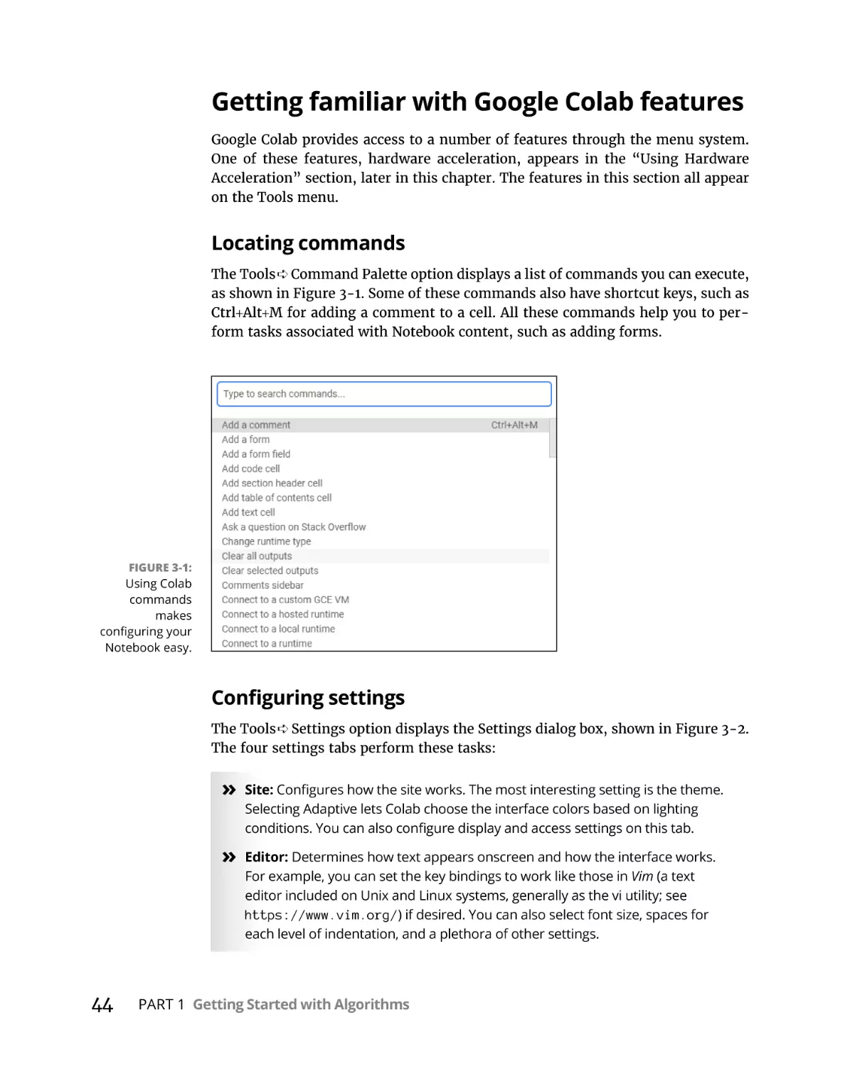
Getting familiar with Google Colab features. . . . . . . . . . . . . . . . . . .
Working with Notebooks . . . . . . . . . . . . . . . . . . . . . . . . . . . . . . . . . . . . . .
Creating a new notebook. . . . . . . . . . . . . . . . . . . . . . . . . . . . . . . . . . .
Opening existing notebooks . . . . . . . . . . . . . . . . . . . . . . . . . . . . . . . .
Saving notebooks . . . . . . . . . . . . . . . . . . . . . . . . . . . . . . . . . . . . . . . . .
Performing Common Tasks. . . . . . . . . . . . . . . . . . . . . . . . . . . . . . . . . . . .
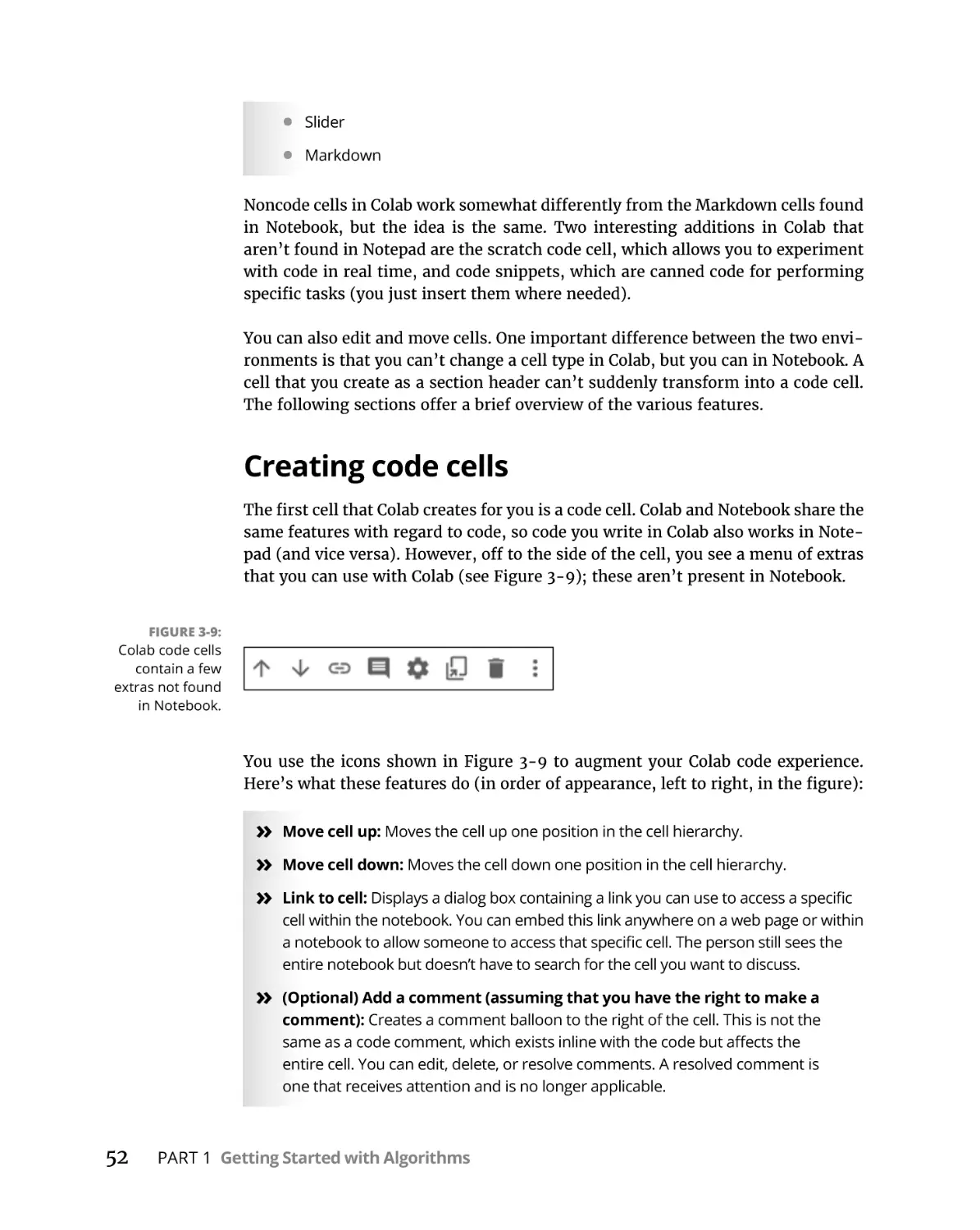
Creating code cells . . . . . . . . . . . . . . . . . . . . . . . . . . . . . . . . . . . . . . . .
Creating text cells . . . . . . . . . . . . . . . . . . . . . . . . . . . . . . . . . . . . . . . . .
Creating special cells. . . . . . . . . . . . . . . . . . . . . . . . . . . . . . . . . . . . . . .
Editing cells. . . . . . . . . . . . . . . . . . . . . . . . . . . . . . . . . . . . . . . . . . . . . . .
Moving cells . . . . . . . . . . . . . . . . . . . . . . . . . . . . . . . . . . . . . . . . . . . . . .
Using Hardware Acceleration . . . . . . . . . . . . . . . . . . . . . . . . . . . . . . . . . .
Executing the Code. . . . . . . . . . . . . . . . . . . . . . . . . . . . . . . . . . . . . . . . . . .
Getting Help. . . . . . . . . . . . . . . . . . . . . . . . . . . . . . . . . . . . . . . . . . . . . . . . .
CHAPTER 4:
42
42
44
47
47
47
50
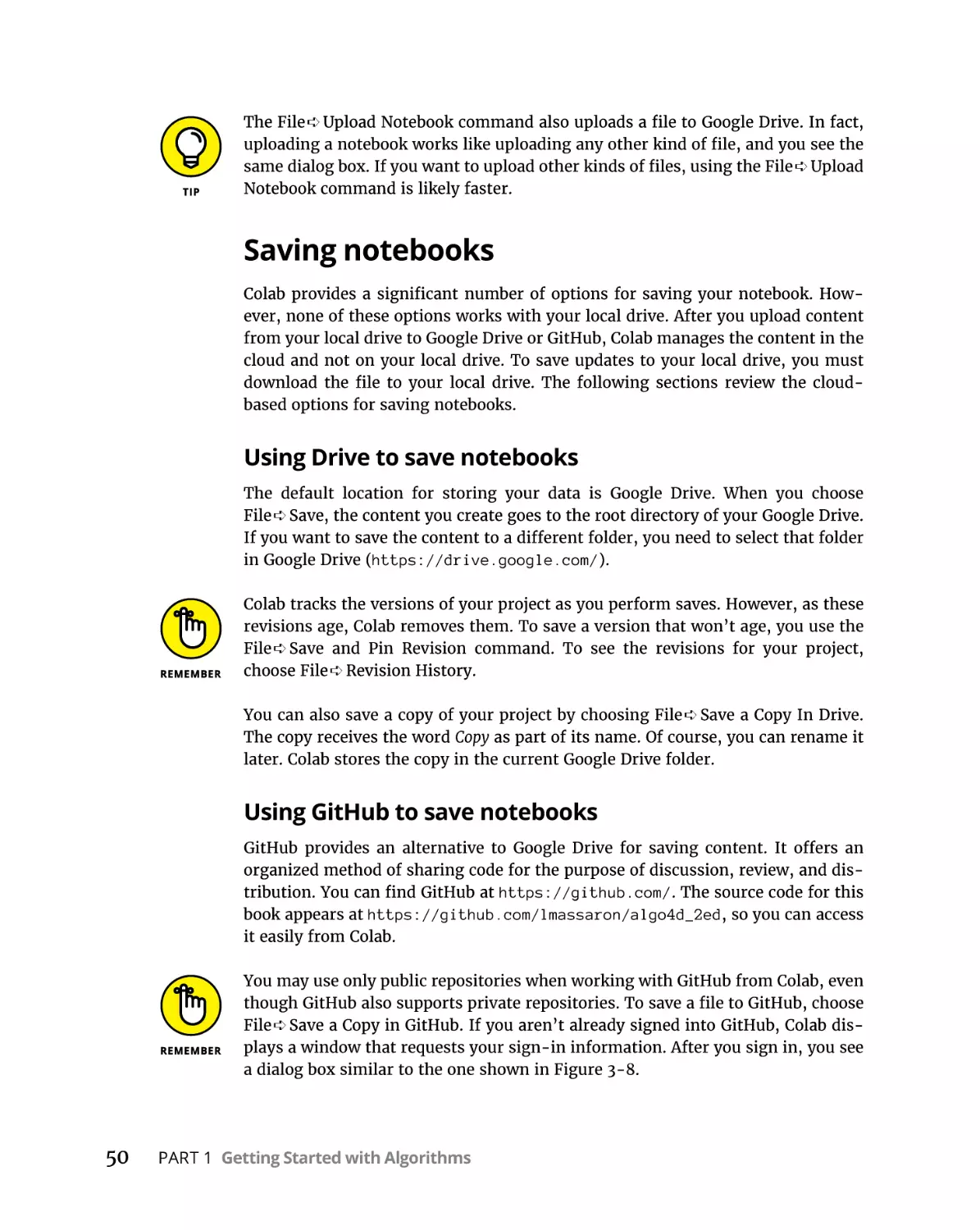
51
52
54
54
55
55
55
56
57
Performing Essential Data Manipulations
Using Python . . . . . . . . . . . . . . . . . . . . . . . . . . . . . . . . . . . . . . . . . . . . . . 59
Performing Calculations Using Vectors and Matrixes . . . . . . . . . . . . . .
Understanding scalar and vector operations . . . . . . . . . . . . . . . . . .
Performing vector multiplication . . . . . . . . . . . . . . . . . . . . . . . . . . . .
Creating a matrix is the right way to start. . . . . . . . . . . . . . . . . . . . .
Multiplying matrixes. . . . . . . . . . . . . . . . . . . . . . . . . . . . . . . . . . . . . . .
Defining advanced matrix operations . . . . . . . . . . . . . . . . . . . . . . . .
Creating Combinations the Right Way. . . . . . . . . . . . . . . . . . . . . . . . . . .
Distinguishing permutations. . . . . . . . . . . . . . . . . . . . . . . . . . . . . . . .
Shuffling combinations. . . . . . . . . . . . . . . . . . . . . . . . . . . . . . . . . . . . .
Facing repetitions . . . . . . . . . . . . . . . . . . . . . . . . . . . . . . . . . . . . . . . . .
Getting the Desired Results Using Recursion . . . . . . . . . . . . . . . . . . . . .
Explaining recursion. . . . . . . . . . . . . . . . . . . . . . . . . . . . . . . . . . . . . . .
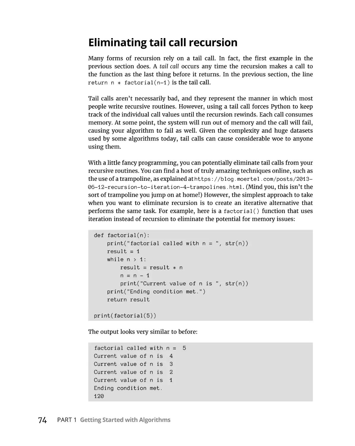
Eliminating tail call recursion. . . . . . . . . . . . . . . . . . . . . . . . . . . . . . . .
Performing Tasks More Quickly . . . . . . . . . . . . . . . . . . . . . . . . . . . . . . . .
Considering divide and conquer. . . . . . . . . . . . . . . . . . . . . . . . . . . . .
Distinguishing between different possible solutions. . . . . . . . . . . .
vi
33
34
34
35
36
37
38
Algorithms For Dummies
60
61
63
63
64
65
67
68
69
70
71
71
74
75
75
78
CHAPTER 5:
Developing a Matrix Computation Class . . . . . . . . . . . . . 79
Avoiding the Use of NumPy. . . . . . . . . . . . . . . . . . . . . . . . . . . . . . . . . . . .
Understanding Why Using a Class is Important. . . . . . . . . . . . . . . . . . .
Building the Basic Class . . . . . . . . . . . . . . . . . . . . . . . . . . . . . . . . . . . . . . .
Creating a matrix. . . . . . . . . . . . . . . . . . . . . . . . . . . . . . . . . . . . . . . . . .
Printing the resulting matrix . . . . . . . . . . . . . . . . . . . . . . . . . . . . . . . .
Accessing specific matrix elements . . . . . . . . . . . . . . . . . . . . . . . . . .
Performing scalar and matrix addition . . . . . . . . . . . . . . . . . . . . . . .
Performing multiplication . . . . . . . . . . . . . . . . . . . . . . . . . . . . . . . . . .
Manipulating the Matrix. . . . . . . . . . . . . . . . . . . . . . . . . . . . . . . . . . . . . . .
Transposing a matrix . . . . . . . . . . . . . . . . . . . . . . . . . . . . . . . . . . . . . .
Calculating the determinant . . . . . . . . . . . . . . . . . . . . . . . . . . . . . . . .
Flattening the matrix. . . . . . . . . . . . . . . . . . . . . . . . . . . . . . . . . . . . . . .
80
81
82
83
84
85
86
87
90
91
91
95
PART 2: UNDERSTANDING THE NEED
TO SORT AND SEARCH . . . . . . . . . . . . . . . . . . . . . . . . . . . . . . . . . . . . . . . . . . . 97
CHAPTER 6: Structuring Data. . . . . . . . . . . . . . . . . . . . . . . . . . . . . . . . . . . . . . . . . . 99
Determining the Need for Structure. . . . . . . . . . . . . . . . . . . . . . . . . . . .100
Making it easier to see the content. . . . . . . . . . . . . . . . . . . . . . . . . . 100
Matching data from various sources . . . . . . . . . . . . . . . . . . . . . . . . 101
Considering the need for remediation. . . . . . . . . . . . . . . . . . . . . . . 102
Stacking and Piling Data in Order. . . . . . . . . . . . . . . . . . . . . . . . . . . . . . 105
Ordering in stacks. . . . . . . . . . . . . . . . . . . . . . . . . . . . . . . . . . . . . . . . 105
Using queues. . . . . . . . . . . . . . . . . . . . . . . . . . . . . . . . . . . . . . . . . . . . 107
Finding data using dictionaries. . . . . . . . . . . . . . . . . . . . . . . . . . . . . 108
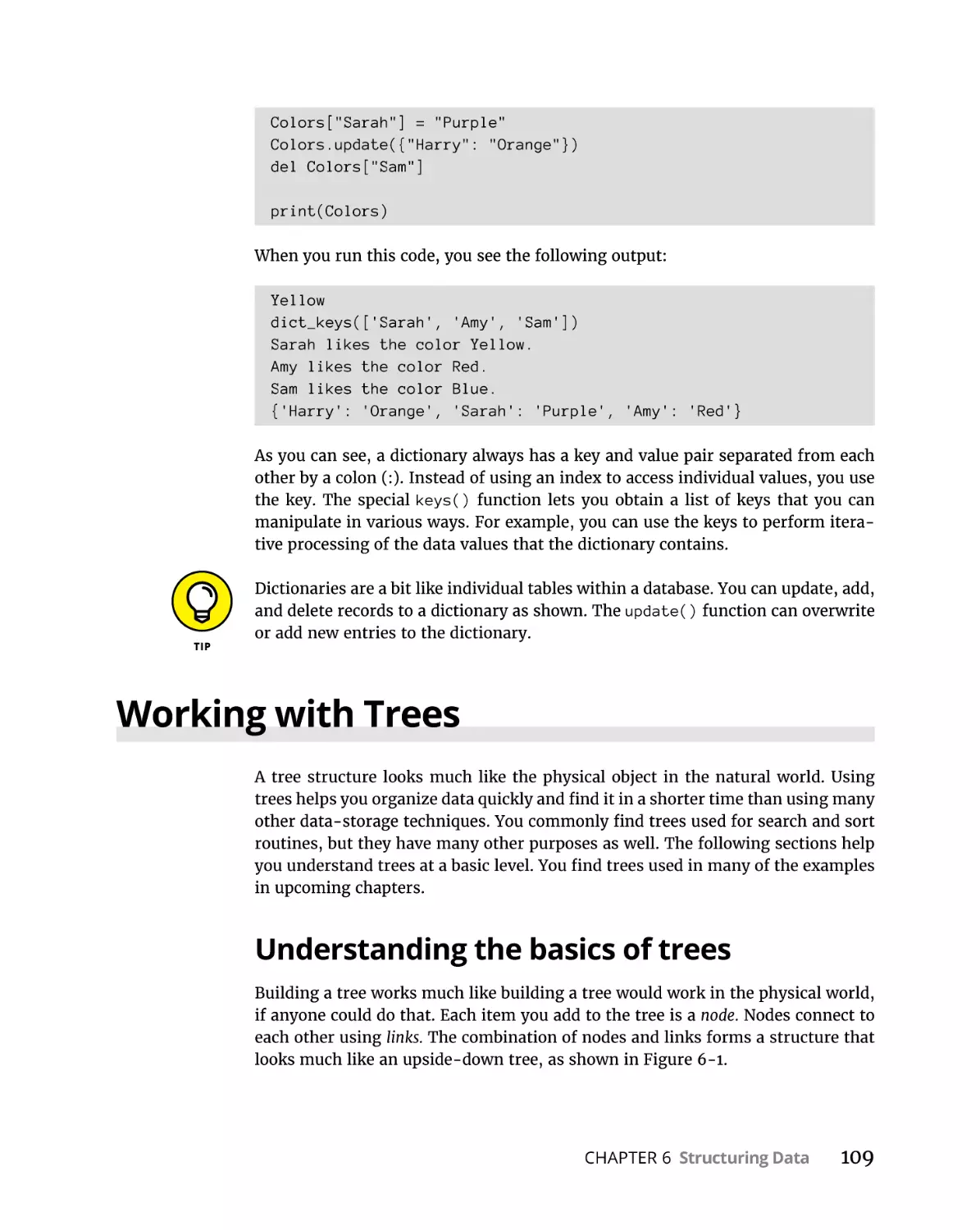
Working with Trees. . . . . . . . . . . . . . . . . . . . . . . . . . . . . . . . . . . . . . . . . . 109
Understanding the basics of trees . . . . . . . . . . . . . . . . . . . . . . . . . . 109
Building a tree . . . . . . . . . . . . . . . . . . . . . . . . . . . . . . . . . . . . . . . . . . . 110
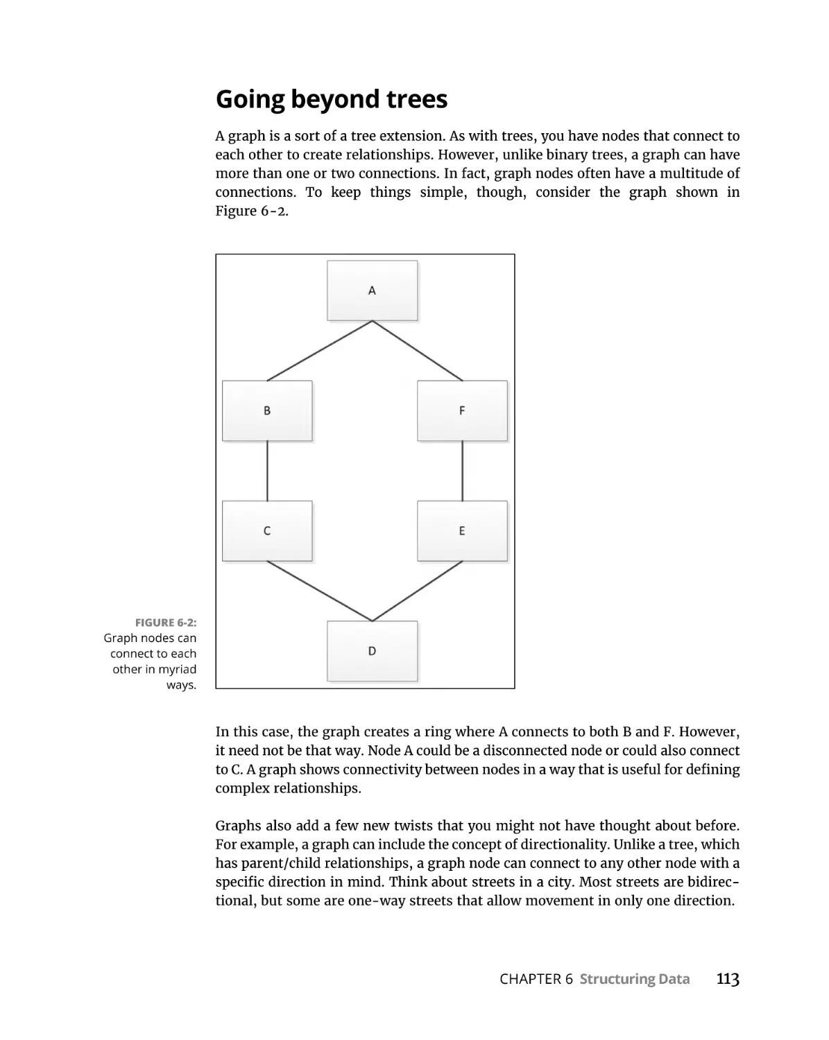
Representing Relations in a Graph. . . . . . . . . . . . . . . . . . . . . . . . . . . . . 112
Going beyond trees. . . . . . . . . . . . . . . . . . . . . . . . . . . . . . . . . . . . . . . 113
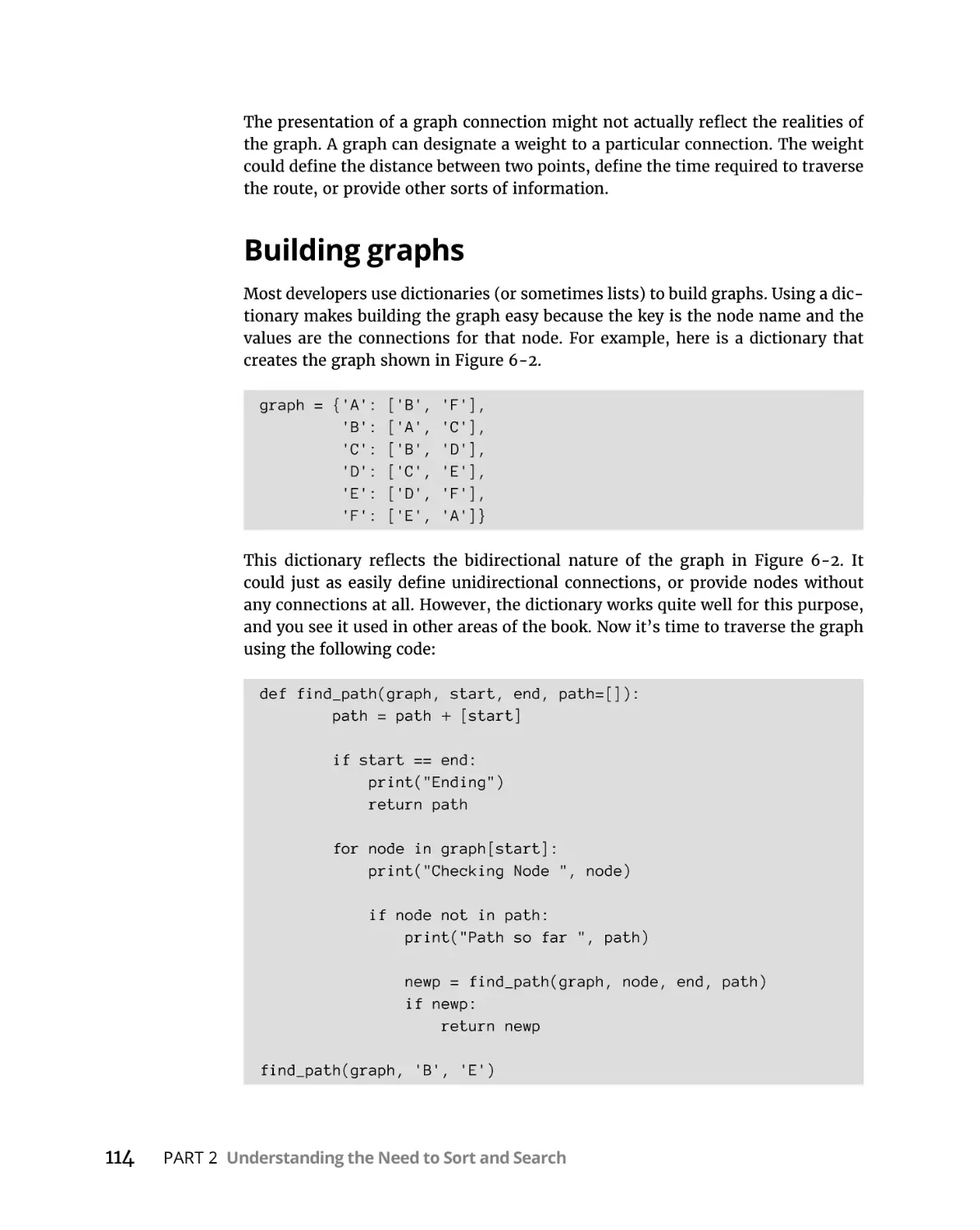
Building graphs . . . . . . . . . . . . . . . . . . . . . . . . . . . . . . . . . . . . . . . . . . 114
CHAPTER 7:
Arranging and Searching Data . . . . . . . . . . . . . . . . . . . . . . .
117
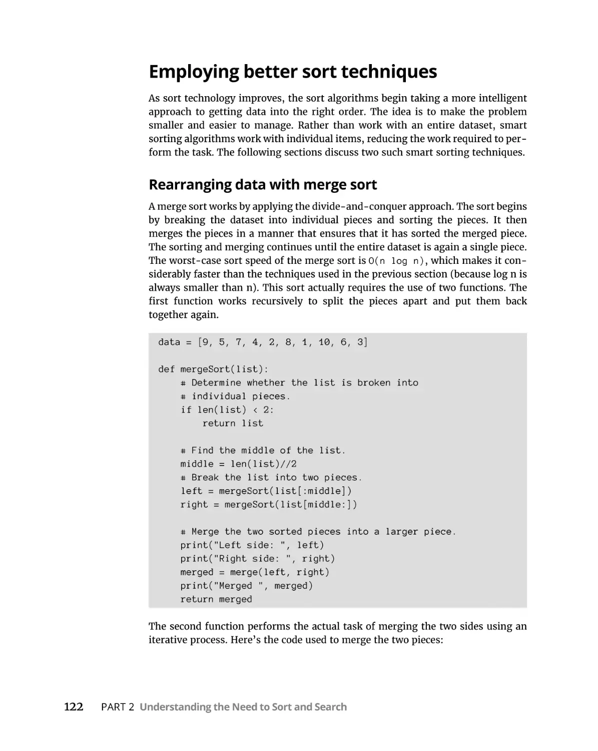
Sorting Data Using Merge Sort and Quick Sort. . . . . . . . . . . . . . . . . . .
Understanding why sorting data is important . . . . . . . . . . . . . . . .
Employing better sort techniques. . . . . . . . . . . . . . . . . . . . . . . . . . .
Using Search Trees and the Heap. . . . . . . . . . . . . . . . . . . . . . . . . . . . . .
Considering the need to search effectively. . . . . . . . . . . . . . . . . . .
Building a binary search tree. . . . . . . . . . . . . . . . . . . . . . . . . . . . . . .
Performing specialized searches using a binary heap. . . . . . . . . .
Relying on Hashing . . . . . . . . . . . . . . . . . . . . . . . . . . . . . . . . . . . . . . . . . .
Putting everything into buckets. . . . . . . . . . . . . . . . . . . . . . . . . . . . .
Avoiding collisions. . . . . . . . . . . . . . . . . . . . . . . . . . . . . . . . . . . . . . . .
Creating your own hash function . . . . . . . . . . . . . . . . . . . . . . . . . . .
118
118
122
127
127
129
131
132
132
134
135
Table of Contents
vii
PART 3: EXPLORING THE WORLD OF GRAPHS. . . . . . . . . . . . .
CHAPTER 8: Understanding Graph Basics . . . . . . . . . . . . . . . . . . . . . . . . .
139
141
Explaining the Importance of Networks. . . . . . . . . . . . . . . . . . . . . . . . .142
Considering the essence of a graph. . . . . . . . . . . . . . . . . . . . . . . . . 142
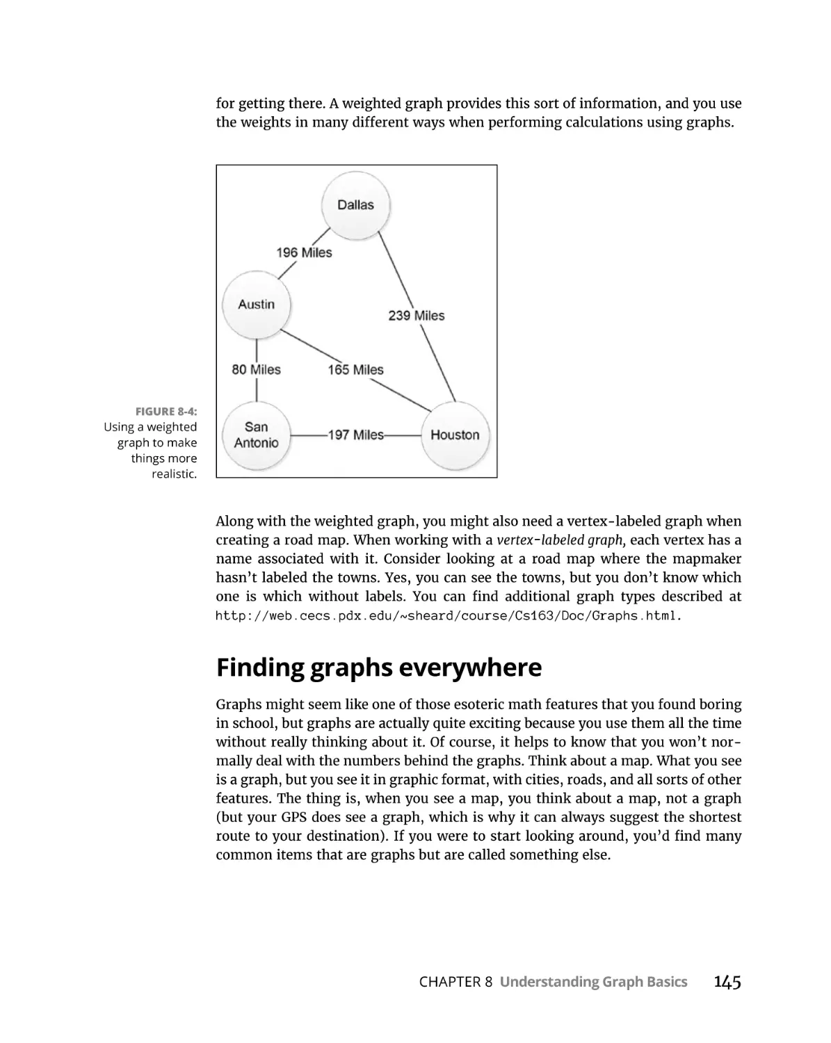
Finding graphs everywhere . . . . . . . . . . . . . . . . . . . . . . . . . . . . . . . . 145
Showing the social side of graphs. . . . . . . . . . . . . . . . . . . . . . . . . . . 146
Understanding subgraphs. . . . . . . . . . . . . . . . . . . . . . . . . . . . . . . . . 147
Defining How to Draw a Graph. . . . . . . . . . . . . . . . . . . . . . . . . . . . . . . . 148
Distinguishing the key attributes . . . . . . . . . . . . . . . . . . . . . . . . . . . 149
Drawing the graph. . . . . . . . . . . . . . . . . . . . . . . . . . . . . . . . . . . . . . . . 150
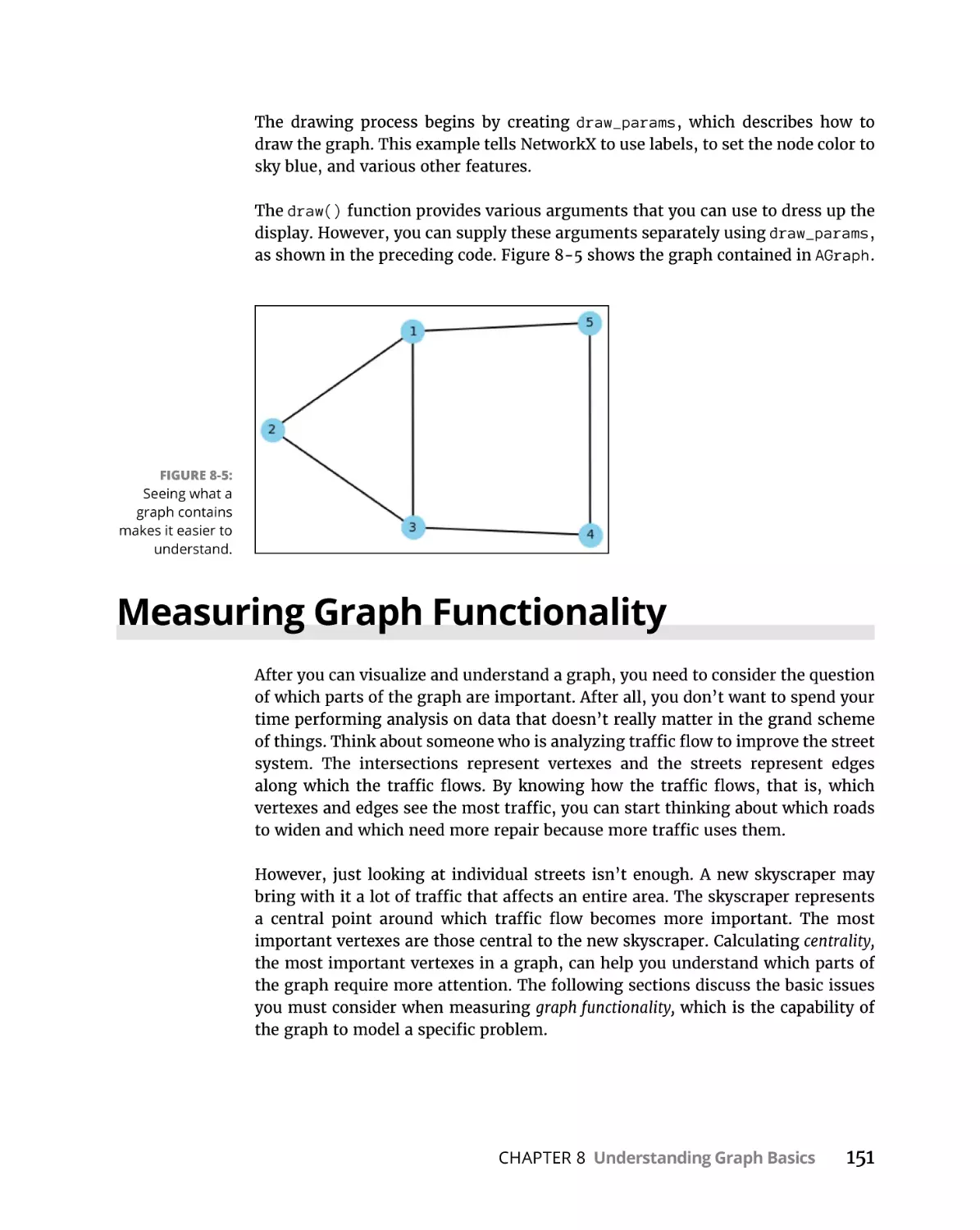
Measuring Graph Functionality. . . . . . . . . . . . . . . . . . . . . . . . . . . . . . . . 151
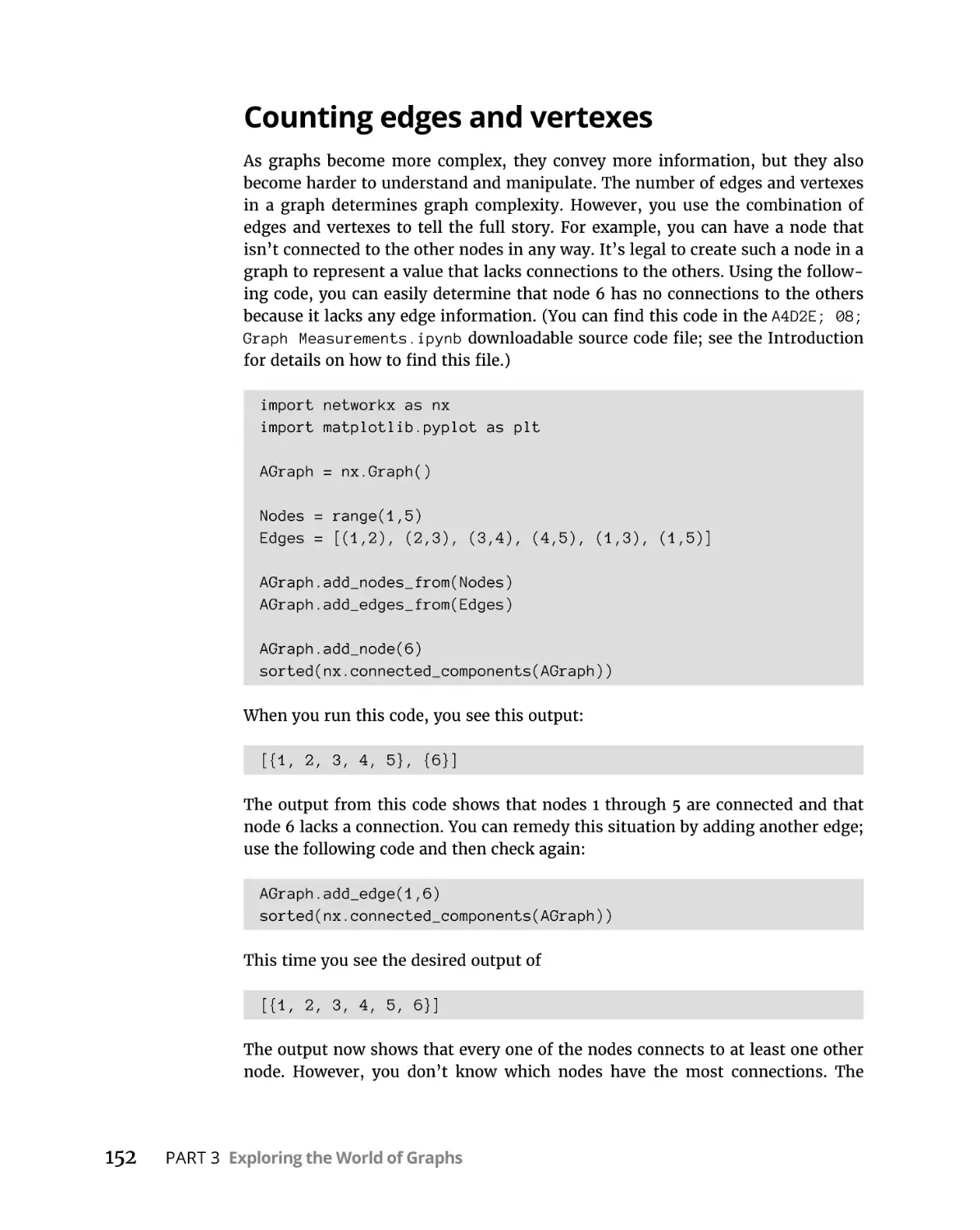
Counting edges and vertexes . . . . . . . . . . . . . . . . . . . . . . . . . . . . . . 152
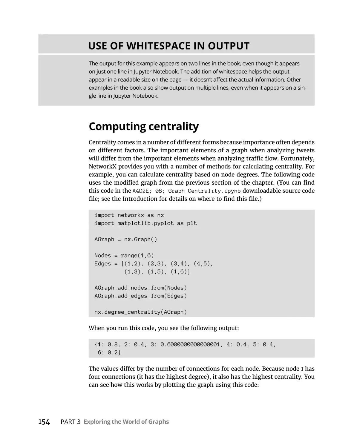
Computing centrality. . . . . . . . . . . . . . . . . . . . . . . . . . . . . . . . . . . . . .154
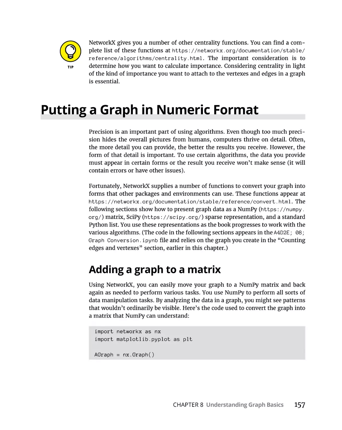
Putting a Graph in Numeric Format. . . . . . . . . . . . . . . . . . . . . . . . . . . . 157
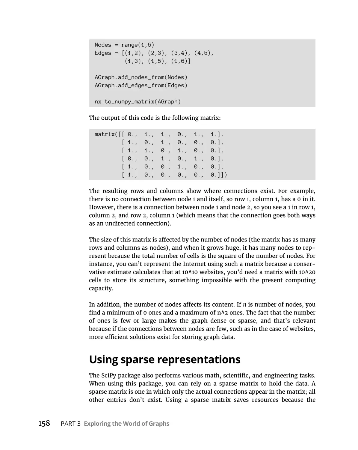
Adding a graph to a matrix . . . . . . . . . . . . . . . . . . . . . . . . . . . . . . . . 157
Using sparse representations . . . . . . . . . . . . . . . . . . . . . . . . . . . . . . 158
Using a list to hold a graph . . . . . . . . . . . . . . . . . . . . . . . . . . . . . . . . 159
CHAPTER 9:
viii
Reconnecting the Dots . . . . . . . . . . . . . . . . . . . . . . . . . . . . . . . .
161
Traversing a Graph Efficiently . . . . . . . . . . . . . . . . . . . . . . . . . . . . . . . . .
Creating the graph . . . . . . . . . . . . . . . . . . . . . . . . . . . . . . . . . . . . . . .
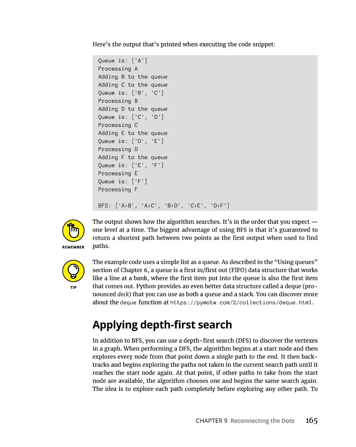
Applying breadth-first search . . . . . . . . . . . . . . . . . . . . . . . . . . . . . .
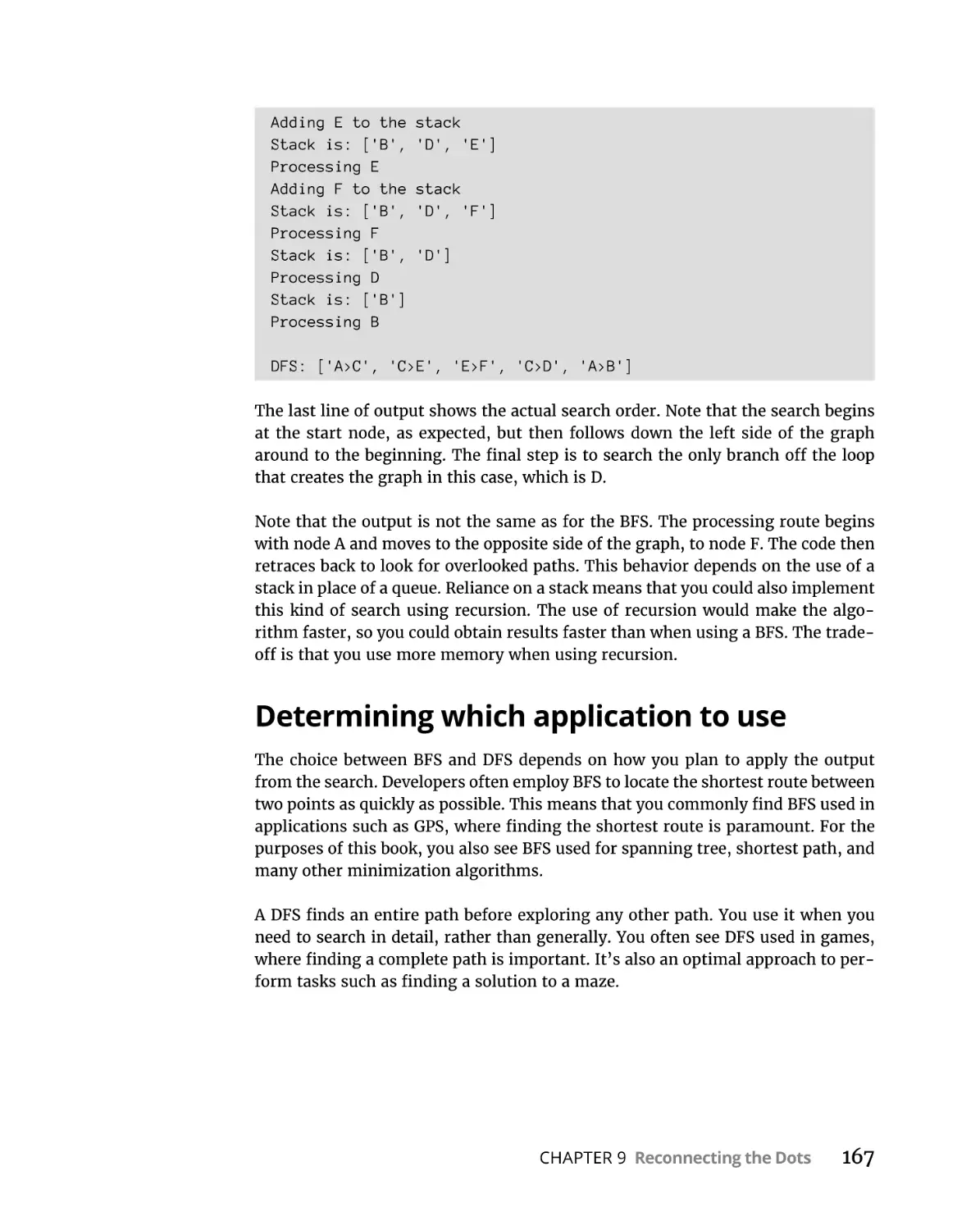
Applying depth-first search . . . . . . . . . . . . . . . . . . . . . . . . . . . . . . . .
Determining which application to use. . . . . . . . . . . . . . . . . . . . . . .
Sorting the Graph Elements. . . . . . . . . . . . . . . . . . . . . . . . . . . . . . . . . . .
Working on Directed Acyclic Graphs (DAGs). . . . . . . . . . . . . . . . . .
Relying on topological sorting. . . . . . . . . . . . . . . . . . . . . . . . . . . . . .
Reducing to a Minimum Spanning Tree. . . . . . . . . . . . . . . . . . . . . . . . .
Getting the minimum spanning tree historical context. . . . . . . . .
Working with unweighted versus weighted graphs. . . . . . . . . . . .
Creating a minimum spanning tree example . . . . . . . . . . . . . . . . .
Discovering the correct algorithms to use. . . . . . . . . . . . . . . . . . . .
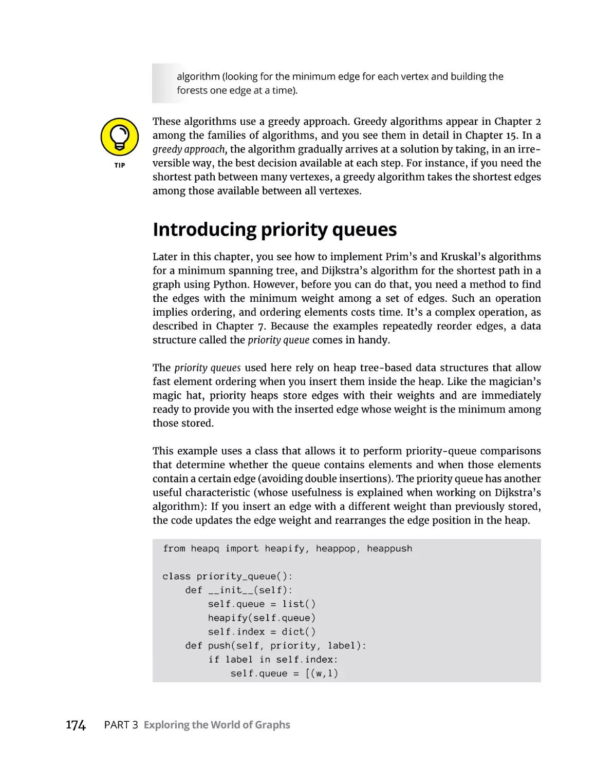
Introducing priority queues. . . . . . . . . . . . . . . . . . . . . . . . . . . . . . . .
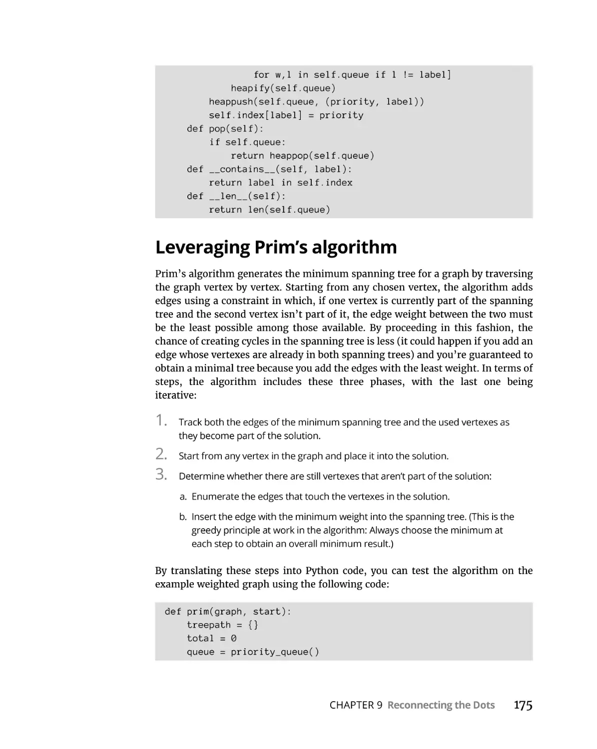
Leveraging Prim’s algorithm . . . . . . . . . . . . . . . . . . . . . . . . . . . . . . .
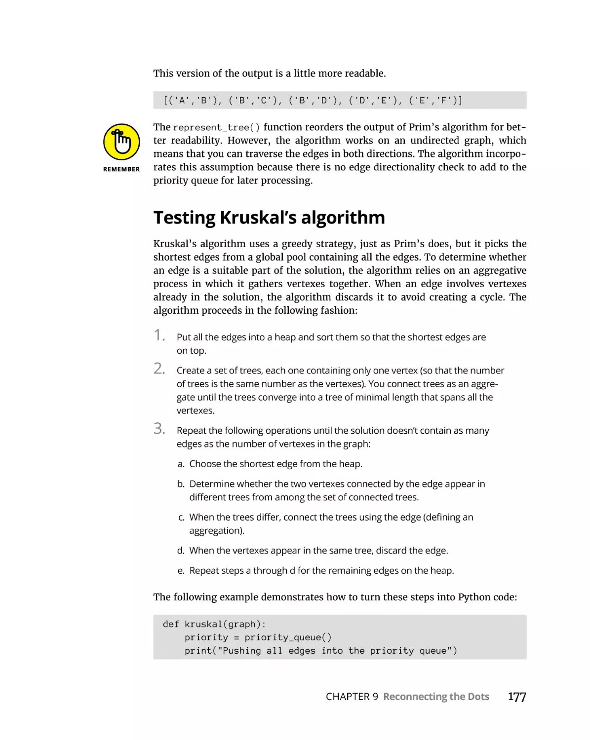
Testing Kruskal’s algorithm . . . . . . . . . . . . . . . . . . . . . . . . . . . . . . . .
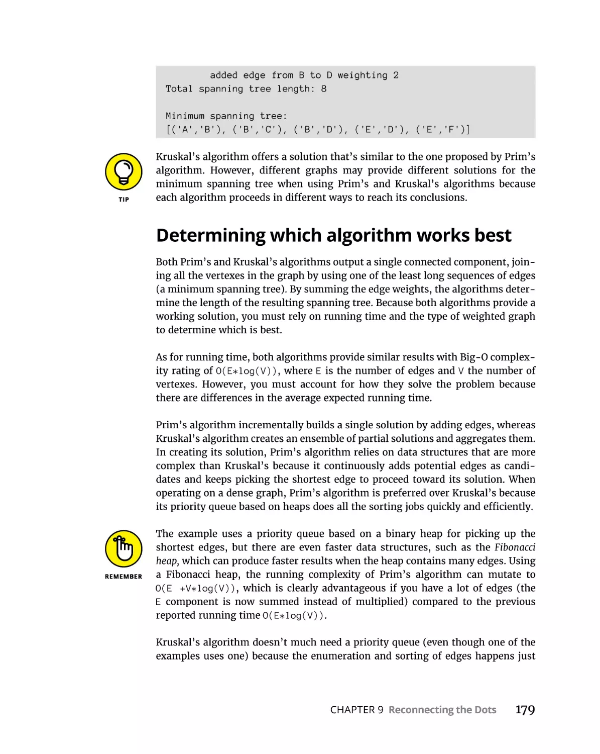
Determining which algorithm works best . . . . . . . . . . . . . . . . . . . .
Finding the Shortest Route . . . . . . . . . . . . . . . . . . . . . . . . . . . . . . . . . . .
Defining what it means to find the shortest path. . . . . . . . . . . . . .
Adding a negative edge . . . . . . . . . . . . . . . . . . . . . . . . . . . . . . . . . . .
Explaining Dijkstra’s algorithm . . . . . . . . . . . . . . . . . . . . . . . . . . . . .
Explaining the Bellman-Ford algorithm. . . . . . . . . . . . . . . . . . . . . .
Explaining the Floyd-Warshall algorithm. . . . . . . . . . . . . . . . . . . . .
162
163
164
165
167
168
169
169
170
170
171
171
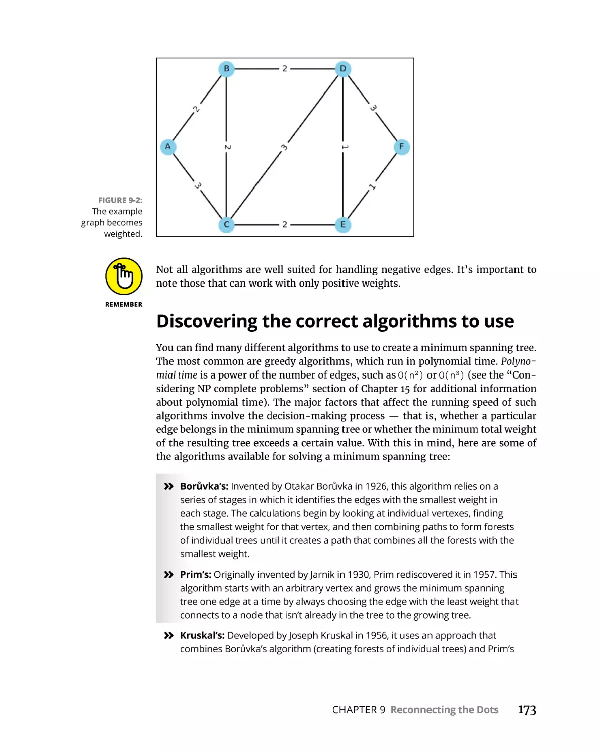
173
174
175
177
179
180
180
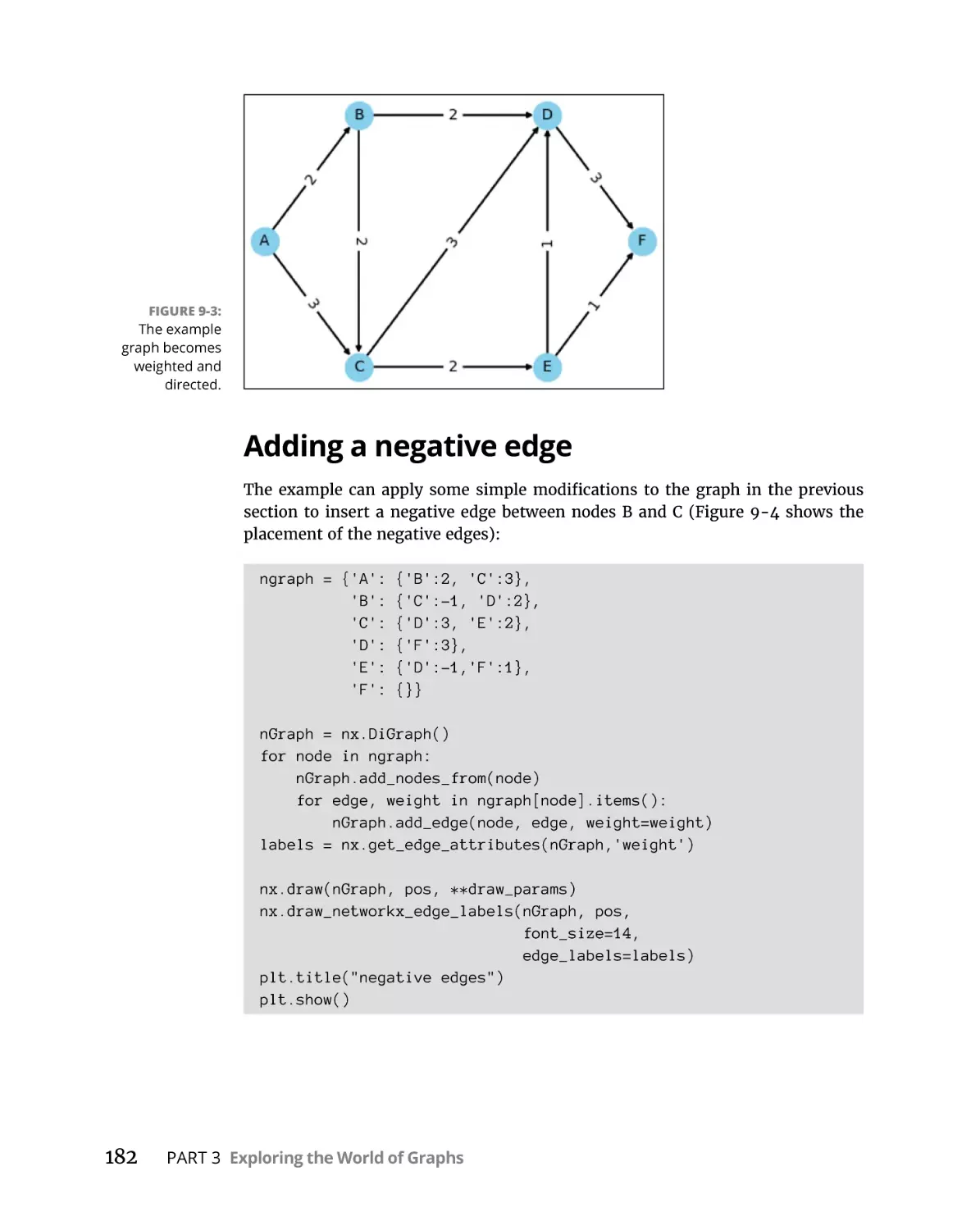
182
184
187
190
Algorithms For Dummies
CHAPTER 10:
Discovering Graph Secrets. . . . . . . . . . . . . . . . . . . . . . . . . . . .
195
Envisioning Social Networks as Graphs. . . . . . . . . . . . . . . . . . . . . . . . .
Clustering networks in groups. . . . . . . . . . . . . . . . . . . . . . . . . . . . . .
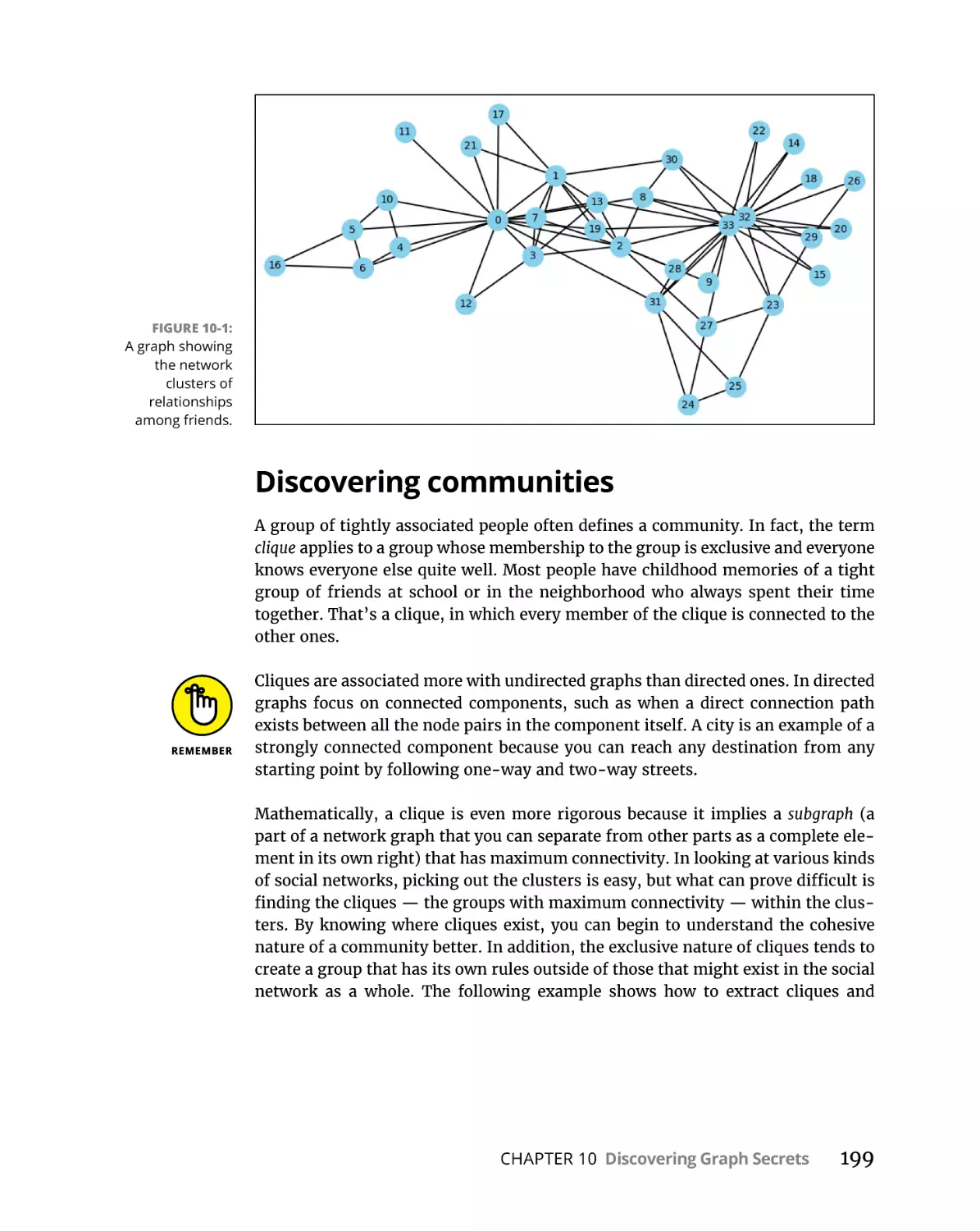
Discovering communities. . . . . . . . . . . . . . . . . . . . . . . . . . . . . . . . . .
Navigating a Graph. . . . . . . . . . . . . . . . . . . . . . . . . . . . . . . . . . . . . . . . . .
Counting the degrees of separation. . . . . . . . . . . . . . . . . . . . . . . . .
Walking a graph randomly. . . . . . . . . . . . . . . . . . . . . . . . . . . . . . . . .
196
196
199
202
202
204
Getting the Right Web page . . . . . . . . . . . . . . . . . . . . . . . . . .
207
Finding the World in a Search Engine. . . . . . . . . . . . . . . . . . . . . . . . . . .
Searching the Internet for data. . . . . . . . . . . . . . . . . . . . . . . . . . . . .
Considering how to find the right data . . . . . . . . . . . . . . . . . . . . . .
Explaining the PageRank Algorithm . . . . . . . . . . . . . . . . . . . . . . . . . . . .
Understanding the reasoning behind the
PageRank algorithm . . . . . . . . . . . . . . . . . . . . . . . . . . . . . . . . . . . . . .
Explaining the nuts and bolts of PageRank. . . . . . . . . . . . . . . . . . .
Implementing PageRank . . . . . . . . . . . . . . . . . . . . . . . . . . . . . . . . . . . . .
Implementing a Python script. . . . . . . . . . . . . . . . . . . . . . . . . . . . . .
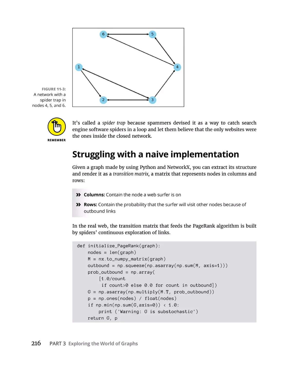
Struggling with a naive implementation . . . . . . . . . . . . . . . . . . . . .
Introducing boredom and teleporting. . . . . . . . . . . . . . . . . . . . . . .
Looking inside the life of a search engine. . . . . . . . . . . . . . . . . . . .
Considering other uses of PageRank . . . . . . . . . . . . . . . . . . . . . . . .
Going Beyond the PageRank Paradigm. . . . . . . . . . . . . . . . . . . . . . . . .
Introducing semantic queries . . . . . . . . . . . . . . . . . . . . . . . . . . . . . .
Using AI for ranking search results. . . . . . . . . . . . . . . . . . . . . . . . . .
208
208
209
210
PART 4: WRANGLING BIG DATA. . . . . . . . . . . . . . . . . . . . . . . . . . . . . .
CHAPTER 12: Managing Big Data . . . . . . . . . . . . . . . . . . . . . . . . . . . . . . . . . . . . .
223
225
Transforming Power into Data . . . . . . . . . . . . . . . . . . . . . . . . . . . . . . . .
Understanding Moore’s implications. . . . . . . . . . . . . . . . . . . . . . . .
Finding data everywhere . . . . . . . . . . . . . . . . . . . . . . . . . . . . . . . . . .
Getting algorithms into business . . . . . . . . . . . . . . . . . . . . . . . . . . .
Streaming Flows of Data . . . . . . . . . . . . . . . . . . . . . . . . . . . . . . . . . . . . .
Analyzing streams with the right recipe. . . . . . . . . . . . . . . . . . . . . .
Reserving the right data. . . . . . . . . . . . . . . . . . . . . . . . . . . . . . . . . . .
Sketching an Answer from Stream Data . . . . . . . . . . . . . . . . . . . . . . . .
Filtering stream elements by heart. . . . . . . . . . . . . . . . . . . . . . . . . .
Demonstrating the Bloom filter . . . . . . . . . . . . . . . . . . . . . . . . . . . .
Finding the number of distinct elements. . . . . . . . . . . . . . . . . . . . .
Learning to count objects in a stream . . . . . . . . . . . . . . . . . . . . . . .
226
226
228
231
233
234
235
240
240
243
246
247
CHAPTER 11:
Table of Contents
210
212
212
213
216
219
220
221
221
222
222
ix
CHAPTER 13:
249
Managing Immense Amounts of Data. . . . . . . . . . . . . . . . . . . . . . . . . .
Understanding the parallel paradigm . . . . . . . . . . . . . . . . . . . . . . .
Distributing files and operations. . . . . . . . . . . . . . . . . . . . . . . . . . . .
Employing the MapReduce solution. . . . . . . . . . . . . . . . . . . . . . . . .
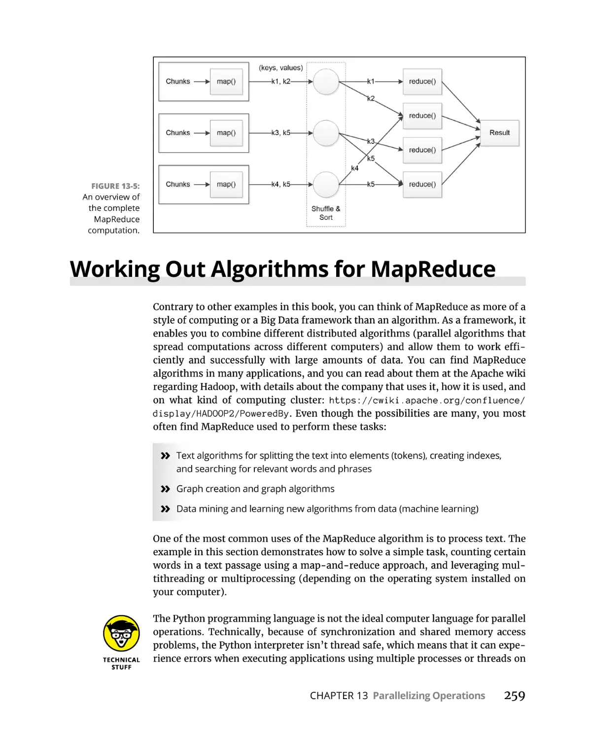
Working Out Algorithms for MapReduce. . . . . . . . . . . . . . . . . . . . . . . .
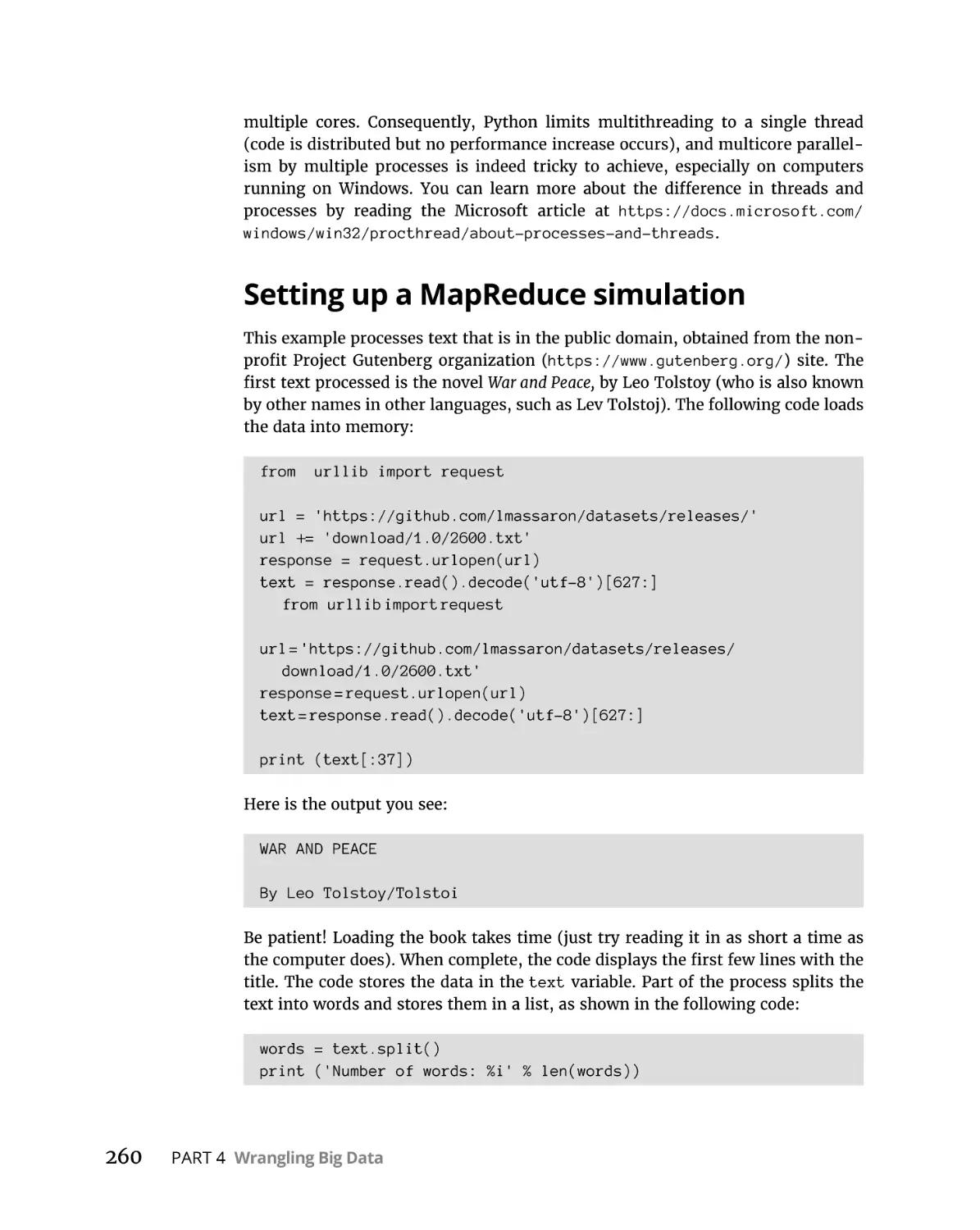
Setting up a MapReduce simulation. . . . . . . . . . . . . . . . . . . . . . . . .
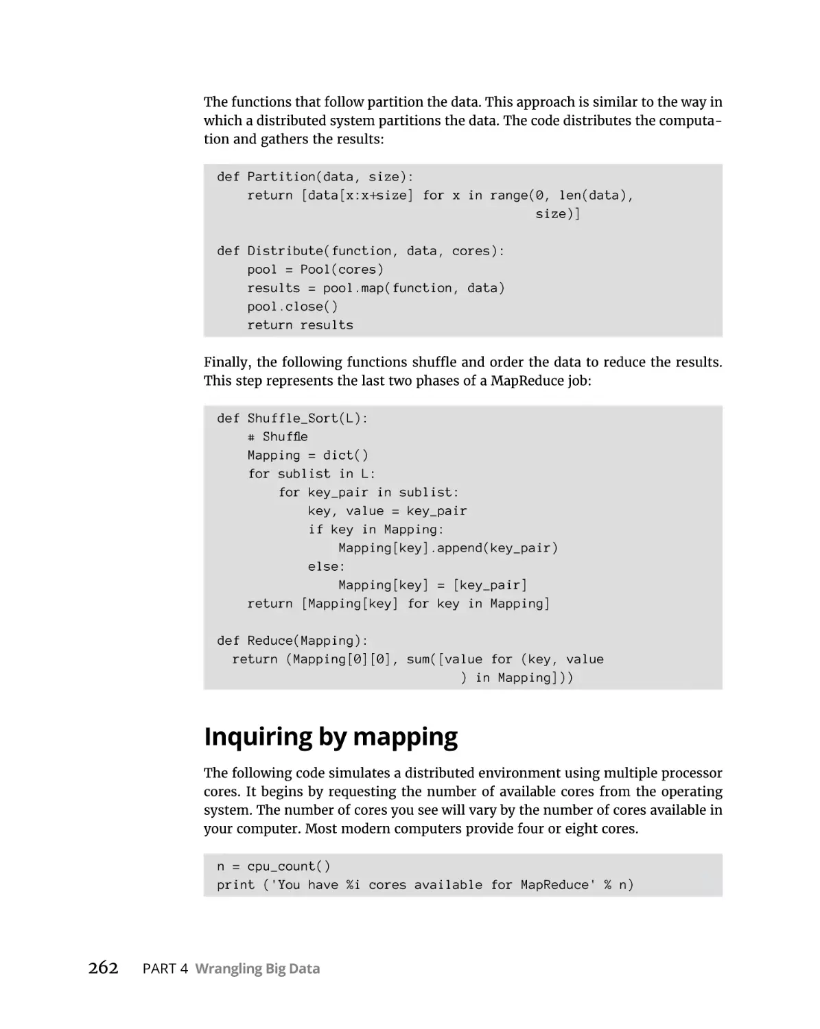
Inquiring by mapping . . . . . . . . . . . . . . . . . . . . . . . . . . . . . . . . . . . . .
250
251
253
255
259
260
262
Compressing and Concealing Data. . . . . . . . . . . . . . . . . .
267
Making Data Smaller. . . . . . . . . . . . . . . . . . . . . . . . . . . . . . . . . . . . . . . . .
Understanding encoding . . . . . . . . . . . . . . . . . . . . . . . . . . . . . . . . . .
Considering the effects of compression . . . . . . . . . . . . . . . . . . . . .
Choosing a particular kind of compression. . . . . . . . . . . . . . . . . . .
Choosing your encoding wisely. . . . . . . . . . . . . . . . . . . . . . . . . . . . .
Encoding using Huffman compression . . . . . . . . . . . . . . . . . . . . . .
Remembering sequences with LZW. . . . . . . . . . . . . . . . . . . . . . . . .
Hiding Your Secrets with Cryptography. . . . . . . . . . . . . . . . . . . . . . . . .
Substituting characters. . . . . . . . . . . . . . . . . . . . . . . . . . . . . . . . . . . .
Working with AES encryption. . . . . . . . . . . . . . . . . . . . . . . . . . . . . . .
268
268
270
271
273
276
278
282
283
285
PART 5: CHALLENGING DIFFICULT PROBLEMS. . . . . . . . . . . .
CHAPTER 15: Working with Greedy Algorithms. . . . . . . . . . . . . . . . . . . .
289
Deciding When It Is Better to Be Greedy. . . . . . . . . . . . . . . . . . . . . . . .
Understanding why greedy is good . . . . . . . . . . . . . . . . . . . . . . . . .
Keeping greedy algorithms under control. . . . . . . . . . . . . . . . . . . .
Considering NP complete problems. . . . . . . . . . . . . . . . . . . . . . . . .
Finding Out How Greedy Can Be Useful . . . . . . . . . . . . . . . . . . . . . . . .
Arranging cached computer data. . . . . . . . . . . . . . . . . . . . . . . . . . .
Competing for resources. . . . . . . . . . . . . . . . . . . . . . . . . . . . . . . . . .
Revisiting Huffman coding. . . . . . . . . . . . . . . . . . . . . . . . . . . . . . . . .
292
293
294
297
299
299
301
303
Relying on Dynamic Programming. . . . . . . . . . . . . . . . . .
307
Explaining Dynamic Programming. . . . . . . . . . . . . . . . . . . . . . . . . . . . .
Obtaining a historical basis . . . . . . . . . . . . . . . . . . . . . . . . . . . . . . . .
Making problems dynamic. . . . . . . . . . . . . . . . . . . . . . . . . . . . . . . . .
Casting recursion dynamically. . . . . . . . . . . . . . . . . . . . . . . . . . . . . .
Leveraging memoization . . . . . . . . . . . . . . . . . . . . . . . . . . . . . . . . . .
Discovering the Best Dynamic Recipes . . . . . . . . . . . . . . . . . . . . . . . . .
Looking inside the knapsack . . . . . . . . . . . . . . . . . . . . . . . . . . . . . . .
Touring around cities . . . . . . . . . . . . . . . . . . . . . . . . . . . . . . . . . . . . .
Approximating string search. . . . . . . . . . . . . . . . . . . . . . . . . . . . . . .
308
308
309
311
314
316
317
321
326
CHAPTER 14:
CHAPTER 16:
x
Parallelizing Operations. . . . . . . . . . . . . . . . . . . . . . . . . . . . . . .
Algorithms For Dummies
291
CHAPTER 17:
CHAPTER 18:
Using Randomized Algorithms. . . . . . . . . . . . . . . . . . . . . . .
331
Defining How Randomization Works . . . . . . . . . . . . . . . . . . . . . . . . . . .
Considering why randomization is needed. . . . . . . . . . . . . . . . . . .
Understanding how probability works. . . . . . . . . . . . . . . . . . . . . . .
Understanding distributions . . . . . . . . . . . . . . . . . . . . . . . . . . . . . . .
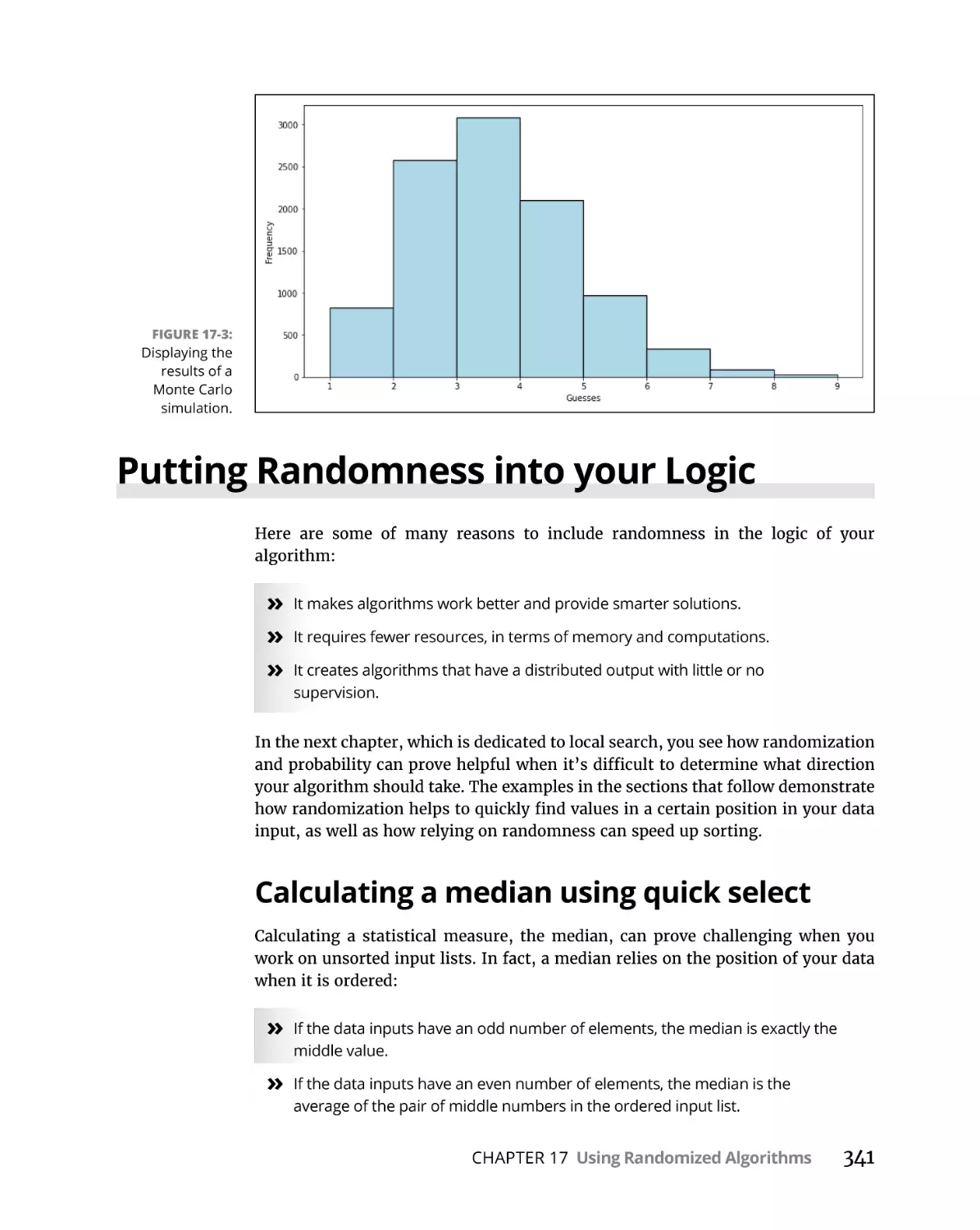
Simulating the use of the Monte Carlo method. . . . . . . . . . . . . . .
Putting Randomness into your Logic . . . . . . . . . . . . . . . . . . . . . . . . . . .
Calculating a median using quick select. . . . . . . . . . . . . . . . . . . . . .
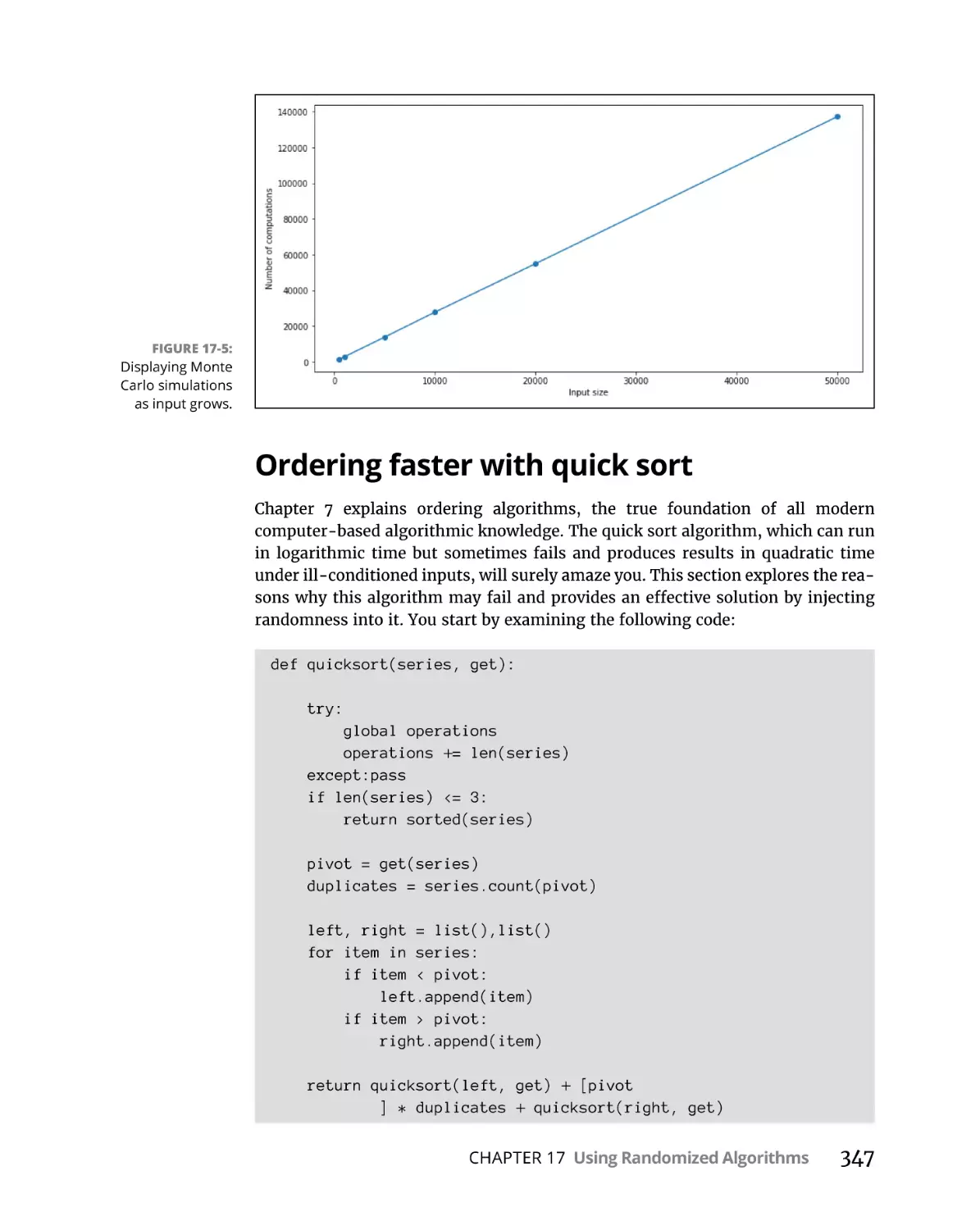
Doing simulations using Monte Carlo . . . . . . . . . . . . . . . . . . . . . . .
Ordering faster with quick sort. . . . . . . . . . . . . . . . . . . . . . . . . . . . .
332
333
334
335
339
341
341
344
347
Performing Local Search . . . . . . . . . . . . . . . . . . . . . . . . . . . . . .
349
Understanding Local Search . . . . . . . . . . . . . . . . . . . . . . . . . . . . . . . . . . 350
Knowing the neighborhood. . . . . . . . . . . . . . . . . . . . . . . . . . . . . . . . 351
Presenting local search tricks . . . . . . . . . . . . . . . . . . . . . . . . . . . . . . . . . 353
Explaining hill climbing with n-queens. . . . . . . . . . . . . . . . . . . . . . . 354
Discovering simulated annealing . . . . . . . . . . . . . . . . . . . . . . . . . . . 357
Avoiding repeats using Tabu Search. . . . . . . . . . . . . . . . . . . . . . . . .358
Solving Satisfiability of Boolean Circuits . . . . . . . . . . . . . . . . . . . . . . . . 359
Solving 2-SAT using randomization. . . . . . . . . . . . . . . . . . . . . . . . . .360
Implementing the Python code. . . . . . . . . . . . . . . . . . . . . . . . . . . . . 361
Realizing that the starting point is important. . . . . . . . . . . . . . . . . 365
CHAPTER 19:
CHAPTER 20:
Employing Linear Programming. . . . . . . . . . . . . . . . . . . . .
367
Using Linear Functions as a Tool. . . . . . . . . . . . . . . . . . . . . . . . . . . . . . .
Grasping the basic math you need. . . . . . . . . . . . . . . . . . . . . . . . . .
Learning to simplify when planning. . . . . . . . . . . . . . . . . . . . . . . . .
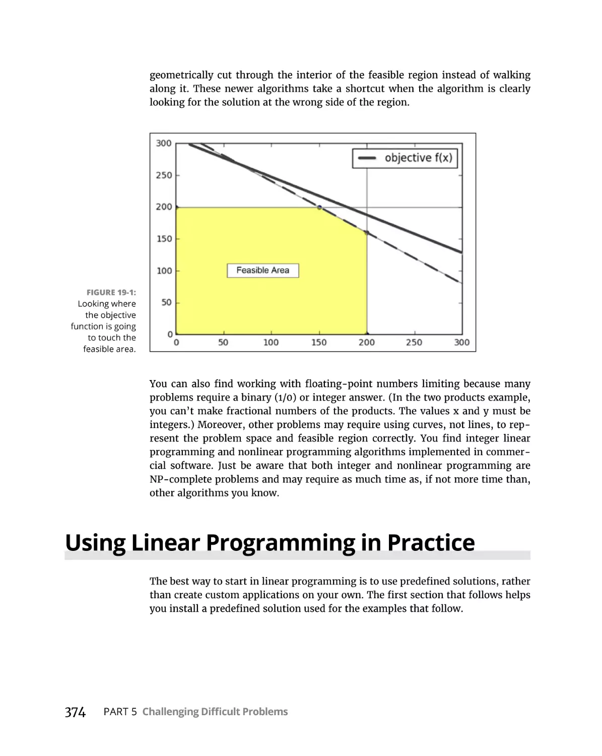
Working with geometry using simplex. . . . . . . . . . . . . . . . . . . . . . .
Understanding the limitations. . . . . . . . . . . . . . . . . . . . . . . . . . . . . .
Using Linear Programming in Practice. . . . . . . . . . . . . . . . . . . . . . . . . .
Setting up PuLP at home . . . . . . . . . . . . . . . . . . . . . . . . . . . . . . . . . .
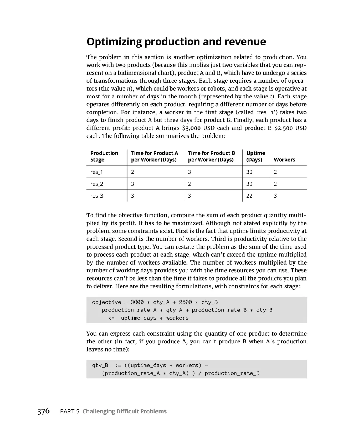
Optimizing production and revenue . . . . . . . . . . . . . . . . . . . . . . . .
368
369
371
372
373
374
375
376
Considering Heuristics. . . . . . . . . . . . . . . . . . . . . . . . . . . . . . . . .
381
Differentiating Heuristics. . . . . . . . . . . . . . . . . . . . . . . . . . . . . . . . . . . . .
Considering the goals of heuristics. . . . . . . . . . . . . . . . . . . . . . . . . .
Going from genetic to AI. . . . . . . . . . . . . . . . . . . . . . . . . . . . . . . . . . .
Routing Robots Using Heuristics. . . . . . . . . . . . . . . . . . . . . . . . . . . . . . .
Scouting in unknown territories . . . . . . . . . . . . . . . . . . . . . . . . . . . .
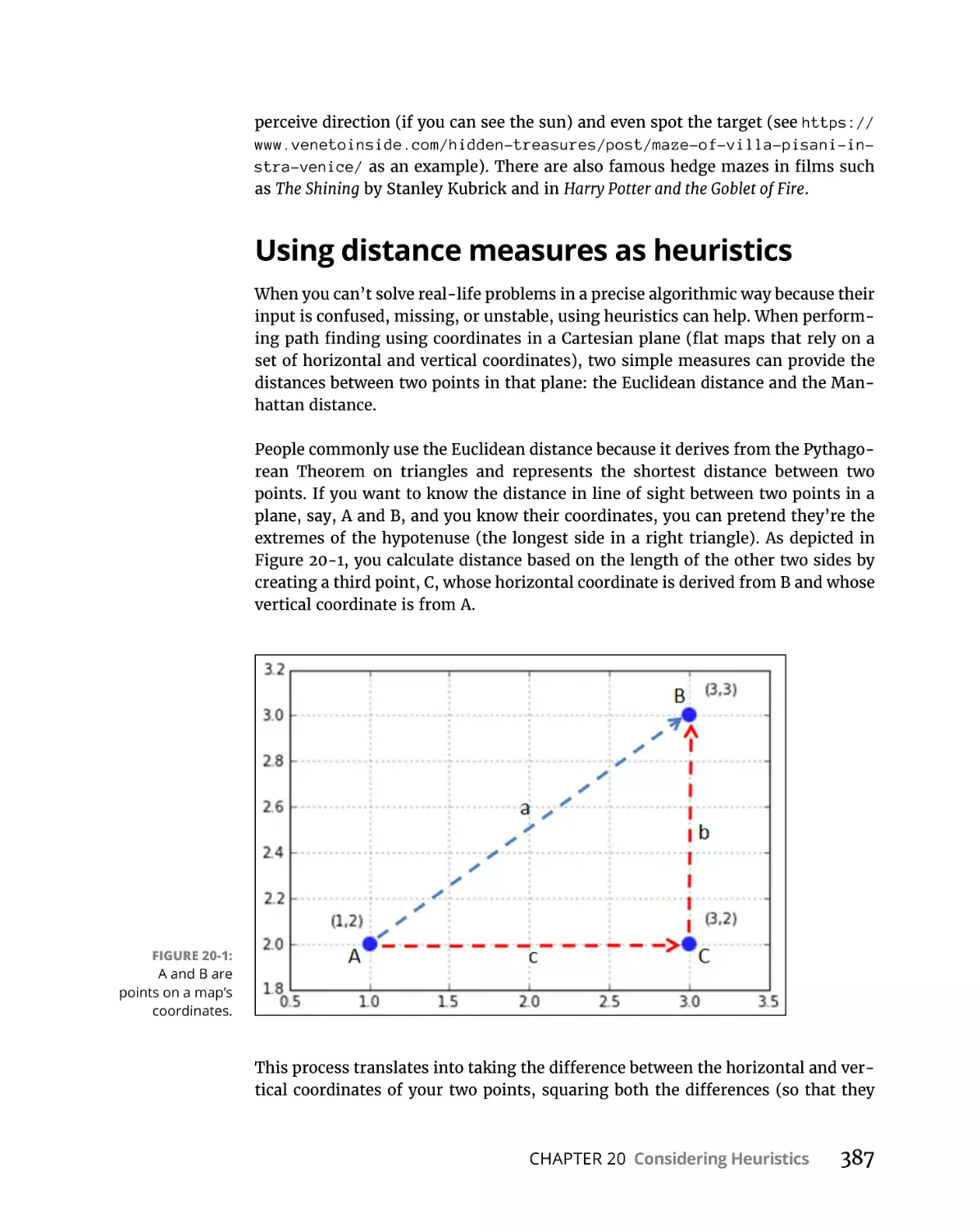
Using distance measures as heuristics . . . . . . . . . . . . . . . . . . . . . .
Explaining Path Finding Algorithms . . . . . . . . . . . . . . . . . . . . . . . . . . . .
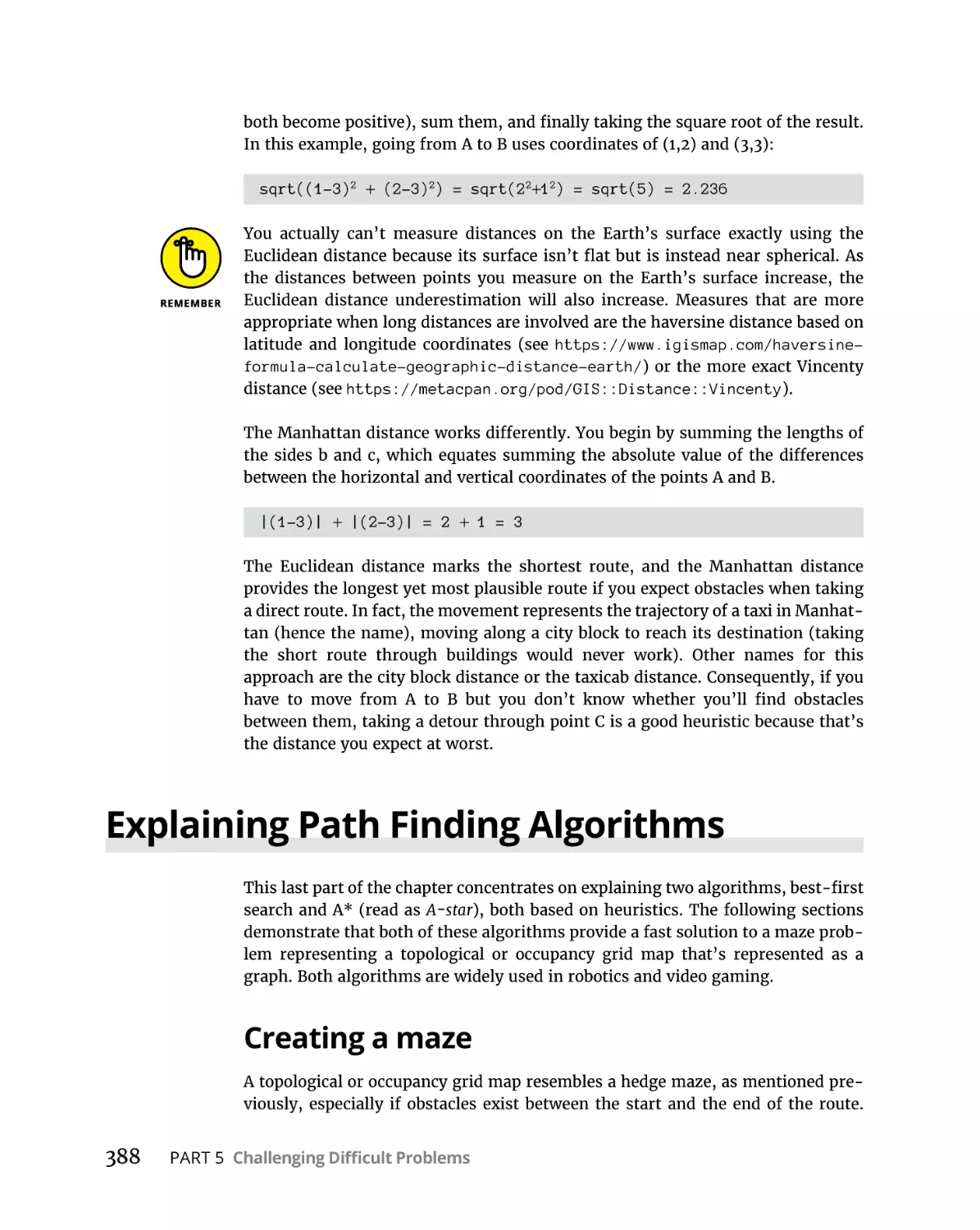
Creating a maze. . . . . . . . . . . . . . . . . . . . . . . . . . . . . . . . . . . . . . . . . .
Looking for a quick best-first route. . . . . . . . . . . . . . . . . . . . . . . . . .
Going heuristically around by A* . . . . . . . . . . . . . . . . . . . . . . . . . . .
382
383
383
384
385
387
388
388
392
396
Table of Contents
xi
PART 6: THE PART OF TENS. . . . . . . . . . . . . . . . . . . . . . . . . . . . . . . . . . . .
CHAPTER 21: Ten Algorithms That Are Changing the World. . . . .
403
Using Sort Routines. . . . . . . . . . . . . . . . . . . . . . . . . . . . . . . . . . . . . . . . . .
Looking for Things with Search Routines. . . . . . . . . . . . . . . . . . . . . . . .
Shaking Things Up with Random Numbers. . . . . . . . . . . . . . . . . . . . . .
Performing Data Compression . . . . . . . . . . . . . . . . . . . . . . . . . . . . . . . .
Keeping Data Secret . . . . . . . . . . . . . . . . . . . . . . . . . . . . . . . . . . . . . . . . .
Changing the Data Domain . . . . . . . . . . . . . . . . . . . . . . . . . . . . . . . . . . .
Analyzing Links. . . . . . . . . . . . . . . . . . . . . . . . . . . . . . . . . . . . . . . . . . . . . .
Spotting Data Patterns. . . . . . . . . . . . . . . . . . . . . . . . . . . . . . . . . . . . . . .
Dealing with Automation and Automatic Responses. . . . . . . . . . . . . .
Creating Unique Identifiers . . . . . . . . . . . . . . . . . . . . . . . . . . . . . . . . . . .
404
404
405
406
406
407
407
408
409
409
Ten Algorithmic Problems Yet to Solve. . . . . . . . . . . . .
411
CHAPTER 22:
401
Solving Problems Quickly. . . . . . . . . . . . . . . . . . . . . . . . . . . . . . . . . . . . . 412
Solving 3SUM Problems More Efficiently. . . . . . . . . . . . . . . . . . . . . . . . 412
Making Matrix Multiplication Faster. . . . . . . . . . . . . . . . . . . . . . . . . . . . 413
Determining Whether an Application Will End. . . . . . . . . . . . . . . . . . . 413
Creating and Using One-Way Functions. . . . . . . . . . . . . . . . . . . . . . . . .414
Multiplying Really Large Numbers . . . . . . . . . . . . . . . . . . . . . . . . . . . . . 414
Dividing a Resource Equally. . . . . . . . . . . . . . . . . . . . . . . . . . . . . . . . . . . 415
Reducing Edit Distance Calculation Time. . . . . . . . . . . . . . . . . . . . . . . . 415
Playing the Parity Game. . . . . . . . . . . . . . . . . . . . . . . . . . . . . . . . . . . . . . 416
Understanding Spatial Issues . . . . . . . . . . . . . . . . . . . . . . . . . . . . . . . . . 416
INDEX. . . . . . . . . . . . . . . . . . . . . . . . . . . . . . . . . . . . . . . . . . . . . . . . . . . . . . . . . . . . . .
xii
Algorithms For Dummies
417
Introduction
Y
ou need to learn about algorithms for school or work. Yet, all the books
you’ve tried on the subject end up being more along the lines of really good
sleep-inducing aids rather than texts to teach you something. Assuming
that you can get past the arcane symbols obviously written by a demented
two-year-old with a penchant for squiggles, you end up having no idea of why
you’d even want to know anything about them. Most math texts are boring!
However, Algorithms For Dummies, 2nd Edition is different. The first thing you’ll
note is that this book has a definite lack of odd symbols (especially of the squiggly
sort) floating about. Yes, you see a few (it is a math book, after all), but what you
find instead are clear instructions for using algorithms that actually have names
and a history behind them and that perform useful tasks. You’ll encounter simple
coding techniques to perform amazing tasks that will intrigue your friends. You
can certainly make them jealous as you perform feats of math that they can’t
begin to understand. You get all this without having to strain your brain, even a
little, and you won’t even fall asleep (well, unless you really want to do so). New
in this edition of the book are more details about how algorithms work, and you
even get to create your own basic math package so that you know how to do it for
that next job interview.
About This Book
Algorithms For Dummies, 2nd Edition is the math book that you wanted in college
but didn’t get. You discover, for example, that algorithms aren’t new. After all,
the Babylonians used algorithms to perform simple tasks as early as 1,600 BC. If
the Babylonians could figure this stuff out, certainly you can, too! This book actually has three things that you won’t find in most math books:
»» Algorithms that have actual names and a historical basis so that you can
remember the algorithm and know why someone took time to create it
»» Simple explanations of how the algorithm performs awesome feats of data
manipulation, data analysis, or probability prediction
»» Code that shows how to use the algorithm without actually dealing with
arcane symbols that no one without a math degree can understand
Introduction
1
Part of the emphasis of this book is on using the right tools. This book uses Python
to perform various tasks. Python has special features that make working with
algorithms significantly easier. For example, Python provides access to a huge
array of packages that let you do just about anything you can imagine, and more
than a few that you can’t. However, unlike many texts that use Python, this one
doesn’t bury you in packages. We use a select group of packages that provide great
flexibility with a lot of functionality but don’t require you to pay anything. You can
go through this entire book without forking over a cent of your hard-earned
money.
You also discover some interesting techniques in this book. The most important is
that you don’t just see the algorithms used to perform tasks; you also get an
explanation of how the algorithms work. Unlike many other books, Algorithms For
Dummies, 2nd Edition enables you to fully understand what you’re doing, but
without requiring you to have a PhD in math. Every one of the examples shows the
expected output and tells you why that output is important. You aren’t left with
the feeling that something is missing.
Of course, you might still be worried about the whole programming environment
issue, and this book doesn’t leave you in the dark there, either. This book relies on
Google Colab to provide a programming environment (although you can use Jupyter Notebook quite easily, too). Because you access Colab through a browser, you
can program anywhere and at any time that you have access to a browser, even on
your smartphone while at the dentist’s office or possibly while standing on your
head watching reruns of your favorite show.
To help you absorb the concepts, this book uses the following conventions:
»» Text that you’re meant to type just as it appears in the book is in bold. The
exception is when you’re working through a step list: Because each step is
bold, the text to type is not bold.
»» Words that we want you to type in that are also in italics are used as place-
holders, which means that you need to replace them with something that
works for you. For example, if you see “Type Your Name and press Enter,” you
need to replace Your Name with your actual name.
»» We also use italics for terms we define. This means that you don’t have to rely
on other sources to provide the definitions you need.
»» Web addresses and programming code appear in monofont. If you’re reading
a digital version of this book on a device connected to the Internet, you can
click the live link to visit that website, like this: http://www.dummies.com.
»» When you need to click command sequences, you see them separated by a
special arrow, like this: File ➪ New File, which tells you to click File and then
New File.
2
Algorithms For Dummies
Foolish Assumptions
You might find it difficult to believe that we’ve assumed anything about you —
after all, we haven’t even met you yet! Although most assumptions are indeed
foolish, we made certain assumptions to provide a starting point for the book.
The first assumption is that you’re familiar with the platform you want to use,
because the book doesn’t provide any guidance in this regard. (Chapter 3 does,
however, tell you how to access Google Colab from your browser and use it to work
with the code examples in the book.) To give you the maximum information about
Python with regard to algorithms, this book doesn’t discuss any platform-specific
issues. You really do need to know how to install applications, use applications, and
generally work with your chosen platform before you begin working with this book.
This book isn’t a math primer. Yes, you see lots of examples of complex math, but
the emphasis is on helping you use Python to perform common tasks using algorithms rather than learning math theory. However, you do get explanations of
many of the algorithms used in the book so that you can understand how the
algorithms work. Chapters 1 and 2 guide you through a what you need to know in
order to use this book successfully. Chapter 5 is a special chapter that discusses
how to create your own math library, which significantly aids you in understanding how math works with code to create a reusable package. It also looks dandy on
your resume to say that you’ve created your own math library.
This book also assumes that you can access items on the Internet. Sprinkled
throughout are numerous references to online material that will enhance your
learning experience. However, these added sources are useful only if you actually
find and use them. You must also have Internet access to use Google Colab.
Icons Used in This Book
As you read this book, you encounter icons in the margins that indicate material
of interest (or not, as the case may be). Here’s what the icons mean:
Tips are nice because they help you save time or perform some task without a lot
of extra work. The tips in this book are time-saving techniques or pointers to
resources that you should try so that you can get the maximum benefit from
Python, or in performing algorithm-related or data analysis–related tasks.
Introduction
3
We don’t want to sound like angry parents or some kind of maniacs, but you
should avoid doing anything that’s marked with a Warning icon. Otherwise, you
might find that your application fails to work as expected, you get incorrect
answers from seemingly bulletproof algorithms, or (in the worst-case scenario)
you lose data.
Whenever you see this icon, think advanced tip or technique. You might find these
tidbits of useful information just too boring for words, or they could contain the
solution you need to get a program running. Skip these bits of information whenever you like.
If you don’t get anything else out of a particular chapter or section, remember the
material marked by this icon. This text usually contains an essential process or a
bit of information that you must know to work with Python, or to perform
algorithm-related or data analysis–related tasks successfully.
Beyond the Book
This book isn’t the end of your Python or algorithm learning experience — it’s
really just the beginning. We provide online content to make this book more flexible and better able to meet your needs. That way, as we receive email from you,
we can address questions and tell you how updates to Python, or its associated
add-ons affect book content. In fact, you gain access to all these cool additions:
»» Cheat sheet: You remember using crib notes in school to make a better mark
on a test, don’t you? You do? Well, a cheat sheet is sort of like that. It provides
you with some special notes about tasks that you can do with Python, Google
Colab, and algorithms that not every other person knows. To find the cheat
sheet for this book, go to www.dummies.com and enter Algorithms For
Dummies, 2nd Edition Cheat Sheet in the search box. The cheat sheet contains
really neat information such as finding the algorithms that you commonly
need to perform specific tasks.
»» Updates: Sometimes changes happen. For example, we might not have seen
an upcoming change when we looked into our crystal ball during the writing
of this book. In the past, this possibility simply meant that the book became
outdated and less useful, but you can now find updates to the book, if we
make any, by going to www.dummies.com and entering Algorithms For
Dummies, 2nd Edition in the search box.
In addition to these updates, check out the blog posts with answers to reader
questions and demonstrations of useful book-related techniques at http://
blog.johnmuellerbooks.com/.
4
Algorithms For Dummies
»» Companion files: Hey! Who really wants to type all the code in the book and
reconstruct all those plots manually? Most readers prefer to spend their time
actually working with Python, performing tasks using algorithms, and seeing
the interesting things they can do, rather than typing. Fortunately for you, the
examples used in the book are available for download, so all you need to do is
read the book to learn algorithm usage techniques. You can find these files by
searching Algorithms For Dummies, 2nd Edition at www.dummies.com and
scrolling down the left side of the page that opens. The source code is also at
http://www.johnmuellerbooks.com/source-code/, and https://
github.com/lmassaron/algo4d_2ed.
Where to Go from Here
It’s time to start your algorithm learning adventure! If you’re completely new to
algorithms, you should start with Chapter 1 and progress through the book at a
pace that allows you to absorb as much of the material as possible. Make sure to
read about Python, because the book uses this language as needed for the examples.
If you’re a novice who’s in an absolute rush to get going with algorithms as quickly
as possible, you can skip to Chapter 3 with the understanding that you may find
some topics a bit confusing later.
Readers who have some exposure to Python, and have the appropriate language
versions installed, can save reading time by moving directly to Chapter 5. You can
always go back to earlier chapters as necessary when you have questions. However, you do need to understand how each technique works before moving to the
next one. Every technique, coding example, and procedure has important lessons
for you, and you could miss vital content if you start skipping too much
information.
Introduction
5
1
Getting Started
with Algorithms
IN THIS PART . . .
Defining algorithms and their design
Using Google Colab to work with algorithms
Performing essential data manipulations
Building a matrix manipulation class
IN THIS CHAPTER
»» Defining what is meant by algorithm
»» Relying on computers to use
algorithms to provide solutions
»» Determining how issues differ from
solutions
»» Performing data manipulation so
that you can find a solution
Chapter
1
Introducing Algorithms
I
f you’re in the majority of people, you’re likely confused as you open this book
and begin your adventure with algorithms, because most texts never tell you
what an algorithm is, much less why you’d want to use one. Hearing about
algorithms is like being in school again with the teacher droning on; you’re falling
asleep from lack of interest because algorithms don’t seem particularly useful to
understand at the moment.
The first section of this chapter is dedicated to helping you understand precisely
what the term algorithm means and why you benefit from knowing how to use
algorithms. Far from being arcane, algorithms are actually used all over the place,
and you have probably used or been helped by them for years without really knowing it. So, they’re stealth knowledge! In truth, algorithms are becoming the spine
that supports and regulates what is important in an increasingly complex and
technological society like ours.
The second section of this chapter discusses how you use computers to create
solutions to problems using algorithms, how to distinguish between issues and
solutions, and what you need to do to manipulate data to discover a solution. The
goal is to help you differentiate between algorithms and other tasks that people
confuse with algorithms. In short, you discover why you really want to know
about algorithms, as well as how to apply them to data.
CHAPTER 1 Introducing Algorithms
9
The third section of the chapter discusses algorithms in a real-world manner, that
is, by viewing the terminologies used to understand algorithms and to present
algorithms in a way that shows that the real world is often less than perfect.
Understanding how to describe an algorithm in a realistic manner also helps to
temper expectations to reflect the realities of what an algorithm can actually do.
The final section of the chapter discusses data. The algorithms you work with
in this book require data input in a specific form, which sometimes means
changing the data to match the algorithm’s requirements. Data manipulation
doesn’t change the content of the data. Instead, it changes the presentation and
form of the data so that an algorithm can help you see new patterns that weren’t
apparent before (but were actually present in the data all along).
Describing Algorithms
Even though people have solved algorithms manually for thousands of years,
doing so can consume huge amounts of time and require many numeric computations, depending on the complexity of the problem you want to solve. Algorithms
are all about finding solutions, and the speedier and easier, the better. A huge gap
exists between mathematical algorithms historically created by geniuses of their
time, such as Euclid (https://www.britannica.com/biography/Euclid-Greekmathematician), Sir Isaac Newton (https://www.britannica.com/biography/
Isaac-Newton), or Carl Friedrich Gauss (https://www.britannica.com/biography/
Carl-Friedrich-Gauss), and modern algorithms created in universities as well
as private research and development laboratories. The main reason for this gap is
the use of computers. Using computers to solve problems by employing the appropriate algorithm speeds up the task significantly. You may notice that more problem solutions appear quickly today, in part, because computer power is both cheap
and constantly increasing.
When working with algorithms, you consider the inputs, desired outputs, and the
process (a sequence of actions) used to obtain a desired output from a given input.
However, you can get the terminology wrong and view algorithms in the wrong
way because you haven’t really considered how they work in a real-world setting.
Sources of information about algorithms often present them in a way that proves
confusing because they’re too sophisticated or even downright incorrect. Although
you may find other definitions, this book uses the following definitions for terms
that people often confuse with algorithms (but aren’t):
10
PART 1 Getting Started with Algorithms
»» Equation: Numbers and symbols that, when taken as a whole, equate to a
specific value. An equation always contains an equals sign so that you know
that the numbers and symbols represent the specific value on the other side
of the equals sign. Equations generally contain variable information presented
as a symbol, but they’re not required to use variables.
»» Formula: A combination of numbers and symbols used to express information or ideas. Formulas normally present mathematical or logical concepts,
such as defining the Greatest Common Divisor (GCD) of two integers (the
video at https://www.khanacademy.org/math/cc-sixth-grade-math/
cc-6th-factors-and-multiples/cc-6th-gcf/v/greatest-commondivisor tells how this works). Generally, they show the relationship between
two or more variables.
»» Algorithm: A sequence of steps used to solve a problem. The sequence
presents a unique method of addressing an issue by providing a particular
solution. An algorithm need not represent mathematical or logical concepts,
even though the presentations in this book often do fall into those categories
because people most commonly use algorithms in this manner. In order for a
process to represent an algorithm, it must be:
•
Finite: The algorithm must eventually solve the problem. This book
discusses problems with a known solution so that you can evaluate
whether an algorithm solves the problem correctly.
•
Well-defined: The series of steps must be precise and present steps that
are understandable. Especially because computers are involved in
algorithm use, the computer must be able to understand the steps to
create a usable algorithm.
•
Effective: An algorithm must solve all cases of the problem for which
someone defined it. An algorithm should always solve the problem it has
to solve. Even though you should anticipate some failures, the incidence of
failure is rare and occurs only in situations that are acceptable for the
intended algorithm use.
With these definitions in mind, the following sections help to clarify the precise
nature of algorithms. The goal isn’t to provide a precise definition for algorithms,
but rather to help you understand how algorithms fit into the grand scheme of
things so that you can develop your own understanding of what algorithms are
and why they’re so important.
CHAPTER 1 Introducing Algorithms
11
The right way to make toast:
Defining algorithm uses
An algorithm always presents a series of steps and doesn’t necessarily perform
these steps to solve a math formula. The scope of algorithms is incredibly large.
You can find algorithms that solve problems in science, medicine, finance, industrial production and supply, and communication. Algorithms provide support for
all parts of a person’s daily life. Anytime a sequence of actions achieving something in our life is finite, well-defined, and effective, you can view it as an algorithm. For example, you can turn even something as trivial and simple as making
toast into an algorithm. In fact, the making toast procedure often appears in computer science classes, as discussed at http://brianaspinall.com/now-thatshow-you-make-toast-using-computer-algorithms/.
Unfortunately, the algorithm on the site is flawed. The instructor never removes
the bread from the wrapper and never plugs the toaster in, so the result is damaged plain bread still in its wrapper stuffed into a nonfunctional toaster (see the
discussion at http://blog.johnmuellerbooks.com/2013/03/04/proceduresin-technical-writing/ for details). Even so, the idea is the correct one, yet it
requires some slight, but essential, adjustments to make the algorithm finite and
effective.
One of the most common uses of algorithms is as a means of solving formulas. For
example, when working with the GCD of two integer values, you can perform the
task manually by listing each of the factors for the two integers and then selecting
the greatest factor that is common to both. For example, GCD (20, 25) is 5 because
5 is the largest number that divides evenly into both 20 and 25. However, processing every GCD manually is time consuming and error prone, so the Greek mathematician Euclid created a better algorithm to perform the task. You can see the
Euclidean method demonstrated at https://www.khanacademy.org/computing/
computer-science/cryptography/modarithmetic/a/the-euclideanalgorithm.
However, a single formula, which is a presentation of symbols and numbers used
to express information or ideas, can have multiple solutions, each of which is an
algorithm. In the case of GCD, another common algorithm is one created by
Derrick Henry Lehmer (https://www.imsc.res.in/~kapil/crypto/notes/
node11.html). Because you can solve any formula multiple ways, people spend a
great deal of time comparing algorithms to determine which one works best in a
given situation. (See a comparison of Euclid to Lehmer at http://citeseerx.
ist.psu.edu/viewdoc/download?doi=10.1.1.31.693&rep=rep1&type=pdf.)
Because our society and its accompanying technology are changing quickly, we
need algorithms that can keep the pace. Scientific achievements such as
12
PART 1 Getting Started with Algorithms
sequencing the human genome were possible in our age because scientists found
algorithms that run fast enough to complete the task. Measuring which algorithm
is better in a given situation, or in an average usage situation, is really serious
stuff and is a topic of discussion among computer scientists.
When it comes to computer science, the same algorithm can have multiple
presentations; why do it one way when you can invent multiple methods just for
fun? For example, you can present the Euclidean algorithm in both recursive and
iterative forms, as explained at http://cs.stackexchange.com/questions/1447/
what-is-most-efficient-for-gcd. In short, algorithms present a method of
solving formulas, but it would be a mistake to say that just one acceptable algorithm exists for any given formula or that only one acceptable presentation of an
algorithm exists. Using algorithms to solve problems of various sorts has a long
history — it isn’t something that has just happened.
Even if you limit your gaze to computer science, data science, artificial intelligence, and other technical areas, you find many kinds of algorithms — too many
for a single book. For example, The Art of Computer Programming, by Donald
E. Knuth (Addison-Wesley), spans 3,168 pages in four volumes (see http://
www.amazon.com/exec/obidos/ASIN/0321751043/datacservip0f-20/) and still
doesn’t manage to cover the topic (the author intended to write more volumes).
However, here are some interesting uses for you to consider:
»» Searching: Locating information or verifying that the information you see is the
information you want is an essential task. Without this ability, you couldn’t
perform many tasks online, such as finding the website on the Internet selling
the perfect coffee pot for your office. These algorithms change constantly, as
shown by Google’s recent change in its algorithm (https://www.youaretech.
com/blog/2021/1/26/webpage-experience-a-major-google-algorithmupdate-in-2021nbsp).
»» Sorting: Determining which order to use to present information is important
because most people today suffer from information overload, and putting
information in order is one way to reduce the onrush of data. Imagine going
to Amazon, finding that more than a thousand coffee pots are for sale there,
and yet not being able to sort them in order of price or the most positive
review. Moreover, many complex algorithms require data in the proper order
to work dependably, so ordering is an important requisite for solving more
problems.
»» Transforming: Converting one sort of data to another sort of data is critical
to understanding and using the data effectively. For example, you might
understand imperial weights just fine, but all your sources use the metric
system. Converting between the two systems helps you understand the data.
CHAPTER 1 Introducing Algorithms
13
»» Scheduling: Making the use of resources fair to all concerned is another way
in which algorithms make their presence known in a big way. For example,
timing lights at intersections are no longer simple devices that count down the
seconds between light changes. Modern devices consider all sorts of issues,
such as the time of day, weather conditions, and flow of traffic.
»» Graph analysis: Deciding on the shortest path between two points finds all sorts
of uses. For example, in a routing problem, your GPS couldn’t function without
this particular algorithm because it could never direct you along city streets using
the shortest route from point A to point B. And even then, your GPS might direct
you to drive into a lake (https://theweek.com/articles/464674/8drivers-who-blindly-followed-gps-into-disaster).
»» Cryptography: Keeping data safe is an ongoing battle with hackers constantly
attacking data sources. Algorithms make it possible to analyze data, put it into
some other form, and then return it to its original form later.
»» Pseudorandom number generation: Imagine playing games that never
varied. You start at the same place; perform the same steps, in the same
manner, every time you play. Without the capability to generate seemingly
random numbers, many computer tasks become impossible.
This list presents an incredibly short overview. People use algorithms for many
different tasks and in many different ways, and constantly create new algorithms
to solve both existing problems and new problems. The most important issue to
consider when working with algorithms is that given a particular input, you
should expect a specific output. Secondary issues include how many resources the
algorithm requires to perform its task and how long it takes to complete the task.
Depending on the kind of issue and the sort of algorithm used, you may also need
to consider issues of accuracy and consistency.
Finding algorithms everywhere
The previous section mentions the toast algorithm for a specific reason. For some
reason, making toast is probably the most popular algorithm ever created. Many
grade-school children write their equivalent of the toast algorithm long before
they can even solve the most basic math. It’s not hard to imagine how many
variations of the toast algorithm exist and what the precise output is of each of
them. The results likely vary by individual and the level of creativity employed.
There are also websites dedicated to telling children about algorithms, such as the
one at https://www.idtech.com/blog/algorithms-for-kids. In short, algorithms appear in great variety and often in unexpected places.
14
PART 1 Getting Started with Algorithms
Every task you perform on a computer involves algorithms. Some algorithms
appear as part of the computer hardware. The very act of booting a computer
involves the use of an algorithm. You also find algorithms in operating systems,
applications, and every other piece of software. Even users rely on algorithms.
Scripts help direct users to perform tasks in a specific way, but those same steps
could appear as written instructions or as part of an organizational policy
statement.
Daily routines often devolve into algorithms. Think about how you spend your
day. If you’re like most people, you perform essentially the same tasks every day
in the same order, making your day an algorithm that solves the problem of how
to live successfully while expending the least amount of energy possible. After all,
that’s what a routine does; it makes us efficient.
Throughout this book, you see the same three elements for every algorithm:
1.
2.
3.
Describe the problem.
Create a series of steps to solve the problem (well defined).
Perform the steps to obtain a desired result (finite and effective).
Using Computers to Solve Problems
The term computer sounds quite technical and possibly a bit overwhelming to
some people, but people today are neck deep (possibly even deeper) in computers.
You wear at least one computer, your smartphone, most of the time. If you have
any sort of special device, such as a pacemaker, it also includes a computer. A car
can contain as many as 150 computers in the form of embedded microprocessors
that regulate fuel consumption, engine combustion, transmission, steering, and
stability (see https://spectrum.ieee.org/software-eating-car for details),
provide Advanced Driver-Assist Systems (ADAS), and more lines of code than a jet
fighter. A computer exists to solve problems quickly and with less effort than
solving them manually. Consequently, it shouldn’t surprise you that this book
uses still more computers to help you understand algorithms better.
Computers vary in a number of ways. The computer in a watch is quite small; the
one on a desktop quite large. Supercomputers are immense and contain many
smaller computers all tasked to work together to solve complex issues, such as
predicting tomorrow’s weather. The most complex algorithms rely on special
computer functionality to obtain solutions to the issues people design them to
solve. Yes, you could use lesser resources to perform the task, but the trade-off is
waiting a lot longer for an answer, or getting an answer that lacks sufficient
CHAPTER 1 Introducing Algorithms
15
accuracy to provide a useful solution. In some cases, you wait so long that the
answer is no longer important. With the need for both speed and accuracy in mind,
the following sections discuss some special computer features that can affect
algorithms.
Getting the most out of modern CPUs
and GPUs
General-purpose processors, CPUs, started out as a means to solve problems using
algorithms. However, their general-purpose nature also means that a CPU can
perform a great many other tasks, such as moving data around or interacting with
external devices. A general-purpose processor does many things well, which
means that it can perform the steps required to complete an algorithm, but not
necessarily fast. Owners of early general-purpose processors could add math
coprocessors (special math-specific chips) to their systems to gain a speed advantage (see https://www.computerhope.com/jargon/m/mathcopr.htm for details).
Today, general-purpose processors have the math coprocessor embedded into
them, so when you get an Intel i9 processor, you actually get multiple processors
in a single package.
A GPU is a special-purpose processor with capabilities that lend themselves to
faster algorithm execution. For most people, GPUs are supposed to take data,
manipulate it in a special way, and then display a pretty picture onscreen. However, any computer hardware can serve more than one purpose. It turns out that
GPUs are particularly adept at performing data transformations, which is a key
task for solving algorithms in many cases. It shouldn’t surprise you to discover
that people who create algorithms spend a lot of time thinking outside the box,
which means that they often see methods of solving issues in nontraditional
approaches.
The point is that CPUs and GPUs form the most commonly used chips for performing algorithm-related tasks. The first performs general-purpose tasks quite
well, and the second specializes in providing support for math-intensive tasks,
especially those that involve data transformations. Using multiple cores makes
parallel processing (performing more than one algorithmic step at a time) possible. Adding multiple chips increases the number of cores available. Having more
cores adds speed, but a number of factors keeps the speed gain to a minimum.
Using two i9 chips won’t produce double the speed of just one i9 chip.
16
PART 1 Getting Started with Algorithms
Working with special-purpose chips
A math coprocessor and a GPU are two examples of common special-purpose
chips in that you don’t see them used to perform tasks such as booting the system.
However, algorithms often require the use of uncommon special-purpose chips to
solve problems. This isn’t a hardware book, but it pays to spend time showing you
all sorts of interesting chips, such as the artificial neurons that UCSD is working
on (https://www.marktechpost.com/2021/06/03/ucsd-researchers-develop-
an-artificial-neuron-device-that-could-reduce-energy-use-and-sizeof-neural-network-hardware/). Imagine performing algorithmic processing
using devices that simulate the human brain. It would create an interesting environment for performing tasks that might not otherwise be possible today.
Neural networks, a technology that is used to simulate human thought and make
deep learning techniques possible for machine learning scenarios, are now benefitting from the use of specialized chips (the article at https://analytics
indiamag.com/top-10-gpus-for-deep-learning-in-2021/ outlines ten of
them). These kinds of chips not only perform algorithmic processing extremely
fast but also learn as they perform the tasks, making them faster still with each
iteration. Learning computers will eventually power robots that can move (after a
fashion) on their own, akin to the robots seen in the movie I Robot. Some
robots even sport facial expressions now (https://www.sciencedaily.com/
releases/2021/05/210527145244.htm).
No matter how they work, specialized processors will eventually power all sorts of
algorithms that will have real-world consequences. You can already find many of
these real-world applications in a relatively simple form. For example, imagine the
tasks that a pizza-making robot would have to solve — the variables it would have
to consider on a real-time basis. This sort of robot already exists (this is just one
example of the many industrial robots used to produce material goods by employing algorithms), and you can bet that it relies on algorithms to describe what to do,
as well as on special chips to ensure that the tasks are done quickly (https://www.
therobotreport.com/picnic-pizza-making-robot-is-now-available/).
Eventually, it might even be possible to use the human mind as a processor and
output the information through a special interface. At one point, people experimented with putting processors directly into the brain, but the latest innovation
relies on the use of veins to make the connection (https://www.independent.
co.uk/life-style/gadgets-and-tech/brain-computer-interface-veinals-stent-neuralink-b1556167.html). Imagine a system in which humans can
solve problems using algorithms at the speed of computers, but with the creative
“what if” potential of humans.
CHAPTER 1 Introducing Algorithms
17
Networks: Sharing is more than caring
Unless you have unlimited funds, using some algorithms effectively may not be
possible, even with specialized chips. In that case, you can network computers
together. Using special software, one computer, a host, can use the processors of
all client computers running an agent (a kind of in-memory background application that makes the processor available). Using this approach, you can solve
incredibly complex problems by offloading pieces of the problem to a number of
client computers. As each computer in the network solves its part of the problem,
it sends the results back to the host, which puts the pieces together to create a
consolidated answer, a technique called cluster computing.
Lest you think this is the stuff of science fiction, people are using cluster computing techniques (https://www.geeksforgeeks.org/an-overview-of-clustercomputing/) in all sorts of interesting ways. For example, the article at https://
turingpi.com/12-amazing-raspberry-pi-cluster-use-cases/ details how you
can build your own supercomputer (among other tasks) by combining multiple
Raspberry Pi (https://www.raspberrypi.org/) boards into a single cluster.
Distributed computing, another version of cluster computing (but with a looser organization) is also popular. In fact, you can find a list of distributed computing projects at https://en.wikipedia.org/wiki/List_of_distributed_computing_
projects. The list of projects includes some major endeavors, such as Search for
Extraterrestrial Intelligence (SETI). You can also donate your computer’s extra
processing power to work on a cure for cancer. The list of potential projects is
amazing. Most of these projects are hosted by Berkeley Open Infrastructure for
Network Computing (https://boinc.berkeley.edu/), but you can find other
sponsors.
Leveraging available data
Part of solving problem using an algorithm has nothing to do with processing
power, creative thinking outside the box, or anything of a physical nature. To create a solution to most problems, you also need data on which to base a conclusion.
For example, in the toast-making algorithm, you need to know about the availability of bread, a toaster, electricity to power the toaster, and so on before you can
solve the problem of actually making toast. The data becomes important because
you can’t finish the algorithm when missing even one element of the required
solution. Of course, you may need additional input data as well. For example, the
person wanting the toast may not like rye. If this is the case and all you have is rye
bread to use, the presence of bread still won’t result in a successful result.
Data comes from all sorts of sources and in all kinds of forms. You can stream data
from a source such as a real-time monitor, access a public data source, rely on
18
PART 1 Getting Started with Algorithms
private data in a database, scrape the data from websites, or get it in myriad other
ways too numerous to mention here. The data may be static (unchanging) or
dynamic (constantly changing). You may find that the data is complete or missing
elements. The data may not appear in the right form (such as when you get imperial units and require metric units when solving a weight problem). The data may
appear in a tabular format when you need it in some other form. It may reside in
an unstructured way (for instance, in a NoSQL database or just in a bunch of different data files) when you need the formatting of a relational database. In short,
you need to know all sorts of things about the data used with your algorithm in
order to solve problems with it.
Because data comes in so many forms and you need to work with it in so many
ways, this book pays a lot of attention to data. Starting in Chapter 6, you discover
just how data structure comes into play. Moving on to Chapter 7, you begin looking at how to search through data to find what you need. Chapters 12 through 14
help you work with big data. However, you can find some sort of data-specific
information in just about every chapter of the book because without data, an algorithm can’t solve any problems.
Distinguishing between Issues
and Solutions
This book discusses two parts of the algorithmic view of the real world. On the one
hand, you have issues, which are problems that you need to solve. An issue can
describe the desired output of an algorithm, or it can describe a hurdle you must
overcome to obtain the desired output. Solutions are the methods, or steps, used to
address the issues. A solution can relate to just one step or many steps within the
algorithm. In fact, the output of an algorithm, the response to the last step, is a
solution. The following sections help you understand some of the important
aspects of issues and solutions.
Being correct and efficient
Using algorithms is all about getting an acceptable answer. The reason you look
for an acceptable answer is that some algorithms generate more than one answer
in response to fuzzy input data. Life often makes precise answers impossible to
get. Of course, getting a precise answer is always the goal, but often you end up
with an acceptable answer instead.
Getting the most precise answer possible may take too much time. When you seek
a precise answer that takes too long to obtain, the information becomes useless
CHAPTER 1 Introducing Algorithms
19
and you’ve wasted your time. Choosing between two algorithms that address the
same issue may come down to a choice between speed and precision. A fast algorithm may not generate a precise answer, but the answer may still work well
enough to provide useful output.
Wrong answers can be a problem. Creating a lot of wrong answers fast is just as
bad as creating a lot of precisely correct answers slowly. Part of the focus of this
book is helping you find the middle ground between too fast and too slow, and
between inaccurate and too accurate. Even though your math teacher stressed the
need for providing the correct answer in the way expressed by the book you used
at the time, real-world math often involves weighing choices and making middleground decisions that affect you in ways you might not think possible.
Discovering there is no free lunch
You may have heard the common myth that you can have everything in the way of
computer output without putting much effort into deriving the solution. Unfortunately, no absolute solution exists to any problem, and better answers are often quite
costly. When working with algorithms, you quickly discover the need to provide additional resources when you require precise answers quickly. The size and complexity
of the data sources you use greatly affect the solution resolution as well. As size and
complexity increase, you find that the need to add resources increases as well.
Adapting the strategy to the problem
Part 5 of this book looks at strategies you can use to decrease the cost of working
with algorithms. The best mathematicians use tricks to get more output from less
computing. For example, you can create an ultimate algorithm to solve an issue,
or you can use a host of simpler algorithms to solve the same issue, but using
multiple processors. The host of simple algorithms will usually work faster and
better than the single, complex algorithm, even though this approach seems
counterintuitive.
Describing algorithms in a lingua franca
Algorithms do provide a basis for communication between people, even when
those individuals have different perspectives and speak different languages. For
example, Bayes’ Theorem (the probability of an event occurring given certain
premises; see https://betterexplained.com/articles/an-intuitive-andshort-explanation-of-bayes-theorem/ for a quick explanation of this amazing
theorem)
P(B|E) = P(E|B)*P(B)/P(E)
20
PART 1 Getting Started with Algorithms
appears the same whether you speak English, Spanish, Chinese, German, French, or
any other language. Regardless what language you speak, the algorithm looks the
same and acts the same given the same data. Algorithms help cross all sorts of
divides that serve to separate humans from each other by expressing ideas in a form
that anyone can prove. As you go through this book, you discover the beauty and
magic that algorithms can provide in communicating even subtle thoughts to others.
Apart from universal mathematical notations, algorithms take advantage of programming languages as a means for explaining and communicating the formulas
they solve. You can find all the sorts of algorithms in C, C++, Java, Fortran, Python
(as in this book), and other languages. Pseudocode is a way to describe computer
operations by using common English words. Some writers rely on pseudocode to
overcome the fact that an algorithm may be proposed in a programming language
that you don’t know. In addition, pseudocode can be more concise than a programming language because you can use intuitive ideas that the programming
language may not capture well.
Facing problems that are like brick walls,
only harder
An important consideration when working with algorithms is that you can use
them to solve issues of any complexity. The algorithm doesn’t think, have emotion,
or care how you use it (or even abuse it). You can use algorithms in any way required
to solve an issue. For example, the same group of algorithms used to perform facial
recognition to act as an alternative to computer passwords (for security purposes)
can find terrorists lurking in an airport or recognize a lost child wandering the
streets. The same algorithm has different uses; how to use it depends on the interests of the user. Part of the reason you want to read this book carefully is to help
you solve those hard problems that may require only a simple algorithm to address.
Structuring Data to Obtain a Solution
Humans think about data in nonspecific ways and apply various rules to the same
data to understand it in ways that computers never can. A computer’s view of data
is structured, simple, uncompromising, and most definitely not creative. When
humans prepare data for a computer to use, the data often interacts with the algorithms in unexpected ways and produces undesirable output. The problem is one
in which the human fails to appreciate the limited view of data that a computer
has. The following sections describe two aspects of data that you see illustrated in
many of the chapters to follow.
CHAPTER 1 Introducing Algorithms
21
Understanding a computer’s point of view
A computer has a simple view of data, but it’s also a view that humans typically
don’t understand. For one thing, everything is a number to a computer because
computers aren’t designed to work with any other kind of data. Humans see characters on the computer display and assume that the computer interacts with the
data in that manner, but the computer doesn’t understand the data or its implications. The letter A is simply the number 65 to the computer. In fact, it’s not truly
even the number 65. The computer sees a series of electrical impulses that equate
to a binary value of 0100 0001.
Computers also don’t understand the whole concept of uppercase and lowercase.
To a human, the lowercase a is simply another form of the uppercase A, but to a
computer they’re two different values. A lowercase a appears as the number 97 (a
binary value of 0110 0001).
If these simple sorts of single letter comparisons could cause such problems
between humans and computers, it isn’t hard to imagine what happens when
humans start assuming too much about other kinds of data. For example, a computer can’t hear or appreciate music. Yet, music comes out of the computer speakers. The same holds true for graphics. A computer sees a series of 0s and 1s, not a
graphic containing a pretty scene of the countryside.
It’s important to consider data from the computer’s perspective when using algorithms. The computer sees only 0s and 1s, nothing else. Consequently, when you
start working through the needs of the algorithm, you must view the data in that
manner. You may actually find it beneficial to know that the computer’s view of
data makes some solutions easier to find, not harder. You discover more about this
oddity in viewing data as the book progresses.
Arranging data makes the difference
Computers also have a strict idea about the form and structure of data. When you
begin working with algorithms, you find that a large part of the job involves making the data appear in a form that the computer can use when using the algorithm
to find a solution to an issue. Although a human can mentally see patterns in data
that isn’t arranged precisely right, computers really do need the precision to find
the same pattern. The benefit of this precision is that computers can often make
new patterns visible. In fact, that’s one of the main reasons to use algorithms with
computers — to help locate new patterns and then use those patterns to perform
other tasks. For example, a computer may recognize a customer’s spending pattern so that you can use the information to generate more sales automatically.
22
PART 1 Getting Started with Algorithms
IN THIS CHAPTER
»» Considering how to solve a problem
»» Using a divide-and-conquer approach
to solving problems
»» Understanding the greedy approach
to solving problems
»» Determining the costs of problem
solutions
»» Performing algorithm measurements
Chapter
2
Considering Algorithm
Design
A
n algorithm consists of a series of steps used to solve a problem, that could
include input data to provide the basis of solving the problem and sometimes constraints that any solution must consider before anyone will
regard the algorithm as effective. The first section of this chapter helps you consider the problem solution (the solution to the problem you’re trying to solve). It
helps you understand the need to create algorithms that are both flexible (can
handle a wide range of data inputs) and effective (yield the desired output).
The second section of this chapter considers how to derive a solution. Feeling
overwhelmed by a problem is common and the most common way to solve the
issue is to divide the problem into smaller, manageable pieces. This divide-andconquer approach to problem solving originally referred to warfare (see a history
of this approach at https://classroom.synonym.com/civilization-inventeddivide-conquer-strategy-12746.html). However, people use the same ideas to
cut problems of all sorts down to size.
CHAPTER 2 Considering Algorithm Design
23
The third section of the chapter refers to the greedy approach to problem solving.
Greed normally has a negative connotation (like stealing your friend’s fruit cup
from their plate), but not in this case. A greedy algorithm is one that makes an optimal choice at each problem-solving stage. By doing so, it hopes to obtain an overall optimal solution to solve the problem. Unfortunately, this strategy doesn’t
always work, but it’s always worth a try. It often yields a good enough solution,
making it a good baseline.
No matter what problem-solving approach you choose, every algorithm comes
with costs. Being good shoppers, people who rely heavily on algorithms want the
best possible deal, which means performing a cost/benefit analysis. Of course,
getting the best deal also assumes that a person using the algorithm has some
idea of what sort of solution is good enough. Getting a solution that is too precise
(one that offers too much detail) or one that offers too much in the way of output
is often wasteful, so part of keeping costs under control is getting what you need
as output and nothing more.
To know what you have with an algorithm, you need to know how to measure it in
various ways. Measurements create a picture of usability, size, resource usage,
and cost in your mind. More important, measurements offer the means of making
comparisons. You can’t compare algorithms without measurements. Until you can
compare the algorithms, you can’t choose the best one for a task.
Starting to Solve a Problem
Before you can solve any problem, you must understand it. Doing so isn’t just a
matter of sizing up the problem, either. Knowing that you have certain inputs and
require certain outputs is a start, but that’s not really enough to create a solution.
Part of the solution process is to
»» Discover how other people have created new problem solutions
»» Know what resources you have on hand
»» Determine the sorts of solutions that worked for similar problems in the past
»» Consider what sorts of solutions haven’t produced a desirable result
The following sections help you understand these phases of solving a problem.
Realize that you won’t necessarily perform these phases in order and that sometimes you revisit a phase after getting more information. The process of starting
a problem solution is iterative; you keep at it until you have a good understanding
of the problem at hand.
24
PART 1 Getting Started with Algorithms
Modeling real-world problems
Real-world problems differ from those found in textbooks, mostly because the
real world has no imagination at all. When creating a textbook, the author often
creates a simple example to help the reader understand the basic principles at
work. The example models just one aspect of a more complex problem. A realworld problem may require that you combine several techniques to create a complete solution. For example, to locate the best answer to a problem, you may:
1.
2.
3.
Need to sort the answer set by a specific criterion.
Perform some sort of filtering and transformation.
Search the result.
Without this sequence of steps, comparing each of the answers adequately may
prove impossible, and you end up with a less-than-optimal result. A series of
algorithms used together to create a desired result is an ensemble. You can read
about their use in machine learning in Machine Learning For Dummies, 2nd Edition,
by John Paul Mueller and Luca Massaron (Wiley). The article at https://
machinelearningmastery.com/tour-of-ensemble-learning-algorithms/
gives you a quick overview of how ensembles work.
However, real-world problems are even more complex than simply looking at
static data or iterating that data only once. For example, anything that moves, such
as a car, airplane, or robot, receives constant input. Each updated input includes
error information that a real-world solution will need to incorporate into the result
in order to keep these machines working properly. In addition to other algorithms,
the constant calculations require the proportional integral derivative (PID)
algorithm (see https://www.ni.com/en-us/innovations/white-papers/06/
pid-theory-explained.html for a detailed explanation of this algorithm) to control the machine using a feedback loop. Every calculation brings the solution used
to control the machine into better focus, which is why machines often go through
a settling stage when you first turn them on.
When modeling a real-world problem, you must also consider non-obvious issues
that crop up. An obvious solution, even one based on significant mathematical
input and solid theory, may not work. For example, during WWII, the allies had a
serious problem with bomber losses. Therefore, the engineers analyzed every bullet hole in every plane that came back. After the analysis, the engineers used their
solution to armor the allied planes more heavily to ensure that more of them would
come back. It didn’t work. Enter Abraham Wald. This mathematician suggested a
non-obvious solution: Put armor plating in all the places that lacked bullet holes
(because the areas with bullet holes are already strong enough; otherwise the plane
wouldn’t have returned). The resulting solution did work and is now used as the
basis for survivor bias (the fact that the survivors of an incident often don’t show
CHAPTER 2 Considering Algorithm Design
25
what actually caused a loss) in working with algorithms. You can read more about
this fascinating bit of history at https://medium.com/@penguinpress/anexcerpt-from-how-not-to-be-wrong-by-jordan-ellenberg-664e708cfc3d.
Real-world modeling may also include the addition of what scientists normally
consider undesirable traits. For example, scientists often consider noise undesirable because it hides the underlying data. Consider a hearing aid, which removes
noise to enable someone to hear better (see the discussion at https://www.ncbi.
nlm.nih.gov/pmc/articles/PMC4111515/ for details). Many methods exist for
removing noise, some of which you can find in this book starting with Chapter 9
as part of other topic discussions.
However, as counterintuitive as it might seem, adding noise to the data also
requires an algorithm that provides useful output with that noise in place. For
example, Ken Perlin wanted to get rid of the machine-like look of computergenerated graphics in 1983, and he created an algorithm to do so. The result is
Perlin noise (see https://catlikecoding.com/unity/tutorials/pseudorandomnoise/perlin-noise/ for details). The effect is so useful that Perlin won an
Academy Award for his work (see https://cs.nyu.edu/~perlin/doc/oscar.
html for details). A real-world scenario often requires choices that may not be
obvious when working in the lab or during the learning process.
The main gist of this section is that solutions often require several iterations to
create, you may have to spend a lot of time refining them, and obvious solutions
may not work at all. When modeling a real-world problem, you do begin with the
solutions found in textbooks, but then you must move beyond theory to find the
actual solution to your problem. As this book progresses, you’re exposed to a wide
variety of algorithms — all of which help you find solutions. The important thing
to remember is that you may need to combine these examples in various ways and
discover methods for interacting with data so that it lends itself to finding patterns that match the output you require.
Finding solutions and counterexamples
The previous section introduces you to the vagaries of discovering real-world
solutions, ones that consider issues that solutions found in the lab can’t take into
account. However, just finding a solution — even a good one — isn’t sufficient
because even good solutions fail on occasion. Playing the devil’s advocate by
locating counterexamples is an important part of starting to solve a problem. The
purpose of counterexamples is to
»» Potentially disprove the solution
»» Provide boundaries that define the solution better
26
PART 1 Getting Started with Algorithms
»» Consider situations in which the hypothesis used as a basis for the solution
remains untested
»» Help you understand the limits of the solution
A common scenario that illustrates a solution and counterexample is the statement that all prime numbers are odd. (Prime numbers are positive integers that can
be evenly divided by themselves and 1 to produce an integer result.) Of course, the
number 2 is prime, but it’s also even, which makes the original statement false.
Someone making the statement could then qualify it by saying that all prime
numbers are odd except 2. The partial solution to the problem of finding all the
prime numbers is that you need to find odd numbers, except in the case of 2,
which is even. In this second case, disproving the solution is no longer possible,
but adding to the original statement provides a boundary.
By casting doubt on the original assertion, you can also consider situations in
which the hypothesis, all prime numbers except 2 are odd, may not hold true. For
example, 1 is an odd number but isn’t considered prime (see the discussion at
https://primes.utm.edu/notes/faq/one.html for details). So now the original
statement has two boundaries, and you must restate it as follows: Prime numbers
are greater than 1 and usually odd, except for 2, which is even. The boundaries for
prime numbers are better defined by locating and considering counterexamples.
As the complexity of a problem grows, the potential for finding counterexamples
grows as well. An essential rule to consider is that, as with reliability, having more
failure points means greater potential for a failure to occur. Thinking of algorithms in this way is important. Ensembles of simple algorithms can produce
better results with fewer potential counterexamples than a single complex
algorithm.
Standing on the shoulders of giants
A myth that defies explanation is that the techniques currently used to process
huge quantities of data are somehow new. Yes, new algorithms do appear all the
time, but the basis for these algorithms is all of the algorithms that have gone
before. In fact, when you think about Sir Isaac Newton, you might think of someone who invented something new, yet even he stated (using correct spelling for
his time), “If I have seen further it is by standing on the sholders of Giants” (see
https://en.wikiquote.org/wiki/Isaac_Newton for additional quotes and
insights).
The algorithms you use today weren’t even new in the days of Aristotle (see
https://plato.stanford.edu/entries/aristotle-mathematics/) and Plato
(see https://www.storyofmathematics.com/greek_plato.html). The origins of
CHAPTER 2 Considering Algorithm Design
27
algorithms in use today are so hidden in history that the best anyone can say is
that math relies on adaptations of knowledge from ancient times. The use of algorithms since antiquity should give you a certain feeling of comfort because the
algorithms in use today are based on knowledge tested for thousands of years.
This isn’t to say that some mathematicians haven’t overturned the apple cart over
the years. For example, John Nash’s theory, Nash Equilibrium, significantly
changed how economics is considered today (see https://www.masterclass.
com/articles/nash-equilibrium-explained). Of course, recognition for such
work comes slowly. Nash had to wait for a long time before he received much in
the way of professional recognition (see the story at https://www.princeton.
edu/main/news/archive/S42/72/29C63/index.xml) despite having won a Nobel
Prize in economics for his contributions. Just in case you’re interested, John
Nash’s story is depicted in the movie A Beautiful Mind, which contains some muchdebated scenes, including one containing a claim that the Nash Equilibrium somehow overturns some of the work of Adam Smith, another contributor to economic
theories. (See one such discussion at https://www.quora.com/Was-AdamSmith-wrong-as-claimed-by-John-Nash-in-the-movie-A-Beautiful-Mind.)
Dividing and Conquering
If solving problems were easy, everyone would do it. However, the world is still
filled with unsolved problems and the condition isn’t likely to change anytime
soon, for one simple reason: Problems often appear so large that no solution is
imaginable. Ancient warriors faced a similar problem. An opposing army would
seem so large and their forces so small as to make the problem of winning a war
unimaginably hard, perhaps impossible. Yet, by dividing the opposing army into
small pieces and attacking it a little at a time, a small army could potentially
defeat a much larger opponent. (The ancient Greeks, Romans, and Napoleon
Bonaparte were all great users of the divide-and-conquer strategy; see Napoleon
For Dummies, by J. David Markham [Wiley], for details.)
You face the same problem as those ancient warriors. Often, the resources at your
disposal seem quite small and inadequate. However, by dividing a huge problem
into small pieces so that you can understand each piece, you can eventually create
a solution that works for the problem as a whole. Algorithms have this premise at
their core: to use steps to solve problems one small piece at a time. The following
sections help you understand the divide-and-conquer approach to problem solving in more detail.
28
PART 1 Getting Started with Algorithms
Avoiding brute-force solutions
A brute-force solution is one in which you try each possible answer, one at a time,
to locate the best possible answer. (This is also called an exhaustive approach,
mostly because you’re so tired when you finish.) It’s thorough, this much is
certain, but it also wastes time and resources in most cases. Testing every answer,
even when it’s easy to prove that a particular answer has no chance of success,
wastes time that an algorithm can use on answers that have a better chance of
success. In addition, testing the various answers using this approach generally
wastes resources, such as memory. Think of it this way: You want to break the
combination for a lock, so you begin at 0, 0, 0, even though you know that this
particular combination has no chance of success given the physical characteristics
of combination locks. A brute-force solution would proceed with testing 0, 0, 0
anyway and then move on to the equally ridiculous 0, 0, 1.
Every solution type does come with advantages, although sometimes quite small.
A brute-force solution has one such advantage. Because you test every answer,
you don’t need to perform any sort of preprocessing. The time saved in skipping
the preprocessing, though, is unlikely to ever pay back the time lost in trying
every answer. However, you may find occasion to use a brute-force solution when
»» Finding a perfect solution, if one exists, is essential.
»» The problem size is limited.
»» You can use heuristics to reduce the size of the solution set.
»» Simplicity of implementation is more important than speed.
Keeping it simple, silly (KISS)
The brute-force solution, described in the previous section, has a serious drawback. It looks at the entire problem at one time. It’s sort of like going into a library
and hunting book by book through the shelves without ever considering any
method of making your search simpler. The divide-and-conquer approach to
book searches is different. In this case, you begin by dividing the library into children’s and adults’ sections. After that, you divide the adults’ section into categories. Finally, you search just the part of the category that contains the book of
interest. This is the purpose of classification systems such as the Dewey Decimal
System (see https://mcpl.info/childrens/how-use-dewey-decimal-system).
The point is that divide and conquer simplifies the problem.
CHAPTER 2 Considering Algorithm Design
29
The divide part of divide and conquer is an essential way to understand a problem
better as well. Trying to understand the layout of an entire library could prove difficult. However, knowing that the book you want to find on comparative psychology appears as part of Class 100 in Division 150 of Section 156 makes your job
easier. You can understand this smaller problem because you know that every
Section 156 book will contain something about the topic you want to know about.
Algorithms work the same way. By making the problem simpler, you can create a
set of simpler steps to finding a problem solution, which reduces the time to find
the solution, reduces the number of resources used, and improves your chances of
finding precisely the solution you need.
Breaking down a problem is usually better
After you have divided a problem into manageable pieces, you need to conquer the
piece in question. This means creating a precise problem definition. You don’t
want just any book on comparative psychology; you want one written by George
Romanes. Knowing that the book you want appears in Section 156 of the Dewey
Decimal System is a good start, but it doesn’t solve the problem. Now you need a
process for reviewing every book in Section 156 for the specific book you need. The
process might go further still and look for books with specific content. To make
this process viable, you must break the problem down completely, define precisely
what you need, and then, after you understand the problem thoroughly, use the
correct set of steps (algorithm) to find what you need.
Learning that Greed Can Be Good
In some cases, you can’t see the end of a solution process or even know whether
you’re winning the war. All you can really do is ensure that you win the individual
battles to create a problem solution in hopes of also winning the war. A greedy
method to problem solving uses this approach. It looks for an overall solution by
choosing the best possible outcome at each problem solution stage.
It seems that winning each battle would necessarily mean winning the war as
well, but sometimes the real world doesn’t work that way. A Pyrrhic victory is one
in which someone wins every battle but ends up losing the war because the cost of
the victory exceeds the gains of winning by such a large margin. You can read
about five Pyrrhic victories at https://www.history.com/news/5-famouspyrrhic-victories. These histories show that a greedy algorithm often does
work, but not always, so you need to consider the best overall solution to a problem rather than become blinded by interim wins. The following sections describe
how to avoid the Pyrrhic victory when working with algorithms.
30
PART 1 Getting Started with Algorithms
Applying greedy reasoning
Greedy reasoning is often used as part of an optimization process. The algorithm
views the problem one step at a time and focuses just on the step at hand. Every
greedy algorithm makes two assumptions:
»» You can make a single optimal choice at a given step.
»» By choosing the optimal selection at each step, you can find an optimal
solution for the overall problem.
You can find many greedy algorithms, each optimized to perform particular tasks.
Here are some common examples of greedy algorithms used for graph analysis
(see Chapter 9 for more about graphs) and data compression (see Chapter 14 for
more about data compression) and the reason you might want to use them:
»» Kruskal’s Minimum Spanning Tree (MST): The algorithm chooses the edge
between two nodes with the smallest value, not the greatest value as the
word greedy might initially convey. This sort of algorithm might help you find
the shortest path between two locations on a map or perform other graphrelated tasks.
»» Prim’s MST: This algorithm splits an undirected graph (one in which direction
isn’t considered) in half. It then selects the edge that connects the two halves
to make the total weight of the two halves the smallest it can be. You might
find this algorithm used in a maze game to locate the shortest distance
between the start and finish of the maze.
»» Huffman Encoding: The algorithm assigns a code to every unique data entry in
a stream of entries, with the most commonly used data entry receiving the
shortest code. For example, the letter E would normally receive the shortest code
when compressing English text, because you use it more often than any other
letter in the alphabet. By changing the encoding technique, you can compress
the text and make it considerably smaller, reducing transmission time.
Reaching a good solution
Scientists and mathematicians use greedy algorithms so often that Chapter 15
covers them in depth. However, what you really want is a good solution, not just a
particular solution. In most cases, a good solution provides optimal results of the
sort you can measure, but the word good can include many meanings, depending
on the problem domain. You must ask what problem you want to solve and which
solution solves the problem in a manner that best meets your needs. For example,
when working in engineering, you might need to weigh solutions that consider
CHAPTER 2 Considering Algorithm Design
31
weight, size, cost, or other considerations, or perhaps some combination of all
these outputs that meet a specific requirement.
To put this issue in context, say that you build a coin machine that creates change
for particular monetary amounts using the fewest coins possible (maybe as part of
an automatic checkout at a store). The reason to use the fewest coins possible is to
reduce equipment wear, the weight of coins needed, and the time required to
make change (your customers are always in a hurry, after all). A greedy solution
solves the problem by using the largest coins possible. For example, to output
$0.16 in change, you use a dime ($0.10), a nickel ($0.05), and a penny ($0.01).
A problem occurs when you can’t use every coin type in creating a solution. The
change machine might be out of nickels, for example. To provide $0.40 in change,
a greedy solution would start with a quarter ($0.25) and a dime ($0.10). Unfortunately, there are no nickels, so the coin machine then outputs five pennies (5 ×
$0.01) for a total of seven coins. The optimal solution in this case is to use four
dimes instead (4 × $0.10). As a result, the greedy algorithm provides a particular
solution, but not an optimal solution. The change-making problem receives considerable attention because it’s so hard to solve. You can find additional discussions such as “Combinatorics of the Change-Making Problem,” by Anna
Adamaszeka and Michal Adamaszek (https://www.sciencedirect.com/
science/article/pii/S0195669809001292) and “Coin Change” by Mayukh
Sinha (https://www.geeksforgeeks.org/coin-change-dp-7/).
Computing Costs and Following Heuristics
Even when you find a good solution, one that is both efficient and effective, you
still need to know precisely what the solution costs. You may find that the cost of
using a particular solution is still too high, even when everything else is considered. Perhaps the answer comes almost, but not quite, on time or it uses too many
computing resources. The search for a good solution involves creating an environment in which you can fully test the algorithm, the states it creates, the operators it uses to change those states, and the time required to derive a solution.
Often, you find that a heuristic approach, one that relies on self-discovery and produces sufficiently useful results (not necessarily optimal, but good enough) is the
method you actually need to solve a problem. Getting the algorithm to perform
some of the required work for you saves time and effort because you can create
algorithms that see patterns better than humans do. Consequently, self-discovery
is the process of allowing the algorithm to show you a potentially useful path to a
solution (but you still have to count on human intuition and understanding to
know whether the solution is the right one). The following sections describe
32
PART 1 Getting Started with Algorithms
techniques you can use to compute the cost of an algorithm using heuristics as a
method of discovering the actual usefulness of any given solution.
Representing the problem as a space
A problem space is an environment in which a search for a solution takes place. A
set of states and the operators used to change those states represent the problem
space. For example, consider a tile game that has eight tiles in a 3-x-3 frame. Each
tile shows one part of a picture, and the tiles start in some random order so that
the picture is scrambled. The goal is to move one tile at a time to place all the tiles
in the right order and reveal the picture. You can see an example of this sort of
puzzle at https://www.proprofsgames.com/puzzle/sliding/.
The combination of the start state, the randomized tiles, and the goal state — the
tiles in a particular order — is the problem instance. You could represent the puzzle
graphically using a problem space graph. Each node of the problem space graph
presents a state (the eight tiles in a particular position). The edges represent
operations, such as to move tile number eight up. When you move tile eight up,
the picture changes — it moves to another state.
Winning the game by moving from the start state to the goal state isn’t the only
consideration. To solve the game efficiently, you need to perform the task in the
least number of moves possible, which means using the smallest number of operations. The minimum number of moves used to solve the puzzle is the problem
depth.
You must consider several factors when representing a problem as a space. For
example, you must consider the maximum number of nodes that will fit in memory, and whether the number of nodes that memory can support matches the
expected number of nodes necessary to solve the problem, which represents the
space complexity. When you can’t fit all the nodes in memory at one time, the computer must generate them only when necessary and then discard the previous
nodes to free memory or store some nodes in other locations. To determine
whether the nodes will fit in memory, you must consider time complexity because
longer algorithm runs determinate the maximum number of nodes created to
solve the problem. In addition, it’s important to consider the branching factor,
which is the average number of nodes created at each step in the problem space
graph to solve a problem. For the same solution, an algorithm with a higher
branching factor will generate more nodes than one with a lower branching factor.
CHAPTER 2 Considering Algorithm Design
33
Going random and being blessed by luck
Solving a search problem using brute-force techniques (described in “Avoiding
brute-force solutions,” earlier in this chapter) is possible. The advantage of this
approach is that you don’t need any domain-specific knowledge to use one of
these algorithms. A brute-force algorithm tends to use the simplest possible
approach to solving the problem. The disadvantage is that a brute-force approach
works well only for a small number of nodes. Here are some of the common bruteforce search algorithms:
Technique
Description
Cons
Pros
Breadth-first
search
Begins at the root node,
explores each of the
child nodes first, then
moves down to the next
level. It progresses level
by level until it finds a
solution.
Must store every
node in memory,
which means that it
uses a considerable
amount of memory
for a large number
of nodes.
Can check for duplicate nodes to save
time and always
comes up with a
solution.
Depth-first
search
Begins at the root node
and explores a set of
connected child nodes
until it reaches a leaf
node. It progresses
branch by branch until
it finds a solution.
Can’t check for
duplicate nodes,
which means that it
might traverse the
same node paths
more than once.
It’s memory
efficient.
Bidirectional
search
Searches simultaneously from the root
node and the goal node
until the two search
paths meet in the
middle.
It’s time efficient
and uses memory
more efficiently
than other
approaches, and it
always finds a
solution.
Complexity of implementation, translating into a longer
development cycle.
Using a heuristic and a cost function
For some people, the word heuristic just sounds complicated. It would be just as
easy to say that the algorithm makes an educated guess and then tries again when
it fails. Unlike brute-force methods, heuristic algorithms learn by iteratively trying to improve the solution over time. They also use cost functions to make better
choices. Consequently, heuristic algorithms are more complex, but they have a
distinct advantage in solving complex problems. As with brute-force algorithms,
there are many heuristic algorithms, and each comes with its own set of advantages, disadvantages, and special requirements. The following list describes a few
of the most common heuristic algorithms:
34
PART 1 Getting Started with Algorithms
»» Pure heuristic search: Expands nodes in order of their cost. It maintains two
lists. The closed list contains the nodes it has already explored; the open list
contains the nodes it must yet explore. In each iteration, the algorithm
expands the node with the lowest possible cost. All its child nodes are placed
in the closed list and the individual child node costs are calculated. The
algorithm sends the child nodes with a low cost back to the open list and
deletes the child nodes with a high cost.
»» A * search: Tracks the cost of nodes as it explores them (and choosing the
least expensive ones) using this equation: f(n) = g(n) + h(n), where
•
•
•
•
n is the node identifier.
g(n) is the cost of reaching the node so far.
h(n) is the estimated cost to reach the goal from the node.
f(n) is the estimated cost of the path from n to the goal.
»» Greedy best-first search: Chooses the path that is closest to the goal using
the equation f(n) = h(n). It can find solutions quite quickly, but it can also
get stuck in loops, so many people don’t consider it an optimal approach to
finding a solution.
Evaluating Algorithms
Gaining insights into precisely how algorithms work is important because otherwise you can’t determine whether an algorithm actually performs in the way you
need it to. Also, without good measurements, you can’t perform accurate comparisons to know whether you really do need to discover a new method of solving
a problem when an older solution works too slowly or uses too many resources.
Knowing the basis to use to compare different solutions and deciding between
them is an essential skill when dealing with algorithms.
The issue of efficiency has been part of discovering and designing new algorithms
since the concept of algorithms first came into being, which is why you see so
many different algorithms competing to solve the same problem. The concept of
measuring the size of the functions within an algorithm and analyzing how the
algorithm works isn’t new; both Ada Lovelace and Charles Babbage considered the
problems of algorithm efficiency in reference to computers as early as 1843 (see
https://www.computerhistory.org/babbage/adalovelace/).
Donald Knuth (https://www-cs-faculty.stanford.edu/~knuth/), computer scientist, mathematician, professor emeritus at Stanford University, and author of the
milestone, multivolume book The Art of Computer Programming (Addison-Wesley),
CHAPTER 2 Considering Algorithm Design
35
devoted much of his research and studies to comparing algorithms. He strove to
formalize how to estimate the resource needs of algorithms in a mathematical way
and to allow a correct comparison between alternative solutions. He coined the
term analysis of algorithms, which is the branch of computer science devoted to
understanding how algorithms work in a formal way. The analysis measures
resources required in terms of the number of operations an algorithm requires to
reach a solution or by its occupied space (such as the storage an algorithm requires
in computer memory).
Analysis of algorithms requires some mathematical understanding and some
computations, but it’s extremely beneficial in your journey to discover, appreciate, and effectively use algorithms. This topic is considerably more abstract than
other topics in this book. To make the discussion less theoretical, later chapters
present more practicalities of such measurement by examining algorithms
together in detail. The following sections give you the basics.
Simulating using abstract machines
The more operations an algorithm requires, the more complex it is. Complexity is
a measure of algorithm efficiency in terms of time usage because each operation
takes some time. Given the same problem, complex algorithms are generally less
favorable than simple algorithms because complex algorithms require more time.
Think about those times when speed of execution makes the difference, such as in
the medical or financial sector, or when flying on automatic pilot on an airplane
or space rocket. Measuring algorithm complexity is a challenging task, though a
necessary one if you want to employ the right solution. The first measurement
technique uses abstract machines like the Random Access Machine (RAM).
Abstract machines aren’t real computers but rather theoretical ones — computers
that are imagined in their functioning. It’s sort of like daydreaming for computer
scientists. You use abstract machines to consider how well an algorithm would
work on a computer without testing it on the real thing, yet is bound by the type
of hardware you’d use. A RAM computer performs basic arithmetic operations and
interacts with information in memory, and that’s all. Every time a RAM computer
does anything, it takes a time step (a time unit). When you evaluate an algorithm
in a RAM simulation, you count time steps using the following procedure:
1.
2.
3.
36
Count each simple operation (arithmetic ones) as a time step.
Break complex operations into simple arithmetic operations and count time
steps as defined in Step 1.
Count every data access from memory as one time step.
PART 1 Getting Started with Algorithms
To perform this accounting, you write a pseudocode version of your algorithm (as
mentioned in Chapter 1) and perform these steps using paper and pencil. In the
end, it’s a simple approach based on a basic idea of how computers work, a useful
approximation that you can use to compare solutions regardless of the power and
speed of your hardware or the programming language you use.
Using a simulation is different from running the algorithm on a computer because
you use a standard and predefined input. Real computer measurements require
that you run the code and verify the time required to run it. Running code on a
computer is actually a benchmark, another form of efficiency measurement, in
which you also account for the application environment (such as the type of hardware used and the software implementation). A benchmark is useful but lacks
generalization. Consider, for instance, how newer hardware can quickly execute
an algorithm that took ages on your previous computer.
Getting even more abstract
If you thought things were abstract before, this section makes those previous sections seem concrete, but grit your teeth and move on because you really are up to
the task! Measuring a series of steps devised to achieve a solution to a problem
poses quite a few challenges. The previous section discusses counting time steps
(number of operations), but sometimes you also need to compute space (such as
the memory an algorithm consumes). You consider space when your problem is
greedy for resources. Depending on the problem, you may consider an algorithm
to be better when it works efficiently with regard to one of these resource consumption aspects:
»» Running time
»» Computer memory requirements
»» Hard-disk usage
»» Power consumption
»» Data-transmission speed in a network
Some of these aspects relate to others in an inverse manner, so if, for instance,
you want speedier execution time, you can sometimes increase memory or power
consumption to get it. Not only can you have different efficiency configurations
when running an algorithm, you can also change the hardware characteristics and
software implementation to accomplish your goals. In terms of hardware, using a
supercomputer or a general-purpose computer does matter, and the software, or
language used to write the algorithm, is definitely a game changer. In addition,
the quantity and kind of data you feed the algorithm could result in better or
worse performance measurements.
CHAPTER 2 Considering Algorithm Design
37
RAM simulations count time because when you can employ a solution in so many
environments, and its resource usage depends on so many factors, you have to
find a way to simplify comparisons so that they become standard. Otherwise, you
can’t compare possible alternatives. The solution is, as so often happens with
many other problems, to use a single measure and say that one size fits all. In this
case, the measure is time, which you make equal to the number of operations, that
is, the complexity of the algorithm.
A RAM simulation places the algorithm in a situation that’s both language and
machine-agnostic (it’s independent of programming language and computer
type). However, explaining how a RAM simulation works to others requires quite
an effort. The analysis of algorithms proposes to use the number of operations you
get from a RAM simulation and turn them into a mathematical function expressing how your algorithm behaves in terms of time, which is a quantification of the
steps or operations required when the number of data inputs grows. For instance,
if your algorithm sorts objects, you can express complexity using a function that
reports how many operations it needs depending on the number of objects it
receives.
Working with functions
A function in mathematics is simply a way to map some inputs to a response.
Expressed in a different way, a function is a transformation (based on math operations) that transforms (maps) your input to an answer. For certain values of input
(usually denoted by the letters x or n), you have a corresponding answer using the
math that defines the function. For instance, a function like f(n) = 2n tells you
that when your input is a number n, your answer is the number n multiplied by 2.
A function describing how an algorithm relates its solution to the quantity of data
it receives is something you can analyze without specific hardware or software
support. It’s also easy to compare with other solutions, given the size of your
problem. Analysis of algorithms is really a mind-blowing concept because it
reduces a complex series of steps into a mathematical formula.
In most cases, an analysis of algorithms isn’t interested in defining the function
exactly. What you really need is a comparison of a target function with one or
more other functions. These comparison functions appear within a set of proposed functions that perform poorly when contrasted to the target function. In
this way, you don’t have to plug numbers into functions of greater or lesser complexity; instead, you deal with simple, premade, and well-known functions. It’s
more effective and is similar to classifying the performance of algorithms into
categories, rather than obtaining an exact performance measurement.
38
PART 1 Getting Started with Algorithms
The set of generalized functions is called Big O notation, and in this book, you
often encounter this small set of functions (put into parentheses and preceded by
a capital O) used to represent the performance of algorithms. Figure 2-1 shows the
analysis of an algorithm. A Cartesian coordinate system can represent its function
as measured by RAM simulation, where the abscissa (the x coordinate) is the size
of the input and the ordinate (the y coordinate) is its resulting number of operations. You can see three curves represented. Input size matters. However, quality
also matters (for instance, when ordering problems, it’s faster to order an input
that’s already almost ordered). Consequently, the analysis shows a worst case,
f1(n), an average case, f2(n), and a best case, f3(n). Even though the average
case might give you a general idea, what you really care about is the worst case,
because problems may arise when your algorithm struggles to reach a solution.
The Big O function is the one that, after a certain n0 value (the threshold for considering an input big), always results in a larger number of operations given the
same input than the worst-case function f1. Thus, the Big O function is even more
pessimistic than the one representing your algorithm, so no matter the quality of
input, you can be sure that things can’t get worse than that.
FIGURE 2-1:
Complexity of an
algorithm in case
of best, average,
and worst input
case.
Many possible functions can result in worse results, but the choice of functions
offered by the Big O notation that you can use is restricted because its purpose is
to simplify complexity measurement by proposing a standard. This section
CHAPTER 2 Considering Algorithm Design
39
contains just the few functions that are part of the Big O notation. The following
list describes them in growing order of complexity:
»» Constant complexity O(1): The same time, no matter how much input you
provide. In the end, it is a constant number of operations, no matter how long
the input data is.
»» Logarithmic complexity O(log n): The number of operations grows at a
slower rate than the input, making the algorithm less efficient with small
inputs and more efficient with larger ones. A typical algorithm of this class is
the binary search, as described in Chapter 7 on arranging and searching data.
»» Linear complexity O(n): Operations grow with the input in a 1:1 ratio.
A typical algorithm is iteration, which is when you scan input once and
apply an operation to each element of it. Chapter 4 discusses iterations.
»» Linearithmic complexity O(n log n): Complexity is a mix between logarith-
mic and linear complexity. It is typical of some smart algorithms used to order
data, such as merge sort, heapsort, and quicksort. Chapter 7 tells you about
most of them.
»» Quadratic complexity O(n ): Operations grow as a square of the number
2
of inputs. When one iteration is nested inside another iteration, you have
quadratic complexity. For instance, you have a list of names and, in order
to find the most similar ones, you compare each name against all the other
names. Some less efficient ordering algorithms present such complexity:
bubble sort, selection sort, and insertion sort.
»» Cubic complexity O(n ): Operations grow even faster than quadratic complex3
ity because there are multiple nested iterations. When an algorithm has this
order of complexity and processes a modest amount of data (100,000 elements)
it may run for years. When you have a number of operations that is a power of
the input, it is common to refer to the algorithm as running in polynomial time.
»» Exponential complexity O(2 ): The algorithm takes twice the number of
n
previous operations for every new element added. When an algorithm has
this complexity, even small problems may take forever. Many algorithms
doing exhaustive searches have exponential complexity. However, the classic
example for this level of complexity is the calculation of Fibonacci numbers
(which, being a recursive algorithm, is dealt with in Chapter 4).
»» Factorial complexity O(n!): If the input is 100 objects and an operation
on a computer takes 10-6 seconds (a reasonable speed for computers today),
completing the task will require about 10140 years (an impossible amount
of time because the age of the universe is estimated as being 1014 years).
A famous factorial complexity problem is the traveling salesman problem,
in which a salesman has to find the shortest route for visiting many cities
and coming back to the starting city (presented in Chapter 18).
40
PART 1 Getting Started with Algorithms
IN THIS CHAPTER
»» Considering what Google Colab
provides
»» Using Google Colab to perform
common development tasks
»» Making applications run in Google
Colab
»» Getting help when you need it
Chapter
3
Working with Google
Colab
C
olaboratory (https://colab.research.google.com/notebooks/welcome.
ipynb), or Colab for short, is a Google cloud-based service that lets you
write Python code using a notebook-like environment, rather than the
usual IDE. (Jupyter Notebook, https://jupyter.org/, provides a similar environment to Colab on the desktop if you don’t have an Internet connection.) You
don’t have to install anything on your system to use it. The benefit of this approach
is that you can work with code in small pieces and obtain nearly instant results
from any work you do. A notebook format also lends itself to output in a report
format that works well for presentations and reports. The first section of this
chapter helps you work through some Colab basics and understand how Colab differs from a standard IDE (and why this difference has a significant benefit when
learning algorithms).
You can use Colab to perform specific tasks in a cell-oriented paradigm. The next
sections of the chapter go through a range of task-related topics that start with
the use of notebooks. Of course, you also want to perform other sorts of tasks,
such as creating various cell types and using them to create notebooks that have a
report-like appearance with functional code.
CHAPTER 3 Working with Google Colab
41
Part of working with Colab is knowing how to run the example code, making it run
as quickly as possible. Two sections of the chapter are dedicated to using hardware
acceleration and running the example code in various ways.
Finally, this chapter can’t address every aspect of Colab, so the final section of the
chapter serves as a handy resource for locating the most reliable information
about Colab.
You don’t have to type the source code for this chapter manually. In fact, using the
downloadable source is a lot easier. You can find the source for this chapter in the
\A4D2E\ A4D2E; 03; Colab Examples.ipynb file of the downloadable source. See
the Introduction for details on how to find these source files.
Defining Google Colab
Colab is designed to mimic a desktop application called Jupyter Notebook
(https://jupyter.org/). In fact, it’s somewhat difficult to tell the two applications apart in the functionality they provide. Google Colab is the cloud version of
Notebook, and the Welcome page makes this fact apparent. It even uses IPython
(the previous name for Jupyter) Notebook (.ipynb) files for the site.
Even though the two applications are similar and they both use .ipynb files, they
do have some differences that you need to know about. The previous edition of
this book used Jupyter Notebook, but Colab offers the ability to compute anywhere
on any device that sports a browser, so this edition of the book focuses on Colab
instead. The following sections help you understand the Colab differences.
Understanding what Google Colab does
You can use Colab to perform many tasks, but for the purpose of this book, you use
it to write and run code, create its associated documentation, and display graphics. The downloadable source for this book is designed to run on Colab, but you can
also use it with Jupyter Notebook if you want.
Jupyter Notebook is a localized application in that you use local resources with it.
You could potentially use other sources, but doing so could prove inconvenient or
impossible in some cases. For example, according to https://docs.github.com/
repositories/working-with-files/using-files/working-with-non-codefiles, your Notebook files will appear as static HTML pages when you use a
GitHub repository (GitHub is a cloud-based storage technology specifically oriented to working with code.) In fact, some features won’t work at all. Colab enables
42
PART 1 Getting Started with Algorithms
you to fully interact with your Notebook files using GitHub as a repository, and
Colab supports a number of other online storage options as well, so you can regard
Colab as your online partner in creating Python code.
The other reason that you really need to know about Colab is that you can use it
with your alternative device. During the writing process, some of the example
code was tested on an Android-based tablet (an ASUS ZenPad 3S 10). The target
tablet has Chrome installed and executes the code well enough to follow the
examples. All this said, you likely won’t want to try to write code using a tablet of
that size — the text was incredibly small, for one thing, and the lack of a keyboard
could be a problem, too. The point is that you don’t absolutely have to have a Windows, Linux, or OS X system to try the code, but the alternatives might not provide
quite the performance you expect.
Google Colab generally doesn’t work with browsers other than Chrome (the
browser used in this chapter), Firefox, or Safari (initial tests with Microsoft Edge
have also been encouraging). In most cases, you see an error message, such as
This site may not work in your browser. Please use a supported browser,
and no other display if you try to start Colab in a browser that it doesn’t support.
The included More Info link takes you to https://research.google.com/
colaboratory/faq.html#browsers, where you can learn more information.
SOME FIREFOX ODDITIES
Even with online help, you may still find that your copy of Firefox displays a
SecurityError: The operation is insecure. error message. The initial error
dialog box points to some unrelated issue, such as cookies, but you see this error message when you click Details. Simply dismissing the dialog box by clicking OK makes
Colab appear to be working because it displays your code, but you won’t see results
from running the code.
As a first step toward fixing this problem, make sure that your copy of Firefox is current;
older versions don’t provide the required support. After you’ve updated your copy, setting the network.websocket.allowInsecureFromHTTPS preference using
About:Config to True should resolve the problem, but sometimes it doesn’t. In this
case, verify that Firefox actually does allow third-party cookies by selecting both the
Always for the Accept Third Party Cookies and Site Data option and the Remember
History option in the History section on the Privacy & Security tab of the Options dialog
box. Restart Firefox after each change and then try Colab again. If none of these fixes
works, you must use Chrome to work with Colab on your system.
CHAPTER 3 Working with Google Colab
43
Getting familiar with Google Colab features
Google Colab provides access to a number of features through the menu system.
One of these features, hardware acceleration, appears in the “Using Hardware
Acceleration” section, later in this chapter. The features in this section all appear
on the Tools menu.
Locating commands
The Tools ➪ Command Palette option displays a list of commands you can execute,
as shown in Figure 3-1. Some of these commands also have shortcut keys, such as
Ctrl+Alt+M for adding a comment to a cell. All these commands help you to perform tasks associated with Notebook content, such as adding forms.
FIGURE 3-1:
Using Colab
commands
makes
configuring your
Notebook easy.
Configuring settings
The Tools ➪ Settings option displays the Settings dialog box, shown in Figure 3-2.
The four settings tabs perform these tasks:
»» Site: Configures how the site works. The most interesting setting is the theme.
Selecting Adaptive lets Colab choose the interface colors based on lighting
conditions. You can also configure display and access settings on this tab.
»» Editor: Determines how text appears onscreen and how the interface works.
For example, you can set the key bindings to work like those in Vim (a text
editor included on Unix and Linux systems, generally as the vi utility; see
https://www.vim.org/) if desired. You can also select font size, spaces for
each level of indentation, and a plethora of other settings.
44
PART 1 Getting Started with Algorithms
»» Colab Pro: Provides an advertisement for Colab Pro (https://colab.
research.google.com/signup), which gives you some significant benefits
like faster GPUs, longer runtimes, and more memory — all of which let you
get more work done in a shorter time.
»» Miscellaneous: Contains fun settings. You can choose from three visual
effects: adding thunder and lightning using the Power Level setting; letting a
Corgi run across the top of the display; and allowing a kitten to run across the
top of the display. You can choose any mix of these visual effects.
FIGURE 3-2:
The Settings
dialog box helps
you configure the
Colab IDE.
Customizing keyboard shortcuts
If you don’t like the default keyboard shortcuts, you can customize them to match
your needs. To do so, choose Tools ➪ Keyboard Shortcuts, and you see the Keyboard Preferences dialog box, shown in Figure 3-3. If you see Set Shortcut, it
means that the command doesn’t currently have a shortcut, so you can add one if
desired. Here’s how you work with shortcuts:
»» To add or change a shortcut, place the cursor in the box next to the command
and press the shortcut key you want to use for that command.
»» To remove a shortcut, press Delete.
CHAPTER 3 Working with Google Colab
45
FIGURE 3-3:
Customize
shortcut keys for
speed of access
to commands.
Comparing files
Sometimes you need to compare two files to see how they differ. When you select
Tools ➪ Diff Notebooks, Colab opens a new browser tab and shows you two notebooks side by side, as shown in Figure 3-4. These are files selected by random
from your Google Drive. To select the files you actually want to work with, click
the down arrow next to the file path in each pane. The differences appear onscreen.
FIGURE 3-4:
Colab lets you
compare two files
to see how they
differ.
46
PART 1 Getting Started with Algorithms
Working with Notebooks
The notebook forms the basis for interactions with Colab. In fact, Colab is built on
notebooks, as previously mentioned. When you place the mouse on certain parts
of the Welcome page at https://colab.research.google.com/notebooks/
welcome.ipynb, you see opportunities for interacting with the page by adding
either code or text entries (which you can use for notes as needed). These entries
are active, so you can interact with them. You can also move cells around and copy
the resulting material to your Google Drive. Of course, although interacting with
the Welcome page is both unexpected and fun, the real purpose of this chapter is
to demonstrate how to interact with Colab notebooks. The following sections
describe how to perform basic notebook-related tasks with Colab.
Creating a new notebook
To create a new notebook, choose File ➪ New Notebook. You see a new Python 3
notebook like the one shown in Figure 3-5. (The latest version of Colab doesn’t
provide support for Python 2, so you can’t use Python 2 with it.)
FIGURE 3-5:
Create a new
Python 3
Notebook.
The notebook shown in Figure 3-5 lets you change the filename by clicking it. To
run the code in a particular cell, you click the right-pointing arrow on the left side
of that cell. After you run the code, you must choose the next cell directly.
Opening existing notebooks
You can open existing notebooks found in local storage, on Google Drive, or on
GitHub. You can also open any of the Colab examples or upload files from sources
that you can access, such as a network drive on your system. In all cases, you
CHAPTER 3 Working with Google Colab
47
begin by choosing File ➪ Open Notebook. You see the dialog box shown in
Figure 3-6.
FIGURE 3-6:
Use this dialog
box to open
existing
notebooks.
The default view shows all the files you opened recently, regardless of location.
The files appear in alphabetical order. You can filter the number of items displayed by typing a string into the Filter Notebooks field. Across the top are other
options for opening notebooks.
Even if you’re not logged in, you can still access the Colab example projects. These
projects help you understand Colab but won’t allow you to do anything with your
own projects. Even so, you can still experiment with Colab without logging into
Google first. The following sections tell you more details about these options.
Using Google Drive for existing notebooks
Google Drive is the default location for many operations in Colab, and you can
always choose it as a destination. When working with Google Drive, you see a list
of files similar to those shown in Figure 3-6. To open a particular file, you click its
link in the dialog box. The file opens in the current tab of your browser.
Using GitHub for existing notebooks
When working with GitHub, you initially need to provide the location of the source
code online, as shown in Figure 3-7. The location must point to a public project;
you can’t use Colab to access private projects.
48
PART 1 Getting Started with Algorithms
FIGURE 3-7:
When using
GitHub, you must
provide the
location of the
source code.
After you make the connection to GitHub, you see two lists: repositories, which
are containers for code related to a particular project; and branches, a particular
implementation of the code. Selecting a repository and branch displays a list of
notebook files that you can load into Colab. Simply click the required link, and it
loads as if you were using a Google Drive (https://drive.google.com/), which is
another type of online storage.
Using local storage for existing notebooks
If you want to use the downloadable source for this book, or any local source for
that matter, you select the Upload tab of the dialog box. In the center is a single
button, Choose File. Clicking this button opens the File Open dialog box for your
browser. You locate the file you want to upload, just as you normally would for
opening any file.
Selecting a file and clicking Open uploads the file to Google Drive. If you make
changes to the file, those changes appear on Google Drive, not on your local drive.
Depending on your browser, you usually see a new window open with the code
loaded. However, you could also simply see a success message, in which case you
must now open the file using the same technique as you would when using Google
Drive. In some cases, your browser asks whether you want to leave the current
page. You should tell the browser to do so.
CHAPTER 3 Working with Google Colab
49
The File ➪ Upload Notebook command also uploads a file to Google Drive. In fact,
uploading a notebook works like uploading any other kind of file, and you see the
same dialog box. If you want to upload other kinds of files, using the File ➪ Upload
Notebook command is likely faster.
Saving notebooks
Colab provides a significant number of options for saving your notebook. However, none of these options works with your local drive. After you upload content
from your local drive to Google Drive or GitHub, Colab manages the content in the
cloud and not on your local drive. To save updates to your local drive, you must
download the file to your local drive. The following sections review the cloudbased options for saving notebooks.
Using Drive to save notebooks
The default location for storing your data is Google Drive. When you choose
File ➪ Save, the content you create goes to the root directory of your Google Drive.
If you want to save the content to a different folder, you need to select that folder
in Google Drive (https://drive.google.com/).
Colab tracks the versions of your project as you perform saves. However, as these
revisions age, Colab removes them. To save a version that won’t age, you use the
File ➪ Save and Pin Revision command. To see the revisions for your project,
choose File ➪ Revision History.
You can also save a copy of your project by choosing File ➪ Save a Copy In Drive.
The copy receives the word Copy as part of its name. Of course, you can rename it
later. Colab stores the copy in the current Google Drive folder.
Using GitHub to save notebooks
GitHub provides an alternative to Google Drive for saving content. It offers an
organized method of sharing code for the purpose of discussion, review, and distribution. You can find GitHub at https://github.com/. The source code for this
book appears at https://github.com/lmassaron/algo4d_2ed, so you can access
it easily from Colab.
You may use only public repositories when working with GitHub from Colab, even
though GitHub also supports private repositories. To save a file to GitHub, choose
File ➪ Save a Copy in GitHub. If you aren’t already signed into GitHub, Colab displays a window that requests your sign-in information. After you sign in, you see
a dialog box similar to the one shown in Figure 3-8.
50
PART 1 Getting Started with Algorithms
FIGURE 3-8:
Using GitHub
means storing
your data in a
repository.
If your account doesn’t currently have a repository, you must either create a new
repository or choose an existing repository in which to store your data. After you
save the file, it appears in the GitHub repository of your choice. The repository
includes a link to open the data in Colab by default, unless you choose not to
include this feature.
Using GitHub gists to save notebooks
You use GitHub gists as a means of sharing single files or other resources with
other people. Some people use them for full projects as well, but the idea is that
you have a concept that you want to share — something that isn’t quite fully
formed and doesn’t represent a usable application. You can read more about gists
at https://help.github.com/articles/about-gists/.
Performing Common Tasks
Most tasks in Colab and Notebook work the same. Each has both code cells and
noncode cells, and you can create code cells in both Colab and Notebook by using
the options on the Insert menu. Likewise, both environments have noncode cells
that come in three forms:
»» Text
»» Section header
»» Form field, which comes in these types:
• Dropdown
• Input
CHAPTER 3 Working with Google Colab
51
•
•
Slider
Markdown
Noncode cells in Colab work somewhat differently from the Markdown cells found
in Notebook, but the idea is the same. Two interesting additions in Colab that
aren’t found in Notepad are the scratch code cell, which allows you to experiment
with code in real time, and code snippets, which are canned code for performing
specific tasks (you just insert them where needed).
You can also edit and move cells. One important difference between the two environments is that you can’t change a cell type in Colab, but you can in Notebook. A
cell that you create as a section header can’t suddenly transform into a code cell.
The following sections offer a brief overview of the various features.
Creating code cells
The first cell that Colab creates for you is a code cell. Colab and Notebook share the
same features with regard to code, so code you write in Colab also works in Notepad (and vice versa). However, off to the side of the cell, you see a menu of extras
that you can use with Colab (see Figure 3-9); these aren’t present in Notebook.
FIGURE 3-9:
Colab code cells
contain a few
extras not found
in Notebook.
You use the icons shown in Figure 3-9 to augment your Colab code experience.
Here’s what these features do (in order of appearance, left to right, in the figure):
»» Move cell up: Moves the cell up one position in the cell hierarchy.
»» Move cell down: Moves the cell down one position in the cell hierarchy.
»» Link to cell: Displays a dialog box containing a link you can use to access a specific
cell within the notebook. You can embed this link anywhere on a web page or within
a notebook to allow someone to access that specific cell. The person still sees the
entire notebook but doesn’t have to search for the cell you want to discuss.
»» (Optional) Add a comment (assuming that you have the right to make a
comment): Creates a comment balloon to the right of the cell. This is not the
same as a code comment, which exists inline with the code but affects the
entire cell. You can edit, delete, or resolve comments. A resolved comment is
one that receives attention and is no longer applicable.
52
PART 1 Getting Started with Algorithms
»» Open editor settings: Opens the same dialog box shown in Figure 3-2 and
discussed in the “Getting familiar with Google Colab features” section, earlier
in this chapter. You need to select some code before this option appears.
»» Mirror cell in tab: Mirrors the currently selected cell in a Cell pane that
appears on the right side of the window. You can scroll wherever you want
within the code in the left pane and keep this code accessible. The rightpointing arrow lets you execute the cell at any time after making changes in
left-pane code. A pair of double-pointing arrows lets you move the focus back
to the selected code in the left pane with a single click. You can also move the
cell code to a scratch cell, where you can play with it without modifying your
original code. You can have more than one Cell pane. You simply select the
one you want and move between them as needed, which lets you move easily
from place to place in your code. Close a Cell pane by clicking the X next to the
word Cell.
»» Delete Cell: Removes the cell from the notebook.
»» Vertical ellipses: Contains a number of additional features in a menu (not all
of which may appear because they depend on the file you have opened, the
tasks you have performed, and your rights to work with the file content):
•
Copy Cell: Copies the content of the currently selected cell to the
clipboard.
•
Cut Cell: Deletes the content of the currently selected cell and places it on
the Clipboard.
•
Clear Output: Removes the output from the cell. You must run the code
again to regenerate the output.
•
View Output Fullscreen: Displays the output (not the entire cell or any
other part of the notebook) in full-screen mode on the host device. This
option is useful when displaying a significant amount of content, or when a
detailed view of graphics helps explain a topic. Press Esc to exit full-screen
mode.
•
Add a Form: Inserts a form into the cell to the right of the code. You use
forms to provide a graphical input for parameters. Forms don’t appear in
Notebook, but because of how you create them, they won’t prevent you
from running the code in Notebook. You can read more about forms at
https://colab.research.google.com/notebooks/forms.ipynb.
Code cells also tell you about the code and its execution. The little icon next to the
output displays information about the execution when you hover your mouse over
it. Clicking the icon clears the output. You must run the code again to regenerate
the output.
CHAPTER 3 Working with Google Colab
53
Creating text cells
Text cells work much like Markup cells in Notebook. However, Figure 3-10 shows
that you receive additional help in formatting the text using a graphical interface.
The markup is the same, but you have the option of allowing the GUI to help you
create the markup. For example, in this case, to create the hash sign (#) for a
heading, you click the double T icon that appears first in the list. Clicking the
double T icon again would increase the header level. To the right, you see how the
text will appear in the notebook.
Notice the menu to the right of the text cell. This menu contains many of the same
options that a code cell does. For example, you can create a list of links to help
people access specific parts of your notebook through an index. In contrast to
Notebook, you can’t execute text cells to resolve the markup they contain.
Creating special cells
The special cells that Colab provides are variations of the text cell. These special
cells, which you access using the Insert menu option, make creating the required
cells faster. However, you shouldn’t use these special cells if you need to maintain
compatibility between Colab and Notebook. The following sections describe each
of these special cell types.
Working with headings
When you choose Insert ➪ Section Header Cell, you see a new cell created below
the currently selected cell that has the appropriate header level 1 entry in it. You
can increase the heading level by clicking the double T icon. The GUI looks the
same as the one in Figure 3-10, so you have all the standard formatting features
for your text.
FIGURE 3-10:
Use the GUI to
make formatting
your text easier.
54
PART 1 Getting Started with Algorithms
Working with a table of contents
An interesting addition to Colab is the automatic generation of a table of content
for your notebook. To use this feature, click the Table of Contents icon on the left
side of the window. The table of contents contains one entry for each heading you
provide in your code. The entries are automatically organized according to level,
so you see the hierarchy of your code. Clicking an entry automatically takes you to
that location in your code.
Editing cells
Both Colab and Notebook have Edit menus that contain the options you expect,
such as the ability to cut, copy, and paste cells. The two products also have some
interesting differences. For example, Notebook allows you to split and merge cells.
Colab contains an option to show or hide the code as a toggle. These differences
give each product a slightly different flavor but don’t really change your ability to
use each one to create and modify Python code.
Moving cells
The same technique you use for moving cells in Notebook also works with Colab.
The only difference is that Colab relies exclusively on toolbar buttons (refer to in
Figure 3-9); Notebook also has cell movement options on the Edit menu. To move
a cell, select it and then click the Move cell up or Move cell down buttons as
needed.
Using Hardware Acceleration
Even though you won’t need it for the examples in this book, Colab does offer
hardware acceleration in the form of a Graphics Processing Unit (GPU) or Tensor
Processing Unit (TPU). Both of these special processors offer the ability to process
multiple sets of data in parallel at high speed. When working with big data (see
Chapter 12) in a machine learning or deep learning environment, a GPU or TPU
can make a huge difference in the time required to accomplish a task. The main
difference between a GPU and a TPU is that a GPU appears as part of most highend display adapters today and can double for rendering complex graphics, while
a TPU is a custom processor designed by Google specifically for machine learning
and deep learning tasks. (There are other differences, but they aren’t important
for this book.)
CHAPTER 3 Working with Google Colab
55
GPU and TPU support are disabled by default in Colab. To enable GPU or TPU support, choose Runtime ➪ Change Runtime Type. A Notebook Settings dialog box
appears. In this dialog box is the Hardware Accelerator drop-down list, from
which you can choose None (the default), GPU, or TPU.
Executing the Code
For your code to be useful, you need to run it at some point. Previous sections have
mentioned the right-pointing arrow that appears in the current cell. Clicking it
runs just the current cell. Of course, you have other options than clicking the
right-pointing arrow, and all these options appear on the Runtime menu (the Cell
menu in Notebook). The following list summarizes these options:
»» Running the current cell: Instead of clicking the right-pointing arrow, you
can also choose Runtime ➪ Run the Focused Cell to execute the code in the
current cell.
»» Running other cells: Colab provides options on the Runtime menu for
executing the code in the next cell, the previous cell, or a selection of cells.
Simply choose the option that matches the cell or set of cells you want to
execute.
»» Running all the cells: In some cases, you want to execute all the code in a
notebook. In this case, choose Runtime ➪ Run All. Execution starts at the top
of the notebook, in the first cell containing code, and continues to the last cell
that contains code in the notebook. You can stop execution at any time by
choosing Runtime ➪ Interrupt Execution.
Choosing Runtime ➪ Manage Sessions displays a dialog box containing a list of all
the sessions that are currently executing for your account on Colab. You can use
this dialog box to determine when the code in that notebook last executed and how
much memory the notebook consumes. Click the trash can icon to end execution
for a particular notebook.
56
PART 1 Getting Started with Algorithms
Getting Help
The most obvious place to obtain help with Colab is from the Colab Help menu.
The menu doesn’t have a general help link, but you can find it at https://colab.
research.google.com/notebooks/welcome.ipynb (which requires you to log
into the Colab site). This menu does contain all the usual entries:
»» Frequently Asked Questions (FAQs): Takes you to a page containing
questions that other people have asked.
»» Search Code Snippets: Opens a pane showing common tasks, such as
working with a camera, in which you can search for example code that could
meet your needs with a little modification. Clicking the Insert button inserts
the code at the current cursor location in the cell that has focus. Each of the
entries also shows an example of the code.
»» Report a Bug: Takes you to a page where you can report Colab errors.
»» Ask a Question on Stack Overflow: Displays a new browser tab, where you
can ask questions from other users. You see a login screen if you haven’t
already logged in to Stack Overflow.
»» Send Feedback: Displays a dialog box with links for locations where you can
obtain additional information. If you really do want to send feedback, then
you click the Continue Anyway link at the bottom of the dialog box.
CHAPTER 3 Working with Google Colab
57
IN THIS CHAPTER
»» Using matrixes and vectors to
perform calculations
»» Obtaining the correct combinations
»» Employing recursive techniques to
obtain specific results
»» Considering ways to speed
calculations
Chapter
4
Performing Essential
Data Manipulations
Using Python
Y
ou’ve probably used online tutorials or other methods to learn the basics of
the Python language — the arcane symbols you use to communicate with
your computer. (If not, you can find good basic tutorials at https://
www.w3schools.com/python/ and https://www.tutorialspoint.com/python/
index.htm). However, simply knowing how to control a language by using its
constructs to perform tasks isn’t enough to create a useful application. The goal of
mathematical algorithms is to turn one kind of data into another kind of data.
Manipulating data means taking raw input and doing something with it to achieve
a desired result. (This is a topic covered in Python for Data Science For Dummies, by
John Paul Mueller and Luca Massaron [Wiley].) For example, until you do something with traffic data, you can’t see the patterns that emerge that tell you where
to spend additional money in improvements. The traffic data in its raw form does
nothing to inform you — you must manipulate it to see the pattern in a useful
manner.
CHAPTER 4 Performing Essential Data Manipulations Using Python
59
In times past, people performed the various manipulations to make data useful by
hand, which required advanced math knowledge. Fortunately, you can find Python
packages to perform most of these manipulations using a little code. You don’t
have to memorize arcane manipulations anymore — just know which Python features to use. That’s what this chapter helps you achieve. You discover the means
to perform various kinds of data manipulations using easily accessed Python
packages designed especially for the purpose. (Chapter 5 takes the next step and
shows you how to create your own library of hand-coded algorithms.) This chapter begins with vector and matrix manipulations. Later sections discuss techniques such as recursion that can make the tasks even simpler, plus perform some
tasks that are nearly impossible using other means. You also discover how to
speed up the calculations so that you spend less time manipulating the data and
more time doing something really interesting with it.
You don’t have to type the source code for this chapter manually. In fact, using the
downloadable source is a lot easier. You can find the source for this chapter in the
\A4D2E\A4D2E; 04; Basic Vectors and Matrixes.ipynb, \A4D2E\A4D2E; 04;
Binary Search.ipynb, and \A4D2E\A4D2E; 04; Recursion.ipynb files of the
downloadable source. See the Introduction for details on how to find these source
files.
Performing Calculations Using Vectors and
Matrixes
To perform useful work with Python, you often need to work with larger amounts
of data that come in specific forms. These forms have odd-sounding names, but
the names are quite important. The three terms you need to know for this chapter
are as follows:
»» Scalar: A single base data item. For example, the number 2 shown by itself
is a scalar.
»» Vector: A one-dimensional array (essentially a list) of data items. For example,
an array containing the numbers 2, 3, 4, and 5 would be a vector.
»» Matrix: A two-or-more-dimensional array (essentially a table) of data items.
For example, an array containing the numbers 2, 3, 4, and 5 in the first row
and 6, 7, 8, and 9 in the second row is a matrix.
Python provides an interesting assortment of features on its own, but you’d still
need to do a lot of work to perform some tasks. To reduce the amount of work you
60
PART 1 Getting Started with Algorithms
do, you can rely on code written by other people and found in packages. The following sections describe how to use the NumPy package (https://numpy.org/) to
perform various tasks on scalars, vectors, and matrixes. This chapter provides an
overview of NumPy by emphasizing the features you use later (see https://www.
w3schools.com/python/numpy/default.asp for more details).
Understanding scalar and vector
operations
The NumPy package provides essential functionality for scientific computing in
Python. To use numpy, you import it using a command such as import numpy as
np. Now you can access numpy using the common two-letter abbreviation np.
Python provides access to just one data type in any particular category. For example, if you need to create a variable that represents a number without a decimal
portion, you use the integer data type. Using a generic designation like this is useful because it simplifies code and gives the developer a lot less to worry about.
However, in scientific calculations, you often need better control over how data
appears in memory, which means having more data types, something that numpy
provides for you. For example, you might need to define a particular scalar as a
short (a value that is 16 bits long). Using numpy, you could define it as myShort =
np.short(15). The NumPy package provides access to an assortment of data
types (https://numpy.org/doc/stable/reference/arrays.scalars.html).
Use the numpy array() function to create a vector. For example, myVect =
np.array([1, 2, 3, 4]) creates a vector with four elements. In this case, the
vector contains standard Python integers. You can also use the arrange() function to produce vectors, such as myVect = np.arange(1, 10, 2), which fills
myVect with [1, 3, 5, 7, 9]. The first input tells the starting point, the second
the stopping point, and the third the step between each number. A fourth argument lets you define the data type for the vector.
You can also create a vector with a specific data type. All you need to do is specify
the data type like this: myVect = np.int16([1, 2, 3, 4]) to fill myVect with a
vector containing 16-bit integer values. To verify this for yourself, you can use
print(type(myVect[0])), which outputs <class 'numpy.int16'>.
You can perform basic math functions on vectors as a whole, which makes numpy
incredibly useful and less prone to errors that can occur when using programming
constructs such as loops to perform the same task. For example, when starting
with myVect = np.array([1, 2, 3, 4]), myVect + 1 produces an output of
array([2, 3, 4, 5], dtype=int16). Note that the output tells you specifically
which data type is in use. As you might expect, myVect - 1 produces an output of
array([0, 1, 2, 3], dtype=int16).
CHAPTER 4 Performing Essential Data Manipulations Using Python
61
As a final thought on scalar and vector operations, you can also perform both logical and comparison tasks. For example, the following code performs comparison
operations on two arrays:
a = np.array([1, 2, 3, 4])
b = np.array([2, 2, 4, 4])
print(a == b)
print(a < b)
The output in this case is:
[False True False True]
[ True False True False]
Starting with two vectors, a and b, the code checks whether the individual elements in a equal those in b. In this case, a[0] doesn’t equal b[0]. However, a[1]
does equal b[1]. The output is a vector of type bool that contains True or False
values based on the individual comparisons.
Logical operations rely on special functions. You check the logical output of the
Boolean operators AND, OR, XOR, and NOT. Here is an example of the logical
functions:
a = np.array([True, False, True, False])
b = np.array([True, True, False, False])
print(np.logical_or(a, b))
print(np.logical_and(a, b))
print(np.logical_not(a))
print(np.logical_xor(a, b))
When you run this code, you see these outputs:
[ True True True False]
[ True False False False]
[False True False True]
[False True True False]
You can read more about the logic functions at https://numpy.org/doc/stable/
reference/routines.logic.html.
62
PART 1 Getting Started with Algorithms
Performing vector multiplication
Adding, subtracting, or dividing vectors occurs on an element-by-element basis,
as described in the previous section. However, when it comes to multiplication,
things get a little odd. In fact, depending on what you really want to do, things can
become quite odd indeed. Consider the sort of multiplication discussed in the
previous section. Both myVect * myVect and np.multiply(myVect, myVect)
produce an element-by-element output of [ 1, 4, 9, 16] when starting with an
array of [1, 2, 3, 4].
Unfortunately, an element-by-element multiplication can produce incorrect
results when working with algorithms. In many cases, what you really need is a
dot product, which is the sum of the products of two number sequences. When
working with vectors, the dot product is always the sum of the individual
element-by-element multiplications and results in a single number. For example,
myVect.dot(myVect) results in an output of 30. If you sum the values from
the element-by-element multiplication, you find that they do indeed add up
to 30. The discussion at https://www.mathsisfun.com/algebra/vectors-dotproduct.html tells you about dot products and helps you understand where they
might fit in with algorithms. You can learn more about the linear algebra manipulation functions for numpy at https://numpy.org/doc/stable/reference/
routines.linalg.html.
Creating a matrix is the right way to start
Many of the same techniques you use with vectors also work with matrixes. To
create a basic matrix, you simply use the array() function as you would with a
vector, but you define additional dimensions. A dimension is a direction in the
matrix. For example, a two-dimensional matrix contains rows (one direction) and
columns (a second direction). The array call myMatrix = np.array([[1,2,3],
[4,5,6], [7,8,9]]) produces a matrix containing three rows and three columns,
like this:
[[1 2 3]
[4 5 6]
[7 8 9]]
Note how you embed three lists within a container list to create the two dimensions. To access a particular array element, you provide a row and column index
value, such as myMatrix[0, 0] to access the first value of 1. You can find a full
listing of vector and matrix array-creation functions at https://numpy.org/doc/
stable/reference/routines.array-creation.html.
CHAPTER 4 Performing Essential Data Manipulations Using Python
63
The NumPy package supports an actual matrix class. The matrix class supports
special features that make it easier to perform matrix-specific tasks. You discover
these features later in the chapter. For now, all you really need to know is how to
create a matrix of the matrix data type. The easiest method is to make a call similar to the one you use for the array function, but using the mat function instead,
such as myMatrix = np.mat([[1,2,3], [4,5,6], [7,8,9]]), which produces
the following matrix:
[[1 2 3]
[4 5 6]
[7 8 9]]
To determine that this actually is a matrix, try print(type(myMatrix)), which
outputs <class 'numpy.matrix'>. You can also convert an existing array to a
matrix using the asmatrix() function. Use the asarray() function to convert a
matrix object back to an array form.
The only problem with the matrix class is that it works on only two-dimensional
matrixes. If you attempt to convert a three-dimensional matrix to the matrix
class, you see an error message telling you that the shape is too large to be a
matrix.
Multiplying matrixes
Multiplying two matrixes involves the same concerns as multiplying two vectors
(as discussed in the “Performing vector multiplication” section, earlier in this
chapter). The following code produces an element-by-element multiplication of
two matrixes:
a = np.array([[1,2,3],[4,5,6]])
b = np.array([[1,2,3],[4,5,6]])
print(a*b)
The output looks like this:
[[ 1 4 9]
[16 25 36]]
Note that a and b are the same shape: two rows and three columns. To perform an
element-by-element multiplication, the two matrixes must be the same shape.
Otherwise, you see an error message telling you that the shapes are wrong. As
with vectors, the multiply() function also produces an element-by-element
result.
64
PART 1 Getting Started with Algorithms
Dot products work completely differently with matrixes. In this case, the number
of columns in matrix a must match the number of rows in matrix b. However, the
number of rows in matrix a can be any number, and the number of columns in
matrix b can be any number as long as you multiply a by b. For example, the following code produces a correct dot product:
a = np.array([[1,2,3],[4,5,6]])
b = np.array([[1,2,3],[3,4,5],[5,6,7]])
print(a.dot(b))
with an output of:
[[22 28 34]
[49 64 79]]
Note that the output contains the number of rows found in matrix a and the number of columns found in matrix b. So how does this all work? To obtain the value
found in the output array at index [0,0] of 22, you sum the values of a[0,0] *
b[0,0] (which is 1), a[0,1] * b[1,0] (which is 6), and a[0,2] * b[2,0] (which is 15) to
obtain the value of 22. The other entries work precisely the same way.
To perform an element-by-element multiplication using two matrix objects, you
must use the numpy multiply() function.
Defining advanced matrix operations
This book takes you through all sorts of interesting matrix operations, but you use
some of them commonly, which is why they appear in this chapter. When working
with arrays, you sometimes get data in a shape that doesn’t work with the algorithm. Fortunately, numpy comes with a special reshape() function that lets you
put the data into any shape needed. In fact, you can use it to reshape a vector into
a matrix, as shown in the following code:
changeIt = np.array([1,2,3,4,5,6,7,8])
print(changeIt)
changeIt = changeIt.reshape(2,4)
print(changeIt)
changeIt = changeIt.reshape(2,2,2)
print(changeIt)
CHAPTER 4 Performing Essential Data Manipulations Using Python
65
When you run this code, you see these outputs (spaces added for clarity):
[1 2 3 4 5 6 7 8]
[[1 2 3 4]
[5 6 7 8]]
[[[1 2]
[3 4]]
[[5 6]
[7 8]]]
The starting shape of changeIt is a vector, but using the reshape() function
turns it into a matrix. In addition, you can shape the matrix into any number of
dimensions that work with the data. However, you must provide a shape that fits
with the required number of elements. For example, calling changeIt.
reshape(2,3,2) will fail because there aren’t enough elements to provide a
matrix of that size.
You may encounter two important matrix operations in some algorithm formulations. They are the transposition and inverse of a matrix. Transposition occurs
when a matrix of shape n x m is transformed into a matrix m x n by exchanging
the rows with the columns. Most texts indicate this operation by using the superscript T, as in AT. You see this operation used most often for multiplication in order
to obtain the right dimensions. When working with numpy, you use the transpose
function to perform the required work. For example, when starting with a matrix
that has two rows and four columns, you can transpose it to contain four rows
with two columns each, as shown in this example:
changeIt = np.array([[1, 2, 3, 4], [5, 6, 7, 8]])
print(changeIt)
changeIt = np.transpose(changeIt)
print(changeIt)
The outputs look like this:
[[1 2 3 4]
[5 6 7 8]]
[[1
[2
[3
[4
66
5]
6]
7]
8]]
PART 1 Getting Started with Algorithms
You apply matrix inversion to matrixes of shape m x m, which are square matrixes
that have the same number of rows and columns. This operation is quite important because it allows the immediate resolution of equations involving matrix
multiplication, such as y = bX, where you know vector y and matrix X, and you
have to discover the values in the vector b. Because most scalar numbers (exceptions include zero) have a number whose multiplication results in a value of 1, the
idea is to find a matrix inverse whose multiplication will result in a special matrix
called the identity matrix. To see an identity matrix in numpy, use the identity
function, like this:
print(np.identity(4))
which produces an output of:
[[1.
[0.
[0.
[0.
0.
1.
0.
0.
0.
0.
1.
0.
0.]
0.]
0.]
1.]]
Note that an identity matrix contains all ones on the diagonal. Finding the inverse
of a scalar is quite easy (the scalar number n has an inverse of n–1 that is 1/n). It’s
a different story for a matrix. Matrix inversion involves quite a large number of
computations. The inverse of a matrix A is indicated as A–1. When working with
numpy, you use the linalg.inv() function to create an inverse. The following
example shows how to create an inverse, use it to obtain a dot product, and then
compare that dot product to the identity matrix by using the allclose() function.
a = np.array([[1,2], [3,4]])
b = np.linalg.inv(a)
print(np.allclose(np.dot(a,b), np.identity(2)))
The output of True tells you b is the inverse of a. Sometimes, finding the inverse
of a matrix is impossible. When a matrix cannot be inverted, it is referred to as a
singular matrix or a degenerate matrix. Singular matrixes aren’t the norm; they’re
quite rare.
Creating Combinations the Right Way
Shaping data often involves viewing the data in multiple ways. Data isn’t simply a
sequence of numbers — it presents a meaningful sequence that, when ordered the
proper way, conveys information to the viewer. Creating the right data
CHAPTER 4 Performing Essential Data Manipulations Using Python
67
combinations by manipulating data sequences is an essential part of making algorithms do what you want them to do. The following sections look at three datashaping techniques: permutations, combinations, and repetitions.
Distinguishing permutations
When you receive raw data, it appears in a specific order. The order can represent
just about anything, such as the log of a data input device that monitors something like a production line. Perhaps the data is a series of numbers representing
the number of products made at any particular moment in time. The reason that
you receive the data in a particular order is important, but that order might not
lend itself to obtaining the output you need from an algorithm. Creating a data
permutation, a reordering of the data so that it presents a different view, might
help to achieve a desired result.
You can view permutations in a number of ways. One method of viewing a permutation is as a random presentation of the sequence order. In this case, you can use
the numpy random.permutation() function, as shown here:
a = np.array([1,2,3])
print(np.random.permutation(a))
What you see is a randomized version of the original data, such as [2 1 3]. Each
time you run this code, you receive a different random ordering of the data
sequence, which comes in handy with algorithms that require you to randomize
the dataset to obtain the desired results. For example, sampling is an essential
part of data analytics, and the technique shown is an efficient way to perform this
task.
Another way to view the issue is the need to obtain all the permutations for a
dataset so that you can try each one in turn. To perform this task, you need to
import the itertools package. The following code shows a technique you can use
to obtain a list of all the permutations of a particular vector:
from itertools import permutations
a = np.array([1,2,3])
for p in permutations(a):
print(p)
68
PART 1 Getting Started with Algorithms
The output you see looks like this:
(1,
(1,
(2,
(2,
(3,
(3,
2,
3,
1,
3,
1,
2,
3)
2)
3)
1)
2)
1)
If you want to use the list comprehension (https://www.w3schools.com/python/
python_lists_comprehension.asp) approach, which is a shorter method of performing repetitive tasks, you can use [print(p) for p in permutations(a)]
instead. You can read more about itertools at https://docs.python.org/3/
library/itertools.html.
Shuffling combinations
In some cases, you don’t need an entire dataset; all you really need are a few of the
members in combinations of a specific length. For example, you might have a
dataset containing four numbers and want only two-number combinations from
it. (The ability to obtain parts of a dataset is a key function for generating a fully
connected graph, which is described in Part 3 of the book.) The following code
shows how to obtain such combinations:
from itertools import combinations
a = np.array([1,2,3,4])
for comb in combinations(a, 2):
print(comb)
which produces this output:
(1,
(1,
(1,
(2,
(2,
(3,
2)
3)
4)
3)
4)
4)
The output contains all the possible two-number combinations of a. Note that this
example uses the itertools combinations() function (the permutations()
function appears in the previous section). Of course, you might not need all those
CHAPTER 4 Performing Essential Data Manipulations Using Python
69
combinations; perhaps a random subset of them would work better. In this case,
you can rely on the random.sample() function to come to your aid, as shown here:
import random
pool = []
for comb in combinations(a, 2):
pool.append(comb)
print(random.sample(pool, 3))
The precise combinations you see as output will vary, such as [(1, 2), (2, 3),
(1, 4)]. However, the idea is that you’ve limited your dataset in two ways. First,
you’re not using all the data elements all the time, and second, you’re not using
all the possible combinations of those data elements. The effect is to create a relatively random-looking set of data elements that you can use as input to an algorithm. Python provides a whole host of randomizing methods that you can see at
https://docs.python.org/3/library/random.html. Many of the later examples
in this book also rely on randomization to help obtain the correct output from
algorithms.
Facing repetitions
Repeated data can unfairly weight the output of an algorithm so that you get inaccurate results. Sometimes you need unique values to determine the outcome of a
data manipulation. Fortunately, Python makes it easy to remove certain types of
repeated data. Consider this example:
a = np.array([1,2,3,4,5,6,6,7,7,1,2,3])
b = np.array(list(set(a)))
print(b)
The output contains only the unique elements:
[1, 2, 3, 4, 5, 6, 7]
In this case, a begins with an assortment of numbers in no particular order and
with plenty of repetitions. In Python, a set never contains repeated data. Consequently, by converting the list in a to a set and then back to a list, and then
placing that list in an array, you obtain a vector that has no repeats.
70
PART 1 Getting Started with Algorithms
Getting the Desired Results
Using Recursion
Recursion, an elegant method of solving many computer problems, relies on the
capability of a function to continue calling itself until it satisfies a particular condition. The term recursion actually comes from the Latin verb recurrere, which
means to run back.
When you use recursion, you solve a problem by calling the same function multiple times but modifying the terms under which you call it. The main reason for
using recursion is that it provides an easier way to solve problems when working
with some algorithms because it mimics the way a human would solve it. Unfortunately, recursion is not an easy tool because it requires some effort to understand how to build a recursive routine, and it can cause out-of-memory problems
on your computer if you don’t set some memory settings. The following sections
detail how recursion works and give you an example of how recursion works in
Python.
Explaining recursion
Many people have a problem using recursion because they can’t easily visualize
how it works. In most cases, you call a Python function, it does something, and
then it stops. However, in recursion, you call a Python function, it does
something, and then it calls itself repeatedly until the task reaches a specific
condition — but all those previous calls are still active. The calls unwind themselves one at a time until the first call finally ends with the correct answer, and
this unwinding process is where most people encounter a problem. Figure 4-1
shows how recursion looks when using a flow chart.
Notice the conditional in the center. To make recursion work, the function must
have such a conditional or it could become an endless loop. The conditional determines one of two things:
»» The conditions for ending recursion haven’t been met, so the function must
call itself again.
»» The conditions for ending recursion have been met, so the function returns a
final value that is used to calculate the ending result.
CHAPTER 4 Performing Essential Data Manipulations Using Python
71
FIGURE 4-1:
In the recursion
process, a
function
continuously calls
itself until it
meets a
condition.
When a function calls itself, it doesn’t use the same arguments that were passed
to it. If it continuously used the same arguments, the condition would never
change and the recursion would never end. Consequently, recursion requires that
subsequent calls to the function must change the call arguments in order to bring
the function closer to an ending solution.
One of the most common examples of recursion for all programming languages is
the calculation of a factorial. A factorial is the multiplication of a series of numbers
between a starting point and an ending point in which each number in the series
is one less than the number before it. For example, to calculate 5! (read as five
factorial), you multiple 5 * 4 * 3 * 2 * 1. The calculation represents a perfect and
simple example of recursion. Here’s the Python code you can use to perform the
calculation.
def factorial(n):
print("factorial called with n = ", str(n))
if n == 1 or n == 0:
72
PART 1 Getting Started with Algorithms
print("Ending condition met.")
return 1
else:
return n * factorial(n-1)
print(factorial(5))
Here is the output you see when running this example:
factorial called
factorial called
factorial called
factorial called
factorial called
Ending condition
120
with
with
with
with
with
met.
n
n
n
n
n
=
=
=
=
=
5
4
3
2
1
The code meets the ending condition when n == 1. Each successive call to
factorial() uses factorial(n-1), which reduces the starting argument by 1.
The output shows each successive call to factorial and the meeting of the final
condition. The result, 120, equals 5! (five factorial).
It’s important to realize that there isn’t just one method for using recursion to
solve a problem. As with any other programming technique, you can find all sorts
of ways to accomplish the same thing. For example, here’s another version of the
factorial recursion that uses fewer lines of code but effectively performs the same
task:
def factorial(n):
print("factorial called with n = ", str(n))
if n > 1:
return n * factorial(n-1)
print("Ending condition met.")
return 1
print(factorial(5))
Note the difference. Instead of checking the ending condition, this version checks
the continuation condition. As long as n is greater than 1, the code will continue
to make recursive calls. Even though this code is shorter than the previous version, it’s also less clear because now you must think about what condition will end
the recursion.
CHAPTER 4 Performing Essential Data Manipulations Using Python
73
Eliminating tail call recursion
Many forms of recursion rely on a tail call. In fact, the first example in the
previous section does. A tail call occurs any time the recursion makes a call to
the function as the last thing before it returns. In the previous section, the line
return n * factorial(n-1) is the tail call.
Tail calls aren’t necessarily bad, and they represent the manner in which most
people write recursive routines. However, using a tail call forces Python to keep
track of the individual call values until the recursion rewinds. Each call consumes
memory. At some point, the system will run out of memory and the call will fail,
causing your algorithm to fail as well. Given the complexity and huge datasets
used by some algorithms today, tail calls can cause considerable woe to anyone
using them.
With a little fancy programming, you can potentially eliminate tail calls from your
recursive routines. You can find a host of truly amazing techniques online, such as
the use of a trampoline, as explained at https://blog.moertel.com/posts/201306-12-recursion-to-iteration-4-trampolines.html. (Mind you, this isn’t the
sort of trampoline you jump on at home!) However, the simplest approach to take
when you want to eliminate recursion is to create an iterative alternative that
performs the same task. For example, here is a factorial() function that uses
iteration instead of recursion to eliminate the potential for memory issues:
def factorial(n):
print("factorial called with n = ", str(n))
result = 1
while n > 1:
result = result * n
n = n - 1
print("Current value of n is ", str(n))
print("Ending condition met.")
return result
print(factorial(5))
The output looks very similar to before:
factorial called
Current value of
Current value of
Current value of
Current value of
Ending condition
120
74
with n =
n is 4
n is 3
n is 2
n is 1
met.
PART 1 Getting Started with Algorithms
5
The basic flow of this function is the same as the recursive function. A while loop
replaces the recursive call, but you still need to check for the same condition and
continue looping until the data meets the condition. The result is the same. However, replacing recursion with iteration is nontrivial in some cases, as explored in
the example at https://blog.moertel.com/posts/2013-06-03-recursionto-iteration-3.html.
Performing Tasks More Quickly
Obviously, getting tasks done as quickly as possible is always ideal. However, you
always need to carefully weigh the techniques you use to achieve this efficiency.
Trading a little memory to perform a task faster is great as long as you have the
memory to spare. Later chapters in the book explore all sorts of ways to perform
tasks faster, but you can try some essential techniques no matter what sort of
algorithm you’re working with at any given time. The following sections explore
some of these techniques.
Considering divide and conquer
Some problems look overwhelming when you start them. Take, for example, writing a book. If you consider the entire book, writing it is an overwhelming task.
However, if you break the book into chapters and consider just one chapter, the
problem seems a little more doable. Of course, an entire chapter can seem a bit
daunting, too, so you break the task down into first-level headings, which seems
even more doable, but still not quite doable enough. The first-level headings could
contain second-level headings and so on until you have broken down the problem
of writing about a topic into short articles as much as you can. This is how divide
and conquer works. You break a problem down into smaller problems until you
find a problem that you can solve without too much trouble.
Computers can use the divide-and-conquer approach as well. Trying to solve a
huge problem with an enormous dataset could take days — assuming that the
task is even doable. However, by breaking the big problem down into smaller
pieces, you can solve the problem much faster and with fewer resources. For
example, when searching for an entry in a database, searching the entire database
isn’t necessary if you use a sorted database. Say that you’re looking for the word
Hello in the database. You can begin by splitting the database in half (letters A
through M and letters N through Z). The letter H in Hello is less than M in the
alphabet, so you look at the first half of the database rather than the second. Splitting the remaining half again (letters A through G and letters H through M), you
now find that you need the second half of the remainder, which is now only a
CHAPTER 4 Performing Essential Data Manipulations Using Python
75
quarter of the database. Further splits eventually help you find precisely what you
want by searching only a small fraction of the entire database. You call this search
approach a binary search. The problem becomes one of following these steps:
1.
2.
3.
4.
Split the content in question in half.
Compare the keys for the content with the search term.
Choose the half that contains the key.
Repeat Steps 1 through 3 until you find the key.
Most divide-and-conquer problems follow a similar approach, even though some
of these approaches become quite convoluted. For example, instead of just splitting the database in half, you might split it into thirds in some cases. However, the
goal is the same in all cases: Divide the problem into a smaller piece and determine whether you can solve the problem using just that piece as a generalized
case. After you find the generalized case that you know how to solve, you can use
that piece to solve any other piece as well. The following code shows an extremely
simple version of a binary search that assumes that you have the list sorted.
def search(searchList, key):
mid = int(len(searchList) / 2)
print("Searching midpoint at ", str(searchList[mid]))
if mid == 0:
print("Key Not Found!")
return key
elif key == searchList[mid]:
print("Key Found!")
return searchList[mid]
elif key > searchList[mid]:
print("searchList now contains ",
searchList[mid:len(searchList)])
search(searchList[mid:len(searchList)], key)
else:
print("searchList now contains ",
searchList[0:mid])
search(searchList[0:mid], key)
aList = list(range(1, 21))
search(aList, 5)
76
PART 1 Getting Started with Algorithms
When you run this code, you see this output:
Searching midpoint at 11
searchList now contains [1,
Searching midpoint at 6
searchList now contains [1,
Searching midpoint at 3
searchList now contains [3,
Searching midpoint at 4
searchList now contains [4,
Searching midpoint at 5
Key Found!
2, 3, 4, 5, 6, 7, 8, 9, 10]
2, 3, 4, 5]
4, 5]
5]
This recursive approach to the binary search begins with aList containing the
numbers 1 through 20. It searches for a value of 5 in aList. Each iteration of the
recursion begins by looking for the list’s midpoint, mid, and then using that midpoint to determine the next step. When the key matches the midpoint, the value
is found in the list and the recursion ends.
Note that this example makes one of two recursive calls. When key is greater than
the midpoint value of the existing list, searchList[mid], the code calls search
again with just the right side of the remaining list. In other words, every call to
search uses just half the list found in the previous call. When key is less than or
equal to searchList[mid], search receives the left half of the existing list.
The list may not contain a search value, so you must always provide an escape
method for the recursion or the stack (a special area of memory used to store the
https://www.geeksforgeeks.org/stack-vs-heapcall
information;
see
memory-allocation/ for details) will fill, resulting in an error message. In this
case, the escape occurs when mid == 0, which means that there is no
more searchList to search. For example, if you change search(aList, 5) to
search(aList, 22), you obtain the following output instead:
Searching midpoint at 11
searchList now contains [11,
19, 20]
Searching midpoint at 16
searchList now contains [16,
Searching midpoint at 18
searchList now contains [18,
Searching midpoint at 19
searchList now contains [19,
Searching midpoint at 20
12, 13, 14, 15, 16, 17, 18,
17, 18, 19, 20]
19, 20]
20]
CHAPTER 4 Performing Essential Data Manipulations Using Python
77
searchList now contains [20]
Searching midpoint at 20
Key Not Found!
Note also that the code looks for the escape condition before performing any other
work to ensure that the code doesn’t inadvertently cause an error because of the
lack of searchList content. When working with recursion, you must remain proactive or endure the consequences later.
Distinguishing between different
possible solutions
Recursion is part of many different algorithmic programming solutions, as you
see in the upcoming chapters. In fact, it’s hard to get away from recursion in
many cases because an iterative approach proves nonintuitive, cumbersome, and
time consuming. However, you can create a number of different versions of the
same solution, each of which has its own characteristics, flaws, and virtues.
The solution that this chapter doesn’t consider is sequential search, because a
sequential search generally takes longer than any other solution you can employ.
In a best-case scenario, a sequential search requires just one comparison to complete the search, but in a worst-case scenario, you find the item you want as the
last check. As an average, sequential search requires (n+1)/2 checks or O(n) time
to complete. (The “Working with functions” section of Chapter 2 tells you more
about big-O notation.)
The binary search in the previous section does a much better job than a sequential
search does. It works on logarithmic time or O(log n). In a best-case scenario, it
takes only one check, as with a sequential search, but the output from the example
shows that even a worst-case scenario, where the value doesn’t even appear in the
list, takes only six checks rather than the 21 checks that a sequential search would
require.
If you look at performance times alone, however, the data you receive can mislead
you into thinking that a particular solution will work incredibly well for your
application when in fact it won’t. You must also consider the kind of data you
work with, the complexity of creating the solution, and a host of other factors.
That’s why later examples in this book also consider the pros and cons of each
approach — the hidden dangers of choosing a solution that seems to have potential and then fails to produce the desired result.
78
PART 1 Getting Started with Algorithms
IN THIS CHAPTER
»» Defining why you want to create your
own class
»» Putting the basic class together
»» Performing some standard matrix
computations
»» Using the resulting class
Chapter
5
Developing a Matrix
Computation Class
T
he use of Python libraries undoubtedly makes the developer’s life easier
because these libraries perform much of the coding work. And if the code is
properly vetted, developers have fewer bugs to worry about in their code. So it
might be hard to imagine a scenario in which you wouldn’t want to use a library like
NumPy (https://numpy.org/) to perform matrix manipulations. After all, it usually
ranks in the top ten of Python libraries (see https://towardsdatascience.com/
best-python-libraries-for-every-python-developer-77daab4fa40e). But even
though using NumPy in most situations is beneficial, the first part of this chapter
discusses why you might not want to use NumPy, and it tells you about some benefits of creating your own class to perform at least basic matrix manipulation tasks.
The next section of the chapter takes you through the process of creating a basic
class for working with matrixes, which includes essentials like multiplying one
matrix by another. This isn’t going to be a commercial-quality class. Rather, the
idea is to help you understand what’s involved in creating such a class. A real class
will likely need to provide more functionality, but this class serves well for demonstration purposes.
After you have a basic class to use, you start adding features to it to manipulate
the matrixes that the class creates. For example, you may need to know how to
CHAPTER 5 Developing a Matrix Computation Class
79
flatten your matrix for certain types of calculation — and that’s the purpose of the
third section of the chapter. Again, it doesn’t give you anything even approaching
commercial quality, but you can get a good idea of what you might need to do to
create your own extensions to the basic class.
You don’t have to type the source code for this chapter manually. In fact, using the
downloadable source is a lot easier. You can find the source for this chapter in the
\A4D2E\A4D2E; 05; Matrix Class.ipynb file of the downloadable source. See
the Introduction for details on how to find this source file.
Avoiding the Use of NumPy
NumPy is a phenomenal Python library with a great deal of flexibility that provides robust performance and reliability. Of course, these are all reasons to use
NumPy and discard any thoughts you might have about building your own class.
However, there is no free lunch: Just as with any other developer aid, using NumPy
comes with a price. If the cost of using NumPy in your organization is too high,
you might want to review other libraries or simply build your own. Here are some
issues to consider when working with NumPy.
»» NumPy is used by a great many people, not just your organization. So a
breaking change to the NumPy package that benefits the majority more than
it harms the minority will always take place, according to https://numpy.
org/neps/nep-0023-backwards-compatibility.html. In other words,
something as simple as a NumPy update could cause your application to fail.
»» Working with NumPy is a complex undertaking. The User Guide is 486 pages
long (https://numpy.org/doc/1.20/numpy-user.pdf) and it doesn’t cover
every aspect of using NumPy (or even close to it). Consequently, developers
using NumPy face a rather steep learning curve for features that they may not
even need.
»» Making the changes you need to NumPy might be difficult when you consider
the guidelines at https://numpy.org/doc/stable/dev/. That is, to get the
kind of NumPy your organization needs, you may end up jumping through
hoops that you’d never face when creating your own class.
»» The underlying implementation details for NumPy require that you know C/
C++ in addition to Python. For example, NumPy structures like matrixes rely
on C++ arrays, rather than Python’s doubly linked lists. The advantage of this
approach is that NumPy gives you a significant speed boost, but at the cost of
using multiple programming languages. Using a native approach to working
with matrixes is slower, but easier to understand.
80
PART 1 Getting Started with Algorithms
»» Using NumPy differs from using Python, which could be a problem even if the
trade-off is simpler. For example, if you have two row matrixes and want to
add them, NumPy allows you to do so using a single addition like this: A + B.
The same code in Python produces a concatenation, which means that the
two row matrixes are joined together. To add two matrixes together using
Python, you could use a list comprehension solution, such as [a + b for a,
b in zip(A, B)]. Yes, the Python approach is more complicated, but it’s
also pure Python.
»» NumPy uses values that Python doesn’t understand. The most common
complaint provides a value called NaN, or Not-a-Number, to represent missing
values. A lack of support for NaN in Python makes it hard to compare values,
so now you’re stuck with finding a NumPy solution to what should be a Python
problem (see https://medium.com/nerd-for-tech/a-z-with-numpylibrary-6269de9c5413 for details).
»» Using a contiguous range of memory to store data in NumPy could mean that
NumPy will actually prove slower if the Python code performs a lot of
insertions and deletions because the data will need to be shifted. The very
thing that makes NumPy such a speed demon can also prove to be its
undoing in the right circumstances (see https://towardsdatascience.
com/python-lists-are-sometimes-much-faster-than-numpy-heresa-proof-4b3dad4653ad for additional information).
There are other considerations to make with regard to using native Python over
NumPy, but this list provides a good overview of what you should think about.
However, it would also be less than useful to make a generalization and say that
you should always use Python or always create your own matrix class. When making development decisions, you need to consider the application as a whole and
determine which trade-offs make sense in a given situation.
Understanding Why Using a Class is
Important
There are a great many reasons to use classes in Python. Many of these reasons
focus on Object-Oriented Programming (OOP) techniques, such as:
»» Encapsulation
»» Inheritance
»» Polymorphism
CHAPTER 5 Developing a Matrix Computation Class
81
You can read about these reasons in articles like https://www.programiz.com/
python-programming/object-oriented-programming and https://realpython.
com/python3-object-oriented-programming/. However, these reasons don’t
really cover why you’d want to create classes for your matrix library; especially if
you use functional programming techniques (see https://www.geeksforgeeks.
org/functional-programming-in-python/ as an example). The need for a class
goes beyond using a particular programming paradigm or the usual “it seems like
a good idea” excuse that people use without quite having any idea of what they
mean by that phrase. So here are some reasons to use a class (or classes) to hold
your matrix routines:
»» Organization: Matrix routines can become quite complex in their own right
without your having to remember where you put them. Using classes helps
you organize the routines no matter what paradigm you employ to
create them.
»» Ease of access: Placing your matrix routines in a single file means that you
can access all of them with a single import. However, if that import is
immense, you’ve now dedicated substantial resources to potentially use just
one or two features. By using classes to hold your matrix routines, you can
divide your package into manageable parts and just import the part you need.
»» Easier development: Creating your own matrix routines will require
advanced programming skills. You could easily become overwhelmed with the
complexity of the problem. By using the divide-and-conquer approach, you
can divide the problems you need to solve into smaller pieces, making the
entire package easier to develop because you need to deal with only one
piece at a time.
»» Collision elimination: Using a class brings everything together under one
roof. More important, you access the methods within the class using the same
class name, so you’re less likely to encounter any sort of name-collision
problem when working with other packages.
»» Cohesiveness: Bringing all the code together in a single class tends to
promote a cohesive (united) approach to coding so that you don’t use one
approach for one part of the package and a different approach for other parts
of the package.
Building the Basic Class
A class or group of classes that deal with matrix manipulation will become quite
complicated at some point if you want to create a fully functional and somewhat
generic package. The level of complexity will depend greatly on how you plan to
82
PART 1 Getting Started with Algorithms
use the package. NumPy is so complex because it must address the needs of a large
group of people in a generic way. Your class can be simpler because you know your
specific needs. Even so, the following sections help you address the basic elements
that will likely appear in any matrix class.
The Matrix class is written with simplicity in mind so that you can more easily see
the operations taking place. Consequently, it doesn’t include type checking code,
checks for matrix size, or any error trapping. A class used in the real world would
contain all these elements (and more) to ensure that the class works with few
errors. Keep the lack of these features in mind when working with the Matrix
class by verifying that the input is correct.
Creating a matrix
The example Matrix class begins simply by providing code to create a
two-dimensional matrix. You build onto this class as the chapter progresses, but
starting with a good foundation is important. The following code helps you create
two-dimensional matrixes (the most common used) that don’t replicate the
NumPy way of doing things. (In fact, the Matrix class shows alternative methods
to the NumPy way of doing things throughout the chapter.)
class Matrix:
rows = 0
columns = 0
matrix = []
matrixRow = []
dataCount = 0
matrixList = []
tempProduct = 0
def __init__(self, Rows, Columns, Data = []):
if Data == []:
Data = [None] * (Rows * Columns)
self.matrix = []
self.rows = Rows
self.columns = Columns
for i in range(Rows):
self.matrixRow = []
for j in range(Columns):
self.matrixRow.append(
Data[self.dataCount])
self.dataCount += 1
self.matrix.append(self.matrixRow)
CHAPTER 5 Developing a Matrix Computation Class
83
The example makes a number of the variables used in the construction, maintenance, and manipulation of the matrixes available for viewing and use within the
supporting code. These variables appear at the top of the class definition so that
they’re easy to find. The __init__() function (the class constructor) used to create a matrix won’t use all of these variables, but you see them used with later
functions.
The Matrix constructor allows the creation of blank matrixes of a certain size, or
matrixes that already have values initialized using a Python list. When creating a
blank matrix, the code fills the values with None so that it’s easy to check whether
the matrix is initialized.
To create a matrix, the code defines individual rows and then appends those rows
to the resulting matrix. Each column within a row contains one value from the
Data list. The dataCount variable tracks the current location within the Data list.
Printing the resulting matrix
This section shows you how the Matrix class works by creating and then printing
a matrix. The following code creates and prints a 2-x-3 matrix that isn’t
initialized:
myMatrix = Matrix(2, 3)
print(myMatrix.rows)
print(myMatrix.columns)
print(myMatrix.matrix)
The output shows that the rows property contains 2 and the columns property
contains 3 as expected. The resulting matrix contains the value None for each
value in the two-dimensional output:
2
3
[[None, None, None], [None, None, None]]
The following code creates an initialized 2-x-3 Matrix containing the values 0
through 5. Using the range() function makes it easy to generate values for testing:
z = list(range(6))
print(z)
myMatrix2 = Matrix(2, 3, z)
print(myMatrix2.matrix)
84
PART 1 Getting Started with Algorithms
The output that follows shows how the __init__() function works. The roworiented function takes each member of the input list in turn and creates a matrix
row from it. You could create a column-oriented class instead, based on your particular needs. To create this same matrix using NumPy, you’d need to import
NumPy and then specify the matrix using code like this: myMatrix = np.array([[1,
2, 3], [4, 5, 6]]), which has the shape already in place.
[0, 1, 2, 3, 4, 5]
[[0, 1, 2], [3, 4, 5]]
Even though NumPy doesn’t provide a direct method of specifying the matrix
shape during initialization, it does provide the reshape() function to modify the
matrix shape after initialization. The Matrix class provides matrixes of a fixed
size. There is no one best way to accomplish tasks, simply the way that works best
in a particular situation, so assuming that the method used by a particular Python
library is always best is usually a bad idea.
Accessing specific matrix elements
It’s important to provide a method for accessing specific matrix elements in your
class. The best way to accomplish this task is to create a __getitem__() function
similar to the one shown here:
def __getitem__(self, index):
return self.matrix[index]
The __getitem__() function is just one of a long list of special method names
available for use in your class. (Make sure that you add __getitem__() and the
functions that follow in upcoming sections directly to the Matrix class and not at
a top level.) You can read about more of these special methods at https://docs.
python.org/3/reference/datamodel.html#special-method-names. These special methods provide a Python-specific method for performing tasks like operator
overloading, so you should use them whenever possible in the creation of your
class.
In the case of __getitem__() (https://docs.python.org/3/reference/datamodel.
html#object.__getitem__), the code provides a method of slicing the matrix. All
you need to do is return the part of the matrix referenced by index. The index can
be any acceptable Python slice, as shown in the following code:
print(myMatrix2[1])
print(myMatrix2[1][2])
CHAPTER 5 Developing a Matrix Computation Class
85
The output demonstrates that Python interprets the index appropriately depending on what the user provides as input (the first index is a row, and the second
provides both row and column):
[3, 4, 5]
5
Performing scalar and matrix addition
Beyond the basic need to create, print, and slice the matrix, it’s also important to
perform some essential manipulations, such as addition. It shouldn’t be too surprising that you use the __add__() special method to perform this task, as shown
here.
def __add__(self, Value):
self.matrixList = []
if type(Value) == list:
for i in range(self.rows):
for j in range(self.columns):
self.matrixList.append(
self.matrix[i][j] + Value[i][j])
else:
for i in range(self.rows):
for j in range(self.columns):
self.matrixList.append(
self.matrix[i][j] + Value)
return Matrix(self.rows, self.columns,
self.matrixList)
The code covers two cases. The first case is that Value contains a matrix, so the
code needs to add one matrix to another matrix. The second case is that Value
contains an integer that is added to every member of the matrix. No matter which
form of input the user provides, the values are added together using matrixList,
which is an internal list variable.
At some point, matrixList contains a list of the correct values. The code then creates a new Matrix of the correct size and returns it to the caller. This approach
ensures that the returned object is of type Matrix, and not of type list, which
would be the case if the function didn’t perform this last step.
The __add__() function works for both scalar and matrix addition, as demonstrated in the following code.
86
PART 1 Getting Started with Algorithms
myMatrix2 += 2
print(myMatrix2.matrix)
myMatrix2 += [[2, 4, 6], [8, 10, 12]]
print(myMatrix2.matrix)
The output shows the correct addition values. (You can verify the outputs using
NumPy, which uses the same addition technique as the Matrix class does.)
[[2, 3, 4], [5, 6, 7]]
[[4, 7, 10], [13, 16, 19]]
Performing multiplication
Any usable matrix manipulation class will also need to support two kinds of multiplication. The first is the element-wise product, which simply performs the
multiplication on an element-by-element basis. The second is a dot product,
which is often used for linear algebra. The following sections show how to perform both types of multiplication using the Matrix class.
Element-wise product
The element-wise product approach is used when you want to combine two
matrixes through multiplication, rather than through some other operation such
as addition. For example, you might have one matrix that shows the number of
hours worked each day and a second matrix that shows the hourly wage for each
worked day. Using the element-wise product would create a third matrix containing the total wage for each worked day. To create this result, you use the __mul__
() function, shown here:
def __mul__(self, MatrixIn):
self.matrixList = []
for i in range(self.rows):
for j in range(self.columns):
self.matrixList.append(
self.matrix[i][j] * MatrixIn[i][j])
return Matrix(self.rows, self.columns,
self.matrixList)
The code simply multiplies the elements in one matrix by the same elements in
the second matrix. To do this, both matrixes have to be the same size for the
Matrix class. When working with NumPy, you have the option of performing a
CHAPTER 5 Developing a Matrix Computation Class
87
scalar or vector multiplication. Obviously, you could add more code to make this
possible in the Matrix class as well. Here’s the Matrix class version in use:
A = Matrix(2, 3, [1, 2, 3, 4, 5, 6])
B = Matrix(2, 3, [1, 2, 3, 4, 5, 6])
print(A.matrix)
print(B.matrix)
print((A * B).matrix)
Notice that you use the * operator when obtaining an inner product with the
Matrix class. The same holds true for NumPy: You use the * to obtain an inner
product. Here’s the output of the multiplication:
[[1, 2, 3], [4, 5, 6]]
[[1, 2, 3], [4, 5, 6]]
[[1, 4, 9], [16, 25, 36]]
As shown, the multiplication is straightforward in this case. For example, A[0][1]
* B[0][1] equates to 2 * 2, which appears as 4 in the output.
Dot product
A lot of people have a hard time understanding why the dot product is useful,
much less how to make it happen. The dot product comes in handy when performing tasks such as trying to compute total sales. Begin with a vector named
Price that contains the prices for three kinds of fruit:
Apples
Cherries
Pears
1
2
1
A matrix, Sales, has the number of pounds of each item sold each day, as shown
here:
88
Monday
Tuesday
Wednesday
Thursday
Friday
Apples
5
3
4
3
2
Cherries
2
3
3
4
4
Pears
1
2
4
2
3
PART 1 Getting Started with Algorithms
The different orientations of the vector to the matrix is important in computing
the dot product. To obtain total sales, you multiply the vector by the columns
of the table. For example, to find the Monday total, you perform the math like this:
(1 * 5) + (2 * 2) + (1 * 1), or $10. The output for all the days would look something
like this.
[[10, 11, 14, 13, 13]]
Working with a matrix is a little more complex. Let’s say you have matrix Prices
that contains the prices for three kinds of fruit for each day of a week like this.
Apples
Cherries
Pears
Monday
1
2
1
Tuesday
1
3
2
Wednesday
2
2
1
Thursday
2
3
2
Friday
1
2
2
So, on Monday, apples sold for $1 a pound, cherries $2 a pound, and pears $1 a
pound. The sales amount changes by day of week, so you can’t say that the value
of each product is constant. The output from such a calculation would look something like this:
[[10,
[13,
[15,
[18,
[11,
11,
16,
14,
19,
13,
14,
21,
18,
25,
18,
13,
19,
16,
22,
15,
13],
20],
15],
22],
16]]
The output values now appear on a diagonal, so the second output would appear
as the value 16, or (1 * 3) + (3 * 3) + (2 * 2), which are the Tuesday values in each
matrix. Wednesday’s total is 18, Thursday’s is 22, and Friday’s is 16. This is the
how NumPy does things. Your custom class might just output the diagonal values,
so no one has to interpret anything.
The code for performing this computation has to be generalized to accept a vector
or a matrix as input, so it looks like this:
def dot(self, MatrixIn):
self.matrixList = []
for i in range(self.rows):
CHAPTER 5 Developing a Matrix Computation Class
89
for j in range(MatrixIn.columns):
tempProduct = 0
for k in range(self.columns):
tempProduct += self.matrix[i][k] * \
MatrixIn[k][j]
self.matrixList.append(tempProduct)
return Matrix(self.rows, MatrixIn.columns,
self.matrixList)
The slicing functionality provided by Python automatically handles the differences between vector and matrix multiplication for you. However, the number of
columns of the first entity (vector or matrix) must always match the number of
rows of the second entity. The testing code for this example looks like this for a
vector:
Price = Matrix(1, 3, [1, 2, 1])
Sales = Matrix(3, 5,
[5, 3, 4, 3, 2, 2, 3, 3, 4, 4, 1, 2, 4, 2, 3])
print(Price.matrix)
print(Sales.matrix)
print(Price.dot(Sales).matrix)
The matrix testing code looks like this:
Prices = Matrix(5, 3,
[1, 2, 1, 1, 3, 2, 2, 2, 1, 2, 3, 2, 1, 2, 2])
print(Prices.matrix)
print(Prices.dot(Sales).matrix)
In both cases, the output is precisely the same as you’d receive from NumPy.
Manipulating the Matrix
Many ways are available to manipulate a matrix, depending on the outcome you
need. In fact, quite a few of these methods appear throughout this book. Some
manipulations are more common than others, though. The following sections
review three of these manipulations: transposition, calculating a determinant,
and flattening.
90
PART 1 Getting Started with Algorithms
Transposing a matrix
The “Dot product” section, earlier in this chapter, reviews how to obtain the dot
product of two matrixes. That section looks at how to obtain total fruit sales, but
it would be hard to overestimate the uses for dot product. To obtain the dot product, the two matrixes have to be oriented in a specific way. However, you might
find that your matrix isn’t oriented in the correct way, which is where transposition comes into play. This section looks at a simple transposition in which rows
become columns. To perform this task, you use the following code:
def transpose(self):
self.matrixList = []
for i in range(self.columns):
for j in range(self.rows):
self.matrixList.append(self.matrix[j][i])
return Matrix(self.columns, self.rows,
self.matrixList)
Essentially, the process involves copying the matrix, but in a manner that reverses
rows and columns. The matrixList now contains the values in column order
rather than row order (row order is normal). To create the correct output, the call
to Matrix() must also reverse columns and rows so that the shape of the resulting
matrix reflects the new order. The test code for this example looks like this:
print(A.matrix)
print(A.transpose().matrix)
The output reflects the change in orientation:
[[1, 2, 3], [4, 5, 6]]
[[1, 4], [2, 5], [3, 6]]
Calculating the determinant
The following sections discuss how to create code to calculate a determinant
(which only applies to square matrices). Of course, you may also need a few
insights into what a determinant is and why you’d want to calculate it, so the next
section covers those details, too.
Why is the matrix so determined?
The determinant of a matrix is a special number that sees use in all sorts of applications, such as calculating the inverse of a matrix (https://www.mathsisfun.
com/algebra/matrix-inverse-minors-cofactors-adjugate.html). The inverse
CHAPTER 5 Developing a Matrix Computation Class
91
of a matrix is the set of values that, when multiplied by the original matrix, results
in an identity matrix. Wow, that sounds like a lot of babble, so here’s a simplified
version: If you have the value 10 and you calculate the inverse of 10, which is 1/10,
then multiplying 10 * 1/10 results in an output of 1. The identity matrix is like the
value 1 for matrixes. If you’re really enthusiastic about learning more about
inverses and the identity matrix, you can find an outstanding write-up at https://
www.mathsisfun.com/algebra/matrix-inverse.html. The point is that you
sometimes need the inverse of a matrix to perform specific tasks, which means
finding the determinant.
You have many ways to find the determinant of a matrix. This example uses the
Laplace expansion, which was originally created by Pierre-Simon Laplace
( https://www.britannica.com/biography/Pierre-Simon-marquis-deLaplace), because this approach lends itself quite easily to the use of recursion.
This is not the fastest way to perform the calculation, but it’s the most
easily understood. If you want to see one of the alternatives, check out the
shortcut method explained at https://www.studypug.com/algebra-help/
the-determinant-of-a-3-x-3-matrix-general-and-shortcut-method.
This is one of those situations when you want to have a special calculator on hand
to verify the output of your code. The Matrix Reshish site at https://matrix.
reshish.com/determinant.php provides calculators for calculating the
determinant of a matrix, along with all sorts of other helpful things like a matrix
transposition and rank. The Symbolab calculator at https://www.symbolab.com/
solver/matrix-determinant-calculator is helpful because it shows how to
solve the determinant problem step by step, which can assist you when writing
your code. It also shows many other methods of working with matrixes and the
solutions to problems you might encounter.
Creating some prerequisite code
The code for this example begins with a copyMatrix() function that enables you
to copy part of a matrix into a new matrix using slicing techniques. The reason
you need to copy parts of a matrix is that the Laplace expansion reduces the task
of calculating the determinant to one simple case; a 2-x-2 matrix. Consequently,
the code requires some method of obtaining the required 2-x-2 matrix, which is
the purpose of the copyMatrix() code, shown here:
def copyMatrix(self):
for i in range(self.rows):
for j in range(self.columns):
self.matrixList.append(self.matrix[i][j])
return Matrix(self.rows, self.columns,
self.matrixList)
92
PART 1 Getting Started with Algorithms
As shown, the code simply creates a new matrix that is precisely the same as the
input matrix. The reason you must take this approach is that copying the matrix
any other way could result in two variables that point to the same memory. Modifying one variable would necessarily modify the content of the other variable as
well. The copyMatrix() function ensures that the new matrix actually does point
to new memory.
Performing the calculation
To calculate the determinant of a 2-x-2 matrix, you multiply the diagonals and
then subtract the first multiplication from the second. For example, you might
start with a matrix that looks like this:
[[1, 2],
[3, 4]]
In this case, the determinant is (1 * 4) – (3 * 2) or 4 – 6 for an output of –2. Keep
recursion in mind now as you look at the calculation for the following 3-x-3
matrix:
[[ 2, 5, 1],
[ 5, 6, 7],
[10, 9, 8]]
What you really see here are three 2-x-2 matrixes that can break down like this:
1.
2.
3.
2 * ((6 * 8) – (9 * 7)) = 2 * (48 – 63) = –30
5 * ((5 * 8) – (10 * 7)) = 5 * (40 – 70) = –150
1 * ((5 * 9) – (10 * 6)) = 1 * (45 – 60) = –15
To obtain the final result, you perform the math like this:
-30 - -150 + -15 = 105
The last part may look a bit tricky because it isn’t readily apparent whether you
add or subtract the 2-x-2 submatrix results. Actually, you just alternate between
addition and subtraction, always beginning with subtraction, as shown. The most
important concept to take away in this case is that you always multiply the top
row by the 2-x-2 submatrix. Working with a 4-x-4 matrix is simply an extension
of this principle. To perform this task, the class contains the following code:
def determinant(self, Result=0):
# Address the simplest case first, the 2 X 2 matrix.
CHAPTER 5 Developing a Matrix Computation Class
93
if len(self.matrix) == 2:
twoOut = self.matrix[0][0] * self.matrix[1][1] - \
self.matrix[1][0] * self.matrix[0][1]
return twoOut
# Determine the number of rows in a matrix larger
# than 2 X 2.
rows = list(range(len(self.matrix)))
# Process each focus column in turn.
for focus in rows:
# Create a copy of the matrix.
submatrix = self.copyMatrix()
# Remove the first row of the submatrix.
submatrix.matrix = submatrix.matrix[1:]
# Obtain the number of remamining rows to
# process.
subrows = len(submatrix.matrix)
# Create the next smaller size matrix by slicing
# out the focus rows.
for i in range(subrows):
submatrix.matrix[i] = \
submatrix.matrix[i][0:focus] + \
submatrix.matrix[i][focus+1:]
# Determine the sign to use when performing the
# multiplication.
sign = (-1) ** (focus % 2)
# Call the determinant() function recursively
# with each smaller matrix.
subdeterminant = submatrix.determinant()
# Total the returns from the recursive calls.
Result += sign * self.matrix[0][focus] * \
subdeterminant
return Result
94
PART 1 Getting Started with Algorithms
The code has two parts. The first is the simple 2-x-2 matrix case that follows the
process outlined earlier.
The second part begins by creating a copy of the current matrix into submatrix.
The code then obtains just the top row in submatrix. Next, it slices out the
next smaller size matrix. So if you’re currently working with a 3-x-3 matrix,
the code creates three 2-x-2 matrixes as described earlier. The code then
determines whether to add or subtract each of the submatrix calculations and
calls determinant() recursively. The final step is to add or subtract each of the
recursive call results.
Flattening the matrix
Numerous algorithms require that you flatten a matrix (essentially turn it into a
list) to obtain a desired result. You may also want to flatten a matrix to see the
result of an algorithm more clearly or to use it in a specific way. Oddly enough,
this particular task also sees a lot of activity for job interviews. No matter what
reason you have for flattening a matrix, you have many ways to accomplish this
task, and you can see discussions about them online. Here’s the technique used for
the Matrix class:
def flatten(self):
self.matrixList = []
for i in range(self.rows):
for j in range(self.columns):
self.matrixList.append(self.matrix[i][j])
nestedResult = Matrix(1, self.rows * self.columns,
self.matrixList)
nestedResult.matrix = nestedResult.matrix[0]
return nestedResult
As with other elements of the class, this technique isn’t guaranteed to provide the
fastest result, but it does provide a straightforward method of accomplishing the
problem. The code simply creates a matrixList that appends each of the elements
in the matrix one after another. However, the result of this nested loop is a list, not
a Matrix, so the next step is to create a Matrix containing a one-dimensional list.
CHAPTER 5 Developing a Matrix Computation Class
95
The problem with the output at this point is that the resulting Matrix actually
contains a list nested within another list. To correct the result, the code makes
nestedResult.matrix equal to nestedResult.matrix[0]. The result is now a
truly flattened matrix of type Matrix. Here’s the test code for this example:
A = Matrix(3, 3, [1, 2, 3, 4, 5, 6, 7, 8, 9])
print(A.matrix)
print(A.flatten().matrix)
The output shows that the original matrix is indeed flattened in the output:
[[1, 2, 3], [4, 5, 6], [7, 8, 9]]
[1, 2, 3, 4, 5, 6, 7, 8, 9]
96
PART 1 Getting Started with Algorithms
2
Understanding
the Need to Sort
and Search
IN THIS PART . . .
Stacking and piling data
Interacting with trees and graphs
Using merge sort and quick sort
Relying on search trees and the heap
Hashing data
IN THIS CHAPTER
»» Defining why data requires structure
»» Working with stacks, queues, lists,
and dictionaries
»» Using trees to organize data
»» Using graphs to represent data with
relations
Chapter
6
Structuring Data
R
aw data is just that: raw. It’s not structured or cleaned in any way. Before
you can do anything with most data, you must structure it in some manner
so that you can begin to see what the data contains (and, sometimes, what
it doesn’t). The first part of this chapter discusses the need for turning raw data
into structured data.
Python provides access to a number of organizational structures for data. The
book uses these structures, especially stacks, queues, and dictionaries, for many
of the examples. Each data structure provides a different means of working with
the data and a different set of tools for performing tasks such as sorting the data
into a particular order. This chapter presents you with the most common organizational methods, including both trees and graphs (both of which are so important that they appear in their own sections).
You don’t have to type the source code for this chapter manually. In fact, using
the downloadable source is a lot easier. You can find the source for this chapter
in the A4D2E; 06; Graphs.ipynb, A4D2E; 06; Remediation.ipynb, A4D2E; 06;
Stacks, Queues, and Dictionaries.ipynb, and A4D2E; 06; Trees.ipynb files
of the downloadable source. See the Introduction for details on how to find these
source files.
CHAPTER 6 Structuring Data
99
Determining the Need for Structure
Structuring data entails organizing it in some way so that all the data has the
same attributes, appearance, and components. For example, you might get data
from one source that contains dates in string form and another source that uses
date objects. To use the information, you must make the kinds of data match. Data
sources might also structure the data differently. One source might have the last
and first name in a single field; another source might use individual fields for the
same information. An important part of structuring data is organization. You
aren’t changing the data in any way — simply making the data more useful.
(Structuring data contrasts with remediating or shaping the data, in which you
sometimes do change values to convert one data type to another, or experience a
loss of accuracy, such as with dates, when moving between data sources.)
Structure is an essential element in making algorithms work. As shown in the
binary search example in Chapter 4, implementing an algorithm using structured
data is much easier than trying to figure out how to interpret the data in code. For
example, the binary search example relies on having the data in sorted order. Trying to perform the required comparisons with unsorted data would require a lot
more effort and might even prove impossible to implement. With all this in mind,
you need to consider the structural requirements for the data you use with your
algorithms, as discussed in the following sections.
Making it easier to see the content
To work with data, it’s essential to understand the data content. A search algorithm works only when you understand the dataset so that you know what to
search for using the algorithm. Looking for words when the dataset contains
numbers is an impossible task that always results in errors. Yet, search errors that
result from not understanding the dataset content happen often, even with the
best search engines. Humans make assumptions about dataset content that cause
algorithms to fail. Consequently, the better you can see and understand the content through structured formatting, the easier it becomes to perform algorithmbased tasks successfully.
However, even looking at the content is often error prone when dealing with
humans and computers. For example, if you attempt to search for a number formatted as a string when the dataset contains the numbers formatted as integers,
the search will fail. Computers don’t automatically translate between strings and
integers as humans do. In fact, computers see everything as numbers, and strings
are only an interpretation imposed on the numbers by a programmer. Therefore,
when searching for “1” (the string), the computer sees it as a request for the
number 49 when using ASCII characters. To find the numeric value 1, you must
search for a 1 as an integer value.
100
PART 2 Understanding the Need to Sort and Search
Structure also enables you to discover nuanced data details. For example, a telephone number can appear in the form (555)555-1212. If you perform a search or
other algorithm task using the form 555-555-1212, the search might fail because
of the handling of the area code at the beginning of the search term, using
555- instead of (555). These sorts of issues cause significant problems because
most people see the two forms as equal, but the computer doesn’t. Trying to
impose form on humans rarely works and generally results in frustration that
makes using the algorithm even harder, so structure imposed through data
manipulation becomes even more important.
Matching data from various sources
Interacting with data from a single source is one problem; interacting with data
from several sources is quite another. However, datasets today generally come
from more than one source, so you need to understand the complications that
using multiple data sources can cause. When working with multiple data sources,
you must do the following:
»» Determine whether both datasets contain all the required data. Two
designers are unlikely to create datasets that contain precisely the same data,
in the same format, of the same type, and in the same order. Consequently,
you need to consider whether the datasets provide the data you need, or
whether you need to remediate the data in some way to obtain the desired
result, as discussed in the next section.
»» Check both datasets for data type issues. One dataset could have dates
input as strings, and another could have the dates input as actual date
objects. Inconsistencies between data types will cause problems for an
algorithm that expects data in one form and receives it in another.
»» Ensure that all datasets place the same meaning on data elements. Data
created by one source might have a different meaning than data created by
another source. For example, the size of an integer can vary across sources,
so you might see a 16-bit integer from one source and a 32-bit integer from
another. Lower values have the same meaning, but the 32-bit integer can
contain larger values, which can cause problems with the algorithm.
»» Verify the data attributes. Data items have specific attributes (see https://
www.w3schools.com/python/python_datatypes.asp for details). Chapter 4
points out that this interpretation can change when using numpy. In fact, you
find that data attributes change between environments, and developers can
change them even more by creating custom data types. To combine data
from various sources, you must understand these attributes to ensure that
you interpret the data correctly.
CHAPTER 6 Structuring Data
101
The more time you spend verifying the compatibility of data from each of the
sources you want to use for a dataset, the less likely you are to encounter problems
when working with an algorithm. Data incompatibility issues don’t always appear
as outright errors. In some cases, an incompatibility can cause other issues, such
as errant results that look correct but provide misleading information.
Combining data from multiple sources may not always mean creating a new dataset that looks precisely like the source datasets, either. In some cases, you create
data aggregates or perform other forms of manipulation to create new data from
the existing data. Analysis takes all sorts of forms, and some of the more exotic
forms can produce terrible errors when used incorrectly. As an extreme example,
consider what would happen when combining patient information from several
sources and then creating combined patient entries in a new data source with all
sorts of mismatches. A patient without a history of a particular disease could end
up with records showing diagnosis and care of the disease.
Considering the need for remediation
After you find problems with your dataset, you need to remediate it so that the
dataset works properly with the algorithms you use. For example, when working
with conflicting data types, you must change the data types of each data source so
that they match, and then create the single data source used with the algorithm.
Most of this remediation, although time consuming, is straightforward. You simply need to ensure that you understand the data before making changes, which
means being able to see the content in the context of what you plan to do with it.
However, you need to consider what to do in two special cases: data duplication
and missing data. The following sections show how to deal with these issues.
Dealing with data duplication
Duplicated data occurs for a number of reasons. Some of them are obvious. A user
could enter the same data more than once. Distractions cause people to lose their
place in a list, and sometimes two users enter the same record. Some of the sources
of duplication are less obvious. Combining two or more datasets could create multiple records when the data appears in more than one location. You could also
create data duplications when using various data-shaping techniques to create
new data from existing data sources. Fortunately, packages such as Pandas let you
remove duplicate data, as shown in the following example.
import pandas as pd
df = pd.DataFrame({'A': [0,0,0,0,0,1,0],
'B': [0,2,3,5,0,2,0],
'C': [0,3,4,1,0,2,0]})
102
PART 2 Understanding the Need to Sort and Search
print(df, "\n")
df = df.drop_duplicates()
print(df)
When you run this code, you see the following output, which shows the original
data first and then the data with duplicates dropped:
0
1
2
3
4
5
6
A
0
0
0
0
0
1
0
B
0
2
3
5
0
2
0
C
0
3
4
1
0
2
0
0
1
2
3
5
A
0
0
0
0
1
B
0
2
3
5
2
C
0
3
4
1
2
The drop_duplicates() function removes the duplicate records found in rows 4
and 6 in this example. By reading your data from a source into a pandas DataFrame,
you can quickly remove the extra entries so that the duplicates don’t unfairly
weight the output of any algorithms you use.
Dealing with missing values
Missing values can also skew the results of an algorithm’s output. In fact, they can
cause some algorithms to react oddly or even raise an error. You have many
options when working with missing values. For example, you could set them to a
standard value, such as 0 for integers. Of course, using a standard setting could
also skew the results. Another approach is to use the mean of all the values, which
tends to make the missing values not count. Using a mean is the approach taken
in the following example:
import pandas as pd
import numpy as np
CHAPTER 6 Structuring Data
103
df = pd.DataFrame({'A': [0,0,1,None],
'B': [1,2,3,4],
'C': [np.NAN,3,4,1]},
dtype=int)
print(df, "\n")
values = pd.Series(df.mean(), dtype=int)
print(values, "\n")
df = df.fillna(values)
print(df)
When you run this code, you see the original data that includes both a NaN and a
None entry first, and then the data with missing values filled in:
0
1
2
3
A
0
0
1
None
B
1
2
3
4
C
NaN
3
4
1
A
0
B
2
C
2
dtype: int32
0
1
2
3
A
0
0
1
0
B
1
2
3
4
C
2
3
4
1
The fillna() function enables you to get rid of the missing values whether
they’re not a number (NaN) or simply missing (None). You can supply the missing
data values in a number of forms. This example relies on a series that contains the
mean for each separate column of data (much as you would do when working with
a database).
Note that the code has been carefully created to not introduce errors into the output by ensuring that values is of the right data type. Normally, the mean() function outputs floating-point values, but you can force the series it fills into the
right type. Consequently, the output not only lacks missing values but also contains values of the correct type.
104
PART 2 Understanding the Need to Sort and Search
Understanding other remediation issues
Remediation can take a number of other forms. Applications don’t always enforce
data input rules, so users can enter incorrect state or region names. Users can also
misspell. Also, values are sometimes out of range or are simply impossible in a
given situation.
You may not always be able to clean your data completely on the first try. Often
you become aware of a problem by running the algorithm and noting that the
results are skewed in some way or that the algorithm doesn’t work at all (even if
it did work on a subset of the data). When in doubt, check your data for potential
remediation needs.
Stacking and Piling Data in Order
Python provides a number of storage methodologies (see https://www.
w3schools.com/python/python_lists.asp as an example). As you’ve already
seen in this chapter, packages often offer additional storage methods. Both NumPy
and Pandas provide storage alternatives that you might consider when working
through various data structuring problems.
A common problem of data storage isn’t just the fact that you need to store the data,
but that you must store it in a particular order so that you can access it when necessary. For example, you may want to ensure that the first item you place on a stack of
items to process is also the first item you actually do process. With this dataordering issue in mind, the following sections describe the standard Python methods
for ensuring orderly data storage that let you have a specific processing arrangement.
Ordering in stacks
A stack provides last in/first out (LIFO) data storage. The NumPy package provides
an actual stack implementation. In addition, Pandas associates stacks with objects
such as the DataFrame. However, both packages hide the stack implementation
details, and seeing how a stack works really does help. Consequently, the following example implements a stack using a standard Python list.
MyStack = []
StackSize = 3
CHAPTER 6 Structuring Data
105
def DisplayStack():
print("Stack currently contains:")
for Item in MyStack:
print(Item)
def Push(Value):
if len(MyStack) < StackSize:
MyStack.append(Value)
else:
print("Stack is full!")
def Pop():
if len(MyStack) > 0:
print("Popping: ", MyStack.pop())
else:
print("Stack is empty.")
# Test the stack functionality.
Push(1)
Push(2)
Push(3)
DisplayStack()
Push(4)
Pop()
DisplayStack()
Pop()
Pop()
Pop()
This code comes in two parts. The first part provides the stack implementation.
The second part provides code to test the implementation. When you run this
code, you see the following output:
Stack currently contains:
1
2
3
Stack is full!
Popping: 3
106
PART 2 Understanding the Need to Sort and Search
Stack currently contains:
1
2
Popping: 2
Popping: 1
Stack is empty.
The example ensures that the stack maintains the integrity of the data and works
with it in the order you expect. The code relies on simple list manipulation, but
it’s effective in providing a stack representation that you can use for any need.
Using queues
Unlike stacks, queues are first in/first out (FIFO) data structures. As with stacks,
you can find predefined implementations in many packages, including both
NumPy and Pandas. Fortunately, you can also find a specific queue implementation in Python, which you find demonstrated in the following code:
import queue
MyQueue = queue.Queue(3)
print("Queue empty: ", MyQueue.empty())
MyQueue.put(1)
MyQueue.put(2)
MyQueue.put(3)
print("Queue full: ", MyQueue.full())
print("Popping: ", MyQueue.get())
print("Queue full: ", MyQueue.full())
print("Popping: ", MyQueue.get())
print("Popping: ", MyQueue.get())
print("Queue empty: ", MyQueue.empty())
You see the following output when you run this example:
Queue empty: True
Queue full: True
Popping: 1
CHAPTER 6 Structuring Data
107
Queue full: False
Popping: 2
Popping: 3
Queue empty: True
Using the built-in queue requires a lot less code than building a stack from scratch
using a list, but notice how the two differ in output. The stack example pushes 1,
2, and 3 onto the stack, so the first value popped from the stack is 3. However, in
this example, pushing 1, 2, and 3 onto the queue results in a first popped value of 1.
Finding data using dictionaries
Creating and using a dictionary is much like working with a list except that you
must now define a key and value pair. The great advantage of this data structure
is that dictionaries can quickly provide access to specific data items using the key.
There are limits to the kinds of keys you can use. Here are the special rules for
creating a key:
»» The key must be unique. When you enter a duplicate key, the information
found in the second entry wins; the first entry replaces the second.
»» The key must be immutable. This rule means that you can use strings,
numbers, or tuples for the key. You can’t, however, use a list for a key.
The difference between mutable and immutable values is that immutable
values can’t change. To change the value of a string, for example, Python
actually creates a new string that contains the new value and gives the new
string the same name as the old one. It then destroys the old string.
Python dictionaries are the software implementation of a data structure called a
hash table, an array that maps keys to values. Chapter 7 explains hashes in detail
and how using hashes can help dictionaries perform faster. You have no restrictions on the values you provide. A value can be any Python object, so you can use
a dictionary to access an employee record or other complex data. The following
example helps you understand how to use dictionaries better:
Colors = {"Sam": "Blue", "Amy": "Red", "Sarah": "Yellow"}
print(Colors["Sarah"])
print(Colors.keys())
for Item in Colors.keys():
print("{0} likes the color {1}."
.format(Item, Colors[Item]))
108
PART 2 Understanding the Need to Sort and Search
Colors["Sarah"] = "Purple"
Colors.update({"Harry": "Orange"})
del Colors["Sam"]
print(Colors)
When you run this code, you see the following output:
Yellow
dict_keys(['Sarah', 'Amy', 'Sam'])
Sarah likes the color Yellow.
Amy likes the color Red.
Sam likes the color Blue.
{'Harry': 'Orange', 'Sarah': 'Purple', 'Amy': 'Red'}
As you can see, a dictionary always has a key and value pair separated from each
other by a colon (:). Instead of using an index to access individual values, you use
the key. The special keys() function lets you obtain a list of keys that you can
manipulate in various ways. For example, you can use the keys to perform iterative processing of the data values that the dictionary contains.
Dictionaries are a bit like individual tables within a database. You can update, add,
and delete records to a dictionary as shown. The update() function can overwrite
or add new entries to the dictionary.
Working with Trees
A tree structure looks much like the physical object in the natural world. Using
trees helps you organize data quickly and find it in a shorter time than using many
other data-storage techniques. You commonly find trees used for search and sort
routines, but they have many other purposes as well. The following sections help
you understand trees at a basic level. You find trees used in many of the examples
in upcoming chapters.
Understanding the basics of trees
Building a tree works much like building a tree would work in the physical world,
if anyone could do that. Each item you add to the tree is a node. Nodes connect to
each other using links. The combination of nodes and links forms a structure that
looks much like an upside-down tree, as shown in Figure 6-1.
CHAPTER 6 Structuring Data
109
FIGURE 6-1:
A tree in Python
looks much like
the physical
alternative.
Note that the tree has just one root node — just as with a physical tree. The root
node provides the starting point for the various kinds of processing you perform.
Connected to the root node are either branches or leaves. A leaf node is always an
ending point for the tree. Branch nodes support either other branches or leaves.
The type of tree shown in Figure 6-1 is a binary tree because each node has, at
most, two connections.
In looking at the tree, Branch B is the child of the Root node. That’s because the
Root node appears first in the list. Leaf E and Leaf F are both children of Branch B,
making Branch B the parent of Leaf E and Leaf F. The relationship between nodes
is important because discussions about trees often consider the child/parent relationship between nodes. Without these terms, discussions of trees could become
quite confusing.
Building a tree
Python doesn’t come with a built-in tree object. A basic tree implementation
requires that you create a class to hold the tree data object. The following code
shows how you can create a basic tree class.
class binaryTree:
def __init__(self, nodeData, left=None, right=None):
self.nodeData = nodeData
self.left = left
self.right = right
110
PART 2 Understanding the Need to Sort and Search
def __str__(self):
return str(self.nodeData)
This code just creates a basic tree object that defines the three elements that a
node must include: data storage, left connection, and right connection. Because
leaf nodes have no connection, the default value for left and right is None. The
class also includes a method for printing the content of nodeData so that you can
see what data the node stores.
Using this simple tree requires that you not try to store anything in left or right
other than a reference to another node. Otherwise, the code will fail because there
isn’t any error trapping. The nodeData entry can contain any value. The following
code shows how to use the binaryTree class to build the tree shown in
Figure 6-1:
tree = binaryTree("Root")
BranchA = binaryTree("Branch A")
BranchB = binaryTree("Branch B")
tree.left = BranchA
tree.right = BranchB
LeafC = binaryTree("Leaf
LeafD = binaryTree("Leaf
LeafE = binaryTree("Leaf
LeafF = binaryTree("Leaf
BranchA.left = LeafC
BranchA.right = LeafD
BranchB.left = LeafE
BranchB.right = LeafF
C")
D")
E")
F")
You have many options when building a tree, but building it from the top down (as
shown in this code) or the bottom up (in which you build the leaves first) are two
common methods. Of course, you don’t know whether the tree actually works at
this point. Traversing the tree means checking the links and verifying that they
actually do connect as you think they should. The following code shows how to use
recursion (as described in Chapter 4) to traverse the tree you just built:
def traverse(tree):
if tree.left != None:
traverse(tree.left)
if tree.right != None:
traverse(tree.right)
print(tree.nodeData)
traverse(tree)
CHAPTER 6 Structuring Data
111
The recursive routine, traverse(), starts printing at the leaves and moves toward
the root, so you see the following output:
Leaf C
Leaf D
Branch A
Leaf E
Leaf F
Branch B
Root
You can see that traverse() prints both leaves and the parent of those leaves. The
traversal follows the left branch first, and then the right branch. The root node
comes last.
There are different kinds of data storage structures. Here is a quick list of the
kinds of structures you commonly find:
»» Balanced trees: A kind of tree that maintains a balanced structure through
reorganization so that it can provide reduced access times.
»» Unbalanced trees: A tree that places new data items wherever necessary in
the tree without regard to balance. This method of adding items makes
building the tree faster but reduces access speed when searching or sorting.
»» Heaps: A sophisticated tree that allows data insertions into the tree structure.
The use of data insertion makes sorting faster.
Later in the book, you find algorithms that use balanced trees, unbalanced trees,
and heaps. For instance, Chapter 9 discusses the Dijkstra algorithm, and
Chapter 14 discusses Huffman encoding.
Representing Relations in a Graph
Graphs are another form of common data structure used in algorithms. You see
graphs used in places like maps for GPS and all sorts of other places where the
top-down approach of a tree won’t work. The following sections describe graphs
in more detail.
112
PART 2 Understanding the Need to Sort and Search
Going beyond trees
A graph is a sort of a tree extension. As with trees, you have nodes that connect to
each other to create relationships. However, unlike binary trees, a graph can have
more than one or two connections. In fact, graph nodes often have a multitude of
connections. To keep things simple, though, consider the graph shown in
Figure 6-2.
FIGURE 6-2:
Graph nodes can
connect to each
other in myriad
ways.
In this case, the graph creates a ring where A connects to both B and F. However,
it need not be that way. Node A could be a disconnected node or could also connect
to C. A graph shows connectivity between nodes in a way that is useful for defining
complex relationships.
Graphs also add a few new twists that you might not have thought about before.
For example, a graph can include the concept of directionality. Unlike a tree, which
has parent/child relationships, a graph node can connect to any other node with a
specific direction in mind. Think about streets in a city. Most streets are bidirectional, but some are one-way streets that allow movement in only one direction.
CHAPTER 6 Structuring Data
113
The presentation of a graph connection might not actually reflect the realities of
the graph. A graph can designate a weight to a particular connection. The weight
could define the distance between two points, define the time required to traverse
the route, or provide other sorts of information.
Building graphs
Most developers use dictionaries (or sometimes lists) to build graphs. Using a dictionary makes building the graph easy because the key is the node name and the
values are the connections for that node. For example, here is a dictionary that
creates the graph shown in Figure 6-2.
graph = {'A':
'B':
'C':
'D':
'E':
'F':
['B',
['A',
['B',
['C',
['D',
['E',
'F'],
'C'],
'D'],
'E'],
'F'],
'A']}
This dictionary reflects the bidirectional nature of the graph in Figure 6-2. It
could just as easily define unidirectional connections, or provide nodes without
any connections at all. However, the dictionary works quite well for this purpose,
and you see it used in other areas of the book. Now it’s time to traverse the graph
using the following code:
def find_path(graph, start, end, path=[]):
path = path + [start]
if start == end:
print("Ending")
return path
for node in graph[start]:
print("Checking Node ", node)
if node not in path:
print("Path so far ", path)
newp = find_path(graph, node, end, path)
if newp:
return newp
find_path(graph, 'B', 'E')
114
PART 2 Understanding the Need to Sort and Search
When you run this code, the example begins with node 'A' and moves through all
the graph connections to produce the following output:
Checking Node A
Path so far ['B']
Checking Node B
Checking Node F
Path so far ['B', 'A']
Checking Node E
Path so far ['B', 'A', 'F']
Ending
['B', 'A', 'F', 'E']
Later chapters discuss how to find the shortest path. For now, the code finds only
a path. It begins by building the path node by node. As with all recursive routines,
this one requires an exit strategy, which is that when the start value matches the
end value, the path ends.
Because each node in the graph can connect to multiple nodes, you need a for loop
to check each of the potential connections. When the node in question already
appears in the path, the code skips it (which can prevent the code from entering
an infinite loop — a risk with graph algorithms). Otherwise, the code tracks the
current path and recursively calls find_path() to locate the next node in the path.
CHAPTER 6 Structuring Data
115
IN THIS CHAPTER
»» Performing sorts using merge sort
and quick sort
»» Conducting searches using trees and
the heap
»» Considering the uses for hashing and
dictionaries
Chapter
7
Arranging and
Searching Data
T
his chapter is about using the four data operations — create, read, update,
and delete (CRUD) — to manage data. The first section of this chapter
focuses on sorting data. Placing data in an order that makes it easy to perform CRUD operations is important because the less code you need to make data
access work, the better. In addition, even though sorting data might not seem
particularly important, sorted data makes searches considerably faster, as long as
the sort matches the search. Sorting and searching go together: You sort the data
in a way that makes searching faster.
The second section of the chapter discusses searching. You won’t be surprised to
learn that many different ways are available to search for data. Some of these
techniques are slower than others; some have attributes that make them attractive to developers. The fact is that no perfect search strategy exists, but the exploration for such a method continues.
The final section of the chapter looks at hashing and dictionaries. The use of
indexing makes sorting and searching significantly faster but also comes with
trade-offs that you need to consider (such as the use of additional resources). An
index is a kind of pointer or an address. It’s not the data, but it points to the data,
much as your address points to your home. A block-by-block manual search for
your home in the city would be time consuming because the person looking for
CHAPTER 7 Arranging and Searching Data
117
you would need to ask each person at each address whether you’re there, but finding your address in the phone book and then using that address to locate your
home is much faster.
You don’t have to type the source code for this chapter manually. In fact, using the
downloadable source is a lot easier. You can find the source for this chapter in the
A4D2E; 07; Hashing.ipynb, A4D2E; 07; Search Techniques.ipynb, and A4D2E;
07; Sorting Techniques.ipynb files of the downloadable source. See the Introduction for details on how to find these source files.
Sorting Data Using Merge Sort
and Quick Sort
Sorting is one of the essentials of working with data. Consequently, a lot of people
have come up with a lot of different ways to sort data over the years. All these
techniques result in ordered data, but some work better than others, and some
work exceptionally well for specific tasks. The following sections help you understand the need for searching as well as consider the various search options.
Understanding why sorting
data is important
A case can be made for not sorting data. After all, the data is still accessible, even
if you don’t sort it — and sorting takes time. Of course, the problem with unsorted
data is the same problem as that junk drawer in your kitchen (or wherever you
have your junk drawer — assuming that you can find it at all). Looking for anything in the junk drawer is time consuming because you can’t even begin to guess
where to find something. Rather than just reach in and take what you want, you
must take out myriad other items that you don’t want in an effort to find the one
item you need. Unfortunately, the item you need might not be in the junk drawer
in the first place; you might have thrown it out or put it in a different drawer.
The junk drawer in your home is just like unsorted data on your system. When the
data is unsorted, you need to search one item at a time, and you don’t even know
whether you’ll find what you need without searching every item in the dataset
first. It’s a frustrating way to work with data. The binary search example in the
“Considering divide and conquer” section of Chapter 4 points out the need for
sorting quite well. Imagine trying to find an item in a list without sorting it first.
Every search becomes a time-consuming sequential search.
118
PART 2 Understanding the Need to Sort and Search
Simply sorting the data isn’t enough. If you have an employee database sorted by
last name, yet need to look up an employee by birth date, the sorting isn’t useful.
Say you want to find all the employees who have a birthday on a certain day. To
find the birth date you need, you must still search the entire dataset one item at a
time. Consequently, sorting must focus on a particular need. Yes, you needed the
employee database sorted by department at one point and by last name at another
time, but now you need it sorted by birth date in order to use the dataset
effectively.
The need to maintain several sorted orders for the same data is the reason developers created indexes. Sorting a small index is faster than sorting the entire dataset. The index maintains a specific data order and points to the full dataset so that
you can find what you need extremely fast. By maintaining an index for each sort
requirement, you can effectively cut data access time and allow several people to
access the data at the same time in the order in which they need to access it. The
“Relying on Hashing” section, later in this chapter, gives you an idea of how
indexing works and why you really need it in some cases, despite the additional
time and resources needed to maintain the indexes.
Many ways are available to categorize sorting algorithms. One of these ways is the
speed of the sort. When considering how effective a particular sort algorithm is at
arranging the data, timing benchmarks typically look at two factors:
»» Comparisons: To move data from one location in a dataset to another, you
need to know where to move it, which means comparing the target data to
other data in the dataset. Having fewer comparisons means better
performance.
»» Exchanges: Depending on how you write an algorithm, the data may not get
to its final location in the dataset on the first try. The data might actually move
several times. The number of exchanges affects speed considerably because
now you’re actually moving data from one location to another in memory.
Fewer and smaller exchanges (such as when using indexes) means better
performance.
Ordering data naïvely Ordering data naïvely for the purpose of making searching
(and other tasks) easier means to order it using brute-force methods — without
any regard whatsoever to making any kind of guess as to where the data should
appear in the list. In addition, these techniques tend to work with the entire dataset instead of applying approaches that would likely reduce sorting time (such as
the divide and conquer technique described in Chapter 4). However, these searches
are also relatively easy to understand, and they use resources efficiently, so you
shouldn’t rule them out completely. Even though many searches fall into this category, the following sections look at the two most popular approaches.
CHAPTER 7 Arranging and Searching Data
119
Using a selection sort
The selection sort replaced a predecessor, the bubble sort, because it tends to provide better performance than the bubble sort. Even though both sorts have a
worst-case sort speed of O(n2), the selection sort performs fewer exchanges. A
selection sort works in one of two ways: It either looks for the smallest item in the
list and places it in the front of the list (ensuring that the item is in its correct
location) or looks for the largest item and places it in the back of the list. Either
way, the sort is exceptionally easy to implement and guarantees that items immediately appear in the final location once moved (which is why some people call it
an in-place comparison sort). Here’s an example of a selection sort. (You can find
this code in the A4D2E; 07; Sorting Techniques.ipynb downloadable source
code file; see the Introduction for details.)
data = [9, 5, 7, 4, 2, 8, 1, 10, 6, 3]
for scanIndex in range(0, len(data)):
minIndex = scanIndex
for compIndex in range(scanIndex + 1, len(data)):
if data[compIndex] < data[minIndex]:
minIndex = compIndex
if minIndex != scanIndex:
data[scanIndex], data[minIndex] = \
data[minIndex], data[scanIndex]
print(data)
You see the following output as the code runs. Notice how each number arrives in
the correct position as the sort progresses:
[1,
[1,
[1,
[1,
[1,
[1,
[1,
5,
2,
2,
2,
2,
2,
2,
7,
7,
3,
3,
3,
3,
3,
4,
4,
4,
4,
4,
4,
4,
2,
5,
5,
5,
5,
5,
5,
8,
8,
8,
6,
6,
6,
6,
9,
9,
9,
9,
7,
7,
7,
10, 6, 3]
10, 6, 3]
10, 6, 7]
10, 8, 7]
10, 8, 9]
8, 10, 9]
8, 9, 10]
Switching to an insertion sort
An insertion sort works by using a single item as a starting point and adding items
to the left or right of it based on whether these items are less than or greater than
the selected item. As the number of sorted items builds, the algorithm checks new
items against the sorted items and inserts the new item into the right position in
120
PART 2 Understanding the Need to Sort and Search
the list. An insertion sort has a best-case sort speed of O(n) and a worst case sort
speed of O(n2).
An example of best-case sort speed is when the entire dataset is already sorted
because the insertion sort won’t have to move any values. An example of the
worst-case sort speed is when the entire dataset is sorted in reverse order because
every insertion will require moving every value that already appears in the output.
You can read more about the math involved in this sort at https://www.
khanacademy.org/computing/computer-science/algorithms/insertionsort/a/analysis-of-insertion-sort.
The insertion sort is still a brute-force method of sorting items, but it can require
fewer comparisons than a selection sort. Here’s an example of an insertion sort:
data = [9, 5, 7, 4, 2, 8, 1, 10, 6, 3]
for scanIndex in range(1, len(data)):
temp = data[scanIndex]
minIndex = scanIndex
while minIndex > 0 and temp < data[minIndex - 1]:
data[minIndex] = data[minIndex - 1]
minIndex -= 1
data[minIndex] = temp
print(data)
The example output shows that it requires nine iterations for this example, in
contrast to seven for the previous example. However, you find that the insertion
sort performs better than the selection sort in other cases. It depends on the data
you use as input.
[5, 9, 7, 4, 2, 8, 1, 10, 6, 3]
[5, 7, 9, 4, 2, 8, 1, 10, 6, 3]
[4, 5, 7, 9, 2, 8, 1, 10, 6, 3]
[2, 4, 5, 7, 9, 8, 1, 10, 6, 3]
[2, 4, 5, 7, 8, 9, 1, 10, 6, 3]
[1, 2, 4, 5, 7, 8, 9, 10, 6, 3]
[1, 2, 4, 5, 7, 8, 9, 10, 6, 3]
[1, 2, 4, 5, 6, 7, 8, 9, 10, 3]
[1, 2, 3, 4, 5, 6, 7, 8, 9, 10]
CHAPTER 7 Arranging and Searching Data
121
Employing better sort techniques
As sort technology improves, the sort algorithms begin taking a more intelligent
approach to getting data into the right order. The idea is to make the problem
smaller and easier to manage. Rather than work with an entire dataset, smart
sorting algorithms work with individual items, reducing the work required to perform the task. The following sections discuss two such smart sorting techniques.
Rearranging data with merge sort
A merge sort works by applying the divide-and-conquer approach. The sort begins
by breaking the dataset into individual pieces and sorting the pieces. It then
merges the pieces in a manner that ensures that it has sorted the merged piece.
The sorting and merging continues until the entire dataset is again a single piece.
The worst-case sort speed of the merge sort is O(n log n), which makes it considerably faster than the techniques used in the previous section (because log n is
always smaller than n). This sort actually requires the use of two functions. The
first function works recursively to split the pieces apart and put them back
together again.
data = [9, 5, 7, 4, 2, 8, 1, 10, 6, 3]
def mergeSort(list):
# Determine whether the list is broken into
# individual pieces.
if len(list) < 2:
return list
# Find the middle of the list.
middle = len(list)//2
# Break the list into two pieces.
left = mergeSort(list[:middle])
right = mergeSort(list[middle:])
# Merge the two sorted pieces into a larger piece.
print("Left side: ", left)
print("Right side: ", right)
merged = merge(left, right)
print("Merged ", merged)
return merged
The second function performs the actual task of merging the two sides using an
iterative process. Here’s the code used to merge the two pieces:
122
PART 2 Understanding the Need to Sort and Search
def merge(left, right):
# When the left side or the right side is empty,
# it means that this is an individual item and is
# already sorted.
if not len(left):
return left
if not len(right):
return right
# Define variables used to merge the two pieces.
result = []
leftIndex = 0
rightIndex = 0
totalLen = len(left) + len(right)
# Keep working until all of the items are merged.
while (len(result) < totalLen):
# Perform the required comparisons and merge
# the pieces according to value.
if left[leftIndex] < right[rightIndex]:
result.append(left[leftIndex])
leftIndex+= 1
else:
result.append(right[rightIndex])
rightIndex+= 1
# When the left side or the right side is longer,
# add the remaining elements to the result.
if leftIndex == len(left) or \
rightIndex == len(right):
result.extend(left[leftIndex:]
or right[rightIndex:])
break
return result
mergeSort(data)
The print statements in the code help you see how the merging process works.
Even though the process seems quite complex, it really is relatively straightforward when you work through the merging process shown here:
Left side: [9]
Right side: [5]
CHAPTER 7 Arranging and Searching Data
123
Merged [5,
Left side:
Right side:
Merged [2,
Left side:
Right side:
Merged [2,
Left side:
Right side:
Merged [2,
Left side:
Right side:
Merged [1,
Left side:
Right side:
Merged [3,
Left side:
Right side:
Merged [3,
Left side:
Right side:
Merged [1,
Left side:
Right side:
Merged [1,
9]
[4]
[2]
4]
[7]
[2, 4]
4, 7]
[5, 9]
[2, 4, 7]
4, 5, 7, 9]
[8]
[1]
8]
[6]
[3]
6]
[10]
[3, 6]
6, 10]
[1, 8]
[3, 6, 10]
3, 6, 8, 10]
[2, 4, 5, 7, 9]
[1, 3, 6, 8, 10]
2, 3, 4, 5, 6, 7, 8, 9, 10]
Solving sorting issues the best
way using quick sort
The quick sort is one of the fastest methods of sorting data. In reading about merge
sort and quick sort online, you find that some people prefer to use one over the
other in a given situation. For example, most people feel that a quick sort works
best for sorting arrays, and merge sort works best for sorting linked lists (see the
discussion at https://www.geeksforgeeks.org/why-quick-sort-preferredfor-arrays-and-merge-sort-for-linked-lists/). Tony Hoare wrote the first
version of quick sort in 1959, but since that time, developers have written many
other versions of quick sort. The average sort time of a quick sort is O(n log n),
but the worst-case sort time is O(n2).
124
PART 2 Understanding the Need to Sort and Search
UNDERSTANDING QUICK SORT
WORST-CASE PERFORMANCE
Quick sort seldom incurs the worst-case sort time. However, even modified versions of
the quick sort can have a worst-case sort time of O(n2) when one of these events
occurs:
•
•
•
The dataset is already sorted in the desired order.
The dataset is sorted in reverse order.
All the elements in the dataset are the same.
All these problems occur because of the pivot point that a less intelligent sort function
uses (often, the choice made is a poor one). Fortunately, using the right programming
technique can mitigate these problems by defining something other than the leftmost
or rightmost index as the pivot point. The techniques that modern quick sort versions
rely on include:
•
•
•
Choosing a random index
Choosing the middle index of the partition
Choosing the median of the first, middle, and last element of the partition for the
pivot (especially for longer partitions)
The first part of the task is to partition the data. The code chooses a pivot point
that determines the left and right side of the sort. Here is the partitioning code
for this example:
data = [9, 5, 7, 4, 2, 8, 1, 10, 6, 3]
def partition(data, left, right):
pivot = data[left]
lIndex = left + 1
rIndex = right
while True:
while lIndex <= rIndex and data[lIndex] <= pivot:
lIndex += 1
while rIndex >= lIndex and data[rIndex] >= pivot:
rIndex -= 1
if rIndex <= lIndex:
break
CHAPTER 7 Arranging and Searching Data
125
data[lIndex], data[rIndex] = \
data[rIndex], data[lIndex]
print(data)
data[left], data[rIndex] = data[rIndex], data[left]
print(data)
return rIndex
The inner loop of this example continuously searches for elements that are in the
wrong place and swaps them. When the code can no longer swap items, it breaks
out of the loop and sets a new pivot point, which it returns to the caller. This is the
iterative part of the process. The recursive part of the process handles the left and
right side of the dataset, as shown here:
def quickSort(data, left, right):
if right <= left:
return
else:
pivot = partition(data, left, right)
quickSort(data, left, pivot-1)
quickSort(data, pivot+1, right)
return data
quickSort(data, 0, len(data)-1)
The amount of comparisons and exchanges for this example are relatively small
compared to the other examples. Here is the output from this example:
[9,
[6,
[6,
[6,
[1,
[1,
[1,
[1,
[1,
[1,
126
5,
5,
5,
5,
5,
5,
2,
2,
2,
2,
7,
7,
3,
3,
3,
3,
3,
3,
3,
3,
4,
4,
4,
4,
4,
4,
4,
4,
4,
4,
2,
2,
2,
2,
2,
2,
5,
5,
5,
5,
8,
8,
8,
1,
6,
6,
6,
6,
6,
6,
1,
1,
1,
8,
8,
8,
8,
8,
8,
7,
3,
3,
7,
7,
7,
7,
7,
7,
7,
8,
6,
9,
9,
9,
9,
9,
9,
9,
9,
9,
10]
10]
10]
10]
10]
10]
10]
10]
10]
10]
PART 2 Understanding the Need to Sort and Search
Using Search Trees and the Heap
Search trees enable you to look for data quickly. Chapter 4 introduces you to the
idea of a binary search, and the “Working with Trees” section of Chapter 6 helps
you understand trees to some extent. Obtaining data items, placing them in sorted
order in a tree, and then searching that tree is one of the faster ways to find
information.
A special kind of tree structure is the binary heap, which places each of the node
elements in a special order. The root node always contains the smallest value.
When viewing the branches, you see that upper-level branches are always a
smaller value than lower-level branches and leaves. The effect is to keep the tree
balanced and in a predictable order so that searching becomes extremely efficient.
The cost is in keeping the tree balanced. The following sections describe how
search trees and the heap work in detail.
Considering the need to search effectively
Of all the tasks that applications do, searching is the most time consuming as well
as the one required the most. Even though adding data (and sorting it later) does
require some amount of time, the benefit to creating and maintaining a dataset
comes from using it to perform useful work, which means searching it for important information. Consequently, you can sometimes get by with less efficient
CRUD functionality and even a less-than-optimal sort routine, but searches must
proceed as efficiently as possible. The only problem is that no one search performs
every task with absolute efficiency, so you must weigh your options based on what
you expect to do as part of the search routines.
Two of the more efficient methods of searching involve the use of the binary
search tree (BST) and binary heap. Both search techniques rely on a tree-like
structure to hold the keys used to access data elements. However, the arrangement of the two methods is different, which is why one has advantages over the
other when performing certain tasks. Figure 7-1 shows the arrangement for a BST.
Note how the keys follow an order in which lesser numbers appear to the left and
greater numbers appear to the right. The root node contains a value that is in the
middle of the range of keys, giving the BST an easily understood, well-adjusted
approach to storing the keys. Contrast this arrangement to the binary heap shown
in Figure 7-2.
CHAPTER 7 Arranging and Searching Data
127
FIGURE 7-1:
The arrangement
of keys when
using a BST.
FIGURE 7-2:
The arrangement
of keys when
using a binary
heap.
Each level contains values that are less than the previous level, and the root contains the maximum key value for the tree. In addition, in this particular case, the
lesser values appear on the left and the greater on the right (although this order
isn’t strictly enforced). The figure actually depicts a binary max heap. You can also
create a binary min heap in which the root contains the lowest key value and each
level builds to higher values, with the highest values appearing as part of the
leaves.
128
PART 2 Understanding the Need to Sort and Search
As previously noted, BST has some advantages over binary heap when used to
perform a search. The following list provides some of the highlights of these
advantages:
»» Searching for an element requires O(log
n) time when the tree is balanced,
contrasted to O(n) time for a binary heap.
»» Printing the elements in order requires only O(log
n) time, contrasted to
O(n log n) time for a binary heap.
»» Finding the floor and ceiling requires O(log n) time.
»» Locating Kth smallest/largest element requires O(log
n) time when the tree
is properly configured.
Whether these times are important depends on your application. BST tends to
work best in situations in which you spend more time searching and less time
building the tree. A binary heap tends to work best in dynamic situations in which
keys change regularly. The binary heap also offers advantages, as described in the
following list:
»» Creating the required structures requires fewer resources because binary
heaps rely on arrays, making them cache friendlier as well.
»» Building a binary heap requires O(n) time, contrasted to BST, which requires
O(n log n) time.
»» Using pointers to implement the tree isn’t necessary.
»» Relying on binary heap variations (for example, the Fibonacci Heap) offers
advantages such as increase and decrease key times of O(1) time (for
performing tasks such as adding and removing items).
Building a binary search tree
You can build a BST using a variety of methods. Some people use a dictionary;
others use custom code (see the articles at https://interactivepython.
org/courselib/static/pythonds/Trees/SearchTreeImplementation.html
and https://code.activestate.com/recipes/577540-python-binary-searchtree/ for examples). However, most developers don’t want to reinvent the wheel
when it comes to BST. With this in mind, you need a package, such as bintrees,
which provides all the required functionality to create and interact with BST using
a minimum of code. To download and install bintrees, open a command prompt,
type pip install bintrees, and press Enter. You see bintrees installed on your system. The documentation for this package appears at https://pypi.org/
project/bintrees/2.2.0/.
CHAPTER 7 Arranging and Searching Data
129
You can use bintrees for all sorts of needs, but the example in this section looks
specifically at a BST. In this case, the tree is unbalanced. The following code shows
how to build and display a BST using bintrees. (You can find this code in the
A4D2E; 07; Search Techniques.ipynb downloadable source code file; see the
Introduction for details.)
from bintrees import BinaryTree
data = {3:'White', 2:'Red', 1:'Green', 5:'Orange',
4:'Yellow', 7:'Purple', 0:'Magenta'}
tree = BinaryTree(data)
tree.update({6:'Teal'})
def displayKeyValue(key, value):
print('Key: ', key, 'Value: ', value)
tree.foreach(displayKeyValue)
print('Item 3 contains: ', tree.get(3))
print('The maximum item is: ', tree.max_item())
You see this output when you run the code:
Key: 0 Value: Magenta
Key: 1 Value: Green
Key: 2 Value: Red
Key: 3 Value: White
Key: 4 Value: Yellow
Key: 5 Value: Orange
Key: 6 Value: Teal
Key: 7 Value: Purple
Item 3 contains: White
The maximum item is: (7, 'Purple')
To create a binary tree, you must supply key and value pairs. One way to perform
this task is to create a dictionary as shown. After you create the tree, you can use
the update() function to add new entries. The entries must include a key and
value pair as shown.
This example uses a function to perform a task with the data in tree. In this case,
the function merely prints the key and value pairs, but you could use the tree as
input to an algorithm for analysis (among other tasks). The function,
displayKeyValue(), acts as input to the foreach() function, which displays the
key and value pairs as output. You also have access to myriad other features, such
as using get to obtain a single item, or max_item() to obtain the maximum item
stored in tree.
130
PART 2 Understanding the Need to Sort and Search
Performing specialized searches
using a binary heap
As with BST, you have many ways to implement a binary heap. Writing one manually or using a dictionary does work well, but relying on a package makes things
considerably faster and more reliable. The heapq package comes with Python, so
you don’t even need to install it. You can find the documentation for this package
at https://docs.python.org/3/library/heapq.html. The following example
shows how to build and search a binary heap using heapq:
import heapq
data = {3:'White', 2:'Red', 1:'Green', 5:'Orange',
4:'Yellow', 7:'Purple', 0:'Magenta'}
heap = []
for key, value in data.items():
heapq.heappush(heap, (key, value))
heapq.heappush(heap, (6, 'Teal'))
heap.sort()
for item in heap:
print('Key: ', item[0], 'Value: ', item[1])
print('Item 3 contains: ', heap[3][1])
print('The maximum item is: ', heapq.nlargest(1, heap))
Running this code produces the following output:
Key: 0 Value: Magenta
Key: 1 Value: Green
Key: 2 Value: Red
Key: 3 Value: White
Key: 4 Value: Yellow
Key: 5 Value: Orange
Key: 6 Value: Teal
Key: 7 Value: Purple
Item 3 contains: White
The maximum item is: [(7, 'Purple')]
The example code performs the same tasks and provides the same output as the
example in the previous section, except that it relies on a binary heap in this case.
The dataset is the same as before. However, note the difference in the way you add
the data to the heap using heappush(). In addition, after adding a new item, you
must call sort() to ensure that the items appear in sorted order. Manipulating the
CHAPTER 7 Arranging and Searching Data
131
data is much like manipulating a list, in contrast to the dictionary approach used
for bintrees. Whichever approach you use, it pays to choose an option that works
well with the application you want to create and provides the fastest possible
search times for the tasks you perform.
Relying on Hashing
A major problem with most sort routines is that they sort all the data in a dataset.
When the dataset is small, you hardly notice the amount of data that the sort routine attempts to move. However, as the dataset gets larger, the data movement
becomes noticeable as you sit staring at the screen for hours on end. A way around
this problem is to sort just the key information. A key is the identifying data for a
particular data record. When you interact with an employee record, the employee
name or number usually serves as a key for accessing all the other information
you have about the employee. It’s senseless to sort all the employee information
when you really need only the keys sorted, which is what using hashing is all
about. When working with these data structures, you gain a major speed advantage by sorting the smaller amount of data presented by the keys, rather than the
records as a whole.
Putting everything into buckets
Until now, the search and sort routines in the book work by performing a series of
comparisons until the algorithm finds the correct value. The act of performing
comparisons slows the algorithms because each comparison takes some amount
of time to complete.
A smarter way to perform the task involves predicting the location of a particular
data item in the data structure (whatever that structure might be) before actually
looking for it. That’s what a hash table does — provides the means to create an
index of keys that points to individual items in a data structure so that an algorithm can easily predict the location of the data. Placing keys into the index
involves using a hash function that turns the key into a numeric value. The numeric
value acts as an index into the hash table, and the hash table provides a pointer to
the full record in the dataset. Because the hash function produces repeatable
results, you can predict the location of the required data. In many cases, a hash
table provides a search time of O(1). In other words, you need only one comparison to find the data.
132
PART 2 Understanding the Need to Sort and Search
A hash table contains a specific number of slots that you can view as buckets for
holding data. Each slot can hold one data item. The number of filled slots when
compared to the number of available slots is the load factor. When the load factor
is high, the potential for collisions (where two data entries have the same hash
value) becomes greater as well. The next section of the chapter discusses how to
avoid collisions, but all you really need to know for now is that they can occur.
One of the more typical methods for calculating the hash value for an input is to
obtain the modulus of the value divided by the number of slots. For example, if
you want to store the number 54 into a hash table containing 15 slots, the hash
value is 9. Consequently, the value 54 goes into slot 9 of the hash table when the
slots are numbers from 0 through 14. A real hash table will contain a lot more
slots, but 15 works fine for the purposes of this section. After placing the item into
the hash slot, you can use the hash function a second time to find its location.
Theoretically, if you have a perfect hash function and an infinite number of slots,
every value you present to the hash function will produce a unique value. In some
cases, the hash calculation can become quite complex to ensure unique values
most of the time. However, the more complex the hash calculation, the less benefit you receive from hashing, so keeping things simple is the best way to go.
Hashing can work with all sorts of data structures. However, for the purposes of
demonstration, the following example uses a simple list to hold the original data
and a second list to hold the resulting hash. (You can find this code in the A4D2E;
07; Hashing.ipynb downloadable source code file; see the Introduction for
details.)
data = [22, 40, 102, 105, 23, 31, 6, 5]
hash_table = [None] * 15
tblLen = len(hash_table)
def hash_function(value, table_size):
return value % table_size
for value in data:
hash_table[hash_function(value, tblLen)] = value
print(hash_table)
Running this code produces the following hash values:
[105, 31, None, None, None, 5, 6, 22, 23, None, 40, None,
102, None, None]
CHAPTER 7 Arranging and Searching Data
133
To find a particular value again, you just run it through hash_function(). For
example, print(hash_table[hash_function(102, tblLen)]) displays 102 as
output after locating its entry in hash_table. Because the hash values are unique
in this particular case, hash_function() can locate the needed data every time.
Avoiding collisions
A problem occurs when two data entries have the same hash value. If you simply
write the value into the hash table, the second entry will overwrite the first,
resulting in a loss of data. Collisions, the use of the same hash value by two values,
require you to have some sort of strategy in mind for handling them. Of course,
the best strategy is to avoid the collision in the first place.
One of the methods for avoiding collisions is to ensure that you have a large
enough hash table. Keeping the load factor low is your first line of defense against
having to become creative in the use of your hash table. However, even with a
large table, you can’t always avoid collisions. Sometimes the potential dataset is
so large, but the used dataset so small, that avoiding the problem becomes impossible. For example, if you have a school with 400 children and rely on their social
security number for identification, collisions are inevitable because no one is
going to create a hash table with a billion entries for that many children. The
waste of memory would be enormous. Consequently, a hash function may have to
use more than just a simple modulus output to create the hash value. Here are
some techniques you can use to avoid collisions:
»» Partial values: When working with some types of information, part of that
information repeats, which can create collisions. For example, the first three
digits of a telephone number can repeat for a given area, so removing those
numbers and using just the remaining four may help solve a collision problem.
»» Folding: Creating a unique number might be as easy as dividing the original
number into pieces, adding the pieces together, and using the result for the
hash value. For example, using the telephone number 555-1234, the hash
could begin by breaking it into pieces: 55 51 234, and then adding the result
together to obtain 340 as the number used to generate the hash.
»» Mid-square: The hash squares the value in question, uses some number of
digits from the center of the resulting number, and discards the rest of those
digits. For example, consider the value 120. When squared, you get 14,400.
The hash could use 440 to generate the hash value and discard the 1 from the
left and the 0 from the right.
134
PART 2 Understanding the Need to Sort and Search
Obviously, there are as many ways to generate the hash as someone has imagination to create them. Unfortunately, no amount of creativity is going to solve every
collision problem, and collisions are still likely to occur. Therefore, you need
another plan. When a collision does occur, you can use one of the following methods to address it:
»» Linear probing (a kind of open addressing): The code stores the value in the
next open slot by looking through the slots sequentially until it finds an open
slot to use. The problem with this approach is that it assumes an open slot for
each potential value, which may not be the case. In addition, open addressing
means that the search slows considerably after the load factor increases. You
can no longer find the needed value on the first comparison.
»» Rehashing: The code hashes the hash value plus a constant. For example,
consider the value 1,020 when working with a hash table containing 30 slots
and a constant of 100. The hash value in this case is 22. However, if slot 22
already contains a value, rehashing ((22 + 100) % 30) produces a new
hash value of 2. In this case, you don’t need to search the hash table sequentially for a value. When implemented correctly, a search might still include a
low number of comparisons to find the target value.
»» Chaining: Each slot in the hash table can hold multiple values. You can
implement this approach by using a list within a list. Every time a collision
occurs, the code simply appends the value to the list in the target slot. This
approach offers the benefit of knowing that the hash will always produce the
correct slot, but the list within that slot will still require some sort of sequential
(or other) search to find the specific value.
Creating your own hash function
You may at times need to create custom hash functions in order to meet the needs
of the algorithm you use or to improve its performance. Apart from cryptographic
uses (which deserve a book alone), Chapter 12 presents common algorithms that
leverage different hash functions, such as the Bloom Filter, the HyperLogLog, and
the Count-Min Sketch, that leverage the properties of custom hash functions to
extract information from huge amounts of data.
CHAPTER 7 Arranging and Searching Data
135
DISCOVERING UNEXPECTED
USES OF HASHES
Apart from the algorithms detailed in this book, other important algorithms are based
on hashes. For instance, the Locality-sensitive Hashing (LSH) algorithm relies on a large
number of hash functions to stitch apparently separated information together. If you
wonder how marketing companies and intelligence services put different chunks of
information together based on names and addresses that aren’t identical (for example,
guessing that “Los Angels,” “Los Angles,” and “Los Angleles” all refer to Los Angeles) the
answer is LSH. LSH chunks the information to check into parts and digests it using many
hash functions, resulting in the production of a special hash result, which is an address
for a bucket used to hold similar words. LSH is quite complex in its implementation, but
check out this material from the Massachusetts Institute of Technology (MIT): http://
www.mit.edu/~andoni/LSH/.
You can find many examples of different hash functions in the Python hashlib
package. The hashlib package contains algorithms such as these:
»» Secure Hash Algorithms (SHA): These algorithms include SHA1, SHA224,
SHA256, SHA384, and SHA512. Released by the National Institute of Standards
and Technology (NIST) as a U.S. Federal Information Processing Standard
(FIPS), SHA algorithms provide support for security applications and protocols.
»» RSA’s MD5 algorithm: Initially designed for security applications, this hash
turned into a popular way to checksum files. Checksums reduce files to a
single number that enables you to determine whether the file was modified
since hash creation (letting you determine whether the file you downloaded
wasn’t corrupted and hasn’t been altered by a hacker). To ensure file integrity,
just check whether the MD5 checksum of your copy corresponds to the
original one communicated by the author of the file.
However, you can combine the output of multiple hash functions when working
with complex applications that rely on a large dataset. Simply sum the results of
the various outputs after having done a multiplication on one or more of them.
The sum of two hash functions treated in this way retains the qualities of the
original hash functions, even though the result is different and impossible to
recover as the original elements of the sum. Using this approach means that you
have a brand-new hash function to use as your secret hash recipe for algorithms
and applications.
136
PART 2 Understanding the Need to Sort and Search
The following code snippet relies on the hashlib package and the md5 and sha1
hash algorithms. You just provide a number to use for the multiplication inside
the hash sum. (Because numbers are infinite, you have a function that can produce infinite hashes.)
from hashlib import md5, sha1
def hash_f(element, i, length):
""" Function to create many hash functions """
h1 = int(md5(element.encode('ascii')).hexdigest(),16)
h2 = int(sha1(element.encode('ascii')).hexdigest(),16)
return (h1 + i*h2) % length
Here is some code to test the hash_f() function with its associated output:
print (hash_f("CAT", 1, 10**5))
64018
print (hash_f("CAT", 2, 10**5))
43738
If you wonder where to find other uses of hash tables around you, check out
Python’s dictionaries. Dictionaries are, in fact, hash tables, even though they have
a smart way to deal with collisions, and you won’t lose your data because two
hashed keys casually have the same result. The fact that the dictionary index uses
a hash is also the reason for its speed in checking whether a key is present. Also,
the use of a hash explains why you can’t use every data type as a key. The key you
choose must be something that Python can turn into a hash result. Lists, for
instance, are unhashable because they are mutable; you can change them by adding or removing elements. Nevertheless, if you transform your list into a string,
you can use it as a key for a dictionary in Python.
CHAPTER 7 Arranging and Searching Data
137
3
Exploring the
World of Graphs
IN THIS PART . . .
Considering graphs and their uses
Interacting with graphs in various ways
Navigating graphs to meet specific needs
Searching and ranking web pages
IN THIS CHAPTER
»» Defining why networks are important
»» Demonstrating graph drawing
techniques
»» Considering graph functionality
»» Using numeric formats to represent
graphs
Chapter
8
Understanding Graph
Basics
G
raphs are structures that present a number of nodes (or vertexes) connected by a number of edges or arcs (depending on the representation).
When you think about a graph, think about a structure like a map, where
each location on the map is a node and the streets are the edges. This presentation
differs from a tree where each path ends up in a leaf node. A tree could look like
an organizational chart or a family hierarchy. Most important, tree structures
actually do look like trees and have a definite start and end. This chapter begins by
helping you understand the importance of networks, which are a kind of graph
commonly used for all sorts of purposes.
You can represent graphs in a variety of ways, most of them abstract. Unless you’re
really good at visualizing abstractions in your mind (most people aren’t), you need
to know how to draw a graph so that you can actually see it. People rely on their
vision to understand how things work. The act of turning the numbers that represent a graph into a graphic visualization is plotting. Languages like Python excel at
plotting because it’s such an incredibly important feature. In fact, plotting is one
of the reasons that this book uses Python rather than another language, such as C
(which is good at performing a completely different set of tasks).
CHAPTER 8 Understanding Graph Basics
141
After you can visualize a graph, you need to know what to do with the graphic
representation. This chapter starts you off by measuring graph functionality. You
perform tasks like count the edges and vertexes to determine things like graph
complexity. Seeing a graph also enables you to perform tasks like computing centrality with greater ease. You build on what you discover in this chapter in
Chapter 9.
The numeric presentation of a graph is important, even if it makes understanding
the graph hard. The plot is for you, but the computer doesn’t really understand the
plot (despite having drawn it for you). Think of the computer as more of an
abstract thinker. With the need to present a graph in a form that the computer can
manipulate, this chapter discusses three techniques for putting a graph into
numeric format: matrixes, sparse representations, and lists. All these techniques
have advantages and disadvantages, and you use them in specific ways in future
chapters (beginning with Chapter 9). Other ways are also available to put a graph
in numeric format, but these three methods will serve you well in communicating
with the computer.
You don’t have to type the source code for this chapter manually. In fact, using the
downloadable source is a lot easier. You can find the source for this chapter in the
A4D2E; 08; Draw Graph.ipynb, A4D2E; 08; Graph Centrality.ipynb, A4D2E;
08; Graph Conversion.ipynb, and A4D2E; 08; Graph Measurements.ipynb
files of the downloadable source. See the Introduction for details on how to find
these source files.
Explaining the Importance of Networks
A network is a kind of graph that associates names with the vertexes (nodes or
points), edges (arcs or lines), or both. Associating names with the graph features
reduces the level of abstraction and makes understanding the graph easier. The
data that the graph models becomes real in the mind of the person viewing it,
even though the graph truly is an abstraction of the real world put into a form that
both humans and computers can understand in different ways. The following sections help you understand the importance of networks better so that you can see
how their use in this book simplifies the task of discovering how algorithms work
and how you can benefit from their use.
Considering the essence of a graph
Graphs appear as ordered pairs in the form G = (V, E), where G is the graph, V is a
list of vertexes, and E is a list of edges that connect the vertexes. An edge is
142
PART 3 Exploring the World of Graphs
actually a numeric pair that expresses the two vertexes that it connects. Consequently, if you have two vertexes that represent cities, Houston (which equals 1)
and Dallas (which equals 2), and you want to connect them with a road, you create
an edge, Highway, that contains a pair of vertex references, Highway = [Houston,
Dallas]. The graph would appear as G = [(Houston, Dallas)], which simply
says that there is a first vertex, Houston, with a connection to Dallas, the second
vertex. Using the order of presentation of the vertexes, Houston is adjacent to
Dallas; in other words, a car would leave Houston and enter Dallas.
Graphs come in several forms. An undirected graph (as shown in Figure 8-1) is one
in which the order of the edge entries doesn’t matter. A road map would represent
an undirected graph in most cases because traffic can travel along the road in both
directions.
FIGURE 8-1:
Presenting a
simple undirected
graph.
A directed graph, like the one shown in Figure 8-2, is one in which the order of the
edge entries does matter because the flow is from the first entry to the second. In
this case, most people call the edges arcs to differentiate them from undirected
entries. Consider a graph representation of a traffic light sequence where Red
equals 1, Yellow equals 2, and Green equals 3. The three arcs required to express
the sequence are: Go = [Red, Green], Caution = [Green, Yellow], and Stop =
[Yellow, Red]. The order of the entries is important because the flow from Go, to
Caution, to Stop is important. Imagine the chaos that would result if the signal
light chose to ignore the directed graph nature of the sequence.
CHAPTER 8 Understanding Graph Basics
143
FIGURE 8-2:
Creating the
directed version
of the same
graph.
A third essential kind of graph that you must consider is the mixed graph. Think
about the road map again. It isn’t always true that traffic flows both ways on all
roads. When creating some maps, you must consider the presence of one-way
streets. In Figure 8-3, you see that you must go from Point D to get to Point
A. However, you can go from Point E in any of four directions and from Points B,
D, F, and H to get into Point E. Consequently, you need both undirected and
directed subgraphs in the same graph, which is what you get with a mixed graph.
FIGURE 8-3:
A mixed graph
shows a mix of
directed and
undirected
subgraphs.
Another graph type to consider is the weighted graph (shown in Figure 8-4), which
has values assigned to each of the edges or arcs. Think about the road map again.
People often want to know more than simply the direction to travel; they also
want to know how far away the next destination is or how much time to allocate
144
PART 3 Exploring the World of Graphs
for getting there. A weighted graph provides this sort of information, and you use
the weights in many different ways when performing calculations using graphs.
FIGURE 8-4:
Using a weighted
graph to make
things more
realistic.
Along with the weighted graph, you might also need a vertex-labeled graph when
creating a road map. When working with a vertex-labeled graph, each vertex has a
name associated with it. Consider looking at a road map where the mapmaker
hasn’t labeled the towns. Yes, you can see the towns, but you don’t know which
one is which without labels. You can find additional graph types described at
http://web.cecs.pdx.edu/~sheard/course/Cs163/Doc/Graphs.html.
Finding graphs everywhere
Graphs might seem like one of those esoteric math features that you found boring
in school, but graphs are actually quite exciting because you use them all the time
without really thinking about it. Of course, it helps to know that you won’t normally deal with the numbers behind the graphs. Think about a map. What you see
is a graph, but you see it in graphic format, with cities, roads, and all sorts of other
features. The thing is, when you see a map, you think about a map, not a graph
(but your GPS does see a graph, which is why it can always suggest the shortest
route to your destination). If you were to start looking around, you’d find many
common items that are graphs but are called something else.
CHAPTER 8 Understanding Graph Basics
145
Some graphs aren’t visual in nature, but you still don’t see them as graphs. For
example, telephone menu systems are a form of directional graph. In fact, for all
their seeming simplicity, telephone graphs are actually somewhat complex. They
can include loops and all sorts of other interesting structures. Something you
might try is to map the graph for a menu system at some point. You might be
surprised at just how complex some of them can be.
Another form of menu system appears as part of applications. To perform tasks,
most applications take you through a series of steps in a special kind of subapplication called a wizard. The use of wizards makes seemingly complex applications much easier to use, but to make the wizards work, the application developer
must create a graph depicting the series of steps.
It may surprise you to find that even recipes in cookbooks are a kind of graph (and
creating a pictorial representation of the relationships between ingredients can
prove interesting). Each ingredient in the recipe is a node. The nodes connect
using the edges created by the instructions for mixing the ingredients. Of course,
a recipe is just a kind of chemistry, and chemical graphics show the relationship
between elements in a molecule. (Yes, people actually are having this discussion;
you can see one such thread at https://stackoverflow.com/questions/7749073/
representing-a-cooking-recipe-in-a-graph-database, and you can even find
an article about it at https://medium.com/@condenastitaly/when-food-meetsai-the-smart-recipe-project-eea259f53ed2.)
The point is that you see these graphs all the time, but you don’t see them as
graphs — you see them as something else, such as a recipe or a chemical formula.
Graphs can represent many kinds of relationships between objects, implying an
order sequence, time dependence, or causality.
Showing the social side of graphs
Graphs have social implications because they often reflect relationships between
people in various settings. One of the most obvious uses of graphs is the organizational chart. Think about it: Each node is a different person in the organization,
with edges connecting the nodes to show the various relationships between individuals. The same holds true for all sorts of graphs, such as those that show family
history. However, in the first case, the graph is undirected because communication flows both ways between managers and subordinates (although the nature of
the conversation differs based on direction). In the second case, the graph is
directed because two parents bear children. The flow shows the direction of heredity from a founding member to the current children.
Social media benefits from the use of graphs as well. For example, a whole industry exists for analyzing the relationships between tweets on Twitter (https://
146
PART 3 Exploring the World of Graphs
twittertoolsbook.com/10-awesome-twitter-analytics-visualizationtools/ talks about just some of these tools). The analysis relies on the use of
graphs to discover the relationships between individual tweets.
However, you don’t have to look at anything more arcane than email to see
graphs used for social needs. The Enron corpus includes the 200,399 email messages of 158 senior executives, dumped onto the Internet by the Federal
Energy Regulatory Commission (FERC). Scientists and scholars have used this
corpus to create many social graphs to disclose how the seventh largest company
in the United States needed to file bankruptcy in 2001 (see https://www.
technologyreview.com/2013/07/02/177506/the-immortal-life-of-theenron-e-mails/ and https://new.pythonforengineers.com/blog/analysingthe-enron-email-corpus/ to learn how this corpus has helped and is actually
helping advance the analysis of complex graphs).
Even your computer has social graphs on it. No matter which email application
you use, you can group emails in various ways, and these grouping methods normally rely on graphs to provide a structure. After all, trying to follow the flow of
discussion without knowing which messages are responses to other messages is a
lost cause. Yes, you could do it, but as the number of messages increases, the
effort requires more and more time until it’s wasted because of the time constraints most people have.
Understanding subgraphs
Relationships depicted by graphs can become quite complex. For example, when
depicting city streets, most streets allow traffic in both directions, making an
undirected graph perfect for representation purposes. However, some streets
allow traffic in only one direction, which means that you need a directed graph in
this case. The combination of two-way and one-way streets makes representation
using a single graph type impossible (or at least inconvenient). Mixing undirected
and directed graphs in a single graph means that you must create subgraphs to
depict each graph type and then connect the subgraphs in a larger graph. Some
graphs that contain subgraphs are so common that they have specific names,
which is a mixed graph in this case.
Subgraphs are useful for other purposes as well. For example, you might want to
analyze a loop within a graph, which means describing that loop as a subgraph.
You don’t need the entire graph, just the nodes and edges required to perform the
analysis. All sorts of disciplines use this approach. Yes, developers use it to ensure
that parts of an application work as expected, but city engineers also use it to
understand the nature of traffic flow in a particularly busy section of the city.
Medical professionals also use subgraphs to understand the flow of blood or other
liquids between organs in the body. The organs are the nodes and the blood
CHAPTER 8 Understanding Graph Basics
147
vessels are the edges. In fact, many of these graphs are weighted — it’s essential
to know how much blood is flowing, not just that it’s flowing.
Complex graphs can also hide patterns that you need to know about. For example,
the same cycle can appear in multiple parts of the graph, or you might see the
same cycle within different graphs. By creating a subgraph from the cycle, you can
easily perform comparisons within the same graph or between graphs to see how
they compare. For example, a biologist might want to compare the cycle of mutation for one animal against the cycle of mutation for another animal. To make this
comparison, the biologist would need to create the representation as a subgraph
of the processes for the entire animal. (You can see an interesting view of this particular use of graphs at https://www.sciencedirect.com/science/article/
pii/S1359027896000569.) The graph appears near the beginning of the article as
Figure 1.
Defining How to Draw a Graph
A few people can visualize data directly in their minds. However, most people
really do need a graphic presentation of the data to understand it. This point is
made clear by the use of graphics in business presentations. You could tell others
about last year’s sales by presenting tables of numbers. After a while, most of your
audience would nod off and you’d never get your point across. The reason is simple: The tables of numbers are precise and present a lot of information, but they
don’t do it in a way that people understand.
Plotting the data and showing the sales numbers as a bar chart helps people see
the relationships between the numbers with greater ease. If you want to point out
that sales are increasing each year, a bar chart with bars of increasing length
makes this point quickly. Interestingly enough, using the plot actually presents
the data in a less accurate way. Trying to see that the company made $3,400,026.15
last year and $3,552,215.82 this year when looking at a bar chart is nearly impossible. Yes, the table would show this information, but people don’t really need to
know that level of detail — they simply need to see the annual increase — the
contrast in earnings from year to year. However, your computer is interested in
details, which is why plots are for humans and matrixes are for computers.
The following sections help you discover the wonders of plotting. You get a quick
overview of how plots work with Python. (These principles appear in later chapters in a more detailed form.) The sections that follow offer a start so that you can
more easily understand the plots presented later.
148
PART 3 Exploring the World of Graphs
Distinguishing the key attributes
Before you can draw a graph, you need to know about graph attributes. As previously mentioned, graphs consist of nodes (or vertexes) and either edges (for undirected graphs) or arcs (for directed graphs). Any graph that you want to draw will
contain these elements. However, how you represent these elements depends
partly on the package you choose to use. For the sake of simplicity, the book relies
on a combination of two packages:
»» NetworkX (https://networkx.org/): Contains code for drawing graphs.
»» matplotlib (http://matplotlib.org/): Provides access to all sorts of
drawing routines, some of which can display graphs created by NetworkX.
To use packages in Python, you must import them. When you need to use external
packages, you must add special code, such as the following lines of code that provide access to matplotlib and networkx. (You can find this code in the A4D2E;
08; Draw Graph.ipynb downloadable source code file; see the Introduction for
details.)
import networkx as nx
import matplotlib.pyplot as plt
Now that you have access to the packages, you create a graph. In this case, a graph
is a sort of container that holds the key attributes that define the graph. Creating
a container lets you draw the graph so that you can see it later. The following code
creates a NetworkX Graph object:
AGraph = nx.Graph()
Adding the key attributes to AGraph comes next. You must add both nodes and
edges using the following code:
Nodes = range(1,5)
Edges = [(1,2), (2,3), (3,4), (4,5), (1,3), (1,5)]
As previously mentioned, Edges describe connections between Nodes. In this case,
Nodes contains values from 1 through 5, so Edges contains connections between
those values.
CHAPTER 8 Understanding Graph Basics
149
NETWORKX API
Sometimes a developer makes a major, code-breaking change to an Application
Programming Interface (API) to make a product better. This book uses NetworkX extensively to reduce the work required to create graphs. However, the version of NetworkX
used in this book is a newer version that is incompatible with older code. In order to
work with the examples in this book, you must have NetworkX 2.5 or above installed.
The examples were tested using NetworkX 2.6.2, but any version 2.5 or above will
work. To verify your NetworkX version, use either the pip list or the conda list
networkx command. You find NetworkX used in Chapters 8, 9, 10, 11, and 16.
Of course, the Nodes and Edges are just sitting there now and won’t appear as part
of AGraph. You must put them into the container to see them. Use the following
code to add the Nodes and Edges to AGraph.
AGraph.add_nodes_from(Nodes)
AGraph.add_edges_from(Edges)
The NetworkX package contains all sorts of functions you can use to interact with
individual nodes and edges, but the approach shown here is the fastest way to do
things. Even so, you might find that you want to add additional edges later. For
example, you might want to add an edge between 2 and 4, in which case you would
call the AGraph.add_edge(2, 4) function.
Drawing the graph
You can interact in all sorts of ways with the AGraph container object that you create in the previous section, but many of those ways to interact are abstract and not
very satisfying if you’re a visually oriented person. Sometimes it’s just nice to see
what an object contains by looking at it. The following code displays the graph
contained in AGraph:
draw_params = {
'with_labels':True,
'node_color':'skyblue',
'node_size':700, 'width':2,
'font_size':14,
'pos': nx.layout.spring_layout(AGraph, seed=1)}
nx.draw(AGraph, **draw_params)
plt.show()
150
PART 3 Exploring the World of Graphs
The drawing process begins by creating draw_params, which describes how to
draw the graph. This example tells NetworkX to use labels, to set the node color to
sky blue, and various other features.
The draw() function provides various arguments that you can use to dress up the
display. However, you can supply these arguments separately using draw_params,
as shown in the preceding code. Figure 8-5 shows the graph contained in AGraph.
FIGURE 8-5:
Seeing what a
graph contains
makes it easier to
understand.
Measuring Graph Functionality
After you can visualize and understand a graph, you need to consider the question
of which parts of the graph are important. After all, you don’t want to spend your
time performing analysis on data that doesn’t really matter in the grand scheme
of things. Think about someone who is analyzing traffic flow to improve the street
system. The intersections represent vertexes and the streets represent edges
along which the traffic flows. By knowing how the traffic flows, that is, which
vertexes and edges see the most traffic, you can start thinking about which roads
to widen and which need more repair because more traffic uses them.
However, just looking at individual streets isn’t enough. A new skyscraper may
bring with it a lot of traffic that affects an entire area. The skyscraper represents
a central point around which traffic flow becomes more important. The most
important vertexes are those central to the new skyscraper. Calculating centrality,
the most important vertexes in a graph, can help you understand which parts of
the graph require more attention. The following sections discuss the basic issues
you must consider when measuring graph functionality, which is the capability of
the graph to model a specific problem.
CHAPTER 8 Understanding Graph Basics
151
Counting edges and vertexes
As graphs become more complex, they convey more information, but they also
become harder to understand and manipulate. The number of edges and vertexes
in a graph determines graph complexity. However, you use the combination of
edges and vertexes to tell the full story. For example, you can have a node that
isn’t connected to the other nodes in any way. It’s legal to create such a node in a
graph to represent a value that lacks connections to the others. Using the following code, you can easily determine that node 6 has no connections to the others
because it lacks any edge information. (You can find this code in the A4D2E; 08;
Graph Measurements.ipynb downloadable source code file; see the Introduction
for details on how to find this file.)
import networkx as nx
import matplotlib.pyplot as plt
AGraph = nx.Graph()
Nodes = range(1,5)
Edges = [(1,2), (2,3), (3,4), (4,5), (1,3), (1,5)]
AGraph.add_nodes_from(Nodes)
AGraph.add_edges_from(Edges)
AGraph.add_node(6)
sorted(nx.connected_components(AGraph))
When you run this code, you see this output:
[{1, 2, 3, 4, 5}, {6}]
The output from this code shows that nodes 1 through 5 are connected and that
node 6 lacks a connection. You can remedy this situation by adding another edge;
use the following code and then check again:
AGraph.add_edge(1,6)
sorted(nx.connected_components(AGraph))
This time you see the desired output of
[{1, 2, 3, 4, 5, 6}]
The output now shows that every one of the nodes connects to at least one other
node. However, you don’t know which nodes have the most connections. The
152
PART 3 Exploring the World of Graphs
count of edges to a particular node is the degree. The higher the degree, the more
complex the node becomes. By knowing the degree, you can develop an idea of
which nodes are most important. The following code shows how to obtain the
degree for the example graph:
print([val for (node, val) in AGraph.degree()])
When you run this code, you see the degrees for each node in order:
[4, 2, 3, 2, 2, 1]
The degree values appear in node order, so node 1 has four connections and node
6 has only one connection. Node 1 is therefore the most important, followed by
node 3, which has three connections.
When modeling real-world data, such as the tweets about a particular topic, the
nodes also tend to cluster. You might think of this tendency as a kind of
trending — what people feel is important now. The fancy math term for this
tendency is clustering, and measuring this tendency helps you understand which
group of nodes is most important in a graph. Here is the code you use to measure
clustering for the example graph:
nx.clustering(AGraph)
The output of this measurement proves interesting, as shown here:
{1: 0.16666666666666666, 2: 1.0, 3: 0.3333333333333333,
4: 0.0, 5: 0.0, 6: 0.0}
The output shows that the nodes are most likely to cluster around node 2 even
though node 1 has the highest degree. That’s because both nodes 1 and 3 have high
degrees and node 2 is between them.
Clustering graphs aids in understanding data. The technique helps to show that
some nodes in the graph are better connected and some nodes risk isolation. When
you understand how elements connect in a graph, you can determine how to
strengthen its structure or, on the contrary, destroy it. During the Cold war,
military scientists from both the United States and the Soviet bloc studied graph
clustering to better understand how to disrupt the other side’s supply chain in
case of a conflict.
CHAPTER 8 Understanding Graph Basics
153
USE OF WHITESPACE IN OUTPUT
The output for this example appears on two lines in the book, even though it appears
on just one line in Jupyter Notebook. The addition of whitespace helps the output
appear in a readable size on the page — it doesn’t affect the actual information. Other
examples in the book also show output on multiple lines, even when it appears on a single line in Jupyter Notebook.
Computing centrality
Centrality comes in a number of different forms because importance often depends
on different factors. The important elements of a graph when analyzing tweets
will differ from the important elements when analyzing traffic flow. Fortunately,
NetworkX provides you with a number of methods for calculating centrality. For
example, you can calculate centrality based on node degrees. The following code
uses the modified graph from the previous section of the chapter. (You can find
this code in the A4D2E; 08; Graph Centrality.ipynb downloadable source code
file; see the Introduction for details on where to find this file.)
import networkx as nx
import matplotlib.pyplot as plt
AGraph = nx.Graph()
Nodes = range(1,6)
Edges = [(1,2), (2,3), (3,4), (4,5),
(1,3), (1,5), (1,6)]
AGraph.add_nodes_from(Nodes)
AGraph.add_edges_from(Edges)
nx.degree_centrality(AGraph)
When you run this code, you see the following output:
{1: 0.8, 2: 0.4, 3: 0.6000000000000001, 4: 0.4, 5: 0.4,
6: 0.2}
The values differ by the number of connections for each node. Because node 1 has
four connections (it has the highest degree), it also has the highest centrality. You
can see how this works by plotting the graph using this code:
154
PART 3 Exploring the World of Graphs
draw_params = {
'with_labels':True,
'node_color':'skyblue',
'node_size':700, 'width':2,
'font_size':14,
'pos': nx.layout.spring_layout(AGraph, seed=5)}
nx.draw(AGraph, **draw_params)
This code produces the output shown in Figure 8-6.
FIGURE 8-6:
Plotting the graph
can help you see
degree centrality
with greater ease.
Node 1 is indeed in the center of the graph with the most connections. The node 1
degree ensures that it’s the most important based on the number of connections.
When working with directed graphs, you can also use the in_degree_centrality() and out_degree_centrality() functions to determine degree centrality
based on connection type rather than just the number of connections.
When working with traffic analysis, you might need to determine which locations
are central based on their distance to other nodes. Even though a shopping center
in the suburbs may have all sorts of connections to it, the fact that it is in the
suburbs may reduce its impact on traffic. Yet, a supermarket in the center of the
city with few connections might have a great impact on traffic because it’s close
to so many other nodes. To see how this works, add another node, 7, that is disconnected to the graph. The centrality of that node is infinite because no other
node can reach it. The following code shows how to calculate the closeness centrality for the various nodes in the example graph:
AGraph.add_node(7)
nx.closeness_centrality(AGraph)
CHAPTER 8 Understanding Graph Basics
155
When you run this code, you see the following output:
{1:
2:
3:
4:
5:
6:
7:
0.6944444444444445,
0.5208333333333334,
0.5952380952380952,
0.462962962962963,
0.5208333333333334,
0.4166666666666667,
0.0}
The output shows the centrality of each node in the graph based on its closeness
to every other node. Notice that node 7 has a value of 0, which means that it’s an
infinite distance to every other node. On the other hand, node 1 has a high value
because it’s close to every node to which it has a connection. By calculating the
closeness centrality, you can determine which nodes are the most important based
on their location.
Another form of distance centrality is betweenness. Say that you’re running a
company that transfers goods throughout the city. You’d like to know which nodes
have the greatest effect on these transfers. Perhaps you can route some traffic
around this node to make your operation more efficient. When calculating
betweenness centrality, you determine the node that has the highest number of
short paths coming to it. Here’s the code used to perform this calculation (with
the disconnected node 7 still in place):
nx.betweenness_centrality(AGraph)
The output of this check is
{1:
2:
3:
4:
5:
6:
7:
0.36666666666666664,
0.0,
0.13333333333333333,
0.03333333333333333,
0.06666666666666667,
0.0,
0.0}
As you might expect, node 7 has no effect on transfer between other nodes because
it has no connections to the other nodes. Likewise, because node 6 is a leaf node
with only one connection to another node, it has no effect on transfers. Look again
at Figure 8-6. The subgraph consisting of nodes 1, 3, 4, and 5 have the greatest
effect on the transfer of items in this case. No connection exists between nodes 1
and 4, so nodes 3 and 5 act as intermediaries. In this case, node 2 acts like a leaf
node.
156
PART 3 Exploring the World of Graphs
NetworkX gives you a number of other centrality functions. You can find a complete list of these functions at https://networkx.org/documentation/stable/
reference/algorithms/centrality.html. The important consideration is to
determine how you want to calculate importance. Considering centrality in light
of the kind of importance you want to attach to the vertexes and edges in a graph
is essential.
Putting a Graph in Numeric Format
Precision is an important part of using algorithms. Even though too much precision hides the overall pictures from humans, computers thrive on detail. Often,
the more detail you can provide, the better the results you receive. However, the
form of that detail is important. To use certain algorithms, the data you provide
must appear in certain forms or the result you receive won’t make sense (it will
contain errors or have other issues).
Fortunately, NetworkX supplies a number of functions to convert your graph into
forms that other packages and environments can use. These functions appear at
https://networkx.org/documentation/stable/reference/convert.html. The
following sections show how to present graph data as a NumPy (https://numpy.
org/) matrix, SciPy (https://scipy.org/) sparse representation, and a standard
Python list. You use these representations as the book progresses to work with the
various algorithms. (The code in the following sections appears in the A4D2E; 08;
Graph Conversion.ipynb file and relies on the graph you create in the “Counting
edges and vertexes” section, earlier in this chapter.)
Adding a graph to a matrix
Using NetworkX, you can easily move your graph to a NumPy matrix and back
again as needed to perform various tasks. You use NumPy to perform all sorts of
data manipulation tasks. By analyzing the data in a graph, you might see patterns
that wouldn’t ordinarily be visible. Here’s the code used to convert the graph into
a matrix that NumPy can understand:
import networkx as nx
import matplotlib.pyplot as plt
AGraph = nx.Graph()
CHAPTER 8 Understanding Graph Basics
157
Nodes = range(1,6)
Edges = [(1,2), (2,3), (3,4), (4,5),
(1,3), (1,5), (1,6)]
AGraph.add_nodes_from(Nodes)
AGraph.add_edges_from(Edges)
nx.to_numpy_matrix(AGraph)
The output of this code is the following matrix:
matrix([[
[
[
[
[
[
0.,
1.,
1.,
0.,
1.,
1.,
1.,
0.,
1.,
0.,
0.,
0.,
1.,
1.,
0.,
1.,
0.,
0.,
0.,
0.,
1.,
0.,
1.,
0.,
1.,
0.,
0.,
1.,
0.,
0.,
1.],
0.],
0.],
0.],
0.],
0.]])
The resulting rows and columns show where connections exist. For example,
there is no connection between node 1 and itself, so row 1, column 1, has a 0 in it.
However, there is a connection between node 1 and node 2, so you see a 1 in row 1,
column 2, and row 2, column 1 (which means that the connection goes both ways
as an undirected connection).
The size of this matrix is affected by the number of nodes (the matrix has as many
rows and columns as nodes), and when it grows huge, it has many nodes to represent because the total number of cells is the square of the number of nodes. For
instance, you can’t represent the Internet using such a matrix because a conservative estimate calculates that at 10^10 websites, you’d need a matrix with 10^20
cells to store its structure, something impossible with the present computing
capacity.
In addition, the number of nodes affects its content. If n is number of nodes, you
find a minimum of 0 ones and a maximum of n^2 ones. The fact that the number
of ones is few or large makes the graph dense or sparse, and that’s relevant
because if the connections between nodes are few, such as in the case of websites,
more efficient solutions exist for storing graph data.
Using sparse representations
The SciPy package also performs various math, scientific, and engineering tasks.
When using this package, you can rely on a sparse matrix to hold the data. A
sparse matrix is one in which only the actual connections appear in the matrix; all
other entries don’t exist. Using a sparse matrix saves resources because the
158
PART 3 Exploring the World of Graphs
memory requirements for a sparse matrix are small. Here is the code you use to
create a SciPy sparse matrix from a NetworkX graph:
print(nx.to_scipy_sparse_matrix(AGraph))
This is the output you can expect to see from this code:
(0,
(0,
(0,
(0,
(1,
(1,
(2,
(2,
(2,
(3,
(3,
(4,
(4,
(5,
1)
2)
4)
5)
0)
2)
0)
1)
3)
2)
4)
0)
3)
0)
1
1
1
1
1
1
1
1
1
1
1
1
1
1
As you can see, the entries show the various edge coordinates. Each active coordinate has a 1 associated with it. The coordinates are 0 based. This means that (0,
1) actually refers to a connection between nodes 1 and 2.
Using a list to hold a graph
Depending on your needs, you might find that you also require the ability to create
a dictionary of lists. Many developers use this approach to create code that
performs various analysis tasks on graphs. You can see one such example at
https://www.geeksforgeeks.org/generate-graph-using-dictionary-python/.
The following code shows how to create a dictionary of lists for the example graph:
nx.to_dict_of_lists(AGraph)
Here is the dictionary of lists form of the graph (note that the order of the numbers you see might vary):
{1: [2, 3, 5, 6], 2: [1, 3], 3: [1, 2, 4], 4: [3, 5],
5: [1, 4], 6: [1]}
Notice that each node represents a dictionary entry, followed by a list of the nodes
to which it connects. For example, node 1 connects to nodes 2, 3, 5, and 6.
CHAPTER 8 Understanding Graph Basics
159
IN THIS CHAPTER
»» Working with graphs
»» Performing sorting tasks
»» Reducing the tree size
»» Locating the shortest route between
two points
Chapter
9
Reconnecting the Dots
G
lobal Positioning System (GPS) setups work because you can use algorithms to traverse the points on the map and the streets that connect
them. In fact, by the time you finish this chapter, you understand the basis
used to make a GPS navigator work (but not necessarily the mechanics of making
it happen). Of course, the fundamental requirement for using a graph to create a
GPS navigator is the capability to search for connections between points on the
map, as discussed in the first section of the chapter.
To make sense of a graph, you need to sort the nodes, as described in the second
section of the chapter, to create a specific organization. Without organization,
making any sort of decision becomes impossible. An algorithm might end up
going in circles or giving inconvenient output.
When you view a map, you don’t look at the information in the lower-right corner
when you actually need to work with locations and roads in the upper-left corner.
A computer doesn’t know that it needs to look in a specific place until you tell it to
do so. To focus attention in a specific location, you need to reduce the graph size,
as described in the third section of the chapter.
After the problem is simplified, an algorithm can find the shortest route between
two points, as described in the fourth section of the chapter. After all, you don’t
want to spend any more time in traffic than necessary, fighting your way from
home to your destination (and back again). The concept of finding the shortest
CHAPTER 9 Reconnecting the Dots
161
route is a bit more convoluted than you might think, so the fourth section looks at
some of the specific requirements for performing routing tasks in detail.
You don’t have to type the source code for this chapter manually. In fact, using the
downloadable source is a lot easier. You can find the source for this chapter in the
A4D2E; 09; Graph Traversing.ipynb, A4D2E; 09; Minimum Spanning Tree.
ipynb, and A4D2E; 09; Shortest Path.ipynb files of the downloadable source.
See the Introduction for details on how to find these source files.
Traversing a Graph Efficiently
Traversing a graph means to search (visit) each vertex (node) in a specific order.
The process of visiting a vertex can include both reading and updating it. As you
traverse a graph, an unvisited vertex is undiscovered. After a visit, the vertex
becomes discovered (because you just visited it) or processed (because the algorithm
tried all the edges departing from it). The order of the search determines the kind
of search performed, and many algorithms are available to perform this task. The
following sections discuss two such algorithms.
CONSIDERING REDUNDANCY
When traversing a tree, every path ends in a leaf node so that you know that you have
reached the end of that path. However, when working with a graph, the nodes interconnect such that you might have to traverse some nodes more than once to explore the
entire graph. As the graph becomes denser, the possibility of visiting the same node
more than once increases. Dense graphs can greatly increase both computational and
storage requirements.
To reduce the negative effects of visiting a node more than once, it’s common to mark
each visited node in some manner to show that the algorithm has visited it. When the
algorithm detects that it has visited a particular node, it can simply skip that node and
move onto the next node. Marking visited nodes decreases the performance penalties
inherent in redundancy.
Marking visited nodes also enables verification that the search is complete. Otherwise,
an algorithm can end up in a loop and continue to make the rounds through the graph
indefinitely.
162
PART 3 Exploring the World of Graphs
Creating the graph
To see how traversing a graph might work, you need a graph. The examples in this
section rely on a common graph so that you can see how the two techniques work.
The following code shows the adjacency list found at the end of Chapter 8.
graph = {'A':
'B':
'C':
'D':
'E':
'F':
['B',
['A',
['A',
['B',
['C',
['D',
'C'],
'C', 'D'],
'B', 'D', 'E'],
'C', 'E', 'F'],
'D', 'F'],
'E']}
The graph features a bidirectional path that goes from A, B, D, and F on one side
(starting at node A) and A, C, E, and F along the second side (again, starting at
node A). There are also connections (that act as possible shortcuts) going from B
to C, from C to D, and from D to E. Using the NetworkX package presented in
Chapter 8 lets you display the adjacency as a picture so that you can see how the
vertexes and edges appear (see Figure 9-1) by using the following code:
import networkx as nx
import matplotlib.pyplot as plt
Graph = nx.Graph()
for node in graph:
Graph.add_nodes_from(node)
for edge in graph[node]:
Graph.add_edge(node,edge)
pos = { 'A': [0.00, 0.50], 'B': [0.25, 0.75],
'C': [0.25, 0.25], 'D': [0.75, 0.75],
'E': [0.75, 0.25], 'F': [1.00, 0.50]}
draw_params = {'with_labels':True,
'node_color':'skyblue',
'node_size':700, 'width':2,
'font_size':14}
nx.draw(Graph, pos, **draw_params)
plt.show()
CHAPTER 9 Reconnecting the Dots
163
FIGURE 9-1:
Representing the
example graph by
NetworkX.
Applying breadth-first search
A breadth-first search (BFS) begins at a start node and explores every node that
attaches to the root. It then searches the next level — exploring each level in turn
until it reaches the end. Consequently, in the example graph, the search explores
from A to B and C before it moves on to explore D. BFS explores the graph in a
systematic way, exploring vertexes all around the starting vertex in a circular
fashion. It begins by visiting all the vertexes a single step from the starting vertex;
it then moves two steps out, and then three steps out, and so on. The following
code demonstrates how to perform a breadth-first search:
def bfs(graph, start):
queue = [start]
queued = [start]
path = list()
while queue:
print('Queue is: %s' % queue)
vertex = queue.pop(0)
print('Processing %s' % vertex)
for candidate in graph[vertex]:
if candidate not in queued:
queued.append(candidate)
queue.append(candidate)
path.append(vertex + '>' + candidate)
print('Adding %s to the queue'
% candidate)
return path
steps = bfs(graph, 'A')
print('\nBFS:', steps)
164
PART 3 Exploring the World of Graphs
Here’s the output that’s printed when executing the code snippet:
Queue is: ['A']
Processing A
Adding B to the
Adding C to the
Queue is: ['B',
Processing B
Adding D to the
Queue is: ['C',
Processing C
Adding E to the
Queue is: ['D',
Processing D
Adding F to the
Queue is: ['E',
Processing E
Queue is: ['F']
Processing F
queue
queue
'C']
queue
'D']
queue
'E']
queue
'F']
BFS: ['A>B', 'A>C', 'B>D', 'C>E', 'D>F']
The output shows how the algorithm searches. It’s in the order that you expect —
one level at a time. The biggest advantage of using BFS is that it’s guaranteed to
return a shortest path between two points as the first output when used to find
paths.
The example code uses a simple list as a queue. As described in the “Using queues”
section of Chapter 6, a queue is a first in/first out (FIFO) data structure that works
like a line at a bank, where the first item put into the queue is also the first item
that comes out. Python provides an even better data structure called a deque (pronounced deck) that you can use as both a queue and a stack. You can discover more
about the deque function at https://pymotw.com/2/collections/deque.html.
Applying depth-first search
In addition to BFS, you can use a depth-first search (DFS) to discover the vertexes
in a graph. When performing a DFS, the algorithm begins at a start node and then
explores every node from that point down a single path to the end. It then backtracks and begins exploring the paths not taken in the current search path until it
reaches the start node again. At that point, if other paths to take from the start
node are available, the algorithm chooses one and begins the same search again.
The idea is to explore each path completely before exploring any other path. To
CHAPTER 9 Reconnecting the Dots
165
make this search technique work, the algorithm must mark each vertex it visits.
In this way, it knows which vertexes require a visit and can determine which path
to take next. Using BFS or DFS can make a difference according to the way in
which you need to traverse a graph. From a programming point of view, the difference between the two algorithms is how each one stores the vertexes to explore
the following:
»» A queue for BFS, a list that works according to the FIFO principle. Newly
discovered vertexes don’t wait long for processing.
»» A stack for DFS, a list that works according to the last in/first out (LIFO)
principle.
The following code shows how to create a DFS:
def dfs(graph, start):
stack = [start]
parents = {start: start}
path = list()
while stack:
print('Stack is: %s' % stack)
vertex = stack.pop(-1)
print('Processing %s' % vertex)
for candidate in graph[vertex]:
if candidate not in parents:
parents[candidate] = vertex
stack.append(candidate)
print('Adding %s to the stack'
% candidate)
path.append(parents[vertex] + '>' + vertex)
return path[1:]
steps = dfs(graph, 'A')
print('\nDFS:', steps)
Here is the output that’s printed when executing the code snippet:
Stack is: ['A']
Processing A
Adding B to the
Adding C to the
Stack is: ['B',
Processing C
Adding D to the
166
stack
stack
'C']
stack
PART 3 Exploring the World of Graphs
Adding E to the
Stack is: ['B',
Processing E
Adding F to the
Stack is: ['B',
Processing F
Stack is: ['B',
Processing D
Stack is: ['B']
Processing B
stack
'D', 'E']
stack
'D', 'F']
'D']
DFS: ['A>C', 'C>E', 'E>F', 'C>D', 'A>B']
The last line of output shows the actual search order. Note that the search begins
at the start node, as expected, but then follows down the left side of the graph
around to the beginning. The final step is to search the only branch off the loop
that creates the graph in this case, which is D.
Note that the output is not the same as for the BFS. The processing route begins
with node A and moves to the opposite side of the graph, to node F. The code then
retraces back to look for overlooked paths. This behavior depends on the use of a
stack in place of a queue. Reliance on a stack means that you could also implement
this kind of search using recursion. The use of recursion would make the algorithm faster, so you could obtain results faster than when using a BFS. The tradeoff is that you use more memory when using recursion.
Determining which application to use
The choice between BFS and DFS depends on how you plan to apply the output
from the search. Developers often employ BFS to locate the shortest route between
two points as quickly as possible. This means that you commonly find BFS used in
applications such as GPS, where finding the shortest route is paramount. For the
purposes of this book, you also see BFS used for spanning tree, shortest path, and
many other minimization algorithms.
A DFS finds an entire path before exploring any other path. You use it when you
need to search in detail, rather than generally. You often see DFS used in games,
where finding a complete path is important. It’s also an optimal approach to perform tasks such as finding a solution to a maze.
CHAPTER 9 Reconnecting the Dots
167
Decide between BFS and DFS based on the limitations of each technique. BFS
needs lots of memory because it systematically stores all the paths before finding
a solution. DFS needs less memory, but you have no guarantee that it’ll find the
shortest and most direct solution.
Sorting the Graph Elements
The ability to search graphs efficiently relies on sorting. After all, imagine going to
a library and finding the books placed in any order the library felt like putting them
in on the shelves. Locating a single book would take hours. A library works because
the individual books appear in specific locations that make them easy to find.
Libraries also exhibit another property that’s important when working with certain kinds of graphs. When performing a book search, you begin with a specific
category, and then a row of books, and then a shelf in that row, and finally the
book. You move from less specific to more specific when performing the search,
which means that you don’t revisit the previous levels. Therefore, you don’t end
up in odd parts of the library that have nothing to do with the topic at hand.
The following sections review Directed Acyclic Graphs (DAGs), which are finite
directed graphs that don’t have any loops in them. In other words, you start from
a particular location and follow a specific route to an ending location without ever
going back to the starting location. This kind of graph has all sorts of practical
uses, such as schedules, with each vertex representing a particular milestone.
GRAPHS WITH LOOPS
Sometimes you need to express a process in such a manner that a set of steps repeats.
For example, when washing your car, you rinse, soap down, and then rinse again.
However, if you find a dirty spot, an area that the soap didn’t clean the first time, you
soap it again and rinse it again to verify that the spot is gone. That’s what a loop does; it
creates a situation in which a set of steps repeats in one of two ways:
•
•
168
Meets a specific condition: The spot on the car is gone.
Performs a specific number of times: This is the maximum number of repetitions
you perform to prevent damage to the car’s paint job.
PART 3 Exploring the World of Graphs
Working on Directed Acyclic Graphs (DAGs)
Directed acyclic graphs (DAGs) are among the most important kinds of graphs
because they see so many practical uses. The basic principles of DAGs are that they
»» Follow a particular order so that you can’t get from one vertex to another and
back to the beginning vertex using just any route.
»» Provide a specific path from one vertex to another (even if multiple paths
exist) so that you can create a predictable set of routes.
You see DAGs used for many organizational needs. For example, a family tree is an
example of a DAG. Even when the activity doesn’t follow a chronological or other
overriding order, the DAG enables you to create predictable routes, which makes
DAGs easier to process than many other kinds of graphs you work with.
However, DAGs can use optional routes. Imagine that you’re building a burger.
The menu system starts with a bun bottom. You can optionally add condiments to
the bun bottom, or you can move directly to the burger on the bun. The route
always ends up with a burger, but you have multiple paths for getting to the
burger. After you have the burger in place, you can choose to add cheese or bacon
before adding the bun top. You take a specific path, but each path can connect to
the next level in several ways.
Relying on topological sorting
An important element of DAGs is that you can represent a myriad of activities
using them. However, some activities require that you approach tasks in a specific
order. This is where topological sorting comes into play. Topological sorting orders
all the vertexes of a graph on a line with the direct edges pointing from left to
right. Arranged in such a fashion, the code can easily traverse the graph and process the vertexes one after the other, in order.
When you use topological sorting, you organize the graph so that every graph vertex leads to a later vertex in the sequence. For example, when creating a schedule
for building a skyscraper, you don’t start at the top and work your way down. You
begin with the foundation and work your way up. Each floor can represent a milestone. When you complete the second floor, you don’t go to the third and then
redo the second floor. Instead, you move on from the third floor to the fourth
floor, and so on. Any sort of scheduling that requires you to move from a specific
starting point to a specific ending point can rely on a DAG with topological sorting.
Topological sorting can help you determine that your graph has no cycles (because
otherwise, you can’t order the edges connecting the vertexes from left to right; at
CHAPTER 9 Reconnecting the Dots
169
least one node will refer to a previous node). In addition, topological sorting also
proves helpful in algorithms that process complex graphs because it shows the
best order for processing them.
You can obtain topological sorting using the DFS traversal algorithm. Simply note
the processing order of the vertexes by the algorithm. In the previous example,
the output appears in this order: A, C, E, F, D, and B. Follow the sequence in
Figure 9-1 and you notice that the topological sorting follows the edges on the
external perimeter of graph. It then makes a complete tour: After reaching the last
node of the topological sort, you’re just a step away from A, the start of the
sequence.
Reducing to a Minimum Spanning Tree
Many problems that algorithms solve rely on defining a minimum of resources to
use, such as defining an economical way to reach all the points on a map. This
problem was paramount in the late nineteenth and early twentieth centuries when
railway and electricity networks started appearing in many countries, revolutionizing transportation and ways of living. Using private companies to build such
networks was expensive (it took a lot of time and workers). Using less material
and a smaller workforce offered savings by reducing redundant connections.
Some redundancy is desirable in critical transportation or energy networks even
when striving for economical solutions. If only one method connects the network,
it’s easily disrupted, interrupting services to many customers.
Getting the minimum spanning
tree historical context
In Moravia, the eastern part of Czech Republic, the Czech mathematician Otakar
Borůvka found a solution in 1926 that allows constructing an electrical network
using the least amount of wire possible. His solution is quite efficient because it
not only allowed for finding a way to connect all the towns in Moravia in the most
economical way possible, but also had a time complexity of O(m*log n), where m
is the number of edges (the electrical cable) and n the number of vertexes (the
towns). Others have improved Borůvka’s solution since then. Even though the
algorithms you find in books are better designed and easier to grasp (such as those
from Prim and Kruskal), they don’t achieve better results in terms of time
complexity.
A minimal spanning tree defines the problem of finding the most economical way
to accomplish a task. A spanning tree is the list of edges required to connect all the
170
PART 3 Exploring the World of Graphs
vertexes in an undirected graph. A single graph could contain multiple spanning
trees, depending on the graph arrangement, and determining how many trees it
contains is a complex issue. Each path you can take from start to completion in a
graph is another spanning tree. The spanning tree visits each vertex only once; it
doesn’t loop or do anything to repeat path elements.
Working with unweighted versus
weighted graphs
When you work on an unweighted graph, the spanning trees are the same length.
In unweighted graphs, all edges have the same length, and the order you visit
them in doesn’t matter because the path is always the same. All possible spanning
trees have the same number of edges, n-1 edges (n is the number of vertexes), of
the same exact length. Moreover, any graph traversal algorithm, such as BFS or
DFS, suffices to find one of the possible spanning trees.
Things become tricky when working with a weighted graph with edges of different lengths. In this case, of the many possible spanning trees, a few, or just one,
have the minimum length possible. A minimum spanning tree is a spanning tree
that guarantees a path with the least possible edge weight. An undirected graph
generally contains just one minimum spanning tree, but, again, it depends on the
configuration. Think about minimum spanning trees this way: When looking at a
map, you see a number of paths to get from point A to point B. Each path has
places where you must turn or change roads, and each of these junctions is a vertex. The distance between vertexes represents the edge weight. Generally, one
path between point A and point B provides the shortest route.
Creating a minimum spanning
tree example
Minimum spanning trees need not always consider the obvious. For example,
when considering maps, you might not be interested in distance; you might
instead want to consider time, fuel consumption, or myriad other needs. Each of
these needs could have a completely different minimum spanning tree. With this
in mind, the following example helps you understand minimum spanning trees
better and demonstrates how to solve the problem of figuring out the smallest
edge weight for any given problem. To demonstrate a minimum spanning tree
solution using Python, the following code updates the previous graph by adding
edge weights.
import networkx as nx
import matplotlib.pyplot as plt
CHAPTER 9 Reconnecting the Dots
171
graph = {'A':
'B':
'C':
'D':
'E':
'F':
{'B':2,
{'A':2,
{'A':3,
{'B':2,
{'C':2,
{'D':3,
'C':3},
'C':2, 'D':2},
'B':2, 'D':3, 'E':2},
'C':3, 'E':1, 'F':3},
'D':1, 'F':1},
'E':1}}
Graph = nx.Graph()
for node in graph:
Graph.add_nodes_from(node)
for edge, weight in graph[node].items():
Graph.add_edge(node,edge, weight=weight)
pos = { 'A': [0.00, 0.50], 'B': [0.25, 0.75],
'C': [0.25, 0.25], 'D': [0.75, 0.75],
'E': [0.75, 0.25], 'F': [1.00, 0.50]}
draw_params = {'with_labels':True,
'arrows': True,
'node_color':'skyblue',
'node_size':700, 'width':2,
'font_size':14}
labels = nx.get_edge_attributes(Graph,'weight')
nx.draw(Graph, pos, **draw_params)
nx.draw_networkx_edge_labels(Graph, pos,
font_size=14,
edge_labels=labels)
plt.show()
Figure 9-2 shows that all edges have a value now. This value can represent something like time, fuel, or money. Weighted graphs can represent many possible
optimization problems that occur in geographical space (such as movement
between cities) because they represent situations in which you can come and go
from a vertex.
Interestingly, all edges have positive weights in this example. However, weighted
graphs can have negative weights on some edges. Many situations take advantage
of negative edges. For instance, they’re useful when you can both gain and lose
from moving between vertexes, such as gaining or losing money when transporting or trading goods, or releasing energy in a chemical process.
172
PART 3 Exploring the World of Graphs
FIGURE 9-2:
The example
graph becomes
weighted.
Not all algorithms are well suited for handling negative edges. It’s important to
note those that can work with only positive weights.
Discovering the correct algorithms to use
You can find many different algorithms to use to create a minimum spanning tree.
The most common are greedy algorithms, which run in polynomial time. Polynomial time is a power of the number of edges, such as O(n2) or O(n3) (see the “Considering NP complete problems” section of Chapter 15 for additional information
about polynomial time). The major factors that affect the running speed of such
algorithms involve the decision-making process — that is, whether a particular
edge belongs in the minimum spanning tree or whether the minimum total weight
of the resulting tree exceeds a certain value. With this in mind, here are some of
the algorithms available for solving a minimum spanning tree:
»» Borůvka’s: Invented by Otakar Borůvka in 1926, this algorithm relies on a
series of stages in which it identifies the edges with the smallest weight in
each stage. The calculations begin by looking at individual vertexes, finding
the smallest weight for that vertex, and then combining paths to form forests
of individual trees until it creates a path that combines all the forests with the
smallest weight.
»» Prim’s: Originally invented by Jarnik in 1930, Prim rediscovered it in 1957. This
algorithm starts with an arbitrary vertex and grows the minimum spanning
tree one edge at a time by always choosing the edge with the least weight that
connects to a node that isn’t already in the tree to the growing tree.
»» Kruskal’s: Developed by Joseph Kruskal in 1956, it uses an approach that
combines Borůvka’s algorithm (creating forests of individual trees) and Prim’s
CHAPTER 9 Reconnecting the Dots
173
algorithm (looking for the minimum edge for each vertex and building the
forests one edge at a time).
These algorithms use a greedy approach. Greedy algorithms appear in Chapter 2
among the families of algorithms, and you see them in detail in Chapter 15. In a
greedy approach, the algorithm gradually arrives at a solution by taking, in an irreversible way, the best decision available at each step. For instance, if you need the
shortest path between many vertexes, a greedy algorithm takes the shortest edges
among those available between all vertexes.
Introducing priority queues
Later in this chapter, you see how to implement Prim’s and Kruskal’s algorithms
for a minimum spanning tree, and Dijkstra’s algorithm for the shortest path in a
graph using Python. However, before you can do that, you need a method to find
the edges with the minimum weight among a set of edges. Such an operation
implies ordering, and ordering elements costs time. It’s a complex operation, as
described in Chapter 7. Because the examples repeatedly reorder edges, a data
structure called the priority queue comes in handy.
The priority queues used here rely on heap tree-based data structures that allow
fast element ordering when you insert them inside the heap. Like the magician’s
magic hat, priority heaps store edges with their weights and are immediately
ready to provide you with the inserted edge whose weight is the minimum among
those stored.
This example uses a class that allows it to perform priority-queue comparisons
that determine whether the queue contains elements and when those elements
contain a certain edge (avoiding double insertions). The priority queue has another
useful characteristic (whose usefulness is explained when working on Dijkstra’s
algorithm): If you insert an edge with a different weight than previously stored,
the code updates the edge weight and rearranges the edge position in the heap.
from heapq import heapify, heappop, heappush
class priority_queue():
def __init__(self):
self.queue = list()
heapify(self.queue)
self.index = dict()
def push(self, priority, label):
if label in self.index:
self.queue = [(w,l)
174
PART 3 Exploring the World of Graphs
for w,l in self.queue if l != label]
heapify(self.queue)
heappush(self.queue, (priority, label))
self.index[label] = priority
def pop(self):
if self.queue:
return heappop(self.queue)
def __contains__(self, label):
return label in self.index
def __len__(self):
return len(self.queue)
Leveraging Prim’s algorithm
Prim’s algorithm generates the minimum spanning tree for a graph by traversing
the graph vertex by vertex. Starting from any chosen vertex, the algorithm adds
edges using a constraint in which, if one vertex is currently part of the spanning
tree and the second vertex isn’t part of it, the edge weight between the two must
be the least possible among those available. By proceeding in this fashion, the
chance of creating cycles in the spanning tree is less (it could happen if you add an
edge whose vertexes are already in both spanning trees) and you’re guaranteed to
obtain a minimal tree because you add the edges with the least weight. In terms of
steps, the algorithm includes these three phases, with the last one being
iterative:
1.
2.
3.
Track both the edges of the minimum spanning tree and the used vertexes as
they become part of the solution.
Start from any vertex in the graph and place it into the solution.
Determine whether there are still vertexes that aren’t part of the solution:
a. Enumerate the edges that touch the vertexes in the solution.
b. Insert the edge with the minimum weight into the spanning tree. (This is the
greedy principle at work in the algorithm: Always choose the minimum at
each step to obtain an overall minimum result.)
By translating these steps into Python code, you can test the algorithm on the
example weighted graph using the following code:
def prim(graph, start):
treepath = {}
total = 0
queue = priority_queue()
CHAPTER 9 Reconnecting the Dots
175
queue.push(0, (start, start))
while queue:
weight, (node_start, node_end) = queue.pop()
if node_end not in treepath:
treepath[node_end] = node_start
if weight:
print("Added edge from %s" \
" to %s weighting %i"
% (node_start, node_end, weight))
total += weight
for next_node, weight \
in graph[node_end].items():
queue.push(weight , (node_end, next_node))
print("Total spanning tree length: %i" % total)
return treepath
treepath = prim(graph, 'A')
The code execution prints the following output:
Added
Added
Added
Added
Added
Total
edge from A to B weighting
edge from B to C weighting
edge from B to D weighting
edge from D to E weighting
edge from E to F weighting
spanning tree length: 8
2
2
2
1
1
The algorithm prints the processing steps, showing the edge it adds at each stage
and the weight the edge adds to the total. The example displays the total sum of
weights and the algorithm returns a Python dictionary containing the ending vertex as key and the starting vertex as value for each edge of the resulting spanning
tree. Another function, represent_tree(), turns the key and value pairs of the
dictionary into a tuple and then sorts each of the resulting tuples for better readability of the tree path:
def represent_tree(treepath):
progression = list()
for node in treepath:
if node != treepath[node]:
progression.append((treepath[node], node))
return sorted(progression, key=lambda x:x[0])
print(represent_tree(treepath))
176
PART 3 Exploring the World of Graphs
This version of the output is a little more readable.
[('A','B'), ('B','C'), ('B','D'), ('D','E'), ('E','F')]
The represent_tree() function reorders the output of Prim’s algorithm for better readability. However, the algorithm works on an undirected graph, which
means that you can traverse the edges in both directions. The algorithm incorporates this assumption because there is no edge directionality check to add to the
priority queue for later processing.
Testing Kruskal’s algorithm
Kruskal’s algorithm uses a greedy strategy, just as Prim’s does, but it picks the
shortest edges from a global pool containing all the edges. To determine whether
an edge is a suitable part of the solution, the algorithm relies on an aggregative
process in which it gathers vertexes together. When an edge involves vertexes
already in the solution, the algorithm discards it to avoid creating a cycle. The
algorithm proceeds in the following fashion:
1.
2.
3.
Put all the edges into a heap and sort them so that the shortest edges are
on top.
Create a set of trees, each one containing only one vertex (so that the number
of trees is the same number as the vertexes). You connect trees as an aggregate until the trees converge into a tree of minimal length that spans all the
vertexes.
Repeat the following operations until the solution doesn’t contain as many
edges as the number of vertexes in the graph:
a. Choose the shortest edge from the heap.
b. Determine whether the two vertexes connected by the edge appear in
different trees from among the set of connected trees.
c. When the trees differ, connect the trees using the edge (defining an
aggregation).
d. When the vertexes appear in the same tree, discard the edge.
e. Repeat steps a through d for the remaining edges on the heap.
The following example demonstrates how to turn these steps into Python code:
def kruskal(graph):
priority = priority_queue()
print("Pushing all edges into the priority queue")
CHAPTER 9 Reconnecting the Dots
177
treepath = list()
connected = dict()
for node in graph:
connected[node] = [node]
for dest, weight in graph[node].items():
priority.push(weight, (node,dest))
print("Totally %i edges" % len(priority))
print("Connected components: %s"
% connected.values())
total = 0
while len(treepath) < (len(graph)-1):
(weight, (start, end)) = priority.pop()
if end not in connected[start]:
treepath.append((start, end))
print("Summing %s and %s components:"
% (connected[start],connected[end]))
print("\tadded edge from %s " \
"to %s weighting %i"
% (start, end, weight))
total += weight
connected[start] += connected[end][:]
for element in connected[end]:
connected[element]= connected[start]
print("Total spanning tree length: %i" % total)
return sorted(treepath, key=lambda x:x[0])
print('\nMinimum spanning tree: %s' % kruskal(graph))
Kruskal’s algorithm, when running, returns the following output:
Pushing all edges into the priority queue
Totally 9 edges
Connected components: dict_values([['A'], ['E'], ['F'],
['B'], ['D'], ['C']])
Summing ['E'] and ['D'] components:
added edge from E to D weighting 1
Summing ['E', 'D'] and ['F'] components:
added edge from E to F weighting 1
Summing ['A'] and ['B'] components:
added edge from A to B weighting 2
Summing ['A', 'B'] and ['C'] components:
added edge from B to C weighting 2
Summing ['A', 'B', 'C'] and ['E', 'D', 'F'] components:
178
PART 3 Exploring the World of Graphs
added edge from B to D weighting 2
Total spanning tree length: 8
Minimum spanning tree:
[('A','B'), ('B','C'), ('B','D'), ('E','D'), ('E','F')]
Kruskal’s algorithm offers a solution that’s similar to the one proposed by Prim’s
algorithm. However, different graphs may provide different solutions for the
minimum spanning tree when using Prim’s and Kruskal’s algorithms because
each algorithm proceeds in different ways to reach its conclusions.
Determining which algorithm works best
Both Prim’s and Kruskal’s algorithms output a single connected component, joining all the vertexes in the graph by using one of the least long sequences of edges
(a minimum spanning tree). By summing the edge weights, the algorithms determine the length of the resulting spanning tree. Because both algorithms provide a
working solution, you must rely on running time and the type of weighted graph
to determine which is best.
As for running time, both algorithms provide similar results with Big-O complexity rating of O(E*log(V)), where E is the number of edges and V the number of
vertexes. However, you must account for how they solve the problem because
there are differences in the average expected running time.
Prim’s algorithm incrementally builds a single solution by adding edges, whereas
Kruskal’s algorithm creates an ensemble of partial solutions and aggregates them.
In creating its solution, Prim’s algorithm relies on data structures that are more
complex than Kruskal’s because it continuously adds potential edges as candidates and keeps picking the shortest edge to proceed toward its solution. When
operating on a dense graph, Prim’s algorithm is preferred over Kruskal’s because
its priority queue based on heaps does all the sorting jobs quickly and efficiently.
The example uses a priority queue based on a binary heap for picking up the
shortest edges, but there are even faster data structures, such as the Fibonacci
heap, which can produce faster results when the heap contains many edges. Using
a Fibonacci heap, the running complexity of Prim’s algorithm can mutate to
O(E +V*log(V)), which is clearly advantageous if you have a lot of edges (the
E component is now summed instead of multiplied) compared to the previous
reported running time O(E*log(V)).
Kruskal’s algorithm doesn’t much need a priority queue (even though one of the
examples uses one) because the enumeration and sorting of edges happens just
CHAPTER 9 Reconnecting the Dots
179
once at the beginning of the process. Being based on simpler data structures that
work through the sorted edges, it’s the ideal candidate for regular, sparse graphs
with fewer edges.
Finding the Shortest Route
The shortest route between two points isn’t necessarily a straight line, especially
when a straight line doesn’t exist in your graph. Say that you need to run electrical
lines in a community. The shortest route would involve running the lines as
needed between each location without regard to where those lines go. However,
real life tends not to allow a simple solution. You may need to run the cables
beside roads and not across private property, which means finding routes that
reduce the distances as much as possible.
Defining what it means to find
the shortest path
Many applications exist for shortest-route algorithms. The idea is to find the path
that offers the smallest distance between point A and point B. Finding the shortest
path is useful for both transportation (how to arrive at a destination consuming
the least fuel) and communication (how to route information to allow it to arrive
earlier). Unexpected applications of the shortest-path problem may also arise in
image processing (for separating contours of images), gaming (how to achieve
certain game goals using the fewest moves), and many other fields in which you
can reduce the problem to an undirected or directed weighted graph.
The Dijkstra algorithm has found the most uses in solving the shortest-path
problem. Edsger W. Dijkstra, a Dutch computer scientist, devised the algorithm to
demonstrate the processing power of the ARMAC computer (http://www-set.
win.tue.nl/UnsungHeroes/machines/armac.html) in 1959. The algorithm initially solved the shortest distance between 64 cities in the Netherlands based on a
simple graph map.
Other algorithms can solve the shortest-path problem. The Bellman-Ford and
Floyd-Warshall are more complex but can handle graphs with negative weights.
(Negative weights can present some problems for the Dijkstra algorithm.) Though
it is not immediately intuitive, negative weights have a meaningful representation
in the real world. If you’re measuring energy consumption when moving between
points in space and you’re using an electric engine, consider that when going
downhill, an electric car produces energy, so its energy consumption will be negative in a graph for that arc. Other examples of negative weights could be in a social
180
PART 3 Exploring the World of Graphs
network when you consider dislikes together with likes, or when you map financial transactions into a graph.
Because the shortest-path problem involves graphs that are both weighted and
directed, the example graph requires another update before proceeding (you can
see the result in Figure 9-3).
import networkx as nx
import matplotlib.pyplot as plt
graph = {'A':
'B':
'C':
'D':
'E':
'F':
{'B':2, 'C':3},
{'C':2, 'D':2},
{'D':3, 'E':2},
{'F':3},
{'D':1,'F':1},
{}}
Graph = nx.DiGraph()
for node in graph:
Graph.add_nodes_from(node)
for edge, weight in graph[node].items():
Graph.add_edge(node,edge, weight=weight)
pos = { 'A': [0.00, 0.50], 'B': [0.25, 0.75],
'C': [0.25, 0.25], 'D': [0.75, 0.75],
'E': [0.75, 0.25], 'F': [1.00, 0.50]}
draw_params = {'with_labels':True,
'arrows': True,
'node_color':'skyblue',
'node_size':700, 'width':2,
'font_size':14}
nx.draw(Graph, pos, **draw_params)
nx.draw_networkx_edge_labels(Graph, pos,
font_size=14,
edge_labels=labels)
plt.show()
CHAPTER 9 Reconnecting the Dots
181
FIGURE 9-3:
The example
graph becomes
weighted and
directed.
Adding a negative edge
The example can apply some simple modifications to the graph in the previous
section to insert a negative edge between nodes B and C (Figure 9-4 shows the
placement of the negative edges):
ngraph = {'A':
'B':
'C':
'D':
'E':
'F':
{'B':2, 'C':3},
{'C':-1, 'D':2},
{'D':3, 'E':2},
{'F':3},
{'D':-1,'F':1},
{}}
nGraph = nx.DiGraph()
for node in ngraph:
nGraph.add_nodes_from(node)
for edge, weight in ngraph[node].items():
nGraph.add_edge(node, edge, weight=weight)
labels = nx.get_edge_attributes(nGraph,'weight')
nx.draw(nGraph, pos, **draw_params)
nx.draw_networkx_edge_labels(nGraph, pos,
font_size=14,
edge_labels=labels)
plt.title("negative edges")
plt.show()
182
PART 3 Exploring the World of Graphs
FIGURE 9-4:
Negative edges
are added to the
example graph.
A special case is when there are negative cycles in a graph. Having negative cycles
poses problems to all algorithms computing the shortest route. A necessary condition to include a negative-weight cycle in a graph is to use negative weights for
the edges, but that’s not enough. You also need to have a cycle, that is, a series of
circularly connected nodes, whose weights sum to a negative number. Because the
sum of the cycle is negative, a greedy algorithm trying to minimize the total cost
of the edges it transits may never escape it and ends up being trapped there (as
shown in Figure 9-5 between A and C).
ncgraph = {'A': {'B':1},
'B': {'C':1, 'D':2},
'C': {'A':-3, 'D':3, 'E':2},
'D': {'F':3},
'E': {'D':1,'F':1},
'F': {}}
ncGraph = nx.DiGraph()
for node in ncgraph:
ncGraph.add_nodes_from(node)
for edge, weight in ncgraph[node].items():
ncGraph.add_edge(node, edge, weight=weight)
labels = nx.get_edge_attributes(ncGraph,'weight')
nx.draw(ncGraph, pos, **draw_params)
nx.draw_networkx_edge_labels(ncGraph, pos,
font_size=14,
edge_labels=labels)
plt.title("negative cycle")
plt.show()
CHAPTER 9 Reconnecting the Dots
183
FIGURE 9-5:
A negative cycle
in a graph can
create problems
for some
algorithms.
This variation of the original graph uses modifications to create a negative cycle
around the nodes A, B, and C: When arriving at the C node, the algorithm can’t get
back to A because it’s the less costly move and because the cycle can lower the
overall path cost.
Explaining Dijkstra’s algorithm
Dijkstra’s algorithm requires a starting and (optionally) ending vertex as input. If
you don’t provide an ending vertex, the algorithm computes the shortest distance
between the starting vertex and every other vertex in the graph. When you define
an ending vertex, the algorithm stops upon reading that vertex and returns the
result up to that point, no matter how much of the graph remains unexplored.
The algorithm starts by estimating the distance of the other vertexes from the
starting point. This is the starting belief it records in the priority queue and is set
to infinity by convention. Then the algorithm proceeds to explore the neighboring
nodes, similar to a breadth-first search (BFS). This allows the algorithm to determine which nodes are near and that their distance is the weight of the connecting
edges. It stores this information in the priority queue by an appropriate weight
update.
Naturally, the algorithm explores the neighbors because a directed edge connects
them with the starting vertex. Dijkstra’s algorithm accounts for the edge direction.
At this point, the algorithm moves to the nearest vertex on the graph based on the
shortest edge in the priority queue. Technically, the algorithm visits a new vertex.
It starts exploring the neighboring vertexes, excluding the vertexes that it has
already visited, determines how much it costs to visit each of the unvisited
184
PART 3 Exploring the World of Graphs
vertexes, and evaluates whether the distance to visit them is less than the distance
it recorded in the priority queue.
When the distance in the priority queue is infinite, this means that it’s the algorithm’s first visit to that vertex, and the algorithm records the shorter distance.
When the distance recorded in the priority queue isn’t infinite, but it’s more than
the distance that the algorithm has just calculated, it means that the algorithm
has found a shortcut, a shorter way to reach that vertex from the starting point,
and it stores the information in the priority queue. Of course, if the distance
recorded in the priority queue is shorter than the one just evaluated by the algorithm, the algorithm discards the information because the new route is longer.
After updating all the distances to the neighboring vertexes, the algorithm determines whether it has reached the end vertex. If not, it picks the shortest edge
present in the priority queue, visits it, and starts evaluating the distance to the
new neighboring vertexes.
As the narrative of the algorithm explained, Dijikstra’s algorithm keeps a precise
accounting of the cost to reach every vertex that it encounters, and it updates its
information only when it finds a shorter way. The running complexity of the algorithm using a binary heap in Big-O notation is O((E + V)*log(V)), where E is the
number of edges and V the number of nodes (vertexes) in the graph. Using a Fibonacci heap, the complexity can lower to O(E + V*log(V)). The following code
shows how to implement Dijikstra’s algorithm using Python:
def dijkstra(graph, start, end):
inf = float('inf')
known = set()
priority = priority_queue()
path = {start: start}
for vertex in graph:
if vertex == start:
priority.push(0, vertex)
else:
priority.push(inf, vertex)
last = start
while last != end:
(weight, actual_node) = priority.pop()
if actual_node not in known:
for next_node in graph[actual_node]:
upto_actual = priority.index[actual_node]
upto_next = priority.index[next_node]
to_next = upto_actual + \
CHAPTER 9 Reconnecting the Dots
185
graph[actual_node][next_node]
if to_next < upto_next:
priority.push(to_next, next_node)
print("Found shortcut from %s to %s"
% (actual_node, next_node))
print("\tTotal length up so far: %i"
% to_next)
path[next_node] = actual_node
last = actual_node
known.add(actual_node)
return priority.index, path
dist, path = dijkstra(graph, 'A', 'F')
After running the code, you receive the following output:
Found shortcut from A
Total length up so
Found shortcut from A
Total length up so
Found shortcut from B
Total length up so
Found shortcut from C
Total length up so
Found shortcut from D
Total length up so
Found shortcut from E
Total length up so
to C
far:
to B
far:
to D
far:
to E
far:
to F
far:
to F
far:
3
2
4
5
7
6
The algorithm returns a couple of useful pieces of information: the shortest path
to destination and the minimum recorded distances for the visited vertexes. To
visualize the shortest path, you need a reverse_path() function that rearranges
the path to make it readable:
def reverse_path(path, start, end):
progression = [end]
while progression[-1] != start:
progression.append(path[progression[-1]])
return progression[::-1]
print(reverse_path(path, 'A', 'F'))
186
PART 3 Exploring the World of Graphs
Here is the output you see after running the code.
['A', 'C', 'E', 'F']
You can also know the shortest distance to every node encountered by querying
the dist dictionary:
print(dist)
The output shows the correlation between node and distance, as shown here:
{'D': 4, 'A': 0, 'B': 2, 'F': 6, 'C': 3, 'E': 5}
Explaining the Bellman-Ford algorithm
The Bellman-Ford algorithm is probably one of the most studied algorithms in
computer science courses at universities all around the world because it has many
important real-world applications. This algorithm is used to find the shortest
path to reach each router in a server network, and it’s particularly apt in doing so
because, contrary to other algorithms, it can be distributed; that is the computations necessary for the algorithm to complete can be shared among multiple computers, making the task speedier and easier,
The Bellman-Ford algorithm, devised to solve the same problem as Dijkstra’s,
takes a different approach to solve the problem, which makes it more suitable for
a world of networked computers. Although the Dijkstra algorithm takes a greedy
approach by exploring only the nearest edges before deciding on a particular path,
Bellman-Ford’s algorithm instead checks and proceeds on them all.
This choice affects the running complexity of the algorithm in Big-O notation,
which is now O(E*V), where E is the number of edges and V the number of nodes
(vertexes) in the graph. However, this choice also makes it easier to split the algorithm’s computations into separate tasks because each computer can explore a
different set of consecutive edges.
Routing information more efficiently
This section’s implementation of the Bellman-Ford algorithm requires the graph
and a starting point as input because it considers all the other nodes of the graph
as ending points. Starting at the beginning, it traces two pieces of information:
the distance of each terminal node (which initially is set to infinite) and the last
node that made the algorithm update the distance information about each other
node. Both pieces of information are recorded using a Python dictionary.
CHAPTER 9 Reconnecting the Dots
187
The algorithm then iterates through each node and then through each edge of the
graph (based on the node being explored). This is an exhaustive search through
the structure of the edges of the graph. At each iteration step, the algorithm computes the actual distance from the starting node to the node being evaluated, adding the edge being explored. If the sum of the two represents a shorter path than
presently known, the information is updated both in the distance dictionary and
in the last node dictionary (because this dictionary represents the previous node
in the shorter path).
def bellman_ford(graph, start):
inf = float('inf')
distance = {node: inf if node!=start else 0.0 for node in
graph}
previous = {node: None for node in graph}
for actual_node in graph:
for next_node in graph[actual_node]:
edge_weight = graph[actual_node][next_node]
tempDistance = (distance[actual_node] +
edge_weight)
if tempDistance < distance[next_node]:
distance[next_node] = tempDistance
previous[next_node] = actual_node
return distance, previous
When all the iterations are completed, the function returns the distance and the
previous node dictionaries for further computations.
Proving algorithm versatility
The Bellman-Ford algorithm is more versatile than other algorithms. Even if you
can’t use the distances it returns immediately, further data manipulations provide
more usable information. First, by reiterating the graph edges, you can spot when
there are discrepancies. Summing the shortest distance to a node with the edge
cost to reach another destination node and comparing it to the shortest distance
to that destination node provides a hint about a negative cycle when there is a discrepancy, because the sum should always be equal to or greater than the shortest
distance. When there is a negative cycle, distance estimates using the BellmanFord algorithm are not exact. Second, using the previous node information, you
can rebuild the shortest path from the source node to every other node.
def detect_negative_cycle(graph, distance, previous):
for actual_node in graph:
for next_node in graph[actual_node]:
edge_weight = graph[actual_node][next_node]
188
PART 3 Exploring the World of Graphs
if distance[actual_node] + edge_weight <
distance[next_node]:
return True
return False
def retrace_shortest_path(previous, end):
path = [end]
while path[0] != 'A':
path = [previous[end]] + path
end = previous[end]
return path
Using the following code, you can see the two previous functions detect_
negative_cycle() and retrace_shortest_path() working on the original graph
data:
distance, previous = bellman_ford(graph, 'A')
print(distance)
print("path:", retrace_shortest_path(previous, 'F'))
neg_cycle = detect_negative_cycle(graph, distance, previous)
print(f"There are negative cycles in the graph: {neg_cycle}")
The output returns the exact distances to each destination node and the path to
reach node F from node A. More important, you know that there are no negative
cycles in the graph and can trust the results.
{'A': 0.0, 'B': 2.0, 'C': 3.0, 'D': 4.0, 'E': 5.0, 'F': 6.0}
path: ['A', 'C', 'E', 'F']
There are negative cycles in the graph: False
The following code tests the algorithm using a graph containing a negative edge:
distance, previous = bellman_ford(ngraph, 'A')
print(distance)
print("path:", retrace_shortest_path(previous, 'F'))
neg_cycle = detect_negative_cycle(ngraph, distance, previous)
print(f"There are negative cycles in the graph: {neg_cycle}")
The following result points out a new shortest path to reach node F from node A,
this time leveraging the presence of the negative edge. The absence of negative
cycles ensures the validity of the computations.
{'A': 0.0, 'B': 2.0, 'C': 1.0, 'D': 2.0, 'E': 3.0, 'F': 4.0}
path: ['A', 'B', 'C', 'E', 'F']
There are negative cycles in the graph: False
CHAPTER 9 Reconnecting the Dots
189
Finally, you can test the algorithm using a graph that has a negative cycle.
distance, previous = bellman_ford(ncgraph, 'A')
print(distance)
print("path:", retrace_shortest_path(previous, 'F'))
neg_cycle = detect_negative_cycle(ncgraph, distance, previous)
print(f"There are negative cycles in the graph: {neg_cycle}")
The output is similar to the other outputs but for two significant details: one of the
shortest distances is negative (reaching the start node from the start node) and
the function detecting negative cycles has raised an alarm.
{'A': -1.0, 'B': 1.0, 'C': 2.0, 'D': 3.0, 'E': 4.0, 'F': 5.0}
path: ['A', 'B', 'C', 'E', 'F']
There are negative cycles in the graph: True
In the end, you can’t trust the results provided for this graph because it has a
negative cycle. By examining a few nodes and edges, you can easily spot a negative
edge, but on larger graphs, you can rely only on the Bellman-Ford algorithm for
the fastest check.
Explaining the Floyd-Warshall algorithm
Robert W. Floyd, a computer scientist and recipient of the Turing award in 1978,
devised the Floyd-Warshall algorithm in its present form. You can find other
forms of this algorithm formulated by other computer scientists in the past:
»» Bernard Roy in 1959
»» Stephen Warshall in 1962
»» It is also similar to the Kleene’s algorithm published in 1956
Floyd-Warshall is a dynamic programming algorithm because it solves overlapping subproblems (so you can avoid recomputing duplicate calculations) and its
solution is obtained by using the solutions of its subproblems (a property called
optimal substructure).
The Floyd-Warshall algorithm, as well as other algorithms seen so far in this
book, can compute distances between nodes in a graph, and it works fine with
edges showing a negative cost. It outputs a square matrix relating all the nodes in
a graph with their relative distances (technically called a distance matrix). Because
the algorithm iterates three times across the nodes of the graph in a nested way,
190
PART 3 Exploring the World of Graphs
its time complexity depends uniquely on the number of nodes present and is
O(V3), where V stands for vertexes, that is nodes.
Comparing with other algorithms
Even though the Floyd-Warshall algorithm performance resembles Dijkstra and
Bellman-Ford, there are a few important differences:
»» The Dijkstra algorithm works the best (it has the lower complexity) when
finding the distance between two nodes in a graph, though it cannot perform
properly if some edges in the graph have a negative cost.
»» The Bellman-Ford algorithm returns the distance of a node with respect to all
the nodes present in the graph. It performs properly even when there are
negative weights, but it’s slower than Dijkstra.
»» The Floyd-Warshall algorithm returns the distance of every node with respect
to all the other nodes present in the graph and is relatively efficient in doing
so, but it’s the slowest of the three because it returns much more information.
However, in some cases, Dijkstra’s and Bellman-Ford’s algorithms can produce
the same result as the Floyd-Warshall algorithm, but require longer execution
times and more computations.
Both Bellman-Ford and Floyd-Warshall’s algorithms can handle negative weights
if there are no negative cycles. Instead, in case of negative edge weights, Dijkstra
algorithm exploits the situation to avoid visiting every node. In such an occurrence, the results provided by a Dijkstra algorithm are unreliable.
A different situation occurs when there are negative cycles in the graph. In such a
case, the Bellman-Ford will fail and won’t return a solution, but the FloydWarshall will complete its execution nevertheless. You can also detect the negative
cycle because, in the returned matrix, you find that some node has a negative
distance to itself (distances to itself are on the diagonal of the matrix).
Using three passes is better
This implementation of the Floyd-Warshall algorithm uses two functions. The
first one, given a graph, obtains the distance between two nodes if they are adjacent; otherwise, the function returns zero distance if the two nodes are the same
one, or infinite distance if the nodes are different.
def dist(graph, start, end):
if end in graph[start]:
return float(graph[start][end])
elif start == end:
CHAPTER 9 Reconnecting the Dots
191
return 0.0
else:
return float('inf')
Using the dist() function, it’s easy to create the initial distance matrix of the
Floyd-Warshall algorithm as a dictionary of dictionaries, a way to represent a
square distance matrix with which you can determine the shortest distance
between a starting node (represented on rows) and an ending node (represented
in columns). The core idea of the algorithm is, in fact, to start from a square
matrix whose known distances are just the distances of adjacent nodes and expand
it to contain the shortest path between nodes (when they are reachable; otherwise
the distance remains infinite).
def floyd_warshall(graph):
mat = {row: {col: dist(graph, row, col)
for col in graph} for row in graph}
for k in mat:
for i in mat:
for j in mat:
if mat[i][j] > mat[i][k] + mat[k][j]:
mat[i][j] = mat[i][k] + mat[k][j]
return mat
The algorithm operates using three nested cycles. In all the cycles, it iterates
through nodes. During the iterations, the algorithm checks the distances between
the pivot node (from the first iteration, k in the code), the starting node (from the
second iteration, i in the code) and the destination node (from the third iteration,
j in the code). Because this is a triangulation, it updates the distance between the
starting node and the destination node if it is greater than the distance of reaching
the destination node from the starting node and passing by the pivot node. By
going through all the passes of the algorithm, you can be sure that the algorithm
computes the exact distance matrix if the graph has no negative cycles.
The function returns the distance matrix as an output. Because a dictionary of
dictionaries expresses the result, you need a code snippet to unfold it into a list of
lists, a data structure that contains the row and column labels for easier reading.
Naturally, you could also use other data structures like a Pandas DataFrame
(https://pandas.pydata.org/pandas-docs/stable/reference/api/pandas.
DataFrame.html) in which you could represent the row and column labels better,
but this example uses a lower level of sophistication to demonstrate its workings
better:
192
PART 3 Exploring the World of Graphs
def print_mat(mat):
els = [item for item in mat]
labels = [' '] + [item for item in els]
printable = [labels]
for k, row in enumerate(els):
printable.append([labels[k+1]] + [mat[row][col] for col
in els])
return printable
To determine whether there are negative cycles, you need to consider what happens to nodes whose initial distance is zero under such circumstances. Usually,
such a situation occurs when you compute the distance of a node to itself. In this
case, because the Floyd-Warshall algorithm looks for alternative shorter paths
passing by another node, you won’t ever find an alternative node unless the node
is part of a negative cycle. Hence, observing the diagonal of the distance matrix
produced by the algorithm, where the distance paths to the same nodes lie, if you
spot any negative value, it signifies the presence of negative cycles in the graph.
The following code just extracts the diagonal of the distance matrix:
def extract_diagonal(mat):
return [mat[item][item] for item in mat]
Now that the code is complete, you can run the algorithm on the example graph:
print_mat(floyd_warshall(graph))
You see the following distance matrix and read it looking for the starting node on
the row labels (on the leftmost column) and the ending node on the column labels
(to be found on the first row). The diagonal, representing the distance of a node to
itself, should be filled by zero values. If on a cell of the matrix you find an infinite
value (inf), it implies that there is no way in the graph to reach that node given
that starting point. (It happens normally on directed graphs.)
[[' ',
['A',
['B',
['C',
['D',
['E',
['F',
'A',
0.0,
inf,
inf,
inf,
inf,
inf,
'B',
2.0,
0.0,
inf,
inf,
inf,
inf,
'C',
3.0,
2.0,
0.0,
inf,
inf,
inf,
'D',
4.0,
2.0,
3.0,
0.0,
1.0,
inf,
'E',
5.0,
4.0,
2.0,
inf,
0.0,
inf,
'F'],
6.0],
5.0],
3.0],
3.0],
1.0],
0.0]]
You can also inspect the distance matrix of the graph with the negative edge:
print_mat(floyd_warshall(ngraph))
CHAPTER 9 Reconnecting the Dots
193
The output reveals that some paths have negative values:
[[' ', 'A', 'B', 'C', 'D', 'E', 'F'],
['A', 0.0, 2.0, 1.0, 2.0, 3.0, 4.0],
['B', inf, 0.0, -1.0, 0.0, 1.0, 2.0],
['C', inf, inf, 0.0, 1.0, 2.0, 3.0],
['D', inf, inf, inf, 0.0, inf, 3.0],
['E', inf, inf, inf, -1.0, 0.0, 1.0],
['F', inf, inf, inf, inf, inf, 0.0]
Finally you can produce the distance matrix for the graph with the negative cycle
and extract its diagonal.
mat = floyd_warshall(ncgraph)
extract_diagonal(mat)
The outputted diagonal contains negative values:
[-1.0, -1.0, -2.0, 0.0, 0.0, 0.0]
There are no shortest paths between any pair of edges that are part of a negative
cycle. This is because the length produced by any such paths will be arbitrarily
negative depending on the passes of the algorithm.
194
PART 3 Exploring the World of Graphs
IN THIS CHAPTER
»» Seeing social networks in graph form
»» Interacting with graph content
Chapter
10
Discovering Graph
Secrets
C
hapter 8 helps you understand the foundations of graphs as they apply to
mathematics. Chapter 9 increases your knowledge by helping you see the
relationship of graphs to algorithms. This chapter helps you focus on
applying the theories of these previous two chapters to interact with graphs in
practical ways.
The first section conveys the character of social networks by using graphs. It considers the importance of connections created by social networks. For example,
conversation analysis can reveal patterns that help you understand the underlying
topic better than simply reading the conversations would do. A particular conversation branch might attract greater attention because it’s more important than
another conversation branch. Of course, you must perform this analysis while
dealing with issues such as spam. Analysis of this sort can lead to all sorts of
interesting conclusions, such as where to spend more advertising money to attract
the most attention and, therefore, sales.
The second section looks at navigating graphs to achieve specific results. For
example, when driving, you might need to know the best route to take between
two points given that, even though one route is shorter, it also has construction
that makes a second route better. Sometimes you need to randomize your search
to discover a best route or a best conclusion. This section of the chapter also discusses that issue.
CHAPTER 10 Discovering Graph Secrets
195
You don’t have to type the source code for this chapter manually. In fact, using the
downloadable source is a lot easier. You can find the source for this chapter in the
A4D2E; 10; Graph Secrets.ipynb file of the downloadable source. See the Introduction for details on how to find this source file.
Envisioning Social Networks as Graphs
Every social interaction necessarily connects with every other social interaction of
the same type. For example, consider a social network such as Facebook. The links
on your page connect with family members, but they also connect with outside
sources that in turn connect with other outside sources. Each of your family members also has external links. Direct and indirect connections between various
pages eventually link every other page together, even though the process of getting from one page to another may require the use of myriad links. Connectivity
occurs in all sorts of other ways as well. The point is that studying social networks
simply by viewing a Facebook page or other source of information is hard. Social
Network Analysis (SNA) is the process of studying the interactions in social networks using graphs called sociograms, in which nodes (such as a Facebook page)
appear as points, and ties (such as external page links) appear as lines. The following sections discuss some of the issues surrounding the study of social networks as graphs.
Clustering networks in groups
People tend to form communities — clusters of other people who have similar
ideas and sentiments. By studying these clusters, attributing certain behaviors to
the group as a whole becomes easier (although attributing a general behavior to
an individual is both dangerous and unreliable). The idea behind the study of clusters is that if a connection exists between people, they often have a common set of
ideas and goals. By finding clusters, you can determine these ideas by inspecting
group membership. For instance, it’s common to try to find clusters of people in
insurance fraud detection and tax inspection. Unexpected groups of people might
raise suspicion that they’re part of a group of fraudsters or tax evaders because
they lack the usual reasons for people to gather in such circumstances.
Friendship graphs can represent how people connect with each other. The nodes
represent individuals and the edges represent their connections, such as family
relationships, business contacts, or friendship ties. Typically, friendship graphs
are undirected because they represent mutual relationships, and sometimes
they’re weighted to represent the strength of the bond between two persons.
196
PART 3 Exploring the World of Graphs
When looking for clusters in a friendship graph, the connections between nodes in
these clusters depend on triads — essentially, special kinds of triangles. Connections between three people can fall into these categories:
»» Closed: All three people know each other. Think about a family setting in this
case, in which everyone knows everyone else.
»» Open: One person knows two other people, but the two other people don’t
know each other. Think about a person who knows an individual at work and
another individual at home, but the individual at work doesn’t know anything
about the individual at home.
»» Connected pair: One person knows one of the other people in a triad but
doesn’t know the third person. This situation involves two people who know
something about each other meeting someone new — someone who
potentially wants to be part of the group.
»» Unconnected: The triad forms a group, but no one in the group knows each
other. This last one might seem a bit odd, but think about a convention or
seminar. The people at these events form a group, but they may not know
anything about each other. However, because they have similar interests, you
can use clustering to understand the behavior of the group.
Many studies focus on undirected graphs that concentrate solely on associations.
You can also use directed graphs to show that Person A knows about Person B, but
Person B doesn’t even know that Person A exists. In this case, you actually have
16 different kinds of triads to consider. For the sake of simplicity, this chapter
focuses solely on these four types: closed, open, connected pair, and unconnected.
Triads occur naturally in relationships, and many Internet social networks have
leveraged this idea to accelerate the connections among participants. The density
of connections is important for any kind of social network because a connected
network can spread information and share content more easily. For instance,
when LinkedIn, the professional social network (https://www.linkedin.com/),
decided to increase the connection density of its network, it started by looking for
open triads and trying to close them by inviting people to connect. Closing triads
is at the foundation of LinkedIn’s Connection Suggestion algorithm. You can discover
more about how it works and improvements that LinkedIn has made by reading
https://engineering.linkedin.com/blog/2021/optimizing-pymk-forequity-in-network-creation.
The example in this section relies on the Zachary’s Karate Club sample
graph described at https://documentation.sas.com/doc/en/pgmsascdc/v_009/
casmlnetwork/casmlnetwork_network_examples06.htm. It’s a small graph that
lets you see how networks work without spending a lot of time loading a large
CHAPTER 10 Discovering Graph Secrets
197
dataset. Fortunately, this dataset appears as part of the networkx package introduced in Chapter 8. The Zachary’s Karate Club network represents the friendship
relationships among 34 members of a karate club from 1970 to 1972. Sociologist
Wayne W. Zachary used it as a topic of study. He wrote a paper on it entitled “An
Information Flow Model for Conflict and Fission in Small Groups.” The interesting fact about this graph and its paper is that in those years, a conflict arose in the
club between one of the karate instructors (node number 0) and the president of
the club (node number 33). By clustering the graph, you can almost perfectly predict the split of the club into two groups shortly after the occurrence.
Because this example also draws a graph showing the groups (so that you can visualize them easier), you also need to use the matplotlib package. The following
code shows how to graph the nodes and edges of the dataset. (You can find this
code in the A4D2E; 10; Social Networks.ipynb downloadable source code file;
see the Introduction for details.)
import networkx as nx
import matplotlib.pyplot as plt
%matplotlib inline
graph = nx.karate_club_graph()
pos=nx.spring_layout(graph)
nx.draw(graph, pos, with_labels=True)
plt.show()
To display the graphic onscreen, you also need to provide a layout that determines
how to position the nodes onscreen. This example uses the FruchtermanReingold force-directed algorithm (the call to nx.spring_layout). However, you
can choose one of the other layouts described in the Graph Layout section at
https://networkx.github.io/documentation/networkx-1.9/reference/
drawing.html. Figure 10-1 shows the output from the example. (Your output may
look different because of how the algorithm generates the graph.)
The Fruchterman-Reingold force-directed algorithm for generating automatic
layouts of graphs creates understandable layouts with separated nodes and edges
that tend not to cross by mimicking what happens in physics between electrically
charged particles or magnets bearing the same sign. In looking at the graph output, you can see that some nodes have just one connection, some two, and some
more than two. The edges form triads, as previously mentioned. However, the
most important consideration is that Figure 10-1 clearly shows the clustering that
occurs in a social network.
198
PART 3 Exploring the World of Graphs
FIGURE 10-1:
A graph showing
the network
clusters of
relationships
among friends.
Discovering communities
A group of tightly associated people often defines a community. In fact, the term
clique applies to a group whose membership to the group is exclusive and everyone
knows everyone else quite well. Most people have childhood memories of a tight
group of friends at school or in the neighborhood who always spent their time
together. That’s a clique, in which every member of the clique is connected to the
other ones.
Cliques are associated more with undirected graphs than directed ones. In directed
graphs focus on connected components, such as when a direct connection path
exists between all the node pairs in the component itself. A city is an example of a
strongly connected component because you can reach any destination from any
starting point by following one-way and two-way streets.
Mathematically, a clique is even more rigorous because it implies a subgraph (a
part of a network graph that you can separate from other parts as a complete element in its own right) that has maximum connectivity. In looking at various kinds
of social networks, picking out the clusters is easy, but what can prove difficult is
finding the cliques — the groups with maximum connectivity — within the clusters. By knowing where cliques exist, you can begin to understand the cohesive
nature of a community better. In addition, the exclusive nature of cliques tends to
create a group that has its own rules outside of those that might exist in the social
network as a whole. The following example shows how to extract cliques and
CHAPTER 10 Discovering Graph Secrets
199
communities from the Karate Club graph used in the previous section (note that
the import statement on the first two lines should all appear on a single line):
from networkx.algorithms.community.kclique import
k_clique_communities
graph = nx.karate_club_graph()
# Finding and printing all cliques of four
cliques = nx.find_cliques(graph)
print ('All cliques of four: %s'
% [c for c in cliques if len(c)>=4])
# Joining cliques of four into communities
communities = nx.k_clique_communities(graph, k=4)
communities_list = [list(c) for c in communities]
nodes_list = [node for community in communities_list for
node in community]
print ('Found these communities: %s' % communities_list)
# Printing the subgraph of communities
subgraph = graph.subgraph(nodes_list)
nx.draw(subgraph, with_labels=True)
plt.show()
All cliques of four: [[0, 1, 2, 3, 13], [0, 1, 2, 3, 7],
[33, 32, 8, 30], [33, 32, 23, 29]]
Found these communities: [[0, 1, 2, 3, 7, 13],
[32, 33, 29, 23], [32, 33, 8, 30]]
The example begins by extracting just the nodes in the Karate Club dataset that
have four or more connections, and then prints the cliques with a minimum size
of four. Of course, you can set any level of connectivity between the nodes that you
deem relevant. Perhaps you consider a clique a community in which each node has
20 connections, but other people might see a clique as a community in which each
node has just three connections.
Finally, you can draw the subgraph and display it. Figure 10-2 shows the output
of this example, which displays the ensemble of cliques with four or more
connections.
Finding cliques in graphs is a complex problem requiring many computations.
(It’s a difficult problem because the number of cliques can grow exponentially
with every added node.) The problem can be solved by using an algorithm based
on a brute-force search, which means trying all possible subsets of nodes to
200
PART 3 Exploring the World of Graphs
determine whether they’re cliques. However, you can also try something smarter,
such as the algorithm invented by Dutch scientists Coenraad Bron and Joep Kerboschin in 1973, which will list all largest cliques in a given graph.
FIGURE 10-2:
Communities
often contain
cliques that can
prove useful
for SNA.
The algorithm works by recursion and systematic exploration. In the end, it lists
all the maximal cliques. A clique is said to be maximal when you can’t add more
nodes to it. For its operations, the algorithm uses three sets of vertices, conventionally called R, for potential cliques; P, for nodes remaining to explore; and X,
for nodes to skip because they have already been explored (the algorithm doesn’t
repeat itself). At start, R and X are empty and P contains all the nodes of the graph.
The algorithm runs by iterating through the nodes in the set P, considering each
one as a candidate to a clique. Iteration after iteration, the algorithm considers
only the neighbors of the candidate, placing them in R, and moves the others into
the set X. At the end of the exploration, the resulting maximal clique is returned
from the set R containing all the nodes that are neighbors to each other. In spite
of being both recursive and iterative, in practice this algorithm is seen as one of
the fastest algorithms in finding cliques because, in the worst-case scenario, its
running time in an n-vertex graph is O(3n/3).
The list of cliques alone doesn’t really help you much, though, if you want to see
the communities. To see them, you need to rely on specialized and complex
algorithms to merge overlapping cliques and find clusters, such as the clique
percolation method described at https://www.salatino.org/wp/cliquepercolation-method-in-python/. The NetworkX package offers k_clique_
communities, an implementation of the clique percolation algorithm, which
results in the union of all the cliques of a certain size (the k parameter). These
cliques of a certain size share k-1 elements (that is, they differ by just one component, a truly strict rule).
CHAPTER 10 Discovering Graph Secrets
201
Clique percolation provides you with a list of all the communities found. In this
example, one clique revolves around the karate instructor and another revolves
around the president of the club. In addition, you can extract all the nodes that are
part of a community into a single set, which helps you create a subgraph made just
of communities.
Navigating a Graph
Navigating or traversing a graph means visiting each of the graph nodes. The purpose of navigating a graph can include determining node content or updating it as
needed. When navigating a graph, it’s entirely possible that the code will visit
particular nodes more than once because of the connectivity that graphs provide.
Consequently, you also need to consider marking nodes as visited after you see
their content. The act of navigating a graph is important in determining how the
nodes connect so that you can perform various tasks. Previous chapters discuss
basic graph navigation techniques. The following sections help you understand a
few of the more advanced graph-navigation techniques.
Counting the degrees of separation
The term degrees of separation defines the distance between nodes in a graph.
When working with an undirected graph without weighted edges, each edge
counts for a value of one degree of separation. However, when working with other
sorts of graphs, such as maps, where each edge can represent a distance or time
value, the degrees of separation can become quite different. The point is that
degrees of separation indicate some sort of distance. The example in this section
(and the one that follows) relies on the following graph data. (You can find this
code in the A4D2E; 10; Graph Navigation.ipynb downloadable source code file;
see the Introduction for details.)
import networkx as nx
import matplotlib.pyplot as plt
%matplotlib inline
data
202
= {'A':
'B':
'C':
'D':
'E':
'F':
'G':
['B',
['A',
['B',
['C',
['D',
['E',
['E',
'F', 'H'],
'C'],
'D'],
'E'],
'F', 'G'],
'A'],
'H'],
PART 3 Exploring the World of Graphs
'H': ['G', 'A']}
graph = nx.DiGraph(data)
pos=nx.spring_layout(graph)
nx.draw_networkx_labels(graph, pos, font_size=16)
nx.draw_networkx_nodes(graph, pos, node_shape="o",
node_color='skyblue', node_size=800)
nx.draw_networkx_edges(graph, pos, width=1, arrows=True,
arrowstyle='-|>', arrowsize=20)
plt.show()
This is an expansion of the graph used in the “Going beyond trees” section of
Chapter 6 (Figure 6-2). Figure 10-3 shows how this graph appears so that you
can visualize what the function call is doing. Note that this is a directed graph
(networkx DiGraph) because using a directed graph has certain advantages
when determining degrees of separation (and performing a wealth of other
calculations).
FIGURE 10-3:
A sample graph
used for
navigation
purposes.
To discover the degrees of separation between two items, you must have a starting
point. For the purpose of this example, you can use node ’A’. The following code
shows the required networkx package function call and output:
nx.shortest_path_length(graph, 'A')
{'A': 0, 'B': 1, 'C': 2, 'D': 3, 'E': 2, 'F': 1, 'G': 2,
'H': 1}
The distance between node A and node A is 0, of course. The greatest degree of
separation comes from node A to node D, which is 3. You can use this kind of
CHAPTER 10 Discovering Graph Secrets
203
information to determine which route to take or to perform an analysis of the cost
in gas versus the cost in time of various paths. The point is that knowing the
shortest distance between two points can be quite important. The networkx
package used for this example comes with a wide array of distance-measuring
algorithms, as described at https://networkx.org/documentation/stable/
reference/algorithms/shortest_paths.html.
To see how using a directed graph can make a big difference when performing
degrees-of-separation calculations, try removing the connection between nodes
A and F. Change the data so that it looks like this:
data
= {'A':
'B':
'C':
'D':
'E':
'F':
'G':
'H':
['B',
['A',
['B',
['C',
['D',
['E',
['E',
['G',
'H'],
'C'],
'D'],
'E'],
'F', 'G'],
'A'],
'H'],
'A']}
When you perform the call to nx.shortest_path_length this time, the output
becomes quite different because you can no longer go from A to F directly. Here’s
the new output from the call:
{'A': 0, 'B': 1, 'C': 2, 'D': 3, 'E': 3, 'F': 4, 'G': 2,
'H': 1}
Notice that the loss of the path has changed some of the degrees of separation.
The distance to node F is now the longest at 4.
Walking a graph randomly
You might find a need to walk a graph randomly. The act of walking the graph
randomly, rather than looking for a specific path, can simulate natural activities,
such as an animal foraging for food. It also applies to all sorts of other interesting
activities, such as playing games. However, random graph walking can have practical aspects. For example, a car is held up in traffic because of an accident, so the
shortest path is no longer available. In some cases, choosing a random alternative
might work best because traffic along the second shortest route could be heavy as
a result of the traffic jam along the shortest route.
204
PART 3 Exploring the World of Graphs
The networkx package doesn’t provide the means for obtaining a random path
directly. However, it does provide the means for finding all available paths, after
which you can select a path from the list randomly. The following code shows how
this process might work using the graph from the previous section:
import random
random.seed(0)
paths = nx.all_simple_paths(graph, 'A', 'H')
path_list = []
for path in paths:
path_list.append(path)
print("Path Candidate: ", path)
sel_path = random.randint(0, len(path_list) - 1)
print("The selected path is: ", path_list[sel_path])
Path Candidate: ['A',
Path Candidate: ['A',
Path Candidate: ['A',
The selected path is:
'B', 'C', 'D', 'E', 'G', 'H']
'H']
'F', 'E', 'G', 'H']
['A', 'H']
The code sets the seed to a specific value to ensure that you get the same result
every time. However, by changing the seed value, you can see different results
from the example code. The point is that even the simple graph shown in
Figure 10-3 offers three ways to get from node A to node H (two of which are definitely longer than the selected path in this case). Choosing just one of them
ensures that you get from one node to the other, albeit by a potentially roundabout way.
CHAPTER 10 Discovering Graph Secrets
205
IN THIS CHAPTER
»» Understanding why finding what you
want on the web is hard
»» Reviewing problems that PageRank
solves
»» Implementing the PageRank
algorithm with teleporting
»» Learning how PageRank usage is
evolving
Chapter
11
Getting the Right
Web page
T
he last few chapters review graphs at length. The web is one of the most
interesting examples of a graph structure because of the extent and complexity of its interconnected pages. This chapter explains why the ability to
search for information was both important and challenging, and how early search
engines almost failed in their task until Google and its search algorithm, the
PageRank, appeared.
After providing an understanding of the basic algorithms that allow graph traversal and extraction of useful structures (such as the presence of clusters or
communities), this chapter completes the discussion of graphs by presenting the
PageRank algorithm that has revolutionized people’s lives as much as the web and
Internet did because it makes the web usable. The PageRank algorithm transforms
links on pages into recommendations, akin to the input of expert scholars. Using
examples and code, the chapter shows how the growing scale of the web also plays
a role in the success of the algorithm. The larger the web, the more likely you are
to get good signals for a smart algorithm like PageRank. PageRank isn’t only the
engine behind Google and many other search engines, but it’s a smart way to
derive latent information, such as relevance, importance, and reputation, from a
graph structure (for instance in fraud detection or natural conservation).
CHAPTER 11 Getting the Right Web page
207
You don’t have to type the source code for this chapter manually. In fact, using the
downloadable source is a lot easier. You can find the source for this chapter in the
A4D2E; 11; PageRank.ipynb file of the downloadable source. See the Introduction for details on how to find this source file.
Finding the World in a Search Engine
Libraries rely on catalogues and librarians to offer an easy way to find particular
texts or explore certain subjects. Books aren’t all the same: Some are good at presenting certain kinds of information; others are better. Scholar recommendations
make a book an authoritative source because these recommendations often appear
in other books as quotes and citations. This sort of cross-reference didn’t exist on
the web initially. The presence of certain words in the title or in the text of the
body recommended a particular web page. This approach was practically like
judging a book by its title and the number of words it contains.
For many people their personal and professional lives are unimaginable without
the Internet and the web today. The Internet network is composed of interconnected pages (among other things). The web is composed of sites that are reachable by domains, each one composed of pages and hyperlinks that connect sites
internally and with other sites externally. Service and knowledge resources are
available through the web if you know exactly where to look. Accessing the web is
unthinkable without search engines — those sites that allow you to find anything
on the web using a simple query.
Searching the Internet for data
With an estimated size fluctuating between 35–40 billion pages (https://www.
worldwidewebsize.com/), the web isn’t easy to represent in graph form. Studies
describe the web as a bowtie-shaped graph (see https://immorlica.com/
socNet/broder.pdf). The web mainly consists of an interconnected core and
other parts that link to that core. Since its first expansion at the beginning of the
1990s, many noticed a problem in estimating the shape and size of the web. In
addition, traverse it to find information wasn’t easy; many parts of it were disconnected or difficult to reach.
Search engines were developed to make the web’s odd size and shape easier to
deal with: to make the web accessible and useful for everyone. By taking any road
in the real world, you can go anywhere (you may have to cross the oceans to do it).
On the web, though, you can’t touch all the sites just by following its structure;
some parts aren’t easily accessible (they are disconnected, or you’re not in a position to reach them). If you want to find something on the web, even when time
isn’t a problem, you still need an index.
208
PART 3 Exploring the World of Graphs
Considering how to find the right data
Finding the right data has been a problem since the early years of the web, but the
first search engines didn’t appear until the 1990s. Search engines weren’t thought
of earlier because other solutions, such as simple domain listings or specialized
site catalogues, worked fine. Only when these solutions stopped scaling well
because of the rapidly growing size of the web did search engines such as Lycos,
Magellan, Yahoo!, Excite, Inktomi, and AltaVista appear.
All these search engines worked by having specialized software autonomously
visit the web, using domain lists and testing hyperlinks found on the visited pages.
These spiders explored each new link in a process called crawling. Spiders are pieces
of software that read the pages as plain text (they can’t understand images or
other nontextual content).
Early search engines worked by crawling the web, collecting the information from
spiders, and processing it in order to create inverted indexes. The indexes allowed
the retracing of pages based on the words the pages contained. When you made a
query, such inverted indexes reported all the pages containing the terms and
helped score the pages, thus creating a ranking that turned into a search result
The result was a list of ordered pages, ranging from the anticipated most useful
page to the least useful page.
The scoring was quite naive because it often counted how frequently the keywords
appeared on pages or whether they appeared in the titles or in the header of the
page itself. Sometimes keywords were even scored more if they mixed or clustered
together. Such simple indexing and scoring techniques allowed some web users to
take advantage by using various tricks:
»» Web spammers: Used their ability to fill the search results with pages
containing poor content and a lot of advertising.
»» Unethical search engine optimization: Used by people who employ their
knowledge of search engines to make the search engine ranking higher for
pages they manipulated despite their poor quality. Unfortunately, these issues
still persist because search engines, even the most evolved ones, aren’t
immune to people who want to game the system to obtain a higher search
engine ranking. The PageRank algorithm may eliminate many of the older
spammers and unethical SEO people, but it’s not a panacea.
It’s essential to distinguish unethical SEO from ethical SEO. People who use
ethical SEO are professionals who employ their knowledge of search engines
to better promote valid and useful pages in a legal and ethical way.
CHAPTER 11 Getting the Right Web page
209
The emergence of such actors and the possibility of manipulating search engines’
results created the need for better ranking algorithms in search engines. One such
result is the PageRank algorithm.
Explaining the PageRank Algorithm
The PageRank algorithm is named after Google cofounder Larry Page. It made its
first public appearance in a 1998 paper entitled “The Anatomy of a LargeScale
Hypertextual Web Search Engine,” by Sergey Brin and Larry Page, published by
the journal Computer Networks and ISDN Systems (http://ilpubs.stanford.
edu:8090/361/1/1998-8.pdf). At that time, both Brin and Page were PhD candidates, and the algorithm, the very foundation of Google’s search technology, was
initially a research project at Stanford University.
Simply stated, PageRank scores the importance of each node in a graph in such a
way that the higher the score, the more important the node in a graph. Determining the node importance in a graph like the web means computing whether a page
is relevant as part of a query’s results, thus better servicing users looking for good
web content.
A page is a good response to a query when it matches the query’s criteria and has
prominence in the system of hyperlinks that ties pages together. The logic behind
prominence is that because users build the web, a page has importance in the
network for good reason (the quality and authority of the page’s content is
assessed by its importance in the web’s network of hyperlinks).
Understanding the reasoning behind
the PageRank algorithm
In 1998, when both Brin and Page were still students at Stanford, the quality of
search results was an issue for anyone using the web. Mainstream search engines
of the time struggled both with an ever-growing web structure (Part 4 discusses
algorithm scaling issues and how to make them work with big data) and with a
myriad of spammers.
The term spammers in this case doesn’t refer to email spammers (those who send
unrequested emails to your Inbox) but rather to web spammers (those who know
the economic importance of having pages at the top of search results). This group
devised sophisticated and malicious tricks in order to fool search results. Popular
hacks by web spammers of the day include:
210
PART 3 Exploring the World of Graphs
»» Keyword stuffing: Implies overusing particular keywords in a page to trick
the search engine into thinking the page seriously discusses the keyword topic.
»» Invisible text: Requires copying the content of a page result on top of a query
into a different page using the same color for both characters and background.
The copied content is invisible to users but not to the search engine’s spiders
(which were, and still are, just scanning textual data) and to its algorithms.
The trick ranks the page with invisible text as high as the originating page
in a search.
»» Cloaking: Defines a more sophisticated variant of invisible text so that,
instead of text, scripts or images provide content to search engine spiders
that differs from what users actually see.
Web spammers used such tricks to trick search engines to rank pages highly, even
though the page content was poor and, at best, misleading. These tricks have consequences. For instance, a user might look for information relating to university
research and instead be exposed to commercial advertising or inappropriate content. Users became disappointed because they often ended up at pages unrelated
to their needs, requiring them to restate their queries and to spend time digging
for useful information among pages of results, wasting energy in distinguishing
good references from bad ones. Scholars and experts, noting the need to cope with
spam results and fearing that the development of the web could halt because users
had difficulties finding what they really wanted, started working on possible
solutions.
As Brin and Page worked on their solving algorithm, other ideas were drafted and
publicized, or developed in parallel. One such idea was Hyper Search, by Massimo
Marchiori, who first pointed out the importance of web links in determining the
prominence of a web page as a factor to consider during a search: https://www.
w3.org/People/Massimo/papers/WWW6/. Another interesting solution was a web
search engine project called HITS (Hypertext-Induced Topic Search), also based
on the web links structure and developed by Jon Kleinberg, a young scientist
working at IBM Almaden in Silicon Valley. The interesting fact about HITS is that
it classifies pages into hubs (a page with many links to authoritative pages) and
authorities (pages considered authoritative by many links from hubs), something
that PageRank doesn’t do explicitly (but implicitly does in computations) (http://
pi.math.cornell.edu/~mec/Winter2009/RalucaRemus/Lecture4/lecture4.
html).
When the time is ripe, the same idea or something similar often sprouts in different places. Sometimes sharing of basic ideas occurs between researchers and scientists; sometimes ideas are developed in a completely independent way (see
the history of Japanese mathematician Takakazu Seki https://mathshistory.
st-andrews.ac.uk/Biographies/Seki/, who independently discovered many of
CHAPTER 11 Getting the Right Web page
211
the same things as European mathematicians such as Newton, Leibniz, and Bernoulli did around the same period). In 1998, only Brin and Page took steps to create a search engine company based on their algorithm by taking a leave from
Stanford University and their doctoral studies to focus on making their algorithm
work with more than a billion web pages.
Explaining the nuts and bolts of PageRank
The innovation brought about by PageRank is that an inverted index of terms isn’t
enough to determine whether a page matches a user’s information query. Matching words (or meaning, the semantic query match discussed at the end of the
chapter) between a query and the page text is a prerequisite, but it isn’t sufficient
because hyperlinks are necessary to assess whether the page offers quality content and is authoritative.
When discussing sites, distinguishing between inbound and outbound links is
important, and you shouldn’t consider internal links that connect within the same
site. The links you see on a page are outbound when they lead to another page on
another site. The links that bring someone to your page from another page on
another site are inbound links (backlinks). As the page creator, you use outbound
links to provide additional information to the page content. You presumably won’t
use random links on your page (or links pointing to useless or bad content)
because that would spoil the page quality. As you point to good content using
links, other page creators use links on their pages to point to your page when your
page is interesting and of high quality.
It’s a chain of trust. Hyperlinks are like endorsements or recommendations for
pages. Inbound links show that other page creators trust you, and you share part
of that trust by adding outbound links on your pages to point to other pages.
Implementing PageRank
Representing this chain of trust mathematically requires simultaneously determining how much authority your page has, as measured by inbound links, and
how much it donates to other pages by outbound links. You can achieve such computations in two ways:
»» Simulation: Uses the behavior of a web surfer who browses randomly on
the web (a random surfer). This approach requires that you recreate the web
structure and run the simulation.
212
PART 3 Exploring the World of Graphs
»» Matrix computation: Replicates the behavior of a random surfer using
a sparse matrix (a matrix in which most data is zero) replicating the web
structure. This approach requires some matrix operations, as explained in
Chapter 5, and a series of computations that reach a result by successive
approximation.
Even though it’s more abstract, using the matrix computation for PageRank
requires fewer programming instructions, and you can easily implement it using
Python. (You can try the PageRank algorithm on real-world sites using an automatic PageRank checker, such as https://checkpagerank.net/index.php.
Unfortunately, the program may produce inaccurate results for newer sites
because they haven’t been crawled properly yet, it can give you an idea of what
PageRank is like in practice.)
Implementing a Python script
PageRank is a function that scores the nodes in a graph with a number (the higher
the number, the more important the node). When scoring a web page, the number
could represent the probability of a random surfer visit. You express probabilities
using a number from 0.0 to a maximum 1.0 and, ideally, when representing the
probability of being on a particular site among all available sites, the sum of all the
probabilities of the pages on the web should equal 1.0.
Many versions of PageRank exist, each one changing its recipe a little to fit the
kind of graph it has to score. The example in this section presents you with the
original version for the web presented in the previously mentioned paper by Brin
and Page and in the paper “The PageRank Citation Ranking: Bringing Order to the
Web” (http://ilpubs.stanford.edu:8090/422/1/1999-66.pdf).
The example creates three different web networks made of six nodes (web pages).
The first one is a good working network, and the other two demonstrate problems
that a random surfer may encounter because of the web structure or a web spammer’s actions. This example also uses the NetworkX commands discussed in
Chapter 8 and the NumPy package for matrix computations, as described in
Chapter 4.
import numpy as np
import networkx as nx
import matplotlib.pyplot as plt
Graph_A = nx.DiGraph()
Graph_B = nx.DiGraph()
Graph_C = nx.DiGraph()
CHAPTER 11 Getting the Right Web page
213
Nodes = range(1,6)
Edges_OK = [(1,2),(1,3),(2,3),(3,1),(3,2),(3,4),(4,5),
(4,6),(5,4),(5,6),(6,5),(6,1)]
Edges_dead_end = [(1,2),(1,3),(3,1),(3,2),(3,4),(4,5),
(4,6),(5,4),(5,6),(6,5),(6,1)]
Edges_trap = [(1,2),(1,3),(2,3),(3,1),(3,2),(3,4),(4,5),
(4,6),(5,4),(5,6),(6,5)]
Graph_A.add_nodes_from(Nodes)
Graph_A.add_edges_from(Edges_OK)
Graph_B.add_nodes_from(Nodes)
Graph_B.add_edges_from(Edges_dead_end)
Graph_C.add_nodes_from(Nodes)
Graph_C.add_edges_from(Edges_trap)
This code displays the first network, the good one, as shown in Figure 11-1.
np.random.seed(2)
pos=nx.shell_layout(Graph_A)
draw_params = {'with_labels':True,
'arrows': True,
'node_color':'skyblue',
'node_size':700, 'width':2,
'font_size':14}
nx.draw(Graph_A, pos, **draw_params)
plt.show()
FIGURE 11-1:
A strongly
connected
network.
All nodes connect with each other. This is an example of a strongly connected
graph, which contains no isolated nodes or single nodes and enclaves that act as
dead ends. A random surfer can freely run through it and never stop, and any node
can reach any other node. The NetworkX representation of a directed graph uses
214
PART 3 Exploring the World of Graphs
arrows to represent the direction of an edge. For example, a surfer can go from
node 4 to node 6 because there is a thick line entering node 6 from node 4. However, the surfer can’t go from node 6 to node 4 because the line entering node 4
from node 6 is thin.
The second graph isn’t strongly connected. It presents a trap for a random surfer
because node 2 has no outbound links, and a user visiting the page could stop
there and find no way out. This isn’t an unusual event considering the structure
of the web, but it could also show a spammer artifact, such that the spammer created a spam factory with many links that direct to a dead end site to trap web
surfers. Figure 11-2 shows the output of the following code, which was used to
display this graph.
np.random.seed(2)
pos=nx.shell_layout(Graph_B)
nx.draw(Graph_B, pos, **draw_params)
plt.show()
FIGURE 11-2:
A network with a
dead end in
node 2.
Another situation that may be natural or the result of a spammer’s action is a
spider trap. It’s another dead end for a surfer, this time not on a single page but
on a closed site that lacks links to an outside network of pages. Figure 11-3 shows
the output of the following code, which was used to display this graph.
np.random.seed(2)
pos=nx.shell_layout(Graph_C)
nx.draw(Graph_C, pos, **draw_params)
plt.show()
CHAPTER 11 Getting the Right Web page
215
FIGURE 11-3:
A network with a
spider trap in
nodes 4, 5, and 6.
It’s called a spider trap because spammers devised it as a way to catch search
engine software spiders in a loop and let them believe that the only websites were
the ones inside the closed network.
Struggling with a naive implementation
Given a graph made by using Python and NetworkX, you can extract its structure
and render it as a transition matrix, a matrix that represents nodes in columns and
rows:
»» Columns: Contain the node a web surfer is on
»» Rows: Contain the probability that the surfer will visit other nodes because of
outbound links
In the real web, the transition matrix that feeds the PageRank algorithm is built
by spiders’ continuous exploration of links.
def initialize_PageRank(graph):
nodes = len(graph)
M = nx.to_numpy_matrix(graph)
outbound = np.squeeze(np.asarray(np.sum(M, axis=1)))
prob_outbound = np.array(
[1.0/count
if count>0 else 0.0 for count in outbound])
G = np.asarray(np.multiply(M.T, prob_outbound))
p = np.ones(nodes) / float(nodes)
if np.min(np.sum(G,axis=0)) < 1.0:
print ('Warning: G is substochastic')
return G, p
216
PART 3 Exploring the World of Graphs
The Python code creates the function initialize_PageRank(), which extracts
both the transition matrix and the initial vector of default PageRank scores.
G, p = initialize_PageRank(Graph_A)
print(G)
[[
[
[
[
[
[
0.
0.5
0.5
0.
0.
0.
0.
0.
1.
0.
0.
0.
0.33333333
0.33333333
0.
0.33333333
0.
0.
0.
0.
0.
0.
0.5
0.5
0.
0.
0.
0.5
0.
0.5
0.5
0.
0.
0.
0.5
0.
]
]
]
]
]
]]
The printed transition matrix G represents the transition matrix of the network
described in Figure 11-1. Each column represents a node in the sequence 1 through
6. For instance, the third column represents node 3. Each row in the column shows
the connections with other nodes (outbound links toward nodes 1, 2, and 4) and
values that define the probability of a random surfer using any of the outbound
links (that is, 1/3, 1/3, 1/3).
The diagonal of the matrix is always zero unless a page has an outbound link
toward itself (it is a possibility).
The matrix contains more zeros than values. This is also true in reality because
estimates show that each site has only ten outbound links on average. Because
billions of sites exist, the nonzero values in a transition matrix representing the
web are minimal. In this case, it’s helpful to use a data structure such as an adjacency list (explained in the “Creating the graph” section of Chapter 9 and mentioned again in the “Distributing files and operations” section of Chapter 13) to
represent data without wasting disk or memory space with zero values:
from scipy import sparse
sG = sparse.csr_matrix(G)
print (sG)
(0,
(0,
(1,
(1,
(2,
(2,
(3,
(3,
(4,
2)
5)
0)
2)
0)
1)
2)
4)
3)
0.333333333333
0.5
0.5
0.333333333333
0.5
1.0
0.333333333333
0.5
0.5
CHAPTER 11 Getting the Right Web page
217
(4, 5)
(5, 3)
(5, 4)
0.5
0.5
0.5
This example has just 12 links out of 30 possible (without counting links to self,
which is the current site). Another particular aspect of the transition matrix to
note is that if you sum the columns, the result should be 1.0. If it is a value less
than 1.0, the matrix is substochastic (which means that the matrix data isn’t representing probabilities properly because probabilities should sum to 1.0) and cannot work perfectly with PageRank estimations.
Accompanying G is a vector p, the initial estimate of the total PageRank score,
equally distributed among the nodes. In this example, because the total PageRank
is 1.0 (the probability of a random surfer being in the network, which is 100 percent), it’s distributed as 1/6 among the six nodes:
print(p)
[ 0.16666667
0.16666667
0.16666667 0.16666667
0.16666667]
0.16666667
To estimate the PageRank, take the initial estimate for a node in the vector p,
multiply it by the corresponding column in the transition matrix, and determine
how much of its PageRank (its authority) transfers to other nodes. Repeat for all
nodes and you’ll know how PageRank transfers between nodes because of the
network structure. You can achieve this computation using a matrix-vector
multiplication:
print(np.dot(G, p))
[ 0.13888889
0.16666667
0.13888889 0.25
0.16666667]
0.13888889
After the first matrix-vector multiplication, you obtain another estimate of PageRank that you use for redistribution among the nodes. By redistributing multiple
times, the PageRank estimate stabilizes (results won’t change), and you’ll have
the score you need. Using a transition matrix containing probabilities and estimation by successive approximation using matrix-vector multiplication obtains the
same results as a computer simulation with a random surfer:
def PageRank_naive(graph, iters = 50):
G, p = initialize_PageRank(graph)
for i in range(iters):
p = np.dot(G,p)
218
PART 3 Exploring the World of Graphs
return np.round(p,3)
print(PageRank_naive(Graph_A))
[ 0.154
0.154
0.231
0.154
0.154
0.154]
The new function PageRank_naive() wraps all the previously described operations and emits a vector of probabilities (the PageRank score) for each node in the
network. Node 3 emerges as the one with most importance. Unfortunately, the
same function doesn’t work with the other two networks:
print(PageRank_naive(Graph_B))
Warning: G is substochastic
[ 0. 0. 0. 0. 0. 0.]
print(PageRank_naive(Graph_C))
[ 0.
0.
0.
0.222 0.444
0.333]
In the first case, the probabilities seem to drain out of the network — the effect of
a dead-end website and the resulting substochastic transition matrix. In the second case, the bottom half of the network unfairly gets all the importance, leaving
the top part as insignificant.
Introducing boredom and teleporting
Both dead ends (rank sinks) and spider traps (cycles) are common situations on the
web because of users’ choices and spammers’ actions. The problem, however, is
easily solved by making the random surfer randomly jump to another network
node (teleporting, as in the sci-fi devices that take you instantaneously from one
place to another). The theory is that a surfer will get bored at one point or another
and move away from deadlocking situations. Mathematically, you define an alpha
value representing the probability of continuing the random journey on the graph
by the surfer. The alpha value redistributes the probability of being on a node
independently of the transition matrix.
The value originally suggested by Brin and Page for alpha (also called the damping
factor) is 0.85 (or only a 0.15 chance of teleporting), but you can change it according to your needs. For the web, it works the best between 0.8 and 0.9 (read about
why at https://www.cise.ufl.edu/~adobra/DaMn/talks/damn05-santini.pdf).
The smaller the alpha value, the shorter the trip of the surfer on the network, on
average, before restarting somewhere else.
def PageRank_teleporting(graph, iters=50, alpha=0.85,
rounding=3):
CHAPTER 11 Getting the Right Web page
219
G, p = initialize_PageRank(graph)
u = np.ones(len(p)) / float(len(p))
for i in range(iters):
p = alpha * np.dot(G,p) + (1.0 - alpha) * u
return np.round(p / np.sum(p), rounding)
print('Graph A:', PageRank_teleporting(Graph_A,
rounding=8))
print('Graph B:', PageRank_teleporting(Graph_B,
rounding=8))
print('Graph C:', PageRank_teleporting(Graph_C,
rounding=8))
Graph A: [ 0.15477863 0.15346061 0.22122243
0.15787985 0.15787985]
Warning: G is substochastic
Graph B: [ 0.16502904 0.14922238 0.11627717
0.20222118 0.20222118]
Graph C: [ 0.0598128
0.08523323 0.12286869
0.30623677 0.23588508]
0.15477863
0.16502904
0.18996342
After applying the modifications to a new function, PageRank_teleporting(),
you can get similar estimates for the first graph as well as much more realistic
(and useful) estimates for both the second and third graphs, without falling into
the traps of dead ends or rank sinks. Interestingly, the function is equivalent to
the one provided by NetworkX: https://networkx.org/documentation/stable/
reference/algorithms/generated/networkx.algorithms.link_analysis.
pagerank_alg.pagerank.html.
nx.pagerank(Graph_A, alpha=0.85)
{1:
2:
3:
4:
5:
6:
0.15477892494151968,
0.1534602056628941,
0.2212224378270561,
0.15477892494151968,
0.1578797533135051,
0.15787975331350507}
Looking inside the life of a search engine
Though it reports only on the web hyperlink structure, PageRank reveals how
authoritative a page can become. However, Google’s ranking algorithm isn’t composed only of PageRank. The algorithm provides solid foundations for any query, and
it initially bootstrapped Google’s fame as a reliable search engine. Today, PageRank
is just one of the many ranking factors that intervene when processing a query.
220
PART 3 Exploring the World of Graphs
Specialized sources in SEO knowledge quote more than 200 factors as contributing
to the results that Google provides. To see what other sorts of ranking factors
Google considers, consult the lists at https://moz.com/learn/seo/on-pagefactors and https://moz.com/learn/seo/off-site-seo (made by MOZ, a
U.S. company).
You must also consider that the Google algorithm has received many updates, and
at this point, it’s more of an ensemble of different algorithms, each one named
with a fantasy name (Caffeine, Panda, Penguin, Hummingbird, Pigeon, Mobile
Update). You can find a complete, curated list by year at https://www.search
enginejournal.com/google-algorithm-history/ thanks to SEJ, the Search
Engine Journal. Many of these updates have caused shake-ups of previous search
rankings and were motivated by the need to fix spamming techniques or make
surfing the web more useful for users; for instance, the Mobile Update induced
many sites to render their interfaces mobile-phone friendly.
Considering other uses of PageRank
Although PageRank provides better search results, its applicability isn’t limited to
Google or search engines. You can use PageRank anywhere you can reduce your
problem to a graph. Just modify and tune the algorithm to your needs. Cornell
University has enumerated some other potential uses of PageRank in different
sectors (https://blogs.cornell.edu/info2040/2014/11/03/more-than-justa-web-search-algorithm-googles-pagerank-in-non-internet-contexts/),
and surprising reports have emerged of the algorithm being successfully used in
computational biology (https://www.wired.com/2009/09/googlefoodwebs/).
By creating a teleportation tied to specific nodes that you want to explore, you see
the algorithm shining at diverse applications such as the following:
»» Fraud detection: Revealing how certain persons and facts are related in
unexpected ways
»» Product recommendation: Suggesting products that a person with a certain
affinity might like
Going Beyond the PageRank Paradigm
In recent years, Google has done more than introduce more ranking factors that
modify the original PageRank algorithm. It has introduced some radical changes
that leverage page content better (to avoid being fooled by the presence of certain
keywords) and has adopted AI algorithms that rank the relevance of a page in a
search result autonomously. These changes have led some search experts to
CHAPTER 11 Getting the Right Web page
221
declare that PageRank doesn’t determine the position of a page in a search any
longer (see https://www.entrepreneur.com/article/269574). They still debate
the question, but it’s most likely safe to assume that PageRank is still powering
the Google engine as a ranking factor, albeit not sufficiently to enlist a page into
the best results after a query.
Introducing semantic queries
If you currently try to pose questions, not just chains of keywords, to Google,
you’ll notice that it tends to answer smartly and gets the sense of the question. As
of 2012, Google became better able to understand synonyms and concepts. However, after August 2013, the Hummingbird update (https://searchengineland.
com/google-hummingbird-172816) truly changed the game because the search
engine became capable of understanding conversational searches (queries in
which you ask something as you would say it to another person) as well as the
semantics behind queries and a page’s contents.
Since this update, the Google algorithm has worked by disambiguating both users’
intentions and the meanings expressed by pages, not just by the keywords. The
update made the search engine work more in a semantic way, which means
understanding what words imply on both sides: the query and resulting web
pages. In this sense, it can’t be tricked anymore by playing with keywords. Even
without much support from PageRank, the search engine can look at how a page
is written and get a sense of whether the page contains content good enough for
inclusion in the results of a query.
Using AI for ranking search results
PageRank is still at the core of search result ranking, but the results have
less weight because of the introduction of machine learning technology into
ranking, the so-called RankBrain. According to some sources (see https://
www.searchenginejournal.com/google-algorithm-history/rankbrain/), the
machine learning algorithm now acts as a preconditioner, a filtering device that
assesses the received query and computes proper weights for the signals it spots
in the query.
Even though RankBrain is still cloaked in secrecy, its importance has grown, and
the algorithm seems to be capable of guessing, with much higher accuracy than
performed by a human being, whether the contents of a page can appear in search
results. It overrides all other ranking factors in cases that are difficult to judge.
This is another example of an additional algorithm that limits the role played by
the original PageRank algorithm.
222
PART 3 Exploring the World of Graphs
4
Wrangling
Big Data
IN THIS PART . . .
Interacting with and managing big data
Processing big data in more efficient ways
Making data smaller
Hiding data using encryption
IN THIS CHAPTER
»» Becoming familiar with Moore’s Law
and its implications
»» Understanding big data and its 4 Vs
»» Discovering how to deal with infinite
streaming data
»» Leveraging sampling, hashing, and
sketches for stream data
Chapter
12
Managing Big Data
B
ig data is more than a buzzword used by vendors to propose innovative ways
to store data and analyze it. Big data is also not a fad. Instead, it’s a reality
and a driving force of our times. You may have heard it mentioned in many
specialized scientific and business publications and even wondered what big data
really means (no, it isn’t about placing information on billboards in large letters).
From a technical point of view, big data refers to large and complex amounts of
computer data, so large (as the name implies) and intricate that the data you can’t
deal with it by making more storage available on your computers or by making
new computers more powerful and faster in their computations. The first part of
this chapter discusses the implications of big data and what it means with regard
to algorithms.
You need to know more about data than where it comes from or its implications
for hardware, software, and analysis. The second part of the chapter looks at the
idea of streaming data, which involves putting it into a form for it to be reviewed in
an orderly fashion. This means applying algorithmic tools such as sampling and
hashing, which you can read about in the second section of this chapter. You also
consider the effects of sampling, which is the process of reserving the correct data
for various uses. (Hashing is covered in detail in the “Relying on Hashing” section
of Chapter 7.)
The third section of the chapter looks at sketching, which is a method of creating a
simple and approximate data summary. This process begins with hashing, but
then moves on to creating the data summary using various algorithms.
CHAPTER 12 Managing Big Data
225
You don’t have to type the source code for this chapter manually. In fact, using the
downloadable source is a lot easier. You can find the source for this chapter in the
\A4D2E\A4D2E; 12; Managing Big Data .ipynb file of the downloadable source.
See the Introduction for details on how to find these source files.
Transforming Power into Data
In 1965, Gordon Moore, cofounder of Intel and Fairchild Semiconductor (two giant
companies that produce electronic components for electronics and computers),
stated in an Electronics magazine paper entitled “Cramming More Components
Onto Integrated Circuits” that the number of components found in integrated
circuits would double every year for the next decade (https://www.britannica.
com/technology/Moores-law). (He later revised his prediction to every two
years.) At that time, transistors dominated electronics. Being able to stuff more
transistors into a circuit using a single electronic component that gathered the
functionalities of many of them (an integrated circuit), meant being able to make
electronic devices more capable and useful. This process is integration and implies
a strong process of electronics miniaturization (making the same circuit much
smaller, which makes sense because the same volume should contain double the
circuitry as the previous year).
As miniaturization proceeds, electronic devices, the final product of the process,
become smaller or simply more powerful. For instance, today’s computers aren’t
larger than computers of a decade ago, yet they are decisively more powerful. The
same goes for mobile phones. Even though they’re the same size as their predecessors, they have become able to perform more tasks. Other devices, such as sensors, are simply smaller, which means that you can put them everywhere and even
find new unforeseen uses.
Understanding Moore’s implications
What Moore stated in the article mentioned at the beginning of this section proved
true for many years, and the semiconductor industry calls it Moore’s Law (see
http://www.mooreslaw.org/ for details). Doubling did occur for the first ten
years, as predicted. In 1975, Moore corrected his statement, forecasting a doubling
every two years. Figure 12-1 shows the effects of this doubling. This rate of
doubling is still valid (https://www.wired.com/beyond-the-beyond/2020/03/
preparing-end-moores-law/), but some naysayers aren’t happy about it, so they
say it’s going to end. (Others disagree.) Starting in 2012, a mismatch occurs
between the expectation of cramming more transistors into a component to make
it faster and what semiconductor companies can achieve with regard to
226
PART 4 Wrangling Big Data
miniaturization. In truth, physical barriers exist to integrating more circuitry into
an integrated circuit using the present silica components. (However, innovation
will continue; you can read the article at https://www.nature.com/news/thechips-are-down-for-moore-s-law-1.19338 for more details.) In addition,
Moore’s Law isn’t actually a law — it’s an observation, or even a tentative, implicit
goal for the industry to strive to achieve (a self-fulfilling prophecy, in a certain
sense).
FIGURE 12-1:
Stuffing more and
more transistors
into a CPU.
Eventually, Moore’s Law may not apply anymore because industry will switch to
new technology, such as making components by using optical lasers instead of
transistors (see the article at https://sciencenordic.com/computers-denmarkforskerzonen/optical-computers-light-up-the-horizon/1454763 for details
about optical computing) or turning to quantum computing (see the article at
https://www.nasa.gov/feature/ames/quantum-supremacy). What matters is
that since 1965, about every two years the computer industry experienced great
advancements in digital electronics that had consequences.
Some people advocate that Moore’s Law already no longer holds. The chip industry has kept up the promise so far, but now it’s lowering expectations. Intel has
already increased the time between its generations of CPUs, saying that in five
years, chip miniaturization will hit a wall. (Read about the waves in chip development at https://scitechdaily.com/twilight-for-silicon-end-of-mooreslaw-in-view-as-silicon-chip-density-nears-physical-limit/.)
CHAPTER 12 Managing Big Data
227
POLITICS AND THE LEGAL STUFF
Depending on whom you talk with, the whole issue of whether a law will stand the test
of time can look different because that person will have a different perspective. This
book isn’t here to convince you of one point of view or another; it simply reports the
prevalent view. For example, Moore’s Law is arguably every bit as proven as the laws
of thermodynamics. If you look into conventional physics more, you can find many discrepancies with its laws and many of its assumptions. It’s not a matter of devaluing science in any way — just pinpointing the fact that everything in science, including its laws,
is a work in progress.
As to whether Moore’s Law will cease to exist, generally speaking, laws don’t stop applying; scientists refurbish them so that they are more in line with the facts. Really? Did
we say that? Well, what we really meant was that Moore’s Law may undergo the same
transformation. Linear or overly simplistic laws rarely apply in a general sense because
there are no straight lines anywhere in nature, including its temporal models. Therefore,
the most likely scenario is that Moore’s Law will change into a more sigmoidal function
in an attempt to adhere to reality.
Moore’s Law has a direct effect on data. It begins with smarter devices. The
smarter the devices, the more the diffusion. (Electronics are everywhere in our
day and age.) The greater the diffusion, the lower the price becomes, creating an
endless loop that drove and is driving the use of powerful computing machines
and small sensors everywhere. With large amounts of computer memory available
and larger storage disks for data, the consequences are an expansion of the availability of data, such as websites, transaction records, a host of various measurements, digital images, and other sorts of data flooding in from everywhere.
Finding data everywhere
Scientists began fighting against impressive amounts of data for years before
anyone coined the term big data. At this point, the Internet didn’t produce the vast
sums of data that it does today. It’s useful to remember that big data is not just
simply a fad created by software and hardware vendors but has a basis in many of
the following fields:
»» Astronomy: Consider the data received from spacecraft on a mission (such as
Voyager or Galileo) and all the data received from radio telescopes, which are
specialized antennas used to receive radio waves from astronomical bodies. A
common example is the Search for Extraterrestrial Intelligence (SETI) project
228
PART 4 Wrangling Big Data
(https://www.seti.org/), which looks for extraterrestrial signals by
observing radio frequencies arriving from space. The data is based on
technosignatures, millions of them, that generate huge amounts of data
(https://www.sciencealert.com/scientists-detected-26-millionpossible-technosignatures-they-all-came-from-us) even if they
mostly come from human sources. Proxima Centauri did recently call
(https://theconversation.com/seti-new-signal-excites-alienhunters-heres-how-we-could-find-out-if-its-real-152498), but it’s
the exception rather than the rule (making everyone feel like moms who don’t
hear from their kids).
Another example of the astonishing amount of data generated from different
telescopes is the assembly of the first image of a black hole located at the
center of the galaxy M87 (for more details, read: https://www.jpl.nasa.
gov/edu/news/2019/4/19/how-scientists-captured-the-firstimage-of-a-black-hole/).
»» Meteorology: Think about trying to predict weather for the near term given
the large number of required measures, such as temperature, atmospheric
pressure, humidity, winds, and precipitation at different times, locations, and
altitudes. Weather forecasting is really one of the first problems in big data,
and quite a relevant one. According to Weather Analytics, a company that
provides climate data, more than 33 percent of Worldwide Gross Domestic
Product (GDP) is determined by how weather conditions affect agriculture,
fishing, tourism, and transportation, just to name a few. Dating back to the
1950s, the first supercomputers of the time were used to crunch as much
data as possible because, in meteorology, the more data, the more accurate
the forecast (see https://bigdataanalyticsnews.com/big-dataenhance-weather-forecasting/ for details).
»» Physics: Consider the large amounts of data produced by experiments using
particle accelerators in an attempt to determine the structure of matter,
space, and time. For example, the Large Hadron Collider (https://home.
cern/science/accelerators/large-hadron-collider), the largest
particle accelerator ever created, produces 15PB (petabytes, or 1 million
gigabytes) of data every year as a result of particle collisions (https://home.
cern/science/computing).
»» Genomics: Sequencing a single DNA strand, which means determining the
precise order of the many combinations of the four bases — adenine,
guanine, cytosine, and thymine — that constitute the structure of the
molecule, requires quite a lot of data. For instance, a single chromosome, a
structure containing the DNA in the cell, may require from 50MB to 300MB.
A human being has 46 chromosomes, and the DNA data for just one person
consumes an entire DVD. Just imagine the massive storage required to
CHAPTER 12 Managing Big Data
229
document the DNA data of a large number of people or to sequence other
life forms on earth (see https://www.zymergen.com/blog/the-art-
of-biological-data-science-bringing-biologys-greatunknowns-into-focus/).
»» Oceanography: There are many sensors placed in the oceans measure
temperature, currents, and other useful information. In addition, by using
hydrophones, it’s possible to record sounds for acoustic monitoring for
scientific purposes (discovering facts about fish, whales, and plankton) and for
military defense purposes (finding sneaky submarines from other countries).
Oddly enough, Covid-19 has made collecting even more data less difficult
(read https://www.eurekalert.org/news-releases/749064 for details).
»» Satellites: Recording images from the entire globe and sending them back to
earth in order to monitor the Earth’s surface and its atmosphere isn’t a new
business (TIROS 1, the first satellite to send back images and data, dates back
to 1960). The question of just how many satellites are up there is a complex
one, but you can get an idea of the number active satellites and their purpose
at https://www.geospatialworld.net/blogs/how-many-satellitesare-orbiting-the-earth-in-2021/. The amount of data arriving on earth
is astonishing, and it serves both military (surveillance) and civilian purposes,
such as tracking economic development, monitoring agriculture, and monitoring changes and risks. A single European Space Agency’s satellite, Sentinel 1A,
generates 5PB of data during two years of operation, as you can read at
https://spaceflightnow.com/2016/04/28/europes-sentinelsatellites-generating-huge-big-data-archive/.
Accompanying these older data trends, new amounts of data are now generated or
carried about by the Internet, creating new issues and requiring solutions in terms
of both data storage and algorithms for processing:
»» The statistics of Internet usage are ever growing, and you can’t determine
whether the numbers you read one day are still valid the next (https://www.
internetadvisor.com/key-internet-statistics). In recent years, more
people have gained access to Internet, not just by means of computers but
also by mobile devices such as smart phones. The COVID-19 pandemic has
even heightened this trend because it forced many to stay at home and shop
or work from there.
»» The Internet of Things (IoT) has become a reality. You may have heard the
term many times in the last 20 years, but now the growth of the stuff connected to the Internet has exploded. The idea is to put sensors and transmitters on everything and use the data to both better control what happens in
the world and to make objects smarter (plus, it’s also a handy way for the
government to monitor people, if you’re a conspiracy theorist). Transmitting
230
PART 4 Wrangling Big Data
devices are getting tinier, cheaper, and less power-demanding; some are
already so small that they can be put everywhere. IoT devices also come in
forms that you might not expect (https://www.asme.org/topicsresources/content/9-cool-iot-devices-for-our-daily-lives).
Experts estimate that in 2019, IoT devices already produced around 17.3ZB
(a zettabyte corresponds to one million petabytes) of data. That figure is
expected to grow by more than four times and become 73.1ZB by 2025
(https://dataprot.net/statistics/iot-statistics/).
Getting algorithms into business
The human race is now at an incredible intersection of technologies: unprecedented volumes of data that are generated by increasingly smaller and more powerful hardware and are being analyzed by algorithms that this same process
helped develop. It’s not simply a matter of volume, which by itself is a difficult
challenge. As formalized by the research company Gartner in 2001 and then
reprised and expanded by other companies, such as IBM, big data can be summarized by four Vs representing its key characteristics (https://edudataonline.
com/4-vs-of-big-data/):
»» Volume: The amount of data
»» Velocity: The speed of data generation
»» Variety: The number and types of data sources
»» Veracity: The quality and authoritative voice of the data (quantifying errors,
bad data, and noise mixed with signals), a measure of the uncertainty of
the data
Read on for more details of these key characteristics.
Volume
Each big data characteristic offers a challenge and an opportunity. For instance,
volume is a challenge for storage systems, forcing an organization to revise its
prevalent methods and solutions and pushing present technologies and algorithms to look ahead. However, volume is also an opportunity because you can
expect a certain amount of useful information in all that data. This useful information provides new capabilities and helps achieve results that weren’t possible
before. As an example, consider how more data can help in understanding shifting
consumer preferences in global markets or in serving a company’s customers in
the best way.
CHAPTER 12 Managing Big Data
231
Velocity
In addition to the challenges of volume, velocity requires that you catch data in a
timely manner or it will slip out of sight. For the organizations that are fast
enough to grasp it, velocity opens up the ability to react to threats in real time and
presents additional opportunities for gains of various sorts (such as a financial
gain). It doesn’t matter whether the data is from security threats or financial
markets, it can inform you about anything that happens under the sun.
Variety
Variety requires that you to cope with data in many formats. Some of the formats
are expected because you planned and devised them; others are unexpected and
complicated because other entities produced them. Variety implies that you can’t
count on finding what you’re looking for in specific places, or written in ways you
can immediately understand. Techniques used to search for and process information become much more flexible in the time of big data, requiring skills more similar to those of a researcher or an investigator than of a librarian or warehouser.
Veracity
The veracity characteristic helps the democratization of data itself. In the past,
organizations hoarded data because it was precious and difficult to obtain. At this
point, various sources create data in such growing amounts that hoarding it is
meaningless (90 percent of the world’s data has been created in the last two
years), so limiting access is pointless. Data is turning into such a commodity that
many open data programs go on all around the world. (The United States has a
long tradition of open access; the first open data programs date back to the 1970s
when the National Oceanic and Atmospheric Administration, NOAA, started
releasing weather data freely to the public.) However, because data has become a
commodity, the uncertainty of that data has become an issue. You no longer know
whether the data is completely true because you may not even know its source.
Data has become so ubiquitous that its value is no longer in the actual information
(such as data stored in a firm’s database). The value of data exists in how you use
it. Here, algorithms come into play and change the game. A company like Google
feeds itself from freely available data, such as the content of websites or the text
found in publicly available texts and books. Yet, the value Google extracts from the
data mostly derives from its algorithms. For example, data value resides in the
PageRank algorithm (discussed in Chapter 11), which is the very foundation of
Google’s business. The value of algorithms is true for other companies as well.
Amazon’s recommendation engine contributes a significant part of the company’s revenues. Many financial firms use algorithmic trading and robo-advice,
leveraging freely available stock data and economic information for investments.
232
PART 4 Wrangling Big Data
Streaming Flows of Data
When data flows in huge amounts, storing it all may be difficult or even impossible. In fact, storing it all might not even be useful. Here are some figures from the
most recent statistics, from 2019–2020, of just some of what you can expect to
happen within a single minute on the Internet:
»» 188 million emails sent
»» 350,000 new tweets sent on Twitter
»» 3.8 million queries requested on Google
»» 1,000,000 people logged in to their account on Facebook
Given such volumes, accumulating the data all day for incremental analysis might
not seem efficient. You simply store it away somewhere and analyze it some other
day (which is the widespread archival strategy that’s typical of databases and data
warehouses). However, useful data queries tend to ask about the most recent data
in the stream, and data becomes less useful when it ages (in some sectors, such as
financial, a day can be a lot of time). Moreover, you can expect even more data to
arrive tomorrow (the amount of data increases daily), and that makes it difficult,
if not impossible, to pull data from repositories as you push new data in. Pulling
old data from repositories as fresh data pours in is akin to the punishment of Sisyphus. Sisyphus, as a Greek myth narrates, received a terrible punishment from
the god Zeus: being forced to eternally roll an immense boulder up to the top of a
hill, only to watch it roll back down each time (see https://www.mythweb.com/
encyc/gallery/sisyphus_c.html for additional details).
Sometimes data can arrive so fast and in such large quantities that writing it to
disk is impossible: New information arrives faster than the time required to write
it to the hard disk. This is a problem typical of particle experiments with particle
accelerators such as the Large Hadron Collider, requiring scientists to decide what
data to keep (https://home.cern/science/computing/storage). Of course, you
may queue data for some time, but not for too long, because the queue will quickly
grow and become impossible to maintain. For instance, if kept in memory, queue
data will soon lead to an out-of-memory error.
Because new data flows may render the previous processing of old data obsolete,
and procrastination is not a solution, people have devised multiple strategies to
deal instantaneously with massive and changeable data amounts. People use three
ways to deal with large amounts of data:
»» Stored: Some data is stored as it is because it may help answer unclear
questions later. This method relies on techniques to store it immediately and
process it later very fast, no matter how massive it is.
CHAPTER 12 Managing Big Data
233
»» Summarized: Some data is summarized because keeping it all as it is makes
no sense; only the important information is kept.
»» Consumed: The remaining data is consumed because its usage is predeter-
mined. Algorithms can instantly read, digest, and turn the data into signals or
actions. After that, the system forgets the data forever.
The book deals with the first point in Chapter 13, which is about distributing data
among multiple computers and understanding the algorithms used to deal with it
(a divide-and-conquer strategy). The following sections address the second and
third points, applying them to data that streams in systems.
When talking of massive data arriving into a computer system, you will often hear
a water metaphor: streaming data, data streams, data fire hose. You discover how
working with data streams is like consuming tap water: For the latter, opening the
tap lets you collect water for storage in cups or drinking bottles, or you can use it
for cooking, scrubbing food, cleaning plates, or washing hands. In any case, after
any of these uses, most or all of the water is gone, yet it has been very useful and
indeed vital.
Analyzing streams with the right recipe
Streaming data needs streaming algorithms, and the key point to know about
streaming algorithms is that, apart from a few measures that it can compute
exactly, a streaming algorithm necessarily provides approximate results. The
algorithm output is almost correct; it doesn’t guess the precise answer, but one
close to it.
In addition to the water metaphor of the previous section, another useful metaphor for understanding streams relates to combining ingredients in a recipe.
(We’re truly not trying to make you soggy or hungry.) When dealing with streams,
you clearly have to concentrate only on the measures of interest and leave out
many details. You could be interested in a statistical measurement, such as mean,
minimum, or maximum. Moreover, you could want to count elements in the
stream or distinguish old information from new. There are many algorithms to
use, depending on the problem, yet the recipes always use the same ingredients.
The trick of cooking the perfect stream is to use one or all of these algorithmic
tools as ingredients:
»» Sampling: Reduce your stream to a more manageable data size; represent
the entire stream or the most recent observations using a shifting
data window.
234
PART 4 Wrangling Big Data
»» Hashing: Reduce infinite stream variety to a limited set of simple integer
numbers (as seen in the “Relying on Hashing” section of Chapter 7).
»» Sketching: Create a short summary of the measure you need, removing the
less useful details. This approach lets you leverage a simple working storage,
which can be your computer’s main memory or its hard disk.
Another characteristic to keep in mind about algorithms operating on streams is
their simplicity and low computational complexity. Data streams can be quite fast.
Algorithms that require too many calculations can miss essential data, which
means that the data is gone forever. When you view the situation in this light, you
can appreciate how hash functions prove useful because they’re prompt in transforming inputs into something easier to handle and search. Hash functions are
prompt because for both operations, complexity is O(1) (see the “Working with
functions” section of Chapter 2 for a discussion of complexity). You can also
appreciate the sketching and sampling techniques, which bring about the idea of
lossy compression (see more on compression in Chapter 14). Lossy compression
enables you to represent something complex by using a simpler form. You lose
some detail but save a great deal of computer time and storage.
Sampling means drawing a limited set of examples from your stream and treating
them as if they represented the entire stream. Sampling is a well-known tool in
statistics through which you can make inferences about a larger context (technically called the universe or the population) by using a small part of it.
Reserving the right data
Statistics was born in a time when obtaining a complete census was almost impossible. A census is a systematic investigation of a population, which includes counting it and acquiring useful data from it. The government asks all the people in a
country about where they live, their family, their daily life, and their work. The
census has its origins in ancient times. In the Bible, a census occurs in the book of
Numbers; the Israelite population is counted after the exodus from Egypt. For tax
purposes, the ancient Romans periodically held a census to count the population
of their large empire. Historical documents provide accounts of similar census
activities in ancient Egypt, Greece, India, and China.
Statistics, in particular the branch of statistics called inferential statistics, can
achieve the same outcome as a census, with an acceptable margin of error, by
interrogating a smaller number of individuals (called a sample). Thus, by querying
CHAPTER 12 Managing Big Data
235
a few people, pollsters can determine the general opinion of a larger population on
a variety of issues, such as who will win an election. In the United States, for
instance, the statistician Nate Silver made news by predicting the winner of the
2020 presidential election in all 50 states, using data from samples (https://
projects.fivethirtyeight.com/2020-election-forecast/).
Clearly, holding a census implies huge costs (the larger the population, the greater
the costs) and requires a lot of organization (which is why censuses are infrequent), whereas a statistical sample is faster and cheaper. Reduced costs and
lower organizational requirements also make statistics ideal for big data streaming: Users of big data streaming don’t need every scrap of information, and they
can summarize the data’s complexity.
However, there’s a problem with using statistical samples. At the core of statistics
is sampling, and sampling requires randomly picking a few examples from the
pool of the entire population. The key element of the recipe is that every element
from the population has exactly the same probability of being part of the sample.
If a population consists of a million people and your sample size is one, each person’s probability of being part of the sample is one out of a million. In mathematical terms, if you represent the population using the variable N and the sample size
is n, the probability of being part of a sample is n/N, as shown in Figure 12-2. The
represented sample is a simple random sample. (Other sample types have greater
complexity; this is the simplest sample type, and all the others build upon it.)
FIGURE 12-2:
How sampling
from a bucket
works.
Using a simple random sample is just like playing the lottery, but you need to have
all the numbers inside a container in order to extract a few to represent the whole.
You can’t easily put data streams into a repository from which you can extract a
sample; instead, you have to extract your sample on the fly. What you really need
is another sample type named reservoir sampling. Just as a reservoir retains water
236
PART 4 Wrangling Big Data
for later use, yet its water isn’t still because some enters and some leaves, so this
algorithm works by randomly choosing elements to keep as samples until other
elements arrive to replace them. You can find this algorithm used in monitoring
Internet communication networks as well as in running query systems on databases and search engines, such as Google’s. It is most useful in taming large flows
of data into more manageable sets bound to produce approximate, yet reliable,
information.
The reservoir sampling algorithm is more sophisticated than another algorithmic
strategy, called windowing, in which you create a queue and let new elements enter
the queue (see Figure 12-3). Older elements leave the queue based on a trigger.
This method applies when you want reports from the stream at exact time intervals. For instance, you may want to know how many pages users request from an
Internet server each minute. Using windowing, you start queuing page requests at
a particular minute of time, accumulate page count elements for a specific interval, count the elements in the queue, report the number, discard the content of the
queue, and start queuing again.
Another motivation for using windowing is to have a fixed amount of the most
recent data. In that case, every time you insert an element into the queue, the oldest element leaves. A queue is a first in/first out (FIFO) structure, which is mentioned in Chapter 6.
FIGURE 12-3:
An example of
windowing a
stream of
DNA data.
Windowing looks at samples using a sliding window — it shows the elements
under the window, which represent a certain time slice or a certain segment of the
stream. Reservoir sampling represents the entire stream scope instead by offering
a manageable amount of data, which is a statistical sample of the stream.
Here is how reservoir sample works: Given a stream of data containing many elements, you initialize the reservoir sample with elements taken from the stream
CHAPTER 12 Managing Big Data
237
until the sample is complete. For instance, if the sample contains 1,000 elements,
a number that usually fits in the computer’s internal memory, you start by picking the first 1,000 stream elements. The number of elements you want in the
sample is k, and k implies a sample that fits into the computer’s memory. At the
point when you reserve the first k stream elements, the algorithm starts making
its selections:
1.
2.
3.
From the beginning of the stream, the algorithm counts every new element
that arrives. It tracks the counting using the variable named n. When the
algorithm gets into action, the value of n is equivalent to k.
Now, new elements arrive, and they increment the value of n. A new element
arriving from the stream has a probability of being inserted into the reservoir
sample of k/n and a probability of not being inserted equal to (1 – k/n).
The probability is verified for each new element that arrives. It’s like a lottery:
If the probability is verified, the new element is inserted. On the other hand,
if it isn’t inserted, the new element is discarded. If it’s inserted, the algorithm
discards an old element in the sample according to some rule (the easiest
being to pick an old element at random) and replaces it with the new element.
The following code shows a simple example in Python so that you can see this
algorithm in action. The example relies on a sequence of alphabet letters (pretend
that they are a data stream) and creates a sample of five elements. (You can find
this code in the A4D2E; 12; Managing Big Data.ipynb downloadable source code
file; see the Introduction for details.)
import string
datastream = list(string.ascii_uppercase)
datastream += list(string.ascii_lowercase)
print(datastream)
['A',
'M',
'Y',
'k',
'w',
'B',
'N',
'Z',
'l',
'x',
'C',
'O',
'a',
'm',
'y',
'D',
'P',
'b',
'n',
'z']
'E',
'Q',
'c',
'o',
'F',
'R',
'd',
'p',
'G',
'S',
'e',
'q',
'H',
'T',
'f',
'r',
'I',
'U',
'g',
's',
'J',
'V',
'h',
't',
'K',
'W',
'i',
'u',
'L',
'X',
'j',
'v',
Apart from strings, the example uses functions from the random package to create a seed (for stable and replicable solutions) and, drawing a random integer
number, it checks whether it needs to change an element in the reservoir. Apart
from the seed value, you can experiment with modifying the sample size or even
feeding the algorithm a different stream (it should be in a Python list for the
example to work correctly).
238
PART 4 Wrangling Big Data
from random import seed, randint
seed(9) # change this value for different results
sample_size = 5
sample = []
for index, element in enumerate(datastream):
# Until the reservoir is filled, we add elements
if index < sample_size:
sample.append(element)
else:
# Having filled the reservoir, we test a
# random replacement based on the elements
# seen in the data stream
drawn = randint(0, index)
# If the drawn number is less or equal the
# sample size, we replace a previous
# element with the one arriving from the
# stream
if drawn < sample_size:
sample[drawn] = element
print(sample)
['y', 'e', 'v', 'F', 'i']
This procedure assures you that, at any time, your reservoir sample is a good
sample representing the overall data stream. In this implementation, the variable
index plays the role of n and the variable sample_size acts as k. Note two particular aspects of this algorithm:
»» As the variable index grows because the stream floods with data, the
probability of being part of the sample decreases. Consequently, at the
beginning of the stream, many elements enter and leave the sample, but the
rate of change decreases as the stream continues to flow.
»» If you check the probability of adding an individual element from datastream
to sample and you average them all, the average will approximate the
probability of a particular element found in datastream (the population)
being picked into any sample (not necessarily this specific sample), which
is k/n.
CHAPTER 12 Managing Big Data
239
Sketching an Answer from Stream Data
Sampling is an excellent strategy for dealing with streams but it doesn’t answer
all the questions you may have from your data stream. For instance, a sample
can’t tell you when you’ve already seen a stream element because the sample
doesn’t contain all the stream information. The same holds true for problems
such as counting the distinct number of elements in a stream or computing element frequency.
To achieve such results, you need hash functions (as seen in Chapter 7) and
sketches, which are simple and approximate data summaries. The following sections start with hashes, and you discover how to be correct in finding when an
arriving stream element has appeared before, even if your stream is infinite and
you can’t keep an exact memory of everything that flowed before.
Filtering stream elements by heart
At the heart of many streaming algorithms are Bloom filters. Created almost 50
years ago by Burton H. Bloom, at a time when computer science was still quite
young, the original intent of this algorithm’s creator was to trade space (memory)
and/or time (complexity) against what he called allowable errors. His original paper
is entitled Space/Time Trade-offs in Hash Coding with Allowable Errors (see: https://
dl.acm.org/doi/10.1145/362686.362692 for details).
You may wonder about the space and time that Bloom considers motivators for his
algorithm. Imagine that you need to determine whether an element has already
appeared in a stream using some previously created or processed data structure.
Such can be useful for a variety of applications, especially in cyber security, safe
Internet browsing, and even in electronic wallets (for instance, using digital currencies such as Bitcoin). You can find a detailed list at https://iq.opengenus.
org/applications-of-bloom-filter/.
Finding something in a stream implies that recording and searching are fast, so a
hash table seems an ideal choice. Hash tables, as discussed in Chapter 7, simply
require adding the elements that you want to record and storing them. Recovering
an element from a hash table is fast because the hash table uses easily manipulated values to represent the element, rather than the element itself (which could
be quite complex). Yet, storing both elements and an index to those elements has
limitations. If a hash table faces more elements than it can handle, such as the
elements in a continuous and potentially infinite stream, you’ll end up incurring
memory problems at some point.
240
PART 4 Wrangling Big Data
An essential consideration for Bloom filters is that false positives can occur, but
false negatives can’t. For example, a data stream might contain real-time monitoring data for a power plant. When using a Bloom filter, the analysis of the data
stream would show that expected readings are probably part of the set of allowed
readings, with some errors allowed. However, when an error occurs in the system,
the same analysis shows that the readings aren’t part of the set of allowed readings. The false positives are unlikely to cause problems, but the absence of false
negatives means that everyone remains safe. Because of the potential for false
positives, filters such as the Bloom filter are probabilistic data structures — they
don’t provide a certain answer but rather a probable one.
Hashes, the individual entries in a hash table, are fast because they act like the
index of a book. You use a hash function to produce the hash; the input is an element containing complex data, and the output is a simple number that acts as an
index to that element. A hash function is deterministic because it produces the
same number every time you feed it a specific data input. You use the hash to
locate the complex information you need. Bloom filters are helpful because they’re
a frugal way to record traces of many elements without having to store them away
as a hash table does. They work in a simple way and use the following as main
ingredients:
»» A bit vector: A list of m bit elements, where each bit in the element can have
a value of 0 or 1. The greater m is, the better, though there are ways of
optimally defining its size.
»» A series of hash functions: Each hash function represents a different value.
The hash functions can quickly crunch data as an index into a list and produce
uniformly distributed results within the list of m bit elements, which are
results equally ranging from the minimum to the maximum output values of
the hash.
Adding elements to Bloom filters
Generally, you create Bloom filters of a fixed size (recently developed versions
allow you to resize the filter). You operate them by adding new elements to the
filter and looking them up when already present. It’s not possible to remove an
element from the filter after adding it (the filter has an indelible memory). When
adding an element to a bit vector, the bit vector has some bits set to 1, as shown in
Figure 12-4. In this case, the Bloom filter adds X to the bit vector.
You can add as many elements as is necessary to the bit vector. For example,
Figure 12-5 shows what happens when adding another element, Y, to the bit vector. Note that bit 7 is the same for both X and Y. Consequently, bit 7 represents a
collision between X and Y. These collisions are the source of the potential false
positives; because of them, the algorithm could say that an element is already
CHAPTER 12 Managing Big Data
241
added to the bit vector when it isn’t. Using a larger bit vector makes collisions less
likely and improves the performance of the Bloom filter, but does so at the cost of
both space and time.
FIGURE 12-4:
Adding a single
element to a bit
vector.
FIGURE 12-5:
Adding a second
element can
cause collisions.
Searching a Bloom filter for an element
Searching a Bloom filter lets you determine whether a particular element appears
in the bit vector. During the search process, the algorithm looks for the presence
of a 0 in the bit vector. For example, the previous section added elements X and Y
to the bit vector. In searching for element Z, the algorithm finds a 0 in the second
bit, as shown in Figure 12-6. The presence of a 0 means that Z isn’t part of the bit
vector.
FIGURE 12-6:
Locating an
element and
determining that
it exists means
searching for 0s
in the bit vector.
242
PART 4 Wrangling Big Data
Demonstrating the Bloom filter
This example uses Python to demonstrate a Bloom filter and shows the result with
a graphical visualization. Say that you’re using a crawler, which is specialized
software that journeys the web to check whether something has changed in the
monitored websites (which may imply copying part of the website’s data, an
activity known as scraping). The example uses a short bit vector and three hash
functions, which isn’t the best setting for handling a large number of elements
(the bit vector will get filled quickly), but it’s enough for a working example.
hash_functions = 3
bit_vector_length = 10
bit_vector = [0] * bit_vector_length
from hashlib import md5, sha1
def hash_f(element, i, length):
""" This is a magic function """
h1 = int(md5(element.encode('ascii')).hexdigest(),16)
h2 = int(sha1(element.encode('ascii')).hexdigest(),16)
return (h1 + i*h2) % length
def insert_filter(website):
result = list()
for hash_number in range(hash_functions):
position = hash_f(website, hash_number,
bit_vector_length)
result.append(position)
bit_vector[position] = 1
print ('Inserted in positions: %s' % result)
def check_filter(website):
result = list()
for hash_number in range(hash_functions):
position = hash_f(website, hash_number,
bit_vector_length)
result.append((position,bit_vector[position]))
print ('Bytes in positions: %s' % result)
The code begins by creating a bit vector and some functions that can do the
following:
»» Generate multiple hash functions (see the “Creating your own hash function”
section in Chapter 7 for details) based on the md5 and sha1 hashing algorithms
CHAPTER 12 Managing Big Data
243
»» Insert an object into the bit vector
»» Check whether the bytes relative to an object in the bit vector are turned on
All these elements together constitute a Bloom filter (though the bit vector is the
key part of it). This example has the crawler first visiting the website wikipedia.
org to take some information from a few pages:
insert_filter('wikipedia.org')
print(bit_vector)
Here are the results:
Inserted in positions: [0, 8, 6]
[1, 0, 0, 0, 0, 0, 1, 0, 1, 0]
That activity turns on the bits in positions 0, 6, and 8 of the bit vector. The example now crawls the youtube.com website (which has some new videos of kittens)
and so the crawler inserts the information of the visit into the Bloom filter:
insert_filter('youtube.com')
print(bit_vector)
Here are the updated results:
Inserted in positions: [3, 0, 7]
[1, 0, 0, 1, 0, 0, 1, 1, 1, 0]
Here the Bloom filter is activated on positions 0, 3, and 7. Given the short length
of the bit vector, there is already a collision on position 0, but positions 3 and 7 are
completely new. At this point, because the algorithm can’t remember what it visited before (but visited sites can be verified using the Bloom filter), the example
verifies that it hasn’t visited yahoo.com in order to avoid redoing things, as shown
in Figure 12-7:
check_filter('yahoo.com')
Bytes in positions: [(7, 1), (5, 0), (3, 1)]
As graphically represented, in this case you can be sure that the example
never visited yahoo.com because the Bloom filter reports at least one position,
position 5, whose bit was never set on.
244
PART 4 Wrangling Big Data
FIGURE 12-7:
Testing
membership of a
website using a
Bloom filter.
A crawler is often concerned with getting new content from websites and not
copying data that it has already recorded and transmitted. Instead of hashing the
domain or the address of a single page, you can directly populate a Bloom filter
using part of the website content, and you can use it to check the same website for
changes later.
There is a simple and straightforward way of decreasing the probability of having
a false positive. You just increase the size of the bit vector that is the core of a
Bloom filter. More addresses equate fewer chances for a collision by the hash functions’ results. Ideally, the size m of the bit vector can be calculated by estimating
n, the number of distinct objects that you expect to add by keeping m much larger
than n. The ideal number k of hash functions to use to minimize collisions can
then be estimated by using the following formula (ln is the natural logarithm):
k = (m/n)*ln(2)
After you have m, n, and k defined, this second formula helps you estimate the
probability of a collision (a false positive rate) using a Bloom filter:
false positive rate = (1-exp(-kn/m))^k
If you can’t determine n because of the variety of the data in the stream, you have
to change m, the bit vector size (which equates to memory space), or k, the number of hash functions (which equates to time), to adjust the false positive rate. The
trade-off reflects the relationships that Bloom considers in the original paper
between space, time, and probability of an error.
CHAPTER 12 Managing Big Data
245
Finding the number of distinct elements
Even though a Bloom filter can track objects arriving from a stream, it can’t tell
how many objects are there. A bit vector filled by ones can (depending on the
number of hashes and the probability of collision) hide the true number of objects
being hashed at the same address.
Knowing the distinct number of objects is useful in various situations, such as
when you want to know how many distinct users have seen a certain website page
or the number of distinct search engine queries. Storing all the elements and finding the duplicates among them can’t work with millions of elements, especially
coming from a stream. When you want to know the number of distinct objects in
a stream, you still have to rely on a hash function, but the approach involves taking a numeric sketch.
Sketching means taking an approximation, that is an inexact yet not completely
wrong value as an answer. Approximation is acceptable because the real value is
not too far from it. In one kind of sketching algorithm, HyperLogLog, which is
based on probability and approximation, you observe the characteristics of numbers generated from the stream. HyperLogLog derives from the studies of computer scientists Nigel Martin and Philippe Flajolet. Flajolet improved their initial
algorithm, Flajolet–Martin (or the LogLog algorithm), into the more robust HyperLogLog version, which works like this:
1.
2.
3.
4.
A hash converts every element received from the stream into a number.
The algorithm converts the number into binary, the base 2 numeric standard
that computers use.
The algorithm counts the number of initial zeros in the binary number and
tracks of the maximum number it sees, which is n.
The algorithm estimates the number of distinct elements passed in the stream
using n. The number of distinct elements is 2^n.
For instance, the first element in the string is the word dog. The algorithm hashes
it into an integer value and converts it to binary, with a result of 01101010. Only
one zero appears at the beginning of the number, so the algorithm records it as
the maximum number of leading zeros seen. The algorithm then sees the words
parrot and wolf, whose binary equivalents are 11101011 and 01101110, leaving n
unchanged. However, when the word cat passes, the output is 00101110, so n
becomes 2. To estimate the number of distinct elements, the algorithm computes
2^n, that is, 2^2=4. Figure 12-8 shows this process.
246
PART 4 Wrangling Big Data
FIGURE 12-8:
Counting only
leading zeros.
The trick of the algorithm is that if your hash is producing random results, equally
distributed (as in a Bloom filter), by looking at the binary representation, you can
calculate the probability that a sequence of zeros appeared. Because the probability of a single binary number to be 0 is one in two, for calculating the probability
of sequences of zeros, you just multiply that 1/2 probability as many times as the
length of the sequence of zeros:
»» 50 percent (1/2) probability for numbers starting with 0
»» 25 percent (1/2 * 1/2) probability for numbers starting with 00
»» 12.5 percent (1/2 * 1/2 * 1/2) probability for numbers starting with 000
»» (1/2)^k probability for numbers starting with k zeros (you use powers for
faster calculations of many multiplications of the same number)
The fewer the numbers that HyperLogLog sees, the greater the imprecision. Accuracy increases when you use the HyperLogLog calculation many times using different hash functions and average together the answers from each calculation. As an
alternative, you can resort to stochastic averaging, which means to use the same hash
but divide the stream into groups (such as by separating the elements into groups
as they arrive based on their arrival order) and for each group, you keep track of the
maximum number of trailing zeros. In the end, you compute the distinct element
estimate for each group and compute the arithmetic average of all the estimates.
Learning to count objects in a stream
This last algorithm in the chapter also leverages hash functions and approximate
sketches. It does so after filtering duplicated objects and counting distinct elements that have appeared in the data stream. Learning to count objects in a stream
can help you find the most frequent items or rank usual and unusual events. You
use this technique to solve problems like finding the most frequent queries in a
CHAPTER 12 Managing Big Data
247
search engine, the bestselling items from an online retailer, the highly popular
pages in a website, or the most volatile stocks (by counting the times a stock is
sold and bought).
You apply the solution to this problem, Count-Min Sketch, to a data stream. It
requires just one data pass and stores as little information as possible. This algorithm is applied in many real-world situations (such as analyzing network traffic
or managing distributed data flows). The recipe requires using a bunch of hash
functions, each one associated with a count vector, in a way that resembles a
Bloom filter, as shown in Figure 12-9:
1.
2.
3.
Initialize all the count vectors to zeroes in all positions.
Apply the hash function for each count vector when receiving an object from a
stream. Use the resulting numeric address to increment the value at that
position.
Apply the hash function to an object and retrieve the value at the associated
position when asked to estimate the frequency of an object. Of all the values
received from the count vectors, you take the smallest as the number of times
the object occurred in the stream.
FIGURE 12-9:
How values are
updated in a
Count-Min
Sketch.
Because collisions are always possible when using a hash function, especially if
the associated count vector has few slots, having multiple count vectors at hand
makes it more likely that at least one of them keeps the correct value. The value of
choice should be the smallest because it isn’t mixed with as many false positive
counts due to collisions.
248
PART 4 Wrangling Big Data
IN THIS CHAPTER
»» Understanding why simply bigger,
larger, and faster isn’t always the
right solution
»» Looking inside the storage and
computational approaches of
Internet companies
»» Figuring out how using clusters of
commodity hardware reduces costs
»» Reducing complex algorithms into
separable parallel operations by
MapReduce
Chapter
13
Parallelizing Operations
M
anaging immense amounts of data using streaming or sampling strategies has clear advantages (as discussed in Chapter 12) when you have to
deal with massive data processing. Using streaming and sampling algorithms helps you obtain a result even when your computational power is limited
(for instance, when using your own computer). However, some costs are associated with these approaches:
»» Streaming: Handles infinite amounts of data. Yet your algorithms perform at
low speed because they process individual pieces of data and the stream
speed rules the pace.
»» Sampling: Applies any algorithms on any machine. Yet the obtained result is
imprecise because you have only a probability, not a certainty, of getting the
right answer. Most often, you just get something plausible.
The first part of this chapter discusses some problems that require handling great
amounts of data in both a precise and a timely fashion, and how to avoid costs of
streaming and sampling. Examples abound in the digital world, such as making a
keyword query among billions of websites or processing multiple pieces of information (searching for an image in a video repository or a match in multiple DNA
sequences). Doing such calculations sequentially would take a lifetime.
CHAPTER 13 Parallelizing Operations
249
The mainstream solution for solving the problem of speed with precision is using
distributed computing, as explained in the “Distributing files and operations” section, which means interconnecting many computers in a network and using their
computational capabilities together, combined with algorithms running on them
in an independent, parallel manner. This is where the second part of the chapter
comes into play. After presenting MapReduce in the “Employing the MapReduce
solution” section, the chapter shows examples of how to set up MapReduce processing in detail.
You don’t have to type the source code for this chapter manually. In fact, using the
downloadable source is a lot easier. You can find the source for this chapter in
the \A4D2E\A4D2E; 13; Map_Reduce.ipynb file of the downloadable source. See
the Introduction for details on how to find the source files.
Managing Immense Amounts of Data
The use of the Internet to perform a wide range of tasks, along with the increase
in popularity of its most successful applications such as search engines or social
networking, has required professionals in many fields to rethink how to apply
algorithms and software solutions to cope with a deluge of data. Searching for
topics and connecting people drive this revolution.
Just imagine the progression, in terms of available websites and pages, that has
occurred in the last 15 years. Even if you use a smart algorithm, such as PageRank
(discussed and explored in Chapter 11), coping with ever larger and changeable
data is still hard. The same goes for social networking services offered by companies such as Facebook, Twitter, Pinterest, LinkedIn, and so on. As the number of
users increases and their reciprocal relationships unfold, the underlying graph
connecting them turns massive in scale. With such a large scale, handling nodes
and links to find groups and connections becomes incredibly difficult. (Part 3 of
the book discusses graphs in detail.)
In addition to communication-based data, consider online retailers that provide
virtual warehouses of thousands and thousands of products and services (books,
films, games, and so on). Even though you understand why you bought something, the retailer sees the items in your basket as small pieces of a purchase
decision-making puzzle to solve to understand buying preferences. Solving the
puzzle enables a retailer to suggest and sell alternative or supplementary products.
250
PART 4 Wrangling Big Data
Understanding the parallel paradigm
CPU makers found a simple solution when challenged to stuff more computing
power into microprocessors (as forecasted and partially prescribed by Moore’s
law, discussed in Chapter 12). Yet, bigger, larger, and faster isn’t always the right
solution. When they found that power absorption and heat generation limited the
addition of more CPUs to a single chip, engineers compromised by creating multicore processing units, which are CPUs made by stacking two or more CPUs together.
The use of multicore technology provided access to parallel computing to a larger
audience.
Parallel computing has existed for a long time, but it mainly appeared in highperformance computers, such as the Cray super-computers created by Seymour
Cray at Control Data Corporation (CDC) starting in the 1960s. Simply stated, the
associative and commutative properties in math express the core idea of parallelism. In a math addition, for instance, you can group part of the sums together, or
you can add the parts in a different order than the one shown by the formulas:
Associative property
2 + (3 + 4) = (2 + 3) + 4
Commutative property
2 + 3 + 4 = 4 + 3 + 2
The same concepts apply to computing algorithms, regardless of whether you
have a series of operations or a mathematical function. Most often, you can reduce
the algorithm to a simpler form when you apply associative and commutative
properties, as shown in Figure 13-1. Then you can split the parts and have different units perform atomic operations separately, summing the result at the end.
In this example, two CPUs split a simple function with three inputs (x, y, and z)
by leveraging both associative and commutative properties. The equation solution
requires sharing common data (CPU1 needs x and y values; CPU2 needs y and z
values). The processing proceeds in parallel until the two CPUs emit their results,
which are summed to obtain the answer.
Parallelism allows processing of large numbers of calculations simultaneously.
The more processes, the higher the speed of computation execution, although the
time spent is not linearly proportional to the number of parallel executors. (It
isn’t completely true that two CPUs imply double speed, three CPUs imply three
times the speed, and so on.) In fact, you can’t expect the associative or commutative properties to work on every part of your algorithm or computer instructions.
The algorithm simply can’t make some parts parallel as stated by Amdahl’s law,
which helps determine the parallelism speed advantage of your computation
CHAPTER 13 Parallelizing Operations
251
(for details, see https://www.geeksforgeeks.org/computer-organizationamdahls-law-and-its-proof/). In addition, other aspects can dampen the positive effect of parallelism:
»» Overhead: You can’t sum the results in parallel.
»» Housekeeping: The underlying conversion from a human-readable language
to machine language requires time. Keeping the processors working together
increases the conversion costs, making it impossible to see a doubling effect
from two processors even if you can perform every part of the task in parallel.
»» Asynchronous Outputs: Because parallel executors don’t perform tasks at
the same exact speed, the overall speed is bound to the slowest one. (As with
a fleet, the speed of the fleet is determined by the slowest boat.)
FIGURE 13-1:
Associative and
commutative
properties allow
parallelism.
Even if not always as beneficial as expected, parallelism can potentially address
the problem of handling a massive number of operations faster than using a single
processor (if a massive number of executors can process them in parallel). Yet,
parallelism can’t address the massive amounts of data behind the computations
without another solution: distributed computing on distributed systems.
252
PART 4 Wrangling Big Data
When you buy a new computer, the seller likely tells you about cores and threads.
Cores are the CPUs that are stacked inside the single CPU chip and that work in a
parallel fashion using multiprocessing. Because each core is independent, the
tasks occur simultaneously. Threads refer instead to the capability of a single core
to split its activity between multiple processes, in an almost parallel way. However, in this case, each thread takes its turn with the processor, so the tasks don’t
occur simultaneously. This is called multithreading.
Distributing files and operations
Large graphs; huge amounts of text files, images, and videos; and immense adjacency relation matrices call forth the parallel approach. Fortunately, you no longer
need a supercomputer to deal with them, but can instead rely on parallelism by a
bunch of much less powerful computers. The fact that these large data sources
keep growing means that you need a different approach than using a single computer specially designed to handle them. The data grows so fast that when you
finish designing and producing a supercomputer for crunching the data, it may
well be no longer suitable because the data has already grown too large.
Everything started in 2004 when the MapReduce concept became public in
“MapReduce: Simplified Data Processing On Large Clusters,” written by Jeffery
Dean and Sanjay Ghemawat (at https://citeseerx.ist.psu.edu/viewdoc/down
load?doi=10.1.1.324.78&rep=rep1&type=pdf). The paper describes how Google
collected and analyzed data for websites to optimally power up its search system.
The authors’ description of the MapReduce approach, and how it worked on the
Google File System (GFS), sprouted much interest by the open source community,
and the Apache open source foundation started quite a few projects. One such
project was Nutch (http://nutch.apache.org/), an open source search engine;
another was Apache Lucene (https://lucene.apache.org/), which was used for
powering text searches in databases. Things got more interesting in 2006 when
Doug Cutting, an employee of Yahoo!, designed Hadoop and named it after his
son’s toy elephant. Released as an open source project in 2007, it took the spotlight and became a top-level project at the Apache Software Foundation. The same
core ideas behind Hadoop also inspired many other parallel analogous projects
or large-scale data processing, with Spark (https://spark.apache.org/), a
research project at the U.C. Berkeley AMPLab and then passed to Apache Software
Foundation, being the best known one.
Most of these projects for large data processing work in a similar fashion. Engineers put many existing technological ideas together and create a Distributed File
System (DFS) of some sort. When using a DFS, data isn’t stored in a single powerful computer with a giant hard disk; instead, the DFS spreads it among multiple
smaller computers, similar to a personal computer. The engineers arrange the
computers into a cluster, a physical system of racks and cable connections. Racks
CHAPTER 13 Parallelizing Operations
253
are the true backbone of the network, in which multiple computers are stored next
to each other. In a single rack of the network, you may find a variable number of
computers, from eight to 64, each one connected to the other. Each rack connects
to other racks by means of a cable network, created by interconnecting the racks
not directly between themselves, but to various layers of switches, which are
computer-networking devices able to efficiently handle and manage the data
exchange between racks, as shown in Figure 13-2.
FIGURE 13-2:
A schema
representing a
computing
cluster.
You can find all this hardware at any computer store, yet it’s exactly what makes
the DFS infrastructure viable. Theoretically, you could find a million or more
computers interconnected in a network. (You can read about the Google version
of this setup, based on the most recent available estimates, at https://www.
datacenterknowledge.com/archives/2017/03/16/google-data-center-faq.)
The interesting point is that these services increase computational power when
needed by adding more computers, not by creating new networks.
In this system, as data arrives, the DFS splits it into chunks (each one up to 64MB
in size). The DFS copies the chunks into multiple duplicates and then distributes
each copy to a computer on the network. The action of splitting data into chunks,
duplicating it, and distributing it is quite fast, no matter how the data is structured (tidy and ordered information or messy ensemble). The only requirement
pertains to the recording of the chunks’ address in the DFS, which is achieved by
an index for each file (itself replicated and distributed), called the master node.
The DFS execution speed is due to how the DFS handles the data. Contrary to previous storage techniques (such as data warehouses), a DFS doesn’t require any
particular sorting, ordering, or cleaning operation on the data itself; on the contrary, it does the following:
254
PART 4 Wrangling Big Data
»» Handles data of any size because the data is split into manageable chunks
»» Stores new data by piling it next to the old data; a DFS never updates any
previously received data
»» Replicates data redundantly so that you don’t need to back it up; duplication is
in itself a backup
Computers fail in a number of ways: hard disk, CPU, power system, or some other
component. Statistically, you can expect a computer serving in a network to work
for about 1,000 days (about three years). (The precise mean time between failures,
or MTBF, is a little complicated to calculate because there are so many variables,
but the article at https://www.trentonsystems.com/blog/how-to-calculatea-rackmount-computer-failure-rate provides you with some idea of what is
involved.) Consequently, a service with a million computers can expect 1,000 of its
computers to fail every day. That is why the DFS spreads three or more copies of
your data inside multiple computers in the network. Replication reduces the likelihood of losing data because of a failure. The probability of having a failure that
involves only computers where the same chunk of data is stored is about one out
of a billion (assuming that the DFS replicates the data three times), making this a
tiny, acceptable risk.
Employing the MapReduce solution
Even though distributed systems store data quickly, retrieving data is much
slower, especially when performing analysis and applying algorithms. The same
sort of problem occurs when you break a jigsaw puzzle into pieces and scatter the
pieces around (easy). You must then pick the pieces up and recreate the original
image (hard and time consuming). When working with data in a DFS:
1.
2.
3.
Get the master node and read it to determine the location of the file parts.
Dispatch a fetch order to the computers in the network to obtain the previously stored data chunks.
Gather the data chunks stored on multiple computers onto a single computer
(if doing so is possible; some files may be too large to store on a single
machine).
Obviously, this process can become complex, so web service engineers have
decided that it’s better not to recompose files before processing them. A smarter
solution is to leave them in chunks on the source computers and let the hosting
computer process them. Only a reduce version, which is already almost completely processed, would have to move across the network, limiting the data
transmission. MapReduce is the solution that provides the means to process algorithms in parallel in a data-distributed system. As an algorithm itself, MapReduce
consists of just two parts, map and reduce.
CHAPTER 13 Parallelizing Operations
255
USING A PACKAGE SOLUTION
FOR MAPREDUCE
Even though the book demonstrates how to create a MapReduce solution from
scratch, you don’t need to reinvent the wheel every time you want to perform this
task. Packages such as MrJob (actually stands for “Map Reduce Job”: https://mrjob.
readthedocs.io/en/latest/index.html) enable you to test and perform
MapReduce tasks quickly and easily on your local computer. In addition, by using a
package such as MrJob, you can make it easy to transmit and execute the task using
cloud-based resources, such as Amazon Web Services using Elastic MapReduce (EMR)
(https://aws.amazon.com/emr/) or with Hadoop (http://hadoop.apache.org/).
The point is that you do need to know how the algorithm works, which is the point of
this book, but having to write all the required code may be unnecessary in the right
situation.
Explaining map
The first phase of the MapReduce algorithm is the map part, a function found in
many functional programming languages (a style of programming that treats computing as a mathematical function). map() is straightforward: You begin with a
one-dimensional array (which, in Python, could be a list) and a function. By
applying the function on each array element, you obtain an identically shaped
array whose values are transformed. The following example contains a list of ten
numbers that the function transforms into their power equivalent:
def mapper(fun, *iter):
for i in zip(*iter):
yield fun(*i)
L = [0, 1, 2, 3, 4, 5, 6, 7, 8, 9]
m = list(mapper(lambda x: x**2, L))
print(m)def mapper(fun, *iter):
for i in zip(*iter):
The output shows that each of the outputs is the square of the input.
[0, 1, 4, 9, 16, 25, 36, 49, 64, 81]
The mapper() function applies the Python lambda function A lambda function is a
function defined on the fly (see Functional Programming For Dummies, by John Paul
Mueller [Wiley] for help in understanding lambda functions). In the preceding
example, the lambda function transforms each element in the initial list into a
resulting element. Figure 13-3 shows the result of this mapping process.
256
PART 4 Wrangling Big Data
FIGURE 13-3:
Mapping a list of
numbers by a
square function.
Note that each list element transformation is independent of the others. You can
apply the function to the list elements in any order. (However, you must store the
result in the right position in the final array.) The capability to process the list
elements in any order creates a scenario that is naturally parallelized without any
particular effort.
Not all problems are naturally parallel, and some will never be. However, sometimes you can rethink or redefine your problem in order to achieve a set of computations that the computer can deal with in a parallel way.
Explaining reduce
The second phase of the MapReduce algorithm is the reduce part (there is also an
intermediate step, shuffle and sort, explained in the next section, but not important for now unless you feel like dancing). When given a list, reduce applies a
function in a sequence that cumulates the results. Thus, when using a summation
function, reduce applies the summation to all the input list elements. reduce
takes the first two array elements and combines them. Then it combines this partial result with the next array element, and so on until it completes the array.
You can also supply a starting number. When you supply a starting number,
reduce starts by combining the starting number with the first list element to
obtain the first partial result. The following example uses the result from the
mapping phase and reduces it using a summation function (as displayed in
Figure 13-4):
def reducer(fun, seq):
if len(seq)==1:
return seq[0]
else:
return fun(reducer(fun, seq[:-1]), seq[-1])
L = [0, 1, 2, 3, 4, 5, 6, 7, 8, 9]
m = list(mapper(lambda x: x**2, L))
r = reducer(lambda x, y: x+y, m)
print(r)def reducer(fun, seq):
CHAPTER 13 Parallelizing Operations
257
if len(seq)==1:
return seq[0]
else:
return fun(reducer(fun, seq[:-1]), seq[-1])
The output is the sum of the previous squared numbers as shown here:
285
FIGURE 13-4:
Reducing a list of
numbers to
its sum.
The reducer() function operates on the input array as if it were a data stream (as
discussed in Chapter 12). It usually works with one element at a time and tracks
the intermediate results.
Distributing operations
Between the map() and reduce() phases is an intermediate phase, shuffling and
sorting. As soon as a map task completes, the host redirects the resulting tuples of
key and value pairs to the right computer on the network to apply the reduce()
phase. This is typically done by grouping matching key pairs into a single list and
using a hash function on the key in a manner similar to Bloom filters (see
Chapter 12). The output is an address in the computing cluster for transferring the
lists.
On the other end of the transmission, the computer performing the reduce()
phase starts receiving lists of tuples of one or multiple keys. Multiple keys occur
when a hash collision occurs, which happens when different keys result in the
same hashed value, so they end up going to the same computer. The computer
performing the reduce phase sorts them into lists containing the same key before
feeding each list into the reduce phase, as shown in Figure 13-5.
As shown in the figure, MapReduce takes multiple inputs at each computer in the
computing cluster where they are stored, maps the data, and transforms it into
tuples of key and value pairs. Arranged into lists, the host transmits these tuples
to other computers over the network, where the receiving computers operate sort
and reduce operations that lead to a result.
258
PART 4 Wrangling Big Data
FIGURE 13-5:
An overview of
the complete
MapReduce
computation.
Working Out Algorithms for MapReduce
Contrary to other examples in this book, you can think of MapReduce as more of a
style of computing or a Big Data framework than an algorithm. As a framework, it
enables you to combine different distributed algorithms (parallel algorithms that
spread computations across different computers) and allow them to work efficiently and successfully with large amounts of data. You can find MapReduce
algorithms in many applications, and you can read about them at the Apache wiki
regarding Hadoop, with details about the company that uses it, how it is used, and
on what kind of computing cluster: https://cwiki.apache.org/confluence/
display/HADOOP2/PoweredBy. Even though the possibilities are many, you most
often find MapReduce used to perform these tasks:
»» Text algorithms for splitting the text into elements (tokens), creating indexes,
and searching for relevant words and phrases
»» Graph creation and graph algorithms
»» Data mining and learning new algorithms from data (machine learning)
One of the most common uses of the MapReduce algorithm is to process text. The
example in this section demonstrates how to solve a simple task, counting certain
words in a text passage using a map-and-reduce approach, and leveraging multithreading or multiprocessing (depending on the operating system installed on
your computer).
The Python programming language is not the ideal computer language for parallel
operations. Technically, because of synchronization and shared memory access
problems, the Python interpreter isn’t thread safe, which means that it can experience errors when executing applications using multiple processes or threads on
CHAPTER 13 Parallelizing Operations
259
multiple cores. Consequently, Python limits multithreading to a single thread
(code is distributed but no performance increase occurs), and multicore parallelism by multiple processes is indeed tricky to achieve, especially on computers
running on Windows. You can learn more about the difference in threads and
processes by reading the Microsoft article at https://docs.microsoft.com/
windows/win32/procthread/about-processes-and-threads.
Setting up a MapReduce simulation
This example processes text that is in the public domain, obtained from the nonprofit Project Gutenberg organization (https://www.gutenberg.org/) site. The
first text processed is the novel War and Peace, by Leo Tolstoy (who is also known
by other names in other languages, such as Lev Tolstoj). The following code loads
the data into memory:
from
urllib import request
url = 'https://github.com/lmassaron/datasets/releases/'
url += 'download/1.0/2600.txt'
response = request.urlopen(url)
text = response.read().decode('utf-8')[627:]
from urllib import request
url = 'https://github.com/lmassaron/datasets/releases/
download/1.0/2600.txt'
response = request.urlopen(url)
text = response.read().decode('utf-8')[627:]
print (text[:37])
Here is the output you see:
WAR AND PEACE
By Leo Tolstoy/Tolstoi
Be patient! Loading the book takes time (just try reading it in as short a time as
the computer does). When complete, the code displays the first few lines with the
title. The code stores the data in the text variable. Part of the process splits the
text into words and stores them in a list, as shown in the following code:
words = text.split()
print ('Number of words: %i' % len(words))
260
PART 4 Wrangling Big Data
The output shows that there are a lot words in the text (Tolstoy’s fingers must
have been mighty tired):
Number of words: 566218
The words variable now contains individual words from the book. It’s time to
import the necessary Python packages and the functions for the example using
the following code:
import os
if os.name == "nt":
#Safer multithreading on Windows
from multiprocessing.dummy import Pool
else:
#Multiprocessing on Linux,Mac
from multiprocessing import Pool
from multiprocessing import cpu_count
from functools import partial
import string
Depending on your operating system, the example relies on multiprocessing or
multithreading. Windows uses multithreading, which splits the task into multiple
threads processed at the same time by the same core. On Linux and Mac systems,
the code executes in parallel instead, and each operation is taken care of by a different computer core.
The code that comes next counts words from a list that corresponds to a set of
keywords. After removing any punctuation, the code compares words, and if it
finds any match with a keyword, the function returns a tuple consisting of a key,
the matched keyword, and a unit value, which is a count. This output represents
the core of the MapReduce map:
def remove_punctuation(text):
return ''.join([l for l in text if l in
string.ascii_letters])
def count_words(list_of_words, keywords):
results = list()
for word in list_of_words:
for keyword in keywords:
if keyword == remove_punctuation(
word.upper()):
results.append((keyword,1))
return results
CHAPTER 13 Parallelizing Operations
261
The functions that follow partition the data. This approach is similar to the way in
which a distributed system partitions the data. The code distributes the computation and gathers the results:
def Partition(data, size):
return [data[x:x+size] for x in range(0, len(data),
size)]
def Distribute(function, data, cores):
pool = Pool(cores)
results = pool.map(function, data)
pool.close()
return results
Finally, the following functions shuffle and order the data to reduce the results.
This step represents the last two phases of a MapReduce job:
def Shuffle_Sort(L):
# Shuffle
Mapping = dict()
for sublist in L:
for key_pair in sublist:
key, value = key_pair
if key in Mapping:
Mapping[key].append(key_pair)
else:
Mapping[key] = [key_pair]
return [Mapping[key] for key in Mapping]
def Reduce(Mapping):
return (Mapping[0][0], sum([value for (key, value
) in Mapping]))
Inquiring by mapping
The following code simulates a distributed environment using multiple processor
cores. It begins by requesting the number of available cores from the operating
system. The number of cores you see will vary by the number of cores available in
your computer. Most modern computers provide four or eight cores.
n = cpu_count()
print ('You have %i cores available for MapReduce' % n)
262
PART 4 Wrangling Big Data
In this case, the output shows four cores (your output may show a different number of cores):
You have 4 cores available for MapReduce
If you’re running the code on Windows, for technical reasons you work with a
single core, so you won’t take advantage of the total number of available cores.
The simulation still appears to work, but you won’t see any increase in speed.
In order to start, the code first defines the map operation. It then distributes the
map function to threads, each of which processes a partition of the initial data
(the list containing the words from War and Peace). The map operation finds the
words peace, war (is there more war or peace in War and Peace?), Napoleon, and
Russia:
Map = partial(count_words,
keywords=['WAR', 'PEACE', 'RUSSIA',
'NAPOLEON'])
map_result = Distribute(Map,
Partition(
words,len(words)//n+1), n)
print ('map_result is a list made of %i elements' %
len(map_result))
print ('Preview of one element: %s]'% map_result[0][:5])
After a while, the code prints the results (the number of elements shown may
vary):
Map is a list made of 4 elements
Preview of one element: [('WAR', 1), ('PEACE', 1), ('WAR', 1),
('WAR', 1), ('RUSSIA', 1)]]
In this case, the resulting list contains four elements because the host system has
four cores (you may see greater or fewer elements, depending on the number of
cores on your machine). Each element in the list is another list containing the
results of the mapping on that part of the word data. By previewing one of these
lists, you can see that it’s a sequence of coupled keys (depending on the keyword
found) and unit values. The keys aren’t in order; they appear in the order in which
the code generated them. Consequently, before passing the lists to the reduce
phase for summing the total results, the code arranges the keys in order and sends
them to the appropriate core for reducing:
Shuffled = Shuffle_Sort(map_result)
print ('Shuffled is a list made of %i elements' %
CHAPTER 13 Parallelizing Operations
263
len(Shuffled))
print ('Preview of first element: %s]'% Shuffled[0][:5])
print ('Preview of second element: %s]'% Shuffled[1][:5])
As shown in the example, the Shuffle_Sort function creates a list of four lists,
each one containing tuples featuring one of the four keywords (your list might
vary from that shown):
Shuffled is a list made of 4 elements
Preview of first element: [('RUSSIA', 1), ('RUSSIA', 1),
('RUSSIA', 1), ('RUSSIA', 1), ('RUSSIA', 1)]]
Preview of second element: [('NAPOLEON', 1), ('NAPOLEON',
1), ('NAPOLEON', 1), ('NAPOLEON', 1), ('NAPOLEON', 1)]]
In a cluster setting, this processing equates to having each mapping node pass
through the emitted results, and, by using some kind of addressing (for instance,
using a hash function, as seen in the bit vector of a Bloom filter Chapter 12), they
send (shuffle phase) the tuple data to the appropriate reducing node. The receiving node places each key in the appropriate list (order phase):
result = Distribute(Reduce, Shuffled, n)
print ('Emitted results are: %s' % result)
The reduce phase sums the distributed and ordered tuples and reports the total
summation for each key, as seen in the result printed by the code that replicates a
MapReduce (your output may vary from that shown):
Emitted results are: [('RUSSIA', 162), ('NAPOLEON', 475),
('WAR', 295), ('PEACE', 111)]
Reading the results, you can see that Tolstoy mentions war more than peace in
War and Peace, but he mentions Napoleon even more often.
You can easily repeat the experiment on other texts or, even hack the map function in order to apply a different function to the text. For instance, you could
choose to analyze some of the most famous novels by Sir Arthur Conan Doyle and
try to discover how many times Sherlock Holmes used the phrase “Elementary,
Watson”:
from
urllib import request
url = 'https://github.com/lmassaron/datasets/releases/'
url += 'download/1.0/1661-0.txt'
264
PART 4 Wrangling Big Data
response = request.urlopen(url)
text = response.read().decode('utf-8')[932:]
words = text.split()
print (text[:60])
print ('\nTotal words are %i' % len(words))
Map = partial(count_words,
keywords=['WATSON', 'ELEMENTARY'])
result = Distribute(Reduce,
Shuffle_Sort(Distribute(Map,
Partition(words,len(words)//n), n)),
1)
print ('Emitted results are: %s' % result)
The result may be surprising!
The Adventures of Sherlock Holmes
by Arthur Conan Doyle
Total words are 107411
Emitted results are: [('WATSON', 81), ('ELEMENTARY', 1)]
You never actually find that phrase in the novels; it’s a catchphrase that authors
inserted later into the film screenplays: https://www.phrases.org.uk/
meanings/elementary-my-dear-watson.html.
CHAPTER 13 Parallelizing Operations
265
IN THIS CHAPTER
»» Creating efficient and smart
encodings
»» Leveraging statistics and building
Huffman trees
»» Compressing and decompressing
using the Lempel-Ziv-Welch (LZW)
algorithm
»» Performing encryption tasks
Chapter
14
Compressing and
Concealing Data
T
he last decade has seen the world flooded by data. In fact, data is the new
oil, and specialists of all sorts hope to extract new knowledge and richness
from it. As a result, you find data piled everywhere, and it’s often archived
as soon as it arrives. The first part of this chapter focuses on using various compression techniques to store data efficiently. It’s split into two major subsections:
encoding techniques and data compression. The discussion in the first part begins
with encoding techniques.
The first part also discusses data compression in a second subsection. Data compression algorithms offer the solution of compacting data to store more of it on a
single device at the cost of computer processing time. Trading disk space for computer time reduces costs. Compression is also handy in situations in which data
infrastructure growth doesn’t match data growth, which is especially true of both
wireless and mobile bandwidth in developing countries. In addition, compression
helps deliver complex web pages faster, stream videos efficiently, store data on a
mobile device, or reduce mobile phone data-transmission costs. The data compression discussion relies on two popular compression techniques: Huffman
encoding and the Lempel-Ziv-Welch (LZW) algorithm.
CHAPTER 14 Compressing and Concealing Data
267
The second part of this chapter discusses the use of encoding for another purpose,
encryption. Making data unreadable by those who shouldn’t see it has a long history. Even the ancient Egyptians used cryptography, as explained at http://www.
cs.trincoll.edu/~crypto/historical/intro.html. Of course, modern ciphers
are far more complicated than those ancient methods.
You don’t have to type the source code for this chapter manually. In fact, using the
downloadable source is a lot easier. You can find the source for this chapter in the
A4D2E; 14; Compression.ipynb and A4D2E; 14; Cryptography.ipynb files of
the downloadable source. See the Introduction for details on how to find this
source file.
Making Data Smaller
Computer data is made of bits — sequences of zeros and ones. This chapter
explains the use of zeros and ones to create data in more depth than previous
chapters because compression leverages these zeros and ones in multiple ways. To
understand compression, you must know how a computer creates and stores
binary numbers. The following sections discuss the use of binary numbers in
computers.
Understanding encoding
Zeros and ones are the only numbers in the binary system. They represent the two
possible states in an electric circuit: absence and presence of electricity. Computers started as simple circuits made of tubes or transistors; using the binary system
instead of the human decimal system made things easier. Humans use ten fingers
to count numbers from 0 to 9. When they have to count more, they add a unit
number to the left. You may never have thought about it, but you can express
counting by using powers of ten. Therefore, a number such as 199 can be expressed
as 102 * 1 + 101 * 9 + 100 * 9 = 199; that is, you can separate hundreds from tens and
units by multiplying each figure by the power of ten relative to its position: 100 for
units; 101 for tens; 102 for hundreds; and so on.
Knowing this information helps you understand binary numbers better because
they actually work in exactly the same way. However, binary numbers use powers
of two rather than powers of ten. For instance, the number 11000111 is simply
27*1+26*1+25*0+24*0+23*0+22*1+21*1+20*1 =
128*1+64*1+32*0+16*0+8*0+4*1+2*1+1*1 =
128+64+4+2+1 = 199
268
PART 4 Wrangling Big Data
You can represent any number as a binary value in a computer. A value occupies
the memory space required by its total length. For example, binary 199 is 8 figures, each figure is a bit, and 8 bits are called a byte. The computer hardware
knows data only as bits because the circuitry can store only bits. However, from a
higher point of view, computer software can interpret bits as letters, ideograms,
pictures, films, and sounds, which is where encoding comes into play.
Encoding uses a sequence of bits to represent something other than the number
expressed by the sequence itself. For instance, you can represent a letter using a
particular sequence of bits. Computer software commonly represents the letter A
using the number 65, or binary 01000001 when working with the American Standard Code for Information Interchange (ASCII) encoding standard. You can see
sequences used by ASCII system at https://www.asciitable.com/. ASCII uses
just 7 bits for its encoding (8 bits, or a byte, in the extended version), which means
that you can represent 128 different characters (the extended version has
256 characters). Python can represent the string “Hello World” using bytes:
print (''.join(['{0:08b}'.format(ord(l))
for l in "Hello World"]))
This example provides the following output:
01001000011001010110110001101100011011110010000001010111
01101111011100100110110001100100
When using extended ASCII, a computer knows that a sequence of exactly 8 bits
represent a character. It can separate each sequence into 8-bit bytes and, using a
conversion table called a symbolic table, it can turn these bytes into characters.
ASCII encoding can represent the standard Western alphabet, but it doesn’t support the variety of accented European characters or the richness of non-European
alphabets, such as the ideograms used by the Chinese and Japanese languages.
Chances are that you’re using a robust encoding system such as UTF-8 or another
form of Unicode encoding (see https://home.unicode.org/ for more information). Unicode encoding is the default encoding in Python 3.
Using a complex encoding system requires that you use longer sequences than
those required by ASCII. Depending on the encoding you choose, defining a
character may require up to 4 bytes (32 bits). When representing textual information, a computer creates long bit sequences. It decodes each letter easily because
encoding uses fixed-length sequences in a single file. Encoding strategies, such as
Unicode Transformation Format 8 (UTF-8), can use variable numbers of bytes
(1 to 4 in this case). You can read more about how UTF-8 works at https://www.
fileformat.info/info/unicode/utf8.htm.
CHAPTER 14 Compressing and Concealing Data
269
Considering the effects of compression
The use of fixed-sized character sequences leaves a lot of room for improvement.
You may not use all the letters in an alphabet, or you use some letters more than
others. This is where compression comes into play. By using variable-length
character sequences, you can greatly reduce the size of a file. However, the file
also requires additional processing to turn it back into an uncompressed format
that applications understand. Compression removes space in an organized and
methodical manner; decompression adds the space back into the character strings.
It’s like those just add water drinks you buy at the store: First they were a drink,
then a powder, and then a drink again. When it’s possible to compress and decompress data in a manner that doesn’t result in any data loss, you’re using lossless
compression.
The same idea behind compression goes for images and sounds that involve framing
sequences of bits of a certain size in order to represent video details or to reproduce
a second of a sound using the computer’s speakers. Videos are simply sequences of
bits, and each bit sequence is interpreted by software as a pixel, which is composed
of small points that constitute an image. Likewise, audio is composed of sequences
of bits that represent an individual sample. Audio files store a certain number of
samples per second to recreate a sound. The discussions at https://www.wowza.
com/blog/video-codecs-encoding and https://developer.mozilla.org/docs/
Web/Media/Formats/Audio_codecs provide more information about both video and
audio storage. Computers store data in many predefined formats of long sequences
of bits (commonly called bit streams). Compression algorithms can exploit the way
each format works to obtain the same result using a shorter, custom format.
You can compress data that represents images and sounds further by eliminating
details that you can’t process. Humans have both visual and aural limits, so they
aren’t likely to notice the loss of detail imposed by compressing the data in specific ways. You may have heard of MP3 compression that allows you to store entire
collections of CDs on your computer or on a portable reader. The MP3 file format
simplifies the original cumbersome WAV format used by computers. WAV files
contain all the sound waves received by the computer, but MP3 saves space
by removing and compacting waves that you can’t hear. (For more information
about MP3, see the article at https://arstechnica.com/features/2007/10/
the-audiofile-understanding-mp3-compression/).
Removing details from data creates lossy compression. JPEG, DjVu, MPEG, MP3,
and WMA are all lossy compression algorithms specialized in a particular kind of
media data (images, video, sound), and there are many others. Lossy compression
is fine for data meant for human input; however, by removing the details, you
can’t revert to the original data structure. Thus, you can get good digital photo
270
PART 4 Wrangling Big Data
compression and represent it in a useful way on a computer’s screen. Yet when
you print the compressed photo on paper, you may notice that the quality, though
acceptable, is not as good as the original picture. The display provides output at
96 dots per inch (dpi), but a printer typically provides output at 300 to 1200 dpi (or
higher). The effects of lossy compression become obvious because a printer is able
to display them in a manner that humans can see.
Choosing between lossless and lossy compression is important. Discarding details
is a good strategy for media, but it doesn’t work so well with text, because losing
words or letters may change the meaning of the text. (Discarding details doesn’t
work for programming languages or computer instructions for the same reason.)
Even though lossy compression is an effective compression solution when details
aren’t as important, it doesn’t work in situations in which precise meaning must
be retained.
Choosing a particular kind of compression
Lossless algorithms simply compress data to reduce its size and decompress it to
its original state. Lossless algorithms have more general applications than lossy
compression because you can use them for any data problem. (Even when using
lossy compression, you remove some detail and further compress what remains
using lossless compression.) Just as you can find many lossy algorithms that are
specialized for use with different media, so can you find many lossless algorithms,
each one adept at exploiting some data characteristics. (To get an idea of how
large the lossless algorithm family is, read more details at http://ethw.org/
History_of_Lossless_Data_Compression_Algorithms.)
AN EXAMPLE OF LOSSY COMPRESSION
BENEFITS
An example of the difference that lossy compression can make is in photography. A raw
formatted picture file contains all the information originally provided by the camera’s
sensor, so it doesn’t include any sort of compression. When working with a certain camera, you might find that this file consumes 29.8MB of hard drive space. A raw file often
uses the .raw file extension to show that no processing has occurred. Opening the file
and saving it as a lossy .jpeg might result in a file size of only 3.7MB, but with a corresponding loss of detail. To save some of the detail but obtain some savings in file size as
well, you might choose to use the .jpeg file format with less compression. In this case,
the file size might be 12.4MB, which represents a good compromise in file size savings
to loss of image data.
CHAPTER 14 Compressing and Concealing Data
271
It’s essential to remember that the goal of both lossy and lossless compression is
to reduce the redundancy contained in data. The more redundancies the data contains, the more effective the compression.
Chances are that you have many lossless data compression programs installed on
your computer that output files such as ZIP, LHA, 7-Zip, and RAR, and you aren’t
sure which one is better. A “best” option may not exist, because you can use bit
sequences in many different ways to represent information on a computer; also,
different compression strategies work better with different bit sequences. This is
the no-free-lunch problem discussed in Chapter 1. The option you choose depends
on the data content you need to compress.
To see how compression varies by the sample you provide, you should try various
text samples using the same algorithm. The following Python example uses the
ZIP algorithm to compress the text of The Adventures of Sherlock Holmes, by Arthur
Conan Doyle, and then to reduce the size of a randomly generated sequence of letters. (You can find the complete code for this example in the Compression Performances section of the A4D2E; 14; Compression.ipynb file of the downloadable
source code for this book; see the Introduction for details.)
from urllib import request
import zlib
from random import randint
url = 'https://github.com/lmassaron/datasets/releases/'
url += 'download/1.0/1661-0.txt'
response = request.urlopen(url)
sh = response.read().decode('utf-8')[932:]
sh_length = len(sh)
rnd = ''.join([chr(randint(0, 126)) for k in
range(sh_length)])
def zipped(text):
return len(zlib.compress(text.encode("utf-8'")))
print ("Original size for both texts: %s characters" %
sh_length)
print ("The Adventures of Sherlock Holmes to %s" %
zipped(sh))
print ("Random file to %s " % zipped(rnd))
The output of the example is enlightening. Even though the example application
can reduce the size of the short story to less than half of its original size, the size
272
PART 4 Wrangling Big Data
reduction for the random text is much less (both texts have the same original
length).
Original size for both texts: 592905 characters
The Adventures of Sherlock Holmes to 227478
Random file to 519679
The output implies that the ZIP algorithm leverages the characteristics of the
written text but doesn’t do as well on random text that lacks a predictable
structure.
When performing data compression, you can measure performance by calculating
the compression ratio: Just divide the new compressed size of the file by the original size of the file. The compression ratio can tell you about algorithm efficiency
in saving space, but high-performance algorithms also require time to perform
the task. In case time is your concern, most algorithms let you trade some compression ratio for speedier compression and decompression. In the preceding
example for the Sherlock Holmes text, the compression ratio is 226824 / 594941;
that is, about 0.381. The compress() method found in the example has a second
optional parameter, level, which controls the level of compression. Changing
this parameter controls the ratio between the time to perform the task and the
amount of compression achieved.
Choosing your encoding wisely
The example in the preceding section shows what happens when you apply the
ZIP algorithm to random text. The results help you understand why compression
works. Boiling down all the available compression algorithms, you discover four
main reasons:
»» Shrinking character encoding: Compression forces characters to use fewer
bits by coding them according to some feature, such as commonality of use.
For example, if you use only some of the characters in a character set, you can
reduce the number of bits to reflect that level of usage. It’s the same difference that occurs between ASCII, which uses 7 bits, and extended ASCII, which
uses 8 bits. This solution is particularly effective with problems like DNA
encoding, in which you can devise a better encoding than the standard one.
»» Shrinking long sequences of identical bits: Compression uses a special
code to identify multiple copies of the same bits and replaces those copies
with just one copy, along with the number of times to repeat it. This option is
very effective with images (it works fine with fax black and white images) or
with any data that you can rearrange in order to group similar characters
together (DNA data is one of this kind).
CHAPTER 14 Compressing and Concealing Data
273
»» Leveraging statistics: Compression encodes frequently used characters
using a shorter numeric sequence than less frequently used characters, which
use a longer numeric sequence. For example, the letter E appears commonly
in English, so if the letter E uses only 3 bits, rather than a full 8 bits, you save
considerable space. This is the strategy used by Huffman encoding, in which
you recreate the symbolic table and save space, on average, because common characters have shorter encodings.
»» Encoding frequent long sequences of characters efficiently: This is similar
to shrinking long sequences of identical bits, but it works with character
sequences rather than single characters. This is the strategy used by LZW,
which learns data patterns on the fly and creates a short encoding for long
sequences of characters.
To understand how rethinking encoding can help in compression, start with the
first reason. Scientists working on the Genome Project around 2008 (https://
www.genome.gov/human-genome-project) managed to drastically reduce the size
of their data using a simple encoding trick. Using this trick made the task of mapping the entire human DNA simpler, helping scientists understand more about the
life, disease, and death scripted into our body cells.
Scientists describe DNA using sequences of the letters A, C, T, and G (representing
the four nucleotides present in all living beings). The human genome contains six
billion nucleotides (you find them associated in couples, called bases) that add up
to more than 50GB using ASCII encoding. In fact, you can represent A, C, T, and G
in ASCII encoding as follows:
print (' '.join(['{0:08b}'.format(ord(l))
for l in "ACTG"]))
01000001 01000011 01010100 01000111
The sum of the preceding line is 32 bits, but because DNA maps just four characters, you can use 2 bits each, saving 75 percent of the previously used bits:
00 01 10 11
Such a gain demonstrates the reason to choose the right encoding. The encoding
works fine in this case because the DNA alphabet is made of four letters, and using
a full ASCII table based on 8 bits is overkill. If a problem requires that you use the
complete ASCII alphabet, you can’t compress the data by redefining the encoding
used. Instead, you have to approach the problem using Huffman compression.
274
PART 4 Wrangling Big Data
If you can’t shrink the character encoding (or you have already done it), you can
still shrink long sequences, reducing them to a simpler encoding. Observe how
binary data can repeat long sequences of ones and zeros:
00000000 00000000 01111111 11111111 10000011 11111111
In this case, the sequence starts from zero. You can therefore count the number of
zeros, and then count the number of ones that follow, and then repeat with the
next count of zeros, and so on. Because the sequence has only zeros and ones, you
can count them and obtain sequence of counts to compress the data. In this case,
the data compresses into values of 17 15 5 10. Translating these counts into bytes
shortens the initial data in an easily reversible way:
00010001 00001111 00000101 00001010
Instead of using 6 bytes to represent the data, you now need only 4 bytes. To use
this approach, you limit the maximum count to 255 consecutive values, which
means:
»» You can encode each sequence in a byte.
»» The first value is a zero when the sequence starts from 1 instead of 0.
»» When a block of values is longer than 255 elements, you insert a 0 value (so
the decoder switches to the other value for 0 counts and then starts counting
the first value again).
This algorithm, run-length encoding (RLE), is very effective if your data has many
long repetitions. This algorithm enjoyed great success in the 1980s because it
could reduce fax transmission times. Fax machines worked on just black-andwhite images, and by land-line telephone, so shrinking the long sequences of
zeros and ones that made up images and text proved to be convenient. Though
businesses seldom use fax machines now, scientists still use RLE for DNA compression in combination with the Burrows-Wheeler Transform (an advanced
algorithm that you can read about at https://marknelson.us/posts/1996/09/01/
bwt.html), which rearranges (in a reversible way) the genome sequence in long
runs of the same nucleotide. You also find RLE used for compression of other data
formats, such as JPEG and MPEG (see https://motorscript.com/mpeg-jpegcompression/ for additional details).
Data characteristics rule the success of a compression algorithm. By knowing how
algorithms work and exploring your data characteristics, you can choose the bestperforming algorithm or combine more algorithms in an effective way. Using
multiple algorithms together creates an ensemble of algorithms.
CHAPTER 14 Compressing and Concealing Data
275
Encoding using Huffman compression
Redefining an encoding, such as when mapping nucleotides in DNA, is a smart
move that works only when you use a part of the alphabet that the encoding represents. When you use all the symbols in the encoding, you can’t use this solution.
David A. Huffman discovered another way to encode letters, numbers, and symbols efficiently even when using all of them. He achieved this accomplishment
when he was a student at MIT in 1952 as part of a term paper required by his
professor, Prof. Robert M. Fano. His professor and another famous scientist,
Claude Shannon (the father of information theory), had struggled with the same
problem.
In his paper, “A Method for the Construction of Minimum-Redundancy Codes,”
Huffman describes in just three pages his mind-blowing encoding method. It
changed the way we stored data until the end of 1990s. You can read the details
about this incredible algorithm in a September 1991 Scientific American article
at http://www.huffmancoding.com/my-uncle/scientific-american. Huffman
codes have three key ideas:
»» Encode frequent symbols with shorter sequences of bits. For instance, if
your text uses the letter a often, but rarely uses the letter z, you can encode a
using a couple of bits and reserve an entire byte (or more) for z. Using shorter
sequences for common letters means that overall your text requires fewer
bytes than when you rely on ASCII encoding.
»» Encode shorter sequences using a unique series of bits. When using
variable length bit sequences, you have to ensure that you can’t misinterpret a
shorter sequence in place of a longer one because they are similar. For
instance, if the letter a in binary is 110 and z is 110110, you could misinterpret
the letter z as a series of two-letter a characters. Huffman encoding avoids this
problem by using prefix-free codes: The algorithm never reuses shorter
sequences as initial parts of longer sequences. For example, if a is 110, then z
will be 101110 and not 110110.
»» Manage prefix-free coding using a specific strategy. Huffman encoding
manages prefix-free codes by using binary trees in a smart way. Binary trees
are a data structure discussed in Chapters 6 and 7. The Huffman algorithm
uses binary trees (called Huffman trees) in an advanced fashion. You can read
more about the internals of the algorithm in the tutorial at https://www.
tutorialspoint.com/huffman-trees-in-data-structure.
The algorithm used to perform Huffman encoding uses an iterative process that
relies on heaps, which are specialized tree-based data structures (mentioned in
Chapter 6). A heap is a complex data structure. Because of the manner in which
you use a heap to arrange data, it’s useful for achieving a greedy strategy. In the
276
PART 4 Wrangling Big Data
next chapter, which is devoted to greedy algorithms, you test Huffman encoding
yourself, using the working examples in the downloadable code accompanying the
book (the Huffman Compression example in the A4D2E; 15; Greedy Algorithms.
ipynb file; see the Introduction for details on where to file this file).
For the moment, as an example of a Huffman encoding output, Figure 14-1 shows
the Huffman encoding binary tree used to encode a long sequence of ABCDE letters
distributed in a way that A is more frequent than B, B more than C, C more than D,
and D more than E.
FIGURE 14-1:
A Huffman tree
and its symbolic
table of
conversion.
The square nodes represent branch nodes, where the algorithm places the number
of the remaining letters it distributes to the child nodes (those that are below the
branch nodes in the hierarchy). The round nodes represent leaf nodes, where you
find the successfully encoded letters. The tree starts at the root with 300 letters
left to distribute (the length of the text). It distributes the letters by branching the
0 and 1 bits, respectively, on the left and on the right branches until it reaches all
the leaves necessary for encoding. By reading from the top of the sequence of
branches to a specific letter, you determine the binary sequence representing that
letter. Less frequent letters (D and E) get the longest binary sequences.
Following the Huffman tree from bottom to top lets you compress a symbol into a
binary sequence. By following the tree from top to bottom, you can decompress a
binary sequence into a symbol (as represented by the first leaf node you encounter).
For decompression, you need to store both the compressed binary sequence and
the Huffman tree that made the compression possible. When your text or data is
too short, the Huffman tree could require more space than the compressed data,
thus making compression ineffective. Huffman code works best on larger data
files.
CHAPTER 14 Compressing and Concealing Data
277
Remembering sequences with LZW
Huffman encoding takes advantage of the most frequent characters, numbers, or
symbols in data and shortens their encoding. The LZW algorithm performs a similar task but extends the encoding process to the most frequent sequences of characters. The LZW algorithm dates to 1984 and was created by Abraham Lempel,
Jacob Ziv, and Terry Welch based on an earlier LZ78 algorithm (developed in 1978
by Lempel and Ziv alone). Both Unix compression and the GIF image format rely
on this algorithm. LZW leverages repetitions, so it’s also ideal for document and
book text compression because humans often use the same words when writing.
In addition, LZW can operate on streaming data, but Huffman can’t; Huffman
needs the full dataset to build its mapping table.
As the algorithm skims through the data-bit stream, it learns sequences of characters from it and assigns each sequence to a short code. Thus, when later reencountering the same series of characters, LZW can compress them using a simpler
encoding. Interestingly, this algorithm starts from a symbolic table made of single
characters (usually the ASCII table) and then enlarges that table using the character sequences it learns from the data it compresses.
Moreover, LZW doesn’t need to store the learned sequences in a table for decompression; it can rebuild them easily by reading the compressed data. LZW can
reconstruct the steps it took when compressing the original data and the sequences
it encoded. This capability comes at a price: LZW isn’t efficient at first. It works
best with large pieces of data or text (a characteristic common to other compression algorithms).
LZW isn’t a complex algorithm, but you need to see a number of examples to understand it fully. You can find quite a few good tutorials at https://marknelson.us/
posts/2011/11/08/lzw-revisited.html and http://www.matthewflickinger.
com/lab/whatsinagif/lzw_image_data.asp. The second tutorial explains how to
use LZW to compress images. The following example shows a Python implementation. (You can find the complete code for this example in the LZW section of the
A4D2E; 14; Compression.ipynb file of the downloadable source code for this
book; see the Introduction for details).
def lzw_compress(text):
dictionary = {chr(k): k for k in range(256)}
encoded = list()
s = text[0]
for c in text[1:]:
if s+c in dictionary:
s = s+c
278
PART 4 Wrangling Big Data
else:
print ('> %s' %s)
encoded.append(dictionary[s])
print ('found: %s compressed as %s' %
(s,dictionary[s]))
dictionary[s+c] = max(dictionary.values()) + 1
print ('New sequence %s indexed as %s' %
(s+c, dictionary[s+c]))
s = c
encoded.append(dictionary[s])
print ('found: %s compressed as %s'
%(s,dictionary[s]))
return encoded
In this example, the algorithm scans the text by checking the text a character at a
time. It begins by encoding characters using the initial symbolic table, which is
actually the ASCII table in this case. The best way to see how this code works is to
see a series of output messages and then analyze what has taken place, as shown
here:
text = "ABABCABCABC"
compressed = lzw_compress(text)
print('\nCompressed: %s \n' % compressed)
As the output shows, the data really is compressed:
> A
found: A compressed as 65
New sequence AB indexed as 256
> B
found: B compressed as 66
New sequence BA indexed as 257
> AB
found: AB compressed as 256
New sequence ABC indexed as 258
> C
found: C compressed as 67
New sequence CA indexed as 259
> ABC
found: ABC compressed as 258
New sequence ABCA indexed as 260
found: ABC compressed as 258
CHAPTER 14 Compressing and Concealing Data
279
Here is a quick synopsis of what these output messages mean:
1.
2.
3.
4.
5.
6.
The first letter, A, appears in the initial symbolic table, so the algorithm encodes
it as 65.
The second letter, B, is different from A but also appears in the initial symbolic
table, so the algorithm encodes it as 66.
The third letter is another A, so the algorithm reads the next letter, which is a B,
and encodes the two-letter combination, AB, as 256.
The fourth letter, a C, is different from any of the previous letters and also
appears in the initial symbolic table, so the algorithm encodes it as 67.
The next letter has already appeared before; it’s an A. The next letter is a B,
which makes the AB letter combination; this also appears in the symbolic table.
However, the next letter is a C, which makes a new sequence and which the
algorithm now encodes as 258.
The final three letters are another set of ABC, so the code for them is 258 again.
Consequently, the encoded output for ABABCABCABC is
Compressed: [65, 66, 256, 67, 258, 258]
All the learning and encoding operations translate into final compression data
consisting of just six numeric codes (costing 8 bits each) against the initial 11 test
letters. The encoding results in a good compression ratio of about half the initial
data: 6/11 = 0.55.
Retrieving the original text from the compressed data requires a different, inverse
procedure, which accounts for the only situation when LZW decoding may fail to
reconstruct the symbolic table when a sequence starts and ends with the same
character. This particular case is taken care of by Python using an if-then-else
command block, so you can safely use the algorithm to encode and decode
anything:
def lzw_decompress(encoded):
reverse_dictionary = {k:chr(k) for k in range(256)}
current = encoded[0]
output = reverse_dictionary[current]
print ('Decompressed %s ' % output)
print ('>%s' % output)
for element in encoded[1:]:
previous = current
current = element
if current in reverse_dictionary:
s = reverse_dictionary[current]
280
PART 4 Wrangling Big Data
print ('Decompressed %s ' % s)
output += s
print ('>%s' % output)
new_index = max(reverse_dictionary.keys()) + 1
reverse_dictionary[new_index
] = reverse_dictionary[previous] + s[0]
print ('New dictionary entry %s at index %s' %
(reverse_dictionary[previous] + s[0],
new_index))
else:
print ('Not found:',current,'Output:',
reverse_dictionary[previous
] + reverse_dictionary[previous][0])
s = reverse_dictionary[previous
] + reverse_dictionary[previous][0]
print ('New dictionary entry %s at index %s' %
(s, max(reverse_dictionary.keys())+1))
reverse_dictionary[
max(reverse_dictionary.keys())+1] = s
print ('Decompressed %s' % s)
output += s
print ('>%s' % output)
return output
Running the function on the previously compressed sequence recovers the original information by scanning through the symbolic table, as shown here:
print ('\ndecompressed string : %s' %
lzw_decompress(compressed))
print ('original string was : %s' % text)
Decompressed A
> A
Decompressed B
> AB
New dictionary entry AB at index 256
Decompressed AB
> ABAB
New dictionary entry BA at index 257
Decompressed C
> ABABC
New dictionary entry ABC at index 258
Decompressed ABC
> ABABCABC
CHAPTER 14 Compressing and Concealing Data
281
New dictionary entry CA at index 259
Decompressed ABC
> ABABCABCABC
New dictionary entry ABCA at index 260
decompressed string : ABABCABCABC
original string was : ABABCABCABC
Hiding Your Secrets with Cryptography
In an age in which everyone seems to be prying into everyone else’s business,
cryptography, the art of making text unreadable in a manner that those in the know
can reverse later, has taken on added meaning. Cryptography is all about keeping
secret text out of the hands of people who don’t need to know about it. As mentioned earlier in this chapter, cryptography is an old art (because one has to be
creative to define a unique cryptographic technique) and science (because the
cryptography has to be reversible), originating with the Egyptians. The basics of
cryptography haven’t changed in thousands of years. The process
1.
2.
3.
4.
Uses plain text (the original data)
Encrypts it (to become unreadable)
Sends the data to a recipient as cipher text (which is unreadable)
Decrypts it (to make it readable again)
Modern cryptography relies on all sorts of advanced mathematical methods to
perform the encryption and decryption steps. It would require several books (or
even more) to discuss the topic at any depth, and by then your brain would be pure
jelly (it happens to everyone). The following sections provide you with a brief
overview of cryptography — just enough for you to act smart at your next office
party, but not enough to turn your brain to jelly.
The examples in the sections that follow are toy examples that are meant to teach
principles, not create unbreakable cryptographic output. Consequently, you should
use the examples to understand how cryptography works, not encrypt your next
secret missive to your best friend and hope that no one else can read it. After all,
anyone who reads this book will be able to read your message and let the entire
world know!
282
PART 4 Wrangling Big Data
Substituting characters
Character substitution is one of the simplest and fastest methods to encrypt data.
It’s also one of the most breakable because this form of encryption doesn’t hide
the natural patterns of data very well (as evidenced by those puzzle books that
allow you to solve this form of encryption with nothing more than pattern recognition). One of the first character substitution methods was devised by Julius Caesar, and you can read about it at https://www.dcode.fr/caesar-cipher. Still,
with a little ingenuity, you can create a character-substitution cipher using Python
that provides variable encryption:
import random
random.seed(input("Provide an encryption value: "))
letters = ["a", "b", "c", "d",
"j", "k", "l", "m",
"s", "t", "u", "v",
"A", "B", "C", "D",
"J", "K", "L", "M",
"S", "T", "U", "V",
randomLetters = letters.copy()
random.shuffle(randomLetters)
print(letters)
print(randomLetters)
"e",
"n",
"w",
"E",
"N",
"W",
"f",
"o",
"x",
"F",
"O",
"X",
"g",
"p",
"y",
"G",
"P",
"Y",
"h",
"q",
"z",
"H",
"Q",
"Z",
"i",
"r",
"!",
"I",
"R",
" "]
The example starts with a list of letters, the space, and the exclamation mark. It
copies these letters to randomLetters and then shuffles them based on the random.seed() value you provide. The seed value is a key, essentially a secret value
known only to you. Because it isn’t hard coded in the application, you must know
the key to decrypt the input string later. When you run this code with a seed value
of 5, you see the following output:
Provide an encryption value: 5
['a', 'b', 'c', 'd', 'e', 'f', 'g', 'h', 'i', 'j', 'k', 'l',
'm', 'n', 'o', 'p', 'q', 'r', 's', 't', 'u', 'v',
'w', 'x', 'y', 'z', '!', 'A', 'B', 'C', 'D', 'E',
'F', 'G', 'H', 'I', 'J', 'K', 'L', 'M', 'N', 'O',
'P', 'Q', 'R', 'S', 'T', 'U', 'V', 'W', 'X', 'Y',
'Z', ' ']
['x', 'q', 'i', 'y', 'l', 'B', 'u', 'a', 'z', 'L', 'v', 'A',
'P', 'O', 'X', 'e', 'c', 'D', 't', 'f', 'Z', 'p',
'k', 'V', 'm', 'S', 's', '!', ' ', 'H', 'R', 'Q',
'U', 'E', 'h', 'j', 'Y', 'n', 'b', 'I', 'M', 'J',
'g', 'N', 'K', 'C', 'o', 'F', 'd', 'T', 'G', 'W',
'r', 'w']
CHAPTER 14 Compressing and Concealing Data
283
This example doesn’t use any sort of complex algorithm to encrypt or decrypt the
input string, but the steps are similar to any other algorithm. To decrypt a string,
you must reverse whatever you did to encrypt it, as shown here:
def encrypt(text):
result=""
for i in range(len(text)):
char = text[i]
result += randomLetters[letters.index(char)]
return result
def decrypt(text):
result=""
for i in range(len(text)):
char = text[i]
result += letters[randomLetters.index(char)]
return result
The algorithm uses simple substitution to perform the task. Consequently, when
you run this code:
encrypted = encrypt("Hello There!")
print(encrypted)
you see an output that’s precisely the same length as the input string, but also
quite hard to read:
hlAAXwoalDls
The decryption process needs to be sure that you’re the originator of the encrypted
string, so it again asks for the seed value, as shown here:
random.seed(input("Provide a decryption value: "))
randomLetters = letters.copy()
random.shuffle(randomLetters)
decrypted = decrypt(encrypted)
print(decrypted)
Inputting the wrong seed value, the wrong key, will result in a string that’s not
decrypted properly. This process is much the same as the one that more
complicated encryption techniques use. The difference is in the algorithm.
For example, the Advanced Encryption Standard (AES) provides an incredibly
284
PART 4 Wrangling Big Data
complex algorithm, as described at https://www.geeksforgeeks.org/advancedencryption-standard-aes/. You can find other examples of Python encryption
techniques at https://www.tutorialspoint.com/cryptography_with_python/
cryptography_with_python_quick_guide.htm.
Working with AES encryption
Now that you’ve seen a basic example, it’s time to look at basic code you could use
in the real world. However, before you can use this example, you need to install
the PyCrypto package (https://pypi.org/project/pycrypto/) using the following command at the Anaconda prompt (don’t use the normal prompt and you
may have to open the Anaconda prompt with administrative privileges):
conda install pycrypto
The example in this section uses a process very similar to the one in the previous
section, but the algorithm is more complex and the results much harder to break.
The encryption and decryption code looks like this:
import base64, re
from Crypto.Cipher import AES
from Crypto import Random
def encrypt(key, blk_sz, raw):
raw = raw + '\0' * (blk_sz - len(raw) % blk_sz)
raw = raw.encode('utf-8')
secretKey = Random.new().read(AES.block_size)
cipher = AES.new(key.encode('utf-8'), AES.MODE_CBC,
secretKey)
return base64.b64encode(
secretKey + cipher.encrypt(raw) ).decode(
'utf-8')
def decrypt(key, enc):
enc = base64.b64decode(enc)
secretKey = enc[:16]
cipher = AES.new(key.encode('utf-8'), AES.MODE_CBC,
secretKey)
return re.sub(b'\x00*$', b'',
cipher.decrypt(enc[16:])).decode(
'utf-8')
CHAPTER 14 Compressing and Concealing Data
285
FIXING THE TIME.CLOCK() ERROR
After you install PyCrypto, you may need to perform an additional step. The time.
clock() call is deprecated in Python 3.3 and removed in Python 3.8 and above.
If you receive an error of AttributeError: module 'time' has no attribute
'clock' when running this example, the fix is relatively easy. You can read about it at
https://stackoverflow.com/questions/58569361/attributeerror-moduletime-has-no-attribute-clock-in-python-3-8. Essentially, you open the C:\
Users\<Your Name>\anaconda3\Lib\site-packages\Crypto\Random\_
UserFriendlyRNG.py file on your system, and then search for t = time.clock().
Change each of these entries to t = time.time() and save the file. This problem
should be fixed when a new version of the PyCrypto library is released.
The encryption process begins by padding (adding nulls at the end) the text to
decrypt so that it divides equally into the block size. For example, if the original
message has 25 characters (and the block size is 32 characters), this padding process adds 7 nulls to make the message 32 characters long. The text is also encoded
as UTF-8, so the nulls don’t appear as control character 0 but rather as \x00. The
reason you need to pad the message is that the example is using a block cipher.
The next step of the process generates a secret key for encrypting the message,
as described at https://www.dlitz.net/software/pycrypto/doc/#cryptopublickey-public-key-algorithms. This secret key is in contrast to the public
key you provide when calling the encrypt() function. Because the secret key is
unknown, it’s nearly impossible to guess it to make the message content known
without having the public key (the one that is known). The secret key is now used
to encode the message using AES.new() (described at https://pycryptodome.
readthedocs.io/en/latest/src/cipher/aes.html) and output it as cipher.
Finally, the encrypt() function outputs a combination of the secret key (used for
decrypting the message later) and the cipher decoded in UTF-8 form and encoded
in base64 form.
Base64 encoding ensures that strings remain in human-readable form and aren’t
hindered by platform differences in handling special character types like control
characters. You can read more about base64 encoding at https://levelup.
gitconnected.com/what-is-base64-encoding-4b5ed1eb58a4. The sites at
https://www.base64encode.org/ and https://www.base64decode.org/ demonstrate how base64 encoding works.
286
PART 4 Wrangling Big Data
Decryption follows a somewhat opposite process from encryption. The code begins
by decoding the base64 encrypted message, It then extracts the secretKey from
the first 16 characters of the combined message and uses the key and secretKey
to create the cipher object, which you then use to decrypt the message. The call to
re.sub() (see https://docs.python.org/3/library/re.html) removes the
previously added padding, and you end up with the original message. The following code shows how to use these two functions:
encryp_msg = encrypt("1234567890ABCDEF", 16,
"This is a secret message.")
print(encryp_msg)
msg = decrypt("1234567890ABCDEF", encryp_msg)
print(msg)
The code first calls encrypt() with the public key, block size, and message to
encrypt. Note that the public key is 16 characters long. You can’t use a smaller key
unless you pad it to 16 characters in this case because the block size is 16 characters. When you run this code, you see jumbled output similar to this:
r6KPOR0pbHqE7oZzCrpF4wVgV6/YrakgD7pSwHBVTPYUrOwmZpbknqZADtvxOxBN
The call to decrypt() provides the public key again, along with the encrypted
message. When you run this code, you see your original message again.
CHAPTER 14 Compressing and Concealing Data
287
5
Challenging
Difficult
Problems
IN THIS PART . . .
Using greedy, dynamic, and randomized algorithms
Reaching a compromise using local search
Employing linear programming techniques
Exploring the different flavors of heuristics
IN THIS CHAPTER
»» Understanding how to design new
algorithms and use solving paradigms
»» Explaining how an algorithm can act
greedy and get great results
»» Drafting a greedy algorithm of
your own
»» Revisiting Huffman coding and
illustrating some other classical
examples
Chapter
15
Working with Greedy
Algorithms
A
fter taking your first steps into the world of algorithms by presenting what
algorithms are and discussing ordering, searching, graphs, and big data,
it’s time to enter a more general part of the book. In this latter part of the
book, you deal with some difficult examples and see general algorithmic
approaches that you can use under different circumstances when solving realworld problems.
By taking new routes and approaches, this chapter goes well beyond the divideand-conquer recursion approach that dominates in most sorting problems. Some
of the discussed solutions aren’t completely new; you’ve seen them in previous
chapters. However, this chapter discusses those previous algorithms in greater
depth, under the new paradigms that the chapter discusses. These paradigms
include a look at the application rules and conditions, the general approach and
steps to the solution of a problem, and analysis of problem complexity, limitations, and caveats.
Making some solutions general and describing them as widely applicable paradigms is a way to offer hints to solve new practical problems and is part of the
CHAPTER 15 Working with Greedy Algorithms
291
analysis and design of algorithms. The remainder of this book discusses other
general approaches.
You don’t have to type the source code for this chapter manually. In fact, using
the downloadable source is a lot easier. You can find the source for this chapter
in the A4D2E; 15; Greedy Algorithms.ipynb file of the downloadable source.
See the Introduction for details on how to find this source file.
Deciding When It Is Better to Be Greedy
Greedy algorithms come in handy for solving a wide array of problems, especially
when drafting a global solution is difficult. Sometimes, it’s worth giving up complicated plans and simply starting to look for low-hanging fruit that resembles
the solution you need. In algorithms, you can describe a shortsighted approach
like this as greedy (unlike those times where you want a second dessert, which
could also be considered greedy). Looking for easy-to-grasp solutions constitutes
the core distinguishing characteristic of greedy algorithms. A greedy algorithm
reaches a problem solution using sequential steps during which, at each step, it
makes a decision based on the best solution at that time, without considering
future consequences or implications.
Two elements are essential for distinguishing a greedy algorithm:
»» At each turn, you always make the best decision you can at that particular instant.
»» You hope that making a series of best decisions results in the best final
solution.
Greedy algorithms are simple, intuitive, small, and fast because they usually run
in linear time (the running time is proportional to the number of inputs provided).
Unfortunately, they don’t offer the best solution for all problems, but when they
do, they provide the best results quickly. Even when they don’t offer the top
answers, they can give a nonoptimal solution that may suffice or that you can use
as a starting point for further refinement by another algorithmic strategy. It’s sort
of like those times when you need to make a quick decision that’s good enough.
Interestingly, greedy algorithms resemble how humans solve many simple problems without using much brainpower or with limited information. For instance,
when working as cashiers and making change, a human naturally uses a greedy
approach. You can state the make-change problem as paying a given amount
(the change) using the least number of bills and coins among the available
292
PART 5 Challenging Difficult Problems
denominations. The following Python example demonstrates the make-change
solution using a greedy approach:
def change(to_be_changed, denomination):
resulting_change = list()
for bill in denomination:
while to_be_changed >= bill:
resulting_change.append(bill)
to_be_changed = to_be_changed - bill
return resulting_change, len(resulting_change)
currency = [100, 50, 20, 10, 5, 1]
amount = 367
print ('Change: %s (using %i bills)'
% (change(amount, currency)))
Change: [100, 100, 100, 50, 10, 5, 1, 1] (using 8 bills)
The algorithm, encapsulated in the change() function, scans the denominations
available, from the largest to the smallest. It uses the largest available currency to
make change until the amount due is less than the denomination. It then moves
to the next denomination and performs the same task until it finally reaches the
lowest denomination. In this way, change() always provides the largest bill possible for the amount to deliver. (This is the greedy principle in action.)
Greedy algorithms are appreciated for scheduling problems, optimal caching
(making your computer operating system and web browser work better), and
compression using Huffman coding. They also work fine for some graph problems. For instance, Kruskal’s and Prim’s algorithms for finding a minimum-cost
spanning tree, and Dijkstra’s shortest-path algorithm, are all greedy ones (see
Chapter 9 for details). A greedy approach can also offer a nonoptimal yet acceptable first approximation solution to difficult problems such as the traveling salesman problem (TSP). In addition greedy algorithms can also solve special cases of
problems that are otherwise solvable by more complicated algorithms, such as the
knapsack problem when quantities aren’t discrete (Chapter 16 discusses both
problems).
Understanding why greedy is good
It shouldn’t surprise you that a greedy strategy works so well in the make-change
problem. In fact, some problems don’t require farsighted strategies: The solution
is built using intermediate results (a sequence of decisions), and at every step the
right decision is always the best one according to an initially chosen criteria.
CHAPTER 15 Working with Greedy Algorithms
293
Acting greedy is also a very human (and effective) approach to solving economic
problems. In the 1987 film Wall Street, Gordon Gecko, the protagonist, declares
that “Greed, for lack of a better word, is good” and celebrates greediness as a
positive act in economics. Greediness (not in the moral sense, but in the sense of
using a greedy algorithm) is at the core of the neoclassical economy. Economists
such as Adam Smith, in the 18th century, theorized that the individual’s pursuit
of self-interest greatly benefits society as a whole and renders it prosperous
in economy: https://plus.maths.org/content/adam-smith-and-invisiblehand.
Detailing how a greedy algorithm works (and under what conditions it can work
correctly) is straightforward, as explained in the following four steps:
1.
2.
3.
4.
You can divide the problem into partial problems. The sum (or other combination) of these partial problems provides the right solution. In this sense, a
greedy algorithm isn’t much different from a divide-and-conquer algorithm
(like Quicksort or Mergesort, both of which appear in Chapter 7).
The successful execution of the algorithm depends on the successful execution
of every partial step. This is the optimal substructure characteristic because an
optimal solution is made only of optimal subsolutions. You can confirm that
your problem has an optimal substructure analytically or by retracing systematically from an optimal solution.
To achieve success at each step, the algorithm considers the input data only at
that step. That is, situation status (previous decisions) determines the decision
the algorithm makes, but the algorithm doesn’t consider consequences. This
complete lack of a global strategy is the greedy choice property because being
greedy at every phase is enough to offer ultimate success. As an analogy, it’s
akin to playing the game of chess by not looking ahead more than one move,
and yet winning the game.
The greedy choice property provides hope for success, so a greedy algorithm
lacks a complex decision rule because it needs, at worst, to consider all the
available input elements at each phase. There is no need to compute possible
decision implications; consequently, the computational complexity is at worst
linear O(n). Greedy algorithms take the simple route to solving highly complex
problems that other algorithms take forever to compute because they look too
deeply.
Keeping greedy algorithms under control
When faced with a new difficult problem, it’s not hard to come up with a greedy
solution using the four steps described in the previous section. All you have to do
294
PART 5 Challenging Difficult Problems
is divide your problem into phases and determine which greedy rule to apply at
each step. That is, you do the following:
»» Choose how to make your decision (determine which approach is the
simplest, most intuitive, smallest, and fastest).
»» Start solving the problem by applying your decision rule.
»» Record the result of your decision (if needed) and determine the status of
your problem.
»» Repeatedly apply the same approach at every step until reaching the problem
conclusion.
No matter how you apply the previous steps, you must determine whether you’re
accomplishing your goal by relying on a series of myopic decisions. The greedy
approach works for some problems, but it doesn’t work for every problem. For
instance, the make-change problem works perfectly with U.S. currency but produces less-than-optimal results with other currencies. To see this problem, consider a fictional currency (credits) with denominations of 1, 15, and 25 credits, the
previous algorithm fails to deliver the optimal change for a due sum of 30 credits:
print ('Change: %s (using %i bills)'
% (change(30, [25, 15, 1])))
Change: [25, 1, 1, 1, 1, 1] (using 6 bills)
Clearly, the optimal solution is to return two 15 credit bills, but the algorithm,
being shortsighted, started with the highest denomination available (25 credits)
and then used five 1 credit bills to make up the residual 5 credits.
Some
complex mathematical frameworks called matroids (see https://
jeremykun.com/2014/08/26/when-greedy-algorithms-are-perfect-thematroid/ for details) can help verify whether you can use a greedy solution to
optimally solve a particular problem. If phrasing a problem using a matroid
framework is possible, a greedy solution will provide an optimal result. Yet there
are problems that have optimal greedy solutions that don’t abide by the matroid
framework. (You can read about matroid structures being sufficient, but not necessary, for an optimal greedy solution in the article found at http://cstheory.
stackexchange.com/questions/21367/does-every-greedy-algorithm-havematroid-structure.) There is also an interesting video, “Matroids for Greedy
Algorithms,” at https://www.youtube.com/watch?v=VWRm1IZAsVE.
CHAPTER 15 Working with Greedy Algorithms
295
The greedy algorithms user should know that greedy algorithms do perform well
but don’t always provide the best possible results. When they do, it’s because the
problem consists of known examples or because the problem is compatible with
matroid mathematical framework. Even when a greedy algorithm works best in
one setting, changing the setting may break the toy and generate just good or
acceptable solutions. In fact, the cases of just good or acceptable results are many,
because greedy algorithms don’t often outperform other solutions, as shown by
»» The make-change problem solutions earlier show how a change in setting can
cause a greedy algorithm to stop working.
»» The scheduling problem (described in the “Finding Out How Greedy Can Be
Useful” section, later in this chapter) illustrates how a greedy solution works
perfectly with one worker, but not with more than one.
»» The Dijkstra shortest-path algorithm works only with edges having positive
weights. (Negative weights will cause the algorithm to loop around some
nodes indefinitely.)
Demonstrating that a greedy algorithm works the best is a hard task, requiring a
solid knowledge of mathematics. Otherwise, you can devise a proof in a more
empirical way by testing the greedy solution against one of the following:
»» One of the techniques used to prove the correctness of greedy algorithms is
greedy exchange. The greedy exchange proof morphs a solution produced by
any other algorithm into the solution produced by your greedy algorithm in a
way that doesn’t worsen the solution’s quality. Using this technique shows
that any other solution is no better than the greedy solution, which proves
that the greedy solution does return the optimal solution.
»» Another algorithm when, as you see the greedy solution unfolding, you notice
that the greedy solution stays ahead of the optimal algorithm; that is, the
greedy solution always provides a better solution at every step than is
provided by another algorithm.
Even considering that it’s more the exception than a rule that a successful greedy
approach will determine the top solution, greedy solutions often outperform other
tentative solutions. You may not always get the top solution, but the solution will
provide results that are good enough to act as a starting point (as a minimum),
which is why you should start by trying greedy solutions first on new problems.
296
PART 5 Challenging Difficult Problems
Considering NP complete problems
Usually you think of a greedy algorithm because other choices don’t compute the
solution you need in a feasible time. The greedy approach suits problems for which
you have many choices and have to combine them. As the number of possible
combinations increases, complexity explodes, and even the most powerful computer available fails to provide an answer in a reasonable time. For example, when
attempting to solve a puzzle, you could try to solve it by determining all the possible ways you can fit the available pieces together. A more reasonable way is to
start solving the problem by choosing a single location and then finding the bestfitting piece for it. Solving the puzzle this way means using time to find the best
fitting piece, but you don’t have to consider that location again, reducing the total
number of pieces for each iteration.
Puzzle problems, in which the number of possible decisions can become huge, are
more frequent than you expect. Some problems of this type have already been
solved, but many others aren’t, and it isn’t possible to transform them (yet) into
versions with known solutions. Until someone is smart enough to find a generic
solution for these problems, a greedy approach may be the easiest way to approach
them, provided that you accept that you won’t always get the best solution, but a
roughly acceptable one instead (in many cases).
These difficult problems vary in characteristics and problem domain. One example of a difficult problem is that of protein unfolding (which can help cure cancer
and recently made great advancements thanks to Google DeepMind and its deep
learning–powered AI named AlphaFold 2: https://www.nature.com/articles/
d41586-020-03348-4). Another example of a difficult problem is that of breaking
strong password encryption, such as the popular RSA cryptosystem (https://
www.okta.com/identity-101/rsa-encryption/). In the 1960s, researchers
found a common pattern for all strong password encryption: They are all equally
difficult to solve. This pattern is called the NP-completeness theory (NP stands for
nondeterministic polynomial). In a sense, difficult problems distinguish themselves from others because it’s not yet possible to find a solution in a reasonable
time — that is, in polynomial time.
Polynomial time means that, in the worst case, an algorithm runs in powers of the
number of inputs (known as P problems). Linear time is polynomial time because
it runs O(n1). Also quadratic O(n2) and cubic O(n3) complexities are polynomial
time, and though they grow quite fast, they don’t compare to exponential time,
that is, O(cn). Exponential time complexity makes it impossible to find a reasonable
solution for any of these problems using brute force. In fact, if n is large enough,
CHAPTER 15 Working with Greedy Algorithms
297
you may easily have to try a number of solutions larger than the number of atoms
present in the known universe. This issue enters the territory of NP problems, and
at present, you can hope to solve any of these problems in polynomial time only if
you have a nondeterministic Turing machine available. Such a machine is a kind
of a magic machine (therefore it is just theoretical) that could potentially work
thanks to infinite parallel processors. Each parallel stream of computations,
though it doesn’t communicate with the other ones, can take care of a part of the
solution, hence in theory at the end it can solve difficult problems in polynomial
time, thus escaping the trap of exponential time.
Because nondeterministic Turing machines are theoretical, no way to quickly
solve any NP problem is at hand, but they get solved anyway because people are
smart enough to devise a solution. Also, when we find a solution to an NP problem, it’s easy to check whether the solution is valid because, by definition, it can
take only polynomial time to verify the solution. For instance, linear programming has long been reputed a NP problem, but in 1979 it was shown to be a P
problem by the ellipsoid algorithm of the Russian mathematician Leonid Khachiyan. Therefore, don’t despair; sooner or later, many NP problems become P ones
thanks to the efforts of many researchers and scientists.
Among NP problems, there is a subset called NP-complete problems (see
Figure 15-1). These problems are very special problems because we know that
solving them could be the key to solving in polynomial time many other NP problems simultaneously. The hope of algorithm experts is that someone will find a
way to solve any one of these problems in the future, thus opening the door to
solving all the NP problems at one time. Solving NP-complete problems is one of
the “Millennium Prize Problems” proposed by the Clay Mathematics Institute,
which offers an award of one million USD to anyone who can devise a solution
(http://www.claymath.org/millennium-problems/p-vs-np-problem).
However, NP-complete problems do not really complete the number of hard
problems that you can solve and unlock all the NP problems simultaneously, as
you can see in Figure 15-1. Actually, NP-complete are part of a much larger set of
problems called NP-Hard problems. The fact that NP-complete problems are also
part of NP makes them reasonably verifiable (as mentioned previously, they can
checked in polynomial time), but NP-hard are not in NP. This fact implies that
checking their solutions also requires exponential time, which makes solving and
checking them a real nightmare for current algorithmic capabilities. If scientists
can break through a hard problem and find the Holy Grail of algorithms, probably
it will happen solving an NP-complete, not an NP-hard problem.
298
PART 5 Challenging Difficult Problems
FIGURE 15-1:
The sets of P, NP,
NP-complete and
NP-hard
problems.
Finding Out How Greedy Can Be Useful
Previous sections of the chapter offer a general understanding of greedy algorithms. This part of the chapter shows some of these algorithms in detail to give
you a deeper look and help you determine how to reuse their strategies for solving
other problems. The following sections describe how a computer cache (an algorithm always found under the hood of any computer) works. In addition, you discover how to schedule tasks correctly to achieve deadlines and priorities. The
production of material goods relies strongly on greedy algorithms to schedule
resources and activities. Usually, activity algorithms appear at the core of Material
Requirements Planning (MRP) software, and they help run a factory efficiently
(http://searchmanufacturingerp.techtarget.com/definition/Materialrequirements-planning-MRP). Finally, the following sections review the Huffman
coding algorithm to provide more insight on how it works to create new efficient
encoding systems.
Arranging cached computer data
Computers often process the same data multiple times, making some people think
that they’re obsessive, when they’re really being thorough. Obtaining data from
disk or the Internet requires sufficient bandwidth and costs computational time.
Consequently, it’s useful to store often-used data in local storage, where it’s easier to access (and maybe already preprocessed). A cache, which is usually a series
of memory slots or space on disk reserved for that need, fulfills the purpose.
CHAPTER 15 Working with Greedy Algorithms
299
For instance, when reviewing your web browser’s history, you likely notice that
only a part of traffic is made of new websites, whereas you spend a large amount
of time and page requests on sites you know well. Storing in cache some parts of
commonly seen websites (such as the header, background, some pictures, and
some pages that seldom change) can really improve your web experience because
it reduces the need to download data again. All you need is the new data from the
Internet because most of what you want to see is already somewhere in your computer. (The cache of a web browser is a disk directory.)
The problem isn’t new. In the 1960s, László Bélády, a Hungarian computer scientist working at IBM Research, hypothesized that the best way to store information
in a computer for prompt reuse is to know what data is needed in the future and
for how long. You can’t implement such forecasting in practice because computer
usage can be unpredictable and not predetermined.
Yet, as a principle, the idea of anticipating the future can inspire an optimal
replacement strategy, a greedy choice based on the idea of keeping the pages that
you expect to use soon based on previous requests to the cache. Bélády’s optimal
page replacement policy (also known as the clairvoyant replacement algorithm)
works on a greedy principle: to discard data from the cache whose next use will
likely occur farthest in the future in order to minimize the chance of discarding
something you need soon. To implement this idea, the algorithm follows these
steps:
1.
2.
3.
Fill the computer cache by recording data from every request made. Only
when the cache is full do you start discarding past stuff to make room for
new data.
Define a method for determining recent usage. This algorithm can use file
date stamps or a system of memory flags (which flags recently used pages and
clears all the flags after a certain time) to make the determination.
When you have to fit new data, you discard data that hasn’t been used
recently from the cache. The algorithm picks one piece of data randomly
among the ones not used.
For instance, if your cache has only four memory slots, and it is filled by four
alphabet letters that arrive in the following order:
A
B
C
D
when a new letter is processed, such as the letter E, the computer makes space for
it by removing one of the letters that are less likely to be requested at this point.
In this example, good candidates are A, B, or C (D is the most recent addition). The
algorithm will pick one slot randomly and evict its data from the cache in order to
let E in.
300
PART 5 Challenging Difficult Problems
Competing for resources
No, this section isn’t about a new game show whose winning contestants walk off
with amazing prizes. Instead, it’s about solving a common problem that arises
when you want to achieve an objective, such as to create a service or produce a
material object. The problem is scheduling several competing activities that
require exclusive access to resources. Resources can include time on a production
machine. Examples of such situations abound in the real world, ranging from
scheduling your attendance at university courses to arranging the supplies of an
army, or from assembling a complex product such as a car to organizing a computational job sequence in a data center. Invariably, common goals in such situations are to
»» Achieve getting the most jobs done in a certain amount of time
»» Manage jobs as quickly as possible, on average
»» Respect some strict priorities (hard deadlines)
»» Respect some priority indications (soft deadlines)
Job scheduling falls into two categories:
»» Jobs that are hard to solve properly and require advanced algorithms to solve
»» Jobs that are easier to deal with and can be solved by simple greedy
algorithms
Most of the scheduling you perform actually falls among those solvable by greedy
algorithms. For instance, managing jobs as quickly as possible is a common
requirement for industrial production or the service industry when each job serves
the needs of a client and you want to do your best for all your clients. Here’s how
you can determine a context for such an algorithm:
»» You have a single machine (or worker) that can work out orders.
»» Orders arrive in batches, so you have many to choose from at a time.
»» Orders differ in length, each requiring a different execution time.
For instance, you receive four jobs from four business customers requiring 8, 4,
12, and 3 hours, respectively, to execute. Even though the total execution time
remains the same, changing the job-execution order changes the time when you
complete the jobs and dictates how long each business customer has to wait before
having its job done. The following sections consider different methods for meeting business customer needs given specific goals.
CHAPTER 15 Working with Greedy Algorithms
301
Addressing customer satisfaction
Business is about keeping customers happy. If you execute the jobs in the order
presented, the work takes 8 + 4 + 12 + 3 = 27 hours to execute completely. Yet, the
first customer will receive its job after 8 hours, the last one after 27 hours. In fact,
the first job completes in 8 hours, the second in 8 + 4 = 12 hours, the third in
8 + 4 + 12 = 24 hours, the last in 8 + 4 + 12 + 3 = 27 hours.
If you aim at to keep all your customers happy and satisfied, you should strive to
minimize the average waiting time for each of them. This measure is given by the
average of the delivery times: (8 + 12 + 24 + 27) / 4 = 17.75 hours on average to wait
for a job. To reduce the average wait time, you could start simulating all the possible combinations of order execution and recalculate the estimate. This is feasible for a few jobs on a single machine, but if you have hundreds of them on
multiple machines, that becomes a very heavy computational problem. A greedy
algorithm can save the day without much planning: just execute the shortest
first. The resulting average will be the smallest possible: (3 + (3 + 4) + (3 + 4 + 8) +
(3 + 4 + 8 + 12)) / 4 = 13 hours on average.
To obtain the average wait time, you take the average of the cumulated sums of
runtimes. If you instead take the average of raw times, you obtain the average
length of a task, which doesn’t represent the customer’s waiting time.
The greedy principle is simple: Because you sum cumulative times, if you start by
running the longest tasks, you extend the longest run to all successive execution
times (because it is a cumulative sum). If instead you start with the shortest jobs,
you draw the smallest times first, positively affecting the average (and your customers’ average level of satisfaction — but the customer with the longest job may
still not be happy).
Meeting deadlines
Sometimes, more than just wanting to make your customers wait for less time,
you also have to respect their time requirements, meaning that you have deadlines. When you have deadlines, the greedy mechanism changes. Now you don’t
start from the shortest task but with the task that you must deliver the earliest,
according to the principle the earlier, the better. This is the problem of hard deadlines, and it’s a problem you can actually fail to solve. (Some deadlines are simply
impossible to meet.)
If you try a greedy strategy and can’t solve the problem, you can acknowledge that
no solution to the required deadline exists. When hard deadlines can’t work, you
can try to solve the problem using soft deadlines instead, meaning that you have
to respect a priority (executing certain tasks first).
302
PART 5 Challenging Difficult Problems
In this example, you have both the lengths of the tasks, as discussed in the previous section, and you have a value (a weight) that defines the task importance
(larger weights have higher priority). It’s the same problem, but this time you
must minimize the weighted average completion time. To achieve this goal, you
create a priority score by dividing the time lengths by the weights, and you start
with the tasks that have the lowest score. If a task has the lowest score, it’s because
it is high priority or very short.
For instance, reprising the previous example, you now have tuples of both weights
and lengths: (40, 8), (30, 4), (20, 12), (10, 3), where 40 in the first tuple is a weight
and 8 is a length. Divide each length by the weight and you get priority scores of
0.20, 0.13, 0.60, and 0.30. Start from the lowest-priority score and, adding the
lowest priority score that’s left, you obtain a best schedule that assures that you
both minimize times and respect priorities: (30, 4), (40, 8), (10, 3), (20, 12).
Revisiting Huffman coding
As seen in the previous chapter, Huffman coding can represent data content in a
more compact form by exploiting the fact that some data (such as certain characters of the alphabet) appear more frequently in a data stream. By using encodings
of different length (shorter for the most frequent characters, longer for the least
frequent ones), the data consumes less space. Prof. Robert M. Fano (Huffman’s
professor) and Claude Shannon already envisioned such a compression strategy
but couldn’t find an efficient way to determine an encoding arrangement that
would make it impossible to mistake one character for another.
Prefix-free codes are necessary in order to avoid errors when decoding the message. It means that no previously used bit encoding should be used as the starting
point for another bit encoding. Huffman found a simple and workable solution for
implementing prefix-free codes using a greedy algorithm. The solution to the
prefix-free problem found by Huffman is to transform the originally balanced tree
(a data structure discussed in Chapter 6) containing the fixed-length encoding
into an unbalanced tree, as shown in Figure 15-2.
An unbalanced tree has a special characteristic in that each node has only one
branch that keeps on developing in other nodes and branches, whereas the other
branch terminates with an encoded character. This characteristic assures that no
previously used encoding sequence can start a new sequence (graphically, a
branch terminating with an encoded character is a dead end).
Apart from graphically drafting the unbalanced structure, a greedy algorithm can
also construct an unbalanced tree. The idea is to build the structure down from the
root, starting with the least frequently used characters. The algorithm creates the
lower levels of the tree by aggregating less frequent characters in sequence until
there are no more characters and you reach the bottom.
CHAPTER 15 Working with Greedy Algorithms
303
FIGURE 15-2:
From a balanced
tree (left) to
an unbalanced
tree (right).
To demonstrate the greedy recipe behind the algorithm, this section provides a
Python code example based on DNA. DNA is represented as a sequence of the letters A, C, T, and G (the four nucleotides present in all living beings). A good trick is
to use just two bits in order to represent each of the four letters, which is already
a good memory-saving strategy when compared to using a full ASCII encoding
(which is at least 7 bits).
The nucleotides aren’t uniformly distributed. The distribution varies depending
on what genes you study. The following table shows a gene with an uneven distribution, allowing for a predominance of A and C nucleotides.
Nucleotides
Percentage
Fixed Encoding
Huffman Encoding
A
40.5%
00
0
C
29.2%
01
10
G
14.5%
10
110
T
15.8%
11
111
2.00
1.90
Weighted bit average:
By multiplying the number of bits of the two encodings by their percentage and
summing everything, you obtain the weighted average of bits used by each of
them. In this case, the result is 1.9 for the Huffman encoding versus 2.0 for the
fixed encoding. This means that you obtain a five percent bit saving in this example. You could save even more space when having genes with an even more unbalanced distribution in favor of some nucleotide.
The following example generates a random DNA sequence and shows how the
code systematically generates the encoding. (If you change the seed value, the
random generation of the DNA sequences may lead to a different result, both in
the distribution of nucleotides and Huffman encoding.)
304
PART 5 Challenging Difficult Problems
from random import shuffle, seed
from collections import defaultdict, Counter
generator = ["A"]*6+["C"]*4+["G"]*2+["T"]*2
text = ''
seed(4)
for i in range(1000):
shuffle(generator)
text += generator[0]
frequencies = Counter(list(text))
print(f"{text[:25]} ...\n{frequencies}")
CAACCCCGACACGCCTCCATAGCCA ...
Counter({'A': 405, 'C': 292, 'T': 158, 'G': 145})
After making the data inputs ready to compress, the code prepares a heap data
structure (see the “Performing specialized searches using a binary heap” section
of Chapter 7 for details) to arrange the results efficiently along the steps the algorithm takes. The elements in the heap contain the nucleotide characters and the
frequency number of nucleotides. With a log-linear time complexity, O(n*log(n)),
a heap is the right structure to use to order the results and allow the algorithm to
draw the two smallest elements quickly.class BinaryHeap():
def __init__(self):
self.heap = []
def swap(self, i, j):
self.heap[i], self.heap[j] = self.heap[j], self.heap[i]
def insert(self, key, value):
index = len(self.heap)
self.heap.append([key, value])
while index!=0:
parent = (index - 1) // 2
if self.heap[parent][1] < self.heap[index][1]:
self.swap(parent, index)
index = parent
heap = BinaryHeap()
for key_value_pair in frequencies.items():
heap.insert(*key_value_pair)
print(heap.heap)
[['A', 405], ['C', 292], ['G', 145], ['T', 158]]
CHAPTER 15 Working with Greedy Algorithms
305
When you run the algorithm, based on the sorting done by the binary heap, it
picks the nucleotides with fewer frequencies from the heap (the greedy choice). It
then aggregates these nucleotides into a new element, replacing the previous two.
The process continues until the last aggregation reduces the number of elements
left to extract from the heap to one.
encoding = {item[0]:'' for item in heap.heap}
for i in range(1, len(heap.heap)):
aggregate = heap.heap[-i:]
new = heap.heap[-i-1]
# putting a 1 in front of previous element
for item in aggregate:
encoding[item[0]] = '1' + encoding[item[0]]
# putting a 0 in front of following element
encoding[new[0]] = '0' + encoding[new[0]]
print(f"{aggregate} + {new} =\n{encoding}\n")
[['T', 158]] + ['G', 145] =
{'A': '', 'C': '', 'G': '0', 'T': '1'}
[['G', 145], ['T', 158]] + ['C', 292] =
{'A': '', 'C': '0', 'G': '10', 'T': '11'}
[['C', 292], ['G', 145], ['T', 158]] + ['A', 405] =
{'A': '0', 'C': '10', 'G': '110', 'T': '111'}
As the aggregations put the nucleotides together, constituting different levels of
the unbalanced tree, their Huffman encoding is systematically modified; adding a
zero in front of the encoding of the element next to enter the aggregate and adding one in front of the elements already in the aggregate. In this way, the algorithm efficiently replicates the unbalanced tree structure previously illustrated.
The final step is to print the result, showing how the aggregate built up and how
the encodings changed. The last aggregation is presenting the final symbol table
generated.
306
PART 5 Challenging Difficult Problems
IN THIS CHAPTER
»» Understanding what dynamic means
when used with programming
»» Using memoization effectively for
dynamic programming
»» Discovering how the knapsack
problem can be useful for
optimization
»» Working with the NP-complete
traveling salesman problem
Chapter
16
Relying on Dynamic
Programming
I
nstead of using brute force, which implies trying all possible solutions to a
problem, greedy algorithms provide an answer that is quick and often satisfying. In fact, a greedy algorithm can potentially solve the problem fully. Yet,
greedy algorithms are also limited because they make decisions that don’t consider the consequences of their choices. Chapter 15 shows that you can’t always
solve a problem using a greedy algorithm.
This chapter presents dynamic programming. It explains how an algorithm may
make an apparently optimal decision at a certain stage, which later appears limiting and suboptimal for achieving the best solution. A better algorithm, one that
doesn’t rely on the greedy approach, can revise past decisions or anticipate that an
apparently good decision is not as promising as it might seem. This is the approach
that dynamic programming takes.
This chapter offers you more than a simple definition of dynamic programming.
In the first part, it also explains why dynamic programming has such a complicated name. In addition, you find out how to transform any algorithm (especially
recursive ones) into dynamic programming using Python and its function
CHAPTER 16 Relying on Dynamic Programming
307
decorators (powerful tools in Python that allow changing an existing function
without rewriting its code). Practical applications explain dynamic programming
better than theory, so the second half of the chapter shows dynamic programming
applications that optimize resources and returns, create short tours between
places, and compare strings in an approximate way. Dynamic programming provides a natural approach to dealing with many problems you encounter while
journeying through the world of algorithms.
You don’t have to type the source code for this chapter manually. In fact, using the
downloadable source is a lot easier. You can find the source for this chapter in the
\A4D2E\A4D2E; 16; Fibonacci.ipynb, \A4D2E\A4D2E; 16; Knapsack.ipynb, \
A4D2E\A4D2E; 16; Levenshtein.ipynb, and \A4D2E\A4D2E; 16; TSP.ipynb
files of the downloadable source. See the Introduction for details on how to find
these source files.
Explaining Dynamic Programming
Dynamic programming is an algorithm approach devised in the 1950s by Richard
Ernest Bellman (an applied mathematician also known for other discoveries in the
field of mathematics and algorithms; read more at https://mathshistory.
st-andrews.ac.uk/Biographies/Bellman/) that tests more solutions than a
corresponding greedy approach. Testing more solutions provides the ability to
rethink and ponder the consequences of decisions. Dynamic programming avoids
performing heavy computations thanks to a smart caching system called memoization, a term defined later in the chapter. (A cache is a storage system that collects
data or information.)
Dynamic programming is as effective as an exhaustive algorithm — thus providing correct solutions — yet it is often as efficient as an approximate solution (the
computational time of many dynamic programming algorithms is polynomial). It
seems to work like magic because the solution you need often requires the algorithm to perform the same calculations many times. By modifying the algorithm
and making it dynamic, you can record the computation results and reuse them
when needed. Reusing takes little time when compared to recalculating, thus the
algorithm finishes the steps quickly. The following sections discuss what dynamic
programming involves in more detail.
Obtaining a historical basis
You can boil dynamic programming down to having an algorithm remember the
previous problem results where you’d otherwise have to perform the same
308
PART 5 Challenging Difficult Problems
calculation repeatedly. Even though dynamic programming might appear to be
quite complex, the implementation is actually straightforward. However, it does
have some interesting historical origins.
Bellman described the name dynamic programming as being the result of necessity
and convenience in his autobiography, In the Eye of the Hurricane. He writes that the
name choice was a way to hide the true nature of his research at the RAND Corporation (a research and development institution funded by both the U.S. government and private financers) from Charles Erwin Wilson, the Secretary of Defense
under the Eisenhower presidency. Cloaking the true nature of his research
helped Bellman remain employed at the RAND Corporation. You can read his
explanation in more detail in the excerpt at: http://theory.cs.utah.edu/
fall18/algorithms/dy_birth.pdf. Some researchers don’t agree about the
name source. For example, Stuart Russell and Peter Norvig, in their book Artificial
Intelligence: A Modern Approach, argue that Bellman actually used the term dynamic
programming in a paper dating to 1952, which is before Wilson became Secretary
in 1953 (and Wilson himself was CEO of General Motors before becoming an engineer involved in research and development).
Computer programming languages weren’t widespread during the time that
Bellman worked in operations research, a discipline that applies mathematics to
make better decisions when approaching mainly production or logistic problems
(but is also used for other practical problems). Computing was at the early stages
and used mostly for planning. The basic approach of dynamic programming is the
same as linear programming, another algorithmic technique (see Chapter 19)
defined in those years when programming meant planning a specific process to
find an optimal solution. The term dynamic reminds you that the algorithm moves
and stores partial solutions. Dynamic programming is a complex name for a smart
and effective technique to improve algorithm running times.
Making problems dynamic
Because dynamic programming takes advantage of repeated operations, it operates well on problems that have solutions built around solving subproblems that
the algorithm later assembles to provide a complete answer. To work effectively,
a dynamic programming approach uses subproblems nested in other subproblems. (This approach is akin to greedy algorithms, which also require an optimal
substructure, as explained in Chapter 15.) Only when you can break a problem
down into nested subproblems can dynamic programming beat brute-force
approaches that repeatedly rework the same subproblems.
CHAPTER 16 Relying on Dynamic Programming
309
As a concept, dynamic programming is a huge umbrella covering many different
applications because it isn’t really a specific algorithm for solving a specific problem. Rather, it’s a general technique that supports problem solving. You can trace
dynamic programming to two large families of solutions:
»» Bottom-up: Builds an array of partial results that aggregate into a complete solution
»» Top-down: Splits the problem into subproblems, starting from the complete
solution (this approach is typical of recursive algorithms) and using memoization (defined in the next section) to avoid repeating computations
Typically, the top-down approach is more computationally efficient because it
generates only the subproblems necessary for the complete solution. The bottomup approach is more explorative and, using trial and error, often obtains partial
results that you won’t use later. On the other hand, bottom-up approaches better
reflect the approach that you’d take in everyday life when facing a problem (thinking recursively, instead, requires abstraction and training before application).
Both top-down and bottom-up approaches aren’t all that easy to understand at
times. That’s because using dynamic programming transforms the way you solve
problems, as detailed in these steps:
1.
2.
3.
4.
Create a working solution using brute force and possibly recursion. The
solution works but it takes a long time or won’t finish at all.
Store the results of subproblems to speed your computations and reach a
solution in a reasonable time.
Change the way you approach the problem and gain even more speed.
Redefine the problem approach, in a less intuitive but more efficient way to
obtain the greatest advantage from dynamic programming.
Transforming algorithms using dynamic programming to make them work efficiently generally makes them harder to understand. In fact, you might look at the
solutions and think they work by magic. Becoming proficient in dynamic programming requires repeated observations of existing solutions and some practical
exercise. This proficiency is worth the effort, however, because dynamic programming can help you solve problems for which you have to systematically compare or compute solutions.
Dynamic programming is especially known for helping solve (or at least make less
time demanding) combinatorial optimization problems, which are problems that
require obtaining combinations of input elements as a solution. Examples of such
problems solved by dynamic programming are the traveling salesman and the
knapsack problems, described later in the chapter.
310
PART 5 Challenging Difficult Problems
Casting recursion dynamically
The basis of dynamic programming is to achieve something as effective as bruteforce searching without actually spending all the time doing the computations
required by a brute-force approach. You achieve the result by trading time for disk
space or memory, which is usually done by creating a data structure (a hash table,
an array, or a data matrix) to store previous results. Using lookup tables allows
you to access results without having to perform a calculation a second time.
The technique of storing previous function results and using them instead of the
function is memoization, a term you shouldn’t confuse with memorization.
Memoization derives from memorandum, the Latin word for “to be remembered.”
Caching is another term that you find used when talking about memoization.
Caching refers to using a special area of computer memory to serve data faster
when required, which has more general uses than memoization.
To be effective, dynamic programming needs problems that repeat or retrace previous steps. A good example of a similar situation is using recursion, and the
landmark of recursion is calculating Fibonacci numbers. The Fibonacci sequence
is simply a sequence of numbers in which the next number is the sum of the previous two. The sequence starts with 0 followed by 1. After defining the first two
elements, every following number in the sequence is the sum of the previous ones.
Here are the first eleven numbers:
[0, 1, 1, 2, 3, 5, 8, 13, 21, 34, 55]
As with indexing in Python, counting starts from the zero position, and the last
number in the sequence is the tenth position. The inventor of the sequence, the
Italian mathematician Leonardo Pisano, known as Fibonacci, lived in 1200. Fibonacci thought that the fact that each number is the sum of the previous two should
have made the numbers suitable for representing the growth patterns of a group
of rabbits. The sequence didn’t work great for rabbit demographics, but it offered
unexpected insights into both mathematics and nature itself because the numbers
appear in botany and zoology. For instance, you see this progression in the
branching of trees and in the arrangements of leaves in a stem and of seeds in a
sunflower (you can read about this arrangement at https://www.goldennumber.
net/spirals/).
Fibonacci was also the mathematician who introduced Hindu-Arabic numerals to
Europe, the system we daily use today. He described both the numbers and the
sequence in his masterpiece, the Liber Abaci, in 1202.
CHAPTER 16 Relying on Dynamic Programming
311
You can calculate a Fibonacci number sequence using recursion. When you input a
number, the recursion splits the number into the sum of the previous two Fibonacci numbers in the sequence. After the first split, the recursion proceeds by
performing the same task for each element of the split, splitting each of the two
numbers into the previous two Fibonacci numbers. The recursion continues splitting numbers into their sums until it finally finds the roots of the sequence, the
numbers 0 and 1. Reviewing the two types of dynamic programming algorithms
described in the “Making problems dynamic” section, earlier in this chapter, this
solution uses a top-down approach. The following code shows the recursive
approach in Python. (You can find this code in the A4D2E; 16; Fibonacci.ipynb
downloadable source code file; see the Introduction for details.)
def fib(n, tab = 0):
if n == 0:
return 0
elif n == 1:
return 1
else:
print(f"lvl {tab}", end = ': ')
print(f"summing fib({n - 1}) and fib({n - 2})")
return fib(n - 1, tab + 1) + fib(n - 2, tab + 1)
The code prints the splits generated by each recursion level. The following output
shows what happens when you call fib() with an input value of 7:
fib(7)
lvl
lvl
lvl
lvl
lvl
lvl
lvl
lvl
lvl
lvl
lvl
lvl
lvl
lvl
lvl
lvl
lvl
312
0:
1:
2:
3:
4:
5:
4:
3:
4:
2:
3:
4:
3:
1:
2:
3:
4:
summing
summing
summing
summing
summing
summing
summing
summing
summing
summing
summing
summing
summing
summing
summing
summing
summing
fib(6)
fib(5)
fib(4)
fib(3)
fib(2)
fib(1)
fib(1)
fib(2)
fib(1)
fib(3)
fib(2)
fib(1)
fib(1)
fib(4)
fib(3)
fib(2)
fib(1)
and
and
and
and
and
and
and
and
and
and
and
and
and
and
and
and
and
PART 5 Challenging Difficult Problems
fib(5)
fib(4)
fib(3)
fib(2)
fib(1)
fib(0)
fib(0)
fib(1)
fib(0)
fib(2)
fib(1)
fib(0)
fib(0)
fib(3)
fib(2)
fib(1)
fib(0)
lvl 3: summing fib(1) and fib(0)
lvl 2: summing fib(2) and fib(1)
lvl 3: summing fib(1) and fib(0)
13
The output shows 20 splits. Some numbers appear more than once as part of the
splits. It seems like an ideal case for applying dynamic programming. The following code adds a dictionary, called memo, which stores previous results. After the
recursion splits a number, it checks whether the result already appears in the dictionary before starting the next recursive branch. If it finds the result, the code
uses the precomputed result, as shown here:
memo = dict()
def fib_mem(n, tab = 0):
if n == 0:
return 0
elif n == 1:
return 1
else:
if (n-1, n-2) not in memo:
print (f"lvl {tab}", end=': ')
print (f"summing fib({n-1}) and fib({n-2})")
memo[(n-1,n-2)] = fib_mem(n-1,tab+1
) + fib_mem(n-2,tab+1)
return memo[(n-1,n-2)]
Using memoization, the recursive function doesn’t compute 20 additions but
rather uses just six, the essential ones used as building blocks to solve the initial
requirement for computing a certain number in the sequence:
fib_mem(7)
lvl
lvl
lvl
lvl
lvl
lvl
0:
1:
2:
3:
4:
5:
summing
summing
summing
summing
summing
summing
fib(6)
fib(5)
fib(4)
fib(3)
fib(2)
fib(1)
and
and
and
and
and
and
fib(5)
fib(4)
fib(3)
fib(2)
fib(1)
fib(0)
13
CHAPTER 16 Relying on Dynamic Programming
313
Looking inside the memo dictionary, you can find the sequence of sums that define
the Fibonacci sequence starting from 1:
memo
{(1, 0): 1, (2, 1): 2, (3, 2): 3, (4, 3): 5, (5, 4): 8,
(6, 5): 13}
Leveraging memoization
Memoization is the essence of dynamic programming. You often find the need to
use it when scripting an algorithm yourself. When creating a function, whether
recursive or not, you can easily transform it using a simple command, a decorator,
which is a special Python function that transforms functions. To see how to work
with a decorator, start with a recursive function, stripped of any print statement:
def fib(n):
if n==0:
return 0
elif n == 1:
return 1
else:
return fib(n-1) + fib(n-2)
When using Jupyter Notebook, you can use built-in magic commands, such as
timeit, to measure the execution time of a command on your computer:
%timeit -n 1 -r 1 print(fib(36))
14930352
12.7 s ± 0 ns per loop (mean ± std. dev. of 1 run, 1 loop each)
The output shows that the function requires about 12.7 seconds to execute on the
computer used for this test (a Windows system running on an Intel Core i3 processor). However, depending on your machine, function execution may require
more or less time. No matter the speed of your computer, it will certainly take a
few seconds to complete, because the Fibonacci number for 36 is quite huge:
14930352. Testing the same function for higher Fibonacci numbers takes even
longer.
Now it’s time to see the effect of decorating the function. Using the lru_cache()
function from the functools package can radically reduce execution time. This
function is available only when using Python 3. It transforms a function by automatically adding a cache to hold its results. You can also set the cache size by
using the maxsize parameter (lru_cache() uses a cache with an optimal
314
PART 5 Challenging Difficult Problems
replacement strategy, as explained in Chapter 15). If you set maxsize=None, the
cache uses all the available memory, without limits.
from functools import lru_cache
@lru_cache(maxsize=None)
def fib(n):
if n==0:
return 0
elif n == 1:
return 1
else:
return fib(n-1) + fib(n-2)
Note that the function is the same as before. The only addition is the imported
lru_cache()
function
(https://docs.python.org/3/library/functools.
html), which you call by putting an @ symbol in front of it. Any call with the @
symbol in front is an annotation and in this case calls the lru_cache() function as
a decorator of the following function.
Using decorators is an advanced technique in Python. Decorators don’t need to be
explained in detail in this book, but you can still take advantage of them because
they are so easy to use. (You can find additional information about decorators
at https://pythonbasics.org/decorators/ and https://www.freecodecamp.
org/news/python-decorators-explained-with-examples/.) Just remember
that you call them using annotations (@ + decorator function’s name) and that you
put them in front of the function you want to transform. The original function is
fed into the decorator and comes out transformed. In this example of a simple
recursive function, the decorator outputs a recursion function enriched by
memoization. It’s time to test the function speed, as before:
%timeit -n 1 -r 1 print(fib(36))
14930352
707 µs ± 0 ns per loop (mean ± std. dev. of 1 run, 1 loop each)
Even if your execution time is different, it should decrease from seconds to milliseconds. Such is the power of memoization. You can also explore how your function uses its cache by calling the cache_info() method from the decorated
function:
fib.cache_info()
CacheInfo(hits=34, misses=37, maxsize=None, currsize=37)
CHAPTER 16 Relying on Dynamic Programming
315
The output tells you that there are 37 function calls that didn’t find an answer in
the cache. However, 34 other calls did find a useful answer in the cache.
Just by importing lru_cache() from functools and using it in annotations in
front of many heavy-duty algorithms in Python, you’ll experience a great increase
in performance (unless they are greedy algorithms).
If instead of using a pre-made function, you would like to write down a memoization function of your own, you can use the following function:
def memoize(fun):
cache = dict()
def memoized(*args):
if args in cache:
return cache[args]
result = fun(*args)
cache[args] = result
return result
return memoized
memoized_fib = memoize(fib)
%timeit -n 1 -r 1 print(memoized_fib(36))
14930352
956 µs ± 0 ns per loop (mean ± std. dev. of 1 run, 1 loop each)
In Python, when a function returns another function, the returned function gets
associated with all the variables from the mother function. In this way, you can
enrich the fib() function with a dictionary recording of all the previous results,
which you can recall when the function is again required with the same
parameters.
Discovering the Best Dynamic Recipes
Even dynamic programming has limitations. The biggest limitation of all relates
to its main strength: If you keep track of too many partial solutions to improve
running time, you may run out of memory. You may have too many partial solutions in store because the problem is complex, or simply because the order you use
to produce partial solutions is not an optimal one and too many of the solutions
don’t fit the problem requirements.
316
PART 5 Challenging Difficult Problems
The order used to solve subproblems is something you must track. The order you
choose should make sense for the efficient progression of the algorithm (you solve
something that you’re going to reuse immediately) because the trick is in smart
reuse of previously built building blocks. Therefore, using memoization may not
provide enough benefit. Rearranging your problems in the right order can improve
the results. You can learn how to correctly order your subproblems by learning
directly from the best dynamic programming recipes available: knapsack, traveling
salesman, and approximate string search, as described in the sections that follow.
Looking inside the knapsack
The knapsack problem has been around since at least 1897 and is likely the work
of Tobias Dantzig (https://www.britannica.com/biography/Tobias-Dantzig).
In this case, you have to pack up your knapsack with as many items as possible.
Each item has a value, so you want maximize the total value of the items you
carry. The knapsack has a threshold capacity, or you have a limit of weight you can
carry, so you can’t carry all the items.
The general situation fits any problem that involves a budget and resources, which
you want to allocate in the smartest way possible. This problem setting is so common that many people consider the knapsack problem to be one of the most popular
algorithmic problems. The knapsack problem finds applications in computer science, manufacturing, finance, logistics, and cryptography. For instance, real-world
applications of the knapsack problem are how to best load a cargo ship with goods
or how to optimally cut raw materials, thus creating the least waste possible.
Even though it’s such a popular problem, this book doesn’t explore the knapsack
problem again because the dynamic approach is incontestably one of the best
solving approaches. It’s important to remember, though, that in specific cases —
for example, when the items are quantities — other approaches, such as using
greedy algorithms, may work equally well (or even better).
This section shows how to solve the 0-1 knapsack problem. In this case, you have a
finite number of items and can put each of them into the knapsack (the one status) or not (the zero status). It’s useful to know there are other possible variants
of the problem:
»» Fractional knapsack problem: Deals with quantities. For example, an item
could be kilograms of flour, and you must pick the best quantity. You can
solve this version using a greedy algorithm.
»» Bounded knapsack problem: Puts one or more copies of the same item into
the knapsack. In this case, you must deal with minimum and maximum
number requirements for each item you pick.
CHAPTER 16 Relying on Dynamic Programming
317
»» Unbounded knapsack problem: Puts one or more copies of the same item
into the knapsack without constraints. The only limit is that you can’t put a
negative number of items into the knapsack.
The 0-1 knapsack problem relies on a dynamic programming solution and runs in
pseudo-polynomial time (which is worse than just polynomial time) because the
running time depends on the number of items (n) multiplied by the number of
fractions of the knapsack capacity (W) that you use when building your partial
solution. When using big-O notation, you can say that the running time is O(nW).
The brute-force version of the algorithm instead runs in O(2n). The algorithm
works like this:
1.
2.
Given the knapsack capacity, test a range of smaller knapsacks (subproblems).
In this case, given a knapsack capable of carrying 20 kilograms, the algorithm
tests a range of knapsacks carrying from 0 kilograms to 20 kilograms.
For each item, test how it fits in each of the knapsacks, from the smallest
knapsack to the largest. At each test, if the item can fit, choose the best value
from the following:
(a) The solution offered by the previous smaller knapsack
(b) The test item, plus you fill the residual space with the best valued solution
previously that filled that space
The example program solves the knapsack problem with the following set of six
items of different weight and value combinations as well as a 20-kg knapsack:
Item
1
2
3
4
5
6
Weight in kg
2
3
4
4
5
9
Profit in 100 USD
3
4
3
5
8
10
Here is the code to execute the dynamic programming procedure described. (You
can find this code in the A4D2E; 16; Knapsack.ipynb downloadable source code
file; see the Introduction for details.)
values = [3, 4, 3, 5, 8, 10]
weights = [2, 3, 4, 4, 5, 9]
items = len(weights)
capacity = 20
memo = dict()
for size in range(0, capacity+1, 1):
memo[(-1, size)] = ([], 0)
318
PART 5 Challenging Difficult Problems
for item in range(items):
for size in range(0, capacity+1, 1):
# if the object doesn't fit in the knapsack
if weights[item] > size:
memo[item, size] = memo[item-1, size]
else:
# if the object fits, we check what can best fit
# in the residual space
previous_row, previous_row_value = memo[
item-1, size-weights[item]]
if memo[item-1, size][1] > values[item
] + previous_row_value:
memo[item, size] = memo[item-1, size]
else:
memo[item, size] = (previous_row + [item
], previous_row_value + values[item])
The best solution is the cached result when the code tests inserting the last item
with the full capacity (20 kg) knapsack:
best_set, score = memo[items-1, capacity]
best_set_weights = [weights[item] for item in best_set]
print(f'The best set is {best_set}', end= ', ')
print(f'it weights {sum(best_set_weights)}', end= ' ')
print(f'and it values {score}')
The best set is [0, 3, 4, 5], it weights 20 and it values 26
You may be curious to know what happened inside the memoization dictionary:
print(len(memo))
147
print(memo[2, 10])
([0, 1, 2], 10)
knapsacks = len(range(0, capacity+1, 1))
print(f"tested {items} items, tested {knapsacks} knapsacks")
tested 6 items, tested 21 knapsacks
CHAPTER 16 Relying on Dynamic Programming
319
It contains 147 subproblems. In fact, six items multiplied by 21 knapsacks (with
capacities ranging from 0 to 20) is 126 solutions, but you have to add another 21
naive solutions to allow the algorithm to work properly (naive means leaving the
knapsack empty), which increases the number of subproblems to 147.
You may find solving 147 subproblems daunting (even though they’re blazingly
fast to solve). Using brute force alone to solve the problem means solving fewer
subproblems in this particular case. Solving fewer subproblems requires less time,
a fact you can test by solving the problem using Python and the comb() function:
from scipy.special import comb
objects = 6
print(sum([comb(objects,k+1) for k in range(objects)]))
63.0
objects = 20
print(sum([comb(objects,k+1) for k in range(objects)]))
1048575.0
It takes testing 63 combinations to solve this problem. However, if you try using
more objects, say, 20, running times look much different because there are now
1,048,575 combinations to test. Contrast this huge number with dynamic programming, which requires solving just 20 * 21 + 21 = 441 subproblems (of course,
this value holds true only for knapsacks that hold 20 items).
The previous results show the difference between quasi-polynomial and exponential time. (As a reminder, the book discusses exponential complexity in Chapter 2 when illustrating the Big O Notation. In Chapter 15, you discover polynomial
time as part of the discussion about NP complete problems.) Using dynamic programming becomes fruitful when your problems are complex. Toy problems are
good for learning but they can’t demonstrate the full extent of employing smart
algorithm techniques such as dynamic programming. Each solution tests what
happens after adding a certain item when the knapsack has a certain size. The
preceding example adds item 2 (weight = 4, value = 3) and outputs a solution that
puts items 0, 1, and 2 into the knapsack (total weight 9 kg) for a value of 10. This
intermediate solution leverages previous solutions and is the basis for many of the
following solutions before the algorithm reaches its end.
You may wonder whether the result offered by the script is really the best one
achievable. Unfortunately, the only way to be sure is to know the right answer,
which means running a brute-force algorithm (when feasible in terms of running
time on your computer). This chapter doesn’t use brute force for the knapsack
320
PART 5 Challenging Difficult Problems
problem, but you’ll see a brute-force approach used in the traveling salesman
problem that follows.
Touring around cities
The traveling salesman problem (TSP for short) is at least as widely known as the
knapsack problem. You use it mostly in logistics and transportation; for example,
for goods delivery by a single vehicle as well as a fleet of vehicles. The TSP problem asks a traveling salesperson to visit a certain number of cities and then come
back to the initial starting city (because it’s circular, it’s called a tour) using the
shortest path possible.
TSP is similar to graph problems, but without the edges because the cities are all
interconnected. For this reason, TSP usually relies on a distance matrix as input,
which is a table listing the cities on both rows and columns (a square matrix
because the number of the rows is the same as the columns). The intersections
contain the distance from a row city to a column city. TSP problem variants may
provide a matrix containing time or fuel consumption instead of distances.
TSP is an NP-hard problem, but you can solve the problem using various
approaches, some approximate (heuristic) and some exact (dynamic programming). The problem, as with any other NP-hard problem, is the running time.
Although you can count on solutions that you hope are good enough to solve the
problem (you can’t be certain except when solving short tours), you can’t know
for sure with problems as complex as touring the world: http://www.math.
uwaterloo.ca/tsp/world/. The following example tests various algorithms, such
as brute force, greedy, and dynamic programming, on a simple tour of six cities,
represented as a weighted graph (see Figure 16-1). (You can find this code in the
A4D2E; 16; TSP.ipynb downloadable source code file; see the Introduction for
details.)
import networkx as nx
import matplotlib.pyplot as plt
from random import seed
D = [[0,20,16,25,24],[20,0,12,12,27],
[16,12,0,10,14],[25,12,10,0,20],
[24,27,14,20,0]]
Graph = nx.Graph()
nodes = len(D[0])
Graph.add_nodes_from(range(nodes))
for i in range(nodes):
for j in range(nodes):
CHAPTER 16 Relying on Dynamic Programming
321
Graph.add_edge(i, j, weight=D[j][i])
seed(2)
pos=nx.shell_layout(Graph)
draw_params = {'with_labels':True,
'node_color':'skyblue',
'node_size':800, 'width':2,
'font_size':14}
nx.draw(Graph, pos, **draw_params)
labels = nx.get_edge_attributes(Graph, 'weight')
nx.draw_networkx_edge_labels(Graph,pos,
edge_labels=labels)
plt.show()
FIGURE 16-1:
Cities
represented as
nodes in a
weighted graph.
After defining the D (distance) matrix, the example tests the first, simplest solution to determine the shortest tour starting and ending from city zero. This solution relies on brute force, which generates all the possible order permutations
between the cities, leaving out zero because it’s the starting and stopping point.
The distance from zero to the first city and from the last city of the tour to zero is
added after the total distance of each solution is calculated. When all the solutions
are available, you simply choose the shortest.
from itertools import permutations
best_solution = [None, sum([sum(row) for row in D])]
for solution in list(permutations(range(1, nodes))):
start, distance = (0, 0)
for next_one in solution:
322
PART 5 Challenging Difficult Problems
distance += D[next_one][start]
start = next_one
distance += D[0][start]
if distance <= best_solution[1]:
best_solution = [[0]+list(solution)+[0], distance]
prt = str(best_solution)[1:-1]
print(f'Best solution so far: {prt} kms')
Best solution so far: [0, 1, 2, 3, 4, 0], 86 kms
Best solution so far: [0, 1, 3, 2, 4, 0], 80 kms
Best solution so far: [0, 4, 2, 3, 1, 0], 80 kms
The brute-force algorithm quickly determines the best solution and its symmetrical path. However, as a result of the small problem size, you obtain a prompt
answer because, given four cities, just 24 possible solutions exist. As the number
of cities increases, the number of permutations to test becomes intractable, even
after removing the symmetrical paths (which halves the permutations) and using
a fast computer. For example, consider the number of computations when working with 13 cities plus the starting/ending point:
from scipy.special import perm
print(perm(13, 13) / 2)
3113510400.0
Dynamic programming can simplify the running time. The Held–Karp algorithm
(also known as the Bellman–Held–Karp algorithm because Bellman published it
in 1962, the same year as Michael Held and Richard Karp) can cut time complexity
to O(2n). It’s still exponential complexity, yet it requires less time than applying
the exhaustive enumeration of all tours by brute force, which have a complexity
of O(n!).
Approximate and heuristic algorithms can provide fast and useful results. (Even
though the result may not always reflect the optimal solution, it’s usually good
enough.) You see TSP again later in the book (see Chapters 18 and 20), when dealing with local search and heuristics.
To find the best TSP solution for n cities, starting and ending from city zero, the
algorithm proceeds from city zero and keeps records of the shortest path possible,
considering different settings. It always uses a different ending city and touches
only a city subset. As the subsets become larger, the algorithm learns how to solve
the problem efficiently. Therefore, when solving TSP for five cities, the algorithm
CHAPTER 16 Relying on Dynamic Programming
323
first considers solutions involving two cities, then three cities, then four, and
finally five. (Sets have dimensions 1 to n.) Here are the steps the algorithm uses:
1.
2.
3.
4.
5.
6.
7.
Initialize a table to track the distances from city 0 to all other cities. These sets
contain only the initial city and a destination city because they represent the
initial step.
Consider every possible set size, from two to the number of tour cities. This is a
first iteration, the outer loop.
Inside the outer loop, for each set size, consider every possible combination of
cities of that size, with none containing the initial city. This is an inner iteration.
Inside the inner iteration (Step 3), for every available combination, consider
each city inside the combination as the ending city. This is another inner
iteration.
Inside the inner iteration (Step 4), given a different destination city, determine
the shortest path connecting the cities in the set from the city that starts the
tour (city 0). In finding the shortest path, use any useful, previously stored
information, thus applying dynamic programming. This step saves computations and provides the rationale for working by growing subsets of cities.
Reusing previously solved subproblems, you find the shorter tours by adding
to a previous shortest path the distance necessary to reach the destination city.
Given a certain set of cities, a specific initial city, and a specific destination city,
the algorithm stores the best path and its length.
When all the iterations end, you have as many different shortest solutions as
n-1 cities, with each solution covering all the cities but ending at a different
city. Add a closing point, the city 0, to each one to conclude the tour.
Determine the shortest solution and output it as the result.
The Python implementation of this algorithm isn’t very simple because it involves
some iterations and manipulating sets. It’s an exhaustive search reinforced by
dynamic programming, and it relies on an iterative approach, with subsets of cities and with candidates to add to them. The following commented Python example explores how this solution works. You can use it to calculate customized tours
(possibly using cities in your region or county as entries in the distance matrix).
The script uses advanced commands such as frozenset() (a command that makes
a set usable as a dictionary key) and operators for sets in order to achieve the
solution:
from itertools import combinations
memo = {(frozenset([0, idx+1]), idx+1): (dist, [0,idx+1])
324
PART 5 Challenging Difficult Problems
for idx,dist in enumerate(D[0][1:])}
cities = nodes
for subset_size in range(2, cities):
# Here we define the size of the subset of cities
new_memo = dict()
for subset in [frozenset(comb) | {0} for comb in
combinations(range(1, cities),
subset_size)]:
# We enumerate the subsets having a certain subset
# size
for ending in subset - {0}:
# We consider every ending point in the subset
all_paths = list()
for k in subset:
# We check the shortest path for every
# element in the subset
if k != 0 and k!=ending:
length = memo[(subset-{ending},k)][0
] + D[k][ending]
index = memo[(subset-{ending},k)][1
] + [ending]
all_paths.append((length, index))
new_memo[(subset, ending)] = min(all_paths)
# In order to save memory, we just record the previous
# subsets since we won't use shorter ones anymore
memo = new_memo
# Now we close the cycle and get back to the tour start
# of the tour, city zero
tours = list()
for distance, path in memo.values():
distance += D[0][path[-1]]
tours.append((distance, path + [0]))
# We can now declare the shortest tour
distance, path = min(tours)
print('Shortest dynamic programming tour is:', end=' ')
print(f'{path}, {distance} kms')
Shortest dynamic programming tour is:
[0, 1, 3, 2, 4, 0], 80 kms
CHAPTER 16 Relying on Dynamic Programming
325
Approximating string search
Determining when one word is similar to another isn’t always simple. Words may
differ slightly because of misspellings or different ways of writing the word itself,
thus rendering any exact match impossible. This isn’t just a problem that raises
interesting issues during a spell check, though. For example, putting similar text
strings together (such as names, addresses, or code identifiers) that refer to the
same person may help create a one-customer view of a firm’s customer base, or
help a national security agency locate a dangerous criminal.
Approximating string searches has many applications in machine translation,
speech recognition, spell checking and text processing, computational biology,
and information retrieval. Thinking about the manner in which sources input data
into databases, you know there are many mismatches between data fields that a
smart algorithm must solve. Matching a similar, but not precisely equal, series of
letters is an ability that finds uses in fields such as genetics when comparing DNA
sequences (expressed by letters representing nucleotides G,A,T, and C) to determine whether two sequences are similar and how they resemble each other.
Vladimir Levenshtein, a Russian scientist expert in information theory (see
http://ethw.org/Vladimir_I._Levenshtein for details), devised a simple measure (named after him) in 1965 that computes the grade of similarity between two
strings by counting how many transformations it takes to change the first string
into the second. The Levenshtein distance (also known as edit distance) counts
how many changes are necessary in a word:
»» Deletion: Removing a letter from a word
»» Insertion: Inserting a letter into a word and obtaining another word
»» Substitution: Replacing one letter with another, such as changing the p letter
into an f letter and obtaining fan from pan
Each edit has a cost, which Levenshtein defines as 1 for each transformation.
However, depending on how you apply the algorithm, you could set the cost differently for deletion, insertion, and substitution. For example, when searching for
similar street names, misspellings are more common than outright differences in
lettering, so substitution might incur only a cost of 1, and deletion or insertion
might incur a cost of 2. On the other hand, when looking for monetary amounts,
similar values quite possibly will have different numbers of numbers. Someone
could enter $123 or $123.00 into the database. The numbers are the same, but the
number of numbers is different, so insertion and deletion might cost less than
substitution. (A value of $124 is not quite the same as a value of $123, so substituting 3 for 4 should cost more.)
326
PART 5 Challenging Difficult Problems
You can render the counting algorithm as a recursion or an iteration. However, it
works much faster using a bottom-up dynamic programming solution, as
described in the 1974 paper “The String-to-string Correction Problem,” by
Robert A. Wagner and Michael J. Fischer (http://www.inrg.csie.ntu.edu.tw/
algorithm2014/homework/Wagner-74.pdf). The time complexity of this solution
is O(mn), where n and m are the lengths in letters of the two words being compared. The following code computes the number of changes required to turn the
word Saturday into Sunday by using dynamic programming with a matrix (see
Figure 16-2) to store previous results (the bottom-up approach). (You can find
this code in the A4D2E; 16; Levenshtein.ipynb downloadable source code file;
see the Introduction for details.)
s1 = 'Saturday'
s2 = 'Sunday'
m = len(s1)
n = len(s2)
D = [list(range(n+1))]
for i in range(m):
D.append([i+1] + [0] * n)
for j in range(1, n+1):
for i in range(1, m+1):
if s1[i-1] == s2[j-1]:
D[i][j] = D[i-1][j-1]
else:
deletion = D[i-1][j] + 1
insertion = D[i][j-1] + 1
substitution = D[i-1][j-1] + 1
D[i][j] = min(deletion,
insertion,
substitution)
print (f'Levenshtein distance is {D[-1][-1]}')
Levenshtein distance is 3
You can plot or print the result using Pandas (a package for data analysis and
visualization). Pandas will print a nice header and row labels for the matrix represented by the list of lists D:
import pandas as pd
pd.DataFrame(D, columns=list(' '+s2), index=list(' '+s1))
CHAPTER 16 Relying on Dynamic Programming
327
FIGURE 16-2:
Transforming
Saturday into
Sunday.
Getting back to The algorithm builds the matrix, placing the best solution in the
last cell. After building the matrix using the letters of the first string as rows and
the letters of the second one as columns, it proceeds by columns, computing the
differences between each letter in the rows compared to those in the columns. In
this way, the algorithm makes a number of comparisons equivalent to the product
of the number of the letters in the two strings. As the algorithm continues, it
accounts for the result of previous comparisons and chooses the solution with the
least number of edits.
When the matrix iteration completes, the resulting number represents the minimum number of edits necessary for the transformation to occur — the smaller the
number, the more similar the two strings. Retracing from the last cell to the first
one by moving to the previous cell with the least value (if more directions are
available, it prefers to move diagonally) hints at what transformations to execute
(see Figure 16-3). Note that the path isn’t necessarily unique. The underlines
show where two possible choices are available.
»» A diagonal backward movement hints at a substitution in the first string if the
letters on the row and column differ (otherwise, no edit needs to be done).
»» An upward movement dictates a deletion of a letter in the first string.
»» A left backward move indicates that an insertion of a new letter should be
done on the first string.
328
PART 5 Challenging Difficult Problems
FIGURE 16-3:
Highlighting what
transformations
are applied.
In this example, the backtracking points out the following transformations (two
deletions and one substitution):
Saturday => Sturday => Surday => Sunday
CHAPTER 16 Relying on Dynamic Programming
329
IN THIS CHAPTER
»» Understanding how randomness can
prove smarter than more
reasoned ways
»» Introducing key ideas about
probability and its distributions
»» Discovering how a Monte Carlo
simulation works
»» Learning about quick select and
revisiting quick sort algorithms
Chapter
17
Using Randomized
Algorithms
R
andom number generators are a key function in computing and play an
important role in the algorithmic techniques discussed in this part of the
book. As described in the first part of the chapter, randomization isn’t just
for gaming or gambling; people also employ it to solve a large variety of problems.
Randomization sometimes proves more effective during optimization than other
techniques, and in obtaining the right solution than more reasoned ways. It helps
different techniques work better, for example local search, simulated annealing to
heuristics, cryptography, and distributed computing (with cryptography for concealing information being the most critical).
The “Understanding how probability works” section illustrates the basic principles of probability and then explains how probability distribution can connect to
randomization. Using examples from the game of cards and the quick select sorting algorithm, the last part of the chapter demonstrates how randomization can
find shortcuts and reach a result in an easier way than other algorithms.
In fact, randomization makes finding a solution simpler, trading time for complexity. Simplifying tasks isn’t its only advantage: Randomization saves resources
and operates in a distributed way with a reduced need for communication and
CHAPTER 17 Using Randomized Algorithms
331
coordination. This chapter introduces you to the information needed to understand how enriching your algorithms with randomness can help solve problems
(the chapter uses the term injecting randomness, as if it were a cure). Even more
applications wait in the following chapters, so this chapter also discusses key topics such as probability basics, probability distributions, and Monte Carlo
simulations.
You don’t have to type the source code for this chapter manually. In fact, using the
downloadable source is a lot easier. You can find the source for this chapter in the
A4D2E; 17; Probability.ipynb and A4D2E; 17; Quickselect.ipynb files of
the downloadable source. See the Introduction for details on how to find these
source files.
Defining How Randomization Works
You can find randomization unexpectedly embedded into everyday tools. The first
versions of the robot vacuum cleaner Roomba (designed by a company founded by
people from the Massachusetts Institute of Technology [MIT]) cleaned rooms
without having a precise plan or a blueprint of the place. The tool worked most of
the time by wandering randomly around the room and, according to the original
patent, after hitting an obstacle, it turned a random number of degrees and started
in a new direction. Yet Roomba always completed its cleaning chores. (If you are
curious about how it operated and how, over the years, it has improved its capabilities to navigate the house, check out https://www.explainthatstuff.com/
how-roomba-works.html.)
From a historical perspective, randomized algorithms are a recent innovation
because the first algorithm of this kind, the closest-pair algorithm was developed
by Michael Rabin in 1976. The closest-pair algorithm determines the pair of
points, among many on a geometric plane, that have the smallest distance between
them, and does so without having to compare them all. The closest-pair algorithm
was followed the next year by the randomized primality test (an algorithm for
determining whether a number is a composite or a probable prime number), by
Robert M. Solovay and Volker Strassen. Soon after, applications in cryptography
and distributed computing made randomization more popular and the subject of
intense research, although the field is still new and largely uncharted.
Randomization relies on the capability of your computer to generate random
numbers, which means creating the number without a plan. Therefore, a random
number is unpredictable, and as you generate subsequent random numbers, they
shouldn’t relate to each other.
332
PART 5 Challenging Difficult Problems
However, randomness is hard to achieve. Even when you throw dice, the result
can’t be completely unexpected because of the way you hold the dice, the way you
throw them, and the fact that the dice aren’t perfectly shaped. Computers aren’t
good at creating random numbers, either. They generate randomness by using
algorithms or pseudorandom tables (which work by using a seed value as a starting point, a number equivalent to an index) because a computer can’t create a
truly random number. Computers are deterministic machines; everything inside
them follows a well-defined response pattern, which means that it imitates randomness in some way.
Considering why randomization is needed
Even if a computer can’t create true randomness, streams of pseudorandom numbers (numbers that appear as random but are somehow predetermined) can still
make the difference in many computer science problems. Any algorithm that
employs randomness in its logic can appear as a randomized algorithm, no matter
whether randomness determines its results, improves performance, or mitigates
the risk of failing by providing a solution in certain cases.
Usually you find randomness employed in selecting input data, the starting point
of the optimization, or the number and kind of operations to apply to the data.
When randomness is a core part of the algorithm logic and not just an aid to its
performance, the expected running time of the algorithm and even its results may
become uncertain and subject to randomness, too; for instance, an algorithm may
provide different, though equally good, results during each run. It’s therefore
useful to distinguish between kinds of randomized solutions, each one named
after iconic gambling locations:
»» Las Vegas: These algorithms are notable for using random inputs or
resources to provide the correct problem answer every time. Obtaining a
result may take an uncertain amount of time because of its random procedures. An example is the quick sort algorithm.
»» Monte Carlo: Because of their use of randomness, Monte Carlo algorithms may
not provide a correct answer or even an answer at all, although these outcomes
seldom happen. Because the result is uncertain, a maximum number of trials in
their running time may bind them. Monte Carlo algorithms demonstrate that
algorithms do not necessarily always successfully solve the problems they are
supposed to. An example is the Solovay–Strassen primality test.
»» Atlantic City: These algorithms run in polynomial time, providing a correct
problem answer at least 75 percent of the time. Monte Carlo algorithms are
always fast but not always correct, and Las Vegas algorithms are always
correct but not always fast. People therefore think of Atlantic City algorithms
as halfway between the two because they are usually both fast and correct.
CHAPTER 17 Using Randomized Algorithms
333
This class of algorithms was introduced in 1982 by J. Finn in an unpublished
manuscript entitled Comparison of Probabilistic Test for Primality. Created for
theoretical reasons to test for prime numbers, this class comprises hard-todesign solutions, thus very few of them exist today.
Understanding how probability works
Probability tells you the likelihood of an event, which you normally express as a
number. In this book, and generally in the field of probabilistic studies, the probability of an event is measured in the range between 0 (no probability that an
event will occur) and 1 (certainty that an event will occur). Intermediate values,
such as 0.25 or 0.75, indicate that the event will happen with a certain frequency
under conditions that could lead to that event (referred to as trials). Even if a
numeric range from 0 to 1 doesn’t seem intuitive at first, working with probability
over time makes the reason for using such a range easier to understand. When an
event occurs with a probability of 0.25, you know that out of 100 trials, the event
will more likely happen around 0.25 * 100 = 25 times.
For instance, when the probability of your favorite sports team winning is 0.75,
you can use the number to determine the chances of success when your team plays
a game against another team. You can even get more specific information, such as
the probability of winning a certain tournament (your team has a 0.65 probability
of winning a match in this tournament) or conditioned by another event (when a
visitor, the probability of winning for your team decreases to 0.60).
Probabilities can tell you a lot about an event, and they’re helpful for algorithms,
too. In a randomized algorithmic approach, you may wonder when to stop an
algorithm because it should have reached a solution. It’s good to know how long
to look for a solution before giving up. Probabilities can help you determine how
many iterations you may need. The discussion of the 2-satisfiability (or 2-SAT)
algorithm in Chapter 18 provides a working example of using probabilities as
stopping rules for an algorithm.
You commonly hear about probabilities as percentages in sports and economics,
telling you that an event occurs a certain number of times after 100 trials.
It’s exactly the same probability no matter whether you express it as 0.25 or
25 percent. That’s just a matter of conventions. In gambling, you even hear about
odds, which is another way of expressing probability, where you compare the
likelihood of an event (for example, having a certain horse win the race) against
not having the event happen at all. In this case, you express 0.25 as 25 against 75,
25 to 75, or in any other way resulting in the same ratio.
You can multiply a probability for a number of trials and get an estimated number
of occurrences of the event, but by doing the inverse, you can empirically estimate
334
PART 5 Challenging Difficult Problems
a probability. Perform a certain number of trials, observe each of them, and count
the number of times an event occurs. The ratio between the number of occurrences and the number of trials is your probability estimate. For instance, the
probability 0.25 is the probability of picking a certain suit when choosing a card
randomly from a deck of cards. French playing cards (the most widely used
deck; it also appears in America and Britain) provide a classic example for explaining probabilities. (The Italians, Germans, and Swiss, for example, use decks
with different suits, which you can read about at http://healthy.uwaterloo.
ca/museum/VirtualExhibits/Playing%20Cards/decks/index.html.) The deck
contains 52 cards equally distributed into four suits: clubs and spades, which are
black, and diamonds and hearts, which are red. If you want to determine the probability of picking an ace, you must consider that, by picking cards from a deck, you
will observe four aces. Your trials at picking the cards are 52 (the number of cards),
therefore the answer in terms of probability is 4/52 = 0.077.
You can get a more reliable estimate of an empirical probability by using a larger
number of trials. When using a few trials, you may not get a correct estimate of
the event probability because of the influence of chance. As the number of trials
grows, event observations will get nearer to the true probability of the event itself.
The principle there is a generating process behind events. To understand how the
generating process works, you need many trials. Using trials in such a way is also
known as sampling from a probabilistic distribution.
Understanding distributions
Probability distribution is another idea that is important for working out better
algorithms. A distribution is a table of values or a mathematical function that links
every possible value of an input to the probability that such values could occur.
Probability distributions are usually (but not solely) represented in charts whose
abscissa axis represents the possible values of an input and whose ordinal axis
represents the probability of occurrence. Most statistical models rely on the normal distributions, a distribution which is symmetric and has a characteristic bell
shape. Representing a normal distribution in Python (as shown in Figure 17-1)
requires a few lines of code. (You can find this code in the A4D2E; 17; Probability.ipynb downloadable source code file; see the Introduction for details.) Note
how the code forces the computer to draw the same casual numbers by using the
command seed(0), which recalls a specific sequence of random number that is
stored into the computer memory. As mentioned previously, computers are deterministic, and randomness can only be mimicked in some way.
from random import seed, gauss, uniform
import matplotlib.pyplot as plt
seed(0)
normal_distribution = [gauss(mu=25, sigma=100)
CHAPTER 17 Using Randomized Algorithms
335
for r in range(10_000)]
weights = [1./10_000] * 10_000
plt.figure(figsize=(12, 6))
plt.hist(normal_distribution, bins=20, weights=weights,
color='lightblue', edgecolor='black',
linewidth=1.2)
plt.xlabel("Value")
plt.ylabel("Probability")
plt.show()
FIGURE 17-1:
A histogram of a
normal
distribution.
The plotted distribution represents an input of 10,000 numbers whose average is
about 100. Each bar in the histogram represents the probability that a certain
range of values will appear in the input. If you sum all the bars, you obtain the
value of 1, which comprises all the probabilities expressed by the distribution.
In a normal distribution, most of the values are around the mean value. Therefore,
if you pick a random number from the input, you most likely get a number around
the center of the distribution. You may also draw a number far from the center less
often. If your algorithm works better by using the mean than it does with any
other number, picking a number at random from a distribution centered on the
mean makes sense and may be less trouble than devising a more sophisticated
way to elaborate values for your input.
Another important distribution mentioned in this chapter is the uniform distribution. You can represent it using some Python code (the output appears in
Figure 17-2), too:
336
PART 5 Challenging Difficult Problems
seed(0)
uniform_distribution = [uniform(a=0, b=100)
for r in range(10_000)]
weights = [1./10_000] * 10_000
plt.figure(figsize=(12, 6))
plt.hist(uniform_distribution, bins=20, weights=weights,
color='lightblue', edgecolor='black',
linewidth=1.2)
plt.xlabel("Value")
plt.ylabel("Probability")
plt.show()
FIGURE 17-2:
A histogram of a
uniform
distribution.
The uniform distribution is noticeably different from the normal distribution
because each number has the same probability of being in the input as any other.
Consequently, the histogram bars are all roughly of the same size, and picking a
number in a uniform distribution means giving all the numbers the same chance
to appear. It’s a way to avoid systematically picking the same groups of numbers
when your algorithm works better with varied inputs. For instance, uniform distributions work well when your algorithm works fine with certain numbers, so-so
with most, and badly with a few others, and you prefer to pick numbers randomly
to avoid picking a series of bad numbers. This is the strategy used by the quick
select and randomized quick sort algorithms, described later in the chapter.
Because algorithms need numeric inputs, knowing their distribution can help
make them work smarter. It’s not just the initial distribution that counts. You can
also take advantage of how data distribution changes as the algorithm proceeds.
CHAPTER 17 Using Randomized Algorithms
337
As an example of how a changing distribution can improve your algorithm, the
following code shows how to guess a card in a French deck by random choice:
numbers = [
'Ace', '2', '3', '4', '5', '6', '7', '8', '9',
'10', 'Jack', 'Queen', 'King']
seeds = ['Clubs','Spades','Diamonds','Hearts']
deck = [s+'_'+n for n in numbers for s in seeds]
from random import choice
seed(0)
my_cards = deck.copy()
guessed = 0
for card in deck:
if card == choice(my_cards):
guessed += 1
print('Guessed %i card(s)' % guessed)
Guessed 2 card(s)
The code begins by creating a deck using a combination of the potential card values: Ace through King, and the potential card suits: Clubs through Hearts with
Python list comprehensions, so that the resulting deck contains values like
'Hearts_King' and 'Clubs_Ace'. The code then imports the choice() function,
which can select an item from the deck at random. The call to seed(0) ensures
you get the same result every time, but normally you wouldn’t set a seed value in
this manner to ensure that the result actually does look random. The next step is
to create a copy of deck, my_cards, to use for comparison. The code then relies on
a loop to go through each card in deck in order and obtains a random card from
my_cards by calling choice(). When the two match, the value of guessed is
incremented.
This strategy brings few results, and on average, you’ll guess a single card in all
52 trials. In fact, for each trial, you have a 1/52 probability of guessing the correct
card, which amounts to 1 after picking all the cards: (1/52) * 52 = 1. Instead, you
can change this simple random algorithm by discarding the cards that you’ve seen
from your possible choices:
seed(0)
my_cards = deck.copy()
guessed = 0
for card in deck:
338
PART 5 Challenging Difficult Problems
if card == choice(my_cards):
guessed += 1
else:
my_cards.pop(my_cards.index(card))
print('Guessed %i card(s)' % guessed)
Guessed 3 card(s)
Now, on average, you’ll guess the right card more often because as the deck
decreases, your chances of guessing correctly increase, and you’ll likely guess
correctly more often when nearing the end of the game. (Your chances are 1 divided
by the number of cards left in the deck.)
Counting cards can provide an advantage in card games. A team of MIT students
used card counting and probability estimates to win huge amounts in Las Vegas
until the practice was banned from Casinos. The story even inspired a 2008 film
entitled 21, starring Kevin Spacey. You can read more about the story at https://
www.bbc.com/news/magazine-27519748.
Simulating the use of the
Monte Carlo method
Calculating probabilities, apart from the operations discussed earlier in this chapter, is beyond the scope of this book. Understanding how an algorithm incorporating randomness works is not an easy task, even when you know how to compute
probabilities, because it may be the result of blending many different probability
distributions. However, a discussion of the Monte Carlo method casts light on the
results of the most complex algorithms and helps you understand how they work.
This method sees use in both mathematics and physics to solve many problems.
For instance, scientists such as Enrico Fermi and Edward Teller used Monte Carlo
simulations on specially devised supercomputers during the Manhattan project
(which developed the atomic bomb during World War II) to accelerate their experiments. You can read more about this use at https://www.atomicheritage.org/
history/computing-and-manhattan-project.
Don’t confuse the Monte Carlo method with a Monte Carlo algorithm. The Monte
Carlo method is a way to understand how a probability distribution affects a problem, whereas, as discussed previously, a Monte Carlo algorithm is a randomized
algorithm that isn’t guaranteed to reach a solution.
CHAPTER 17 Using Randomized Algorithms
339
In a Monte Carlo simulation, you repeatedly sample the algorithm results. You
store a certain number of results and then calculate statistics, such as the mean,
and visualize them as a distribution. For instance, if you want to understand better how reducing the size of the deck you’re drawing from can help you achieve
better results (as in the previous Python script), you iterate the algorithm a few
times and record the success rate:
import numpy as np
seed(0)
samples = list()
for trial in range(10_000):
my_cards = deck.copy()
guessed = 0
for card in deck:
if card == choice(my_cards):
guessed += 1
else:
my_cards.pop(my_cards.index(card))
samples.append(guessed)
Running a Monte Carlo simulation may take a few seconds. The time required
depends on the speed of the algorithm, the size of the problem, and the number of
trials. However, when sampling from distributions, the more trials you make, the
more stable the result. This example performs 10,000 trials. You can both estimate
and visualize the expected result (see Figure 17-3) using the following code:
plt.figure(figsize=(12, 6))
plt.hist(samples, bins=8, color='lightblue',
edgecolor='black', linewidth=1.2)
plt.xlabel("Guesses")
plt.ylabel("Frequency")
plt.show()
mean = round(sum(samples) / len(samples), 2)
print(f'On average you can expect {mean} guesses each run')
On average you can expect 3.13 guesses each run
Observing the resulting histogram, you can determine that you get a result of
three in about 3,000 runs out of the 10,000 trials, which gives three the highest
probability of happening. Interestingly, you never receive a result of zero, but
it is also rare to score seven or more hits. Later examples in the chapter use
Monte Carlo simulations to understand how more sophisticated randomized
algorithms work.
340
PART 5 Challenging Difficult Problems
FIGURE 17-3:
Displaying the
results of a
Monte Carlo
simulation.
Putting Randomness into your Logic
Here are some of many reasons to include randomness in the logic of your
algorithm:
»» It makes algorithms work better and provide smarter solutions.
»» It requires fewer resources, in terms of memory and computations.
»» It creates algorithms that have a distributed output with little or no
supervision.
In the next chapter, which is dedicated to local search, you see how randomization
and probability can prove helpful when it’s difficult to determine what direction
your algorithm should take. The examples in the sections that follow demonstrate
how randomization helps to quickly find values in a certain position in your data
input, as well as how relying on randomness can speed up sorting.
Calculating a median using quick select
Calculating a statistical measure, the median, can prove challenging when you
work on unsorted input lists. In fact, a median relies on the position of your data
when it is ordered:
»» If the data inputs have an odd number of elements, the median is exactly the
middle value.
»» If the data inputs have an even number of elements, the median is the
average of the pair of middle numbers in the ordered input list.
CHAPTER 17 Using Randomized Algorithms
341
A median is like a mean, a single value that can represent a distribution of values.
The median, based on the input vector element order, isn’t influenced much by the
values present in your list. It’s simply the middle value. Instead, the values present
at the head and tail of the input can influence the mean when they’re extremely
small or large. This robustness makes the median very helpful in many situations
when using statistics. A simple example of a median calculation using Python functions helps you understand this measure. (You can find this code in the A4D2E; 17;
Quickselect.ipynb downloadable source code file; see the Introduction for details.)
from random import randint, random
from random import choice, seed
import sys
sys.setrecursionlimit(1500)
n = 501
seed(0)
series = [randint(1,25) for i in range(n)]
from statistics import median
# https://docs.python.org/3/library/statistics.html
print(f'Median is {median(series)}')
Median is 12.0
The code creates a list of 501 elements and obtains the list median using the
median() function from the NumPy package. The reported median is actually the
middle point of the ordered list, which is the 251st element:
elem_251 = sorted(series)[250]
print(f'251st element of the ordered series is {elem_251}')
251st element of the ordered series is 12
Ordering the list and extracting the necessary element demonstrates how
median() works. Because ordering is involved in calculating a median, you can
expect a best running time of O(n*log(n)). By using randomization provided by
the quick select algorithm, you can get an even better result, a running time of
O(n). Quick select works recursively, which is why you must set a higher recursion
limit in Python, given a list and the position of the value needed from an ordered
list. The value index is called k, and the algorithm is also known as the largest kth
value algorithm. It uses the following steps to obtain a result:
1.
342
Determine a pivot number in the data list and split the list into two parts, a left
list whose numbers are less than the pivot number, and a right list whose
numbers are higher.
PART 5 Challenging Difficult Problems
2.
3.
4.
Determine the length of each list. When the length of the left list is larger than
the kth position, the median value is inside the left part. The algorithm applies
itself recursively to just that list.
Compute the number of pivot number duplicates in the list (subtract from the
length of the list the length of the left and right sides).
Determine whether the number of duplicates is more than k.
(a) When this condition is true, it means that the algorithm has found the
solution because the kth position is contained in the duplicates (it’s the
pivot number).
(b) When this condition isn’t true, remove the number of duplicates from k and
apply the result recursively to the right side, which must contain the value
of the kth position.
Now that you understand the process, you can look at some code. The following
example shows how to implement a quick select algorithm:
def quickselect(series, k):
pivot = choice(series)
left, right = list(), list()
for item in series:
if item < pivot:
left.append(item)
if item > pivot:
right.append(item)
length_left = len(left)
if length_left > k:
return quickselect(left, k)
k -= length_left
duplicates = len(series) - (length_left + len(right))
if duplicates > k:
return float(pivot)
k -= duplicates
return quickselect(right, k)
quickselect(series, 250)
12.0
The algorithm works well because it keeps reducing the problem size. It works
best when the random pivot number is drawn nearer to the kth position. (The
CHAPTER 17 Using Randomized Algorithms
343
stopping rule is that the pivot number is the value in the kth position.) Unfortunately, because you can’t know the kth position in the unordered list, drawing
randomly by using a uniform distribution (each element in the list has the same
chance of being chosen) is the best solution because the algorithm eventually
finds the right solution. Even when random chance doesn’t work in the algorithm’s favor, the algorithm keeps on reducing the problem, thus getting more
chances to find the solution, as demonstrated earlier in the chapter when guessing the cards randomly picked from a deck. As the deck gets smaller, guessing the
answer gets easier. The following code shows how to use quick select to determine
the median of a list of numbers:
def my_median(series):
if len(series) % 2 != 0:
return quickselect(series, len(series)//2)
else:
left = quickselect(series, (len(series)-1) // 2)
right = quickselect(series, (len(series)+1) // 2)
return (left + right) / 2
my_median(series)
12.0
Doing simulations using Monte Carlo
As part of understanding the quick select algorithm, it pays to know how it works
internally. By setting a counter inside the quickselect() function, you can check
performance under different conditions using a Monte Carlo simulation:
def quickselect(series, k, counter=0):
pivot = choice(series)
left, right = list(),list()
for item in series:
if item < pivot:
left.append(item)
if item > pivot:
right.append(item)
counter += len(series)
length_left = len(left)
if length_left > k:
344
PART 5 Challenging Difficult Problems
return quickselect(left, k, counter)
k -= length_left
duplicates = series.count(pivot)
if duplicates > k:
return float(pivot), counter
k -= duplicates
return quickselect(right, k, counter)
The first experiment tries to determine how many operations the algorithm needs,
on average, to find the median of an input list of 10,001 numbers:
results = list()
n = 10_001
for run in range(1, n):
series = [randint(1, 25) for i in range(n)]
med, count = quickselect(series, n//2)
assert(med==median(series))
results.append(count)
avg_ops = sum(results) / len(results)
print(f"Mean operations: {avg_ops}")
Mean operations: 27564.3649
Displaying the results on a histogram (see Figure 17-4) reveals that the algorithm
computes from two to four times the size of the input, with three times being the
most likely number of processed computations.
import matplotlib.pyplot as plt
plt.figure(figsize=(12, 6))
plt.hist(results, bins=30, color='lightblue',
edgecolor='black', linewidth=1.2)
plt.xlabel("Computations")
plt.ylabel("Frequency")
plt.show()
If on average it takes about three times the size of the input, quick select is providing good performance. However, you may wonder whether the proportion
between inputs and computations will hold when the input size grows. As seen
when studying NP-complete problems, many problems explode when the input
size grows. You can prove this theory by using another Monte Carlo simulation on
top of the previous one and plotting the output, as shown in Figure 17-5.
CHAPTER 17 Using Randomized Algorithms
345
FIGURE 17-4:
Displaying the
results of a
Monte Carlo
simulation on
quick select.
input_size = [501, 1001, 5001, 10001, 20001, 50001]
computations = list()
for n in input_size:
results = list()
for run in range(1000):
series = [randint(1, 25) for i in range(n)]
med, count = quickselect(series, n//2)
assert(med==median(series))
results.append(count)
avg_ops = sum(results) / len(results)
computations.append(avg_ops)
plt.figure(figsize=(12, 6))
plt.plot(input_size, computations, '-o')
plt.xlabel("Input size")
plt.ylabel("Number of computations")
plt.show()
Completing the computations from this example may take up to ten minutes
(some Monte Carlo simulations may be quite time consuming), but the result
helps you visualize what it means to work with an algorithm that works with linear time. As the input grows (represented in abscissa), the computations (represented on the ordinal axis) grow proportionally, making the growth curve a
perfect line.
346
PART 5 Challenging Difficult Problems
FIGURE 17-5:
Displaying Monte
Carlo simulations
as input grows.
Ordering faster with quick sort
Chapter 7 explains ordering algorithms, the true foundation of all modern
computer-based algorithmic knowledge. The quick sort algorithm, which can run
in logarithmic time but sometimes fails and produces results in quadratic time
under ill-conditioned inputs, will surely amaze you. This section explores the reasons why this algorithm may fail and provides an effective solution by injecting
randomness into it. You start by examining the following code:
def quicksort(series, get):
try:
global operations
operations += len(series)
except:pass
if len(series) <= 3:
return sorted(series)
pivot = get(series)
duplicates = series.count(pivot)
left, right = list(),list()
for item in series:
if item < pivot:
left.append(item)
if item > pivot:
right.append(item)
return quicksort(left, get) + [pivot
] * duplicates + quicksort(right, get)
CHAPTER 17 Using Randomized Algorithms
347
This is another implementation of the algorithm from Chapter 7. However, this
time the code extracts the function that decides the pivot the algorithm uses to
recursively split the initial list. The algorithm decides the split by taking the first
list value. It also tracks how many operations it takes to complete the ordering
using the operations global variable, which is defined, reset, and accessed as a
counter outside the function. The following code tests the algorithm, under unusual conditions, requiring it to process an already ordered list. Note its
performance:
series = list(range(25))
operations = 0
sorted_list = quicksort(series, choose_leftmost)
print(f"Operations: {operations}" )
In this example, choose_leftmost() provides a basic output as shown here of
selecting the leftmost item in a list:
def choose_leftmost(l): return l[0]
The output shows the number of operations.
Operations: 322
In this case, the algorithm takes 322 operations to order a list of 25 elements,
which is horrid performance. Using an already ordered list causes the problem
because the algorithm splits the list into two lists: an empty one and another one
with the residual values. It has to repeat this unhelpful split for all the unique
values present in the list. Usually the quick sort algorithm works fine because it
works with unordered lists, and picking the leftmost element is equivalent to randomly drawing a number as the pivot. To avoid this problem, you can use a variation of the algorithm that provides a true random draw of the pivot value.
def choose_random(l): return choice(l)
seed(0)
series = [randint(1,25) for i in range(25)]
operations = 0
sorted_list = quicksort(series, choose_random)
print(f"Operations: {operations}" )
Operations: 92
Now the algorithm performs its task using a slightly higher number of operations,
which is near the estimated running time of n * log(n), that is, 25 *
log(25) = 80.5.
348
PART 5 Challenging Difficult Problems
IN THIS CHAPTER
»» Determining how to perform a local
search on an NP-hard problem
»» Working with heuristics and
neighboring solutions
»» Discovering the many tricks to apply
to a local search
»» Solving the 2-SAT problem with local
search and randomization
Chapter
18
Performing Local Search
P
revious chapters show how solving algorithms does not always correspond
to finding an exact solution because of time and resource constraints, or
because of the difficulty (or perhaps impossibility) of the problem you’re
facing. Such dire situations call for compromise, trading exact solutions for feasible approximations. This chapter discusses an approach, local search (a kind of
optimization), that helps create a compromise with difficult problems and reach
satisfying solutions. Local search is also sometimes called a local improvement
technique.
The first part of the chapter introduces the principles under which local search
works, and then analyzes the core ingredients of a local search solution. It also
introduces the key concepts of heuristics and neighboring solutions, without
which local search wouldn’t exist. Finally, you explore a host of tricks for making
local search algorithms work better. (Randomization is a really good match for
most local search solutions.)
The concluding part delves deep into a problem, the 2-satisfiability (2-SAT)
problem. This problem has deep implications in industrial production (for
product personalization), air-traffic control planning, and sports-tournaments
scheduling.
CHAPTER 18 Performing Local Search
349
You don’t have to type the source code for this chapter manually. In fact, using the
downloadable source is a lot easier. You can find the source for this chapter in the
A4D2E; 18; Local Search.ipynb file of the downloadable source. See the Introduction for details on how to find this source file.
Understanding Local Search
When dealing with an NP-hard problem, a problem for which no known solution
has a running complexity less than exponential (see the NP-completeness theory
discussion in Chapter 15), you have a few alternatives worth trying. Based on the
idea that NP-class problems require some compromise (such as accepting partial
or nonoptimal results), the following options offer a solution to this otherwise
intractable problem:
»» Identify special cases under which you can solve the problem efficiently in
polynomial time using an exact method or a greedy algorithm. This approach
simplifies the problem and limits the number of solution combinations to try.
»» Employ dynamic programming techniques (described in Chapter 16) that
improve on brute-force search and reduce the complexity of the problem.
»» Compromise and sketch an approximate algorithm that finds a partial,
close-to-optimal solution. When you’re satisfied with a partial solution, you cut
the algorithm’s running time short. Approximate algorithms can be
•
•
•
Greedy algorithms (as discussed in Chapter 15)
Linear programming (the topic of Chapter 19)
Choose a heuristic or a meta-heuristic (a heuristic that helps you determine
which heuristic to use) that works well for your problem in practice.
However, it has no theoretical guarantee and tends to be empirical.
»» Employ local search using randomization or some other heuristic technique.
Local search is a general problem=solving approach that comprises a large range
of algorithms. Using local search helps you escape the exponential complexities of
many NP problems. A local search starts from an imperfect problem solution and
moves away from it, a step at a time. It determines the viability of nearby solutions, potentially leading to a perfect solution, based on random choice or an
astute heuristic (no exact method is involved).
350
PART 5 Challenging Difficult Problems
A heuristic is an educated guess about a solution, such as a rule of thumb that
points to the direction of a desired outcome, but can’t tell exactly how to reach it.
It’s like being lost in an unknown city and having people tell you to go a certain
way to reach your hotel (but without precise instructions) or just how far you are
from it. Some local search solutions use heuristics, so you find some examples of
them in this chapter. Chapter 20 delves into the full details of using heuristics to
perform practical tasks.
You have no guarantee that a local search will arrive at a problem solution, but
your chances do improve from the starting point when you provide enough time
for the search to run its computations. It stops only after it can’t find any further
way to improve the solution it has reached.
Knowing the neighborhood
Local search algorithms iteratively improve from a starting solution, moving one
step at a time through neighboring solutions until it isn’t possible to improve the
solution any further. Because local search algorithms are as simple and intuitive
as greedy algorithms, designing a local search approach to an algorithmic problem is not difficult. The key is to define the correct procedure:
1.
2.
3.
4.
Start with an existing solution (usually a random solution or a solution from
another algorithm).
Search for a set of possible new solutions within the current solution’s
neighborhood, which constitutes the candidates’ list.
Determine which solution to use in place of the current solution based on the
output of a heuristic that accepts the candidates’ list as input.
Continue performing Steps 2 and 3 until you see no further improvement on
the solution, which means that you have the best solution available in this
neighborhood.
Although easy to design, local search solutions may not find a solution in a reasonable time (you can stop the process after a while and use the current solution)
or produce a minimum-quality solution. You can employ some tricks of the trade
to ensure that you get the most out of this approach.
At the start of the local search, you pick an initial solution. If you decide on a random solution, it’s helpful to wrap the search in repeated iterations in which you
generate different random start solutions. Sometimes, arriving at a good final
solution depends on the starting point. If you start from an existing solution that
you want to refine, plugging the initial solution provided by a greedy algorithm
may prove to be a good compromise because it won’t take long to produce the
CHAPTER 18 Performing Local Search
351
greedy solution and to fit a local search solution directly from it. After choosing a
starting point, define the neighborhood and determine its size. Defining a neighborhood requires figuring the smallest change you can impose on your solution. If
a solution is a set of elements, all the neighboring solutions are the sets in which
one of the elements mutates. For instance, in the traveling salesman problem
(TSP), neighboring solutions could involve changing the ending cities of two (or
more) trips, as shown in Figure 18-1.
FIGURE 18-1:
Switching ending
trips in a TSP
problem may
bring better
results.
Based on how you create the neighborhood, you may have a smaller or a larger
candidates’ list. Larger lists require more time and computations but, contrary to
short lists, may offer more opportunities for the process to end earlier and better.
List length involves a trade-off that you refine by using experimentation after
each test to determine whether enlarging or shrinking the candidate list brings an
advantage or a disadvantage in terms of time to complete and solution quality.
Base the choice of the new solution on a heuristic and, given the problem, decide
on the best solution. For instance, in the TSP problem, use the trip switches that
shorten the total tour length the most. In certain cases, you can use a random
choice in place of a heuristic (as you discover in the SAT-2 problem, also called a
2-SAT problem, in this chapter). Even when you have a clear heuristic, the algorithm could find multiple best solutions. Injecting some randomness could make
your local search more efficient. When faced with many solutions, you can safely
choose one randomly.
Ideally, in a local search, you get the best results when you run multiple searches,
injecting randomness as much as you can into the start solution and along the way
as you decide the next process step. Let the heuristic decide only when you see a
clear advantage to doing so. Local search and randomness are good friends.
352
PART 5 Challenging Difficult Problems
Your search has to stop at a certain point, so you need to choose stopping rules for
the local search. When your heuristic can’t find good neighbors anymore, or it
can’t improve solution quality (for instance, computing a cost function, as it happens in TSP, by measuring the total length of the tour). Depending on the problem, if you don’t create a stopping rule, your search may go on forever or take an
unacceptably long time. In case you can’t define a stopping point, limit the time
spent looking for solutions or count the number of trials. However, when watching the clock or counting trials, you’re basing decisions on the algorithm’s probability of success at a certain point of the process. Although this is a convenient
approach, basing the process on time or trials may lead to less-than-acceptable
solutions.
Presenting local search tricks
Local search tracks the current solution and moves to neighboring solutions one
at a time until it finds a perfect solution (or can’t improve on the present solution). It presents some key advantages when working on NP-hard problems
because it
»» Is simple to devise and execute
»» Uses little memory and computer resources (but searches require running
time)
»» Finds acceptable or even good problem solutions when starting from a
less-than-perfect solution (neighboring solutions should create a path to the
perfect solution)
You can see the problems that a local search can solve as a graph of interconnected
solutions. The algorithm traverses the graph, moving from node to node looking
for the node that satisfies the task requirements. Using this perspective, a local
search takes advantage of graph-exploration algorithms such as depth-first
search (DFS) or breadth-first search (BFS), both discussed in Chapter 9.
Local search provides a viable way to find acceptable solutions to NP-hard problems. However, local search can’t work properly without the right heuristic. Randomization can provide a good match with local search, and it helps by using
»» Random sampling: Generating solutions to start
»» Random walk: Picking a random solution that neighbors the current one
(You find more on random walks in the “Solving 2-SAT using randomization”
section, later in this chapter.)
CHAPTER 18 Performing Local Search
353
Randomization isn’t the only heuristic available. A local search can rely on a more
reasoned exploration of solutions using an objective function to get directions (as
in hill-climbing optimization) and avoid the trap of so-so solutions (as in simulated
annealing and Tabu Search). An objective function is a computation that can assess
the quality of your solution by outputting a score number. If you need higher
scores in hill climbing, you have a maximization problem; if you are looking for
smaller score numbers, you have a problem of minimization.
Explaining hill climbing with n-queens
You can easily find analogies of the techniques employed by local search because
many phenomena imply a gradual transition from one situation to another. Local
search isn’t just a technique devised by experts on algorithms but is actually a
process that you see in both nature and human society. In society and science,
for instance, you can view innovation as a local search of the next step among
the currently available technologies: https://www.technologyreview.com/
2017/01/13/154580/mathematical-model-reveals-the-patterns-of-howinnovations-arise/. Many heuristics derive from the physical world, taking
inspiration from the force of gravity, the fusion of metals, the evolution of DNA in
animals, and the behavior of swarms of ants, bees, and fireflies (the paper at
https://arxiv.org/pdf/1003.1464.pdf explains the Lévy-Flight Firefly algorithm and other nature-inspired algorithms).
Hill climbing takes inspiration from the force of gravity. It relies on the observation that as a ball rolls down a valley, it takes the steepest descent; then, when it
encounters a hill, it tends to take the most direct upward direction to reach the
top. Gradually, one step after the other, no matter whether it’s climbing up or
down, the ball arrives at its destination, where proceeding higher or lower isn’t
possible.
In local search, you can mimic the same procedure successfully using an objective
function, a measurement that evaluates the neighboring solutions and determines
which one improves on the current one. Using the hill-climbing analogy, having
an objective function is like feeling the inclination of the terrain and determining
the next best move. From the current position, a hiker evaluates each direction to
determine the terrain’s slope. When the goal is to reach the top, the hiker chooses
the direction with the greatest upward slope to reach the top. However, that’s just
the ideal situation; hikers often encounter problems during a climb and must use
other solutions to circumnavigate them.
An objective function is similar to a greedy criterion (see Chapter 5). It’s blind
with respect to its final destination, so it can determine direction but not detect
354
PART 5 Challenging Difficult Problems
obstacles. Think about the effect of blindness when climbing the mountains —
it’s difficult to say when a hiker reaches the top. Flat terrain that lacks any opportunities for upward movement could indicate that the hiker reached the top.
Unfortunately, a flat spot can also be a plain, a depression, or even a hole the hiker
happened to fall into. You can’t be sure because the hiker can’t see.
The same problem happens when using a local search guided by a hill-climbing
heuristic: It pursues progressively better neighbor solutions until it can’t find a
better solution by checking the solutions that exist around the current one. At this
point, the algorithm declares it found a solution. It also says that it has found a
global solution, even though, as illustrated in Figure 18-2, it may have simply
found a local maximum, a solution that’s the best around because it’s surrounded
by worse solutions. It’s still possible to find a better solution through further
exploration.
FIGURE 18-2:
Local search
explores the
landscape by hill
climbing.
An example of hill climbing in action (and of the risks of getting stuck in a local
maximum or local minimum when you’re descending, as in this example) is the
n-queens puzzle, first created by the chess expert Max Bezzel, in 1848, as a challenge for chess lovers. In this problem, you have a number of queens (this number
is n) to place on a chessboard of n x n dimensions. You must place them so that no
queen is threatened by any other. (In chess, a queen can attack by any direction by
row, column, or diagonal.)
CHAPTER 18 Performing Local Search
355
This is really a NP-hard problem. If you have eight queens to place on a 8-x-8
chessboard, there are 4,426,165,368 different ways to place them but only 92 configurations to solve the problem. Clearly, you can’t solve this problem using brute
force or luck alone. Local search solves this problem in a very simple way by using
hill climbing:
1.
2.
3.
4.
5.
Place the n queens randomly on the chessboard so that each one is on a
different column (no two queens on the same column).
Evaluate the next set of solutions by moving each queen one square up or
down in its column. This step requires 2 * n moves.
Determine how many queens are attacking each other after each move.
Determine which solution has the fewest queens attacking each other and use
that solution as the starting point for the next iteration.
Perform Steps 2 through 4 until you find a solution.
Unfortunately, this approach works only about 14 percent of the time using a
standard 8 x 8 board because it often gets stuck in a chessboard configuration that
won’t allow any further improvement 86 percent of the time. (The number of
queens under attack won’t diminish for all 2 * n moves available as next solutions.) The only way you get away from such a block is to restart the local search
from scratch by choosing another random starting configuration of the queens on
the chessboard. On average, perseverance will be rewarded one in ten attempts, a
less rewarding result than trying all possible solutions systematically. Figure 18-3
shows a successful solution.
FIGURE 18-3:
An 8-queen
puzzle solved.
356
PART 5 Challenging Difficult Problems
In spite of their weakness in finding a best solution (or a solution at all) on the
first attempt, hill-climbing algorithms are used everywhere, especially in artificial intelligence and machine learning. Neural networks that recognize sounds or
images, power mobile phones, and motivate self-driving cars mostly rely on a
hill-climbing optimization called gradient descent. Randomized starts and random
injections in the hill-climbing procedure make it possible to escape any local
solution and reach the global maximum. Both simulated annealing and Tabu
Search are smart ways to use random decisions in hill climbing.
Discovering simulated annealing
At a certain point in the search, if your objective function stops giving you the
right indications, you can use another heuristic to control the situation and try to
find a better path to a better task solution. This is how both simulated annealing
and Tabu Search work: They provide you with an emergency exit when needed.
Simulated annealing takes its name from a technique in metallurgy, which heats
the metal to a high temperature and then slowly cools it to soften the metal for
cold working and to remove internal crystalline defects (see https://www.azom.
com/article.aspx?ArticleID=20195 for details on this metal-working process).
Local search replicates this idea by viewing the solution search as an atomic structure that changes to improve its workability. The temperature is the game changer
in the optimization process. Just as high temperatures make the structure of a
material relax (solids melt and liquids evaporate at high temperatures), so high
temperatures in a local search algorithm induce relaxation of the objective function, allowing it to prefer worse solutions to better ones. Simulated annealing
modifies the hill-climbing procedure, keeping the objective function for neighbor
solution evaluation but allowing it to determine the search solution choice in a
different way:
1.
2.
3.
4.
5.
Obtain a temperature expressed as probability. (The Gibbs-Boltzmann physics
function is a formula that converts temperature to probability, but you can also
use simpler approaches that map temperature to probability.)
Set a temperature schedule. The temperature decreases at a certain rate as
time passes and the search runs.
Define a starting solution (using random sampling or another algorithm) and
start a loop. As the loop proceeds, the temperature decreases.
Stop the optimization when the temperature is zero.
Propose the current result as the solution.
CHAPTER 18 Performing Local Search
357
At this point, you must iterate the search for solutions. For each step in the previous iteration, between the preceding Steps 3 and 4, do the following:
1.
2.
3.
List the neighboring solutions and choose one at random.
Set the neighboring solution as the current solution when the neighboring
solution is better than the current one.
Otherwise, pick a random number between 0 and 1 based on a threshold
probability associated with the actual temperature, and determine whether it’s
less than the threshold probability:
•
If it’s less, set the neighboring solution as the current solution (even if it’s
worse than the current solution, according to the objective function).
•
If it’s more, keep the current solution.
Simulated annealing is a smart way to improve hill climbing because it avoids
having the search stopped at a local solution. When the temperature is high
enough, the search might use a random solution and find another way to a better
optimization. Because the temperature is higher at the beginning of the search,
the algorithm has a chance of injecting randomness into the optimization. As the
temperature cools to zero, less and less chance exists for picking a random solution, and the local search proceeds as in hill climbing. In TSP, for instance, the
algorithm achieves simulated annealing by challenging the present solution at
high temperatures by
»» Choosing a segment of the tour randomly and traversing it in the opposite direction
»» Visiting a city earlier or later in the tour, leaving the order of visit to the other
cities the same
If the resulting adjustments worsen the tour’s length, the algorithm keeps or
rejects them according to the temperature in the simulated annealing process.
Avoiding repeats using Tabu Search
Tabu is an ancient word from Polynesian Tongan that says certain things can’t be
touched because they’re sacred. The word tabu (which is spelled as taboo in English) passed from anthropological studies to the everyday language to indicate
something that is prohibited. In local search optimization, it’s common to become
stuck in a neighborhood of solutions that don’t offer any improvement; that is,
it’s a local solution that appears as the best solution but is far from being the solution you want. Tabu Search relaxes some rules and enforces others to offer a way
out of local minima and help you reach better solutions.
358
PART 5 Challenging Difficult Problems
The Tabu Search heuristics wraps objective functions and works its way along
many neighboring solutions. It intervenes when you can’t proceed because the
next solutions don’t improve on your objective. When such happens, Tabu Search
does the following:
»» Allows use of a pejorative solution for a few times to see whether moving
away from the local solution can help the search find a better path to the
best solution.
»» Remembers the solutions that the search tries and forbids it from using them
anymore, thus assuring that the search doesn’t loop between the same
solutions around the local solution without finding an escape route.
»» Creates a long-term or short-term memory of Tabu solutions by modifying the
length of the queue used to store past solutions. When the queue is full, the
heuristic drops the oldest Tabu to make space for the new one.
You can relate Tabu Search to caching and memoization (see Chapter 16) because
it requires the algorithm to track its steps to save time and avoid retracing previously used solutions. In the TSP, it can help when you try optimizing your solution
by swapping the visit order of two or more cities to avoid repeat solution sets.
Solving Satisfiability of Boolean Circuits
As a practical view of how a local search works, the example in this section delves
into circuit satisfiability, a classic NP-complete problem with quite a few applications in the real world, including industrial planning, sports scheduling, and air
traffic control. The algorithm is also used for testing how electronic circuits work,
optimizing them by removing circuits that won’t transport electrical signals
(they’re redundant). Moreover, the solving algorithm sees use in quite a few other
applications: automatic labeling on maps and charts; discrete tomography; scheduling with constraints; data clustering into groups; and other problems for which
you have to make conflicting choices. It uses a randomization and Monte Carlo
algorithm approach. As seen in Chapter 17, a Monte Carlo algorithm relies on random choices during its optimization process and isn’t guaranteed to succeed in its
task, although it has a high likelihood of completing the task successfully.
The example revolves around computer circuit testing. Computer circuits are
composed of a series of connected components, each one opening or closing a
circuit based on its inputs. Such elements are called logic gates (physically, their
role is played by transistors) and if you build a circuit with many logic gates, you
need to understand whether electricity can pass through it and under what
circumstances.
CHAPTER 18 Performing Local Search
359
Chapter 14 discusses the internal representation of a computer, based on zeros
(absence of electricity in the circuit) or ones (presence of electricity). You can render this 0/1 representation from a logical perspective, turning signals into False
(there isn’t electricity in the circuit) or True (there is indeed electricity) conditions. Chapter 4 examines the Boolean operators (AND, OR, and NOT), as shown in
Figure 18-4, which will interact with True and False inputs to transform them
into different outputs. All these concepts help you represent a physical electric
circuit as a sequence of Boolean operators defining logic gates. The combination
of all their conditions determines whether the circuit can carry electricity.
FIGURE 18-4:
Symbols and
truth tables of
logic operators
AND, OR,
and NOT.
This logic representation is a Boolean combinational circuit, and the test to verify its
functionality is the circuit satisfiability problem. In the easiest scenario, the circuit
consists of only NOT conditions (called inverters) that accept one wire input, and OR
conditions that accept two wires as inputs. This is a 2-satisfiability (2-SAT) scenario, and if the algorithm were to go through it using an exhaustive search, it
would take at worst 2k trials (having k as the number of input wires) to find a set
of conditions that makes electricity pass through the whole circuit, if one exists.
There are even more complex versions of the problem, which accept more inputs
for each OR logic gate and use AND gates, but they are beyond the scope of this book.
Solving 2-SAT using randomization
No matter the electronic circuit you have to test using a Boolean representation,
you can render it as a vector of Boolean variables. You can also create another vector to contain the clauses, the set of conditions the circuit needs to satisfy (for
example, that wire A and wire B should both be True). This isn’t the only way to
represent the problem; in fact, there are other solutions involving the use of
graphs. However, for this example, these two vectors are enough.
You can solve the problem using a randomized local search in polynomial time.
Professor Christos H. Papadimitriou, teaching at the University of California at
360
PART 5 Challenging Difficult Problems
Berkeley (https://www.engineering.columbia.edu/faculty/christos-papad
imitriou), devised this algorithm, called RandomWalkSAT. He presented it in his
paper “On Selecting a Satisfying Truth Assignment,” published in 1991 by the
Proceedings of the 32nd IEEE Symposium on the Foundations of Computer Science. The algorithm is competitive when compared to more reasoned ways, and it
is an exemplary local search approach because it makes just one change at a time
on the current solution. It uses two nested loops, one for trying the starting solution multiple times and one for randomly amending the initial random solution.
Repeat the outer loop log2(k) times (where k is the number of wires). The inner
loop uses the following steps:
1.
2.
Pick a random problem solution.
Repeat the following steps 2*k2 times:
(a) Determine whether the current solution is the right one. When it is the
correct solution, break free of all the loops and report the solution.
(b) Pick an unsatisfied clause at random. Choose one of the conditions in it at
random and amend it.
Implementing the Python code
To solve the 2-SAT problem using Python and the RandomWalkSAT algorithm,
you need to set a few helpful functions. The create_clauses() and signed()
functions help generate a circuit problem to solve by handling the OR and NOT
gates, respectively. Using these functions, you specify the number of OR gates and
provide a seed number that guarantees that you can recreate the resulting problem later (allowing you to try the problem multiple times and on different
computers).
The create_random_solutions() function provides a cold problem start by giving a random solution that sets the inputs. The chances of finding the right solution using random luck is slim (one out of the power of two to the number of
gates), but on average, you can expect that three quarters of the gates are correctly
set (because, as seen using the truth table for the OR function, three inputs out of
four possible are True). The check_solution() function determines when the
circuit is satisfied (indicating a correct solution). Otherwise, it outputs what conditions aren’t satisfied. (You can find this code in the A4D2E; 18; Local Search.
ipynb downloadable source code file; see the Introduction for details.)
import random
from math import log2
def signed(v):
CHAPTER 18 Performing Local Search
361
return v if random.random() < 0.5 else -v
def create_clauses(i, seed=1):
random.seed(seed)
return [(signed(random.randint(0, i-1)),
signed(random.randint(0, i-1)))
for j in range(i)]
def create_random_solution(i, *kwargs):
return {j:signed(1)==1 for j in range(i)}
def check_solution(solution, clauses):
violations = list()
for k,(a,b) in enumerate(clauses):
if not (((solution[abs(a)]) == (a > 0)) |
((solution[abs(b)]) == (b > 0))):
violations.append(k)
return violations
After setting these functions, you have all the building blocks for a sat2() function to solve the problem. This solution uses two nested iterations: The first replicates many starts; the second picks unsatisfied conditions at random and makes
them True. The solution runs in polynomial time. The function isn’t guaranteed
to find a solution, if one exists, but chances are, it will provide a solution when one
exists. In fact, the internal iteration loop makes 2*k2 random attempts to solve the
circuit, which usually proves enough for a random walk on a line to reach its
destination.
A random walk is a series of computations representing an object that moves away
from its initial position by taking a random direction at every step. You might
imagine a random walk as the journey of a drunken person from one light pole to
the next. Random walks are useful for representing a mathematical model of
many real-world aspects. They find applications in biology, physics, chemistry,
computer science, and economics, especially in stock market analysis. If you
want to know more about random walks, go to http://www.mit.edu/~kardar/
teaching/projects/chemotaxis(AndreaSchmidt)/random.htm.
A random walk on a line is the easiest example of a random walk. On average, k2
steps of a random walk are required to arrive at a k distance from the starting
point. This expected effort explains why RandomWalkSAT requires 2*k2 random
chances to amend the starting solution. The number of chances provides a high
probability that the algorithm will fix the k clauses. Moreover, it works in the
same manner as the random card guessing game discussed in the previous chapter. As the algorithm proceeds, choosing the right answer becomes easier. The
362
PART 5 Challenging Difficult Problems
external replications guarantee an escape from unfortunate internal-loop random
choices that may stop the process in a local solution.
def sat2(clauses, n, start=create_random_solution):
not_solved = True
for external_loop in range(round(log2(n))):
solution = start(n, clauses)
history = list()
for internal_loop in range(2 * n**2):
response = check_solution(solution, clauses)
unsatisfied = len(response)
history.append(unsatisfied)
if unsatisfied==0:
print ("Solution in %i external loops," %
(external_loop + 1), end=" ")
print ("%i internal loops" %
(internal_loop + 1))
not_solved = False
break
else:
r1 = random.choice(response)
r2 = random.randint(0, 1)
clause_to_fix = clauses[r1][r2]
solution[abs(clause_to_fix)] = (
clause_to_fix>0)
else:
continue
break
if not_solved is True:
print("Not solvable")
return history, solution
Now that all the functions are correctly set, you can run the code to solve a problem. Here’s the first example, which tries the circuit created by seed 0 and uses
1,000 logic gates:
n = 1000
clauses = create_clauses(n, seed=0)
history, solution = sat2(clauses, n,
start=create_random_solution)
Found solution in 1 external loops, 674 internal loops
CHAPTER 18 Performing Local Search
363
Plotting the solution as a chart representing the number of steps on the abscissa
(random emendations of the solution) and the clauses left to fix on the ordinal
axis, you can verify that the algorithm tends to find the correct solution in the
long run, as shown in Figure 18-5.
import matplotlib.pyplot as plt
plt.figure(figsize=(12, 6))
plt.plot(history, 'b-')
plt.xlabel("Random adjustments")
plt.ylabel("Unsatisfied clauses")
plt.grid(True)
plt.show()
FIGURE 18-5:
The number of
unsatisfiable
clauses decreases
after random
adjustments.
Not all clauses are actually solvable. You can try different seeds and find some that
take a long time to process, such as the circuit with 1,000 gates that you can create
by setting the seed equal to 12. When you create an unsolvable circuit the script
returns a message telling you that the circuit is not solvable after it has performed
the correct number of trials. It takes more time when an unsolvable set of clauses
is met. It happens because of the external loop that needs to exhaust the equivalent of log2(k) the number of clauses in order to have a statistical assurance that
you’re not finding a solution because the circuit is not working, and not because
you are just unlucky in the randomized local search.
364
PART 5 Challenging Difficult Problems
Realizing that the starting point
is important
Even though the RandomWalkSAT algorithm has a runtime complexity of
O(log2k * k2) at worst, with k the number of inputs, you can speed it up by hacking the starting point. In fact, even though starting with a random configuration
means that a quarter of the clauses remain unsatisfied at the start on average, you
can fix many of them by performing a pass over the data.
The problem with clauses is that many require a True input, and simultaneously,
many others require a False input. When all clauses require an input to be True
or False, you can set it to the required condition, which satisfies a large number
of clauses and makes solving the residual ones easier. The following new
RandomWalkSAT implementation includes a start phase that immediately solves
the situations in which an input requires a specific True or False setting by all the
clauses they interact with:
def better_start(n, clauses):
clause_dict = dict()
for pair in clauses:
for clause in pair:
if abs(clause) in clause_dict:
clause_dict[abs(clause)].add(clause)
else:
clause_dict[abs(clause)] = {clause}
solution = create_random_solution(n)
for clause, value in clause_dict.items():
if len(value) == 1:
solution[clause] = value.pop() > 0
return solution
The code defines a new function for the cold start, where it scans through the
solution and finds all the inputs associated with a single state (True or False)
after generating a random solution. By setting them immediately to the required
state, you can reduce the number of clauses requiring amendment, and have the
local search do less work and complete earlier:
n = 1000
clauses = create_clauses(n, seed=0)
history, solution = sat2(clauses, n, start=better_start)
Found solution in 1 external loops, 400 internal loops
CHAPTER 18 Performing Local Search
365
By providing this new, simplified starting point, you can immediately see an
improvement after charting the results. On average, fewer operations are needed
to complete the task.
In a local search, always consider that the starting point is important to allow the
algorithm to complete earlier and more successfully, as shown in Figure 18-6. In
sum, try to provide the best-quality start for your search as possible.
FIGURE 18-6:
Execution is
speedier because
the starting point
is better.
366
PART 5 Challenging Difficult Problems
IN THIS CHAPTER
»» Discovering how optimization
happens using linear programming
»» Transforming real-world problems
into math and geometry ones
»» Learning how to use Python to solve
linear programming problems
Chapter
19
Employing Linear
Programming
L
inear programming (LP) is also called linear optimization and is a method for
finding the maximum or minimum value of a function called the objective
function. The objective function is constrained by some bounds, also called
constraints. As the name hints, LP works by relying on functions and bounds
based on linearity, in which everything can be represented as a line in a graph; no
curves admitted. Despite such limitations, if you can simplify and define your
problem based on linear functions, LP is powerful. Commonly, its applications are
vast and important, touching everyday problems in production and logistics.
This chapter helps you understand linear programming. The first part provides
you with the concepts needed to know how to use linear programming effectively.
It includes the basic math you can’t avoid when implementing it. This first part
also shows how simpler problems can be visually represented graphically by a
chart.
In the second part you see how to apply linear programming to real-world problems by using Python as the tool to express those problems in code. It introduces
you to the PuLP Python package, which is both easy to run and to apply to your
own problems. Using this package gives you the chance to solve problems that,
though still linear, are so complex that you can’t represent them with paper and
pencil on a chart.
CHAPTER 19 Employing Linear Programming
367
You don’t have to type the source code for this chapter manually. In fact, using
the downloadable source is a lot easier. You can find the source for this chapter
in the A4D2E; 19; Linear Programming.ipynb file of the downloadable source.
See the Introduction for details on how to find this source file.
Using Linear Functions as a Tool
LP made a first appearance during World War II, when logistics proved critical in
maneuvering armies of millions of soldiers, weapons, and supplies across geographically variegated battlefields. Tanks and airplanes needed to refuel and
rearm, which required a massive organizational effort to succeed in spite of limitations in time, resources, and actions from the enemy.
You can express most of these military problems in mathematical form. Mathematician George Bernard Dantzig, who was employed in the U.S. Air Force Office
of Statistical Control, devised a smart way to solve these problems using the simplex algorithm. Simplex is the core idea that created interest in numerical optimization after the war and gave birth to the promising field of linear programming.
The availability of the first useful computers of the time also increased interest,
rendering complex computations solvable in a new and fast way. You can view the
early history of computing in the 1950s and 1960s as a quest to optimize logistical
problems using the simplex method and applying both high-speed computers and
specialized programming languages.
Dantzig died in 2005, and the field he inaugurated is still under constant development. In the recent years, fresh ideas and methods related to linear programming
continue to make successful appearances, such as the following:
»» Constraint programming: Expresses the relationships between the variables
in a computer program as constraints in linear programming.
»» Genetic algorithms: Considers the idea that math formulas can replicate and
mutate in order to solve problems in the same manner as DNA does in nature
by evolution. Genetic algorithms also appear in Chapter 20 because of their
heuristic approach to optimization.
To start working with LP, you first need to grasp its different approach and terminology to the solutions explored so far. This section shows how to address a
problem whose objective and constraints have been transformed into linear functions. The objective of a problem is the representation of cost, profit, or some other
quantity to maximize or minimize, subject to the constraints. The constraints are
linear inequalities derived from the application, such as the limit of a 40-hour
368
PART 5 Challenging Difficult Problems
work week. The purpose of LP is to provide an optimum numeric solution, which
could be a maximum or a minimum value, and the set of conditions to obtain it.
This definition of linear programming may sound a little bit tricky because both
math and some abstraction is involved (objective and constraints as linear functions), but things become clearer after considering what a function is and when
you can determine whether a function is linear. Beyond the math jargon, linear
programming is just a different point of view when dealing with algorithmic
problems: You trade operations and manipulations of data inputs with mathematical functions, and you perform calculations using a software program called an
optimizer.
You can’t use linear programming to solve all problems, but a large number of
them fit linear programming requirements, especially problems requiring optimization using previously defined limits. Previous chapters discuss how dynamic
programming is the best approach when you need to optimize problems subject to
constraints. Dynamic programming works with problems that are discrete; that
is, the numbers you work with are whole numbers. Linear programming mainly
works with decimal numbers, although special optimization algorithms are available that provide solutions as integer numbers; for example, you can solve the
traveling salesman problem using integer linear programming. Linear programming has a wider scope, because it can cope with almost any polynomial time
problem.
Linear programming sees use in manufacturing, logistics, transportation (especially for airlines, for defining routes, timetables, and the cost of tickets), marketing, finance, and telecommunications. All these applications require that you
obtain a maximum economic result at a minimum cost while optimizing available
resource allocation and satisfying all constraints and limitations. In addition, you
can apply linear programming to common applications such as video games and
computer visualization, because games rely on bidimensional and tridimensional
complex shapes, and you need to determine whether any shapes collide as well as
ensure that they respect the rules of the game. You achieve these aims via the
convex hull algorithm powered by linear programming (see https://0fps.net/
category/programming/video-games/). Finally, linear programming is at work
in search engines for document-retrieval problems; you can transform words,
phrases, and documents into functions and determine how to maximize your
search result (getting the documents you need to answer your query) when you
look for documents with certain mathematical characteristics.
Grasping the basic math you need
In computer programming, functions provide the means for packaging code that
you intend to use more than once. Functions turn code into a black box, an entity
CHAPTER 19 Employing Linear Programming
369
to which you provide inputs and expect certain outputs. (Chapter 4 discusses how
to create functions in Python.) Mathematics uses functions in a similar manner to
programming; they are a set of mathematical operations that transform some
input into an output. The input can include one or more variables, resulting in a
unique output based on the input. Usually a function has this form:
f(x) = x * 2
»» f: Determines the function name. It can be anything; you can use any letter of
the alphabet or even a word.
»» (x): Specifies the input. In this example, the input is the variable x, but you can
use more inputs and of any complexity, including multiple variables or
matrices.
»» x * 2: Defines the set of operations that the function performs after receiving
the input. The result is the function output in the form of a number.
If you plug the input 2 as x in this example, you obtain:
f(2) = 4
In math terms, by calling this function, you mapped the input 2 to the output 4.
Functions can be simple or complex, but every function has one and only one
result (even if that result is a tuple) for every set of inputs that you provide (even
when the input is made of multiple variables).
Linear programming leverages functions to render the objectives it has to reach in
a mathematical way to solve the problem at hand. When you turn objectives into a
math function, the problem translates into determining the input to the function
that maps the maximum output (or the minimum, depending on what you want
to achieve). The function representing the optimization objective is the objective
function. In addition, linear programming uses functions and inequalities to
express constraints or bounds that keep you from plugging just any input you
want into the objective function. For instance, inequalities are
0 >= x <= 4
y + x < 10
The first of these inequalities translates into limiting the input of the objective
function to values between 0 and 4. Inequalities can involve more than one input
variable at a time. The second of these inequalities ties the values of an input to
other values because their sum can’t exceed 10.
370
PART 5 Challenging Difficult Problems
Bounds imply an input limitation on a value, as in the first example. Constraints
always involve a math expression comprising more than one variable, as in the
second example.
The final linear programming requirement is for both the objective function and
the inequalities to be linear expressions. This means that the objective function
and inequalities can’t contain variables that multiply each other, or contain variables raised to a power (squared or cubed, for instance).
All the functions in an optimization should be linear expressions because the procedure represents them as lines in a Cartesian space. (If you need to review the
concept of a Cartesian space, you can find useful information at https://www.
mathsisfun.com/data/cartesian-coordinates.html.) As explained in the
“Using Linear Programming in Practice” section, later in this chapter, you can
imagine working with linear programming more as solving a geometric problem
than a mathematical one.
Learning to simplify when planning
The problems that the original simplex algorithm solved were all of the kind that
you usually read as word problems in a textbook. In such problems, all the data,
information, and limitations are stated clearly; there is no irrelevant or redundant
information; and you clearly have to apply a math formula (and most likely the
one you just studied) to solve the problem.
In the real world, solutions to problems are never so nicely laid out. Instead, they
often appear in a confused way, and some necessary information isn’t readily
available for you to process. Yet, you can analyze the problem and locate required
data and other information. In addition, you can discover limitations such as
money, time, or some rule or order that you must consider. When solving the
problem, you gather the information and devise the means to simplify it.
Simplification implies some loss of realism but renders the problem description
simpler, which can highlight the underlying processes that make things move,
thereby helping you decide what happens. A simpler problem allows you to develop
a model representing the reality. A model can approximate what happens in reality, and you can use it for both managing simulations and linear programming.
For instance, if you work in a factory and have to plan a production schedule, you
know that the more people you add, the speedier production will be. However, you
won’t always obtain the same gain with the same addition of people. For example,
the skills of the operators you add to the job affects results. In addition, you may
find that adding more people to the job brings decreasing results when those people spend more time communicating and coordinating among themselves than
CHAPTER 19 Employing Linear Programming
371
performing useful work. Yet, you can make the model easier by pretending that
every person you add to the task will produce a certain amount of final or intermediate goods.
Working with geometry using simplex
Classic examples of linear programming problems imply production of goods
using limited resources (time, workers, or materials). For an example of depicting
how linear programming approaches such challenges, imagine a factory that
assembles two or more products that it must deliver in a certain time. The factory
workers produce two products, x and y, during an eight-hour shift. For each product, they get a different profit (that you compute by subtracting costs from revenue), different hourly production rates, and different daily demands from the
market:
»» Revenue in USD for each product: x = 15, y = 25
»» Production rate per hour: x = 50, y = 40
»» Daily demand per product: x = 300, y = 200
In essence, the business problem is to decide whether to produce more x, which is
easier to assemble but pays less, or y, which guarantees more revenue but less
production. To solve the problem, first determine the objective function. Express
it as the sum of the quantities of the two products, multiplied by their expected
unit revenue, which you know you have to maximize (only if the problem is about
costs do you have to minimize the objective function):
f(x, y) = 15 * x + 25 * y
This problem has inequalities, which are bounded by x and y values that have to
hold true to obtain a valid result from the optimization:
0 <= x <= 300
0 <= y <= 200
In fact, you can’t produce a negative number of products, nor does it make sense
to produce more products than the market demands. Another important limitation is available time, because you can’t exceed eight hours for each work shift.
This means calculating the time to produce both x and y products and constraining the total time to less than or equal to eight hours.
x / 40 + y / 50 <= 8
372
PART 5 Challenging Difficult Problems
You can represent functions on a Cartesian plane. (For a refresher on plotting
functions, consult https://www.mathplanet.com/education/pre-algebra/
graphing-and-functions/linear-equations-in-the-coordinate-plane.)
Because you can express everything using functions in this problem, you can also
solve the linear programming problems as geometry problems on a Cartesian
coordinate space. If the problem doesn’t involve more than two variables, you can
plot the two variables and their constraints as lines on a plane, and determine how
they delimit a geometric shape. You’ll discover that the lines delimit an area,
shaped as a polygon, called the feasible region. This region is where you find the
solution, which contains all the valid (according to constraints) inputs for the
problem.
When the problem deals with more than two variables, you can still imagine it
using lines intersecting in a space, but you can’t represent this visually because
each input variable needs a dimension in the graph, and graphs are bound to the
three dimensions of the world we live in.
At this point, the linear programming algorithm explores the delimited feasible
region in a smart way and reports back with the solution. In fact, you don’t need
to check every point in the delimited area to determine the best problem solution.
Imagine the objective function as another line that you represent on the plane
(after all, even the objective function is a linear function). You can see that the
solution you are looking for is the coordinate points where the feasible area and
the objective function line first touch each other (see Figure 19-1). When the
objective function line descends from above (arriving from outside the feasible
region, where results occur that you can’t accept because of the constraints), at a
certain point it will touch the area. This contact point is usually a vertex of the
area, but it could be an entire side of the polygon (in which case, each point on
that side is an optimal solution).
As a practical matter, the simplex algorithm can’t make lines visually descend, as
in this example. Instead, it walks along the border of the feasible area (by enumerating the vertexes) and tests the resulting objective function values at each
vertex until it finds the solution. Consequently, the effective running time depends
on the number of vertexes, which for its part depends on the number of constraints and variables involved in the solution. (More variables mean more dimensions and more vertexes.)
Understanding the limitations
As you gain more confidence with linear programming and the problems become
more challenging, you require more complex approaches than the basic simplex
algorithm presented in this chapter. In fact, the original simplex isn’t used anymore because more sophisticated algorithms have replaced it — algorithms that
CHAPTER 19 Employing Linear Programming
373
geometrically cut through the interior of the feasible region instead of walking
along it. These newer algorithms take a shortcut when the algorithm is clearly
looking for the solution at the wrong side of the region.
FIGURE 19-1:
Looking where
the objective
function is going
to touch the
feasible area.
You can also find working with floating-point numbers limiting because many
problems require a binary (1/0) or integer answer. (In the two products example,
you can’t make fractional numbers of the products. The values x and y must be
integers.) Moreover, other problems may require using curves, not lines, to represent the problem space and feasible region correctly. You find integer linear
programming and nonlinear programming algorithms implemented in commercial software. Just be aware that both integer and nonlinear programming are
NP-complete problems and may require as much time as, if not more time than,
other algorithms you know.
Using Linear Programming in Practice
The best way to start in linear programming is to use predefined solutions, rather
than create custom applications on your own. The first section that follows helps
you install a predefined solution used for the examples that follow.
374
PART 5 Challenging Difficult Problems
When working with a software product, you may find significant differences
between open source software and commercial packages. Although open source
software offers a wide spectrum of algorithms, performance could be disappointing on large and complex problems. Much art is still involved in implementing
linear programming algorithms as part of working software, and you can’t expect
open source software to run as fast and smoothly as commercial offerings.
Even so, open source provides some nice options for learning linear program. The
following sections use an open source Python solution named PuLP that allows
you to create linear programming optimizations after defining a cost function and
constraints as Python functions. It’s mostly a didactic solution, suitable to help
you test how linear programming works on some problems and get insight on
formulating problems in math terms.
PuLP provides an interface to the underlying solver programs. Python comes with
a default, open source, solver program that PuLP helps you access. The performance (speed, accuracy, and scalability) that PuLP provides depends almost
entirely on the solver and optimizer that the user chooses. The best solvers are
commercial products, such as CPLEX (https://www.ibm.com/analytics/cplexoptimizer), XPRESS (https://www.fico.com/fico-xpress-optimization/
docs/latest/overview.html), and GuRoBi (https://www.gurobi.com/), which
provide a huge speed advantage when compared to open source solvers.
Setting up PuLP at home
PuLP is a Python open source project created by Jean-Sebastien Roy, later modified and maintained by Stuart Antony Mitchell. The PuLP package helps you define
linear programming problems and solve them using the internal solver (which
relies on the simplex algorithm). You can also use other solvers that are available
on public domain repositories or by paying for a license. The project repository
(containing all the source code and many examples) is at https://github.com/
coin-or/pulp. The complete documentation is located at https://coin-or.
github.io/pulp/.
PuLP isn’t readily available as part of the Anaconda distribution, thus you have to
install it yourself. You must use the Anaconda3 (or above) command prompt to
install PuLP because the older versions of the Anaconda command prompt won’t
work. Open a command-line shell, type pip install pulp, and press Enter. If you
have Internet access, the pip command downloads the PuLP package and installs
it in Python. (The version used by the examples in this chapter is PuLP 1.6.1, but
later versions should provide the same functionality.) The example will need to
operate on some vectors of values, so you also need to have the NumPy available
(just type pip install numpy if it’s not present in your Python environment).
CHAPTER 19 Employing Linear Programming
375
Optimizing production and revenue
The problem in this section is another optimization related to production. You
work with two products (because this implies just two variables that you can represent on a bidimensional chart), product A and B, which have to undergo a series
of transformations through three stages. Each stage requires a number of operators (the value n), which could be workers or robots, and each stage is operative at
most for a number of days in the month (represented by the value t). Each stage
operates differently on each product, requiring a different number of days before
completion. For instance, a worker in the first stage (called ‘res_1’) takes two
days to finish product A but three days for product B. Finally, each product has a
different profit: product A brings $3,000 USD each and product B $2,500 USD
each. The following table summarizes the problem:
Production
Stage
Time for Product A
per Worker (Days)
Time for Product B
per Worker (Days)
Uptime
(Days)
Workers
res_1
2
3
30
2
res_2
3
2
30
2
res_3
3
3
22
3
To find the objective function, compute the sum of each product quantity multiplied by its profit. It has to be maximized. Although not stated explicitly by the
problem, some constraints exist. First is the fact that uptime limits productivity at
each stage. Second is the number of workers. Third is productivity relative to the
processed product type. You can restate the problem as the sum of the time used
to process each product at each stage, which can’t exceed the uptime multiplied
by the number of workers available. The number of workers multiplied by the
number of working days provides you with the time resources you can use. These
resources can’t be less than the time it takes to produce all the products you plan
to deliver. Here are the resulting formulations, with constraints for each stage:
objective = 3000 * qty_A + 2500 * qty_B
production_rate_A * qty_A + production_rate_B * qty_B
<= uptime_days * workers
You can express each constraint using the quantity of one product to determine
the other (in fact, if you produce A, you can’t produce B when A’s production
leaves no time):
qty_B <= ((uptime_days * workers) –
(production_rate_A * qty_A) ) / production_rate_B
376
PART 5 Challenging Difficult Problems
You can record all the values relative to each stage for production_rate_A,
production_rate_B, uptime_days, and workers for easier access into a Python
dictionary. Keep profits in variables instead. (You can find this code in the
A4D2E; 19; Linear Programming.ipynb downloadable source code file; see the
Introduction for details.)
import numpy as np
import matplotlib.pyplot as plt
import pulp
res_1 = {'A':2, 'B':3, 't':30, 'n':2}
res_2 = {'A':3, 'B':2, 't':30, 'n':2}
res_3 = {'A':3, 'B':3, 't':22, 'n':3}
res = {'res_1':res_1, 'res_2':res_2, 'res_3':res_3}
profit_A = 3000
profit_B = 2500
Having framed the problem in a suitable data structure, try to visualize it using
the Python plotting functions. Set product A as the abscissa and, because you
don’t know the solution, represent the production of product A as a vector of
quantities ranging from 0 to 30 (quantities can’t be negative). As for product B (as
seen in the formulations above), derive it from the production remaining after A
is done. Formulate three functions, one for each stage, so that as you decide the
quantity for A, you get the consequent quantity of B — considering the
constraints:
a = np.linspace(0, 30, 30)
c1 = ((res['res_1']['t'] *
res['res_1']['A']*a)
c2 = ((res['res_2']['t'] *
res['res_2']['A']*a)
c3 = ((res['res_3']['t'] *
res['res_3']['A']*a)
res['res_1']['n'])/ res['res_1']['B']
res['res_2']['n'])/ res['res_2']['B']
res['res_3']['n'])/ res['res_3']['B']
plt.figure(figsize=(12, 6))
plt.plot(a, c1, label='constrain #1')
plt.plot(a, c2, label='constrain #2')
plt.plot(a, c3, label='constrain #3')
axes = plt.gca()
axes.set_xlim([0,30])
axes.set_ylim([0,30])
plt.xlabel('qty model A')
CHAPTER 19 Employing Linear Programming
377
plt.ylabel('qty model B')
border = np.array((c1,c2,c3)).min(axis=0)
plt.fill_between(a, border, color='yellow', alpha=0.5)
plt.scatter(*zip(*[(0,0), (20,0),
(0,20), (16,6), (6,16)]))
plt.legend()
plt.show()
The constraints turn into three lines on a chart, as shown in Figure 19-2. The lines
intersect among themselves, showing the feasible area. This is the area delimited
by the three lines whose A and B values are always inferior or equal compared to
the values on any of the constraint lines. (The constraints represent a frontier; you
can’t have A or B values beyond them.)
FIGURE 19-2:
Wondering which
vertex is the
right one.
According to the simplex method, the optimal solution is one of the five vertexes
of the polygon (which are (0,0), (20,0), (0,20), (16,6), and (6,16)). You can discover which one is the solution by setting the necessary functions from the PuLP
package. First, define the problem and call it model. By doing so, you determine
that it’s a maximization problem and that both A and B should be positive:
model = pulp.LpProblem("max_profit", pulp.LpMaximize)
A = pulp.LpVariable('A', lowBound=0)
B = pulp.LpVariable('B', lowBound=0)
378
PART 5 Challenging Difficult Problems
The PuLP solver can also look for integer solutions, something the original simplex can’t do. Just add cat='Integer' as a parameter when defining a variable:
A = pulp.LpVariable('A', lowBound=0, cat='Integer'), and you get only
whole numbers as a solution. Be aware that in certain problems, integer number
results may prove less optimal than the decimal number results; therefore, use an
integer solution only if it makes sense for your problem (for instance, you can’t
produce a fraction of a product).
Next, add the objective function by summing the sum of the two variables defined
by pulp.LpVariable and representing the ideal quantities of products A and B,
multiplied by each unit profit value:
model += profit_A * A + profit_B * B
Finally, add the constraints, in exactly the same way as the objective function. You
create the formulation by using the appropriate values (taken from the data dictionary) and the predefined A and B variables:
model += res['res_1']['A'] * A + res['res_1']['B'
] * B <= res['res_1']['t'] * res['res_1']['n']
model += res['res_2']['A'] * A + res['res_2']['B'
] * B <= res['res_2']['t'] * res['res_2']['n']
model += res['res_3']['A'] * A + res['res_3']['B'
] * B <= res['res_3']['t'] * res['res_3']['n']
The model is ready to optimize (it has ingested both the objective function and the
constraints). Call the solve method and then check its status. (Sometimes a solution may prove impossible to find or may not be optimal.)
model.solve()
print(f"Completion status: {pulp.LpStatus[model.status]}")
Completion status: Optimal
Having received confirmation that the optimizer found the optimal solution, you
print the related quantities of product A and B:
print(f"Production of model A = {A.varValue:0.1f}")
print(f"Production of model B = {B.varValue:0.1f}")
Production of model A = 16.0
Production of model B = 6.0
CHAPTER 19 Employing Linear Programming
379
In addition, you print the resulting total profit achievable by this solution.
print(f"Maximum profit achieved: {pulp.value(model.
objective):0.1f}")
Maximum profit achieved: 63000.0
380
PART 5 Challenging Difficult Problems
IN THIS CHAPTER
»» Understanding when heuristics are
useful to algorithms
»» Discovering how pathfinding can be
difficult for a robot
»» Getting a fast start using the bestfirst search
»» Improving on Dijkstra’s algorithm
and taking the best heuristic route
using A*
Chapter
20
Considering Heuristics
A
s a concluding algorithm topic, this chapter completes the overview of
heuristics started in Chapter 18 that describes heuristics as an effective
means of using a local search to navigate neighboring solutions. Chapter 18
defines heuristics as educated guesses about a solution — that is, they are sets of
rules of thumb pointing to the desired outcome, thus helping algorithms take the
right steps toward it; however, heuristics alone can’t tell you exactly how to reach
the solution.
The chapter starts by examining the different flavors of heuristics, some of which
are quite popular now because of AI and robotics applications: swarm heuristics,
metaheuristics; machine learning–based modeling; and heuristic routing. Next,
the chapter discusses how heuristics are used by mobile robots to safely and effectively navigate known and unknown territories to accomplish their tasks. All such
heuristics are based on distance, and the section “Using distance measures as
heuristics” presents how two of the most common distance measures, Euclidean
distance and Manhattan distance, are calculated and can help in different problem
settings.
The chapter closes by demonstrating two powerful pathfinding algorithms to help
robots reach their destinations safely: the best-first search algorithm and the A*
(pronounced A-star) algorithm. The A* algorithm is famous because it powered
Shakey the robot, as explained in the chapter. Before showing the Python code
CHAPTER 20 Considering Heuristics
381
that explains how the algorithms work, the chapter also discusses how to create a
maze in an effectively manner (which is an algorithm in itself) to simulate an
environment with some challenges (obstacles) for the heuristic-based pathfinding algorithms to navigate.
You don’t have to type the source code for this chapter manually. In fact, using the
downloadable source is a lot easier. You can find the source for this chapter in the
A4D2E; 20; Heuristic Algorithms.ipynb file of the downloadable source. See
the Introduction for details on how to find this source file.
Differentiating Heuristics
The word heuristic comes from the ancient Greek heuriskein, which meant to invent
or discover. Its original meaning underlines the fact that employing heuristics is
a practical means of finding a solution that isn’t well defined, but that is found
through exploration and an intuitive grasp of the general direction to take. Heuristics rely on the lucky guess or a trial-and-error approach of trying different
solutions. A heuristic algorithm, which is an algorithm powered by heuristics, solves
a problem faster and more efficiently in terms of computational resources by sacrificing solution precision and completeness. These solutions are in contrast to
most of the algorithms discussed so far in the book, which have certain output
guarantees. When a problem becomes too complex, a heuristic algorithm can represent the only way to obtain a solution.
You have to consider that there are shades of heuristics, just as there can be shades
to the truth. Heuristics touch the fringes of algorithm development today. The AI
revolution builds on the algorithms presented so far in the book that order,
arrange, search, and manipulate data inputs. At the top of the hierarchy are heuristic algorithms that power optimization, as well as searches that determine how
machines learn from data and become capable of solving problems autonomously
from direct intervention.
Heuristics aren’t silver bullets; no solution solves every problem. Heuristic algorithms have serious drawbacks, and you need to know when to use them. In addition, heuristics can lead to wrong conclusions for both computers and humans.
In fact, for humans, everyday heuristics that save time can often prove wrong,
such as when evaluating a person or situation at first glance in a prejudiced manner. Even more reasoned rules of conduct taken from experience obtain the right
solution only under certain circumstances. For instance, consider the habit of hitting electric appliances when they don’t work. If the problem is a loose connection, hitting the appliance may prove beneficial by reestablishing the electric
382
PART 5 Challenging Difficult Problems
connection, but you can’t make hitting appliances a general heuristic because in
other cases, that “solution” may prove ineffective or even cause serious damage
to the appliance.
Considering the goals of heuristics
Heuristics can speed the long, exhaustive searches performed by other solutions,
especially with NP-hard problems that require an exponential number of attempts
based on the number of their inputs. For example, consider the traveling salesman
problem or variants of the SAT problem (2-SAT appears in Chapter 18), such as
the MAX-3SAT (see https://people.maths.bris.ac.uk/~csxam/bccs/approx.
pdf for additional details). Heuristics determine the search direction using an
estimation, which eliminates a large number of the combinations it would have to
test otherwise.
Because a heuristic is an estimate or a guess, it can lead the algorithm that relies
on it to a wrong conclusion, which could be an inexact solution or just a suboptimal solution. A suboptimal solution is a solution that works, but is not the best
possible. For example, in a numerical estimation, a heuristic might provide a
solution that is a few numbers off the correct answer. This suboptimal solution
might be acceptable for many situations, but some situations require an exact
solution. Other problems often associated with heuristics are the impossibility of
finding all the best solutions as well as the variability of time and computations
required to reach a solution. A heuristic provides a perfect match when working
with algorithms that would otherwise incur a high cost when interacting with
other algorithmic techniques. For instance, you can’t solve certain problems
without heuristics because of the poor quality and overwhelming number of data
inputs. The traveling salesman problem (TSP) is one of these: If you have to tour
a large number of cities, you can’t use any exact method. TSP and other problems
exclude any exact solution. AI applications fall into this category because many AI
problems, such as recognizing spoken words or the content of an image, aren’t
solvable in an exact sequence of steps and rules.
Going from genetic to AI
The Chapter 18 local search discussion presents heuristics such as simulated
annealing and Tabu Search. You use these heuristics to help with hill-climbing
optimization (an optimization that helps by not getting stuck with solutions that
are less than ideal). Apart from these, the family of heuristics comprises many
different applications, among which are the following:
»» Swarm intelligence: A set of heuristics based on the study of the behavior of
insect swarms (such as bees, ants, or fireflies) or particles. The method uses
CHAPTER 20 Considering Heuristics
383
multiple attempts to find a solution using agents that interact cooperatively
between themselves and the problem setting. An agent is an independent
computational unit, such as when running several independent instances of
the same algorithm, with each one working on a different piece of the
problem. Professor Marco Dorigo, one of the top experts and contributors on
the study of swarm intelligence algorithms, provides more information on this
topic at https://scholar.google.com/citations?user=PwYT6EMAAAAJ
(which contains a listing of his various works).
»» Metaheuristics: Heuristics that help you determine (or even generate) the
right heuristic for your problem. Among metaheuristics, the most widely
known are genetic algorithms, inspired by natural evolution. Genetic algorithms
start with a pool of possible problem solutions and then generate new
solutions using mutation (they add or remove something in the solution) and
cross-over (they mix parts of different solutions when a solution is divisible).
For instance, in the n-queens problem (Chapter 18), you see that you can split
a chessboard vertically into parts because the queens don’t move horizontally
as part of the problem solution, making it a problem suitable for cross-over.
When the pool is large enough, genetic algorithms select the surviving
solutions by ruling out those that don’t work or lack promise. The selected
pool then undergoes another iteration of mutation, cross-over, and selection.
After enough time and iterations, genetic algorithms can find solutions that
perform better and are completely different from the initial ones.
»» Machine learning: Approaches such as neuro-fuzzy systems, support vector
machines, and neural networks are the foundation of how a computer learns
to estimate and classify from training examples that are provided as part of
sets of data. Similarly to how a child learns by experience, machine learning
algorithms determine how to deliver the most plausible answer without using
precise rules and detailed rules of conduct. (See Machine Learning For
Dummies, 2nd Edition, by John Paul Mueller and Luca Massaron [Wiley], for
details on how machine learning works.)
»» Heuristic routing: A set of heuristics that helps robots (but is also found in
network telecommunications and transportation logistics) to choose the best
path to avoid obstacles when moving around.
Routing Robots Using Heuristics
Guiding a robot in an unknown environment means avoiding obstacles and finding a way to reach a specific target. It’s both a fundamental and challenging task
in artificial intelligence. Robots can rely on different sensors such as laser rangefinder, lidar (devices that allow you to determine the distance to an object by means
384
PART 5 Challenging Difficult Problems
of a laser ray), or sonar arrays (devices that use sounds to see their environment)
to navigate their surroundings. Yet, the sophistication of the hardware used to
equip robots doesn’t matter; robots still need proper algorithms to:
»» Find the shortest path to a destination (or at least a reasonably short one)
»» Avoid obstacles on the way
»» Perform custom behaviors such as minimizing turning or braking
A pathfinding (also called path planning or simply pathing) algorithm helps a robot
start in one location and reach a goal using the shortest path between the two,
anticipating and avoiding obstacles along the way. (It isn’t enough to react after
hitting a wall.) Pathfinding is also useful when moving any other device to a target
in space, even a virtual one, such as in a video game or the pages on websites.
Routing autonomously is a key capability of self-driving cars (SDC), which are
vehicles that can sense the road environment and drive to the destination without
any human intervention. (You still need to tell the car where to go; it can’t read
minds.) This recent article from Automotive World Magazine offers a good overview
about the developments and expectations for self-driving cars: https://www.
automotiveworld.com/articles/the-future-of-driving-what-toexpect-in-2021/.
Scouting in unknown territories
Pathfinding algorithms accomplish all the previously discussed tasks to achieve
shortest routing, obstacle avoidance, and other desired behaviors. Algorithms
work by using basic schematic maps of their surroundings. These maps are of two
kinds:
»» Topological maps: Simplified diagrams that remove every unnecessary detail.
The maps retain key landmarks, correct directions, and some scale proportions for distances. Real-life examples of topological maps include subway
maps of Tokyo (https://www.tokyometro.jp/en/subwaymap/) and London
(https://tfl.gov.uk/maps/track/tube).
»» Occupancy grid maps: These maps divide the surroundings into small, empty
squares or hexagons, filling them in when the robot’s sensors find an obstacle
on the spot they represent. You can see an example of such a map at the Czech
Technical University in Prague: http://cmp.felk.cvut.cz/cmp/demos/Omni/
mobil/. In addition, check out the videos showing how a robot builds and
visualizes such a map at https://www.youtube.com/watch?v=zjl7NmutMIc
and https://www.youtube.com/watch?v=RhPlzIyTT58.
CHAPTER 20 Considering Heuristics
385
You can visualize both topological and occupancy grid maps as graphic diagrams.
However, they’re best understood by algorithms when rendered into an appropriate data structure. The best data structure for this purpose is the graph because
vertexes can easily represent squares, hexagons, landmarks, and waypoints.
Edges can connect vertexes in the same way that roads, passages, and paths do.
Your GPS navigation device operates using graphs. Underlying the continuous,
detailed, colorful map that the device displays on screen, road maps are elaborated
behind the scenes as sets of vertexes and edges traversed by algorithms helping
you find the way while avoiding traffic jams.
Representing the robot’s territory as a graph re-introduces problems discussed in
Chapter 9, which examines how to travel from one vertex to another using the
shortest path. The shortest path can be the path that touches the fewest vertexes
or the path that costs less (given the sum of the cost of the crossed edge weights,
which may represent the length of the edge or some other cost). As when driving
your car, you choose a route based not only on the distance driven to reach your
destination but also on traffic (roads crowded with traffic or blocked by traffic
jams), road conditions, and speed limits that may influence the quality of your
journey.
When finding the shortest path to a destination in a graph, the simplest and most
basic algorithms in graph theory are depth-first search and Dijkstra’s algorithm
(described in Chapter 9). Depth-first search explores the graph by going as far as
possible from the start and then retracing its steps to explore other paths until it
finds the destination. Dijkstra’s algorithm explores the graph in a smart and
greedy way, considering only the shortest paths. Despite their simplicity, both
algorithms are extremely effective when evaluating a simple graph, as in a bird’seye view, with complete knowledge of the directions you must take to reach the
destination and little cost in evaluating the various possible paths.
The situation with a robot is slightly different because it can’t perceive all the
possible paths at one time, being limited in both visibility and range of sight
(obstacles may hide the path or the target may be too far). A robot discovers its
environment as it moves and, at best, can assess the distance and direction of its
final destination. It’s like solving a maze, though not as when playing in a puzzle
maze but more akin to immersion in a hedge maze, where you can feel the direction you are taking or you can spot the destination in the distance.
Hedge mazes are found everywhere in the world. Some of the most famous were
built in Europe from the mid-16th century to eighteenth century. In a hedge maze,
you can’t see where you’re going because the hedges are too high. You can
386
PART 5 Challenging Difficult Problems
perceive direction (if you can see the sun) and even spot the target (see https://
www.venetoinside.com/hidden-treasures/post/maze-of-villa-pisani-instra-venice/ as an example). There are also famous hedge mazes in films such
as The Shining by Stanley Kubrick and in Harry Potter and the Goblet of Fire.
Using distance measures as heuristics
When you can’t solve real-life problems in a precise algorithmic way because their
input is confused, missing, or unstable, using heuristics can help. When performing path finding using coordinates in a Cartesian plane (flat maps that rely on a
set of horizontal and vertical coordinates), two simple measures can provide the
distances between two points in that plane: the Euclidean distance and the Manhattan distance.
People commonly use the Euclidean distance because it derives from the Pythagorean Theorem on triangles and represents the shortest distance between two
points. If you want to know the distance in line of sight between two points in a
plane, say, A and B, and you know their coordinates, you can pretend they’re the
extremes of the hypotenuse (the longest side in a right triangle). As depicted in
Figure 20-1, you calculate distance based on the length of the other two sides by
creating a third point, C, whose horizontal coordinate is derived from B and whose
vertical coordinate is from A.
FIGURE 20-1:
A and B are
points on a map’s
coordinates.
This process translates into taking the difference between the horizontal and vertical coordinates of your two points, squaring both the differences (so that they
CHAPTER 20 Considering Heuristics
387
both become positive), sum them, and finally taking the square root of the result.
In this example, going from A to B uses coordinates of (1,2) and (3,3):
sqrt((1-3)2 + (2-3)2) = sqrt(22+12) = sqrt(5) = 2.236
You actually can’t measure distances on the Earth’s surface exactly using the
Euclidean distance because its surface isn’t flat but is instead near spherical. As
the distances between points you measure on the Earth’s surface increase, the
Euclidean distance underestimation will also increase. Measures that are more
appropriate when long distances are involved are the haversine distance based on
latitude and longitude coordinates (see https://www.igismap.com/haversineformula-calculate-geographic-distance-earth/) or the more exact Vincenty
distance (see https://metacpan.org/pod/GIS::Distance::Vincenty).
The Manhattan distance works differently. You begin by summing the lengths of
the sides b and c, which equates summing the absolute value of the differences
between the horizontal and vertical coordinates of the points A and B.
|(1-3)| + |(2-3)| = 2 + 1 = 3
The Euclidean distance marks the shortest route, and the Manhattan distance
provides the longest yet most plausible route if you expect obstacles when taking
a direct route. In fact, the movement represents the trajectory of a taxi in Manhattan (hence the name), moving along a city block to reach its destination (taking
the short route through buildings would never work). Other names for this
approach are the city block distance or the taxicab distance. Consequently, if you
have to move from A to B but you don’t know whether you’ll find obstacles
between them, taking a detour through point C is a good heuristic because that’s
the distance you expect at worst.
Explaining Path Finding Algorithms
This last part of the chapter concentrates on explaining two algorithms, best-first
search and A* (read as A-star), both based on heuristics. The following sections
demonstrate that both of these algorithms provide a fast solution to a maze problem representing a topological or occupancy grid map that’s represented as a
graph. Both algorithms are widely used in robotics and video gaming.
Creating a maze
A topological or occupancy grid map resembles a hedge maze, as mentioned previously, especially if obstacles exist between the start and the end of the route.
388
PART 5 Challenging Difficult Problems
There are specialized algorithms for both creating and processing mazes, most
notably the Wall Follower (known since antiquity: You place your hand on a wall
and never pull it away until you get out of the maze) or the Pledge algorithm.
(Read more about the seven maze classifications at http://www.astrolog.org/
labyrnth/algrithm.htm.) However, pathfinding is fundamentally different from
maze solving because in pathfinding, you know where the target should be,
whereas maze-solving algorithms try to solve the problem in complete ignorance
of where the exit is.
Consequently, the procedure for simulating a maze of obstacles that a robot has to
navigate takes a different and simpler approach. Instead of creating a riddle of
obstacles, you create a graph of vertexes arranged in a grid (resembling a map)
and randomly remove connections to simulate the presence of obstacles. The
graph is undirected (you can traverse each edge in both directions) and weighted
because it takes time to move from one vertex to another. In particular, it takes
longer to move diagonally than t upward/downward or left/right.
The first step is to import the necessary Python packages. The code defines the
Euclidean and the Manhattan distance functions next. (You can find this code in
the A4D2E; 20; Heuristic Algorithms.ipynb downloadable source code file; see
the Introduction for details.)
import
import
import
import
string
networkx as nx
matplotlib.pyplot as plt
random
def euclidean_dist(a, b, coord):
(x1, y1) = coord[a]
(x2, y2) = coord[b]
return ((x1 - x2)**2 + (y1 - y2)**2)**0.5
def manhattan_dist(a, b, coord):
(x1, y1) = coord[a]
(x2, y2) = coord[b]
return abs(x1 - x2) + abs(y1 - y2)
def non_informative(a,b):
return 0
def ravel(listsoflists):
return [item for elem in listsoflists for item in elem]
CHAPTER 20 Considering Heuristics
389
The next step creates a function to generate random mazes. It’s based on an integer number seed of your choice that allows you to recreate the same maze every
time you provide the same number. Otherwise, maze generation is completely
random. There is also a general function, node_neighbors(), to create because it
provides the directions to take from a vertex in a graph, and it makes the code
creating the maze more readable.
def node_neighbors(graph, node):
return [exit for _,
exit in graph.edges(node) if exit!=node]
def create_maze(seed=2, drawing=True):
random.seed(seed)
letters = [l for l in string.ascii_uppercase[:25]]
checkboard = [letters[i:i+5]
for i in range(0, len(letters), 5)]
Graph = nx.Graph()
for j, node in enumerate(letters):
Graph.add_nodes_from(node)
x, y = j // 5, j % 5
x_min = max(0, x-1)
x_max = min(4, x+1)+1
y_min = max(0, y-1)
y_max = min(4, y+1)+1
adjacent_nodes = ravel(
[row[y_min:y_max]
for row in checkboard[x_min:x_max]])
exits = random.sample(adjacent_nodes,
k=random.randint(1, 4))
for exit in exits:
if exit not in node_neighbors(Graph, node):
Graph.add_edge(node, exit)
spacing = [0.0, 0.2, 0.4, 0.6, 0.8]
coordinates = [[x, y] for x in spacing \
for y in spacing]
position = {l:c for l,c in zip(letters, coordinates)}
for node in Graph.nodes:
for exit in node_neighbors(Graph, node):
length = int(round(
euclidean_dist(
node, exit, position)*10,0))
Graph.add_edge(node,exit,weight=length)
390
PART 5 Challenging Difficult Problems
if drawing:
draw_params = {'with_labels':True,
'node_color':'skyblue',
'node_size':700, 'width':2,
'font_size':14}
nx.draw(Graph, position, **draw_params)
labels = nx.get_edge_attributes(Graph,'weight')
nx.draw_networkx_edge_labels(Graph, position,
edge_labels=labels)
plt.show()
return Graph, position
The functions return a NetworkX graph (Graph), a favorite data structure for representing graphs, which contains 25 vertexes (or nodes, if you prefer) and a Cartesian map of points (position). The vertexes are placed on a 5-x-5 grid, as shown
in Figure 20-2. The output also applies distance functions and calculates the position of vertexes.
graph, coordinates = create_maze(seed=7)
FIGURE 20-2:
A maze
r epresenting a
topological map
with obstacles.
In the maze generated by a seed value of 7, every vertex connects with the others.
Because the generation process is random, some maps may contain disconnected
vertexes, which precludes going between the disconnected vertexes. To see how
this works, try a seed value of 6. This actually happens in reality; for example,
sometimes a robot can’t reach a particular destination because it’s surrounded by
obstacles.
CHAPTER 20 Considering Heuristics
391
Looking for a quick best-first route
The depth-first search algorithm explores the graph by moving from vertex to
vertex and adding directions to a stack data structure. When it’s time to move, the
algorithm moves to the first direction found on the stack. It’s like moving through
a maze of rooms by taking the first exit you see. Most probably, you arrive at a
dead end, which isn’t your destination. You then retrace your steps to the previously visited rooms to see whether you encounter another exit, but it takes a long
time when you’re far from your target.
Heuristics can greatly help with the repetition created by a depth-first search
strategy. Using heuristics can tell you whether you’re getting nearer or farther
from your target. This combination is called the best-first search algorithm (BFS).
In this case, the best in the name hints at the fact that, as you explore the graph,
you don’t take the first edge in sight. Rather you evaluate which edge to take based
on the one that should take you closer to your desired outcome based on the heuristic. This behavior resembles greedy optimization (the best first), and some
people also call this algorithm greedy best-first search. BFS will probably miss the
target at first, but because of heuristics, it won’t end up far from target and will
retrace less than it would if using depth-first search alone.
You use the BFS algorithm principally in web crawlers that look for certain information on the web. In fact, BFS allows a software agent to move in a mostly
unknown graph, using heuristics to detect how closely the content of the next
page resembles the initial one (to explore for better content). The algorithm is also
widely used in video games, helping characters controlled by the computer move
in search of enemies and bounties, thereby resembling a greedy, target-oriented
behavior.
Demonstrating BFS in Python using the previously built maze illustrates how a
robot can move in a space by seeing it as a graph. The following code shows some
general functions, which are also used for the next algorithm in this section. The
graph_weight() function determines the cost of going from one vertex to another.
Weight represents distance or time.
def graph_weight(graph, a, b):
return graph.edges[(a, b)]['weight']
The path-planning algorithm simulates robot movement in a graph. When it finds
a solution, the plan translates into movement. Therefore, path-planning algorithms provide an output telling you how to best move from one vertex to another;
you still need a function to translate the information and determine the route to
take and calculate trip length. The functions reconstruct_path() and compute_
path() provide the plan in terms of steps and expected cost when given the result
from the path-planning algorithm.
392
PART 5 Challenging Difficult Problems
def reconstruct_path(connections, start, goal):
if goal in connections:
current = goal
path = [current]
while current != start:
current = connections[current]
path.append(current)
return path[::-1]
def compute_path_dist(path, graph):
if path:
run = 0
for step in range(len(path)-1):
A = path[step]
B = path[step+1]
run += graph_weight(graph, A, B)
return run
else:
return 0
Having prepared all the basic functions, the example creates a maze using a seed
value of 30. This maze presents a few main routes going from vertex A to vertex Y
because there are some obstacles in the middle of the map (as shown in
Figure 20-3). There is also a dead end on the way (vertex I).
graph, coordinates = create_maze(seed=30)
start = 'A'
goal = 'Y'
scoring = manhattan_dist
FIGURE 20-3:
An intricate maze
to be solved by
heuristics.
CHAPTER 20 Considering Heuristics
393
The BFS implementation is a bit more complex than the depth-first search code
found in Chapter 9. It uses two lists: one to hold the never-visited vertexes (called
open_list), and another to hold the visited ones (closed_list). The open_list
list acts as a priority queue, one in which a priority determines the first element
to extract. In this case, the heuristic provides the priority, thus the priority queue
provides a direction that’s closer to the target. The Manhattan distance heuristic
works best because of the obstacles obstructing the way to the destination:
# Best-first search
path = {}
open_list = set(graph.nodes())
closed_list = {start: manhattan_dist(start, goal,
coordinates)}
while open_list:
candidates = open_list&closed_list.keys()
if len(candidates)==0:
print ("Cannot find a way to the goal %s" % goal)
break
frontier = [(closed_list[node],
node) for node in candidates]
score, min_node =sorted(frontier)[0]
if min_node==goal:
print ("Arrived at final vertex %s" % goal)
print ('Unvisited vertices: %i' % (len(
open_list)-1))
break
else:
print("Processing vertex %s, " % min_node, end="")
open_list = open_list.difference(min_node)
neighbors = node_neighbors(graph, min_node)
to_be_visited = list(neighbors-closed_list.keys())
if len(to_be_visited) == 0:
print ("found no exit, retracing to %s"
% path[min_node])
else:
print ("discovered %s" % str(to_be_visited))
for node in neighbors:
if node not in closed_list:
394
PART 5 Challenging Difficult Problems
closed_list[node] = scoring(node, goal,
coordinates)
path[node] = min_node
print ('\nBest path is:', reconstruct_path(
path, start, goal))
print ('Length of path: %i' % compute_path_dist(
reconstruct_path(path, start, goal), graph))
The verbose output from the example tells you how the algorithm works:
Processing vertex A, discovered
Processing vertex G, discovered
Processing vertex H, discovered
Processing vertex M, discovered
Processing vertex N, discovered
Processing vertex J, discovered
Processing vertex O, discovered
Processing vertex T, discovered
Arrived at final vertex Y
Unvisited vertices: 16
['F',
['H',
['M']
['R',
['J']
['E',
['S',
['Y',
'B', 'G']
'C', 'L', 'K']
'N']
'O']
'T']
'X']
Best path is: ['A', 'G', 'H', 'M', 'N', 'J', 'O', 'T', 'Y']
Length of path: 18
BFS keeps moving until it runs out of vertexes to explore. When it exhausts the
vertexes without reaching the target, the code tells you that it can’t reach the target and the robot won’t budge. When the code does find the destination, it stops
processing vertexes, even if open_list still contains vertexes, which saves time.
Finding a dead end, such as ending up in vertex I, means looking for a previously
unused route. The best alternative immediately pops up thanks to the priority
queue, and the algorithm takes it. In this example, BFS efficiently ignores 16 vertexes and takes the upward route in the map, completing its journey from A to Y
in 18 steps.
You can test other mazes by setting a different seed number and comparing the
BFS results with the A* algorithm described in the next section. You’ll find that
sometimes BFS is both fast and accurate in choosing the best way, and sometimes
it’s not. If you need a robot that searches quickly, BFS is the best choice.
CHAPTER 20 Considering Heuristics
395
Going heuristically around by A*
The A* algorithm speedily produces best shortest paths in a graph by combining
the Dijikstra greedy search discussed in Chapter 9 with an early stop (the algorithm stops when it reaches its destination vertex) and a heuristic estimate
(usually based on the Manhattan distance) that hints at the graph area to explore
first. A* was developed at the Artificial Intelligence Center of Stanford Research
Institute (now called SRI International) in 1968 as part of the Shakey the robot
project. Shakey was the first mobile robot to autonomously decide how to go
somewhere, although it was limited to wandering around a few rooms in the labs.
(If you watch the video at https://www.youtube.com/watch?v=qXdn6ynwpiI, you
see that it’s the person filming who’s shaky, not the robot. But, as always, it’s
easier to blame the robot.) Shakey was a milestone robotic implementation that
demonstrated how it was technologically possible to build a mobile robot operating without human supervision at the end of the 1960s.
To render Shakey fully autonomous, its developers came up with the A* algorithm, the Hough transform (an image-processing transformation to detect the
edges of an object), and the visibility graph method (a way to represent a path as
a graph). The article at http://www.ai.sri.com/shakey/ describes Shakey in
more detail and even shows it in action. The A* algorithm is currently the best
available algorithm when you’re looking for the shortest route in a graph and you
must deal with partial information and expectations (as captured by the heuristic
function guiding the search). A* is able to
»» Find the shortest path solution every time: The algorithm can do this if
such a path exists and if A* is properly informed by the heuristic estimate. A*
is powered by the Dijkstra algorithm, which guarantees always finding the
best solution.
»» Find the solution faster than any other algorithm: A* can do this if given
access to a fair heuristic — one that provides the right directions to reach the
target proximity in a similar, though even smarter, way as BFS.
»» Computes weights when traversing edges: Weights account for the cost of
moving in a certain direction. For example, turning may take longer than going
straight, as in the case of Shakey the robot.
A proper, fair, admissible heuristic provides useful information to A* about the
distance to the target by never overestimating the cost of reaching it. Moreover,
A* makes greater use of its heuristic than BFS, therefore the heuristic must perform calculations quickly or the overall processing time will be too long.
396
PART 5 Challenging Difficult Problems
The Python implementation in this example uses the same code and data structures used for BFS, but there are differences between them. The main differences
are that as the algorithm proceeds, it updates the cost of reaching from the start
vertex to each of the explored vertexes. In addition, when it decides on a route, A*
considers the shortest path from the start to the target, passing by the current
vertex, because it sums the estimate from the heuristic with the cost of the path
computed to the current vertex. This process allows the algorithm to perform
more computations than BFS when the heuristic is a proper estimate and to determine the best path possible.
Finding the shortest path possible in cost terms is the core Dijkstra algorithm
function. A* is simply a Dijkstra algorithm in which the cost of reaching a vertex
is enhanced by the heuristic of the expected distance to the target. Chapter 9
describes the Dijkstra algorithm in detail. Revisiting the Chapter 9 discussion will
help you better understand how A* operates in leveraging heuristics.
# A*
open_list = set(graph.nodes())
closed_list = {start: manhattan_dist(
start, goal, coordinates)}
visited = {start: 0}
path = {}
while open_list:
candidates = open_list&closed_list.keys()
if len(candidates)==0:
print ("Cannot find a way to the goal %s" % goal)
break
frontier = [(closed_list[node],
node) for node in candidates]
score, min_node =sorted(frontier)[0]
if min_node==goal:
print ("Arrived at final vertex %s" % goal)
print ('Unvisited vertices: %i' % (len(
open_list)-1))
break
else:
print("Processing vertex %s, " % min_node, end="")
open_list = open_list.difference(min_node)
current_weight = visited[min_node]
CHAPTER 20 Considering Heuristics
397
neighbors = node_neighbors(graph, min_node)
to_be_visited = list(neighbors-visited.keys())
for node in neighbors:
new_weight = current_weight + graph_weight(
graph, min_node, node)
if node not in visited or \
new_weight < visited[node]:
visited[node] = new_weight
closed_list[node] = manhattan_dist(node, goal,
coordinates) + new_weight
path[node] = min_node
if to_be_visited:
print ("discovered %s" % to_be_visited)
else:
print ("getting back to open list")
print ('\nBest path is:', reconstruct_path(
path, start, goal))
print ('Length of path: %i' % compute_path_dist(
reconstruct_path(path, start, goal), graph))
When the A* has completed analyzing the maze, it outputs a best path that’s
shorter than the BFS solution:
Processing
Processing
Processing
Processing
Processing
Processing
Processing
Processing
Processing
Processing
Processing
Processing
Processing
Processing
Processing
Processing
398
vertex
vertex
vertex
vertex
vertex
vertex
vertex
vertex
vertex
vertex
vertex
vertex
vertex
vertex
vertex
vertex
A,
B,
F,
G,
C,
K,
H,
L,
P,
M,
Q,
R,
U,
N,
V,
S,
discovered ['F', 'B', 'G']
discovered ['C']
discovered ['L', 'K']
discovered ['H']
getting back to open list
discovered ['Q', 'P']
discovered ['M']
discovered ['R']
discovered ['U', 'V']
discovered ['N']
discovered ['W']
discovered ['S']
getting back to open list
discovered ['J']
getting back to open list
discovered ['Y', 'X', 'O']
PART 5 Challenging Difficult Problems
Processing vertex W, getting back to open list
Processing vertex X, discovered ['T']
Processing vertex J, discovered ['E']
Arrived at final vertex Y
Unvisited vertices: 5
Best path is: ['A', 'F', 'L', 'R', 'S', 'Y']
Length of path: 13
This solution comes at a cost: A* explores almost all the present vertexes, leaving
just five vertexes unconsidered. As with Dijkstra, its worst running time is O(v2),
where v is the number of vertexes in the graph; or O(e + v*log(v)), where e is
the number of edges, when using min-priority queues, an efficient data structure
when you need to obtain the minimum value for a long list. The A* algorithm is
not different in its worst running time than Dijkstra’s, though on average, it performs better on large graphs because it first finds the target vertex when correctly
guided by the heuristic measurement (in the case of a routing robot, the Manhattan distance).
CHAPTER 20 Considering Heuristics
399
6
The Part of Tens
IN THIS PART . . .
Developing advanced data processing approaches
Relying more heavily on automation and automatic
responses
Performing data manipulation tasks faster
Ensuring algorithms behave as needed and desired
IN THIS CHAPTER
»» Considering sort and search routines
»» Using random numbers
»» Making data smaller
»» Ensuring that data remains secret,
and more . . .
Chapter
21
Ten Algorithms That Are
Changing the World
I
t’s hard to imagine an algorithm doing much of anything physical, much less
changing the world. However, algorithms today appear everywhere, and you
might not even realize just how much effect they have on your life.
Most people realize that online stores and other sales venues rely on algorithms to
determine which add-on products to suggest based on previous purchases. However, most people are unaware of the uses of algorithms in medicine, many of
which help a doctor decide what diagnosis to provide.
Algorithms appear in the oddest places. The timing of traffic lights often depends
on the calculations of algorithms. Algorithms help your smartphone talk to you,
and algorithms make your television do more than any television has done in the
past. Consequently, it’s not all that impossible to believe that algorithms are
poised to change the world. This chapter highlights ten of them.
For algorithm purists, you can say that the algorithm has changed the world
throughout the centuries, so nothing has really changed for thousands of years.
The Babylonians used algorithms to perform factorization and find square roots
as early as 1800 to 1600 BCE (https://www.historyofinformation.com/detail.
php?entryid=4379). Al-Khawarizmi described algorithms to solve both linear and
quadratic equations around 820 AD (https://www.newscientist.com/people/
muhammad-ibn-musa-al-khwarizmi/). This chapter focuses on computer-based
algorithms, but algorithms have been around for a long time.
CHAPTER 21 Ten Algorithms That Are Changing the World
403
Using Sort Routines
Without ordered data, most of the world would come to a stop. To use data, you
must be able to find it. You can find hundreds of sort algorithms explained on sites
such as https://betterexplained.com/articles/sorting-algorithms/ and as
part of this book (see Chapter 7).
However, the three most common sort routines are merge sort, quick sort, and
heapsort because of the superior speed they provide (see the time comparisons at
https://www.cprogramming.com/tutorial/computersciencetheory/sortcomp.
html). The sort routine that works best for your application depends on the
following:
»» What you expect the application to do
»» The kind of data you work with
»» The computing resources you have available
The point is that the capability to sort data into whatever form an application
needs to accomplish a task makes the world run, and this capability is changing
how the world works.
Some businesses today thrive as a result of using sorting algorithms. For example,
consider the fact that Google exists because it helps people find things, and this
ability resides substantially in the capability to sort data to make it readily accessible. Consider just how hard it would be to find an item on Amazon without the
sort routine. Even that recipe application on your computer at home relies heavily
on sort routines to keep the data it contains in order. In fact, it probably wouldn’t
be too much of a stretch to say that any substantial application relies heavily on
sort routines.
Looking for Things with Search Routines
As with sort routines, search routines appear in nearly every application of any
size today. The applications appear everywhere, even in places that you might not
think too much about, such as your car. Finding information quickly is an essential part of daily life. For example, imagine being late for an appointment and
suddenly discovering that your GPS can’t find the address you need. As with
sort routines, search routines come in all shapes and sizes, and you can find
404
PART 6 The Part of Tens
them described on sites such as https://tekmarathon.com/2012/10/05/bestsearching-algorithm-2/ and https://www.geeksforgeeks.org/searchingalgorithms/. In fact, if anything, there are more search routines than sort
routines because search requirements are often more strenuous and complex.
You find a lot of search routines discussed in this book as well (see Chapter 7).
Shaking Things Up with Random Numbers
All sorts of things would be a lot less fun without randomness. For example,
imagine starting Solitaire and seeing precisely the same game every time you start
it. No one would play such a game. Consequently, random number generation is
an essential part of the gaming experience. In fact, as expressed in a number of
chapters in this book, some algorithms actually require some level of randomness
to work properly (see the “Considering why randomization is needed” section of
Chapter 17 as an example). You also find that testing works better when using
random values in some cases (see the “Choosing a particular kind of compression” section of Chapter 14 as an example).
The numbers that you obtain from an algorithm are usually from Pseudo-Random
Number Generators (PRNGs), which means that you can potentially predict the
next number in a series by knowing the algorithm and the seed value used to generate the number. That’s why this information is so closely guarded. It’s possible
to install hardware on a computer to create a True Random Number Generator
(TRNG), as described in the article “Generating Random Numbers Is a Lot
Harder Than You Think” at https://betterprogramming.pub/generatingrandom-numbers-is-a-lot-harder-than-you-think-b121c3e75d08. Unfortunately, TRNGs come with some problems, like creating insecure cryptography in
some cases. So, the article also describes the Cryptographically-Secure Pseudorandom Number Generator (CSPRNG). In other words, you may encounter all sorts
of methods of creating random numbers, each with their own target use.
Computer hardware-based methods of creating random numbers can rely on
atmospheric noise or temperature changes (see https://engineering.mit.edu/
engage/ask-an-engineer/can-a-computer-generate-a-truly-randomnumber/ for details). In fact, you can get a hardware-based random number
solution, such as TrueRNG (https://www.amazon.com/exec/obidos/ASIN/
B01KR2JHTA/datacservip0f-20/) and ChaosKey (https://altusmetrum.org/
ChaosKey/) (schematic only) and plug it into your USB slot to generate what likely
are true random numbers. The interesting thing about the ChaosKey site is that it
provides you with a schematic to show how it collects random noise and changes
it into a random number.
CHAPTER 21 Ten Algorithms That Are Changing the World
405
Performing Data Compression
Chapter 14 discusses data compression techniques and uses the kind of compression that you normally find used for files. However, data compression affects
every aspect of computing today. For example, most graphics, video, and audio
files rely on data compression. Without data compression, you couldn’t possibly
obtain the required level of throughput to make tasks such as streamed movies
work.
However, data compression finds even more uses than you might expect. Just
about every Database Management System (DBMS) relies on data compression to
make data fit in a reasonable amount of space on disk. Cloud computing wouldn’t
work without data compression because downloading items from the cloud to
local machines would take too long. Even web pages often rely on data compression to get information from one place to another.
Keeping Data Secret
The concept of keeping data secret isn’t new. In fact, it’s one of the oldest reasons
to use an algorithm of some sort. The word cryptography actually comes from two
Greek words: kryptós (hidden or secret) and graphein (writing). In fact, the Greeks
were probably the first users of cryptography (see https://www.britannica.
com/topic/cipher), and ancient texts report that Julius Caesar used encrypted
missives to communicate with his generals. The point is, keeping data secret is
one of the longest running battles in history. The moment one party finds a way
to keep a secret, someone else finds a way to make the secret public by breaking
the cryptography. General uses for computer-driven cryptography today include:
»» Confidentiality: Ensuring that no one can see information exchanged
between two parties
»» Data integrity: Reducing the likelihood that someone or something can
change the content of data passed between two parties
»» Authentication: Determining the identity of one or more parties
»» Nonrepudiation: Reducing the ability of a party to say they didn’t commit a
particular act
Besides keeping a secret when using computers, the history of computer-based
cryptographic algorithms is long and interesting. The “Hiding Your Secrets with
Cryptography” section of Chapter 14 offers a good overview of cryptographic techniques. You can also find a list of commonly used algorithms (both present and
406
PART 6 The Part of Tens
historical) at https://www.axel.org/2021/05/28/history-of-encryption/ and
https://komodoplatform.com/en/academy/history-of-cryptology/. The guide
at https://www.owasp.org/index.php/Guide_to_Cryptography provides additional details on how cryptography works.
Changing the Data Domain
The Fourier Transform and Fast Fourier Transform (FFT) make a huge difference
in how applications perceive data. These two algorithms transform data from the
frequency domain (how fast a signal oscillates) to the time domain (the time differential between signal changes). In fact, it’s impossible to get any sort of computer hardware degree without having spent time working with these two
algorithms extensively. Timing is everything.
By knowing how often something changes, you can figure out the time interval
between changes and therefore know how long you have to perform a task before
a change in state requires that you do something else. These algorithms commonly see use in filters of all sorts. Without the filtering effects of these algorithms, reproducing video and audio faithfully through a streamed connection
would be impossible. All these applications sound rather advanced, and they are,
but some amazing tutorials give you a better sense of how these algorithms work
(see the tutorial at https://w.astro.berkeley.edu/~jrg/ngst/fft/fft.html
as an example). The tutorial at https://betterexplained.com/articles/
an-interactive-guide-to-the-fourier-transform/ is possibly the most
interesting and especially entertaining if you like smoothies.
Analyzing Links
The capability to analyze relationships is something that has made modern computing unique. The capability to first create a representation of these relationships
and then analyze them is the subject of Part 3 of this book. The whole idea of the
web, in fact, is to create connections, and connectivity was a consideration at the
start of what has become a worldwide phenomenon. Without the capability to
analyze and utilize links, applications such as databases and email wouldn’t work.
You couldn’t communicate well with friends on Facebook.
As the web has matured and people have become more in tune with devices that
make connectivity both simpler and ubiquitous, applications such as Facebook
and sales sites such as Amazon have made greater use of link analysis to do things
CHAPTER 21 Ten Algorithms That Are Changing the World
407
like sell you more products. Of course, some of this connectivity has a negative
outcome (see https://www.pcmag.com/opinions/facebook-a-tool-for-evil
and https://www.minotdailynews.com/opinion/national-columnists/2021/
10/facebook-the-new-evil-empire/ as examples), but for the most part, link
analysis does make it possible for people to remain better informed and in better
contact with the world around them.
Of course, link analysis does more than inform in a connected sort of way. Consider the use of link analysis to provide driving directions or to find casual links
between human activity and disease. Link analysis enables you to see the connection between things that you might not ordinarily consider but that do have an
impact on your daily life. Because of link analysis, you might live longer because
a doctor can advise you on which habits to change to correct issues that could
become problems later. The point is that connections exist everywhere, and link
analysis offers a method to determine where these connections exist and whether
they’re actually important.
Spotting Data Patterns
Data doesn’t exist in a vacuum. All sorts of factors affect data, including biases
that color how humans perceive data. Chapter 10 discusses how data tends to cluster in certain environments and how analysis of these clusters can tell you all
sorts of things about the data.
Pattern analysis is at the forefront of some of the more amazing uses of
computers today. For example, the Viola–Jones object detection framework (see
https://towardsdatascience.com/understanding-face-detection-withthe-viola-jones-object-detection-framework-c55cc2a9da14 for details)
makes real-time facial recognition possible. This algorithm could enable people to
create better security in places like airports where nefarious individuals currently
ply their trade. Similar algorithms could help your doctor detect cancers of various
sorts long before the cancer is actually visible to the human eye. Earlier detection
makes a full recovery a higher probability. The same holds true for all sorts of
other medical problems (such as finding bone fractures that are currently too
small to see but cause pain nonetheless).
You also find pattern recognition used for more mundane purposes. For example,
pattern analysis lets people detect potential traffic problems before they occur.
It’s also possible to use pattern analysis to help farmers grow more food at a lower
cost by applying water and fertilizer only when necessary. The use of pattern recognition can also help move drones around fields so that the farmer becomes
408
PART 6 The Part of Tens
more time efficient and can work more land at a lower cost. Without algorithms,
these sorts of patterns, which have such a high impact on daily life, can’t be
recognized.
Dealing with Automation and
Automatic Responses
The proportional integral derivative algorithm is quite a mouthful. Just try saying
it three times fast! However, it’s one of the most important secret algorithms
you’ve never heard about, yet rely on every day. You can find some details about
this algorithm at https://www.ni.com/en-us/innovations/white-papers/06/
pid-theory-explained.html, including a block diagram showing one potential
implementation.
The proportional integral derivative algorithm relies on a control loop feedback
mechanism to minimize the error between the desired output signal and the real
output signal. You see it used all over the place to control automation and automatic responses. For example, when your car goes into a skid because you brake
too hard, this algorithm helps ensure that the Automatic Braking System (ABS)
actually works as intended. Otherwise, the ABS could overcompensate and make
matters worse.
Just about every form of machinery today uses the proportional integral derivative
algorithm. In fact, robotics wouldn’t be possible without it. Imagine what would
happen to a factory if all the robots constantly overcompensated for every activity
they engaged in. The resulting chaos would quickly convince owners to stop using
machines for any purpose whatsoever.
Creating Unique Identifiers
It seems as if everyone is just a number. Actually, not just one number — lots and
lots of numbers. People’s credit cards all have a number, as do people’s driver’s
license and government identifier. Likewise for all sorts of other businesses and
organizations. People actually have to keep lists of all the numbers because they
simply have too many to track. Yet, each of these numbers must identify the person uniquely to some party. Behind all this uniqueness are various kinds of
algorithms.
CHAPTER 21 Ten Algorithms That Are Changing the World
409
Chapter 7 discusses hashes, which are one way to ensure uniqueness. Underlying
both hashes and cryptography is integer factorization, a kind of algorithm that
breaks really large numbers into prime numbers. In fact, integer factorization is
one of the hardest kinds of problems to solve with algorithms, but people are
working on the problem all the time. So much of society today depends on your
ability to identify yourself uniquely that the hidden secrets of creating these identifiers is an essential part of a modern world.
410
PART 6 The Part of Tens
IN THIS CHAPTER
»» Performing tasks faster and better
»» Solving new problem types
»» Considering the feasibility of
hypercomputers
»» Employing one-way functions, and
more . . .
Chapter
22
Ten Algorithmic
Problems Yet to Solve
A
lgorithms have indeed been around for centuries, so you’d think that scientists would have discovered and perfected every algorithm by now.
Unfortunately, the opposite is true. Solving a problem using a particular
algorithm often presents a few more questions that the algorithm doesn’t solve
and that didn’t seem apparent until someone did come up with the solution. In
addition, changes in technologies and lifestyle often present new challenges that
call for yet more algorithms. For example, the connected nature of society and the
use of robots have both increased the need for new algorithms.
As presented in Chapter 1, algorithms consist of a series of steps used to solve a
problem, and you shouldn’t confuse them with other entities, such as equations.
An algorithm is never a solution in search of a problem. No one would create a
series of steps to solve a problem that doesn’t yet exist (or may never exist). In
addition, many problems are interesting but have no pressing need for a solution.
Consequently, even though everyone knows about the problem and understands
that someone might want a solution for it, no one is in a hurry to create the
solution.
This chapter is about algorithmic problems that would serve a purpose should
someone find a solution for them. In short, the reason you need to care about this
chapter is that you might find a problem that you’d really like to solve, and you
might even decide to become part of the team that solves it.
CHAPTER 22 Ten Algorithmic Problems Yet to Solve
411
Solving Problems Quickly
As machine learning takes off and people increasingly count on computers to
solve problems, the issue of how quickly a computer can solve a problem becomes
critical. The P-versus-NP problem simply asks whether a computer can solve a
problem quickly when it can verify the solution to the problem quickly (see the
“Considering NP complete problems” section of Chapter 15 for details). In other
words, if the computer can reasonably ascertain that a human response to a problem is correct in polynomial time or less, can it also solve the problem itself in
polynomial time or less?
John Nash originally discussed this question in the 1950s in letters to the National
Security Agency (NSA), and the discussion arose again in letters between Kurt
Gödel and John von Neumann. In addition to machine learning (and AI in general),
this particular problem is a concern to many other fields, including mathematics,
cryptography, algorithm research, game theory, multimedia processing, philosophy, and economics.
Solving 3SUM Problems More Efficiently
The 3SUM problem asks whether, given a set of real numbers, any three of these
numbers will sum to zero. The problem can even be generalized to k numbers for
special purposes, thus becoming a k-SUM problem. At first, 3SUM doesn’t seem
like a problem worth solving. It’s generally used in computational geometry to
solve problems like these:
»» Determining when a point set contains three collinear points (points lying on
the same straight line)
»» Calculating the area of the union of a set of triangles
»» Deciding whether one convex polygon can be placed within another convex
polygon
However, many situations occur in real life that involve three actors, and the sum
of their interactions should be zero (as in a zero-sum game). One easy example is
in a mediated financial transaction. You can find an even more pertinent example
in the exchange of carbon credits for carbon neutrality, which involves exchanging emissions for credits between companies or countries to maintain a stable
emission of carbon dioxide.
412
PART 6 The Part of Tens
Although you can easily solve the 3SUM problem in O(n2) time, various computer
scientists have worked to lower the time complexity of solving the 3SUM algorithm. After various improvements, the current best algorithm can solve the 3SUM
problem in O(n2(log log n)O(1)/log2n), but scientists believe that on theoretical
grounds, the boundary can be even pushed lower.
Making Matrix Multiplication Faster
Matrix multiplication is used almost everywhere now to solve a wide range
of problems. The problem is that matrix multiplication is slow — really slow —
because it takes so many steps. The current goal is to reach multiplication
steps of n2, according to the article at https://www.quantamagazine.org/
mathematicians-inch-closer-to-matrix-multiplication-goal-20210323/.
(The current math textbook approach requires n3 steps.) Achieving the goal would
mean taking four steps to multiply a 2-x=2 matrix instead of the eight multipli
cation steps (and some additions) that it takes now. According to https://
iq.opengenus.org/unsolved-problems-in-algorithms/, matrix multiplication
is one of the top unsolved problems in algorithms.
So where do you see matrix multiplication used? Many uses are the sort of things
that mathematicians and graphic artists love, such as skewing the Mona Lisa so
that she looks weird (see https://betterexplained.com/articles/matrixmultiplication/). The discussion at https://www.quora.com/What-are-someof-the-real-time-applications-of-Matrix-multiplication gives you some
useful real-world ideas, like where to locate a new firehouse.
Determining Whether an
Application Will End
One of the problems that Alan Turing proposed in 1936 is the issue of whether an
algorithm, given a description of a program and an input, could determine whether
the program would eventually halt (the halting problem). When working with a
simple application, it’s easy to determine in many cases whether the program will
halt or continue running in an endless loop. However, as program complexity
increases, determining the result of running the program with any given input
becomes harder. A Turing machine can’t make this determination; the result is
buggy code with infinite loops. No amount of testing that uses current technology
can solve this issue.
CHAPTER 22 Ten Algorithmic Problems Yet to Solve
413
A hypercomputer is a computing model that goes beyond the Turing machine to
solve problems such as the halting problem. However, such machines aren’t possible using current technology. If they were possible, you would be able to ask
them all kinds of imponderables that computers can’t currently answer. The article at https://www.newscientist.com/article/mg22329781-500-what-willhypercomputers-let-us-do-good-question/ gives you a good idea of what
would happen if someone were able to solve this problem. You can read about a
potential future implementation at https://www.foprc.org/quantum-hyper
computing-by-means-of-evanescent-photons.php.
Creating and Using One-Way Functions
A one-way function is a function that’s easy to use to obtain an answer in one
direction, but nearly impossible to use with the inverse of that answer. In other
words, you use a one-way function to create something like a hash that would
appear as part of a solution for cryptography, personal identification, authentication, or other data security needs.
The existence of a one-way function is less mystery and more a matter of proof.
Many telecommunications, e-commerce, and e-banking systems currently rely
on functions that are purportedly one way, but no one truly knows whether they
really are one way. The existence of a one-way function is currently a hypothesis,
not a theory (see an explanation of the difference between the two at https://
www.diffen.com/difference/Hypothesis_vs_Theory). If someone were able to
prove that a one-way function exists, data security issues would be easier to solve
from a programming perspective.
Multiplying Really Large Numbers
Really large numbers exist in many places. For example, consider performing the
calculations involving distances to Mars, or perhaps Pluto. Methods currently do
exist for performing multiplication on really large numbers, but they tend to be
slow because they require multiple operations to complete. The problem occurs
when the numbers are too large to fit in the processor’s registers. At that point,
the multiplication must occur in more than one step, which slows things considerably. The current solutions include:
»» Gauss’s complex multiplication algorithm
»» Karatsuba multiplication
414
PART 6 The Part of Tens
»» Toom-Cook
»» Fourier transform methods
Even though many of the methods currently available produce acceptable results,
they all take time, and when you have a lot of calculations to perform, the time
problem can become critical. Consequently, large-number multiplication is one of
those problems that requires a better solution than those available today.
Dividing a Resource Equally
Dividing resources equally may not seem hard, but humans, being the envious
sort, might see the resource as being unequally divided unless you can find a way
to assure everyone that the division is indeed fair. This is the envy-free cakecutting problem. When you cut a cake, no matter how fairly you attempt to do it,
there is always the perception that the division is unfair. Creating a fair division of
resources is important in daily life to minimize strife between stakeholders in any
organization, making everyone more efficient.
Two solutions already exist for the envy-free cake-cutting problem with a specific
number of people, but no general solution exists. When there are two people
involved, the first cuts the cake and the second chooses the first piece. In this way,
both parties are assured of an equal division. The problem becomes harder with
three people, but you can find the Selfridge-Conway solution for the problem at
https://archive.ochronus.com/cutting-the-pie/. (The site discusses pie but
the process is the same.) However, after you get to four people, no solution exists.
Reducing Edit Distance Calculation Time
The edit distance between two strings is the number of operations required to
transform one string into the other string. The distance calculation revolves
around the Levenshtein distance operations, which are the removal, insertion, or
substitution of a character in the string. This particular technique sees use in
natural language interfaces, DNA sequence quantification, and all sorts of other
places where you can have two similar strings that require some sort of comparison or modification.
A number of solutions for this problem currently exist, all of them quite slow. In
fact, most of them take O(n2) time, so the time required to perform a transformation quickly adds up to the point where humans can see pauses in the processing
of input. The pause isn’t quite so bad when using a word processor that performs
CHAPTER 22 Ten Algorithmic Problems Yet to Solve
415
automatic word checks and changes a misspelled word into the correct one. However, when using voice interfaces, the pause can become quite noticeable and
cause the human operator to make mistakes. The current goal is to allow edit
distance calculation in subquadratic time: O(n2−ϵ).
Playing the Parity Game
At first, solving a game might not seem all that useful in real life. Yes, games are
fun and interesting, but they don’t really provide a background for doing anything
useful — at least, that’s the general theory. However, game theory does come into
play in a large number of real-life scenarios, many of which involve complex processes that someone can understand more easily as games than as actual processes. In this case, the game helps people understand automated verification and
controller synthesis, among other things. You can read more about the parity
game at http://www.sciencedirect.com/science/article/pii/S089054011
5000723. In fact, you can play it if you’d like, at https://www.abefehr.com/
parity/.
Understanding Spatial Issues
To put this particular problem into context, think about moving boxes around in
a warehouse, or some other situations that cause you to consider the space in
which things move. Obviously, if you have many boxes in a big warehouse and
they all require a forklift to pick up, you don’t want to try to figure out how to
store them optimally by physically rearranging them. This is where you need to
work through the problem by visualizing a solution.
However, the question is whether all spatial problems have a solution. In this
case, think about one of those kids’ puzzles that has you putting a picture together
by sliding the little tiles around. It seems as if a solution should exist in all cases,
but in some situations, a bad starting point can result in a situation that has no
solution. You can find a discussion of such a problem at https://math.stack
exchange.com/questions/754827/does-a-15-puzzle-always-have-a-solution.
Mathematicians such as Sam Loyd (see https://www.mathsisfun.com/puzzles/
sam-loyd-puzzles-index.html) often use puzzles to demonstrate complex math
problems, some of which have no solution today. Visiting these sites is fun because
you not only get some free entertainment but also food for thought. The issues
these puzzles raise do have practical applications, but they’re presented in a
fun way.
416
PART 6 The Part of Tens
Index
A
A* algorithm, 35, 381, 388, 396–399
abscissa (x coordinate), 39
abstract machines, 36–37
Adamaszek, Michal, 32
Adamaszek, Anna, 32
admissible heuristic, 396
Advanced Driver-Assist Systems (ADAS), 15
Advanced Encryption Standard (AES), 284–287
agent, defined, 18
AGraph, 149, 150
AI (artificial intelligence) 222, 383–384
algorithmic problems, ones yet to solve, 411–415
algorithms. See also specific algorithms
nature-inspired algorithms, 354
path finding algorithms, 388–399
randomized algorithms, 331–348
recursive algorithms, 13, 40, 310
same algorithm as having difference uses, 21
simplex algorithm, 368, 372–373
that are changing the world, 403–410
uses of, 12–14
Al-Khawarizmi, 403
allowable errors, 240
Amazon, link analysis on, 407
American Standard Code for Information
Interchange (ASCII) encoding standard, 269
“The Anatomy of a Large Scale Hypertextual Web
Search Engine” (Brin and Page), 210
as all about getting acceptable answer, 19–20
Apache Lucene, 253
analysis of, 36
Apache Software Foundation, 253
categorization of, 119
Application Programming Interface (API), 150
comparison of as using measurement, 24
applications, determining whether one will end,
412–413
complex ones as generally less favorable than
simple ones, 36
costs of, 24, 32–35
defined, 11
described, 10–15, 20–21
design of, 23–40
discovering correct ones to use, 173–174
as distinct from equations, 411
elements of, 15
evaluation of, 35–40
finding them everywhere, 14–15
genetic algorithms, 368, 384
getting them into business, 231–232
greedy algorithms, 24, 31, 32, 174, 291–306
heuristic algorithms, 34–35, 382
historical creation of, 10, 27–28, 403
importance of precision in using, 157
iterative form of, 13
languages of, 21
modern-day creation of, 10
Aristotle, 27
The Art of Computer Programming (Knuth), 13,
35–36
Artificial Intelligence: A Modern Approach (Russell
and Norvig), 309
artificial intelligence (AI), 222, 383–384
artificial neurons, 17
astronomy, as field where big data has a basis in,
228–229
asynchronous outputs, as aspect that can dampen
parallelism, 252
Atlantic City randomized solutions, 333
authorities, 211
automatic responses/automation dealing
with, 409
B
Babbage, Charles, 35
backlinks, 212
Index
417
base64 encoding, 285, 287
Caesar, Julius, 283, 406
Bayes’ Theorem, 20–21
Cartesian space, 371, 373
A Beautiful Mind (film), 28
census, 235, 236
Bélády, László, 300
centrality, 151, 154
Bellman, Richard Ernest, 308, 309
chaining, 135
Bellman-Ford algorithm, 180, 187–190, 191
ChaosKey, 405
benchmarks, 37, 119
character substitution, 283–285
Berkeley Open Infrastructure for Network
Computing, 18
Cheat Sheet, 4
best-first search (BFS) algorithm, 381, 388,
392–395
clairvoyant replacement algorithm, 300
Bezzel, Max, 355
BFS (breadth-first search), 34, 164–168
bidirectional search, as example of brute-force
search algorithm, 34
big data, 225–248
Big O notation, 39–40
binary heap, 127, 128, 129, 131–132, 185
binary max heap, 128
binary min heap, 128
binary search, 76, 78, 100
binary search tree (BST), 127, 128, 129–130
bit streams, defined, 270
Bloom, Burton H., 240
Bloom filters, 135, 240–245, 264
Boolean circuits, solving satisfiability of, 359–365
Boolean combinational circuit, 360
boredom, 219–220
Borůvka, Otakar, 173, 170
Borůvka’s minimum spanning tree (MST), 173
bounded knapsack problem, 317
bounds, 371
branch nodes (of tree), 110, 277
breadth-first search (BFS), 34, 164–168
Brin, Sergey, 210–212, 213
Bron, Coenraad, 201
BST (binary search tree) 127, 128, 129–130
brute-force solution, 29, 34, 121
Burrows-Wheeler Transform, 275
class, building basic class, 82–90
clauses, 360
clique percolation method, 201–202
cliques, 199–201
cloaking, 211
cluster, 253, 254
cluster computing, 18
clustering, 153
code, 56, 92–93. See also encoding
code cells, 52–53
Colab (Google)
defining, 42–46
executing code in, 56
getting familiar with features of, 44–46
getting help for, 57
performing common tasks in, 51–55
understanding what it does, 42–43
using hardware acceleration, 55–56
working with, 41–57
working with notebooks in, 47–51
Colab Pro (settings tab in Colab), 45
collisions, 133, 134–135, 248
“Combinatorics of the Change-Making Problem”
(Adamszek and Adamaszek), 32
comparison, as factor in timing benchmarks, 119
Comparison of Probabilistic Test for Primality
(Finn), 334
compression, 270–273
compression techniques, 267, 270
computer cache, 299–300
C
computers
cache, defined, 299, 308
caching, defined, 311
418
circuit satisfiability problem, 360
Algorithms For Dummies
Cray super-computers, 251
every task performed on as involving
algorithms, 15
failures of, 255
compressing and concealing of, 267–287
getting the most out of modern CPUs and
GPUs, 16
considering need for remediation of, 102–105
hypercomputer, 413
dealing with data duplication, 102–103
understanding point of view of, 22
use of to solve problems, 15–19
variation in, 15–16
Connection Suggestion algorithm, 197
constraint programming, 368
constraints, 368–369, 371, 379
consumption (of data), 234
costs
of algorithms, 24
computing costs and following heuristics, 32–35
counterexamples, finding of in problem solving,
26–27
Count-Min Sketch (algorithm), 135, 248
CPLEX, 375
CPUs, 16, 227
“Cramming More Components Onto Integrated
Circuits” (Moore), 226
crawling, 209
Cray, Seymour, 251
Cray super-computers, 251
create, read, update, and delete (CRUD), 117
Cryptographically-Secure Pseudorandom Number
Generator (CSPRNG), 405
cryptography, 14, 268, 282–287, 406–407
customer satisfaction, addressing of, 302
Cutting, Doug, 253
cycles (spider traps), 219
D
consumption of, 234
dealing with missing values, 103–104
determining need for structure of, 100–105
distinguishing permutations in, 68–69
facing repetitions in, 70
finding it everywhere, 228–231
finding of using dictionaries, 108–109
how to find the right data, 209–210
keeping it secret, 406
leveraging available data, 18–19
making it smaller, 268–282
managing immense amounts of, 250–259
manipulation of, 59
matching of from various sources, 101–102
performing compression of, 406
raw data, 99
representing relations of in graph, 112–115
reserving the right data, 235–236
searching Internet for, 208
shuffling combinations of, 69–70
size and complexity of data sources as greatly
affecting solution resolution, 20
sketching an answer from stream data, 240–248
sorting of using merge sort and quick sort,
118–126
spotting patterns in, 408–409
stacking and piling of in order, 105–109
storage of, 105, 234
streaming flows of, 233–239
structure of to obtain solution, 21–22
DAGs (Directed Acyclic Graphs), 168, 169
structuring of, 99–115
damping factor, 219
summarization of, 234
Dantzig, George Bernard, 368
transforming power into, 226–233
data, 67–70
understanding data content, 100–101
arranging and searching of, 117–137
understanding encoding of, 268–269
arranging cached computer data, 299–300
value of is in how it is used, 232
arranging of as making the difference, 22
ways of dealing with large amounts of,
233–234
big data, 225–248
changing domain of, 407
working with trees, 109–112
Index
419
data domain, changing of, 407
data patterns, spotting of, 408–409
Database Management System (DBMS), 406
dead ends (rank sinks), 219
deadlines, meeting of, 302–303
Dean, Jeffery, 253
decorators, 315
traveling salesman problem (TSP). See traveling
salesman problem (TSP)
E
edit distance, 326, 414–415
Editor (settings tab in Colab), 44
decryption, 284, 286
effective, as requirement for process to represent
an algorithm, 11
degenerate matrix, 67
Elastic MapReduce (EMR), 256
degrees of separation, counting of, 202–204
elements, finding number of distinct elements,
246–247
depth-first search (DFS), 34, 165–168
deque, use of, 165
determinant, calculation of, 90, 91–95
Dewey Decimal System, 29
DFS (Distributed File System), 18, 250
dictionaries, 108–109, 137
element-wise product approach, 87–88
encapsulation, as OOP technique, 81
encoding, 268–269, 273–275, 276–277, 278
encryption, use of encoding for, 268
Enron corpus, 147
Dijkstra, Edsger W., 180
ensemble, 25, 275
Dijkstra’s algorithm, 180, 184–187, 191, 293,
386, 397
equation, defined, 11
Euclid, 10, 12
dimension, 63
Euclidean distance, 387, 388, 389
Directed Acyclic Graphs (DAGs), 168, 169
exchanges, as factor in timing benchmarks, 119
directed graph, 143, 182, 204
exhaustive approach, 29
directional graph, 146
exponential time, 297, 298
discovered vertex, 162
distributed computing, 18, 250
Distributed File System (DFS), 253, 254
distributions, understanding of, 335–339
divide-and-conquer approach, 28–30, 75–78, 82,
119, 122, 234
DjVu, 270
DNA, 237, 274, 304–305
Dorigo, Marco, 384
dot product, 63, 65, 88–90
dynamic programming
approximately string search, 326–329
bottom-up solutions in, 310
casting recursion dynamically, 311–314
as compared to linear programming (LP), 369
defined, 308
discovering the best dynamic recipes, 316–329
explaining of, 308–316
knapsack problem, 312, 317–321
420
Algorithms For Dummies
F
Facebook, 196, 233, 250, 407
factorial, 72
Fano, Robert M., 276, 303
Fast Fourier Transform (FFT), 407
Fermi, Enrico, 339
Fibonacci heap, 179
Fibonacci numbers, 40, 311–312, 314
files
comparison of in Colab, 46
distributing of, 253–255
finite, as requirement for process to represent an
algorithm, 11
Finn, J., 334
Firefox, 43
Fischer, Michael J., 326
Flajolet, Philippe, 246
Flajolet-Martin (LogLog algorithm), 246
Global Position System (GPS), 161
flattening, 90, 95–96
Gödel, Kurt, 411
Floyd, Robert W., 190
good enough solutions, 24
Floyd-Warhsall algorithm, 180, 190–194
Google, change in algorithm of, 13
folding, as technique to avoid collisions, 134
Google Colaboratory (Colab), 41–57
formulas, 11, 12–13
Google DeepMind, 297
Fourier Transform, 407, 414
Google Drive, 48
fractional knapsack problem, 317
Google File System (GFS), 253
fraud detection, use of PageRank in, 221
friendship graphs, 196
Google PageRank algorithm, 207, 209, 210–222,
232, 250
Fruchterman-Reingold force-directed
algorithm, 198
GPUs (Graphics Processing Unit), 16, 17, 55–56
gradient descent, 357
function decorators, 307–308
graph analysis, as use for algorithms, 14
Functional Programming For Dummies
(Mueller), 256
graph functionality, 151
functional programming languages, 256
functions
Big O notation, 39–40
creating and using one-way functions, 413
form of, 370
lambda functions, 256
in linear programming (LP), 370
objective function, 354–355, 376, 379
working with, 38–40
G
G = (V, E), 142–143
game theory, 415
Gartner, 231
Gauss, Carl Friedrich, 10
Gauss’s complex multiplication algorithm, 413
graphs
adding of to matrix, 157–158
building of, 114–115
computing centrality, 154–157
considering essence of, 142–145
counting edges and vertexes in, 152–153
creating of, 163–164
defined, 141
defining how to draw, 148–151
directed graph, 143–144, 182, 204
directional graph, 146
discovering graph secrets, 195–205
distinguishing key attributes of, 149–150
drawing of, 150–151
envisioning social networks as, 196–202
as extension of tree, 113
finding them everywhere, 145–146
GCD (Greatest Common Divisor), 11, 12
forms of, 143
Gecko, Gordon (fictional character in Wall
Street), 294
friendship graphs, 196
GPS navigation devices as operating, 386
general-purpose processors, 16
with loops, 168
“Generating Random Numbers Is a Lot Harder
Than You Think,” 405
measuring graph functionality, 151–157
genetic algorithms, 368, 384
navigating of, 202–205
Genome Project, compression of data in, 274
genomics, 229–230
Ghemawat, Sanjay, 253
GitHub, 42, 48–49, 50–51
mixed graph, 144
putting of in numeric format, 157–159
representing relations in, 112–115
representing robot’s territory as, 386
showing social side of, 146–147
Index
421
graphs (continued)
hash functions, 132, 135–137, 235, 240, 241, 264
sorting graph elements, 168–170
hash tables, 108, 132, 133, 137, 240, 241
traversing of, 202–205
hashes, 241, 410
traversing of efficiently, 162–168
hashing, 132–137, 235
understanding basics of, 141–159
heaps, defined, 276
understanding subgraphs, 147–148
hedge mazes, 386–387
undirected graph, 143
heuristic algorithms, 34–35, 382
unweighted graph, 171
heuristic approach, 32–35
using list to hold a graph, 159
heuristic routing, 384
vertex-labeled graph, 145
heuristics
walking a graph randomly, 204–205
admissible heuristic, 396
web as example of graph structure, 207
considering of, 381–399
weighted graph, 144–145, 171, 172, 173, 182
creating mazes, 388–391
working with unweighted versus weighted
graphs, 171
defined, 351, 381
Zachary’s Karate Club sample graph, 197–
198, 200
explaining path finding algorithms, 388–399
differentiating of, 382–384
goals of, 383
Greatest Common Divisor (GCD), 11, 12
going from genetic to AI, 383–384
greed, learning that it can be good, 30–32
going heuristically around by A*, 396–399
greedy, deciding when it is better to be, 292–299
looking for quick best-first route, 392–395
greedy algorithms
origin of term, 382
introduction, 291–292
routing robots using, 384–388
addressing customer satisfaction, 302
scouting in unknown territories, 385–387
competing for resources, 301–303
deciding when it is better to be greedy, 292–299
defined, 24
finding out how greedy can be useful, 299–306
how they work, 294
keeping them under control, 294–296
meeting deadlines, 302–303
as providing a particular solution, but not an
optimal solution, 32
using distance measures as, 387–388
hill-climbing optimization, 354–357
HITS (Hypertext-Induced Topic Search), 211
Hoare, Tony, 124
housekeeping, 252
hubs, 211
Huffman, David A., 276
Huffman compression, 274, 276–277, 278
as taking shortest edges among those available
between all vertexes, 174
Huffman encoding/coding, 31, 267, 303–306
understanding why greedy is good, 293–294
hypercomputer, 413
Hyper Search, 211
greedy approach/method, use of, 24, 30–32, 174
hyperlinks, 212
greedy best-first search, 35
HyperLogLog (algorithm), 135, 246
greedy exchange, 296
Hypertext-Induced Topic Search (HITS), 211
greedy reasoning, 31
greedy strategy, use of heaps in achieving, 276
I
IBM, 231
H
icons, explained, 3–4
Hadoop, 253, 256
identity matrix, 67
halting problem, 412
In the Eye of the Hurricane (Bellman), 309
422
Algorithms For Dummies
inbound links, 212
Large Hadron Collider, 229, 233
index, defined, 117
Las Vegas randomized solutions, 333
inferential statistics, 235
laser range-finder, 384
“An Information Flow Model for Conflict and
Fission in Small Groups” (Zachary), 198
leaf nodes (of tree), 110, 277
inheritance, as OOP technique, 81
Lempel, Abraham, 278
injecting randomness, 332
insertion sort, switching to, 120–121
integration, process of, 226
Intel, on chip miniaturization, 227
Intel i9 processor, 16
Internet
growth in usage of, 230
searching of for data, 208
Lehmer, Derrick Henry, 12
Lempel-Ziv-Welch (LZW) algorithm, 267, 278–282
Levenshtein, Vladimir, 326
Levenshtein distance (aka edit distance), 326
Lévy-Flight Firefly algorithm, 354
Liber Abaci (Fibonacci), 311
lidar, 384–385
linear functions, using of as a tool, 368–374
Internet of Things (IoT), 230–231
linear probing, as method to address
collisions, 135
inverters, 360
linear programming (LP), 309, 367–380
invisible text, 211
linear time, 292, 297
issues, as distinguished from solutions, 19–21
link (of tree), 109
link analysis, 407–408
J
Jarnik, 173
JPEG, 270, 275
Jupyter Notebook, 41, 42–43. See also Notebook
K
LinkedIn, 197
list comprehension, 68
lists, 142, 159
load factor, 133
local improvement technique, 349
local search
implementing Python code, 361–364
Karatusba multiplication, 413
knowing the neighborhood, 351–353
Kerboschin, Joep, 201
performing of, 349–366
keyboard shortcuts, 45–46
presenting local search tricks, 353–359
keyword stuffing, 211
realizing that the starting point is important,
365–366
Khachiyan, Leonid, 298
Kleene’s algorithm, 190
Kleinberg, Jon, 211
knapsack problem, 310, 317–321
Knuth, Donald E., 13, 35–36
Kruskal, Joseph, 173
Kruskal’s minimum spanning tree (MST), 31,
173–174, 177–180, 293
solving 2-SAT using randomization, 360–361
solving satisfiability of Boolean circuits, 359–365
understanding of, 350–353
Locality-sensitive Hashing (LSH) (algorithm), 136
logic, putting randomness into yours,
341–348
logic gates, 359
kth value algorithm, 342
loops, graphs with, 168
L
Lovelace, Ada, 35
lambda function, 256
Laplace, Pierre-Simon, 92
lossy compression, 235, 270, 271–272
Loyd, Sam, 415
LZW (Lempel-Ziv-Welch) algorithm, 267,
278–282
Index
423
M
machine learning, 384
Machine Learning For Dummies, 2nd Edition
(Mueller and Massaron), 25
make-change problem and solution, 292–293
making toast algorithm, 12, 14
Manhattan distance, 387, 388, 389, 394, 399
mapping, inquiring by, 262–265
MapReduce, 253, 255–265
“MapReduce: Simplified Data Processing On Large
Clusters” (Dean and Ghemawat), 253
maps, 256–257, 385–386, 388
Marchiori, Massimo, 211
Markham, J. David, 28
Martin, Nigel, 246
Massaron, Luca, 25, 59
Material Requirements Planning (MRP)
software, 299
as technique for putting graph into numeric
format, 142
transition matrix, 216, 217
matroids, 295
“Matroids for Greedy Algorithms” (video), 295
MAX-3SAT, 383
mazes, 386–391, 393
mean time between failures (MTBF), 255
measurement, role of, 24
memoization, 308, 311, 313, 314
merge sort, 122–124
metaheuristics, 384
meteorology, 229
“A Method for the Construction of MinimumRedundancy Codes” (Huffman), 276
mid-square, as technique to avoid collisions, 134
“Millennium Prize Problems” (Clay Mathematics
Institute), 298
matplotlib, 149, 198
minimum spanning tree (MST), 170–180. See also
Kruskal’s minimum spanning tree (MST);
Prim’s minimum spanning tree (MST)
Matrix Reshish, 92
Miscellaneous (settings tab in Colab), 45
matrixes
Mitchell, Stuart Antony, 375
math coprocessors, 16, 17
accessing specific elements of, 85–86
mixed graph, 144
adding graph to, 157–158
Monte Carlo method, 339–341, 344–347
creating of, 83–84
Monte Carlo randomized solutions, 333
creating one as right way to start, 63–64
Moore, Gordon, 226
defined, 60
Moore’s Law, 226–228
defining advanced operations of, 65
MP3, 270
degenerate matrix, 67
MPEG, 270, 275
developing matrix computation class, 79–96
MrJob (Map Reduce Job), 256
element-wise product approach, 87–88
MRP (Material Requirements Planning)
software, 299
identity matrix, 67
inversion of, 67
manipulation of, 90–96
matrix inversion, 67
multiplying of, 64–65, 87–90, 412
performing calculations using, 60–67
performing scalar and matrix addition, 86–87
printing of, 84
singular matrix, 67
sparse matrix, 213
substochastic matrix, 218
424
Algorithms For Dummies
MST (minimum spanning tree). See minimum
spanning tree (MST)
Mueller, John Paul, 25, 59, 256
multicore processing units, 251
multithreading, 253
N
Napoleon For Dummies (Markham), 28
Nash, John, 28, 411
Nash Equilibrium, 28
nature-inspired algorithms, 354
optimal page replacement policy, 300
negative edge, adding of, 182–184
optimal substructure, 190
negative weights, 180–181
optimizer, 369, 379
networks
ordinate (y coordinate), 39
clustering of in groups, 196–199
organizational chart, as graph, 146
discovering communities in, 199–202
outbound links, 212
explaining importance of, 142–148
overhead, as aspect that can dampen
parallelism, 252
as kind of graph that associates names with
vertexes, edges, or both, 142
neural networks, 17
for running agent, 18
social networks, 196–202
NetworkX, 149, 150–151, 154, 157, 163, 164, 201
Neumann, John von, 411
neural networks, as benefitting from use of
specialized chips, 17
Newton, Isaac, 10, 27
node (of tree), 109
noise, 26
normal distribution, 336
Norvig, Peter, 309
Notebook, performing commons tasks in, 51–55
notebooks, working with, 47–51
NP-complete problems, 297–299
NP-completeness theory, 297
NP-hard problem, 350, 353
n-queens, 355–357, 384
NumPy, 61, 64, 79, 80–81
Nutch, 253
O
P
padding, 285
Page, Larry, 210–212, 213
PageRank (algorithm), 207, 209, 210–222, 232, 250
PageRank checker, 213
“The PageRank Citation Ranking: Bringing Order to
the Web” (Brin and Page), 213
Pandas, 102, 105, 107, 221, 192, 326
Pandas DataFrame, 192
Papadimitrious, Christos H., 360–361
paradigms, 291
parallel computing, 251
parallel paradigm, understanding of, 251–253
parallelism, 252
parallelizing operations
managing immense amounts of data, 250–259
working out algorithms for MapReduce, 259–265
parity game, playing of, 415
partial values, as technique to avoid collisions, 134
path finding algorithms, 388–399
path planning, 385
pathfinding, 385, 389
objective (of problem), 368
pathing, 385
objective function, 354–355, 376, 379
path-planning algorithm, 392
Object-Oriented Programming (OOP), 81
pattern analysis, 408–409
objects, learning to count objects in a stream,
247–248
Perlin, Ken, 26
occupancy grid maps, 385–386, 388
permutation, distinguishing of in data, 68–69
oceanography, 230
“On Selecting a Satisfying Truth Assignment”
(Papadimitriou), 361
one-way functions, creating and using of, 413
operations, distributing of, 253–255, 258
Perlin noise, 26
physics, as field where big data has a basis in, 229
PID (proportional integral derivative) algorithm,
25, 409
Pisano, Leonardo (aka Fibonacci), 311
pixel, described, 270
Index
425
Plato, 27
pseudorandom numbers, 14, 333
Pledge algorithm, 389
PuLP, 375, 379
plotting (of graphs), 141
pure heuristic search, 35
polymorphism, as OOP technique, 81
PyCrypto, 284
polynomial time, 173, 297, 298
Pyrrhic victory, 30
prime numbers, 27
Python
Prim’s minimum spanning tree (MST), 31, 173,
175–177, 179, 293
as excelling at plotting, 141
priority queue, 174–175, 185
implementing script of, 213–216
probability, 334–335
problem depth, 33
problem instance, 33
problem solution, defined, 23
problem solving
avoiding brute-force solutions in, 29
breaking down of problem, 30
computing costs and following heuristics in,
32–35
distinguishing between possible solutions, 78
divide-and-conquer approach to, 23
dividing and conquering in, 28–30
finding solutions and counterexamples, 26–27
going random and being blessed by luck, 34
greedy approach/method to, 24, 30–32
keeping it simple, silly (KISS), 29–30
modeling real-world problems, 25–26
quickness of as algorithmic problem, 411
reaching a good solution, 31–32
representing problem as a space, 33
start of, 24–28
understanding the problem first, 24
using a heuristic and a cost function, 34–35
problem space, 33
problem space graph, 33
processed vertex, 162
product recommendation, 221
Project Gutenberg, 260
proportional integral derivative (PID) algorithm,
25, 409
Proxima Centauri, 229
pseudocode, 21
Pseudo-Random Number Generators
(PRNGs), 405
426
Algorithms For Dummies
implementing Python code, 361–364
as not coming with built-in tree object, 110
as not ideal language for parallel operations,
259–260
performing essential data manipulations using,
59–78
as providing access to number of organizational
structures for data, 99
as providing number of storage
methodologies, 105
use of classes in, 81–82
use of Python libraries, 79, 80
Python 3 Notebook, creating, 47
Python for Data Science For Dummies (Mueller and
Massaron), 59
Q
queues, 107–108, 165, 174–175, 185, 237
quick select algorithm, 337, 341–344, 345, 346
quick sort, 124–126, 347–348
R
Rabin, Michael, 332
RAM simulations, 38
Random Access Machine (RAM), 36
random numbers, shaking things up with, 405
random sampling, 353
random walk, 353, 362
randomization, 332–341, 353, 360–361
randomized algorithms
calculating median using quick select, 341–344
considering why randomization is needed,
333–334
defining how randomization works, 332–341
doing simulations using Monte Carlo, 344–347
problems with, 236
ordering faster with quick sort, 347–348
random sampling, 353
putting randomness into your logic, 341–348
reservoir sampling, 236–238
simulating use of Monte Carlo method, 339–341
understanding distributions, 335–339
understanding how probability works, 334–335
RandomWalkSAT, 361, 362, 365
rank sinks (dead ends), 219
RankBrain, 222
Raspberry Pi, 18
raw data, 99
really large numbers, multiplying of, 413–414
real-world problems, modeling of, 25–26
recursion, 71–75, 78, 311–314
recursive algorithms, 13, 40, 310
reduce, explaining of, 256–257
redundancy, considering of, 162
rehashing, as method to address collisions, 135
replacement strategy, 300
reservoir sampling, 236–238
resources
competing for, 301–303
dividing one equally, 414
RLE (run-length encoding), 275
robots
employing algorithms in, 17
routing of using heuristics, 384–388
Shakey the robot, 381, 396
Roomba, 332
Roy, Bernard, 190
RSA cryptosystem, 297
RSA’s MDS algorithm, 136
run-length encoding (RLE), 275
Russell, Stuart, 309
S
sample, defined, 235
sampling
as algorithmic tool, 234
defined, 225, 235, 249
limitations of, 240
simple random sample, 236
satellites, as field where big data has a basis
in, 230
scalar, 60, 61–62, 86–87
scheduling, as use for algorithms, 14
SciPy package, 158
scraping, 243
SDC (self-driving cars), 385
search engine optimization (SEO), 209, 221
search engines, 208–210, 220–221
Search for Extraterrestrial Intelligence (SETI),
18, 228
search routines, 404–405
search trees, 127–132
Search-Engine Journal (SEJ), 221
searches/searching
considering need to search effectively, 127
performing local search, 349–366
performing specialized ones using binary heap,
131–132
as use for algorithms, 13
Secure Hash Algorithms (SHA), 136
Seki, Takakazu, 211–212
selection sort, use of, 120
self-driving cards (SDC), 385
Selfridge-Conway solution, 414
semantic queries, 222
Sentinel 1A, 230
SEO (search engine optimization), 209, 221
sequences, remembering of with LZW, 278–282
SETI (Search for Extraterrestrial Intelligence),
18, 228
Settings dialog box (in Colab), 45
SHA (Secure Hash Algorithms), 136
Shakey the robot, 381, 396
Shannon, Claude, 276, 303
shortcut, defined, 185
shortest route, finding of between two points,
180–194
Silver, Nate, 236
Index
427
simplex algorithm, 368, 372–373
starting point, realizing that it is important,
365–366
simplification, learning to simplify when planning,
371–372
stochastic averaging, 247
storage (of data), 105, 233–234
simulated annealing, 354, 357–358
Strassen, Volker, 332
simulation, in implementing PageRank, 212
strategies, adapting of to the problem, 20
singular matrix, 67
stream elements, filtering of by heart, 240–243
Site (settings tab in Colab), 44
streaming, defined, 249
sketching, 225, 235, 240–248
streaming data, 225, 233–235
Smith, Adam, 28, 294
streams, learning to count objects in, 247–248
Social Network Analysis (SNA), 196
“The String-to-string Correction Problem” (Wagner
and Fischer), 326
simple random sample, 236
social networks, envisioning of as graphs, 196–202
sociograms, 196
Solovay, Robert M., 332
solutions, as distinguished from issues, 19–21
sonar arrays, 385
sort routines, use of, 404
sorting
employing better sort techniques, 122–126
relying on hashing, 132–137
relying on topological sorting, 169–170
switching to insert sort, 120–121
understanding why sorting data is important,
118–121
as use for algorithms, 13
using a selection sort, 120
Space/Time Trade-offs in Hash Coding with Allowable
Errors (Bloom), 240
spammers, 210
spanning tree, 170–171. See also minimum
spanning tree (MST)
Spark, 253
sparse matrix, 213
sparse representation, 142, 158–159
spatial issues, understanding of, 415
special cells, creating of, 54–55
special processors/specialized processors, 17,
55–56
special-purpose chips, 17
spider traps (cycles), 219
spiders, defined, 209
stacks, as LIFO data structures, 105–107
428
Algorithms For Dummies
structure, as essential element in making
algorithms work, 100
subgraphs, 147–148
suboptimal solution, 383
substochastic, 218
summarization (of data), 234
survivor bias, 25–26
swarm intelligence, 383–384
switches, 254
Symbolab calculator, 92
symbolic table, 269
T
Tabu Search, 354, 358–359
tail call, 74
tasks, performing them more quickly, 75–78
teleporting, 219–220
Teller, Edward, 339
Tensor Processing Unit (TPU), 55–56
text cells, creating of, 54
threads, 253
3SUM problems, solving of more efficiently,
411–412
TIROS 1, 230
Toom-Cook, 414
topological maps, 385–386, 388
topological sorting, 169–170
transforming, as use for algorithms, 13
transition matrix, 216, 217
transposition, of matrix, 66, 90, 91
traveling salesman problem (TSP), 293, 310,
321–325, 352, 383
trees
balanced trees, 112
building of, 110–112
heaps, 112
Huffman tree, 277
traversing of, 111
unbalanced trees, 112
velocity, as one of four key characteristics of big
data, 231, 232
veracity, as one of four key characteristics of big
data, 231, 232
vertex-labeled graph, 145
volume, as one of four key characteristics of big
data, 231
W
Wagner, Robert A., 326
understanding basics of, 109–110
Wald, Abraham, 25
using search trees, 127–132
Wall Follower algorithm, 389
working with, 109–112
Wall Street (film), 294
trials, 334
Warshall, Stephen, 190
True Random Number Generator (TRNG), 405
Weather Analytics, 229
TrueRNG, 405
web, finding the world in a search engine,
208–210
TSP (traveling salesman problem), 293, 310,
321–325, 352, 383
web spammers, 209, 210–211
Turing, Alan, 412
weighted graph, 144–145, 171, 172, 173, 182
Turing machines, 298, 412
Welch, Terry, 278
Twitter, 146–147, 233
well-defined, as requirement for process to
represent an algorithm, 11
2-satisfiability (2-SAT) problem, 349, 352, 360–
361, 383
U
unbounded knapsack problem, 318
undirected graph, 143
undiscovered vertex, 162
Unicode encoding, 269
Unicode Transformation Format 8 (UTF-8), 269
whitespace, use of in output, 154
Wilson, Charles Erwin, 309
windowing, 237
wizard, 146
WMA, as lossy compression algorithm, 270
X
XPRESS, 375
uniform distribution, 337
unique identifiers, creating of, 409–410
unweighted graph, 171
updates (to book), 4
V
Z
Zachary, Wayne W., 198
Zachary’s Karate Club sample graph, 197–198, 200
ZIP algorithm, 272, 273
Ziv, Jacob, 278
variety, as one of four key characteristics of big
data, 231, 232
vectors, performing calculations using, 60–67
Index
429
About the Authors
John Paul Mueller is a freelance author and technical editor. He has writing in his
blood, having produced 121 books and more than 600 articles to date. The topics
range from networking to artificial intelligence and from database management to
heads-down programming. Some of his current books include discussions of data
science, machine learning, and algorithms. He also writes about computer languages such as C++, C#, and Python. His technical editing skills have helped more
than 70 authors refine the content of their manuscripts. John has provided technical editing services to a variety of magazines, performed various kinds of consulting, and he writes certification exams. Be sure to read John’s blog at http://blog.
johnmuellerbooks.com/. You can reach John on the Internet at John@JohnMueller
Books.com. John also has a website at http://www.johnmuellerbooks.com/.
Luca Massaron is a data scientist and a marketing research director who specializes in multivariate statistical analysis, machine learning, and customer insight,
with over a decade of experience in solving real-world problems and generating
value for stakeholders by applying reasoning, statistics, data mining, and algorithms. From being a pioneer of web audience analysis in Italy to achieving the
rank of top ten Kaggler on kaggle.com, he has always been passionate about
everything regarding data and analysis and about demonstrating the potentiality
of data-driven knowledge discovery to both experts and nonexperts. Favoring
simplicity over unnecessary sophistication, he believes that a lot can be achieved
in data science by understanding and practicing the essentials of it. Luca is also a
Google Developer Expert (GDE) in machine learning.
John’s Dedication
This book is dedicated to all of the people who have supported me through the
various transitions in my life.
Luca’s Dedication
I dedicate this book to my wife, Yukiko, whom I always find curious and ready
to marvel at the wonders of this amazing and baffling technological world.
With love.
John’s Acknowledgments
Thanks to my wife, Rebecca. Even though she is gone now, her spirit is in every
book I write and in every word that appears on the page. She believed in me when
no one else would.
Rod Stephens deserves thanks for his technical edit of this book. He greatly added
to the accuracy and depth of the material you see here. Rod’s critical thinking
skills force me to truly think through all the book elements. He’s also the sanity
check for my work.
Matt Wagner, my agent, deserves credit for helping me get the contract in the first
place and taking care of all the details that most authors don’t really consider. I
always appreciate his assistance. It’s good to know that someone wants to help.
A number of people read all or part of this book to help me refine the approach,
test the coding examples, and generally provide input that all readers wish they
could have. These unpaid volunteers helped in ways too numerous to mention
here. I especially appreciate the efforts of Eva Beattie, who provided general input,
read the entire book, and selflessly devoted herself to this project.
Finally, I would like to thank Kelsey Baird, Susan Christophersen, Michelle Hacker,
and the rest of the editorial and production staff.
Luca’s Acknowledgments
My first greatest thanks to my family, Yukiko and Amelia, for their support, sacrifices, and loving patience during the long days/nights, weeks, and months I’ve
been involved in working on this book.
I thank all the editorial and production staff at Wiley, in particular Kelsey Baird
and Susan Christophersen, for their great professionalism and support in all the
phases of writing this book of the For Dummies series.
Publisher’s Acknowledgments
Senior Acquisitions Editor: Kelsey Baird
Production Editor: Mohammed Zafar Ali
Project and Copy Editor: Susan Christophersen
Cover Image: © Kobol75/Shutterstock
Technical Editor: Rod Stephens
Take dummies with you
everywhere you go!
Whether you are excited about e-books, want more
from the web, must have your mobile apps, or are swept
up in social media, dummies makes everything easier.
Find us online!
dummies.com
Leverage the power
Dummies is the global leader in the reference category and one
of the most trusted and highly regarded brands in the world. No
longer just focused on books, customers now have access to the
dummies content they need in the format they want. Together
we’ll craft a solution that engages your customers, stands out
from the competition, and helps you meet your goals.
Advertising & Sponsorships
Connect with an engaged audience on a powerful multimedia site,
and position your message alongside expert how-to content.
Dummies.com is a one-stop shop for free, online information
and know-how curated by a team of experts.
•
•
•
Targeted ads
Video
Email Marketing
•
•
Microsites
Sweepstakes
sponsorship
20
MILLION
PAGE VIEWS
EVERY SINGLE MONTH
15
MILLION
UNIQUE
VISITORS PER MONTH
43%
OF ALL VISITORS
ACCESS THE SITE
VIA THEIR MOBILE DEVICES
700,000 NEWSLETTER
SUBSCRIPTIONS
TO THE INBOXES OF
300,000 UNIQUE
INDIVIDUALS
EVERY WEEK
of dummies
Custom Publishing
you from competitors, amplify your message, and encourage customers to make a
buying decision.
•
•
Apps
Books
•
•
eBooks
Video
•
•
Audio
Webinars
Brand Licensing & Content
Leverage the strength of the world’s most popular reference brand to reach new
audiences and channels of distribution.
For more information, visit dummies.com/biz
PERSONAL ENRICHMENT
9781119187790
USA $26.00
CAN $31.99
UK £19.99
9781119179030
USA $21.99
CAN $25.99
UK £16.99
9781119293354
USA $24.99
CAN $29.99
UK £17.99
9781119293347
USA $22.99
CAN $27.99
UK £16.99
9781119310068
USA $22.99
CAN $27.99
UK £16.99
9781119235606
USA $24.99
CAN $29.99
UK £17.99
9781119251163
USA $24.99
CAN $29.99
UK £17.99
9781119235491
USA $26.99
CAN $31.99
UK £19.99
9781119279952
USA $24.99
CAN $29.99
UK £17.99
9781119283133
USA $24.99
CAN $29.99
UK £17.99
9781119287117
USA $24.99
CAN $29.99
UK £16.99
9781119130246
USA $22.99
CAN $27.99
UK £16.99
PROFESSIONAL DEVELOPMENT
9781119311041
USA $24.99
CAN $29.99
UK £17.99
9781119255796
USA $39.99
CAN $47.99
UK £27.99
9781119293439
USA $26.99
CAN $31.99
UK £19.99
9781119281467
USA $26.99
CAN $31.99
UK £19.99
9781119280651
USA $29.99
CAN $35.99
UK £21.99
9781119251132
USA $24.99
CAN $29.99
UK £17.99
9781119310563
USA $34.00
CAN $41.99
UK £24.99
9781119181705
USA $29.99
CAN $35.99
UK £21.99
9781119263593
USA $26.99
CAN $31.99
UK £19.99
9781119257769
USA $29.99
CAN $35.99
UK £21.99
9781119293477
USA $26.99
CAN $31.99
UK £19.99
9781119265313
USA $24.99
CAN $29.99
UK £17.99
9781119239314
USA $29.99
CAN $35.99
UK £21.99
9781119293323
USA $29.99
CAN $35.99
UK £21.99
dummies.com
WILEY END USER LICENSE AGREEMENT
Go to www.wiley.com/go/eula to access Wiley’s ebook EULA.