/


Текст
Dynamic Programming
and Optimal Control
Volume I
Dimitri P. Bertsekas
Massachusetts Institute of Technology
Athena Scientific, Belmont, Massachusetts
'1
\
__J
Athena Scientific
Post Officc Dox 391
Belmont, Mass. 02178-9998
U.S.A.
Elnail: at.llcllasc({ilworl(l.st.d.cOlll
Cover Design: Ann Gallager
( ;;'\iii{ j
........
/"
-'
.
'"
,. j
!!:/
Contents'
@ 1995 Dimitri P. Bertsekas
All rights rescrvcd. No part of this book may be reproduced in any form
by any elcctronic or mechanical means (including photocopying, recording,
or information storage and retrieval) without permission in writing from
the publishcr.
V 1. The Dynamic Programming Algorithm
1.1. Introduction ...........
1.2. The Basic Problem. . . . . . . . .
1.3. The Dynamic Programming Algorithm
1.4. State Augmentation
1.5. Somc Mathematical Issues
1.6. Notcs, Sources, and Exercises
Portions of this volunle arc adaptcd and reprinted from the author's Dy-
nmnic Pl"O!/mmmin!/: Dctenninistic and Stochastic Models, Prentice-Hall,
1987, by permission of Prentice-Hall, Inc.
2. Deterministic Systems and the Shortest Path Problem
2.1. Finite-State Systems and Shortest Paths
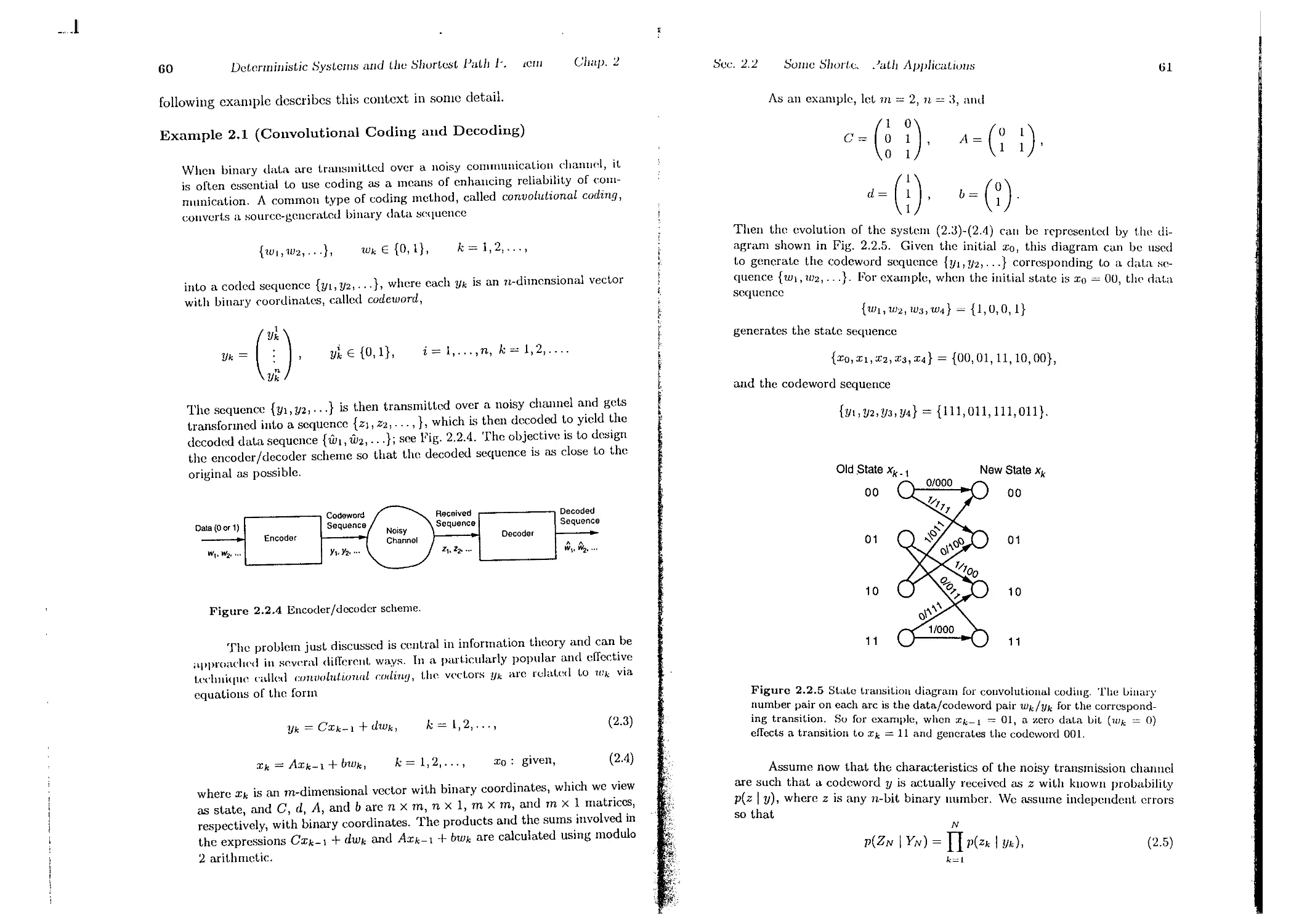
2.2. Some Shortest Path Applications
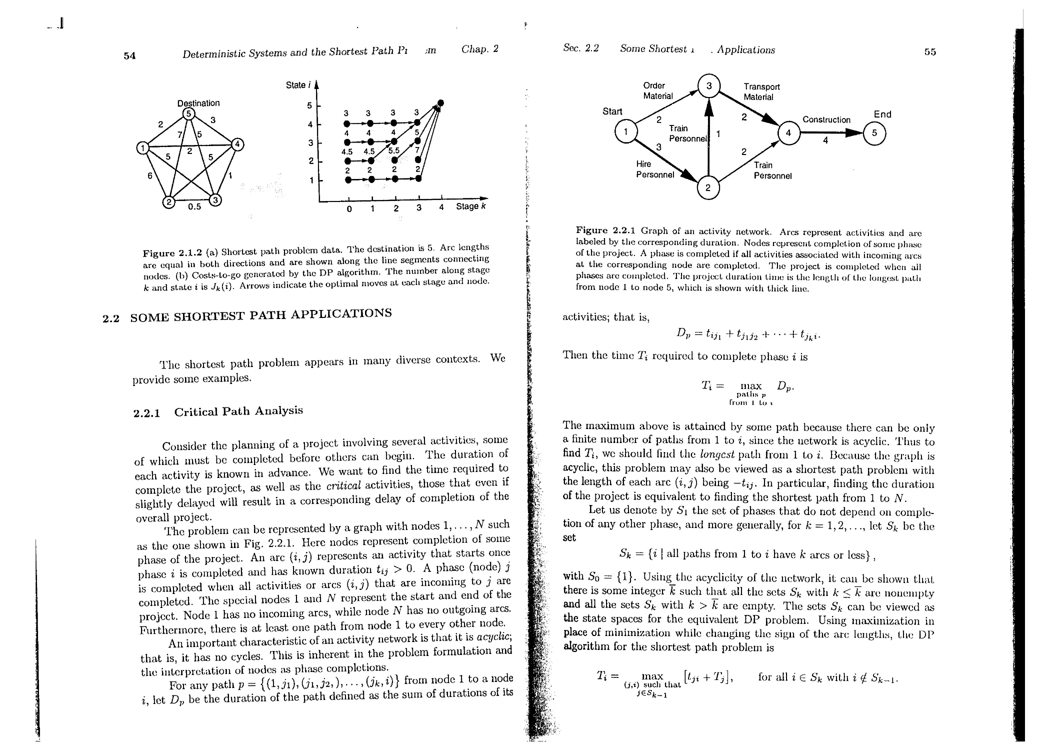
2.2.1. Critical Path Analysis . . . . .
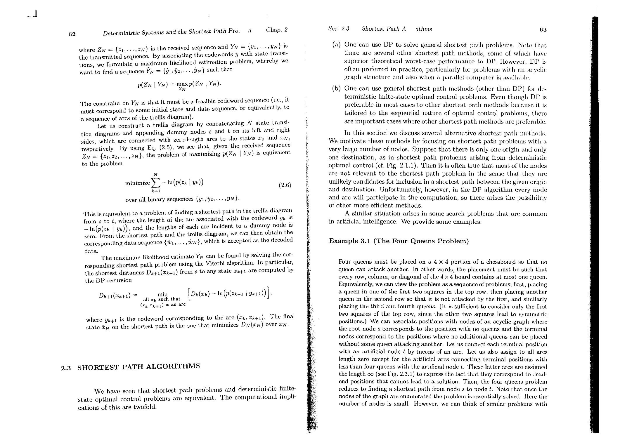
2.2.2. Hidden Markov Models and the Vit.erbi Algorithm
2.3. Shortest Path Algorithms . . .
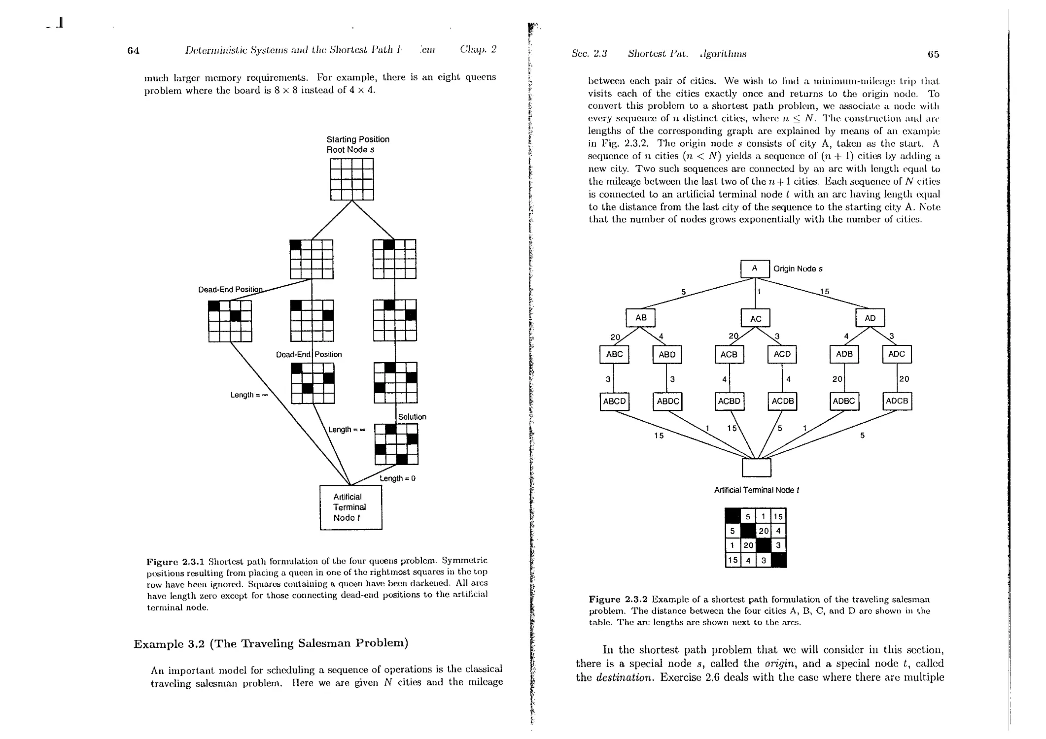
2.3.1. Label Correcting Methods
2.3.2. Auction Algorithms
2.4. Notes, Sources, and Exercises .
Publisher's Catalogillg-in-Publication Data
Dertsckas, Dimitri P.
Dynamic Programming and Optimal Control
Llcludes Bibliography and Index
1. Mat.hematical Optimization. 2. Dynamic Programming. 1. Title.
QA402.5 .D465 1995 519.703 95-075041
, 3. Deterministic Continuous-Time Optimal Control
3.1. Continuous-Time Optimal Control . . .
3.2. The Hamilton-Jacobi-Bellman Equation
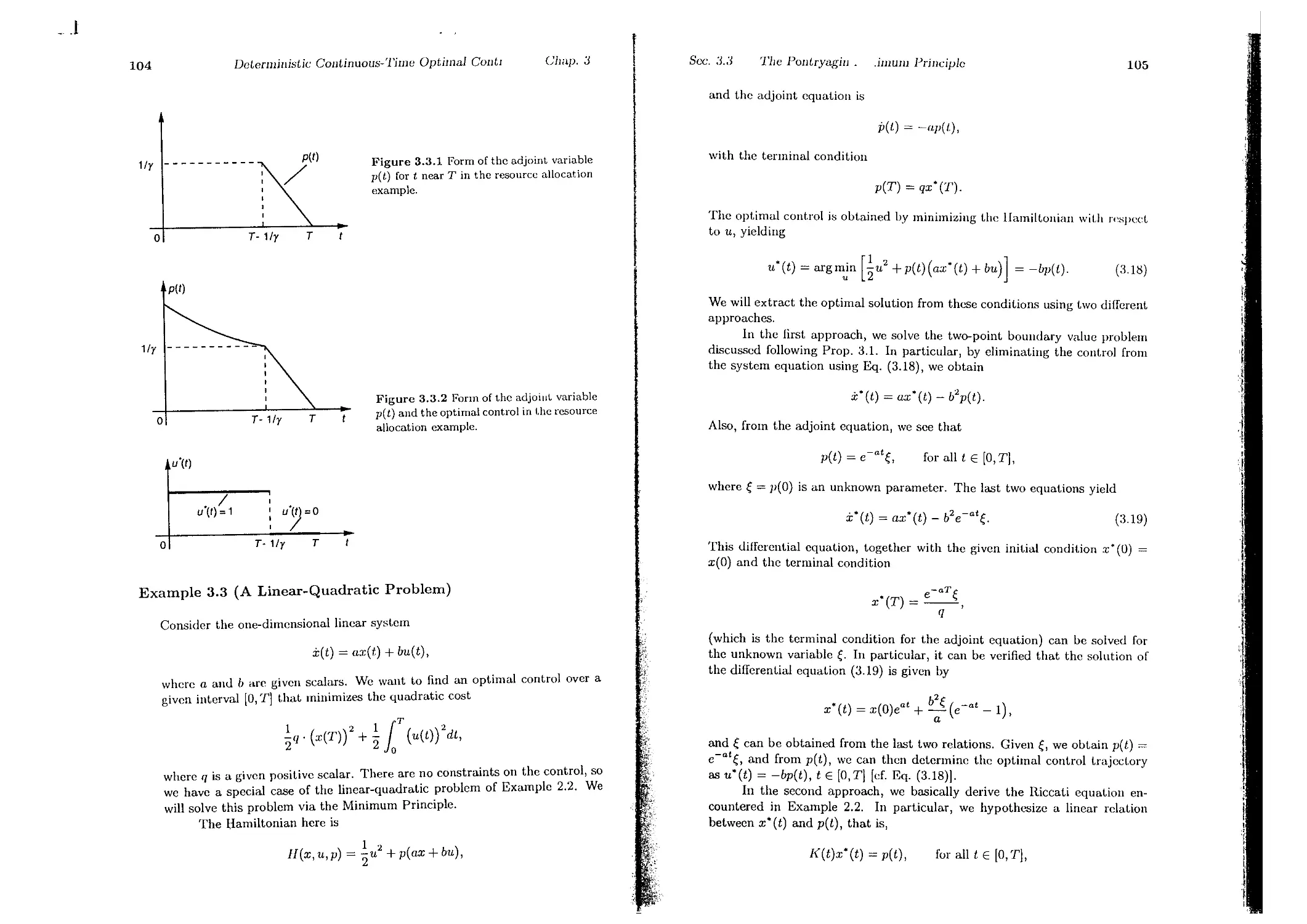
3.3. The Pontryagin Minimum Principle . .
3.3.1. An Informal Derivation Using the HJD Equation
3.3.2. A Derivation Dascd on Variational Ideas
3.3.3. Minimum Principle for Discrete-Time Problems
3.4. Extensions of the Minimum Principle
3.4.1. Fixcd Terminal Stat.e
3.4.2. Free Initial State
3.4.3. Free Terminal Time
3.4.4. Time-Varying System and Cost
3.il.5. Singular Problems . . . . . .
ISDN 1-886G2U-12-4 (Vol. 1)
ISDN 1-886529-13-2 (Vol. II)
ISDN 1-886.529-11-6 (Vol. I ami II)
p. 2
p. 10
p. 16
p. 30
p.3G
p.37
p. GO
p. G4
p. 54
p. Sf)
p. G2
p.66
p.74
p. 81
p.88
p. 91
p.97
p.07
p. lOG
p. 110
p.112
p. 112
p. 116
p. 116
p. 119
p. 120
iii
_..1
iv
3.5. Notes, Sources, and Exercises . . . . . .
4. Problems with Perfect State Information
4.1. Linear Systems and Quadratic Cost
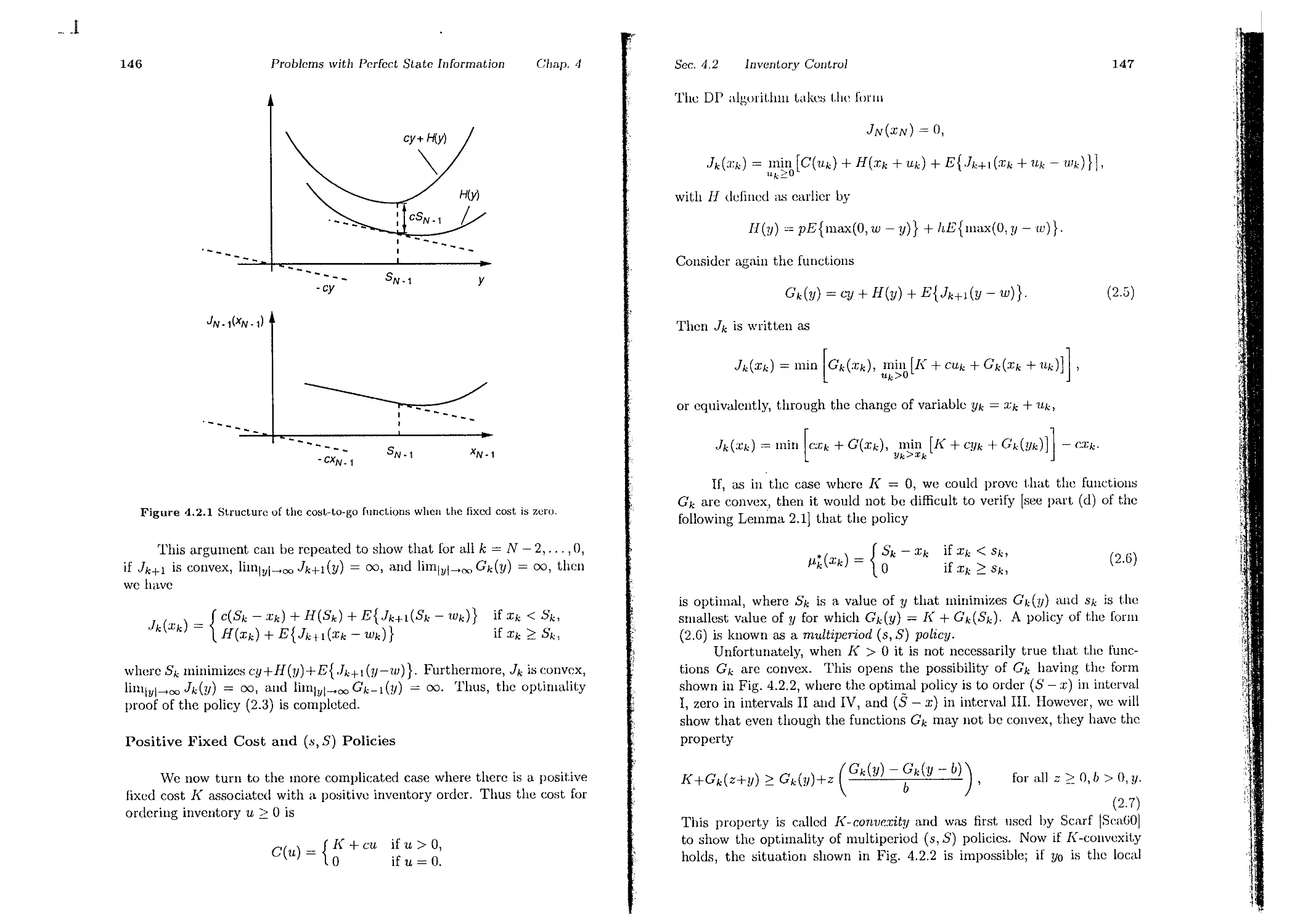
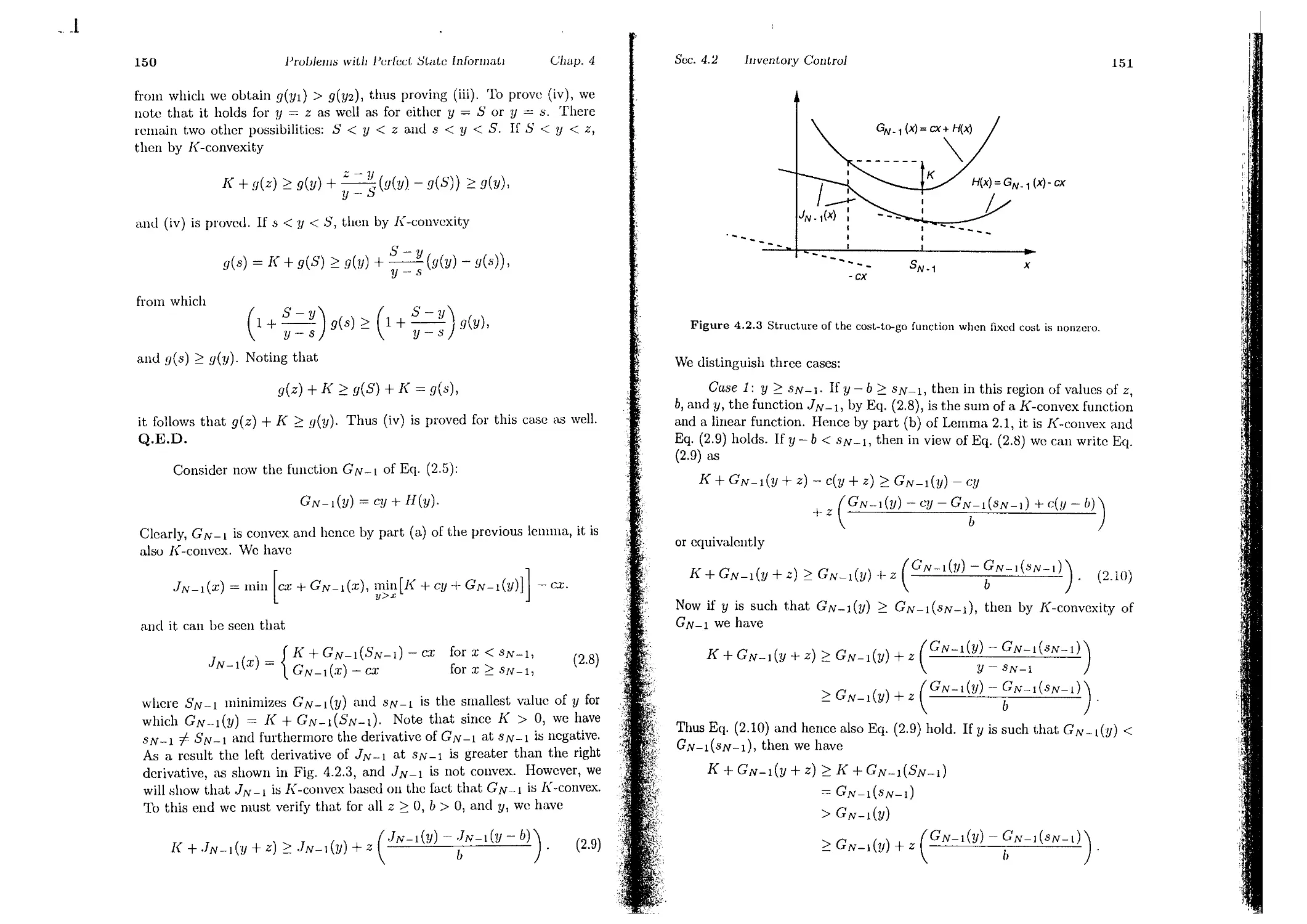
4.2. Inventory Control . . . .
4.3. Dynamic Portfolio Analysis . . . .
4.4. Optimal Stopping Problems . . . .
4.5. Scheduling and the Interchange Argument
4.6. Notes, Sources, and Exercises . . . . . .
, 5. Problems with Imperfect State Information
J 5.1. Reduction to the Perfect Information Case
\; 5.2. Linear Systems and Quadratic Cost
5.3. Minimum Variance Control of Linear Systems
5.4. Sufficient Statistics and Finite-State Markov Chains
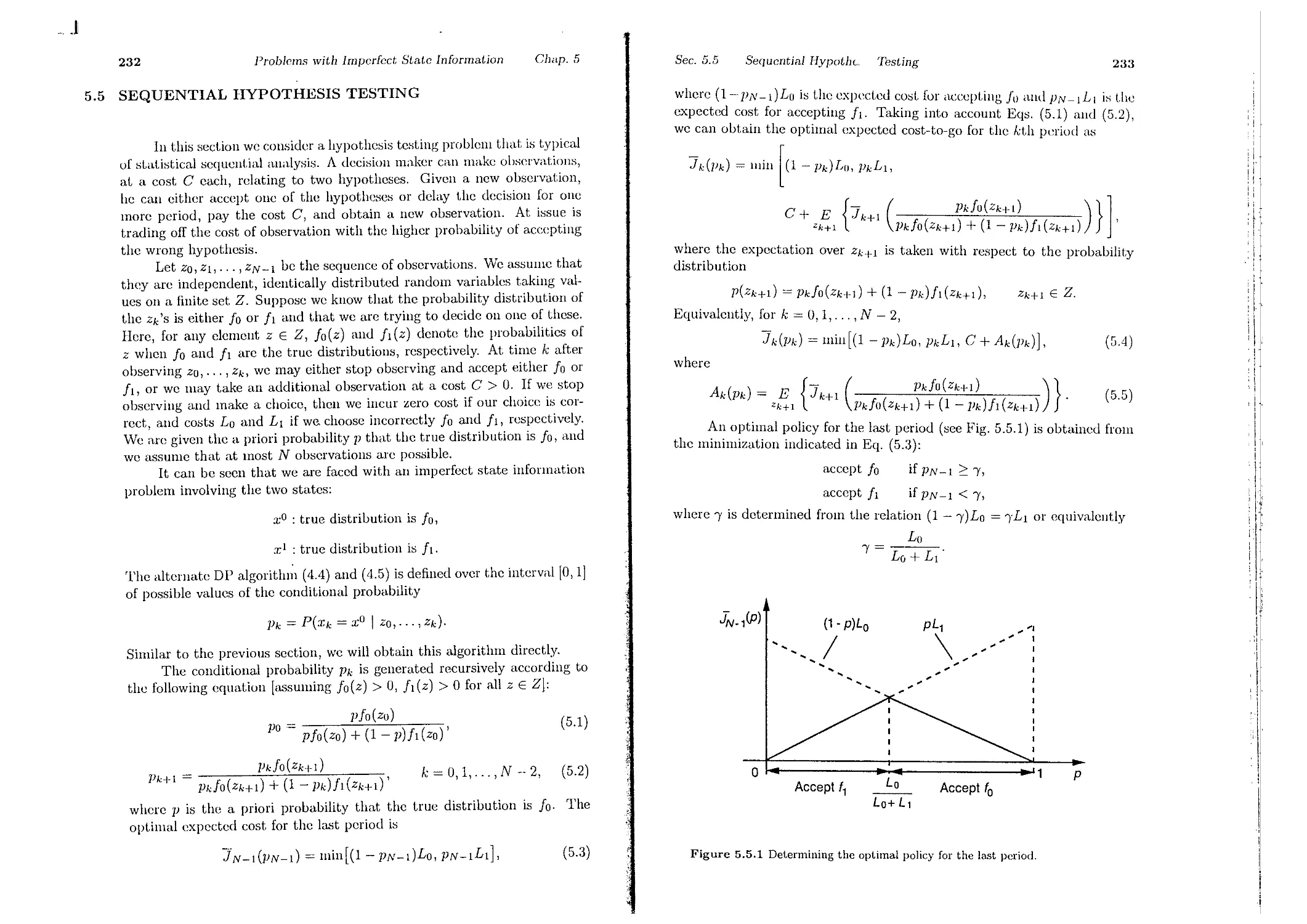
5.5. Sequential Hypothesis Testing
5.6. Notes, Sources, and Exercises . .
6. Suboptimal and Adaptive Control
6.1. Certainty Equivalent and Adaptive Control
G.1.1. Caution, Probing, and Dual Control
6.1.2. Two-Phase Control and Identifiability
6.1.3. Certainty Equivalent Control and Identifiability
6.1.4. Self-Tuning Regulators . . . . . . .
6.2. Open-Loop Feedback Control . . . . . . .
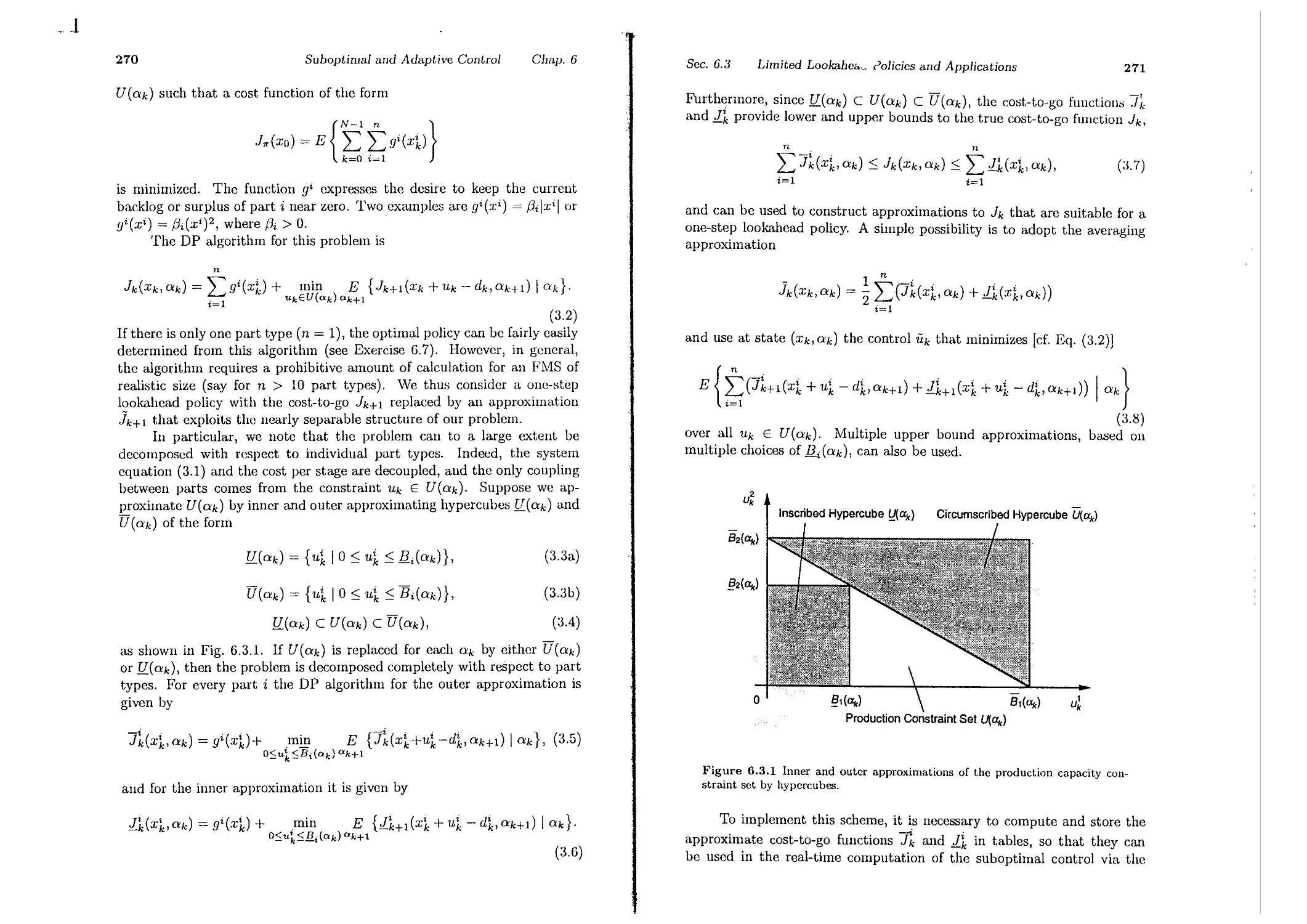
6.3. Limited Lookahead Policies and Applications
6.3.1. Flexible Manufacturing . . . . . .
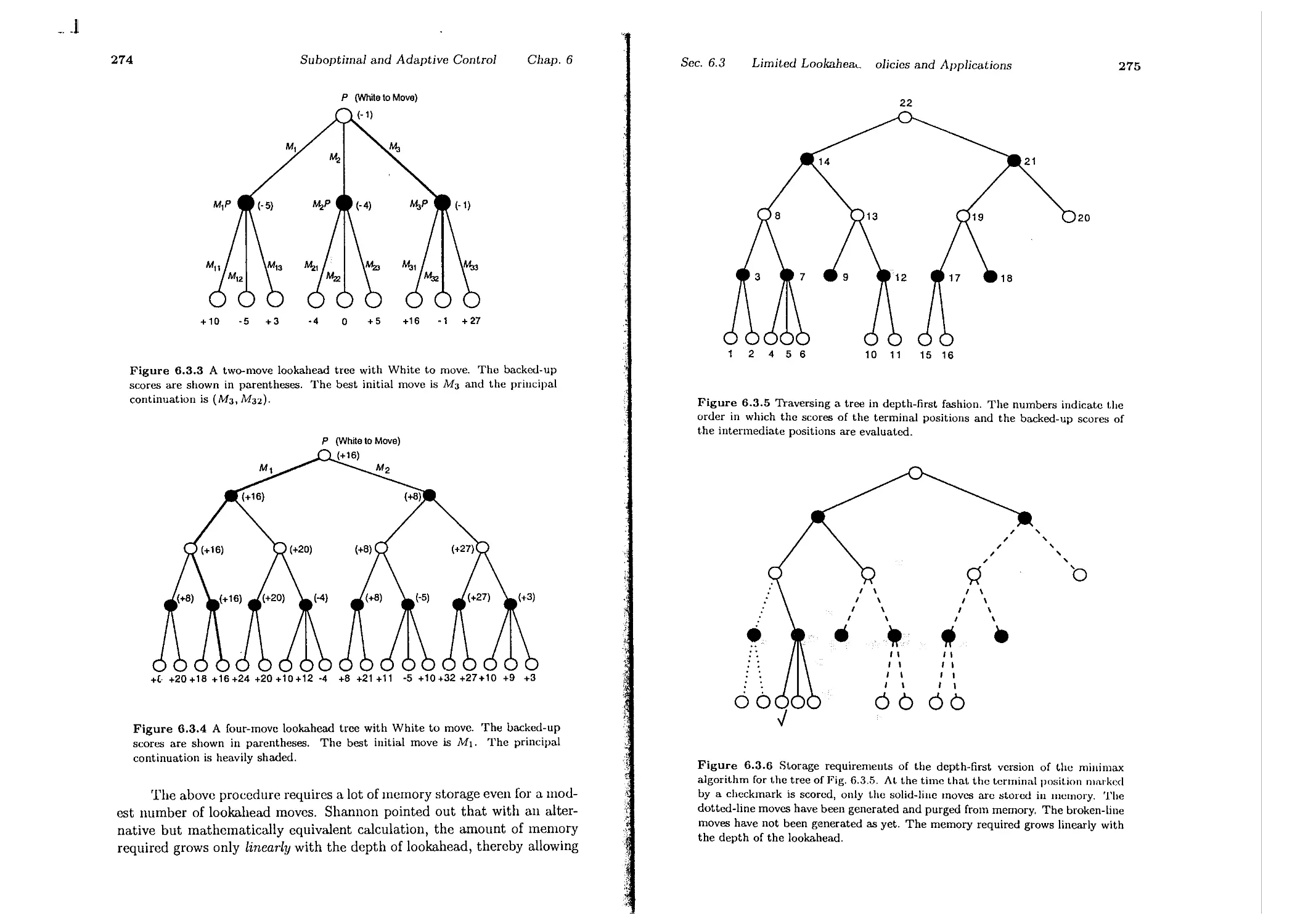
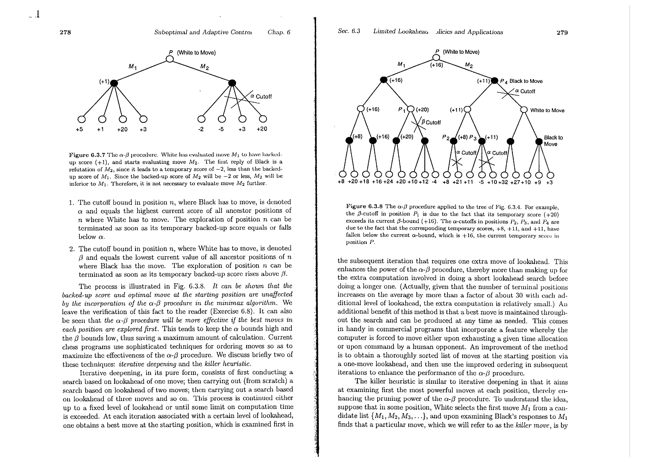
6.3.2. Computer Chess . . . . . . . . . .
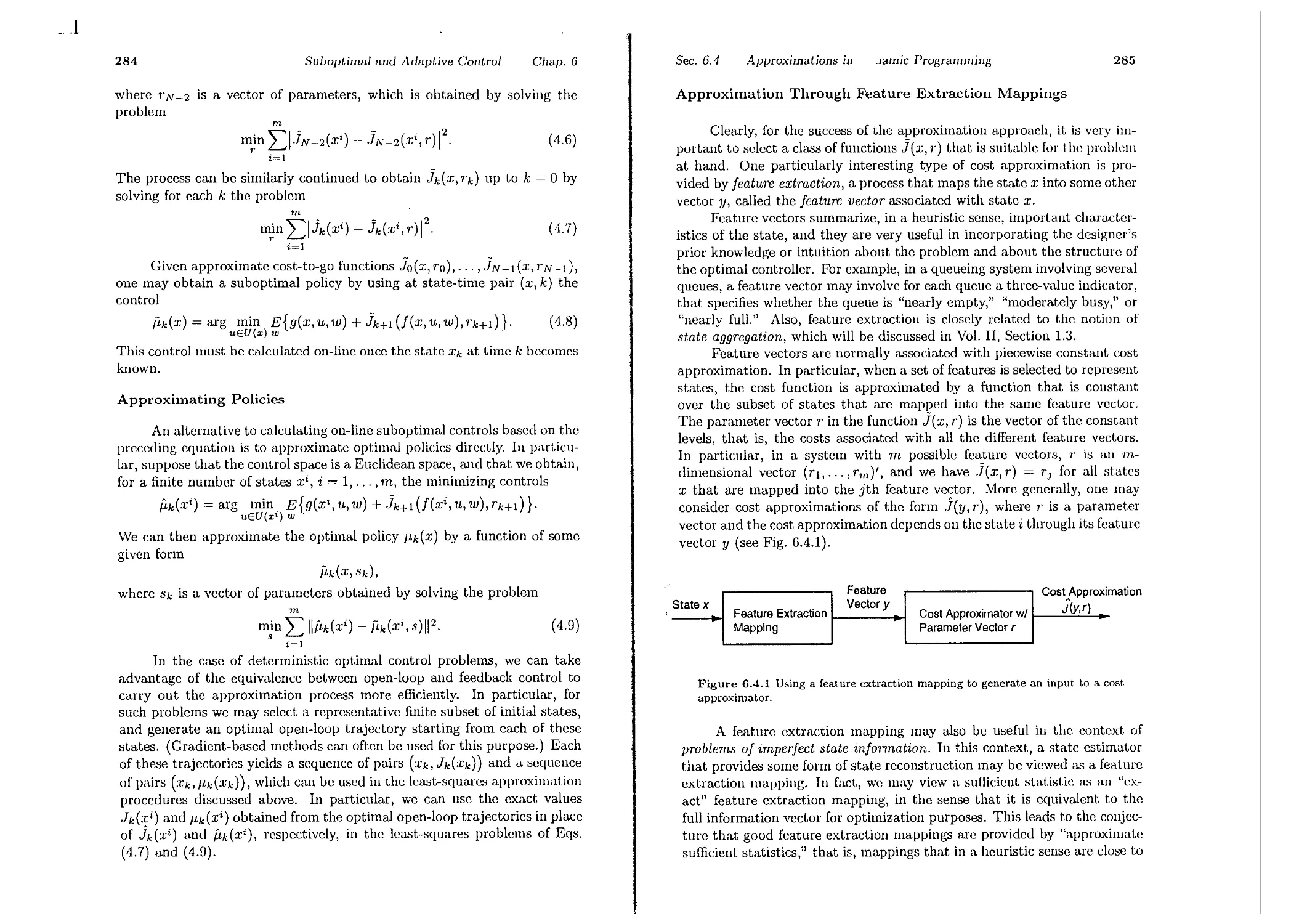
6.4. Approximations in Dynamic Programming
6.4.1. Discretization of Optimal Control Problems
6.4.2. Cost-to-Go Approximation
6.4.3. Other Approximations
6.5. Notes, Sources, and Exercises . .
7. Introduction to Infinite Horizon Problems
7.1. An Overview . . . . . . . . .
7.2. Stochastic Shortest Path Problems
7.3. Discounted Problems . . . .
7.4. Average Cost Problems. . .
7.5. Notes, Sources, and Exercises
Contents
Contents
p. 123
Appendix A: Mathematical Review
A.1. Sets . . . . . .
A.2. Euclidean Space .
A.3. Matrices . . . .
A.4. Analysis . . . .
A.5. Convex Sets and Functions
p. 130
p.144
p. 152
p. 158
p. 168
p. 172
Appendix B: On Optimization Theory
B.1. Optimal Solutions . . . . . . .
B.2. Optimality Conditions . . . . .
B.3. Minimization of Quadratic Forms
p. 186
p. 1!J6
p.203
p. 21!J
p.232
p. 237
Appendix C: On Probability Theory
C.1. Probability Spaces. . .
C.2. Random Variables. . .
C.3. Conditional Probability
p. 246
p. 251
p. 252
p.254
p. 25!J
p.261
p.265
p.2G9
p. 272
p.280
p.280
p. 282
p. 286
p.287
Appendix D: On Finite-State Markov Chains
D.1. Stationary Markov Chains
D.2. Classification of States
D.3. Limiting Probabilities
D.4. First Passage Times .
Appendix E: Kalman Filtering
E.1. Least-Squares Estimation.
E.2. Linear Least-Squares Estimation
E.3. State Estimation - Kalman Filter
E.4. Stability Aspects . . . . . . .
E.5. Gauss-Markov Estimators
E.6. Deterministic Least-Squares Estimation
Appendix F: Modeling of Stochastic Linear Systems
F.1. Linear Systems with Stochastic Inputs
F.2. Processes with Rational Spectrum
F.3. The ARMAX Model . . . . . . . .
p. 2!J2
p. 2%
p.306
p.310
p. 324
References
Index . . . . . . . . . . . . . . . . . . . . . . . . . .
v
p. 329
p.330
p.331
p.334
p.337
p.338
p.340
p. 310
p.341
p. 342
p.344
p.346
p. 347
p.348
p.349
p.350
p. 352
p.360
p.365
p.367
p.370
p.371
p.372
p.374
p. 375
p.385
_. ..J
vi
CONTENTS OF VOLUME II
1. Infinite Horizon - Discounted Problems
1.1. Minimization of Total Cost - Introduction
1.2. Discounted Problems with Dounded Cost per Stage
1.3. Finitc-Statc Systcms - Computational Methods
1.3.1. Value Itcration and Error Bounds
1.3.2. Policy Itcration
1.3.3. Adaptivc Aggrcgation
1.3.4. Lincar Programming
1.4. Thc Role of Contraction Mappings
1.5. Schcduling and Multiarmed Bandit Problmns
1.6. Notcs, Sourccs, and Exercises
2. Stochastic Shortest Path Problems
2.1. Main Rcsults
2.2. Computational Mcthods
2.2.1. Valuc Iteration
2.2.2. Policy Itcration
2.3. Simulation-Bascd Mcthods
2.3.1. Policy Evaluation by Monte-Carlo Simulation
2.3.2. Q-Learning
2.3.3. Approximat.iuns
2.3.4. Extcnsions to Discounted Proulems
2.3.5. Thc Rolc of Parallel Computation
2.4. Notcs, Sourccs, and Excrciscs
3. Undiscoullted Problems
3.1. Unboundcd Custs per St.age
3.2. Linem' Systcms and Quadratic Cost
3.3. Invcntory Control
3.4. Opt.imal St.opping
3.G. Optimal Gambling SLrat.C'gies
3.6. Nonstationary and Periodic Problcms
3.7. Note,;, Sources, and Excrciscs
4. Average Cost per Stage Problems
4.1. Prclilninary An;llysis
4.2. Optimality Conditions
4.3. Computational Mct.hods
4.3.1. Value Iteration
4.3.2. Policy Iteration
nicnt.s
Conienis
vii
4.3.3. Lincar Programming
4.3.4. Simulation-Dased Mcthods
4.4. Infinitc State Space
4.5. Notes, Sources, and Excrcises
5. Continuous-Time Problems
5.1. U niformiz,ation
5.2. Qucueing Applications
5.3. Scmi-Markov Problems
5.4. Notcs, Sources, and Exercises
_. J
ABOUT THE AUTHOR
Dimit.ri Dert.sekas studied Mechanical and Electrical Engineering at.
the National 'l'eclmical University or At.hens, Greece, and obtained his
Ph.D. in system science from the Massachusetts Institute of Technology. He
has held faculty positions with the Engineering-Economic Systems Dcpt.,
Stanford University and the Electrical Engineering Dept. of the Univer-
sity of Illinois, Urbana. He is currently Professor of Electrical Engineering
and Computer Science at the Massachusetts Institute of Technology. He
consults regularly with private industry and has held editorial positions in
several journals. He has been elected Fellow of the IEEE.
Professor Bertsekas has done research in a broad variety of suujects
from control theory, optimization theory, parallel and distributed computa-
tion, data communication networks, and systems analysis. He has written
numerous papers in each of these areas. This book is his fourth on dynamic
programming and optimal control.
Preface
This two-volume book is based on a first-year graduate course on
dynamic programming and optimal control that I have taught for over
twenty years at Stanford University, the University of Illinois, and thc Mas-
sachusetts Institute of Technology. The course has been typically attended
by students from engineering, operations research, economics, ,111d applied
mathematics. Accordingly, a principal objective of the book has been to
provide a unified treatment of the subject, suitable for a broad audience.
In particular, problems with a continuous character, such as stochastic con-
trol problems, popular in modern control theory, arc simultaneously treated
with problems with a discrete character, such as Markovian decision prob-
lems, popular in operations research. Furthermore, many applications and
examples, drawn from a broad variety of fields, are discussed.
The book may be viewed as a greatly expanded and pedagogically
improved version of my 1987 book "Dynamic Programming: Det.erminist.ic
and Stochastic Models," published by Prentice-Hall. I have included much
new material on deterministic and stochastic shortest path problems, as
well as a new chapter on continuous-time optimal control proulcms and the
Pontryagin Maximum Principle, developed from a dynamic programming
viewpoint. I have also added a fairly extensive exposition of simulation-
based approximation techniques for dynamic programming. These tech-
niques, which are often referred to as "neuro-dynamic programming" or
"reinforcement learning," represent a breakthrough in the practical ap-
plication of dynamic programming to complex problems that involve the
dual curse of large dimension and lack of an accurate mathematical model.
Other material was also augmented, substantially modified, and updated.
With the new material, however, the book grew so much in size that it
became necessary to divide it into two volumes: one on finite horizon, and
the other on infinite horizon problems. This division was not only natural in
terms of size, but also in terms of style and orientation. The first volume is
more oriented towards modeling, and the second is more oriented towards
mathematical analysis and computation. To make the first volume self-
contained for instructors who wish to cover a modest amount of infinite
horizon material in a course that is primarily oriented towards modcling,
Other books by the author:
1) Dynamic Programming and Stochastic Control, Academic Press, 1976.
2) Stochastic Optimal Control: The Discrete-Time Case, Academic Press,
1978 (with S. E. Shreve; translated in Russian).
3) Constrained Optimization and Lagrange Multiplier Methods, Academic
Press, 1982 (t.ranslated in Russian).
4) Dynamic Programming: Deterministic and Stochastic Models, Prenti-
ce-Hall, 1987.
5) Data Nctwo1"ks, Prentice-Hall, 1987 (with R. G. Gallager; translated
in Russian and Japanese); 2nd Edition 1992.
6) Parallel and Distributed Computation: Numerical Methods, Prentice-
Hall, 1989 (with J. N. Tsitsiklis).
7) Linear Netwo1'k Optimization: Algorithms and Codes, M.1.T. Press
1991.
viii
ix
_.II
. J
x
Preface
Preface
xi
conceptualization, and finite horizon problems, I have added a final chapter
that provides an introductory treatment of infinite horizon problems,
Many topics in the book are relatively independent of the others. For
example Chapter 2 of Vol. I on shortest path problems can be skipped
without loss of continuity, and the same is true for Chapter 3 of Vol. I,
which deals with continuous-time optimal control. As a result, the book
can be used to teach several diIrerent types of courses.
(a) A two-semester course that covers both volumes.
(b) A one-semester course primarily focused on finite horizon problems
that covers most of the first volume.
(c) A one-semester cOlll'se focused on stochastic optimal control that. cov-
en; Chapters 1, 4, 5, and 6 of Vol. I, and Chapters 1, 2, and 4 of Vol.
II.
subjects developed somewhat infol"lually here.
Finally, I am thankful to a number of individuals and iustitutions
for their contributions to the book. My understanding of the subject was
sharpened while I worked with St.evell Shreve on our 1978 lnOilOgraph.
My iuteraction and collaboration with John Tsitsiklis on stochastic short-
est paths and approximate dynamic programming have bC(,lI most. valu-
able. Michael Caramauis, Emmanuel H rnandez-Gaucherand, Pierre IIllln-
bid, Lennart Ljung, and John Tsitsiklis taught from versions of the book,
and contributed several substantive comments and homework problems. A
number of colleagues offered valuable insights and information, particularly
David Castanon, Eugene Feinberg, and Krishna Pattipati. NSF provided
research support. Prentice-Hall graciously allowed t.he use of material from
my 1987 book. Teaching ami interacting wit.h t.he st.udent.s aL MI'l' haV<'
kept up my interest and excitcment for the subject.
A one-semester course that covers Chapter 1, about 50% of Chapters
2 through 6 of Vol. I, and about 70% of Chapters 1, 2, and 4 of Vol.
II. This is the course I usually teach at MIT.
(d) A one-quarter engineering course that covers the first three chapters
and parts of Chapters 4 through G of Vol. 1.
(e) A one-quarter mathematically oriented course focused on infinite hori-
ZOIl problems t.hat covers Vol. II.
The mathematical prerequisit.e for the text is knowledge of advanced
cakulus, introductory prob,1bility theory, and matrix-vector algebra. A
SUlllnlary of this material is provided in the appendixes. Nat.urally, prior
exposure to dynamic system theory, control, optimization, or operations
research will be helpful t.o the reader, but based on my experiencc, the
material given here is reasonably self-contained.
The book contains a large number of exercises, and the serious reader
will benefit greatly by going through them. Solutions to all exercises are
compiled in a manual that is available to instructors from Athena Scientific
or from the author. Many thanks are due to the several people who spent
long hours contributing to this manual, particularly Steven Shreve, Eric
Lo;edcrman, Lakis Polymenakos, and Cynara \Vu.
Dynamic programming is a conceptually simple technique that can
be adequately explained using elementary analysis. Yet a mathematically
rigorous treatment of general dynamic programming requires the compli-
cat.ed machinery of mea.';ure-theoretic probability. My choice ha.,; becn t.o
bypass the complicated mat.hematics by developing the subject in general-
ity, while claiming rigor only when the underlying probability spaces are
countable. A mathematically rigorous treatment of the subject is carried
out in my monograph "Stocha.stic Opt.imal Control: The Discrete Time
Case," Academic Press, IU78, coauthored by Stevcn Shreve. This mono-
graph complements the present text and provides a solid foundation for the
(c)
Dimitri P. Bertsekas
bertsekas@lids.mit.edll
_.I
1
The Dynamic Programming
Algorithm
Contents
1.1. Introduction . . . . . . . . . .
1.2. The Basic Problem . . . . . . .
1.3. The Dynamic Programming Algorithm
1.4. State Augmentation. . . . .
1.5. Some Mathematical Issues . .
1.6. Notes, Sources, and Exercises.
p. 2
p. 10
p. 16
p. 30
p. 35
p. 37
1
_ J
2
Tile Dynamic Programming Algor
Chap. 1
Sec. 1.1
Introduct.
3
Life can only be understood going backwards,
but it must be lived going forwards.
Kierkegaard
The cost function is additive ill the sense th,lt the cost. in(,\II"I(.d at.
time k, denoted by gk(Xk, Uk, Wk), accumulates over time. The total r.ost
is
N-I
!/N(XN) + L .'Jk(Xk,Uk,Wk),
k=O
1.1 INTRODUCTION
where 9N(XN) is a terminal cost incurred at thc end of the process. How-
ever, because of the presence of Wk, cost is generally a random variable and
cannot be meaningfully optimized. We therefore formulate the problem as
an optimization of the expected cost
This book deals with situations where decisions arc made in stages.
The out.eonle of ( ach decision is not. fully predidaulc but can h( iI.1lLici-
patcd to some extent before the next decision is made. The objective is to
minimize a certain cost - a mathematical expression of what is considNed
an unde::;irable out.collle.
A key aspect of such situations is that decisions cannot be viewed in
isolation since one must balance the desire for low present cost with the
undesirability of high future costs. The dynamic programming tedmique
captures this tradeoff. At each stage, decisions arc ranked based on the
sum of the present cost and the expected future cost, assuming optimal
decision making for subsequent stages.
There is a very broad variety of practical problems that can be treated
by dynamic programming. In this book, we try to keep the main ideas
uncluttered by irrelevant assumptions on problem structure. To this end,
we formulate in this section a broadly applicable model of optimal control
of a dynamic system over a finite number of stages (a finite horizon). This
1II0del will occupy us for the first six chapters; its infinite horizon version
will be the subject of the last chapter and Vol. II.
Our basic model has two principal features: (1) an underlying disc1-ete-
t'imc dynamic systcm, and (2) a cost function that is additivc ovcr I:imc.
The dynamic system is of the form
{ N-I }
}:; !/N(:J;N) + !/k(:l;k,'II.k,Wd ,
k=O
where the expectation is with respect to the joint distribution of the random
variables involved. The optimization is over the controls '11.0, '11.1, . . . , UN -I,
but some qualification is needed here; each control Uk is selected with sOllie
knowledge of the current state Xk (either its exact value or some other
information relating to it).
A more precise definition of the terminology just used will be given
shortly. We first provide some orientation by means of examples.
Example 1.1 (Inventory Control)
Xk+l = fk(Xk, Uk, Wk),
k = O,l,...,IV - 1,
Consider a problem of ordering a quantity of a certain item at each of N
periods so as to meet. a stochast.ic demand. Let. us denot.e
Xk stock available at the beginning of t.he kth period,
Uk stock ordered (and immediately delivered) at t.he beginning of t.he kth
period,
Wk demand during the kth period with given probability distribut.ion.
'vVe assume that WQ,Wl,...,WN_l are independent random variables,
and that. excess demand is backlogg<:d and filled iI. :.;oon as additional illv!'l1-
t.ory becomes available. Thus, st.ock evolves according t.o t.he discrete-t.ime
equation
where
k indexes discret.e time,
.7: k is the state of the system and summarizes past information that is
relevant for future optimization,
Uk is the control or decision variable to be selected at time k,
Xk+l = Xk + Uk -- Wk,
Wk
is a random parameter (also called disturbance or noise depending on
the context),
IV is the horizon or number of times control is applied.
where negative stock corrcspomls to backlogged demand (see Fig. 1.1.1).
The cost incurred in period k consists of two components:
(a) A cost r(xk) representing a penalt.y for either posit.ive stock Xk (holding
Cost for eXCess inventory) or negative stock Xk (shortage cost for unfilled
demand) .
(b) The purchasing cost. CUk, where C is Cost per unit ordered.
_ J
4
The Dynamic Programmiug Algorit.
Suc. 1.1
5
Chap. 1
lntroducUo
Wk Demand at Period k
and each possiblc value of :I:k,
/Lk(Xk) = amount. that should bc orderr'd at. time k if the st.oek is :q.
The sequence "Tr = {/Lo,.", /LN -I} will be referred to as a policy or
cont7'Ollaw. For cach "Tr, the corf('A ponding cost. for a fixed initial st.ock .DO IS
J,,(xo) = E { R(XN) + (r(xk) + C/Lk(Xk)) } ,
and we want t.o mllllluize J" (xu) for a given Xu ovcr all "Tr that satis(y thc
constraints of t.he problem. This is a typical dynamic programming problcm.
Wc will analyze this problem in various forms in subsequcnt sections. For
example, we will show in Section 4.2 that for a reasonable choice of t.hc cost.
function, the optimal ordcring policy is of thc form
( ) { Sk - Xk if Xk < .'h,
/Lk Xk = 0 otherwisc,
where Sk is a suit.able threshold level determincd by t.he data of the problcm.
In other words, whcn stock falls below thc threshold Sk, order just cnough to
bring stock up to Sk.
Stock at Period k
xk
Stock at Period k + 1
Inventory
System
Xk + 1 = xk + Uk - wk
Cost of Period k
r(xk) + cU k
Stock Ordered at
Period k
uk
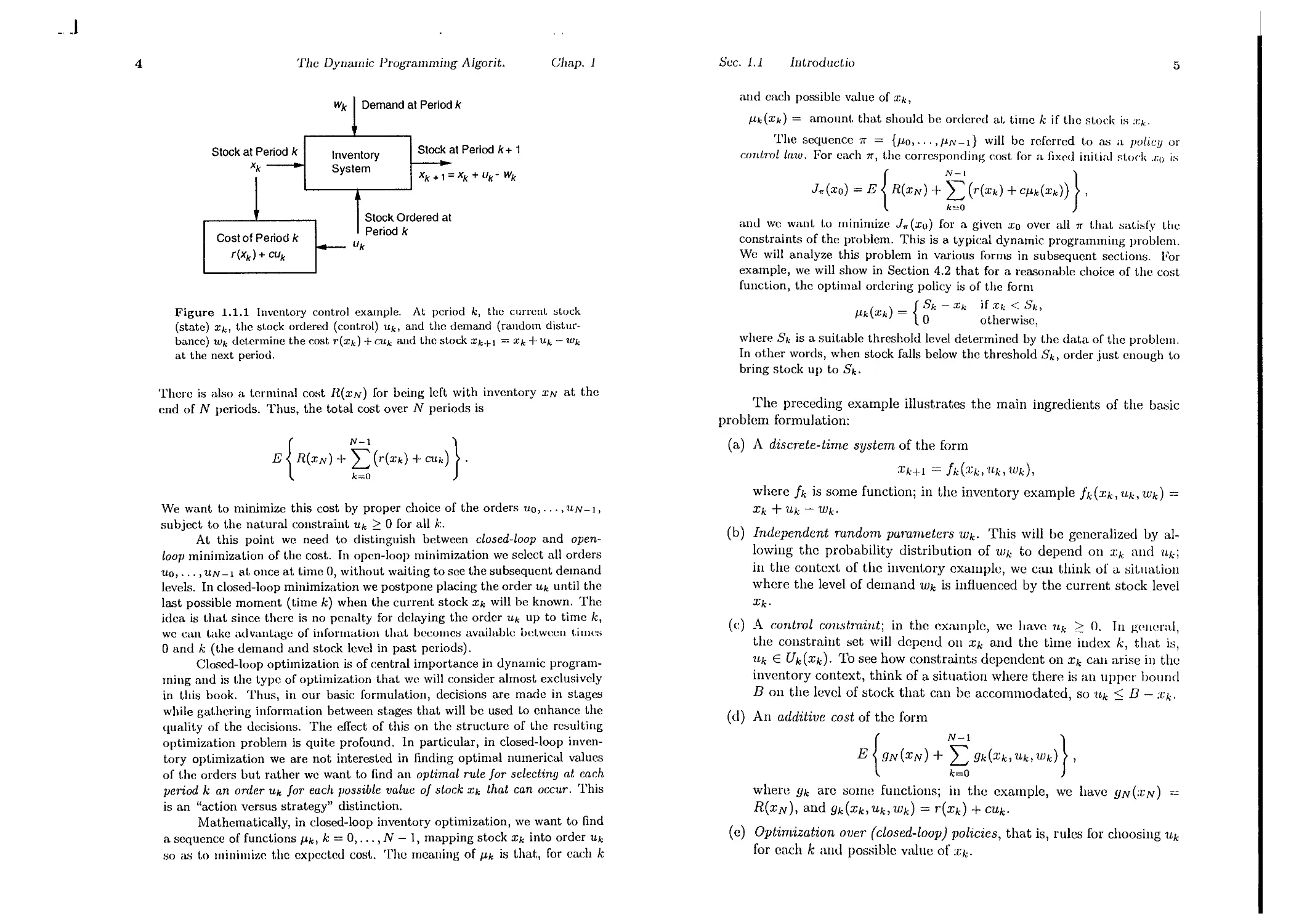
Figure 1.1.1 Inventory control example. At period k, the current. st.ock
(state) Xk, thc stock ordered (control) Uk> and thc demand (random distur-
bancc) Wk det.ermine the cost "(Xk) -I- CUk and the st.ock Xk+l = Xk -I-Uk - Wk
at the next period.
Thcrc is also a tcrminal cost R(XN) for being left with inventory XN at the
end of N periods. Thus, the total cost over N periods is
The preceding example illustrates the main ingredients of the basic
problcm formulation:
(a) A discrete-time system of the form
Xk+l = h(:!:k,'1I.k,wd,
wherc fk is some function; in the inventory example h (.Tk, 'Uk, Wk) =
Xk + 'Uk - Wk.
(b) Independent random parameters Wk. This will be generalized by al-
lowing the probability distribution of 11Jk to depend on :l:k and 1Lk;
in the context of the inventory cxamplc, we can think of a situaLion
whcre the level of demand 11Jk is influenced by the current stock level
Xk.
(c) A mnt7'Ol constr'aint; in t.he ( xalllple, we have Uk :::: O. Tn gPlwral,
the constraint set will dcpend on Xk and the time index k that is
Uk E Uk(Xk). To see how constraints dependent on Xk can arise in th
inventory context, think of a situation wherc there is an IIppcr bound
B on the level of stock that can be accommodated, so Uk ::; B - Xk'
(d) An additive cost of thc form
E {9N(XN) + 9k(Xk,'Uk,Wk)},
where gk arc some functions; in the example, we have gN (;l: N) =
R(XN), and 9k(Xk, 'Uk, 11Jk) = r(Xk) + C'Uk.
(e) Optimization over (closed-loop) policies, that is, rules for choosing 'Uk
for each k ami possiblc valuc of ;l:k.
E {R(XN) + (r(xk) -I- CUk)}'
We want to minimize this cost by proper choice of the orders uo, . . . , UN - I ,
subject to the natural const.raint Uk 2': 0 for all k.
At t.his point we need to distinguish bet.ween closed-loop and open-
loop minimizat.ion of thc cost. Tn opcn-loop minimization wc selcct all orders
'11.0,. .. ,UN -I at once at timc 0, without waiting to sce the subsequcnt demand
levels. In closed-loop minimization we postpone placing the order Uk until the
last possiblc moment (time k) when the current stock Xk will be known. The
idea is that since thcre is no penalty for delaying the order Uk up to time k,
we can take advantage of information that becomes available between times
o and k (the demand and stock level in past periods).
Closed-loop optimization is of central importance in dynamic program-
ming and is t.he type of optimization t.hat we will consider almost exclusively
in this book. Thus, in our basic formulation, decisions are made in stages
while gathering information between stages that will be used to enhanc.e the
qualit.y of the decisions. The effect of this on the structure of the rcsulting
optimization problem is quite profound. 1n particular, in closed-loop inven-
tory optimization we are not interested in finding optimal numerical values
of t.he orders but rather we want to find an optimal rule Jar selecting at each
period k an order Uk Jar each ]JOssible value oj stock Xk that can occur, This
is an "action versus strategy" distinction.
Mathematically, in closed-loop inventory optimization, we want to find
a sequence of functions /Lk, k = 0,..., N - 1, mapping stock Xk into order Uk
so as t.o minimize the expected cost. The meaning of /Lk is that, for each k
_.J
6
The Dynamic Programming Algl
,m
ClJap. 1
Sec. 1.1
Introduciic
7
Discrete-State and Finite-State Systems
Example 1.2 (Machine Replacement)
In the preceding example, the state Xk was a continuous real variaulc,
and it is easy to think of multidimensional generalizations where t.he st.ate
is an n-dimensional vector of real variables. It is also possible, however,
that the state takes values from a discrete set, such as t.he integcrs.
A version of the inventory problem where a discrcte viewpoint is more
natural arises when stock is measured in whole units (such as cars), each
of which is a significant fraction of Xk, Uk, or Wk. It is more appropriate
thcn to take as state space thc sct of all integers rather than the set of real
!lumbers. The form of the system cquation and the cost per pcriod will, of
course, stay the same.
In other systems the state is nat urally discrete and there is no contin-
uous counterpart of the problcm. Such systems are often convenicntly spec-
ified in terms of the probabilities of transition between the states. What. we
need to know is 11,j (u, k), which is the probability at time k that the next
state will be j, given that the currcnt state is i, and the control selected is
u, i.e.,
Consider a proulem of operating eflicienlly over N t.ime periolb a machine
t.hat. can be in anyone of n states, denot.ed 1,2".., n. The implication here
is t.hat state i is better than state i + 1, and state 1 corresponds t.o a machine
in perfect condition. In particular, we denote by g(i) the operating cost. per
period when the machine is in state i, and we ussume t.hat
g(l) ::; g(2) ::; .,. ::; g(n).
During a period of operation, the state of the machine can become worse
or it may stay unchanged. We thus assume that. the t.ransition probabilities
Pi) = P {next state will be j I current state is i}
satisfy
P'j = a
if j < i.
Xk+l = Wk,
\Ve assume that at t.he start of each period we know the state of t.he
machine and we must choose one of the following t.wo options:
(a) Let the machine operate one more period in t.he state it. currently is.
(b) Repair the machine and bring it to the perfect state 1 at a cost R.
\Ne assume that the machine, onc.e repaired, is guaranteed to st.ay iu st.ate
1 for one period. In subsequent periods, it. may deteriorate to states j > I
according t.o t.he transit.ion probabilitic:,; Plj.
Thus the objective here is to decide on the level of deteriorat.ion (st.ate)
at which it is worth paying the cost of machine repair, thereby obtaining the
benefit of smaller future operating Costs. Note that the decision should also
be affected by the period we are in. For example, we would be Icss inclined
t.o repair the machine when there are few periods left.
The system equation for this problem is represented by t.he graphs of
Fig. 1.1.2. These graphs depict the transition probabilities between various
pairs of states for each value of t.he control and arc known as tmnsition proba-
bility graphs or simply transition graphs. Note that there is a difl"erent. graph
for each control; in the present case t.here are t.wo cont.rols (rcpair or not
repair).
Pij(u,k) =P{:rk+l =j IXk =i,Uk =u}.
Such a system can be described alternatively in terms of the discrete-time
system equation
where the probabilit.y distribntion of the random parameter Wk is
P{Wk = j I Xk = i,Uk = u} = Pij(u,k).
Conversely, given a discret.e-state system in the form
Xk+l = fk(Xk, Uk, Wk),
together with the probability distribution Pk(Wk I Xk, Uk) of Wk, we can
provide an equivalent transition probability description. The corresponding
transition probabilitics arc given by
Pij(U, k) = pk{Wdi, u,j) I Xk = i,Uk = u},
where W (i, u, j) is thc set
Example 1.3 (Control of a Queue)
Wk(i,u,j) = {w I j = fk(i,u,w)}.
Consider a queueing system with room for n customers operat.ing over N
time periods. We assume that service of a customer can st.art. (cnd) only
at the beginning (end) of the period and that. the system can scrve only
one customer at. a time. The probability Pm of m customer arrivals during
a period is given, and the numbers of arrivals in two different periods are
independent. Customers finding the system full depart without attempting
to enter later. The system offers t.wo kinds of service, fast and slow, wit.h cost.
per period Cf and c., respectively. Service can be switched between fust and
Thus a discrete-state system can equivalently be described in terms
of a difference equation and in terms of transition probabilities. Depending
on the given problem, it may be notationally more convenient t.o use one
description over the other.
The following thrce examples illustrate discrete-state systems.
_..J
8
The Dynamic Programming Alg(
!)
P1n
Do not repair
m
Chap. 1
Sec. 1.1
1nirodud.,
and it equals t.hc probabilit.y of 1L or morc cllstomcr arrivals when j = n,
POn(Uf) = POn(U,,) = L Pm.
When there is at least one cust.omer in the syst.em (i > 0), we have
piJ(1I.f) = 0,
if j < i-I,
p.j(Uf) = qf]Jo,
ifj=i-l,
Poj (u f) = P {j - i + 1 arrivals, service complded}
+ P{j - i arrivals, service not complded}
= (jf]Jj-i+l + (1- qf)pj-.,
if i-I < j < n - 1,
Pi(n-l)(Uf) = qf L pm + (1 - IlJ)Pn-l-.,
fn=n-i
Pin(Uf)=(1-(jf) L Pm.
Repair
m=n-1.
The transition probabilities when slow service is provided are also given by
these formulas with U f and (jf replaced by Us and qs, respectively.
Figure 1.1.2 Machine replacement example. Transition probability graphs for
each of the two possible controls (repair or not repair). At each stage and state i,
the cost of repairing is R+g(l), and the cost of not repairing is g(i). The terminal
cost is O.
Example 1.4 (Optimizing a Chess Match Strategy)
A player is about to play a two-game chess match with an opponent., and
want.s t.o maximize his winlling chances. Each gamc can have one of t.wo
outcomes:
slow at the beginning of each period. With fust (slow) service, a customer in
service at the beginning of a period will terminate service at the end of the
period with probability qf (respectively, qs) independently of the number of
periods the customer has been in service and the number of customers in the
system (qf > qs). There is a cost r(i) for each period for which there are i
customers in t.he syst.em. There is also a t.erminal cost R(i) for i C1lst.omers
left in t.he syst.em at t.he end of the last period. The problem is to choose, at
each period, the type of service as a function of the number of customers in
the syst.em so as to minimize the expected total cost over N periods.
It is appropriate to take as state here the number i of customers in the
system at the st.art of a period and as control the type of scrvice provided.
The cost per period then is r(i) plus Cf or C s depending on whether fast or
slow service is provided. We derive the transition probabilities of the system.
When the system is empty at the start of the period, the probability
that the next state is j is independent of the type of service provided. It
equals the given probability of j customer arrivals when j < n,
pOj(Uf) = POj(u s ) = Pj,
j = 0,1,..., n - 1,
(a) A win by one of the players (1 point for the winner and 0 for the loser).
(b) A draw (1/2 point for each of the two players).
If the score is tied at. 1-1 at. the ('nd of tll( two games, t.h(' mat.ch gO('S int.o
sudden-death mode, whereby the players continue to play until the first time
one of them wins a game (and the match). The player has two playing styles
and he can choose one of the two at will in each game, independently of the
style he chose in previous games.
(1) Timid play with which he draws with probability ]Jd > 0, and he loses
with probability (1 - pd).
(2) Bold play with which he wins wit.h probability Pw, and he loses wit.h
probability (1 - Pw).
Thus, in a given game, timid play never wins, while bold play never draws.
The player wants to find a style selection strategy that. maximizes his proba-
bility of winning t.he match. Note that once the match gets into sudden deat.h,
the player should play bold, since wit.h timid play he can at best. prolong the
_....1
10
The Dynamic Programming Algon
Chap. 1
Sec. 1.2
The Basic 1'.
Cln
11
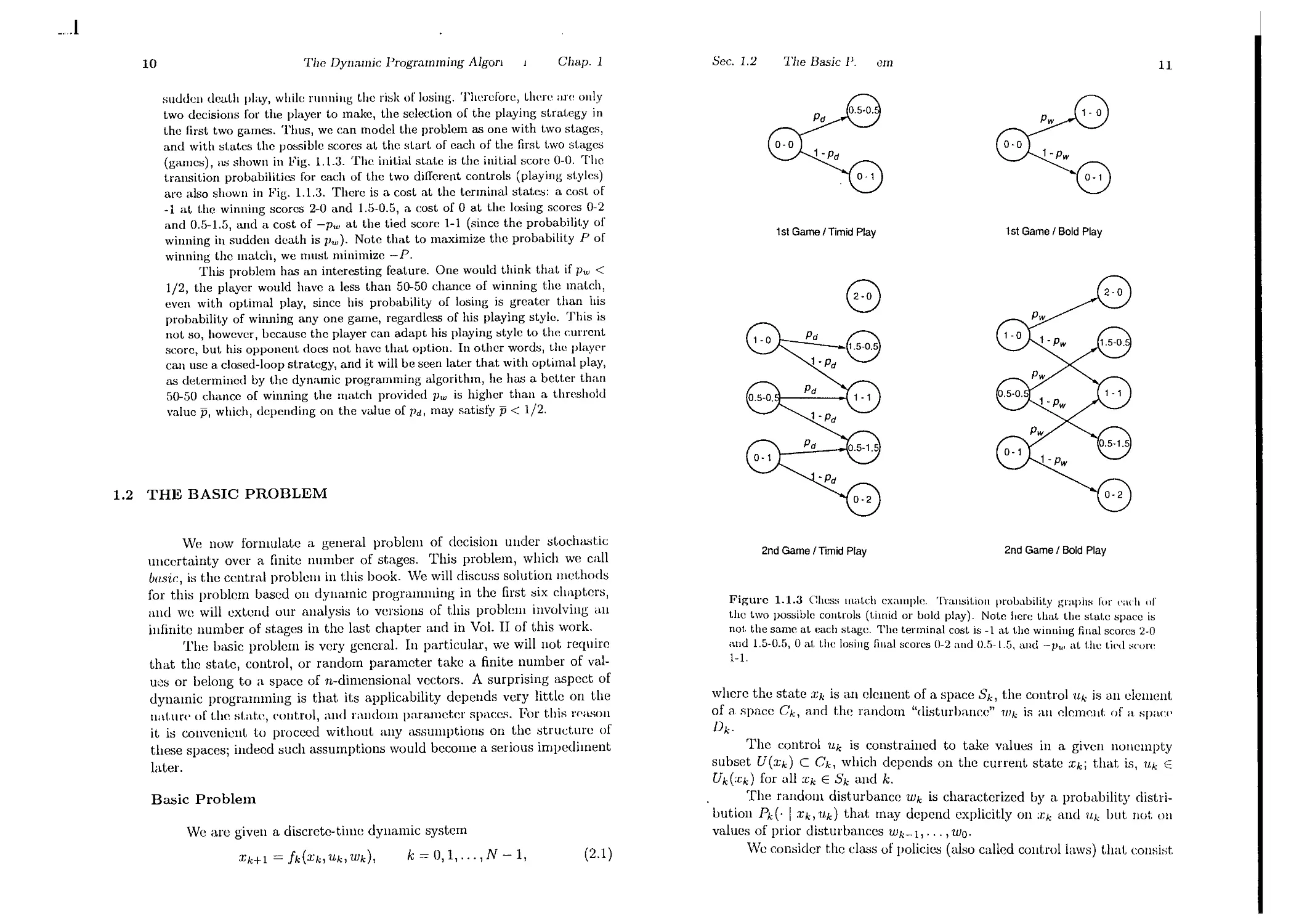
suudall deat.h play, while running the risk of losing. Therefore, t.here "H' only
two decisiolls for the player to make, the selection of the playing strat.egy in
the first two games. Thus, we can model the problem as one with t.wo stages,
and with st.ates the possible scorcs at the start of each of the first t.wo st.ages
(games), as shown in Fig. 1.1.3. The init.ial state is t.he init.ial score 0-0. The
t.ransition probabilitics for each of the two different. controls (playing styles)
arc also shown in Fig. 1.1.3. There is a cost at the terminal states: a cost of
-1 at t.he winning scorcs 2-0 anu 1.5-0.5, a cost of 0 at t.he losing scores 0-2
and 0.5-1.5, and a cost of -pw at the tied score 1-1 (since the probability of
winning in sudden death is Pw). Note that to maximize the probability P of
winning the mat.ch, we must minimize -Po
This problem has an interesting feature. One would think that if pw <
1/2, the player would have a less than 50-50 chance of winning the mat.ch,
even with opt.imal play, since his probability of losing is greater than his
probability of winning anyone game, regardless of his playing style. This is
not so, however, because the player can adapt his playing style to the current
score, but his opponent docs not have that option. In other words, the play<:'r
can use a closed-loop strategy, and it. will be seen later that with opt.imal play,
as det.ermined by t.he dynamic programming algorithm, he has a belter than
50-50 chance of winning the match provided pw is higher than a t.hr<:'shold
value 15, which, depending on the value of Pd, may satisfy 15 < 1/2.
1st Game I Timid Play
1st Game I Bold Play
e
1.2 THE BASIC PROBLEM
We now formulate a general problcm of decision under stochastic
uncertainty over a finite number of stages. This problem, which we call
basic:, is the cent.rn'! problem in this book. We will discuss solution methods
for this problem based all dynamic programming in the first six chapters,
and we will extend our allalysis to versiolls of this problem involvillg an
infinite number of stages in the last chapter and in Vol. II of this work.
The basic problem is very gencral. In particular, we willllot rcquire
that t.he st.ate, control, or random parameter take a finitc number of val-
UeS or belong to a space of n-dimensional vectors. A surprising aspect of
dynamic programming is that its applicability depends very little on t.he
nat.IIl"<' of t.he sLate, (,ollt.rol, and ralldom parameter spaces. For this rPH.o.;on
it is cOllvenicnt to proceed without allY assumptions on the structure of
these spaces; indeed such assumpt.ions would become a serious impediment
later.
2nd Game I Timid Play
2nd Game I Bold Play
Figure 1.1.3 Chess match example. Transil.ion probabilit.y graphs ror (';I("h or
t.he two possible cont.rols (t.imid or bold play). Not.e here t.hat. the stat.e space is
not the same at each stage. The terminal cost. is -1 at the winning final scores 2-0
and 1.5-0.5, 0 at. the losing final scores 0-2 and 0.5-1.5, and -1'", at. t.he t.ied s("ore
1-1.
XHI = !k(Xk, Uk, Wk),
k=O,I,...,N-1,
(2.1 )
whcre the statc Xk is an element of a spacc Sk, the control UI,; is an clement.
of a space Ck, and t.he random "disturbance" WI,; is an dement. of a spacp
Dk'
The control Uk is constrained to take values in a given nonempty
subset U(Xk) C Ck, which depends on the current state Xk; that is, Uk E
Uk(:Ck) for all Xk E Sk and k.
The random disturbance Wk is characterized by a probability distri-
bution Pk(' I xk, Uk) that may depend explicitly on :Ck and UI,; but not on
valucs of prior dist.urbanccs WI,;-l, . . . , Woo
We consider the class of policics (also called control laws) that consist
Basic Problem
We arc given a discrete-time dynamic system
12
The Dynamic Programming Alg( WI
Chap. I
See. 1.2
The l3asjc :JblclIJ
13
of a sequence of functions
The Rolc and Valuc of Informat.ion
Xk+1 = fk(xk>/lk(xk),wk),
k = 0,1,..., N - 1,
(2.2)
'vVe mentioned earlier the distinction between open-loop lIlIlIlIlllza-
tion, where we select all controls 'Uu,..., UN -1 at once at. tillle 0, alld
clo:,;ed-loop minimization, where we select 11 policy {JIU,..., IIN __[} (.11 at.
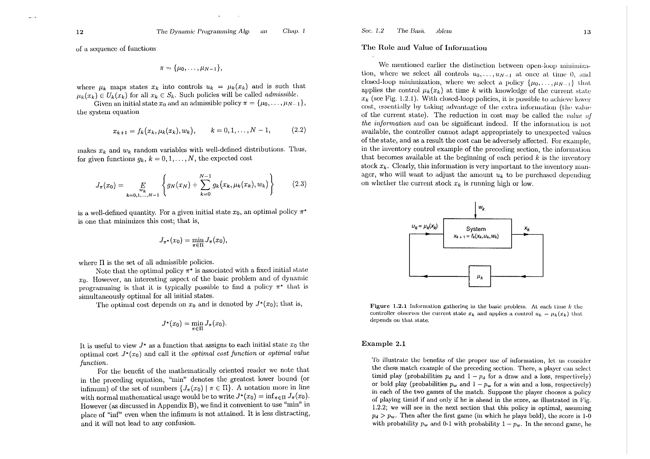
applies the control /lk(xd at time k with knowledge of the currellt state
Xk (see Fig. 1.2.1). With closed-loop policies, it i:,; po:,;sible to achieve lower
COHt, essentially by taking advantage of the extra illforlllat.ioll (Llw vallI<'
of the current state). The reduction in cost may be called the value of
the information and can be significant. indeed. If the informatioll is not
available, the controller cannot. adapt appropriately to unexpected values
of t.he state, and as a result the cost. can be adversely affect.ed. For cX<1l11ple,
in the invent.ory control example of the preceding section, the informat.ion
that becomes available at the beginning of ea.ch period k is the invcntory
stock Xk. Clearly, this information is very important to the inventory man-
ager, who will want to adjust the amount Uk t.o be purchased depending
on whether the current stock :Ck is running high or low.
n = {/lO,... ,/IN-I},
where /lk maps stat.es Xk into controls Uk = /lk(Xk) and is such that
ILk(Xk) E Uk(:cd for all Xk E Sk. Such policies will be called admissible.
Given an initial stat.e Xu and an admissible policy n = {IIO, . . . , II,N -1},
the sy:,;tem equation
makes Xk and Wk random variables wit.h well-defined distributions. Thus,
for given functions gk, k = 0, 1, . . . , N, the expected cost
J"/r(XO) = k=O'I 'N-l {gN(:CN) + gk(:Ck, /lk(Xk), Wk) } (2.3)
is a well-defined quantit.y. For a given initial state Xo, an optimal policy n*
is one t.hat minimizes t.his cost.; t.hat is,
Wk
Uk= Jlk(xk)
System
Xk+ 1 = 'k(Xk,Uk,Wk)
Xk
J"/r* (xu) = minJ"/r(xu),
"/rEf!
where II is the sct. of all admissible policies.
Note that the optimal policy n* is associat.ed with a fixed initial state
xu. However, an interesting aspect of the basic problem and of dynamic
programming is that it. is typically possiule to find a policy 7r* that is
simultaneously optimal for all init.ial states.
The optimal cost depends on Xu and is denoted by J*(xo); that is,
J*(XO) = minJ"/r(xo).
"/rEf!
Figure 1.2.1 Information gathering in the basic problem. At each Lime k the
controller observes the current state Xk and applies a control Uk = /ldxk) thaI,
depends on that. state.
It is useful to view J* as a function that assigns to each initial state Xo the
optimal cost J*(xo) and call it the optimal cost function or optimal value
function.
For the benefit of the mathematically oriented reader we note that
in the preceding equat.ion, "min" denotes the greatest lower bound (or
infimum) of the set of numbers {J"/r (xo) In E II}. A notation more in line
with normal mathematical usage would be to write J* (xo) = inf"/rEIT J"/r (xo).
However (as discussed in Appendix B), we find it convenient to use "min" in
place of "inf" even when the infimum is not attained. It is less distracting,
and it will not lead to any confusion.
Example 2.1
To illustrate the benefits of the proper use of information, let us cOllsider
the chess match example of the preceding section. There, a player can select.
timid play (probabilitiPB Pd and 1 - Pd for a draw and a loss, respect.iwly)
or bold play (probabilities pw and 1 - pw for a win and a loss, respectively)
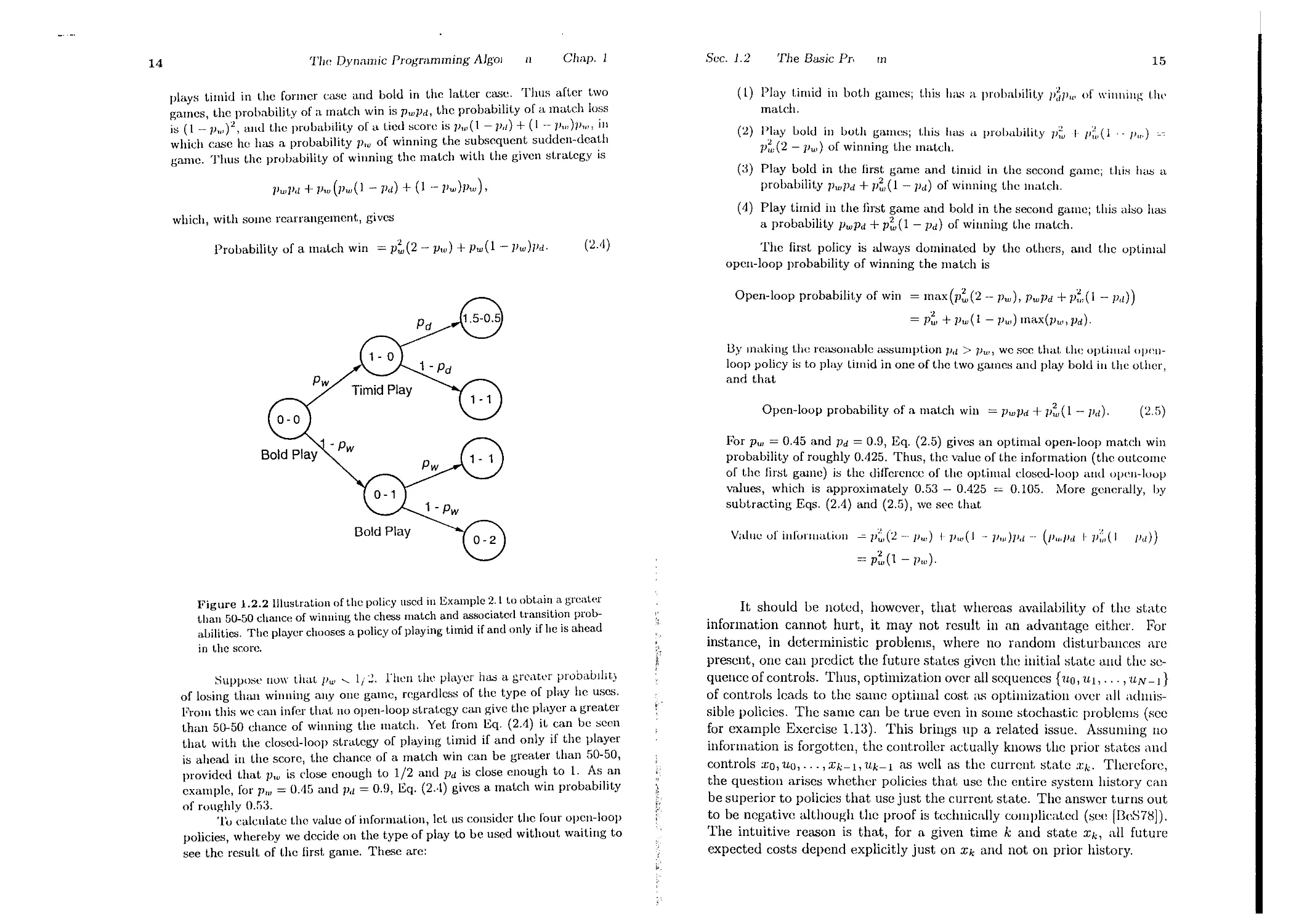
in each of the two games of the match. Suppose the player chooses a policy
of playing timid if and only if he is ahead in the score, as illustrated in Fig.
1.2.2; we will see in the next section that this policy is optimal, assuming
Pd > Pw. Then after the first game (in which he plays bold), the score is 1-0
with probability Pw and 0-1 with probability 1 - pw. In the second game, he
14
The Dynamic Programming AlgoJ
Chap. 1
n
plays timid in the former case and bold in the latter Ca.:l . Thus after two
games, t.he probability of a mat.ch win is P",Pd, the probabllIt.y of a mat.ch lo:s
is (1- ]1,.,)2, and tile probabilit.y of a tied score is ]1,.,(1 - ]1d) + (I - P,.,)Pw, 111
whieh case he has a probability p", of winning t.he subsequent sudden-death
game. Thus the probabilit.y of winning the mat.ch with the given st.rategy is
1)",]1d + Pw (Pw(1 - Pd) + (1 - Pw)Pw),
which, wit.h some rearrangement, gives
Probability of a match win = p (2 - pw) + p",(1 - )Jw)Pd.
(2A)
Figure 1.2.2 Illustration of the policy used in Example 2.1 to obtain a greater
than 50-50 chalice of winlling the chess match and associated transitIOn prob-
abilities. The player chooses a policy of playing timid if and only if he is ahead
in the score.
Suppmie 1101\' that Jlw ..... Ii J. rhen the player ha.:; a greater probabdJt)
of losing than winning anyone game, regardless of the type of play he uses.
From this we can infer that. no open-loop strat.egy can give the player a great.er
than 50-50 chance of winning the match. Yet from Eq. (2.4) it can be seen
that with the closed-loop st.rategy of playing timid if and only if the player
is ahead in the score, t.he chance of a mat.ch win can be greater than 50-50,
provided that pw is close enough to 1/2 and Pd is close enougl to 1. As .an
example, for Pw = OA5 and Pd = 0.9, Eq. (2..1) gives a match wm probabilIty
of ronghly 0.53.
'1'0 calcnlate the value of information, let US consider the four open-loop
policies, whereby we decide on the type of play to be used without waiting to
see the rcsult of the first game. These are:
Sec. 1.2
The Basic Pr,
rn
15
(I) Play timid in bot.h games; t.his ha.. a probability JI P,,' or \\'inllillg till'
match.
(2) Play bold ill both games; this has a probability P v I- JI ,(I . - f}".) cc
P (2 - ]1",) of winning t.he match.
(3) Play bold in thc first game and timid in the second game; this has a
probability P",Pd + p;;'( 1 - )Jd) of winning t.he mat.ch.
(4) Play timid in the first game and bold in the second game; this abo has
a probability ]JwPd + p;;,(1 - Pd) of winning the mat.ch.
The first policy is always dominated by the others, and the opt.imal
open-loop probability of winning the match is
Open-loop probabilit.y of win = max(p (2 - p",), P",Pd + p ,(l -- Pd))
= P , + P", (1 - ]1",) max(]1w, )Jd).
]Jy making the reasonable assumption IJ,l > )Jw, we see that. the optilllal Opell-
loop policy is to play timid in one of the two games and play bold in the other,
and that
Open-loop probability of a mat.ch win = pw)Jd + P;v(1 -- Pd). (2.5)
For pw = 0.45 and Pd = 0.9, Eq. (2.5) gives an optimal open-loop match win
probability of roughly 0.425. Thus, the value of t.he information (the outcome
of t.he first game) is t.he diJTerence of the optimal closed-loop and open-loop
values, which is approximately 0.53 - 0.425 = 0.105. More generally, by
suut.racting Eqs, (2.4) and (2.5), we see that
V,due of inl'JI"lliatioli p;;,(2 - Pw) I-]Iw(l -- ]1w)]},j -- (P,,,P,j l]i:;,(1 /I,d)
=, p ,(l - /iw).
\
It should be noted, however, that whereas availability of the state
information cannot hurt, it may not result in an advantage either. For
instance, in deterministic problems, where no random dist.urbances are
present, one can predict the future stat.es given the initial state and the se-
quence of controls. Thus, optimization over all sequenccs {1Lo, 1LI, . . . , 'lLN -1}
of controls leads to the same opt.imal cost ,J... optimization over all admis-
sible policics. The same can be true even in some stochastic problems (see
for example Exercise 1.13). This brings up a relat.ed issue. Assuming no
information is forgotten, the cont.roller actually knows the prior states and
controls :ro, 1Lo, . . . , Xk-I, 1Lk-1 as well as t.he current stat.e irk. Therefore,
the question arises whether policies that use the entire system history can
be superior to policies that use just the current state. The answer turns out
to be negativc although the proof is t.echnically complicated (see [DeS78]).
The intuitive reason is that, for a given time k and state Xk, all future
expected cost.s depcnd explicitly just on Xk and not on prior history.
_..J
16
The Dynamic Programming Alg
'!In
Chap. I
Sec. 1.3
The Dynam
mgralIlming Algorithm
17
1.3 THE DYNAMIC PROGRAMMING ALGORITHM
Thc dynamic programming (DP) tcchnique rests on a vcry simple
idea, thc principle of optimality. The name is due to Bellman, who con-
tributed a great deal to the popularization of DP and to its transformation
into a systematic tool. Roughly, the principle of optimality states the fol-
lowing rathcr obvious fact.
Period N - 1: Assume that at the beginning of period N - 1 the stuck
is x N -1. Clcarly, no matter what happened in the past, the inventory
manager should order the amount of invcntory that minimizes over "lLN -I 2:
o the sum of thc ordcring cost and the expect cd t.crlninal holding/short.age
cost C"lLN-l -I- E{R(XN)}, which can bc written as
C"lLN-l + E {R(XN-l -I- "lLN-l - WN-I)}.
WN_l
Principle of Optimality
Let 7r* = {/l'a, /1i, . . . , J.1.N _ d be an optimal policy for the basic prob-
lem, and assume that when using 7r*, a given state Xi occurs at time
i with positive probability. Consider the subproblem whercby we are
at Xi at time i and wish to minimize the "cost-ta-go" from time i to
time N
Adding thc holding/shortage cost of period N - 1, the optimal cost for the
last period (plus thc tcrminal cost) is
IN-1(XN-1) = T(J:N-l)
-I- min [ cnN-1+ E {R(:I:N-l-1-nN-1--WN-IJ} j .
UN_l O 1lJN-l
{ N-l }
E gN(XN) + f;9k(Xk,/1k(Xk),Wk) .
Naturally, J N -1 is a function of the stock :1: N -1' It is calculatcd either
analytically or numerically (in which case a table is used for computcr
storagc of the funcLion J N -1). In the process of calculating J N -1, we obtain
the optimal inventory policy J.1.?v -1 (XN -1) for thc last period; /1 ?v -I (XN - d
is the value of nN-l that minimizes thc right-hand sidc of the preccding
equation for a given value of XN-l.
Period N - 2: Assumc that at the beginning of period N - 2 the stock is
x N - 2. It is clear that the inventory manager should order the amount of
invcntory that minimizcs not just thc expccLed cost of period N - 2 hut
rather the
Then the truncated policy {JLi, /1i+l' . . , , J.1.?v -I} is optimal for this sub-
problem.
The intuitivc justification of the principle of optimality is very simple.
If thc truncat.ed policy V<, 1<+ l' . . . , It N -I} were not optimal as stated, wc
would be able to reduce the cost further by switching to an optimal policy
for thc subproblcm once we reach x,. For an auto travel analogy, supposc
that t.he fastest rout.c from Los Anl!;dcs to Doston pasSCI> through Chicago.
The principlc of optimality translates to the obvious facL that thc Chicago
to Boston portion of thc route is also the fastest route for a trip that starts
from Chicago and cnds in Boston.
The principlc of optimality suggests that an optimal policy can be
constructcd in piecemeal fashion, first constructing an optimal policy for
the "tail subproblem" involving the last stage, then extending the optimal
policy to the "tail subproblem" involving the last two stages, and continuing
in this manner until an optimal policy for the entire problem is constructed.
The DP algorithm is based on this idea. We introduce the algorithm by
means of an exam pie.
( XI)( ('t( d ('ost nf' period N - 2) I (exp(.('ted ('ost of' lH'riod N I,
given that an optimal policy will be used at period N - 1),
which is equal to
r(xN-2) -I- CUN-2 -I- E{ .1N-l (.TN - J)}.
Using the systcm equation J:N-l = :£N-2 -I- "lLN-2 - 111N-2, t.he last t.enll is
also written as I N - 1 (XN-2 -I- nN-2 - WN-2).
Thus the optimal cost for the last two pcriods given that we at'( at.
statc XN-2, denoted IN-2(XN-2), is given by
Consider the inventory control cxample of the prcvious section and
the following procedurc for determining the optimal ordering policy starting
with the last period and proceeding backward in time.
I N - 2 (XN-2) = r(xN-2)
-I- min [ CUN-2 -I- E {1N-l(XN-2 -I- nN-2 - WN-2) } j
"N-2;::O WN-2
The DP Algorithm for the Inventory Control Example
Again I N - 2 (XN-2) is calculated for every :CN-2' At the samc time, the
optimal policy /1?v-2(XN-2) is also computed.
18
The Dynamic Programming
oriillln
Chilp. 1
Sec. 1.3
The DYIW
Programming Algorithm
19
Period k: Similarly, we have that at period k, when the stock is .Tk, the
inventory manager should order Uk to minimize
(,xpected (:o t of period k) + (expected cost of periods k -1- 1,..., N - 1,
given that an opt.imal policy will be used [or thcsc period ).
",:,here the expectation is taken with respect to the probability distribu-
tIOn of Wk, which depends on Xk and 1L k Furthermore if u* - It * ( , c )
. , k - k' k
minimizes the right side of Eq. (3.3) for each Xk anel k, the policy
71"* = {/Lo, . . . , ILM _ J} is optimal.
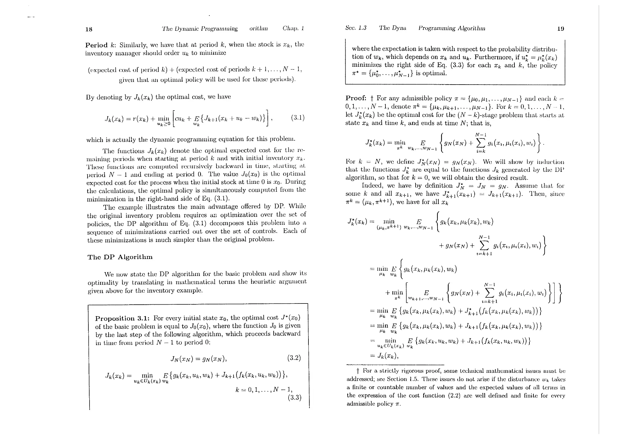
Dy denoting by Jd.Tk) t.he optimal cost, we have
.h(.rk) = 1'(:Ck) + min [ ClLk + E {.h+l (:Ck + "Ilk - wd } ] ,
uk::O: 0 wk
(3.1)
Proof: t For any admissible policy 71" = {/LO, /Ll,..., 11N-J} and each k =
0,1,..., N -1, denote 71"k = {/Lk,/Lk+J,... ,/LN-J}. For k = 0, 1,..., N -1.
let Ji,(xd be the optimal cost for the (N- k)-stage problem that. tarts at.
state Xk anel time k, and ends at time Nj that is,
The DP Algorithm
Jj;(Xk) = l tn wk,...1fvN-l {.<IN(XN) + IYi('T"/L'(:Ci)'W')}'
For k = N, we define .lM(:CN) = .<IN(:r:N)' We will show by induction
that the functions .lie are equal to the [unctions Jk generat.ed l.Jy the DJ'
algorithm, so that for k = 0, we will obtain the elesired result.
Indeed, we have by definition J M = I N = .<IN. Assume t.hat for
some k and all Xk+1, we have Jk'+J(Xk+J) = J k +1(Xk+J). Then, since
71"k = (/Lk,71"k+I), we have for all Xk
Jk'(Xk) = mip I E { 9k(Xk,ltd.Tk),Wk)
(J1.k>1T + ) Wk'''',WN_J
+.<IN(XN) + Yi(.T,,/L,(Xi),W,) }
,=k+l
which is actually the dynamic programming cquation for this problem.
The functions .h(:I:d denote the optim,ll expected cost. [or the l'C-
maining periods when st.art.ing at period k and with initial invent.ory ;Z'k.
Thc e funct.ions are computed recursively backward in timc, sLutiug al,
period N - 1 and ending at period O. The value Jo(xo) is the optimal
expected cost for the process when the initial stock at time 0 is .TO. During
the calculations, the optimal policy is simultaneously computed from the
minimization in thc right-hanel side of Eq. (3.1).
The example illustrates t.he main advantage offcred by DP. While
the original inventory problem requires an optimizat.ion over the set of
policies, the DP algorithm of Eq. (3.1) decomposes this problem into a
sequence of minimizat.ions carried out over the set. of controls. Each of
these minimizations is much simpler than the original problem.
Proposition 3.1: For every initial state Xo, the optimal cost J*(xo)
of the basic problem is equal to 1o(xo), where the function Jo is given
by the last step of the following algorithm, which proceeds backward
in timc from pcriod N - 1 to period 0:
= min E { .<Jk(:Ck,/LdXk),Wk)
JLk 11Jk
+ m 1 [ E { YN(:CN) + t 1 gi(Xi, Il,(Xi), w,) }] }
1T 1Uk+l,...,tlJN_}
,=k+l
= min E {Yk (:Ck, /Ldxk), Wk) + Jk' + 1 (h (:rk, ILk(:rk), Wk ) ) }
Ilk Wk
= min E {9k(Xk,/Lk(Xk),Wk) + Jk+l(fk(Xk,/Lk(Xk),1lJk ))}
J1.k Wk
n ( I J il ( 1 ) E {.lJk(:Ck, 1J.k, Wk) + .1,.,1-1 (fk(Xk, "Ilk, wd)}
ll.kE k Xk IlIk
We now state t.he DP algorithm for the basic problem and show it.s
opt.imality by translating in mathematical terms the heurist.ic argument
givcn above for the inventory example.
IN(XN) = YN(XN),
(3.2)
= JdXk),
.h(:r;k) = min E {gk(:Ck,lLk, Wk) + Jk+l (Jk(Xk, 1J.k, Wk))},
UkEUk(Xk) Wk
k = O,l,...,fV - 1,
(3.3)
t For a strictly rigorous proof, some t.edlllical mathcmatical issues must ue
addressed; see Section 1.5. These issues do not. arise if t.he disturba.nce Wk Lakes
a finite or countable number of values and the expected values of all terms in
the expression of t.he cost function (2.2) arc well defined and finit.e for ev('rv
admissible policy 71". .
_..1
20
TIJC Dynamic Programming Alg_
Jln
Chap. 1
Sec. 1.3
The Dynal
PrugramlIIwg AlguriihlII
21
complet.ing the induction. In the second equation above, we moved the
minimum over 7r k + 1 inside the braced expression, using the assumption
that the probability distribution of Wi, i = k -I- 1,. . . , N - 1, depends only
on Xi and Ui. In the third equation, we used the definition of J;;+1> and in
the fourth equation we used the induction hypothesis. In the fifth equation,
we converted the minimization over P,k to a minimization over Uk, using
the fact that for any function F of X and u, we have
min F(X,IL(X)) = min F(x,u),
,<EM uEU(x)
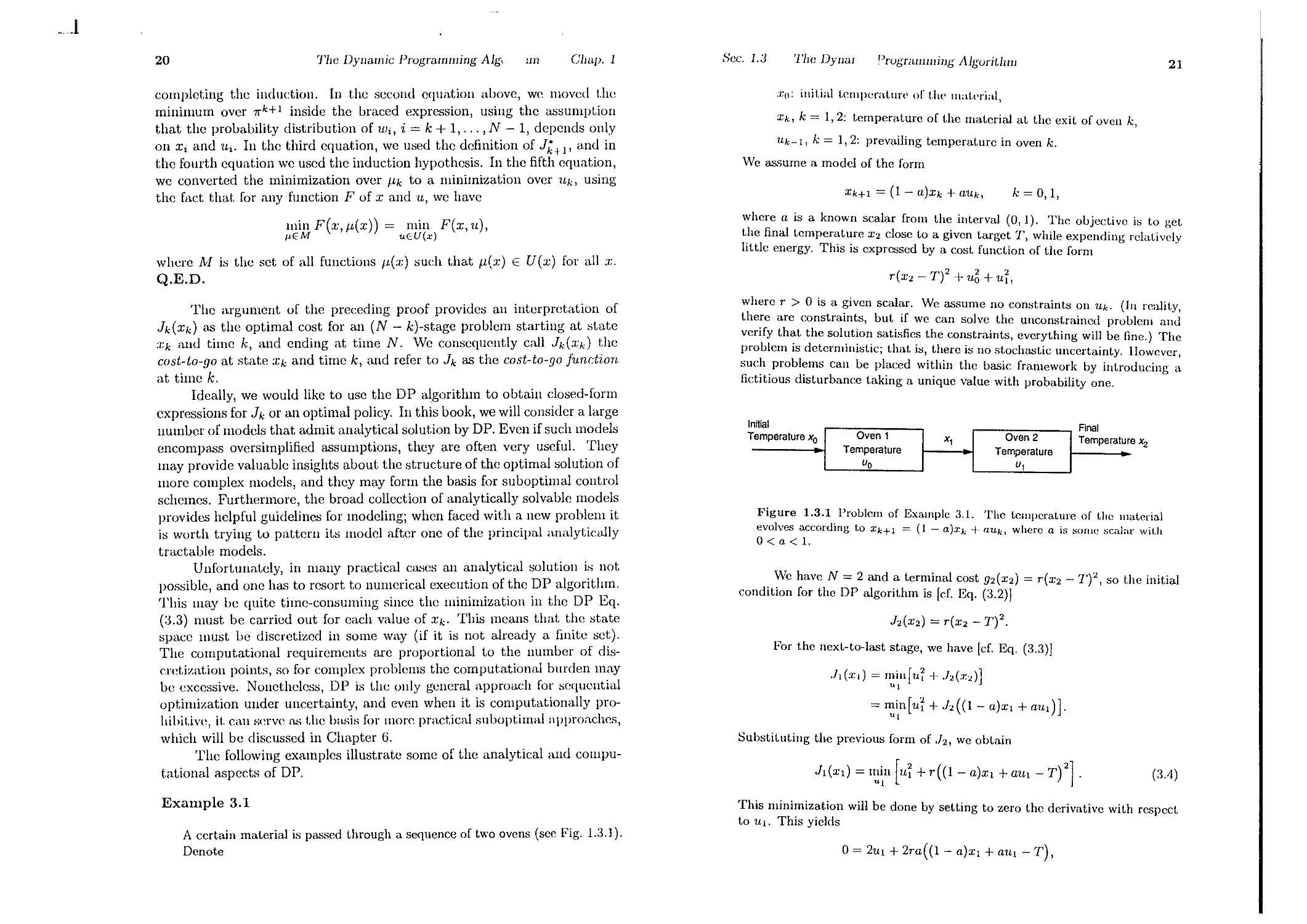
'DO: illitial t.elllperat.m'(' or t.iI(' material,
Xk, k = 1,2: temperature of the mat.erial at the exit of oven k,
Uk-I, k = 1,2: prevailing temperat.ure in oven k.
We assume a model of t.he form
Xk+l = (1 - a)xk -I- aUk,
k = 0,1,
where M is the set of all functions IL(X) such that p,(x) E U(x) for all .T.
Q.E.D.
where a is a known scalar from the interval (0,1). The objective is to get.
t..he final temperat re X2 close to a given target '1', while expending relatively
httle energy. This IS exprcssed by a cost function of the form
r(X2 - '1')2 -I- u6 -I- ui,
The argument of the preceding proof provides an interpretation of
Jk(Xk) as the optimal cost for an (N - k)-stage problem starting at state
:Z;k and time k, and ending at time N. We consequently call Jk(J;k) the
cost-to-go at state Xk and time k, and refer to J k as the cost-to-go fundion
at time k.
Ideally, we would like to use the DP algorithm to obtain closed-form
expressions for Jk or an optimal policy. In this book, we will consider a large
number of models that admit analytical solution by DP. Even if such models
encompass oversimplified assumptions, they are often very useful. They
may provide valuable insights about the structure of the optimal solution of
more complex models, and they may form the basis for suboptimal control
schemes. Furthermore, the broad collection of analytically solvable models
provides helpful guidelines for modeling; when faced with a new problem it
is worth trying to pattern its model after one of the principal analytically
tractable models.
Unfortunately, in many practical ca.ses an analytical solution i" not
possible, and one has to resort to numerical execution of the DP algorithm.
This may be quite time-consuming since the minimization in the DP Eq.
(3.3) must be carried out for each value of Xk. This means that the state
space must be discretized in some way (if it is not already a finite set).
The computational requirements are proportional to the number of dis-
cretization points, so for complex problems the computational burden may
be excessive. Nonetheless, DP is the only general approach for sequential
optimilmtion under uncertainty, and even when it is computationally pro-
hibit.ive, it. can serve 0"; the ba.<;iH for more practical suboptimal approaches,
which will be discussed in Chapter 6.
The following examples illustrate some of the analytical and compu-
tat.ional aspects of DP.
where r > 0 is a iven scalar. We assume no constraints on Uk. (In reality,
t.he:e are constramts, but If we can solve the unconst.rained problem and
verify th t the sol t on satisfies the constraints, everything will be fine.) The
problem IS deterl1lnllst.IC; that IS, t.here is no stochastic uncertainty. However,
SUC l . probl ms can be placed within the basic framework by int.roducing a
fictItIOus disturbance t.aking a unique value with probability one.
Innial
Temperature Xo
Oven 1
Temperature
U o
Oven 2
Temperature
u j
Final
Temperature x 2
Figure 1.3.1 Problem of Example 3.1. The temperature of the material
evolves according to xk+l = (1 - a)xk + aUk, where a is SOBle scalar wit.h
O<a<1.
. e have N = 2 and a terminal cost 92(X2) = r(x2 - 7')2, so the initial
conditIOn for thc DP algorit.hm is [cf. Eq. (3.2)]
h(X2) = r(x2 - '1')2.
For thc next-to-Iast stage, we have [cf. Eq. (3.3)]
.l1(:Z;1) = rnill[1L -I- .h(:1:2)]
"I
= min[1Li -I- h((1- a)xI -I- a1Ll) ] '
Ul
Substit.uting the previous form of h, wc obtain
h(Xd = l n H -I- r((1- a)xl -I- aUI - '1')21.
(3.4)
Example 3.1
A certain mat.erial is passed through a sequence of two ovcns (see Fig, 1.3.1).
Dcnote
This minimization will be done by setting to zero t.he derivative with rcspect
t.o 1LI. This yields
0= 21Ll -I- 2ra( (1 - a)xl -I- a1Ll - '1'),
.J
22
The Dynamic Programming Algo
Chap. 1
23
1]
Sec. 1.3
The DynamJ :ugramming Algorithm
and by collect.ing terms and solving for 1Ll, we obtain t.he optimal temperature
for the last oven:
One not.cworthy feature in the precedillg eXHmple is t.he facilit.y with
which we obt.ained an analytical solut.ion. A little thought while tracing
the steps of the algorit.hm will convince the reader that what simplifies the
solution is the quadratic nature of the cost and the linearity of thc system
equation. In Section 4.1 wc will sec that, gcnerally, when the syst.( 1Il is
linear and thc cost is quadratic thcn, regardless of the numuer of stages N,
the optimal policy is given by a closed-form expression.
Another noteworthy feature of the example is that the optimal policy
remains unaffected when a zero-mea.n stochastic disturbance is addcd in
the system equation. To see this, assume that the material's t.cmperature
evolves according to
. ra(T - (1 - a)xJ)
ILl (xl) = 1 + ra2
Not.e that. t.his is \lot. a single control hut rather a cont.rol function, a rule that.
tells liS the optimal oven t.emperature Ul = , (XI) for each possible st.at.c XI.
By subst.ituting the optimalul in the expression (3.4) for JI, we obt.a1l1
1.2a2({l-a)xl-T)2 ( ra2(T-(1-a):cl) _T ) 2
J ( ) - + r ( 1 - a ) xJ + 2
J Xl -- (1 + ra2)2 1 + ra
r 2 a 2 ((1- a)xl - '1')2 + l' ( _ _ 1 ) 2 ((1- a)Xl _ '1')2
(1 + ra 2 )2 1 + m 2
2
r((1- a)Xl - '1')
1 + ra 2
XkH = (1 - a)Xk + aUk + 1lJk,
k = 0, 1,
where 1lJo, 1lJl are independent random variables with given clistribution,
zcro mean
We now go back onc stage. We havc [ef. Eq. (3.3)]
Jo(xu) = min [u + J1(XI)] = min[u +.h ((1 - a)xo + auo)],
1'0 uo
E{ lIJ o} = E{lIJJ} = 0,
ancl finitc variance. Then the equatioll for J I [ef. Eq. (3.3)] becomcs
a\ld by subst.it.ut.ing the exprcssion already obtained for J l , we have
,ft(:q) = mill E { 1LI + r((l - a)xl + aUI + WI - T)2 }
1Ll WI
= min[ui + r((l - a)xl + aUI - T)2
Ul
+ 2r E{ wJ} ((1 - a)xI + aUI - T) + rE{wD].
. [ 2 r((1-a)2XU+(1-a)aUO-T)2 ] .
Jo(:cu) = lfiln Uo + 1 + ra2
Uo
Since E {1IJ I} = 0, we obtain
'vVe minimize wit.h respect. t.o .u,o by set.ting t.he corresponding derivat.ive t.o
zero. We obtain
Jl(Xl) = n [ui + r((l - a)xI + aUl - T)2] + rE{wn.
21"(1- a)a((1- u)2xo + (1 - a)au,o - T)
o = 2uo + 1 + ra 2 .
Comparing this cquation with Eq. (3.4), wc sec that the prcsenc( of WI
has resultcd in an additional inconsequential term, 1'E{wn. Therefore,
the optimal policy for the last stagc rcmains unaffected by the presence
of WI, while JI (XI) is increased by thc constant term I'E{wn. It can be
seen that a similar sit.uation also holds for the first stage. In particular,
the optimal cost is given by the same cxpression as beforc exccpt for an
additive constant that depends on E{w5} and E{wt}.
If the optimal policy is unaffectcd when thc disturbanccs are rcplaced
by their mcans, we say that certainty equivalence holds. We will derive
certainty equivalence rcsults for several types of problems involving a linear
system and a quadratic cost (see Sections 4.1, 5.2, and 5.3).
This yields, aft.er some calculation, the opt.imal temperature of t.he first oven:
. r(l - a)a(T - (1 - a)2xo)
ILo(Xo) = 1 + ra2(1 + (1 _ a)2) .
The opt.imal cost is obtained by substit.uting this exprcssio.n in the fo mula
for Jo. This leads to a straightforward but le\lgthy calculatIOn, which 111 the
end yields t.he rather simple formula
r((1-a)2xo-T)2 .
Jo(xo) = 1 + ra2(1 + (1 - a)2)'
Example 3.2
This complet.es the solution of the problem.
To illustrate the computational aspects of DP, consider an invent.ory cont.rol
problem that is slightly different from the one of Sections 1.1 and 1.2. [n
_ J
24
The Dynamic Programming AlgG 1m
Chap. 1
Sec. 1.3
The DynaJ.
Programming Algorithm
25
particular, we assume that inventory Uk and t.he demand Wk are nonnegat.ive
integers, and that the excess demand (Wk - Xk - Uk) is lost. As a result, the
stock equation takes the form
Xk+l = 11Ia.-'«0,."tk + Uk - Wk).
Stock; 2 Stock; 2 Siock ; 2 0
Stock; 1 Stock; 1 Stock; 1
Stock; 1
Stock; 0
stock; 2
We also assume that t.here is an upper bound of 2 units on t.he stock that Call
he stored, i.e. t.herc is a constraint Xk + Uk 2. The holding/st.orage cost. for
the kt.h period is given by
Stock; 0
Slock ; 0
Stock; 0
Siock purchased; 0
Stock purchased; 1
(Xk + Uk - Wk)1,
implying a penalt.y bot.h for excess invent.ory and for unmct demand at. t.he
end of t.he kt.h period, The ordering cost. is 1 per unit st.ock ordered. Thus
t.he cost per period is
Stock;2 0
Slock ; 2
Stock; 1 0
Slock ; 1
Yk( ;k, ltk, Wk) = Uk + (Xk + ltk - Wk)2.
The t.erminal cost is assumed t.o be 0,
Stock; 0
Stock; 0
YN(."CN) = O.
Slock purchased; 2
p(Wk = 0) = 0.1,
p(Wk = 1) = 0.7,
p(Wk = 2) = 0.2.
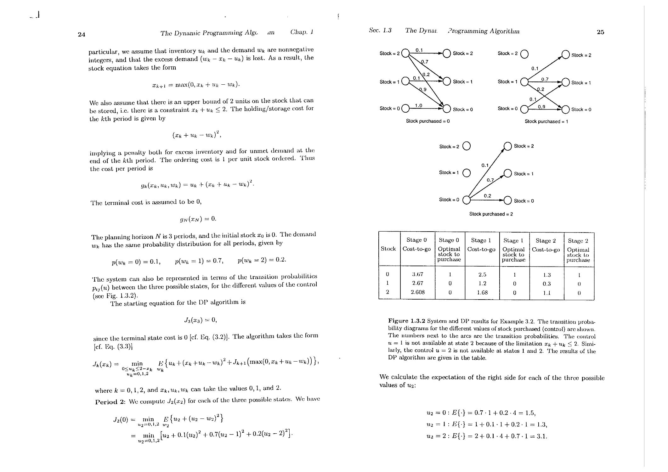
Stage 0 Stage 0 Stage 1 St.age 1 Stage 2 Stage 2
Stock Cost-to-go Optimal Cost-ta-go Optimal Cost-to-go Optimal
stock t.o stock to stock to
purchase purchase purchase
0 3.07 1 2.5 1 1.3 I
1 2.67 0 1.2 0 0.3 0
2 2.608 0 1.68 0 1.1 0
The planning horizon N is 3 periods, and t.he initial stock Xo is O. The demand
Wk has t.he same probability dist.ribution for all periods, given by
The system can also be reprc:,;ent.ed in terms of the t.ransition prohalJilities
P'J(u) between t.he three possible stat.es, for t.he different. values of the control
(see Fig. 1.3.2).
The st.arting equation for the DP algorithm is
h(X3) = 0,
Figure 1.3.2 System and OP results for Example 3.2. The trausition proba-
blhty diagrams for the different values of stock purchased (control) arc shown.
The numbers next to the arcs are the transition probabilities. The coutrol
U = 1 is not available at state 2 because of the limitation Xk + Uk < 2. Simi-
lady, the control U = 2 is not available at states 1 and 2. The res;;-lts uf the
OP algonthm are given in the table.
since t.he t.erminal state cost is 0 [ef. Eq. (3.2)]. The algorithm takes the form
[ef. Eq. (3.3)]
Jk(Xk) =
min 1<) {Uk + (Xk +Uk -Wk)1 + Jk+1 (max(O, Xk -I-Uk -Wk))},
osuk 2-xk wk
uk=O,l,2
We calculate the expectatioll of the right side for each of the three possible
values of 112:
where k = 0,1,2, and Xk, l1k, Wk can take t.he values 0,1, and 2.
Period 2: 'We compute h( ;2) for each of t.he three possible :>t.at.e:>. We have
h(O) = min, E{U1 -I- (U2 - W1)1}
1L'2=U,l,:.l tl'2
min [U2 -I- 0.1(U2)2 -I- 0.7(U2 - 1)2 + 0.2(U2 - 2)2].
1.£2=0,1,2
U2 = 0: E{.} = 0.7.1 -I- 0.2.4 = 1.5,
11.2 = 1 : E{.} = 1 + 0.1.1 + 0.2.1 = 1.3,
U2 = 2: E{.} = 2 -I- 0.1. 4 -I- 0.7.1 = 3.1.
_ J
26
The Dynamic Programming Algo,
Chap. 1
n
Hence we have, by selecting the minimizing U2,
h(O) = 1.3,
JL (0) = 1.
For X2 = 1, we have
h(l)= min E{u2+(I+U2- W 2)2}
1£2=0,1 1JI2
= min [U2 + 0.1(1 + U2)2 + 0.7(U2)2 + 0.2(U2 - 1)2].
H2=O,1
U2 = a : E{,} = 0.1 . 1 + 0.2.1 = 0.3,
U2 = 1 : E{'} = 1 + 0.1. 4 + 0.7.1 = 2.1.
II ence
h(l) = 0.3, JL (l) = 0,
For ;2 = 2, the only admissible control is U2 = 0, so we have
,h(2) = E{(2- wd} = 0.1,4 +0.7.1 = 1.1,
. '"2
h(2) = 1.1,
JL (2) = O.
. l' A T'tin we compute 1 1 (xl) for each of the t.hree possible st.at.es
Period . g,. I . I ,1 ( 0 ) J (1) h(2) obtained in t.he prevIOus
;2 = 0, 1,2, usmg t Ie va ues 2 , 2 ,
period. For XI = 0, we have
1 1 (0)= min E{Ul+(lL1-Wl)2+h(max(0,ul-Wl))},
1q =0,1,2 wI
III = 0 : J';{.} 0.1 . h(O) 1- 0.7( 1 + h(O)) + 0.2(4 + ,h(0)) = 2.8,
111 = 1 : 1':{.} = 1 + 0.1(1 + h(I)) + 0.7. h(O) + 0.2(1-1- h(O)) = 2.G,
Ul = 2: E{.} = 2 + 0.1(4 + h(2)) + 0.7(1 + h(l)) + 0,2. h(O) = 3.68,
Jl(O) = 2.G, (Li(O) = 1.
1'()1' XI = 1, we have
11(1)= min E{1LI+(1+UI-WI)2+h(max(0,1+UI-WI))},
1£1=0,1 wI
ILl = 0 : J {.} = 0.1 (1 + h( I)) + 0.7. h(O) + O.2( 1 + h(O)) = 1.2,
UI = 1 : E{.} = 1 + 0.1(4 + h(2)) + 0.7(1 + h(I)) + 0.2. J 2 (0) = 2,68,
.h(l) = 1.2, (Li(l) = O.
For .1;1 = 2, the only admissible cont.rol is IJ,I = 0, so we have
.Jl(2) E{(2-w1)2I-h(max(0,2-Wl))}
WI
-OI(II.l.,(:!))+O.7(1+.fc(I))+O.2..J 2 (O)
= 1.68,
Sec. 1.3
The Dynamic ogramming Algorithm
27
1 1 (2) = 1.68,
JLi (2) = O.
Period 0: Here we need to compute only Jo(O) since the init.ial st.at.C' is known
to be O. We have
10(0) = min 1': {uo + (uo - wof I- J l (max(O, Uo - wo))},
'UO=O,1,2 UJQ
Uo = 0: EO = 0.1. .1 1 (0) + 0.7(1 + 1 1 (0)) + 0.2(4 + .h(O)) = ;j.0.
Uo = 1 : E{.} = 1 + 0.1(1 + .11(1)) + 0.7. .h(O) + 0,2(1 + h(O)) = 3.67,
Uo = 2: E{.} = 2 + 0.1(4 + .11(2)) + 0.7(1 + J 1 (1)) I- 0.2. h(O) = 5.108,
.10(0) = 3.67,
II. (O) = I.
If the initial state were not known a priori, we would have to comput.e
in a similar manner .1 0 (1) and .1 0 (2), as well as the minimizing Uo. The reader
may verify (Exercise 1.2) t.hat these calculations yield
.1 0 (1) = 2.67,
(L (I) = 0,
1 0 (2) = 2.608,
JL (2) = O.
f:,:
Thus the optimal ordering policy for each period is t.o order one unit. if t.he
current stock is zero and order nothing ot.herwise. The results of t.h,' D1>
algorithm are given in tabular form in Fig. 1.3.1.
..
':"1
;'
t
k-
:
1.';;.'
t:i
Example 3.3 (Optimizing a Chess Match Strategy)
Consider the chess match example considered in Sedion 1.1. There, ,I player
can select timid play (probabilities Pd and 1 - Pd for a draw or loss, respec-
tively) or bold play (probabilities p," and 1- p," for a win or loss, respectively)
in each game of t.he match. We want to formulate a DP algorit.hm for linding
the policy that maximizes t.he player's probability of winning the mat.ch. Not.e
that here we are dealing with a maximization problem. We can cOnvert the
problem to a minimization problem by changing t.he sign of the Cost fundion,
but a simpler alternative, which we will generally adopt, is t.o replace t.he
minimizat.ion in t.he DP algorithm with Inaximizat.ioll.
Let us consider t.he general case of an N-game match, and let t.h(, st.ate
be the net score, that is, the difference bet.ween t.he point.s of the playC'r
minus the points of the opponent (so a st.ate of 0 corresponds t.o all eVC'n
score). The optimal cost.-ta-go function at t.he st.art. of t.he kth ganlf' is giV<'1I
by t.he dynamic programming recursion
.h(Xk) = max[p,t.lk11(:Ck) + (1- Pd)Jk1 I(J;k - I),
P,u.lk+l (Xk + 1) + (1 - Pw).Jk+l (.I;k - 1)].
(3.G)
The maximum above is t.akcn ovcr t.he two possible decisions:
_...1
28
The Dynamic Programming AlgG ifrJ
Chap. 1
(a) Timid play, which keeps the score at Xk wit.h probabilit.y pd, and changes
Xk t.o Xk - 1 with probability 1 - Pd.
(1)) Bold play, which changes Xk t.o Xk -I- 1 or to Xk - 1 with probabilities
P", or (1 - JI",), respectively.
It is optimal to play bold when
l'w.h+I(Xk -I- 1) -I- (1 - p",).h+l(Xk -1)::0: p,dk+l(Xk) -I- (l-l'd)J k + 1 (Xk - 1)
or cqnivalently, if
P Jk+l ( Xk) - Jk+l(Xk -1)
>
Pd - .h+l(Xk -I- 1) - Jk+I(Xk - 1)'
(3.6)
The dynamic programming recursion is started with
.IN(:I:N) = { w
if XN > 0,
if :I:N 0,
if XN < O.
(:\7)
We have IN(O) = p", because when the score is even aft.er N games (:rN , O),
it is optimal to play bold in the first game of su den eat.h. . .
By executing the DP algorithm (3.5) startmg with the tcrmmal condl-
t.ion (3.7), and using the criterion (3.6) for optimality of bold play, \\"(' find
the following, assllming that Pd > pw:
IN-l(XN-l) = 1 for XN-l > 1; opt.imal play: eit.her
I N -I(l) = max[Pd -I- (1 - Pd)p", , P", -I- (1 - p",)pw]
= Pd -I- (1 - Pd)pw; optimal play: timid
IN-I(O) = ])",; optimal play: bold
IN-l(-I) =P ; optimal play: bold
IN-l(XN-J) = 0 for XN-l < -1; optimal play: eit.her.
Also, given IN-I(XN-l), and Eqs. (3.5) and (3.6) we obtain
IN-Z(O) = max[pdp", -I- (1 - Pd)p , P",(Pd -I- (1- Pd)p",) -I- (1 - Pw)p ]
= JI"'(p", -I- (p", -I- Pd)(1- p",»)
'uHI that if t.he score is even with 2 games remaining, it is opt.im, 1 t l o pl y
, I I t. . I olic y for both peno( S IS .0
b Id Thus for a 2-game malc I, tie op nna p .' .
a . timid if and only if the player is ahead in the score. The reg.lOn of p,alrs
P ( y P ) f or which the player has a better than 50-50 chance to wm a 2-game
PWI d
tHat.ch is
Rz = {(Pw,pd) I Jo(O) = pw(p", -I- (p", -I- Pd)(l - PW)) > I/2},
and, as noted in t.he preceding section, it includes points where P", < 1/2.
(
/
f'
:
If
,
r,
Ii
1,-.;
h
¥\
r
(,
"
h'
r
i\
r
t
i
Sec. 1.3
The DYIli
. rrogralllllling AIguriUllrJ
29
Example 3.4 (Finite-State Systems)
We mentioned earlier (d. the examples in Section 1.1) that syst.ems wit.h a
finite number of states can be represent.ed eit.her in terms of a discrete-t.ime
system equation or in terms of the probabilities of transit.ion between the
states. Let us work out the DP algorithm corresponding to the latter case.
We will assume for the sake of the following discussion that the problem is
stationary (i.e., the transition probabilities, the cost per stage, and t.he control
constraint sets do not change from one stage to the next). Then, if
p,;(U) = P{Xk+l = j I Xk = i, Uk = u}
are the transition probabilities, we can alternatively represent the system by
the system equation (d. the discussion of t.he previous section)
Xk+l = Wk,
where the probabilit.y dist.ribulion of the dist.urbance 1IIk is
P{Wk = j I Xk = i, Uk = u} = Pij(U).
Using t.his system equation and denoting by g(i, u) t.he expected cost per st.age
at state i when control U is applied, the D1' algorithm can be rewritten as
Jk(i) = min [g(i,u)-I-E{Jk+l(Wk)}]
uEU(i)
or equivalently (in view of the distribution of Wk given previously)
Jk(i) = min [ 9(i'U) -I- "" Pij(U)A+l(j) ] .
UEU(,)
j
As an illustration, in the machine replacement example of Section 1.1,
this algorithm t.akes t.he form
IN(i) =0, i=l,...,n,
A(i) = min [R -I- g(I) -I- Jk+l(I), g(i) -I- tP,jJk+l(j)]
The two expressions in the above minimization correspond to the two available
decisions (replace or not replace the machine).
In the queueing example of Section 1.1, the DP algorithm takes the
form
IN(i)=R(i), i=O,I,...,n,
Jk(i) = min [r(i) -I- Cf -I- Pij(lLf)Jk+I(j), rei) -I- c., -I- 1"J(1l,).hll(j)]
The two expressions in the above minimization correspond to the two possible
decisions (fast and slow service).
_ J
30
The Dynamic Programming AlgI
Chap. 1
'n
1.4 STATE AUGMENTATION
We now discuss how to deal with situations wherc somc of the as-
sumptions of thc basic problcm arc violatcd. Gcncrally, in such cases t.hc
problem can be reformulated into the basic problem format. This process is
called state auqmentatian bccause it typically involves the enlargement of
the statc spac . The gencral guidelinc in statc augmentation is to include
in the enlarged state at time k all the infarmatian that is kna"Wn to. the
controllcT a.t timc k and can be used with a.dvantage in sclcctiny Uk. U n-
fortunately, statc augmcntation oftcn comes at a price: thc refonnula ed
problcm may havc very complex state and/or control spaces. \Ve provide
somc examplcs.
Time Lags
In many applications thc systcm state XkH dcpcnds not only on thc
preceding state :Ck and control 'Uk but also on earlier stat.cs. and contr.ols.
In other words statcs and controls influence future states with somc tnnc
lag. Such situ:ttions can bc handled by state augmcntation; thc state is
expanded to includc an appropriate number of earlicr. statcs a ld controls.
For simplicity, assumc that there is at most a smglc pel"lod t.unc lug
in t.he state and control; that is, t.hc systcm equation has the form
Xk+l = !k(:Ck,:rk-l,uk,U'k-I,"Wk),
k = 1,2,...,lY - 1,
(4.1 )
1:1 = /o(:co, UO, wo).
Time lags of morc than one pcriod can be handlcd similarly.
If wc introducc additional stat.e variables )lk and Sk, and we makc thc
idcntifications )lk = :Ck-l, 5k = Uk-- 1, the system cquation (4.1) yields
( :Z:k+l ) ( !k(:l:k, )lk: k, 5k, "Wk) )
'!hl.l .q, .
S k t I Uk
(lJ.2)
Dy dcfining :l:k = (:I:k, Yk, 5k) as the ncw state, we have
Xk+1 = 1k(xk, Uk, "Wk),
wherc thc systcm function1k is dcfincd from Eq. (4.2). By using the prec?d-
ing cquation a.<; thc system equation and by expressing the co t functIOn
in terms of the new statc, thc problem is reduced to the basic problem
without time lags. Naturally, thc control Uk should now dcpcnd on the
ncw state ik, or equivalently a policy should consist of functions iLk of thc
Sec. 1.4
State A ugn, "tion
31
current state :1:k, as well a.<; the preceding statc Xk-I and thl preceding
control Uk-I.
When the DP algorithm for thc reformulatcd problem is translated
in tcrms of the variables of the original problem, it takcs the form
IN(XN) = 9N(XN),
IN -I (XN -I, XN-2, 1LN-2)
= rnin E { 9N-I(J:N-I,lL N - I ,"W N -J)
"N-l EUN_)(xN_l) WN-l
+ IN(JN-I(XN-I,XN-2,lLN-I,lLN-2,11JN_J))},
Jk(Xk,:Ck-l, lL k-J) = min E { 9k(Xk, Uk, 11Jk)
"kEUkCxk) wk
+ Jk+J(h(J:k,J:k-I,"Il.k,"Il.k_I,W..),:q,Uk) }, k = 1,...,lY - 2,
Jo(xo) = min E {go(XO,lLo,11Jo) + .h(Jo(:l:o,lLo,'Wo),:eo,"Il.o)}.
uoEUo(xo) wo
Similar reformulations arc possible when timc lags appcar in the cost;
for cxample, in thc ca.<;e where the cost is of the form
{ N-l }
E 9N(XN,XN-I) +90(xo,lLo,11Jo)+ t;9k(:Z:k,Xk-I,lJ.k,1JJ d .
The extremc case of time lags in thc cost ariscs in the nonadditivc fol'lu
E {9 N (x N , X N - 1 , . . . , xo, 1L N - I , . . . , Uo, W N _ I , . . . , 11Jo) } .
Then, the problcm can be rcduccd to the basic problcm format, by taking
as augmentcd stat.c
Xk = (:l:k,Xk-I,... ,Xo, lLk-I,..., lLo, 'Wk-l,..., wo)
,,;
and E{gN(XN)} as reformulated cost. Policies consist of functions Ilk of the
prcscnt and past statcs Xk,. .. ,:ro, thc past controls lLk-I,... ,Uo, and the
past disturbances Wk-l,"', WOo Naturally, we must assumc that the past
disturbances are known to thc controller. Otherwise, we are fac:( d with
a problcm where the state is imprecisely known to thc controller. Such
problems arc known as problems with imperfcct state information and will
be discusscd in Chapt.cr 5.
f
-
f
"
_...1
32
The Dynamic Programming Algor. .1
Chap. 1
Correlat.ed Disturbances
Wc t.urn now t.o the case whcre t.he disturbances Wk are correlated
ovcr time. A COlIllllOII sit.uatioll that C;l1I be halldlcd cflicienUy by state
augmcntation arises when t.he proccss Wo,. .. , WN-l can bc represented as
the output of a lincar systcm driven by independcnt random variables. As
an example, supposc that by using statistical methods, we determine that
the evolution of Wk can be modeled by an cquation of the form
Wk = AWk-l + k,
whcrc A is a givcn scalar and { d is a scquencc of independcnt. random
vectors with given distribution. Then we can introduce an additional statc
variable
Yk = 11Jk-l
and obtain a ncw systcm cquation
( Xk+l ) = ( !k (Xk, Uk, AYk + k) ) ,
Yk+l AYk + k
whcre thc ncw state is the pair Xk = (Xk, Yk) and the new disturbance is
the vector k'
Morc gcncrally, supposc that Wk can bc modeled by
Wk = CkYk+l,
where
Yk+l = AkYk + k,
k = 0,. . . , N - 1,
A k , C k are known matriccs of appropriatc dimcnsion, and k arc indepen-
dent random vcctors with givcn distribution (sce Fig. 1.4.1). By viewing
Yk as an additional state variable, wc obtain the new system equation
( Xk+l ) = ( !k(.Tk,Uk,Ck(AkYk + d) ) .
Yk+l AkYk + k
Yk+ 1 = AkYk+ k C k
Figure 1.4.1 Representing correlated disturbances as the output of a linear sys-
tem driven by independent random vectors.
,."
Sec. 1.4
SLaLe Augn
,Lion
33
Note that in order to hav(, lH'rr('cl. stale inronna!.ion, 1.11(' ('olll.roll('r
must be able to observe Yk. Unfortunately, this is true only in the minority
of practical cases; for examplc when Ck is the idcntity matrix and "Uik-I is
observed before Uk is applied. In the ca.o.;e of jH,rfect. stat.e infonllaLion 1.11<'
DP algorithm take::; the form '
IN(XN,YN) = gN(XN),
,h(Xk, Yk) = min E{gk(xk. Uk, Ck(AkYk + d)
UkEUdxk) k
+ Jk+l (h(Xk,Uk, Ck(AkYk + k)), AkYk + k)}.
Forecasts
Finally, considcr the case wherc at time k the cont.rollcr has access t.o
a forccast Yk that re::;ults in a reasscssment of thc probability distribut.ion
of Wk and possibly of futurc disturbances. For exampl(', Uk limy he ;111 ( xact
predict.ion of 11Jk or all exact prcdiction that the probability dbtribution of
Wk is a specific one out of a finite collcction of distributions. Forccasts of
intcrcst in practice arc, for examplc, probabilistic predictions on thc state
of thc weathcr, the interest ratc for moncy, and thc demand for invcnt.ory.
Gcnerally, forecasts can bc handlcd by statc augmentation although
the reformulation into the basic problem format may bc quitc complex. We
will treat here only a simple spccial casc.
Assume that at the beginning of each period k, thc controller rc-
ceives an accuratc prediction that the next disturbance 11Jk will be sdect.ed
according to a particular probability distribution out of a givcn collection
of distributions {Ql,..., Qm}; that is, if the forecast is i, thcn "Wk is sc-
lected according to Qi. The a priori probability that thc foreca::;t will be i
is denoted by Pi and is given.
As <In example, supposc that in our carlier invcntory example t.he de-
mand Wk is determined according to onc of three distributions Ql, Q2, and
Q3, corresponding to "small," "mcdium," and "largc" demand. Each of thc
thrce types of demand occurs with a given probabilit.y at each timc pcriod,
independently of the values of demand at prcvious time pcriods. Howevcr,
the inventory managcr, prior to ordering Uk, gcts to know through a forc-
c t .the .type of dcmand that will occur. (Note that it is the probnbility
dlstnbutlOn of demand that bccomes known through thc forecast, 1101, the
demand itself.)
The forecasting process can be represented by means of the equation
Yk+l = k,
where Yk+l can take the values 1,. . . , m, corresponding to the m possiblc
forecasts, and k is a random variable taking the value i with probability
_..1
34
Tlw Dynamic Programming Algc
Chap. 1
/II
pi. The interpret.ation here s tl.lat vhen k takes the value i, then Wk+l
will occur according to the dlstnbutlOn Qi. . . _
Dy combining the system equati n with the forecast equatIOn Yk+ 1 -
k, we obtain an augmented system given by
( .1:k+l ) = ( !k(Xk,Uk,Wk) ) .
Yk+l k
'I'll(' IlPW t.at.P i :1:,. = (.1:", yd, and because the forecast Yk s I nowli ;It t l\e
. ..... ..... Ii' ", ." .\ ,.!., rh.' ".'W ,JI:,turl':1IlCe I:' Ii't.. = (1/',. ,I; .
':11\';'1'1:': '1 ''';h::;q;I;:\' '\;:;,tl 'II'\'I/h'.'ll '\;: dt'{\'llllllh'd b) IlH' dl t.rIbll{lUn (J{ dud
the probabilities Pi, and depends explicitly 011 Xk (via Yd but not on the
prior disturbances. Thus, by suitable rcformulatioll of the cost, the probl:m
can be cast into the basic problem format. Note that t.he control apphed
depellds on both the current state and the current forecast.
The DP algorithm takes the form
IN(XN,YN) = gN(:I;N), (4.3)
Jk(Xk, Yk) = mill E { gdXk' Uk, Wk)
UkEUk(Xk) Wk
(4.4)
+ f1J,.h+l (h(:I;k, 11'k, Wk), i) I Yk}'
i=l
where 1/k may t.ake the values 1,..., m, and the expect.ation over Wk is
taken wit.h respect to the distribut.ion QYk'
There is a lIice simplification of the above algorithm that allows DP
to be executed over a smaller spacc. In particular, define
m
.J k (:1:k) = LP;Jk(:rk, i),
i=1
k = 0, 1,..., N - 1,
and
.J N(:!:N) = gN (:!:N)'
Theil [rom Eq. (4.4), we obtain the algorithm
Jd:I;k) = f 11, min E {!Jk(:I;k' Uk, Wk)
,=1 "kEUk(xd wk
+ .J k +1Ud.1: k ,Uk,Wk))1 Yk = i},
which is executed over the space of Xk rather than Xk and Yk. This simpli-
fication arises also in other contexts where the state has a component that
cannot be affected by the choice of control (see Exercise 1.22).
It should be clear that the preceding formulation admits several ex-
tensions; one example is the case where forecasts can be influenced by
the cOIlt.rol action and involv() several future disturbances. However, the
price for these extensions is incre,lSed complexity of the correspolldillg D P
algorithm.
Sec. 1.5
Some Mathe, ..kal Issues
35
1.5 SOME MATHEMATICAL ISSUES
Let us now discuss some technical issues relating to the basic prob-
lem formulation. The reader who is not mathematically inclined lIeed 1I0t
be concerned about these issues and can skip this section without loss of
continuity.
Once an admissible policy {lLa,.. ., 11N-I} is adopted, the followillg
sequence of events is envisioned at the typical stage k:
1. The controller observes Xk and applies Uk = ILk(Xk).
2. The disturbance Wk is generated according to the given distribution
Pk(- I Xk,ILk(xk)).
3. The cost Yk(Xk,11k(Xk),Wk) is incurred and added to previous costs.
4. The next state Xk+l is generated according to the system equatioll
Xk+l = !k (Xk, l1.k(:1:k), Wk)'
If this is the last stage (k = N - 1), t.he terminal cost. YN(:rN) is
added to previous costs and the process terminates. Otherwise, k is
incremented, and the same sequence of events is repeated for the next
stage.
For each stage, the above process is well-defined and is couched ill pre-
cise probabilistic terms. Matters are, however, complicated by thc lIeed to
view the cost as a well-defined random variable with well-dcfined expect.ed
value. The framework of probability theory requires that for each policy
we define an underlyillg probability space, that is, a set n, a collection of
events in n, and a probability measure on these events. In addition, the
cost must be a well-defined random variable on this space ill t.he scnse of
Appelldix C (a measurable fUllction from the probability space illto the real
line in the termillology of measure-theoretic probability theory). For this
to be true, additional (mcasurability) ,lSsumptions on the functions !k, gk,
and ILk may be required, and it may be neccssary to introduce additional
structure on the spaces Sk, Ck, and Dk. Furthermore, these assumptiolls
may restrict the class of admissible policies, since the fUlictions Pk may bc
constrained to satisfy additional (measurability) requirements.
Thus, unless these additional assumptiolls and structure are specified,
the b,lSic problem is formulated inadequat.ely. Unfortunat.ely, a rigorous
formulation for general state, cOlltrol, alld disturbance spaces is well heyolld
the mathematical framework of this introductory book and will not be
undertaken here. Nonetheless, it turns out that these difficulties arc mainly
technical alld do not substantially affect the basic results to be obtaiJl( d.
l<or this reason, we find it convenient to proceed with informal derivations
and arguments; this is consistent with most of the literature on the subjed.
_. J
I;
.
f
. "
!
:
,
! "
.
f
I".
I.
I
r
"
36
T1JC DYllamic Programming Algor. .11
Chap. 1
We would likc to strcss, however, that undcr at least onc frcquently
satisfied assumption, thc mathematical difficulties mentioned above disap-
pear. In particular, let us assume that the disturbance spaces Dk arc all
countable and the expected valucs of all terms in the cost are finitc for
every admissible policy (this is true in particular if thc spaccs Dk arc finitc
sets). Then, for every admissible policy, the expected values of all the cost
terms can be written as (possibly infinite) sums involving thc probabilities
of the elements of the spaces Dk'
Alternatively, one lIlay writc the cost as
J1f(xo) = Xl,.I?xN {9N(XN) + 9k(Xk,J1.k(Xk))} , (5.1)
wherc
9k(:Ck,fld x d) = E{!/k(Xk,J1.k(Xk),Wk) I Xk,flk(:Ck)},
Wk
with the prcceding cxpectation taken with respect to the distribution Pk (- I
Xk, J1.k(Xk)) defined on the countable sct Dk. Then one ma,!' take as thc ua-
sic probability space the Cartesian product of the spaces 8 k , k = 1,..., N,
given for all k by
Sk+l = {Xk+1 E Sk+l I :Ck+1 = fk(Xk,J1.k(Xk),Wk), Xk E Sk, Wk E Dk},
where So = {xo}. The set Sk is the subset of all states that can be reached
at time k when the policy {J1.0"" ,J1.N-l} is used. Because the disturbance
spaces Dk are countable, the sets Sk are also countable (this is true since the
union of any countable collection of countable sets is a countable set). The
system equation Xk+l = h(XbJ1.k(Xk),Wk), the probability distributions
Pk('\ XbJ1.k(Xk)), the initial state XO, and the poli<:?, {J1.0,'" 'I!:N-d define
a probability distribution on the countable set 81 x .., X 8N, and the
expected value in the cost expression (5.1) is defined with respect to this
latter distribution.
In conclusion, the basic problem has been formulated rigorously only
when the disturbance spaces Do,..., D N - 1 arc countable sets. In the ab-
sence of countability of these spaces, the reader should interpret subsequent
results and conclusions as essentially correct but mathematically imprecise
statements. In fact, when discussing infinite horizon problems (where the
need for precision is greatcr), we will make the countability assumption
explicit.
We note, however, that the advanccd reader will have little difficulty
in establishing rigorously most of our subsequent results cOllceming f>pe-
cific finite horizon applications, even if the countability assumption is not
satisfied. This can be done by using the DP algorithm as a verification
Sec. 1.6
Notes, Source .lId Exercises
37
theorcm. In particular, if onc can find within a subset of policics CI (such
as thosc satisfying certain measurability restrictions) a policy that attains
thc minimum in thc D algorithm, thcn this policy can be rcadily shown
to be optimal within 11. This result is developed in Excrcbe 1.12, and
can be uscd by t.hc mathcmatically orient.ed rcadcr to establish rigorously
many of our subsequent results concerning specific applications. For cx-
ample, in linear-quadratic problcms (Section 4.1) one determincs from the
DP algorithm a policy in closcd form, which is linear in the currcnt stat.e.
When Wk can t.akc llncollnt,lbly many valucs, it. is nccessary t.hat. admis-
sible policies consist of Borel measurable functions J1.k. Since thc lincar
policy obtained from the DP algorithm belongs to this class, thc rcsult of
Exercise 1.12 guarantees that this policy is optimal. For a rigorous math-
emat.ical treat.ment of DP that resolves the associatcd measurability issucs
and supplcments thc prescnt text, see [BcS78].
1.6 NOTES, SOURCES, AND EXERCISES
Dynamic programming is a simplc mathcmatical tcchniquc that has
been used for many years by engineers, mathematicians, and social scien-
tists in a variety of contexts. It was Bellman, however, who fCalizcd in
the early fifties that DP could be developed (in conjunction with the thcn
appearing digital computer) into a systematic tool for optimization. In his
influential books [Bel57], [BeD62J, Bellman demonstrated the broad scopc
of DP and helpcd strcamline its thcory.
Following Bellman's works, therc was much rcsearch on DP. In par-
ticular, the mathematical and algorithmic issues associated with infinitc
horizon problems were extensively invcstigated, cxtcnsions to cOlltillUOllS-
time problcms were formulated and analyzed, and the mathemat.ical issucs
discussed in the preceding section relating to the formulation of DP werc
addressed. In addition, DP was used in a very broad variety of applica-
tions, ranging from many branches of engineering to statistics, economics,
finance, and some of the social scienccs. Samples of these applications will
be given in subsequent chapters.
EXERCISES
1.1
Consider t.he system
Xk+l = Xk + Uk + Wk,
k=O,1,2,3,
_.I
38
The Dynamk Programming Ah - vhm
Chap. 1
wit.h init.ial stat.e :I:u = ::i, and t.he cost. function
3
2 2
L)Xk + Uk)'
k=O
Apply the OJ> algorithm for the following three cases:
(a) The control constraint set Uk(xd is {u I 0 S; Xk + uS; ::i, u : int.eger}
for all Xk and k, and the disturbance Wk is equal to zero for all k.
(b) The control constraint and the disturbance Wk are as in part (a), but
there is in addit.ion a constraint X4 = 5 on the final state. llint: For
t.his problem you need to define a state space for X4 that consists of just
t.he value :1:4 = ::i, and also to redefine U 3 (X3)' Alternatively, YOIl lIIay
IIse a terminal cost. 94(X4) equal to a very large number for X4 f S.
(c) The control constraint. i", as in part (a) and the dist.urbanc(' 10,- t.ake",
the value", -1 and 1 wit.h equal prouauility 1/'2 for all Xk and Uk, except
if Xk + Uk is equal t.o 0 or 5, in which case Wk = 0 with probabilit.y 1.
1.2
Carry out the calculations needed to verify that J o (l)
2.608 in Example 3.2.
2.67 and Jo(2)
1.3
Suppose we have a machine that is either running or is broken down. If it
rnns thronghout. one we(,k, it. makes a gross profit of $100. If it. fails dming
the week, gross profit is zero. 1£ it is running at the start of the week and
we perform preventive maintenance, the probability that it will fail during
the week is 0.'1. If we do not perform such maintenance, the probability of
failure is 0.7. However, maintenance will cost $20. When the machine is
broken down at the start of the week, it may either be repaired at a co",t of
$40, in which case it will fail during the week with a probability of 0.4, or it
may be replaced at a cost of $150 by a new machine that is guaranteed t.o run
t.hrollgh it.s first. w('(,k of op('ratioll. Filld t.he opt.imal repair, n'plm'eIlH'lIt. alld
maint.enance policy t.hat maximi?e", total profit over four we(,ks, ,!.'i",uming a
nl'\\' machinl' at. th(' start of th(' first week.
1.4
A game of the blackjack variety is played by two players as follows: Both
players throw a die. The first player, knowing his opponent's result, may stop
or may throw the die again and add the result to the rC8ult of his previous
throw. He then may stop or throw again and add the result of the new throw
to the sum of his previons t.hrows. lie may repeat t.his process as many times
as he wishes. If his sum exceeds seven (i.e., he busts), he loses the game. If
,
r
r
[.
k
(,
f
Sec. 1.6
Notes, SOL
" and Exercises
39
he slops bcf()re l''-("l'el!ing Sl'\"<'II. Ihl' cl'l)lId pb ,'r \;lkl' ,)\<'\" ,11\.1 t \11,'\" t h,'
die successively until the sum of his throws is four or higher. If I he slim of
the second player is over seven, he loses the game. Otherwise the player with
t.he larger sum wins, and in case of a tie the second player wins. The probl<'ln
is t.o determine a stopping strategy for the first player t.hat ma.ximizes his
probabilit.y of winning for each possible init.ial throw of t.he s('('ond plaVl'r.
Formulat.e the problem in tenll'" of OJ> and find an opt.imal stopping st.rat.l'g '
for the case where the second player's initial throw is three. llinl: Take N = ()
and a tate space consisting of the following 1::i st.ates:
Xl : busted
1+. I I .
x : a reae y stopped at sum 'l (1 S; i <; 7),
X 8 + i : current sum is i but the player has not. yet. st.opped (1 <; i :S 7).
The optimal strategy is t.o throw until the sum is four or higher.
1.5 (Min-Max Problems)
In the framework of the basic problem, consider the case where the dist.ur-
bances Wu, WI,. . . , WN-l do not have a probabilistic descript.ion but. rat.her
are known t.o belong to corresponding given sets Wk(Xk, Uk) C J)k, k =
0,1,..., N - 1, which may depend on the current state Xk and control Uk.
Consider the problem of finding a policy 7f = {Jlo,..., IlN- d with /1.;-(:1:..) E
Uk(Xk) for all Xk, k, which minimizes the cost function
[ N-l ]
J,,(XO) = max 9N(XN)+ 9k(Xk,Jlk(Xk),Wk)
wkEWk(xkol"k(xk)) L....
k=O.I.....N-l k=O
The 01' algorithm for this problem takes t.he form
IN(XN) = 9N(XN),
Jk(Xk)= min max [9k(Xk,Uk,Wk) + J k + I ( !k(Xk,1lk,Wk) )] .
"kEU(xk) wkEWk(xk'''k)
Assuming that Jk(Xk) > -00 for all Xk and k, show that the optimal cost
equals .7 o (.T.o). llint.: Imitate the proof for the sl.odla.'it.ic "a.'ic. I'rov,' alld liS"
the following fact.: 11" U, vV, X are three sets, 1 : W . X is a function and
M is the set of all functions Jl : X -> U, then for any funct.ions Go : W ->
( -00,00], G I : X X U -> (-00,00] such that.
mill G 1 (I(w), 1l) > -00,
ttEU
for all W E W
we have
min max [Go(w) + G 1 (1(111), JI.(J( w)))] = max [ G u ( w) + mill G l ( /(111), 11. )] .
p.ENI wEW wEW uEU
_. J
40
T1JC Dynamic l'rogralI1ll1ing Algo
C1Jilp. I
u
1.6 (Discounted Cost per Stage)
In the framework of t.he basic problem, consider the C;llie where the cost is of
t.he form
E
tvk
k=O,l....,N-1
{ N-l }
o:N 9N (J;N) + ak9k(xk,Uk,Wk) ,
where 0: is a discount fact.or with 0 < (X < 1. Show that an alt.ernate form of
the D1' algorit.hm is given by
VN(:rN) = 9N(."rN),
Vd.q.) = !llin E {9k(Xk' !Lk, Wk) + a V k + 1 (Jk(Xk' !Lk, Wk)) }.
t1kt:U1,;(xk) U'k
1.7 (Exponential Cost Function)
In t.he framework of the basic problem, consider the case where the cost. is of
tl1(. fl'rln
/ '
"
Wk
k=O.I....,N-l
{ex p (9N(XN) + 9k('"rk'Uk'Wk)) }.
(a) Show t.hat t.he optimal cost aud itn optimal policy can be obt.ained from
the 0 l' -Ii ke algori thm
IN(XN) =exp(9N(XN)),
Jk(Xk) = min E{Jk+l(Jk(Xk,Uk,wk))exp(9k(Xk,U",wd)}.
"kEU,,(xk) U'k
(b) Define the functions Vk(Xk) = In Jk(Xk). Assume also that gk is a
function of Xk and Uk only (and not of Wk)' Show that the above
algorithm can be rewritten as
VN(XN) =9N(XN),
Vk(:Ck) = min { 9k(Xk, Uk) + In E {exp(Vk+l (Jk(Xk, Uk, Wk))) } .
ukEUk(xk) wk
::ice. 1.6
Noies, ::ionfL . and Bxercisvs
41
1.8 (Terminating Process)
In the framework of the basic proulem, consider t.he ('a. e where the sys(elll
evolut.ion terminat.es at. time i when a given valne w, of t.he disturuance at.
t.ime i occurs, or when a terminat.ion decision u, is made by t.he cont.roll,.r. If
t.ermination occurs at time i, the rl'.sult.ing cost is
T+ Lgk(Xk,Uk'W,,),
k=O
where T is a termination cost.. If the process has not. t.el"lllinat.ed lip t.o t.he finitl
time N, the resulting cost is 9N(XN) + I:,::OI 9k(Xk, Uk, Wk). ncfol"lnulat.e t.he
problem into the framework of t.he basic problem. Hin/.: Augment t.he st.at.l'
space with a special t.ermination state.
1.9 (Multiplicative Cost)
In the framework of the basic problem, consider t.he case where t.he cost has
the multiplicative form
E {9N(XN) . 9N-.l(XN-l, UN-I, WN-l)' .. 90(XO, Uo, Wo)}.
wk
k=O,I,...,N-I
,
f
Develop a DP-like algorithm for this problem assuming that 9k(.Ck, Ilk, Wk) 2:
o for all Xk, Uk, Illk, and k.
1.10
t
f
r.
t
Assume that we have a vessel whose maximum weight capacit.y is z and whose
cargo is to consist. of different quantit.ies of N different items. Let Vi denot.e
the value of the ith type of item, Ill, the weight of ith type of item, and x,
the number of items of type i that arc loaded in the vessel. The problem is
to find the most valuable cargo, Le., to maximize I:,::l x,v, subject to the
constraints I:,::l Xillli z and x, = 0,1,2,... Formulatc t.his problem in
terms of DI'.
I.
L
I
1.11
"
I'
f.
;
:-
Consider a device consisting of N st.ages cOllnect.ed in series, where each st.age
consists of a particular component. The compollents are subject to failure,
and to increase the reliability of the device duplicate components are provided.
For j = 1,2,..., N, let (I + 1nJ) be t.he number of components for t.hl' jt.lt
stage, let pJ(m J ) be t.he probability of successful operation of the jth stage
when (I + 1nj) components are used, and let Cj denote the cost of a single
component. at the jt.h st.age. Formulat.e in terms of 01' t.he problem of finding
\
r:
_ J
42
Thc Dynamic Programming Alga.
n
Chap. 1
t.he number of component. at. each t.il.ge that maximize th,' reliabilit.y of the
device expres ed by
]J1( 1H l)' ]J2( 1H 2)" 'PN(mN),
subject. t.o t.he cost. consl.raiut L. cl ('./1/1,./ -::: A, where A > ° is ).';iv('II.
1.12 (Minimization over a Subset of Policies)
This problem is primarily of theoretical interest (see the end of Section 1.5).
Consider a variation of the basic problem whereby we seek
mi l J,,(Xo),
"Ell
where fl is some given subset of t.he set. or sequences {/l,n, 1/.1, . . . , I',N _ I} or
functions ILk: Sk -> Ck with ILk(:I:k) E Ud:I:k) for all Xk E ::h. Assume t.hat
Jr* = {IL ,JL;,... ,Jt -l}
bclongs t.o 11 and attains the minimum in the DP algorithm; t.hat is, for all
k = 0, I,..., N - I and :J;k E ,(h,
JdXk) = E {9k (Xk' ILZ(Xk), Wk) + J k + 1 (Jk(Xk, ILZ(Xk), Wk)) }
Wk
min E {9k(Xk, Uk, Wk) + Jk+1 (!k(Xk, Uk, Wk)) } ,
"kEUk(xk) Wk
with IN (XN) = gN (XN). Assume further that t.he functions .h arc real-valued
and that the preceding expectations are well defined and finite. Show that
Jr' is optimal wit.hin Ii and that the corre ponding optimal co t is equal 1,0
Jo(xo).
1.13 (Semilinear Systems)
Consider a problem involving t.he yst.em
Xk+1 = Akxk + !k(Uk) + Wk,
where Xk E n", !k arc given functions, and Ak and Wk arc random n x n
matrices and n-vectors, respectively, with given probabilit.y distributions that.
do not. depend on Xk, Uk or prior values of Ak and Wk. Assume that the cOst
is of the form
{ N-l }
B C'r,XN + L (r xk + 9k(ILk(Xk))) ,
Ak,wk
k=O.I..".N-l k=O
where Ck are given vect.ors and gk arc given functions. Show t.hat. if the
optimal cost. for this proulem is finite and t.he control const.raint set.s Uk(Xk)
are illdepeudeut. of ;/:k, theu the cost-to-go fuuctious of lIw OJ> algorithm arc
alfine (linear plus constant). Assuming that there is at least one optimal
policy, show that there exists an optimal policy that consist.s of constant
functions ILk; t.hat is, ILZ(Xk) = constant for all Xk E n.
Sec. 1. G
Notes, SOUl
and Exercises
'13
1.14
A farmer annually producing Xk unit.s of a certain crop stores (1- Uk )Xk units
of his production, where ° ::; Uk ::; 1, and invests t.he remaiuillg lI.k./:k ullits.
thus increa:-;inJ.'; the u('xt year's production to a 1,'v('1 :q I I giv('11 hy
Xk+l = Xk + WkUkXk,
k = 0, 1,..., N - I.
The scalars Wk arc independent random variables with identical prohahilil.y
di5t.ributions that. do not depend either on Xk or Uk. Furt.hermore, E {/lid =
ill > O. The problem is to find the optimal investment policy that. Illaximiz('s
the t.otal expected product stored over N ycars
{ N-I }
k=O'/ "N-l XN + (1 - UdXk .
Show t.he opt.imality of the following policy that consist.s of coust.,1Ilt runct iOllS:
(a) Ifw> 1,llo(xO)="'=IL?v_l(XN-I)=l.
(b) ffO < w < I/N, ILo(XO) =... = 1 ?v_,(J:N-l) = 0.
(c) If l/N::; w::; 1,
I" (xo) =... = I'N-k-,(:/;N-k_,) 1,
IL _k(J;N_k) =... = Il?v_/(XN_l) = 0,
where k i uch that 1/(k + 1) < ill ::; I/k.
1.15
Let Xk denote the number of educators in a cert.ain country at timc k and
let. Yk denot.e the number of research scient.ist at time k. New cicnt.i t.s (po-
tential educators or research scientists) arc produced during t.he kt.h period
by educators at. a rat.c /k pcr cducat.or, while educator and rcscarch scicn-
tists leave the field due to death, retirement, and transfcr at a rate 8k. The
scalars /k, k = 0,1,..., N - 1, arc independent idcntically di tributed ran-
dom variables taking values within a closed and bounded interval of positive
numbers. Similarly 8k, k = 0,1,. . . ,N - 1, arc independent. ident.ically dis-
t.ributcd and t.ake value in an int.erval [8,8'] wit.h ° < b ::; 8' < 1. By means
of incentives, a cience policy maker can detcrmine t.he proportion Uk of new
scient.ists produced at. t.illle k who become educators. Thus, the nUllluer of
rc ca.r("h Kcicntixt.s and pducal.orx evolves according t.o t.he cqllal.iOllx
Xk+l = (1 - 8k)Xk + Uk/kXk,
Yk+l = (I - 8k)Yk + (1 - ukhk.Tk.
,
J,
f
,:
_.I
44
Tlw Dynamic Programming AlgL
/lJ
Chap.
Scc. 1.6
Nail's, Sourc,
.nd Exercises
45
The init.ial numbers xo, yo are known, and it is required to find a. policy
{tL (XO'Yo)",' ,tL7v_l(XN-l,YN-l)}
1.18 (Computer Assignment)
Jk(Xk,Yk) = kXk + (kYk.
Iu the classical game of blackjack t.h(. player draws cards kuowiug ouly OU('
card of t.he dealer. The player loses llpon reaching a sum ,)f cards ('x("l'"ding 21.
If the player stops before exceeding 21, the dealer draws cards until reaching
17 or higher. The dealer loses upon reaching a sum exceeding 21 or stopping
at a lower sum than t.he player's. If player and dealer end up with an equal
sum no one wins. In all ot.her cases the dealer wins. An ace for t.he player
may be counted as a 1 or an 11 as the player chooses. An ace for tlw dealer is
counted as an 11 if t.his result.s in a sum from 17 t.o 21 and as a I ot.herwise.
Jacks, queens, and kings count as 10 for both dealer and player. We assume
an infinite card deck so the probability of a particular card showing up is
independent. of earlier cards.
(a) For every possible initial dealer card, calculate the prubauility t.hat t.he
dealer will reach a sum of 17,18,19,20,21, or over 21.
(b) Calculat.e the opt.imal choice of t.he player (draw or stop) for each uf
the possible combinations of dealer's card and player's sum of 12 t.o 20.
Assume t.hat. t.he player's cards do not include an ace.
(c) Repeat part (b) for the case where the player's cards include an ace.
with
0< (X tLk(Xk, Yk) (3 < 1, for all Xk, Yk, and k,
which maximizes E"Yk.bk {YN} (i.e., the expected final number of research sci-
entists after N periods). The scalars a and (3 are given.
(a) Show t.hat the cost-t.o-go functions JdXk, Yk) are linear; that is, for
some scalars k, (k,
(c)
Derive an optimal policy {tL , . . . ,tL7v- d under the assumption Ebd >
E{ od and show t.hat this optimal policy can consist of const.ant func-
tions.
Assume that the proportion of new scientists who become educators at
time k is Uk + Lk (rather than Uk), where <k are identically distributed
independent random variables that are also independent of "jk, Ok and
t.ake values in the int.erval [-a, 1- {3]. Derive the form of t.he cost-t.o-go
functions and the optimal policy.
(b)
1.16
1.19 [Shr81]
Given a sequence of matrix multiplications
M 1 M 2 ...AhAh/I...MN,
where each Mk is a matrix of dimension nk x nk+l, the order in which mul-
tiplications are carried out can make a difference. For example, if nl = 1,
71 2 = 10, 7Ia = 1, and n4 = 10, the calculation ((M 1 M 2 )!vh) requires 20
scalar multiplications, but the calculation (MI (M2M3)) requires 200 scalar
multiplications (multiplying an m x n matrix with an n x k matrix requires
mnk scalar multiplications). Derive a DP algorithm for finding the optimal
multiplication order. Solve the problem for N = 3, nl = 2, n2 = 10, n3 = 5,
and n4 = 1.
A decision maker must continually choose bet.weeu t.wo activit.ies over a time
illt.( rval [0, rrI. Clioosing activit.y i a.t t.itIl( /" wh( rc i = 1,2, ('arliS n ward ;d,
a rate gi(t), and every switch between the two activities costs c> O. Thus,
for example, the reward for st.arting with activity 1, switching to 2 at time
1.1, ,md swi tching back to 1 at time t2 > h carns total reward
1 '1 1 '2 j T
gl(t)dt+ g2(t)dt+ gl(t)dt-2c.
o 'I '2
1.17
We want to find a set of switching times that. maximize t.he tot.al reward.
Assume that the function gl(t) - g2(t) changes sign a finite number of times
in the interval [0, '1']. Formulate the problem as a finite horizon problem and
write the corresponding DP algorithm.
The paragraphing problem deals with breaking up a sequence of N words of
given lengt.hs into lines of length A. Let Wl,..., WN be the words and let
Ll,' . . ,LN be their lengths. In a simple version of the problem, words are
separated by blanks whose ideal width is b, but blanks can stretch or shrink
if necessary, so that a line Wi, Wi+l,. . . ,Wi+k has length exactly A. The cost
associated with the line is (k+ 1)lb' -bl, where b' = (A- L, -. ..- LiH)/(k+ 1)
is the actual average width of the blanks, except. if we have the last. line (N =
'i + k), in which case the cost is zero when b' 2: b. Formulate a DP algorithm
for finding the minimum cost separation. Hint: Consider the subproblems of
optimally separating Wi,. . . ,WN for i = 1,. .. ,N.
1.20 (Games)
(a) Consider a smaller version of a popular puzzle game. Three square tiles
numbered 1, 2, and 3 arc placed in a 2 x 2 grid with one space left empty.
The two tiles adjacent to the empty space can be moved into that. space,
t.hereby ereat.illg new cOllfigurat.ions. Use a 01' argulllcnt to answer the
question whether it is possible to generate a given configurat.ion starting
from any other configuration.
(b) From a pile of eleven matchsticks, two players take turns removing one
or four sticks. The player who removes the last stick wins. Use a DP
_ J
46
The Dynamic Programming Algori,
Chap. 1
argumellt. to show that. there is a winning strategy for the player who
plays first.
1.21 (The Counterfeit Coin Problem)
We are given six coins, one of which is counterfeit and is known to have
different weight than the rest. Construct a strategy to find t.lm count.erfeit.
coin using a t.wo-pan scale iu a minimum average numbl'l' of tries. flint: There
arc t.wo initial dccisions that make sense: (I) test t.wo of the coins agaiust. t.wo
ot.hers, aud (2) test oue of t.he coins against oue other.
1.22 (DP for Uncontrollable State Components)
Consider the case where t.he stat.e is a composite (Xk, Yk) of two components
Xk and Yk. The evolut.ion of the main component is affect.ed by the control
Uk according to t.he equation
Xk+l = Jk(Xk,Yk,lLk,Wk),
where t.he probabilit.y distribution Pk(Wk I Xk, ?/k, Uk) is given. The evolu-
tion of the ot.her component. is governed by a given conditional dist.ribution
Pk(Yk I Xk) and cannot be al[ected by the control, except indirectly through
Xk. Defiue
Jk(:rk) = I'; {.h(:i:k, Yk) I :rd.
Yk
Show that. an equivalent DP algorit.hm is given by
.h(:rk) = I,,' { JIlin 1-: {!lk(Xk, Yk, Uk, Illk)
Yk "kEUk(xk.Yk) wk
+ Jk+1(Jdxk,Yk,Uk,1llk))}1 Xk}.
Discuss the advant.ages of t.his algorithm.
1.23 (Monotonicity Property of DP)
An evident, yet. very important propert.y of the DP algorithm is that if t.he
terminal cost. gN is changed to a uniformly larger cost. UN [i.e., !IN(XN) ::;
YN(XN) for all XN], then t.he last stage cost-to-go IN-l(XN-l) will be uni-
formly incrcased. More generally, giveu t.wo functions Jk+ 1 and .J k+ 1 with
,h+l(Xk+l)::; .!k+l(:rk+d for all Xk+l, we have, for all Xk and Uk E Uk(Xk),
J.; {Yk(Xk, Uk, Wk) + .h+l (JdXk' Uk, Wk))}
1J/k
::; R{gk(:rk,Uk,Wk) + jk+1(Jdxk,1Lk,11Ik))}.
wi.:
See. l.G
Notes, Source.'
,d bxercises
.17
Suppose now that in t.he basic problem t.he syst(,lll and cost are t.in\(' invariant.;
t.hat is, Eh == S, C k == C, Dk == D, !k == J, lh(xk) == U(Xk), and !Jk = !J
for some S, C, D, J, U(.), and g. Show t.hat if in the DP algorit.hm we have
IN-l(X) ::; IN(x) for all xES, then
.1.(:1:)::; .hll(:I:),
for all :1: C ,c..o' "".I 1.:.
Similarly, if we have IN-1(X) 2. IN(x) for aU XES, then
.h(x) 2. .1.+1 (x),
for all xES and k.
1.24
t
t:
An unscrupulous innkeeper charges a different. rat.e for a room as t.he day
progresses, depending on whether he has many or few vacancies. lIis objective
is t.o maximize his expected total iucome during t.he day. Let x be t.he number
of empty rooms at the start of t.he day, and let. Y be the number of customers
that will ask for a room in the course of the day. We assume (somewhat.
unrealist.ically) that. t.he iunkeeper knows Y wit.h certa.inty, and upon arrival
of a customer, quotes one of Tn prices I'i, i = 1,...,711., where 0 < 1'1 ::; "'2
. .. ::; I'm. A quote of a rat.e 1', is accept('d wit.h probabilit.y Pi and is rejected
with probability 1 - 11" in which case the cllstomer departs, never to return
during t.hat day.
(a) Formulat.e t.his as a problem wit.h Y stages and show that. the maximal
expected income as a function of x and Y satisfies the recursion
,
(
);"
If
t
:
.
t'
r:
.
r-;
I
I
J(X,y) = . milX [p,(I', + J(x - 1,y - 1)) + (1- p,)J(x,y - l)J,
t=l,...,rH
for all x :::: 1 and Y 2. 1, with initial conditions
./(J:,O) = ./(O,!/) = 0,
for all :/; and y.
(b)
Assuming that the product. p,l'; is monot.onically nondecreasing with t,
show that the innkeeper should always charge the highest rate 1"m.
Consider a variant of the problem where each arriving customer offers a
price 1', for a room, which the innkeeper may accept or reject., ill which
case the customer departs, never to return during that day. Show t.hat
an appropriate DP algorithm is
J(X,y) = I>;max[l'i + J(x -I,y -1), J(x,y-1)],
i=l
with initial condit.ions
J(X,O) = J(O, y) = 0,
for all x and y.
Show also that for given x and !/ it is opt.imal t.o accept a Clls(,Ol\l('r's
ofl"er if it. is larger t.h,lll >;ollle t.hrcshokl 1'(.1:, V). llinl.: This part. is rela(,cd
to DP for uncontrollable state component.s (cf. Exercise 1.22).
_ J
41:\
Tile I )YIJil.llIic J 'rogf"illJJ/llilJg IIlgori.
Clia". I
1.25 (Investing in a Stock)
An invf'sl.or ob ervC' at t.hC' jwginlling of each I)('riod k I.h" price:q of" to('k
and decides whether to bny I unit, sell I unit, or do not.hing. There is a
t.ransa.ction cost (' for bllying or sf'lling. The st.ock pricC' can t.ake 011(' of 11.
dilferent values Vi, . . . ,v" and t.he t.ransit.ion probabilities p = P{ Xk+l =
vi I :Ck = v'} are known. The invest.or want.s t.o maximize the t.ot.al wort.h of
his stock at a fixed final period N minus his investment. costs from period D
t.o period N 1 (revenue from a sale is viewed iJ.5 nC'gative cost). WC' a sume
t.hat E{ :r:N I Xk = x} - x is monotonically nonincreasing as a functiou of :r;;
t.hat i , t.he <'xIH'ct.ed profit. frolll a pnrchase i a nonillnea«illg fnl1ction of t.h"
purch<1Se price.
(a) Assume t.hat t.he investor st.art.s with N or 1II0re units of st.ock and an
nnlimited ,unount of cash, so t.hat a purcha«e or sale decision i possible
at. ('ach period regardless of the past decisions and t.he current. price.
Show t.hat for every period k, there is a t.hreshold Xk such t.hat it is
optimal t.o buy if Xk ::; Xk - c, sell if Xk 2 Xk + c, and do nothing ot.h-
erwise. Assuming that P J is independent of /';, under what conditious
can you argue t.hat. as /,; --> 00, Xk tends to a constant valuC', which can
be viewed as the long term average price of t.he stock? !lint.: Formulate
the problem iJ.5 one of maximizing E{ :=-Ol (ukgdxk) - clukl)}, where
Uk, E {-I,D, l} and gdXk) = E{XN I xd - Xk.
(b) Formulate an eflicient. DP algorithm for t.he case whcre the invest.or
starts with less than N units of stock and an unlimited amount. of ciJ.5h.
Show t.hat. it is still optimal t.o buy if x" ::; x" - r: ami i t. i still not
optimal to sell if Xk < Xk + c. Could it. be optimal to buy at any prices
Xk great.er than Xk - c?
(c) Consider the situation wherc the invest.or initially has N or more units
of stock bllt a limited amount uf cash. 'vVe model this situation by
impotiing t.he constraint t.hat for any time k the number of purchase
decisions up to /,; should not exceed the number of sale decisions up
to k by more t.han a given fixed number m. Formulate an efficient DP
algorit.hm for this case. Show that it is still optimal to sell if Xk 2 Xk + c
and it is still not opt.imal to buy if Xk > Xk - c.
(d) Consider the situation where the invest.or init.ially has less than N unit.s
of stock as well as a limit.ed amount of ciJ.5h. Derive a DP algorit.hm for
t.his problem.
(e) How would t.he analysis of (a)-(d) be affected if cash is invested at a
givcn fixed interest. rat.e'?
(f) Formulate problems similar to the ones of parts (a)-(c), where the in-
vestor can buy or sell two or more types of stock. Derive the corre-
sponding DP algorit.hms.
2
Deterministic Systems and the
Shortest Path Problem
Contents
2.1. Finite-State Systems and Shortest Paths
2.2. Some Shortest Path Applications . . .
2.2.1. Critical Path Analysis . . . , .
2.2.2. Hidden Markov Models and the Viterbi Algorithm
2.3. Shortest Path Algorithms
2.3.1. Label Correcting Methods
2.3.2. Auction Algorithms
2.4. Notes, Sources, and Exercises
p. 50
p. 54
p. 54
p. 56
p. 62
p. 66
p.74
p. Sl
49
_.-1
50
Deterministic Sy:;tems and the Shortest Path Jblem
Chap. 2
III t.bis chapt.( r, w( foclls (ill d( (,( nllillistic problems, t.bat. is, problems
whcrc cach disturbancc Wk can takc only onc valuc. Such problcms arise
in many important contexts and they also arise in cases where the problem
is really stochastic but, as an approximation, the disturbance is fixed at
somc typical valuc; see Chaptcr 6.
An important property of deterministic problems is that, in contrast
with stochastic problems, using feedback r-esults in no advantage in terms
of cost I'eduction. In other words, minimizing the cost ovcr admissible
policies VLo, . . . , fl N - d results in the same optimal cost as minimiziug over
sequences of control vcctors {uo,..., uN-d. This is true because given a
policy and the initial state, the future evolution of the system's state and
thc corresponding future coutrols arc perfectly predictable. Iu particular,
the cost achieved by an admissible policy {flO, . . . , flN -I} for a deterministic
problem is also achieved by the control sequence {uo,..., uN-d defined by
Uk = JLdxd,
k = 0,1,..., N - 1,
where the states XI, . . . , XN -I are determined from Xo aud {flo, . . . , JLN-d
by
Xk+1 = h(Xk,JLk(Xk)),
k = 0, 1,...,N - 1.
As a result, we lIlay restrict attention to sequences of controls without loss
of optimality.
The difference just discussed between deterministic aud stochastic
problems often has important computational implications. In particular,
in a deterministic problem with a "continuous space" character (states and
controls are Euclidean vectors), optimal control sequences may be found
by variational techniques to be discussed in Chapter 3, and by widely used
optimal control algorithms such as steepest descent, conjugate gradient,
and Newton's method (see e.g., [Der95], [Lue84], and [Pol71]). These algo-
rithms, when applicable, are usually more efficient than DP. On the other
hand, DP has a widcr scope of applicability since it can handle difficult
constraint sets such as integer or discrcte sets. Furthermore, DP leads to
a globally optimal solution as opposed to variational techniques, for which
this cannot be guaranteed in general.
In this chapter, we consider deterministic problems with a discrete
character for which variational optimal control techniques are inapplicable,
and specialized forms of DP are the principal solution methods.
2.1 FINITE-STATE SYSTEMS AND SHORTEST PATHS
Consider a deterministic problem where the state space Sk is a finite
set for each k. Then at any state Xk, a control Uk can be associated with
Sec. 2.1
Finite-State [
JInS and Shortest Paths
51
a transition from the state Xk to the state !k (:rk', 1/...), at a cost. rid:!:... /I..).
Thus a finite-state deterministic problem can be equivalently represented
by a graph such as the one of Fig. 2.1.1, where the arcs correspond t.o
transitions between states at successive stages and each arc has a cost
associated with it. To handle the final stage, we have also added an artificial
terminal node t. Each state XN at stage N is connected to the terminal
node t with an arc having cost gN(XN). Control sequences correspond t.o
paths originating at theiniUal state (node s at stage 0) allcl t.ermillat.illg
at one of the nodes corresponding to the final st.age N. If we view the cost
of an arc as its length, we see that a detcr-m'inistic finite-state p1'Oblcm is
equivalent to finding a minimum-length (or shortest) path f1'Om the initial
node s of the !lmph to the tenninal nodc t. Here, by a path we llWill\
a sequence of arcs of the form (jl,j2), (j2JI),..., (jk-l,jd, alld by t.he
length of a path we mean the sum of the lengths of its arcs.
Stage 0
Stage 1
Stage 2
. .. Stage N. 1
Stage N
Figure 2.1.1 Transition graph for a deterministic finite-state system. Nodes
correspond to states. An arc with start and end nodes Xk and xk+l, respectively,
corresponds to a transition of the form xk+l = fk(Xk, Uk)' The length of LIds arc
is equal to the cost of the corresponding transition flk(Xk, Uk)' The prol>lelll is
equivalent t.o finding a shortest path from t.he initial node s to the terminal nodc
t.
Let us denote
a j Cost of transition at time k from state i E Sk to state j E Sk+l,
aft. = Terminal cost of state i E SN [which is gN(i)],
where we a.dopt the convention at = 00 if there is no control that moves
the state from i to j at time k. The DP algorithm takcs the form
IN(i) = aft.,
Jk(i) = min [a j + Jk+I(j)],
JESk+l
i E SN, (1.1)
iESk, k=O,I,...,N-l. (1.2)
_ J
52
Dctcnnillistic Systems alld the Shortest Path
Chap. 2
blellJ
Thc optimal cost is J o (s) and is equal to thc length of the shortcst path
from s to t.
A Forward DP Algorithm
The prcceding algorithm proceeds backward in time. It is possible to
derive an equivalent algorithm that procceds forward in time by means of
the following simple obscrvation. An optimal path from s to t is also an
optimal path from t to s in a "reverse" shortest path problcm where the
direction of each arc is reversed and its length is left unchanged. The DP
algorithm corresponding to this "reverse" problem starts from the states
XI E SI of stage 1, proceeds to states X2 E 52 of stage 2, and continues all
the way to states XN E 5N of stage N. It is given by
IN(j) = a J'
j E 51,
J - ( . ) . [ N -k J - ( . )]
k J =. mm aij + k+ I l ,
'ESN-k
j E SN-k+l,
k = 1,2,. . . ,N -1.
Thc optimal cost is
Jo(t) = min [aii' + Jl(i)].
'ESN
The backward algorithm (1.1 )-(1.2) and the forward algorithm (1.3)-(1.4)
yield the same result in the sense that
.10(05) = .!o(t),
and an optimal control scquencc (or shortest path) obtained from anyone
of the two is optimal for the original problem. We may view Jdj) in Eq.
(1.4) as an optimal cost-to-an'ive to state j from the initial state s. This
should bc contrastcd with Jk(i) in Eq. (1.2), which rcprcsents the optimal
cost-to-go from state i to the terminal state t.
An important use of thc forward DP algorithm arises in rcal-time
applications where the stage k problem data are unknown prior to stage
k. An example will be given in connection with the state estimation of .,
Hidden Markov Models in Section 2.2.2. Note that to derive the forward
DP algorithm, we used the short cst path formulation, which is available
only for deterministic problems. Indeed, for stochastic problcms, there is
no analog of thc forward DP algorithm.
In conclusion, a deterministic finite-state problcm is equivalent to a
special type of shortest path problem and can be solved by either the ordinary
(backward) DP algorithm or by an alterna.tive forward DP algorithm. It is
also interesting to note that any shortest path problem can be posed as a
deterministic finite-state DP problem, as we now show.
(1.3)
Sec. 2.1
Finite-State Sys. .s and Shortest Paths
53
Converting a Shortest Path Problem to a Deterministic Finite-
State Problem
(1.4)
Let {1, 2, . . . ,N, t} be the set of nodes of a graph, and lct a'J be the
cost of moving from Bode 'i 1.0 node j (also rd( rr(,d t.o a:-; t.he lcnylh of t.l".
arc joining i and j). Node t is a special node, which we call the destinatiun.
We allow the possibility aij = 00 to account for the casc where thcrc is no
arc joining nodes i and j. We want to find a shortest path from cach nodc
i to node t, that is, a sequence of moves that minimizes total cost to get to
t from each of the nodes 1,2,.. . , N.
For the problem to have a solution, it is necessary to make an assump-
tion relating to cycles, that is, paths of the form (i, j r), (j I, h), . . . , Ch, i)
that start and end at the same node. We must exclude the possibility that
a cycle has negative total length. Otherwise, it would be possible to de-
crease the length of some paths to arbitrarily small values simply by adding
more and more negative-length cycles. Wc thus assumc that all cycles have
nonnegative length. With this assumption, it is clear that an optimal path
need not takc more than N moves, so we may limit t.he number of nwves
.. to N. We formulate the problem as onc whcrc we require exactly N moves
but allow degenerate moves from a node i to itself with cost a,i = O. We
denote for i = 1,..., N, k = 0,..., N - 1,
Jk(i) = optimal cost of getting from i to t in N - k moves.
Then the cost of the optimal path from i to t is Jo(i).
It is possible to formulate this problcm within thc framework of the
basic problem and subsequently apply the DP algorithm. For sinlplicity,
however, we write directly the DP equation, which takcs the int.uitively
clear form
optimal cost from i to t in N - k moves
= . min [aij + (optimal cost from j to t in N - k - 1 moves)],
J=l,...,N
(1.5)
Jk(i) = . min [aij + Jk+l(j)],
)=l,...,N
k = 0, 1,...,N - 2,
IN-l(i)=ait, i=I,2,...,N.
The optimal policy when at node i after k moves is to move to a node j* that
minimizes aij + Jk+1 (j) over all j = 1,.. . , N. If the optimal path obtaincd
flam the algorithm contains dcgeneratc moves from a node to itself, this
. ply means that the path involves in reality less than N moves.
To demonstrate the algorithm, consider thc problcm shown in Fig.
.1.2(a) where the costs aij with i # j arc shown along thc conBccting line
. ents (we assumc aij = aji)' Figure 2.1.2(b) shows thc cost-to-go Jk(i)
at each node i and index k together with the optimal path. The optimal
paths are
1 -+ 5, 2 -+ 3 -+ 4 -+ 5, 3 -+ 4 -+ 5, 4 -+ 5.
_ J
54
Deterministic Systems and the Shortest Path PI Jm
Chap. 2
State i
5
4
3
2
o
2
3
4 Stage k
Figure 2.1.2 (a) Shorlest path problem data. The destination is 5. Arc lengths
are equal in bolh directions and are shown along t.he line segments connecting
nodes. (1)) Cosls-to-go generated by the DP algorithm. The number along stage
k and slale i is Jdi). Arrows indicate lhe optimal moves at each stage and node.
2.2 SOME SHORTEST PATH APPLICATIONS
The shortest path problem appears in many diverse contexts. We
provide somc examples.
2.2.1 Critical Path Analysis
Consider thc planning of a project involving several activities, some
of which must be completed before othcrs can begin. The duration of
each activity is known in advance. We want to find the time required to
complete the projcct, as well as the critical activities, those that even if
slightly delayed will result in a corresponding delay of completion of the
overall project.
The problem can be rcpresented by a graph with nodes 1,. .. , N such
as the one shown in Fig. 2.2.1. Herc nodes represent completion of some
phase of the project. An arc (i, j) represents an activity that starts once
phase i is completed and has known duration tij > O. A phase (node) j
is completed when all activities or arcs (i, j) that are incoming to j are
completed. The special nodes 1 and N represent the start and end of the
project. Node 1 has no incoming arcs, while node N has no outgoing arcs.
Furthermore, there is at least one path from node 1 to every other node.
An important characteristic of an activity network is that it is acyclic;
that is, it has no cycles. This is inherent in the problem formulation and
the interpretation of nodes as phase completions.
For any path p = {(I,jl),(jI,j2,),... , (jk,i)) from node 1 to a node
i let D be the duration of the P ath defined as the sum of durations of its
, p
t'
t
I
f,'.
I
I
Sec. 2.2
Some Shortest 1 . Applications
55
Figure 2.2.1 Graph of an activity network. Arcs represent activities and are
labeled by the correspo dmg duration. Nodes represenl completion of some pha..,e
of lhe proJect. A phillie IS compleled if all activities associaled with incoming arcs
at the correspondmg node are completed. The project is completed when all
phases arc compleled. The projecl duration time is the length of t.he longest pat.h
from node 1 lo node 5, which is shown with lhick line.
activities; that is,
D p = tih + thh + . . . + thi.
Then the time T i required to complete phase i is
T i = max D p .
pa.ths l'
rrol1l 1 to 1
T e .maximum above is attained by some path because there can be only
a fimte number of paths from 1 to i, since the network is acyclic. Thus to
find i, w should find the longcst path from 1 to i. Because t.hc graph is
acychc, tillS problem may also be viewed as a shortest path problem with
the length. of e.ach a c (i, j) being -tij. In particular, finding the duration
of the project lS eqUlvalent to finding the shortest path from 1 to N.
. Let us denote by SI the set of phases that do not depend on comple-
tIon of any other phase, and more generally for k = 1 2 let S I tl
set ' , ,..., , k)C le
Sk = {i I all paths from 1 to i have k arcs or lcss} ,
with o = {I}.. Using_the acyclicity of the network, it can be shown that.
there IS some mteger k such t at all the sets Sk with k :::; k are nonelllpty
and all the sets Sk with k > k are empty. The sets Sk can be viewed as
the state s.p ce.s fo.r the equivalent DP problem. Using maximization in
place. of mll1UlllzatlOn while changing the sign of the arc leugths, the DP
algorIthm for the shortest path problem is
Ti = max [ tji + '1' ]
(i,i) such that J ,
jESk_l
for all i E Sk with i 1- 8k-l.
_....1
56
Deterministic Systems and the Shortest Path PI', m
Chap. 2
Note that this is a forward algorithm; that is, it starts at the origin 1 and
procceds towards the dcstination N. An altcrnative backward algorithm,
which starts at Nand procecds towards 1, is also possible, as discussed
in the preceding scction. A shortest path is also callcd a critical path. A
delay by a given amount in the completion of one of the activities on thc
critical path will delay the completion of the overall project by t.hc samc
amount.
As an example, for the activity network of Fig. 2.2.1, we havc
So = {I}, Sl = {1, 2}, S2 = {1, 2, 3},
S:J = {I, 2, 3, 4}, S4 = {I, 2, 3, 4, 5}.
A calculation using the preceding formula yields
'1'1 = 0, '1'-2 = 3, '13 = 4, 14 = G, '1'" = 10.
The critical path is 1 -> 2 -> 3 -> 4 -> 5.
2.2.2 Hidden Markov Models and the Viterbi Algorithm
Consider a Markov chain with a finite number of statcs and given
statc transition probabilitics Ihj. Suppose that when a transition 0CCurS,
we obtain an observation that relates to that transition. Given a sequcnce
of obscrvations, we want to cstimate in some optimal sense the sequence
of corrcsponding transitions. Wc are given the probabilit.y r(z; 'i, j) of an
observation taking value Z when the state transition is from .i to j. We
assume independent observations; that is, an observation depends only on
its corrcsponding transition and not on other transitions. Wc arc also given
thc probability 11'i that the initial statc takcs value i. The probabilitics
Pij and 1'(z; i, j) arc assumcd to be independent of time for notational
convcnience. The methodology to be described admits a straightforward
cxtcnsion to the case of time-varying system and obscrvation statistics.
Markov chains whose statc transitions are imperfectly observed ac-
cording t.o t.hc probabilistic mcchanism just dcscribcd are callcd Hidden
Mar'kov Models (HMMs for short) or partially observable Mar'kov cha'ins.
In Chapter 5 we will discuss the control of such Markov chains in the
context of stochastic optimal control problems with imperfect state infor-
mation. In the present section, we will focus on the problem of estimating
the state sequence given a corresponding observation sequencc. This is an
important problem, which arises in a broad variety of practical contexts.
We use a "most likely state" estimation criterion, whereby givcn the
observation sequence ZN = {Zl, Z2,..., ZN}, we adopt as our estimate the
statc transition sequcncc X N = {xo, Xl,..., XN} that maximizes ovcr all
XN = {XO,Xl,...,XN} the conditional probability p(X N I ZN). It turns
f'
Sec. 2.2
Some Shortest ,I] ApplicaUolJs
57
out th,lt. .f(N can bc fOllnd by solving a shortest path problclU, as \V(' UOIV
dcscribe.
Wc have
F
U
!
t'
I
I
,
p( X I z ) = P(XN,ZN)
N N p(ZN)'
wherc p(XN, ZN) and p(ZN) arc the unconditional probabilitics of OCCIlr-
rence of (XN, ZN) and ZN, respectively. Since p(ZN) is a positive conijtant
?:lCC ZN is .k own';,e can maximize P(XN,ZN) in place of p(XN I ZN).
lhc probablhty p(XN,ZN) can be writtcn as
p(X N , ZN) = p(:I:O, Xl,. . . , .TN, Zl, Z2,. .. , ZN)
= 11':rop(.Tl,...,.TN,Zl,Z2,...,ZN I :DO)
= 11' x op(:Dl, ZI I J:O)P(X2,. . . , XN, Z2, . . . ,ZN I :1:0, :DI, ZI)
= 11'xOPxoxi r(zl; Xo, Xl)p(X2,. . . ,:DN, Z2,. . ., ZN I Xo, J:I, ZI).
Thiij calculat.ion can be cOIlLinued by writ.illg
p(J:2, . . . , J:N, Z2, . . . ,ZN I Xo, XI, Zl)
= p(:1:2,Z2 I XO,Xl,Zl)p(X3,... ,:I:N,Z:J,... ,ZN I :r:0,Xl,Zl,:1:2, Z2)
= PXj X 2 r '(Z2; Xl, .T2)p(X3,. . . , XN, Z3,. . ., ZN I Xo, :Dl, Zl, :1:2, Z2),
where to obtain thc last equation, wc used thc assumcd independencc of
the observations. Combining the abovc two relat.ions, we havc
P(XN,ZN) = 11'XOPXOXlr(zl;xo,:Dl)pxP:2T'(Z2;XI,X2)
. P(.'C3, . . . ,:CN, Z3, . . . , ZN I .TO, X], Zl, X2, Z'2),
and continuing in the samc manner, we obtain
N
p(XN,ZN) = 11'xo I1Pxk_l.l:kT'(Zk;.Tk-l,:J:k). (2.1)
k=1
We now show how thc ma.ximization of the abovc cxprcssion can bc
viewed as a shortest path problem. In particular, we conijtruct. a graph of
state-time pairs, called the trellis diagram, by concatcnating N + 1 copics
of the state space, and by preceding and following thcm with dummy nodcs
sand t, respectively, as shown in Fig. 2.2.2. Thc nodcs of the kth copy
correspond to thc :;tates Xk-I at time k - 1. An arc cOllllectij a lIode Xk-I
of the kth copy with a node Xk of the (k + l)st copy if the correspondinrr
transition probability PXk-l Xk is positive. Since maximizing a positive cos7
functio.n is equivalcnt to maximizing its logarithm, we sce from Eq. (2.1)
that, glvcn t.hc obscrvation sequcncc ZN = {Zl, Z2,..., ZN}, thc problcm of
maximizing P(XN, ZN) is cquivalcnt to thc problem
N
minimize -In(11'xo) - Lln( PX k_1 X kT'(Zk;Xk-I,.1:d)
k=1 (2.2)
over all possible sequences {xo, Xl, . . . , X N }.
_ J
58
J)ct(,l"ministic Systems and i1JC SllOrtcst Path Pr0 n
Chap. 2
Dy assigning to an arc (c , :1:0) the length -In(7fxo)' to an arc (:CN, t) the
length 0, and to an arc (Xk-I,Xk) the length -In(PXk_1Xkr(Zk;;1;k-l,xd),
we see that the above minimization problem is equivalent to the problem
of finding the shortest path from s to t in the trellis diagram. This shortest
path defines the estimated state sequence {:1;0, X I, . . . , j; N }.
s
Xo
Xj
X2
XN-l
X N
Figure 2.2.2 State estimation of an lIMM viewed as a problem of linding a.
shortest path from s to t. Length of arcs from s to states xo is -In(7f xo ), and
length of arcs from states XN to t is zero. Lengt.h of an arc from a state Xk-l to
Xk is -In(PXk_lxkT(Zk;Xk-l,XkJ), where Zk is the kth observation.
In practice, the shortest path is most conveniently constructed se-
qucntially by forward DP, that is, by first calculating the shortest distance
from s to each node x I, then using these distances to calculate the shortest
distance from s to each node X2, etc. In particular, suppose that wc have
computcd the shortest distanccs Ddxk) from s to all states Xk on the basis
of the observation sequence Zk, and suppose that the new observation Zk+l
is obtained. Then the shortest distanccs Dk+I(Xk+l) from s to any state
Xk+l can be computed by the DP recursion
Dk+l(Xk+l) = min [ Dk(Xk) -In(PXkXk+lr(zk+l;Xk, ;1;k+1))]'
all x k such that
PXkxk+l >0
The initial condition is Do(xo) = -In(7fxo)' The final estimated state
sequence XN corresponds to the shortest path from s to the final state
iN that minimizes DN(xN) over the finite set of possible states XN. An
advantage of this procedure is that it can be executed in real time, as soon
as cach new observation is obtained.
There arc a number of practical schcmes for estimating a portion of
the state sequence without waiting to receive the entire observation sc-
quence ZN, and this is useful if ZN is a long sequence. For example, one
can check fairly easily whether for some k, all shortest paths from s to
states Xk pass through a single node in the subgraph of states Xo,.. . ,Xk-l.
Sec. 2.2
Some Shortest Pat
pplications
59
If so, it can be secll from Pig. 2.2.:) that t.hc gllOrtcst. pat.h from s t.o t.hat.
node will not be affected by reception of additional observations, and there-
fore the subsequence of state estimates up to that node can be determined
without waiting for the rcmaining observations.
I
t
(
L
,
l
1(.
'
[
&
!
ft
,
I
!,
i
t
f
'
f
Shortest Path
from s to m
/
Xk xk + 1
,,0
,
,
,
':----0
,0
, ,
.
,,' "'0
"
Figure 2.2.3 Estimating a portion of the state sequence prior to receiving the
entire observation sequence. Suppose that the shortest paths from s to all states
Xk pass through a single node m. If an additional observation is received the
shortest paths from s to all states xk+l will continue to pass through m. TllCre-
fore, the portion of the state sequence up to node m can be safely estimated
because additional observations will not change the initial portion of the shortest
paths from s up to m.
The shortest path-based estimation procedure just described is known
as the Viterbi algorithm, and finds numerous applications in a variety of
contexts. An example is speech recognition, where the basic goal is to tran-
scribe a spoken word sequence in terms of elemcntary speech units called
phonemes. One possibility is to associate the states of the HHM with
pho lemes, and given a sequenc,e of recorded phonemes ZN = {Zl,..., ZN},
to find a phonemic sequence XN = {XI,...,XN} that maximizes over all
X N = {Xl,..., XN} the conditional probability p(X N I ZN). The probabil-
ities r(zk; Xk-l, Xk) and PXk-1Xk can be experimentally obtained, if neccs-
sary by specialized "training" for each speaker that uses the speech recog-
nition system. The Viterbi algorithm can then be used to find the most
likely phonemic sequence. There are also other HMMs used for word and
sentence recognition, where only phonemic sequences that constitute words
from a given dictionary are considered. We refer the reader to [Pic90] and
[Rab89] for a general review of HMMs applied to speech recognition and for
further references to related work. It is also possible to use similar models
for computerized recognition of handwriting.
The Viterbi algorithm was originally developed as a scheme for de-
coding data after transmission over a noisy communication channel. The
_....1
60
DeierIninisiic ysiems and ilw IJUriesi Paih 1>, 'CIIl
Chap. 2
following example describes this context in some detail.
Example 2.1 (Convolutional Coding and Decoding)
When binary dat.a arc t.ransmitted over a noisy communicat.ion chanlld, it
is often essential t.o use coding as a means of enhancing reliability of com-
munication. A common type of coding method, called convolutional coding,
convcrts a source-{;enerat.ed binary data sequence
{1U I, 1V2, . . .},
Wk E {a, I},
k=1,2,...,
into a coded sequence {Yl, Y2, . . .}, where each Yk is an n-dimcnsional vector
with binary coordinates, called codeword,
( 1
Yk
,, J
yi E {a, 1},
i= 1,...,n, k= 1,2,....
The sequence {Yl, Y2, . . .} is then transmitted over a noisy channel and get.s
transformed into a sequence {Zl' Z2, . . . , }, which is then decoded to yield the
decoded data sequence {WI, W2, .. .}; see Fig. 2.2.4. The objective is to design
the encoder/decoder scheme so that the decoded sequence is as close to the
original as possible.
Data (0 or 1)
Z"Z2' .,"
Received
Sequence
Decoded
Sequence
Decoder
Encoder
A A
w 1 . w 2 ....
W I .W2''''
Y"Y2' ...
Figure 2.2.4 Encoder/decoder scheme.
The problem just discussed is central in information theory and can be
approadu.d in Heventl differellt waYH. Tn a particularly popular and effective
techlliqlw called couvolul.i.ou"l coding, the vedors Yk arc related to Wk via
equations of the fOrIn
Yk = CXk-l + dWk,
k=1,2,...,
Xk = AXk-l + bWk,
k = 1,2,...,
Xo: given,
where Xk is an m-dimensional vector wit.h binary coordinates, which we view
as state, and C, d, A, and bare n x m, n x 1, m x m, and m x 1 matrices,
respectively, with binary coordinates. The products and the sums involved in
the expressions CXk-l + dWk and AXk-l + bWk are calculated using modulo
2 arit.hmetic.
r
,
,
!
\'
l
t
J
t
"
(2.3)
(2.4)
cc. 2.1
Ol11C horic. . Jaih ApjJlical,ioIls
61
As an example, let. m = 2, n = ; , and
C=G D
A=( ),
d= (D,
b= (n.
Then the evol tiOl of the syst.em (2.3)-(2.4) can be represent.ed by the di-
agram shown m FIg. 2.2.5. Given the initial Xo, this diagram can be Ilsed
to generate t.he codeword sequence {YI, Y2,. . .} corresponding t.o a dat.a se-
quence {WI, 102, . . .}. For example, when thc initial state is Xo = 00 th(' data
sequence '
{WI, 102, W3,W4} = {l, 0, 0, I}
gencrates the state sequencc
{XO,Xl,X2,X3,X4} = {00,01, 11, 1O,00},
and the codeword seqUence
{YI,Y2'Y3,Y4} = {111,011,111,011}.
Old .State xk _ 1 New State xk
00 00
01 01
10 10
11 11
Figurc 2.2.5 State transition diagram for convolutional coding. The binary
?umber pa r on each arc is the data/codeword pair Wk/Yk for the correspond-
mg transltlolL Su for example, when Xk-I = 0], a zero data bit (llIk = 0)
effects a transition to Xk = 11 and generates the codeword 001.
Assume now that the characteristics of the noisy transmission channel
are such that a c?deword Y is actually received as Z with known probability
p(z I V), where Z IS allY n-bit binary number. We assume independent. errors
so that
N
p(ZN I Y N ) = II p(Zk I Yk), (2.5)
k=l
_.I
62
Deterministic Systcms and the Shortest Path Pro. .1
Chap. 2
h . e Z - {z Z N} is the received sequence and YN = {Yl,... ,YN} is
w el N - 1,.." . .'
the transmitted sequence. By associating the codewords Y with state t.ranSl-
tions, we formulate a maximum likelihood estimation problem, whereby we
W;1nt. t.o lind a sequence Y N = {Yl, Y2, . . . , Y N} such t.hat
p(ZN I YN) = maxp(ZN I Y N ).
YN
The const.raint. on YN is t.hat. it must be a feasible codeword sequence (i.e., it
must correspond to some initial state and data sequence, or eqUivalently, t.o
a sequence of arcs of the trellis diagram). . . "
Let us construct a trellis diagram by concatenatmg N state transI-
tion diagrams and appending dummy nodes sand t on its left and rIght.
sides, which are connected with zero-length arcs. to the state Xo and XN,
t . 1 Busin g E q ( 2 5) we see that given the recClved sequence
respec lve y. y ..," ( I y ) . . I t
ZN = {ZI,Z2,... ,ZN}, the problem of maximizing p ZN N IS eqUlva en
to the problem
N
minimize L -In(1'(zk I Yk))
k=l
over all binary sequences {Yl, Y2,... , YN}.
This is equivalent to a problcm of flnding;1 shortest path in t.he trellis diagral
from s to t, where the length of the arc associated with the codeword Yk s
_ In (1'( Zk I Yk)), and the lengths of each. ar incident to a dummy node IS
zero. From t.he shortest path and the trelhs diagram, we can then obtam the
corresponding dat.a sequence {WI, . . . , W N }, which is accepted as the decoded
data. ' 1 ' 11
The maximum likelihood estimate YN can be found by so vmg , e cor-
responding shortest path problem using the Viterbi algorithm. In particular,
the shortest distances Dk+I(Xk+l) from s to any state Xk+1 are computed by
the D1> recursion
(2.6)
Dk+l(Xk+J) =
min [ Dk(Xk) -In(p(Zk+l I Yk+l))],
all "'k such that
(xk,xk+l) is an arc
where Yk+l is the codeword corresponding to t.h a c (Xk,Xk+J). The final
stat.e XN on the shortest path is the one t.hat mml1l11ZeS DN(XN) over XN.
2.3
SHORTEST PATH ALGORITHMS
We have seen that short.est path problems and deterministic finite-
state optimal control problems are equivalent. The computational impli-
cations of this are twofold.
Sec. 1.3
Slwrtest l'aUJ A
ithl11s
63
(a) One can use DP to solve general shortest path problems. Not.e that
there are several other shortest path methods, some of which have
superior theoretical worst-case performance t.o DP. IIowever, DP is
often preferred in practice, particularly for problems with an acyclic
graph st.ructure ,\.lid also whcn a parallel comput.er i" avail"hl,'.
r!:
j'.
(b) One can use general shortest path methods (other than DP) for de-
terministic finite-state optimal control problems. Even though DP is
preferable in most cases to other shortest path methods because it. b
tailored to the sequential uature of optimal control problems, there
arc important cases where other shortest path methods are preferable.
In this section we discuss several alternative shortest path m<'!,lwds.
We motivate these methods by focusing on shortest path problems with a
very large number of nodes. Suppose that there is only one origin and only
one destination, as in shortest path problems arising from deterministic
optimal control (d. Fig. 2.1.1). Then it is often true that most of the Ilodes
are not relevant to the shortest path problem in the sense thnt they arc
unlikely candidates for incl usioll ill a short.est path bctweeu the gi ven origin
and destination. Unfortunately, however, in the DP algorithm every node
and arc will participate in the computation, so there arises the possibility
of other more efficient methods.
A similar situation arises ill some search problems that are COllllllon
in artificial intelligence. We provide some examples.
k
t:,
,
f
Fe
:
t
!
j
Example 3.1 (The Four Queens Problem)
Four queens must be placed on a 4 x 4 portion of a chessboard so t.hat no
queen can attack another. In other words, the placement must be such t.hat
every row, column, or diagonal of the 4 x <1 board contains at most one queen.
Equivalently, we can view the problem as a sequence of problems; first, placing
a queen in one of the first t.wo squares in the top row, then placing another
queen in the second row so that it is not attacked by the first, and similarly
placing the third and fourth queens. (It is suJIicient to consider only t.he lirst.
two squares of the top row, since the other t.wo squares lead to symmetric
positions.) We can associate positions with nodes of an acyclic graph where
the root node s corresponds to the position with no queens and the terminal
nodes correspond to the positions where no additional queens call be placed
without some qUeen attacking another. Let us connect each terminal position
with an artificial node t by means of an arc. Let us also assign t.o all arcs
length zero except for the artificial arcs connecting terminal positions with
lcss than four queens with t.he artificial node t. These laUer arcs am w<sign"d
the length 00 (see Fig. 2.3.1) to exprcss t.he fact. that t.hey correspond t.o deaJ-
end positions that cannot lead to a solution. Then, the four queens problem
reduces to finding a shortest path from node s t.o node t. Not.e t.hat. once the
nodes of the graph are enumerat.ed the problem is essentially solved. llere t.he
number of nodes is small. However, we can think of similar problems with
_.I
64
DctcrllJinisiic SystclIJs and Uw SllOrtcst Path r
Chap. 2
.'CIll
much larger memory requirements. For example, there is an eight. queens
problem where the board is 8 x 8 instead of 4 x 4.
Starting Position
Root Node s
/
. .
ad-End Posilio
. .
. . .
Dead-End Position
. .
. .
. .
LengUl =
SoJuti
Lenglh = .
.
.
.
,/
ength = 0
Artificial
Terminal
Node t
De
on
Figure 2.3.1 Shortest path formulation of the four queens problem. Symmetric
positions resnlting from placing a queen in one of the rightmost squares in the top
row have been ignored. Squares containing a queen have been darkened. All arcs
have length zero except for those connecting dead-end positions to the artificial
terminal noele.
Example 3.2 (The Traveling Salesman Problem)
An import.ant. model for scheduling a sequence of operations is t.he classical
traveling salesman problem. lIere we are given N cities and the mileage
,
[
I
l',
,
.
',.
I';
t'
t,
.
I:
r
j
,
r
t
t:
t
j.
r
r
i
i
.
t
.
.
i
t:
r,
l;
.
.
!
I
I
:
t
Sec. 2.:3
G5
Slwrtcst 1)at. . Jgoritlnns
between each p,tir of cities. We wish to lind a minimum-mileage t.rip that.
visits each of the cities exactly once and returns to the origin node. To
convert this problem to a shortest path problem, we associat.e a node with
every sequence of n dist.inct. cit.ies, wl\('re " -S N. The const.ruction and arc
lengths of the corresponding graph are explained by means of an example
in Fig. 2.3.2. The origin node s consists of city A, taken as t.he start. A
sequence of n cities (n < N) yields a sequence of (n + 1) cit.ies by adding a
new city. Two such sequences are connected by an arc with length ('qual to
the mileage between the last t.wo of the n + 1 cities. Each sequence of N cities
is connected to an artificial terminal node t with an arc having lengt.h equal
to the distance from the last city of the sequence to the starting cit.y A. Note
that t.he number of nodes grows exponentially with the number of cities.
Artificial Terminal Node t
Figure 2.3.2 Example of a shortest path formulation of the traveling salesman
problem. The distance between the four cities A, I3, C, and D arc shown in t.he
table. The arc lcngt.hs arc shown next. to t.he arcs.
,
,
I
In the shortest path problem that we will consider ill this section,
there is a special node s, called the origin, and a special node t, called
the destination. Exercise 2.6 deals with the case where there are multiple
r..:o
_J
66
Deterministic Systems and the Shortest Pat]] .
Chap. 2
)lem
destinations. A node j is called a child of node i if there is an arc (i, j)
connecting i with j. The length of arc (i, j) is denoted byai) and we assume
that all arcs have nonnegative lcngth. Exercise 2.7 deals with the case where
all cycle lengths (rather than arc lengths) are assumed nonnegative. We
wish to find a shortest path from origin to destination.
2.3.1 Label Correcting Methods
We now discuss a general type of shortest path algorithm. The idea
is to progressively discover shorter paths from the origin s to every othcr
node i, and to maintain thc length of the shortest path found so far in
a variable d i called the label of i. Each time d i is reduced following the
discovcry of a shorter path to i, the algorithm checks to see if the labels
d j of the children j of i can be "corrccted," that is, they can be reduced
by setting them to d i + aij [the length of the shortest path to i found thus
far followed by arc (i, j)]. The label d t of the destination is maintained
in a variable called UPPER, which plays a special role in the algorithm.
Init.ially, d s = 0 and d i = 00 for all other nodes i.
The algorithm also lllakes use of a list of nodes called OPEN (another
name frequeutly used is candidate list). The list OPEN contains nodes
that are currently active in the sense that they are candidates for further
examination by the algorithm and possible inclusion in the shortest path.
Initially, OPEN contains just the origin node s. Each node that has ent.ercd
OPEN at least. once, except s, is assigned a "parent," which is some other
node. The. parent nodes are not necessary for the computation of the
shortest distance; they are needed for tracing the shortest path t.o the
origin aft.er the algorithm terminates. The steps of the algorithm are as
follows:
Label Correcting Algorithm
Step 1: Remove a node i from OPEN and for each child j of i, execut.e
step 2.
Step 2: H d i + aij < min{d j , UPPER}, set d j = d i + aij and set i to
be the parent of j. In addition, if j # t, place j in OPEN if it is not
already in OPEN, while if j = t, set UPPER t.o the new value di + ait
of d t .
Step 3: If OPEN is empty, terminate; else go to step 1.
It can be secn by induction that, throughout the algorithm, d j is
either 00 (if node j has not yet entered the OPEN list), or else it is the
length of some path from s to j consisting of nodes that have entered the
OI'GN list. at. lcast oncc. In t.he latter case, t.his pat.h can be construct.ed
by tracing backward the parent nodes starting with the parent of node j.
F'
Sec. 2.3
Shortest Path
orithms
67
t.
I
f.
r:'
t
.
I
1<0'
t
I,
1..;
f
,
t.
I
W
Ii
f
f
Furthermore, UPPER is either 00, or else it. is t.he lengt.h of sonll' path
from s to t, and consequently it is an upper bound of the shortest distance
from s to t. The idea in the algorithm is that when a path from s to j
is discovered that is shorter than those considered earlier (d, + aLj < d)
in step 2), the value of dj is accordingly reduced, and node j enters the
OPEN list so that paths passing through j and reaching the children of j
can be taken into account. It makes sense to do so, however, only whcn the
path considered has a chance of leading to a path from s to t with length
smaller than the upper bound UPPER of the shortest. distance from s to t.
In view of the non negativity of the arc lengths, this is possible only if the
path length d i + aij is smaller than UPPER. This provides the rationale
for entering j into OPEN in step 2 only if d i + aij is less than UPPER..
Tracing the steps of t.he algorithm, we see that it will first remove nodc
s from OPEN and sequentially examine its children. If t is not a child of s,
the algorithm will place all children j of s in OPEN after setting d j = asj.
If t is a child of s, then the algorithm will place all childrell j of s examined
before t in OPEN and will set their labels to asj; then it will examine t
and set UPPER to ast; finally, it will place each of the remaining children
j of s in OPEN only if asj is less than the current value of UPPER, which
is a.t. The algorithm will subsequently take a child i # t of s from OPEN,
and sequentially place in OPEN those of its children j # t that satisfy the
criterion of step 2; etc. Note that the origin s can never reenter OPEN
because d s cannot be reduced from its initial value of zero. Furt.hermore,
by the rules of the algorithm, the destination can never cnter OPEN. vVhen
the algorithm terminates, we will show shortly that a shortest pat.h can be
obtained by tracing backwards the parent nodes starting from t and going
towards s. Figure 2.3.3 illustrates the use of the algorithm to solve the
traveling salesman problem of Fig. 2.3.2.
The following proposition establishes the validity of the algorithm.
Proposition 3.1: If there exists at least one path from the origin to
the destination, the label correcting algorithm terminat.es with UPPER
equal to the shortest distance from the origin to the destination. Oth-
erwise the algorithm terminates with UPPER = 00.
Proof: We first show that the algorithm will terminate. Indeed, each time
a node j enters the OPEN list, its label is decreased and becomcs equal
to the length of some pat.h frolll oS to .i. On tlw ot.her hand, t.he nllln[H'r
of distinct lengths of paths from s to j that are smaller than any givell
number is finite. The reason is that each path can be decomposed into
a path with no repeated nodes (there is a finite numbcr of distinct such
paths), plus a (possibly enlpty) set. of cycles, ':ach having a nOIlIl<:gat.ivl:
length. Therefore, there can be only a finite number of label reductions,
_.J
68
Deterministic Sysicms iLnd ilw Shoricst Paih Jblcm
Chap. 2
:tJ
Artificial Terminal Node t
Iter. No. Node Exiting OPEN OPEN at the Elld of Iteration UPPER
0 - 1 00
1 1 2,7,10 00
2 2 3, 5, 7, 10 00
3 3 4, 5, 7, 10 00
4 4 5,7,10 43
5 5 6,7, 10 43
6 6 7,10 13
7 7 8,10 13
8 8 9,10 13
9 9 10 13
10 10 Empty 13
Figure 2.3.3 The algorithm applied to the traveling salesman problem of Fig.
2.3.2. The optimal solution ABDC is found after examining nodes 1 through 10
in the figure in that order. The table shows the successive contents of the OPEN
list.
implying that the algorithm will terminat.e.
Suppose that there is no path from s to t. Then a node i such that
(i, t) is an arc cannot enter the OPEN list, because as argued earlier, this
would establish that there is a path from 8 to i, and therefore also a path
from 8 to t. Thus, based on the rules of the algorithm, UPPER call never
SllOricsi Paih 1\., iillllls
uti
be reduced from its initial value of 00.
Suppose now that there is a path from s to t. Then, since there is a
finite number of distinct lengths of paths from 5 to t that are smaller than
any given number, there is also a shortest path. Let (5, jl, 12,.. . , j},;, t)
be a shortest path and let d* be the corresponding shortest dist.ance. We
will show that the value of UPPER llpon termination must be equal to
d*. Indeed, each subpath (8, jl, . . . , jm), Tn = 1,. . . , k, of the shortest path
,(9,jl,j2,'" ,jk, t) must be a shortest path from 5 to jm. If the value of
UPPER is larger than d* at termination, the same must be true throughout
the algorithm, and therefore UPPER will also be larger than the lengt.h of
all the paths (8,jl,...,jm), m = 1,...,k, throughout the algorithm, in
view of the nonnegative arc length assumption. It follows that node jk will
never enter the OPEN list with d h equal to the shortest distance from s
to jk, since in this case UPPER would be set. t.o d' in step 2 inllncdiaLdy
following the next time node j},; is examined by the algorit.hm in st.ep 2.
Similarly, and using also the nonnegative length assumption, this means
that node jk-l will never enter the OPEN list with d jk _ 1 equal to the
shortest distance from 8 to jk-l. Proceeding backward, we conclude that
;1 never enters the OPEN list with djJ equal to the shortest distance from 8
to jl [which is equal to t.he length of the arc (8, jl)]. This happens, however,
at the first iteration of the algorithm, obtaining a contradiction. It follows
that at termination, UPPER will be equal to the shortest distance from s
to t. Q.E.D.
From the preceding proof, it can also be seen that, upon termination
of the algorithm, the path constructed by tracing the parent nodes back-
ward from t to 5 has length equal to UPPER, so it is a shortest path from
s to t. Thus the algorithm yields not just the shortest. distance but. also a
shortest path, provided that we keep track of the parent of each node that.
enters OPEN.
An important property of the algorithm is that nodes j for which
c4 + aij 2:: UPPER in step 2 need not enter OPEN and be examined later.
As a result the number of nodes that enter OPEN may be much smaller
than the total number of nodes. Furthermore, if we know a good lower
bound to the shortest distance from s to t (or the shortest distance itself),
we can terminate the computation once UPPER reaches that bound within
an acceptable tolerance. This is useful, for example, in the four queens
problem, where the shortest distance is known to be zero or infinity. Theil
the algorithm will terminate once a solution is found.
Specific Label Correcting Methods
There is considerable freedom in selecting the node to be removed
from OPEN at each iteration. This gives rise to several different methods.
The following are some of the most important.
_..-1
70
Deterministic Systems and the Shortest Path Pn
n
C1Jap. 2
(a) Breadth-first sear'ch, also known as thc Bellman-Ford method, which
adopts a first-in/first-out policy; that is, the node is always removed
from the top of OPEN and each node entering OPEN is placed at the
bottom of OPEN. [Here and in the following methods except (c), we
assume that OPEN is structured as a qucue.]
(b) Depth-first search, which adopts a last-in/first-out policy; that i ,
the node is always rcmoved from the top of OPEN and each node
entering OPEN is placed at the top of OPEN. One motivation for
this mcthod is that it oftcn rcquires relatively little mcmory. For
example, suppose that the graph has a tree-like structurc whcreby
there is a unique path from the origin node to every node othcr than
the destination as shown in Fig. 2.3.4. Then the nodes will enter
OPEN only once and in the order shown in Fig. 2.3.4. At any onc
time, it is only necessary to store a small portion of the graph as
shuwn in Fig. 2.3.5.
Origin Node 5
1
Figure 2.3.4 Searching a tree in depth-first
fashion. The numbers next to the nodes indi-
cate the order in which nodes exit the OPEN
list.
Deslinalion Node t
(c) Best-first scar'ch, which at cach itcration removes from OPEN a node
with minimum value of label, i.e., a node i with
d i = min d j .
j in OPEN
This method, also known as Dijkstra's method or label settin!l method,
has a part.icularly illt.ercst.ing propNty. II. can be shown t.hat in this
methud, a node will enter the OPEN li t at must once ( ec Exercise
2.4). The drawback of this method is the overhead required to find at
1
Sec. 2.3
Shurtest Pa, llgorithms
71
>
t.
I
Figure 2.3.5 Memory requirements of depth-
first search for the graph of Fig. 2.3.4. At the
time the node marked by the checklllark ('xits
the OPEN list, only the solid-lille portion of
the tree is needed in memory. The dotted-lille
portion h: , beell gellerated a.nd pllrged fro III
memory based on the rule that for a graph
where there is only one path from the origin
to every node other than the destillation. it is
unnecessary to store a node once all of its suc-
cessors arc out of the OPEN list. The broken-
line portion of the tree has not yet been gl'n-
erated.
f
I.
,
f,
(
t
t.
f;
,\
{,
t
i
I
P.
. .
6 b
I \
I \
I \
0 Q
I \
I \
I \
0 0
v
cach iteration tlw node of OPEN t.hat. ha;; lIIinillllllll labd. S"v('ral so-
phisticated methods have been developed to carry out thi operation
efficiently (see e.g., [Der91a]).
(d) D 'Esopo-Pape method, which at cach itcration rcmovcs the node thaI,
is at the top of OPEN, but inserts a node at the top of OPEN if it has
already been in OPEN earlier, and inserts the node at the bottom of
OPEN otherwise.
(e) Small-Label-First (SLF) method, which at each itcration removcs the
nodc that is at the top of OPEN, but inserts a node i at the top
of OPEN if its label d i is less than or equal to the label d j of t.he
top node j of OPEN; otherwise it inserts i at the bottom of OPEN.
This is a low-overhead approximation to the best-first search strategy.
As a complemcnt to thc SLF strategy, one may also try to avoid
removing nodes with relatively large labels from OPEN using the
following device, known as the Large- Label- Last (LLL) strategy: at
the start of an iteration, the top node of OPEN is compared with the
average of the labels of the nodes in OPEN and if it is larger, the
top node is placed at the bottom of OPEN and the new top nodc of
OPEN is similarly tested against the average of the labels. III thi
way the removal of nodes with relatively large labels is postponed
in favor of nodes with relatively small labels. The extra ovcrhcad
rcquired in this method is to maintain the sum of the labels and the
number of nodes in OPEN. When starting a new iteration, the ratio
of these numbers gives the desired average. There are also several
other methods, which are based on the idea of examining nodes with
small labels first (sec [Bcrg3] and [DGM94] for dctailcd de criJ>tiowi
and computational studies).
GCllerally, it. appears t.hat. for nOllll( gat.ive arc lengt.hs, 1.1i" Illllltl)( r
of iterations is reduced as the method b more succcssful in rcmoving from
_.I
72
Deterministic Systems and the Shortest Path Pnwlem
Chap. 2
OPEN node with a relatively small label. For a upporting lleuri tic ar-
gument, note that. for a node j to reenter OPEN, some node i such t.lw.t
(l, + aij < el j must first exit OPEN. Thus, the smaller el j wa. at. the previ-
ous exit of.i from OPEN, the less likely it is that d, -1- aij will subsequcllt.ly
become le thau el J for some nmlc -i ill OPEN anLi arc (i,j). In part.icular,
if dj <:: mini ill OPEN el" it is impossible that subsequent to the exit of j
from OPEN we will have d, + a'j < elj for some i ill OPEN, ince the ,m:
lcngths ail arc nonnegative. The SLF and ot.her relat.ed but more sophi -
ticated methods, often require a number of it.erations, which i close to the
minimum (the one required by the best-first method). However, they can
be much fa. ter t.han the best.-first. method, becau e they rcquire much less
ov( rhead for determining the node to be removed from OPEN.
Variations of Label Correcting Met.hods
We mentioned carlier that a key idea of the algorithm i t.o save
comput.ation by foregoing the examination of nodes j t.hat cannot lie on
a shortest path. This b based on the test d, + a,j < UPPER that node
j must pass before it can be placed in the OPEN list in step 2. We can
strengt.hen this test if we can find a positive underestimate It j of the shortest.
distance of node j to t.he destination. Such an estimate can be obtained
frolIl special knowledge about the problem at hand. We may then speed up
the computation substantially by placing a node j in OPEN in step 2 only
when d i + ail + It j < UPPER (instead of d i + aij < UPPER). In this way,
fewer nodes will potentially be placed in OPEN before termination. Using
the fact that hj is an underestimate of the true shortest distance from j to
the destination, the argument given in the proof of Prop. 3.1 shows that
the algorithm will terminate with a shortest path.
The idea just described is one way to sharpen the test el i + a,) <
UPPER for admission of node j into the OPEN list. An alternative idea
is to try to reduce the value of UPPER by obtaining for the node j in step
2 an upper' bound Tn) of the shortest distance from j to the destination.
Then if d j + Tnj < UPPER after step 2, we can reduce UPPER to el j + Tnj,
thereby making t.he test. for future admissibility into OPEN more stringent.
Thb idea is u ed in some versions of the branch-and-bound algorithm, one
of which we now briefly describe (see also [PaS82] and [Pea84] for further
discussion) .
Example 3.3 (Branch-and-Bound Algorithm)
Consider a problem of minimizing a cost function f(x) over a finite set of
feasible olutions X. Thc branch-and-bound algorithm uses an acyclic graph
with nodes that correspond on a one-to-onc basis with a collectioll ,y of
subscts X. We require the following:
1. X E ,y (i.e., the ct of all solut.ions i a node).
r
"
!
t
r
t
r
E
i
t
Sec. 2.3
Shortest Path,. Jrjthms
73
2. If x i a Olllt.ioll, t.hcll {:r} E :t' (i.e., each :>olut.ioll viewcd ik'i a ill!;lct.ull
set i a node).
3. If a set Y E X cont.ains more t.han one solut.ion x EX, t.hcn t.hen' .'xist.
sets Y 1 ,..., ) , EX slIch that Y; f Y ror all i and
Uy,=y.
i=l
The set Y i:> called the parent of Y j , . . . , Y n , and the sets Y l , . . . , y;, are
called the children of Y.
4. Each set. in ,y other than X has at. least one parent..
The collection of sets ,y defines an acyclic graph with root noue the
set of all feasible solutions X and terminal nodes t.he singleton solutions {x}
:l; c= X (S('" Fig. 2.:1.(;). The arcs or !.I,,; graph an, I.hose I.hal. COIIII('('1. pan'"I.
Y and their childrcn Y,. Suppose that for every nonterminal node }/ t.here
is an algorit.hm that calculates upper and lowcr bounds J and f for t.he
minimum cost over Y: -y y
f y <:: minf(x) <::fy.
- xEY
A sume further t.hat. thc upper and lowcr bonnLls arc exact. for each singleton
solution node {x}:
[{x} = J(x) = fix}'
for all :c E X.
Figure 2.3.6 A tree corresponding to a uranch-and-bound algorit.hm. Each
node (subset) except t.hose consisting of a single solution is pa,.t.itiolled into
several other nodes (subsets).
_..1
Pi = 0, for all i
74
Deterministic Systems and the Shortest Path Prob
75
Chap. 2
Shortest Path Alge lms
Defille now the length of an arc involving a parent Y and a child Y;, to
ue t.he lower uound difference
. destination becomes the tcrminal node of thc path, the ,dgorithm teruli-
nates.
To get an intuitive sense of the algorithm, think of a mouse moving in
a graph-like maze, trying to reach a destination. The mouse criss-crosses
the maze, either advancing or backtracking along its current path. Each
.time the mouse backtracks from a node, it records a measure of the desir-
ability of revisiting and advancing from that node in the future (this will
be represented by a suitable variable). The mouse revisits and procceds
forward from a node when the node's mcasure of desirability is judged
superior to those of other nodes. The algorithm emulates efficiently this
. search process using simple data structures.
The algorithm maintains a path P = ((S,il),(il,i2),...,(ik_l,ik))
with no cycles, and modifics P using two operations, extension and eon-
troction. If ikH is a node not on P and (ik, ik+d is an arc, an extension of
P by ikH replaces P by the path ((s, il), (iI, i2),. .. , (ik-b ik), (ik, ik+d).
If P does not consist of just the origin node s, a contraction of P replaces
P by the path ((s, il), (ii, i2),..., (ik-2, ik-l)).
We introduce a variable Pi for each node i, called the price of node i.
.y/e denote by P the price vector of all node prices. The algorithm maintains
a price vector P satisfying together with P the following property
t" -[v.
Then the lengt.h of any path from the origin node X to any node Y is Ly'
Since J = J(x) for all feasible solutions x EX, it is clear that minimizing
-{x}
J(:1;) over x E X is equivalent. t.o findillg a shortest path from the origin node
to one of the singleton nodes {x}.
Consider now a variation of the label correcting method where in ad-
dit.ion we use our kllowledge of the upper bounds 1 y to reduce t.he value of
UPPER. Initially, OPEN contains just. X, and UPPER equals Ix.
Branch-and-Bound Algorithm
Step 1: Remove a node Y from OPEN. For each child Y j of Y, do
the following: If J y ' < UPPER, then place Y j in OPEN. If in addition
- J
In < UPPER, then set UPPER = 1 yj' and if Y j consists of a single
::;olution, mark that ::;olution as being the best solution found so far.
Step 2: (Termination Test) If OPEN is nonempty, go to step 1.
Otherwise, terminate; the best solution found so far is optimal.
for all arcs (i, j) ,
(3.1a)
Pi :::: aij + Pj,
An alt.ernative t.ermination step 2 for the preceding algorithm i::; to set
it t.olerance '- > 0, and check whether UPPER and the minimum lower bound
J over all sets Y in the OPEN list differ by less t.han Co If so, the algorithm is
Illinated and some set in OPEN must contain a solution that is within € of
being oPtil al. There are a number of other variat.ions of the algorithm. For
example, if the upper bound I y at a node is actually the cost J(x) of some
element x E Y, then this element can be taken as the best solution found so
far whenever I y < UPPER in step 2. Other variations relate to the method
of selecting a node from OPEN in step 1. For example, two strategies of the
uest-first type are to select the node with minimal lower or upper bound. In
closing, we note that to apply branch-and-bound effectively it is important
t.o have algorit.hms for generating as sharp as practically possible upper and
lowcr hOIlI1<b at. cach 11<)(1<-. Then, fewe'l" nodes will be admitted into OPEN,
with attendallt. computational savings.
Pi = aij + Pj, for all pairs of successive nodes i and j of P, (3.1b)
referred to as complementary slackness (CS for short), bccause of its rc-
lation to a corresponding linear programming notion (see [Der91aJ). We
assume that the initial pair (P,p) satisfies CS. This is not restrictive, since
, the default pair
P = (s),
isfies es in view of the nonnegative arc lcngth assumption. To define
e algorithm we also need to assume that all cycles have positive length;
cise 2.9 indicates how this assumption can be relaxed.
It can be shown that if a pair (P,p) satisfies the CS conditions, t.hen
,the portion of P between nodc s and any nodc i E P is a shortest path
,from s to i, while ps - Pi is the corresponding shortest distance. To see this,
. te that by Eq. (3.lb), Pi - Pk is the length of the portion of P between
and k, and that every path connecting i to k must have length at least
ual to Pi - Pk [add Eq. (3.1a) along the arcs of the path].
The .algorithm proceeds in iterations, transforming a pair (P, p) sat-
es into another pair satisfying es. At each iteration, the path P
ther is extended by a new node or else is contracted by deleting its ter-
. al node. In the latter case the price of the terminal node is increased
ictly. A degenerate case occurs when the path consists of just the origin
e Sj in this case the path either is extended or is left unchanged with
e price Ps being strictly increased. The iteration is as follows.
2.3.2 Auction Algorithms
We now discuss anothcr class of algorithms for finding a shortest path
from the origin s to the destination t. These are callcd auction algorithms
because they can be shown to be closely related to an algorithm for opti-
mally assigning persons to objects, which resembles a real-life auction; see
[Dcr91a]. The main algorithm is very simple. It maintains a single path
starting at the origin. At each iteration, the path is either extended by
adding a new node, or contracted by delcting its terminal node. When the
_ J
76
Deterministic Systems and the Shortest Path Proolem
Chap. 2
Typical Iteration of the Auction Algorithm
Let i be the terminal node of P. If
Pi < min [aij + pj],
Uj(i,j) is all arc}
(3.2)
go to Step 1; else go to Step 2.
Step 1 (Contract path): Set
Pi := min [aij + Pj],
UICi,j) is all arc}
(3.3)
and if i f. s, contract P. Go to the next iteration.
Step 2 (Extcnd path): Extend P by node ji where
ji=arg min [ai.+p'],
UI(i,j) is an arc} J J
(3.4)
If ji is the destination t, stop; P is the desired shortest path. Other-
wise, go to the next iteration.
It is easily seen that the algorithm maintains CS. Furthermore, the
addition of the node ji to P following an extension does not create a cycle,
since otherwise, in view of the condition Pi S; aij + Pj, for every arc (i, j)
of the cycle we would have Pi = aij + pj. By adding this equality along
the cycle, we see that the length of the cycle must be zero, which is not
possible by our assumptions.
Figure 2.3.7 illustrates the algorithm. It can be seen from the exam-
ple of this figure that the terminal node traces the tree of shortest paths
from the origin to the nodes that are closer to the origin than the given
destination. This behavior is typical when the initial prices are all zero (see
Exercise 2.10).
There is an interesting interpretation of the CS conditions in terms
of a mechanical model. Think of cach node as a ball, and for every arc
(i,j), connect i and j with a string of length aij' (This requires that
aij = aji > 0, which we assume for the sake of the interpretation.) Let
the resulting balls-and-strings model be at an arbitrary position in three-
dimensional space, and let Pi be the vertical coordinate of node i. Thcn
the CS condition Pi - Pj S; aij clearly holds for all arcs (i,j), as illustrated
in Fig. 2.3.8(b). If the model is picked up and left to hang from the origin
node (by gravity - strings that are tight arc perfectly vertical), then for
all the tight strings (i,j) we have Pi - pj = aij, so any tight chain of
strings corresponds to a shortest path between the end nodes of the chain,
,1 _C .L.. ..:..1., ,.1 ,,;n
t
\
r
Sec. 2.3
Shortest . cdh Algorithms
77
P3 =3
Shortest path problem with arc
lengths as shown
Trajectory of terminal node
and final prices generated by
the algorithm
f
I
I
t
Itel'ation # Path P prior Price vector p prior Type of action
to iteration to iteration during iteration
1 (1) (0,0,0,0) contraction at 1
2 (1) (1,0,0,0) cxtcnsion to 2
3 (1,2) (1,0,0,0) contraction at 2
4 (J) (1,1.5,0,0) contraction at 1
5 (J) (2, 1.5,0,0) extcnsion to 3
6 (1,3) (2, 1.5,0,0) contraction at 3
7 (1) (2, 1.5,3,0) contraction at 1
8 (1) (2.5,1.5,3,0) cxtension to 2
9 (1,2) (2.5,1.5,3,0) extension to 4
10 (1,2,4) (2.5,1.5,3,0) stop
Figure 2.3.7 An example illustrating the auction algorithm starting with P = (1)
and p = 0.
connecting the origin node s to any other node i is ps - Pi and is also equal
to the shortest distance from s to i.
The algorithm can also be interpreted in terms of the balls-and-strings
model; it can be viewed as a process whereby nodes are raised in stages as
illustrated in Fig. 2.3.g. Initially all nodes are resting on a flat surface. At
each stage, we raise the last node in a tight cha.in that starts at t.he origin
to the level at which at least one more string becomes tight.
The following proposition establishes the validity of the auction algo-
rithm.
_..1
78
Deterministic Systems and the Shortest Path Prc Jm
Chap. 2
Shortest path prOblem with
arc lengths shown next to the arcs.
Node 1 is the origin.
Node 4 is the destination.
(a)
P1 =2.5
P1
P4 =0
P2 = 1.5 - - - -
P2 -
P3
P4
P3 = 0..5
(b)
(c)
Figure 2.3.8 Illustration of the CS conditions for the shortest path problem. If
each node is a ball, and for every arc (i, j), nodes i and j are connected with a
string of length aij, the vertical coordinates Pi of the nodes satisfy Pi - Pj :S aij,
as shown in (b) for the problem given in (a). If the model is picked up and left
to hang from the origin node s, then Ps - Pi gives the shortest distance to each
node i, as shown in (c).
Proposition 3.2: If there exists at least one path from the origin
to the destination, the auction algorithm terminates with a shortest
path from the origin to the destination. Otherwise the algorithm never
terminates and Ps -+ 00.
Proof: We first show by induction that (P, p) satisfies CS throughout the
algorithm. Indeed, the initial pair satisfies CS by assumption. Consider an
iteration that starts with a pair (P,p) satisfying CS and produces a pair
( P , p). Let i be the terminal node of P. If
Pi = min [aij + pj],
{jl(i,j) is an arc}
(3.5)
then P is the extension of P by a node ji and p = p, implying that the CS
condition (3.1h) holds for all ilrcs of P as well as arc (i,ji) [since)i atta,ins
i
Sec. 2.3
2.0
1.5
1.0
0.5
o
3.0
2.5
2.0
1.5
1.0
0.5
o
Shortest 1 _uh Algorithms
79
Shortest path problem with
arc lengths shown next to the arcs.
Node 1 is the origin.
Node 4 is the destination.
(a)
Initial position
After 1 st stage
After 2nd stage
4
4
After 3rd stage
After 5th stage
After 4th stage
The ball marked by gray (the terminal node of the
current path P) is raised at each stage.
(b)
Figure 2.3.9 Illustration of the auction algorithm in terms of the balls-and-
strings model for the problem shown in (a). The model initially rests on a flat
surface, and various balls are then raised in stages. At each stage we raise a
single ball i =i' t (marked by gray), which is at a lower level than the origin s
and can be reached from s through a sequence of tight strings; i should not have
any tight string connecting it to another ball, which is at a lower level, that. is, i
should be the last ball in a tight chain hanging from s. (If s does not have any
tight string connecting it to another ball, which is at a lower level, we use i = s.)
We then raise i to the first level at which one of the strings connecting it to a
ball at a lower level becomes tight. Each stage corresponds to a contraction plus
all the extensions up to the next contraction. The ball i, which is being raised,
_ J
80
DeienninisLie Syst.ems and ilw Slwriesi }Jaih Problcm
Chap. 2
Suppose next that
]h < min [11.'J \. JlJ J.
(jl(i,j) is all arc}
Then if P is the degenerat.e path (5), the CS condition holds vacuously.
Otherwise, P is obtained by contracting P, and for all nodes j E P, we
have Pj = PJ, implying conditions (3.1a) and (3.1b) for arcs outgoing from
nodes of P. Also, for the terminal node i, we have
Pi = min [aij + pj] ,
(jl("j) is an arc}
implying condition (3.Lt) for arcs outgoing from that node as well. Finally,
since p, > Pi and Pk = Pk for all k i= i, we have Pk ::; akj + Pj for all arcs
(k, j) out.going from nodes k f: P. This completes the induction proof that
(P, p) satisfies CS throughout the algorithm.
Assume first that there is a path from node 5 t.o the destination t.
Dy adding the CS condition (3.1a) along that path, we see that ps - PI is
an underestimate of the (finite) shortest distance from 5 to t. Since ps is
monotonically nondecreasing, and PI is fixed throughout the algorithm, it
follows that ps must. stay bounded.
We next claim that Pi must. stay bounded for all i. Indeed, in order t.o
have Pi --> 00, node i must become the terminal node of P infinitely often.
Each t.ime this happens, ps - Pi is equal to t.he shortest distance from 5 t.o
i, which is a contradiction since Ps is bounded.
We next show that the algorithm terminates. Indeed, it can be seen
with a straightforward induction argument that for every node i, Pi is eit.her
equal to its init.ial value, or else it is the length of somc path starting at i
plus t.he initial price of the final node of the path; we call this the modified
length of the path. Every path from 5 to i can be decomposed into a path
with no cycles toget.her with a finite number of cycles, each having positive
length by assumption, so the number of distinct modified path lengt.hs
within any bounded interval is bounded. Now Pi was shown earlier t.o be
bounded, and each time i becomes the terminal node by ext.ension of the
path P, Pi is strictly larger over the preceding time i became the terminal
node of P, corresponding to a strictly larger modified path length. It follows
that the number of times i can become a t.erminal node by extension of the
path P is bounded. Since the number of path contractions between two
consecutive path extensions is bounded by the number of nodes in t.he
graph, the number of it.erations of t.he algorithm is bounded, implying that
the algorithm terminates.
Assume now t.hat there is no path from node 5 to the destination.
Then, t.he algorithm will never terminate, so by t.he preceding argument,
some node i will become the terminal node by extension of the path P
infinitely oft.en and Pi --> 00. At the end of iterations where this happens,
Sec. 2..}
Noies, Sources, and L
.:lses
IH
ps - Pi must be equal to the shortest distance from s to i, implying that.
Ps --> 00. Q.E.D.
There are a number of variations of thc basic algorithm for which
we refer to the literature. The most significant of these relates to a for-
ward/reverse version of the algorithm that maint.ains, in addition to t.he
path P, another path R that cnds at tltc destination. Such an algorit.hm
can be interpreted in terms of the balls-and-strings model of Fig. 2.3.8 as
follows. \Vhen the forward part of the algorithm is used, we raise nodes in
stages as illustrat.ed in Fig. 2.3.9. When the reverse part of the algorithm
is used, we lower nodes in stages; at each stage, we lower the top node in a
tight chain that ends at the destination t.o the level at which at least one
more string becomes tight. The algorithm terminates when the origin and
the destination arc joined by a tight chain.
When implemented in its forward/reverse version, the auction algo-
rithm has been found to perform very well for many types of problems,
particularly those involving few destinations and a graph with relatively
small diameter. However, t.he algorithm as presented here, can perform
poorly in some specially constructed problems (in the language of COlll-
putational complexity theory, it is nOllpolynomial); for an example see
Exercise 2.8. There are a number of improved versions of the basic algo-
rithm [Ber91aJ, [Ber91 bJ, [CDP92J, including some polynomial variations
developed in [BPS92]; see also Exercise 2.9. The auction algorithm is also
well-suited for implementation in parallel computers; see [PoB94].
2.4 NOTES, SOURCES, AND EXERCISES
'. '
Work on the shortest path problem is very extensive. Literature sur-
veys are given in [Dre69J, [DePS4J, and [GaPS8]. For a detailed textbook
treatment of shortest paths and a variety of associated computer codes, see
[Ber91a]. For ,t discussion of application of shortest path methods in mti-
ficial intelligence, see [PeaS4]. For a t.reatment of critical path analysis, see
[Elm7S]. A tu..torial survey of Hidden Markov Models is given in [RabS9].
The Viterbi algorithm, first proposed in [Vit67J, is also discussed in [For73].
For applications in communicat.ion systems, see [PrS04] and [SkISS]. For
applications in speech recognition, see [RabS9] and [Pic90].
Label correcting methods draw their origin from the works of Dellman
[Be157] and Ford [For56]. The D'Esopo-Pape algorit.hm appeared ill [Pap7(t]
based on an earlier suggestion of D'Esopo. l:<or a discussion of various
implementations of Dijkstra's algorithm, see [Ber91a]. The SLF method
and some variations were proposed by the author [DerU3]; see also [DGM!:J4],
where the LLL strategy as well as implementations on a parallel computer
j t
",\"
f
'f"
_. J
82
Deterministic Systems and the Shortest jJath Problem
Cllaj). 2
of various label correcting methods arc discussed. The auction algorithm
for shortest paths is due to the author [Der!:J1a], [Der91b].
EXERCISES
2.1
Find a shortest path from each node to node 6 for t.he graph of Fig. 2.11.1 by
using the OP algorithm.
Figure 2.4.1 Graph for Exercise 2.1. The
arc lengths are shown next to the arcs.
2.2
Find a shortest path frolll node 1 to node 5 for the graph of Fig. 2.1.2 by
using the label correcting method of Section 2.3.1 and the auction algorithm
of Section 2.3.2.
Origin
Figure 2.4.2 Graph for Exercise 2.2. The arc lengths are shown next to the arcs.
Sec. 2.4
Notes, Sources, and L cises
83
2.3
Air transportation is available between n cities, in some cases directly and in
others through intermediate stops and change of carrier. The a.irfare between
cities i and j is denoted by aij. We assume that aij = aji, and for notational
convenience, we write aij = 00 if there is no direct flight between i and j. The
problem is to find the cheapest airfare for going between t.wo cit.ies perhaps
through intermediate stops. Let n = 6 and al2 = 30, al3 = 60, al4 = 25,
al5 = al6 = 00, an = a24 = a25 = 00, a26 = 50, a34 = 35, a35 = a36 = 00,
a45 = 15, a46 = 00, a56 = 15. Find the cheapest airfare from every cit.y t.o
every other city by using the OP algorithm.
2.4 (Dijkstra's Algorithm for Shortest Paths)
Consider the best-first version of the label correcting algorithm of Section
2.3.1. Here at each iteration we remove from OPEN a node that has minimum
label over all nodes in OPEN.
(a) Show that each node j will enter OPEN at most. once, and show that.
at the time it exits OPEN, its label d j is equal to the shortest distance
from s to j. Hint: Use the nonnegative arc length assumption t.o argue
that in the label correcting algorithm, in order for the node i tha.t.
exits OPEN to reenter, there must exist another node k in OPEN with
dk + aki < d i .
(b) Show t.hat the number of arithmetic operations required for terminatioH
is bounded by cN 2 where N is the number of nodes and c is some
constant.
2.5 (Label Correcting for Acyclic Graphs)
Consider a shortest path problem involving an acyclic graph. Let Sk be the
set of nodes i such that all paths from the origin to i have k arcs or less and
at least one such path has k arcs. Consider a label correcting algorithm that
removes from OPEN a node of Sk only if there are no nodes of Sl, . . . ,Sk-l in
OPEN. Show that each node with enter OPEN at most once. How docs this
result relate to the type of shortest path problem arising from deterministic
OP (d. Fig. 2.1.1)?
2.6 (Label Correcting with Multiple Destinations)
Consider the problem of finding a shortest path from Hode s to each node
in a subset T, assuming that all arc lengths arc nonnegative. Show t.hat. t.he
following modified version of the label correcting algorithm of Section 2.3.1
solves the problem. Initially, UPPER = 00, d s = 0, and d i = 00 for all i =I s.
Step 1: Remove a node i from OPEN and for each child j of i, execute step
2.
84
Deterministic Systems and the Shortest Path PI, .em
Notes, Sources, anu L. . ciscs
tlG
_. J
Step 2: If d, + ail < min{d j , UPPER}, set. d] = d, + a,], seL i to be the
parent of j, and place j in OPEN if it is not already in OPEN. In addition,
if JET, seL UPPER = maXtE1' dt.
Step 3: If OPEN is empt.y, t.erminate; else go to step 1.
Prove a termination property such as the one of Prop. 3.1 for this algorithm.
(c) Apply t.he algorit.hm to the probkm or l' xl'rl'isl' 2.K alld \"'riry th;1i it
performs much belter than the auction algorithm given in Sl'l't.ion 2.:).2.
2.7 (Label Correcting with Negative Arc Lengths)
Consider the auction algorithm wit.h all init.ial prices equal to 0. Sho\\" that
if node j becomes for the first. time the terminal node of ]J aft.er node idol's,
then the shortest distance from 1 to j is not less than the shortest dist.ance
from 1 to i.
Consider the problem of finding a shortest path from node s t.o node t,
assume that all cycle lengths are nonnegative (instead of all arc lengths
nonnegative). Suppose that a scalar Uj is known for each node j, which is
underestimat.e of t.he shortest distance from j to t (Uj can be taken -00
underestimate is known). Consider a modified version of the typical
of the label correcting algorithm of Section 2.3.1, where step 2 is replaced
the following:
Modified Step 2: If d i +a'j < min{dj, UPPER- Uj}, set d] = d, +aij
set i to be the parent of j. In addition, if j of t, place j in OPEN if it is
already in OPEN, while if j = t, set UPPER t.o the new value d, + ait of
(a) Show that the algorithm terminates.
(b) Why is the algorithm of Section 2.3.1 a special case of the one of
exercise?
11 (DP on Two Parallel Processors [Las85])
Formulate a DP algorithm t.o solvc the ddel"lilillistic prol'\"111 of" S"..t.ioll 2.1
. on a parallel computer with two processors. One processor should cxecutp a
forward algorithm and the other a backward algorithm.
.12 (Doubling Algorithms)
Consider a deterministic finite-st.ate problem that is time-invariant in t.he
5eIlSe that the state and control spaces, t.he cost per stage, aud t.h(' syst.l'm
equation are the same for each time period. Let. Jk(X, y) be t.he opt.imal cost
to reach state y at time k start.in! from stat.e x at. t.ime 0. Show that for all k
2.8
hk(X, y) = min{ Jk(X, z) + .h(z, y)}.
Consider the problem of finding a shortest path from node 1 to node 5 in
graph consisting of arcs (1,2), (2,3), (3,1), (4,2), and (3,5) with correspon .
lengths al2 = 1, a23 = 1, a34 = 1, a42 = 1, a35 = L, where L is a I
integer. Show that the auction algorithm requircs a number of iterations thai;
is proportional to L. .
Discuss how this equation may be used wit.h advantage to solve problems wit.h
a large number of stages.
,3 (Distributed Shortest Path Computation [Ber82a])
2.9 (An Auction Algorithm with Graph Reduction [BPS92])
Consider the problem of finding a shortest. path from nodes 1,2,..., N (,0
node t, and assume that all a.rc lengths are nonnegat.ive and all cycle lengt.hs
are positive. Consider the iteration
Consider the variant of the auction algorithm t.hat has the following add
feature: each time that a node j becomes the terminal node of the path P
through an extension using arc (i,j), all incoming arcs (k,j) of j with k of.
are deleted from the graph. Also, each time that a node j with no outgo'
arcs becomes the terminal node of P, the path P is contracted and the nod
j is deleted from the graph.
(a) Show t.hat t.he arc deletion process leaves the shortest distance from "0
to t IInafrcct.cd, and that t.11I' algorit.hm terminates either by finding a
shortest pat.h from s t.o t or by deleting s, depending on whether there'1
exists at least one pa.th from s to t or not.
(b) Show t.hat the conclusion of part (a) holds even if there are cycles
zero length.
d k + 1 . [ d k ]
i = IlIm aij + j ,
]
.i = 1,2,...,N,
(,1.1 )
d +l = 0.
It was shown in Section 2.1 t.hat. if t.he initial condition is d? = 00 for
i = 1,...,N and d = 0, then the iteration (4.1) yields the shortest.
distances in N st.eps. Show that if t.he init.ial condition is d;' = 0, for
all i = 1,..., N, t, t.hen the it"rat.ion (-1.1) yields LlII' shor(,,, (, di t.all('('s
in a finite number of steps.
Assume that the iteration
d i := min [aij + dj]
]
(4.2)
_ J
86
Determjnjstjc Systems and the Shortest Path PlObler,
Chap. 2
is executed at node i in parallel with the corresponding iteration for rlJ
at every other node j. However, the t.imes of execution of this iteration
at. the various nodes are not synchronized. Furt.hermore, each Hode i
communicates the results of its latest computation of rl, at. arbit.rary
times with potentially large communication delays. Therefore, there is
t.he possibilit.y of a node execut.ing it.erat.iou (1.2) several t.imes before
receiving a communication from every other neighboring node. Assume
t.hat each node never stops executing iteration (4.2) and transmit.t.ing
the result. t.o the ot.her nodes. Show that the values rl?' available at time
T at the corresponding nodes i are equal to the shortest distances for
all T great.er than a finite time T. lIint: Let. -;17 and Q be generat.ed
by it.eration (1.2) when st.arting from the lirst. and the se(;Qud iHil.ial
conditions in part (a), respectively. Show that for every k there exists
k T -k
a time Tk such that for all T 2: 1k and k, we have Q, ::; rl i ::; rl,.
For a detailed analysis of asynchronous iterative algorithms, including
algorithms for shortest paths and DP, see [BeT89].
3
p. 88
p.91
p. 97
p. 97
p.106
p. 110
p.112
p. 112
p. 116
p. 116
p. 119
p.120
p.123
Deterministic Continuous- Time
Optimal Control
.';
>j
.
Contents
3.1. Continuous-Time Optimal Control
3.2. The Hamilton-Jacobi-Dellman Equation
The Pontryagin Minimum Principle . .
3.3.1. An Informal Derivation Using the HJB Equation
3.3.2. A Derivation Based on Variational Ideas . . .
3.3.3. Minimum Principle for Discrete-Time Problems
Extensions of the Minimum Principle
3.4.1. Fixed Terminal State
3.4.2. Free Initial State
3.4.3. Free Terminal Time .
3.4.4. Time- Varying System and Cost
3.4.5. Singular Problems
3.5. Notes, Sources, and Exercises
87
_ J
88
Dcicnni"istic Cont.inuolls- Timc Optimal ContrL
Chap. 3
In this chapter, we provide an int.roduction to continuous-timc de-
tcrministic optimal control. 'vVe derive the analog of the DP algorithm,
which is the Hamilton-Jacobi-Bellman equation. Furthermore, we discuss
t.he Pontryagin Minimum Principle and its variations. We give two dift'erent
derivations of this result, one of whkh hi based on DP. We also illustrate
thc result by means of examples.
3.1 CONTINUOUS-TIME OPTIMAL CONTROL
We consider a continuous-time dynamic system
:i:(t) = I(x(t), u(t)),
(1.1)
o :S t :S T,
:/:(0) : given,
whcrc x(t) E n is thc state vector at time t, :i:(t) E 3t n is the vector of first
order time derivat.ives of the states at time t, u(t) E U C ffi'm is the control
vector at time t, U is the control constraint set, and T is the terminal time.
The components of I, :/:, :i:, and u will be denoted by Ii, :1':" :i:" and Ui,
respectively. Thus, t.he syst.< l1l (1.1) r"I)I'es( nt.s the "I/. first ordm' dirrnrent.ial
e(luations
d:r,(t) ( ( ) ( ))
- = Ii X t , nt,
dt
We view :i:(t), :r(t), and u(t) as column vectors. We assume that the system
function I, is continuously differentiable with respect to x and is continuous
with respect to u. The admissible control functions, also called control
I.mjectories, arc the piecewise continuous functions {u(t) I t E [0, Tn with
n(t) E U for all t E [0, TJ.
We should stress at the outset that the subject of this chapter is
highly sophisticated, and it is beyond our scope to develop it ttccording
to high standards of mathematical rigor. In particular, we assume that,
for any admissible control trajectory {u( t) I t E [0, Tn, the system of
differential equations (1.1) has a unique solution, which is denoted {x"(t) I
t E [0, Tn and is called the corresponding state tr-ujectory. In a more
rigorous treatment, the issue of existence and uniqueness of this solution
would have to be addressed more carefully.
We want to find an admissible control trajectory {u(t) I t E [0, Tn,
which, t.ogether with its corresponding state trajectory {xu(t) I t E [0, Tn,
minimizes a cost function of the form
i = 1,... ,no
T
h(xu(T)) + 1 .q(:ru(t), u(t))dt,
where the functions 9 and h arc continuously differentiable with respect to
:1' and 9 is continuous with respect to u..
:
Sec. 3.1
Continuous- Timc Optj...._J Control
8U
Example 1.1 (Motion Control)
A unit. mass moves on a line under the influence of a force 1/.. Let. J:l(t)
and x2(1.) be t.he posit.ion and velocity of t.he mass at. t.ime I., respcctively.
From a given (Xl(O),X2(O)) we want t.o bring the ltliJ.o.;S "ncar" a given lina.!
posit.ion-velocit.y pair (Xl, X2) at. t.ime T. In part.icular, wc w;mt to
minimize IX1(T) _x11 2 + IJ:2(T) _x21 2
subject. to the control constraint
lu(t)1 :s: I,
for all L E [0,'1'].
The corresponding continuous-t.ime system is
XI(L) = :r2(1.),
X2(t) = u(t.),
aJld the problem fit.s the general framework given earlier wit.h cost. fUIlct.ions
given by
h(J:(T)) = l:rj(T) _x11 2 + IX2('1') -x21",
q(:r(I), n(I.)) , 0, «)!' alii. r: [0, T].
There are many variations of t.he problem; for example, the fina.l posi-
tion and/or velocity may be fixed. These variations can be handled by various
reformulations of the general continuous-time opt.imal control problem, whi('.I,
will be given later.
Example 1.2 (Resource Allocation)
A producer with prouuct.ion rat.e x(t) at time t may allocat.e a port.iol1 n(l.)
of his/her product.ion rat.e to reinvestment and 1 - u(L) to production of a
storable good. Thus x(L) evolves according to
x(L) = ,u(L)x(t),
where I > 0 is a given constant. The producer wants t.o maximiw t.he I.otnl
amount of product st.ored
.']'
1 (1 - u(t) ):!:(t)dt
subject to
O:S: 1J.(L) <; I,
ror alii E [0,'1'].
The initial production rate x(O) is a given positive l1umber.
We will now derive informally a partial differential equation, which is
ed by the optimal cost-to-go function. This equation is the continuous-
e analog of the DP algorithm, and will be motivated by applying DP
a discrete-time approximation of the continuous-time optimal control
oblem.
Let us divide the time horizon [0, T] into N pieces using the discretiza-
tion interval
_ J
90
Deterministic Continuous-Time Optimal Con,,, 01
Chap.
Examplc 1.3 (Calculus of Variations Problems)
Calculus of variations problems involve liuJing (possibly multidimensional)'"
cmves x(t) with certain optimality properties. They are among the most}
celebrated problems of applied mat.hematics and have been worked on by'),
many of the illustrious mathematicians of the past 400 years (Euler, Lagrange,;
Bernoulli, Gauss, de,). We will see that calculus of variations problems can ;'
be reformulat.ed as optimal control problems. We illustrate this reformulation :,
by a simple example.
Suppose t.hat we want to find a curve from a given point to a givcnline,;,
t.hat has minimum length. The allSwer is of course evident, but we want to ;f
derive it. by using a continuous-time optimal control formulation. Without'
loss of generality, we let (0, a) be the given point, and we let the givenlinc be,.
the vertical line that passes t.hrough (7',0), as shown in Fig. :.:1.1.1. Let also.\
(t, x( i)) be the points of the curve (0 ::; t ::; T). The port.ion of the curveo
joining the points (t,x(t)) and (t + dt,x(i + dt)) can be approximated, for):
small dt, by the hypot.enuse of a right triangle with sides dt and x(t)dt. Thus.:
the length of this portion is .
/ ( dt)2 + (x(t)) 2 (dt)2.
which is equal to
\ /1 + (.i;(I)) 2 dt.
::c:- ;)rC' lf;j-': 1:; L'
minimize j V 1+ (i:(t)f dt
o'
We denote
subject to x(O) = a.
To reformulate t.he problem as a continuous-time optimal control problem,
we introduce a control u and the system equation
The Hamilton-Jacobi-Be."nan Equation
91
Given/
Point
Length = I 1 + (u(t))2dt
\ 0 I
I
I
I
I""-Given
I L .
I me
I
o
T
Igure 3.1.1 Problem of finding a curve of minimum length from a given point
a given line and its formulation as a calculus of variations problem.
HAMILTON-JACOBI-BELLMAN EQUATION
T
b = N'
Xk = x(kb),
Uk = u(kb),
k = 0, 1,.. . , N,
k = 0,1,. . . , N.
We approximate the continuous-time system by
Xk+l = Xk + f(Xk, Uk) . b
xCi) = u(t),
x(O). = a.
Our problem then becomes
T
minimize 1 V I + (u(t)f dt.
This is a problem that fits our continuous-time optimal control framework.
N-l
h(XN) + L g(Xk, Uk) .8.
k=O
We now apply DP to the discrete-timc approximation. Let.
J*(t, x) : Optimal cost-to-go at time t and state x
for the continuous-time problem,
_ J
92
DcicrmilJisiic CO/JiilJ[lOl1s-'1'ime Opiimal ContrL
Chap. 3
.l*(t, x) : Optimal cost-to-go at t.ime t and state x
for the discrete-time approximation.
The DP equat.ions arc
.l*(N15,x) = h(x),
.l*(ko,:c) = min[g(x,u).0-t-.l*((k-l-1).15,:c-l- f(x,u).15)], k = a,... ,N 1.
uEU
Assuming that .l* has the required differentiability properties, we expand
it int.o a first order Taylor series, obtaining
.l*((k -I- 1). O,X -I- f(:1;,u), b) = .l*(k15,x) -I- Vt.l*(kb,x). 15
-I- V x .l*(k15,x)'f(x,u). 0 -I- o(b),
whcre 0(15) rcpresents second order terms satisfying lim6 o 0(15)/0 = 0,
V I. denotes partial derivative with rcspect to t, and V x denotcs thc n-
dimensional (column) vector of partial derivatives with respect to ;Z:. Sub-
stitut.ing in t.h( DP e(jlmtion, wc obtain
J*(kb,;i:) = minly(;/:,u)' b -I- J*(kb,x) -t Vt.J*(kb,x)' b
uEU
-I- V x.J*(kb, ;c)' f(:r, u) . (5 -I- 0(15)].
C<1ncding .l* (ko, :1:) from both sides, dividing by 0, and taking the limit as
15 ---> a, while assuming that thc discrete-time cost-to-go function yields in
the limit its continuous-time counterpart,
lim .l*(kb,;r) = J*(I,,;z;),
k--->O<J, b O, kb=t
for all t, ;r,
we obtain t.hc following cquation for thc cost-to-go function J*(t, x):
0= min[g(;r,u) -I- Vtl*(t,x) -I- V:rJ*(t,;c)'f(x,u)],
uEU
for all t, x,
wit.h the boundary condition J* ('1', :1;) = h(x).
This is the Hamilton-Jacobi-Bellman (HJB) equation. It b a partial
differcntial equation, which is satisfied for all time-state pairs (t, x) by the
cost-to-go function J* (t, x). Of course we do not know a priori that J*(t, ;c)
is differentiable, which was assumed in the preceding informal derivation.
Howcver, if we can solve thc HJB equation analytically or computationally,
t.heu we can obtain an optimal control policy by minimizing its right-hand-
side, as shown in the following proposit.ion. This situation is similar to
DP; if we can executc thc DP algorithm, which may not be possible due
to exccssive computational rcquircments, we can find an optimal policy by
minimization of the right-hand side.
Sec, 3.2
The lIamiltol1-Jac0 Jellma/J }<;ql1aiiol1
93
Proposition 2.1: (Sufficiency Theorem) Suppose V(t,;z:) is a so-
lution to thc HJB equation; that is, V is continuously differcntiable in
;c ancl t, aud is such that
a = min[g(x,u) -I- VtV(t,x) -I- VxV(t,x)'f(x,u)],
uEU
for all t.;z:,
V(T, x) = h(x),
(2.1)
(2.2)
for all x.
Suppose also that J-L*(t, x) attains the minimum in Eq. (2.1) for all t
and x. Lct {x* (t) I t E [0, TJ} be the state trajectory obtaincd from
the given initial condition x(O) when the control trajectory u*(t) =
J-L*(t,x*(t)), t E [a,T] is used [that is, x*(O) = x(O) and for all t E
[0,'1'], x*(t) = f(x*(t),J-L*(t,x*(t))); we assume that this differcntial
equation has a unique solution starting at any pair (t,x) and that the
control trajectory {J-L*(t,x*(t)) It E [O,TJ} is piecewise continuous as
a function of t]. Then V is the unique solution of the HJD equation
and is equal to the optimal cost-to-go function, i.e.,
V(t,x) = J*(t,x),
for all t, ;c.
Furthermore, the control trajcctory {u*(t) It E [0, TJ} is optimal.
Proof: Let {u( t) I t E [0, Tn bc any admissible control trajectory and let
{i:(t) It E [0, Tn be the corresponding state trajectory. From Eq. (2.1) wc
have for all t E [0, '1']
O:S y(.i:(t),u,(t)) -I- VtV(t,x(t)) -I- VxV(t,;i;(t))'f(:r(t),iL(t)).
Using the system cquation :i:(t) = f(x(t), u(t)), the right.-hand sidp of the
above inequality is equal to the cxpression
g(x(t), u(t)) -I- :t (V(t, x(t))),
where d/ dt(-) dcnotcs total derivative with rcspcct to t. Integrating t.his
expression over t E [0, '1'], and using the preccding incquality, we obtain
T
O:S 1 g(.i(t),u(t))dt -I- V(T,x(T)) - v(a,i:(a)).
Thus by using the tel'lninal condition V (1',:J:) = h(:c) of Eq. (2.2) and Llle
initial condition x(O) = x(a), we have
T
V(a,x(O)) :S h(i:(T)) -I- 1 g(.i(t),u(t))dt.
_ J
D4
Vcl.c/"Ininisiic GoniillllOlls-'l'i1lJe Opiimal Gontrv
Chap. :3
If we u:;e u*(t) and :c*(t) in place of 11(t) and i;(t), re:;pectively, tlw preceding
inequalities become:; equalitie:;, and we obtain
T
V(O,:c(O)) = h(:c*(T)) + 1 g(:c*(t),u*(t))dt.
Therefore the cost corresponding to {u*(t) It E [O,T]} is V(O,.1:(O)) and
i:; no larger than the co:;t corresponding to any other admissible control
trajectory {ii,(t) It E [O,1']}. It follows that {u*(t) I t E [0, T]} i:; optimal
and that
V(O,:r(O)) = J*(O,.1:(O)).
We now note that the preceding argument can be repeated with any initial
time t E [0, T] and any initial state .1:. We thus obtain
V(t,x) = J*(t,x),
for all t, x.
Q.E.D.
Example 2.1
To illu:;t.rate t.he IIJB equation, let. u:; consider a simple example involving
the scalar syst.em
x(t) = 11(1),
with the constraint lu(t)1 ::; 1 for all t E [0, TJ. The cost is
(X(T)t
The lIJB equation here is
0= min [\7,Y(L,x) + \7xV(L,x)u],
1"1::;1
for all L, x,
(2.3)
with the t.enninal condition
1 2
V(T,x) = -x .
2
(2.4)
There is an evident calldiJate for optimality, namely moving the state
t.owards 0 as quickly as possible, and keeping it at 0 once it is at O. The
corresponding cont.rol policy is
Il*(1-,X) = -sgn(x) = {
-1
if x < °
if x = °
if x> O.
(2.5)
For a given initial time t and initial state x, the cost associated with this
policy can be calculated to be
J*(I,x) = (lI1ax{O, Ixl- (1' - t)} (
(2.6)
Sec. :3.2
The llamiholJ-Jaco. .JellmalJ B<juaiiolJ
!J5
Thi:; funct.ion, which is illust.rated in Fig. 3.2.1, sat.islies t.he tel"lninal mndit i011
(2.4), since 1* (1', x) = (1/2)x 2 . Let us verify that this fUllctioll also satislies
the 11.113 Eq. (2.:1), and that. 11 = -sgn(:r) at.l.ains U", llIinillllnn in U", riglit-
hand side of the equat.ion for all Land x. Proposit.ion 2.1 will t.hen f!.lIaranll'l'
that t.he state and control trajectories corresponding to t.he policy II: (I., :1;) aI"('
optimal.
Indeed, we have
\7tof'(t,:c) = max{O, Ixl- (1' - I.)},
\7 x J*(t,x) = sgn(x). max{O, Ixl- (1' - I.)}.
Substituting these expressions, the HJB Eq. (2.3) becomes
0= min [1 + sgn(x). u] max{O, Ixl- (T - I.)},
1"19
(2.7)
which can be seen to hold as an ident.it.y for all (I., :1:). 1.'lIrth,'rnlol"(', the
minimum is attained for u = -sgn(x). 'vVe therefore conclude based on Pl'Op.
2.1 that .J' (t, x) as given by Eq. (2.6) is indeed the optimal cosHo-go function,
and that the policy defined by Eq. (2.5) is optimal. Note, however, t.hat the
optimal policy is not unique. Based on Prop. 2.1, a.ny policy for which th"
minimum is attained in Eq. (2.7) is opt.imal. In particular, when Ix(t)1 ::; 'l'-t,
applying any control from the range [-1, 1] is optimal.
The preceding derivation generalizes to the case of t.he cost
h(x(T)),
where h is a nonnegative differentiable convex function with h(O) = O. The
corresponding optimal cost-to-go function i:;
{ h(X-('1'-t))
J'(t,x)= (X+(T-t))
ifx>1'-t
if x < -('1' - t)
if Ixl::; 1'-1,
and can be similarly verified to be a solution of the I-IJB equat.ion.
J*(t,x)
.. {
- (T - t)
x
o
T - t
-"'-
Figure 3.2.1 Optimal cost-to-go function J*(t,x) for Example 2.1.
};
_ J
96
Dct.onninisUc ConUnuous-Timc Opiimal ContrL
Chap. 3
Example 2.2 (Lincar-Quadratic Problems)
Consider the n-dimensional linear system
i:(t) = /h(t) + lJu(t),
where A and 13 arc given matrices, and t.he quadratic cost.
:I:(T)'Ch:r(T) + (T (:/;(t)'Q:I:(t) _I: n(t)' Ull(t))dt,
./0
wl"'l"l' t.he IlIat.rices Qr Hlld CJ are sY"III.tric positive l'llIidelillitl', .IlId the
matrix R is symmet.ric positive definite (Appendix A defines posit.ive dclillit.e
and semidefinite matrices). The HJB equation is
0= min [x'Qx+u'Ru+V'tV(t,:I:) +V'xV(t,x)'(Ax + lJu)], (2.8)
uE3FH
VCl',:I:) = "JQTX.
Let us t.ry a solution of t.he form
V(t,,/;) = x' K(t)x, K(t) : n x n symmetric,
and see if we can solve t.he II.JB equation. We have V'xV(t,x) = 2J\(t)x and
V'tV(t,x) = x'l«t)x, where k(t) is the matrix with clements t.he first order
derivatives of t.he l'kment.s of J\(t,) wit.h rcspect. t.o time. By snbstituting
t.hese expressions in Eq. (2.8), we obtain
0= min [x'Qx + u' Hu + x' k(t)x + 2x'I«t)Ax + 2x' I«t)Bu]. (2.!J)
u
The minimum is attained at. a u for which t.he gradient with respect to u is
zero, that. is,
2B'I«L)x + 2Ru = 0
or
1t=-R- 1 B'I«t)x. (2.10)
Substit.uting t.he minimizing value of u in Eq. (2.0), we obtain
0= x'(k(L) + I«t)A + A'I«t) - I«L)JJJC I ]3'K(L) + Q)x, for all (L,x).
Therefore, in order [or V(t, x) = x'I«t)x t.o solve the IIJ8 equation,
I< (L) must satis[y t.he following matrix diUerential equation (knowll as the
continuous-time Hiccati equation)
k(t) = -K(t)A - A'I«t) + K(L)BIC 1 ]3' I«t) - Q (2.11)
wit.h the terminal condition
K(T) = QT.
(2.12)
Reversing the argument., we see t.hat. if j((t) is a solution o[ the Riccati
equation (2.11) with the boundary condition (2.12), t.hen V(t,x) = x'I«L)x
is a solut.ion of the IIJB equation. Thus, by using Prop. 2.1, we conclude that
the optimal cost-t.o-go function is
.J'(t,x) = x'J{(L)x.
Furthel"lnow, ill vi"w of the exprcssion d"rivl'd for the control that. minimizes
in the right-hand side of the llJB equat.ion [ef. Eq. (2.10)], an optimal policy
is
Jl*(t,X) = -R-1B'K(t)x.
i)'I
Sec. 3.3
The Poniryagin 1\[1.. ..1I1m Principle
97
3.3 THE PONTRYAGIN MINIMUM PRINCIPLE
In this section wc discuss the continuous-time and the Jiserctc-tilllc
versions of the Minimum Principle, starting with a DP-ba.'ied informal ar-
gument.
3.3.1 An Illfol'lllal Derivation U::;illg l,he H.ID Eqllat.ioll
Recall the HJD equation
0= min[g(:r,u) + 'Vd*(t,:r) + 'VxJ*(t,:r)'f(:r,u)], for all t,:t, (:).1)
uEU
J*(T,x) = h(x),
for all :c.
(3.2)
We argued that the optimal cost-to-go function J*(t, :r) satisfies t.his equa-
tion under somc conditions. Furthermore, the sufficiency theorem of thc
preccding section suggests t.hat. if for a given initial st.at< :r(O), t.he nJllt.rol
trajectory {u*(t) I t E [0, T]} is optimal with corresponding state t.rajectory
{x*(t) It E [O,T]}, then for all t E [0,1'],
u*(I) = arg min[g(x*(t), u) + 'V xl* (t, .1;*(1))' f(x*(t), u)]. (3.3)
uEU
Note that to obtain the optimal control trajectory via this equation, we
do not need to know \7 xJ* at all values of x and t; it is sufficient to know
'Vxl* at only one value of x for each t, that is, to know only 'V x.J*(t,x*(t)).
The Minimum Principle is basically Eq. (3.3) above. Its application is
facilitated by streamlining the computation of the derivative 'V x J* (t, x* (t)).
It turns out. that we can often calculate 'VxJ*(t,x*(t)) along the opt.imal
state trajectory far more easily than we can solve the HJD equation. In
particular, 'V xl* (t, x* (t)) satisfies a certain differential equation, called the
adjoint equation. We will derive this equation informally by differentiating
the HJB equation (3.1). We first need the following lemma, which indicatef
how to differentiate functions involving minima.
Lemma 3.1: Let F(t, x, u) be a continuously differentiable function
of t E R, x ERn, andu E Rm, and let U be a convex subset of Rm.
Assume that 11* (t, x) is a continuously differentiable function such that
f-L*(t,x) = argminF(t,x,u),
uEU
for all t, x.
Then
_ J
98
Del,efminist.ic Con iIJIlOlls-Time Op i[[Jal Con rol
Chap. 3
Vt { minF(t,x,u) } = VtF(t,x,J-L*(t,x)),
uEU
for all t, x,
V" { min F(t, J;, U) } = V "F(t, .x, J-L*(t, x)), for all t, :r.
uEU
[Note: On the left-hand side, V t {-} and V x{.} denote the gradients
of the function G(t, x) = minuEu F(t, x, u) with respect to t and .x,
respectively. On the right-hand side, Vt and V x denote the vectors of
partial derivatives of F with respect to t and x, respectively, evaluated
at (x,p*(t,x)).]
Proof: For notational simplicity, denote y = (t, .x), F(y, u) ,= F(t, .x, u),
anrlll*(Y) = Il*(t,x). Since miuuEu F(y,u) = F(Y,ll*(Y)),
V { illF(Y,u)} = VyF(Y,ll*(Y)) + Vp*(y)V u F(y,J1*(lI))'
We will prove the result by showing that the second term in the right-
hand side above is 7.cro. This is true wheu U = 3 m, because then Il*(Y)
is an unconstrained minimum of F(y,u) and \1uF(y,p*(y)) = O. More
generally, for every fixed y, we have
(u -It*(lI))'\1uF(y,ll*(y)) :::: 0,
for a1l1l E U,
[see Eq. (D.2) in Appendix DJ. Now by Taylor's Theorem, we have that
when y chauges to 11 + !:!.y, the minimi7.ing Il* (y) changes [rom JL* (y) to
sOllie vector 1[* (y + !:!.y) = II.*(Y) + V p* (y)'!:!.y + o(ll!:!.yll) of U, so
(Vp*(Y)'!:!.Y + u(II!:!.YII))'VuF(y,ll*(y)) :::: 0,
for all !:!.y,
im plying that
\1p*(y)V u F(y,p*(y)) = o.
Q.E.D.
Consider the HJB equation (3.1), and for any (t,x), suppose that
I[*(t,:c) is a coutrol attaiuing the minimum in the right-hand side. We
make the restrictive assumptions that U is a convex set, and that p* (t, x)
is continuously differentiable in (t, x), so that we can use Lemma 3.1. (We
note, however, that alternative derivations of the Minimum Principle do
not require these a. sumptions; see Section 3.3.2.)
'!
..-"-
,
,
.
'.j
;Ji;
"M
I .
Sec. 3.3
The l'on ryagin Mim,...l[[J Prindple
uu
vVe diflerentiate the HJD equatiou with rC'spect to :1: <1ud with re-
spect to t, and we rely on Lemma 3.1 to disregard the terms involving the
derivatives of Il*(I., :1:) wiLh respect t.o t ,lull :c. \\le uutain !()l" aU (1" .1:),
0= \1xg(x, J1*(t, x)) + V J*(t,.x) + V xJ*(t,:I:)f(:l:,IJ,*(t,:c))
+ V x f (;z;, Il* (t, .x)) \1 x .1 * (t, :1:),
0= V;tJ*(t,x) + \1 tJ*(t,.x)'f(x,p*(t,:I:)),
where Vxf(.X,ll*(t,x)) is the matrix
( !!..ll
aXI
V f = .
x .
!.!h.
BXn
!!...bl. )
aXI
d&
BX n
(3.4)
(:3.5)
with the partial derivatives evaluated at the argument (;Z;,ll*(t,:c)).
The above equations hold for all (t, x). Let \IS specialize them aloug
an optimal state and control trajectory {(x*(t),u*(t)) It E [Q,'1'J}, wl\( re
u*(t) = p*(t,x*(t)) for all t E [0,'1']. We have for aU t,
j;*(t) = /(x*(t), u*(t)),
so that the term
';-
\1 tJ*(t,x*(t)) + \1 xJ*(t,x*(t))f(x*(t),u*(t))
in Eq. (3.4) is equal to the foUowiug total derivative with respect to /,
d
dt (VxJ*(t,x*(t))).
Similarly, the term
V;t J * (t, x*(t)) + V;'tJ* (t, .x* (t))' f (.x* (t), u*(t))
in Eq. (3.5) is equal to the total derivative
d
dt (VtJ*(t,x*(t))).
Thus, by denoting
p(t) = VxJ*(t,x*(t)),
po(t) = VtJ*(t,.x*(t)),
Eq. (3.4) becomes
]J(t) = -\1,,/(;z;*(t), lI,*(t))p(t,) - \1.I:!l(x*U),u*(t))
(3.G)
(3.7)
(:1.8)
]jo(t) = 0
The Pontryagin Mini!. .,n Principle
101
_. J
100
Deterministic Continuous-Time Optimal Ce,. Jol
and Eq. (3.5) becomes
condition
or equivalently,
p(T) = V'h(x*(T)),
(3.17)
po(t) = constant, for all t E [O,TJ.
Equation (3.8) is a system of n first order differential equations kno
as the adjoint equation. From the boundary condition
J*(1',x) = h(.r), for all x, (3.10)
we have, by differentiation with respect to x, the relation V' xJ*(T, x) ';!i
V'h(:c), and by using the definition V'xJ*(t,x*(t)) = p(t), we obtain
p(1') = V'h(x*(T)). (3.11)7
Thus, we have a terminal boundary condition for the adjoint equation (3.8).
To summarize, along optimal state and control trajectories x*(t)/,
u*(t), t E [0, T], the adjoint equation (3.8) holds together with the bOillldi'
ary condition (3.11), while Eq. (3.3) and the definition of p(t) imply th
u * (t) satisfies
1/.*(1.) = nrglllillLq(:r*(t),u) + p(t)'J(:r*(t),lI.)], for all t E [0,1'].
HEll
(3.12);\
cost function. Then, for ail t E [0,1'],
= arg min H(x* (t), u, p(t)).
uEU
(3,15)
a constant C such that
for all t E [0, TJ.
; All the assertions of the Minimum Principle have been (informally)
'ved earlier except for the last assertion. To see why the Hamiltonian
ion is constant for t E [0,1'] along the optimal st.ate and cont.rol tra-
ries, note that by Eqs. (3.1), (3.6), and (3.7), we have for all t E [0,1']
Hamiltonian Formulation
H(x*(t),u*(t),p(t)) = -V'tl*(t,x*(t)) = -po(t),
x*(t) = J(x*(t),u*(t))
])o(t) is constant by Eq. (3.9). We should note here that the Hamil-
function need not be constant along the optimal trajectory if the
and cost are not time-independent, contrary to our assumption thus
(see Section 3.4.4).
It is important to note that the Minimum Principle provides neces-
optimality conditions, so all optimal control trajectories satisfy these
'tions, but if a control trajectory satisfies these conditions, it is not
ily optimal. Further analysis is needed to guarantee optimality.
_ ,method that often works is to prove that an optimal control trajec-
."::', exists, and to verify that there is only one control trajectory satisfying
"'conditions of the Minimum Principle (or that all control trajectories
. . g these conditions have equal cost). Another possibility to con-
.optimality arises when the system function J is linear in (x, u), the
aint set U is convex, and the cost functions hand g arc convex.
it can be shown that the conditions of the Minimum Principle are
necessary and sufficient for optimality.
.The Minimum Principle can often be used as the basis of a numerical
,tion. One possibility is the two-point boundary p1'Oblem method. In
method, we use the minimum condition
Motivated by the condition (3.12), we introduce the Hamiltonian T
function lIlapping triplets (:r:,u,p) E 3 n x 3(m X 3(n to real numbers an"
given by
H(.r, u,p) = g(x, u) + p' J(x, u).
Note that the adjoint equation can be compactly written in terms of
Hamiltonian as
p(t) = -V'xH(x*(t),u*(t),p(t)).
We state the Minimum Principle in terms of the Hamiltonian function.
Proposition 3.1: (Minimum Principle) Let {u*(t) I t E [0, Tn;,'
be an optimal control trajectory and let {.r*(t) I t E [O,TJ} be the:
corresponding state trajectory, i.e.,
x*(O) = x(O) : given.
Let also p(t) be the solution of the adjoint equation
p(t) = -V'xH(x*(t),u*(t),p(t)),
u*(t) = argminH(x*(t),u,p(t)),
uEU
ress u*(t)in terms of x*(t) and p(t). We then substitute the result
the system and the adjoint equations, to obtain a set of 2n first order
_ J
102
Deterministic Cuntinuuus- Time Optimal Control
Chap. 3
differential equations in the components of x* (t) and p( t). Thesc cq \lations
can be solved using the split boundary conditions
x' (0) = x(O),
p(T) = V'h(x'(T)).
The number of boundary conditiolls (which is 2n) is cqual to the numuer
of differential cquations, so that we gencrally expect to be able to solve
these dHrerential cq uations numcrically.
Using the Minimum Principle to obtain an analytical solutioll b pos-
sible in many interesting problems, but typically requires considerable crc-
ativity. Wc give somc simple examples.
Examplc 3.1 (Calculus of Variations Continued)
Consider the problem of finding t.he curve of minimum lengt.h from a point
(0,0') to the line {(T,y) lyE n}. In Section 3.1, we formulated this problem
as the problem of linding an optimal cont.rol t.rajectory {u( t) I t E [0, T]} t.hat
rniniIni",es
."1"
1 V I + (U(t))2 dt
subject to
i(t) = u(t),
x(O) = o'.
Let. us apply the preceding necessary conditions. The llamilt.onian is
l1(x,u,p) = + pu,
and t.he adjoint equation is
jJ(t) = 0,
p(T) = 0.
It follows t.hat
p(t) = 0,
for all t E [0, T],
so minimization of t.he Hamiltonian gives
u'(t) = argmin = 0,
uEal
for all t E [0, TJ.
Therefore we have ;j;.(t) = U for all t, which implies that :1;'(t) is constant
Using t.he initial condition x' (0) = a, it follows t.hat
x'(t) = a,
for all t E [U, '1'].
We thus obtain the (a priori obvious) opt.imal solution, which is the horiwntal
line passing through (0,0').
Sec. 3.3
'j'he jJontryagin jl,Jil' .11n Principle
10:3
Example 3.2 (Resource Allocation Continucd)
Consider the optimal production problem (Example 1.2 in Sect.ion 3.1). We
want to maximize
T
1 (1 -u(t))x(t)dt
subject to
O::;u(t)::;l,
for all t E [0, T],
x(t) = ,u.(t)x(t),
x(O) > ° : given.
The Hamiltonian is
lI(x, u,p) = (1 - u)x + JYYux.
The adjoint equation is
jJ(t) = -,u'(t)p(t) - 1 + u,(t),
p(T) = 0.
Maximization of the Hamilt.onian over u E [0,1] yields
u'(t) = { ° if p(t) < ,
1 ifp(1-) 2: .
Since p(T) = 0, for t close to T we will have p(t) < lIT and /L'U) = O.
Therefore, for t near T the adjoint equation has the form jl(t) = I and p(t)
has the form shown in Fig. 3.3.1.
Thus, near t = T, p(t) decreases with slope -1. For t = T - lIT, p(t)
is equal to 1/1, so u'(t) changes to u'(t) = 1. It follows that for t < T - ]/1,
the adjoint equation is
p(t) = -,p(t)
or
p(t) = e-"'I( + constant.
Piccing together p(I.) for t greater lUtd less than T - 1/" we ol>t.ain t.he fOl"ln
shown in Fig. 3.3.2 for p(t) and u'(t). Note that if T < 1/1, the opt.imill
control is u'(t) = ° for aU t E [0, T]; that is, for a short enough horizon, it.
does not pay to rcinvest at any time.
- .I
104
Deterministic Continuous-Time Optimal ContI
Chap. J
1/y
Figure 3.3.1 Form of thc adjoint variable
p(t) for t near T in the resource allocation
example.
o
T- 1/y
p(t)
1/y
Figure 3.3.2 Form of thc adjoiliL variable
p(t) and the optimal control in t.he resource
allocation example.
o
T-1/y
T
u.(t)
./
u(t)=1
u'(t) =0
/
T- 1/y T
o
Example 3.3 (A Linear-Quadratic Problem)
Considcr the one-dimcnsionallincar systcm
x(t) = ax(t) + bu(t),
whcrc a amI I> arc givcn scalars. Wc want to find an optimal control over a
givcn intcrval [0, '1'] that minimizes thc quadratic cost
T
q'(X('1'))2+ 1 (U(t))2 dt ,
whcre q is a givcn positivc scalar. There are no constraints on the control, so
we havc a special case of the linear-quadratic problem of Examplc 2.2. We
will solve this problem via the Minimum Principle.
The Hamiltonian here is
H(x, u,p) = U2 + p(ax + bu),
Sec. J.J
The Pontryagin _ .ill1ullJ lJrinciplc
105
and t.he adjoint equation is
P(t.) = -ap(t.) ,
with the terminal condition
p('1') = qx'('1').
The optimal control is obt.ained by minimizing the lIamiltonian wit.h r"spect.
to u, yielding
u'(t) = argmJn [ U2 + p(t) (ax'(t) + bu)] = -I>p(t).
(: .11))
We will extract the optimal solution from these conditions using two different
approaches.
In thc first approach, we solve the two-point boundary value problem
discussed following Prop. 3.1. In particular, by eliminating the control from
the system equation using Eq. (3.18), we obtain
x'(t) = ax'(t) - 1>2p(t).
Also, from the adjoint equation, we see that
p(t) = e- at (,
for all t E [0, '1'],
where ( = p(O) is an unknown parameter. The last two equations yield
x'(t) = ax'(t) _ b 2 e- at (.
(:3.19)
This differential equation, together with the given initial condit.ion x' (0)
x(O) and the terminal condition
x'('1') = e- aT ( ,
q
(which is the terminal condition for the adjoint equation) can be solved for
the unknown variable (. In particular, it can be verified that the solution of
the differential equation (3.19) is givcn by
x'(t) = x(O)e at + b 2 ( (e- at -1),
a
and ( can be obtained from the last two relations. Given (, we obtain p(t) =
e- at (, and from p(t), we can then determine the optimal control t.rajectory
as u'(t) = -bp(t), t E [0, '1'1 [cf. Eq. (3.18)1.
In the secolld approach, we basically derive the Riccati equation en-
countered in Example 2.2. In particular, we hypothesize a linear relation
between x*(t) and p(t), that is,
J((t)x*(t) = p(t),
for all t E [0, '1'j,
106
Deterministic Continllolls-Time Optimal Contm.
Chap. 3
Sec. 3.3
The Pontryagin Jl.l1. .urn Principle
107
_ J
and we how that K(t) can be obtaincd by olving t.he Riccati equat.ion.
Indeed, from Eq. (3.18) we have
can be reformulated as a t.erminal co t. by int.roducing a IW\\" st.ate \'ariahh'
y and the additional difl'erential equation
u*(t) = -I>K(t):c*('-),
iJ(t) = g(x(t),u(t)).
(3.21)
which by substitution in the system equation, yields
:i:*(t) = (a 1>2 [(1»):1;*('-).
The cost thell becomes
h(x(T)) +y(T),
(3.:!2)
I3y differentiat.ing the equation K(t)x*(t) = p('-) and by also u ing tlw adjoint
equation, we obtain
k(t)x*(t) + K(t):i:*(t) = p(t) = -ap(t) = -o.K(t):1;*(t).
and the Minimum Principle corresponding to this terminal cost yields the
Minimum Principle for the general cost (3.20).
We illtroduce some a.o.;sumptions:
13y combining the lillit two relation , we have
k(t)x*(t) + K(t)(a - b 2 K(t»)x*(t) = --aK(t)x*(t),
Convexity Assumption: For every state x the set
from which we see that K(t) should satisfy
D = {J(x, u) I u E U}
k(t) = -2aK(t.) + b 2 (K(t)(
is convex.
Thi i the Riccati equat.ion of Example 2.2, speciali2ed t.o the problem of t.he
pre ent example. This equation can be solved using the terminal condition
K('1') = <1,
The convexity assumption is satisfied if U is a convex set and f is
linear in u [and g is linear in 'U in the case where there is an integral cost
of the form (3.20), which is reformulated a.'i a terminal cost by using the
additional state variable y of Eq. (3.21 )]. Thus the convexity assumption is
quite restrictive. However, the Minimum Principle typically holds without
the convexity assumption, because even when the set D = {J(x, u) I U E U}
is nonconvex, any vector in the convex hull of D can be generated by
quick alternation between vectors from D (for an example, see Exercise
3.10). This involves the complicated mathematical concept of randomized
or relaxed controls and will not be discussed further.
which is implied by the terminal condition peT) = <1x* (T) for the adjoint
equation. Once K(t) is known, the optimal control is obtained in the closed-
loop form u*(t) = -bK(t)x*(t). I3y reversing the preceding arguments, this
control can then be shown to satisfy all t.he conditions of the Minimum Prin-
ciple.
3.3.2 A Derivation Based on Variational Ideas
In this subsection we outline an alternative and more rigorous proof
of t.h;:) JVlinilllulll Principle. This proof i:; primarily directed towards the ad-
vanced reader, and is based on a comparison of an optimal trajectory with
neighboring trajectories, which are obtained by making small variations in
the optimal trajectory.
For convenience, we restrict attention to the case where the cost is
Regularity Assumption: Let u(t) and u*(t), t E [0, T], be any two
admissible control trajectories and let {x*(t) It E [0, Tn be the state
trajectory corresponding tou*(t). For any E E [0,1], the solution
{x.(t) I t E [0, Tn of the system
x.(t) = (1- t)f(x.(t),u*(t)) + Ef(x.(t),u(t)),
(3.23)
h(x(T)).
with x.(O) = x*(O), satisfies
The more general cost
x.(t) = x*(t) + t (t) + O(E),
(3.24)
T
h(x(T)) + 10 g(x(t),u(t))dt
(3.20)
where { (t) I t E [0, T]} is the solution of the linear differential system
_. J
108
Deterministic Gantinuaus- Time Optimal Gantn
Sec. 3.3 The Pantryagin M,,,.mum Principle
Ghap.3
109
{(t) = Y'x!(x*(t),u*(t»)W) + !(x*(t),u(t)) - !(x*(t), u*(t)), (3.25)
Using a standard result in thc theory of linear difl'erential (xluations
(see e.g. [CoL65]), thc solution of the linear differential systcm (3.25) can
be written in closed form as
with initial condition ((0) = O.
W) = <I!(t,T)((T)+ 1 t q)(t,T)(J(x*(T),u(T))-!(:I;*(T),u*(T)))dT, (3.27)
The regularity assumption "typically" holds because from Eq. (3.23)
we have
where the square matrix 1> satisfies for all t and T,
x«(t) - x*(t) = !(x«(t), u*(t)) - !(x*(t), u*(t))
+ f(J(X«(t), u(t)) - !(x«(t),u*(t))),
D1>(t, T) ( ) '
(37 = -1>(t,T)Y'x! X*(T),U*(T) ,
1>(t, t) = [.
Since ((0) = 0, we have from Eq. (3.27),
so from a first order Taylor series expansion we obtain
ox(t) = Y'!(x*(t),u*(t))'ox(t) +o(llox(t)lI)
+ f(J(X«(t),u(t)) - !(x«t), u*(t))),
((T) = iT 1>(T,t)(J(x*(t),u(t)) - !(x*(t),u*(t)))dt.
where
Dcfine
ox(t) = x«t) - x*(t).
Dividing by f and taking the limit as f --> 0, we see that the function
p(T) = Y'h(x*(T)),
p(t) = 1>(T, t)'p(T), t E [0, T].
W) = lim ox(t)/t,
(->0
t E [0, T],
By differentiating with respect to t, we obtain
should "typically" solve the linear system of differential equations (3.25),
while satisfying Eq. (3.24). .
Suppose llOW that {.u*(t) It C [0, T]) i::; all opt.imal cOlltrol t.raJectory,
and let {x* (t) I t E [0, T]} be the correspollding state trajectory. Then for
any other admissible cOlltrol trajectory {-u(t) It E [0, T]} and any f E [0,1],
the convexity assumption guaralltees that for each t, there eXl:>ts a control
u(t) E U such that
!(x«(t),u(t)) = (1- f)!(X«(t),u*(t)) + f!(X«(t),u(t)).
p(t) = a1> , t)' p(T).
(3.28)
(3.29)
(3.30)
Combining this equatioll with Eqs. (3.28) and (3.30), we see that p(t) is
generated by the differential equation
This is the adjoint equation corresponding to {(x*(t),u*(t)) It E [O,T]}.
Now, to obtain the Minimum Principle, we note that from Eqs. (3.26),
(3.29), and (3.30) we have
p(t) = -Y'x!(x*(t), u*(t))p(t),
with the terminal condition
Thus, the state trajectory {x«t) I t E [0, T]} of Eq. (3.23) corre.sponds
to the admissible control trajectory {u(t) I t E [O,T]}. Hence, llsmg the
optimality of {x*(t) It E [0, T]} and the regularity assumption, wc have
p(T) = Y'h(x*(T)).
h(x*(T)) ::::; h(x:(T))
= h(x* (T) + f((T) + o( f))
= h(x*(T)) + fY'h(x*(T))'((T) + O(f),
o ::::; p(T)'((T)
T
=p(T)'l <I>(T,t)(J(x*(t),u(t)) - !(x*(t),u*(t)))dt
= iT p(t)'(J(x*(t), u(t)) - !(x*(t), u*(t)))dt,
which implies that
Y'h(x*(T))'((T) 2: o.
(3.26)
(3.31)
(3.32)
(3.33)
_. J
110
Deterministic Continuous-Time Optimal Cant.
Chap. 3
from which it can be shown that for all t at which "lL*(') is continuou , we
have
p(t)'f(x*(t),"lL*(t)) ::; p(t)'f(:I;*(t),"lL),
for all "lL E U.
(3.34)
Indeed, if for some it E U and to E [0, T], we havc
p(to)' f(:r*(to), "lL*(to)) > p(to)'f(x*(to), it),
while {"lL*(t) I t E [0, T]} is continuous at to, we would also have
p(t)' j(:I:*(t), 1L*(t)) > p(t)'f(:/:*(t),il.),
for all t in somc nontrivial interval I containing to. Dy taking
u(t) = { *(t)
for tEl
for t r/c I,
we would then outain a contradiction of Eq. (3.33). \Vc have thus proved
the Minimum Principle (3.34) under the convexity and regularity assump-
tions.
To prove the Minimum Principle for the morc general integral cost
function (3.20), one can apply the preceding development to the ystem of
differential equations :i; = f(x, u) augmented by the additional Eq. (3.21)
and thc cquivalent terminal cost (3.22).
3.3.3 Minimum Principle for Discrete-Time Problems
In t.his sub ection we briefly dcrive a version of the Minimum Princi-
ple for discrcte-time detcrministic opt.imal control problems. Interestingly,
it is essential to make some convexity assumptions in order for the Min-
imum Principle to hold. For continuous-time problems these convexity
assumptions arc typically not needed, because, as mentioned earlier, the
differential system can generate any :i;(t) in the convex hull of the set. of
possi ble vectors j (:/:(t) , u(t)) by randomi,r,at.ion (see for eXftlllplc Excrcise
3.10).
Suppose that. we want to find a control sequence ("lLO, U 1, . . . , "lL N - J)
and a corw ponding state sequence (:co,.r 1, . . . , X N ), which minimize
N--J
J(u) = .rJN(XN) + L !Jk(:Ck,"lL,.),
k=O
subjcct to the discrete-timc syst.em constraints
,rH-1 = h,(:I:k, ud, /.; = 0,..., N - 1,
:ro: givcn,
Sec. 3.3
The Pontryagin. .1imum Principle
111
and the control constraints
Uk E Uk C ffi'm,
k = 0, . . . , N - 1.
We first develop an expression for thc gradient 'V J(uo,. . . ,UN- I). We
have, using the chain rule,
'VUkJ(uo,..., UN-I) = 'Vuklk . 'V Xk+Jk+1 ... 'VJ:N_lfN-1 . 'Vg N
+ 'Vuklk. 'VXk+llk+l'" 'VJ:N_ 2 fN-2' 'VXN_l!/N-l
+ 'Vuklk. 'VJ:k+lflk+l
+ 'VUkg k ,
whcre all gradients arc evaluated along the control trajectory (uo,. . . ,"lLN-J)
and the corresponding state trajectory. To streamline the computation, we
introduce the discrete-time adjoint equation
Pk = 'V xkfk . Pk+l + 'V xk.rJk, k = 1,.. ., N - 1,
with terminal condition
PN = 'V.rJN.
Then it is straightforward to verify that
'VUkJ(UO,...,UN-J) = 'VukHk(Xk,Uk,Pk+J),
(3.35)
wherc Hk is the Hamiltonian function defined by
Hdxk, 1Lk,Pk+J) = gk(Xk, Uk) + Pk+llk(Xk, ud.
We will assume that the constraint sets Uk are convex, so t.hat. we can
apply the optimality condition
N-l
L 'Vl1kJ(U ,..., u N _ 1 )'(1J.k -. uiJ 2: 0,
k=O
for all feasible (uo,...,UN-l) (see Appendix B). This condition can be
decomposcd into the N conditions
'VUJ(u o ,... ,UN_l)'(1Lk - u :) 2: 0,
for all Uk E Uk, k = 0,. . . ,N - 1.
(3.3(j)
We thus obtain:
112
Deterministic Continuous-Time Optimal Contra.
Chap. 3
Sec. 3.4
Extensions of the. .Jimum Principle
113
_. J
have
Proposition 3.2. (Discrete-Time Minimum Principle) Sup-
pose that (ui), ui . . . , uN -1) is an optimal control trajectory and that
(xi), xi,... , xN) is the corresponding state trajectory. Assume also
that the constraint sets Uk are convex. Then for all k = 0,. .. , N - 1,
we have
J*(T,x)= { O ifx= (T)
00 otherwIse.
Thus J* (T, x) cannot be differentiated with respect to :r, and thc terminal
boundary condition p(T) = Vh(x*(T)) for the adjoint equation docs 1101.
hold. However, as compensation, we have the extra conditioll
V u Jh(x k ,'u k ,]1k+1)'(uk - uk) 2: 0,
for all Uk E Uk,
(3.37)
x(T) : given,
thus mailltaining the balance between boundary conditions and ullkllowns.
If ollly some of the terminal states arc fixed, that is,
wherc the vcctors ]11,... ,]1N arc obtained from the adjoint equation
Pk = V xk/k . ]1k+l + V xkgk,
k = 1,...,lV - 1,
(3.38)
Xi(T) : givcn,
for all i E I,
where I is some index set, wc have thc partial boundary condition
with the terminal condition
PN = VgN(xN)'
(3.39)
. ( ) _ 8h(x*(T))
]1] T - iJ '
x]
for all J r.t I,
The partial derivatives above are evaluated along the optimal state and
control trajectories. If, in addition, the Hamiltonian Ih is a convex
function of Uk for any fixed Xk and ]1k+l, we have
for thc adjoint equation.
Example 4.1
Uk = arg min H k (x k ,uk,Pk+l),
ukEUk
for all k = 0,. .. ,lV - 1. (3.40)
Consider the problem of finding the curve of minimum length connecting two
points (0,0:) and (1', {3). This is a fixed endpoint variation of Example 3.1 in
the preceding section. We have
Proof: Equation (3.37) is a restatement of the necessary condition (3.36)
using thc expression (3.35) for the gradicnt of J. If Hk is convex with
respect to Uk, Eq. (3.36) is a sufficient condition for the minimum condition
(3.39) to hold (see Appendix D). Q.E.D.
x(t) = u(t),
x(o) = 0:, x(1') = {J,
and the cost is
iT V I + (U(t))2 dt.
The adjoint equation is
p(t) = 0,
implying that
3.4 EXTENSIONS OF THE MINIMUM PRINCIPLE
p(t) = constant,
for all t E [0,1'1.
Minimization of the Hamiltonian,
We now consider some variations of the continuous-time optimal con-
trol problem and derive corresponding variations of the Mini um Principle.
min [ + p(t)u ] ,
uEm:
yields
Suppose that in addition to the initial state x(O), the final state x(T)
is given. Then the preceding informal derivations still hold except that the
terminal condition J*(T,x) = h(x) is not true anymore. In cffect, here we
u*(i.) = eOllstallt., for all I. C IO,'!'j.
Thus the optimal trajectory {x* (t) I t E [O,1']} is a straight line. Since
this trajectory must. pass through (0,0:) and (1',{J), we obtain the (a priori
obvious) optimal solution shown in Fig. 3.4.1.
3.4.1 Fixed Terminal State
_ J
114
Deterministic Continuolls-Time Optimal Control
Chap. 3
a
Ji
I
I
I
1
1
I
o
T
Figure 3.4.1 Optimal solution of the problem of connecting the two points (0, e<)
and (T, (3) with a minimum length curve (cf. Example 4.1).
Example 4.2 (The Brachistochrone Problem)
In 1696 Johann Bernoulli challenged the mathematical world of his time with
a problem that played an instrumental role in the development of t.he calculus
of variations: Given t.wo points A and B, find a curve connecting J\ and B
such that a body moving along the curve under thc force of gravity reaches
B in minimum time (see Fig. 3,4.2). Let A be (0,0) and B be ('1', -b) with
b> 0. Then it can be seen that the problem is to find {x(t) I t E [O,1']} with
x(o) = ° and x(T) = b, which minimi:lCs
i T F+
dt,
a v 2 I'x(t)
whcre r is thc acceleration due to gravity. Herc {( t, -x( t)) I t E [0, 1'J}, is
the desired curve, the term V I + (x(t)) 2 dt is the length of the curVe from
x(t) to x(t + dt), and t.he tcrm J'2')'x(t) is the velocity of the body upon
reaching the level x(t) [if m and v denote the mass and the velocity of the
body, the kinetic energy is mv 2 /2, which at level x(t) must be equal to t.he
change in potential cnergy, which is mrx(t); t.his yields v = J2I'x(t) ].
We introduce the syst.cm x = U, and we obtain a fixed terminal state
problcm [x(O) = ° and x(T) = b]. Letting
JI+U2
g(x,u) = = ,
y 2 r x
the Hamil tonian is
H(x, u, p) = !/(x, u) + pu.
Wc minimizc t.he Hamiltonian by setting to zero it.s derivative with respect
t.o u:
p(t) = -Y'ug(x*(t),u*(t)).
Sec. 3..1
Extensions of UlC J\., nUl1J 1 'rinciplc
115
We know from the Minimum Principk t.hat. t.he Ilalllilt.oJlian is const.ant along
an optimal trajectory, i.e"
g(x*(t),u*(t)) - Y'ug(x*(t),u*(t.))u*(t) = const.ant,
Using the expression for g, t.his can be written as
forallIE[O,T).
VI + (U*(t))2
J2I'x*(t)
(U*(t))2
= constant,
V I + (U*(t))2 J21'2;*U)
for all I. E [0, '1'],
or equivalently
1
= constant for all t E [0, '1'].
V I + (U*(t))2 J2I'x*U) ,
Using the relation x'(t) = u*(t), this yields
x*(t)(I+x*(t)2)=C, for all tE[O,T],
for some constant C. Thus an optimal traject.ory satisfies t.he differential
equation
x*(t) =
C-.x*(t)
x*(t)
for all t E [0,1'].
The solution of this differential cquation was known at. 13ernoulli's time to
be a cycloid; see Fig. 3.4.2. The unknown parameters of thc cycloid are
determined by the boundary conditions x*(O) = ° and x*(T) = b.
A
Distance A to 'B = Arc 'B to B
Distance A to 'c = Arc 'c to C
'c T '8
.-
, v
v
" "
I I :1
, , " I
- _\ - - - - - \ B /
, , ;
, , , ,
-- ....--
Cycloid: Trajectory of point A
as the circle turns moving
horizontally towards T.
Radius of the circle is such that
(T,b) lies on the cycloid.
,
,
,
,
.\1
;
,
Figure 3.4.2 Formulation and optimal solution of the brachistochrone problem.
_. J
116
Deterministic Con inuous-TilJlc Qptillwl Con l"'
Cilap. :J
3.4.2 l<ree Initial State
If the initial state :c(O) is nut fixed but is subject to optimization, we
have
.7*(0,:/;*(0)) :S; .7*(0,:/:),
for all:1: E lJ n,
yielding
VxJ*(O,x*(O)) = 0
and the extra boundary condition for the adjoint equation
p(O) = O.
Also if there is a cost e(x(O)) on the initial state, i.e., the cost is
T
£(x(O)) + 1 g(x(t), u(t))dt + h(x(T)),
the boundary condition becomes
p(O) = -V£(x*(O)).
This follows by setting to zero the gradient with respect to x of €(:c) +
J(O, x), i.e.,
Vx{£(x) + J(O,x)}lx=x*(o) = O.
3.4.3 Free Terminal Time
Suppose the initial state and/or the terminal state are given, but the
terminal time T is subject to optimization.
Let {(x*(t), 11.* (t)) It E [0, TJ} be an optimal state-control trajectory
pair and let T* be the optimal terminal time. Then if the terminal time
were fixed at T*, {(u*(t),x*(t)) It E [O,TJ} would satisfy the conditions
of the Minimum Principle. In particular,
11. * (t) = arg min H (x* (t), 11., p( t)) ,
uEU
for all t E [0, T*],
where p(t) is the solution of the adjoint equation. What we lose with the
terminal time being free, we gain with an extra condition derived as follows.
We argue that if the terminal time were fixed at T* and the initial
state were fixed at the given x(O), but instead the initial time were subject
to optimization, it would be optimal to start at t = O. This means that
the first order variation of the optimal cost with respect to the initial time
must be zero; i.e.,
Vd*(t,x*(t))lt=o = o.
Sec. 3..j
EX elJsiow; of hc
.illlUIJI Principle
117
The H.JD equation can be written along the optinlill t.raj('(-(,ory a;;
Vt.J*(t,:r*(t)) = -H(:c*(t),1J.*(t),p(l.)), for all t. Cc [0,'1'*]
[ef. Eqs. (3.1) and (3.6)], so the last two equations yield
H(x*(O), u*(O),p(U)) = U.
Sin e the Hamiltonian was shown earlier to be constant along the optimal
trajectory, we obtain for the case of a free terminal tinlf'
H(x*(t),u*(t),p(t)) = 0,
for all t E [0, T*].
Example 4.3 (Minimum-Time Problem)
A unit. IIlasS object moves horizontally under the influence of a force u(t),
that is,
jj(t) = u(t),
wh r y(t) is the position of the object at time t. Give(l t.he object's initial
positiOn y(O) and initial velocity y(O), it is required to bring the object. to
rest (zero velocity) at. a given position, say zero, while using at most. unit.
magnitude force,
-1::;u(t)::;I,
for all to
We want. to accomplish this transfer in minimum time. Thus, we want. to
minimize T = iT Idt.
Not.e that the integral cost, g(x(t),u(t)) =- 1, is unusual here; it does not
de end on. he state or t.he control. However, the t.heory docs not. preclude
this posslblhty, and the problem is still meaningful because the terminal time
T is free and subject. to optimization.
Let the state variables be
Xl(t) = y(t),
X2(t) = i;(t),
so t.he system equation is
X!(t) = X2(t),
X2(t) = u(t).
The initial st.ate (Xl(0),X2(0)) is given and the terminal st.ate is also givcll
xl(T) = 0,
x2(T) = O.
. If {u*(t I t [0, TJ} is an optimal control t.rajectory, u*(t) must. mini-
mize the Hamiltonian for each t, Le.,
u*(t) = arg min [1 + Pl(t)X;(t) + p2(t)U ] .
-l::;u::;!
11,
_. .I
118
Dctenninistic Continuous-Time Optimal Contm
Chap. 3
Therefore
u' (t) = { I
-1
i[ P2(t) < 0,
if P2(t) O.
The adjoint equation i
Pl(t) =0,
1)2(t) = -PI(t),
so
PI (l) = Cl, P2(l) = C2 - c11.,
where CI and C2 are const.ants. It follows that {p2(t) I t E [0, TJ} has OIle of
t.he [our forms shown in Fig. 3,4.3(a); that. is, {p2(t) It E [0, TJ} witches
at most once in going from negative to po::;itive or reversely. [Note that it
is not possible for P2 (t) to be equal to 0 for all t because this implies that
PI (t) is also equal to 0 for all t, SO t.hat the Hamiltonian is equal to 1 for
all t; the necessary conditions require that thc Hamiltonian be 0 along t.he
optimal trajectory.] The corresponding control trajectories are shown in Fig.
3.4.:3(b). The conclusion is that., for each t, u*(t) is eithcr +1 or -I, and
{u*(t) It E [0, TJ} has at mo::;t one swit.ching point in the int.erval [0, TJ.
p,(11
p,(I)
p,t l )
p,{l)
1"
,
,
,
1"
,
(a)
U(I)
u'(I)
U'(I)
u'(1)
---,
,
,
.-------.
, ,
, ,
o
.1
1',
,
, 1',
!...--...!
I'
.1
.,
(b)
Figure 3.4.3 (a) Possible forms of the adjoint variable P2(t). (b) Correspond-
ing forms of the optimal control trajectory.
To determine the precise form of the optimal control t.rajectory, we use
the given initial and final states. For u(t) == (, where ( = :1:1, the system
evolves according to
( 2
Xl (t) = Xl(O) + X2(0)t + t ,
2
X2(t) = X2(0) + (t.
Sec. 3.4
Extensions oE the M1"...WTD Principle
llU
13y eliminating the t.ime t ill these two equations, we ('(' t.hat I'm alii
1 ) 2 1 ( ) 2
Xl(t) - 2((:/;2(t) = Xl(O) - 2( ):2(0) .
Thus for intervals where u(t) == I, the systcm moves along the curve whcrc
Xl(t) - (X2(t))2 is constant, shown in Fig, 3,4.4(a). For int.crvals where
2
u(t) == -1, the syst.em moves along the curves where Xl(t) + (X'2(t,)) is
constant, shown in Fig. 3.4.4(b).
X 2
X 2
x,
x,
(a)
(b)
Figure 3.4.4 State trajectories when the control is u(t) == I [Fig. (a)] and
whcn the control is u(t) == -I [Fig. (b)].
To bring the systcm from the initial st.at.e (Xl(0),X2(0)) t.o the orig;in
with at most one switch in the value of cont.rol, we must follow the following
rules involving the switching curve shown in Fig. 3.4.5.
(a) If the initial statc lies above the switching curve, use u*(t) == -1 until
t.he state hits the switching curve; t.hen use u*(t) == 1 until reaching t.he
origin.
(b) If the initial state lies below the switching curve, use u*(t) == 1 until the
stat.e hits the switching curve; then use u*(t) == -1 until reaching the
origin,
(c) If the initial state lies on the top (bottom) part of the switching curve,
usc u*(t) == -1 [u*(t) == 1, respectively] until reaching the origin.
3.4.4 Time- Varying System and Cost
If the system equation and the integral cost depend on the time t,
Le.,
x(t) = f(x(t), u(t), t),
120
Deterministic Continuous- Time Optimal Contm
Chap. 3
Sec. 3.'1
Extensions of ilJe M. .WIll Principle
121
_.J
X2
interval of time. Such problems are called singula.r. Their optimal tra.i('c(o-
ries con:>ist of portions, called regular arcs, where u*(t) can be determined
from the minimum condition (4.1), and other portions, callcu , i'l/.!lula'" au;",
which can be determined from the condition that the Hamiltonian is inde-
pendent of u. The following is an example.
Example 4.4 (Road Construction)
X1
Suppo:>e that we want to construct a road over a one-dimensional terrain
whose ground elevation (altitude measured from sOllie reference point) is
known and is given by z(t), t E [0, TJ. The elevation of the road is de-
noted by x(t), t E [0, TJ, and the difference x(t) - z(t) must. be made up by
fill-in or excavation. It is desired to minimize
l i T 2
2 0 (x(t) - z(t)) dt,
Figure 3.4.5 Switching curve (shown with a thick line) and closed-loop op-
timal control for the minimum time example,
subject. t.o the constraint that the gradient of the road x(t) lies between -a
and a, where a is a specified maximum allowed slope. Thus we have the
constraint
cost = h(x(T)) + iT g(x(t),u(t),t)dt,
lu(t)1 ::; a,
t E [0, T],
where
we can convert the problem to one involving a time-independent system
and cost by introducing an extra sta.te variable y(t) representing time:
x(t) = u(t),
t E [0, T].
The adjoint equation here is
y(t) = 1,
y(O) = 0,
p(t) = -x*(t) + z(t),
with the terminal condition
x(t) = !(x(t),u(t),y(t)), x(O): given,
T
cost = h(x(T)) + 1 g(x(t),u(t),y(t))dt.
p(T) = o.
Minimization of the Hamiltonian
After working out the corresponding optimality conditions, we see
that they are the same as when the system and cost are time-independent.
The only difference is that the Hamiltonian depends explicitly on time and
need ,lOt be constant along the optimal trajectory.
II(x*(t),u,p(t),t) = (x*(t) - Z(t))2 +p(t)u
with respect to u yields
u*(t) = arg min p(t)u,
lulSa
3.4.5 Singular Problems
u* (t) = arg min H(x*(t), u, p(t), t)
uEU
(4.1 )
for all t, and shows that optimal trajectories are obt.ained by concatenation
of three types of arcs:
(a) Regular arcs where p(t) > 0 and u*(t) = -a (maximum downhill slope
arcs) .
(b) Regular arcs where p(t) < 0 and u* (t) = a (maximum uphill slope arcs).
(c) Singular arcs where p(t) = 0 and u* (t) can take any value in [-a, a] that
maintains the condition p(t) = O. From the adjoint. equation we :>ee t.hat.
In some cases, the minimum condition
is insufficient to det.ermine u*(t) for all t, because the values of x*(t) and
p(t) arc such that H(:r;*(t), u,p(t), t) is independent of u over a nontrivial
_ J
122
DetvrmhJistic Continuous-Time Optimal COl.
Chap, j
singular arcs are those along which p(l.) = 0 and x*(t) = z(I.), i.e., the
road follows the ground elevation (no fill-in or excavation). Along such
arcs we must. have z(i) = u*(t) E [-a,a].
Optimal solutions can be obtained by a graphical method using the
above observations. Consider the shar'ply uphill inl.e7'1Jals 7 such that. z(i) 2 a
for all t E 7, and the sharply downhill intervals L such that z(t) :S -a for
all /, E L Clearly, within each sharply uphill int.erval 7 the opt.inlal slope is
u* (t) = a, but the optimal slope is also a within a la..:Eer maximum uphill slope
interval V::) Y, which is such that p(t) < 0 wit.hin V and p(tl) = p(i2) = 0 at.
the endpoints t] and t2 of 17. In view of the form of the adjoint. equation, we
see that the endpoints tl and t2 of 17 should be such that
1 '2
(z(t) :1:*(1))<11 = 0;
,[
t.hat. is, t.he total Jill-in should be equal 10 the tol.al excavation within 17, (see
Fig. 3.4.6). Similarly, each sharply downhill interval L should be contained
within a larger maximum downhill slope interval,!:::. ::) L which is such that.
p(t) > 0 within,!:::., while t.he total fill-in should be equal to the total cxcavatiD!.!:
un thin ,!:::., (see Fig. 3.4.6). Thus t.he regular MCS consist of the intervals V
and V described above. Between the regular arcs there can be one or more
sing '1r arcs where x*(t) = z(t). The opt.imal solut.ion can be pieced together
starting at the endpoint t = T [where we know that p(7') = 0], and proceeding
backwards.
._______z(I)
51 Iopea
r oa .
_X(I)
I
I
,
o
T
='
Regular arcs
I
V
Figure 3.4.6 Graphical method for solving the road construction example. The
sharply uphill (downhill) intervals 7 (respectively, D are first identified, and are
t.hen embedded wit.hin maximuIII uphill (r"spect.ivcly, downhill) slope regular arcs
V (reslwctively, ) within which t.he t.otal fill-in is eqnal to the total excavation.
The regular arcs are joined by singular arcs where there is no fill-in or excavation.
The graphical process is started at the endpoint t = T.
Sec. 3.5
Notes, Sources, aJ. lExercjses
123
3.5 NOTES, SOURCES, AND EXERCISES
"
il
Iii
I
il!
it
j:
The calculus of variations is a classical subject that originated with
the works of the great matlwmaticial1s of the 17th al1d 18t.h ('cnt\ll"i( s. Its
rigorous development (by modern mathematical standards) took pla('(' ill
the lU30s and lU40s, with the work of a group of mathematicians that
originated mostly from the University of Chicago; Bliss, McShane, and
Hestenes ,He some of the most prominent members of this group. Curiously,
this development preceded the development of nonlinear programming; lJ}"
many years.t The nlOuern theory of detcrministic optimal control has its
roots primarily in the work of Pontryagin and his students in the lOGOs.
The t.heordical and applica!.ions lit.erature on the subject is very cxtcllsiv(:.
We give three representative references: the book by Athans and Falb
[AtF66] (a classical extensive text that includes engineering applications),
the book by Hestenes [HesG6] (a rigorous mathematical treatment), and
the book by Luenberger [Lue69] (which deals with optimal control within
a broader infinite dimensional context). The book by Cannon, Cullultl, and
Polak [CCP70] gives a detaileu treatment of discrete-time op!.inwl cont.rol
that includes proofs of the Minimum Principle under weaker convexity
assumpt.ions than the one given here.
EXERCISES
3.1
Solve the problem of Example 2.1 for the case where t.he cost function is
T
(:r,(T)) 2 + 1 (u(t)) 2 di.
I
--j
:';:
':
S;,
1 '
'f.
:,:,',
t III the 30s and 40s journal spacc was at. a premium, and Iinite-dill1cusional
optimizat.ion research was thought t.o be a simple special ca.se of th(' ca.lculus
of variations, thus insufliciently challenging or novel for publicat.ion. Indeed the
modern optimality conditions of finite-dimensional opt.imi,mt.iou subject to ('qual-
ity and inequalit.y constraint.s were first developed in the 1939 Master's t.hrsis hy
Karush but first appeared in a journal quite a few years later under t.he nallles
of other researchers.
,j
J!
;j!
I.!.
j,:'
'i.
, '
i:i
t
I
_. J
124
Deterministic Continuous-Time Optimal Can.. 01
Chap. 3
3.2
An egocentric young man has inheritcd a large sum S and plans La spend it
so as Lo maximize his cnjoyment through the rcst of his lifc without working.
Ile estimat.es that hc will live exactly T more years and that his capit.al x(t)
should bc reduced to zcro at timc T, i.e., x(1') = O. Also hc models the
evolution of his capital by the differential equation
dx(t)
-;It = exx(t) - u(t),
where x(O) = S is his initial capit.al, ex > ° is a given int.erest rat.e, and
u(t) 2:: 0 is his rate of expenditure, The total enjoyment he will obtain is
given by
iT e- 13t V;;W dt.
Herc /3 2:: 0 is a given discount factor for future enjoyment. Find the optimal
{u(t) It E [0, TJ}.
3.3
Consider the system of rcservoirs shown in Fig. 3.5.1. The syst.em equations
are
Xl(t) = -Xl(t) + u(t),
X2(t) = Xl(t),
and the cont.rol constraint is ° :S u(t) :S 1 for all t. Initially
Xl (0) = .1:2(0) = O.
We want to maximize x2(1) subject to the constraint Xl (1) = 0,5. Solve the
problem.
u
-
Xl : Level of reservoir 1
x 2 : Level of reservoir 2
u : Inflow to reservoir 1
Figure 3.5.1 Reservoir system for Ex-
ercise 3.3.
Scc, 3.5
Notes, Sourccs, and. Jcises
.
'"
125
3.4
"Vork out t.he minimum-time problem (Example 4.3) for t.he case whel'<' t.hNe
is friction and the object's position moves according t.o
jj(l) = -aiJ(t) + u(t),
whcre a > 0 is given. Hint: The solution of the systcm
pl(t)=O,
P2(t) = -Pl(t) + ap2(t),
is
Pl(t) = Pl(O),
P2(t) = .!.(l- e ut )pl(O) + e ut p2(0),
a
The trajcctories of the syst.em for u(t) == -1 and u(t) == I arc sk('\'ch('d ill Fig.
3.5.2.
X2
x,
Xl
Figure 3.5.2 State trajectories of the system of Exercise 3.4 for u(t) == -1 and
u(t) == 1.
3.5 (Isoperimetric Problem)
Analyze the problem of finding a curve {x( t) I t E [0, T)} t.hat maximiz('s t.he
arca under X,
iT x(t)dt,
_. J
126
DeterminisUc Continuolls-Timc OpUmal Cont
Chap. 3
subject. t.o t.hc constraint.s
X(O) = a,
T
1 V I + (x(t))> dt = L,
x(T) = b,
whcrc a, b, aud L arc given positive scalars, The last constraint. is known
as an isopcrimetric constraint.; it requires that the lengt.h of t.he curve be L.
Hint: Introduce the system Xl = U, X2 = V1+U"2, and view t.he problem as
a fixed terminal stat.e problem. Show that the optimal u'(t) depends linearly
on t. Under some assumptions on a, b, and L, the optimal curve is a circular
arc.
3.6 (L'H6pital's Problem)
Let a, b, and T be positive scalars, and jet A = (0, a) and B = (T, b) be
two points in a medium wit.hin which the velocity of propagat.ion of light is
proportional to the vertical coordinate. Thus the t.ime it takes for light to
propagate from A to B along a curve {x(t) It E [0, TJ} is
I T VI + (X(t))2
o Cx(t) dt,
where C is a given positive constant. Find the curve of minimum travel time
of light from A to B, and show that it. is an arc of a circle of the form
X(t)2 + (t - d)2 = D,
where d and D are some constants.
3.7
A boat moves with constant unit velocity in a stream moving at constant
velocity s, The problem is to find the steering angle u(t), 0 ::; t ::; T, which
minimizes the time T required for the boat to move between the point (0,0)
to a given point (a, b). The equations of motion are
XI (t) = s + cosu(t),
X2(t) = sin 11(1.),
where Xl (t) and X2(t) are t.he positions of the boat parallel and perpendicular
to the stream velocity, rcspcctively, Show that the optimal solution is to steer
at. a constant angle.
Sec. 3,5
Notes, Sources, and L . Giscs
127
3.8
A unit mass object moves 011 a straight lille frolll a givcll illit.ialposit.ioll ./"1 (U)
and velocity X2(0). Find the force {u(t) It E [0, 1J} that. brings t.he object. at.
time 1 to rest. [x,(I) = 0] at. position Xl (1) = 0, andminimi2es
1 1 (u(t))' dt.
3.9
Usc the Millimum Principle to solve the linear-quadratic proble111 of Example
2.2. Hint: Follow the lines of Example 3.3.
3.10 (On the Need for Convexity Assumptions)
Solve the continuous-time problcm involving the system x(t) = 11(1.), t.he
terminal cost (x(T))', and the control constraint u(t) = -lor 1 for all /', and
show that thc solut.ion satisfies the Minimum Principle. Show that, depending
on the initial state Xo, this may not be true for t.he discrete-timc version
involving the systcm Xk+l = Xk + Uk, t.he terminal cost x , and the cont.rol
constraint Uk = -lor 1 for all k.
3.11
Use the discret.e-t.ime Minimum Principle to solve Exercise 1.14 of Chapter I,
assuming that each Wk is fixcd at a known dcterministic value.
3.12
Use the discretc-time l'"linimum Principle to solve Exercise 1.15 of Chapter 1,
assuming that 'Yk and Ok are fixed at known deterministic values.
"\(
_ J
4
Problems with Perfect State
Information
p.130
p. 144
p.152
p.158
p.168
p.172
Contents
4.1. Linear Systems and Quadratic Cost
4. .Inventory Control . . . . .
4.3. Dynamic Portfolio Analysis
4,4. Optimal Stopping Problems
4.5.. Scheduling and the Interchange Argument
4.().Notes, Sources, and Exercises. . . . . .
t":
-
.
129
_. J
130
l'rooiems with PCl'feci State informaL
Chap. 4
In this chapter we consider a number of applications of discrete-time
stochastic optimal control with perfect state information. These appli-
cations are special cases of the basic problem of Section 1.2 and can be
addressed via the DP algorithm. In all these applications the stochastic
nature of the disturbances is significant. For this reason, in contrast with
the deterministic problems of the preceding two chapters, the use of closed-
loop control is esscntial to achieve optimal performance.
4.1 LINEAR SYSTEMS AND QUADRATIC COST
In this section we consider the special case of a linear system
:r:k+l = Ak:rk + BkUk + 'Wk,
k=O,I,...,N-l,
and the quadratic cost
{ N-l }
k=O.I ,N-l XNQNXN + E (XkQkXk + Uk RkUk ) .
In these expressions, Xk and Uk arc vectors of dimension nand m, respec-
tively, and the matrices Ak, Bk, Qk, Rk are given and have appropriate
dimension. We assume that the matrices Qk arc positive semidefinite sym-
metric, and the matrices Rk are positive definite symmetric. The controls
Uk are unconstrained. The disturbances 'Wk are independent random vec-
tors with givcn probability distributions that do not depend on Xk and Uk.
Furthermore, each 'Wk has zero mean and finite second moment.
The problem described above is a popular formulation of a regulation
problcm whereby we want to keep the state of the system close to the origin.
Such problems arc common in the theory of automatic control of a motion
or a process. The quadratic cost function is often reasonable because it
induces a high penalty for large deviations of the state from the origin but
a relatively small penalty for small deviations. Also, the quadratic cost is
frequently used, even when it is not entirely justified, because it leads to a
nice analytical solution. A number of variations and generalizations have
similar solutions. For example, the disturbances 1lJk could have nonzero
means and the quadratic cost could have the form
{ N-l }
E (''!:N - XN )'Q N(:rN - XN) + L ((:rk - xd'Qd.Tk - xd + ILkRkUk) ,
k=O
which expresses a desire to keep the state of thc system close to a given
trajectory (xo, Xl, . . . , XN) rather tha.n close to the origin. Another gener-
ali;r,ed version of the problem arises when Ak, Bk are independent random
Sec. 4.1
Linear Systems and c.. lratic Cost
131
matrices, rather than being known. This case is considered at. t.he cnd ur
this section.
Applying now the DP algorithm, we have
IN(XN) = XNQNXN, (1.1)
Jk(Xk) = minE{xkQkXk + UkRkUk + .h+l(AkXk + Ihuk + Wk)}. (1.2)
Uk
It turns out that the cost-to-go functions J k arc quadratic and as a result
the optimal control law is a linear function of the state. These facts can be
verified by straightforward induction. We write Eq. (1.2) for k = N - 1,
IN-l(XN-I) = min E{.1:N_IQN-IXN-l +uN_IRN-IILN-1
tLN_l
+ (AN-IXN-l + BN-1UN-I + WN-l)'QN
. (AN-1XN-I + BN-1UN-I + WN-rJ},
and we expand the last quadratic form in the right-hand side. We then use
the fact E{WN-r} = 0 to eliminate the term E{wN_1QN(AN-IXN-1 +
BN-IUN-I)}, and we obtain
IN-l(XN-l) = xN_IQN-l.TN-l + min [UN_1RN-IUN-l
UN_I
+ UN_1B'tv_1QNBN-lUN-l + 2XN_IAN_1QNBN-IUN-J]
+ x'tv_1AN_IQNAN-1XN-l + E{w'tv_1QN1lJN-r}.
By differentiating with respect to UN -1 and by setting the derivative equal
to zero, we obtain
(RN-I + BN_IQNBN-rJUN-I = -BN_IQNAN-I:I:N-I.
'(
The matrix multiplying UN-Ion the left is positive definite (and hence
invertible), since RN -1 is positive definite and B'tv -1 Q N B N -1 is positive
semidefinite. As a result, the minimizing control vector is givcn by
U N _ l = -(RN-l + B'tv_1QNBN-l)-lB'tv_1QNAN-IXN-1.
By substitution into the expression for I N - 1 , we have
IN-l(XN-l) = xN_l](N-lXN-1 + E{w'tv'_IQNWN-.r},
whcre by straightforward calculation, the matrix l\. N -I is veri lieu to bc
KN-l = AN_l(QN - QNBN-l(B'tv_lQNBN-l + RN-rJ-1B'tv_1QN)AN-J
+QN.-I.
_ J
132
Problems wit!1 PerFect State InForm.. .1
Chap. 4
The matrix KN-l is clearly symmetric. It is also positive semidefinite. To
see this, note that from the preceding calculation we have for x E n
x' KN-1X = min[x'QN_IX + U'RN-IU
u
+ (AN-IX + BN-IU)'QN(AN-1X + BN-IU)].
Since Q N -1, RN-l, and Q N are positive semidefinite, the expression within
brackets is nonnegative. Minimization over U preserves nonnegativity, so
it follows that x' KN-IX 2: 0 for all x E n. Hence K N - l is positive
semi definite.
Since J N -1 is a positive semidefinite quadratic function (plus an in-
consequential constant term), we may proceed similarly and obtain from
the DP equation (1.2) the optimal control law for stage N - 2. As earlier,
we show that IN-2 is a positive semidefinite quadratic function, and by
proceeding sequentially, we obtain the optimal control law for every k. It
has the form
jJ.'k(Xk) = LkXk,
(1.3)
where the gain matrices Lk are given by the equation
Lk = -(BIJ<k+lBk + Rk)-lB£KkHAk,
(1.4)
and where the symmetric positive semidefinite matrices Kk are given re-
cursively by the algorithm
KN = QN,
(1.5)
Kk = Ak(I<k+l - Kk+lBdB;J<k+1Bk + Rk)-lBIJ<kH)Ak + Qk. (1.6)
Just like DP, this algorithm starts at the terminal time N and proceeds
backwards. The optimal cost is given by
N-l
Jo(xo) = xoKoxo + L E{wkKk+lWk}.
k=O
The control law (1.3) is simple and attractive for implementation in
engineering applications: the current state Xk is being fed back as input
through the linear feedback gain matrix Lk as shown in Fig. 4.1.1. This
accounts in part for the popularity of the linear-quadratic formulation. As
we will see in Chapter 5, the linearity of the control law is still maintained
even for problems where the state Xk is not completely observable (imper-
fect state information).
Sec. 4.1
Linear Systems an ,!uadratic Cost
133
W k
Uk
Xk+ 1 = A0k+ B,pk+ W k
Xk
Figure 4.1.1 Linc<1r fccdback structurc of thc optimal controllcr for the liucar-
quadratic problem.
The Riccati Equation and Its Asymptotic Behavior
Equation (1.6) is called the discrete-time Riccati equation. It plays
an important role in control theory. Its properties have been studied exten-
sively and exhaustively. One interesting property of the Riccati equation is
that whenever the matrices A k , Bk, Qk, Rk are constant and cqual to A, B,
Q, R, rcspectively, then the solution Kk converges as k -> -00 (undcr mild
assumptions) to a steady-state solution K satisfying the al!lcbmic Riccati
equation
K = A'(K - KB(B'KB + R)-lB'K)A + Q.
(1.7)
This property, to be proved shortly, indicates that for the system
Xk+l = AXk + BUk + Wk,
k = 0,1,..., N - 1,
(1.8)
and a large number of stages N, one can reasonably approximate the control
law (1.3) by the control law {jJ.*, jJ.*, . . . , jJ.*}, where
jJ.*(x) = Lx,
(1.9)
L = -(B'KB + R)-lB'KA,
(1.10)
and K solves the algebraic Riccati equation (1.7). This control law is
stationary; that is, it docs not change over time.
We now turn to proving convergence of the sequence of matrices {K k}
generated by the Riccati equation (1.6). We first introduce the notions
of controllability and observability, which are very important in control
theory.
i
;':
l'
'I
,.
_....1
134
Problems with PerFect State InForrnat
Chap. 4
Definition 1.1: A pair (A, B), where A is an n x n matrix and B is
an n x m matrix, is said to be controllable if the n x nm matrix
[B,AB,A2B,... ,An-IB]
has full rank (Le., has linearly independent rows). A pair (A, G), where
A is an n x n matrix and G an m x n matrix, is said to be observable if
the pair (A', G') is controllable, where A' and G' denote the transposes
of A and G, respectively.
One may show that if the pair (A, B) is controllable, then for any
initial state Xo there exists a sequence of control vectors uo, Ul,. .., 'Un-l
that force the state X n of the system
Xk+1 = AXk + HUk
(1.11)
to be equal to zero at time n. Indeed, by successively applying the above
equation for k = n - 1, n - 2,.. .,0, we obtain
X n = Anxo + BUn-1 + ABu n -2 +... + An-IBuo
or equivalent.ly
X n Anx, (B, AB, H ,An-' B{f: ) (112)
If (A, B) is controllable, the matrix (B, AB, . . . , An-l B) has full rank
and as a result the right-hand side of Eq. (1.12) can be made equal to any
vector in n by appropriate selection of (uo, UI,..., un-I). In particular,
one can choose (uo, UI, . . . , U n - tJ so that the right-hand side of Eq. (1.12)
is equal to -Anxo, which implies X n = O. This property explains the name
"controllable pair" and in fact is often used to define controllability.
The notion of observability has an analogous interpretation in the
context of estimation problems; that is, given measurements Zo, ZI, . . . , Zn-I
of the form Zk = GXk, it is possible to infer the initial state Xo of the system
."Lk+ I = A:tk, in view of the relation
(1') Cd;},
Alternatively, it can be seen that observability is equivalent to the property
that, in the absence of control, if Xk -; 0 then GXk -; O.
Sec. 4.1
Linear Systems anc .,Juadratic Cost
135
The notion of stability is of paramount importance in cont.rol t.hcory.
In the context of our problem it is important that. the stationary wntrol
law (1.9) results in a stable closed-loop system; that is, in the ab::;ence of
input disturbance, the state of the system
Xk+1 = (A + BL)xk,
k = 0,1,...,
tends to zero as k -; 00. Since Xk = (A + BL )kxo, it follows that the
closed-loop system is stable if and only if (A + BL)k -; 0, or equivalently
(see Appendix A), if and only if the eigenvalues of the matrix (A + ilL)
are strictly within the unit circle.
The following proposition shows that for a stationary controllable
system and constant matrices Q and R, the solution of the Riccati equation
(1.6) converges to a positive definite symmetric matrix J( for an arbitrary
positive semidefinite symmetric initial matrix. In addition, the proposition
shows that the corresponding closed-loop system is stable. The proposit.ion
also requires an observability assumption, namely, that Q can be written
as G'G, where the pair (A, G) is observable. Note that if l' is the rank of Q,
there exists an r x n matrix G of rank r such that Q = G'G (:'ice Appendix
A). The implication of the observability assumption is that in the absence
of control, if the state cost per stage XkQ."Lk tends to :lero or equivalently
GXk -; 0, then also Xk -; O.
To simplify notation, we reverse the time indexing of the Riccati
equation in the following proposition. Thus Pk in the following Eq. (1.13)
corresponds to I<N -k in Eq. (1.6). A graphical proof of the proposition for
the case of a scalar system is given in Fig. 4.1.2.
Proposition 4.1: Let A be an n x n matrix, B be an n x m mat.rix,
Q be an n x n positive semidefinitc symmetric matrix, and R be an
m x m positive definite symmetric matrix. Consider the discrete-time
Riccati equation
PHI = A'(Pk - PkB(B'PkB + R)-IB'Pk)A + Q, k = 0,1,...,
(1.13)
where the initial matrix Po is an arbitrary positive semi definite sym-
metric matrL'I:. Assume that the pair (A, B) is controllable. Assume
also that Q may be written as G'G, where the pair (A, G) is observable.
Then:
(a) There exists a positive definite symmetric matrix P such that for
every positive semidefinite symmetric initial matrix Po we have
lim P k = P.
k-+oo
: !
I
_ .J
136
Proulems with PerFect State InFormati,
Chap. 4
Furthermore, P is the unique solution of the algebraic matrix equation
P = A'(P - PB(B'PB + R)-lB/P)A + Q
(1.14)
within the class of positive semidefinite symmetric matrices.
(b) The corresponding closed-loop system is stable; that is, the eigen-
values of the lIlatrix
D = A + BL,
(1.15)
where
L = -(B'PB + R)-lB'PA,
(1.16)
arc strictly within the unit circle.
Proof: The proof proceeds in several steps. First we sho,,": conv.ergence of
the sequence generated by Eq. (1.13) when the initial matnx Po IS equ.al to
zero. Next we show that the corresponding matrix D of Eq. (1.15) satisfies
Dk -> O. Then we show the convergence of the sequence generated by Eq.
(1.13) when Po is any positive semidefinite symmetric matrix, and finally
we show uniqueness of the solution of Eq. (1.14).
Initial Matrix Po = O. Consider the optimal control problem of find-
ing Uo, UI,..., Uk-l that minimize
k-l
2)X QXi + u Ru,)
i=O
(1.17)
subject to
i = 0,1,..., k - 1, (1.18)
according to the
XHl = AXi + BUi,
where Xo is given. The optimal value of this problem,
theory of this section, is
X Pk(O)XO,
where Pk(O) is given by the Riccati equation (1.13) with Po = O.
control sequence (1LO, U 1, . . . , Uk) we have
k-I k
L(.'<Q:l:i + U RUi) :S L(X QXi + U:RUi)
i=O i=O
For any
and hence
k-l
X Pk(O)XO = n l)X QXi + U RUi)
i=O,...,k-l i=O
k
:S in 2)X QXi + U RUi) = XoPk+l(O)XO'
,
i:::::Q,...,k i=O
.
Sec. 4.1
Linear Systems ane. ladratic Cost
137
2
A +Q
B
P k
P k + 1 p'
p
Figure 4.1.2 Graphical proof of Prop. 4.1 for the case of a scalar stationary
system (onL dimensional state and control), assuming that A ¥' 0, 13 ¥' 0. Q > 0.
and R> O. The Riccati equation (1.13) is given by
( B2 p2 )
P - A 2 P k
k+l - k - B2Pk + R + Q,
which can be equivalently written as
Pk+l = F'(i\).
where the function F' is given by
A 2 RP
F(P) = 2 +Q.
B P+R
Because F is concave and monotonically increasing in the interval (-RI B 2 , 00),
as shown in the figure, the equation P = F(P) has one positive solution p' and
one negative solution p, The Riccati iteration Pk+1 = F(Pk) converges to P*
starting anywhere in the interval (P, 00) as shown in the figure.
where both minimizations are subject to the system equation constraint
Xi+! = Ax; + flu;. Furthermore, for it fixed ;];0 and for eV0,ry k, .1:;jP,.,(O):I:O
is bounded from above by the cost corresponding to a control sequcnce that
forces Xo to the origin in n steps and applies zero control after t.hat. Such
a sequence exists by t.he controllability assumption. Thus t.he sequen('.c
{XOPk(O)XO} is nondecreasing with respect to k and bounded from above,
and therefore converges to some real number for every Xo E ffi'n. It follows
that the sequence {Pk(O)} converges to some matrix P in the sense that
each of the sequences of the clements of PdO) converges to the correspond-
_ J
138
Problems with l'erfed State InformaL
Chap. 4
ing clements of P. To see this, take Xo = (1,0,. . . ,0). Then x PdO)xo is
equal to the first diagonal element of Pk(O), so it follows that the sequence
of first diagonal elements of Pk (0) converges; the limit of this sequence is the
first diagonal clement of P. Similarly, by taking :Co = (0,. . . ,0,1,0, . . . ,0)
with the 1 in the ith coordinate, for i = 2, . . . ,n, it follows that all the di-
agonal elements of Pk (0) converge to the corresponding diagonal elements
of P. Ncxt take Xo = (1,1,0,...,0) to show that the second clements of
the first. row converge. Continuing similarly, we obtain
lilll h(O) = P,
k-.oo
wherc Pk(O) are generated by Eq. (1.13) with Po = O. Furthermore, sincc
Pk(O) is positive semidefinite and symmetric, so is the limit matrix P. Now
by taking the limit in Eq. (1.13) it follows that P satisfics
P = A'(P - PB(B'PB + R)-lB'P)A + Q.
(1.19)
In addition, by dircct calculation we can verify the following useful equality
P = D' P D + Q + L'RL,
(1.20)
where D and L are given by Eqs. (1.15) and (1.16). An alteruative way to
dcrive t.his equalit.y is t.o observe t.hat from the DP algorithm corresponding
to a finite horizon N we have for all states ."L N-k
:C _kPk+l(O)XN-k = x _kQXN-k + jJ:N_k(XN-k)' RJ1.N_k(XN-k)
+ x _k+lPdO)XN-k+l.
By using the optimal controller expressionILN_k(XN-k) = LN-k:CN-k and
the closed-loop system equation XN-k+l = (A + BLN-k)XN-k, we thus
obtain
Pk+l(O) = Q + L _kRLN-k + (A + BLN-k)'Pk(O)(A + BLN-k). (1.21)
Equation (1.20) then follows by taking the limit as k -> 00 in Eq. (1.21).
Stability of the Closed-Loop System. Consider the system
Xk+l = (A + BL)Xk = DXk
(1. 22)
for an arbitrary initial state xo. We will show that Xk -> 0 as k -> 00. We
have for all k, by using Eq. (1.20),
;C"+LP;Ck+I-X"PXk =x,,(D'PD-P)xk = -x,,(Q+L'RL)Xk'
Hence
k
X"+lPXk+l = x Pxo - 2:.:>;(Q + L'RL)x,.
;=0
(1.23)
Sec. 4. I
Linear Systems ane. ,uadratic Cost
139
The left-hand side of this equation is boundcu lwlow by ;oel"O, so it. follows
that
lim x,,(Q + L'RL);I:k = O.
k oo
Since R is positive definite and Q may be written as C'C, w( obt.ain
lim CXk = 0,
k -HXJ
lim LXk = lim li* (:rd = O.
k-+oo 1.,-+00
( 1.2,1)
The preceding relations imply that as the control asyllljJt.otically be-
comes n gligibl:, :re h we limk oo C;Ck = 0, and in view of the observabilit.y
a:'sumptlOn, tIlls nnphes that Xk -> O. To express this argument more pre-
cisely, let us use the relation Xk+L = (A + BL)Xk [ef. Eq. (1.22)], to write
C (."Lk+n-l - 2::::/ A'-l BLxk+n-i-l)
C (Xk+n-2 - 2:::: 1 2 Ai-I BLxk+n-i_2)
( CAn_l J
_ CA.,.-2 .
- : Xk.
CA
C
(1.25)
C(;Ck+l - BLxd
C."Lk
Since LXk -> 0 by Eq. (1.24), the left-hand side tends to zcro and hence
the right-hand side tends to zero also. By the observability a..<;sumption,
however, the matrix multiplying Xk on the right side of (1.25) has full rank.
It follows that Xk -> O.
I,
ii
(
,
"
Positive Definiteness of P. Assume the contrary, i.e., there exists
some Xo 01 0 such that x Pxo = O. Since P is positive semidefinite, from
Eq. (1.23) we obtain
i '
I'
'I'
:c,,(Q + L'RL)l:k = 0,
k=O,l,...
Since Xk -> 0, we obtain X"QXk = :C"C'CXk = 0 and x"L'RLxk = 0, or
CXk = 0,
LXk = 0,
k = 0,1,...
;>
J:'
I.:,
Thus all the controls IL* (Xk) = LXk of the closed-loop system arc zero while
we have CXk = 0 for all k. Based on the observability assumption, we will
show that this implies Xo = 0, thereby reaching a contradiction. Indecd
consider Eq. (1.25) for k = O. By the preceding equalities, the left-hand
side is zero and hence
i;, '
L:
[:{
:1"
5.
( CA;n_l )
CA Xo.
C
Since the matrix multiplying Xo above has full rank by the observability
assumption, we obtain Xo = 0, which contradicts the hypothesis Xo 01 0
and proves that P is positive definite.
0=
'"\;
_ .I
140
I>roblems with I>erfcci State InformaL
ClJap. 4
Sec. /1.1
Linear Systems a, ..Juadraiic Cost
141
Arbitmnj Initial Matrix Po. Next we show that the sequence of ma-
trices {Pk(PO)}, defined by Eq. (1.13) when the starting matrix is an
arbitrary positive semidefinite symmetric matrix Po, converges to P =
limk oo PdO). Indeed, the optimal cost of the problem of minimizing
for an arbitrary positive semi<lefinite symmetric init.iallllat.rix 1)).
Uniqueness of Solution. If P is another positivc semidefinitc synnnet-
ric solution of the algebraic Riccati equation (1.14), wc ha\'(' F'dP) cc_ j"
for all k = 0,1, . . . From the convergence result jllst. proved, w( thcn obt.ain
k-l
X POXk + 2)X;QXi + U;RUi)
i=O
( 1.26)
lim Pk (p) = P,
k-+oo
subject to the system equation Xi+! = AXi + BUi is equal to xoPk(AJ)xo.
Hence we have for every Xo E n
implying that P = P. Q.E.D.
lim PdO) = P.
k-+oo
( 1.28)
The assumptions of the preceding proposition can be relaxed some-
what. Suppose that, instead of controllability of the pair (A, B), we assume
that the system is stabilizable in the sense that there exists an m x n feed-
back gain matrix G such that the closed-loop system .Tk+l = (A + EG)Xk
is stable. Then the proof of convergence of Pk(O) to some positive semidef-
inite P given previously carries through. [We use t.he stationary control
law j-L(x) = Gx for which the closed-loop system is stable to ensure that
X Pk(O)XO is bounded.] Suppose that, instead of observability of the pair
(A, C), the system is assumed detectable in the sense that A is such that if
Uk -> 0 and CXk -> 0 then it follows that Xk -> O. (This essentially means
that instability of the system can be detected by looking at. the measurc-
ment sequence {zd with Zk = Cxd Then Eq. (1.24) implies that Xk -> 0
and that the system Xk+l = (A + BL)Xk is stable. The other parts of
the proof of the proposition follow similarly, with the exception of positive
definiteness of P, which cannot be guaranteed anymore. (As an example,
take A = 0, B = 0, C = 0, R > O. Then both the stabilizability and the
detectability assumptions are satisfied, but P = 0.)
To summarize, if the controllability and observability assumptions of
the proposition are replaced by the preceding stabilizability and detectabil-
ity assumptions, the conclusions of the proposition hold with the exception
of positive definiteness of the limit matrix P, which can now only be guar-
anteed to be positive semi definite.
X Pk(O)XO X Pk(PO)XO'
Consider now the cost (1.26) corresponding to the controller Il(:I;d = Uk =
LJ:k, where L is defined by Eq. (1.20). This cost is
Xu (Dk' PODk + Di'(Q + L'RL)Di) Xo
and is greater or equal to XoPk(PO)XO, which is the optimal value of the
cost (1.26). Hence we have for all k and X E n
x' Pk(O)X x' Pk(PO)X x' (Dk' PODk + Di'(Q + L'RL)Di) x.
(1.27)
Now we have proved that.
We also have, IIsing the fact limk oo Dk' PODk = 0, and the relation Q +
L'RL = P - D'PD [ef. Eq. (1.20)],
} { Dk' PoDk + Di'(Q + L' RL)Di}
= !im { D"(Q + L'RL)D' }
k oo (1.29)
i=O
= !im { D"(P - D' P D)Di }
k-+oo
i=O
=P.
Random System Matrices
We consider now the case where {Au, Eo},..., {AN-I' EN-d arc not.
known but rather are independent random matrices that are also indepen-
dent of wo, WI,..., WN-l. Their probability distributions arc given, and
they arc assumed to have finite second moments. This problem falls again
within the framework of the basic problem by considering as disturbance
at each time k the triplet (Ak, Bk, Wk). The DP algorithm is written w;
i1,
Combining the preceding three equations, we obtain
IN(XN) = XNQNXN,
Ii
r
lim PdP o ) = P,
k-+oo
Jk(Xk) = min E {XkQkXk + U RkUk + Jk+l (AkXk + BkUk + Wk)}'
Uk wk,Ak;B k
_. J
142
Problems with Perfect State Informatio.
Chap. 4
Calculations very similar to those for the C,l.<;e wherc Ak, ilk arc not random
show that the optimal control law has the form
I-Lic(Xk) = Lk:£k,
(1.30)
wherc the gain matrices Lk arc given by
Lk = -(Rk + E{BIJ<k+1Bk}) -1 E{B Kk+1Ad,
(1.31)
and where the matriccs Kk arc given by the recursive equation
KN = QN,
(1.32 )
Kk = E{A"Kk+1 A d
_ E{AIJ<k+1ild(Rk + E{B Kk+1Bd) -1 E{B J(k+lAd + Qk.
( 1.33)
In the casc of a stationary system and constant matrices Qk and Rk it
is not necessarily true that the above equation converges to a steady-state
solution. This is demonstrated in Fig. 4.1.3 for a scalar system, where it is
shown that if the expression
2 2
l' = E{A2}E{B2} - (E{A}) (E{il})
exceeds a certain threshold, the matrices Kk diverge to 00 starting from
any nonnegative initial condition. A possible interpretation is that if there
is a lot of uncert.ainty about. the system, as quantified by T, optimization
ovcr a long horizon is meaningless. This phenomenon has been called the
uncertainty threshold principle; see [AGK77], [KuA77].
On Certainty Equivalence
'vVe close this section by making an observation about the natme of
the quadratic cost. Consider the minimization over u of
E{ (ax + bu + w)2},
w
where a and b arc given scalars, x is known, and w is a random variable.
The optimum is at.tained for
u* = - ( ) x - 0) E{w}.
Thus 'u* depends on the probability distribution of w only through the
mean E{w}. In particlll;1l', the result of the optimization is the same as
for the corresponding deterministic problcm where w is replaced by E{w}.
T
i
Sec. 4.1
Linear Syctems aIh ..!uadraticCost
143
.-'3-,
2
E{a} :
p
Figure 4.1.3 Graphical illustration of the DSymptotic behavior of the generalized
Riccati equation (1.33) in the CDSe of a scalar stationary system (one-dimensional
state and control). Using Pk in place of KN-k. this equation is written as
P k + 1 = P(1'k),
where the function j? is given by
f'(P) = E{A2}RP + Tp 2
E{B2}P+R Q+ E{li2}P+R '
T = E{A 2 }E{B 2 } - (E{A})2(E{B}t
If T = 0, DS in the Ca.'3e where A and B are not random, the Riccati equation
becomes identical with the one of Fig. 4.1.2 and converges to a steady-state.
Convergence also occurs when T hDS a small positive value. However, as illustrated
in the figure, for T large enough, the graph of the function l- and the 45-degrcc
Ime that pa.'3ses through the origin do not intersect at a positive value of 1', and
the Riccati equation diverges to infinity.
This property is called the certainty equivalence principle and appcars in
arious forms in many (but not all) st.ochastic control problems involving
Imear systems and quadratic cost. For the first problem of this section,
whcre A k , ilk are known, certainty cquivalence holds bccause t.he optimal
control law (1.3) is the same as the one that would be obtained from the
corresponding deterministic problem where Wk is not random but rather is
known and is equal to zero (its expected value). Howevcr, for the problcm
where A k , ilk are random, the certainty cquivalence principle docs not
hold, sinc if one replaces Ak, ilk with their cxpected valucs in Eq. (1.33),
the resultmg control law need not be optimal.
_ J
144
Problems wiLl} Perfect State InformL AJ
Chap, 4
Sec. .1.2
Inventory Can. ,
145
Xk+l = Xk + Uk - Wk,
k = O,I,...,IV - 1.
The function H can be eent.o.be convex, ince Uw functions Inil.x(l1, il',: y)
and max(O, Y-Wk) are convex 111 Y for each fixed 'Wk, and taking expectation
over Wk preserves convexity. We will prove shortly that .h+ I it; convex, but.
for t.he moment let, us proceed by assuming this fact. Then t.he function in
br.a kets auove is convex. Suppose that t.his fnllction has an uncoust.ra.ined
mnul1lum with. respect to Yk, denoted by Sk. Then it is seen that (in vipw
of the constrall1t. Yk 2:. :cd a lllinillli ing Yk e<jwL!s Sk if .Tk < Sk, and
equals Xk o.tl erwlse: USll1g the reverse transformation Uk = Yk .Tk, we see
that the 11l1l11mUm 111 the DP equation (2.2) is attained at. It,. = S,. - .r.. if
:Ck < Sk, and at Uk = 0 otherwise. An optimal policy is determined by the
sequence of scalars {So, 51, . . . , SN -d and has the form .
4.2 INVENTORY CONTROL
We consider now the inventory cont.rol problem discussed ill Sections
1.1 and 1.2. We assume that excess demand at each period is backlogged
and is filled when additional inventory becomes available. This is repre-
sented by negative inventory in the system equation
We assume that the demands Wk take values within some bounded inter-
val and are independent. We will analyze the problcm for the case of a
holding/shortage cost of the form
7'(:C) = ]Jmax(O, -:c) + hmax(O,;I;),
11* ( ' ) _ { Sk-Xk
"'k 'Ck - 0
if .Tk < Sk,
if :Ck 2: Sk'
(2.3)
where ]J and h arc given nonnegat.ivc scalars. Thus t.he total expect( d cost.
to be minimized is
For each k, thc scalar S k minillli:ws t.he function
{ N-l }
k=O,: N-l (CUk + pmax(O,wk - Xk - Uk) + hmax(O,xk + Uk - Wk))
Cdy) = cy + H(y) + E{ h+I(Y -w)}.
(2.4)
Wc assume that the purchase cost per unit stock C is positive and that
p > c. The last assumption is necessary for the problem to be well posed;
if c, the purchase cost per unit, were greater than p, the depletion cost. per
unit, it. would never be optimal to buy new stock at the last period and
possibly in earlier periods. Much of the subsequent analysis generalizes to
the case where r is a convex function that grows to infinity with asymptotic
slopes p and h as its argument tends to 00 and -00, respectively.
By applying the DP algorithm, we have
Thus, the optimality of the policy (2.3) will be proved if we can show
that the cost-to-go functions h [and hence also the functions G k of Ell.
(2:4)] are convex, and furthermore limlvl--+oo Ck(Y) = 00, so that the mini-
nnZll1g scalars Sk exist. .We proceed to show these properties inductiwly.
We h ve hat J N IS the zero function, so it is convex. Since c < p
and. th denvatlve of H(y) tends to -[1 as Y -> -00, we see that GN-I(Y)
[whIch IS cY + H.( )] has a derivative that becomes negative as Y -> -00
and becomes posltJVe as Y -> 00 (see Fig. 4.2.1). Therefore
lim GN-I(y) = 00.
Ivl--+oo
IN(XN) =0
h(Xk) = min [CUk + H(Xk + Uk) + E{Jk+1 (Xk + Uk - Wk)}],
"k2:0
(2.1)
(2.2)
Thus, as shown above, an optimal policy at time IV - 1 is given by
where the function H is defined by
* ( ) { SN-I-.TN-I
JlN_I .TN-I = 0
if :CN-l < SN-I,
if .TN-I 2: SN-I.
H(y) = pE{ max(O, Wk - y)} + hE{ max(O, y - Wk)}'
Furthermore, from the DP equation (2.1) we have
Actually, H depends on k whenever the probability distribution of Wk de-
pends on k. To simplify notation, we do not show this dependence and
assume that all demands are identically distributed, but the following anal-
ysis carries through even when t.he demand statistics are time-varying.
By introducing the variable Yk = Xk + Uk, we can write the right-hand
side of the DP equation (2.2) as
min [C'lJk + H(Yk) + E{ Jk+l(Yk - Wk)}] - CXk.
Vk2: x k
IN-1(."CN-J) = { C(SN-J - XN-J) + H(SN_I)
H(XN-tJ
if .T N - I < ,'iN. I,
if x N - I 2: S N - ] ,
which is a convex function because If is convex and SN _ I minimizes CII -/-
H(y) (see Fig. 4.2.1). Thus, given the convexity of IN, we were abl<: to
prove the convexity of J N -1. Furthermore
,
lim I N - 1 (y) = 00.
Ivl--+oo
146
Problems with PerFect State InFormation
Chap. 4
Sec. 4.2
Inventory Control
147
. . .. ; . i . . .. . . .f. .
'," '
:.:.
J
:1
_ J
The DP algorit.hm takct; t.he fmlll
IN(XN) =0,
Jk(:J.:k) = min [C(Uk) + H(Xk + Uk) + E{ ,h+l (Xk + UA, - Vlk)} 1,
llk:2: 0
with H defined as earlier by
H(y) = pE{max(O,w - V)} + hE{max(O,y - w)}.
. --
---
---
---
---
Consider again the functions
-cy
SN.l
y
Gdy) = cy + H(y) + E{ Jk+l(y - w)}.
(2.G)
I N _ 1 (XN.l)
Then Jk is written as
. --
---
I ---
--
I -
Jk(xd = min [ G k (.7: k ), min [I< + CUk + GdXk + UdJ ] ,
"k>O
or equivalently, through the change of variable Yk = Xk + Uk,
-C X N.l
SN_l
XN_l
Jk(Xk) = min [ C:Ek + G(Xk), min [I< + CYk + GdYk)J ] - CXk.
Vk>Xk
---
---
Figure 4.2.1 Structure of the cost-to-go functions when the fixed cost is zero.
If, as in thc casc where I< = 0, we could prove t.hat the functions
Gk are convex, then it would not be difficult to verify [see part (d) of the
following Lemma 2.1] that the policy
This argument can be repcated to show that for all k = N - 2,.. . ,0,
if Jk+l is convex, limlvl->ooJk+l(Y) = 00, and limlvl->ooGk(Y) = 00, thcn
wc h,LVe
. ( ) { Sk - Xk
J1.k Xk = 0
if Xk < Sk,
if Xk 2: Sk,
(2.6)
Jdxd = { C(Sk - Xk) + H(Sk) + E{Jk+l(Sk - wd}
H(Xk) + E{Jk+l (Xk - Wk)}
if Xk < Sk,
if Xk 2: Sk,
is optimal, where Sk is a value of Y that minimizes Gk(y) and Sk is the
smallest value of y for which Gdy) = J( + Gk(Sd. A policy of the form
(2.6) is known as a multiperiod (s, S) policy.
Unfortunately, when K > 0 it is not necessarily true that the func-
tions G k are convex. This opens the possibility of Gk having the form
shown in Fig. 4.2.2, where the optimal policy is to order (S - :E) in interval
I, zero in intervals II and IV, and (8 - x) in interval III. However, we will
show that even though the functions Gk may not be convex, they have thc
property
where Sk minimizes cy+H(y)+ E{ .h+l (y-w)}. Furthermore, J k is convcx,
limlvl->oo h(y) = 00, and limlvl->oo G k - 1 (y) = 00. Thus, the optimality
proof of the policy (2.3) is completed.
Positive Fixed Cost and (. , S) Policies
We now turn to the more complicated case where there is a positive
fixed cost J( associated with a positive inventory order. Thus the cost for
ordering inventory 11. :2: 0 is
( Gk(Y) - Gk(y - b) )
K+G k (z+y):2: Gdy)+z b '
for all z :2: 0, b > 0, y.
C(U) = { O J( + cu if 11. > 0,
ifu = O.
(2.7)
This property is called K-convl'.xity and was first used by Scarf [SeaGO]
to show the optimality of multiperiod (s, S) policies. Now if K-convexity
holds, the situation shown in Fig. 4.2.2 is impossible; if Yo is the 10c,1l
!:t
'I'
.,
148
Problems with Perfect State Information
Cllap. 4
Sec. 4.2
Inventory Control
149
_ .J
maximum in the interval III, then we must have, for sufficiently small
b > a,
Gk(y)
,
,
,
I
. I
I
I
,S ' -
Yo ,S
.1. + oj. Y
UI IV
Lemma 2.1:
(a) A real-valued convex function 9 is also a-convex and hcnce also
K-convex for all K ;::: a.
(b) If gl(Y) and g2(Y) are K-convex and L-collvex (1(;::: 0, L:::: 0),
respectively, then agl(Y) + {3g2(Y) is (aK + {3L)-convcx for all
a > a and {3 > o.
(c) If g(y) is K-convcx and w is a random variable, thcn Ew{g(y-
w)} is also K -convex, provided Ew {Ig(y - w) I} < 00 for all y.
(d) If 9 is a continuous K-convex function and g(y) -> 00 as Iyl-> 00,
then there exist scalars 8 and 5 with 8 :::; 5 such that
(i) g(5) :::; g(y), for all scalars Yi
(ii) g(5) + K = g(8) < g(y), for all y < 8i
(iii) g(y) is a decreasing function on (-00,8);
(iv) g(y) :::; g(z) + K for all y, z with 8:::; y:::; z.
Gk(YO) - Gk(YO - b)
b :::: a,
and from Eq. (2.7) it follows that
K + Gk(S) ;::: Gk(YO),
which contradicts the construction shown in Fig. 4.2.2. More generally, it
will be shown by using part (d) of the following Lemma 2.1 that if the
K-convexity Eq. (2.7) holds, then an optimal policy takes the (8,5) form
(2.6).
Proof: Part (a) follows from elcmentary properties of convex functions,
and parts (b) and (c) follow from the dcfinition of a K -convex function.
We will thus concentrate on proving part (d).
Since 9 is continuous and g(y) -> 00 as Iyl -> 00, therc exists a
minimizing point of g. Let 5 be such a point. Also let 8 bc thc smallest
scalar z for which z :::; 5 and g(5) + K = g(z). For all y with y < 5, we
have from thc definition of K-convexity
Figure 4.2.2 Potential form of the function Gk when the fixed cost is nomlcro.
If G k had indeed the form shown in the figure, the optimal policy would be to
order (8 - x) in interval I, zero in intervals II and IV, and (8 - x) in interval III.
The use of K-convexity allows us to show that the form of Gk shown in the figure
is impossible.
5-8
K + g(5) ;::: g(8) + - (g(8) - g(y)).
8-y
Definition 2.1: Wc say that a real-valued function 9 is K-convcx,
where K ;::: 0, if
Since K + g(5) - g(5) = a, we obtain g(8) - g(y) :::; a. Since y < 5 and 5 is
the smallest scalar for which g(5) + K = g(8), we must have g(8) < g(y)
and (ii) is proved. To prove (iii) , note that for Yl < Y2 < 5, we have
K + g(z + y) ;::: g(y) + z ( g(y) - (y - b) ) ,
5 - 112
K + g(5) :::: g(Y2) + (g(Y2) - g(yJ)).
Y2 - YI
for all z:::: a,b > O,y.
Also from (ii),
g(Y2) > g(5) + K,
Some properties of K -convex functions are provided in the following
lemma. Part (d) of thc lemma essentially proves the optimality of the (8,5)
policy (2.6) when the functions Gk are K-convex.
and by adding thesc two inequalities we have
5-Y2 )
a > - (g(Y2) - g(yJ) ,
Y2 - Yl
_ J
150
JJrolJJems wiih J'eded Hiaie InformaiJ
Chap. '1
from which we obtain g(YI) > g(yz), thus proving (iii). To prove (iv), we
notc that it holds for y = z as well a,<; for either y = S or Y = s. There
rcmain t.wo other possibilities: S < y < z and 8 < y < S. If S < Y < z,
then by K-convexity
Z-1j
K -I- g(z) :0.:: g(y) -I- (g(y) - g(S)) 2: g(y),
y-
and (iv) is provcd. If s < y < S, thcn by K-convexity
8-y
g(8) = J( -I- g(8) :0.:: g(y) -I- -(g(y) - g(s)),
Y-8
from which
( 1 -I- 8 - y ) g(8) :0.:: ( 1 -I- 8 - y \ ) g(y),
Y-8 y-s
and g( 8) :0.:: g(y). Noting that
g(z) -I- K :0.:: g(8) -I- J( = g(s),
it follows that g(z) -I- J( :0.:: g(y). Thus (iv) is proved for this case as well.
Q.E.D.
Consider now the function GN-l of Eq. (2.5):
GN-I(Y) = cy -I- H(y).
Clearly, G N -1 is convex and hence by part (a) of the previous lemma, it is
also K -convex. We have
IN-l(X) = min [ G:l; -I- GN-l(:r:), min[K -I- cy -I- GN-l(Y)] ] - C:I;.
y>x
and it can be seen that
IN-l(X) = { J( -I- G N-l(8 -d - c:r
GN-l(X) - ex
for x < 8N-l,
for x :0.:: 8N-l,
where 8N--l minimizes GN-l(Y) and 8N-l is the smallest valuc of y for
which GN-l(Y) = J{ -I- GN-l(8N-d. Note that since J{ > 0, we have
8 N -1 f. 8 N -1 and furthermore the derivative of G N -1 at 8 N -1 is negative.
As a result the left derivative of IN-l at 8N-l is greater than t.he right
derivative, as shown in Fig. 4.2.3, and IN-l is not convex. However, we
will show t.hat J N -1 is J{ -convex based on the fact that G N -1 is J{ -convex.
To this end we must verify that for all z :0.:: 0, b > 0, and y, wc have
( IN-l(y) - .IN-l(Y - b) )
[{-I-.JN_I(y-I- Z ):o.::JN_l(Y)-I- Z II .
(2.8)
(2.9)
Sec. 4.2
Jnveniory ConiroI
151
.
-
-
SN_1
x
-ex
Figure 4.2.3 Structure of the cost-ta-go function when fixed cost is nonzero.
We distinguish three cases:
Ca8e 1: y :0.:: 8N-l. If Y - b:o.:: 8N-l, then in this region of values of z,
b, and y, the function IN-l, by Eq. (2.8), is the sum of a K-convex function
and a linear function. Hence by part (b) of Lemma 2.1, it is J{-convex and
Eq. (2.9) holds. If y - b < 8N-l, then in view of Eq. (2.8) we can write Eq.
(2.9) as
J{ -I- GN-l(Y -I- z) - c(y -I- z) :0.:: GN-l(Y) - ey
-I- z ( GN--I(Y) - cy - GNb-I(8N-d -I- c(y - b) )
or equivalcntly
J( -I- GN-l(y -I- z) :0.:: GN-l(y) -I- z ( GN-l(Y) - N-I(SN-l) ). (2.10)
Now if y is such that GN-l(Y) :0.:: GN-l(SN-l), then by J{-convexity of
GN-l we have
J{ -I- GN-l(Y -I- z):o.:: GN-l(Y) -I- z ( GN-l(y) - GN-l(SN-d )
Y - 8N-l
> G ( ) ( GN-l(Y) - GN-l(8 N - d )
- N-l y -I- z b .
Thus Eq. (2.10) and hence also Eq. (2.9) hold. Ify is such t.hat G N - 1 (y) <
GN-l(8N-l), then we have
K -I- GN-l(Y -I- z) :0.:: K -I- GN-l(8N-d
= GN-l(SN-d
> GN-l(y)
> G _ ( 1 ) z ( GN-l(Y) - GN-l(8 N - d )
_N1J-I- II .
_. .1
152
Problcms wiih Pcrfcct Statc Informatio.
ClJap. 4
So for this case, Eq. (2.10) holds, and hence also the desired K-convexity
Eq. (2.9) holds.
Case 2: y ::; Y + z::; SN-l. In this region, by Eq. (2.8), the function
IN-l is linear and hence the K-convexity Eq. (2.9) holds.
Case 3: y < SN-l < Y + z. For this case, in view of Eq. (2.8), we can
write the K-convexity Eq. (2.9) as
K + GN-l(Y + z) - c(y + z) :::: GN-l(SN-d - cy
+ z ( G N -I (s N -I) - cy - N -I (s N - d + c(y - Ii) ) ,
or cquivalently
I< + GN-l(Y + z) :::: GN-1(SN-J),
which holds by the definition of SN-l.
We have thus proved that I< -convexity and continuity of G N -I, to-
gether with the fact that G N -1 (y) --> 00 as Iyl --> 00, imply I< -convexity
of IN-J. In addition, IN-I can be seen to be continuous. Now using
Lemma 2.1, it follows from Eq. (2.5) that GN-2 is a I<-convex function.
Furthermore, by using the boundedness of W N _ 2, it follows that G N - 2 is
continuous and, in addition, GN-2(Y) --> 00 as Iyl --> 00. Repeating the
preceding argument, we obtain that I N -2 is K-convex, and proceeding
similarly, we prove I<-convexity and continuity of the functions G k for all
k, as well as that Gk(Y) --> 00 as Iyl --> 00. At the same time [by using part
(d) of Lemma 2.1] we prove optimality of the multiperiod (s, S) policy of
Eq. (2.6).
The optimality of policies of the (s, S) type can be proved for several
other inventory problems (see Exercises 4.3 to 4.10).
4.3 DYNAMIC PORTFOLIO ANALYSIS
Portfolio theory deals with the question of how to invest a certain
amount of wealth among a collection of assets, perhaps over a long time
interval. One approach, to be discussed in this section, is to assume that
an investor makes a decision in each of several successive time periods with
the objective of maximizing final wealth. We will start with an analysis of
a single-period modd and thcn cxtend I.he result.s to the multiperiod ca.<;e.
Let Xo denote the initial wealth of the investor and assume that there
are n risky assets, with corresponding random rates of return eJ,. . . , en
among which the investor can allocate his wealth. The investor can also
invest in a riskless asset offering a sure rate of return s. If we dcnote by
Sec. 4.3
Dynamic Portfolio 1. lysjs
153
Ul,.. ., 11n the corresponding amounts invested in the 11, risky asset.s and hy
(xo - UI - . . . - 11n) the amount invested in the riskless asset, the wealth
at the end of the first period is given by
n
Xl = 8(XO - 111 - . . . - 11n) + L ei 11 i,
i=l
or equivalently
n
XI = SXO + L(ei - 8)11i.
i=1
The objective is to maximize over 111, . . . ,11n,
(3.1)
E{U(:cJ) },
.;
'.
where U is a known function, referred to as the utility function for the in-
vestor. We assume that U is concave and twice continuously differentiable,
and that the given expected value is well defined and finite for all Xo and
11i. We will not impose constraints on 111,..., 11n. This is necessa.ry in order
to obtain the results in convenient form. A few additional assumptions will
be made later.
Let us denote by 117 = 11-'* (xo), i = 1,. . . ,n, the optimal amounts to
be invested in the n risky assets when the initial wealth is xo. We will show
that when the utility function satisfies
"j
U'(x)
- U"(x) =a+bx,
for all X,
(3.3)
where U' and U" denote the I1rst and second derivatives of U, respectively,
and a and b are some scalars, then the optimal portfolio is given by the
linear policy
': !
ILi*(XO) = ai(a + bsxo),
i = 1,... ,11"
(3.4)
where a i are some constant scalars. .Furthermore, if J(xo) is the optimal
value of the problem
J(xo) = maxE{U(:rJ)},
Ui
(3.5)
then we have
1'(xo) a
- J"(xo) = -.; + bxo, for all Xo. (3.6)
It can be veril1ed that the following utility functions U(:c) sat.isfy
condition (3.3):
exponential: e- x / a , for b = 0,
logarithmic: In(x + a), for b = 1,
power: (l/(b -l))(a + bx)J-(1/b), [or b oJ 0, b 11.
l
f
t
i'
.1,
:'
J;
l" I
1:
F
_ J
154
Problems with Perfect State InformaUoJ.
Chap. 4
Only concave utility functions from this class are admissible for our prob-
lcm. Furthermore, if a utility function that is not defined ovcr the whole
real line is used, the problem should be formulated in a way that ensures
that all possible values of the resulting final wealth are within the domain
of definition of the utility function.
To show the desired relations, let us hypothesize that an optimal
portfolio exists and is of the form
p,i*(XO) = ai(xo)(a -I- b8Xo),
where ai(xo), i = 1,. . . , n, are some differentiable functions. We will prove
that dai(xo)/dxo = 0 for all XO, implying that the functions a' must be
constant, so the optimal portfolio has the lincar form (3.4).
We have for cvery Xo and i = 1,. .., n, by the optimality of Iii' (xo),
dE{U(Xl)} { ( . ) }
. = E U' sXo -I- L..,.(Cj - 8)a J (xO)(a -I- bsxo) (Ci - 8)
du, j=l
= O.
(3.7)
Diffcrentiating each of thc n equations above with respect to ;£0 yields
{ (( ) 2 ( )( )) } ( d<>I(.T.O) )
Cl - 8 .., Cl - 8 Cn - 8 -----.rxo
E : U"(xt)(a -I- bsxo) :
(C n - s)(el - )... (C n - 8)2 JO: ' ( ;O)
( E{U"(Xt)(CI - 8)8(1 -I- L: l (Ci - s)ai(xo)b)} )
E {U"(:ct)(C n - 8 )8(1 L: l (c, - s )ai(xo)b) }
(3.8)
Using relation (3.4), we have
U'(XI)
U"(:z:t) = - a -I- b(sxo -I- L: l (Ci - s)ai(xo)(a -I- bsxo))
U'(Xl)
(a -I- b8:Co) (1 -I- L =I(Ci - 8)a i (xo)b)'
(3.9)
Substituting in Eq. (3.8) and using Eq. (3.7), we have that the right-hand
sidc of Eq. (3.8) is the 7:cro vector. Thc matrix on the left in Eq. (3.8),
cxcept for degenerate cascs, can be shown to be nonsingular. Assuming
that it is indeed nonsingular, we obtain
dai(xo)
=o,
i = 1,... ,n,
If
Sec. '1.3
Dynamic Portfolio J., .lysis
155
and a'(xo) = ai, whcre a' arc some constants, thus proving the optimality
of the linear policy (3.4). .
Wc now prove Eq. (3.6). We have
J(Xo) = E{U(xt)}
= E {U ( (1 -I- t(Ci - 8)a i b) Xo -I- t(C' - s)aLa) }
and hence
J'(xo) = E {U'(:Z;I)S (1 -I- t(C' - 8)a i b) },
J"(Xo) E { U"(.T>J,' (1+ t. (e, - ,)a'b) '} .
The last relation after somc calculation using Eq. (3.9) yields
(3.10)
J"(xo) = _ E{U'(xd 8 (1 -I- L =l (c, - s)a'b) }s
a -I- bsxo
By combining Eqs. (3.10) and (3.11), we obtain thc desired rcsult:
(3.11 )
J'(xo) a
-- J " ( ) = - -I- b.TO.
.TO S
(3.12)
The Multiperiod Problem
We no,,:", extend the preceding one-period analysis to the multi period
case. We will assumc that the current wealth can be reinvested at the
beginning of cach of N consecutive t.ime periods. We denot.c
:Ck: the wealth of the investor at the start of the kth period,
uf: the amount invested at the start of the kth period in thc ith risky
ct, .
e : the rate of return of the ith risky asset during the kth period,
Sk: the rate of return of thc riskless asset during the kth p( ri()d.
We have the system equation
n
Xk+l = 8k X k -I- L(c7 - sk)u7,
,=1
k = O,l,...,N - 1.
(3.13)
_..1
156
Problems wjih Perfect State InformaUo_
Chap. 4
We assume that the vectors e k = (e ,..., e ), k = 0,... , N - 1, are in-
dependent with given probability distributions that yield finite expected
values throughout the following analysis. The objective is to maximize
E{U(XN)}, the expected utility of the tcrminal wcalth XN, whcre we as-
sume that U satisfies
U'(X)
-- =a+bx
U"(x) ,
for all x.
Applying the DP algorithm to this problem, we have
IN(XN) = U(XN),
(3.14)
JdXk) = "r E {JkH (SkXk + (e - Sk)U ) } . (3.15)
From the solution of the one-period problem, we have that the optimal
policy at period N - 1 has the form
IJ.N-l (XN-l) = ClN-l(a + bSN-1XN-l),
where ClN -1 is an appropriate n-dimensional vector. Furthermore, we have
J _I(X) = + bx.
J7._1(X) SN-l
(3.16)
Hence, applying the one-period result in the DP Eq. (3.15) for the next to
the last period, we obtain the optimal policy
J1.N_2(XN-2) = ClN-2 ( + bS N - 2 XN-2 ) ,
SN-l
where ClN -2 is again an appropriate n-dimensional vector.
Proceeding similarly, we have for the kth period
J1.'k(Xk) = Clk ( a + bSkXk ) ,
SN-l'" Sk+l
(3.17)
where Clk is an n-dimensional vector that depends on the probability distri-
butions of the rates of return e k of the risky assets and are determined by
I f .
maximizatioll in t.he DP Eq. (3.15). The corresponding cost.-to-go ullctlOns
satisfy
Jk(X) _ a
-- - +bx,
Jf(x) SN-l"'Sk
k = O,I,...,N - 1.
(3.18)
Sec. 4.3
Dynamjc PortfoJjo A" Jysjs
157
Thus it is sccn that the investor, whcn faced with t.he opport.unit.y t.o
sequentially rcinvest his wealth, uses a policy similar to that of t.hc single-
period case. Carrying the analysis one step further, it. is seen that if t.l1<'
utility funclion U is such that a = 0, that is, U has onc of the forms
lnx, forb=l,
C 1 ) (bx)l-(1jb),
for b 1 0, b 11,
then it follows from Eq. (3.17) that the investor acts at each stage k as
if he were faced with a single-period investmcnt charactcrized by the rates
of return Sk and e7, and t.he objective function E{U(Xk+l)}. This policy
whereby t.he investor can ignore the fact t.hat he will havc t.hc opportunity
to reinvcst his wealth is called a myopic policy.
Note that a myopic policy is also optimal when Sk = 1 for all k,
which mcans that wcalth is discounted at the rat.e of rct.um of the riskless
asset. Furthermore, it can be proved that when a = 0 a myopic policy
is optimal even in the more general case where the rates of return Sk are
independent random variablcs [Mos68], and for the casc where forecasts on
the probability distributions of the rates of return e of the risky assets
become available during the investment process (see Exercise 4.14).
It turns out that even in the more general case where a 1 0 only a
small amount of foresight is required on the part of the decision maker. It
can be seen [compare Eqs. (3.15) to (3.18)] that the optimal policy (3.17)
at period k is the one that the investor would use in a single-period problem
to maximize over u , i = 1,. . . , n,
E{U(SN_l ... sk+Jxk+d}
subject to
n
xk+l = SkXk + 2)c - Sk)Uf.
i=J
In other words, the investor at period k should maximize the expected
utility of wealth that results if amounts u are invested in the risky assets in
period k and the resulting wealth Xk+J is subsequently invested exclusively
in the riskless asset during the remaining periods k + 1, . . . , N - 1. This
is known as a partially myopic policy. Such a policy can also be shown to
be optimal when forecasts on the probability distributions of the rates of
return of the risky assets become available during the invcstmcnt process
(see Exercise 4.14).
AnoLlwr int.erest.ing aspect. uf t.he c' e whel'( a ! 0 is t.hat. if -'k > 1 1l)J"
all k, then as the horizon becomes increasingly long (N --> (0), the policy
in the initial stages approaches a myopic policy [comparc Eqs. (3.17) and
(3.18)]. Thus, for Sk > 1, a partially myopic policy becomes asymptotically
myopic as the horizon tends to infinity.
_..I
158
Problems with Perfect State lnformatio.
Chap. 4
4.4 OPTIMAL STOPPING PROBLEMS
Optimal stopping problems of the type that we will consider in this
and subsequent sections are characterized by the availability, at cach state,
of a control that stops the evolution of the system. Thus at each stage
the decision maker observes the current state of the system and decides
whether to continue the process (perhaps at a certain cost) or stop the
process and incur a certain loss. If the decision is to continue, a control
must be selected from a given set of available choices. If there is only one
choice other than stopping, then each policy is characterized at each period
by the stopping set, that is, the set of states where the policy stops the
system.
Asset Selling
As a first example, consider a person having an asset (say a piece of
land) for which he is offered an amount of money from period to period.
We assume that the offers, denoted WO,Wl,...,WN-l, are random and
independent, and take values within some bounded interval. We consider
a horizon of N stages and assume that if the person accepts the offer, he
can invest the money at a fixed rate of interest 7' > 0, and if he rejects
the offer, he waits until the next period to consider the next offer. Offers
rejected are not renewed, and we assume that the last offer W N -1 must be
accepted if every prior offer has been rejected. The objective is to find a
policy for accepting and rejecting offers that maximizes the revenue of the
person at the Nth period.
The DP algorithm for this problem can be derived by elementary
reasoning. As a modeling exercise, however, we will try to embed the
problem in the framework of the basic problem by defining the state space,
control space, disturbance space, system equation, and cost function. We
consider as disturbance at time k the random offer Wk and as corresponding
disturbance space the real line. The control space consists of two elements
u 1 and u 2 , which correspond to the decisions "sell" and "do not sell,"
respectively. We define the state space to be the real line, augmented with
an additional state (call it T), which is a termination state. The system
moves into the termination state as soon as the asset is sold. By writing
that the system is at a state Xk 'I T at time k, we lllean that the asset has
not been sold as yet and the current offer under consideration is equal to
:!:k. Dy writing that the syst.em is at state :\'k = T at time k, we mean that
the asset has already been sold.
With these conventions we may write a system equation of the form
Xk+l = h(Xk, llk, Wk),
k = O,I,...,N - 1,
Sec. 4.'1
Optimal Stopping Prob
15U
i
I
where the state space is the real line augment.ed by t.he t.ennination st.at.e
T, and the [unction fk is defined via the relation
{ T
Xk+l =
Wk
if Xk = T, or if Xk 'I T and Uk = u l (sell),
otherwise.
The corresponding reward function may be written as
{ N-l }
k=O.I' ,'N-l 9N(XN) + t; gdXk, llk, Wk)
where
{ XN
.(}N(XN) = 0
if XN 'I T,
ot.herwise,
{ ( 1 + r ) N-kx
gk(Xk, llk, Wk) = 0 . k
if Xk l T and Uk = 'u l (sell),
otherwise.
Dased on this formulation we can write the corresponding DP algo-
rithm:
{ XN
.IN(XN) = 0
if XN iT,
if XN = T,
(4.1 )
Jk(Xk) = { max[(1 + r)N-kxk, E{.lk+l (wd}]
. 0
i[ ;£k I T,
if :£k = T.
( 4.2)
In the above equation, (1 + r)N-k xk is the revenue resulting from decision
u 1 (sell) when the offer is Xk, and E{JkH(Wk)} represents the expected
revenue corresponding to the decision u 2 (do not sell). Thus, the optimal
policy is to accept an offer if it is greater than E{ J k + 1 (Wk)} /(1 + 7.)N -k,
which represents expected revenue discounted to the present time:
accept the offer Xk
if Xk > O'.k,
.
reject the offer Xk
if Xk < O'.k,
where
E{.h+J(wd}
CXk = (1 + 7.)N-k .
When Xk = O'.k, both acceptance and rejection are optimal. Thus the
optimal policy is determined by the scalar sequence {O'.d (see Fig. 4.4.1).
_..I
160
Problems with Perfect State Informatio
Chap. 4
k
Figure 4.4.1 Optimal policy for accepting offers in the asset selling problem.
Properties of the Optimal Policy
We will now derive some properties of the optimal policy with some
further analysis. Let us assume that the offers "Wk are identically dis-
tributed, and to simplify notation, let us drop the time index k and uenote
by Ew{-} the expected value of the corresponding expression over Wk, for
all k. We will then show that
Qk :0.:: Qk+l,
for all k,
which expresses the intuitive fact that if an offer is good enough to be
acceptable at time k, it should also be acceptable at time k + 1 when there
.will be one less chance for improvement. We will also obtain an equation
for the limit of Qk as k -t -00.
Let us introduce the functions
.h(xd
VdXk) = (1 + r)N-k '
Xk IT.
It can be seen from Eqs. (4.1) and (4.2) that
VN(XN) = XN,
Vd.Tk) = max [Xk, (1 +r)-l {Vk+l(W))],
k = 0,1,.. .,f{ - 1,
and that
Ew {Vk+1 (w)}
Qk = .
l+r
(4.3)
(4.4)
Sec. 4.4
Optimal Stopping ProL .IS
161
To prove that Qk:o.:: CtHI, note that from Eqs. (4.:)) alld (/1.<1), W(' h;\.\,('
V N - 1 (:I:) 2: VN(:I:),
for all :I: 2: o.
Applying Eq. (4.4) for k = f{ - 2 and k = f{ - 1, and llsing t.he pn ccding
inequality, we obtain for all x :0.:: 0
VN-2(X) = max [X, (1 + 1')-1 {VN-1 (w)} ]
:0.:: max [x, (1 + r)-l {p,{VN(W)}]
= VN-l(X).
Continuing in the same manner, we see tlult
Vdx) 2: Vk+1(X),
for all .T 2: 0 and k.
Since Qk = Ew{V k + 1 (w)} /(1 + 1'), we obtain Qk :0.:: Qk+1, as uesired.
Let us now see what happens when the horizon f{ is very large. From
the algorithm (4.3) and (4.4) we have
Vk(Xk) = max(xk,Qk). (4.5)
Hence we obtain
1
Qk = -Ew{Vk+l(W)}
l+r
1 l "k+l 1 1 00
= - Qk+1dP(W) + - wdP(w),
1 + r 0 1 + l' "k+l
where the function P is defined [or all scalars .\ by
P(.\) = Prob{w < .\}.
The difference equation for Qk may also be written as
.
P(Qk+l) 1 1 00
Qk = Qk+1 + - wdP(w),
1 + r 1 + l' "k+l
for all k,
(Hi)
with QN = O.
Now since we have
P ( Q ) 1
0<-<-<1
-1+r-l+1' '
for all Q:o.:: 0,
1 1 00 E{w}
o - wdP(w) -,
l+r "'k+l 1+1'
for all k,
Ii
__-1
162
Problems with Perfect State In[ormatio.
Cllap. 4
it can be seen, using the property D:k 2: D:k+l, that the sequence {D:d
generated (backward) by the difference equation (4.6) converges (as k ->
- 00) to a constant a satisfying
(1 + r)a = P(a)a + L oo wdP(w).
This equation is obtained from Eq. (4.6) by taking limits as k --> -00 and
by using the fact that P is continuous from the left.
Thus, when the horizon N tends to become longer, the optimal policy
for every fixed k 2: 1 can be approximated by the stationary policy
accept. the offer .(;k
reject the ofl'er :Ck
if Xk > a,
if Xk < a.
The optimalit.y of t.hi::; policy for t.he corresponding infinite horiE:OH problem
will be shown in Section 7.3.
Purchasing with a Deadline
Let us consider another stopping problem that has similar nature.
As::;ume that a certain quantity of raw material is requircd by a certain
time. If the price of t.his material fluctuates, there arises the problem of
deciding whether to purchase at the current price or wait a further period,
during which the price may go up or down. We thus want to minimize
the expected price of purchase. We nS3ume that successive price::; Wk are
independent and identically distributed with distribution P(Wk), and that
the purchase must be made within N time periods.
This problem and the earlier asset selling problem have obvious sim-
ilarities. Let us denote by
Xk+l = Wk
the price prevailing at the beginning of pcriod k + 1. We have ::;imilar to
the earlier problem the DP algorithm
IN(J:N) = J:N,
.h(.l:d = min[:I:k' E{.lk+I(IJJk)}].
Note that Jk(Xk) is the optimal cost-to-go when the current price is Xk and
t.he material has not. been purchased yet. To be strictly formal, we should
iHtroduce a termination state T, to which the system moves following a
purchasing decision and at which the sy::;tem subsequently stays at no cost.
A nonzero cost is incurred only when moving from Xk to T; this cost is
equal to Xk. Thus the cost-to-go from the termination state Tis 0, and for
this reason it was neglected in the preceding DP equation.
Sec. 4.4
Optimal Stopping Prob. .;
IG3
The optimal policy is given by
purchase if Xk < D:k,
do HOt. plln:ha. e if .7:,- > (I'..,
where
D:k = E{Jk+l(Wk)}.
Similar to the asset selling problem, the thresholds D:l, 0:2, .. . , ON -I can
be obtained from the discrete-time equation
J "'k+l
O:k = CXk+l(l - P(CXk+l)) + wdP(w),
.0
with the terminal condition
CXN-l = 1 00 wdP(w) = E{w}.
The Case of Corrclated Prices
Consider now a variation of the purchasing problem where we do not
assume that the successive prices WO,..., WN-l are independent. Inst.ead,
we assume that they are correlated and can be represented as the staLe of
a linear system driven by independent disturbances (d. Section 1.4). In
particular, we have
Wk = .Tk+l,
k = 0,1,... ,tv - 1,
with
Xk+l = AXk + k,
Xo = 0,
where A is a scalar wit.h 0 :S: A < 1 and o, 6, . . . , N -I are independent
identically distributed random variables taking positive values with given
probability distribution. As discussed in Section 1.4, the DP algorithm
under these circumstances has the form
IN(XN) = XN,
JdXk) = min[J:k, E{Jk+I(AXk + k)}],
where the cost associated wit.h the purchasing decision is J:k and the co::;t
associated with the waiting decision is E { Jk+ I (AXk + d}.
We will show t.hat in this case the opt.imal policy is of the same type
as the one for independent prices. Indeed, we have
IN-1(:l:N-I) = min[:l:N_l, A.TN-l + ],
_ J
164
Problems with Perfect SLaLe In[ormaUoL
Chap. 4
XN..1
,
,
,
,
""",
""""
AXN_1 +
o
XN.'
---
Purchase aN_'
Do not Purchase
Figure 4.4.2 Structure of the cost-to-go function IN-dxN-d when priccs are
correlated.
where = E{ N-d. As shown in Fig. 4.4.2, an optimal policy at time
N - 1 is given by
purchase if XN-I < O'.N-I,
do not purchase if XN-I > O'.N-I,
where O'.N-l is defined from the equation O'.N-l = AO'.N-l + j that is,
O'.N-l = 1 - A '
Note that
IN-l(X) s: IN(X),
for all x,
and that IN-l is concave and increasing in x. Using this fact in the DP
algorithm, one lIlay show (the lllonotonicit.y property of DPj Exercise 1.23
in Chapter 1) that
Jk(X) s: J k + l (x),
for all x and k,
and that Jk is concave and increasing in x for all k. Furthermore, since
= E{ d > 0 for all k, one can show that
E {Jk+l ( k)} > 0,
for all k.
These facts imply (as illustrated in Fig. 4.4.3) that the optimal policy for
every period k is of the form
purchase if Xk < O'.k,
Sec. ,1.4
OpUmal SLopping ProL. ,,5
165
do not purcha. e if XI.; > Ok,
where the scalar 0'.1.; is obtained as the unique positive solut.ion of t.he equa-
tion
x = E{JI.;+I(A:r + k)}.
Note t.hat the relation Jd:r) s: JI.;+I(X) for all:c and k implies that.
0'.1,;-1 s: 0'1,; s: 0'.1.;+1,
for all k,
and hence (as one would expect) the threshold price to purchase incl'< ases
as the deadline gets closer.
o
E{J k + 1 ().x + k)}
/
x
Purchase ak
Do not Purchase
Figure 4.4.3 Determining the optimal policy when prices are correlated.
General Stopping Problems and the One-Step-Look-Ahead Rule
\Ve now fUl"lnulat.e a general type of N-stag,e problem where st.opping
is mandatory at or before stage N. Consider the stationary version of
the basic problem of Chapter 1 (state, control, and disturbance spaces,
disturbance distribution, control constraint set, and cost per stage arc the
same for all times). Assume that at each state XI.; and at time k there
is available, in addition to the controls Uk E U(Xk), a stopping action
that forces the system to enter a termination state at a cost t(XI.;) and
subsequently remain there at no cost. The terminal cost, assuming st.opping
has not occurred by the last stage, is t(XN). Thus, in effect, we a.o.;sume
that the termination cost will always be incurred either at. the last. stage
or earlier.
The DP algorithm is givcn by
i'
r.
i'.
I'
I:'
I
1
i" i
:1
I."j
i
i
;
I .
"
,Ir '
.t!
! 1 1 \ .
b
I':;
IN(XN) = t(XN)
(.1. 7)
_. J
166
l'rovlews wit.h l>crfcct. St.at.e In[onnat.iol.
Chap. 4
Jk(Xk) = min [ t(:c d , min E{g(Xk' lLk, Wk) + Jk+1 (J(:I;k,Uk, wd) } ] ,
1LkEU(a:d
(.1.8)
and it is optimal to stop at time k for states x in the set
11. = { J; I t(:c):::; min E{g(:c, lL, w) + Jk+1 (J(x, 11., W))} } .
uEU(x)
We have from Eqs. (4.7) and (4.8)
IN-I(X) :::; IN(X), for all x,
and using this fact in the DP equation (4.8), we obtain inductively
Jk(X) :::; Jk+l(X), for all x and k.
[We arc making use here of the stationarity of the problem and the mono-
tonicity property of DP (Exercise 1.23 in Chapter 1).] Using this fact and
the definition of 11.. we see that
To c... C 110 C n+1 C... C TN-I' (4.9)
We will now consider a condition guaranteeing that all the stopping
sets Tk are equal. Suppose that the set TN-I is absorbing in the sense that
if a state belongs to TN -I and termination is not selected, the next state
will also be in TN-I; t.hat is,
f(x, lL, w) E TN-l, for all x E TN -1,U E U(x), w. (4.10)
We will show that equality holds in Eq. (4.0) and for all k we have
Tk = TN-I = { X E S I t(x):::; min E{g(X,lL,W) +t(J(X,lL,W))} } .
uEU(x)
To see this, note that by the definition of TN -I, we have
IN_I(X) = t(x), for all x E TN-I,
and using Eq. (4.10) we obtain for x E 1N-l
min E{g(:C,lL,W) + IN-I(J(J:,U,1JJ))}
uEU(a:)
= min E{g(X,lL,W)-I-t(J(x,U,1JJ))}
uEU(a:)
2: t(x).
Therefore, stopping is optimal for all XN -2 E TN-lor equivalently TN -I C
TN-2. This together with Eq. (4.9) implies 7N-2 = TN-I, Proceeding
similarly, we obt.ain 11.. = 1N -I for all k.
In conclusion, if condition (4.10) hoLds (the one-step stopping set
TN-I is absorbing), then the stopping sets Tk are aLL equaL to the set of
states faT which -it is better to stop rather than continue faT one more stage
and thcn stop. A policy of t.his t.ype i;; knowll as a onc-stc]l-look-n.hcad
poLicy. Such a policy turns out to be optimal in several types of applica-
t.ions. We provide next some examples. Additional examples are given in
t.he exercises, and in Vol. II, Chapter 3, where the stopping problem will
be reexamined in an infmite horizon cont.ext.
Sec. .1..1
Opt.imal St.opping Fl"<.. ws
lU7
Example 4.1 (Asset Sellillg with Past. Offers Retained)
C.ollsi(k.. Lhe assd sellillg prohlelll discllssed earlie.. ill Lhis sl'dioll wit.h the
dIfference that. rejected offers ca.n be accept.ed at. a later t.illle. Theil if t.he
asset. IS not sold at. time k t.he st.ate evolves according Lo
:/:k 1-1 = III ax (:rk', III..}
instead of Xk+l = Wk. The DP equat.ions (4.:3) anu (4.4) t.hen UCCOIllC
VN(XN) = XN,
Vk(Xk) = maX[J:k, (1 +r)-lE{V k + l (llIax(:z;k,llIk))}]'
The one-st.ep stopping set is
TN-l = {x I x (1 +r)-IE{rnax(x,w)}}.
It is seen [compare with Eqs. (4.5) and (4.6)] that. an alt.ernative charact.eri-
zation is
TN-l={xlx2:a},
where Q is obtained frolll t.he equation
(4.11)
(1 + r)a = P(a)a + lX> wdp(w).
Since past. offers can be accepted at. a 1at.er date, the effect.ive offer available
annot d crease with time, and it follows that. the one-step stopping set. (4.11)
IS abs.orbmg m the sense of Eq. (4.10). Therefore, the one-st.ep-look-ahead
st.oppmg rule that accepts t.he first offer that equals or exceeds Q is opt.imal.
Note that this policy is independent of the horizon lengt.h N.
Example 4.2 (The Rational Burglar [Whi82])
A burglar may at. any night k choose to retire with his acculllulat.ed eal'llillgs
Xk or enter a house and bring home an amount. Wk. Howevcr, in Lhc lattcr
case he gets caught with probability p, and then he is forced t.o t.crminat.e his
tiv ties and fo feit his arnings thus far. The amounts Wk are independent.,
lden lc llY dlstnbut.ed with mean w. The problem is to find a policy t.hat.
maxl1ll\zes the burglar's expected earnings over N night.s.
. We call formulate t.his problem as a stopping problem wit.h two act.ions
(retire or continue) and a state space consist.ing of t.he real line, t.he retirement.
state, and a special stat.e corresponding to t.he burr;lar r;dt.illg ('aught.. The
DP algorit.hm is givcn by
IN(XN) = XN
.h(Xk) = max [;Z;k, (1 - p) J'; { .h+l (Xk + Wk)}].
_.1
168
Problems with Perfect Siat.e Information
Chap. 4
TIIP one-step stopping sd is
_ { I (l-P)W }
TN-l = {x I x (1 - p)(x + w)} = x x P ,
(more accurately this set together with the special state corresponding to the
burglar's arrest), Since this set is absorbing in the sense of Eq. (4.10), e
see that the onc-step-look-ahead policy by which the burglar retires when Ills
earnings reach or exceeu (1 - p)wjp is optimal. The optimalit.y of litis. policy
for the corresponding infinite horizon problem will be demonstrat.ed 111 Vol.
II, Chapter 3.
4.5 SCHEDULING AND THE INTERCHANGE ARGUMENT
Suppose one has a collection of tasks to perform bu.t the orderin of
the tasks is subject to optimal choice. As examples, consider the ordenng
of operations in a construction project so as to minimize construction time
or the scheduling of jobs in a workshop so as to minimize machine idle time.
In such problems a useful technique is to start with some schedule and tl en
to interchange two adjacent tasks and see what happens. 'vVe first provide
some examples, and we then formalize mathematically the technique.
Example 5.1 (A Quiz Contest)
Consider a quiz contest where a person is given a list of N questions and can
answer these questions in any order he chooses. Question i will be answered
correctly with probability pi, and the person will then receive reward R i .
At the first incorrect answer, the quiz terminates and the person IS allowe? to
keep his previous rewards. The problem is to choose the ordermg of questIOns
so as to maximize expected rewards.
Let i anu j be the klh and (k + l)st questions in an optimally ordered
list
L = (i o ,... ,ik-l,i,j,ik+2,... ,iN-l).
Consider the list
L' = (io,... ,'ik-l,j,'i,ik+2,... ,iN-i)
obtaineu from L by interch,lnging the order of questions i and j. We comparc
t.he expected rewards of Land L'. We have
E{reward of L} = E{reward of {io,... ,ik-d}
+ Pio'" Pik-l (p,Ri + p,pjRJ)
+ p,o" 'Pik_1PiPJE{reward of {ik+2"" ,iN-d}
Sec. 4.5
Scheduling and the In. . change J1rgument.
169
E {reward of r/} = E {reward of {in, . . . , i k _ I } }
+ Pin'" Pi k _ 1 (pj IlJ + PJPiR.)
+ PiO ... Pik_lPJPiE{ reward of {i.H-2,. .., iN- d }.
Since L is optimally ordered, we have
E{reward of L} E{reward of L'},
so it follows from t.hese equations that
piR i + PiPJRj pJRJ + P)P,Ri
or equivalently
1), Il, > pjR)
1 - Pi - 1 - Pj .
Therefore, to maximiz8 expect.ed rewards, questions should be antiwered ill
decreasing order of PiR.j(l - Pi).
Example 5.2 (Job Scheduling on a Single Processor)
Suppose we have N jobs to process in tiequent.ial order with t.he lth job requir-
ing a random t.ime T, for it.s execution. The times T j , . . . , TN are independent..
If job l is complet.ed at time t, the reward is a' R" where a is a diticount fact.or
with 0 < a < 1. The prob1Cln is to find a schedule that maximizes t.he tot.al
expecleu reward.
It can be seen that the state for this problem is jUtit. t.he collection of jobs
yet to be processed. Indeed, because the execution t.imes 'ii arc independent.,
and also because future costs arc multiplicatively affected t.hrough discounting
by the completion times of preceding jobs, t.he optimization of t.he schcuuling
of future jobs is unaffected by the completion times of preceding jobs. As a
result these times need not be ineluued in the state; this would not be so if
either the times T i were correlated or if t.he reward for completing job i at.
time t were not a'R i but instead hau a general dependence on I.. Now, given
that the state is the collection of jobs yet to be processed, it. is clear t.hat. an
optimal policy can be mappeu into an opt.imal job schedule (io, . . ., iN-I).
Suppose that L = (i o ,...,ik-l,i,j,ik+2,...,i N _ l ) is an optimal job
schedule, anu consider the schedule L' = (io,.,. ,ik-l,j,i,ik+2,... ,iN-I) OU-
tained by interchanging i and j. Let tk be the time of completion of job lk-l'
We compare the rewards of the schedules Land L', similar to the preceding
example. Since the reward for completing t.he remaining jobs ik+ 2, . . . , iN-l
is indepenuent of the order in which jobs i and j arc executed, we outain
E{ at.k+1 R. + Q'k+T,+1j R)} 2: E{ c,/k+Tj R] + a'k+1j+Ti R.}.
Since ik, 'ii, and 7j are independent, this relation can be written as
E{a'k}(E{aTi}Ri + E{a T '}E{a 1J }R j )
2: E{a'k}(E{aTj}Rj + E{nTJ}B{aT,}U,),
_.1
170
Problems with Perfee( State Information
Chap. ,1
from whidl we finally obt.ain
E{ o:r,} H, E{ ( 1 )} Hj
2
1- B{a 1i } 1- E{aTJ}'
It. follows t.hat schedulin jobs in order of decrcasin E {aT;} H;j (I - E {nT, })
maximizes expected rewards. The structure of the opt.imal policy is idcntical
with the one we derived for the preceding quiz contest example (identify
E{ aT;} with the probability p; of answering correctly question i).
Example 5.3 (Job Scheduling on Two Processors in Series)
Con idcr the scheuulin!; of N jobs on t.wo processors ;1 anu U, nch that fJ
accepts the output of A as input. Job i requires known times a, anu v; for
processing in A and 13, respectively. The problem is t.o find a schedulp that
rniuimizes the total processing time.
To formulate the problem into the form of the basic problem, we in-
crement discret.e time at the moments when processing of a job is completed
at machine A and the next job is started. We take as state at time k t.he
collection of jobs X k that remain to be processed at A, together with the
backlog of work Tk at. machine B, that is, the amount of time that t.he jobs
currently at B need to clear B. Thus if (Xk,Tk) is the state at stage k and
job i is complet.ed at. machine A, the state changes to (Xk+I, Tk+l) givcn by
X HI = X k - {i},
Tk+l = bi + max(D, Tk - a;).
The corresponding DP algorithm is
Jk(Xk, Tk) = i i [a; + Jk+l (Xk - {i}, b; + max(D, Tk - a;))]
with the terminal condition
I N (0, TN) = TN,
where 0 is the empty set.
Since the problem is deterministic, there exists an optimal open-loop
schedule
{io, . . . , j'k-l, i, j, ik+2, . . . , iN-I}'
By arguing that the cost of this schedule is no worse than the cost of the
schpdnle
{io,..., ik-l,j, i, ik+2,..., iN-I},
obt.ained by interchanging i and j, it can be verified that
Jk+2(Xk - {i} - {j},T;j) ::; Jk+2(Xk - {i} - {j},Tj;), (5.1)
Sec. 4.5
V'
f:
I I' ,
, (i
It
Scheduling and the L change Argument
171
wherp T'J and TJI arc the bilcklogs at Inilchine 11 at t.inH' k I :2 wh('n I i
pro:essed before j and j is processed before i, respectively, awl the backlog
at tune k was Tk. A straightforward calculation shows t.hat
T'J = b i + b j - a, - aj + max(Tk, a;, a, + a J - v,),
(5.2)
TJi = b j + b, - aj - a; + max( Tk, a J , aj f- a; - b j ).
(5.:!)
ClPHrly, .h+2 is monot.onically illC1"l".. illg ill T, so frolll Eq. (:>.1) W(' obtain
Tt) Tjt.
In view of Eqs. (5.2) and (5.:3), this relation implies t.wo possibilities. The
firs t is
Tk 2: Inax(l1. tJ at + (J,J - btL
Tk 2 max(aj,aj + a; - Vj),
in which case TiJ = TJ' and the order of i and j makes no uifference. (This is
the case where the backlog at t.ime k is so large that both jobs i and j will
find B working on an earlier job.) The second possibility is that
max(a" a, +aj -b;)::; max(aj,aj +ai -b j ),
which can be seen to be equivalent to
min(a;,v J )::; min(aj,v,).
,
,
A schedule satisfying t.hese necessary conditions for opt.imalil.y can bp
constructed by the following procedure:
1. Find min, min(a" b,).
2. If t.he minimizing value is an a take the cOlTespondillg job first; if it is
a b, take the corresponding job last.
3. Repeat the procedure with the remaining jobs until a complete scheuule
is co nstructed.
To show that this schedule is indeed optimal, we start wit.h all opt.imal
schedule. We consider the job io that minimizes min(ai, b,) and by successive
interchanges we move it t.o t.he same position as in I.Iw schedule f'onst.ruet.pd
previously. It is seen frolll t.he preceding analysis that t.he resultillg sdwdul"
is still optimal. Similarly, cont.inuing through successive interchanges and
maintaining optimality throughout, we can transform the optimal schedule
into the schedule constructed earlier. We leave t.he det.ails to t.he reauer.
1.
_. J
172
Problems with Perfect State fnformatiol
Chap. 4
The Interchange Argument
Let us now consider the basic problem of Chapter 1 and formalize the
interchange argument used in the preceding examples. The main require-
ment is that t.he problem has structure such that. thae exists an opcn-loop
[Iolicy that is optimal, that is, a sequence of controls that performs as well
as any sequence of control functions. This is certainly true in detenninistic
problems as discussed in Chapter 1, but it is abo true in some stoclHlst.ic
problems such as those of Examples 5.1 and 5.2.
To apply t.he int.erchange argument, we start with an optimal seq\1ellce
{Uo, . . . , 'Uk-1, u', U, Uk+2, . . . ,UN -1}
and focus attention on t.he controls u' and u applied at times k and k + 1,
respectively. We t.hen argue that if t.he order of u' and u is int.erclmnged
the expected cost C<1l1110t decrease. In particular, if X k is the set of states
that. can occur with positive probability starting from the given initial state
Xo and using the control subsequence {uo,..., uk-d, we must have for all
;Ck E Xk
E{gk(Xk,U',Wk) + gk+l(XZ+1,ii,wk+1) + .J +2(xk+2)}
s: E{gdxk, ii, Wk) + gk+1(Xk-f-1, u', Wk+tJ + .J +2(h+2)},
(5.4)
where xk+1 and xk+2 (or Xk+1 and ik+2) are the states subsequent to Xk
when Uk = u' and Uk+1 = 11 (or Uk = ii and Uk+l = u', respectively) are
applied, and .Jk+2(') is the optimal cost-to-go function for time k + 2.
Relation (5.4) is a necessary condition for optimality. It holds for
every k and every optimal policy that is open-loop. There is no guarantee
that this necessary condit.ion is powerful enough to lead to an optimal
solution, but. it is worth considering in some specially structured problems.
4.6 NOTES, SOURCES, AND EXERCISES
The certaint.y equivalence principle for dynamic linear-quadratic prob-
lems was first discussed in [Sim56]. His work was preceded by [The54], who
considered a single-period case, and [HMS55], who considered a determin-
istic case. Similar problems were independently considered in [KaK58],
[JoT61], and [GuFG3]. The linear-quadratic problem has received a lot of
att.ention in control theory. See the special issue [IEE71], which contains
hundreds of references.
The lit.erature on inventory control st.imulated by the pioneering pa-
per of Arrow et al. [AHM51] is also voluminous. The 19G6 survey paper
I t
Sec. 4.6
Notes, Sources, and ,.-..ercises
173
[VdG6] contains 118 references. An imporhl t. '1- . -
the respareh \1 ) ". . ' I \VOl, sUnllnan;l,llIp; nlOst of
. tl A. - 1' 1 to 1 908 s [AKS5S]. The proof of optilllali t.y of (s. S) poliej('s
l1\ 1e c e 0 nonzero fi ed osts is due to [Sca60].
. Most of t.he material l1\ Section 4.3 is taken from [Mos68] M.
apphcatlOlIs of DP in econonlies C"m b , r I . [S J " ,tny
Tl' - , e lOUn( III aI'/)7 and [StL/)Uj
5 l' .le m te [ r;:;; of Section 4.4 is largely drawn from [Whj(j0]. EX,;lllPk
.: d ls given III s70], Example 5.2 is given in [Ros83 ] and EX'u nl)le " 3
IS ue to [ WePSO ] A t . " - d..
. n ex enSlve reference on scheduling is [Pin95].
i
I
I
EXERCISES
4.1 (Linear-Quadratic Problems with Forecasts)
onsid)er t.he linear-quadratic problem first examined in Section 4.1 (A. H .
nown for the case where at. the be g innin g of I )cri od I. we 11 ' 1 e . r k, k t '
1 E { I 2 } .. ,. . ,v ,I WI ccas
Vk " . . . ,n conslstmg of an accurate P rediction th t . 11 b I
i d . I a Wk WI e se ected
T n h accor anee Wit 1 a particular probability distribution P k l ( cf SectiOl 1 1 4)
e vectors w. need t b' . Yk" .
I . k no ,we zero meflll undcr t.he dist.ribut.ion I' SI.
t lat. the optlllial control law is of the forll! klllk' . 10\\
/-Lk(Xk, Vk) = -(B [(k+1Bk + Rk)-l B f(k+1 (AkXk + E{ Wk I vd) + Ok,
wherc the matrices](' . b } . .
. k are given y tiC Rlccatl equat.ion (1.5) alld ( I G ) . d
CXk are approprIate vectors. . an
4.2
Consider a scalar linear system
Xk+l = akxk + bkUk + Wk k = 0 1 N - 1
, , "." ,
whcre ak b k E Rand' I . G .
d .' 2' , cae I Wk IS a aUSSlan random variable with zero Illcan
an varIance a . Show that the control law { '" . . .
the cost function /-Lo, /-LI,." ,/-LN-d that IllIlllIlllzes
E{ex p [x + (x +ru )]},
r > 0,
. lte r in the state variable. .We assumc no control constraints, independent.
IS ur anc s, a. d that the ptI aI cost. is finite for every xo. Show by cxam )le
that th ?ausslan assumptIOn IS essential for thc result to hold ( "' or I I.
of multld . I . . L" ana yses
1l11CnSIOna vcrslons of this cxercisc, see [Jae73] and [WhiS2].)
_. .1
174
Problems with Perfect State InFormation
Chap. 4
4.3
Consider an invent.ory problem similar t.o t.he problem of Section 1\.2 (zero
fixed cost). The only difference is t.hat. at t.he beginning of each period k the
decision maker, in addit.ion to knowing t.he current. inventory level Xk, receives
an accurate forecast. t.hat t.he demand Wk will be selected in accordance with
one out of two possible prolmbility tlist.ributions Fe, Ps (large demand, small
demand). The a priori probability of a large demand forecast is known (d.
Section 1.4).
(a) Obtain t.he optimal invent.ory ordering policy for t.he case of a single-
period problem.
(b) Extend the result. t.o the N-period case.
(c) Ext.end t.he result. t.o t.he case of any finite number of possible dist.ribu-
tions.
4.4
COllsider t.he invent.ory problem ofSect.ion 1\.2 (zero fixed cost), where t.he pur-
chase cost.s Ck, k = 0,1, . . . ,N - 1, are not initially known, but instead they
are independent. random variables wit.h a priori known probability distribu-
t.ions. The exact. value of t.he cost. Ck, however, becomes known t.o t.he decision
maker at the beginning of t.he kth period, so t.hat t.he invent.ory purchasing
decision at t.ime k is made with exact knowledge of the cost Ck, Characterize
the optimal ordering policy assuming that p is greater than all possible values
of Ck.
4.5
Consider t.he inventory problem of Section 4.2 for the case where the cost has
the general form
E { rk(Xk) } .
The functions rk are convex and differentiable and
lim drk(X) = -00,
X-+-OQ dx
I" drk(x)
x oo = 00,
k= O,...,N.
(a) Assume that. the fixed cost is zero. Write the DP algorithm for this
problem and show that the optimal ordering policy has the same form
as t.he one derived in Section 4.2.
(b) Suppose there is a one-period t.ime lag bet.ween the order and the de-
livery of invent.ory; t.hat is, the syst.em equation is of t.he form
Xk+l = Xk + "Uk-l - Wk,
k=O,l,...,N-l,
of!
Sec. fl.G
Notes, Sources, and L Clses
175
where II- I is given. H.<'iormulat.e t.he probklll so LhaL it. h"s Lhe rOrln
of t.he problem of part. (a). flint.: Make a changl' of ,'ariabl"S.llk -.
Xk+Uk-l.
(c) Repeat parts (a) and (b) for the case where t.he lixcu cost is lIonzero.
4.6 (Invent.ory Control for Nonzcro Fixed Cost.)
Consider the invent.ory problem of Section 1\.2 (nonzero fixed cost) ullder t.he
assumption t.hat unfilled delnand al. (';I('h stage is not. backlogg,'d bilL raLhl'r
is lost; t.hat. is, t.he system equation is Xk+l = max(O, Xk + "Uk - wd insteau of
Xk+l = Xk + "Uk - Wk. Complete the details of the following argument., which
shows that. a 1l1ultiperiod (s, S) policy is optimal.
Abbrcviated Proof: (S. Shreve) Let IN(J;) = 0 and for all k
Gk(V) = cV+E{h max(O, y-wk)+pmax(O, wk-v)+.h+l (max(O, V-Wk)) },
,hex) = -c.r + min [[(6(n) + GdJ: + It) ] ,
u?::o
where 0(0) = 0, 6(n) = 1 for "U > O. The result. will follow ir we ("all show Lhat
G k is [{-convex, continuous, and Gdv) --t 00 as Ivl --t 00. The diflicult. part. is
to show K-convexity, since [(-convexity of G k - I docs IIOt. imply [( -convexit.y
of E{.h-H(max(O, V - w))}. It will be :;uflicicnt. t.o show t.hat. I\-l"oIlVl'xity (;1'
Gk+l implies [(-convcxit.y of .
H(V) = pmax(O, -V) + JHl (max(O,v)),
(G.l)
or equivalently that.
f .' + fl(y + 7 ) 2: 11 (VI ) + 7 ( Il(y) - b Il(Y-I)) ) ,
' _ _ z 2: 0, {) > 0, V C: n. (>.2)
By [(-convexity of Gk+1 we have for appropriate scalars Sk+1 anu Sk+l such
that GH1(Sk+l) = miny GHI(V) and ]{ + Gk+l(Sk+J) = Gk+J(Sk+l):
J ( ) { ]{ + GH1(S'k+J) - CX
k+1 X =
GH1(X) - C."r
if x < Sk+l,
if x 2: 8k+l,
(G.3)
and Jk+1 is [{-convex by the t.heory of Section 4.2.
Case J: 0 ::; V - b < V ::; V + Z . In this region, Eg. (G.2) follolVs from
K-convexity of Jk+l.
Case 2: y - b < y ::; y + Z ::; 0 . In this region, H is linear amI hence
K-convex.
Case 3: y-b < V::; 0::; y+z. III t.his region, Eq. (G.2) Ina)' be writt.('11
[in view of Eq. (6.1)] as
J( + kf-!(Y + z) 2: kt-l(O) - p(y + z).
_ J
176
Problems witil Perfect State InformatioJ.
Chap. 4
We will show that
K + Jk+l(Z) 2: Jk+l(O) = pZ,
z o.
(6.4)
If 0 < Sk+l ::; z, then using Eq. (6.3) and the fact p > c, we have
K + .Jk+l(Z) = J( - cz + Gk+I(Z) 2: [( - pz + Gk+l(S'k+l) = .h+I(O) = l'Z.
If 0 ::; Z ::; Ski 1, then using Eq. (6.3) and t.he fact p > e, we have
[( +JU1(Z) = 2[( -cz+GUl(,'h+d 2: [( -pZ+GU1(">\+I) = .h+l(O) -pz.
If Sk+l ::; 0 ::; z, then using Eq. (6.3), the fact p > c, and part. (iv) of t.he
lemma in Section 4.2, we have
[( + Jk+l(Z) = J( - cz + Gk+I(Z) 2: Gk+I(O) - pz = .h+l(O) - pz.
Thus Eq. (6.4) is proved and Eq. (6.2) follows for the c;lSe under consiueration.
Casc 4: y - b < 0 < y ::; y + Z . Then 0 < y < b. If
ll(y) - H(O) H(y) - H(y - b)
y 2: b '
(6.5)
then since 1I agrees with J UI on [0,00) and Jk+1 is K-convex,
K + H(y + z) 2: H(y) + Z ( lI(Y) fI(O) )
( ) ( II(y)-fI(Y-b) )
Hy+z b '
where the last. step follows from Eq. (6.5). If
H(y) - fICO) < H(y) - !I(y - b)
y b
then we have
H(y) - II(O) < ¥(H(y) - H(y - b)) = ¥(II(y) - H(O) + p(y - b)).
It follows that
(1 - t) (H(y) - H(O)) < (¥) p(y - b) = -py (1- ¥) ,
and since b > y,
H(y) - H(O) < -py. (6.6)
Now we have, using the definition of II, Eqs. (6.4), and (6.6),
fI(y)-H(y-b) ( ) ( fI(O)-PY-H(O)+P(y-b) )
H(y) + z b = II y + Z b
= H(y) - pz
< II(O) - p(y + z)
::;K+ll(y+z).
Hence Eq. (6.4) is proved for this cclSe as well. Q.E.D.
"
<.
Sec. 4.6
Notes, Sources, and f. eises
177
4.7
Consider the inventory problem of Section 4.2 (zero fixed cost) with the dif-
ference that successive demanus are corrclateu and satisfy a relat.ioll of the
form
Wk = ek - jCk-l,
/,; = U, 1,...,
where j is a given scalar, ek are indepelldent ranuolIl variahlps, alld C-l is
given.
(a) Show that t.his problem can be converted into an inventory problelll wit.h
independent. demands. ffinl.: Given1llu, 1111,..., 1IIk-l, we can (It.t.cnnine
Ck _ I in view of the relation
k-l
k '" i
ek-l = j C-I + L.; j Wk-I-i.
t=O
Define Zk = Xk + ICk-l as a new state variable.
(b) Show that the same is true when in addition there is a ol\{ -period delay
in the delivery of inventory (cL Exercise 4.5).
4.8
Consider the inventory problem of Section 4.2 (zero fixed cost), the only
difference being that there is an upper bound b and a lower bound Q to t.he
allowable values of the stock Xk. This imposes the additional constraint on
Uk
Q + d ::; Uk + Xk ::; b,
where d > 0 is the ma.ximum value that the demanu Wk can take (we assume
Q + d < b). Show that an optimal policy {ji'Q,. . . , Ill, -I} is of t.he form
. '.
. { Sk - Xk
ji.dXk) = 0
if Xk < !:>\,
if Xk 2: Sk,
where So, Sl,..., SN-l are some scalars.
4.9
Consider the invent.ory problem of Section 4.2 (nonzero fixed cost) with the
difference that demand is deterministic and must be met at each time period
(i.e., the shortage cost per nnit is 00). Show that it b opt.imal t.o ordcr a
positivc amount at. period k if and olily if t.he st.ock :q is illsnllici"lIl. t.o 111(',,(,
the demand Wk. Furthermore, when a positive amount is orden'd, it. should
bring up stock to a level that will satisfy uemalld for an integrailiumber of
periods.
I.
!
;j\1
1 m '"
I .
',1
: 1\"
_.J
i
178 Problems with Perfect State InformaUOl.
Chap. ,1
Sec. 4.6
Notes, Sources, an, xercises
179
11
J:
4.10 [Vei65], [Tsi84b]
4.12
Consider the inventory control problem of Section 4.2 (zero fixed cost) with
t.he only difference that the orders 'Uk arc const.rained to be nonnegat.ive 1.n-
I.egers. Let. Jk be the optimal cost-to-go function. Show that:
( a) J k is continuous.
(b) Jk(X + 1) - Jk(X) is a nondecreasing function of x.
(c) There exists a sequence {Sd of numbers such that the policy given by
\Ve want to use a machine to produce a cert.ain item in quantities that meet
as closely as possible a known (nonrandom) S('(jnCIH'(' of d('ma.nd (h OWl" N
periods. The machine can be in one of t.wo states: good (G) or bad (H). The
st.ate of the machine is perfectly observed and evolves from one period t.o t.he
next. according to
peG I G) = AG, PCB I G) = l-Ac;, PCB I B) = All, peG 113) = l-A/3,
I f
: 1
ILk(:I;k) = {
if ,'h - n :S Xk < ,'h - n + 1,
if Xk 2: Sk
n =- 1,2,.. 'J
where AG and AB are given probabilities. Let. Xk be t.he stock at. t.he bq,;inning
of the kt.h period. If the machine is in good state at. period k, it. can produce
Uk, where Uk E [0, u], and the stock evolves according t.o
Xk+l = Xk + Uk - d k :
otherwise the st.ock evolves according to
Xk+l = Xk - d k .
There is a cost g(Xk) for having stock Xk in period k, and t.he terminal cost
is also g(XN). We assume that. the cost per stage 9 is a convex function such
that g(x) -+ 00 as Ixi -+ 00. The objective is to find a production poliey that
minimizes t.he t.ot.al expect.ed cost..
(a) Prove inductively a convexity property of the cost-to-go functions, and
show that for each k there is a target stock level Sk+l such t.hat if t.he
machine is in the good state, it is opt.imal to produce 'Uk E [0, u] that
will bring Xk+l as close as possible to Sk+l.
(b) Generalize part (a) for the case where each demand dk is random and
t.akes values in an int.erval [0, dl wit.h given probability dist.ribution. The
st.ock and the state of the machine are still perfectly observable.
is optimal.
4.11 (Capacity Expansion Problem)
Consider a problem of expanding over N time periods the capacity of a pro-
duction facility. Let us denote by Xk the production capacity at the beginning
of t.he Hh period and by Uk 2: 0 t.he addit.ion to capacity during the J.:t.h pe-
riod. Thus capacity evolves according to
Xk+l = Xk + 'Uk,
k = 0,1,.. .,N - 1.
The demand at the kl.h period is denoted Wk and has a known probability dis-
tribution that does not depend on eit.her Xk or Uk. Also, successive demands
are assumed to be independent and bounded. We denote:
Ck(Uk): expansion cost associated with adding capacity Uk
Pk(Xk+Uk-Wk): penalty associated with capacity Xk+Uk and demand
Wk
k=O.I .N-l { -S(XN) + (Ck(Uk) + Pk(Xk + Uk - Wk)) } .
A gambler enters a game whereby he may at time k stake any amount 'Uk 2: 0
that does not exceed his current fortune Xk (defined to be his init.ial capit.al
plus his gain or minus his loss thus far). He wins his stake back and as
much more with probability p, where < p < 1, and he loses his stake
with probability (1 - p). Show t.hat t.he gambling strategy that. maximizcs
E{ln XN}, where XN denotes his fortune after N plays, is to stake at. each
time k an amount Uk = (2p - l)xk. Hint: The problem is rclated to the
portfolio problem of Section 4.3.
I:'
I:
I'
i:'
I:
I'
f;
i'
I,'
I
I
.! '
4.13 (A Gambling Problcm)
S(XN): salvage value of final capacity XN.
Thus the cost function has the form
(a) Derive the DP algorithm for this problem.
(b) Assume that S is a concave function with limx oo dS(x)jdx = 0, Pk
are convex functions, and the expansion cost Ck is of the form
4.14
{ f( + CkU
Cd") = 0
if U > 0,
if u = 0,
Consider the dynamic. portfolio problcm or Sedioll '1.:1 ("or t.he ("a.,;(' will''"'' at
each period k there is a forecast that the rates of return of the risky assets
for that period will be selected in accordance with a particular probabilit.y
distribut.ion as in Section 1.4. Show that a partially myopic policy is opt.imal.
;1
I
I ,
, I
where K 2: 0, Ck > 0 for all k. Show that the optimal policy is of the
(8, S) type assuming CkY + E {Pk(Y - Wk)} -+ 00 as lyl -+ 00.
I
I
_. J
180
J>rovleIns wjth Perfect State In[ormaiiol.
ClJap. 4
4.15
Consider a problem involving t.he linear system
Xk+l = Ak ;k + Ih1!k,
k = 0, I, . . . , N - 1,
where the n x n matrices Ak are given, and the n x m matrices Hk are random
and independent with given probability distributions that do not depend on
Xk, Uk. The problem is to find a policy t.hat maximizes E {U (c' XN) }, where
c is a given n-dimensional vector. We assume that U is a concave twice
continuously different.iable ut.ility function satisfying for all y
U'(y)
- U"(y) = a + by,
and that the control is unconstrained. Show that. the optimal policy consists
of linear functions of the current st.ate. Hint: Reduce the problem to a one-
dimensional problem and use the re;;ults of Section 4.3.
4.16
Suppose that a person wants to sell a house and an offer comes at the begin-
ning of each day. We assume that ,;uccessive offers are independent and an
offer is w J with probability pj, j = 1,. . . , n, where Wj are given nonnegative
scalars. Any offer not immediately accepted is not lost but may be accepted
at any later date. Also, a maintenance cost c is incurred for each day that the
house remains unsold. The objective is to maximize the price at which the
house is sold minus the maintenance costs. Consider t.he problem when there
is a deadline t.o sell the house wit.hin N days and characterize the optimal
policy.
4.17
Assume that we have Xo items of a certain type that we want to sell over a
period of N days. At each day we may sell at most one item. At the kth day,
knowing the currcnt number Xk of remaining unsold items, we can set the
selling price Uk of a unit item to a nonnegative number of our choice; then,
the probability Ak(Uk) of selling an item on the kth day depends on Uk as
follows:
"'\k( lt k) -=-..:: lH..:-- 1Lk ,
where a: is a given scalar with 0 < a: ::; 1. The objective is to find the optimal
price sett.ing policy so as to maximize t.he total expect.ed revenue over N days.
(a) Assuming that, for all k, the cost-to-go function Jk(Xk) is monotonically
nondecreasing as a function of J;k, prove that for Xk > 0, the optimal
prices have the form
J.Lk(Xk) = 1 + Jk+l(Xk) - -h+l(Xk - I),
Sec. 4.6
Notes, Sources, and. rCIses
u!!
and t.hat.
Jk(Xk) = a:e-"k(Xk) + Jk+l(Xk).
! t'
(b)
Prove simultaneously by induction that., for all k, t.he cost-to-go functiou
.h(:q) is indeed monot.onically nond"(TeiL'iing Wi a function of CD,. t.hat.
the optimal price J.Lk(Xk) is monotonically nonincreasing as a function
of Xk, and that Jk{xk) is given in closed form by
.
"
{ (N - k)a:c- l
Jk ( Xk ) = ,\"N-,ck -I,*(xk) + -1
i=k oe 1 .7:k Q e
o
if Xk 2 N - k,
if 0 < Xk < N - k,
if Xk = O.
II:'
4.18 (Optimal Termination of Sampling)
This is a classical problem, which when appropriately paraphrased, is known
as the job selection, or as the secretary selection, or as the spouse selection
problem. A collect.ion of N 2 2 objects is observed randomly and sequentially
one at a time. The observer may either select the current object observed,
in which case the selection process is terminated, or reject the object and
proceed to observe the next. The observer can rank each object relat.ive t.o
those already observed, and the objective is to maximize the probability of
selecting the "best" object according to some criterion. It is assumed t.hat no
two objects can be judged to be equal. Let r* be the smallest posit.ive int.eger
r such that
1 1 1
-+-+...+-<1.
N-I N-2 r-
Show that an optimal policy rel/uires that the first r' objeds be observed. If
the r* th object has rank 1 relative to the others already observed, it should
be selected; otherwise, the observation process should be continued until an
object of rank 1 relative to those already observed is founeL Hint.: We assume
that, if the rth object has rank 1 relative to the previous (r -1) objects, then
the probability that it is best is riN. For k 2 r*, let Jk(O) be the maximal
probability or finding the best object assuming k objects have been selected
and the kth object is not best relative to the previous (k - I) objects. Show
that
k ( 1 1 )
Jk(O) = - - + ... + -
N N-I k .
4.19
.
A driver is looking for parking on the way to his de;;t.in,lt.ion. Each parkillg
place is free with probability p independently of whet.her other parking places
are free or not. The driver cannot observe whether a parking place is free
until he reaches it.. If he parks k places from his destination, he incurs a cost.
k. If he reaches the dest.ination without having parked the cos(, is C.
_..1
182
Problems with Perfect. State Infonnaiion
Ch«p. 1
Sec. 1.6
Naif's, Sources, «nd
rcises
183
(a) Let. Fk be t.hc minimal expected east if he is k parking places from his
destinat.ion. Show that.
Fa =C,
money hc get.s over N periods by optiuwl dlOi('(' of t.hl' l'ayuH'1I1 d"UlaIHls Ilk.
(Note t.hat therc is no addit.ional penalty for being denouuced t.o t.hc police.)
\Vrite a DP algorithm and fiud the opt.irnal policy.
1,1.. =pmin(k,I'k_l) +qI'k-l,
k=I,2,...,
where q = 1 - p.
(b) Show that an optimal policy is of t.he form: uever park if k :::: k*, but
take t.he first. free place if k < k', wl,,'re !.: is t!H, 111111I1",,' of parkillg
places from the destination and k* is the smallest int.eger i satisfying
qi-l < (pC + q)-l.
4.23 [Whi82]
4.20 [Whi82]
The Creek adventurer Theseus is trapped in Kjng Minos' Labyriuth mam.
lie ("lIl try 011 each day olle of N pa. sag('s. I f I... ('I1I.,'rs 1);1. s"g" I I... will
escape with probability Pi, he will be killed with probabilit , q" aud hI' will
determine t.hat t.he passage is a dead end with probabilit.y (I-Pi -qi), in which
case he will return t.o the point from which he st.arted. Use an int.erchange
argument t.o show that. trying passages in order of decreasing p,/'1' maximizes
t.he probabi1it.y of escape within N days.
.
; ,
A person may go huuting for a cert.aiu type of animal on a given day or stay
home. When the animal population is x, the probability of capt.uring one
animal is p(x), a known increasiug function, and the probability of capt.uring
more than one is zero. A capt.ured animal is wort.h one unit and a day of
hunting costs c units. Assume that x does not. change due to dcaths or
birt.hs, that. t.he hunt.er knows x at. all times, that the horizon is finite, and
that the terminal reward is zero. Show that it is optimal to hunt only when
p(x) :::: c.
4.24 (Hardy's Theorem)
Let {al,'" ,an} and {b l ,... ,Un} be monotonically nondecreasing sequences
of numbers. Let us associate with each i = 1,.,., n a distinct jndex j" and
consider the expression L =l a.b ji . Use an interchange argument. to show
that this ""xpression is maximized when j, = i for all i, and is minimized
when ji = n - i + 1 for all i.
4.21
4.25
Considcr t.he scalar linear syst.em
Xk+l = aXk + bUk,
A busy professor has to complete N projects. Each project. k has a deadline
d k and the t.ime it takes the professor to complete it. is tk. The professor can
work on only one project at a time and must complete it before moving on
to a new project. For a given order of completion of the projects, denote by
Ck the time of completion of project k, i.e.,
where a and u are known. At each period k we have the option of using a
cont.rol Uk and incurring a cost qXk + 7'uL or else st.opping and incurring a
stopping cost tXk. If we have not stopped by period N, the terminal cost. is
the stopping cost Lx"iv. We assume that q :::: 0, r > 0, t > O. Show that there
is a threshold value for t below which immediate stopping is optimal at. every
initial state, and above which continuing at every state Xk and pcriod k is
opt.imal.
Ck = tk +
L
ti.
projects i
completed before k
The professor wants to order the projects so as to minimize the maximum
t.ardiness, given by
Considcr a situat.ion involving a blackmailer and his victim. In each period
thc blackmailer has a choice of: a) Accepting a lump sum paymcnt of R from
the vict.im and promising not to blackmail again. b) Demanding a payment of
u, where u E [0,1]. If blackmailed, the victim will cithcr: 1) Comply with t.he
demand and pay U to the blackmailer. This happens with probability 1 - u.
2) Refuse to pay and denounec the blackmailer to the po1icc. This happcns
with probability u. Once known to the policc, the blackmailer cannot. osk for
any more money. The blackmailer wants t.o maximizc the cxpected amount of
max max(O, Ck - d k ).
kE(1,....N}
Use an interchange argument to show that it is optimal to completc the
projects in the order of their deadlines (do the project with the closest dcadlinc
first).
4.22
.'
?-
.I
f.
__J
ii
i
"
5
ii'
:1:
I,
p
Hi
p,.
I'"
! ! , I
;f
I,
. !
Problems with Imperfect State
Information
Contents
5.1. Reduction to the Perfect Information Case
5.2. Linear Systems a.nd Quadratic Cost . . .
5.3, Minimum Variance Control of Linear Systems
5.4. Sufficient Statistics and Finite-State Markov Chains
5.5. Sequentia.l Hypothesis Testing
::i.6. Notes, Sources, and Exercises. . . . . . . . . .
p.186
p.196
p.203
p.219
p.232
p. 237
185
I::
, ,I"
1 11
'
, !
: t i
. F.L
_.J
186
Problems lVit,h Imperfect StaLe, Information
Chap. 5
We have assumed so far that the controller has access to thc cxact
value of the current state, but this assumption is often unrealistic. For
example, some state variables may be inaccessible, the sensors used for
measuring them ma.y be inaccurate, or the cost. of obtaining the exact
value of the state may be prohibitive. We model sit.uations of this type
by assuming that at each stage the controller receives some observations
about the value of the current state, which may be corrupted by stochastic
uncertainty.
Problems where the controller uses observations of this type in place
of the state are called problems of imperfect state information, and are
the subject of this chapter. We will find that even though there are DP
algorithms for imperfect information problems, these algorithms arc far
more computationally intensive than in the perfect information case. For
this reason, in the absence of an analytical solution, imperfect information
problems arc typically solved suboptimally in practice. On the other hand,
we will see that concept.ually, imperfect state information problems arc no
different than the perfect state information problems we have been studying
so far. In fact by various reformlllations, we can red uce an imperfect state
information problem to one with perfect state information. 'vVe will study
two difrerent reductions of this type, which will yield two different DP
algorithms. The first reduction is the subject of the next section, while the
second reduction will be given in Section G.4.
5.1 REDUCTION TO THE PERFECT INFORMATION CASE
We first formulate the imperfect state information counterpart of the
basic problem.
Basic Problem with Imperfect State Information
Consider the basic problem of Section 1.2 where the controller, instead
of having perfect knowledge of the state, has access to observations Zk of
the form
Zo = ho(xo, vo),
Zk = hk(Xk, Uk-I, Vk),
k = 1,2, ..., N - 1. (1.1)
The observation Zk belongs to a given observation space Zk. The random
observation disturbance Vk belongs to a given space V k and is characterized
by a given probability distribution
P1Jk (- I Xk, . . . ,Xo, Uk-I, . . . ,Uo, Wk-l, . . . , lUo, Vk-l, . . . , vo),
which depcnds on the current state and the past states, controls, and dis-
turbances.
Sec. 5.1
Heduction to the Per.
Information Case
187
The initial st.ate .1:0 is also random and charad,('riz('d hy ;\ gi\"l'll pl"l,h-
ability distribution P.To' The probability distribution P Wk (- I .7;k, Uk) of Wk
is given, and it may depend explicitly on Xk and Uk but not on the prior
disturbances Wo,..., Wk-l, vo,..., Uk-I. The control Uk is L:onsl.railled t.o
take values from a given nonempty subset Uk of the control space n,. It. is
assumed that this subset does not depend on 1:k.
Let us denote by h the information available to the controller at t.ime
k and call it the information vector. We have
i
;
i
1k = (zu,Zj",.,Zk,UO,Ul,...,Uk_l),
10 = ZOo
k = 1,2,.. .,N - 1,
(1.2)
5C'
We consider the class of policies consisting of a sequence of funct.ions
7r = {fLO, fLl,. . . ,fLN-J}, where each function p.k maps the information vec-
tor h into the control space C k and
ILk(h) E Uk,
for all h, k = 0,1,. . . , N - 1.
Such policies are called admissible. We want to lilld ,1!l admbsible policy
7r = {JiO, ILl, . . . , JLN-d that minimizes the cost function
{ N-l }
J rr = E gN(XN) + L 9k(Xk,fLk(h),lUk)
;TQ,Wk, 1J k
k=O,...,N-I k=U
(1.3)
subject to the system equation
, ,
I
!,
Xk+l = fk(xk,JLk(h),wk),
k = O,I,...,N - 1,
and the measurement equation
i
,
Zo = ho(xo, vo),
Zk = h k (Xk, 11k-l (h-J), Vk),
k = 1,2,... ,N - 1.
I
i
.f'
! ,
I i
i!
. I.;',
, 'I, '1;'
, I
t
. ,;!
Note the difference from the perfect state information case. Whered.o.;
before we were trying to find a rule that would specify the control 'ILk t.o
be applied for each state Xk and time k, now we are looking for a rule that
gives the control to be applied for every possible information vector h (or
state of inform,Ltion), that is, for every sequence of observat.iolls received
and controls employed up to time k.
Example 1.1 (M ultiaccess Communication)
Consider a collection of transmitting stations sharing a common channel,
for example, a set of ground stat.ions communicating with a satellite at a
common frequency. The stations are synchronized to transmit packet.s of
_. J
188
l'rovIems with lmperfect. State Information
Chap. 5
data at integer times, Each packet requires one t.ime unit (also called a
slot) for t.ransmission. The total number ak of packet arrivals during slot
k is iudependeut of prior arrivals and has a given probabilit.y distribution.
The st.ations do not. know t.he backlog J:k at t.he beginning of t.he hh slot.
(thl:' nlllnber of packets wait.ing t.o be transmit.t.ed). Packet. t.rausmissions are
scheduled using a strat.egy (known as slolled Aloha) whereby each packet
residing in the system at the beginning of the kth slot is transmitted during
the kt.h slot with probabilit.y Uk (common for all packets). If two or mOl'e
packets arc t.rausmit.t.ed simult.aueously, t.hey collide and have t.o rejoin t.he
backlog for retransmission at a later slot, However, the stations cau observe
the channel and determine whether in anyone slot. there was a collision (two
or more packets), a success (one packet.) , or an idle (uo packet.s). These
observatious provide information about the state of the system (the backlog
Xk) and can be used to select appropriat.ely the control (the t.ransmission
probability Uk)' The objective is to keep the backlog small, so we assume a
cost per st.age gk(Xk), which is a monotOllically increasing function of :Ck.
The stat.e of the syst.cm here is the backlog Xk and evolves accordiug to
t.hc cquatiou
Xk+l = Xk + ak - tk,
where <Lk is the number of new arri vals a.nd tk is the number of packets
successfully transmitted during slot k. Both ak and tk may be viewed as
disturbances, and the distribution of tk depends on the state Xk and the
control Uk. It can be seen that tk = 1 (a success) with probability xk u k(l -
Uk)Xk- l , and tk = ° (idle or collision) ot.herwise [the probability of anyone
of t.he Xk waiting packets being transmitted, while all the other packet.s are
not transmitted, is Uk (1- UdXk-IJ.
If we had perfect state information (i.e., the backlog Xk were known at
the beginning of slot k), the optimal policy would be to select the value of
Uk that. maximizes XkUk(1 - Uk)Xk- l , which is the success probability.t By
setting the derivative of this probability to zero, we find the optimal (perfect
state information) policy to be
1
/Lk(xk) = -,
Xk
for all Xk 2: 1.
t For a more det.ailed derivation, note that the DP algorithm for the perfect
st.ate information problem is
Jk(Xk) = gk(Xk) + min E{P(Xk,Uk)Jk+l(Xk + ak - 1)
u:::;uk:S 1 ak
+ (I - p(:q,uk)).hl-l(Xk + <Lk)},
where p(:rk,uk) is the success probabilit.y XkUk(1 _Uk)Xk- 1 . Since t.he cost. per
st.age Yk(:Ck) is au iucre<lliiug fuuction of the backlog Xk, it is clear t.hat each
cost.-to-go funet.ion A(Xk) is an increasing function of Xk (this cau also be easily
proved by induction), Thus Jk+l(Xk + <Lk) 2: Jk+l(Xk + ak - 1) for all Xk and
ak, based on which the DP algorithm implies that the optimal Uk maximizes
p(Xk, Uk) over [0,1].
Sec. 5.1
neduction to the PedeL .Ji"ormatiou Case
H!U
In practice, however, Xk is not. known (imperfect st.aLl' infol"lllatiou).
and the optimal control must be chosen on the basis of the available ob-
servatious (i.e., the cut ire chauucl history of successes, idles, alld collisions).
These observat.ions relate t.o t.he backlog history (t.he pa:o;t. sLIt.es) and t II(' past
transmission probabilit.ies (the past cont.rols), but. al'l:' ("O!Tupt.('!i by st.ocha:;t.ic
uncertainty. Mat.hematically, we may write an cquat.iou Zk+ 1 = /Jk 1-1, whcrc
Zk+l is the observation obtained a.t the end of t.he kth slot., and t.he ran-
dom variable Vk+l yields an idle with probabilit.y (1 - UkYk, a success wit.h
probabilit.y 'ck ILk( 1 - ltd""k -. I , and a. colli",ion ot.hcrwis(..
It can be seen t.hat t.his is a problem that fit.s t.he given imperfect. st.aLe
information framework. Unfortunately, the optimal solution to this problem
is very complicated and for all practical purposes cannot. be compnt.ed. A
subopt.imal solution will be discussed in Section 6.1.
Reformulation as a Perfect State Information Problem
\Vc now show how to effect the reduction from imperfect. l.o perfect.
state information. As in the discussion of state augmentation in Sect.ion
1.4, it is intuitively clear that we should define a new system whose state
at time k is the set of all variables the knowledge of which can be of benefit
to thc controller when ma.kiug the kth decision. Thus a [init candiuat.c a:;
the state of the new system is the information vector h. Indeed we will
show that this choice is appropriate.
We have by the definition of the information vector [ef. Eq. (1.2)]
h+l = (h, Zk+l, Uk),
k = 0,1,.. .,]V - 2,
10 = ZOo
(1.4)
These equations can be viewed as describing the evolution of a system of
the same natw'e as the one considered in the ba.sic pmblrm of Section 1.2.
The state of the system is h, the control is Uk, and Zk+l can be viewed as
a random disturba.nce. Furthermore, we have
P(Zk+1 I h, Uk) = P(Zk+l I h, Uk, Zo, Zl,..., Zk), (1.5)
since Zo, Zl, . . . , Zk are part of the information vector h. Thus t.he probabil-
ity distribution of Zk+l dcpends explicitly only on the state h and control
Uk of the uew system (1.4) and not on thc prior "disturbances" Zk,..., Zu.
By writing
E{Yk(."I:k, Uk, "Wk)} = E { E {9d:Ck, uk, "Wk) I h,I1.k} } ,
xk, 1V k
we can similarly reformulat.e t.he cost. fun<:l.ioll in t.erms of t.he variables of
the new system. The cost pcr stage as a function of the ncw state hand
the control Uk is
fjdh,Uk) = E {gk(xk,uk,Wk) I h,uk}.
'Ck,Wk
(1.0)
190
Problems with Imperfect State Informaiio,
Chap. 5
Sec. 5.1
HeduciiolJ to the PerL Information Case
l!H
_. J
Thus the basic problem with imperfect statc information has been
reformulated as a problem with perfect state information that involves the
system (1.4) and thc cost per stage (1.6). I3y writing the DP algorithm
for this lattcr problem and substituting the exprcssions (1.4) and (1.G), we
obtain
- 1
P(G 1 :c = }') = 4'
:\
P(lJ 1.1:= }') 4;
see Fig. 5.1.1. After each inspection one of two po siblc actions can [)('
takcn:
.IN-I (IN-I) = min [ E {9N(JN-I(XN-I,UN-I,WN-tJ)
tLN-IEUN_l XN-l'WN_l
+ f}N-I(XN-I, UN-I,WN-d 1 I N - J , UN-I}],
(1.7)
c: Continuc opcration of the machinc.
S: Stop the machinc, Jeterminc its state through an accuratc diagnost.ic
tcst, and if it is in thc bad slat.e P bring it back t.o t.he good stat.( I'
At each period there is a cost of 2 and ° units for starting t.11<' ]wri()d
with a machine in the bad statc P and the good state P, respectively. The
cost for taking the stop-and-repair action 5' is 1 unit and thc tenninal cost
is 0.
and for k = 0,1,. . . , N - 2,
Jk(h) = min [ E {9k(Xk, Uk, Wk) + Jk+1 (h, Zk+l, Uk) I h, u d ] .
ukEUk .r;k! wk, zk+l
( 1.8)
Thcse equations constitute one possiblc DP algorithm for thc imper-
fcct state information problem. An optimal policy {ILo,ILj,...,JLN_d is
obtained by first minimizing in the right-hand sidc of the DP Eq. (1.7) for
every possible value of the information vector IN -I to obtain JLN -I (IN -d.
Simultancously, .IN -I (IN -1) is computcd and uscd in the computation of
IN-2(IN-2) via thc minimization in the DP Eq. (1.8), which is carried
out for every possible value of IN-2. Proceeding similarly, one obtains
IN-3(IN-3) and JLN-3 and so on, until Jo(Io) = Jo(zo) is computeJ. The
optimal cost .1* is then obtaincd from
Figure 5.1.1 State transition diagram and probabilities of inspection outcomes
in the Inachinc repair cxan1plc.
\
\!i
J* = .e{Ju(zu)}.
ZO
(1.9)
Thc probkm is t.o dct."rmine th( policy that. minimi7.cs tlw exp('.cf.<'d
costs over the three timc periods. In other words, we want t.o jiIlll the
optimal action after the result of the first inspection is known, and aftcr
the results of the first and second inspections, a::; wcll as the action takcn
after the first inspection, are known.
It can be seen that this example falls within thc gencral framework
of the problem of this section. The state space consists of the two states P
and P,
I
j
Machine Repair Example
A machine can be in one of two statcs denoted P and P. State P
corresponds to a machinc in proper condition (good state) and state P to
a machine in improper condition (bad statc). If the machine is operatcd
for onc timc pcriod, it stays in statc P with probability 1 if it started in P,
and it stays in state P with probability 1 if it started in P. The machine is
operatcd for a total of three time periods and starts in state P. At the end
of the first and second timc pcriods the machine is inspected and there are
two possible inspection outcomes denoted G (probably good state) and B
(probably bad state). If the machine is in thc good state P, thc inspection
outcome is G with probability j if the machine is in the bad state P, the
inspcction outcomc is B with probability :
state space = {P, P},
and the control space consists of the two actions
I \
control space = {C, S}.
The system evolution may be described by introducing a system equa-
tion
Xk+1 = Wk,
k = 0,1,
whcrc for k = 0,1, the probability distribut.ion of Wk is givcn by
3
P(G I :r = P) = 4'
1
P(B I x = P) = 4'
2
P(Wk = P 1 Xk = P, Uk = C) = '3'
- 1
P(Wk = PI :rk = P,ILk '-.0 C) =},
_.1
192
Problems witlJ Imperfect State InFormatic.
ClJap. 5
P(lIJk = P I Xk = 15,1Lk = C) = 0,
2
P(Wk = PI Xk = P,Uk = S) = 3'
- 2
P(Wk = P I ;rk = P, Ilk = S) = 3'
P(Wk = 15 I ;rk = 15, 1Lk = C) = 1,
- 1
P(Wk = P I Xk = P, Uk = S) = 3'
1
P(Wk = 15! :l;k = 15,lI.k = 8) c- 3
We denote by Xo, XI, X2 the state of the machine at the end of the first,
second, and third time period, respectively. Also we denote by Uo the
action taken after the first inspection (end of first time period) and by 1LI
the action taken after the second inspection (end of second time period).
The probability distribution of :Z:O is
2
P(J;o = P) = 3'
- 1
P(xo = P) = -.
3
Note that we do not have perfect state information, since the inspec-
tions do not reveal the state of the machine with certainty. Rather the
result of each inspection may be viewed as a measurement of the system
state of the form
Zk = Vk,
where for k = 0,1, the probability distribution of Vk is given by
k = 0,1,
3
P(Vk = G I Xk = P) = 4'
- 1
P(Vk = G I :Z:k = P) = 4'
1
P(Vk = B I Xk = P) = -,
4
- 3
P(Vk = B I Xk = P) = -.
4
is
The cost resulting from a sequence of states Xo, Xl and actions uo, 1LI
g(Xo, uo) + g(XI' U]),
whcre
y(P, C) = 0,
g(P, S) = 1,
g(P, C) = 2,
g(15, S) = 1.
fo = ZO,
The information vector at times 0 and 1 is
h = (ZO,ZI,UO),
Hnd we seek functions ILo{Io), ILl (h) that minimize
E {g(xO,J.Lo(Io)) + g(:Z:I,J.LI(h))}
.rO,WO, tlJ l
lIU,VL
= E {9(xo,ILo(zo)) + g(XI,J.LI(ZO, Zl,JLO(ZO)))}.
XQ,WO,Wl
110,1 1 1
We now a.pply the DP algorithm.
(1.10)
I'
I
Sec. 5.1
Reduction to the Pel. InFormation Case
193
La.st Sta!le: \Ve use Eq. (1.7) t.o comput.e .1 1 (II) for ('i\(:h or t.ll(' eight.
possi ble information vectors f I = (zo, Zl, uo). For each of these vectors, we
shall compute the expected cost of the two possible actions, "ILl = C Hnd
UI = S, Hnd select as optimal the action with the smallest. cost. vVe have
'I
,I
;1
: il
cost of C = 2. P(XI = 15 lId,
cost. of S = 1,
and therefore
JI(h) = min[2P(xl = 15 I h), 1].
The probabilities P(Xl = 15 I h) can be computed by using Bayes' rule
and the problem data. Some of the details will be omitted. We have:
(1) For 1 1 = (G,G,S)
P ( x = 15 I G G S ) = P(X] = P,G,G,S)
I , , P( G, G, S)
.1 . 1. ( 1 ..Lt .1 . .1 ) 1
J 4 3 4 3 4
( 1. ;1 + 1. .1 ) 2 7
3 4 3 4
. I
11
I
I
:1
I
fl
II
I:
I
I
I
.
Hence
Jl(G, G, S) = ,
7
J.Li(G, G, S) = C.
(2) For h = (B, G, S)
- - 1
P(XI = P I B,G,S) = P(.""C] = PI G,G,S) =-,
7
2
JI(B,G,S) =-,
7
J.Li(B, G, S) = C.
(3) For h = (G, B, S)
P ( x = P 1 GB S ) = P(Xl = 15,G,B,S)
I , , P(G,B,S)
i. . ( . + *. )
( 1. .1 + 1. ;1 ) ( 1 . ;1 + 1. .1 )
34343434
I'
;,
3
" '
v
h(G, B, S) = 1,
(4) For h = (B, B, S)
P(XI = PI B,B,S) = P(XI = 15 I G,B,S) = ,
G
J.Li(G, B, S) = S. ,
JI(B,B,S) = 1,
J.Li(B,B,S) = S.
_ J
194
Problem:; wiih Imperfect State lnfoT1nat.ic
Clmp. 5
(5) :For h = (G,G,C)
P ( x = ]5 I G G C ) = P(:CI '-' r,G,G,C) =
1 , , P(G,G,C) G'
2
Jl(G,G,C) = 5' ILj(G,G,C) = C.
(G) For h = (B, G, C)
- 11
P(XI = PI B,G,C) = 23 '
22
J1(B,G,C) = 23 ' /lj(B,G,C) = C.
(7) For II = (G, B, C)
- !)
P(:rl = PI G,lJ,C) = 13 '
Jl(G,B,C) = 1, ILj(G,B,C) = S.
(8) For II = (B, n, C)
- :33
P(XI = PI B,n,C) = 37 '
Jl(B,n,C) = 1, ILj(n,B,C) = S.
SUllnllari"illg the results for t.he la,,:t. stage, t.he optimal policy is to
contillue (Ul = C) if the result of the last inspection was G, <Llld to stop
(Ul = S) if the result of the last inspection was B.
First Stage: Here we use the DP Eq. (1.8) to compute Jo(fo) for each
of the two possible illforlllation vectors 10 = (G), 10 = (B). We have
cost of C = 2P(xo = ]5 I la, C) -1- E{ Jl(fO, ZI, C) I 10, C}
Zl
= 2P(.LO = ]5 I 10, C) + P(ZI = G I la, C)J 1 (fa, G, C)
+ P(ZI = B I 1 0 , C)Jl (fo, n, C),
cost. of S = 1 + E{ Jl(fo, ZI, S) I 1 0 , S}
ZI
= 1 +- P(ZI = G I la, S).1 1 (fa, G, 8) +- P(ZI = n I 1 0 , S)Jl(fO, n, 8),
alld
.1 0 (10) = min[2P(1;O = ]5 I Io,C) +- E{JI(fo,zl,C) I Io,C},
21
1 +E{Jl(f0,ZI,8) I Io,S}]
Zl
Sec. 5.1
Hedllctjon to the Pc t 1nfurnwtiolJ CIl:;C
(1) For 10 = (G): Direct calculation yields
1G
P(ZI = G I G,C) =-,
28
lJ
P ( ZI = lJ I G,C ) =-,
28
7 [)
P(ZI = G I G,8) = -, P ( ZI = B I G,S) =-,
12 12
- 1
P(:ro = P I G,C) =-,
7
alld hellce
[ 1 15 13
Jo(G) = lllin 2. - + - 8 J1(G,G,C) + -.lI(G,n,C),
7 2 28
7 5 ]
1 + - 2 J1(G,G,8) + -JI(G,B,8) .
1 12
Using t.he values of J 1 obtained ill the previous stage
. [ 1 15 2 13 7 2 5 ]
Jo(G) = nun 2. - + - . - + - . 1 1 + - . - + - . 1
7 28 5 28' 12 7 12
[ 27 19 ] 27
= min 28 ' 12 = 28 '
J ( G ) = 27
a 28'
/lo(G) = C.
(2) For In = (B): Direct calculatioll yields
23
P(ZI = G I B, C) = -,
60
37
P(ZI = niB, C) = -,
GO
7 [)
P(ZI = G I B,S) = _ 2 ' P(ZI = n I n,8) =-,
1 12
- 3
P( Xo = P I B, C) = -,
5
and
. [ 3 23 37
Jo(B) = mlIl 2. - + -Jl(B, G, C) + -.lI(B, lJ, C),
5 60 60
1 + .h(B,G,s) + .11(n,n,S) ] .
12 12
Using the values of Jl obtained in the previous state
,
': ;
J ( B ) = min [ 19 ] = 19
o GO ' 12 12'
195
r:
I,
,
i'
I
I
I,
Ii:
I:
I
I'
I;
.t
I:
I
r
I;
I'
I
I!
I'
i:
II
I
\'
I:
I:
II
!
t!
!:
j'
!:
I
!
_ .J
196
Problems with Imperfect State In[ormath
Chap. 5
Sec. 5.2
Linear Systems and
adratic Cost
197
19
./o(B) = 12 '
I
1j, (B) = s.
where Zk E ?s, Ck is a given s x 11. matrix, and 'Ilk (: ., is all obs('r\"atioll
noise vector with given probability distribution. Furthermore, the vectors
Vk are independent, and independent from Wk and Xo as well. W" lIIake
the same assumptions as in Section 4.1 concerning the input uisturbances
Wk, Le., that they are independent, zero mean, and that they have finite
variance. The system matrices Ak, Bk are known; there is no analyt.ical
solution of t.he imperfect. information counterpart of the moue! with ranuolll
system matrices considered in Section 4.1.
From the DP Eq. (1.7) we have
I:
I:
I.:
Summarizing, the optimal policy for both stages is to continue if the
result. of the latest inspection is G, and to stop and repair otherwise.
The optimal cost is
J* = P(G).Jo(G) -I- P(B)./o(B).
We can verify that P( G) = f,;, and P( B) = f2, so that
7 27 [) 19 176
.1* = 12 . 28 -I- 12 . 12 = 144 '
-I- E {w'tv_lQNWN-d
WN-I
i
Ii
r
I.
I
I
l i, . .
j
i
Ii
II
In the above example, the computation of the optimal policy amI the
optimal cost by means of the DP algorithm (1.7) and (1.8) was possible
because the problem Willi very simple. It is eilliY to see that for a more com-
plex problcm, the computational requirements of the DP algorithm can be
prohibitive, part.icularly if the number of possible information vectors h is
large (or inflllite). Unfortunately, even if the control and observation spaces
are simple (one-dimensional or finite), the space of the information vector
h may have large dimension. This makes the application of the algorithm
very difficult or computationally impossible in many cases. However, there
arc problems where an analytical solution can be found, and the next two
sections deal with such problems.
.IN-l (IN-I) = lIlin [ E {.L'rv_lQN-lXN-l -I- U'rv_lRN-1UN-l
uN_l xN-l,wN_l
-I- (AN-l:/:N-l -I- BN-IUN-l -I- 'lIJN-I)'
. QN(AN-lJ:N-l -I- BN-1UN-l -I- WN-I) I IN-I}]
Since E{WN-l I IN-I} = E{WN-d = 0, this expression can be written as
.IN-l(IN-I) = E {:t:'tv_l(A'rv_1QNA N - 1 -I-QN-d;!:N-l I IN-I}
XN-l
The minimization yields the optimal policy for the last stage:
-I- min [u'tv_l(B'tv_lQNBN-l -I- RN-J)UN-I
tlN-l
-I- 2E{XN-l I IN-d' A'rv_1QNBN-lUN-I].
(2.1)
5.2 LINEAR SYSTEMS AND QUADRATIC COST
We will show how the DP algorit.hm of the preceding section can
be used to solve the imperfect state information analog of the linear sys-
tem/quadratic cost problem of Section 4.1. We have the same linear system
UN-l = IlN-l(IN-l)
= -(B'tv_lQNBN-l -I- RN-I)-lB'tv_1QNAN-lE{XN_l I IN-d,
(2.G)
but now the controller does not have access to the current state. Instead
it. receivcs at the beginning of each pcriod k an obscrvation of the form
where the matriccs K N - l and PN-l are given by
(2.6)
. 1 .
;.
r.
I:
t
It
i'
I
I:
I)
Ii
i
and upon subst.itution in Eq. (2.4), we obtain
Xk+l = AkXk -I- BkUk -I- Wk,
k=0,1,...,N-1,
(2.1)
.IN-l(IN-I) = E {X'tv_lKN-1XN-l I IN-d
XN_l
and quadratic cost
-I- E {(XN-l - E{XN-l I IN-d)'
XN-l
{ N-l }
E X'tvQNXN -I- (X QkXk -I- uicRkuk) ,
(2.2)
. PN-l(XN-l - E{.LN-l I IN-d) I IN-d
-I- E {w'tv_lQNWN-d,
WN-l
Zk = CkXk -I- "Uk,
k = 0, 1,...,N - 1,
(2.3)
P N - 1 = A'rv_IQNBN-l(RN-1 -I- B'rv_lQNBN-I)-IBN_IQNAN I,
K N - l = A'rv_lQNAN-l - P N - l -I- QN-l.
_ J
!'
IU8
Problems wiil1 Imperfeci Siaie lnfonnaiic
Chap. 5
Sec. 5.2
Linear Sysiems ill. Juadraiic Cosi
IUU
I!
Note that the opt.imal policy (2.G) is identical to its perfect. st.ate
illformation counterpart except that x N _I is rcplaced by its cOlHlitional
expect.ation E{XN-l I IN-d. Note also that the cost-to-go IN-l(IN-tJ
exhibits a corresponding similarity to its perfect state information counter-
part. except t.hat. J N -I (IN _ tJ cont.ains an addit.iollal middle term, which is
ill efrect a penalty for estimation error.
Now the DP equation for period N - 2 is
'/N-2(IN-2) = min [ E {.T'rv_2QN-2;CN-2 + U'rv_2 RN -2 1I N-2
UN-2 XN_2'WN_2'ZN_l
+'/N-l(I N - l ) I I N - 2 ,UN-2}]
= E{;C'rv_2QN-2 X N-2 I I N -2}
+ min [u'rv_2RN-2'UN-2 + x'rv_lJ(N-l;CN-l I I N - 2 }]
UN-2
alld when their system disturbance and observation noise vectors ,11"(' alsu
identical,
'WI.: = 'Wk,
'Uk = 'lfJ,;,
k = 0,1,... , N - 1.
Consider the vectors
Zk = (zo"",Zk)',
\lVk = (wO,...,Wk)',
k
Z =(zo,...,Zk)',
Vk = (vo,...,Vk)',
Uk = (uo, . . . , Uk)'
{
I,i
F
!'
Linearity implies the existence of matrices P k , Gk, and fh such t.hat.
Xk = Fk.TO + GkUk-l + JfJ,;Wk-l,
Xk = FiJo + HkWk-l.
t-E{(:I;N-l - E{;CN-l I IN-d)'
,PN-l(.TN-l-E{XN-ll IN-d) I IN-2,1LN-2}
+ E {w'rv_lQNwN-d.
WN-I
Since the vector Uk-l = (uo,... ,uk-d' is part of the information vector
h, we have Uk-l = E{Uk-l I h}, so
E{Xk I h} = }kE{XO I h} + GkUk-l + fhE{Wk-l I h},
E{Xk I h} = FkE{xo I h} + HkE{Wk-l I h}.
I:,
' I:,
I::
(2.7)
Note that we have excluded the next to last term from the millimization
with respect to UN -2. We have done so since this term turns out to be
independent of UN-2. To show this fact, we need the following lemma.
The lemma says essentially that the quality of estimation as expressed
by the statistics of the error Xk - E{Xk I h} cannot be influenced by the
choice of control. This is due to the linearity of both the system and the
mea.<-;uremellt cquation.
We thus obtain
Xk - E{Xk I h} = Xk - E{Xk I h}.
From the equations for Zk and Zk, we see that
-k
Z = Zk - RkUk-l = 5k Wk-l + Tk Vk,
Lemma 2.1: For every k, there is a function A1J,; such that we have
where R k , 5k, and '11 are some matrices of appropriate dimension. Thus,
the information provided by h = (Zk, Uk-l) regarding Xk is summarized
in Zk, and we have E{Xk I h} = E{Xk I Zk}, so that
.Tk - E{Xk I h} = Mk(XO, Wo,. .., Wk-l, vo,..., Vk),
-k
Xk - E{Xk I h} = Xk - EfTk I Z }.
independently of the policy being used.
The function Mk given by
We can now justify excluding the term
i
\
I,.
L
"
I
if
J!
I
I'
)1
j:1
Proof: Fix a policy and consider the following two systems. In the first
systcm thcre is control as determined by the policy,
Xk+1 = AkXk + BkUk + Wk, Zk = GkXk + Vk,
while in the second system there is no control,
Xk+l = AkXk + 'iiJJ,;, Zk = GkXk + 'i:i}.;.
We consider the evolution of these two systems when their initial conditions
are identical,
J\1J.:( x o, wo,..., Wk-l, Vo,..., vJ.:) = Xk - E{Xk I Zk}
serves the purpose stated in the lemma. Q.E.D.
E{(XN-l-E{.TN_l I IN-d)'PN-l(XN-l-E{XN_11 IN-d) I IN-2,UN--2}
from the minimization in Eq. (2.7), as being independent of UN-2. Indeed,
by using the lemma, we see that
Xu = Xu,
XN-l - E{;J;N-l I IN-I} = N-I,
!,
_ J
200
Problems with Imperfect State Informatic
Chap. 5
Sec. 5.2
Lincar Systems ant. ouadratic Cost
201
where N -I is a function of 1:0, Wo, . . . ,11J N -2, "/10, . . . ,"/IN-I. vV( have' that.
N-l as well as IN-2 are independent of UN-2, so the condit.ional expec-
tation of eN _I PN -I N -I satisfies
/LjJh) = LkE{:Ck I h},
(2.8)
Furt.hel"lilore, t.he gaill mat.rix Lk is independent. of" t.he st.a(,ist.i(" of" t.lH'
problem and is the same as the one t.hat would be used if we were faced
with the deterministic problem, where Wk and 1:0 wOlllcl be fixed ami eqllal
to their expecteu values. On the other hand, as shown in Appendix E, the
estimatei: of a random vector :r given some informat.ion (randolll v(:clor)
I, which minimizes the mean squared error E.r{Il.1: - il1 2 II} is precisdy
the conditional expectation E {x I I} (expand the quadratic form and set
to zero the derivative with respect to x). Thus t.he cstimator poTtiun of {he
optlmal controllcr is an optimal sollLtion of the problem of estimatil/g the
state Xk asslLming no control takes place, while the acbwtor portion is an
optimal sollLtion of the control problem asslLmin!/ perfect statc info1'1naUo1/.
prevails. This property, which shows that the two portions of the optimal
controller can be designed independently as optimal solut.ions of an est.i-
mation and a control problem, has been called the separation theorem for
linear systcms and qlLadratic cost and occupies a central posit.ion in model'll
automatic control theory.
ii
:t
E{ 'tv__JPN-l N-1 I IN-2, UN-2} = E{ 'tv_1PN-l N-l I IN-2}.
Retuming now to our problem, the minimization in Eq. (2.7) yields,
llsing an argument similar to the olle for the last. stage,
ll N _ 2 = /L N _ 2 (IN-2)
= -(RN-2 + B'tv_2J(N-IBN-2)-IBN_2J(N-IAN-2E{XN-2 IIN-2}.
We can proceed similarly to obtain the optimal policy for every st.age:
Uk
Lk
E{Xk"J
Zk
I"
i'
1.1
I;
ii
I'
I,
I
I'
f'((
L;
1:;
I
I..
i
I
i
where the matrix Lk is given by
Lk = -(Rk + BkJ(k+lBk)-IB .f(k+1Ak,
(2.9)
W k
Vk
with the matrices J(k given recursively by the Riccati equation
Xk
Zk
Xk+ t = A.0k+ 8IPk+ Wk
Zk= Ck"k+ Vk
Uk
KN = QN,
n = AV<k+IBk(Rk + BkKk+1Bk)-IBkKk+1Ak,
J(k = AkJ(k+1Ak - Pk + Qk.
(2.10)
(2.11 )
The key step in this derivation is t.hat at stage k of the DP algorithm, the
minimization over Uk that defines Jdh) involves the additional term:>
E{ (1:s - E{xs lIs})' Ps(xs - E{1: s I Is}) I h,llk},
Figure 5.2.1 Strudure of the optimal controller for the linear-quadratic prob-
lem. It consists of an estimator, which generates the conditional expectation
E{Xk I h}, and an actuator, which multiplies E{Xk I h} by the gam matrix f'k'
where s = k + 1, . . . ,N - 1. Dy using thc argument of the proof of t.he
earlier lemma, it can be seen that none of these terms depends on Uk so
that. the prcsence of these terms docs not affect the minimization in the
DP algorithm. As a result, the optimal policy is the same as the one for
the perfect information case, except that the st.ate Xk is replaced by its
conuitional expectation E{.1:k I h}.
It is interesting to note that the optimal controller can be decomposed
into the two parts shown in Fig. 5.2.1:
(a) An csti71wtO'l', which uses the data to gellcwte the conditional expec-
tation E{:rk I h}.
(b) An actuatur', which multiplies EVk I h} by t.he gain lllatrix Lk and
applies the control input Uk = LkE{:Ck I h}.
Another interesting observation is that the optimal controller applies
at each time k the control that would be applied when faced with the
deterministic problem of minimizing the cost-to-go
N-l
X't,QNXN + L (X;QiXi + ll;Ri U i ),
i=k
and the input dist.urbances Wk, Wk+l,"', 11JN-l and current. tat.e Xk were
known and fixed at their conditional expected values, which are zero and
E{ Xk I h}, respectively. This is another manifestation of the certa.inty
equivalence principle, which was referred t.o in Section ,1.1. A similar result.
holds in the case of correlated disturbances; see Exercise 5.1.
i
,
"
I':
,
_..1
202
Problems with Imperfect State InformatiOl.
Chap. 5
Implementation Aspects - Steady-State Controller
AH explained in t.he pcrfect information case, t.he lincar form of Lll( ac-
t.uator portion of the opt.imal policy is part.icularly attractive for implemcn-
t.ation. In the imperfect. informat.ion ca.o.;c, however, we lH ed t.o implclllcnt.
an cstimator that produces the conditional expectation
Xk = E{Xk I h},
and this is not easy in general. Fortunat.ely, in thc important spccial case,
where the distu7'bances Wk, Vk, and the indial state Xo a're Gaussian mnrlum
vectors, a convenient implementation of thc estimator is possible by means
of thc Kalman filtcring algorithm, which is developed in Appendix E. This
algorithm h; organizcd rccursively so that to producc Xk-H at time /.; + 1,
only thc most recent measurement Zk+l is needed, together with Xk and
Uk. In particular, we have for all k = 0,.. ., N - 1,
Xk+l = Ak:h + BkUk + I:k+llk+lq+INk 1 (Zk+l - Ck+I(AkXk + Bknd),
(2.12)
and
;/;0 = E{xo} + I:oloCbNol(zo - CoE{xo}) ,
(2.13)
where the matrices I:kl k are precomputable and are givcn recursively by
L:k+lik+l = L:k+llk - L:k+llkCk+1 (Ck+I k+llkCk+1 + Nk+r)-ICk+1 L:k-Hlk,
(2.14)
I: k +lI k = AkL:klkA" + !.h, k = 0,1,..., N - 1, (2.15)
wit.h
I:ol o = S - SCb(CoSCQ + NO)-ICOS.
In thcse equations, Mk, Nk, and S are the covariance matrices of Wk, 'Uk,
and Xo, respectively, and we a. sume that Wk and Vk have zero mcan; that
is
E{wd = E{Vk} = 0,
M k = E{WkWk}, Nk = E{'Uk'U k },
S = E{(xo - E{xo})(xo - E{xo})'}.
In addition, the matrices Nk arc assumed to be positive definite.
Consider now thc case where the system and measurement equations
and the disturbance statistics are stationary. We can then drop subscripts
from the system matrices. Assume that the pair (A, B) is controllable and
that the matrix Q can be written as Q = F' F, whcre F is a matrix such that
thc pair (A, F) is observable. By the thcory of Section 4.1, if the horizon
tends to infinity, the optimal controller tcnds to the steady-state policy
J1*(h) = L.ik,
(2.16)
Sec. 5.3
lIIinimullJ Fariance ,Itro] of Linear Systems
203
wlwre
L = -(R + B'I<B)-IB' I<A,
(2.17)
and. j( s the uniq c positive scmidefinitc symmctric solut.ion of the al).!;l'-
bralc H,lCcat.1 cquat.lon
',I
"
f( = A' (K - KB(R + B'J(B)-IB'J() A + Q.
(2.18)
By a similar argument, it can be shown (see Appendix E) t.hat. .1',. can
be genera Leu in t.hc limit as k --+ 00 by a steauy-state Kalman filt.ering
algorithm:
,
.'
"
I
I;
I
I
i.
i'
j p
'
I
!
i
I
I:
I
Xk+l = (A + BL)Xk + I;C' N-I (Zk+l - C(A + BL)Xk),
(2.10)
whcre I; is given by
I; = I: - I:C'(CI:C' + N)-lCI:,
(2.20)
anu I: is t.hc unique positive semidefinitc symmctric solution of the RiccaU
equation
I: = A(I: - I:C'(CI:C' + N)-ICE)A' + M.
(2.21)
The assumptions required for this are that the pair (A, C) IS obscruablc
and that the matrix NI can be written as !vI = DD', whcTe D is 0. mr!tl'i:r;
such that the pair (A, D) is contmllable. The steady-stat.e controller of
Eqs. (2:16), (2.17), and (2.19) is particularly attractive for practical illlple-
mentatIon. Furthermore, as shown in Appendix E, it rcsult.s ill a st.able
closcd-loop system, under t.he preceding controllability and obscrvability
assumptions. .
i,
I.
(.'
I
.'
I:
l-
I
I
I
5.3 MINIMUM VARIANCE CONTROL OF LINEAR SYSTEMS
'Are havc considered so far the control of linear systems ill state vari-
able form as in thc prcvious scction. However, linear systems arc often
modeled by means of an input-output equation, which is morc economical
in the number of parametcrs needed to describe the system dynamics. In
this section we consider single-input, single-output, linear, time-invariant
systems: an.d a sp:cial typc of quadratic cost function. The rCHultin).!; opt.i-
mal pohcy IS particularly simple ctnd has found wide applicat.ion. \Ve first
introduce some of the basic facts regarding linear systems ill input-out.put.
form. Detailcd discussions may be fouud ill [AsW84] , [AsW90], [GoS84],
and [Whi63].
I
: I
- J
204
Problems with Imperfed State Informatio,
Chap. 5
See. 5.3
Minimum Variance
liro] of Linear Sysiems
205
We consider a single-input single-out.put discrde-tinw linear syst.em,
which is specified by an equation of the form
or
Yk + alYk-l +... + amYk-m = bouk + b1Uk-l +... + bmuk-m, (3.1)
where ai, hi are given scalars. The scalar sequences {1Lk I k = 0, :1.:1, :1.:2,.. .},
{Uk I k = 0, :1.:1, :1.:2,.. .} arc viewed as the input and output of the syst.em,
respectively. Note that we allow time to extend to -00 as well as +OOj
this will be useful for describing generic properties of the system relating
to stability. We williatcr revert to our usual convention of starting at time
o and proceeding forward.
It is convenient to describe this type of system by means of the
backward shift operator, denoted 05, which when operating on a sequence
{:Ck I k = 0, :1.:1, :1.:2,. ..} shifts its index by one unit; that is,
A(s)
B(s) Yk = Uk.
The meaning of both equations is that the sequences {yd and {'ud are
related via A(S)Yk = B(S)Uk' There is a certain ambiguity here in that,
for a fixed {ud, the equation A( S )Yk = B( S )Uk ha, an infinit.e number of
solutions in {yd. For example, the equation
Yk + aYk-l = Uk
f;
I:
: I .'
I...'-j
1[,
. : 1 ' i
i :j
II;'
1.1
f
i
I
o51'(Xd = Xk-1',
k = 0, :1.:1, ::1::2,.. .
(3.2)
for Uk == 0 has as solutions all sequences of the form Yk = {3( -a)k, where
{3 is any scalar; the solution becomes unique only after some boundary
condition for the sequence {Yk} is specified. As will be discussed shortly,
however, for stable systems and for a bounded sequence {ud there is a
unique solution {yd that is bounded. It is this solution that will be denoted
by (B(05)/A(s))Uk in what follows. The reader who is familiar with linear
dynamic system theory will note that B(s)/ A( 05) can be viewed as a tmnsfe1'
function involving z-transforms.
We now introduce some terminology. When the sequences {Yd and
{ud satisfy A( s )Yk = B (05 )Uk, we say that Yk is obtained by passing Uk
throu!/h the filter B (05) / A (s). This comes from engineering terminology,
where linear time-invariant systems arc commonly referred to as filters.
We also refer to the equation A(S)Yk = B(S)1Lk as the filter B(s)/A(s).
A filter B(s)/A(s) is said to be stable if the polynomial A(s) has all its
(complex) roots strictly outside the unit circle of the complex plane; that
is, Ipl > 1 for all complex p satisfying A(p) = O. A stable filter B(s)/A(s)
has the following two properties:
(a) Every solution {yd of
S(Xk) = :I:k-l,
k = 0, ::1::1, 1:2,...
We denote by 051' the operator resulting from l' successive applications of 05:
A(S)Yk = 0
We also write for simplicity o51'Xk = :Ck-1" The forward shift opcmtor,
denoted 05- 1 , is the inverse of 05 and is defined by
S-l(Xk) = Xk+l,
k = 0, ::1::1, :1.:2,...
Thus the notation (3.2) holds for all integers 1'. We can forlll linear com-
binations of operators of the form s1'. Thus, for example, the operator
(05 + 205 2 ) is defined by
(05 + 2s2)(Xk) = Xk-l + 2Xk-2,
k = 0, :1.:1, :1.:2,. . .
A(S)Yk = B(s)uk,
(3.3)
satisfies limk-+oo Yk = OJ that is, the output Yk tends to zero if the
input sequence {ud is identically zero.
(b) For every bounded sequence fad, the equation
With this notation, Eq. (3.1) can be written as
where A( s), B (05) arc the operators
A(S)Yk = B(05)'fik
A(s) = 1 + alS +... -1- a",sm,
(3.4)
has a unique solution W.,} within the class of bounded sequences.
Furthermore, every solution {yd (possibly unbounded) of the equa-
tion satisfies
B(s) = bo + blS +... + b",s"'. (3.5)
Sometimes it is convenient to write the equation A(S)Yk = B(S)Uk as
lim (Yk - Tlk) = O.
k-+oo
(3.G)
For example, consider the system
B(s)
Yk = A(s) Uk
Yk - 0.5Yk-l = Uk.
_' J
206
Problems with Imperfect State In[ormatio,
Chap. 5
Given the bounded input sequence Uk = {.. . , 1, 1,1, . . .}, the ,;et of
all solutions is given by
(3
Yk = 2 + 2 k '
wherc (1 is a scalar, but. of these the only bounded solut.ion is ilk
{.. . ,2,2,2,. . .}. The solution {yd can thus be naturally associated
with the input sequence {Uk}; it is also known as the forced n,s]uJnse
of the system due to the input {ud.
ARMAX Models - Reduction to State Space Form
We now consider a linear system with output Yk, which is driven by
two inputs: a random noise input fk, and a control input 'ILk. It ha",; the
forlll
Yk + alYk-1 +... + amYk-m = bl1Lk-1 +... + bmUk-",
+ f.. + Clfk-l +... + C",fk-m,
(3.7)
and it is known as an ARMAX model (AutoRegressive, Moving Average,
with eXogenous input). We assume throughout that the random variables
fk arc mutually independent. We can write the model in the shorthand
form
A(S)Yk = B(S)Uk + C(S)fk,
wherc the polynomials A(s), B(s), and C(s) arc given by
A(s) = 1 + alS +... + ams m ,
B(s) = /1105 +... + b",s"',
C(s) = 1 + C1S +... + c",s"'.
The ARMAX model is very common ancl its derivation is outlined
in Appcndix F, where it is shown that. wit.hout loss of generalit.y we can
assume that C(s) has no roots strictly inside the unit circle. For much
of t.he analysis in subsequent sections, it will be necessary to exclude the
critical case where C(s) has roots on the unit circle and assume that C(s)
has all its roots strictly outside the unit circle. This assumption is satisfied
in most practical cases.
In several situations, analysis and algorithms relating to the ARMAX
model are greatly simplified if C(s) = 1 sO that the noise terms C(s )fk = Ck
arc independent. However, this is typically an unrealistic assumption. To
emphasize this point and see how easily the noise can be correlated, suppose
that we have a first-order system
:Ck+1 = aXk + 1lJk,
See. 5.3
'I
d
it
[I
I,f
f
;
II
Ii
II
l
Minimum Variance .1t1'Ol of Linear Syste1lls
207
where we observe
Yk = Xk + Vk.
Then
Yk+l = .Lk+l + Vk+1
= (U;k + "llIk + Vk t I
= a(Yk - lid + Wk + lik./.I,
so finally
Yk+l = aYk + Vk+l - (LVk + Wk.
However, the noise sequence {Vk+l - aVk + wd is correlated even if {lid
and {wd are individually and mutually independent..
The ARMAX model (3.7) can be put into state space form. The
process is ba1ied on state augmentation and can perhaps be best understood
in terms of an example. Consider the system
Yk + alYk-l + a2Yk-2 = h U k-l + b2Uk-2 + fk + CIEk-l. (3.8)
We have
( YEI ) ( -r
Ek+1 0
-a2 b 2
o 0
o 0
o 0
'i'
Cl ) ( Yk ) ( bl ) ( ck+ I )
o Yk-I 0 0
O + 1 Uk + 0
Uk-I
o Ek 0 Ek+ 1
(:3.U)
'I'
'i,
i
[i,
t.,
t: ;
.1\,
i . F;;;
' ...... ; . '
: ii,
,
/'1.
, i
'j
i
i
:
I':
\:,
1.,-:
I"
j
jd
j:i
!
I!i
HI
I"
!
,
.,
By setting
( Yk )
Yk-l
Xk = ,
Uk-l
Ek
1lJk =
( Ek+ I )
Ek l '
B n}
L(T
-a2 b2
o 0
o 0
o 0
)
o '
o
we can write Eq. (3.9) as
Xk+l = AXk + BUk + 1lJk,
(:UO)
, .
, .
where {1lJd is a stationary independent process. We have arrived at this
state space model through state augmentation. Notice that the state Xk
includes Ek. Thus if the controller is assumed to know at time k only the
present and past outputs Yk,)/k-l,"', and past controls Uk-I, Uk-2, .. .
(but not Ek, ck-l,. . .), we are faced with a model of imperfect state infor-
mation. If Cl = 0 in Eq. (3.8) then the state space model can be simplified
so that
( Yk )
Xk = Yk-l ,
Uk-l
_. J
E { (Yk)2} .
Minimum Variance ContI... of Linear Systems
Minimum Variance Control: Perfect Stat.e Information Case
!II.- = (k
! f'
209
(3.1G)
,
I
(:\. Hi)
208 Problems with Imperfect State InformatioJ Chap.
y
,
in which ca8C we have perfect. 8tate information. More generally, we have.
perfect state illfol'Illation in the ARMAX model (3.7) if bt i= 0 and Cl .
Cz = . . . = Crn = O.
Ii(s) = hI + hzs +... + hms lll - J = s-llJ(s),
The resulting closed-loop system is
(3.7):
N E{(Ek)2}.
Consider t.h( perfect st;lI.( informatioll case of t.he ARMAX mod
Yk + alYk-J +... + amYk-m = hl"U.k-l +... + h m "/1,k-m + EI.-,
tice that the optimal policy, called minimum val'iance control law, IS
e invariant and does not depend on the horizon N.
where hI i= O. A problem of interest, known as the minimum varia
conl1'ol p1'Ohlem., is to select Uk as a function of the present and past outpu
Yk, Yk-l, . . ., as well as t.he pa8t. controls Uk-I, Uk-Z,' . . , so as to mi . .
the cost
£k
1
A(s)
There are no constraints on 11,k. By transforming the system to state s
form, we 8ce that this problem can be reduced to a perfect state informati
linear-quadratic problem where the state :Ck is
Uk
B(s)
A(s)
+
Yk
(Uk, Uk-I,. " , Yk-m+l, Uk-I,' . . , Uk-rn+l)'.
The problem is of the same nature as the linear-quadratic problem of,
tion 4.1 except that the corresponding matrices Rk in the quadratic
function are zero here. Nonetheless, in Section 4.1 we used the invertib' .
of Rk only to ensure that variou8 matrices in the optimal policy and
Riccati equation arc invertible. If invertibility of these matrices can
guaranteed by other means, the same analysis ;tpplies even if Rk is
tive semidefinite. This is indeed the case here. An analysis analogous
the one of Section 4.1 shows that the optimal control uk at time k ( .
YI.-, Yk-l,..., Yk-rn+1 and Uk-I,..., Uk-m+l) is the same as the one
would be applied if all future disturbances (k+1,' . ., EN were set equal
zero, their expected v;11ue (certainty equivalence). It follows that
Uk
B(s)
;\(s)
Yk
Figure 5.3.1 Minimum variance control with pcrfect state information. Structure
oCthe optimal closed-loop system, where A(s) = 1 + ajS +... + amS m , 8(s) =
.6I"+'" + bms m , A(s) = S-l (A(s) - 1), and B(s) = s-l 8(s).
1
1 1 "k(Yk,..., Yk-m+l, uk-I,..., Uk-m+J) = b";(a1Yk +... + a m Yk-m+1
- hZUk-l - ... - bmUk-m
Whereas the optimal closed-loop system as given by Eq. (3.16) is
.... ly stable, we can anticipate serious difficulties if the filter A(s)/ll(s)
.:J%... -
i. e feedback loop is unstable. For if B(s) has some roots inside the
circle, then the sequence {ud will tend to be unbounded. This is
rated by the following example.
and {ILk} is generated via the equation
pIe 3.1 (An Optimal but Unstable Controller)
\ I
, I
,I
J
In other words, {uk} is generated by passing {yd through the linear
A(s)/B(s), where
A(s) = 0,1 + azs +... + a m s m - 1 = s-I(A(s) -1),
Yk + Yk-.I = Uk-l - 2U'k-2 + (k.
:::(
. i
i
, ,
I
'1
hlU'k+hZ/L'k_1 +.. .+bmU'k_m+l = al)Jk+o,z)Jk-l +.. .+amYk-m+l'
Uk = 2Uk-l + Yk
- J
210
Problems with Imperfect State lnformat.ior.
Chap. 5
and thc optimal closed-loop systcm is
Yk = Ck,
which is a st.ahlc sysl.cll1. 011 thc otlH'r hand, tlJ(' la. t. t.wo <,qllat.ions .vi"ld
Uk = 2Uk_1 + Ek.
TIlliS, Uk is generatcd by an unstable syst.em, alld in fad it. is givclI hy
k
Uk = L 2 u Ck_n..
n=O
Thereforc, cvcn t.hough thc out.put Yk stays bounded, the control Uk typically
becomcs unbounded.
For another view of the same difficulty, suppose that the coefficients
b I , . . . , h m of JJ (s) are slightly different from the ones of the true system.
We will show that if the feedback filter A( s) III (s) is unstable, then the
closed-loop system is also unstable in the sense that both Uk and Yk become
unbounded with probability one.
Assume that the system is governed by
AO(S)Yk = BO(S)Uk + Ek,
(3.17)
while the policy is calculated under the assumption that the system model
IS
A(S)Yk = B(S)Uk + Ek,
where the coefficients of A(s) and B(s) differ slightly from those of AO(s),
--.-0 -0
BO(s). Define A (s), 13 (s) by
--.-0
1 + sA (s) = AO(s),
(3.18a)
s]3°(s) = BO(s). (3.18b)
--0 - -0 -
Note l,hat A (s) = A(8) and B (8) = B(8) if AO(8) = A(s), BO(s) = B(s).
I3y nmlt.iplyillg Eq. (3.17) wit.h ll(s) and by using the relation defining the
optimal policy
B(S)Uk = A(S)Yk'
we obtain
B(s)AO(s)Yk = BO(s)A(s)Yk + ll(S)Ek'
--.-0 -0 - -
If the coefficients of A (s) and B (s) arc close to those of A (s), B (s), then
t.he roots of the polynomial
ll(s) + s(ll(s)jf1(s) -llo(s)A(s))
, '
Sec. 5.3
Minimum Variance l .I.rol uf Linear Systems
211
are close to t.he roots of ll(, ). Thus the closed-looJl systclI/. is s(lIblt. only if
the roots o{IJ(s) arc outside the unit circle, or 0fjllivalcllt.ly, if awl only if t.!J('
filter A(s)/IJ(s) is stable. If our model is exact., t.he closed-loop syst.elll will
be stable due to what is commonly referred to as a j!olc-zem call.cellat.iulI,
Howev(,r, 1.11(' slighl.(,st. Ill()(!..lillg discrq);l.ll<'Y will illdllc(' illsl."hilil.y.
The conclusion from the preceding analysis is that t.he minilllulli vnri-
ance control law is advisable only if it can be realized through a stabh, tilter
[ll(s) has root.s outside the unit circle]. Even if B(s) has its roots out.side
the unit circle, but some of these roots arc near the unit circle, t.lw perfor-
mance of the minimum variance policy can be very sensitive to variatiolls
in the parameters of the polynomials A(s) and B(s). Olle way to overc:onle
this sensitivity is to change the cost t.o
E { ((Yk)2 + R(Uk_I)2) } ,
where R is some positive parameter. This requires solution Viii !.lw Hic:cati
equation as in Section 4.1. For a detailed derivation, see [Ast83].
In some problems, the system equation includes an additional ext.ernal
input sequence {Vk}, the values of which can be meilSuwd by t.he controlkr
as they occur. In particular, consider the scalar system
,.'
I
,
:J!
Yk + UIYk-1 +... + amYk-.m = bPLk-l +... + b m 1L k-m
+ dlVk-l +... + dmVk-.m + fk,
where each value Vk becomes known to t.he controller wit.hout. error at tinw
k. The minimum variance controller then takes the form
/l'k(Yk,..., Yk-m+l,Uk-l,..., Uk-m+l, Vk,"', V/,:-m+l)
1
= t;;(alYk +... + amYk-m+l - dlvk -... - d",v/,: -m+1
- b2Uk-l'" - bmUk-m+I),
1.1'
and the optimal controls {un arc generated by
ij
ll(s)1L'k = A(S)Yk - D (S)Vk,
where
J 1'
A(s) = al + a2S +... + a m S m -l,
B(s) = b i + b 2 s +... + bmS m - l ,
D (s) = d l + rhs +... + rlrns m - l .
The closed-loop system is again Yk = £/,:, but for practical pmposes it. is
stable only if ll(s) has its roots outside t.he unit circle. The process whcrcLy
external inputs are measured and used for control is commonly referred to
as feedforward control.
0:
_ J
212
Problems with Imperfcct State Information
Chap. 5
Imperfect State Information Case
Consider now the general ARMAX model
Yk + alYk-l + ... + amYk-m = bMUk-M + ... + bmUk-m
+ Ek + CIEk-l + . . . + CmEk-m
or, equivalently,
..4(S)Yk = B(S)Uk + C(S)Ek,
where
..4(S) = 1 + alS + ... + ams m ,
B(s) = bMs M +... + bms"',
C(8) = 1 + C1S +... + cms m .
We assume the following:
(1) bM i- 0 and 1 ::; M ::; m.
(2) {Ed is a zero mean, independent, stationary process.
(3) The polynomial C(8) has all its roots outside the unit circle. (As
explained in Appendix F, this assumption is not overly restrictive.)
The controller knows at each time k the past inputs and outputs.
Thus the information vector at time k is
Ik = (Yk, Yk-l,..., Y-m+l, Uk-I, Uk-2,..., 'U-m+M)'
(3.19)
(We include in the information vector the control inputs U-I,..., U-m+M.
If control starts at time 0, these inputs will be zero.) There are no con-
straints on Uk. The problem is to find a policy {Jlo(Io),,,',JlN-l(IN-d}
that minimizes
E { (Yk)2 } .
By using state augmentation, we can cast this problem into the frame-
work of the linear-quadratic problem of Section 5.2. The corresponding
linear system in state space format involves a state Xk given by
Xk = (Yk+M-I"'" Yk+M-m, Uk-I,..., Uk+M-m, Ek+M-l,..., Ek+M-m)'
Because Yk+A-f-I,...,Yk+l and Ek+M-l,...,Ek+M-m are unknown to the
controller, we are faced with a problem of imperfect state information.
An analysis analogous to the one of Section 5.2 shows that certainty
equivalence holds; that is, the oplimal cont1'Ol 'ILk al limc k !/ivcn h -is lhe
same as the one that would be applied in the deterministic problem where
the current state
Xk = (Yk+M-l,... ,Yk+M-m,Uk-I,... ,Uk+M-m, Ek+M-I,... ,Ek+M-m)
Sec. 5.3
l\Iinimurn Variance l. .,trol of Linear Systems
213
is set equal to its conditional expect cd valuc given h, iLnd thc futurc dis-
tur'ba c S f k+ AI, - . '. ' EN ar'c 8cl cqual to zcro (th.eir c:r:pcclcd /il/.lu.r).
lhus the opt.unal control uk = 11'k(h) is obtainecl by soh'in'" for 11,.
the equation - h
E{Yk+M I uk,h} = E { Yk+M I Y k Y }
., k-l,... ,Y-m+l,Uk, Uk-I,..., IL ",+i\l
=0.
,. _ (;).20)
1I11s leads t.o the problem of calculating E{Yk+M I h, ud, known as the
forecastmg or prediction problem, which is important in its own right. We
first treat the easier case where there is no delay (!vI = 1) and then discuss
the more general case where the delay can be positive.
Forecasting for ARMAX Models - No Delay (M = 1)
Assume that !vI = 1. We would like to generate an equation for
the forecast E{Yk+l I h, "U.d, and then determine the optimal control
uk = Il'k(h) by setting this forecast to zero. Let. us introduce an auxil-
iary sequence {zd via the equation
zk = Yk - Ek.
(:).21)
A key fact is that, since {Ed is an independent, zero-mean sequence, we
have
E{Zk+1 I h, ud = E{Yk+l I h, ud.
We can thus obtain the desired forecast of Yk+l by forecasting zk+1 instead.
We can the l obtain the l timal control uk by setting E{Zk+l I h, uk} = O.
By usmg the defimtlOn Zk = Yk - Ek to express Yk in terms of Zk in
the ARMAX model equation for M = 1, we obtain
Zk+l + C1Zk +... + CmZk-m+l = bl"Uk +... + bmUk-m+l + Wk, (3.22)
where
Wk = (CI - al)Yk + . . . + (c m - iLm)Yk-m+l.
We note that Wk is perfectly observable by the controller however the
I ' ,
sca ars Zk, . . . ,Zk-m+l are not known to the controller because the initial
conditions Zo, . . . ,Zl-m of the system (3.22) are unknown. Nonetheless, the
system (3.22) is stable, since the roots of the polynomial C(s) have beell
assumeu t.o be outside the unit circle. As a result, t.he initial cundiLiulls du
no.t matter asymptotically. In other words, if we generate a sequence {yd
usmg the system (3.22) and zero initial conditions, i.e.,
!
K'
't
: I:'
!.
W
I I
jl
,!i
"
Ii:
I
i:
,;1
Ii
Yk + l + Cl . Qk + . . . + C ",y A k _ ll'+1 b lL + + I -t
= I k ... i",ILk_"'+1 - Wk,
(:).23)
_ J
214
Problems with imperfect. State information
Chap. 5
Sec. 5.3
Minimum V,"lriance Guntrol of Linear Syst.ems
215
I
i: _
,
,
with
Forecasting: The General Case
Yo = 0,
Y_I =0,
YI-m = 0,
lim (Yk - Zk) = o.
k---+oo
Considcr now thc gcncral case where the delay AI can 1)(' greater Ih.1I1
1. The forecastiug problem cau still be uiccly solved by usiug a certain Irick
to transform thc ARMAX equatiou into a nlOre convenient fOl"ln. To thi,,;
end, wc first obtain polynomials F(s) and G(s) of the form
, "
theu we will have
C(s) = A(s)F(s) -I- sMG(S).
(:3,2(j)
[:
f!
'I
:'(!
t : ::
[, ':
II, <
\:1;',1
1.1",
Thus, :01.+ I h; au asymptotically accurate approximation to the optimal
forecast E{Yk+1 I h,ud.
F(s) = 1 -I-!Is -1-... -I- 1M_IS M - I ,
(J.:2.I)
Minirnum Variance Control: Imperfect State Information and
No Delay
G(s) = go -I- gls -1-... -I- grn_IS m - 1
(:3.25)
that ;atisfy
I3ased on the earlier discussion, an asymptotically accurate approx-
imation to the minimum variancc policy is obtained by setting Uk to the
value that makes Yk+l = 0; that is, by solving for Uk thc equation
The cocfficicnts of F( s) and G( s) arc uniquely determiued from thos(' of
C (s) aud A (s) by equating coefficicnts of both sides of thc relation
Yk+l -I- CIYk -I- ... -I- CrnYk-m+1 = hi Uk -I- .., -I- bmUk-m+1 -I- Wk.
1 -I- CIS -1-... -I- cms m = (1 -I- a.IS -1-'" -I- n m s 'T1 )(1 -I- lis I.... -1- fAl . I S l\l-l)
-I- sM (gO -I- gls -I- . . . -I- gm_IS m - I ).
If this policy is followcd, however, thc earlier forecasts ih,. .. , ih-m+1 will
bc cqual to zero. Thus thc (approximatc) minimum variance policy is given
by
Example 3.2
1
Uk = b l (Wk - b 2 uk-1 - ... - bmUk.-m+l)
1
= hI ((al - CJ)Yk -1-... -I- (am - C",)Yk-m-1
- b Uk-l - ... - hm"ILk-m+I).
Let m = :3 and AI = 2. Then t.he preceding equation takes t.he form
1 -I- CIS -I- C2S 2 -I- C3S J = (1 -t- o.1S -I- a2s2 -I- o.3s3)(1 + !is) -I- s2(gO -I- gls -I- g2S2).
and by equating coefIicicnts we have
I3y substituting this policy in the ARMAX model
cl=o.l+!i, c2=o.2+o.l!i-l-go, c3=a3-1-a2!i-l-gl, aJ!I-I-g2=O,
[rom which h, go, gl, and g2 are uniqucly determined.
Yk+1 -I- alYk -1-... -I- amYk-",+1 = hlUk -1-..' -I- 11",'l1k-m+1
-I- Ek+l -I- CIEk -I- .. . + CmEk-m+J,
The ARMAX model can be written as
we see that the closed-loop system becomcs
A(S)Yk+M = B(S)Uk -I- C(Sh+M,
C .27)
i,
I'
F(s)A(s)Yk+M = F(. fIJ(s)Uk -I- F(s)C(' h+A1,
Yk+1 - Ek+1 -I- CJ (Yk - Ek) -I- . . . -I- Cm(Yk-m+1 - Ek-m+J) = 0,
wherc
or equivalcntly C(S)(:l)k - Ek) = O. Since C(s) has its roots outside the unit
circle, this is a stable systcm, and wc havc
B(s) = s-MB(s) = hM -I- bM+IS -1-'" -I- bms m - M .
Multiplying both sides of Eq. (3.27) with F(s), wc have
Vk = Ek -I- ,(k),
and using Eq. (3.26) to exprcss F(s)A(s) as C(s) - sAfG(s), wc obtain
wherc ,(k) -> 0 as k -> 00.
(C(s) - sMG(s))Yk+M = F(s)B(s)Uk -I- F(S)C(S)Ek+Af,
.1
>1
_ J
216
Problems with Imperfect State In[ormatiofl
Chap. 5
Sec. 5.3
Minimum Variance ( .w1 of Lincar Systems
217
or cquivalcntly
and
C(S) (Yk+M - F(S)Ek+M) = F(s)ll(s)Uk + G(S)Yk.
(3.28)
m
E{Zk+M I h,uk} = Yk+M + L ii(k)E{ZM-i I h,lIA:},
i=1
Let us now introduce the auxiliary sequencc {zd via the equation
wherc il (k), . . . , im (k) are appropriatc scalars depending on k. Sincc C (s)
has all its roots outside thc unit circle, we have (compare with thc discussion
on stability earlier in this section)
Zk+M = Yk+M - F(S)Ek+M = Yk+M - (k+M - hEk+M-l -... - !M-IEk+l'
(:3.29)
Not.e that whcn M = 1, wc havc F(s) = 1 and Zk = Yk - Ek, so {zd is the
samc sequence as the one introduccd earlicr for the case of no delay. Again,
since {Ed is an indcpendent, zcro-mcan sequence, by taking cxpcctations
in thc dcfinition Zk+M = Yk+M - F(S)EkHd, we obtain
lim il(k) = lim i2(k) = .., = lim im(k) = O.
/..;-00 k-+oo k-OJ
(:L!fi)
It follows that, for large values of k,
Yk+M c::: E{Zk+M I h, ud = E{Yk+M I h, ud.
E{Zk+M I h,uk} = E{Yk+M I h,'lld,
C(S)Zk+M = Wk
(Morc prccisely, we have IYk+M - E{Yk+M I h, 11.dl -> 0 as k -> 00, where
thc convcrgcnce is in the mean-squarc sense.)
In conclusion, an asymptotically accurate approximation to the opti-
mal forccast E{Yk+M I h, ud is givcn by fh+M and is gencmted by the
equation
and wc can obtain the dcsircd forccast of Yk+M by forccasting Zk-t-M in its
placc. Furthcrmore, by Eq. (3.28), Zk+M is written as
or
Yk+M + CIYk+M-l +... + CmYk+M-m = F(s)B(s)Uk + G(S)Yk (3.3G)
Zk+M + CIZk+M-l +... + CmZk+M-m = Wk,
(3.30)
with the initial condition
where
Wk = F(s)B(s)Uk + G(S)Yk.
(3.31)
YM-l = YM-2 = '" = YM-m = O.
(3.37)
Since the scalar Wk of Eq. (3.31) is availablc at time k (i.e., it is
determined from h and Uk), the system (3.30) can serve as a basis for
forecasting Zk+M. We would be ablc to prcdict exact.ly Zk+M and use
it as a forecast of Yk+M if we knew appropriate initial conditions with
which to start the cquation (3.30) that generates it. Wc don't know such
initial conditions, but because this equation represents a stable system, the
choice of initial conditions does not matter asymptotically, as we proceed
to explain more formally.
We consider thc sequence Yk+M generated by
/1
Minimum Variance Control: The Gcneral Case
Bascd on the earlier discussion, the minimum variance policy is ob-
tained by solving for Uk the equation E{Yk+M I h, ud = O. Thus an
asymptotically accurate approximation is obtained by setting Uk t.o the
value that makes Yk+M = 0, that is, by solving for Uk the equation [ef. Eqs.
(3.36) and (3.37)]
t,
;f{'
,.
.,."
F(s)ll(s)Uk + G(S)Yk = 0;
(3.:!i))
Yk+M + CIYk+M-l +... + CmYk+M-m = Wk
(3.32)
F(s)B(s)Uk + G(S)Yk = QYk+M-l +... + Cr"Yk+M-m'
YM-l = YM-2 = ... = YM-m = 0,
(3.33)
If this policy is followed, however, the earlicr forecasts Yk+M -I, . . . ,Yk+M-m
will be equal to zero. Thus the (approximate) minimum variancc policy is
given by
with initial condition
and wc claim that the forecast E{Zk+M I h} can be approximated by
Yk+M. To sce this, note that from Eqs. (3.30) to (3.33) we have
that is, uk is gcncrated by passing Yk through the linear filter
Zk+M = Yk+M + (Jl(k)ZM-l +... + rm(k)ZM-m)
(3.34)
-G(s)/F(s)B(s),
_. J
218
Problems wUh Impedect State In[onuatioJ.
Chap. 5
Ek
C(s)
A(s)
Uk
+
Yk
!J l
A(s)
Uk
-
F(s)B(s)
Yk
Figure 5.3.2 Minimum variance control with imperfect state information. Struc-
ture of the optimal closed-loop system.
as shown in Fig. 5.3.2.
From Eqs. (3.28) and (3.38), we obtain the equation for the closed-
loop system
C(S)(Yk+M - F(S)Ek+M) = O.
Since C(s) has its roots outside the unit circle, we obtain
Yk+M = F(S)Ek+M + i(k),
where ,(k) --> 0 as k --> 00. So asymptotically, the closed-loop system takes
the form
Yk = Ek + !1Ek-1 +... + fM-IEk-M-t-l.
Let us consiuer now the stability properties of the closed-loop system
when the true system parameters differ slightly from those of the assumed
mode!. Let the true system be described by
-=0
AO(S)Yk = sMB (S)Uk + CO(S)Ek,
(3.39)
while Uk is given by the minimum variance policy
F(s)B(s)Uk + G(S)Yk = 0,
(3.40)
where
C(S) = A(s)F(s) + sM G(s).
Operating on Eq. (3.39) with F(s)B(s) and using Eq. (3.40), we obtain
-=0 -
F(s)13(s)AO(s)Yk = -sM B (s)G(S)Yk + F(s)B(s)CO(S)Ek'
See. 5..1
SuIlicienl, ::Jl,aiisiic., .d Finite-::Jtaf.e Markov Chains
21!J
"
,
Combining the last two equations and collecting t.('l"Ins, \\"c have
{F(s)B(s)AO(s) + (c(s) - A(s)F(s))lt(s)}yk = F(s)IJ(s)ClI(sh
;f
'I
fi
; II
1' [ ' ,
I I
I '
, r l ' ,, '
/.'
I,
t..;.
I I ': '
f'
, i
r
or
{13\s)C(s) + F(s)(13(s)AO(s) - A(s)BO(s))}uk = F(s)13(s)ClI(s)Ek.
If the coefficients of AO(s), 130(s), and CO(s) arc near those of A(s), B(s),
and C(s), then the poles of the closed-loop systcm will be near t.he root."
of [J(s)C(s). Thus thc closed-luop system will be in effect stable only if the
roots ofB(s) are strictly outside the unit circle, similar to the perfect state
information case examined earlier.
5.4 SUFFICIENT STATISTICS AND FINITE-STATE MARKOV
CHAINS
The main difficulty \\lith the DP algorithm for imperfect st.ate infor-
mation problems is that it is carried out over a state space of expanding
dimension. As a new measurement is added at each stage k, the dimen-
sion of the state (the information vect.or h) increases accordiJlgIy. This
motivat.es an effort to reduce the data that are truly necessary for control
purposes. In other worus, it is of interest to look for quantities known
as sufficient statistics, which ideally would be of smaller dimension than
h and yet sUlllmarize all the essential content of h as far as control is
concerned.
Consider the DP algorithm (1.7) and (1.8) restated here for conve-
nience:
IN-l(IN-l) = min [ E {gN(JN-I(XN-l, UN-l,WN-J))
UN-IEUN_l XN-l,WN-l
+ gN-I(XN-I, UN-I, WN-l) I IN-I,UN-J}],
( 4.1)
Jk(h) = min [ E {9k(Xk,Uk,Wk) + Jk+l(h,Zk+l,Uk) I h,ud ] .
11.k EU k Xk,Wk,Zk+l
(4.2)
Suppose that we can find a funct.ion 5k (h) of the informat.ion vector, such
that a minimbling control in Eqs. (4.1) and (4.2) depends on h via Si.;{h).
By this we mean that the minimization in t.he right-hand side of the DP
algorithm (4.1) and (4.2) can be writ.ten ill terms of some function Ih as
;
min Hk(Sk(h),Uk).
ukE[Tk
I
"
_ J
220
Problems with Imperfeci State In[ormatioi
Chap. 5
Sec. 5.4
Sullicient Statistics a iinite-State Markov Chains
221
Such a function Sk is called a sufficient statistic. Its salient feature h; that
an optimal policy obtained by the preceding minimization can be written
as
IL'kUd = Jik(Sdh)) ,
Note that ifthe conditional distribution P.ckl1k is uniquely dctel"1ninl'd
by another expression Sk(h), that is, PXkllk = Gk(Sk(h)) for an appropri-
ate function Gk, then Sk(h) is also a sufficient statistic. Thus, for example,
if we can show that Pxkl 1k is a Gaussian distribution, theu the mean alld
the covilriance mat.rix corresponding to J>ckl1k form a sufficicllt. st.at.ist.ic.
Regardless of its computational value, t.he representation of the opti-
lllal policy as a sequence of functions of the conditional probability dist.ri-
bution PXkllk'
wherc Jik is an appropriatc function. Thus, if the ;uflicicnt 8tati:,;tic is
characterized by a set of fewer numbers than the information vector h, it
may be easier to implement the policy in the form Uk = Jik(Sk(h)) and
take advantage of the resulting data reduction.
The Conditional State Distribution as a Sufficient Statistic
llk(h) = Jik(PXkllk)' k = 0,1,..., N - I,
is conceptually very useful. It provides a decomposition of the optimal
controller in two parts:
(a) An estimator, which uses at time k the measurement Zk and the
control Uk-l to generate the probability distribution PXkl/k'
(b) An actuator, which generates a control input. to the system a1; a fUIlc-
tion of the probability distribution P xk1h (Fig. 5.4.1).
This interpretation has formed the basis for various suboptimal control
schemes that separate the controller a priori into an estimator and an actu-
ator and attempt to design each part in a manner that seems "reasonable."
Schemes of this type will be discussed in Chapter 6.
There are many different functions that can serve as sufficient statis-
tics. The identity function Sk(h) = h is certainly one of them. To obtain
another important sufficient statistic, we assume that the probability dis-
tribution of the observa.tion disturbance Vk+ I depends explicitly only on the
immediately pr'ecedin!l state, control, and system disturuance :L:k, "ILk, Wk,
and not on Xk-l,"',XO, Uk-l,...,UO, 1lJk-l...,1lJO, Vk-l,...,Vo. Under
t.his assumption we can show that a sufficient statistic is given by the condi-
tion,tl probability distribution Pxkl 1k of the state xk, given the information
vector h.
Indeed, for a fixed h and Uk, in order to calculate the expression
E {Yk(Xk, Uk, 1lJk) + Jk+l(h,Zk+l,Uk) I h,Uk}
xk,wk,zk+l
Wk
Vk
in the DP equation (4.2), we need the joint distribution
Uk
System
X k + 1 = fi/,Xk,Uk.Wk)
Xk
Measurement
zk= hi/,xk,Uk _1. v k)
z.
P(Xk, Wk, Zk+l I h, Uk)
Uk .,
or, equivalently,
p(Xk, Wk, hk+l (Jk(Xk, Uk, Wk), Uk, Vk+l) I h, Uk)'
Dy using Bayes' rule, this distribution can be expressed in terms of PXkllk'
the given distributions
Px l/
z.
P(1lJk I :J;k,Uk),
p( Vk+l I fk(xk, Uk, 1lJk), Uk, 1lJk),
Figure 5.4.1 Conceptual separation of the optimal controller into an estimator
and an actuator.
and the system equation Xk+l = fk(Xk, Uk, Wk). Therefore the DP algo-
rithm can be written as
Alternative Perfect State Information Reduction
Jk(h) = min Hk(PXkI1k,Uk)
UkEUk
By using the sufficient statistic PTkl1k we can also write the DP algo-
rithm in an alternative form. The key fact here is that PXkl1k is generated
recursively in time and can be viewed as the state of a controlled discrete-
time dynamic system. In particular, as we discuss shortly, it turns out that
for a suitable functioll Hk, and the distribution PXkl1k is a sufficient statis-
tic.
_. J
:[
222
Problems with Impeded. State [n[ormatior.
Chap. 5
Sec. 5.4
Suflicicnt Statistics ilL Finite-Sf,ate Markov Chains
223
we can write for all k
PXk+lllk+1 = <Pk (P'CkI1k , Uk, Zk+I),
( 4.3)
that describes the evolution of t.he nHlditiollal dist.ribut.ion j"'kl1k lit.s th.
framework of the basic problem. Furthermore, the controller can calculate
(at least in principle) the state P'Ckl1k of this system at time k, so l)('rfpct.
state information prevails. Thus the alternate DP algorithm (4.4) and (4.G)
may be viewed as the DP algorit.hm of the perfect. st"lte illfonnat.iun prohkln
that involves the above system whose state is Pxkl h and an appropriately
reformulated cost function. III the absence of perfect knowledge of the state,
the contr'oller can be viewed as controlling the "probabilist'ic statc" P ck1h
so as to minimize the expected cost-to-go conditioned 011. thc info1'1n.a.tioll
h available.
where <Pk is somc funct.ion t.hat can be determincd from thc data of t.he
problem, 'Uk is the cOlltrol of the system, and Zk+ 1 plays the role of a random
disturbance, the statistics of which are known and depend explicitly only
on P"kl1k and 1Lk, and not on Zk,...,ZO. Suppose now_that. we use the
sufficient statistic property of P'Ckl1k to define functions J k by
-:h(l)ckl1k) = Jk(h) = min [ E {!ldXk,lIk,11Jd
ukEUk XbWk,Zk+l
+ Jk+l(h+d I h,Uk}].
The Conditional State Distribution Recursion
We can t.hen use the recursion (4.3) to write the DP algorithm for k < N -1
in the ,llt.C'rnat.e form
There remains to justify the recursion
]dP:CkI1k) = ruin [ E {9k(Xk,uk,11Jd
1LkEUk Xk, 11J k,Zk+l
PXk+lllk+l = <Pk(PXkllk,"lLk,Zk+I).
Let us first give an example.
+]k+l(<I>dPXkI1k,"llk,Zk-fl)) I h,nd].
(4.4)
Example 4.1 (Search Problem)
In the case where k = N - 1, the l:Orresponding equation is
min
tLN-IEU N - 1
[ E {.lJN(JN-I(:CN-I, UN-I, 11JN-l))
xN-l,wN--l
+ 9N-l(XN-I, "llN-I,11JN-I) I IN-I, UN-I}]'
( 4.5)
In a classical problem of search, one has to decide at each period whether to
search a site that may contain a treasure. If a treasure is present, the search
reveals it with probability (3, in which case the treasure is removed from the
sit.e. Here t.he st.ate has t.wo values: either a t.reasure is prescnt. in the sit.(.
or it is not. The control Uk takes two values: search and not. search. If the
site is searched, the observation Zk+l takes two values, treasure found or not.
found, while if the site is not. searched, t.he value of Zk+1 is irrelevant.
Denot.e
]N-I(PXN_tlIN_I)
I3y minimizing on the right-hand side of the above equations, this
altel'llat.e DP algorithm yields a policy of the form
Pk: probability a treasure is present at. the beginning of period k.
JL'k(Pxkllk)'
k = 0,1,..., N - 1.
This probability evolves according to the equation
In addition, the optimal cost is given by
J* = Epo(Pxolzo)}'
ZO
{ Pk
P - 0
k+1 - Pk(1-{3J
Pk(1-{3J+I-Pk
i[ the site is not searched at time k,
i[ the site is searched and a t.reasure is found,
if the site is searched but no treasure is [ound.
whcn, .10 is obt.ailHxl by t.hc last step of t.his a.lgorithm, and t.he proba-
bilit.y distribution of Zo is obtained hum the measurement equatioll Zo =
11. 0 (:1:0, vo) and the statistics of :r.o and vo.
The preceding ,lllalysis is in effect an alternate reduction of t.he basic
problem with imperfect state information to a problem with perfcct. st.ate
information. Indeed, the system
PXk+tl1k+l = <Pk(P'CklIk,"U.k,Zk+l)
The seeoud rclatioll holds becau e the treasure i rellloved aileI' a suecr'ssrul
search. The third relation [ollows by application of Bayes' rule (Pk+l is equal
to the kth pcriod probability of a treasure being present. and t.he search being
unsuccessful, divided by the probability of an unsuccessful search). The pre-
ceding equat.ion delines t.he desired recursion for t.he colldi\.iollal dist.rihut.ioll
o[ the state.
This recursion can be used t.o writc thc DP algorithm (4.4), assuming
that. the treasure's worth is V, that. each search costs C, alld t.hat. Ollee we
_..1
224
Problems with Imperfect State InformatiOJ.
Chap. 5
Sec. 5.4
Sullicient Statistics i. Finite-State Markuv CJWillS
225
I
II I '
fl':
f
: t
I;
I
I
i I '
I'
I
;,'r;
:1"
I.e,
It,
II
1\.
(
:1':
: \ '
t.."
II
; 1 '
I
I
: !
; i
I:
: I:
! I I:
j',.
I,'
'
i' ;
decide not to search at a particular t.ime, t.hen we cannot search at. future
t.imes. The algorit.hm t.akes t.he form
Finite-State Systems
]ik{3V C,
Wlwll t.he system is a fillit.c-st.at.e Markov chaill, t.lte cOlldit.iollal fJl'OiJ-
abilit.y dist.ribut.ion P."kllk is characterized by a finit.(. sd of 1l11l1l!H'rs. This
is particularly convenient, and leads to further simplificaUoll whell t.h(' COll-
trol and observation spaces are also finite sets. It then turns out that the
cost-to-go fUllctions ] k in the DP algorithm (4.4) alld (4.G) <Ire piecewise
lincar ;lIld concave. The demonstration of this fact is I>traightforward, but
tedious, and is outlined in Exercise 5.7. The piecewise lillearit.y of]/.: is,
however, an important property since it shows that] k can be characterized
by a fillit.e set. of I>calars. St.ill, however, for fixcd k, t.he IlllllllJcr of these
scalars can increase feuit with N, and there may be no l'omput,;lti()llall '
efficient way to solve the problem (see [PaT88]). We will not discuss hprc
allY special procedures for computing J k (see [Lov91], [SmS73], [So1l71]).
Instead we will demonstrate the DP algorithm by means of examples.
- [ , - ( ]lk(I (J) )]
.h(]lk) = lIlax 0, -C + ]lk{JV + (1- Pk j).h+l (1 j) J '
Pk - + - 1'k
wit.h ] N(JlN) = O. It can be shown by induction that the functions ]k sat.isfy
}k(pk) = 0 for all Jlk ::; Cj({3V). Furt.hermore, it is optimal to search at
period k if and only if
t.hat. is, if and only if the expected reward fwm the lIext search i gr"ater or
equal to the cost of the search.
The general form of the recursion PXk+Jilk+l = <Pk(PXkllk,lL/.:,Zk+l)
is developed in Exercise 5.7 for the case where the state, control, observa-
tion, and disturbance spaces are finite sets. In the case where these spaces
are the real line and all random variables involved possess probability den-
sity functions, the conditional density p(Xk+l I h+tJ is generated from
p(:J:k I h), 11k, alld Zk+1 by means of the equation
Example 4.2 (Machine Repair)
111 the two-state machine repair example of Sedioll 5.], let liS <1['1101.('
p(Xk+l I h+tJ = p(Xk+l I h, Uk, Zk+l)
p(Xk+l, Zk+l I h, 1L k)
p(Zk+l I h, Uk)
p(Xk+l I h,Uk)p(Zk+l I h,Uk,Xk+tJ
J.':, p(Xk+l I h, Uk)p(Zk+l I h, Uk, Xk+tJdXk+l
PI = P(XI = P I h),
Po = P(xo = ]5 I 10).
The equation relat.ing 1'1,Po,UO,ZI [ef. Eq. (4.3)] is writ.tcn as
1'1 = <I>o(Po, Un, Zl)'
On" may verify by st.raightforward calculat.ion t.hat <I'o is given by
In this equation all the probability densities appearing in the right-hand
side may be expressed in terms of p(Xk I h), Uk, and Zk+l. In particu-
lar, the density p(Xk+l I h,Uk) may be expressed through p(Xk I h), Uk,
and the system equation Xk+l = fdxk, Uk, 1JJk) using the given density
p(1JJk I Xk, Uk) and the relation
p( 1JJ k I h,Uk) = 1: p(Xk I h)p( 1JJ k I Xk,Uk)dxk.
{ I
'1
3
PI = <Po(PO,UO,ZI) = +2PO
7-4PO
3+6PO
5+4PO
if lLo = S,
if Uo = S,
iful = C,
if Uo = C,
Zl = G,
Zj = B,
Zl = G,
Zl = B.
The DP algorit.hm (4.4) and (4.5) may be writt.en in t.erms of Po, PI, and <f>o
above as
p(Xk I h), p( 1JJ k I Xk, Uk), p(Vk+l I Xk, Uk, 1JJk)'
}l(pJ) = min[2pl, I],
}o(po) = min [21'0 + P(ZI = G I Io,C)J1«I>0(po,C,G))
+ P(ZI = B I 10, C)Jl (<J>o(po, C, B)),
1 + P(ZI = G I fo, S)J l (<J>o(po, S, G))
+p(Zl = B I IO,S)Jl(<PO(po,S,B))].
The probabilities entering in the second cquation may be expresscd ill t.erms
of po by st.raightforward calculat.ion as
I
i I
I
, J
;,1
!
Similarly, the density p(Zk+l I h, Uk, ;I:k+l) is expressed through the mea-
surement equation Zk+l = h k + 1 (Xk+l,11k,Vk+J) using the densities
I3y substituting these expressions in the equation for p(Xk+l I h+l), we ob-
tain a dynamic system equation for the conditional state distribution of the
desired form. Ot.her similar examples will be given in subsequent sections.
A mathematically rigorous substantiation of the recursion PXk+lllk+1 =
<PI:( PXkllk' Uk, Zk+l) and the alternate DP algorithm (4.4) and (4.5) can be
found in [BeS78].
7 - 'Ipo
P(ZI = G I Io,C) = ,
7
P(ZI = G I Io,S) = 12 '
5 + -Ipo
P(ZI = JJ I Jo,C) = ,
P(ZI = B I Io,S) = l G 2
_.J
U8ing t.he8e values we have
Problems with Imperfect State Informatio.
Chap. 5
226
Jo(po) = min [ 2 PO + 7 - 1 ,;po JJ ( 1 + 2po ) + 5 + 1p0 71 ( 3 + 6PO )
" 7 - 1po 12' [) + 1pu '
1 7- ( 1 ) 5- ( 3 )]
+ 12 h 7 + 12 Jl "5 .
Now by minimization in thc equation defining Jl(Pl), we obtain an optimal
policy for thc last stage
_' ( { C
ILl p!) = S
if PI::; 4,
if PI> 4.
Also by sub8t.itution OfJI(PI) and by carrying out t.he straight.forward <:alcu-
lat.ioll we obtain
{ 19
- 12
J 0 (po) = 7+ 32 po
12
and an optimal policy for the first. stage
_' ( { C
/-Lo ]10) =
.'3
Notc that
- 1
P(xo = 1> I Zo = G) = 7'
7
P(zo = G) = 12 '
so that the formula
if ::; po ::; 1,
if 0 ::; po ::; ,
if Po ::; ,
if Po > .
- 3
P(xo = P I Zo = B) = ,
iJ
5
P ( z = B ) = -
o 12'
. { - ( } 7 - ( 1 ) 5 - ( 3 ) 176
J = E J 0 Pxo I '0) = - J 0 - + - J 0 - =-
'0 12 7 12 5 141
yields the 8amc optimal C08t as the one obtained in Section 5.1 by mcans of
t.hc DP algorit.hm (1.7) and (1.8).
A Problem of Instruction
Consider a problem of instruction where the objcctive is to teach a
student a certain simple item. At the beginning of each period, the student
may be in one of two possible states:
L: Item learned.
'"
Sec. 5.4
Suilicicnt Statistics aJ
'inite-State Markov Chains
227
I: Item not leamed.
At the beginning of each period, the instructor must makc onc of two
decisions:
T: Terminate thc instruction.
T: Continue the instruction for one pcriod and then conduct a. test that.
indicates whether the studcnt has leamcd thc item.
The test has two p08siblc outcomes:
R: Studcnt gives a correct answer.
R: Studcnt gives an incorrect answer.
The transition probabilities from onc state to the ncxt if instmctioll
takes place a.re given by
P(Xk+l = L I ."Lk = L) = 1,
P(Xk+l = L I Xk = L) = t,
P(Xk+l = L I J:k = L) = 0,
P(Xk+l = L I Xk = L) = 1 - t,
where t is a given scalar with 0 < t < 1.
The outcome of the test depends probabilistically on the state of
knowledge of thc tudent as follows:
P(Zk = R I Xk = L) = 1,
P(Zk = R I J;k = I) = 7',
P(Zk = R I :Ck = L) = 0,
P(Zk = R I J:k = I) = 1 - 7',
where r is a given scalar with 0 < r < 1. The probabilist.ic structme of tlw
problem is illustrated in Fig. 5.4.2.
Figure 5.4.2 Probabilistic structure of the instrncl.ion prohlem.
The cost of instruction and tcsting is I per pcriod. Thc cost. of termi-
nating instruction is 0 or C > 0 if the t. udent has Icamet! or has nol. lcamed
the item, respectively. The objective is to find an optimal instruction-
termination policy for each period k as a function of the tcst information
accrued up to that period, assuming that there is a maximum of N pcriods
of instruction.
_ J
228
Problems with Imperfed State In[ormatiG
Chap. 5
It is straightforward to reformulate this problem int.o the framework
of the basic problem with imperfect state information and to conclude that
the decision whether to terminate or continue instruction at period k should
depend on the conditional probability that the student has learaed the item
given the test results so far. This probability is denoted
Vk = P(xklh) = P(Xk = L I Zu, ZI,..., Zk).
In addition, we can use the DP algorithm (4.4) and (4.5) defined over the
space of the sufficient statistic Pk to obtain an optimal policy. However,
rather than proceeding with this elaborate reformulation, we prefer to argue
and obtain this DP algorithm directly.
Concerning the evolution of the conditional probability Pk (a.<,suming
instruction occurs), we have by Bayes' rule
P(Xk+l = L, Zk+l I ZO, . .. , Zk)
Pk+l = P(Xk+1 = L I zo,... ,Zk+1) = P( I )
-"k+1 o,...,Zk
where
P(Zk+l I zo,.. . ,Zk)
= P(Xk+l =L I zo,...,Zk)P(Zk+ll Zo,...,Zk,Xk+1 =L)
+ P(Xk+l = L I Zo,.. ., Zk)P(Zk+l I Zo,.. . , Zk, Xk+l = L).
From the probabilistic descriptions given, we have
{ 1 if Zk+ I = R,
P(Zk+1 I zo,..., Zk, ;Ck+l = L) = P(Zk+l I ;Ck+l = L) = 0 f R
i Zk+l = -.
P(Zk+l I Zo,"', Zk, Xk+l = L) = P(Zk+l I Xk+l = L)
{ 1" if Zk+1 = R,
= 1 - r if Zk+1 = R.
P(Xk+1 = L I Zo,. . . , Zk) = Pk + (1 - Pk)t,
P(Xk+l = L I Zo,'" ,zd = (1 - Pk)(l - t).
Combining these equations, we obtain
{
- "" ( Z ) - Pk+(1-Pk)t+(1-Pk)(1-t)r
Pk+l - '¥ Pb k+1 -
o
if Zk-j-l = R,
if Zk+1 = R,
or equivalently
{ 1-(I-t)(I-Pk)
- "" (]J Z ) - 1- ( I-t)(l-r )( I-Pk )
Pk+l - '¥ k, k+1 -
o
if Zk+l = R,
if Zk+l = R.
(4.6)
Sec. 5.1
SlIfTiciCllf. Sf.aUsf.ics a. Finif.e-St,,,t.,, MarkoI' (;!,aills
22!)
This equatiun is a sJwci:d ca:>e of t.he general n'cursi\"e updat.e ('qu;tI.ioll for
thc conditional probability of the state; cf. Eq. (4.3). A cursory examina-
tion of Eq. (4.6) shows that, as expected, the conditional probability ]!!.-+ I
that the student has learned the itcm incrcascs wit.h every coned answm'
and drops to zero with every incorrcct answer.
We now derive the DP algorithm for the problem. At, the end of
the Nth period, assuming instruction has continued to that period, t.he
cxpected cost is
IN(PN) = (1- PN)C.
(<1.7)
At thc cnd of period N - 1, the instructor has calculated the conditional
probability PN -1 that the student has learncd the item and wishes t.o decide
whether to terminate instruction and incur an cxpccted cost (1 - PN-dC
or continue thc instruction and incur an expected cost I + E {J N (]I N ) }.
This leads to thc following equation for thc optimal expected cost-t.o-go:
: (
J N-l(PN-d = min[(l - PN-dC, 1+ (1 - t)(1 - PN-dC].
The term (1- P N -1) C is the cost of terminating instruction, while the term
(1 - t)(l - PN-1) is the probability that thc student still ha.<; not karned
the itelll following an additional period of instruction.
Similarly, the algorithm is written for cvcry stage k by replacing N
by k + 1:
'I'
i
, ,
Jk(Pk) = min [ (1 - Pk)C, 1+ _ E Pk+l (<I>(pk, zk+d) } ] .
"k+l
Now using expression (4.6) for thc function <I> and the probabilities
P(Zk+1 = R I vd = (1 - t)(l - 1")(1 - Pk),
P(Z"+1 = R I Pk) = 1 - (1 -- t)(1 - 1")(1 - pd,
we have
Jdpd = min[(1- Pk)C, 1+ Ak(Pk)],
(4.8)
where
Adpk) = P(Zk+1 = R I h)J k +1(<I>(Pk,R))
+Ph+1 = R I h)J k + 1 (<I>(Pk,R))
or, cquivalently, using Eq. (4.G),
, . -
- ( l-(l-t)(I-Pk) )
Ak(Pk) = (1 - (1 - t)(1 - r)(1 - Pk)).Jk+1 1 _ (1 _ t)(l -1')(1 - pd
+ (1 - t)(l - r)(l - Pk)Jk+l(O).
, i
I
(4.9)
_ J
230
Problems with Imperfect State Information
Chap. 5
Sec. 5.,1
Suilicjent Statistics
. Finite-State Markov Chains
231
1< tC,
(4.10)
An optimal policy for period /.; is given by
continue instruction if Pk :S O'k,
terminate instruction if Pk > nj,-.
Since the functions Adp) are monotonically nOllJecrca.,illg with )"C-
spect to k, it follows from Fig. 5.4.4 that
1
CY.N-l < CY.N-2 < .., < CY. k < ... < 1 - -
- - - - - C'
and therefore the sequence {nd converges to somc scalar a as /.; --> -00.
Thus, as the horizon get.s longer, the optimal policy (at least for the initial
stages) can ue approximated by the stationary policy
!
As shown in Fig. 5.4.3, if I -I- (1 - t)C :::: Cor, cquivalently, if
then thcre exists a. scalar O'N-l with 0 < CtN-l < 1 that determincs an
optimal policy for the last period:
continue instruction
terminate instruction
if PN-l :S CY.N-l,
if PN-l > CY.N-l'
In the opposite case, where 12 tC, the cost of instruction is so high relative
to the cost of not learning that instrucLing the studcnt is nevcr optimal.
continue instruction
terminate instruction
if Pk :S ak,
if Pk > ak.
(4.101)
'I
C
(1- p)C
,/
I+A N . 1 (p)
\
---
c
o
p
Continue aN - 1
Instruction
Terminate
Instruction
o
(Y.N_1
(Y.N_2 (Y.N-3 1.1
C
p
Figure 5.4.3 Determining the optimal instruction policy in the last period.
It may be shown by induction (Exercisc 5.8) that if I < tC, the
functions Adp) arc concave and piecewise linear for each k and satisfy, for
all k,
Figure 5.4.4 Demonstrating that the instruction thresholds are decreasing with
time.
.fh(l) = o.
(4.11)
Adp) 2 Ak(p'),
for 0 :S P < 11' :S 1,
( 4.12)
It turns out that this stationary policy has a convenient implementa-
tion that docs not require the calculation of the conditional probability at
each stage. From Eq. (4.G) we have that Pk+l increases over Pk, if it correct
answer R is given and drops to zero if an incorrect allswer R is givell. For
m = 1,2,. . ., define recursively the probability 7r m of getting m successive
correct answers following an incorrect answer:
7r1 = (1)(0, R), 7r2 = <l.J(7rl, R), ,7rk+l = <I>(7rk, R),...
Let n be the smallest integer for which tr n > a. Then the stationary
policy (4.14) can be implemented by terminating illstruction if and only if
n successive correct answers have been received.
Furthermore, they satisfy for all k,
Ak-l(P) :::: Ak(p) :::: Ak+l(P), for all P E [0,1]. (4.13)
Thus the functions (1 - pdC and 1+ Ak(1Ik) intersect at a single point,
alld from the DP algorithm (4.8), we obtain that the optimal policy for
each period is determined by the unique scalars ak, which arc such that
(1 - ak)C = 1+ Adad,
k = 0,1,..., N - 1.
_ J
232
Problems with Imperfect State Information
Chap. 5
233
Sec. 5.5
Sequential HypotJ](.. Testing
5.5
SEQUENTIAL HYPOTHESIS TESTING
where (I-PN-1)Lo is the expected cost. for accept.ing fo and PN-1L, is the
expected co t for accepting fr. Taking into account Eqs. (5.1) and (5.2),
we can obtam the optnnal expected cost-to-go for the kth period as
]dJid = min [(1 - fJdL o , JikLl,
In this section we consider a hypothesis testing problem that is typical
of statistical sequential analysis. A decision maker can make observat.ions,
at a cost C each, relating to two hypotheses. Given a new observation,
he can either accept one of the hypotheses or delay the decision [or one
more period, pay the cost C, and obtain a new observation. At issue is
trading off the cost of observation with the higher probability of accepting
the wrong hypothesis.
Let Zo, Zl, . . . , ZN -1 be the sequence of observations. We assume that
they are independent., identically distributed random variables taking val-
ues on a finite set Z. Suppose we know that the probability distribution of
the Zk'S is either fo or Jr and that we are trying to decide on one of these.
Here, for any clement Z E Z, Jo(z) and fr(z) denote the probabilities of
Z when fo and Jr are the true distributions, respectively. At time k after
observing Zo,. . . , Zk, we may either stop observing and accept either fo or
fr, or we may take an additional observation at a cost C > O. If we stop
observing and make a choice, then we incur ",ero cost if our choice is cor-
rect, and costs Lo and Ll if we. choose incorrectly fo and Jr, respectively.
We are given the a priori probability p that the true distribution is fo, and
we assume that at most N observations are possible.
It can be seen that we are faced with an imperfect state information
problem involving the two states:
C + E { 7 ( pdO(Zk+l) ) } ]
Zk+l . H1 PkfO(ZH1) + (1- Pk)fr(Zk+l) ,
where the expectation over Zk+l is taken with respect to the probability
distribution
p(ZHd = Pkfo(zHJ) + (1 - Pk)fr(Zk+l),
Equivalently, for k = 0,1,. .. , N - 2,
]dPk) = min[(1 - pdLo, PkLl, C + Ak(pd], (G.4)
Zk+1 E Z.
where
Ak(Pk) = E { ]k H ( pk/O(Zk+rJ ) } (5.G)
Zk+l Pkfo(zkH) + (1 - Pk)fr (Zk+1) .
An optimal policy for the last period (see Fig. 5.5.1) is obtained from
the minimization indicated in Eq. (5.3):
accept fo if PN -1 :::: "
accept Jr ifpN_I <"
where, is determined from the relation (1 - ,)Lo = ')"L I or equivalently
Lo
,=
Lo + Ll .
x O : true distribution is fo,
Xl : true distribution is fr.
The altemate DP algorithm (4.4) and (4.5) is defined over the interval [0,1]
of possible values of the conditional probability
.1:
.1
..I
I
I
\
, f
:\
t
i
I
I
!
Pk = P(Xk = X O I zo,..., Zk).
I N - 1 (P)
pL 1
\
(1 . p)Lo
/
Similar to the previous section, we will obtain this algorithm directly.
The conditional probability Pk is generated recursively according to
the following equation [assuming fo(z) > 0, h(z) > ° for all z E Z]:
pfo(zo)
po = pJo(zo) + (1 - p)Jdzo) '
p
(5.1)
Pkfo(zkH)
PHl = Pkfo(zk+1) + (1 - Pk)h(Zk+1) '
where P is the a priori probability that the true distribution is Jo. The
optimal expected cost for the last period is
k = 0, 1,. .. ,N -- 2, (5.2)
o
La
La+ Ll
Accept f 1
Accept fo
] N -I (PN-1) = min [(1 - PN-l)Lo, PN _lLr],
(5.3)
Figure 5.5.1 Determining the optimal policy for the last period.
_ J
234
Problems wjth Imperfect State In[ormatjon
Chap. [j
Sec. 5.5
0equentjal I1ypoth I( stjIJg
235
We !lOW prove the following Icmma.
this inequality is equivalent to
Ak(O) = Adl) = 0,
A I J ( Pi!o(Z') ) (1 - -')6 -- ( P"2fO(ZI) )
-' l + (1- -')6 k+1 I + -'6 + (1- -')6 J k + 1 "2
S J k + 1 ( (-'PI + (1 - -')P2)fO(Zi) )
-' I + (1 - -')6 .
Lemma 5.1: Thc functions Ak : [0,1] -> R of Eq. (5.5) are concave,
and satisfy for all k and p E [0,1]
A k - 1 (P) S Ak(p).
This relation, howevcr, is implicd b y the concavit y of J
k+l.
Q.E.D.
Using Lemma 5.1, we obtain (see Fig. 5.5.2) that if
]N-2(p) S min[(l- p)Lo, pLo] = IN-l(P).
C ' + A ( L o ) LoLl
N-2 <
Lo + L 1 Lo + Ll '
Proof: We havc for all p E [0,1]
thell an optimal policy for each period k is of t.lw fO)"l]1
By lllakilig use of the stat.iollarity of t.he systcm and the mOlioLonicity
propcrty of DP (Excrcise 1.23 in Chapter 1), we obtain
accept fo if Pk :::: ak,
Jdp) S ]k+l(p)
accept /1 if Pk S {Jk,
for all k and P E [0,1]. Using Eq. (5.5), wc obtain Ak+l(p) S Adp) for all
k alld p E [0,1].
To provc concavity of Ak in view of Eqs. (G.3) and (5.4), it is sutficient
to show that com:avity of J k+1 implics concavity of Ak through relation
(5.G). Indeed, assumc that J k + 1 is concave over [0,1]. Let zl,z2,...,zn
uenote thc elements of the obscrvation spacc Z. We have from Eq. (5.5)
that
continue the observations if {3k < Pk < Q;k,
whcrc thc scalars ak, fJk arc determined from the relation::;
fJkLl = C + AdfJk),
(1 - adLo = C + Adak)'
F\lrthermore, we have
. . - ( pfo(z') )
Adp) = L...,Jpfo(z') + (1- p)/1(z'))Jk+ 1 1 I fo(z') + (1 - p)fl(z') .
, I
C
'.. S ak+l S Ctk < Ctk-I < ... < 1 - -
- - -- Do '
. - ( pfo(z') )
H,(p) = (pfo(z') + (1 - p)/1(Z')).Jk+l pfO(Zi) + (1 - p)/1(z') .
C
. . . :::: fJk+l :::: fJk :::: fJk-l 2: . . . :::: L 1 '
!!ence as !'1-> 00 the scquenccs {CtN-;}, {fJN-,} converge to scalars a,
fJ, :espcctlvely, and the optimal policy is approximated by the stationary
pohcy
I-Icnce it is sufficient to show that concavity of J k+ 1 implies concavity of
each of thc functions
'it) show concaviLy of Hi, we lllust show that for cvcry -' E [0,1], PI,
P"2 E [0,1] we have
accept fo if Pk :::: a,
(G.Ga)
(5.Gb)
accept h if Pk S 73,
-'IIi (p!) + (1 - -,)H, (P2) S II, (API + (1 - -,)p2).
continue the ob::;ervatioll::; if 7J < ]Jk < a.
Now the conditional probability Pk is given by
(G.Gc)
Using the notation
I = piJo(z') + (1 - PI)fl(Z'),
6 = p210(Zi) + (1 - P2)/1(Z'),
_ pfo(zo) . . . fO(Zk)
Pk -
pfo(zo)'" fo(zd f- (1- p)/1(zo)'" !i(ZI.)'
(5.7)
_ J
236
Problems wiLl] imperfeci State information
Chap. 5
wherc p is the a priori probability that fo is the true hypothesis. Using Eq.
(5.7), the stationary policy (5.6) can be written in the form
accept !o if Rk :::: A,
accept h if Rk ::; B,.
continue the observations if B < Rk < A,
where
(1 - p)fi
A= ,
p(l - fi)
(l-p)!3
B= ,
p(l - (3)
and
(5.8a)
(5.8b)
(5.8c)
fo(zo) .,. !O(Zk)
Rk = h(zo)'" h(Zk)'
Note that Rk can be easily generated by means of the recursive equation
Rk+l = fO(Zk+l Rk'
h(Zk+l)
(1 - p)Lo
................../
pL 1
\
I
I
I
I
I
I
I
I
I
I
I
--- C
I
LoL1
Lo+ L1
/-t+A N _ 2 (P)
C+A N _ 3 (P)
C
o
I
C l I L \ \ C
- {3N-3 {3N'2 (l.N-2 (l.N-31 --
L1 La+ L1 La
Figure 5.5.2 Determining the optimal hypothesis testing policy.
p
The policy (5.8) is known as the sequential probability mti test, an.d
was among the first formal methods studied in statistical sequential an.al y sls
[WaI47]. The optimality of this policy for the infinite horizon versIOn of
the problem will be shown in Vol. II, Chapter 3.
Sec. 5.6
Notes, Sources, all<.. ..xercises
237
5.6 NOTES, SOURCES, AND EXERCISES
For literature on linear-quadratic problems with illlp( rfect stat, in-
formation, see the references quoted [or Section 4.1 and Witscllhauscll's
survey paper [Wit71]. Detailed discussions of the Kalman filtering algo-
rithm can be found in many textbooks [AnM79], [Jaz70], [LjS83], [Med69],
[Mcn73], [Nah69]. For lincar-quadrat.ic problClns wit.h Gaussian ullccrt.ain-
ties and observation cost in the spirit of Exercise 5.6, see [AoL69]. Exercise
5.1, which indicates the form of the certainty equivalence principle when
the random disturbances arc correlated, is based on an unpublished report
by the author [Ber70]. Thc minimum variance approach is also described
in [AsW84] and [Whi63]. Imperfect state information problems with expo-
nential cost functions are discussed in [JBE94] and [FeM94].
The idea of data reduction via a sufficient statistic gained wide at-
tention following the 1965 paper by Striebel [Str65]; see also [ShiG4] and
[Shi66]. For the analog of the sufficicnt statistic idea in sequenLi,,1 minimax
problcms, sce [DeR73].
Sufficient statistics havc been used for analysis of finite-state problcms
with imperfect state information in [Eck68], [SmS73], and [Son71]. The
proof of pieccwise linearity of thc cost-to-go functions, and an algorithm for
their computation are given in [SmS73] and [Son71]. For further material
on finite-state problems with imperfect state information, sec [ADF93],
[Lov91], and [WhS89]. The instruction model described in Scction 5.4 has
been considered (with some variations) by a numbcr of authors [ABC6G],
[GrA66], [KaD66], [Sma71].
For a discussion of thc sequential probability ratio test and related
subjects, see [Che72], rDeG70], [Whi82], and the references quoted therein.
The treatment given here stems from [ABG49].
EXERCISES
5.1
';I
Consider t.he linear system and measuremcnt. equation of Section G.2 and
consider the problem of finding a policy {I-'o (In), . . . , /l.iv _ 1 (IN _ I )} that. mi 11-
imizes the quadratic cost
{ N-l }
E X'rvQXN + U RkUk .
_.I
238
Problems with Imperfect. State Information
Chap. 5
Sec. 5.G
Notes, Sources, all(.. ercises
239
Assume, however, that t.he random vectors Xo, WO,. . . , WN-l, vo,. . . , VN -I an
correlated and have a given joint probability distribution, and linit.e first and
second moments. Show that the optimal policy is given by
5.3
A linear system with Gaussian disturbanccs
J.L'k(h) = LkE{Yk I h},
Xk+l = AXk + BUk + Wk,
wherc the gain matrices Lk are obt.ained from the algorithm
Lk = -(BU<k-t-1IJk + Rk)-I [J I<k+lAk,
KN =Q,
Kk = A (I<k+l - Kk+l[Jk(H I<k+1IJk + Rk)-l IJ I<k+i)Ak'
and the vectors Yk are given by
Yk = Xk + AklWk + Ak l Ak IWk-t-l + .., + Ak i '" A;;;' IWN-'1
(assuming the mat.rices Ao, Ai,..., AN-l arc invertible). Ilint: Show that
the cost can be written as
E {y J{kYO + (Uk - LkYk)' jJk(Uk - LkYk) } ,
is to be cont.rolled so as to minimize a quadratic cost similar to t.hat. in Section
G.2. The difference is that. t.he cont.roller has t.he opt.ion of choosing at each
time k one of two types of measurements for t.he next. st.age (k t- I):
first. type:
second type:
Zk+l = C1Xk+l + vk+1
Zk+l = C2Xk+1 + V +l'
Here C l and C 2 are given mat.rices of appropriate dimension, and {vD and
{vi;} are zero-mean, independent, random sequences wit.h given finite covari-
ances that do not depend on Xo and {Wk}. There is a cost 91 (or 92) each time
a measurement of type 1 (or type 2) is taken. The problem is t.o find the op-
timal control and measurement selection policy that minimizes t.he expected
value of t.he sum of the quadratic cost
where
Xk+l = Xk + U.k + Wk,
N-l
X'r,QXN + 2.)X Qxk + U. RUk)
k=O
and the total measurement cost. Assume for convenience t.hat N = 2 and that.
the first measurement. Zo is of type 1. Show t.hat t.he optimal measurement.
selection at k = 0 and k = 1 does not depend on the value of the informat.ion
vectors fo and 1" and can be determined a priori. Describe t.he nature of t.he
optimal policy.
P k = B I<k+lBk + Rk.
5.2
Consider the scalar system
Zk = Xk + Vk,
where we assume that the initial condition XO, and the disturbances Wk and
Vk are all independent. Let the cost. be
5.4
E { x7v + % (x% + un } ,
and let the given probability distributions be
1 1
p(xo=2)=2' p(wk=1)=2'
1 1
p(xo = -2) = 2' p(Wk = -1) = 2'
Consider a scalar single-input, single-output system given by
Yk + alYk-1 +... + amYk-", = bMUk-M +... + bmUk-m
+ Ck + C1Ck-l + .., + CmCk-m + "Uk-n,
P (Vk = D = ,
P (Vk = -D = .
where :::;!vI:::; m, 0 :::; n :::; m, and Vk is generated by an equat.ion of t.he
form
(c) DetcrIuine t.he asympt.ot.ic form of the policies in parts (a) and (b) as
N --> 00.
Vk + dlvk-l +... + dmVk-m = k + (I k-l +... + C"' k-m,
and the polynomiaL" (1 + CIS + ... + ems"'), (1 + dls + .,. + dms"'), and
(1 + (IS + ... + cmS m ) have roots strictly outside the unit circle. The vahll'
of the scalar Vk is observed by the controller at time k together wit.h !Jk. The
sequences {cd and { k} arc zero mean independent. identically distribut.ed
with finite variances. Find an easily implement.able approximation t.o the min-
imum v riance controller minimizing E {L =o(Yk)2}. Discuss t.he st.ability
properttes of the closed-loop system.
(a) Determine the optimal policy. IIint: For this problem, E{Xk I h} can
be determined from E{Xk_1 I h-J), Uk-I, and Zk.
(b) Dct.Nmine the policy that is opt.imal within the class of all policies t.hat
arc linear functions of the measurements.
_ J
240
Prohlems with Imperfect; St.aJe Information
Chap. .5
Sec. 5.6
Notes, Sources, i11,
.xercises
241
Xk+l = Akxk -I- HkUk -I- !Uk,
Zk = C k 3;k -I- "Uk.
with a machine in good st.at.e at a cost R. The cost for producing a bad it('m
is C > O. Write a DP algorithm for obtaining an optimal inspection policy
assuming a machine initially in good stat.e and a horizon of N lJl'riods. Solve
the problem for t = 0.2, I = 1, H = 3, C = 2, and N = 8. (Th,' optimal
policy is to inspect at the end of the third period and not. inspect in any ot.her
period.)
5.5
(a) Within t.he framework of the basic problem with imperfect stat.e infor-
mation, consider the cose where the system and the observations are
linear:
5.7 (Finite-State Systems - Imperfect State Informat.ion)
The initial st.ate Xo and the disturbances !Uk and "Uk are assumed Gaus-
sian and mutually independent. Their covariances are given, and !Uk
and "Uk have zero mean. Show that E{xo I Io},..., E{XN-l I IN-I}
constitute a sufficient statistic for this problem.
(b) Use t.he result of part (a) to obtain an optimal policy for the special case
of the single-stage problem involving the scalar system and observation
Zo = Xo -I- "Uo,
Consider a system that at any time call be in anyone of a finit.e number of
states 1,2,..., n. When a control U is applied, t.he system moves from state
i to state j with probabilit.y p,j(u). The control Ii is dlOscn from a finit.c
collection u l , u 2 ,. . . ,urn. Following each state transition, an observat.ion is
made by the controller. There is a finite number of possible observation
outcomes Zl, Z2,. . . ,zq. The probabilit.y of occurrence of zO, given that the
current state is j and t.he preceding control was u, is denot.ed by 7' J (n,O),
O=l,...,q.
(a) Consider t.he column vector of conditional probabilit.ies
i
.1
I
,I
1
I
. i
Xl = ;co -I- no,
and the cost function E{lxkl}.
(c) Generalize part (b) for the case of the scalar syst.em
Pk = [P1".. ,Pk]',
whcrc
Xk+l = aXk -I- Uk,
p =P(Xk =j I zO,...,Zk,UO,...,Uk_I),
j = 1,... ,11"
Zk = =k -I- "Uk,
and the cost function E{L =llxkl}. The scalars a and c are given.
Note: You may find useful the following "differentiation of an integral"
formula:
and show that it can be updat.ed according to
J L l PkPij(uk)rj(uk, zk+d
Pk+l =
L;=l L =l P Pi.(uk)r.(uk, zk+d'
j=l,...,n.
i j l3(Y)
, f(y, )d =
. n(y)
(13(Y) df(y, ) d
J a(y) dy
d{3(y) ( ) dC\'(1j)
-I-f(y,{3(y))d)j-f y,C\'(Y) d(j'
Write this equation in the compact form
[r(uk,zk+d] * [P(Uk)'Pk]
Pk+l =
r( Uk, Zk+l)' P(Uk)' Pk
Consider a machine that can be in one of two states, good or bad. Suppose
that the machine produces an item at the end of each period. The item
produced is either good or bad depending on whether the machine is in a
good or bad st.ate at. t.he beginning of the corresponding period, respectively.
We suppose that. once the machine is in a bad state it remains ill that state
until it is replaced. If the machine is in a good state at the beginning of a
certain period, then with probability t it will be in the bad state at the end of
the period. Once an item is produced, we may inspect the item at a cost I or
not inspect. If an inspected item is found to be bad, the machine is replaced
where prime denotes t.ransposition and
P(Uk) is the n x n transition probability mat.rix with ijt.h element.
P.j(Uk),
r( Uk, Zk+ I) is the column vector with j th coordinate 7') (Uk, Zk+ 1),
[P(Uk)' P k L is the jth coordinate of t.he vector P(Uk)' Pk,
[r(uk,zk+l)] * [P(Uk)'P k ] is t.he vect.or whose jt.h C"oordinatc is
the scalar r)(Uk'Zk+l) [P(Uk)'PkL.
(b) Assume that there is a cost for each stage k denoted gd i, u, j) and
<JSsociated with the control U and a transition from i to j. There is no
terminal cost. Consider the problem of finding a policy that. minimizes
5.6
_ J
242
Problems with Imperfect State Information
Chap. 5
the sum of expected cost.s per stage over N periods. Show t.hat. the
corresponding D1> algorithm is given by
IN-I(P N - 1 ) = min J> _lGN-I(1i),
uE{u1,,,.,u m }
min [ P Gk( u)
uE{u 1 ,.."u 1n }
q " - ( [r(u,o)] * [P(U)'Pk] )]
+ r(u,O) P(u) Pdk+l r(u,O)'P(U)'Pk '
where Gk(U) is the vector of expected kth stage cost.s given by
Jk(Pk) =
( L:;=I Plj( )9k(1,U,j) )
Gk(U) = : .
L::'=I Pnj (u)gk(n, u, j)
(c) Show that, for all k, Jk when viewed as a function on the set of vectors
with nonnegative coordinates, is positively homogeneous; that IS,
Jk(M'k) = >.Jk(Pk),
A> 0.
Use this fact to write the D1" algorithm in the simpler form
Jk(Pk) = min [ P Gk(1i) + tJk+l ([r(u,O)] * [P(U)I Pk ]) ] .
UE{ul....,u ffi } 0=1
(d) Show by induction that, for all k, J k has the form
- [ :>1 I P ' ffik ]
J k(P k ) = min 1 kOik,"', kOik '
where Oil, . . . ,Oi nk are some vectors in n.
5.8
Consider the functions Jk(Pk) in the inst.ruction problem. Show inductively
t.hat each of these functions is piecewise linear, concave, and of t.he form
- 1 1 :2 2 mk (3 11J'k ]
Jk(Pk)=min[ak+/hpk, Oi k+(3kPk,...,Oi k + k pk,
where Uk,. . . , u 'k, /11,. . . ,{J 'k arc suit.able sc;dars.
Sec. 5.6
Notes, Source.>, ane .erClses
243
5.9
A person is offered N free plays to be distributed as he pleases between t.wo
slot. machines !I. and 13. Machine A pays U dollars wit.h Imown probabilit.y "
and nothing with probability (1 - s). Machine 13 pays (3 dollars wit.h prob-
ability P and nothing with probability (1 - p). The person does not know p
but instead has an a priori probabilit.y dist.ribut.ion F(p) for p. The problem
is to find a playing policy t.hat maximizes expected profit. Let (m+ n) denote
the number of plays in machine B after k free plays (m + n ::; k), and let. m
denote the number of successes and n t.he number of failures. Show t.hat. a
DP algorithm for this problem is given for m + n ::; k by
IN-l(m,n) = max[sOi, p(m,n)(3],
Jk(m,n) = max[s(Oi + Jk+l(m,n)) + (1- S)J k + 1 (m,n),
p(rn,n)(r'I+]k+l(m+ I,n)) + (1--p(rn,1I.))]k+l(m,1I.+ I)]
where
t pffi+l(l - p)ndF(p)
p(rn,n) = 0 I .
fa pm(1 - p)ndF(p)
Solve the problem for N = 6, Ct = (3 = 1, S = 0.6, dF(p)jdp = 1 for ° ::; p ::; 1.
[The answer is to play machine 13 for the following pairs (rn,n) : (0,0), (1,0),
(2,0), (3,0), (4,0), (5,0), (2,1), (3,1), (4,1). Otherwise, machine A should
be played.]
5.10
Ji
!I. person is offered 2 to 1 odds in a coin-tossing game where he wins whenever
a tail occurs. However, he suspects that the coin is biased and has an a priori
probability distribution F(p) for the probability p that a head occurs at. each
toss. The problem is to find an optimal policy of deciding whether to continue
or stop participating in the game give.l the outcomes of the game so far. A
maximum of N tossings is allowed. Indicate how such a policy can be found
by means of D P.
5.11
Consider the ARMAX model of Section 5.3 where instead of E {L::=l (Yk)2},
the cost is
E { t(Yk - Y)2 } ,
k=l
where y is a given scalar. Generalize the minimum variance policy for t.his
case.
_. J
244
Problcms witl} Impedeci State Information
Chap. 5
5.12
Consider the ARMAX model
!lk -I- aYk-l = Uk-AI + (k,
where M 1. Show that the minimum variance controller is
AI M
2 +... _ (__1)M- 1 a M - 1 Uk_AHI - (-1) a !lk,
IlkCh) = aUk-I - a Uk-2
that the resulting closed-loop system is
2 .,. ( _1 ) M-1aM-1Ck_M+l'
!lk = (k - aCk-l + a (k-2 - +
and t.hat. the long-term out.put variance is
1 - a 2M 2
E{(yd} = E{((k) }.
Discuss the qualitat.ive difference belweenthe cases la\ < 1 illlllla\ > 1, nd
relate it to the stability properties of the uncontrolled system Yk + aYk-l - Ck
and the size of t.he delay M.
6
Suboptimal and
Adaptive Control
Contents
6.1. Certainty Equivalent and Adaptive Control
6.1.1. Caution, Probing, and Dual Control .
6.1.2. Two-Phase Control and Identifiability
6.1.3. Certainty Equivalent Control and Identifiability
6.1.4. Self-Tuning Regulators. . . . . . .
6.2. Open-Loop Feedback Control. . . . . . .
6.3. Limited Lookahead Policies and Applications
6.3.1. Flexible Manufact.uring .....
6.3.2. Computer Chess . . . . .
6.4. Approximations in Dynamic Programming
6.4.1. Discretization of Optimal Control Problems
6.4.2. Cost-to-Go Approximation
6.4.3. Other Approximations
6.5. Notes, Sources, and Exercises. .
p.246
p.251
p.252
p. 254
p. 259
p.261
p.265
p. 26U
p.272
p.280
p.280
p.282
p. 28G
p. 287
245
_ J
246
Suvoptimal and Adaptive Control
Chap. (j
We have seen that it is sometimes possible to solve the DP algorithm
and to obtain an optimal policy in closed form. However, this tends to be
the exception. In most cases, one has to resort to a numerical solution.
The computational requirements for this are often overwhelming, and for
many problems a complete solution of the problem by DP is illlpossible.
The reason lies in what Bellman has called the "curse of dimensionality."
Consider for example a problem where the state, control, and distur-
bance spaces are the Euclidean spaces n, m, and r, respectively. In a
straightforward numerical approach, these spaces are discretized. Taking
d discretization points per state axis results in a state space grid with d n
points. For each of these points the minimization in the right-hand side
of the DP equation must be carried out numerically, which involves com-
parison of as many as d m numbers. To calculate each of these numbers,
one must calculate an expected value over the disturballce, which is the
weighted sum of as many as d r liumbers. Finally, the calculations must be
done for each of N stages. Thus as a first approximation, the number of
computational operations is at least of the order of N d n and cali be of the
order of N d n + m + r . It follows that for perfect state information problems
with Euclidean state and control spaces, DP can be applied numerically
only if the dimensions of the spaces arc relatively small. Based on the
analysis of the preceding chapter, we can also conclude that for problems
of imperfect state information the situation is hopeless, except, for very
simple or very special cases.
Tlnls, in practice one often has to settle for a suboptimal cont;rol
scheme that strikes a reasonable balance between convenient implementa-
tion and adequate performance. In this chapter we discuss some general
approaches for suboptimal control.
6.1
CERTAINTY EQUIVALENT AND ADAPTIVE CONTROL
The certainty equivalent controllcr (CEC) is a suboptimal control
schem-, that is motivated by linear-quadratic control theory. It applies
at each stage the control that would be optimal if some or all of the un-
certain quantities were fixed at their expected values; that is, it acts as if
a form of the certainty equivalence principle were holding.
We take as our model the basic problem with imperfect state infor-
mation of Section 5.1. Let us assume that the probability distributions of
the disturbances llIk do not depend on :I:k and Uk, a.nd that the state spaces
and disturbance spaces are convex subsets of Euclidean spaces, so that the
expected values
Xk = E{a:k I h},
llh = E{wk},
Sec. 6.1
Certainty Equivalcl. nd Adaptive Control
247
belong to the corresponding spaces. Example 1.2 describes a moditication
to handle the imperfectly observed Markov chain case.
The control input jiJ.-{h) applied by the CEC at each time I.- is det('l"-
mined by the following rule:
(1) Given the information vector h, compute
Xk = E{Xk I h}.
(2) Find a control sequence {Uk, -ij'k+1, . . . , UN _ d that solves the deter-
ministic problem obtained by fixing the uncertain quantities :Ck and
Wk,..., WN-l at their typical values, that is,
N-1
minimize gN(XN) + L g,(:I:i, Ii" TIi,)
,=k
subject to the initial condition Xk = Xk and t.he constrnints
u, E U i ,
Xi+1 = fi(Xi, U" w,),
i = k, k + 1,. . . , N - 1.
(3) Apply the cont.rol input
P'k(h) =Uk.
"
''!-)
Note that step (1) is unnecessary if we have perfect statr infonnatiol1.
The determin\1,tic optimization problem in step (2) must be solved at. each
time k, once the initial state Xk = E {Xk I h} becomes known by mC<1ns of
an estimation (or perfect observation) procedure. (In practice, one oft.en
uses a suboptimal estimation scheme that generates an approximation to
Xk') A total of N such problems must be solved by the CEC at. every system
run. Each of these problems, however, is deterministic. In many cases of
interest, these problems can be solved by powerful Ilumerical teclmiques
such as steepest descent, conjugate gradient, and Newton's method, see
e.g. [Der82b], [Lue84], and [Ber95]. Furthermore, the implemcntation of
the CEC requires no storage of the type required for the optimal feedback
controller.
An alternative to solving N optimal control problems in an "on-line"
fashion is to solve these problems a priori. This is accomplished by com-
puting an optimal feedback controller for the deterministic optimal con-
trol problem obtained from t.he original problem by replacing allllllCl ltaill
quantities by their expected values. It is easy to verify, based on the equiv-
alence of open-loop and feedback implementation of optimal controllers for
deterministic problems, that the implementation of the CEC given earlier
is equivalent to the following.
\ ;i
i
[
. I
i
I
i
K
)
'''Ii'
"",;
:,:,
.
)
! )
', i
,,1
_ J
248
SuUoptillJai ilnd Adapiive Contra.
Chap. (j
fiec. (j.1
Certainty loJquivak . ilnd Adapiive Control
249
Let {J.Lg(xo),..., J.L'fv-1 (XN-I)} be an optimal controller obtained from
the DP algorithm for the deterministic problem
N 1
minimize 9N(XN) + L 9k(Xk,fJ.d x d,llh)
k=O
subject to :rk+1 = /k (Xk, rtdXk), 'iIh), 11k(Xk) E Uk, k = 0, . . . ,N - 1.
Then the control input j"tk(h) applied by the CEC at time k is givcn by
j"lk(h) = J.LHE{Xk I h}) = Il CXk)
as shown in Fig. 6.1.1.
then the control input j"tk(h) applied by t.his variant of CEC at. t.illlc k b
given by
jtdh) -. II.r(.ed.
Wk
Vk
Generally, there are several variants of the CEC, where tbo st.ocllil. t.ic
uncertainty about some of the unknown quantities is explicitly dealt with,
while all other unknown quantities are replaced by estimates obtained in a
vmiety of ways.
The CEC approach often performs well in practice and yields near-
optimal policies. In fact, for the linear-quadratic problems of Scct.iolls -1.1
and 5.2, the CEC is identical to the optimal controller (certainty equiva-
lence prillciple). It is possible, however, that a CEC performs strictly worse
than the optimal open-loop controller (see Exercise 6.2). We now provide
some exam pies.
Uk;Jl (Xk)
Syslem
X k + 1 ; fi/.Xk 'Uk 'Wk)
Xk
Measurement
Zk; hi/.xk,uk .,.vk)
Zk
Example 1.1 (Multiaccess Communication)
Uk .,
Xk; E(Xkl/k}
Zk
Consider the slotted Aloha system described in Example 1.1 of Scct.io!l :>.1. I (
is very difficult to obtain an optimal policy for this problem, primarily because
there is no simple characterization of the conditional distribution of the stat.e
(the system backlog), given t.he channel transmission history. We t.herefore
resort to a suboptimal policy. As discussed in Section 5.1, t.he perfect. st.at.e
information version of the problem admits a simple optimal policy:
Figure 6.1.1 Structure of the certainty equivalent controller when implemented
in feed back form.
1
Itk(Xk) = -,
Xk
for all Xk 2: 1.
As a result, there is a natural CEC,
In other words, an alternative implementation of the CEC consists of
finding a feedback controller {J.Lg, J.L , . . . , J.L'fv -1} that is optimal for a cor-
responding deterministic problem, and subsequently using this control er
for control of the uncertain system (modulo substitution of the state by ltS
expected value). Either one of the definitions given for the CEC can serve
as a basis for its implementation. Depending on the nature of the problem,
one method may be preferable to thc other.
The preceding description of the CEC sets all future disturbances
w, to their expected values Wi. A useful variation for some imperfect
state information problems is to take into account the stochastic nature
of these disturbances, and to treat the problem as one of perfect state
information, using an estimate Xk of Xk as if it were exact. In particular,
if {ll (XO),...,J.Lj,,_1(XN-1)} is an optimal policy obtained from the DP
algorit.hm for the stochastic perfect state 1.11formo.twn problem
minimize k=O,I 'N-l {9N(XN) + 9k(Xk,J.LdXk),Wk)}
subject to Xk+l = h (Xk, Ildxd, Wk), ILdxk) E Uk, k = 0,. . . , N - 1,
it..(h) = min [1, J '
where Xk is an estimate of the current packet backlog based on t.he enUre
past channel history of successeS, idles, and collisions. Recursive estimat.ors
for generating Xk are discussed in [Mik79], [HaL82], [Riv85], [13eG92], and
[Tsi87].
The versions of the CEC discussed above apply to t.he case wherc the Late
and disturbance spaces are Euclidean, so that Xk and lIik are well defined
as averages. In the case where the system is a finit.e-stat.e J\larkov "hnin
under imperfect state informat.ion, t.h('se avernge have no lIIf'aning, hilt. 1.1..,
CEC approach can be applied ill the modilied form described earlier. The
idea is to solve the corresponding problem of perfect st.ate informat.ion, and
then use the controller thus obtained for control of the imperfectly obsorved
system, modulo substitution of the exact state by an estimat.e obt.ained via
the Vit.erbi algorit.llIll described in Section 2.2.2. III part.icular, snppos(' that.
Example 1.2 (A Modified CEC for Finite-State Markov Chains)
_ J
250
Suboptimal and Adi1pt.ive Contrc
Chap. 6
Sec. 6.1
Cert.aint.,v EquivaIc.
nd Adapt.ivc Cont.rol
251
{/l.r;, . . . ,/l' -I} is an optimal policy for the corre;;ponding problem where t.he
;;tat.e i;; perfectly observed. Then the modified version of t.he CEC, given t.he
information vector h, u;;e;; the Viterbi algorithm to obtain (in real time) an
estimate x(h) of the current stat.e Xk, and then applies t.he control
thi'i i'i t.J"Il<' for example if for a fixed 0, t.he problem i'i linear-quadrat i.. of I Ill'
type considered in Sections 4.1 and 5.2. Then a version of the CEC t.ake'i t.he
form
Tt.dh) = ILk(h,(h),
[ik(h) = J.L (xk(h)).
where ih is some estimate of 0 ba<.;ed on the information vector h. Thu'i, in
t.his approach, the system is identified while it is being cont.rolled. llo\\'e\'('r.
t.he estimates of the unknown paramet.ers are used as if they were exact..
Example 1.3 (Control of Systems with Unknown Paramctcrs)
'vVe have been dealing so far with systems having a known stilte equat.ion. In
practice, however, there are many cases where the system parameters are not
known exactly or change over time. One possible approach is to estimate the
unknown paramc1.ers from input-output records of the system by using system
identification techniques (see [KuV8G], [LjS83], [Lju86]). This, however, can
be time consuming. Furthermore, the estimation must be repeated if the
paramcters change.
The alternative is to formulate the stocha.5tic control problem SO that
unknown parameters are dealt with directly. It can be shown that problems
involving unknown system parameters can be embedded within the frame-
work of our basic problem with imperfect state information by using state
augmentat.ion. Indeed, let the system equation be of the form
The approach of the preceding example is one of the principalllldhods
of adaptive control, that is, control that adapts itself to changing values of
system paranlCters. In the renwinder of t.hi" section, we discuss SOllie of
the associated issues.
6.1.1 Caution, Probing, and Dual Control
ii
'I
I
Suboptimal control is often guided by the qualitative nature of op-
timal control. It is therefore important to try to underst.and some of the
characteristic features of the latter in the case where some of the system
parameters are unknown. One of these is the need for balance octween
"caution" and "probing," two notions that are best explaincd by IIIcaWi of
all example; see also [Uar8!].
'1
I
i
I
Xk+l = Jd;l:k, 0, Uk, Wk),
where 0 is a vector of unknown parameters with a given a priori prouability
distribution. We introduce an additional state variable Yk = 0 and obt.ain a
system equation of the form
Example 1.4 [Kum83]
Consider the linear scalar syst.em
, f
: i
I
( Xk+l ) = ( h(Xk,Yk,Uk,Wk) ) .
Yk+l Yk
Xk+l = .Tk + bUk + Wk,
k = 0, I,. . . , N - I,
Xk+l = lk(xk,uk,wk),
and the quadratic t.erminal cost. E{ (XN)2}. Here everyt.hing is a'i in Section
4.1 (perfect state information) except that t.he control codlicil'nt b is unknown.
Inst.ead, it is known that the a priori probability dist.riuut.ion of {) is Gaussian
with mean and variance
This equation can be written compactly as
where Xk = (Xk, Yk) is t.he new state, and 1 k is an appropriat.e function. The
initial state is
b E{b}>O,
2 { - 2 }
G'b = E (b - b) .
Xo = (xo,O).
Furthermore, Wk is zero mean Gaussian with variance G' for each k.
Consider first t.he case where N = 1, so the cost is calculated t.o be
With a suitable reformulation of t.he cost function, the resulting proulcm
becomes one that fits our usual framework.
Unfortunately, however, since Yk = ° is unobservable, we are faced wit.h
a problem of imperfect stat.e information eyen if the controller knows the st.ate
:l:k exactly. Thus, typically an optimal solution cannot be found. Nonet.heless,
a certainty equivalent controller is often convenient. In particular, suppose
that for a fixed parameter vector 0, we can compute the corresponding optimal
policy
E{ (Xr)2} = J {(xo + buo WO)2} = :r6 + 2bJ:01Lo + (b 2 + G'nnG I (J, ,.
The minimum oYer Uo is attained at.
{1.L (l0,0),... ,J.L",,-I(lN-l,O)};
{;
Uo = - xo,
b + G'
_ J
252
Suvoptimal and Adaptive COIJtn
Chap. 6
Sec. (j.l
Certainty .E(juivalel
JJ Adapt,ive Control
:.![);J
a (1) 2 2
Jl(h)= _ 2 Xl+a w ,
(b(l)) + aW)
(1.1)
a parameter identification phasc and a contr-ul pha.se. In the first phase tl\('
unknown parameters are identified, while t.he cont.rol takes no accollnt of
the interim result.s of identification. The final paramder est.illlat.<.s [rOll!
the first phase are then used to implement an opt.imal control law in t.he
second phase. This alternation of identification and control phases may be
repeated several times during any system run in order to t.ake int.o account.
subsequent changes of t.he parameters.
One drawback of this approach is that information gathered during
the identification phase is not used to adjust the control law until the begin-
ning of the second phase. Furthermore, it is not always easy to determine
when to terminate one phase and start the other.
A second difficulty, of a more fundamental nature, is due to t.he fact
that the control process may make some of the unknown parameters in-
vi::iib1c to t.he identification process. This is t.he problem of paralndcr
identifiability [Lju86], which is best explained by means of an example.
ami the optimal cost is verified by straightforward calculat.ion to be
2
(J& 2 2
xo+aw'
b + a
Therefore, the optimal control here is cautious in that the optimum Juo I de-
crea.<;es as t.he uncertaint.y in b (i.e., a ) inCreases.
Consider next the case where N = 2. The optimal cost-to-go at stage
1 is obtained by the preceding calculation: '
where h = (Xo,1/.0, Xl) is t.he informat.ion vector and
b(l) = .E{b lId,
a (l) = E{(b-b(1))2 1 h}.
Example 1.5
Let. us focus on the term a (1) in the expression (1.1) for .II (lJ). We
can obtain at(1) from the equation Xl = Xo + buo + Wo (which we view as a
noise-corrupted measurement of b) and least-squares estimation theory (see
Appendix B). The formula for at(l) will be of no further use to us, so we just
state it without going into the calculation:
Consider the scalar system
Xk+l = aXk + bUk + Wk,
k = 0, 1,..., N - 1,
wit.h the quadratic cost
E {t(Xk)2}.
2 2
2 (1) = _ (J/,a",
ab 2 2 2 .
uOa& + a w
( 1.2)
The salient feature of this equation is that at (1) is affected by the control Uo.
Basically, if 111.01 is small, t.he measurement Xl = Xo + buo + Wo is dominated
by Wo and the "signal-to-noise ratio" is small. Thus to achieve small error
variance a (l) [which is desirable in view of Bq. (1.1)], we must. apply a
control 11.0 that is large in absolute value. A choice of large control to enhance
parameter identification is often referred to as probing. On the other hand,
if luol is large, Ixd will also be large, and this is not desirable in view of Bq.
(1.1). Therefore, in choosing Uo we must strike a balance bet.ween caution
(choosing a small value to keep Xl reasonably small) and probing (choosing a
large value to improve the signal-to-noise ratio and enhance estimation of b).
\'lIe assume perfect state information, so if the parameters a and b are known,
this is a minimum variance control problem (ef. Section 5.3), and the optimal
control law is
J1.k(Xk) = - Xk'
Assume now that t.he parameters a and b are unknown and consider the two-
phase method. During the first phase the control law
ji.k(Xk) = "(Xk
(1.3)
The tradeoff between the control objective and the parameter estima-
tion objective is comlllonly referred to as dual control. It manifests itself
often when system parameters are unknown, but unfortunately it cannot
be quantified precisely in most cases.
is used ("( is some scalar; for example, "( = -a/b, where a and T, arc a priori
estimates of a and b, respectively). At the end of the first phase, the control
law is changed t.o
ji.k(Xk) = - Xk'
b
where hand b are the estimates obtained from the identificat.ion process.
However, wit.h the control law (1.3), t.he closed-loop syst.em is
6.1.2 Two-Phase Control and Idcntifiability
Xk+l = (a + b"()Xk + Wk,
An apparcntly reasonable form of suboptimal control in the presence
of unknown parameters is to separate the control process into two phases,
so the ident.ificatioll process can at best identify t.he value of (a + b"() but
not the values of both a and b. In other words, the identiftcat.ioll proc(,ss
_...1
254
Suboptimal and Adaptive Contr
Chap. G
Sec. G.l
Certainty Bquivall .wd Adaptive Control
255
cannot discriminate between pairs of values (al,b J ) and (a2,b 2 ) such that.
al + bn = a2 + byy. Therefore, a and b are not identifiable when feedback
cont.rol of t.he forlll (1.3) is applied.
One way to correct the difIiculty is to add an additional known input
Ok to the control law (1.3); that is, use
where ih is an estimate of 0 based on the information
I k -= {.Cu,:c: 1, . . . , .CA:, '/I.u, It 1 , . . . , lJ.k - d
available at time kj for example,
fik(:J:k) = "(Xk + Ok.
Ok = E{O I h}
Xk+l = (a + b"()Xk + bOk + Wk,
or, more likely in practice, an estimate obtained via an on-line system
identification method (see [KuV86], [LjS83], [Lju86]).
One would hope that when the horizon is very long, the parameter
estimates Ok will converge to the true value 0, so the certainly equivalent
controller will become asymptotically optimal. Unfortunately, we will see
that difficulties related to identifiability arise here as well.
Suppose for simplicity that the system is stationary with a priori
known transition probabilities P{Xk+1 I.Tk,lJ.k, O} and that the control law
used is also stationary:
Then the closed-loop system becomes
and the knowledge of {xd and {od makes it possible t.o identify (a + b"() and
b. Given "(, one can t.hen obtain estimates of a and b. Actually, to guaran-
tee this in a more general context where the system is of higher dimension,
the sequence {Ok} must satisfy certain conditions: it must be "persistently
exciting" (see [LjS83]).
A second possibilit.y to bypass the identifiability problem is to change
the structure of the syst.em by artificially introducing a one-unit. delay in
the control feedback. Thus, instead of considering control laws of the form
jLk(Xk) = "(Xk, we consider cont.rols of the form
Mk(h) = IL*(Xk,Bk),
k = 0,1,...
Uk = ILk(Xk-J) = "(Xk-J.
There are three systems of interest here (d. Fig. 6.1.2):
(a) The system (perhaps falsely) believed by the controller to be true,
which evolves probabilistically according to
The closed-loop system then becomes
p{Xk+ll.I:k,/J.*(:I:k,Ok),Od.
Xk+l = aXk + b"(Xk-J + Wk,
and given "(, it is possible t.o identify both parameters a and b. This technique
can be generalized for systems of arbitrary order, but artificially introducing
a control delay makes the system less responsive to control.
(b) The true closed-loop system, which evolves probabilistically according
to
P{Xk+ll Xk,IJ.*(xk,ih),O}.
6.1.3 Certainty Equivalent Control and Identifiability
(c) The optimal closed-loop system that corresponds to the true value of
the parameter, which evolves probabilistically according to
P{Xk+ll Xk,IL*(.Tk,O),O}.
At the opposite extreme of t.he two-phase method we have t.he cer-
taint:r equivalent control approach, where the parameter estimates arc in-
corporated into the control law as they are generated, and they are treated
as if they were true values. In terms of the system
Xk+1 = /k(.Tk, 0, Uk, Wk)
For asymptotic optimality, we would like the last two systems to be equal
asymptotically. This will certainly be true if ih -t 0. However, it is quite
possible that either
(1) fh does not converge to anything, or that
(2) ih converges to a parameter 0 i- 0.
There is not much we can say about the first C<1. e, so we cOllcentmtc
on the second. To see how the parameter estimates can converge to a wrong
value, assume that for some iJ i- 0 and all Xk+l, :I:k, we have
considered in Example 1.3, suppose that, for each possible value of 0, the
control law 71"* (0) = {1J. o (', 0), . . . , ILN -1 (.,O)} is optimal with respect to a
certain cost J,,(xu, 0). Then the (suboptimal) control used at time k is
Mk(h) = 1L (Xk, Ok),
P{Xk+11 Xk,/l*(.Tk,O),B} = p{Xk+1 I Xk,IL*(:rk,B),O}.
(1.4)
_. J
256
Suboptimal ami AJaptive Cont.re
Chap. (j
Sec. 6.1
CeriainLy Equivalc. .nJ AJapiive Conirol
257
In words, therc is a false value of parameter for which thc systcm under
dosed-loop control looks cxactly as if the false value were truc. Then, if thc
c01\troller estimates at some timc the parameter to be iJ, subsc(!uent. data
will tend to reinforcc this erroncous cstimatc. As a rcsult, a situation may
develop whcrc the identificat.ion procedure locks Ollto a wrong paramd( r
value, regardless of how long information is collccted. This is a diJliculty
with identifiability of the t.ypc discussed earlier in connection with two-
phasc control.
On thc othcr hand, if thc parametcr cstimatcs converge to some (pos-
sibly wrong) value, wc can argue intuitively that the first two systems
(believcd and true) typically become cqual in thc limit <l.'i k --+ 00, since,
generally, parametcr estimate convergcncc in idcntification mcthods im-
plics that the data obtaincd arc asymptotically consistent with thc view of
thc system one has bascd on thc current estimates. Howcvcr, the believed
and truc systems mayor may not become asymptotically equal to the opti-
mal closed-loop system. Wc first present two examples that illustrate how,
cven whcn the parametcr cstimatcs convcrge, the truc closed-loop system
can differ asymptotically from the optimal, thereby resulting in a certainty
cquivalcnt controller that is strictly suboptimal. We then discuss thc spe-
cial case of the self-tuning regulator for ARMAX models with unknown
paramcters, whcre, rcmarkably, it turns out that all thrce of thc above sys-
tems are typically equal in the limit, even though the paramet(,r est.imates
typically converge to falsc values.
Example 1.6 [Bo V79]
Consider a two-statc system wit.h two controls IL I and ILl. The transitiun
probabilities depend on the control applied as well as a parameter 0 which
is known to take one of t.wo values 0' and O. They arc as shown in Fi . 6.1..1.
There is ,.;cro cost for a transition from st.at.e I t.o it.self and a unit. ("ost. lor
all ot.her t.ransitions. Therefore, the opt.imal control at. st.at.p 1 is !II(' on,' t.hat
maximizes t.he probabilit.y of t.he st.at.e remaining at. 1. Assume t.hat. the t.rue
paramet.er is r)' and that
PII (11. 1,0) > PII (11. 2 ,0), P II (u 1, 0') < P II (IL 2 , 0').
Then t.he opt.imal control is u 2 , but if t.he controller think.< that. t.he t.rnc
parameter is 0, it will apply Ul. Suppose also that
pII(U 1 ,0) =PII(UI,O').
Thcn, undcr 11. 1 the system looks identical for bo.th values of t.he parameter,
so if the controller estimates the parameter to be 0 and applies u 1 , subsequent.
dat.a wi!l tend to reinforce the controller's belief that the t.rue parameter is
indeed O.
PI1(U 2 ) = 0.6
Cost = 1
P 1 1(U 1 ) = 0.5 Cost = 1
Cost=O : =:0
Optimal Closed-Loop System
P(Xk + 1 I X. ,,u' (Xk, 0),8}
True Closed-Loop System
P(Xk + 1 I Xk,,u' (Xk'ok). 0 }
Transition probabilities for IJ = IJ'
(true parameter value)
Cost = 1
System Believed to beTrue
P(Xk + 1 I xk,,u'(xk,9k),9k }
P 11 (U 1 ) = 0.5
Cost=O "=:0
P11 (u 2 ) = 0.3 Cost = 1
Transition probabilities for IJ = iJ
(false parameter value)
Figure 6.1.2 The three systems involved in certainty eqnivalent control, where
o is the trne paramcler and ih is the parametcr estimate at time k. Loss of
opt.imality occurs when the true system differs asympt.ot.ic..lly from t.he optimal
closed-loop system. If the parameter estimates converge to some v..lue 0, the true
syst.em t.ypically becomes asymptotically equal t.o the system believed t.o be true.
However, the parameter estimates need not converge, and even if they do, both
systems may be different asymptotically from the optimal.
Figure 6.1.3 Transition probabilities for t.he two-state system of Examplc
1.6. Under the nonoptimal cont.rolu l , the system looks ident.ic..] nnder the
true and the false values of the paramet.er O.
More precisely, suppose that we estimate 0 by sclect.ing al. each timc k
the valuc that. maximizes
P{O I h} = P{h 10}P(0)
P(h)
_ J
258
Suboptimal and Adaptive Contr
Chap. 6
See. G.1
Certainty Equivalc. .nd Adaptive Control
259
where prO) is the a priori probabilit.y that the true parameter is 0 (this is a
popular estimation method). Then if prO) > P(O'), it can be seen, by using
iuduction, that at. each t.ime k, the coutroller will est.imate falsely () t() be
a and apply t.he incorrect control u l . To avoid t.he difficulty illustrat.ed in
t.his example, it has beeu suggest.ed t.o occasionally deviate from tI\(' certaint.y
equivalent cont.rol, applying other controls that enhance the identilication of
t.he unknown parameter (see [DoS80], [KuL82]). For example, by making sure
that t.he control u 2 is used infrequently but. inlinitely often, we C,Ul guarantee
that the correct parameter value will be identified by the preceding est.imation
scheme.
Consider the linear scalar system
If at time k the controller estimates incorrectly t.he parameters t.o be rI = (1, 1),
because Vk(O) < VdO), the control applieu will be Uk = -."Ck/2 and t.he I.me
closed-loop syst.cm will evolve accoruing t.o
Xk
Xk+l = 2 + Wk. (1.7)
On the ot.her hanu, the controller thmks (given the est.imat.e () t.hat. t.he dosed-
loop syst.elll will evolve accoruing to
Xk Xk
Xk-j-I = Xk + Uk + Wk = Xk - 2 + Wk = 2 + Wk, (1.8)
so from Eqs. (1.6) and (1.7) we see t.hat undcr thc cuntrollaw Uk = .--.l:k/2,
the closed-loop system evolves identically for both the true and the false values
of the parameters [ef. Eq. (1.4)].
To see what. can go wrong, note t.hat if Vdrl) < Vk(O) for some k we
will have, from Eqs. (1.5)-(1.8),
Example 1.7 [Kum83]
N-l
L:((xd+ 2 (ud),
k=O
Xk+l + Uk = Xk+l - Xk - Uk,
so from Eqs. (1.5a) and (1.5b) we obtain
Vk+l(O) < Vk+l(O).
Therefore, if VI (0) < VI (0), the least-squares ident.ification method will yield
the wrong est.imate () for evel'y k. To see that this can happen wit.h positive
probabilit.y, note that, since the true system is Xk+l = -Uk + Wk, we have
VI (0) = (Xl - Xo - UO)2 = (wo - Xo - 2uo)",
Vl(O) = (Xl + uo)" = w5.
Therefore, the inequality VI (0) < VI (0) is equivalent to
(xo + 2UO)2 < 2wo(xo + 2uo),
which will occur with positive probability since Wo is Gaussian.
Xk+1 = aXk + bUk + Wk,
where we know that. t.he parameters are eit.her (a., b) = (1,1) or (a,lJ) =
(0, -I). The sequence {wd is independent., stationary, zero mean, and Gaus-
sian. The cost. is quadratic of the form
where N is very large, so the stat.ionary forlll of the optimal control law is
used (see Section 4.1). This cont.rol law can be calculated via t.he Riccat.i
equation t.o be
J.t*(Xk) = { f
if (a,b) = (I, I),
if (a, b) = (0, -1).
The preceding examples illustrate that loss of identifiability is a se-
rious problem that frequently arises in the context of certainty equivalent
control.
To est.imat.e (a, lJ), we use a least-squares identification method. The value of
t.he least-squares crj terion at. time k is given by
k-l
"" 2
Vk(l, 1) = L../Xi+l - Xi - u;) ,
i=O
6.1.4 Self-Tuning Regulators
for (n,b) = (1,1),
(1.5a)
Xk+1 = -Uk + Wk.
(1.6)
We described earlier the nature of the identifiability issue in cer-
tainty equivalent control: under closed-loop control, incorrect parameter
estimates can make the system behave as if these estimates were correct
[ef. Eq. (1.4)]. As a result, the identification scheme may lock onto false
parameter values. This is not necessarily bad, however, since it Illay hap-
pen that the control 1,1w implemented on the basis of the false parameter
values is near opt.imal. Indeed, through a fortuitous coincidence, it turns
out that in the practically important mini1lw.m "I!!LT'ilI.1l.ce colI.lml !o'!"1/1.'//.la-
tion (Section 5.3), whcn the pammeter estimates converge, they typicaLLy
converge to false valnes, but the l'csulting con/.rollaw typically Clin"l!c lye", to
the optimal. We can get an idea about this phenomenon by means of all
example.
k-I
VdO,-l) = L(Xi+l +Ui)2,
t=O
for (a, b) = (0, -1).
(1.5b)
The cont.rol a.pplied at time k is
{ _::.&.
Uk ji.k(h) = 0"
if Vk(l, 1) < VdO, -1),
irVdl,l) > VdO,-I).
Suppose the t.rue parameters are 0 = (0, --I). Then t.he true system evolves
according t.o
_. J
260
SllvopLimal and AdapLivc Contr,
Chap. 6
Examplc 1.8
Consider the simplest AIUvIAX model:
Yk+l + aYk = bUk + Ek+l.
The minimum variancc control law when a and b arc known is
a
Uk = ILk(h) = bYk.
Suppose now that. a and b arc not known but. arc identified on-linc by means
of SOIllC schcmc. Thc control applicd is
ak
Uk = -;;-Yk,
bk
(1.9)
where ak and bk are thc cstimates obtained at timc k. Then the difficulty
with idcntifiability occurs when
ak a)
bk --> b,
where a and b arc such that thc true closed-loop system given by
ba
Yk+l + aYk = -;:-Yk + Ek+l
b
coincides with the closcd-loop system that the controller thinks is true on the
basis of thc estimates a and b. This latter system is
Yk+l = Ek+l.
For t.hesc two systcms to be idcntical, we must have
a a
b t;'
which mcans that the control law (1.9) a.<;ymptotically becomes opt.imal de-
spitc the fact that the asymptotic estimates a and b may be incorrect..
Example 1.8 can be extended to the general ARMAX model of Section
5.3 with no delay:
m m m
Yk + L aiYk-i = L biuk-i + Ek + L CiEk-i.
i=1 i=1 i=1
(1.10)
If the parameter estimates converge (regardless of the identification method
used and regardless of whether the limit values are correct), then a min-
imum variance controller thinks that the closed-loop system is asymptoti-
cally
Yk = Ek.
(1.11)
Sec. 6.2
Open-Loop Feedv<lc )onirol
261
Furthermore, parameter estimate convergence intuitively nwans that the
true closed-loop system is also asymptotically Yk = Ek, and this is clearly
the optimal closed-loop system. Results of this type have been proved
in the literature in connection with several popular methods for parameter
estimation. In fact, surprisingly, in some of these results, the model adopted
by the controller is allowed to be incorrect to some extent.
One issue that we have not discussed is whether the paramct.er esti-
mates indeed converge. A complete analysis of this issue is quite difficult.
We refer to the survey paper [Kum85], and the textbooks [GoS84], [Ku V86],
and [AsW90] for a discussion and sources on this subject. However, exten-
sive simulations have shown that with proper implementation, these esti-
mates typically converge for the type of systems likely to arise in many
applications. For this reason, self-tuning regulator schemes are presently
used widely in practice as general purpose process control algorithms.
6.2 OPEN-LOOP FEEDBACK CONTROL
. ,
The open-loop feedback controller (OLFC) is similar to the CEC ex-
cept that it takes into account the uncertainty about Xk,Wk,...,WN-1
when calculating the control 7lk(h) to be applied at time k. This control
is determined as follows:
(1) Given the information vector h, compute the conditional probability
distribution PXk11k'
(2) Find a control sequence {Uk, Uk+l"", UN-I} that minimizes
{ N-1 }
E gN(XN) + L 9i(Xi, Ui, wiJ I h
Xk, W k,...,wN_l
i=k
subject to the constraints
Xi+l = !i(Xi, Ui, Wi),
Ui E U i ,
i = k, k + 1,..., N - 1.
(3) Apply the control input
:
7lk(Ii) = Uk.
Thus the OLFC uses at time k the new measurement Zk to calcu-
late the conditional probability distribution P xk1h ' However, it selects the
control input as if no further measurements will be received in the future.
Similar to the CEC, the OLFC requires the solution of N optimal con-
trol problems. Each problem may again be solved by deterministic optimal
_ J
262
Suboptimal and Adaptive Contro,
Chap. 6
Sec. 6.2
Open-Loop Feedbu Control
263
control tcchniqucs. Thc computations, however, may be more complicatcd
than thosc for thc CEC, sincc now thc cost involves an expectation with
respect to the uncertain quantities. The main difficulty in the implementa-
tion of the OLFC is the computation of PXk11k' In many cases one cannot
compute PXkl1k cxactly, in which case some "reasonablc:' appro imatio.n
scheme must be used. Of course, if we have perfect state mformatlOn, this
difficulty does not arise.
In any suboptimal control scheme, one would like to be assured that
measurements are advantageously used. By this we mean that the scheme
performs at least as well as any open-loop policy that uses a sequcnce
of controls that is independent of the valucs of thc measurements re-
ceived. An optimal open-loop policy can be obtained by finding a sequence
{ u o , U i , .. . , uN _ I} that minimizes
] k(h) = E {!lk (:rk, /idh), Wk)
Xk,Wb V k+l
+ ] k+l (h, hk+1 (ik (Xk, /ik(h), Wk), /ik(h), Vk+l), /ik(h)) I h},
k = 0,..., N - 1,
(2.4)
where h k is the function involvcd in the measurcmcnt equation as in the
basic problem with imperfect state information of Section 5.1.
Considcr the functions Jk(h), k = 0,1,. . ., N - 1, defined by
Jk(h) =
{ N-l }
min E gN(XN) + L gt(X t , Ui, Wi) I h .
uiEUi xk''Wi
i=k,...,N-l x t +l==/i(xi,ui''Wi) i=k
i=k.....N-l
{ N-l }
](uo Ul,...,UN-d= E gN(XN) + Lgk(Xk,Uk,Wk)
, xQ''Wk
k=O,I,...,N-l k=O
(2.5)
The minimization problem in this equation is the one that must be solved
at time k in order to calculate the control /ik(h) of the OLFC. Clearly,
Jk(h) can be interpreted as the optimal open-loop cost from time k to
time N whcn the current information vector is h. It can bc scen that
subject to the constraints Xk+l = fk(Xk, Uk, Wk), and Uk E Uk, k =
0,1,. . ., N -1. A nice property of the OLFC is that it performs at least as
well as an optimal open-loop policy, as shown by the following proposition.
Dy contrast, the CEC does not have this property (sce Exercise 6.2).
E{ J8(zo)} S J o .
zo
(2.6)
i
I
We will prove that
]k(h) S Jk(h),
for all hand k.
(2.7)
Proposition 2.1: The cost Jw corresponding to an OLFC satisfies
Then from Eqs. (2.2), (2.6), and (2.7), it will follow that
hSJ o ,
(2.1)
hSJ o ,
where J o is the cost corresponding to an optimal open-loop policy.
which is the relation to be proved. We show Eq. (2.7) by induction.
By the definition of the OLFC and Eq. (2.5), we have
Proof: We assume throughout the proof that all expected values appear-
ing are well dcfined and finite, and that the minimum in the following Eq.
(2.5) is attained for every h. Lct'if = {/iO,/iI,...,/iN-d bc the OLFC.
Its cost is given by
]N-l(IN-tJ = J'iv_l(IN-d,
for all IN-I,
and hence Eq. (2.7) holds for k = N - 1. Assume that
]k+l(h+l) S Jk+l(h+l),
for all h+l.
(2.8)
h = E{Jo(Io)} = E{Jo(zo)}, (2.2)
20 20
Then from Eqs. (2.4), (2.5), and (2.8), we have
]N-l(IN-I) = E {9N(JN-I(XN-I,/iN_1(IN-1),WN-tJ)
XN-l,WN-l (2.3)
+ gN-I (XN-I, /iN-I (IN-tJ, WN-I) I IN-I},
]k(h) = E {gk(Xk,/ik(h),Wk)
Xk,Wk'Vk+l
+ ] UI (h, hk+l (ik (Xk, /ik(h), Wk), /ik(h), VU1), /ik(h)) I h}
S E {gk(Xk,/ik(h),Wk)
Xk,Wk,Vk+l
wherc ]0 is obtained from the recursive algorithm
+ J k + 1 (h, hk+l (ik (Xk, /ik(h), Wk), /ik(h), Vk+l), /idh)) I h}
_..1
264
Suboptimal and Adaptive Contra.
Chap. 6
E { min E { 9k (Xk, Jidh), Wk)
xk,wk,vk+l . uiEUi xk+l,wi
1.=k+l,....N -1 xi+l =Ii(xi,ui,wi)
i=k+l.....N-l
N-l }
+ i 1 gi(Xi, Ui, Wi) + gN(XN) I h+l} I h
s:
m i n
uiEUi
i=k+l.....N-l
{!/N(:r:N) +!/k (:r:k, Tik(h), Wk)
E
xk,wk,wi
xi+l =fi(xi,ui,wi)
i=k+l.....N-l
""k+l =h(""k./ik(lk)''''k)
N-l
+ L Yi(Xi, Ui, Wi) I h}
i=k+1
= Jk(h).
The second inequality follows by interchanging expectation and minimiza-
tion (since we generally have E{min[']) s: min[E{.}]) and by "intcgrating
out" Vk+l. Thc last equality follows from the definition of OLFC. Thus
Eq. (2.7) is proved for all k and the dBsired result is shown. Q.E.D.
It is worth noting that by Eq. (2.7), Jk(Id, which is the calculated
open-loop optimal cost from time k to time N, provides a readily obtainable
performance bound for thc OLFC.
The preceding proposition shows that the OLFC uses the measure-
ments advantageously even though it selects at each period the present
control input as if no further measurements will be taken in the future. Of
course, this says nothing about how closely the resulting cost approximates
the optimal. It appears, however, that the OLFC is a fairly satisfactory
mode of control for many problems.
Partial Open-Loop Feedback Control
A form of suboptimal control that is intermediate between the optimal
feedback controller and the OLFC is provided by what we call thc partial
open-loop feedback controller (POLFC for short). This controllcr uses past
measurements to compute Pxllk' but calculates the control input on the
ba:sis that some (but not all) of the measurements will in fact bc takcn in
thc future, and the other measurements will not be taken.
This method often allows one to deal with those measurements that
are troublesome and complicate the solution. As an example consider an
inventory problem such as the one cousidercd in Sect.ion 4.2, where forccasts
in the form of a probability distribution of each of the future demands
become available over time. A POLFC calculates at each stage an optimal
(8, S) policy based on the current forecast of future demands and follows
this policy until a new forecast bccomes available. When this happens,
Sec. 6.3
Limited Lookaheaa ..,jicies and Applications
265
the currcnt. policy is abandoned in favor of a I1CW onc t.hat is calculated
on the basis of the new probability distribution of future dcmands, ctc.
Thus t le complications due to the forccasts are bypasscd at thc cxpcusc of
suboptl1nahty of the policy obtaincd.
We notc that an analog of Prop. 2.1 can bc shown for t.he POLFC
(see [Ber76]). In fact thc corresponding error bound is potentially much
better than the bound (2.1), reflccting thc fact that thc POLFC t.akes int.o
acconnt. thc futurc availability of somc of t.he mcasuremcnts.
6.3 LIMITED LOOKAHEAD POLICIES AND APPLICATIONS
A practical way to rcducc thc computation rcquircd by DP is to trun-
cate the time horizon and use at cach stage a dccision based on loolmhcad
of a small number of stages. The simplest possibility is to use a one..
step look ahead policy whereby at stage k and statc Xk onc uses thc control
Jik(Xk), which attains the minimum in the expression
m U iI ( l ) E{9k(Xk,Uk,Wk) + Jk+I(!k(Xk,Uk,Wk) )} ,
Uk E k xk
",:he e J k + 1 is some approximation of the true cost-to-go function Jk+l.
Smularly, a two-step lookahead policy applies at timc k and state Xk, the
contrC?,1 ii-k(xd attaining the minimum in the preceding equation, where
now J k +1 is obtained itself on the basis of a one-stcp lookahcad approxi-
mation. In other words, for all possible statcs
Xk+1 = fk(Xk, Uk, Wk),
we have
lk+I(Xk+d = min E{gk+I(Xk+l,Uk+I,Wk+l)
Uk+l EUk+l (xk+d
+ lk+2 Uk+l (Xk+l, Uk+l, Wk+iJ) },
w lere lk+2 is some approximation of the cost-to-go function J k + 2 . Policies
with lookahead of more than two stages are similarly dcfined.
The computational savings of this approach are evident. For a OI1C-
st.ep lookahead policy, only a :;ingle 1I1ini1l1i",ation probleln lm.'i t.o 1)(, sol ved
per stage, while in a two-step policy the number of states at which the DP
equation has to be solved at stage k is one plus the number of all possible
next states Xk+l that can be generated from the current state Xk. Note
also that the fixed lookahead approach can be combined with the certainty
_ J
266
Suboptimal and Adaptive Control
Chap. 6
equivalent and open-loop-feedback control approachcs of Sections 6.1 and
6.2 to simplify cven further thc calculations.
Note that thc limited lookahcad approach can be used cqually well
with infinite horizon problems. One simply uses as thc terminal cost-to-go
function an approximation to the optimal cost of the infinite horizon prob-
lem that starts at the end of the lookahead. Thus the following discussion
applics to both finite and infinite horizon problcms.
Solving Limited Lookahead Subproblems
An important fact that facilitates the application of limited lookahead
policies is that a perfect state information problcm with a small number
of stages can often be solved as a nonlinear programming problem with
a relatively small number of variables. In particular, suppose that the
control spacc is the Euclidean space 3(m, and the disturbance can take a
finite numbcr of valucs, say r. Then it can be shown that for a givcn initial
state, an N-stage perfcct state information problem can be formulated as a
nonlinear programming problem with m(l+rN-l) variablcs. We illustrate
this by means of an important example and then discuss the general case.
Example 3.1 (Two-Stage Stochastic Programming)
Hcre we want to find an optimal two-stage decision rule for the following
situation: In the first stagc we will choose a vector Uo from a subset Uo C m
with cost !Jo(uo). Thcn an unccrtain evcnt represcntcd by a random variable w
will occur whcre w will take one of thc values Wi, . . . ,w r with corresponding
probabilities pi,. . . ,pr. Wc will know the value w j oncc it occurs, and e
must then choose a vector u{ from a subset U l C m at a cost 9l(U{,W J ).
Thc objectivc is to minimize the expect cd cost
9o(uo) + 2::>j 9l(U{, w j )
j=l
SU )jcct to
Uo E Uo,
u{EU l , j=l,...,'I'.
This is a nonlincar programming problcm of dimension m(l + r) (thc opti-
mization variables are Uo, u;,.. . ,uD. It can also bc viewed as a two-stage
pcrfect state information problcm, where Xl = Wo is the state equation, Wo
can take the values Wi,.. ., w r wit.h probabilities pi,. . ., pT, the cost of t.he
I1rst stage is 90(uo), and the cost of the second stage is 9l(XI, Ul).
The preceding example can be generalized. Consider the basic prob-
lem of Chapter 1 for the case where there are only two stages (N = 2)
and the disturbances Wo and WI can independently take one of the r values
Sec. 6.3
Limited Lookahcac. Ajcies and ApplicaUons
267
w l , . . . ,w T with corrcsponding probabilities pl, . . . ,pT. Thc optimal cost
function Jo(xo) is given by the two-stage DP algorithm
Jo(xo) =
min [ tpJ { 90(X O ' Uo, w j )
uoEUo(xo) ,
J=1
+ j min . [ t pi {91 (Jo(xo, uo,wj),ui, w')
U l EUI (fo(xo,uo,wJ)) i=1
+ 92(/1 (Jo(xo, uo, w j ), uL w')) } ] } ] .
This DP algorithm is cquivalent to solving thc nonlinear programming
pro blem
minimize P.i {90(XO, Uo, w j ) + p,{ 91 (Jo(xo, uo, wJ), u , wi)
subject to Uo E Uo(xo),
+,1]2 (h (Jo(xo, Uo, w j ), u{, Wi)) } }
u{ E Ul(JO(XO,uo,w j )), j = 1,...,1'.
If the controls Uo and u 1 are elements of 3(m, the number of variables in
the abovc problcm is m(l + r). More generally, for an N -stagc perfcct state
information problcm a similar reformulation as a nonlinear programming
problem rcquires m(l + r N - 1 ) variables. Thus if the number of lookahead
stages is relatively small, a nonlinear programming approach may be thc
preferred option in calculating suboptimal limited lookahead policics.
Terminal Cost-to-Go Approximations
A key issue in implementing a limited lookahead policy is the selection
of the cost-to-go approximation at the final step. It may appcar important
at first that the true cost-to-go function should be approximated wcll ovcr
the range of relevant states; however, this is not necessarily true. What
is important is that the cost-to-go differentials (or relative values) be ap-
proximated well; that is, for an n-step lookahead policy it is important to
have
Jk+n(X) - Jk+n(x') Jk+n(X) - Jk+n(:r'),
for any two states x and x' that can be generated n steps ahead from the
c_urrent state. For example, if cquality were to hold above for all x, x', then
Jk+n(X) and Jk+n(x) would differ by the same constant for each relevant
x and the n-step lookahead policy would be optimal.
_..1
268
Suboptimal and Adaptive Contro.
Chap. 6
Sec. 6.3
Limited Lookahcau Aides and Applications
269
The manncr in which the cost-to-go approximation is selccted dc-
pends very much on the problem being solved. There is a wide variety of
possibilities here. For example, in some games like chess, the approximate
cost-to-go in a certain position (state) involves a heuristic incorporation of
certain features of the position into a score for the position. In other prob-
lems, a cost-to-go approximation may be based on solution of a simpler
problem that is tractable computationally or analytically. We illustrate
this possibility with an example; see also the manufacturing problem in
Section 6.3.1.
tradc off accuracy of t.he cost-to-go approximat.ion with siw or lookahead;
that is, by looking additional stages ahead, we can ameliorate the effect of
errors in the cost-to-go approximation. The following subsections illustrate
some of thesc approaches.
6.3.1 Flexible Manufacturing
J (x, y) = . max [Pi (r d J (x - 1, y - 1)) + (1 - Pi) J (x, y - 1)] ,
t=l"..,rn
Flexible manufacturing systems (FMS) provide a popular approach
for increasing productivity in manufacturing small batchcs of related parts.
There are several workstations in an FMS, and each is capable of carrying
out a variety of operations. This allows the simultaneous manufacturing
of morc than one pa.rt type, reduces idle time, and allows production to
continuc even when a workstation is out of service because of failure or
maintenance.
Consider a work center in which n part types are produced. Denote
u : the amount of part i produced in period k.
d : a known demand for part i in period k.
xl: the cumulative difference of amount of part i produced and de-
manded up to period k.
Let us denote also by Xk, Uk, d k the n-dimensional vectors with coordinates
xL Uk' dL respectively. We then havc
Example 3.2
Consider the problem of the unscrupulous innkeeper who charges one of m
different rates rl,..., r m for a room as the day progresses, dependillg on
whether he has many or few vacancies, so as to maximize his expected total
income during the day (Exercise 1.24 in Chapter 1). A quote of a rate ri is
accepted with probability Pi and is rejected with probability 1 - p" in which
case the customer departs, never to return during that day. When the number
y of customers that will ask for a room during the rest of the day (including the
customer currently asking for a room) is known and the number of vacancies
is x, the optimal expected income J(x, y) of the innkeeper is given by the DP
recursion
for all x 2: 1 and y 2: 1, with initial conditions
J(x,O) = J(O, y) = 0,
for all x and y.
Xk+1 = Xk + uk - dk.
(3.1 )
On the other hand, when the innkeeper does not know y at the times of
decision, but instead only has a probability distriuution for y, it can be seen
that the problem becomes a difficult imperfect state information problem. Yet
a reasonable one-step lookahead policy is based on approximating the optimal
cost-to-go of subsequent decisions with J(x-1, y-1) or J(x, y-1), where the
function J is calculated by the above recursion and y is the closest integer to
the expected value of y. In particular, according to this one-step lookahead
policy, when the innkeeper has a number of vacancies x 2: 1, he quotes to the
current customer the rate that maximizes p, (r i + J (x - 1, Ti - 1) - J (x, Ti - 1)).
The work center consists of a number of workstations t.hat fail and get.
repaired in random fashion, thereby affecting the productive capacity of the
system (i.e., thc constraints on Uk)' Roughly, our problem is to schedule
part production so that Xk is kept around zero to the extent possible.
The productive capacity of the system depends on a random variable
ak that reflects the status of the workstations. In particular, we assume
that the production vector Uk must belong to a constraint set U(ad. Wc
model the evolution of CXk by a Markov chain with known transition prob-
abilities P(CXk+l I CXk). In practice, these probabilities must be cstimated
from individual station failure and repair rates, but we will not go into thc
matter further. Note also that in practicc these probabilities may depend
on Uk. This dependence is ignored for the purpose of developmcnt of a
cost-to-go approximation [ef. the following Eq. (3.7)]. It may be takcn into
account whcn the actual suboptimal cont.rol is computed [cf. the lilillillliza-
tion in the following Eq. (3.8)].
We select as system state the pair (Xk, CXk), where Xk evolves according
to Eq. (3.1) and CXk evolves according to the Markov chain described earlier.
The problem is to find for every state (Xk, ak) a production vector Uk E
Another approach, is to base a cost-to-go approximation on a subop-
timal policy such as a certainty equivalent or open-loop-feedback controller.
Generally, if a reasonably good suboptimal policy is known, it can be used
to evaluate a cost-to-go approximation. For example, one may use simu-
lation to evaluate the cost-to-go for some represelltative initial states and
then use interpolation for the remaining states. Finally, one may start with
a given cost-to-go approximation, obtain a corresponding policy by single
or multiple stage lookahead, use that policy to obtain an improved cost-
to-go approximation, and iterate. It is reasonable to assume that one can
_ J
270
Suboptimal and Adaptive Control
Chap. 6
Sec. 6.3
Limited Looka.hea ?olicics and Applications
271
U(ak) such that a cost function of the form
{ N-1 n }
J,,(xo) = E gi(xkJ
Furthermore, since !l(ak) C U(ak) C U(ak), the cost-to-go functions }
and l. provide lower and upper bounds to the true cost-to-go function Jk,
is minimized. The function gi expresses the desire to keep the current
backlog or surplus of part i near zero. Twoexamples are gi(xi) = .Bilxi[ or
gi(xi) = .Bi(X i )2, where .Bi > O.
The DP algorithm for this problem is
n n
LJ (xk,ak):::; A(xk,ak):::; Ll. (xk,ak),
i=1 i=1
(:3.7)
and can be used to construct approximations to Jk that are suitable for a
one-step lookahead policy. A simple possibility is to adopt the averaging
approximation
n
A(xk,ak)=Lgi(xk)+ min E {Jk+l(Xk+Uk-dk,ak+l) lad.
i=1 UkEU(o.k) o.k+1
(3.2)
If there is only one part type (n = 1), the optimal policy can be fairly easily
determined from this algorithm (see Exercise 6.7). Howevcr, in gencral,
thc algorithm rcquires a prohibitivc amount of calculation for an FMS of
realistic size (say for n > 10 part types). We thus considcr a one-step
lookahead policy with the cost-to-go Jk+l replaced by an approximation
J k + 1 that cxploits the nearly separable structure of our problem.
In particular, we note that the problem can to a large extent be
decomposed with respect to individual part types. Indeed, the system
cquation (3.1) and the cost per stage are decoupled, and the only coupling
between parts comes from the constraint Uk E U(ak)' Suppose we ap-
proximate U(ak) by inner and outer approximating hypercubes !l(ak) and
U(ak) of the form
n
Jk(Xk, ak) = L(J (x , ak) + l.k(xL ak))
i=1
and use at state (Xk, ak) the control Uk that minimizes [ef. Eq. (3.2)]
E {t(J +1(X + u - dLak+J) + l. +l(xk + ut - dL a k+1)) I ak}
(3.8)
over all Uk E U(ak). Multiple upper bound approximations, based 011
multiple choices of IIi (ak), can also be used.
ut
Inscribed Hypercube !:!(a,.) Circumscribed Hypercube U(cxk)
(3.3b)
(3.4)
!?2(a,.)
!11(a,.) Bl(cxk)
Production Constraint Set U(a,.)
u
!l(ak) = {ut 10:::; ut :::;fl.;(ak)},
U(ak) = {ut 10:::; ut :::;Bi(ak)},
!l(ak) C U(ak) C U(ak),
(3.3a)
as shown in Fig. 6.3.1. If U(ak) is replaced for each ak by eithcr U(ak)
or !l(ak), then the problem is decomposed completely with respect to part
types. For every part i the DP algorithm for the outer approximation is
given by
J (Xk' ak) = gi(xk)+ ml!.J. E {J (Xk +ul-d k , ak+1) I ak}, (3.5)
O::;u1::;B i (o.k) o.k+l
aud for the inner approximation it is given by
Figure 6.3.1 Inner and outer approximations of the production capacity con-
straint set by hypercubes.
l.l(xk,ak) =gi(X k ) + min E {l.l+1(Xk+uk-dt,ak+1) [ak}'
o::;u1::;lli(o.k) 0./';+1
(3.6)
To implement this scheme, it is necessary to compute and store the
approximate cost-to-go functions and l.l in tables, so that they can
be used in the real-time computation of the suboptimal control via the
_..1
272
Suboptimal and Adaptive Control
Chap. 6
Sec. 6.3
Limited Loolmhea, olicies and Applications
273
minimization of expression (3.8). Thc corresponding calculations [cf. the
DP algorithms (3.5) and (3.6)] are nontrivial, but they can bc carricd out
off-linc, and in any case they are much less than what would be required
to compute the optimal controller. Thc feasibility and the benefits of the
overall approach have been demonstratcd by simulation for FIVIS of realistic
size in [Kim82]. See also [KGD82] and [Tsi84a].
p
6.3.2 Computer Chess
Chess-playing computer programs are one of the morc visible suc-
cesses of artificial intelligencc. Their underlying methodology relics on DP
and provides an intercsting case study in the use of suboptimal control. It
involves the idea of limited lookahead, but also illustrates somc DP ideas
that we have not had much opportunity to look at in detail. These are the
idea of a forward search, an important mcmory-saving technique that was
discussed in Section 2.3 in thc context of label correcting methods, and the
idca of alpha-beta pruning, which is an effective method for reducing the
amount of calculation required to find optimal game stratcgies.
The fundamental paper on which all computer chess programs arc
based was written by one of the most illustrious modern-day applicd math-
ematicians, C. Shannon [Sha50]. It was argued by Shannon that whether
the starting chess position is a win, loss, or draw is a question that can
bc answered in principle, but the answer will probably never be known.
He estimated that, based on the chess rule requiring a pawn advance or
a capture every 50 moves (otherwise a draw is declared), there are on the
order of 10 120 differcnt possible sequences of moves in a chcss game. He
concludcd that to examine these and sclect the best initial move for White
would require 10 90 years of a "fast" computer's time (fast here relates to
the standards of the '50s). As an alternative, Shannon proposed a limited
look ahead of a few moves and evaluating the end positions by means of a
scoring function. The scoring function may involve, for example, the calcu-
lation of a numcrical value for each of a set of major features of a position
(:.;uch as material balance, mobility, pawn structure, and othcr positional
factors), together with a mcthod to combine these numerical valucs into a
singlc IJcore. The convcntion hcre is that White is favored in positions with
high score, while Black is favored in positions with low score.
Consider first a one-move lookahead strategy for selecting the first
move in a given position P. Lct NIt,. . . , M r be all the legal moves that
can be llladc in position P by thc side to move. Denote the resulting
positions by M1P,..., MrP, and let S(M1P)"", S(MrP) be thc corre-
sponding scores. Then the Illove selectcd by White (Black) in position P is
the move with maximum (minimum) score. This is known as the backed-up
score of P and is given by
M 1 P
%P
%P
M 4 P
Figure 6.3.2 A one-move lookahead tree. If White moves at position P, the best
move is Ml and the backed-up score is +5. If Black moves in position P, the best
move is M3, and the backed-up score of Pis -3.
This process is illustrated in Fig. 6.3.2.
Consider next a two-move lookahead strategy in a given position P.
Assume for concreteness that Whitc movC8, and let the legal moves be
M1,..., AIr and the corresponding positions be M 1 P,..., MrP. Then in
each of the positions MiP, i = 1,..., r, apply the one-move lookahead
strategy with Black to move. This gives a best movc and a backed-up
score BS(MiP) for Black in each of the positions M,P, i = 1,...,1'. Finally,
based on the backed-up scores BS(M 1 P),..., BS(MrP), apply a onc-move
lookahcad strategy for White, thereby obtaining the best move at position
P and a backcd-up score for position P of
BS(P) = max{ BS(M1P),... , BS(MrP)}.
BS(P) = { max{ S(M1 P )"" , S(MrP)}
min{ S(M 1 P),..., S(MrP)}
if White is to move in P,
if Black is to movc in P.
The sequcnce of best moves is known as the principal continuation. The
process is illustrated in Fig. 6.3.3. It is clear that Shannon's method as just
described can be generalized for an arbitrary number of lookahead moves
(sce Fig. 6.3.4).
Generally, to evaluate the best move at a given position P and the
corresponding backed-up scorc using lookahead of n moves, one can use the
following DP-like procedure:
1. Evaluate the scores of all possible positions that are n moves ahead
from thc givcn position P.
2. Using the scores of the terminal positions just evaluated, calculate
the backed-up scores of all possible positions that are n - 1 1ll0VPS
ahead from P.
3. For k = 1,..., n - 1, using the backed-up scores of all possible po-
sitions that are n - k moves ahead from P, calculate the backed-up
scores of all positions that are n - k - 1 moves ahead frolll P.
_ J
274
Suboptimal and Adaptive Control
Sec. 6.3
Limited LookaheaL olicies and Applications
275
Chap. 6
P (White to Move)
+10 -5 +3
+16 -1 +27
.4
o
+5
2 4 5 6
10 11
Figure 6.3.3 A two-move lookahead tree with White to move. The backed-up
scores are shown in parentheses. The best initial move is M J and the principal
continuation is (MJ, Mn).
22
20
15 16
Figure 6.3.5 Traversing a tree in depth-first fashion. The numbers indicate the
order in which the scores of the terminal positions and the backed-up scores of
the intermediate positions are evaluatE.'C!.
, ,
, ,
, ,
, ,
, ,
Q b
I \ I \
I \ I \
I \ I \
I \ I \
. , t .
P
+(. +20 + 18 + 16 +24 +20 + 10 + 12 -4 +8 +21 +11 -5 + 1 0 +32 +27 + 1 0 +9 +3
.
Figure 6.3.4 A four-move lookahead tree with White to move. The backed-up
scores are shown in parentheses. The best initial move is MI. The principal
continuation is heavily shaded.
J
, I II
, , I I
I \ I I
I I , I
66 66
The above procedure requircs a lot of memory storage evcn for a mod-
est number of lookal1ead moves. Shannon pointed out that with an alter-
native but mathematically equivalent calculation, the amount of memory
required grows only linearly with the depth of lookahead, thereby allowing
Figure 6.3.6 Storage requirements of the depth-first version of the mnnmax
algorithm for the tree of Fig. 6.3.5. At the time that the t.erminal position IlIarked
by a checkmark is scored, only the solid-!iue moves are stored in memory. The
dotted-line moves have been generated and purged from memory. The broken-line
moves have not been generated as yet. The memory required grows linearly with
the depth of the !ookahead.
_. J
276
Suboptimal and Adaptive Control
Chap. 6
Sec. 6.3
Limited Loolmhead _ Jlicies and Applications
277
TBS(n) := max{TBS(n), BS(ni)};
Thus the numbcr of tcrminal positions grows exponent.ially with t.he si"c of
lookahead, practically limiting n to no more than roughly 10 with prcsent
computers. Unfortunately, in some chess positions it is essential to look
a substantially larger number of moves ahead. In particular, in dynamic
positions involving many captures and countercapturcs, the necessary size
of lookahead can be very large.
Thcse considerations led Shannon to consider another strategy, called
type B, whereby the depth of the search tree is variable. He suggested that
at each position the computcr give all legal moves a preliminary exam-
ination and discard those that are "obviously bad." A scoring function
togcther with somc heuristic strategy can be used for this purpose. Sim-
ilarly, he suggested that some positions that arc dynamic, such as those
involving many captures or checkmate threats, be cxplorcd furthcr beyond
the nominal depth of the search.
Chess-playing computer programs typically use a variation of Shan-
non's type B strategy. These programs use scoring functions, the forms
of which have evolved by trial-and-error, but they also use sophisticated
heuristics to evaluate dynamic terminal positions in detail. In particular,
an effective algorithm, known as swupofJ, is used to quickly analyze long
sequences of captures and countercaptures, thereby making it possiblc to
score realistically complex, dynamic positions (see [Lev84] for a descrip-
tion). Onc may view such heuristics as cither defining a sophisticated
scoring function, or as implementing a type B strategy.
chcss programs to operate in limitcd-memory microprocessor systcms. This
is accomplished by searching the tree of moves in depth-first fashion, and
by generating new moves only when needed, as illustrated in Figs. 6.3.5
and 6.3.6. It is only necessary to store the one move sequence under cur-
rent examination together with one list of legal moves at each level of the
search tree. The precise algorithm is described by the following routine,
which calls itself recursively.
Minimax Algorithm
To determine the backed-up score BS(n) of position n, do the follow-
ing:
1. If n is a terminal position return its score. Otherwise:
2. Generate the list of legal moves at position n and let the cor-
responding positions be nl, " . , n r . Set the tcntative backed-up
score TBS(n) of position n to 00 if it is White's turn to move at
n and to -00 if it is Black's turn to move at n.
3. For i = 1,..., r, do;
a. Determine the backed-up score BS(ni) of position ni.
b. If it is White's move at position n, set
Alpha-Beta Pruning
if it is Black's move at position n, set
TBS(n):= min{TBS(n), BS(ni)}.
The efficiency of the mmlmax algorithm can be substantially im-
proved by using the alpha-beta pruning procedure (denoted 0'.-/3 for short),
which can be used to forego some calculations involving positions that can-
not affect the selection of the best move. To understand the 0'.-/3 procedure,
consider a chess player pondering the next move at position P. Suppose
that the playcr has already exhaustively analyzed one relatively good move
MI with corresponding score BS(M1P) and proceeds to examinc the next
movc M2. Suppose that as the opponcnt's replies are examined, a partic-
ularly strong response is found, which assures that the score of M 2 will be
worse than that of MI. Such a response, called a refutation of move M 2 ,
makes further consideration of move M 2 unnccessary (i.e., the portion of
the search trec that desccnds from movc M 2 can be discarded). An example
is shown in Fig. 6.3.7.
The 0'.-/3 procedure can be generalized to trees of arbitrary or irregular
depth and can be incorporated very simply into thc minimax algorithm.
Generally, if in the process of updating the backed-up score of a given
position (step 3b) this score crosses a certain bound, then no further cal-
culation is needed regarding that position. The cutoff bounds are adjusted
dynamically as follows:
4. Return BS(n) = TBS(n).
The idea of solving one-step lookahead problems with a terminal cost
(or backcd-up score) that summarizes future costs is of. c urse centr 1 in
the D? algorithm. Indeed, it can be seen that the ml1llmax algonthm
just described is nothing but the DP algorithm for minimax prob.lems .(see
Exercise 1.5 in Chapter 1). Here, positions and moves can be Identified
with states and controls, respectively, therc are only terminal costs (the
scores of the tcrminal positions), and the backed-up score of a position is
nothing but the optimal cost-to-go at the corresponding state.
The minimax algorithm is also known as the type A strategy. Shannon
argued that with this strategy, one could not expect a computer to seriously
challenge human players of even moderate strength. In a typical chess
position there are around 30 to 35 legal moves. It follows that for an n-move
lookahead there will be around 30 n to 35 n terminal positions to be scored.
_. .I
278
Suboptimal and Adaptive Control
Chap. 6
Sec. 6.3
Limited Lookaheac. Aicies and Applications
279
p
+5
+1
+20
+3
-2
-5
+3
+20
Figure 6.3.7 The a-{J procedure. White has evaluated move M I t.o have backed-
up score (+1), and starts evaluating move M2. The first reply of I31ack is a
refutation of M2, since it leads to a temporary score of -2, less than the backed-
up score of MI. Since the backed-up score of M2 will be -2 or less, M 2 will be
inferior to MI. Therefore, it is not necessary to evaluate move M 2 further.
+8 +20 +18 +16 +24 +20 +10+12 -4 +8 +21 +11 -5 +10+32 +27+10 +9 +3
1. The cutoff bound in position n, where Black has to move, is denoted
a and equals the highest current score of all ancestor positions of
n where White has to move. The exploration of position n can be
terminated as soon as its temporary backed-up score equals or falls
below a.
2. The cutoff bound in position n, where White has to move, is denoted
fJ and equals the lowest current value of all ancestor positions of n
where Black has the move. The exploration of position n can be
terminated as soon as its temporary backed-up scorc rises above fl.
The process is illustrated in Fig. 6.3.8. It can be shown that the
backed-up score and optimal move at the starting position are unaffected
by the incorporation of the a-fJ procedur'e in the minimax algorithm. We
leave the verification of this fact to the reader (Exercise 6.8). It can also
be seen that the a-fJ p7'Ocedure will be more effective if the best moves in
each position are explored first. This tends to keep the a bounds high and
the fJ bounds low, thus saving a maximum amount of calculation. Current
chess programs use sophisticated techniques for ordering moves so as to
maximize the effectivencss of the a-fJ procedure. We discuss briefly two of
these techniques: iterative deepening and the killer heuristic.
Iterative deepening, in its pure form, consists of first conducting a
search based on lookahead of one move; then carrying out (from scratch) a
scarch based on lookahead of t.wo moves; thcn carrying out a search bascd
on lookahead of three movcs and so OIl. This process is continued either
up to a fixed level of lookahead or until some limit on computation time
is exceeded. At each iteration associated with a certain level of lookahead,
one obtains a best move at the starting position, which is examined first in
Figure 6.3.8 The a-{J procedure applied to the tree of Fig. 6.3.4. For example,
the {J-cutoff in position PI is due to the fact that its temporary score (+20)
exceeds its current {J-bound (+16). The a-cntoffs in positions P2, P3, and P4 are
due to the fact that the corresponding temporary scores, +8, +11, and +11, have
fallen below the current a-bound, which is + 16, the current temporary scor" ill
position P.
the subsequent iteration that requires one extra move of lookahead. This
enhances the power of the a-fJ procedure, thereby more than making up for
the extra computation involved in doing a short lookahead search beforc
doing a longer one. (Actually, given that the number of terminal posit.ions
increases on the average by more than a factor of about 30 with each ad-
ditional level of lookahead, the extra computation is rclativcly small.) An
additional benefit of this method is that a best move is maintained through-
out the search and can be produced at any time as needed. This comes
in handy in commercial programs that incorporate a feature whereby the
computer is forced to move either upon exhausting a given time allocation
or upon command by a human opponent. An improvement of the method
is to obtain a thoroughly sorted list of moves at the starting position via
a one-move lookahead, and then use the improved ordering in subscquent
iterations to enhance the performance of the a-fJ procedure.
The killer heuristic is similar to iterative deepening in that it aims
at examining first the most powerful moves at each position, tlwwby en-
hancing the pruning power of the a-fJ procedure. To understand the idca,
suppose that in some position, White selects the first move JVh [rom a can-
didate list {Ml, M2, M3,.. .}, and upon examining Black's responses to Ml
finds that a particular move, which we will refer to as the killer move, is by
_ J
280
Suboptimal and Adaptive Control
Chap. 6
far Black's best. Then it is often true that the killer move is also Black's
best response to the second and subsequent moves lVh, M 3 , . .. in White's
list. It is therefore a good idea from the point of view of CY.-/3 pruning to
consider the killer move first as a potential response to thc remaining moves
M2, M3,. . . Of course, this does not always work as hoped, in which case it
is advisable to change the killer move depending on subsequent rcsults of
the computation. In fact, some programs maintain lists of more than one
killcr move at each level of lookahead.
The CY.-/3 procedure is safe in the sense that searching a game tree
with and without it will producc thc same result. Somc computer chess
programs use more drastic tree-pruning proccdures, which usually rcquire
lcss computation for a given level of looka.head, but may miss on occasion
the st.rongcst move. There is some debate at present regarding thc mcrits of
such procedures. References [Lev84] and [New75] consider this subject, and
provide a broader discussion of the limitations of computer chess programs.
6.4 APPROXIMATIONS IN DYNAMIC PROGRAMMING
Another general method to deal with the "curse of dimensionality" is
based on low-dimensional approximations of the DP algorithm. Thcre are
two general approaches here:
(a) Approximating the original problem by a computationally "simpler"
problem.
(b) Approximating the DP algorithm (for the original problem) by a com-
putationally "simpler" algorithm.
In this section, we will provide an informal discussion of these two ap-
proaches.
6.4.1 Discretization of Optimal Control Problems
A typical example of approximation arises in problems with contin-
uous state, control, or disturbance spaces, which are discretized in ordcr
to execute the DP algorithm. Here each of the continuous spaces of the
problem is replaced by a space with a finite number of elements, and the
system equation is appropriately modified. The approximate problem in-
volves a finite number of states, and the system equation is essentially
replaced by a set of transition probabilities between these states. Once the
discretization is done, the DP algorithm is executed to yield the optimal
cost-to-go functions and an optimal policy for the discrete approximating
problem. The optimal cost function and/or the optimal policy for the dis-
crete problem may then be extended to an approximate cost function or a
Sec. 6,4
Approximations iI. J 'namic Programming
281
suboptimal policy for the original continuous problem through some form
of interpolation.
A prerequisitc for success of this typc of discretization is consistency.
By this we mean that t.he opt.imal cost of t.he original problem should be
achieved in the limit as the discrctization bccomes finer and fincr. Consis-
tency is typically guaranteed if there is a "sufficient amount of continuity"
in the problem; for cxample, if the cost-to-go functions and the opt.imal
policy of the original problem arc continuous functions of the state. This
in turn can be guaranteed through appropriate continuity assumptions on
the original problem data (see the refcrcnces).
Continuity of the cost-to-go functions may be sufficicnt to guarantee
consistency, evcn if the optimal policy is discontinuous in the state. What
may happen hcre is that for somc statcs thcre may be a large discrepancy
between thc optimal policy of thc continuous problem and the optimal
policy of its discretized vcrsion, but this discrepancy may occur over a
portion of the state space that diminishes as the discretization becomes
finer. As an example consider the inventory control problem of Sect.ion 4.2
with nonzero fixed cost. We obtained an optimal policy of the (s, S) typc
. ( ) { Sk - Xk
J.Lk Xk = 0
ifxk<sk,
if Xk 2: Sk,
which is discontinuous at the lower threshold Sk. The optimal policy ob-
tained from the discretized problem may not approximate well the optimal
around the point of discontinuity Sk, but it is intuitively clear that the dis-
crepancy has a diminishing effect on the optimal cost as the discretization
becomes finer.
In the case of a continuous-time problem, the time must also be dis-
cretized, so that the original cont.inuous-time problem is rcplaced by a
discrete-time problem. The issue of consistency becomes now considerably
more complex, because the time discretization intcrval affects not only the
system cquation but also the control constraint set. Furthermore the con-
trol constraint set lIlay change considerably as we pass to the ap ropriatc
discrete-time approximation. As an example, consider the two-dimensional
system
Xl(t) = Ul(t),
X2(t) = U2(t),
with the control constraint lIu(t)1I = 1. It can be seen thcn that the state
at time t+.6.t can be anywhere within thc sphere centered at x(t) of radius
.6.t (note that the effect of zero control can be obtained in the continuous-
time system by "chattering" between two control vectors that have norm
equal to 1 alld arc opposite t.o each othcr). Thus, given .6.t, the appropriaLc
discrete-time approximation of the control constraint set should involve a
discretization of the entire sphere of radius Ilt and not just its surface. All
example that illust.rates some of the pitfalls associated with the discrctii:a-
tion process is given in Excrcise 6.10.
_. .1
282
Suboptimal and Adaptive Contro.
CIJap. 6
There is an interesting general method to address the discretization
i;;stle;; of cont.inuous-time opt.imal control. The main idea in this method
is to discretizc, in addition to time, thc state space using some kind of
grid, and then to approximate the cost-to-go of nongrid states by linear
intcrpolation of the cost-to-go valucs of the nearby grid states. By this we
mean that if a nongrid state x is expressed as
m
X = LEix i
i=l
in terms of the grid statcs xl, . . . , x m , where the positive weights E i add to
to 1, then the cost-to-go of x is approximated by
m
L iJ(xi),
i=l
whcrc J(x i ) is the cost-to-go of xi. When this is worked out, one ends up
with a stochastic optimal control problem having as states the finite num-
ber of grid states, and transition probabilities that are detcrmined from the
weights , above. If the original continuous-time optimal control problem
has fixed terminal time, the resulting stochastic control approximation has
finite horizon. If the terminal time of the original problem is free and sub-
ject to optimization, the stochastic control approximation is of the stochas-
tic shortest path type to be discussed in Section 7.2. We refer to the papers
[GoR85] and [FaI87], the survey [Kus90], and the monograph [KuD92] for a
descript.ion and analysis of the associated issues. An important special case
is the continuous-spacc shortest path problem (see Exercise 6.10). For this
problem, a finitcly tcrminating adaptation of the Dijkstra shortest path
algorithm has been developed [Tsi93] (sce also [PDT95]).
6.4.2 Cost-to-Go Approximation
Let us now consider the approach of approximating the DP algo-
rithm by a computationally simpler algorithm. Such an algorithm need
not ir.volve an explicit discretization of the state space. The main idea
is to calculate (possibly approximate) values for the cost-to-go (and/or
the optimal policy) at a finite set of state-time pairs, and then to make
a "least-squares fit" of these values with a function of a given type, such
as a polynomial function, a Fourier expansion, a wavelet expansion, or the
output of a neural network.
In particular, suppose that we have calculated the correct value of
the optimal cost-to-go I N _ 1 (X i ) at the next to last stage for m states
xl, . . . , x m through the D P formula
IN-l(X) = min E{g(x,u,w) + IN(J(X,U,w))},
uEU(x) w
(4.1)
Sec. 6.4
Approximations in . .amic Programming
283
and the given terminal cost function J N. (For simplicity in this and the
following formulas, wc drop the subscript.s of g, x, "IL, and w, ,).<;sllming it
stationary problem, but this is !lot esse!ltial for the met.hodology uescriueu.)
We can then approximate the entire function J N -1 (x) by a function of some
given form
I N - 1 (x,rN_l),
where rN-l is a vector of parameters, which can be obtained by solving
thc problem
m
min LIJN-l (Xi) - I N - l (xi, rW.
r
i=l
(4.2)
For example if x is an n-dimensional vector and J N -1 is spccified to be
linear, the vector r consists of an n-dimensional vector a and a scalar (3,
and
IN-l(X,r) =a ' x+{3.
The least squares problem (4.2) is
(4.3)
m
min LIJ N - 1 (X i ) - a'xi - (312
a, (3 i=l
(4.4)
and can be solved in closed form. Actually, a linear approximating function
is seldom adequate, but there are other possibilities that can be tailored to
the problem at hand.
Note that this approximation procedurc can be enhanced if we have
additional information on the true cost-to-go function IN-1(X). For ex-
ample, if we know that IN-l(X) 0 for all x, wc may first compute thc
approximation J N -1 (x, rN -1) by solving the lcast-squarcs problem (4.2)
and thcn rcplace this approximation by max{ 0, I N - 1 (X, TN-J)}. This idea
applies to all the approximation procedures to bc prescnted in this section
and later.
Once an approximating function I N - 1 (x,rN-d for the next to last
stage has becn obtained, it can be used to similarly obtain an approxi-
mating function I N - 2 (X, rN-2). In particular, (approximate) cost-to-go
function values I N _ 2 (X i ) are obtained for m statcs xl,... ,x m through the
(approximate) DP formula
I N - 2 (X) = rnin E{g(x,u,w) + I N - 1 (J(X,u,W),rN-l)}. (4.5)
uEU(x) w
These values are then used to approximate the cost-to-go function IN-2(X)
by a function of some given form
I N - 2 (X,rN-2),
_. J
284
Suboptimal and Adaptive Control
Chap. G
Sec. 6.4
Approximations in
.Jamie Programming
285
wherc 1'N -2 is a vector of parameters, which is obtaincd by solving thc
problem
Approximation Through Feature Extraction Mappings
m
min 2:=1 J N _2(Xi) - .J N -2 (:Z;i , r) 1 2 .
T
i=1
The process can be similarly continued to obtain ik(x, rk) up to k = 0 by
solving for each k thc problem
m
mjn 2:]J k (X i ) - J k (x i ,r)!2.
i=1
Given approximate cost-to-go functions Jo(x, ro),..., IN-dx, rN -1),
one may obtain a suboptimal policy by using at state-time pair (x, k) the
control
ilk(x)=arg min E{g(x,u,w) + J k +1(J(x,u,w),rk+1)}' (4.8)
uEU(x) w
This control must bc calculatcd on-linc once thc statc Xk at time k becomcs
known.
( 4.7)
Clearly, for thc success of thc approximation approach, it is vcry im-
portant to select a class of functions i(;z;,1') t.hat is suitable for the problem
at hand. One particularly interesting type of cost approximation is pro-
vided by feature extraction, a process that maps the state x into some other
vector y, called the feature vector associated with state x.
Feature vectors summarize, in a heuristic sensc, important charactcr-
istics of the state, and they are very useful in incorporating the dcsigner's
prior knowledge or intuition about the problem and about thc structure of
the optimal controller. For example, in a queueing system involving scveral
queues, a feature vector may involvc for each queuc a three-value indicator,
that specifies whether the queue is "nearly cmpty," "moderatcly busy," or
"nearly full." Also, feature extraction is closely related to the notion of
state aggregation, which will be discussed in Vol. II, Section 1.3.
Feature vectors arc normally associated with piecewise constant cost
approximation. In particular, when a set of features is selected to reprcsent
states, the cost function is approximated by a function that is constant
ovcr the subset of states that are mapped into the same fcaturc vector.
The parameter vector r in the function i(x, r) is the vector of the constant
levels, that is, the costs associated with all the different feature vectors.
In particular, in a system with m possible feature vectors, l' is an m-
dimensional vector (r1,...,r m )', and we have J(x,r) = 1'j for all statcs
x that are mapped into the jth feature vector. More gcnerally, one may
consider cost approximations of the form J(y,1'), where r is a parameter
vector and the cost approximation depends on the state i through its feature
vector y (see Fig. 6.4.1).
(4.6)
Approximating Policies
An alternative to calculating on-line suboptimal controls based on the
preceding cquation is to approximate opt.imal policies directly. In partiCll-
lar, suppose that the control space is a Euclidean space, and that we obtain,
for a finite number of states xi, i = 1, . . . , m, the minimizing controls
jJ.k(X i ) = arg min E{9(Xi, u, w) + J k + 1 (J(xi, U, w), rk+1)}'
uEU(x') W
We can then approximate the optimal policy Jlk(X) by a function of some
given form
iik(X, Sk),
where Sk is a vector of parameters obtained by solving the problem
m
aa ure Cost Approxi
State x Feature Extraction Vector y Cost Approximator wI J(y,r)
Mapping Parameter Vector r
F t
mation
m}n L IIMk(X i ) - Mk(X i , s)112. (4.9)
i=l
In the case of deterministic optimal control problems, we can take
advantage of the equivalence between open-loop and feedback control to
carry out the approximation process more efficiently. In particular, for
such problems we may select a representative finite subset of initial states,
and generate an optimal open-loop trajectory starting from each of these
states. (Gradient-based methods can often be used for this purpose.) Each
of these trajectories yields a sequence of pairs (Xk, Jk(Xk)) and a sequence
of pairs (:rk,JLk(:rk)), which can be used in the least-squares approximation
procedures discussed above. In particular, we can use the exact values
Jk(X i ) and /-Lk(Xi) obtained from the optimal open-loop trajectories ill place
of Jk(X i ) and Mk(X i ), respectively, in thc least-squares problems of Eqs.
(4.7) and (4.0).
Figure 6.4.1 Using a feature extraction mapping to generate an input to a cost
approximator.
A feature extraction mapping may also be useful in thc context of
problems of imperfect state information. In this context, a state cstimator
that provides some form of state reconstruction may be vicwed as a feature
extraction mapping. In fact, we may view a sufIicient stat.istic. a.. all "ex-
act" feature extraction mapping, in the sense that it is equivalent to the
full information vector for optimization purposes. This leads to the conjec-
turc that good feature extraction mappings arc provided by "approximate
sufficient statistics," that is, mappings that in a heuristic sensc arc close to
__J
286
Suboptimal and Adaptive Contra.
Chap. 6
being a sufficient statistic for the given problem.
G.4.3 Other Approximations
We meution briefly two additional approaches for using approxima-
tions. In the first approach, the optimal cost-to-go functions Jk(xd are
approximated with functions lk(xk,rk), where r = (rO,rl,...,rN) is a
vector of unknown parameters, which is chosen to minimize some form of
error in the DP equations; for example by solving the problem
mjn L _ ! lk(Xk, rk)
(xk,k)ES
- min E { 9(Xk,U, Wk) + lk+l (J(Xk, u, Wk), 1'k+l) } 1 2
uEU(xk) wk
( 4.10)
where S is a suitably chosen subset of "representative" state-time pairs.
The above minimization can be attempted using some type of gradient
method. Note that there is some difficulty in doing so because the cost
function of Eq. (4.10) may be nondifferentiable for some values of r. I-Iow-
ever, there are adaptations of gradient methods that work with nondiffer-
entiable cost functions, and for which we refer to the specialized literature.
One possibility is to replace the nondifferentiable term
min E { 9(Xk, u, Wk) + lk+l (J(Xk, u, Wk), r k + l ) }
uEU(Xk) Wk
by a smooth approximation (see [Ber82b], Ch. 3). Thc approach of approx-
imating cost-to-go functions by minimizing the error in the DP equations
will also be discusscd in more detail within an infinitc horizon context (see
Vol. II, Section 1.3).
The second approach is bascd Qn policy approximation. Thus in place
of an overall optimal policy, we look for an optimal policy within some
rcstricted class that is parameterized by somc vector s of relatively low
dimeusion. In particular, we consider policies of a given form
1rs = {ilo(xo,s),iLl(Xl,S),...,ilN-l(XN-l,S)},
where s is the unknown parameter vector, and P'k are given functions with
certain structure (e.g. linear in Xk). We then minimize over s the expected
cost
E{J".(xo)},
XQ
where the expectation is with respect to some suitable probability distribu-
tion of the initial state xo. The advantage of this approach is that it applies
Sec. 6.5
Notes, Sources, and
lfcises
287
even for complex problems where t.here is no explicit. model for t.he syst.('m
and the cost; instead the cost corresponding to a given policy may be cal-
culated by simulatiou. One difficulty is that the gradieut of the cost. with
respect. to s may not be easily calculated. However, optimizatiou methods
that require only cost values (and not. gradicnts) may be lIsed. Wf'. rcfer to
the specialized literature for description and analysis of such mcthous.
6.5 NOTES, SOURCES, AND EXERCISES
Excellent surveys of adaptive control are given in [Ast83] and [K um85],
which contain many other references. For textbook treatments, see [AsW90],
[GoS84], [Her89], [Ku V86], and [LjS83]. Self-tuning rcgulators received
wide att.ention following the paper by Astrom and Wittenmark [AsW73].
Open-loop feedback control was suggcsted by Dreyfus [DreG5]. Its
superiority over open-loop cont.rol was established by the author in the
context of minimax control [Ber72]. A generalization of this result is givcn
in [WhH80]. The POLFC was proposed in [Ber76].
For consistency analyses of various discrcti:lation and approxima-
tion procedures for discrete-time stochastic optimal control problems, sce
[Ber75], [Ber76a], [ChT89], [ChT91], [Fox71], [Whi78], [Whi79]. The dis-
cretization issues of continuous-time optimal control problems have been
the subject of considerable research; see the monograph [KuD92], thc sur-
vey [Kus90], and the sources cited there.
Whenever a suboptimal controller is used in practice it is desirable to
know how close the resulting cost approximatcs the optimal. Tight bounds
on the performance of the suboptimal controller arc useful but are usually
quite hard to obtain. For some interesting results in this direction, see
[Wit69] and [Wit70].
EXERCISES
6.1
Consider a problem with perfect state information involving the n-dimensional
linear system of Section 4.1:
Xk+l = Akxk + BkUk + Wk,
k = 0, 1,..., N - 1,
....1
288
Suboptimal and Adaptive Contn
Chap. 6
and a cost function of the form
{ N-I }
k=O'I .N-l 9N(C'XN) + 9k(Uk) ,
where cERn is a given vector. Show that the DP algorithm for this problem
can be carried out over a one-dimensional state space.
6.2 [Th W66]
Consider the following two-dimensional, two-stage linear system with scalar
control and disturbance
Xk+1 = Xk + bUk + dWk, k = 0,1,
where b = (1,0)' and d = (1/2, ../2/2)'. The initial state is Xo = O. The
controls Uo and Ul are unconstrained. The disturbances Wo and WI are in-
dependent random variables and each takes the values 1 and -1 with equal
probabilit.y 1/2. Perfect state information prevails. The cost is
E {lIx211},
WO,Wl
where 11.11 denotes the usual Euclidean norm. Show that t.he optimal open-loop
cost and the optimal closed-loop cost arc both ,;3/2, but the cost correspond-
ing to the CEC is 1.
6.3
Consider a two-stage problem with perfect state information involving the
scalar system
xo=l, XI=XO+UO+wo, x2=/(Xl,UI).
The control constraints are Uo, Ul E {O, -I}. The random variable Wo takes
the values 1 and -1 with equal probability 1/2. The function 1 is defined by
1(1,0) = 1(1,-1) = 1(-1,0) = 1(-1,-1) = 0.5,
1(2,0) = 0, 1(2, -1) = 2, 1(0, -1) = 0.6, 1(0,0) = 2.
The cost function is
E{X2}.
wo
(a) Show that one possible OLFC for this problem is
/i o( xo ) = -1, - ( ) - { o if ."!;l = ::1:1,2,
J1.l Xl - -1 if Xl =0,
and the rc. ulting cost is 0.5.
(b) Show that one possible CEC for this problem is
jio ( xo ) = 0, - ( . ) _ { 0 if XI = ::1:1,2,
ILl XI - -1 ifxl=O,
and the resulting cost is 0.3. Show also that this CEC is an optimal
feedback controller.
Sec. 6.5
Notes, Sources, and
..Jrcjses
28!J
6.4
Consider the system and cost function of Exercise 6.3 but. with the difTerence
t.hat
1(0, -1) = O.
fi
(a)
(b)
::,
;i
f
.;<
Show that the controller of part (a) of Exercise 6.3 is bot.h an OLFC
and a CEC, and that the corresponding cost is 0.5.
Assume that the control constraint set for the first stage is {O} rat.her
than {O, -I}. Show that. the controller of part. (b) of Exercise 6.3 is both
an OLFC and a CEC and that. the corresponding cost is O. Note: This
problem illustrates a pathology that occurs generically in suboptimal
control; that is, if the control constraint set is restricted, the perfor-
mance of a suboptimal scheme may be improved. To see t.his, consider
a problem and a suboptimal control scheme that is not optimal for t.he
problem. Let 71"* = {J1.o,... ,J1.N-d be an optimal policy. Rest.rict the
control constraint set so that only the optimal control ILk (Xk) is allowed
at state Xk. Then the cost attained by the suboptimal control scheme
will be improved.
6.5
Consider the ARMAX model
Yk+l + aYk = bUk + Ek+l + CEk,
where the parameters a, b, and C are unknown. The controller hypothesizes
a model of the form
Yk+l + aYk = Uk + Ck+l
and uses at each k the minimum variance/certainty equivalent control
Uk = UkYk,
where Uk is the least-squares estimate of a obtained as
"
,'1
k
_ . "' ( * ) 2
ak = argmm Yn + aYn-l - Un-l .
a
n=l
i' ,
'.
!;
Writ.e a computer program to test the hypothesis that. the sequence {<1d
converges to t.he optimal value, which is (c -- a)/b. Experiment. with values
lal < 1 and lal > 1.
1:
6.6 (Scmilincar Systems)
Consider the basic problem for semilinear systems (Exercise 1.13 in Chapter
1). Show that the CEC and the OLFC are optimal for this problem.
_ J
290
Suboptimal and Adaptive ContT<.
Chap. 6
6.7
Consider the production control problem of Scction 6.3.1 for thc case where
there is only one part type (n = 1), and assume that the cost per stage is a
convex function g with Iimlrl_4l g(x) = 00.
(a) Show that the cost-to-go function Jk(Xk,CXk) is convex as a function of
Xk for each value of CXk.
(b) Show that for cach k and CXk, there is a target value Xk+l such that
for each Xk it is optimal to choose the control Uk E Uk(CXk) that brings
Xk+l = Xk + Uk - d k as close as possible to Xk+l.
6.8
Provide a careful argument showing that searching a chess position wit.h and
without cx-{3 pruning will give the same result.
6.9
In a version of the game of Nim, two players start with a stack of fivc pcnnies
and t.ake t.urns removing one, two, or thrce pennies from the stack. The playcr
who removes the last penny loses. Construct the game tree and verify that
the second player to move can win with optimal play.
6.10 (Continuous Space Shortest Path Problems)
Considcr the two-dimensional system
Xl(t) = Ul(t),
X2(t) = U2(t),
with the control constraint Ilu(t)1I = 1. We want to find a state trajecto,ry that
starts at a given point x(O), ends at another given point x(T), and minimizes
T
1 r(x(t))dt.
The function r(') is nonnegative and continuous, and the final timc T is
subjcct to optimization. Suppose we discrctize the plane with a mesh of
size D. that passes through x(O) and x(T), and we introduce a shortest path "
problem of going from x(O) to x(T) using moves of the following type: from
each mesh point x = (Xl, X2) we can go to each of the mesh points (XI + D., X2),
(Xl - D., X2), (Xl, X2 + D.), and (Xl, X2 - D.), at a cost r(x)D.. Show by example
that this is a bad discretization of the original problem in the sense that the
shortest distance need not approach the optimal cost of the original problem
as D. -+ O.
7
Introduction to
Infinite Horizon Problems
Contents
7.1. An Overview . . . . . . . . . .
7,2. Stochastic Shortest Path Problems
7.3. Discounted Problems
7.4. Average Cost Problems
7.5. Notes, Sources, and Exercises
p. 292
p.295
p.306
p.310
p.324
291
_. J
292
Introduciion to Irlfjnjte IIorjzOIJ Problem.
Chap. 7
In this chapter, we provide an introduction to infinitc horizon prob-
lems. These problems differ from those considered so far in two respects:
(a) The number of stages is infinitc.
(b) The systcm is stationary, that is, the systcm equation, the cost. per
stage, and thc random disturbancc statistics do not changc from one
stage to the next.
The assumption of an inJinite numbcr of st.ages is never satisfied in practice,
but constitutes a reasonable approximation for problems involving a finitc
but very large number of stages. The assumption of stationarity is often
satisfied in practice, and in other cases it approximates well a situation
where the system parametcrs vary slowly with time.
Infinite horizon problems are interesting bccause their analysis is el-
egant and insightful, and the implementation of optimal policies is often
simple. For example, optimal policies are typically stationary; that is, the
optimal rule for choosing controls docs not change from one stage to the
next.
On the other hand, infinite horizon problems generally require more
sophisticated analysis than their finite horizon counterparts, because of
the need to analyze limiting behavior as the horizon tends to infinity. This
analysis is often nontrivial and at times reveals surprising possibilities.
Our treatment will be limited to finite-state problems. A far more detailed
development, together with applications from a variety of fields can be
found in Vol. II of this work.
7.1
AN OVERVIEW
There are four principal classes of infinite horizon problems. In the
first three classes, we try to minimize the total cost over an infinite number
of stages, givcn by
J,,(xo) = lim E
N -+ex:> Wk
k=O,l,...
{ N-l }
akg(xk' J.Lk(Xk), Wk) ,
where J,,(xo) dcnotes the cost associated with an initial state xo and a
policy 7r = {J.LO, J.L 1, .. .}, and a is a positive scalar with 0 < a ::; 1, called
the discount factor. Thc mcaning of a < 1 is that future costs matter to
us less than the same costs incurred at the present time. As an example,
think of kth period dollars depreciated to initial period dollars by a factor
of (1 +r)-k, where r is a rate of interest; here a = 1/(1 +r). An important
concern in total cost problems is that the limit in the definition of J,,(xo) be
Sec. 7.1
An Overvjew
293
finite. In the first two of the following classes of problems, this is guarant.eed
through various assumptions on the problem structure and the discount
factor. In the third class, the analysis is adjusted to deal with inJinite cost.
for some of the policies. In the fourth class, this sum need not. be finite for
any policy, and for this reason, the cost. is appropriately reclcJincd.
(a) Stochastic shortest path problems. Here, a = 1 but there is a special
cost-free termination state; once the system rcaches that. state it re-
mains there at no further cost. vVe will assume a problem struct.ure
such that termination is inevitable (this assumption will be relaxed
somewhat in Chapter 2 of Vol. II). Thus the horizon is in effcct finitc,
but its length is random and may be affected by the policy being
used. These problems will be considered in the next section and their
analysis will provide the foundation for the analysis of the other types
of problems considercd in this chapter.
(b) Discounted problems with bounded cost per stage. Here, a < 1 and
the absolute cost per stage Ig(x, u, w)1 is bounded from above by
some constant M; this makes the cost J,,(xo) well defincd because
it is the infinite sum of a sequence of numbers that arc bounded in
absolute value by the decreasing geometric progression {a k M}. We
will consider these problems in Section 7.3.
(c) Discounted and undiscounted problems with unbounded cost per stage.
Here the discount factor a mayor may not be less than 1, and t.he cost.
per stage may be unboundcd. These problems requirc a complicated
analysis because the possibility of infinite cost for some of the policies
is explicitly dcalt with. We will not consider these problems here; see
Chapter 3 of Vol. II.
(d) A vemge cost per stage problems. Minimization of the total cost J" (xo)
makes sense only if J,,(xo) is finite for at least some admissible policies
7r and some initial states Xo. Frequently, however, it turns out that
J,,(xo) = 00 for every policy 7r and initial state Xo (think of the case
where a = 1, and the cost for every state and control is positive).
It turns out that in many such problems thc avem!/e cost per sta!/e,
defined by
{ N-l }
lim N 1 E L 9(Xk' J.Lk(Xk), Wk) ,
N -CXJ Wk
k=O,I,... k=O
is well defined and finite. We will consider some of these problems in
Section 7.4.
A Preview of Infinite Horizon Results
There are several analytical and computational issues regarding infi-
nite horizon problems. Many of t.hese revolve around thc relation between
_J
294
Introduction to Infinite Horizon Problem,
Chap. 7
the optimal cost-to-go function J* of the infinite horizon problem and the
optimal cost-to-go functions of the corresponding N-stage problems. In
particular, consider the case Q = 1 and let J N (x) denote the optimal cost
of the problem involving N stages, initial state x, cost per stage g(x, u, w),
and zero terminal cost. The optimal N-stage cost is generated aft.er N
iterations of the DP algorithm
Jk+l(X) = min E {g(x, u, w) + J k (J(x, U, w))} ,
uEU(x) w
k = 0,1,... (1.1)
starting from the initial condition Jo(x) = 0 for all x (note here that we
have reversed the time indexing to suit our purposes). Since the infinite
horizon cost of a given policy is, by definition, the limit of the corresponding
N-stage costs as N --> 00, it is natural to speculate that:
(1) The optimal infinite horizon cost is the limit of the corresponding
N-stage optimal costs as N --> 00; that is,
J*(x) = lim IN(x)
N--+oo
(1.2)
for all states x. This relation is extremely valuable computationally
and analytically, and, fortunately, it typically holds. In particular, it
holds for the models of the next two sections [categories (a) and (b)
above]. However, there are some unusual exceptions for problems in
category (c) above, and this illustrates that infinite horizon problems
should be approached with some care.
(2) The following limiting form of the DP algorithm should hold for all
states x,
J*(x)= min E{9(x,u,w)+J*(J(x,u,w))}, (1.3)
uEU(x) w
as suggested by Eqs. (1.1) and (1.2). This is not really an algorithm,
but rather a system of equations (one equation per state), which has
as solution the costs-to-go of all the states. It can also be viewed as
a functional equation for' the cost-to-go function J*, and it is called
Bellman's equation. Fortunately again, an appropriate form of this
equation holds for every type of infinite horizon problem of interest.
(3) If J-L(x) attains the minimum in the right-hand side of Bellman's equa-
tion for each x, then the policy {J-L, J-L, . . .} should be optimal. This is
true for most infinite horizon problems of interest and in particular,
for all the models discussed in the subsequent sections.
Most of the analysis of infinite horizon problems revolves around the
above three issues and also around the issue of efficient computation of
J* and an optimal policy. In the next three sections we will provide a
discussion of these issues for some of the simpler infinite horizon problems,
all of which involve a finite state space.
Sec. 7.2
Stochastic SlJOrtet .Jth Problems
295
Total Cost Problcm Formulation
Throughout this chapter we assume a controlled discrete-time dy-
namic system whereby, at state i, the use of a control u specifies t.he t.ran-
sition probability Pij (u) to the next state j. Here t.he st.at.e i is an element.
of a finite state space, and the control u is constrained to take values in a
given finite constraint set U(i), which may depend on the current state i.
As discussed in Section 1.1, the underlying system equation is
Xk+l = Wk,
where Wk is the disturbance. We will generally suppress Wk from the cost to
simplify notation. Thus we will assume a kth stage cost g(Xk, Uk) for using
control Uk at st.ate Xk. This amounts to averaging the cost per stage over
all successor states in our calculations, which makes no essential difference
in the subsequent analysis. Thus, if fj( i, u, j) is the cost of using .u at state
i and moving to st.ate j, we use as cost per stage the expected cost g(i,u)
given by
g(i, u) = LPij(U)fj(i, u,j).
j
The total expected cost associated with an initial state i and a policy
7r = {J-Lo, J-Ll, . . .} is
{ N-l }
J 7T (i) = J r;,E L QkY(Xk,J-Lk(xd) I Xo = i ,
k=O
where Q is a discount factor with 0 < Q ::; 1. In the following two sections,
we will impose assumptions that guarantee the existence of the above limit.
The optimal cost from state i, that is, the minimum of J 7T (i) over all ad-
missible 7r, is denoted by 1* (i). A stationary policy is an admissible policy
of the form 7r = {J-L, J-L, . . .}, and itli corresponding cost function is denoted
by J" (i). Fur brevity, we refer t.o {/l', fl" . . .} as t.he stationary policy /1.. We
say that J-L is optimal if J,"(i) = J*(i) for all states i.
1.2 STOCHASTIC SHORTEST PATH PROBLEMS
Here, we <1ssume that there is no discounting (0: = 1), and t.o ulake
the cost meaningfuJ, we assume that. there is a special cost-fr"cf termination
state t. Once the system reaches that state, it remains there at. no further
cost, that is, Ptt(u) = 1 and g(t, u) = 0 for all u E U(t). We denute by
1,. . . , n the states other than the termination state t.
_ J
296
lniroduciion io lnfiniic Horizon Problcms
Chap. 7
Scc. 7.2
SioclJastic ShortesL . ..lih Problems
297
We are interested in problems where reaching the termination state
is inevitable, at least under an optimal policy. Thus, the essence of the
problem is t.o reach t.he t.ermination st.ate wit.h minimum expect.ed cost.. 'vVe
call this problem the stochastic shortest path problem. The deterministic
shortest path problem is obtained as the special case where for each stat.e-
control pair (i, u), the transition probability Pij (u) is equal to 1 for a unique
statc j that depends on (i, u). The reader may also verify that the fi.nite
horizon problem of Chapter 1 can be obtaincd as a special case by viewing
as state the pair (Xk, k) (see also Section 3.6 of Vol. II).
Certain conditions are required to guarantee that, at least under an
optimal policy, termination occurs with probability 1. We will make the
following assumption that guarantees eventual termination under all poli-
cies:
Sincc p" depends only on the first m compollents of the policy 11", it follows
that thcrc is only a finite number of distinct valucs of p" so that
p<1.
We t.herefore have for any 11" and any initial st.ate i
P{X2m i= t I Xo = i, 11"} = P{X2m i= t I X m i= t, Xo = i, 11"}
X P{x m i= t 1."Lo = i,1I"}
p2.
Morc gencrally, for each admissible policy 7r, the probability of not rcaching
the termination state after km stages diminishes like pk rcgardless of the
initial statc, that is,
(2.3)
P7r = .max P{x m i= t I Xo = i,7r} < 1.
'l.=l,...,n
(2.1)
P{xkmi=tIXo=i,7r} pk, i=l,...,n. (2.4)
Thus the limit defining the associated total cost vector J" exists and is
finite, since the expected cost incurred in the m periods betwcen km and
(k + l)m - 1 is bounded in absolute value by
mpk max Ig(i, u)/.
t=l,...,n
uEU(i)
Assumption 2.1: There exists an integer m such that regardless of
the policy used and the initial state, there is positive probability that
the termination statc will be reached after no more that m stages; that
is, for all admissible policies 7r we have
In particular, we have
We note, howcver, that the results to be presented are valid under
more general circumstances. t Furthermore, it can be shown that if there
exists an integer m with the property of Assumption 2.1, then there also
exists all integer less or cqual to n with this property (Exercise 7.12). Thus,
we can always use m = n in Assumption 2.1, if no smaller value of m is
known. Let
00
IJ,,(i)! Lmpk!.nax [g(i,u)1 = max Ig(i,u)l. (2.5)
'-l.....n 1 - P ,=1 n
k=O uEU(i) UEU'('i)
The results of the following proposition are basic and are typical of
many infinite horizon problems. The key idea of t.he proof is that the "tail"
of the cost series,
00
p = maxp".
"
(2.2)
L E {9(Xk,J.!k(Xk))}
k=mK
vanishes as K increases to 00, since t.he probability that XmJ( i= t decreases
like pK [ef. Eq. (2.4)].
t Let us call a stationary policy 7r proper if the cOndition (2.1) is satisfied
for some m, and call 7r improper otherwise. It can be shown that Assumpt.ion
2.1 is equivalent to the seemingly weaker assumption that. all stationary policies
are proper (sce Vol. ll, Exercise 2.3). However, the rc:,;ults of Prop. 2.1 can also
be shown under the genuinely weaker assumption that there exists at least. one
proper policy, and furthermore, every improper policy results in infinite expected
cost from at least one initial state (see [BeT8!!], [BeT!!l], or Vol. II, Chapter 2).
These assumptions, when specialized to deterministic shortest path problems, are
similar to the ones we used in Chapter 2. They imply that there is at least one
path to the destination from every starting node and that all cycles have positive
cost.
Proposition 2.1 Undt";)r Assumption 2.1, the following hold for the
stochastic shortest path problem;
(a) Given any initial conditions Jo(l),..., Jo(n), the sequence ,h(i)
generated by the DP iteration
Jk+1(i) = min [ 9(i,U) + tPij(U)JkU) ] ,
uEU(,) .
;=1
i = 1,... ,n,
(2.6)
converges to the optimal cost. J*(i) for each i.
-
298
Introduciion to lnfinite Horizon Problems
Chap. 7
Sec. 7.2
Stochastic Shorte ath Problems
299
J*(i) = min [ 9(i,U) + tpij(U)J*(j) ] ,
uEU(0 j=l
i = 1,... ,n,
The expected cost during the Kt.h 111.-stage cycle [stage:; /\.111. to (1\.1 1 )/1/ 1]
is upper bounded by MpK [ef. Eqs. (2.4) and (2.5)], so that
I J oo E { tl g(Xk' fLk(Xk)) } I ::; M f pk = pi,!! .
k=mK k=K 1 P
(b) The optimal costs J*(I),..., J*(n) satisfy Dellman's equation,
(2.7)
Also, denoting Jo(t) = 0, let us view J o as a terminal cost function and
bound its expected value under 7r after mJ( stages. We have
and in fact they are the unique solution of this equation.
(c) For any stationary policy fL, the costs J,.(I),. .. , J,.(n) are the
unique solution of the equation
n
J,.(i) = g(i,fL(i)) + LPij(fL(i))J,.(j),
j=l
i=l,...,n.
IE{Jo(XmK)} I = I P(XmK = i I XO,7r)Jo(i)1
::; (tP(XmK = i I XO,7r)) i V,ax.JJo(i)1
::; pK . max IJo(i)l,
:::;l,...tn
Furthermore, given any initial conditions Jo(I),..., Jo(n), the
sequence Jk(i) generated by the DP iteration
n
Jk+l(i) = g(i,fL(i)) + LPij(fL(i))Jk(j),
j=l
i=l,...,n,
since the probability that XmK i= t is less or equal to pK for any policy.
Combining the preceding relations, we obtain
{ N-l }
J,,(xo) = lim E L 9(xk,fLk(Xk))
N->oo
k=O
{ mK-l }
= E g(Xk,fLk(Xk))
{ N-l }
+ lim E L y(xk,fLk(Xk)) .
N->oo
k=mK
_pK !.nax IJo(i)1 + J,,(xo)
t l,...,1L
{ mK-I } K
::; E JO(XmK) + L g(Xk,fLk(Xk)) + p M
k=O 1 - P
::; pK . max IJo(i)1 + J,,(xo).
t=l,...,n
(2.8)
Note that the expected value in the middle term of the above inequalities is
the mK-stage cost of policy 7r starting from state Xo, with a terminal cost
J o (.XmK ); the minimum of this cost over all 7r is equal to the value J mK (:1:0),
which IS generated by the DP recursion (2.6) after mK iterations. Thus,
by taking the minimum over 7r in Eq. (2.8), we obtain for all Xo and K,
converges to the cost J,.(i) for each i.
(d) A stationary policy fL is optimal if and only if for every state i,
fL( i) attains the minimum in Bellman's equation (2.7).
Proof: ( a) For every positive integer J{, initial st.ate XO, and policy 7r =
{fLo, fL I, . . .}, we break down the cost J" (xo) into the portions incurred over
the first mK stages and over the remaining stages
pKJvI
-pK!.nax IJo(i)1 + J*(xo) ::; JmK(:[O) + -
'-l....,n 1 - P
::; pK!.nax IJo(i)1 + J*(:/;o),
t-l,...,n
(2.9)
and by taking the limit. as J{ -t 00, we obtain limK->oo JmK(XO) = J*(.7:o)
for all Xo. Since
Let M denote the following upper bound on t.he cost of an m-stage cycle,
assuming termiriation does not occur during the cycle,
IJmK+q(XO) - JmK(xo)1 ::; pKM,
q = 1,... ,1/1,
M=mmax j!/(i,u)j.
=l,...,n
uEU(i)
we see that limJ(->ooJmK+q(xo) is the samc [or all q = 1,...,m, so that
we have limk->oo Jk(XO) = 1*(:[0).
_..1
300
Introduction to Infinite Horizon Problems
Chap. 7
Sec. 7.2
Stochastic SIJOrte, ath ]Jroblems
301
(b) By taking the limit as k -t 00 in the DP itcration (2.6) and using the
result of part (a), we see that 1*(1),..., J*(n) satisfy Bellman's equation.
'1'0 shuw uniqueness, observe that. if J(l),..., J(n) sat.isfy Bellman's eqll<L-
tion, then the DP iteration (2.6) starting from J(l),..., J(n) just repli-
cates .1(1),..., .1(n). It follows from the convergcnce rcsult of part (a) that
.1(i) = .1*(i) for all i.
(c) Given the stationary policy J.L, we can consider a modified stochastic
shortest path problem, which is the same as the original exccpt that the
control constraint set contains only one element for each state i, the con-
trol J.L(i); that is, the control constraint set is U(i) = {J.L(i)} instead of
U(i). From part (b) we then obtain that .11-'(1),..., .11,(n) solve uniquely
l3ellman's equation for this modified problem, that is,
In the special case where t.here is only one cont.rol at. each stat.e, .l'(i) repre-
sents the mean first passage time from i t.o t (see Appendix D). These times,
d(.not.ed m., are t.he uni'/lI<' solut.ion of the (''luations
mi = 1 + LPiJmJ'
J=l
-i = 1,... ,n.
Example 2.2
n
.11,(i) = g(i,ll(i)) + Lllij(ll(i)).1,,(j),
j=l
i = 1,... ,n,
A spider and a fly move along a straight line at times k = 0,1,... The initial
positions of the fly and the spider are integer. At each time period, the
fly moves one unit to the left with probability p, one unit to the right with
probability p, and stays where it is with probabilit.y 1- 2p. The spider, knows
the position of the fly at the beginning of each period, and will always move
one unit towards the fly if its distance from the fly is more that one unit. If the
spider is one unit away from the fly, it will either move one unit towards the
fly or stay where it is. If the spider and the fly land in the same position at the
end of a period, then the spider captures the fly and the process terminates,
The spider's objective is to capture the fly in minimum expected time.
We view as state the distance between spider and fly. Then the problem
can be formulated as a st.ochastic shortest path problem wit.h st.at.es 0, 1, . . . ,n,
where n is the initial distance. State 0 is the termination state where the
spider captures the fly. Let us denote Plj(M) and Plj( M) the t.ransition
probabilities from st.ate 1 to state j if the spider moves and docs not. move,
respectively, and let us denote by P,j the transition probabilities from a st.ate
i 2:: 2. We have
and from part (a) it follows that the corresponding DP iteration convcrges
to .11-'(i).
(d) We have that J.L(i) attains the minimum in Eq. (2.7) if and only if we
have
.1*(i) = min [ 9(i,U) + 'tPij(U).1*(j) ]
uEU(,) j=l
n
= g(i,J.1(i)) + LPij(lt(i))1*(j),
j=l
i = 1,..., n.
p.. = P, Pi(i-l) = 1 -- 2p, Pi(i-2) = P,
i 2:: 2,
Part (c) and the abovc cquation imply that .11-'(i) = .1*(i) for all i. Con-
versely, if .11-'(i) = 1* (i) for all i, parts (b) and (c) imply thc above equation.
Q.E.D.
Pll(M) = 2p, PIO(M) = 1 - 2p,
PI2( M ) = P, PI\( M ) = 1 - 2p, PIO( M ) = P,
with all other transition probabilities being O.
For states i 2:: 2, Bellman's equation is written as
Example 2.1 (Minimizing the Expected Time to Termination)
J*(i) = 1 + pJ*(i) + (1 - 2p)J*(i - 1) + pJ*(i - 2), i 2:: 2,
(2.10)
The case where
g(i,u) = 1,
i=I,...,n, UEU(i),
where J* (0) = 0 by definition. The only state where the spider has a choice
is when it is one unit away from the fly, and for that state Bellman's equat.ion
is given by
corresponds to a problem where t.he object.ive is to terminate as fast as possible
on the average, while the corresponding optimal cost J* (-i) is the minimum
expected t.ime to t.ermiuat.iol1 start.ing from state i. Under our ,.. sumpt.ions,
the costs J* (i) uniquely solve Bellman's equation, which has the form
J*(I) = 1 +min[2pJ*(1), pJ*(2) + (1- 2p)J*(I)] ,
(2.11 )
J*(i) = min [ 1 + tpij(U)J*(j) ] ,
uEU(,)
j=l
where the first. and t.he second exprcssion within the bracket above are asso-
ciated with the spider moving and not moving, respectively. By writing Eq.
(2.10) for i. = 2, we obtain
i = 1,.., ,n.
.1*(2) = 1 + pJ*(2) -I- (1 - 2p).l*(I),
_ J
302
Introduction to Infinite Horizon Provlem6
Chap. 7
from which
P(2) = + (1 - 2p)F(1) .
1-p 1-p
Substituting this expression in Eq. (2.11), we obtain
(2.12)
P(l) = 1 + min [ 2 P P(1), + p(l - 2p)P(1) + (1 - 2 P )P(1) ] ,
1-p 1-p
or equivalently,
P(l) = 1 + min [2 P J*(1), 1 p + (1 -12 *(1) ] .
To solve the above equation, we consider the two cases where the first
expression within the bracket is larger and is smaller than the second expres-
sion. Thus we solve for F(l) in the two cases where
J*(l) = 1 + 2pP(1),
2 P(l) < + (1 - 2p)F(1)
p -l-p 1-p'
(2.13a)
(2.13b)
and
P(l) = 1 + + (1- 2 p )J'(1) ,
1-p 1-p
2pJ*(1) + (1 - 2p)F(1) .
1-p 1-p
The solution of Eq. (2.13a) is seen to be J*(l) = 1/(1 - 2p), and by substi-
tution in Eq. (2.13b), we find that this solution is valid when
(2.14a)
(2.14b)
< +
1 - 2p - 1 - p 1 - p'
or equivalently (after some calculation), p 1/3. Thus for p 1/3, it is
opt.imal for the spider to move when it is one unit away from the fly.
Similarly, the solution of Eq. (2.14a) is seen to be F(l) = l/p, and by
sabstitution in Eq. (2.13b), we find that this solution is valid when
2> + 1-2p
- 1 - p p(l - p)'
or equivalcntly (after some calculation), p 1/3. Thus, for p 1/3 it is
optimal for the spider not to move when it is one unit away from the fly.
The minimal expected number of steps for capture when the spider is
one unit away from the fly was calculated earlier to be
.r (1) = { 1/(1 - 2p) if p 1/3,
l/p if p 1/3.
Given the value of F(l), we can calculate from Eq. (2.12) the minimal ex-
pected number of steps for capture when two units away, 1*(2), and we can
then obtain the remaining values J*(i), i = 3,..., n, from Eq. (2.10).
Sec. 7.2
Stochastic Short( 'ath Problems
303
Value Iteration and Error Bounds
The DP it.eration
.h+l(i) = u J(,) [ 9(i' u) + tP'j(U)Jk(j) ] , i = 1,..., n, (2.1G)
J=l
is called value iteration and is a principal method for calculating the optimal
cost function J'. Generally, value iteration requires an infinite number of
iterations, although there are important special cases where it terminates
finitely (see Vol. II, Section 2.2). Note that from Eq. (2.9) we obtain t.hat
the error
IJmK(i) - J'(i)1
is bounded by a constant multiple of pK.
The value iteration algorithm can sometimes be strengthened with
the use of some error bounds. In particular, it; can be shown (see Exercise
7.13) that for all k and j, we have
Jk+1(j) + (N.(j) -l)!2k J'(j) JJ1.k(j) Jk+1(j) + (Nk(j) -l)ck,
(2.16)
where ILk is such that p,k(i) attains the minimum in the kth value iteration
(2.15) for all i, and
N. (j): The average number of stages to reach t starting from j and
using some optimal stationary policy,
Nk(j): The average number of stages to reach t starting from j and
using the stationary policy p,k,
!2k =_min [Jk+1(i) - Jk(i)), Ck = . max [Jk+1(i) - Jdi)).
t-l,,,,,n t=l,...,n
Unfortunately, the values N.(j) and Nk(j) are easily computed or approx-
imated only in the presence of special problem structure (see for example
the next section). Despite this fact, the bounds (2.16) often provide a use-
ful guideline for stopping the value iteration algorithm while being assured
that Jk approximates J' with sufficient accuracy.
Policy Iteration
There is an alternative to value iteration, which always terminates
finitely. This algorithm is called policy iteration and operates as follows:
we start with a stationary policy ILo, and we generate a sequence of new
policies p,1, p,2, . . . Given the policy Ilk, we perform a Jlolicy evaluation stcp,
that computes J1,k (i), i = 1,. . . , n, as the solut.ion of t.he (linear) syst.em of
equations
n
J(i) = g(i,p,k(i)) + LPij(p,k(i))J(j),
j=l
i=I,...,n,
(2.17)
_.I
304
Introduction to infinite Horizon Problems
Chap. 7
Sec. 7.2
Stochastic Shorte " Path Problems
305
in the n unknowns J(I),..., J(n) [ef. Prop. 2.1(c)]. We then perform a
policy improvement step, which computes a new policy JLk+1 as
Jtk+l(i) = arg min [ 9(i,U) + tP,J(U)J,.k(j) ] ,
uEU(.) )=1
i = 1,..., n.
for all i, and by cont.inuing similarly we have
.fo(i) 2: .f 1 (i) 2:...2: IN(i) 2: .IN+I(i) 2: "',i = 1,. ..,n. (2.1!J)
Since by Prop. 2.1(c), IN(i) -> .f/-Lk+l(i), we obtain Jo(i) 2: J,"k+l(i) or
J/-Lk(i) 2: .f/-Lk+l(i), i = 1,...,11., k = 0,1,....
Thus the sequence of generated policies is improving, and since the numbcr
of stationary policies is finite, we must after a finitc number of iterations,
say k + 1, obtain J/-Lk(i) = J/-Lk+l(i) for all i. Then we will have equality
holding throughout in Eq. (2.19), which means that
J/-Lk(i) = u J?i) [ 9(i'U)+tpi)(U)J/-Lk(j) ] . i=I,...,n.
J=l
Thus thc costs J/-Lk(I)...., J/-Lk(n) solve l3ellman's cquation, and by Prop.
2.1(b), it follows that J/-Lk(i) = J*(i) and that /lk is optimal. Q.E.D.
(2.18)
Thc process is rcpcatcd with JLk+ 1 used in placc of JLk, unlcss we havc
J,"k+l (i) = J/-Lk (i) for all i, in which case the algorithm terminates with
the policy /lk. The following proposition establishes thc validity of policy
iteration.
Proposition 2.2 Under Assumption 2.1, thc policy iteration algo-
rithm for the stochastic shortest path problem generates an improving
sequence of policies [that is, J/-Lk+l(i) :s; JJ.Lk(i) for all i and k] and
terminates with an optimal policy.
n
IN+1(i) = !/(i,/lk+1(i)) + L,lh) (/lk+1(i))JN(j),
)=1
i = 1,... ,n,
The linear system of equations (2.17) of the policy cvaluation step
can be solved by standard methods such as Gaussian elimination, but whcn
the number of states is large, this is cumbersome and time-consuming. A
typically more efficient altcrnative is to approximate the policy cvaluation
step with, few value iterations aimed at solving the corresponding system
(2.17). One can show that the policy iteration mcthod that uses such
approximate policy evaluation yields in the limit the optimal costs and an
optimal stationary policy, cven if we evaluate each policy using any positive
number of value iterations (see Vol. II, Section 1.3).
Proof: For any k, consider the sequence generated by the rccursion
wherc N = 0,1,..., and
Jo(i) = J1.k(i),
From Eqs. (2.17) and (2.18), we have
i = 1,... ,n.
Linear Programming
n
Suppose that we use value itcration to gencrate a scquencc of vec-
tors Jk = (Jk(l),..., Jk(n)) starting with an initial condition vector .fo =
(.10(1),..., Jo(n)) such that
Jo(i):::; min [ 9(i,U)+tPi)(U)Jo(j) ] i=l,...,n.
uEU(,) .
J=l
Then we will have Jk(i) :::; Jk+1(i) for all k and i (the monotonicity propcrty
of DP; Exercisc 1.23 in Chapter 1). It follows from Prop. 2.1(a) that we will
also have Jo(i) :::; J*(i) for all i. Thus J* is the "largest" J that satisfies
the constraint
n
Jo(i) = g(i,Jtk(i)) + L,Pij(JLk(i))Jo(j)
)=J
::::: g(i,JLk+ 1 (i)) + L,Pij(JL k + 1 (i))J o (j)
)=1
= .h(i),
for all i. By using thc above inequality we obtain (compare with the mono-
tonicity property of DP, Exercisc 1.23 in Chapter 1)
n
J 1 (i) = g(i" L k+1(i)) + I:>'j(/lk+1(i))J o (j)
)=1
n
n
J(i) :::; g(i, u) + LP'j(u)J(j), for all i = 1,..., nand U E U(i).
)=1
In particular, J*(I),...,J*(n) solve the linear program of maximizing
2:7=1 J(i) subject to the above constraint (see Fig. 7.2.1). Unfortunately,
for large n the dimension of this program can be very large and its solution
can bc impractical, particularly in the absence of special structurc.
::::: y(i,ILk'\-!(i)) + LPij(/lk+1(i))J1(j)
j=l
= h(i),
_. .1
306
Intmductioll to Infinite Horizon Problems
Chap. 7
Sec. 7.3
Discounted ProL s
307
Pij(U)
Pi/{u) ill:. : Pj/u) apjj(u)
Pji(u)
apij(u)
J(2)
J(2) = g(2.u')+ P ,(u')J(1)+p,iu')J(2)
o
J(1)
Figure 7.3.1 Transition probabilities for an a-discounted problem and its associ-
ated stochastic shortest path problem. In the latter problem, the probability that
the state is not t after k stages is a k . The expected cost per stage at each state
i = I,..., n is g(i, u) for both problems, but it must be multiplied by a k lwcause
of discounting (in the discounted case) or because it is incmrcd with probability
a k when termination has not yet been reached (in the stochastic shortest path
case).
J(1)= g(1.u')+ p.,(u')J(1) + pdu')J(2)
Figure 7.2.1 Linear program ussociated with a two-state stochastic shortest
path problem. The constraint set is shaded, and the objective to maximize is
J(I) + J(2).
Proposition 3.1 The following hold for the discounted cost problem:
(a) The value iteration algorithm
7.3 DISCOUNTED PROBLEMS
Jk+l(i) = min [ 9(i,u)+atPij(U)Jk(j) ] ,
uEU(,) j=1
i = 1,... ,17.,
We now consider a discounted problem, where there is a discount
factor a < 1. We will show that this problem can be convcrted to a
stochastic shortest path problcm for which the analysis of the preceding
section holds. To sce this, let i = 1,...,17. be the states, and consider an
associated stochastic shortest path problem involving the states 1,...,17.
plus an extra termination state t, with state transitions and costs obtained
as follows: From a state i # t, when control U is applied, a cost !/(i, u)
is incurred, and thc next state is j with probability ap,j (u) and t with
probability 1- a; see Fig. 7.3.1. Note that Assumption 2.1 of the preceding
section is satisfied for thc associated stoclwBtic shortest path problem.
Suppose now that we use the samc policy in the discounted prob-
lem and in the associated stochastic shortest path problem. Then, as long
as termination has not occurred, the state evolution in the two problems
is governed by the samc transition probabilities. Furthermore, the ex-
pected cost of the kth stage of the associated shortest path problcm is
!/(Xk,JLdxk)) multiplied by the probability that state t has not yet been
reacheu, which i:,; n k . Thb is also the expect.eu cost of the kth stage for the
discounted problem. We conclude that the cost of any policy starting from
a given state, is the same for the original discounted problem and for the
associated stochastic shortest path problem. We can thus apply t.he rcsults
of thc preceding section to the latter problem and obtain the following:
(3.1)
converges to the optimal costs J*(i), i = 1,...,17., starting from
arbitrary initial conditions Jo(l),..., Jo(n).
The optimal costs J*(l),..., J*(n) of the discounted problem
satisfy Bellman's equation,
(b)
J*(i) = min [ 9(i,U) + a'tpij(U)J*(j) ]
uEU(,) j=1
i = 1,... ,n,
(3.2)
(c)
and in fact they are the unique solution of this equation.
For any stationary policy J.L, the costs JI'(I),..., JI'(n) are the
unique solution of the equation
n
JJl.(i) = g(i,J.L(i)) + a LPij(J.L(i))J1,(j),
j=1
i=I,...,n.
Furthermore, given any initial conditions J o (I),..., Jo(n), thc
sequence Jk( i) generated by the DP iteration
_ J
308
Introduction to Infinite Horizon Provle1I16
ClJap. 7
Sec. 7.3
Discounted Prob.. .s
309
n
Jk+l(i) = g(i,p,(i)) + Q I>ij(p,(i))Jk(j),
j=l
i = 1,... ,n,
reach the termination state t is 1/( 1 - a), so that the terms N * U) - 1 and
Nk(j) - 1 appearing in Eq. (2.16) arc equal to a/(l - a). We note also
that there arc a number of additional enhancements to the value iteration
algorithm for the discounted problem (see Section 1.3 of Vol. 11). There arc
also discounted cost variants of the approximate policy iteration aud linear
programming approaches discussed for stochastic shortest path problems.
(d)
converges to the cost Jp.(i) for each i.
A stationary policy p, is optimal if and only if for every state i,
p,(i) attains the minimum in Bellman's equation (3.2).
The policy iteration algorithm given by
Example 3.1 (Asset Selling)
generates an improving sequence of policies and terminates with
an optimal policy.
Considcr an infinite horizon version of the asset sclling example of Section
4.4, assuming the set of possible offers is finite. Here, if acccptcd, t.hc aIllount
Xk offered in period k, will be invested at a rate of interest r. By depreciating
the sale amount to period 0 dollars, we view (1 + r)-k xk as the reward for
selling the asset in period k at a price Xk, whcre r > 0 is the rate of int.erest.
Then we have a total discounted rcward problem with discount factor a =
1/(1 + r). The analysis of the present section is applicable, and the optimal
value function J* is the unique solution of Bellman's equat.ion
(e)
p,k+l(i) = arg min [ 9(i' u) + Q tPij(U)JP.k(j) ] , i = 1,..., n,
uEU(.) j=l
Proof: Parts (a)-(d) and part (e) arc proved by applying parts (a)-(d) of
Prop. 2.1, and Prop. 2.2, respectively, to the associated stochastic shortest
path problem described above. Q.E.D.
* [ EU*(W)} ]
J (x) = max x, ,
l+r
[cf. Eq. (4.4) in Section 4.4]. The optimal reward function is charactcrizcd by
the critical number
Bellman's equation (3.2) has a familiar DP interpretation. At state
i, the optimal cost J*(i) is the minimum over all controls of the sum of
the expected current stage cost and the expected optimal cost of all future
stages. The former cost is g(i, u). The latter cost is J*(j), but since this
cost starts accumulating after one stage, it is discounted by multiplication
with a.
As in the case of stochastic shortest path problems [see Eq. (2.9) and
the discussion following the proof of Prop. 2.1], we can show that the error
_ EU*(w)}
a=
l+r '
which can be calculated as in Section 4.4. An optimal policy is to sell if and
only if the current offer Xk is great.er than or equal to a.
Example 3.2
IJk(i) - J*(i)1
A manufacturer at cach timc pcriod receivcs an ordcr for her product wit.h
probability p and receives no order with probability 1 - p. At any pcriod
she has a choice of processing all t.he unfilled orders in a batch, or process no
ordcr at all. The cost pcr unfilled order at cach time period is c > 0, and thc
setup cost to process the unfilled orders is K > O. The manufacturcr wants
to find a processing policy that minimizes the total expectcd cost, assuming
the discount factor is a < 1 and the maximum number of ordcrs that can
remain unfilled is n.
Here thc state is the number of unfillcd orders at thc beginning of cach
period, and Bellman's cquation takes thc form
is bounded by a constant times a k . Furthermore, the error bounds (2.16)
become
Jk+l(j) + _ 1 a rk:; J*(j):; Jp.k(j):; Jk+l(j) + _ 1 a Ck, (3.3)
-Q -Q
where p,k is such that p,k(i) attains the minimum in the kth value iteration
(3.1) for all i, and
rk = . mill [Jk+l(i) - Jk(i)],
t=l,.o.,n
Ck = . max [Jk+1(i) - Jk(i)],
1.=l,...,n
J"('i)=minlK+u(l-p)J'(O)+opJ"(l),ci-ln([---p)J"(i) t (>1'./'(/.11)],
(3.4)
for the states i = 0, 1, . . . , n - 1, and takes the form
since for the associated stochastic shortest path problem it can be shown
that for every policy and starting state, the expected number of stages to
J*(n) = K + a(1 - p)J*(O) + apJ*(l)
(3.5)
_. J
310
Introduction to Infinite Horizon Problem
Chap. 7
Scc. 7.'1
A vcrage Cost pCI .age Problcms
311
for state n. The first exprcssion within brackets in Eq. (3.4) corrcsponds
to processing the i unfilled orders, while the second expression corrcsponds
to leaving the orders unfilled for one more period. When the maximum n
of unfilled orders is reached, the orders must necessarily be processed, as
indicated by Eq. (3.5).
To solve the problem, we observe that the optimal cost J* (i) is mono-
tonically nondecreasing in i. This is intuitively clear, and can be rigorously
proved by using the value iteration method. In particular, we can show by us-
ing the (finite horizon) DP algorithm that the k-stagc optimal cost. functions
Jk(i) are monotonically non decreasing in i for all k (Exercise 7.7), and then
argue that the optimal infinite horizon cost function J* (i) is also monotoni-
cally nondecreasing in i, since J*(i) = limk oo Jk(i) by Prop. 3.1(0.). Given
that. J*(i) is monotonically nondecreasing in i, from Eq. (3.4) we have that
if processing a batch of m orders is optimal, that is,
To this end we note that the average cost. per st.age of" a policy pri-
marily expresses cost incurred in the long term. Costs incurred in t.he early
stages do not matter since their contribution to the average cost per stage
is reduced to zero as N -> 00; that is,
K + a(1 - p)J*(O) + apJ*(I) ::; em + a(1 - p)J*(m) + apJ*(m + 1),
oo E { t9(.Tk'J1k(Xk)) } =0,
k=O
for any fixed J(. Consider now a stationary policy II and two states i and
j such that the system will, under J1, eventually reach j with probability 1
starting from i. Then intuitively, it is clear that the average costs per stage
starting from i and from j cannot be different, since the costs incurred in
the process of reaching j from i do not contribute essentially to the average
cost per stage. More precisely, let J(ij(J1) be the first passage time from i
to j under J1, that is, the first index k for which Xk = j starting from Xo = i
under II (see Appendix D). Then the average cost per stage corresponding
to initial condition Xo = i can be expressed as
(4.1 )
then processing a batch of m + 1 orders is also optimal. Therefore a threshold
policy, that is, a policy that processes the orders if thcir number cxceeds some
threshold integer m *, is optimaL
We leave it as Exercise 7.8 for the reader to verify that. if we start
t.he policy iteration algorithm with a thrcshold policy, every subsequently
generated policy will be a threshold policy. Since thcrc are n + 1 distinct.
threshold policies, and the sequence of generated policies is improving, it
follows t.hat the policy iteration algorit.hm will yicld an optimal policy aft.er
at most n itcrations.
1 { Kij(I.)-l }
J,..(i) = N E 9(Xk,II(Xk))
+ E { t Y(;Ck'II(;Ck)) } '
k=Kij("')
If E{ J(ij(II)} < 00 (which is equivalent to assuming that the system even-
tually reaches j starting from i with probability 1; see Appendix D), then
it can be seen that the first limit is zero [ef. Eq. (4.1)], while the second
limit is equal to J,..(j). Therefore,
7.4 AVERAGE COST PER STAGE PROBLEMS
J,..(i) = J,..(j),
for all i,j with E{ I(ij(J1)} < 00.
The methodology of the last two sections applies mainly to problems
where the optimal total expected cost is finite either because of discounting
or because of a cost-free termination state that the system eventually en-
ters. 1'1 many situations, however, discollnting is inappropriate and there is
no natural cost-free termination state. In such situations it is often mean-
ingful to optimize the average cost per stage starting from a state i, which
is defined by
The preceding argument suggests that the optimal cost J* (i) should
also be independent of the initial state i under normal circumstances. To
see this, assume that for any two states i and j, there exists a stationary
policy J1 (dependent on i and j) such that j can be reached from i with
probability 1 under J1. Then it is impossible that
J*(j) < J*(i),
{ N--l }
J,,(i) = E L g(J:k,flk(Xk)) I ;TO = i .
k=O
since when starting from i we can adopt the policy J1 up to the Lime when
j is first reached and then switch to a policy that is optimal when st.arting
from j, thereby achieving an average cost start.ing from i t.hat. is equal t.o
J*(j). Indeed, it can be shown that
Let us first argue heuristically that. for most problems of inteTesl thc
average cost per stage of a policy and the optimal average cost per stage are
independent of the initial state.
J*(i) = J*(j),
for all i, j = 1,. . . , n,
under the preceding assumption (see Vol. II, Section 4.2).
_J
312
Tntrodllction to Tnfinite Horizon Problem;,
Cha.p. 7
The Associated Stochastic Shortest Path Problem
The results to be developed in this section can be proved under a
variety of different assumptions (see Chaptcr 4 in Vol. II). Here, we will
make the following assumption, which will allow us to use the stochastic
shortest path analysis of Section 7.2.
ASSUIuptiou 4.1: One of the statcs, by convention state n, is sllch
that for some integer m > 0, and for all initial states and all policies,
n is visited with positive probability at least once within the first m
stages.
Assumption 4.1 can be shown to be equivalent to the assumption that
the special state n is recurrent in the Markov chain corresponding to each
stationary policy (see Appendix D).
Under Assumption 4.1 we will make an important connection of the
average cost problem with an associated stochastic shortest path problem.
To motivate this connection, consider a sequence of generated states, and
divide it into cycles marked by successive visits to the state n. The first
cycle includes the transitions from the initial state to the first visit to
state n, and the kth cycle, k = 2,3, . . ., includes the transitions from the
(k - l)th to the kth visit to state n. Each of the cycles can be viewed as a
state trajectory of a corresponding stochastic shortest path problem with
the termination state being essentially n. More precisely, this problem is
obtained by leaving unchanged all transition probabilities Pij (u) for j i-
n, by setting all transition probabilities PinCU) to 0, and by introducing
an artificial termination state t to which we movc from each state i with
probability Pin(U); see Fig. 7.4.1. Note that Assumption 4.1 is equivalent
to the Assumption 2.1 of Section 7.2 under which the results of Section 7.2
on stochastic shortest path problems were shown.
We have not yet fixed the cost structure of the stochastic shortest
path problem. We will next argue that if we fix the expected stage cost
incurrcd at state i to be
g(i,U)-A*,
where A * is the optimal average cost per stage starting from the special state
n, then the associated stochastic shortest path problem becomes essentially
equivalent to the original average cost per stage problem. Furthermore,
Bellman's equation for the associated stochastic shortest path problem can
be viewed as Dellman's equation for the original average cost per stage
problcm.
For a heuristic argument of why this is so, note that under all station-
ary policies there will be an infinite number of cycles marked by successive
visits to state n. From this, it can be conjectured (and it can also be shown)
Sec. 7.'1
A verage Cost per .ge Problems
313
Pii(U)
Pjj(U)
(
Artificial Termination State
Figure 7.4.1 Transition probabilities for an average cost problem and its asso-
ciated stochastic shortest path problem. The latter problem is obtaincd by intro-
ducing, in addition to 1, . . . ,n, an artificial termination state t to which we move
from each state i with probability Pin(U), by setting all transition probabilities
Pin(U) to 0, and by leaving unchanged all other transition probabilities.
that the average cost problem amounts to finding a stationary policy J1 that
minimizes the average cycle cost
AI> = G nn (J1)
N nn (J1) ,
( 4.2)
where for a fixed Jt,
G nn (JL) : expected cost starting from n up to the first return to n,
N nn (J1) : expected number of stages to return to n starting from n.
The optimal average cost per stage A * starting from n, sat.isfies A,. :::: A *
for all J1, so from Eq. (4.2) we obtain
Gnn(fL) - Nnn(JL)A* :::: 0,
(4.3)
with equality holding if J1 is optimal. Thus, to attain such an optimal JL,
we must minimize over J1 the expression G nn (J1) - Nnn(lt)A*, which is the
expected cost of It starting from n in the associated stochastic shortest
path problem with state costs
g(i,u) - A*,
i = 1,... ,n.
(4.4)
Let us denote by h * (i) the optimal cost of this stochastic shortest path
problem when starting at the nontermination states i = 1, . . . , n. Then by
Prop. 2.1(b), h*(I),..., h*(n) solve uniquely the corresponding Bellman's
equation, which has the form
[ n-l ]
h*(i) = min g(i,u) - A* + LPij(u)h*(j) ,
uEU(,) j=l
i=l,...,n, (4.5)
_. J
314
Introduction to Infinite Horizon Problem.
Chap. 7
Sec. 7.3
A verage Cost per .ge Problems
315
since in the stochastic shortest path problem, the transition probability
from i to j cI n is Pij (u) and the transition probability from i to n is
zero undcr all u. If It* is an optimal statiollary policy for t.he average cost
problem, then this policy must satisfy, in view of Eq. (4.2),
C nn (J1.*) - NTm(J1.*).. = 0,
(b) If a scalar).. and a vector 11. = {h(I), . . . ,11.( n)} satisfy Bellman's
equation, t.hen ).. is the average optimal cost per stage for e,Lch
initial state.
(c) Given a stationary policy J1. with corresponding average cost per
stage )../.', there is a unique vector 11.1' = {h , .(I),..., hl,(n)} such
that h/.'(n) = 0 and
and from Eq. (4.3), this policy must also be optimal for the associated
stochastic shortest path problem. Thus, we must have
h*(n) = C nn (J1.*) - N nn (J1.*)..* = O.
(4.6)
n
)..J1. + h/.'(i) = g(i,J1.(i)) + LPij(J1.(i))h/.'U),
j=l
i = 1,... ,n.
Dy using this equation, we can now write Dellman's equation (4.5) as
(4.0)
)"*+h*(i) = min [ 9(i'U)+"tPij(U)h*(j) ] , i=l,...,n. (4.7)
uEU(,) j=l
Proof: (a) Let us denote
Equatioll (4.7), which is really Dellman's equation for t.he associated
stochastic shortest path problem, will be viewed as Bellman's equation
for the average cost per stage problem. The preceding argument indicates
that this equation has a unique solution as long as we impose the constraint
h*(n) = O. Furthermore, by minimization of its right-hand side we should
obtain an optimal stationary policy. We will now prove these facts formally.
"\ . C nn (J1.)
II = mln - N ( ) '
J1. nn J1.
(4.10 )
where C nn (J1.) and N nn (J1.) have been defined earlier, and the minimum is
taken over the finite set of all stationary policies. Note that Cnn(lt) and
N nn (J1.) are finite in view of Assumption 4.1 and the results of Sectioll 7.2.
Then we have
C nn (J1.) - N nn (J1.))" :::: 0,
(4.11)
The followillg proposition provides the main results regarding l3ell-
man's equation.
with equality holding for all J1. that attain the minimum in Eq. (4.10). Con-
sider the associated stochastic shortest path problem when the expected
stage cost incurred at state i is
Bellman's Equation
g(i, u) - )".
( 4.12)
Proposition 4.1 Under Assumption 4.1 the following hold for the
average cost per stage problem:
(a) The optimal average cost )..* is the same for all initial states
and together with some vector 11.* = {h*(1),..., h*(n)} satisfies
Bellman's equation
Then by Prop. 2.1(b), the costs h*(l),...,h*(n) solve uniquely the corre-
sponding Bellman's equation
)..* + 11.* (i) = min [ 9(i,U) + "tPij(U)h*(j) ] ,
uEU(D j=l
i = 1,... ,n.
11.*( i) = min [ 9(i' u) - )" + I: Pij (u)h* (j) ] ,
uEU(i) j=l
since the transition probability from i to n is zero in the associated stochas-
tic shortest path problem. An optimal stationary policy must minimize the
cost C nn (J1.) - N nn (J1.))" and reduce it to zero [in view of Eq. (4.10)], so we
see that
(4.13)
( 4.8)
Furthermore, if J1.(i) attains the minimum in the above equation
for all i, the stationary policy fL is optimal. In addition, out of
all vectors 11.* satisfying this equation, there is a unique vector
for which h*(n) = O.
h*(n) = o.
(4.14)
Thus, Eq. (4.13) is written as
)" + h*(i) = min [ 9(i,U) + "tPij(U)h*U) ]
uEU(,) j=l
i = 1,... ,n.
( 4.15)
_. J
316
Introduction to Infinite Horizon Problcm6
Chap. 7
Sec. 7.3
A verage Cost per S ) Problems
317
We will show that this relation implies that = ). *.
Indeed, let 7r = {J1.o, J1.1, . ..} be any admissible policy, let N be a
positive integer, and for all k = 0, . . . , N -1, define J k( i) using the following
recursion
Jo(i) = h*(i),
i = 1,... ,n,
average cost per stage of 7r starting at state i.. The r(,11"on is that. from
the definition (4.1G), IN(i) is the N-stage cost of 7r starting at 'i, when the
terminal cost function is h*; when we take the limit of (ljN)JN(i), the
dependence on the terminal cost fnnct.ioll h* disappears. TilliS, by t.akill
the limit as N ---+ 00 in Eq. (4.17), we obtain
n
Jk+1(i) = g(i,JLN-k-l(i)) + LPij(JLN-k-l(i))Jdj), i = 1,... ,n.
j=l
( 4.16)
Note that J N (i) is the N -stage cost of 7r when the starting state is i and
the terminal cost function is h*. From Eq. (4.15), we have
). .J-rr(i),
i = 1,... ,11.,
for all admissible 7r, with equality if 7r is a stationary policy IL snch t.hat
J1.(i) attains the minimum in Eq. (4.15) for all i and k. It follows that
= min J-rr(i) =).*,
-rr
i = 1,... ,n,
n
+ h*(i) g(i,J1.N-l(i)) + Lp,j(J1.N-l(i))h*(j), i = 1,..., n,
j=1
+ Jo(i) :::; J 1 (i),
i = 1,... ,no
and from Eq. (4.15), we obtain the desired Eq. (4.8).
Finally, Eqs. (4.14) and (4.15) are equivalent to Bellman's equation
(4.13) for the associated stochastic shortest path problem. Since the sol u-
tion to the latter equation is unique, the same is tme for the SOllltioll of
Eqs. (4.14) and (4.15).
(b) The proof of this part is obtained by using the argument of the proof
of part (a) following Eq. (4.15).
(c) The proof of this part is obtained by specializing part (a) to the case
where the constraint set at each state i is U(i) = {J1.(i)}. Q.E.D.
or equivalently, using Eq. (4.16) for k = 0 and the definition of Jo,
Using this relation, we have
n
g(i,J1.N-2(i)) + + LPij(J1.N-2(i))Jo(j)
j=1
n
An examination of the preceding proof shows that the unique vector
h* in Dellman's equation (4.8) for which h* (n) = 0 is the optimal cost vect.or
for the associated stochastic shortest path problem when the expected stage
cost at state i is
9(i,J1.N-2(i)) + LPij(J1.N-2(i))Jl(j), i = 1,... ,n.
j=l
By Eq. (4.15) and the definition Jo(j) = h*(j), the left-hand side of the
above inequality is no less than 2 + h*(i), while by Eq. (4.16), the right-
hand side is equal to h(i). We thus obtain
- 1 1
). + N N JN(i),
i = 1,... ,n.
( 4.17)
g(i,u) - ).*,
[ef. Eq. (4.13)]. Consequently, h*(i) has the interpretation of a relative 01'
diffC'rential cost; it is the minimum of the difference between the expected
cost to reach n from i for the first time and the cost that would be incurred
if the cost per stage was the average). *. We note that the relation be-
tween optimal policies of the stochastic shortest path and the average cost
problems is clarified in Exercise 7.15.
We finally mention that Prop. 4.1 can be shown under considerably
weaker conditions (see Section 4.2 of Vol. II). In particular, Prop. 4.1 can
be shown assuming that all stationary policies have a single recurrent class,
even if their corresponding recurrent classes do not have state n in common.
The proof, however, requires a more sophisticated use of the connection
with all associated stochastic shortest path problem. Proposition 4.1 can
also be shown assuming that for every pair of states i and j, there exists
a stationary policy under which there is positive probability of reaching
j starting from i. In this case, however, an associated stochastic shortest
path problem cannot be defined and the corresponding connection with the
2 + h*(i) :::; h(i),
i = 1,..., n.
Dy repeating this argument several times, we obtain
k + h*(i) :::; Jk(i),
k = 0,..., N, i = 1,..., n,
and in particular, for k = N,
Furthermore, equality holds in the above relation if ILk( i) attains the min-
imum in Eq. (4.15) for all i and k.
Let us now take the limit as N ---+ 00 in Eq. (4.17). The left-hand
side tends to . We claim that the right-hand side tends to J-rr(i), the
_.J
318
Introduction to Infinite Horizon Problcn.
Chap. 7
Scc. 7.'1
A verage Cost pcr. .ge ]Jrovlems
:nu
average cost per stage problem cannot be made. The analysis of Chapter 4
of Vol. II relies on another connection that exists between the average cost
per stage problem and the discount.ed cost problem, but. t.o establish t.his
connection and to fully explore its ramifications, a much more sophisticated
analysis is required.
To show this, let us define the recursion
J k + 1 (i) = nlin [ 9(i' u) + 't)hJ (IL)J k (J) ]
uEU( j=1
'i = 1,. . . , II,
(-l. (])
Example 4.1
with the initial condition
Consider t.he average cost vcrsion of the manufacturcr's problem of Example
3.2. Here, state 0 plays the role of the special state n in Assumption 4.L
Bellman's equation takes the form
JO'(i) = h*(i),
i = 1,...,"It,
(4.21)
where h* is a differential cost vector satisfying Bellman's equation
).* + h*(i) = min[ K + (1 - p)h*(O) + ph*(I), ci + (1 - p)h*(i) + ph*(i + 1)],
(4.18)
for the states i = 0, 1,..., n - 1, and takes the form
).* + h*(n) = K + (1 - p)h*(O) + ph*(I)
)..* + h*(i) = min [ 9(i' u) + tp'j(U)h*(j) ] ,
uEU(,) j=1
i = 1, .. . , n. (4.22)
for st.ate n. The first expression within brackets in Eq. (4.18) corresponds
to processing thc i unfilled orders, while the second exprcssion corrcsponds
to leaving the orders unfilled for one more period. The optimal policy is to
process i unfilled orders if
Using this equation, it can be shown by induction that for all k we have
Jk(i) = k)"* + h*(i),
i = 1,.., ,n.
(4.23)
On the other hand, it can be seen that for all k,
K + (1 - p)h*(U) + ph*(I) ::; ci + (1 - p)h*(i) + ph*(i + 1).
IJk(i) - .J k (i) I ::; .max j.Jo(j) - h*(j)l,
J=l,...,n
i = 1,... ,n.
(4.24 )
If we view h*(i), i = 1,..., n, as different.ial costs associated with an opt.imal
policy, it is int.uitively clear that h* (i) is monotonically nondccrcru;ing with
i (t.his can also be proved with an analysis bascd on the theory presented in
Vol. 11, Section 4.2). As in Example 3.2, the monotonicity property of h*(i)
implies that a threshold policy is optimal.
The reason is t.hat .Jk(i) and Jk(i) are optimal cost.s for two k-stage prob-
lems that differ only in the corresponding terminal cost functions, which
arc .10 and h*, respectively. From the preceding two equations, we see that
for all k,
Value Iteration
l.Jk(i) - k)..*j SE1ax l.Jo(j) - h*(j)[ + nax Ih*(j)[,
J-l''''Jn J-l,...,n
i=I,...,n.
.Jk+l(i) = min [ 9(i' u) + tP'j(U).J dj ) ]
uEU(,) j=l
i=l,...,n.
(4.19)
(4.25)
so that .Jk(i)/k converges to )..* at the rate of a constant divided by k.
Note that the above proof shows that .Jk(i)/k converges to )..* under any
conditions that guarantee that Bellman's equation (4.22) holds for some
vector h*.
The value iteration method just described is simple and stT<lightfor-
ward, but has two drawbacks. First, since typically some of the compo-
nents of J k diverge to 00 or -00, direct calculation of limk oo Jdi)/k is
numerically cumbersome. Second, this method will not provide us with a
corresponding differential cost vector h*. We can bypass both difticultics
by subt,racting the same constant from iLlI COllll)()lJCnt.s of t.lw vcctor .h,
so that the difference, call it hk, remains bounded. In particular, we can
consider the algorithm
The most natural version of the value iteration method for the average
cost problem is simply to select arbitrarily a terminal cost function, say J o ,
and to generate successively the corresponding optimal k-stage costs Jk(i),
k = 1,2,... This can be done by executing the DP algorithm starting with
Jo, that is, by using the recursion
It is natural to expect that t.he ratios Jdi)/k should converge to t.he optimal
average cost per stage )..* as k -+ 00, that is,
Jk ( i )
lim - = )..*.
k oo k
hk(i) = Jk(i) - Jd, ),
i = 1,... ,n.
(4.2G)
_. J
320
IJJiroduciion to InllJJiie Horizon ProblclT.
Chap. 7
Scc. 7.'1
Average Cosi per
C Prublc11I8
321
whcre s is some fixcd state. Dy using Eq. (4.10), we thcn obt.ain
of the relativc valuc it.erat.ion for which convergence is guarant.eed unt!l'r
Assumption 4.1. This variant is given by
h k + 1 (i) = Jk+l(i) - Jk+1(S)
= 1nin [ !/(i,U) + f:JJ,j (U)Jk (j) ]
uEU(,) .
J=l
- min [ !/(S,U) + tP.j(U)Jk(j) ]
uEU(.) .
J=l
hk+l (i) = (1 - T)hk( i) + min [ 9(i' u) + T t Pij (U)hk(j) ]
uEU(,) j=l
- min [ g(S'U)+TtpSj(U)hk(j) ] , i=l,...,n,
uEU(.) j=l
(4.28)
from which in view of the relation hk(j) = Jdj) - Jk(S), we have
where T is a scalar such that 0 < T < 1. Notc that for T = 1, we obtain
the relative value iteration (4.27). The convergence proof of t.his algorithm
is is somewhat complicated. It can be found in Section 4.3 of Vol. II.
hk+l(i) = min [ 9(i,1L) + tpij(U)hk(j) ]
nEUe,) .
J=l
- min [ g(S,U) + tp'j(U)h dj ) ]
uEU(.) .
J=l
Policy Iteration
( 4.27)
It is possible to use a policy iteration algorit.hm for the avcrage cost
problem. This algorithm operates similar to thc policy iteration algorithms
of the preceding sections: given a stationary policy, we obtain an improved
policy by means of a minimization process until no further improvement
is possible. In particular, at the typical step of the algorithm, wc have a
stationary policy J.Lk. We then perform a policy evaluation step; that is, we
obtain corresponding average and differential costs )..k and h k (i) sat.isfying
i = 1,... ,no
The above algorithm, known as relative value iteration, is mathemat-
ically equivalent to the value iteration method (4.19) that generates Jk(i).
The iterates generated by the two methods merely differ by a constant [ef.
Eq. (4.26)], and the minimization problems involved in the corresponding
iterations of the two methods are mathematically equivalent. However, un-
der Assumption 4.1, it can be shown that the iterates hk(i) generated by
the relative value iteration method arc bounded, while this is typically not
true for the value iteration method.
It can be seen that if the relative value iteration (4.27) converges to
some vector h, then we have
n
)..k + hk(i) = g(i,J.Lk(i)) + LPij(J.Lk(i))hk(j),
j=l
i = 1,...,n, (4.29)
hk(n) = O.
(4.30)
\Ve subsequently perform a policy impmvement step; that is, we find a
stationary policy J.Lk+1, where for all i, J.Lk+1(i) is such that
)"+h(i) = min [ 9(i'U)+tpij(U)h(j) ]
uEU(,) .
J=l
n
g(i,J.Lk+l(i)) + LPij(J.Lk+ 1 (i))h k (j)
j=l
).. = min [ g(S,U) + tpSj(IL)h(j) ] .
uEU(.) .
J=l
= min [ 9(i,U) + tpij(U)hk(j) ]
uEU( j=l
(4.31)
where
Dy Prop. 4.1(b), this implies that).. is the optimal average cost per stage
for all initial states, and h is an associated differential cost vector. Unfor-
tunately, t.he convergence of the relative value iteration is not guaranteed
under Assumption 4.1 (sec Exercise 7.14 for a counterexample). A stronger
assumption is required. It turns out, however, that there is a simple variant
If )..k+1 = )..k and hk+1(t) = hk(i) for all i, thc algorithm t.ermillates;
otherwisc, the process is repeated with J.Lk+ 1 replacing ILk.
To prove that the policy iteration algorithm terminates, it. is sufficicnt
that cach iteration makes some irreversible progress towards optimality,
since there arc finitely many stat.ionary policies. The type of irrcvcrsible
progress that we can demonstrate is described in the following proposition,
which also shows that an optimal policy is obtained upon termination.
_.I
322
Introduction to Infinite Horizon Problem
Chap. 7
Proposition 4.2 Under Assumption 4.1, in the policy iteration algo-
ritllln, for each k we either have
Ak+1 < Ak
( 4.32)
or else we have
Ak+1 = A k ,
hk+l(i) hk(i), i=I,...,n.
( 4.33)
Furthermore, the algorithm terminate:; and the policies I k and flk+ 1
obtained upon termination are optimal.
Proof: To simplify notation, denote flk = I , I k+l = Ti, A k = A, Ak+l = ):,
hk(i) = h(i), hk+ 1 (i) = h(i). Define for N = 1,2,...
n
hN (i) = g( i, Ti(i)) + L Pij (Ti(i)) hN -1 (j),
j=l
i=I,...,n,
(4.34)
where
ho(i)=h(i), i=l,...,n. (4.35)
Note that hN(i) is the N-stage cost of policy II starting from i when the
terminal cost function is h. Thus we have
- 1 )
A = JJi(i) = lim N hN(i,
N oo
i = 1,...,n,
(4.36)
since the contribution of the terminal cost to (l/N)hN(i) vanishes when
N ---> 00. Dy the definition oflI and Prop. 4.1(c), we have for all i
n
'q(i) = g(i,lI(i)) + LPij(lI(i))ho(j)
j=1
n
g(i,fl(i)) + LP'j(fl(i))ho(j))
j=l
( 4.37)
= A + ho(i).
From the above equation, we also obtain
n
h2(i) = g(i,Jl(i)) + LPi) (Jl(i))hl(j)
j=1
n
g( i, lI( i)) + L Pij (lI(i))(A + ho(j))
j=1
Sec. 7.3
Discounted Problt
323
n
= A + !/(i,7J.(i)) + Lll,j(7J.(i))ho(j)
j=1
n
:::; A + g(i,IL(i)) + LPij(J1(i))ho(j)
)=1
= 2A + ho(i),
and by proceeding similarly, we see that for all i and N we have
hN(i) :::; NA + ho(i).
(4.38)
Thus,
hN(i) :::; A + ho(i),
and by taking the limit as N ---> 00 and using Eq. (4.36), we obtain): :::; A.
If ): = A, then it is seen that the iteration that produces flk+1 is a
policy improvement step for the associated stochastic shortest path problem
with cost per stage
!/(i, u) - A.
Furthermore, h( i) and h( i) are the optimal costs starting from i and cor-
responding to J1 and lI, respectively, in this associated stochastic shortest
path problem. Thus, by Prop. 2.2, we must have h(i) h(i) for all i.
Let us now show that when the algorithm terminates with ): = A
and h(i) = h(i) for all i, the policies II and J1 are optimal. Indeed, upon
termination we have for all i
A + h(i) = ): + h(i)
n
= g(i,lI(i)) + LPij(Jl(i))h(j)
j=1
,
:i
'.4
n
= g(i,7J.(i)) + LPij(7J.(i))h(j)
j=1
= min [ 9(i,U) + t 1 J;j(U)h(j) ] .
uEU(,) )=1
Thus A and h satisfy Bellman's equation, and by Prop. 4.1(b), A must
be equal to the optimal average cost. Furthermore, lI(i) attains the mini-
mum in the right-hand side of Bellman's equation, so by Prop. 4.1(a), II is
optimal. Since we also have for all i
n
>. + h(i) = g(i,fl(i)) + LPij(J.L(i))h(j),
j=1
i
1.
the same is true for Ii. Q.E.D.
We note that policy iteration can be shown to terminate under less
restrictive conditions than Assumption 4.1 (see Vol. II, Section 4.3).
_...1
324
Introduction to Infinite Horizon Pro bIen
Chap. 7
7.5 NOTES, SOURCES, AND EXERCISES
This chapter is an introduction to infinite horizon problems. There is
an extensive theory for these problems with interesting mathematical and
computational content. Volume II provides a comprehensive treatment
and gives many references to the literature. The line of development given
here is original in that it uses the stochastic shortest path problem as the
starting point for the analysis of the other problems. Also, the error bounds
(2.16) are new.
EXERCISES
7.1
A tennis player has a Fast serve and a Slow serve, denoted F and S, respec-
tively. The probability of F (or S) landing in bounds is [iF (or ps, respec-
tively). The probability of winning the point assuming the serve landed in
bounds is qF (or qS, respectively). We assume that PF < ps and qF > qs.
The problem is to find the serve to be used at each possible scoring situation
during a single game in order to maximize the probability of winning that
game.
(a) Formulate this as a stochastic shortest path problem, argue that As-
sumption 2.1 of Section 7.2 holds, and write Bellman's equation.
(b) Computer assignment: Assume that qF = 0.6, qS = 0.4, and ps = 0.95.
Use value iteration to calculate and plot (in increments of 0.05) the
probability of t.he server winning a game with optimal serve selection
as a function of PF.
7.2
A quarterback can choose between running and passing the ball on any given
play. The number of yards gained by running is integer and is Poisson dis-
t.ributed with parameter AT' A pass is incomplete with probability P, is inter-
cepted with probability q, and is completed with probability 1 - P - q. When
completed, a pass gains an integer number of yards that is Poisson distributed
with parameter Ap. We assume that the probability of scoring a touchdown
on a single play starting i yards from the goal is equal to the probability of
gaining a number of yards greater than or equal to i. We assume also that
yardage cannot be lost on any play and that there are no penalties. The ball
Sec. 7.4
Notes, Sources, al. ;xercises
325
is turned over t.o t.he ot.he'r team on a fourt.h down or when <In int"ITept.ion
occurs.
(a) Formulate the problem as a stochast.ic shortest path problem, argue' that.
Assumption 2.1 of Section 7.2 holds, and write Bellman's equation.
(b) Computer assignment: Use value iterat.ion to compute the quarterback's
play-selection policy that maximizes the probability of scoring a t.ouch-
down on any single drive for AT = 3, Ap = 10, P = 0.4, and q = 0.05.
7.3
A computer manufacturer can be in one of two states. In state 1 his product.
sells wel!, while in state 2 his product sells poorly. While in state 1 he can au-
vertise his product in which the one-stage reward is 4 units, ,,"nd the transit.ion
probabilities are PII = 0.8 and Pl2 = 0.2. If in state 1, he does not advert.ise,
the reward is 6 units anu t.he transition probabilit.ies arc ]ill = 1'12 = n.G.
While in state 2, he call do research to improve his prouuct, ill which ca.", the
one-stage reward is -5 units, and the transition probabilities are [J2l = 0.7
and P22 = 0.3. If in state 2 he does not do research, the reward is -3, and
the transition probabilities are [J2l = 0.4 and P22 = 0.6. Consider the infinite
horizon, discounted version of this problem.
(a) Show that when the discount factor ex is sufficiently small, the computer
manufacturer should follow the "shortsighted" policy of not advertising
(not doing research) while in state 1 (state 2). By contrast, when ex
is sufficiently close t.o unity, he should follow the "farsighted" policy of
advertising (doing research) while in st.ate 1 (state 2).
(b) For ex = 0.9 calculate the optimal policy using policy iteration.
(c) For ex = 0.99, use a computer to solve the problem by value iteration,
with and without the error bounds (3.3).
7.4
"r
An energetic salesman works every day of the week. I-Ie can work in only one
of two towns A and 13 on each day. For each day he works in town A (or 13)
his expected reward is r A (or r B, respectively). The cost for changing towns
is c. Assume that c > r A > r B and that there is a discount factor ex < 1.
(a) Show that for ex sufficiently small, the optimal policy is to stay in t.he
town he starts in, and that for ex sufficiently close to 1, the optimal
policy is to move to town A (if not starting there) and stay in A for all
subsequent times.
(b) Solve the problem for c = 3, rA = 2, rn = I, and ex = 0.9 using policy
iteration.
Ji
,
;
:
1
.'!
'p
ii-!.
(c) Use a computer to solve the problem of part (b) by value iteration, with
and without the error bounds (3.3).
_. J
326
Introduction to Infinite Horizon Problel,
Cliap. 7
Sec. 7.5
Notes, Sources, aI. ;xercises
327
7.5
7.9
A person has an umbrella that she takes from home to office and vice versa.
There is a probability p of rain at the time she leaves home or office indepen-
dently of earlier weather. If the umbrella is in the place where she is and it
rains she takes the umbrella to go to the other p1acc (this involves no cost).
If th re is no umbrella and it rains, therc is a cost W for getting wet. If
the umbrella is in the place where she is but it does not rain, she may take
the umbrella to go to thc other place (this involves an inconvcniencc cost
V) or she may leave thc umbrella behind (this involves no cost). Costs are
discountcd at a factor a < 1.
Solvc the avcrage cost vcrsion (a = 1) of the computcr manufacturer's prob-
lem (Exercise 7.3).
7.10
(a)
Formulatc this as an infinite horizon total cost discount cd prob1cm.
Hint: Try to use as fcw statcs as possible.
Characterize thc optimal policy as best as you can.
An unemployed worker receives a job offer at. each time period, which she Illay
accept or reject. The offered salary takes one of n possible values Wi,.. . ,111"
with given probabilities, indcpendcntly of preccding offers. If she accept.s t.he
offer, she must kcep the job for the rest of her lifc at the same salary level.
If she rejects thc offer, she rcceives unemploymcnt. compcnsation c for t.he
current period and is eligiblc to accept future offcrs. Assume that income is
discountcd by a factor a < 1.
(a) Show that there is a thrcshold 'ill such that it is optimal to accept an
offer if and only if its salary is larger than 'ill, and characterize w.
(b) Consider the variant of the problcm where thcre is a given probability
Pi that thc worker will bc fired from hcr job at anyone period if her
salary is Wi. Show t.hat the rcsult of part. (a) holds in the casc where 11,
is t.he same for all i. Analyze the casc whcre Pi depends on i.
(b)
7.6
For the tcnnis player's problem (Excrcise 7.1), show that it is optimal (re-
gardlcss of score) to use F on both serves if (PFqF)/(PSqs) > 1, to use Son
both scrves if (PFqF)/(PSqs) < 1 + PI" - ps, and to use F on thc first scrve
and S on thc second otherwise.
7.11
7.7
Do part (b) of Exercisc 7.10 for the case whcrc incomc is not. discounted and
the workcr maximizes hcr average income per period.
Consider the value iteration method for the Example 3.2:
7.12
Jk+l(i) = min[K + a(l- p)Jk(O) + aph(I),
ci + a(1 - p)Jk(i) + apJk(i + 1)],
i = 0,1,. ., ,n - 1,
Show that one can always take m = n in Assumption 2.1. lIint: For any 7f
and i, lct Sk(i) bc t.he sct of states that arc reachable with positive probabilit.y
from i undcr 7f in k stages or less. Show that under Assumption 2.1, we cannot
have Sk(i) = Sk+l(i) while t f. Sk(i).
Jk+l(n) = K + a(1 - p)Jk(O) + apJ k (I),
wherc Jo(i) = 0 for all i. Show by induction that Jk(i) is monotonically
nondecrcasing in i.
7.13
7.8
Show the error bounds (2.16). Hint: Complete the details of the following
argumcnt. Lct ,.l(i) attain the minimum in the value iteration (2.15) for all
i. Then, in vector form, we have
Consider the policy iteration algorithm for thc problcm of Example 3.2.
(a) Show that if wc start thc algorithm with a threshold policy, every sub-
sequcntly gencrated policy will bc a threshold policy.
(b) Carry out the algorithm for the casc c = 1, K = 5, n = 10, P = 0.5,
a = O.!J, and an initial policy that always processes thc unfilled orders.
.h+l = gk + PkJk,
where Jk and gk are the vectors with component.s Jk{i) , i = 1,..., n, and
gk(i,,.l(i)) , i = 1,...,n, respectively, and P k is t.he mat.rix with plement.s
Pi) (ILk(i)). Also from Bellman's cquation, we have
J*:S gk + PkJ',
_ J
328
Introduction to Infinite Horizon Pro bIen
CIJap.7
where the vector inequality above is meant to hold separat.ely for each com-
ponent. Let e = (1,.. .,1)' be t.he unit vector. Using t.he above t.wo relations,
we have
J* - Jk ::; J* - Jk+l + Cke ::; Pk(J* - Jk) + Cke.
Mult.iplying this relation with Pk and adding; CkC, we obtain
Pk(J* - Jk) + Cke ::; P (J* - Jk) + Ck(I + Pk)e.
Similarly cont.inuing, we have for all r 2: 1
J* - Jk+l + Cke ::; P"k(J* - Jk) + Ck(I + P k + ... + p;-I)C.
For s = 1,2,. .., t.he it.h component. of the vector Pke is equa] to the probabil-
ity P{x. of. t I Xo = i, J.l.k} that t has not been reached after s stages starting
from i and using the stationary policy fJ.k. Thus, Assumption 2.1 implies that
limr = P; = 0, while we have
(5.1)
lim (1 + Pk +... + p;-1)C = N k ,
r oo
where N k is t.he vector (N k (1),..., Nk(n) )'. Combining the above two rela-
tions, we obtain
J* ::; Jk+1 + ck(N k - e),
proving the desired upper bound.
The lower bound is proved similarly, by using in place of fJ.k, an optimal
stationary policy It*. In particular, in place of Eq. (5.1), we can show that
Jk - J* ::; Jk+l - J* - fke::; F*(Jk - J*) - fke,
where P* is the matrix with elements Pij (fJ.* (i)), We similarly obtain for all
r 2: 1
Jk+l - J* - fke::; (PT(Jk - J*) - fk(I + p* +... + (F*)'-l)C,
from which A+l +fk(N* -e) ::; J*, where N* is the vector (N° (1),.. . , N*(n) )'.
7.14
Apply the relative value iteration algorit.hm (4.27) for the case where there
are two stat.es and only one control per state. The transition probabilities are
VII = €, Pl2 = 1 - €, P2l = 1 - €, and ])22 = €, where 0 ::; € < 1. Show that if
o < € the algorit.hm converges, but if € = 0, the algorithm may not converge.
Show also that the variation (4.28) converges when € = 0.
7.15
Consider the average cost problem and its associated stochastic shortest path
problem when the expected cost incurred at state i is g(i,u) - >.*.
(a) Use Prop. 2.1(d) and Prop. 4.1(a) to show that if a stationary policy is
optimal for the latter problem it is also optimal for the fonner.
(b) Show by example that the reverse of part (a) need not be true.
APPENDIX A:
Mathematical Review
The purpose of this appendix is to provide a list of mathematical
definitions, notations, and results that are used frequently in the text. For
detailed cxpositions, the reader may consult references [HoK61], [Roc70],
[Roy68], [Rud64], and [Str76].
SETS
If x is a member of the set S, we writc XES. We write x t/:. 3 if x is
not a member of 3. A set S may be specified by listing its elements within
braces. For example, by writing 3 = {Xl,X2,... ,Xn} we mean that the set
S consists of the elements Xl, X2, . . . , Xn. A set 3 may also be specificd in
the generic form
S = {x I x satisfies P}
as the set of elements satisfying property P. For example,
S = {:c I x: real, 0 ::; x ::; 1}
denotes the set of all real numbers x satisfying 0 ::; x ::; 1.
The union of two sets Sand T is denoted by SUT and the intcr'scction
of 3 and T is denoted by SnT. The union and the intersection of a sequence
of sets 31,3 2 ,..., Sk,... are denoted by U l 3k ami n l 3k, respectively.
If S is a subset of T (i.e., if every element of 3 is also an clement of T), we
write SeT or T::) 3.
329
_ J
330
Mathcmatical HcviclV
,ppcnJix A
Finite and Countable Sets
A set S is said to be finite if it consists of a finite number of clements.
It is said to be countable if there exists a one-to-one function from S into
the sct. of nonnegative intcgers. Thus, according to our definition, a finitc
sct is also countable but not conversely. A countable set S t.hat. is not
finite may be represented by listing its elements XO,X1,X2,... (i.e., S =
{:ro, :r 1, :f.2, . . . } ). A co untable union of countable sets is countable, that is,
if A = {ao, a I, . . .} is a countablc set and Sao, Sa 1 , . .. arc each countable
sets, thcn Uk=OSak is also a countable set.
Sets of Real Numbers
If a and b arc real numbers or +00, -00, we denote by [a, b] the set
of numbers x satisfying a ::; x ::; b (including the possibility x = +00 or
:r = - 00). A rounded, instead of square, bracket denotes strict inequ lit in
the definition. Thus (a, b], [a, b), and (a, b) denote the set of all x satlsfymg
a < x < b a < x < b and a < x < b, respectively.
If S \s ;; set of' real numbers that is bounded above, then there is a
smallest real number y sucl, that x ::; y for all xES. This number is called
the least uppcr bound or supremum of S and is denoted by sup{ x I XES} or
max{x I XES}. (This is somewhat inconsistent with normal mathematic l
usage, where the use of max in place of sup indicates that thc suprcmum IS
attained by some element of S.) Similarly, the greatest real number z such
that z < x for all xES is called the greatest lower bound or infimmn of
S and i denoted by inf{x I XES} or min{x I XES}. If S is unbounded
above, we write sup{x I xES} = +00, and if it is unbounded below, we
write inf{x I XES} = -00. If S is the empty sct, then by convention we
writc inf{x I XES} = +00 and sup{x I XES} = -00.
A.2
EUCLIDEAN SPACE
The set of all n-tuples x = (Xl,"" J;n) of real numbers constitutes
the n-dimensional Euclidean space, denoted by ?n. The elements of 3?n
arc referred to as n-dimensional vectors or simply vectors when confusion
cannot arise. The one-dimensional Euclidean space 3?1 consists of all the
real numbers and is denoted by 3? Vectors in 3?n can bc added by adding
their corresponding components. Thcy can be multiplied by a scalar by
multiplication of each component by a scalar. The inner produ t of t o
vectors x = (X1,...,X n ) and y = (Y1,...,Yn) is denoted by xy and IS
e q ual to 2:: n _ XiYi. The norm of a vector x = (Xl" . . , Xn) E 3?n is denoted
,-1 1/2
by II xII and is equal to (X'X)1/2 = (2:: =1 x ) .
Sec. A.3
Matrices
331
. A sct of vectors aI, a2, . . . , ak is said to be lincarl depcndcnt if there
eXlst scalars AI, A2,... ,Ak, not all zero, such that 2::i=l Aiai = O. If no
such sct of scalars exists, the vectors arc said to be linearly indepcndent.
A.3
MATRICES
An 1n x n matrix is a rectangular array of numbers, referred to as
elements, which are arranged in m rows and n columns. If m = n the
matrix is said to be square. The element in the ith row and jth column
of a matrix A is denoted by a subscript ij, such as aij, in which case we
write A = [aij]. The n x n identity matrix, denoted by I, is thc matrix
with elements aij = 0 for i cI j and aii = 1, for i = 1,..., n. The sum
of two m x n matrices A and B is written as A + B and is the matrix
whose elements are the sum of the corresponding elements in A and B.
The product of a matrix A and a scalar A, written as AA or AA, is obtained
by multiplying each element of A by A. The product AB of an Tn x n
matrix A and an n x p matrix B is the m x p matrix C with elemcnts
Cij = 2:: =1 aikbkj. If b is an n-dimensional column vector and A is an
m x n matrix, then Ab is an m-dimensional column vector.
The transpose of an m x n matrix A is the n x 111 matrix A' with
elements a;j = aji. The elements of a given row (or column) of A constitut.e
a vector called a row vector (or column vector, respectively) of A. A square
matrix A is symmetric if A' = A. An n x n matrix A is called nonsingular
or invertible if there is an n x n matrix called the inverse of A and denoted
by A-I, such that A-1A = I = AA-I, where I is the n x n identity
matrix. An n x n matrix is nonsingular if and only if its n row vectors are
linearly independent or, equivalently, if its n column vcct.ors are lincarly
independent. Thus, an n x n matrix A is nonsingular if and only if the
relation Av = 0, where v E 3?'", implies that v = O.
Rank of a Matrix
The rank of a matrix A is equal to the maximum number of linearly
independent row vectors of A. It is also equal to the maximum nmnber of
linearly independent column vectors. Thus, the rank of an m x n matrix
is at most equal to the minimum of the dimensions Tn and n. An m x n
matrix is said to be of full rank if its rank is maximal, that is, if its rank is
equal to the minimum of m and n. A square matrix is of full rank if and
only if it is nonsingular.
Eigenvalues
Given a square n x n matrix A, the determinant of the matrix II - A,
where I is the n x n identity matrix and I is a scalar, is an nt.h dq,;rcc
__ J
332
MaLllClIlatical lievjew
ppendjx A
Sec. A.3
Mairjccs
333
polynomial. The n roots of this polynomial arc called the eigenvalues of A.
Thus, , is an eigenvalue of A if and only if the matrix ,I - A is singular,
or equivalellt.ly, if and only if there exist.s a non"ero vector v sllcli that
Av = ,v. Such a vector v is called an eigenvector corresponding to ,.
The eigenvalues and eigenvectors of A can be complex even if A is real. A
matrix A is singular if and only if it has an eigenvalue that is equal to zero.
If A is nonsingular, t.hen t.he eigenvalues of A -I are the reciprocals of t.he
eigenvalues of A. The eigenvalues of A and A' coincide.
If ,1, . . . , ,n are the eigenvalues of A, then the eigenvalues of cI + A,
where c is a scalar and I is the identity matrix, arc c + ,1, . . . , c + ,n' The
eigenvalues of Ak, where k is any positive integer, are equal to , , . . . , ,k.
From this it follows that limk-->o Ak = 0 if and only if all the eigenvalues of
A lie strictly within the unit. circle of the complex plane. Furthermore, if
the latter condition holds, the iteration Xk+1 = Ark + b, where b is a given
vector, converges to x = (I - A)-Ib, which is the unique solution of the
equation x = Ax + b.
If all the eigenvalues of A are distinct, then their number is exactly
11., and there exists a set of corresponding linearly independent eigenvec-
tors. In this case, if ,1, . . . , ,n are the eigenvalues and VI, . . . , V n are such
eigenvectors, every vector x E n can be decomposed as
A positive definite symmetric matrix is invert.ible and its inverse is
also positive definite symmetric. Also, an invertiblc positive semidefinitc
sYllllndric mat.rix is positive definite. Allalogolls result.s hold for llcgativc
definite and semidefinite symmetric matrices. If A and Bare n x n positive
semidefinite (definite) symmctric matrices, then the matrix )"A + /l.B is also
positive semidefinite (definite) symmetric for all ).. > 0 and J1 > O. If A is
an II. x 1/. positive sellliddinit.e symmetric nwtrix ,lml G is an II! x I/, InaLrix,
then the matrix GAG' is positive semidefinite symmctric. If A is positive
definite symmetric, and G has rank m (equivalently, m ::; nand G has full
rank), then GAG' is positive definite symmetric.
An n x n positive definite symmetric matrix A can be written as
GG' where G is a square invertible matrix. If A is positive semidefinite
symmctric and its rank is m, then it can be written as GG', where G is an
n x Tn matrix of full rank.
A symmetric n x n matrix A has real eigenvalues and a set of n real
linearly independent eigenvectors, which are orthogonal (thc inner product
of any pair is 0). If A is positive semidefinite (definite) symmetric, its
eigenvalues arc nonnegative (respectively, positive).
Partitioned Matrices
n
X = L iVi'
i=1
It is often convenient to partition a matrix into submatrices. For
example, the matrix
where i arc some unique (possibly complex) numbers. Furthermore, we
have for all positivc integers k,
( all
A = a21
a31
a12 al3
a22 a23
a32 a33
a14 )
a24
a34
n
Ak x = L ,f iVi.
i=1
may be partitioned into
A = ( All
A 21
A I2 )
A 22 '
If A is a transition probability matrix, that is, all the elements of A
are nonnegative and the sum of the elements of each of its rows is equal to
one, then all the eigenvalues of A lie within the unit circle of the complex
plane Furthermore, 1 is an eigenvalue of A and the unit vector (1,1,. .. , 1)
is a corresponding eigenvector.
where
A square symmetric n x n matrix A is said to be positive semidefinite
if :r' Ax 0 for all x E n. It is said to be positive definite if x' Ax > 0
for all nonzero x E n. The matrix A is said to be negative semidefinite
(definite) if -A is positive semidefinite (definite). In this book, the notions
of positive definiteness and semidefiniteness will be used only in connection
with symmetric matrices.
All = (all aI2), A I2 = (a13 aI4),
A - ( a21 a22 ) A ( a23 a24 )
21 - ,22 = .
a31 a32 a33 a34
We separate the components of a partitioned matrix by a space, as in (B G),
or by a comma, as in (B, G). The transpose of the partitioned matrix A is
A' = ( A I A 1 )
A 2 A 2 .
Partitioned matrices may be multiplied just as non partitioned matrices,
provided the dimensions involved in the partitions are compatible. Thus if
A= ( All A12 ) B= ( Bll B12 )
A2l A 22 ' B 21 B 22 '
Positive Definite and Semidefinite Symmetric Matrices
_...1
334
Mathematical Review
ppelJdlx A
Sec. AA
Analysis
335
AB = ( AllBll + A 12 B 21
A21Bll + A 22 B21
AllBl2 + Al2B22 )
A 21 B 12 + A22B22 '
A vcctor x is said to be a limit point of a S('qIH'IH'(' {.I'd if I.IH'I"(' iii
a subscquence of {xd that converges to :/:, that is, if thcre is an infinite
subset f( of the nonnegativc integers such that for any c > 0, then' is an
integer N such that. for all kEf( wit.h k :2': N we have II.I'/,;- .1:11 < ( .
A sequence of real numbers {1'k}, which is monotonically lIonde-
creasing (nonincreasing), that is, satisfies Tk ::; r/,;+1 for all k, must ei-
ther converge to a real number or be unbounded above (below). In t.he
lat.ter case we write limk ooTk = 00 (-00). Givcn ,my bOllllded ii('-
quence of real numbers {rd, we may consider the sequence {sk}, where
5k = sup{r; 1 i 2:: k}. Since this sequence is monotonically nonincreasing
and bounded, it must have a limit. This limit is called the limit superior
of {Tk} and is denoted by limsuPk oo rk. The limit inferior of {1'k} is
similarly defined and is denoted by lim inf/,; oo rk. If {TJ.:} is unbounded
above, we writ.e limsuPk oo 1'k = 00, and if it is unbounded below, we write
lim infk oo rk = -00. We also use this notation if l'k E [-00,00] for all k.
then
provided the dimensions of the submatrices are such that the preceding
products A,jBjk, i,j, k = 1,2 can be formed.
Matrix Inversion Formulas
Let A and B be square invertible matrices, and let C be a matrix of
appropriate dimension. Then, if all the following inverses exist, we have
(A + CBC/)-1 = A-I - A-1C(B-l + C/A-1C)-IC'A-l.
The equation can be verified by multiplying the right-hand side by A +
CBC' and showing that the product is the identity matrix.
Consider a partitioned matrix M of the form
Open, Closed, and Compact Sets
M=( ).
M-1 = (
_D 9 1CQ
-QBD-l )
D-l + D-ICQBD-l '
A subset 8 of Rn is said to be open if for every vector :/: E 8 one
can find an E > 0 such that {z I Ilz - xii < E} C S. A set 8 is closed if
and only if every convergent sequence {xd with elements in 8 converges
to a point that also belongs to 8. A set S is said to be compact if and
only if it is both closed and bounded (Le., it is closed and for some M > 0
we have Ilxll M for all XES). A set 8 is compact if and only if every
sequence {Xk} with elements in 8 has at least one limit point that belongs
to S. Another important fact is that if So, SI,..., Sk,... is a sequence
of nonempty compact sets in Rn such that Sk =:J Sk+l for all k, then the
intersection nk=oSk is a nonempty and compact set.
Then we have
where
Q = (A - BD-IC)-l,
provided all the inverses exist. The proof is obtained by multiplying M
with the expression given for M-l and verifying that the product yields
the identity matrix.
Continuous Functions
Convergence of Sequences
A function f mapping a set SI into a set S2 is denoted by f : Sl -> S2.
A function f : n -> m is said to be continuous if for all x, f(Xk) -> f(:I;)
whenever Xk -> x. Equivalently, f is continuous if, given x E Rn and E > 0
there is a 8> 0 such that whenever Ily-xll < 8, we have Ilf(y) - f(.1:) II < c:
The function
AA
AN A.L YSIS
(adl + a2h)(.) = al/1(') + a2h(')
A sequence of vectors XO,X1,...,Xk,'" in n, denoted by {xd, is
said to converge to a limit x if Ilxk - xII -> 0 as k -> 00 (Le., if, given any
E > 0, there is an integer N such that for all k 2:: N we have IIxk - xII < E).
If {xd converges to x, we write Xk -> x or limk-+oo Xk = x. We have
AXk + BYk -> Ax + By if Xk ---+ x, Yk -> y, and A, B are matrices of
appropriate dimension.
is continuous for any two scalars a I, az and any t.wo cont.il1uous fUl1ctiolls
/1, h : ac n -> m. If b\, Sz, 83 are any sets and /1 : 8 1 ---+ 82, h : 8 2 -> 83
are functions, the function h . /1 : SI ---+ 83 defined by (f2 . /1)(x) =
h (/1 (:£)) is called the composition of it and h. If it : 3(n -> m and
h : m -> p are continuous, then h . it is also continuous.
_J
336
Mathematjcal Revjew
ppendix A
Derivatives
Let f : " f-> be some function. For a fixed x E a n, the first partial
derivative of f at the point x with respect to the ith coordinate is defined
by
af(x) = lim f(x + aei) - f(x) ,
ax, 0--->0 a
where ei is the ith unit vector, and we assume that the above limit exists.
If the partial derivatives with respect to all coordinates exist, f is called
differentiable at x and its gradient at x is defined to be the column vector
( 8f(x) )
8Xl
'ilf(x) = : .
8f(x)
BXn
Thc function f is callcd differcntiable if it is diffcrentiable a.t every :c E n.
If 'il f(x) exists for every x and is a continuous function of x, f is said to
be continuously differentiable. Such a function admits, for every fixed x,
the first order expansion
f(x + y) = f(x) + y''il f(x) + o(llyl!),
where o(lIyl!) is a function of y with the property limllYII--->o oUlyl!)/llyll = o.
A vector-valued function f : " f-> m is called differentiable (re-
spectively, continuously differentiable) if each component fi of f is differ-
entiable (respectively, continuously differentiable). The gradient matrix of
f, denoted by 'il f(x), is the n x m matrix whose ith column is the gradient
'il fi(X) of J;. Thus,
'ilf(x) = ['ilh(x)"''ilfm(X)].
The transp se of 'il f is the Jacobian of f; it is the matrix whose ijth entry
is equal to the partial derivative afi/fJx j .
If the gradient 'il f(x) is itself a differentiable function, then f is said
to be twice differentiable. We denote by 'il 2 f(x) the Hessian matrix of f
at x, that is, the matrix
'il 2 X = [ a 2 f(X) ]
f() axiax j
the elements of which arc the second partial derivatives of f at x.
Let f : k f-> m and g : m f-> n be continuously differentiable
functions, and let h(x) = g(J(x)). The chain rule for differentiation states
that
'ilh(x) = 'ilf(x)'ilg(J(x)), for all x E k.
For example, if A and B are given matrices, then if h(x) = Ax, we have
'ilh(x) = A' and if h(x) = ABx, we have 'ilh(x) = B'A'.
1 A.5
I
I
Sec. A.S
Convex Sets 1.. FuncUons
337
CONVEX SETS AND FUNCTIONS
A subset C of n is said to be convex if for every x, y E C ,tJ1d every
scalar a with 0 ::; a ::; 1, we have ax + (1 - a)y E C. In words, C is
convex if the line segment connecting any two points in C belongs to C.
A function f : C -> defined over a convex subset C of n is said t.o he
convex if for every x, y E C and every scalar a with 0 ::; a ::; 1 we have
f(ax + (1 - a)y) ::; af(x) + (1 - a)f(y).
Thc function f is said to be concave if (- f) is convex, or equivalently if
for every x, y E C and every scalar a with 0 ::; a ::; 1 we have
f(ax + (1 - a)y) ;::: af(x) + (1 - a)f(y).
If f : C -> is convex, then thc sets r,\ = {x I x E C, f(:1.;) :S ..\} arc
also convex for every scalar..\. An important property is that a rea.l-valucd
convex function on n is continuous.
If h, h, . . . , f m arc convex functions over a convex subset C of n and
a I, 0'2, . . . , am are nonnegative scalars, then the function a I h + . . . + am fm
is also convex over C. If f : m -> is convex, A is an m x n matrix,
and b is a vector in m, the function g : n -> defined by g(x) =
f (Ax + b) is also convex. If f : n -> is convex, then the function
g(x) = Ew{f(x + w)}, where w is a random vector in n, is a convex
function provided the expected value is finite for every x E n.
For functions f : n -> that are differentiable, there are alternative
characterizations of convexity. Thus, the function f is convex if and only
if
f(y) ;::: f(x) + 'il f(x)'(Y - x),
for all x,y E n.
If f is twice continuously differentiable, then f is convex if and only if
'il 2 f(x) is a positive semi definite symmetric matrix for every x E n.
_....1
Sec. D.l
Optjmal Solut. s
339
Note that a minimizing clement need not exist.. For exampk, the scalar
functions f(x) = x and f(x) = eX have no minimi ing clements over t.lw
sct of real numbers. Thc first function decreases without bound to -00 as
x tends toward -00, while the second decreases toward 0 as x tends toward
-00 but always takes positive values. Given the range of values that f(x)
takes as x ranges over X, that is, the set of real numbers
APPENDIX B:
{J(x) I x EX},
On Optimization Theory
there an two possibilities:
1. The set {J(x) I x E X} is unbounded below (Le., contains arbitrarily
small real numbers) in which case we write
min{J(x) I x E X} = -00 or
min f(x) = -00.
xEX
2. The set {f(x) I x E X} is bounded below; that is, there exist.s a scalar
M such that M :::; f(x) for all x E X. The greatest lowcr bound of
{J(x) I x E X} is also denoted by
The purpose of this appendix is to provide a few definitions and result.s
of deterministic optimization. For detailed expositions, see references such
as [Lue84] and [Der05].
min{J(x) 11: E X} or
m}l f (:1:).
x"x
In either case we callminxEx f(x) thc optimal valuc of problem (D.1).
A maximization problem of the form
B.1
OPTIMAL SOLUTIONS
maximize f (x)
subject to x E X
Given a set S, a real-valued function f : S --> , and a subset XeS,
the optimization problem
may be converted to the minimization problem
minimize f (x)
subject to x E X,
(B.l)
minimize - f (x)
subject to x E X,
is to find an clement :1;* E X (called a minimizing element or an optimal
solution) such that
f(;I;*) :::; f(x),
for all x E X.
in the sense that both problems have the same optimal solutions, and the
optimal value of one is equal to minus the optimal value of the other. The
optimal value for the maximization problem is denoted by max.rEX f (1;).
Existence of at least one optimal solution in problem (13. j) is guar-
anteed if f : n --> is a cont.inuous function and X is a compact subset.
of n. This is the Weierstrass theorem. By a related result, existence of
an optimal solution is guaranteed if f : n --> is a continuous function,
X is dosed, and f(x) --> 00 if 111:11 --> 00.
For any minimizing element x*, we write
x* = arg mi f(x).
xEX
338
_. J
340
On Optimization Theory
Appendix B
B.2 OPTIMALITY CONDITIONS
Optimality conditions are available when f is a differentiable function
on n and X is a convex subset of n (possibly X = n). In particular, if
x* is an optimal solution of problem (D.1), f : n --> is a continuously
differentiable function on n, and X is convex, we have
"'\1f(x*)'(x - x*) 2: 0,
(B.2)
for all x E X,
where "'\1f(x*) denotes the gradient of f at X*. When X = n (i.c., the
minimization is unconstrained), the necessary condition (B.2) is equivalent
to
"'\1 f(x*) = O.
(D.3)
When f is twice continuously differentiable and X = n, an additional nec-
essary condition is that the Hessian matrix "'\12 f(:/;*) be positive semidcfinite
at X*. An important fact is that if f : n --> is a convex function and X
is convex, then Eq. (B.2) is both a necessary and a sufficient condition for
optimality of x* .
B.3 MINIMIZATION OF QUADRATIC FORMS
Let f : n --> be a quadratic form
f(x) = 1x'Qx + b'x,
where Q is a symmetric n x n matrix and b E n. Its gradient is given by
"'\1f(x) = Qx + b.
The function f is convex if and only if Q is positive semidefinite. If Q is
positive definite, then f is convex and Q is invertible, so by Eq. (B.3), a
vector x* minimizes f if and only if
"'\1f(x*) = Qx* + b = 0,
or cquivalently
x* = -Q-Ib.
APPENDIX C:
On Probability Theory
This appendix lists selectively some of the basic probabilistic notions
that we will be using. Its main purpose is to familiarize the reader with
some of our terminology. It is not meant to be exhaustive, and the reader
should consult references such as [Ash70], [FeI68], [Pap65], and [Ros85] for
detailed treatments. For fairly accessible treatments of measure theoretic:
probability, see [AdG86] and [Ash72].
C.1
PROBABILITY SPACES
A probability space consists of
(a) A set n.
(b) A collection :F of subsets of n, called events, which includes nand
has the following properties:
(1) If A is an event, then the complement. A = {w E n I w rf A}
is also an event. (The complement of n is the empty set and is
considered to be an event.)
(2) If AI and A 2 arc events, then Al n A2 and AI U A 2 are also
events.
341
_ J
342
On Probability T1Jeory
Sec. G.2
343
HandoIlJ
Appendix C
iables
(3) If Al,A2,...,Ak,... are events, then UblAk and nk=lAk are
also cvents.
(c) A function P(.) assigning to each event A a real number P(A), called
the probability of the event A, and satisfying:
(1) P(A) :::: 0 for every event A.
(2) p(n) = 1.
(3) P(AI U A2) = P(Al) + P(A2) for every pair of disjoint events
AI, A 2 .
(4) P(Uk=l A k ) = 2:r=l P(A k ) for every sequence of mutually dis-
joint events AI, A2,..., Ak,...
random vector x = (Xl,.T2,... ,x n ) by
F(ZI, Z2,..., z,,) = P( {w E n I .1:1(W) S Zl,:C2(W) :S: Z2,..., .r,,(w) , :'n}).
Given thc distrilmtion function of a random vector:1: = (.1:1,..., .1:,,),
thc (marginal) distribution function of each random variable Xi is obtained
fro 111
F,(Zi) = lim. F(Zl' Z2,. . ., z,,).
Zj--+ CXJ tJ:f:.1.
The random variablcs Xl, . . . , X n arc said to bc independent if
F(Zl, Z2,. . . , zn) = Fl (ZJ)F2(Z2)' . . F,,(zn),
Thc function P is referred to as a probability measure.
for all scalars Zl, . . '.' Zn.
The expected value of a random variable :r with distribution fnnction
F is dcfined by
Convention for Finite and Countable Probability Spaces
E{:r} = I: zdF(z)
The case of a probability space wherc the set n is a countable (possi-
bly finite) set is encountered frequently in this book. When we specify that
n is finite or countable, we implicitly assumc that the associated collection
of events is the collection of all subsets of n (including nand thc empty set).
Then, if n is a finite set, n = {WI, W2, . . . , w n }, the probability space is spec-
ified by the probabilities PI, P2, . . . , Pn, where Pi dcnotes the probability of
the event consisting of Wi. Similarly, if n = {WI, W2, . . . , Wk, . . .}, the proba-
bility space is specified by the corresponding probabilities PI, P2, . . . , Pk, . . .
In either case we refer to (Pl,P2,... ,Pn) or (pl,p2,'" ,Pk,..') as a proba-
bility distribution over n.
provided the integral is well defined. The expected value of a random vector
x = (Xl,.." Xn) is the vector
E{x} = (E{xI}, E{X2},..., E{x n }).
The covariance matrix of a random vector x = (Xl"", Xn) with cxpected
val ue E {x} = (Xl" . . , x n ) is defined to be the n x n positive semidcfinitc
symmetric matrix
( E{(:rl-xl)2}
E{(x" -X1 )(XI-XJ)}
E{(:I:I - Xl (X" - X,,)} )
: '
E{ (x n - x n )2}
C.2
RANDOM VARIABLES
A random variable on a probability space(n, F, P) is a function x :
n --> such t.hat for every scalar .>- the set
provided the expectations arc well defined.
Two random vectors x and yare said to be uncorrelated if
{wEnlx(w):s:.>-}
E{(x-E{x})(Y-E{y})/} =0,
is an evcnt (i.e., belongs to the collection F). An 11r-dimensional random
vector' :1: = (.1:1, :1:2,. . . , :I: n ) is an 11r-tnple of randoln vari,lhles :/:1, .7:2,. . . ,Tn,
each defined on the same probability space.
We define the distribution function F : --> of a random variable
x by
where (x - E{:r}) is viewed as a column vcctor and (y - E{y})' is viewed
as a row vector.
The random vector x = (Xl,. .. , Xn) is said to be characterized by a
probability density function f : n --> if
J Z! J Z2 J zn
F(Zl,Z'2,,,,,ZH) = ... f(Yl,...,y,,)dYl...dYH'
-00 -00 -00
F(z) = p({w E n I :r(w) :S: z});
that is, F(z) is the probability that the random variable takes a value less
than or equal to z. We define the distribution function F : 1ftn --> 1ft of a
[or evcry Zl,. . . , Zn.
_. J
344
On Probability Theory
ppendix C
C.3
CONDITIONAL PROBABILITY
We shall restrict ourselves to the case where the underlying probabil-
ity space n is a countable (possibly finite) set and the set of events is the
set of all subsets of n.
Given two events A and B, we define the conditional probability of B
given A by
{ p(AnB) . f P(A) 0
P(B I A) = J5(A) 1 > ,
o if P(A) = O.
We also use the notation P{B I A} in place of P(B I A). If Bl, B2,... are a
countable (possibly finite) collection of mutually exclusive and exhaustive
events (Le., the sets B, arc disjoint and their union is n) and A is an event,
then we have
P(A) = L P(A n B i ).
From the two preceding relations it is seen that
P(A) = 'L P(Bi)P(A I B,).
We thus obtain for every k,
(B I A) = P(A n B k ) = P(Bk)P(A I B k )
P k P(A) 2:i P(Bi)P(A I B i ) ,
assuming that P(A) > O. This relation is referred to as Bayes' rule.
Consider now two random vectors x and y taking values in n and
m, respectively [Le., x(w) E n, y(w) E m for all wEn]. Given two
subsets X and Y of n and m, respectively, we denote
P(X I Y) = p({w I x(w) E X} I {w I y(w) E Y}).
For a fixed vector v E n, we define the conditional distribution function
of x given v by
F(z I v) = p({w I x(w):::; z} I {w I y(w) = v}),
and the conditional expectation of x given v by
E{x I v} = ( zdF(z I v),
J!RU
assuming that the integral is well defined. Note that E {x Iv} is a function
mapping v into n.
Sec. G.3
Condiiional Prob, ty
345
Finally, let us derive Bayes' rule for random vect.ors. If WJ, We,. . . an'
the elements of n, denote
z, = :E(Wi),
v, = y(w,),
i'-= 1,2,...
Also, for any vectors z E a n, v E m, let us denote
P(z) = p({w I x(w) = z}),
P(v) = P({w I y(w) = v}).
We have P(z) = 0 if z cI Zi, i = 1,2,.. ., and P( v) = 0 if Ii cI Vi, i = 1,2, .. .
Denote also
P(z I v) = P({w I x(w) = z} I {w I y(w) = v}),
P(v I z) = p({w I y(w) = v} I {w I x(w) = z}).
Then, for all k = 1,2,..., Bayes' rule yields
{ d [> ( v l z d
P(Zk I v) = f,I'(Z,W(V1z,J
if f)(v) > 0,
if P(v) = O.
_ J
APPENDIX D:
On Finite-State Markov Chains
This appendix provides some of the basic probabilistic notions related
to stationary Markov chains with a finite number of states. For detailed
presentations, see [Ash70], [Chu60], [KeS60], and [Ros85].
D.l
STATIONARY MARKOV CHAINS
A square n x n matrix [pij] is said to be a stochastic matrix if all its
clements are nonnegative, that is, Pij 2:: 0, i, j = 1,. . . , n, and the sum of
the elements of each of its rows is equal to 1, that is, 'L,7=1 Pij = 1 for all
i = 1,. . ,n.
SUPPOS() we arc giveu a stocha. tic n x n matrix P together with a
finite set of sLates S = t 1,. .., n}. The pair (8, P) will be referred to as
a statio1/.ary finite-state Mm'kov chain. We associate with (S, P) a process
w hereby an initial state :I:o E 8 is chosen in accord,lllce with some initial
probability distribution
7'0 = (1'6,1'5,..., 1' ).
Subsequently, a transition is made from state Xo to a new state Xl E 8 in
accordance with a probability distribution specified by P as follows. The
346
Sec. D.2
Classification of, ,cs
347
probability that the new state will bc .i is equal to 11,j whenever the initi<1l
state is i, that is,
P(Xl = j I Xo = i) = Pij,
i,j=l,...,n.
Similarly, subsequent transitions produce states :C2, X3,... in accordance
with
P(Xk+l = j I Xk = i) = Pij,
i,j=l,...,n.
(D.l)
The probability that after the kth transition the state Xk will be j, given
that the initial state :ro is i, is denoted by
P j = P(Xk = j I Xo = i),
i,j = 1,...,n.
(D.2)
A straightforward calculation shows that these probabilities arc cqual to
the elements of the matrix pk (P raised to the kth power), in the sense
that P j is the element in the ith row and jth column of pk:
pk = [P k ]
'J .
(D.3)
Given the initial probability distribution po of the state Xo (viewed as a row
vector in n), the probability distribution of the state Xk after k transitions
rk = (r ,r ,... ,r k )
(viewed again as a row vector) is given by
7'k = roPk,
k = 1,2,...
(D.4)
This relation follows from Eqs. (D.2) and (D.3) once we write
n n
r = L P(Xk = j I Xo = i)ro = LP j1'o'
i=l i=l
CLASSIFICATION OF STATES
Given a stationary finite-state Markov chain (8, P), we say that two
states i and j communicate if there exist two positive integers k l and k2
such that p } > 0 and P;; > O. In words, states i and j communicate if
one can b reached from the other with positive probability.
Let S c 8 be a subset of states such that:
1. All states in S communicate.
_. J
D.3
348
On Finite-State Markov Chains
Jpendix D
2. If i E Sand j S, t.hen p J = 0 for all k.
Then we say that S forms a recurrent class of states.
If S forms by itself a recurrent class (Le., all states cOlllmullicate with
each other), then we say that the Markov chain is irnducible. It is possible
that thcre exist several rccurrellt classes. It is also possible to prove that at
least one recurrent class must exist. A state that belongs to some recurrent
class is called rccurr-ent; otherwise it. is called tmn.sient. We have
lim pt = 0 if and only if i is transient.
k -+ CXJ
In other words, if the process starts at a transient state, the probability
of returnillg to the same state after k transitions diminishes to zero as k
tends to infinity.
The defillitions imply that if the process starts within a recurrent
class, it stays within that class. If it starts at a transient state, it eventually
(with probability olle) enters a recurrent class after a llumber of transitions
and subsequently remains there.
LIMITING PROBABILITIES
An im portant property of any stochastic matrix P is that the matrix
p. defined by
. 1 N-l
p. = hm - ""' pk
N oo N L
k=O
exists [in the sense that the sequences of the elements of (1/ N) L, :ol pk
converge to the corresponding clements of P']. The elements pi j of p.
satisfy
n
""' P '. = 1
tJ '
j=l
Thus, p. is a stochastic matrix. A proof of this is given in Prop. A.1 of
Appendix A in Vol. II.
Note that the (i, j)th element of the matrix pk is the probability that
the state will be j after k transitions starting from state i. With this in
mind, it can be seen from the definition (D.5) that P'i j can be interpreted as
the long term fraction of time that the state is j given that the initial state
is i. This suggests that for any two states i and i' in the same recurrent
class we have p' = p'" and this can indeed be proved. In particular, if a
tJ t J
Markov chain is irreducible, the matrix p' has identical rows. Also, if j is
a transient state, we have
pi j 2: 0,
i,j = 1,...,n.
pi j = 0,
for all i = 1,.. . , n,
(D.5)
Sec. D.4
First Passage Time
34U
so the columJis of the mat.rix p. correspondillg to trallsicnt st.atl's rOllsist.
of zeroes.
FIRST PASSAGE TIMES
Let. us denot.e by q the probabilit.y that. thc st.atc will be j {(H' LlH'
first time after exactly k 2: 1 transitions given that the initial state is i,
that is,
q j = P(."'Ck = j, X m 1= j, 1 ::; m < k I Xo = i).
Denotc also, for fixedi and j,
Kij = min{ k 2: 1 I Xk = j, :00 = i}.
Then J{ij, called the first passage time from i to j, may hc viewed a.'i it
random variablc. We havc, for cvery k = 1,2,. . . ,
P(Kij = k) = q j'
and we write
00
P(Kij = (0) = P(Xk 1= j, k = 1,2,... I Xo = i) = 1 - L q j'
k=l
Note that it is possible that L, l qfj < 1. This will occur, for example, if
j cannot be reached from i, in which case qfj = 0 for all k = 1,2, . . . The
mean first passa!/e time from i to j is the expected value of K'J:
{ "'00 k k
E{I(,j} = k=l qij
. f ",k k 1
I k=l qij = ,
. f ",00 k 1
1 k=l qij < .
It may be proved that if i and j belong to the same recurrent class thcn
E{K ij } < 00.
In fact if there is only one recurrent class and t is a state of that class, the
mean first passage times E{ Kit} are the unique solution of the following
linear system of equations
n
E{Kit} = 1 + L p,jE{I{jt},
j=l,ji't
i = 1,. .., n, i 1= t;
see Example 2.1 in Section 7.2. If i and j belong to two ditferent recurrent
classes, then E {Kij} = E{ Kj'} = 00. If i belongs to a recurrent class and
j is transient, we have E {Kij} = 00.
_ J
Sec. E.l
Least-Squares
imation
351
APPENDIX E:
:r: lllay have been the expected value E{:r}, once t.he valne of if is kilo\\" II ,
we want to form an updated estimate x(y) of the value x. This updated
estimate depends, of course, on the value of y, so we arc interested in a
rule that gives us the estimate for each possible value of y, i.e., we arc
interested in a function xC), where :r(y) is the estimate of :r given y. Such
a function x(.) : 1R m --> 1R m is called an estimator. We are seeking an
estimator that is optimal in some sense and the criterion we shall ( lllploy
is based on minimization of
Kalman Filtering
E{llx-x(y)112}.
x,y
(E.1)
Here, 11.11 denotes the usual norm in1R n (lIz112 = z'z for z E 3 n). Further-
more, throughout the appendix, we assume that all encountered expected
values are finite.
An estimator that minimizes the expected s(!uared error above over
all x(.) : 1R n --> 1R m is called a least-squares estimator and is denoted by
x*(.). Since
E {llx - x(y)112} = E{E{II:r - x(y)1121 y}},
x,y y x
In this appendix we present the basic principles of least-squares esti-
mation and their application in estimating the state of a linear discrete-time
dynamic system using measurements that are linear in the state variables.
Fundamentally, the problem is the following. There are two random
vectors :I: and 1/, which are related through their joint probability distri-
bution so that the value of one provides information about the value of
the other. We get to know the value of y, and we want to estimate the
value of x so that the average squared error between x and its estimate
is minimized. A related problem is to find the best estimate of x wit.hin
the class of all estimates that are linear in the measured vector y. 'vVe
will specialize these problems to a case where there is an underlying linear
dynamic system. In particular, we will estimate the state of the system
using measurements that are obtained sequentially in time. Dy exploiting
the special structure of the problem, the computation of the state estimate
can be organized conveniently in a recursive algorithm - the Kalman filter.
it is clear that x* (.) is a least-squares estimator if x* (y) mllllmlZCS the
conditional expect.ation in the right-hand side above for every y E m,
that is,
E{lIx-x*(y)112Iy}= min E{lIx-zI1211/},
x zE!Rm. x
for all y E 3 rn. (E.2)
By carrying out this minimization, we obtain the following proposition.
Proposition E.l: The least-squares estimator x*(-) is given by
x*(y) = E{x I y},
x
for all y E 1R m .
(E.3)
Proof: We have for every fixed z E 1R"
E.l
LEAST-SQUARES ESTIMATION
E{llx - zl12 I y} = E{II:r:1121 y} - 2z' E{.T I y} + IIz11 2 .
x x x
Consider t.wo jointly distributed random vectors x and y taking values
in 3 " and 1R rn , rcspectively. We view y as a measurement that provides
some information about x. Thus, while prior to knowing y our estimate of
By setting to zero the derivative with respect to z, we see that the above
expression is minimized by z = Ex{x I y}, and the rcsult follows. Q.E.D.
350
_.1
352
Kalman Filtering
Jpendix E
Sec. E.2
Unear Least-S res EsUmatiolJ
353
E.2
LINEAR LEAST-SQUARES ESTIMATION
To simplify our proof we assume that I: is a posit.ive dcfinit.e synlllldric
matrix so that it possesses an inverse; the result, however, holds without
this assumption. Since z is Gaussian, its probability density function is of
the form
The least-squares est.imat.or Ex{x I y} may be a complicat.ed nonlinear
function of y. As a result its practical calculation may be difficult. This
motivates finding optimal estimators within the restricted class of linear
estimators, Le., estimators of the form
p(z) = p(x, y) = cc-1(z-z)'E- l (z-z),
where
x(y) = Ay + b,
(E.4)
c = (27r)-(n+m)/2(dctI:)-1/2
where A is an n x m matrix and b is an n-dimensional vector. An estimator
x(y) = Ay + b
and det I: denotes the determinant of I:. Similarly the probabilit.y density
functions of x and yare of the form
where A and b minimize
l ( - ) ' -1 ( - )
p(x) = qc--'; x-x ""xx x-x,
E {lix - Ay - b11 2 }
x,y
p(y) = C2 c - 1 (y-1i)'EY"J , (y-1i)
over all n x m matrices A and vectors b E 1R n is called a linear least-squares
estimator.
In the special case where x and y are jointly Gaussian random vectors
it turns out that the conditional expectation Ex {x I y} is a linear function
of y (plus a constant vector), and as a result, a linear least-squares estimator
is also a least-squares estimat.or. This is shown in the next proposition.
wherc Cl and C2 are appropriate constants. Dy Baycs' rule thc conditional
probability densit.y function of x given y is
p(x I y) = p(x ( ,y ) ) = c-H(z-z)'E-l(z-z)_(Y-1i)'EY"J(Y-1i»). (E.7)
p y C2
Proposition E.2: If x, yare jointly Gaussian random vectors, then
the least-squares estimate Ex {x I y} of x given y is linear in y.
It can now be seen that there exist a positive definite symmetric n x n
matrix D, an n x m matrix A, a vector b E 1R n , and a scalar s such that
z=( )
(z - z)'I:-l(z- z) - (y- Y)'I:yJ(y -y) = (x - Ay -b)'D-l(x - Ay -b) +s.
(E.8)
This is because by substitution of the expressions for z and I: of Eqs. (E.5)
and (E.6), the left-hand side of Eq. (E.8) becomes a quadratic form in x
and y, which can be put in the form indicated in the right-hand side of Eq.
(E.8). In fact, by computing the inverse of I: using the partitioned matrix
inversion formula (Appendix A) it can be verified that A, b, D, and s in Eq.
(E.8) have the form
Proof: Consider the random vector z E 1Rn+m
and assume that z is Gaussian with mean
z = E{z} = ( E{X} ) = ( )
E{y} y
(E.5)
A = I:XyI:yJ,
b = x-I:xyI:ilJy,
D = I:xx - I:XyI:yJ I: yx ,
s = o.
and covariance matrix
I: = E{(z -z)(z -z)'} = ( E{(X -x)(x -x)'}
E{ (y - y)(x - x)'}
_ ( I:xx I: xy )
- I:yx I:yy .
E{ (x - x)(y - Y)'} )
E{ (y - y)(y - y)'}
Now it follows from Eqs. (E.8) and (E.7) that the conditional expectation
Ex {x I y} is of the form Ay + b, where A is some n x m matrix and b E 1R n .
Q.E.D.
(E.6)
'vVe now turn to the characterization of t.he linear least-squares esti-
mator.
_ J
354
Kalman Filtcrjng
ppcndix E
See, E.2
Ljncar Least- ares Estimation
355
so t.hat
Proposition E.3: Let x, y be random vectors taking values in 1R n
and 1R m , respectively, with given joint probability distribution. The
expected values and covariance matrices of x, yare denoted by
A I
Y E {A(y - y) - (x - x)} = o.
x,y
(E.18)
By subtracting Eq. (E.18) from Eq. (E.17), wc obtain
E{x} = x
E{ (:r - x)(:r - x)'} = ELI'
E{ (x - x)(y - ilY} = Exy,
E{y} = y,
E{ (y - y)(y - y)1} = Eyy,
E{ (y - y)(x - X)I} = Ei y ,
(E.9)
A I
E{(y-y)(A(y-y)-(x-x))} =0.
x,y
(E.lO)
(E.ll )
Equivalently,
Eyy.1 ' - Eyx = 0,
and we assume that Eyy is invertible. Then the linear least-squares
estimator of x given y is
from which
.A = E xEyJ = ExyEyJ.
(E.19)
x(y) = x + ExyEyJ(y - y).
(E.12)
Using the expressions (E.16) and (E.19) for b and .A, respectively, we obtain
The corrcsponding crror covariance mat.rix is given by
i(y) =.A.y + b = x + ExyL.yyl(y - y),
E {(x - x(y)) (x - X(y))'} = Exx - ExyEyJEyx.
x,y
(E.13)
which was to be proved. The desired Eq. (E.13) for the error covariance fol-
lows upon substitution of the exprcssion for x(y) obtained above. Q.E.D.
Proof: The lincar least-squares estimator is defined as
We list some of the properties of the least-squares estimator as corol-
laries.
x(y) = .1y + b,
Corollary E.3.1: The linear least-squares estimator is unbiased, Le.,
where .1,b minimizc the function f(A,b) = Ex,y{lIx - Ay - b11 2 } over A
and b. Taking the derivatives of f(A, b) with respect to A and b and setting
them to ero, we obtain the two conditions
E{X(Y)} =X.
y
0= ?f I d = 2 E {(b +.1y - X)yl},
aA A,b x,y
(E.14)
Proof: This follows from Eq. (E.12). Q.E.D.
Df I A A
o =- a ..=2E{b+Ay-x}.
b A,b x,y
(E.15 )
The second condition yields
Corollary E.3.2: The estimation error x - x(y) is uncorrelated with
both y andx(y), Le.,
b = x - .1y,
(E.16)
E {y(x - X(y))'} == 0,
x,y
E {x(y)(x - X(y))'} = o.
x,y
and by substitution in the first, we obtain
E {y(.A.(y - y) - (J: - X))'} o.
x,y
(E.17)
A } '
E {A(y - y) - (x - x) = 0,
X,y
Proof: The first equality is Eq. (E.14). The second equality can be written
A A I
as Ex,y{(Ay + b)(x - x(y)) } = 0 and follows from the first equality and
Cor. E.3.1. Q.E.D.
We havc
_ .1
356
Kalman Filterjng
Sec. E.2
Uncar Lea:;i-. .lrcs EsthnaUon
ppcndix IE
Corollary E.3.2 is known as the orthogonal projection principle. It
statcs a propcrty that characterizes the linear least-squares estimate and
forms the basis for an altcrnative treatment of least-squares estimation as a
problem of projection in a Hilbert space of random variables (see [Lue60]).
x(z) = x + ExyC'(CEyyC')-l(z - CfJ - u),
and the corresponding error covariance matrix is
357
(E.21)
Corollary E.3.3: Consider in addition to x and y, the random vector
z defined by
E {(x - x(z)) (x - :i:(z))'} = Exx - ExyC'(CEyyC')-lCEyx. (E.22)
X,z
Proof: We have
z=Cx,
where C is a given p x m matrix. Then the linear least-squares estimate
of z given y is
z=E{z}=Cy+u,
Ezz = E{ (z - z)(z - z)'} = CEyyC',
E zx = E{ (z - z)(x - x)'} = CE yx ,
E xz = E{ (x - x)(z - z)'} = ExyC'.
From Prop. E.3 we have
z(y) = Ci(y),
and the corresponding error covariance matrix is given by
E {(z - z(y)) (z - z(y))'} = C E {(x - i(y))(x - i(y))'}C'.
z,y . . x,y
Proof: We have E{z} = z = Cx and
Ezz = E{ (z - z)(z - z)'} = CExxC',
z
E zy = E {(z - z)(y - V)'} = CE.T.Y,
z,y
i(z) = x + ExzE;}(z - z),
E {(x - i(z)) (x - x(z))'} = Exx - ExzE;}E zx ,
X,z
(E.23a)
(E.2: b )
(E.23c)
(E.23d)
(E.2..ta)
(E.24b)
wherc Ezz = CEyyC' has an inverse, since Eyy is invcrtible alHl C has rank
p. Dy substituting the relations (E.23) into Eqs. (E.24a) and (E.24b) t.he
result follows. Q.E.D.
Eyz = Ei y = Eyx C '.
Dy Prop. E.3 we have
z(y) = z + EzyE;;(y - y) = Cx + CExyE;;(y - y) = Cx(y),
E {(z - z(y)) (z - z(y))'} = Ezz - EzyE;;Eyz
x,y
Frequently we want to estimate a vector of paramcters x E 3{n given
a measurement vector z E 1R m of the form z = Cx + v, where C is a givcn
m x n matrix, and v E ac m is a random measurement error vector. The
following corollary gives the linear least-squares estimate x(z) and its error
covariancc.
= C(Exx - ExyEyylEyx)C'
= C E {(x - :i:(y)) (x - :i:(y))'}C'.
x,y
Q.E.D.
Corollary E.3.5: Let
z = Cx + v,
where C is a given m x n matrix, and the random vectors x E (n and
v E 1R m are uncorrelated. Denote
Corollary E.3.4: Consider in addition to x and y, an additional
random vector z of the form
z""" Cy + u,
(E.20)
E{x} = x,
E{ (x - x)(x - x)'} = Exx,
E{(v-v)(v-v)'} = Evv,
where C is a given px m matrix of rank p and u is a given vector in
1Rp. Then the linear least-squares estimate i(z) of x given z is
E{v} = v,
and assume further that Evv is a positive definite matrix. Then
_ J
358
Kalman Filtering
pendix E
i(z) = x + ExxC'(CExxC' -\_l:vv)-I(Z - Cx -.v),
E {(x - x(z)) (x - x(z))'} = Exx - ExxC'(CExxC' + Evv)- lCE xx.
x,v
Proof: Define
y = (x' v' )' ,
y = (x' v')',
C=(C 1).
Then we have z = Cy, and by Cor. E.3.3,
x(z) = (I 0 )Y(z),
E{ (x - x(z)) (x - x(z))'} = (I 0) E{ (y - y(z)) (y - y(z))'} ( ) ,
where y(z) is the linear least-squares estimate of y given z. By applying
Cor. E.3.4 with u = 0 and x = y we obtain
y(z) = y + E yy C'(CE yy C')-l(z - Cy),
E{ (y - y(z)) (y - y(z))'} = Eyy - EyyC'(CEyyC')-lCEyy.
Dy using the equations
E ( Exx
yy = 0
E J,
C=(C 1),
and by carrying out the straightforward calculation the result follows.
Q.E.D.
The next two corollaries deal with least-squares estimates involving
multiple measurement vectors that are obtained sequentially. In particular,
the corollaries show how to modify an existing least-squares estimate x(y)
to obtain x(y, z) once an additional vector z becomes known. This is a
central operation in Kalman filtering.
Corollary E.3.6: Consider in addition to x and y, an additional
random vector z taking values in Rp, which is uncorrelated with y.
Then the linear least-squares estimate x(y, z) of x given y and z [Le.,
given the composit.e vector (y, z)] has t.he ["orin
x(y, z) = x(y) + x(z) - x,
(E.25)
Sec. E.2
Linear Least-Squ. "s Estimation
359
where (y) and x(z) are the linear least-squares estimates of :r given
y and given z, respectively. Furthermore,
X E {(x - x(y, z)) (x - x(y, z))'} = Exx - ExyE;JEyx - ExzE;}E zx ,
,y,z
(E.26)
where
E xz = E{(X-x)(z-z)'},
x,z
E zx = E{(z-z)(x-x)'},
x,z
Ezz = E{ (z - z)(z - z),},
z
z = E{z},
z
and it is assumed that Ezz is invertible.
Proof: Let
w=(n, w=(;).
By Eq. (E.12) we have
x(w) = x + ExwE;;; (w - w).
(E,27)
Furthermore
Exw = [Exy, E xz ],
and since y and z are uncorrelated, we have
E _ ( Eyy
JWW - 0
E J.
Substituting the above expressions in Eq. (E.27), we obtain
x(w) = x + ExyEyyl(y - y) + ExzE;}(z - z) = x(y) + i:(z) - x,
and q. (E.25) is proved. The proof of Eq. (E.26) is similar by using the
relatIOns above and the covariance Eq. (E.13). Q.E.D.
Corollary E.3.7: Let 'z be as in the preceding corollary and assume
that y and z are not necessarily uncorrclated, that ii>, we may have
Eyz = Ei y = E {(y - y)(z - z)'} # o.
y,z
_. .1
360
Kalman FjJtering
Appendix E
Sec. E.2
361
State Esti, ,on - The Kalman FjJier
Then
\Vc lIse thc notation
S = E{ (xo - E{.TO}) (xo - E{xo}) '}, lvh = E{ 1JJ k W ;J,
N k =- E{VkV },
(E.:U)
x(y, z) = i(y) + x(z - z(y)) - x,
(E.28)
where i(z - i(y)) denotes the linear least-squares estimate of x given
the random vector z-i(y) and i(y) is the linear least-squares estimate
of z given y. Furthermore,
and we assume that N k is positive definite for all k.
A Nonrecursive Least-Squares Estimate
E {(x - iCy, z))(x - iCy, z))'} = Exx - ExyE;;Eyx - txzt;}t zx ,
x,y,z
(E.29)
We first give a straightforward but somewhat tedious method to de-
rive the linear least-squares estimate of .Tk+1 or .Tk given the valm's of
Zo, Zl, . . . , Zk. Let us denote
Zk - ( z' z' , ) ' ( ' " )
.- 0' l""' k' rk-1= xO,.WO,w1"",w _I'.
In this method, we first find the linear least-squares estimate of 1'k-l giv( n
Zk, and we thell obtain the lincar least-squares cst.imat.e of :I:k givcn Zk
after expressing Xk as a linear function of 1'k-1.
For each i with 0 :::: i :::: k we have, by using the system equation,
X'+l = Lir"
where L i is the n x (n(i + 1)) matrix
L, = (Ai...Ao, Ai...A 1 , , A" 1).
As a result we may write
where
t xz = E {(x-x)(z-i(y))'},
x,y,z
t zz = E {(z - z(y))(z - z(y))'},
y,z
t zx = E {(z-i(y))(x-x)'}.
x,y,z
Proof: It can be seen that, since iCy) is a linear function of y, the linear
least.-squares C>it.illlat.c of :1: given y and z is t.he samc a ; t.h( lilH ar lca. t.-
squares estimate of x given y and z - i(y). By Cor. E.3.2 the random
vectors y and z - i(y) are uncorrelated. Givell this observation the result
follows by applicatioll of the preceding corollary. Q.E.D.
Zk = Wk-11'k-1 + V k ,
where
Vk = (vb, v , .. . , vU',
and Wk-1 is an s(k + 1) x (nk) matrix of the form
Wk-l = ( c L J
C k - 1 L k - 2 0
CkL k - l
the equations above,
alld the data of the
E.3
STATE ESTIMATION - THE KALMAN FILTER
Consider now a linear dynamic system of the type considered in Sec-
tion 5.2 but without a control vector (Uk == 0)
We can thus use Cor. E.3.5,
problem to compute
Xk+l = Ak.1:k + Wk,
k = 0,1,..., N -- 1,
(E.30)
where Xk E 1R n and Wk E 1R n denote the state and random disturbance
vectors, respectively, and the matrices Ak are known. Consider also the
measurement equation
rk-1(Zk) and E{ h-1 - 7\-1(Zk)) (rk-1 -7\-1(Zk))'}.
Let ,us denote t lC linear least-squares estimates of :1:k+l and :Ck given Zk
by xk+l!k and .xklk, respectively. We can now obtain xklk = ik(Zk) and
the corrcspondmg error covariance matrix by using Cor. E.3.3, that is,
.1:klk = Lk-1':k-I(Zd,
E{(.1:k - xklk)(Xk - Xk!k)'}
= Lk-1E{ h-l - rk-l(Zd) h-l - 7:k-l(Zk))'}L _1'
These equations may in turn be Ilsed to yield Xk+1lk and thc corresponding
error covariance again via Cor. E.3.3.
zk = CkXk + Vk,
k = O,I,...,N - 1,
(E.31 )
where Zk E 1R s and 1Jk E 1R s are the observation and observation noise
vectors, respectively.
We assume that xo, wo, . . . , W N -1, vo, . . . , V N -1 are independent ran-
dom vectors with givcn probability distributions and that
E{wk} = E{vk} = 0,
k = 0,1,. ..,N - 1.
(E.32)
_. J
362
Kalman Filtering
fJGnJix E
Sec. E.2
State EstimL .1- The Kalman nIter
363
The Kalman Filtering Algorithm
Using Eqs. (E.36)-(E.:38) in Prop. E.;I, We' oht.ain
The preceding method for obtaining the least-squares estimate of Xk
is cumbersome when the number of measurements is large, Fortunately,
the sequential structure of the problem can be exploited and the computa-
tions can be organized conveniently, as first proposed by Kalman [Ka160].
The main attractive feature of the Kalman filtering algorithm is that the
estimate :1:k+llk can be obtained by means of a simple equation that in-
volves the previous estimate :1:klk-l and the new measurement Zk but does
not involve any of the past measurements Zo, ZI,..., Zk-l'
Suppose that we have computed the estimate :1:klk-l together with
the covariance matrix
:h (zk-h(Zk-l)) = E{xd+ E klk_l Ck(Ck2:klk-l C£ +Nd- l (Zk-Ck:i\lk_I),
and Eq. (E.35) is writ.ten as
Xklk = xklk-l + Eklk-1C£(CkEklk_1C£ + Nk)-I(Zk - Cki:kl k - 1 )'
(E.30)
Dy using Cor. E.3.3 we also have
klk-l = E{(:l:k - :1:klk-l)(:l:k - :/:klk-l)'}.
(E.;)il )
At time k we receive t.he addit.ional measurement
Xk+llk = AkXklk.
(E.10)
Zk = CkXk + Vk.
We may use now Cor. E.3.7 to compute the linear least-squares estimate
of Xk given Zk-l = (zb, z , . . . , zk_l)' and Zk. This estimate is denoted by
xklk and, by Cor. E.3.7, it is given by
Concerning the covariance matrix Ek+llk, we have from Eqs. (E.30), (E.32),
(E.33), and Cor. E.3.3,
Xklk = i:k\k-l + :1:k(Zk - Zk(Zk-l)) - E{Xk},
(E.35)
Ek+llk = AkEklkA + Mk,
(E.41)
where Zk(Zk-l) denotes the linear least-squares estimate of Zk given Zk-l
and :/;k (Zk - Zk(Zk-l)) denotes the linear least-squares estimate of Xk given
(Zk - .h(Zk-l))'
We now calculate the term Xk(Zk - Zk(Zk-l)) in Eq. (E.35). We have
by Eqs. (E.31), (E.32), and Cor. E.3.3,
where
Eklk = E{ (Xk - xklk)(Xk - xklk)'}.
The error covariance matrix Eklk Illay be computed via Cor. E.3.7 similar
to xklk [ef. Eq. (E.35)]. Thus, we have from Eqs. (E.29), (E.37), (E.38)
h(Zk-l) = CkXklk-l.
(E.36)
Also we use Cor. E.3.3 to obtain
Eklk = E k1k - 1 - Eklk-1Ck(CkEklk-1C£ + Nk)-ICkEklk_l' (E.42)
E{ (Zk - Zk(Zk-JJ) (Zk - Zk(Zk-l))'} = C k E k l k - 1 C£ + Nk,
E{X;,.(Zk - Zk(Zk-l))'}
= E{:Ck(Cdxk - ikl k - I ))'} + E{:CkVU
= E { (:Ck - :1:klk-1 ) (:I:k -- :/:klk-l)'} C , + E{ i: k1k - l (:I:k - xklk- tJ' }C".
(E.37)
Equations (E.39)-(E.42) with the initial conditions [cf. Eq. (E.33)]
£01-1 = E{xo},
2: 0 1-1 = S,
(E.43 )
E{Xk(Zk - Zk(Zk-l))'} = Eklk-1C£,
(E.38)
const.it.ut.e t.lw Kalm!l.7/. jiltC7i7/..'} !l.lyori/.hm.. This algoriUllll n:cursivdy g':u-
erates the linear least-squares estimates ik+llk or xklk toget.her with the
associated error covariance matrices Ek+llk or Eklk' In particular, given
E k1k - 1 and :1:klk-l, Eqs. (E.39) and (E.42) yield Eklk and xklk, and then
Eqs. (E.41) and (E.40) yield Ek+llk and :1:k+llk.
The last terlll in the right-hand side above is 2ero by Cor. E.:3.2, so by using
Eq. (E.34) we have
_..1
364
Kalman Filtering
Appendix }<;
An alternative expression for Eq. (E.3!)) is
Xklk = Ak-1Xk-llk-l + 1',klkCkN;l(Zk - CkAk-1Xk-llk-l), (E.'l4)
which can be obtained from Eqs. (E.39) and (E.40) by using thc following
equality
1',klkC N;l = 1',klk_1C (Ck1',klk_1C + Nk)-l.
This equality may be verified by using Eq. (E.42) to write
(E.45)
1',klkC N;l = (1',klk-l - 1',klk-1C (Ck1',klk-1C + Nk)-lCk1',klk_l)C Nel
= 1',klk_1C (N;1 - (Ck1',klk-lq + Nk)-lCk1',klk_1C N;1),
and then use in the above formula the following calculation
Ne 1 = (Ck1',klk-1C + Nk)-1(Ck1',klk-1C + Nk)Ne l
= (Ck1',klk-1C + Nk)-I(Ck1',klk_1C N;1 + I).
When the system equation contains a control vector Uk,
Xk+l = Akxk + BkUk + Wk,
k = O,l,...,N - 1,
it is straightforward to show that Eq. (E.44) takes the form
Xklk = Ak-1Xk-1Ik-l + Bk-1Uk-l
+ 1',klkC N;l(Zk - CkAk-1Xk-1Ik-l - CkBk-1Uk-I),
(E.46)
wherc xklk is the linear least-squares estimate of Xk given zo, Zl, . . . ,Zk and
Uo, Ul,..., Uk-l. The equations (E.41)-(E.43) that generate 1',klk remain
unchanged.
Steady-State Kalman Filtering Algorithm
Finally we note that Eqs. (E.41) and (E.42) yield
1',k+llk = Ak(1', k1k - 1 - 1',klk-lq(Ck1',klk-lq + Nk)-lCk1',klk-l)A + M k ,
(E.47)
with thc initial condition 1',01- 1 = S. This cquation is a matrix Riccati
equation of the type considered in Section 4.1. Thus when Ak, Ck, Nk,
and Mk are constant matrices,
Ak = A, Ck = C, Nk = N, Mk = M,
k = O,I,...,N - 1,
Sec. ]<;,2
StalJility A ;ts
365
we have by invoking t.he proposition proved t.lH'w, t.hat. ) k I ilk h'nds t.o
a positive definite symmetric matrix 1', t.hat solves the algebraic Riccati
equation
1', = A(1', - 1',C'(C1',C' + N)-lC1',)A' -1- AI,
assuming obscrvability of the pair (A, C) and controllability of LIt(' pair
(A, D), where M = DD'. Under the same conditions, we havc 1',klk ---> ,
whcre from Eq. (E.42),
E = 1', - 1',C'(C1',C' + N)-lC1',.
We may then write the Kalman filtcr recursion [cf. Eq. (E.44)] in the n.. YII1P-
totic form
Xklk = AXk-llk-l + EC'N-l(Zk - CAXk_llk_l)'
(E.48)
This estimator is simple and convenient for implementation.
EA
STABILITY ASPECTS
Let us consider now the stability properties of the steady-statc form
of the Kalman filter. From Eqs. (E.39) and (E.40), we have
Xk+1lk = AXklk-l + A1',C'(C1',C' + N)-I(Zk - CXklk-d.
(E.49)
Let Ck denote the "one-step prediction" error
Ck = Xk - xklk-l'
Dy using Eq. (E.49), the system equation
Xk+1 = A.Tk + Wk,
and the measurement equation
Zk = C:rk + Vk,
we obtain
Ck+l = (A - A1',C'(C1',C' + N)-lC)ek + Wk - A1',C'(C1',C' + N)-lVk.
(E.GO)
_.I
366
Kalman Filtering
Ippendix E
From the practical point of view it is important that thc error equa-
tion (E. 50) represents a stable system, that is, the matrix
A - A C'(CEC' + N)-IC
(E.51)
has eigenvalues strictly within the unit circle. This, however, follows by
Prop. 4.1 of Scction4.1 under the observability and controllability assump-
tions given earlier, since is the unique positive semidefinite symmetric
solution of the algebraic Riccati equation
= A( - CI(C CI + N)-IC )A' + M.
Actually this proposition yiclds that the transpose of the matrix (E.51)
has eigenvalues strictly within thc unit circle, but this is sufficient for our
purposes since the eigenvalues of a matrix are the same as those of its
transpose.
Let us consider also the stability properties of the equation govcrning
the estimation error
Ck = Xk - Xkjk'
We have by a straightforward calculation
ek = (I - CI(C CI + N)-IC)ek - CI(C CI + N)-luk.
(E.52)
Dy multiplying both sides of Eq. (E.50) by I - CI(C C' + N)-lC and
by usillg Eq. (E.52), we obtain
CHI + CI(C C' + N)-IUk+1
= (A - CI(C CI + N)-ICA) (Ck + C'(C C' + N)-I Uk )
+ (I - CI(C CI + N)-IC) (Wk - A C'(C C' + N)-I Uk ),
or equivalently
CHI = (A - C'(C CI + N)-lCA)Ck
+ (I -- 2:CI(C C' + N)-IC)Wk - C'(C C' + N)-IUk+I'
(E.53)
Since the matrix (E.G1) has eigenvalues strictly within the unit circle, the
sequellce {Ck} gcnerated by Eq. (E,50) tends to zero whenever the vcctors
Wk and Uk are identically zero for all k. Hence, by Eq. (E.52), the same is
truc for the sequencc {cd. It follows from Eq. (E. 53) that the matrix
A - C'(C CI + N)-ICA
(E.54)
has eigenvalues strictly within the unit circle, and the estimation crror
seq uence {e d is generated by a stable system.
Sec. B-2
Gauss-Ale >v Estimators
367
Let us finally consider thc stability properties of 1,11<' 2/i-dilll<'lIsioll,il
system of equations with state vector (x , xU:
:Ck+1 = A.rk 1- IJ L.i:k,
(E.S »)
Xk+1 = EC'N-ICAxk + (A + IJL - ECIN-ICA)Xk.
(E.SG)
This is thc steady-state, asymptotically optimal closcd-Ioop systelll that
was encountered at the end of Section 5.2.
We assume that the appropriate observability and controllability as-
sumptions stiLted there are in effect. Dy using the equation
EC'N-I = C'(C C' + N)-l,
shown earlicr, wc obtain frolll Eqs. (B.5S) and (E.5G) that
(.1:k+1 - h+l) = (A - EC'(C C' + N)-lCA)(:rk - :i;d.
Since we havc proved that the matrix (E. 54) has eigenvalucs strictly within
the unit circle, it follows that
lim (Xk+l - :i:k+IJ = 0,
k-oo
(KG 7)
for arbitrary initial states :ro and xo. From Eq. (E.5G) wc obtain
Xk+l = (A + BL).Tk + IJL(Xk - ;z:d.
(E.S8)
Since in accordance with thc theory of Section 4.1 the matrix (A -+ IJL)
has eigenvalues strictly within the unit circle, it follows from Eqs. (E.57)
alld (E.58) that we have
lim Xk = 0
k-oo
(E.G9)
and hence from Eq. (E.57),
lim Xk = O.
k-+oo
(E.GO)
Sincc the equations above hold for arbitrary initial states :ro and :i:o it.
follows that the system defined by Eqs. (E. 55) and (E.5G) is stable.
E.5
GAUSS-MARKOV ESTIMATORS
Suppose that we want to estimatc a vector .1: E n given a nW<1sur('-
ment vcctor z E !J m that is related to x by
z = Cx + u,
(E.Gl)
_. J
368
Kalman Filiering
Appcndix E
Sec. B.2
Gauss-Ala. / Estimators
369
where C is a given m x n mat.rix with rank 'In, and v is a random nJe,J. urc-
mcnt crror vector. Lct us assume that v is un correlated with :r, and has a
known mean and a positive definite covariance matrix
To derive thc optimal solution A of probbn (E,(;'I), 1('(, u; (knot(' tll<'
ith row of A. We have
E{v} = v,
E{ (v - v)(v - v)'} = Evv.
(E.62)
JlA(v - v)112 = (v - v)' (a1
an) ( ": ) (v - v)
an
If the a priori probability distribution of :r is known, we can obt.ain
a linear least-squares estimate of x given z by using the theory of Section
E.2 (d. Cor. E.3.5). In many cases, however, t.he probability distribution
of x is unknown. In such cascs we can usc t.hc Gauss-Markov estimator,
which is optimal within the class of linear estimators that sat.isfy cC1tain
rcstrictions, as described below.
Let us consider an estimator of the form
n
= 2)v - v)'aia;(v - v)
i=1
n
= L a;(v - v)(v - v)'ai.
i=l
X(z) = A(z - v),
Hcnce, the minimization problem (E.G4) can also be written as
f(A) = E {11:r - A(z - v)11 2 }
x,z
(E.G3)
n
minimize L a;Evvai
<=1
subject to C'ai = ei,
i=l,...,n,
w here A minimizes
over all n x m matrices A. Since x and v are uncorrelated, we have using
Eqs. (E.G1 )-(E.63)
f(A) = E {llx - ACx - A(v - v)112}
X,v
= E{II(I - AC)xI1 2 } + E{JlA(v - v)Jl2},
x v
where ei is the ith column of the identity matrix. The minimization can
be carried out separately for each i, yielding
Xi = E;;v1C(C'EvvC)-1Ci,
i = 1,... ,n,
and finally
A = (C'E;;;C)-1C'E;;v 1 .
Thus, the Gauss-Markov estimator is given by
where I is the n x n identity matrix. Since f(A) depends on the unknown
statistics of x, we sce that the optimal matrix A also depends on these
statistics. We can circumvent this difficulty by requiring that
X(z) = (C'E;;;C)-1C'E;;;(z - v).
(E.65)
AC=I.
Let us also calculate the corresponding error covariance matrix. Wc have
minimize E{JlA(v - v)112}
v
(E.64)
E{ (x - x(z)) (x - x(z))'} = E{ (x - A(z - v)) (x - A(z - v))'}
= E{A(v -v)(v -v)'A'}
= AEvvA'
= (C'E;; v 1 C)-lC'E;;; EvvE;;v1C( C'E;;;C)-1,
Thcn our problem becomes
subject to AC = I.
Note that the requirement AC = I is not only convenient. analyti-
cally, but also makes sense concept.ually. In particular, it is equivalent t.o
requiring that the estimator x(z) = A(z - v) be unbiased in the sense t.hat.
and finally
E{ (:r - x(z))(J: - .i;(z))'} = (C'E;;,;C)-l.
(E.GG)
E{x(z)} = E{J;} = X,
for all x E 1R n .
Finally, let us compare t.he Gauss-Markov cst.imator wit.h t.h(, linpar
least-squares estimator of Cor. E.3.5. Assuming that Exx is invertible, a
straightforward calculation shows that the latter estimator can be written
as
This can bc sccn by writing
E{x(z)} =E{A(Cx+v-v)} = ACE {x} =ACx=x.
A ( ) _ - + ( ",-1 C ,"'-1 C) -l c ,"'-1 ( C - - )
X Z - X L.,xx + L.,vv L.,vv z - x - v .
(E.67)
_.J
370
Kalll1an Jo'ilicring
Jpcndix }<;
By comparing Eqs. (E.G5) and (E.G7), we see that the Gauss-Markov esti-
mator is obtaincd fwm the linear least-squares estimator by sctting :I: = 0
and E;1 = 0, Le., a zero mean and infinite covariance for the unknown
random variable x. Thus, the Gauss-Markov estimat.or may be view( d as
a limiting /(JI'nl or th( lincar kast.-sqllal"<'s <'st.illlat.or. Tlw error <:oVarii\.I1('(
matrix (E.6G) of thc Gauss-Markov et;timat.or is similarly relat.ed wit.b t.be
crror covariance matrix of the lincar least-squares cstimator.
APPENDIX F:
E.G
DETERMINISTIC LEAST-SQUARES ESTIMATION
Supposc again that we want to cstimate a vector :c E :} n givf n a
IlH'a>iIlI"<'IlH'Ilt. v('c!.or :c ( \) III !.hat. is rcb!."d !.o .1: by
Modeling of Stochastic Linear
z = Cx +"V,
Systems
wherc C is a known m x n matrix of rank m. However, we know nothing
about thc probability distribution of :c and "v, and thus wc call't. usc a
statistically-based cstimator. Thcn it is rcasonable t.o select as our cstimate
the vcctor :i: that minimizes
J(x) = IIz - C:cI1 2 ,
that is, t.he cstimate that fits best the dat.a in a least-squares sense. We
denote this estimate by:i:(z).
By setting to zero thc gradient of J at i(z), we obtain
In this appendix we show how controlled lincar timc-invariant syst.cms
with stochastic inputs can be represented by the ARMAX model used in
Section 5.3.
VJlx(z) = 2C'(Cx(z) - z) = 0,
from which
F.l
LINEAR SYSTEMS WITH STOCHASTIC INPUTS
i(z) = (C'C)-lC'z.
(E.6S)
An intcresting observation is that the estimate (KGS) is thc same as
the Gauss-Markov estimate given by Eq. (E.65), provided the measurement
error has zero mean and covariance matrix equal to the identity, i.e., v = 0,
EVlI = I. In fact, if instead of Ilz - Cx1l 2 , wc minimize
(z - v - Cx)'E;;,;(z - v - C:c),
then the deterministic least-squares estimate obtained is identical to the
Gauss-Markov estimate. If instead of IIz - CxI12 we minimize
(x - x)'E;1(z - x) + (z - v - Cx)'E;;lI l (z - 11 - C.T),
Consider a linear system with output {yk}, control input {uk}, and
an additional zero-mean random input {wk}. We assume that {wk} is
a stationary (up to second order) st.ochastic process. That is, {wk} is a
sequence of random variables satisfying, for all i, k = 0,::1::1, ::1::2, . . . ,
E{wk} = 0,
E{WOWi} = E{WkWk+d < 00.
thcn thc cstimat.c obtained is identical to thc linear least.-squares cst.imate
given by Eq. (E.67). Thus, we arrive at the interesting conclusion that
the cstimators obtained earlier on the basis of a stochast.ic opt.imization
framework can also be obtaincd by minimization of a deterministic measure
of fitness of estimated parameters t.o the data at ham!.
(All references to stationary processes in this section are mcant in the
limited sense just described.) By linearity, Yk is the sum of one sequence
{yD due to the presence of {uk} and another sequence {YD due to the
presence of {wk}:
Yk = yi, + y'f.,. (1".1)
Vve assume that Yk and YZ are generated by some filters n 1 (s) / A I (s) ,Uld
B2 (s) / A2 (s), respectively:
Al(S)Yk = Bl(S)Uk,
(F.2a)
371
_. J
372
Mudeling of Stuchastic Lincar Systems
,ppendix 1<'
Scc. 1<'.:2
1 'roccsses \ . HationaJ Spcctrum
373
A2(S)Y = B2(S)Wk.
(F.2b)
where a is a scalar, C(z) and D(z) arc some polynomials with real cod li-
cients
Operating on Eqs. (F.2a) and (F.2b) with A2(S) and Al(S), rct;p(x;-
tively, adding, and using Eq. (F.1), we obtain
C(z) = 1 + CIZ +... + c",z"',
(F.Ga)
A(S)Yk = B(S)1Lk + Uk,
(1<'.:3)
D(z) = 1 + (hz + '" + d",zrn,
(F.Gh)
Uk = Al(S)B2(S)Wk,
(FA)
and D(z) has no roots on the unit circle {z Ilzl = 1}.
Thc following facts are of intcrest:
(a) If {ud is anuncorrclated process with V(O) = a 2 , V(k) = 0 for k I- 0,
then
where A(s) = Al(S)A2(S), B(s) = A2(S)Bl(S), and {vd, givcn by
is a zero-mean, generally correlatcd, stationary stochastic process.
We are interested in the case where Uk is a control input applied
after Yk has occurred and has becn observed, so that in Eq. (F.2a) we havc
Bl(O) = O. Then, we may assume that the polynomials A(s) and B(s)
have the form
SV(A) = a 2 ,
A E [-7r,7r],
(b)
and clearly {vd has rational spectrum.
If {vd has rational spectrum Sv given by Eq. (F.5), thcn Sv can be
written as
A(s) = 1 + UIS + ... + u"'osm o ,
B(s) = b1s +... + b",osrno
S ( A ) = 0-2 1 (eP')12
v ID(eP')12'
A E [-7r, 7r],
for some scalars Ui and bi, and SOUle positive integer mo.
To summarize, we have constructed a model of the form
where 0- is a scalar and C(z), D(z) are unique real polynomials of the
form
A(S)Yk = B(S)Uk + Vk,
C(z) = 1 + GIZ +... + G",Zrn,
wherc A(s) and B(s) are polynomials of thc prcceding form and {ud is
some zero-mean, correlated, stationary stochastic process. Wc now nced to
model further the sequence {vd.
D(z) = 1 + (Ilz +... + (I",zrn,
Given a zero-mean, stationary scalar process {Vk}, denote by V(k)
t.hc autocorrelation function
such that:
(1) C(z) has all its roots outside or on the unit circle, and if C(z)
has no roots on the unit circle, then the samc is truc for C(:.:).
(2) D(z) has all roots strictly outside the unit circle.
These facts are seen by noting that if p f. 0 is a root of D(:.:), then
ID(e J >')1 2 = D(ej>')D(e- j >.) contains a factor
F.2
PROCESSES WITH RATIONAL SPECTRUM
V(k) = E{ViVi+d,
k = 0, :1:1, :1:2,...
(1- p- 1 e j >')(1 - p-1e- j >') = p-2(p - d>')(p - cJ>').
IC(e i >')12
Sv(A) = a2 ID(ej>')12 '
AE[-7r,7r],
(F.5)
A little reflection shows that the roots of D( z) should bc p or p-l
depending on whether p is outside or inside the unit circle. Similarly,
the roots of C(z) are obtained from the roots of C(z). Thus thc
polynomials C(z) and D(z) as well a.. 0- 2 can be nniquely determined.
We may thus assume without loss of generality that C(z) and D(z)
in Eq. (F.5) havc no roots inside the unit circle.
There is a fundamental result here that relates to the realization of
processes with rational spectrum. The proof is hard; see for example,
[AsG75, pp. 75-76].
We say that {Vk} has rational spectrum if the transform of {V (k)} defined
by
00
Sv(A) = L V(k)e- jk >'
k=-OQ
exists for A E [-7r,7r] and can be expressed as
_...1
374
Modeling of Siochasiic Linear Systems
Appendix F
Proposition F .1: If {vk} is a zero-mean, stationary stochastic pro-
cess with rational spectrum
IC(e P ')12
Sv(..\) = 0'2 ID(e P ' )1 2 '
..\ E [-71",71"],
where the polynomials C(s) and D(s) are given by
D(s) = 1 + d1S +... + dms m ,
References
C(s) = 1 + C1S +... + cms m ,
and are assumed (without loss of generality) to have no roots .inside
the unit circle, then there exists a zero-mean, uncorrelated statlOnary
process {Ek} with E{ €n = 0'2 such that for all k
[ABC65] Atkinson, R. C., Dower, G. H., and Crothers, E. J., 1965. An
Introduction to Mathematical Learning Theory, Wiley, N. Y.
[ABF93] Arapostathis, A., Borkar, V., Fernandez-Gaucherand, E., Ghosh,
M., and Marcus, S., 1993. "Discrete- Time Controlled Markov Processes
with Average Cost Criterion: A Survey," SIAM J. on Control and Opti-
mization, Vol. 31, pp. 282-344.
[ADG49] Arrow, K. J., Blackwell, D., and Girshick, M. A., 1949. "Daycs
and Minimax Solutions of Sequential Design Problems," Econometrica, Vol.
17, pp. 213-244.
[AGK77] Athans, M., Ku, R., and Gershwin, S. B., 1977. "The Uncertainty
Threshold Principle," IEEE Trans. on Automatic Control, Vol. AC-22, pp.
491-495.
Vk + d1Vk-1 +... + dmVk-m = €k + C1€k-1 +... + Cm€k-m.
F.3
THE ARMAX MODEL
Let us now return to the problem of representatio of a line system
with stochastic inputs. We had arrived at the model A(S)Yk = B(S)Uk +
Vk. If the zero-mean stationary process {vk} has ratio al spectrum, the
preceding analysis and proposition show that there eX1sts a zero-mean,
uncorrelated stationary process {€k} satisfying
[AHM51] Arrow, K. J., Harris, T., and Marschack, J., 1951. "Optimal
Inventory Policy," Econometrica, Vol. 10, pp. 2GO-272.
[AKS58] Arrow, K. J., Karlin, S., and Scarf, H., 1958. Studies in the Math-
ematical Theory of Inventory and Production, Stanford Univ. Press, Stan-
ford, CA.
[AdG86] Adams, M., and Guillemin, V., 1986. Measure Theory and Prob-
ability, Wadsworth and Brooks, Monterey, CA.
[AsG75] Ash, R. B., and Gardner, M. F., 1975. Topics in Stochastic Pro-
cesses, Academic Press, N. Y.
[AnM79] Anderson, B. D.O., and Moore, J. D., 1979. Optimal Filt.ering,
Prentice-Hall, Englewood Cliffs, N. J.
[AoL69] Aoki, M., and Li, M. T., 1969. "Optimal Discrde-TilIl(' Cont.rol
Systems with Cost for Ouservat.ion," IEEE Trans. Aut.omatk Cont.rol, Vol.
AC-14, pp. 1G5-175.
[AsW73] Astrom, K. J., and Wittenmark, 8., 1973. "On'SelVI'uning Reg-
ulators," Automatica, Vol. 9, pp. 185-199.
D(S)Vk = C(S)€k,
(F.7)
where C(s) and D(s) are polynomials, and C(s) h no root insidc the
unit circle. Operating on both sides of the equation A(S)Yk = B(S)Uk + Vk
with D(s) and using the relation D(s)vk = C(S)€k, we obtain
A(S)Yk = B(S)Uk + C(S)fk'
(F.8)
where A(s) = D(s)A(s) and B(s) = D(s)1i(s). Since A(O) = 1, n(O) = 0,
we can write Eq. (F.8) as
m m m
)Jk + ai)Jk-i = b i 1L k-i + Ok + Ci€k-i,
i=1 i=l ,=1
. . -- Tl' . th ARMAX
for some mteger m and scalars ai, bi, Ci, - 1, . . . , m. liS 1S e
model that we have used in Section 5.3.
375
_..1
376
References
Heferenccs
377
[AsWS4] Astrom, K. J., and Wittenmark, D., 19S4. Computer Controlled
Systems, Prentice-Hall, Englewood Cliffs, N. J.
[AsW90] Astrom, K. J., and Wittenmark, B., 1990. Adaptive Control,
Addison- Wesley, Reading, MA.
[Ash70] Ash, R. B., 1970. Basic Probability Theory, Wiley, N. Y.
[Ash72] Ash, R. B., 1972. Real Analysis and Probability, Academic Press,
N. Y.
[AstS3] Astrom, K. J., 19S3. "Theory and Applications of Adaptive Control
- A Survey," Automatica, Vol. 19, pp. 471-4S6.
[AtF66] Athans, M., and Falb, P., 1066. Optimal Control, McGraw-Hill, N.
Y.
[BGM94] Bertsekas, D. P., Guerriero, F., and Musmanno, R., 1994. "Par-
allel Label Corrrecting Methods for Shortest Paths," Lab. for Info. and
Decision Systems Report LIDS-P-2250, Massachusetts Institute of Tech-
nology, J.O.T.A., to appear.
[DPS92] Dertseka.s, D. P., Pallottino, S., and Scutella', M. G., 1992. " ]y-
nomial Auction Algorithms for Shortest Paths," Lab. for Info. and DeCISiOn
Systems Report. LIDS Report P-2107, Massachusetts Institute of Technol-
ogy; also Computational Optimization and Applications, Vol. 4, 1U95, pp.
99-125.
[BarS1] Bar-Shalom, Y., 10S1. "Stochastic Dynamic Programming: Cau-
tion and Probing," IEEE Trans. on Automatic Control, Vol. AC-26, pp.
l1S4-1105.
[BeD62] Bellman, R., and Dreyfus, S., 19G2. Applied Dynamic Program-
ming, Princeton Univ. Press, Princeton, N. J.
[BeG92] Bertsekas, D. P., and Gallager, R. G., 1992. Data Networks (2nd
Edition), Prentice-Hall, Englewood Cliffs, N. J.
[BeR73] Bertsekas, D. P., and Rhodes, 1. B., 1973. "Sufficient.ly Inform -
tive Functions and the Minimax Feedback Control of Uncertam Dynamic
Systems," IEEE Trans. Automatic Control, Vol. AC-18, pp. 117-124.
[BeS7S] Bertsekas, D. P., and Shreve, S. E., 1975. Stochastic Optimal Con-
trol: The Discrete Time Case, Academic Press, N. Y.
[BeTS9] Dertsekas, D. P., and Tsitsiklis, J. N., 19S9. Parallel and D s-
tributed Computation: Numerical Methods, Prentice-Hall, Englewood Chffs,
N. J.
[BeT91] Bertsekas, D. P., and Tsitsiklis, J. N., 1991. "An Analysis of
Stochastic Shortest Path Problems," Math. Operations Res., Vol. 16, pp.
5S0-595.
[Del57] Bellman, R., 1957. Applied Dynamic Programming, Priuc('(on Uui-
versity Press, Princeton, N. J.
[Ber70] Dertsekas, D. P., 1970. "On the Separation Theorem for Linear
Systems, Quadratic Criteria, and Correlated Noise," Unpublished Report.,
Electronic Systems Lab., Massachusetts Institute of Technology.
[Ber72] Bertsekas, D. P., 1072. "On the Solution of Some Minimax Cont.rol
Problems," Proc. 1972 IEEE Decision and Control Conf., New Orleans,
LA.
[Ber75] Bertsekas, D. P., 1975. "Convergence of Discretization Procedures
in Dynamic Programming," IEEE Trans. Automatic Control, Vol. AC-20,
pp. 415-419.
[Ber76] Bertsekas, D. P., 1976. Dynamic Programming and Stochastic Con-
trol, Academic Press, N. Y.
[Ber82a] Bertsekas, D. P., 19S2. "Distributed Dynamic Programming,"
IEEE Trans. Automatic Control, Vol. AC-27, pp. 610-616.
[DerS2b] Bertsekas, D. P., 1982. Constrained Optimization and Lagrange
Multiplier Methods, Academic Press, N. Y.
[Der91a] Bertsekas, D. P., 1991. Linear Network Optimhmtion: Algorithms
and Codes, MIT Press, Cambridge, MA.
[Der91b] Bertsekas, D. P., 1991. "The Auction Algorithm for Shortest
Paths," SIAM J. on Optimization, Vol. 1, pp. 425-447.
[Ber93] Bertsekas, D. P., 1993. "A Simple and Fast Label Correcting Algo-
rithm for Shortest Paths," Networks, Vol. 23, pp. 703-709.
[Ber95] Bertsekas, D. P., 1995. Nonlinear Programming, Athena Scient.ific,
Belmont, MA, to appear.
[BoV70] Borkar, V., and Varaiya, P. P., 1979. "Adaptive Control of Markov
Chains, I: Finite Parameter Set," IEEE Trans. Automatic Control, Vol.
AC-24, pp. 053-95S.
[CCP70] Cannon, M. D., Cullum, C. D., and Polak, E., 1970. Theory of
Optimal Control and Mathematical Programming, McGraw-Hill, N. Y.
[CDP02] Cerulli, R., De Leone, R., and Piacenti, G., 1092. "A Modified
Auction Algorithm for the Shortest Path Problem," University of Salerno
Report, J. of Optimization and Software, to appear.
[ChTSO] Chow, C.-S., and Tsitsiklis, J. N., 19S9. "The Complexit.y of
Dynamic Programming," Journal of Complexity, Vol. 5, pp. 4G6-488.
[ChT91] Chow, C.-S., and Tsitsiklis, J. N., 1991. "An Optimal One-Way
Multigrid Algorithm for Discrete-Time Stochastic Control," IEEE Trans.
on Automatic Control, Vol. AC-36, 1991, pp. S9S-914.
_. J
378
J{c[crcnccs
Hcfcrences
37!J
[FeM94] Fernandez-Gaucherand, E., and Markus, S. 1., 1994. "Risk Sensi-
tive Optimal Control of Hidden Markov Models," Proc. 33rd IEEE Conf.
Dec. Control, Lake Duena Vista, Fla.
[FelGS] Feller, W., 19G5. An Introduction to Probability Theory and Its
Applications, Wiley, N. Y.
[ForG6] Ford, L. R., Jr., 1956. "Network Flow Theory," Report P-923, The
Rand Corporation, Santa Monica, CA.
[For7: ] Forney, G. D., 1973. "The Viterbi Algorithm," Proc. IEEE, Vol.
61, pp. 26S-27S.
[Fox71] Fox, 13. L., 1 U71. "Finite Stat.e Appl"Oxinlat.ions t.o ]),:llullll:ralJk
State Dynamic Progams," J. Math. Anal. Appl., Vol. 34, pp. 665-670.
[GaPS8] Gallo, G., and Pallottino, S., 19S8. "Shortest Path Algorit.hms,"
Annals of Operations Research, Vol. 7, pp. 3-70.
[GoRS5] Gonzalez, R., and Rofman, E., 10SG. "On Det.erminist.ic Control
Problems: An Approximation Procedure for the Optimal Cost, Parts I, II,"
SIAM J. Control Optimization, Vol. 23, pp. 242-285.
[GoSS4] Goodwin, G. C., and Sin, K. S. S., 1984. Adaptive Filtering, Pre-
diction, and Control, Prentice-Hall, Englewood Cliffs, N. J.
[GrA66] Groen, G. J., and Atkinson, R. C., 19GG. "Models for Optimizing
the Learning Process," Psychol. Bull., Vol. 66, pp. 309-320.
[GuF63] Gunckel, T. L., and Franklin, G. R., 1963. "A General Solution
for Linear Sampled-Data Control," Trans. ASME Ser. D. J. Basic Engrg.,
Vol. S5, pp. 197-201.
[HMS55] Holt, C. C., Modigliani, F., and Simon, H. A., 1955. "A Lincar
D( cision Rule for Production and Employment. Scheduling," Management
Sci., Vol. 2, pp. 1-30.
[HaLS2] Hajek, D., and van Loon, T., 1982. "Decent.ralized Dynamic Con-
trol of a Multiaccess Broadcast Channel," IEEE Trans. Automatic Control,
Vol. AC-27, pp. 559-569.
[Hes66] Hestenes, M. R., 1966. Calculus of Variations and Optimal Control
Theory, Wiley, N. Y.
[HerS9] Hernandez-Lerma, 0., 19S9. Adaptive Markov Control Processes,
Springer-Verlag, N. Y.
[HoK61] Hoffman, K., and Kunze, R., 10G1. Linear Algebra, Prentice-Hall,
Englewood Cliffs, N. J.
[IEE71] IEEE Trans. Automatic Control, 1971. Special Issue on Linear-
Quadratic Gaussian Problem, Vol. AC-16.
[JDE04] James, M. R., Baras, J. S., and Elliott, R. J., 1994. "Risk-Sensitive
Control and Dynamic Games for Partially Observed Discrete-Time Nonlin-
ear Systems," IEEE Trans. on Automatic Control, Vol. AC-39, pp. 780-792.
[Jac73] Jacobson, D. H., 1973. "Optimal Stochastic Linear Systems With
Exponential Performance Criteria and their Relation to Deterministic Dif-
ferential Games," IEEE Trans. Automatic Control, Vol. AC-1S, pp. 124-
131.
[Che72] Chernoff, H., 1072. "Sequential Analysis and Optimal Design,"
Regional Conference Series in Applied Mathematics, SIAM, Philadelphia,
PA.
[Chu60] Chung, K. L., 1960. Markov Chains with Stationary Transition
Probabilities, Springer-Verlag, Derlin and N. Y.
[CoL55] Coddington, E. A., and Levinson, N., 195G. Theory of Ordinary
Differential Equations, McGraw-Hill, N. Y.
[DeG70] DeGroot, M. H., 1070. Optimal Statistical Decisions, McGraw-
Hill, N. Y.
[DePS4] Deo, N., and Pang, C., 19S4. "Shortest Path Problems: Taxonomy
and Annotation," Networks, Vol. 14, pp. 275-323.
[DoS80] Doshi, D., and Shreve, S., HJ80. "Strong Consistency of a lVlodi-
f\Cd Maximum Likelihood Estimator for Controlled Markov Chains," J. of
Applied Probability, Vol. 17, pp. 726-734.
[DreG5] Dreyfus, S. D., 1065. Dynamic Programming and the Calculus of
Variations, Academic Press, N. Y.
[DreG9] Dreyfus, S. D., 1969. "An Appraisal of Some Shortest-Path Algo-
rithms," Operations Research, Vol. 17, pp. 395-412.
[Eck68] Eckles, J. E., 1965. "Optimum Maintenance with Incomplete In-
formation," Operations Res., Vol. 1G, pp. 1058-1067.
[Elm78] Elmaghraby, S. E., 1978. Activity Networks: Project Planning and
Control by Network Models, Wiley - Interscience, N. Y.
[FaI87] Falcone, M., 10S7. "A Numerical Approach to the Infinite Horizon
Problem of Deterministic Control Theory," Appl. Math. Opt., Vol. 15, pp.
1-13.
[Jaz70] Jazwinski, A. H., 1070. Stochastic Processes and Filtering Theory,
Academic Press, N. Y.
[JoT61] Joseph, P. D., and Tou, J. T., 1961. "On Linear Control Theory,"
AlEE Trans., Vol. SO (II), pp. 193-196.
[K81382] KinlCmia, J., Gershwill, S.D., and 13erLsekas, D.P., lU82. "COlll-
putation of Production Control Policies by a Dynamk Programming Tech-
nique," in Analysis and Optimization of Syst.ems, A. Densoussan awl .1. L.
Lions (eds.), Sprillger- Verlag, N. Y., pp. 243-269.
_..1
380
"c[crcnccs
Hcfcrcnccs
381
[KaD66] Karush, W., and Dear, E. E., 1966. "Optimal Stimulus Presen-
tation Strategy for a Stimulus Sampling Model of Learning," J. Math.
Psychology, Vol. 3, pp. 15-47.
[KaK58] Kalman, R. E., and Koepcke, R. W., 1958. "Optimal SYllthesis of
Linear Sampling Control Systems Using Generalized Performance Indexes,"
Trans. ASME, Vol. 80, pp. 1820-1826.
[KaIGO] Kalman, R. E., 1960. "A New Approach to Linear Filtering and
Prediction Problems," Trans. ASME Ser. D. J. Basic Engrg., Vol. 82, pp.
35-45.
[KeS60] Kemeny, J. G., and Snell, J. L., 1960. Finite Markov Chains, Van
Nostrand-Reinhold, N. Y.
[Kim82] Kimemia, J., lU82. "Hierarchical Control of Production in Flexible
Manufacturing Systems," Ph.D. Thesis, Dep. of Electrical Engineering and
Computer Science, Massachusetts Institute of Technology.
[KuA77] Ku, R., and Athans, M., 1977. "Further Results on the Uncer-
tainty Threshold Principle," IEEE Trans. on Automatic Control, Vol. AC-
22, pp. 866-868.
[KuD92] Kushner, H. J., and Dupuis, P. G., 1992. Numerical Methods for
Stochastic Control Problems in Continuous Time, Springer-Verlag, N. Y.
[KuL82] Kumar, P. R., and Lin, W., 1982. "Optimal Adaptive Controllers
for Unknown Markov Chains," IEEE Trans. Automatic Control, Vol. AC-
27, pp. 765-774.
[KuV86] Kumar, P. R., and Varaiya, P. P., 1986. Stochastic Systems: Es-
timation, Identification, and Adaptive Control, Prentice-Hall, Englewood
Cliffs, N. J.
[Kum83] Kumar, P. R., 1983. "Optimal Adaptive Control of Linear-Quad-
ratic-Gaussian Systems," SIAM J. on Control and Optimizatioll, Vol. 21,
pp. 163-178.
[Kum85] Kumar, P. R., 1985. "A Survey of Some Results in Stochastic
Adaptive Control," SIAM J. on Control and Optimization, Vol. 23, pp.
329-38J.
[LjS83] Ljung, L., and Soderstrom, T., 1983. Theory and Practice of Hc-
cursive Identification, MIT Press, Cambridge, MA.
[Lju86] Ljung, L., 1U86. System Identification: Theory for the User, l'rent.ice-
Hall, Englewood Clift's, N. J.
[Lov91] Lovejoy, W. S., 1991. "A Survey of Algorithmic Methods for Par-
tially Observed Markov Decision Processes," Allnab of Operations 11e-
search, Vol. 18, pp. 47-66.
[Lue69] Luenberger, D. G., 1969. Optimization by Vector Space Methods,
Wiley, N. Y.
[Lue84] Luenberger, D. G., 1984. Linear and Nonlinear Programming, Addi-
son- Wesley, Reading, MA.
[Med69] Meditch, J. S., 1969. Stochastic Optimal Linear Estimation and
Control, McGraw-Hill, N. Y.
[Men73] Mendel, J. M., 1973. Discrete Techniques of Parameter Estimation
- The Equation Error Formulation, Marcel Dekker, N. Y.
[Mik79] Mikhailov, V. A., 1979. Methods of Random Multiple Access, Can-
didate Ellgineering Thesis, Moscow Institute of Physics and Technology,
Moscow.
[Mos68] Mossin, J., 1968. "Optimal Multi-Period Portfolio Policies," J.
Business, Vol. 41, pp. 215-220.
[Nah69] Nahi, N., 1960. Estimation Theory and Applications, Wiley, N. Y.
[New75] Newborn, M., 1975. Computer Chess, Academic Press, N. Y.
[PDT95] Polymenakos, L. C., Bertsekas, D. P., and Tsitsiklis, J. N., 1995.
"Efficient Algorithms for Continuous-Space Shortest Path Problems," Lab.
for Info. and Decision Systems Report LIDS-P-2292, Massachusetts Insti-
tute of Technology.
[PaS82] Papadimitriou, C. H., and Steiglitz, K., 1982. Combinatorial Opti-
mization: Algorithms and Complexity, Prentice-Hall, Englewood Cliffs, N.
J.
[Kus90] Kushner, H. J., 1090. "Numerical Methods for Continuous Control
Problems in Continuous Time," SIAM J. on Control and Optimizatioll,
Vol. 28, pp. 990-1048.
[Las85] Lasserre, J. D., 1985. "A Mixed Forward-Dackward Dynamic Pro-
gramming Method Using Parallel Computation," J. Optimization Theory
Appl., Vol. 4G, pp. IG5-1G8.
[Lev84] Levy, D., 1084. The Chess Computer Handbook, B. T. Batsford
Ltd., London.
[PaT87] Papadimitriou, C. H., and Tsitsiklis, J. N., 1987. "The Complexity
of Markov Decision Processes," Math. Operations Res., Vol. 12, pp. 441-
450.
[Pap74] Pape, V., 1074. "Implementation and Efficiency of Moore Algo-
rithms for the Shortest Path Problem," Math. Progr., Vol. 7, pp. 212-222.
[Pap65] Papoulis, A., 1965. Probability, Random Variables and Stocha. tic
Processes, McGraw-Hill, N. Y.
[Pea84] Pearl, J., 1984. Heuristics, Addison-Wesley, Reading, MA.
_..I
382
J{e[crCIlCCS
Hc[crCllCC:;
383
[PicOO] Picone, J., 1990. "Continuous Speech Recognition Using Hidden
Markov Models," IEEE ASSP Magazine, July Issue, pp. 26-41.
[piuDG] Pinedo, M., 19DG. Scheduling: Theory, Algorithms, and Systems,
Prentice-Hall, Englewood Cliffs, N. J.
[PoB94] Polymenakos, L. C., and Bertsekas, D. P., 1994. "Parallel Shortest
Path Auction Algorithms," Parallel Computing, Vol. 20, pp. 1221-1247.
[PoI71] Polak, E., 1971. Computational Methods in Optimization: A Uni-
fied Approach, Academic Press, N. Y.
[PrS94] Proakis, J. G., and Salehi, M., 1994. Communication Systems En-
gineering, Prentice-Hall, Englewood Cliffs, N. Y.
[RabS9] Rabiner, L. R., 10S9. "A Tutorial on Hidden Markov Models and
Selected Applications in Speech Recognition," Proc. of the IEEE, Vol. 77,
pp. 257-2S6.
[Riv85] Rivest, R. L., 19S5. "Network Control by Dayesian Broadcast,"
Lab. for Computer Science Report LCS/TM-2S5, Massachusetts Institute
of Technology.
[Roc70] Rockafellar, R. T., 1970. Convex Analysis, Princeton Uuiversity
Press, Princeton, N. J.
[RosS3] Ross, S. M., 19S3. Introduction to Stochastic Dynamic Program-
ming, Academic Press, N. Y.
[RosS5] Ross, S. M., 10S5. Probability Models, Academic Press, Orlando,
Fla.
[Roy6S] Royden, H. L., 19G5. Principles of Mathematical Analysis, McGraw-
Hill, N. Y.
[Rud64] Rudin, W., 1964. Real Analysis, McGraw-Hill, N. Y.
[Sar87] Sargent, T. .1., 19S7. Dynamic Macroeconomic Theory, Harvard
Univ. Press, Cambridge, MA.
[Sca60] Scarf, H., 1960. "The Optimality of (8, S) Policies for the Dynamic
Inventory Problem," Proceedings of the 1st Stanford Symposium on Math-
ematical Methods in the Social Sciences, Stanford University Press, Stan-
ford, CA.
[Sha50] Shannon, C., 1050. "Programming a Digital Computer for Playing
Chess," Phil. Mag., Vol. 41, pp. 356-375.
[Shi64] Shiryaev, A. N., 1964. "On Markov Sufficient Statistics in Non-
Additive Bayes Problems of Sequential Analysis," Theory of Probability
and Applications, Vol. 9, pp. 604-61S.
[Shi66] Shiryaev, A. N., 1966. "On the Theory of Decision Functions and
Control by an Observation Process with Incomplete Data," Selected Trans-
lations in Jvlath. Statistics and Probability, Vol. 6, pp. 162-188.
[ShrS1] Shreve, S. E., 19S1. "A Note on Optimal Switching Detween Two
Activities," Naval Research Logistics Quarterly, Vol. 28, 185-1UO.
[Sim5G] Simon, l-I. A., 1956. "Dynamic Programming Under UnccrLaillty
with a Quadratic Criterion Function," Econometrica, Vol. 24, pp. 74-151.
[SkISS] Sklar, B., 19S8. Digital Communications: F\l1ldanll nLals alHl Ap-
plications, Prentice-Hall, Englewood Cliffs, N. Y.
[SmS73] Smallwood, R. D., and Sondik, E. .1., 1973. "The Optimal Cont.rol
of Partially Observable Markov Processes Over a Finite Horizon," Opera-
tions Res., Vol. 11, pp. 1071-10SS.
[Sma71] Smallwood, R. D., 1971. "The Analysis of Economic Teaching
Strategies for a Simple Learning Model," J. Math. Psychology, Vol. 8, pp.
2S5-301.
[Son71] Sondik, E. J., 1971. "The Optimal Control of Partially Observ-
able Markov Processes," Ph.D. Dissertation, Department of Engineering-
Economic Systems, Stanford University, Stanford, CA.
[StLS9] Stokey, N. L., and Lucas, R. E., 19S9. Recursive Methods in Eco-
nomic Dynamics, Harvard University Press, Cambridge, MA.
[Str65] Striebel, C. T., 1965. "Sufficient Statistics in the Optimal Control
of Stochastic Systems," J. Math. Anal. Appl., Vol. 12, pp. 576-592.
[Str76] Strang, G., 197G. Linear Algebra and its Applications, Academic
Press, N. Y.
[ThW66] Thau, F. E., and Witsenhausen, H. S., 1966. "A Comparison of
Closed-Loop and Open-Loop Optimum Systems," IEEE Trans. Automatic
Control, Vol. AC-11, pp. 619-G21.
[The54] Theil, E., 1954. "Econometric Models and Welfare Maximization,"
Weltwirtsch. Arch., Vol. 72, pp. 60-S3.
[Tsi84a] Tsitsiklis, J. N., 19S4. "Convexity and Characterization of Optimal
Policies in a Dynamic Routing Problem," J. Optimization Theory Appl.,
Vol. 44, pp. 105-136.
[Tsi84b] Tsitsiklis, J. N., 19S4. "Periodic Review Inventory Systems with
Continuous Demand and Discrete Order Sizes," Management Sci., Vol. 30,
pp. 1250-1254.
[TsiS7] Tsitsiklis, J. N., 19S7. "Analysis of a Multiaccess Control Scheme,"
IEEE Trans. Automatic Control, Vol. AC-32, pp. 1017-1020.
[Tsi93] Tsitsiklis, J. N., 1993. "Efficient Algorithms for Globally Optimal
Trajertories," Lab. for Info. and Decision Systems Report LIDS-P-221O,
Massachusetts Institute of Technology, IEEE Trans. on Automatic Control,
_...1
384
Hc[crcnces
to appear.
[Vei65] Veinott, A. F., Jr., 1965. "The Optimal Inventory Policy for Dat.ch
Ordering," Operations Res., Vol. 13, pp. 424-432.
[Vei66] Veinott, A. F., Jr., 19G6. "The Status of Mathematical Inventory
Theory," Management Sci., Vol. 12, pp. 745-777.
[Vit67] Viterbi, A. J., 1967. "Error Dounds for Convolutional Codes and
an Asymptotically Optimum Decoding Algorithm," IEEE Trans. on Info.
Theory, Vol. 1T-13, pp. 2GO-269.
[WaI47] Wald, A., 1947. Sequential Analysis, Wiley, N. Y.
[WeP80] Weiss, G., and Pinedo, M., 1980. "Scheduling Tasks with Expo-
nential Service Times on Nonidentical Processors to Minimize Various Cost
Functions," J. Appl. Prob., Vol. 17, pp. 187-202.
[WhH80] White, C. C., and Harrington, D. P., 1980. "Application of Jen-
sen's Inequality to Adaptive Suboptimal Design," J. Optimization Theory
Appl., Vol. 32, pp. 89-99.
[WhS80] White, C. C., and Scherer, W. T., 1989. "Solution Procedures for
Partially Observed Markov Decision Processes," Operations Res., Vol. 30,
pp. 791-797.
[WhiG3] Whittle, P., 19G3. Prediction and Regulation by Linear Least-
Square Methods, English Universities Press, London.
[WhiG9] White, D. J., 1969. Dynamic Programming, Holden-Day, San Fran-
cisco, CA.
[Whi78] Whitt, W., 1978. "Approximations of Dynamic Programs I," Math.
Operations Res., Vol. 3, pp. 231-243.
[Whi79] Whitt, W., 1979. "Approximations of Dynamic Programs II,"
Math. Operations Res., Vol. 4, pp. 179-185.
[Whi82] Whittle, P., 1982. Optimization Over Time, Wiley, N. Y., Vol. 1,
1982, Vol. 2, 1983.
[Wit69] Witsenhausen, H. S., 1969. "Inequalities for the Performance of
Suboptimal Uncertain Systems," Automatica, Vol. 5, pp. 507-512.
[Wit70] Witsenhausen, H. S., 1970. "On Performance Bounds for Uncertain
Systems," SIAM J. on Control, Vol. 8, pp. 55-89.
[Wit71] Witsenhausen, H. S., 1971. "Separation of Estimation and Control
for Discrete-Time Systems," Proc. IEEE, Vol. 59, pp. 1557-1566.
INDEX
A
ARMAX model, 20G, 371, 374
Adaptive control, 250
Admissible policy, 12
Aggregation, 285
Alpha-beta pruning, 272, 277
Asset selling, 158, 309
Asynchronous algorithms, 85
Auction algorithm, 74, 84
Augmentation of state, 30
Autoregressive process, 206
Average cost problem, 293, 310
B
Dackward shift operator, 204
Dasic problem, 10, 186
Bayes' rule, 344
Bellman's equation, 294
Best-first search, 70, 82
Brachistochrone problem, 114
Branch-and-bound algorithm, 72
Breadth-first search, 69
c
Calculus of variations, 90, 102
Capacity expansion, 178
Caution, 251
Certainty equivalence principle, 23,
142
Certainty equivalent controller, 246,
254
Chess, 9, 13, 27, 272
Closed-loop control, 4
Closed set, 335
Communicating states, 347
Compact set, 335
Composition of functions, 335
Concave function, 337
Conditional probability, 344
Continuous function, 33G
Controllability, 134
Control law, 11
Control trajectory, 88
Convergence of sequences, 334
Convex function, 337
Convex set, 337
Convolutional coding, 60
Correlated disturbances, 32, 163
Cost-to-go function, 20
Countable set, 330
Covariance matrix, 343
Critical path analysis, 54
D
D'Esopo-Pape method, 71
DP algorithm proof, 19
Delays, 30
Depth-first search, 69
Detectability, 141
Differential cost, 317
Dijkstra's algorithm, 71, 82
Discounted cost, 40, 293, 30G
Discretization, 280
Distributed computation, 85
Distribution function, 342
Disturbance, 11
Dual control, 252
E
Eigenvalue, 332
Eigenvector, 332
Euclidean space, 330
Event, 341
Existence of optimal solutions, 339
Expected value, 343
385
_.J
386
Exponential cost function, 40, 173
F
Feature extraction, 285
Feature vectors, 285
First passage time, 340
Flexible manllfacturing, 2G9
Forecasts, 33, 1G7, 173, 264
Forward DP algorithm, 52
Forward search, 272
Forward shift operator, 204
Four queens problem, 63
G
Gambling, 170
Gauss-Markov estimator, 3G7
Gaussian random vector, 202, 352
H
Hamilton-J acobi-Dellman eq uation,
91
Hamiltonian function, 100
Hidden Markov model, 56
Hypothesis testing, 232
I
Identifiability, 252
Improper policy, 296
Independent random variables, 343
Information vector, 187
Inner product, 330
Interchange argument, 172
Inventory control, 3, 144, 175
Investmcnt problems, 48, 152
Irreducible Markov chain, 348
Isoperimctric problem, 125
Iterative deepening, 278
K
K-convexity, 148
Kalman filter, 202, 350, 360
Killer heuristic, 279
Inrlex
Index
L
p
L'H6pital's problem, 12G
LLL strat.egy, 71
Label correcting method, 66, 83
Label setting method, 71
Limitedloolmhead policy, 26G
Limit inferior, 335
Limit point, 335
Limit superior, 335
Linear independence, 331
Linear programming, 305
Linear quadratic problems, 23, 96,
104, 130, 173, 196, 208, 237
Partially myopic policy, 157
Partial open-loop feedback control,
264
Pole-zero cancellation, 211
Policy, 11
Policy iteration, 303, 308, 321
Pontryagin minimum principle, 97
Portfolio analysis, 152
Positive definite matrix, 332
Positive semidefinite matrix, 332
Principle of optimality, 16
Probing, 251
Probability density function, 343
Probability distribution, 342
Probability space, 341
Proper policy, 29G
Purchasing problem:,;, 162
M
Manufacturing, 2G9
Markov chains, 346
Maxinlllm likelihoud decoJ"r, 5G
Mean first passage time, 34U
Minimax algorithm, 276
Minimum principle, 07, 110
Minimum-time problem, 117
Minimum variance control, 203, 2G9
Min-ma.'C problems, 39, 276
Moving average process, 206
Multiaccess communication, 187,240
Multiplicative cost, 41
Myopic policy, 1G7
Q
Quadratic cost, 23, 96, 104, 130,
173,106,208,237,258
Queueing control, 7
R
Random variable, 342
Rank of a matrix, 331
Rational spectrum, 373
Recurrent state, 348
Relative cost, 317
Replacement problems, 7
Riccati equation, 96, 133
Riccati equation convergence, 135
N
Norm, 330
o
Observability, 134
One-step-lookahead rule, 165
Open-loop control, 4, 262
Open-loop feedback control, 261
Open set, 335
Optimal cost, function, 12
Optimal value function, 12
Optimality principle, 16
s
SLF method, 71
Scheduling problems, 64, 168, 183
Self-tuning regulator, 259
Semilinear systems, 42, 2R J
Separation theorem, 201
Sequential hypothesis testing, 232
Sequential probability ratio, 236
3S7
Shortcst pat.h problem, Gl, 8 , 90
Singular problem, 120
Slotted Aloha, 188
Stabilizability, 141
Stable filter, 205
Stable system, 135
Statc trajectory, 88
Stationary policy, 295
Stochastic matrix, 346
Stochastic programming, 2Gli
Stochastic shortest, paths, 282, 29;),
295
Stopping problems, 158
Sufficient statistic, 219
T
Terminating process, 41
Time lags, 30
Transient stat,e, 318
Transition probabilities, 6
Transition probability graph, 6
Traveling salesman problcm, 64
u
Uncertainty threshold principle, 142
Uncorrelated random variables, 343
v
Value iteration, 303, 307, 318
Value of information, 13
Viterbi algorithm, 56
w
Weierstrass theorem, 339