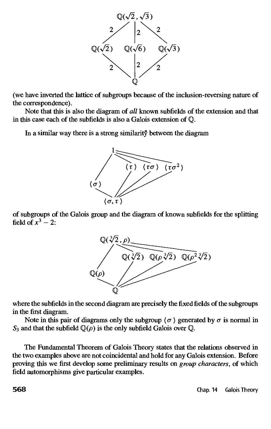
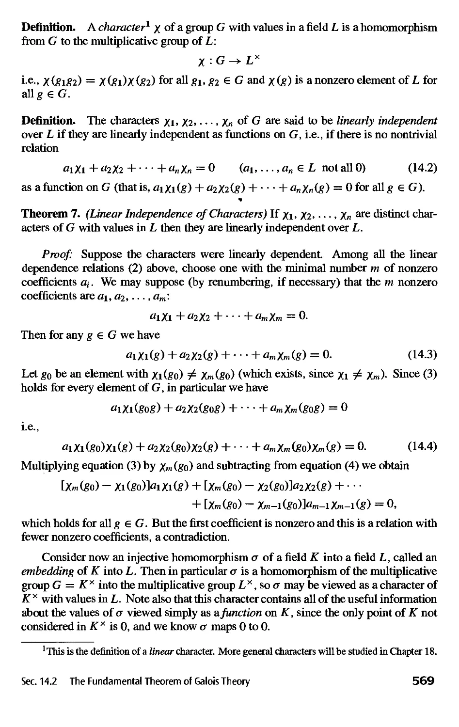
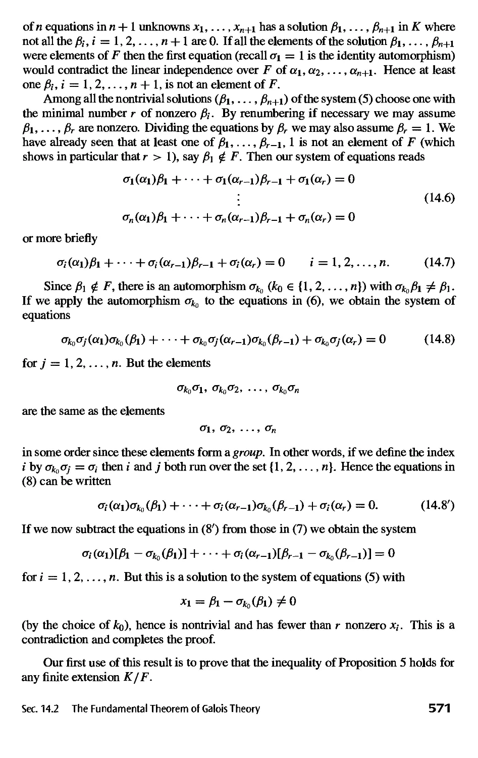
/


Автор: David S.
Теги: mathematics higher mathematics student book abstract algebra john wiley and sons publisher
ISBN: 0-471-43334-9
Год: 2004

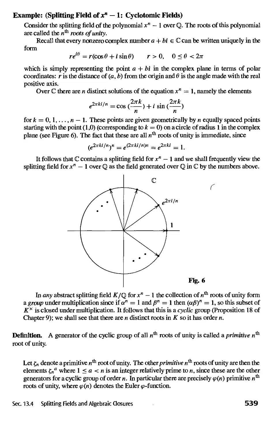
Текст
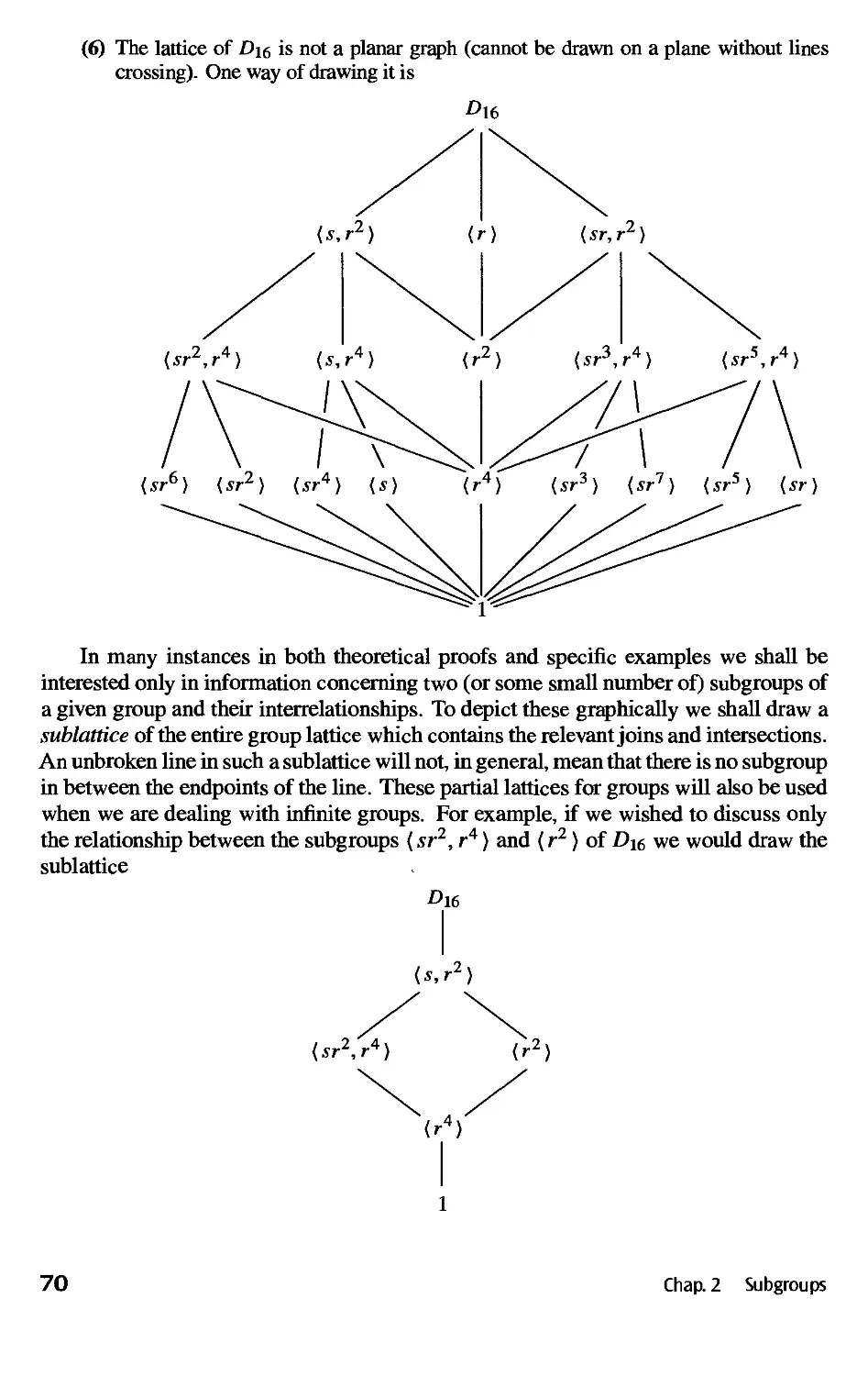
BST RACT
ALGEBRA
THIRD EDITION
DAVID S. DUMMIT
RICHARD M. FOOTE
Frequently Used Notation
f~\A)
a \b
\A\,\x\
Z/nZ
(Z/nZ)x
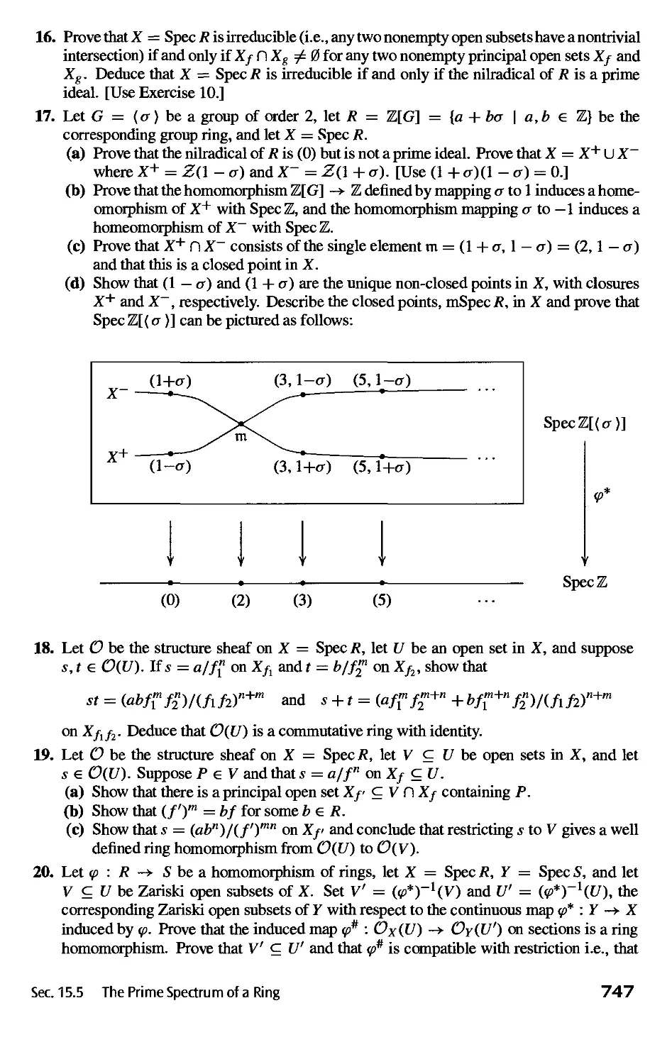
AxB
H <G
Zn
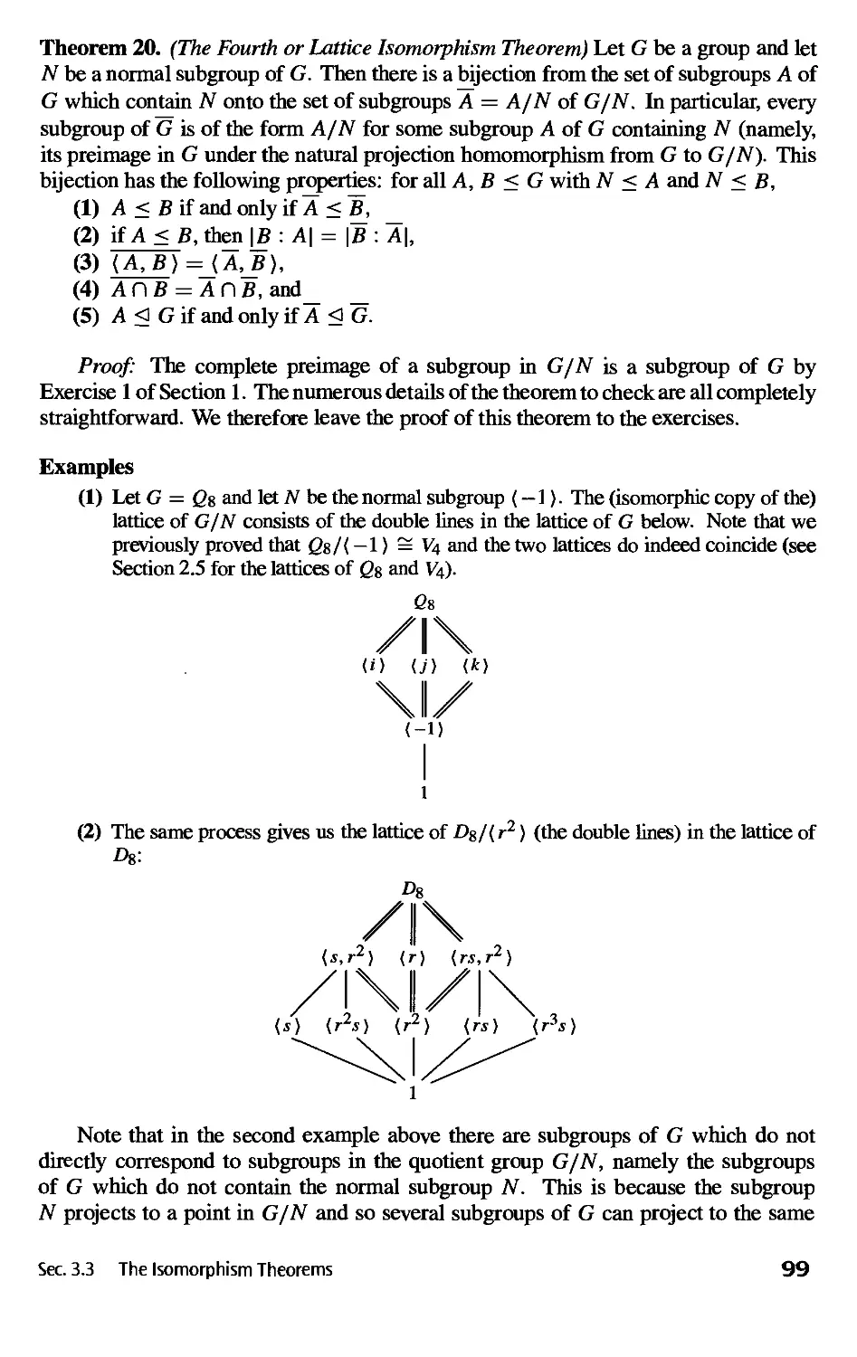
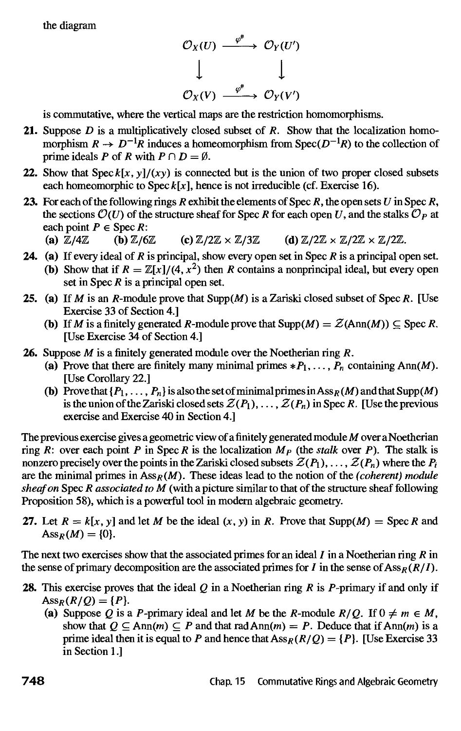
G8
v4
¥N
GLn(F), GL(V)
SLn(F)
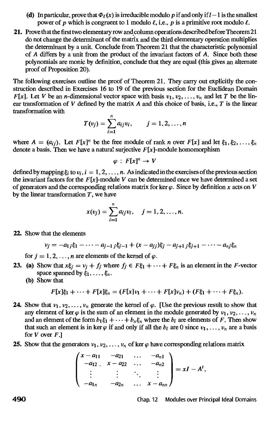
A = B
CG(A), NG(A)
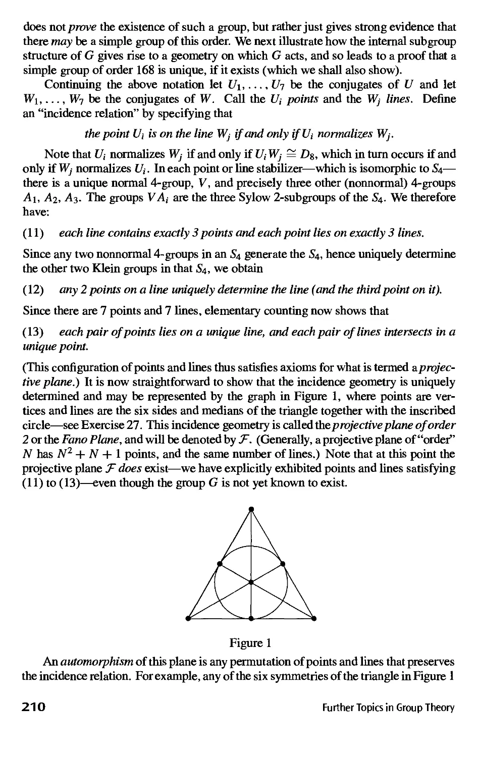
Z(G)
Gs
ker <p, im (p
N <G
gH,Hg
\G : H\
Aut(G)
SylP(G)
np
[x,y]
HxK
H
Rx
R[x],R[xi,...,xn]
RG,FG
OK
lim A,, ljm A,-
the inverse image or preimage of A under /
a divides b
the greatest common divisor oia,b
also the ideal generated by a, b
the order of the set A, the order of the element x
the integers, the positive integers
the rational numbers, the positive rational numbers
the real numbers, the positive real numbers
the complex numbers, the nonzero complex numbers
the integers modulo n
the (multiplicative group of) invertible integers modulo n
the direct or Cartesian product of A and B
H is a subgroup of G
the cyclic group of order n
the dihedral group of order 2«
the symmetric group on n letters, and on the set £2
the alternating group on n letters
the quaternion group of order 8
the Klein 4-group
the finite field of N elements
the general linear groups
the special linear group
A is isomorphic to B
the centralizer, and normalizer in G of A
the center of the group G
the stabilizer in the group G of s
the group generated by the set A, and by the element x
generators and relations (a presentation) for G
the kernel, and the image of the homomorphism <p
N is a normal subgroup of G
the left coset, and right coset of H with coset representative g
the index of the subgroup H in the group G
the automorphism group of the group G
the set of Sylow p-subgroups of G
the number of Sylow p-subgroups of G
the commutator of x, y
the semidirect product of H and K
the real Hamilton Quaternions
the multiplicative group of units of the ring R
polynomials in x, and in x\,..., xn with coefficients in R
the group ring of the group G over the ring R, and over the field F
the ring of integers in the number field K
the direct, and the inverse limit of the family of groups At ■
the p-adic integers, and the p-adic rationals
the direct sum of A and B
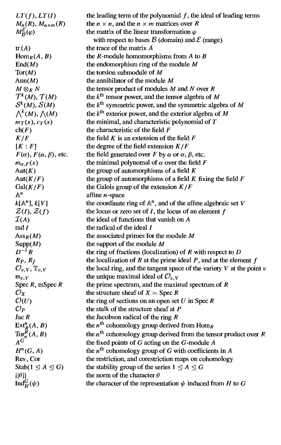
LT(f),LT(I)
Mn(R),MnXm(R)
trG4)
HomR(A,B)
End(M)
Tor(M)
Ann(M)
M®R N
Tk(M), T(M)
Sk{M), S(M)
Ak(.M), AW)
mT(x),cT(x)
ch(F)
K/F
[K:F]
F(a),F(a,P), etc.
ma,F(.x)
Aut(K)
Aut(K/F)
G&XK/F)
A"
Jfc[An], k[V]
), Z(f)
rad/
AssR(M)
Supp(M)
RP,Rf
Spec R, mSpec R
Ox
O{U)
Op
JacR
Exi"R{A,B)
AG
Hn(G,A)
Res, Cor
Stab(l < A < G)
Indg(^)
the leading term of the polynomial /, the ideal of leading terms
the n x n, and the n x m matrices over R
the matrix of the linear transformation (p
with respect to bases B (domain) and £ (range)
the trace of the matrix A
the R -module homomorphisms from A to B
the endomorphism ring of the module M
the torsion submodule of M
the annihilator of the module M
the tensor product of modules M and N over R
the kth tensor power, and the tensor algebra of M
the kth symmetric power, and the symmetric algebra of M
the k& exterior power, and the exterior algebra of M
the minimal, and characteristic polynomial of T
the characteristic of the field F
the field K is an extension of the field F
the degree of the field extension K/F
the field generated over F by a or a, fi, etc.
the minimal polynomal of a over the field F
the group of automorphisms of a field K
the group of automorphisms of a field K fixing the field F
the Galois group of the extension K/F
affine n-space
the coordinate ring of A", and of the affine algebraic set V
the locus or zero set of /, the locus of an element /
the ideal of functions that vanish on A
the radical of the ideal /
the associated primes for the module M
the support of the module M
the ring of fractions (localization) of R with respect to D
the localization of R at the prime ideal P, and at the element /
the local ring, and the tangent space of the variety V at the point v
the unique maximal ideal of Ovy
the prime spectrum, and the maximal spectrum of R
the structure sheaf of X = Spec R
the ring of sections on an open set U in Spec R
the stalk of the structure sheaf at P
the Jacobson radical of the ring R
the «* cohomology group derived from HomR
the «* cohomology group derived from the tensor product over R
the fixed points of G acting on the G-module A
the «* cohomology group of G with coefficients in A
the restriction, and corestriction maps on cohomology
the stability group of the series 1 < A < G
the norm of the character 6
the character of the representation \j/ induced from H to G
ABSTRACT ALGEBRA
Third Edition
David S. Dummit
University of Vermont
Richard M. Foote
University of Vermont
John Wiley & Sons, Inc.
ASSOCIATE PUBLISHER Laurie Rosatone
ASSISTANT EDITOR Jennifer Battista
FREELANCE DEVELOPMENTAL EDITOR Anne Scanlan-Rohrer
SENIOR MARKETING MANAGER Julie Z. Lindstrom
SENIOR PRODUCTION EDITOR KenSantor
COVER DESIGNER Michael Jung
This book was typeset using the Y&Y TeX System with DVIWindo. The text was set in Times Roman
using MathJime from Y&Y, Inc. Titles were set in OceanSans. This book was printed by Malloy Inc.
and the cover was printed by Phoenix Color Corporation.
This book is printed on acid-free paper.
Copyright © 2004 John Wiley and Sons, Inc. All rights reserved.
No part of this publication may be reproduced, stored in a retrieval system or transmitted in any form or by
any means, electronic, mechanical, photocopying, recording, scanning, or otherwise, except as permitted
under Sections 107 or 108 of the 1976 United States Copyright Act, without either the prior written
permission of the Publisher, or authorization through payment of the appropriate per-copy fee to the
Copyright Clearance Center, Inc., 222 Rosewood Drive, Danvers, MA 01923, E08) 750-8400. fax E08) 750-
4470. Requests to the Publisher for permission should be addressed to the Permissions Department, John
Wiley & Sons, Inc., 111 River Street, Hoboken, NJ 07030. B01O48-6011, fax B01O48-6008, E-mail:
PERMREQ@WILEY.COM.
To order books or for customer service please call 1-806-CALL WILEY B25-5945).
ISBN 0-471-43334-9
WIE 0-471-45234-3
Printed in the United States of America.
10 987654321
Dedicated to our families
especially
Janice, Evan, and Krysta
and
Zsuzsanna, Peter, Kamline, and Alexandra
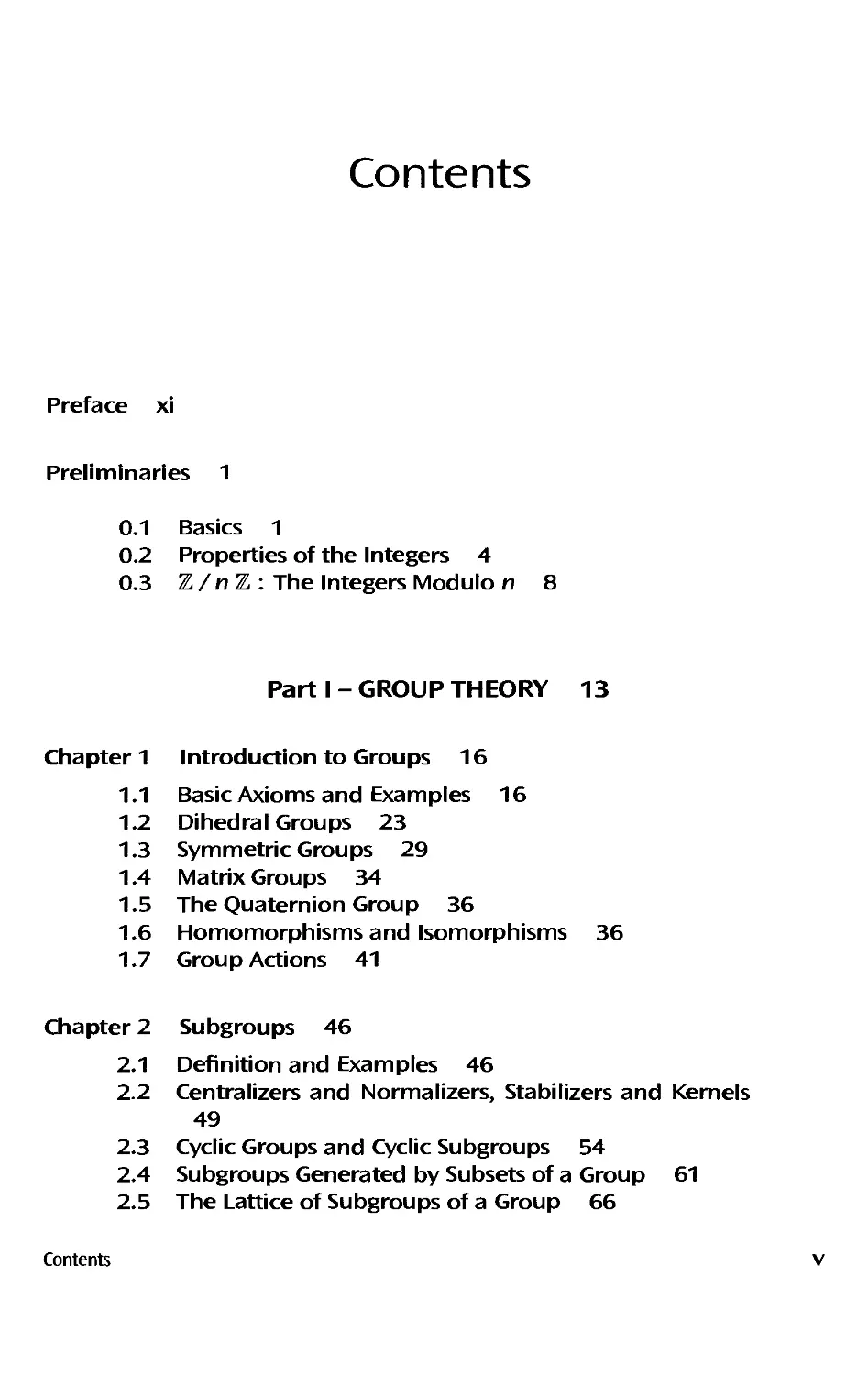
Contents
Preface xi
Preliminaries 1
0.1 Basics 1
0.2 Properties of the Integers 4
0.3 Z/nZ: The Integers Modulo n
8
Part I - GROUP THEORY 13
Chapter 1 Introduction to Groups 16
1.1 Basic Axioms and Examples 16
1.2 Dihedral Groups 23
1.3 Symmetric Groups 29
1.4 Matrix Groups 34
1.5 The Quaternion Group 36
1.6 Homomorphisms and Isomorphisms
1.7 Group Actions 41
36
Chapter 2 Subgroups 46
2.1 Definition and Examples 46
2.2 Centralizers and Normalizers, Stabilizers and Kernels
49
2.3 Cyclic Groups and Cyclic Subgroups 54
2.4 Subgroups Generated by Subsets of a Group 61
2.5 The Lattice of Subgroups of a Group 66
Contents
Chapter 3 Quotient Groups and Homomorphisms 73
3.1 Definitions and Examples 73
3.2 More on Cosets and Lagrange's Theorem 89
3.3 The Isomorphism Theorems 97
3.4 Composition Series and the Holder Program 101
3.5 Transpositions and the Alternating Group 106
Chapter 4 Group Actions 112
4.1 Group Actions and Permutation Representations 112
4.2 Groups Acting on Themselves by Left Multiplication—Cayley's
Theorem 118
4.3 Groups Acting on Themselves by Conjugation—The Class
Equation 122
4.4 Automorphisms 133
4.5 The Sylow Theorems 139
4.6 The Simplicity of An 149
Chapter 5 Direct and Semidirect Products and Abelian Groups 152
5.1 Direct Products 152
5.2 The Fundamental Theorem of Finitely Generated Abelian
Groups 158
5.3 Table of Groups of Small Order 167
5.4 Recognizing Direct Products 169
5.5 Semidirect Products 175
Chapter 6 Further Topics in Group Theory 188
6.1 p-groups, Nilpotent Groups, and Solvable Groups 188
6.2 Applications in Groups of Medium Order 201
6.3 A Word on Free Groups 215
Part II - RING THEORY 222
Chapter 7 Introduction to Rings 223
7.1 Basic Definitions and Examples 223
7.2 Examples: Polynomial Rings, Matrix Rings, and Group
Rings 233
7.3 Ring Homomorphisms an Quotient Rings 239
7.4 Properties of Ideals 251
7.5 Rings of Fractions 260
7.6 The Chinese Remainder Theorem 265
VI
Contents
Chapter 8 Euclidean Domains, Principal Ideal Domains and
Unique Factorization Domains 270
8.1 Euclidean Domains 270
8.2 Principal Ideal Domains (RI.D.s) 279
8.3 Unique Factorization Domains (U.F.D.s) 283
Chapter 9 Polynomial Rings 295
9.1 Definitions and Basic Properties 295
9.2 Polynomial Rings over Fields I 299
9.3 Polynomial Rings that are Unique Factorization Domains
303
9.4 Irreducibility Criteria 307
9.5 Polynomial Rings over Fields II 313
9.6 Polynomials in Several Variables over a Field and Grobner
Bases 315
Part III - MODULES AND VECTOR SPACES 336
Chapter 10 Introduction to Module Theory 337
10.1 Basic Definitions and Examples 337
10.2 Quotient Modules and Module Homomorphisms 345
10.3 Generation of Modules, Direct Sums, and Free Modules
351
10.4 Tensor Products of Modules 359
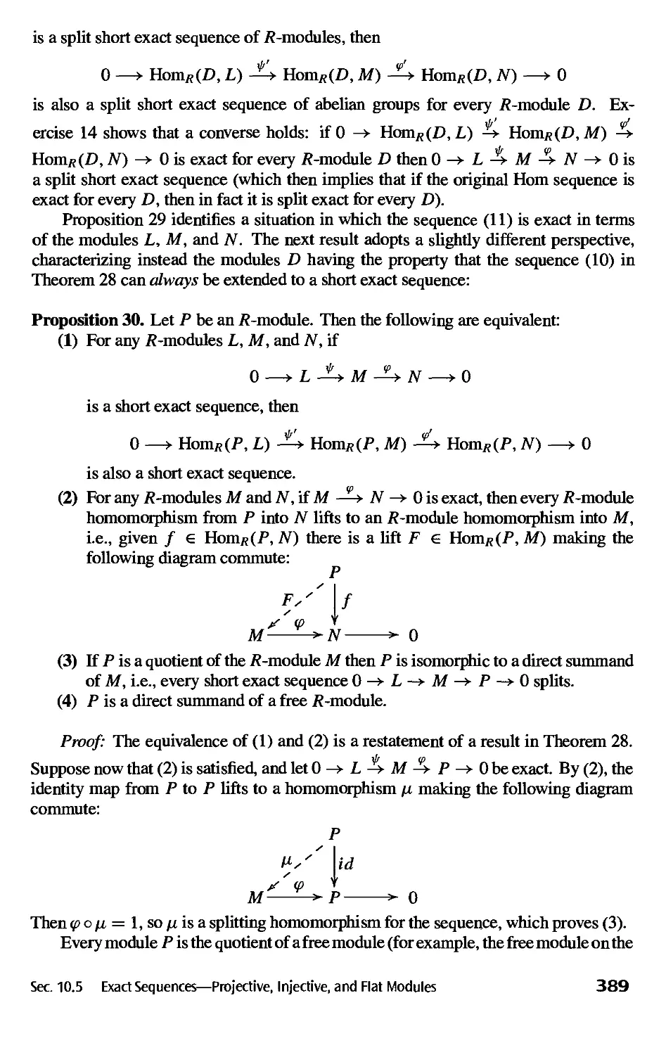
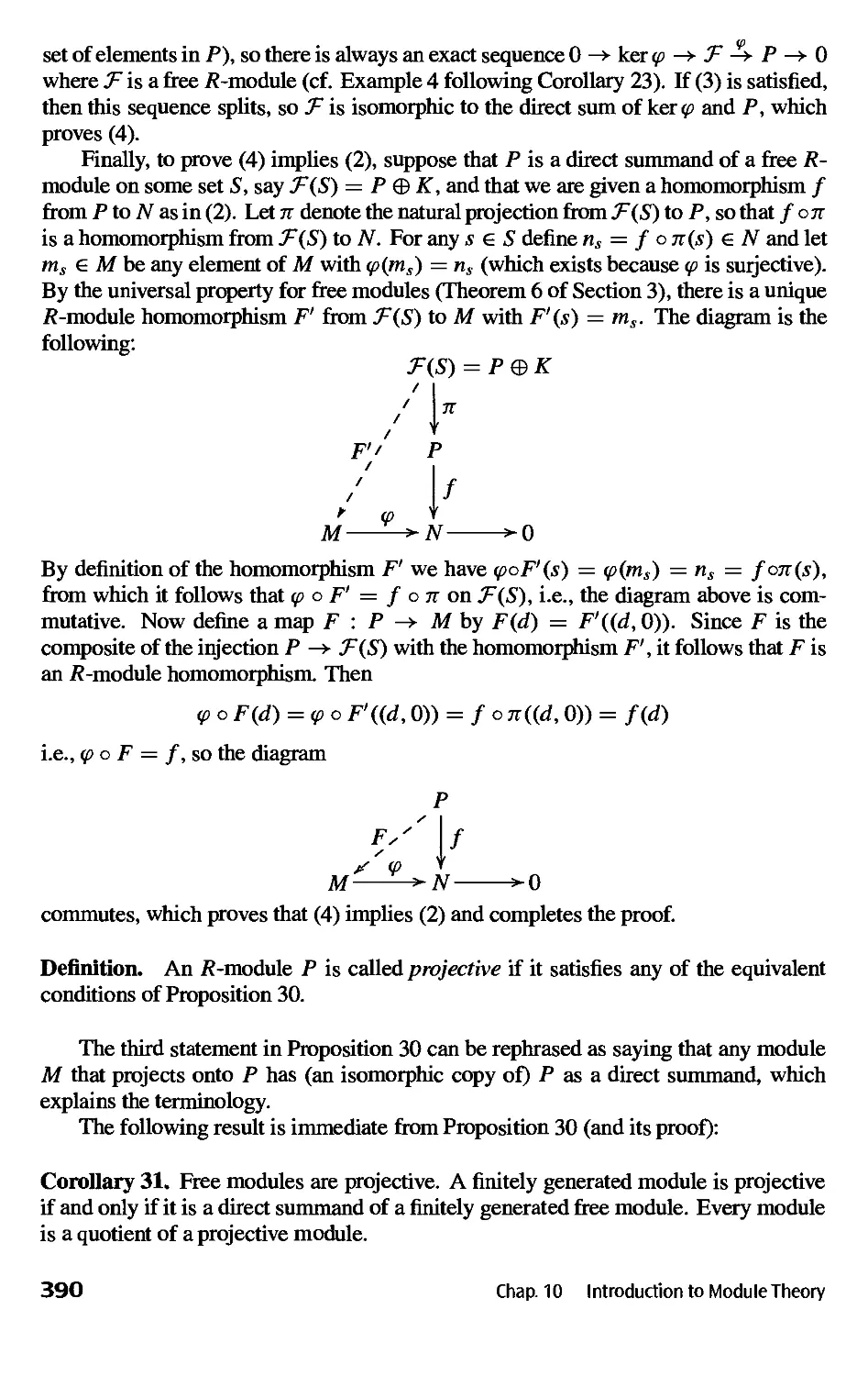
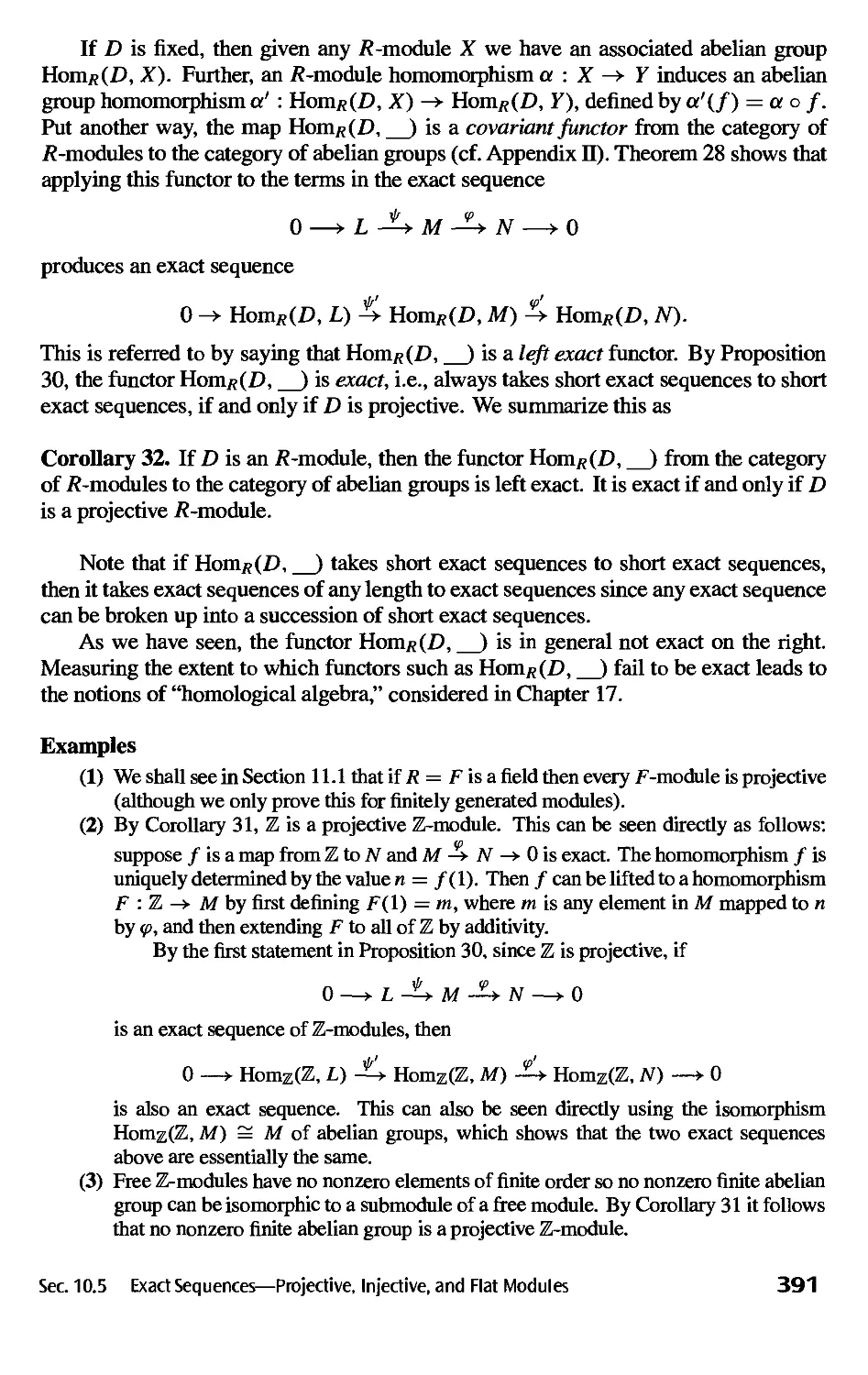
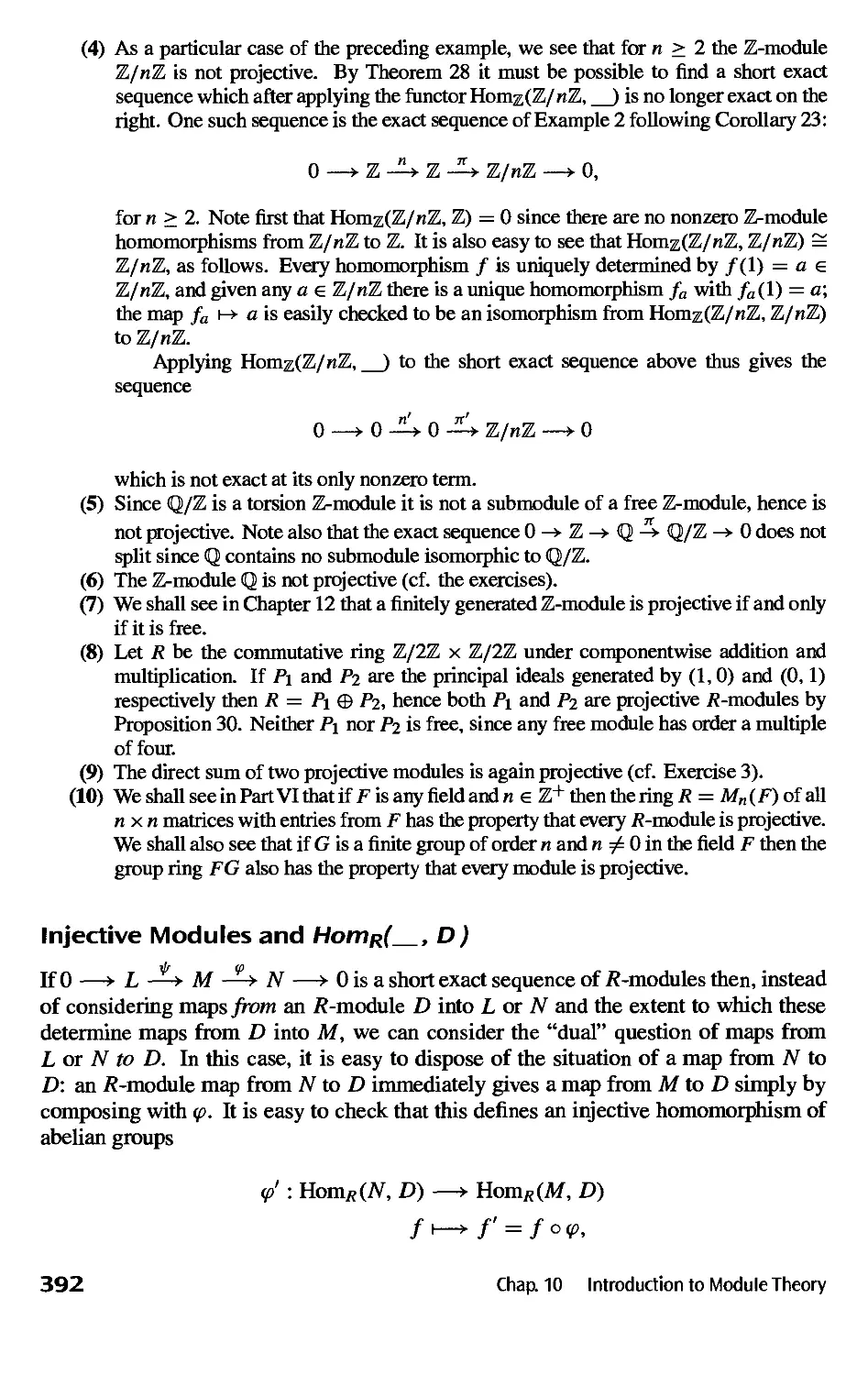
10.5 Exact Sequences—Projective, Injective, and Flat Modules
378
Chapter 11 Vector Spaces 408
11.1 Definitions and Basic Theory 408
11.2 The Matrix of a Linear Transformation 415
11.3 Dual Vector Spaces 431
11.4 Determinants 435
11.5 Tensor Algebras, Symmetric and Exterior Algebras
441
Chapter 12 Modules over Principal Ideal Domains 456
12.1 The Basic Theory 458
12.2 The Rational Canonical Form 472
12.3 The Jordan Canonical Form 491
Contents
VII
Part IV - FIELD THEORY AND GALOIS THEORY 509
Chapter 13 Reid Theory 510
' 13.1 Basic Theory of Field Extensions 510
13.2 Algebraic Extensions 520
13.3 Classical Straightedge and Compass Constructions
13.4 Splitting Fields and Algebraic Closures 536
13.5 Separable and Inseparable Extensions 545
13.6 Cyclotomic Polynomials and Extensions 552
531
Chapter 14 Galois Theory 558
14.1 Basic Definitions 558
14.2 The Fundamental Theorem of Galois Theory 567
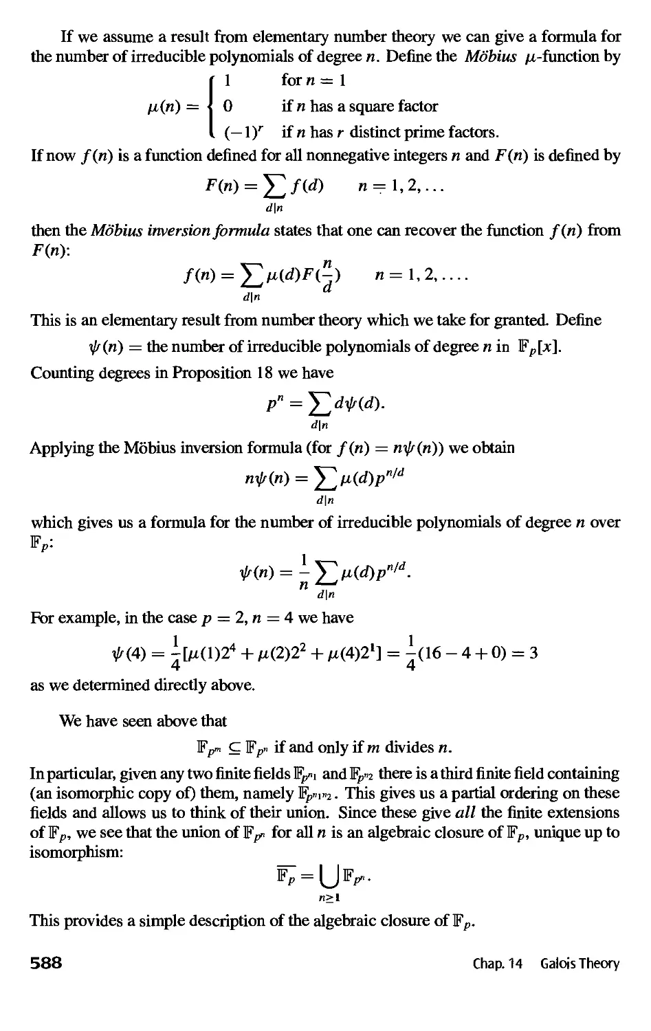
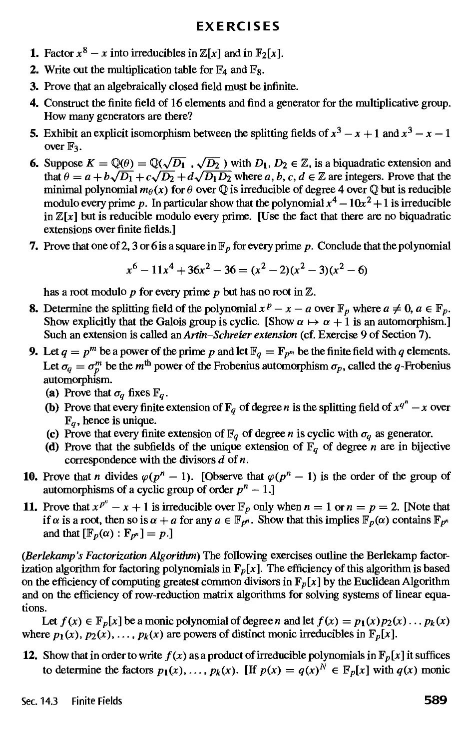
14.3 Finite Fields 585
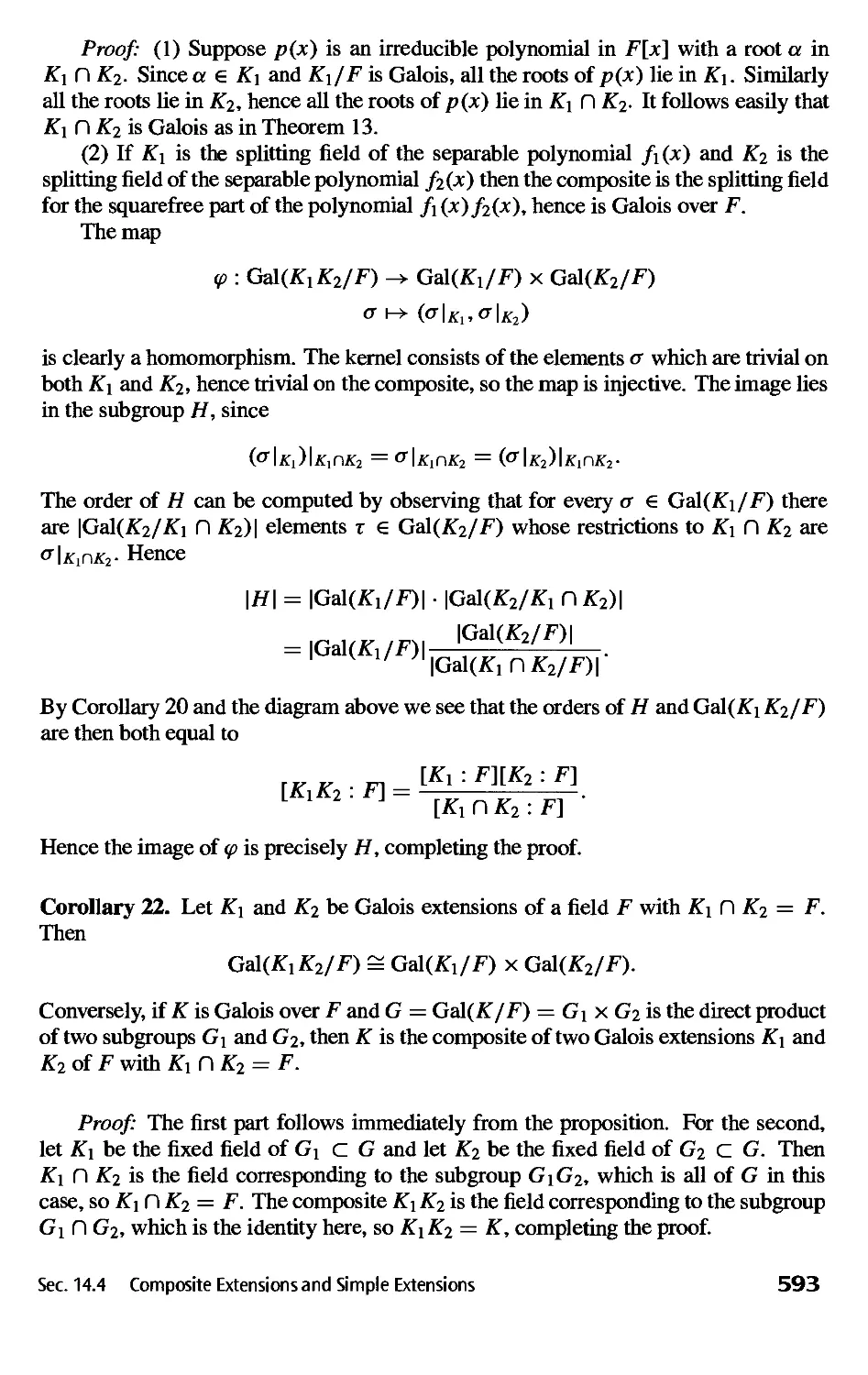
14.4 Composite Extensions and Simple Extensions 591
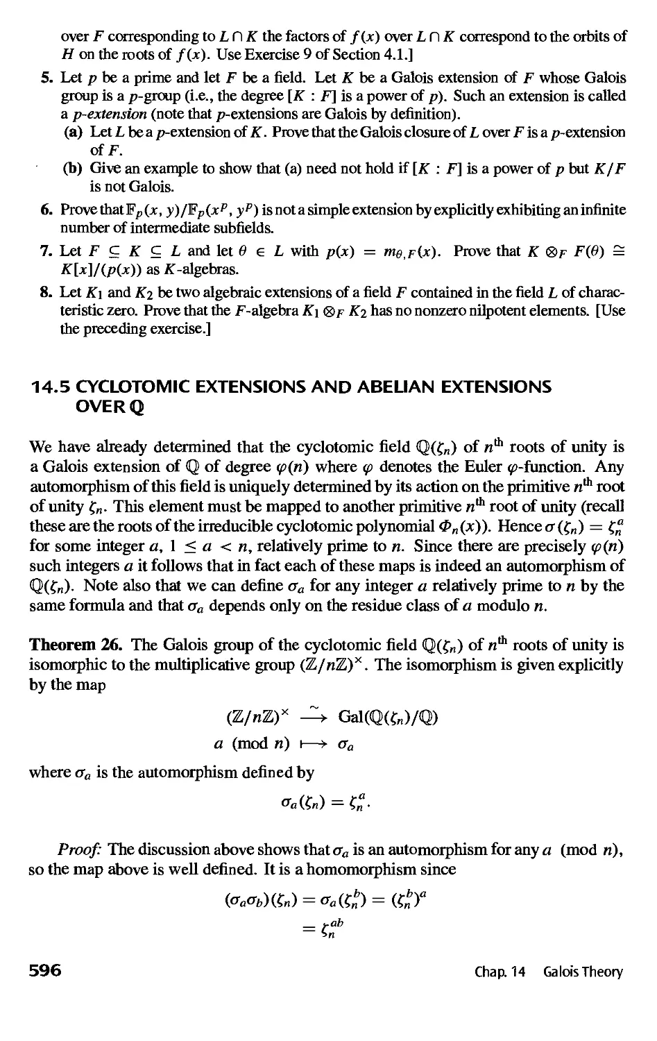
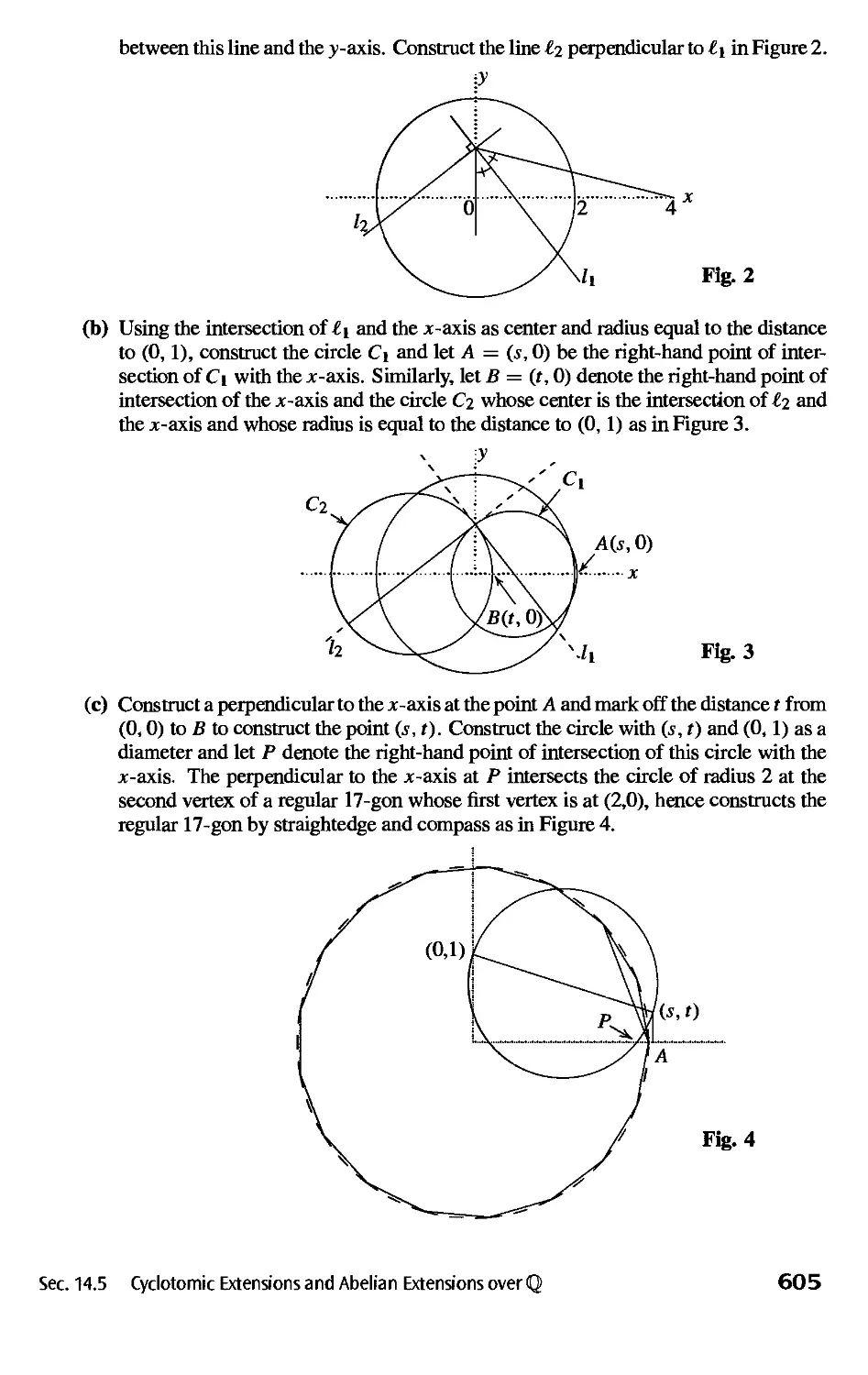
14.5 Cyclotomic Extensions and Abelian Extensions over Q
596
14.6 Galois Groups of Polynomials 606
14.7 Solvable and Radical Extensions: InsolvabilityoftheQuintic
625
14.8 Computation of Galois Groups over <Q> 640
14.9 Transcendental Extensions, Inseparable Extensions, Infinite
Galois Groups 645
Part V - AN INTRODUCTION TO COMMUTATIVE RINGS,
ALGEBRAIC GEOMETRY, AND
HOMOLOGICAL ALGEBRA 655
Chapter 15 Commutative Rings and Algebraic Geometry 656
15.1 Noetherian Rings and Affine Algebraic Sets 656
15.2 Radicals and Affine Varieties 673
15.3 Integral Extensions and Hilbert's Nullstellensatz 691
15.4 Localization 706
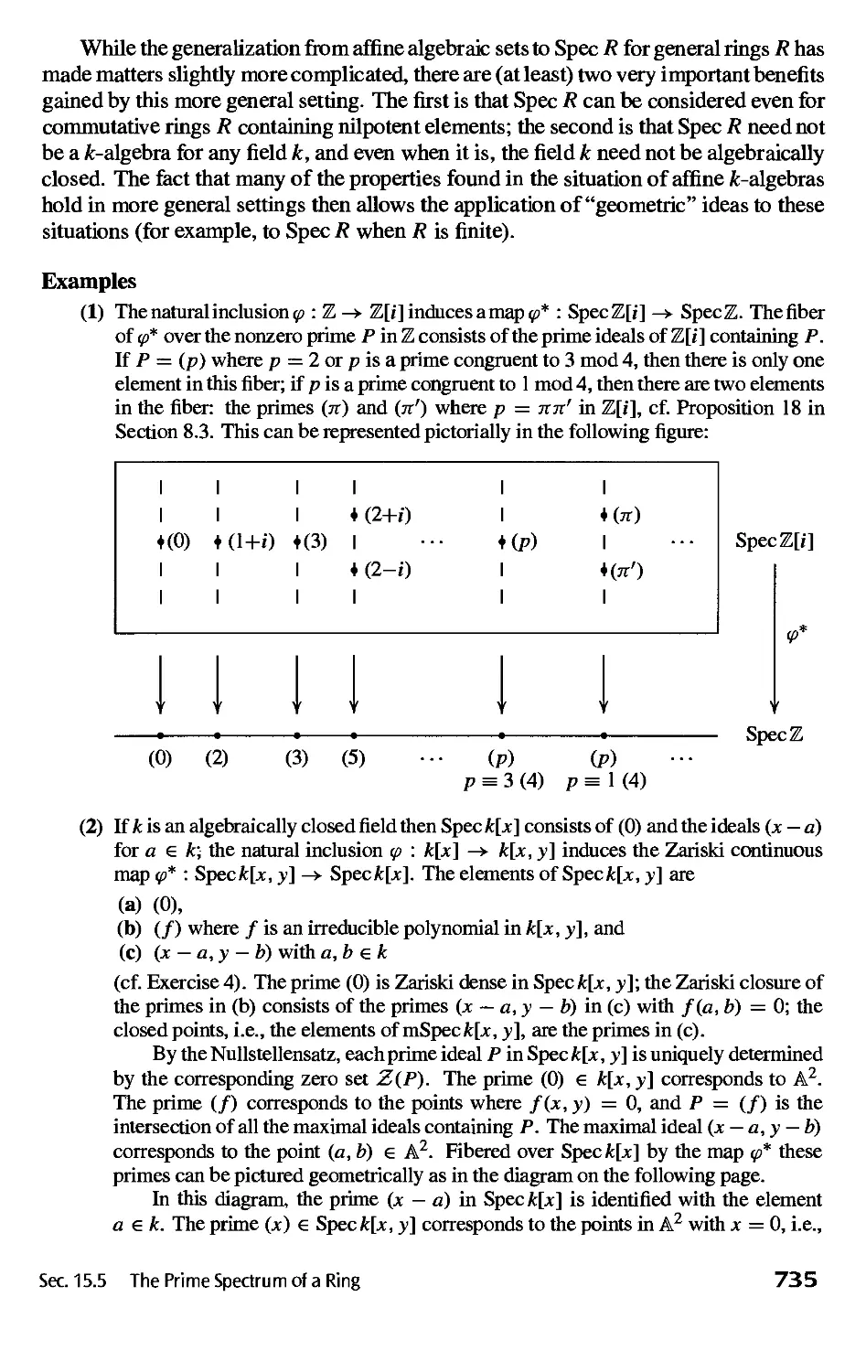
15.5 The Prime Spectrum of a Ring 731
Chapter 16 Artinian Rings, Discrete Valuation Rings, and
Dedekind Domains 750
16.1 Artinian Rings 750
16.2 Discrete Valuation Rings 755
16.3 Dedekind Domains 764
VIII
Content
Chapter 17 Introduction to Homological Algebra and
. Group Cohomology 776
17.1 Introduction to Homological Algebra—Ext and Tor
17.2 The Cohomology of Groups 798
17.3 Crossed Homomorphisms and H1(G, A) 814
17.4 Group Extensions, Factor Sets and H2(G, A) 824
777
Part VI - INTRODUCTION TO THE REPRESENTATION
THEORY OF FINITE GROUPS 839
Chapter 18 Representation Theory and Character Theory 840
18.1 Linear Actions and Modules over Group Rings 840
18.2 Wedderburn's Theorem and Some Consequences 854
18.3 Character Theory and the Orthogonality Relations 864
Chapter 19 Examples and Applications of Character Theory 880
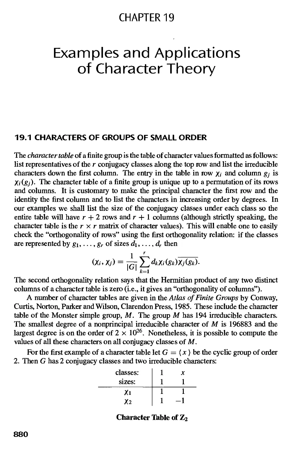
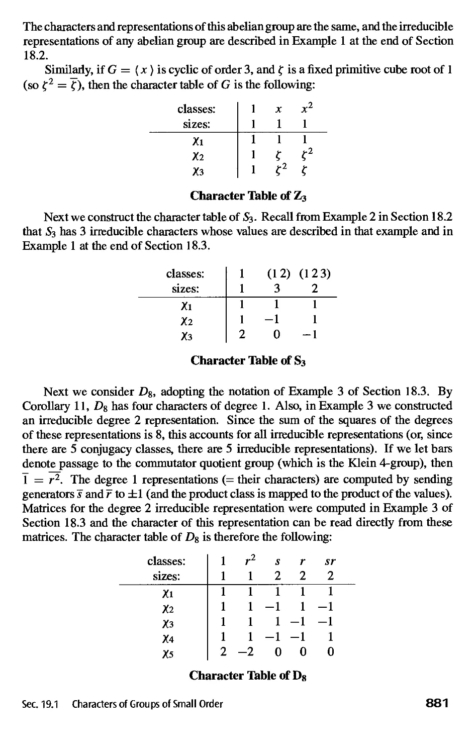
19.1 Characters of Groups of Small Order 880
19.2 Theorems of Burnside and Hall 886
19.3 Introduction to the Theory of Induced Characters 892
Appendix I: Cartesian Products and Zorn's Lemma 905
Appendix II: Category Theory 911
Index 919
Contents
IX
Preface to the Third Edition
The principal change from the second edition is the addition of Grobner bases to this
edition. The basic theory is introduced in a new Section 9.6. Applications to solving
systems of polynomial equations (elimination theory) appear at the end of this section,
rounding it out as a self-contained foundation in the topic. Additional applications and
examples are then woven into the treatment of affine algebraic sets and Jt-algebra homo-
morphisms in Chapter 15. Although the theory in the latter chapter remains independent
of Grobner bases, the new applications, examples and computational techniques sig-
significantly enhance the development, and we recommend that Section 9.6 be read either
as a segue to or in parallel with Chapter 15. A wealth of exercises involving Grobner
bases, both computational and theoretical in nature, have been added in Section 9.6
and Chapter 15. Preliminary exercises on Grobner bases can (and should, as an aid to
understanding the algorithms) be done by hand, but more extensive computations, and
in particular most of the use of Grobner bases in the exercises in Chapter 15, will likely
require computer assisted computation.
Other changes include a streamlining of the classification of simple groups of order
168 (Section 6.2), with the addition of a uniqueness proof via the projective plane of
order 2. Some other proofs or portions of the text have been revised slightly. A number
of new exercises have been added throughout the book, primarily at the ends of sections
in order to preserve as much as possible the numbering schemes of earlier editions.
In particular, exercises have been added on free modules over noncommutative rings
A0.3), on Krull dimension A5.3), and on flat modules A0.5 and 17.1).
As with previous editions, the text contains substantially more than can normally
be covered in a one year course. A basic introductory (one year) course should probably
include Part I up through Section 5.3, Part II through Section 9.5, Sections 10.1, 10.2,
10.3, 11.1, 11.2 and Part IV. Chapter 12 should also be covered, either before or after
Part IV. Additional topics from Chapters 5, 6, 9,10 and 11 may be interspersed in such
a course, or covered at the end as time permits.
Sections 10.4 and 10.5 are at a slightly higher level of difficulty than the initial
sections of Chapter 10, and can be deferred on a first reading for those following the text
sequentially. The latter section on properties of exact sequences, although quite long,
maintains coherence through a parallel treatment of three basic functors in respective
subsections.
Beyond the core material, the third edition provides significant flexibility for stu-
students and instructors wishing to pursue a number of important areas of modern algebra,
xi
either in the form of independent study or courses. For example, well integrated one-
semester courses for students with some prior algebra background might include the
following: Section 9.6 and Chapters 15 and 16; or Chapters 10 and 17; or Chapters 5,
6 and Part VI. Each of these would also provide a solid background for a follow-up
course delving more deeply into one of many possible areas: algebraic number theory,
algebraic topology, algebraic geometry, representation theory, Lie groups, etc.
The choice of new material and the style for developing and integrating it into the
text are in consonance with a basic theme in the book: the power and beauty that accrues
from a rich interplay between different areas of mathematics. The emphasis throughout
has been to motivate the introduction and development of important algebraic concepts
using as many examples as possible. We have not attempted to be encyclopedic, but
have tried to touch on many of the central themes in elementary algebra in a manner
suggesting the very natural development of these ideas.
A number of important ideas and results appear in the exercises. This is not because
they are not significant, rather because they did not fit easily into the flow of the text
but were too important to leave out entirely. Sequences of exercises on one topic
are prefaced with some remarks and are structured so that they may be read without
actually doing the exercises. In some instances, new material is introduced first in
the exercises—often a few sections before it appears in the text—so that students may
obtain an easier introduction to it by doing these exercises (e.g., Lagrange's Theorem
appears in the exercises in Section 1.7 and in the text in Section 3.2). All the exercises
are within the scope of the text and hints are given [in brackets] where we felt they were
needed. Exercises we felt might be less straightforward are usually phrased so as to
provide the answer to the exercise; as well many exercises have been broken down into
a sequence of more routine exercises in order to make them more accessible.
We have also purposely minimized the functorial language in the text in order to
keep the presentation as elementary as possible. We have refrained from providing
specific references for additional reading when there are many fine choices readily
available. Also, while we have endeavored to include as many fundamental topics as
possible, we apologize if for reasons of space or personal taste we have neglected any
of the reader's particular favorites.
We are deeply grateful to and would like here to thank the many students and
colleagues around the world who, over more than 15 years, have offered valuable
comments, insights and encouragement—their continuing support and interest have
motivated our writing of this third edition.
David Dummit
Richard Foote
June, 2003
xii Preface
Preliminaries
Some results and notation that are used throughout the text are collected in this chapter
for convenience. Students may wish to review this chapter quickly at first and then read
each section more carefully again as the concepts appear in the course of the text.
O.I BASICS
The basics of set theory: sets, D, U, e, etc. should be familiar to the reader. Our
notation for subsets of a given set A will be
B = {a G A | ... (conditions on a) ...}.
The order or cardinality of a set A will be denoted by \A\. If A is a finite set the order
of A is simply the number of elements of A.
It is important to understand how to test whether a particular x € A lies in a subset
B of A (cf. Exercises 1-4). The Cartesian product of two sets A and B is the collection
AxB = {(a, b) | a G A, b e B}, of ordered pairs of elements from A and B.
We shall use the following notation for some common sets of numbers:
A) Z = {0, ±1, ±2, ±3,...} denotes the integers (the Z is for the German word for
numbers: "Zahlen").
B) Q = [a/b | a, b e Z, b ^ 0} denotes the rational numbers (or rationals).
C) R = { all decimal expansions ± d\di • • • dn.a\aia?,...} denotes the real numbers
(or reals).
D) C = [a + bi \ a, b € M., i2 = —1} denotes the complex numbers.
E) Z+, Q+ and R+ will denote the positive (nonzero) elements in Z, Q and R, respec-
respectively.
f
We shall use the notation f: A—>BorA—>Bto denote a function / from A
to B and the value of / at a is denoted f(a) (i.e., we shall apply all our functions on
the left). We use the words function and map interchangeably. The set A is called the
domain of/ and B is called the codomain off. The notation f : a\-> bora \-> bif f
is understood indicates that f(a) = b, i.e., the function is being specified on elements.
If the function / is not specified on elements it is important in general to check
that / is well defined, i.e., is unambiguously determined. For example, if the set A
is the union of two subsets Ax and A-i then one can try to specify a function from A
to the set {0,1} by declaring that / is to map everything in Ai to 0 and is to map
everything in A% to 1. This unambiguously defines / unless A\ and A% have elements
in common (in which case it is not clear whether these elements should map to 0 or to
1). Checking that this / is well defined therefore amounts to checking that A\ and A-i
have no intersection.
The set
/(A) = {b G B | b = f{d). for some a e A}
is a subset of B, called the range or image of / (or the image of A under f). For each
subset C of B the set
f-\C) = [a g A | fia) g C}
consisting of the elements of A mapping into C under / is called thepreimage or inverse
image of C under /. For each b e B, the preimage of {&} under / is called theater of
/ over b. Note that f~l is not in general a function and that the fibers of / generally
contain many elements since there may be many elements of A mapping to the element
b.
If / : A —»■ B and g : B —»■ C, then the composite map g o / : A —»■ C is defined
by
Let / : A -» £.
A) / is infective or is an injection if whenever ai ^ O2> then /(fli) y^ f(fli)-
B) / is surjective or is a surjection if for all fc e 2? there is some a e A such that
/(a) = fc, i.e., the image of / is all of B. Note that since a function always maps
onto its range (by definition) it is necessary to specify the codomain B in order for
the question of surjectivity to be meaningful.
C) / is bijective or is a bijection if it is both injective and surjective. If such a bijection
/ exists from A to B, we say A and B are in bijective correspondence.
D) / has a left inverse if there is a function g : B -* A such that g o / : A —»■ A is
the identity map on A, i.e., (g o f)(a) = a, for all a G A.
E) / has a rigfo inverse if there is a function h : B —»■ A such that f o h : B —> B is
the identity map on Z?.
Proposition 1. Let / : A ->■ B.
A) The map / is injective if and only if / has a left inverse.
B) The map / is surjective if and only if / has a right inverse.
C) The map / is a bijection if and only if there exists g : B -»■ A such that fog
is the identity map on B and g o / is the identity map on A.
D) If A and B are finite sets with the same number of elements (i.e., \A\ = \B\),
then / : A —> B is bijective if and only if / is injective if and only if / is
surjective.
Proof: Exercise.
In the situation of part C) of the proposition above the map g is necessarily unique
and we shall say g is the 2-sided inverse (or simply the inverse) of /.
2 Preliminaries
A permutation of a set A is simply a bijection from A to itself.
If A c B and / : B —»■ C, we denote the restriction of / to A by /|^. When the
domain we are considering is understood we shall occasionally denote /1 a again simply
as / even though these are formally different functions (their domains are different).
If A c B and g : A -»■ C and there is a function f : B -* C such that f\A = g,
we shall say / is an extension ofgtoB (such a map / need not exist nor be unique).
Let A be a nonempty set.
A) A binary relation on a set A is a subset/? of Ax Aandwewritea ~fcif(a,fc) e /?.
B) The relation ~ on A is said to be:
(a) reflexive if a ~ a, for all a G A,
(b) symmetric if a ~ b implies b ~ a for all a, ft G A,
(c) transitive if a ~ fc and fc ~ c implies a ~ c for all a,b,c€ A.
A relation is an equivalence relation if it is reflexive, symmetric and transitive.
C) If ~ defines an equivalence relation on A, then the equivalence class of a G A is
defined to be {x e A | x ~ a}. Elements of the equivalence class of a are said
to be equivalent to a. If C is an equivalence class, any element of C is called a
representative of the class C.
D) A partition of A is any collection {A, | i e /} of nonempty subsets of A (/ some
indexing set) such that
(a) A = Uig/A,- , and
(b) A, n Aj = 0, for all i, j e / with / ^ j
i.e., A is the disjoint union of the sets in the partition.
The notions of an equivalence relation on A and a partition of A are the same:
Proposition 2. Let A be a nonempty set.
A) If ~ defines an equivalence relation on A then the set of equivalence classes of
~ form a partition of A.
B) If {A, | i £ /} is a partition of A then there is an equivalence relation on A
whose equivalence classes are precisely the sets A,, / e /.
Proof: Omitted.
Finally, we shall assume the reader is familiar with proofs by induction.
EXERCISES
In Exercises 1 to 4 let A. be the set of 2 x 2 matrices with real number entries. Recall that
matrix multiplication is defined by
Let
Sect. 0.1 Basics
(o b\(P i\ = (aP + br aq+bs\
c d)\r s J \cp + dr cq + ds J
(i !)
and let
B = {X € A | MX = XM).
1. Determine which of the following elements of A. lie in B:
(I 1\ A 1\ /0 0\ /I l\ (I 0\ @ l\
2. Prove that if P, Q € B, then P+Q e B (where + denotes the usual sum of two matrices).
3. Prove that if P, Q € B, then P-Q e B (where • denotes the usual product of two matrices).
4. Find conditions on p, q, r, s which determine precisely when
lp q I € B.
5. Determine whether the following functions / are well defined:
(a) / : Q -*■ Z defined by f(a/b) = a.
(b) / : Q -*■ Q defined by f(a/b) = a2/b2.
6. Determine whether the function / : R+ —*■ 1 defined by mapping a real number r to the
first digit to the right of the decimal point in a decimal expansion of r is well defined.
7. Let / : A —>• B be a surjective map of sets. Prove that the relation
a ~ b if and only if f(a) = f(b)
is an equivalence relation whose equivalence classes are the fibers of /.
0.2 PROPERTIES OF THE INTEGERS
The following properties of the integers Z (many familiar from elementary arithmetic)
will be proved in a more general context in the ring theory of Chapter 8, but it will
be necessary to use them in Part I (of course, none of the ring theory proofs of these
properties will rely on the group theory).
A) (Well Ordering of Z) If A is any nonempty subset of Z+, there is some element
m G A such that m < a, for all a G A (m is called a minimal element of A).
B) If a, b G Z with a ^ 0, we say a divides b if there is an element ceZ such that
b = ac. In this case we write a \ b; if a does not divide b we write a \ b.
C) If a, b G Z — {0}, there is a unique positive integer d, called the greatest common
divisor of a and b (or g.c.d. of a and b), satisfying:
(a) d | a and d \ b (so d is a common divisor of a and b), and
(b) if e | a and e | fc, then e | d (so d is the greatest such divisor).
The g.c.d. of a and b will be denoted by (a, b). If (a, b) = 1, we say that a and b
are relatively prime.
D) If a, fc G Z — {0}, there is a unique positive integer /, called the least common
multiple of a and b (or lx.m. of a and b), satisfying:
(a) a | / and b | / (so / is a common multiple of a and b), and
(b) if a | m and fc | m, then I | m (so I is the least such multiple).
The connection between the greatest common divisor d and the least common
multiple / of two integers a and b is given by dl = ab.
E) The Division Algorithm: ifa,b G Z — {0}, then there exist unique #, r G Z such
that
a = qb + r and 0<r<|fc|,
4 Preliminaries
where q is the quotient and r the remainder. This is the usual "long division"
familiar from elementary arithmetic.
F) The Euclidean Algorithm is an important procedure which produces a greatest
common divisor of two integers a and b by iterating the Division Algorithm: if
a,b eZ — {0}, then we obtain a sequence of quotients and remainders
a = qob + r0 @)
b = qir0 + n A)
ro = qir\ + r2 B)
r\ = q^r2 + r3 C)
rn-2 = qnrn-\ + rn (n)
rn-i=qn+irn (n+1)
where rn is the last nonzero remainder. Such an rn exists since \b\ > |ro| > \r\ | >
• • • > \rn | is a decreasing sequence of strictly positive integers if the remainders
are nonzero and such a sequence cannot continue indefinitely. Then rn is the g.c.d.
(a, b) of a andb.
Example
Suppose a = 57970 and b = 10353. Then applying the Euclidean Algorithm we obtain:
57970 = EI0353 + 6205
10353 = AN205+ 4148
6205 = AL148 + 2057
4148 = BJ057 + 34
2057 = F0K4 + 17
34 = BI7
which shows that E7970,10353) = 17.
G) One consequence of the Euclidean Algorithm which we shall use regularly is the
following: if a, b e Z — {0}, then there exist xjeZ such that
(a, b) = ax +by
that is, the g.c.d. of a and b is a Z-linear combination of a and b. This follows
by recursively writing the element rn in the Euclidean Algorithm in terms of the
previous remainders (namely, use equation (n) above to solve for rn = rn_2—qnrn-\
in terms of the remainders rn-\ and rn-%, then use equation (n — 1) to write rn in
terms of the remainders rn-% and rn_3, etc., eventually writing rn in terms of a and
b).
Sec. 0.2 Properties of the Integers 5
Example
Supposeo = 57970 andfc = 10353, whose greatest common divisor we computed above to
be 17. From the fifth equation (the next to last equation) in the Euclidean Algorithm applied
to these two integers we solve for their greatest common divisor: 17 = 2057 - F0K4.
The fourth equation then shows that 34 = 4148 — BJ057, so substituting this expression
for the previous remainder 34 gives the equation 17 = 2057 - F0)[4148 — BJ057], i.e.,
17 = A21J057 — F0L148. Solving the third equation for 2057 and substituting gives
17 = A21)[6205 - AL148] - F0L148 = A21N205 - A81L148. Using the second
equation to solve for 4148 and then the first equation to solve for 6205 we finally obtain
17 = C02M7970 - A691I0353
as can easily be checked directly. Hence the equation ax + by = (a, b) for the greatest
common divisor of a and b in this example has the solution x = 302 and y = —1691. Note
that it is relatively unlikely that this relation would have been found simply by guessing.
The integers x and y in G) above are not unique. In the example with a = 57970
and b = 10353 we determined one solution to be x = 302 and y = —1691, for
instance, and it is relatively simple to check that x = —307 and y = 1719 also
satisfy 57970x + 10353y = 17. The general solution for x and y is known (cf. the
exercises below and in Chapter 8).
(8) An element p of Z+ is called a prime if p > 1 and the only positive divisors of p are
1 and p (initially, the word prime will refer only to positive integers). An integer
n > 1 which is not prime is called composite. For example, 2,3,5,7,11,13,17,19,...
are primes and 4,6,8,9,10,12,14,15,16,18,... are composite.
An important property of primes (which in fact can be used to define the primes
(cf. Exercise 3)) is the following: if p is a prime and p \ ab, for some a, b e Z,
then either p \ a or p \ b.
(9) The Fundamental Theorem of Arithmetic says: if n G Z, n > 1, then n can
be factored uniquely into the product of primes, i.e., there are distinct primes
Pi, Pi, ••■, Ps and positive integers ct\, a-i,..., as such that
This factorization is unique in the sense that if q\,q%, ...,qt are any distinct primes
and f$\, fa, • • •, fit positive integers such that
then s = t and if we arrange the two sets of primes in increasing order, then qi = pi
anda,- = ft, 1 < i < s. For example, n = 1852423848 = 233211219331 and this
decomposition into the product of primes is unique.
Suppose the positive integers a and b are expressed as products of prime powers:
where Pi, P2, ■ ■ ■, Ps are distinct and the exponents are > 0 (we allow the exponents
to be 0 here so that the products are taken over the same set of primes—the exponent
will be 0 if that prime is not actually a divisor). Then the greatest common divisor
of a and Ms
(a, b) = p*™*-"^p*™****'^ # # . pmin(as,ft)
Preliminaries
(and the least common multiple is obtained by instead taking the maximum of the
a, and /3,- instead of the minimum).
Example
In the example above, a = 57970 and b = 10353 can be factored as a = 2 • 5 • 11 • 17 • 31
and b = 3 • 7 • 17 • 29, from which we can immediately conclude that their greatest common
divisor is 17. Note, however, that for large integers it is extremely difficult to determine
their prime factorizations (several common codes in current use are based on this difficulty,
in fact), so that this is not an effective method to determine greatest common divisors in
general. The Euclidean Algorithm will produce greatest common divisors quite rapidly
without the need for the prime factorization of a and b.
10) The Eider (p-function is defined as follows: for n G Z+ let (p(n) be the number of
positive integers a < n with a relatively prime to n, i.e., (a, ri) = 1. For example,
<p(\2) = 4 since 1, 5, 7 and 11 are the only positive integers less than or equal
to 12 which have no factors in common with 12. Similarly, (p(l) = 1, (pB) = 1,
<pC) = 2, <pD) = 2, <pE) = 4, <pF) = 2, etc. For primes p, <p(p) = p - 1, and,
more generally, for all a > 1 we have the formula
The function (p is multiplicative in the sense that
<p(ab) = (p(a)<p(b) \f(a,b) = l
(note that it is important here that a and b be relatively prime). Together with the for-
formula above this gives a general formula for the values of (p : if n = pi' p%2... p"s,
then
= PT~\P1 - DP?-\P2 - 1) ■•• P?-\ps - 1).
For example, <pA2) = <pB2)<pC) = 2XB - 1K°C - 1) = 4. The reader should
note that we shall use the letter (p for many different functions throughout the text
so when we want this letter to denote Eider's function we shall be careful to indicate
this explicitly.
EXERCISES
1. For each of the following pairs of integers a and b, determine their greatest common
divisor, their least common multiple, and write their greatest common divisor in the form
ax + by for some integers x and y.
(a) a = 20, b = 13.
(b) a = 69, b = 372.
(c) a = 792, b = 275.
(d) a = 11391, b = 5673.
(e) a = 1761, b = 1567.
(f) a = 507885, b = 60808.
2. Prove that if the integer k divides the integers a and b then k divides as + bt for every pair
of integers s and t.
Sec. 0.2 Properties of the Integers 7
3. Prove that if n is composite then there are integers a and b such that n divides ab but n
does not divide either a or b.
4. Let a, b and N be fixed integers with a and b nonzero and let d = (a, b) be the greatest
common divisor of a and b. Suppose xo and yo are particular solutions to ax + by = N
(i.e., oxq + byo = N). Prove for any integer t that the integers
b a
x = xo + -t and y = yO—-t
a a
are also solutions to ax + by = N (this is in fact the general solution).
5. Determine the value (p(n) for each integer n < 30 where (p denotes the Euler ^-function.
6. Prove the Well Ordering Property of Z by induction and prove the minimal element is
unique.
7. If p is a prime prove that there do not exist nonzero integers a and b such that a2 = pb2
(i.e., ,/p is not a rational number).
8. Let p be a prime, « € Z+. Find a formula for the largest power of p which divides
«! = «(«— 1)(« — 2)... 2 • 1 (it involves the greatest integer function).
9. Write a computer program to determine the greatest common divisor (a, b) of two integers
a and b and to express (a, b) in the form ax + by for some integers x and y.
10. Prove for any given positive integer N there exist only finitely many integers n with
(p(n) = N where (p denotes Euler's ^-function. Conclude in particular that (p(n) tends to
infinity as n tends to infinity.
11. Prove that if d divides n then (p(d) divides (p(n) where (p denotes Euler's ^-function.
03 Z/n Z : THE INTEGERS MODULO n
Let n be a fixed positive integer. Define a relation on Z by
a ~ b if and only if n \ (b — a).
Clearly a ~ a, and a ~ b implies b ~ a for any integers a and b, so this
relation is trivially reflexive and symmetric. If a ~ b and b ~ c then n divides a — fc
and n divides b — c so n also divides the sum of these two integers, i.e., n divides
(a — b) + (b — c) = a — c, so a ~ c and the relation is transitive. Hence this is an
equivalence relation. Write a = b (mod ri) (read: a is congruent to fc mod n) if a ~ fc.
For any teZwe shall denote the equivalence class of a by a — this is called the
congruence class or residue class of a mod n and consists of the integers which differ
from a by an integral multiple of n, i.e.,
a = {a + kn \ k e Z}
= {a,a±n,a±2n,a±3n,...}.
There are precisely n distinct equivalence classes mod n, namely
0,1,2, ...,n-\
determined by the possible remainders after division by n and these residue classes
partition the integers Z. The set of equivalence classes under this equivalence relation
8 Preliminaries
will be denoted by Z/nZ and called the integers modulo n (or the integers mod n).
The motivation for this notation will become clearer when we discuss quotient groups
and quotient rings. Note that for different n's the equivalence relation and equivalence
classes are different so we shall always be careful to fix n first before using the bar
notation. The process of finding the equivalence class mod n of some integer a is often
referred to as reducing a mod n. This terminology also frequently refers to finding the
smallest nonnegative integer congruent to a mod n (the least residue of a mod n).
We can define an addition and a multiplication for the elements of Z/nZ, defining
modular arithmetic as follows: for a, b e Z/nZ, define their sum and product by
a+b = a + b and d-b = ab.
What this means is the following: given any two elements a and b in Z/nZ, to compute
their sum (respectively, their product) take any representative integer a in the class
a and any representative integer b in the class b and add (respectively, multiply) the
integers a and b as usual in Z and then take the equivalence class containing the result.
The following Theorem 3 asserts that this is well defined, i.e., does not depend on the
choice of representatives taken for the elements a and b of Z/nZ.
Example
Suppose n = 12 and consider Z/12Z, which consists of the twelve residue classes
6,1,2,....IT
determined by the twelve possible remainders of an integer after division by 12. The
elements in the residue class 5, for example, are the integers which leave a remainder of 5
when divided by 12 (the integers congruent to 5 mod 12). Any integer congruent to 5 mod
12 (such as 5,17,29,... or —7, —19,...) will serve as a representative for the residue class
5. Note that Z/12Z consists of the twelve elements above (and each of these elements of
Z/12Z consists of an infinite number of usual integers).
Suppose now that a = 5andfo = 8. The most obvious representative for a is the integer
5 and similarly 8 is the most obvious representative for b. Using these representatives for
the residue classes we obtain 5 + 8=13 = 1 since 13 and 1 lie in the same class modulo
n = 12. Had we instead taken the representative 17, say, for a (note that 5 and 17 do lie in
the same residue class modulo 12) and the representative —28, say, for b, we would obtain
5 + 8 = A7-28) = —11 = 1 and as we mentioned the result does not depend on the
choice of representatives chosen. The product of these two classes is o-i» = 5 • 8 = 40 = 4,
also independent of the representatives chosen.
Theorem 3. The operations of addition and multiplication on Z/nZ defined above
are both well defined, that is, they do not depend on the choices of representatives for
the classes involved. More precisely, if a\, a% G Z and b\,b% G Z with a[ = bi and
«2 = b2, then a\ +a2 = b\ + b2 and a[ai = b\bi, i.e., if
ai = b\ (mod n) and a% = bi (mod n)
then
a\ + fl2 = b\ + &2 (mod n) and a\a% = b\b% (mod n).
Sec. 0.3 Z/nZ: The Integers Modulo n 9
Proof: Suppose^ = b\ (mod n),i.e.,ai — b\ is divisible by n. Thenai = b\+sn
for some integer s. Similarly, a2 = bi (mod ri) means 02 = *2 +1n for some integer t.
Thenai+fl2 = (bi+b2)+(s+t)n sothatai+fl2 = *i+&2 (mod ri), which shows that
the sum of the residue classes is independent of the representatives chosen. Similarly,
flifl2 = (bi+sn)(l>2+tn) = b\b2+(blt+b2S+stri)n shows that aia2 = b\bi (mod ri)
and so the product of the residue classes is also independent of the representatives
chosen, completing the proof.
We shall see later that the process of adding equivalence classes by adding their
representatives is a special case of a more general construction (the construction of
a quotient). This notion of adding equivalence classes is already a familiar one in
the context of adding rational numbers: each rational number a/b is really a class of
expressions: a/b = 2a/2b = —3a/ — 3b etc. and we often change representatives
(for instance, take common denominators) in order to add two fractions (for example
1/2 + 1/3 is computed by taking instead the equivalent representatives 3/6 for 1/2
and 2/6 for 1/3 to obtain 1/2 + 1/3 = 3/6 + 2/6 = 5/6). The notion of modular
arithmetic is also familiar: to find the hour of day after adding or subtracting some
number of hours we reduce mod 12 and find the least residue.
It is important to be able to think of the equivalence classes of some equivalence
relation as elements which can be manipulated (as we do, for example, with fractions)
rather than as sets. Consistent with this attitude, we shall frequently denote the elements
of Z/nZ simply by {0, 1,..., n — 1} where addition and multiplication are reduced mod
n. It is important to remember, however, that the elements of Z/nZ are not integers, but
rather collections of usual integers, and the arithmetic is quite different. For example,
5 + 8 is not 1 in the integers Z as it was in the example of Z/12Z above.
The fact that one can define arithmetic in Z/nZ has many important applications
in elementary number theory. As one simple example we compute the last two digits in
the number 21000. First observe that the last two digits give the remainder of 21000 after
we divide by 100 so we are interested in the residue class mod 100 containing 21000.
We compute 210 = 1024 = 24 (mod 100), so then 220 = B10J = 242 = 576 = 76
(mod 100). Then 240 = B20J = 762 = 5776 = 76 (mod 100). Similarly 280 =
2i60 _ 2320 = 2640 = 76 (mod 100). Finally, 21000 = 26402320240 = 76 • 76 • 76 = 76
(mod 100) so the final two digits are 76.
An important subset of Z/nZ consists of the collection of residue classes which
have a multiplicative inverse in Z/nZ:
(Z/nZ)x = {a g Z/nZ | there exists c e Z/nZ with a ■ c = 1}.
Some of the following exercises outline a proof that (Z/nZ)x is also the collection
of residue classes whose representatives are relatively prime to n, which proves the
following proposition.
Proposition 4. (Z/nZ)x = [a e Z/nZ | (a, ri) = 1}.
It is easy to see that if any representative of a is relatively prime to n then all
representatives are relatively prime to n so that the set on the right in the proposition is
well defined.
10 Preliminaries
Example
For n = 9 we obtain (Z/9Z)X = {T, 2,4,5,7, 8} from the proposition. The multiplicative
inverses of these elements are {1,5,7,2,4, 8}, respectively.
If a is an integer relatively prime to n then the Euclidean Algorithm produces integers
x and y satisfying ax + ny = 1, hence ax = 1 (mod ri), so that x is the multiplicative
inverse of a in Z/nZ. This gives an efficient method for computing multiplicative
inverses in Z/nZ.
Example
Suppose n = 60 and a = 17. Applying the Euclidean Algorithm we obtain
60= CI7 + 9
17 =A)9+ 8
9 = A)8 + 1
so that a and n are relatively prime, and (-7I7 + BN0 = 1. Hence ^7 = 53 is the
multiplicative inverse of 17 in Z/60Z.
EXERCISES
1. Write down explicitly all the elements in the residue classes of Z/18Z.
2. Prove that the distinct equivalence classes in Z/nZ are precisely 6,1,2,...,« — 1 ( use
the Division Algorithm).
3. Prove that if a = on10" + On-ilO" -\ h a\ 10 + o0 is any positive integer then
a = an + an-i H + a\ + oo (mod 9) (note that this is the usual arithmetic rule that
the remainder after division by 9 is the same as the sum of the decimal digits mod 9 — in
particular an integer is divisible by 9 if and only if the sum of its digits is divisible by 9)
[note that 10=1 (mod 9)].
4. Compute the remainder when 37100 is divided by 29.
5. Compute the last two digits of 91500.
6. Prove that the squares of the elements in Z/4Z are just 6 and 1.
7. Prove for any integers a and b that a2 + b2 never leaves a remainder of 3 when divided by
4 (use the previous exercise).
8. Prove that the equation a2 + b2 = 3c2 has no solutions in nonzero integers a, b and c.
[Consider the equation mod 4 as in the previous two exercises and show that a, b and c
would all have to be divisible by 2. Then each of a2, b2 and c2 has a factor of 4 and by
dividing through by 4 show that there would be a smaller set of solutions to the original
equation. Iterate to reach a contradiction.]
9. Prove that the square of any odd integer always leaves a remainder of 1 when divided by
10. Prove that the number of elements of (Z/«Z)X is <p(n) where <p denotes the Euler <p-
function.
11. Prove that if a, b € (Z/«Z)X, then a-be (Z/«Z)X.
Sec. 0.3 Z/nZ: The Integers Modulon 11
12. Let n e Z, n > 1, and let a e Z with 1 < a < n. Prove if a and n are not relatively prime,
there exists an integer b with 1 < b < n such that ab = O (mod «) and deduce that there
cannot be an integer c such that ac = 1 (mod «).
13. Let n e Z, n > 1, and let o € Z with 1 < a < n. Prove that if a and « are relatively prime
then there is an integer c such that ac = 1 (mod ri) ^[use the fact that the g.c.d. of two
integers is a Z-linear combination of the integers].
14. Conclude from the previous two exercises that (Z/nZ) x is the set of elements a of Z/nZ
with (a, n) = 1 and hence prove Proposition 4. Verify this directly in the case n = 12.
15. For each of the following pairs of integers a and n, show that a is relatively prime to n and
determine the multiplicative inverse of a in Z/nZ.
(a) o = 13, n = 20.
(b) o = 69, « = 89.
(c) o = 1891, n = 3797.
(d) a - 6003722857, « = 77695236973. [The Euclidean Algorithm requires only 3
steps for these integers.]
16. Write a computer program to add and multiply mod «, for any n given as input. The output
of these operations should be the least residues of the sums and products of two integers.
Also include the feature that if (a, n) = 1, an integer c between 1 and « — 1 such that
a ■ c = 1 may be printed on request. (Your program should not, of course, simply quote
"mod" functions already built into many systems).
12 Preliminaries
Parti
GROUP THEORY
The modern treatment of abstract algebra begins with the disarmingly simple abstract
definition ofa group. This simple definition quickly leads to difficult questions involving
the structure of such objects. There are many specific examples of groups and the power
of the abstract point of view becomes apparent when results for all of these examples
are obtained by proving a single result for the abstract group.
The notion of a group did not simply spring into existence, however, but is rather the
culmination of a long period of mathematical investigation, the first formal definition
of an abstract group in the form in which we use it appearing in 1882.1 The definition
of an abstract group has its origins in extremely old problems in algebraic equations,
number theory, and geometry, and arose because very similar techniques were found
to be applicable in a variety of situations. As Otto Holder A859-1937) observed, one
of the essential characteristics of mathematics is that after applying a certain algorithm
or method of proof one then considers the scope and limits of the method. As a result,
properties possessed by a number of interesting objects are frequently abstracted and
the question raised: can one determine all the objects possessing these properties?
Attempting to answer such a question also frequently adds considerable understanding
of the original objects under consideration. It is in this fashion that the definition of an
abstract group evolved into what is, for us, the starting point of abstract algebra.
We illustrate with a few of the disparate situations in which the ideas later formalized
into the notion of an abstract group were used.
A) In number theory the very object of study, the set of integers, is an example of a
group. Consider for example what we refer to as "Euler's Theorem" (cf. Exercise
22 of Section 3.2), one extremely simple example of which is that a40 has last two
digits 01 if a is any integer not divisible by 2 nor by 5. This was proved in 1761
by Leonhard Euler A707-1783) using "group-theoretic" ideas of Joseph Louis
Lagrange A736-1813), long before the first formal definition of a group. From
our perspective, one now proves "Lagrange's Theorem" (cf. Theorem 8 of Section
3.2), applying these techniques abstracted to an arbitrary groupy-and then recovers
Euler's Theorem (and many others) as a special case.
1For most of the historical comments below, see the excellent bookA History of Algebra, by B. L.
vanderWaerden, Springer-Verlag, 1980 and the references there, particularly The Genesis of the Abstract
Group Concept: A Contribution to the History of the Origin of Abstract Group Theory (translated from
the German by Abe Shenitzer), by H. Wussing, MIT Press, 1984. See also Number Theory, An Approach
Through History from Hammurapai to Legendre, by A. Weil, Birich&iser; 1984.
13
B) Investigations into the question of rational solutions to algebraic equations of the
form y2 = x3 — 2x (there are infinitely many, for example @,0), (—1,1), B, 2),
(9/4, -21/8), (-1/169, 239/2197)) showed that connecting any two solutions by
a straight line and computing the intersection of this line with the curve y2 =
x3 — 2x produces another solution. Such "Diophantine equations," among others,
were considered by Pierre de Fermat A601-1655) (this one was solved by him in
1644), by Euler, by Lagrange around 1777, and others. In 1730 Euler raised the
question of determining the indefinite integral / dx/^/l — x4 of the "lemniscatic
differential" dx/*Jl — x4, used in determining the arc length along an ellipse (the
question had also been considered by Gottfried Wilhelm Leibniz A646-1716) and
Johannes Bernoulli A667-1748)). In 1752 Euler proved a "multiplication formula"
for such elliptic integrals (using ideas of G.C. di Fagnano A682-1766), received
by Euler in 1751), which shows how two elliptic integrals give rise to a third,
bringing into existence the theory of elliptic functions in analysis. In 1834 Carl
Gustav Jacob Jacobi A804-1851) observed that the work of Euler on solving certain
Diophantine equations amounted to writing the multiplication formula for certain
elliptic integrals. Today the curve above is referred to as an "elliptic curve" and
these questions are viewed as two different aspects of the same thing — the fact
that this geometric operation on points can be used to give the set of points on an
elliptic curve the structure of a group. The study of the "arithmetic" of these groups
is an active area of current research.2
C) By 1824 it was known that there are formulas giving the roots of quadratic, cubic
and quartic equations (extending the familiar quadratic formula for the roots of
ax2 + bx + c = 0). In 1824, however, Niels Henrik Abel A802-1829) proved
that such a formula for the roots of a quintic is impossible (cf. Corollary 40 of
Section 14.7). The proof is based on the idea of examining what happens when
the roots are permuted amongst themselves (for example, interchanging two of the
roots). The collection of such permutations has the structure of a group (called,
naturally enough, a "permutation group"). This idea culminated in the beautiful
work of Evariste Galois A811-1832) in 1830-32, working with explicit groups
of "substitutions." Today this work is referred to as Galois Theory (and is the
subject of the fourth part of this text). Similar explicit groups were being used
in geometry as collections of geometric transformations (translations, reflections,
etc.) by Arthur Cayley A821-1895) around 1850, Camille Jordan A838-1922)
around 1867, Felix Klein A849-1925) around 1870, etc., and the application of
groups to geometry is still extremely active in current research into the structure of
3-space, 4-space, etc. The same group arising in the study of the solvability of the
quintic arises in the study of the rigid motions of an icosahedron in geometry and
in the study of elliptic functions in analysis.
The precursors of today's abstract group can be traced back many years, even
before the groups of "substitutions" of Galois. The formal definition of an abstract
group which is our starting point appeared in 1882 in the work of Walter Dyck A856-
1934), an assistant to Felix Klein, and also in the work of Heinrich Weber A842-1913)
2See The Arithmetic of Elliptic Curves by J. Silverman, Springer-Verlag, 1986.
14
in the same year.
It is frequently the case in mathematics research to find specific application of
an idea before having that idea extracted and presented as an item of interest in its
own right (for example, Galois used the notion of a "quotient group" implicitly in his
investigations in 1830 and the definition of an abstract quotient group is due to Holder in
1889). It is important to realize, with or without the historical context, that the reason the
abstract definitions are made is because it is useful to isolate specific characteristics and
consider what structure is imposed on an object having these characteristics. The notion
of the structure of an algebraic object (which is made more precise by the concept of
an isomorphism — which considers when two apparently different objects are in some
sense the same) is a major theme which will recur throughout the text.
15
CHAPTER 1
Introduction to Groups
1.1 BASIC AXIOMS AND EXAMPLES
In this section the basic algebraic structure to be studied in Part I is introduced and some
examples are given.
Definition.
A) A binary operation • on a set G is a function • : GxG —»■ G. For any a,b e G
we shall write a * b for *(a, b).
B) A binary operation • on a set G is associative if for all a, b, c e G we have
a * (b * c) = (a * b) * c.
C) If • is a binary operation on a set G we say elements a and boiG commute if
a*b = b*a. We say + (oi G) is commutative if for all a, b e G,a*b = b*a.
Examples
A) + (usual addition) is a commutative binary operation on Z (or on Q, R, or C respec-
respectively).
B) x (usual multiplication) is a commutative binary operation on Z (or on Q, R, or C
respectively).
C) - (usual subtraction) is a noncommutative binary operation on Z, where — (a, b) =
a — b. The map a t->- — a is not a binary operation (not binary).
D) — is not a binary operation on Z+ (nor Q+, R+) because for o, fc € Z+ with a < b,
a-b#Z+, that is, - does not map Z+ x Z+ into Z+.
E) Taking the vector cross-product of two vectors in 3-space R3 is a binary operation
which is not associative and not commutative.
Suppose that • is a binary operation on a set G and H is a subset of G. If the
restriction of * to H is a binary operation on H, i.e., for all a, b e //, a * b e //,
then H is said to be closed under *. Observe that if • is an associative (respectively,
commutative) binary operation on G and • restricted to some subset H of G is a binary
operation on H, then • is automatically associative (respectively, commutative) on H
as well.
Definition.
A) A group is an ordered pair (G, •) where G is a set and • is a binary operation
on G satisfying the following axioms:
16
(i) (a + b)*c = a*(b* c), for all a, b, c e G, i.e., • is associative,
(ii) there exists an element e in G, called an identity of G, such that for all
a G G we have a*e = e*a=a,
(iii) for each a e G there is an element a of G, called an inverse of a,
such that a * a~x = a • a = e.
B) The group (G, •) is called abelian (or commutative )ii a*b = b • a for all
We shall immediately become less formal and say G is a group under • if (G, •) is
a group (or just G is a group when the operation • is clear from the context). Also, we
say G is a finite group if in addition G is a finite set. Note that axiom (ii) ensures that
a group is always nonempty.
Examples
A) Z, Q, R and C are groups under + with e = 0 and o = — a, for all a.
B) Q - {0}, R - {0}, C - {0}, Q+, R+ are groups under x with e = 1 and a'1 = -,
a
for all a. Note however that Z — {0} is no* a group under x because although x is an
associative binary operation on Z — {0}, the element 2 (for instance) does not have an
inverse in Z - {0}.
We have glossed over the fact that the associative law holds in these familiar ex-
examples. For Z under + this is a consequence of the axiom of associativity for addition
of natural numbers. The associative law for Q under + follows from the associative
law for Z — a proof of this will be outlined later when we rigorously construct <Q> from
Z (cf. Section 7.5). The associative laws for R and, in turn, C under + are proved
in elementary analysis courses when R is constructed by completing Q — ultimately,
associativity is again a consequence of associativity for Z. The associative axiom for
multiplication may be established via a similar development, starting first with Z. Since
R and C will be used largely for illustrative purposes and we shall not construct R from
<Q> (although we shall construct C from R) we shall take the associative laws (under +
and x ) for R and C as given.
Examples (continued)
C) The axioms for a vector space V include those axioms which specify that (V, +) is an
abelian group (the operation + is called vector addition). Thus any vector space such
as R" is, in particular, an additive group.
D) For n € Z+, Z/nZ is an abelian group under the operation + of addition of residue
classes as described in Chapter 0. We shall prove in Chapter 3 (in a more general
context) that this binary operation + is well defined and associative; for now we take
this for granted. The identity in this group is the element 6 and for each a € Z/nZ,
the inverse of a is ~^a. Henceforth, when we talk about the group Z/nZ it will be
understood that the group operation is addition of classes mod n.
E) For n e Z+, the set (Z/«Z)X of equivalence classes a which have multiplicative
inverses mod «is an abelian group under multiplication of residue classes as described
in Chapter 0. Again, we shall take for granted (for the moment) that this operation
is well defined and associative. The identity of this group is the element 1 and, by
Sec. 1.1 Basic Axioms and Examples 17
definition of (Z/nZ)x, each element has a multiplicative inverse. Henceforth, when
we talk about the group (Z/nZ)x it will be understood that the group operation is
multiplication of classes mod n.
F) If (A, •) and (B, o) are groups, we can form a new group A x B, called their direct
product, whose elements are those in the Cartesian product
A xB = {(a,b)\aeA, b € B)
and whose operation is defined componentwise:
@1, bi)(a2, bi) = @1 *ci2,bio b£).
For example, if we take A = B = E (both operations addition), E x E is the familiar
Euclidean plane. The proof that the direct product of two groups is again a group is
left as a straightforward exercise (later) — the proof that each group axiom holds in
AxBisa consequence of that axiom holding in both A and B together with the fact
that the operation in A x B is defined componentwise.
There should be no confusion between the groups "L/riL (under addition) and
(Z/nZ)x (under multiplication), even though the latter is a subset of the former — the
superscript x will always indicate that the operation is multiplication.
Before continuing with more elaborate examples we prove two basic results which
in particular enable us to talk about the identity and the inverse of an element
Proposition 1. If G is a group under the operation •, then
A) the identity of G is unique
B) for each a € G, a~x is uniquely determined
C) (fiT1) =aforalla€G
D) (fl*fe)-1 = (fe)*(fl-1)
E) for any at, «2,..., an € G the value of a.\ *<X2 * • • • *an is independent of how
the expression is bracketed (this is called the generalized associative law).
Proof: A) If / and g are both identities, then by axiom (ii) of the definition of a
group / • g = / (take a = / and e = g). By the same axiom / • g = g (take a = g
and e = /). Thus f = g, and the identity is unique.
B) Assume b and c are both inverses of a and let e be the identity of G. By axiom
(iii), a*b = e and c*a = e. Thus
c = c*e (definition of e - axiom (ii))
= c * (a *b) (since e = a+b)
= (c*d)*b (associative law)
= e • b (since e = c * a )
= b (axiom (ii)).
C) To show (a) = a is exactly the problem of showing a is the inverse of a
(since by part B) a has a unique inverse). Reading the definition of a, with the roles
of a and a~l mentally interchanged shows that a satisfies the defining property for the
inverse of a, hence a is the inverse of a.
18 Chap. 1 Introduction to Groups
D) Let c = (a*b) 1 so by definition of c, (a • b) • c = e. By the associative law
a • (b • c) = e.
Multiply both sides on the left by a to get
a + (a + (b + c)) = a • e.
The associative law on the left hand side and the definition of e on the right give
(a-1+a) + (b + c)=a-i
so
e • (b • c) = a
hence
b + c = a~l.
Now multiply both sides on the left by b~x and simplify similarly:
e*c =
as claimed.
E) This is left as a good exercise using induction on n. First show the result is true
for n = 1,2, and 3. Next assume for any k < n that any bracketing of a product of k
elements, bi*b2*---*bk can be reduced (without altering the value of the product) to
an expression of the form
Now argue that any bracketing of the product a.\ * a% * • ■ • • an must break into 2
subproducts, say (a.\ • a.% • • • • • a*) * fe+i *fl*+2 * • • • * an), where each sub-product
is bracketed in some fashion. Apply the induction assumption to each of these two
sub-products and finally reduce the result to the form a\ • (a.2 * fe •(•••• an ))...) to
complete the induction.
Note that throughout the proof of Proposition 1 we were careful not to change
the order of any products (unless permitted by axioms (ii) and (iii)) since G may be
non-abelian.
Notation:
A) For an abstract group G it is tiresome to keep writing the operation • throughout
our calculations. Henceforth (except when necessary) our abstract groups G, H,
etc. will always be written with the operation as • and a • b will always be written
as ab. In view of the generalized associative law, products of three or more group
elements will not be bracketed (although the operation is still a binary operation).
Finally, for an abstract group G (operation •) we denote the identity of G by 1.
Sec 1.1 Basic Axioms and Examples 19
B) For any group G (operation • implied) and x e G and n e Z+ since the product
xx ■■ -x (n terms) does not depend on how it is bracketed, we shall denote it by x".
Denote x^x'1 ■ ■ ■ x'1 (n terms) by x~". Let x° = 1, the identity of G.
This new notation is pleasantly concise. Of course, when we are dealing with
specific groups, we shall use the natural (given) operation. For example, when the
operation is +, the identity will be denoted by 0 and for any element a, the inverse a~l
will be written —a and a + a-\ \-a(n > 0 terms) will be written na; —a — a a
(n terms) will be written — na and Oa = 0.
Proposition 2. Let G be a group and let a,b € G. The equations ax = b and ya = b
have unique solutions for x, y € G. In particular, the left and right cancellation laws
hold in G, i.e.,
A) if au = av, then u = v, and
B) if ub = vb, then u = v.
Proof: We can solve ax — b by multiplying both sides on the left by aT1 and
simplifying to get x = a~lb. The uniqueness of x follows because aT1 is unique.
Similarly, if ya = b, y = ba~l. If aw = av, multiply both sides on the left by a~x and
simplify to get u = v. Similarly, the right cancellation law holds.
One consequence of Proposition 2 is that if a is any element of G and for some
b € G, ab = e or ba = e, then b = a~1, i.e., we do not have to show both equations
hold. Also, if for some b € G,ab = a (or ba = a), then b must be the identity of G,
i.e., we do not have to check bx = xb = x for all x e G.
Definition. For G a group and x e G define the order of x to be the smallest positive
integer n such that x" = 1, and denote this integer by |jc|. In this case x is said to be of
order n. If no positive power of x is the identity, the order of x is defined to be infinity
and x is said to be of infinite order.
The symbol for the order of x should not be confused with the absolute value symbol
(when Gclwe shall be careful to distinguish the two). It may seem injudicious to
choose the same symbol for order of an element as the one used to denote the cardinality
(or order) of a set, however, we shall see that the order of an element in a group is the
same as the cardinality of the set of all its (distinct) powers so the two uses of the word
"order" are naturally related.
Examples
A) An element of a group has order 1 if and only if it is the identity.
B) In the additive groups Z, Q, E or C every nonzero (i.e., nonidentity) element has
infinite order.
C) In the multiplicative groups E - {0} or Q - {0} the element -1 has order 2 and all
other nonidentity elements have infinite order.
D) In the additive group Z/9Z the element 6 has order 3, since 6/6,6+6 = 12 = 3/6,
but 6 + 6 + 6= 18 = 6, the identity in this group. Recall that in an additive group the
powers of an element are the integer multiples of the element. Similarly, the order of
the element 5 is 9, since 45 is the smallest positive multiple of 5 that is divisible by 9.
20 Chap. 1 Introduction to Groups
E) In the multiplicative group (Z/7Z)X, the powers of the element 2 are 2,4, 8 = I, the
identity in this group, so 2 has order 3. Similarly, the element 3 has order 6, since 36
is the smallest positive power of 3 that is congruent to 1 modulo 7.
Definition. Let G = {g\, g2,..., gn} be a finite group with gi = 1. The multiplica-
multiplication table or group table of G is the n x n matrix whose i, j entry is the group element
8i8j-
For a finite group the multiplication table contains, in some sense, all the information
about the group. Computationally, however, it is an unwieldly object (being of size the
square of the group order) and visually it is not a very useful object for determining
properties of the group. One might think of a group table as the analogue of having a
table of all the distances between pairs of cities in the country. Such a table is useful
and, in essence, captures all the distance relationships, yet a map (better yet, a map with
all the distances labelled on it) is a much easier tool to work with. Part of our initial
development of the theory of groups (finite groups in particular) is directed towards a
more conceptual way of visualizing the internal structure of groups.
EXERCISES
Let G be a group.
1. Determine which of the following binary operations are associative:
(a) the operation • on Z defined by a*b = a -b
(b) the operation • on E defined by a*b = a + b + ab
(c) the operation • on Q defined by a *b = —-—
(d) the operation • on Z x Z defined by (a, b) • (c, d) = (ad + be, bd)
(e) the operation * on Q — {0} defined by a * b = -.
b
2. Decide which of the binary operations in the preceding exercise are commutative.
3. Prove that addition of residue classes in Z/nZ is associative (you may assume it is well
defined).
4. Prove that multiplication of residue classes in Z/nZ is associative (you may assume it is
well defined).
5. Prove for all n > 1 that Z/nZ is not a group under multiplication of residue classes.
6. Determine which of the following sets are groups under addition:
(a) the set of rational numbers (including 0 = 0/1) in lowest terms whose denominators
are odd
(b) the set of rational numbers (including 0=0/1) in lowest terms whose denominators
are even
(c) the set of rational numbers of absolute value < 1
(d) the set of rational numbers of absolute value > 1 together with 0
(e) the set of rational numbers with denominators equal to 1 or 2
(f) the set of rational numbers with denominators equal to 1, 2 or 3.
7. Let G = {x € E | 0 < x < 1} and for x, y € G let x • y be the fractional part of x + y
(i.e., x*y = x + y — [x + y] where [a] is the greatest integer less than or equal to a).
Prove that • is a well defined binary operation on G and that G is an abelian group under
• (called the real numbers mod 1).
Sec 1.1 Basic Axioms and Examples 21
8. LetG = {z € C I z" = 1 forsomen € Z+}.
(a) Prove that G is a group under multiplication (called the group of roots of unity in C).
(b) Prove that G is not a group under addition.
9. Let G = {a + b-Jl € E | a, b € Q).
(a) Prove that G is a group under addition.
(b) Prove that the nonzero elements of G are a group under multiplication. ["Rationalize
the denominators" to find multiplicative inverses.]
10. Prove that a finite group is abelian if and only if its group table is a symmetric matrix.
11. Find the orders of each element of the additive group Z/12Z.
12. Find the orders of the following elements of the multiplicative group (Z/12Z)X: 1,-1,
5, 7, =7,13.
13. Find the orders of the following elements of the additive group Z/36Z: T, 2, 6, 9,10,12,
=T, =10, =18.
14. Find the orders of the following elements of the multiplicative group (Z/36Z)X: T, —1,
5, T3, =11,17.
15. Prove that @102 • • • an)'1 = a~la~\ ... a^1 for all 01,02, • • • ■ an e G.
16. Let x be an element of G. Prove that x2 = 1 if and only if \x | is either 1 or 2.
17. Let* be an element of G. Prove that if |jc| = nforsome positive integern then x~* =x"~1.
18. Let x and y be elements of G. Prove thatxy = yx if and onlyif y^'jcy = x ifandonlyif
x-'y-^y = l.
19. Let x € G and let a, b € Z+.
(a) Prove that xa+h = xaxh and (xa)b = xah.
(b) Prove that (jc0)-1 = x~a.
(c) Establish part (a) for arbitrary integers a and b (positive, negative or zero).
20. For x an element in G show that x and x have the same order.
21. Let G be a finite group and let x be an element of G of order n. Prove that if n is odd, then
x = (x2)k for some k.
22. If x and g are elements of the group G, prove that |jc| = \g~*xg\. Deduce that \ab\ = \ba\
for all a, b € G.
23. Suppose x € G and |jc| =n < 00. If« = st for some positive integers s and t, prove that
\xs\ = t.
24. If a and b are commuting elements of G, prove that (ab)n = anb" for all n € Z. [Do this
by induction for positive n first.]
25. Prove that ifjt2 = lforalljt€G then G is abelian.
26. Assume H is a nonempty subset of (G, •) which is closed under the binary operation on
G and is closed under inverses, i.e., for all h and k e H,hk and h-1 € H. Prove that H is
a group under the operation • restricted to H (such a subset // is called a subgroup of G).
27. Prove that if x is an element of the group G then {jc" \ n € Z} is a subgroup (cf. the
preceding exercise) of G (called the cyclic subgroup of G generated by x).
28. Let (A, •) and (B, o) be groups and let A x B be their direct product (as defined in Example
6). Verify all the group axioms for A x B:
(a) prove that the associative law holds: for all (o,-, £>,-) € A x B, i = 1,2, 3
@1, fci)[(o2, &2)(«3, £3)] = [@1, bi)(a2,
22 Chap. 1 Introduction to Groups
(b) prove that A,1) is the identity of A x B, and
(c) prove that the inverse of (a, b) is (a~1, b~*).
29. Prove that A x B is an abelian group if and only if both A and B are abelian.
30. Prove that the elements (a, 1) and A, b) of A x B commute and deduce that the order of
(a, b) is the least common multiple of \a\ and \b\.
31. Prove that any finite group G of even order contains an element of order 2. [Let t(G) be
the set {g € G \ g / g}- Show that t(G) has an even number of elements and every
nonidentity element of G — t (G) has order 2.]
32. If x is an element of finite order n in G, prove that the elements 1, x, x2,..., xn~x are all
distinct Deduce that \x\ < \G\.
33. Let x be an element of finite order n in G.
(a) Prove that if n is odd then xi / x~' for all i = 1,2,...,«- 1.
(b) Prove that if n = 2k and 1 < i < n then xl = x~' if and only if i = k.
34. If x is an element of infinite order in G, prove that the elements x", n € Z are all distinct.
35. If x is an element of finite order n in G, use the Division Algorithm to show that any
integral power of x equals one of the elements in the set {l,x,x2,.. .,x"~1} (so these are
all the distinct elements of the cyclic subgroup (cf . Exercise 27 above) of G generated by
x).
36. Assume G = {1, a, b, c] is a group of order 4 with identity 1. Assume also that G has no
elements of order 4 (so by Exercise 32, every element has order < 3). Use the cancellation
laws to show that there is a unique group table for G. Deduce that G is abelian.
1.2 DIHEDRAL GROUPS
An important family of examples of groups is the class of groups whose elements are
symmetries of geometric objects. The simplest subclass is when the geometric objects
are regular planar figures.
For each n e Z+, n > 3 let D%n be the set of symmetries of a regular n-gon, where
a symmetry is any rigid motion of the n-gon which can be effected by taking a copy
of the n-gon, moving this copy in any fashion in 3-space and then placing the copy
back on the original n-gon so it exactly covers it. More precisely, we can describe the
symmetries by first choosing a labelling of the n vertices, for example as shown in the
following figure.
Sec 1.2 Dihedral Groups
23
Then each symmetry s can be described uniquely by the corresponding permutation a
of {1, 2, 3,..., n} where if the symmetry s puts vertex / in the place where vertex j
was originally, then a is the permutation sending i to j. For instance, if s is a rotation
of 2n/n radians clockwise about the center of the n-gon, then a is the permutation
sending i to i + 1, 1 < i < n — 1, and o(n) = 1. Now make D%n into a group by
defining st for s, t € £>2n to be the symmetry obtained by first applying t then s to
the n-gon (note that we are viewing symmetries as functions on the n-gon, so st is just
function composition — read as usual from right to left). If s, t effect the permutations
ct, r, respectively on the vertices, then st effects a o r. The binary operation on Din
is associative since composition of functions is associative. The identity of D%n is the
identity symmetry (which leaves all vertices fixed), denoted by 1, and the inverse of
s € £>2n is the symmetry which reverses all rigid motions of s (so if s effects permutation
a on the vertices, s~x effects ct). In the next paragraph we show
\D2n\ = 2n
and so Dm is called the dihedral group of order 2n. In some texts this group is written
Dn; however, Din (where the subscript gives the order of the group rather than the
number of vertices) is more common in the group theory literature.
To find the order \Din | observe that given any vertex i, there is a symmetry which
sends vertex 1 into position i. Since vertex 2 is adjacent to vertex 1, vertex 2 must
end up in position / + 1 or i — 1 (where n + 1 is 1 and 1 — 1 is n, i.e., the integers
labelling the vertices are read mod n ). Moreover, by following the first symmetry by a
reflection about the line through vertex i and the center of the n-gon one sees that vertex
2 can be sent to either position i + 1 or i — 1 by some symmetry. Thus there are n • 2
positions the ordered pair of vertices 1, 2 may be sent to upon applying symmetries.
Since symmetries are rigid motions one sees that once the position of the ordered pair
of vertices 1, 2 has been specified, the action of the symmetry on all remaining vertices
is completely determined. Thus there are exactly 2n symmetries of a regular n-gon. We
can, moreover, explicitly exhibit 2n symmetries. These symmetries are the n rotations
about the center through 27r//n radian, 0 < / < n — 1, and the n reflections through the
n lines of symmetry (if n is odd, each symmetry line passes through a vertex and the
mid-point of the opposite side; if n is even, there are n/2 lines of symmetry which pass
through 2 opposite vertices and n/2 which perpendicularly bisect two opposite sides).
For example, if n = 4 and we draw a square at the origin in an x, y plane, the lines of
symmetry are
41
3J
/
ri
24
N y = — x
Chap. 1 Introduction to Groups
the lines x = 0 (y-axis), y = 0 (x-axis), y = x and y = — x (note that "reflection"
through the origin is not a reflection but a rotation of n radians).
Since dihedral groups will be used extensively as an example throughout the text
we fix some notation and mention some calculations which will simplify future com-
computations and assist in viewing £>2n as an abstract group (rather than having to return to
the geometric setting at every instance). Fix a regular n-gon centered at the origin in an
x, y plane and label the vertices consecutively from 1 to n in a clockwise manner. Let r
be the rotation clockwise about the origin through 2n/n radian. Let s be the reflection
about the line of symmetry through vertex 1 and the origin (we use the same letters for
each n, but the context will always make n clear). We leave the details of the following
calculations as an exercise (for the most part we shall be working with D$ and Dg, so
the reader may wish to try these exercises for n = 3 and n = 4 first):
A) 1, r, r2,..., r" are all distinct and r" = 1, so \r | = n.
B) M=2.
C) s ^ r1 for any i.
D) sr' ^ srj, for all 0 < i, j < n — 1 with i ^ j, so
D2n = {1, r, r2,..., rn~\ s, sr, sr2,..., sr"'1}
i.e., each element can be written uniquely in the form skr' for some k = 0 or
1 andO < / < n — 1.
E) rs = sr~l. [First work out what permutation s effects on {1,2,..., n] and
then work out separately what each side in this equation does to vertices 1
and 2.] This shows in particular that r and s do not commute so that £>2n is
non-abelian.
F) r's = sr~', for all 0 < i < n. [Proceed by induction on i and use the fact that
ri+1s = r(r's) together with the preceding calculation.] This indicates how to
commute s with powers of r.
Having done these calculations, we now observe that the complete multiplication
table of £>2n can be written in terms r and s alone, that is, all the elements of Din have a
(unique) representation in the form skrl, k = 0 or 1 and 0 < i < n — 1, and any product
of two elements in this form can be reduced to another in the same form using only
"relations" A), B) and F) (reducing all exponents mod ri). For example, if n = 12,
(sr9)(sr6) = s(r9s)r6 = s(sr-9)r6 = s2r~9+6 = r = r9.
Generators and Relations
The use of the generators r and s for the dihedral group provides a simple and succinct
way of computing in D^. We can similarly introduce the notions of generators and
relations for arbitrary groups. It is useful to have these concepts early (before their
formal justification) since they provide simple ways of describing and computing in
many groups. Generators will be discussed in greater detail in Section 2.4, and both
concepts will be treated rigorously in Section 6.3 when we introduce the notion of free
groups.
Sec. 1.2 Dihedral Groups 25
A subset S of elements of a group G with the property that every element of G
can be written as a (finite) product of elements of S and their inverses is called a set of
generators of G. We shall indicate this notationally by writing G = (S) and say G
is generated by S or S generates G. For example, the integer 1 is a generator for the
additive group Z of integers since every integer is a sum of a finite number of+l's and
— l's, so Z = A). By property D) of D2n the set S = {r, s] is a set of generators of
D2n, so D2n = (r, s). We shall see later that in a finite group G the set S generates
G if every element of G is a finite product of elements of S (i.e., it is not necessary to
include the inverses of the elements of S as well).
Any equations in a general group G that the generators satisfy are called relations
in G. Thus in D2n we have relations: r" = 1, s2 = 1 and rs = sr~l. Moreover, in
D2n these three relations have the additional property that any other relation between
elements of the group may be derived from these three (this is not immediately obvious;
it follows from the fact that we can determine exactly when two group elements are
equal by using only these three relations).
In general, if some group G is generated by a subset S and there is some collection
of relations, say R\, R2,..., Rm (here each /?, is an equation in the elements from
S U {1}) such that any relation among the elements of S can be deduced from these, we
shall call these generators and relations a presentation of G and write
G = {S\RuR2,...,Rm).
One presentation for the dihedral group D2n (using the generators and relations above)
is then
= {r,s \r" =s2 = 1, rs = sr~l). A.1)
We shall see that using this presentation to describe D2n (rather than always reverting
to the original geometric description) will greatly simplify working with these groups.
Presentations give an easy way of describing many groups, but there are a number of
subtleties that need to be considered. One of these is that in an arbitrary presentation it
may be difficult (or even impossible) to tell when two elements of the group (expressed
in terms of the given generators) are equal. As a result it may not be evident what the
order of the presented group is, or even whether the group is finite or infinite!' For
example, one can show that {xit y\ \ x2 = y2 = (x\y{J = 1) is a presentation of a
group of order 4, whereas (x2, y2 | x\ = y| = (x2y2K = 1) is a presentation of an
infinite group (cf. the exercises).
Another subtlety is that even in quite simple presentations, some "collapsing" may
occur because the relations are intertwined in some unobvious way, i.e., there may be
"hidden," or implicit, relations that are not explicitly given in the presentation but rather
are consequences of the specified ones. This collapsing makes it difficult in general to
determine even a lower bound for the size of the group being presented. For example,
suppose one mimicked the presentation of D2n in an attempt to create another group by
defining:
X2n = (x,y\xn = y2=l, xy = yx2). A.2)
The "commutation" relation xy = yx2 determines how to commute y and x (i.e., how
to "move" y from the right of x to the left), so that just as in the group D2n every element
in this group can be written in the form ykxl with all the powers of y on the left and all
26 Chap. 1 Introduction to Groups
the powers of x on the right. Also, by the first two relations any powers of x and y can be
reduced so that / lies between 0 and n — 1 and k is 0 or 1. One might therefore suppose
that X%n is again a group of order 2n. This is not the case because in this group there is
a "hidden" relation obtained from the relation x = xy2 (since y2 = 1) by applying the
commutation relation and the associative law repeatedly to move the y's to the left:
x = xy2 = (xy)y = (yx2)y = (yx)(xy) = (yx)(yx2)
= y(xy)x2 = y(yx2)x2 = y2x4 = x4.
Since x4 = x it follows by the cancellation laws that x3 = 1 in X^, and from the
discussion above it follows that Xin has order at most 6 for any n. Even more collapsing
may occur, depending on the value of n (see the exercises).
As another example, consider the presentation
Y = {u,v | u4 = v3= 1, uv = v2u2). A.3)
In this case it is tempting to guess that Y is a group of order 12, but again there are
additional implicit relations. In fact this group Y degenerates to the trivial group of
order 1, i.e., u and v satisfy the additional relations u = 1 and v = 1 (a proof is outlined
in the exercises).
This kind of collapsing does not occur for the presentation of Din because we
showed by independent (geometric) means that there is a group of order In with gen-
generators r and s and satisfying the relations in A). As a result, a group with only these
relations must have order at least 2n. On the other hand, it is easy to see (using the
same sort of argument for Xin above and the commutation relation rs = sr'1) that any
group defined by the generators and relations in A) has order at most In. It follows that
the group with presentation A) has order exactly In and also that this group is indeed
the group of symmetries of the regular n-gon.
The additional information we have for the presentation A) is the existence of a
group of known order satisfying this information. In contrast, we have no independent
knowledge about any groups satisfying the relations in either B) or C). Without such
independent "lower bound" information we might not even be able to determine whether
a given presentation just describes the trivial group, as in C).
While in general it is necessary to be extremely careful in prescribing groups by
presentations, the use of presentations for known groups is a powerful conceptual and
computational tool. Additional results about presentations, including more elaborate
examples, appear in Section 6.3.
EXERCISES
In these exercises, D2n has the usual presentation D2n = {r, s \ r" = s2 = 1, rs = sr~* >.
1. Compute the order of each of the elements in the following groups:
(a)D6 (b)As (c)£>io.
2. Use the generators and relations above to show that if x is any element of D%n which is
not a power of r, then rx = xr~l.
3. Use the generators and relations above to show that every element of D-m which is not a
Sec. 1.2 Dihedral Groups 27
power of r has order 2. Deduce that Din is generated by the two elements * and sr, both
of which have order 2.
4. If n = Ik is even and n > 4, show that z = r* is an element of order 2 which commutes
with all elements of Din • Show also that z is the only nonidentity element of Din which
commutes with all elements of Din- [cf. Exercise 33 of Section L]
5. If n is odd and n > 3, show that the identity is the only element of Din which commutes
with all elements of Din. [cf. Exercise 33 of Section 1.]
6. Let x and y be elements of order 2 in any group G. Prove that if t = xy then tx = xt~*
(so that if « = \xy\ < oo then x, t satisfy the same relations in G as s, r do in Din).
7. Show that (a, b \ a2 = b2 = (ab)n = 1 > gives a presentation for Din in terms of the two
generators a = s and b = sr of order 2 computed in Exercise 3 above. [Show that the
relations for r and * follow from the relations for a and b and, conversely, the relations for
a and b follow from those for r and s.]
8. Find the order of the cyclic subgroup of Din generated by r (cf. Exercise 27 of Section 1).
In each of Exercises 9 to 13 you can find the order of the group of rigid motions in R3 (also called
the group of rotations) of the given Platonic solid by following the proof for the order of Din:
find the number of positions to which an adjacent pair of vertices can be sent. Alternatively,
you can find the number of places to which a given face may be sent and, once a face is fixed,
the number of positions to which a vertex on that face may be sent.
9. Let G be the group of rigid motions in R3 of a tetrahedron. Show that |G| = 12.
10. Let G be the group of rigid motions in R3 of a cube. Show that \G \ = 24.
11. Let G be the group of rigid motions in R3 of an octahedron. Show that \G\ = 24.
12. Let G be the group of rigid motions in R3 of a dodecahedron. Show that \G \ = 60.
13. Let G be the group of rigid motions in R3 of an icosahedron. Show that \G\ = 60.
14. Find a set of generators for Z.
15. Find a set of generators and relations for Z/nZ.
16. Show that the group (jq, yi \ x\ = y2 = (x\ yi J = 1 > is the dihedral group D4 (where
x\ may be replaced by the letter r and yx by s). [Show that the last relation is the same as:
xi yi = yi-KJ.]
17. Let Xin be the group whose presentation is displayed in A.2).
(a) Showthatifn = 3k, then Xin has order 6, and it has the same generators and relations
as D(> when x is replaced by r and y by s.
(b) Show that if C,«) = 1, then x satisfies the additional relation: x = 1. In this case
deduce that Xin has order 2. [Use the facts that x" = 1 and x3 = 1.]
18. Let Y be the group whose presentation is displayed in A.3).
(a) Show that v2 = v'1. [Use the relation: v3 = 1.]
(b) Show that 1; commutes with w3. [Show that v2u3v = w3 by writing the left hand side
as (v2u2)(uv) and using the relations to reduce this to the right hand side. Then use
part (a).]
(c) Show that 1; commutes with u. [Show that u9 = u and then use part (b).]
(d) Show that uv =1. [Use part (c) and the last relation.]
(e) Show that u = 1, deduce that 1; = 1, and conclude that Y = 1. [Use part (d) and the
equation w4i>3 = 1.]
28 Chap. 1 Introduction to Groups
1.3 SYMMETRIC GROUPS
Let £2 be any nonempty set and let S& be the set of all bijections from £2 to itself (i.e.,
the set of all permutations of £2). The set S& is a group under function composition: o.
Note that o is a binary operation on S& since if o : £2 —»■ £2 and r : £2 —»■ £2 are both
bijections, then ct o r is also a bijection from £2 to £2. Since function composition is
associative in general, o is associative. The identity of S& is the permutation 1 defined
by l(a) = a, for all a G £2. For every permutation a there is a B-sided) inverse
function, a~l : £2 —> £2 satisfying a o ct = ct o ct = 1. Thus, all the group axioms
hold for (S^, o). This group is called the symmetric group on the set £2. It is important
to recognize that the elements of S& are the permutations of £2, not the elements of £2
itself.
In the special case when £2 = {1, 2, 3,..., «}, the symmetric group on £2 is de-
denoted Sn, the symmetric group of degree n.1 The group Sn will play an important role
throughout the text both as a group of considerable interest in its own right and as a
means of illustrating and motivating the general theory.
First we show that the order of Sn is «!. The permutations of {1, 2, 3,...,«} are
precisely the injective functions of this set to itself because it is finite (Proposition 0.1)
and we can count the number of injective functions. An injective function a can send
the number 1 to any of the n elements of {1, 2, 3,..., n}; crB) can then be any one of
the elements of this set except cr(l) (so there are n — 1 choices for cr B)); ctC) can be
any element except cr(l) or cr B) (so there are n — 2 choices for crC)), and so on. Thus
there are precisely n ■ (n — 1) • (n — 2) ... 2 • 1 = n! possible injective functions from
{1, 2, 3,.... n} to itself. Hence there are precisely n! permutations of {1, 2, 3,..., n}
so there are precisely n! elements in Sn.
We now describe an efficient notation for writing elements a of Sn which we shall
use throughout the text and which is called the cycle decomposition.
A cycle is a string of integers which represents the element of Sn which cyclically
permutes these integers (and fixes all other integers). The cycle (a\ a.2 ... am) is the
permutation which sends a* to ai+\, 1 < i < m — 1 and sends am to a\. For example
B 1 3) is the permutation which maps 2 to 1, 1 to 3 and 3 to 2. In general, for each
a g Sn the numbers from 1 to n will be rearranged and grouped into k cycles of the
form
(a\ a.2...am)(am+i am+2.. ■ am2)...(amk_1+iamk_1+2...amk)
from which the action of a on any number from 1 to n can easily be read, as follows.
For any x e {1, 2, 3,.... n} first locate x in the above expression. If x is not followed
immediately by a right parenthesis (i.e., x is not at the right end of one of the k cycles),
then ct(jc) is the integer appearing immediately to the right of x. If x is followed by a
right parenthesis, then a (x) is the number which is at the start of the cycle ending with
x (i.e., if x = ami, for some i, then a (x) = ami_1+i (where mo is taken to be 0)). We
can represent this description of a by
JWe shall see in Section 6 that the structure of Sn depends only on the cardinality of f2, not on the
particular elements of f2 itself, so if f2 is any finite set with n elements, then Sn "looks like" Sn.
Sec. 1.3 Symmetric Groups 29
«mi+2
--s
The product of all the cycles is called the cycle decomposition of a.
We now give an algorithm for computing the cycle decomposition of an element a
of Sn and work through the algorithm with a specific permutation. We defer the proof
of this algorithm and full analysis of the uniqueness aspects of the cycle decomposition
until Chapter 4.
Let n = 13 and let a G S13 be defined by
ctA)=12, ctB)=13, aC) = 3, a D) = 1, aE) = 11,
ctF) = 9, a G) = 5, a(8) = 10, a(9) = 6, aA0) = 4,
= 7, a(l2) = 8, aA3) = 2.
Cycle Decomposition Algorithm
Method
To start a new cycle pick the smallest element of {1, 2, n]
which has not yet appeared in a previous cycle — call it a (if
you are just starting, a = 1); begin the new cycle: (a
Read off a (a) from the given description of a — call it b. If
b = a, close the cycle with aright parenthesis (without writing
b down); this completes a cycle — return to step 1. If b ^ a,
write b next to a in this cycle: (a b
Read off a(b) from the given description of a — call it c. If
c = a, close the cycle with aright parenthesis to complete the
cycle — return to step 1. If c ^ a, write c next to o in this
cycle: {abe Repeat this step using the number c as the new
value for b until the cycle closes.
Example
A
cr(l) = 12 = b, 12 ^ 1 so write:
A12
crA2) = 8, 8 ^ 1 so continue the
cycle as: A128
Naturally this process stops when all the numbers from {1, 2,..., n] have appeared
in some cycle. For the particular a in the example this gives
a = A 12 8 10 4)B 13)C)E 11 7)F 9).
The length of a cycle is the number of integers which appear in it. A cycle of length
t is called a t-cycle. Two cycles are called disjoint if they have no numbers in common.
30
Chap. 1 Introduction to Groups
Thus the element a above is the product of 5 (pairwise) disjoint cycles: a 5-cycle, a
2-cycle, a 1-cycle, a 3-cycle, and another 2-cycle.
Henceforth we adopt the convention that 1-cycles will not be written. Thus if some
integer, /, does not appear in the cycle decomposition of a permutation r it is understood
that r(i) = i, i.e., that r fixes i. The identity permutation of Sn has cycle decomposition
A)B) ... (n) and will be written simply as 1. Hence the final step of the algorithm is:
Cycle Decomposition Algorithm (cont.)
Final Step: Remove all cycles of length 1
The cycle decomposition for the particular a in the example is therefore
a = A 12 8 10 4)B 13)E 11 7)F 9)
This convention has the advantage that the cycle decomposition of an element r of
Sn is also the cycle decomposition of the permutation in Sm for m > n which acts as r
on {1, 2, 3,..., n} and fixes each element of {n +1, n + 2,..., m}. Thus, for example,
A 2) is the permutation which interchanges 1 and 2 and fixes all larger integers whether
viewed in S2, S3 or S4, etc.
As another example, the 6 elements of S3 have the following cycle decompositions:
The group S3
Values of oy
Or1(l) = l,OriB) = 2,Or1C)=3
fT2(l) = l,Or2B)=3,fT2C)=2
or3(l) = 3, or3B) = 2, or3C) = 1
o-4(l) = 2,04B) = 1, o-4C) = 3
o-5(l) = 2,o-5B) = 3,0-5 C) =1
Cycle Decomposition of 07
1
B 3)
A3)
A2)
A2 3)
For any a G Sn, the cycle decomposition of a l is obtained by writing the num-
numbers in each cycle of the cycle decomposition of a in reverse order. For example, if
a = A 12 8 10 4)B 13)E 11 7)F 9) is the element of S13 described before then
a'1 = D 10 8 12 1)A3 2)G 11 5)(9 6).
Computing products in Sn is straightforward, keeping in mind that when computing
a o r in Sn one reads the permutations from right to left. One simply "follows" the
elements under the successive permutations. For example, in the product A 2 3) o
A 2) C 4) the number 1 is sent to 2 by the first permutation, then 2 is sent to 3 by
the second permutation, hence the composite maps 1 to 3. To compute the cycle
decomposition of the product we need next to see what happens to 3. It is sent first to 4,
Sec. 1.3 Symmetric Groups
31
then 4 is fixed, so 3 is mapped to 4 by the composite map. Similarly, 4 is first mapped to
3 then 3 is mapped to 1, completing this cycle in the product: A3 4). Finally, 2 is sent
to 1, then 1 is sent to 2 so 2 is fixed by this product and so A 2 3) o A 2)C 4) = A 3 4)
is the cycle decomposition of the product.
As additional examples,
A2) o A3) = A3 2) and A 3) o A 2) = A 2 3).
In particular this shows that
Sn is a non-abelian group for all n > 3.
Each cycle (aifl2 • • am) in a cycle decomposition can be viewed as the permutation
which cyclically permutes a\, a2, ■ ■ ■, am and fixes all other integers. Since disjoint
cycles permute numbers which lie in disjoint sets it follows that
disjoint cycles commute.
Thus rearranging the cycles in any product of disjoint cycles (in particular, in a cycle
decomposition) does not change the permutation.
Also, since a given cycle, (a\ a2... am), permutes [m, a2,..., am} cyclically, the
numbers in the cycle itself can be cyclically permuted without altering the permutation,
i.e.,
(ai a2 ■ ■ ■ am) = (a2 a3...am a{) = (a3 a4 ... am a\ a2) = ■ ■ ■
= (am a\ a.2.. .am_i).
Thus, for instance, A 2) = B 1) and A 2 3 4) = C 4 1 2). By convention, the smallest
number appearing in the cycle is usually written first.
One must exercise some care working with cycles since a permutation may be
written in many ways as an arbitrary product of cycles. For instance, in S3, A 2 3) =
A 2)B 3) = A 3)A 3 2)A 3) etc. But, (as we shall prove) the cycle decomposition of
each permutation is the unique way of expressing a permutation as a product of disjoint
cycles (up to rearranging its cycles and cyclically permuting the numbers within each
cycle). Reducing an arbitrary product of cycles to a product of disjoint cycles allows
us to determine at a glance whether or not two permutations are the same. Another
advantage to this notation is that it is an exercise (outlined below) to prove that the order
of a permutation is the Lent, of the lengths of the cycles in its cycle decomposition.
EXERCISES
1. Let a be the permutation
and let x be the permutation
li-^5 2i-^3 3i-^2
Find the cycle decompositions of each of the following permutations: a, t, a2, at, to,
and T2<x.
32 Chap. 1 Introduction to Groups
2. Let a be the permutation
Ik 13 2 k
6k6 7k
11k 7 12 k
and let x be the permutation
1 k 14 2 k
6k6 7k
11k 8 12 k
2
12
9
9
5
7
3i-
■» 15
8k 3
13 k 5
3k
8k
13k
10
11
4
4k
9k
14 k
4k
9k
14 k
14
4
11
2
15
1
5k
10 k
15 k
5k
10 k
15 k
10
1
8
12
3
13.
Find the cycle decompositions of the following permutations: a, x, a2, ax, xa, and t2ct.
3. For each of the permutations whose cycle decompositions were computed in the preceding
two exercises compute its order.
4. Compute the order of each of the elements in the following groups: (a) 53 (b) 54.
5. Find the order of A 12 8 10 4)B 13)E 11 7)F 9).
6. Write out the cycle decomposition of each element of order 4 in 54.
7. Write out the cycle decomposition of each element of order 2 in 54.
8. Prove that if Q = {1,2, 3,...} then Sn is an infinite group (do not say 00! = 00).
9. (a) Let a be the 12-cycle A23456789 10 11 12). For which positive integers i is
a1 also a 12-cycle?
(b) Let t be the 8-cycle A234567 8). For which positive integers i is xl also an
8-cycle?
(c) Let to be the 14-cycle A 2 3 4 5 6 7 8 9 10 11 12 13 14). For which positive integers
i is col also a 14-cycle?
10. Provethatifcristhem-cycle(oiO2 ■•■ am), then for all/ € {1, 2,..., m}, al(ak) = a/c+i,
where k + i is replaced by its least residue mod m when k + i > m. Deduce that \a\ = m.
11. Let a be the m-cycle A2 ... m). Show that a1 is also an m-cycle if and only if i is
relatively prime to m.
12. (a) If t = A 2)C 4)E 6)G 8)(9 10) determine whether there is a n-cycle a (n > 10)
with x =ak for some integer k.
(b) If t = A 2)C 4 5) determine whether there is an n-cycle a (« > 5) with x = ak for
some integer k.
13. Show that an element has order 2 in Sn if and only if its cycle decomposition is a product
of commuting 2-cycles.
14. Let p be a prime. Show that an element has order p in Sn if and only if its cycle decom-
decomposition is a product of commuting p-cycles. Show by an explicit example that this need
not be the case if p is not prime.
15. Prove that the order of an element in Sn equals the least common multiple of the lengths
of the cycles in its cycle decomposition. [Use Exercise 10 and Exercise 24 of Section 1.]
16. Show that if n > m then the number of m-cycles in Sn is given by
m
[Count the number of ways of forming an m-cycle and divide by the number of represen-
representations of a particular m-cycle.]
Sec. 1.3 Symmetric Groups 33
17. Show that if n > 4 then the number of permutations in Sn which are the product of two
disjoint 2-cycles is «(« - 1)(« - 2)(« - 3)/8.
18. Find all numbers n such that S$ contains an element of order n. [Use Exercise 15.]
19. Find all numbers n such that 57 contains an element of order n. [Use Exercise 15.]
20. Find a set of generators and relations for S3.
1.4 MATRIX GROUPS
In this section we introduce the notion of matrix groups where the coefficients come
from fields. This example of a family of groups will be used for illustrative purposes
in Part I and will be studied in more detail in the chapters on vector spaces.
Afield is the "smallest" mathematical structure in which we can perform all the
arithmetic operations +, —, x, and -=- (division by nonzero elements), so in particular
every nonzero element must have a multiplicative inverse. We shall study fields more
thoroughly later and in this part of the text the only fields F we shall encounter will
be Q, R and Z/pZ, where p is a prime. The example Z/pZ is a finite field, which, to
emphasize that it is a field, we shall denote by Fp. For the sake of completeness we
include here the precise definition of a field.
Definition.
A) Afield is a set F together with two binary operations + and • on F such that
(F, +) is an abelian group (call its identity 0) and (F — {0}, •) is also an abelian
group, and the following distributive law holds:
a ■ (b + c) = (a ■ b) + (a • c), for alia, b,ceF.
B) For any field F let Fx = F - {0}.
All the vector space theory, the theory of matrices and linear transformations and
the theory of determinants when the scalars come from R is true, mutatis mutandis,
when the scalars come from an arbitrary field F. When we use this theory in Part I we
shall state explicitly what facts on fields we are assuming.
For each n G Z+ let GLn(F) be the set of all n x n matrices whose entries come
from F and whose determinant is nonzero, i.e.,
GLn(F) = {A I A is an n x n matrix with entries from F and det(A) ^ 0 },
where the determinant of any matrix A with entries from F can be computed by the
same formulas used when F = R. For arbitrary n x n matrices A and B let AB be the
product of these matrices as computed by the same rules as when F = R. This product
is associative. Also, since det(AB) = det(A) • det(fi), it follows that if det(A) ^ 0
and det(fi) ^ 0, then det(AB) ^ 0, so GLn(F) is closed under matrix multiplication.
Furthermore, det(A) ^ 0 if and only if A has a matrix inverse (and this inverse can be
computed by the same adjoint formula used when F = R), so each A e GLn(F) has
an inverse, A, in GLn(F):
AA~l = A'1 A = I,
34 Chap. 1 Introduction to Groups
where / is the n x n identity matrix. Thus GLn(F) is a group under matrix multipli-
multiplication, called the general linear group of degree n.
The following results will be proved in Part in but are recorded now for convenience:
A) if F is a field and |F| < oo, then |F| = pm for some prime p and integer m
B) if \F\ = q < oo, then \GLn(F)\ = (q" - l)(q" - q)(q" - q2) ... (q" - q"~l).
EXERCISES
Let F be a field and let n € Z+.
1. Prove that \GL2(¥2)\ = 6.
2. Write out all the elements of GL2OF2) and compute the order of each element.
3. Show that GL2(V2) is non-abelian.
4. Show that if « is not prime then Z/nZ is not a field.
5. Show that GLn(F) is a finite group if and only if F has a finite number of elements.
6. If |F| = q is finite prove that \GLn(F)\ < q.
7. Let p be a prime. Prove that the order of GZ,2(IFp) is p4 — p3 — p2 + p (do not just quote
the order formula in this section). [Subtract the number of 2 x 2 matrices which are not
invertible from the total number of 2 x 2 matrices over Fp. You may use the fact that a
2x2 matrix is not invertible if and only if one row is a multiple of the other.]
8. Show that GLn (F) is non-abelian for any « > 2 and any F.
9. Prove that the binary operation of matrix multiplication of 2 x 2 matrices with real number
entries is associative.
10. LetG = {/^ b\ \a,b,ceR, o / 0, c/0}.
(a) Compute the product of ( J 1 ) and I 2 I to show that G is closed under
\ 0 c\) \ 0 C2)
matrix multiplication.
(b) Find the matrix inverse of I ) and deduce that G is closed under inverses.
(c) Deduce that G is a subgroup of GL2(M) (cf. Exercise 26, Section 1).
(d) Prove that the set of elements of G whose two diagonal entries are equal (i.e., a = c)
is also a subgroup of GL2(M).
The next exercise introduces the Heisenberg group over the field F and develops some of its
basic properties. When F = M. this group plays an important role in quantum mechanics
and signal theory by giving a group theoretic interpretation (due to H. Weyl) of Heisenberg's
Uncertainty Principle. Note also that the Heisenberg group may be defined more generally —
for example, with entries in Z.
11. Let H(F) = {I 0 1 c \ \a,b,c € F}— called the Heisenberg gwup over F. Let
( ( e\
0 1 c|andr=|0 1 /) be elements of H(F).
/ \ 1/
(a) Compute the matrix product XY and deduce that H(F) is closed under matrix mul-
multiplication. Exhibit explicit matrices such that XY / YX (so that H(F) is always
non-abelian).
Sec. 1.4 Matrix Groups 35
(b) Find an explicit formula for the matrix inverse X l and deduce that H(F) is closed
under inverses.
(c) Prove the associative law for H(F) and deduce that H(F) is a group of order |F|3.
(Do not assume that matrix multiplication is associative.)
(d) Find the order of each element of the finite group H (Z/2Z).
(e) Prove that every nonidentity element of the group H(R) has infinite order.
1.5 THE QUATERNION GROUP
The quaternion group, Q&, is defined by
Qs = {1, -1, i, -i, j, -j, k, -k]
with product • computed as follows:
1 • a = a ■ 1 = a, for all a g Qs
(—1) (—1) = 1, (-1) ■ a = a ■ (-1) =-a, for all a egg
i ■ i = j ■ j = k ■ k = — 1
» • j = k, j i = -k
j k = i, k- j = -i
ki = j, i k = -j.
As usual, we shall henceforth write ab for a ■ b. It is tedious to check the associative
law (we shall prove this later by less computational means), but the other axioms are
easily checked. Note that Qs is a non-abelian group of order 8.
EXERCISES
1. Compute the order of each of the elements in Qg.
2. Write out the group tables for 53, D& and Q%.
3. Find a set of generators and relations for Q%.
1.6 HOMOMORPHISMS AND ISOMORPHISMS
In this section we make precise the notion of when two groups "look the same," that is,
have exactly the same group-theoretic structure. This is the notion of an isomorphism
between two groups. We first define the notion of a homomorphism about which we
shall have a great deal more to say later.
Definition. Let (G, •) and (fl, o) be groups. A map q> : G ->■ H such that
(p(x *y) = (p(x) <xp(y), for all*, y e G
is called a homomorphism.
36 Chap. 1 Introduction to Groups
When the group operations for G and H are not explicitly written, the homomor-
phism condition becomes simply
<p(xy) = <p(x)<p(y)
but it is important to keep in mind that the product xy on the left is computed in G
and the product <p(x)<p(y) on the right is computed in H. Intuitively, a map q> is a
homomorphism if it respects the group structures of its domain and codomain.
Definition. The map <p : G —► H is called an isomorphism and G and H are said to
be isomorphic or of the same isomorphism type, written G = H, if
A) q> is a homomorphism (i.e., (p(xy) = (p(x)<p(y)), and
B) <p is a bijection.
In other words, the groups G and H are isomorphic if there is a bijection between
them which preserves the group operations. Intuitively, G and H are the same group
except that the elements and the operations may be written differently in G and H.
Thus any property which G has which depends only on the group structure of G (i.e.,
can be derived from the group axioms — for example, commutativity of the group) also
holds in H. Note that this formally justifies writing all our group operations as • since
changing the symbol of the operation does not change the isomorphism type.
Examples
A) For any group G, G = G. The identity map provides an obvious isomorphism but
not, in general, the only isomorphism from G to itself. More generally, let Q be
any nonempty collection of groups. It is easy to check that the relation = is an
equivalence relation on Q and the equivalence classes are called isomorphism classes.
This accounts for the somewhat symmetric wording of the definition of "isomorphism."
B) The exponential map exp : R -> R+ defined by exp(x) = ex, where e is the base of
the natural logarithm, is an isomorphism from (R, +) to (R+, x). Exp is a bijection
since it has an inverse function (namely log,,) and exp preserves the group operations
since ex+y = exey. In this example both the elements and the operations are different
yet the two groups are isomorphic, that is, as groups they have identical structures.
C) In this example we show that the isomorphism type of a symmetric group depends
only on the cardinality of the underlying set being permuted.
Let A and £2 be nonempty sets. The symmetric groups 5a and Sq are isomorphic
if | A| = |£2|. We can see this intuitively as follows: given that | A| = |£2|, there is a
bijection 6 from A onto £2. Think of the elements of A and £2 as being glued together
via 6, i.e., each x e A is glued to 6(x) e £2. To obtain a map <p : 5 a —*■ Sq let a € 5a
be a permutation of A and let cp(a) be the permutation of £2 which moves the elements
of £2 in the same way a moves the corresponding glued elements of A; that is, if
a(x) = y, for some x, y € A , then cp(a) F (x)) = 6(y) in £2. Since the set bijection 6
has an inverse, one can easily check that the map between symmetric groups also has
an inverse. The precise technical definition of the map <p and the straightforward, albeit
tedious, checking of the properties which ensure <p is an isomorphism are relegated to
the following exercises.
Conversely, if 5a = Sq, then | A| = |£2|; we prove this only when the underlying
Sec. 1.6 Homomorphisms and Isomorphisms 37
sets are finite (when both A and Q are infinite sets the proof is harder and will be
given as an exercise in Chapter 4). Since any isomorphism between two groups G
and H is, a priori, a bijection between them, a necessary condition for isomorphism
is |5a| = |Sn|- When A is a finite set of order n, then |5aI = «!. We actually only
proved this for Sn, however the same reasoning applies for 5a- Similarly, if Q is a
finite set of order m, then \Sq | = ml. Thus if 5a andSn are isomorphic then n! = ml,
som = n, i.e., |A| = |£2|.
Many more examples of isomorphisms will appear throughout the text. When
we study different structures (rings, fields, vector spaces, etc.) we shall formulate
corresponding notions of isomorphisms between respective structures. One of the
central problems in mathematics is to determine what properties of a structure specify
its isomorphism type (i.e., to prove that if G is an object with some structure (such as a
group) and G has property V, then any other similarly structured object (group) X with
property V is isomorphic to G). Theorems of this type are referred to as classification
theorems. For example, we shall prove that
any non-abelian group of order 6 is isomorphic to S3
(so here G is the group 53 and V is the property "non-abelian and of order 6"). From
this classification theorem we obtain D6 = S3 and GL2OF2) = S3 without having to
find explicit maps between these groups. Note that it is not true that any group of order
6 is isomorphic to S3. In fact we shall prove that up to isomorphism there are precisely
two groups of order 6: S3 and Z/6Z (i.e., any group of order 6 is isomorphic to one
of these two groups and S3 is not isomorphic to Z/6Z). Note that the conclusion is
less specific (there are two possible types); however, the hypotheses are easier to check
(namely, check to see if the order is 6). Results of the latter type are also referred to as
classifications. Generally speaking it is subtle and difficult, even in specific instances,
to determine whether or not two groups (or other mathematical objects) are isomorphic
— constructing an explicit map between them which preserves the group operations
or proving no such map exists is, except in tiny cases, computationally unfeasible as
indicated already in trying to prove the above classification of groups of order 6 without
further theory.
It is occasionally easy to see that two given groups are not isomorphic. For example,
the exercises below assert that if <p : G —► H is an isomorphism, then, in particular,
(a) \G\ = \H\
(b) G is abelian if and only if H is abelian
(c) for all x G G, |x| = \<p(x)\.
Thus S3 and Z/6Z are not isomorphic (as indicated above) since one is abelian and the
otherisnot. Also, (R—{0}, x) and(R, +) cannot be isomorphic because in (R—{0}, x)
the element — 1 has order 2 whereas (R, +) has no element of order 2, contrary to (c).
Finally, we record one very useful fact that we shall prove later (when we discuss
free groups) dealing with the question of homomorphisms and isomorphisms between
two groups given by generators and relations:
Let G be a finite group of order n for which we have a presentation and let
S = {$i,..., sm] be the generators. Let H be another group and {ri,..., rm} be el-
elements of H. Suppose that any relation satisfied in G by the Si is also satisfied in H
38 Chap. 1 Introduction to Groups
when each st is replaced by r*. Then there is a (unique) homomorphism <p : G —► H
which maps st to r,. If we have a presentation for G, then we need only check the
relations specified by this presentation (since, by definition of a presentation, every
relation can be deduced from the relations given in the presentation). If H is generated
by the elements {ri,..., rm}, then q> is surjective (any product of the r*'s is the image
of the corresponding product of the $'s). If, in addition, H has the same (finite) or-
order as G, then any surjective map is necessarily injective, i.e., q> is an isomorphism:
G = H. Intuitively, we can map the generators of G to any elements of H and obtain
a homomorphism provided that the relations in G are still satisfied.
Readers may already be familiar with the corresponding statement for vector spaces.
Suppose V is a finite dimensional vector space of dimension n with basis S and W is
another vector space. Then we can specify a linear transformation from V to W by
mapping the elements of S to arbitrary vectors in W (here there are no relations to
satisfy). If W is also of dimension n and the chosen vectors in W span W (and so are a
basis for W) then this linear transformation is invertible (a vector space isomorphism).
Examples
A) Recall that Ihn = (r> * I r" = s2 = 1, sr = r~xs). Suppose H is a group containing
elements a and b with o" = 1, b2 = 1 and ba =a~1b. Then there is a homomorphism
from £>2n to H mapping r to a and * to b. For instance, let k be an integer dividing n
with k > 3 and let Dw = (n, *i | r\ = s2 = 1, sin = r^si). Define
<p : Thn -> £>2* by e>(>") = ri and ^(*) = si.
If we write n = km, then since r\ = 1, also r\ = (rf )m = 1. Thus the three relations
satisfied by r, s in £>2n are satisfied by r\, s\ in £J/t. Thus <p extends (uniquely) to a
homomorphism from D2n to Z>2fc. Since {r\, s{\ generates D2k> <P is surjective. This
homomorphism is not an isomorphism if k < n.
B) Following up on the preceding example, let G = Df, be as presented above. Check
that in H = S3 the elements a = A2 3) and b = A2) satisfy the relations: o3 = 1,
b2 = 1 and ba = ab~1. Thus there is a homomorphism from Df, to 53 which sends
r y^- a and s i->- fc. One may further check that 53 is generated by a and b, so this
homomorphism is surjective. Since De and 53 both have order 6, this homomorphism
is an isomorphism: De = S3.
Note that the element a in the examples above need not have order n (i.e., n need
not be the smallest power of a giving the identity in H) and similarly b need not have
order 2 (for example b could well be the identity if a = a~l). This allows us to more
easily construct homomorphisms and is in keeping with the idea that the generators and
relations for a group G constitute a complete set of data for the group structure of G.
EXERCISES
Let G and H be groups.
1. Let (p : G —*■ H be a homomorphism.
(a) Prove that tp(xn) = <p(x)n for all n € Z+.
(b) Do part (a) for n = -1 and deduce that <p(xn) = <p(x)n for all n € Z.
Sec. 1.6 Homomorphisms and Isomorphisms 39
2. If <p : G -*■ H is an isomorphism, prove that \cp(x)\ = \x\ for all x e G. Deduce that any
two isomorphic groups have the same number of elements of order n for each n € Z+. Is
the result true if <p is only assumed to be a homomorphism?
3. If <p : G -*■ H is an isomorphism, prove that G is abelian if and only if H is abelian. If
(p : G —*■ H is a homomorphism, what additional conditions on q> (if any) are sufficient to
ensure that if G is abelian, then so is HI
4. Prove that the multiplicative groups R - {0} and C — {0} are not isomorphic.
5. Prove that the additive groups R and Q are not isomorphic.
6. Prove that the additive groups Z and Q are not isomorphic.
7. Prove that Dg and Qg are not isomorphic.
8. Prove that if n / m, Sn and Sm are not isomorphic.
9. Prove that D24 and 54 are not isomorphic.
10. Fill in the details of the proof that the symmetric groups S& and S& are isomorphic if
|A| = I£21 as follows: let# : A -> ft be a bijection. Define
<p : 5a -*■ Sn by <p(o) = 6 o a o 6~l for all a e 5A
and prove the following:
(a) <p is well defined, that is, if a is a permutation of A then 6 00 o6~1 is a permutation
of ft.
(b) #> is a bijection from 5A onto S&. [Find a 2-sided inverse for <p.]
(c) ^) is a homomorphism, that is, (p(a o t) = ^)(cr) o <p(x).
Note the similarity to the change of basis or similarity transformations for matrices (we
shall see the connections between these later in the text).
11. Let A and B be groups. Prove that A x B = B x A.
12. Let A, B, and C be groups andtetG = AxBandH = BxC. Prove ihatGxC = AxH.
13. Let G and H be groups and let <p : G -+ H be a homomorphism. Prove that the image
of ^>, q>(G), is a subgroup of H (cf. Exercise 26 of Section 1). Prove that if <p is injective
then G = <p(G).
14. Let G and H be groups and let <p : G -+ H be a homomorphism. Define the ferae/ of
#> to be {g € G I cp(g) = 1#} (so the kernel is the set of elements in G which map to
the identity of H, i.e., is the fiber over the identity of H). Prove that the kernel of <p is a
subgroup (cf. Exercise 26 of Section 1) of G. Prove that <p is injective if and only if the
kernel of <p is the identity subgroup of G.
15. Define a map it : R2 -*■ R by 7r((jc, y)) = jc. Prove that n is a homomorphism and find
the kernel of it (cf. Exercise 14).
16. Let A and B be groups and let G be their direct product, Ax B. Prove that the maps
it\ : G -> A and 712 '■ G -*■ B defined by 7Ti((o, fc)) = o and it2((a,b)) = b are
homomorphisms and find their kernels (cf. Exercise 14).
17. Let G be any group. Prove that the map from G to itself defined by g (->• g is a
homomorphism if and only if G is abelian.
18. Let G be any group. Prove that the map from G to itself defined by g (->• g2 is a homo-
homomorphism if and only if G is abelian.
19. Let G = [z e C | z" = 1 for some n e Z+}. Prove that for any fixed integer k > 1
the map from G to itself defined by z (->• zk is a surjective homomorphism but is not an
isomorphism.
40 Chap. 1 Introduction to Groups
20. LetGbeagroupandletAut(G) be the set of all isomorphisms from G onto G. Prove that
Aut(G) is a group under function composition (called the automorphism group of G and
the elements of Aut(G) are called automorphisms of G).
21. Prove that for each fixed nonzero k € Q the map from Q to itself defined by q (->• kq is an
automorphism of Q (cf. Exercise 20).
22. Let A be an abelian group and fix some k € Z. Prove that the map a i->- ak is a homomor-
phism from A to itself. If k = — 1 prove that this homomorphism is an isomorphism (i.e.,
is an automorphism of A).
23. Let G be a finite group which possesses an automorphism a (cf. Exercise 20) such that
cr(g) = g if and only if g = 1. If a2 is the identity map from G to G, prove that G is
abelian (such an automorphism a is called fixed point free of order 2). [Show that every
element of G can be written in the form x~la(x) and apply a to such an expression.]
24. Let G be a finite group and let x and y be distinct elements of order 2 in G that generate
G. Prove that G = Z>2n, where n = \xy\. [See Exercise 6 in Section 2.]
25. Let n e Z+, let r and * be the usual generators of Z>2n and let 6 = 2n/n.
(a) Prove that the matrix I .s „ sl" I is the matrix of the linear transformation
\sm6 cos# /
which rotates the x, y plane about the origin in a counterclockwise direction by 6
radians.
(b) Prove that the map <p : Ih.n -*■ GL2OR) defined on generators by
, , . /0
cos*) and *W=(l
extends to a homomorphism of D2n into GL20R)-
(c) Prove that the homomorphism <p in part (b) is injective.
26. Let i and _/ be the generators of Q% described in Section 5. Prove that the map (p from
to GL,2(C) defined on generators by
0 \ . ... /0 -1\
0 -V=t) and ^) = (i oj
extends to a homomorphism. Prove that <p is injective.
1.7 GROUP ACTIONS
In this section we introduce the precise definition of a group acting on a set and present
some examples. Group actions will be a powerful tool which we shall use both for
proving theorems for abstract groups and for unravelling the structure of specific ex-
examples. Moreover, the concept of an "action" is a theme which will recur throughout
the text as a method for studying an algebraic object by seeing how it can act on other
structures.
Definition. A group action of a group G on a set A is a map from G x A to A (written
as ga, for all g e G and a G A) satisfying the following properties:
A) £i • (g2-a) = (gig2) a, for all gug2^G,aeA, and
B) 1-a = a, for all a eA.
Sec. 1.7 Group Actions 41
We shall immediately become less formal and say G is a group acting on a set A.
The expression g ■ a will usually be written simply as ga when there is no danger of
confusing this map with, say, the group operation (remember, • is not a binary operation
and ga is always a member of A). Note that on the left hand side of the equation in
property A) g% a is an element of A so it makes sense to act on this by gi. On the
right hand side of this equation the product (gig2) is taken in G and the resulting group
element acts on the set element a.
Before giving some examples of group actions we make some observations. Let
the group G act on the set A. For each fixed geGwe get a map ag defined by
ag : A —> A
We prove two important facts:
(i) for each fixed g e G,ag is a permutation of A, and
(ii) the map from G to Sa defined by g i-> ag is a homomorphism.
To see that ag is a permutation of A we show that as a set map from A to A it has a
2-sided inverse, namely ag-\ (it is then a permutation by Proposition 1 of Section 0.1).
For all a G A
(crg-i o og)(a) = ag-\ (og(a)) (by definition of function composition)
= g~1-(g-a) (by definition of ag-\ and og)
= i.g~lg)-a (by property A) of an action)
= \a = a (by property B) of an action).
This proves ag-\ o ag is the identity map from A to A. Since g was arbitrary, we may
interchange the roles of g and g~l to obtain og o ag-\ is also the identity map on A.
Thus og has a 2-sided inverse, hence is a permutation of A.
To check assertion (ii) above let q> : G —► Sa be defined by <p(g) = ag. Note that
part (i) shows that ag is indeed an element of Sa. To see that <p is a homomorphism
we must prove (pigigd = <p(gi) o <p(g2) (recall that SA is a group under function
composition). The permutations <p(gig2) and<p(gi)o<p(g2) areequalif and only if their
values agree on every element a G A. For all a e A
<P(gig2Ka) = cglg2(a) (by definition of <p)
- (gig2> ■ a (by definition of aglg2)
= gi ■ (g2 • a) (by property A) of an action)
= CTg] (crg2 (a)) (by definition of crgi and crg2)
= (<P(gi)° <P(g2))(a) (by definition of <p).
This proves assertion (ii) above.
Intuitively, a group action of G on a set A just means that every element g in G acts
as a permutation on A in a manner consistent with the group operations in G; assertions
(i) and (ii) above make this precise. The homomorphism from G to Sa given above is
42 Chap. 1 Introduction to Groups
called the permutation representation associated to the given action. It is easy to see
that this process is reversible in the sense that if q> : G —► Sa is any homomorphism
from a group G to the symmetric group on a set A, then the map from G x A to A
defined by
g ■ a = <p(g)(a) for all g G G, and all a G A
satisfies the properties of a group action of G on A. Thus actions of a group G on a
set A and the homomorphisms from G into the symmetric group Sa are in bijective
correspondence (i.e., are essentially the same notion, phrased in different terminology).
We should also note that the definition of an action might have been more precisely
named a left action since the group elements appear on the left of the set elements. We
could similarly define the notion of a right action.
Examples
Let G be a group and A a nonempty set. In each of the following examples the check of
properties A) and B) of an action are left as exercises.
A) Let ga = a, for all g € G , a e A. Properties A) and B) of a group action follow
immediately. This action is called the trivial action and G is said to act trivially on
A. Note that distinct elements of G induce the same permutation on A (in this case
the identity permutation). The associated permutation representation G —*■ Sa is the
trivial homomorphism which maps every element of G to the identity.
If G acts on a set B and distinct elements of G induce distinct permutations of
B, the action is said to be faithful. A faithful action is therefore one in which the
associated permutation representation is injective.
The ferae/of theaction of G on i? is defined to be {g e G \ gb = b for eAlb e B),
namely the elements of G which fix all the elements of B. For the trivial action, the
kernel of the action is all of G and this action is not faithful when \G\ > 1.
B) The axioms for a vector space V over a field F include the two axioms that the
multiplicative group Fx act on the set V. Thus vector spaces are familiar examples
of actions of multiplicative groups of fields where there is even more structure (in
particular, V must be an abelian group) which can be exploited. In the special case
when V = Rn and F = R the action is specified by
a(n, n rn) = (aru ar2, arn)
for all a € R, (r\, r2,..., rn) € W, where ar\ is just multiplication of two real
numbers.
C) For any nonempty set A the symmetric group S& acts on A by a -a = cr(a), for all
a € Sa, a e A. The associated permutation representation is the identity map from
Sa to itself.
D) If we fix a labelling of the vertices of a regular n-gon, each element a of D%n gives
rise to a permutation aa of {1,2,...,«} by the way the symmetry a permutes the
corresponding vertices. The map of Din x {1, 2,...,«} onto {1, 2,...,«} defined
by (a, i) ->■ <Tq,(i) defines a group action of D2n on {1,2,...,«}. In keeping with
our notation for group actions we can now dispense with the formal and cumbersome
notation cra(i) and write ai in its place. Note that this action is faithful: distinct
symmetries of a regular n-gon induce distinct permutations of the vertices.
When n = 3 the action of D& on the three (labelled) vertices of a triangle gives
an injective homomorphism from D& to 53. Since these groups have the same order,
this map must also be surjective, i.e., is an isomorphism: D& = S3. This is another
Sec. 1.7 Group Actions 43
proof of the same fact we established via generators and relations in the preceding
section. Geometrically it says that any permutation of the vertices of a triangle is a
symmetry. The analogous statement is not true for any n-gon with « > 4 (just by order
considerations we cannot have D%n isomorphic to Sn for any n > 4).
E) Let G be any group and let A = G. Define a map from G x A to A by g-a = ga,
for each g e G and a e A, where ga on the right hand side is the product of g and
a in the group G. This gives a group action of G on itself, where each (fixed) g eG
permutes the elements of G by left multiplication:
g :a i->- ga for all a € G
(or, if G is written additively, we get a t->- g + a and call this left translation). This
action is called the left regular action of G on itself. By the cancellation laws, this
action is faithful (check this).
Other examples of actions are given in the exercises.
EXERCISES
1. Let F be a field. Show that the multiplicative group of nonzero elements of F (denoted
by Fx) acts on the set F by g-a = ga, where g e Fx, a e F and ga is the usual product
in F of the two field elements (state clearly which axioms in the definition of a field are
used).
2. Show that the additive group Z acts on itself by z-a = z + a for all z, a eZ.
3. Show that the additive group R acts on the x, y plane R x R by r-(x, y) = (x + ry, y).
4. Let G be a group acting on a set A and fix some a e A. Show that the following sets are
subgroups of G (cf. Exercise 26 of Section 1):
(a) the kernel of the action,
(b) [g eG | ga = o} — this subgroup is called the stabilizer of a in G.
5. Prove that the kernel of an action of the group G on the set A is the same as the kernel of
the corresponding permutation representation G -*■ Sa (cf. Exercise 14 in Section 6).
6. Prove that a group G acts faithfully on a set A if and only if the kernel of the action is the
set consisting only of the identity.
7. Prove that in Example 2 in this section the action is faithful.
8. Let A be a nonempty set and let k be a positive integer with k < \A\. The symmetric group
Sa acts on the set B consisting of all subsets of A of cardinality k by a ■ {ai,..., at) =
{cr(ai),...,cr(ak)}.
(a) Prove that this is a group action.
(b) Describe explicitly how the elements A2) and A 2 3) act on the six 2-element subsets
of {1,2, 3,4}.
9. Do both parts of the preceding exercise with "ordered fc-tuples" in place of "fc-element
subsets," where the action on fc-tuples is defined as above but with set braces replaced by
parentheses (note that, for example, the 2-tuples A,2) and B,1) are different even though
the sets {1,2} and {2,1} are the same, so the sets being acted upon are different).
10. With reference to the preceding two exercises determine:
(a) for which values of k the action of Sn on fc-element subsets is faithful, and
(b) for which values of k the action of Sn on ordered fc-tuples is faithful.
44 Chap. 1 Introduction to Groups
11. Write out the cycle decomposition of the eight permutations in 54 corresponding to the
elements of D& given by the action of Dg on the vertices of a square (where the vertices
of the square are labelled as in Section 2).
12. Assume « is an even positive integer and show that D2n acts on the set consisting of pairs
of opposite vertices of a regular n-gon. Find the kernel of this action (label vertices as
usual).
13. Find the kernel of the left regular action.
14. Let G be a group and let A = G. Show that if G is non-abelian then the maps defined by
g-a = ag for all g, a € G do not satisfy the axioms of a (left) group action of G on itself.
15. Let G be any group and let A = G. Show that the maps defined by g-a = ag~l for all
g,a € G do satisfy the axioms of a (left) group action of G on itself.
16. Let G be any group and let A = G. Show that the maps defined by g-a = gag~l for all
g,a € G do satisfy the axioms of a (left) group action (this action of G on itself is called
conjugation).
17. Let G be a group and let G act on itself by left conjugation, so each g € G maps G to G
by
x (->• gxg .
For fixed g € G, prove that conjugation by g is an isomorphism from G onto itself (i.e.,
is an automorphism of G — cf. Exercise 20, Section 6). Deduce that x and gxg~l have
the same order for all x in G and that for any subset A of G, \A\ = \gAg~1] (here
gAg'1 = {gag'1 I a e A)).
18. Let H be a group acting on a set A. Prove that the relation ~ on A defined by
a ~ b if and only if a = hb for some h € H
is an equivalence relation. (For each x € A the equivalence class of x under ~ is called
the orbit of x under the action of H. The orbits under the action of H partition the set A.)
19. Let H be a subgroup (cf. Exercise 26 of Section 1) of the finite group G and let H act on
G (here A = G) by left multiplication. Let x e G and let O be the orbit of x under the
action of H. Prove that the map
H^> O defined by h^-hx
is a bijection (hence all orbits have cardinality | H |). From this and the preceding exercise
deduce Lagrange 's Theorem:
ifG is a finite group and H is a subgroup of G then \H\ divides \G\.
20. Show that the group of rigid motions of a tetrahedron is isomorphic to a subgroup (cf.
Exercise 26 of Section 1) of S4.
21. Show that the group of rigid motions of a cube is isomorphic to 54. [This group acts on
the set of four pairs of opposite vertices.]
22. Show that the group of rigid motions of an octahedron is isomorphic to a subgroup (cf.
Exercise 26 of Section l)of 54. [This group acts on the set of four pairs of opposite faces.]
Deduce that the groups of rigid motions of a cube and an octahedron are isomorphic. (These
groups are isomorphic because these solids are "dual" — see Introduction to Geometry
by H. Coxeter, Wiley, 1961. We shall see later that the groups of rigid motions of the
dodecahedron and icosahedron are isomorphic as well — these solids are also dual.)
23. Explain why the action of the group of rigid motions of a cube on the set of three pairs of
opposite faces is not faithful. Find the kernel of this action.
Sec. 1.7 Group Actions 45
CHAPTER 2
Subgroups
2.1 DEFINITION AND EXAMPLES
One basic method for unravelling the structure of any mathematical object which is
defined by a set of axioms is to study subsets of that object which also satisfy the
same axioms. We begin this program by discussing subgroups of a group. A second
basic method for unravelling structure is to study quotients of an object; the notion of
a quotient group, which is a way (roughly speaking) of collapsing one group onto a
smaller group, will be dealt with in the next chapter. Both of these themes will recur
throughout the text as we study subgroups and quotient groups of a group, subrings and
quotient rings of a ring, subspaces and quotient spaces of a vector space, etc.
Definition. Let G be a group. The subset H of G is a subgroup of G if H is nonempty
and H is closed under products and inverses (i.e., x,y G H implies x~l G H and
xy G H). If H is a subgroup of G we shall write H < G.
Subgroups of G are just subsets of G which are themselves groups with respect
to the operation defined in G, i.e., the binary operation on G restricts to give a binary
operation on H which is associative, has an identity in H, and has inverses in H for all
the elements of H.
When we say that H is a subgroup of G we shall always mean that the operation
for the group H is the operation on G restricted to H (in general it is possible that the
subset H has the structure of a group with respect to some operation other than the
operation on G restricted to H, cf. Example 5(a) following). As we have been doing for
functions restricted to a subset, we shall denote the operation for G and the operation
for the subgroup H by the same symbol. If H < G and H^Gwe shall write H <G
to emphasize that the containment is proper.
If H is a subgroup of G then, since the operation for H is the operation for G
restricted to H, any equation in the subgroup H may also be viewed as an equation in
the group G. Thus the cancellation laws for G imply that the identity for H is the same
as the identity of G (in particular, every subgroup must contain 1, the identity of G)
and the inverse of an element x in H is the same as the inverse of x when considered
as an element of G (so the notation x is unambiguous).
46
Examples
A) Z < Q and Q < IR with the operation of addition.
B) Any group G has two subgroups: H = G and H = {1}; the latter is called the trivial
subgroup and will henceforth be denoted by 1.
C) If G = Ihn is the dihedral group of order 2n, let H be {1, r,r2,..., r"}, the set of
all rotations in G. Since the product of two rotations is again a rotation and the inverse
of a rotation is also a rotation it follows that H is a subgroup of D2n of order n.
D) The set of even integers is a subgroup of the group of all integers under addition.
E) Some examples of subsets which are not subgroups:
(a) Q — {0} under multiplication is not a subgroup of R under addition even though
both are groups and Q — {0} is a subset of R; the operation of multiplication on
Q — {0} is not the restriction of the operation of addition on R.
(b) Z+ (under addition) is not a subgroup of Z (under addition) because although
Z+ is closed under +, it does not contain the identity, 0, of Z and although each
x € Z+ has an additive inverse, —x, in Z, —x g Z+ , i.e., Z+ is not closed under
the operation of taking inverses (in particular, Z+ is not a group under addition).
For analogous reasons, (Z - {0}, x) is not a subgroup of (Q - {0}, x).
(c) De is not a subgroup of D% since the former is not even a subset of the latter.
F) The relation "is a subgroup of is transitive: if H is a subgroup of a group G and K
is a subgroup of H, then K is also a subgroup of G.
As we saw in Chapter 1, even for easy examples checking that all the group axioms
(especially the associative law) hold for any given binary operation can be tedious at
best. Once we know that we have a group, however, checking that a subset of it is (or
is not) a subgroup is a much easier task, since all we need to check is closure under
multiplication and under taking inverses. The next proposition shows that these can be
amalgamated into a single test and also shows that for finite groups it suffices to check
for closure under multiplication.
Proposition 1. (The Subgroup Criterion) A subset H of a group G is a subgroup if and
only if
A) H 56 0, and
B) forall*,y efl.jty-1 e H.
Furthermore, if H is finite, then it suffices to check that H is nonempty and closed
under multiplication.
Proof: If H is a subgroup of G, then certainly A) and B) hold because H contains
the identity of G and the inverse of each of its elements and because H is closed under
multiplication.
It remains to show conversely that if H satisfies both A) and B), then H < G. Let
x be any element in H (such x exists by property A)). Let y = x and apply property
B) to deduce that 1 = xx'1 e H, so H contains the identity of G. Then, again by B),
since H contains 1 and x, H contains the element lx, i.e., x~l G H and H is closed
under taking inverses. Finally, if x and y are any two elements of H, then H contains
x and y by what we have just proved, so by B), H also contains ^(y) = xy.
Hence H is also closed under multiplication, which proves H is a subgroup of G.
Sec. 2.1 Definition and Examples 47
Suppose now that H is finite and closed under multiplication and let x be any
element in H. Then there are only finitely many distinct elements among x, x2, x3,...
and so xa = xb for some integers a, b with b > a. If n = b — a, then xn = 1 so in
particular every element x e H is of finite order. Then*" = x~l is an element of H,
so H is automatically also closed under inverses.
EXERCISES
Let G be a group.
1. In each of (a) - (e) prove that the specified subset is a subgroup of the given group:
(a) the set of complex numbers of the form a + ai,a eM. (under addition)
(b) the set of complex numbers of absolute value 1, i.e., the unit circle in the complex
plane (under multiplication)
(c) for fixed n € Z+ the set of rational numbers whose denominators divide n (under
addition)
(d) for fixed n € Z+ the set of rational numbers whose denominators are relatively prime
to n (under addition)
(e) the set of nonzero real numbers whose square is a rational number (under multiplica-
multiplication).
2. In each of (a) - (e) prove that the specified subset is not a subgroup of the given group:
(a) the set of 2-cycles in Sn for n > 3
(b) the set of reflections in D2« for n > 3
(c) for n a composite integer > 1 and G a group containing an element of order n, the set
[xeG\\x\=n}U[l}
(d) the set of (positive and negative) odd integers in Z together with 0
(e) the set of real numbers whose square is a rational number (under addition).
3. Show that the following subsets of the dihedral group Dg are actually subgroups:
(a){l,r2,s,sr2}, (b) {I,r2,sr,sr3}.
4. Give an explicit example of a group G and an infinite subset H of G that is closed under
the group operation but is not a subgroup of G.
5. Prove that G cannot have a subgroup H with \H\=n—l, where n = \G\ >2.
6. Let G be an abelian group. Prove that [g e G \ \g\ < oo} is a subgroup of G (called the
torsion subgroup of G). Give an explicit example where this set is not a subgroup when
G is non-abelian.
7. Fix some n e Z with n > 1. Find the torsion subgroup (cf. the previous exercise) of
Z x (Z/nZ). Show that the set of elements of infinite order together with the identity is
not a subgroup of this direct product.
8. Let H and K be subgroups of G. Prove that H U K is a subgroup if and only if either
H £ K or K £ H.
9. Let G = GLn(F), where F is any field. Define
SLn(F) = {Ae GLn(F) \ det(A) = 1}
(called the special linear group). Prove that SLn(F) < GLn(F).
10. (a) Prove that if H and K are subgroups of G then so is their intersection H C\ K.
(b) Prove that the intersection of an arbitrary nonempty collection of subgroups of G is
again a subgroup of G (do not assume the collection is countable).
11. Let A and B be groups. Prove that the following sets are subgroups of the direct product
A xB:
48 Chap. 2 Subgroups
(a) {(o, 1) | a € A]
(b) {(l,b)\beB]
(c) {(a, a)\ a € A], where here we assume B = A (called the diagonal subgroup).
12. Let A be an abelian group and fix some n € 1. Prove that the following sets are subgroups
of A:
(a) {o" | a € A}
(b) {o € A | a" = 1}.
13. Let H be a subgroup of the additive group of rational numbers with the property that
1/x € H for every nonzero element x of H. Prove that H = 0 or Q.
14. Show that {x € D2n \ x2 = 1} is not a subgroup of D2n (here « > 3).
15. Let H\ < #2 < • • • be an ascending chain of subgroups of G. Prove that U^ji/, is a
subgroup of G.
16. Let« € Z+ and let F be a field. Prove that the set {(o,,-) € GLn(F) \ atj = 0 for all i > y}
is a subgroup of GLn (F) (called the group of upper triangular matrices).
17. Let« € Z+ and let F be a field. Prove that the set {(o,;) € GLn(F) \ atj =0 for alii > j,
and an = 1 for all i} is a subgroup of GLn (F).
2.2 CENTRALIZERS AND NORMALIZERS, STABILIZERS AND KERNELS
We now introduce some important families of subgroups of an arbitrary group G which
in particular provide many examples of subgroups. Let A be any nonempty subset
ofG.
Definition. Define CG(A) = {g e G \ gag'1 = a for all a e A}. This subset of G
is called the centralizer of A in G. Since gag'1 = a if and only if ga = ag, Cc(A) is
the set of elements of G which commute with every element of A.
We show CG(A) is a subgroup of G. First of all, CG(A) ^ 0 because 1 e CG(A):
the definition of the identity specifies that la = a 1, for all a e G (in particular, for
all a G A) so 1 satisfies the defining condition for membership in Co (A). Secondly,
assume x, y e Cg(A), that is, for all a e A, jccuc^1 = a and yay = a (note that
this does not mean xy = yx). Observe first that since yay~l = a, multiplying both
sides of this first on the left by y~l, then on the right by y and then simplifying gives
a = y~lay, i.e., y~l G CG(A) so that CG(A) is closed under taking inverses. Now
(xy)a(xy)~1 = (xy)a(y~1x~1) (by Proposition 1.1D) applied to (xy)'1 )
= x (yay~1 )x ~x (by the associative law)
= xax'1 (since y G CG(A) )
= a (since x G CG(A) )
so xy G CG(A) and CG(A) is closed under products, hence CG(A) < G.
In the special case when A = {a} we shall write simply CG(a) instead of CG({a}).
In this case a" G CG(a) for all« G Z.
Sec. 2.2 Centralizers and Normalizers. Stabilizers and Kernels 49
For example, in an abelian group G, Co (A) = G, for all subsets A. One can
check by inspection that CqsA) = {±1, ±/}. Some other examples are specified in the
exercises.
We shall shortly discuss how to minimize the calculation of commutativities be-
between single group elements which appears to be inherent in the computation of cen-
tralizers (and other subgroups of a similar nature).
Definition. Define Z(G) = {g e G \ gx = xg for all x e G}, the set of elements
commuting with all the elements of G. This subset of G is called the center of G.
Note that Z(G) = CG(G), so the argument above proves Z(G) < G as a special
case. As an exercise, the reader may wish to prove Z(G) is a subgroup directly.
Definition. Define gAg~l = {gag~l \ a G A}. Define the normalizer of A in G to
be the set NG(A) = {g e G \ gAg~l = A}.
Notice that if g e CG(A), then gag'1 = a G A for all a G A so CG(A) < NG(A).
The proof that NG(A) is a subgroup of G follows the same steps which demonstrated
that CG(A) < G with appropriate modifications.
Examples
A) IfGisabelian then all the elements of G commute, so Z(G) = G. Similarly, CG (A) =
NG(A) = G for any subset A of G since gag'1 = gg~la = a for every g e G and
every a e A.
B) Let G = Dg be the dihedral group of order 8 with the usual generators r and s and
let A = {1, r, r2, r3} be the subgroup of rotations in D%. We show that Cd8(A) = A.
Since all powers of r commute with each other, A < CDs(A). Since sr = r* / r*
the element * does not commute with all members of A, i.e., * g Cd8 (A). Finally, the
elements of D& that are not in A are all of the form sr1 for some i € {0,1,2,3}. If
the element sr1 were in Cd8 (A) then since Cd8 (A) is a subgroup which contains r we
would also have the element * = (srl)(r~l) in CDs(A), a contradiction. This shows
CDs(A) = A.
C) As in the preceding example let G = Ds and let A = {1, r, r2, r3}. We show that
^Dg(^) = As- Since, in general, the centralizer of a subset is contained in its nor-
normalizer, A < Nds(A). Next compute that
sAs'1 = {sls~\ srs'1, sr2s~\ sr3s~1} = {1, r3, r2, r} = A,
so that* € Nds(A). (NoteihatihesetsAs^ equals ihesetA even though theelements
in these two sets appear in different orders — this is because s is in the normalizer of
A but not in the centralizer of A.) Now both r and s belong to the subgroup Nds (A)
and hence s'ri e Nds(A) for all integers i and j, that is, every element of Dg is in
Nds (A) (recall that r and * generate Dg). Since D% < Nog (A) we have Nds (A) = D&
(the reverse containment being obvious from the definition of a normalizer).
D) We show that the center of D& is the subgroup {1, r2}. First observe that the center
of any group G is contained in CG (A) for any subset A of G. Thus by Example 2
above Z(Dg) < CDs(A) = A, where A = {1, r, r2, r3}. The calculation in Example
2 shows that r and similarly r3 are not in Z(Ds), so Z(D&) < {1, r2}. To show the
50 Chap. 2 Subgroups
reverse inclusion note that r commutes with r2 and calculate that s also commutes
with r2. Since r and s generate Dg, every element of Dg commutes with r2 (and 1),
hence {1, r2} < Z(D%) and so equality holds.
E) LetG = S'i and let A bethe subgroup {1, A2)}. We explain why Cs3 (A) = iVS3(A) =
A. One can compute directly that Cs3 (A) = A, using the ideas in Example 2 above to
minimize the calculations. Alternatively, since an element commutes with its powers,
A < Cs3 (A). By Lagrange's Theorem (Exercise 19 in Section 1.7) the order of the
subgroup Cs3 (A) of S3 divides \S^\ = 6. Also by Lagrange's Theorem applied to the
subgroup A of the group C$3(A) we have that 2 | |Cs3(A)|. The only possibilities
are: |CS3(A)| = 2 or 6. If the latter occurs, CS3(A) = S3, i.e., A < Z(S3); this is a
contradiction because A2) does not commute with A2 3). Thus|Cs3(A)| =2andso
A = CS3(A).
Next note that JVs3 (A) = A because cr € JVs3 (A) if and only if
{crlcr-1,CrA2)cr-1} = {l, A2)}.
Since o\o~l = 1, this equality of sets occurs if and only if <r(l 2)cr~1 = A2) as
well, i.e., if and only if cr € Cs3 (A).
The center of S3 is the identity because Z{Si) < Cs3 (A) = A and A2)
Stabilizers and Kernels of Group Actions
The fact that the normalizer of A in G, the centralizer of A in G, and the center of G
are all subgroups can be deduced as special cases of results on group actions, indicating
that the structure of G is reflected by the sets on which it acts, as follows: if G is a
group acting on a set S and s is some fixed element of S, the stabilizer of s in G is the
set
Gs = {g € G I g ■ s = s}
(see Exercise 4 in Section 1.7). We show briefly that Gs < G: first 1 € Gs by axiom
B) of an action. Also, if y € Gs,
s = 1 ■ s = (y~*y) ■ s
= y-1 ■ (y ■ s) (by axiom A) of an action )
= y-1 . s (since y ^ G*)
so >~1 € Gs as well. Finally, if x, y € Gs, then
(xy) ■ s = x ■ (y ■ s) (by axiom A) of an action)
= x ■ s (since y € Gs)
= s (since jc € Gs).
This proves Gs is a subgroup1 of G. A similar (but easier) argument proves that the
kernel of an action is a subgroup, where the kernel of the action of G on S is defined as
{g € G I g ■ s = s, for all s € S}
(see Exercise 1 in Section 1.7).
xNotice how the steps to prove Gs is a subgroup are the same as those to prove Cc(A) < G with
axiom A) of an action taking the place of the associative law.
Sec. 2.2 Centralizers and Normalizers. Stabilizers and Kernels 51
Examples
A) The group G = Dg acts on the set A of four vertices of a square (cf. Example 4 in
Section 1.7). The stabilizer of any vertex a is the subgroup {1, t} of D$, where t is
the reflection about the line of symmetry passing through vertex a and the center of
the square. The kernel of this action is the identity subgroup since only the identity
symmetry fixes every vertex.
B) The group G = D% also acts on the set A whose elements are the two unordered pairs
of opposite vertices (in the labelling of Figure 2 in Section 1.2, A = {{1,3}, {2,4}}).
The kernel of the action of Dg on this set A is the subgroup {1, s, r2, sr2} and for either
element a € A the stabilizer of a in Dg equals the kernel of the action.
Finally, we observe that the fact that centralizers, normalizers and kernels are sub-
subgroups is a special case of the facts that stabilizers and kernels of actions are subgroups
(this will be discussed further in Chapter 4). Let S = V(G), the collection of all subsets
of G, and let G act on S by conjugation, that is, for each g e G and each B c G let
g : B -+ gBg-1 where gBg~l = {gbg~l \ b e B]
(see Exercise 16 in Section 1.7). Under this action, it is easy to check that NG(A) is
precisely the stabilizer of A in G (i.e., NG(A) = Gs where s = A e V(G)), so NG(A)
is a subgroup of G.
Next let the group NG (A) act on the set S = A by conjugation, i.e., for all g €
NG(A) and a € A
g:cn^> gag'1.
Note that this does map A to A by the definition of NG (A) and so gives an action on
A. Here it is easy to check that CG(A) is precisely the kernel of this action, hence
CG(A) < NG(A); by transitivity of the relation "<," CG(A) < G. Finally, Z(G) is the
kernel of G acting on S = G by conjugation, so Z(G) < G.
EXERCISES
1. Prove that CG(A) = {g € G \ g~lag = a for all a € A}.
2. Prove that CG(Z(G)) = G and deduce that NG(Z(G)) = G.
3. Prove that if A and B are subsets of G with A c B then CG(B) is a subgroup of CG(A).
4. For each of 5^3, Dg, and Qg compute the centralizers of each element and find the center of
each group. Does Lagrange's Theorem (Exercise 19 in Section 1.7) simplify your work?
5. In each of parts (a) to (c) show that for the specified group G and subgroup A of G,
CG(A) = A and NG(A) = G.
(a) G = S3 and A = {1, A23), A32)}.
(b) G = Dg and A = {1, s, r2, sr2}.
(c) G = Dw and A = {1, r, r2, r3, r4}.
6. Let H be a subgroup of the group G.
(a) Show that H < NG (H). Give an example to show that this is not necessarily true if
H is not a subgroup.
(b) Show that H < CG (H) if and only if H is abelian.
7. Let n e Z with n > 3. Prove the following:
(a)
52 Chap. 2 Subgroups
(b)
8. Let G = Sn, fix an i € {1,2,..., n) and let G, = {cr e G | cr(«) = «} (the stabilizer of i in
G). Use group actions to prove that G, is a subgroup of G. Find |G,-1.
9. For any subgroup H of G and any nonempty subset A of G define Nh(A) to be the set
{h e H \ hAh~l = A}. Show that NH(A) = NG(A) n ff and deduce that NH(A) is a
subgroup of H (note that A need not be a subset of H).
10. Let ff be a subgroup of order 2 in G. Show that NG(H) = CG(H). Deduce that if
NG{H) = G then H < Z(G).
11. Prove that Z(G) < NG (A) for any subset A of G.
12. Let i? be the set of all polynomials with integer coefficients in the independent variables
jci, X2, *3, X4 i.e., the members of R are finite sums of elements of the form a*^1*^2*^3*^4,
where a is any integer and r\,.. .,r$ are nonnegative integers. For example,
ll - 18*2*3 i3
is a typical element of R. Each a € S4 gives a permutation of {*i,..., X4} by defining
a ■ xi = xa(i). This may be extended to a map from R to R by defining
<T • p(xi, X2, *3, *4) = p(*CT(l), *CTB), *<rC), *CTD))
for all p(x\, X2, *3, x4) € R (i.e., a simply permutes the indices of the variables). For
example, if a = A 2)C 4) and p(jq,..., X4) is the polynomial in (*) above, then
a ■ p(jCi, X2, X3, X4) = 12*2*1 ^3 "" 18*1*4 + 11*1*1 *4*|3
= 12*/*|*3 - 18*^*4
(a) Let p = p(*i,..., *4> be the polynomial in (*) above, let a = A 2 3 4) and let
r = A 2 3). Compute cr • p, r • (cr • p), (r o a) • p, and (a o r) • p.
(b) Prove that these definitions give a (left) group action of S4 on J?.
(c) Exhibit all permutations in S4 that stabilize *4 and prove that they form a subgroup
isomorphic to ^3.
(d) Exhibit all permutations in S4 that stabilize the element *i + *2 and prove that they
form an abelian subgroup of order 4.
(e) Exhibit all permutations in S4 that stabilize the element *i*2 + *3*4 and prove that
they form a subgroup isomorphic to the dihedral group of order 8.
(f) Show that the permutations in S4 that stabilize the element (*i + *2>(*3 + *4> are
exactly the same as those found in part (e). (The two polynomials appearing in parts
(e) and (f) and the subgroup that stabilizes them will play an important role in the
study of roots of quartic equations in Section 14.6.)
13. Let n be a positive integer and let R be the set of all polynomials with integer coefficients in
the independent variables *i, *2,..., xn, i.e., the members of R are finite sums of elements
of the form ax^1 xr22 ■■■ *«", where a is any integer and r\,...,rn are nonnegative integers.
For each a € Sn define a map
a.R^-R by a ■ p(*i,*2, ...,*„) = p(*<T(i),*CTB). ...,xa(n)).
Prove that this defines a (left) group action of Sn on R.
14. Let H(F) be the Heisenberg group over the field F introduced in Exercise 11 of Section
1.4. Determine which matrices lie in the center of H(F) and prove that Z(H(F)) is
isomorphic to the additive group F.
Sec. 2.2 Centralizers and Normalizers. Stabilizers and Kernels 53
23 CYCLIC GROUPS AND CYCLIC SUBGROUPS
Let G be any group and let x be any element of G. One way of forming a subgroup H
of G is by letting H be the set of all integer (positive, negative and zero) powers of x
(this guarantees closure under inverses and products at least as far as x is concerned).
In this section we study groups which are generated by one element.
Definition. A group H is cyclic if H can be generated by a single element, i.e., there
is some element x e H such that H = [x" | n € Z} (where as usual the operation is
multiplication).
In additive notation H is cyclic if H = {nx \ n e Z}. In both cases we shall write
H = (x) and say H is generated by x (and x is a generator of //). A cyclic group
may have more than one generator. For example, if H = (x), then also H = (x~l)
because (x~l)n = x~n and as n runs over all integers so does —n so that
{xn \neZ} = {(x-1)" \n eZ}.
We shall shortly show how to determine all generators for a given cyclic group H. One
should note that the elements of (x) are powers of x (or multiples of x, in groups
written additively) and not integers. It is not necessarily true that all powers of x are
distinct. Also, by the laws for exponents (Exercise 19 in Section 1.1) cyclic groups are
abelian.
Examples
A) Let G = £»2« = (r, s \ r" = s2 = 1, rs = sr*1), n > 3 and let H be the subgroup
of all rotations of the n-gon. Thus H = (r) and the distinct elements of H are
1, r, r2,..., r"~l (these are all the distinct powers of r). In particular, \H\ = n and
the generator, r, of H has order n. The powers of r "cycle" (forward and backward)
with period n, that is,
r" = \, rn+l=r, rn+2=r2,...
r-i=rr>-\r-2 = rn-2,... etc.
In general, to write any power of r, say rf, in the form rk, for some k between 0 and
n — 1 use the Division Algorithm to write
t =nq + k, where 0 < k < n,
so that
r* = r"q+k = (r")qrk = \qrk = rk.
For example, in Ds, r4 = 1 so r105 = r4^1 = r and a-"2 = r^~l»+2 = r2.
Observe that D^ itself is not a cyclic group since it is non-abelian.
B) Let H = Z with operation +. Thus H = A) (here 1 is the integer 1 and the identity
of H is 0) and each element in H can be written uniquely in the form n • 1, for some
n € Z. In contrast to the preceding example, multiples of the generator are all distinct
and we need to take both positive, negative and zero multiples of the generator to
obtain all elements of H. In this example \H\ and the order of the generator 1 are
both oo. Note also that H = (— 1) since each integer x can be written (uniquely) as
54 Chap. 2 Subgroups
Before discussing cyclic groups further we prove that the various properties of finite
and infinite cyclic groups we observed in the preceding two examples are generic. This
proposition also validates the claim (in Chapter 1) that the use of the terminology for
"order" of an element and the use of the symbol | | are consistent with the notion of
order of a set.
Proposition 2. If H = (x), then \H\ = |jc| (where if one side of this equality is
infinite, so is the other). More specifically
A) if\H\ =n < oo,thenjt" = landl, x, x2,... ,x"~l are all the distinct elements
of H, and
B) if \H\ = oo,thenx" ^ 1 foralln ^Oandxfl ^ xb foralla ^ fcinZ.
Proof: Let |jc| = n and first consider the case when n < oo. The elements
1, x, x2,..., x"~l are distinct because if xa = xb, with, say, 0 < a < b < n, then
xb~a = x° = 1, contrary to n being the smallest positive power of x giving the identity.
Thus H has at least n elements and it remains to show that these are all of them. As we
did in Example 1, if x* is any power of x, use the Division Algorithm to write t =nq+k,
where 0 < k < n, so
x' = x"q+k = (x")qxk = \qxk = xk € {1, x, x2,..., x"-1},
as desired.
Next suppose |jc | = oo so no positive power of x is the identity. If x" = xb, for
some a and b with, say, a < b, then xb~" = 1, a contradiction. Distinct powers of x
are distinct elements of H so | H \ = oo. This completes the proof of the proposition.
Note that the proof of the proposition gives the method for reducing arbitrary
powers of a generator in a finite cyclic group to the "least residue" powers. It is not a
coincidence that the calculations of distinct powers of a generator of a cyclic group of
order n are carried out via arithmetic in Z/nZ. Theorem 4 following proves that these
two groups are isomorphic.
First we need an easy proposition.
Proposition 3. Let G be an arbitrary group, x € G and let m, n € Z. If x" = 1 and
xm = l,thenjcd = 1, whered = (m,n). In particular, if xm = 1 forsomem € Z,then
|jc| divides m.
Proof: By the Euclidean Algorithm (see Section 0.2 F)) there exist integers r and
s such that d = mr + ns, where d is the g.c.d. of m and n. Thus
xd = xmr+ns = ^my^ny = jrj, = l
This proves the first assertion.
If xm = 1, let n = |jc|. If m = 0, certainly n | m, so we may assume m ^ 0. Since
some nonzero power of x is the identity, n < oo. Let d = (m, n) so by the preceding
result xd = 1. Since 0 < d < n and n is the smallest positive power of x which gives
the identity, we must have d = n, that is, n | m, as asserted.
Sec. 2.3 Cyclic Groups and Cyclic Subgroups 55
Theorem 4. Any two cyclic groups of the same order are isomorphic. More specifically,
A) if n e Z+ and (x) and (y) are both cyclic groups of order n, then the map
(p:(x)-* (y)
xk t-+ yk
is well defined and is an isomorphism
B) if (x) is an infinite cyclic group, the map
^:Z-> (jc>
k i->- xk
is well defined and is an isomorphism.
Proof: Suppose (jt)and(>>) are both cyclic groups of order n. Letcp : (x) ->■ {y)
be defined by <p(xk) = yk; we must first prove q> is well defined, that is,
if xr = xs, then v(xr) = y(xs).
Since xr~s = 1, Proposition 3 implies n | r — s. Write r = tn + s so
<p{xr) = <p(xtn+s)
= ys=v(xs).
This proves <p is well defined. It is immediate from the laws of exponents that <p (xa xb) =
(p(xa)(p(xh) (check this), that is, <p is a homomorphism. Since the element yk of (y)
is the image of xk under q>, this map is surjective. Since both groups have the same
finite order, any surjection from one to the other is a bijection, so <p is an isomorphism
(alternatively, q> has an obvious two-sided inverse).
If (x) is an infinite cyclic group, let q> : Z ->■ (x) be defined by <p(k) = xk. Note
that this map is already well defined since there is no ambiguity in the representation
of elements in the domain. Since (by Proposition 2) x" ^ xb, for all distinct a, b € Z,
q> is injective. By definition of a cyclic group, q> is surjective. As above, the laws of
exponents ensure q> is a homomorphism, hence q> is an isomorphism, completing the
proof.
We chose to use the rotation group (r) as our prototypical example of a finite cyclic
group of order n (instead of the isomorphic group Z/nZ) since we shall usually write
our cyclic groups multiplicatively:
Notation: For each n € Z+, let Zn be the cyclic group of order n (written multiplica-
multiplicatively).
Up to isomorphism, Zn is the unique cyclic group of order n and Zn = Z/nZ. On
occasion when we find additive notation advantageous we shall use the latter group as
56 Chap. 2 Subgroups
our representative of the isomorphism class of cyclic groups of order n. We shall occa-
occasionally say "let (x) be the infinite cyclic group" (written multiplicatively), however
we shall always use Z (additively) to represent the infinite cyclic group.
As noted earlier, a given cyclic group may have more than one generator. The next
two propositions determine precisely which powers of x generate the group (x).
Proposition 5. Let G be a group, let x e G and let a e Z — {0}.
A) If |jc| = oo, then \xa\ = oo.
B) If |jc| = n < oo, then |xa| = ——.
(n,a)
C) In particular, if" |jc| = n < oo and a is a positive integer dividing n, then
I—I = "•
a
Proof: A) By way of contradiction assume |jc| = oo but \x"\ = m < oo. By
definition of order
\ = (xa)m=xam.
Also,
Now one oiam or —am is positive (since neither a nor m is 0) so some positive power of
x is the identity. This contradicts the hypothesis |jc| = oo, so the assumption \xa | < oo
must be false, that is, A) holds.
B) Under the notation of B) let
y=xa, (n,a)=d and write n=db,a=dc,
for suitable b, c € Z with b > 0. Since d is the greatest common divisor of n and a,
the integers b and c are relatively prime:
(b,c) = l.
To establish B) we must show |>>| = b. First note that
yb = xab = Xdcb = (Xdb)c = (xnY = T = 1
so, by Proposition 3 applied to (y), we see that \y\ divides b. Let k = \y\. Then
xak = yk _ j
so by Proposition 3 applied to (x), n | ak, i.e., db | dck. Thus b | ck. Since b and c
have no factors in common, b must divide k. Since b and k are positive integers which
divide each other, b = k, which proves B).
C) This is a special case of B) recorded for future reference.
Proposition 6. Let H = (x).
A) Assume |jc| = oo. Then H = (xa ) if and only if a = ±1.
B) Assume |jc| = n < oo. Then H = {xa ) if and only if (a, n) = 1. In particular,
the number of generators of H is (p(n) (where (p is Euler's ^-function).
Sec. 2.3 Cyclic Groups and Cyclic Subgroups 57
Proof: We leave A) as an exercise. In B) if |jc| = n < oo, Proposition 2 says x"
generates a subgroup of ff of order |jta|. This subgroup equals all of ff if and only if
|jca| = |jc|. By Propositions,
\xa \ = \x\ if and only if = n, i.e. if and only if (a, n) = 1.
(a,n)
Since cp(n) is, by definition, the number of a € {1, 2,..., n} such that (a, n) = 1, this
is the number of generators of ff.
Example
Proposition 6 tells precisely which residue classes mod n generate Z/nZ: namely, a gen-
generates Z/nZ if and only if (a, n) = 1. For instance, 1,5,7 and 11 are the generators of
Z/12Zand<pA2) = 4.
The final theorem in this section gives the complete subgroup structure of a cyclic
group.
Theorem 7. Let ff = (x) be a cyclic group.
A) Every subgroup of ff is cyclic. More precisely, if K < ff, then either K = {1}
or K = (xd), where d is the smallest positive integer such that xd e K.
B) If |ff | = oo, then for any distinct nonnegative integers a and b, (x") ^
(xb). Furthermore, for every integer m, (xm) = (jt'm'), where \m\ denotes
the absolute value of m, so that the nontrivial subgroups of ff correspond
bijectively with the integers 1,2,3,
C) If |ff | = n < oo, then for each positive integer a dividing n there is a unique
subgroup of ff of order a. This subgroup is the cyclic group (xd), where d = —.
a
Furthermore, for every integer m, (xm ) = {x{"'m)), so that the subgroups of
ff correspond bijectively with the positive divisors of n.
Proof: (l)Let^T < ff. If K = {1}, the proposition is true for this subgroup, so we
assume K ^ {1}. Thus there exists some a ^ 0 such that x" € K. If a < 0 then since
K is a group also x~a = (jc")" € K. Hence K always contains some positive power
of x. Let
V = {b | b € Z+ and/e K}.
By the above, V is a nonempty set of positive integers. By the Well Ordering Principle
(Section 0.2) V has a minimum element—call it d. Since K is a subgroup and xd e K,
{xd) < K. Since K is a subgroup of ff, any element of K is of the form xa for some
integer a. By the Division Algorithm write
a = qd + r 0 <r < d.
Then xr — x(a-qd) = xa (xd)~q is an element of K since both xa and xd are elements of
K. By the minimality ofd it follows that r = 0,i.e.,a = ^dandsojc" = (xd)q € (jcd).
This gives the reverse containment K < (xd) which proves A).
We leave the proof of B) as an exercise (the reasoning is similar to and easier than
the proof of C) which follows).
58 Chap. 2 Subgroups
C) Assume \H\ = n < oo and a \ n. Let d = - and apply Proposition 5C) to
obtain that (xd ) is a subgroup of order a, showing the existence of a subgroup of order
a. To show uniqueness, suppose K is any subgroup of H of order a. By part A) we
have
v — i Y-b \
K — (x )
where b is the smallest positive integer such that xb € K. By Proposition 5
n b n
so d = (n,b). In particular, d | fc. Since fc is a multiple of d, xb e (xd ), hence
Since |(^)| =a = |/sT|, we have K = (xd ).
The final assertion of C) follows from the observation that (xm) is a subgroup of
(jt;("'m)) (check this) and, it follows from Proposition 5B) and Proposition 2 that they
have the same order. Since (n, m) is certainly a divisor of n, this shows that every
subgroup of H arises from a divisor of n, completing the proof.
Examples
A) We can use Proposition 6 and Theorem 7 to list all the subgroups of Z/nZ for any
given n. For example, the subgroups of Z/12Z are
(a) Z/12Z =JT) = E) = G) = (TT) (order 12)
(b) B) = A0) (order6)
(c) C) = {?) (order4)
(d) D) = {8) (order3)
(e) F) (order 2)
@ @) (order 1).
The inclusions between them are given by
(a)<{b) if and only if (fc, 12) | (a, 12), l<a,fc<12.
B) We can also combine the results of this section with those of the preceding one. For
example, we can obtain subgroups of a group G by forming Cg((x )) and Nc((x)),
for each x € G. One can check that an element g in G commutes with x if and only
if g commutes with all powers of x, hence
As noted in Exercise 6, Section 2, (x) < Ng(( x )) but equality need not hold. For
instance, if G = Qs and x = i,
CG«i)) = {±l,±i} = {i) and NG({i))=Qs.
Note that we already observed the first of the above two equalities and the second is
most easily computed using the result of Exercise 24 following.
Sec. 2.3 Cyclic Groups and Cyclic Subgroups 59
EXERCISES
1. Find all subgroups of Z45 = (x), giving a generator for each. Describe the containments
between these subgroups.
2. If x is an element of the finite group G and |jc| = \G\, prove that G = (x). Give an
explicit example to show that this result need not be true if G is an infinite group.
3. Find all generators for Z/48Z.
4. Find all generators for Z/202Z.
5. Find the number of generators for Z/49000Z.
6. In Z/48Z write out all elements of (a) for every a. Find all inclusions between subgroups
in Z/48Z.
7. LetZ48 = (x) and use the isomorphism Z/48Z = Z48 given by 1 h+ x to list all subgroups
of Z48 as computed in the preceding exercise.
8. Let Z48 = (x). For which integers a does the map <pa defined by <pa : 1 h+ xa extend to
an isomorphism from Z/48Z onto Z48.
9. Let Z36 = (x). For which integers a does the map ij/a defined by ij/a : 1 1-+ xa extend
to a well defined homomorphism from Z/48Z into Z36. Can \jra ever be a surjective
homomorphism?
10. What is the order of 30 in Z/54Z? Write out all of the elements and their orders in C0).
11. Find all cyclic subgroups of D%. Find a proper subgroup of D$ which is not cyclic.
12. Prove that the following groups are not cyclic:
(a) Z2 x Z2
(b) Z2 x Z
(c) Z x Z.
13. Prove that the following pairs of groups are not isomorphic:
(a) Z x Z2 and Z
(b) Q x Z2 and Q.
14. Let a = A 2 3 4 5 6 7 8 9 10 11 12). For each of the following integers a compute aa:
a = 13,65,626,1195, -6, -81, -570 and -1211.
15. Prove that Q x Q is not cyclic.
16. Assume |jc| = n and |y| = m. Suppose that x and y commute: xy = yx. Prove that
\xy\ divides the least common multiple of m and n. Need this be true if x and y do not
commute? Give an example of commuting elements x, y such that the order of xy is not
equal to the least common multiple of \x | and \y\.
17. Find a presentation for Zn with one generator.
18. Show that if H is any group and h is an element of H with h" — 1, then there is a unique
homomorphism from Zn = (x) to H such that x h+ h.
19. Show that if H is any group and h is an element of H, then there is a unique homomorphism
from Z to H such that 11->- h.
20. Let p be a prime and let n be a positive integer. Show that if x is an element of the group
G such that xp" = 1 then \x\= pm for some m <n.
21. Let p be an odd prime and let n be a positive integer. Use the Binomial Theorem to show
that A + p)P"~1 = l(mod p") but A + p)P"~2 # l(mod p"). Deduce that 1 + p is an
element of order pn~x in the multiplicative group (Z/p"Z)x.
60 Chap. 2 Subgroups
22. Let n be an integer > 3. Use the Binomial Theorem to show that A+22J" 2 = I(mod2")
but A + 22J" # l(mod 2"). Deduce that 5 is an element of order 2"~2 in the multi-
multiplicative group (Z/2"Z)X.
23. Show that (Z/2"Z)X is not cyclic for any n > 3. [Find two distinct subgroups of order 2.]
24. Let G be a finite group and let jc € G.
(a) Prove that if g € Ng « *)) then gjcg = xa for some a € Z.
(b) Prove conversely that if gjcg = xa for some a € Z then g € Nc((x)). [Show
first that gJ^g-1 = (gxg)* = xak for any integer k, so that g (x) g~l < (x). If
jc has order n, show the elements gx1 g~l, i = 0,1,..., n — 1 are distinct, so that
\g (x)g~1\ = \(x)\ =n and conclude that g (x)g~* = (x).]
Note that this cuts down some of the work in computing normalizers of cyclic subgroups
since one does not have to check ghg~l € (x) for every h € (x).
25. Let G be a cyclic group of order n and let k be an integer relatively prime to n. Prove
that the map x \-> xk is surjective. Use Lagrange's Theorem (Exercise 19, Section 1.7)
to prove the same is true for any finite group of order n. (For such k each element has a
fc root in G. It follows from Cauchy's Theorem in Section 3.2 that if k is not relatively
prime to the order of G then the map jc i-^- jc* is not surjective.)
26. Let Zn be a cyclic group of order n and for each integer a let
aa : Zn -*■ Zn by oa(x) = x" for all x € Zn.
(a) Prove that aa is an automorphism of Zn if and only if a and n are relatively prime
(automorphisms were introduced in Exercise 20, Section 1.6).
(b) Prove that aa = Ob if and only if a = b (mod n).
(c) Prove that every automorphism of Zn is equal to aa for some integer a.
(d) Prove that craooj, = aab. Deduce that the map a i-» aa is an isomorphism of (Z/nZ)x
onto the automorphism group of Zn (so Aut(Zn) is an abelian group of order <p(n)).
2.4 SUBGROUPS GENERATED BY SUBSETS OF A GROUP
The method of forming cyclic subgroups of a given group is a special case of the general
technique where one forms the subgroup generated by an arbitrary subset of a group. In
the case of cyclic subgroups one takes a singleton subset {jc} of the group G and forms
all integral powers of jc, which amounts to closing the set {jc} under the group operation
and the process of taking inverses. The resulting subgroup is the smallest subgroup of
G which contains the set {jc} (smallest in the sense that if H is any subgroup which
contains {jc}, then H contains ( jc )). Another way of saying this is that ( jc ) is the unique
minimal element of the set of subgroups of G containing jc (ordered under inclusion).
In this section we investigate analogues of this when {jc} is replaced by an arbitrary
subset of G.
Throughout mathematics the following theme recurs: given an object G (such as
a group, field, vector space, etc.) and a subset A of G, is there a unique minimal
subobject of G (subgroup, subfield, subspace, etc.) which contains A and, if so, how
are the elements of this subobject computed? Students may already have encountered
this question in the study of vector spaces. When G is a vector space (with, say, real
number scalars) and A = {vi, V2, ■.., vn], then there is a unique smallest subspace of
Sec. 2.4 Subgroups Generated by Subsets of a Group 61
G which contains A, namely the (linear) span ofvi,v2,...,vn and each vector in this
span can be written as kivi + k2v2 H 1- knvn, for some ki, ...,kn e E. When A is
a single nonzero vector, v, the span of {v} is simply the 1-dimensional subspace or line
containing v and every element of this subspace is of the form kv for some k e E. This
is the analogue in the theory of vector spaces of cyclic subgroups of a group. Note that
the 1-dimensional subspaces contain kv, where k e E, not just kv, where k € Z; the
reason being that a subspace must be closed under all the vector space operations (e.g.,
scalar multiplication) not just the group operation of vector addition.
Let G be any group and let A be any subset of G. We now make precise the notion
of the subgroup of G generated by A. We prove that because the intersection of any set
of subgroups of G is also a subgroup of G, the subgroup generated by A is the unique
smallest subgroup of G containing A; it is " smallest" in the sense of being the minimal
element of the set of all subgroups containing A. We show that the elements of this
subgroup are obtained by closing the given subset under the group operation (and taking
inverses). In succeeding parts of the text when we develop the theory of other algebraic
objects we shall refer to this section as the paradigm in proving that a given subset
is contained in a unique smallest subobject and that the elements of this subobject are
obtained by closing the subset under the operations which define the object. Since in the
latter chapters the details will be omitted, students should acquire a solid understanding
of the process at this point.
In order to proceed we need only the following.
Proposition 8. If A is any nonempty collection of subgroups of G, then the intersection
of all members of A is also a subgroup of G.
Proof: This is an easy application of the subgroup criterion (see also Exercise 10,
Section 1). Let
Since each H e A is a subgroup, 1 € H, so 1 € K, that is, K ^ 0. Ifa,beK,
then a, b € H, for all H e A. Since each H is a group, ab~l e H, for all H, hence
ab~l € K. Proposition 1 gives that K <G.
Definition. If A is any subset of the group G define
(A>=
ACH
H<G
This is called the subgroup ofG generated by A.
Thus (A) is the intersection of all subgroups of G containing A. It is a subgroup
of G by Proposition 8 applied to the set A = {H < G \ A c H] (A is nonempty since
G € .A). Since A lies in each H € A A is a subset of their intersection, (A). Note that
(A) is the unique minimal element of A as follows: (A) is a subgroup of G containing
A, so (A) € A; and any element of A contains the intersection of all elements in A,
i.e., contains (A).
62 Chap. 2 Subgroups
When A is the finite set {ai, 02,..., an] we write (a\, 02, ...,an) for the group
generated by a\, 02,..., an instead of ([ai, 02,.. -, an}). If A and B are two subsets
of G we shall write (A, B) in place of (A U B).
This "top down" approach to defining (A) proves existence and uniqueness of the
smallest subgroup of G containing A but is not too enlightening as to how to construct
the elements in it. As the word "generates" suggests we now define the set which is the
closure of A under the group operation (and the process of taking inverses) and prove
this set equals (A). Let
A = {a\lae22 ...aen" |neZ, n > 0 and at e A, e; = ±1 for each i)
where A = {1} if A = 0, so that A is the set of all finite products (called words) of
elements of A and inverses of elements of A. Note that the a,'s need not be distinct,
so a2 is written aa in the notation defining A. Note also that A is not assumed to be a
finite (or even countable) set.
Proposition 9.~A= (A).
Proof: We first prove A is a subgroup. Note that A ^ 0 (even if A = 0). If
a,b € A with a = a\lc% ...aen« andb = b\lb% ...£&•, then
<xd —axa2...an om om_1 ...t>x
(where we used Exercise 15 of Section 1.1 to compute b~l). Thus ab~l is a product
of elements of A raised to powers ±1, hence ab~l e A. Proposition 1 implies A is a
subgroup of G.
Since each a € A may be written a1, it follows that A c A, hence (A) c A. But
(A) is a group containing A and, since it is closed under the group operation and the
process of taking inverses, (A) contains each element of the form a^d? ■■■a%1, that
is, A c (A). This completes the proof of the proposition.
We now use (A) in place of A and may take the definition of A as an equivalent
definition of (A). As noted above, in this equivalent definition of (A), products of the
form a ■ a, a a ■ a, a • a", etc. could have been simplified to a2, a3,1, etc. respectively,
so another way of writing (A) is
(A) = {a^2 ---«"" I for each i, a{ € A, at € Z, a; ^ ai+1 and n € Z+}.
In fact, when A = {x} this was our definition of (A).
If G is abelian, we could commute the a,'s and so collect all powers of a given
generator together. For instance, if A were the finite subset {ai, a2, ---,«*} of the
abelian group G, one easily checks that
(A) = {a a? ... af \ a, € Z for each i}.
If in this situation we further assume that each a,- has finite order d{, for all i, then
since there are exactly di distinct powers of a,-, the total number of distinct products of
the forma^2 ■■■aT is at most d\d.2 . - -*4, that is,
Sec. 2.4 Subgroups Generated by Subsets of a Group 63
It may happen that aabfi = arbs even though a01 ^ a? and bp ^ bs. We shall explore
exactly when this happens when we study direct products in Chapter 5.
When G is non-abelian the situation is much more complicated. For example, let
G = Dg and let r and s be the usual generators of Dg (note that the notation Dg = (r, s)
is consistent with the notation introduced in Section 1.2). Let a = s, let b = rs and
let A = {a, b}. Since both s and r (= rs - s) belong to (a, b), G = (a, b), i.e., G is
also generated by a and b. Both a and b have order 2, however Dg has order 8. This
means that it is not possible to write every element of Dg in the form aab^,a, ft e Z.
More specifically, the product aba cannot be simplified to a product of the form aab&.
In fact, if G = D2n for any n > 2, and r, s, a, fc are defined in the same way as above,
it is still true that
\a\ = \b\ = 2, D2n = (a,b) and \D2n\ = In.
This means that for large n, long products of the form abab ...ab cannot be further
simplified. In particular, this illustrates that, unlike the abelian (or, better yet, cyclic)
group case, the order of a (finite) group cannot even be bounded once we know the
orders of the elements in some generating set.
Another example of this phenomenon is Sn:
SB = {A2), A23...
ThusSn is generated by an element of order 2 together with one of order n, yet \Sn \ = n!
(we shall prove these statements later after developing some more techniques).
One final example emphasizes the fact that if G is non-abelian, subgroups of G
generated by more than one element of G may be quite complicated. Let
G = GL2(K), « = (? J). b=^°/2
so a2 = b2 = 1 but ab = I ^ I. It is easy to see that ab has infinite order, so
(a, b) is an infinite subgroup of GL2(K) which is generated by two elements of order
2.
These examples illustrate that when |A| > 2 it is difficult, in general, to compute
even the order of the subgroup generated by A, let alone any other structural properties.
It is therefore impractical to gather much information about subgroups of a non-abelian
group created by taking random subsets A and trying to write out the elements of (or
other information about) (A). For certain "well chosen" subsets A, even of a non-
abelian group G, we shall be able to make both theoretical and computational use of
the subgroup generated by A. One example of this might be when we want to find
a subgroup of G which contains (x) properly; we might search for some element y
which commutes with x (i.e., y e Cc(x)) and form (x, y). It is easy to check that
the latter group is abelian, so its order is bounded by |jc| |>>|. Alternatively, we might
instead take y in NG ((x)) — in this case the same order bound holds and the structure
of (x, y) is again not too complicated (as we shall see in the next chapter).
The complications which arise for non-abelian groups are generally not quite as
serious when we study other basic algebraic systems because of the additional algebraic
structure imposed.
64 Chap. 2 Subgroups
EXERCISES
1. Prove that if H is a subgroup of G then (H) = H.
2. Prove that if A is a subset of B then (A) < (B). Give an example where A c B with
3. Prove that if H is an abelian subgroup of a group G then (/f, Z(G)) is abelian. Give an
explicit example of an abelian subgroup Hofa group G such that (H, Cg(H) ) is not
abelian.
4. Prove that if H is a subgroup of G then H is generated by the set H — {1}.
5. Prove that the subgroup generated by any two distinct elements of order 2 in S3 is all of
S3.
6. Prove that the subgroup of S4 generated by A 2) and A 2)C 4) is a noncyclic group of
order 4.
7. Prove that the subgroup of S4 generated by A 2) and A 3)B 4) is isomorphic to the
dihedral group of order 8.
8. Prove that S4 = (A234), A243)).
9. Prove that SL2 (F3) is the subgroup of GL2 (F3) generated by ( J and ( J. [Re-
[Recall from Exercise 9 of Section 1 that SL2 (F3) is the subgroup of matrices of determinant
1. You may assume this subgroup has order 24 — this will be an exercise in Section 3.2.]
10. Prove that the subgroup of 5i2(F3) generated by I land I J is isomorphic
to the quaternion group of order 8. [Use a presentation for Qg.]
11. Show that SL2(F3) and S4 are two nonisomorphic groups of order 24.
12. Prove that the subgroup of upper triangular matrices in GL3(F2) is isomorphic to the
dihedral group of order 8 (cf. Exercise 16, Section 1). [First find the order of this subgroup.]
13. Prove that the multiplicative group of positive rational numbers is generated by the set
{i Ipisaprime}.
14. A group H is called finitely generated if there is a finite set A such that H = {A).
(a) Prove that every finite group is finitely generated.
(b) Prove that Z is finitely generated.
(c) Prove that every finitely generated subgroup of the additive group Q is cyclic. [If H
is a finitely generated subgroup of Q, show that H < (-), where k is the product of
all the denominators which appear in a set of generators for H.]
(d) Prove that Q is not finitely generated.
15. Exhibit a proper subgroup of Q which is not cyclic.
16. A subgroup M of a group G is called a maximal subgroup ifM^G and the only subgroups
of G which contain M are M and G.
(a) Prove that if H is a proper subgroup of the finite group G then there is a maximal
subgroup of G containing H.
(b) Show that the subgroup of all rotations in a dihedral group is a maximal subgroup.
(c) Show that if G = (x) is a cyclic group of order n > 1 then a subgroup H is maximal
if and only H = (xp ) for some prime p dividing n.
17. This is an exercise involving Zorn's Lemma (see Appendix I) to prove that every nontrivial
finitely generated group possesses maximal subgroups. Let G be a finitely generated
Sec. 2.4 Subgroups Generated by Subsets of a Group 65
group, say G = (gi, g2, • • •, gn) , and let S be the set of all proper subgroups of G. Then
S is partially ordered by inclusion. Let C be a chain in S.
(a) Prove that the union, H, of all the subgroups in C is a subgroup of G.
(b) Prove that H is a proper subgroup. [If not, each gi must lie in H and so must lie in
some element of the chain C. Use the definition of a chain to arrive at a contradiction.]
(c) Use Zorn's Lemma to show that S has a maximal element (which is, by definition, a
maximal subgroup).
18. Let p be a prime and let Z = {z € C | zp" = 1 for some n € Z+} (so Z is the multiplicative
group of all p-power roots of unity in C). For each k € Z+ let Hk = [z € Z | zp =1}
(the group of p*th roots of unity). Prove the following:
(a) Hk < Hm if and only if k < m
(b) Hk is cyclic for all k (assume that for any n € Z+, {e2nitln \ t = 0,1,..., n - 1} is
the set of all n roots of 1 in C)
(c) every proper subgroup of Z equals Hk for some k € Z+ (in particular, every proper
subgroup of Z is finite and cyclic)
(d) Z is not finitely generated.
19. A nontrivial abelian group A (written multiplicatively) is called divisible if for each element
a € A and each nonzero integer k there is an element x € A such that xk = a, i.e., each
element has a fc root in A (in additive notation, each element is the fc multiple of some
element of A).
(a) Prove that the additive group of rational numbers, Q, is divisible.
(b) Prove that no finite abelian group is divisible.
20. Prove that if A and B are nontrivial abelian groups, then A x B is divisible if and only if
both A and B are divisible groups.
2.5 THE LATTICE OF SUBGROUPS OF A GROUP
In this section we describe a graph associated with a group which depicts the relation-
relationships among its subgroups. This graph, called the lattice2 of subgroups of the group, is
a good way of "visualizing" a group — it certainly illuminates the structure of a group
better than the group table. We shall be using lattice diagrams, or parts of them, to
describe both specific groups and certain properties of general groups throughout the
chapters on group theory. Moreover, the lattice of subgroups of a group will play an
important role in Galois Theory.
The lattice of subgroups of a given finite group G is constructed as follows: plot
all subgroups of G starting at the bottom with 1, ending at the top with G and, roughly
speaking, with subgroups of larger order positioned higher on the page than those of
smaller order. Draw paths upwards between subgroups using the rule that there will
be a line upward from A to B if A < B and there are no subgroups properly between
A and B. Thus if A < B there is a path (possibly many paths) upward from A to B
passing through a chain of intermediate subgroups (and a path downward from B to
A if B > A). The initial positioning of the subgroups on the page, which is, a priori,
somewhat arbitrary, can often (with practice) be chosen to produce a simple picture.
Notice that for any pair of subgroups H and K of G the unique smallest subgroup
2The term "lattice" has a precise mathematical meaning in terms of partially ordered sets.
66 Chap. 2 Subgroups
which contains both of them, namely (H,K) (called the join of H and K), may be
read off from the lattice as follows: trace paths upwards from H and K until a common
subgroup A which contains H and K is reached (note that G itself always contains all
subgroups so at least one such A exists). To ensure that A = (H, K) make sure there is
no Ai < A (indicated by a downward path from A to A\) with both H and K contained
in Ai (otherwise replace A with Ai and repeat the process to see if Ai = {H, K)). By
a symmetric process one can read off the largest subgroup of G which is contained in
both H and K, namely their intersection (which is a subgroup by Proposition 8).
There are some limitations to this process, in particular it cannot be carried out per
se for infinite groups. Even for finite groups of relatively small order, lattices can be
quite complicated (see the book Groups of Order 2", n < 6 by M. Hall and J. Senior,
Macmillan, 1964, for some hair-raising examples). At the end of this section we shall
describe how parts of a lattice may be drawn and used even for infinite groups.
Note that isomorphic groups have the same lattices (i.e., the same directed graphs).
Nonisomorphic groups may also have identical lattices (this happens for two groups of
order 16 — see the following exercises). Since the lattice of subgroups is only part of
the data we shall carry in our descriptors of a group, this will not be a serious drawback
(indeed, it might even be useful in seeing when two nonisomorphic groups have some
common properties).
Examples
Except for the cyclic groups (Example 1) we have not proved that the following lattices
are correct (e.g., contain all subgroups of the given group or have the right joins and
intersections). For the moment we shall take these facts as given and, as we build up more
theory in the course of the text, we shall assign as exercises the proofs that these are indeed
correct.
A) For G = Zn = Z/nZ, by Theorem 7 the lattice of subgroups of G is the lattice of
divisors of n (that is, the divisors of n are written on a page with n at the bottom, 1 at
the top and paths upwards from a to b if b | a). Some specific examples for various
values of n follow.
Z/2Z = A) Z/4Z = A) (note: < 1) = <3»
I I
B) = {0} B)
I
D) = {0}
Z/8Z=A) (note: A) = C) = E) = G))
I
B)
(8) = {0}
Sec. 2.5 The Lattice of Subgroups of a Group 67
In general, if p is a prime, the lattice of Z/p"Z is
Z/p"Z = {1)
I
(P)
(P2)
I
={0}
Z/12Z
A2) = {0}
B) The Klein 4-group (Viergruppe), V4, is the group of order 4 with multiplication table
V4
and lattice
1
Note that V4 is abelian and is not isomorphic to Z4 (why?). We shall see that D% has
an isomorphic copy of V4 as a subgroup, so it will not be necessary to check that the
associative law holds for the binary operation defined above.
1
a
b
c
1
1
a
b
c
a
a
1
c
b
b
b
c
1
a
c
c
b
a
1
(a) (b) (c)
68
Chap. 2 Subgroups
C) The lattice of S3 is
(A23))
(A2)) (A3)) (B3))
D) Using our usual notation for D% = (r, s), the lattice of Dg is
(s,rZ) (r) (rs,r2)
(s) {r2s) (r2) {rs) (r3s)
E) The lattice of subgroups of Qg is
Q%
T
(«) (j) (k)
\l/
(-1)
1
Sec. 2.5 The Lattice of Subgroups of a Group
69
F) The lattice of D^ is not a planar graph (cannot be drawn on a plane without lines
crossing). One way of drawing it is
In many instances in both theoretical proofs and specific examples we shall be
interested only in information concerning two (or some small number of) subgroups of
a given group and their interrelationships. To depict these graphically we shall draw a
sublattice of the entire group lattice which contains the relevant joins and intersections.
An unbroken line in such a sublattice will not, in general, mean that there is no subgroup
in between the endpoints of the line. These partial lattices for groups will also be used
when we are dealing with infinite groups. For example, if we wished to discuss only
the relationship between the subgroups (sr2, r4) and (r2) of D^ we would draw the
sublattice
is,r2)
<r2)
<r4)
70
Chap. 2 Subgroups
Note that (s, r2) and (r4) are precisely the join and intersection, respectively, of these
two subgroups in D^.
Finally, given the lattice of subgroups of a group, it is relatively easy to compute
normalizers and centralizers. For example, in D% we can see that Cog(s) = (s, r2) be-
because we first calculate that r2 e C^is) (see Section 2). This proves (s, r2) < C^is)
(note that an element always belongs to its own centralizer). The only subgroups which
contain (s, r2) are that subgroup itself and all of Ds. We cannot have CDs(s) = Dg
because r does not commute with s (i.e., r g Cds(s)). This leaves only the claimed
possibility for CCg (s).
EXERCISES
1. Let H and K be subgroups of G. Exhibit all possible sublattices which show only G, 1,
H, K and their joins and intersections. What distinguishes the different drawings?
2. In each of (a) to (d) list all subgroups of Die that satisfy the given condition.
(a) Subgroups that are contained in (sr2, r4)
(b) Subgroups that are contained in (sr1, r4)
(c) Subgroups that contain (r4)
(d) Subgroups that contain (s).
3. Show that the subgroup (s, r2) of Ds is isomorphic to V4.
4. Use the given lattice to find all pairs of elements that generate Ds (there are 12 pairs).
5. Use the given lattice to find all elements x € Dk, such that Dk, = (x,s) (there are 16
such elements x).
6. Use the given lattices to help find the centralizers of every element in the following groups:
(a) Ds (b) Qs (c) S3 (d) Di6.
7. Find the center of Di6.
8. In each of the following groups find the normalizer of each subgroup:
(a) S3 (b) Qs.
9. Draw the lattices of subgroups of the following groups:
(a) Z/16Z (b)Z/24Z (c) Z/48Z. [See Exercise 6 in Section 3.]
10. Classify groups of order 4 by proving that if \G\ = 4 then G = Z4 or G = V4. [See
Exercise 36, Section 1.1.]
11. Consider the group of order 16 with the following presentation:
QDi6 = {a, x I cr8 = r2 = 1, ax = to3)
(called the quasidihedral or semidihedral group of order 16). This group has three sub-
subgroups of order 8: (r, a2 ) = Ds, {0) = Zs and (a2, ox) = Qs and every proper
subgroup is contained in one of these three subgroups. Fill in the missing subgroups in the
lattice of all subgroups of the quasidihedral group on the following page, exhibiting each
subgroup with at most two generators. (This is another example of a nonplanar lattice.)
The next three examples lead to two nonisomorphic groups that have the same lattice of sub-
subgroups.
12. The group A = Z2 x Z4 = (a,b \ a2 = b4 = 1, ab = ba) has order 8 and has
three subgroups of order 4: {a,b2) = V4, (b) = Z4 and {ab) = Z4 and every proper
Sec. 2.5 The Lattice of Subgroups of a Group 71
<r<rz) {**) {**) <r) (a1*)
<**)
subgroup is contained in one of these three. Draw the lattice of all subgroups of A, giving
each subgroup in terms of at most two generators.
13. The group G = Z2 x Zg = (x, y \ x2 = ys = 1, xy = yx) has order 16 and has three
subgroups of order 8: (x, y2) = Z2 x Z4, (y) = Zg and (xy) = Zg and every proper
subgroup is contained in one of these three. Draw the lattice of all subgroups of G, giving
each subgroup in terms of at most two generators (cf. Exercise 12).
14. Let M be the group of order 16 with the following presentation:
(u, v I u2 = vs = 1, vu = uv5)
(sometimes called the modular group of order 16). It has three subgroups of order 8:
(m, v2), (v) and (uv) and every proper subgroup is contained in one of these three.
Prove that (u, v2) = Z2 x Z4, (v) = Zg and (uv) = Zg. Show that the lattice of
subgroups of M is the same as the lattice of subgroups of Z2 x Zg (cf. Exercise 13) but
that these two groups are not isomorphic.
15. Describe the isomorphism type of each of the three subgroups of Dk, of order 8.
16. Use the lattice of subgroups of the quasidihedral group of order 16 to show that every
element of order 2 is contained in the proper subgroup (r, a2) (cf. Exercise 11).
17. Use the lattice of subgroups of the modular group M of order 16 to show that the set
{x € M I x2 = 1} is a subgroup of M isomorphic to the Klein 4-group (cf. Exercise 14).
18. Use the lattice to help find the centralizer of every element of £2^16 (cf. Exercise 11).
19. Use the lattice to help find NDl6((s,r4)).
20. Use the lattice of subgroups of QDi& (cf. Exercise 11) to help find the normalizers
(a) NQDl6({ to )) (b) NQDl6(( r, a4)).
72
Chap. 2 Subgroups
CHAPTER 3
Quotient Groups and
Homomorphisms
3.1 DEFINITIONS AND EXAMPLES
In this chapter we introduce the notion of a quotient group of a group G, which is
another way of obtaining a "smaller" group from the group G and, as we did with
subgroups, we shall use quotient groups to study the structure of G. The structure of
the group G is reflected in the structure of the quotient groups and the subgroups of G.
For example, we shall see that the lattice of subgroups for a quotient of G is reflected
at the "top" (in a precise sense) of the lattice for G whereas the lattice for a subgroup
of G occurs naturally at the "bottom." One can therefore obtain information about the
group G by combining this information and we shall indicate how some classification
theorems arise in this way.
The study of the quotient groups of G is essentially equivalent to the study of the
homomorphisms of G, i.e., the maps of the group G to another group which respect
the group structures. If ^ is a homomorphism from G to a group H recall that the
fibers of <p are the sets of elements of G projecting to single elements of H, which we
can represent pictorially in Figure 1, where the vertical line in the box above a point a
represents the fiber of q> over a.
G
<p
H
Fig. 1
73
The group operation in H provides a way to multiply two elements in the image
of <p (i.e., two elements on the horizontal line in Figure 1). This suggests a natural
multiplication of the fibers lying above these two points making the set of fibers into
a group: if Xa is the fiber above a and Xb is the fiber above b then the product of Xa
with Xb is defined to be the fiber Xab above the product ab, i.e., XaXb = Xab- This
multiplication is associative since multiplication is associative in H, the identity is the
fiber over the identity of H, and the inverse of the fiber over a is the fiber over a",
as is easily checked from the definition. For example, the associativity is proved as
follows: (XaXb)Xc = (Xab)Xc = X(ab)c and Xa(XbXc) = Xa(Xbc) = Xa{bc). Since
(ab)c = a(bc) in H, (XaXb)Xc = Xa(XbXc). Roughly speaking, the group G is
partitioned into pieces (the fibers) and these pieces themselves have the structure of a
group, called a quotient group of G (a formal definition follows the example below).
Since the multiplication of fibers is defined from the multiplication in H, by con-
construction the quotient group with this multiplication is naturally isomorphic to the image
of G under the homomorphism (p (fiber Xa is identified with its image a in H).
Example
Let G = Z, let H = Zn = {x) be the cyclic group of order n and define <p : Z —> Zn by
<p(a) = xa. Since
<p(a +b)= xa+b = xaxb = <p(a)<p{b)
it follows that <p is a homomorphism (note that the operation in Z is addition and the
operation in Zn is multiplication). Note also that <p is surjective. The fiber of <p over xa is
then
<p-l(xa) = {m € Z \xm = xa} = {m € Z | xm~a = 1}
= {m € Z | n divides m — a] (by Proposition 2.3)
= {m € Z | m = a (mod ri)} = a,
i.e., the fibers of <p are precisely the residue classes modulo n. Figure 1 here becomes:
0
±n
±2n
±3n
1
\±n
l±2n
l±3n
a
a±n
a±2n
a±3n
n-l
(n-l)±n
(n-l)±2n
(n-l)±3n
z
x° x1
'-n
Fig. 2
74
Chap. 3 Quotient Groups and Homomorphisms
The multiplication in Zn isjustjcajcfc = xa+b. The corresponding fibers are a, b, anda +b,
so the corresponding group operation for the fibers is a ■ b = a + b. This is just the group
Z/nZ under addition, a group isomorphic to the image of <p (all of Zn).
The identity of this group (the fiber above the identity in Zn) consists of all the multiples
of n in Z, namely nZ, a subgroup of Z, and the remaining fibers are just translates, a + nZ,
of this subgroup. The group operation can also be defined directly by taking representatives
from these fibers, adding these representatives in Z and taking the fiber containing this sum
(this was the original definition of the group Z/nZ). From a computational point of view
computing the product of a and b by simply adding representatives a and b is much easier
than first computing the image of these fibers under <p (namely, xa and xh), multiplying
these in H (obtaining xa+h) and then taking the fiber over this product.
We first consider some basic properties of homomorphisms and their fibers. The
fiber of a homomorphism tp : G -*■ H lying above the identity of H is given a name:
Definition. If ^ is a homomorphism q> : G ->■ H, the kernel of (p is the set
{g € G | V(g) = 1}
and will be denoted by ker <p (here 1 is the identity of H).
Proposition 1. Let G and H be groups and let q> : G -*■ H be a homomorphism.
A) <pAg) = 1h, where 1G and 1# are the identities of G and H, respectively.
B) cpig-1) = (p{g)-1 for all g € G.
C) p(g") = ?(£)" for all n€Z.
D) ker q> is a subgroup of G.
E) im ((p), the image of G under q>, is a subgroup of H.
Proof: A) Since (p(\g) = V>(\g^g) = <p(\g)<p(\g), the cancellation laws show
that A) holds.
B) (p(\G) = (p{gg~l) = V(g)(p(,g~l) and, by part A), <p(\G) = \H, hence
Multiplying both sides on the left by (p{g)~l and simplifying gives B).
C) This is an easy exercise in induction for n € Z+. By part B), conclusion C)
holds for negative values of n as well.
D) Since lc 6 ker^, the kernel of <p is not empty. Let x, y € ker^, that is
<p(x) = <p(y) = \H. Then
(Pixy'1) = (pixMy-1) = (pixMyy1 = 1# I = \H
that is, xy-1 € ker (p. By the subgroup criterion, ker (p <G.
E)Since^(lc) = 1//, the identity of H lies in the image of ^, soim(^) is nonempty.
If x and y are in im(^), say x = (p(a), y = (p(b), then >>~1 = (pQ)-1) by B) so that
xy-1 = (pip^yibr1) = (piab-1) since q> is a homomorphism. Hence also xy-1 is in
the image of q>, so im(^) is a subgroup of H by the subgroup criterion.
We can now define some terminology associated with quotient groups.
Sec. 3.1 Definitions and Examples 75
Definition. Let (p : G -*■ H be a homomorphism with kernel K. The quotient group
or factor group, G/K (read G modulo K or simply G mod ^T), is the group whose
elements are the fibers of q> with group operation defined above: namely if X is the
fiber above a and Y is the fiber above b then the product of X with Y is defined to be
the fiber above the product ab.
The notation emphasizes the fact that the kernel K is a single element in the group
G/K and we shall see below (Proposition 2) that, as in the case of Z/nZ above, the
other elements of G/K are just the "translates" of the kernel K. Hence we may think
of G/K as being obtained by collapsing or "dividing out" by K (or more precisely, by
equivalence modulo K). This explains why G/K is referred to as a "quotient" group.
The definition of the quotient group G/K above requires the map <p explicitly,
since the multiplication of the fibers is performed by first projecting the fibers to H
via <p, multiplying in H and then determining the fiber over this product. Just as for
Z/nZ above, it is also possible to define the multiplication of fibers directly in terms
of representatives from the fibers. This is computationally simpler and the map q> does
not enter explicitly. We first show that the fibers of a homomorphism can be expressed
in terms of the kernel of the homomorphism just as in the example above (where the
kernel was nZ and the fibers were translates of the form a + nZ).
Proposition 2. Let q> : G -*■ H be a homomorphism of groups with kernel K. Let
X € G/K be the fiber above a, i.e., X = y~l (a). Then
A) For any u e X, X = {uk \ k e K]
B) For any u e X, X = {ku \ k e K}.
Proof: We prove A) and leave the proof of B) as an exercise. Let u € X so, by
definition of X, q>(u) = a. Let
uK = {uk | k € K}.
We first prove uK Q X. For any k € K,
(p(uk) = (p(u)q>(k) (since q> is a homomorphism)
= (p(u)l (since k € ker^)
= a,
that is, uk € X. This proves uK c X. To establish the reverse inclusion suppose
g € X and let k = u~lg. Then
(p(k) = y(u~l)(p(g) = (p(u)~l(p(g) (by Proposition 1)
= a~la = \.
Thus k € ker#). Since k = u~1g, g = uk € uK, establishing the inclusion X c uK.
This proves A).
The sets arising in Proposition 2 to describe the fibers of a homomorphism q> are
defined for any subgroup K of G, not necessarily the kernel of some homomorphism
(we shall determine necessary and sufficient conditions for a subgroup to be such a
kernel shortly) and are given a name:
76 Chap. 3 Quotient Groups and Homomorphisms
Definition. For any N < G and any g € G let
gN = [gn | n € N] and Ng = {ng \ n e N]
called respectively a /e/r cosef and a rig/if cosef of N in G. Any element of a coset is
called a representative for the coset.
We have already seen in Proposition 2 that if N is the kernel of a homomorphism
and gi is any representative for the coset gN then giN = gN (and if gi € Ng then
Wg! = Ng). We shall see that this fact is valid for arbitrary subgroups N in Proposition
4 below, which explains the terminology of a representative.
If G is an additive group we shall write g + N and N + g for the left and right
cosets of N in G with representative g, respectively. In general we can think of the left
coset, gN, of N in G as the left translate of N by g. (The reader may wish to review
Exercise 18 of Section 1.7 which proves that the right cosets of N in G are precisely
the orbits of N acting on G by left multiplication.)
In terms of this definition, Proposition 2 shows that the fibers of a homomorphism
are the left cosets of the kernel (and also the right cosets of the kernel), i.e., the elements
of the quotient G/K are the left cosets gK, g € G. In the example of Z/nZ the
multiplication in the quotient group could also be defined in terms of representatives
for the cosets. The following result shows the same result is true for G/K in general
(provided we know that K is the kernel of some homomorphism), namely that the
product of two left cosets X and Y in G/K is computed by choosing any representative
u of X, any representative v of Y, multiplying u and v in G and forming the coset
(uv)K.
Theorem 3. Let G be a group and let K be the kernel of some homomorphism from
G to another group. Then the set whose elements are the left cosets of K in G with
operation defined by
uKovK = (uv)K
forms a group, G/K. In particular, this operation is well defined in the sense that if u\ is
any element in uK and vi is any element in vK, then U\v\ € uvK, i.e., U\v\K = uvK
so that the multiplication does not depend on the choice of representatives for the cosets.
The same statement is true with "right coset" in place of "left coset."
Proof: Let X, Y e G/K and let Z = XY in G/K, so that by Proposition 2A) X,
Y and Z are (left) cosets of K. By assumption, K is the kernel of some homomorphism
q> : G -*■ H so X = (p~l(a) and Y = <p~l(b) for some a,b e H. By definition of
the operation in G/K, Z = tp~x(ab). Let u and v be arbitrary representatives of X,
Y, respectively, so that tp(u) = a, q>(y) = b and X = uK, Y = vK. We must show
uv € Z. Now
uv € Z ■&■ Mn € <p~l(ab)
-O- q>(uv) = ab
& q>(u)q>(y) = ab.
Sec. 3.1 Definitions and Examples 77
Since the latter equality does hold, uv e Z hence Z is the (left) coset uvK. (Exercise
2 below shows conversely that every z € Z can be written as mi;, for some u s X and
u € y.) This proves that the product of X with Y is the coset uvK for any choice
of representatives u € X, v € Y completing the proof of the first statements of the
theorem. The last statement in the theorem follows immediately since, by Proposition
2, uK = Ku and vK = Kv for all u and v in G.
In terms of Figure 1, the multiplication in G/K via representatives can be pictured
as in the following Figure 3.
M ,
\ ^
\
\
v\
UV
G
a
ab
H
Fig. 3
We emphasize the fact that the multiplication is independent of the particular rep-
representatives chosen. Namely, the product (or sum, if the group is written additively) of
two cosets X and Y is the coset uvK containing the product uv where u and v are any
representatives for the cosets X and Y, respectively. This process of considering only
the coset containing an element, or "reducing mod K" is the same as what we have been
doing, in particular, in Z/nZ. A useful notation for denoting the coset uK containing
a representative u is u. With this notation (which we introduced in the Preliminaries in
dealing with Z/nZ), the quotient group G/K is denoted G and the product of elements
m and i; is simply the coset containing uv, i.e., uv. This notation also reinforces the fact
that the cosets uK in G/K are elements u in G/K.
Examples
A) The first example in this chapter of the homomorphism <p from Z to Zn has fibers the
left (and also the right) cosets a + nZ of the kernel nZ. Theorem 3 proves that these
cosets form a group under addition of representatives, namely Z/nZ, which explains
the notation for this group. The group is naturally isomorphic to its image under <p, so
we recover the isomorphism Z/nZ = Zn of Chapter 2.
B) If <p : G -*■ H is an isomorphism, then K = 1, the fibers of <p are the singleton
subsets of G and so G/l = G.
78
Chap. 3 Quotient Groups and Homomorphisms
C) Let G be any group, let H = 1 be the group of order 1 and define <p : G -» H by
ip(g) = l,forallg € G. It is immediate that <p is a homomorphism. This map is called
the trivial homomorphism. Note that in this case ker <p = G and G/G is a group with
the single element, G, i.e., G/G = Z\= {1}.
D) Let G = R2 (operation vector addition), let H = R (operation addition) and define
<p : R2 -*■ R by <p( (x, y)) = x. Thus <p is projection onto the x-axis. We show <p is a
homomorphism:
, yi)
= XI + X2 = (p{ (XI,
Now
= {(.x, y) I x = 0} = the y-axis.
Note that ker <p is indeed a subgroup of R2 and that the fiber of <p over a e R is the
translate ofthe y-axis by a, i.e., the line x = a. This is also the left (and the right) coset
of the kernel with representative (a, 0) (or any other representative point projecting to
a):
(fl,0) = (a, 0) + y-axis.
Hence Figure 1 in this example becomes
-1
0
y
i
a
X
Fig. 4
The group operation (written additively here) can be described either by using the map
<p: the sum of the line (x = a) and the line (x = fc)istheline(jc = a +£>); or directly in
terms of coset representatives: the sum of the vertical line containing the point (a, yi)
and the vertical line containing the point (b, y2) is the vertical line containing the point
(a + b, yi + y2). Note in particular that the choice of representatives of these vertical
lines is not important (i.e., the y-coordinates are not important).
E) (An example where the group G is non-abelian.) Let G = Q% and let H = V4 be the
Klein 4-group (Section 2.5, Example 2). Define <p : 08 -*■ V4 by
<p(±l) = 1, <p(±0 = a, <p(±j) = b, «B(±Jt) = c.
Sec. 3.1 Definitions and Examples
79
The check that <p is a homomorphism is left as an exercise — relying on symmetry
minimizes the work in showing <p(xy) = <p(x)<p{y) for all x and y in Qg. It is clear
that <p is surjective and that ker <p = {± 1}. One might think of <p as an "absolute value"
function on Q% so the fibers of <p are the sets E = {±1}, A = {±i}, B = {±j} and
C = {±k}, which are collapsed to I, a, b, and c respectively in Q%/{ ±1) and these
are the left (and also the right) cosets of ker <p (for example, A = i ■ ker <p — {i, — i} =
ker<p i).
By Theorem 3, if we are given a subgroup K of a group G which we know is the
kernel of some homomorphism, we may define the quotient G/K without recourse to
the homomorphism by the multiplication uKvK = uvK. This raises the question of
whether it is possible to define the quotient group G/N similarly for any subgroup N
of G. The answer is no in general since this multiplication is not in general well defined
(cf. Proposition 5 later). In fact we shall see that it is possible to define the structure
of a group on the cosets of N if and only if N is the kernel of some homomorphism
(Proposition 7). We shall also give a criterion to determine when a subgroup N is such
a kernel — this is the notion of a normal subgroup and we shall consider non-normal
subgroups in subsequent sections.
We first show that the cosets of an arbitrary subgroup of G partition G (i.e., their
union is all of G and distinct cosets have trivial intersection).
Proposition 4. Let N be any subgroup of the group G. The set of left cosets of N in G
form a partition of G. Furthermore, for all u, v e G,uN = vN\S and only if v~lu € N
and in particular, uN = vN if and only if u and v are representatives of the same coset.
Proof: First of all note that since N is a subgroup of G, 1 € N. Thusg = g\ € gN
for all g € G, i.e.,
G = \JgN.
geG
To show that distinct left cosets have empty intersection, suppose uN n vN ^ 0. We
show uN = vN. Let x € uN n vN. Write
x = un = vm, for some n,m € N.
In the latter equality multiply both sides on the right by n~1 to get
u = vmn~l = vmi, where mj = mn~l € N.
Now for any element ut of uN (t € N),
ut = (vmi)t = v(m\t) € vN.
This proves uN c vN. By interchanging the roles of u and v one obtains similarly that
vN c uN. Thus two cosets with nonempty intersection coincide.
By the first part of the proposition, uN = vN if and only if u € vN if and only
if m = un, for some n € N if and only if v~lu € N, as claimed. Finally, v € uN is
equivalent to saying v is a representative for uN, hence uN = vN if and only if u and
v are representatives for the same coset (namely the coset uN = vN).
80 Chap. 3 Quotient Groups and Homomorphisms
Proposition 5. Let G be a group and let N be a subgroup of G.
A) The operation on the set of left cosets of N in G described by
uN ■ vN = (uv)N
is well defined if and only if gng~x e N for all g e G and all n € N.
B) If the above operation is well defined, then it makes the set of left cosets of N
in G into a group. In particular the identity of this group is the coset IN and
the inverse of gN is the coset g~1N i.e., (gN)~l = g~*N.
Proof: A) Assume first that this operation is well defined, that is, for all u, v e G,
if m,«i € uN andv, vi € vN then
Let g be an arbitrary element of G and let n be an arbitrary element of N. Letting
u = 1, Mi = n and v = v\ = g~1 and applying the assumption above we deduce that
lg~*N = ng~lN i.e., g~lN = ng^N.
Since 1 € N, ng~l ■ 1 € ng~lN. Thus ng~l e g~lN, hence ng~l = g~lnx, for some
ti\ e N. Multiplying both sides on the left by g gives gng" = ni € N, as claimed.
Conversely, assume gng" € N for all g € G and all n € N. To prove the operation
stated above is well defined let u, u\ € mN and v, vi € vN. We may write
Mi = un and ui = vm, for some n,m s N.
We must prove that Mi ui € uvN:
U\Vi = (un)(vm) = u(vv~1)nvm
= (uv)(v~1nv)m = (uv)(n\rri),
where ni = v~1nv = (u)/!^) is an element of N by assumption. Now N is
closed under products, so n\m € N. Thus
Miui = (uv)ti2, for some n2 € N.
Thus the left cosets uvN and u\V\N contain the common element Uiv\. By the pre-
preceding proposition they are equal. This proves that the operation is well defined.
B) If the operation on cosets is well defined the group axioms are easy to check
and are induced by their validity in G. For example, the associative law holds because
for all m, v, w € G,
(uN)(vNwN) = uN(vwN)
= u(vw)N
= (uv)wN = (uNvN){wN),
since u(vw) = (uv)w in G. The identity in G/N is the coset IN and the inverse of
gN is g~1 N as is immediate from the definition of the multiplication.
As indicated before, the subgroups N satisfying the condition in Proposition 5 for
which there is a natural group structure on the quotient G/N are given a name:
Sec. 3.1 Definitions and Examples 81
Definition. The element gng 1 is called the conjugate of n e N by g. The set
gNg~1 = {gng~1 | n € N] is called the conjugate of N by g. The element g is
said to normalize N if gNg~1 = N. A subgroup AT of a group G is called normal if
every element of G normalizes N, i.e., if gNg~* = N for all g € G. If N is a normal
subgroup of G we shall write N < G.
Note that the structure of G is reflected in the structure of the quotient G/N when
AT is a normal subgroup (for example, the associativity of the multiplication in G/N is
induced from the associativity in G and inverses in G/N are induced from inverses in
G). We shall see more of the relationship of G to its quotient G/N when we consider
the Isomorphism Theorems later in Section 3.
We summarize our results above as Theorem 6.
Theorem 6. Let N be a subgroup of the group G. The following are equivalent:
A) N < G
B) NG(N) = G (recall NG(N) is the normalizer in G of N)
C) gN = Ngfor allg e G
D) the operation on left cosets of N in G described in Proposition 5 makes the set
of left cosets into a group
E) gNg-1 c AT for all g € G.
Proof: We have already done the hard equivalences; the others are left as exercises.
As a practical matter, one tries to minimize the computations necessary to determine
whether a given subgroup N is normal in a group G. In particular, one tries to avoid as
much as possible the computation of all the conjugates gng" forn € ATandg € G. For
example, the elements of A7 itself normalize N since A7 is a subgroup. Also, if one has a
set of generators for N, it suffices to check that all conjugates of these generators lie in
N to prove that A7 is a normal subgroup (this is because the conjugate of a product is the
product of the conjugates and the conjugate of the inverse is the inverse of the conjugate)
— this is Exercise 26 later. Similarly, if generators for G are also known, then it suffices
to check that these generators for G normalize N. In particular, if generators for both
N and G are known, this reduces the calculations to a small number of conjugations
to check. If N is a finite group then it suffices to check that the conjugates of a set
of generators for A7 by a set of generators for G are again elements of N (Exercise
29). Finally, it is often possible to prove directly that NG(N) = G without excessive
computations (some examples appear in the next section), again proving that N is a
normal subgroup of G without mindlessly computing all possible conjugates gng~l.
We now prove that the normal subgroups are precisely the same as the kernels of
homomorphisms considered earlier.
Proposition 7. A subgroup N of the group G is normal if and only if it is the kernel of
some homomorphism.
Proof: If N is the kernel of the homomorphism q>, then Proposition 2 shows that
the left cosets of A7 are the same as the right cosets of N (and both are the fibers of the
82 Chap. 3 Quotient Groups and Homomorphisms
map (p). By C) of Theorem 6, N is then a normal subgroup. (Another direct proof of
this from the definition of normality for N is given in the exercises).
Conversely, if N < G, let H = G/N and define tz : G -> G/N by
n(g) = gM for all g e G.
By definition of the operation in G/N,
n(gigz) = (gig2W = giNg2N = 7r(giOr(g2).
This proves tz is a homomorphism. Now
= {g € G | gTV = IN]
= {gsG\geN} = N.
Thus A7 is the kernel of the homomorphism tz.
The homomorphism tz constructed above demonstrating the normal subgroup N
as the kernel of a homomorphism is given a name:
Definition. Let N < G. The homomorphism tz : G -*■ G/N defined by Tz(g) = gN
is called the natural projection (homomorphismI of G onto G/N. If H < G/N is a
subgroup of G/N, the complete preimage Of H in G is the preimage of // under the
natural projection homomorphism.
The complete preimage of a subgroup of G/N is a subgroup of G (cf. Exercise 1)
which contains the subgroup N since these are the elements which map to the identity
1 € H. We shall see in the Isomorphism Theorems in Section 3 that there is a natural
correspondence between the subgroups of G that contain N and the subgroups of the
quotient G/N.
We now have an "internal" criterion which determines precisely when a subgroup
Nofa given group G is the kernel of some homomorphism, namely,
NG(N) = G.
We may thus think of the normalizer of a subgroup N of G as being a measure of
"how close" AT is to being a normal subgroup (this explains the choice of name for this
subgroup). Keep in mind that the property of being normal is an embedding property,
that is, it depends on the relation of N to G, not on the internal structure of N itself
(the same group N may be a normal subgroup of G but not be normal in a larger group
containing G).
We began the discussion of quotient groups with the existence of a homomorphism
q> of G to H and showed the kernel of this homomorphism is a normal subgroup N of
G and the quotient G/N (defined in terms of fibers originally) is naturally isomorphic
lrThe word "natural" has a precise mathematical meaning in the theory of categories; for our
purposes we use the term to indicate that the definition of this homomorphism is a "coordinate free"
projection i.e., is described only in terms of the elements themselves, not in terms of generators for G
or N (cf. Appendix II).
Sec. 3.1 Definitions and Examples 83
to the image of G under y in H. Conversely, if N < G, we can find a group H
(namely, G/N) and a homomorphism n : G ->■ H such that ker7r = N (namely,
the natural projection). The study of homomorphic images of G (i.e., the images of
homomorphisms from G into other groups) is thus equivalent to the study of quotient
groups of G and we shall use homomorphisms to produce normal subgroups and vice
versa.
We developed the theory of quotient groups by way of homomorphisms rather than
simply defining the notion of a normal subgroup and its associated quotient group to
emphasize the fact that the elements of the quotient are subsets (the fibers or cosets of the
kernel N) of the original group G. The visualization in Figure 1 also emphasizes that N
(and its cosets) are projected (or collapsed) onto single elements in the quotient G/N.
Computations in the quotient group G/N are performed by taking representatives from
the various cosets involved.
Some examples of normal subgroups and their associated quotients follow.
Examples
Let G be a group.
A) The subgroups 1 and G are always normal in G; G/l = G and G/G = 1.
B) If G is an abelian group, any subgroup N of G is normal because for all g € G and
all n € N,
gng~l - gg~ln = n € N.
Note that it is important that G be abelian, not just that N be abelian. The structure of
G/N may vary as we take different subgroups N of G. For instance, if G = Z, then
every subgroup N of G is cyclic:
N = (n) = (— n) = nZ, for some n € Z
and G/N = Z/nZ is a cyclic group with generator 1 = 1 + nZ (note that 1 is a
generator for G).
Suppose now that G = Z& is the cyclic group of order k. Let x be a generator of
G and let N < G. By Proposition 2.6 N = (xd), where d is the smallest power of x
which lies in N. Now
G/N = {gN\geG} = {xaN | a € Z]
and since xaN = (xN)a (see Exercise 4 below), it follows that
G/N = (xN) i.e., G/N is cyclic with xN as a generator.
\G\
By Exercise 5 below, the order of xN in G/N equals d. By Proposition 2.5, d = —.
\N\
In summary,
quotient groups of a cyclic group are cyclic
and the image of a generator g for G is a generator g for the quotient. If in addition G
\G\
is & finite cyclic group and N < G, then |G/iV| = — gives a formula for the order
of the quotient group.
C) If N < Z(G), then N < G because for all g € G and all n e N, gng~l = n € N,
generalizing the previous example (where the center Z(G) is all of G). Thus, in
particular, Z(G) < G. The subgroup (— 1) of Q% was previously seen to be the kernel
of a homomorphism but since (— 1) = Z(Qg) we obtain normality of this subgroup
84 Chap. 3 Quotient Groups and Homomorphisms
now in another fashion. We already saw that Qg/( —1) = V4. The discussion for
Dg in the next paragraph could be applied equally well to Qg to give an independent
identification of the isomorphism type of the quotient.
Let G = Dg and let Z = (r2) = Z(£>8). Since Z = {1, r2}, each coset, gZ,
consists of the two element set {g, gr2}. Since these cosets partition the 8 elements of
Dg into pairs, there must be 4 (disjoint) left cosets of Z in Dg:
1 = 1Z, r = rZ, s=sZ, and rs=rsZ.
Now by the classification of groups of order 4 (Exercise 10, Section 2.5) we know that
Dg/Z(Dg) = Z4 or V4. To determine which of these two is correct (i.e., determine
the isomorphism type of the quotient) simply observe that
(?J = r2Z = 1Z = I
(sJ = s2Z = \Z=\
(FTJ = (rsJZ =\Z=\
so every nonidentity element in Dg/Z has order 2. In particular there is no element
of order 4 in the quotient, hence Dg/Z is not cyclic so Dg/Z(Dg) = V4.
EXERCISES
Let G and H be groups.
1. Let#>: G -*■ /f be a homomorphism and let E be a subgroup of H. Prove that <p~l(E) < G
(i.e., the preimage or pullback of a subgroup under a homomorphism is a subgroup). If
E < H prove that <p~l(E) < G. Deduce that ker <p < G.
2. Let <p : G -*■ H be a homomorphism of groups with kernel K and let a, b € (p(G).
Let X € G/K be the fiber above a and let Y be the fiber above b, i.e., X = <p~l(a),
Y = <p~1(b). Fix an element u of X (so ip(u) = a). Prove that if XY = Z in the quotient
group G/K and w; is any member of Z, then there is some v € Y such that uv = w. [Show
u~lw € 7.]
3. Let A be an abelian group and let B be a subgroup of A. Prove that A/B is abelian. Give
an example of a non-abelian group G containing a proper normal subgroup N such that
G/N is abelian.
4. Prove that in the quotient group G/N, (gN)a =gaN for all a € Z.
5. Use the preceding exercise to prove that the order of the element gN in G/N is n, where
n is the smallest positive integer such that g" € N (and gN has infinite order if no such
positive integer exists). Give an example to show that the order of gN in G/N may be
strictly smaller than the order of g in G.
6. Define <p : Rx -» {±1} by letting <p(x) be x divided by the absolute value of x. Describe
the fibers of <p and prove that <p is a homomorphism.
7. Define 7r : R2 -» R by 7r( (jc, y)) = jc + y. Prove that 7r is a surjective homomorphism
and describe the kernel and fibers of n geometrically.
8. Let <p : Rx -*■ Rx be the map sending x to the absolute value of x. Prove that <p is a
homomorphism and find the image of <p. Describe the kernel and the fibers of <p.
9. Define <p : <CX -» Rx by <p(a + bi) = a2 + b2. Prove that <p is a homomorphism and find
the image of <p. Describe the kernel and the fibers of <p geometrically (as subsets of the
plane).
Sec. 3.1 Definitions and Examples 85
10. Let <p : Z/8Z -► Z/4Z by ip(a) = a. Show that this is a well defined, surjective
homomorphism and describe its fibers and kernel explicitly (showing that <p is well defined
involves the fact that a has a different meaning in the domain and range of <p).
11. Let F be a field and let G = {( a *)|fl,*,c€F, ac ^ 0} < GL2(F).
(a) Prove that the map «?:(n I h* a is a surjective homomorphism from G onto
Fx (recall that Fx is the multiplicative group of nonzero elements in F). Describe
the fibers and kernel of <p.
(b) Prove that the map ty : I I i->- (a, c) is a surjective homomorphism from G
onto Fx x Fx. Describe the fibers and kernel of ty.
(c) Let H = {( I | fc € F}. Prove that H is isomorphic to the additive group F.
12. Let G be the additive group of real numbers, let H be the multiplicative group of complex
numbers of absolute value 1 (the unit circle S1 in the complex plane) and let <p : G —*■ H
be the homomorphism <p : r h* e2nir. Draw the points on a real line which lie in the
kernel of <p. Describe similarly the elements in the fibers of <p above the points — 1, i, and
e4jri/3 of jj (Figure 1 of the text for this homomorphism <p is usually depicted using the
following diagram.)
G =
H=S1 Fig. 5
13. Repeat the preceding exercise with the map <p replaced by the map <p : r \-+ e4nir.
14. Consider the additive quotient group Q/Z.
(a) Show that every coset of Z in Q contains exactly one representative q € Q in the
range 0 < q < 1.
(b) Show that every element of Q/Z has finite order but that there are elements of arbi-
arbitrarily large order.
(c) Show that Q/Z is the torsion subgroup of R/Z (cf. Exercise 6, Section 2.1).
(d) Prove that Q/Z is isomorphic to the multiplicative group of root of unity in <CX.
15. Prove that a quotient of a divisible abelian group by any proper subgroup is also divisible.
Deduce that Q/Z is divisible (cf. Exercise 19, Section 2.4).
16. Let G be a group, let N be a normal subgroup of G and let G = G/N. Prove that if
86 Chap. 3 Quotient Groups and Homomorphisms
G = {x, y) then G = (x, y). Prove more generally that if G = {S) for any subset S of
G,thenG = <S).
17. Let G be the dihedral group of order 16 (whose lattice appears in Section 2.5):
G=(r,s \rs=s2= 1, rs = sr)
and let G = G/( r4) be the quotient of G by the subgroup generated by r4 (this subgroup
is the center of G, hence is normal).
(a) Show that the order of Gjs 8.
(b) Exhibit each element of G in the form sa7b, for some integers a and b.
(c) Find the order of each of the elements of G exhibited in (b).
(d) Write each of the following elements of G in the form sa7h, for some integers a and
b as in (b): 7s, sr~2s, s~1r~1sr.
(e) Prove that H = A,72) is a normal subgroup of G and H is isomorphic to the Klein
4-group. Describe the isomorphism type of the complete preimage of H in G.
(f) Find the center of G and describe the isomorphism type of G/Z(G).
18. Let G be the quasidihedral group of order 16 (whose lattice was computed in Exercise 11
of Section 2.5):
G = (a, x | cr8 = x2 = 1, ax = rcr3)
and let G = G/( cr4) be the quotient of G by the subgroup generated by cr4 (this subgroup
is the center of G, hence is normal).
(a) Show that the order of Gjs 8.
(b) Exhibit each element of G in the form xa~ob, for some integers a and b.
(c) Find the order of each of the elements of G exhibited in (b).
(d) Write each of the following elements of G in the form r^o*, for some integers a and
fcasin(b): crt, xa~2x, x-xa~xxa.
(e) Prove that G = Dg.
19. Let G be the modular group of order 16 (whose lattice was computed in Exercise 14 of
Section 2.5):
G = (u, v | u2 = v8 = 1, vu = uv5)
and let G = G/( v4) be the quotient of G by the subgroup generated by v4 (this subgroup
is contained in the center of G, hence is normal).
(a) Show that the order of Gjs 8.
(b) Exhibit each element of G in the form u"i^, for some integers a and b.
(c) Find the order of each of the elements of G exhibited in (b).
(d) Write each of the following elements of G in the form uavb, for some integers a and
fcasin(b): vu, uv~2u, u~lv~luv.
(e) Prove that G is abelian and is isomorphic to Z2 x Z4.
20. Let G = Z/24Z and let G = G/( 12), where for each integer a we simplify notation by
writing a as a.
(a) Show that G = {6, T,..., fl}.
(b) Find the order of each element of G.
(c) Prove that G = Z/12Z. (Thus (Z/24Z)/A2Z/24Z) = Z/12Z, just as if we inverted
and cancelled the 24Z's.)
21. Let G = Z4 x Z4 be given in terms of the following generators and relations:
G= {x,y I x4 = y4 = 1, xy = yx).
Sec. 3.1 Definitions and Examples 87
Let G = G/{x2y2) (note that every subgroup of the abelian group G is normal).
(a) Show that the order of G is 8.
(b) Exhibit each element of G in the form 3c°yb, for some integers a and b.
(c) Find the order of each of the elements of G exhibited in (b).
(d) Prove that GSZ4XZ2.
22. (a) Prove that if H and K are normal subgroups of a group G then their intersection
H n K is also a normal subgroup of G.
(b) Prove that the intersection of an arbitrary nonempty collection of normal subgroups
of a group is a normal subgroup (do not assume the collection is countable).
23. Prove that the join (cf. Section 2.5) of any nonempty collection of normal subgroups of a
group is a normal subgroup.
24. Prove that if N <G and His any subgroup of G then NC\H <H.
25. (a) Prove that a subgroup N of G is normal if and only if gNg~1 c N for all g € G.
(b) Let G = GL2(Q), let N be the subgroup of upper triangular matrices with integer
entries and 1 's on the diagonal, and let g be the diagonal matrix with entries 2,1. Show
that gNg~1 c N but g does not normalize N.
26. Let a, be G.
(a) Prove that the conjugate of the product of a and b is the product of the conjugate of
a and the conjugate of b. Prove that the order of a and the order of any conjugate of
a are the same.
(b) Prove that the conjugate of a~1 is the inverse of the conjugate of a.
(c) Let N = (S) for some subset S of G. Prove that N ^GifgSg'1 c JVforallg € G.
(d) Deduce that if N is the cyclic group (x), then N is normal in G if and only if for each
g € G, gxg~1 = xk for some k € Z.
(e) Let n be a positive integer. Prove that the subgroup N of G generated by all the
elements of G of order n is a normal subgroup of G.
27. LetJVbea^iwtesubgroupofagroupG. Show that gNg~* c JVifandonlyifgJVg" = N.
Deduce that NG(N) = {g € G | gJVg c w}.
28. Let N be a finite subgroup of a group G and assume N = (S) for some subset 5 of G.
Prove that an element g € G normalizes JV if and only if gSg~1 c jv.
29. Let N be a finite subgroup of G and suppose G = (T) and JV = (S) for some subsets S
and T of G. Prove that JV is normal in G if and only if tSt~l c N for all f € T.
30. Let JV < G and let g € G. Prove that gJV = JVg if and only if g € JVG (N).
31. Prove that if H < G and JV is a normal subgroup of H then ff < NG(N). Deduce that
JVg (AT) is the largest subgroup of G in which N is normal (i.e., is the join of all subgroups
H for which N < H).
32. Prove that every subgroup of Q% is normal. For each subgroup find the isomorphism type
of its corresponding quotient. [You may use the lattice of subgroups for Q% in Section
2.5.]
33. Find all normal subgroups of D% and for each of these find the isomorphism type of its
corresponding quotient. [You may use the lattice of subgroups for Dg in Section 2.5.]
34. Let £>2n = (r, s | r" = s2 = 1, rs = sr~*) be the usual presentation of the dihedral
group of order In and let k be a positive integer dividing n.
(a) Prove that (rk) is a normal subgroup of
(b) Prove that D2n/(rk) = D2k-
88 Chap. 3 Quotient Groups and Homomorphisms
35. Prove that SLn(F) < GLn(F) and describe the isomorphism type of the quotient group
(cf. Exercise 9,»Section 2.1).
36. Prove that if G/Z(G) is cyclic then G is abelian. [If G/Z(G) is cyclic with generator
jtZ(G), show that every element of G can be written in the form xaz for some integer
a € Z and some element z € Z(G).]
37. Let A and B be groups. Show that {(a, 1) | a € A} is a normal subgroup ofAxB and die
quotient of A x B by this subgroup is isomorphic to B.
38. Let A be an abelian group and let D be die (diagonal) subgroup {(a, a) | a e A] of A x A.
Prove that D is a normal subgroup of A x A and (A x A)/D = A.
39. Suppose A is die non-abelian group S3 and D is die diagonal subgroup
{(a, a) I a e A} of A x A. Prove diat D is not normal in A x A.
40. Let G be a group, let JV be a normal subgroup of G and let G = G/N. Prove diat ~x and
y commute in G if and only if x'^y^xy € JV. (The element Jt~1;y-1xy is called die
commutator of jc and y and is denoted by [x, y].)
41. Let G be a group. Prove that JV = (jc"}1"^ | x, y € G) is a normal subgroup of G and
G/JV is abelian (JV is called die commutator subgroup of G).
42. Assume both H and ^T are normal subgroups of G widi flfl^ = l. Prove that xy = yx
for all x € ff and y € A". [Show a;-1/-1*? eflflA:.]
43. Assume T7 = {A,- | 1 € /} is any partition of G with the property that V is a group under
the "quotient operation" defined as follows: to compute the product of A,- with Ay take any
element a,- of A,- and any element ay of Ay and let A,-Ay be the element of V containing a,- aj
(this operation is assumed to be well defined). Prove that the element of V that contains
the identity of G is a normal subgroup of G and the elements of V are the cosets of this
subgroup (so V is just a quotient group of G in the usual sense).
3.2 MORE ON COSETS AND LAGRANGE'S THEOREM
In this section we continue the study of quotient groups. Since for finite groups one
of the most important invariants of a group is its order we first prove that the order of
a quotient group of a finite group can be readily computed: \G/N\ = . In fact
\N\
we derive this as a consequence of a more general result, Lagrange's Theorem (see
Exercise 19, Section 1.7). This theorem is one of the most important combinatorial
results in finite group theory and will be used repeatedly. After indicating some easy
consequences of Lagrange's Theorem we study more subtle questions concerning cosets
of non-normal subgroups.
The proof of Lagrange's Theorem is straightforward and important. It is the same
line of reasoning we used in Example 3 of the preceding section to compute \Ds/Z(Dg) \.
Theorem 8. (Lagrange 's Theorem) If G is a finite group and H is a subgroup of G,
then the order of H divides the order of G (i.e., | H \ | \G\) and the number of left cosets
\G\
of H in G equals .
\H\
Proof: Let \H\ = n and let the number of left cosets of H in G equal k. By
Sec. 3.2 More on Cosets and Lagrange's Theorem 89
Proposition 4 the set of left cosets of H in G partition G. By definition of a left coset
the map:
H ->■ gH defined by h \-+ gh
is a surjection from H to the left coset gH. The left cancellation law implies this map
is injective since gh\ = gh2 implies /ix = h2. This proves that H and gH have the
same order:
\gH\ = \H\=n.
Since G is partitioned into k disjoint subsets each of which has cardinality n,\G\=kn.
Thus k = = , completing the proof.
n \H\
Definition. If G is a group (possibly infinite) and H < G, the number of left cosets
of H in G is called the index of H in G and is denoted by \G : H\.
\c\
In the case of finite groups the index of H in G is . For G an infinite group
the quotient does not make sense. Infinite groups may have subgroups of finite
or infinite index (e.g., {0} is of infinite index in Z and (n) is of index n in Z for every
n>0).
We now derive some easy consequences of Lagrange's Theorem.
Corollary 9. If G is a finite group and x € G, then the order of x divides the order of
G. In particular jc|g| = 1 for all x in G.
Proof: By Proposition 2.2, |jc| = |(jc)|. The first part of the corollary follows from
Lagrange's Theorem applied to H = (x). The second statement is clear since now | G \
is a multiple of the order of x.
Corollary 10. If G is a group of prime order p, then G is cyclic, hence G = Zp.
Proof: Let x € G, x ^ 1. Thus |(x)| > 1 and |(jc)| divides \G\. Since \G\
is prime we must have |(jc )| = \G\, hence G = (x) is cyclic (with any nonidentity
element x as generator). Theorem 2.4 completes the proof.
With Lagrange's Theorem in hand we examine some additional examples of normal
subgroups.
Examples
A) Let H = (A 2 3)) < S3 and let G = S3. We show H < S3. As noted in Section 2.2,
H < NG(H) < G.
By Lagrange's Theorem, the order of H divides the order of NG (H) and the order
of Ng(H) divides the order of G. Since G has order 6 and H has order 3, the only
possibilities for Nc(H) are H or G. A direct computation gives
A 2)A 2 3)A 2) = A 3 2) = A 2 3).
90 Chap. 3 Quotient Groups and Homomorphisms
Since A2) = A2) 1, this calculation shows that A2) conjugates a generator of H to
another generator of H. By Exercise 24 of Section 2.3 this is sufficient to prove that
A 2) € NG(H). Thus NG(H) ^ H so JVG(ff) = G, i.e., ff < S3, as claimed. This
argument illustrates that checking normality of a subgroup can often be reduced to a
small number of calculations. A generalization of this example is given in the next
example.
B) Let G be any group containing a subgroup H of index 2. We prove H < G. Let
g € G — H so, by hypothesis, the two left cosets of H in G are \H and gH. Since
\H = H and the cosets partition G, we must have gH = G — H. Now the two right
cosets of HinG aieHl andHg. Since/fl = H, we again must have Hg — G~H.
Combining these gives gH = Hg, so every left coset of H in G is a right coset. By
Theorem 6, H < G. By definition of index, \G/H\ = 2, so that G/H = Z2. One
must be careful to appreciate that the reason H is normal in this case is not because we
can choose the same coset representatives 1 and g for both the left and right cosets of
H but that there is a type of pigeon-hole principle at work: since lH = H = Hlfor
any subgroup H of any group G, the index assumption forces the remaining elements
to comprise the remaining coset (either left or right). We shall see that this result is
itself a special case of a result we shall prove in the next chapter.
Note that this result proves that (i),(j) and (k) are normal subgroups of 08
and that (s, r2), (r) and (sr, r2) are normal subgroups of D%.
C) The property "is a normal subgroup of is not transitive. For example,
(s)<(s,r2)<Dg
(each subgroup is of index 2 in the next), however, (s) is not normal in D% because
rsr~l =sr2 g (s).
We now examine some examples of non-normal subgroups. Although in abelian
groups every subgroup is normal, this is not the case in non-abelian groups (in some
sense Q& is the unique exception to this). In fact, there are groups G in which the
only normal subgroups are the trivial ones: 1 and G. Such groups are called simple
groups (simple does not mean easy, however). Simple groups play an important role
in the study of general groups and this role will be described in Section 4. For now
we emphasize that not every subgroup of a group G is normal in G; indeed, normal
subgroups may be quite rare in G. The search for normal subgroups of a given group
is in general a highly nontrivial problem.
Examples
A) Let H = (A 2)) < S3. Since H is of prime index 3 in 5^3, by Lagrange's Theorem
the only possibilities for N$3 (H) are H or ^3. Direct computation shows
A 3)A 2)A 3) = A 3)A 2)A 3) = B 3) £ H
so Ns, (H) ^ S3, that is, H is not a normal subgroup of S3. One can also see this by
considering the left and right cosets of H; for instance
A 3)H = {A 3), A 2 3)} and HA 3) = {A 3), A 3 2)}.
Since the left coset A 3)H is the unique left coset of H containing A 3), the right
coset H{\ 3) cannot be a left coset (see also Exercise 6). Note also that the "group
operation" on the left cosets of H in 5^3 defined by multiplying representatives is not
Sec. 3.2 More on Cosets and Lagrange's Theorem 91
even well defined. For example, consider the product of the two left cosets \H and A3)H.
The elements 1 and A 2) are both representatives for the coset Iff, yet 1 • A 3) = A 3)
and A2) A3) = A3 2) are not both elements of the same left coset as they should be if
the product of these cosets were independent of the particular representatives chosen. This
is an example of Theorem 6 which states that the cosets of a subgroup form a group only
when the subgroup is a normal subgroup.
B) Let G = Sn for some n € Z+ and fix some i € {1,2,..., n}. As in Section 2.2 let
d = {a € G | <t@ = i)
be the stabilizer of the point i. Suppose r € G and r(i) = j. It follows directly
from the definition of G,- that for all a € G;, rcr(i) = j. Furthermore, if fi € G and
H(f) = j, then r~1/j,(i) = i, that is, r~1/x € G,-, so /x € rG,-. This proves that
xGi = {fi € G | /t(i) = J},
i.e., the left coset rG,- consists of the permutations in Sn which take i to j. We can
clearly see that distinct left cosets have empty intersection and that the number of
distinct left cosets equals the number of distinct images of the integer i under the
action of G, namely there are n distinct left cosets. Thus |G : G,-| = n. Using the
same notation let k = r~1(.i), so that r(fc) = i. By similar reasoning we see that
G,r = {X € G | k(k) = i],
i.e., tnerightcosetG,rconsistsofthepermutationsinS'n which take ft to i. Ifn > 2, for
some nonidentity element r we have rG,- ^ G,- r since there are certainly permutations
which take i to j but do not take k to i. Thus G; is not a normal subgroup. In fact
NdGi) = Gi by Exercise 30 of Section 1, so G,- is in some sense far from being
normal in Sn. This example generalizes the preceding one.
C) In Dg the only subgroup of order 2 which is normal is the center (r2).
We shall see many more examples of non-normal subgroups as we develop the
theory.
The full converse to Lagrange's Theorem is not true: namely, if G is a finite group
and n divides \G\, then G need not have a subgroup of order n. For example, let A be the
group of symmetries of a regular tetrahedron. By Exercise 9 of Section 1.2, |.A| = 12.
Suppose A had a subgroup H of order 6. Since = 2, H would be of index 2 in
\H\
A, hence H < A and A/H = Zi- Since the quotient group has order 2, the square of
every element in the quotient is the identity, so for all g € A, (gHJ = 1H, that is, for
all g € A, g2 € H. If g is an element of A of order 3, we obtain g = (g2J € H, that
is, H must contain all elements of A of order 3. This is a contradiction since | H \ = 6
but one can easily exhibit 8 rotations of a tetrahedron of order 3.
There are some partial converses to Lagrange's Theorem. For finite abelian groups
the full converse of Lagrange is true, namely an abelian group has a subgroup of order
n for each divisor n of | G | (in fact, this holds under weaker assumptions than "abelian";
we shall see this in Chapter 6). A partial converse which holds for arbitrary finite groups
is the following result:
92 Chap. 3 Quotient Groups and Homomorphisms
Theorem 11. (Cauchy's Theorem) If G is a finite group and p is a prime dividing \G\,
then G has an element of order p.
Proof: We shall give a proof of this in the next chapter and another elegant proof
is outlined in Exercise 9.
The strongest converse to Lagrange's Theorem which applies to arbitrary finite
groups is the following:
Theorem 12. (Sylow) If G is a finite group of order pam, where p is a prime and p
does not divide m, then G has a subgroup of order pa.
We shall prove this theorem in the next chapter and derive more information on the
number of subgroups of order pa.
We conclude this section with some useful results involving cosets.
Definition. Let H and K be subgroups of a group and define
= [hk\hsH, ks K).
Proposition 13. If H and K are finite subgroups of a group then
Proof. Notice that HK is a union of left cosets of K, namely,
HK= {JhK.
h€H
Since each coset of K has | A"| elements it suffices to find the number of distinct left
cosets of the form hK, h e H. But hiK = h2K for hu h2 e H if and only if
h^hi € K. Thus
Z, P' Z, V j-± U~^U r- TJ r\ V j-± U ( TJ r\ V\ U (TJ r\ V\
AiiA = n2fi. <& n<i n\ t ti i i a v? tii\ti 11 a^ = n2\n 11 a^.
Thus the number of distinct cosets of the form h K, for h € H is the number of distinct
cosets h(H (~\ K), for h € H. The latter number, by Lagrange's Theorem, equals
. Thus HK consists of ——— distinct cosets of K (each of which has | A"|
\h n a | \h n a |
elements) which gives the formula above.
Notice that there was no assumption that HA' be a subgroup in Proposition 13.
For example, if G = S3, H = (A 2)) and K = (B3)), then \H\ = \K\ = 2 and
\H n K\ = 1, so \HK\ = 4. By Lagrange's Theorem HK cannot be a subgroup. As a
consequence, we must have S3 = (A2), B 3)).
Sec. 32 More on Cosets and Lagrange's Theorem 93
Proposition 14. If H and K are subgroups of a group, HK is a subgroup if and only
if HK = KH.
Proof: Assume first that HK = KH and let a, b e HK. We prove ab~x e
so HK is a subgroup by the subgroup criterion. Let
a = h\k\ and fc
for some /il5 /12 € // and fci,&2 £ #• Thus fc = k^h^1, so afc" = hikik^h^1-
Letfe = fcifcj* e K and /i3 = /ij1. Thus ab~l = hik3h3. Since HK = KH,
fc3/i3 = h4k4, for some /i4 € H, k4 e /sT.
Thus afc" = h\h4k4, and since /ii/i4 e H,k4 € K, we obtain afc € HK, as desired.
Conversely, assume that HK is a subgroup of G. Since K < HK and H < HK,
by the closure property of subgroups, /£"// c HK. To show the reverse containment
let hk € ///sT. Since HK is assumed to be a subgroup, write M = a, for some
a € H/sT. Ifa = /iifci, then
M = (Mi) = fc]/^1 € KH,
completing the proof.
Note that HK = KH does not imply that the elements of H commute with those
of K (contrary to what the notation may suggest) but rather that every product hk is of
the form k'h' (h need not be h! nor k be k') and conversely. For example, if G = £>2n,
H = (r) and K = (s), then G = H/sT = KH so that H/sT is a subgroup and
rs = sr~l so the elements of H do not commute with the elements of K. This is an
example of the following sufficient condition for HK to be a subgroup:
Corollary 15. If H and K are subgroups of G and H < NG (/sT), then H K is a subgroup
of G. In particular, if K < G then H/sT < G for any // < G.
Paw/- We prove HK = KH. Let /i € H, k € /sT. By assumption, M/T1 € /sT,
hence
hk = Qikh~l)h sKH.
This proves HK C /sTH. Similarly, kh = hQi~lkh) € HK, proving the reverse
containment. The corollary follows now from the preceding proposition.
Definition. If A is any subset of NG(K) (or Cc(K)), we shall say A normalizes K
{centralizes K, respectively).
With this terminology, Corollary 15 states that HK is a subgroup ifH normalizes
K (similarly, HK is a subgroup ifK normalizes H).
In some instances one can prove that a finite group is a product of two of its
subgroups by simply using the order formula in Proposition 13. For example, let
G = S4, H = Ds and let K = (A23)), where we consider Dg as a subgroup of
S4 by identifying each symmetry with its permutation on the 4 vertices of a square
94 Chap. 3 Quotient Groups and Homomorphisms
(under some fixed labelling). By Lagrange's Theorem, H D K = I (see Exercise 8).
Proposition 13 then shows \HK\ = 24 hence we must have HK = S4. Since HK is
a group, HK = KH. We leave as an exercise the verification that neither H nor K
normalizes the other (so Corollary 15 could not have been used to give HK = KH).
Finally, throughout this chapter we have worked with left cosets of a subgroup.
The same combinatorial results could equally well have been proved using right cosets.
For normal subgroups this is trivial since left and right cosets are the same, but for non-
normal subgroups some left cosets are not right cosets (for any choice of representative)
so some (simple) verifications are necessary. For example, Lagrange's Theorem gives
that in a finite group G
the number of right cosets of the subgroup H is .
\H\
Thus in a finite group the number of left cosets of H in G equals the number of right
cosets even though the left cosets are not right cosets in general. This is also true for
infinite groups as Exercise 12 below shows. Thus for purely combinatorial purposes
one may use either left or right cosets (but not a mixture when a partition of G is
needed). Our consistent use of left cosets is somewhat arbitrary although it will have
some benefits when we discuss actions on cosets in the next chapter. Readers may
encounter in some works the notation H \ G to denote the set of right cosets of H in G.
In some papers one may also see the notation G/H used to denote the set of left
cosets of H in G even when H is not normal in G (in which case G/H is called the
coset space of left cosets of H in G). We shall not use this notation.
EXERCISES
Let G be a group.
1. Which of the following are permissible orders for subgroups of a group of order 120: 1,
2,5,7,9,15,60,240? For each permissible order give the corresponding index.
2. Prove that the lattice of subgroups of S3 in Section 2.5 is correct (i.e., prove that it contains
all subgroups of S3 and that their pairwise joins and intersections are correctly drawn).
3. Prove that the lattice of subgroups of Qg in Section 2.5 is correct.
4. Show that if \G\ = pq for some primes p and q (not necessarily distinct) then either G is
abelian or Z(G) = 1. [See Exercise 36 in Section 1.]
5. Let H be a subgroup of G and fix some element g € G.
(a) Prove that gHg~l is a subgroup of G of the same order as H.
(b) Deduce that if n € Z+ and H is the unique subgroup of G of order n then H <G.
6. Let H < G and let g € G. Prove that if the right coset Hg equals some left coset of H in
G then it equals the left coset gH and g must be in NG (H).
7. Let H < G and define a relation ~ on G by a ~ b if and only if b~la e H. Prove
that ~ is an equivalence relation and describe the equivalence class of each a e G. Use
this to prove Proposition 4.
8. Prove that if H and K are finite subgroups of G whose orders are relatively prime then
Sec. 3.2 More on Cosets and Lagrange's Theorem 95
9. This exercise outlines a proof of Cauchy's Theorem due to James McKay (Anotherproof
ofCauchy's group theorem, Amer. Math. Monthly, 66A959), p. 119). Let G be a finite
group and let p be a prime dividing \G\. Let S denote the set of p-tuples of elements of
G the product of whose coordinates is 1:
«-> = {(*i, X2, ■ ■ ■, xp) | xi € G and jcias • • • xp = 1}.
(a) Show that S has IG^" elements, hence has order divisible by p.
Define the relation ~ on S by letting a ~ fi if ^ is a cyclic permutation of a.
(b) Show that a cyclic permutation of an element of S is again an element of «S.
(c) Prove that ~ is an equivalence relation on S.
(d) Prove that an equivalence class contains a single element if and only if it is of the
form (jc, x,..., x) with xp = 1.
(e) Prove that every equivalence class has order 1 or p (this uses the fact that p is aprime).
Deduce that |G|P-1 = k + pd, where k is the number of classes of size 1 and d is the
number of classes of size p.
(f) Since {A,1,..., 1)} is an equivalence class of size 1, conclude from (e) that there
must be a nonidentity element x in G with xp = 1, i.e., G contains an element of
order p. [Show p | k and so k > 1.]
10. Suppose H and K are subgroups of finite index in the (possibly infinite) group G with
\G : H\ = m and \G : K\=n. Prove that l.c.m.(m, ri) < \G : HCiK\<mn. Deduce
that if m and n are relatively prime then \G : H n K\ = \G : H\ ■ \G : K\.
11. Letff <K <G. Prove that|G : H\ = \G : K\ ■ \K : H\ (do not assume G is finite).
12. Let H < G. Prove that the map x h* x~l sends each left coset of H in G onto a right
coset of H and gives a bijection between the set of left cosets and the set of right cosets of
H\nG (hence the number of left cosets of H in G equals the number of right cosets).
13. Fix any labelling of the vertices of a square and use this to identify D% as a subgroup of
S4. Prove that the elements of Dg and (A2 3)) do not commute in S4.
14. Prove that S4 does not have a normal subgroup of order 8 or a normal subgroup of order 3.
15. LetG= Sn andforfixed i € {1,2,.... n}letG; bethe stabilizer of i. Prove that G; = Sn_i.
16. Use Lagrange's Theorem in the multiplicative group (Z/pZ)x to prove Fermat's Little
Theorem: if p is a prime then ap = a(mod p) for all a € Z.
17. Let p be a prime and let n be a positive integer. Find the order of pin (Z/(p"—l)Z)x and
deduce that n | <p(p" — 1) (here <p is Euler's function).
18. Let G be a finite group, let H be a subgroup of G and let N < G. Prove that if \H\ and
\G : N\ are relatively prime then H < AT.
19. Provethatif N is a normal subgroup of the finite group Gand(|AT|, \G : N\) = lth&iN
is the unique subgroup of G of order \N\.
20. If A is an abelian group with A < G and B is any subgroup of G prove that A n B < AB.
21. Prove that Q has no proper subgroups of finite index. Deduce that Q/Z has no proper
subgroups of finite index. [Recall Exercise 21, Section 1.6 and Exercise 15, Section 1.]
22. Use Lagrange's Theorem in the multiplicative group (Z/nZ)x to prove Euler's Theorem:
av(n) = 1 mcKj n for every integer a relatively prime to n, where <p denotes Euler's <p-
function.
23. Determine the last two digits of 33'00. [Determine 3100 mod <p(l00) and use the previous
exercise.]
96 Chap. 3 Quotient Groups and Homomorphisms
33 THE ISOMORPHISM THEOREMS
In this section we derive some straightforward consequences of the relations between
quotient groups and homomorphisms which were discussed in Section 1. In particular
we consider the relation between the lattice of subgroups of a quotient group, G/N,
and the lattice of subgroups of the group G. The first result restates our observations in
Section 1 on the relation of the image of a homomorphism to the quotient by the kernel
(sometimes called the Fundamental Theorem of Homomorphisms):
Theorem 16. (The First Isomorphism Theorem) If (p : G ->■ H is a homomorphism of
groups, then ker^ < G and G/kenp = <p(G).
Corollary 17. Let <p : G -> H be a homomorphism of groups.
A) q> is injective if and only if ker q> = 1.
B) |G
Proof: Exercise.
When we consider abstract vector spaces we shall see that Corollary 17B) gives
a formula possibly already familiar from the theory of linear transformations: if
<p : V -+ Wisalineartransformationofvectorspaces,thendimV = rank^+nullity^.
Theorem 18. (The Second or Diamond Isomorphism Theorem) Let G be a group, let
A and B be subgroups of G and assume A < NG(B). Then AB is a subgroup of G,
B < AB, A n B < A and i4B/B = A/A n B.
Proof: By Corollary 15, AB is a subgroup of G. Since A < NG(B) by assumption
and Z? < NG(B) trivially, it follows that AB < NG(B), i.e., B is a normal subgroup of
the subgroup AB.
Since B is normal in AB, the quotient group AB/B is well defined. Define the map
(p : A ->■ AB/B by ^(a) = aB. Since the group operation in AB/B is well defined it
is easy to see that q> is a homomorphism:
Alternatively, the map q> is just the restriction to the subgroup A of the natural projection
homomorphism tz : AB -*■ AB/B, so is also a homomorphism. It is clear from the
definition of AB that <p is surjective. The identity in AB/B is the coset 1B, so the kernel
of <p consists of the elements a € A with aB = IB, which by Proposition 4 are the
elements a € B, i.e., ker <p = A n B. By the First Isomorphism Theorem, A n B < A
and A/A n Z? = AB/B, completing the proof.
Note that this gives a new proof of the order formula in Proposition 13 in the special
case that A < NG (B). The reason this theorem is called the Diamond Isomorphism is
because of the portion of the lattice of subgroups of G involved (see Figure 6). The
markings in the lattice lines indicate which quotients are isomorphic. The "quotient"
Sec. 3.3 The Isomorphism Theorems 97
AB/A need not be a group (i.e., A need not be normal in AB), however we still have
\AB : A\ = \B : ADB\.
G
AB
/\
A B
\/
ADB
Fig. 6
The third Isomorphism Theorem considers the question of taking quotient groups
of quotient groups.
Theorem 19. (The Third Isomorphism Theorem) Let G be a group and let H and K be
normal subgroups of G with H <K. Then K/H < G/ff and
(G/H)/(K/H) = G/K.
If we denote the quotient by H with a bar, this can be written
G/¥ ^ G//ST.
Proof: We leave as an easy exercise the verification that K/H < G///. Define
p : G/H -> G//ST
(gff) h+ gJT.
To show ^ is well defined suppose g\H = g2H. Then gi = g2h, for some h € H.
Because H < K, the element h is also an element of K, hence giK = g2K i.e.,
<p(giH) = <p(g2H), which shows <p is well defined. Since g may be chosen arbitrarily
in G, q> is a surjective homomorphism. Finally,
kerp = {g// € G/H | v(gff) = IK}
= {gH€G/H\gK=lK}
= [gH sG/H\g€K} = K/H.
By the First Isomorphism Theorem, (G/H)/(K/H) = G/K.
An easy aid for remembering the Third Isomorphism Theorem is: "invert and
cancel" (as one would for fractions). This theorem shows that we gain no new structural
information from taking quotients of a quotient group.
The final isomorphism theorem describes the relation between the lattice of sub-
subgroups of the quotient group G/N and the lattice of subgroups of G. The lattice for
G/N can be read immediately from the lattice for G by collapsing the group N to the
identity. More precisely, there is a one-to-one correspondence between the subgroups
of G containing N and the subgroups of G/N, so that the lattice for G/N (or rather,
an isomorphic copy) appears in the lattice for G as the collection of subgroups of G
between N and G. In particular, the lattice for G/N appears at the "top" of the lattice
for G, a result we mentioned at the beginning of the chapter.
98 Chap. 3 Quotient Groups and Homomorphisms
Theorem 20. (The Fourth or Lattice Isomorphism Theorem) Let G be a group and let
N be a normal subgroup of G. Then there is a bijection from the set of subgroups A of
G which contain N onto the set of subgroups A = A/N of G/N. In particular, every
subgroup of G is of the form A/N for some subgroup A of G containing N (namely,
its preimage in G under the natural projection homomorphism from G to G/N). This
bijection has the following properties: for all A, B < G with N < A and N < B,
A) A < B if and only if A < B, _
B) ifA<g, then \B : A| = |B : A|,
C) (A,Z?) = (A,fi),
D) A n £ = A n B, and_ _
E) A < G if and only if A < G.
The complete preimage of a subgroup in G/N is a subgroup of G by
Exercise 1 of Section 1. The numerous details of the theorem to check are all completely
straightforward. We therefore leave the proof of this theorem to the exercises.
Examples
A) Let G = Qg and let AT be the normal subgroup (— 1). The (isomorphic copy of the)
lattice of G/N consists of the double lines in the lattice of G below. Note that we
previously proved that Qg/( — 1) = V4 and the two lattices do indeed coincide (see
Section 2.5 for the lattices of Qg and V4).
Q%
<') (j)
Ml/
1
B) The same process gives us the lattice of Dg/( r2) (the double lines) in the lattice of
Note that in the second example above there are subgroups of G which do not
directly correspond to subgroups in the quotient group G/N, namely the subgroups
of G which do not contain the normal subgroup N. This is because the subgroup
N projects to a point in G/N and so several subgroups of G can project to the same
Sec. 3.3 The Isomorphism Theorems 99
subgroup in the quotient. The image of the subgroup H of G under the natural projection
homomorphism from G to G/N is the same as the image of the subgroup HN of G,
and the subgroup HN of G contains N. Conversely, the preimage of a subgroup H of
G/N contains N and is the unique subgroup of G containing N whose image in G/N
is H. It is the subgroups of G containing N which appear explicitly in the lattice for
G/N.
The two lattices of groups of order 8 above emphasize the fact that the isomorphism
type of a group cannot in general be determined from the knowledge of the isomorphism
types of G/N and N, since Q8/{ -1) = D8/(r2) and (-1) = (r2) yet Q8 and D8
are not isomorphic. We shall discuss this question further in the next section.
We shall often indicate the index of one subgroup in another in the lattice of sub-
subgroups, as follows:
A
I"
B
where the integer n equals \A : B\. For example, all the unbroken edges in the lattices
of Q8 and D8 would be labelled with 2. Thus the order of any subgroup, A, is the
product of all integers which label any path upward from the identity to A. Also, by
Theorem 20B) these indices remain unchanged in quotients of G by normal subgroups
of G contained in B, i.e., the portion of the lattice for G corresponding to the lattice of
the quotient group has the correct indices for the quotient as well.
Finally we include a remark concerning the definition of homomorphisms on quo-
quotient groups. We have, in the course of the proof of the isomorphism theorems, encoun-
encountered situations where a homomorphism q> on the quotient group G/N is specified by
giving the value of q> on the coset gN in terms of the representative g alone. In each
instance we then had to prove q> was well defined, i.e., was independent of the choice
ofg. In effect we are defining a homomorphism, 0,oa Gitselfby specifying the value
of <p at g. Then independence of g is equivalent to requiring that 0 be trivial on N, so
that
q> is well defined on G/N if and only ifN<ker<P.
This gives a simple criterion for defining homomorphisms on quotients (namely, define
a homomorphism on G and check that N is contained in its kernel). In this situation we
shall say the homomorphism 0 factors through N and <p is the induced homomorphism
on G/N. This can be denoted pictorially as in Figure 7, where the diagram indicates
that 0 = <p o 7t, i.e., the image in H of an element in G does not depend on which path
one takes in the diagram. If this is the case, then the diagram is said to commute.
G
0
Fig. 7
At this point we have developed all the background material so that Section 6.3 on
free groups and presentations may now be read.
100 Chap. 3 Quotient Groups and Homomorphisms
EXERCISES
Let G be a group.
1. Let F be a finite field of order q and let n € Z+. Prove that | GLn(F) : SLn(F)\=q-l.
[See Exercise 35, Section L]
2. Prove all parts of the Lattice Isomorphism Theorem.
3. Prove that if H is a normal subgroup of G of prime index p then for all K < G either
(i) K<H or
(ii) G = HK and \K : K n H\ = p.
4. Let C be a normal subgroup of the group A and let D be a normal subgroup of the group
B. Prove that (C x D) < (A x B) and (A x B)/(C x D) = (A/C) x (B/£»).
5. Let QDi6 = (a, x) be the quasidihedral group described in Exercise 11 of Section 2.5.
Prove that (a4) is normal in QDie and use the Lattice Isomorphism Theorem to draw the
lattice of subgroups of QDie/( a4). Which group of order 8 has the same lattice as this
quotient? Use generators and relations for QD\e/(a4) to decide the isomorphism type
of this group.
6. Let M = (v, u) be the modular group of order 16 described in Exercise 14 of Section
2.5. Prove that (u4) is normal in M and use the Lattice Isomorphism Theorem to draw
the lattice of subgroups of M/( v4). Which group of order 8 has the same lattice as this
quotient? Use generators and relations for M/ {v4) to decide the isomorphism type of this
group.
7. Let M and N be normal subgroups of G such that G = MN. Prove that
G/(M n N) = (G/M) x (G/N). [Draw the lattice.]
8. Let p be a prime and let G be the group of p-power roots of 1 in C (cf. Exercise 18,
Section 2.4). Prove that the map z i-> zp is a surjective homomorphism. Deduce that G
is isomorphic to a proper quotient of itself.
9. Let p be a prime and let G be a group of order p"m, where p does not divide m. Assume
P is a subgroup of G of order pa and AT is a normal subgroup of G of order pbn, where
p does not divide n. Prove that \P C\ N\ = pb and \PN/N\ = pa~fc. (The subgroup F
of G is called a Sy/ow p-subgroup of G. This exercise shows that the intersection of any
Sylow p-subgroup of G with a normal subgroup AT is a Sylow p-subgroup of N.)
10. Generalize the preceding exercise as follows. A subgroup H of a finite group G is called
a Hallsubgroup of G if its index in G is relatively prime to its order: (|G : H\, \H\) = 1.
Prove that if H is a Hall subgroup of G and AT < G, then ff D AT is a Hall subgroup of N
and ff AT/iV is a Hall subgroup of G/N.
3.4 COMPOSITION SERIES AND THE HOLDER PROGRAM
The remarks in the preceding section on lattices leave us with the intuitive picture that
a quotient group G/N is the group whose structure (e.g., lattice) describes the structure
of G "above" the normal subgroup N. Although this is somewhat vague, it gives at least
some notion of the driving force behind one of the most powerful techniques in finite
group theory (and even some branches of infinite group theory): the use of induction. In
many instances the application of an inductive procedure follows a pattern similar to the
following proof of a special case of Cauchy's Theorem. Although Cauchy's Theorem is
valid for arbitrary groups (cf. Exercise 9 of Section 2), the following is a good example
Sec. 3.4 Composition Series and the Holder Program 101
of the use of information on a normal subgroup N and on the quotient G/N to determine
information about G, and we shall need this particular result in Chapter 4.
Proposition 21. If G is a finite abelian group and p is a prime dividing \G\, then G
contains an element of order p.
Proof: The proof proceeds by induction on \G\, namely, we assume the result
is valid for every group whose order is strictly smaller than the order of G and then
prove the result valid for G (this is sometimes referred to as complete induction). Since
\G\ > 1, there is an element x e G with x ^ 1. If \G\ = p then x has order p by
Lagrange's Theorem and we are done. We may therefore assume \G\ > p.
Suppose p divides |jc| and write |jc| = pn. By Proposition 2.5C), \x"\ = p, and
again we have an element of order p. We may therefore assume p does not divide |jc|.
Let N = {x). Since G is abelian, N < G. By Lagrange's Theorem, \G/N\ = —-
and since AT ^ 1, \G/N\ < \G\. Since p does not divide \N\, we must have p | \G/N\.
We can now apply the induction assumption to the smaller group G/N to conclude it
contains an element, y = yN, of order p. Since y g N (y ^ I) but yp e N (yp = 1),
we must have (yp) ^ (y), that is, \yp \ < \y\. Proposition 2.5B) implies p | \y\. We
are now in the situation described in the preceding paragraph, so that argument again
produces an element of order p. The induction is complete.
The philosophy behind this method of proof is that if we have a sufficient amount of
information about some normal subgroup, N, of a group G and sufficient information
on G/N, then somehow we can piece this information together to force G itself to have
some desired property. The induction comes into play because both N and G/N have
smaller order than G. In general, just how much data are required is a delicate matter
since, as we have already seen, the full isomorphism type of G cannot be determined
from the isomorphism types of N and G/N alone.
Clearly a basic obstruction to this approach is the necessity of producing a normal
subgroup, N, of G with N ^ 1 or G. In the preceding argument this was easy since
G was abelian. Groups with no nontrivial proper normal subgroups are fundamental
obstructions to this method of proof.
Definition. A (finite or infinite) group G is called simple if \G\ > 1 and the only
normal subgroups of G are 1 and G.
By Lagrange's Theorem if | G | is a prime, its only subgroups (let alone normal ones)
are 1 and G, so G is simple. In fact, every abelian simple group is isomorphic to Zp,
for some prime p (cf. Exercise 1). There are non-abelian simple groups (of both finite
and infinite order), the smallest of which has order 60 (we shall introduce this group as
a member of an infinite family of simple groups in the next section).
Simple groups, by definition, cannot be "factored" into pieces like N and G/N and
as a result they play a role analogous to that of the primes in the arithmetic of Z. This
analogy is supported by a "unique factorization theorem" (for finite groups) which we
now describe.
102 Chap. 3 Quotient Groups and Homomorphisms
Definition. In a group G a sequence of subgroups
1 = No < #i < N2 < • • • < //*_! <Nk = G
is called a composition series if A7; < AT,+i and Ni+i/Nt a simple group, 0 < £ < jfc — 1.
If the above sequence is a composition series, the quotient groups Nt+i/Nt are called
composition factors of G.
Keep in mind that it is not assumed that each N; < G, only that A7; < Nt+i. Thus
1 < {s) < <s,r2) <D8 and I < (r2) < (r) < Ds
are two composition series for Dg and in each series there are 3 composition factors,
each of which is isomorphic to (the simple group) Z2.
Theorem 22. (Jordan-Holder) Let G be a finite group with G ^ 1. Then
A) G has a composition series and
B) The composition factors in a composition series are unique, namely, if
1 = No < N i < • • • < Nr = G and 1 = Mo < Af i < • • • < M5 = G are
two composition series for G, then r = s and there is some permutation, n, of
{1,2,..., r] such that
i, 1 < £ < r.
Proof: This is fairly straightforward. Since we shall not explicitly use this theorem
to prove others in the text we outline the proof in a series of exercises at the end of this
section.
Thus every finite group has a "factorization" (i.e., composition series) and although
the series itself need not be unique (as Dg shows) the number of composition factors and
their isomorphism types are uniquely determined. Furthermore, nonisomorphic groups
may have the same (up to isomorphism) list of composition factors (see Exercise 2).
This motivates a two-part program for classifying all finite groups up to isomorphism:
The Holder Program
A) Classify all finite simple groups.
B) Find all ways of "putting simple groups together" to form other groups.
These two problems form part of an underlying motivation for much of the development
of group theory. Analogues of these problems may also be found as recurring themes
throughout mathematics. We include a few more comments on the current status of
progress on these problems.
The classification of finite simple groups (part A) of the Holder Program) was
completed in 1980, about 100 years after the formulation of the Holder Program. Efforts
by over 100 mathematicians covering between 5,000 and 10,000 journal pages (spread
over some 300 to 500 individual papers) have resulted in the proof of the following
result:
Sec. 3.4 Composition Series and the Holder Program 103
Theorem. There is a list consisting of 18 (infinite) families of simple groups and 26
simple groups not belonging to these families (the sporadic simple groups) such that
every finite simple group is isomorphic to one of the groups in this list.
One example of a family of simple groups is {Zp \ p a prime}. A second infinite
family in the list of finite simple groups is:
[SLn(¥)/Z(SLn(¥)) | n € Z+, n > 2 and ¥ a finite field}.
These groups are all simple except for SL2(¥2) and SL2(F3) where ¥2 is the finite field
with 2 elements and F3 is the finite field with 3 elements. This is a 2-parameter family
(n and ¥ being independent parameters). We shall not prove these groups are simple
(although it is not technically beyond the scope of the text) but rather refer the reader to
the book Finite Group Theory (by M. Aschbacher, Cambridge University Press, 1986)
for proofs and an extensive discussion of the simple group problem. A third family of
finite simple groups, the alternating groups, is discussed in the next section; we shall
prove these groups are simple in the next chapter.
To gain some idea of the complexity of the classification of finite simple groups the
reader may wish to peruse the proof of one of the cornerstones of the entire classification:
Theorem. (Feit-Thompson) If G is a simple group of odd order, then G = Zp for some
prime p.
This proof takes 255 pages of hard mathematics.2
Part B) of the Holder Program, sometimes called the extension problem, was rather
vaguely formulated. A more precise description of "putting two groups together" is:
given groups A and B, describe how to obtain all groups G containing a normal subgroup
N such that N = B and G/N = A. For instance, if A = B = Z2, there are precisely
two possibilities for G, namely, Z4 and V4 (see Exercise 10 of Section 2.5) and the
Holder program seeks to describe how the two groups of order 4 could have been built
from two Z2's without a priori knowledge of the existence of the groups of order 4. This
part of the Holder Program is extremely difficult, even when the subgroups involved
are of small order. For example, all composition factors of a group G have order 2
if and only if \G\ = 2", for some n (one implication is easy and we shall prove both
implications in Chapter 6). It is known, however, that the number of nonisomorphic
groups of order 2" grows (exponentially) as a function of 2", so the number of ways
of putting groups of 2-power order together is not bounded. Nonetheless, there are a
wealth of interesting and powerful techniques in this subtle area which serve to unravel
the structure of large classes of groups. We shall discuss only a couple of ways of
building larger groups from smaller ones (in the sense above) but even from this limited
excursion into the area of group extensions we shall construct numerous new examples
of groups and prove some classification theorems.
One class of groups which figures prominently in the theory of polynomial equations
is the class of solvable groups:
2SolvabUity of groups of odd order, Pacific Journal of Mathematics, 13A963), pp. 775-1029.
104 Chap. 3 Quotient Groups and Homomorphisms
Definition. A group G is solvable if there is a chain of subgroups
1 = Go < Gi < G2 < ... < Gs = G
such that Gt+i/Gi is abelian for i = 0, 1,..., s — 1.
The terminology comes from the correspondence in Galois Theory between these
groups and polynomials which can be solved by radicals (which essentially means there
is an algebraic formula for the roots). Exercise 8 shows that finite solvable groups are
precisely those groups whose composition factors are all of prime order.
One remarkable property of finite solvable groups is the following generalization
of Sylow's Theorem due to Philip Hall (cf. Theorem 6.11 and Theorem 19.8).
Theorem. The finite group G is solvable if and only if for every divisor n of | G\ such
that (n, —) = 1, G has a subgroup of order n.
n
As another illustration of how properties of a group G can be deduced from com-
combined information from a normal subgroup N and the quotient group G/N we prove
ifN and G/N are solvable, then G is solvable.
To see this let G = G/N, let 1 = No < Ni < ... < Nn = N be a chain of subgroups
of N such that N1+i/N; is abelian, 0 < i < n and letl = G^<G7<...< G~Z = G
be a chain of subgroups of G such that G,+i/G,- is abelian, 0 < i < m. By the Lattice
Isomorphism Theorem there are subgroups G,- of G with N < G,- such that Gt/N = G,-
and Gt < G,+i, 0 < i < m. By the Third Isomorphism Theorem
= Gi+1/Gt.
Thus
1 = No < Ni < ... < Nn = N = Go < Gi < ... < Gm = G
is a chain of subgroups of G all of whose successive quotient groups are abelian. This
proves G is solvable.
It is inaccurate to say that finite group theory is concerned only with the Holder
Program. It is accurate to say that the Holder Program suggests a large number of
problems and motivates a number of algebraic techniques. For example, in the study
of the extension problem where we are given groups A and B and wish to find G and
N < G with N = B and G/N = A, we shall see that (under certain conditions) we
are led to an action of the group A on the set B. Such actions form the crux of the next
chapter (and will result in information both about simple and non-simple groups) and
this notion is a powerful one in mathematics not restricted to the theory of groups.
The final section of this chapter introduces another family of groups and although in
line with our interest in simple groups, it will be of independent importance throughout
the text, particularly in our study later of determinants and the solvability of polynomial
equations.
Sec. 3.4 Composition Series and the Holder Program 105
EXERCISES
1. Prove that if G is an abelian simple group then G = Zp for some prime p (do not assume
G is a finite group).
2. Exhibit all 3 composition series for Q% and all 7 composition series for D%. List the
composition factors in each case.
3. Find a composition series for the quasidihedral group of order 16 (cf. Exercise 11, Section
2.5). Deduce that QDi6 is solvable.
4. Use Cauchy's Theorem and induction to show that a finite abelian group has a subgroup
of order n for each positive divisor n of its order.
5. Prove that subgroups and quotient groups of a solvable group are solvable.
6. Prove part A) of the Jordan-Holder Theorem by induction on | G \.
7. If G is a finite group and H < G prove that there is a composition series of G, one of
whose terms is H.
8. Let G be a finite group. Prove that the following are equivalent:
(i) G is solvable
(ii) G has a chain of subgroups: 1 = Ho < Hi < H2 < ... < Hs = G such that Ht+i/Ht
is cyclic, 0 < i < s - 1
(in) all composition factors of G are of prime order
(iv) G has a chain of subgroups: 1 = No < Ni < N2 < ... < Nt = G such that each AT;
is a normal subgroup of G and Nt+i/Nt is abelian, 0 < i < t - 1.
[For (iv), prove that a minimal nontrivial normal subgroup M of G is necessarily abelian
and then use induction. To see that M is abelian, let N < M be of prime index (by (iii)) and
show that *-1;y-1jt:;y € N for all x, y € M (cf. Exercise 40, Section 1). Apply the same
argument to gNg*1 to show that x~l y~x jcy lies in the intersection of all G-conjugates of
N, and use the minimality of M to conclude that jc~1y~1jcy =1.]
9. Prove the following special case of part B) of the Jordan-Holder Theorem; assume the
finite group G has two composition series
1 = No < Ni < ... < Nr = G and 1 = Mo < Mi < M2 = G.
Show that r = 2 and that the list of composition factors is the same. [Use the Second
Isomorphism Theorem.]
10. Prove part B) of the Jordan-Holder Theorem by induction on min{r, s}. [Apply the
inductive hypothesis to H = Nr-\ n Ms-\ and use the preceding exercises.]
11. Prove that if H is a nontrivial normal subgroup of the solvable group G then there is a
nontrivial subgroup A of H with A < G and A abelian.
12. Prove (without using the Feit-Thompson Theorem) that the following are equivalent
0) every group of odd order is solvable
(ii) the only simple groups of odd order are those of prime order.
3.5 TRANSPOSITIONS AND THE ALTERNATING GROUP
Transpositions and Generation of Sn
As we saw in Section 1.3 (and will prove in the next chapter) every element of Sn can
be written as a product of disjoint cycles in an essentially unique fashion. In contrast,
106 Chap. 3 Quotient Groups and Homomorphisms
every element of Sn can be written in many different ways as a (nondisjoint) product of
cycles. For example, even in S3 the element a = A 2 3) may be written
a = A 23) = A 3)A 2) = A 2)A 3)A 2)A 3) = A2)B3)
and, in fact, there are an infinite number of different ways to write a. Not requiring the
cycles to be disjoint totally destroys the uniqueness of a representation of a permutation
as a product of cycles. We can, however, obtain a sort of "parity check" from writing
permutations (nonuniquely) as products of 2-cycles.
Definition. A 2-cycle is called a transposition.
Intuitively, every permutation of {1, 2,..., n} can be realized by a succession of
transpositions or simple interchanges of pairs of elements (try this on a small deck of
cards sometime!). We illustrate how this may be done. First observe that
(ai a2... am) = [ax am)(ai am_i)(ai am_2)... (ai a2)
for any m-cycle. Now any permutation in Sn may be written as a product of cycles (for
instance, its cycle decomposition). Writing each of these cycles in turn as a product of
transpositions by the above procedure we see that
every element ofSn may be written as a product of transpositions
or, equivalently,
Sn = (T) where T = {(i j) | 1 < i < j < n}.
For example, the permutation a in Section 1.3 may be written
a = A128104)B13)E117)F9)
The Alternating Group
Again we emphasize that for any a e Sn there may be many ways of writing a as a
product of transpositions. For fixed a we now show that the parity (i.e., an odd or even
number of terms) is the same for any product of transpositions equaling a.
Let jq,..., xn be independent variables and let A be the polynomial
a=
i.e., the product of all the terms x-, — xj for i < j. For example, when n = 4,
A = (*l - X2)(XI - X3)(X! - X4)(X2 - X3)(X2 -
For each a € Sn let a act on A by permuting the variables in the same way it permutes
their indices:
Sec. 3.5 Transpositions and the Alternating Group 107
For example, if n = 4 and a = A 2 3 4) then
a (A) = (x2 - x3)(x2 - x4)(x2 - xi)(x3 - *4)(*3 -
(we have written the factors in the same order as above and applied a to each factor to
get a (A)). Note (in general) that A contains one factor jt; — xj for all i < j, and since
a is a bijection of the indices, a (A) must contain either Jt; — Xj or xj — jt,-, but not both
(and certainly no Xi — xi terms), for all i < j. If a (A) has a factor xj — jt; where j > i,
write this term as — (*,• — xj). Collecting all the changes in sign together we see that A
and a (A) have the same factors up to a product of — l's, i.e.,
() forallcreS,,.
For each a e Sn let
r+i, i
((T) = \
1-1, i
11 ifa(A) = -
In the example above with n = 4 and a = A 2 3 4), there are exactly 3 factors of the
form xj — Jt; where j > £ in a (A), each of which contributes a factor of —1. Hence
A23 4)(A) = (-1K(A) = -A,
so
€(A2 3 4)) = -1.
Definition.
A) e (a) is called the sign of a.
B) aiscalledanevenpermutationi£€(a) = 1 andanoddpermutationi£€(a) = —1
The next result shows that the sign of a permutation defines a homomorphism.
Proposition 23. The map e : Sn ->• {±1} is a homomorphism (where {±1} is a
multiplicative version of the cyclic group of order 2).
Proof: By definition,
J~[ (xTa(i) - *ro-y)).
Suppose that a (A) has exactly fc factors of the form Xj — xt with j > i, that is
e(a) = (—1)*. When calculating (tct)(A), after first applying a to the indices we see
that (Ta)(A) has exactly k factors of the form xT(j) — xTy) with j > i. Interchanging
the order of the terms in these k factors introduces the sign change (—1)* = e(a), and
now all factors of (tct)( A) are of the form jct(p) — xt(q), with/7 < q. Thus
l<p<q<n
Since by definition of e
108 Chap. 3 Quotient Groups and Homomorphisms
we have (toO(A) = €(a)e(x)A. Thus e(xa) = €(a)e(x) = €(x)e(o), as claimed.
To see the proof in action, let n = 4, a = A 2 3 4), x = D 2 3) so xa = A 3 2 4).
By definition (using the explicit A in this case),
= (x3 - x4)(x3 - x2)(x3 - jci)(jc4 - x2)(x4 - xi)(x2 - xi)
= (-D5A
where all factors except the first one are flipped to recover A . This shows e(xa) = — 1.
On the other hand, since we already computed a (A)
(Tff)(A) = T(ff (A))
where here the third, fifth, and sixth factors need to have their terms interchanged in
order to put all factors in the form jct(p) — xX(q) with p < q. We already calculated that
e(oO = (— IK = — 1 and, by the same method, it is easy to see that e(r) = (—IJ = 1
so e(T(T) = — 1 = €(x)e{a).
The next step is to compute e((i j)), for any transposition (i j). Rather than
compute this directly for arbitrary i and j we do it first for i = 1 and j = 2 and reduce
the general case to this. It is clear that applying A 2) to A (regardless of what n is) will
flip exactly one factor, namely x\ — x2, thus e((l 2)) = —1. Now for any transposition
(i j) let k be the permutation which interchanges 1 and i, interchanges 2 and j, and
leaves all other numbers fixed (if i = 1 or j = 2, X fixes i or j, respectively). Then
it is easy to see that (i j) = k(l 2)k (compute what the right hand side does to any
k € {1,2,..., n}). Since e is a homomorphism we obtain
= -1.
This proves
Proposition 24. Transpositions are all odd permutations and e is a surjective homo-
homomorphism.
Definition. The alternating group of degree n, denoted by An, is the kernel of the
homomorphism e (i.e., the set of even permutations).
Note that by the First Isomorphism Theorem Sn/An = e(Sn) = {±1}, so that the
order of An is easily determined: \An\ = -\Sn\ = -(«!). Also, Sn — An is the coset of
Sec. 3.5 Transpositions and the Alternating Group 109
An which is not the identity coset and this is the set of all odd permutations. The signs
of permutations obey the usual Z/2Z laws:
(even)(even) = (odd)(odd) = even
(even)(odd) = (odd)(even) = odd.
Moreover, since e is a homomorphism and every a e Sn is a product of transpositions,
say a = tit2- • • xk, thene((r) = e(Ti)- €(jk); since e(T,) = — 1, for* = 1,2, ...,k,
e(a) = (— 1)*. Thus the class of k (mod 2), i.e., the parity of the number of transposi-
transpositions in the product, is the same no matter how we write a as a product of transpositions:
{+1, if a is a product of an even number of transpositions
—1, if a is a product of an odd number of transpositions.
Finally we give a quick way of computing e(a) from the cycle decomposition of a.
Recall that an m-cycle may be written as a product of m — 1 transpositions. Thus
an m-cycle is an odd permutation if and only ifm is even.
For any permutation a let aia2 • • • a* be its cycle decomposition. Then e(a) is
given by e(o!i) • • ■ e(ak) and €(«,) = —1 if and only if the length of at is even. It
follows that for e(a) to be — 1 the product of the e(a,)'s must contain an odd number
of factors of (— 1). We summarize this in the following proposition:
Proposition 25. The permutation a is odd if and only if the number of cycles of even
length in its cycle decomposition is odd.
For example, a = A23456)G 89)A0 11)A213 1415)A6 17 18) has 3 cycles
of even length, soe(or) = -1. On the other hand, x = A 128 104)B 13)E 11 7)F9)
has exactly 2 cycles of even length, hence e(r) = 1.
Be careful not to confuse the terms "odd" and "even" for a permutation a with the
parity of the order of a. In fact, if a is of odd order, all cycles in the cycle decomposition
of a have odd length so a has an even (in this case 0) number of cycles of even length
and hence is an even permutation. If \a\ is even, a may be either an even or an odd
permutation; e.g., A 2) is odd, A 2) C 4) is even but both have order 2.
As we mentioned in the preceding section, the alternating groups An will be im-
important in the study of solvability of polynomials. In the next chapter we shall prove:
An is a non-abelian simple group for all n > 5.
For small values of n, An is already familiar to us: Ai and A2 are both the trivial
group and | A3| = 3 (so A3 = (A 2 3)) = Z3). The group A4 has order 12. Exercise 7
shows A4 is isomorphic to the group of symmetries of a regular tetrahedron. The lattice
of subgroups of A4 appears in Figure 8 (Exercise 8 asserts that this is its complete
lattice of subgroups). One of the nicer aspects of this lattice is that (unlike "virtually
all groups") it is a planar graph (there are no crossing lines except at the vertices; see
the lattice of Die for a nonplanar lattice).
110 Chap. 3 Quotient Groups and Homomorphisms
{A2H4), A3)B4)>
{A2H4))
(A23)) (A24)) (A34)) (B34))
EXERCISES
1. InExercises 1 and2of Section 1.3 you were asked to find the cycle decomposition of some
permutations. Write each of these permutations as a product of transpositions. Determine
which of these is an even permutation and which is an odd permutation.
2. Prove that a2 is an even permutation for every permutation a.
3. Prove that Sn is generated by {(« i + 1) | 1 < i < n - 1}. [Consider conjugates, viz.
B 3)A2)B 3)-1-]
4. Show that Sn = (A 2), A 23...n)) foralln > 2.
5. Show that if p is prime, Sp = {a, x) where a is any transposition and r is any p-cycle.
6. Show that (A 3), A 2 3 4)) is a proper subgroup of S4. What is the isomorphism type of
this subgroup?
7. Prove that the group of rigid motions of a tetrahedron is isomorphic to A4. [Recall Exercise
20 in Section 1.7.]
8. Prove the lattice of subgroups of A4 given in the text is correct. [By the preceding exercise
and the comments following Lagrange's Theorem, A4 has no subgroup of order 6.]
9. Prove that the (unique) subgroup of order 4 in A4 is normal and is isomorphic to V4.
10. Find a composition series for A4. Deduce that A4 is solvable.
11. Prove that S4 has no subgroup isomorphic to Qg.
12. Prove that An contains a subgroup isomorphic to Sn-2 for each n > 3.
13. Prove that every element of order 2 in An is the square of an element of order 4 in Sn. [An
element of order 2 in An is a product of 2k commuting transpositions.]
14. Prove that the subgroup of A4 generated by any element of order 2 and any element of
order 3 is all of M-
15. Prove that if x and y are distinct 3-cycles in $4 with x ^ y, then the subgroup of S4
generated by x and y is A4.
16. Let x and y be distinct 3-cycles in S5 with x ^y~l.
(a) Prove that if x and y fix a common element of {1,..., 5}, then (x, y) = M-
(b) Prove that if x and y do not fix a common element of {1,..., 5}, then (x,y) = A5.
17. If x and y are 3-cycles in Sn, prove that (x, y) is isomorphic to Z3, A4, A5 or Z3 x Z3.
Sec. 3.5 Transpositions and the Alternating Group
111
CHAPTER 4
Group Actions
In this chapter we consider some of the consequences of a group acting on a set. It is
an important and recurring idea in mathematics that when one object acts on another
then much information can be obtained on both. As more structure is added to the
set on which the group acts (for example, groups acting on groups or groups acting
on vector spaces (considered in Chapter 18)), more information on the structure of the
group becomes available. This study of group actions culminates here in the proof of
Sylow's Theorem and the examples and classifications which accrue from it.
The concept of an action will recur as we study modules, vector spaces, canonical
forms for matrices and Galois Theory, and is one of the fundamental unifying themes
in the text.
4.1 GROUP ACTIONS AND PERMUTATION REPRESENTATIONS
In this section we give the basic theory of group actions and then apply this theory to
subgroups of Sn acting on {1,2,..., n} to prove that every element of Sn has a unique
cycle decomposition. In Sections 2 and 3 we apply the general theory to two other
specific group actions to derive some important results.
Let G be a group acting on a nonempty set A. Recall from Section 1.7 that for each
g € G the map
og : A -*■ A defined by ag : a i-»- g ■ a
is a permutation of A. We also saw in Section 1.7 that there is a homomorphism
associated to an action of G on A:
<p : G ->• Sa defined by y(g) = ag,
called the permutation representation associated to the given action. Recall some
additional terminology associated to group actions introduced in Sections 1.7 and 2.2.
Definition.
A) The kernel of the action is the set of elements of G that act trivially on every
element of A: {g e G \ g • a = a for all a e A}.
B) For each a € A the stabilizer of a in G is the set of elements of G that fix the
element a: [g e G \ g ■ a = a] and is denoted by Ga.
C) An action is faithful if its kernel is the identity.
112
Note that the kernel of an action is precisely the same as the kernel of the associated
permutation representation; in particular, the kernel is a normal subgroup of G. Two
group elements induce the same permutation on A if and only if they are in the same coset
of the kernel (if and only if they are in the same fiber of the permutation representation
<p). In particular an action of G on A may also be viewed as a faithful action of the
quotient group G/ker^ on A. Recall from Section 2.2 that the stabilizer in G of an
element a of A is a subgroup of G. If a is a fixed element of A, then the kernel of
the action is contained in the stabilizer Ga since the kernel of the action is the set of
elements of G that stabilize every point, namely P\a€A Ga.
Examples
A) Let n be a positive integer. The group G = Sn acts on the set A = [1,2, ...,n]
by a ■ i = o(i) for all i € {1,..., n}. The permutation representation associated
to this action is the identity map <p : Sn ->• Sn. This action is faithful and for each
i € {1,..., n} the stabilizer G,- (the subgroup of all permutations fixing i) is isomorphic
to Sn-\ (cf. Exercise 15, Section 3.2).
B) Let G = Dg act on the set A consisting of the four vertices of a square. Label these
vertices 1,2,3,4 in a clockwise fashion as in Figure 2 of Section 1.2. Let r be the
rotation of the square clockwise by n/2 radians and let s be the reflection in the line
which passes through vertices 1 and 3. Then the permutations of the vertices given by
r and* are
or = A 2 3 4) and as = B 4).
Note that since the permutation representation is a homomorphism, the permutation
of the four vertices corresponding to sr is asr = asar = A 4)B 3). The action of Dg
on the four vertices of a square is faithful since only the identity symmetry fixes all
four vertices. The stabilizer of any vertex a is the subgroup of Dg of order 2 generated
by the reflection about the line passing through a and the center of the square (so, for
example, the stabilizer of vertex 1 is (s)).
C) Label the four vertices of a square as in the preceding example and now let A be the set
whose elements consist of unordered pairs of opposite vertices: A = {{1,3}, [2,4}}.
Then Dg also acts on this set A since each symmetry of the square sends a pair of
opposite vertices to a pair of opposite vertices. The rotation r interchanges the pairs
{1,3} and [2,4}; the reflection s fixes both unordered pairs of opposite vertices. Thus
if we label the pairs {1,3} and [2,4} as 1 and 2, respectively, then the permutations of
A given by r and s are
ar = A 2) and as = the identity permutation.
This action of Dg is not faithful: its kernel is (s, r2). Moreover, for each a € A the
stabilizer in Dg of a is the same as the kernel of the action.
D) Label the four vertices of a square as in Example 2 and now let A be the following set
of unordered pairs of vertices: {{1,2}, {3,4}}. The group Dg does not act on this set
A because {1,2} € A but r ■ {1, 2} = [2, 3} £ A.
The relation between actions and homomorphisms into symmetric groups may be
reversed. Namely, given any nonempty set A and any homomorphism (p of the group
G into Sa we obtain an action of G on A by defining
ga = (p(g)(a)
Sec. 4.1 Group Actions and Permutation Representations 113
for all g 6 G and all a 6 A. The kernel of this action is the same as ker (p. The permu-
permutation representation associated to this action is precisely the given homomorphism cp.
This proves the following result.
Proposition 1. For any group G and any nonempty set A there is a bijection between
the actions of G on A and the homomorphisms of G into Sa-
In view of Proposition 1 the definition of a permutation representation may be
rephrased.
Definition. If G is a group, a permutation representation of G is any homomorphism
of G into the symmetric group SA for some nonempty set A. We shall say a given action
of G on A affords or induces the associated permutation representation of G.
We can think of a permutation representation as an analogue of the matrix repre-
representation of a linear transformation. In the case where A is a finite set of n elements we
have SA = Sn (cf. Section 1.6), so by fixing a labelling of the elements of A we may
consider our permutations as elements of the group Sn (which is exactly what we did in
Examples 2 and 3 above), in the same way that fixing a basis for a vector space allows
us to view a linear transformation as a matrix.
We now prove a combinatorial result about group actions which will have important
consequences when we apply it to specific actions in subsequent sections.
Proposition 2. Let G be a group acting on the nonempty set A. The relation on A
defined by
a ~ b if and only if a = g ■ b for some g € G
is an equivalence relation. For each a 6 A, the number of elements in the equivalence
class containing a is \G : Ga |, the index of the stabilizer of a.
Proof: We first prove ~ is an equivalence relation. By axiom 2 of an action, a = l-a
for all a e A, i.e., a ~ a and the relation is reflexive. If a ~ b, then a = g b for some
b e G so that
g'1 • a = g-1 -(g-b) = (g^g) .b=lb = b
that is, b ~ a and the relation is symmetric. Finally, if a ~ b and b ~ c, then a = g-b
and b = h ■ c, for some g, h e G so
a = g-b = g-(h-c) = (gh) ■ c
hence a ~ c, and the relation is transitive.
To prove the last statement of the proposition we exhibit a bijection between the
left cosets of Ga in G and the elements of the equivalence class of a. Let Ca be the class
of a, so
Ca = {g ■ a \g 6 G}.
Suppose b = g -a eCa. Then gGa is a left coset of Ga in G. The map
fc = g-flH- gGa
114 Chap. 4 Group Actions
is a map from Ca to the set of left cosets of Ga in G. This map is surjective since for
any g € G the element g • a is an element of Ca. Since g ■ a = h • a if and only if
h-1g 6 Ga if and only if gGa = hGa, the map is also injective, hence is a bijection.
This completes the proof.
By Proposition 2 a group G acting on the set A partitions A into disjoint equivalence
classes under the action of G. These classes are given a name:
Definition. Let G be a group acting on the nonempty set A.
A) The equivalence class {g • a \ g e G] is called the orbit of G containing a.
B) The action of G on A is called transitive if there is only one orbit, i.e., given
any two elements a,b e A there is some g € G such that a — g-b.
Examples
Let G be a group acting on the set A.
A) If G acts trivially on A then Ga = G for all a € A and the orbits are the elements of
A. This action is transitive if and only if | A\ = 1.
B) The symmetric group G = Sn acts transitively in its usual action as permutations on
A = {1,2,...,«}. Note that the stabilizer in G of any point i has index n = |A|in5n.
C) When the group G acts on the set A, any subgroup of G also acts on A. If G is
transitive on A a subgroup of G need not be transitive on A. For example, if G =
(A 2), C 4) > < S4 then the orbits of G on {1,2, 3,4} are {1,2} and {3,4} and there
is no element of G that sends 2 to 3. The discussion below on cycle decompositions
shows that when (a) is any cyclic subgroup of Sn then the orbits of (a) consist of
the sets of numbers that appear in the individual cycles in the cycle decomposition of
a (for example, the orbits of (A 2)C 4 5) > are {1,2} and {3,4,5}).
D) The group D% acts transitively on the four vertices of the square and the stabilizer of
any vertex is the subgroup of order 2 (and index 4) generated by the reflection about
the line of symmetry passing through that point.
E) The group D& also acts transitively on the set of two pairs of opposite vertices. In this
action the stabilizer of any point is (s, r2 > (which is of index 2).
Cycle Decompositions
We now prove that every element of the symmetric group Sn has the unique cycle
decomposition described in Section 1.3. Let A — {1,2,..., «}, let a be an element
of Sn and let G = {a). Then (er ) acts on A and so, by Proposition 2, it partitions
{1,2,... ,n] into a unique set of (disjoint) orbits. Let O be one of these orbits and let
x 6 O. By (the proof of) Proposition 2 applied to A = O we see that there is a bijection
between the left cosets of Gx in G and the elements of O, given explicitly by
a'x i->- a'Gx.
Since G is a cyclic group, Gx < G and G/Gx is cyclic of order d, where d is the
smallest positive integer for which od 6 Gx (cf. Example 2 following Proposition 7 in
Section 3.1). Also, d = \G : Gx\ = \O\. Thus the distinct cosets of Gx in G are
\GX, oGx, o2Gx, ..., od~lGx.
Sec. 4.1 Group Actions and Permutation Representations 115
This shows that the distinct elements of O are
x, o(x), o\x), ..., od~\x).
Ordering the elements of O in this manner shows that a cycles the elements of O,
that is, on an orbit of size d, a acts as a d-cycle. This proves the existence of a cycle
decomposition for each a e Sn.
The orbits of {a ) are uniquely determined by a. The only latitude is in which
order the orbits are listed. Within each orbit, O, we may begin with any element as a
representative. Choosing a1 (jc) instead of x as the initial representative simply produces
the elements of O in the order
<r'(jc), oi+\x), ..., od~\x), x, a(x), ..., ol-\x),
which is a cyclic permutation (forward i — 1 terms) of the original list. It follows that
the cycle decomposition above is unique up to a rearrangement of the cycles and up to
a cyclic permutation of the integers within each cycle.
Subgroups of symmetric groups are called permutation groups. For any subgroup
G of Sn the orbits of G will refer to its orbits on {1, 2,..., n}. The orbits of an element
a in Sn will mean the orbits of the group (a) (namely the sets of integers comprising
the cycles in its cycle decomposition).
The exercises below further illustrate how group theoretic information can be ob-
obtained from permutation representations.
EXERCISES
Let G be a group and let A be a nonempty set.
1. Let G act on the set A. Prove that if a, b e A and b = g ■ a for some g € G, then
Gb = gGag~1 (Ga is the stabilizer of a). Deduce that if G acts transitively on A then the
kernel of the action is r\gec gGag~1.
2. Let G be a permutation group on the set A (i.e., G < Sa), let a € G and let a e A. Prove
that aGaa~1 = Gc(a)- Deduce that if G acts transitively on A then
P| oGaO-1 = 1.
CT€G
3. Assume that G is an abelian, transitive subgroup of Sa- Show that a (a) /a for all
a € G — {1} and alia € A. Deduce that \G\ — \A\. [Use the preceding exercise.]
4. Let 53 act on the set £2 of ordered pairs: {(i,j) \ 1 < i,j < 3} by a ((£,./)) = (cr(i),cr(j))-
Find the orbits of 53 on £2. For each a e S3 find the cycle decomposition of a under this
action (i.e., find its cycle decomposition when a is considered as an element of 59 — first
fix a labelling of these nine ordered pairs). For each orbit O of S3 acting on these nine
points pick some a € O and find the stabilizer of a in 53.
5. For each of parts (a) and (b) repeat the preceding exercise but with 53 acting on the specified
set:
(a) the set of 27 triples {(£, j, k) \ 1 < 1, j, k<3]
(b) the set V{{\, 2,3}) - {0} of all 7 nonempty subsets of {1,2,3}.
6. As in Exercise 12 of Section 2.2 let R be the set of all polynomials with integer coefficients
in the independent variables x\, x%, X3, X4 and let S4 act on R by permuting the indices of
116 Chap. 4 Group Actions
the four variables:
a ■ p(Xl, X2, X-i, X4) = p(xCT(l), Xa<2), XCTC), XCTD))
for all a € 54.
(a) Find the polynomials in the orbit of S4 on R containing x\ + X2 (recall from Exercise
12 in Section 2.2 that the stabilizer of this polynomial has order 4).
(b) Find the polynomials in the orbit of 54 on R containing x\X2 + #3*4 (recall from
Exercise 12 in Section 2.2 that the stabilizer of this polynomial has order 8).
(c) Find the polynomials in the orbit of 54 on R containing (x\ + *2)(*3 + M)-
7. Let G be a transitive permutation group on the finite set A. A block is a nonempty subset
B of A such that for all a € G either o(B) = B or a{B) f~l B = 0 (here o(B) is the set
{a (J>) I b € B}).
(a) Prove that if B is a block containing the element a of A, then the set Gb defined by
Gb = {o € G I a(B) = B} is a subgroup of G containing Ga.
(b) Show that if B is a block and o\ (B), O2(B), ...,an (B) are all the distinct images of
B under the elements of G, then these form a partition of A.
(c) A (transitive) group G on a set A is said to be primitive if the only blocks in A
are the trivial ones: the sets of size 1 and A itself. Show that 54 is primitive on
A = {1,2, 3,4}. Show that D% is not primitive as a permutation group on the four
vertices of a square.
(d) Prove that the transitive group G is primitive on A if and only if for each a e A, the
only subgroups of G containing Ga are Ga and G (i.e., Ga is a maximal subgroup of
G, cf. Exercise 16, Section 2.4). [Use part (a).]
8. A transitive permutation group G on a set A is called doubly transitive if for any (hence
all) a € A the subgroup Ga is transitive on the set A — {a}.
(a) Prove that Sn is doubly transitive on {1,2,...,«} for all« > 2.
(b) Prove that a doubly transitive group is primitive. Deduce that D& is not doubly
transitive in its action on the 4 vertices of a square.
9. Assume G acts transitively on the finite set A and let H be a normal subgroup of G. Let
0i, 02,,..., Or be the distinct orbits of H on A.
(a) Prove that G permutes the sets 0i, 02,... ,Orin the sense that for each g € G and
eachi € {l,...,r} there is &j such that gOi = Oj, where gO = {g-a \ a e 0}(i.e.,
in the notation of Exercise 7 the sets 0i,..., 0r are blocks). Prove that G is transitive
on {0i,..., 0r}. Deduce that all orbits of H on A have the same cardinality.
(b) Prove that if a € 0i then |0i| = \H : HC\Ga\ and prove that r = \G : HGa\.
[Draw the sublattice describing the Second Isomorphism Theorem for the subgroups
H and Ga of G. Note that HCiGa = Ha.]
10. Let H and K be subgroups of the group G. For each x e G define the HK double coset
of x in G to be the set
HxK = {hxk \heH, k e K}.
(a) Prove that HxK is the union of the left cosets x\K, ...,xnK where {x\K,..., xn K}
is the orbit containing xKofH acting by left multiplication on the set of left cosets
of tf.
(b) Prove that HxK is a union of right cosets of H.
(c) Show that HxK and HyK are either the same set or are disjoint for all x, y e G.
Show that the set of HK double cosets partitions G.
(d) Prove that \HxK\ = \K\ ■ \H : H^xKx~l\.
(e) Prove that \HxK\ = \H\ ■ \K : KCix^
Sec. 4.1 Group Actions and Permutation Representations 117
4.2 GROUPS ACTING ON THEMSELVES BY LEFT MULTIPLICATION
— CAYLETS THEOREM
In this section G is any group and we first consider G acting on itself (i.e., A = G)by
left multiplication:
g ■ a = ga for all g e G, a 6 G
where ga denotes the product of the two group elements g and a in G (if G is written
additively, the action will be written g a = g +a and called left translation). We saw
in Section 1.7 that this satisfies the two axioms of a group action.
When G is a finite group of order n it is convenient to label the elements of G with
the integers 1, 2,..., n in order to describe the permutation representation afforded by
this action. In this way the elements of G are listed as gi, g2,..., gn and for each
g 6 G the permutation og may be described as a permutation of the indices 1,2,... ,n
as follows:
ag(i) = j if and only if gg; = gj.
A different labelling of the group elements will give a different description of ag as a
permutation of {1,2,..., n) (cf. the exercises).
Example
Let G = {1, a, b, c} be the Klein 4-group whose group table is written out in Section
2.5. Label the group elements 1, a, b, c with the integers 1,2,3,4, respectively. Under this
labelling we compute the permutation aa induced by the action of left multiplication by
the group element a:
a ■ 1 = a\ = a and so aa{\) = 2
a ■ a = aa = 1 and so aa B) = 1
a-b = ab = c and so aaC) = 4 and
a-c = ac = b and so aaD) = 3.
With this labelling of the elements of G we see that aa = A 2)C 4). In the permutation
representation associated to the action of the Klein 4-group on itself by left multiplication
one similarly computes that
a h* aa = A 2)C 4) b h* ab = A 3)B 4) c h* ac = A 4)B 3),
which explicitly gives the permutation representation G —> S4 associated to this action
under this labelling.
It is easy to see (and we shall prove this shortly in a more general setting) that the
action of a group on itself by left multiplication is always transitive and faithful, and
that the stabilizer of any point is the identity subgroup (these facts can be checked by
inspection for the above example).
We now consider a generalization of the action of a group by left multiplication on
the set of its elements. Let H be any subgroup of G and let A be the set of all left cosets
of H in G. Define an action of G on A by
gaH = gaH for all g 6 G, aH 6 A
where gaH is the left coset with representative ga. One easily checks that this satisfies
the two axioms for a group action, i.e., that G does act on the set of left cosets of H
118 Chap. 4 Group Actions
by left multiplication. In the special case when H is the identity subgroup of G the
coset aH is just {a} and if we identify the element a with the set {a}, this action by left
multiplication on left cosets of the identity subgroup is the same as the action of G on
itself by left multiplication.
When H is of finite index m in G it is convenient to label the left cosets of H with the
integers 1, 2,..., m in order to describe the permutation representation afforded by this
action. In this way the distinct left cosets of H in G are listed as a\H, CI2H,..., amH
and for each g e G the permutation og may be described as a permutation of the indices
1,2,..., m as follows:
og(i) = j if and only if gaiH = ajH.
A different labelling of the group elements will give a different description of ag as a
permutation of {1, 2,..., m) (cf. the exercises).
Example
Let G = Dg and let H = (s >. Label the distinct left cosets \H, rH, r2H, r3H with the
integers 1,2,3,4 respectively. Under this labelling we compute the permutation as induced
by the action of left multiplication by the group element s on the left cosets of H:
s\H = sH=\H and so os(X) = 1
s rH = srH = r3H and so osB) = 4
s • r2H = sr2H = r2H and so as C) = 3
s • r3H = sr3H = rH and so ^D) = 2.
With this labelling of the left cosets of H we obtain crs = B 4). In the permutation
representation associated to the action of Dg on the left cosets of (s) by left multiplication
one similarly computes that ar = A 2 3 4). Note that the permutation representation is a
homomorphism, so once its value has been determined on generators for Dg its value on
any other element can be determined (e.g., asri = asa2).
Theorem 3. Let G be a group, let H be a subgroup of G and let G act by left multi-
multiplication on the set A of left cosets of H in G. Let sin be the associated permutation
representation afforded by this action. Then
A) G acts transitively on A
B) the stabilizer in G of the point \H 6 A is the subgroup H
C) the kernel of the action (i.e., the kernel of Tin) is r\eG xHx~x, and ker itn is
the largest normal subgroup of G contained in H.
Proof: To see that G acts transitively on A, let aH and bH be any two elements
of A, and let g = ba~x. Then g ■ aH = (bcT^aH = bH, and so the two arbitrary
elements aH and bH of A lie in the same orbit, which proves A). For B), the stabilizer
of the point 1 His, by definition, {g 6 G \ g\H = lH},i.e.,{g eG\gH = H} = H.
By definition of jih we have
kemH = {g€G\ gxH = xH for all x 6 G}
= {g 6 G I (jc-V)// = H for all x 6 G]
= {geG\ x^gx e H for all x 6 G]
= {geG\ge xHx'1 for all x 6 G] = f\ xHx'1,
Sec. 4.2 Groups Acting on Themselves by Left Multiplication 119
which proves the first assertion of C). The second assertion of C) comes from observing
first that ker tch < Gandker7Tff < H. If now N is any normal subgroup of G contained
in H then we have N = xNx~x < jcT/jc for all x 6 G so that
N
This shows that ker jih is the largest normal subgroup of G contained in H.
Corollary 4. (Cayley's Theorem) Every group is isomorphic to a subgroup of some
symmetric group. If G is a group of order n, then G is isomorphic to a subgroup of Sn.
Proof: Let H = 1 and apply the preceding theorem to obtain a homomorphism of
G into SG (here we are identifying the cosets of the identity subgroup with the elements
of G). Since the kernel of this homomorphism is contained in H = 1, G is isomorphic
to its image in Sq-
Note that G is isomorphic to a subgroup of a symmetric group, not to the full sym-
symmetric group itself. For example, we exhibited an isomorphism of the Klein 4-group
with the subgroup (A 2) C 4), A 3) B 4)) of S4. Recall that subgroups of symmetric
groups are called permutation groups so Cayley's Theorem states that every group is
isomorphic to a permutation group. The permutation representation afforded by left
multiplication on the elements of G (cosets of H = 1) is called the left regular rep-
representation of G. One might think that we could study all groups more effectively by
simply studying subgroups of symmetric groups (and all finite groups by studying sub-
subgroups of Sn, for all n). This approach alone is neither computationally nor theoretically
practical, since to study groups of order n we would have to work in the much larger
group Sn (cf. Exercise 7, for example).
Historically, finite groups were first studied not in an axiomatic setting as we have
developed but as subgroups of Sn. Thus Cayley's Theorem proves that the historical
notion of a group and the modern (axiomatic) one are equivalent. One advantage of
the modern approach is that we are not, in our study of a given group, restricted to
considering that group as a subgroup of some particular symmetric group (so in some
sense our groups are "coordinate free").
The next result generalizes our result on the normality of subgroups of index 2.
Corollary 5. If G is a finite group of order n and p is the smallest prime dividing \G\,
then any subgroup of index p is normal.
Remark: In general, a group of order n need not have a subgroup of index p (for
example, A4 has no subgroup of index 2).
Proof: Suppose H < G and \G : H\ = p. Let tzh be the permutation represen-
representation afforded by multiplication on the set of left cosets of H in G, let K = ker 71 h
and let \H : K\ = k. Then \G : K\ = \G : H\\H : K\ = pk. Since H has p
left cosets, G/K is isomorphic to a subgroup of Sp (namely, the image of G under 71H)
by the First Isomorphism Theorem. By Lagrange's Theorem, pk = \G/K\ divides pi.
120 Chap. 4 Group Actions
p!
Thus k \ — = (p — 1)!. But all prime divisors of (p — 1)! are less than p and by
the minimality of p, every prime divisor of k is greater than or equal to p. This forces
k = 1, so H = K < G, completing the proof.
EXERCISES
Let G be a group and let H be a subgroup of G.
1. Let G = {1, a, b, c] be the Klein 4-group whose group table is written out in Section 2.5.
(a) Label 1, a, b, c with the integers 1,2,4,3, respectively, and prove that under the left
regular representation of G into 54 the nonidentity elements are mapped as follows:
ai-*A2)C 4) fci-*A4)B 3) c h* A 3)B 4).
(b) Relabel 1, a, b, c as 1,4,2,3, respectively, and compute the image of each element of
G under the left regular representation of G into 54. Show that the image of G in 54
under this labelling is the same subgroup as the image of G in part (a) (even though
the nonidentity elements individually map to different permutations under the two
different labellings).
2. List the elements of S3 as 1, A 2), B 3), A 3), A 2 3), A 3 2) and label these with the
integers 1,2,3,4,5,6 respectively. Exhibit the image of each element of S3 under the left
regular representation of S3 into S&.
3. Let r and s be the usual generators for the dihedral group of order 8.
(a) List the elements of Dg as 1, r, r2, r3, s, sr, sr2, sr3 and label these with the integers
1,2,..., 8 respectively. Exhibit the image of each element of Dg under the left regular
representation of Dg into Sg.
(b) Relabel this same list of elements of Dg with the integers 1,3,5,7,2,4,6, 8 re-
respectively and recompute the image of each element of Dg under the left regular
representation with respect to this new labelling. Show that the two subgroups of Sg
obtained in parts (a) and (b) are different.
4. Use the left regular representation of Qg to produce two elements of Sg which generate a
subgroup of Sg isomorphic to the quaternion group Qg.
5. Let r and s be the usual generators for the dihedral group of order 8 and let H = {s). List
the left cosets of H in Dg as \H, rH, r2H and r3H.
(a) Label these cosets with the integers 1,2,3,4, respectively. Exhibit the image of each
element of Dg under the representation tih of Dg into S4 obtained from the action
of Dg by left multiplication on the set of 4 left cosets of H in Dg. Deduce that this
representation is faithful (i.e., the elements of S4 obtained form a subgroup isomorphic
toDg).
(b) Repeat part (a) with the list of cosets relabelled by the integers 1,3,2,4, respectively.
Show that the permutations obtained from this labelling form a subgroup of S4 that
is different from the subgroup obtained in part (a).
(c) Let K = (sr), list the cosets of K in Dg as IK, rK, r2K and r3K, and label these
with the integers 1,2,3,4. Prove that, with respect to this labelling, the image of Dg
under the representation tik obtained from left multiplication on the cosets of K is
the same subgroup of S4 as in part (a) (even though the subgroups H and K are
different and some of the elements of Dg map to different permutations under the two
homomorphisms).
Sec. 4.2 Groups Acting on Themselves by Left Multiplication 121
6. Let r and s be the usual generators for the dihedral group of order 8 and let N = (r2 >. List
the left cosets of N in Dg as 1N, r N, sN and srN. Label these cosets with the integers
1,2,3,4 respectively. Exhibit the image of each element of Dg under the representation
itfi of Dg into 54 obtained from the action of Dg by left multiplication on the set of 4 left
cosets of N in Dg. Deduce that this representation is not faithful and prove that nN(Dg)
is isomorphic to the Klein 4-group.
7. Let Qg be the quaternion group of order 8.
(a) Prove that Qg is isomorphic to a subgroup of Sg.
(b) Prove that Qg is not isomorphic to a subgroup of Sn for any n < 7. [If Qg acts on
any set A of order < 7 show that the stabilizer of any point a € A must contain the
subgroup (—1).]
8. Prove that if H has finite index n then there is a normal subgroup K of G with K < H
and|G : K\ < «!.
9. Prove that if p is a prime and G is a group of order pa for some a € Z+, then every
subgroup of index p is normal in G. Deduce that every group of order p2 has a normal
subgroup of order p.
10. Prove that every non-abelian group of order 6 has a nonnormal subgroup of order 2. Use
this to classify groups of order 6. [Produce an injective homomorphism into 53.]
11. Let G be a finite group and let n : G —> Sg be the left regular representation. Prove that
if x is an element of G of order n and \G\ = mn, then n(x) is a product of m n-cycles.
I /"* I
Deduce that n(x) is an odd permutation if and only if \x\ is even and —— is odd.
\x\
12. Let G and n be as in the preceding exercise. Prove that if n (G) contains an odd permutation
then G has a subgroup of index 2. [Use Exercise 3 in Section 3.3.]
13. Prove that if \G\ =2k where k is odd then G has a subgroup of index 2. [Use Cauchy's
Theorem to produce an element of order 2 and then use the preceding two exercises.]
14. Let G be a finite group of composite order n with the property that G has a subgroup of
order k for each positive integer k dividing n. Prove that G is not simple.
43 GROUPS ACTING ON THEMSELVES BY CONJUGATION
—THE CLASS EQUATION
In this section G is any group and we first consider G acting on itself (i.e., A = G)by
conjugation:
g -a = gag'1 for all g 6 G, a 6 G
where gag'1 is computed in the group G as usual. This definition satisfies the two
axioms for a group action because
gi ■ (82 -a) = gi- (g2ag2l) = gi(g2ag21)gi1 = (gig2)a(gig2)~1 = (gig2) ■ a
and
\a= lal'1 = a
for all gu g2^G and all a 6 G.
*\22. Chap. 4 Group Actions
Definition. Two elements a and b of G are said to be conjugate in G if there is some
g € G such that b = gag'1 (i.e., if and only if they are in the same orbit of G acting
on itself by conjugation). The orbits of G acting on itself by conjugation are called the
conjugacy classes ofG.
Examples
A) If G is an abelian group then the action of G on itself by conjugation is the trivial
action: g -a = a, for all g, a e G, and for each a e G the conjugacy class of a is {a}.
B) H \G\ > 1 then, unlike the action by left multiplication, G does not act transitively
on itself by conjugation because {1} is always a conjugacy class (i.e., an orbit for this
action). More generally, the one element subset {a} is a conjugacy class if and only if
gag~l = a for all g € G if and only if a is in the center of G.
C) In 53 one can compute directly that the conjugacy classes are {1}, {A 2), A 3), B 3)}
and {A 2 3), A 3 2)}. We shall shortly develop techniques for computing conjugacy
classes more easily, particularly in symmetric groups.
As in the case of a group acting on itself by left multiplication, the action by
conjugation can be generalized. If S is any subset of G, define
gSg-1 = {gsg-1 |*6 5}.
A group G acts on the set V(G) of all subsets of itself by defining g ■ S = gSg~* for
any g 6 G and S e V(G)- As above, this defines a group action of G on V(G). Note
that if S is the one element set {s} then g ■ S is the one element set {gsg'1} and so this
action of G on all subsets of G may be considered as an extension of the action of G
on itself by conjugation.
Definition. Two subsets S and T of G are said to be conjugate in G if there is some
g 6 G such that T = gSg~* (i.e., if and only if they are in the same orbit of G acting
on its subsets by conjugation).
We now apply Proposition 2 to the action of G by conjugation. Proposition 2 proves
that if S is a subset of G, then the number of conjugates of S equals the index \G : Gs\
of the stabilizer Gs of S. For action by conjugation
Gs = {g 6 G I gSg-1 = S} = NG(S)
is the normalizer of S in G. We summarize this as
Proposition 6. The number of conjugates of a subset S in a group G is the index of the
normalizer of S, \ G : NG E) |. In particular, the number of conjugates of an element s
of G is the index of the centralizer of s, \G : CG(s)\.
Proof: The second assertion of the proposition follows from the observation that
= CG(s).
The action of G on itself by conjugation partitions G into the conjugacy classes
of G, whose orders can be computed by Proposition 6. Since the sum of the orders of
these conjugacy classes is the order of G, we obtain the following important relation
among these orders.
Sec. 4.3 Groups Acting on Themselves by Conjugation 123
Theorem 7. (The Class Equation) Let G be a finite group and let gu gi,..., gr be
representatives of the distinct conjugacy classes of G not contained in the center Z(G)
of G. Then
r
J2\G ■ cG(gi)\.
1=1
Proo/- As noted in Example 2 above the element {x} is a conjugacy class of size 1 if
and only if x e Z(G), since then gxg~l = x for all g e G. Let Z(G) = {1,22,..., zm},
let /Ci, /C2,..., Kr be the conjugacy classes of G not contained in the center, and let gt
be a representative of /Q for each i. Then the full set of conjugacy classes of G is given
by
{1}) {Z2h • • • » {Zmh £l» /C2, .. ., /Cr.
Since these partition G we have
1=1 1=1
1=1
where |/C,-1 is given by Proposition 6. This proves the class equation.
Note in particular that all the summands on the right hand side of the class equation
are divisors of the group order since they are indices of subgroups of G. This restricts
their possible values (cf. Exercise 6, for example).
Examples
A) The class equation gives no information in an abelian group since conjugation is the
trivial action and all conjugacy classes have size 1.
B) In any group G we have (g) < Cc(g)', this observation helps to minimize com-
computations of conjugacy classes. For example, in the quaternion group Q& we see
that <i> < CQs(i) < Qg. Since i $. Z(Q&) and |g8 : <OI =2, we must have
CQs(i) = {i). Thus i has precisely 2conjugates in Qg, namely i and -£ = kik'1.
The other conjugacy classes in Qg are determined similarly and are
{1}, {-1}, {±i}, {±j}, {±k}.
The first two classes form Z(Qs) and the class equation for this group is
C) In L>8 we may also use the feet that the three subgroups of index 2 are abelian to
quickly see that if x $ Z(Dg), then |Cd8(x)| =4. The conjugacy classes of Z)g are
{1}, {r2}, {r,r\ [s, sr2}, {sr, sr\
The first two classes form Z(Z)g) and the class equation for this group is
|D8| = 2 + 2 + 2 + 2.
124 Chap. 4 Group Actions
Before discussing more examples of conjugacy we give two important conse-
consequences of the class equation. The first application of the class equation is to show
that groups of prime power order have nontrivial centers, which is the starting point for
the study of groups of prime power order (to which we return in Chapter 6).
Theorem 8. If p is a prime and P is a group of prime power order pa for some a > 1,
then P has a nontrivial center: Z(P) ^ 1.
Proof: By the class equation
r
J2 ■ CP(g;)\
1=1
where g\, ■. ■ ,gr are representatives of the distinct non-central conjugacy classes. By
definition, Cp(gi) ^ P for i = 1,2,..., r so p divides \P : CP(gi)\. Since p also
divides \P\ it follows that p divides |Z(P)|, hence the center must be nontrivial.
Corollary 9. If \P\ = p2 for some prime p, then P is abelian. More precisely, P is
isomorphic to either Zpi or Zp x Zp.
Proof: Since Z(P) ^ 1 by the theorem, it follows that P/Z(P) is cyclic. By
Exercise 36, Section 3.1, P is abelian. If P has an element of order p2, then P is
cyclic. Assume therefore that every nonidentity element of P has order p. Let x be
any nonidentity element of P and let y e P — (x). Since |( x, y )\ > \(x)\ = p, we
must have that P = (x,y). Both x and y have order p so (x) x (y) = Zp x Zp. It
now follows directly that the map (xa, yb) i-> xayb is an isomorphism from (x)x.(y)
onto P. This completes the proof.
Conjugacy in Sn
We next consider conjugation in symmetric groups. Readers familiar with linear algebra
will recognize that in the matrix group GLn(F), conjugation is the same as "change of
basis": A i-> PAP~l. The situation in Sn is analogous:
Proposition 10. Let o, x be elements of the symmetric group Sn and suppose a has
cycle decomposition
(axa2 ... akl) (bib2 ...bkl)....
Then tot has cycle decomposition
( T(aj) r(a2) ... Tfo.) ) ( x(b{) r(b2) ... x(bh) )...,
that is, tot is obtained from a by replacing each entry i in the cycle decomposition
for a by the entry x{i).
Proof: Observe that if a(i) = j, then
xax-\x(i)) = x(j).
Thus, if the ordered pair i, j appears in the cycle decomposition of a, then the ordered
pair x(i), x(j) appears in the cycle decomposition of xox~x. This completes the proof.
Sec. 4.3 Groups Acting on Themselves by Conjugation 125
Example
Let a = A2)C45)F789) and let x = A357)B468). Then
tctt-1=C4)E67)(8129).
Definition.
A) If a 6 Sn is the product of disjoint cycles of lengths n\, n2,..., nr with
ni < n.2 < • • ■ < nr (including its 1-cycles) then the integers «i, «2> ■ ■., nr are
called the cycle type of a.
B) If n 6 Z+, a partition of n is any nondecreasing sequence of positive integers
whose sum is n.
Note that by the results of the preceding section the cycle type of a permutation is
unique. For example, the cycle type of an m-cycle in Sn is 1, 1,..., 1, m, where the m
is preceded by n — m ones.
Proposition 11. Two elements of Sn are conjugate in Sn if and only if they have the
same cycle type. The number of conjugacy classes of Sn equals the number of partitions
of n.
Proof: By Proposition 10, conjugate permutations have the same cycle type. Con-
Conversely, suppose the permutations C\ and 02 have the same cycle type. Order the cycles
in nondecreasing length, including 1-cycles (if several cycles of o\ and 02 have the
same length then there are several ways of doing this). Ignoring parentheses, each
cycle decomposition is a list in which all the integers from 1 to n appear exactly once.
Define x to be the function which maps the Ith integer in the list for o\ to the Ith integer
in the list for a^. Thus x is a permutation and since the parentheses which delineate the
cycle decompositions appear at the same positions in each list, Proposition 10 ensures
that xo\X~x = 02, so that o\ and 02 are conjugate.
Since there is a bijection between the conjugacy classes of Sn and the permissible
cycle types and each cycle type for a permutation in Sn is a partition of n, the second
assertion of the proposition follows, completing the proof.
Examples
A) Let cri = A)C 5)(8 9)B 4 7 6) and let 02 = C)D 7)(8 1)E 2 6 9). Then define r by
tA) = 3, tC) = 4, tE) = 7, t(8) = 8, etc. Then
t = A3425769)(8)
= 05.
B) If in the previous example we had reordered 02 as 02 = C)(8 1)D 7)E 2 6 9) by
interchanging the two cycles of length 2, then the corresponding r described above is
defined by tA) = 3, tC) = 8, tE) = 1, t(8) = 4, etc., which gives the permutation
t = A 3 8 4 2 5)F 9 7)
again with xo\t~l = 02, which shows that there are many elements conjugating 01
into a2.
126 Chap. 4 Group Actions
C) \£n = 5, thepartitions of 5 and corresponding representatives of the conjugacy classes
(with 1-cycles not written) are as given in the following table:
Partition of 5
1,1,1,1,1
1,1,1,2
1,1,3
1,4
5
1,2,2
2,3
Representative of Conjugacy Class
1
A2)
A2 3)
A23 4)
A2 3 4 5)
A2)C 4)
A2)C 4 5)
Proposition 11 and Proposition 6 can be used to exhibit the centralizers of some
elements in Sn. For example, if a is an m-cycle in Sn, then the number of conjugates
of a (i.e., the number of m-cycles) is
n ■ (n - 1) • • • (n - m + 1)
m
\S I
By Proposition 6 this is the index of the centralizer of a: —. Since |5n| = n!
\C(<r)\
we obtain
The element a certainly commutes with 1, a, a2,..., am~1. It also commutes with any
permutation in Sn whose cycles are disjoint from a and there are (n — m)l permutations
of this type (the full symmetric group on the numbers not appearing in a). The product
of elements of these two types already accounts for m • (n — m)! elements commuting
with a. By the order computation above, this is the full centralizer of a in Sn. Explicitly,
if a is an m-cycle in Sn, then Csn(<r) = \plx | 0 < / < m — 1, re Sn-m]
where Sn-m denotes the subgroup of Sn which fixes all integers appearing in the m-cycle
a (and is the identity subgroup ifm = norm = n — 1).
For example, the centralizer of a = A 3 5) in S? is the subgroup
{A 3 5)''t I i = 0,1 or 2, and x fixes 1, 3 and 5}.
Note that x 6 Sa where A = {2, 4,6,7}, so there are 4! choices for x and the centralizer
has order 3-4! =72.
We shall discuss centralizers of other elements of Sn in the next exercises and in
Chapter 5.
We can use this discussion of the conjugacy classes in Sn to give a combinatorial
proof of the simplicity of A5. We first observe that normal subgroups of a group G are
the union of conjugacy classes of G, i.e.,
if H < G, then for every conjugacy class /C of G either /Cc//or/Cnf/ = 0.
This is because if x 6 K fl H, then gxg~x 6 gHg~x for all g 6 G. Since H is normal,
gHg~l = H, so that H contains all the conjugates of x, i.e., Kcfl.
Sec 4.3 Groups Acting on Themselves by Conjugation 127
Theorem 12. A5 is a simple group.
Proof: We first work out the conjugacy classes of A5 and their orders. Proposition
11 does not apply directly since two elements of the same cycle type (which are conjugate
in 55) need not be conjugate in A5. Exercises 19 to 22 analyze the relation of classes
in Sn to classes in An in detail.
We have already seen that representatives of the cycle types of even permutations
can be taken to be
1, A2 3), A23 45) and A 2)C 4).
The centralizers of 3-cycles and 5-cycles in 55 were determined above, and checking
which of these elements are contained in A5 we see that
CA5(A2 3)) = (A2 3)> and CAs((l 23 45)) = (A 23 45)).
These groups have orders 3 and 5 (index 20 and 12), respectively, so there are 20 distinct
conjugates of A 2 3) and 12 distinct conjugates of A 2 3 4 5) in A5. Since there are a
total of twenty 3-cycles in 55 (Exercise 16, Section 1.3) and all of these lie in A5, we
see that
all twenty 3-cycles are conjugate in A5.
There are a total of twenty-four 5-cycles in A5 but only 12 distinct conjugates of the
5-cycle A2 3 4 5). Thus some 5-cycle, a, is not conjugate to A 2 3 4 5) in A5 (in fact,
A 3 5 2 4) is not conjugate in A5 to A 2 3 4 5) since the method of proof in Proposition
11 shows that any element of 55 conjugating A2 3 4 5) into A3524) must be an odd
permutation). As above we see that a also has 12 distinct conjugates in A5, hence
the 5-cycles lie in two conjugacy classes in A5, each of which has 12 elements.
Since the 3-cycles and 5-cycles account for all the nonidentity elements of odd order,
the 15 remaining nonidentity elements of A5 must have order 2 and therefore have
cycle type B,2). It is easy to see that A 2)C 4) commutes with A 3)B 4) but does not
commute with any element of odd order in A5. It follows that |Ca5(A2)C4))| = 4.
Thus A 2)C 4) has 15 distinct conjugates in A5, hence
all 15 elements of order 2 in A5 are conjugate to A 2) C 4).
In summary, the conjugacy classes of A5 have orders 1, 15,20,12 and 12.
Now, suppose H were a normal subgroup of A5. Then as we observed above, H
would be the union of conjugacy classes of A5. Then the order of H would be both
a divisor of 60 (the order of A5) and be the sum of some collection of the integers
{1,12,12,15, 20} (the sizes of the conjugacy classes in A5). A quick check shows the
only possibilities are \H\ = 1 or \H\ = 60, so that A5 has no proper, nontrivial normal
subgroups.
Right Group Actions
As noted in Section 1.7, in the definition of an action the group elements appear to the
left of the set elements and so our notion of an action might more precisely be termed a
left group action. One can analogously define the notion of a right group action of the
128 Chap. 4 Group Actions
group G on the nonempty set A as a map from Ax G to A, denoted by a ■ g for a e A
and g 6 G, that satisfies the axioms:
A) (a • gi) • g2 = a ■ (gig2) for all a 6 A, and gi, g2 6 G, and
B) a • 1 = a for all a € A.
In much of the literature on group theory, conjugation is written as a right group
action using the following notation:
a8 = g~lag for all g, a 6 G.
Similarly, for subsets S of G one defines 5* = g~*Sg. In this notation the two axioms
for a right action are verified as follows:
and
for all glf g2* a € G. Thus the two axioms for this right action of a group on itself take
the form of the familiar "laws of exponentiation." (Note that the integer power a" of
a group element a is easily distinguished from the conjugate a8 of a by the nature of
the exponent: n 6 Z but g e G.) Because conjugation is so ubiquitous in the theory of
groups, this notation is a useful and efficient shorthand (as opposed to always writing
gag'1 or g ■ a for action on the left by conjugation).
For arbitrary group actions it is an easy exercise to check that if we are given a left
group action of G on A then the map Ax G ^> A defined by a ■ g = g~x ■ a is a right
group action. Conversely, given a right group action of G on A we can form a left group
action by g ■ a = a ■ g~l. Call these pairs corresponding group actions. Put another
way, for corresponding group actions, g acts on the left in the same way that g acts on
the right. This is particularly transparent for the action of conjugation because the "left
conjugate of a by g," namely gag'1, is the same group element as the "right conjugate
of a by g~x," namely a8 . Thus two elements or subsets of a group are "left conjugate"
if and only if they are "right conjugate," and so the relation "conjugacy" is the same for
the left and right corresponding actions. More generally, it is also an exercise (Exercise
1) to see that for any corresponding left and right actions the orbits are the same.
We have consistently used left actions since they are compatible with the notation of
applying functions on the left (i.e., with the notation <p(g)); in this way left multiplication
on the left cosets of a subgroup is a left action. Similarly, right multiplication on the
right cosets of a subgroup is a right action and the associated permutation representation
cp is a homomorphism provided the function cp : G —>■ Sa is written on the right as
(gig2)<P (and also provided permutations in SA are written on the right as functions
from A to itself). There are instances where a set admits two actions by a group G: one
naturally on the left and the other on the right, so that it is useful to be comfortable with
both types of actions.
Sec. 4.3 Groups Acting on Themselves by Conjugation 129
EXERCISES
Let G be a group.
1. Suppose G has a left action on a set A, denoted by g ■ a for all g e G and a e A. Denote
the corresponding right action on A by a ■ g. Prove that the (equivalence) relations ~ and
~' defined by
a ~ b if and only if a = g -b for some g € G
and
a ~' fc ifandonlyif a = b-g forsomegeG
are the same relation (i.e., a ~ fc if and only if a ~' fc).
2. Find all conjugacy classes and their sizes in the following groups:
(a) D& (b) g8 (c) A4.
3. Find all the conjugacy classes and their sizes in the following groups:
(a) Z2 x 53 (b) 53 x 53 (c) Z3 x A4.
4. Prove that if S c G and g € G then gNd^g'1 = NdgSg'1) and
5. If the center of G is of index n, prove that every conjugacy class has at most n elements.
6. Assume G is a non-abelian group of order 15. Prove that Z(G) = 1. Use the fact that
< g > < Cdg) for all g e G to show that there is at most one possible class equation for
G. [Use Exercise 36, Section 3.1.]
7. For n = 3, 4, 6 and 7 make lists of the partitions of n and give representatives for the
corresponding conjugacy classes of Sn-
8. Prove that Z(Sn) = 1 for all n > 3.
9. Show that |CSn((l 2)C4))| = 8 • (n - 4)! for all n > 4. Determine the elements in this
centralizer explicitly.
10. Let a be the 5-cyde A 2 3 4 5) in S5. In each of (a) to (c) find an explicit element t e S5
which accomplishes the specified conjugation:
(a) tax-1 = a2
(b) tat-1 = a-1
(c) tat~x = a'1.
11. In each of (a) - (d) determine whether a\ and 02 are conjugate. If they are, give an explicit
permutation t guch that taxt~x = 02-
(a) <7i = A 2)C 4 5) and a2 = A 2 3)D 5)
(b) cri = A 5)C 7 2)A0 6 8 11) and a2 = C 7 5 10)D 9)A3 11 2)
(c) <7i = A 5)C 7 2)A0 6 8 11) and a2 = of
(d) 01 = A 3)B 4 6) and a2 = C 5)B 4)E 6).
12. Find a representative for each conjugacy class of elements of order 4 in Sg and in S12.
13. Find all finite groups which have exactly two conjugacy classes.
14. In Exercise 1 of Section 2 two labellings of the elements {1, a, b, c] of the Klein 4-group
V were chosen to give two versions of the left regular representation of V into St. Let
jti be the version of regular representation obtained in part (a) of that exercise and let
n2 be the version obtained via the labelling in part (b). Let t = B 4). Show that
t o ni(g) o t = n2(g) for each g e V (i.e., conjugation by t sends the image ofjii to
the image of n2 elementwise).
130 Chap. 4 Group Actions
15. Find an element of 5g which conjugates the subgroup of 5g obtained in part (a) of Exercise
3, Section 2 to the subgroup of 5g obtained in part (b) of that same exercise (both of these
subgroups are isomorphic to Dg).
16. Find an element of 54 which conjugates the subgroup of 54 obtained in part (a) of Exercise
5, Section 2 to the subgroup of 54 obtained in part (b) of that same exercise (both of these
subgroups are isomorphic to Dg).
17. Let A be a nonempty set and let X be any subset of Sa- Let
F(X) = {a € A I a(a) = a for all a e X] — the fixed set of X.
Let M(X) = A - F(X) be the elements which are moved by some element of X. Let
D = {a € Sa I \M(a)\ < 00}. Prove that D is a normal subgroup of Sa-
18. Let A be a set, let H be a subgroup of Sa and let F(H) be the fixed points of H on A as
defined in the preceding exercise. Prove that if r e N$A (H) then r stabilizes the set F(H)
and its complement A - F(H).
19. Assume H is a normal subgroup of G, K is a conjugacy class of G contained in H
and x € /C. Prove that K is a union of k conjugacy classes of equal size in H, where
k = \G : HCg(x)\. Deduce that a conjugacy class in Sn which consists of even permuta-
permutations is either a single conjugacy class under the action of An or is a union of two classes
of the same size in AM. [Let A = CG(x) and B = H so ACiB = CH(x). Draw the lat-
lattice diagram associated to the Second Isomorphism Theorem and interpret the appropriate
indices. See also Exercise 9, Section 1.]
20. Let a € An. Show that all elements in the conjugacy class of a in Sn (i.e., all elements
of the same cycle type as a) are conjugate in An if and only if a commutes with an odd
permutation. [Use the preceding exercise.]
21. Let K be a conjugacy class in Sn and assume that /C c An. Show a € Sn does not
commute with any odd permutation if and only if the cycle type of a consists of distinct
odd integers. Deduce that K consists of two conjugacy classes in An if and only if the cycle
type of an element of /C consists of distinct odd integers. [Assume first that a € K does
not commute with any odd permutation. Observe that a commutes with each individual
cycle in its cycle decomposition — use this to show that all its cycles must be of odd
length. If two cycles have the same odd length, k, find a product of k transpositions which
interchanges them and commutes with a. Conversely, if the cycle type of a consists of
distinct integers, prove that a commutes only with the group generated by the cycles in its
cycle decomposition.]
22. Show that if »is odd then the set of all n-cycles consists of two conjugacy classes of equal
size in An.
23. Recall (cf. Exercise 16, Section 2.4) that a proper subgroup M of G is called maximal if
whenever M < H < G, either H = M or H = G. Prove that if M is a maximal subgroup
of G then either Ng (M) = MotNg (M) = G. Deduce that if M is a maximal subgroup of
G that is not normal in G then the number of nonidentity elements of G that are contained
inconjugates of Misatmost (|M| — 1)|G : M\.
24 Assume H is a proper subgroup of the finite group G. Prove G / UgeGgHg~1, i.e., G is
not the union of the conjugates of any proper subgroup. [Put H in some maximal subgroup
and use the preceding exercise.]
25. LetG = GL2(C)andlet# = {( ^ M \a,b,ceC, ac /0}. Prove that every element
of G is conjugate to some element of the subgroup H and deduce that G is the union of
Sec. 4.3 Groups Acting on Themselves by Conjugation 131
conjugates of H. [Show that every element of GZ,2(Q has an eigenvector.]
26. Let G be a transitive permutation group on the finite set A with \A\ > 1. Show that there
is some a e G such that a (a) / a for all a e A (such an element a is called fixed point
free).
27. Let gi, g2,..., gr be representatives of the conjugacy classes of the finite group G and
assume these elements pairwise commute. Prove that G is abelian.
28. Let p and q be primes with p < q. Prove that a non-abelian group G of order pq has a
nonnormal subgroup of index q, so that there exists an injective homomorphism into Sq.
Deduce that G is isomorphic to a subgroup of the normalizer in Sq of the cyclic group
generated by the q-cycle A2... q).
29. Let p be a prime and let G be a group of order p". Prove that G has a subgroup of order
pP, for every ft with 0 < ft < a. [Use Theorem 8 and induction on a.]
30. If G is a group of odd order, prove for any nonidentity element x e G that x and x~x are
not conjugate in G.
31. Using the usual generators and relations for the dihedral group £>2n (cf. Section 1.2) show
that for n = 2k an even integer the conjugacy classes in £>2n are the following: {1}, {rk},
{r*1}, {r±2}, ..., {r^-D}, [sr2b \ b = 1,..., k] and {sr2^1 \ b = 1,..., k}. Give
the class equation for L>2n.
32. For n = 2k + 1 an odd integer show that the conjugacy classes in I>in are {1}, {r*1},
{r±2}, ..., {r^}, {srfe I b = 1,...,«}. Give the class equation for D2n.
33. This exercise gives a formula for the size of each conjugacy class in Sn. Let a be a
permutation in Sn and let mi,W2,...,ms be the distinct integers which appear in the
cycle type of a (including 1-cycles). For each i e {1,2, ...,*•} assume a has ht cycles of
length mt (so that E?=1J^m,- = «). Prove that the number of conjugates of a is
[See Exercises 6 and 7 in Section 1.3 where this formula was given in some special cases.]
34 Prove that if pis a prime and Pis a subgroup of Sp of order p, then |Jv"s,,(P)| = pip— 1).
[Argue that every conjugate of P contains exactly p - 1 p-cycles and use the formula for
the number of p-cycles to compute the index of Nsp (P) in Sp.]
35. Let p be a prime. Find a formula for the number of conjugacy classes of elements of order
p in Sn (using the greatest integer function).
36. Let n : G -> Sg be the left regular representation afforded by the action of G on itself by
left multiplication. For each g e G denote the permutation n (g) by ag, so that ag (x) = gx
for all x € G. Let X : G -> Sg be the permutation representation afforded by the
corresponding right action of G on itself, and for each h e G denote the permutation k(h)
by t/,. Thus th(x) = xh~l for all x e G (X is called the right regular representation of
G).
(a) Prove that ag and t/, commute for all g, h € G. (Thus the centralizer in Sg ofn(G)
contains the subgroup X(G), which is isomorphic to G).
(b) Prove that ag — rg if and only if g is an element of order 1 or 2 in the center of G.
(c) Prove that ag = tf, if and only if g and /* lie in the center of G. Deduce that
7r(G) n X(G) = tt(Z(G)) =
132 Chap. 4 Group Actions
4.4 AUTOMORPHISMS
Definition. Let G be a group. An isomorphism from G onto itself is called an
automorphism of G. The set of all automorphisms of G is denoted by Aut(G).
We leave as an exercise the simple verification that Aut(G) is a group under compo-
composition of automorphisms, the automorphism group of G (composition of automorphisms
is defined since the domain and range of each automorphism is the same). Notice that
automorphisms of a group G are, in particular, permutations of the set G so Aut(G) is
a subgroup of SG.
One of the most important examples of an automorphism of a group G is provided
by conjugation by a fixed element in G. The next result discusses this in a slightly more
general context.
Proposition 13. Let H be a normal subgroup of the group G. Then G acts by con-
conjugation on H as automorphisms of H. More specifically, the action of G on H by
conjugation is defined for each g e G by
h i-> ghg~l for each h e H.
For each g 6 G, conjugation by g is an automorphism of H. The permutation rep-
representation afforded by this action is a homomorphism of G into Aut(//) with kernel
CG(H). In particular, G/CG(H) is isomorphic to a subgroup of Aut(ff).
Proof: (cf. Exercise 17, Section 1.7) Let <pg be conjugation by g. Note that because
g normalizes H, <pg maps H to itself. Since we have already seen that conjugation
defines an action, it follows that <pi = 1 (the identity map on H) and <pa o <pb = <pab
for all a, b e G. Thus each <pg gives a bijection from H to itself since it has a 2-sided
inverse <pg-i. Each <pg is a homomorphism from H to H because
<pg(hk) = g(hk)g-x = gKgg-^kg-1 = (ghg-'Xgkg-1) = <pg(h)<pg(k)
for all h, k 6 H. This proves that conjugation by any fixed element of G defines an
automorphism of H.
By the preceding remark, the permutation representation ijs : G -> SH defined by
■fr(g) = <pg (which we have already proved is a homomorphism) has image contained
in the subgroup Aut(ff) of Sh- Finally,
{g eG \ <pg = id}
= {g eG\ ghg-1 = h for all h 6 H]
= CG(H).
The First Isomorphism Theorem implies the final statement of the proposition.
Proposition 13 shows that a group acts by conjugation on a normal subgroup as
structure preserving permutations, i.e., as automorphisms. In particular, this action
must send subgroups to subgroups, elements of order n to elements of order n, etc. Two
specific applications of this proposition are described in the next two corollaries.
Sec. 4.4 Automorphisms 133
Corollary 14. If K is any subgroup of the group G and g e G, then K = gKg 1.
Conjugate elements and conjugate subgroups have the same order.
Proof: Letting G = H in the proposition shows that conjugation by g 6 G is an
automorphism of G, from which the corollary follows.
Corollary 15. For any subgroup H of a group G, the quotient group NG(H)/CG(H)
is isomorphic to a subgroup of Aut(f/). In particular, G/Z(G) is isomorphic to a
subgroup of Aut(G).
Proof: Since H is a normal subgroup of the group Ng(H), Proposition 13 (applied
with NG(H) playing the role of G) implies the first assertion. The second assertion is
the special case when H = G, in which case NG(G) = G and CG(G) = Z(G).
Definition. Let G be a group and let g 6 G. Conjugation by g is called an inner
automorphism of G and the subgroup of Aut(G) consisting of all inner automorphisms
is denoted by Inn(G).
Note that the collection of inner automorphisms of G is in fact a subgroup of Aut(G)
and that by Corollary 15, Inn(G) = G/Z(G). Note also that if H is a normal subgroup
of G, conjugation by an element of G when restricted to H is an automorphism of H
but need not be an inner automorphism of H (as we shall see).
Examples
A) A group G is abelian if and only if every inner automorphism is trivial. If H is an
abelian normal subgroup of G and H is not contained in Z(G), then there is some
g € G such that conjugation by g restricted to H is not an inner automorphism of
H. An explicit example of this is G = A4, H is the Klein 4-group in G and g is any
3-cycle.
B) Since Z(g8) = < -1 > we have rnn(g8) = V4.
C) Since Z(D8) = (r2 > we have Inn(D8) = V4.
D) Since for all n > 3, Z(Sn) = 1 we have InnEn) = Sn.
Corollary 15 shows that any information we have about the automorphism group
of a subgroup Hofa group G translates into information about NG(H)/CG(H). For
example, if H = Z2, then since H has unique elements of orders 1 and 2, Corollary 14
forces Aut(ff) = 1. Thus if H = Z2, NG(H) = CG(H); if in addition H is a normal
subgroup of G, then H < Z(G) (cf. Exercise 10, Section 2.2).
Although the preceding example was fairly trivial, it illustrates that the action of
G by conjugation on a normal subgroup H can be restricted by knowledge of the
automorphism group of H. This in turn can be used to investigate the structure of G
and will lead to some classification theorems when we consider semidirect products in
Section 5.5.
A notion which will be used in later sections most naturally warrants introduction
here:
134 Cha p. 4 G rou p Actions
Definition. A subgroup H of a group G is called characteristic in G, denoted H char G
if every automorphism of G maps H to itself, i.e., o(H) = H for all a e Aut(G).
Results concerning characteristic subgroups which we shall use later (and whose
proofs are relegated to the exercises) are
A) characteristic subgroups are normal,
B) if H is the unique subgroup of G of a given order, then H is characteristic in G,
and
C) if K char H and H <G, then K < G (so although "normality" is not a transitive
property (i.e., a normal subgroup of a normal subgroup need not be normal), a
characteristic subgroup of a normal subgroup is normal).
Thus we may think of characteristic subgroups as "strongly normal" subgroups. For
example, property B) and Theorem 2.7 imply that every subgroup of a cyclic group is
characteristic.
We close this section with some results on automorphism groups of specific groups.
Proposition 16. The automorphism group of the cyclic group of order n is isomorphic
to (Z/nZ)x, an abelian group of order cp(n) (where <p is Euler's function).
Proof: Let* be a generator ofthe cyclic group Zn. lftjr 6 Aut(Zn),then^(jc) = xa
for some a e Z and the integer a uniquely determines \js. Denote this automorphism
by \jfa. As usual, since |jc| = n, the integer a is only defined mod n. Since \jra is an
automorphism, x and xa must have the same order, hence (a, n) = 1. Furthermore, for
every a relatively prime to n, the map x i-> xa is an automorphism of Zn. Hence we
have a surjective map
* : Aut(Zn) -► (Z/nZ)x
\jfa i-> a (mod n).
The map * is a homomorphism because
fa O fb(x) = fa(xb) = (Xb)a = Xab =
for all ika,fb £ Aut(Zn), so that
*«ra o Vfc) = *Wto) = ab (modn) =
Finally, * is clearly injective, hence is an isomorphism.
A complete description of the isomorphism type of Aut(Zn) is given at the end of
Section 9.5.
Example
Assume G is a group of order pq, where p and q are primes (not necessarily distinct) with
p < q. If p \ q — 1, we prove G is abelian.
If Z(G) / 1, Lagrange's Theorem forces G/Z(G) to be cyclic, hence G is abelian by
Exercise 36, Section 3.1. Hence we may assume Z(G) = 1.
Sec. 4.4 Automorphisms 135
If every nonidentity element of G has order p, then the centralizer of every nonidentity
element has index q, so the class equation for G reads
pq = l+kq.
This is impossible since q divides pq and kq but not 1. Thus G contains an element, x, of
order q.
Let H = (x). Since H has index p and p is the smallest prime dividing \G\, the
subgroup H is normal in G by Corollary 5. Since Z(G) = 1, we must have Cg(H) = H.
Thus G/H = Ng(H)/Cg(H) is a group of order p isomorphic to a subgroup of Aut(#)
by Corollary 15. But by Proposition 16, Aat(H) has order <p(q) = q — 1, which by
Lagrange's Theorem would imply p \ q — 1, contrary to assumption. This shows that G
must be abelian.
One can check that every group of order pq, where p and q are distinct primes
with p < q and p \ q — 1 is cyclic (see the exercises). This is the first instance where
there is a unique isomorphism type of group whose order is composite. For instance,
every group of order 15 is cyclic.
The next proposition summarizes some results on automorphism groups of known
groups and will be proved later. Part 3 of this proposition illustrates how the theory of
vector spaces comes into play in group theory.
Proposition 17.
A) If p is an odd prime and n e Z+, then the automorphism group of the cyclic
group of order p is cyclic of order p—\. More generally, the automorphism
group of the cyclic group of order p" is cyclic of order pn~x (p — 1) (cf. Corollary
20, Section 9.5).
B) For all n > 3 the automorphism group of the cyclic group of order 2" is iso-
isomorphic to Z2 x Z2--2, and in particular is not cyclic but has a cyclic subgroup
of index 2 (cf. Corollary 20, Section 9.5).
C) Let p be a prime and let V be an abelian group (written additively) with the
property that pv = 0 for all v e V. If | V| = pn, then V is an n-dimensional
vector space over the field Fp = Z/pZ. The automorphisms of V are precisely
the nonsingular linear transformations from V to itself, that is
Aut(V) ^ GUV) = GLn(Fp).
In particular, the order of Aut(V) is as given in Section 1.4 (cf. the examples in
Sections 10.2 and 11.1).
D) For all n ^ 6 we have AutEn) = InnEn) = Sn (cf. Exercise 18). For n = 6 we
have |Aut(S6) "■ InnEe)| = 2 (cf. the following Exercise 19 and also Exercise
10 in Section 6.3).
E) Aut(D8) = Dg and Aut@g) = S4 (cf. the following Exercises 4 and 5 and also
Exercise 9 in Section 6.3).
The group V described in Part 3 of the proposition is called the elementary abelian
group of order p" (we shall see in Chapter 5 that it is uniquely determined up to
isomorphism by p and ri). The Klein 4-group, V4, is the elementary abelian group of
order 4. This proposition asserts that
Aut(V4) = GL2(F2).
136 Chap. 4 Group Actions
By the exercises in Section 1.4, the latter group has order 6. But Aut(V4) permutes
the 3 nonidentity elements of V4, and this action of Aut(V4) on V4 — {1} gives an
injective permutation representation of Aut(V4) into 53. By order considerations, the
homomorphism is onto, so
Aut(V4) = GL2(F2) ^ 53.
Note that V4 is abelian, so Inn(V4) = 1.
For any prime p, the elementary abelian group of order p2 is Zp x Zp. Its auto-
automorphism group, GZ,2(Fp), has order pip — YJip + 1). Thus Corollary 9 implies that
for p a prime
if \P\ = p2, |Aut(P)| = p(p - 1) or p(p - lJip + 1)
according to whether P is cyclic or elementary abelian, respectively.
Example
Suppose G is a group of order 45 = 325 with a normal subgroup P of order 32. We show
that G is necessarily abelian.
The quotient G/CciP) is isomorphic to a subgroup of Aut(P) by Corollary 15, and
Aut(P) has order 6 or 48 (according to whether P is cyclic or elementary abelian, respec-
respectively) by the preceding paragraph. On the other hand, since the order of P is the square
of a prime, P is an abelian group, hence P < Cg(P)- It follows that \Cg(P)| is divisible
by 9, which implies \G/CG(P)\ is 1 or 5. Together these imply \G/CG(P)\ = 1, i.e.,
CGiP) = G and P < ZiG). Since then G/ZiG) is cyclic, G must be an abelian group.
EXERCISES
Let G be a group.
1. Ifa € Aut(G) and <pg is conjugation by g prove o(pgo~^ =(pat^). Deduce that Inn(G) <
Aut(G). (The group Aut(G)/Inn(G) is called the outer automorphism group of G.)
2. Prove that if G is an abelian group of order pq, where p and q are distinct primes, then G
is cyclic. [Use Cauchy's Theorem to produce elements of order p and q and consider the
order of their product.]
3. Prove that under any automorphism of Dg, r has at most 2 possible images and s has at
most 4 possible images (r and s are the usual generators — cf. Section 1.2). Deduce that
|Aut(D8)| < 8.
4. Use arguments similar to those in the preceding exercise to show |Aut(gg)| < 24.
5. Use the fact that D8 < D16 to prove that Aut(Dg) = Dg.
6. Prove that characteristic subgroups are normal. Give an example of a normal subgroup
that is not characteristic.
7. If H is the unique subgroup of a given order in a group G prove H is characteristic in G.
8. Let G be a group with subgroups H and K with H < K.
(a) Prove that if H is characteristic in K and K is normal in G then H is normal in G.
(b) Prove that if H is characteristic in K and K is characteristic in G then H is charac-
characteristic in G. Use this to prove that the Klein 4-group V4 is characteristic in 54.
(c) Give an example to show that if H is normal in K and K is characteristic in G then
H need not be normal in G.
Sec. 4.4 Automorphisms 137
9. If r, s are the usual generators for the dihedral group £>2«, use the preceding two exercises
to deduce that every subgroup of (r > is normal in D^.
10. Let G be a group, let A be an abelian normal subgroup of G, and write G = G/A. Show
thatGacts(on the left) by conjugation onAbyg-a = gag'1, where g is any representative
of the coset g (in particular, show that this action is well defined). Give an explicit example
to show that this action is not well defined if A is non-abelian.
11. If p is a prime and P is a subgroup of Sp of order p, prove Nsp (P)/C$p (P) = Aut(P).
[Use Exercise 34, Section 3.]
12. Let G be a group of order 3825. Prove that if H is a normal subgroup of order 17 in G
then H < Z(G).
13. Let G be a group of order 203. Prove that if H is a normal subgroup of order 7 in G then
H < Z(G). Deduce that G is abelian in this case.
14. Let G be a group of order 1575. Prove that if H is a normal subgroup of order 9 in G then
H < Z(G).
15. Prove that each of the following (multiplicative) groups is cyclic: (Z/5Z)x, (Z/9Z)x and
(Z/18Z)X.
16. Prove that (Z/24Z)X is an elementary abelian group of order 8. (We shall see later that
(Z/nZ)x is an elementary abelian group if and only if n | 24.)
17. Let G = (x) be a cyclic group of order n. For n = 2,3,4,5,6 write out the elements
of Aut(G) explicitly (by Proposition 16 above we know Aut(G) = (Z/«Z)X, so for each
element a e (Z/nZ)x, write out explicitly what the automorphism ira does to the elements
2
18. This exercise shows that for n / 6 every automorphism of £„ is inner. Fix an integer n > 2
with n / 6.
(a) Prove that the automorphism group of a group G permutes the conjugacy classes of
G, i.e., for each a € Aut(G) and each conjugacy class /C of G the set a (/C) is also a
conjugacy class of G.
(b) Let /C be the conjugacy class of transpositions in Sn and let K! be the conjugacy class
of any element of order 2 in Sn that is not a transposition. Prove that |/C| / |/C'|.
Deduce that any automorphism of Sn sends transpositions to transpositions. [See
Exercise 33 in Section 3.]
(c) Prove that for each a e AutEn)
a : A 2) h* (a bz), a : A 3) h* (a b3), ..., a : A «) h> (a bn)
for some distinct integers a,b2,b3,...,bne{l,2,...,n}.
(d) Show that A 2), A3), ..., A «) generate Sn and deduce that any automorphism
of Sn is uniquely determined by its action on these elements. Use (c) to show that Sn
has at most n! automorphisms and conclude that AutEn) = InnEn) for n / 6.
19. This exercise shows that |Aut(S6) : InnE6)| < 2 (Exercise 10 in Section 6.3 shows that
equality holds by exhibiting an automorphism of 56 that is not inner).
(a) Let K be the conjugacy class of transpositions in 56 and let K' be the conjugacy class
ofany element oforder 2 in 56 that is not a transposition. Prove that |/C| / |/C'|unless
K! is the conjugacy class of products of three disjoint transpositions. Deduce that
AutE6) has a subgroup of index at most 2 which sends transpositions to transpositions.
(b) Prove that |AutE6) : InnE6)| < 2. [Follow the same steps as in (c) and (d) of
the preceding exercise to show that any automorphism that sends transpositions to
transpositions is inner.]
138 Chap. 4 Group Actions
The next exercise introduces a subgroup, J(P), which (like the center of P) is defined for an
arbitrary finite group P (although in most applications P is a group whose order is a power of
a prime). This subgroup was defined by J. Thompson in 1964 and it now plays a pivotal role
in the study of finite groups, in particular, in the classification of finite simple groups.
20. For any finite group P let d(P) be the minimum number of generators of P (so, for
example,d(P) = 1 if and only if Pisa nontrivial cyclic group and d(Qg) = 2). Letw(P)
be the maximum of the integers d(A) as A runs over all abelian subgroups of P (so, for
example, m(Qg) = 1 and m(Dg) = 2). Define
J(P) = (A | A is an abelian subgroup of P with d(A) = m(P) >.
(J(P) is called the Thompson subgroup of P.)
(a) Prove that J(P) is a characteristic subgroup of P.
(b) For each of the following groups P list all abelian subgroups A of P that satisfy
d(A) = m(P): Qg, Dg, Die and Q£>i6 (where QDi& is the quasidihedral group
of order 16 defined in Exercise 11 of Section 2.5). [Use the lattices of subgroups for
these groups in Section 2.5.]
(c) Show that J(Qg) = Qg, J(Dg) = Ds, J(Di6) = D16 and J(QD16) is a dihedral
subgroup of order 8 in QDi&.
(d) Prove thatif g < P and J(P) is a subgroup of Q, then J(P) = J(Q). Deduce thatif
P is a subgroup (not necessarily normal) of the finite group G and J(P) is contained
in some subgroup Q of P such that Q < G, then J(P) < G.
4.5 SYLOW'S THEOREM
In this section we prove a partial converse to Lagrange's Theorem and derive numerous
consequences, some of which will lead to classification theorems in the next chapter.
Definition. Let G be a group and let p be a prime.
A) A group of order pa for some a > 1 is called a p-group. Subgroups of G which
are p-groups are called p-subgroups.
B) If G is a group of order p"m, where p\m, then a subgroup of order pa is called
a Sylow p-subgwup of G.
C) The set of Sylow p-subgroups of G will be denoted by Sylp (G) and the number
of Sylow p-subgroups of G will be denoted by np(G) (or just np when G is
clear from the context).
Theorem 18. (Sylow''s Theorem) Let G be a group of order pam, where p is a prime
not dividing m.
A) Sylow p-subgroups of G exist, i.e., Sylp(G) =£ 0.
B) If P is a Sylow p-subgroup of G and Q is any p-subgroup of G, then there
exists g 6 G such that Q < gPg~l, i.e., Q is contained in some conjugate of
P. In particular, any two Sylow p-subgroups of G are conjugate in G.
C) The number of Sylow p-subgroups of G is of the form 1 + kp, i.e.,
np = l(modp).
Further, np is the index in G of the normalizer NG(P) for any Sylow p-subgroup
P, hence np divides m.
Sec. 4.5 Sylow's Theorem 139
We first prove the following lemma:
Lemma 19. LetP e Sylp(G). If 0isanyp-subgroupofG,thenj2rWG(P) = QC\P.
Proof: Let H = NG(P) f~l Q. Since P < NG(P) it is clear that P D Q < ff, so
we must prove the reverse inclusion. Since by definition H < Q, this is equivalent to
showing H < P. We do this by demonstrating that P H is a p-subgroup of G containing
both P and f/; but P is a p-subgroup of G of largest possible order, so we must have
PH = P,i.e.,H < P.
Since H < Ng(P), by Corollary 15 in Section 3.2, PH is a subgroup. By Propo-
Proposition 13 in the same section
All the numbers in the above quotient are powers of p, so P H is a p-group. Moreover,
P is a subgroup of PH so the order of PH is divisible by p", the largest power of
p which divides \G\. These two facts force \PH\ = pa = \P\. This in turn implies
P = PH and H < P. This establishes the lemma.
Proof of Sylow's Theorem A) Proceed by induction on|G|. If|G| = 1, there is nothing
to prove. Assume inductively the existence of Sylow p-subgroups for all groups of
order less than \G\.
Up divides |Z(G)|, then by Cauchy's Theorem for abelian groups (Proposition 21,
Section 3.4) Z(G) has a subgroup^, of order p. LetG = G/AT,sothat \G\ = p"-1m.
By induction, G has a subgroup P of order pa~1. If we let P be the subgroup of G
containing N such that P/N = T then \P\ = \P/N\ ■ \N\ = pa and P is a Sylow
p-subgroup of G. We are reduced to the case when p does not divide |Z(G)|.
Let gi, g2,..., gr be representatives of the distinct non-central conjugacy classes
of G. The class equation for G is
|G : CG(gi)\.
1=1
If p | \G : Cg(&)I f°r all *'» trien since P | |G|, we would also have p | |Z(G)|,
a contradiction. Thus for some i, p does not divide \G : Cc(gi)\- For this i let
H = CG(gi) so that
|ff| = pafc, where
Since gt £ Z(G), \H\ < \G\. By induction, f/ has a Sylow p-subgroup, P, which of
course is also a subgroup of G. Since |P| = pa, P is a Sylow p-subgroup of G. This
completes the induction and establishes A).
Before proving B) and C) we make some calculations. By A) there exists a Sylow
p-subgroup, P, of G. Let
{P1,P2,...,Pr} = 5
be the set of all conjugates of P (i.e., <S = {gPg~* \ g 6 G}) and let Q be any p-
subgroup of G. By definition of <S, G, hence also Q, acts by conjugation on <S. Write
<S as a disjoint union of orbits under this action by Q:
s = d u e>2 u • • • u os
140 Chap. 4 Group Actions
where r = | Ox \ -\ \-\Os\. Keep in mind that r does not depend on Q but the number
of g-orbits s does (note that by definition, G has only one orbit on S but a subgroup Q of
G may have more than one orbit). Renumber the elements of <S if necessary so that the
firsts elements of<S are representatives of the g-orbits: P; 6 O,-, 1 < i < s. It follows
from Proposition 2 that |O,-| = \Q : NQ(Pi)\. By definition, ATe(P,) = ATG(P,) n Q
and by Lemma 19, NG(Pi) C\Q = PiC\Q. Combining these two facts gives
\OA = \Q : PiDQ\, l<i<s. D.1)
We are now in a position to prove that r = l(mod p). Since Q was arbitrary we
may take Q = P\ above, so that A) gives
Now, for all i >l,Px^ P,, so Pi D P, < Pi. By A)
|O,-| = |Pi : PiflPjl > 1, 2<i<s.
Since Pi is a p-group, | Pi : Pi D P; | must be a power of p, so that
p\\Oi\, 2<i<s.
Thus
r = |Oi| + (|O2| + ... + |O,|) = l(mod p).
We now prove parts B) and C). Let Q be any p-subgroup of G. Suppose Q is
not contained in P; for any i 6 {1,2,.... r} (i.e., Q ^ gPg-1 for any g 6 G). In "this
situation, QC\ P, < Q for all i, so by A) 7
\Oi\ = \Q : enP,-|>l, 1<i<s.
Thus p | |O,-1 for all i, so p divides |Oi | +... +10, | = r. This contradicts the fact that
r = l(mod p) (remember, r does not depend on the choice of Q). This contradiction
proves Q < gPg~l for some g e G.
To see that all Sylow p-subgroups of G are conjugate, let Q be any Sylow p-
subgroup of G. By the preceding argument, Q < gPg'1 for some g 6 G. Since
|gPg-!| = |j2| = p«, we must have gPg'1 = 0. This establishes part B) of the
theorem. In particular, S = Sylp(G) since every Sylow p-subgroup of G is conjugate
to P, and so np = r = l(mod p), which is the first part of C).
Finally, since all Sylow p-subgroups are conjugate, Proposition 6 shows that
np = \G : NG(P)\ for any P e Sylp(G),
completing the proof of Sylow's Theorem.
Note that the conjugacy part of Sylow's Theorem together with Corollary 14 shows
that any two Sylow p-subgroups of a group (for the same prime p) are isomorphic.
Sec. 4.5 Sylow's Theorem 141
Corollary 20. Let P be a Sylow p-subgroup of G. Then the following are equivalent:
A) P is the unique Sylow p-subgroup of G, i.e., np = \
B) P is normal in G
C) P is characteristic in G
D) All subgroups generated by elements of p-power order are p-groups, i.e., if X
is any subset of G such that |jc | is a power of p for all x € X, then (X) is a
p-group.
Proo/- If A) holds, then gPg'1 = P for all g e G since gPg 6 Sylp(G), i.e., P
is normal in G. Hence A) implies B). Conversely, if P < Gand£? € Sylp(G), then by
Sylow's Theorem there exists g 6 G such that Q = gPg~l = P. Thus5j/P(G) = {P}
and B) implies A).
Since characteristic subgroups are normal, C) implies B). Conversely, if P < G,
we just proved P is the unique subgroup of G of order pa, hence P char G. Thus B)
and C) are equivalent.
Finally, assume A) holds and suppose X is a subset of G such that |jc| is a power
of p for all x € X. By the conjugacy part of Sylow's Theorem, for each x e X there
is some g e G such that* 6 gPg'1 = P. Thus X C P, and so (X) < P, and (X)
is a p-group. Conversely, if D) holds, let X be the union of all Sylow p-subgroups of
G. If P is any Sylow p-subgroup, P is a subgroup of the p-group (X). Since P is a
p-subgroup of G of maximal order, we must have P = (X), so A) holds.
Examples
Let G be a finite group and let p be a prime.
A) If p does not divide the order of G, the Sylow p-subgroup of G is the trivial group
(and all pans of Sylow's Theorem hold trivially). If \G\ = pa, G is the unique Sylow
p-subgroup of G.
B) A finite abelian group has a unique Sylow p-subgroup for each prime p. This subgroup
consists of all elements x whose order is a power of p. This is sometimes called the
p-primary component of the abelian group.
C) 53 has three Sylow 2-subgroups: < A2) >, < B 3) > and < A 3) >. It has a unique (hence
normal) Sylow 3-subgroup: < A23) > = A3. Note that 3 = l(mod 2).
D) M has a unique Sylow 2-subgroup: < A2)C 4), A 3)B4) > = V4. It has four Sylow
3-subgroups: < A2 3)), < A 24) >, < A 3 4) > and < B 3 4) >. Note that 4 s 1 (mod 3).
E) 54 has «2 = 3 and «3 = 4. Since 54 contains a subgroup isomorphic to Dg, every
Sylow 2-subgroup of £4 is isomorphic to Dg.
Applications of Sylow's Theorem
We now give some applications of Sylow's Theorem. Most of the examples use Sylow's
Theorem to prove that a group of a particular order is not simple. After discussing
methods of constructing larger groups from smaller ones (for example, the formation
of semidirect products) we shall be able to use these results to classify groups of some
specific orders n (as we already did for n = 15).
Since Sylow's Theorem ensures the existence of p-subgroups of a finite group, it
is worthwhile to study groups of prime power order more closely. This will be done in
Chapter 6 and many more applications of Sylow's Theorem will be discussed there.
142 Chap. 4 Group Actions
For groups of small order, the congruence condition of Sylow's Theorem alone
is often sufficient to force the existence of a normal subgroup. The first step in any
numerical application of Sylow's Theorem is to factor the group order into prime powers.
The largest prime divisors of the group order tend to give the fewest possible values for
np (for example, the congruence condition on «2 gives no restriction whatsoever), which
limits the structure of the group G. In the following examples we shall see situations
where Sylow's Theorem alone does not force the existence of a normal subgroup,
however some additional argument (often involving studying the elements of order p
for a number of different primes p) proves the existence of a normal Sylow subgroup.
Example: (Groups of order pq, p and q primes with p <q)
Suppose | G | = pq for primes p and q with p <q. Let P e Sylp (G) and let Q e Sylg (G).
We show that Q is normal in G and if P is also normal in G, then G is cyclic.
Now the three conditions: nq = 1 + kq for some k > 0, nq divides p and p < q,
together force k = 0. Since nq = 1, Q < G.
Since np divides the prime q, the only possibilities are np = 1 or q. In particular, if
p \ q — 1, (that is, if q ^ l(mod p)), then np cannot equal q, so P < G.
Let P = (x) and Q = (y). If P < G, then since G/Cg(P) is isomorphic to a
subgroup of Aut(Zp) and the latter group has order p — 1, Lagrange's Theorem together
with the observation that neither p nor q can divide p — 1 implies that G = Cg(P)- In
this case x e P < Z(G) so x and y commute. (Alternatively, this follows immediately
from Exercise 42 of Section 3.1.) This means \xy\ = pq (cf. the exercises in Section 2.3),
hence in this case G is cyclic: G = Zpg.
If p | q — 1, we shall see in Chapter 5 that there is a unique non-abelian group of order
pq (in which, necessarily, np = q). We can prove the existence of this group now. Let Q be
a Sylow q-subgroup of die symmetric group of degree q, Sg. By Exercise 34 in Section 3,
\Nsq(Q)\ = q(q - 1). By assumption, p \ q — 1 so by Cauchy's Theorem N$q(Q) has a
subgroup, P, of order p. By Corollary 15 in Section3.2, PQis agroup of order pq. Since
Csq (Q) = Q (Example 2, Section 3), P Q is a non-abelian group. The essential ingredient
in the uniqueness proof of PQ is Theorem 17 on the cyclicity of Aut(Zq).
Example: (Groups of order 30)
Let G be a group of order 30. We show that G has a normal subgroup isomorphic to
Z15. We shall use this information to classify groups of order 30 in the next chapter. Note
that any subgroup of order 15 is necessarily normal (since it is of index 2) and cyclic
(by the preceding result) so it is only necessary to show there exists a subgroup of order
15. The quickest way of doing this is to quote Exercise 13 in Section 2. We give an
alternate argument which illustrates how Sylow's Theorem can be used in conjunction
with a counting of elements of prime order to produce a normal subgroup.
Let P € SylsiG) and let Q e Syh(G). If either P or Q is normal in G, by Corollary
15, Chapter 3, PQ is a group of order 15. Note also that if either P or Q is normal, then
both P and Q are characteristic subgroups of PQ, and since PQ < G, both P and Q are
normal in G (Exercise 8(a), Section 4). Assume therefore that neither Sylow subgroup is
normal. The only possibilities by Part 3 of Sylow's Theorem are «5 = 6 and «3 = 10.
Each element of order 5 lies in a Sylow 5-subgroup, each Sylow 5-subgroup contains 4
nonidentity elements and, by Lagrange's Theorem, distinct Sylow 5-subgroups intersect
in the identity. Thus the number of elements of order 5 in G is the number of nonidentity
elements in one Sylow 5-subgroup times the number of Sylow 5-subgroups. This would
Sec. 4.5 Sylow's Theorem 143
be 4 • 6 = 24 elements of order 5. By similar reasoning, the number of elements of order 3
would be 2 • 10 = 20. This is absurd since a group of order 30 cannot contain 24+20 = 44
distinct elements. One of P or Q (hence both) must be normal in G.
This sort of counting technique is frequently useful (cf. also Section 6.2) and works
particularly well when the Sylow p-subgroups have order p (as in this example), since then
the intersection of two distinct Sylow p-subgroups must be the identity. If the order of the
Sylow p-subgroup is pa with a > 2, greater care is required in counting elements, since
in this case distinct Sylow p-subgroups may have many more elements in common, i.e.,
the intersection may be nontrivial.
Example: (Groups of order 12)
Let G be a group of order 12. We show that either G has a normal Sylow 3-subgroup or
G = A4 (in the latter case G has a normal Sylow 2-subgroup). We shall use this information
to classify groups of order 12 in the next chapter.
Suppose«3 / 1 andletP € Sylj(G). Since«3 | 4and«3 = 1 (mod 3), it follows that
«3 = 4. Since distinct Sylow 3-subgroups intersect in the identity and each contains two
elements of order 3, G contains 2-4 = 8 elements of order 3. Since |G : Ng(P)\ =«3 =4,
Ng(P) = P. Now G acts by conjugation on its four Sylow 3-subgroups, so this action
affords a permutation representation
<p:G^> 54
(note that we could also act by left multiplication on the left cosets of P and use Theorem 3).
The kernel K of this action is the subgroup of G which normalizes all Sylow 3-subgroups
of G. In particular, K < Ng(P) = P. Since P is not normal in G by assumption, K = 1,
i.e., <p is injective and
G = <p(G) < S4.
Since G contains 8 elements of order 3 and there are precisely 8 elements of order 3 in
S4, all contained in A4, it follows that <p(G) intersects A4 in a subgroup of order at least 8.
Since both groups have order 12 it follows that <p(G) = A4, so that G = A4.
Note that A4 does indeed have 4 Sylow 3-subgroups (see Example 4 following Corol-
Corollary 20), so that such a group G does exist. Also, let V be a Sylow 2-subgroup of A4.
Since | V| = 4, it contains all of the remaining elements of A4. In particular, there cannot
be another Sylow 2-subgroup. Thus «2(A4) = 1, i.e., V < M (which one can also see
directly because V is the identity together with the three elements of S4 which are products
of two disjoint transpositions, that is, V is a union of conjugacy classes).
Example: (Groups of order p2q, p and q distinct primes)
Let G be a group of order p2q. We show that G has a normal Sylow subgroup (for either
p or q). We shall use this information to classify some groups of this order in the next
chapter (cf. Exercises 8 to 12 of Section 5.5). Let P e Sylp(G) and let Q e Sylg(G).
Consider first when p > q. Since np | q and np = 1 + kp, we must have np = 1.
Thus P < G.
Consider now the case p < q. lfnq = 1, Q is normal in G. Assume therefore that
nq > 1, i.e., nq = 1 + tq, for some t > 0. Now nq divides p2 so nq = p or p2. Since
q > p we cannot have nq = p, hence nq = p2. Thus
144 Chap. 4 Group Actions
Since q is prime, either q \ p — I or q |p+l. The former is impossible since q > p so
the latter holds. Since q > p but q | p + 1, we must have g = p + 1. This forces p — 2,
q = 3 and |G| = 12. The result now follows from the preceding example.
Groups of Order 60
We illustrate how Sylow's Theorems can be used to unravel the structure of groups of
a given order even if some groups of that order may be simple. Note the technique of
changing from one prime to another and the inductive process where we use results on
groups of order < 60 to study groups of order 60.
Proposition 21. If \G\ = 60 and G has more than one Sylow 5-subgroup, then G is
simple.
Proof: Suppose by way of contradiction that \G\ = 60 and n5 > 1 but that there
exists H a normal subgroup of G with H ^ 1 or G. By Sylow's Theorem the only
possibility for n5 is 6. Let P 6 Syls(G), so that \NG(P)\ = 10 since its index is n5.
If 5 | \H\ then H contains a Sylow 5-subgroup of G and since H is normal, it
contains all 6 conjugates of this subgroup. In particular, \H\ > 1 + 6 • 4 = 25, and the
only possibility is \H\ = 30. This leads to a contradiction since a previous example
proved that any group of order 30 has a normal (hence unique) Sylow 5-subgroup. This
argument shows 5 does not divide \H\ for any proper normal subgroup HofG.
If \H\ = 6 or 12, H has a normal, hence characteristic, Sylow subgroup, which is
therefore also normal in G. Replacing H by this subgroup if necessary, we may assume
\H\ = 2, 3_or 4. Let G = G/H, so \G\ = 30, 20 or 15. In each case, G has a normal
subgroup P of order 5 by previous results. If we let Hx be the complete preimage of
P in G, then Hi < G, Hi ^ G and 5 | \Hi\. This contradicts the preceding paragraph
and so completes the proof.
Corollary 22. A5 is simple.
Proof: The subgroups (A2345)) and (A3 2 4 5)) are distinct Sylow 5-subgroups
of A5 so the result follows immediately from the proposition.
The next proposition shows that there is a unique simple group of order 60.
Proposition 23. If G is a simple group of order 60, then G = A5.
Proof: Let G be a simple group of order 60, so n2 = 3, 5 or 15. Let P 6 Syl2(G)
and let N = NG(P), so \G : N\ = n2.
First observe that G has no proper subgroup H of index less that 5, as follows: if
H were a subgroup of G of index 4,3 or 2, then, by Theorem 3, G would have a normal
subgroup K contained in H with G/K isomorphic to a subgroup of 54, 53 or S2. Since
K 7^ G, simplicity forces K = 1. This is impossible since 60 (= \G\) does not divide
4!. This argument shows, in particular, that n2 7^ 3.
If n2 = 5, then N has index 5 in G so the action of G by left multiplication on
the set of left cosets of N gives a permutation representation of G into 55. Since (as
Sec. 4.5 Sylow's Theorem 145
above) the kernel of this representation is a proper normal subgroup and G is simple,
the kernel is 1 and G is isomorphic to a subgroup of S5. Identify G with this isomorphic
copy so that we may assume G < S5. If G is not contained in A5, then 55 = GA5
and, by the Second Isomorphism Theorem, A5 D G is of index 2 in G. Since G has no
(normal) subgroup of index 2, this is a contradiction. This argument proves G < A5.
Since \G\ = \A5\, the isomorphic copy of G in 55 coincides with A5, as desired.
Finally, assume n% = 15. If for every pair of distinct Sylow 2-subgroups P and Q
of G, P D g = 1, then the number of nonidentity elements in Sylow 2-subgroups of G
would be D — 1) • 15 = 45. But ns = 6 so the number of elements of order 5 in G is
E — 1) • 6 = 24, accounting for 69 elements. This contradiction proves that there exist
distinct Sylow 2-subgroups P and Q with \P D Q\ = 2. Let M = NG(P D Q). Since
P and Q are abelian (being groups of order 4), P and Q are subgroups of M and since
G is simple, M±G. Thus 4 divides |M| and \M\ > 4 (otherwise, P = M = g). The
only possibility is \M\ = 12, i.e., M has index 5 in G (recall M cannot have index 3
or 1). But now the argument of the preceding paragraph applied to M in place of N
gives G = A5. This leads to a contradiction in this case because n2(As) = 5 (cf. the
exercises). The proof is complete.
EXERCISES
Let G be a finite group and let p be a prime.
1. Prove that if P € Sylp(G) and H is a subgroup of G containing P then P € Sylp(H).
Give an example to show that, in general, a Sylow p-subgroup of a subgroup of G need
not be a Sylow p-subgroup of G.
2. Prove that if H is a subgroup of G and g € Sylp(H) then ggg € SylpigHg'1) for all
g€G.
3. Use Sylow's Theorem to prove Cauchy's Theorem. (Note that we only used Cauchy's
Theorem for abelian groups — Proposition 3.21 — in the proof of Sylow's Theorem so
this line of reasoning is not circular.)
4. Exhibit all Sylow 2-subgroups and Sylow 3-subgroups of D& and 53 x 53.
5. Show that a Sylow p-subgroup of D^ is cyclic and normal for every odd prime p.
6. Exhibit all Sylow 3-subgroups of A4 and all Sylow 3-subgroups of S4.
7. Exhibit all Sylow 2-subgroups of S4 and find elements of 54 which conjugate one of these
into each of the others.
8. Exhibit two distinct Sylow 2-subgroups of S5 and an element of S5 that conjugates one
into the other.
9. Exhibit all Sylow 3-subgroups of 5L2(F3) (cf. Exercise 9, Section 2.1).
10. Prove that the subgroup of 5L2OF3) generated by I 1 I and I I is the unique
Sylow 2-subgroup of 5L2(F3) (cf. Exercise 10, Section 2.4).
11. Show that the center of 5L2OF3) is the group of order 2 consisting of ±7, where / is the
identity matrix. Prove that 5L2(F3)/ZEL2(F3)) = A4. [Use facts about groups of order
12.]
12. Let 2n = 2ak where k is odd Prove that the number of Sylow 2-subgroups of D^ is k.
[Prove that if P e Syl2(D2n) then ND2n (P) = P.]
146 Chap. 4 Group Actions
13. Prove that a group of order 56 has a normal Sylow p-subgroup for some prime p dividing
its order.
14. Prove that a group of order 312 has a normal Sylow p-subgroup for some prime p dividing
its order.
15. Prove that a group of order 351 has a normal Sylow p-subgroup for some prime p dividing
its order.
16. Let \G\ = pqr, where p, q and r are primes with p < q < r. Prove that G has a normal
Sylow subgroup for either p,qarr.
17. Prove that if \G\ = 105 then G has a normal Sylow 5-subgroup and a normal Sylow
7-subgroup.
18. Prove that a group of order 200 has a normal Sylow 5-subgroup.
19. Prove that if |G| = 6545 then G is not simple.
20. Prove that if |G| = 1365 then G is not simple.
21. Prove that if \G\ = 2907 then G is not simple.
22. Prove that if |G| = 132 then G is not simple.
23. Prove that if \G\ = 462 then G is not simple.
24. Prove that if G is a group of order 231 then Z(G) contains a Sylow 11-subgroup of G and
a Sylow 7-subgroup is normal in G.
25. Prove that if G is a group of order 385 then Z(G) contains a Sylow 7-subgroup of G and
a Sylow 11-subgroup is normal in G.
26. Let G be a group of order 105. Prove that if a Sylow 3-subgroup of G is normal then G is
abelian.
27. Let G be a group of order 315 which has a normal Sylow 3-subgroup. Prove that Z(G)
contains a Sylow 3-subgroup of G and deduce that G is abelian.
28. Let G be a group of order 1575. Prove that if a Sylow 3-subgroup of G is normal then a
Sylow 5-subgroup and a Sylow 7-subgroup are normal. In this situation prove that G is
abelian.
29. If G is a non-abelian simple group of order < 100, prove that G = A5. [Eliminate all
orders but 60.]
30. How many elements of order 7 must there be in a simple group of order 168?
31. For p = 2, 3 and 5 findnp(A5) andnp(S5). [Note that A4 < A5.]
32. Let P be a Sylow p-subgroup of H and let H be a subgroup of K. If P < H and
H < K, prove that P is normal in K. Deduce that if P e Sylp(G) and H = NG(P), then
NG(H) = H (in words: normalize™ of Sylow p-subgrvups are self-normalizing).
33. Let P be a normal Sylow p-subgroup of G and let H be any subgroup of G. Prove that
P fl H is the unique Sylow p-subgroup of H.
34. Let P € Sylp(G) and assume N <i G. Use the conjugacy part of Sylow's Theorem to
prove that PHN is a Sylow p-subgroup of AT. Deduce that PN/N is a Sylow p-subgroup
of G/N (note that this may also be done by the Second Isomorphism Theorem — cf.
Exercise 9, Section 3.3).
35. Let P € Sylp(G) and let H < G. Prove that gPg'1 n ff is a Sylow p-subgroup of ff
for some g e G. Give an explicit example showing that hPh~l C\ H is not necessarily a
Sylow p-subgroup of H for any /* € H (in particular, we cannot always take g = 1 in the
first part of this problem, as we could when H was normal in G).
Sec. 4.5 Sylow's Theorem 147
36. Prove that if N is a normal subgroup of G then np(G/N) < np(G).
37. Let R be a normal p-subgroup of G (not necessarily a Sylow subgroup).
(a) Prove that R is contained in every Sylow p-subgroup of G.
(b) If 5 is another normal p-subgroup of G, prove that RS is also a normal p-subgroup
ofG.
(c) The subgroup OP(G) is defined to be the group generated by all normal p-subgroups
of G. Prove that OP(G) is the unique largest normal p-subgroup of G and OP(G)
equals the intersection of all Sylow p-subgroups of G.
(d) Let G = G/Op(G). Prove that Op(G) = T (i.e., G has no nontrivial normal p-
subgroup).
38. Use the method of proof in Sylow's Theorem to show that if np is not congruent to
l(mod p2) then there are distinct Sylow p-subgroups P and Q of G such that
\P ■■ PHQ\ = \Q : PnQ\=p.
39. Show that the subgroup of strictly upper triangular matrices in GLn(¥p) (cf. Exercise 17,
Section 2.1) is a Sylow p-subgroup of this finite group. [Use the order formula in Section
1.4 to find the order of a Sylow p-subgroup of GLn (Fp).]
40. Prove that the number of Sylow p-subgroups of GL2(Fp) is p + 1. [Exhibit two distinct
Sylow p-subgroups.]
41. Prove that 5L2(F4) = A5 (cf. Exercise 9, Section 2.1 for the definition of 5L2(F4)).
42. Prove that the group of rigid motions in R3 of an icosahedron is isomorphic to A5. [Recall
that the order of this group is 60: Exercise 13, Section 1.2.]
43. Prove that the group of rigid motions in R3 of a dodecahedron is isomorphic to A5. (As
with the cube and the tetrahedron, the icosahedron and the dodecahedron are dual solids.)
[Recall that the order of this group is 60: Exercise 12, Section 1.2.]
44. Let p be the smallest prime dividing the order of the finite group G. If P € Sylp(G) and
P is cyclic prove that NG(P) = CG(P).
45. Find generators for a Sylow p-subgroup of S2P, where p is an odd prime. Show that this
is an abelian group of order p2.
46. Find generators for a Sylow p-subgroup of 5^2, where p is a prime. Show that this is a
non-abelian group of order pp+1.
47. Write and execute a computer program which
(i) gives each odd number n < 10,000 that is not a power of a prime and that has some
prime divisor p such that np is not forced to be 1 for all groups of order n by the
congruence condition of Sylow's Theorem, and
(ii) gives for each n in (i) the factorization of n into prime powers and gives the list of all
permissible values of np for all primes p dividing « (i.e., those values not ruled out
by Part 3 of Sylow's Theorem).
48. Carry out the same process as in the preceding exercise for all even numbers less than
1000. Explain the relative lengths of the lists versus the number of integers tested.
49. Prove that if \G\ = 2nm where m is odd and G has a cyclic Sylow 2-subgroup then G has
a normal subgroup of order m. [Use induction and Exercises 11 and 12 in Section 2.]
50. Prove that if U and W are normal subsets of a Sylow p-subgroup P of G then U is conjugate
to W in G if and only if U is conjugate to W in Ng(P)■ Deduce that two elements in the
center of P are conjugate in G if and only if they are conjugate in Ng(P). (A subset U of
P is normal in P if NP(U) = P.)
148 Chap. 4 Group Actions
51. Let P be a Sylow p-subgroup of G and let M be any subgroup of G which contains A^ (P).
Prove that \G : M\ = l(mod p).
The following sequence of exercises leads to the classification of all numbers n with the property
that every group of order n is cyclic (for example, n = 15 is such an integer). These arguments
are a vastly simplified prototype for the proof that every group of odd order is solvable in the
sense that they use the structure (commutativity) of the proper subgroups and their embedding
in the whole group (we shall see that distinct maximal subgroups intersect in the identity) to
obtain a contradiction by counting arguments. In the proof that groups of odd order are solvable
one uses induction to reduce to the situation in which a minimal counterexample is a simple
group — but here every proper subgroup is solvable (not abelian as in our situation). The
analysis of the structure and embedding of the maximal subgroups in this situation is much
more complicated and the counting arguments are (roughly speaking) replaced by character
theory arguments (as will be discussed in Part VI).
52. Suppose G is a finite simple group in which every proper subgroup is abelian. If M and
N are distinct maximal subgroups of G prove MHN = 1. [See Exercise 23 in Section 3.]
53. Use the preceding exercise to prove that if G is any non- abelian group in which every proper
subgroup is abelian then G is not simple. [Let G be a counterexample to this assertion and
use Exercise 24 in Section 3 to show that G has more than one conjugacy class of maximal
subgroups. Use the method of Exercise 23 in Section 3 to count the elements which lie in
all conjugates of M and N, where M and N are nonconjugate maximal subgroups of G;
show that this gives more than \G\ elements.]
54. Prove the following classification: if G is a finite group of order P1P2 ■ ■ ■ Pr where the
Pi's are distinct primes such that p; does not divide pj - 1 for all £ and j, then G is
cyclic. [By induction, every proper subgroup of G is cyclic, so G is not simple by the
preceding exercise. If N is a nontrivial proper normal subgroup, N is cyclic and G/N acts
as automorphisms of N. Use Proposition 16 to show that N < Z(G) and use induction to
show G/Z(G) is cyclic, hence G is abelian by Exercise 36 of Section 3.1.]
55. Prove the converse to the preceding exercise: if n > 2 is an integer such that every group
of order n is cyclic, then n = p\pr... pr is a product of distinct primes and p; does not
divide pj — 1 for all £, j. [If n is not of this form, construct noncyclic groups of order n
using direct products of noncyclic groups of order p2 and pq, where p | q — 1.]
56. If G is a finite group in which every proper subgroup is abelian, show that G is solvable.
4.6 THE SIMPLICITY OF An
There are a number of proofs of the simplicity of An, n > 5. The most elementary
involves showing An is generated by 3-cycles. Then one shows that a normal subgroup
must contain one 3-cycle hence must contain all the 3-cycles so cannot be a proper
subgroup. We include a less computational approach.
Note that A3 is an abelian simple group and that A4 is not simple (ji2(A4) = 1).
Theorem 24. An is simple for all n > 5.
Proof: By induction on n. The result has already been established for n = 5,
so assume n > 6 and let G = An. Assume there exists H < G with H ^ 1 or G.
Sec. 4.6 The Simplicity of An 149
For each i 6 {1,2,..., n] let G; be the stabilizer of i in the natural action of G on
i 6 {1, 2,..., n}. Thus G, < G and G,- = An_i. By induction, G,- is simple for
1 < i < n.
Suppose first that there is some x e H with x ^ 1 but r(i) = i for some
i 6 {1,2,..., n}. Since t 6 // D G,- and // D G, < G,, by the simplicity of G;
we must have H C\ G; = G;, that is
G; <//.
By Exercise 2 of Section 1, oGto~l = GCT(;), so for all i, aGta~x < oHo~l = H.
Thus
Gj<H, for all y 6 {1,2, ...,n}.
Any A. 6 An may be written as a product of an even number, 2t, of transpositions, so
k = A.iA.2 •••**,
where A.* is a product of two transpositions. Since n > 4 each A.* 6 G7, for some j,
hence
which is a contradiction. Therefore if x ^ 1 is an element of H then t(i) 7^ i for all
i6{l,2 «}, i.e., no nonidentity element of H fixes any element of {1, 2,..., n}.
It follows that if xi, X2 are elements of H with
n(i) = T2O") for some 1, then Xi — X2 D.2)
since then x^Xiii) = i.
Suppose there exists a x 6 H such that the cycle decomposition of x contains a
cycle of length > 3, say
x = (a1a2a3...)(b1b2 ...)....
Let a 6 G be an element with o(a{) = ai, erfe) = a2 but erfe) 7^ aj (note that such
a a exists in An since n > 5). By Proposition 10
Ti ^crrcr = (aia2cr(a3) .. .)(o(bi)o(b2) ...) ...
so x and Ti are distinct elements of H with x(a{) = Xi(ai) = a2, contrary to B). This
proves that only 2-cycles can appear in the cycle decomposition of nonidentity elements
of/7.
Let x 6 H with x ^ 1, so that
x = (ai a2)(a3 a4)(a5 a6)...
(note that n > 6 is used here). Let a = (#i a2)(a3 a5) 6 G. Then
n = oxo'1 = (
hence t and Ti are distinct elements of H with x(a{) = Xi(a{) = a2, again contrary to
B). This completes the proof of the simplicity of An.
150 Chap. 4 Group Actions
EXERCISES
Let G be a group and let fi be an infinite set.
1. Prove that An does not have a proper subgroup of index < n for all n > 5.
2. Find all normal subgroups of Sn for all n > 5.
3. Prove that An is the only proper subgroup of index < n in Sn for all n > 5.
4. Prove that An is generated by the set of all 3-cycles for each n > 3.
5. Prove that if there exists a chain of subgroups Gi < G2 < ... < G such that G = U?^ G;
and each G; is simple then G is simple.
6. Let D be the subgroup of Sq consisting of permutations which move only a finite number
of elements of fi (described in Exercise 17 in Section 3) and let A be the set of all elements
a € D such that a acts as an even permutation on the (finite) set of points it moves. Prove
that A is an infinite simple group. [Show that every pair of elements of D lie in a finite
simple subgroup of D.]
7. Under the notation of the preceding, exercise prove that if H < S& and H / 1 then
A < H, i.e., A is the unique (nontrivial) minimal normal subgroup of S&.
8. Under the notation of the preceding two exercises prove that \D\ = \A\ = |£2|. Deduce
that
[Use the fact that D is generated by transpositions. You may assume that countable unions
and finite direct products of sets of cardinality |fi| also have cardinality |£2|.]
Sec. 4.6 The Simplicity of An 151
CHAPTER 5
Direct and Semidirect Products
and Abelian Groups
In this chapter we consider two of the easier methods for constructing larger groups
from smaller ones, namely the notions of direct and semidirect products. This allows
us to state the Fundamental Theorem on Finitely Generated Abelian Groups, which in
particular completely classifies all finite abelian groups.
5.1 DIRECT PRODUCTS
We begin with the definition of the direct product of a finite and of a countable number
of groups (the direct product of an arbitrary collection of groups is considered in the
exercises).
Definition.
A) The direct product Gi x G2 x • • ■ x Gn of the groups G\, G2, ■.., Gn with
operations *i, *2,..., *„, respectively, is the set of n-tuples (gu g2,..., gn)
where g; e G,- with operation defined componentwise:
(gl, gl, ■ ■ ■ , gn) * (hi, h2,..., K) = (gi *! hu g2 *2h2,..., gn *„ K).
B) Similarly, the direct product Gi x G2 x • • • of the groups Gu G2,... with
operations *i,*2,..., respectively, is the set of sequences (gi, g2,...) where
gi 6 Gt with operation defined componentwise:
(gi, g2, ■ ■ ■) * (hi, h2,...) = (gi *! hi, g2*2h2,...).
Although the operations may be different in each of the factors of a direct product,
we shall, as usual, write all abstract groups multiplicatively, so that the operation in A)
above, for example, becomes simply
(gu gi,..-, gn)(hi, h2,..., hn) = (gihi, g2h2,..., gnhn).
152
Examples
A) Suppose G, = R (operation addition) for i = 1,2,...,«. Then R x R x • • • x R
(n-factors) is the familiar Euclidean n-space Rn with usual vector addition:
{a\,ai, ...,an) + (b\, b2,...,bn) = («i + b\, a2 + hi,..., an + bn).
B) To illustrate that groups forming the direct product (and corresponding operations)
may be completely general, let G\ = Z, let G% = S3 and let G3 = GL2(M), where the
group operations are addition, composition, and matrix multiplication, respectively.
Then the operation in G\ x G2 x G3 is defined by
, (a fcV , (p q\. , (ap + br aq+bs\.
(n,a,[ ))(m,r,[y H ) = («+ m,a o r, I F , H , I).
\c d) \r s) \cp + dr cq+dsj
Proposition 1. If Gi,..., Gn are groups, their direct product is a group of order
IGi| IG2I • • • \Gn\ (if any G, is infinite, so is the direct product).
Proof: Let G = Gi x G2 x • • • x Gn. The proof that the group axioms hold
for G is straightforward since each axiom is a consequence of the fact that the same
axiom holds in each factor, G;, and the operation on G is defined componentwise. For
example, the associative law is verified as follows:
Let (fli, a2,..., a,,), (fci, Z?2,..., bn), and (ci, C2,..., cn) 6 G. Then
(fli, a2,..., an)[(bub2,..., bn)(ci, c2,..., cn)]
i, b2c2,..., bncn)
),..., an(bncn))
i, (a2b2)c2,..., (anbn)cn)
= [(tfi, «2, • • •, an)(bi, hi,..., bn)](ci, c2,..., cn),
where in the third step we have used the associative law in each component. The
remaining verification that the direct product is a group is similar: the identity of
G is the n-tuple (li, I2,..., ln), where 1, is the identity of G, and the inverse of
(gi, g2, ■ ■ ■, gn) is (g^1, g2l,..., g^1), where g~Tl is the inverse of g; in G,.
The formula for the order of G is clear.
If the factors of the direct product are rearranged, the resulting direct product is
isomorphic to the original one (cf. Exercise 7).
The next proposition shows that a direct product, dx G2x • • ■ xGn, contains an
isomorphic copy of each G,. One can think of these specific copies as the "coordinate
axes" of the direct product since, in the case of E x E, they coincide with the x and y
axes. One should be careful, however, not to think of these "coordinate axes" as the only
copies of the groups G, in the direct product. For example in E x E any line through
the origin is a subgroup of E x E isomorphic to E (and E x E has infinitely many pairs
of lines which are coordinate axes, viz. any rotation of a given coordinate system). The
second part of the proposition shows that there are projection homomorphisms onto
each of the components.
Sec. 5.1 Direct Products 153
Proposition 2. Let d, G2, ■ ■ ■, Gn be groups and let G = Gi x • ■ • x Gn be their
direct product.
A) For each fixed i the set of elements of G which have the identity of Gj in the 7th
position for all j 7^ i and arbitrary elements of G,- in position i is a subgroup
of G isomorphic to G,-:
G.^ia.1 1,6,1 DlfieGi},
(here g; appears in the Ith position). If we identify G, with this subgroup, then
G; < G and
G/Gi = Gi x ■ ■ • x G,_i x G,+i x • • • x Gn.
B) For each fixed i define n,< : G —>■ Gi by
7Ii((gl, gl, ■■■,gn)) = gi-
Then 7r, is a surjective homomorphism with
ker 7r, = {{gi,..., g,-_i, 1, g,+i,..., gn) I gj16 G7 for all j ^ i]
= Gi x • • • x G,_i x G,+i x • • • x Gn
(here the 1 appears in position i).
C) Under the identifications in part A), if x € Gi and y 6 G7 for some i ^ j, then
xy = yx.
Proof: A) Since the operation in G is defined componentwise, it follows easily
from the subgroup criterion that {A,1,..., 1, gt, 1,..., 1) | gi 6 G,} is a subgroup of
G. Furthermore, the map gi i-> A,1,..., 1, gi, 1,..., 1) is seen to be an isomorphism
of G, with this subgroup. Identify G, with this isomorphic copy in G.
To prove the remaining parts of A) consider the map
<p : G —> Gi x ■ • • x G;_i x Gl+i x • • • x Gn
defined by
i, g2,--.,gn) = (gl,---, gi-1, gi+1, • • ■ , gn)
(i.e., <p erases the ith component of G). The map <p is a homomorphism since
<P((gl, ■■-, gn)Qlu .., K)) = ipiiglhu -.., gnK))
= igihu ■■■, gi-ihi-i, gi+ihi+i,..., gnhn)
= (gu..., gi-i, gi+i,.., gn)(hi,..., hi-u hi+1, ...
i,..., hn)).
Since the entries in position j are arbitrary elements of G7 for all j, tp is surjective.
Furthermore,
ker tp = {{gi, ...,gn)\gj = l for all j ^ i] = G,.
This proves that G, is a normal subgroup of G (in particular, it again proves this copy
of G, is a subgroup) and the First Isomorphism Theorem gives the final assertion of
part A).
154 Chap. 5 Direct and Semidirect Products and Abelian Groups
In B) the argument that nt is a surjective homomorphism and the kernel is the
subgroup described is very similar to that in part A), so the details are left to the reader.
p() (,.,,g,,,..,)j (,..,,g7,,.,
the indicated entries appear in positions i, j respectively, then
xy=(l,...,l, gi, 1,..., 1, gj, 1,..., 1) = yx
(where the notation is chosen so that i < j). This completes the proof.
A generalization of this proposition appears as Exercise 2.
We shall continue to identify the "coordinate axis" subgroups described in part A)
of the proposition with their isomorphic copies, the G, 's. The Ith such subgroup is often
called the Ith component or Ith factor of G. For instance, when we wish to calculate in
Zn x Zm we can let jc be a generator of the first factor, let y be a generator of the second
factor and write the elements of Zn x Zm in the form xa yb. This replaces the formal
ordered pairs (jc, 1) and A, y) with jc and y (so xayb replaces (jc°, yb)).
Examples
A) Under the notation of Proposition 2 it follows from part C) that if Xj e G,-, 1 < i < n,
then for all k e 7L
(xix2...xn)k = x\x\...xkn.
Since the order of x\X2... xn is the smallest positive integer k such that xf = 1 for all
i, we see that
■•■*«!= l.C.m.(|Xi|, \X2\, .. ., \xn\)
(where this order is infinite if and only if one of the x\ 's has infinite order).
B) Let p be a prime and for n e Z+ consider
Epn = Zp x Zp x • • • x Zp (« factors).
Then Ep* is an abelian group of order pn with the property that xp = 1 for all x e Epn.
This group is the elementary abelian group of order pn described in Section 4.4.
C) For p a prime, we show that the elementary abelian group of order p2 has exactly p +1
subgroups of order p (in particular, there are more than the two obvious ones). Let
E = Epi. Since each nonidentity element of E has order p, each of these generates a
cyclic subgroup of E of order p. By Lagrange's Theorem distinct subgroups of order
p intersect trivially. Thus the p2 — 1 nonidentity elements of E are partitioned into
subsets of size p — 1 (i.e., each of these subsets consists of the nonidentity elements
of some subgroup of order p). There must therefore be
subgroups of order p. When p = 2, E is the Klein 4-group which we have already
seen has 3 subgroups of order 2 (cf. also Exercises 10 and 11).
Sec. 5.1 Direct Products 155
EXERCISES
1. Show that the center of a direct product is the direct product of the centers:
Z(Gi x G2 x • • • x Gn) = Z(Gi) x Z(G2) x • • • x Z(Gn).
Deduce that a direct product of groups is abelian if and only if each of the factors is abelian.
2. Let Gi, G2,..., Gn be groups and let G = G\ x • • • x Gn. Let / be a proper, nonempty
subset of {l,...,n} and let J = {l,...,n} - /. Define G/ to be the set of elements of G
that have the identity of G, in position j for all j e J.
(a) Prove that Gj is isomorphic to the direct product of the groups G,-, i € /.
(b) Prove that G/ is a normal subgroup of G and G/Gi = Gj.
(c) Prove that G = G/ x G/.
3. Under the notation of the preceding exercise let / and K be any disjoint nonempty subsets
of {1,2,...,«} and let G/ and Gk be the subgroups of G defined above. Prove that
xy = yx for all x e Gj and all y € Gk.
4. Let A and B be finite groups and let p be a prime. Prove that any Sylow p-subgroup
of A x B is of the form Pxg, where P € Sylp(A) and Q € Sylp(B). Prove that
«P(A x Z?) = np(A)np(B). Generalize both of these results to a direct product of any
finite number of finite groups (so that the number of Sylow p-subgroups of a direct product
is the product of the numbers of Sylow p-subgroups of the factors).
5. Exhibit a nonnormal subgroup of Qg x Z4 (note that every subgroup of each factor is
normal).
6. Show that all subgroups of Qg x £2" are normal.
7. Let Gi, G2,..., Gn be groups and let n be a fixed element of Sn. Prove that the map
<pn : Gi x G2 x • • • x Gn -> Gw-iA) x Gn-i{2) x • • • x Gw-i(n)
defined by
<Pn(gl, 82, • • •. gn) = (&r-i(l), gn-<B)< ■■■> gn-\n))
is an isomorphism (so that changing the order of the factors in a direct product does not
change the isomorphism type).
8. Let Gi = G2 = • • • = Gn and let G = Gi x • • • x Gn. Under the notation of the
preceding exercise show that <pn e Aut(G). Show also that the map n h* ^ is an
injective homomorphism of Sn into Aut(G). (In particular, <p7ll o <pn2 = (pni7l2. It is at this
point that the 7r-1's in the definition of ^ are needed. The underlying reason for this is
because if e,- is the n-tuple with 1 in position i and zeros elsewhere, 1 < i < n, then Sn
acts on {ei,..., en] by n • e; = en^y, this is aleft group action. If the n-tuple (gi,..., gn)
is represented by giei -\ (- gnen, then this left group action on{ei,...,en] extends to
a left group action on sums by
n • (gi^i + £2^2 H y gnen) = giew(i) + g2eWB) H h gnen(n)-
The coefficient of eW(,) ontherighthandsideisg,-, so the coefficient of e,- isg^-i^). Thus
the right hand side may be rewritten as gn-\ A)ei + gn-\ ^2 H h gn-i („)«„, which is
precisely the sum attached to the n-tuple (gw-i(i), gn-'B)> • ■ • > 8n-'(n))- 1° other words,
any permutation of the "position vectors" e\,...,en (which fixes their coefficients) is the
same as the inverse permutation on the coefficients (fixing the et 's). If one uses n's in place
of Tr^'sin the definition of ^j then the map n h* ^ is not necessarily a homomorphism
— it corresponds to a right group action.)
156 Chap;5 Direct and Semidirect Products and Abelian Groups
9. Let Gi be a field F for all i and use the preceding exercise to show that the set of n x n
matrices with one 1 in each row and each column is a subgroup of GLn (F) isomorphic to
Sn (these matrices are caUed permutation matrices since they simply permute the standard
basis ei,... ,en (as above) of the n-dimensional vector space Fx.Fx.--x F).
10. Let p be a prime. Let A and B be two cyclic groups of order p with generators x and y,
respectively. Set E = A x B so that E is the elementary abelian group of order p2: Epi.
Prove that the distinct subgroups of E of order p are
(x), (xy), {xy2), ..., (xyP-1), (y)
(note that there are p + 1 of them).
11. Let p be a prime and let n € Z+. Find a formula for the number of subgroups of order p
in the elementary abelian group Epn.
12. Let A and B be groups. Assume Z(A) contains a subgroup Z\ and Z(B) contains a
subgroup Z2 with Zi = Z2. Let this isomorphism be given by the map xi h* y,- for all
Xi € Zi. A central product of A and B is a quotient
(A x B)/Z where Z = {(*,-, yr1) | Xi e Z{\
and is denoted by A * Z? — it is not unique since it depends on Z\, Z2 and the isomorphism
between them. (Think of A * B as the direct product of A and B "collapsed" by identifying
each element *,- € Z\ with its corresponding element y,- € Z2.)
(a) Prove that the images of A and B in the quotient group A * B are isomorphic to A
and B, respectively, and that these images intersect in a central subgroup isomorphic
toZi. Find|A*£|.
(b) Let Z4 = (x >. Let Dg = (r, s > and gg = (i, j > be given by their usual generators
and relations. Let Z4 * Dg be the central product of Z4 and Dg which identifies
x2 and r2 (i.e., Z\ = (x2 >, Z2 = {r2 > and the isomorphism is x2 h* r2) and let
Z4 * gg be the central product of Z4 and gg which identifies x2 and -1. Prove that
Z4 * £>g = Z4 * gg.
13. Give presentations for the groups Z4 *Dg and Z4 * gg constructed in the preceding exercise.
14. Let G = Ai x A2 x • • • x An and for each i let Z?, be a normal subgroup of A,. Prove that
Bi x B2 x ■ x Bn <l G and that
(Ai x A2 x • ■ • x An)/(Bi x B2 x ■ ■ ■ x Bn) S (A1/B1) x (A2/B2) x • • • x (An/Bn).
The following exercise describes the direct product of an arbitrary collection of groups. The
terminology for the Cartesian product of an arbitrary collection of sets may be found in the
Appendix.
15. Let / be any nonempty index set and let (G,-, *,) be a group for each £ € /. The direct
product of the groups G,, i € / is the set G = Yliel G' (*e Cartesian product of the G, 's)
with a binary operation defined as follows: if f] <H and FT h ^e elements of G, then their
product in G is given by
(i.e., the group operation in the direct product is defined componentwise).
(a) Show that this binary operation is well defined and associative.
(b) Show that the element f] h satisfies the axiom for the identity of G, where 1, is the
identity of G,- for all i.
Sec. 5.1 Direct Products 157
(c) Show that the element f] ai 1is the inverse of f] a;, where the inverse of each com-
component element a,- is taken in the group G;.
Conclude that the direct product is a group.
(Note that if / = {1,2,...,«}, this definition of the direct product is the same as the
n-tuple definition in the text.)
16. State and prove the generalization of Proposition 2 to arbitrary direct products.
17. Let / be any nonempty index set and let G,- be a group for each i e I. The restricted
direct product or direct sum of the groups G,- is the set of elements of the direct product
which are the identity in all but finitely many components, that is, the set of all elements
I~I«; € Yliei Gi such that a,- = 1,- for all but a finite number of i e I.
(a) Prove that the restricted direct product is a subgroup of the direct product.
(b) Prove that the restricted direct product is normal in the direct product.
(c) Let / = Z+ and let p, be the Ith integer prime. Show that if G,- = Z/p,-Z for all
i € Z+, then every element of the restricted direct product of the G,'s has finite order
but n,€Z+ G' has elements of infinite order. Show that in this example the restricted
direct product is the torsion subgroup of the direct product (cf. Exercise 6, Section
2.1).
18. In each of (a) to (e) give an example of a group with the specified properties:
(a) an infinite group in which every element has order 1 or 2
(b) an infinite group in which every element has finite order but for each positive integer
n there is an element of order n
(c) a group with an element of infinite order and an element of order 2
(d) a group G such that every finite group is isomorphic to some subgroup of G
(e) a nontrivial group G such that G = GxG.
5.2 THE FUNDAMENTAL THEOREM OF FINITELY GENERATED
ABELIAN GROUPS
Definition.
A) A group G is finitely generated if there is a finite subset A of G such that
G = (A).
B) For each r 6 Z with r > 0, let 71 = Z x Z x • • • x Z be the direct product of
r copies of the group Z, where Z° = 1. The group 7/ is called the free abelian
group of rank r.
Note that any finite group G is, a fortiori, finitely generated: simply take A = G
as a set of generators. Also, Zr is finitely generated by e\, e2, ■■., er, where e, is the
n-tuple with 1 in position i and zeros elsewhere. We can now state the fundamental
classification theorem for (finitely generated) abelian groups.
Theorem 3. (Fundamental Theorem of Finitely Generated Abelian Groups) Let G be
a finitely generated abelian group. Then
A)
G = Zr xZni xZn2 x--.xZBl,
for some integers r, nit n^,.. ■, ns satisfying the following conditions:
158 Chap. 5 Direct and Semidirect Products and Abelian Groups
(a) r > 0 and n, > 2 for all j, and
(b) n,-+i | n; for 1 < i < s — 1
B) the expression in A) is unique: if G = U x Zm, x Zmi x • • • x Zmu, where t and
m1,m2, ...,mu satisfy (a) and (b) (i.e., f > 0, m7- > 2 for all 7 and mI+i | m,
for '1 < i < u — 1), then t = r,u = s and m, = n, for all i.
Proof: We shall derive this theorem in Section 12.1 as a consequence of a more
general classification theorem. For finite groups we shall give an alternate proof at the
end of Section 6.1.
Definition. The integer r in Theorem 3 is called the free rank or Betti number of G
and the integers m, «2, ■■ ■ ,ns are called the invariant factors of G. The description of
G in Theorem 3A) is called the invariant factor decomposition of G.
Theorem 3 asserts that the free rank and (ordered) list of invariant factors of an
abelian group are uniquely determined, so that two finitely generated abelian groups
are isomorphic if and only if they have the same free rank and the same list of invariant
factors. Observe that a finitely generated abelian group is a finite group if and only if
its free rank is zero.
The order of a finite abelian group is just the product of its invariant factors (by
Proposition 1). If G is a finite abelian group with invariant factor snx,n2,.. -,ns, where
n,-+i I n,-, 1 < i < s — 1, then G is said to be of type (nu m,..., ns).
Theorem 3 gives an effective way of listing all finite abelian groups of a given
order. Namely, to find (up to isomorphism) all abelian groups of a given order n one
must find all finite sequences of integers m, «2, ■■-,ns such that
A) rij > 2 for all j 6 {1, 2,..., s],
B) ni+1 I n,-, 1 < i < s — 1, and
C) «i«2 ■ ■ -ns = n.
Theorem 3 states that there is a bijection between the set of such sequences and
the set of isomorphism classes of finite abelian groups of order n (where each sequence
corresponds to the list of invariant factors of a finite abelian group).
Before illustrating how to find all such sequences for a specific value of n we make
some general comments. First note that «i > «2 > • • • > ns, so «i is the largest
invariant factor. Also, by property C) each n, divides n. If p is any prime divisor of n
then by C) we see that p must divide n, for some i. Then, by B), p also divides n7 for
all j < i. It follows that
every prime divisor ofn must divide the first invariant factor «i.
In particular, if n is the product of distinct primes (all to the first powerI we see that
n I «i, hence n = nx. This proves that if n is squarefree, there is only one possible list
of invariant factors for an abelian group of order n (namely, the list «i = n):
1Such integers are called squarefree since they are not divisible by any square > 1.
Sec. 5.2 The Fundamental Theorem of Finitely Generated Abelian Groups 159
Corollary 4. If n is the product of distinct primes, then up to isomorphism the only
abelian group of order n is the cyclic group of order n, Zn.
The factorization of n into prime powers is the first step in determining all possible
lists of invariant factors for abelian groups of order n.
Example
Suppose n = 180 = 22 • 32 • 5. As noted above we must have 2-3-5 | «i, so possible
values of «i are
«i = 22 • 32 • 5, 22 • 3 • 5, 2 • 32 • 5, or 2-3-5.
For each of these one must work out all possible «2's (subject to m | «i and «i«2 | «). For
each resulting pair m, nt one must work out all possible «3's etc. until all lists satisfying
A) to C) are obtained
For instance, if n\ = 2 ■ 32 • 5, the only number «2 dividing «i with «i«2 dividing n
is «2 = 2. In this case «i«2 = n, so this list is complete: 2 • 32 • 5, 2. The abelian group
corresponding to this list is Z90 x Z2.
If ni = 2 • 3 • 5, the only candidates for m are «2 = 2, 3 or 6. If m = 2 or 3, then
since «3 | «2 we would necessarily have «3 = «2 (and there must be a third term in the
list by property C)). This leads to a contradiction because «i«2«3 would be divisible by
23 or 33 respectively, but n is not divisible by either of these numbers. Thus the only list
of invariant factors whose first term is 2 • 3 • 5 is 2 • 3 • 5, 2-3. The corresponding abelian
group is Z30 x Z6.
Similarly, all permissible lists of invariant factors and the corresponding abelian groups
of order 180 are easily seen to be the following:
Invariant Factors
22.32.5
2 • 32 • 5, 2
22 • 3 • 5, 3
2-3-5, 2-3
Abelian Groups
Z180
Z90 x Z2
Z60 X Z3
Z30 x Z6
The process we carried out above was somewhat ad hoc, however it indicates that
the determination of lists of invariant factors of all abelian groups of a given order n
relies strongly on the factorization of n. The following theorem (which we shall see
is equivalent to the Fundamental Theorem in the case of finite abelian groups) gives a
more systematic and computationally much faster way of determining all finite abelian
groups of a given order. More specifically, if the factorization of n is
it shows that all permissible lists of invariant factors for abelian groups of order n may
be determined by finding permissible lists for groups of order p"' for each i. For a
prime power, pa, we shall see that the problem of determining all permissible lists is
equivalent to the determination of all partitions of a (and does not depend on p).
160 Chap. 5 Direct and Semidirect Products and Abelian Groups
Theorem 5. Let G be an abelian group of order n > 1 and let the unique factorization
of n into distinct prime powers be
Then
A) G = Ai x A2 x • • • x Ak, where |A,| = pf
B) for each A 6 {Au A2,..., Ak] with \A\ = pa,
A = Zvh x Zpfe x • • • x Zpft
with Pi > £2 > • • • > Pi > 1 and ft + £2 H \-P, = a (where * and
Pi,...,P, depend on i)
C) the decomposition in A) and B) is unique, i.e., if G = B\ x Z?2 x • • • x Bm,
with |B,-| = p for all i, then Z?, = A, and Z?, and A, have the same invariant
factors.
Definition. The integers ph described in the preceding theorem are called the ele-
elementary divisors of G. The description of G in Theorem 5A) and 5B) is called the
elementary divisor decomposition of G.
The subgroups A, described in part A) of the theorem are the Sylow p,-subgroups
of G. Thus A) says that G is isomorphic to the direct product of its Sylow subgroups
(note that they are normal—since G is abelian—hence unique). Part 1 is often referred
to as The Primary Decomposition Theorem for finite abelian groups.2 As with Theorem
3, we shall prove this theorem later.
Note that for pa prime, pP | p^ifandonlyif/J < y. Furthermore, p^ ••• p& = p"
if and only if ft + • • • + p, = a. Thus the decomposition of A appearing in part
B) of Theorem 5 is the invariant factor decomposition of A with the "divisibility"
conditions on the integers p^> translated into "additive" conditions on their exponents.
The elementary divisors of G are now seen to be the invariant factors of the Sylow
p-subgroups as p runs over all prime divisors of G.
By Theorem 5, in order to find all abelian groups of order n = p p^ • • • pkk
one must find for each i, 1 < i < k, all possible lists of invariant factors for groups
of order pf. The set of elementary divisors of each abelian group is then obtained
by taking one set of invariant factors from each of the k lists. The abelian groups are
the direct products of the cyclic groups whose orders are the elementary divisors (and
distinct lists of elementary divisors give nonisomorphic groups). The advantage of this
process over the one described following Theorem 2 is that it is easier to systematize
how to obtain all possible lists of invariant factors, p^, p^2,..., p&, for a group of
prime power order p&. Conditions A) to C) for invariant factors described earlier then
become
A) ft->lforallj6{l,2,...,*},
B) Pi > pi+i for all i, and
C) Pi + Pi + • • • + Pt = P.
2Recall that for abelian groups the Sylow p-subgroups are sometimes called the p-primary components
Sec. 5.2 The Fundamental Theorem of Finitely Generated Abelian Groups 161
Hence, each list of invariant factors in this case is simply a partition of fl (ordered in
descending order). In particular, the number of nonisomorphic abelian groups of order
pP (= the number of distinct lists) equals the number of partitions of /3. This number is
independent of the prime p. For example the number of abelian groups of order p5 is
obtained from the list of partitions of 5:
Invariant Factors
5
4, 1
3, 2
3, 1, 1
2, 2, 1
2, 1, 1, 1
1, 1, 1, 1, 1
Abelian Groups
x Zp
Zp3 X
P3 XZp
■f- X Zn:
x Zp
zp2
n X I
X
Thus there are precisely 7 nonisomorphic groups of order p5, the first in the list being
the cyclic group, Zps, and the last in the list being the elementary abelian group, Eps.
If n = p p%2 • • • Pkk and qt is the number of partitions of at, we see that the
number of (distinct, nonisomorphic) abelian groups of order n equals
Example
If n = 1800 = 23 3252 we list the abelian groups of this order as follows:
Order p?
23
32
Partitions of/?
3;
2,1; 1,1,1
2; 1,1
2; 1,1
Abelian Groups
Zg, Z4 x Z2, Z2 x Z2 x Z2
Z9, Z3 x Z3
Z25, Z5 x Z5
We obtain the abelian groups of order 1800 by taking one abelian group from each of the
three lists (right hand column above) and taking their direct product. Doing this in all
possible ways gives all isomorphism types:
Zg x Z9 x Z25
Z8XZ9XZ5X Z5
Zg x Z3 x Z3 x Z25
Zg x Z3 x Z3 x Z5 x Z5
Z4 X Z2 X Z9 X Z25
Z4 x Z2 x Z9 x Z5 x Z5
Z4 X Z2 X Z3 X Z3 X Z25
Z4 X Z2 X Z3 X Z3 X Z5 X Z5
Z2 x Z2 x Z2 x Z9 x Z25
Z2 x Z2 x Z2 x Z9 x Z5 x Z5
Z2 x Z2 x Z2 x Z3 x Z3 x Z25
Z2 x Z2 x Z2 x Z3 x Z3 x Z5 x Z5.
By the Fundamental Theorems above, this is a complete list of all abelian groups of order
1800 — every abelian group of this order is isomorphic to precisely one of the groups
above and no two of the groups in this list are isomorphic.
We emphasize that the elementary divisors of G are not invariant factors of G (but
invariant factors of subgroups of G). For instance, in case 1 above the elementary
divisors 8,9, 25 do not satisfy the divisibility criterion of a list of invariant factors.
162
Chap. 5 Direct and Semidirect Products and Abelian Groups
Our next aim is to illustrate how to pass from a list of invariant factors of a finite
abelian group to its list of elementary divisors and vice versa We show how to determine
these invariants of the group no matter how it is given as a direct product of cyclic groups.
We need the following proposition.
Proposition 6. Let m,n eZ+.
A) ZmxZn = Znn if and only if (m, n) = 1.
B) If n = PTpT ■■■pT then Zn = Zp? x Zp? x • • • x Zp?.
Proof: Since B) is an easy exercise using A) and induction on k, we concentrate
on proving A). Let Zm = (x), Zn = (y) and let / = l.c.m.(m, n). Note that / = mn
if and only if (m, ri) = 1. Let xayb be a typical element of Zm x Zn. Then (as noted
in Example 1, Section 1)
(xaybI = xlaylb
= lalfe = 1 (becausem | / andn | /).
If (m, n) ^ 1, every element of Zm x Zn has order at most /, hence has order strictly
less than mn, so Zm x Zn cannot be isomorphic to Zmn.
Conversely, if (m.n) = 1, then \xy\ = l.c.m.(|jc|, \y\) = mn. Thus, by order
considerations, Zm x Zn = (xy) is cyclic, completing the proof.
Obtaining Elementary Divisors from Invariant Factors
Suppose G is given as an abelian group of type («i, n%,..., ns), that is
w ^ ^n\ ^ ^ni X • • • X £ns>
Let n = p"xp^ ■ • • p^k = «i«2 • • -ns. Factor each n,- as
m = p*• p^1 ■ ■ ■ ppk'k, where fa > 0.
By the proposition above,
Znt = Zpft, x---xZpeik,
for each i. If pV] = 0, Z % = 1 and this factor may be deleted from the direct
product without changing the isomorphism type. Then the elementary divisors of G
are precisely the integers
pf', l<j<k, 1 < i < s such that A7 ^ 0.
For example, if \G\ = 23 • 32 • 52 and G is of type C0, 30,2), then
G = Z30 x Z30 x Z2.
Since Z30 = Z2 x Z3 x Z5,G = Z2 x Z3 x Z5 x Z2 x Z3 x Z5 x Z2. The elementary
divisors of G are therefore 2, 3, 5,2,3,5,2, or, grouping like primes together (note that
rearranging the order of the factors in a direct product does not affect the isomorphism
type (Exercise 7 of Section 1)), 2, 2, 2, 3, 3, 5, 5. In particular, G is isomorphic to
the last group in the list in the example above.
Sec. 5.2 The Fundamental Theorem of Finitely Generated Abelian Groups 163
If for each j one collects all the foctors Z % together, the resulting direct product
forms the Sylow Pj -subgroup, Aj, of G. Thus the Sylow 2-subgroup of the group in
the preceding paragraph is isomorphic to Z2 x Z2 x Z2 (i.e., the elementary abelian
group of order 8).
Obtaining Elementary Divisors from any cyclic decomposition
The same process described above will give the elementary divisors of a finite abelian
group G whenever G is given as a direct product of cyclic groups (not just when the
orders of the cyclic components are the invariant factors). For example, if G = Z^xZis,
the list 6,15 is neither that of the invariant factors (the divisibility condition fails) nor
that of elementary divisors (they are not prime powers). To find the elementary divisors,
factor 6 = 2-3 and 15 = 3-5. Then the prime powers 2, 3, 3, 5 are the elementary
divisors and
G = Z2x Z3x Z3x Z5.
Obtaining Invariant Factors from Elementary Divisors
Suppose G is an abelian group of order n, where n = p p^2 ■ ■ ■ p%k and we are given
the elementary divisors of G. The invariant factors of G are obtained by following these
steps:
A) First group all elementary divisors which are powers of the same prime together.
In this way we obtain k lists of integers (one for each pf).
B) In each of these k lists arrange the integers in nonincreasing order.
C) Among these k lists suppose that the longest (i.e., the one with the most terms) con-
consists of t integers. Make each of the k lists of length t by appending an appropriate
number of 1 's at the end of each list.
D) For each i e {1, 2,..., t] the ith invariant fector, n,-, is obtained by taking the
product of the ith integer in each of the t (ordered) lists.
The point of ordering the lists in this way is to ensure that we have the divisibility
condition ni+i | n,-.
Suppose, for example, that the elementary divisors of G are given as 2, 3, 2, 25, 3,
2 (so \G\ = 23 • 32 • 52). Regrouping and increasing each list to have 3 (= t) members
gives:
p
=
2
2
2
2
p = 3
3
3
1
p = 5
25
1
1
so the invariant factors of G are 2 - 3 • 25, 2 3 1, 2-1-1 and
G = Z150 x Z6 x Z2.
Note that this is the penultimate group in the list classifying abelian groups of order
1800 computed above.
The invariant fector decompositions of the abelian groups of order 1800 are as
follows, where the Ith group in this list is isomorphic to the ith group computed in the
164 Chap. 5 Direct and Semidirect Products and Abelian Groups
previous list:
Z1800 Z300 x Z6
Z36O x Z5 Z6o x Z30
Z600 x Z3 Z450 xZ2xZ2
Z120 x Zl5 Z90 x Z10 x Z2
Z900 x Z2 Zl50 x Z6xZ2
x Z10 Z30 x Z30 x Z2.
Using the uniqueness statements of the Fundamental Theorems 3 and 5, we can use
these processes to determine whether any two direct products of finite cyclic groups are
isomorphic. For instance, if one wanted to know whether Z6 x Z15 = Z10 x Z9, first
determine whether they have the same order (both are of order 90) and then (the easiest
way in general) determine whether they have the same elementary divisors:
Z6 x Z15 has elementary divisors 2, 3, 3, 5 and is isomorphic to Z2x Zj,x Z^x Z5
Z10 x Z9 has elementary divisors 2, 5, 9 and is isomorphic to Z2 x Z5 x Z9.
The lists of elementary divisors are different so (by Theorem 5) they are not isomorphic.
Note that Z6 x Z15 has no element of order 9 whereas Zi0 x Z9 does (cf. Exercise 5).
The processes we described above (with some elaboration) form a proof (via Propo-
Proposition 6) that for finite abelian groups Theorems 3 and 5 are equivalent (i.e., one implies
the other). We leave the details to the reader.
One can now better understand some of the power and some of the limitations of
classification theorems. On one hand, given any positive integer n one can explicitly
describe all abelian groups of order n, a significant achievement. On the other hand,
the amount of information necessary to determine which of the isomorphism types of
groups of order n a particular group belongs to may be considerable (and is large if n
is divisible by large powers of primes).
We close this section with some terminology which will be useful in later sections.
Definition.
A) If G is a finite abelian group of type (nu n2,..., nt), the integer t is called the
rank of G (the free rank of G is 0 so there will be no confusion).
B) If G is any group, the exponent of G is the smallest positive integer n such that
x" = 1 for all x 6 G (if no such integer exists the exponent of G is 00).
EXERCISES
1. In each of parts (a) to (e) give the number of nonisomorphic abelian groups of the specified
order — do not list the groups: (a) order 100, (b) order 576, (c) order 1155, (d) order
42875, (e) order 2704.
2. In each of parts (a) to (e) give the lists of invariant factors for all abelian groups of the
specified order:
(a) order 270, (b) order 9801, (c) order 320, (d) order 105, (e) order 44100.
3. In each of parts (a) to (e) give the lists of elementary divisors for all abelian groups of the
specified order and then match each list with the corresponding list of invariant factors
Sec. 5.2 The Fundamental Theorem of Finitely Generated Abelian Groups 165
found in the preceding exercise:
(a) onler 270, (b) order 9801, (c) order 320, (d) order 105, (e) order 44100.
4. In each of parts (a) to (d) determine which pairs of abelian groups listed are isomorphic
(here the expression {a\, «2, • •-,«*:} denotes the abelian group Za, x ZO2 x • • • x Zak).
(a) {4,9}, {6,6}, {8,3}, {9,4}, {6,4}, {64}.
(b) {22, 2 • 32}, {22 • 3, 2 • 3}, {23 • 32}, {22 • 32, 2}.
(c) {52-72, 32-5-7}, {32-52-7, 5-72}, {3 -52, 72, 3 -5-7},
{52-7, 32-5,72}.
(d) {22-5-7,23-53, 2-52}, {23-53-7, 23-53}, {22, 2-7, 23, 53. 53},
{2-53,22.53,23,7}.
5. Let G be a finite abelian group of type («i, ti2,.. •, nt). Prove that G contains an element
of order m if and only if m | «i. Deduce that G is of exponent n\.
6. Prove that any finite group has a finite exponent. Give an example of an infinite group with
finite exponent. Does a finite group of exponent m always contain an element of order ml
7. Let p be a prime and let A = (x\) x (X2) x • • • x (xn) be an abelian p-group, where
\x[\ = p"' > 1 for all i. Define the p*-power map
<p : A -> A by <p : x h* xp.
(a) Prove that <p is a homomorphism.
(b) Describe the image and kernel of ^ in terms of the given generators.
(c) Prove both ker <p and A/im <p have rank n (i.e., have the same rank as A) and prove
these groups are both isomorphic to the elementary abelian group, Ep«, of order p".
8. Let A be a finite abelian group (written multiplicatively) and let p be a prime. Let
Ap = {ap | a € A} and Ap = [x \xv = 1}
(so Ap and Ap are the image and kernel of the /7th-power map, respectively).
(a) Prove that A/AP = Ap. [Show that they are both elementary abelian and they have
the same order.]
(b) Prove that the number of subgroups of A of order p equals the number of subgroups
of A of index p. [Reduce to the case where A is an elementary abelian p-group.]
9. Let A = Z6o x Z45 x Z12 x Z^. Find the number of elements of order 2 and the number
of subgroups of index 2 in A.
10. Let n and k be positive integers and let A be the free abelian group of rank n (written
additively). Prove that A/kA is isomorphic to the direct product of n copies of Z/A:Z
(here kA — [ka \ a € A}). [See Exercise 14, Section 1.]
11. Let G be a nontrivial finite abelian group of rank t.
(a) Prove that the rank of G equals the maximum of the ranks of its Sylow subgroups.
(b) Prove that G can be generated by t elements but no subset with fewer than t elements
generates G. [One way of doing this is by using part (a) together with Exercise 7.]
12. Let n and m be positive integers with d = (n,m). Let Zn = (x) and Zm = (y >. Let A
be the central product of (x > and (y > with an element of order d identified, which has
presentation (x, y \ x" = ym = 1, xy — yx, x~i = y~* ). Describe A as a direct product
of two cyclic groups.
13. Let A = (x\ > x • • • x (xr ) be a finite abelian group with \xi \ = n; for 1 < i < r.
Find a presentation for A. Prove that if G is any group containing commuting elements
gi,...,gr such that g"' = 1 for 1 < i < r, then there is a unique homomorphism from A
to G which sends xi to gi for all i.
166 Chap. 5 Direct and Semidirect Products and Abelian Groups
14. For any group G define the dual group of G (denoted G) to be the set of allhomomorphisms
from G into the multiplicative group of roots of unity in C Define a group operation in
G by pointwise multiplication of functions: if x, ^ are homomorphisms from G into the
group of roots of unity then x^ is the homomorphism given by (x^)(g) = x(g)&(g) f°r
all g € G, where the latter multiplication takes place in C
(a) Show that this operation on G makes G into an abelian group. [Show that the identity
is the map g h* 1 for all g € G and the inverse of x € G is the map g h* xCg)-]
(b) If G is a finite abelian group, prove that G = G. [Write G as (xi > x • • • x (xr > and
if «,• = \xi\ define xi to be the homomorphism which sends x; to e2"'^ and sends
xj to 1, for all j / i. Prove Xi has order n,- in G and G = (xi > x • • • x < Xr >•]
(This result is often phrased: a finite abelian group is self-dual. It implies that the lattice
diagram of a finite abelian group is the same when it is turned upside down. Note however
that there is no natural isomorphism between G and its dual (the isomorphism depends on
a choice of a set of generators for G). This is frequently stated in the form: a finite abelian
group is noncanonically isomorphic to its dual.)
15. Let G = (x) x (y) where \x\ = 8 and \y\ = 4.
(a) Find all pairs a, b in G such that G = (a > x (b > (where a and b are expressed in
terms of x andy).
(b) Let H = (x2y, y2 > = Z4 x Z%. Prove that there are no elements a, b of G such that
G = (a > x (b > and # = (a2 > x (b2 > (i.e., one cannot pick direct product generators
for G in such a way that some powers of these are direct product generators for H).
16. Prove that no finitely generated abelian group is divisible (cf. Exercise 19, Section 2.4).
53 TABLE OF GROUPS OF SMALL ORDER
At this point we can give a table of the isomorphism types for most of the groups of
small order.
Each of the unfamiliar non-abelian groups in the table on the following page will
be constructed in Section 5 on semidirect products (which will also explain the notation
used for them). For the present we give generators and relations for each of them (i.e.,
presentations of them).
The group Z3 x Z4 of order 12 can be described by the generators and relations:
(x, v I x4 = y3 = 1, x~*yx = y),
namely, it has a normal Sylow 3-subgroup ((y)) which is inverted by an element of
order 4 (x) acting by conjugation (x2 centralizes y).
The group (Z3 x Z3) x Z2 has generators and relations:
(x,y,z I x2 = y3 = z3 = 1, yz = zy, x~1yx = y~1, x~xzx = z),
namely, it has a normal Sylow 3-subgroup isomorphic to Z3 x Z3 ((y, z)) inverted by
an element of order 2 (x) acting by conjugation.
The group Z5 x Z4 of order 20 has generators and relations:
(x, y I x4 = y5 = 1, x~*yx = y),
namely, it has a normal Sylow 5-subgroup ((y)) which is inverted by an element of
order 4 (x) acting by conjugation (jc2 centralizes y).
Sec. 5.3 Table of Groups of Small Order 167
Order
1
Is)
3
4
5
6
7
8
9
10
11
12
13
14
15
16
17
18
19
20
No. of Isomorphism
Types
1
1
1
2
1
Is)
1
5
2
2
1
5
1
Is)
1
14
1
5
1
5
Abelian Groups
Zi
z2
z3
Z4, Z2 x Z2
z5
z6
z7 _,
Zg, Z4 x Z2,
Z2xZ2x Z2
Z9, Z3 x Z3
Zio
Zn
Zl2, Z6 x Z2
Zi3
Z14
Zi5
Zi6, Zg x Z2,
Z4 x Z4, Z4x Z2x Z2,
Z2x Z2x Z2x Z2
z17
Zl8, Z6 x Z3
Z19
^20. ZiO X Z2
Non-abelian Groups
none
none
none
none
none
S3
none
O8.e8
none
D10
none
A4, D12, Z3 x Z4
none
D14
none
not listed
none
Dig, 53 x Z3,
(Z3 x Z3) x Z2
none
D20
Z5 x Z4, F20
The group F2o of order 20 has generators and relations:
(x,y I x4 = y5 = 1, jcjjc~1 = j2),
namely, ithas a normal Sylow 5-subgroup ((y)) which is squared by an element of order
4 (jc) acting by conjugation. One can check that this group occurs as the normalizer of
a Sylow 5-subgroup in S5, e.g.,
F2o=(B354), A2345)).
This group is called the Frobenius group of order 20.
168 Chap. 5 Direct and Semidirect Products and Abelian Groups
EXERCISE
1. Prove that Dig, Z2 x Dg, Z2 x gg, Z4 * Dg, 2L>i6 and M are nonisomorphic non-abelian
groups of order 16 (where Z4 * Dg is described in Exercise 12, Section 1 and QDi^ and
M are described in the exercises in Section 2.5).
5.4 RECOGNIZING DIRECT PRODUCTS
So far we have seen that direct products may be used to both construct "larger" groups
from "smaller" ones and to decompose finitely generated abelian groups into cyclic
factors. Even certain non-abelian groups, which may be given in some other form, may
be decomposed as direct products of smaller groups. The purpose of this section is
to indicate a criterion to recognize when a group is the direct product of some of its
subgroups and to illustrate the criterion with some examples.
Before doing so we introduce some standard notation and elementary results on
commutators which will streamline the presentation and which will be used again in
Chapter 6 when we consider nilpotent groups.
Definition. Let G be a group, let x, y e G and let A, B be nonempty subsets of G.
A) Define [x, y] = x~xy~lxy, called the commutator of x and y.
B) Define [A, B] = ([a, b] \ a e A, b 6 B), the group generated by commuta-
commutators of elements from A and from B.
C) Define G' = ([x, y] \ x, y 6 G), the subgroup of G generated by commutators
of elements from G, called the commutator subgroup of G.
The commutator of x and y is 1 if and only if x and y commute, which explains
the terminology. The following proposition shows how commutators measure the "dif-
"difference" in G between xy and yx.
Proposition 7. Let G be a group, let x, y 6 G and let H < G. Then
A) xy = yx[x, j] (in particular, xy = yx if and only if [x, y] = 1).
B) H < G if and only if [//, G] < H.
C) a[x, j] = [<t(x), o(y)] for any automorphism a of G, G' char G and G/G' is
abelian.
D) G/G' is the largest abelian quotient of G in the sense that if H < G and G/H
is abelian, then G' < H. Conversely, if G' < H, then H < G and G/H is
abelian.
E) If <p : G ->■ A is any homomorphism of G into an abelian group A, then <p
factors through G' i.e., G' < ker <p and the following diagram commutes:
G/G'
A
Proof: A) This is immediate from the definition of [x, y].
Sec. 5.4 Recognizing Direct Products 169
B) By definition, H < G if and only if g~lhg 6 H for all g e G and all h e H.
For lieff, g~lhg 6 H if and only if h~lg-xhg 6 H, so that // < G if and only if
[h, g] 6 // for all h 6 // and all g 6 G. Thus H < G if and only if [//, G] < //,
which is B).
C) Let a 6 Aut(G) be an automorphism of G and let x, y 6 G. Then
= [cr(*),cr 00].
Thus for every commutator [x, j] of G', er([jt, j]) is again a commutator. Since a has
a 2-sided inverse, it follows that it maps the set of commutators bijectively onto itself.
Since the commutators are a generating set for G', er(G') = G', that is, G' char G.
To see that G/G' is abelian, let xG' and jG' be arbitrary elements of G/G'. By
definition of the group operation in G/G' and since [x, y] 6 G' we have
(xG')iyG') = (xy)G'
= (yx[x,y})G'
= (yx)G' = (yG')(xG'),
which completes the proof of C).
D) Suppose H < G and G/H is abelian. Then for all x, y 6 G we have
(xH)(yH) = (yH)(xH), so
1/7 = (xH
= U, y]H.
Thus [x, y]€ H for all x, y 6 G, so that G' < H.
Conversely, if G' < H, then since G/G' is abelian by C), every subgroup of G/G'
isnormal. In particular, H/G' < G/G'. By the Lattice Isomorphism Theorem H < G.
By the Third Isomorphism Theorem
G/H = (G/G')/(H/Gr)
hence G/H is abelian (being isomorphic to a quotient of the abelian group G/ G'). This
proves D).
E) This is D) phrased in terms of homomorphisms.
Passing to the quotient by the commutator subgroup of G collapses all commutators
to the identity so that all elements in the quotient group commute. As D) indicates, a
strong converse to this also holds: a quotient of G by H is abelian if and only if the
commutator subgroup is contained in H (i.e., if and only if G' is mapped to the identity
in the quotient G/H).
We shall exhibit a group (of order 96) in the next section with the property that one
of the elements of its commutator subgroup cannot be written as a single commutator
[x, j] for any x and y. Thus G' does not necessarily consist only of the set of (single)
commutators (but is the group generated by these elements).
170 Chap. 5 Direct and Semidirect Products and Abelian Groups
Examples
A) A group G is abelian if and only if G' = 1.
B) Sometimes it is possible to compute the commutator subgroup of a group without
actually calculating commutators explicitly. For instance, if G = D&, then since
Z(Dg) = (r2 > < Dg and Dg/Z(Dg) is abelian (the Klein 4-group), the commutator
subgroup D'g is a subgroup of Z(Z)g). Since Z)g is not itself abelian its commutator
subgroup is nontrivial. The only possibility is that D'g = Z(Dg). By a similar
argument, Q'g = Z(gg) = (-1 >. More generally, if G is any non-abelian group of
order p3, where p is a prime, G' = Z(G) and \G'\ = p (Exercise 7).
C) Let L>2n = (r,s \ rn = s2 = I,*™ = r~x). Since [r,s] = r~2, we have
(r~2) = (r2) < D'2n. Furthermore, (r2) < £>2n and the images of r and s in
£W< r2 > generate this quotient. They are commuting elements of order < 2, so the
quotient is abelian and D'2n <(r2). Thus D'2n = {r2 >. Finally, note that if n (= \r\)
is odd, (r2) = {r) whereas if n is even, (r2 > is of index 2 in (r >. Hence D'2n is of
index 2 or 4 in I>in according to whether n is odd or even, respectively.
D) Since conjugation by g € G is an automorphism of G, [ag,bg] = [a,b]g for alia, b €
G by C) of the proposition, i.e., conjugates of commutators are also commutators.
For example, once we exhibit an element of one cycle type in Sn as a commutator,
every element of the same cycle type is also a commutator (cf. Section 4.3). For
example, every 5-cycle is a commutator in S5 as follows: labelling the vertices of a
pentagon as 1,..., 5 we see that L>io < S5 (a subgroup of A5 in fact). By the preceding
example an element of order 5 is a commutator in £>io, hence also in S5. Explicitly,
A425 3) = [A2345), B5)D3)].
The next result actually follows from the proof of Proposition 3.13 but we isolate
it explicitly for reference:
Proposition 8. Let H and K be subgroups of the group G. The number of distinct
ways of writing each element of the set H K in the form hk, for some h € H and k 6 K
is \H ( K\. In particular, if H D K = 1, then each element of HK can be written
uniquely as a product hk, for some h € H and k 6 K.
Proof: Exercise.
The main result of this section is the following recognition theorem.
Theorem 9. Suppose G is a group with subgroups H and K such that
A) H and K are normal in G, and
B) HC\K= 1.
Then HK = H x K.
Proof: Observe that by hypothesis A), H K is a subgroup of G (see Corollary 3.15).
Let h 6 H and let k 6 K. Since H < G, k~lhk 6 H, so that h'^k^hk) 6 H.
Similarly, (h^k^hjk 6 K. Since H C\ K = 1 it follows that h^k^hk = 1, i.e.,
hk = kh so that every element of H commutes with every element of K.
Sec. 5.4 Recognizing Direct Products 171
By the preceding proposition each element of HK can be written uniquely as a
product hk, with h 6 H and k 6 K. Thus the map
<p: HK -+ H x K
hk i-> 0, k)
is well defined. Toseethat^isahomomorphismnotethatif/ii, /12 6 Handk\,k2 € iC,
then we have seen that /12 and ki commute. Thus
and the latter product is the unique way of writing 0i*iH2*2) in the form hk with
/i€fl and k € K. This shows that
= 01, *iH2, *2) =
so that #> is a homomorphism. The homomorphism (p is a bijection since the represen-
representation of each element of HK as a product of the form hk is unique, which proves that
cp is an isomorphism.
Definition. If G is a group and f/ and K are normal subgroups of G with HC\K = 1,
we call HK the internal direct product of f/ and ^T. We shall (when emphasis is called
for) call H x K the external direct product of H and ^T.
The distinction between internal and external direct product is (by Theorem 9)
purely notational: the elements of the internal direct product are written in the form
hk, whereas those of the external direct product are written as ordered pairs 0, *). We
have in previous instances passed between these. For example, when Zn = {a) and
Zm = (b) we wrote x = (a, 1) and y = A, b) so that every element of Zn x Zm was
written in the form xrys.
Examples
A) If n is a positive odd integer, we show D4n = £>2n x Z2. To see this let
D4n = (r, s I r2n = s2 = 1, srs = r >
be the usual presentation of D4n. Let H = (*, r2 > and let if = (r" >. Geometrically,
if ZLn is the group of symmetries of a regular 2n-gon, H is the group of symmetries of
the regular n-gon inscribed in the 2n-gon by joining vertex 2i to vertex 2i + 2, for all
i mod In (and if one lets r\ = r2, H has the usual presentation of the dihedral group
of order In with generators r\ and s). Note that H < D4n (it has index 2). Since
\r\ —In, \rn\ =2. Since srs = r~l, we have ir"* =r~" = r", that is, s centralizes
r". Since clearly r centralizes r", £ < Z(D4n). Thus /sT < D4n. Finally, £ £ #
since r2 has odd order (or because r" sends vertex i into vertex i + n, hence does
not preserve the set of even vertices of the 2n-gon). Thus H D K = 1 by Lagrange.
Theorem 9 now completes the proof.
B) Let / be a subset of {1,2,.... n} and let G be the setwise stabilizer of / in Sn, i.e.,
G = {a € Sn I a(i) € / for all i € /}.
172 Chap. 5 Direct and Semidirect Products and Abelian Groups
Let J = {1,2,..., n] — I be the complement of / and note that G is also the setwise
stabilizer of J. Let H be the pointwise stabilizer of / and let K be the pointwise
stabilizer of {1, 2,..., n] — /, i.e.,
, ] ,
H = {a € G | or(i) = i for all i € /}
£ = {t € G I tG) = j for all 7 € J}.
H d K l b f G (i
It is easy to see that H and K are normal subgroups of G (in fact they are kernels of
the actions of G on / and J, respectively). Since any element of H f~l K fixes all of
{1,2,..., n}, we have H f~l K = 1. Finally, since every element a of G stabilizes the
sets / and J, each cycle in the cycle decomposition of a involves only elements of /
or only elements of J. Thus a may be written as a product 07ct;, where 07 € H and
oj € £. This proves G = #£. By Theorem 9,G = H * K. Now any permutation
of J can be extended to a permutation in Sn by letting it act as the identity on /.
These are precisely the permutations in H (and similarly the permutations in K are
the permutations of / which are the identity on J), so
H^Sj K^Si and G S Sm x 5n_m,
where w = |/| (and, by convention, 50 = 1).
C) Let a e Sn and let / be the subset of {1,2,..., n] fixed pointwise by a:
If C = Csn(q), then by Exercise 18 of Section 4.3, C stabilizes the set / and its
complement J. By the preceding example, C is isomorphic to a subgroup of H x K,
where H is the subgroup of all permutations in Sn fixing / pointwise and K is the set
of all permutations fixing J pointwise. Note that a e H. Thus each element, a, of C
can be written (uniquely) as a = ajaj, for some ct[ € H and aj e K. Note further
that if t is any permutation of {1, 2,..., n} which fixes each j € J (i.e., any element
of K), then a and r commute (since they move no common integers). Thus C contains
all such t, i.e., C contains the subgroup K. This proves that the group C consists of
all elements ajaj e H x K such that aj is arbitrary in K and a\ commutes with a
mH:
CSn(a) = CH(o) x K
= CSj(a).xSi.
In particular, if a is an w-cycle in Sn,
The latter group has order m(n-m)!, as computed in Section 4.3.
EXERCISES
Let G be a group.
1. Prove that if x, y € G then [y, x] = [x, y]. Deduce that for any subsets A and B of G,
[A, B] = [B, A] (recall that [A, B] is the subgroup of G generated by the commutators
2. Prove that a subgroup H of G is normal if and only if [G, H] < H.
3. Let a,b,c€ G. Prove that
(a) [a, be] = [a, c\{c~l[a, b]c)
Sec. 5.4 Recognizing Direct Products 173
(b) [ab,c] = (b-l[a,c]b)[b,c].
4. Find the commutator subgroups of 54 and A4.
5. Prove that An is the commutator subgroup of Sn for all n > 5.
6. Exhibit a representative of each cycle type of A5 as a commutator in S5.
7. Prove that if p is a prime and P is a non-abelian group of order p3 then P' = Z(P).
8. Assume x, y € G and both x and y commute with [x, y]. Prove that for all n e Z+,
(xy)n = xnytl\y,xy^11.
9. Prove that if p is an odd prime and P is a group of order p3 then the p* power map
x h* xp is a homomorphism of P into Z(P). If P is not cyclic, show that the kernel of the
/7th power map has order p2 or p3. Is the squaring map a homomorphism in non-abelian
groups of order 8? Where is the oddness of p needed in the above proof? [Use Exercise 8.]
10. Prove that a finite abelian group is the direct product of its Sylow subgroups.
11. Prove that if G = H K where H and K are characteristic subgroups of G with H f~l K = 1
then Aut(G) = Aut(fl) x Aut(J?). Deduce that if G is an abelian group of finite order
then Aut(G) is isomorphic to the direct product of the automorphism groups of its Sylow
subgroups.
12. Use Theorem 4.17 to describe the automorphism group of a finite cyclic group.
13. Prove that D%n is not isomorphic to D^n x Z2.
14. Let G = {(fiij) € GLn(F) \ a;j = 0 if 1 > j, and an = a22 = • • • = ann], where F is
a field, be the group of upper triangular matrices all of whose diagonal entries are equal.
Prove that G = D x [/, where D is the group of all nonzero multiples of the identity
matrix and U is the group of upper triangular matrices with l's down the diagonal.
15. If A and B are normal subgroups of G such that G/A and G/B are both abelian, prove
that G/(A n B) is abelian.
16. Prove that if K is a normal subgroup of G then K' < G.
17. If J? is a normal subgroup of G and K is cyclic, prove that G' < Cg(K). [Recall that the
automorphism group of a cyclic group is abelian.]
18. Let Kx, K2 Kn be non-abelian simple groups and let G = Kx x K% x • • • x Kn.
Prove that every normal subgroup of G is of the form G/ for some subset / of {1,2,..., n]
(where G/ is defined in Exercise 2 of Section 1). [If N < G and x = (ax,..., an) € N
with some a,- / 1, then show that there is some gi € G; not commuting with a\. Show
[A,..., git..., 1), x] € Kt n N and deduce K; < N.]
19. A group H is csi&edperfect if H' = H (i.e., H equals its own commutator subgroup).
(a) Prove that every non-abelian simple group is perfect.
(b) Prove that if H and K are perfect subgroups of a group G then (H, K > is also perfect.
Extend this to show that the subgroup of G generated by any collection of perfect
subgroups is perfect.
(c) Prove that any conjugate of a perfect subgroup is perfect.
(d) Prove that any group G has a unique maximal perfect subgroup and that this subgroup
is normal.
20. Let H(F) be the Heisenberg group over the field F, cf. Exercise 11 of Section 1.4. Find
an explicit formula for the commutator [X, Y], where X, Y € H(F), and show that the
commutator subgroup of H(F) equals the center of H(F) (cf. Section 2.2, Exercise 14).
174 Chap. 5 Direct and Semidirect Products and Abelian Groups
5.5 SEMIDIRECT PRODUCTS
In this section we study the "semidirect product" of two groups H and K, which is a
generalization of the notion of the direct product of H and K obtained by relaxing the
requirement that both H and K be normal. This construction will enable us (in certain
circumstances) to build a "larger" group from the groups H and K in such a way that
G contains subgroups isomorphic to H and K, respectively, as in the case of direct
products. In this case the subgroup H will be normal in G but the subgroup K will not
necessarily be normal (as it is for direct products). Thus, for instance, we shall be able
to construct non-abelian groups even if H and K are abelian. This construction will
allow us to enlarge considerably the set of examples of groups at our disposal. As in
the preceding section, we shall then prove a recognition theorem that will enable us to
decompose some familiar groups into smaller "factors," from which we shall be able to
derive some classification theorems.
By way of motivation suppose we already have a group G containing subgroups H
and K such that
(a) H <G (but K is not necessarily normal in G), and
(b) HC\K = \.
It is still true that HK is a subgroup of G (Corollary 3.15) and, by Proposition 8,
every element of HK can be written uniquely as a product hk, for some h € H and
k 6 K, i.e., there is a bijection between HK and the collection of ordered pairs (h, k),
given by hk i-> (h, k) (so the group H appears as the set of elements (h, 1) and K
appears as the set of elements A, k)). Given two elements hiki and /i2^2 of HK, we
first see how to write their product (in G) in the same form:
E.1)
where h^ = hiQcfak^1) and k$ = kik2. Note that since H < G, k^k^1 6 H, so
hi € H and £3 6 K.
These calculations were predicated on the assumption that there already existed a
group G containing subgroups H and K with H < G and H f\ K = 1. The basic
idea of the semidirect product is to turn this construction around, namely start with two
(abstract) groups H and K and try to define a group containing (an isomorphic copy
of) them in such a way that (a) and (b) above hold. To do this, we write equation A),
which defines the multiplication of elements in our group, in a way that makes sense
even if we do not already know there is a group containing H and K as above. The
point is that k^ in equation A) is obtained only from multiplication in K (namely kfa)
and /i3 is obtained from multiplying hi and k^k^1 in H. If we can understand where
the element k\ h^1 arises (in terms of H and K and without reference to G), then the
group HK will have been described entirely in terms of H and K. We can then use
this description to define the group HK using equation A) to define the multiplication.
Sec. 5.5 Semidirect Products 175
Since H is normal in G, the group K acts on H by conjugation:
k-h = khk~1 forheH,keK
(we use the symbol-to emphasize the^action) so that A) can be written
^)- E.2)
The action of K on H by conjugation gives a homomorphism <p of K into Aut(//), so
B) shows that the multiplication in HK depends only on the multiplication in H, the
multiplication in K and the homomorphism <p, hence is defined intrinsically in terms
of/Zand/sT.
We now use this interpretation to define a group given two groups H and K and a
homomorphism <p from K to Aut(//) (which will turn out to define conjugation in the
resulting group).
Theorem 10. Let H and K be groups and let <p be a homomorphism from K into
Aut(/7). Let denote the (left) action of K on H determined by <p. Let G be the set of
ordered pairs (h, k) with h e H and k 6 K and define the following multiplication on
G:
i) = (/ii krh2 , hk2).
A) This multiplication makes G into a group of order \G\ = \H\\K\.
B) The sets {(h, 1) | /j 6 H] and {A, fc) | fc 6 #} are subgroups of G and the
maps h i-> (/j, 1) forhsH and fc i-> A, k) for fc 6 K are isomorphisms of
these subgroups with the groups H and K respectively:
H ^ {(/j, 1) | /j e H] and /sT ^ {A, fc) | k 6 #}.
Identifying H and ^T with their isomorphic copies in G described in B) we have
C) H < G
D) H D K = 1
E) for all /j 6 // and A: 6 K, khk~l = k-h = <p(k)(h).
Proof: It is straightforward to check that G is a group under this multiplication
using the fact that-is an action of K on H. For example, the associative law is verified
as follows:
((a, x)(b, y)) (c, z) = (ax-b, xy)(c, z)
= (ax-b(xy)-c, xyz)
= (ax-bx-(y-c), xyz)
= (ax-(by-c), xyz)
= (a,x)(by-c, yz)
= (.a,x)((.b,yKc,z))
for all (a, x), (b, y), (c, z) € G. We leave as an exercise the verification that A,1) is
the identity of G and that
176 • Chap. 5 Direct and Semidirect Products and Abelian Groups
for each (h, k) € G. The order of the group G is clearly the product of the orders of H
and K, which proves A).
Let H = {(h, 1) | h € H} and K = {A, k) | k € #}. We have
(a, 1Kb, I) = (alb, \) = (ab,\)
for all a, b € // and
f or all x, y € K, which show that H and K are subgroups of G and that the maps in
B) are isomorphisms.
It is clear that H D K = 1, which is D). Now,
A, k)(h, 1)A, A:) = (A, k)(h, 1))A, AT1)
= (khk-l, kk'1)
= (kh, 1)
so that identifying (h, 1) with /j and A, £) with k by the isomorphisms in B) we have
MAT1 =£•/?, which is E).
Finally, we have just seen that (under the identifications in B)) K < NG (H). Since
G = HK and certainly H < NG(H), we have NG(H) = G, i.e., H < G, which
proves C) and completes the proof.
Definition. Let H and K be groups and let <p be a homomorphism from ^T into Aut(//).
The group described in Theorem 10 is called the semidirect product of H and K with
respect to <p and will be denoted by H *iv K (when there is no danger of confusion we
shall simply write H -a K).
The notation is chosen to remind us that the copy of H in H >i K is the normal
"factor" and that the construction of a semidirect product is not symmetric in H and
K (unlike that of a direct product). Before giving some examples we clarify exactly
when the semidirect product of H and K is their direct product (in particular, we see
that direct products are a special case of semidirect products). See also Exercise 1.
Proposition 11. Let H and K be groups and let (p : K -> Aut(//) be a homomorphism.
Then the following are equivalent:
A) the identity (set) map between H x K and H x K is a group homomorphism
(hence an isomorphism)
B) <p is the trivial homomorphism from K into Aut(//)
C) K < H xi K .
Proof: A) =^ B) By definition of the group operation in H xi K
forall/ji,/j2 € Handki,k2 € K. By assumption A), (/ji,£i)(/j2, k2) = (hifi2,kik2).
Equating the first factors of these ordered pairs gives ki -hi = h% for all h% € H and all
ki € K, i.e., K acts trivially on H. This is B).
Sec. 5.5 Semidirect Products 177
B) =3- C) If <p is trivial, then the action of K on H is trivial, so that the elements of
H commute with those of K by Theorem 10E). In particular, H normalizes K. Since
K normalizes itself, G = HK normalizes K, which is C).
C) =*■ A) If K is normal in H xi K then (as in the proof of Theorem 9) for all
h € H and k € K, [h, k] € H D K = 1. Thus M = kh and the action of K on //
is trivial. The multiplication in the semidirect product is then the same as that in the
direct product:
(Jii, h)(h2, k2) - (hih2, kik2)
for all hi, h2 € H and ki, k2 € .ST. This gives A) and completes the proof.
Examples
In all examples H and K are groups and q> is a homomorphism from # into Aut (ff) with
associated action of K on H denoted by a dot. Let G = H » K and as in Theorem 10 we
identify H and K as subgroups of G. We shall use Propositions 4.16 and 4.17 to determine
homomorphisms <p for some specific groups H. In each of the following examples the
proof that <p is a homomorphism is easy (since K will often be cyclic) so the details are
omitted.
A) Let H be any abelian group (even of infinite order) and let K = {x) = Z2 be the
group of order 2. Define <p : K —> Aut(ff) by mapping x to the automorphism of
inversion on H so that the associated action isx-h = K~l, for all h € H. Then G
contains the subgroup H of index 2 and
xhx~l = h'1 for all h € H.
Of particular interest is the case when H is cyclic: if H = Zn, one recognizes G as
D2n and if H = Z we denote G by Doo.
B) We can generalize the preceding example in a number of ways. One way is to let H be
any abelian group and to let K = (x) = Zin be cyclic of order 2n. Define <p again by
mapping x to inversion, so that x2 acts as the identity on H. In G, xhx~l = hr~l and
x2hx~2 = h for all h € H. Thus x2 e Z(G). In particular, if H = Z3 and K = Z4,
G is a non-abelian group of order 12 which is not isomorphic to A4 or D12 (since its
Sylow 2-subgroup, K, is cyclic of order 4).
C) Following up on the preceding example let H = (h) — Z2- and let K = (x) = Z4
with xhx"^ = hT^ in G. As noted above, x2 e Z(G). Since x inverts h (i.e., inverts
H), x inverts the unique subgroup (z > of order 2 in ff, where z = fr2" '. Thus
xzx~~x = z = z, so x centralizes z. It follows that z € Z(G). Thus x2z e Z(G)
hence (x2z) ^ G. Let G = G/{x2z)- Since x2 and z are distinct commuting
elements of order 2, theorderofx2zis2, so \G\ ~ j\G\ =2n+1. By factoring out the
product x2z to form G we identify x2 and h2"~ in the quotient. In particular, when
n = 2, both 3c and /i have order 4,3c inverts /i and h2 = 5c2. It follows that GSg8in
this case. In general, one can check that G has a unique subgroup of order 2 (namely
(x2 » which equals the center of G. The group G is called the generalized quaternion
group of order 2n+1 and is denoted by Q2*+i:
G2»+i = <fr,*|fr2" =x4 = l, x-lhx = h'\ hT~l =x2).
D) Let H = <Q> (under addition) and let A" = {x) ~ Z. Define <p by mapping x to the
map "multiplication by 2" on H, so that x acts on h € H by xh = 2h. Note that
multiplication by 2 is an automorphism of H because it has a 2-sided inverse, namely
178 Chap. 5 Direct and Semidirect Products and Abelian Groups
multiplication by \. In the group G, Z < <Q> and the conjugate xZx 1 of Z is a
proper subgroup of Z (namely 2Z). Thus x <£ Nc(Z) even though xZx'1 < Z (note
that x~1Zx is not contained in Z). This shows that in order to prove an element g
normalizes a subgroup A in an infinite group it is not sufficient in general to show that
the conjugate of A by g is just contained in A (which is sufficient for finite groups).
E) For H any group let K = Aut(ff) with <p the identity map from K to Aut(ff). The
semidirect product H x Aat(H) is called the holomorph of ff and will be denoted by
Hol(ff). Some holomorphs are described below; verifications of these isomorphisms
are given as exercises at the end of this chapter.
(a) Hol(Z2 x Z2) = S4.
(b) If \G\ = n and n : G -*■ Sn is the left regular representation (Section 4.2), then
Nsn(jr(G)) = Hol(G). In particular, since the left regular representation of a
generator of Zn is an n-cycle in Sn we obtain that for any n-cycle A2 ... n):
NSn ((A2 ... n)» = Hol(Zn) = Zn x Aut(Zn).
Note that the latter group has order n<p(n).
F) Let /? and q be primes with p < q, let ff = Z9 and let K — Zp. We have already seen
that if p does not divide q — 1 then every group of order /?<? is cyclic (see the example
following Proposition 4.16). This is consistent with the fact that if p does not divide
q—l, there is no nontrivial homomorphism from Zp into Aut(Z9) (the latter group is
cyclic of order q — 1 by Proposition 4.17). Assume now that p \ q — 1. By Cauchy's
Theorem, Aut(Z9) contains a subgroup of order p (which is unique because Aut(Z9)
is cyclic). Thus there is a nontrivial homomorphism, <p, from K into Aut(H). The
associated group G = H x K has order pq and K is not normal in G (Proposition 11).
In particular, G is non-abelian. We shall prove shortly that G is (up to isomorphism)
the unique non-abelian group of order pq. If p = 2, G must be isomorphic to £>29.
G) Let p be an odd prime. We construct two nonisomorphic non-abelian groups of order
p3 (we shall later prove that any non-abelian group of order p3 is isomorphic to one
of these two).
Let H = Zp x Zp and let K = Zp. By Proposition 4.17, Aut(ff) = GL2(FP)
and |GL2(FP)| = (p2 - 1)(/?2 - /?). Since p \ |Aut(ff)|, by Cauchy's Theorem H
has an automorphism of order p. Thus there is a nontrivial homomorphism, <p, from
K into Aut(H) and so the associated group H x K is a non-abelian group of order /?3.
More explicitly, if H = (a) x (b >, and x is a generator for # then x acts on a and b
by
xa=ab and xb = b
which defines the action of x on all of ff. With respect to the Fp-basis a, b of the
2-dimensional vector space H the action of x (which can be considered in additive
notation as a nonsingular linear transformation) has matrix
0?)
€ GL2(¥P).
The resulting semidirect product has the presentation
{x, a, b | xp = ap = bp = 1, ab = ba, xax'1 = ab, xbx'1 =b)
(in fact, this group is generated by {x, a}, and is called the Heisenberg group over
Z//?Z, cf. Exercise 25).
Next let H = Zpi and K = Zp. Again by Proposition 4.17, Aut(ff) = Zp(p_i),
so H admits an automorphism of order p. Thus there is a nontrivial homomorphism,
Sec. 5.5 Semidirect Products 179
<p, from K into Aut(H) and so the group H x K is non-abelian and of order /?3. More
explicitly, if H = {y), andx is a generator for K thenx acts on y by
The resulting semidirect product has the presentation
p = yp2 = 1 xyx~l = y1+p >
{x, y | xp = yp2 = 1, xyx
>.
These two groups are not isomorphic (the former contains no element of order
p2, cf. Exercise 25, and the latter clearly does, namely y).
(8) Letff = Qg x (Z2 x Z2) = (i, j) x ((a) x (fc» and let K = (y) = Z3. The map
defined by
i i-> _/ _/ i-> k = ij ah> £> bh+ ab
is easily seen to give an automorphism of ff of order 3. Let ^ be the homomorphism
from K to Aut(ff) defined by mapping y to this automorphism, and let G be the
associated semidirect product, so that y € G acts by
y-i = j y-j = k y-a = b y-b = ab.
The group G = H x K is a non-abelian group of order 96 with the property that the
element i2a € G' but i2a cannot be expressed as a single commutator [x, y], for any
x, y € G (checking the latter assertion is an elementary calculation).
As in the case of direct products we now prove a recognition theorem for semidirect
products. This theorem will enable us to "break down" or "factor" all groups of certain
orders and, as a result, classify groups of those orders. The strategy is discussed in
greater detail following this theorem.
Theorem 12. Suppose G is a group with subgroups H and K such that
A) H < G, and
B) Hf\K = l.
Let <p : K -*■ Aat(H) be the homomorphism defined by mapping k € K to the
automorphism of left conjugation by k on H. Then HK = H >i K. In particular, if
G = HK with H and K satisfying A) and B), then G is the semidirect product of H
mAK.
Proof: Note that since H < G, //^T is a subgroup of G. By Proposition 8 every
element of HK can be written uniquely in the form hk, for some h € H and k € K.
Thus the map hk \-> (h, k) is a sef bijection from //^T onto H >i K. The fact that this
map is a homomorphism is the computation at the beginning of this section which led
us to the formulation of the definition of the semidirect product.
Definition. Let H be a subgroup of the group G. A subgroup K of G is called a
complement for H in G if G = //# and # n /T = 1.
With this terminology, the criterion for recognizing a semidirect product is simply
that there must exist a complement for some proper normal subgroup of G. Not every
group is the semidirect product of two of its proper subgroups (for example, if the group
is simple), but as we have seen, the notion of a semidirect product greatly increases our
list of known groups.
180 Chap. 5 Direct and Semidirect Products and Abelian Groups
Some Classifications
We now apply Theorem 12 to classify groups of order n for certain values of n. The
basic idea in each of the following arguments is to
(a) show every group of order n has proper subgroups H and K satisfying the hypoth-
hypothesis of Theorem 12 with G = HK
(b) find all possible isomorphism types for H and K
(c) for each pair H, K found in (b) find all possible homomorphisms <p : K -> Aut(//)
(d) for each triple H, K, <p found in (c) form the semidirect product H >i K (so any
group G of order n is isomorphic to one of these explicitly constructed groups) and
among all these semidirect products determine which pairs are isomorphic. This
results in a list of the distinct isomorphism types of groups of order n.
In order to start this process we must first find subgroups H and K (of an arbitrary
group G of order n) satisfying the above conditions. In the case of "small" values
of n we can often do this by Sylow's Theorem. To show normality of H we use the
conjugacy part of Sylow's Theorem or other normality criteria established in Chapter 4
(e.g., Corollary 4.5). Some of this work has already been done in the examples in
Section 4.5. In many of the examples that follow, \H\ and |^T| are relatively prime, so
H (~\K = 1 holds by Lagrange's Theorem.
Since H and K are proper subgroups of G one should think of the determination
of H and K as being achieved inductively. In the examples we discuss, H and K will
have sufficiently small order that we shall know all possible isomorphism types from
previous results. For example, in most instances H and K will be of prime or prime
squared order.
There will be relatively few possible homomorphisms <p : K -> Aut(//) in our
examples, particularly after we take into account certain symmetries (such as replacing
one generator of K by another when K is cyclic).
Finally, the semidirect products which emerge from this process will, in our exam-
examples, be small in number and we shall find that, for the most part, they are (pairwise) not
isomorphic. In general, this can be a more delicate problem, as Exercise 4 indicates.
We emphasize that this approach to "factoring" every group of some given order
n as a semidirect product does not work for arbitrary n. For example, Q% is not a
semidirect product since no proper subgroup has a complement (although we saw that
it is a quotient of a semidirect product). Empirically, this process generally works well
when the group order n is not divisible by a large power of any prime. At the other
extreme, only a small percentage of the groups of order pa for large a (p a prime) are
nontrivial semidirect products.
Example: (Groups of Order pq, p and q primes with p <q)
Let G be any group of order/?#, let P € Sylp(G) and let Q e Sylq(G). InExamplelofthe
applications of Sylow's Theorems we proved that G = Q x P, for some <p : P -*■ Aut(<2).
Since P and Q are of prime order, they are cyclic. The group Aut(<2) is cyclic of order
q — 1. If p does not divide q — \, the only homomorphism from P to Aut(<2) is the trivial
homomorphism, hence the only semidirect product in this case is the direct product, i.e.,
G is cyclic.
Consider now the case when p \ q — 1 and let P = {y). Since Aut@ is cyclic it
contains a unique subgroup of order p, say (y), and any homomorphism <p : P —> Aut( Q)
Sec. 5.5 Semidirect Products 181
must map y to a power of y. There are therefore phomomorphisms^y: P -*■ Aut(<2) given
by (piiy) = y', 0 < i < p — 1. Since <po is the trivial homomorphism, <2>V P = Q-x. P
as before. Each <p,- for i ^ 0 gives rise to a non-abelian group, G,-, of order /?<?. It is
straightforward to check that these groups are all isomorphic because for each <pi, i > 0,
there is some generator y,- of P such that (piiyi) = y. Thus, up to a choice for the
(arbitrary) generator of P, these semidirect products are all the same (see Exercise 6. See
also Exercise 28 of Section 4.3).
Example: (Groups of Order 30)
By the examples following Sylow's Theorem every group G of order 30 contains a subgroup
H of order 15. By the preceding example H is cyclic and H is normal in G (index 2). By
Sylow's Theorem there is a subgroup K of G of order 2. Thus G = HK and H n K = 1
soG = H x K, for some q>: K -> Aut(H). By Proposition 4.16,
Aut(Zis) = (Z/15Z)X = Z4 x Z2.
The latter isomorphism can be computed directly, or one can use Exercise 11 of the pre-
preceding section: writing H as {a) x {b) = Z$ x Z3, we have (since these two subgroups
are characteristic in H)
Aut(ff) = Aut(Z5) x Aut(Z3).
In particular, Aut(ff) contains precisely three elements of order 2, whose actions on the
group H = (a) x (b) are the following:
{a i-> a 1 fa i-> a-1 1 fa i-> a}
b h+ b-1] \ b h> fc J {fc h+ Zr1 J "
Thus there are three nontrivial homomorphisms from K into Aut(ff) given by sending the
generator of K into one of these three elements of order 2 (as usual, the trivial homomor-
homomorphism gives the direct product: H x K = Z30).
Let K = (k). If the homomorphism q>\ : K ->• Aut(ff) is defined by mapping k to
the first automorphism above (so that ka = a and kb = b~l gives the action of A: on H)
then G\ = H xVl K is easily seen to be isomorphic to Z5 x I>6 (note that in this semidirect
product k centralizes the element a of H of order 5, so the factorization as a direct product
is(a)x (*,*».
If <p2 is defined by mapping k to the second automorphism above, then G2 = H x^ K
is easily seen to be isomorphic to Z3 x D10 (note that in this semidirect product k centralizes
the element b of H of order 3, so the factorization as a direct product is (b) x (a, k >).
If <p$ is defined by mapping k to the third automorphism above then G3 = ff xV3 A' is
easily seen to be isomorphic to D30.
Note that these groups are all nonisomorphic since their centers have orders 30 (in the
abelian case), 5 (for Gi), 3 (for G2), and 1 (for G3).
We emphasize that although (in hindsight) this procedure does not give rise to any
groups we could not already have constructed using only direct products, the argument
proves that this is the complete list of isomorphism types of groups of order 30.
Example: (Groups of Order 12)
Let G be a group of order 12, let V € Syh(G) and let T € Syh(G). By the discussion of
groups of order 12 in Section 4.5 we know that either V or T is normal in G (for purposes
of illustration we shall not invoke the full force of our results from Chapter 4, namely that
either T < G or G = A4). By Lagrange's Theorem V n T = 1. Thus G is a semidirect
product. Note that V = Z4 or Z2 x Z2 and T = Z3.
182 Chap. 5 Direct and Semidirect Products and Abelian Groups
Case 1:V<G
We must determine all possible homomorphisms from T into Aut(V). If V = Z4,
then Aut(V) = Z2 and there are no nontrivial homomorphisms from T into Aut(V). Thus
the only group of order 12 with a normal cyclic Sylow 2-subgroup is Zyi.
Assume therefore that V = Z2 x Z2. In this case Aut(V) = S3 and there is a unique
subgroup of Aut(V) of order 3, say {y). Thus if T = {y), there are three possible
homomorphisms from T into Aut(V):
(Pi-.T -> Aut(V) defined by <p;(y) = /", i = 0,1,2.
As usual, (pq is the trivial homomorphism, which gives rise to the direct product
Z2 x Z2 x Z3. Homomorphisms tp\ and <p2 give rise to isomorphic semidirect products
because they differ only in the choice of a generator for T (i.e., q>\ (y) = y and (pity1) = y,
where / = y2 and y' is another choice of generator for T — see also Exercise 6). The
unique non-abelian group in this case is A4.
Case2: T <G
We must determine all possible homomorphisms from V into Aut(!T). Note that
Aut(r) = {X) = Z2, where X inverts T. lfV = (x) = Z4, there are precisely two
homomorphisms from V into Aut(r): the trivial homomorphism and the homomorphism
which sends x to X. As usual, the trivial homomorphism gives rise to the direct product:
Z3 x Z4 = Z12. The nontrivial homomorphism gives the semidirect product which was
discussed in Example 2 following Proposition 11 of this section.
Finally, assume V = (a) x. (b) = Z2 *■ Z2. There are precisely three nontrivial
homomorphisms from V into Aut(!T) determined by specifying their kernels as one of the
three subgroups of order 2 in V. For example, tp\ (a) = X and <pi (b) = X has kernel (ab >,
that is, in this semidirect product both a and b act by inverting T and ab centralizes T. If
<P2 and (p-i have kernels (a) and (b >, respectively, then one easily checks that the resulting
three semidirect products are all isomorphic to S3 x Z2, where the Z2 direct factor is the
kernel of 9?. For example,
T>v V = (a,T)x{ab).
In summary, there are precisely 5 groups of order 12, three of which are non-abelian.
Example: (Groups of Order p3, p an odd prime)
Let G be a group of order p3, p an odd prime, and assume G is not cyclic. By Exercise 9
of the previous section the map x i-> xp is a homomorphism from G into Z(G) and the
kernel of this homomorphism has order p2 or p3. In the former case G must contain an
element of order p2 and in the latter case every nonidentity element of G has order p.
Case 1: G has an element of order p2
Let x be an element of order p2 and let H = (x). Note that since H has index
p, H is normal in G by Corollary 4.5. If E is the kernel of the /7th power map, then in
this case E = Zp x Zp and E C\H = (xp). Let y be any element of E — H and let
K = {y). By construction, H n K = 1 and so G is isomorphic to Z^ x Zp, for some
(p : K -» Aut(ff). If <p is the trivial homomorphism, G = Z^ x Zp, so we need only
consider the nontrivial homomorphisms. By Proposition 4.17 Aut(ff) = Zp(p_i) is cyclic
and so contains a unique subgroup of order p, explicitly given by (y) where
y(x) = x1+p.
As usual, up to choice of a generator for the cyclic group K, there is only one nontrivial
homomorphism, <p, from K into Aut(ff), given by <p(y) = y; hence up to isomorphism
Sec. 5.5 Semidirect Products 183
there is a unique non-abelian group H x K in this case. This group is described in Example 7
above.
Case 2: every nonidentity element of G has order p
In this case let H be any subgroup of G of order p2 (see Exercise 29, Section 4.3).
Necessarily H = ZP*.ZP. Let K = (y) for any element yofG — H. Since H has index
p, H < G and since # has order /? but is not contained in H, H n K = 1. Then G is
isomorphic to (Zp x Zp) x Zp, for some ^>: K -» Aut(ff). If q> is trivial, GSZpxZpxZp
(the elementary abelian group), so we may assume <p is nontrivial. By Proposition 4.17,
Aut(ff) = GL2(Fp)
so |Aut(ff)| = (p2 — l)(p2 — p). Note that a Sylow p-subgroup of Aut(ff) has order
/? so all subgroups of order p in Aut(ff) are conjugate in Aut(ff) by Sylow's Theorem.
Explicitly, (as discussed in Example 7 above) every subgroup of order p in Aut(ff) is
conjugate to (y >, where if H = {a) x (b), the automorphism y is defined by
Y(a) = ab and y(b) = b.
With respect to the Fp-basis a, b of the 2-dimensional vector space H the automorphism
has matrix
(i!)
€ GL2(Fp).
Thus (again quoting Exercise 6) there is a unique isomorphism type of semidirect product
in this case.
Finally, since the two non-abelian groups have different orders for the kernels of the
/7th power maps, they are not isomorphic. A presentation for this group is also given in
Example 7 above.
EXERCISES
Let H and K be groups, let q> be a homomorphism from K into Aut(ff) and, as usual, identify
H and K as subgroups ofG = H»,pK.
1. Prove that CK (H) = ker <p (recall that CK (H) = CG (H) n K).
2. Prove that CH(K) = NH{K).
3. In Example 1 following the proof of Proposition 11 prove that every element of G — H
has order 2. Prove that G is abelian if and only if h2 = 1 for all h € H.
4. Let p = 2 and check that the construction of the two non-abelian groups of order /?3 is
valid in this case. Prove that both resulting groups are isomorphic to D&.
5. Let G = Hol(Z2 x Z2).
(a) Prove that G = H x K where H = Z2y.Z2 and K = S3. Deduce that \G\ = 24.
(b) Prove that G is isomorphic to S4. [Obtain a homomorphism from G into S4 by letting
G act on the left cosets of K. Use Exercise 1 to show this representation is faithful.]
6. Assume that K is a cyclic group, H is an arbitrary group and tp\ and <p2 are homomorphisms
from K into Aut(ff) such that q>\ (K) and ^ (K) are conjugate subgroups of Aut(ff). If # is
infinite assume tp\ and tpx are injective. Prove by constructing an explicit isomorphism that
H y\VlK = H-a^K (in particular, if the subgroups q>\ (K) and qn.(K) are equal in Aut(ff),
then the resulting semidirect products are isomorphic). [Suppose a<pi(K)a~l = <P2(K)
so that for some a € Z we have oq>\ (A:)^ = (p2(k)a for all A: € K. Show that the map
184 Chap. 5 Direct and Semidirect Products and Abelian Groups
i{r : HytVl K -*■ HxV2 K defined by $((h, k)) = @Q1), k°) is a homomorphism. Show
■ty is bijective by constructing a 2-sided inverse.]
7. This exercise describes thirteen isomorphism types of groups of order 56. (It is not too
difficult to show that every group of order 56 is isomorphic to one of these.)
(a) Prove that there are three abelian groups of order 56.
(b) Prove that every group of order 56 has either a normal Sylow 2-subgroup or a normal
Sylow 7-subgroup.
(c) Construct the following non-abelian groups of order 56 which have a normal Sylow
7-subgroup and whose Sylow 2-subgroup S is as specified:
one group when S = Z2 x Z2 x Z2
two nonisomorphic groups when S = Z4 x Z2
one group when S=Z%
two nonisomorphic groups when S = Q%
three nonisomorphic groups when S = Dg.
[For a particular S, two groups are not isomorphic if the kernels of the maps from S
into Aut(Z?) are not isomorphic]
(d) Let G be a group of order 56 with a nonnormal Sylow 7-subgroup. Prove that if S is
the Sylow 2-subgroup of G then S = Z2 x Z2 x Z2. [Let an element of order 7 act
by conjugation on the seven nonidentity elements of S and deduce that they all have
the same order.]
(e) Prove that there is a unique group of order 56 with a nonnormal Sylow 7-subgroup.
[For existence use the fact that \GL^(¥2)\ = 168; for uniqueness use Exercise 6.]
8. Construct a non-abelian group of order 75. Classify all groups of order 75 (there are three
of them). [Use Exercise 6 to show that the non-abelian group is unique.] (The classification
of groups of order pq2, where p and q are primes with p < q and p not dividing q — 1,
is quite similar.)
9. Show that the matrix ( I is an element of order 5 in GL2(¥i9). Use this matrix
to construct a non-abelian group of order 1805 and give a presentation of this group.
Classify groups of order 1805 (there are three isomorphism types). [Use Exercise 6 to
prove uniqueness of the non-abelian group.] (A general method for finding elements
of prime order in GLn(Fp) is described in the exercises in Section 12.2; this particular
matrix of order 5 in GL2OF19) appears in Exercise 16 of that section as an illustration of
the method.)
10. This exercise classifies the groups of order 147 (there are six isomorphism types).
(a) Prove that there are two abelian groups of order 147.
(b) Prove that every group of order 147 has a normal Sylow 7-subgroup.
(c) Prove that there is a unique non-abelian group whose Sylow 7-subgroup is cyclic.
(d)
= I Jandf2=@ 2) be elements of GL2OF7). Prove P = (fi,f2> is
a Sylow 3-subgroup of GL2OF7) and that P = Z3 x Z3. Deduce that every subgroup
of GL2OF7) of order 3 is conjugate in GL2(¥n) to a subgroup of P.
(e) By Example 3 in Section 1 the group P has four subgroups of order 3 and these
are: Pi = (n>, P2 = {t2), Pj, = {ht2), and P4 = (fif|). For i = l,2,3,41et
G; = (Z7 x Z7) xi Vi Z3, where <pt is an isomorphism of Z3 with the subgroup Pi of
Aut(Z? x Z7). For each 1 describe G,- in terms of generators and relations. Deduce
that Gi = G2.
(f) Prove that Gi is not isomorphic to either G3 or G4. [Show that the center of G\ has
Sec. 5.5 Semidirect Products 185
order 7 whereas the centers of G3 and G4 are trivial.]
(g) Prove that G3 is not isomorphic to G4. [Show that every subgroup of order 7 in G3
is normal in G3 but that G4 has subgroups of order 7 that are not normal.]
(h) Classify the groups of order 147 by showing that the six nonisomorphic groups de-
described above (two from part (a), one from part (c) and G\, G3, and G4) are all the
groups of order 147. [Use Exercise 6 and part (d).] (The classification of groups of
order pq2, where p and q are primes with p < q and p | q — 1, is quite similar.)
11. Classify groups of order 28 (there are four isomorphism types).
12. Classify the groups of order 20 (there are five isomorphism types).
13. Classify groups of order 4/?, where p is a prime greater than 3. [There are four isomorphism
types when p = 3 (mod 4) and five isomorphism types when p = l(mod 4).]
14. This exercise classifies the groups of order 60 (there are thirteen isomorphism types).
Let G be a group of order 60, let P be a Sylow 5-subgroup of G and let Q be a Sylow
3-subgroup of G.
(a) Prove that if P is not normal in G then G = A$. [See Section 4.5.]
(b) Prove that if P < G but Q is not normal in G then G = A4 x Z5. [Show in this case
that P < Z{G\ G/P = A4, a Sylow 2-subgroup T of G is normal and T Q = A4.]
(c) Prove that if both P and Q are normal in G then G = Zi5 x T where T = Z4 or
Z2 x Z2. Show in this case that there are six isomorphism types when T is cyclic
(one abelian) and there are five isomorphism types when T is the Klein 4-group (one
abelian). [Use the same ideas as in the classifications of groups of orders 30 and 20.]
15. Let p be an odd prime. Prove that every element of order 2 in GZ,2(FP) is conjugate to a
diagonal matrix with ±l's on the diagonal. Classify the groups of order 2p2. [If A is a
2x2 matrix with A2 — I and i>i, i>2 is a basis for the underlying vector space, look at A
acting on the vectors u>i = vi +1>2 and u>2 = i>i — V2-]
16. Show that there are exactly 4 distinct homomorphisms from Z2 into Aut(Zs). Prove that
the resulting semidirect products are the groups: Z& x Z2, D^, the quasidihedral group
QDie and the modular group M (cf. the exercises in Section 2.5).
17. Show that for any n > 3 there are exactly 4 distincthomomorphisms from Z2 into Aut(Z2«).
Prove that the resulting semidirect products give 4 nonisomorphic groups of order 2n+1.
[Recall Exercises 21 to 23 in Section 2.3.] (These four groups together with the cyclic
group and the generalized quaternion group, <22"+i, are all the groups of order 2n+1 which
possess a cyclic subgroup of index 2.)
18. Show that if H is any group then there is a group G that contains H as a normal sub-
subgroup with the property that for every automorphism a of H there is an element g € G
such that conjugation by g when restricted to H is the given automorphism a, i.e., every
automorphism of H is obtained as an inner automorphism of G restricted to H.
19. Let H be a group of order n, let K = Aut(H) and form G = Hol(H) = H*K (where <p
is the identity homomorphism). Let G act by left multiplication on the left cosets of K in
G and let jt be the associated permutation representation jt : G -*■ Sn.
(a) Prove the elements of H are cosetrepresentatives for the left cosets of K in G and with
this choice of coset representatives n restricted to H is the regular representation of H.
(b) Prove n(G) is the normalizer in Sn of n(H). Deduce that under the regular repre-
representation of any finite group H of order n, the normalizer in Sn of the image of H is
isomorphic to Hol(H). [Show \G\ = \N$n (n(H))| using Exercises 1 and 2 above.]
(c) Deduce that the normalizer of the group generated by an n -cycle in Sn is isomorphic
to Hol(Zn) and has order rnpih).
186 Chap. 5 Direct and Semidirect Products and Abelian Groups
20. Let p be an odd prime. Prove that if P is a non-cyclic p-group then P contains a normal
subgroup U with U = Zp x Zp. Deduce that for odd primes p a p-group that contains
a unique subgroup of order p is cyclic. (For p = 2 it is a theorem that the generalized
quaternion groups <22» are the only non-cyclic 2-groups which contain a unique subgroup
of order 2). [Proceed by induction on |P|. Let Z be a subgroup of order p in Z(P) and
let P = P/Z. If P is cyclic then P is abelian by Exercise 36 in Section 3.1 — show the
result is true for abelian groups. When P is not cyclic use induction to produce a normal
subgroup H of P with H = Zp x Zp. Let H be the complete preimage of H in P, so
|ff | = p3. Let flb = {* € ff | xp = 1} so that Ho is a characteristic subgroup of H of
order /?2 or p3 by Exercise 9 in Section 4. Show that a suitable subgroup of flb gives the
desired normal subgroup U.]
21. Let p be an odd prime and let P be a p-group. Prove that if every subgroup of P is normal
then P is abelian. (Note that <2s is a non-abelian 2-group with this property, so the result
is false for p = 2.) [Use the preceding exercises and Exercise 15 of Section 4.]
22. Let F be a field let n be a positive integer and let G be the group of upper triangular
matrices in GLn(F) (cf. Exercise 16, Section 2.1)
(a) Prove that G is the semidirect product U » D where U is the set of upper triangular
matrices with l's down the diagonal (cf. Exercise 17, Section 2.1) and D is the set of
diagonal matrices in GLn(F).
(b) Let n=2. Recall that U = F and D = Fx x Fx (cf. Exercise 11 in Section 3.1).
Describe the homomorphism from D into Aut(t/) explicitly in terms of these isomor-
isomorphisms (i.e., show how each element of Fx x Fx acts as an automorphism on F).
23. Let K and L be groups, let n be a positive integer, let p : K —> Sn be a homomorphism
and let H be the direct product of n copies of L. In Exercise 8 of Section 1 an injective
homomorphism ifr from Sn into Aut(H) was constructed by letting the elements of Sn
permute the n factors of H. The composition ^ o p is a homomorphism from G into
Aut(H). The wreath product of L by K is the semidirect product H » K with respect to
this homomorphism and is denoted by Li K (this wreath product depends on the choice
of permutation representation pofK — if none is given explicitly, p is assumed to be the
left regular representation of K).
(a) Assume K and L are finite groups and p is the left regular representation of K. Find
\LiK\ in terms of \K\ and \L\.
(b) Let p be a prime, let K = L = Zp and let p be the left regular representation of K.
Prove that Zp i Zp is a non-abelian group of order pp+i and is isomorphic to a Sylow
p-subgroup of Sp2. [The p copies of Zp whose direct product makes up H may be
represented by p disjoint p-cycles; these are cyclically permuted by K.]
24. Let n be an integer > 1. Prove the following classification: every group of order n is
abelian if and only if n = p"' p%2 ---p"', where p\,..., pr are distinct primes, a; = 1 or
2 for all i € {1 r} and p; does not divide p^J - 1 for all i and j. [See Exercise 56 in
Section 4.5.]
25. Let H(FP) be the Heisenberg group over the finite field Fp = Z/pZ (cf. Exercise 20 in
Section 4). Prove that H(F2) = D%, and that H(Fp) has exponent p and is isomorphic to
the first non-abelian group in Example 7.
Sec. 5.5 Semidirect Products 187
CHAPTER 6
Further Topics in Group Theory
6.1 p-GROUPS, NILPOTENT GROUPS, AND SOLVABLE GROUPS
Let p be a prime and let G be a finite group of order pan, where p does not divide
n. Recall that a (finite) p-group is any group whose order is a power of p. Sylow's
Theorem shows that p-groups abound as subgroups of G and in order to exploit this
phenomenon to unravel the structure of finite groups it will be necessary to establish
some basic properties of p-groups. In the next section we shall apply these results in
many specific instances.
Before giving the results on p-groups we first recall a definition that has appeared
in some earlier exercises.
Definition. A maximal subgroup of a group G is a proper subgroup M of G such that
there are no subgroups HofG with M < H < G.
By order considerations every proper subgroup of a finite group is contained in
some maximal subgroup. In contrast, infinite groups may or may not have maximal
subgroups. For example, p"L is a maximal subgroup of Z whereas Q (under +) has no
maximal subgroups (cf. Exercise 16 at the end of this section).
We now collect all the properties of p-groups we shall need into an omnibus theo-
theorem:
Theorem 1. Let p be a prime and let P be a group of order pa, a > 1. Then
A) The center of P is nontrivial: Z(P) / 1.
B) If H is a nontrivial normal subgroup of P then H intersects the center non-
trivially: H D Z(P) ^ 1. In particular, every normal subgroup of order p is
contained in the center.
C) If H is a normal subgroup of P then H contains a subgroup of order pb that is
normal in P for each divisor pb of | H\. In particular, P has a normal subgroup
of order pb for every b € {0, 1,..., a}.
D) If H < P then H < Np(H) (i.e., every proper subgroup of P is a proper
subgroup of its normalizer in P).
E) Every maximal subgroup of P is of index p and is normal in P.
Proof: These results rely ultimately on the class equation and it may be useful for
the reader to review Section 4.3.
188
Part 1 is Theorem 8 of Chapter 4 and is also the special case of part 2 when H = P.
We therefore begin by proving B); we shall not quote Theorem 8 of Chapter 4 although
the argument that follows is only a slight generalization of the one in Chapter 4. Let
H be a nontrivial normal subgroup of P. Recall that for each conjugacy class C of P,
either C c H or C(~\H = 0 because H is normal (this easy fact was shown in a remark
preceding Theorem 4.12). Pick representatives of the conjugacy classes of P:
with a\,..., fljt € H and cik+i,..., ar £ H. Let C; be the conjugacy class of at in P,
for all i. Thus
Ci QH, \<i <k and C,- l~l // = 0, k + 1 < j < r.
By renumbering ai,..., a^ if necessary we may assume a\, ...,as represent classes of
size 1 (i.e., are in the center of P) and as+i, ...,au represent classes of size > 1. Since
H is the disjoint union of these we have
^ IPI
= |//nZ(P)|+ ^ ' '
Now p divides \H\ and p divides each term in the sum $Zi=s+i \P '■ Cp{ai)\ so p
divides their difference: \H D Z(P)|. This proves H D Z(P) / 1. If \H\ = p, since
H D Z(P) / 1 we must have H < Z(P). This completes the proof of B).
Next we prove C) by induction on a. If a < lor// = 1, the result is trivial. Assume
therefore that a > 1 and H / 1. By part 2, H D Z(P) / 1 so by Cauchy's Theorem
H D Z(P) contains a (normal) subgroup Z of order p. Use bar notation to denote
passage to the quotient group P/Z. This quotient has order p°~l and H < P. By
induction, for every nonnegative integer fc such that ffi divides |//| there is a subgroup
K of H of order pfc that is normal in P. If K is the complete preimage of K in P then
|^T| = pb+1. The set of all subgroups of H obtained by this process together with the
identity subgroup provides a subgroup of H that is normal in P for each divisor of\H\.
The second assertion of part 3 is the special case H = P. This establishes part 3.
We prove D) also by induction on \P\. If P is abelian then all subgroups of P
are normal in P and the result is trivial. We may therefore assume |P| > p (in fact,
\P\ > p2 by Corollary 4.9). Let H be a proper subgroup of P. Since all elements
of Z(P) commute with all elements of P, Z{P) normalizes every subgroup of P. By
part 1 we have that Z(P) ^ 1. If Z{P) is not contained in H, then H is properly
contained in (H, Z(P)) and the latter subgroup is contained in Np(H) so D) holds.
We may therefore assume Z(P) < H. Use bar notation to denote passage to the
quotient P/Z(P). Since P has smaller order than P by A), by induction H is properly
contained in N-p{H). It follows directly from the Lattice Isomorphism Theorem that
Np(H) is the complete preimage in P of N-p(H), hence we obtain proper containment
of H in its normalizer in this case as well. This completes the induction.
To prove E) let M be a maximal subgroup of P. By definition, M < P so by part
4, M < Np(M). By definition of maximality we must therefore have Np(M) = P,
i.e., M < P. The Lattice Isomorphism Theorem shows that P/M is a p-group with
no proper nontrivial subgroups because M is a maximal subgroup. By part 3, however,
Sec 6.1 p-groups, Nilpotent Groups, and Solvable Groups 189
P/M has subgroups of every order dividing | P/M\. The only possibility is \P/M\ = p.
This proves E) and completes the proof of the theorem.
Definition.
A) For any (finite or infinite) group G define the following subgroups inductively:
Z0(G) = 1, Zi(G) = Z(G)
and Z,+i(G) is the subgroup of G containing Zi(G) such that
= Z(G/Zi(G))
(i.e., Z,-+i(G) is the complete preimage in G of the center of G/Zt(G) under
the natural projection). The chain of subgroups
Zo(G) < Zi(G) < Z2(G) <■■■
is called the upper central series ofG. (The use of the term "upper" indicates
thatZ,(G)<ZI+i(G).)
B) A group G is called nilpotent if ZC(G) = G for some c € Z. The smallest such
c is called the nilpotence class of G.
One of the exercises at the end of this section shows that Zi(G) is a characteristic
(hence normal) subgroup of G for all i. We use this fact freely from now on.
Remarks:
A) If G is abelian then G is nilpotent (of class 1, provided \G\ > 1), since in this
case G = Z(G) = Zi(G). One should think of nilpotent groups as lying between
abelian and solvable groups in the hierarchy of structure (recall that solvable groups
were introduced in Section 3.4; we shall discuss solvable groups further at the end
of this section):
cyclic groups C abelian groups C nilpotent groups C solvable groups C all groups
(all of the above containments are proper, as we shall verify shortly).
B) For any finite group there must, by order considerations, be an integer n such that
Zn(G) = ZB+i(G) = Zn+2(G) = ■■■.
For example, Zn{Ss) = 1 for all n € Z+. Once two terms in the upper central
series are the same, the chain stabilizes at that point (i.e., all terms thereafter are
equal to these two). For example, if G = Z2 x S3,
Z(G) = ZX(G) = Z2(G) = Zn(G) has order 2 for all n.
By definition, Zn(G) is a proper subgroup of G for all n for non-nilpotent groups.
C) For infinite groups G it may happen that all Zt{G) are proper subgroups of G (so
G is not nilpotent) but
= Qz,(G).
i=0
190 Further Topics in Group Theory
Groups for which this hold are called hypernilpotent — they enjoy some (but
not all) of the properties of nilpotent groups. While we shall be dealing mainly
with finite nilpotent groups, results that do not involve the notion of order, Sylow
subgroups etc. also hold for infinite groups. Even for infinite groups one of the
main techniques for dealing with nilpotent groups is induction on the nilpotence
class.
Proposition 2. Let p be a prime and let P be a group of order pa. Then P is nilpotent
of nilpotence class at most a — I.
Proof: For each i > 0, P/Zi(P) is a p-group, so
if |P/Z,-(P)| > 1 then Z(P/Z,(P)) / 1
by Theorem 1A). Thus if Z,(P) / G then \Zi+1(P)\ > p\Z,-(P)\ and so \Zi+1(P)\ >
pi+1. In particular, |Za(P)| > pa, so P = Za(P). Thus P is nilpotent of class < a.
The only way P could be of nilpotence class exactly equal to a would be if | Zt (P) | = p'
for all i. In this case, however, Za_2(P) would have index p2 in P, so P/Za_2(P)
would be abelian (by Corollary 4.9). But then P/Za_2(P) would equal its center and
so Za_i(P) would equal P, a contradiction. This proves that the class of P is < a — 1.
Example
Both Dg and Q% are nilpotent of class 2. More generally, D2« is nilpotent of class n — 1.
This can be proved inductively by showing that |Z(£»2»)I = 2 and £>2"/Z(£>2») = D2>-i
for n > 3 (the details are left as an exercise). If n is not a power of 2, £>2n is not nilpotent
(cf. Exercise 10).
We now give some equivalent (and often more workable) characterizations of nilpo-
nilpotence for finite groups:
Theorem 3. Let G be a finite group, let p\, p2, ■ ■ ■, ps be the distinct primes dividing
its order and let P,- € SylPi(G), 1 < i < s. Then the following are equivalent:
A) G is nilpotent
B) if H < G then H < Ng(H), i.e., every proper subgroup of G is a proper
subgroup of its normalizer in G
C) Pi < G for 1 < i < s, i.e., every Sylow subgroup is normal in G
D) G^PixPiX-xPs.
Proof: The proof that A) implies B) is the same argument as for p-groups — the
only fact we needed was if G is nilpotent then so is G/Z(G) — so the details are omitted
(cf. the exercises).
To show that B) implies C) let P = Pt for some / and let N = NG(P). Since
P < N, Corollary 4.20 gives that P is characteristic in N. Since P char N < NG(N)
we get that P < NG(N). This means NG(A0 < N and hence NG(N) = N. By B) we
must therefore have N = G, which gives C).
Next we prove C) implies D). For any t, 1 < t < s we show inductively that
PlP2 • • • P, = Px x P2 x • • • x P,.
Sec. 6.1 p-groups, Nilpotent Groups, and Solvable Groups 191
Note first that each P; is normal in G so Pi • • • Pt is a subgroup of G. Let H be the
product Pi • • Pt_i and let K = Pt, so by induction // = Pi x • • • x Pt_i. In particular,
|//| = |Pi| • |P2| • • • |Pr_i|. Since \K\ = \P,\, the orders of H and K are relatively
prime. Lagrange's Theorem implies H C\ K = 1. By definition, P1 ■ ■ Pt = HK,
hence Theorem 5.9 gives
HK = H x tf = (Pi x • • • x P,_0 x P, = Pi x • • • x P,
which completes the induction. Now take t = s to obtain D).
Finally, to prove D) implies A) use Exercise 1 of Section 5.1 to obtain
Z(Pi x • • • x Ps) ^ Z(Pi) x • • • x Z(PS).
By Exercise 14 in Section 5.1,
G/Z(G) = (Pi/Z(Pi)) x • • x (PS/Z(PS)).
Thus the hypotheses of D) also hold for G/Z(G). By Theorem 1, if Pt / 1 then
Z(P() / 1, so if G / 1, \G/Z(G)\ < \G\. By induction, G/Z(G) is nilpotent, so by
Exercise 6, G is nilpotent. This completes the proof.
Note that the first part of the Fundamental Theorem of Finite Abelian Groups
(Theorem 5 in Section 5.2) follows immediately from the above theorem (we shall give
another proof later as a consequence of the Chinese Remainder Theorem):
Corollary 4. A finite abelian group is the direct product of its Sylow subgroups.
Next we prove a proposition which will be used later to show that the multiplicative
group of a finite field is cyclic (without using the Fundamental Theorem of Finite Abelian
Groups).
Proposition 5. If G is a finite group such that for all positive integers n dividing its
order, G contains at most n elements x satisfying xn = 1, then G is cyclic.
Proof: Let \G\ = p ■ ■ • p"' and let Pt be a Sylow p,-subgroup of G for
i = 1, 2,..., s. Since pf \ \G\ and the pf elements of P,- are solutions of xPi> = 1,
by hypothesis Pt must contain all solutions to this equation in G. It follows that P,- is
the unique (hence normal) Sylow p,-subgroup of G. By Theorem 3, G is the direct
product of its Sylow subgroups. By Theorem 1, each P,- possesses a normal subgroup
Mi of index p,-. Since \Mt\ = p"''1 and G has at most p"''1 solutions to xp<<' = 1,
by Lagrange's Theorem (Corollary 9, Section 3.2) M contains all elements x of G
ai — 1 a,-
satisfying xPi = 1. Thus any element of P,- not contained in M,- satisfies xPi = 1
Oj-l
but xPi ^ 1, i.e., x is an element of order p.'. This proves Pt is cyclic for all i, so G
is the direct product of cyclic groups of relatively prime order, hence is cyclic.
The next proposition is called Frattini's Argument. We shall apply it to give another
characterization of finite nilpotent groups. It will also be a valuable tool in the next
section.
192 Further Topics in Group Theory
Proposition 6. (Frattini 's Argument) Let G be a finite group, let H be a normal subgroup
of G and let P be a Sylow p-subgroup of H. Then G = HNG(P) and |G : //| divides
\NG(P)\.
Proof: By Corollary 3.15, HNG(P) is a subgroup of G and HNG(P) = NG(P)H
since // is a normal subgroup of G. Let g € G. Since Pg < Hg = H, both P and Pg
are Sylow p-subgroups of H. By Sylow's Theorem applied in H, there exists x € H
such that P8 = Px. Thusgjc € NG(P)andsog € NG(P)x. Since g was an arbitrary
element of G, this proves G = NG(P)H.
Apply the Second Isomorphism Theorem to G = NG(P)H to conclude that
\G : H\ = \NG(P) : NG(P)DH\
so |G : //| divides \NG(P)\, completing the proof.
Proposition 7. A finite group is nilpotent if and only if every maximal subgroup is
normal.
Proof: Let G be a finite nilpotent group and let M be a maximal subgroup of G.
As in the proof of Theorem 1, since M < NG(M) (by Theorem 3B)) maximality of M
forces NG(M) = G, i.e., M < G.
Conversely, assume every maximal subgroup of the finite group G is normal. Let
P be a Sylow p-subgroup of G. We prove P < G and conclude that G is nilpotent by
Theorem 3C). If P is not normal in G let M be a maximal subgroup of G containing
NG(P). By hypothesis, M < G hence by Frattini's Argument G = MNG(P). Since
NG(P) < M we have MNG(P) = M, a contradiction. This establishes the converse.
Commutators and the Lower Central Series
For the sake of completeness we include the definition of the lower central series of a
group and state its relation to the upper central series. Since we shall not be using these
results in the future, the proofs are left as (straightforward) exercises.
Recall that the commutator of two elements x, y in a group G is defined as
[x, y] = x~ly~lxy,
and the commutator of two subgroups H and K of G is
[H, K] = {[h, k] \h€H, k€K).
Basic properties of commutators and the commutator subgroup were established in
Section 5.4.
Definition. For any (finite or infinite) group G define the following subgroups induc-
inductively:
G° = G, G1 = [G, G] and G'+1 = [G, G1].
The chain of groups
G° > G1 > G2 > • • •
Sec. 6.1 p-groups, Nilpotent Groups, and Solvable Groups 193
is called the lower central series ofG. (The term "lower" indicates that G' > Gl+1.)
As with the upper central series we include in the exercises at the end of this section
the verification that G' is a characteristic subgroup of G for all i. The next theorem
shows the relation between the upper and lower central series of a group.
Theorem 8. A group G is nilpotent if and only if Gn = 1 for some n > 0. More
precisely, G is nilpotent of class c if and only if c is the smallest nonnegative integer
such that Gc = 1. If G is nilpotent of class c then
Zt(G) < Gc-'-1 < Z,+i(G) for all i € {0, 1,..., c - 1}.
Proof: This is proved by a straightforward induction on the length of either the
upper or lower central series.
The terms of the upper and lower central series do not necessarily coincide in
general although in some groups this does occur.
Remarks:
A) If G is abelian, we have already seen that G' = G1 = 1 so the lower central series
terminates in the identity after one term.
B) As with the upper central series, for any finite group there must, by order consid-
considerations, be an integer n such that
Gn = Qn+l = G«+2 = . . .
For non-nilpotent groups, G" is a nontrivial subgroup of G. For example, in
Section 5.4 we showed that S3 = S3 = A3. Since S3 is not nilpotent, we must have
Sf = A3. In fact
A23) = [A2), A32)] € [S3, S31] = S32.
Once two terms in the lower central series are the same, the chain stabilizes at that
point i.e., all terms thereafter are equal to these two. Thus S3 = A3 for all i > 2.
Note that S3 is an example where the lower central series has two distinct terms
whereas all terms in the upper central series are equal to the identity (in particular,
for non-nilpotent groups these series need not have the same length).
Solvable Groups and the Derived Series
Recall that in Section 3.4 a solvable group was defined as one possessing a series:
1 = Ho < Hi < • • • < Hs = G
such that each factor Hi+1/H( is abelian. We now give another characterization of
solvability in terms of a descending series of characteristic subgroups.
194 Further Topics in Group Theory
Definition. For any group G define the following sequence of subgroups inductively:
G@) = G, Gm = [G, G] and G(i+1) = [G(l), G(o] for all i > 1.
This series of subgroups is called the derived or commutator series of G.
The terms of this series are also often written as: GA) = G', GB) = G", etc. Again
it is left as an exercise to show that each G(l) is characteristic in G for all i.
It is important to note that although G@) = G° and GA) = G1, it is not in general
true that G(l) = G'. The difference is that the definition of the i+lst term in the lower
central series is the commutator of the Ith term with the whole group G whereas the
j+lst term in the derived series is the commutator of the Ith term with itself. Hence
G@ < Gl for all i
and the containment can be proper. For example, in G = S3 we have already seen that
G1 = G' = A3 and G2 = [S3, A3] = A3, whereas GB) = [A3, A3] = 1 (A3 being
abelian).
Theorem 9. A group G is solvable if and only if G(n) = 1 for some n > 0.
Proof: Assume first that G is solvable and so possesses a series
l = H0<H1<-<Hs = G
such that each factor Ht+i/Hi is abelian. We prove by induction that G(l) < //s-,-. This
is true for i = 0, so assume G(l) < //s_,-. Then
G('+D = [G(i)f G(D] < [Hs_., Hsil
Since //s_;///s_i_i is abelian, by Proposition 5.7D), [//s_,, //s_;] < //s-,_i. Thus
G('+i) < Hs-i-i, which completes the induction. Since //o = 1 we have G(s) = 1.
Conversely, if G(n) = 1 for some n > 0, Proposition 5.7D) shows that if we take
Hi to be G("~() then Hi is a normal subgroup of Hi+\ with abelian quotient, so the
derived series itself satisfies the denning condition for solvability of G. This completes
the proof.
If G is solvable, the smallest nonnegative n for which G(n) = 1 is called the
solvable length of G. The derived series is a series of shortest length whose successive
quotients are abelian and it has the additional property that it consists of subgroups that
are characteristic in the whole group (as opposed to each just being normal in the next
in the initial definition of solvability). Its "intrinsic" definition also makes it easier to
work with in many instances, as the following proposition (which reproves some results
and exercises from Section 3.4) illustrates.
Proposition 10. Let G and K be groups, let H be a subgroup of G and let <p : G —> K
be a surjective homomorphism.
A) H(l) < G@ for all i > 0. In particular, if G is solvable, then so is H, i.e.,
subgroups of solvable groups are solvable (and the solvable length of H is less
than or equal to the solvable length of G).
Sec. 6.1 p-groups, Nilpotent Groups, and Solvable Groups 195
B) #>(G(|)) = K('\ In particular, homomorphic images and quotient groups of
solvable groups are solvable (of solvable length less than or equal to that of the
domain group).
C) If N is normal in G and both N and G/N are solvable then so is G.
Proof: Part 1 follows from the observation that since H < G, by definition of
commutator subgroups, [H, H] < [G, G], i.e., Hm < GA). Then, by induction,
//@<G@ forall/ e Z+.
In particular, if G(n) = 1 for some n, then also //(n) = 1. This establishes A).
To prove B) note that by definition of commutators,
<P([x, y]) = {<p(x), <p(y)]
so by induction #>(G(|)) < K('^. Since <p is surjective, every commutator in K is the
image of a commutator in G, hence again by induction we obtain equality for all i.
Again, if G(n) = 1 for some n then K{n) = 1. This proves B).
Finally, if G/N and N are solvable, of lengths n and m respectively then by B)
applied to the natural projection <p : G —> G/N we obtain
<p{G(n)) = (G/N)in) = IN
i.e., G(n) < N. Thus G(n+m) = (G(n))(m) < N(m) = 1. Theorem 9 shows that G is
solvable, which completes the proof.
Some additional conditions under which finite groups are solvable are the following:
Theorem 11. Let G be a finite group.
A) (Burnside) If \G\ = paqb for some primes p and q, then G is solvable.
B) (Philip Hall) If for every prime p dividing |G| we factor the order of G as
\G\ = fPm where (p, tri) = 1, and G has a subgroup of order m, then G is
solvable (i.e., if for all primes p, G has a subgroup whose index equals the order
of a Sylow p-subgroup, then G is solvable — such subgroups are called Sylow
p-complements).
C) (Feit-Thompson) If \G\ is odd then G is solvable.
D) (Thompson) If for every pair of elements x, y € G, ( jc, y) is a solvable group,
then G is solvable.
We shall prove Burnside's Theorem in Chapter 19 and deduce Philip Hall's gener-
generalization of it. As mentioned in Section 3.5, the proof of the Feit-Thompson Theorem
takes 255 pages. Thompson's Theorem was first proved as a consequence of a 475 page
paper (that in turn relies ultimately on the Feit-Thompson Theorem).
A Proof of the Fundamental Theorem of Finite Abelian Groups
We sketch a group-theoretic proof of the result that every finite abelian group is a
direct product of cyclic groups (i.e., Parts 1 and 2 of Theorem 5, Section 5.2) — the
Classification of Finitely Generated Abelian Groups (Theorem 3, Section 5.2) will be
derived as a consequence of a more general theorem in Chapter 12.
196 Further Topics in Group Theory
By Corollary 4 it suffices to prove that for p a prime, any abelian p-group is a direct
product of cyclic groups (the divisibility condition in Theorem 5.5 is trivially achieved
by reordering factors). Let A be an abelian p-group. We proceed by induction on | A\.
If £ is an elementary abelian p-group (i.e., xp = 1 for all x € E), we first prove
the following result:
for any x € E, there exists M < E with E = M x (x).
If x = 1, let M = E. Otherwise let M be a subgroup of E of maximal order subject to
the condition that x not be an element of M. If M is not of index p in E, let E = E/M.
Then E is elementary abelian and there exists y € E — (J). Since y has order p, we
also have ]c ^ (y). The complete preimage of (y) in E is a subgroup of E that does
not contain x and whose order is larger than the order of M, contrary to the choice of
M. This proves \E : M\= p, hence
E = M{x) and MD{x) = l.
By the recognition theorem for direct products, Theorem 5.9, E = M x (x), as asserted.
Now let <p : A ->■ A be defined by <p(x) = xp (see Exercise 7, Section 5.2). Then
<p is a homomorphism since A is abelian. Denote the kernel of <p by K and denote the
image of <p by H. By definition K = {x € A \ xp = 1} and H is the subgroup of A
consisting of pA powers. Note that both K and A/H are elementary abelian. By the
First Isomorphism Theorem
|A : H\ = \K\.
By induction,
H = (hl)x---x(hr)
= Zp*, x ■ • • x Zpar ai > 1, i = 1, 2,..., r.
By definition of <p, there exist elements gi € A such that gf = ht, 1 < i < r. Let
Ao = {gi, ■ ■ ■ , gr )■ It is an exercise to see that
(a) A0 = (gi) x--- x(gr),
(b) Ao/H = (gi//) x • • • x (gr//) is elementary abelian of order pr, and
(c) H D ^T = (/jj ) x • • • x (Jir ) is elementary abelian of order pr.
If K is contained in //, then \K\ = \KC\H\ = pr = |A0 : H\. In this case by
comparing orders we see that Ao = A and the theorem is proved. Assume therefore
that K is not a subgroup of H and use the bar notation to denote passage to the quotient
group A/H. Let x € K — H, so |3c| = |jc| = p. By the initial remark of the proof
applied to the elementary abelian p-group E = A, there is a subgroup M of A such
that
A = Mx(x).
If M is the complete preimage in A of M, then since x has order p and jc ^ M, we have
(x) D M = 1. By the recognition theorem for direct products,
A = Mx(jc).
Sec. 6.1 p-groups, Nilpotent Groups, and Solvable Groups 197
By induction, M is a direct product of cyclic groups, hence so is A. This completes the
proof.
The uniqueness of the decomposition of a finite abelian group into a direct product
of cyclic groups (Part 3 of Theorem 5.5) can also be proved by induction using the p&-
power map (i.e., using Exercise 7, Section 5.2). This is essentially the procedure we
follow in Section 12.1 for the uniqueness part of the proof of the Fundamental Theorem
of Finitely Generated Abelian Groups.
EXERCISES
1. Prove that Z, (G) is a characteristic subgroup of G for all i.
2. Prove Parts 2 and 4 ofTheorem 1 for G a finite nilpotent group, not necessarily a p-group.
3. If G is finite prove that G is nilpotent if and only if it has a normal subgroup of each order
dividing \G\, and is cyclic if and only ifit has a unique subgroup of each order dividing \G\.
4. Prove that a maximal subgroup of a finite nilpotent group has prime index.
5. Prove Parts 2 and 4 of Theorem 1 for G an infinite nilpotent group.
6. Show that if G/Z(G) is nilpotent then G is nilpotent.
7. Prove that subgroups and quotient groups of nilpotent groups are nilpotent (your proof
should work for infinite groups). Give an explicit example of a group G which possesses
a normal subgroup H such that both H and G/H are nilpotent but G is not nilpotent.
8. Prove that if p is a prime and Pisa non-abelian group of order p3 then \Z(P)\ = p and
P/Z(P) = Zp x Zp.
9. ProvethatafinitegroupGisnilpotentifandonlyifwhenevera, b € Gwith(|a|, \b\) = 1
then ab = ba. [Use Part 4 ofTheorem 3.]
10. Prove that Din is nilpotent if and only if n is a power of 2. [Use Exercise 9.]
11. Give another proof of Proposition 5 under the additional assumption that G is abelian by
invoking the Fundamental Theorem of Finite Abelian Groups.
12. Find the upper and lower central series for A4 and S4.
13. Find the upper and lower central series for An and Sn,n>5.
14. Prove that G' is a characteristic subgroup of G for all 1.
15. Prove that Z,(£>2») = £>£TW.
16. Prove that <Q> has no maximal subgroups. [Recall Exercise 21, Section 3.2.]
17. Prove that G(l) is a characteristic subgroup of G for all i.
18. Show that if G'/G" and G"/G'" are both cyclic then G" = 1. [You may assume G'" = 1.
Then G/G" acts by conjugation on the cyclic group G".]
19. Show that there is no group whose commutator subgroup is isomorphic to S4. [Use the
preceding exercise.]
20. Let p be a prime, let P be a p-subgroup of the finite group G, let N be a normal subgroup
of G whose order is relatively prime to p and let G = G/N. Prove the following:
(a) %(P) = NG(P) [Use Frattini's Argument.]
(b) Cc(P) = C^P). [Use part (a).]
For any group G the Frattini subgroup of G (denoted by 0 (G)) is defined to be the intersection
of all the maximal subgroups of G (if G has no maximal subgroups, set <P(G) = G). The next
198 Further Topics in Group Theory
few exercises deal with this important subgroup.
21. Prove that &(G) is a characteristic subgroup of G.
22. Prove that if N < G then <P(N) < <P(G). Give an explicit example where this containment
does not hold if N is not normal in G.
23. Compute 3>(S3), ^(A4), <P(S4), <P(A5) and <P(S5).
24. Say an element x of G is a nongenerator if for every proper subgroup H of G, {x, H)
is also a proper subgroup of G. Prove that <P(G) is the set of nongenerators of G (here
\G\ > 1).
25. Let G be a finite group. Prove that <P(G) is nilpotent. [Use Frattini's Argument to prove
that every Sylow subgroup of <P(G) is normal in G.]
26. Let p be a prime, let P be a finite p-group and let T = P/<P(P).
(a) Prove that P is an elementary abelian p-group. [Show that P' < <P(P) and that
xp e #(p)forallx€ P.]
(b) Prove that if N is any normal subgroup of P such that P/N is elementary abelian
then <P(P) < N. State this (universal) property in terms of homomorphisms and
commutative diagrams.
(c) Let P be elementary abelian of order pr (by (a)). Deduce from Exercise 24 that if
3q, X2,..., x^ are any basis for the r-dimensional vector space P over Fp and if x;
is any element of the coset xj, then P = (xi,x2,...,xr). Show conversely that
if yi, yi, ■ ■ ■. ys is any set of generators for P, then s > r (you may assume that
every minimal generating set for an r-dimensional vector space has r elements, i.e.,
every basis has r elements). Deduce Burnside's Basis Theorem: a set yi,..., ys is
a minimal generating set for P if and only if yi,..., yj is a basis of P = P/&(P).
Deduce that any minimal generating set for P has r elements.
(d) Prove that if P/<P(P) is cyclic then P is cyclic. Deduce that if P/P' is cyclic then
so is P.
(e) Let a be any automorphism of P of prime order q with q ^ p. Show that if a fixes
the coset x&(P) then a fixes some element of this coset (note that since <P(P) is
characteristic in P every automorphism of P induces an automorphism of P/<P(P)).
[Use the observation that a acts a permutation of order 1 or q on the pa elements in
the coset x<P(P).]
(f) Use parts (e) and (c) to deduce that every nontrivial automorphism of P of order
prime to p induces a nontrivial automorphism on P/&(P). Deduce that any group
of automorphisms of P which has order prime to p is isomorphic to a subgroup of
AutCP) = GLr(Fp).
27. Generalize part (d) of the preceding exercise as follows: let p be a prime, let P be a p-group
and let P = P/0(P) be elementary abelian of order pr. Prove that P has exactly
P- 1
maximal subgroups. [Since every maximal subgroup of P contains <P(P), the maximal
subgroups of P are, by the Lattice Isomorphism Theorem, in bijective correspondence
with the maximal subgroups of the elementary abelian group P. It therefore suffices to
show that the number of maximal subgroups of an elementary abelian p-group of order
pr is as stated above. One way of doing this is to use the result that an abelian group is
isomorphic to its dual group (cf. Exercise 14 in Section 5.2) so the number of subgroups
of index p equals the number of subgroups of order p.\
28. Prove that if pis a prime and P = Zp x Zpi then|#(P)| = psnAP/0{P) = Zp x Zp.
Deduce that P has p + 1 maximal subgroups.
Sec. 6.1 p-groups, Nilpotent Groups, and Solvable Groups 199
29. Prove that if p is a prime and P is a non-abelian group of order p3 then 0(P) = Z(P)
and P/0(P) = ZP x Zp. Deduce that P has p + 1 maximal subgroups.
30. Let /? be an odd prime, let P\ = Zpy. Zpi and let P2 be the non-abelian group of order p3
which has an element of order p2. Prove that Pi and Pi have the same lattice of subgroups.
31. For any group G a minimal normal subgroup is a normal subgroup M of G such that the
only normal subgroups of G which are contained in M are 1 and M. Prove that every
minimal normal subgroup of a finite solvable group is an elementary abelian p-group
for some prime p. [If M is a minimal normal subgroup of G, consider its characteristic
subgroups: M' and {xp \ x € M).]
32. Prove that every maximal subgroup of a finite solvable group has prime power index. [Let
// be a maximal subgroup of G and let M be a minimal normal subgroup of G — cf.
the preceding exercise. Apply induction to G/M and consider separately the two cases:
M < H and M ^ H.]
33. Let jt be any set of primes. A subgroup H of a finite group is called a Hall n-subgroup of G
iftheonlyprimesdividing|//|areinthesetjrand|//|isrelativelyprimeto|G : //|. (Note
that if jt = {/?}, Hall jr-subgroups are the same as Sylow p-subgroups. Hall subgroups
were introduced in Exercise 10 of Section 3.3). Prove the following generalization of
Sylow's Theorem for solvable groups: if G is a finite solvable group then for every set jt
of primes, G has a Hall jr-subgroup and any two Hall jr-subgroups (for the same set jt)
are conjugate in G. [Fix jt and proceed by induction on \G\, proving both existence
and conjugacy at once. Let M be a minimal normal subgroup of G, so M is a p-group for
some prime p. If p € n, apply induction to G/M. If/? £ jr, reduce to the easel G\ = pan,
where p" = \M\ and n is the order of a Hall jr-subgroup of G. In this case let N/M be
a minimal normal subgroup of G/M, so N/M is a #-group for some prime q # p. Let
Q € Sylq (N). If Q < G argue as before with Q in place of M. If Q is not normal in G,
use Frattini's Argument to show NG (<2) is a Hall jr-subgroup of G and establish conjugacy
in this case too.]
The following result shows how to produce normal p-subgroups of some groups on which
the elements of order prime to p act faithfully by conjugation. Exercise 26(f) then applies to
restrict these actions and give some information about the structure of the group.
34. Let p be a prime dividing the order of the finite solvable group G. Assume G has no
nontrivial normal subgroups of order prime to p. Let P be the largest normal p-subgroup
of G (cf. Exercise 37, Section 4.5). Note that Exercise 31 above shows that P ^ 1. Prove
that CG(P) < P, i-e., CG(P) = Z(P). [Let N = CG(P) and use the preceding exercise
to show N = Z(P) x H for some Hall jr-subgroup H of N — here jt is the set of all prime
divisors of |iV| except for p. Show H < G to obtain the desired conclusion: H = 1.]
35. Prove that if G is a finite group in which every proper subgroup is nilpotent, then G
is solvable. [Show that a minimal counterexample is simple. Let M and N be distinct
maximal subgroups chosen with \MHN\ as large as possible and apply Part 2 of Theorem
3 to show that M n N = 1. Now apply the methods of Exercise 53 in Section 4.5.]
36. Let p be a prime, let V be a nonzero finite dimensional vector space over the field of p
elements and let <p be an element of GL(V) of order a power of p (i.e., V is a nontrivial
elementary abelian p-group and <p is an automorphism of V of p-power order). Prove that
there is some nonzero element v e V such that <p(v) = v, i.e., <p has a nonzero fixed point
onV.
37. Let V be a finite dimensional vector space over the field of 2 elements and let q> be an
elementof GL(V) of order 2. (i.e., Vis a nontrivial elementary abelian 2-group and ip is an
200 Further Topics in Group Theory
automorphism of Voforder2). Prove that the map v i-> v+^(v)isahomomorphismfrom
V to itself. Show that every element in the image of this map is fixed by^>. Deduce that the
subspace of elements of V which are fixed by q> has dimension > | (dimension V). (Note
that if G is the semidirect product of V with (<p >, where V < G and <p acts by conjugation
on V by sending each v € V to <p(v), then the fixed points of q> on V are CvifP) and the
above map is simply the commutator map: v i->- [v, <p]. In this terminology the problem
is to show that \Cv(<p)\2 > I V|.)
38. Use the preceding exercise to prove that if P is a 2-group which has a cyclic center and
M is a subgroup of index 2 in P, then the center of M has rank < 2. [The group G/M of
order 2 acts by conjugation on the F2 vector space: {z € Z(M) \ z2 = 1} and the fixed
points of this action are in the center of P.]
6.2 APPLICATIONS IN GROUPS OF MEDIUM ORDER
The purpose of this section is to work through a number of examples which illustrate
many of the techniques we have developed. These examples use Sylow's Theorems ex-
extensively and demonstrate how they are applied in the study of finite groups. Motivated
by the Holder Program we address primarily the problem of showing that for certain
n every group of order n has a proper, nontrivial normal subgroup (i.e., there are no
simple groups of order n). In most cases we shall stop once this has been accomplished.
However readers should be aware that in the process of achieving this result we shall
already have determined a great deal of information about arbitrary groups of given
order n for the n that we consider. This information could be built upon to classify
groups of these orders (but in general this requires techniques beyond the simple use of
semidirect products to construct groups).
Since for p a prime we have already proved that there are no simple p-groups
(other than the cyclic group of order p, Zp) and since the structure of p-groups can be
very complicated (recall the table in Section 5.3), we shall not study the structure of
p-groups explicitly. Rather, the theory of p-groups developed in the preceding section
will be applied to subgroups of groups of non-prime-power order.
Finally, for certain n (e.g., 60, 168, 360, 504,...) there do exist simple groups of
order n so, of course, we cannot force every group of these orders to be nonsimple.
As in Section 4.5 we can, in certain cases, prove there is a unique simple group of
order n and unravel some of its internal structure (Sylow numbers, etc.). We shall study
simple groups of order 168 as an additional test case. Thus the Sylow Theorems will
be applied in a number of different contexts to show how groups of a given order may
be manipulated.
We shall end this section with some comments on the existence problem for groups,
particularly for finite simple groups.
For n < 10000 there are 60 odd, non-prime-power numbers for which the congru-
congruence conditions of Sylow's Theorems do not force at least one of the Sylow subgroups
to be normal i.e., np can be > 1 for all primes p | n (recall that np denotes the number
of Sylow p-subgroups). For example, no numbers of the form pq, where p and q are
distinct primes occur in our list by results of Section 4.5. In contrast, for even numbers
< 500 there are already 46 candidates for orders of simple groups (the congruence
Sec. 6.2 Applications in Groups of Medium Order 201
conditions allow many more possibilities). Many of our numerical examples arise from
these lists of numbers and we often use odd numbers because the Sylow congruence
conditions allow fewer values for np. The purpose of these examples is to illustrate the
use of the results we have proved. Many of these examples can be dealt with by more
advanced techniques (for example, the Feit-Thompson Theorem proves that there are
no simple groups of odd composite order).
As we saw in the case n = 30 in Section 4.5, even though Sylow's Theorem
permitted n5 = 6 and nj, = 10, further examination showed that any group of order 30
must have both n$ = 1 and nj, = 1. Thus the congruence part of Sylow's Theorem is a
sufficient but by no means necessary condition for normality of a Sylow subgroup. For
many n (e.g., n = 120) we can prove that there are no simple groups of order n, so there
is a nontrivial normal subgroup but this subgroup may not be a Sylow subgroup. For
example, S$ and SX2OF5) both have order 120. The group S5 has a unique nontrivial
proper normal subgroup of order 60 (A5) and SX2OF5) has a unique nontrivial proper
normal subgroup of order 2 (Z(SX2(Fs)) = Z2), neither of which is a Sylow subgroup.
Our techniques for producing normal subgroups must be flexible enough to cover such
diverse possibilities. In this section we shall examine Sylow subgroups for different
primes dividing n, intersections of Sylow subgroups, normalizers of p-subgroups and
many other less obvious subgroups. The elementary methods we outline are by no
means exhaustive, even for groups of "medium" order.
Some Techniques
Before listing some techniques for producing normal subgroups in groups of a given
("medium") order we note that in all the problems where one deals with groups of
order n, for some specific n, it is first necessary to factor n into prime powers and then
to compute the permissible values of np, for all primes p dividing n. We emphasize
the need to be comfortable computing mod p when carrying out the last step. The
techniques we describe may be listed as follows:
A) Counting elements.
B) Exploiting subgroups of small index.
C) Permutation representations.
D) Playing p-subgroups off against each other for different primes p.
E) Studying normalizers of intersections of Sylow p-subgroups.
Counting Elements
Let G be a group of order n, let p be a prime dividing n and let P € Sylp(G). If
\P\ = p, then every nonidentity element of P has order p and every element of G of
order p lies in some conjugate of P. By Lagrange's Theorem distinct conjugates of P
intersect in the identity, hence in this case the number of elements of G of order p is
np(p - 1).
If Sylow p-subgroups for different primes p have prime order and we assume none
of these is normal, we can sometimes show that the number of elements of prime order
is > \G\. This contradiction would show that at least one of the np's must be 1 (i.e.,
some Sylow subgroup is normal in G).
This is the argument we used (in Section 4.5) to prove that there are no simple
202 Further Topics in Group Theory
groups of order 30. For another example, suppose \G\ = 105 = 3-5-7. If G were
simple, we must have nj, = 7, n$ = 21 and «7 = 15. Thus
the number of elements of order 3 is 7 • 2 = 14
the number of elements of order 5 is 21 • 4 = 84
the number of elements of order 7 is 15 • 6 = 90
the number of elements of prime order is 188 > \G\.
Sometimes counting elements of prime order does not lead to too many elements.
However, there may be so few elements remaining that there must be a normal subgroup
involving these elements. This was (in essence) the technique used in Section 4.5 to
show that in a group of order 12 either n2 = 1 or n3 = 1. This technique works
particularly well when G has a Sylow p-subgroup P of order p such that NG(P) = P.
For example, let \G\ = 56. If G were simple, the only possibility for the number of
Sylow 7-subgroups is 8, so
the number of elements of order 7 is 8 • 6 = 48.
Thus there are 56 — 48 = 8 elements remaining in G. Since a Sylow 2-subgroup
contains 8 elements (none of which have order 7), there can be at most one Sylow
2-subgroup, hence G has a normal Sylow 2-subgroup.
Exploiting Subgroups of Small Index
Recall that the results of Section 4.2 show that if G has a subgroup H of index ft,
then there is a homomorphism from G into the symmetric group Sk whose kernel is
contained in H. If ft > 1, this kernel is a proper normal subgroup of G and if we are
trying to prove that G is not simple, we may, by way of contradiction, assume that this
kernel is the identity. Then, by the First Isomorphism Theorem, G is isomorphic to a
subgroup of Sjfc. In particular, the order of G divides ft!. This argument shows that if ft
is the smallest integer with \G\ dividing ft! for a finite simple group G then G contains
no proper subgroups of index less than ft. This smallest permissible index ft should be
calculated at the outset of the study of groups of a given order n. In the examples we
consider this is usually quite easy: n will often factor as
T Pi < P2 < • • • < Ps
and as is usually equal to 1 or 2 in our examples. In this case the minimal index of a
proper subgroup will have to be at least ps (respectively 2ps) and this is often its exact
value.
For example, there is no simple group of order 3393, because if n = 3393 =
32 • 13 • 29, then the minimal index of a proper subgroup is 29 in does not divide 28!
because 29 does not divide 28!). However any simple group of order 3393 must have
«3 = 13, so for P € SyhiG), Nc(P) has index 13, a contradiction.
Permutation Representations
This method is a refinement of the preceding one. As above, if G is a simple group of
order n with a proper subgroup of index ft, then G is isomorphic to a subgroup of Sk.
We may identify G with this subgroup and so assume G < Sk- Rather than relying only
Sec. 6.2 Applications in Groups of Medium Order 203
on Lagrange's Theorem for our contradiction (this was what we did for the preceding
technique) we can sometimes show by calculating within Sk that Sk contains no simple
subgroup of order n. Two restrictions which may enable one to show such a result are
A) if G contains an element or subgroup of a particular order, so must Sk, and
B) if P € Sylp(G) and if P is also a Sylow p-subgroup of Sk, then \NG(P)\ must
divide
Condition B) arises frequently when p is a prime, k = p or p + 1 and G has a
subgroup of index k. In this case p2 does not divide k!, so Sylow p-subgroups of G are
also Sylow p-subgroups of Sk- Since now Sylow p-subgroups of Sk are precisely the
groups generated by a p-cycle, and distinct Sylow p-subgroups intersect in the identity,
the no. of p-cycles
the no. of Sylow p-subgroups of Sk =
the no. of p-cycles in a Sylow p-subgroup
k ■ (k - 1) • • • (k - p + 1)
Pip ~ 1)
This number gives the index in Sk of the normalizer of a Sylow p-subgroup of Sk- Thus
f or k = p or p + 1
\NSt(P)\ = P(P-D (k = pork = p + l)
(cf. also the corresponding discussion for centralizers of elements in symmetric groups
in Section 4.3 and the last exercises in Section 4.3). This proves, under the above
hypotheses, that \NG(P)\ must divide p(p — 1).
For example, if G were a simple group of order 396 = 22 • 32 • 11, we must have
mi = 12, so if P € Syln(G), \G : NG(P)\ = 12 and \NG(P)\ = 33. Since G has
a subgroup of index 12, G is isomorphic to a subgroup of S12. But then (considering
G as actually contained in Si2) P € Syln(Sn) and \NSl2(P)\ = 110. Since NG(P) <
Nsl2(P), this would imply 33 | 110, clearly impossible, so we cannot have a simple
group of order 396.
We can sometimes squeeze a little bit more out of this method by working in Ak
rather than Sk- This slight improvement helps only occasionally and only for groups of
even order. It is based on the following observations (the first of which we have made
earlier in the text).
Proposition 12.
A) If G has no subgroup of index 2 and G < Sk, then G < Ak-
B) If P € Sylp(Sk) for some odd prime p, then P € Sylp(Ak) and \NAk(P)\ =
\ |AW)|.
Proof: The first assertion follows from the Second Isomorphism Theorem: if G is
not contained in Ak, then Ak < GAk so we must have GAk = Sk- But now
2 = \Sk : Ak\ = \GAk : Ak\ = \G : GDAk\
so G has a subgroup, G f) Ak, of index 2.
204 Further Topics in Group Theory
To prove B) note that if P € Sylp(Sk), for some odd prime p, by A) (or order con-
considerations) P < Ak, hence P € Sylp(Ak) as well. By Frattini's Argument (Proposition
6)
Sk = NSk(P)Ak
so, in particular, NSk(P) is not contained in Ak. This forces NSk(P) n Ajt (= N
to be a subgroup of index 2 in A^ (P).
For example, there is no simple group of order 264. Suppose G were a simple
group of order 264 = 23 • 3 • 11. We must have tin = 12. As usual, G would be
isomorphic to a subgroup of S12. Since G is simple (hence contains no subgroup of
index 2), G < Au. Let P € Syln(G). Since nn = 12 = \G : NG(P)\, we have
\NG(P)\ = 22. As above,
\NAn(P)\ = ±\NSu(P)\ = f 11A1 - 1) = 55;
however, 22 does not divide 55, a contradiction to NG(P) < Na12(P)-
Finally, we emphasize that we have only barely touched upon the combinatorial
information available from certain permutation representations. Whenever possible in
the remaining examples we shall illustrate other applications of this technique.
Playing p-Subgroups Off Against Each Other for Different Primes p
Suppose p and q are distinct primes such that every group of order pq is cyclic. This
is equivalent to p \ q — 1, where p < q. If G has a Sylow ^-subgroup Q of order
q and p \ \NG(Q)\, applying Cauchy's Theorem in NG(Q) gives a group P of order
p normalizing Q (note that P need not be a Sylow p-subgroup of G). Thus PQ is a
group and if P Q is abelian, we obtain
PQ < NG(P) and so q \ \NG(P)\.
(A symmetric argument applies if Sylow p-subgroups of G have order p and q divides
the order of a Sylow p-normalizer). This numerical information alone may be sufficient
to force NG(P) = G(i.e., P < G), or at least to force NG(P) to have index smaller than
the minimal index permitted by permutation representations, giving a contradiction by
a preceding technique.
For example, there are no simple groups of order 1785. If there were, let G be
a simple group of order 1785 = 3 ■ 5 ■ 7 ■ 17. The only possible value for tin is
35, so if Q is a Sylow 17-subgroup, \G : NG(Q)\ = 35. Thus |JVG@)| = 3 ■ 17.
Let P be a Sylow 3-subgroup of NG(Q). The group PQ is abelian since 3 does not
divide 17 - 1, so Q < NG(P) and 17 | \NG(P)\. In this case P € Syl3(G). The
permissible values of nj, are 7, 85 and 595; however, since 17 | \NG(P)\, we cannot
have 17 | \G : NG(P)\ = n$. Thus n$ = 7. But G has no proper subgroup of index
< 17 (the minimal index of a proper subgroup is 17 for this order), a contradiction.
Alternatively, if n$ = 7, then \NG(P)\ =3-5-17, and by Sylow's Theorem applied in
NG(P) we have Q < NG(P). This contradicts the fact that \NG(Q)\ = 3 ■ 17.
We can refine this method by not requiring P and Q to be of prime order. Namely,
if p and q are distinct primes dividing \G\ such that Q € Sylq(G) and p | |A^g(!2)I'
let P € Sylp(NG(Q)). We can then apply Sylow's Theorems in NG(Q) to see whether
Sec. 6.2 Applications in Groups of Medium Order 205
P <! NG(<2), and if so, force NG(P) to be of small index. If P is a Sylow p-subgroup of
the whole group G, we can use the congruence part of Sylow's Theorem to put further
restrictions on \NG(P)\ (as we did in the preceding example). If P is not a Sylow
p-subgroup of G, then by the second part of Sylow's Theorem P < P* € Sylp(G). In
this case since P < P*, Theorem 1D) shows that P < NP*(P). Thus NG(P) (which
contains NP*(P)) has order divisible by a larger power of p than divides | P\ (as well
as being divisible by | Q\).
For example, there are no simple groups of order 3675. If there were, let G be
a simple group of order 3675 = 3 • 52 • 72. The only possibility for n7 is 15, so for
Q € Syh(G), \G : NG(Q)\ = 15 and \NG(Q)\ = 245 = 5 • 72. Let N = NG(Q) and
let P € Syls(N). By the congruence conditions of Sylow's Theorem applied in N we
get P < N. Since \P\ = 5, P is not itself a Sylow 5-subgroup of G so P is contained
in some Sylow 5-subgroup P* of G. Since P is of index 5 in the 5-group P*, P < P*
by Theorem 1, that is P* < NG(P). This proves
(N. P*) < NG(P) so 72 • 52 | |JVG(P)|.
Thus \G : NG(P)\ | 3, which is impossible since P is not normal and G has no
subgroup of index 3.
Studying Normalizers of Intersections of Sylow p-Subgroups
One of the reasons the counting arguments in the first method above do not immediately
generalize to Sylow subgroups which are not of prime order is because if P € Sylp(G)
for some prime p and \P\ = pa, a > 2, then it need not be the case that distinct
conjugates of P intersect in the identity subgroup. If distinct conjugates of P do
intersect in the identity, we can again count to find that the number of elements of
p-power order is np{\ P\ — 1).
Suppose, however, there exists R € Sylp(G) with R / P and P D R / 1. Let
Po = P D R. Then Po < P and Po < R, hence by Theorem 1
Po < NP(P0) and Po < NR(P0).
One can try to use this to prove that the normalizer in G of Po is sufficiently large (i.e.,
of sufficiently small index) to obtain a contradiction by previous methods (note that this
normalizer is a proper subgroup since Po ^ 1).
One special case where this works particularly well is when |P0| = pa~x i.e., the
two Sylow p-subgroups R and P have large intersection. In this case set N = NG(Po).
Then by the above reasoning (i.e., since Po is a maximal subgroup of the p-groups P
and R), Po < P and Po < R, that is,
N has 2 distinct Sylow p-subgroups: P and R.
In particular, \N\ = pak, where (by Sylow's Theorem) k > p + 1.
Recapitulating, if Sylow p-subgroups pairwise intersect in the identity, then count-
counting elements of p-power order is possible; otherwise there is some intersection of Sylow
p-subgroups whose normalizer is "large." Since for an arbitrary group order one cannot
necessarily tell which of these two phenomena occurs, it may be necessary to split the
nonsimplicity argument into two (mutually exclusive) cases and derive a contradiction
206 Further Topics in Group Theory
in each. This process is especially amenable when the order of a Sylow p-subgroup is
p2 (for example, this line of reasoning was used to count elements of 2-power order in
the proof that a simple group of order 60 is isomorphic to A5 — Proposition 23, Section
4.5).
Before proceeding with an example we state a lemma which gives a sufficient
condition to force a nontrivial Sylow intersection.
Lemma 13. In a finite group G if np # l(mod p2), then there are distinct Sylow
p-subgroups P and R of G such that P D R is of index p in both P and R (hence is
normal in each).
Proof: The argument is an easy refinement of the proof of the congruence part of
Sylow's Theorem (cf. the exercises at the end of Section 4.5). Let P act by conjugation
on the set Sylp(G). Let O\,..., Os be the orbits under this action with O\ = [P}. If
p2 divides \P : P fl R\ for all Sylow p-subgroups RofG different from P, then each
Oi has size divisible by p2, i = 2,3,..., s. In this case, since np is the sum of the
lengths of the orbits we would have np = 1 + kp2, contrary to assumption. Thus for
some R € Sylp(G), \P : PDR\ = p.
For example, there are no simple groups of order 1053. If there were, let G be a
simple group of order 1053 = 34 • 13 and let P € Syh(G). We must have n3 = 13.
But 13 # I(mod32) so there exist P, R € Syl3(G) such that \P n R\ = 33. Let
N = NG(P n R), so by the above arguments P,R< N. Thus 34 | |7V| and \N\ > 34.
The only possibility is N = G, i.e., P fl R < G, a contradiction.
Simple Groups of Order 168
We now show how many of our techniques can be used to unravel the structure of
and then classify certain simple groups by classifying the simple groups of order 168.
Because there are no nontrivial normal subgroups in simple groups, this process departs
from the methods in Section 5.5, but the overall approach typifies methods used in the
study of finite simple groups.
We begin by assuming there is a simple group G of order 168 = 23 • 3 • 7. We
first work out many of its properties: the number and structure of its Sylow subgroups,
the conjugacy classes, etc. All of these calculations are based only on the order and
simplicity of G. We use these results to first prove the uniqueness of G; and ultimately
we prove the existence of the simple group of order 168.
Because \G\ does not divide 6! we have
A) G has no proper subgroup of index less than 7,
since otherwise the action of G on the cosets of the subgroup would give a (necessarily
injective since G is simple) homomorphism from G into some Sn with n < 6.
The simplicity of G and Sylow's Theorem also immediately imply that
B) n7 = 8, so the normalizer of a Sylow 7-subgroup has order 21. In particular, no
element of order 2 normalizes a Sylow 7-subgroup and G has no elements of order 14.
Sec. 6.2 Applications in Groups of Medium Order 207
If G had an element of order 21 then the normalizer of a Sylow 3-subgroup of G would
have order divisible by 7. Thus n^ would be relatively prime to 7. Since then n3 | 8 we
would have «3 = 4 contrary to A). This proves:
C) G has no elements of order 21.
By Sylow's Theorem n3 = 7 or 28; we next rule out the former possibility. Assume
n3 = 7, let P € Syh(G) and let T be a Sylow 2-subgroup of the group NG(P) of order
24. Each Sylow 3-subgroup normalizes some Sylow 7-subgroup of G so P normalizes
a Sylow 7-subgroup R of G. For every t € T we also have that P = tPt'1 normalizes
tRt'1. The subgroup T acts by conjugation on the set of eight Sylow 7-subgroups of G
and since no element of order 2 in G normalizes a Sylow 7-subgroup by B), it follows
that T acts transitively, i.e., every Sylow 7-subgroup of G is one of the tRt~x. Hence
P normalizes every Sylow 7-subgroup of G, i.e., P is contained in the intersection
of the normalizers of all Sylow 7-subgroups. But this intersection is a proper normal
subgroup of G, so it must be trivial. This contradiction proves:
D) n3 = 28 and the normalizer of a Sylow 3-subgroup has order 6.
Since n2 = 7 or 21, we have n2 # 1 mod 8, so by Exercise 21 there is a pair of distinct
Sylow 2-subgroups that have nontrivial intersection; over all such pairs let Ti and T2
be chosen with U = T\ D T2 of maximal order. We next prove
E) U is a Klein 4-gwup and NG(U) = S4-
Let N = Ng(U). Since \U\ = 2 or 4 and N permutes the nonidentity elements of
U by conjugation, a subgroup of order 7 in N would commute with some element of
order 2 in U, contradicting B). It follows that the order of N is not divisible by 7. By
Exercise 13, N has more than one Sylow 2-subgroup, hence \N\ = 2a • 3, where a = 2
or 3. Let P € Syh(N). Since P is a Sylow 3-subgroup of G, by D) the group NN(P)
has order 3 or 6 (with P as its unique subgroup of order 3). Thus by Sylow's Theorem
N must have four Sylow 3-subgroups, and these are permuted transitively by N under
conjugation. Since any group of order 12 must have either a normal Sylow 2-subgroup
or a normal Sylow 3-subgroup (cf. Section 4.5), \N\ = 24. Let K be the kernel of N
acting by conjugation on its four Sylow 3-subgroups, so K is the intersection of the
normalizers of the Sylow 3-subgroups of N. If K = 1 then N = S4 as asserted; so
consider when K / 1. Since K < NN(P), the group K has order dividing 6, and
since P does not normalize another Sylow 3-subgroup, P is not contained in K. It
follows that IKI = 2. But now N/K is a group of order 12 which is seen to have more
than one Sylow 2-subgroup and four Sylow 3-subgroups, contrary to the property of
groups of order 12 cited earlier. This proves N = S4. Since S4 has a unique nontrivial
normal 2-subgroup, V4, E) holds. Since N = S4, it follows that N contains a Sylow
2-subgroup of G and also that NN(P) = S3 (so also NG(P) = S3 by D)). Hence we
obtain
F) Sylow 2-subgroups ofG are isomorphic to D%, and
G) the normalizer in Gofa Sylow 3-subgroup is isomorphic to S3 and so G has no
elements of order 6.
208 Further Topics in Group Theory
By B) and G), no element of order 2 commutes with an element of odd prime order.
If T € Syl2(G), then T = Ds by F), so Z(T) = {z) where z is an element of order
2. Then T < CG(z) and |CG(z)| has no odd prime factors by what was just said,
so Cc(z) = T. Since any element normalizing T would normalize its center, hence
commute with z, it follows that Sylow 2-subgroups of G are self-normalizing. This
gives
(8) n2 = 21 andCG(z) = T, where T € Syl2(G) andZ(T) = (z).
Since |Cg(z)| = 8, the element z in (8) has 21 conjugates. By F), G has one conjugacy
class of elements of order 4, which by F) and (8) contains 42 elements. By B) there are
48 elements of order 7, and by D) there are 56 elements of order 3. These account for
all 167 nonidentity elements of G, and so every element of order 2 must be conjugate
to z, i.e.,
(9) G has a unique conjugacy class of elements of order 2.
Continuing with the same notation, let T € Syl2(G) with U < T and let W be the other
Klein 4-group in T. It follows from Sylow's Theorem that U and W are not conjugate
in G since they are not conjugate in NG(T) = T (cf. Exercise 50 in Section 4.5). We
argue next that
A0) NG(W) = S4.
To see this let W = {z, w) where, as before, (z) = Z(T). Since w is conjugate in
G to z, Cc(w) = To is another Sylow 2-subgroup of G containing W but different
from T. Thus W = T D To- Since U was an arbitrary maximal intersection of Sylow
2-subgroups of G, the argument giving E) implies A0).
We now record results which we have proved or which are easy consequences of
Proposition 14. If G is a simple group of order 168, then the following hold:
A) n2 = 21, n?, = 7 and n7 = 8
B) Sylow 2-subgroups of G are dihedral, Sylow 3- and 7-subgroups are cyclic
C) G is isomorphic to a subgroup of Ay and G has no subgroup of index < 6
D) the conjugacy classes of G are the following: the identity; two classes of el-
elements of order 7 each of which contains 24 elements (represented by any
element of order 7 and its inverse); one class of elements of order 3 containing
56 elements; one class of elements of order 4 containing 42 elements; one class
of elements of order 2 containing 21 elements
(in particular, every element of G has order a power of a prime)
E) if T € Syl2(G) and U, W are the two Klein 4-groups in T, then U and W are
not conjugate in G and NG(U) = NG(W) = S4
F) G has precisely three conjugacy classes of maximal subgroups, two of which
are isomorphic to S4 and one of which is isomorphic to the non-abelian group
of order 21.
All of the calculations above were predicated on the assumption that there exists a
simple group of order 168. The fact that none of these arguments leads to a contradiction
Sec. 6.2 Applications in Groups of Medium Order 209
does not pwve the existence of such a group, but rather just gives strong evidence that
there may be a simple group of this order. We next illustrate how the internal subgroup
structure of G gives rise to a geometry on which G acts, and so leads to a proof that a
simple group of order 168 is unique, if it exists (which we shall also show).
Continuing the above notation let Ui,..., Ui be the conjugates of U and let
Wi,..., W7 be the conjugates of W. Call the i/, points and the Wj lines. Define
an "incidence relation" by specifying that
the point £/; is on the line Wj if and only ifUi normalizes Wj.
Note that £/; normalizes Wj if and only if (/,- Wj = Ds, which in turn occurs if and
only if Wj normalizes £/,. In each point or line stabilizer—which is isomorphic to S4—
there is a unique normal 4-group, V, and precisely three other (nonnormal) 4-groups
A\, A2, A3. The groups VAt are the three Sylow 2-subgroups of the S4. We therefore
have:
A1) each line contains exactly 3 points and each point lies on exactly 3 lines.
Since any two nonnormal 4-groups in an S4 generate the S4, hence uniquely determine
the other two Klein groups in that S4, we obtain
A2) any 2 points on a line uniquely determine the line (and the third point on it).
Since there are 7 points and 7 lines, elementary counting now shows that
A3) each pair of points lies on a unique line, and each pair of lines intersects in a
unique point.
(This configuration of points and lines thus satisfies axioms for what is termed apwjec-
tive plane.) It is now straightforward to show that the incidence geometry is uniquely
determined and may be represented by the graph in Figure 1, where points are ver-
vertices and lines are the six sides and medians of the triangle together with the inscribed
circle—see Exercise 27. This incidence geometry is called the pwjective plane of order
2 or the Fano Plane, and will be denoted by T. (Generally, a projective plane of "order"
N has N2 + N + 1 points, and the same number of lines.) Note that at this point the
projective plane T does exist—we have explicitly exhibited points and lines satisfying
A1) to A3)—even though the group G is not yet known to exist.
Figure 1
An automorphism of this plane is any permutation of points and lines that preserves
the incidence relation. For example, any of the six symmetries of the triangle in Figure 1
210 Further Topics in Group Theory
give automorphisms of T, but we shall see that T has many more automorphisms than
these.
Each g € G acts by conjugation on the set of points and lines, and this action
preserves the incidence relation. Only the identity element in G fixes all points and so
via this action the group G would be isomorphic to a subgroup of the group of Aut(.F),
the group of all automorphisms of T.
Any automorphism of T that fixes two points on a line as well as a third point not
on that line is easily seen to fix all points. Thus any automorphism of T is uniquely
determined by its action on any three noncollinear points. Since one easily computes
that there are 168 such triples, T has at most 168 automorphisms. This proves
if the simple group G exists it is unique and G = Aut(.F).
Two steps in the classification process yet remain: to prove that T does have 168
automorphisms and to prove Aut(^) is indeed a simple group. Although one can do
these graph-theoretically, we adopt an approach following ideas from the theory of
"algebraic groups." Let V be a 3-dimensional vector space over the field of 2 elements,
F2, so V is the elementary abelian 2-group Z2 x Z2 x Z2 of order 8. By Proposition 17
in Section 4.4, Aut(V) = GL(V) = GL3(¥2) has order 168. Call the seven 1-
dimensional subspaces (i.e., the nontrivial cyclic subgroups) of V points, call the seven
2-dimensional subspaces (i.e., the subgroups of order 4) lines, and say the point p is
incident to the line L if p c L. Then the points and lines are easily seen to satisfy the
same axioms A1) to A3) above, hence to represent the Fano Plane. Since GL( V) acts
faithfully on these points and lines preserving incidence, Aut(^) has order at least 168.
In light of the established upper bound for |Aut(^)| this proves
Aut(^) = GL(V) = GL3(F2) and Aut(^) has order 168.
Finally we prove that GL(V) is a simple group. By way of contradiction assume
H is a proper nontrivial normal subgroup of GL(V). Let £2 be the 7 points and let N be
the stabilizer in GL{ V) of some point in Q.. Since GL(V) acts transitively on £2, N has
index 7. Since the intersection of all conjugates of N fixes all points, this intersection is
the identity. Thus H -£ N, and so GL(V) = HN. Since \H : HC\N\ = \HN : N\
we have 7 | \H\. Since GL(V) is isomorphic to a subgroup of S7 and since Sylow
7-subgroups of S7 have normalizers of order 42, GL(V) does not have a normal Sylow
7-subgroup, so by Sylow's Theorem ni(GL(V)) = 8. A normal Sylow 7-subgroup of
H would be characteristic in H, hence normal in GL(V), so also H does not have a
unique Sylow 7-subgroup. Since n^H) = 1 mod 7 and n^H) < n7(GL( V)) = 8 we
must have nq{H) = 8. This implies \H\ is divisible by 8, so 56 | \H\, and since H
is proper we must have \H\ = 56. By usual counting arguments (cf. Exercise 7(b) of
Section 5.5) H has a normal, hence characteristic, Sylow 2-subgroup, which is therefore
normal in GL(V). But then GL(V) would have a unique Sylow 2-subgroup. Since
the set of upper triangular matrices and the set of lower triangular matrices are two
subgroups of GL3(¥2) each of order 8, we have a contradiction. In summary we have
now proven the following theorem.
Sec. 6.2 Applications in Groups of Medium Order 211
Theorem 15. Up to isomorphism there is a unique simple group of order 168, GL3 (F2),
which is also the automorphism group of the projective plane T.
Note that we might just as well have called the Wj points and the £/,■ lines. This
"duality" between points and lines together with the uniqueness of a simple group of
order 168 may be used to prove the existence of an outer automorphism of G that
interchanges points and lines i.e., conjugates U to W.
Many families of finite simple groups can be classified by analogous methods.
In more general settings geometric structures known as buildings play the role of the
projective plane (which is a special case of a building of type A2)- In this context the
subgroups Nc(U) and Nc(W) are parabolic subgroups of G, and U, W are their unipo-
tent radicals respectively. In particular, all the simple linear groups (cf. Section 3.4)
are characterized by the structure and intersections of their parabolic subgroups, or
equivalently, by their action on an associated building.
Remarks on the Existence Problem for Groups
As in other areas of mathematics (such as the theory of differential equations) one
may hypothesize the existence of a mathematical system (e.g., solution to an equation)
and derive a great deal of information about this proposed system. In general, if after
considerable effort no contradiction is reached based on the initial hypothesis one begins
to suspect that there actually is a system which does satisfy the conditions hypothesized.
However, no amount of consistent data will prove existence. Suppose we carried out
an analysis of a hypothetical simple group G of order 33 • 7 • 13 • 409 analogous to our
analysis of a simple group of order 168 (which we showed to exist). After a certain
amount of effort we could show that there are unique possible Sylow numbers:
n3 = 7-409 n7 = 32-13-409 n13 = 32 • 7 • 409 n4O9 = 32-7-l3.
We could further show that such a G would have no elements of order pq, p and
q distinct primes, no elements of order 9, and that distinct Sylow subgroups would
intersect in the identity. We could then count the elements in Sylow p-subgroups for
all primes p and we would find that these would total to exactly \G\. At this point
we would have the complete subgroup structure and class equation for G. We might
then guess that there is a simple group of this order, but the Feit-Thompson Theorem
asserts that there are no simple groups of odd composite order. (Note, however, that
the configuration for a possible simple group of order 33 • 7 • 13 • 409 is among the
cases that must be dealt with in the proof of the Feit-Thompson Theorem, so quoting
this result in this instance is actually circular. We prove no simple group of this order
exists in Section 19.3; see also Exercise 29.) The point is that even though we have as
much data in this case as we had in the order 168 situation (i.e., Proposition 14), we
cannot prove existence without some new techniques.
When we are dealing with nonsimple groups we have at least one method of building
larger groups from smaller ones: semidirect products. Even though this method is fairly
restrictive it conveys the notion that nonsimple groups may be built up from smaller
groups in some constructive fashion. This process breaks down completely for simple
groups; and so this demarcation of techniques reinforces our appreciation for the Holder
212 Further Topics in Group Theory
Program: determining the simple groups, and finding how these groups are put together
to form larger groups.
The study of simple groups, as illustrated in the preceding discussion of groups of
order 168, uses many of the same tools as the study of nonsimple groups (to unravel their
subgroup structures, etc.) but also requires other techniques for their construction. As
we mentioned at the end of that discussion, these often involve algebraic or geometric
methods which construct simple groups as automorphisms of mathematical structures
that have intrinsic interest, and thereby link group theory to other areas of mathematics
and science in fascinating ways. Thus while we have come a long way in the analysis
of finite groups, there are a number of different areas in this branch of mathematics on
which we have just touched.
The analysis of infinite groups generally involves quite different methods, and in
the next section we introduce some of these.
EXERCISES
Counting elements:
1. Prove that for fixed P € Sylp{G) if PHR = lforallfl € Sylp(G)-{P], then P^P2 = 1
whenever Pi and P2 are distinct Sylow p-subgroups of G. Deduce in this case that the
number of nonidentity elementsof p-power order in G is (|P| — 1)|G : Nc(P)\-
2. In the group S3 x S3 exhibit a pair of Sylow 2-subgroups that intersect in the identity and
exhibit another pair that intersect in a group of order 2.
3. Prove that if \G\ = 380 then G is not simple. [Just count elements of odd prime order.]
4. Prove that there are no simple groups of order 80, 351,3875 or 5313.
5. Let G be a solvable group of order pm, where p is a prime not dividing m, and let
P € Sylp(G). If Ng(P) = P, prove that G has a normal subgroup of order m. Where
was the solvability of G needed in the proof? (This result is true for nonsolvable groups
as well — it is a special case of Burnside's N/C-Theorem.)
Exploiting subgroups of small index:
6. Prove that there are no simple groups of order 2205,4125, 5103,6545 or 6435.
Permutation representations:
7. Prove that there are no simple groups of order 1755 or 5265. [Use Sylow 3-subgroups to
show G < S13 and look at the normalizer of a Sylow 13-subgroup.]
8. Prove that there are no simple groups of order 792 or 918.
9. Prove that there are no simple groups of order 336.
Playing p-subgroups off against each other:
10. Prove that there are no simple groups of order 4095, 4389, 5313 or 6669.
11. Prove that there are no simple groups of order 4851 or 5145.
12. Prove that there are no simple groups of order 9555. [Let Q € Syl\3 (G) and let P €
Syh(NG(Q))- Argue that Q < Nq{P) — why is this a contradiction?]
Normalizers of Sylow intersections:
13. Let G be a group with more than one Sylow p-subgroup. Over all pairs of distinct Sylow
p-subgroups let P and Q be chosen so that \P n Q\ is maximal. Show that Nc(P D Q)
Sec. 6.2 Applications in Groups of Medium Order 213
has more than one Sylow p-subgroup and that any two distinct Sylow p-subgroups of
Ng(P n Q) intersect in the subgroup PC\Q. (Thus \NG{P n Q)\ is divisible by p ■ \P n Q\
and by some prime other than p. Note that Sylow p-subgroups of Nq(P n Q) need not
be Sylow in G.)
14. Prove that there are no simple groups of order 144, 525, 2025 or 3159.
General exercises:
15. Classify groups of order 105.
16. Prove that there are no non-abelian simple groups of odd order < 10000.
17. (a) Prove that there is no simple group of order 420.
(b) Prove that there are no simple groups of even order < 500 except for orders 2, 60,
168 and 360.
18. Prove that if G is a group of order 36 then G has either a normal Sylow 2-subgroup or a
normal Sylow 3-subgroup.
19. Show that a group of order 12 with no subgroup of order 6 is isomorphic to A4.
20. Show that a group of order 24 with no element of order 6 is isomorphic to £4.
21. Generalize Lemma 13 by proving that if np ^ 1 (mod pk) then there are distinct Sylow
p-subgroups P and R of G such that P n R is of index < p* in both P and R.
22. Suppose over all pairs of distinct Sylow p-subgroups of G, P and R are chosen with
\P n R\ maximal. Prove that Nc(.P n R) is not a p-group.
23. Let A and B be normal subsets of a Sylow p-subgroup P of G. Prove that if A and B are
conjugate in G then they are conjugate in Nc(P).
24. Let G be a group of order pqr where p, q and r are primes with p <q < r. Prove that a
Sylow r-subgroup of G is normal.
25. Let G be a simple group of order p2qr where p, q and r are primes. Prove that | G\ = 60.
26. Prove or construct a counterexample to the assertion: if G is a group of order 168 with
more than one Sylow 7-subgroup then G is simple.
27. Show that if T is any set of points and lines satisfying properties A1) to A3) in the
subsection on simple groups of order 168 then the graph of incidences for T is uniquely
determined and is the same as Figure 1 (up to relabeling points and lines). [Take a line
and any point not on this line. Depict the line as the base of an equilateral triangle and
the point as the vertex of this triangle not on the base. Use the axioms to show that the
incidences of the remaining points and lines are then uniquely determined as in Figure 1.]
28. Let G be a simple group of order 33 • 7 • 13 • 409. Compute all permissible values of np
for each p € {3,7,13,409} and reduce to the case where there is a unique possible value
for each np.
29. Given the information on the Sylow numbers for a hypothetical simple group of order
33 • 7 • 13 • 409, prove that there is no such group. [Work with the permutation representation
of degree 819.]
30. Suppose G is a simple group of order 720. Find as many properties of G as you can (Sylow
numbers, isomorphism type of Sylow subgroups, conjugacy classes, etc.). Is there such a
group?
214 Further Topics in Group Theory
63 A WORD ON FREE GROUPS
In this section we introduce the basic theory of so-called free groups. This will enable
us to make precise the notions of generators and relations which were used in earlier
chapters. The results of this section rely only on the basic theory of homomorphisms.
The basic idea of a free group F(S) generated by a set S is that there are no relations
satisfied by any of the elements in S (S is "free" of relations). For example, if S is the
set [a, b} then the elements of the free group on the two generators a and b are of the
form a, aa, ab, abab, bob, etc., called words in a and b, together with the inverses of
these elements, and all these elements are considered distinct. If we group like terms
together, then we obtain elements of the familiar form a, b~~3, aba^b2 etc. Such
elements are multiplied by concatenating their words (for example, the product of aba
and b~1a3b would simply be abab~la3b). It is natural at the outset (even before we
know S is contained in some group) to simply define F(S) to be the set of all words in S,
where two such expressions are multiplied in F(S) by concatenating them. Although
in essence this is what we do, it is necessary to be more formal in order to prove that
this concatenation operation is well defined and associative. After all, even the familiar
notation an for the product aa-a(n terms) is permissible only because we know that
this product is independent of the way it is bracketed (cf. the generalized associative law
in Section 1.1). The formal construction of F(S) is carried out below for an arbitrary
setS.
One important property reflecting the fact that there are no relations that must be
satisfied by the generators in S is that any map from the set S to a group G can be
uniquely extended to a homomorphism from the group F(S) to G (basically since we
have specified where the generators must go and the images of all the other elements
are uniquely determined by the homomorphism property — the fact that there are
no relations to worry about means that we can specify the images of the generators
arbitrarily). This is frequently referred to as the universal property of the free group
and in fact characterizes the group F(S).
The notion of "freeness" occurs in many algebraic systems and it may already be
familiar (using a different terminology) from elementary vector space theory. When
the algebraic systems are vector spaces, F(S) is simply the vector space which has S
as a basis. Every vector in this space is a unique linear combination of the elements of
S (the analogue of a "word"). Any set map from the basis S to another vector space
V extends uniquely to a linear transformation (i.e., vector space homomorphism) from
F(S) to V.
Before beginning the construction of F(S) we mention that one often sees the
universal property described in the language of commutative diagrams. In this form it
reads (for groups) as follows: given any set map <p from the set S to a group G there is a
unique homomorphism 0 : F(S) -> G such that 0 \s = <p i.e., such that the following
diagram commutes:
> F(S)
Sec. 6.3 A Word on Free Groups 215
As mentioned above, the only difficulty with the construction of F(S) is the ver-
verification that the concatenation operation on the words in F(S) is well defined and
associative. To prove the associative property for multiplication of words we return to
the most basic level where all the exponents in the words of S are ±1.
We first introduce inverses for elements of S and an identity.
Let S be any set disjoint from S such that there is a bijection from S to S.
For each s € S denote its corresponding element in S by s^1 and similarly for each
t € S let the corresponding element of S be denoted by t~l (so (s) = s). Take
a singleton set not contained in S U S and call it {1}. Let I = 1 and for any
x €SUS-1U{l}letjc1=Jc.
Next we describe the elements of the free group on the set S. A word on S is by
definition a sequence
(si, S2, s3,...) where si € SI) S U {1} and s,- = 1 for all i sufficiently large
(that is, for each sequence there is an N such that s,- = 1 for all i > N). Thus we can
think of a word as a finite product of elements of S and their inverses (where repetitions
are allowed). Next, in order to assure uniqueness of expressions we consider only words
which have no obvious "cancellations" between adjacent terms (such as baa~1b = bb).
The word fa, S2, s3,...) is said to be reduced if
A) Si+i ^ s^1 for all i with s,- ^ 1, and
B) if Sk = 1 for some k, then st = 1 for all i > k.
The reduced word A,1, 1,...) is called the empty word and is denoted by 1. We
now simplify the notation by writing the reduced word (Sj1, s^2,..., s*n, 1, 1,1,...),
Si € S, et = ±1, as s^sff ...sln. Note that by definition, reduced words rj'rj2 • •. r£m
and slls22 ■•■s*n are equal if and only if n = m and 5,- = €,-, 1 < i < n. Let F (S) be
the set of reduced words on S and embed S into F (S) by
s h+ (s, 1,1,1,...).
Under this set injection we identify S with its image and henceforth consider S as a
subset of F(S). Note that if S = 0, F(S) = {1}.
We are now in a position to introduce the binary operation on F(S). The principal
technical difficulty is to ensure that the product of two reduced words is again a reduced
word. Although the definition appears to be complicated it is simply the formal rule
for "successive cancellation" of juxtaposed terms which are inverses of each other
(e.g., ab~1a times a~1ba should reduce to ad). Let r^r^2 ...r^ and Sj1^2 • • • sn" be
reduced words and assume first that m < n. Let k be the smallest integer in the range
1 < k < m + 1 such that s^k ^ r^J^j1. Then the product of these reduced words is
defined to be:
f ri ■ ■ ■ rm-htAk •■•<"' tf * < m
(r^rz2 ...r^Xsl's? ...senn)= • s^[...s^, ifk = m+l<n
1, if k = m+1 and m = n.
The product is defined similarly when m > n, so in either case it results in a reduced
word.
216 Further Topics in Group Theory
Theorem 16. F(S) is a group under the binary operation defined above.
Proof: One easily checks that 1 is an identity and that the inverse of the reduced
word s^sf ...sln is the reduced word s~£ns~i"{*... s^£l. The difficult part of the proof
is the verification of the associative law. This can be done by induction on the "length"
of the words involved and considering various cases or one can proceed as follows: For
each seSUr'Ufl} define as : F(S) -*■ F(S) by
Since <rs-i o as is the identity map of F(S) -> F(S), as is a permutation of F(S). Let
A(F) be the subgroup of the symmetric group on the set F(S) which is generated by
{<rs | s € S}. It is easy to see that the map
is a (set) bijection between F(S) and A(S) which respects their binary operations. Since
A(S) is a group, hence associative, so is F(S).
The universal property of free groups now follows easily.
Theorem 17. Let G be a group, S a set and <p : S -> G a set map. Then there is a unique
group homomorphism 0 : F(S) -> G such that the following diagram commutes:
Proof: Such a map <£ must satisfy &(s\ls^ ... s^") = (p(s{)ei(p(s2y2 ■ ■ ■ (p(sn)e"
if it is to be a homomorphism (which proves uniqueness), and it is straightforward to
check that this map is in fact a homomorphism (which proves existence).
Corollary 18. F(S) is unique up to a unique isomorphism which is the identity map
on the set S.
Proof: This follows from the universal property. Suppose F(S) and F'(S) are
two free groups generated by S. Since S is contained in both F(S) and F'(S), we have
natural injections S °> /"'(S^andS ^-» F(S). By the universal property in the theorem,
it follows that we have unique associated group homomorphisms 0 : F(S) -> F'(S)
and 0' : F'(S) -> F(S) which are both the identity on S. The composite 0'0 is a
homomorphism from F(S) to F(S) which is the identity on S, so by the uniqueness
statement in the theorem, it must be the identity map. Similarly 0 0' is the identity, so
0 is an isomorphism (with inverse 0'), which proves the corollary.
Sec. 6.3 A Word on Free Groups 217
Definition. The group F(S) is called the free group on the set S. A group F is a free
group if there is some set S such that F = F(S) — in this case we call S a set of free
generators (or a free basis) of F. The cardinality of S is called the rank of the free
group.
One can now simplify expressions in a free group by using exponential notation, so
we write a3b~~2 instead of the formal reduced word aaab~1b~1. Expressions like aba,
however, cannot be simplified in the free group on [a, b). We mention one important
theorem in this area.
Theorem 19. (Schreier) Subgroups of a free group are free.
This is not trivial to prove and we do not include a proof. There is a nice proof of
this result using covering spaces (cf. Trees by J.-P. Serre, Springer-Verlag, 1980).
Presentations
Let G be any group. Then G is a homomorpnic image of a free group: take S = G
and <p as the identity map from G to G; then Theorem 16 produces a (surjective)
homomorpnism from F(G) onto G. More generally, if S is any subset of G such
that G = (S), then again there is a unique surjective homomorpnism from F(S) onto
G which is the identity on S. (Note that we can now independently formulate the
notion that a subset generates a group by noting that G = (S) if and only if the map
n : F(S) -> G which extends the identity map of S to G is surjective.)
Definition. Let S be a subset of a group G such that G = (S).
A) A presentation for G is apair (S, R), where/? is a set of words in F(S) such that
the normal closure of (R) in F(S) (the smallest normal subgroup containing
(R)) equals the kernel of the homomorpnism it : F(S) -> G (where n extends
the identity map from S to S). The elements of S are called generators and those
of R are called relations of G.
B) We say G is finitely generated if there is a presentation (S, R) such that S is a
finite set and we say G is finitely presented if there is a presentation (S, /?) with
both S and R finite sets.
Note that if (S, /?) is a presentation, the kernel of the map F(S) -*■ G is not (R)
itself but rather the (much larger) group generated by R and all conjugates of elements
in R. Note that even for a fixed set S a group will have many different presentations (we
can always throw redundant relations into R, for example). If G is finitely presented
with S = [si, s2,..., sn} and R = {w\, W2,..., Wk), we write (as we have in preceding
chapters):
G = {SU S2, . . . , Sn | W! = W2 = ■ ■ ■ = Wk = 1 )
and if w is the word wiw^1, we shall write W\ = w2 instead of w = 1.
218 Further Topics in Group Theory
Examples
A) Every finite group is finitely presented. To see this let G — {gi,..., gn] be a finite
group. Let S — G and let jr : F(S) -*■ G be the homomorphism extending the identity
mapofS. Let i?o be the set of words gigjg^1, where?, j = 1, ...,nandg,-g/ =gjfcin
G. Clearly Ro < ker jr. If N is the formal closure of Ro in F(S) and G - F(S)/N,
then G is a homomorphic image of G (i.e., rr factors through N). Moreover, the set of
elements {g; | i — 1,..., n] is closed under multiplication. Since this set generates
G, it must equal G. Thus \G\ — \G\ and so N = ker jr and (S, ifo) is a presentation
ofG.
This illustrates a sufficient condition for (S, 7?) to be a presentation for a given finite
group G:
(i) S must be a generating set for G, and
(ii) any group generated by S satisfying the relations in R must have order < \G\.
B) Abelian groups can be presented easily. For instance
ZxZ={a,b\[a,b] = l),
ZnxZm = (a,b\an = bm = [a, b] = l).
(Recall [a, fc] = a-1fc-1afc).
C) Some familiar non-abelian groups introduced in earlier chapters have simple presen-
presentations:
Dm = {r,s\rn = s2 = 1, s^rs = r~l )
Qs = a, j i i4 = i, f = i2, rla = r1 )•
To check, for example, the presentation for D^ note that the relations in the presenta-
presentation (r, s | r" = s2 = 1, s~lrs = r~]) imply that this group has a normal subgroup
(generated by r) of order < n whose quotient is generated by s (which has order < 2).
Thus any group with these generators and relations has order at most 2n. Since we
already know of the existence of the group T>in of order 2n satisfying these conditions,
the abstract presentation must equal D2n-
D) As mentioned in Section 1.2, in general it is extremely difficult even to determine if a
given set of generators and relations is or is not the identity group (let alone determine
whether it is some other nontrivial finite group). For example, in the following two
presentations the first group is an infinite group and the second is the identity group
(cf. Trees, Chapter 1):
{xi,X2,X3,x4 I X2X\x^X =x2, x^X2X^1 =x\, X4X3X41 =x2, xi-fcixj =x2)
(Xl, X2, X3, I X2X\X^ — X2, X3X2X^~ = x\, X\Xt,X^ = X2 ).
E) It is easy to see that Sn is generated by the transpositions A2), B3),.... (n— 1 n),
and that these satisfy the relations
(A1 + 1H + 11+2)K = 1 and [(i* + l),C/./ + l)] = l, whenever \i- j\ > 2
(here \i—j\ denotes the ab solute value of the integer 1—j). One can prove by induction
on n that these form a presentation of Sn:
Sn = (fi,..., rn_! I tf = 1, (fiti+iK = 1, and [r,-, tj] = 1
whenever \i - j\ > 2, 1 < 1, j < n — 1).
Sec. 6.3 A Word on Free Groups 219
As mentioned in Section 1.6 we can use presentations of a group to find homomor-
phisms between groups or to find automorphisms of a group. We did this in classifying
groups of order 6, for example, when we proved that any non-abelian group of order 6
was generated by an element of order 3 and an element of order 2 inverting it; thus there is
a homomorphism from S3 onto any non-abelian group of order 6 (hence an isomorphism,
by computing orders). More generally, suppose G is presented by, say, generators a, b
with relations n ,...,/•*. If a', V are any elements of a group H satisfying these rela-
relations, there is a homomorphism from G into H. Namely, if n : F([a, b}) -*■ G is the
presentation homomorphism, we can define it' : F([a, b}) -*■ H by n'(a) = a' and
Jt'(b) = b'. Then ker it < ker it' so it' factors through ker n and we obtain
G = F({a,b})/ker n —+ H.
In, particular, if {a', b1) = H = G, this homomorphism is an automorphism of G.
Conversely, any automorphism must send a set of generators to another set of generators
satisfying the same relations. For example, Dg = {a, b \ a2 = b4 = 1, aba = b~~x)
and any pair a', V of elements, where a' is a noncentral element of order 2 and b1 is of
order 4, satisfies the same relations. Since there are four noncentral elements of order
2 and two elements of order 4, Dg has 8 automorphisms.
Similarly, any pair of elements of order 4 in Qg which are not equal or inverses of
each other necessarily generate Qg and satisfy the relations given in Example 3 above.
It is easy to check that there are 24 such pairs, so
|Aut(g8)|=24.
Free objects can be constructed in (many, but not all) other categories. For instance,
a monoid is a set together with a binary operation satisfying all of the group axioms
except the axiom specifying the existence of inverses. Free objects in the category of
monoids play a fundamental role in theoretical computer science where they model the
behavior of machines (Turing machines, etc.). We shall encounter free algebras (i.e.,
polynomial algebras) and free modules in later chapters.
EXERCISES
1. Let Fi and F2 be free groups of finite rank. Prove that F\ = F2 if and only if they have the
same rank. What facts do you need in order to extend your proof to infinite ranks (where
the result is also true)?
2. Prove that if \S\ > 1 then F(S) is non-abelian.
3. Prove that the commutator subgroup of the free group on 2 generators is not finitely gener-
generated (in particular, subgroups of finitely generated groups need not be finitely generated).
4. Prove that every nonidentity element of a free group is of infinite order.
5. Establish a finite presentation for A4 using 2 generators.
6. Establish a finite presentation for S4 using 2 generators.
7. Prove that the following is a presentation for the quaternion group of order 8:
Qg ={a,b\a2 = b1, a~lba = b~l).
8. Use presentations to find the orders of the automorphism groups of the groups Z2 x Z4
and Z4 x Z4.
220 Further Topics in Group Theory
9. Prove that Aut@8) = S4.
10. This exercise exhibits an automorphism of S$ that is not inner (hence, together with Ex-
Exercise 19 in Section 4.4 it shows that |Aut(S6> : Inn(S6)| = 2). Let t[ = A 2)C 4)E 6),
4 = A 4)B 5)C 6), t'3 = A 3)B 4)E 6), t\ = A 2)C 6)D 5), and t'5 = A 4)B 3)E 6).
Show that t[,...,t'5 satisfy the following relations:
2
;
(titjJ = 1 for all i and j with \i - j\ > 2, and
(,t';t'i+lK = 1 for all i € {1,2,3,4}.
Deduce that Se = < t'v ..., t'5) and that the map
A2)^r|, B 3)h+4, C 4)^4 D 5) h^ t\, E 6)h+4
extends to an automorphism of S$ (which is clearly not inner since it does not send trans-
transpositions to transpositions). [Use the presentation for S6 described in Example 5.]
11. Let S be a set. The group with presentation (S, R), where R = {[s, t] \ s, t € S} is called
the free abelian group on S — denote it by A(S). Prove that A(S) has the following
universal property: if G is any abelian group and q>: S -» G is any set map, then there is
a unique group homomorphism 0 : A(S) -» G such that &\s = <p. Deduce that if A is a
free abelian group on a set of cardinality n then
A = ZxZx---xZ (n factors).
12. Let S be a set and let c be a positive integer. Formulate the notion of a free nilpotent group
on S of nilpotence class c and prove it has the appropriate universal property with respect
to nilpotent groups of class < c.
13. Prove that there cannot be a nilpotent group N generated by two elements with the property
that every nilpotent group which is generated by two elements is a homomorphic image
of N (i.e., the specification of the class c in the preceding problem was necessary).
Sec. 6.3 A Word on Free Groups 221
Part II
RING THEORY
The theory of groups is concerned with general properties of certain objects having
an algebraic structure defined by a single binary operation. The study of rings is
concerned with objects possessing two binary operations (called addition and multipli-
multiplication) related by the distributive laws. We first study analogues for the basic points
of development in the structure theory of groups. In particular, we introduce subrings,
quotient rings, ideals (which are the analogues of normal subgroups) and ring homo-
morphisms. We then focus on questions about general rings which arise naturally from
the presence of two binary operations. Questions concerning multiplicative inverses
lead to the notion of fields and eventually to the construction of some specific fields
such as finite fields. The study of the arithmetic (divisibility, greatest common divisors,
etc.) of rings such as the familiar ring of integers, Z, leads to the notion of primes and
unique factorizations in Chapter 8. The results of Chapters 7 and 8 are then applied to
rings of polynomials in Chapter 9.
The basic theory of rings developed in Part II is the cornerstone for the remaining
four parts of the book. The theory of ring actions (modules) comprises Part III of the
book. There we shall see how the structure of rings is reflected in the structure of the
objects on which they act and this will enable us to prove some powerful classification
theorems. The structure theory of rings, in particular of polynomial rings, forms the
basis in Part IV for the theory of fields and polynomial equations over fields. There the
rich interplay among ring theory, field theory and group theory leads to many beautiful
results on the structure of fields and the theory of roots of polynomials. Part V continues
the study of rings and applications of ring theory to such topics as geometry and the
theory of extensions. In Part VI the study of certain specific kinds of rings (group rings)
and the objects (modules) on which they act again gives deep classification theorems
whose consequences are then exploited to provide new results and insights into finite
groups.
222
CHAPTER 7
Introduction to Rings
7.1 BASIC DEFINITIONS AND EXAMPLES
Definition.
A) A ring R is a set together with two binary operations + and x (called addition
and multiplication) satisfying the following axioms:
(i) (/?, +) is an abelian group,
(ii) x is associative : (a xb) xc = a x (b xc) for all a, b, c € R,
(iii) the distributive laws hold in R : for all a, b, c € R
(a+b)xc = (axc) + (bxc) and ax(b+c) = {a xb) + (axc).
B) The ring R is commutative if multiplication is commutative.
C) The ring R is said to have an identity (or contain a 1) if there is an element
1 € R with
1 x a = a x 1 = a for all a € R.
We shall usually write simply ab rather than a x b for a, b € R. The additive
identity of R will always be denoted by 0 and the additive inverse of the ring element
a will be denoted by —a.
The condition that R be a group under addition is a fairly natural one, but it may
seem artificial to require that this group be abelian. One motivation for this is that if the
ring R has a 1, the commutativity under addition is forced by the distributive laws. To
see this, compute the product A + 1)(a+2?) in two different ways, using the distributive
laws (but not assuming that addition is commutative). One obtains
A + \)ia
and
A + \){a + b) = A + l)a + A + \)b = la + la + \b + \b = a + a + b + b.
Since R is a group under addition, this implies b+a ~ a+b, i.e., that R under addition
is necessarily commutative.
Fields are one of the most important examples of rings. Note that their definition
below is just another formulation of the one given in Section 1.4.
223
Definition. A ring R with identity 1, where 1 ^ 0, is called a division ring (or skew
field) if every nonzero element a € R has a multiplicative inverse, i.e., there exists
b € R such that ab = ba = 1. A commutative division ring is called & field.
More examples of rings follow.
Examples
A) The simplest examples of rings are the trivial rings obtained by taking R to be any
commutative group (denoting the group operation by +) and defining the multiplication
xoni?byaxi = 0 for all a, b € R. It is easy to see that this multiplication defines
a commutative ring. In particular, if R = {0} is the trivial group, the resulting ring R
is called the zero ring, denoted R = 0. Except for the zero ring, a trivial ring does
not contain an identity (R = 0 is the only ring where 1 = 0; we shall often exclude
this ring by imposing the condition 1 ^ 0). Although trivial rings have two binary
operations, multiplication adds no new structure to the additive group and the theory of
rings gives no information which could not already be obtained from (abelian) group
theory.
B) The ring of integers, Z, under the usual operations of addition and multiplication is a
commutative ring with identity (the integer 1). The ring axioms (as with the additive
group axioms) follow from the basic axioms for the system of natural numbers. Note
that under multiplication Z—{0} is nor a group (in fact, there are very few multiplicative
inverses to elements in this ring). We shall come back to the question of these inverses
shortly.
C) Similarly, the rational numbers, <Q>, the real numbers, K, and the complex numbers, C,
are commutative rings with identity (in fact they are fields). The ring axioms for each
of these follow ultimately from the ring axioms for Z. We shall verify this when we
construct <Q> from Z (Section 7.5) and C from K (Example 1, Section 13.1); both of
these constructions will be special cases of more general processes. The construction
of K from <Q> (and subsequent verification of the ring axioms) is carried out in basic
analysis texts.
D) The quotient group Z/nZ is a commutative ring with identity (the element 1) under the
operations of addition and multiplication of residue classes (frequently referred to as
"modular arithmetic"). We saw that the additive abelian group axioms followed from
the general principles of the theory of quotient groups (indeed this was the prototypical
quotient group). We shall shortly prove that the remaining ring axioms (in particular,
the fact that multiplication of residue classes is well defined) follow analogously from
the general theory of quotient rings.
In all of the examples so far the rings have been commutative. Historically, one of the first
noncommutative rings was discovered in 1843 by Sir William Rowan Hamilton A805-
1865). This ring, which is a division ring, was extremely influential in the subsequent
development of mathematics and it continues to play an important role in certain areas of
mathematics and physics.
E) (The (real) Hamilton Quaternions) Let H be the collection of elements of the form
a + bi + cj + dk where a,b,c,d € K are real numbers (loosely, "polynomials in
1, i, j, k with real coefficients") where addition is defined "componentwise" by
(a+bi+cj+dk) + (a'+b'i+c'j+d'k) = (a+ar) + (b+b')i + (c+c')j + (d+d')k
and multiplication is denned by expanding (a + bi + cj + dk)(a' + Vi + dj + d'k)
using the distributive law (being careful about the order of terms) and simplifying
224 Chap. 7 Introduction to Rings
using the relations
i2 = j2 = k2 = -1, ij = -ji = k, jk = -kj = i, ki = -ik = j
(where the real number coefficients commute with i, j and k). For example,
(l+i+2j)(J+k) = l(j+k) + i(J+k) + 2j(J+k) = j +k + ij + ik + 2j2 + 2jk
= j+k + k+ (-j) + 2(-l) + 2@ = -2 + 2i + 2k.
The fact that H is a ring may be proved by a straightforward, albeit lengthy, check
of the axioms (associativity of multiplication is particularly tedious). The Hamilton
Quaternionsareanoncommutativeringwithidentity(l = 1 +0if+Oj +0A:). Similarly,
one can define the ring of rational Hamilton Quaternions by taking a, b, c, d to be
rational numbers above. Both the real and rational Hamilton Quaternions are division
rings, where inverses of nonzero elements are given by
/ , L- , • , jiA-l a-bi-cj-dk
(a + bi +cj + dk) = -
F) One important class of rings is obtained by considering rings of functions. Let X
be any nonempty set and let A be any ring. The collection, R, of all (set) functions
/ : X -» Aisaringundertheusualdefinitionofpointwiseadditionandmultiplication
of functions: (/ + g)(x) = f(x) + g(x) and (/g)(x) = f(x)g(x). Each ring axiom
for R follows directly from the corresponding axiom for A. The ring R is commutative
if and only if A is commutative and R has a 1 if and only if A has a 1 (in which case
the 1 of R is necessarily the constant function 1 on X).
If X and A have more structure, we may form other rings of functions which
respect those structures. For instance, if A is the ring of real numbers K and X is
the closed interval [0,1] in K we may form the ring of all continuous functions from
[0,1] to K (here we need basic limit theorems to guarantee that sums and products of
continuous functions are continuous) — this is a commutative ring with 1.
G) An example of a ring which does not have an identity is the ring 2Z of even integers
under usual addition and multiplication of integers (the sum and product of even
integers is an even integer).
Another example which arises naturally in analysis is constructed as follows. A
function / : K —»• K is said to have compact support if there are real numbers a, b
(depending on /) such that f(x) = 0 for all x £ [a, b] (i.e., / is zero outside some
bounded interval). The set of all functions / : K -» K with compact support is a
commutative ring without identity (since an identity could not have compact support).
Similarly, the set of all continuous functions / : K -» K with compact support is a
commutative ring without identity.
In the next section we give three important ways of constructing "larger" rings
from a given ring (analogous to Example 6 above) and thus greatly expand our list
of examples. Before doing so we mention some basic properties of arbitrary rings.
The ring Z is a good example to keep in mind, although this ring has a good deal
more algebraic structure than a general ring (for example, it is commutative and has
an identity). Nonetheless, its basic arithmetic holds for general rings as the following
result shows.
Sec. 7.1 Basic Definitions and Examples 225
Proposition 1. Let R be a ring. Then
A) Ofl = flO = 0 for all a € R.
B) (—a)b = a(—b) = —(ab) for all a, b € R (recall —a is the additive inverse of
a).
C) (-a)(-b) = ab for all a, b € /?.
D) if /? has an identity 1, then the identity is unique and —a = (— \)a.
Proof: These all follow from the distributive laws and cancellation in the additive
group R. For example, A) follows from Oa = @ + 0)a = 0a + 0a. The equality
(-a)b = -(ab) in B) follows from ab + (-a)b = (a + (-a))b = Ob = 0. The rest
follow similarly and are left to the reader.
This proposition shows that because of the distributive laws the additive and mul-
multiplicative structures of a ring behave well with respect to one another, just as in the
familiar example of the integers.
Unlike the integers, however, general rings may possess many elements that have
multiplicative inverses or may have nonzero elements a and b whose product is zero.
These two properties of elements, which relate to the multiplicative structure of a ring,
are given special names.
Definition. Let R be a ring.
A) A nonzero element a of R is called a zero divisor if there is a nonzero element
b in R such that either ab = 0 or ba = 0.
B) Assume R has an identity 1 / 0. An element u of R is called a unit in R if there
is some v in R such that uv = vu = 1. The set of units in R is denoted Rx.
It is easy to see that the units in a ring R form a group under multiplication so Rx
will be referred to as the group of units of R. In this terminology afield is a commutative
ring F with identity l^Oin which every nonzero element is a unit, i.e., F* = F — {0}.
Observe that a zero divisor can never be a unit. Suppose for example that a is a
unit in R and that ab = 0 for some nonzero bin R. Then va = 1 for some v € R, so
b = \b = (va)b = v(ab) = vO = 0, a contradiction. Similarly, if ba = 0 for some
nonzero b then a cannot be a unit.
This shows in particular that fields contain no zero divisors.
Examples
A) The ring Z of integers has no zero divisors and its only units are ±1, i.e., Zx = {±1}.
Note that every nonzero integer has an inverse in the larger ring Q, so the property of
being a unit depends on the ring in which an element is viewed.
B) Let n be an integer > 2. In the ring Z/nZ the elements u for which u and n are
relatively prime are units (we shall prove this in the next chapter). Thus our use of the
notation (Z/nZ)x is consistent with the definition of the group of units in an arbitrary
ring.
If, on the other hand, a is a nonzero integer and a is not relatively prime to n then
we show that a is a zero divisor in Z/nZ. To see this let d be the g.c.d. of a and n and
let b = —. By assumption d > lso0<£><n, i.e., b ^ 6. But by construction n
d
226 Chap. 7 Introduction to Rings
divides ab, that is, ab = 6 in Z/nZ. This shows that every nonzero element ofZ/nZ
is either a unit or a zero divisor. Furthermore, every nonzero element is a unit if and
only if every integer a in the range 0 < a < n is relatively prime to n. This happens
if and only if n is a prime, i.e., Z/nZ is afield if and only ifn is a prime.
C) If R is the ring of all functions from the closed interval [0,1] to K then the units of R
are the functions that are not zero at any point (for such / its inverse is the function
—). If / is not a unit and not zero then / is a zero divisor because if we define
then g is not the zero function but f(x)g(x) = 0 for all x.
D) If R is the ring of all continuous functions from the closed interval [0,1] to K then
the units of R are still the functions that are not zero at any point, but now there are
functions that are neither units nor zero divisors. For instance, f(x) =x—\ has only
one zero (at x = \) so / is not a unit. On the other hand, if gf = 0 then g must
be zero for all x ^ \, and the only continuous function with this property is the zero
function. Hence / is neither a unit nor a zero divisor. Similarly, no function with
only a finite (or countable) number of zeros on [0,1] is a zero divisor. This ring also
contains many zero divisors. For instance let
0, 0 < x < \
x—\, \<x < 1
and let g(x) = /(I — x). Then / and g are nonzero continuous functions whose
product is the zero function.
E) Let D be a rational number that is not a perfect square in <Q> and define
Q(VD) — {a + b\T5 | a, b € <Q>}
as a subset of C. This set is clearly closed under subtraction, and the identity (a +
b«JT))(c + d«JT)) = (ac + bdD) + (ad + bc)«/D shows that it is also closed under
multiplication. Hence Q(*fb~) is a subring of C (even a subring of K if D > 0), so in
particular is a commutative ring with identity. It is easy to show that the assumption
that D is not a square implies that every element of Q(-fb~) may be written uniquely
in the form a + b\[D. This assumption also implies that if a and b are not both 0 then
a2 — Db2 is nonzero, and since (a + b\Tb~)(a — b\Tb~) = a2 — Db2 it follows that if
a + b\[D # 0 (i.e., one of a or b is nonzero) then -z -^ is the inverse of a + b«/D
a1 — Db1
in Q(Vd ). This shows that every nonzero element in this commutative ring is a unit,
i.e., Q(Vd ) is a field (called a quadratic field, cf. Section 13.2).
The rational number D may be written D = f^D1 for some rational number / and
a unique integer D' where D' is not divisible by the square of any integer greater than
1, i.e., D' is either -1 or ±1 times the product of distinct primes in Z (for example,
8/5 = B/5J • 10). Call D' the squarefree part of D. Then 4d = f-Jb1, and so
Q(VD ) = Q(\/D7). Thus there is no loss in assuming that D is a squarefree integer
(i.e., / = 1) in the definition of the quadratic field Q(Vd ).
Sec. 7.1 Basic Definitions and Examples 227
Rings having some of the same characteristics as the integers Z are given a name:
Definition. A commutative ring with identity 1 ^ 0 is called an integral domain if it
has no zero divisors.
The absence of zero divisors in integral domains give these rings a cancellation
property:
Proposition 2. Assume a, b and c are elements of any ring with a not a zero divisor. If
ab = ac, then either a = 0 or b = c (i.e., if a ^ 0 we can cancel the a's). In particular,
if a, b, c are any elements in an integral domain and ab = ac, then either a = 0 or
b = c.
Proof: If ab = ac then a(b — c) = 0 so either a = Oor b — c = 0. The second
statement follows from the first and the definition of an integral domain.
Corollary 3. Any finite integral domain is a field.
Proof: Let R be a finite integral domain and let a be a nonzero element of R. By
the cancellation law the map x i-» ax is an injective function. Since R is finite this map
is also surjective. In particular, there is some b € R such that ab = 1, i.e., a is a unit
in R. Since a was an arbitrary nonzero element, R is a field.
A remarkable result of Wedderburn is that a finite division ring is necessarily com-
commutative, i.e., is a field. A proof of this theorem is outlined in the exercises at the end
of Section 13.6.
In Section 5 we study the relation between zero divisors and units in greater detail.
We shall see that every nonzero element of a commutative ring that is not a zero divisor
has a multiplicative inverse in some larger ring. This gives another perspective on the
cancellation law in Proposition 2.
Having denned the notion of a ring, there is a natural notion of a subring.
Definition. A subring of the ring R is a subgroup of R that is closed under multipli-
multiplication.
In other words, a subset S of a ring R is a subring if the operations of addition and
multiplication in R when restricted to S give S the structure of a ring. To show that a
subset of a ring R is a subring it suffices to check that it is nonempty and closed under
subtraction and under multiplication.
Examples
A number of the examples above were also subrings.
A) Z is a subring of <Q> and Q is a subring of K. The property "is a subring of is clearly
transitive.
B) 2Z is a subring of Z, as is nZ for any integer n. The ring Z/nZ is not a subring (or a
subgroup) of Z for any n > 2.
228 Chap. 7 Introduction to Rings
C) The ring of all continuous functions from R to R is a subring of the ring of all functions
from R to R. The ring of all differentiable functions from R to R is a subring of both
of these.
D) S = Z + Zi + Zj + Zk, the integral Quaternions, form a subring of either the real or
the rational Quaternions — it is easy to check that multiplying two such quaternions
together gives another quaternion with integer coefficients. This ring (which is not a
division ring) can be used to give proofs for a number of results in number theory.
E) If R is a subring of a field F that contains the identity of F then R is an integral
domain. The converse of this is also true, namely any integral domain is contained in
a field (cf. Section 5).
Example: (Quadratic Integer Rings)
Let D be a squarefree integer. It is immediate from the addition and multiplication that the
subset Z\\fD ] = {a + b^D \ a,b € Z} forms a subring of the quadratic field Q(->/D)
defined earlier. If D = 1 mod 4 then the slightly larger subset
is also a subring: closure under addition is immediate and (a + bl+%^)(c +
{ac + bd^^) + (ad + be + bdI+^ together with the congruence on D shows closure
under multiplication.
Define
a'b € Z}'
where
1 + J15
ifD=lmod4,
called the ring of integers in the quadratic field Q(Vd ). The terminology comes from the
fact that the elements of the subring O of the field Q(Vd ) have many properties analogous
to those of the subring of integers Z in the field of rational numbers <Q> (and are the integral
closure of Z in Q(->/D) as explained in Section 15.3).
In the special case when D = — 1 we obtain the ring Z[i] of Gaussian integers, which
are the complex numbers a + bi € C with a and b both integers. These numbers were
originally introduced by Gauss around 1800 in order to state the biquadratic reciprocity law
which deals with the beautiful relations that exist among fourth powers modulo primes.
We shall shortly see another useful application of the algebraic structure of this ring to
number theoretic questions.
Define the field norm N : Q(Vd ) -» <Q> by
N(a + b*S5) = (a + b>/D)(a - fc^D) = a2 - Db2 e Q,
which, as previously mentioned, is nonzero if a + b«/D # 0. This norm gives a measure
of "size" in the field Q(->/D). For instance when D = —1 the norm ofa +bi is a2 +b2,
which is the square of the length of this complex number considered as a vector in the
complex plane. We shall use the field norm in this and subsequent examples to establish
many properties of the rings O.
Sec. 7.1 Basic Definitions and Examples 229
It is easy to check that N is multiplicative, i.e., that N(afi) = N(a)N(fi) for all
a, ft € Q(Vd ). On the subring O it is also easy to see that the field norm is given by
32-Dfc2, ifD = 2,3mod4
32 + ab H —b2, if D = 1 mod 4
4
where _
> = 2,3mod4
It follows that N(a) is in fact an integer for every a € O.
We may use this norm to characterize the units in O. If a € O has field norm
N(a) = ±1, the previous formula shows that (a + bw)~l = ±(a + bw), which is again
an element of O and so a is a unit in O. Suppose conversely that a is a unit in O, say
afi — 1 for some fi € O. Then the multiplicative property of the field norm implies that
N(a)N(fi) = N(aP) = N(l) = 1. Since both N(a) and N(fi) are integers, each must be
±1. Hence,
the element a is a unit in O if and only ifN(a) = ±1.
In particular the determination of the integer solutions to the equation x2 — Dy2 = ±1
(called Pell's equation in elementary number theory) is essentially equivalent to the deter-
determination of the units in the ring O.
When D = — 1, the units in the Gaussian integers Z[i] are the elements a + bi with
a2 + b2 = ±1, a, b € Z, so the group of units consists of {±1, ±i}. When D = —3, the
units in Z[(l + V=3)/2] are determined by the integers a, b with a2 + ab + b2 = ±1, i.e.,
with Ba + bJ + 3b2 = ±4, from which it is easy to see that the group of units is a group
of order 6 given by {±1, ±p, ±p2} where p = (—1 + V=3)/2. For any other D < 0 it is
similarly straightforward to see that the only units are {±1}.
By contrast, when D > 0 it can be shown that the group of units Ox is always infinite.
For example, it is easy to check that 1 + -Jl is a unit in the ring O — Z[\^] (with field
norm —1) and that {±A + -</2)n \ n € Z}, is an infinite set of distinct units (in fact the full
group of units in this case, but this is harder to prove).
EXERCISES
Let R be a ring with 1.
1. Show that (-1J = 1 in R.
2. Prove that if u is a unit in R then so is — u.
3. Let R be a ring with identity and let S be a subring of R containing the identity. Prove that
if m is a unit in S then u is a unit in R. Show by example that the converse is false.
4. Prove that the intersection of any nonempty collection of subrings of a ring is also a subring.
5. Decide which of the following (a) - (f) are subrings of <Q>:
(a) the set of all rational numbers with odd denominators (when written in lowest terms)
(b) the set of all rational numbers with even denominators (when written in lowest terms)
(c) the set of nonnegative rational numbers
(d) the set of squares of rational numbers
(e) the set of all rational numbers with odd numerators (when written in lowest terms)
230 Chap. 7 Introduction to Rings
(f) the set of all rational numbers with even numerators (when written in lowest terms).
6. Decide which of the following are subrings of the ring of all functions from the closed
interval [0,1] to E:
(a) the set of all functions f(x) such that f(q) = 0 for all q € <Q> n [0,1]
(b) the set of all polynomial functions
(c) the set of all functions which have only a finite number of zeros, together with the
zero function
(d) the set of all functions which have an infinite number of zeros
(e) the set of all functions / such that lim f(x) = 0
(f) the set of all rational linear combinations of the functions sinnx and cosmx, where
m,w€ {0,1,2,...}.
7. The center of a ring R is {z € R \ zr = rz for all r e R] (i.e., is the set of all elements
which commute with every element of R). Prove that the center of a ring is a subring that
contains the identity. Prove that the center of a division ring is a field.
8. Describe the center of the real Hamilton Quaternions H. Prove that {a +bi \a,b e R} is
a subring of H which is a field but is not contained in the center of EL
9. For a fixed element a € R define C(a) = {r € R \ra = ar). Prove that C(a) is a subring
of R containing a. Prove that the center of R is the intersection of the subrings C(a) over
alia € R.
10. ProvethatifDisadivisionringthenC(a)isadivisionringforalla € D (cf. the preceding
exercise).
11. Prove that if R is an integral domain and x2 = 1 for some x e R then x = ±1.
12. Prove that any subring of a field which contains the identity is an integral domain.
13. An element x in R is called nilpotent if xm = 0 for some m € Z+.
(a) Show that if n = akb for some integers a and b then ab is a nilpotent element of
(b) If a € Z is an integer, show that the element a € Z/nZ is nilpotent if and only if
every prime divisor of n is also a divisor of a. In particular, determine the nilpotent
elements of Z/72Z explicitly.
(c) Let R be the ring of functions from a nonempty set X to a field F. Prove that R
contains no nonzero nilpotent elements.
14. Let x be a nilpotent element of the commutative ring R (cf. the preceding exercise).
(a) Prove that x is either zero or a zero divisor.
(b) Prove that rx is nilpotent for all r e R.
(c) Prove that 1+ x is a unit in R.
(d) Deduce that the sum of a nilpotent element and a unit is a unit
15. A ring R is called a Boolean ring if a2 = a for all a € R. Prove that every Boolean ring
is commutative.
16. Prove that the only Boolean ring that is an integral domain is Z/2Z.
17. Let R and S be rings. Prove that the direct product R x S is a ring under componentwise
addition and multiplication. Prove that R x S is commutative if and only if both R and
S are commutative. Prove that R x S has an identity if and only if both R and S have
identities.
18. Prove that {(r, r) | r € R] is a subring of R x R.
19. Let / be any nonempty index set and let Rt be a ring for each i e I. Prove that the direct
Sec. 7.1 Basic Definitions and Examples 231
product n«e/ R> is a ™8 under componentwise addition and multiplication.
20. Let 7? be the collection of sequences (ai, 02.03,...) of integers ai, 02,03, • • • where all
but finitely many of the at are 0 (called the direct sum of infinitely many copies of Z).
Prove that R is a ring under componentwise addition and multiplication which does not
have an identity.
21. Let X be any nonempty set and let V(X) be the set of all subsets of X (the power set of
X). Define addition and multiplication on V(X) by
A + B = (A-B)\J(B-A) and AxB=AnB
i.e., addition is symmetric difference and multiplication is intersection.
(a) Prove that V(X) is a ring under these operations (V(X) and its subrings are often
referred to as rings of sets).
(b) Prove that this ring is commutative, has an identity and is a Boolean ring.
22. Give an example of an infinite Boolean ring.
23. Let D be a squarefree integer, and let O be the ring of integers in the quadratic field <Q>( \Td ).
For any positive integer / prove that the set Of = Z[/&>] = {a + bfco \ a, b e Z} is a
subring of O containing the identity. Prove that [O : Of] = f (index as additive abelian
groups). Prove conversely that a subring of O containing the identity and having finite
index / in O (as additive abelian group) is equal to Of. (The ring Of is called the order
of conductor f in the field Q(Vd ). The ring of integers O is called the maximal order in
24. Show for D = 3,5,6, and 7 that the group of units Ox of the quadratic integer ring O is
infinite by exhibiting an explicit unit of infinite (multiplicative) order in each ring.
25. Let / be the ring of integral Hamilton Quaternions and define
N:I-*Z by N(a + bi + cj + dk) = a2 + b2+c2+d2
(the map N is called a norm).
(a) Prove that N(.a) = aa for all a € /, where if a = a + bi + cj + dk then
a = a — bi —cj — dk.
(b) Prove that N(.afi) = N(a)N(P) for all a, fi € /.
(c) Prove that an element of / is a unit if and only if it has norm +1. Show that /x is
isomorphic to the quaternion group of order 8. [The inverse in the ring of rational
quaternions of a nonzero element a is . 1
N(a)
26. Let K be a field. A discrete valuation on K is a function v : K* -» Z satisfying
(i) v(ab) = v(a) + v(b) (i.e., v is a homomorphism from the multiplicative group of
nonzero elements of K to Z),
(ii) v is surjective, and
(iii) v(x +y) > min{v(x), v(y)} for all x, y € K* with x + y # 0.
The set R = {x € K* \ v(x) > 0} U {0} is called the valuation ring of v.
(a) Prove that R is a subring of K which contains the identity. (In general, a ring R is
called a discrete valuation ring if there is some field K and some discrete valuation v
on K such that R is the valuation ring of v.)
(b) Prove that for each nonzero element x € K either x or x~l is in R.
(c) Prove that an element x is a unit of R if and only if v(x) = 0.
27. A specific example of a discrete valuation ring (cf. the preceding exercise) is obtained
232 Chap. 7 Introduction to Rings
when p is a prime, K = Q and
vp : Qx -*■ Z by vp(—) = a where — = pa-j, p /cand /? J(d.
Prove that the corresponding valuation ring R is the ring of all rational numbers whose
denominators are relatively prime to p. Describe the units of this valuation ring.
28. Let R be a ring with 1 ^ 0. A nonzero element a is called a left zero divisor in R if there is
a nonzero element x e R such that ax = 0. Symmetrically, fc ^ 0 is a rig/if zero divisor if
there is a nonzero y € /? such that yb = 0 (so a zero divisor is an element which is either
a left or a right zero divisor). An element u e R has a left inverse in 7? if there is some
s € R such that sw = 1. Symmetrically, v has a right inverse if vt = I for some t e R.
(a) Prove that m is a unit if and only if it has both a right and a left inverse (i.e., u must
have a two-sided inverse).
(b) Prove that if u has a right inverse then u is not a right zero divisor.
(c) Prove that if u has more than one right inverse then u is a left zero divisor.
(d) Prove that if R is a finite ring then every element that has a right inverse is a unit (i.e.,
has a two-sided inverse).
29. Let A be any commutative ring with identity 1^0. Let R be the set of all group homo-
morphisms of the additive group A to itself with addition denned as pointwise addition of
functions and multiplication denned as function composition. Prove that these operations
make R into a ring with identity. Prove that the units of R are the group automorphisms
of A (cf. Exercise 20, Section 1.6).
30. Let A = ZxZxZx-bethe direct product of copies of Z indexed by the positive integers
(so A is a ring under componentwise addition and multiplication) and let R be the ring of
all group homomorphisms from A to itself as described in the preceding exercise. Let q>
be the element of R defined by q>(ai, 02,03, ...) = @2,03,...). Let xjr be the element of
R defined by i/f(ai, 02,03,...) = @, a\, 02,03,...).
(a) Prove that ip-ifr is the identity of R but xjfip is not the identity of R (i.e., ^ is a right
inverse for <p but not a left inverse).
(b) Exhibit infinitely many right inverses for <p.
(c) Find a nonzero element jt in R such that <p7t = 0 but jr^> # 0.
(d) Prove that there is no nonzero element X € R such that kq> = 0 (i.e., q> is a left zero
divisor but not a right zero divisor).
7.2 EXAMPLES: POLYNOMIAL RINGS, MATRIX RINGS,
AND GROUP RINGS
We introduce here three important types of rings: polynomial rings, matrix rings, and
group rings. We shall see in the course of the text that these three classes of rings are
often related. For example, we shall see in Part VI that the group ring of a group G over
the complex numbers C is a direct product of matrix rings over C.
These rings also have many important applications, in addition to being interesting
in their own right. In Part III we shall use polynomial rings to prove some classification
theorems for matrices which, in particular, determine when a matrix is similar to a
diagonal matrix. In Part VI we shall use group rings to study group actions and to prove
some additional important classification theorems.
Sec. 7.2 Polynomial Rings, Matrix Rings, and Group Rings 233
Polynomial Rings
Fix a commutative ring R with identity. We define the ring of polynomials in a form
which may already be familiar, at least for polynomials with real coefficients. A defi-
definition in terms of Cartesian products is given in Appendix I. Let x be an indeterminate.
The formal sum
anxn + an^\xn~~x -\ h aix + a0
with n > 0 and each a; € R is called a polynomial in x with coefficients a,- in R.
If an / 0, then the polynomial is said to be of degree n, anxn is called the leading
term, and an is called the leading coefficient (where the leading coefficient of the zero
polynomial is taken to be 0). The polynomial is monic if an = 1. The set of all such
polynomials is called the ring of polynomials in the variable x with coefficients in R
and will be denoted R[x].
The operations of addition and multiplication which make /?[x] into a ring are the
same operations familiar from elementary algebra: addition is "componentwise"
(anxn + fln-ix" + h aix + ao) + (bnxn + b^x"'1 + h b\x + bo)
= (an + bn)xn + (a«_i + bn-i)xn~l + • • • + (ax + bi)x + (oo + b0)
(here an or bn may be zero in order for addition of polynomials of different degrees
to be defined). Multiplication is performed by first defining (ax')(bxJ) = abx'+' for
polynomials with only one nonzero term and then extending to all polynomials by the
distributive laws (usually referred to as "expanding out and collecting like terms"):
(a0 + aix + a2x2 + ...) x (b0 + b\x + b2x2 + ...)
= aobo + (aobi + aibo)x + (ao^2 + «i*i + a2b0)x2 + ...
(in general, the coefficient of xk in the product will be J3/=o ai^k-i )• These operations
make sense since R is a ring so the sums and products of the coefficients are defined.
An easy verification proves that R[x] is indeed a ring with these definitions of addition
and multiplication.
The ring R appears in R [x] as the constant polynomials. Note that by definition of
the multiplication, R[x] is a commutative ring with identity (the identity 1 from /?).
The coefficient ring R above was assumed to be a commutative ring since that is the
situation we shall be primarily interested in, but note that the definition of the addition
and multiplication in R[x] above would be valid even if R were not commutative or
did not have an identity. If the coefficient ring R is the integers Z (respectively, the
rationals Q) the polynomial ring Z[x] (respectively, Q[x]) is the ring of polynomials
with integer (rational) coefficients familiar from elementary algebra.
Another example is the polynomial ring Z/3Z[x] of polynomials in x with coeffi-
coefficients in Z/3Z. This ring consists of nonnegative powers of x with coefficients 0, 1,
and 2 with calculations on the coefficients performed modulo 3. For example, if
p(x)=x2 + 2x + l and q(x) = x3 +x + 2
then
p(x) + q(x) = x3 + x2
234 Chap. 7 Introduction to Rings
and
p(x)q(x) = x5 + 2x4 + 2x3 +x2 + 2x+2.
The ring in which the coefficients are taken makes a substantial difference in the
behavior of polynomials. For example, the polynomial x2 + 1 is not a perfect square in
the polynomial ring Z[jc], but is a perfect square in the polynomial ring Z/2Z[x], since
(x + IJ = x2 + 2x + 1 = x2 + 1 in this ring.
Proposition 4. Let R be an integral domain and let p(x),q (x) be nonzero elements of
R[x]. Then
A) degree p(x)q(x) = degree p(x) + degree q(x),
B) the units of R[x] are just the units of R,
C) R[x] is an integral domain.
Proof: If R has no zero divisors then neither does R[x]; if p(x) and q(x) are
polynomials with leading terms anxn and bmxm, respectively, then the leading term of
p(x)q(x) is anbmxn+m, and anbm ^ 0. This proves C) and also verifies A). If p(x) is
a unit, say p(x)q(x) = 1 in R[x], then degree p(x) + degree q(x) = 0, so both p(x)
and q(x) are elements of /?, hence are units in R since their product is 1. This proves
B).
If the ring R has zero divisors then so does R[x], because R C R[x]. Also, if f(x)
is a zero divisor in R[x] (i.e., f(x)g(x) = 0 for some nonzero g(x) € R[x]) then in
fact c/(x) = 0 for some nonzero c € R (cf. Exercise 2).
If S is a subring of /? then S[x] is a subring of R[x]. For instance, Z[jc] is a subring
of Q[x]. Some other examples of subrings of R[x] are the set of all polynomials in x2
(i.e., in which only even powers of x appear) and the set of all polynomials with zero
constant term (the latter subring does not have an identity).
Polynomial rings, particularly those over fields, will be studied extensively in Chap-
Chapter^
Matrix Rings
Fix an arbitrary ring R and let n be a positive integer. Let Mn (/?) be the set of all n x n
matrices with entries from R. The element (aij) of Mn(R) is an n x n square array
of elements of R whose entry in row i and column j is a-,j € R. The set of matrices
becomes a ring under the usual rules by which matrices of real numbers are added and
multiplied. Addition is componentwise: the i, j entry of the matrix (ay) + (b,j) is
ciij + bij. The i, j entry of the matrix product (aij) x (bij) is Y2=i aikbkj (note that
these matrices need to be square in order that multiplication of any two elements be
defined). It is a straightforward calculation to check that these operations make Mn(R)
into a ring. When R is a field we shall prove that Mn (/?) is a ring by less computational
means in Part HI.
Note that if R is any nontrivial ring (even a commutative one) and n > 2 then
Mn(R) is not commutative: if ab ^ 0 in R let A be the matrix with a in position 1,1
and zeros elsewhere and let B be the matrix with b in position 1,2 and zeros elsewhere;
then ab is the (nonzero) entry in position 1,2 of A B whereas BA is the zero matrix.
Sec. 7.2 Polynomial Rings, Matrix Rings, and Group Rings 235
These two matrices also show that Mn(R) has zero divisors for all nonzero rings R
whenever n > 2.
An element {aij) of Mn(R) is called a scalar matrix if for some a € R, an = a
for all i € {1,..., n} and a^ = 0 for all i ^ j (i.e., all diagonal entries equal a and
all off-diagonal entries are 0). The set of scalar matrices is a subring of Mn(R). This
subring is a copy of R (i.e., is "isomorphic" to R): if the matrix A has the element a
along the main diagonal and the matrix B has the element b along the main diagonal
then the matrix A + B has a + b along the diagonal and AB has ab along the diagonal
(and all other entries 0). If R is commutative, the scalar matrices commute with all
elements of Mn(R). If R has a 1, then the scalar matrix with l's down the diagonal
(the n x n identity matrix) is the 1 of Mn(R). In this case the units in Mn(R) are the
invertible n x n matrices and the group of units is denoted GLn(R), the general linear
group of degree n over R.
If S is a subring of R then Mn E) is a subring of Mn(R). For instance Mn (Z) is a sub-
subring of Mn (Q) and Mn BZ) is a subring of both of these. Another example of a subring
of Mn(R) is the set of upper triangular matrices: {(aij) | apq = 0 whenever p > q)
(the set of matrices all of whose entries below the main diagonal are zero) — one easily
checks that the sum and product of upper triangular matrices is upper triangular.
Group Rings
Fix a commutative ring R with identity 1^0 and let G = {gi, g2, ■ ■ ■, gn} be any finite
group with group operation written multiplicatively. Define the group ring, RG, of G
with coefficients in R to be the set of all formal sums
g + a2g2 H h angn «i € R, 1 < i < n.
If g\ is the identity of G we shall write a\g\ simply as a\. Similarly, we shall write the
element \g for g € G simply as g.
Addition is defined "componentwise"
+ a2g2 H h angn) + (fag! + b2gi H h bngn)
(a2 + b2)g2 + h(an+ bn)gn.
Multiplication is performed by first defining (agi)(bgj) = (ab)gk, where the product
ab is taken in R and g;gj = gk is the product in the group G. This product is then
extended to all formal sums by the distributive laws so that the coefficient of gk in the
product (fligi H \-angn) x {bigi H \-bngn) is £gj&=a «;*/• It is straightforward
to check that these operations make RG into a ring (again, commutativity of R is not
needed). The associativity of multiplication follows from the associativity of the group
operation in G. The ring RG is commutative if and only if G is a commutative group.
Example
Let G = Dg be the dihedral group of order 8 with the usual generators r, s (r4 = s2 = 1
and rs = sr) and let R = Z. The elements a =r +r2 -2s and fi = -3r2 + rs are
236 Chap. 7 Introduction to Rings
typical members of ZD&. Their sum and product are then
a + fi = r - 2r2 - Is + rs
«£ = (r + r2 - 2s) (-3r2 + rs)
= r(-3r2 + rs) + r2(-3r2 + rs) - 2s(-3r2 + rs)
= -3r3 + r2s - 3 + r3s + 6r2s - 2r3
= -3-5r3+7r2s+r3s.
The ring R appears in RG as the "constant" formal sums i.e., the R-multiples of the
identity of G (note that the definition of the addition and multiplication in RG restricted
to these elements is just the addition and multiplication in /?). These elements of R
commute with all elements of RG. The identity of R is the identity of RG.
The group G also appears in RG (the element g; appears as lg,- — for example,
r,s € Z)8 are also elements of the group ring ZZ)8 above) — multiplication in the ring
RG restricted to G is just the group operation. In particular, each element of G has a
multiplicative inverse in the ring RG (namely, its inverse in G). This says that G is a
subgroup of the group of units of RG.
If \G\ > 1 then RG always has zero divisors. For example, let g be any element
of G of order m > 1. Then
A - g)(l + g + ■ ■ ■ + gm~l) = 1 - gm = 1 - 1 = 0
so 1 — g is a zero divisor (note that by definition of RG neither of the formal sums in
the above product is zero).
If S is a subring. of R then SG is a subring of RG. For instance, ZG (called the
integral group ring of G) is a subring of QG (the rational group ring of G). Furthermore,
if H is a subgroup of G then RH is a subring of RG. The set of all elements of RG
whose coefficients sum to zero is a subring (without identity). If \G\ > 1, the set of
elements with zero "constant term" (i.e., the coefficient of the identity of G is zero) is
not a subring (it is not closed under multiplication).
Note that the group ring M<28 is not the same ring as the Hamilton Quaternions H
even though the latter contains a copy of the quaternion group Q% (under multiplication).
One difference is that the unique element of order 2 in Q& (usually denoted by — 1) is not
the additive inverse of 1 in Mgs- In other words, if we temporarily denote the identity
of the group Q& by gi and the unique element of order 2 by g2, then gi + g2 is not zero
in MQ&, whereas 1 + (— 1) is zero in H. Furthermore, as noted above, the group ring
MQs contains zero divisors hence is not a division ring.
Group rings over fields will be studied extensively in Chapter 18.
EXERCISES
Let R be a commutative ring with 1.
1. Let p{x) = 2x3 - 3x2 + Ax - 5 and let q{x) = 7x3 + 33x - 4. In each of parts (a), (b)
and (c) compute p{x) + q(x) and p(x)q(x) under the assumption that the coefficients of
the two given polynomials are taken from the specified ring (where the integer coefficients
are taken mod n in parts (b) and (c)):
(a) R = Z, Qt)R = Z/2Z, (c) R = '.
Sec. 7.2 Polynomial Rings, Matrix Rings, and Group Rings 237
2. Let p(x) =anxn + an-ixll~1 -\ \- a\x + ao be an element of the polynomial ring R[x].
Prove that p(x) is a zero divisor in R[x] if and only if there is a nonzero b € R such that
bp(x) = 0. [Letg(x) = bmxm+bm-ixm~1 -\ \-bo be a nonzero polynomial of minimal
degree such that g(x)p(x) = 0. Show that bmOn = 0 and so ang(x) is a polynomial of
degree less than m that also gives 0 when multiplied by p(x). Conclude that ang(x) = 0.
Apply a similar argument to show by induction on i that an_,-g(x) =Ofori =0,1, ...,n,
and show that this implies bmp(x) = 0.]
3. Define the set ^[[x]] of formal power series in the indeterminate x with coefficients from
R to be all formal infinite sums
oo
/ anxn = ao + a\x + 02* + a-$x + • • •.
n=0
Define addition and multiplication of power series in the same way as for power series
with real or complex coefficients i.e., extend polynomial addition and multiplication to
power series as though they were "polynomials of infinite degree":
00 00 00
n=0 n=0 n=0
00 00 00 n
> anx x > bnx = > I > akbn-k)x .
n=0 n=0 n=0 /fc=0
(The term "formal" is used here to indicate that convergence is not considered, so that
formal power series need not represent functions on R.)
(a) Prove that R[[x]] is a commutative ring with 1.
(b) Show that 1 — x is a unit in R[[x]] with inverse 1 + x + x2 -\ .
(c) Prove that J2T=o anx" is a umt m ^IM! if and only if ao is a unit in R.
4. Prove that if R is an integral domain then the ring of formal power series R[[x]] is also an
integral domain.
5. Let F be a field and define the ring F((x)) of formal Laurent series with coefficients from
Fby
00
F((*)) = {Y anX" I a« € F and A/ € Z}.
n>N
(Every element of F((x)) is a power series in x plus a polynomial in 1/x, i.e., each element
of F((x)) has only a finite number of terms with negative powers of x.)
(a) Prove that F((x)) is a field.
(b) Define the map
00
where a^ is the first nonzero coefficient of the series (i.e., N is the "order of zero or
pole of the series at 0"). Prove that v is a discrete valuation on F((x)) whose discrete
valuation ring is F[[x]], the ring of formal power series (cf. Exercise 26, Section 1).
6. Let S be a ring with identity 1^0. Let n € Z+ and let A be an n x n matrix with entries
from S whose i, j entry is aij. Let Eij be the element of Mn{S) whose i, j entry is 1 and
whose other entries are all 0.
238 Chap. 7 Introduction to Rings
(a) Prove that E;j A is the matrix whose Ith row equals the j& row of A and all other rows
are zero.
(b) Prove that AEtj is the matrix whose j& column equals the Ith column of A and all
other columns are zero.
(c) Deduce that EpqAErs is the matrix whose p, s entry is aqr and all other entries are
zero.
7. Prove that the center of the ring Mn (R) is the set of scalar matrices (cf. Exercise 7, Section
1). [Use the preceding exercise.]
8. Let S be any ring and let n > 2 be an integer. Prove that if A is any strictly upper triangular
matrix in Mn (S) then A" = 0 (a strictly upper triangular matrix is one whose entries on
and below the main diagonal are all zero).
9. Let a = r + r2 — 2s and fi = —3r2 + rs be the two elements of the integral group ring
ZDg described in this section. Compute the following elements of ZDg:
(a) pa, (b)a2, (c)ap-pa, (d) pap.
10. Consider the following elements of the integral group ring ZS3:
a = 3A 2) - 5B 3) + 14A 2 3) and p = 6A) + 2B 3) - 7A 3 2)
(where A) is the identity of S3). Compute the following elements:
(a)a + /», (b) 2a-3A (c)a/», {A) pet, (e)a2.
11. Repeat the preceding exercise under the assumption that the coefficients of a and P are in
Z/3Z (i.e., a,pe Z/3ZS3).
12. LetG = {gi,...,gn} be a finite group. Prove that the element N = gi +gi +... + gn is
in the center of the group ring RG (cf. Exercise 7, Section 1).
13. Let K = {k\,..., km} be a conjugacy class in the finite group G.
(a) Prove that the element K = ki + ... + km is in the center of the group ring RG (cf.
Exercise 7, Section 1). [Check that g~lKg = K for all g € C]
(b) Let K\,..., Kr be the conjugacy classes of G and for each Ki let Ki be the element
of RG that is the sum of the members of Ki. Prove that an element a € RG is in the
center of RG if and only if a = aiK\+a2K2-\ \-OrKr for some at, 02, ■ .-,0? € R.
73 RING HOMOMORPHISMS AND QUOTIENT RINGS
A ring homomorphism is a map from one ring to another that respects the additive and
multiplicative structures:
Definition. Let R and 5 be rings.
A) A ring homomorphism is a map <p : R -> S satisfying
(i) cp(a + b) = cp(a) + <p(b) for all a, b € R (so <p is a group homomor-
homomorphism on the additive groups) and
(ii) <p(ab) = <p(a)<p(b) for all a, b € R.
B) The kernel of the ring homomorphism <p, denoted ker <p, is the set of elements
of R that map to 0 in S (i.e., the kernel of <p viewed as a homomorphism of
additive groups).
C) A bijective ring homomorphism is called an isomorphism.
Sec. 7.3 Ring Homomorphisms and Quotient Rings 239
If the context is clear we shall simply use the term "homomorphism" instead of
"ring homomorphism." Similarly, if A and B are rings, A = B will always mean an
isomorphism of rings unless otherwise stated.
Examples
A) The map <p : Z ->■ Z/2Z defined by sending an even integer to 0 and an odd integer
to 1 is a ring homomorphism. The map is additive since the sum of two even or odd
integers is even and the sum of an even integer and an odd integer is odd. The map is
multiplicative since the product of two odd integers is odd and the product of an even
integer with any integer is even. The kernel of <p (the fiber of <p above 0 € Z/2Z) is
the set of even integers. The fiber of <p above 1 e Z/2Z is the set of odd integers.
B) For n € Z the maps <pn : Z -*■ Z defined by <pn (x) = nx are not in general ring homo-
morphisms because <pn(xy) = nxy whereas <pn(x)<f>n(y) = nxny = n2xy. Hence <pn
is a ring homomorphism only when n2 = n, i.e., n = 0,1. Note however that <pn is
always a group homomorphism on the additive groups. Thus care should be exercised
when dealing with rings to be sure to check that both ring operations are preserved.
Note that <po is the zero homomorphism and <pi is the identity homomorphism.
C) Let <p : Q[x] -*■ Q be the map from the ring of polynomials in x with rational
coefficients to the rationals defined by <p(p(x)) = p@) (i.e., mapping the polynomial
to its constant term). Then <p is a ring homomorphism since the constant term of the
sum of two polynomials is the sum of their constant terms and the constant term of
the product of two polynomials is the product of their constant terms. The fiber above
a € <Q> consists of the set of polynomials with a as constant term. In particular, the
kernel of <p consists of the polynomials with constant term 0.
Proposition 5. Let R and S be rings and let (p :/?->• S be a homomorphism.
A) The image of (p is a subring of S.
B) The kernel of (p is a subring of R. Furthermore, if a G ker^> then ra and
ar e ker^i for every r e R, i.e., kermis closed under multiplication by elements
from R.
Proof: A) If si, S2 G im <p then si = (p(r{) and *2 = ^(^2) for some r\, r2 G R.
Then <p(ri — r2) = si — «2 and <p(rir2) = si*2- This shows s\ — S2, s\S2 G im (p, so the
image of <p is closed under subtraction and under multiplication, hence is a subring of
S.
B) If a, P G ker <p then <p{a) = q>(P) = 0. Hence <p(a - P) = 0 and q>(aP) = 0,
so ker<p is closed under subtraction and under multiplication, so is a subring of R.
Similarly, for any r G R we have <p(ra) = q>(r)<p(a) = (p(r) 0 = 0, and also
<p(ar) = (p(a)<p(r) = 0 <p(r) = 0, so ra, ar G ker <p.
In the case of a homomorphism <p of groups we saw that the fibers of the homo-
homomorphism have the structure of a group naturally isomorphic to the image of (p, which
led to the notion of a quotient group by a normal subgroup. An analogous result is true
for a homomorphism of rings.
Let <p : R —>■ S be a ring homomorphism with kernel /. Since R and S are in
particular additive abelian groups, <p is in particular a homomorphism of abelian groups
240 Chap. 7 Introduction to Rings
and the fibers of <p are the additive cosets r + / of the kernel / (more precisely, if r is
any element of R mapping to a e S, <p(r) = a, then the fiber of <p over a is the coset
r + / of the kernel /). These fibers have the structure of a ring naturally isomorphic to
the image of <p: if X is the fiber over a e S and Y is the fiber over fceS, then X + Y is
the fiber over a + b and XF is the fiber over ab. In terms of cosets of the kernel / this
addition and multiplication is
(r + I) + (s + I) = (r+s) + I G.1)
(r + /) x (s + I) = (rs) + I. G.2)
As in the case for groups, the verification that these operations define a ring structure
on the collection of cosets of the kernel / ultimately rests on the corresponding ring
properties of S. This ring of cosets is called the quotient ring of R by / = ker <p and
is denoted R/I. Note that the additive structure of the ring R/I is just the additive
quotient group of the additive abelian group R by the (necessarily normal) subgroup
/. When / is the kernel of some homomorphism <p this additive abelian quotient group
also has a multiplicative structure, defined by G.2), which makes R/I into a ring.
As in the case for groups, we can also consider whether A) and B) can be used to
define a ring structure on the collection of cosets of an arbitrary subgroup / of R. Note
that since R is an abelian additive group, the subgroup / is necessarily normal so that
the quotient R/I of cosets of / is automatically an additive abelian group. The question
then is whether this quotient group also has a multiplicative structure induced from the
multiplication in R, defined by B). The answer is no in general (just as the answer is no
in trying to form the quotient by an arbitrary subgroup of a group), which leads to the
notion of an ideal in R (the analogue for rings of a normal subgroup of a group). We
shall then see that the ideals of R are exactly the kernels of the ring homomorphisms
of R (the analogue for rings of the characterization of normal subgroups as the kernels
of group homomorphisms).
Let / be an arbitrary subgroup of the additive group R. We consider when the
multiplication of cosets in B) is well defined and makes the additive abelian group R/I
into a ring. The statement that the multiplication in B) is well defined is the statement
that the multiplication is independent of the particular representatives r and s chosen,
i.e., that we obtain the same coset on the right if instead we use the representatives r+a
and s + ft for any a, ft e /. In other words, we must have
for all r,s e R and all a, j8 e /.
Letting r = s = 0, we see that / must be closed under multiplication, i.e., / must
be a subring of R.
Next, by letting s = 0 and letting r be arbitrary, we see that we must have r/J e /
for every re/? and every ft e /, i.e., that / must be closed under multiplication on the
left by elements from R. Letting r = 0 and letting s be arbitrary, we see similarly that
/ must be closed under multiplication on the right by elements from R.
Conversely, if / is closed under multiplication on the left and on the right by
elements from R then the relation (*) is satisfied for all a, ft e /. Hence this is a
necessary and sufficient condition for the multiplication in B) to be well defined.
Sec. 7.3 Ring Homomorphisms and Quotient Rings 241
Finally, if the multiplication of cosets defined by B) is well defined, then this
multiplication makes the additive quotient group R/I into a ring. Each ring axiom in
the quotient follows directly from the corresponding axiom in R. For example, one of
the distributive laws is verified as follows:
(r + I)[(s + /) + (* + /)] = (r + I)[(s + t) + I]
= r(s + t) + I = (rs +rt) + I
= (rs + I) + (rt + I)
= [(r + I)(s + /)] + [(r + I)(t + I)].
This shows that the quotient R/I of the ring R by a subgroup / has a natural ring
structure if and only if / is also closed under multiplication on the left and on the right
by elements from R (so in particular must be a subring of R since it is closed under
multiplication). As mentioned, such subrings / are called the ideals of R:
Definition. Let R be a ring, let / be a subset of R and let r G R.
A) rl = [ra \ a G /} and lr = [ar \ a e /}.
B) A subset / of R is a left ideal of R if
(i) / is a subring of R, and
(ii) / is closed under left multiplication by elements from R, i.e., rl Q 1
for all r e R.
Similarly / is a right ideal if (i) holds and in place of (ii) one has
(ii)' / is closed under right multiplication by elements from R, i.e., lr c /
for all r e R.
C) A subset / that is both a left ideal and a right ideal is called an ideal (or, for
added emphasis, a two-sided ideal) of R.
For commutative rings the notions of left, right and two-sided ideal coincide. We
emphasize that to prove a subset / of a ring R is an ideal it is necessary to prove that / is
nonempty, closed under subtraction and closed under multiplication by all the elements
of R (and not just by elements of /). If R has a 1 then (— Y)a = —a so in this case / is
an ideal if it is nonempty, closed under addition and closed under multiplication by all
the elements of R.
Note also that the last part of Proposition 5 proves that the kernel of any ring
homomorphism is an ideal.
We summarize the preceding discussion in the following proposition.
Proposition 6. Let R be a ring and let / be an ideal of R. Then the (additive) quotient
group R/I is a ring under the binary operations:
(r + /) + (s + I) = (r + s) + I and (r + I) x (s + I) = (rs) + I
for all r, s e R. Conversely, if / is any subgroup such that the above operations are
well defined, then / is an ideal of R.
242 Chap. 7 Introduction to Rings
Definition. When / is an ideal of R the ring R/I with the operations in the previous
proposition is called the quotient ring of R by /.
Theorem 7.
A) (The First Isomorphism Theorem for Rings) If (p : R-*■ S is a homomorphism
of rings, then the kernel of (p is an ideal of R, the image of (p is a subring of S
and 7?/ ker ^> is isomorphic as a ring to ^>G?).
B) If / is any ideal of R, then the map
R -+ R/I defined by r i-> r + I
is a surjective ring homomorphism with kernel / (this homomorphism is called
the natural projection of R onto R/I). Thus every ideal is the kernel of a ring
homomorphism and vice versa.
Proof: This is just a matter of collecting previous calculations. If / is the kernel of
q>, then the cosets (under addition) of / are precisely the fibers of <p. In particular, the
cosets r + I,s + I and rs + / are the fibers of <p over <p(r), q>(s) and <p(rs), respectively.
Since <p is a ring homomorphism q>(r)q>(s) = <p(rs), hence (r + 7)(s + 7) = rs + 7.
Multiplication of cosets is well defined and so 7 is an ideal and 7?/7 is a ring. The
correspondence r + 7 i->- <p(r) is a bijection between the rings R/I and ^>G?) which
respects addition and multiplication, hence is a ring isomorphism.
If 7 is any ideal, then 7?/7 is a ring (in particular is an abelian group) and the map
7r:ri-^r + 7isa group homomorphism with kernel 7. It remains to check that it is a
ring homomorphism. This is immediate from the definition of multiplication in 7?/7:
n : rs i-> rs + 7 = (r + I)(s + 7) = 7r(rOr(s).
As with groups we shall often use the bar notation for reduction mod 7: r = r + 7.
With this notation the addition and multiplication in the quotient ring 7?/7 become
simply 7 + 1 = r + s and 71 = 7s.
Examples
Let R be a ring.
A) The subrings R and {0} are ideals. An ideal / is proper if / / R. The ideal {0} is
called the trivial ideal and is denoted by 0.
B) It is immediate that nZ is an ideal of Z for any n € Z and these are the only ideals of
Z since in particular these are the only subgroups of Z. The associated quotient ring
is Z/nZ (which explains the choice of notation and which we have now proved is a
ring), introduced in Chapter 0. For example, if n = 15 then the elements of Z/15Z
are the cosets 0,1,..., 13,14. To add (or multiply) in the quotient, simply choose any
representatives for the two cosets, add (multiply, respectively) these representatives
in the integers Z, and take the corresponding coset containing this sum (product,
respectively). For example, 7 + TT=18andl8 = 3, so7 + TT=3in Z/15Z.
Similarly, 7 IT = 77 = 2 in Z/ 15Z. We could also express this by writing 7+11 =
3 mod 15,7A1) = 2 mod 15.
The natural projection Z -*■ Z/nZ is called reduction mod n and will be discussed
further at the end of these examples.
Sec. 7.3 Ring Homomorphisms and Quotient Rings 243
C) Let R = Z[jc] be the ring of polynomials in x with integer coefficients. Let / be the
collection of polynomials whose terms are of degree at least 2 (i.e., having no terms
of degree 0 or degree 1) together with the zero polynomial. Then / is an ideal: the
sum of two such polynomials again has terms of degree at least 2 and the product of a
polynomial whose terms are of degree at least 2 with any polynomial again only has
terms of degree at least 2. Two polynomials p(x), q(x) are in the same coset of / if
and only if they differ by a polynomial whose terms are of degree at least 2, i.e., if
and only if p(x) and^Oc) have the same constant and first degree terms. For example,
the polynomials 3 + 5x + x3 + x5 and 3 + 5x — x4 are in the same coset of /. It
follows easily that a complete set of representatives for the quotient R/I is given by
the polynomials a + bx of degree at most 1.
Addition and multiplication in the quotient are again performed by representatives.
For example,
(
and
A + 3x )(-4 + 5x ) = (-4 - Ix + 15x2) = -4 - Ix .
Note that in this quotient ring R/I we have 3c 3c = x2 = 0, for example, so that
R/I has zero divisors, even though R = Z[jc] does not.
D) Let A be a ring, let X be any nonempty set and let R be the ring of all functions from
X to A. For each fixed v € X the map
Ec : R -> A defined by Ec(f) = f(c)
(called evaluation at c) is a ring homomorphism because the operations in R are
pointwise addition and multiplication of functions. The kernel of Ec is given by
{/ € R | /(c) = 0} (the set of functions from X to A that vanish at c). Also, Ec is
surjective: given any a € A the constant function f(x) = a maps to a under evaluation
at c. Thus R/ ker Ec = A.
Similarly, let X be the closed interval [0,1] in K and let R be the ring of all
continuous real valued functions on [0,1]. For each c € [0,1], evaluation at c is
a surjective ring homomorphism (since R contains the constant functions) and so
R/ ker Ec = K. The kernel of Ec is the ideal of all continuous functions whose graph
crosses the jc-axis at c. More generally, the fiber of Ec above the real number yo is the
set of all continuous functions that pass through the point (c, yo).
E) The map from the polynomial ring R{x\ to /{defined by p(x) i-»- p(O) (evaluation at 0)
is a ring homomorphism whose kernel is the set of all polynomials whose constant term
is zero, i.e., p@) = 0. We can compose this homomorphism with any homomorphism
from R to another ring S to obtain a ring homomorphism from R [x ] to S. For example,
let R = Z and consider the homomorphism Z[x] -> Z/2Z defined by the composition
p(x) i->- p@) I-* p@) mod 2 € Z/2Z. The kernel of this composite map is given by
{p(x) € Z[jc] | p@) € 2Z}, i.e., the set of all polynomials with integer coefficients
whose constant term is even. The other fiber of this homomorphism is the coset
of polynomials whose constant term is odd, as we determined earlier. Since the
homomorphism is clearly surjective, the quotient ring is Z/2Z.
F) Fix some n € Z with n > 2 and consider the noncommutative ring Mn(R). If J
is any ideal of R then Mn(J), the n x n matrices whose entries come from J, is a
two-sided ideal of Mn(R). This ideal is the kernel of the surjective homomorphism
Mn(R) ->■ Mn(R/J) which reduces each entry of a matrix mod J, i.e., which maps
each entry aij to off (here bar denotes passage to R/J). For instance, when n = 3 and
R = Z, the i1 x 3 matrices whose entries are all even is the two-sided ideal M3BZ)
244 Chap. 7 Introduction to Rings
of M3(Z) and the quotient M3(Z)/M3BZ) is isomorphic to M3(Z/2Z). If the ring R
has an identity then the exercises below show that every two-sided ideal of Mn (R) is
of the form Mn (J) for some two-sided ideal J of R.
G) Let R be a commutative ring with 1 and let G = {gi,..., gn] be a finite group. The
map from the group ring RG to R defined by J21=i ai8i •-»■ Jl"=i ai1S easily seen to
be a homomorphism, called the augmentation map . The kernel of the augmentation
map, the augmentation ideal, is the set of elements of RG whose coefficients sum to
0. For example, gi — gj is an element of the augmentation ideal for all i, j. Since the
augmentation map is surjective, the quotient ring is isomorphic to R.
Another ideal in RG is {^2"=i agi I « g R), i.e., the formal sums whose coeffi-
coefficients are all equal (equivalently, all /{-multiples of the element gi -\ \- gn).
(8) Let R be a commutative ring with identity 1/0 and let n e Z with n > 2. We exhibit
some one-sided ideals in the ring Mn (/?). For each j e {1,2,..., n] let Lj be the set
of all n x n matrices in Mn (R) with arbitrary entries in the j * column and zeros in all
other columns. It is clear that Lj is closed under subtraction. It follows directly from
the definition of matrix multiplication that for any matrix T € Mn (R) and any A € Lj
the product T A has zero entries in the Ith column for all i / j. This shows Lj is a left
ideal of Mn (R). Moreover, Lj is not a right ideal (hence is not a two-sided ideal). To
see this, let Epq be the matrix with 1 in the pth row and q^1 column and zeros elsewhere
(p, q € {1,..., n\). Then E\j € Lj but EijEji = En ^ Lj if i / j, so Lj is not
closed under right multiplication by arbitrary ring elements. An analogous argument
shows that if Rj is the set of all n x n matrices in Mn (R) with arbitrary entries in the
7th row and zeros in all other rows, then Rj is a right ideal which is not a left ideal.
These one-sided ideals will play an important role in Part VI.
Example: (The Reduction Homomorphism)
The canonical projection map from Z to Z/nZ obtained by factoring out by the ideal nZ of
Z is usually referred to as "reducing modulo n." The fact that this is a ring homomorphism
has important consequences for elementary number theory. For example, suppose we are
trying to solve the equation
x2 + y2 = 3z2
in integers x, y and z (such problems are frequently referred to as Diophantine equations
after Diophantus, who was one of the first to systematically examine the existence of
integer solutions of equations). Suppose such integers exist. Observe first that we may
assume x, y and z have no factors in common, since otherwise we could divide through this
equation by the square of this common factor and obtain another set of integer solutions
smaller than the initial ones. This equation simply states a relation between these elements
in the ring Z. As such, the same relation must also hold in any quotient ring as well.
In particular, this relation must hold in Z/nZ for any integer n. The choice n = 4 is
particularly efficacious, for the following reason: the squares mod 4 are just 02,12,22,32,
i.e., 0,1 (mod 4). Reading the above equation mod 4 (that is, considering this equation in
the quotient ring Z/4Z), we must have
where the | |, for example, indicates that either a 0 or a 1 may be taken. Checking
the few possibilities shows that we must take the 0 each time. This means that each
Sec. 7.3 Ring Homomorphisms and Quotient Rings 245
of x, y and z must be even integers (squares of the odd integers gave us 1 mod 4). But
this contradicts the assumption of no common factors for these integers, and shows
that this equation has no solutions in nonzero integers.
Note that even had solutions existed, this technique gives information about the
possible residues of the solutions mod n (since we could just as well have examined
the possibilities mod n as mod 4) and note that for each choice of n we have only
a finite problem to solve because there are only finitely many residue classes mod
n. Together with the Chinese Remainder Theorem (described in Section 6), we can
then determine the possible solutions modulo very large integers, which greatly assists
in finding them numerically (when they exist). We also observe that this technique
has a number of limitations — for example, there are equations which have solutions
modulo every integer, but which do not have integer solutions. An easy example (but
extremely hard to verify that it does indeed have this property) is the equation
3jc3+4y3+5z3=O.
As a final example of this technique, we mention that the map from the ring
Z[jc] of polynomials with integer coefficients to the ring Z/pZ[jc] of polynomials with
coefficients in Z/pZ for a prime p given by reducing the coefficients modulo p is a
ring homomorphism. This example of reduction will be used in Chapter 9 in trying to
determine whether polynomials can be factored.
The following theorem gives the remaining Isomorphism Theorems for rings. Each
of these may be proved as follows: first use the corresponding theorem from group
theory to obtain an isomorphism of additive groups (or correspondence of groups,
in the case of the Fourth Isomorphism Theorem) and then check that this group iso-
isomorphism (or correspondence, respectively) is a multiplicative map, and so defines a
ring isomorphism. In each case the verification is immediate from the definition of
multiplication in quotient rings. For example, the map that gives the isomorphism
in B) below is defined by^> : r + I i-> r + J. This map is multiplicative since
(n + I)(j2 + I) = r\T2 + / by the definition of the multiplication in the quotient ring
R/I, and r^2 + / i-> r&2 + J = (n + J)(r2 + J) by the definition of the multiplication
in the quotient ring R/J, i.e., <p(rir2) = <p(r{)(p(r2). The proofs for the other parts of
the theorem are similar.
Theorem 8. Let R be a ring.
A) (The Second Isomorphism Theorem for Rings) Let A be a subring and let B be
an ideal of R. Then A +B = {a + b \ a € A, fee B} is a subring of R, A n B
is an ideal of A and (A + B)/B = A/(A n B).
B) (The Third Isomorphism Theorem for Rings) Let / and J be ideals of R with
/ c J. Then J/I is an ideal of R/I and (R/I)/(J/I) = R/J.
C) (The Fourth or Lattice Isomorphism Theorem for Rings) Let / be an ideal of R.
The correspondence A -o- A/1 is an inclusion preserving bijection between the
set of subrings A of R that contain / and the set of subrings of R/I. Furthermore,
A (a subring containing /) is an ideal of R if and only if A/1 is an ideal of R/I.
246 Chap. 7 Introduction to Rings
Example
Let R = Z and let / be the ideal 12Z. The quotient ring fl = R/I = Z/12Z has
ideals ~R, 2Z/12Z, 3Z/12Z, 4Z/12Z, 6Z/12Z, and 0 = 12Z/12Z corresponding to
the ideals R = Z, 2Z, 3Z, 4Z, 6Z and 12Z = / of R containing /, respectively.
If / and J are ideals in the ring R then the set of sums a + b with a G / and b e J
is not only a subring of R (as in the Second Isomorphism Theorem for Rings), but is an
ideal in R (the set is clearly closed under sums and r(a + b) = ra+rb G / + J since
rae/ and rb e J). We can also define the product of two ideals:
Definition. Let / and J be ideals of R.
A) Define the sum of / and J by / + J = {a + b | a e /, foe/}.
B) Define the product of / and J, denoted by IJ, to be the set of all finite sums of
elements of the form ab with a e / and fceJ.
C) For any n > 1, define the n* power of /, denoted by /", to be the set consisting
of all finite sums of elements of the form axa.2 • • ■ an with a, e / for all i.
Equivalently, /" is defined inductively by defining I1 = I, and /" = 7/" for
It is easy to see that the sum I + J of the ideals / and J is the smallest ideal of R
containing both / and J and that the product / J is an ideal contained in / n J (but may
be strictly smaller, cf. the exercises). Note also that the elements of the product ideal IJ
are finite sums of products of elements ab from / and J. The set {ab | a G /, foe/}
consisting just of products of elements from / and J is in general not closed under
addition, hence is not in general an ideal.
Examples
A) Let / = 6Z and J = 10Z in Z. Then I + J consists of all integers of the form 6x + lOy
with x, y € Z. Since every such integer is divisible by 2, the ideal / + J is contained
in 2Z. On the other hand, 2 = 6B) + 10(-l) shows that the ideal I + J contains the
ideal 2Z, so that 6Z + 10Z = 2Z. In general, mZ + nZ = dZ, where d is the greatest
common divisor of m and n. The product IJ consists of all finite sums of elements of
the form Fjc)A0y) with x, y € Z, which clearly gives the ideal 60Z.
B) Let / be the ideal in Z[jc] consisting of the polynomials with integer coefficients whose
constant term is even (cf. Example 5). The two polynomials 2 and x are contained in
/, so both 4 = 2-2 and x2 = x ■ x are elements of the product ideal I2 = II, as is
their sumx2+4. It is easy to check, however, that x2 +4 cannot be written as a single
product p(x)q(x) of two elements of /.
EXERCISES
Let R be a ring with identity 1/0.
1. Prove that the rings 2Z and 3Z are not isomorphic.
2. Prove that the rings Z[x] and Q[x] are not isomorphic.
3. Find all homomorphic images of Z.
Sec. 7.3 Ring Homomorphisms and Quotient Rings 247
4. Find all ring homomorphisms from Z to Z/30Z. In each case describe the kernel and the
image.
5. Describe all ring homomorphisms from the ring Z x Z to Z. In each case describe the
kernel and the image.
6. Decide which of the following are ring homomorphisms from M2(Z) to Z:
(a) I a I \-> a (projection onto the 1,1 entry)
(b) I a , I ■-»■ a + d (the trace of the matrix)
\c d)
(c) I a I \-+ ad — be (the determinant of the matrix).
7. Let R = {[ *? J | a, b, d € Z} be the subring of M2(Z) of upper triangular matrices.
Prove that the map
<p : R -»■ Z x Z defined by ^ : ( a b ) k> (a, d)
is a surjective homomorphism and describe its kernel.
8. Decide which of the following are ideals of the ring Z x Z:
(a) {(a,a)\aeZ]
(b) {Ba,2b)\a,beZ}
(c) {B«,0)|«€Z}
(d) {(a, -a) | a € Z}.
9. Decide which of the sets in Exercise 6 of Section 1 are ideals of the ring of all functions
from [0,1] to K.
10. Decide which of the following are ideals of the ring Z[jc]:
(a) the set of all polynomials whose constant term is a multiple of 3
(b) the set of all polynomials whose coefficient of x2 is a multiple of 3
(c) the set of all polynomials whose constant term, coefficient of x and coefficient of x2
are zero
(d) Z[jc2] (i.e., the polynomials in which only even powers of x appear)
(e) the set of polynomials whose coefficients sum to zero
(f) thesetofpolynomialsp(jc)suchthatp'@) = 0, where p'(x)is the usual first derivative
of p(x) with respect to x.
11. Let R be the ring of all continuous real valued functions on the closed interval [0,1]. Prove
that the map q> : R -*■ M. defined by <p(f) = /0 f(t)dt is a homomorphism of additive
groups but not a ring homomorphism.
12. Let D be an integer that is not a perfect square in Z and let S = {[ " ) \a,beZ}.
\Db a)
(a) Prove that S is a subring of M2(Z).
(b) If D is not a perfect square in Z prove that the map <p : Z[«/D] -*■ S defined by
<p(a + b«/D) = I ^, I is a ring isomorphism.
\Db a)
(c) IfL>= 1 mod4 is squarefree, prove that the set {( a1N, , I \a,beZ]
\ (V — l)b/4 a +b )
is a subring of A?2(Z) and is isomorphic to the quadratic integer ring O.
248 Chap. 7 Introduction to Rings
13. Prove that the ring M2OR) contains a subring that is isomorphic to <C.
14. Prove that the ring M4(R) contains a subring that is isomorphic to the real Hamilton
Quaternions, H.
15. Let X be a nonempty set and let V(X) be the Boolean ring of all subsets of X defined in
Exercise 21 of Section 1. Let R be the ring of all functions from X into Z/2Z. For each
A € V(X) define the function
f 1 ifxeA
XA.X^ Z/2Z by Xa(x) = | n .,
10 if x <£ A
(Xa is called the characteristic function of A with values in Z/2Z). Prove that the map
V{X) -*■ R defined by A \-> xa is a ring isomorphism.
16. Let <p : R -*■ S be a surjective homomorphism of rings. Prove that the image of the center
of R is contained in the center of S (cf. Exercise 7 of Section 1).
17. Let R and S be nonzero rings with identity and denote their respective identities by 1«
and I5. Let <p :/?—»■ S be a nonzero homomorphism of rings.
(a) Prove that if #>Ar) / Is then #>Ar) is a zero divisor in S. Deduce that if S is an
integral domain then every ring homomorphism from R to S sends the identity of R
to the identity of S.
(b) Prove that if <pAr) — Is then <p(u) is aunit in S and that (p(u~l) = (p(u)~l for each
unit u of R.
18. (a) If / and J are ideals of R prove that their intersection / n J is also an ideal of R.
(b) Prove that the intersection of an arbitrary nonempty collection of ideals is again an
ideal (do not assume the collection is countable).
19. Prove that if /1 c /2 c ... are ideals of R then U^ /„ is an ideal of R.
20. Let / be an ideal of R and let S be a subring of R. Prove that / n S is an ideal of S. Show
by example that not every ideal of a subring S of a ring R need be of the form / n S for
some ideal / of R.
21. Prove that every (two-sided) ideal of Mn (R) is equal to Mn (J) for some (two-sided) ideal
J of R. [Use Exercise 6(c) of Section 2 to show first that the set of entries of matrices in
an ideal of Mn (R) form an ideal in /?.]
22. Let a be an element of the ring R.
(a) Prove that {x € R \ ax = 0} is a right ideal and {y € R \ ya = 0} is a left ideal (called
respectively the right and left annihilators of a in R).
(b) Prove that if L is a left ideal of R then {x e R \ xa = 0 for all a e L] is a two-sided
ideal (called the left annihilator of L in R).
23. Let 5 be a subring of R and let / be an ideal of R. Prove that if S n / = 0 then ~S = S,
where the bar denotes passage to R/I.
1A. Let <p : R ->■ S be a ring homomorphism.
(a) Prove that if J is an ideal of S then <p~l (J) is an ideal of R. Apply this to the special
case when R is a subring of 5 and <p is the inclusion homomorphism to deduce that if
J is an ideal of S then J n /? is an ideal of /?.
(b) Prove that if <p is surjective and / is an ideal of R then <p(I) is an ideal of S. Give an
example where this fails if <p is not surjective.
25. Assume R is a commutative ring with 1. Prove that the Binomial Theorem
(a + b)n = ^~] I \akb"~k
*=o ^
Sec. 7.3 Ring Homomorphisms and Quotient Rings 249
holds in R, where the binomial coefficient Q) is interpreted in R as the sum 1 +1H hi
of the identity 1 in R taken Q) times.
26. The characteristic of a ring R is the smallest positive integer n such that 1 +1H 1-1=0
(n times) in R; if no such integer exists the characteristic of R is said to be 0. For example,
Z/nZ is a ring of characteristic n for each positive integer n and Z is a ring of characteristic
0.
(a) Prove that the map Z -» R denned by
11+H Uptimes) if k > 0
0 ifk = O
_1_1 l(-/t times) if/fc<0
is a ring homomorphism whose kernel is nZ, where n is the characteristic of R (this
explains the use of the terminology "characteristic 0" instead of the archaic phrase
"characteristic oo" for rings in which no sum of l's is zero).
(b) Determine the characteristics of the rings <Q>, Z[x], Z/nZ[x].
(c) Prove that if p is a prime and if R is a commutative ring of characteristic p, then
(a +b)P =aP +bP for alia,fc € R.
27. Prove that a nonzero Boolean ring has characteristic 2 (cf. Exercise 15, Section 1).
28. Prove that an integral domain has characteristic p, where p is either a prime or 0 (cf.
Exercise 26).
29. Let R be a commutative ring. Recall (cf. Exercise 13, Section 1) that an element x e R
is nilpotent if xn —0 for some n € Z+. Prove that the set of nilpotent elements form an
ideal — called the nilradical of R and denoted by 9t(/?). [Use the Binomial Theorem to
show 9T(/?) is closed under addition.]
30. Prove that if R is a commutative ring and 9T(/?) is its nilradical (cf. the preceding exercise)
then zero is the only nilpotent element of R/Vl(R) i.e., prove that 9T(/?/9T(/?)) = 0.
31. Prove that the elements I I and I I are nilpotent elements of M2(Z) whose
sum is not nilpotent (note that these two matrices do not commute). Deduce that the set
of nilpotent elements in the noncommutative ring M2(Z) is not an ideal.
32. Let <p : R —> S be a homomorphism of rings. Prove that if x is a nilpotent element of R
then <p(x) is nilpotent in S.
33. Assume R is commutative. Let p(x) = anxn + an-ixn~l -\ + a\x + ao be an element
of the polynomial ring R[x].
(a) Prove that p(x) is a unit in R[x] if and only if ao is a unit and a\, ai,.. •, an are
nilpotent in R. [ See Exercise 14 of Section 1.]
(b) Prove that p(x) is nilpotent in R[x] if and only if ao, a\,...,an are nilpotent elements
of/?.
34. Let / and J be ideals of R.
(a) Prove that / + J is the smallest ideal of R containing both / and J.
(b) Prove that IJ is an ideal contained in / n J.
(c) Give an example where / J / / n J.
(d) Prove that if R is commutative and if / + J = R then IJ = I n J.
35. Let /, J, K be ideals of R.
(a) Prove that I(J + K) = IJ +IK and (/ + J)K = IK + JK.
(b) Prove that if J c / then / n (J + K) = J + (I n K).
250 Chap. 7 Introduction to Rings
36. Show that if / is the ideal of all polynomials in Z[x] with zero constant term then
/" = [anxn + an+ixn+l H + an+mxn+m | a, € Z, m > 0} is the set of polynomials
whose first nonzero term has degree at least n.
37. An ideal N is called nilpotent if N" is the zero ideal for some n > 1. Prove that the ideal
is a nilpotent ideal in the ring Z///"Z.
7.4 PROPERTIES OF IDEALS
Throughout this section R is a ring with identity 1^0.
Definition. Let A be any subset of the ring R.
A) Let (A) denote the smallest ideal of R containing A, called the ideal generated
by A.
B) Let R A denote the set of all finite sums of elements of the form ra with r G /?
and a G A i.e., RA = {r^ + r2a2 H 1- rnan \ r{ G R, at G A, n e Z+}
(where the convention is RA = 0 if A = 0).
Similarly, AR = {ain + a2r2 H 1- anrn | r, G R, a{ G A, n G Z+} and
RAR = {riair[ + r2a2r2 + ■■■+ rnanr'n \ rt, r[ G R, at G A, n G Z+}.
C) An ideal generated by a single element is called & principal ideal.
D) An ideal generated by a finite set is called & finitely generated ideal.
When A = [a] or {ai, 02. • • • }> etc., we shall drop the set brackets and simply write
(a), (oi, fl2. • • •) for (A), respectively.
The notion of ideals generated by subsets of a ring is analogous to that of subgroups
generated by subsets of a group (Section 2.4). Since the intersection of any nonempty
collection of ideals of R is also an ideal (cf. Exercise 18, Section 3) and A is always
contained in at least one ideal (namely R), we have
/ an ideal
i.e., (A) is the intersection of all ideals of R that contain the set A.
The left ideal generated by A is the intersection of all left ideals of R that contain
A. This left ideal is obtained from A by closing A under all the operations that define
a left ideal. It is immediate from the definition that RA is closed under addition and
under left multiplication by any ring element. Since R has an identity, RA contains
A. Thus RA is a left ideal of R which contains A. Conversely, any left ideal which
contains A must contain all finite sums of elements of the form ra, r G R and a G A
and so must contain RA. Thus RA is precisely the left ideal generated by A. Similarly,
AR is the right ideal generated by A and RAR is the (two-sided) ideal generated by
A. In particular,
ifR is commutative then RA = AR = RAR = (A).
When R is a commutative ring and a G R, the principal ideal (a) generated by
a is just the set of all /^-multiples of a. If R is not commutative, however, the set
Sec. 7.4 Properties of Ideals 251
{ras | r, s e R] is not necessarily the two-sided ideal generated by a since it need not
be closed under addition (in this case the ideal generated by a is the ideal RaR, which
consists of ail finite sums of elements of the form ras, r, s G R).
The formation of principal ideals in a commutative ring is a particularly simple way
of creating ideals, similar to generating cyclic subgroups of a group. Notice that the
element foe/? belongs to the ideal (a) if and only if b = ra for some re/?, i.e., if and
only if b is a multiple of a or, put another way, a divides b in R. Also, b G (a) if and
only if (£>) C (a). Thus containment relations between ideals, in particular between
principal ideals, is seen to capture some of the arithmetic of general commutative rings.
Commutative rings in which all ideals are principal are among the easiest to study and
these will play an important role in Chapters 8 and 9.
Examples
A) The trivial ideal 0 and the ideal R are both principal: 0 = @) and R = A).
B) In Z we have nZ = Zn = (n) = (—n) for all integers n. Thus our notation for aR
is consistent with the definition of riZ we have been using. As noted in the preceding
section, these are all the ideals of Z so every ideal of Z is principal. For positive integers
n and m, nZ c mZ if and only if m divides n in Z, so the lattice of ideals containing
nZ is the same as the lattice of divisors of n. Furthermore, the ideal generated by two
nonzero integers n and m is the principal ideal generated by their greatest common
divisor, d: (n, m) = (d). The notation for {n, m) as the greatest common divisor of
n and m is thus consistent with the same notation for the ideal generated by n and m
(although a principal generator for the ideal generated by n and m is determined only
up to a ± sign — we could make it unique by choosing a nonnegative generator). In
particular, n and m are relatively prime if and only if (n, m) = A).
C) We show that the ideal B, x) generated by 2 and x in Z[x] is not a principal ideal.
Observe that B, x) = {2p(x) + xq(x) | p(x), q(x) e Z[x]} and so this ideal consists
precisely of the polynomials with integer coefficients whose constant term is even
(as discussed in Example 5 in the preceding section) — in particular, this is a proper
ideal. Assume by way of contradiction that B, x) = (a(x)) for some a(x) € Z[x].
Since 2 € (a(x)) there must be some p(x) such that 2 = p(x)a(x). The degree of
p(x)a (x) equals degree p(x) + degreea (x), hence boihp(x) anda (x) must be constant
polynomials, i.e., integers. Since 2 is a prime number, a(x), p(x) € {±1, ±2}. If
a(x) were ±1 then every polynomial would be a multiple of a(x), contrary to (a(x))
being a proper ideal. The only possibility is a(x) = ±2. But now x € (a(x)) = B) =
(—2) and so x = 2q(x) for some polynomial q(x) with integer coefficients, clearly
impossible. This contradiction proves that B, x) is not principal.
Note that the symbol (A) is ambiguous if the ring is not specified: the ideal
generated by 2 and x in Q[jc] is the entire ring A) since it contains the element
J2=l.
We shall see in Chapter 9 that for any field F, all ideals of F[x] are principal.
D) If R is the ring of all functions from the closed interval [0,1 ] into K let M be the ideal
{/ I /(§) = 0} (the kernel of evaluation at |). Let g(x) be the function which is zero
at x = I and 1 at all other points. Then / = fg for all / € M so M is a principal
ideal with generator g. In fact, any function which is zero at | and nonzero at all other
points is another generator for the same ideal M.
On the other hand, if R is the ring of all continuous functions from [0,1 ] to R then
{/ I fi\) — 0} is not principal nor is it even finitely generated (cf. the exercises).
252 Chap. 7 Introduction to Rings
E) If G is a finite group and R is a commutative ring with 1 then the augmentation ideal
is generated by the set {g — 1 | g € G}, although this need not be a minimal set of
generators. For example, if G is a cyclic group with generator a, then the augmentation
ideal is a principal ideal with generator a — 1.
Proposition 9. Let / be an ideal of R.
A) I = R if and only if / contains a unit.
B) Assume R is commutative. Then R is a field if and only if its only ideals are 0
and/?.
Proof: A) If / = R then / contains the unit 1. Conversely, if u is a unit in / with
inverse v, then for any r e R
r = r • 1 = r(vu) = (rv)u e I
hence R = I.
B) The ring R is a field if and only if every nonzero element is a unit. If R is a
field every nonzero ideal contains a unit, so by the first part R is the only nonzero ideal.
Conversely, if 0 and R are the only ideals of R let u be any nonzero element of R. By
hypothesis (m) = R and so 1 G (m). Thus there is some v € R such that 1 = vu, i.e., u
is a unit. Every nonzero element of R is therefore a unit and so R is a field.
Corollary 10. If R is a field then any nonzero ring homomorphism from R into another
ring is an injection.
Proof: The kernel of a ring homomorphism is an ideal. The kernel of a nonzero
homomorphism is a proper ideal hence is 0 by the proposition.
These results show that the ideal structure of fields is trivial. Our approach to
studying an algebraic structure through its homomorphisms will still play a fundamental
role in field theory (Part IV) when we study injective homomorphisms (embeddings) of
one field into another and automorphisms of fields (isomorphisms of a field to itself).
If D is a ring with identity 1 ^ 0 in which the only left ideals and the only right
ideals are 0 and D, then D is a division ring. Conversely, the only (left, right or two-
sided) ideals in a division ring D are 0 and D, which gives an analogue of Proposition
9B) if R is not commutative (see the exercises). However, if F is a field, then for
any n > 2 the only two-sided ideals in the matrix ring Mn(F) are 0 and Mn(F), even
though this is not a division ring (it does have proper, nontrivial, left and right ideals:
cf. Section 3), which shows that Proposition 9B) does not hold for noncommutative
rings. Rings whose only two-sided ideals are 0 and the whole ring (which are called
simple rings) will be studied in Chapter 18.
One important class of ideals are those which are not contained in any other proper
ideal:
Definition. An ideal M in an arbitrary ring S is called a maximal ideal if M =fc S and
the only ideals containing M are M and S.
Sec. 7.4 Properties of Ideals 253
A general ring need not have maximal ideals. For example, take any abelian group
which has no maximal subgroups (for example, Q — cf. Exercise 16, Section 6.1) and
make it into a trivial ring by defining ab = 0 for all a, b. In such a ring the ideals are
simply the subgroups and so there are no maximal ideals. The zero ring has no maximal
ideals, hence any result involving maximal ideals forces a ring to be nonzero. The next
proposition shows that rings with an identity 1^0 always possess maximal ideals.
Like many such general existence theorems (e.g., the result that a finitely generated
group has maximal subgroups or that every vector space has a basis) the proof relies
on Zorn's Lemma (see Appendix I). In many specific rings, however, the presence of
maximal ideals is often obvious, independent of Zorn's Lemma.
Proposition 11. In a ring with identity every proper ideal is contained in a maximal
ideal.
Proof: Let R be a ring with identity and let / be a proper ideal (so R cannot be the
zero ring, i.e., 1 ^ 0). Let S be the set of all proper ideals of R which contain /. Then
<S is nonempty (/ G S) and is partially ordered by inclusion. If C is a chain in <S, define
J to be the union of all ideals in C:
J=\JA.
AeC
We first show that J is an ideal. Certainly J is nonempty because C is nonempty
— specifically, 0 G J since 0 is in every ideal A. If a, b G J, then there are ideals
A, B G C such that a G A and b G B. By definition of a chain either A C. B or B C. A.
In either case a — b G J, so J is closed under subtraction. Since each A G C is closed
under left and right multiplication by elements of R, so is J. This proves J is an ideal.
If J is not a proper ideal then 1 G J. In this case, by definition of J we must
have 1 G A for some A G C. This is a contradiction because each A is a proper ideal
(A G C c S). This proves that each chain has an upper bound in S. By Zorn's Lemma
S has a maximal element which is therefore a maximal (proper) ideal containing /.
For commutative rings the next result characterizes maximal ideals by the structure
of their quotient rings.
Proposition 12. Assume R is commutative. The ideal M is a maximal ideal if and only
if the quotient ring R/M is a field.
Proof: This follows from the Lattice Isomorphism Theorem together with Proposi-
Proposition 9B). The ideal M is maximal if and only if there are no ideals / with M C / C R.
By the Lattice Isomorphism Theorem the ideals of R containing M correspond bijec-
tively with the ideals of R/M, so M is maximal if and only if the only ideals of R/M
are 0 and R/M. By Proposition 9B) we see that M is maximal if and only if R/M is
a field.
The proposition above indicates how to construct some fields: take the quotient
of any commutative ring R with identity by a maximal ideal in R. We shall use this
in Part IV to construct all finite fields by taking quotients of the ring Z[x] by maximal
ideals.
254 Chap. 7 Introduction to Rings
Examples
A) Let n be a nonnegative integer. The ideal nZ of Z is a maximal ideal if and only if
Z/nZ is a field. We saw in Section 3 that this is the case if and only if n is a prime
number. This also follows directly from the containment of ideals of Z described in
Example 2 above.
B) The ideal B, x) is a maximal ideal in Z[x] because its quotient ring is the field Z/2Z
— cf. Example 3 above and Example 5 at the end of Section 3.
C) The ideal (x) in Z[x] is not a maximal ideal because (x) c B,x) c Z[x\. The quotient
ring Z[x]/(x) is isomorphic to Z (the ideal (x) in Z[x] is the kernel of the surjective
ring homomorphism from Z[x] to Z given by evaluation at 0). Since Z is not a field,
we see again that (x) is not a maximal ideal in Z[x].
D) Let R be the ring of all functions from [0,1] to K and for each a € [0,1] let Ma be the
kernel of evaluation at a. Since evaluation is a surjective homomorphism from R to
ffi, we see that R/Ma = R and hence Ma is a maximal ideal. Similarly, the kernel of
evaluation at any fixed point is a maximal ideal in the ring of continuous real valued
functions on [0,1].
E) If F is a field and G is a finite group, then the augmentation ideal / is a maximal
ideal of the group ring FG (cf. Example 7 at the end of the preceding section). The
augmentation ideal is the kernel of the augmentation map which is a surjective homo-
homomorphism onto the field F (i.e., FG/I = F, a field). Note that Proposition 12 does
not apply directly since FG need not be commutative, however, the implication in
Proposition 12 that / is a maximal ideal if R/I is a field holds for arbitrary rings.
Definition. Assume R is commutative. An ideal P is called a prime ideal if P =fc R
and whenever the product ab of two elements a, b G R is an element of P, then at least
one of a and b is an element of P.
The notion of a maximal ideal is fairly intuitive but the definition of a prime ideal
may seem a little strange. It is, however, a natural generalization of the notion of a
"prime" in the integers Z. Let n be a nonnegative integer. According to the above
definition the ideal nL is a prime ideal provided n ^ 1 (to ensure that the ideal is
proper) and provided every time the product ab of two integers is an element of nL,
at least one of a, b is an element of nL. Put another way, if n ^ 0, it must have the
property that whenever n divides ab, n must divide a or divide b. This is equivalent to
the usual definition that n is a prime number. Thus the prime ideals ofL are just the
ideals pL ofL generated by prime numbers p together with the ideal 0.
For the integers Z there is no difference between the maximal ideals and the nonzero
prime ideals. This is not true in general, but we shall see shortly that every maximal
ideal is a prime ideal. First we translate the notion of prime ideals into properties of
quotient rings as we did for maximal ideals in Proposition 12. Recall that an integral
domain is a commutative ring with identity 1^0 that has no zero divisors.
Proposition 13. Assume R is commutative. Then the ideal P is a prime ideal in R if
and only if the quotient ring R/P is an integral domain.
Proof: This proof is simply a matter of translating the definition of a prime ideal
into the language of quotients. The ideal P is prime if and only ifP^R and whenever
Sec. 7.4 Properties of Ideals 255
ab G P, then either a G P or b e P. Use the bar notation for elements of R/P:
7 = r + P. Note that r e P if and only if the element 7 is zero in the quotient ring
R/ P. Thus in the terminology of quotients P is a prime ideal if and only if R ^ 0 and
whenever ab = ab = 0, then either a = 0 or b = 0, i.e., R/P is an integral domain.
It follows in particular that a commutative ring with identity is an integral domain
if and only if 0 is a prime ideal.
Corollary 14. Assume R is commutative. Every maximal ideal of R is a prime ideal.
Proof: If M is a maximal ideal then R/M is a field by Proposition 12. A field is
an integral domain so the corollary follows from Proposition 13.
Examples
A) The principal ideals generated by primes in Z are both prime and maximal ideals. The
zero ideal in Z is prime but not maximal.
B) The ideal (x) is a prime ideal in Z[x] since Z[x]/(x) = Z. This ideal is not a maximal
ideal. The ideal 0 is a prime ideal in Z[jc], but is not a maximal ideal.
EXERCISES
Let R be a ring with identity 1 / 0.
1. Let Lj be the left ideal of Mn (R) consisting of arbitrary entries in the j column and zero
in all other entries and let Eij be the element of Mn (/?) whose i, j entry is 1 and whose
other entries are all 0. Prove that Lj = Mn(R)Eij for any i. [See Exercise 6, Section 2.]
2. Assume R is commutative. Prove that the augmentation ideal in the group ring RG is
generated by {g — 1 | g e G}. Prove that if G = (a) is cyclic then the augmentation ideal
is generated by a — 1.
3. (a) Let p be a prime and let G be an abelian group of order p". Prove that the nilradical
of the group ring ¥PG is the augmentation ideal (cf. Exercise 29, Section 3). [Use
the preceding exercise.]
(b) Let G = {gi,..., gn] be a finite group and assume R is commutative. Prove that if r
is any element of the augmentation ideal of RG then r (gi H 1- gn) = 0. [Use the
preceding exercise.]
4. Assume R is commutative. Prove that R is a field if and only if 0 is a maximal ideal.
5. Prove that if M is an ideal such that R/M is a field then M is a maximal ideal (do not
assume R is commutative).
6. Prove that R is a division ring if and only if its only left ideals are @) and R. (The analogous
result holds when "left" is replaced by "right.")
7. Let R be a commutative ring with 1. Prove that the principal ideal generated by x in the
polynomial ring R[x] is a prime ideal if and only if R is an integral domain. Prove that
(x) is a maximal ideal if and only if R is a field.
8. Let R be an integral domain. Prove that (a) = (b) for some elements a, b e R, if and only
if a = ub for some unit u of R.
9. Let/? be the ring ofall continuous functions on [0,1] and let/be the collection of functions
f(x) in R with /A/3) = /A/2) = 0. Prove that / is an ideal of R but is not a prime
ideal.
256 Chap. 7 Introduction to Rings
10. Assume R is commutative. Prove that if P is a prime ideal of R and P contains no zero
divisors then R is an integral domain.
11. Assume R is commutative. Let / and J be ideals of R and assume P is a prime ideal of R
that contains IJ (for example, if P contains / n J). Prove either / or J is contained in P.
12. Assume R is commutative and suppose I = (ai,O2,..., an) and J = (by, hi,..., bm) are
two finitely generated ideals in R. Prove that the product ideal / J is finitely generated by
the elements a\bj for / = 1,2,..., n, and j = 1.2,..., m.
13. Let <p :/?—»■ S be a homomorphism of commutative rings.
(a) Prove that if Pis a prime ideal of 5 then either ^"'(P) = .Ror^^C/^isaprimeideal
of R. Apply this to the special case when R is a subring of S and #> is the inclusion
homomorphism to deduce that if P is a prime ideal of S then P n /? is either /? or a
prime ideal of R.
(b) Prove that if M is a maximal ideal of S and <p is surjective then ^-1 (M) is a maximal
ideal of R. Give an example to show that this need not be the case if <p is not surjective.
14. Assume R is commutative. Let x be an indeterminate, let f(x) be a monic polynomial
in R[x] of degree n > 1 and use the bar notation to denote passage to the quotient ring
*[*]/(/(*)).
(a) Show that every element of R[x]/(f(x)) is of the form p(x) for some polynomial
p(x) € R[x] of degree less than n, i.e.,
R[x]/(f(x)) = {a0 + alX + ■ ■ ■ + an-ixn-1 | «o, «i, • • •,an-Y € R}.
[If f(x) = xn+ bn-ixn-x + ■ ■ ■ + b0 then x" = -(^-i*" + • • • + *o). Use this
to reduce powers of 3c in the quotient ring.]
(b) Prove that if p (x) and q (x) are distinct polynomials in R[x] which are both of degree
less than n, then p(x) / q(x). [Otherwise p(x) — q(x) is an /?[jc]-multiple of the
monic polynomial /(*).]
(c) If f(x) = a(x)b(x) where both a (x) and b(x) have degree less than n, prove that a (x)
is a zero divisor in R[x]/(f(x)).
(d) If f(x) = xn — a for some nilpotent element a € R, prove that 3c is nilpotent in
(e) Let p be a prime, assume R =¥p and f(x) = xp — a for some a € Fp. Prove that
x -a is nilpotent in /?[jc]/(/(jc)). [Use Exercise 26(c) of Section 3.]
15. Let x2 + x + 1 be an element of the polynomial ring E = F2M and use the bar notation
to denote passage to the quotient ring F2M/QC2 + x + 1).
(a) Prove that E has 4 elements: 0,1,3c and x + 1.
(b) Write out the 4x4 addition table for E and deduce that the additive group E is
isomorphic to the Klein 4-group.
(c) Write out the 4 x 4 multiplication table for E and prove that £x is isomorphic to the
cyclic group of order 3. Deduce that E is a field.
16. Let jc4 — 16 be an element of the polynomial ring E = Z[x] and use the bar notation to
denote passage to the quotient ring Z[x]/(x4 — 16).
(a) Find a polynomial of degree < 3 that is congruent to 7jc13 - 1 Ijc9 + 5jc5 — 2jc3 + 3
modulo (jc4 — 16). _
(b) Prove that x — 2 and x + 2 are zero divisors in E.
17. Let jc3 — 2jc +1 be an element of the polynomial ring E = Z[x] and use the bar notation to
denote passage to thequotientringZ[jc]/(jc3-2jc+l). LetpOc) = 2jc7-7jc5+4jc3-9jc+1
andlet4(x)= (x - IL.
Sec. 7.4 Properties of Ideals 257
(a) Express each of the following elements of E in the form f(x) for some polynomial
f(x) of degree < 2: ~p~(x), q(x), p(x) + q(x) and p(x)q(x).
(b) Prove that E is not an integral domain.
(c) Prove that 3c is a unit in E.
18. Prove that if R is an integral domain and R[[x]] is the ring of formal power series in the
indeterminate x then the principal ideal generated by x is a prime ideal (cf. Exercise 3,
Section 2). Prove that the principal ideal generated by x is a maximal ideal if and only if
R is a field.
19. Let R be a finite commutative ring with identity. Prove that every prime ideal of R is a
maximal ideal.
20. Prove that a nonzero finite commutative ring that has no zero divisors is a field (if the ring
has an identity, this is Corollary 3, so do not assume the ring has a 1).
21. Prove that a finite ring with identity 1/0 that has no zero divisors is a field (you may
quote Wedderburn's Theorem).
22. Let p € Z+ be a prime and let the Fp Quaternions be defined by
a+bi+cj + dk a, b,c,de Z/pZ
where addition is componentwise and multiplication is defined using the same relations
on i, j, k as for the real Quaternions.
(a) Prove that the Fp Quaternions are a homomorphic image of the integral Quaternions
(cf. Section 1).
(b) Prove that the Fp Quaternions contain zero divisors (and so they cannot be a division
ring). [Use the preceding exercise.]
23. Prove that in a Boolean ring (cf. Exercise 15, Section 1) every prime ideal is a maximal
ideal.
24. Prove that in a Boolean ring every finitely generated ideal is principal.
25. Assume R is commutative and for each a € R there is an integer n > 1 (depending on a)
such that a" =a. Prove that every prime ideal of R is a maximal ideal.
26. Prove that a prime ideal in a commutative ring R contains every nilpotent element (cf.
Exercise 13, Section 1). Deduce that the nilradical of R (cf. Exercise 29, Section 3) is
contained in the intersection of all the prime ideals of R. (It is shown in Section 15.2 that
the nilradical of R is equal to the intersection of all prime ideals of R.)
27. Let R be a commutative ring with 1/0. Prove that if a is a nilpotent element of R then
1 — ab is a unit for all b € R.
28. Prove that if R is a commutative ring and N = (a\, 02,..., am) whereeacha, isanilpotent
element, then N is a nilpotent ideal (cf. Exercise 37, Section 3). Deduce thatif the nilradical
of R is finitely generated then it is a nilpotent ideal.
29. Let p be a prime and let G be a finite group of order a power of p (i.e., a p-group). Prove
that the augmentation ideal in the group ring Z/pZG is a nilpotent ideal. (Note that this
ring may be noncommutative.) [Use Exercise 2.]
30. Let / be an ideal of the commutative ring R and define
rad / = {r € R | r" € / for some n € Z+}
called the radical of /. Prove that rad / is an ideal containing / and that (rad /)// is the
nilradical of the quotient ring R/I, i.e., (rad /)// = 9t(/?//) (cf. Exercise 29, Section 3).
31. An ideal / of the commutative ring R is called a radical ideal if rad / = /.
258 Chap. 7 Introduction to Rings
(a) Prove that every prime ideal of R is a radical ideal.
(b) Let n > 1 be an integer. Prove that 0 is a radical ideal in Z/nZ if and only if n is a
product of distinct primes to the first power (i.e., n is square free). Deduce that (n) is
a radical ideal of Z if and only if n is a product of distinct primes in Z.
32. Let / be an ideal of the commutative ring R and define
Jac / to be the intersection of all maximal ideals of R that contain /
where the convention is that Jac R = R. (If / is the zero ideal, Jac 0 is called the Jacobson
radical of the ring R, so Jac / is the preimage in R of the Jacobson radical of R/I.)
(a) Prove that Jac / is an ideal of R containing /.
(b) Prove that rad / c Jac /, where rad / is the radical of / defined in Exercise 30.
(c) Let n > 1 be an integer. Describe Jac nZ in terms of the prime factorization of n.
33. Let R be the ring of all continuous functions from the closed interval [0,1] to K and for
each c € [0,1] let Mc = {/€/? | /(c) = 0} (recall that Mc was shown to be a maximal
ideal of R).
(a) Prove that if M is any maximal ideal of R then there is a real number c € [0,1] such
that M = Mc.
(b) Prove that if b and care distinct points in [0,1] then Mi, / Mc.
(c) Prove that Mc is not equal to the principal ideal generated by x — c.
(d) Prove that Mc is not a finitely generated ideal.
The preceding exercise shows that there is a bijection between the points of the closed interval
[0,1 ] and the set of maximal ideals in the ring R of all of continuous functions on [0,1 ] given
by c -o- Mc. For any subset X of K or, more generally, for any completely regular topological
space X, the map c \-> Mc is an injection from X to the set of maximal ideals of R, where
R is the ring of all bounded continuous real valued functions on X and Mc is the maximal
ideal of functions that vanish at c. Let fi(X) be the set of maximal ideals of R. One can put
a topology on fi(X) in such a way that if we identify X with its image in fl(X) then X (in its
given topology) becomes a subspace of P(X). Moreover, fi(X) is a compact space under this
topology and is called the Stone-Cech compactification of X.
34. Let R be the ring of all continuous functions from K to K and for each c € K let Mc be
the maximal ideal {/ € R | /(c) = 0}.
(a) Let / be the collection of functions f(x) in R with compact support (i.e., f(x) = 0
for |jc| sufficiently large). Prove that / is an ideal of R that is not a prime ideal.
(b) Let M be a maximal ideal of R containing / (properly, by (a)). Prove that M / Mc
for any c € K (cf. the preceding exercise).
35. Let A = (ai, a2,..., an) be a nonzero finitely generated ideal of R. Prove that there is
an ideal B which is maximal with respect to the property that it does not contain A. [Use
Zorn's Lemma.]
36. Assume R is commutative. Prove that the set of prime ideals in R has a minimal element
with respect to inclusion (possibly the zero ideal). [Use Zorn's Lemma.]
37. A commutative ring R is called a local ring if it has a unique maximal ideal. Prove that
if R is a local ring with maximal ideal M then every element of R — M is a unit. Prove
conversely that if R is a commutative ring with 1 in which the set of nonunits forms an
ideal M, then R is a local ring with unique maximal ideal M.
38. Prove that the ring of all rational numbers whose denominators is odd is a local ring whose
unique maximal ideal is the principal ideal generated by 2.
39. Following the notation of Exercise 26 in Section 1, let A" be a field, let v be a discrete
Sec. 7.4 Properties of Ideals 259
valuation on K and let R be the valuation ring of v. For each integer k > 0 define
Ak = {reR\v(r)>k}U{0}.
(a) Prove that At is a principal ideal and that Ao 2 Ai 2 A2 2 • • •.
(b) Prove that if / is any nonzero ideal of R, then / = A& for some k > 0. Deduce that
/? is a local ring with unique maximal ideal Ai.
40. Assume R is commutative. Prove that the following are equivalent: (see also Exercises
13 and 14 in Section 1)
(i) R has exactly one prime ideal
(ii) every element of R is either nilpotent or a unit
(in) R/tj(R) is a field (cf. Exercise 29, Section 3).
41. A proper ideal Q of the commutative ring R is called primary if whenever ab & Q and
a ^ 2 then bn € Q for some positive integer n. (Note that the symmetry between a and
& in this definition implies that if Q is a primary ideal and ab € Q with neither a nor &
in B, then a positive power of a and a positive power of b both lie in Q.) Establish the
following facts about primary ideals.
(a) The primary ideals of Z are 0 and (pn), where p is a prime and n is a positive integer.
(b) Every prime ideal of R is a primary ideal.
(c) An ideal Q of R is primary if and only if every zero divisor in R/ Q is a nilpotent
element of/?/£).
(d) If Q is a primary ideal then rad(Q) is a prime ideal (cf. Exercise 30).
7.5 RINGS OF FRACTIONS
Throughout this section R is a commutative ring. Proposition 2 shows that if a is not
zero nor a zero divisor and ab = ac in /? then b — c. Thus a nonzero element that is not
a zero divisor enjoys some of the properties of a unit without necessarily possessing a
multiplicative inverse in R. On the other hand, we saw in Section 1 that a zero divisor
a cannot be a unit in R and, by definition, if a is a zero divisor we cannot always cancel
the a's in the equation ab = ac to obtain b = c (take c = 0 for example). The aim of
this section is to prove that a commutative ring R is always a subring of a larger ring
Q in which every nonzero element of R that is not a zero divisor is a unit in Q. The
principal application of this will be to integral domains, in which case this ring Q will
be a field — called its field of fractions or quotient field. Indeed, the paradigm for the
construction of Q from R is the one offered by the construction of the field of rational
numbers from the integral domain Z.
In order to see the essential features of the construction of the field Q from the
integral domain Z we review the basic properties of fractions. Each rational number
may be represented in many different ways as the quotient of two integers (for example,
12 3
— = — = — = ..., etc.). These representations are related by
2 4 6
a c
~ = — if and only if ad = be.
b d
In more precise terms, the fraction - is the equivalence class of ordered pairs (a, b)
b
of integers with b =£ 0 under the equivalence relation: (a,b) ~ (c, d) if and only if
260 Chap. 7 Introduction to Rings
ad = be. The arithmetic operations on fractions are given by
a c ad + be a c ac
—I— = and — x — = —.
b d bd b d bd
These are well defined (independent of choice of representatives of the equivalence
classes) and make the set of fractions into a commutative ring (in fact, a field), Q. The
integers Z are identified with the subring {— | a G Z) of Q and every nonzero integer
a has an inverse - in Q.
a
It seems reasonable to attempt to follow the same steps for any commutative ring
R, allowing arbitrary denominators. If, however, b is zero or a zero divisor in R, say
bd = 0, and if we allow b as a denominator, then we should expect to have
J d bd 0
d = T = T = b = °
in the "ring of fractions" (where, for convenience, we have assumed R has a 1). Thus
if we allow zero or zero divisors as denominators there must be some collapsing in
the sense that we cannot expect R to appear naturally as a subring of this "ring of
fractions." A second restriction is more obviously imposed by the laws of addition and
multiplication: if ring elements b and d are allowed as denominators, then bd must
also be a denominator, i.e., the set of denominators must be closed under multiplication
in R. The main result of this section shows that these two restrictions are sufficient to
construct a ring of fractions for R. Note that this theorem includes the construction of
Q from Z as a special case.
Theorem 15. Let R be a commutative ring. Let D be any nonempty subset of R that
does not contain 0, does not contain any zero divisors and is closed under multiplication
(i.e., ab G D for all a, b G D). Then there is a commutative ring Q with 1 such that
Q contains R as a subring and every element of D is a unit in Q. The ring Q has the
following additional properties.
A) every element of Q is of the form rd~l for some r G Randd G D. In particular,
if D = R - {0} then Q is a field.
B) (uniqueness of Q) The ring Q is the "smallest" ring containing R in which all
elements of D become units, in the following sense. Let S be any commutative
ring with identity and let <p :/?—>■ S be any injective ring homomorphism
such that (p(d) is a unit in S for every d e D. Then there is an injective
homomorphism 4> : Q —> S such that 4>\R = <p. In other words, any ring
containing an isomorphic copy of R in which all the elements of D become
units must also contain an isomorphic copy of Q.
Remark: In Section 15.4 a more general construction is given. The proof of the general
result is more technical but relies on the same basic rationale and steps as the proof
of Theorem 15. Readers wishing greater generality may read the proof below and the
beginning of Section 15.4 in concert.
Proof: Let T = {(r, d) | r G R, d G D} and define the relation ~ on T by
(r, d) ~ (s, e) if and only if re = sd.
Sec. 7.5 Rings of Fractions 261
It is immediate that this relation is reflexive and symmetric. Suppose (r, d) ~ (s, e)
and (s, e) ~ (t, /). Then re — sd = 0 and sf — te = 0. Multiplying the first of these
equations by / and the second by d and adding them gives (rf — td)e = 0. Since
eeDis neither zero nor a zero divisor we must have rf — td = 0, i.e., (r, d) ~ (f, /).
This proves ~ is transitive, hence an equivalence relation. Denote the equivalence class
l- = {(a,b)\a^R, b G D and rb = ad},
d
r re
Let Q be the set of equivalence classes under ~. Note that — = — in Q for all e G D,
d de
since D is closed under multiplication.
We now define an additive and multiplicative structure on Q:
a c ad + be a c ac
—I— = and — x — = —.
b d bd b d bd
In order to prove that Q is a commutative ring with identity there are a number of things
to check:
A) these operations are well defined (i.e., do not depend on the choice of representatives
for the equivalence classes),
0
B) Q is an abelian group under addition, where the additive identity is — for any d G D
d
and the additive inverse of — is —,
d d
C) multiplication is associative, distributive and commutative, and
D) Q has an identity (= — for any d G D).
d
These are all completely straightforward calculations involving only arithmetic in
R and the definition of ~. Again we need D to be closed under multiplication for
addition and multiplication to be defined.
a a'
For example, to check that addition is well defined assume — = — (i.e., ab' = a'b)
c c' „ ,JX „, L L ad + bc a'd' + b'c' .
and — = — (i.e., cd = c a). We must show that = , i.e.,
d d' bd b'd'
(ad + bc)(b'd') = ia'd' + b'c^bd).
The left hand side of this equation is ab'dd' + cd'bb' substituting a'b for ab' and c'd
for cd' gives a'bdd' + c'dbb', which is the right hand side. Hence addition of fractions
is well defined. Checking the details in the other parts of A) to D) involves even easier
manipulations and so is left as an exercise.
Next we embed R into Q by defining
rd
i : R —>• Q by i:ri-> — where d is any element of D.
d
rd re
Since — = — for all d, e G D, i(r) does not depend on the choice of d G D. Since
d e
D is closed under multiplication, one checks directly that i is a ring homomorphism.
262 Chap. 7 Introduction to Rings
Furthermore, i is injective because
d d
because d (hence also d2) is neither zero nor a zero divisor. The subring i(R) of Q is
therefore isomorphic to R. We henceforth identify each r G /? with i(r) and so consider
R as a subring of Q.
Next note that each d G D has a multiplicative inverse in Q: namely, if d is
represented by the fraction — then its multiplicative inverse is —. One then sees that
e de
every element of Q may be written as r • d~l for some r G R and some d G D. In
particular, if D = R — {0}, every nonzero element of Q has a multiplicative inverse and
Q is a field.
It remains to establish the uniqueness property of Q. Assume <p : R —>■ S is an
injective ring homomorphism such that <p(d) is a unit in S for all d G D. Extend ^> to a
map 3> : g ->■ S by defining ^(rd) = ^(r)^(d) for all r g R, d G D. This map
is well defined, since rd~x = se implies re = sd, so (p(r)(p(e) = y(s)(p(d), and then
<P(rd~l) = v1 1 1
It is straightforward to check that 4> is a ring homomorphism—the details are left as an
exercise. Finally, <P is injective because rd~l G ker 0 implies r G ker 4> D R = kei<p;
since ^> is injective this forces r and hence also rd~l to be zero. This completes the
proof.
Definition. Let R, D and Q be as in Theorem 15.
A) The ring Q is called the ring of fractions of D with respect to R and is denoted
D^R.
B) If R is an integral domain and D = R — {0}, Q is called the field of fractions
or quotient field of /?.
If A is a subset of a field F (for example, if A is a subring of F), then the intersection
of all the subfields of F containing A is a subfield of F and is called the subfield
generated by A. This subfield is the smallest subfield of F containing A (namely, any
subfield of F containing A contains the subfield generated by A).
The next corollary shows that the smallest field containing an integral domain R is
its field of fractions.
Corollary 16. Let R be an integral domain and let Q be the field of fractions of R. If
a field F contains a subring R' isomorphic to R then the subfield of F generated by R'
is isomorphic to Q.
Proof: Let (p : R = R' c F be a (ring) isomorphism of R to R'. In particular,
<p : R -*■ F is an injective homomorphism from R into the field F. Let 4> : Q —> F be
the extension of (p to Q as in the theorem. By Theorem 15, <P is injective, so <P(Q) is an
isomorphic copy of Q in F containing (p(R) = R'. Now, any subfield of F containing
R' = (p(R) contains the elements (p(r{)(p(r2)~l = (pinr^1) for all r\, r2 G R. Since
Sec. 7.5 Rings of Fractions 263
every element of Q is of the form r^1 for some n, r% G R, it follows that any subfield
of F containing R' contains the field <P(Q), so that <P(Q) is the subfield of F generated
by R', proving the corollary.
Examples
A) If R is a field then its field of fractions is just R itself.
B) The integers Z are an integral domain whose field of fractions is the field <Q> of rational
numbers. The quadratic integer ring O of Section 1 is an integral domain whose field
of fractions is the quadratic field Q(*/D).
C) The subring 2Z of Z also has no zero divisors (but has no identity). Its field of fractions
is also Q. Note how an identity "appears" in the field of fractions.
D) If R is any integral domain, then the polynomial ring R[x] is also an integral domain.
The associated field of fractions is the field of rational functions in the variable x
over R. The elements of this field are of the form , where p(x) and q(x) are
q(x)
polynomials with coefficients in R with q{x) not the zero polynomial. In particular,
p(x) and q(x) may both be constant polynomials, so the field of rational functions
contains the field of fractions of R: elements of the form - such that a,b e R and
b
b / 0. If F is a field, we shall denote the field of rational functions by F(x). Thus if
F is the field of fractions of the integral domain R then the field of rational functions
over R is the same as the field of rational functions over F, namely F(x).
For example, suppose R = Z, so F = <Q>. If p(x), q(x) are polynomials in
Q[x] then for some integer N, Np(x), Nq(x) have integer coefficients (let N be a
common denominator for all the coefficients in p(x) and q(x), for example). Then
= can be written as the quotient of two polynomials with integer co-
q(x) Nq(x)
efficients, so the field of fractions of Q[x] is the same as the field of fractions of
Z[x].
E) If R is any commutative ring with identity and d is neither zero nor a zero divisor in R
we may form the ring R[l/d] by setting D = {1, d, d2, d3,...) and defining R[l/d]
to be the ring of fractions D~lR. Note that R is the subring of elements of the form
-. In this way any nonzero element of R that is not a zero divisor can be inverted in
a larger ring containing R. Note that the elements of R[l/d] look like polynomials in
\/d with coefficients in R, which explains the notation.
EXERCISES
Let R be a commutative ring with identity 1/0.
1. Fill in all the details in the proof of Theorem 15.
2. Let R be an integral domain and let D be a nonempty subset of R that is closed under
multiplication. Prove that the ring of fractions D~lR is isomorphic to a subring of the
quotient field of R (hence is also an integral domain).
3. Let F be a field. Prove that F contains a unique smallest subfield Fo and that Fo is
isomorphic to either Q or Z/pZ for some prime p (Fo is called the prime subfield of F).
[See Exercise 26, Section 3.]
4. Prove that any subfield of M must contain <Q>.
264 Chap. 7 Introduction to Rings
5. If F is a field, prove that the field of fractions of F[[x]] (the ring of formal power series in
the indeterminate x with coefficients in F) is the ring F((x)) of formal Laurent series (cf.
Exercises 3 and 5 of Section 2). Show the field of fractions of the power series ring Z[[x]]
is properly contained in the field of Laurent series Q((jc)). [Consider the series for ex.]
6. Prove that the real numbers, K, contain a subring A with 1 € A and A maximal (under
inclusion) with respect to the property that \ $ A. [Use Zorn's Lemma.] (Exercise 13
in Section 15.3 shows K is the quotient field of A, so K is the quotient field of a proper
subring.)
7.6 THE CHINESE REMAINDER THEOREM
Throughout this section we shall assume unless otherwise stated that all rings are com-
commutative with an identity 1^0.
Given an arbitrary collection of rings (not necessarily satisfying the conventions
above), their (ring) direct product is defined to be their direct product as (abelian) groups
made into a ring by defining multiplication componentwise. In particular, if R% and R2
are two rings, we shall denote by Ri x R2 their direct product (as rings), that is, the set
of ordered pairs (ri, r2) with rj G Rx and r2 G R2 where addition and multiplication
are performed componentwise:
A, r2) + (si, s2) = in +Si,r2 + s2) and (n, r2)(si, s2) = (nsi, r2s2).
We note that a map <p from a ring R into a direct product ring is a homomorphism if
and only if the induced maps into each of the components are homomorphisms.
There is a generalization to arbitrary rings of the notion in Z of two integers n and
m being relatively prime (even to rings where the notion of greatest common divisor is
not defined). In Z this is equivalent to being able to solve the equation nx + my = 1
in integers x and y (this fact was stated in Chapter 0 and will be proved in Chapter 8).
This in turn is equivalent to nZ + mZ = Z as ideals (in general, nZ + mZ = (m, n)Z).
This motivates the following definition:
Definition. The ideals A and B of the ring R are said to be comaximal if A + B = R.
Recall that the product, AB, of the ideals A and B of R is the ideal consisting of all
finite sums of elements of the form xy, x € A and y e B (cf. Exercise 34, Section 3).
If A = (a) and B = (b), then AB = (ab). More generally, the product of the ideals
Ai, A2, • • •, Ak is the ideal of all finite sums of elements of the form X1X2 • • • Xk such
that Xi G At for all i. If A,- = (at), then Ay • • • At = (ax • • • ak).
Theorem 17. (Chinese Remainder Theorem) Let Ax, A2,..., At be ideals in R. The
map
R -► R/AixR/A2-x----xR/Ak definedby r i-> (r+Ai,r+A2,... ,r+Ak)
is a ring homomorphism with kernel A1fl.A2n---n.Afc. If for each i, j G {1, 2,... ,k]
with i ^ j the ideals A; and Aj are comaximal, then this map is surjective and
A! n A2 n • • • n Ak = A1A2 ■ ■ ■ Ak, so
R/(AiA2 ■■■Ak) = R/(Ai n A2 n • • • n Afc) = R/Ai x R/A2 x • • • x R/Ak.
Sec. 7.6 The Chinese Remainder Theorem 265
Proof: We first prove this for k = 2; the general case will follow by induction.
Let A = Ai and B = A2. Consider the map tp : R ->■ R/A x R/B defined by
(p(r) = (r mod A, r mod B), where mod A means the class in R/A containing r (that
is, r + A). This map is a ring homomorphism because (p is just the natural projection
of R into R/A and R/B for the two components. The kernel of (p consists of all the
elements r G 2? that are in A and in B, i.e., A fl B. To complete the proof in this case it
remains to show that when A and B are comaximal, ^> is surjective and A D B = AB.
Since A + B = R, there are elements x G A and ;y G 2? such that x + y = 1. This
equation shows that ^>(x) = @, l)and(p(y) = A, 0) since, for example, x is an element
of A and x = I — y € 1 + B. If now (ri mod A, r2 mod 2?) is an arbitrary element in
R/A x R/B, then the element r2x + ny maps to this element since
<p(r2x + ny) = <p(r2)<p(x) + <p(n)<p(y)
= (r2 mod A, r2 mod B)@,1) + (n mod A, n mod 2?)A, 0)
= @, r2 mod B) + (^ mod A, 0)
= (rj mod A, r2 mod 2?).
This shows that <p is indeed surjective. Finally, the ideal AB is always contained in
A n B. If A and 2? are comaximal and x and ;y are as above, then for any c e A n B,
c = cl = ex + cy G A2?. This establishes the reverse inclusion A n 2? C AB and
completes the proof when k = 2.
The general case follows easily by induction from the case of two ideals using
A = Aj and B = A2 • ■ ■ Ak once we show that Aj and A2 • • • Ak are comaximal. By
hypothesis, for each i e {2,3,..., k] there are elements xi G Ai and ^,- G A; such that
x; + yi = 1. Since *,- + )>; s )>, mod A\, it follows that 1 = (#2 + 3*2) • • • (xk + yk) is
an element in A\ + (A2 • • • Ak). This completes the proof.
This theorem obtained its name from the special case Z/mnZ = (Z/mZ) x (Z/nZ)
as rings when m and n are relatively prime integers. We proved this isomorphism just
for the additive groups earlier. This isomorphism, phrased in number-theoretic terms,
relates to simultaneously solving two congruences modulo relatively prime integers
(and states that such congruences can always be solved, and uniquely). Such problems
were considered by the ancient Chinese, hence the name. Some examples are provided
in the exercises.
Since the isomorphism in the Chinese Remainder Theorem is an isomorphism of
rings, in particular the groups of units on both sides must be isomorphic. It is easy to
see that the units in any direct product of rings are the elements that have units in each
of the coordinates. In the case of Z/mnZ the Chinese Remainder Theorem gives the
following isomorphism on the groups of units:
(Z/mnZ)x ^ (Z/mZ)x x (Z/nZ)x.
More generally we have the following result.
266 Chap. 7 Introduction to Rings
Corollary 18. Let n be a positive integer and let piaip2a2 ■ ■ ■ Pk"k be its factorization
into powers of distinct primes. Then
Z/nZ = (Z/p!aiZ) x (Z/p2Z) x • • • x (Z/pk"kZ),
as rings, so in particular we have the following isomorphism of multiplicative groups:
(Z/nZ)x = (Z//>rZ)x x (Z/p2Z)x x • • • x (Z/pkakZ)*.
If we compare orders on the two sides of this last isomorphism, we obtain the
formula
for the Euler ^-function. This in turn implies that <p is what in elementary number
theory is termed a multiplicative function, namely that <p(ab) = (p(a)<p(b) whenever a
and b are relatively prime positive integers. The value of <p on prime powers pa is easily
seen to be (p(pa) = pa~l(p — 1) (cf. Chapter 0). From this and the multiplicativity of
<p we obtain its value on all positive integers.
Corollary 18 is also a step toward a determination of the decomposition of the
abelian group (Z/nZ)x into a direct product of cyclic groups. The complete structure
is derived at the end of Section 9.5.
EXERCISES
Let R be a ring with identity 1/0.
1. An element e € R is called an idempotent if e2 = e. Assume e is an idempotent in R and
er = re for all r e R. Prove that Re and R(l — e) are two-sided ideals of R and that
R = Re x R(l — e). Show that e and 1 — e are identities for the subrings Re and R(l — e)
respectively.
2. Let R be a finite Boolean ring with identity 1/0 (cf. Exercise 15 of Section 1). Prove
that R = Z/2Z x • • • x Z/2Z. [Use the preceding exercise.]
3. Let R and S be rings with identities. Prove that every ideal of R x S is of the form / x J
where / is an ideal of R and J is an ideal of S.
4. Prove that if R and S are nonzero rings then R x S is never a field.
5. Letnj, ti2,..., nk be integers which are relatively prime in pairs: (n,-, rij) = 1 for all i / j.
(a) Show that the Chinese Remainder Theorem implies that for any a\,..., ak € Z there
is a solution x € Z to the simultaneous congruences
x = ai mod ni , x = az mod n2 , ..., x = ak mod nk
and that the solution x is unique mod n = n\ri2 ...nk.
(b) Let n\ = n/ni be the quotient of n by n-t, which is relatively prime to n,- by assumption.
Let ti be the inverse of n\ mod n,-. Prove that the solution x in (a) is given by
x ■=. a\t\n\ + a2*2«2 H 1" atteijt m°d «•
Note that the elements ti can be quickly found by the Euclidean Algorithm as described
in Section 2 of the Preliminaries chapter (writing ant + bri{ = (n,-, n't) = 1 gives
t\ = b) and that these then quickly give the solutions to the system of congruences
above for any choice of ai, aa,. -., ak.
Sec. 7.6 The Chinese Remainder Theorem 267
(c) Solve the simultaneous system of congruences
x = 1 mod 8 , x = 2 mod 25 , and x = 3 mod 81
and the simultaneous system
y = 5mod8, y = 12 mod 25, and y= 47 mod 81.
6. Let fi(x), fi(x),..., fk(x) be polynomials with integer coefficients of the same degree
d. Let «i, ri2, ...,nti be integers which are relatively prime in pairs (i.e., (n,-, rij) = 1 for
alli / _/). Use the Chinese Remainder Theorem to prove there exists a polynomial f(x)
with integer coefficients and of degree d with
= fi(x)modni, f(x) = f2(x)modn2, ..., f(x) = fk(x) modnk
i.e., the coefficients of f(x) agree with the coefficients of /; (x) mod m. Show that if all
the /; (x) are monic, then /(x) may also be chosen monic. [Apply the Chinese Remainder
Theorem in Z to each of the coefficients separately.]
7. Let m and n be positive integers with n dividing m. Prove that the natural surjective ring
projection Z/mZ -»■ Z/nZ is also surjective on the units: (Z/mZ)x -+ (Z/nZ)x.
The next four exercises develop the concept of direct limits and the "dual" notion of inverse
limits. In these exercises / is a nonempty index set with a partial order < (cf. Appendix I). For
each i e I let A,- be an additive abelian group. In Exercise 8 assume also that / is a directed
set. for every i, j € 1 there is some k € / with i < k and j < k.
8. Suppose for every pair of indices i, j with i < j there is a map pij : A,- —*■ Aj such that
the following hold:
i. pjii o pij = pa whenever i < j < &, and
ii, p,-t- = 1 for all i e /.
Let B be the disjoint union of all the A;. Define a relation ~ on B by
a ~ b if and only if there exists k with«', j < k and /0,-jt (a) = Pjk(b),
for a € A,- and b e Aj.
(a) Show that ~ is an equivalence relation on B. (The set of equivalence classes is called
the direct or inductive limit of the directed system {A,-}, and is denoted lim A;. In the
remaining parts of this exercise let A = lim A,-.)
(b) Let 3c denote the class of x in A and define pi : A,- ->■ A by pi (a) = a. Show that
if each p-tj is injective, then so is pi for all i (so we may then identify each A,- as a
subset of A).
(c) Assume all pij are group homomorphisms. Fora € Ai,b € Aj show that the operation
a + b = pik(a) + Pjk(b)
where k is any index with i, j < k, is well defined and makes A into an abelian group.
Deduce that the maps pt in (b) are group homomorphisms from A; to A.
(d) Show that if all A,- are commutative rings with 1 and all ptj are ring homomorphisms
that send 1 to 1, then A may likewise be given the structure of a commutative ring
with 1 such that all pi are ring homomorphisms.
(e) Under the hypotheses in (c) prove that the direct limit has the following universal
property: if C is any abelian group such that for each / e / there is a homomorphism
<pi : Ai -*■ C with <pi = <pjopij wheneven < j, then there is a unique homomorphism
<p : A -*■ C such that <po pt =(pi for all i.
268 Chap. 7 Introduction to Rings
9. Let / be the collection of open intervals U = (a, b) on the real line containing a fixed real
number/?. Order these by reverse inclusion: U < VifV c. {/(notethat/is a directed set).
For each U let Au be the ring of continuous real valued functions on U. For V c \J define
the restriction maps puv '• Au —*■ Ay by / w- f\v, the usual restriction of a function on
U to a function on the subset V (which is easily seen to be a ring homomorphism). Let
A = Urn Au be the direct limit. In the notation of the preceding exercise, show that the
maps pu : Au -*■ A are not injective but are all surjective (A is called the ring of germs
of continuous functions at p).
We now develop the notion of inverse limits. Continue to assume / is a partially ordered set
(but not necessarily directed), and A,- is a group for all i e I.
10. Suppose for every pair of indices i, j with / < j there is a map /xy,- : Ay -*■ A; such that
the following hold:
i. fiji o fikj = fj,ki whenever i < j < k, and
ii. /x,-,- = 1 for all i e 1.
Let/3 be the subset of elements (a,),-e/ in the direct product ]~[,e/ M such that /xy,-(ay) = a,-
whenever i < j (here a; and ay are the Ith and 7 th components respectively of the element
in the direct product). The set P is called the inverse or projective limit of the system {A,-},
and is denoted ]Jm A,-.)
(a) Assume all /xy,- are group homomorphisms. Show that P is a subgroup of the direct
product group (cf. Exercise 15, Section 5.1).
(b) Assume the hypotheses in (a), and let / = Z+ (usual ordering). For each i € / let
fii: P -*■ A,- be the projection of P onto its 1th component. Show that if each /xy,- is
surjective, then so is /x,- for all i (so each A,- is a quotient group of P).
(c) Show that if all A; are commutative rings with 1 and all /xy,- are ring homomorphisms
that send 1 to 1, then A may likewise be given the structure of a commutative ring
with 1 such that all /x,- are ring homomorphisms.
(d) Under the hypotheses in (a) prove that the inverse limit has the following universal
property: if D is any group such that for each i € / there is a homomorphism
Tti : D ->■ At withjr; = /xy,-ojry wheneveri < 7,thenthereisauniquehomomorphism
n : D -*■ P such that /x,- o n = jr,- for all i.
11. Let p be a prime let / = Z+, let A; = Z/p'Z and let /xy,- be the natural projection maps
/xy; : a (mod pi) 1—> a (mod pl).
The inverse limit l|mZ/p'Z is called the ring of p-adic integers, and is denoted by Zp.
(a) Show that every element of Zp may be written uniquely as an infinite formal sum
bo+bip + b2P2+b3p3-\ with each b\ € {0,1,..., p — 1}. Describe the rules for
adding and multiplying such formal sums corresponding to addition and multiplication
in the ring Zp. [Write a least residue in each Z/pl Z in its base p expansion and then
describe the maps /xy,-.] (Note in particular that Zp is uncountable.)
(b) Prove that Zp is an integral domain that contains a copy of the integers.
(c) Prove that bo+bip + bip2 + bip3 -\ as in (a) is a unit in Zp ifandonlyif&o / 0.
(d) Prove that pZp is the unique maximal ideal of Zp and Zp/pZp = Z/pZ (where
p = 0 + \p + Op2 + Op3 -\ ). Prove that every ideal of Zp is of the form p"Zp
for some integer n > 0.
(e) Show that if a\ #0 (mod p) then there is an element a = (a,-) in the direct limit Zp
satisfying a? = 1 (mod pi) and /xyi(ay) = a\ for all j. Deduce that Zp contains
p — 1 distinct (p — l)st roots of 1.
Sec. 7.6 The Chinese Remainder Theorem 269
CHAPTER 8
Euclidean Domains,
Principal Ideal Domains,
and Unique Factorization Domains
There are a number of classes of rings with more algebraic structure than generic
rings. Those considered in this chapter are rings with a division algorithm (Euclidean
Domains), rings in which every ideal is principal (Principal Ideal Domains) and rings in
which elements have factorizations into primes (Unique Factorization Domains). The
principal examples of such rings are the ring Z of integers and polynomial rings F[x]
with coefficients in some field F. We prove here all the theorems on the integers Z
stated in the Preliminaries chapter as special cases of results valid for more general
rings. These results will be applied to the special case of the ring F[x] in the next
chapter.
All rings in this chapter are commutative.
8.1 EUCLIDEAN DOMAINS
We first define the notion of a norm on an integral domain R. This is essentially no
more than a measure of "size" in R.
Definition. Any function TV : R -+ Z+ U {0} with N@) = 0 is called a norm on the
integral domain R. If N(a) > 0 for a ^ 0 define N to be a positive norm.
We observe that this notion of a norm is fairly weak and that it is possible for the
same integral domain R to possess several different norms.
Definition. The integral domain R is said to be a Euclidean Domain (or possess a
Division Algorithm) if there is a norm N on R such that for any two elements a and b
of R with b ^ 0 there exist elements q and r in R with
a=qb+r with r = 0 or N(r) < N(b).
The element q is called the quotient and the element r the remainder of the division.
270
The importance of the existence of a Division Algorithm on an integral domain R
is that it allows a Euclidean Algorithm for two elements a and b of R: by successive
"divisions" (these actually are divisions in the field of fractions of R) we can write
a = qob + r0 @)
b = qir0 + n A)
r0 = qm + r2 B)
rn-2 = qnrn-\ + rn (n)
rn-\ = qn+irn in + 1)
where rn is the last nonzero remainder. Such an rn exists since N(b) > N(r0) >
N(rx) > ••• > N(rn) is a decreasing sequence ofnonnegative integers if the remainders
are nonzero, and such a sequence cannot continue indefinitely. Note also that there is
no guarantee that these elements are unique.
Examples
@) Fields are trivial examples of Euclidean Domains where any norm will satisfy the
defining condition (e.g., N(a) = 0 for all a). This is because for every a, b with b / 0
we have a = qb + 0, where q = ab~l.
A) The integers Z are a Euclidean Domain with norm given by N(a) = \a\, the usual
absolute value. The existence of a Division Algorithm in Z (the familiar "long division"
of elementary arithmetic) is verified as follows. Let a and b be two nonzero integers
and suppose first that b > 0. The half open intervals [nb, (n+l)b), n € Z partition
the real line and so a is in one of them, say a € [kb, (k+l)b). For q = k we have
a — qb = r € [0, \b\) as needed. If b < 0 (so — b > 0), by what we have just seen
there is an integer q such that a = q(—b) + r with either r = 0 or \r\ < | — b\; then
a = (—q)b + r satisfies the requirements of the Division Algorithm for a and b. This
argument can be made more formal by using induction on \a\.
Note that if a is not a multiple of b there are always two possibilities for the
pair q, r: the proof above always produced a positive remainder r. If for example
b > 0 and q, r are as above with r > 0, then a = q'b + r' with q' = q + 1 and
r' = r — b also satisfy the conditions of the Division Algorithm applied toa,b. Thus
5 = 2-2+1=3-2— 1 are the two ways of applying the Division Algorithm in Z to
a = 5 and b = 2. The quotient and remainder are unique if we require the remainder
to be nonnegative.
B) If F is a field, then the polynomial ring F[x] is a Euclidean Domain with norm
given by N(p(x)) = the degree of p(x). The Division Algorithm for polynomials is
simply "long division" of polynomials which may be familiar for polynomials with
real coefficients. The proof is very similar to that for Z and is given in the next chapter
(although for polynomials the quotient and remainder are shown to be unique). In
order for a polynomial ring to be a Euclidean Domain the coefficients must come from
a field since the division algorithm ultimately rests on being able to divide arbitrary
nonzero coefficients. We shall prove in Section 2 that R[x] is not a Euclidean Domain
if R is not a field.
C) The quadratic integer rings O in Section 7.1 are integral domains with a norm defined
by the absolute value of the field norm (to ensure the values taken are nonnegative;
Sec. 8.1 Euclidean Domains 271
when D < 0 the field norm is itself a norm), but in general O is not Euclidean with
respect to this norm (or any other norm). The Gaussian integers Z[i] (where D = —1),
however, are a Euclidean Domain with respect to the norm N(a + bi) = a2 + b2, as
we now show (cf. also the end of Section 3).
Let a = a + bi, p = c + di be two elements of Z[i] with p / 0. Then in the field
Q@ we have - = r+si where r = (ac + bd)/\<?-+d2) and s = (bc-ad)/(c2 + d2)
P
are rational numbers. Let p be an integer closest to the rational number r and let q be
an integer closest to the rational number s, so that both \r — p\ and |* — q | are at most
1 /2. The Division Algorithm follows immediately once we show
a = (p +qi)p + y for some y € Z[i] with N(y)<-N(fi)
which is even stronger than necessary. Let 8 = (r — p) + (s — q)i and set y = f58.
Theny =a — (p+qi)fi, sothaty € Zft] is a Gaussian integer and a = (p+qi)P + y.
SmceN(8) = (r - pJ + (s-qJ is at most 1/4+ 1/4= l/2,themultiplicativityof
the norm N implies that N(y) = NF)N(J3) < -N(fi) as claimed.
Note that the algorithm is quite explicit since a quotient p + qi is quickly deter-
determined from the rational numbers r and s, and then the remainder y =a — (p+qi)P
is easily computed. Note also that the quotient need not be unique: if r (or s) is half
of an odd integer then there are two choices for p (or for q, respectively).
This proof that Z[«] is a Euclidean Domain can also be used to show that O
is a Euclidean Domain (with respect to the field norm defined in Section 7.1) for
D = -2, -3, -7, -11 (cf. the exercises). We shall see shortly that Z[\Z=5] is not
Euclidean with respect to any norm, and a proof that Z[(l + V—19)/2] is not a
Euclidean Domain with respect to any norm appears at the end of this section.
D) Recall (cf. Exercise 26 in Section 7.1) that a discrete valuation ring is obtained as
follows. Let K be a field. A discrete valuation on K is a function v : K* -*■ Z
satisfying
(i) v(ab) = v(a) + v(b) (i.e., v is a homomorphism from the multiplicative group of
nonzero elements of K to Z),
(ii) v is surjective, and
(Iii) v(x + y) > min{v(jc), v(y)} for all x, y € K* with x + y / 0.
The set {x e K* | v(x) > 0} U {0} is a subring of K called the valuation ring of v.
An integral domain R is called a discrete valuation ring if there is a valuation v on its
field of fractions such that R is the valuation ring of v.
For example the ring R of all rational numbers whose denominators are relatively
prime to the fixed prime p € Z is a discrete valuation ring contained in Q.
A discrete valuation ring is easily seen to be a Euclidean Domain with respect
to the norm defined by N@) = 0 and N = v on the nonzero elements of R. This is
because for a, b € R with b / 0
(a) if N(a) < N(b) then a = 0 • b + a, and
(b) if N(a) > N(b) then it follows from property (i) of a discrete valuation that
q = ab~l € R, so a = qb + 0.
The first implication of a Division Algorithm for the integral domain R is that it
forces every ideal of R to be principal.
272 Chap. 8 Euclidean, Principal Ideal, and Unique Factorization Domains
Proposition 1. Every ideal in a Euclidean Domain is principal. More precisely, if / is
any nonzero ideal in the Euclidean Domain R then I = (d), where d is any nonzero
element of / of minimum norm.
Proof: If / is the zero ideal, there is nothing to prove. Otherwise let d be any
nonzero element of / of minimum norm (such a d exists since the set {N(a) | a e /}
has a minimum element by the Well Ordering of Z). Clearly (d) C. I since d is an
element of /. To show the reverse inclusion let a be any element of / and use the
Division Algorithm to write a = qd+r withr = Oor N(r) < N(d). Thenr = a — qd
and both a and qd are in /, so r is also an element of /. By the minimality of the norm
of d, we see that r must be 0. Thus a = qd G (d) showing I = (d).
Proposition 1 shows that every ideal of Z is principal. This fundamental property
of Z was previously determined (in Section 7.3) from the (additive) group structure of
Z, using the classification of the subgroups of cyclic groups in Section 2.3. Note that
these are really the same proof, since the results in Section 2.3 ultimately relied on the
Euclidean Algorithm in Z.
Proposition 1 can also be used to prove that some integral domains R are not
Euclidean Domains (with respect to any norm) by proving the existence of ideals of R
that are not principal.
I
Examples \
A) Let R = Z[x]: Since the ideal B, x) is not principal (cf. Example 3 at the beginning
of Section 7.4), it follows that the ring Z[x] of polynomials with integer coefficients
is not a Euclidean Domain (for any choice of norm), even though the ring Q[x] of
polynomials with rational coefficients is a Euclidean Domain.
B) Let R be the quadratic integer ring ZJa/^5], let N be the associated field norm
N(a +&\/=5) = a2 +5b2 and consider the ideal / = C,2+->/=5) generated by 3 and
2+\/^3. Suppose/ = (a+b'/^S), a, b € Z, were principal, i.e., 3 = a (a+fc->/^3)
and 2+\/=5 = P(a + &<>/—5) for some a,fi € R. Taking norms in the first equation
gives 9 = N(a)(a2 + 5b2) and since a2 + 5b2 is a positive integer it must be 1,3 or 9.
If the value is 9 then N (a) = 1 and a = ±1, so a + b*/^5 = ±3, which is impossible
by the second equation since the coefficients of 2+->/=5 are not divisible by 3. The
value cannot be 3 since there are no integer solutions to a2 + 5b2 = 3. If the value is 1,
then a + b^/^5 = ±1 and the ideal / would be the entire ring R. But then 1 would be
an element of/, so 3y + B+\/=5 )S = 1 for some y, S e R. Multiplying both sides
by 2—sf^5 would then imply that 2—v/^5 is a multiple of 3 in R, a contradiction. It
follows that / is not a principal ideal and so R is not a Euclidean Domain (with respect
to any norm).
One of the fundamental consequences of the Euclidean Algorithm in Z is that it
produces a greatest common divisor of two nonzero elements. This is true in any
Euclidean Domain. The notion of a greatest common divisor of two elements (if it
exists) can be made precise in general rings.
Sec. 8.1 Euclidean Domains 273
Definition. Let R be a commutative ring and let a, b e R with b ^ 0.
A) a is said to be a multiple of fo if there exists an element x e R with a = bx. In
this case b is said to divide a or be a divisor of a, written b \ a.
B) A greatest common divisor of a and b is a nonzero element d such that
(i) d | a and d | b, and
(ii) ifd'|aandd'|fothend'|d.
A greatest common divisor of a and b will be denoted by g.cd. (a, fo), or (abusing
the notation) simply (a,b).
Note that fo | a in a ring R if and only if a G (fo) if and only if (a) C (fo). In
particular, if d is any divisor of both a and b then (d) must contain both a and fo and
hence must contain the ideal generated by a and b. The defining properties (i) and (ii)
of a greatest common divisor of a and b translated into the language of ideals therefore
become (respectively):
if / is the ideal of R generated by a and b, then d is a greatest common divisor of
a and b if
(i) / is contained in the principal ideal (d), and
(ii) if id') is any principal ideal containing / then (d) C (d1).
Thus a greatest common divisor of a and b (if such exists) is a generator for the unique
smallest principal ideal containing a and b. There are rings in which greatest commdn
divisors do not exist.
This discussion immediately gives the following sufficient condition for the exis-
existence of a greatest common divisor.
Proposition 2. If a and b are nonzero elements in the commutative ring R such that the
ideal generated by a and b is a principal ideal (d), then d is a greatest common divisor
of a and b.
This explains why the symbol {a, b) is often used to denote both the ideal generated
by a and b and a greatest common divisor of a and b. An integral domain in which
every ideal {a, b) generated by two elements is principal is called a Bezout Domain.
The exercises in this and subsequent sections explore these rings and show that there
are Bezout Domains containing nonprincipal (necessarily infinitely generated) ideals.
Note that the condition in Proposition 2 is not a necessary condition. For example,
in the ring R = l\x\ the elements 2 and x generate a maximal, nonprincipal ideal (cf.
the examples in Section 7.4). Thus R = A) is the unique principal ideal containing
both 2 and x, so 1 is a greatest common divisor of 2 and x. We shall see other examples
along these lines in Section 3.
Before returning to Euclidean Domains we examine the uniqueness of greatest
common divisors.
Proposition 3. Let R be an integral domain. If two elements d and d' of R generate the
same principal ideal, i.e., (d) = id'), then d' = ud for some unit u in R. In particular,
if d and d' are both greatest common divisors of a and b, then d! = ud for some unit u.
274 Chap. 8 Euclidean, Principal Ideal, and Unique Factorization Domains
Proof: This is clear if either d or d' is zero so we may assume d and d' are nonzero.
Since d G (d!) there is some x G R such that d = xd'. Since d' g (d) there is some
y G /? such that d' = ;yd. Thus d = xyd and so d(\ — xy) = 0. Since d ^ 0, xy = 1,
that is, both x and ;y are units. This proves the first assertion. The second assertion
follows from the first since any two greatest common divisors of a and b generate the
same principal ideal (they divide each other).
One of the most important properties of Euclidean Domains is that greatest common
divisors always exist and can be computed algorithmically.
Theorem 4. Let R be a Euclidean Domain and let a and b be nonzero elements of
R. Let d = rn be the last nonzero remainder in the Euclidean Algorithm for a and b
described at the beginning of this chapter. Then
A) d is a greatest common divisor of a and b, and
B) the principal ideal (d) is the ideal generated by a and b. In particular, d can be
written as an R-linear combination of a and b, i.e., there are elements x and y
in R such that
d = ax + by.
Proof: By Proposition 1, the ideal generated by a and b is principal so a, b do have
a greatest common divisor, namely any element which generates the (principal) ideal
(a, b). Both parts of the theorem will follow therefore once we show d = rn generates
this ideal, i.e., once we show that
(i) d | a saAd \ b (so (a, b) C (d))
(ii) d is an R-linear combination of a and b (so (d) C (a, b)).
To prove that d divides both a and b simply keep track of the divisibilities in the
Euclidean Algorithm. Starting from the (n+l)st equation, rn_i = qn+irn, we see that
rn | rn_!. Clearly rn \rn. By induction (proceeding from index n downwards to index
0) assume rn divides rk+i and rk. By the (fc+l)st equation, rk-i = qk+irk + rk+i, and
since rn divides both terms on the right hand side we see that rn also divides rk~i. From
the 1st equation in the Euclidean Algorithm we obtain that rn divides b and then from
the 0th equation we get that rn divides a. Thus (i) holds.
To prove that rn is in the ideal {a, b) generated by a and b proceed similarly by
induction proceeding from equation @) to equation (n). It follows from equation @)
thatr0 e (a, b) and by equation A) thatri = b — qiro e (b, r0) C (a, b). By induction
assume rk-\, rk G (a, b). Then by the (fc+l)st equation
rk+i = rk-x - qk+irk G (rk-i, rk) C (a, b).
This induction shows rn G (a, b), which completes the proof.
Much of the material above may be familiar from elementary arithmetic in the case
of the integers Z, except possibly for the translation into the language of ideals. For
example, if a — 2210 and b = 1131 then the smallest ideal of Z that contains both a
and b (the ideal generated by a and b) is 13Z, since 13 is the greatest common divisor
of 2210 and 1131. This fact follows quickly from the Euclidean Algorithm:
2210=1 1131+ 1079
Sec. 8.1 Euclidean Domains 275
1131 = 1-1079 + 52
1079 = 20-52 + 39
52=1-39 + 13
39 = 3 • 13
so that 13 = B210, 1131) is the last nonzero remainder. Using the procedure of
Theorem 4 we can also write 13 as a linear combination of 2210 and 1131 by first
solving the next to last equation above for 13 = 52 — 1 • 39, then using previous
equations to solve for 39 and 52, etc., finally writing 13 entirely in terms of 2210 and
1131. The answer in this case is
13 = (-22)-2210+ 43-1131.
The Euclidean Algorithm in the integers Z is extremely fast. It is a theorem that
the number of steps required to determine the greatest common divisor of two integers
a and b is at worst 5 times the number of digits of the smaller of the two numbers.
Put another way, this algorithm is logarithmic in the size of the integers. To obtain an
appreciation of the speed implied here, notice that for the example above we would
have expected at worst 5 • 4 = 20 divisions (the example required far fewer). If we had
started with integers on the order of 10100 (large numbers by physical standards), we
would have expected at worst only 500 divisions.
There is no uniqueness statement for the integers x and y in (a, b) = ax + by.
Indeed, x' = x + b and y' = y — a satisfy (a, b) — ax' + by'. This is essentially
the only possibility — one can prove that if xo and yo are solutions to the equation
ax + by = TV, then any other solutions x and y to this equation are of the form
b
for some integer m (positive or negative).
This latter theorem (a proof of which is outlined in the exercises) provides a com-
complete solution of the First Order Diophantine Equation ax+by = N provided we know
there is at least one solution to this equation. But the equation ax + by = N is simply
another way of stating that TV is an element of the ideal generated by a and b. Since we
know this ideal is just (d), the principal ideal generated by the greatest common divisor
d of a and b, this is the same as saying TV G (d), i.e., TV is divisible by d. Hence, the
equation ax + by = N is solvable in integers x and y if and only ifN is divisible by
the g.cd. of a and b (and then the result quoted above gives a full set of solutions of
this equation).
We end this section with another criterion that can sometimes be used to prove
that a given integral domain is not a Euclidean Domain.1 For any integral domain let
'The material here and in some of the following section follows the exposition by J.C. Wilson in
A principal ideal ring that is not a Euclidean ring, Math. Mag., 46A973), pp. 34-38, of ideas of Th.
Motzkin, and use a simplification by Kenneth S. Williams in Note on non-Euclidean Principal Ideal
Domains, Math. Mag., 48A975), pp. 176-177.
276 Chap. 8 Euclidean, Principal Ideal, and Unique Factorization Domains
R = R* U{0} denote the collection of units of R together with 0. An element u G R—R
is called a universal side divisor if for every x G R there is some z G R such that u
divides x — z in R, i.e., there is a type of "division algorithm" for u: every x may be
written x = qu + z where z is either zero or a unit The existence of universal side
divisors is a weakening of the Euclidean condition:
Proposition 5. Let R be an integral domain that is not a field. If R is a Euclidean
Domain then there are universal side divisors in R.
Proof: Suppose R is Euclidean with respect to some norm TV and let u be an element
of R — R (which is nonempty since R is not a field) of minimal norm. For any x G R,
write x = qu + r where r is either 0 or N(r) < N(u). In either case the minimality of
u implies r G R. Hence u is a universal side divisor in R.
Example
We can use Proposition 5 to prove that the quadratic integer ring R = Z[(l +V—T9)/2] is
not a Euclidean Domain with respect to any norm by showing that R contains no universal
side divisors (we shall see in the next section that all of the ideals in R are principal,
so the technique in the examples following Proposition 1 do not apply to this ring). We
have already determined that ±1 are the only units in R and so R = {0, ±1}. Suppose
u € R is a universal side divisor and let N(a + b{\ + V—19)/2) = a2 + ab + 5b2
denote the field norm on R as in Section 7.1. Note that if a, b e Z and b / 0 then
a2 +ab + 5b2 = (a+ b/2J + 19/4b2 > 5 and so the smallest nonzero values of N on R
are 1 (for the units ±1) and 4 (for ±2). Taking x = 2 in the definition of a universal side
divisor it follows that u must divide one of 2 — 0 or 2 ± 1 in R, i.e., u is a nonunit divisor
of 2 or 3 in R. If 2 = afi then 4 = N(a)N(P) and by the remark above it follows that
one of a or fi has norm 1, i.e., equals ±1. Hence the only divisors of 2 in R are {±1, ±2}.
Similarly, the only divisors of 3 in R are {±1, ±3}, so the only possible values for u are
±2 or ±3. Taking x = A + V—19 )/2 it is easy to check that none of x, x ± 1 are divisible
by ±2 or ±3 in R, so none of these is a universal side divisor.
EXERCISES
1. For each of the following five pairs of integers a and b, determine their greatest common
divisor d and write d as a linear combination ax + by of a and b.
(a) a = 20, b = 13.
(b) a = 69, b = 372.
(c) a = 11391,^ = 5673.
(d) a = 507885, b = 60808.
(e) a = 91442056588823, b = 779086434385541 (the Euclidean Algorithm requires
only 7 steps for these integers).
2. For each of the following pairs of integers a and n, show that a is relatively prime to n and
determine the inverse of a mod n (cf. Section 3 of the Preliminaries chapter).
(a) a = 13,n = 20.
(b) a = 69, n = 89.
(c) a = 1891, n = 3797.
Sec. 8.1 Euclidean Domains 277
(d) a = 6003722857, n = 77695236973 (the Euclidean Algorithm requires only 3 steps
for these integers).
3. Let/? be a Euclidean Domain. Letmbetheminimumintegerinthesetofnormsofnonzero
elements of R. Prove that every nonzero element of R of norm m is a unit. Deduce that a
nonzero element of norm zero (if such an element exists) is a unit.
4. Let R be a Euclidean Domain.
(a) Prove that if (a, b) = 1 and a divides be, then a divides c. More generally, show that
if a divides be with nonzero a, b then divides c.
(a, *0
(b) Consider the Diophantine Equation ax + by = N where a, b and N are integers and
a, b are nonzero. Suppose jto, yo is a solution: axo + byo = N. Prove that the full set
of solutions to this equation is given by
b a
x = xo+m7—-, y = yo-m——
(a, b) (a, b)
as m ranges over the integers. [If x, y is a solution to ax + by = N, show that
a(x - x0) = b(y0 - y) and use (a).]
5. Determine all integer solutions of the following equations:
(a) 2x+4y-5
(b) 17jc + 29y = 31
(c) 85* + 145y = 505.
6. (The Postage Stamp Problem) Let a and b be two relatively prime positive integers. Prove
that every sufficiently large positive integer N can be written as a linear combination
ax + by of a and b where x and y are both nomegative, i.e., there is an integer A^ such that
for all N > No the equation ax + by = N can be solved with both x and y nonnegative
integers. Prove in fact that the integer ab — a — b cannot be written as a positive linear
combination of a and b but that every integer greater than ab — a — b is a positive linear
combination of a and b (so every "postage" greater than ab — a — b can be obtained using
only stamps in denominations a and b).
7. Find a generator for the ideal (85,l+13i) in Zft], i.e., a greatest common divisor for 85
and 1+13j, by the Euclidean Algorithm. Do the same for the ideal D7 — 13i, 53 + 56i).
It is known (but not so easy to prove) that D = -1, -2, -3, -7, -11, -19, -43, -67, and
—163 are the only negative values of D for which every ideal in O is principal (i.e., O is a P.I.D.
in the terminology of the next section). The results of the next exercise determine precisely
which quadratic integer rings with D < 0 are Euclidean.
8. Let F = Q(\/D) be a quadratic field with associated quadratic integer ring O and field
norm N as in Section 7.1.
(a) Suppose D is — 1, —2, —3, —7 or —11. Prove that O is a Euclidean Domain with
respecttoAf. [Modify the proof for Zp] (D = -l)in the text. ForD = -3, -7, -11
prove that every element of F differs from an element in O by an element whose norm
is at most A + |£»|J/A6|D|), which is less than 1 for these values of D. Plotting the
points of O in C may be helpful.]
(b) Suppose that D = -43, -67, or -163. Prove that O is not a Euclidean Domain with
respect to any norm. [Apply the same proof as for D = —19 in the text]
9. Prove thatthering of integers© in the quadratic integer ring Q(V^) is a Euclidean Domain
with respect to the norm given by the absolute value of the field norm N in Section 7.1.
10. Prove that the quotient ring Z[i]// is finite for any nonzero ideal / of Z[i]. [Use the fact
278 Chap. 8 Euclidean, Principal Ideal, and Unique Factorization Domains
that / = (a) for some nonzero a and then use the Division Algorithm in this Euclidean
Domain to see that every coset of / is represented by an element of norm less than N(a).]
11. Let R be a commutative ring with 1 and let a and b be nonzero elements of R. A least
common multiple of a and b is an element e of R such that
(i) a | e and b \ e, and
(ii) if a | e'andb | e'thenel e>.
(a) Prove that a least common multiple of a and b (if such exists) is a generator for the unique
largest principal ideal contained in (a) n (b).
(b) Deduce that any two nonzero elements in a Euclidean Domain have a least common
multiple which is unique up to multiplication by a unit.
(c) Prove that in a Euclidean Domain the least common multiple of a and b is , where
(a,b)
(a, b) is the greatest common divisor of a and b.
12. (A Public Key Code) Let N be a positive integer. Let M be an integer relatively prime to
N and let d be an integer relatively prime to <p(N), where <p denotes Euler's ^-function.
Prove that if Mj = Md (mod N) then M = M( (mod N) where d' is the inverse of d
mod<p(N): dd' = 1 (mod <p(N)).
Remark: This result is the basis for a standard Public Key Code. Suppose N = pq istheproduct
of two distinct large primes (each on the order of 100 digits, for example). If M is a message,
then Mi = Md (mod N) is a scrambled (encoded) version of M, which can be unscrambled
(decoded) by computing Md (mod N) (these powers can be computed quite easily even for
large values of M and N by successive squarings). The values of N and d (but not p and q)
are made publicly known (hence the name) and then anyone with a message M can send their
encoded message Md (mod N). To decode the message it seems necessary to determine d',
which requires the determination of the value <p(N) = <p(pq) = (p — l)(q — 1) (no one has
as yet proved that there is no other decoding scheme, however). The success of this method
as a code rests on the necessity of determining the factorization of N into primes, for which
no sufficiently efficient algorithm exists (for example, the most naive method of checking all
factors up to -</N would here require on the order of 10100 computations, or approximately 300
years even at 10 billion computations per second, and of course one can always increase the
size of p and q).
8.2 PRINCIPAL IDEAL DOMAINS (P.I.D.s )
Definition. A Principal Ideal Domain (P.I.D.) is an integral domain in which every
ideal is principal.
Proposition 1 proved that every Euclidean Domain is a Principal Ideal Domain
so that every result about Principal Ideal Domains automatically holds for Euclidean
Domains.
Examples
A) As mentioned after Proposition 1, the integers Z are a P.I.D. We saw in Section 7.4
that the polynomial ring Z[jc] contains nonprincipal ideals, hence is not a P.I.D.
B) Example 2 following Proposition 1 showed that the quadratic integer ring Z[\/^3 ]
is not a P.I.D., in fact the ideal C,1 + V—5) is a nonprincipal ideal. It is possible
Sec. 8.2 Principal Ideal Domains (P.I.D.s) 279
for the product IJ of two nonprincipal ideals / and J to be principal, for example the
ideals C,1 + V—5) and C,1— *f—5) are both nonprincipal and their product is the
principal ideal generated by 3, i.e., C,1 + -J^)C,1 - >/=5) = C) (cf. Exercise 5
and the example preceding Proposition 12 below).
It is not true that every Principal Ideal Domain is a Euclidean Domain. We shall
prove below that the quadratic integer ring Z[(l + V~ 19)/2], which was shown not
to be a Euclidean Domain in the previous section, nevertheless is a P.I.D.
From an ideal-theoretic point of view Principal Ideal Domains are a natural class
of rings to study beyond rings which are fields (where the ideals are just the trivial
ones: @) and A)). Many of the properties enjoyed by Euclidean Domains are also
satisfied by Principal Ideal Domains. A significant advantage of Euclidean Domains
over Principal Ideal Domains, however, is that although greatest common divisors exist
in both settings, in Euclidean Domains one has an algorithm for computing them. Thus
(as we shall see in Chapter 12 in particular) results which depend on the existence
of greatest common divisors may often be proved in the larger class of Principal Ideal
Domains although computation of examples (i.e., concrete applications of these results)
are more effectively carried out using a Euclidean Algorithm (if one is available).
We collect some facts about greatest common divisors proved in the preceding
section.
Proposition 6. Let R be a Principal Ideal Domain and let a and b be nonzero elements
of R. Let d be a generator for the principal ideal generated by a and b. Then
A) d is a greatest common divisor of a and b
B) d can be written as an R-linear combination of a and b, i.e., there are elements
x and y in R with
d = ax + by
C) d is unique up to multiplication by a unit of R.
Proof: This is just Propositions 2 and 3.
Recall that maximal ideals are always prime ideals but the converse is not true in
general. We observed in Section 7.4, however, that every nonzero prime ideal of Z is
a maximal ideal. This useful fact is true in an arbitrary Principal Ideal Domain, as the
following proposition shows.
Proposition 7. Every nonzero prime ideal in a Principal Ideal Domain is a maximal
ideal.
Proof: Let (p) be a nonzero prime ideal in the Principal Ideal Domain R and let
/ = (m) be any ideal containing (p). We must show that / = (p) or / = R. Now
p G (m) so p = rm for some re/?. Since (p) is a prime ideal and rm G (p), either r
or m must lie in (p). If m G (p) then (p) = (m) = I. If, on the other hand, r G (p)
write r = ps. In this case p = rm = psm, so sm = 1 (recall that R is an integral
domain) and m is a unit so / = R.
280 Chap. 8 Euclidean, Principal Ideal, and Unique Factorization Domains
As we have already mentioned, if F is a field, then the polynomial ring F[x] is a
Euclidean Domain, hence also a Principal Ideal Domain (this will be proved in the next
chapter). The converse to this is also true. Intuitively, if / is an ideal in R (such as the
ideal B) in Z) then the ideal (/, x) in R[x] (such as the ideal B, x) in Z[x]) requires
one more generator than does /, hence in general is not principal.
Corollary 8. If R is any commutative ring such that the polynomial ring R[x] is a
Principal Ideal Domain (or a Euclidean Domain), then R is necessarily a field.
Proof: Assume R[x] is a Principal Ideal Domain. Since R is a subring of R[x] then
R must be an integral domain (recall that R[x] has an identity if and only if R does).
The ideal (x) is a nonzero prime ideal in R[x] because R[x]/(x) is isomorphic to the
integral domain R. By Proposition 7, (x) is a maximal ideal, hence the quotient R is a
field by Proposition 12 in Section 7.4.
The last result in this section will be used to prove that not every P.I.D. is a Euclidean
Domain and relates the principal ideal property with another weakening of the Euclidean
condition.
Definition. Define TV to be a Dedekind-Hasse norm if TV is a positive norm and for
every nonzero a,b G R either a is an element of the ideal (b) or there is a nonzero
element in the ideal (a, b) of norm strictly smaller than the norm of b (i.e., either b
divides a in R or there exist s,t G R with 0 < N(sa — tb) < N(b)).
Note that R is Euclidean with respect to a positive norm TV if it is always possible
to satisfy the Dedekind-Hasse condition with s = 1, so this is indeed a weakening of
the Euclidean condition.
Proposition 9. The integral domain R is a P.I.D. if and only if R has a Dedekind-Hasse
norm.2
Proof: Let / be any nonzero ideal in R and let b be a nonzero element of / with TV (b)
minimal. Suppose a is any nonzero element in /, so that the ideal {a, b) is contained
in /. Then the Dedekind-Hasse condition on TV and the minimality of b implies that
a G (b), so / = (b) is principal The converse will be proved in the next section
(Corollary 16).
2That a Dedekind-Hasse norm on R implies that R is a P.I.D. (and is equivalent when R is a ring
of algebraic integers) is the classical Criterion ofDedekindandHasse, cf. Ubereindeutige Zeiiegung in
Primelemente oder in Primhauptideale in Integritdtsbereichen, Jour, fur die Reine und Angew. Math.,
159A928), pp. 3-12. The observation that the converse holds generally is more recent and due to
John Greene, Principal Ideal Domains are almost Euclidean, Amer. Math. Monthly, 104A997), pp.
154-156.
Sec. 8.2 Principal Ideal Domains (P.I.D.s) 281
Example
Let/? = Z[(l + V—19) /2] be the quadratic integer ring considered at the end of the previous
section. We show that the positive field norm N(a + b(l + V-19)/2) = a2 + ab + 5b2
defined on R is a Dedekind-Hasse norm, which by Proposition 9 and the results of the
previous section will prove that R is a P.I.D. but not a Euclidean Domain.
Suppose a, p are nonzero elements of R and a/p g R. We must show that there are
elements s,t e R with 0 < N(sa — tfi) < N(fi), which by the multiplicativity of the field
norm is equivalent to
0<N(^s-t)<h (*)
P
Write — = € Q[V—19] with integers a,b,c having no common divisor and
P c .
with c > 1 (since p* is assumed not to divide a). Since a, b, c have no common divisor
there are integers x, y, z with ax + by + cz = 1. Write ay — I9bx = cq +r for some
quotient q and remainder r with \r\ < c/2 and let s = y + x-J—19 and t = q — zV—19.
Then a quick computation shows that
(. ,) ^ fry 7> +(+y +c*) .. i , 19
N c2 "" 4 c2
and so (*) is satisfied with this s and t provided c > 5.
Suppose that c = 2. Then one of a, b is even and the other is odd (otherwise a/p* e R),
and then a quick check shows that s = 1 and t = are elements of R
satisfying (*).
Suppose that c = 3. The integer a2 + 19b2 is not divisible by 3 (modulo 3 this is
a2 + b2 which is easily seen to be 0 modulo 3 if and only if a and b are both 0 modulo 3;
but then a,b,c have a common factor). Write a2 + 19b2 = 3q +r with r = 1 or 2. Then
again a quick check shows that s = a — b-^—19, t = q are elements of R satisfying (*).
Finally, suppose that c = 4, so a andfc are not both even. If one of a, b is even and the
other odd, then a2 + 19b2 is odd, so we can write a2 + 19b2 = 4q + r for some q, r e Z
and 0 < r < 4. Then s = a — b^/—19 and t = q satisfy (*). If a and b are both odd, then
a2 + 19b2 = 1 + 3 mod 8, so we can write a2 + 19b2 = Sq + 4 for some q e Z. Then
s = and t = q are elements of R that satisfy (*).
EXERCISES
1. Prove that in a Principal Ideal Domain two ideals (a) and (b) are comaximal (cf. Section
7.6) if and only if a greatest common divisor of a and b is 1 (in which case a and b are
said to be coprime or relatively prime).
2. Prove that any two nonzero elements of a P.I.D. have a least common multiple (cf. Exercise
11, Section 1).
3. Prove that a quotient of a P.I.D. by a prime ideal is again a P.I.D.
4. Let R be an integral domain. Prove that if the following two conditions hold then R is a
Principal Ideal Domain:
(i) any two nonzero elements a and b in R have a greatest common divisor which can be
written in the form ra + sb for some r,s € R, and
282 Chap. 8 Euclidean, Principal Ideal, and Unique Factorization Domains
(ii) if a\, cq, a-i,... are nonzero elements of R such that ai+i | a; for all i, then there is
a positive integer N such that an is a unit times o.n for all n > N.
5. Let R be the quadratic integer ring ZlV^?]. Define the ideals /2 = B,1 + \/=5),
/3 = C,2 + V^5), and /^ = C, 2 - V=5).
(a) Prove that h, h> and /j are nonprincipal ideals in R. [Note that Example 2 following
Proposition 1 proves this for 73.]
(b) Prove that the product of two nonprincipal ideals can be principal by showing that /|
is the principal ideal generated by 2, i.e., /| = B).
(c) Prove similarly that 72/3 = A—V—5) and 72/3 = (l+\/=5)areprincipal. Conclude
that the principal ideal F) is the product of 4 ideals: F) = l\hl'v
6. Let R be an integral domain and suppose that every prune ideal in R is principal. This
exercise proves that every ideal of R is principal, i.e., R is a P.I.D.
(a) Assume that the set of ideals of R that are not principal is nonempty and prove that
this set has a maximal element under inclusion (which, by hypothesis, is not prime).
[Use Zorn's Lemma.]
(b) Let/beanidealwWchismaximalwithrespecttobeingnonprincipal,andleta,fc € R
with ab € / but a $ I and b $ I. Let Ia = (I, a) be the ideal generated by / and a,
let It = (I, b) be the ideal generated by / and b, and define J = {r e R | rla c /}.
Prove that Ia = (a) and J = ifi) are principal ideals in R with / C Ib c J and
la J = (a?) c /.
(c) If x € / show that x = sa for some s € J. Deduce that / = Ia J is principal, a
contradiction, and conclude that R is a P.LD.
7. An integral domain R in which every ideal generated by two elements is principal (i.e.,
for every a,b € R, (a, b) = (d) for some d € R) is called a Bezout Domain, [cf. also
Exercise 11 in Section 3.]
(a) Prove that the integral domain R is a Bezout Domain if and only if every pair of
elements a, b of R has a g.c.d. d in R that can be written as an /{-linear combination
of a and b, i.e., d = ax + by for some x, y € R.
(b) Prove that every finitely generated ideal of a Bezout Domain is principal, [cf. the
exercises in Sections 9.2 and 9.3 for Bezout Domains in which not every ideal is
principal.]
(c) Let F be the fraction field of the Bezout Domain R. Prove that every element of F can
be written in the form a/b with a, b e R and a and b relatively prime (cf. Exercise 1).
8. Prove that if R is a Principal Ideal Domain and D is a multiplicatively closed subset of R,
then D~lR is also a P.I.D. (cf. Section 7.5).
8.3 UNIQUE FACTORIZATION DOMAINS (U.F.D.S )
In the case of the integers Z, there is another method for determining the greatest
common divisor of two elements a and b familiar from elementary arithmetic, namely
the notion of "factorization into primes" for a and b, from which the greatest common
divisor can easily be determined. This can also be extended to a larger class of rings
called Unique Factorization Domains (HF.D.s) — these will be defined shortly. We
shall then prove that
every Principal Ideal Domain is a Unique Factorization Domain
Sec. 8.3 Unique Factorization Domains (U.F.D.s) 283
so that every result about Unique Factorization Domains will automatically hold for
both Euclidean Domains and Principal Ideal Domains.
We first introduce some terminology.
Definition. Let R be an integral domain.
A) Suppose r g R is nonzero and is not a unit. Then r is called irreducible in R
if whenever r = ab with a,b G R, at least one of a or b must be a unit in R.
Otherwise r is said to be reducible.
B) The nonzero element p G R is called prime in R if the ideal (p) generated by
p is a prime ideal. In other words, a nonzero element p is a prime if it is not a
unit and whenever p | ab for any a,b € R, then either p | a or p | £>.
C) Two elements a and boiR differing by a unit are said to be associate in /? (i.e.,
a = ub for some unit u in /?).
Proposition 10. In an integral domain a prime element is always irreducible.
Proof: Suppose (p) is a nonzero prime ideal and p = ab. Then ab = p G (p), so
by definition of prime ideal one of a or b, say a, is in (p). Thus a = pr for some r.
This implies p = ab = prb so rb = 1 and £> is a unit. This shows that p is irreducible.
It is not true in general that an irreducible element is necessarily prime. For
example, consider the element 3 in the quadratic integer ring R = Z[V—5 ]. The
computations in Section 1 show that 3 is irreducible in R, but 3 is not a prime since
B+yf^5)B-yf^5) = 32 is divisible by 3, but neither 2+yf^5 nor 2-v^5 is divis-
divisible by 3 in R.
If R is a Principal Ideal Domain however, the notions of prime and irreducible
elements are the same. In particular these notions coincide in Z and in F[x] (where F
is a field).
Proposition 11. In a Principal Ideal Domain a nonzero element is a prime if and only
if it is irreducible.
Proof: We have shown above that prime implies irreducible. We must show con-
conversely that if p is irreducible, then p is a prime, i.e., the ideal (p) is a prime ideal. If
M is any ideal containing (p) then by hypothesis M = (m) is a principal ideal. Since
p G (m), p = rm for some r. But p is irreducible so by definition either r or m is a
unit. This means either (p) = (m) or (m) = A), respectively. Thus the only ideals
containing (p) are (p) or A), i.e., (p) is a maximal ideal. Since maximal ideals are
prime ideals, the proof is complete.
Example
Proposition 11 gives another proof that the quadratic integer ring Z[\f^5 ] is not a P.I.D.
since 3 is irreducible but not prime in this ring.
284 Chap. 8 Euclidean, Principal Ideal, and Unique Factorization Domains
The irreducible elements in the integers Z are the prime numbers (and their nega-
negates) familiar from elementary arithmetic, and two integers a and b are associates of
le another if and only if a = ±b.
In the integers Z any integer n can be written as a product of primes (not necessarily
stinct), as follows. If n is not itself a prime then by definition it is possible to write
= n\n,2 for two other integers n\ and m neither of which is a unit, i.e., neither of
hich is ±1. Both n\ and n2 must be smaller in absolute value than n itself. If they are
)th primes, we have already written n as a product of primes. If one of ni or n2 is not
ime, then it in turn can be factored into two (smaller) integers. Since integers cannot
screase in absolute value indefinitely, we must at some point be left only with prime
iteger factors, and so we have written n as a product of primes. .
For example, if n = 2210, the algorithm above proceeds as follows: n is not
self prime, since we can write n = 2- 1105. The integer 2 is a prime, but 1105 is not:
105 = 5-221. The integer 5 is prime, but 221 is not: 221 = 1317. Here the algorithm
rminates, since both 13 and 17 are primes. This gives the prime factorization of 2210
i 2210 = 2 • 5 • 13 • 17. Similarly, we find 1131 = 3 • 13 • 29. In these examples each
ime occurs only to the first power, but of course this need not be the case generally.
In the ring Z not only is it true that every integer n can be written as a product of
imes, but in fact this decomposition is unique in the sense that any two prime fac-
rizations of the same positive integer n differ only in the order in which the positive
ime factors are written. The restriction to positive integers is to avoid considering
le factorizations C)E) and (—3)(—5) of 15 as essentially distinct. This unique fac-
mzation property of Z (which we shall prove very shortly) is extremely useful for the
ithmetic of the integers. General rings with the analogous property are given a name.
efinition. A Unique Factorization Domain (U.F.D.) is an integral domain R in which
rery nonzero element re/? which is not a unit has the following two properties:
(i) r can be written as a finite product of irreducibles pt of R (not necessarily
distinct): r = pip2 • • • pn and
(ii) the decomposition in (i) is unique up to associates: namely, if r = q\q2 • • • qm
is another factorization of r into irreducibles, then m = n and there is some
renumbering of the factors so that pt is associate to qt for i = 1, 2,..., n.
xamples
A) A field F is trivially a Unique Factorization Domain since every nonzero element is a
unit, so there are no elements for which properties (i) and (ii) must be verified.
B) As indicated above, we shall prove shortly that every Principal Ideal Domain is a
Unique Factorization Domain (so, in particular, Z and F[x] where F is a field are both
Unique Factorization Domains).
C) We shall also prove in the next chapter that the ring R[x] of polynomials is a Unique
Factorization Domain whenever R itself is a Unique Factorization Domain (in contrast
to the properties of being a Principal Ideal Domain or being a Euclidean Domain, which
do not carry over from a ring R to the polynomial ring /{[*]). This result together with
the preceding example will show that Z[x] is a Unique Factorization Domain.
D) The subring of the Gaussian integers R = Z[2i] = [a + 2bi | a, b e Z}, where
i2 = — 1, is an integral domain but not a Unique Factorization Domain (rings of this
nature were introduced in Exercise 23 of Section 7.1). The elements 2 and 2i are
c 8.3 Unique Factorization Domains (U.F.D.s) 285
irreducibles which are not associates in R since i ^ R, and 4 = 2-2 = (-2i) ■ Bi)
has two distinct factorizations in R. One may also check directly that 2i is irreducible
but not prime in R (since R/Bi) = Z/4Z). In the larger ring of Gaussian integers,
Z[i], (which is a Unique Factorization Domain) 2 and 2i are associates since i isaunit
in this larger ring. We shall give a slightly different proof that Z[2i] is not a Unique
Factorization Domain at the end of Section 9.3 (one in which we do not have to check
that 2 and 2i are irreducibles).
E) The quadratic integer ring Zl-v/^5] is another example of an integral domain that is
not a Unique Factorization Domain, since 6 = 2-3 = (l + \/^5)(l — */^5) gives
two distinct factorizations of 6 into irreducibles. The principal ideal F) in Z[\/^-5]
can be written as a product of 4 nonprincipal prime ideals: F) = P2P3P3 and the
two distinct factorizations of the element 6 in Zf-v/^5] can be interpreted as arising
from two rearrangements of this product of ideals into products of principal ideals:
the product of P\ = B) with P3P^ = C), and the product of P2P3 = A + y/^5)
with P2P3 = A - V^5) (cf. Exercise 8).
While the elements of the quadratic integer ring O need not have unique factor-
factorization, it is a theorem (Corollary 16.16) that every ideal in O can be written uniquely
as a product of prime ideals. The unique factorization of ideals into the product of
prime ideals holds in general for rings of integers of algebraic number fields (exam-
(examples of which are the quadratic integer rings) and leads to the notion of a Dedekind
Domain considered in Chapter 16. It was the failure to have unique factorization into
irreducibles for elements in algebraic integer rings in number theory that originally
led to the definition of an ideal. The resulting uniqueness of the decomposition into
prime ideals in these rings gave the elements of the ideals an "ideal" (in the sense of
"perfect" or "desirable") behavior that is the basis for the choice of terminology for
these (now fundamental) algebraic objects.
The first property of irreducible elements in a Unique Factorization Domain is
that they are also primes. One might think that we could deduce Proposition 11 from
this proposition together with the previously mentioned theorem (that we shall prove
shortly) that every Principal Ideal Domain is a Unique Factorization Domain, however
Proposition 11 will be used in the proof of the latter theorem.
Proposition 12. In a Unique Factorization Domain a nonzero element is a prime if and
only if it is irreducible.
Proof: Let R be a Unique Factorization Domain. Since by Proposition 10, primes
of R are irreducible it remains to prove that each irreducible element is a prime. Let
p be an irreducible in R and assume p | ab for some a, b e R; we must show that
p divides either a or b. To say that p divides ab is to say ab = pc for some c in R.
Writing a and b as a product of irreducibles, we see from this last equation and from the
uniqueness of the decomposition into irreducibles of ab that the irreducible element p
must be associate to one of the irreducibles occurring either in the factorization of a or
in the factorization of b. We may assume that p is associate to one of the irreducibles
in the factorization of a, i.e., that a can be written as a product a = (up)p2 • • • pn for
u a unit and some (possibly empty set of) irreducibles P2,... ,pn- But then p divides
a, since a = pd with d = up2 • • • pn> completing the proof.
286 Chap. 8 Euclidean, Principal Ideal, and Unique Factorization Domains
In a Unique Factorization Domain we shall now use the terms "prime" and "irre-
"irreducible" interchangeably although we shall usually refer to the "primes" in Z and the
"irreducibles" in F[x].
We shall use the preceding proposition to show that in a Unique Factorization
Domain any two nonzero elements a and b have a greatest common divisor:
Proposition 13. Let a and b be two nonzero elements of the Unique Factorization
Domain R and suppose
a = upieip2e2 • • • Pn" and b = vpiflp2h ■ ■ ■ pj"
are prime factorizations for a and b, where u and v are units, the primes pi, pi,..., pn
are distinct and the exponents ei and f, are > 0. Then the element
A — -min(ei,/i) min(e2,/2) . _ min(*■„,/„)
u — F\ F2 Pn
(where d = 1 if all the exponents are 0) is a greatest common divisor of a and b.
Proof: Since the exponents of each of the primes occurring in d are no larger than
the exponents occurring in the factorizations of both a and b, d divides both a and
b. To show that d is a greatest common divisor, let c be any common divisor of a
and b and let c = qiglq2g2 • • • ?m8" be the prime factorization of c. Since each qi
divides c, hence divides a and b, we see from the preceding proposition that qt must
divide one of the primes pj. In particular, up to associates (so up to multiplication
by a unit) the primes occurring in c must be a subset of the primes occurring in a
and b : [qi, q2, ■ • ■, qm] ^ [pi, Pi, • • •. Pn}- Similarly, the exponents for the primes
occurring in c must be no larger than those occurring in d. This implies that c divides
d, completing the proof.
Example
In the example above, where a =2210 and b — 1131, we find immediately from their
prime factorizations that (a, b) = 13. Note that if the prime factorizations for a and b are
known, the proposition above gives their greatest common divisor instantly, but that finding
these prime factorizations is extremely time-consuming computationally. The Euclidean
Algorithm is the fastest method for determining the g.c.d. of two integers but unfortunately
it gives almost no information on the prime factorizations of the integers.
We now come to one of the principal results relating some of the rings introduced
in this chapter.
Theorem 14. Every Principal Ideal Domain is a Unique Factorization Domain. In
particular, every Euclidean Domain is a Unique Factorization Domain.
Proof: Note that the second assertion follows from the first since Euclidean Do-
Domains are Principal Ideal Domains. To prove the first assertion let R be a Principal
Ideal Domain and let r be a nonzero element of R which is not a unit. We must show
first that r can be written as a finite product of irreducible elements of R and then we
must verify that this decomposition is unique up to units.
Sec. 8.3 Unique Factorization Domains (U.F.D.s) 287
The method of proof of the first part is precisely analogous to the determination
of the prime factor decomposition of an integer. Assume r is nonzero and is not a
unit. If r is itself irreducible, then we are done. If not, then by definition r can be
written as a product r = ryr2 where neither rj nor r2 is a unit. If both these elements
are irreducibles, then again we are done, having written r as a product of irreducible
elements. Otherwise, at least one of the two elements, say r\ is reducible, hence can be
written as a product of two nonunit elements r\ = rur12, and so forth. What we must
verify is that this process terminates, i.e., that we must necessarily reach a point where
all of the elements obtained as factors of r are irreducible. Suppose this is not the case.
From the factorization r = rxr2 we obtain aproper inclusion of ideals: (r) C (n) c R-
The first inclusion is proper since r2 is not a unit, and the last inclusion is proper since r\
is not a unit. From the factorization of rj we similarly obtain (r) c (n) C (rn) c R-
If this process of factorization did not terminate after a finite number of steps, then we
would obtain an infinite ascending chain of ideals:
(r) C (n) C (ru) C • • • C R
where all containments are proper, and the Axiom of Choice ensures that an infinite
chain exists (cf. Appendix I).
We now show that any ascending chain /j c /2 c • • • c R of ideals in a Principal
Ideal Domain eventually becomes stationary, i.e., there is some positive integer n such
that Ik = In for all k > n? In particular, it is not possible to have an infinite ascending
chain of ideals where all containments are proper. Let I = U?^/,-. It follows easily (as
in the proof of Proposition 11 in Section 7.4) that / is an ideal. Since R is a Principal
Ideal Domain it is principally generated, say I = (a). Since / is the union of the ideals
above, a must be an element of one of the ideals in the chain, say a G /„. But then we
have /„ c / = (a) c /„ and so / = /„ and the chain becomes stationary at /„. This
proves that every nonzero element of R which is not a unit has some factorization into
irreducibles in R.
It remains to prove that the above decomposition is essentially unique. We proceed
by induction on the number, n, of irreducible factors in some factorization of the element
r. If n = 0, then r is a unit. If we had r = qc (some other factorization) for some
irreducible q, then q would divide a unit, hence would itself be a unit, a contradiction.
Suppose now that n is at least 1 and that we have two products
r = PxPi ■■■ Pn = q\qi ■■■qm m>n
for r where the pt and qj are (not necessarily distinct) irreducibles. Since then p\
divides the product on the right, we see by Proposition 11 that p\ must divide one of the
factors. Renumbering if necessary, we may assume p\ divides q\. But then q\ = p\u
for some element u of R which must in fact be a unit since q\ is irreducible. Thus pi
and qi are associates. Cancelling pi (recall we are in an integral domain, so this is
legitimate), we obtain the equation
P2 ■ ■ ■ pn = uq2q3 ■■■qm = q-iqz■■ -qm m>n.
3This same argument can be used to prove the more general statement: an ascending chain of ideals
becomes stationary in any commutative ring where all the ideals are finitely generated. This result will
be needed in Chapter 12 where the details will be repeated.
288 Chap. 8 Euclidean, Principal Ideal, and Unique Factorization Domains
where q-i = uq2 is again an irreducible (associate to qi). By induction on n, we
conclude that each of the factors on the left matches bijectively (up to associates) with
the factors on the far right, hence with the factors in the middle (which are the same, up
to associates). Since pi and qi (after the initial renumbering) have already been shown
to be associate, this completes the induction step and the proof of the theorem.
Corollary 15. (Fundamental Theorem of Arithmetic) The integers Z are a Unique
Factorization Domain.
Proof: The integers Z are a Euclidean Domain, hence are a Unique Factorization
Domain by the theorem.
We can now complete the equivalence (Proposition 9) between the existence of a
Dedekind-Hasse norm on the integral domain R and whether R is a P.I.D.
Corollary 16. Let R be a P.I.D. Then there exists a multiplicative Dedekind-Hasse
norm on R.
Proof: If R is a P.I.D. then R is a U.F.D. Define the norm TV by setting 7V@) = 0,
N(u) = 1 if u is a unit, and N(a) = 2" if a = pipi • • • pn where the pi are
irreducibles in R (well defined since the number of irreducible factors of a is unique).
Clearly N(ab) = N(a)N(b) so TV is positive and multiplicative. To show that TV is a
Dedekind-Hasse norm, suppose that a, b are nonzero elements of R. Then the ideal
generated by a and b is principal by assumption, say (a, b) = (r). Ifa is not contained in
the ideal (b) then also r is not contained in (b), i.e., r is not divisible by b. Since b = xr
for some x e R, it follows that x is not a unit in R and so N(b) = N(x)N(r) > 7V(r).
Hence (a, b) contains a nonzero element with norm strictly smaller than the norm of b,
completing the proof.
Factorization in the Gaussian Integers
We end our discussion of Unique Factorization Domains by describing the irreducible
elements in the Gaussian integers Z[i] and the corresponding application to a famous
theorem of Fermat in elementary number theory. This is particularly appropriate since
the classical study of Z[«] initiated the algebraic study of rings.
In general, let O be a quadratic integer ring and let TV be the associated field norm
introduced in Section 7.1. Suppose or G O is an element whose norm is a prime p in
Z. If or = fry for some jSjeO then p = TV (or) = N(p)N(y) so that one of 7V08)
or N(y) is ±1 and the other is ±p. Since we have seen that an element of O has norm
±1 if and only if it is a unit in O, one of the factors of or is a unit. It follows that
ifN(a) is ± a prime (in Z ), then or is irreducible in O.
Suppose that n is a prime element in O and let (n) be the ideal generated by n in
O. Since (n) is a prime ideal in O it is easy to check that (n) n Z is a prime ideal in
Z (if a and b are integers with ab G (n) then either a or b is an element of (n), so a
or b is in (n) fl Z). Since 7VGr) is a nonzero integer in (n) we have (n) D Z = pZ
for some integer prime p. It follows from p e (n) that n is a divisor in O of the
Sec. 8.3 Unique Factorization Domains (U.F.D.s) 289
integer prime /?, and so the prime elements in O can be found by determining how
the primes in Z factor in the larger ring O. Suppose n divides the prime p in O, say
p = nn'. Then N(n)N(n') = N(p) = p2, so since n is not a unit there are only two
possibilities: either N(n) = ±p2 or N(n) = ±p. In the former case N(n') = ±1,
hence n' is a unit and p = n (up to associates) is irreducible in Z[i]. In the latter case
N(n) = N(n') = ±p, hence n' is also irreducible and p = nn' is the product of
precisely two irreducibles.
Consider now the special case D = —1 of the Gaussian integers Z[i]- Wehaveseen
that the units in Z[i] are the elements ±1 and ±i. We proved in Section 1 that Z[i] is a
Euclidean Domain, hence is also a Principal Ideal Domain and a Unique Factorization
Domain, so the irreducible elements are the same as the prime elements, and can be
determined by seeing how the primes in Z factor in the larger ring Z[i]-
In this case a = a+bi has N(a) = aa = a2+b2, where a = a—bi is the complex
conjugate of or. It follows by what we just saw that p factors in Z[i] into precisely two
irreducibles if and only if p = a2 + b2 is the sum of two integer squares (otherwise
p remains irreducible in Z[i]J. If p = a2 + b2 then the corresponding irreducible
elements in Z[i] are a ± bi.
Clearly 2 = I2 + I2 is the sum of two squares, giving the factorization 2 =
A + i)(l — 0 = —«A + 02- The irreducibles 1 + i and 1 — i = — iA + i) are associates
and it is easy to check that this is the only situation in which conjugate irreducibles
a + bi and a — bi can be associates.
Since the square of any integer is congruent to either 0 or 1 modulo 4, an odd prime
in Z that is the sum of two squares must be congruent to 1 modulo 4. Thus if p is
a prime of Z with p = 3 mod 4 then p is not the sum of two squares and p remains
irreducible in Z[i].
Suppose now that p is a prime of Z with p = 1 mod 4. We shall prove that p cannot
be irreducible in Z[i] which will show that p = (a + bi)(a — bi) factors as the product
of two distinct irreducibles in Z[i] or, equivalently, that p = a2 + b2 is the sum of two
squares. We first prove the following result from elementary number theory:
Lemma 17. The prime number peZ divides an integer of the form n2 + 1 if and only
if p is either 2 or is an odd prime congruent to 1 modulo 4.
Proof: The statement for p = 2 is trivial since 2 | I2 + 1. If/? is an odd prime,
note that p | n2 + 1 is equivalent to n2 = — 1 in Z/pZ. This in turn is equivalent to
saying the residue class of n is of order 4 in the multiplicative group (Z/pZ)x. Thus
p divides an integer of the form n2 + 1 if and only if (Z/pZ)x contains an element
of order 4. By Lagrange's Theorem, if (Z/pZ)x contains an element of order 4 then
|(Z/pZ)x | = p — 1 is divisible by 4, i.e., p is congruent to 1 modulo 4.
Conversely, suppose p — 1 is divisible by 4. We first argue that (Z/pZ)x contains
a unique element of order 2. If m2 s 1 mod/? then/? divides m2 — 1 = (m — l)(m +1).
Thus p divides either m — 1 (i.e., m = 1 mod/?) or m + 1 (i.e., m = — 1 mod/?), so —1
is the unique residue class of order 2 in (Z//?Z)X. Now the abelian group (Z//?Z)X
contains a subgroup H of order 4 (for example, the quotient by the subgroup {±1}
contains a subgroup of order 2 whose preimage is a subgroup of order 4 in (Z//?Z)X).
290 Chap. 8 Euclidean, Principal Ideal, and Unique Factorization Domains
Since the Klein 4-group has three elements of order 2 whereas (Z//?Z)X — hence also
H — has a unique element of order 2, H must be the cyclic group of order 4. Thus
(Z//?Z)X contains an element of order 4, namely a generator for H.
Remark: We shall prove later (Corollary 19 in Section 9.5) that (Z/pZ)x is a cyclic
group, from which it is immediate that there is an element of order 4 if and only if p — 1
is divisible by 4.
By Lemma 17, if p = 1 mod 4 is a prime then p divides n2 + 1 in Z for some
n e Z, so certainly p divides n2 + 1 = (n + i)(n — 0 in Z[«]. If p were irreducible
in Z[« ] then p would divide either n + i or n — i in Z[i ]. In this situation, since p is a
real number, it would follow that p divides both n + i and its complex conjugate n — i;
hence p would divide their difference, 2i. This is clearly not the case. We have proved
the following result:
Proposition 18.
A) (Fermat's Theorem on sums of squares) The prime p is the sum of two integer
squares, p = a2 + b2,a,b e Z, if and only if p = 2 or p = 1 mod4. Except
for interchanging a and b or changing the signs of a and b, the representation
of p as a sum of two squares is unique.
B) The irreducible elements in the Gaussian integers Z[«] are as follows:
(a) 1 + i (which has norm 2),
(b) the primes peZ with p = 3 mod 4 (which have norm p2), and
(c) a + bi, a — bi, the distinct irreducible factors of p = a2 + b2 =
(a + bi)(a — bi) for the primes p e Zwithp = 1 mod 4 (both of which
have norm p).
The first part of Proposition 18 is a famous theorem ofFermat in elementary number
theory, for which a number of alternate proofs can be given.
More generally, the question of whether the integer n e Z can be written as a sum
of two integer squares, n = A2 + B2, is equivalent to the question of whether n is the
norm of an element A + Bi in the Gaussian integers, i.e., n = A2 + B2 = N(A + Bi).
Writing A + Bi = it\it2 • ■ • 7tk as a product of irreducibles (uniquely up to units) it
follows from the explicit description of the irreducibles in Z[« ] in Proposition 18 that n
is a norm if and only if the prime divisors of n that are congruent to 3 mod 4 occur to
even exponents. Further, if this condition on n is satisfied, then the uniqueness of the
factorization of A + Bi in Z[« ] allows us to count the number of representations of n
as a sum of two squares, as in the following corollary.
Corollary 19. Let n be a positive integer and write
where pi,..., pr are distinct primes congruent to 1 modulo 4 and q\,..., qs are distinct
primes congruent to 3 modulo 4. Then n can be written as a sum of two squares in Z,
i.e., n = A2 + B2 with A, B e Z, if and only if each bt is even. Further, if this condition
on n is satisfied, then the number of representations of n as a sum of two squares is
4(ai + l)@2 + 1) • • • (ar + 1).
Sec. 8.3 Unique Factorization Domains (U.F.D.s) 291
Proof: The first statement in the corollary was proved above. Assume now that
b\,...,bs are all even. For each prime p, congruent to 1 modulo 4 write p, = 7r,7z7
for i = 1, 2,..., r, where 7T; and Tt[ are irreducibles as in B)(c) of Proposition 18. If
N(A + Bi) = n then examining norms we see that, up to units, the factorization of
A + Bi into irreducibles in Z[i] is given by
with nonnegative integers aA, a,2 satisfying a^i + ai2 = a, for« = 1, 2,..., r. Since
Oj,i can have the values 0,1,..., a, (and then a,2 is determined), there are a total of
(ai + I)(fl2 + 1) • • • («r + 1) distinct elements A + Bi in Z[i] of norm n, up to units.
Finally, since there are four units in Z[i], the second statement in the corollary follows.
Example
Since 493 = 17 29 and both primes are congruent to 1 modulo 4, 493 = A2 + B2 is
the sum of two integer squares. Since 17 = D + 0D - 0 and 29 = E + 20E - 2i)
the possible factorizations of A + Bi in Z[i] up to units are D + i)E + 2i) = 18 + 13i,
D + 0E - 20 = 22 - 3i, D - 0E - 20 = 22 + 3«, and D - 0E - 20 = 18 - 13i.
Multiplying by —1 reverses both signs and multiplication by i interchanges the A and B
and introduces one sign change. Then 493 = (±18J + (±13J = (±22J + (±3J with
all possible choices of signs give 8 of the 16 possible representations of 493 as the sum of
two squares; the remaining 8 are obtained by interchanging the two summands.
Similarly, the integer 58000957 = 76 ■ 17 • 29 can be written as a sum of two squares
in precisely 16 ways, obtained by multiplying each of the integers A, B in 493 = A2 + B2
above by 73.
Summary
In summary, we have the following inclusions among classes of commutative rings with
identity:
fields C Euclidean Domains C P.I.D.s C U.F.D.s C integral domains
with all containments being proper. Recall that Z is a Euclidean Domain that is not a
field, the quadratic integer ring Z[(l + V—19)/2] is a Principal Ideal Domain that is
not a Euclidean Domain, Z[x] is a Unique Factorization Domain (Theorem 7 in Chapter
9) that is not a Principal Ideal Domain and Z[V^5 ] is an integral domain that is not a
Unique Factorization Domain.
EXERCISES
1. Let G = Qx be the multiplicative group of nonzero rational numbers. If a = p/q e G,
where p and q are relatively prime integers, let <p ; G -*■ G be the map which inter-
interchanges the primes 2 and 3 in the prime power factorizations of p and q (so, for example,
<pB431151132) = 3^2n5l\32, <pQ/\6) = <pC/24) = 2/34 = 2/81, and <p is the identity
on all rational numbers with numerators and denominators relatively prime to 2 and to 3).
(a) Prove that <p is a group isomorphism.
(b) Prove that there are infinitely many isomorphisms of the group G to itself.
292 Chap. 8 Euclidean, Principal Ideal, and Unique Factorization Domains
(c) Prove that none of the isomorphisms above can be extended to an isomorphism of the
ring <Q> to itself. In fact prove that the identity map is the only ring isomorphism of <Q>.
2. Let a and b be nonzero elements of the Unique Factorization Domain R. Prove that a and
b have a least common multiple (cf. Exercise 11 of Section 1) and describe it in terms of
the prime factorizations of a and b in the same fashion that Proposition 13 describes their
greatest common divisor.
3. Determine all the representations of the integer 2130797 = 172 -73-101 asasumof two
squares.
4. Prove that if an integer is the sum of two rational squares, then it is the sum of two integer
squares (for example, 13 = A/5J + A8/5J = 22 + 32).
5. Let R = Zf-y/—n ] where n is a squarefree integer greater than 3.
(a) Prove that 2, V—" and 1 + V—« are irreducibles in R.
(b) Prove that R is not a U.F.D. Conclude that the quadratic integer ring O is not a U.F.D.
for D = 2,3 mod4, D < -3 (so also not Euclidean and not a P.I.D.). [Show that
either -,/—n or 1 + V^n is not prime.]
(c) Give an explicit ideal in R that is not principal. [Using (b) consider a maximal ideal
containing the nonprime ideal (V^n) or A + V11^).]
6. (a) Prove that the quotient ring Z[i]/A + i) is a field of order 2.
(b) Let q € Z be a prime with q = 3 mod4. Prove that the quotient ring Z[i]/(q) is a
field with q2 elements.
(c) Let p € Z be a prime with p = 1 mod 4 and write p = nn as in Proposition 18. Show
that the hypotheses for the Chinese Remainder Theorem (Theorem 17 in Section 7.6)
are satisfied and that Z[«]/(p) = Z[i]/(n)xZ[i]/(n) as rings. Show that the quotient
ring Zp]/(p) has order p2 and conclude that Z[i]/(n) and Z[i]/(n) are both fields
of order p.
7. Let n be an irreducible element in Z[i].
(a) For any integer n > 0, prove that (nn+1) = n"+1Z[i] is an ideal in (n") = n"Z[i]
and that multiplication by nn induces an isomorphism Z[i]/(n) = (ixn)/{ixn+1) as
additive abelian groups.
(b) Prove that |Z[i]/Gr")| = |Z[i]/Gr)|".
(c) Prove for any nonzero a in Zft] that the quotient ring Z[i]/(a) has order equal to
N(a). [Use (b) together with the Chinese Remainder Theorem and the results of the
previous exercise.]
8. Let R be the quadratic integer ring Z[\/=5 ] and define the ideals h = B,1 + V^),
73 = C,2 + -v/3?), and /^ = C,2 - V=5).
(a) Prove that 2, 3, 1 + V^5 and 1 — -v/^3 are irreducibles in R, no two of which
are associate in R, and that 6 = 2 • 3 = A + «/—5) • A - \/=5) are two distinct
factorizations of 6 into irreducibles in R.
(b) Prove that h, h-, and l'3 are prime ideals in R. [One approach: for 73, observe
that R/I3 = (/?/C))/(/3/C)) by the Third Isomorphism Theorem for Rings. Show
that R/C) has 9 elements, (/3/C)) has 3 elements, and that R/I3 = Z/3Z as an
additive abelian group. Conclude that 73 is a maximal (hence prime) ideal and that
R/I3 = Z/3Z as rings.]
(c) Show that the factorizations in (a) imply the equality of ideals F) = B) C) and
F) = A + \/=5)(l - \/=5). Show that these two ideal factorizations give the
same factorization of the ideal F) as the product of prime ideals (cf. Exercise 5 in
Section 2).
Sec. 8.3 Unique Factorization Domains (U.F.D.s) 293
9. Suppose that the quadratic integer ring O is a P.I.D. Prove that the absolute value of
the field norm N on O (cf. Section 7.1) is a Dedekind-Hasse norm on O. Conclude
that if the quadratic integer ring O possesses any Dedekind-Hasse norm, then in fact the
absolute value of the field norm on O already provides a Dedekind-Hasse norm on O.
[Ifa,peO then (a, fi) = (y) for some y € O. Show that if fi does not divide a then
0< \N(y)\ < \N(fi)\—use the fact that the units in O are precisely the elements whose
norm is ±1.]
Remark: If O is a Euclidean Domain with respect to some norm it is not necessarily true that
it is a Euclidean Domain with respect to the absolute value of the field norm (although this is
true for D < 0, cf. Exercise 8 in Section 1). An example is D = 69 (cf. D. Clark, A quadratic
field which is Euclidean but not norm-Euclidean, Manuscripta Math., 83A994), pp. 327-330).
10. (k-stage Euclidean Domains) Let R be an integral domain and let N :/?—»■ Z+ U {0} be
a norm on R. The ring R is Euclidean with respect to N if for any a,b € R with b / 0,
there exist elements q and r in R with
a = qb + r with r = 0 or N(r) < N(b).
Suppose now that this condition is weakened, namely that for any a,b € R with b / 0,
there exist elements q, q' and r, r' in R with
a=qb + r, b = q'r+r' with r' = 0 or N(r') < N(b),
i.e., the remainder after two divisions is smaller. Call such a domain a 2-stage Euclidean
Domain.
(a) Prove that iterating the divisions in a 2-stage Euclidean Domain produces a greatest
common divisor of a and b which is a linear combination of a and b. Conclude that
every finitely generated ideal of a 2-stage Euclidean Domain is principal. (There
are 2-stage Euclidean Domains that are not P.I.D.s, however.) [Imitate the proof of
Theorem 4.]
(b) Prove that a 2-stage Euclidean Domain in which every nonzero nonunit can be factored
into a finite number of irreducibles is a Unique Factorization Domain. [Prove first
that irreducible elements are prime, as follows. If p is irreducible and p \ ab with
p not dividing a, use part (a) to write px + ay ~ 1 for some x, y. Multiply through
by b to conclude that p \ b, so p is prime. Now follow the proof of uniqueness in
Theorem 14.]
(c) Make the obvious generalization to define the notion of a /fc-stage Euclidean Domain
for any integer k > 1. Prove that statements (a) and (b) remain valid if -stage
Euclidean" is replaced by "&-stage Euclidean."
Remarks: There are examples of rings which are 2-stage Euclidean but are not Euclidean.
There are also examples of rings which are not Euclidean with respect to a given norm but
which are &-stage Euclidean with respect to the norm (for example, the ring Z[Vl4] is not
Euclidean withrespect to the usual norm N (a+by/\A) = \a1 — \^b2\, but is 2-stage Euclidean
with respect to this norm). The &-stage Euclidean condition is also related to the question of
whether the group GLn(R) of invertible n x n matrices with entries from R is generated by
elementary matrices (matrices with l's along the main diagonal, a single 1 somewhere off the
main diagonal, and 0's elsewhere).
11. (Characterization of P.I.D.s) Prove that R is a P.I.D. if and only if R is a U.F.D. that is
also a Bezout Domain (cf. Exercise 7 in Section 2). [One direction is given by Theorem
14. For the converse, let a be a nonzero element of the ideal / with a minimal number of
irreducible factors. Prove that / = (a) by showing that if there is an element b e I that is
not in (a) then (a, b) = (d) leads to a contradiction.]
294 Chap. 8 Euclidean, Principal Ideal, and Unique Factorization Domains
CHAPTER 9
Polynomial Rings
We begin this chapter on polynomial rings with a summary of-facts from the preceding
two chapters (with references where needed). The basic definitions were given in
slightly greater detail in Section 7.2. For convenience, the ring R will always be a
commutative ring with identity 1^0.
9.1 DEFINITIONS AND BASIC PROPERTIES
The polynomial ring R[x] in the indeterminate x with coefficients from R is the set
of all formal sums anx" + an^ix"~1 + • • • + a\x + ao with n > 0 and each at G R.
If an =fc 0 then the polynomial is of degree n, anx" is the leading term, and an is the
leading coefficient (where the leading coefficient of the zero polynomial is defined to be
0). The polynomial is monic if a,, = 1. Addition of polynomials is "componentwise":
i=0 i=0 i=0
(here an or bn may be zero in order for addition of polynomials of different degrees
to be defined). Multiplication is performed by first defining (ax')(bxJ) = abxi+J and
then extending to all polynomials by the distributive laws so that in general
(
) () (
1=0 ' ^ i=0 ' k=0 ^ i=0
n+m
In this way R\x\ is a commutative ring with identity (the identity 1 from R) in which
we identify R with the subring of constant polynomials.
We have already noted that if R is an integral domain then the leading term of a
product of polynomials is the product of the leading terms of the factors. The following
is Proposition 4 of Section 7.2 which we record here for completeness.
Proposition 1. Let R be an integral domain. Then
A) degree p(x)q(x) = degree p(x) + degree q(x) if p(x), q(x) are nonzero
B) the units of R[x] are just the units of R
C) R[x] is an integral domain.
Recall also that if R is an integral domain, the quotient field of R[x] consists of all
295
quotients where q(x) is not the zero polynomial (and is called the field of rational
q(x)
functions in x with coefficients in R).
The next result describes a relation between the ideals of R and those of R[x].
Proposition 2. Let / be an ideal of the ring R and let (/) = I[x] denote the ideal of
R[x] generated by / (the set of polynomials with coefficients in /). Then
In particular, if / is a prime ideal of R then (/) is a prime ideal of R[x].
Proof: There is a natural map <p : R[x] —> (R/I)[x] given by reducing each of the
coefficients of a polynomial modulo /. The definition of addition and multiplication
in these two rings shows that <p is a ring homomorphism. The kernel is precisely the
set of polynomials each of whose coefficients is an element of /, which is to say that
ker<p = I[x] = (/), proving the first part of the proposition. The last statement follows
from Proposition 1, since if / is a prime ideal in R, then R/I is an integral domain,
hence also (R/I)[x] is an integral domain. This shows if / is a prime ideal of R, then
(/) is a prime ideal of R[x].
Note that it is not true that if / is a maximal ideal of R then (/) is a maximal ideal
of R[x]. However, if / is maximal in R then the ideal of R[x] generated by / and x is
maximal in R[x].
We now give an example of the "reduction homomorphism" of Proposition 2 which
will be useful on a number of occasions later ("reduction homomorphisms" were also
discussed at the end of Section 7.3 with reference to reducing the integers mod ri) .
Example
Let R = Z and consider the ideal nZ of Z. Then the isomorphism above can be written
Z[jc]/hZ[jc] S Z/nZ[x\
and the natural projection map of Z[x] to Z/nZ[x] by reducing the coefficients modulo n is
a ring homomorphism. If n is composite, then the quotient ring is not an integral domain.
If, however, n is a prime p, then Z/pZ is a field and so Z/pZ[x] is an integral domain (in
fact, a Euclidean Domain, as we shall see shortly). We also see that the set of polynomials
whose coefficients are divisible by p is a prime ideal in Z[x].
We close this section with a description of the natural extension to polynomial rings
in several variables.
Definition. The polynomial ring in the variables Xi, X2,..., xn with coefficients in R,
denoted R[x\. X2,..., xn], is defined inductively by
R[xlt x2,..., Xn\ = R[xt, x2,..., xn_i][xn]
This definition means that we can consider polynomials in n variables with coeffi-
coefficients in R simply as polynomials in one variable (say xn) but now with coefficients that
296 Chap. 9 Polynomial Rings
are themselves polynomials inn—I variables. In a slightly more concrete formulation,
a nonzero polynomial in x\, X2, ■ ■ ■, xn with coefficients in R is a finite sum of nonzero
monomial terms, i.e., a finite sum of elements of the form
axt x2 ...xn
where a e R (the coefficient of the term) and the dt are nonnegative integers. A monic
term xf'x^2... xd" is called simply a monomial and is the monomial part of the term
ax^x^2 ... xdn. The exponent a\ is called the degree in xi of the term and the sum
d = dt + d2 + ■ ■ • + dn
is called the degree of the term. The ordered n-tuple (d\, di,..., dn) is the multidegree
of the term. The degree of a nonzero polynomial is the largest degree of any of its
monomial terms. A polynomial is called homogeneous or a form if all its terms have the
same degree. If / is a nonzero polynomial in n variables, the sum of all the monomial
terms in / of degree k is called the homogeneous component off of degree k. If / has
degree d then / may be written uniquely as the sum fo + fi + • • ■ + fd where fk is
the homogeneous component of / of degree k, for 0 < k < d (where some fk may be
zero).
Finally, to define a polynomial ring in an arbitrary number of variables with coef-
coefficients in R we take finite sums of monomial terms of the type above (but where the
variables are not restricted to just xi,..., xn), with the natural addition and multiplica-
multiplication. Alternatively, we could define this ring as the union of all the polynomial rings in
a finite number of the variables being considered.
Example
The polynomial ring Z[x, y] in two variables x and y with integer coefficients consists of
all finite sums of monomial terms of the form ax1 yj (of degree i + j). For example,
p(x, y)=2x3 + xy- y2
and
are both elements of Z[jc, y], of degrees 3 and 5, respectively. We have
P(x, y) + q(x, y) = 2x3 - 2xy + y2 + x2y3
and
p(x, y)q(x, y) = -6x4y + 4x3y2 + 2x5y3 - 3x2y2 + 5xy3 + x3y4 - 2yA - x2y5,
a polynomial of degree 8. To view this last polynomial, say, as a polynomial in y with
coefficients in Z[x] as in the definition of several variable polynomial rings above, we
would write the polynomial in the form
(-6x4)y + Dx3 - 3x2)y2 + Bx5 + 5x)y3 + (x3 - 2)y4 - (x2)y5.
The nonzero homogeneous components of / = f(x, y) = p(x, y)q(x, y) are the poly-
polynomials /4 = -3x2y2 + 5xy3 - 2y4 (degree 4), /5 = -6x4y + 4x3y2 (degree 5),
fy = x3y4 - *V (degree 7), and /g = 2x5y3 (degree 8).
Sec. 9.1 Definitions and Basic Properties 297
Each of the statements in Proposition 1 is true for polynomial rings with an arbitrary
number of variables. This follows by induction for finitely many variables and from
the definition in terms of unions in the case of polynomial rings in arbitrarily many
variables.
EXERCISES
1. Let p(x, y, z) = 2x2y - 3xy3z + 4y2z5 and q(x, y, z) = lx2 + 5x2y3z4 - 3x2z3 be
polynomials in Z[jc, y, z].
(a) Write each of p and q as a polynomial in x with coefficients in Z[y, z].
(b) Find the degree of each of p and q.
(c) Find the degree of p and q in each of the three variables x, y and z.
(d) Compute pq and find the degree of pq in each of the three variables x, y and z.
(e) Write pq as a polynomial in the variable z with coefficients in Z[x, y].
2. Repeat the preceding exercise under the assumption that the coefficients of p and q are in
Z/3Z.
3. If R is a commutative ring and x\, X2,..., xn are independent variables over R, prove
that R[xn(i),xnB),...,xn(n)\ is isomorphic to R[xi,X2,..., xn] for any permutation n
4. Prove that the ideals (x) and (x, y) are prime ideals in Q[x, y] but only the latter ideal is
a maximal ideal.
5. Prove that (x, y) and B, x, y) are prime ideals in Z[x, y] but only the latter ideal is a
maximal ideal.
6. Prove that (x, y) is not a principal ideal in Q[x, y].
7. Let R be a commutative ring with 1. Prove that a polynomial ring in more than one variable
over R is not a Principal Ideal Domain.
8. Let F be a field and let R = F[x, x2y, x3y2,..., xnyn~1,... ] be a subring of the poly-
polynomial ring F[x, y].
(a) Prove that the fields of fractions of R and F[x, y] are the same.
(b) Prove that R contains an ideal that is not finitely generated.
9. Prove that a polynomial ring in infinitely many variables with coefficients in any commu-
commutative ring contains ideals that are not finitely generated.
10. Prove that the ring Z[jci , X2, x$,... ]/0ci*2, X3X4, x^xe,...) contains infinitely many min-
minimal prime ideals (cf. Exercise 36 of Section 7.4).
11. Show that the radical of the ideal I = (x, y2) in Q[jc, y] is (x, y) (cf. Exercise 30, Section
7.4). Deduce that / is a primary ideal that is not a power of a prime ideal (cf . Exercise 41,
Section 7.4).
12. Let R = Q[x, y, z] and let bars denote passage to Q[x, y, z\/(xy - z2). Prove that
p = Cc, z) is a prime ideal. Show that Icy € P but that no power of y~ lies in P . (This
shows P is a prime ideal whose square is not a primary ideal — cf. Exercise 41, Section
7.4).
13. Prove that the rings F[x, y]/(y2 — x) and F[x, y]/(y2 — x2) are not isomorphic for any
field F.
14. Let R be an integral domain and let f, j be relatively prime integers. Prove that the ideal
(xl — yi) is a prime ideal in R[x, y]. [Consider the ring homomorphism <p from R[x, y]
to R[t] defined by mapping x to tJ and mapping y to t'. Show that an element of R[x, y]
298 Chap. 9 Polynomial Rings
differs from an element in (xl — yJ) by a polynomial f(x) of degree at most j — 1 in y
and observe that the exponents of <p(xrys) are distinct for 0 < s < j.]
15. Let p(x\, X2,..., xn) be a homogeneous polynomial of degree k in R[x\,..., xn]. Prove
that for all X € /? we have p(Xxi, Ajt2,..., Xxn) = Xkp(xi, X2,..., xn).
16. Prove that the product of two homogeneous polynomials is again homogeneous.
17. An ideal / in R[xi,..., xn] is called a homogeneous ideal if whenever p € / then each
homogeneous component of p is also in /. Prove that an ideal is a homogeneous ideal if
and only if it may be generated by homogeneous polynomials. [Use induction on degrees
to show the "if" implication.]
The following exercise shows that some care must be taken when working with polynomials
over noncommutative rings R (the ring operations in R[x] are defined in the same way as for
commutative rings R), in particular when considering polynomials as functions.
18. Let R be an arbitrary ring and let Func(/?) be the ring of all functions from R to itself.
If p(x) € R[x] is a polynomial, let fp € Func(/?) be the function on R defined by
fp (r) = p(r) (the usual way of viewing a polynomial in R[x] as defining a function on R
by "evaluating at r").
(a) For fixed a e R, prove that "evaluation at a" is a ring homomorphism from Func(/?)
to R (cf. Example 4 following Theorem 7 in Section 7.3).
(b) Prove that the map <p : R[x] -*■ Func(/?) defined by <p(p(x)) = fp is not a ring homo-
homomorphism in general. Deduce that polynomial identities need not give corresponding
identities when the polynomials are viewed as functions. [If R = H is the ring of real
Hamilton Quaternions show that p(x) = x2 + 1 factors as (x + i)(x — i), but that
pG) = 0while(j+0G-0/0.]
(c) For fixed a e R, prove that the composite "evaluation at a" of the maps in (a) and (b)
mapping R[x] to R is a ring homomorphism if and only if a is in the center of R.
9.2 POLYNOMIAL RINGS OVER FIELDS I
We now consider more carefully the situation where the coefficient ring is afield F.
We can define a norm on F[x] by defining N(p(x)) = degree of p(x) (where we set
7V@) = 0). From elementary algebra we know that we can divide one polynomial with,
say, rational coefficients by another (nonzero) polynomial with rational coefficients to
obtain a quotient and remainder. The same is true over any field.
Theorem 3. Let F be a field. The polynomial ring F[x] is a Euclidean Domain.
Specifically, if a(x) and b(x) are two polynomials in F[x] with b(x) nonzero, then
there are unique qix) and r(x) in F[x] such that
a(x) = q(x)b(x) + r(x) with r(x) = 0 or degree r(x) < degree b(x) .
Proof: If a(x) is the zero polynomial then take q(x) = r(x) = 0. We may
therefore assume a(x) ^ 0 and prove the existence of q(x) and r(x) by induction on
n = degree a(x). Let b(x) have degree m. If n < m take q(x) = 0 and r(x) = a(x).
Otherwise n > m. Write
a(x) = anxn + an-]Xn~x H \-
Sec. 9.2 Polynomial Rings over Fields I 299
and
b(x) = bmxm + bm^xm~l + --- + blX + b0.
Then the polynomial a'(x) = a(x) — -^-x"~mb(x) is of degree less than n (we have
bm
arranged to subtract the leading term from a(x)). Note that this polynomial is well
defined because the coefficients are taken from afield and bm ^ 0. By induction then,
there exist polynomials q'(x) and r(x) with
a'{x) = q'(x)b(x) + r(x) with r(x) = 0 or degree r(x) < degree b(x).
Then, letting q(x) = q'(x) + ^-xn~m we have
bm
a(x) = q(x)b(x) + r(x) with r(x) = 0 or degree r(x) < degree b(x)
completing the induction step.
As for the uniqueness, suppose qi(x) and n(x) also satisfied the conditions of the
theorem. Then both a(x) — q(x)b(x) and a(x) — qi(x)b(x) are of degree less than
m = degree b(x). The difference of these two polynomials, i.e., b(x)(q(x) — qi(x)) is
also of degree less than m. But the degree of the product of two nonzero polynomials
is the sum of their degrees (since F is an integral domain), hence q(x) — qiix) must be
0, that is, q(x) = qi(x). This implies r(x) = n(x), completing the proof.
Corollary 4. If F is a field, then F[x] is a Principal Ideal Domain and a Unique
Factorization Domain.
Proof: This is immediate from the results of the last chapter.
Recall also from Corollary 8 in Section 8.2 that if R is any commutative ring such
that R[x] is a Principal Ideal Domain (or Euclidean Domain) then R must be a field.
We shall see in the next section, however, that R[x] is a Unique Factorization Domain
whenever R itself is a Unique Factorization Domain.
Examples
A) By the above remarks the ring Z[x] is not a Principal Ideal Domain. As we have
already seen (Example 3 beginning of Section 7.4) the ideal B, x) is not principal in
this ring.
B) Q[jc] is a Principal Ideal Domain since the coefficients lie in the field <Q>. The ideal
generated in Z[x] by 2 and x is not principal in the subring Z[x] of Q[x], However, the
ideal generated in Q[jc] is principal; in fact it is the entire ring (so has 1 as a generator)
since 2 is a unit in Q[jc].
C) If p is a prime, the ring Z/pZ[x] obtained by reducing Z[jc] modulo the prime ideal
(p) is a Principal Ideal Domain, since the coefficients lie in the field Z/pZ. This
example shows that the quotient of a ring which is not a Principal Ideal Domain may
be a Principal Ideal Domain. To follow the ideal B, x) above in this example, note
that if p = 2, then the ideal B, x) reduces to the ideal (x) in the quotient Z/2Z[jc],
which is a proper (maximal) ideal. If p / 2, then 2 is a unit in the quotient, so the
ideal B, x) reduces to the entire ring Z/pZ[jc].
D) Q[x, y], the ring of polynomials in two variables with rational coefficients, is not a
Principal Ideal Domain since this ring is Q[x][y] and Q[x] is not a field (any element
300 Chap. 9 Polynomial Rings
of positive degree is not invertible). It is an exercise to see that the ideal (x, y) is not a
principal ideal in this ring. We shall see shortly that Q[x, y] is a Unique Factorization
Domain.
We note that the quotient and remainder in the Division Algorithm applied to
a(x), b(x) G F[x] are independent of field extensions in the following sense. Suppose
the field F is contained in the field E and a(x) = Q(x)b(x) + R(x) for some Q(x),
R(x) satisfying the conditions of Theorem 3 in E[x]. Write a(x) = q(x)b(x)+r(x) for
some q(x), r(x) G F[x] and apply the uniqueness condition of Theorem 3 in the ring
E[x] to deduce that Q(x) = q(x) and R(x) = r(x). In particular, b(x) divides a(x)
in the ring E[x] if and only if b(x) divides a(x) in F[x]. Also, the greatest common
divisor of a(x) and b(x) (which can be obtained from the Euclidean Algorithm) is the
same, once we make it unique by specifying it to be monic, whether these elements are
viewed in F[x] or in E[x].
EXERCISES
Let F be a field and let x be an indeterminate over F.
1. Let f{x) € F[x] be a polynomial of degree n > 1 and let bars denote passage to the
quotient F[x]/(f(x)). Prove that for each g(x) there is a unique polynomial go(x) of
degree < n — 1 such that g(x) = go(x) (equivalently, the elements l,x,..., xn~l are a
basis of the vector space F[x]/(f(x)) over F — in particular, the dimension of this space
isn). [Use the Division Algorithm.]
2. Let F be a finite field of order q and let f(x) be a polynomial in F[x\ of degree n > 1.
Prove that F[x]/(f(x)) has qn elements. [Use the preceding exercise.]
3. Let f{x) be a polynomial in F[x]. Prove that F[x]/(f(x)) is a field if and only if f(x) is
irreducible. [Use Proposition 7, Section 8.2.]
4. Let F be a finite field. Prove that F[x] contains infinitely many primes. (Note that over
an infinite field the polynomials of degree 1 are an infinite set of primes in the ring of
polynomials).
5. Exhibit all the ideals in the ring F[x]/(p(x)), where F is a field and p(x) is a polynomial
in F[x] (describe them in terms of the factorization of p(x)).
6. Describe (briefly) the ring structure of the following rings:
(a) Z[x]/B), (b)Z[x]/(x), (c) Z[x]/(x2), (d) Z[x,y]/(x2, f ,2).
Show that a2 = 0 or 1 for every a in the last ring and determine those elements with
a2 = 0. Determine the characteristics of each of these rings (cf . Exercise 26, Section 7.3).
7. Determine all the ideals of the ring Z[jc]/B, x3 + 1).
8. Determine the greatest common divisor of a(x) = x3 - 2 and b(x) = x + 1 in Q[x] and
write it as a linear combination (in Q[x]) ofa(x) and b(x).
9. Determine the greatest common divisor of a (x) = xs+2x3+x2+x+l and the polynomial
b(x) = x5 + x4 + 2x3 + 2x2 + 2x + 1 in Q[x] and write it as a linear combination (in
QM) of a(x) and b(x).
10. Determine the greatest common divisor of a(x) = x3 +4x2 + x — 6 and b(x) = jc5 —6jc +5
in Q[x] and write it as a linear combination (in Q[x]) of a(x) and b(x).
11. Suppose / (x) and g(x) are two nonzero polynomials in Q[x] with greatest common divisor
d(x).
Sec. 9.2 Polynomial Rings over Fields I 301
(a) Given h(x) € Q[x], show that there are polynomials a(x), b(x) e Q[x] satisfying the
equation a(x)f(x) + b(x)g(x) = h(x) if and only if h(x) is divisible by d(x).
(b) If ao(x), bo(x) € Q[x] are particular solutions to the equation in (a), show that the
full set of solutions to this equation is given by
d(x)
f(x)
b(x) = bO(x) - m(x)^ri
d(x)
as m(x) ranges over the polynomials in Q[x]. [cf. Exercise 4 in Section 8.1]
12. Let F[x, yi,yi,...]be the polynomial ring in the infinite set of variables x, y\, y2,...
over the field F, and let / be the ideal (x — y2, y\ — y\,..., yi — yf+1,...) in this ring.
Define R to be the ring F[x, yi,y2,... ]//, so that in R the square of each y,+i is yi and
y\ = x modulo /, i.e., x has a 2' th root, for every i. Denote the image of y,- in R as x1/2>.
Let Rn be the subring of R generated by F and xl/2".
(a) Prove that Ri c R2 c ... and that R is the union of all Rn, i.e., R = U^/fn.
(b) Prove that Rn is isomorphic to a polynomial ring in one variable over F, so that Rn is
a P.I.D. Deduce that R is a Bezout Domain (cf. Exercise 7 in Section 8.2). [First show
that the ring Sn = F[x, yi,..., yn]/(x -y\,y\-y\,--., yn-\ - yl) is isomorphic
to the polynomial ring F[yn]. Then show any polynomial relation yn satisfies in Rn
gives a corresponding relation in S^ for some N >n.]
(c) Prove that the ideal generated by x, xl/2, x1/4,... in R is not finitely generated (so
R is not a P.I.D.).
13. This exercise introduces a noncommutative ring which is a "right" Euclidean Domain (and
a "left'' Principal Ideal Domain) but is not a "left" Euclidean Domain (and not a "right"
Principal Meal Domain). Let F be a field of characteristic p in which not every element is
a p* power: F / Fp (for example the field F = ¥p (t) of rational functions in the variable
t with coefficients in Fp is such a field). Let R = F{x\ be the "twisted" polynomial ring
of polynomials J21=o atx' m x w*m coefficients in F with the usual (termwise) addition
1=0 i=0 i=0
but with a noncommutative multiplication defined by
This multiplication arises from defining xa = apx for every a € F (so the powers of x
do not commute with the coefficients) and extending in a natural way. Let N be the norm
defined by taking the degree of a polynomial in R: N(f) = deg(/).
(a) Show that xka = ap xk for every a € F and every integer k > 0 and that R is a
ring with this definition of multiplication. [Use the fact that (a + b)p = ap +bp for
every a,b € F since F has characteristic p, so also (a + b)pk = apk + bpk for every
a,beF.]
(b) Prove that the degree of a product of two elements of R is the sum of the degrees of
the elements. Prove that R has no zero divisors.
302 Chap. 9 Polynomial Rings
(c) Prove that R is "right Euclidean" with respect to N, i.e., for any polynomials f,g e R
with g 5^ 0, there exist polynomials q and r in R with
f =qg + r with r = 0 or deg(r) < deg(g).
Use this to prove that every left ideal of R is principal.
(d) Let / = Gx for some 6 e F, 6 <£. FP and let g = x. Prove that there are no
polynomials q and r in R with
f = g<l + r with r = 0 or deg(r) < deg(g),
so in particular R is not "left Euclidean" with respect to N. Prove that the right ideal
of R generated by x and 6x is not principal. Conclude that R is not "left Euclidean"
with respect to any norm.
9.3 POLYNOMIAL RINGS THAT ARE UNIQUE
FACTORIZATION DOMAINS
We have seen in Proposition 1 that if R is an integral domain then R[x] is also an integral
domain. Also, such an R can be embedded in its field of fractions F (Theorem 15,
Section 7.5), so that R[x] C F[x] is a subring, and F[x] is a Euclidean Domain (hence
a Principal Ideal Domain and a Unique Factorization Domain). Many computations for
R[x] may be accomplished in F[x] at the expense of allowing fractional coefficients.
This raises the immediate question of how computations (such as factorizations of
polynomials) in F[x] can be used to give information in R[x],
For instance, suppose p(x) is a polynomial in R[x\. Since F[x] is a Unique
Factorization Domain we can factor p(x) uniquely into a product of irreducibles in
F[x]. It is natural to ask whether we can do the same in R[x], i.e., is R[x] a Unique
Factorization Domain? In general the answer is no because if R[x] were a Unique
Factorization Domain, the constant polynomials would have to be uniquely factored
into irreducible elements of R[x], necessarily of degree 0 since the degrees of products
add, that is, R would itself have to be a Unique Factorization Domain. Thus if R
is an integral domain which is not a Unique Factorization Domain, R[x] cannot be a
Unique Factorization Domain. On the other hand, it turns out that if R is a Unique
Factorization Domain, then R[x] is also a Unique Factorization Domain. The method
of proving this is to first factor uniquely in F[x] and then "clear denominators" to obtain
a unique factorization in R\x\. The first step in making this precise is to compare the
factorization of a polynomial in F[x] to a factorization in R[x].
Proposition 5. (Gauss'Lemma) Let R be a Unique Factorization Domain with field of
fractions F and let p(x) G R[x]. If p(x) is reducible in F[x] then p(x) is reducible
in R[x]. More precisely, if p(x) = A(x)B(x) for some nonconstant polynomials
A(x), B(x) G F[x], then there are nonzero elements r,s € F such that r A(x) = a{x)
and sB(x) = b(x) both lie in R[x] and p(x) = a(x)b(x) is a factorization in R[x].
Proof: The coefficients of the polynomials on the right hand side of the equation
p(x) = A{x)B{x) are elements in the field F, hence are quotients of elements from
the Unique Factorization Domain R. Multiplying through by a common denominator
Sec. 9.3 Polynomial Rings that are Unique Factorization Domains 303
for all these coefficients, we obtain an equation dp(x) = a'(x)b'(x) where now a'(x)
and b'(x) are elements of R[x\ and d is a nonzero element of R. If d is a unit in R, the
proposition is true with a(x) = d~1a'(x) and b(x) = b'(x). Assume d is not a unit and
write d as a product of irreducibles in R, say d = pi ■ ■ ■ pn. Since pi is irreducible in
R, the ideal (pi) is prime (cf. Proposition 12, Section 8.3), so by Proposition 2 above,
the ideal piR[x] is prime in R[x] and (R/piR)[x] is an integral domain. Reducing the
equation dp{x) = a'{x)b'{x) modulo p\, we obtain the equation 0 = a'(x) Vix) in this
integral domain (the bars denote the images of these polynomials in the quotient ring),
hence one of the two factors, say a'(x) must be 0. But this means all the coefficients of
a'(x) are divisible by p\, so that — a'(x) also has coefficients in R. In other words, in
the equation dp(x) = a'{x)b'{x) we can cancel a factor of pi from d (on the left) and
from either a'(x) or b'(x) (on the right) and still have an equation in R[x]. But now the
factor d on the left hand side has one fewer irreducible factors. Proceeding in the same
fashion with each of the remaining factors of d, we can cancel all of the factors of d into
the two polynomials on the right hand side, leaving an equation p(x) = a(x)b(x) with
a(x), b{x) G R[x] and with a(x), b(x) being F-multiples of A(x), B(x), respectively.
This completes the proof.
Note that we cannot prove that a(x) and b(x) are necessarily /?-multiples of A(x),
B(x), respectively, because, for example, we could factor x2 in Q[x] with A(x) = 2x
and B(x) = \x but no integer multiples of A(x) and B(x) give a factorization of x2 in
Z[*].
The elements of the ring R become units in the Unique Factorization Domain
F[x\ (the units in F[x] being the nonzero elements of F). For example, Ix factors
in Z[x] into a product of two irreducibles: 7 and x (so Ix is not irreducible in Z[x]),
whereas Ix is the unit 7 times the irreducible x in Q[x] (so Ix is irreducible in Q[x]).
The following corollary shows that this is essentially the only difference between the
irreducible elements in R[x\ and those in F[x].
Corollary 6. Let R be a Unique Factorization Domain, let F be its field of fractions and
let p(x) e R[x]. Suppose the greatest common divisor of the coefficients of p(x) is 1.
Then p(x) is irreducible in R[x] if and only if it is irreducible in F[x\. In particular, if
p{x) is a monic polynomial that is irreducible in R[x], then p(x) is irreducible in F[x].
Proof: By Gauss' Lemma above, if p(x) is reducible in F[x], then it is reducible
in R\x\. Conversely, the assumption on the greatest common divisor of the coefficients
of p(x) implies that if it is reducible in R[x], then p(x) = a(x)b(x) where neither a(x)
nor b(x) are constant polynomials in R[x]. This same factorization shows that p(x) is
reducible in F[x], completing the proof.
Theorem 7. R is a Unique Factorization Domain if and only if R[x] is a Unique
Factorization Domain.
Proof: We have indicated above that R[x] a Unique Factorization Domain forces R
to be a Unique Factorization Domain. Suppose conversely that R is a Unique Factoriza-
Factorization Domain, F is its field of fractions and p(x) is a nonzero element of R[x\. Let d be
304 Chap. 9 Polynomial Rings
the greatest common divisor of the coefficients of p(x), so that p(x) = dp'(x), where
flie g.c.d. of the coefficients of p'(x) is 1. Such a factorization of p(x) is unique up to a
change in d (so up to a unit in /?), and since d can be factored uniquely into irreducibles
in R (and these are also irreducibles in the larger ring /?[x]), it suffices to prove that
p'{x) can be factored uniquely into irreducibles in R[x\. Thus we may assume that the
greatest common divisor of the coefficients of p(x) is 1. We may further assume p(x)
is not a unit in R[x], i.e., degree p(x) > 0.
Since F[x] is a Unique Factorization Domain, p(x) can be factored uniquely into
irreducibles in F[x]. By Gauss' Lemma, such a factorization implies there is a factor-
factorization of p(x) in R[x] whose factors are F-multiples of the factors in F[x]. Since the
greatest common divisor of the coefficients of p(x) is 1, the g.c.d. of the coefficients in
each of these factors in R[x] must be 1. By Corollary 6, each of these factors is an irre-
irreducible in R[x]. This shows that p{x) can be written as a finite product of irreducibles
in R[x].
The uniqueness of the factorization of p(x) follows from the uniqueness in F[x].
Suppose
P(x) = qi(x) ■ ■ ■ qr(x) = q[(x)-- q's(x)
are two factorizations of p{x) into irreducibles in R\x\. Since the g.c.d. of the co-
coefficients of p{x) is 1, the same is true for each of the irreducible factors above —
in particular, each has positive degree. By Corollary 6, each qi(x) and q'Ax) is an
irreducible in F[x\. By unique factorization in F[x], r = s and, possibly after re-
rearrangement, qi (x) and q[(x) are associates in F[x] for all i G {1,..., r}. It remains to
show they are associates in R[x]. Since the units of F[x] are precisely the elements of
Fx we need to consider when q(x) = fq'(x) for some q(x),q'(x) € R[x] and nonzero
elements a, b of R, where the greatest common divisor of the coefficients of each of
q(x) andq'(x) is 1. In this case bq(x) = aq'(x); the g.c.d. of the coefficients on the left
hand side is b and on the right hand side is a. Since in a Unique Factorization Domain
the g.c.d. of the coefficients of a nonzero polynomial is unique up to units, a = ub for
some unit u in R. Thus q(x) = uq'(x) and so q(x) and q'(x) are associates in R as
well. This completes the proof.
Corollary 8. If R is a Unique Factorization Domain, then a polynomial ring in an
arbitrary number of variables with coefficients in R is also a Unique Factorization
Domain.
Proof: For finitely many variables, this follows by induction from Theorem 7, since
a polynomial ring in n variables can be considered as a polynomial ring in one variable
with coefficients in a polynomial ring in n — 1 variables. The general case follows from
the definition of a polynomial ring in an arbitrary number of variables as the union of
polynomial rings in finitely many variables.
Examples
A) Z[x], l\x, y], etc. are Unique Factorization Domains. The ring 1\x\ gives an example
of a Unique Factorization Domain that is not a Principal Ideal Domain.
B) Similarly, Q[x], Q[x, y], etc. are Unique Factorization Domains.
Sec. 9.3 Polynomial Rings that are Unique Factorization Domains 305
We saw earlier that if R is a Unique Factorization Domain with field of fractions
F and p(x) e R[x], then we can factor out the greatest common divisor d of the
coefficients of p(x) to obtain p(x) = dp'(x), where p'(x) is irreducible in both R[x]
and F[x]. Suppose now that R is an arbitrary integral domain with field of fractions F.
In R the notion of greatest common divisor may not make sense, however one might
still ask if, say, a monic polynomial which is irreducible in R[x] is still irreducible in
F[x] (i.e., whether the last statement in Corollary 6 is true).
Note first that if a monic polynomial p(x) is reducible, it must have a factorization
p{x) = a(x)b(x) in R[x] with both a(x) and b(x) monic, nonconstant polynomials
(recall that the leading term of p(x) is the product of the leading terms of the factors, so
the leading coefficients of both a(x) and b(x) are units — we can thus arrange these to
be 1). In other words, a nonconstant monic polynomial p(x) is irreducible if and only
if it cannot be factored as a product of two monic polynomials of smaller degree.
We now see that it is not true that if R is an arbitrary integral domain and p(x) is a
monic irreducible polynomial in R[x], then p{x) is irreducible in F[x]. For example,
let R = Z[2i] = {a + 2bi |fl,fc eZ}(a subring of the complex numbers) and let
p(x) = x2+1. Then the fraction field of R is F = {a+bi \ a, b e Q}. The polynomial
p(x) factors uniquely into aproductof two linearfactors in F[x\: x2+\ = (x—i)(x+i)
so in particular, p(x) is reducible in F[x]. Neither of these factors lies in R[x] (because
i ^ R) so p(x) is irreducible in R[x]. In particular, by Corollary 6, Z[2i] is not a
Unique Factorization Domain.
EXERCISES
1. Let R be an integral domain with quotient field F and let p(x) be a monic polynomial in
R[x]. Assume that p(x) = a(x)b(x) where a(x) and b(x) are monic polynomials in F[x]
of smaller degree than p(x). Prove that if a(x) £ R[x] then R is not a Unique Factorization
Domain. Deduce that Z[2V2] is not a U.F.D.
2. Prove that if f(x) and g(x) are polynomials with rational coefficients whose product
f(x)g(x) has integer coefficients, then the product of any coefficient of g(x) with any
coefficient of f(x) is an integer.
3. Let F be a field. Prove that the set R of polynomials in F[x] whose coefficient of x is
equal to 0 is a subring of F[x] and that R is not a U.F.D. [Show that x6 = (x2K = (x3J
gives two distinct factorizations of x6 into irreducibles.]
4. Let R = Z+xQ[x] C Q[x] be the set of polynomials in x with rational coefficients whose
constant term is an integer.
(a) Prove that R is an integral domain and its units are ±1.
(b) Show that the irreducibles in R are ±p where p is a prime in Z and the polynomi-
polynomials f(x) that are irreducible in Q[x] and have constant term ±1. Prove that these
irreducibles are prime in R.
(c) Show that x cannot be written as the product of irreducibles in R (in particular, x is
not irreducible) and conclude that R is not a U.F.D.
(d) Show that x is not a prime in R and describe the quotient ring R/(x).
5. Let R = Z + x<Q[x] C Q[x] be the ring considered in the previous exercise.
(a) Suppose that f(x), g(x) e Q[x] are two nonzero polynomials with rational coeffi-
coefficients and that xr is the largest power of x dividing both f(x) and g(x) in Q[x], (i.e.,
r is the degree of the lowest order term appearing in either f(x) or g(x)). Let fr and
306 Chap. 9 Polynomial Rings
gr be the coefficients of xr in f(x) and g(x), respectively (one of which is nonzero
by definition of r). Then Z/r + Zgr = 1dr for some nonzero dr e Q (cf . Exercise 14
in Section 2.4). Prove that there is a polynomial d(x) e Q[x] that is a g.c.d. of f(x)
and g(x) in Q[jc] and whose term of minimal degree is drxr.
(b) Prove that f(x) = d(x)qi(x) and g(x) = d(x)q2<,x) where q^x) and #200 are
elements of the subring R of Q[x].
(c) Prove that d(x) = a(x)f(x) + b(x)g{x) for polynomials a(x), b(x) in R. [The
existence of a(x), b(x) in the Euclidean Domain Q[x] is immediate. Use Exercise 11
in Section 2 to show that a(x) and b(x) can be chosen to lie in R.]
(d) Conclude from (a) and (b) that Rf(x) + Rg(x) = Rd(x) in Q[x] and use this to prove
that R is a Bezout Domain (cf. Exercise 7 in Section 8.2).
(e) Show that (d), the results of the previous exercise, and Exercise 11 of Section 8.3
imply that R must contain ideals that are not principal (hence not finitely generated).
Prove that in fact / = xQ[x] is an ideal of R that is not finitely generated.
9.4 IRREDUCIBILITY CRITERIA
If R is a Unique Factorization Domain, then by Corollary 8 a polynomial ring in any
number of variables with coefficients in R is also a Unique Factorization Domain. It
is of interest then to determine the irreducible elements in such a polynomial ring,
particularly in the ring R[x]. In the one-variable case, a nonconstant monk polynomial
is irreducible in R[x] if it cannot be factored as the product of two other polynomials of
smaller degrees. Determining whether a polynomial has factors is frequently difficult to
check, particularly for polynomials of large degree in several variables. The purpose of
irreducibility criteria is to give an easier mechanism for determining when some types
of polynomials are irreducible.
For the most part we restrict attention to polynomials in one variable where the
coefficient ring is a Unique Factorization Domain. By Gauss' Lemma it suffices to
consider factorizations in F[x] where F is the field of fractions of R (although we
shall occasionally consider questions of irreducibility when the coefficient ring is just
an integral domain). The next proposition considers when there is a factor of degree
one (a linear factor).
Proposition 9. Let F be a field and let p(x) G F[x]. Then p(x) has a factor of degree
one if and only if p(x) has a root in F, i.e., there is an a € F with p(a) = 0.
Proof: If p(x) has a factor of degree one, then since F is a field, we may assume
the factor is monic, i.e., is of the form (x — a) for some a € F. But then p(a) = 0.
Conversely, suppose p(a) = 0. By the Division Algorithm in F[x] we may write
p(x) = q(x)(x -a) + r
where r is a constant. Since p(a) = 0,r must be 0, hence p(x) has (x — a) as a factor.
Proposition 9 gives a criterion for irreducibility for polynomials of small degree:
Sec. 9.4 Irreducibility Criteria 307
Proposition 10. A polynomial of degree two or three over a field F is reducible if and
only if it has a root in F.
Proof: This follows immediately from the previous proposition, since a polynomial
of degree two or three is reducible if and only if it has at least one linear factor.
The next result limits the possibilities for roots of polynomials with integer coef-
coefficients (it is stated for Z[x] for convenience although it clearly generalizes to R[x],
where R is any Unique Factorization Domain).
Proposition 11. Let p(x) = anxn + an-\Xn~x + • • • + «o be a polynomial of degree
n with integer coefficients. If r/s € Q is in lowest terms (i.e., r and s are relatively
prime integers) and r/s is a root of p(x), then r divides the constant term and s divides
the leading coefficient of p(x): r | «o and s | a,,. In particular, if p(x) is a monic
polynomial with integer coefficients and p(d) / 0 for all integers d dividing the constant
term of p(x), then p(x) has no roots in Q.
Proof: By hypothesis, p(r/s) = 0 = an(r/s)n + ^^(r/s)"-1 H (- «o- Multi-
Multiplying through by sn gives
0 = anrn + an-irn-ls + ■ ■ ■ +aosn.
Thus anrn = s(—an-irn~l — ■ • • — aosn~l), so s divides anr". By assumption, s is
relatively prime to r and it follows that s | an. Similarly, solving the equation for a§sn
shows that r \ ag. The last assertion of the proposition follows from the previous ones.
Examples
A) The polynomial jc3 — 3x — 1 is irreducible in Z[jc]. Tb prove this, by Gauss' Lemma
and Proposition 10 it suffices to show it has no rational roots. By Proposition 11 the
only candidates for rational roots are integers which divide the constant term 1, namely
±1. Substituting both 1 and —1 into the polynomial shows that these are not roots.
B) For p any prime the polynomials x2 — p and x3 — p are irreducible in Q[je]. This is
because they have degrees < 3 so it suffices to show they have no rational roots. By
Proposition 11 the only candidates for roots are ± 1 and ±p, but none of these give 0
when they are substituted into the polynomial.
C) The polynomial x2 + 1 is reducible in Z/2Z[x] since it has 1 as a root, and it factors
as (x + IJ.
D) The polynomial x2 + x + 1 is irreducible in Z/2Z[x] since it does not have a root in
Z/2Z: 02 + 0+l = landl2-|-1+1 = 1.
E) Similarly, the polynomial x3 + x + 1 is irreducible in Z/2Z[x].
This technique is limited to polynomials of low degree because it relies on the
presence of a factor of degree one. A polynomial of degree 4, for example, may be
the product of two irreducible quadratics, hence be reducible but have no linear factor.
One fairly general technique for checking irreducibility uses Proposition 2 above and
consists of reducing the coefficients modulo some ideal.
308 Chap. 9 Polynomial Rings
Proposition 12. Let / be a proper ideal in the integral domain R and let p(x) be a
nonconstant monic polynomial in R[x]. If the image of p(x) in (R/I)[x] cannot be
factored in (R/I)[x] into two polynomials of smaller degree, then p(x) is irreducible
in R[x].
Proof: Suppose p(x) cannot be factored in (/?//) [x] but that p(x) is reducible
in R[x]. As noted at the end of the preceding section this means there are monic,
nonconstant polynomials a(x) and b(x) in R[x] such that p(x) = a(x)b(x). By
Proposition 2, reducing the coefficients modulo / gives a factorization in (R/I)[x]
with nonconstant factors, a contradiction.
This proposition indicates that if it is possible to find a proper ideal / such that
the reduced polynomial cannot be factored, then the polynomial is itself irreducible.
Unfortunately, there are examples of polynomials even in Z[x] which are irreducible
but whose reductions modulo every ideal are reducible (so their irreducibility is not
detectable by this technique). For example, the polynomial x4 + 1 is irreducible in
Z[x] but is reducible modulo every prime (we shall verify this in Chapter 14) and the
polynomial x4 — 72x2 + 4 is irreducible in Z[x] but is reducible modulo every integer.
Examples
A) Consider the polynomial p(x) = x2 +x +1 in l\x\. Reducing modulo2, we see from
Example 4 above that p(x) is irreducible in l\x\. Similarly, jc3 + x + 1 is irreducible
in Z[x] because it is irreducible in Z/2Z[x].
B) The polynomial x2 + 1 is irreducible in Z[x] since it is irreducible in Z/3Z[x] (no
root in Z/3Z), but is reducible mod 2. This shows that the converse to Proposition 12
does not hold.
C) The idea of reducing modulo an ideal to determine irreducibility can be used also
in several variables, but some care must be exercised. For example, the polynomial
x2 + xy + 1 in Z[x, y] is irreducible since modulo the ideal (y) it is x2 + 1 in Z[x],
which is irreducible and of the same degree. In this sort of argument it is necessary to
be careful about "collapsing." For example, the polynomial xy + x + y + 1 (which
is (x + l)(y + 1)) is reducible, but appears irreducible modulo both (x) and (y). The
reason for this is that nonunit polynomials in Z[x, y] can reduce to units in the quotient.
To take account of this it is necessary to determine which elements in the original ring
become units in the quotient. The elements in l\x, y] which are units modulo (y), for
example, are the polynomials in Z[x, y] with constant term ±1 and all nonconstant
terms divisible by y. The fact that x2 + xy + 1 and its reduction mod (y) have the
same degree therefore eliminates the possibility of a factor which is a unit modulo (y),
but not a unit in Z[x, y] and gives the irreducibility of this polynomial.
A special case of reducing modulo an ideal to test for irreducibility which is fre-
frequently useful is known as Eisenstein's Criterion (although originally proved earlier by
Schonemann, so more properly known as the Eisenstein-Schonemann Criterion):
Proposition 13. (Eisenstein's Criterion) Let P be a prime ideal of the integral domain
R and let f(x) = xn +an_1x'1~1 -\ h«ix +a0 be a polynomial in R[x] (here n > 1).
Suppose an-\,..., a.\, «o are all elements of P and suppose a0 is not an element of P2.
Then f(x) is irreducible in R[x].
Sec. 9.4 Irreducibility Criteria 309
Proof: Suppose f(x) were reducible, say f(x) = a(x)b(x) in R[x], where a(x)
and b(x) are nonconstant polynomials. Reducing this equation modulo P and using
the assumptions on the coefficients of /(x) we obtain the equation xn = a(x)b(x) in
(R/P)[x], where the bar denotes the polynomials with coefficients reduced mod P.
Since P is a prime ideal, R/P is an integral domain, and it follows that both a(x) and
b(x) have 0 constant term, i.e., the constant terms of both a(x) and b(x) are elements
of P. But then the constant term «o of f(x) as the product of these two would be an
element of P2, a contradiction.
Eisenstein's Criterion is most frequently applied to Z[x] so we state the result
explicitly for this case:
Corollary 14. (Eisenstein's Criterion for "L[x\) Let p be a prime in Z and let
f(x) = x" + an-\xn~l + • • • + a\x + ao € Z[x], n > 1. Suppose p divides at
for all i e {0,1,..., n— 1} but that p2 does not divide «o- Then /(x) is irreducible in
both Z[x] and Q[x].
Proof: This is simply a restatement of Proposition 13 in the case of the prime ideal
(p) in Z together with Corollary 6.
Examples
A) The polynomial x4 + IOje + 5 in Z[x] is irreducible by Eisenstein's Criterion applied
for the prime 5.
B) If a is any integer which is divisible by some prime p but not divisible by p2, then xn — a
is irreducible in l\x\ by Eisenstein's Criterion. In particular, xn — p is irreducible for
all positive integers n and so for n > 2 the «* roots of p are not rational numbers (i.e.,
this polynomial has no root in Q).
C) Consider the polynomial f(x) = x4 +1 mentioned previously. Eisenstein's Criterion
does not apply directly to fix). The polynomial g(x) = f(x +1) is (x +1L +1, i.e.,
x4 + 4x3 + 6x2 +4x + 2, and Eisenstein's Criterion for the prime 2 shows that this
polynomial is irreducible. It follows then that f(x) must also be irreducible, since any
factorization for f(x) would provide a factorization for g(x) (just replace x by x + 1
in each of the factors). This example shows that Eisenstein's Criterion can sometimes
be used to verify the irreducibility of a polynomial to which it does not immediately
apply.
D) As another example of this, let p be a prime and consider the polynomial
*() ^ P 1
an example of a cyclotomic polynomial which we shall consider more thoroughly in
Part IV. Again, Eisenstein's Criterion does not immediately apply, but it does apply
for the prime p to the polynomial
X
since all the coefficients except the first are divisible by p by the Binomial Theorem.
As before, this shows <Pp(x) is irreducible in 1\x\.
E) As an example of the use of the more general Eisenstein's Criterion in Proposition 13
we mimic Example 2 above. Let R = Q[x] and let n be any positive integer. Consider
310 Chap. 9 Polynomial Rings
the polynomial X" — x in the ring R[X]. The ideal (x) is prime in the coefficient
ring R since R/(x) = Q[x]/(x) is the integral domain Q. Eisenstein's Criterion for
the ideal (x) of R applies directly to show that X" — x is irreducible in R[X]. Note
that this construction works with Q replaced by any field or, indeed, by any integral
domain.
There are now efficient algorithms for factoring polynomials over certain fields.
For polynomials with integer coefficients these algorithms have been implemented in a
number of computer packages. An efficient algorithm for factoring polynomials over
¥p, called the Berlekamp Algorithm, is described in detail in the exercises at the end of
Section 14.3.
EXERCISES
1. Determine whether the following polynomials are irreducible in the rings indicated. For
those that are reducible, determine their factorization into irreducibles. The notation ¥p
denotes the finite field Z/pZ, p a prime.
(a) x2+x + lm¥2[x].
(b) x3
(c) x4
(d) x4
2. Prove that the following polynomials are irreducible in Z\x\.
(a) x4-4x3+6
(b) x6 + 3(k5 - 15;t3 + fee - 120
(c) x4 + 4x3 + 6x2 + 2x + 1 [Substitute x - 1 for x.]
(x -|- 2)p — 2P
(d) , where p is an odd prime.
3. Show that the polynomial (x—l)(x—2) • ■ • (x—n) — 1 is irreducible over Z for all n > 1.
[If the polynomial factors consider the values of the factors atx = 1,2,... ,n.]
4. Show that the polynomial (x — l)(x — 2) • ■ • (x — n) + 1 is irreducible over Z for all n > 1,
«#4.
5. Find all the monic irreducible polynomials of degree < 3 in F2M, and the same in F3[x].
6. Construct fields of each of the following orders: (a) 9, (b) 49, (c) 8, (d) 81 (you
may exhibit these as F[x]/(f(x)) for some F and /). [Use Exercises 2 and 3 in Section 2.]
7. Prove that M[x]/(x2 + 1) is a field which is isomorphic to the complex numbers.
8. Prove that Ki=¥u [x]/(x2 +1) and K2 = Fi 1 [y]/(y2 + 2y + 2) are both fields with 121
elements. Prove that the map which sends the element p(x) of Ki to the element p(y +1)
of K2 (where p is any polynomial with coefficients in Fi 1) is well defined and gives a ring
(hence field) isomorphism from Ki to K.2-
9. Prove that the polynomial x2 — V2 is irreducible over Z[V2] (you may use the fact that
Z[V2] is a U.F.D. — cf. Exercise 9 of Section 8.1).
10. Prove that the polynomial p(x) = x4 — Ax2 + Sx + 2 is irreducible over the quadratic
field F = Q(v^=2) = {a + fc^/=2 | a, b e Q}. [First use the method of Proposition 11
for the Unique Factorization Domain Z[^/=2 ] (cf. Exercise 8, Section 8.1) to show that if
a e 1\fJ—2] is a root of p(x) then a is a divisor of 2 in Z[V—2]. Conclude that a must
be ±1, ±^/=2 or ±2, and hence show p(x) has no linear factor over F. Show similarly
that p(x) is not the product of two quadratics with coefficients in F.]
Sec. 9.4 Irreducibility Criteria 311
11. Prove that x2 + y2 - 1 is irreducible in Q[x, y].
12. Prove that xn~l + x"~2 + ■ ■ ■ + x + 1 is irreducible over Z if and only if n is a prime.
13. Prove that x3 + nx + 2 is irreducible over Z for all integers « # 1, —3, —5.
14. Factor each of the two polynomials: xs — 1 and x6 — 1 into irreducibles over each of the
following rings: (a) Z, (b) Z/2Z, (c) Z/3Z.
15. Prove that if F is a field then the polynomial Xn — x which has coefficients in the ring
F[[x]\ of formal power series (cf. Exercise 3 of Section 7.2) is irreducible over F[[x]].
[Recall that F[[x]\ is a Euclidean Domain — cf. Exercise 5, Section 7.2 and Example 4,
Section 8.1.]
16. Let F be a field and let f(x) be a polynomial of degree n in F[x]. The polynomial
g(x) = x"f(l/x) is called the reverse of f(x).
(a) Describe the coefficients of g in terms of the coefficients of /.
(b) Prove that / is irreducible if and only if g is irreducible.
17. Prove the following variant of Eisenstein's Criterion: let P be a prime ideal in the Unique
Factorization Domain R and let /(x) = anxn +On-ixn~l -\ \-a\x +oq be apolynomial
in R[x], n > 1. Suppose a« £ P, an-\ oq e P and ao £ P2- Prove that f(x) is
irreducible in F[x], where F is the quotient field of R.
18. Show that 6x5 + Ux3 - 2\x + 35 and 18x5 - 30x2 + 120x + 360 are irreducible in Q[x].
19. Let F be a field and let f(x) = anxn + an-\xn~^ -\ \-a0 e F[x]. The derivative,
Dx(f(x)), off(x) is defined by
DAfW) = nanxn-1 + («-l)an_1x«-2 + ■ • ■ +at
where, as usual, na = a+a-\ \-a(n times). Note that D^(/(x)) is again apolynomial
with coefficients in F.
The polynomial f(x) is said to have a multiple wot if there is some field E containing F
and some a e E such that (x — aJ divides f(x) in E[x]. For example, the polynomial
f(x) = (x — lJ(x — 2) e Q[x] has a = 1 as a multiple root and the polynomial
f(x) = x4 + 2x2 + 1 = (x2 + IJ e R[x] has a = ±i e C as multiple roots. We shall
prove in Section 13.5 that a nonconstant polynomial f(x) has a multiple root if and only
if f{x) is not relatively prime to its derivative (which can be detected by the Euclidean
Algorithm in F[x]). Use this criterion to determine whether the following polynomials
have multiple roots:
(a) jc3 - 3x - 2 e Q[x]
(b) x3 + 3x + 2eQ[x]
(c) jc6 - 4x4 + 6x3 + Ax2 - 12x + 9 6 Q[x]
(d) Show for any prime p and any a e¥p that the polynomial xp — a has a multiple root.
20. Show that the polynomial f(x) = x in Z/6Z[x] factors as Cx + 4)Dx + 3), hence is not
an irreducible polynomial.
(a) Show that the reduction of f(x) modulo both of the nontrivial ideals B) and C) of
Z/6Z is an irreducible polynomial, showing that the condition that R be an integral
domain in Proposition 12 is necessary.
(b) Show that in any factorization f(x) = g(x)h(x) in Z/6Z[x] the reduction of g(x)
modulo B) is either 1 or x and the reduction of h(x) modulo B) is then either x or 1,
and similarly for the reductions modulo C). Determine all the factorizations of f(x)
inZ/6Z[x]. [Use the Chinese Remainder Theorem.]
(c) Show that the ideal C, x) is a principal ideal in Z/6Z[x].
(d) Show that over the ring Z/30Z[x] the polynomial f(x) = x has the factorization
312 Chap. 9 Polynomial Rings
f(x) = A0x + 21)A5x + 16)Fx + 25). Prove that the product of any of these factors
is again of the same degree. Prove that the reduction of f(x) modulo any prime
in Z/30Z is an irreducible polynomial. Determine all the factorizations of f(x) in
Z/30Z[x]. [Consider the reductions modulo B), C) and E) and use the Chinese
Remainder Theorem.]
(e) Generalize part (d) to Z/«Z[x] where n is the product of k distinct primes.
9.5 POLYNOMIAL RINGS OVER FIELDS II
Let F be a field. We prove here some additional results for the one-variable polynomial
ring F[x]. The first is a restatement of results obtained earlier.
Proposition 15. The maximal ideals in F[x] are the ideals (/(x)) generated by irre-
irreducible polynomials /(x). In particular, F[x]/(/(x)) is a field if and only if /(x) is
irreducible.
Proof: This follows from Proposition 7 of Section 8.2 applied to the Principal Ideal
Domain F[x].
Proposition 16. Let g(x) be a nonconstant element of F[x] and let
be its factorization into irreducibles, where the f (x) are distinct. Then we have the
following isomorphism of rings:
F[x]/(g(x)) = F[x]/(MxD x F[x]/(/2(xD x • • • x F[x]/(/*(xD.
Proof: This follows from the Chinese Remainder Theorem (Theorem 7.17), since
the ideals (fix)"') and (fj(x)"') are comaximal if ft(x) and fj(x) are distinct (they
are relatively prime in the Euclidean Domain F[x], hence the ideal generated by them
is F[x]).
The next result concerns the number of roots of a polynomial over a field F. By
Proposition 9, a root a corresponds to a linear factor (x—a) of /(x). If /(x) is divisible
by (x — a)m but not by (x — a)m+1, then a is said to be a root of multiplicity m.
Proposition 17. If the polynomial /(x) has roots ai,a2,... ,akin F (not necessarily
distinct), then /(x) has (x — «i) • • • (x — ak) as a factor. In particular, a polynomial
of degree n in one variable over a field F has at most n roots in F, even counted with
multiplicity.
Proof: The first statement follows easily by induction from Proposition 9. Since
linear factors are irreducible, the second statement follows since F[x] is a Unique
Factorization Domain.
This last result has the following interesting consequence.
Sec. 9.5 Polynomial Rings over Fields II 313
Proposition 18. A finite subgroup of the multiplicative group of a field is cyclic. In
particular, if F is a finite field, then the multiplicative group Fx of nonzero elements
of F is a cyclic group.
Proof: We give a proof of this result using the Fundamental Theorem of Finitely
Generated Abelian Groups (Theorem 3 in Section 5.2). A more number-theoretic proof
is outlined in the exercises, or Proposition 5 in Section 6.1 may be used in place of
the Fundamental Theorem. By the Fundamental Theorem, the finite subgroup can be
written as the direct product of cyclic groups
Z/mZ x Z/n2Z x ■ • • x Z/n*Z
where n^ \jik-i | ■• • | «2 | wi. In general, if G is a cyclic group and d | \G\ then G
contains precisely d elements of order dividing d. Since n^ divides the order of each
of the cyclic groups in the direct product, it follows that each direct factor contains
rik elements of order dividing n^. If k were greater than 1, there would therefore be a
total of more than nu such elements. But then there would be more than n^ roots of the
polynomial x"k — 1 in the field F, contradicting Proposition 17. Hence k = I and the
group is cyclic.
Corollary 19. Let p be a prime. The multiplicative group (Z//?Z) x of nonzero residue
classes mod p is cyclic.
Proof: This is the multiplicative group of the finite field Z/pZ.
Corollary 20. Let n > 2 be an integer with factorization n = p p%2 ■ • • p"r in Z, where
pi,..., pr are distinct primes. We have the following isomorphisms of (multiplicative)
groups:
A) (Z/nZ)x ^ (Z/pJ*Z)x x (Z/p£2Z)x x ■ ■ • x (Z/p^Z)x
B) (Z/2aZ)x is the direct product of a cyclic group of order 2 and a cyclic group
of order 2a~2, for all a > 2
C) (Z///*Z) x is a cyclic group of order pa~l (p — 1), for all odd primes p.
Remark: These isomorphisms describe the group-theoretic structure of the automor-
automorphism group of the cyclic group, Zn, of order n since Aut(Zn) = (Z/nZ)x (cf. Propo-
Proposition 16 in Section 4.4). In particular, for p a prime the automorphism group of the
cyclic group of order p is cyclic of order p — 1.
Proof: This is mainly a matter of collecting previous results. The isomorphism in
A) follows from the Chinese Remainder Theorem (see Corollary 18, Section 7.6). The
isomorphism in B) follows directly from Exercises 22 and 23 of Section 2.3.
For p an odd prime, (Z/paZ)x is an abelian group of order pa~1(p — 1). By
Exercise 21 of Section 2.3 the Sylow p-subgroup of this group is cyclic. The map
Z/paZ -* Z/pZ defined by a + (pa) t^a + (p)
is a ring homomorphism (reduction mod p) which gives a surjective group homo-
morphism from (Z///*Z)X onto (Z/pZ)x. The latter group is cyclic of order p — 1
314 Chap. 9 Polynomial Rings
(Corollary 19). The kernel of this map is of order pa 1, hence for all primes^ /p,the
Sylow ^-subgroup of (Z/paZ)x maps isomorphically into the cyclic group (Z/pZ)x.
All Sylow subgroups of (Z/paZ)x are therefore cyclic, so C) holds, completing the
proof.
EXERCISES
1. Let F be a field and let f(x) be a nonconstant polynomial in F[x]. Describe the nilradical
of F[x]/(f(x)) in terms of the factorization of f(x) (cf. Exercise 29, Section 7.3).
2. For each of the fields constructed in Exercise 6 of Section 4 exhibit a generator for the
(cyclic) multiplicative group of nonzero elements.
3. Let p be an odd prime in Z and let n be a positive integer. Prove that xn — p is irreducible
over Z[i]. [Use Proposition 18 in Chapter 8 and Eisenstein's Criterion.]
4. Prove that x3 + \2x2 + ISx + 6 is irreducible over Z[i]. [Use Proposition 8.18 and
Eisenstein's Criterion.]
5. Let <p denote Euler's ^-function. Prove the identity ^d\n <p(d) = n, where the sum is
extended over all the divisors d of n. [First observe that the identity is valid when n = pm
is the power of a prime p since the sum telescopes. Write n = pmn' where p does not
divide ri. Prove that Y.d\n fid) = Hd"\P"' <P(d") 12d'\n' <P(d') bv multiplying out the right
hand side and using the multiplicativity <p(ab) = <p(a)<p(b) when a and b are relatively
prime. Use induction to complete the proof. This problem may be done alternatively
by letting Z be the cyclic group of order n and showing that since Z contains a unique
subgroup of order d for each d dividing n, the number of elements of Z of order d is <p (d).
Then \Z\ is the sum of <p(d) as d runs over all divisors of «.]
6. Let G be a finite subgroup of order n of the multiplicative group F x of nonzero elements
of the field F. Let <p denote Euler's #>-function and let \jr (d) denote the number of elements
of G of order d. Prove that ilr(d) = <p(d) for every divisor d of n. In particular conclude
that ilr(n) > 1, so that G is a cyclic group. [Observe that for any integer iV > 1 the
polynomial xN — 1 has at most iV roots in F. Conclude that for any integer iV we have
^2d\N ^(*0 — N- Since 5Z^|^ <p(d) = N by the previous exercise, show by induction that
i^(d) < <p(d) for every divisor d of n. Since J^d\n i}r(d) = n = £^|n <p(d) show that this
implies i}r(d) = <p(d) for every divisor d of «.]
7. Prove that the additive and multiplicative groups of a field are never isomorphic. [Consider
three cases: when |F| is finite, when -1 / 1 in F, and when -1 = 1 in F.]
9.6 POLYNOMIALS IN SEVERAL VARIABLES OVER A FIELD
AND GROBNER BASES
In this section we consider polynomials in many variables, present some basic computa-
computational tools, and indicate some applications. The results of this section are not required
in Chapters 10 through 14. Additional applications will be given in Chapter 15.
We proved in Section 2 that a polynomial ring F[x] in a variable x over a field F
is a Euclidean Domain, and Corollary 8 showed that the polynomial ring F[x\,..., xn]
is a U.F.D. However it follows from Corollary 8 in Section 8.2 that the latter ring is
not a P.I.D. unless n = 1. Our first result below shows that ideals in such polynomial
rings, although not necessarily principal, are always finitely generated. General rings
with this property are given a special name:
Sec. 9.6 Polynomials in Several Variables over a Field and Grobner Bases 315
Definition. A commutative ring R with 1 is called Noetherian if every ideal of R is
finitely generated.
Noetherian rings will be studied in greater detail in Chapters 15 and 16. In this
section we develop some of the basic theory and resulting algorithms for working with
(finitely generated) ideals in F[x\,..., xn].
As we saw in Section 1, a polynomial ring in n variables can be considered as a
polynomial ring in one variable with coefficients in a polynomial ring in n — 1 variables.
By following this inductive approach—as we did in Theorem 7 and Corollary 8—we
can deduce that F[xi, x2,..., xn] is Noetherian from the following more general result.
Theorem 21. (Hubert's Basis Theorem) If R is a Noetherian ring then so is the poly-
polynomial ring R[x].
Proof: Let / be an ideal in R[x] and let L be the set of all leading coefficients of
the elements in /. We first show that L is an ideal of R, as follows. Since / contains
the zero polynomial, OeL. Let / = axd + • • • and g = bxe + • • • be polynomials in
/ of degrees d, e and leading coefficients a,b e R. Then for any re/? either ra — b
is zero or it is the leading coefficient of the polynomial rxef — xdg. Since the latter
polynomial is in / we have ra — b e L, which shows L is an ideal of R. Since R is
assumed Noetherian, the ideal L in R is finitely generated, say by a\, a2,..., an e R.
For each i = 1,..., n let f be an element of / whose leading coefficient is at. Let et
denote the degree of ft, and let TV be the maximum of e\, e2,..., en.
For each d e {0, 1,..., TV— 1}, let Ld be the set of all leading coefficients of
polynomials in / of degree d together with 0. A similar argument as that for L shows
each Ld is also an ideal of R, again finitely generated since R is Noetherian. For each
nonzero ideal Ld let bd,i, bd,2, • • •, bd,nd £ R be a set of generators for Ld, and let fd,i
be a polynomial in / of degree d with leading coefficient bdj.
We show that the polynomials /i, ...,/„ together with all the polynomials fd,i for
all the nonzero ideals Ld are a set of generators for /, i.e., that
/ = ({/i, ...,/„} U {/*,• | 0 < d < N, \<i<nd}).
By construction, the ideal /' on the right above is contained in / since all the generators
were chosen in /. If /' ^ /, there exists a nonzero polynomial / G / of minimum
degree with / ^ /'. Let d = deg / and let a be the leading coefficient of /.
Suppose first that d > N. Since aelwe may write a as an /?-linear combination
of the generators of L: a = na\-\ \-rnan. Theng = nxd~ei ft-\ \-rnxd~e"fn is
an element of /' with the same degree d and the same leading coefficient a as /. Then
/ — g G / is a polynomial in / of smaller degree than /. By the minimality of /, we
must have / — g = 0, so / = g G /', a contradiction.
Suppose next that d < TV. In this case a e Ld for some d < N, and so we may
write a = nbd,i H 1- rndbnd for some r,- e R. Then g = nfd,i H 1- rnjnd is a
polynomial in /' with the same degree d and the same leading coefficient a as /, and
we have a contradiction as before.
It follows that / = /' is finitely generated, and since / was arbitrary, this completes
the proof that R[x] is Noetherian.
316 Chap. 9 Polynomial Rings
Since a field is clearly Noetherian, Hilbert's Basis Theorem and induction imme-
immediately give:
Corollary 22. Every ideal in the polynomial ring F[xi, x2,..., xn] with coefficients
from a field F is finitely generated.
If / is an ideal in F[xi,..., xn] generated by a (possibly infinite) set S of polyno-
polynomials, Corollary 22 shows that / is finitely generated, and in fact / is generated by a
finite number of the polynomials from the set S (cf. Exercise 1).
As the proof of Hilbert's Basis Theorem shows, the collection of leading coefficients
of the polynomials in an ideal / in R[x] forms an extremely useful ideal in R that can
be used to understand /. This suggests studying "leading terms" in F[xi, x2,..., xn]
more generally (and somewhat more intrinsically). To do this we need to specify a
total ordering on the monomials, since without some sort of ordering we cannot in
general tell which is the "leading" term of a polynomial. We implicitly chose such an
ordering in the inductive proof of Corollary 22—we first viewed a polynomial / as a
polynomial in xi with coefficients in R = F[x2,..., xn], say, then viewed its "leading
coefficient" in F[x2,..., xn] as a polynomial in x2 with coefficients in F[x$,..., xn],
etc. This is an example of a lexicographic monomial ordering on the polynomial
ring F[xi,..., xn] which is defined by first declaring an ordering of the variables, for
example xi > x2 > • • • > xn and then declaring that the monomial term Ax^x^2 ■••x"n
withexponents(ai,a2> • • • ,«n) has higher order than the monomial term fiXj'x^-x^"
with exponents (b\, b2,..., bn) if the first component where the n-ruples differ has
at > b{. This is analogous to the ordering used in a dictionary (hence the name),
where the letter "a" comes before "b" which in turn comes before "c", etc., and then
"aardvark" comes before "abacus" (although the 'word' a2 = aa comes before a in
the lexicographical order). Note that the ordering is only defined up to multiplication
by units (elements of Fx) and that multiplying two monomials by the same nonzero
monomial does not change their ordering. This can be formalized in general.
Definition. A monomial ordering is a well ordering ">" on the set of monomials that
satisfies mm\ > mm2 whenever m\ > m2 for monomials m, m\, m2. Equivalently,
a monomial ordering may be specified by defining a well ordering on the n-ruples
a = (at,... ,an) e IT of multidegrees of monomials Axj1 • • • x"» that satisfies
a + Y > P + Y if a > N.
It is easy to show for any monomial ordering that m > 1 for every monomial m
(cf. Exercise 2). It is not difficult to show, using Hilbert's Basis Theorem, that any total
ordering on monomials which for every monomial m satisfies m > 1 and mm\ > mm2
whenever m\ > m2, is necessarily a well ordering (hence a monomial ordering)—this
equivalent set of axioms for a monomial ordering may be easier to verify. For simplicity
we shall limit the examples to the particularly easy and intuitive lexicographic ordering,
but it is important to note that there are useful computational advantages to using other
monomial orderings in practice. Some additional commonly used monomial orderings
are introduced in the exercises.
Sec. 9.6 Polynomials in Several Variables over a Field and Grobner Bases 317
As mentioned, once we have a monomial ordering we can define the leading term
of a polynomial:
Definition. Fix a monomial ordering on the polynomial ring F[xi, x2,..., xn].
A) The leading term of a nonzero polynomial / in F[x\, x2,..., xn], denoted
LT(f), is the monomial term of maximal order in / and the leading term of
/ = 0 is 0. Define the multidegree of f, denoted 8(/), to be the multidegree
of the leading term of /.
B) If / is an ideal in F[xi, x2,..., xn], the ideal of leading terms, denoted LT(I),
is the ideal generated by the leading terms of all the elements in the ideal, i.e.,
LT(I) = (LT(f) | / e /).
The leading term and the multidegree of a polynomial clearly depend on the choice
of the ordering. For example LTBxy + y3) = Ixy with multidegree A, 1) if x > y,
but LTBxy + y3) = y3 with multidegree @, 3) if y > x. In particular, the leading
term of a polynomial need not be the term of largest total degree. Similarly, the ideal
of leading terms LT(I) of an ideal / in general depends on the ordering used. Note
also that the multidegree of a polynomial satisfies d(fg) = 8/ + dg when / and g are
nonzero, and that in this case LT(fg) = LT(f) + LT(g) (cf. Exercise 2).
The ideal LT(I) is by definition generated by monomials. Such ideals are called
monomial ideals and are typically much easier to work with than generic ideals. For
example, a polynomial is contained in a monomial ideal if and only if each of its
monomial terms is a multiple of one of the generators for the ideal (cf. Exercise 10).
It was important in the proof of Hilbert's Basis Theorem to have all of the leading
terms of the ideal /. If / = (/i,..., fm), then LT(I) contains the leading terms
LT(fi),..., LT(fm) of the generators for / by definition. Since LT(I) is an ideal, it
contains the ideal generated by these leading terms:
(LT(ft),..., LT(fm)) c LT(I).
The first of the following examples shows that the ideal LT(I) of leading terms can
in general be strictly larger than the ideal generated just by the leading terms of some
generators for /.
Examples
A) Choose the lexicographic ordering x > y on F[x,y]. The leading terms of the
polynomials /i = x3y — xy2 + 1 and f2 = x2y2 — y3 - 1 are LT(fi) = x3y (so
the multidegree of /i is 9(/i) = C,1)) and LT(f2) = x2y2 (so 9(/2) = B, 2)). If
I = (ft, f2) is the ideal generated by /i and f2 then the leading term ideal LT(I)
contains LT(fi) = x3y and LT(f2) = x2y2, so (x3y, x2y2) c LT(I). Since
yfl ~ */2 = y(*3y - xy2 + 1) - x(x2y2 - y3 - 1) = x + y
weseethatg = x+y isanelementof /and so the ideal LTG) also contains the leading
term LT(g) = x. This shows that LT(I) is strictly larger than (LT(fi), LT(f2)),
since every element in (LT(fi), LT(f2)) = (x3y, x2y2) has total degree at least 4.
We shall see later that in this case LT(I) = (x, y4).
318 Chap. 9 Polynomial Rings
B) With respect to the lexicographic ordering y > x, the leading terms of /i and f2
in the previous example are LT(fi) = —xy2 (which one could write as — y2x to
emphasize the chosen ordering) and LT(f2) = —y3. We shall see later that in this
ordering LT(I) = (x4, y), which is a different ideal than the ideal LT(I) obtained
in the previous example using the ordering x > y, and is again strictly larger than
(LT(fi), LT(f2)).
C) Choose any ordering on F[x, y] and let / = f(x, y) be any nonzero polynomial. The
leading term of every element of the principal ideal / = (/) is then a multiple of the
leading term of /, so in this case LT(I) = (LT(f)).
In the case of one variable, leading terms are used in the Division Algorithm to
reduce one polynomial g modulo another polynomial / to get a unique remainder r, and
this remainder is 0 if and only if g is contained in the ideal (/). Since F[x\,x2,... ,xn]
is not a Euclidean Domain if n > 2 (since it is not a P.I.D.). the situation is more
complicated for polynomials in more than one variable. In the first example above,
neither f\ nor f2 divides g in F[x,y] (by degree considerations, for example), so
attempting to first divide g by one of f\ or f2 and then by the other to try to reduce g
modulo the ideal / would produce a (nonzero) "remainder" of g itself. In particular,
this would suggest that g = yfi — xf2 is not an element of the ideal / even though
it is. The reason the polynomial g of degree 1 can be a linear combination of the two
polynomials f\ and f2 of degree 4 is that the leading terms in yfi and xf2 cancel in the
difference, and this is reflected in the fact that LT(ft) and LT(f2) are not sufficient
to generate LT(I). A set of generators for an ideal / in F[xi,..., xn] whose leading
terms generate the leading terms of all the elements in / is given a special name.
Definition. A Grobner basis for an ideal / in the polynomial ring F[xi,..., xn] is a
finite set of generators {gi,..., gm} for / whose leading terms generate the ideal of all
leading terms in /, i.e.,
I = (gu--,gm) and LT(I) = (LT(gi),...,LT(gm)).
Remark: Note that a Grobner "basis" is in fact a set of generators for / (that depends on
the choice of ordering), i.e., every element in / is a linear combination of the generators,
and not a basis in the sense of vector spaces (where the linear combination would be
unique, cf. Sections 10.3 and 11.1). Although potentially misleading, the terminology
"Grobner basis" has been so widely adopted that it would be hazardous to introduce a
different nomenclature.
One of the most important properties of a Grobner basis (proved in Theorem 23
following) is that every polynomial g can be written uniquely as the sum of an element
in / and a remainder r obtained by a general polynomial division. In particular, we
shall see that g is an element of / if and only if this remainder r is 0. While there is
a similar decomposition in general, we shall see that if we do not use a Grobner basis
the uniqueness is lost (and we cannot detect membership in / by checking whether the
remainder is 0) because there are leading terms not accounted for by the leading terms
of the generators.
Sec. 9.6 Polynomials in Several Variables over a Field and Grobner Bases 319
We first use the leading terms of polynomials defined by a monomial ordering
on F[xi,..., xn] to extend the one variable Division Algorithm to a noncanonical
polynomial division in several variables. Recall that for polynomials in one variable,
the usual Division Algorithm determines the quotient q(x) and remainder r(x) in the
equation f(x) = q(x)g(x) + r(x) by successively testing whether the leading term of
the dividend f(x) is divisible by the leading term of g(x): if LT(f) = a(x)LT(g),
the monomial term a(x) is added to the quotient and the process is iterated with f(x)
replaced by the dividend f(x) — a(x)g(x), which is of smaller degree since the leading
terms cancel (by the choice of a(x)). The process terminates when the leading term
of the divisor g(x) no longer divides the leading term of the dividend, leaving the
remainder r(x). We can extend this to division by a finite number of polynomials in
several variables simply by allowing successive divisions, resulting in a remainder and
several quotients, as follows.
General Polynomial Division
Fix a monomial ordering on F[xi,..., xn], and suppose gi,.... gm is a set of nonzero
polynomials in F[x\,..., xn]. If / is any polynomial in F[xi,..., xn], start with a
set of quotients q\,..., qm and a remainder r initially all equal to 0 and successively
test whether the leading term of the dividend / is divisible by the leading terms of the
divisors g\,..., gm, in that order. Then
i. KLT(f) is divisible by LT(gt), say, LT(f) = a{LT(gi), adda,- to the quotient #,
replace / by the dividend / — a,g,- (a polynomial with lower order leading term),
and reiterate the entire process.
ii. If the leading term of the dividend / is not divisible by any of the leading terms
LT(gi),.... LT(gm), add the leading term of / to the remainder r, replace / by
the dividend / — LT(f) (i.e., remove the leading term of /), and reiterate the
entire process.
The process terminates (cf. Exercise 3) when the dividend is 0 and results in a set of
quotients q\,... ,qm and a remainder r with
/ = qigi H 1- qmgm + r.
Each qigi has multidegree less than or equal to the multidegree of / and the remainder
r has the property that no nonzero term in r is divisible by any of the leading terms
LT(gi),..., LT(gm) (since only terms with this property are added to r in (ii)).
Examples
Fix the lexicographic ordering x > y on F[x, y\.
A) Suppose / = x3y3 + 3x2y4 and g — xy4. The leading term of / is x3y3, which is
not divisible by (the leading term of) g, so x3y3 is added to the remainder r (so now
r = x3y3) and / is replaced by / — LT(f) — 3x2y4 and we start over. Since 3x2y4
is divisible by LT(g) = xy4, with quotient a = 3x, we add 3x to the quotient q (so
q = 3x), and replace 3x2y4 by 3x2y4 — aLT(g) = 0, at which point the process
terminates. The result is the quotient q = 3x and remainder r = x3y3 and
x3y3 + 3x2y4 = f = qg + r = Cx)(xy4) + x3y3.
320 Chap. 9 Polynomial Rings
Note that if we had terminated at the first step because the leading term of / is
not divisible by the leading term of g (which terminates the Division Algorithm for
polynomials in one variable), then we would have been left with a 'remainder' of /
itself, even though 'more' of / is divisible by g. This is the reason for step 2 in the
division process (which is not necessary for polynomials in one variable).
B) Let/ = x2+x— y2+y, andsupposegi = xy+l andg2 = x+y. In the first iteration,
the leading term x2 of / is not divisible by the leading term of gi, but is divisible by
the leading term of g2, so the quotient #2 is x and the dividend / is replaced by the
dividend / — xg2 = —xy + x — y2 + y. In the second iteration, the leading term
of — xy + x — y2 + y is divisible by LT(gi), with quotient —1, so q\ = —1 and the
dividend is replaced by (—xy + x — y2 + y) — (—l)gi = x — y2 + y + I. Inxhe third
iteration, the leading term of x — y2 + y +1 is not divisible by the leading term of gi,
but is divisible by the leading term of #2. with quotient 1, so 1 is added to 92 (which is
now 42 =* + l)and the dividend becomes (x—y2+y + l) — (l)(g2) = —y2 + l. The
leadingtermisnow—y2, which is not divisible by eitherLr(gi) = xyoiLT(g2) = x,
so — y2 is added to the remainder r (which is now — y2) and the dividend becomes
simply 1. Finally, 1 is not divisible by either LT(gi) or LT(g2), so is added to the
remainder (so r is now — y2 + 1), and the process terminates. The result is
qi = —l, Q2 = x + 1, r = -y2 + 1 and
f=x2+x-y2 + y = (-l)(xy + 1) + (x + l)(x + y) + (-y2 + 1)
C) Let / = x2 + x — y2 + y as in the previous example and interchange the divisors gi
and g2- gi = x + y and g2 = xy + 1. In this case an easy computation gives
qi = x - y + 1, Q2 = 0, r — 0 and
/ = x2 + x - y2 + y = (x - y + l)(x + y) = qigi + q2g2 + r,
showing that the quotients qi and the remainder r are in general not unique and depend
on the order of the divisors gi,...,gm.
The computation in Example 3 shows that the polynomial / = x2 + x — y2 + y is
an element of the ideal / = (x + y,xy + 1) since the remainder obtained in this case
was 0 (in fact / is just a multiple of the first generator). In Example 2, however, the
same polynomial resulted in a nonzero remainder — y2 +1 when divided by xy +1 and
x + y, and it was not at all clear from that computation that / was an element of /.
The next theorem shows that if we use a Grobner basis for the ideal / then these
difficulties do not arise: we obtain a unique remainder, which in turn can be used to
determine whether a polynomial / is an element of the ideal /.
Theorem23. Fix amonomial ordering on/? = F[xi,... ,xn] and suppose {gt,..., gm]
is a Grobner basis for the nonzero ideal / in R. Then
A) Every polynomial / G R can be written uniquely in the form
f = fi+r
where // G / and no nonzero monomial term of the 'remainder' r is divisible
by any of the leading terms LT(gi),..., LT(gm).
Sec. 9.6 Polynomials in Several Variables over a Field and GrObner Bases 321
B) Both // and r can be computed by general polynomial division by gi,..., gm
and are independent of the order in which these polynomials are used in the
division.
C) The remainder r provides a unique representative for the coset of / in the
quotient ring F\x\,..., xn]/I. In particular, / e / if and only if r = 0.
Proof: Letting // = Y17=il2'f>i e / in the general polynomial division of /
by gi, ■■., gm immediately gives a decomposition / = fj + r for any generators
gi, ••■, gm- Suppose now that {gi,..., gm} is a Grobner basis, and/ = fi+r = f'j+r'.
Thenr—r' = f'j — fi G /, so its leading term Lr(r-r') is an element of LT(I), which
is the ideal (LT(gi),..., LT(gm)) since {gi,..., gm} is a Grobner basis for /. Every
element in this ideal isasum of multiples of the monomial terms LT(g{),..., LT(gm),
so is a sum of terms each of which is divisible by one of the LT(g{). But both r
and r', hence also r — r', are sums of monomial terms none of which is divisible by
LT(gt),..., LT(gm), which is a contradiction unless r — r' = 0. It follows that r = r'
is unique, hence so is // = / — r, which proves A).
We have already seen that // and r can be computed algorithmically by polynomial
division, and the uniqueness in A) implies that r is independent of the order in which the
polynomials g\, ■ ■ ■, gm are used in the division. Similarly // = Yl?=i liSi is uniquely
determined (even though the individual quotients qi are not in general unique), which
gives B).
The first statement in C) is immediate from the uniqueness in A). If r = 0, then
/ = //€/. Conversely, if / G /, then / = / + 0 together with the uniqueness of r
implies that r = 0, and the final statement of the theorem follows.
As previously mentioned, the importance of Theorem 23, and one of the principal
uses of Grobner bases, is the uniqueness of the representative r, which allows effective
computation in the quotient ring F\_X\,..., xn]/I.
We next prove that a set of polynomials in an ideal whose leading terms generate
all the leading terms of an ideal is in fact a set of generators for the ideal itself (and so
is a Grobner basis—in some works this is taHn as the definition of a Grobner basis),
and this shows in particular that a Grobner basis always exists.
Proposition 24. Fix a monomial ordering on/? = F[xi,... ,xn] and let /be a nonzero
ideal in /?.
A) Ifgu ...,gm are any elements of / such that LT(I) = (LT(gl),..., LT(gm)),
then {gi,..., gm} is a Grobner basis for /.
B) The ideal / has a Grobner basis.
Proof: Suppose git...,gmel with LT(I) = (LT(gl),..., LT(gm)). We need
to see that gi,..., gm generate the ideal /. If / e /, use general polynomial division
to write / = Yl?=i Qi8i + r where no nonzero term in the remainder r is divisible by
any LT(gi). Since / e /, also re/, which means LT(r) is in LT(I). But then
LT(r) would be divisible by one of LT(gi),..., LT(gm), which is a contradiction
unless r = 0. Hence / = Yl?=i 1i8i and gi,..., gm generate /, so are a Grobner basis
for /, which proves A).
322 Chap. 9 Polynomial Rings
For B), note that the ideal LT(I) of leading terms of any ideal / is a monomial ideal
generated by all the leading terms of the polynomials in /. By Exercise 1 afinite number
of those leading terms suffice to generate LT(I), say LT(I) = (LT(ht),..., LT(hk))
for some hi,..., hk € /. By A), the polynomials hi,..., hk are a Grobner basis of /,
completing the proof.
Proposition 24 proves that Grobner bases always exist. We next prove a criterion
that determines whether a given set of generators of an ideal / is a Grobner basis,
which we then use to provide an algorithm to find a Grobner basis. The basic idea is
very simple: additional elements in LT(I) can arise by taking linear combinations of
generators that cancel leading terms, as we saw in taking yfi — xf2 in the first example
in this section. We shall see that obtaining new leading terms from generators in this
simple manner is the only obstruction to a set of generators being a Grobner basis.
In general, if /i, /2 are two polynomials in F[xi,... ,xn] and M is the monic least
common multiple of the monomial terms LT(fi) and LT(f2) then we can cancel the
leading terms by taking the difference
The next lemma shows that these elementary linear combinations account for all can-
cancellation in leading terms of polynomials of the same multidegree.
Lemma 25. Suppose fi,..., fm € F[xi,... ,xn] are polynomials with the same
multidegree a and that the linear combination h = aifi H + amfm with constants
at e F has strictly smaller multidegree. Then
m
h = ^2 biS(fi-i, fi), for some constants bt e F.
i=2
Proof: Write fi = c{ f! where c,- e F and f! is a monic polynomial of multidegree
a. We have
h = J>Q# = alCl(f{ - f^
'm_x ~ f'J + {a\c\ -\ (- amcm)f'm.
Note that f{_t - f{ = S(fi-i, fi). Then since h and each f[_x - f{ has multidegree
strictly smaller than a, we have a\c\ -\ + amcm — 0, so the last term on the right
hand side is 0 and the lemma follows.
The next proposition shows that a set of generators g\,..., gm is a Grobner basis if
there are no new leading terms among the differences S(g{, g,) not already accounted
for by the gt. This result provides the principal ingredient in an algorithm to construct
a Grobner basis.
For a fixed monomial ordering on R = F[x\,... ,xn] and ordered set of polyno-
polynomials G = {gi,..., gm} in R, write / = r mod G if r is the remainder obtained by
general polynomial division of / e R by g\,..., gm (in that order).
Sec. 9.6 Polynomials in Several Variables over a Field and Grobner Bases 323
Proposition 26. (Buchberger's Criterion) Let R = F[xi,..., xn] and fix a monomial
ordering on R. If / = (gi,..., gm) is a nonzero ideal in R, then G = {gi,..., gm] is
a Grobner basis for / if and only if S(gi, gj) = 0 mod G for 1 < i < j < m.
Proof: If {gi,..., gm] is a Grobner basis for /, then S(gi, gj) = 0mod G by
Theorem 23 since each S(gi, gj) is an element of /.
Suppose now that S(gi, gj) = 0 mod G for 1 < i < j < m and take any element
/ G /. To see that G is a Grobner basis we need to see that (LT(gi),..., LT(gm))
contains LT(f). Since / e /, we can write / = Yl?=i higi for some polynomials
hi, ...,hm. Such a representation is not unique. Among all such representations
choose one for which the largest multidegree of any summand (i.e., max,=i m d(h;gi))
is minimal, say a. It is clear that the multidegree of / is no worse than the largest
multidegree of all the summands htgi, so 8(/) < a. Write
1=1 3(higi)=a
= J2 LT(hi)8i+ J2 (hi-LT(hi))gt+
8(/ijg,)=a d(higi)=a 8(h,gi)<a
Suppose that 8(/) < a. Then since the multidegree of the second two sums is also
strictly smaller than a it follows that the multidegree of the first sum is strictly smaller
than a. If at e F denotes the constant coefficient of the monomial term LT(h{) then
LT(h{) = aih'; where h\ is a monomial. We can apply Lemma 25 to 5Zai(^gi) to
write the first sum above as J2bis(K-i8i-i' h'iSi) with 3(/i;_1gl_i) = 9(/»;#•) = a.
Let /J,"-i,i be the multidegree of the monic least common multiple of LT(gi-i) and
LT(gj). Then an easy computation shows that Sih'f^gi-i, h\g{) is just £(g,-_i, gi)
multiplied by the monomial of multidegree a — j6,_i,i- The polynomial S(g;-i, gt) has
multidegree less than j6,_it,- and, by assumption, £(#,•_!, g{) = 0 mod G. This means
that after general polynomial division of S(gi-i, gi) by gi,..., gm, each £(g,--i, gi) can
be written as a sum ^qjgj with 9 (qjgj) < A"-i,i- ItfollowsthateachS^^jg,-!,^^,)
is a sum ^q)gj with 9(gjg,-) < a. But then all the sums on the right hand side of
equation B) can be written as a sum of terms of the form ptgt with polynomials pt
satisfying d(pjgj) < a. This contradicts the minimality of a and shows that in fact
8(/) = a, i.e., the leading term of / has multidegree a.
If we now take the terms in equation B) of multidegree a we see that
LT(f)= J2 LT(ht)LT(gi),
3(higi)=a
so indeed LT(f) G (LT(gl),..., LT(gm)). It follows that G = {gl,..., gm} is a
Grobner basis.
Buchberger's Algorithm
Buchberger's Criterion can be used to provide an algorithm to find a Grobner basis
for an ideal /, as follows. If / = (gi,..., gm) and each S(g{, gj) leaves a remainder
of 0 when divided by G = {gi,..., gm} using general polynomial division then G
324 Chap. 9 Polynomial Rings
is a Grobner basis. Otherwise S(gi, gj) has a nonzero remainder r. Increase G by
appending the polynomial gm+i — r: G' = {gu ...,gm, gm+i) and begin again (note
that this is again a set of generators for / since gm+\ € /). It is not hard to check
that this procedure terminates after a finite number of steps in a generating set G that
satisfies Buchberger's Criterion, hence is a Grobner basis for / (cf. Exercise 16). Note
that once an S(gt, gj) yields a remainder of 0 after division by the polynomials in G it
also yields a remainder of 0 when additional polynomials are appended to G.
If {gi,..., gm] is a Grobner basis for the ideal/ and LT(gj) is divisible by LT(gt)
for some./' / i,thenLT(gj) is not needed asagenerator for LT(I). By Proposition 24
we may therefore delete gj and still retain a Grobner basis for /. We may also assume
without loss that the leading term of each gt is monic. A Grobner basis {g\, ■ ■ ■, gm)
for / where each LT{gf) is monic and where LT(gj) is not divisible by LT(gi) for
i ^ j is called a minimal Grobner basis. Whip a minimal Grobner basis is not unique,
the number of elements and their leading terms are unique (cf. Exercise 15).
Examples
A) Choose the lexicographic ordering x > y on F[jc, >»]andconsidertheideal/ generated
by /i = x3y — xy2 + 1 and fa = x2y2 — y3 — 1 as in Example 1 at the beginning of
this section. To test whether G = {/i, fa) is a Grobner basis we compute 5(/i, fa) —
yfi — xf2 = x + y, which is its own remainder when divided by {f\, fa}, so G is not a
Grobner basis for/. Set/3 = x+y, and increase the generating set G' = {/1, fa, /3}.
Now 5(/i, fa) = 0 mod G', and a brief computation yields
S(fi, /3) = /l - x2yfa = -x2y2 - xy2 + 1 = 0 mod G'
S(fa, /3) = fa - xy2f3 = -xy3-y3-l=y4-y3-l mod G'.
Let /4 = y4 — y3 — 1 and increase the generating set to G" = {/1, fa, fa, U). The
previous 0 remainder is still 0, and now S(fa, fa) = 0 mod G" by the choice of fy.
Some additional computation yields
S(fi, U) s S(fa, U) = S(fy, U) s 0 mod G"
and so {x3y — xy2 + 1, x2y2 — y3 — 1, x + y, y4 — y3 — 1} is a Grobner basis for
/. In particular, LT(I) is generated by the leading terms of these four polynomials,
so LT(I) = (x3y, x2y2, x, y4) — (x, y4), as previously mentioned. Then x + y
and y4 — y3 — 1 in / have leading terms generating LT(I), so by Proposition 24,
{x + y, y4 — y3 — 1} gives a minimal Grobner basis for /:
I=(x + y,y4-y3-l).
This description of / is much simpler than / = (x3y — xy2 + 1, x2y2 — y3 — 1).
B) Choose the lexicographic ordering y > x on F[x, y] and consider the ideal / in the
previous example. In this case, 5(/i, fa) produces a remainder of fa = — x — y; then
S(fi, fa) produces a remainder of fy = — x4 — x3 + 1, and then all remainders are 0
with respect to the Grobner basis {x3y — xy2 +1, x2y2 — y3 — 1, — x — y, —x4 — x3 +
1}. Here LT(I) = (—xy2, —y3, —y, —x4) = (y, x4), as previously mentioned, and
{x + y, x4 + x3 — 1} gives a minimal Grobner basis for / with respect to this ordering:
a different simpler description of /.
Sec. 9.6 Polynomials in Several Variables over a Field and GrObner Bases 325
In Example 1 above it is easy to check that {x+y4 — y3+y — 1, y4 — y3 — 1} is again
a minimal Grobner basis for / (this is just {fa + fa, fa}), so even with a fixed monomial
ordering on F[x\,..., xn] a minimal Grobner basis for an ideal / is not unique. We can
obtain an important uniqueness property by strengthening the condition on divisibility
by the leading terms of the basis.
Definition. Fix a monomial ordering on R = F[x\,..., xn]. A Grobner basis
{gi> • • • > gm) for the nonzero ideal / in R is called a reduced Grobner basis if
(a) each gt has monic leading term, i.e., LT(g{) is monic, i = 1,..., m, and
(b) no term in gj is divisible by LT(g{) for j ^i.
Note that a reduced Grobner basis is, in particular, a minimal Grobner basis. If
G = igi> •■■ ■> gm) is a minimal Grobner basis for/, then the leading term LT(gj) is not
divisible by LT(g{) for any i ^ j. As aresult, if we use polynomial division to divide
gj by the other polynomials in G we obtain a remainder g'j in the ideal / with the same
leading term as gj (the remainder g'j does not depend on the order of the polynomials
used in the division by B) of Theorem 23). By Proposition 24, replacing gj by g', in G
again gives a minimal Grobner basis for /, and in this basis no term of g'j is divisible
by LT(gi) for any i ^ j. Replacing each element in G by its remainder after division
by the other elements in G therefore results in a reduced Grobner basis for /. The
importance of reduced Grobner bases is that they are unique (for a given monomial
ordering), as the next result shows.
Theorem 27. Fix a monomial ordering on R = F[xi,..., xn]. Then there is a unique
reduced Grobner basis for every nonzero ideal / in R.
Proof: By Exercise 15, two reduced bases have the same number of elements and
the same leading terms since reduced bases are also minimal bases. If G = {g\,..., gm]
and G' = {g[,..., g^} are two reduced bases for the same nonzero ideal /, then after a
possible rearrangement we may assume LT(gi) = LT(gt) = hi for i = 1,..., m. For
any fixed i, consider the polynomial fi = gi — g[. If f{ is nonzero, then since f; € /, its
leading term must be divisible by some hj. By definition of a reduced basis, hj for j ^ f
does not divide any of the terms in either gi or g1^ hence does not divide LT(fj). But ht
also does not divide LT(f,) since all the terms in ft have strictly smaller multidegree.
This forces fi = 0, i.e., g{ = g\ for every i, so G = G'.
One application of the uniqueness of the reduced Grobner basis is a computational
method to determine when two ideals in a polynomial ring are equal.
Corollary 28. Let / and J be two ideals in F[xi,..., xn]. Then / = J if and only
if / and J have the same reduced Grobner basis with respect to any fixed monomial
ordering on F\x\,..., xn].
Examples
A) Consider the ideal/ = (hi,h2, /i3)withfci =x2+xy5+y4,h2 = xy6-xy3+y5-y2,
and &3 = xy5 — xy2 in F[x, y]. Using the lexicographic ordering x > y we find
326 Chap. 9 Polynomial Rings
S(hi, h2) = S(hi, h3) s 0 mod {hi, h2, h3] andS(h2, h3) = y5-y2 mod {hi, h2, h3)
Setting h* = y5 - y2 we find S(hi, hj) = 0 mod {hi, h2, h3, h*} for 1 < i < j < 4,
so
x2 + xy5 + y4, xy6 - xy3 +y5 - y2, xy5 - xy2, y5 — y2
is a Grobner basis for/. The leading terms ofthis basis are x2,xy6,xy5, y5. Since y5
divides both xy6 and xy5, we may remove the second and third generators to obtain a
minimal Grobner basis {x2 + xy5 + y4, y5 — y2} for /. The second term in the first
generator is divisible by the leading term y5 of the second generator, so this is not a
reduced Grobner basis. Replacing x2 + xy5 + y4 by its remainder x2 + xy2 + y4 after
division by the other polynomials in the basis (which in this case is only the polynomial
y5 — y2% we are left with the reduced Grobner basis {x2 + xy2 + y4, y5 — y2} for /.
B) Consider the ideal J = (hi, h2, h3) with hi = xy3 + y3 + 1, h2 = x3y - x3 + 1, and
h3 = x + y in F[x, y]. Using the lexicographic monomial ordering x > y we find
S(hi, h2) s 0 mod {hi, h2, h3] andS(hi,h3) = y4-y3-1 mod {hi, h2, h3}. Setting
/i4 = y4 - y3 - 1 we find S(ht, hj) = 0 mod {hi, h2, h3, h$\ for 1 < i < j < 4, so
xy3 + y3+l, x3y-x3 + l, x+y, y4 - y3 - 1
is a Grobner basis for J. The leading terms of this basis are xy3, x3y, x, and y4, so
{x + y, y4 — y3 — 1} is a minimal Grobner basis for J. In this case none of the terms
in y4 — y3 — 1 are divisible by the leading term of x + y and none of the terms in
x+y are divisible by the leading term in y4 — y3 — 1, so {x + y, y4 — y3 — 1} is the
reduced Grobner basis for J. This is the basis for the ideal / in Example 1 following
Proposition 26, so these two ideals are equal:
(x3y - xy2 + 1, x2y2 - y3 - 1) = (xy3 + y3 + 1, x3y - x3 + 1, x + y)
(and both are equal to the ideal (x + y, y4 — y3 — 1)).
Grobner Bases and Solving Algebraic Equations: Elimination
The theory of Grobner bases is very useful in explicitly solving systems of algebraic
equations, and is the basis by which computer algebra programs attempt to solve systems
of equations. Suppose S = {/i,..., fm] is a collection of polynomials in n variables
xi,... ,xn and we are trying to find the solutions of the system of equations /i = 0,
f2 = 0, ..., fm = 0 (i.e., the common set of zeros of the polynomials in S). If
{ai,..., an) is any solution to this system, then every element / of the ideal / generated
by S also satisfies f(a\,..., a^) = 0. Furthermore, it is an easy exercise to see that if
S' = {gi,..., gs} is any set of generators for the ideal / then the set of solutions to the
system gi = 0,..., gs = 0 is the same as the original solution set.
In the situation where fi, • ■■, fm are linear polynomials, a solution to the system
of equations can be obtained by successively eliminating the variables xi,x2,... by
elementary means—using linear combinations of the original equations to eliminate
the variable xi, then using these equations to eliminate x2, etc., producing a system of
equations that can be easily solved (this is "Gauss-Jordan elimination" in linear algebra,
cf. the exercises in Section 11.2).
The situation for polynomial equations that are nonlinear is naturally more com-
complicated, but the basic principle is the same. If there is a nonzero polynomial in the
Sec. 9.6 Polynomials in Several Variables over a Field and GrObner Bases 327
ideal / involving only one of the variables, say p(xn), then the last coordinate an is
a solution of p(xn) = 0. If now there is a polynomial in / involving only xn_i and
xn, say q(xn-i, xn), then the coordinate an-\ would be a solution of q{xn-\, an) = 0,
etc. If we can successively find polynomials in / that eliminate the variables Xi, x2,...
then we will be able to determine all the solutions (ai, an) to our original system
of equations explicitly.
Finding equations that follow from the system of equations in S, i.e., finding ele-
elements of the ideal / that do not involve some of the variables, is referred to as elimi-
elimination theory. The polynomials in / that do not involve the variables X\,...,xu i.e.,
/ n F[xi+i,..., xn], is easily seen to be an ideal in F[xi+\,..., xn] and is given a name.
Definition. If / is an ideal in F[xt,..., xn] then /,• = / n F[xi+i, ...,*„] is called
the Ith elimination ideal of / with respect to the ordering xi > • • • > xn.
The success of using elimination to solve a system of equations depends on being
able to determine the elimination ideals (and, ultimately, on whether these elimination
ideals are nonzero).
The following fundamental proposition shows that if the lexicographic monomial
ordering xi > • • • > xn is used to compute a Grobner basis for I then the elements
in the resulting basis not involving the variables xi,..., xt not only determine the Ith
elimination ideal, but in fact give a Grobner basis for the Ith elimination ideal of /.
Proposition 29. (Elimination) Suppose G = {gi,..., gm} is a Grobner basis for the
nonzero ideal / in F[x\,..., xn] with respect to the lexicographic monomial ordering
xi > • • • > xn. Then G Pi F[xi+\,..., xn] is a Grobner basis of the Ith elimination
ideal /,• = / Pi F\xi+\,..., xn] of /. In particular, / Pi F[xi+i,..., xn] = 0 if and only
Proof: Denote G; = G (~\ F\xi+\,... ,xn]. Then G,- c /,-, so by Proposition
24, to see that G,- is a Grobner basis of // it suffices to see that LT{G\), the leading
terms of the elements in G,-, generate LT(Ij) as an ideal in F[xi+i,..., xn]. Certainly
(LT(Gj)) c LT(I{) as ideals in F[xi+i,...,xn]. To show the reverse containment,
let / be any element in /,-. Then / e / and since G is a Grobner basis for / we have
LT(f) = ai{xu .. .,xn)LT(gl) + ■■■ +am(xu .. .,xn)LT(gm)
for some polynomials a\,...,am e F[xu ...,xn]. Writing each polynomiala-t as a
sum of monomial terms we see that LT(f) is a sum of monomial terms of the form
fljcj1 ... xfrLT(gj). Since LT(f) involves only the variables xi+i,..., xn, the sum of
all such terms containing any of the variables x\,..., xt must be 0, so LT(f) is also the
sum of those monomial terms only involving x,+i,.. .,xn. It follows that LT(f) can be
written as a F[xi+l,..., xn]-linear combination of some monomial terms Z,r(gf) where
LT(gt) does not involve the variables xu ..., xt. But by the choice of the ordering,
if LT(gt) does not involve X\,..., xt, then neither do any of the other terms in gt,
i.e., gt € G,-. Hence LT(f) can be written as a F[xi+\,..., xn]-linear combination of
elements LT(G{), completing the proof.
Note also that Grobner bases can be used to eliminate any variables simply by using
an appropriate monomial ordering.
328 Chap. 9 Polynomial Rings
Examples
A) The ellipse 2x2 + 2xy + y2 - 2x - 2y = 0 intersects the circle x2 + y2 = 1 in two
points. To find them we compute a Grobner basis for the ideal I = Bx2 + 2xy + y2 —
2x — 2y, x2 + y2 — 1) C R[jr, y] using the lexicographic monomial order x > y to
eliminatex,obtaininggi = 2x + y2+5y3 — 2andg2 = 5y4 — 4y3. Hence5>>4 = 4y3
and y = 0 or y = 4/5. Substituting these values into g\ = 0 and solving for x we find
the two intersection points are A,0) and (—3/5,4/5).
Instead using the lexicographic monomial order y > x to eliminate y results in
the Grobner basis {y2 + x2 - 1,2>a - 2y + x2 - 2x + 1,5*3 - 7*2 - x + 3}. Then
5*3 - 7x2 - * + 3 = (x - 1JE* + 3) shows that x is 1 or -3/5 and we obtain the
same solutions as before, although with more effort.
B) In the previous example the solutions could also have been found by elementary means.
Consider now the solutions in C to the system of two equations
*3 - 2xy + y3 = 0 and *5 - 2x2y2 + y5 = 0.
Computing a Grobner basis for the ideal generated by /i = x3 - 2xy + y3 and
fz = x5 — 2x2y2 + y5 with respect to the lexicographic monomial order x > y we
obtain the basis
gl = x3 - 2xy + y3
g2 = 200xy2 + 193/ + 158>-8 - 45>>7 - 456/ + 50>>5 - 100/
Any solution to our original equations would satisfy gi = g2 = g3 = 0. Since
g3 = y6(y - \J{y2 + 2y + 2), we have y — 0, y = 1 or y = -1 ± i. Since
gi(x, 0) = x3 and gz(x, 0) = 0, we see that @,0) is the only solution with y = 0.
Since g\(x, 1) = x3 — 2x + landg2(*» 1) = 200(jr —1) have only x = las a common
zero, the only solution with _y=lis(l,l). Finally,
gl (jr, -1 ± /) = *3 + B =f 2i)x + B ± 21)
gz(x, -1 ± 0 = -400i(* + 1 ± i),
and a quick check shows the common zero x = — 1 =p i when y = — 1 ± i, respectively.
Hence, there are precisely four solutions to the original pair of equations, namely
(jr, y) = @,0), A,1), (-1 + 1,-1-i), or (—1 — f, —1 + 0-
C) Consider the solutions in C to the system of equations
x2 + y2 + z2 = 2
The reduced Grobner basis with respect to the lexicographic ordering x > y > z is
{x+y + z-h y2 + yz-y + z2-z-(l/2), z3 - z2 - (l/2)z - A/6)}
and so z is a root of the polynomial t3 — t2 — A /2)t — A /6) (by symmetry, also x and y
are roots of this same polynomial). For each of the three roots of this polynomial, there
are two values of y and one corresponding value of x making the first two polynomials
in the Grobner basis equal to 0. The resulting six solutions are quickly checked to be
the three distinct roots of the polynomial t3 -12 — A /2)t — A /6) (which is irreducible
over Q) in some order.
Sec. 9.6 Polynomials in Several Variables over a Field and GrObner Bases 329
As the previous examples show, the study of solutions to systems of polynomial
equations ft = 0, f2 = 0,..., fm = 0 is intimately related to the study of the ideal
/ = (ft, f2,..., fm) the polynomials generate in F[x\,...,xn]. This fundamental
connection is the starting point for the important and active branch of mathematics
called "algebraic geometry", introduced in Chapter 15, where additional applications
of Grobner bases are given.
We close this section by showing how to compute the basic set-theoretic op-
operations of sums, products and intersections of ideals in polynomial rings. Sup-
Suppose / = (ft,..., fs) and J = (hi,..., h,) are two ideals in F[x\,..., xn]. Then
I + J = (ft,...,fs,hu..., ht) and/J = (fthu..., fihj,..., fsht). The following
proposition shows how to compute the intersection of any two ideals.
Proposition 30. If / and J are any two ideals in F[xi,..., xn] then tl + A — t) J
is an ideal in F[t,Xi,...,xn] and I (~\ J = (tl + A — t)J) n F[xx,...,xn]. In
particular, / n J is the first elimination ideal of tl + A — t) J with respect to the
ordering t > xx > • • • > xn.
Proof: First, tl and (\ — t)J are clearly ideals in F[xi,... ,xn, t], so also their sum
tl + (l-t)J isanidsalin F[xu ...,xn,t]. If/ e /n J, then/ = tf + (l-t)f shows
/njc(f/ + (l-1) J) n F[xu ..., Xn\. Conversely, suppose / = tfx + A - t)f2 is
an element of F[xu ..., xn], where /,e/ and f2 G J. Then t(fi -/2) = /-/2e
F[xu ...,xn] shows that ft - f2 = 0 and / = f2, so / = ft = f2, e / n J.
Since /flJ = (t/ + (l- t) J) n F[xi,..., xn\ I n J is the first elimination ideal of
tl + A — t) J with respect to the ordering t > X\ > • • • > xn.
Wehaver/+(l-rV = (tft,..., tfs, (l-t)hu ..., (l-t)ht)ifl = (ft,...", /,)
and J = (hi,... ,ht). By Proposition 29, the elements not involvings in a Grobner basis
for this ideal in F[t, x\,..., xn], computed for the lexicographic monomial ordering
t > x\ > • • • > xn, give a Grobner basis for the ideal / Pi J in F[x\,..., xn].
Example
Let / = (x, yJ = (x2, xy, y2) and let J = (x). For the lexicographic monomial ordering
t > x >y the reduced Grobner basis fortl+ (l—t)J inF[t, x,y]is{tx —x,ty2,x2,xy]
and so / f~l J = (x2, xy).
EXERCISES
1. Suppose / is an ideal in F[x\, ...,xn] generated by a (possibly infinite) set S of poly-
polynomials. Prove that a finite subset of the polynomials in S suffice to generate /. [Use
Theorem 21 to write / = (/i,..., fm) and then write each /; € / using polynomials in
S.]
2. Let > be any monomial ordering.
(a) Prove that LT(fg) = LT(f)LT(g) and d(fg) = 9(/) + 9(g) for any nonzero
polynomials / and g.
(b) Prove that 9(/ + g) < max(9(/), 9(g)) with equality if 9(/) # 9(g).
330 Chap. 9 Polynomial Rings
(c) Prove that m > 1 f or every monomial m.
(d) Prove that if mi divides wi2 then wi2 > mi. Deduce that the leading term of a
polynomial does not divide any of its lower order terms.
3. Prove that if > is any total or partial ordering on a nonempty set then the following are
equivalent:
(i) Every nonempty subset contains a minimum element,
(ii) There is no infinite strictly decreasing sequence a\ > a.2 > «3 > • • • (this is called
the descending chain condition or D.C.C.).
Deduce that General Polynomial Division always terminates in finitely many steps.
4. Let > be a monomial ordering, and for monomials mi, W12 define mi >g W12 if either
' degmi > degwi2, or degmi = degwi2 and mi > W12.
(a) Prove that >g is also a monomial ordering. (The relation >g is called the grading
of >. An ordering in which the most important criterion for comparison is degree is
sometimes called a graded or a degree ordering, so this exercise gives a method for
constructing graded orderings.)
(b) The grading of the lexicographic ordering x\ > ••• > xn is called the grlex monomial
ordering. Show that x\ > x2x2 > x\x\ > x\ > x\ with respect to the grlex ordering
and xfx2 > x\x^ > x\ > x\ > x| with respect to the lexicographic ordering.
5. The grevlex monomial ordering is defined by first choosing an ordering of the variables
{x 1, X2,..., xn}, then defining m 1 > W12 for monomials m 1, W12 if either deg m 1 > deg W12
or degmi = degwi2 and the first exponent of xn, xB-i...., x\ (in that order) where mi
and W12 differ is smaller in m 1.
(a) Prove that grevlex is a monomial ordering that satisfies x\ > X2 > • • • > xn.
(b) Prove that the grevlex ordering on F[x\,X2] with respect to {x\, X2] is the graded
lexicographic ordering with x 1 > X2, but that the grevlex ordering on F[x 1, X2, x$\ is
not the grading of any lexicographic ordering.
(c) Show thatxiX2-«3 > x2x2 > x\xl^ > xlx\ > x\xi > x\ > xix3 > Jtf > -*i > -*2 f°r
the grevlex monomial ordering with respect to {x\, X2, X3).
6. Show that x3y > x3z2 > x3z > x2y2z > x2y > xz2 > y2z2 > y2z with respect to
the lexicographic monomial ordering x > y > z. Show that for the corresponding grlex
monomial ordering x3z2 > x2y2z > x3y > x3z > y2z2 > x2y > xz2 > y2z, and that
x2y2z > x3z2 > x3y > x3z > y2z2 > x2y > y2z > xz2 for the grevlex monomial
ordering with respect to {x, y, z}.
7. Order the monomials x2z, x2y2z, xy2z, x3y, x3z2, x2, x2yz2, x2z2 for the lexicographic
monomial ordering x > y > z, for the corresponding grlex monomial order, and for the
grevlex monomial ordering with respect to {x, y, z).
8. Show there are n\ distinct lexicographic monomial orderings on F[xi,...,xn]. Show
similarly that there are n\ distinct grlex and grevlex monomial orderings.
9. It can be shown that any monomial ordering on F [x 1,..., xn ] may be obtained as follows.
For k < n let v\, t>2,..., tfc be nonzero vectors in Euclidean n-space, R", that are pairwise
orthogonal: v; ■ vj = 0 for all i ^ j, where • is the usual dot product, and suppose also that
all the coordinates of vi are nonnegative. Define an order, >, on monomials by mi > W12
if and only if for some t < k we haven,- • 9(mi) = v; ■ 9(wi2) for all i € {1,2, ...,t — 1}
and vt ■ 9(mi) > vt • 9(m2).
(a) Let k = n and let vt = @,..., 0,1,0 0) with 1 in the Ith position. Show that >
defines the lexicographic order with xi > X2 > • • • > xn.
(b) Let k = n and define vi = A,1,..., 1) and vt = A,1,..., 1, -n + i - 1,0,..., 0),
Sec. 9.6 Polynomials in Several Variables over a Field and GrObner Bases 331
where there are i — 2 trailing zeros, 2 < i < n. Show that > defines the grlex order
with respect to {x\,..., xn}.
10. Suppose / is a monomial ideal generated by monomials mi,..., m^. Prove that the
polynomial / € F\x\, xn] is in / if and only if every monomial term fi of / is
a multiple of one of the my. [For polynomials a\,..., ak € F[x\,..., xn] expand the
polynomial aim\-\ \- <nrn.k and note that every monomial term is a multiple of at least
oneofthem,-.] Showthatx2;yz+3x;y2isanelementoftheideal/ = (xyz,y2) C F[x,y,z\
but is not an element of the ideal /' = (xz2, y2).
11. Fix a monomial ordering on R = F[xi,..., xn] and suppose {gi,..., gm] is a Grobner
basis for the ideal / in R. Prove that h € LT(I) if and only if ft is a sum of monomial
terms each divisible by some LT(gi), 1 < i < m. [Use the previous exercise.]
12. Suppose / is a monomial ideal with monomial generators g\,...,gm- Use the previous
exercise to prove directly that {g\,..., gm} is a Grobner basis for /.
13. Suppose / is a monomial ideal with monomial generators g\,...,gm- Use Buchberger's
Criterion to prove that {g\,..., gm] is a Grobner basis for /.
14. Suppose / is a monomial ideal in R = F\x\,...,xn] and suppose {mi,..., m^} is a
minimal set of monomials generating /, i.e., each m,- is a monomial and no proper subset
of {mi wifc} generates /. Prove that the m,-, 1 < i < k are unique. [Use Exercise 10.]
15. Fix a monomial ordering on R = F\x\,..., xn].
(a) Prove that {gi,..., gm} is a minimal Grobner basis for the ideal / in R if and only if
{LT(gi),..., LT(gm)} is a minimal generating set for LT(I).
(b) Prove that the leading terms of a minimal Grobner basis for / are uniquely determined
and the number of elements in any two minimal Grobner bases for / is the same. [Use
(a) and the previous exercise.]
16. Fix a monomial ordering on F[x\,...,xn] and suppose G = {gi,..., gm} is a set of
generators for the nonzero ideal /. Show that if S(g,-, gj) ^ 0 mod G then the ideal
(LT(gi),.... LT(gm), LT(S(g{, g,))is strictly larger than the ideal (LT(gi),.... LT(gm)).
Conclude that the algorithm for computing a Grobner basis described following Proposition
26 terminates after a finite number of steps. [Use Exercise 1.]
17. Fix the lexicographic ordering x > y on F[x, y]. Use Buchberger's Criterion to show that
{x2y — y2, x3 — xy] is a Grobner basis for the ideal / = (x2y — y2, x3 — xy).
18. Show {x — y3,y5—y6} is the reduced Grobner basis for the ideal/ = (x—y3, —x2 + xy2)
with respect to the lexicographic ordering defined by x > y in F[x, >>].
19. Fix the lexicographic ordering x > y on F[x, y].
(a) Show that {x3 — y, x2y — y2, xy2 —y2,y3 — y2} is the reduced Grobner basis for the
ideal / = (—x3 + y, x2y — y2).
(b) Determine whether the polynomial f = x6 — x5y is an element of the ideal /.
20. Fix the lexicographic ordering x > y > z on F[x, y, z\. Show that {x2 + xy + z, xyz +
z2, xz2, z3} is the reduced Grobner basis for the ideal / = (x2 + xy + z, xyz + z2) and in
particular conclude that the leading term ideal LT(I) requires four generators.
21. Fix the lexicographic ordering x > y on F[x, y]. Use Buchberger's Criterion to show that
[x2y — y2, x3 - xy} is a Grobner basis for the ideal / = (x2y — y2, x3 — xy).
22. Let / = (x2 - y, x2y - z) in F[x, y, z].
(a) Show that {x2 — y,y2 — z] is the reduced Grobner basis for / with respect to the
lexicographic ordering defined by x > y > z.
(b) Show that {x2 — y,z - y2} is the reduced Grobner basis for / with respect to the
332 Chap. 9 Polynomial Rings
lexicographic ordering defined by z > x > y (note these are essentially the same
polynomials as in (a)).
(c) Show that {y — x2,z — x4} is the reduced Grobner basis for / with respect to the
lexicographic ordering defined by z > y > x.
23. Show that the ideals / = (x2y + xy2 - 2y, x2 + xy - x + y2 - 2y, xy2 -x-y+y3) and
J = (x — y2, xy — y, x2 — y) in F[x, y] are equal.
24. Use reduced Grobner bases to show that the ideal / = (x3 — yz, yz + y) and the ideal
J = (x3z + x3, x3 + y) in F[x, y, z] are equal.
25. Show that the reduced Grobner basis using the lexicographic ordering x > y for the ideal
/ = (x2 + xy2, x2 — y3, y3 — y2) is {x2 — y2, y3 — y2, xy2 + y2}.
26. Show that the reduced Grobner basis for the ideal I = (xy + y2, x2y + xy2 + x2) is
{x2, xy + y2, y3} with respect to the lexicographic ordering x > y and is {y2 + yx, x2]
with respect to the lexicographic ordering y > x.
There are generally substantial differences in computational complexity when using different
monomial orders. The grevlex monomial ordering often provides the most efficient computation
and produces simpler polynomials.
27. Show that {x3-y3, x2+xy2+y4, x2}>+x;y3+;y2}isareduced Grobner basis forthe ideal/
in the example following Corollary 28 with respect to the grlex monomial ordering. (Note
that while this gives three generators for / rather than two for the lexicographic ordering
as in the example, the degrees are smaller.)
28. Let / = (x4 — y4 + z3 — 1, x3 + y2 + z2 — 1). Show that there are five elements in a
reduced Grobner basis for / with respect to the lexicographic ordering with x > y > z (the
maximum degree among the five generators is 12 and the maximum number of monomial
terms among the five generators is 35), that there are two elements for the lexicographic
ordering y > z > x (maximum degree is 6 and maximum number of terms is 8), and that
{x3 + y2 + z2 — 1, xy2 + xz2 — x + y4 — z3 + 1} is the reduced Grobner basis for the
grevlex monomial ordering.
29. Solve the system of equations x2 — yz = 3, y2 — xz = 4, z2 — xy = 5 over C.
30. Find a Grobner basis for the ideal/ = (x2+xy+y2—l,x2+4y2— 4) forthe lexicographic
ordering* > yanduseittofindthefourpointsofintersectionoftheellipsex2+x>'+>'2 = 1
with the ellipse x2 + Ay2 — 4 in R2.
31. UseGr6bnerbasestofindallsixsolutionstothesystemofequations2jc3+2jc2>>2+3>'3 = 0
and 3x5 + 2x3y3 + 2y5 = 0 over C.
32. Use Grobner bases to show that (x, z) f~l (y2, x — yz) = (xy, x — yz) in F[x, y, z].
33. Use Grobner bases to compute the intersection of the ideals (x 3y—xy2 +1, x2y2 — y3 — 1)
and (x2 - y2, x3 + y3) in F[x, y].
The following four exercises deal with the ideal quotient of two ideals / and J in a ring R.
Definition. The ideal quotient (I: J) of two ideals /, J in a ring R is the ideal
(/ : J) = {r € R | r J € /}.
34. (a) Suppose R is an integral domain, 0 # / € R and / is an ideal in R. Show that if
{gi, ■ ■ ■, gs) are generators for the ideal /n(/), then {g\/f, ...,&//} are generators
for the ideal quotient (/ : (/)).
(b) If / is an ideal in the commutative ring R and f\,...,fs s R, show that the ideal
quotient (I: (ft,... /,)) is the ideal n?=1 (/ : (ft)).
Sec. 9.6 Polynomials in Several Variables over a Field and Grfibner Bases 333
35. If / = (x2y + z3,x+y3-z,2y4z-yz2-z3) and J = (x2y5,x3z4,y3z7)in<Q[x,y,z\
show (/ : J) is the ideal (z2, y + z, x — z). [Use the previous exercise and Proposition 30.]
36. Suppose that K is an ideal in R, that / is an ideal containing K, and J is any ideal. If 7
and J denote the images of / and J in the quotient ring R/K, show that (/ : J) = (/ : J)
where (/ : J) is the image in R/K of the ideal quotient (/ : J).
37. Let K be the ideal (y5 - z4) in R = Q[y, z]. For each of the following pairs of ideals
/ and J, use the previous two exercises together with Proposition 30 to verify the ideal
quotients (/ : J) in the ring R/K:
i. / = (y3, y5 - z4), J = (z), G :_7)^ (y3, z3).
ii. / = (y3, z, y5 - z4), J = (y), (/ :_/)_= (y2, z).
ffi. / = (y, y3, z, y5 - z4), J = A), (/ : J) = (y, z).
Exercises 38 to 44 develop some additional elementary properties of monomial ideals in
F[x\,...,xn]. It follows from Hilbert's Basis Theorem that ideals are finitely generated,
however one need not assume this in these exercises—the arguments are the same for finitely
or infinitely generated ideals. These exercises may be used to give an independent proof of
Hilbert's Basis Theorem (Exercise 44). In these exercises, M and N are monomial ideals with
monomial generators {m,- | i € /} and {«/ | j € J] for some index sets / and J respectively.
38. Prove that the sum and product of two monomial ideals is a monomial ideal by showing
that M + N = (mt, rij \ i € 1, j € J), and MN = (m,-/i/ | i € /, j € J).
39. Show that if {Ms \ s € 5} is any nonempty collection of monomial ideals that is totally
ordered under inclusion then UssgMs is a monomial ideal. (In particular, the union of any
increasing sequence of monomial ideals is a monomial ideal, cf. Exercise 19, Section 7.3.)
40. Prove that the intersection of two monomial ideals is a monomial ideal by showing that
M n N = (fiij |ie/, j € J), where e,-j is the least common multiple of m,- and nj.
[Use Exercise 10.]
41. Prove that for any monomial n, the ideal quotient (M : («)) is (m,/d,- | i e I), where dt
is the greatest common divisor of m,- and n (cf. Exercise 34). Show that if iV is finitely
generated, then the ideal quotient (M : N) of two monomial ideals is a monomial ideal.
42. (a) Show that M is a monomial prime ideal if and only if M = E) for some subset of 5 of
{x\, X2,..., xn}. (In particular, there are only finitely many monomial prime ideals,
and each is finitely generated.)
(b) Show that (x i,..., xn) is the only monomial maximal ideal.
43. (Dickson 's Lemma—a special case of Hilbert's Basis Theorem) Prove that every monomial
ideal in F[x\,..., xn] is finitely generated as follows.
Let S = {N | N is a monomial ideal that is not finitely generated}, and assume by way of
contradiction S # 0.
(a) Show that S contains a maximal element M. [Use Exercise 30 and Zorn's Lemma.]
(b) Show that there are monomials x, y not in M with xy € M. [Use Exercise 33(a).]
(c) For x as in (b), show that M contains a finitely generated monomial ideal Afo such
that Afo + (x) = M + (x) and M = M0 + (x)(M : (x)), where (M : (x)) is the
(monomial) ideal defined in Exercise 32, and (x)(M : (x)) is the product of these
two ideals. Deduce that M is finitely generated, a contradiction which proves S = 0.
[Use the maximality of M and previous exercises.]
44. If /is a nonzero ideal in F[x\,..., xn], use Dickson's Lemma to prove thatL!T(/) is finitely
generated. Conclude that / has a Grobner basis and deduce Hilbert's Basis Theorem, [cf.
Proposition 24.]
334 Chap. 9 Polynomial Rings
45. (n-colorings of graphs) A finite graph Q of size N is a set of vertices i € {1,2,..., N}
and a collection of edges (i, j) connecting vertex i with vertex j. An n-coloring of Q
is an assignment of one of n colors to each vertex in such a way that vertices conneaed
by an edge have distinct colors. Let F be any field containing at least n elements. If
we introduce a variable x,- for each vertex i and represent the n colors by choosing a set
5 of n distinct elements from F, then an n-coloring of Q is equivalent to assigning a
value x,- = a,- for each i = 1,2,..., N where a,- e 5 and a,- ^ ay if (i, j) is an edge
in Q. If /(x) = flaest* — «) is the polynomial in F[x] of degree n whose roots are
the elements in 5, then x,- = a,- for some a,- € 5 is equivalent to the statement that x,-
is a solution to the equation /(x,) = 0. The statement a,- # ay is then the statement
that /(x,-) = /(xy) but xi ^ xy, so x,- and xy satisfy the equation g(x,-, xy) = 0, where
g(x[, xj) is the polynomial (/(x,) — /(xy))/(x,- — xy) in F[x,-, xy]. It follows that finding
an n-coloring of <7 is equivalent to solving the system of equations
j/(x,) = O, for* = l,2,...,iV.
I g(*i >-*/) = 0, for all edges (i, j) in Q
(note also we may use any polynomial g satisfying a,- # ay if g(a,-, ay) = 0). It follows by
"Hilbert's Nullstellensatz" (cf. Corollary 33 in Section 15.3) that this system of equations
has a solution, hence Q has an n-coloring, unless the ideal / in F[x\, x2,..., xN] generated
by the polynomials /(x,) for i = 1,2,..., N, together with the polynomials g(x;, xy) for
all the edges (i, j) in the graph Q, is not a proper ideal. This in turn is equivalent to the
statement that the reduced Grobner basis for / (with respect to any monomial ordering) is
simply [1}. Further, when an n-coloring does exist, solving this system of equations as in
the examples following Proposition 29 provides an explicit coloring for Q.
There are many possible choices of field F and set 5. For example, use any field F
containing a set 5 of distinct n roots of unity, in which case /(x)=xn — 1 and we may
take g(xt, xy) = (x? - x?)/(x,- - xy) = x? + x?~2xy + • • • + x,-x?~2 + x?, or use
any subset 5 of F = ¥p with a prime p > n (in the special case n = p, then, by Fermat's
Little Theorem, we have /(x) = xP - x and g(xt, xy) = (x,- - xy)^ - 1).
(a) Consider a possible 3-coloring of the graph Q with eight vertices and 14 edges A,3),
A,4), A,5), B,4), B,7), B, 8), C,4), C,6), C, 8), D,5), E,6), F,7), F, 8), G,8).
Take F = F3 with 'colors' 0,1,2 € F3 and suppose vertex 1 is colored by 0. In this case
/(x) = x(x - l)(x - 2) = x3 - x ^ F3[x] and g(x,-, xy) = x? + x,-xy + x? - 1. If / is
the ideal generated by x\, xf — x,-, 2 < i < 8 and g(x,-, xy) for the edges (i, j) in Q, show
that the reduced Grobner basis for / with respect to the lexicographic monomial ordering
xi > X2 > • • • > xg is {xi,x2, X3 + xg,X4 + 2xg,X5 + xg, X6, X7 + xg,x| + 2}. Deduce
that Q has two distinct 3-colorings, determined by the coloring of vertex 8 (which must be
colored by a nonzero element in F3), and exhibit the colorings of Q.
Show that if the edge C,7) is added to Q then the graph cannot be 3-colored.
(b) Take F — F5 with four 'colors' 1,2,3,4 € F5, so /(x) = x4 - 1 and we may use
g(x,-, xy) = x? + x?xy + x,-x? + xf. Show that the graph Q with five vertices having 9
edges A, 3), A,4), A,5), B, 3), B,4), B,5), C,4), C,5), D, 5) (the "complete graph
on five vertices" with one edge removed) can be 4-colored but cannot be 3-colored.
(c) Use Grobner bases to show that the graph Q with nine vertices and 22 edges A,4), A,6),
A, 7), A, 8), B,3), B,4), B,6), B,7), C,5), C, 7), C,9), D,5), D,6), D, 7), D,9),
E,6), E,7), E, 8), E,9), F,7), F,9), G, 8) has precisely four 4-colorings up to a
permutation of the colors (so a total of 96 total 4-colorings). Show that if the edge A,5)
is added then Q cannot be 4-colored.
Sec. 9.6 Polynomials in Several Variables over a Field and GrObner Bases 335
Part III
MODULES AND VECTOR SPACES
In Part III we study the mathematical objects called modules. The use of modules
was pioneered by one of the most prominent mathematicians of the first part of this
century, Emmy Noether, who led the way in demonstrating the power and elegance of
this structure. We shall see that vector spaces are just special types of modules which
arise when the underlying ring is a field. If R is a ring, the definition of an /?-module
M is closely analogous to the definition of a group action where R plays the role of
the group and M the role of the set. The additional axioms for a module require that
M itself have more structure (namely that M be an abelian group). Modules are the
"representation objects" forrings, i.e., they are, by definition, algebraic objects on which
rings act. As the theory develops it will become apparent how the structure of the ring
R (in particular, the structure and wealth of its ideals) is reflected by the structure of its
modules and vice versa in the same way that the structure of the collection of normal
subgroups of a group was reflected by its permutation representations.
336
CHAPTER 10
Introduction to Module Theory
10.1 BASIC DEFINITIONS AND EXAMPLES
We start with the definition of a module.
Definition. Let R be a ring (not necessarily commutative nor with 1). A left R-module
or a left module over R is a set M together with
A) a binary operation + on M under which M is an abelian group, and
B) an action of R on M (that is, a map R x M ->■ M) denoted by rm, for all r e /?
and for all m e M which satisfies
(a) (r + s)m = rm + sm, for all r, s € /?, m € M,
(b) (rs)m = r(sm), for all r, s € /?, m e M, and
(c) r(m + n) = rm + rn, for all r € /?, m, n e M.
If the ring /? has a 1 we impose the additional axiom:
(d) \m = m, for all m e M.
The descriptor "left" in the above definition indicates that the ring elements appear
on the left; "right" /?-modules can be defined analogously. If the ring R is commutative
and M is a left /?-module we can make M into a right /?-module by defining mr = rm
form e Mandr e R. If R is not commutative, axiom 2(b) in general will not hold with
this definition (so not every left /?-module is also a right /?-module). Unless explicitly
mentioned otherwise the term "module" will always mean "left module." Modules
satisfying axiom 2(d) are called unital modules and in this book all our modules will be
unital (this is to avoid "pathologies" such as having rm = 0 for all r e R and m e M).
When R is a field F the axioms for an /?-module are precisely the same as those
for a vector space over F, so that
modules over afield F and vector spaces over F are the same.
Before giving other examples of /?-modules we record the obvious definition of
submodules.
Definition. Let R be a ring and let M be an /?-module. An R-submodule of M is a
subgroup TV of M which is closed under the action of ring elements, i.e., rn e TV, for
all r e R, n G N.
337
Submodules of M are therefore just subsets of M which are themselves modules
under the restricted operations. In particular, if R = F is a field, submodules are the
same as subspaces. Every /?-module M has the two submodules M and 0 (the latter is
called the trivial submodule).
Examples
A) Let R be any ring. Then M = R is a left /{-module, where the action of a ring element
on a module element is just the usual multiplication in the ring R (similarly, R is a right
module over itself). In particular, every field can be considered as a A-dimensional)
vector space over itself. When R is considered as a left module over itself in this
fashion, the submodules of R are precisely the left ideals of R (and if R is considered
as a right /{-module over itself, its submodules are the right ideals). Thus if R is not
commutative it has a left and right module structure over itself and these structures
may be different (e.g., the submodules may be different) — Exercise 21 at the end of
this section gives a specific example of this.
B) Let R = F be a field. As noted above, every vector space over F is an F-module and
vice versa. Let n € Z+ and let
Fn = {(ai, a2, ...,an)\aie F, for all i]
(called affine n-space over F). Make Fn into a vector space by defining addition and
scalar multiplication componentwise:
(ai, a2, ■ ■ ■, an) + (b\,b2,..., bn) = (ai + bi, a2 + b2 an + bn)
ct(ai,...,an) = (aai,...,aan), a € F.
As in the case of Euclidean n-space (i.e., when F = R), affine n-space is a vector space
of dimension n over F (we shall discuss the notion of dimension more thoroughly in
the next chapter).
C) Let R be a ring with 1 and let n € Z+. Following Example 2 define
R" = {(ai,a2,..., an) | m € R, for all i}.
Make R" into an /{-module by componentwise addition and multiplication by elements
of R in the same manner as when R was a field. The module Rn is called the free
module of rank n over R. (We shall see shortly that free modules have the same
"universal property" in the context of /{-modules that free groups were seen to have
in Section 6.3. We shall also soon discuss direct products of /{-modules.) An obvious
submodule of Rn is given by the Ith component, namely the set of n-tuples with
arbitrary ring elements in the Ith component and zeros in the 7 th component for all
D) The same abelian group may have the structure of an /{-module for a number of
different rings R and each of these module structures may carry useful information.
Specifically, if M is an-/{-module and 5 is a subring of R with ls = 1r, then M
is automatically an 5-module as well. For instance the field R is an R-module, a
Q~ module and a Z-module.
E) If M is an /{-module and for some B-sided) ideal / of R, am = 0, for all a e I and
all m € M, we say M is annihilated by I. In this situation we can make M into an
(/{//)-module by defining an action of the quotient ring R/I on M as follows: for
each m € M and coset r +1 in R/I let
(r + I)m = rm.
338 Chap. 10 Introduction to Module Theory
Since am = 0 for all a € / and all m € M this is well defined and one easily checks
that it makes M into an (/?//)-module. In particular, when / is a maximal ideal in the
commutative ring R and IM = 0, then M is a vector space over the field R/I (cf. the
following example).
The next example is of sufficient importance as to be singled out. It will form the
basis for our proof of the Fundamental Theorem of Finitely Generated Abelian Groups
in Chapter 12.
Example: (Z-modules)
Let R = Z, let A be any abelian group (finite or infinite) and write the operation of A as +.
Make A into a Z-module as follows: for any n e Z and a € A define
Ia + a-\ \-a (n times) if n > 0
0 if n = 0
—a — a a (—n times) if n < 0
(here 0 is the identity of the additive group A). This definition of an action of the integers
on A makes A into a Z-module, and the module axioms show that this is the only possible
action of Z on A making it a (unital) Z-module. Thus every abelian group is a Z-module.
Conversely, if M is any Z-module, a fortiori M is an abelian group, so
Z-modules are the same as abelian groups.
Furthermore, it is immediate from the definition that
Z-submodules are the same as subgroups.
Note that for the cyclic group (a) written multiplicatively the additive notation na becomes
an, that is, we have all along been using the feet that (a > is a right Z-module (checking that
this "exponential" notation satisfies the usual laws of exponents is equivalent to checking
the Z-module axioms—this was given as an exercise at the end of Section 1.1). Note that
since Z is commutative these definitions of left and right actions by ring elements give the
same module structure.
If A is an abelian group containing an element x of finite order n then nx = 0. Thus,
in contrast to vector spaces, a Z-module may have nonzero elements x such that nx =0 for
some nonzero ring element n. In particular, if A has order m, then by Lagrange's Theorem
(Corollary 9, Section 3.2) mx = 0, for all x € A. Note that then A is a module over
Z/mZ.
In particular, if p is a prime and A is an abelian group (written additively) such that
px = 0, for all x e A, then (as noted in Example 5) A is a Z/pZ-module, i.e., can be
considered as a vector space over the field Fp = Z/pZ. For instance, the Klein 4-group is
a B-dimensional) vector space over F2. These groups are the elementary abelian p-groups
discussed in Section 4.4 (see, in particular, Proposition 17C)).
The next example is also of fundamental importance and will form the basis for
our study of canonical forms of matrices in Sections 12.2 and 12.3.
Sec. 10.1 Basic Definitions and Examples 339
Example: (F[jc]-modules)
Let F be a field, let x be an indeterminate and let R be the polynomial ring F[x], Let V be
a vector space over F and let T be a linear transformation from V to V (we shall review
the theory of linear transformations in the next chapter — for the purposes of this example
one only needs to know the definition of a linear transformation). We have already seen
that V is an F-module; the linear map T will enable us to make V into an F[x]-module.
First, for the nonnegative integer n, define
Tn = ToTo---oT (n times)
where / is the identity map from V to V and o denotes function composition (which makes
sense because the domain and codomain of T are the same). Also, for any two linear
transformations A, B from V to V and elements a,fieF, let a A + fiB be defined by
(i.e., addition and scalar multiplication of linear transformations are defined pointwise).
Then a A + flB is easily seen to be a linear transformation from V to V, so that linear
combinations of linear transformations are again linear transformations.
We now define the action of any polynomial in x on V. Let p(x) be the polynomial
p(x) = anxn
where oq, ... ,an € F. For each v € V define an action of the ring element p(x) on the
module element v by
= anTn(v) + an-iT"-1 („) + ••• + aiT(v)
(i.e., p(x) acts by substituting the linear transformation T for x in p(x) and applying
the resulting linear transformation to v). Put another way, x acts on V as the linear
transformation T and we extend this to an action of all of F[x] on V in a natural way. It is
easy to check that this definition of an action of F[x] on V satisfies all the module axioms
and makes V into an F[x]-module.
The field F is naturally a subring of F[x] (the constant polynomials) and the action
of these field elements is by definition the same as their action when viewed as constant
polynomials. In other words, the definition of the F[x] action on V is consistent with the
given action of the field F on the vector space V, i.e., the definition extends the action of
F to an action of the larger ring F[x\.
The way F[x] acts on V depends on the choice of T so that there are in general many
different F[x]-module structures on the same vector space V. For instance, if T = 0,
and p(x), v are as above, then p(x)v = oqv, that is, the polynomial p(x) acts on v simply
by multiplying by the constant term of p(x), so that the F[x]-module structure is just the
F-module structure. If, on the other hand, T is the identity transformation (so Tn (u) = v,
for all n and v), then p(x)v — anv + an-\ v-\ + oqv = (an -\ + ao)v, so that now
p(x) multiplies v by the sum of the coefficients of p(x).
To give another specific example, let V be affine n-space Fn and let T be the "shift
operator"
T(xi, X2, ■ ■ ■, xn) = (x2, X3,..., xn, 0).
340 Chap. 10 Introduction to Module Theory
Let e,- be the usual Ith basis vector @, 0 0,1, 0 0) where the 1 is in position i.
Then
ei-k if i > k
0 if i<k
so for example, if m < n,
(amxm + am-\xm~Y H \- ao)en = @,..., 0, am, am-\ ,...,ao).
From this we can determine the action of any polynomial on any vector.
The construction of an F[x]-module from a vector space V over F and a linear trans-
transformation T from V to V in fact describes all F[x]-modules; namely, an F[x]-module is a
vector space together with a linear transformation which specifies the action of x. This is
because if V is any F[x]-module, then V is an F-module and the action of the ring element
x on V is a linear transformation from V to V. The axioms for a module ensure that the
actions of F and xonV uniquely determine the action of any element of F[x] on V. Thus
there is a bijection between the collection of F[x]-modules and the collection of pairs V, T
II f V a vector space over F |
V an F[x]-module [ <—> { and }
J [ T : V -*■ V a linear transformation J
given by
the element x acts on V as the linear transformation T.
Now we consider F[x]-submodules of V where, as above, V is any F[x]-module and
T is the linear transformation from V to V given by the action of x. An F[x]-submodule W
of V must first be an F-submodule, i.e., W must be a vector subspace of V. Secondly, W
must be sent to itself under the action of the ring element x, i.e., we must have T(w) € W,
for all w € W. Any vector subspace U of V such that T(U) c U is called T-stable or
T-invariant. If 1/ is any T-stable subspace of V it follows that Tn(U) C I/, forall« € Z+
(for example, T(U) c 1/ implies T2(U) = T(T(U)) c r(I/) c I/). Moreover any linear
combination of powers of T then sends U into f/ so that U is also stable by the action of
any polynomial in T. Thus U is an F[x]-submodule of V. This shows that
the F[x]-submodules of V are precisely the T-stable subspaces of V.
In terms of the bijection above,
II f W a subspace of V |
W an F[x]-submodule [ <—► | and |
J I WisT-stable J
which gives a complete dictionary between F[x]-modules V and vector spaces V together
with a given linear transformation T from V to V.
For instance, if T is the shift operator defined on affine n-space above and k is any
integer in the range 0 < k < n, then the subspace
Uk={(xi,X2,...,xk,0,...,0)\xi &F)
is clearly T-stable so is an F[x]-submodule of V.
Sec. 10.1 Basic Definitions and Examples 341
We emphasize that an abelian group M may have many different R-module struc-
structures, even if the ring R does not vary (in the same way that a given group G may act in
many ways as a permutation group on some fixed set Q). We shall see that the structure
of an R-module is reflected by the ideal structure of R. When R is a field (the subject
of the next chapter) all R -modules will be seen to be products of copies of R (as in
Example 3 above).
We shall see in Chapter 12 that the relatively simple ideal structure of the ring F[x]
(recall that F[x] is a Principal Ideal Domain) forces the F[x]-module structure of V to
be correspondingly uncomplicated, and this in turn provides a great deal of information
about the linear transformation T (in particular, gives some nice matrix representations
for T: its rational canonical form and its Jordan canonical form). Moreover, the same
arguments which classify finitely generated F[x]-modules apply to any Principal Ideal
Domain R, and when these are invoked for R = Z, we obtain the Fundamental Theorem
of Finitely Generated Abelian Groups. These results generalize the theorem that every
finite dimensional vector space has a basis.
In Part VI of the book we shall study modules over certain noncommutative rings
(group rings) and see that this theory in some sense generalizes both the study of F[x]-
modules in Chapter 12 and the notion of a permutation representation of a finite group.
We establish a submodule criterion analogous to that for subgroups of a group in
Section 2.1.
Proposition 1. (The Submodule Criterion) Let R be a ring and let M be an R-module.
A subset TV of M is a submodule of M if and only if
A) TV / 0, and
B) x + ry G TV for all r G R and for all x, y e TV.
Proof: If TV is a submodule, then 0 € TV so TV ^ 0. Also TV is closed under addition
and is sent to itself under the action of elements of R. Conversely, suppose A) and B)
hold. Let r = — 1 and apply the subgroup criterion (in additive form) to see that TV is
a subgroup of M. In particular, 0 € TV. Now let x = 0 and apply hypothesis B) to see
that TV is sent to itself under the action of R. This establishes the proposition.
We end this section with an important definition and some examples.
Definition. Let R be a commutative ring with identity. An R-algebra is a ring A with
identity together with a ring homomorphism / : R -*■ A mapping 1» to I a such that
the subring /(/?) of A is contained in the center of A.
If A is an /?-algebra then it is easy to check that A has a natural left and right
(unital) /?-module structure defined by r ■ a = a ■ r = f(r)a where f(r)a is just the
multiplication in the ring A (and this is the same as af{r) since by assumption /(r)
lies in the center of A). In general it is possible for an /?-algebra A to have other left (or
right) /?-module structures, but unless otherwise stated, this natural module structure
on an algebra will be assumed.
342 Chap. 10 Introduction to Module Theory
Definition. If A and B are two /?-algebras, an R-algebra homomorphism (or isomor-
isomorphism) is a ring homomorphism (isomorphism, respectively) <p : A ->■ B mapping 1^
to lB such that <p(r ■ a) = r ■ <p(a) for all r € R and a € A.
Examples
Let R be a commutative ring with 1.
A) Any ring with identity is a Z-algebra.
B) For any ring A with identity, if R is a subring of the center of A containing the identity
of A then A is an /{-algebra. In particular, a commutative ring A containing 1 is an
/{-algebra for any subring R of A containing 1. For example, the polynomial ring
R[x] is an /{-algebra, the polynomial ring over R in any number of variables is an
/{-algebra, and the group ring RG for a finite group G is an /{-algebra (cf. Section 7.2).
C) If A is an /{-algebra then the /{-module structure of A depends only on the subring
/(/{) contained in the center of A as in the previous example. If we replace R by its
image /(/{) we see that "up to a ring homomorphism" every algebra A arises from a
subring of the center of A that contains 1^.
D) A special case of the previous example occurs when R = F is afield. In this case
F is isomorphic to its image under /, so we can identify F itself as a subring of A.
Hence, saying that A is an algebra over a field F is the same as saying that the ring A
contains the field F in its center and the identity of A and of F are the same (this last
condition is necessary, cf. Exercise 23).
Suppose that A is an /?-algebra. Then A is a ring with identity that is a (unital) left
/?-module satisfying r ■ (ab) — (r • a)b = a{r ■ b) for all r € R and a,b € A (these
are all equal to the product f(r)ab in the ring A—recall that /(/?) is contained in the
center of A). Conversely, these conditions on a ring A define an /?-algebra, and are
sometimes used as the definition of an /?-algebra (cf. Exercise 22).
EXERCISES
In these exercises R is a ring with 1 and M is a left /{-module.
1. Prove that Om = 0 and (— l)m = —m for all m € M.
2. Prove that Rx and Af satisfy the two axioms in Section 1.7 for a growp action of the
multiplicative group /{x on the set M.
3. Assume that rm = 0 for some r € /{ and some m e M with m ^ 0. Prove that r does not
have a left inverse (i.e., there is no s € R such that sr = 1).
4. Let M be the module Rn described in Example 3 and let h, I2, - - -, ln be left ideals of R.
Prove that the following are submodules of M:
(a) {(xi, xz, ■ ■ ■, xn) I xi € /,-}
(b) {(xi,X2 *„) |*j €/{ and xi + x2 H M« =0}.
5. For any left ideal I of R define
IM = {^2 ainii I ai € /, m,- € M]
finite
to be the collection of all finite sums of elements of the form am where a € / and m € M.
Prove that IM is a submodule of Af.
6. Show that the intersection of any nonempty collection of submodules of an /{-module is
a submodule.
Sec. 10.1 Basic Definitions and Examples 343
7. Let Ni c N2 c - ■ ■ be an ascending chain of submodules of M. Prove that U^jiV; is a
submodule of Af.
8. An element m of the /{-module M is called a torsion element if rm = 0 for some nonzero
element r € R. The set of torsion elements is denoted
Tor(Af) = {m € M \ rm = 0 for some nonzero r e R}.
(a) Prove that if R is an integral domain then Tor(Af) is a submodule of M (called the
torsion submodule of M).
(b) Give an example of a ring R and an /?-module M such that Tor(M) is not a submodule.
[Consider the torsion elements in the /{-module R.]
(c) If/? has zero divisors show that every nonzero /{-module has nonzero torsion elements.
9. If N is a submodule of M, the annihilator ofN in R is defined to be
{r € R I rn = 0 for all n € N}. Prove that the annihilator ofN in /? is a 2-sided ideal of /?.
10. If / is a right ideal of R, the annihilator of I in M is defined to be
{m € Af I am = 0 for all a e I}. Prove that the annihilator of / in M is a submodule of M.
11. Let M be the abelian group (i.e., Z-module) Z/24Z x Z/15Z x Z/50Z.
(a) Find the annihilator of M in Z (i.e., a generator for this principal ideal).
(b) Let / = 2Z. Describe the annihilator of / in M as a direct product of cyclic groups.
12. In the notation of the preceding exercises prove the following facts about annihilators.
(a) Let N be a submodule of M and let / be its annihilator in R. Prove that the annihilator
of / in M contains N. Give an example where the annihilator of / in M does not
equal iV.
(b) Let/bearightidealof/?andletiVbeitsannihilatorinAf. Prove that the annihilator of
NinR contains /. Give an example where the annihilator of N in R does not equal /.
13. Let / be an ideal of R. Let M' be the subset of elements a of M that are annihilated by
some power, /*, of the ideal /, where the power may depend on a. Prove that M' is a
submodule of M. [Use Exercise 7.]
14. Let z be an element of the center of R, i.e., zr = rz for all r e R. Prove that zM is a
submodule of M, where zM = {zm \ m € M}. Show that if R is the ring of 2 x 2 matrices
over a field and e is the matrix with a 1 in position 1,1 and zeros elsewhere then eR is not
a left /?-submodule (where M = R is considered as a left /?-module as in Example 1) —
in this case the matrix e is not in the center of R.
15. If M is a finite abelian group then M is naturally a Z-module. Can this action be extended
to make M into a Q-module?
16. Prove that the submodules Uk described in the example of F[x]-modules are all of the
F[x]-submodules for the shift operator.
17. Let T be the shift operator on the vector space V and let e\,..., en be the usual basis vectors
describedin the example of F[x]-modules. Ifm > nftn&(amxm+am-\xm~1-\ \-ao)en.
18. Let F = R, let V = R2 and let T be the linear transformation from V to V which
is rotation clockwise about the origin by n/2 radians. Show that V and 0 are the only
F[x]-submodules for this T.
19. Let F = R, let V = R2 and let T be the linear transformation from V to V which is
projection onto the y-axis. Show that V, 0, the x-axis and the y-axis are the only F[x]-
submodules for this T.
20. Let F = R, let V = R2 and let T be the linear transformation from V to V which is
rotation clockwise about the origin by n radians. Show that every subspace of V is an
344 Chap. 10 Introduction to Module Theory
F[x]-submodule for this T.
21. Let n € Z+, n > 1 and let R be the ring of n x n matrices with entries from a field F. Let
M be the set of n x « matrices with arbitrary elements of F in the first column and zeros
elsewhere. Show that M is a submodule of R when R is considered as a left module over
itself, but M is not a submodule of R when /? is considered as a right /{-module.
22. Suppose that A is a ring with identity I a that is a (unital) left /{-module satisfying r • (ab) =
(r • a)b = a(r • b) for all r e R and a, b € A. Prove that the map f : R -*■ A defined
by f(r) = r ■ \a is a ring homomorphism mapping 1r to \a and that f(R) is contained
in the center of A. Conclude that A is an /{-algebra and that the /{-module structure on A
induced by its algebra structure is precisely the original /{-module structure.
23. Let A be the direct product ring C x C (cf. Section 7.6). Let ri denote the identity map
on C and let X2 denote complex conjugation. For any pair p, q € {1,2} (not necessarily
distinct) define
/M:C-»-CxC by fM(z) = (xp(z), xq(z)).
So, for example, /2,i : z *-*■ (z,z), where! is the complex conjugate of z, i.e., T2(z).
(a) Prove that each fp<q is an injective ring homomorphism, and that they all agree on
the subfield R of C. Deduce that A has four distinct C-algebra structures. Explicitly
give the action z • (u, v) of a complex number z on an ordered pair in A in each case.
(b) Prove that if fp<q ^ /p'>?'thentheidentitymaponAis«ofaC-algebrahomomorphism
from A considered as a C-algebra via /M to A considered a C-algebra via /p',?'
(although the identity is an R-algebra isomorphism).
(c) Prove that for any pair p, q there is some ring isomorphism from A to itself such that
A is isomorphic as a C-algebra via /M to A considered as C-algebra via /u (the
"natural" C-algebra structure on A).
Remark. In the preceding exercise A = C x C is not a C-algebra over either of the direct factor
component copies of C (for example the subring C x 0 = C) since it is not a unital module
over these copies of C (the 1 of these subrings is not the same as the 1 of A).
10.2 QUOTIENT MODULES AND MODULE HOMOMORPHISMS
This section contains the basic theory of quotient modules and module homomorphisms.
Definition. Let R be a ring and let M and TV be R-modules.
A) A map cp : M -*■ N is an R-module homomorphism if it respects the R-module
structures of M and N, i.e.,
(a) <p(x + y) = cp(x) + (p(y), for all x, y G M and
(b) <p(rx) = rcp(x), for all r € R, x € M.
B) An /?-module homomorphism is an isomorphism (of R-modules) if it is both
injective and surjective. The modules M and TV are said to be isomorphic,
denoted M = TV, if there is some R-module isomorphism <p : M -> TV.
C) If cp : M -> TV is an R-module homomorphism, let ker q> = {m e M \ <p(m) =
0} (the kernel of <p) and let (p(M) = {n e TV | n = <p(m) for some m e M] (the
image of q>, as usual).
D) Let M and TV be /?-modules and define HoniR(M, TV) to be the set of all R-
module homomorphisms from M into TV.
Sec. 10.2 Quotient Modules and Module Homomorphisms 345
Any R -module homomorphism is also a homomorphism of the additive groups, but
not every group homomorphism need be a module homomorphism (because condition
(b) may not be satisfied). The unqualified term "isomorphism" when applied to R-
modules will always mean R -module isomorphism. When the symbol=is used without
qualification it will denote an isomorphism of the respective structures (which will be
evident from the context).
It is an easy exercise using the submodule criterion (Proposition 1) to show that
kernels and images of R-module homomorphisms are submodules.
Examples
A) If R is a ring and M = R is a module over itself, then /{-module homomorphisms (even
from R to itself) need not be ring homomorphisms and ring homomorphisms need not
be /{-module homomorphisms. For example, when R = Z the Z-module homomor-
homomorphism x i->- 2x is not a ring homomorphism A does not map to 1). When R = F[x]
the ring homomorphism (p : f(x) *-*■ f(x2) is not an F[x]-module homomorphism
(if it were, we would have x2 = <p(x) = <p(x ■ 1) = x(p(l) = x).
B) Let R be a ring, let n € Z+ and let M = R". One easily checks that for each
i € {1,...,«} the projection map
■Hi : R" -► R by 7r,(xi ,xn)=xi
is a surjective /{-module homomorphism with kernel equal to the submodule of n-
tuples which have a zero in position i.
C) If R is a field, /{-module homomorphisms are called linear transformations. These
will be studied extensively in Chapter 11.
D) For the ring R = Z the action of ring elements (integers) on any Z-module amounts to
just adding and subtracting within the (additive) abelian group structure of the module
so that in this case condition (b) of a homomorphism is implied by condition (a). For
example, <pBx) = <p(x + x) = <p(x) + <p(x) = 2<p(x), etc. It follows that
Z-module homomorphisms are the same as abelian group homomorphisms.
E) Let R be a ring, let / be a 2-sided ideal of R and suppose M and N are /{-modules
annihilated by / (i.e., am = 0 and an = 0 for all a € I, n € N and m € M).
Any /{-module homomorphism from N to M is then automatically a homomorphism
of (/{//)-modules (see Example 5 of Section 1). In particular, if A is an additive
abelian group such that for some prime p, px = 0 for all x € A, then any group
homomorphism from A to itself is a Z/pZ-module homomorphism, i.e., is a linear
transformation over the field Fp. In particular, the group of all (group) automorphisms
of A is the group of invertible linear transformations from A to itself: GL(A).
Proposition 2. Let M, N and L be R -modules.
A) A map (p : M ->■ TV is an 7?-module homomorphism if and only if
q>(rx + y) = ry(x) + (p(y) for all x, y e M and all r € R.
B) Let <p, f be elements of HomR(M, TV). Define q> + f by
(<p + yjr){m) = <p(m) + \}r(m) for all m e M.
Then^j+^f e HoniR(M, TV) and with this operation HomR(M, TV) is an abelian
group. If R is a commutative ring then for r € R define r<p by
(r<p)(m) = r(<p(m)) for all m € M.
346 Chap. 10 Introduction to Module Theory
Then r<p G Hom»(M, N) and with this action of the commutative ring R the
abelian group HomR(M, N) is an /?-module.
C) If <p e HomR(L, M) and ifr e HomR(M, N) then ^ o tp e HomR(L, TV).
D) With addition as above and multiplication defined as function composition,
HomR(M, M) is a ring with 1. When /? is commutative HomR(M, M) is an
/?-algebra.
Proof: A) Certainly #>(rx+>>) = r^(x)+^(y)if^ is an/?-module homomorphism.
Conversely, if <p(rx + y) = r<p(x) + #>(>>), take r = 1 to see that #> is additive and take
y = 0 to see that q> commutes with the action of R on M (i.e., is homogeneous).
B) It is straightforward to check that all the abelian group and /?-module axioms
hold with these definitions — the details are left as an exercise. We note that the
commutativity of R is used to show that r<p satisfies the second axiom of an /?-module
homomorphism, namely,
(by definition of n<p)
= r\rz((p(m)) (since (p is a homomorphism)
= r2n<p(m) (since R is commutative)
= r2(n<p)(m) (by definition of n<p).
Verification of the axioms relies ultimately on the hypothesis that TV is an /?-module.
The domain M could in fact be any set — it does not have to be an R-module nor an
abelian group.
C) Let <p and \}r be as given and let r € R,x,y € L. Then
($ o (p)(rx + y) = ijf(<p(rx + y))
= f(r<p(x) + <p(y)) (by A) applied to <p)
= nlr(q>(x)) + t((p(y)) (by A) applied to ty)
= r(.f o <p)(x) + {f o <p)(y)
so, by A), ty o (p is an /?-module homomorphism.
D) Note that since the domain and codomain of the elements of HoniR(M, M)
are the same, function composition is defined. By C), it is a binary operation on
HoniR (M, M). As usual, function composition is associative. The remaining ring
axioms are straightforward to check — the details are left as an exercise. The identity
function, /, (as usual, I(x) = x, for all x e M) is seen to be the multiplicative identity
of HoniR(M, M). If R is commutative, then B) shows that the ring HoniR(M, M) is
a left /?-module and defining <pr = r<p for all <p € HomR(M, M) and r € R makes
HoniR(M, M) into an /?-algebra.
Definition. The ring HoniR(M, M) is called the endomorphism ring of M and will
often be denoted by EndR (M), or just End(M) when the ring R is clear from the context.
Elements of End(M) are called endomorphisms.
Sec. 10.2 Quotient Modules and Module Homomorphisms 347
When R is commutative there is a natural map from R into End(M) given by
r i-> rl, where the latter endomorphism of M is just multiplication by r on M (cf.
Exercise 7). The image of R is contained in the center of End(M) so if R has an
identity, End(M) is an /?-algebra. The ring homomorphism (cf. Exercise 7) from R to
EndR(M) may not be injective since for some r we may have rm = 0 for all m e M
(e.g., R = Z, M = Z/2Z, and r = 2). When /? is a field, however, this map is injective
(in general, no unit is in the kernel of this map) and the copy of R in Ends(M) is called
the (subring of) scalar transformations.
Next we prove that every submodule TV of an /?-module M is "normal" in the
sense that we can always form the quotient module M/N, and the natural projection
n : M ->■ M/N is an /?-module homomorphism with kernel TV. The proof of this fact
and, more generally, the subsequent proofs of the isomorphism theorems for modules
follow easily from the corresponding facts for groups. The reason for this is because a
module is first of all an abelian group and so every submodule is automatically a normal
subgroup and any module homomorphism is, in particular, a homomorphism of abelian
groups, all of which we have already considered in Chapter 3. What remains to be proved
in order to extend results on abelian groups to corresponding results on modules is to
check that the action of R is compatible with these group quotients and homomorphisms.
For example, the map n above was shown to be a group homomorphism in Chapter 3
but the abelian group M/N must be shown to be an /?-module (i.e., to have an action
by R) and property (b) in the definition of a module homomorphism must be checked
forTr.
Proposition 3. Let R be a ring, let M be an /?-module and let TV be a submodule of M.
The (additive, abelian) quotient group M/N can be made into an /?-module by defining
an action of elements of R by
r(x + TV) = (rx) + TV, for all r G R, x + TV G M/N.
The natural projection map n : M -> M/N defined by n(x) = x + TV is an /?-module
homomorphism with kernel TV.
Proof: Since M is an abelian group under + the quotient group M/N is defined
and is an abelian group. To see that the action of the ring element r on the coset x + TV is
well defined, suppose x+N = y+N, i.e., x — y € TV. Since TV is a (left) /?-submodule,
r(x — y) G TV. Thus rx — ry e TV and rx + TV = ry + TV, as desired. Now since the
operations in M/N are "compatible" with those of M, the axioms for an /?-module are
easily checked in the same way as was done for quotient groups. For example, axiom
2(b) holds as follows: for all r\, r2 € R and x + TV € M/N, by definition of the action
of ring elements on elements of M/N
(rir2)(x + N) = (rir2x) + N
= rl(r2x+N)
= r1(r2(x+TV)).
348 Chap. 10 Introduction to Module Theory
The other axioms are similarly checked—the details are left as an exercise. Finally,
the natural projection map n described above is, in particular, the natural projection
of the abelian group M onto the abelian group M/N hence is a group homomorphism
with kernel N. The kernel of any module homomorphism is the same as its kernel when
viewed as a homomorphism of the abelian group structures. It remains only to show n
is a module homomorphism, i.e., n(rm) = rn(m). But
n(rm) = rm + N
= r(m + N) (by definition of the action of R on M/N)
= m(m).
This completes the proof.
All the isomorphism theorems stated for groups also hold for /?-modules. The
proofs are similar to that of Proposition 3 above in that they begin by invoking the
corresponding theorem for groups and then prove that the group homomorphisms are
also /?-module homomorphisms. To state the Second Isomorphism Theorem we need
the following.
Definition. Let A, B be submodules of the R-module M. The sum of A and B is the
set
A + B = {a + b | a G A, b G B}.
One can easily check that the sum of two submodules A and B is a submodule and
is the smallest submodule which contains both A and B.
Theorem 4. (Isomorphism Theorems)
A) (The First Isomorphism Theorem for Modules) Let M, TV be /?-modules and let
<p : M -*■ TV be an R-module homomorphism. Then ker q> is a submodule of
B) (The Second Isomorphism Theorem) Let A, B be submodules of the /?-module
M. Then (A + B)/B = A/(A n B).
C) (The Third Isomorphism Theorem) Let M be an /?-module, and let A and B be
submodules of M with AQB. Then (M/A)/(B/A) = M/B.
D) (The Fourth or Lattice Isomorphism Theorem) Let TV be a submodule of the
ft-module M. There is a bijection between the submodules of M which contain
TV and the submodules of M/N. The correspondence is given by A ■e- A/TV,
for all A 3 TV. This correspondence commutes with the processes of taking
sums and intersections (i.e., is a lattice isomorphism between the lattice of
submodules of M/N and the lattice of submodules of M which contain TV).
Proof: Exercise.
Sec. 10.2 Quotient Modules and Module Homomorphisms 349
EXERCISES
In these exercises R is a ring with 1 and M is a left /{-module.
1. Use the submodule criterion to show that kernels and images of /{-module homomorphisms
are submodules.
2. Show that the relation "is /{-module isomorphic to" is an equivalence relation on any set
of /{-modules.
3. Give an explicit example of a map from one /{-module to another which is a group homo-
morphism but not an /{-module homomorphism.
4. Let A be any Z-module, let a be any element of A and let n be a positive integer. Prove that
the map <pa : Z/nZ —*■ A given by <p(k) = ka is a well defined Z-module homomorphism
if and only if na = 0. Prove that Homz(Z/«Z, A) = An, where An = {a € A \ na = 0}
(so An is the annihilator in A of the ideal («) of Z — cf. Exercise 10, Section 1). /
5. Exhibit all Z-module homomorphisms from Z/30Z to Z/21Z.
6. Prove that Homz(Z/nZ, Z/mZ) = Z/(n, m)Z.
7. Let z be a fixed element of the center of R. Prove that the map m i-> zmis an R-
module homomorphism from M to itself. Show that for a commutative ring R the map
from R to Ends(M) given by r i->- rl is a ring homomorphism (where / is the identity
endomorphism).
8. Let <p : M -*■ N be an /{-module homomorphism. Prove that <p(Joi(M)) c Tor(N) (cf.
Exercise 8 in Section 1).
9. Let R be a commutative ring. Prove that Horns (/{, M) and Af are isomorphic as left
/{-modules. [Show that each element of Hom/{(R, M) is determined by its value on the
identity of R.]
10. Let R be a commutative ring. Prove that HomR(R, R) and R are isomorphic as rings.
11. Let A i, A2,..., An be /{-modules and let /?,- be a submodule of A,- for each i = 1,2 «.
Prove that
(A! x - - - x An)/(fi! x - - - x £„) =■ (Ai/BO x - - - x (An/Bn).
[Recall Exercise 14 in Section 5.1.]
12. Let / be a left ideal of R and let« be a positive integer. Prove
Rn/IRn = R/IR x - - - x R/IR (« times)
where IRn is defined as in Exercise 5 of Section 1. [Use the preceding exercise.]
13. Let / be a nilpotent ideal in a commutative ring R (cf. Exercise 37, Section 7.3), let M
and N be /{-modules and let <p : M ->■ N be an /{-module homomorphism. Show that if
the induced map Ip : M/lM -*■ N/lN is surjective, then <p is surjective.
14. Let R = Z[x] be the ring of polynomials in x and let A = Z[ti, fy,... ] be the ring of
polynomials in the independent indeterminates t\, fy, Define an action of R on A as
follows: 1) let 1 € R act on A as the identity, 2) for n > 1 let xn o 1 = tn, let xn o u = tn+i
for i = 1,2,..., and let x" act as 0 on monomials in A of (total) degree at least two, and
3) extend Z-linearly, i.e., so that the module axioms 2(a) and 2(c) are satisfied.
(a) Show that xp+q o t{ = xP o (xq o t[) = tp+q+i and use this to show that under this
action the ring A is a (unital) /{-module.
(b) Show that the map <p : R -*■ A defined by <p(r) = r o 1^ is an /{-module homomor-
homomorphism of the ring R into the ring A mapping 1 r to 1^, but is not a ring homomorphism
from R to A.
350 Chap. 10 Introduction to Module Theory
10.3 GENERATION OF MODULES, DIRECT SUMS, AND
FREE MODULES
Let R be a ring with 1. As in the preceding sections the term "module" will mean "left
module." We first extend the notion of the sum of two submodules to sums of any finite
number of submodules and define the submodule generated by a subset.
Definition. Let M be an /?-module and let TVi,..., Nn be submodules of M.
A) The sum of TVi,..., TV,, is the set of all finite sums of elements from the sets TV;:
{a\ + a2 H + an \ at e TV; for all i}. Denote this sum by TVi H (- Nn.
B) For any subset A of M let
RA = {nal+r2a2-\ \-rmam \n,...,rm€ R, flh-.-.^eA, m eZ+}
(where by convention RA = {0} if A = 0). If A is the finite set {«i, a2, - - -, an}
we shall write Ra\ + Ra2 H + Ran for RA. Call RA the submodule ofM
generated by A. If TV is a submodule of M (possibly TV = M) and TV = RA,
for some subset A of M, we call A a set of generators or generating set for TV,
and we say TV is generated by A.
C) A submodule TV of M (possibly TV = M) is finitely generated if there is some
finite subset A of M such that TV = RA, that is, if TV is generated by some finite
subset.
D) A submodule TV of M (possibly TV = M) is cyclic if there exists an element
a e M such that TV = Ra, that is, if TV is generated by one element:
TV = Ra = {ra \ r G R}.
Note that these definitions do not require that the ring R contain a 1, however
this condition ensures that A is contained in RA. It is easy to see using the Submodule
Criterion that for any subset A of M, R A is indeed a submodule of M and is the smallest
submodule of M which contains A (i.e., any submodule of M which contains A also
contains RA). In particular, for submodules TVi,..., TVn of M, TVi H + TVn is just
the submodule generated by the set TVi U - - - U TVn and is the smallest submodule of M
containing TV;, for all i. If N\,..., Nn are generated by sets A\,.. .,An respectively,
then TVi H + TVn is generated by Ai U - - - U An. Note that cyclic modules are, a
fortiori, finitely generated.
A submodule TV of an /?-module M may have many different generating sets (for
instance the set TV itself always generates TV). If TV is finitely generated, then there is a
smallest nonnegative integer d such that TV is generated by d elements (and no fewer).
Any generating set consisting of d elements will be called a minimal set of generators
for TV (it is not unique in general). If TV is not finitely generated, it need not have a
minimal generating set.
The process of generating submodules of an /?-module M by taking subsets A of
M and forming all finite "/?-linear combinations" of elements of A will be our primary
way of producing submodules (this notion is perhaps familiar from vector space theory
where it is referred to as taking the span of A). The obstruction which made the
analogous process so difficult for groups in general was the noncommutativity of group
Sec. 10.3 Generation of Modules. Direct Sums, and Free Modules 351
operations. For abelian groups, G, however, it was much simpler to control the subgroup
(A) generated by A, for a subset A of G (see Section 2.4 for the complete discussion
of this). The situation for /?-modules is similar to that of abelian groups (even if R is
a noncommutative ring) because we can always collect "like terms" in elements of A,
i.e., terms such as r\a\ + r2a2 + «i«i can always be simplified to (rt + S\)ai + r2a2.
This again reflects the underlying abelian group structure of modules.
Examples
A) Let R = Z and let M be any /{-module, that is, any abelian group. If a € M, then
Za is just the cyclic subgroup of M generated by a: (a > (compare Definition 4 above
with the definition of a cyclic group). More generally, M is generated as a Z-module
by a set A if and only if M is generated as a group by A (that is, the action of ring
elements in this instance produces no elements that cannot already be obtained from
A by addition and subtraction). The definition of finitely generated for Z-modules is
identical to that for abelian groups found in Chapter 5.
B) Let R be a ring with 1 and let M be the (left) /{-module R itself. Note that R is
a finitely generated, in fact cyclic, /{-module because R = R\ (i.e., we can take
A = {1}). Recall that the submodules of R are precisely the left ideals of R, so saying
/ is a cyclic /{-submodule of the left /{-module R is the same as saying / is a principal
ideal of R (usually the term "principal ideal" is used in the context of commutative
rings). Also, saying / is a finitely generated /{-submodule of R is the same as saying
/ is a finitely generated ideal. When R is a commutative ring we often write AR or
aR for the submodule (ideal) generated by A or a respectively, as we have been doing
for Z when we wrote riL. In this situation AR = RA and aR = Ra (elementwise
as well). Thus a Principal Ideal Domain is a (commutative) integral domain R with
identity in which every /{-submodule of R is cyclic.
Submodules of a finitely generated module need not be finitely generated: take
M to be the cyclic /{-module R itself where R is the polynomial ring in infinitely
many variables X1.x2.x3,... with coefficients in some field F. The submodule (i.e.,
2-sided ideal) generated by {x\, x2,...} cannot be generated by any finite set (note
that one must show that no finite subset of this ideal will generate it).
C) Let R be a ring with 1 and let M be the free module of rank n over R, as described in
the first section. For each 1 e {1,2 «} let et = @,0,..., 0,1,0 0), where
the 1 appears in position i. Since
1=1
it is clear that M is generated by {e\,...,en}. If R is commutative then this is a
minimal generating set (cf. Exercises 2 and 27).
D) Let F be a field, let x be an indeterminate, let V be a vector space over F and let
T be a linear transformation from V to V. Make V into an F[x]-module via T.
Then V is a cyclic F[x]-module (with generator v) if and only if V = {p(x)v \
p(x) € F[x]}, that is, if and only if every element of V can be written as an F-linear
combination of elements of the set [Tn(v) | n > 0}. This in turn is equivalent to
saying {v, T(v), T2(v),...} span V as a vector space over F.
For instance if T is the identity linear transformation from V to V or the zero linear
transformation, then for every v € V and every p(x) e F[x] we have p(x)v = an for
some a € F. Thus if V has dimension > 1, V cannot be a cyclic F[x]-module.
352 Chap. 10 Introduction to Module Theory
For another example suppose V is affine n-space and T is the "shift operator"
described in Section 1. Let a be the Ith basis vector (as usual) numbered so that T
is defined by Tk(en) = en-k for 1 < k < n. Thus V is spanned by the elements
en, T(en),..., Tn~l{en), that is, V is a cyclic F[x]-module with generator en. For
n > 1, V is not, however, a cyclic F-module (i.e., is not a 1-dimensional vector space
over F).
Definition. Let Mi,..., Mk be a collection of /?-modules. The collection of fc-tuples
(wii, wi2,..., wfy) where m, € M,- with addition and action of R defined componentwise
is called the direct product of Mi,..., Mk, denoted Mi x • • • x Mk.
It is evident that the direct product of a collection of /?-modules is again an R-
module. The direct product of Mi,..., Mk is also referred to as the (external) direct
sum of Mi,..., Mk and denoted Mi © • • • © Mk. The direct product and direct sum of
an infinite number of modules (which are different in general) are defined in Exercise
20.
The next proposition indicates when a module is isomorphic to the direct product
of some of its submodules and is the analogue for modules of Theorem 9 in Section 5.4
(which determines when a group is the direct product of two of its subgroups).
Proposition 5. Let TVi, N2,.. •, Nk be submodules of the /?-module M. Then the
following are equivalent:
A) The map n : TVi x TV2 x • • • x Nk ->• TVi + TV2 H 1- Nk defined by
n(aua2,..., ak) = ai + a2 H \-ak
is an isomorphism (of /?-modules): Ni+N2-\ (- Nk = Ni x N2 x • • • x Nk.
B) Njn(Nl+N2 + --- + Nj-l+Nj+}+ ■■ + Nk) = 0forallj€{l,2,...,k}.
C) Every x e Ni H i-Nk can be written uniquely in the form <x\ +a2 + - ■ -+ak
with a, G TV,.
Proof: To prove A) implies B), suppose for some j that B) fails to hold and let
Uj G (TVi + • • • + Nj-i + Nj+i + --- + Nk)C\ Nj, with a-3 / 0. Then
aj=ai-\ (- aj-i + aj+l H (- ak
for some a, G TV,, and (a.\,..., aj-i, —aj,aj+i,..., ak) would be a nonzero element
of ker n, a contradiction.
Assume now that B) holds. If for some module elements at, bt e TV, we have
«i + a2 H \-ak = bi+b2-\ (- bk
then for each j we have
aj+{) H \-(bk-ak).
The left hand side is in TV/ and the right side belongs to TVi H (- TV/_ 1 + Nj+i -\
Thus
aj - bj G TVy n (TVi + • ■ ■ + TVy_i +
This shows aj = bj for all j, and so B) implies C).
Sec. 10.3 Generation of Modules. Direct Sums, and Free Modules 353
Finally, to see that C) implies A) observe first that the map n is clearly a surjec-
tive R-module homomorphism. Then C) simply implies n is injective, hence is an
isomorphism, completing the proof.
Ifan/?-moduleM = Ni+N2-\ |-TV* is the sum of submodules TVi, TV2, --.,Nk
of M satisfying the equivalent conditions of the proposition above, then M is said to be
the (internal) direct sum of TVi, N2,..., Nk, written
m = Ni © n2 © • • • e Nk.
By the proposition, this is equivalent to the assertion that every element m of M can be
written uniquely as a sum of elements m = «i + n2 H (- nk with n, € TV,. (Note that
part A) of the proposition is the statement that the internal direct sum of TVi, N2,..., Nk
is isomorphic to their external direct sum, which is the reason we identify them and use
the same notation for both.)
Definition. An /?-module F is said to be free on the subset A of F if for every
nonzero element x of F, there exist unique nonzero elements r\, r2,..., rn of R and
unique ai, a2,... ,an in A such that x = r^i +r2a2-\ \-rnan, for some n € Z+. In
this situation we say A is a basis or set of free generators for F. If R is a commutative
ring the cardinality of A is called the rank of F (cf. Exercise 27).
One should be careful to note the difference between the uniqueness property of
direct sums (Proposition 5C)) and the uniqueness property of free modules. Namely,
in the direct sum of two modules, say TVi © N2, each element can be written uniquely
as «i + n2; here the uniqueness refers to the module elements «i and n2. In the case of
free modules, the uniqueness is on the ring elements as well as the module elements.
For example, if R = Z and M = N2 = Z/2Z, then each element of TVi © N2 has a
unique representation in the form n\ + n2 where each n, e TV,, however «i (for instance)
can be expressed as n\ or 3«i or 5n\... etc., so each element does not have a unique
representation in the form r\a\ + r2a2, where r\, r2 e R, a\ € TV] and a2 € TV2. Thus
Z/2Z © Z/2Z is not a free Z-module on the set {A,0), @,1)}. Similarly, it is not free
on any set.
Theorem 6. For any set A there is a free R-module F(A) on the set A and F(A) satisfies
the following universal property: if M is any /?-module and <p : A -> M is any map
of sets, then there is a unique /?-module homomorphism 0 : F(A) -> M such that
&(a) = <p(a), for all a € A, that is, the following diagram commutes.
When A is the finite set {a\ ,a2, ...,an}, F(A) = Rat © Ra2 © • ■• © Ran = R".
(Compare: Section 6.3, free groups.)
Proof: Let F(A) = {0} if A = 0. If A is nonempty let F(A) be the collection of
all set functions / : A ->• R such that f(a) = 0 for all but finitely many a G A. Make
354 Chap. 10 Introduction to Module Theory
F(A) into an /?-module by pointwise addition of functions and pointwise multiplication
of a ring element times a function, i.e.,
(/ + g)(a) = f(a) + g(a) and
(rf)(a) = r(f(a)), for all a G A, r e R and /, g G F(A).
It is an easy matter to check that all the /?-module axioms hold (the details are omitted).
Identify A as a subset of F(A) by a i->- fa, where fa is the function which is 1 at a and
zero elsewhere. We can, in this way, think of F(A) as all finite /?-linear combinations
of elements of A by identifying each function / with the sum r^i + r2a2 H 1- rnan,
where / takes on the value r, at a, and is zero at all other elements of A. Moreover,
each element of F{A) has a unique expression as such a formal sum. To establish the
universal property of F (A) suppose <p : A -> M is a map of the set A into the /?-module
M. Define 0 : F(A) -+ Mby
0 :
By the uniqueness of the expression for the elements of F(A) as linear combinations
of the a, we see easily that 0 is a well defined /?-module homomorphism (the details
are left as an exercise). By definition, the restriction of 0 to A equals (p. Finally, since
F(A) is generated by A, once we know the values of an /?-module homomorphism on
A its values on every element of F(A) are uniquely determined, so 0 is the unique
extension of <p to all of F (A).
When A is the finite set {a.\, a2, ...,an) Proposition 5C) shows that F(A) = Rai ©
Ra2 © - - - © Ran. Since R = Rai for all i (under the map r h» rat) Proposition 5A)
shows that the direct sum is isomorphic to Rn.
Corollary 7.
A) If Fi and F2 are free modules on the same set A, there is a unique isomorphism
between F\ and F2 which is the identity map on A.
B) If F is any free /?-module with basis A, then F = F(A). In particular, F enjoys
the same universal property with respect to A as F(A) does in Theorem 6.
Proof: Exercise.
If F is a free /?-module with basis A, we shall often (particularly in the case of
vector spaces) define /?-module homomorphisms from F into other /?-modules simply
by specifying their values on the elements of A and then saying "extend by linearity."
Corollary 7B) ensures that this is permissible.
When R = Z, the free module on a set A is called the free abelian group on A. If
\A\ = n, F(A) is called the free abelian group of rankn and is isomorphic to Zffi- - -ffiZ
(n times). These definitions agree with the ones given in Chapter 5.
Sec. 10.3 Generation of Modules. Direct Sums, and Free Modules 355
EXERCISES
In these exercises R is a ring with 1 and M is a left /{-module.
1. Prove that if A and B are sets of the same cardinality, then the free modules F(A) and
F(B) are isomorphic.
2. Assume R is commutative. Prove that Rn = Rm if and only if n = m, i.e., two free
/{-modules of finite rank are isomorphic if and only if they have the same rank. [Apply
Exercise 12 of Section 2 with / a maximal ideal of R. You may assume that if F is a field,
then F" = Fm if and only if n = m, i.e., two finite dimensional vector spaces over F
are isomorphic if and only if they have the same dimension — this will be proved later in
Section 11.1.]
3. Show that the F[x]-modules in Exercises 18 and 19 of Section 1 are both cyclic.
4. An /{-module M is called a torsion module if for each m e M there is a nonzero element
r € R such that rm = 0, where r may depend on m (i.e., M = Tor(Af) in the notation of
Exercise 8 of Section 1). Prove that every finite abelian group is a torsion Z-module. Give
an example of an infinite abelian group that is a torsion Z-module.
5. Let R be an integral domain. Prove that every finitely generated torsion /{-module has a
nonzero annihilator i.e., there is a nonzero element r € R such that rm = 0 for all m € M
— here r does not depend on m (the annihilator of a module was defined in Exercise 9 of
Section 1). Give an example of a torsion /{-module whose annihilator is the zero ideal.
6. Prove that if M is a finitely generated /{-module that is generated by n elements then every
quotient of M may be generated by n (or fewer) elements. Deduce that quotients of cyclic
modules are cyclic.
7. Let N be a submodule of M. Prove that if both M/N and N are finitely generated then so
isM.
8. Let 5 be the collection of sequences @1,02,03,...) of integers 01,02,03,... where all
but finitely many of the a,- are 0 (called the direct sum of infinitely many copies of Z).
Recall that 5 is a ring under componentwise addition and multiplication and 5 does not
have a multiplicative identity — cf. Exercise 20, Section 7.1. Prove that 5 is not finitely
generated as a module over itself.
9. An /{-module M is called irreducible if M ^ 0 and if 0 and M are the only submodules
of M. Show that M is irreducible if and only if M ^ 0 and M is a cyclic module with any
nonzero element as generator. Determine all the irreducible Z-modules.
10. Assume R is commutative. Show that an /{-module M is irreducible if and only if M is
isomorphic (as an /{-module) to R/I where / is a maximal ideal of R. [By the previous
exercise, if M is irreducible there is a natural map R -*■ M defined by r \-± rm, where m
is any fixed nonzero element of M.]
11. Show that if M1 and M2 are irreducible /{-modules, then any nonzero /{-module homomor-
phism from M1 to M2 is an isomorphism. Deduce that if M is irreducible then End^ (Af) is
a division ring (this result is called Schur's Lemma). [Consider the kernel and the image.]
12. Let R be a commutative ring and let A, B and M be /{-modules. Prove the following
isomorphisms of /{-modules:
(a) HomR(A x B, M) = HomR(A, M) x HomR(B, M)
(b) HomR(M, A x B) = HomR(M, A) x HomR(M, B).
13. Let R be a commutative ring and let F be a free /{-module of finite rank. Prove the
following isomorphism of /{-modules: HomR(F, R) = F.
356 Chap. 10 Introduction to Module Theory
14. Let R be a commutative ring and let F be the free /{-module of rank n. Prove that
HoniR(F, Af) = M x • • • x M (n times). [Use Exercise 9 in Section 2 and Exercise 12.]
15. An element e e R is called a central idempotent if c2 = c and cr = re for all r € R. If c is
a central idempotent in R, prove that M = eM © A— e)M. [Recall Exercise 14 in Section
1-]
The next two exercises establish the Chinese Remainder Theorem for modules (cf. Section 7.6).
16. For any ideal I of R let IM be the submodule defined in Exercise 5 of Section 1. Let
A\,..., Ak be any ideals in the ring R. Prove that the map
M -*■ M/AiM x --- x M/AkM defined by m i-» (m + AiM,... ,m + AkM)
is an /?-module homomorphism with kernel A\M (~l A2M (~l — (~l AkM.
17. In the notation of the preceding exercise, assume further that the ideals A\,...,Ak are
pairwise comaximal (i.e., A,- + Aj = R for all i # j). Prove that
Af/(Ai - - - Ak)M = M/AiM x • - • x M/AkM.
[See the proof of the Chinese Remainder Theorem for rings in Section 7.6.]
18. Let R be a Principal Ideal Domain and let M be an /{-module that is annihilated by the
nonzero, proper ideal (a). Let a = V\ P2 ' '' pT ^e me uni<3ue factorization of a into
distinct prime powers in R. Let M,- be the annihilator of p"' in M, i.e., Af; is the set
{m € M I p"'m = 0} — called the pi-primary component of M. Prove that
M = Mi © M2 © - - - © M*.
19. Show that if Af is a finite abelian group of order a = p p^2 ■ ■ ■ p"k then, considered as a
Z-module, M is annihilated by (a), the /^-primary component of Af is the unique Sylow
Pi -subgroup of M and M is isomorphic to the direct product of its Sylow subgroups.
20. Let /be a nonempty index set and for each i € / let M,<be an /{-module. The direct product
of the modules Af, is defined to be their direct product as abelian groups (cf. Exercise 15
in Section 5.1) with the action of R componentwise multiplication. The direct sum of the
modules Mi is defined to be the restricted direct product of the abelian groups Af,- (cf.
Exercise 17 in Section 5.1) with the action of R componentwise multiplication. In other
words, the direct sum of the Af,•' s is the subset of the direct product, ]~[,- <= / Mi, which consists
of all elements Yiiei m> suc^ ^at on^v finitely many of the components m,- are nonzero;
the action of R on the direct product or direct sum is given by r Ylisim' ~ 11,'e/ rtni (cf-
Appendix I for the definition of Cartesian products of infinitely many sets). The direct
sum will be denoted by ©,e/Af,-.
(a) Prove that the direct product of the Af,'s is an /{-module and the direct sum of the
Af, 's is a submodule of their direct product.
(b) Show that if R — Z, / = Z+ and Af,- is the cyclic group of order i for each i, then the
direct sum of the Af,- 's is not isomorphic to their direct product. [Look at torsion.]
21. Let / be a nonempty index set and for each i e I let iV, be a submodule of Af. Prove that
the following are equivalent:
(i) the submodule of Af generated by all the iV,- 's is isomorphic to the direct sum of the
Nt's
(ii) if {f 1, i2...., ik] is any finite subset of / then Nh n (Nh -\ h Nik) = 0
(iii) if {ii,«2,--->«"*:} is any finite subsetof/ then Ni -\ \- Nk — Ni © - - - © Nk
-* (iv) for every element x of the submodule of Af generated by the N{ 's there are unique
elements a,- € N{ for all f e / such that all but a finite number of the a,- are zero and
x is the (finite) sum of the a,-.
Sec. 10.3 Generation of Modules. Direct Sums, and Free Modules 357
22. Let R be a Principal Ideal Domain, let Af be a torsion /{-module (cf. Exercise 4) and let p
be a prime in R (do not assume M is finitely generated, hence it need not have a nonzero
annihilator — cf. Exercise 5). The p-primary component of M is the set of all elements
of M that are annihilated by some positive power of p.
(a) Prove that the p-primary component is a submodule. [See Exercise 13 in Section 1.]
(b) Prove that this definition of p-primary component agrees with the one given in Exer-
Exercise 18 when M has a nonzero annihilator.
(c) Prove that Af is the (possibly infinite) direct sum of its p-primary components, as p
runs over all primes of R.
23. Show that any direct sum of free /{-modules is free.
24. (An arbitrary direct product of free modules need not be free) For each positive integer i
let Af,- be the free Z-module Z, and let Af be the direct product 11^2+ M' (cf. Exercise
20). Each element of Af can be written uniquely in the form (ai, O2> fl3» - - -) with a,- € Z
for all i. Let N be the submodule of Af consisting of all such tuples with only finitely
many nonzero a,-. Assume Af is a free Z-module with basis B.
(a) Show that N is countable.
(b) Show that there is some countable subset B\ of B such that N is contained in the
submodule, Ni, generated by B\. Show also that N\ is countable.
(c) Let Af = M/Ni. Show that Af is a free Z-module. Deduce that if x is any nonzero
element of Af then there are only finitely many distinct positive integers k such that
x =km for some m e M (depending on k).
(d) Let S = {(bi, b2, b$,...)\bi= ±i! for all i}. Prove that S is uncountable. Deduce
that there is some s € S with s £ N\.
(e) Show that the assumption Af is free leads to a contradiction: By (d) we may choose
s € S with s £ Ni. Show that for each positive integer k there is some m e M with
s = km, contrary to (c). [Use the fact that N c A^.]
25. In the construction of direct limits, Exercise 8 of Section 7.6, show that if all A, are R-
modules and the maps ptj are /{-module homomorphisms, then the direct limit A = lim A,-
may be given the structure of an /{-module in a natural way such that the maps pt : A,- -*■ A
are all /{-module homomorphisms. Verify the corresponding universal property (part (e))
for /{-module homomorphisms <pt : A,- —»• C commuting with the pij.
26. Carry out the analysis of the preceding exercise corresponding to inverse limits to show
that an inverse limit of /{-modules is an /{-module satisfying the appropriate universal
property (cf. Exercise 10 of Section 7.6).
27. (Free modules over noncommutative rings need not have a unique rank) Let Af be the
Z-module Z x Z x • - • of Exercise 24 and let R be its endomorphism ring, R = Endz(Af)
(cf. Exercises 29 and 30 in Section 7.1). Define <pi, <p2 € R by
i, a2, a3,...) = (ai, a3, a5,...)
<P2(ai, a2,03,...) = (fl2, fl4, O6. - - -)
(a) Prove that {(pi, <p2\ is a free basis of the left /{-module R. [Define the maps ijri and
ijs2 by \h(ai> a2,...) = (ai, 0, a2, 0,...) and \^2(«l. «2> - - -) = @, a\, 0, a2, - - -).
Verify that <pi \fo = 1, cpifa — 0 = <P2&i and &i<Pi + &2<P2 — 1- Use these relations
to prove that <p\, <P2 are independent and generate R as a left /{-module.]
(b) Use (a) to prove that R = R2 and deduce that R = Rn for all n € Z+.
358 Chap. 10 Introduction to Module Theory
10.4 TENSOR PRODUCTS OF MODULES
In this section we study the tensor product of two modules M and TV over a ring (not
necessarily commutative) containing 1. Formation of the tensor product is a general
construction that, loosely speaking, enables one to form another module in which one
can take "products" mn of elements m € M and n e TV. The general construction
involves various left- and right- module actions, and it is instructive, by way of moti-
motivation, to first consider an important special case: the question of "extending scalars"
or "changing the base."
Suppose that the ring R is a subring of the ring S. Throughout this section, we
always assume that 1R = ls (this ensures that S is a unital /?-module).
If TV is a left S-module, then TV can also be naturally considered as a left R-module
since the elements of R (being elements of S) act on TV by assumption. The S-module
axioms for TV include the relations
(«i + s2)n = sin + s2n and s(m + n2) = sm + sn2 A0.1)
for all s, s\, s2 € S and all n, m, n2 € TV, and the relation
(sis2)n = si(s2n) for allsi,S2 € S, and alln G TV. A0.2)
A particular case of the latter relation is
(sr)n = s(rn) for all s e S, r e R and n G TV. A0.2')
More generally, if / : R -> S is aringhomomorphism from/? into S with /Ar) = Is
(for example the injection map if R is a subring of S as above) then it is easy to see that
TV can be considered as an ft-module with rn = f(r)n for r e R and n e TV. In this
situation S can be considered as an extension of the ring R and the resulting /?-module
is said to be obtained from TV by restriction of scalars from S to R.
Suppose now that R is a subring of S and we try to reverse this, namely we start
with an /?-module TV and attempt to define an S-module structure on TV that extends
the action of R on TV to an action of S on TV (hence "extending the scalars" from R
to S). In general this is impossible, even in the simplest situation: the ring R itself is
an /?-module but is usually not an S-module for the larger ring S. For example, Z is
a Z-module but it cannot be made into a Q-module (if it could, then | o 1 = z would
be an element of Z with z + z = 1, which is impossible). Although Z itself cannot be
made into a Q-module it is contained in a Q-module, namely Q itself. Put another way,
there is an injection (also called an embedding) of the Z-module Z into the Q-module Q
(and similarly the ring R can always be embedded as an /?-submodule of the S-module
S). This raises the question of whether an arbitrary /?-module TV can be embedded as
an /?-submodule of some S-module, or more generally, the question of what /?-module
homomorphisms exist from TV to S-modules. For example, suppose TV is a nontrivial
finite abelian group, say TV = Z/2Z, and consider possible Z-module homomorphisms
(i.e., abelian group homomorphisms) of TV into some Q-module. A Q-module is just
a vector space over Q and every nonzero element in a vector space over Q has infinite
(additive) order. Since every element of TV has finite order, every element of TV must
map to 0 under such a homomorphism. In other words there are no nonzero Z-module
homomorphisms from this TV to any Q-module, much less embeddings of TV identifying
Sec. 10.4 Tensor Products of Modules 359
TV as a submodule of a Q-module. The two Z-modules Z and Z/2Z exhibit extremely
different behaviors when we try to "extend scalars" from Z to Q: the first module maps
injectively into some Q-module, the second always maps to 0 in a Q-module.
We now construct for a general R -module TV an S-module that is the "best possible"
target in which to try to embed TV. We shall also see that this module determines all of
the possible /?-module homomorphisms of TV into S-modules, in particular determining
when TV is contained in some S-module (cf. Corollary 9). In the case of R = Z and
S = Q this construction will give us Q when applied to the module TV = Z, and will give
us 0 when applied to the module TV = Z/2Z (Examples 2 and 3 following Corollary 9).
If the /?-module TV were already an S-module then of course there is no difficulty
in "extending" the scalars from R to S, so we begin the construction by returning to
the basic module axioms in order to examine whether we can define "products" of the
form sn, for s e S and n € TV. These axioms start with an abelian group TV together
with a map from S x TV to TV, where the image of the pair (s, n) is denoted by sn. It is
therefore natural to consider the free Z-module (i.e.,, the free abelian group) on the set
S x TV, i.e., the collection of all finite commuting sums of elements of the form (s,, n,)
where s, e S and n, e TV. This is an abelian group where there are no relations between
any distinct pairs (s, n) and (s1, n'), i.e., no relations between the "formal products"
sn, and in this abelian group the original module TV has been thoroughly distinguished
from the new "coefficients" from S. To satisfy the relations necessary for an S-module
structure imposed in equation A) and the compatibility relation with the action of R on
TV in B'), we must take the quotient of this abelian group by the subgroup H generated
by all elements of the form
(si + s2, n) - (Si, n) - (s2, n),
(s,ni + n2)-(s,m)-(s,n2), and A0.3)
(sr, n) - (s, rn),
for s, S\,s2 € S, n,n\,n2 € TV and r e R, where rn in the last element refers to the
/?-module structure already denned on TV.
The resulting quotient group is denoted by S <g>R TV (or just S <g> TV if R is clear from
the context) and is called the tensor product of S and TV over R. If s <g> n denotes the
coset containing (s, n) in S <S>r TV then by definition of the quotient we have forced the
relations
(si + s2) <S> n = si <S> n + s2 <S> n,
s ® («i + n2) = s 0 n\ + s ® n2, and A0.4)
sr <S> n = s <S> rn.
The elements of S(g)R TV are called tensors and can be written (non-uniquely in general)
as finite sums of "simple tensors" of the form s <g> n with s e S, n € TV.
We now show that the tensor product S <8>r TV is naturally a left S-module under
the action denned by
(YlSt® n>)=
finite ^ finite
360 Chap. 10 Introduction to Module Theory
We first check this is well defined, i.e., independent of the representation of the
element of S ®R TV as a sum of simple tensors. Note first that if s' is any element of S
then
(s'Csi + s2), n) - (s'su n) - (s's2, n) ( = (s'sv+ s's2, n) - (s'sun) - (s's2, n)),
(s's, «i + n2) — (s's- ni) ~ (s'si ni), and
(s'(sr), n) - (s's, rn) ( = ((s's)r, n) - (s's, rn))
each belongs to the set of generators in C), so in particular each lies in the subgroup
H. This shows that multiplying the first entries of the generators in C) on the left by s'
gives another element of H (in fact another generator). Since any element of H is a sum
of elements as in C), it follows that for any element XXS<> n<) m H a^so J2(s'si> n<)
lies in H. Suppose now that J2 si ® n>* = 5Z s\ ® n\ are two representations for the
same element in S <g>R TV. Then^Cs,, «<) — 5^(*,', n\) is an element of H, and by what
we have just seen, for any s e S also 2^(ssj,n() — J2(ss't, n'f) is an element of H. But
this means that ^ sst <g> n; —J2 ssl ® n; m S ®R ^> so ^ expression in E) is indeed
well defined.
It is now straightforward using the relations in D) to check that the action defined
in E) makes S <g>R TV into a left S-module. For example, on the simple tensor s, <g> n(,
(s + s') (st ®tii) = ((s + s')si) ® nt by definition E)
= (sst +s'st) ®nt
= ssi ® n-i + s'si ® rii by the first relation in D)
= s (st ®nt) + s' (st ® nt) by definition E) .
The module S ®r TV is called the (left) S-module obtained by extension ofscalars
from the (left) R-module TV.
There is a natural map i : TV -> S ®R TV defined by n t-+ 1 ® n (i.e., first map
n e TV to the element A, n) in the free abelian group and then pass to the quotient
group). Since 1 ® rn = r ® n = r(\ ® n) by D) and E), it is easy to check that t is
an R-module homomorphism from TV to S ®r TV. Since we have passed to a quotient
group, however, i is not injective in general. Hence, while there is a natural R -module
homomorphism from the original left /?-module TV to the left S-module S ®R TV, in
general S ®r TV need not contain (an isomorphic copy of) TV. On the other hand, the
relations in equation C) were the minimal relations that we had to impose in order to
obtain an S-module, so it is reasonable to expect that the tensor product S ®R TV is
the "best possible" S-module to serve as target for an R-module homomorphism from
TV. The next theorem makes this more precise by showing that any other R-module
homomorphism from TV factors through this one, and is referred to as the universal
property for the tensor product S ®r TV. The analogous result for the general tensor
product is given in Theorem 10.
Sec. 10.4 Tensor Products of Modules 361
Theorem 8. Let R be a subring of S, let TV be a left /?-module and let t: TV -> S ®R TV
be the /?-module homomorphism defined by t (n) = 1 <g> n. Suppose that L is any left S-
module (hence also an /?-module) and that <p : TV -> Z, is an /?-module homomorphism
from TV to L. Then there is a unique S-module homomorphism 0 : S<giRN -+ L such
that <p factors through 0, i.e., <p = & oi and the diagram
commutes. Conversely, if 0 : S <S>r TV —*■ L is an S-module homomorphism then
(p = 0 o t is an /?-module homomorphism from TV to L.
Proof: Suppose <p : TV -> L is an /?-module homomorphism to the S-module L.
By the universal property of free modules (Theorem 6 in Section 3) there is a Z-module
homomorphism from the free Z-module F on the set S x TV to L that sends each generator
(s, n) to s<p(n). Since <p is an /?-module homomorphism, the generators of the subgroup
H in equation C) all map to zero in L. Hence this Z-module homomorphism factors
through H, i.e., there is a well defined Z-module homomorphism 0 from F/H =
S <S>r TV to L satisfying <P (s <g> n) = s<p(n). Moreover, on simple tensors we have
s'<P(s ® n) = s'(s<p(n)) = (s's)<p(n) = <P((s's) <g> n) = <P(s'(s <g> n)).
for any s' e S. Since <P is additive it follows that <P is an S-module homomorphism,
which proves the existence statement of the theorem. The module S <giR TV is generated
as an S-module by elements of the form 1 <g> n, so any S-module homomorphism is
uniquely determined by its values on these elements. Since 0 A <g>n) = <p(n), it follows
that the S-module homomorphism 0 is uniquely determined by <p, which proves the
uniqueness statement of the theorem. The converse statement is immediate.
The universal property of S <g>R TV in Theorem 8 shows that R-module homomor-
phisms of TV into S-modules arise from S-module homomorphisms from S <S>r TV. In
particular this determines when it is possible to map TV injectively into some S-module:
Corollary 9. Let i : TV -> S <S>r TV be the /?-module homomorphism in Theorem 8.
Then TV/ ker t is the unique largest quotient of TV that can be embedded in any S-module.
In particular, TV can be embedded as an /?-submodule of some left S-module if and only
if i is injective (in which case TV is isomorphic to the /?-submodule t(TV) of the S-module
S ®R TV).
Proof: The quotient TV/ ker t is mapped injectively (by t) into the S-module S<S>rN.
Suppose now that <p is an /?-module homomorphism injecting the quotient TV/ ker <p
of TV into an S-module L. Then, by Theorem 8, kert is mapped to 0 by <p, i.e.,
kert c ker<p. Hence TV/ker<p is a quotient of TV/kert (namely, the quotient by
the submodule ker<p/kert)- It follows that TV/kert is the unique largest quotient of
TV that can be embedded in any S-module. The last statement in the corollary follows
immediately.
362 Chap. 10 Introduction to Module Theory
Examples
A) For any ring R and any left /{-module N we have R ®r N = N (so "extending scalars
from R to R" does not change the module). This follows by taking <p to be the identity
map from N to itself (and S = /?) in Theorem 8: t is then an isomorphism with inverse
isomorphism given by <f>. In particular, if A is any abelian group (i.e., a Z-module),
then Z ®2 A = A.
B) Let R = Z, 5 = <Q> and let A be a finite abelian group of order n. In this case the
Q-module Q ®z A obtained by extension of scalars from the Z-module A is 0. To see
this, observe first that in any tensor product l®0=l®@ + 0) = l®0+l®0, by
the second relation in D), so
1 ® 0 = 0.
Now, for any simple tensor q ® a we can write the rational number q as (q/ri)n. Then
since na = 0 in A by Lagrange's Theorem, we have
q®a = (--ri)®a=-® (na) = (q/ri) ® 0 = (q/n)(l ® 0) = 0.
n n
It follows that <Q> ®2 A = 0. In particular, the map i: A —*■ S ®r A is the zero map.
By Theorem 8, we see again that any homomorphism of a finite abelian group into a
rational vector space is the zero map. In particular, if A is nontrivial, then the original
Z-module A is not contained in the Q-module obtained by extension of scalars.
C) Extension of scalars for free modules: lfN = Rnisa free module of rank n over R then
5 ® r N = Sn is a free module of rank n over 5. We shall prove this shortly (Corollary
18) when we discuss tensor products of direct sums. For example, Q ®z Z" = Q".
In this case the module obtained by extension of scalars contains (an isomorphic copy
of) the original /{-module N. For example, <Q> ®z IT = Q" and Z" is a subgroup of
the abelian group Q".
D) Extension of scalars for vector spaces: As a special case of the previous example, let
F be a subfield of the field K and let V be an n-dimensional vector space over F (i.e.,
V = Fn). Then K ®F V = Kn is a vector space over the larger field K of the same
dimension, and the original vector space V is contained in K ®f V as an F-vector
subspace.
E) Induced modules for finite groups: Let R be a commutative ring with 1, let G be a
finite group and let H be a subgroup of G. As in Section 7.2 we may form the group
ring RG and its subring RH. For any /{//-module N define the induced module
RG ®r# N. In this way we obtain an RG-modnle for each /{//-module N. We shall
study properties of induced modules and some of their important applications to group
theory in Chapters 17 and 19.
The general tensor product construction follows along the same lines as the ex-
extension of scalars above, but before describing it we make two observations from this
special case. The first is that the construction of S <S>r N as an abelian group involved
only the elements in equation C), which in turn only required S to be a right /?-module
and TV to be a left R-module. In a similar way we shall construct an abelian group
M <S>r N for any right R-module M and any left R-module N. The second observation
is that the S-module structure on S <S>r N defined by equation E) required only a left
S-module structure on S together with a "compatibility relation"
s'(sr) = (s's)r for s, s' e S, r G R,
Sec. 10.4 Tensor Products of Modules 363
between this left S-module structure and the right /?-module structure on S (this was
needed in order to deduce that E) was well defined). We first consider the general
construction of M ®R TV as an abelian group, after which we shall return to the question
of when this abelian group can be given a module structure.
Suppose then that TV is a left R-module and that M is a right ft-module. The
quotient of the free Z-module on the set M x TV by the subgroup generated by all
elements of the form
(mi + m2, n) - (mi, n) — (m2, n),
(m, m + n2) - (m. m) — (m, n2), and A0.6)
(mr, n) — (m, rn),
for m, mi, m2 € M,n,m,n2 € TV and r e R is an abelian group, denoted by M ®R TV,
or simply M®N if the ring R is clear from the context, and is called the tensor product
ofM and TV over R. The elements of M ®R TV are called tensors, and the coset, m®n,
of (m, n) in M ®R TV is called a simple tensor. We have the relations
(mi +m2) ® n = mi ® n + m2
m ® (ni + n2) = m ® n\ + m ® n2, and A0.7)
mr ®n = m ®rn.
Every tensor can be written (non-uniquely in general) as a finite sum of simple tensors.
Remark: We emphasize that care must be taken when working with tensors, since each
m®n represents a coset in some quotient group, and so we may have m ® n = m' ® n'
where m ^ m' or n ^ n'. More generally, an element of M ® TV may be expressible in
many different ways as a sum of simple tensors. In particular, care must be taken when
defining maps from M <g>R TV to another group or module, since a map from M <g> TV
which is described on the generators m ®n in terms of m and n is not well defined unless
it is shown to be independent of the particular choice of m ® n as a coset representative.
Another point where care must be exercised is in reference to the element m®n
when the modules M and TV or the ring R are not clear from the context. The first two
examples of extension of scalars give an instance where M is a submodule of a larger
module M', and for some m G M and n e TV we have m ®n = 0 in M' ®R TV but m ®n
is nonzero in M®RN. This is possible because the symbol "m ® n" represents different
cosets, hence possibly different elements, in the two tensor products. In particular, these
two examples show that M ®R TV need not be a subgroup of M' ®R TV even when M
is a submodule of M' (cf. also Exercise 2).
Mapping M x TV to the free Z-module on M x TV and then passing to the quotient
defines a map i : M x TV -*■ M ®R TV with i(m, n) = m ® n. This map is in general
not a group homomorphism, but it is additive in both m and n separately and satisfies
i(mr, n) = mr ® n = m ® rn = i(m, rn). Such maps are given a name:
364 Chap. 10 Introduction to Module Theory
Definition. Let M be a right R-module, let TV be a left /J-module and let L be an
abelian group (written additively). A map <p : M x TV -> L is called R-balanced or
middle linear with respect to R if
<p(mi+m2,n) = <p(mi, n) + <p(m2,n)
<p(m, m + n2) = <p(m, m) + <p(m,n2)
<p(m, rn) = <p(mr, n)
for allm, mi,m2 € M,n,m,n2 € TV, andr € R.
With this terminology, it follows immediately from the relations in G) that the map
i : M x TV -> M ®R TV is /?-balanced. The next theorem proves the extremely useful
universal property of the tensor product with respect to balanced maps.
Theorem 10. Suppose R is a ring with 1, M is a right /?-module, and TV is a left
/?-module. Let M ®R TV be the tensor product of M and TV over R and let i: M x N ->
M <8>r TV be the /?-balanced map defined above.
A) If 0 : M <S>r TV -> L is any group homomorphism from M ®r TV to an abelian
group L then the composite map <p = <P o t is an /?-balanced map from M xN
toL.
B) Conversely, suppose L is an abelian group and <p : M x TV -> L is any /?-
balanced map. Then there is a unique group homomorphism <£ : M®KN —*■ L
such that (p factors through t, i.e., <p = <P o t as in A).
Equivalently, the correspondence ^ *> (? in the commutative diagram
MxTV—^ M®RTV
establishes a bijection
{R-balanced maps 1 f group homomorphisms 1
<p : M x TV -> L J ^~^ { (? : M ®R TV -> L J
/- The proof of A) is immediate from the properties of t above. For B), the
map <p defines a unique Z-module homomorphism q> from the free group on M x TV to
L (Theorem 6 in Section 3) such that ip(m, n) = <p(m, n) G L. Since <p is R-balanced,
ip maps each of the elements in equation F) to 0; for example
<i> ((mr, n) — (m, rn)) = <p(mr, n) — <p(m, rn) = 0.
It follows that the kernel of q> contains the subgroup generated by these elements, hence
ip induces a homomorphism 0 on the quotient group M ®R TV to L. By definition we
then have
<P(m <g> n) = <p(m, n) = <p(m, n),
i.e., (p = 0 o i. The homomorphism 0 is uniquely determined by this equation since
the elements m®n generate M ®R TV as an abelian group. This completes the proof.
Sec. 10.4 Tensor Products of Modules 365
Theorem 10 is extremely useful in defining homomorphisms on M ®r N since it
replaces the often tedious check that maps defined on simple tensors m ®n are well
defined with a check that a related map defined on ordered pairs (m, n) is balanced.
The first consequence of the universal property in Theorem 10 is a characterization
of the tensor product M ®r N as an abelian group:
Corollary 11. Suppose D is an abelian group and i' : M x N ->■ D is an i?-balanced
map such that
(i) the image of i' generates D as an abelian group, and
(ii) every i?-balanced map defined onMxiV factors through i' as in Theorem 10.
Then there is an isomorphism / : M ®r N = D of abelian groups with i' = f o i.
Proof: Since i' : M x N ->■ D is a balanced map, the universal property in B)
of Theorem 10 implies there is a (unique) homomorphism / : M <S>r N ->■ D with
i' = f o i. In particular i'(m, n) = f(m <g> n) for every m e M, n e N. By the first
assumption on t', these elements generate D as an abelian group, so / is a surjective
map. Now, the balanced map i : M x N ->■ M ®« N together with the second
assumption on t' implies there is a (unique) homomorphism g : D ->■ M ®« iV with
i = g o i'. Then m0n = (go /)(w ® ")• Since the simple tensors m®n generate
M ®R N, it follows that g o / is the identity map on M <8>R N and so / is injective,
hence an isomorphism. This establishes the corollary.
We now return to the question of giving the abelian group M ®R N a module
structure. As we observed in the special case of extending scalars from R to 5 for the
i?-module N, the 5-module structure on 5 <S>r N required only a left 5-module structure
on 5 together with the compatibility relation s'(sr) = (s's)r for s,s' € 5 and r e R.
In this special case this relation was simply a consequence of the associative law in
the ring 5. To obtain an 5-module structure on M <S>r N more generally we impose a
similar structure on M:
Definition. Let R and 5 be any rings with 1. An abelian group M is called an E, R)-
bimodule if M is a left 5-module, a right i?-module, and s(mr) = (sm)r for all s € 5,
r e R and m e M.
Examples
A) Any ring S is an (S, /?)-bimodule for any subring R with Ir = Is by the associativity
of the multiplication in 5. More generally, if f : R -*■ S is any ring homomorphism
with /(Ir) = Is then S can be considered as a right /{-module with the action
s -r = sf(r), and with respect to this action S becomes an (S, /?)-bimodule.
B) Let / be an ideal (two-sided) in the ring R. Then the quotient ring R/I is an (R/I, R)-
bimodule. This is easy to see directly and is also a special case of the previous example
(with respect to the canonical projection homomorphism R —*■ R/I).
C) Suppose that R is a commutative ring. Then a left (respectively, right) /{-module M
can always be given the structure of a right (respectively, left) /{-module by defining
mr = rm (respectively, rm = mr), for all m € M and r € R, and this mates M into
366 ChapilO Introduction to Module Theory
an (R, /?)-bimodule. Hence every module (right or left) over a commutative ring R
has at least one natural (R, /?)-bimodule structure.
D) Suppose that M is a left S-module and R is a subring contained in the center of S (for
example, if S is commutative). Then in particular R is commutative so M can be given
a right /{-module structure as in the previous example. Then for any s e S, r € R and
m € M by definition of the right action of R we have
(sm)r = r(sm) = (rs)m = (sr)m = s(rm) = s(mr)
(note that we have used the fact that r commutes with s in the middle equality). Hence
M is an (S, /?)-bimodule with respect to this definition of the right action of R.
Since the situation in Example 3 occurs so frequently, we give this bimodule struc-
structure a name:
Definition. Suppose M is a left (or right) i?-module over the commutative ring R.
Then the (R, i?)-bimodule structure on M defined by letting the left and right i?-actions
coincide, i.e., mr = rm for all m e M and r e R, will be called the standard i?-module
structure on M.
Suppose now that N is a left i?-module and M is an E, i?)-bimodule. Then just as
in the example of extension of scalars the E, i?)-bimodule structure on M implies that
s I J]m; ®n,- j = ^2,(snii) <g>n,- A0.8)
^ finite ' finite
gives a well defined action of 5 under which M ®R N is a left S-module. Note that
Theorem 10 may be used to give an alternate proof that (8) is well defined, replacing
the direct calculations on the relations defining the tensor product with the easier check
that a map is i?-balanced, as follows. It is very easy to see that for each fixed s € S
the map (m, n) m> sm <g> n is an i?-balanced map from M x N to M ®« N. By
Theorem 10 there is a well defined group homomorphism ks from M ®« N to itself
such that ks(m <gi n) = sm <g> n. Since the right side of (8) is then ks(^2nti <g> n,),
the fact that ks is well defined shows that this expression is indeed independent of
the representation of the tensor ]T m,- <E> n,- as a sum of simple tensors. Because ks is
additive, equation (8) holds.
By a completely parallel argument, if M is a right i?-module and N is an (R, S)-
bimodule then the tensor product M<8>RN has the structure of a right S-module, where
(£>,- ®n,M = X>; <g> (nts).
Before giving some more examples of tensor products it is worthwhile to highlight
one frequently encountered special case of the previous discussion, namely the case
when M and N are two left modules over a commutative ring R and 5 = R (in some
works on tensor products this is the only case considered). Then the standard i?-module
structure on M defined previously gives M the structure of an (R, i?)-bimodule, so in
this case the tensor product M ®« N always has the structure of a left i?-module.
The corresponding map i : M x N ->■ M <g>R N maps M x N into an i?-module
and is additive in each factor. Since r(m <g> n) = rm <g> n = mr <g> n = m <g> rn it also
satisfies
n(m, n) = i(rm, n) = i(m, rn).
Sec. 10.4 Tensor Products of Modules 367
Such maps are given a name:
Definition. Let R be a commutative ring with 1 and let M, TV, and L be left i?-modules.
The map (p : M x N ->■ L is called R-bilinear if it is i?-linear in each factor, i.e., if
+ r2m2, ri) = rnp(mi, ri) + r2<p(m2, ri), and
<p(m, nm + r2n2) = rnp(m, n{) + r2<p(m, n2)
for all m, mi, m2 e M, n, ni, n2 e N and ri, r2 e R.
With this terminology Theorem 10 gives
Corollary 12. Suppose R is a commutative ring. Let M and N be two left i?-modules
and let M ®R N be the tensor product of M and TV over R, where M is given the standard
i?-module structure. Then M ®r N is a left i?-module with
r(m <g> n) = (rm) <g> n = (mr) 0 n = m <g> (rn),
and the map i : M x N ->■ M ®« A^ with t(m, n) = m ® n is an i?-bilinear map. If L
is any left i?-module then there is a bijection
i?-bilinear maps 1
<p: MxTV^Lj
i?-module homomorphisms
0 : M ®R N -► L
where the correspondence between ^ and 0 is given by the commutative diagram
i
Proof: We have shown M ®« N is an i?-module and that i is bilinear. It remains
only to check that in the bijective correspondence in Theorem 10 the bilinear maps
correspond with the i?-module homomorphisms. If#>:Mx7V—*Lis bilinear then it
is an i?-balanced map, so the corresponding 0 : M <g>R N is a group homomorphism.
Moreover, on simple tensors &((rm) <g> ri) = (p(rm, ri) = rcp{m, ri) = r&(m <E> ri),
where the middle equality holds because (p is i?-linear in the first variable. Since <P is
additive this extends to sums of simple tensors to show <P is an i?-module homomor-
homomorphism. Conversely, if <P is an i?-module homomorphism it is an exercise to see that the
corresponding balanced map <p is bilinear.
Examples
A) In any tensor product M <S>r Nv/e have m ® 0 = m ® @ + 0) = (m ® 0) + (m ® 0),
so m ® 0 = 0. Likewise 0 ® n = 0.
B) We have Z/2Z ®z Z/3Z = 0, since 3a = a for a € Z/2Z so that
and every simple tensor is reduced to 0. In particular 1 ® 1 = 0. It follows that there
are no nonzero balanced (or bilinear) maps from Z/2Z x Z/3Z to any abelian group.
368 Chap. 10 Introduction to Module Theory
On the other hand, consider the tensor product Z/2Z ®g Z/2Z, which is generated
as an abelian group by the elements 0®0= 1®O = O®1 =0andl®l. In this case
1 ® 1 / 0 since, for example, the map Z/2Z x Z/2Z -»■ Z/2Z defined by (a, b) h+ ab
is clearly nonzero and linear in both a and b. Since 2A ® 1) = 2 ® 1 = 0 ® 1 = 0,
the element 1 ® 1 is of order 2. Hence Z/2Z ®z Z/2Z = Z/2Z.
C) In general,
Z/mZ ®z Z/nZ = Z/dZ,
where d is the g.c.d. of the integers m and n. To see this, observe first that
l) = (ab) ® 1 = ab(l ® 1),
from which it follows that Z/mZ ®z Z/nZ is a cyclic group with 1 ® 1 as generator.
Since m(l ®l)=m®l=0®l=0 and similarly n(l ® 1) = 1 ® n = 0, we have
d(l ® 1) = 0, so the cyclic group has order dividing d. The map <p : Z/mZ x Z/nZ ->■
Z/dZ defined by ^>(a mod m, fc mod n) = afc mod d is well defined since d divides
bothmandn. It is clearly Z-bilinear. The induced map 4> : Z/mZ®zZ/nZ-s- Z/dZ
from Corollary 12 maps 1 ® 1 to the element 1 € Z/dZ, which is an element of order
d. In particular Z/mZ ®g Z/nZ has order at least d. Hence 1 ® 1 is an element of
order d and <P gives an isomorphism Z/mZ <S>z Z/nZ = Z/dZ.
D) In Q/Z ®z Q/Z a simple tensor has the form (a/fcmodZ) ® (c/dmodZ) for some
rational numbers a/b and c/d. Then
(- modZ) ® (- modZ) = d(^- modZ) ® (- modZ)
b d bd d
= (-^- modZ) ® d(- modZ) = (— modZ) ® 0 = 0
bd d bd
and so
; = o.
In a similar way, A ®g B = 0 for any divisible abelian group A and torsion abelian
group B (an abelian group in which every element has finite order). For example
Q ®z Q/Z = 0.
E) The structure of a tensor product can vary considerably depending on the ring over
which the tensors are taken. For example Q ®q Q and Q ®z Q are isomorphic as left
Q-modules (both are one dimensional vector spaces over Q) — cf. the exercises. On
the other hand we shall see at the end of this section that C ®c C and C ®r C are
not isomorphic C-modules (the former is a 1-dimensional vector space over C and the
latter is 2-dimensional over C).
F) General extension ofscalars or change of base: Let /:/?—>■ S be a ring homomor-
phism with /A«) = Is. Then s ■ r = sf(r) gives S the structure of a right /{-module
with respect to which S is an (S, /?)-bimodule. Then for any left /{-module N, the
resulting tensor product S ®r N is a left S-module obtained by changing the base
from R to S. This gives a slight generalization of the notion of extension of scalars
(where R was a subring of S).
G) Let / : R —>■ S be a ring homomorphism as in the preceding example. Then we
have S <g>R R = S as left S-modules, as follows. The map <p : S x R ^> S defined
by (*, r) h+ sr (where sr = sf(r) by definition of the right /{-action on S), is an
/{-balanced map, as is easily checked. For example,
<p(si + s2, r) = (si + S2)r = sxr + s2r = <p(si,r) + <p(s2, r)
ec. 10.4 Tensor Products of Modules 369
and
<p(sr, r') = (sr)r' = s(rr') = <p(s, rr').
By Theorem 10 we have an associated group homomorphism & : S <8>r R -> S with
<P (s ® r) = sr. Since <P (s'(s ® r)) = <P (s's ® r) = s'sr = s'<P (s <S> r), it follows that
<P is also an S-module homomorphism. The map <P': S -*■ S<S>rR with s h+ s ® 1 is
an S-module homomorphism that is inverse to <P because <P o &'(s) = &(s ® 1) = s
gives 4>0' = 1, and
<P' o <P(s ® r) = <t>'(sr) = sr®\=s®r
shows that <P'<P is the identity on simple tensors, hence <P'<P = 1.
(8) Let R be a ring (not necessarily commutative), let / be a two sided ideal in R, and let N
be a left /{-module. Then as previously mentioned, R/I is an (/?//, /?)-bimodule, so
the tensor product R/I <B)r N is a left /{//-module. This is an example of "extension
of scalars" with respect to the natural projection homomorphism R -*■ R/I.
Define
IN=112 a'ni'ai
I finite
€ /, nt € N
which is easily seen to be a left /f-submodule of N (cf. Exercise 5, Section 1). Then
(/?//) ®r N = N/IN,
as left /f-modules, as follows. The tensor product is generated as an abelian group by
the simple tensors (r mod /) ® n = r A ® ri) for r € R and n € iV (viewing the R/I-
module tensor product as an R -module on which / acts trivially). Hence the elements
1 ® n generate (/?//) ®r N as an /{//-module. The map N -*■ {R/I) ®r N defined
by n h+ 1 <g> n is a left /{-module homomorphism and, by the previous observation,
is surjective. Under this map aini with a; € / and n,- € N maps to 1 ® a;ni =
«< ® «/ = 0, and so IN is contained in the kernel. This induces a surjective /{-module
homomorphism / : N/IN ->■ (R/I) ®r N with f(n mod I) = 1 ® n. We show /
is an isomorphism by exhibiting its inverse. The map (R/I) x N -> N/IN defined
by mapping (r mod /, ri) to (rn mod IN) is well defined and easily checked to be R-
balanced. It follows by Theorem 10 that there is an associated group homomorphism
g : (R/I) ® N -*■ N/IN with g((r mod /) ® ri) = rn mod IN. As usual, fg = 1 and
g/ = 1, so / is a bijection and (/?//) ®« N = N/IN, as claimed.
As an example, let R = Z with ideal I = mL and let AT be the Z-module Z/nZ.
Then IN = m(Z/nZ) = (mZ + nZ)/nZ = rfZ/nZ where d is the g.c.d. of m and n.
Then N/IN = 'L/d'L and we recover the isomorphism Z/mZ ®z Z/nZ S Z/dZ of
Example 3 above.
We now establish some of the basic properties of tensor products. Note the frequent
application of Theorem 10 to establish the existence of homomorphisms.
Theorem 13. (The "Tensor Product" of Two Homomorphisms) Let M, M' be right
i?-modules, let N, N' be left i?-modules, and suppose <p : M -> M' and rjr : N ->■ N'
are i?-module homomorphisms.
A) There is a unique group homomorphism, denoted by <p <g> i}r, mapping M <8>RN
into M' ®r N' such that (<p ® i}r)(m ® ri) = <p(m) <g> ijr(n) for all m e M and
370 Chap. 10 Introduction to Module Theory
B) If M, M' are also E, i?)-bimodules for some ring 5 and <p is also an S-module
homomorphism, then^®^ is a homomorphism of left 5-modules. In particular,
if R is commutative then <p <g> ty is always an i?-module homomorphism for the
standard i?-module structures.
C) If A : M' ->■ M" and fi : N' ->■ TV" are i?-module homomorphisms then
(k <g> fi) o (q> <& ifr) = (k o (p) <g> (fi o ifr).
Proof: The map (m,n) m> (p(m) <g> \^(n) from M x TV to M' ®^ AT is clearly
i?-balanced, so A) follows immediately from Theorem 10.
In B) the definition of the (left) action of 5 on M together with the assumption that
<p is an S-module homomorphism imply that on simple tensors
> n)) = Up® ^r)(sm <g> n) = <p(sm) <g> i{r(n) = scp(m)
Since <p <g> ijr is additive, this extends to sums of simple tensors to show that <p ® # is
an S-module homomorphism. This gives B).
The uniqueness condition in Theorem 10 implies C), which completes the proof.
The next result shows that we may write M <g> TV <g> L, or more generally, an n-fold
tensor product Mi <g> Mi <g> ■ ■ ■ <g> Mn, unambiguously whenever it is defined.
Theorem 14. (Associativity of the Tensor Product) Suppose M is a right i?-module, N
is an (R, J)-bimodule, and L is a left T-module. Then there is a unique isomorphism
(M ®« TV) ®r L = M ®« (/V ®r L)
of abelian groups such that (m ® n) ® I i->- m <g> (n ® /). If M is an (S, i?)-bimodule,
then this is an isomorphism of S-modules.
Proof: Note first that the (R, 7>bimodule structure on TV makes M <g>R N into a
right J-module and N <S>t L into a left i?-module, so both sides of the isomorphism are
well defined. For each fixed / e L, the mapping (m, n) m> m <g> (n <g> /) is i?-balanced,
so by Theorem 10 there is a homomorphism M <8>r N ->■ M ®« (A^ ®r i-) wifli
m (8in i-> m <g> (n ®/). This shows that the map from (M <g>R TV) x L to M <g>R (TV ®r L)
given by (m ® n, /) m> m ® (n ® 0 is well defined. Since it is easily seen to be T-
balanced, another application of Theorem 10 implies that it induces a homomorphism
(M <8>r TV) <8>T L ->■ M <8>r (TV (g^ L) such that (m ® ri) ® I \-+ m ® (n ® I). In a
similar way we can construct a homomorphism in the opposite direction that is inverse
to this one. This proves the group isomorphism.
Assume in addition M is an (S, i?)-bimodule. Then for s e S and t € T we have
s ((m <g> nH = s(m <g> n?) = sm®nt = (sm <g> n)f = (s(m <g> n)) ?
so that M <8>r N is an (S, 7>bimodule. Hence (M <8>R TV) ®r L is a left S-module.
Since TV <8>T L is a left i?-module, also M <£>« (TV ®r L) is a left S-module. The group
isomorphism just established is easily seen to be a homomorphism of left S-modules
by the same arguments used in previous proofs: it is additive and is S-linear on simple
tensors since s ((m <g> n) <g> /) = s(m <g> n) <g> / = (sm <gi n) <g> / maps to the element
sm <g> (n <g> /) = s (m <g> (n <g> /)). The proof is complete.
Sec. 10.4 Tensor Products of Modules 371
Corollary 15. Suppose R is commutative and M, N, and L are left R-modules. Then
(M <g> N) <g> L = M <g> (N <g> L)
as i?-modules for the standard R-module structures on M, N and L.
There is a natural extension of the notion of a bilinear map:
Definition. Let R be a commutative ring with 1 and let Mi, M2, ■.., Mn and L be
R-modules with the standard i?-module structures. A map (p : Mi x • • ■ x Mn ->■ L is
called n-multilinear over R (or simply multilinear if n and i? are clear from the context)
if it is an i?-module homomorphism in each component when the other component
entries are kept constant, i.e., for each i
(p(mi,..., m-,-1, rmi + r'm\, mi+i,...,mn)
= r<p(mi,..., m,-,..., mn) + r'<p(mi,..., m\,..., mn)
for all nt;, m\ e M; and r, r' e R. When n = 2 (respectively, 3) one says (p is bilinear
(respectively trilinear) rather than 2-multilinear (or 3-multilinear).
One may construct the n-fold tensor product Mi ® M2 ® ■ ■ ■ ® Mn from first
principles and prove its analogous universal property with respect to multilinear maps
from Mi x ■ ■ ■ x Mn to L. By the previous theorem and corollary, however, an n-
fold tensor product may be obtained unambiguously by iterating the tensor product of
pairs of modules since any bracketing of Mj <g> • • • <g> Mn into tensor products of pairs
gives an isomorphic R -module. The universal property of the tensor product of a pair
of modules in Theorem 10 and Corollary 12 then implies that multilinear maps factor
uniquely through the R-module Mx <g> • • ■ <g> Mn, i.e., this tensor product is the universal
object with respect to multilinear functions:
Corollary 16. Let R be a commutative ring and let Mi,..., Mn, L be R -modules. Let
Mi <g> M2 <£> • ■ ■ <£> Mn denote any bracketing of the tensor product of these modules and
let
1 : Mi x ■ ■ ■ x Mn ->■ Mi <g> • ■ ■ (81 Mn
be the map defined by i(nti,..., mn) = mi <g> • • ■ <g> mn. Then
A) for every R -module homomorphism^ : Mi®-<g>Mn ->■ L the map <p = <Poi
is n-multilinear from Mi x • • • x Mn to L, and
B) if <p : Mi x • • • x Mn ->■ L is an n-multilinear map then there is a unique
R -module homomorphism <P : Mx <g> • • ■ <g> Mn ->■ L such that <p = <P 01.
Hence there is a bijection
{n-multilinear maps 1 f i?-module homomorphisms 1
<p : Mi x • • • x Mn -+ L J "* > \ 0:Mi®---®Mn^L J
with respect to which the following diagram commutes:
M x • • • x Mn
372 Chap. 10 Introduction to Module Theory
We have already seen examples where Mi <g>R N is not contained in M ®R N
even when M\ is an i?-submodule of M. The next result shows in particular that (an
isomorphic copy of) M\ ®R N is contained in M <g>R N if Mi is an R -module direct
summand of M.
Theorem 17. [Tensor Products of Direct Sums) Let M, M' be right i?-modules and let
N, N' be left R-modules. Then there are unique group isomorphisms
(M © M') ®RN = (M ®R N) © (M' <g>* TV)
M®R(N® TV') = (M ®R TV) © (M ®R TV')
such that (m, m')<g>n i-> (m®n, m'<g>n)andm<g>Oi, n') i-> {m®n, m®n') respectively.
If M, M' are also E, i?)-bimodules, then these are isomorphisms of left S-modules. In
particular, if R is commutative, these are isomorphisms of R -modules.
Proof: The map (M©M')x TV -► (M®RN)®(M'®RN) defined by ((m, m'), n) i-^-
(m ® n, wi' ® n) is well defined since m and m' in Af © M' are uniquely defined in
the direct sum. The map is clearly R -balanced, so induces a homomorphism / from
(M ®M')®N to (M ®R N) © (M' ®fl TV) with
/((m, m') <g> n) = (m <£> n, m' ® n).
In the other direction, the R -balanced maps MxN ->■ (M®M')<8>RN and M' x TV ->■
(M®M')<8>RN given by (m,n) i-> (m, 0) ®n and (m',n) m> @,m')(8in, respectively,
define homomorphisms from M ®«iV and M ®R N to (M 0 M') ®«iV. These in turn
give a homomorphism g from the direct sum (M <8>R N) 0 (M' <g>R N) to (M © M') <g>R N
with
> m, m' ® n2)) = (m, 0) ® nx + @, m')
An easy check shows that / and g are inverse homomorphisms and are 5-module
isomorphisms when M and M' are E, i?)-bimodules. This completes the proof.
The previous theorem clearly extends by induction to any finite direct sum of R-
modules. The corresponding result is also true for arbitrary direct sums. For example
M ® (©,-6//V;) £ ©,-6/(M ® TV;),
where / is any index set (cf. the exercises). This result is referred to by saying that
tensor products commute with direct sums.
Corollary 18. (Extension ofScalarsfor Free Modules) The module obtained from the
free i?-module TV = R" by extension of scalars from R to 5 is the free 5-module 5",
i.e.,
S®RRn = Sn
as left 5-modules.
Proof: This follows immediately from Theorem 17 and the isomorphism S<g>RR =
5 proved in Example 7 previously.
Sec. 10.4 Tensor Products of Modules 373
Corollary 19. Let R be a commutative ring and let M = Rs and N = Rf be free
i?-modules with bases m\,...,ms and n\,...,nt, respectively. Then M ®r N is a free
i?-module of rank st, with basis mt <g> n-}, 1 < i < s and 1 < j < t, i.e.,
i?* <g>fi R' ^ i?".
Remark: More generally, the tensor product of two free modules of arbitrary rank over
a commutative ring is free (cf. the exercises).
Proof: This follows easily from Theorem 17 and the first example following Corol-
Corollary^
Proposition 20. Suppose R is a commutative ring and M, N are left i?-modules,
considered with the standard i?-module structures. Then there is a unique i?-module
isomorphism
M ®R N = N <g>* M
mapping m®n\on®m.
Proof: The map M x N ->■ N <g> M defined by (m, n) m> n <g> m is i?-balanced.
Hence it induces a unique homomorphism / from M®NXoN®M with f(m®ri) =
n®m. Similarly, we have a unique homomorphism g from N ® M to M ® N with
g(n ®m) = m ®n giving the inverse of /, and both maps are easily seen to be i?-module
isomorphisms.
Remark: When M = TV it is not in general true that a <g> b = b ® a for a, b € M. We
shall study "symmetric tensors" in Section 11.6.
We end this section by showing that the tensor product of i?-algebras is again an
i?-algebra.
Proposition 21. Let R be a commutative ring and let A and B be i?-algebras. Then the
multiplication (a <g> b)(a' <gi b') = aa' <E> bb' is well defined and makes A ®r B into an
i?-algebra.
Proof: Note first that the definition of an R -algebra shows that
r(a ®b) = ra®b = ar®b = a®rb = a®br = {a® b)r
for every r e R, a e A and b e B. To show that A <£> B is an i?-algebra the main task is,
as usual, showing that the specified multiplication is well defined. One way toproceedis
to use two applications of Corollary 16, as follows. Themap^ : AxBxAxB ->■ A®B
defined by f(a, b, a', b') = aa' <g> bb' is multilinear over R. For example,
f(a, nbi + r2b2, a', b') = aa' <g> (nbi + r2b2)b'
= aa' <g> nbib' + aa' <g> r2b2b'
= nf{a, bu a', b') + r2f(a, bz, a', b').
374 Chap. 10 Introduction to Module Theory
By Corollary 16, there is a corresponding R-module homomorphism <P from A <g> B <g>
A <g> B to A <g> B with <P(a®b®a'®b') = aa' <g> 66'. Viewing A<g>B<g>A<g>Bas
(A <g> B) <g> (A <g> B), we can apply Corollary 16 once more to obtain a well defined R-
bilinear mapping <p' from (A <g>#) x (A <g>#) to A <g>B with ^'(« ®6,«' ®#) = ««' ®6#.
This shows that the multiplication is indeed well defined (and also that it satisfies the
distributive laws). It is now a simple matter (left to the exercises) to check that with
this multiplication A <g> B is an R-algebra.
Example
The tensor product C ®k C is free of rank 4 as a module over K with basis given by
e\ = 1 ® 1, ei = 1 ® i, ej, = i ® 1, and e$ = i ® i (by Corollary 19). By Proposition 21,
this tensor product is also a (commutative) ring with e\ = 1, and, for example,
e\ = {i® i)(i ® 0 = i2 ® i2 = (-1) ® (-1) = (-1)(-1) ® 1 = 1.
Then (e4 — I)(e4 + 1) = 0, so C ®r C is not an integral domain.
The ring C ®r C is an K-algebra and the left and right K-actions are the same: xr = rx
for every r € K and x € C <B>w C. The ring C ®r C has a structure of a left C-module
because the first C is a (C, K)-bimodule. It also has a right C-module structure because
the second C is an (K, (C)-bimodule. For example,
i ■ ei = i ■ A ® 1) = (i ■ 1) ® 1 = i ® 1 = e3
and
e\ ■ i = A ® 1) ■ i = 1 ® A ■ i) = 1 ® i = e2.
This example also shows that even when the rings involved are commutative there may be
natural left and right module structures (over some ring) that are not the same.
EXERCISES
Let R be a ring with 1.
1. Let /:/?—>■ S be a ring homomorphism from the ring R to the ring S with /A«) = Is-
Verify the details that sr = sf(r) defines a right /{-action on S under which S is an
(S, /?)-bimodule.
2. Show that the element ® 1" is 0 in Z ®z Z/2Z but is nonzero in 2Z ®z Z/2Z.
3. Show that C®kC and C®cC are both leftK-modules but are not isomorphic as K-modules.
4. Show that Q®zQ and Q ®q Q are isomorphic left Q-modules. [Show they are both
1-dimensional vector spaces over Q.]
5. Let A be a finite abelian group of order n and let pk be the largest power of the prime p
dividing n. Prove that Z/pkZ <S>z A is isomorphic to the Sylow p-subgroup of A.
6. If R is any integral domain with quotient field Q, prove that (Q/R) <B)r (Q/R) = 0.
7. If R is any integral domain with quotient field Q and N is a left /{-module, prove that
every element of the tensor product Q ®^ N can be written as a simple tensor of the form
A/d) ® n for some nonzero d e R and some n e N.
8. Suppose R is an integral domain with quotient field Q and let N be any /{-module. Let
U = R* be the set of nonzero elements in R and define U'1 N to be the set of equivalence
classes of ordered pairs of elements (u, ri) with u € U and n e N under the equivalence
relation (u, n) ~ (u', ri) if and only if u'n = un' in N.
Sec. 10.4 Tensor Products of Modules 375
(a) Prove that U N is an abelian group under the addition defined by («i,ni) +
(, «2> = ("i, «i + "i«2)- Prove that r(u, n) = (u, rn) defines an action of R
on U~1 N making it into an R-module. [This is an example of localization considered
in general in Section 4 of Chapter 15, cf. also Section 5 in Chapter 7.]
(b) Show that the map from Q x N to U~lN defined by sending (a/b,n) to (b,an)
for a € R, b € f/, n € N, is an /{-balanced map, so induces a homomorphism /
from Q <B)r N to f/^. Show that the map g from t/^ to Q <8>r N defined by
g((u,n)) = A/u)®m is well defined and is an inverse homomorphism to/. Conclude
that Q<S>rN = U^N as /{-modules.
(c) Conclude from (b) that (l/d) ® n is 0 in Q <B)r N if and only if rn = 0 for some
nonzero r e R.
(d) If A is an abelian group, show that Q ®z A = 0 if and only if A is a torsion abelian
group (i.e., every element of A has finite order).
9. Suppose R is an integral domain with quotient field Q and let N be any /{-module. Let
Q ®r N be the module obtained from N by extension of scalars from R to Q. Prove that
the kernel of the /{-module homomorphism t: N -*■ Q ®r N is the torsion submodule of
N (cf. Exercise 8 in Section 1). [Use the previous exercise.]
10. Suppose R is commutative and N = Rn is a free /{-module of rank n with /{-module basis
e\,...,en.
(a) For any nonzero /{-module M show that every element of M ® N can be written
uniquely in the form Yl"=i mi ® ei where m; € M. Deduce that if X)"=i w< ® ei =0
in M ® N then m,- = 0 for i = 1,..., n.
(b) Show that if £ m,- ® n,- = 0 in M ® iV where the n,- are merely assumed to be R-
linearly independent then it is not necessarily true that all the m; are 0. [Consider
R = Z, n = 1, M = Z/2Z, and the element 1 ® 2.]
11. Let {ei, e2] be a basis of V = K2. Show that the element e\ ® e2 + e2 <S> e\ in V ®k V
cannot be written as a simple tensor w ® u> for any u, w € K2.
12. Let V be a vector space over the field F and let v, v' be nonzero elements of V. Prove that
v®v' = v'®vinV ®f V if and only if v = av' for some a € F.
13. Prove that the usual dot product of vectors defined by letting (a\,..., an) ■ (b\,..., bn) be
a\b\ -\ V anbn is a bilinear map from Kn x Kn to K.
14. Let / be an arbitrary nonempty index set and for each i e I let Ni be a left /{-module. Let
M be a right /{-module. Prove the group isomorphism: M ® (®,-6/ A/j) = ©,-6/ (M ® iV,-),
where the direct sum of an arbitrary collection of modules is defined in Exercise 20,
Section 3. [Use the same argument as for the direct sum of two modules, taking care to
note where the direct sum hypothesis is needed — cf. the next exercise.]
15. Show that tensor products do not commute with direct products in general. [Consider
the extension of scalars from Z to Q of the direct product of the modules M,- = Z/2'Z,
i = l,2,...]
16. Suppose R is commutative and let / and / be ideals of R, so R/I and R/J are naturally
/{-modules.
(a) Prove that every element of R/I ®r R/J can be written as a simple tensor of the form
(lmod/)® (rmod/).
(b) Prove that there is an /{-module isomorphism R/I <g>R R/J = R/(I + J) mapping
(r mod /) ® (r' mod /) to rr' mod (/ + /).
17. Let/ = B, jc)betheidealgeneratedby2andj<:inthering/{ = Z[x]. TheringZ/2Z = R/I
is naturally an /{-module annihilated by both 2 and x.
376 Chap. 10 Introduction to Module Theory
(a) Show that the map <p : I x I ->■ Z/2Z defined by
<p(a0 + a\x + ■ ■ ■ + anxn, b0 + b\x + ■ ■ ■ + bmxm) = yfci mod2
is /{-bilinear.
(b) Show that there is an /{-module homomorphism from / ®r I -*■ Z/2Z mapping
p(x) <g> q(x) to <?'@) where q' denotes the usual polynomial derivative of q.
(c) Show that 2 ® x / x ® 2 in / ®R I.
18. Suppose / is a principal ideal in the integral domain R. Prove that the /{-module / ®r /
has no nonzero torsion elements (i.e., rm = 0 with 0 / r € R and m e I ®r / implies
that m = 0).
19. Let / = B, x) be the ideal generated by 2 and x in the ring R = Z[x] as in Exercise 17.
Show that the nonzero element 2®*— * ® 2 in / ®r / is a torsion element. Show in
fact that 2<S>x—x<S>2is annihilated by both 2 and x and that the submodule of / <g>R I
generated by 2®* — * ® 2 is isomorphic to R/I.
20. Let / = B, x) be the ideal generated by 2 and x in the ring R = Z[x]. Show that the
element 2 <g> 2 + x ® x in / ®« / is not a simple tensor, i.e., cannot be written as a ® fc for
somea,b e I.
21. Suppose /? is commutative and let / and / be ideals of R.
(a) Show there is a surjective /{-module homomorphism from / <S>r J to the product ideal
// mapping i ® j to the element ij.
(b) Give an example to show that the map in (a) need not be injective (cf. Exercise 17).
22. Suppose that M is a left and a right /{-module such that rm = mr for all r € R and
m € M. Show that the elements rir2 and r^n act the same on M for every /i, r2 € R.
(This explains why the assumption that R is commutative in the definition of an /{-algebra
is a fairly natural one.)
23. Verify the details that the multiplication in Proposition 19 makes A<B)rB into an /{-algebra.
24. Prove that the extension of scalars from Z to the Gaussian integers Z[i] of the ring K is
isomorphic to C as a ring: Z[i] ®z K = C as rings.
25. Let R be a subring of the commutative ring S and let x be an indeterminate over S. Prove
that S[x] and S <S>r R[x] are isomorphic as S-algebras.
26. Let S be a commutative ring containing R (with ls = 1R) and let xi,..., xn be indepen-
independent indeterminates over the ring S. Show that for every ideal / in the polynomial ring
R[xi,...,xn\thatS®R(R[Xl,...,*„]//) SS[*i xn]/IS[Xl,...,*„]asS-algebras.
The next exercise shows the ring C ®k C introduced at the end of this section is isomorphic
toCxC. One may also prove this via Exercise 26 and Proposition 16 in Section 9.5, since
C = R[x]/(x2 + 1). The ring C x C is also discussed in Exercise 23 of Section 1.
27. (a) Write down a formula for the multiplication oftwo elements a-
and a' ■ 1 + b1 ■ e2 + d ■ e$ + d' ■ e$ in the example A = C <B>w C following Proposition
21 (where 1 = 1 ® 1 is the identity of A).
(b) Letei = 2(l®l+i®0ande2 = j(l®l-i®i). Showthateie2 = 0,ei+e2 = l.and
e? = €j for j = 1,2 (ei and €2 are called orthogonal idempotents in A). Deduce that
A is isomorphic asaring to the directproduct oftwo principal ideals: A = Ae\ x Ae2
(cf. Exercise 1, Section 7.6).
(c) Prove that the map <p :CxC-> C xCby^>(zi, z.2) = (ziZ2, Z1I2), wherein denotes
the complex conjugate of 12, is an K-bilinear map.
Sec. 10.4 Tensor Products of Modules 377
(d) Let <P be the K-module homomorphism from AtoCxC obtained from <p in (c).
Show that <P(ei) = @,1) and <P(e2) = A,0). Show also that <P is C-linear, where
the action of C is on the left tensor factor in A and on both factors in C x C. Deduce
that <t> is surjective. Show that <t> is a C-algebra isomorphism.
10.5 EXACT SEQUENCES—PROJECTIVE, INJECTIVE, AND
FLAT MODULES
One of the fundamental results for studying the structure of an algebraic object B (e.g.,
a group, a ring, or a module) is the First Isomorphism Theorem, which relates the
subobjects of B (the normal subgroups, the ideals, or the submodules, respectively)
with the possible homomorphic images of B. We have already seen many examples
applying this theorem to understand the structure of B from an understanding of its
"smaller" constituents—for example in analyzing the structure of the dihedral group
Dg by determining its center and the resulting quotient by the center.
In most of these examples we began first with a given B and then determined some
of its basic properties by constructing a homomorphism <p (often given implicitly by
the specification of ker#> c B) and examining both kercp and the resulting quotient
B/ ker <p. We now consider in some greater detail the reverse situation, namely whether
we may first specify the "smaller constituents." More precisely, we consider whether,
given two modules A and C, there exists a module B containing (an isomorphic copy
of) A such that the resulting quotient module B/A is isomorphic to C—in which case
B is said to be an extension ofC by A. It is then natural to ask how many such B exist
for a given A and C, and the extent to which properties of B are determined by the
corresponding properties of A and C. There are, of course, analogous problems in the
contexts of groups and rings. This is the extension problem first discussed (for groups)
in Section 3.4; in this section we shall be primarily concerned with left modules over
a ring R, making note where necessary of the modifications required for some other
structures, notably noncommutative groups. As in the previous section, throughout this
section all rings contain a 1.
We first introduce a very convenient notation. To say that A is isomorphic to a
submodule of B, is to say that there is an injective homomorphism ifr : A ->■ B (so
then A = ^r(A) c B). To say that C is isomorphic to the resulting quotient is to say
that there is a surjective homomorphism <p : B ->■ C with ker <p = ^r(A). In particular
this gives us a pair of homomorphisms:
with image ifr = ker <p. A pair of homomorphisms with this property is given a name:
Definition.
A) The pair of homomorphisms X —> Y —>■ Z is said to be exact (at Y) if
imagea = ker/J.
B) A sequence •••->■ Xn_i ->■ Xn ->■ Xn+i ->■■•■ of homomorphisms is said to be
an exact sequence if it is exact at every Xn between a pair of homomorphisms.
378 Chap. 10 Introduction to Module Theory
With this terminology, the pair of homomorphisms A ->■ B -*■ C above is exact at B.
We can also use this terminology to express the fact that for these maps ijr is injective
and <p is surjective:
Proposition 22. Let A, B and C be R-modules over some ring R. Then
A) The sequence 0 ->■ A ->■ B is exact (at A) if and only ififris injective.
B) The sequence B -4- C -*■ 0 is exact (at C) if and only if cp is surjective.
Proof: The (uniquely defined) homomorphism 0 ->■ A has image 0 in A. This will
be the kernel of \(r if and only if rfr is injective. Similarly, the kernel of the (uniquely
defined) zero homomorphism C -*■ 0 is all of C, which is the image of <p if and only if
(p is surjective.
Corollary 23. The sequence O-»-A-»-£-^-C-»-Ois exact if and only if # is
injective, (p is surjective, and image ijr = ker <p, i.e., B is an extension of C by A.
Definition. The exact sequence 0—*A—►B-^C—►Ois called a short exact
sequence.
In terms of this notation, the extension problem can be stated succinctly as follows:
given modules A and C, determine all the short exact sequences
0 —> A-U B -^-C —> 0. A0.9)
We shall see below that the exact sequence notation is also extremely convenient for
analyzing the extent to which properties of A and C determine the corresponding prop-
properties of B. If A, B and C are groups written multiplicatively, the sequence (9) will be
written
!_^A^bAc^1 A0.9')
where 1 denotes the trivial group. Both Proposition 22 and Corollary 23 are valid with
the obvious notational changes.
Note that any exact sequence can be written as a succession of short exact sequences
since to say X —> Y —> Z is exact at Y is the same as saying that the sequence
0 ->■ a (X) ->■ Y ->■ YI ker /? ->■ 0 is a short exact sequence.
Examples
A) Given modules A and C we can always form their direct sum B = A © C and the
sequence
where i(a) — (a, 0) and it(a, c) — c is a short exact sequence. In particular, it follows
that there always exists at least one extension of C by A.
B) As a special case of the previous example, consider the two Z-modules A = Z and
C = Z/nZ:
0-^Z-Aze (Z/nZ) -£♦■ Z/nZ —♦■ 0,
Sec. 10.5 Exact Sequences—Projective, Injective, and Flat Modules 379
giving one extension of Z/nZ by Z.
Another extension of Z/nZ by Z is given by the short exact sequence
0 -» Z 4- Z A Z/nZ -+ 0
where n denotes the map x v+ nx given by multiplication by n, and n denotes the
natural projection. Note that the modules in the middle of the previous two exact
sequences are not isomorphic even though the respective ".A" and "C" terms are
isomorphic. Thus there are (at least) two "essentially different" or "inequivalent"
ways of extending Z/nZ by Z.
C) If <p : B —> C is any homomorphism we may form an exact sequence:
0 —> ker <p —-* B —> image <p —> 0
where i is the inclusion map. In particular, if <p is surjective, the sequence <p : B —> C
may be extended to a short exact sequence with A = ker <p.
D) One particularly important instance of the preceding example is when M is an /{-module
and S is a set of generators for M. Let F(S) be the free /{-module on S. Then
0 —■* K -U F(S) -£+ M —■* 0
is the short exact sequence where <p is the unique /{-module homomorphism which is
the identity on S (cf. Theorem 6) and K = ker <p.
More generally, when M is any group (possibly non-abelian) the above short exact
sequence (with 1 's at the ends, if M is written multiplicatively) describes a presentation
of M, where K is the normal subgroup of F(S) generated by the relations defining M
(cf. Section 6.3).
E) Two "inequivalent" extensions G of the Klein 4-group by the cyclic group Z2 of order
two are
1 —> Z2 -^ Ds -?+ Z2 x Z2 —> 1, and
1 —^ Z2 -U Qs -^ Z2 x Z2 —^ 1,
where in each case 1 maps Z2 injectively into the center of G (recall that both Z)g and
gg have centers of order two), and <p is the natural projection of G onto G/Z(G).
Two other inequivalent extensions G of the Klein 4-group by Z2 occur when G
is either of the abelian groups Z2^Z2X- Z2 or Z2 x Z4 for appropriate maps 1 and <p.
Examples 2 and 5 above show that, for a fixed A and C, in general there may be
several extensions of C by A. To distinguish different extensions we define the notion
of a homomorphism (and isomorphism) between two exact sequences. Recall first that
a diagram involving various homomorphisms is said to commute if any compositions of
homomorphisms with the same starting and ending points are equal, i.e., the composite
map defined by following a path of homomorphisms in the diagram depends only on
the starting and ending points and not on the choice of the path taken.
380 Chap. 10 Introduction to Module Theory
Definition. LetO -+ A -+ B -+ C -+ OandO -+ A' -+ B' -+ C -+ Obetwo short
exact sequences of modules.
A) A homomorphism of short exact sequences is a triple a, fi, y of module homo-
morphisms such that the following diagram commutes:
0 > A > B > C > 0
1- I' I'
0 ► A' ► B' ► C ► 0
The homomorphism is an isomorphism of short exact sequences if a, fi, y are all
isomorphisms, in which case the extensions B and B' are said to be isomorphic
extensions.
B) The two exact sequences are called equivalent if A = A', C = C", and there is
an isomorphism between them as in A) that is the identity maps on A and C
(i.e., a and y are the identity). In this case the corresponding extensions B and
B' are said to be equivalent extensions.
If B and B' are isomorphic extensions then in particular B and B' are isomorphic
as i?-modules, but more is true: there is an /?-module isomorphism between B and
B' that restricts to an isomorphism from A to A' and induces an isomorphism on the
quotients C and C". For a given A and C the condition that two extensions B and B'
of C by A are equivalent is stronger still: there must exist an i?-module isomorphism
between B and B' that restricts to the identity map on A and induces the identity map
on C. The notion of isomorphic extensions measures how many different extensions of
C by A there are, allowing for C and A to be changed by an isomorphism. The notion
of equivalent extensions measures how many different extensions of C by A there are
when A and C are rigidly fixed.
Homomorphisms and isomorphisms between short exact sequences of multiplica-
multiplicative groups (9') are denned similarly.
It is an easy exercise to see that the composition of homomorphisms of short exact
sequences is also a homomorphism. Likewise, if the triple a, ft, y is an isomorphism
(or equivalence) then a~l, fl~x, y~x is an isomorphism (equivalence, respectively) in
the reverse direction. It follows that "isomorphism" (or equivalence) is an equivalence
relation on any set of short exact sequences.
Examples
A) Let m and n be integers greater than 1. Assume n divides m and let k = tn/n. Define
a map from the exact sequence of Z-modules in Example 2 of the preceding set of
examples:
0 > Z —n—+ 1 —?—»• Z/nZ > 0
I- I' , I-
0 > Z/JfcZ '—+ Z/mZ —^—► Z/nZ > 0
where a and fi are the natural projections, y is the identity map, i maps a modJfc to
na mod m, and n' is the natural projection ofZ/mZ onto its quotient (Z/mZ)/(nZ/mZ)
Sec. 10.5 Exact Sequences—Projective, Injective, and Flat Modules 381
(which is isomorphic to Z/nZ). One easily checks that this is a homomorphism of
short exact sequences.
B) If again 0->Z-^zA Z/nZ -*■ 0 is the short exact sequence of Z-modules defined
previously, map each module to itself by x h+ — x. This triple of homomorphisms
gives an isomorphism of the exact sequence with itself. This isomorphism is not an
equivalence of sequences since it is not the identity on the first Z.
C) The short exact sequences in Examples 1 and 2 following Corollary 23 are not
isomorphic—the extension modules are not isomorphic Z-modules (abelian groups).
Likewise the two extensions, D% and Qg, in Example 5 of the same set are not iso-
isomorphic (hence not equivalent), even though the two end terms "A" and "C" are the
same for both sequences.
D) Consider the maps
0 > Z/2Z —5L_> Z/2Z©Z/2Z
0 > Z/2Z —^—* Z/2Z©Z/2Z —^—► Z/2Z > 0
where \}r maps Z/2Z injectively into the first component of the direct sum and <p projects
the direct sum onto its second component. Also \jr' embeds Z/2Z into the second
component of the direct sum and <p' projects the direct sum onto its first component.
If fi maps the direct sum Z/2Z © Z/2Z to itself by interchanging the two factors,
then this diagram is seen to commute, hence giving an equivalence of the two exact
sequences that is not the identity isomorphism.
E) We exhibit two isomorphic but inequivalent Z-module extensions. Fori = 1,2 define
0 —*■ Z/2Z -^ Z/4Z © Z/2Z -% Z/2Z © Z/2Z —*■ 0
where ijr : 1 h+ B,0) in both sequences, <pi is defined by <p\ (a mod 4, b mod 2) =
(amod2, fcmod2), and^2(amod4, fcmod2) = (b mod 2, a mod 2). It is easy to see
that the resulting two sequences are both short exact sequences.
An evident isomorphism between these two exact sequences is provided by the
triple of maps id, id, y, where y : Z/2Z © Z/2Z -*■ Z/2Z © ZflZ is the map
y((c, d)) = (d, c) that interchanges the two direct factors.
We now check that these two isomorphic sequences are not equivalent, as fol-
follows. Since ^>i@,1) = @,1), any equivalence, id, ft, id, from the first sequence to
the second must map @,1) € Z/AZ © Z/2Z to either A,0) or C,0) in Z/4Z © Z/2Z,
since these are the two possible elements mapping to @,1) by <p2. This is impossible,
however, since the isomorphism 0 cannot send an element of order 2 to an element of
order 4.
Put another way, equivalences involving the same extension module B are au-
automorphisms of B that restrict to the identity on both \jr(A) and B/\jt(A). Any such
automorphism of B = Z/4Z © Z/2Z must fix the coset @,1) + f(A) since this
is the unique nonidentity coset containing elements of order 2. Thus maps which
send this coset to different elements in C give inequivalent extensions. In particular,
there is yet a third inequivalent extension involving the same modules A = Z/2Z,
B = Z/4Z © Z/2Z and C = Z/2Z © Z/2Z, that maps the coset @,1) + f(A) to the
element A,1) € Z/2Z © Z/2Z.
By similar reasoning there are three inequivalent but isomorphic group extensions
of Z2 x Z2 by Z2 with B = Dg (cf. the exercises).
382 Chap. 10 Introduction to Module Theory
The homomorphisms a, fi, y in a homomorphism of short exact sequences are not
independent. The next result gives some relations among these three homomorphisms.
Proposition 24. (The Short Five Lemma) Let a, fi, y be a homomorphism of short
exact sequences
0 > A > B > C > 0
I' I-
0 » A' ► B' » C" ► 0
A) If a and y are injective then so is fi.
B) If a and y are surjective then so is fi.
C) If a and y are isomorphisms then so is fi (and then the two sequences are
isomorphic).
Remark: These results hold also for short exact sequences of (possibly non-abelian)
groups (as the proof demonstrates).
Proof: We shall prove A), leaving the proof of B) as an exercise (and C) follows
immediately from A) and B)). Suppose then that a and y are injective and suppose
b € B with fi(b) = 0. Let ijr : A ->■ B and <p\B^C denote the homomorphisms in
the first short exact sequence. Since fi(b) = 0, it follows in particular that the image
of fi(b) in the quotient C" is also 0. By the commutativity of the diagram this implies
that y((p(b)) = 0, and since y is assumed injective, we obtain (p(b) = 0, i.e., b is
in the kernel of (p. By the exactness of the first sequence, this means that b is in the
image of \{r, i.e., b = \Jr(a) for some a e A. Then, again by the commutativity of
the diagram, the image of a (a) in B' is the same as fi(i}r(a)) = fi(b) = 0. But a and
the map from A' to B' are injective by assumption, and it follows that a = 0. Finally,
b = ijr(a) = rlr(O) = 0 and we see that fi is indeed injective.
We have already seen that there is always at least one extension of a module C by A,
namely the direct sum B = A © C. In this case the module B contains a submodule C"
isomorphic to C (namely C" = 0 0 C) as well as the submodule A, and this submodule
complement to A "splits" B into a direct sum. In the case of groups the existence of
a subgroup complement C" to a normal subgroup in B implies that B is a semidirect
product (cf. Section 5 in Chapter 5). The fact that B is a direct sum in the context
of modules is a reflection of the fact that the underlying group structure in this case is
abelian; for abelian groups semidirect products are direct products. In either case the
corresponding short exact sequence is said to "split":
Definition.
A) Let R be a ring and let0->-A->-i?-^-C->-0bea short exact sequence of
i?-modules. The sequence is said to be split if there is an R -module complement
to ^r(A) in B. In this case, up to isomorphism, B = A 0 C (more precisely,
B = i}r(A) © C for some submodule C", and C is mapped isomorphically onto
C by cp: <p{C) £ C).
Sec. 10.5 Exact Sequences—Projective, Injective, and Flat Modules 383
B) If 1 ->■ A ->■ B -*■ C ->■ 1 is a short exact sequence of groups, then the
sequence is said to be split if there is a subgroup complement to ip- (A) in B. In
this case, up to isomorphism, B = A x C (more precisely, 5 = \HA) x C for
some subgroup C, and C" is mapped isomorphically onto C by ^: <p(C) = C).
In either case the extension B is said to be a split extension of C by A.
The question of whether an extension splits is the question of the existence of a
complement to iJr(A) in B isomorphic (by <p) to C, so the notion of a split extension
may equivalently be phrased in the language of homomorphisms:
Proposition 25. The short exact sequence 0-»-A-»-JB-^-C-»-Oof i?-modules is
split if and only if there is an i?-module homomorphism fi : C ->■ B such that <p o fi
is the identity map on C. Similarly, the short exact sequence 1->A->B->C->1
of groups is split if and only if there is a group homomorphism fi : C ->■ B such that
<p o jx is the identity map on C.
Proof: This follows directly from the definitions: if fi is given define C' = fi(C) c
B and if C is given define \i = (p~x : C = C Cfi.
Definition. With notation as in Proposition 25, any set map fi : C ->■ B such that
^ o £t = id is called a section of ^. If )U, is a homomorphism as in Proposition 25 then
£i is called a splitting homomorphism for the sequence.
Note that a section of <p is nothing more than a choice of coset representatives in B
for the quotient B/kercp = C. A section is a (splitting) homomorphism if this set of
coset representatives forms a submodule (respectively, subgroup) in B, in which case
this submodule (respectively, subgroup) gives a complement to ^r(A) in B.
^
Examples
A) The split short exact sequence 0-> A-i AffiC^C->0 has the evident splitting
homomorphism /x(c) = @, c).
B) The extension 0->Z-VZffi (Z/nZ) 4- Z/nZ -s- 0, of Z/nZ by Z is split (with
splitting homomorphism /x mapping Z/nZ isomorphically onto the second factor of
the direct sum). On the other hand, the exact sequence of Z-modules 0 —> Z —> Z —►
Z/mZ -*■ 0 is not split since there is no nonzero homomorphism of Z/nZ into Z.
C) Neither D& nor gs is a split extension of Z2 x Z2 by Z2 because in neither group is
there a subgroup complement to the center (Section 2.5 gives the subgroup structures
of these groups).
D) The group Z)g is a split extension of Z2 by Z4, i.e., there is a split short exact sequence
1 __» Z4 .1+ z>8 -Z+ Z2 —♦■ 1,
namely,
l—*■<#■)-Ufls-^MS)—*l.
using our usual set of generators for £>8. Here t is the inclusion map and 7r : r"sb h+ 4*
is the projection onto the quotient D%/(r) = Z2. The splitting homomorphism /x
384 Chap. 10 Introduction to Module Theory
maps (s > isomorphically onto the complement (s > for (r) in Dg. Equivalently, Dg
is the semidirect product of the normal subgroup (r > (isomorphic to Z4) with (s)
(isomorphic to Z2).
On the other hand, while Qg is also an extension of Z2 by Z4 (for example,
(i)=Z4 has quotient isomorphic to Z2), Qg is not a split extension of Z2 by Z4: no
cyclic subgroup of Qg of order 4 has a complement in Qg.
Section 5.5 contains many more examples of split extensions of groups.
Proposition 25 shows that an extension B of C by A is a split extension if and only
if there is a splitting homomorphism fi of the projection map (p : B ->■ C from B to the
quotient C. The next proposition shows in particular that for modules this is equivalent
to the existence of a splitting homomorphism for ijr at the other end of the sequence.
Proposition 26. Let 0->-A->-i?-^-C->-0bea short exact sequence of modules
(respectively, l->A-*-B-^-C->- la short exact sequence of groups). Then B =
" for some submodule C" of B with <p{C) = C (respectively, B = ^r(A) x C"
for some subgroup C of B with <p(C) = C) if and only if there is a homomorphism
X : B ->■ A such that X o \(r is the identity map on A.
Proof: This is similar to the proof of Proposition 25. If X is given, define C" =
kerX c B and if C" is given define X : B = ^r(A) 0 C ->■ A by X((^(a), c') = a.
Note that in this case C" = ker k is normal in B, so that C" is a normal complement to
\!r(A) in B, which in turn implies that B is the direct sum of ifr(A) and C" (cf. Theorem
9 of Section 5.4).
Proposition 26 shows that for general group extensions, the existence of a splitting
homomorphism X on the left end of the sequence is stronger than the condition that
the extension splits: in this case the extension group is a direct product, and not just
a semidirect product The fact that these two notions are equivalent in the context of
modules is again a reflection of the abelian nature of the underlying groups, where
semidirect products are always direct products.
Modules and Homn( D, )
Let R be a ring with 1 and suppose the i?-module M is an extension of N by L, with
0—> L -^ M -A N—>0
the corresponding short exact sequence of i?-modules. It is natural to ask whether
properties for L and N imply related properties for the extension M. The first situation
we shall consider is whether an i?-module homomorphism from some fixed i?-module
D to either L or N implies there is also an /?-module homomorphism from D to M.
The question of obtaining a homomorphism from D to M given a homomorphism
from D to L is easily disposed of: if / e HomR (D, L) is an i?-module homomorphism
from D to L then the composite /' = \{r o f is an R -module homomorphism from D to
Sec. 10.5 Exact Sequences—Projective, Injective, and Flat Modules 385
M. The relation between these maps can be indicated pictorially by the commutative
diagram
D
f
Put another way, composition with \{r induces a map
x/r' : HomR(D, L) —> HomR(D, M)
f *-* f = * O f.
Recall that, by Proposition 2, HomR(D, L) and Hom«(D, M) are abelian groups.
Proposition 27. Let D, L and M be i?-modules and let x\r : L ->■ M be an i?-module
homomorphism. Then the map
\fr' : HomR(D, L) —► HomR(D, M)
ft-*f' = 1rof
is a homomorphism of abelian groups. If ty is injective, then ijr' is also injective, i.e.,
if 0 —> L —> M is exact,
a'
then 0 —> HomR(D, L) —> HomR(D, M) is also exact.
Proof: The fact that ty' is a homomorphism is immediate. If ijr is injective, then
distinct homomorphisms / and g from D into L give distinct homomorphisms \/r o f
and i/rog from D into M, which is to say that ifr' is also injective.
While obtaining homomorphisms into M from homomorphisms into the submodule
L is straightforward, the situation for homomorphisms into the quotient TV is much less
evident. More precisely, given an i?-module homomorphism / : D ->■ TV the question
is whether there exists an /?-module homomorphism F : D ->■ M that extends or lifts
f to M, i.e., that makes the following diagram commute:
D
M ^/V
As before, composition with the homomorphism <p induces a homomorphism of abelian
groups
<p' : EomR(D, M) —► UomR(D, TV)
F\—> F' = <p o F.
In terms of <p', the homomorphism f to N lifts to a homomorphism to M if and only if
/ is in the image of <p' (namely, / is the image of the lift F).
386 Chap. 10 Introduction to Module Theory
In general it may not be possible to lift a homomorphism / from D to N to a
homomorphism from D to M. For example, consider the nonsplit exact sequence
0^z4-Z4 Z/2Z -+ 0 from the previous set of examples. Let D = Z/2Z and let
/ be the identity map from D into N. Any homomorphism F of D into M = Z must
map D to 0 (since Z has no elements of order 2), hence n o F maps D to 0 in TV, and
in particular, n o F ^ /. Phrased in terms of the map <p', this shows that
if M -% N —> 0 is exact,
<p'
then Hom«(D, M) —> HomR(D, N) —> 0 is not necessarily exact
These results relating the homomorphisms into L and N to the homomorphisms
into M can be neatly summarized as part of the following theorem.
Theorem 28. Let D, L, M, and N be i?-modules. If
0 —>
then the associated sequence
0 —> L-^- M -^ N —>0 is exact,
0 -+ HomR(D, L) -^ HomR(D, M) 4- HomR(D, N) is exact. A0.10)
A homomorphism / : D ->■ N lifts to a homomorphism F : D ->■ M if and only if
/ e Hom^(D, TV) is in the image of cp'. In general^' : Hom^(D, M) ->■ Hom^(D, N)
need not be surjective; the map cp' is surjective if and only if every homomorphism from
D to N lifts to a homomorphism from D to M, in which case the sequence A0) can be
extended to a short exact sequence.
The sequence A0) is exact for all i?-modules D if and only if the sequence
0 -► lX M \ N is exact.
Proof: The only item in the first statement that has not already been proved is the
exactness of A0) at Hom«(D,M), Le., ker^' = image ifr'. Suppose F : D ->■ M
is an element of E.omR(D, M) lying in the kernel of <p', Le., with <p o F = 0 as
homomorphisms from D to TV. If d € D is any element of D, this implies that
<p(F(d)) = 0 and F(d) e ker^. By the exactness of the sequence defining the extension
M we have ker <p = imaged, so there is some element/ e L with F(d) = \^(/). Since
\(r is injective, the element / is unique, so this gives a well defined map F' : D -*■ L
given by F'(d) = I. It is an easy check to verify that F' is a homomorphism, i.e.,
F' € HomR(D, L). Since ^ o F'(d) = ^@ = ^X we have F = ^r'(F') which
shows that F is in the image of ifr', proving that ker^' c image ifr'. Conversely,
if F is in the image of ty' then F = ^r'(F') for some F' € HomR(D, L) and so
<p(F(d)) = <p(\lr(F'(d))) for any d € D. Since ker ^ = image ip- we have <p ofy = 0,
and it follows that cp(F(d)) = 0 for any d e D, i.e., <p'(F) = 0. Hence F is in the
kernel of <p', proving the reverse containment: image \{r' c ker <p'.
For the last statement in the theorem, note first that the surjectivity of <p was not
required for the proof that A0) is exact, so the "if portion of the statement has already
Sec. 10.5 Exact Sequences—Projective, Injective, and Flat Modules 387
been proved. For the converse, suppose that the sequence A0) is exact for all R -modules
D. In general, Hom«(i?, X) = X for any left /?-module X, the isomorphism being
given by mapping a homomorphism to its value on the element lei? (cf. Exercise
10(b)). Taking D = R in A0), the exactness of the sequence 0 -»■ L 4- M \ N
follows easily.
By Theorem 28, the sequence
0 —*■ Hom*(D, L) -^ Hom*(D, M) -^> Hom*(D, N) —¥ 0 A0.11)
is in general not a short exact sequence since the homomorphism <p' need not be sur-
jective. The question of whether this sequence is exact precisely measures the extent
to which the homomorphisms from D into M are uniquely determined by pairs of ho-
momorphisms from D into L and D into N. More precisely, this sequence is exact if
and only if there is abijection F •«■> (g, /) between homomorphisms F : D ->■ M and
pairs of homomorphisms g : D ->■ L and / : D ->■ TV given by F|^(z.) = ^'(g) and
/ = ¥>'(*?•
One situation in which the sequence A1) is exact occurs when the original sequence
0—*L—*M—*/V—*0isa split exact sequence, i.e., when M = L® N. In this
case the sequence A1) is also a split exact sequence, as the first part of the following
proposition shows.
Proposition 29. Let D, L and TV be i?-modules. Then
A) Horn* (D, L®N) = Horn* (D, L) 0 Horn* (D, N), and
B) Horn* (L ®N,D) = Horn* (L, D) 0 Horn* (TV, D).
Proof: Let7T] : L0/V ->■ L be the natural projection from L®N to Land similarly
let n2 be the natural projection to TV. If / e Hom«(D, L © TV) then the compositions
7Ti o / and n2 o f give elements in Hom«(D, L) and Hom«(D, TV), respectively.
This defines a map from HomR(D, L 0 TV) to Hom«(D, L) © Hom«(D, TV) which
is easily seen to be a homomorphism. Conversely, given f\ € Hom^(D, L) and
f2 e Hom«(D, TV), define the map / e Hom«(D, L © TV) by /(rf) = (/i(rf), /2(rf)).
This defines a map from Hom«(D, L)©Hom«(D, 7V)toHom«(D, L ©TV) that is easily
checked to be a homomorphism inverse to the map above, proving the isomorphism in
A). The proof of B) is similar and is left as an exercise.
The results in Proposition 29 extend immediately by induction to any finite direct
sum of R -modules. These results are referred to by saying that Horn commutes with
finite direct sums in either variable (compare to Theorem 17 for a corresponding result
for tensor products). For infinite direct sums the situation is more complicated. Part
A) remains true if L 0 TV is replaced by an arbitrary direct sum and the direct sum on
the right hand side is replaced by a direct product (Exercise 13 shows that the direct
product is necessary). Part B) remains true if the direct sums on both sides are replaced
by direct products.
This proposition shows that if the sequence
0 —> L-U M -ViV —> 0
388 Chap. 10 Introduction to Module Theory
is a split short exact sequence of i?-modules, then
0 —»• Horn*(D, L) -^ HomR(D, M) -^> Horn* (A TV) —> 0
is also a split short exact sequence of abelian groups for every i?-module D. Ex-
Exercise 14 shows that a converse holds: if 0 ->■ Hom^(D, L) ->■ Hom«(D, M) -^
HomR(D, N) -»■ 0 is exact for every i?-module D then 0-*-L^-M4-7V->-0is
a split short exact sequence (which then implies that if the original Hom sequence is
exact for every D, then in fact it is split exact for every D).
Proposition 29 identifies a situation in which the sequence A1) is exact in terms
of the modules L, M, and N. The next result adopts a slightly different perspective,
characterizing instead the modules D having the property that the sequence A0) in
Theorem 28 can always be extended to a short exact sequence:
Proposition 30. Let P be an i?-module. Then the following are equivalent:
A) For any i?-modules L, M, and N, if
is a short exact sequence, then
0 —> EomR(P, L) -¥+ EomR(P, M) -^> HomR(P, N) —> 0
is also a short exact sequence.
B) For any i?-modules M and N,\fM —> N ->■ 0 is exact, then every i?-module
homomorphism from P into N lifts to an i?-module homomorphism into M,
i.e., given / € HomR(P, N) there is a lift F € Hom«(P, M) making the
following diagram commute:
C) If P is a quotient of the i?-module M then P is isomorphic to a direct summand
of M, i.e., every short exact sequence 0->-L->-M->-.P->-0 splits.
D) P is a direct summand of a free i?-module.
Proof: The equivalence of A) and B) is a restatement of a result in Theorem 28.
Suppose now that B) is satisfied, and let 0 ->■ L X M 4- P -► 0 be exact. By B), the
identity map from P to P lifts to a homomorphism )U making the following diagram
commute:
P
Then ^oju, = l,sojuisa splitting homomorphism for the sequence, which proves C).
Every module P is the quotient of a free module (for example, the free module on the
Sec. 10.5 Exact Sequences—Projective, Injective, and Flat Modules 389
set of elements in P), so there is always an exact sequence 0 ->■ ker <p ->■ T ->■ P ->■ 0
where .F is a free i?-module (cf. Example 4 following Corollary 23). If C) is satisfied,
then this sequence splits, so T is isomorphic to the direct sum of ker (p and P, which
proves D).
Finally, to prove D) implies B), suppose that P is a direct summand of a free R-
module on some set 5, say F(S) = P 0 K, and that we are given a homomorphism /
from P to N as in B). Let n denote the natural projection from F(S) to P, so that f on
is a homomorphism from T(S) to N. For any s € S define ns = f on(s) e N and let
ms € M be any element of M with <p(ms) = ns (which exists because (p is surjective).
By the universal property for free modules (Theorem 6 of Section 3), there is a unique
i?-module homomorphism F' from T(S) to M with F'(s) = ms. The diagram is the
following:
T = P®K
By definition of the homomorphism F' we have cpoF'{s) = (p(ms) = ns = fon(s),
from which it follows that <p o F' = f o n on ^"E), i.e., the diagram above is com-
commutative. Now define a map F : P ->■ M by F(d) = F'((d, 0)). Since F is the
composite of the injection P ->■ ^"E) with the homomorphism F', it follows that F is
an i?-module homomorphism. Then
<p o F(d) = <po F\{d, 0)) = / o 7r((rf, 0)) = f(d)
i.e., ^ o F = /, so the diagram
N
commutes, which proves that D) implies B) and completes the proof.
Definition. An i?-module P is called pwjective if it satisfies any of the equivalent
conditions of Proposition 30.
The third statement in Proposition 30 can be rephrased as saying that any module
M that projects onto P has (an isomorphic copy of) P as a direct summand, which
explains the terminology.
The following result is immediate from Proposition 30 (and its proof):
Corollary 31. Free modules are projective. A finitely generated module is projective
if and only if it is a direct summand of a finitely generated free module. Every module
is a quotient of a projective module.
390 Chap. 10 Introduction to Module Theory
If D is fixed, then given any R -module X we have an associated abelian group
EomR(D, X). Further, an i?-module homomorphism a : X -*■ Y induces an abelian
group homomorphism a' : Hom«(D, X) -*■ HomR(D, Y), defined by «'(/) = a o /.
Put another way, the map Hom«(D, ) is a covariant functor from the category of
i?-modules to the category of abelian groups (cf. Appendix II). Theorem 28 shows that
applying this functor to the terms in the exact sequence
0—> L -^> M -A N —>0
produces an exact sequence
0 -+ EomR(D, L) X Hom*(D, M) 4- Hom*(D, N).
This is referred to by saying that Hom«(D, ) is a left exact functor. By Proposition
30, the functor Hom«(D, ) is exact, i.e., always takes short exact sequences to short
exact sequences, if and only if D is projective. We summarize this as
Corollary 32. If D is an i?-module, then the functor Hom^(D, ) from the category
of i?-modules to the category of abelian groups is left exact. It is exact if and only if D
is a projective i?-module.
Note that if Hom^(D, ) takes short exact sequences to short exact sequences,
then it takes exact sequences of any length to exact sequences since any exact sequence
can be broken up into a succession of short exact sequences.
As we have seen, the functor Hom«(D, ) is in general not exact on the right.
Measuring the extent to which functors such as Hom^(D, ) fail to be exact leads to
the notions of "homological algebra," considered in Chapter 17.
Examples
A) We shall see in Section 11.1 that if R = F is a field then every F-module is projective
(although we only prove this for finitely generated modules).
B) By Corollary 31, Z is a projective Z-module. This can be seen directly as follows:
suppose / is a map from Z to N and M —*■ N —*■ 0 is exact. The homomorphism / is
uniquely determined by the value n = f A). Then / can be lifted to a homomorphism
F : Z -*■ M by first defining F(l) = m, where m is any element in M mapped to n
by <p, and then extending F to all of Z by additivity.
By the first statement in Proposition 30, since Z is projective, if
is an exact sequence of Z-modules, then
0 —*■ Homz(Z, L) -^ Homz(Z, M) -^- Homz(Z, N) —♦■ 0
is also an exact sequence. This can also be seen directly using the isomorphism
Homz(Z, M) = M of abelian groups, which shows that the two exact sequences
above are essentially the same.
C) Free Z- modules have no nonzero elements of finite order so no nonzero finite abelian
group can be isomorphic to a submodule of a free module. By Corollary 31 it follows
that no nonzero finite abelian group is a projective Z-module.
Sec. 10.5 Exact Sequences—Projective, Injective, and Flat Modules 391
D) As a particular case of the preceding example, we see that for n > 2 the Z-module
Z/nZ is not projective. By Theorem 28 it must be possible to find a short exact
sequence which after applying the functor Homz(Z/nZ, ) is no longer exact on the
right. One such sequence is the exact sequence of Example 2 following Corollary 23:
0 —» Z -A- Z -^ Z/nZ —» 0,
for n > 2. Note first that Homz(Z/nZ, Z) = 0 since there are no nonzero Z-module
homomorphisms from Z/nZ to Z. It is also easy to see that Homz(Z/nZ, Z/nZ) =
Z/nZ, as follows. Every homomorphism / is uniquely determined by /(I) = a €
Z/nZ, and given any a € Z/nZ there is a unique homomorphism fa with /a(l) = a;
the map fa h+ a is easily checked to be an isomorphism from Homz(Z/nZ, Z/nZ)
to Z/nZ.
Applying Homz(Z/nZ, ) to the short exact sequence above thus gives the
sequence
0 —» 0 -^ 0 -X> Z/nZ —» 0
which is not exact at its only nonzero term.
E) Since Q/Z is a torsion Z-module it is not a submodule of a free Z-module, hence is
not projective. Note also that the exact sequence 0 -»■ Z -»■ Q -5- Q/Z -»■ 0 does not
split since Q contains no submodule isomorphic to Q/Z.
F) The Z-module Q is not projective (cf. the exercises).
G) We shall see in Chapter 12 that a finitely generated Z-module is projective if and only
if it is free.
(8) Let R be the commutative ring Z/2Z x Z/2Z under componentwise addition and
multiplication. If Pi and P2 are the principal ideals generated by A,0) and @,1)
respectively then R = Pi © P2, hence both Pi and P2 are projective /{-modules by
Proposition 30. Neither Pi nor P2 is free, since any free module has order a multiple
of four.
(9) The direct sum of two projective modules is again projective (cf. Exercise 3).
A0) We shall see in Part VI that if F is any field and n e Z+ then the ring R = Mn (F) of all
nxn matrices with entries from F has the property that every /{-module is projective.
We shall also see that if G is a finite group of order n and n ^ 0 in the field F then the
group ring FG also has the property that every module is projective.
Injective Modules and Hoitir( , D )
If 0 —> L —> M —> N —> 0 is a short exact sequence of i?-modules then, instead
of considering maps from an i?-module D into L or N and the extent to which these
determine maps from D into M, we can consider the "dual" question of maps from
L or N to D. In this case, it is easy to dispose of the situation of a map from N to
D: an i?-module map from N to D immediately gives a map from M to D simply by
composing with (p. It is easy to check that this defines an injective homomorphism of
abelian groups
<p' : HomR{N, D) —> Hom*(M, D)
392 Chap. 10 Introduction to Module Theory
or, put another way,
if M —> N ->■ 0 is exact,
then 0 -»■ EomR(N, D) -% Hom*(M, D) is exact.
(Note that the associated maps on the homomorphism groups are in the reverse direction
from the original maps.)
On the other hand, given an i?-module homomorphism / from L to D it may not
be possible to extend / to a map F from M to D, i.e., given / it may not be possible
to find a map F making the following diagram commute:
For example, consider the exact sequence 0 —> Z —> Z -^> Z/2Z —> 0 of
Z-modules, where \{r is multiplication by 2 and <p is the natural projection. Take
D = Z/2Z and let / : Z -► Z/2Z be reduction modulo 2 on the first Z in the se-
sequence. There is only one nonzero homomorphism F from the second Z in the se-
sequence to Z/2Z (namely, reduction modulo 2), but this F does not lift the map / since
F o f(Z) = FBZ) = 0, so F o f ^ /.
Composition with ifr induces an abelian group homomorphism ijr' fromHom^ (M, D)
to HomR(L, D), and in terms of the map ifr', the homomorphism / € Hom^(L, D)
can be lifted to a homomorphism from M to D if and only if / is in the image of ijr'.
The example above shows that
if 0 —> L —> M is exact,
then HomR(M, D) —> HomR(L, D) —> 0 is not necessarily exact.
We can summarize these results in the following dual version of Theorem 28:
Theorem 33. Let D, L, M, and N be i?-modules. If
then the associated sequence
0 -► EomR(N. D) 4- HomR(M, D) ^- EomR(L, D) is exact. A0.12)
A homomorphism / : L ->■ D lifts to a homomorphism F : M ->■ D if and only if
/ € EomR(L, D) is in the image of ifr'. In general^' : EomR(M, D) ->■ EomR(L, D)
need not be surjective; the map ifr' is surjective if and only if every homomorphism from
L to D lifts to a homomorphism from M to D, in which case the sequence A2) can be
extended to a short exact sequence.
The sequence A2) is exact for all i?-modules D if and only if the sequence
L—►M-^N—*0 is exact.
Sec. 10.5 Exact Sequences^—Projective, Injective, and Flat Modules 393
Proof: The only item remaining to be proved in the first statement is the exactness
of A2) at HomR(M, D). The proof of this statement is very similar to the proof of
the corresponding result in Theorem 28 and is left as an exercise. Note also that the
injectivity of ijr is not required, which proves the "if" portion of the final statement of
the theorem.
Suppose now that the sequence A2) is exact for all i?-modules D. We first show
that <p : M ->■ N is a surjection. Take D = N/cp(M). If tz\ : N ->■ N/<p(M) is
the natural projection homomorphism, then ii\ o <p(M) = 0 by definition of ii\. Since
7T] o (p = <p'(ni), this means that the element n\ € Hom^N, N/cp(M)) is mapped to 0
by <p'. Since <p' is assumed to be injective for all modules D, this means ii\ is the zero
map, i.e., N = (p(M) and so (p is a surjection. We next show that cp o i}r = 0, which
will imply that image \{r c ker (p. For this we take D = N and observe that the identity
map idN on N is contained in EomR(N, N), hence <p'(idN) € Hom^(M, N). Then the
exactness of A2) forD = N implies that (p'(idN) e ker ijr', so \{r'(<p' (idN)) = 0. Then
idN oifr o(p = 0, i.e., \{r o (p = 0, as claimed. Finally, we show that ker (p c image i}r.
Let D = M/ilr(L) and let n2 : M -+ M/tjf{L) be the natural projection. Then
V&i) = 0 since Ti2{^r{L)) = 0 by definition of n2. The exactness of A2) for this D
then implies that ti2 is in the image of cp', say Ti2 = (p'(f) for some homomorphism
/ € BomR{N, M/\lr(L)), i.e., 7t2 = f o <p. If m e ker <p then n2(m) = f(<p(m)) = 0,
which means that m € ifr(L) since 7T2 is just the projection from M into the quotient
M/ifr(L). Hence ker <p c image \{r, completing the proof.
By Theorem 33, the sequence
0 —► EomR(N, D) -^> Hom«(M, D) -^ Hom«(L, D) —> 0
is in general no? a short exact sequence since i}r' need not be surjective, and the question
of whether this sequence is exact precisely measures the extent to which homomor-
homomorphisms from M to D are uniquely determined by pairs of homomorphisms from L and
NtoD.
The second statement in Proposition 29 shows that this sequence is exact when the
original exact sequence 0—*L—*M—►N—►Oisa split exact sequence. In fact in
this case the sequence 0 ->■ HomR(N, D) A- HomR(M, D) ->■ HomR(L, D) ->■ 0 is
also a split exact sequence of abelian groups for every i?-module D. Exercise 14 shows
that a converse holds: if 0 -► BomR(N, D) 4- EomR(M, D) ^i EomR(L, D) -+ 0
is exact for every i?-module D then O^L^M-^A^^Oisa split short exact
sequence (which then implies that if the Horn sequence is exact for every D, then in
fact it is split exact for every D).
There is also a dual version of the first three parts of Proposition 30, which describes
the i?-modules D having the property that the sequence A2) in Theorem 33 can always
be extended to a short exact sequence:
Proposition 34. Let Q be an i?-module. Then the following are equivalent:
A) For any /?-modules L, M, and N, if
394 Chap. 10 Introduction to Module Theory
is a short exact sequence, then
0 —»• Horn*(W, g) -^. Horn*(M, g) -^ Hom«(L, g) —*■ 0
is also a short exact sequence.
iff
B) For any i?-modules L and M, if 0 ->■ L —>• M is exact, then every R-module
homomorphism from L into g lifts to an i?-module homomorphism of M into
g, i.e., given / e Hom«(L, g) there is a lift F € E.omR(M, g) making the
following diagram commute:
Q
C) If g is a submodule of the i?-module M then g is a direct summand of M, i.e.,
every short exact sequence 0—*g—*M—^iV—►() splits.
Proof: The equivalence of A) and B) is part of Theorem 33. Suppose now that B)
is satisfied and let 0 ->■ g ->■ M -4- N ->■ 0 be exact. Taking L = g and / the identity
map from g to itself, it follows by B) that there is a homomorphism F : M ->■ g with
Fo^r = l,soFisa splitting homomorphism for the sequence, which proves C). The
proof that C) implies B) is outlined in the exercises.
Definition. An i?-module g is called injective if it satisfies any of the equivalent
conditions of Proposition 34.
The third statement in Proposition 34 can be rephrased as saying that any module
M into which g injects has (an isomorphic copy of) g as a direct summand, which
explains the terminology.
If D is fixed, then given any i?-module X we have an associated abelian group
Hom«(X, D). Further, an i?-module homomorphism a : X ->■ Y induces an abelian
group homomorphism a' : Hornby, D) ->■ Hom«(X, D), defined by a'(/) = / o a,
that "reverses" the direction of the arrow. Put another way, the map EomR(D, __) is a
contravariant functor from the category of i?-modules to the category of abelian groups
(cf. Appendix II). Theorem 33 shows that applying this functor to the terms in the exact
sequence
produces an exact sequence
0 -► HomR(N, D) 4- UomR(M, D) ^ HomR(L, D).
This is referred to by saying that Hom«( , D) is a left exact (contravariant) functor.
Note that the functor Hom«( , D) and the functor EomR(D, ) considered earlier
Sec. 10.5 Exact Sequences—Projective, Injective, and Flat Modules 395
are both left exact; the former reverses the directions of the maps in the original short
exact sequence, the latter maintains the directions of the maps.
By Proposition 34, the functor Hom« ( , D) is exact, i.e., always takes short exact
sequences to short exact sequences (and hence exact sequences of any length to exact
sequences), if and only if D is injective. We summarize this in the following proposition,
which is dual to the covariant result of Corollary 32.
Corollary 35. If D is an i?-module, then the functor Hom«( , D) from the category
of i?-modules to the category of abelian groups is left exact It is exact if and only if D
is an injective R -module.
We have seen that an i?-module is projective if and only if it is a direct summand
of a free i?-module. Providing such a simple characterization of injective i?-modules
is not so easy. The next result gives a criterion for Q to be an injective i?-module (a
result due to Baer, who introduced the notion of injective modules around 1940), and
using it we can give a characterization of injective modules when R = Z (or, more
generally, when R is a P.I.D.). Recall that a Z-module A (i.e., an abelian group, written
additively) is said to be divisible if A = nA for all nonzero integers n. For example,
both Q and Q/Z are divisible (cf. Exercises 18 and 19 in Section 2.4 and Exercise 15
in Section 3.1).
Proposition 36. Let Q be an i?-module.
A) (Baer's Criterion) The module Q is injective if and only if for every left ideal /
ofi?anyi?-modulehomomorphismg : / ->■ Q can be extended to an R-module
homomorphism G : R ->■ Q.
B) If R is a P.I.D. then Q is injective if and only if r Q = Q for every nonzero
r € R. In particular, a Z-module is injective if and only if it is divisible. When
R is a P.I.D., quotient modules of injective i?-modules are again injective.
Proof: If Q is injective and g : I ->■ Q is an i?-module homomorphism from the
nonzero ideal I of R into Q, then g can be extended to an i?-module homomorphism
from R into Q by Proposition 34B) applied to the exact sequence 0 ->■ / ->■ R, which
proves the "only if" portion of A). Suppose conversely that every homomorphism
8 : I -*■ Q can be lifted to a homomorphism G : R ->■ Q. To show that Q is
injective we must show that if 0 ->■ L ->■ M is exact and / : L -*■ Q is an R-
module homomorphism then there is a lift F : M ->■ Q extending /. If S is the
collection (/', L') of lifts /' : U ->■ Q of / to a submodule L' of M containing L,
then the ordering (/', V) < (/", L") if L' c L" and /" = /' on L' partially orders
S. Since S ^ 0, by Zorn's Lemma there is a maximal element (F, M') in <S. The map
F : M' ->■ B is a lift of / and it suffices to show that M' = M. Suppose that there is
some element m € M not contained in M' and let / = {r e i? | rm e M'}. It is easy to
check that / is a left ideal in R, and the map g : I ->■ Q defined by g(x) = F(xm) is an
i?-module homomorphism from / to Q. By hypothesis, there is a lift G : R ->■ 2 of £•
Consider the submodule M' + i?m of M, and define the map F' : M' + Rm -^- Qby
F'{m' + rm) = F(m') + G(r). If mi + r\m = /M2 + f^m then (ri — ri)m =m2 — m\
396 Chap. 10 Introduction to Module Theory
shows that r\ — r2 € /, so that
G(n - r2) = g(n - r2) = F((n - r2)m) = F(m2 -
and so F(m\) + G(n) = F(m2) + G(r2). Hence F' is well defined and it is then
immediate that F' is an i?-module homomorphism extending / to M' + Rm. This
contradicts the maximality of M', so that M' = M, which completes the proof of A).
To prove B), suppose R is a P.I.D. Any nonzero ideal / of R is of the form / = (r)
for some nonzero element r of R. An R-module homomorphism /:/->■ Q is
completely determined by the image f(r) = q in Q. This homomorphism can be
extended to a homomorphism F : R ->■ Q if and only if there is an element q' in Q
with F(l) = q' satisfying q = f(r) = F(r) = rq'. It follows that Baer's criterion for
Q is satisfied if and only if r Q = Q, which proves the first two statements in B). The
final statement follows since a quotient of a module Q with r Q = Q for all r ^ 0 in R
has the same property.
Examples
A) Since Z is not divisible, Z is not an injective Z-module. This also follows from the
fact that the exact sequence 0 —► Z —► Z —> "L/II. —> 0 corresponding to
multiplication by 2 does not split.
B) The rational numbers Q is an injective Z-module.
C) The quotient Q/Z of the injective Z-module Q is an injective Z-module.
D) It is immediate that a direct sum of divisible Z-modules is again divisible, hence a
direct sum of injective Z-modules is again injective. For example, Q © Q/Z is an
injective Z-module. (See also Exercise 4).
E) We shall see in Chapter 12 that no nonzero finitely generated Z-module is injective.
F) Suppose that the ring R is an integral domain. An /{-module A is said to be a divisible
/{-module if rA = A for every nonzero r € R. The proof of Proposition 36 shows
that in this case an injective /{-module is divisible.
G) We shall see in Section 11.1 that if R = F is a field then every F-module is injective.
(8) We shall see in Part VI that if F is any field and n € Z+ then the ring R = Mn(F)
of all n x n matrices with entries from F has the property that every /{-module is
injective (and also prqjective). We shall also see that if G is a finite group of order
n and n ^ 0 in the field F then the group ring FG also has the property that every
module is injective (and also projective).
Corollary 37. Every Z-module is a submodule of an injective Z-module.
Proof: Let M be a Z-module and let A be any set of Z-module generators of M.
Let T = F(A) be the free Z-module on the set A. Then by Theorem 6 there is a
surjective Z-module homomorphism from T to M and if tC denotes the kernel of this
homomorphism then tC is a Z-submodule of T and we can identify M = TIK. Let Q
be the free Q-module on the set A. Then Q is a direct sum of a number of copies of Q,
so is a divisible, hence (by Proposition 36) injective, Z-module containing T. Then tC
is also a Z-submodule of Q, so the quotient Q/tC is injective, again by Proposition 36.
Since M = TIK c Q/K, it follows that M is contained in an injective Z-module.
Corollary 37 can be used to prove the following more general version valid for
arbitrary i?-modules. This theorem is the injective analogue of the results in Theorem 6
and Corollary 31 showing that every i?-module is a quotient of a projective i?-module.
Sec. 10.5 Exact Sequences—Projective, Injective, and Flat Modules 397
Theorem 38. Let R be a ring with 1 and let M be an i?-module. Then M is contained
in an injective i?-module.
Proof: A proof is outlined in Exercises 15 to 17.
It is possible to prove a sharper result than Theorem 38, namely that there is a
minimal injective i?-module H containing M in the sense that any injective map of
M into an injective i?-module Q factors through H. More precisely, if M c Q for
an injective i?-module Q then there is an injection i : H <^-± Q that restricts to the
identity map on M; using i to identify H as a subset of Q we have M c H c Q. (cf.
Theorem 57.13 in Representation Theory of Finite Groups and Associative Algebras
by C. Curtis and I. Reiner, John Wiley & Sons, 1966). This module H is called the
injective hull or injective envelope of M. The universal property of the injective hull of
M with respect to inclusions of M into injective i?-modules should be compared to the
universal property with respect to homomorphisms of M of the free module F(A) on a
set of generators A for M in Theorem 6. For example, the injective hull of Z is Q, and
the injective hull of any field is itself (cf. the exercises).
Flat Modules and D ®R
We now consider the behavior of extensions 0 —>■ L —> M -^> N —> 0 of
i?-modules with respect to tensor products.
Suppose that D is a right i?-module. For any homomorphism / : X ->■ Y of left
i?-modules we obtain a homomorphism 1 <g> / : D <S>r X ->■ D ®« Y of abelian groups
(Theorem 13). If in addition D is an E, i?)-bimodule (for example, when 5 = R is
commutative and D is given the standard (R, i?)-bimodule structure as in Section 4),
then 1 <gi / is a homomorphism of left S-modules. Put another way,
D ®R _ : X —> D®RX
is a covariant functor from the category of left i?-modules to the category of abelian
groups (respectively, to the category of left S-modules when D is an E, i?)-bimodule),
cf. Appendix II. In a similar way, if D is a left /?-module then ®R D is a covariant
functor from the category of right i?-modules to the category of abelian groups (respec-
(respectively, to the category of right S-modules when D is an (R, S)-bimodule). Note that,
unlike Horn, the tensor product is covariant in both variables, and we shall therefore
concentrate on D <S>r , leaving as an exercise the minor alterations necessary for
_®RD.
We have already seen examples where the map 1 <E> ijr : D ®« L ->■ D <S>r M
induced by an injective map ty : L °->- M is no longer injective (for example the
injection Z ^» Q of Z-modules induces the zero map from Z/2Z <g>z Z = Z/2Z to
Z/2Z<g>zQ = 0). On the other hand, suppose that <p : M ->■ N is a surjective i?-module
homomorphism. The tensor product D ®R N is generated as an abelian group by the
simple tensors d®n for d e Dandn e N. The surjectivity of #> implies that n = <p(m)
for some m e M, and then 1 <gi (p(d ®m) = d® <p(m) = d®n shows that 1 <E> (p is
a surjective homomorphism of abelian groups from D <g>R M to D ®R N. This proves
most of the following theorem.
398 Chap. 10 Introduction to Module Theory
Theorem 39. Suppose that D is a right i?-module and that L, M and N are left
i?-modules. If
0 —> L-U M -A- N —> 0 is exact,
then the associated sequence of abelian groups
D®RL —+ D®RM —* D®RN—>0 is exact. A0.13)
If D is an E, i?)-bimodule then A3) is an exact sequence of left S-modules. In partic-
particular, if 5 = R is a commutative ring, then A3) is an exact sequence of i?-modules with
respect to the standard i?-module structures. The map 1 <g> <p is not in general injective,
i.e., the sequence A3) cannot in general be extended to a short exact sequence.
The sequence A3) is exact for all right R-modules D if and only if
L 4- M 4- N -► 0 is exact
Proof: For the first statement it remains to prove the exactness of A3) at D ®R M.
Since (p o ifr = 0, we have
^ ) = J2 di ® (^
and it follows that image(l<g>^) cker(l<g>^>). In particular, there is a natural projection
n :{D®R M)l image(l <g> \fr) -+ (D ®R M)/ker(l ®<p) = D®RN. The composite
of the two projection homomorphisms
D <8>R M ->■ (D ®« M)j image(l ® \{r) ->■ D ®« ^V
is the quotient of D ®R M by ker(l ® (p), so is just the map 1 <g> (p. We shall show that
Tt is an isomorphism, which will show that the kernel of 1 <g> cp is just the kernel of the
first projection above, i.e., image(l <E> ijr), giving the exactness of A3) at D <g>R M. To
see that n is an isomorphism we define an inverse map. First define n' : D x N ->■
(£> <£>fl M)l image(l ® \^) by n'((d,n)) = d ®m for any m € M with #>(m) = n.
Note that this is well defined: any other element m' e M mapping to n differs from
m by an element in ker#> = image ijr, i.e., m' = m + i}r(l) for some / e L, and
d ®ifr(l) € image(l <E> ijr). It is easy to check that n' is a balanced map, so induces a
homomorphism n : D x N ^>- (D <8>R M)/ image(l <£> \(r) with ft{d ®n) = d ®m.
Then if o 7r(rf (gi m) = tt (d <gi ^(m)) = d ®m shows that A on = I. Similarly,
n o n = 1, so that n and tt are inverse isomorphisms, completing the proof that A3) is
exact Note also that the injectivity of ty was not required for the proof.
Finally, suppose A3) is exact for every right i?-module D. In general, R<g>RX = X
for any left i?-module X (Example 1 following Corollary 9). Taking D = R the
exactness of the sequence L ->■ M 4- N -► 0 follows.
By Theorem 39, the sequence
0 —>D®RL^tD®RM^*D®RN —>0
Sec. 10.5 Exact Sequences—Projective, Injective, and Flat Modules 399
is not in general exact since 1 <8> i[r need not be injective. IfO—*L—*M—►N—►Ois
a split short exact sequence, however, then since tensor products commute with direct
sums by Theorem 17, it follows that
0—>D®RL^iD®RM^*D®RN—>0
is also a split short exact sequence.
The following result relating to modules D having the property that A3) can always
be extended to a short exact sequence is immediate from Theorem 39:
Proposition 40. Let A be a right /?-module. Then the following are equivalent:
A) For any left i?-modules L, M, and N, if
is a short exact sequence, then
is also a short exact sequence.
B) For any left i?-modules L and M, if 0 ->■ L —> M is an exact sequence of
left i?-modules (i.e., ty : L ->■ M is injective) then 0 ->■ A ®R L —> A ®R M
is an exact sequence of abelian groups (i.e., 1 <g> \{r : A <8>R L ->■ A <8>R M is
injective).
Definition. A right i?-module A is called flat if it satisfies either of the two equivalent
conditions of Proposition 40.
For a fixed right i?-module D, the first part of Theorem 39 is referred to by saying
that the functor D <8>R is right exact.
Corollary 41. If D is a right i?-module, then the functor D ®R from the category
of left /?-modules to the category of abelian groups is right exact If D is an E, R)-
bimodule (for example when 5 = R is commutative and D is given the standard
i?-module structure), then D <g>R is a right exact functor from the category of left
i?-modules to the category of left 5-modules. The functor is exact if and only if D is a
flat i?-module.
We have already seen some flat modules:
Corollary 42. Free modules are flat; more generally, projective modules are flat
Proof: To show that the free i?-module F is flat it suffices to show that for any
injective map t}r : L ->■ M of i?-modules L and M the induced map 1 <gi ijr : F ®« L ->■
F ®R M is also injective. Suppose first that F = R" is a finitely generated free R-
module. In this case F <8>R L = R" ®« L = L" since R ®« L = L and tensor products
commute with direct sums. Similarly F <8>R M = M" and under these isomorphisms
400 Chap. 10 Introduction to Module Theory
the map 1 <g> \{r : F <8>r L ->■ F <8>r M is just the natural map of L" to M" induced
by the inclusion \{r in each component. In particular, 1 <g> ijr is injective and it follows
that any finitely generated free module is flat. Suppose now that F is an arbitrary free
module and that the element Ylfi®U e F®RL is mapped to 0 by 1 <g> x/r. This means
that the element XX/<> Mi)) can be written as a sum of generators as in equation F)
in the previous section in the free group onFxM. Since this sum of elements is finite,
all of the first coordinates of the resulting equation lie in some finitely generated free
submodule F' of F. Then this equation implies that J2 ft ® U e F' ®RL is mapped to
0 in F' ®r M. Since F' is a finitely generated free module, the injectivity we proved
above shows that ^ fi ® U is 0 in F' <8>r L and so also in F ®r L. It follows that 1 <g> \\r
is injective and hence that F is flat.
Suppose now that P is a projective module. Then P is a direct summand of a
free module F (Proposition 30), say F = P © P'. If \\r : L ->■ M is injective then
\®ifr:F ®r L ->■ F ®« M is also injective by what we have already shown. Since
F = P ® P' and tensor products commute with direct sums, this shows that
1 <g> %jr : (P ®R L) © (P' ®R L) -+ (P ®« M) © (P' ®« Af)
is injective. Hence 1 <E> ty : P ®« L ->■ P ®« Af is injective, proving that P is flat.
Examples
A) Since Z is a projective Z-module it is flat. The example before Theorem 39 shows
that Z/2Z not a flat Z-module.
B) The Z-module Q is a flat Z-module, as follows. Suppose ^ : L -*■ M is an injective
map of Z-modules. Every element of Q ®z L can be written in the form (\/d) ® / for
some nonzero integer d and some / € L (Exercise 7 in Section 4). If (l/d) ® Us in the
kernel of l®^then (l/d)<B)i^(l) is0inQ®zM. By Exercise 8 in Section 4 this means
cilr(l) = 0 in M for some nonzero integer c. Then ijs(c • I) = 0, and the injectivity of
yjr implies c ■ I = 0 in L. But this implies that (l/d) ® / = (l/cd) ® (c • 0 = 0 in L,
which shows that 1 ® ^ is injective.
C) The Z-module Q/Z is injective (by Proposition 36), but is not flat the injective
map \jr(z) = 2z from Z to Z does not remain injective after tensoring with Q/Z
A ® $ : Q/Z ®zZ-> Q/Z ® Z has the nonzero element (^ + Z) ® 1 in its kernel
— identifying Q/Z = Q/Z ®g Z this is the statement that multiplication by 2 has the
element 1/2 in its kernel).
D) The direct sum of flat modules is flat (Exercise 5). In particular, Q © Z is flat. This
module is neither projective nor injective (since Q is not projective by Exercise 8 and
Z is not injective by Proposition 36 (cf. Exercises 3 and 4).
We close this section with an important relation between Horn and tensor products:
Theorem 43. (Adjoint Associativity) Let R and 5 be rings, let A be a right i?-module, let
B be an (R, 5)-bimodule and let C be a right 5-module. Then there is an isomorphism
of abelian groups:
Homs(A ®R B, C) = EomR(A, Eoms(B, C))
(the homomorphism groups are right module homomorphisms—note that Homs(S, C)
has the structure of a right i?-module, cf. the exercises). If R = S is commutative this
is an isomorphism of i?-modules with the standard R-module structures.
Sec. 10.5 Exact Sequences—Projective, Injective, and Flat Modules 401
Proof: Suppose (p : A <8>R B ->■ C is a homomorphism. For any fixed a € A define
the map <P(a) from B to C by <P(a)(b) = <p(a <g> fe). It is easy to check that 3>(a)
is a homomorphism of right S-modules and that the map 0 from A to Homs(S, C)
given by mapping a to <P (a) is a homomorphism of right i?-modules. Then f((p) = <P
defines a group homomorphism from Homs(A ®R B, C) to Hom«(A, Homs(S, C)).
Conversely, suppose <P : A ->■ Homs(S, C) is a homomorphism. The map from
AxBtoC defined by mapping (a, b) to 3>(a)(c) is an i?-balanced map, so induces a
homomorphism <p from A ®R BtoC. Then g(^0 = cp defines a group homomorphism
inverse to / and gives the isomorphism in the theorem.
As a first application of Theorem 43 we give an alternate proof of the first result
in Theorem 39 that the tensor product is right exact in the case where 5 = R is a
commutative ring. If 0 —> L —> M —> N —> 0 is exact, then by Theorem 33 the
sequence
0 —► EomR(N, E) —> HomR(M, E) —► EomR(L, E)
is exact for every i?-module E. Then by Theorem 28, the sequence
0 -► HomR(D,HomR(N,E))-+ EomR(D,EomR(M,E))-► HomR(D,EomR(L,E))
is exact for all D and all E. By adjoint associativity, this means the sequence
0 —> HomR(D ®R N, E) —► EomR(D ®R M, E) —> HomR(D ®R L, E)
is exact for any D and all E. Then, by the second part of Theorem 33, it follows that
the sequence
D®RL —> D®RM —> D®RN —>0
is exact for all D, which is the right exactness of the tensor product.
As a second application of Theorem 43 we prove that the tensor product of two
projective modules over a commutative ring R is again projective (see also Exercise 9
for a more direct proof).
Corollary 44. If R is commutative then the tensor product of two projective i?-modules
is projective.
Proof: Let Pi and P2 be projective modules. Then by Corollary 32, Hom« (P2,
is an exact functor from the category of i?-modules to the category of i?-modules. Then
the composition HomR(Pi, HomR(P2, )) is an exact functor by the same corollary.
By Theorem 43 this means that Hom« (Pi ®R P2, ) is an exact functor on i?-modules.
It follows again from Corollary 32 that Pi ®R P2 is projective.
Summary
Each of the functors HomR(A, ), Hom«( , A), and A ®R , map left i?-modules
to abelian groups; the functor <£>« A maps right i?-modules to abelian groups. When
R is commutative all four functors map i?-modules to i?-modules.
A) Let A be a left i?-module. The functor HomR(A, ) is covariant and left exact;
the module A is projective if and only if Hom^(A, ) is exact (i.e., is also right
exact).
402 Chap. 10 Introduction to Module Theory
B) Let A be a left /?-module. The functor Hom^ ( , A) is contravariant and left exact;
the module A is injective if and only if Hom^( , A) is exact
C) Let A be a right R-module. The functor A <8>R is covariant and right exact; the
module A is flat if and only if A <8>r is exact (i.e., is also left exact).
D) Let A be a left i?-module. The functor ®r A is covariant and right exact; the
module A is flat if and only if <S>r A is exact.
E) Projective modules are flat. The Z-module Q/Z is injective but not flat. The
Z-module Z © Q is flat but neither projective nor injective.
EXERCISES
Let R be a ring with 1.
1. Suppose that
A'
is a commutative diagram of groups and that the rows are exact. Prove that
(a) if <p and a are surjective, and ft is injective then y is injective. [If c € ker y, show there
is a b € B with <p(b) = c. Show that <p'(P(b)) = 0 and deduce that fi(b) = ijf'(a')
for some a' € A'. Show there is an a € A with a(a) = a' and that fi(ij/(a)) =
Conclude that b — ijr(a) and hence c = <p(b) = 0.]
(b) if ijt', a, and y are injective, then fi is injective,
(c) if <p, a, and y are surjective, then fi is surjective,
(d) if fi is injective, a and y are surjective, then y is injective,
(e) if ft is surjective, y and ^' are injective, then a is surjective.
2. Suppose that
B
Y Y Y Y
is a commutative diagram of groups, and that the rows are exact Prove that
(a) if a is surjective, and fi, S are injective, then y is injective.
(b) if S is injective, and a, y are surjective, then fi is surjective.
3. Let Pi and P2 be /{-modules. Prove that Pi © P2 is a projective /{-module if and only if
both Pi and P2 are projective.
4. Let Qi and Q2 be /{-modules. Prove that Qi © Q2 is an injective /{-module if and only
if both Qi and Q2 are injective.
5. Let Ai and A2 be /{-modules. Prove that Ai © A2 is a flat /{-module if and only if both Ai
and A2 are flat. More generally, prove that an arbitrary direct sum J^ A; of /{-modules is
flat if and only if each A; is flat. [Use the fact that tensor product commutes with arbitrary
direct sums.]
6. Prove that the following are equivalent for a ring R:
(i) Every /{-module is projective.
(ii) Every /{-module is injective.
Sec 10.5 Exact Sequences—Projective, Injective, and Flat Modules 403
7. Let A be a nonzero finite abelian group.
(a) Prove that A is not a projective Z-module.
(b) Prove that A is not an injective Z-module.
8. Let Q be a nonzero divisible Z-module. Prove that Q is not a projective Z-module. Deduce
that the rational numbers Q is not a projective Z-module. [Show first that if F is any free
module then H^L^nF = 0 (use a basis of F to prove this). Now suppose to the contrary
that Q is projective and derive a contradiction from Proposition 30D).]
9. Assume R is commutative with 1.
(a) Prove that the tensor product of two free /{-modules is free. [Use the fact that tensor
products commute with direct sums.]
(b) Use (a) to prove that the tensor product of two projective R-modules is projective.
10. Let R and S be rings with 1 and let M and N be left /{-modules. Assume also that M is
an (R, 5)-bimodule.
(a) For s € S and for <p € Hom^(M, N) define (s<p) : M —*■ N by (s<p)(m) = <p(ms).
Prove that s<p is a homomorphism of left /{-modules, and that this action of S on
Hom«(M, N) makes it into a left S-module.
(b) Let S = R and let M = R (considered as an (R, /?)-bimodule by left and right
ring multiplication on itself). For each n € N define <pn :/?->■ N by <pn(r) = rn,
i.e., <pn is the unique /{-module homomorphism mapping 1^ to n. Show that <pn €
Hom^(/?, N). Use part (a) to show that the map n h+ <pn is an isomorphism of left
/{-modules: N = HomR(R, N).
(c) Deduce that if N is a free (respectively, projective, injective, flat) left /{-module, then
Hom/{(R, N) is also a free (respectively, projective, injective, flat) left /{-module.
11. Let R and S be rings with 1 and let M and N be left /{-modules. Assume also that N is an
(R, 5)-bimodule.
(a) For s e S and for <p e Hom«(M, N) define (<ps) : M -*■ N by (<ps)(m) — <p(m)s.
Prove that <ps is a homomorphism of left /{-modules, and that this action of S on
Hom«(M, N) makes it into a right S-module. Deduce that Hom«(M, R) is a right
/{-module, for any /{-module M—called the dual module to M. .
(b) Let iV = R be considered as an (R, /{)-bimodule as usual. Under the action de-
defined in part (a) show that the map r h+ ^ is an isomorphism of right /{-modules:
Hoijir(R, R) = R, where <pr is the homomorphism that maps Ir to r. Deduce that
if M is a finitely generated free left /{-module, then Hom^(M, R) is a free right
/{-module of the same rank. (cf. also Exercise 13.)
(c) Show that if M is a finitely generated projective /{-module then its dual module
Hom^(M, R) is also projective.
12. Let A be an /{-module, let / be any nonempty index set and for each i e I let £,- be an
/{-module. Prove the following isomorphisms of abelian groups; when R is commutative
prove also that these are /{-module isomorphisms. (Arbitrary direct sums and direct
products of modules are introduced in Exercise 20 of Section 3.)
(a) Horn*(®,.e/ Bt, A) = n,e/ HomR(B,-, A)
(b) Horn*(A, n,e/ Bi) S n,e/ Hom*(A, £,-).
13. (a) Show that the dual of the free Z-module with countable basis is not free. [Use the
preceding exercise and Exercise 24, Section 3.] (See also Exercise 5 in Section 11.3.)
(b) Show that the dual of the free Z-module with countable basis is also not projective.
[You may use the feet that any submodule of a free Z-module is free.]
14. Let 0 —> L —> M -^» N —> 0 be a sequence of /{-modules.
404 Chap. 10 Introduction to Module Theory
(a) Prove that the associated sequence
0 —*■ HomR(D, L) -X- HomR(D, M) -X- HomR(D, N) —» 0
is a short exact sequence of abelian groups for all /{-modules D if and only if the
original sequence is a split short exact sequence. [To show the sequence splits, take
D = N and show the lift of the identity map in Hom^(Ar, N) to Hom^N, M) is a
splitting homomorphism for <p.]
(b) Prove that the associated sequence
0 —*■ HomR(N, D) -^+ HomR(M, D) -^ HomR(L, D) —♦■ 0
is a short exact sequence of abelian groups for all /{-modules D if and only if the
original sequence is a split short exact sequence.
15. Let M be a left /{-module where R is a ring with 1.
(a) Show that Homg(/{, M) is a left /{-module under the action (r<p)(r') = ^>(r'r) (see
Exercise 10).
(b) Suppose that 0 —*■ A —*■ B is an exact sequence of /{-modules. Prove that if every
homomorphism / from A to M lifts to a homomorphism F from B to M with / =
F o ijr, then every homomorphism /' from A to Homg (R, M) lifts to a homomorphism
F' from B to Homz(/{, M) with /' = F' o^. [Given /', show that /(a) = f'(a)(lR)
defines a homomorphism of A to M. If F is the associated lift of / to B, show that
F'(b)(r) = F(rb) defines a homomorphism from Bio Homz(/{, M) that lifts /'.]
(c) Prove that if Q is an injective /{-module then Homz(/{, Q) is also an injective R-
module.
16. This exercise proves Theorem 38 that every left /{-module M is contained in an injective
left /{-module.
(a) Show that M is contained in an injective Z-module Q. [M is a Z-module—use
Corollary 37.]
(b) Show that Hom«(/{, M) c Homz(/{, M) c Homz(/{, Q).
(c) Use the /{-module isomorphism M = HomR(R, M) (Exercise 10) and the previous
exercise to conclude that M is contained in an injective module.
17. This exercise completes the proof of Proposition 34. Suppose that Q is an /{-module with
the property that every short exact sequence 0->- g-^-Mi-^-iV-^O splits and suppose
that the sequence 0 —*■ L —> M is exact. Prove that every /{-module homomorphism /
from L to Q can be lifted to an /{-module homomorphism F from M to Q with / = Fotfr.
[By the previous exercise, Q is contained in an injective /{-module. Use the splitting
property together with Exercise 4 (noting that Exercise 4 can be proved using B) in
Proposition 34 as the definition of an injective module).]
18. Prove that the injective hull of the Z-module Z is Q. [Let H be the injective hull of Z
and argue that Q contains an isomorphic copy of H. Use the divisibility of H to show
1/m € H for all nonzero integers n, and deduce that H = Q.]
19. If F is a field, prove that the injective hull of F is F.
20. Prove that the polynomial ring R[x] in the indeterminate x over the commutative ring R
is a flat /{-module.
21. Let R and S be rings with 1 and suppose M is a right /{-module, and N is an (R, S)-
bimodule. If M is flat over R and N is flat as an S-module prove that M <g>R N is flat as a
right S-module.
Sec. 10.5 Exact Sequences—Projective, Injective, and Flat Modules 405
22. Suppose that R is a commutative ring and that M and N are flat /{-modules. Prove that
M <S>r N is a flat /{-module. [Use the previous exercise.]
23. Prove that the (right) module M®rS obtained by changing the base from the ring R to the
ring S (by some homomorphism /:/{->■ S with /A«) = Is, cf. Example 6 following
Corollary 12 in Section 4) of the flat (right) /{-module M is a flat S-module.
24. Prove that A is a flat /{-module if and only if for any left /{-modules L and M where L is
finitely generated, then ijs : L -»■ M injective implies that also 1 <g> $ : A®rL ->■ A<&rM
is injective. [Use the techniques in the proof of Corollary 42.]
25. (A Flatness Criterion) Parts (a)-(c) of this exercise prove that A is a flat /{-module if and
only if for every finitely generated ideal / of R, the map from A ®r / —> A ®r R = A
induced by the inclusion / c R is again injective (or, equivalently, A <S>r I = AI c A).
(a) Prove that if A is flat then A <B)r I -*■ A <B)r R is injective.
(b) If A ®r I —> A ®r R is injective for every finitely generated ideal /, prove that
A ®r I —>■ A ®fl R is injective for every ideal /. Show that if K is any submodule of
a finitely generated free module F then A <S>r K ->■ A <S>r F is injective. Show that
the same is true for any free module F. [Cf. the proof of Corollary 42.]
(c) Under the assumptionin (b), suppose L and M are /{-modules and L —*■ M is injective.
Prove that A®r L -*■ A ®« M is injective and conclude that A is flat. [Write M as
a quotient of the free module F, giving a short exact sequence
0—-> K —> F M- M —>0.
Show that if / = f~1 {\jr (L)) and i: J —*■ F is the natural injection, then the diagram
0 **K >-F >-M >■ 0
is commutative with exact rows. Show that the induced diagram
A <8>R K >■ A®RF >■ A®RM
is commutative with exact rows. Use (b) to show that 1 ® i is injective, then use
Exercise 1 to conclude that 1 ® $ is injective.]
(d) (A Flatness Criterion for quotients) Suppose A = F/K where F is flat (e.g., if F is
free) and K is an /{-submodule of F. Prove that A is flat if and only if FIDK = KI
for every finitely generated ideal / of R. [Use (a) to prove F ®r I = Fl and observe
the image of K ®« / is KI; tensor the exact sequence 0-»-#-»-F-»-A-»-0 with
/ to prove that A <B)r I = FI/KI, and apply the flatness criterion.]
26. Suppose R is a P.I.D. This exercise proves that A is a flat /{-module if and only if A is
torsion free /{-module (i.e., if a € A is nonzero and r e R, then ra = 0 implies r = 0).
(a) Suppose that A is flat and for fixed r e R consider the map i]rr :/{->■/{ defined
by multiplication by r: Tjrr(x) = rx. If r is nonzero show that Tjrr is an injection.
Conclude from the flatness of A that the map from A to A defined by mapping a to
ra is injective and that A is torsion free.
(b) Suppose that A is torsion free. If / is a nonzero ideal of R, then / = rR for some
nonzero r e R. Show that the map \jrr in (a) induces an isomorphism R = I of
406 Chap. 10 Introduction to Module Theory
/{-modules and that the composite /{—>■/—>■/{ of i]rr with the inclusion i: I c. R
is multiplication by r. Prove that the composite A ®r R —>r A ®r / —► A ®^ R
corresponds to the map a h+ ra under the identification A<g>R R = A and that this
composite is injective since A is torsion free. Show that 1 ® i]rr is an isomorphism
and deduce that 1 ® i is injective. Use the previous exercise to conclude that A is flat.
27. Let M, A and £ be /{-modules.
(a) Suppose / : A -*■ M and g : B ->■ M are /{-module homomorphisms. Prove that
X = {(a, b) | a € A, fc € B with /(a) = g(fc)} is an /{-submodule of the direct sum
A © B (called the pullback or fiber product of / and g) and that there is a commutative
diagram
where 7ri and 7T2 are the natural projections onto the first and second components.
(b) Suppose /': M —*■ A and g' : M —»■ B are /{-module homomorphisms. Prove that
the quotient Y of A © B by {(/'(w), -g'(m)) | m e M] is an /{-module (called the
pushout or fiber sum of /' and g') and that there is a commutative diagram
A ^->- F
where 7r{ and jtj are the natural maps to the quotient induced by the maps into the
first and second components.
28. (a) (Schanuel's Lemma) If 0 -s- K -s- P S- M -s- 0 and 0 -s- K' -s- P' X M -► 0 are
exactsequencesof/{-moduleswhere Pand P' areprojective,prove P @ K' = P' @K
as /{-modules. [Show that there is an exact sequence 0-»-ker7r-»-X-5- P-»-0
with ker7r = K', where X is the fiber product of <p and <o' as in the previous exercise.
Deduce that X = P © K'. Show similarly that X = P' © A^.]
(b) If 0 -► M -s- g 4- L -s- 0 and 0 -s- M -s- g' ^C L' -s- 0 are exact sequences of
/{-modules where Q and g' are injective, prove Q © L' = g' © L as /{-modules.
The /{-modules M and N are said to be projectively equivalent if M © P = iV © P' for some
projective modules P, P'. Similarly, M and N are injectively equivalent if M © g = iV © g'
for some injective modules g, g'. The previous exercise shows K and #' are projectively
equivalent and L and L' are injectively equivalent.
Sec. 10.5 Exact Sequences—Projective, Injective, and Flat Modules 407
CHAPTER 11
Vector Spaces
In this chapter we review the basic theory of finite dimensional vector spaces over
an arbitrary field F (some infinite dimensional vector space theory is covered in the
exercises). Since the proofs are identical to the corresponding arguments for real vector
spaces our treatment is very terse. For the most part we include only those results which
are used in other parts of the text so basic topics such as Gauss-Jordan elimination,
row echelon forms, methods for finding bases of subspaces, elementary properties of
matrices, etc., are not covered or are discussed in the exercises. The reader should
therefore consider this chapter as a refresher in linear algebra and as a prelude to field
theory and Galois theory. Characteristic polynomials and eigenvalues will be reviewed
and treated in a larger context in the next chapter.
11.1 DEFINITIONS AND BASIC THEORY
The terminology for vector spaces is slightly different from that of modules, that is,
when the ring R is a field there are different names for many of the properties of R-
modules which we defined in the last chapter. The following is a dictionary of these new
terms (many of which may already be familiar). The definition of each corresponding
vector space property is the same (verbatim) as the module-theoretic definition with
the only added assumption being that the ring R is a field (so these definitions are not
repeated here).
Terminology for R any Ring Terminology for R a Field
M is an /{-module M is a vector space over R
m is an element of M m is a vector in M
a is a ring element a is a scalar
N is a submodule of M N is a subspace of M
M/N is a quotient module M/N is a quotient space
M is a free module of rank n M is a vector space of dimension n
M is a finitely generated module M is a finite dimensional vector space
M is a nonzero cyclic module M is a 1-dimensional vector space
<p : M -*■ N is an /{-module homomorphism <p : M -> N is a linear transformation
M and N are isomorphic as /{-modules M and N are isomorphic vector spaces
the subset A of M generates M the subset A of M spans M
M = RA each element of M is a linear combination
of elements of A i.e., M = Span(A)
408
For the remainder of this chapter F is a field and V is a vector space over F.
One of the first results we shall prove about vector spaces is that they are free F-
modules, that is, they have bases. Although our arguments treat only the case of finite
dimensional spaces, the corresponding result for arbitrary vector spaces is proved in the
exercises as an application of Zorn's Lemma. The reader may first wish to review the
section in the previous chapter on free modules, especially their properties pertaining
to homomorphisms.
Definition.
A) A subset 5 of V is called a set of linearly independent vectors if an equation
ait>i + a2v2 H \-anvn= 0 withai, a2,..., an € F and vit v2,..., vn e 5
implies a\ = a2 = ■ ■ ■ = an = 0.
B) A basis of a vector space V is an ordered set of linearly independent vectors
which span V. In particular two bases will be considered different even if one
is simply a rearrangement of the other. This is sometimes referred to as an
ordered basis.
Examples
A) The space V = F[x] of polynomials in the variable x with coefficients from the
field F is in particular a vector space over F. The elements 1, x, x2,... are linearly
independent by definition (i.e., a polynomial is 0 if and only if all its coefficients are
0). Since these elements also span V by definition, they are a basis for V.
B) The collection of solutions of a linear, homogeneous, constant coefficient differential
equation (for example, y" — 3y' + 2y = 0) over C form a vector space over C
since differentiation is a linear operator. Elements of this vector space are linearly
independent if they are linearly independent as functions. For example, e* and e2* arc
easily seen to be solutions of the equation y" - 3/ + 2y = 0 (differentiation with
respect to t). They are linearly independent functions since ae' + be2' = 0 implies
a + b = 0 (let t = 0) and ae + be2 = 0 (let t = 1) and the only solution to these two
equations is a = b = 0. It is a theorem in differential equations that these elements
span the set of solutions of this equation, hence are a basis for this space.
Proposition 1. Assume the set A = {t>i, v2,..., vn] spans the vector space V but no
proper subset of A spans V. Then A is a basis of V. In particular, any finitely generated
(i.e., finitely spanned) vector space over F is a free F-module.
Proof: It is only necessary to prove that v\, ify,..., vn are linearly independent
Suppose ai^i + a2v2 + ••■ +anvn = 0 where not all of the a, are 0. By reordering,
we may assume that «i ^ 0 and then
Hi = (a2v2 H \-anvn).
It follows that {v2, t>3,..., vn\ also spans V since any linearcombination oft^, v2,..., vn
can be written as a linear combination of v2, v$,..., vn using the equation above. This
is a contradiction.
Sec. 11.1 Definitions and Basic Theory 409
Example
Let F be a field and consider F[x]/(f(x)) where f(x) = xn+ an-\xn~x -\ h aix + oq.
The ideal (/(*)) is a subspace of the vector space F[x] and the quotient F[x]/(f(x)) is
also a vector space over F. By the Euclidean Algorithm, every polynomial a(x) € F[jc]
can be written uniquely in the form a(x) = q(x)f(x) + r(x) where r(x) e F[x] and
0 < deg r(x) < n — 1. Since q(x)f(x) € (/(*)), it follows that every element of
the quotient is represented by a polynomial r(x) of degree < n — 1. Two distinct such
polynomials cannot be the same in the quotient since this would say their difference (which
is a nonzero polynomial of degree at most n — 1) would be divisible by f(x) (which is
of degree n). It follows that the elements 1, x, x2,..., xn~1 (the bar denotes the image of
these elements in the quotient, as usual) span F[x]/(f(x)) as a vector space over F and
that no proper subset of these elements also spans, hence these elements give a basis for
FM/(f(x)).
Corollary 2. Assume the finite set A spans the vector space V. Then A contains a
basis of V.
Proof: Any subset B of A spanning V such that no proper subset of B also spans
V (there clearly exist such subsets) is a basis for V by Proposition 1.
Theorem 3. (A Replacement Theorem) Assume A = {a\, ci2,..., an] is a basis for
V containing n elements and [bi, b2, • • • > bm} is a set of linearly independent vectors
in V. Then there is an ordering a\, a2, ...,an such that for each k € {1,2,...,m]
the set {bi, b2, • • •, bk, ak+i, ak+2, • • •, an] is a basis of V. In other words, the elements
b\, 62, • • •, bm can be used to successively replace the elements of the basis A, still
retaining a basis. In particular, n>m.
Proof: Proceed by induction on k. If k = 0 there is nothing to prove, since A is
given as a basis for V. Suppose now that {bi, b2,..., bk, a^+i, 0^+2, • • •, an] is a basis
for V. Then in particular this is a spanning set, so bk+i is a linear combination:
b/c+i = Pih + 1- fabic + ak+1ak+1 + h anan. A1.1)
Not all of the a, can be 0, since this would imply b^+i is a linear combination of
b\, b2,..., bk, contrary to the linear independence of these elements. By reordering
if necessary, we may assume a^+i ^ 0. Then solving this last equation for ak+i as a
linear combination of b^+i and bi,b2,..., bk, cik+2, ..-,an shows
Span{fci, b2,..., bk, bk+\, ak+2, ...,an} = Span{fci, b2,..., bk, ak+\, ak+2, ...,an]
and so this is a spanning set for V. It remains to show b\,..., bk, bk+i, ak+2, ...,an
are linearly independent. If
fabt + ... + pkbk + h+ibk+i + ak+2ak+2 + ■■■+ unan = 0 A1.2)
then substituting for bk+i from the expression for bk+i in equation A), we obtain a linear
combination of {bi, b2,..., bk, ak+i, ak+2,..., an] equal to 0, where the coefficient of
ak+i is fy+i. Since this last set is a basis by induction, all the coefficients in this linear
combination, in particular fy+i, must be 0. But then equation B) is
Pibi + ■■■ + pkbk + ak+2ak+2 + ■■■ + anan = 0.
410 Chap. 11 Vector Spaces
Again by the induction hypothesis all the other coefficients must be 0 as well. Thus
{b\, b2, • • •, fa, bk+i, fljt+2,... ,an] is a basis for V, and the induction is complete.
Corollary 4.
A) Suppose V has a finite basis with n elements. Any set of linearly independent
vectors has < n elements. Any spanning set has > n elements.
B) If V has some finite basis then any two bases of V have the same cardinality.
Proof: A) This is a restatement of the last result of Theorem 3 and Corollary 2.
B) This is immediate from A) since a basis is both a spanning set and a linearly
independent set.
Definition. If V is a finitely generated F-module (i.e., has a finite basis) the cardinality
of any basis is called the dimension of V and is denoted by dim p V, or just dim V when
F is clear from the context, and V is said to be finite dimensional over F. If V is not
finitely generated, V is said to be infinite dimensional (written dim V = 00).
Examples
A) The dimension of the space of solutions to the differential equation y" — 3/ + 2y = 0
over C is 2 (with basis e*, e7*, for example). In general, it is a theorem in differential
equations that the space of solutions of an n* order linear, homogeneous, constant
coefficient differential equation of degree n over C form a vector space over C of
dimension n.
B) The dimension over F of the quotient F[x]/(f(x)) by the nonzero polynomial f(x)
considered above is n = deg f(x). The space F[x] and its subspace (/(*)) are infinite
dimensional vector spaces over F.
Corollary 5. (Building-Up Lemma) If A is a set of linearly independent vectors in the
finite dimensional space V then there exists a basis of V containing A.
Proof: This is also immediate from Theorem 3, since we can use the elements of
A to successively replace the elements of any given basis for V (which exists by the
assumption that V is finite dimensional).
Theorem 6. If V is an n dimensional vector space over F, then V = F". In particular,
any two finite dimensional vector spaces over F of the same dimension are isomorphic.
Proof: Let vi, v2, ■.., vn be a basis for V. Define the map
<p : F" -► V by <p(alt a2,..., an) = 01^1+ a2v2 H \-anvn.
The map (p is clearly F-linear, is surjective since the u, span V, and is injective since
the vt are linearly independent, hence is an isomorphism.
Sec. 11.1 Definitions and Basic Theory 411
Examples
A) Let F be a finite field with q elements and let W be a jfc-dimensional vector space over
F. We show that the number of distinct bases of W is
Every basis of W can be built up as follows. Any nonzero vector w\ can be the first
element of a basis. Since W is isomorphic to ¥k, \W\ = qk, so there are qk — 1
choices for w\. Any vector not in the 1-dimensional space spanned by wi is linearly
independent from w\ and so may be chosen for the second basis element, u>2- A
1-dimensional space is isomorphic to F and so has q elements. Thus there are qk — q
choices for W2- Proceeding in this way one sees that at the i* stage any vector not in the
(i — l)-dimensional space spanned by u>i, ue, ..., tu,-_i will be linearly independent
from u>i, u>2,..., wi-i and so may be chosen for the Ith basis vector w-t. An (i — 1)-
dimensional space is isomorphic to F' and so has ql~l elements. Thus there are
qk —q'~l choices for W{. The process terminates when w^ is chosen, for then we have
k linear independent vectors in a ^-dimensional space, hence a basis.
B) Let F be a finite field with q elements and let V be an n-dimensional vector space
over F. For each k e {1,2,..., n] we show that the number of subspaces of V of
dimension k is
iqn_l)(qn_q) (qn_qk-l)
(qk-l)(qk-q)...(qk-qk-1)'
Any jfc-dimensional space is spanned by k independent vectors. By arguing as in the
preceding example the numerator of the above expression is the number of ways of
picking k independent vectors from an n-dimensional space. Two sets of k independent
vectors span the same space W if and only if they are both bases of the jfc-dimensional
space W. In order to obtain the formula for the number of distinct subspaces of
dimension k we must divide by the number of repetitions, i.e., the number of bases of
a fixed jfc-dimensional space. This factor which appears in the denominator is precisely
the number computed in Example 1.
Next, we prove an important relation between the dimension of a subspace, the
dimension of its associated quotient space and the dimension of the whole space:
Theorem 7. Let V be a vector space over F and let W be a subspace of V. Then V/ W
is a vector space with dim V = dim W + dim V/ W (where if one side is infinite then
both are).
Proof: Suppose W has dimension m and V has dimension n over F and let
u>i, W2,..., wm be a basis for W. By Corollary 5, these linearly independent ele-
elements of V can be extended to abasis u>i, W2,..., wm, vm+i,..., vn of V. The natural
surjective projection map of V into V/ W maps each wt to 0. No linear combination of
the vi is mapped to 0, since this would imply this linear combination is an element of
W, contrary to the choice of the t>(. Hence, the image V/W of this projection map is
isomorphic to the subspace of V spanned by the vt, hence dim V/W = n — m, which is
the theorem when the dimensions are finite. If either side is infinite it is an easy exercise
to produce an infinite number of linearly independent vectors showing the other side is
also infinite.
412 Chap. 11 Vector Spaces
Corollary 8. Let <p : V ->■ U be a linear transformation of vector spaces over F. Then
ker (p is a subspace of V, #>( V) is a subspace of U and dim V = dim ker <p + dim cp{V).
Proof: This follows immediately from Theorem 7. Note that the proof of Theorem
7 is in fact the special case of Corollary 8 where U is the quotient V/W and <p is the
natural projection homomorphism.
Corollary 9. Let (p : V ->■ W be a linear transformation of vector spaces of the same
finite dimension. Then the following are equivalent:
A) (p is an isomorphism
B) (p is injective, i.e., ker (p = 0
C) #> is surjective, i.e., (p(V) = W
D) (p sends a basis of V to a basis of W.
Proof: The equivalence of these conditions follows from Corollary 8 by counting
dimensions.
Definition. If (p : V ->■ U is a linear transformation of vector spaces over F, ker #> is
sometimes called the null space of (p and the dimension of ker (p is called the nullity of
#>. The dimension of <p(V) is called the rank of #>. If ker (p = 0, the transformation is
said to be nonsingular.
Example
Let F be a finite field with q elements and let V be an n -dimensional vector space over
F. Recall that the general linear group GL(V) is the group of all nonsingular linear
transformations from V to V (the group operation being composition). We show that the
order of this group is
\GL(V)\ = (qn - \)(qn - q)(qn - q2)... (qn - q^1).
To see this, fix a basis vi,..., vn of V. A linear transformation is nonsingular if and only
if it sends this basis to another basis of V. Moreover, if w\..., wn is any basis of V, by
Theorem 6 in Section 10.3 there is a unique linear transformation which sends vt to «;,-,
1 < i < n. Thus the number of nonsingular linear transformations from V to itself equals
the number of distinct bases of V. This number, which was computed in Example 1 above
(with k - n), is the order of GL(V).
EXERCISES
1. Let V = Rn and let (ai, 02, • • •. On) be a fixed vector in V. Prove that the collection of
elements (*i,X2,■ ■ ■,xn) of V withaixi + 02x2 + ... + anxn = 0 is a subspace of V.
Determine the dimension of this subspace and find a basis.
2. Let V be the collection of polynomials with coefficients in Q in the variable x of degree
at most 5. Prove that V is a vector space over Q of dimension 6, with 1, x, x2,..., x5 as
basis. Prove that 1, l+x, l+x+x2,..., l+* + ji:2+j<;3+ji:4+ji:5isalsoabasisfbr V.
Sec. 11.1 Definitions and Basic Theory 413
3. Let <p be the linear transformation <p : R4 -»■ R1 such that
<p((l,0,0,0)) = 1 ?((l,-l,0,0)) = 0
<p((l, -1,1,0)) = 1 <p((l, -1,1,-1)) = 0.
Determine <p((a, b, c, d)).
4. Prove that the space of real-valued functions on the closed interval [a, b] is an infinite
dimensional vector space over R, where a < b.
5. Prove that the space of continuous real-valued functions on the closed interval [a, b] is an
infinite dimensional vector space over R, where a < b.
6. Let V be a vector space of finite dimension. If <p is any linear transformation from V to V
prove there is an integer m such that the intersection of the image of <pm and the kernel of
<pm is {0}.
7. Let <p be a linear transformation from a vector space V of dimension n to itself that satisfies
<p2 = 0. Prove that the image of <p is contained in the kernel of <p and hence that the rank
of ^> is at most m/2.
8. Let V be a vector space over F and let <p be a linear transformation of the vector space
V to itself. A nonzero element v e V satisfying <p(v) = kv for some A € F is called
an eigenvector of <p with eigenvalue A. Prove that for any fixed A € F the collection of
eigenvectors of <p with eigenvalue A together with 0 forms a subspace of V.
9. Let V be a vector space over F and let <p be a linear transformation of the vector space V
to itself. Suppose for i = l,2,...,k that v,- € V is an eigenvector for <p with eigenvalue
A,,- € F (cf. the preceding exercise) and that all the eigenvalues A,- are distinct Prove that
vi, V2 v/c are linearly independent [Use induction on k: write a linear dependence
relation among the v,- and apply <p to get another linear dependence relation among the v;
involving the eigenvalues—now subtract a suitable multiple of the first linear relation to get
a linear dependence relation on fewer elements.] Conclude that any linear transformation
on an n-dimensional vector space has at most n distinct eigenvalues.
In the following exercises let V be a vector space of arbitrary dimension over a field F.
10. Prove that any vector space V has a basis (by convention the null set is the basis for the
zero space). [Let S be the set of subsets of V consisting of linearly independent vectors,
partially ordered under inclusion; apply Zorn's Lemma to S and show a maximal element
of S is a basis.]
11. Refine your argument in the preceding exercise to prove that any set of linearly independent
vectors of V is contained in a basis of V.
12. If F is a field with a finite or countable number of elements and V is an infinite dimensional
vector space over F with basis B, prove that the cardinality of V equals the cardinality of
B. Deduce in this case that any two bases of V have the same cardinality.
13. Prove that as vector spaces over Q, Rn = R, for all n e Z+ (note that in particular, this
means Rn and R are isomorphic as additive abelian groups).
14. Let A. be a basis for the infinite dimensional space V. Prove that V is isomorphic to the
direct sum of copies of the field F indexed by the set A. Prove that the direct product of
copies of F indexed by A is a vector space over F and it has strictly larger dimension than
the dimension of V (see the exercises in Section 10.3 for the definitions of direct sum and
direct product of infinitely many modules).
414 Chap. 11 Vector Spaces
11.2 THE MATRIX OF A LINEAR TRANSFORMATION
Throughout this section let V, W be vector spaces over the same field F, let B =
{vi, V2,..., vn] be an (ordered) basis of V, let £ = {u>i, w2,..., wm] be an (ordered)
basis of W and let <p e Hom( V, W) be a linear transformation from V to W. For each
j e {1, 2,..., n) write the image of Vj under <p in terms of the basis £:
ijWi. A1.3)
Let Mg((p) = (a(;)bethemxn matrix whose i, j entry is a,;- (that is, use the coefficients
of the Wi 's in the above computation of <p(Vj) for the 7th column of this matrix). The
matrix Mg {(p) is called the matrix ofcp with respect to the bases B, £. The domam basis
is the lower and the codomain basis the upper letters appearing after the "Af." Given
this matrix, we can recover the linear transformation <p as follows: to compute <p(v) far
v € V, write v in terms of the basis B:
v = ^a,Uj, a,- e F,
i=l
and then calculate the product of the m xn and nxl matrices
MeB{<p) x
The image of v under <p is given by
1=1
i.e., the column vector of coordinates of <p(v) with respect to the basis £ are obtained
by multiplying the matrix M| (<p) by the column vector of coordinates of v with respect
to the basis B (sometimes denoted [<p(v)]e =
Definition. The m x n matrix A = (atj) associated to the linear transformation <p
above is said to represent the linear transformation <p with respect to the bases B, £.
Similarly, <p is the linear transformation represented by A with respect to the bases B,
£.
Examples
A) Let V = K3 with the standard basis B = {A, 0, 0), @,1, 0), @,0,1)} and let W =
R2 with the standard basis £ = {A, 0), @,1)}. Let <p be the linear transformation
<p(x, y, z) = (x + 2y, x + y + z). Since <p(l, 0,0) = A.1), <p@,1, 0) = B,1),
<p@,0,1) = @,1), the matrix A = M§(<p) is the matrix |J 2 °).
Sec. 11.2 The Matrix of a Linear Transformation 415
B) Let V = W be the 2-dimensional space of solutions of the differential equation
y" - 3/ + 2y = 0 over C and let B = £ be the basis v\ = e1, V2 = e2'. Since the
coefficients of this equation are constants it is easy to check that if y is a solution then
its derivative / is also a solution. It follows that the map <p = d/dt = differentiation
(withrespecttof)isah'nearttansformationfromVtoitself. Since<p(v\) = d(e')/dt =
and <p(v2) = d{e2t)/dt = 2c2' = 2i>2 we see that the corresponding matrix
e' =
with respect to these bases is the diagonal matrix
I I.
C) Let V = W = Q3 = {(*, y, z) \ x, y, z € Q} be the usual 3-dimensional vector space
of ordered 3-tuples with entries from the field F = Q of rational numbers and suppose
<p is the linear transformation
<p(x, y, z) = (9x + 4y + 5z, -4x - 3z, -6x - Ay - 2z), x,y,z€.Q>
from V to itself. Take the standard basis e\ = A,0,0), e2 = @,1,0), ej, = @,0,1)
for V and for W = V. Since <p(l, 0,0) = (9, -4, -6), <p@,1,0)= D,0, -4),
<p@,0,1) = E, —3, —2), the matrix A representing this linear transformation with
respect to these bases is
Theorem 10. Let V be a vector space over F of dimension n and let W be a vector space
over F of dimension m, with bases B, £ respectively. Then the map Homf(V, W) ->■
Mmxn (F) from the space of linear transformations from V to W to the space ofmxn
matrices with coefficients in F defined by cp m> M|(^) is a vector space isomorphism.
In particular, there is a bijective correspondence between linear transformations and
their associated matrices with respect to a fixed choice of bases.
Proof: The columns of the matrix M|(^) are determined by the action of <p on
the basis B as in equation C). This shows in particular that the map <p m> M§((p) is
an F-linear map since <p is F-linear. This map is surjective since given a matrix M,
the map cp defined by equation C) on a basis and then extended by linearity is a linear
transformation with matrix M. The map is injective since two linear transformations
agreeing on a basis are the same.
Note that different choices of bases give rise to different isomorphisms, so in the
same sense that there is no natural choice of basis for a vector space, there is no natural
isomorphism between HomF(V, W) and Mmxn(F).
Corollary 11. The dimension of HomF(V, W) is (dim V)(dim W).
Proof: The dimension of Mmxn(F) is mn.
Definition. An m x n matrix A is called nonsingular if Ax = 0 with x e F" implies
x = 0.
416 Chap. 11 Vector Spaces
The connection of the term nonsingular applied to matrices and to linear trans-
transformations is the following: let A = Mg(<p) be the matrix associated to the linear
transformation cp (with some choice of bases B, £). Then independently of the choice
of bases, the mxn matrix A is nonsingular if and only if the linear transformation cp is a
nonsingular linear transformation from then-dimensional space V to the m -dimensional
space W (cf. the exercises).
Assume now that U, V and W are all finite dimensional vector spaces over F
with ordered bases V, B and £ respectively, where B and £ are as before and suppose
V = {u\, U2,..., uk}. Assume ijr : U ->■ V andcp : V ->■ Ware linear transformations.
Their composite, <p o ijr, is a linear transformation from U to W, so we can compute its
matrix with respect to the appropri ate bases; namely, M%, ((poifr)is found by computing
<p o i}r(uj) =
1=1
and putting the coefficients yij down the j* column of M^{cp oijr). Next, compute the
matrices of ijr and <p separately:
pjvp and (p{vp) =
p=l i-l
so that M*W) = (apj) and M§((p) = (ftp).
Using these coefficients we can find an expression for the y 's in terms of the o*s
and y6's as follows:
V=i
p=l
n m
p=l
n m
p=l i=l
By interchanging the order of summation in the above double sum we see that ytj, which
is the coefficient of «;,- in the above expression, is
p=l
Computing the product of the matrices for cp and ifr (in that order) we obtain
(.PijXUij) = (%>' where Sij =
p=l
Sec. 11.2 The Matrix of a Linear Transformation 417
By comparing the two sums above and using the commutativity of field multiplication,
we see that for all i and j, yij = &/• This computation proves the following result:
Theorem 12. With notations as above, M^((p o ip-) = M§((p)M^(\lr), i.e., with respect
to a compatible choice of bases, the product of the matrices representing the linear
transformations <p and ijr is the matrix representing the composite linear transformation
Corollary 13. Matrix multiplication is associative and distributive (whenever the di-
dimensions are such as to make products defined). An n x n matrix A is nonsingular if
and only if it is invertible.
Proof: Let A, B and C be matrices such that the products (AB)C and A(BC) are
defined, and let 5, T and R denote the associated linear transformations. By Theorem
12, the linear transformation corresponding to AB is the composite 5 o T so the linear
transformation corresponding to (AB)C is the composite E o T) o R. Similarly, the
linear transformation corresponding to A(BC) is the composite S o (T o R). Since
function composition is associative, these two linear transformations are the same, and
so (AB)C = A(BC) by Theorem 10. The distributivity is proved similarly. Note also
that it is possible to prove these results by straightforward (albeit tedious) calculations
with matrices.
If A is invertible, then Ax = 0 implies x = A~lAx = A~10 = 0, so A is
nonsingular. Conversely, if A is nonsingular, fix bases B, £ for V and let cp be the
linear transformation of V to itself represented by A with respect to these bases. By
Corollary 9, cp is an isomorphism of V to itself, hence has an inverse, cp~l. Let B
be the matrix representing (p~l with respect to the bases £, B (note the order). Then
AB = M%(<p)M£((p-1) = Mee((p o (p-1) = M|(l) = /. Similarly, BA = I so B is
the inverse of A.
Corollary 14.
A) If B is a basis of the n-dimensional space V, the map <p i-> M§((p) is a ring and
a vector space isomorphism of HomF(V, V) onto the space Mn(F) ofnxn
matrices with coefficients in F.
B) GL(V) = GLn(F) where dimV = n. In particular, if F is a finite field
the order of the finite group GLn(F) (which equals \GL(V)\) is given by the
formula at the end of Section 1.
Proof: A) We have already seen in Theorem 10 that this map is an isomorphism
of vector spaces over F. Corollary 13 shows that Mn(F) is a ring under matrix multi-
multiplication, and then Theorem 12 shows that multiplication is preserved under this map,
hence it is also a ring isomorphism.
B) This is immediate from A) since a ring isomorphism sends units to units.
Definition. If A is any m x n matrix with- entries from F, the row rank (respectively,
column rank) of A is the maximal number of linearly independent rows (respectively,
418 Chap. 11 Vector Spaces
columns) of A (where the rows or columns of A are considered as vectors in affine
n-space, m-space, respectively).
The relation between the rank of a matrix and the rank of the associated linear
transformation is the following: the rank of <p as a linear transformation equals the
column rank of the matrix Mf (#>) (cf. the exercises). We shall also see that the row
rank and the column rank of any matrix are the same.
We now consider the relation of two matrices associated to the same linear transfor-
transformation of a vector space to itself but with respect to two different choices of bases (cf.
the exercises for the general statement regarding a linear transformation from a vector
space V to another vector space W).
Definition. Two n x n matrices A and B are said to be similar if there is an invertible
(i.e., nonsingular) n x n matrix P such that P~lAP = B. Two linear transformations
<p and \{r from a vector space V to itself are said to be similar if there is a nonsingular
linear transformation f from V to V such that ff "Vf; = ty.
Suppose I? and £ are two bases ofthe same vector space Vandlet^ e Hom/r(V, V).
Let / be the identity map from V to V and let P = MJ?(I) be its associated matrix
(in other words, write the elements of the basis £ in terms of the basis B — note the
order — and use the resulting coordinates for the columns of the matrix P). Note that
\SB=££ then P is not the identity matrix. Then P~lM%(<p)P — M%(<p). If [v]B is
the nxl matrix of coordinates for v e V with respect to the basis B, and similarly
[v\e is the nxl matrix of coordinates for v e V with respect to the basis £, then
[v]b = P[v]e. The matrix P is called the transition or change of basis matrix from B
to £ and this similarity action on Mg((p) is called a change of basis. This shows that
the matrices associated to the same linear transformation with respect to two different
bases are similar.
Conversely, suppose A and B are nxn matrices similar by a nonsingular matrix P.
Let B be a basis for the n-dimensional vector space V. Define the linear transformation
(p of V (with basis B) to V (again with basis B) by equation C) using the given matrix
A, i.e.,
Then A = Mg((p) by definition of <p. Define a new basis £ of V by using the i*
column of P for the coordinates of w{ in terms of the basis B (so P = M^(I) by
definition). Then B = P^AP = P~xM%{<p)P = M§((p) is the matrix associated to
<p with respect to the basis £. This shows that any two similar n x n matrices arise in
this fashion as the matrices representing the same linear transformation with respect to
two different choices of bases.
Note that change of basis for a linear transformation from V to itself is the same as
conjugation by some element of the group GL(V) of nonsingular linear transformations
of V to V. In particular, the relation "similarity" is an equivalence relation whose
equivalence classes are the orbits of GL(V) acting by conjugation on HomF(V, V). If
Sec. 11.2 TheMatrixof a Linear Transformation 419
<p € GL(V) (i.e., (p is an invertible linear transformation), then the similarity class of
<p is none other than the conjugacy class of <p in the group GL(V).
Example
Let V = Q3 and let <p be the linear transformation
<p(x, y, z) = (9x + 4y + 5z, -Ax - 3z, -6x -4y — 2z), x,y,z€<Q>
from V to itself we considered in an earlier example. With respect to the standard basis,
B, bi = A,0,0), &2 = @,1,0), b$ = @,0,1) we saw that the matrix A representing this
linear transformation is
/ 9 4 5\
A = M§(<p) = -4 0 -3 .
V-6 -4 -2/
Take now the basis, £, e\ = B, -1, -2), e2 = A,0, -1), e3 = C, -2, -2) for V (we
shall see that this is in fact a basis momentarily). Since
<p(ei) = <pB, -1, -2) = D, -2, -4) = 2- ei +0- C2 +0- C3
= <p(l, 0, -1) = D, -1, -4) = 1 • ei + 2- e2 + 0 • e3
= ^C, -2, -2) = (9, -6, -6) = 0 • ei + 0 • C2 + 3 • e3,
the matrix representing ^ with respect to this basis is the matrix
B 1 0\
B = M§(<p) = I 0 2 0 I .
\0 0 3/
Writing the elements of the basis £ in terms of the basis B we have
ei = 2bi - b2 - 2b$
/_2 _1 _2\
1 = 2 2 1
V 1 0 1/
e3 = 3fci - 2fc2 - 2fc3
/ 2 1 3\
so the matrix P = M^(I) = I -1 0-2 1 with inverse P
V-2 -1 -2/
conjugates A into B, i.e., P 1AP = B, as can easily be checked. (Note incidentally that
since P is invertible this proves that £ is indeed a basis for V.)
We observe in passing that the matrix B representing this linear transformation <p is
much simpler than the matrix A representing <p. The study of the simplest possible matrix
representing a given linear transformation (and which basis to choose to realize it) is the
study of canonical forms considered in the next chapter.
Linear Transformations on Tensor Products of Vector Spaces
For convenience we reiterate Corollaries 18 and 19 of Section 10.4 for the special case
of vector spaces.
Proposition 15. Let F be a subfield of the field K. If W is an m -dimensional vector
space over F with basis u>i,..., wm, then K ®F W is an m-dimensional vector space
over K with basis 1 <g> u>i,..., 1 <g> wm.
420 Chap. 11 Vector Spaces
Proposition 16. Let V and W be finite dimensional vector spaces over the field F with
bases vi,..., vn and wi, ..., wm respectively. Then V <S>f W is a vector space over F
of dimension nm with basis vi <8> tty, 1 < i < n and 1 < j < m.
Remark' If d and w are nonzero elements of V and W, respectively, then it follows from
the proposition that v <g> w is a nonzero element of V <g>F W, because we may always
build bases of V and W whose first basis vectors are v, w, respectively. In a tensor
product M <S>r N of two i?-modules where R is not a field it is in general substantially
more difficult to determine when the tensor product m <g> n of two nonzero elements is
zero.
Now let V, W, X, Y be finite dimensional vector spaces over F and let
<p : V -+ X and $ : W -+ Y
be linear transformations. We compute a matrix of the linear transformation
<p®ilr:V®W^-X®Y.
Let <Bi = {v\,..., vn) and B2 = {u>i,..., wm] be (ordered) bases of V and W respec-
respectively, and let E\ = {xi,...,xr} and £2 = {ji,..., ys] be (ordered) bases of X and Y
respectively. Let B = {vt <g> w}} and £ = {x{ <E> yj] be the bases of V <E> W and X <E> y
given by Proposition 16; we shall order these shortly. Suppose
PixP and Vf(";y)
p=l q=l
Then
)
p=i ,=1 A1.8)
p=l 9=1
In view of the order of summation in A1.8) we order the basis £ into r ordered sets,
with the p* list being xp <g> yu xp 0 y2,..., xp ® ys, and similarly order the basis B.
Then equation (8) determines the column entries for the corresponding matrix of <p <gi ifr.
The resulting matrix M§ (<p ® \^) is an r x n block matrix whose p, ^ block is the sxra
matrix aPtqM^(^r). In other words, the matrix for <p <g> \!f is obtained by taking the
matrix for cp and multiplying each entry by the matrix for ijr. Such matrices have a
name:
Definition. Let A = (a,-y) and B be r x n and s x m matrices, respectively, with
coefficients from any commutative ring. The Kronecker product or tensor product of
A and S, denoted by A <g> S, is the rs x nm matrix consisting of an r xn block matrix
whose i, j block is the s x m matrix ayfi.
With this terminology we have
Sec. 11.2 The Matrix of a Linear Transformation 421
Proposition 17. Let <p : V ->■ X and i}r : W ->■ y be linear transformations of finite
dimensional vector spaces. Then the Kronecker product of matrices representing <p and
i}r is a matrix representation of #> <g> \!r.
Example
Let V = X = R3, both with basis ui, U2, V3, and W = Y = R2, both with basis wi, W2-
Suppose <p : R3 -*■ R3 is the linear transformation given by <p(av\ + bv2 + cvj) =
cv\ +2av2—'$bvsanAi]f : R2 -*■ R2 is the linear transformation given by ^ (a wi+bw2) =
(a + 3b)w\ + Db — 2a)W2. With respect to the chosen bases, the matrices for <p and $ are
and
respectively. Then with respect to the ordered basis
B = {vi®U>l, V1&W2, 1>2®M>1> V2®U
we have
tUl, V3 ® W2}
/ °
0
2
-4
0
V 0
0
0
6
8
0
0
0
0
0
0
6
0
0
0
0
_9
-12
1
-2
0
0
0
0
3 \
4
0
0
0
0 /
obtained (as indicated by the dashed lines) by multiplying the 2 x 2 matrix for ^ successively
by the entries in the matrix for <p.
EXERCISES
1. Let V be the collection of polynomials with coefficients in Q in the variable x of degree at
most 5. Determine the transition matrix from the basis 1, x, x2,..., x5 for V to the basis
1,1 + x, 1 + x + x2,..., 1 + x + x2 + x3 + x4 + x5 for V.
2. Let V be the vector space of the preceding exercise. Let <p = d/dx be the linear trans-
transformation of V to itself given by usual differentiation of a polynomial with respect to x.
Determine the matrix of <p with respect to the two bases for V in the previous exercise.
3. Let V be the collection of polynomials with coefficients in F in the variable x of degree
at most n. Determine the transition matrix from the basis 1, x, x2,..., x" for V to the
elements
1, x-k,... , (x-kf-1, (x-kf
where A. is a fixed element of F. Conclude that these elements are a basis for V.
4. Let <p be the linear transformation of R2 to itself given by rotation counterclockwise around
the origin through an angle 6. Show that the matrix of <p with respect to the standard basis
for R2 is
5. Show that the m x n matrix A is nonsingular if and only if the linear transformation <p is a
nonsingular linear transformation from the n-dimensional space V to the m-dimensional
space W, where A = M^(<p), regardless of the choice of bases B and £.
422
Chap. 11 Vector Spaces
6. Prove if <p € HomF(Fn, Fm), and#, £ are the natural bases of F", Fm respectively, then
the range of <p equals the span of the set of columns of AfJ (<p). Deduce that the rank of q>
(as a linear transformation) equals the column rank of M^(<p).
7. Prove that any two similar matrices have the same row rank and the same column rank
8. Let V be an n-dimensional vector space over F and let <p be a linear transformation of the
vector space V to itself.
(a) Prove that if V has a basis consisting of eigenvectors for <p (cf. Exercise 8 of Section 1)
then the matrix representing <p with respect to this basis (for both domain" and range)
is diagonal with the eigenvalues as diagonal entries.
(b) If A is the n x n matrix representing <p with respect to a given basis for V (for both
domain and range) prove that A is similar to a diagonal matrix if and only if V has a
basis of eigenvectors for <p.
9. If W is a subspace of the vector space V stable under the linear transformation <p (i.e.,
<p(W) c W), show that <p induces linear transformations <p\w on W and <p on the quotient
vector space V/W. Ify|wand^arenonsingularprove^>isnonsingular. Prove the converse
holds if V has finite dimension and give a counterexample with V infinite dimensional.
10. Let V be an n-dimensional vector space and let <p be a linear transformation of V to itself.
Suppose W is a subspace of V of dimension m that is stable under <p.
(a) Prove that there is a basis for V with respect to which the matrix for <p is of the form
(A B\
where A is an m x m matrix, B is an m x (n — m) matrix and C is an (n — m) x (n — tri)
matrix (such a matrix is called block upper triangular).
(b) Prove that if there is a subspace W' invariant under <p so that V = W © W decomposes
as a direct sum then the bases for W and W' give a basis for V with respect to which
the matrix for <p is block diagonal:
(A 0\
where A is an m xm matrix and C is an (n — m) x (n — m) matrix,
(c) Prove conversely that if there is a basis for V with respect to which <p is block diagonal
as in (b) then there are ^-invariant subspaces W and W' of dimensions m and n—m,
respectively, with V = W © W.
11. Let <p be a linear transformation from the finite dimensional vector space V to itself such
that <p2 = <p.
(a) Prove that image <p n ker <p = 0.
(b) Prove that V = image <p © ker <p.
(c) Prove that there is a basis of V such that the matrix of <p with respect to this basis is
a diagonal matrix whose entries are all 0 or 1.
A linear transformation <p satisfying <p2 = <p is called an idempotent linear transformation.
This exercise proves that idempotent linear transformations are simply projections onto
some subspace.
12. Let V = R2, vi = A,0), vj = @,1), so that vi, vj are a basis for V. Let <p be the linear
B \\
transformation of V to itself whose matrix with respect to this basis is I I. Prove
that if W is the subspace generated by vi then W is stable under the action of <p. Prove
that there is no subspace W' invariant under <p so that V = W © W.
Sec. 11.2 The Matrix of a Linear Transformation 423
13. Let V be a vector space of dimension n and let W be a vector space of dimension m over
a field F. Suppose A is the m x n matrix representing a linear transformation <p from V to
W with respect to the bases B\ for V and E\ for W. Suppose similarly that B is the m xn
matrix representing ^ with respect to the bases $2 for V and £2 for W. Let P = M^1 (/)
where / denotes the identity map from V to V, and let Q = M£l (/) where / denotes the
identity map from W to W. Prove that Q~l = M^(I) and that Q~lAP = B, giving
the general relation between matrices representing the same linear transformation but with
respect to different choices of bases.
The following exercises recall the Gauss-Jordan elimination process. This is one of the fastest
computational methods for the solution of a number of problems involving vector spaces —
solving systems of linear equations, determining inverses of matrices, computing determinants,
determining the span of a set of vectors, determining linear independence of a set of vectors
etc.
Consider the system of m linear equations
a\\x\
am\x\
... + ainxn =c\
...+ a2nXn = C2
... + amnxn = cm
A1.4)
in the n unknowns x\, X2,..., xn where 0,7, c,-, i = 1, 2,..., m, j = 1,2,..., n are elements
of the field F. Associated to this system is the coefficient matrix:
A =
012
022
and the augmented matrix:
(A I C) =
Oil
021
\ami
011 012
021 022
\am\
... Oln \
... O2n
• • • amn )
... Oln
••• O2n
Q
(the term augmented refers to the presence of the column matrix C = (c,-) in addition to the
coefficient matrix A = @,7) ). The set of solutions in F of this system of equations is not
altered if we perform any of the following three operations:
A) interchange any two equations
B) add a multiple of one equation to another
C) multiply any equation by a nonzero element from F,
which correspond to the following three elementary row operations on the augmented matrix:
A) interchange any two rows
B) add a multiple of one row to another
C) multiply any row by a unit in F, i.e., by any nonzero element in F.
If a matrix A can be transformed into a matrix C by a series of elementary row operations then
A is said to be row reduced to C.
424
Chap. 11 Vector Spaces
14. Prove that if A can be row reduced to C then C can be row reduced to A. Prove that the
relation "A ~ C if and only if A can be row reduced to C" is an equivalence relation.
[Observe that the elementary row operations are reversible.]
Matrices lying in the same equivalence class under this equivalence relation are said to be row
equivalent.
15. Prove that the row rank of two row equivalent matrices is the same. [It suffices to prove
this for two matrices differing by an elementary row operation.]
An m x n matrix is said to be in reduced row echelon form if
(a) the first nonzero entry a^ in row i is 1 and all other entries in the corresponding j* column
are zero, and
(b) 71 < J2 < ... < jr where r is the number of nonzero rows, i.e., the number of initial zeros
in each row is strictly increasing (hence the term echelon).
An augmented matrix (A | C) is said to be in reduced row echelon form if its coefficient
matrix A is in reduced row echelon form. For example, the following two matrices are in
reduced row echelon form:
1
0
0
0
0
1
0
0
5
-1
0
0
7
1
0
0
0
0
1
0
3
-4
6
0
0
-1
1
0
0
0
0
1
0
0
-1
0
0
0
1
0
0
2
-3
(with 71 = 1, 72 = 2, 73 = 5 for the first matrix and j\ = 2, 72 = 4 for the second matrix).
The first nonzero entry in any given row of the coefficient matrix of a reduced row echelon
augmented matrix (in position (i, ji) by definition) is sometimes referred to as apivotal element
(so the pivotal elements in the first matrix are in positions A,1), B,2) and C,5) and the pivotal
elements in the second matrix are in positions A,2) and B,4)). The columns containing pivotal
elements will be calledpivora/ columns and the columns of the coefficient matrix not containing
pivotal elements will be called nonpivotal.
16. Prove by induction that any augmented matrix can be put in reduced row echelon form by
a series of elementary row operations.
17. Let A and C be two matrices in reduced row echelon form. Prove that if A and C are row
equivalent then A = C.
18. Prove that the row rank of a matrix in reduced row echelon form is the number of nonzero
rows.
19. Prove that the reduced row echelon forms of the matrices
1
1
0
1
1
2
-2
4
4
3
2
1
8
9
-2
11
0
0
1
0
-1
-5
14
-13
-1
-2
3
-4
0
0
0
-3
1
2
3
-1
-2
1
0
0
i)
are the two matrices preceding Exercise 16.
The point of the reduced row echelon form is that the corresponding system of linear equations
is in a particularly simple form, from which the solutions to the system AX = C in D) can be
determined immediately:
20. (Solving Systems of Linear Equations) Let (A' | C") be the reduced row echelon form of
the augmented matrix (A | C). The number of zero rows of A' is clearly at least as great
as the number of zero rows of (A' | C).
Sec. 11.2 The Matrix of a Linear Transformation
425
(a) Prove that if the number of zero rows of A' is strictly larger than the number of zero
rows of (A' | C') then there are no solutions to AX = C.
By (a) we may assume that A' and (A' | C") have the same number, r, of nonzero rows
(so n > r).
(b) Prove that if r = n then there is precisely one solution to the system of equations
AX=C.
(c) Prove that if r < n then there are infinitely many solutions to the system of equations
AX = C. Prove in fact that the values of the n — r variables corresponding to the
nonpivotal columns of (A' | C') can be chosen arbitrarily and that the remaining
r variables corresponding to the pivotal columns of (A' | C') are then determined
uniquely.
21. Determine the solutions of the following systems of equations:
(a)
-3* + 3>> + z = 5
x- y =0
2x - 2y = -3
(b)
x — 2y + z = 5
x- Ay 6z = 10
Ax - \\y + llz = 12
(c)
x -2y+ z = 5
y-2z = 17
2*-3>> = 27
(d)
x+ y-3z + 2u = 2
3x-2y+5z+ u - 1
6x + y — Az + 3u = 1
2x + 2y -6z =4
(e)
x+ y+Az+ Su — w = — 1
x + 2y + 3z+ 9u - 5w = -2
-2y + 2z- 2u + v + lAw = 3
x + Ay+ z + llu -I3w = -4
22. Suppose A and B are two row equivalent m x n matrices,
(a) Prove that the set
X =
of solutions to the homogeneous linear equations AX = 0 as in equation D) above
are the same as the set of solutions to the homogeneous linear equations BX = 0. [It
suffices to prove this for two matrices differing by an elementary row operation.]
(b) Prove that any linear dependence relation satisfied by the columns of A viewed as
vectors in Fm is also satisfied by the columns of B.
426 Chap. 11 Vector Spaces
(c) Conclude from (b) that the number of linearly independent columns of A is the same
as the number of linearly independent columns of B.
23. Let A' be a matrix in reduced row echelon form.
(a) Prove that the nonzero rows of A' are linearly independent. Prove that the pivotal
columns of A' are linearly independent and that the nonpivotal columns of A' are
linearly dependent on the pivotal columns. (Note the role the pivotal elements play.)
(b) Prove that the number of linearly independent columns of a matrix in reduced row
echelon form is the same as the number of linearly independent rows, i.e., the row
rank and the column rank of such a matrix are the same.
24. Use the previous two exercises and Exercise 15 above to prove in general that the row rank
and the column rank of a matrix are the same.
25. (Computing Inverses of Matrices) Let A be an n x n matrix.
(a) Show that A has an inverse matrix B with columns B\, B2,..., Bn if and only if the
systems of equations:
ABi =
0
0
\0/
AB2 =
1
0
\0/
ABn =
0
0
have solutions.
(b) Prove that A has an inverse if and only if A is row equivalent to the n x n identity
matrix.
(c) Prove that A has an inverse B if and only if the augmented matrix (A | /) can be row
reduced to the augmented matrix (/ | B) where / is the n x n identity matrix.
26. Determine the inverses of the following matrices using row reduction:
110 2^
0 2 1-1
0 2 0 0
-111 0/
B =
27. (Computing Spans, Linear Independence and Linear Dependencies in Vector Spaces) Let
V be an m-dimensional vector space with basis e\, e2,..., em and let v\, v2,.... vn be
vectors in V. Let A be the mxn matrix whose columns are the coordinates of the vectors
i;,- (with respect to the basis e\, e2,..., em) and let A' be the reduced row echelon form of
A.
(a) Let B be any matrix row equivalent to A. Let w\, W2.,..., wn be the vectors whose
coordinates (with respect to the basis e\,
any linear relation
x1v1+x2v2
e2,..., em) are the columns of B. Prove that
A1.5)
satisfied by vi, v2,..., vn is also satisfied when vt is replaced by wi, i = 1,2,..., n.
(b) Prove that the vectors whose coordinates are given by the pivotal columns of A'
are linearly independent and that the vectors whose coordinates are given by the
nonpivotal columns of A' are linearly dependent on these.
(c) (Determining Linear Independence of Vectors) Prove that the vectors v\,v2, ...,%)„
are linearly independent if and only if A' has n nonzero rows (i.e., has rank n).
(d) (Determining Linear Dependencies of Vectors) By (c), the vectors vi,v2,...,vn are
linearly dependent if and only if A' has nonpivotal columns. The solutions to E)
Sec. 11.2 The Matrix of a Linear Transformation
427
defining linear dependence relations among vi, V2, . ■., vn are given by the linear
equations defined by A'. Show that each of the variables *i, *2,..., xn in E) corre-
corresponding to the nonpivotal columns of A' can be prescribed arbitrarily and the values
of the remaining variables are then uniquely determined to give a linear dependence
relation among vi,v2,... ,vn as in E).
(e) (Determining the Span of a Set of Vectors) Prove that the subspace W spanned by
v\,V2,...,vn has dimension r where r is the number of nonzero rows of A' and that
a basis for W is given by the original vectors vjt (i = 1,2,..., r) corresponding to
the pivotal columns of A'.
28. Let V — R5 with the standard basis and consider the vectors
vi = A,1,3, -2,3), v2 = @,1,0, -1,0), i* = B,3,6, -5,6)
v4 = @, 3,1, -3,1) , v5 = B, -1, -1, -1, -1).
(a) Show that the reduced row echelon form of the matrix
A =
1
1
3
-2
V 3
0
1
0
-1
0
2
3
6
-5
6
0
3
1
-3
1
2\
-1
-1
-1
-1/
whose columns are the coordinates of vi, V2, v^, V4, V5 is the matrix
/I 0 2 0 2\
A' =
0
0
0
\0
0
1
0
0
18
-7
0
0/
where the 1st, 2nd and 4th columns are pivotal and the remaining two are nonpivotal.
(b) Conclude that these vectors are linearly dependent, that the subspace W spanned by
vi, lJ. «3. V4, V5 is 3-dimensional and that the vectors
vi = A,1,3, -2,3), v2 = @,1,0, -1,0) and v4 = @,3,1, -3,1)
are a basis for W.
(c) Conclude from (a) that the coefficients xi, X2, *3, xj, x5 of any linear relation
*1»>1 + *2U2 + *3V3 + MV4 + *5»>5 = 0
satisfied by vi, V2, v$, V4, v$ are given by the equations
xi +2*3 + 2*5 = 0
X2 + *3 + I8JC5 = 0
M- 7*5 = 0.
Deduce that the 3rd and 5th variables, namely xj, and *5, corresponding to the non-
nonpivotal columns of A', can be prescribed arbitrarily and the remaining variables are
then uniquely determined as:
xi = -2*3 - 2*5
X2 — -*3 - 18*5
*4 = 7*5
428
Chap. 11 Vector Spaces
to give all the linear dependence relations satisfied by v\, in, U3, U4,vs. In particular
show that
-2v\ - V2 + V3 = 0
and
+ 7i;4 + 1M = 0
corresponding to (*3 = 1, *s = 0) and (*3 = 0, *s = 1), respectively.
29. For each exercise below, determine whether the given vectors in R4 are linearly inde-
independent. If they are linearly dependent, determine an explicit linear dependence among
them.
(a) A, -4,3,0), @, -1,4, -3), A, -1,1, -1), B,2, -1, -3).
(b) A, -2,4,1), B, -3,9, -1), A,0,6, -5), B, -5,7,5).
(c) A, -2,0,1), B, -2,0,0), (-1,3,0, -2), (-2,1,0,1).
(d) @,1,1,0), A,0,1,1), B,2,2,0), @, -1,1,1).
30. For each exercise below, determine the subspace spanned in M4 by the given vectors and
give a basis for this subspace.
(a) A, -2,5,3), B,3,1, -4), C,8, -3, -5).
(b) B, -5,3,0), @, -2,5, -3), A, -1,1, -1), (-3,2, -1,2).
(c) A, -2,0,1), B, -2,0,0), (-1,3,0, -2), (-2,1,0,1).
(d) A,1,0, -1), A,2,3,0), B,3,3, -1), A,2,2, -2), B,3,2, -3), A,3,4, -3).
31. (Computing the Image and Kernel of a Linear Transformation) Let V be an n-dimensional
vector space with basis e\, ez en and let W be an m-dimensional vector space with
basis /1, /2 fm- Let (p be a linear transformation from V to W and let A be the
corresponding m x n matrix with respect to these bases: A = (ay) where
m
(P(ej) = Y^aufi ' 7 = 1.2 n,
(=1
i.e., the columns of Aare the coordinates of the vectors^(ei), y(ez) <p(en) withrespect
to the basis f\,J2 fm of W. Let A' be the reduced row echelon form of A.
(a) (Determining the Image of a Linear Transformation) Prove that the image <p(V) of
V under <p has dimension r where r is the number of nonzero rows of A' and that a
basis for (p(V) is given by the vectors (p(ejt) (i = 1,2 r), i.e., the columns of
A corresponding to the pivotal columns of A' give the coordinates of a basis for the
image of <p.
(b) (Determining the Kernel of a Linear Transformation) The elements in the kernel of
(p are the vectors in V whose coordinates (^1, ^2 xn) with respect to the basis
ei,e2, ■■-,€„ satisfy the equation
= 0,
and the solutions xi, *2 xn to this system of linear equations are determined by
the matrix A'.
(i) Prove that <p is injective if and only if A' has n nonzero rows (i.e., has rank n).
(ii) By (i), the kernel of <p is nontrivial if and only if A' has nonpivotal columns. Show that
each of the variables xi,X2,... ,xn above corresponding to the nonpivotal columns
of A' can be prescribed arbitrarily and the values of the remaining variables are then
Sec. 11.2 The Matrix of a Linear Transformation 429
uniquely determined to give an element *iei + *2^2 + ... + xnen in the kernel of
<p. In particular, show that the coordinates of a basis for the kernel are obtained
by successively setting one nonpivotal variable equal to 1 and all other nonpivotal
variables to 0 and solving for the remaining pivotal variables. Conclude that the
kernel of <p has dimension n — r where r is the rank of A.
32. Let V = Rs and W = R4 with the standard bases. Let y be the linear transformation
(p : V-* W defined by
(p(x, y,z,u,v) = (x + 2y + 3z + 4u + 4v, -2x - Ay + 2v, x + 2y + u - 2v, x + 1y - v).
(a) Prove that the matrix A corresponding to (p and these bases is
A 2 3 4 4>
-2-4 0 0 2
1 2 0 1-2
1 2 0 0-1,
and that the reduced row echelon matrix A' row equivalent to A is
A2 0 0-1-
0 0 10 3
0 0 0 1-1
0 0 0 0 0;
where the 1st, 3rd and 4th columns are pivotal and the remaining two are nonpivotal.
(b) Conclude that the image of (p is 3-dimensional and that the image of the 1st, 3rd and
4th basis elements of V, namely, A, -2,1,1), C,0,0,0) and D,0,1,0) give a basis
for the image <p(V) of V.
(c) Conclude from (a) that the elements in the kernel of <p are the vectors (x, y, z, u, v)
satisfying the equations
x + 2y - v = 0
z +3u = 0
u- v = 0.
Deduce that the 2nd and 5th variables, namely y and v, corresponding to the nonpivotal
columns of A' can be prescribed arbitrarily and the remaining variables are then
uniquely determined as
x = -2y + v
U = V.
Show that (—2,1,0,0,0) and(l, 0, —3,1,1) give a basis for the 2-dimensional kernel
of <p, corresponding to (y = 1, v = 0) and (y = 0, v = 1), respectively.
33. Let <p be the linear transformation from R4 to itself defined by the matrix
A =
with respect to the standard basis for R4. Determine a basis for the image and for the
kernel of <p.
430 Chap. 11 Vector Spaces
34. Let <p be the linear transformation (p : K4 —► M2 such that
l,0,0,0)) = A, -1) <p((l, -1,0,0)) = @,0)
l, -1,1,0)) = A, -1) <p((l, -1,1, -1)) = @,0).
Determine a basis for the image and for the kernel of <p.
35. Let V be the set of all 2 x 2 matrices with real entries and let <p : V -*■ WL be the map
defined by sending a matrix A e V to the sum of the diagonal entries of A (the trace of
A).
(a) Show that
A 0\ @ 1\ @ 0\ @ 0
is a basis for V.
(b) Prove that <p is a linear transformation and determine the matrix of <p with respect to
the basis in (a) for V. Determine the dimension of and a basis for the kernel of <p.
36. Let V be the 6-dimensional vector space over Q consisting of the polynomials in the
variable x of degree at most 5. Let <p be the map of V to itself defined by <p(f) =
x2f" — 6xf + 12/, where /" denotes the usual second derivative (with respect to x) of
the polynomial / € V and /' similarly denotes the usual first derivative.
(a) Prove that (p is a linear transformation of V to itself.
(b) Determine a basis for the image and for the kernel of (p.
37. Let V be the 7-dimensional vector space over the field F consisting of the polynomials in
the variable x of degree at most 6. Let (p be the linear transformation of V to itself defined
by <P(f) = /'. where /' denotes the usual derivative (with respect to x) of the polynomial
/ € V. For each of the fields below, determine a basis for the image and for the kernel of
(a) F = R
(b) F = ¥2, the finite field of 2 elements (note that, for example, (x2)' = 2x = 0 over
this field)
(c) F = F3
(d) F = F5 .
38. Let A and B be square matrices. Prove that the trace of their Kronecker product is the
product of their traces: tr (A ® B) = tr (A) tr (B). (Recall that the trace of a square matrix
is the sum of its diagonal entries.)
39. LetFbeasubfieldof A'and let ^ : V -*■ W be a linear transformation of finite dimensional
vector spaces over F.
(a) Prove that 1 ® \Jr is a A'-linear transformation from the vector spaces K ®f V to
K <8fW over K. (Here 1 denotes the identity map from K to itself.)
(b) Let B = {vi vn] and E = {wi,..., wm] be bases of V and W respectively.
Prove that the matrix of 1 ® xjr with respect to the bases {1 ® v\,..., 1 ® vn] and
{1 ® w\ 1 ® wm] is the same as the matrix of ijr with respect to B and £.
11.3 DUAL VECTOR SPACES
Definition.
A) For V any vector space over F let V* = Homf (V, F) be the space of linear
transformations from V to F, called the dual space of V. Elements of V* are
called linearfunctionals.
Sec. 11.3 Dual Vector Spaces 431
B) If B = [vi, V2 vn} is abasis of the finite dimensional space V, define v* G V*
for each i e {1,2,.... n} by its action on the basis B:
Proposition 18. With notations as above, {uj, n| v*} is abasis of V*. In particular,
if V is finite dimensional then V* has the same dimension as V.
Proof: Observe that since V is finite dimensional, dim V* = dimHomf (V, F) =
dim V = n (Corollary 11), so since there are n of the v*'s it suffices to prove that they
are linearly independent. If
aii^i + (*iv\ H \-anv* = O in Homf (V, F),
then applying this element to vi and using equation F) above we obtain a-, = 0. Since
i is arbitrary these elements are linearly independent.
Definition. Thebasis {nj, n| v*} of V* is calledthe dual basis to [vi, t>2 vn}.
The exercises later show that if V is infinite dimensional it is always true that
dim V < dim V*. For spaces of arbitrary dimension the space V* is the "algebraic"
dual space to V. If V has some additional structure, for example a continuous structure
(i.e., a topology), then one may define other types of dual spaces (e.g., the continuous
dual of V, defined by requiring the linear functionals to be continuous maps). One has
to be careful when reading other works (particularly analysis books) to ascertain what
qualifiers are implicit in the use of the terms "dual space" and "linear functional."
Example
Let [a, b] be a closed interval in R and let V be the real vector space of all continuous
functions / : [a, b] -> R. If a < b, V is infinite dimensional. For each g e V the function
(pg : V ->■ R defined by <pg(/) = /flfc f(t)g(t)dt is a linear functional on V.
Definition. The dual of V*, namely V**, is called the double dual or second dual of
V.
Note that for a finite dimensional space V, dim V = dim V* and also dim V* =
dim V**, hence V and V** are isomorphic vector spaces. For infinite dimensional
spaces dim V < dim V** (cf. the exercises) so V and V** cannot be isomorphic. In the
case of finite dimensional spaces there is a natural, i.e., basis independent or coordinate
free way of exhibiting the isomorphism between a vector space and its second dual.
The basic idea, in a more general setting, is as follows: if X is any set and S is any set
of functions of X into the field F, we normally think of choosing or fixing an / G S
and computing f(x) as x ranges over all of X. Alternatively, we could think of fixing
a point x in X and computing f(x) as / ranges over all of 5. The latter process, called
evaluation at x shows that for each x € X there is a function Ex : S ->■ F defined by
432 Chap. 11 Vector Spaces
Ex(f) = fix) (i.e., evaluate / at x). This gives a map x i-+ Ex of X into the set of
F-valued functions on 5. If 5 "separates points" in the sense that for distinct points
x and y of X there is some / e S such that f(x) ^ /()>), then the map x i-+ Ex
is injective. The proof of the next lemma applies this "role reversal" process to the
situation where X = V and S = V*, proves Ex is a linear F-valued function on 5,
that is, Ex belongs to the dual space of V*, and proves the map x i-+ Ex is a linear
transformation from V into V**. Note that throughout this process there is no mention
of the word "basis" (although it is convenient to know the dimension of V** — a fact
we established by picking bases). In particular, the proof does not start with the familiar
phrase "pick a basis of V "
Theorem 19. There is a natural injective linear transformation from V to V**. If V is
finite dimensional then this linear transformation is an isomorphism.
Proof: Let v €V. Define the map (evaluation at v)
Ev :V*^F by £„(/) = /(«).
Then Ev(f+ag) = (f+ag)(v) = f(v) + ag(v) = Ev(f)+aEg{v), so that Ev is a
linear transformation from V* to F. Hence Ev is an element of Homf (V*, F) = V**.
This defines a natural map
v : V -► V** by y(v) = Ev.
The map <p is a linear map, as follows: for v, w € V and a € F,
Ev+aw(f) = f(v+aw) = f(v)+af(w) = Ev(f)+aEw(f)
for every / e V*, and so
(p(v +aw) = Ev+aw = Ev+aEw =
To see that <p is injective let v be any nonzero vector in V. By the Building Up Lemma
there is a basis B containing v. Let / be the linear transformation from V to F
denned by sending v to 1 and every element of B — {w} to zero. Then / e V* and
Ev(f) = f(v) = 1. Thus cp(v) = Ev is not zero in V**. This proves ker^> = 0, i.e., <p
is injective.
If V has finite dimension n then by Proposition 18, V* and hence also V** has
dimension n. In this case cp is an injective linear transformation from V to a finite
dimensional vector space of the same dimension, hence is an isomorphism.
Let V, W be finite dimensional vector spaces over F with bases B, £, respectively
and let B*, S* be the dual bases. Fix some <p e Hom/r(V, W). Then for each / e W*,
the composite / o <p is a linear transformation from V to F, that is / o tp e V*. Thus
the map / I-*- / o <p defines a function from W* to V*. We denote this induced function
on dual spaces by <p*.
Sec. 11.3 Dual Vector Spaces 433
Theorem 20. With notations as above, <p* is a linear transformation from W* to V* and
M®1 (#>*) is the transpose of the matrix A/f (#>) (recall that the transpose of the matrix
iflij) is the matrix (a/,-)).
Proof: The map <p* is linear because (/ + ag) o <p = (/ o <p) + a(g o <p). The
equations which define <p are (from its matrix)
1=1
To compute the matrix for <p*, observe that by the definitions of <p* and wk
(Vj) = (W*k o
Also
(=1 '
for all j. This shows that the two linear functionals below agree on a basis of V, hence
they are the same element of V*:
This determines the matrix for <p* with respect to the bases £ * and B* as the transpose
of the matrix for <p.
Corollary 21. For any matrix A, the row rank of A equals the column rank of A.
Proof: Let <p : V ->■ W be a linear transformation whose matrix with respect to
some fixed bases of V and W is A. By Theorem 20 the matrix of <p* : W* -*■ V* with
respect to the dual bases is the transpose of A. The column rank of A is the rank of <p
and the row rank of A (= the column rank of the transpose of A) is the rank of <p* (cf.
Exercise 6 of Section 2). It therefore suffices to show that <p and <p* have the same rank.
Now
/ G ker^>* & cp*(f) = 0 & f o v(v) = 0, for all v G V
& V<Y) C ker/ & f € Ann(cp(V)),
where Ann(S) is the annihilator of 5 described in Exercise 3 below. Thus Ann((p(V)) =
kercp*. By Exercise 3, dimAnn(^>(V)) = dim W — dim^(V). By Corollary 8,
dim kercp* = dim W* — dim (p*(W*). Since W and W* have the same dimension,
dim <p(V) = dim <p*(W*) as needed.
434 Chap. 11 Vector Spaces
EXERCISES
1. Let V be a finite dimensional vector space. Prove that the map <p t->- <p* in Theorem 20
gives a ring isomorphism of End(V) with End(V*).
2. Let V be the collection of polynomials with coefficients in Q in the variable x of degree
at most 5 with 1, x, x2,...,x5 as basis. Prove that the following are elements of the dual
space of V and express them as linear combinations of the dual basis:
(a) E : V -► Q defined by E(p(x)) = pC) (i.e., evaluation at x = 3).
(b) (p : V -+ Q defined by <p(p(*)) = $ p(t)dt.
(c) <p : V -► Q defined by <p(p(*)) = /q1 t2p(t)dt.
(d) y : V -► Q defined by ^(p(*)) = p'E) where //(*) denotes the usual derivative of
the polynomial p(x) with respect to x.
3. Let S be any subset of V* for some finite dimensional space V. Define Ann(S) = {v e
V | /(u) = 0 for all / e S}. (Ann(S) is called the annihilator ofS in V).
(a) Prove that Ann(S) is a subspace of V.
(b) LetWiandW2besubspacesof V*. Prove that Ann(Wi + W2) =Ann(Wi)nAnn(W2)
and Ann(Wi n W2) = Ann(Wi) + Ann(W2).
(c) Let Wi and W2 be subspaces of V*. Prove that Wi = W2 if and only if Ann(Wi) =
Ann(W2).
(d) Prove that the annihilator of S is the same as the annihilator of the subspace of V*
spanned by S.
(e) Assume V is finite dimensional with basis v\,...,vn. Prove that if S = {u*,..., vf}
for some k < n, then AnnE) is the subspace spanned by {vk+i, ■ ■ ■, vn}.
(f) Assume V is finite dimensional. Prove that if W* is any subspace of V* then
dim Ann(W*) = dim V - dim W*.
4. If V is infinite dimensional with basis A, prove that .4* = {v* \ v € A] does not span V*.
5. If V is infinite dimensional with basis A, prove that V* is isomorphic to the direct product
of copies of F indexed by A- Deduce that dim V* > dim V. [Use Exercise 14, Section 1.]
11.4 DETERMINANTS
Although we shall be using the theory primarily for vector spaces over a field, the theory
of determinants can be developed with no extra effort over arbitrary commutative rings
with 1. Thus in this section R is any commutative ring with 1 and Vi, V2,..., Vn, V and
W are i?-modules. For convenience we repeat the definition of multilinear functions
from Section 10.4.
Definition.
A) A map <p : Vi x V2 x • • • x Vn ->■ W is called multilinear if for each fixed i
and fixed elements Vj eVj,j^ i, the map
Vi ^ W defined by x i->- (p(v\,..., w,-_i, x, vi+l,..., vn)
is an i?-module homomorphism. If V; = V, i = 1, 2,..., n, then <p is called
an n-multilinear function on V, and if in addition W = R, <p is called an n-
multilinear form on V.
Sec. 11.4 Determinants 435
B) An n-multilinear function tp on V is called alternating if (p(v\, v2, ■ ■ ■, vn) = 0
whenever vt = vi+i for some i G {1, 2,..., n — 1} (i.e., ^ is zero whenever
two consecutive arguments are equal). The function tp is called symmetric if
interchanging w,- and v,- for any i and j in («i, «2,..., wn) does not alter the
value of tp on this n-tuple.
When n = 2 (respectively, 3) one says <p is bilinear (respectively, trilinear) rather
than 2-multilinear (respectively, 3-multilinear). Also, when n is clear from the context
we shall simply say tp is multilinear.
Example
For any fixed m > 0 the usual dot product on V = Rm is a bilinear form (here the ring R
is the field of real numbers).
Proposition 22. Let <p be an n-multilinear alternating function on V. Then
A) <p(vx,..., vi-i, vi+i, vi, vi+2, ...,«„) = -<p(vi, v2,..., vn) for any i €
{1,2,..., n—1}, i.e., the value of <p on an n-tuple is negated if two adjacent
components are interchanged.
B) For each a e Sn, <p(vaW, vaB),..., va{n)) = e(a)<p(v!, v2,..., vn), where
€(a) is the sign of the permutation a (cf. Section 3.5).
C) If Vi = Vj for any pair of distinct i, j e {1,2,..., n}then^(i;i, v2,..., vn) = 0.
D) If Vi is replaced by vt + avj in (vi,..., vn) for any j ^ i and any a e R, the
value of <p on this n-tuple is not changed.
Proof: A) Let ijr(x, y) be the function <p with variable entries x and y in positions
i and i +1 respectively and fixed entries Vj in position j, for all other j. Thus A) is the
same as showing yjr(y,x) = —yjr(x,y). Since <p is alternating yjr(x + y, x + y) = 0.
Expanding x + y in each variable in turn gives yjr(x + y, x + y) = ijr(x, x) + ijr(x, y) +
ijr(y, x) + yjr(y, y). Again, by the alternating property of <p, the first and last terms on
the right hand side of the latter equation are zero. Thus 0 = ijr(x, y) + yjriy, x), which
gives A).
B) Every permutation can be written as a product of transpositions (cf. Section
3.5). Furthermore, every transposition may be written as a product of transpositions
which interchange two successive integers (cf. Exercise 3 of Section 3.5). Thus every
permutation a can be written as ri • • • rm, where Xk is a transposition interchanging two
successive integers, for all k. It follows from m applications of A) that
i), iVB),..., va(n)) = e(rm) • • • €(ii)(p(vi, v2,..., vn).
Finally, since e is a homomorphism into the abelian group ± 1 (so the order of the factors
±1 does not matter), e(ri) • • • e(rm) = e(ri • • • rm) = ((a). This proves B).
C) Choose a to be any permutation which fixes i and moves j to i + 1. Thus
(^tr(i), »VB), • • •, »V(n)) has two equal adjacent components so <p is zero on this n-tuple.
By B), <p(vaW, iVB), • • •, iV(n)) = ±<p(vi, v2,..., vn). This implies C).
D) This follows immediately from C) on expanding by linearity in the Ith position.
436 Chap. 11 Vector Spaces
Proposition 23. Assume <p is an n-multilinear alternating function on V and that for
some Hi, V2, ■■■,vn and u>i, u>2,..., wn e V and some a,j G R we have
W! = auvi + CX21V2 H 1- anlvn
w2 = anvi + a22V2 H 1- an2vn
wn = alnv! + a2nV2 H 1- annvn
(we have purposely written the indices of the atj in "column format"). Then
x, W2, . . . , Wn) =
Proof: If we expand ^>(ttfi, W2, • • •, ^«) by multilinearity we obtain a sum of n"
terms of the form a,-, ia,-22 .. .a,nn^(i;A, w,-2,..., v;J, where the indices i-i, 12, ••-,'«
each run over 1,2,..., n. By Proposition 22C), <p is zero on the terms where two
or more of the i/s are equal. Thus in this expansion we need only consider the
terms where i"i,..., in are distinct. Such sequences are in bijective correspondence
with permutations in Sn, so each nonzero term may be written as fiftrd) 1^BJ • • •
Uo(n)n<P(Vo(i), vaB), • • •, Va(n)), for some o g Sn. Applying B) of the previous propo-
proposition to each of these terms in the expansion of cp(wi, u>2, ■ ■ ■, wn) gives the expression
in the proposition.
Definition. An n x n determinant function on R is any function
det: Mnxn(R) -► R
that satisfies the following two axioms:
A) det is an n-multilinear alternating form on R" (= V), where the n-tuples are the
n columns of the matrices in Mnxn(R)
B) detG) = 1, where I is the n y. n identity matrix.
On occasion we shall write det(Ai, A2,..., An) for det A, where Ay, A2,..., An
are the columns of A.
Theorem 24. There is a unique nx.n determinant function on R and it can be computed
for any n x. n matrix (a,^) by the formula:
det(a,7) = ^ €(a)aaanaai2J ■ ■ ■ aa(n)n.
Proof: Let A\, A2,..., An be the column vectors in a general n -x n matrix (oty).
We leave it as an exercise to check that the formula given in the statement of the theorem
does satisfy the axioms of a determinant function—this gives existence of a determinant
Sec. 11.4 Determinants 437
function. To prove uniqueness let e, be the column n-tuple with 1 in position i and zeros
in all other positions. Then
+ a2xe2 H
A2 = anex + a22e2 H 1- ocn2en
An = ainei + a2ne2 -\ \- annen.
By Proposition 23, det A = J^aeSn €(a)aamiaaBJ--aain)ndet(eu e2,..., en). Since
by axiom B) of a determinant function det(ei, e2, ...,en) = l,the value of det A is as
claimed.
Corollary 25. The determinant is an n-multilinear function of the rows of Mnxn(R)
and for any n x n matrix A, det A = det(A'), where A' is the transpose of A.
Proof: The first statement is an immediate consequence of the second, so it suffices
to prove that a matrix and its transpose have the same determinant. For A = (a,j) one
calculates that
det A' =
Each number from 1 to n appears exactly once among a A),..., cr(n) so we may
rearrange the product alama2aB) ■ ■ ■ ana(n) as aa-im iaa-iQJ... aa-i(n)n. Also, the
homomorphism e takes values in {±1} so e(cr) = €(a~l). Thus the sum for det A'may
be rewritten as
eeSn
The latter sum is over all permutations, so the index a~l may be replaced by a. The
resulting expression is the sum for det A. This completes the proof.
Theorem 26. (Cramer's Rule) If Ay, A2,..., An are the columns of an n x n matrix
A and B = frAi + faA2 -\ + & An, for some pu...,pn<=R, then
Pi det A = detCA!,..., A,_i, B, Ai+U ..., An).
Proof: This follows immediately from Proposition 22C) on replacing the given
expression for B in the Ith position and expanding by multilinearity in that position.
Corollary 27. If R is an integral domain, then det A = 0 for A e Mn (R) if and only
if the columns of A are i?-linearly dependent as elements of the free i?-module of rank
n. Also, det A = 0 if and only if the rows of A are i?-linearly dependent.
Proof: Since det A = det A' the first sentence implies the second.
Assume first that the columns of A are linearly dependent and
438 Chap. 11 Vector Spaces
is a dependence relation on the columns of A with, say, /?, ^ 0. By Cramer's Rule,
/},- det A = 0. Since R is an integral domain and /},- ^ 0, det A = 0.
Conversely, assume the columns of A are independent. Consider the integral do-
domain R as embedded in its quotient field F so that Mnxn(R) may be considered as
a subring of Mnxn(F) (and note that the determinant function on the subring is the
restriction of the determinant function from Mnxn(F)). The columns of A in this way
become elements of Fn. Any nonzero F-linear combination of the columns of A which
is zero in F" gives, by multiplying the coefficients by a common denominator, a nonzero
i?-linear dependence relation. The columns of A must therefore be independent vectors
in F". Since A has n columns, these form a basis of F". Thus there are elements fa
of F such that for each i, the Ith basis vector e,- in F" may be expressed as
ei = ftiAi + ftiA2 + ■■■ + PniAn.
The n x n identity matrix is the one whose columns are e\, e2,..., en. By Proposition
23 (with (p = det), the determinant of the identity matrix is some F-multiple of det A.
Since the determinant of the identity matrix is 1, det A cannot be zero. This completes
the proof.
Theorem 28. For matrices A, B e Mnxn(R), det AB = (det A)(det B).
Proof: Let B = (#,-) and let Ai, A2,..., An be the columns of A. Then C = AB
is the n x n matrix whose 7th column is C, = PijAi + fhjA2 + • • •+ PnjAn. By
Proposition 23 applied to the multilinear function det we obtain
i,..., Cn) = |
detC = det(Ci,..., Cn) = | £ e(cr)ArA) ^aaJ ... PoMn\ det(Ai,..., An).
The sum inside the brackets is the formula for det B, hence det C = (det 2?) (det A), as
required (R is commutative).
Definition. Let A = (a,y) be an n x n matrix. For each i,j, let A,y be the n—1 x n—1
matrix obtained from A by deleting its Ith row and 7th column (an n—1 x n—1 minor
of A). Then (-1)/+J' det(A,7) is called the ij cofactor of A.
Theorem 29. (The Cofactor Expansion Formula along the Ith row) If A = (aij) is an
n-xn matrix, then for each fixed i e {1, 2,..., n } the determinant of A can be computed
from the formula
det A = (-l)'+1an det An + (-l)I+2a,-2 det A,-2 + • • • + (-l)t+nain det A,
in-
Proof: For each A let D(A) be the element of R obtained from the cofactor expan-
expansion formula described above. We prove that D satisfies the axioms of a determinant
function, hence is the determinant function. Proceed by induction on n. If n = 1,
D((a)) = a, for all 1 x 1 matrices (a) and the result holds. Assume therefore that
n > 2. To show that D is an alternating multilinear function of the columns, fix an
index k and consider the k& column as varying and all other columns as fixed. If j ^ k,
Sec. 11.4 Determinants 439
atj does not depend on k and D(A(J) is linear in the fc* column by induction. Also, as
the k& column varies linearly so does a,*, whereas D(Aik) remains unchanged (the fc*
column has been deleted from Aik). Thus each term in the formula for D varies linearly
in the kth column. This proves D is multilinear in the columns.
To prove D is alternating assume columns k and k + 1 of A are equal. If j'^ k or
k + 1, the two equal columns of A become two equal columns in the matrix A,y. By
induction D(Ay) = 0. The formula for D therefore has at most two nonzero terms:
when j = k and when j = k + 1. The minor matrices A,-* and A, k+i are identical and
<*ik = ai k+i ■ Then the two remaining terms in the expansion for D, (— iy+kaikD(Aik)
and (—l)'+k+loiik+iD(Aik+i) are equal and appear with opposite signs, hence they
cancel. Thus D(A) = 0 if A has two adjacent columns which are equal, i.e., D is
alternating.
Finally, it follows easily from the formula and induction that D(I) = 1, where / is
the identity matrix. This completes the induction.
Theorem 30. (Cofactor Formula for the Inverse of a Matrix) Let A = (a,j) be an
n x n matrix and let B be the transpose of its matrix of cofactors, i.e., B = (fiij), where
fa = (-ly+'det Aji, 1 < i, j < n. Then AB = BA = (det A)/. Moreover, det A is
a unit in R if and only if A is a unit in Mnxn (R); in this case the matrix B is the
det A
inverse of A.
Proof: Thei, j entry of AB isa,iAj+a,2jS2j H \-ainfinj. By definition of the
entries of B this equals
) + ai2(-l)j+2D{Aj2) + ■■■ + ain(-iy'+nD(Ajn). A1.7)
If/ = j, this is the cofactor expansion for det A along the Ith row. The diagonal entries
of AB are thus all equal to det A. If i^ j, let A be the matrix A with the j& row
replaced by the Ith row, so det A = 0. By inspection Ajk = Ajk and a^ = a/jt for every
k G {1,2,..., «}. Bymaking these substitutions in equation G) for each k = 1,2,..., n
one sees that thei, j entry in AB equals an(-l)l+j D(An)-\ \-ctjn(-l)n+j D(Ajn).
This expression is the cofactor expansion for det A along the j& row. Since, as noted
above, det A = 0, this proves that all off diagonal terms of AB are zero, which proves
thatAB = (detAO.
It follows directly from the definition of B that the pair (A', B') satisfies the
same hypotheses as the pair (A, B). By what has already been shown it follows that
(BA)' = A'B' = (det A')I. Since det A' = det A and the transpose of a diagonal ma-
matrix is itself, we obtain B A = (det A) I as well.
If d = det A is a unit in R, then d~lB is a matrix with entries in R whose product
with A (on either side) is the identity, i.e., A is a unit in Mnxn(R). Conversely, assume
that A is a unit in R with B-sided) inverse matrix C. Since det C G R and
1 = det I = det AC = (det A)(det C) = (det C)(det A),
it follows that det A has a 2-sided inverse in R, as needed. This completes all parts of
the proof.
440 Chap. 11 Vector Spaces
EXERCISES
1. Formulate and prove the cofactor expansion formula along the 7th column of a square
matrix A.
2. Let F be a field and let A\, Ai An be (column) vectors in F". Form the matrix A
whose Ith column is A;. Prove that these vectors form a basis of F" if and only if det A / 0.
3. Let R be any commutative ring with 1, let V be an /{-module and let x\, X2, ■ ■ ■, xn e V.
Assume that for some A e Mnxn (R),
' Xy
1 =0.
Prove that (detA)*, =0, for alii e {1,2,...,«}.
4. (Computing Determinants of Matrices) This exercise outlines the use of Gauss-Jordan
elimination (cf. the exercises in Section 2) to compute determinants. This is the most
efficient general procedure for computing large determinants. Let A be an n x n matrix.
(a) Prove that the elementary row operations have the following effect on determinants:
(i) interchanging two rows changes the sign of the determinant
(ii) adding a multiple of one row to another does not alter the determinant
(Hi) multiplying any row by a nonzero element u from F multiplies the determinant
by u.
(b) Prove that det A is nonzero if and only if A is row equivalent to the n x n identity
matrix. Suppose A can be row reduced to the identity matrix using a total of s row
interchanges as in (i) and by multiplying rows by the nonzero elements ui,U2,...,ut
as in (iii). Prove that det A = (— l)s (hi M2... Mr).
5. Compute the determinants of the following matrices using row reduction:
(< a <\ /I 2 -4 4>
1 1 - i I i =*
3 4 -2/ Vo 1 -2 3,
6. (Minkowski's Criterion) Suppose A is an n x n matrix with real entries such that the
diagonal elements are all positive, the off-diagonal elements are all negative and the row
sums are all positive. Prove that det A ^ 0. [Consider the corresponding system of
equations AX = 0 and suppose there is a nontrivial solution (x\,..., xn). If jc,- has the
largest absolute value show that the Ith equation leads to a contradiction.]
11.5 TENSOR ALGEBRAS, SYMMETRIC AND EXTERIOR ALGEBRAS
In this section R is any commutative ring with 1, and we assume the left and right
actions of R on each i?-module are the same. We shall primarily be interested in the
special case when R = F is a field, but the basic constructions hold in general.
Suppose M is an i?-module. When tensor products were first introduced in Section
10.4 we spoke heuristically of forming "products" ntim2 of elements of M, and we
constructed a new module M®M generated by such "products" mi®rri2. The "value"
of this product is not in M, so this does not give a ring structure on M itself. If, however,
Sec. 11.5 Tensor Algebras, Symmetric and Exterior Algebras 441
we iterate this by taking the "products" mitmnts and tnirmrmm^, and all finite sums of
such products, we can construct a ring containing M that is "universal" with respect to
rings containing M (and, more generally, with respect to homomorphic images of A/),
as we now show.
For each integer k > 1, define
Tk(M) = M®RM®R---®RM (k factors),
and set T°(M) = R. The elements of Tk(M) are called k-tensors. Define
TiM) = R®T\M)® 7^(M) 0 T\M) • •• = 0 T*(M).
Every element of TiM) is a finite linear combination of fc-tensors for various k > 0.
We identify M with T1 (Af), so that M is an i?-submodule of T(A/).
Theorem 31. If M is any i?-module over the commutative ring R then
A) TiM) is an i?-algebra containing M with multiplication defined by mapping
(mi ® • • • ® w,)(m'j ®---®m'j) = mi®---®mi®m\®---®m'j
and extended to sums via the distributive laws. With respect to this multiplica-
multiplication T(M)TJ (M) c Ti+J(M)-
B) (Universal Property) If A is any i?-algebra and <p : M -»■ A is an i?-module
homomorphism, then there is a unique i?-algebra homomorphism <P : T(M) ->■
A such that 0|m = (p.
Proof: The map
A/ x M x • • • x M x A/ x M x • • • x M -
i factors j factors
defined by
(mi,..., rtii, mi,..., m'j) m>- mi ® ... ® mi ® m\ ® ... ® m'j
is ^-multilinear, so induces a bilinear map T'(M) x Tj(M) to Ti+i(M) which is
easily checked to give a well defined multiplication satisfying A) (cf. the proof of
Proposition 21 in Section 10.4). To prove B), assume that tp : M —>■ A is an i?-algebra
homomorphism. Then
(mi, nt2,..., mk) m>- (p{mi)(p{mi) ... (p(mk)
defines an i?-multilinear map from M x • • • x M (k times) to A. This in turn induces a
unique R -module homomorphism <P from 7* (A/) to A (Corollary 16 of Section 10.4)
mapping mi ®... ® m* to the element on the right hand side above. It is easy to check
from the definition of the multiplication in A) that the resulting uniquely defined map
0 : T(M) ->■ A is an i?-algebra homomorphism.
442 Chap. 11 Vector Spaces
Definition. The ring T(M) is called the tensor algebra of M.
Proposition 32. Let V be a finite dimensional vector space over the field F with basis
B = {v\,..., vn\. Then the fc-tensors
d,-, ® vh ® ■ ■ • <g) vik with vi} € B
are a vector space basis of T* (V) over F (with the understanding that the basis vector
is the element 1 e F when k = 0). In particular, dim F (Tk(V)) = nk.
Proof: This follows immediately from Proposition 16 of Section 2.
Theorem 31 and Proposition 32 show that the space T(V) may be regarded as the
noncommutativepolynomial algebra over F inthe (noncommuting) variables v\, ...,vn
The analogous result also holds for finitely generated free modules over any commuta-
commutative ring (using Corollary 19 in Section 10.4).
Examples
A) Let R = Z and let M = Q/Z. Then (Q/Z) ®z (Q/Z) = 0 (Example 4 following
Corollary 12 in Section 10.4). Thus T(Q/Z) = Z © (Q/Z), where addition is com-
componentwise and the multiplication is given by (r, ~p)(s, ~q) = (rs, rq + sp). The ring
R/(x) of Exercise 4(d) in Section 9.3 is isomorphic to T(Q/Z).
B) Let /? = Z and let M = Z/nZ. Then (Z/nZ) ®z (Z/nZ) S Z/nZ (Example 3
following Corollary 12 in Section 10.4). Thus T'(M) = M for all i > 0 and so
T(Z/nZ) S Z © (Z/nZ) © (Z/nZ) • ••. It follows easily that T(Z/nZ) = Z[x]/(nx).
Since T WP (A/) C T'+j (A/), the tensor algebra T(M) has a natural "grading"
or "degree" structure reminiscent of a polynomial ring.
Definition.
A) A ring S is called a graded ring if it is the direct sum of additive subgroups:
S = So 0 St 0 S2 e • • • such that $ 5, C 5i+j for all i, j > 0. The elements of
S* are said to be homogeneous of degree k, and S* is called the homogeneous
component ofS of degree k.
B) An ideal / of the graded ring S is called a graded ideal if / = e£0G n 5*)-
C) A ring homomorphism (p : S ->• T between two graded rings is called a
homomorphism of graded rings if it respects the grading structures on S and T,
i.e., if <p(Sk) C Tk for k = 0, 1,2,....
Note that SbSo — So* which implies that 5b is a subring of the graded ring S and
then 5 is an So-module. If So is in the center of S and it contains an identity of 5, then
5 is an So-algebra. Note also that the ideal / is graded if whenever a sum i*, H 1-1^
of homogeneous elements with distinct degrees k\,...,kn is in / then each of the
individual summands i*,,..., i^ is itself in /.
Sec. 11.5 Tensor Algebras, Symmetric and Exterior Algebras 443
Example
The polynomial ring S = R[x\, X2,..., xn] in n variables over the commutative ring R is
an example of a graded ring. Here So = R and the homogeneous component of degree k
is the subgroup of all /{-linear combinations of monomials of degree k.
The ideal / generated by x\,..., xn is a graded ideal: every polynomial with zero
constant term may be written uniquely as a sum of homogeneous polynomials of degree
k > 1, and each of these has zero constant term hence lies in /. More generally, an ideal is
a graded ideal if and only if it can be generated by homogeneous polynomials (cf . Exercise
17 in Section 9.1).
Not every ideal of a graded ring need be a graded ideal. For example in the graded
ring Z[x] the principal ideal J generated by 1+ x is not graded: 1+ x e J and 1 £ J so
1 + x cannot be written as a sum of homogeneous polynomials each of which belongs to
J.
The next result shows that quotients of graded rings by graded ideals are again
graded rings.
Proposition 33. Let 5 be a graded ring, let / be a graded ideal in S and let /* = / fl S*
for all k > 0. Then S/I is naturally a graded ring whose homogeneous component of
degree k is isomorphic to
Proof: The map
s = ®ZoSk —► e£oCs*//4)
(...-,«*,...) i—> (...,skmodlk,...)
is surjective with kernel / = ©£L0/* and defines an isomorphism of graded rings. The
details are left for the exercises.
Symmetric Algebras
The first application of Proposition 33 is in the construction of a commutative quotient
ring of T(A/) through which i?-module homomorphisms from M to any commutative
i?-algebra must factor. This gives an "abelianized" version of Theorem 31. The con-
construction is analogous to forming the commutator quotient G/ G' of a group (cf. Section
5.4).
Definition. The symmetric algebra of an i?-module M is the i?-algebra obtained by
taking the quotient of the tensor algebra T{M) by the ideal C{M) generated by all
elements of the formmi<g)m2 — m2<E)mi,for allmi,m2 e M. The symmetric algebra
T(M)/C(M) is denoted by S(M).
The tensor algebra T(M) is generated as a ring by R = T°(M) and M = T1 (A/),
and these elements commute in the quotient ring S(M) by definition. It follows that
the symmetric algebra S(M) is a commutative ring. The ideal C(M) is generated by
homogeneous tensors of degree 2 and it follows easily that C(M) is a graded ideal.
Then by Proposition 33 the symmetric algebra is a graded ring whose homogeneous
component of degree k is Sk(M) = Tk(M)/Ck(M). Since C(M) consists of fc-tensors
444 Chap. 11 Vector Spaces
with k > 2, we have C(M) n A/ = 0 and so the image of M = Tl(M) in S(M)
is isomorphic to M. Identifying M with its image we see that S1(M) = M and the
symmetric algebra contains M. In a similar way S°(M) = R, so the symmetric algebra
is also an i?-algebra. The i?-module Sk (M) is called the k^ symmetric power of M.
The first part of the next theorem shows that the elements of the fc* symmetric
power of M can be considered as finite sums of simple tensors mi ® • • • <g> m* where
tensors with the order of the factors permuted are identified. Recall also from Sec-
Section 4 that a ^-multilinear map ^>:A/x---xM->-TVis said to be symmetric
if (p(m\,..., mk) = (p(ma(\),..., ma(k)) for all permutations a of 1, 2,..., k. (The
definition is the same for modules over any commutative ring R as for vector spaces.)
Theorem 34. Let M be an i?-module over the commutative ring R and let S(M) be its
symmetric algebra.
A) The fc* symmetric power, Sk(M), of M is equal to M <g> • • • <g) M (k factors)
modulo the submodule generated by all elements of the form
<g> m2 ® • • • <8> mk) - (mam <g> ma{2) ® • • • ® maik))
for all m, e M and all permutations a in the symmetric group S*.
B) (Universal Property for Symmetric Multilinear Maps) If <p : M x • • • x M ->■ TV
is a symmetric ^-multilinear map over /? then there is a unique i?-module
homomorphism <P : Sk(M) ->■ TV such that (p = <p oi, where
i : M x • • • x M ->■ S*(M)
is the map denned by
t(mi,..., m*) = mi ® • • • <8> mn modC(M).
C) (Universal Property for maps to commutative R-algebras) If A is any commu-
commutative i?-algebra and <p : M -»■ A is an i?-module homomorphism, then there
is a unique i?-algebra homomorphism 0 : S(M) -> A such that <P\m = (p.
Proof: The fc-tensors Ck(M) in the ideal C(A/) are finite sums of elements of the
form
mi <g>... <g> m,_i <g> (m;
with mi,..., m* e A/ (where k >2 and 1 < i < fc). This product gives a difference
of two fc-tensors which are equal except that two entries (in positions i and i + 1) have
been transposed, i.e., gives the element in A) of the theorem corresponding to the trans-
transposition (i i+1) in the symmetric group S*. Conversely, since any permutation a in S*
can be written as a product of such transpositions it is easy to see that every element in
A) can be written as a sum of elements of the form above. This gives A).
The proofs of B) and C) are very similar to the proofs of the corresponding "asym-
"asymmetric" results (Corollary 16 of Section 10.4 and Theorem 31) noting that Ck(M) is
contained in the kernel of any symmetric map from Tk(M) to TV by part A).
Sec. 11.5 Tensor Algebras, Symmetric and Exterior Algebras 445
Corollary 35. Let V be an ^-dimensional vector space over the field F. Then S(V) is
isomorphic as a graded F-algebra to the ring of polynomials in n variables over F (i.e.,
the isomorphism is also a vector space isomorphism from Sk(V) onto the space of all
homogeneous polynomials of degree fc). In particular, dim f(<S*(V)) = (***)-
Proof: Let B = [vt,..., vn} be a basis of V. By Proposition 32 there is a bijection
between abasis of 7*(V) and the set Bk of ordered ^-tuples of elements from B. Define
two ^-tuples in Bk to be equivalent if there is some permutation of the entries of one
that gives the other — this is easily seen to be an equivalence relation on Bk. Let S(Bk)
denote the corresponding set of equivalence classes. Any symmetric ^-multilinear
function from Vk to a vector space over F will be constant on all of the basis tensors
whose corresponding fc-tuples lie in the same equivalence class; conversely, any function
from S(Bk) can be uniquely extended to a symmetric ^-multilinear function on Vk. It
follows that the vector space over F with basis S(Bk) satisfies the universal property
of Sk(V) in Theorem 34B), hence is isomorphic to Sk(V). Each equivalence class has
a unique representative of the form (uj1, v^2,..., v%n), where u? denotes the sequence
v,;, vti,..., Vi taken a times, each a, > 0, and a\ H \-an = k. Thus there is a bijection
between the basis 5* (B) and the set jc - - - x%" of monic monomials of degree k in the
polynomial ring F\x\,..., xn]. This bijection extends to an isomorphism of graded
F-algebras, proving the first part of the corollary. The computation of the dimension
of Sk(V) (i.e., the number of monic monomials of degree k) is left as an exercise.
Exterior Algebras
Recall from Section 4 that a multilinear map ^:A/x--xA/->-7Vis called alternating
if (p(m\,..., m^) = 0 whenever mi = mi+1 for some i. (The definition is the same for
any i?-module as for vector spaces.) We saw that the determinant map was alternating,
and was uniquely determined by some additional constraints. We can apply Proposition
33 to construct an algebra through which alternating multilinear maps must factor in a
manner similar to the construction of the symmetric algebra (through which symmetric
multilinear maps factor).
Definition. The exterior algebra of an R-module M is the i?-algebra obtained by
taking the quotient of the tensor algebra T(M) by the ideal A(M) generated by all
elements of the form m®m,form € M. The exterior algebra T(M)/A(M) is denoted
by /\(M) and the image of mi ®m2®-~®mk in /\(M) is denoted by m\ Ant2 A--- Amk.
As with the symmetric algebra, the ideal A(M) is generated by homogeneous
elements hence is a graded ideal. By Proposition 33 the exterior algebra is graded, with
fc* homogeneous component /\k (A/) = Tk (M)/Ak (A/). We can again identify R with
/\ (A/) and M with /\! (A/) and so consider M as an i?-submodule of the i?-algebra
/\(A/). The i?-module /\k(M) is called the fc* exterior power of M.
The multiplication
A • • • A m,) a (m'j A • • • A m'j) = mi A • • • a m; a m\ A • • • A m'j
446 Chap. 11 Vector Spaces
in the exterior algebra is called the wedge (or exterior) product. By definition of the
quotient, this multiplication is alternating in the sense that the product mi A • • • a m*
is 0 in /\(A/) if m, = mi+1 for any 1 < i < k. Then
0 = (m + m') A (m + m')
= (m A m) + (m A rri) + (m' Atri) + (m' A m')
= (m A tri) + (m' A m)
shows that the multiplication is also anticommutative on simple tensors:
m A m! = —m' A m for all m, m! e M.
This anticommutativity does not extend to arbitrary products, however, i.e., we need
not have ab = —ba for all a, b G f\{M) (cf- Exercise 4).
Theorem 36. Let M be an i?-module over the commutative ring R and let
its exterior algebra.
A) The k& exterior power, /\k(M), of M is equal to M <g> • • • <g> M (k factors)
modulo the submodule generated by all elements of the form
mt <g> ni2 <£> • • • <£> m^ where m,- = mj for some i ^ j.
In particular,
mi a nt2 A • • • A nth = 0 if m,- = ntj for some i ^ j.
B) (Universal Property for Alternating Multilinear Maps) H<p : M x • • • x M —> N
is an alternating ^-multilinear map then there is a unique R-module homomor-
phism 0 : /\k(M) ->• TV such that (p = <P o t, where
t : M x • • • x M ->■ /\k(M)
is the map denned by
i(tn\,..., n%k) = w&i a • • • A m^.
Remark: The exterior algebra also satisfies a universal property similar to C) of The-
Theorem 34, namely with respect to i?-module homomorphisms from M to i?-algebras A
satisfying a2 = 0 for all a € A (cf. Exercise 6).
Proof: The fc-tensors Ak(M) in the ideal A(M) are finite sums of elements of the
form
mi ® ... ® m,_i ® (m
with mi, ...,mii,m e A/ (where fc > 2 and 1 < i < fc), which is a fc-tensor with two
equal entries (in positions i and i +1), so is of the form in A). For the reverse inclusion,
note that since
m' ®m = —m ® m! + [(m + m') ® (m + m') — m®m — m' ® m']
= — m ® m! mod A(M),
Sec. 11.5 Tensor Algebras, Symmetric and Exterior Algebras 447
interchanging any two consecutive entries and multiplying by —1 in a simple fc-tensor
gives an equivalent tensor modulo Ak (A/) . Using such a sequence of interchanges and
sign changes we can arrange for the equal entries m,- and nij of a simple tensor as in A)
to be adjacent, which gives an element of Ak(M). It follows that the generators in A)
are contained in Ak (A/), which proves the first part of the theorem.
As in Theorem 34, the proof of B) follows easily from the corresponding result
for the tensor algebra in Theorem 31 since Ak(M) is contained in the kernel of any
alternating map from Tk(M) to TV.
Examples
A) Suppose V is a one-dimensional vector space over F with basis element v. Then
A 00 consists of finite sums of elements of the form aiuAa2UA • • • a a^v, i.e.,
\2 • ak(v a v a • • • a v) for a\, ...,ctk e F. Since v a v = 0, it follows that
A°(V) = F, A1 (V) = V, and A' (V) = 0 for i > 2, so as a graded F-algebra we
have
A(V) = F©V©0©0©....
B) Suppose now that V is a two-dimensional vector space over F with basis v, v'. Here
/\k(V) consists of finite sums of elements of the form (ct\ v+a[ v') a- • • a (akv+a'k v').
Such an element is a sum of elements that are simple wedge products involving only
v and v'. For example, an element in A2 00 is a sum of elements of the form
(av + bv') A (cd + dv') = ac(v Av)+ ad(v A v') + bc(v' A v)
+ bd(v' A v')
= (ad — bc)v A d'.
It follows that A' (V) = 0 for j > 3 since then at least one of v, v' appears twice in
such simple products.
We can see directly ftom A2(*0 = T2(V)M2(V) that v a v' ± 0, as follows.
The vector space T^(V) is 4-dimensional with v®v,v ®v',v' ® v, v' ® v' as basis
(Proposition 16). The elements v ® v, v ® v' 4- v' ® v, v' ® v' and v ® v' are therefore
also a basis for 7^(V). The subspace A2(V) consists of all the 2-tensors in the ideal
generated by the tensors
(av + bv') ® (av + bv') = a2(v ®v) + ab(v ® v' + v' ® v) + b2(v' ® v'),
from which it is clear that A2(V) is contained in the 3-dimensional subspace having
v ® v, v ® v' + v' ® v, and v' ® v' as basis. In particular, the basis element v ® v' of
7^(V) is not contained in A2(V), i.e., v a i/ / 0 in A2(^0-
It follows that /\°(V) = F, A1 (V) = V, /\2(V) = F(v a v'), and A' (V) = 0
for i > 3, so as a graded F-algebra we have
/\(V) = F © V © F(u A v') © 0 ©....
As the previous examples illustrate, unlike the tensor and symmetric algebras, for
finite dimensional vector spaces the exterior algebra is finite dimensional:
448 Chap. 11 Vector Spaces
Corollary 37. Let V be a finite dimensional vector space over the field F with basis
B = [v\,..., vn}. Then the vectors
D,-, A vl2 A • • • A v,k for 1 < i"i < i*2 < • • • < I* < n
are a basis of f\ (V), and /\k(V) = 0 when fc > n (when k = 0 the basis vector is the
element 1 e F). In particular, dimF(/\k(V)) = (*)•
Proof: As the proof of Theorem 36 shows, modulo Ak (A/), the order of the terms
in any simple fc-tensor can be rearranged up to introducing a sign change. It follows
that the fc-tensors in the corollary (which have been arranged with increasing subscripts
on the vi and with no repeated entries) are generators for /\k(V). To show these vec-
vectors are linearly independent it suffices to exhibit an alternating ^-multilinear function
from Vk to F which is 1 on a given vtl A vn A • • • a vit and zero on all other gen-
generators. Such a function / is defined on the basis of T*(V) in Proposition 32 by
/(v/i ® vh ® ''' ® V3k) = e(ff) if <7 is the unique permutation of (ju j2,..., jk) into
(i'i, i2,..., ik), and / is zero on every basis tensor whose fc-tuple of indices cannot be
permuted to (iu i2,..., ik) (where e(a) is the sign of a). Note that / is zero on any
basis tensor with repeated entries. The value e(a) ensures that when / is extended to
all elements of 7*(V) it gives an alternating map, i.e., / factors through Ak{V). Hence
/ is the desired function. The computation of the dimension of /\k(V) (i.e., of the
number of increasing sequences of ^-tuples of indices) is left to the exercises.
The results in Corollary 37 are true for any free i?-module of rank n. In particular
if M = R" withi?-modulebasism\, ...,mn then
is a free (rank 1) i?-module with generator m\ A • • • A mn and
/\"+1(A/) = An+2(A/) = ••• = ().
Example
Let R be the polynomial ring Z[x, y] in the variables x and y. If M = R, then /\2 (Af) = 0
so, for example, there are no nontrivial alternating bilinear maps on R x R by the universal
property of /\2(R) with respect to such maps (Theorem 36).
Suppose now that M = I is the ideal (x, y) generated by x and y in R. Then / /\ / / 0.
Perhaps the easiest way to see this is to construct a nontrivial alternating bilinear map on
/ x /. The map
<p(ax + by, ex + dy) = (ad — be) mod (x, y)
is a well defined alternating /{-bilinear map from / x I to Z = R/I (cf. Exercise 7). Since
ip(x, y) = 1, it follows that x Ay e /\(/) is nonzero. Unlike the situation of free modules
as in the examples following Theorem 36 (where arguments involving bases could be used),
in this case it is not at all a trivial matter to give a direct verification that x a y ^ 0 in
A2(/)-
Remark: The ideal / is an example of a rank 1 (but not free) /{-module (the rank of a
module over an integral domain is defined in Section 12.1), and this example shows that
the results of Corollary 37 are not true in general if the /{-module is not free over R.
Sec. 11.5 Tensor Algebras, Symmetric and Exterior Algebras 449
Homomorphisms of Tensor Algebras
If tp : M ->■ TV is any i?-module homomorphism, then there is an induced map on the
k& tensor power
Tk(<p) : mi <g> nt2 <8> • • • <8> m* i—> <p(m\) <g> <p(mi) ® ■ ■ • <
It follows directly that this map sends generators of each of the homogeneous compo-
components of the ideals C(M) and A(M) to themselves. Thus <p induces i?-module homo-
homomorphisms on the quotients:
Sk(<p) : Sk(M) —► Sk(N) and f\k(cp) : A*(A/) —► f\k(N).
Moreover, each of these three maps is a ring homomorphism (hence they are graded
i?-algebra homomorphisms).
Of particular interest is the case when M = V is an ^-dimensional vector space
over the field F and <p : V -*■ V is an endomorphism. In this case by Corollary 37,
/\"(<p) maps the 1-dimensional space /\"(V) to itself. Let v\,..., vn be a basis of V,
so that di A • • • A vn is a basis of /\"(V). Then
/\"((p)(vi A • • • A Vn) = <p(v{) A • • • A <p(vn) = D(<p)v! A-All,
for some scalar D(cp) € F.
For any n x n matrix A over F we can define the associated endomorphism <p
(with respect to the given basis vt,..., vn), which gives a map D : Mnxn(F) -»■ F
where D(A) = D(^). It is easy to check that this map D satisfies the three axioms
for a determinant function in Section 4. Then the uniqueness statement of Theorem 24
gives:
Proposition 38. If <p is an endomorphism on a ^-dimensional vector space V, then
A"(tfO(«O = det(^)iy for all w e A"(D-
Note that Proposition 38 characterizes the determinant of the endomorphism <p as
a certain naturally induced linear map on /\n(V). The fact that the determinant arises
naturally when considering alternating multilinear maps also explains the source of the
map <p in the example above.
As with the tensor product, the maps Sk(<p) and f\^((p) induced from an injective
map from M to N need not remain injective (so /\ (A/) need not be a submodule of
/\ (TV) when M is a submodule of TV, for example).
Example
The inclusion y : / ^-> R of the ideal (x, y) into the ring R = TL\x, y], both considered as
/{-modules, induces a map
Since A2(^) = 0 and A2(^) / 0, the map cannot be injective.
450 Chap. 11 Vector Spaces
One can show that if M is an i?-module direct summand of TV, then T(M) (respec-
(respectively, S(M) and AW) is an i?-subalgebra of T(TV) (respectively, S(N) and /\(N))
(cf. the exercises). When R = F is a field then every subspace M of TV is a direct
summand of TV and so the corresponding algebra for M is a subalgebra of the algebra
for TV.
Symmetric and Alternating Tensors
The symmetric and exterior algebras can in some instances also be defined in terms
of symmetric and alternating tensors (defined below), which identify these algebras as
swfealgebras of the tensor algebra rather than as quotient algebras.
For any i?-module M there is a natural left group action of the symmetric group St
on M x M x • • • x M (k factors) given by permuting the factors:
a(m1,m2, ...,mk) = (ma-iA), ma~,i2),..., ma-Hk)) for each a e Sk
(the reason for a~x is to make this a left group action, cf. Exercise 8 of Section 5.1).
This map is clearly i?-multilinear, so there is a well defined i?-linear left group action
of S* on 7* (A/) which is defined on simple tensors by
o(m\ ®mi®---® mk) = ma iA) ® ma-iB) ® • • • ® ma~\(k) for each a e Sk.
Definition.
A) An element z € 7* (A/) is called a symmetric fc-tensor if az = z for all a in the
symmetric group S*.
B) An element z € Tk(M) is called an alternating fc-tensor if az = e(a)z for all
a in the symmetric group S*, where e(a) is the sign, ±1, of the permutation a.
It is immediate from the definition that the collection of symmetric (respectively,
alternating) fc-tensors is an i?-submodule of the module of all fc-tensors.
Example
The elements m ® m and mi ® mi + mi ® m\ are symmetric 2-tensors. The element
mi® mi — mi® m\ is an alternating 2-tensor.
It is also clear from the definition that both Ck (M) and Ak(M) are stable under the
action of S*, hence there is an induced action on the quotients Sk(M) and /\k(M).
Proposition 39. Let a be an element in the symmetric group S* and let e(cr) be the
sign of the permutation a. Then
A) for every w e Sk(M) we have aw = w, and
B) for every w G /\k(M) we have aw = e(a)w.
Proof: The first statement is immediate from A) in Theorem 34. We showed in the
course of the proof of Theorem 36 that
mi A • • • A mf A mi+x a • • • A m* = — m\ a • • • a mi+\ A /»,- A • • • A mk,
Sec. 11.5 Tensor Algebras, Symmetric and Exterior Algebras 451
which shows that the formula in B) is valid on simple products for the transposition
a = (i i+l). Since these transpositions generate S* and e is a group homomorphism
it follows that B) is valid for any a € Sk on simple products w. Since both sides are
i?-linear in w, it follows that B) holds for all w e *
By Proposition 39, the symmetric group S* arts trivially on both the swfcmodule
of symmetric fc-tensors and the quotient module Sk(M), the fc* symmetric power of
M. Similarly, Sk acts the same way on the submodule of alternating fc-tensors as on
/\k(M), the fc* exterior power of M. We now show that when kl is a unit in R that
these respective submodules and quotient modules are isomorphic (where k! is the sum
of the 1 of R with itself k\ times).
For any fc-tensor z € Tk(M) define
Sym(z) =
A/ffe) =
For any fc-tensor z, the fc-tensor Sym(z) is symmetric and the fc-tensor Alt(z) is alter-
alternating. For example, for any r e 5^
r Alt(z) = 5^ e(a) xa z
oeSk
= ^2 e(T~1<x') °'z (letting a' = to)
= e(x~l) Y^ e(o') a'z = e(z)Alt{z).
The tensor Sym(z) is sometimes called the symmetrization of z and Alt(z) the skew-
symmetrization of z.
If z is already a symmetric (respectively, alternating) tensor then Sym(z) (respec-
(respectively, Alt(z)) is just k\z. It follows that Sym (respectively, Alt) is an i?-module
endomorphism of 7* (A/) whose image lies in the submodule of symmetric (respec-
(respectively, alternating) tensors. In general these maps are not surjective, but if kl is a unit
in R then
—Sym(z) = z for any symmetric tensor z, and
—Alt(z) = z for any alternating tensor z
K, 1
so that in this case the maps (\/k\)Sym and (l/k\)Alt give surjective i?-module ho-
momorphisms from Tk(M) to the submodule of symmetric (respectively, alternating)
tensors.
452 Chap. 11 Vector Spaces
Proposition 40. Suppose kl is a unit in the ring R and M is an i?-module. Then
A) The map (l/kl)Sym induces an i?-module isomorphism between the k& sym-
symmetric power of M and the i?-submodule of symmetric fc-tensors:
—Sym : Sk(M) = {symmetric fc-tensors}.
kl
B) The map (l/kl)Alt induces an i?-module isomorphism between the k& exterior
power of M and the i?-submodule of alternating fc-tensors:
—Alt : /\k(M) = {alternating fc-tensors}.
/C1
Proof: We have seen that the respective maps are surjective i?-homomorphisms
from 7* (A/) so to prove the proposition it suffices to check that their kernels are Ck (A/)
and Ak(M), respectively. We show the first and leave the second to the exercises. It is
clear that Sym is 0 on any difference of two fc-tensors which differ only in the order of
their factors, so Ck(M) is contained in the kernel of (l/kl)Sym by A) of Theorem 34.
For the reverse inclusion, observe that
z — —
for any fc-tensor z. If z is in the kernel of Sym then the left hand side of this equality
is just z; and since z — az€ Ck(M) for every a € Sk (again by A) of Theorem 34), it
follows that z €Ck (A/), completing the proof.
The maps (l/k[)Sym and (l/kl)Alt are projections (cf. Exercise 11 in Section 2)
onto the submodules of symmetric and antisymmetric tensors, respectively. Equiva-
lently, if kl is a unit in R, we have i?-module direct sums
7*(A/) = kerGr) 0 imaged)
for?r = (l/kl)Symorn = (l/kl)Alt. In the former case the kernel consists of Ck (A/)
and the image is the collection of symmetric tensors (in which case Ck(M) is said to
form an i?-module complement to the symmetric tensors). In the latter case the kernel
is Ak(M) and the image consists of the alternating tensors.
The i?-linear left group action of Sk on 7* (A/) makes 7* (A/) into a module over
the group ring RSk (analogous to the formation of F[jt]-modules described in Section
10.1). In terms of this module structure these projections give i?S*-submodule comple-
complements to the i?S*-submodules Ck(M) and Ak(M). The "averaging" technique used to
construct these maps can be used to prove a very general result (Maschke's Theorem in
Section 18.1) related to actions of finite groups on vector spaces (which is the subject
of the "representation theory" of finite groups in Part VI).
If kl is not invertible in R then in general we do not have such S*-invariant direct
sum decompositions so it is not in general possible to identify, for example, the £*
exterior power of M with the alternating fc-tensors of M.
Note also that when k I is invertible it is possible to define the fc* exterior power of M
as the collection of alternating fc-tensors (this equivalent approach is sometimes found
Sec. 11.5 Tensor Algebras, Symmetric and Exterior Algebras 453
in the literature when the theory is developed over fields such as M. and C). In this case
the multiplication of two alternating tensors z and w is defined by first taking the product
zw = z ® w in T(M) and then projecting the resulting tensor into the submodule of
alternating tensors. Note that the simple product of two alternating tensors need not be
alternating (for example, the square of an alternating tensor is a symmetric tensor).
Example
Let V be a vector space over a field F in which kl ^ 0. There are many vector space
complements to Ak(V) in 7"*(V) Oust extend a basis for the subspace Ak(V) to a basis
for T*(V), for example). These complements depend on choices of bases for T*(V)
and so are indistinguishable from each other from vector space considerations alone. The
additional structure on T*(V) given by the action of S* singles out a unique complement
to Ak(V), namely the subspace of alternating tensors in Proposition 40.
Suppose that Id jt 0 in F for all k > 2 (i.e., the field F has "characteristic 0,"
cf. Exercise 26 in Section 7.3), for example, F = Q. Then the full exterior algebra
/\(V) = ©£>o A*(^0canDe identified with the collection of tensors whose homogeneous
components are alternating (with respect to the appropriate symmetric groups S*).
Multiplication in /\(V) in terms of alternating tensors is rather cumbersome, however.
For example let v\, V2, V3 be distinct basis vectors in V. The product of the two alternating
tensors z = v\ and w = V2 ® U3 — 1K ® V2 is obtained by first computing
Z ® W = Vl ® V2 ® D3 — Vl ® D3 ® V2
in the full tensor algebra. This 3-tensor is not alternating — for example,
A 2)(z ® W) = V2 ® Vl ® D3 — U3 ® Ul ® D2 / — Z
and also A2 3) (z ® iu) = D3 ® di ® V2 — V2 ® di ® ^3 ^ z ® w. The multiplication requires
that we project this tensor into the subspace of alternating tensors. This projection is given
by A/31) Alt (z ® w) and an easy computation shows that
-Alt(z ® W) = - [V\ ® D2 ® V3 + V2 ® D3 ® VI + D3 ® Dl ® V2
0 j
— V\ ® D3 ® D2 — V2 ® Dl ® D3 — D3 ® D2 ® Dl] ,
so the right hand side is the product of z and w in terms of alternating tensors. The same
product in terms of the quotient algebra A(*0 is simply
Vl A BlJ A D3) = 2V] A V2 A U3.
EXERCISES
In these exercises /? is a commutative ring with 1 and M is an /{-module; F is a field and V is
a finite dimensional vector space over F.
1. Prove that if M is a cyclic fl-module then T(M) = S(M), i.e., the tensor algebra T(M)
is commutative.
2. Fill in the details for the proof of Proposition 33 that S/I = ®%L0Sk/Ik. [Show first that
3?// ^ ^+j- Use this to show that the multiplication (S;//,)(Sj//j) c S;+j/l;+j is well
defined, and then check the ring axioms and verify the statements made in the proof of
Proposition 33.]
454 Chap. 11 Vector Spaces
3. Show that the image of the map Symi forthe Z-moduleZ consists of the 2-tensorsa(l® 1)
where a is an even integer. Conclude in particular that the symmetric tensor 1®1 inZ®zZ
is not contained in the image of the map Sym.
4. Prove that m a n\ a «2 a • • • a n* = (— l)*(«i a m a • • • a n* a tri). In particular,
x a (y a z) = (y a z) a x for all x, y, z € M.
5. Prove that if M is a free /f-module of rank n then /\' (M) is a free /f-module of rank (")
forj =0,1,2,....
6. If A is any /f-algebra in which a2 = 0 for all a € A and <p : M -► A is an /{-module
homomorphism, prove there is a unique /f-algebra homomorphism <P : A(*0 -*■ A sucn
7. Let /? = Z[*, y] and / = (*, y).
(a) Prove that if ax + by — a'x + fy in R then a' = a + yf and b' = b — xf for some
polynomial /(*, y) e /?.
(b) Provethatthemap^Ca^+fcy, c^+dy) =ad—be mod (jt, y) in the example following
Corollary 37 is a well defined alternating fl-bilinear map from / x / to Z = R/l.
8. Let R be an integral domain and let F be its field of fractions.
(a) Considering F as an fl-module, prove that /\2 F = 0.
(b) Let / be any fl-submodule of F (for example, any ideal in R). Prove that /\' / is a
torsion fl-module for i > 2 (i.e., for every x € /\' 1 there is some nonzero r € fl
with rx = 0).
(c) Give an example of an integral domain R and an fl-module 1 in F with /\' / / 0 for
every i > 0 (cf. the example following Corollary 37).
9. Let/? = Z[G] be the group ring of the group G = {I,<r}oforder2. LetM = Zei+Ze2be
afreeZ-moduleofrank2withbasisei ande2. Defineo(ei) =
Prove that this makes M into an fl-module and that the fl-module /\2 M is a group of
order 2 with e\ a e2 as generator.
10. Prove that z - (I/it!) AZt(z) = A/ifc!) Ziae,^ (z - e(<r)<7z) for any it-tensor z and use this
to prove that the kernel of the fl-module homomorphism A / Id) Alt in Proposition 40 is
Ak(M).
11. Prove that the image of Altk is the unique largest subspace of T* (V) on which each
permutation a in the symmetric group S^ acts as multiplication by the scalar e(a).
12. (a) Prove that if f(x, y) is an alternating bilinear map on V (i.e., f(x, x) = 0 for all
x € V) then /(*, y) = -/(y, *) for all x, y e V.
(b) Suppose that — 1 / 1 in F. Prove that f(x, y) is an alternating bilinear map on V
(i.e., f(x, x) = 0 for all x e V) if and only if /(*, y) = -f(y, x) for all x, ye V.
(c) Suppose that — 1 = 1 in F. Prove that every alternating bilinear form f(x, y) on V is
symmetric (i.e., f(x, y) = f(y, x) for all x, y e V). Prove that there is a symmetric
bilinear map on V that is not alternating. [One approach: show that C2(V) c A2(V)
and C2(V) ^ A2(V) by counting dimensions. Alternatively, construct an explicit
symmetric map that is not alternating.]
13. Let F be any field in which —1/1 and let V be a vector space over F. Prove that
V ®f V = <S2(V) © A2(*0 i-e-> that every 2-tensor may be written uniquely as a sum of
a symmetric and an alternating tensor.
14. Prove that if M is an fl-module direct factor of the /{-module N then T(M) (respectively,
S(M) and A(^)) is an fl-subalgebra of T(N) (respectively, S(N) and AW)-
Sec. 11.5 Tensor Algebras, Symmetric and Exterior Algebras 455
CHAPTER 12
Modules over
Principal Ideal Domains
The main purpose of this chapter is to prove a structure theorem for finitely generated
modules over particularly nice rings, namely Principal Ideal Domains. This theorem is
an example of the ideal structure of the ring (which is particularly simple for RLD.s)
being reflected in the structure of its modules. If we apply this result in the case where
the P.I.D. is the ring of integers Z then we obtain a proof of the Fundamental Theorem
of Finitely Generated Abelian Groups (which we examined in Chapter 5 without proof).
If instead we apply this structure theorem in the case where the P.I.D. is the ring F[x]
of polynomials in x with coefficients in a field F we shall obtain the basic results on
the so-called rational and Jordan canonical forms for a matrix. Before proceeding to
the proof we briefly discuss these two important applications.
We have already discussed in Chapter 5 the result that any finitely generated abelian
group is isomorphic to the direct sum of cyclic abelian groups, either Z or Z/nZ for
some positive integer n ^ 0. Recall also that an abelian group is the same thing as
a Z-module. Since the ideals of Z are precisely the trivial ideal @) and the principal
ideals («) = «Z generated by positive integers n, we see that the Fundamental Theorem
of Finitely Generated Abelian Groups in the language of modules says that any finitely
generated Z-module is the direct sum of modules of the form Z/7 where 7 is an ideal
of Z (these are the cyclic Z-modules), together with a uniqueness statement when the
direct sum is written in a particular form. Note the correspondence between the ideal
structure of Z and the structure of its (finitely generated) modules, the finitely generated
abelian groups.
The Fundamental Theorem of Finitely Generated Modules over a P.I.D. states that
the same result holds when the Principal Ideal Domain Z is replaced by any P.I.D. In
particular, we have seen in Chapter 10 that a module over the ring F[x] of polynomials
in x with coefficients in the field F is the same thing as a vector space V together
with a fixed linear transformation T of V (where the element x acts on V by the linear
transformation T). The Fundamental Theorem in this case will say that such a vector
space is the direct sum of modules of the form F[x]/I where / is an ideal of F[x],
hence is either the trivial ideal @) or a principal ideal (/(*)) generated by some nonzero
polynomial fix) (these are the cyclic F [x ]-modules), again with a uniqueness statement
when the direct sum is written in a particular form. If this is translated back into the
language of vector spaces and linear transformations we can obtain information on the
456
linear transformation T.
For example, suppose V is a vector space of dimension n over F and we choose
a basis for V. Then giving a linear transformation T of V to itself is the same thing
as giving an n x n matrix A with coefficients in F (and choosing a different basis for
V gives a different matrix B for T which is similar to A i.e., is of the form P~lAP
for some invertible matrix P which defines the change of basis). We shall see that
the Fundamental Theorem in this situation implies (under the assumption that the field
F contains all the "eigenvalues" for the given linear transformation T) that there is a
basis for V so that the associated matrix for T is as close to being a diagonal matrix
as possible and so has a particularly simple form. This is the Jordan canonical form.
The rational canonical form is another simple form for the matrix for T (that does not
require the eigenvalues for T to be elements of F). In this way we shall be able to give
canonical forms for arbitrary n x n matrices over fields F, that is, find matrices which
are similar to a given n x n matrix and which are particularly simple (almost diagonal,
for example).
Example
Let V = Q3 = {(x, y, z) I x, y, z € Q} be the usual 3-dimensional vector space of ordered
3-tuples with entries from the field F = Q of rational numbers and suppose T is the linear
transformation
T(x, y, z) = (9x +4y+ 5Z, -4x - 3z, -6x -4y- 2z), x,y,z€ Q.
If we take the standard basis e\ = A,0,0), e2 = @,1,0), ei = @,0,1) for V then the
matrix A representing this linear transformation is
We shall see that the Jordan canonical form for this matrix A is the much simpler matrix
obtained by taking instead the basis /i = B, -1, -2), f2 - A,0, -1), fo = C, -2, -2)
for V, since in this case
= 7B, -1, -2) = D, -2, -4) = 2 • /! + 0 • /2 + 0 • /3
T(f2) = T(h 0, -1) = D, -1, -4) = 1 • /i +2 • /2 + 0- /3
T(f3) = TO, -2, -2) = (9, -6, -6) = 0 • /! + 0 • /2 + 3 • /3,
so the columns of the matrix representing T with respect to this basis are B,0,0), A,2,0)
and @,0,3), i.e., T has matrix B with respect to this basis. In particular A is similar to the
simpler matrix B.
In fact this linear transformation T cannot be diagonalized (i.e., there is no choice of
basis for V for which the corresponding matrix is a diagonal matrix) so that the matrix B
is as close to a diagonal matrix for T as is possible.
457
The first section below gives some general definitions and states and proves the
Fundamental Theorem over an arbitrary P.I.D., after which we return to the application
to canonical forms (the application to abelian groups appears in Chapter 5). These
applications can be read independently of the general proof. An alternate and compu-
computationally useful proof valid for Euclidean Domains (so in particular for the rings Z and
F[xJ) along the lines of row and column operations is outlined in the exercises.
12.1 THE BASIC THEORY
We first describe some general finiteness conditions. Let R be a ring and let M be a left
i?-module.
Definition.
A) The left i?-module M is said to be a Noetherian R-module or to satisfy the
ascending chain condition on submodules (or A.C.C. on submodules) if there
are no infinite increasing chains of submodules, i.e., whenever
A/i C A/2 C A/3 C • • •
is an increasing chain of submodules of M, then there is a positive integer m
such that for all k > m, A/& = Mm (so the chain becomes stationary at stage m:
Mm = Mm+\ = Mm+2 = ...).
B) The ring R is said to be Noetherian if it is Noetherian as a left module over
itself, i.e., if there are no infinite increasing chains of left ideals in R.
One can formulate analogous notions of A.C.C. on right and on two-sided ideals in
a (possibly noncommutative) ring R. For noncommutative rings these properties need
not be related.
Theorem 1. Let R be a ring and let M be a left i?-module. Then the following are
equivalent:
A) M is a Noetherian i?-module.
B) Every nonempty set of submodules of M contains a maximal element under
inclusion.
C) Every submodule of M is finitely generated.
Proof: [A) implies B)] Assume M is Noetherian and let S be any nonempty
collection of submodules of M. Choose any A/i G S. If A/i is a maximal element of
S, B) holds, so assume Mx is not maximal. Then there is some M2 e £ such that
M[ C M2. If M2 is maximal in S, B) holds, so we may assume there is an A/3 e S
properly containing A/2. Proceeding in this way one sees that if B) fails we can produce
by the Axiom of Choice an infinite strictly increasing chain of elements of S, contrary
to A).
[B) implies C)] Assume B) holds and let TV be any submodule of A/. Let £ be
the collection of all finitely generated submodules of TV. Since {0} e S, this collection
is nonempty. By B) S contains a maximal element TV'. If TV' ^ TV, let x G TV — TV'.
Since TV' e S, the submodule TV' is finitely generated by assumption, hence also the
458 Chap. 12 Modules over Principal Ideal Domains
submodule generated by TV' and x is finitely generated. This contradicts the maximality
of TV', so TV = TV' is finitely generated.
[C) implies A)] Assume C) holds and let Mi C M2 C A/3 ... be a chain of
submodules of M. Let
and note that TV is a submodule. By C) TV is finitely generated by, say, a\, a2, ...,«„.
Since a,- G TV for all i, each a,- lies in one of the submodules in the chain, say Mjr
Let m = max [ji, J2, •••, jn }• Then a; G Mm for all i so the module they generate is
contained in Mm, i.e., TV C A/m. This implies Mm — TV = A/& for all fc > m, which
proves A).
Corollary 2. If R is a P.I.D. then every nonempty set of ideals of R has a maximal
element and R is a Noetherian ring.
Proof: The P.I.D. R satisfies condition C) in the theorem with M = R.
Recall that even if M itself is a finitely generated i?-module, submodules of M
need not be finitely generated, so the condition that M be a Noetherian i?-module is in
general stronger than the condition that M be a finitely generated i?-module.
We require a result on "linear dependence" before turning to the main results of
this chapter.
Proposition 3. Let R be an integral domain and let M be a free i?-module of rank
n < oo. Then any n + 1 elements of M are i?-linearly dependent, i.e., for any
yu yi, • • •. yn+i £ M there are elements n, r2,..., rn+1 e i?, not all zero, such that
nyi + nyi + •. • + rn+iyn+l = o.
Proof: The quickest way of proving this is to embed R in its quotient field F (since
R is an integral domain) and observe that since M = R®R®---(&R(n times) we
obtain A/CF©F©---©F. The latter is an ^-dimensional vector space over F so
any n +1 elements of M are F-linearly dependent. By clearing the denominators of the
scalars (by multiplying through by the product of all the denominators, for example),
we obtain an i?-linear dependence relation among the n + 1 elements of M.
Alternatively, let ey,..., en be a basis of the free i?-module M and let vi,..., yn+i
be any« + 1 elements of M. For 1 <i < h + 1 write >>,- = an et +O2ie2 + ...+aniei in
terms of the basis e\, e2,..., en. Let A be the (« + 1) x (« + 1) matrix whose i, j entry
is aij, 1 < i < n, 1 < j < n + 1 and whose last row is zero, so certainly det A = 0.
Since R is an integral domain, Corollary 27 of Section 11.4 shows that the columns
of A are i?-linearly dependent. Any dependence relation on the columns of A gives a
dependence relation on the v; 's, completing the proof.
If R is any integral domain and M is any i?-module recall that
Tor(M) = [x € M | rx — 0 for some nonzero r e R]
Sec. 12.1 The Basic Theory 459
is a submodule of M (called the torsion submodule of M) and if TV is any submodule of
Tor(M), TV is called a torsion submodule of M (so the torsion submodule of M is the
union of all torsion submodules of M, i.e., is the maximal torsion submodule of A/). If
Tor(M) = 0, the module M is said to be torsion free.
For any submodule TV of M, the annihilator of TV is the ideal of R defined by
Ann(TV) = {r e R \ rn = 0 for all n e TV}.
Note that if TV is not a torsion submodule of M then Ann(TV) = @). It is easy to see
that if TV, L are submodules of M with TV C L, then Ann(L) C Ann(TV). If R is aP.I.D.
and TV C L C M with Ann(TV) = (a) and Ann(L) = (b), then a | b. In particular,
the annihilator of any element x of M divides the annihilator of M (this is implied by
Lagrange's Theorem when R = Z).
Definition. For any integral domain R the rank of an i?-module M is the maximum
number of i?-linearly independent elements of M.
The preceding proposition states that for a free i?-module M over an integral domain
the rank of a submodule is bounded by the rank of M. This notion of rank agrees with
previous uses of the same term. If the ring R = F is a field, then the rank of an
i?-module M is the dimension of M as a vector space over F and any maximal set
of F-linearly independent elements is a basis for M. For a general integral domain,
however, an i?-module M of rank n need not have a "basis," i.e., need not be a free
i?-module even if M is torsion free, so some care is necessary with the notion of rank,
particularly with respect to the torsion elements of M. Exercises 1 to 6 and 20 give
an alternate characterization of the rank and provide some examples of (torsion free)
i?-modules (of rank 1) that are not free.
The next important result shows that if TV is a submodule of a free module of finite
rank over a RLE), then TV is again a free module of finite rank and furthermore it is
possible to choose generators for the two modules which are related in a simple way.
Theorem 4. Let R be a Principal Ideal Domain, let M be a free i?-module of finite rank
n and let TV be a submodule of M. Then
A) TV is free of rank m,m<n and
B) there exists a basis yu yi,---,yn of A/sothatai>'1, d2yi, •••, amym isabasisof
TV where a \, 02, • • •»om are nonzero elements of R with the divisibility relations
a\ I a2 I ••• I dm-
Proof: The theorem is trivial for TV = {0}, so assume TV ^ {0}. For each i?-module
homomorphism <p of M into R, the image ^(TV) of TV is a submodule of R, i.e., an
ideal in R. Since R is a P.I.D. this ideal must be principal, say ^(TV) = (av), for some
av € R. Let
£ = {(op) I cp € UomR(M, R)}
be the collection of the principal ideals in R obtained in this way from the i?-module
homomorphisms of M into R. The collection £ is certainly nonempty since taking <p
460 Chap. 12 Modules over Principal Ideal Domains
to be the trivial homomorphism shows that @) G S. By Corollary 2, £ has at least
one maximal element i.e., there is at least one homomorphism v of M to R so that the
principal ideal v(TV) = (av) is not properly contained in any other element of S. Let
ci] = av for this maximal element and let y e TV be an element mapping to the generator
ci] under the homomorphism v: v(y) = ay.
We now show the element ay is nonzero. Let xy, X2,..., xn be any basis of the free
module M and let m € HomR(M, R) be the natural projection homomorphism onto
the Ith coordinate with respect to this basis. Since TV ^ {0}, there exists an i such that
7r,(TV) ^ 0, which in particular shows that £ contains more than just the trivial ideal
@). Since (ay) is a maximal element of £ it follows that ay ^ 0.
We next show that this element a\ divides <p(y) for every <p e Horn/;(A/, R). To
see this let d be a generator for the principal ideal generated by a y and <p (y). Then d is a
divisor of both ay and ^>(y) in R and J = noi + r2<p(y) for some ri, ra € i?. Consider
the homomorphism ty = r\v + r2<p from M to i?. Then %lr(y) = (nv + r2^>)(y) =
ryay + r2<p(y) = d so that J e iJf(N), hence also (J) C ^r(TV). But J is a divisor of
di so we also have (ay) C (J). Then (ai) C (J) C ^r(TV) and by the maximality of
(ay) we must have equality: (ay) = (d) = ^(TV). In particular (ay) = (J) shows that
ay | ^(>0 since d divides (p(y).
If we apply this to the projection homomorphisms ni we see that ay divides ni (y)
for all i. Write Td(y) = aybt for some bi G R, 1 < i < n and define
Note that ayy\ = y. Since*?! = v(y) = v(aij'i) = o\v(yy) and ai is a nonzero element
of the integral domain i? this shows
We now verify that this element yy can be taken as one element in a basis for M
and that ayyy can be taken as one element in a basis for TV, namely that we have
(a) M = Ryy © ker v, and
(b) TV = Rayyy © (TV n ker v).
To see (a) let x be an arbitrary element in M and write x = v(x)yy +(x — v(x)yy).
Since
v(x - v(x)yy) = v(x) - v
= v(x) — v(x) • 1
. =0
we see that* — v(»)>i is an elementin the kernel ofv. This shows that jc can be written
as the sum of an element in Ryy and an element in the kernel of v, so M = Ryy + ker v.
To see that the sum is direct, suppose ryy is also an element in the kernel of v. Then
0 = v(ryy) = rv(y{) = r shows that this element is indeed 0.
For (b) observe that v(x') is divisible by ay for every x' G TV by the definition of ay
as a generator for v(TV). If we write v(x') = bay where b G R then the decomposition
we used in (a) above is x' = v(x')yy + (x' — v(x')yy) = bayyy + (x' — bayy{) where
the second summand is in the kernel of v and is an element of TV. This shows that
Sec. 12.1 The Basic Theory 461
TV = Raiyt + (TV n ker v). The fact that the sum in (b) is direct is a special case of the
directness of the sum in (a).
We now prove part A) of the theorem by induction on the rank, m, of TV. If m = 0,
then TV is a torsion module, hence TV = 0 since a free module is torsion free, so A)
holds trivially. Assume then that m > 0. Since the sum in (b) above is direct we see
easily that TV D ker v has rank m — \ (cf. Exercise 3). By induction TV PI ker v is then
a free i?-module of rank m — \. Again by the directness of the sum in (b) we see that
adjoining a\y\ to any basis of TV fl ker v gives a basis of TV, so TV is also free (of rank
m), which proves A).
Finally, we prove B) by induction on n, the rank of M. Applying A) to the
submodule ker v shows that this submodule is free and because the sum in (a) is direct
it is free of rank n — 1. By the induction assumption applied to the module ker v (which
plays the role of M) and its submodule ker v n TV (which plays the role of TV), we see
that there is a basis y2, y$,..., yn of ker v such that a2y2, Q3y3, • • •. amym is a basis of
TV n ker v for some elements a2,03,..., «m of R with a2 I «3 I • • • I am. Since the
sums (a) and (b) are direct, yi, y2, • • •, yn is a basis of M and aiy],a2y2, • • •, amym is
a basis of TV. To complete the induction it remains to show that a\ divides a2. Define
a homomorphism <p from M to R by defining <p(y{) = <p(y2) = 1 and <p(y;) = 0, for
all i > 2, on the basis for M. Then for this homomorphism <p we have a\ = <p(aiy{)
so ax e ^(TV) hence also (a{) C cp(N). By the maximality of (ai) in £ it follows that
(cii) = ^(TV). Since a?. = <p(ci2y2) £ ^(TV) we then have 02 £ (ai) i.e., a\ \ a^. This
completes the proof of the theorem.
Recall that the left i?-module C is a cyclic i?-module (for any ring R, not necessarily
commutative nor with 1) if there is an element x € C such that C = Rx. We can then
define an i?-module homomorphism
n : i?->- C
by n(r) = rx, which will be surjective by the assumption C = Rx. The First Isomor-
Isomorphism Theorem gives an isomorphism of (left) i?-modules
R/tern^C.
If R is a P.I.D., ker n is a principal ideal, (a), so we see that the cyclic i?-modules
C are of the form R/(a) where (a) — Ann(C).
The cyclic modules are the simplest modules (since they require only one generator).
The existence portion of the Fundamental Theorem states that any finitely generated
module over a P.I.D. is isomorphic to the direct sum of finitely many cyclic modules.
Theorem 5. (Fundamental Theorem, Existence: Invariant Factor Form) Let R be a
P.I.D. and let M be a finitely generated i?-module.
A) Then M is isomorphic to the direct sum of finitely many cyclic modules. More
precisely,
M = Rr® R/(ai) 0 R/(a2) 0 • • • 0 R/(am)
for some integer r > 0 and nonzero elements 01,02, ■■■ ,amofR which are not
units in R and which satisfy the divisibility relations
a\\a2\---\am.
A62. Chap. 12 Modules over Principal Ideal Domains
B) M is torsion free if and only if M is free.
C) In the decomposition in A),
Tor(M) S R/(ai) © R/(a2) 0 • • • 0 R/(am).
In particular M is a torsion module if and only if r = 0 and in this case the
annihilator of M is the ideal (am).
Proof: The module M can be generated by a finite set of elements by assumption
so let xi, X2,...,xn bea set of generators of M of minimal cardinality. Let R" be
the free i?-module of rank n with basis b\, fa,..., bn and define the homomorphism
n : R" -*■ M by defining Tc(b{) = xi for all i, which is automatically surjective
since x\,...,xn generate M. By the First Isomorphism Theorem for modules we have
Rn I ker n = M. Now, by Theorem 4 applied to Rn and the submodule ker n we can
choose another basis yi, y2, ...,yn of R" so that aiyi,02^2,...,amym is a basis of
ker n for some elements a\, a2, ■ ■., am of R with a\ \ a2 \ ■ ■ ■ \ am. This implies
M S Rn/kern = (Ryt ®Ry2®---® Ryn)/(Raiyi 0 Ra2y2 © • • • © Rchnym).
To identify the quotient on the right hand side we use the natural surjective i?-module
homomorphism
Ryi © *>>2 © • • • © Ryn -► R/(fli) © R/i^) © • • • © i?/(am) © Rn~m
that maps («iyi, ...,anyn) to (c^ mod (ax), ...,am mod (am), am+1,..., an). The
kernel of this map is clearly the set of elements where at divides at, i = 1, 2,..., m,
i.e., Raiyi © Ra2y2 © • • • © Ramym (cf. Exercise 7). Hence we obtain
M = R/(ai) © R/(a2) © • • • © R/(am) © Rn~m.
If a is a unit in R then R/(a) = 0, so in this direct sum we may remove any of the
initial a,- which are units. This gives the decomposition in A) (with r = n — m).
Since R/(a) is a torsion i?-module for any nonzero element a of R, A) immediately
implies M is a torsion free module if and only if M = Rr, which is B). Part C) is
immediate from the definitions since the annihilator of R/(a) is evidently the ideal (a).
We shall shortly prove the uniqueness of the decomposition in Theorem 5, namely
that if we have
M = Rr' © R/(bi) © R/ibi) © • • • © R/(bm>)
for some integer r' > 0 and nonzero elements b\,b2,..., bm> of R which are not units
with
then r =r',m = m' and (a,-) = (&,-) (so a,- = bi up to units) for all i. It is precisely the
divisibility condition a\ \ a2 \ ■ ■ • | am which gives this uniqueness.
Sec. 12.1 The Basic Theory 463
Definition. The integer r in Theorem 5 is called the free rank or the Betti number of
M and the elements a\, ai,..., am G R (defined up to multiplication by units in R) are
called the invariant factors of M.
Note that until we have proved that the invariant factors of M are unique we should
properly refer to a set of invariant factors for M (and similarly for the free rank), by
which we mean any elements giving a decomposition for M as in A) of the theorem
above.
Using the Chinese Remainder Theorem it is possible to decompose the cyclic
modules in Theorem 5 further so that M is the direct sum of cyclic modules whose
annihilators are as simple as possible (namely @) or generated by powers of primes in
R). This gives an alternate decomposition which we shall also see is unique and which
we now describe.
Suppose a is a nonzero element of the Principal Ideal Domain R. Then since R is
also a Unique Factorization Domain we can write
where the pi are distinct primes in R and u is a unit. This factorization is unique
up to units, so the ideals (pf), i — 1,..., s are uniquely denned. For i ^ j we
have (/?"') + (p"J) — R since the sum of these two ideals is generated by a greatest
common divisor, which is 1 for distinct primes /?,-, pj. Put another way, the ideals
(p"'), i = 1,..., s, are comaximal in pairs. The intersection of all these ideals is the
ideal (a) since a is the least common multiple of p, p%2,. ■-, p"s ■ Then the Chinese
Remainder Theorem (Theorem 7.17) shows that
R/ia) = r/(pT) e R/{pa22) e • • • e r/<j>?)
as rings and also as i?-modules.
Applying this to the modules in Theorem 5 allows us to write each of the direct
summands /?/(a,-) for the invariant factor a,- of M as a direct sum of cyclic modules
whose annihilators are the prime power divisors of a,-. This proves:
Theorem 6. (Fundamental Theorem, Existence: Elementary Divisor Form) Let R be a
P.I.D. and let M be a finitely generated i?-module. Then M is the direct sum of a finite
number of cyclic modules whose annihilators are either @) or generated by powers of
primes in R, i.e.,
m = Rr e R/ip) e R/(p?) e • • • e r/<j>?)
where r > 0 is an integer and p^1,..., p"' are positive powers of (not necessarily
distinct) primes in R.
We proved Theorem 6 by using the prime power factors of the invariant factors for
M. In fact we shall see that the decomposition of M into a direct sum of cyclic modules
whose annihilators are @) or prime powers as in Theorem 6 is unique, i.e., the integer
r and the ideals (pf1),..., (p"') are uniquely denned for M. These prime powers are
given a name:
464 Chap. 12 Modules over Principal Ideal Domains
Definition. Let R be a P.I.D. and let M be a finitely generated i?-module as in Theo-
Theorem 6. The prime powers p^1,..., p"' (defined up to multiplication by units in R) are
called the elementary divisors of M.
Suppose M is a finitely generated torsion module over the Principal Ideal Domain
R. Ifforthe distinct primes pi, pi,...,pn occurring in the decomposition in Theorem 6
we group together all the cyclic factors corresponding to the same prime pi we see in
particular that M can be written as a direct sum
M = A/i 0 N2 © • • • © Nn
where TV; consists of all the elements of M which are annihilated by some power of
the prime /?,-. This result holds also for modules over R which may not be finitely
generated:
Theorem 7. (The Primary Decomposition Theorem) Let R be a P.I.D. and let M be a
nonzero torsion i?-module (not necessarily finitely generated) with nonzero annihilator
a. Suppose the factorization of a into distinct prime powers in R is
and let TV,- = [x G M \ pfx = 0}, 1 < i < n. Then TV,- is a submodule of M with
annihilator p"' and is the submodule of M of all elements annihilated by some power
of pi. We have
A/ = TV1ffiTV2ffi---ffiTVn.
If M is finitely generated then each TV,- is the direct sum of finitely many cyclic modules
whose annihilators are divisors of pf.
Proof: We have already proved these results in the case where M is finitely gener-
generated over R. In the general case it is clear that TV; is a submodule of M with annihilator
dividing p"'. Since R is a P.I.D. the ideals (p"') and (p"-') are comaximal for i ^ j, so
the direct sum decomposition of M can be proved easily by modifying the argument in
the proof of the Chinese Remainder Theorem to apply it to modules. Using this direct
sum decomposition it is easy to see that the annihilator of TV,- is precisely p"'.
Definition. The submodule TV; in the previous theorem is called the /?,- -primary com-
component of M.
Notice that with this terminology the elementary divisors of a finitely generated
module M are just the invariant factors of the primary components of Tor(M).
We now prove the uniqueness statements regarding the decompositions in the Fun-
Fundamental Theorem.
Note that if M is any module over a commutative ring R and a is an element of R
then aM = [am \ m G M] is a submodule of M. Recall also that in a Principal Ideal
Domain R the nonzero prime ideals are maximal, hence the quotient of R by a nonzero
prime ideal is a field.
Sec. 12.1 The Basic Theory 465
Lemma 8. Let R be a P.I.D. and let p be a prime in R. Let F denote the field R/(p).
A) Let M = Rr. Then A///?A/ = Fr.
B) Let M = R/(a) where a is a nonzero element of R. Then
F if /? divides a in /?
0 if /? does not divide a in i?.
C) Let M = R/(a{) © R/(a2) © • • • © R/(ak) where each a,- is divisible by p.
Then M/pM = Fk.
Proof: A) There is a natural map from Rr to (R/(p))r denned by mapping
(cfi,..., ar) to (ax mod (/?),..., ar mod (/?)). This is clearly a surjective i?-module
homomorphism with kernel consisting of the r-tuples all of whose coordinates are
divisible by p, i.e., pRr, so Rr/pRr = (i?/(/?))r, which is A).
B) This follows from the Isomorphism Theorems: note first that p(R/(a)) is the
image of the ideal (/?) in the quotient R/(a), hence is (/?)+(a)/(a). The ideal (/?)+(a)
is generated by a greatest common divisor of p and a, hence is (/?) if p divides a and is
R = A) otherwise. Hence/? M = (p)/(a) if p divides a and is R/(a) — M otherwise.
If/? divides a then MjpM = (R/(a))/((p)/(a)) = R/(p), and if/? does not divide
a then A///? A/ = A//A/ = 0, which proves B).
C) This follows from B) as in the proof of part A) of Theorem 5.
Theorem 9. (Fundamental Theorem, Uniqueness) Let R be a P.I.D.
A) Two finitely generated i?-modules A/i and M2 are isomorphic if and only if they
have the same free rank and the same list of invariant factors.
B) Two finitely generated i?-modules A/i and M2 are isomorphic if and only if they
have the same free rank and the same list of elementary divisors.
Proof: If A/i and M2 have the same free rank and list of invariant factors or the
same free rank and list of elementary divisors then they are clearly isomorphic.
Suppose that A/i and M2 are isomorphic. Any isomorphism between A/i and M2
maps the torsion in A/i to the torsion in M2 so we must have Tor(A/i) = Tor(M2). Then
Rri = Mi/Tor(Mi) = M2/Tor(M2) = Rr2 where n is the free rank of A/i and r2 is
the free rank of M2. Let /? be any nonzero prime in R. Then from Rn = Rri we obtain
Rri/pRri = Rri/pRr\ By A) of the previous lemma, this implies Fr> = Fr2 where F
is the field R/pR. Hence we have an isomorphism of an ri-dimensional vector space
over F with an r2-dimensional vector space over F, so that r\ = r2 and A/i and M2
have the same free rank.
We are reduced to showing that A/i and M2 have the same lists of invariant factors
and elementary divisors. To do this we need only work with the isomorphic torsion
modules Tor(A/i) and Tor{M2), i.e., we may as well assume that both M\ and M2 are
torsion i?-modules.
We first show they have the same elementary divisors. It suffices to show that for
any fixed prime /? the elementary divisors which are a power of /? are the same for
both A/i and M2. If A/i = M2 then the /?-primary submodule of A/i ( = the direct
466 Chap. 12 Modules over Principal Ideal Domains
sum of the cyclic factors whose elementary divisors are powers of p) is isomorphic to
the /^-primary submodule of A/2, since these are the submodules of elements which are
annihilated by some power of p. We are therefore reduced to the case of proving that
if two modules A/i and A/2 which have annihilator a power of p are isomorphic then
they have the same elementary divisors.
We proceed by induction on the power of p in the annihilator of A/i (which is the
same as the annihilator of A/2 since A/i and A/2 are isomorphic). If this power is 0,
then both A/i and A/2 are 0 and we are done. Otherwise A/i (and M2) have nontrivial
elementary divisors. Suppose the elementary divisors of M\ are given by
elementary divisors of M\. p, p,..., p , p, p,..., p"s,
m times
where 2 < a\ < a2 < • • • < as, i.e., A/i is the direct sum of cyclic modules with gen-
generators xi, x2,-..,xm, xm+i,..., xm+s, say, whose annihilators are (p), (/?),..., (/?),
(pai),..., (p"s), respectively. Then the submodule pMi has elementary divisors
elementary divisors of pM\: p'1, p'1,..., p"*'1
since pMi is the direct sum of the cyclic modules with generators px\, px2,..., pxm,
pxm+u ..., pxm+s whose annihilators are A), A),..., A), (p""'1),..., (p'1), re-
respectively. Similarly, if the elementary divisors of A/2 are given by
elementary divisors of A/2: p, p,..., p , //', p^2,...,//',
n times
where 2 < f$i < $2 < • • • < A. then pM2 has elementary divisors
elementary divisors of pM2: pft~\ pft~\. •., pA-1.
Since M\ = A/2, also pM\ = pM2 and the power of p in the annihilator of pMi is
one less than the power of p in the annihilator of Mi. By induction, the elementary
divisors for pMi are the same as the elementary divisors for pM2, i.e., s = t and
at — 1 = ^ — 1 for 1 = 1, 2,..., s, hence a,- = ft for i = 1,2,..., s. Finally, since
also Mi/pMi = M2/pM2 we see from C) of the lemma above that Fm+S = Fn+t,
which shows that m + s = n +t hence m =n since we have already seen s = t. This
proves that the set of elementary divisors for M\ is the same as the set of elementary
divisors for M2.
We now show that M\ and M2 must have the same invariant factors. Suppose
01 I a2 I • • • I am are invariant factors for A/i- We obtain a set of elementary divisors for
A/i by taking the prime power factors of these elements. Note that then the divisibility
relations on the invariant factors imply that am is the product of the largest of the prime
powers among these elementary divisors, am-i is the product of the largest prime powers
among these elementary divisors once the factors for dm have been removed, and so
on. If b\ I b2 I • • • I bn are invariant factors for M2 then we similarly obtain a set of
elementary divisors for M2 by taking the prime power factors of these elements. But we
showed above that the elementary divisors for M\ and M2 are the same, and it follows
that the same is true of the invariant factors.
Sec. 12.1 The Basic Theory 467
Corollary 10. Let R be a P.I.D. and let M be a finitely generated i?-module.
A) The elementary divisors of M are the prime power factors of the invariant factors
of M.
B) The largest invariant factor of M is the product of the largest of the distinct prime
powers among the elementary divisors of M, the next largest invariant factor
is the product of the largest of the distinct prime powers among the remaining
elementary divisors of M, and so on.
Proof: The procedure in A) gives a set of elementary divisors and since the ele-
elementary divisors for M are unique by the theorem, it follows that the procedure in A)
gives the set of elementary divisors. Similarly for B).
Corollary 11. (The Fundamental Theorem of Finitely GeneratedAbelian Groups) See
Theorem 5.3 and Theorem 5.5.
Proof: Take R = Z in Theorems 5, 6 and 9 (note however that the invariant factors
are listed in reverse order in Chapter 5 for computational convenience).
The procedure for passing between elementary divisors and invariant factors in
Corollary 10 is described in some detail in Chapter 5 in the case of finitely generated
abelian groups.
Note also that if a finitely generated module M is written as a direct sum of cyclic
modules of the form R/(a) then the ideals (a) which occur are not in general unique
unless some additional conditions are imposed (such as the divisibility condition for
the invariant factors or the condition that a be the power of a prime in the case of the
elementary divisors). To decide whether two modules are isomorphic it is necessary to
first write them in such a standard (or canonical) form.
EXERCISES
1. Let M be a module over the integral domain R.
(a) Suppose x is a nonzero torsion element in M. Show that x and 0 are "linearly
dependent." Conclude that the rank of lbr(M) is 0, so that in particular any torsion
fl-module has rank 0.
(b) Show that the rank of M is the same as the rank of the (torsion free) quotient M/TorM.
2. Let M be a module over the integral domain R.
(a) Suppose that M has rank n and that x\,X2,...,xn is any maximal set of linearly
independent elements of M. Let N = R xi +... + R xn be the submodule generated
by xi, X2 ,xn. Prove that N is isomorphic to Rn and that the quotient M/N is a
torsion /f-module (equivalently, the elements x\,..., xn are linearly independent and
for any y e M there is a nonzero element r € R such that ry can be written as a linear
combination r\x\ +... + rn xn of the xi).
(b) Prove conversely that if M contains a submodule N that is free of rank n (i.e., N =
Rn) such that the quotient M/N is a torsion fl-module then M has rank n. [Let
yi, yi, ■ ■ ■, yn+i be any n + 1 elements of M. Use the fart that M/N is torsion
to write r,->y as a linear combination of a basis for N for some nonzero elements
r\,..., rn+i of R. Use an argument as in the proof of Proposition 3 to see that the
riyi, and hence also the yi, are linearly dependent]
468 Chap. 12 Modules over Principal Ideal Domains
3. Let R be an integral domain and let A and B be /{-modules of ranks m and n, respectively.
Prove that the rank of A (& B is m + n. [Use the previous exercise.]
4. Let R be an integral domain, let M be an /{-module and let N be a submodule of M.
Suppose M has rank n, N has rank r and the quotient M/N has rank s. Prove that
n = r + *. [Let x\,X2,...,xs be elements of M whose images in M/N are a maximal
set of independent elements and let xs+\, xs+2,..., *s+r be a maximal set of independent
elements in N. Prove that x\,X2,..., xs+r are linearly independent in M and that for any
element y € M there is a nonzero element r € R such that ry is a linear combination of
these elements. Then use Exercise 2.]
5. Let /{ = Z[*] and let M = B, *) be the ideal generated by 2 and x, considered as
a submodule of R. Show that {2, x] is not a basis of M. [Find a nontrivial /{-linear
dependence between these two elements.] Show that the rank of M is 1 but that M is not
free of rank 1 (cf. Exercise 2).
6. Show that if R is an integral domain and M is any nonprincipal ideal of R then M is torsion
free of rank 1 but is not a free /{-module.
7. Let R be any ring, let A\, A2, ■.., Am be /{-modules and let By be a submodule of A;,
1 < i < m. Prove that
(Ai ® A2 ® • • • ® Am)/(B! ® £2 ® • • • ® Bm) = (A1/B1) ® (A2/fi2) ® ■ • • ® (Am/Bm).
8. Let R be a P.I.D., let B be a torsion fl-module and let p be a prime in R. Prove that if
pb = 0 for some nonzero fc € B, then Ann(B) c (p).
9. Give an example of an integral domain R and a nonzero torsion /{-module M such that
Ann(M) = 0. Prove that if N is a finitely generated torsion /{-module then Ann(iV) ^ 0.
10. For p a prime in the P.I.D. R and N an /{-module prove that the p-primary component of
N is a submodule of N and prove that N is the direct sum of its p-primary components
(there need not be finitely many of them).
11. Let R be a P.LD., let a be a nonzero element of R and let M = R/(a). For any prime p
of R prove that
if k > n,
where n is the power of p dividing a in R.
12. Let R be a P.LD. and let p be a prime in /{.
(a) Let M be a finitely generated torsion /{-module. Use the previous exercise to prove that
pk~x M/pkM = F"k where F is the field R/(p) and n* is the number of elementary
divisors of M which are powers p" with a >k.
(b) Suppose Mi and M2 are isomorphic finitely generated torsion /{-modules. Use (a) to
prove that, for every k > 0, Mi and M2 have the same number of elementary divisors
p" with a > k. Prove that this implies Mi and M2 have the same set of elementary
divisors.
13. If M is a finitely generated module over the P.LD. R, describe the structure of M/lbr(M).
14. Let R be a P.LD. and let M be a torsion /{-module. Prove that M is irreducible (cf.
Exercises 9 to 11 of Section 10.3) if and only if M = Rm for any nonzero element m e M
where the annihilator of m is a nonzero prime ideal (p).
15. Prove that if R is a Noetherian ring then R" is a Noetherian /{-module. [Fix a basis of /{".
If M is a submodule of R" show that the collection of first coordinates of elements of M
is a submodule of R hence is finitely generated. Let mi, nt2,..., m^ be elements of M
Sec. 12.1 The Basic Theory 469
whose first coordinates generate this submodule of R. Show that any element of M can be
written as an /Minear combination of m\, m2,..., m* plus an element of M whose first
coordinate is 0. Prove that M n Rn~l is a submodule of Rn~l where Rn~l is the set of
elements of R" with first coordinate 0 and then use induction on n.
The following set of exercises outlines a proof of Theorem 5 in the special case where R is
a Euclidean Domain using a matrix argument involving row and column operations. This
applies in particular to the cases R = 7L and R = F[x] of interest in the applications and is
computationally useful.
Let R be a Euclidean Domain and let M be an /{-module.
16. Prove that M is finitely generated if and only if there is a surjective /f-homomorphism
(p : Rn -»• M for some integer n (this is true for any ring R).
Suppose <p :/?"—»• M is a surjective /{-module homomorphism. By Exercise 15, ker^ is
finitely generated. If x\, x2,..., xn is a basis for R" and y\, ...,ym are generators for ker <p
we have
yi = anxx + ai2x2 H h ainxn i = l,2,...,m
with coefficients a,j e /?. It follows that the homomorphism <p (hence the module structure of
M) is determined by the choice of generators for R" and the matrix A = (a,j). Such a matrix
A will be called a relations matrix.
17. (a) Show that interchanging X{ and jty in the basis for R" interchanges the i* column
with the 7th column in the corresponding relations matrix.
(b) Show that, for any a € R, replacing the element xj by Xj - ax\ in the basis for Rn
gives another basis for R" and that the corresponding relations matrix for this basis
is the same as the original relations matrix except that a times the j-th column has
been added to the i* column. [Note that \- a,-*, H \- ajXj H = \- (a,- +
aaj)xi H \-aj(xj — axi) + . •. .]
18. (a) Show that interchanging the generators yi and yj interchanges the i * row with the j *
row in the relations matrix.
(b) Show that, for any a € R, replacing the element yj by yj - ayi gives another set
of generators for ker y and that the corresponding relations matrix for this choice of
generators is the same as the original relations matrix except that -a times the j-th row
has been added to the 7th row.
19. By the previous two exercises we may perform elementary row and column operations on
a given relations matrix by choosing different generators for R" and ker <p. If all relation
matrices are the zero matrix then ker <p = 0 and M = R". Otherwise let a\ be the (nonzero)
g.cd. (recall R is a Euclidean Domain) of all the entries in a fixed initial relations matrix
forM.
(a) Prove that by elementary row and column operations we may assume a\ occurs in a
relations matrix of the form
«i «12 •• a\n ^
«21 «22 • • • O2n
... amn/
where a\ divides arj, i = 1,2 ,m,j = 1,2,..., n .
470 Chap. 12 Modules over Principal Ideal Domains
(b) Prove that there is a relations matrix of the form
<ax 0 ... 0 \
0 a22 ... a2n
\ 0 Om2 ... Omn
where a\ divides all the entries.
(c) Let a2 be a g.c.d. of all the entries except the element a\ in the relations matrix in (b).
Prove that there is a relations matrix of the form
/a\ 0 0 ... 0 \
0 a2 0 ... 0
0 0 a33 ... a3n
0 0 dm'i ... amn f
where a\ divides a2 and a2 divides all the other entries of the matrix.
(d) Prove that there is a relations matrix of the form I J where D is a diagonal
matrix with nonzero entries a\,a2,...,ak,k < n, satisfying
a\ I a2 | ••• | a*.
Conclude that
M S R/(ai) © R/(a2) © • • • © R/(ak) © Rn~k.
If n is not the minimal number of generators required for M then some of the initial
elements a\, a2,... above will be units, so the corresponding direct summands above will be
0. If we remove these irrelevant factors we have produced the invariant factors of the module
M. Further, the image of the new generators for Rn corresponding to the direct summands
above will then be a set of ^-generators for the cyclic submodules of M in its invariant factor
decomposition (note that the image in M of the generators corresponding to factors with a; a
unit will be 0). The column operations performed in the relations matrix reduction correspond
to changing the basis used for R" as described in Exercise 17:
(a) Interchanging the i& column with the j-th column corresponds to interchanging the Ith and
7th elements in the basis for R".
(b) For any a e R, adding a times the j-th column to the i* column corresponds to subtracting
a times the j-th basis element from the j& basis element.
Keeping track of the column operations performed and changing the initial choice of generators
for M in the same way therefore gives a set of ^-generators for the cyclic submodules of M in
its invariant factor decomposition.
This process is quite fast computationally once an initial set of generators for M and initial
relations matrix are determined. The element a\ is determined using the Euclidean Algorithm
as the g.c.d. of the elements in the initial relations matrix. Using the row and column operations
we can obtain the appropriate linear combination of the entries to produce this g.c.d. in the
A, Imposition of a new relations matrix. One then subtracts the appropriate multiple of the first
column and first row to obtain a matrix as in Exercise 19(b), then iterates this process. Some
examples of this procedure in a special case are given at the end of the following section.
20. Let R be an integral domain with quotient field F and let M be any fl-module. Prove that
the rank of M equals the dimension of the vector space F ®r M over F.
Sec. 12.1 The Basic Theory
471
21. Prove that a finitely generated module over a P.I.D. is projective if and only if it is free.
22. Let R be a P.LD. that is not a field. Prove that no finitely generated /{-module is injective.
[Use Exercise 4, Section 10.5 to consider torsion and free modules separately.]
12.2 THE RATIONAL CANONICAL FORM
We now apply our results on finitely generated modules in the special case where the
P.I.D. is the ring F[x] of polynomials in x with coefficients in a field F.
Let V be a finite dimensional vector space over F of dimension n and let T be
a fixed linear transformation of V (i.e., from V to itself). As we saw in Chapter 10
we can consider V as an F[jc]-module where the element x acts on V as the linear
transformation T (and so any polynomial in x acts on V as the same polynomial in
T). Since V has finite dimension over F by assumption, it is by definition finitely
generated as an F-module, hence certainly finitely generated as an F[jc]-module, so
the classification theorems of the preceding section apply.
Any nonzero free F[jc]-module (being isomorphic to a direct sum of copies of
F[x]) is an infinite dimensional vector space over F, so if V has finite dimension over
F then it must in fact be a torsion F[jc]-module (i.e., its free rank is 0). It follows from
the Fundamental Theorem that then V is isomorphic as an F[jc]-module to the direct
sum of cyclic, torsion F[jc]-modules. We shall see that this decomposition of V will
allow us to choose a basis for V with respect to which the matrix representation for
the linear transformation T is in a specific simple form. When we use the invariant
factor decomposition of V we obtain the rational canonical form for the matrix for T,
which we analyze in this section. When we use the elementary divisor decomposition
(and when F contains all the eigenvalues of T) we obtain the Jordan canonical form,
considered in the following section and mentioned earlier as the matrix representing T
which is as close to being a diagonal matrix as possible. The uniqueness portion of the
Fundamental Theorem ensures that the rational and Jordan canonical forms are unique
(which is why they are referred to as canonical).
One important use of these canonical forms is to classify the distinct linear trans-
transformations of V. In particular they allow us to determine when two matrices represent
the same linear transformation, i.e., when two given n x n matrices are similar.
Note that this will be another instance where the structure of the space being acted
upon (the invariant factor decomposition of V for example) is used to obtain significant
information on the algebraic objects (in this case the linear transformations) which
are acting. This will be considered in the case of groups acting on vector spaces in
Chapter 18 (and goes under the name of Representation Theory of Groups).
Before describing the rational canonical form in detail we first introduce some
linear algebra.
Definition.
A) An element k of F is called an eigenvalue of the linear transformation T if there
is a nonzero vector v €V such that T(y) = kv. In this situation v is called an
eigenvector of T with corresponding eigenvalue k.
472 Chap. 12 Modules over Principal Ideal Domains
B) If A is an n x n matrix with coefficients in F, an element X is called an eigenvalue
of A with corresponding eigenvector v if v is a nonzero nxl column vector
such that Av = Xv.
C) If X is an eigenvalue of the linear transformation T, the set [v G V | T(y) = Xv}
is called the eigenspace of T corresponding to the eigenvalue X. Similarly, if X
is an eigenvalue of the n x n matrix A, the set of n x 1 matrices w with Av = Xv
is called the eigenspace of A corresponding to the eigenvalue X.
Note that if we fix a basis B of V then any linear transformation T of V has an
associated nxn matrix A. Conversely, if A is any n x n matrix then the map T defined
by T(v) = Av for v e V, where the v on the right is the nxl vector consisting of
the coordinates of v with respect to the fixed basis B of V, is a linear transformation
of V. Then v is an eigenvector of T with corresponding eigenvalue X if and only if
the coordinate vector of v with respect to B is an eigenvector of A with eigenvalue
X. In other words, the eigenvalues for the linear transformation T are the same as the
eigenvalues for the matrix A of T with respect to any fixed basis for V.
Definition. The determinant of a linear transformation from V to V is the determinant
of any matrix representing the linear transformation (note that this does not depend on
the choice of the basis used).
Proposition 12. The following are equivalent:
A) X is an eigenvalue of T
B) XI — T is a singular linear transformation of V
C) det(X7 - T) = 0.
Proof: Since X is an eigenvalue of T with corresponding eigenvector v if and only
if v is a nonzero vector in the kernel of XI — T, it follows that A) and B) are equivalent.
B) and C) are equivalent by our results on determinants.
Definition. Let x be an indeterminate over F. The polynomial det(jc/ — T) is called
the characteristic polynomial of T and will be denoted cj (x). If A is an n xn matrix
with coefficients in F, det(jc/ — A) is called the characteristic polynomial of A and
will be denoted ca(x).
It is easy to see by expanding the determinant that the characteristic polynomial
of either T or A is a monic polynomial of degree n = dim V. Proposition 12 says
that the set of eigenvalues of T (or A) is precisely the set of roots of the characteristic
polynomial of T (of A, respectively). In particular, T has at most n distinct eigenvalues.
We have seen that V considered as a module over F[x] via the linear transformation
T is a torsion F[jc]-module. Letm(jc) G F[x] be the unique monic polynomial generat-
generating the annihilator of V in F [x]. Equivalently, m(x) is the unique monic polynomial of
minimal degree annihilating V (i.e., such that m(T) is the 0 linear transformation), and
if f(x) € F[x] is any polynomial annihilating V, m(x) divides f(x). Since the ring of
all n x n matrices over F is isomorphic to the collection of all linear transformations of
V to itself (an isomorphism is obtained by choosing a basis for V), it follows that for
Sec. 12.2 The Rational Canonical Form 473
any n x n matrix A over F there is similarly a unique monic polynomial of minimal
degree with m(A) the zero matrix.
Definition. The unique monic polynomial which generates the ideal Ann(V) in F [x]
is called the minimal polynomial of T and will be denoted mr(x). The unique monic
polynomial of smallest degree which when evaluated at the matrix A is the zero matrix
is called the minimal polynomial of A and will be denoted wjaCk).
It is easy to see (cf. Exercise 5) that the degrees of these minimal polynomials are
at most n2 where n is the dimension of V. We shall shortly prove that the minimal
polynomial for T is a divisor of the characteristic polynomial for T (this is the Cayley-
Hamilton Theorem), and similarly for A, so in feet the degrees of these polynomials are
at most n.
We now describe the rational canonical form of the linear transformation T (re-
(respectively, of the n x n matrix A). By Theorem 5 we have an isomorphism
v = F[*]/(fl,(jc)) e f[jc]/(o2(*)) e • • • e fm/(«u*)) A2.1)
of F[x]-modules where ai(x), a2(x), ...,am(x) are polynomials in F[x] of degree at
least one with the divisibility conditions
a\(x) \a2(x) I ••• I am(x).
These invariant factors a,- (x) are only determined up to a unit in F[jc] but since the units
of F[x] areprecisely the nonzero elements of F (i.e., the nonzero constant polynomials),
we may make these polynomials unique by stipulating that they be monic.
Since the annihilator of V is the ideal (am(x)) (part C) of Theorem 5), we imme-
immediately obtain:
Proposition 13. The minimal polynomial mr(x) is the largest invariant factor of V.
All the invariant factors of V divide mr(x).
We shall see below how to calculate not only the minimal polynomial for T but
also the other invariant factors.
We now choose a basis for each of the direct summands for V in the decomposition
A) above for which the matrix for T is quite simple. Recall that the linear transformation
T acting on the left side of A) is the element x acting by multiplication on each of the
factors on the right side of the isomorphism in A).
We have seen in the example following Proposition 1 of Chapter 11 that the elements
1, x,x2,..., xk~l give a basis for the vector space F[x]/(a(x)) where a(x) = xk +
bk-ixk~l-\ 1-b\x+bo is any monic polynomial in F[x] and x = x mod (a(x)). With
respect to this basis the linear transformation of multiplication by x acts in a simple
manner:
1 m> x
X \-> X2
v2 i-+ r3
A I ~ A
x :
z.k-2 ,_. z.k-1
A I T A
jc* m> xk = —b0 — b{x bk-\xk~x
474 Chap. 12 Modules over Principal Ideal Domains
where the last equality is because xk + bk-\xk 1H 1- b\x + bo = 0 since a(x) = 0 in
F[x]/(a(x)). With respect to this basis, the matrix for multiplication by x is therefore
-bo \
0 0
\0 0
Such matrices are given a name:
/0
1
0
0
0
1
-bi
-h-\
Definition. Let a(x) = xk + bk-\xk 1 + • • • + b\x + bo be any monic polynomial
in F[x]. The companion matrix of a(x) is the k x k matrix with l's down the first
subdiagonal, —b0, —b\,..., —bk-\ down the last column and zeros elsewhere. The
companion matrix of a(x) will be denoted by Ca(x).
We apply this to each of the cyclic modules on the right side of A) above and let
Bi be the elements of V corresponding to the basis chosen above for the cyclic factor
F[x]/(ai(x))undertheisomorphismin(l). ThenbydennitiontheUneartransformation
T acts on Bt by the companion matrix for a, (x) since we have seen that this is how
multiplication by x acts. The union B of the Bt 's gives a basis for V since the sum on
the right of A) is direct and with respect to this basis the linear transformation T has as
matrix the direct sum of the companion matrices for the invariant factors, i.e.,
A2.2)
Notice that this matrix is uniquely determined from the invariant factors of the F[x]-
module V and, by Theorem 9, the list of invariant factors uniquely determines the
module V up to isomorphism as an F[jc]-module.
Definition.
A) A matrix is said to be in rational canonical form if it is the direct sum of
companion matrices for monic polynomials a\ (x),..., am (x) of degree at least
one with ai (jc) | a2(x) \ •■• | am(x). The polynomials a, (jc) are called the
invariant factors of the matrix. Such a matrix is also said to be a block diagonal
matrix with blocks the companion matrices for the a, (x).
B) A rational canonical form for a linear transformation T is a matrix representing
T which is in rational canonical form.
We have seen that any linear transformation T has a rational canonical form. We
now see that this rational canonical form is unique (hence is called the rational canonical
form for T). To see this note that the process we used to determine the matrix of T
Sec. 12.2 The Rational Canonical Form
475
from the direct sum decomposition is reversible. Suppose b\(x), ^00, • • •, bt(x) are
monic polynomials in F[x] of degree at least one such that fc, 00 | bi+\ 00 for all i and
suppose for some basis £ of V, that the matrix of T with respect to the basis £ is the
direct sum of the companion matrices of the b;00- Then V must be a direct sum of
T-stable subspaces D,, one for each fc, 00 in such a way that the matrix of T on each D;
is the companion matrix of fc, (x). Let £, be the corresponding (ordered) basis of D, (so
£ is the union of the £,) and let e, be the first basis element in £\. Then it is easy to see
that Di is a cyclic F [jc]-module with generator e, and that the annihilator of D,- is bx (x).
Thus the torsion F[jc]-module V decomposes into a direct sum of cyclic F[jc]-modules
in two ways, both of which satisfy the conditions of Theorem 5, i.e., both of which give
lists of invariant factors. Since the invariant factors are unique by Theorem 9, a, 00
and bi(x) must differ by a unit factor in F\x] and since the polynomials are monic by
assumption, we must have a, 00 = b,(x) for all i. This proves the following result:
Theorem 14. (Rational Canonical Form for Linear Transformations) Let V be a finite
dimensional vector space over the field F and let T be a linear transformation of V.
A) There is a basis for V with respect to which the matrix for T is in rational
canonical form, i.e., is a block diagonal matrix whose diagonal blocks are the
companion matrices for monic polynomials a\(x), 02 00, • • •, «mO0 of degree
at least one with a\ (x) | 0200 I • • • I «mO0-
B) The rational canonical form for T is unique.
The use of the word rational is to indicate that this canonical form is calculated
entirely within the field F and exists for any linear transformation T. This is not the
case for the Jordan canonical form (considered later), which only exists if the field F
contains the eigenvalues for T (cf. also the remarks following Corollary 18).
The following result translates the notion of similar linear transformations (i.e., the
same linear transformation up to a change of basis) into the language of modules and
relates this notion to rational canonical forms.
Theorem 15. Let S and T be linear transformations of V. Then the following are
equivalent:
A) S and T are similar linear transformations
B) the F[jc]-modules obtained from V via S and via T are isomorphic F[x]-
modules
C) S and T have the same rational canonical form.
Proof: [A) implies B)] Assume there is a nonsingular linear transformation U such
that S = UTU~i. The vector space isomorphism U : V -*■ V is also an F[jc]-module
homomorphism, where x acts on the first V via T and on the second via 5, since for ex-
example U(xv) = U(Tv) = UT(v) = SU(v) = x(Uv). Hence this is an F[x]-module
isomorphism of the two modules in B).
[B) implies C)] Assume B) holds and denote by V\ the vector space V made into
an F[jc]-module via S and denote by V2 the space V made into an F[jc]-module via T.
Since V\ = V2 as F[jc]-modules they have the same list of invariant factors. Thus S
and T have a common rational canonical form.
476 Chap. 12 Modules over Principal Ideal Domains
[C) implies A)] Assume C) holds. Since S and T have the same matrix represen-
representation with respect to some choice of (possibly different) bases of V by assumption,
they are, up to a change of basis, the same linear transformation of V, hence are similar.
Let A be any n x n matrix with entries from F. Let V be an ^-dimensional vector
space over F. Recall we can then define a linear transformation T on V by choosing
a basis for V and setting T(v) = Av where v on the right hand side means the nxl
column vector of coordinates of v with respect to our chosen basis (this is just the usual
identification of linear transformations with matrices). Then (of course) the matrix for
this T with respect to this basis is the given matrix A. Put another way, any n x n matrix
A with entries from the field F arises as the matrix for some linear transformation T of
an ^-dimensional vector space.
This dictionary between linear transformations of vector spaces and matrices allows
us to state our previous two results in the language of matrices:
Theorem 16. (Rational Canonical Form for Matrices) Let A be an n x n matrix over
the field F.
A) The matrix A is similar to a matrix in rational canonical form, i.e., there is an
invertible n x n matrix P over F such that P~l AP is a block diagonal ma-
matrix whose diagonal blocks are the companion matrices for monic polynomials
a\(x), a2(x),..., am(x) of degree at least one with a\(x) | a2(*) I • • • I am(x).
B) The rational canonical form for A is unique.
Definition. The invariant factors of an n x n matrix over a field F are the invariant
factors of its rational canonical form.
Theorem 17. Let A and B be n x n matrices over the field F. Then A and B are similar
if and only if A and B have the same rational canonical form.
If A is a matrix with entries from a field F and F is a subfield of a larger field K
then we may also consider A as a matrix over K. The next result shows that the rational
canonical form for A and questions of similarity do not depend on which field contains
the entries of A.
Corollary 18. Let A and B be two n x n matrices over a field F and suppose F is a
subfield of the field K.
A) The rational canonical form of A is the same whether it is computed over K or
over F. The minimal and characteristic polynomials and the invariant factors
of A are the same whether A is considered as a matrix over F or as a matrix
over K.
B) The matrices A and B are similar over K if and only if they are similar over
F, i.e., there exists an invertible n x n matrix P with entries from K such that
B = P~l AP if and only if thereexists an (in general different) invertiblen xn
matrix Q with entries from F such that B = Q~x AQ.
Proof: A) Let M be the rational canonical form of A when computed over the
smaller field F. Since M satisfies the conditions in the definition of the rational canon-
canonical form over K, the uniqueness of the rational canonical form implies that M is also
Sec. 12.2 The Rational Canonical Form 477
the rational canonical form of A over K. Hence the invariant factors of A are the same
whether A is viewed over F or over K. In particular, since the minimal polynomial
is the largest invariant factor of A it also does not depend on the field over which A is
viewed. It is clear from the determinant definition of the characteristic polynomial of
A that this polynomial depends only on the entries of A (we shall see shortly that the
characteristic polynomial is the product of all the invariant factors for A, which will
give an alternate proof of this result).
B) If A and B are similar over the smaller field F they are clearly similar over K.
Conversely, if A and B are similar over K, they have the same rational canonical form
over K. By A) they have the same rational canonical form over F, hence are similar
over F by Theorem 17.
This corollary asserts in particular that the rational canonical form for an n x n
matrix A is an n x n matrix with entries in the smallest field containing the entries
of A. Further, this canonical form is the same matrix even if we allow conjugation of
A by nonsingular matrices whose entries come from larger fields. This explains the
terminology of rational canonical form.
The next proposition gives the connection between the characteristic polynomial
of a matrix (or of a linear transformation) and its invariant factors and is quite useful
for determining these invariant factors (particularly for matrices of small size).
Lemma 19. Let a(x) e F[x] be any monic polynomial.
A) The characteristic polynomial of the companion matrix of a(x) is a(x).
B) If M is the block diagonal matrix
M =
(Ax 0 ... 0\
0 A2 ... 0
\0 0 ... AJ
given by the direct sum of matrices A\, A2,..., A* then the characteristic poly-
polynomial of M is the product of the characteristic polynomials of A\, A2,..., A*.
Proof: These are both straightforward exercises.
Proposition 20. Let A be an n x n matrix over the field F.
A) The characteristic polynomial of A is the product of all the invariant factors of
A.
B) (The Cayley-Hamilton Theorem) The minimal polynomial of A divides the
characteristic polynomial of A.
C) The characteristic polynomial of A divides some power of the minimal poly-
polynomial of A. In particular these polynomials have the same roots, not counting
multiplicities.
The same statements are true if the matrix A is replaced by a linear transformation T
of an ^-dimensional vector space over F.
478 Chap. 12 Modules over Principal Ideal Domains
Proof: Let B be the rational canonical form of A. By the previous lemma the block
diagonal form of B shows that the characteristic polynomial of B is the product of the
characteristic polynomials of the companion matrices of the invariant factors of A. By
the first part of the lemma above, the characteristic polynomial of the companion matrix
Ca(x) for a(x) is just a(x), which implies that the characteristic polynomial for B is Ihe
product of the invariant factors of A. Since A and B are similar, they have the same
characteristic polynomial, which proves A). Assertion B) is immediate from A) since
the minimal polynomial for A is the largest invariant factor of A. The fact that all the
invariant factors divide the largest one immediately implies C). The final assertion is
clear from the dictionary between linear transformations of vector spaces and matrices.
Note that part B) of the proposition is the assertion that the matrix A satisfies its own
characteristic polynomial, i.e., ca(A) = 0 as matrices, which is the usual formulation
for the Cayley-Hamilton Theorem. Note also that it implies the degree of the minimal
polynomial for A has degree at most n, a result mentioned before.
The relations in Proposition 20 are frequently quite useful in the determination
of the invariant factors for a matrix A, particularly for matrices of small degree (cf.
Exercises 3 and 4 and the examples). The following result (which relies on Exercises
16 to 19 in the previous section and whose proof we outline in the exercises) computes
the invariant factors in general.
Let A be an n x n matrix over the field F. Then xl — A is an n x n matrix with
entries in F\x\. The three operations
(a) interchanging two rows or columns
(b) adding a multiple (in F [x]) of one row or column to another
(c) multiplying any row or column by a unit in F[x], i.e., by a nonzero element in F,
are called elementary row and column operations.
Theorem 21. Let A be an n x n matrix over the field F. Using the three elementary
row and column operations above, the n x n matrix xl — A with entries from F[x] can
be put into the diagonal form (called the Smith Normal Form for A)
/I
a\(x)
am(x)J
with monic nonzero elements ai(jc), a2(x),..., am(x) of F[x] with degrees at least
one and satisfying a\(x) | e^OO I • • • I om(x). The elements a\(x),..., am(x) are the
invariant factors of A.
Proof: cf. the exercises.
Sec. 12.2 The Rational Canonical Form
479
Invariant Factor Decomposition Algorithm: Converting to Rational
Canonical Form
As mentioned in the exercises near the end of the previous section, keeping track of
the operations necessary to diagonalize xl — A will explicitly give a matrix P such
that P~lAP is in rational canonical form. Equivalently, if V is a given F[jc]-module
with vector space basis [et,e2, ...,en], then P defines the change of basis giving the
Invariant Factor Decomposition of V into a direct sum of cyclic F[jc]-modules. In
particular, if A is the matrix of the linear transformation T of the F[jc]-module V
defined by x (i.e., T(ej) = xej = £"=1 ay 3 where A = (a;;)), then the matrix P
defines the change of basis for V with respect to which the matrix for T is in rational
canonical form.
We first describe the algorithm in the general context of determining the Invariant
FactorDecompositionofa given F be ]-module V with vector space basis [ei, ^2, ••-,£«]
(the proof is outlined in the exercises). We then describe the algorithm to convert a given
n x n matrix A to rational canonical form (in which reference to an underlying vector
space and associated linear transformation are suppressed).
Explicit numerical examples of this algorithm are given in Examples 2 and 3 fol-
following.
Invariant Factor Decomposition Algorithm
Let V be an F [jc]-module with vector space basis [et, e2, ...,en] (so in particular these
elements are generators for V as an F[jc]-module). Let T be the linear transformation
of V to itself defined by x and let A be the n x n matrix associated to T and this choice
of basis for V, i.e.,
T(ej) = xej = ^2°ijei where A = (ay).
A) Use the following three elementary row and column operations to diagonalize the
matrix xl — A over F[jc] , keeping track of the row operations used:
(a) interchange two rows or columns (which will be denoted by /?,- -o- Rj for the
interchange of the Ith and 7 th rows and similarly by C; -o- Cy for columns),
(b) add a multiple (in F[x]) of one row or column to another (which will be denoted
by Ri + p(x)Rj M> Ri if p(x) times the 7th row is added to the Ith row, and
similarly by C; + p(x)Cj \-+ C; for columns),
(c) multiply any row or column by a unit in F[jc], i.e., by a nonzero element in
F (which will be denoted by uR; if the Ith row is multiplied by u e Fx, and
similarly by uC; for columns).
B) Beginning with the F[jc]-module generators [e\, e2,..., en], for each row operation
used in A), change the set of generators by the following rules:
(a) If the 1th row is interchanged with the 7th row then interchange the Ith and 7-th
generators.
(b) If p(x) times the 7th row is added to the Ith row then subtract p(x) times the
Ith generator from the 7-th generator (note the indices).
480 Chap. 12 Modules over Principal Ideal Domains
(c) If the Ith row is multiplied by the unit u e F then divide the Ith generator by u.
C) When xl — A has been diagonalized to the form in Theorem 21 the genera-
generators [e\, e2,..., en] for V will be in the form of F[x]-linear combinations of
e\, e2, ■ ■ ■, en. Use xej = T(ej) = YH=i aUei to wfite these elements as F-
linear combinations of e\, e2,..., en. When xl — A has been diagonalized, the
first n — m of these linear combinations are 0 (providing a useful numerical check
on the computations) and the remaining m linear combinations are nonzero, i.e.,
the generators for V are in the form [0,..., 0, f\,..., /m] corresponding precisely
to the diagonal elements in Theorem 21. The elements f\,..., fm are a set of
F[jc]-module generators for the cyclic factors in the invariant factor decomposition
of V (withannihilators (ai(x)),..., (am(x)), respectively):
v = fm /, e fm f2 e... e fm fm,
fi = F[x]/(.ai (jc)) i = 1,2 m,
giving the Invariant Factor Decomposition of the F[jc]-module V.
D) The corresponding vector space basis for each cyclic factor of V is then given by
the elements fi,TfhT2fi,..., T**™-1 ft.
E) Write the k& element of the vector space basis computed in D) in terms of the
original vector space basis [e\, e2,..., en] and use the coordinates for the fc* column
of an n xn matrix P. Then P~l AP is in rational canonical form (with diagonal
blocks the companion matrices for the o;(jc)). This is the matrix for the linear
transformation T with respect to the vector space basis in D).
We now describe the algorithm to convert a given n x n matrix A to rational canonical
form, i.e., to determine an n x n matrix P so that P~XAP is in rational canonical form.
This is nothing more than the algorithm above applied to the vector space V = Fn
of n x 1 column vectors with standard basis \e\, e2,..., en] (where e, is the column
vector with 1 in the Ith position and 0's elsewhere) and T is the linear transformation
defined by A and this choice of basis. Explicit reference to this underlying vector space
and associated linear transformation are suppressed, so the algorithm is purely matrix
theoretic.
Converting annxn Matrix to Rational Canonical Form
Let A be an n xn matrix with entries in the field F.
A) Use the following three elementary row and column operations to diagonalize the
matrix xl — A over F[x], keeping track of the row operations used:
(a) interchange two rows or columns (which will be denoted by Ri -o- Rj for the
interchange of the Ith and 7th rows and similarly by C, ■♦> C, for columns),
(b) add a multiple (in F[x]) of one row or column to another (which will be denoted
by Ri + p(x)Rj \-> Ri if p(x) times the 7th row is added to the Ith row, and
similarly by C, + p(x)Cj i->- Cr for columns),
(c) multiply any row or column by a unit in F[x], i.e., by a nonzero element in
F (which will be denoted by uRt if the Ith row is multiplied by u e Fx, and
similarly by mC, for columns).
Sec. 12.2 The Rational Canonical Form 481
Define d\,..., dm to be the degrees of the monic nonconstant polynomials
),..., am(x) appearing on the diagonal, respectively.
B) Beginning with the n x n identity matrix P', for each row operation used in A),
change the matrix P' by the following rules:
(a) If Ri -o- Rj then interchange the Ith and 7th columns of P' (i.e., C, -o- Cj for
n.
(b) If Ri + p(x)Rj i->- R, then subtract the product of the matrix p(A) times the
Ith column of P' from the 7th column of P' (i.e., C, - p(A)Q \-+ Cj for P'
— note the indices).
(c) If uR, then divide the elements of the Ith column of P' by u (i.e., u~xd for
P').
C) When xl — A has been diagonalized to the form in Theorem 21 the first n — m
columns of the matrix P' are 0 (providing a useful numerical check on the compu-
computations) and the remaining m columns of P' are nonzero. For each i = 1,2,..., m,
multiply the Ith nonzero column of P' successively by A0 = /, A1, A2,..., A*,
where d\ is the integer in A) above and use the resulting column vectors (in this
order) as the next di columns of an n x n matrix P. Then P AP is in ratio-
rational canonical form (whose diagonal blocks are the companion matrices for the
polynomialsa\(x),...,am(x) inA)).
In the theory of canonical forms for linear transformations (or matrices) the charac-
characteristic polynomial plays the role of the order of a finite abelian group and the minimal
polynomial plays the role of the exponent (after all, they are the same invariants, one
for modules over the Principal Ideal Domain Z and the other for modules over the
Principal Ideal Domain F[x]) so we can solve problems directly analogous to those
we considered for finite abelian groups in Chapter 5. In particular, this includes the
following:
(A) determine the rational canonical form of a given matrix (analogous to decomposing
a finite abelian group as a direct product of cyclic groups)
(B) determine whether two given matrices are similar (analogous to determining whether
two given finite abelian groups are isomorphic)
(C) determine all similarity classes of matrices over F with a given characteristic poly-
polynomial (analogous to determining all abelian groups of a given order)
(D) determine all similarity classes of n x n matrices over F with a given minimal
polynomial (analogous to determining all abelian groups of rank at most n of a
given exponent).
Examples
A) We find the rational canonical forms of the following matrices over Q and determine
if they are similar:
B -2 14\ /0 -4 85\ B 2 l\
0 3-7j B=\\ 4-30] C=[0 2 -l).
0 0 2/ \0 0 3/ \0 0 3/
A direct computation shows that all three of these matrices have the same characteristic
polynomial: ca(x) = cb(x) — cc(x) = (x — 2J(x — 3). Since the minimal and char-
482 Chap. 12 Modules over Principal Ideal Domains
acteristic polynomials have the same roots, the only possibilities for the minimal poly-
polynomials are (x-2)(x-3) or (*-2J(*-3). We quickly find that (A-2/)(A-3/) = 0,
(B - 2I)(B - 3/) j= 0 (the 1,1-entry is nonzero) and (C - 2/)(C -31) ^0 (the
1,2-entry is nonzero). It follows that
mA(x) = (x- 2)(x - 3), mB(x) = mc(x) = (x - 2J(x - 3).
It follows immediately that there are no additional invariant factors for B and C.
Since the invariant factors for A divide the minimal polynomial and have product
the characteristic polynomial, we see that A has for invariant factors the polynomials
x - 2, (x - 2)(x - 3) = x2 - 5x + 6. (For 2 x 2 and 3 x 3 matrices the determination
of the characteristic and minimal polynomials determines all the invariant factors, cf.
Exercises 3 and 4.) We conclude that B and C are similar and neither is similar to A.
The rational canonical forms are (note (x - 2J(x - 3) = x3 - lx2 + 16* - 12)
'2 0 0\ /0 0 12\ /0 0
0 0-6) 1 0 -16 I 10
^0 15/ \0 1 7/ \0 1
B) In the example above the rational canonical forms were obtained simply by determining
the characteristic and minimal polynomials for the matrices. As mentioned, this is
sufficient for 2 x 2 and 3x3 matrices since this information is sufficient to determine
all of the invariant factors. For larger matrices, however, this is in general not sufficient
(cf. the next example) and more work is required to determine the invariant factors. In
this example we again compute the rational canonical form for the matrix A in Example
1 following the two algorithms outlined above. While this is computationally more
difficult for this small matrix (as will be apparent), it has the advantage even in this
case that it also explicitly computes a matrix P with P~lAP in rational canonical
form.
I. (Invariant Factor Decomposition) We use row and column operations (in Q[x]) to
reduce the matrix
(x-2 2 -14 \
0 x-3 7 I
0 0 x-2)
to diagonal form. As in the invariant factor decomposition algorithm, we shall use the
notation Ri *> Rj to denote the interchange of the Ith and j& rows, R; + aRj h>- Ri
if a times the j-th row is added to the Ith row, simply uR; if the Ith row is multiplied
by u (and similarly for columns, using C instead of R). Note also that the first two
operations we perform below are rather ad hoc and were chosen simply to have integers
everywhere in the computation:
(x-2 2 -14
0 x-3 7
0 0 x-2
Sec. 122 The Rational Canonical Form 483
(
1 — jc+1 7 \ /I 0 7 '
0 -*2+5*-6 7(*-2) I —► 0 -*2+5*-6 7(*-2)
0 0 x-2 ) C2+™ \0 0 x-2 ,
This determines the invariant factors x — 2, x2 — 5* + 6 for this matrix, which we
determined in Example 1 above. Let now V be a 3-dimensional vector space over
Q with basis e\, e2, eg and let T be the corresponding linear transformation (which
defines the action of x on V), i.e.,
xei = T(ei) = lex
xe2 = T(e2) = -2e\ + 3e2
xe3 = T(e3) = 14ei - 7e2 + 2e3.
The row operations used in the reduction above were
ft + «2H Ri, -Ri, R2 + (x- 3)Ri h-> R2, R2 -
Starting with the basis [e\, e2, e$\ for V and changing it according to the rules given
in the text, we obtain
[«i, e2, e3] —> [ei,e2-ei,e3] —> \-e\,e2-ex, e3]
2-ei), e2-e\, e3]
2-ei),e2-ex,e3+l{e2-e\)\
2-ei),e3+l{e2-e\),e2-e\\.
Using the formulas above for the action of x, we see that these last elements are
the elements [0, —7ei + 7e2 + e3, —e\ + e2] of V corresponding to the elements
1, * — 2 and x2 — 5x + 6 in the diagonalized form of xl — A, respectively. The
elements f\ = — le\ + le2 + e3 and f2 = —e\ + e2 are therefore Q[^]-module
generators for the two cyclic factors of V in its invariant factor decomposition as a
Q[jt]-module. The corresponding Q-vector space bases for these two factors are then
/i and fit, xfit = Tfit, i.e., -7«i +le2 + e3 and -ex +e2, T(-ex +e2) = -4ei +3e2.
Then the matrix
/-7 -1 -4\
P=\ 1 1 3 1
V 1 0 0/
conjugates A into its rational canonical form:
2
= 0
Vo
0
0
1
0
-6
5
as one easily checks.
484 Chap. 12 Modules over Principal Ideal Domains
H. (Converting A Directly to Rational Canonical Form) We use the row operations
involved in the diagonalizationof xl — A to determine the matrix P' of the algorithm
above:
A 0 0\ /I -1 0\ /-I -1 0\
0 1 0 1 —► I 0 1 0 1 —► I 0 10)->
0 0 1/ C2^ \0 0 1/ ~Cl \ 0 0 1/
d-(A-3/)C2
Here we have d\ = 1 and da = 2, corresponding to the second and third nonzero
columns of P', respectively. The columns of P are therefore given by
respectively, which again gives the matrix P above.
C) For the 3 x 3 matrix A it was not necessary to perform the lengthy calculations
above merely to determine the rational canonical form (equivalently, the invariant
factors), as we saw in Example 1. For n x n matrices with n > 4, however, the
computation of the characteristic and minimal polynomials is in general not sufficient
for the determination of all the invariant factors, so the more extensive calculations of
the previous example may become necessary. For example, consider the matrix
A 2-4 4>
\-1 \ -2
0 1-2 3;
A short computation shows that the characteristic polynomial of D is (x — IL. The
possible minimal polynomials are then x — 1, (x — IJ, (x -1K and (x — IL. Clearly
D — / ^ 0 and another short computation shows that (D — IJ = 0, so the minimal
polynomial for D is (x — IJ. There are then two possible sets of invariant factors:
x-\,x-\,(x-\J and (x - IJ, (x - IJ.
To determine the invariant factors for D we apply the procedure of the previous example
to the 4x4 matrix
-2
0
-1
The diagonal matrix obtained from this matrix by elementary row and column opera-
operations is the matrix
0
0
(x-lJ
0
which shows that the invariant factors for D are (x — IJ, (x — IJ (one series of
elementary row and column operations which diagonalize xI—D are R\ *> R$, — R\,
Sec. 122 The Rational Canonical Form 485
P =
R2+2Ri h-> R2 , R3 - (x - l)Ri h-> R3 , C3 + (x - V)C\ h-> C3 , C4 + 2Ci h-> C4 ,
R2 o R4 , -R2 , R3 + 2R2 h> R3 , R4 - (x + l)R2 h> R4 , C3 + 2C2 h-> C3 ,
C4 + (* - 3)C2 h> C4).
I. (Invariant Factor Decomposition) If ei, e2, e$, e4 is a basis for V in this case, then
using the row operations in this diagonalization as in the previous example we see that
the generators of V corresponding to the factors above are (x - l)ei — 2e2 — e3 = 0,
—2ei + (x + l)e2 — e4 = 0, e\, e2. Hence a vector space basis for the two direct factors
in the invariant decomposition of V in this case is given by e\, Te\ and e2, Te2 where
T is the linear transformation defined by D, i.e., e\, e\ + 2e2 + e3 and e2, 2e\ —e2+en.
The corresponding matrix P relating these bases is
110 2>
0 2 1-1
0 10 0
0 0 1-
so that P~l DP is in rational canonical form:
P~XDP =
as can easily be checked.
II. (Converting D Directly to Rational Canonical Form) As in Example 2 we determine
the matrix P' of the algorithm from the row operations used in the diagonalization of
xI-D:
0 0 1 0^
0 10 0
-c, I -1 0 0 0
0 0 0
0
1
0
0
_\
2
0
0
0
0
0
1
0
0
_\
2
C,-2C2
0 0 1 0>
-2100
-10 0 0
0 0 0 1-
d+(D-/)C3
'0 0 1 0^
0 10 0
0 0 0 0
0 0
-c2
'0 0 1 0>
0 0 0 1
0 0 0 0
-1 0 0/
C2-2C3
I-+C2
@ -2 1 0^
0 0 0 1
0 0 0 0
-1 0 0/
C2+(D+l)d
0 1 0>
0 0 0 1
0 0 0 0
0 1 0>
0 0 0 1
0 0 0 0
0 0 0/
Here we have di = 2 and d2 = 2, corresponding to the third and fourth nonzero
columns of P'. The columns of P are therefore given by
and
respectively, which again gives the matrix P above.
D) In this example we determine all similarity classes of matrices A with entries from Q
with characteristic polynomial (x4—1) (x2 — 1). First note that any matrix with a degree
486
Chap. 12 Modules over Principal Ideal Domains
6 characteristic polynomial must be a 6 x 6 matrix. The polynomial (x4 — l)(x2 — 1)
factors into irreducibles in <Q[x] as (x — lJ(x + lJ(x2 + 1). Since the minimal
polynomial/HA (x) for Ahas the same roots ascA(x) it follows that (x—I)(x+l)(x2+l)
divides twa(*). Suppose a\(x),..., Om(x) are the invariant factors of some A, so
am (x) = oix (x), a,- (x) | ar+i (x) (in particular, all the invariant factors divide oix (*))
and ai (x)a2 (x) ■ ■ ■ am (x) = (x4 — 1) (x2 — 1). One easily sees that the only permissible
lists under these constraints are
(a) (x - l)(x + 1), (x - l)(x + l)(x2 + 1)
(b) x-1, (x - l)(x + lJ(x2 + 1)
(c) x+l, (x- lJ(x + l)(x2 + 1)
(d) (x-lJ(x+lJ(x2 + l).
One can now easily write out the corresponding direct sums of companion matrices
to obtain representatives of the 4 similarity classes. We shall see in the next section
that there are still only 4 similarity classes even in Ms(C).
E) In this example we find all similarity classes of 3 x 3 matrices A with entries from Q
satisfying A6 = /. For each such A, its minimal polynomial divides x6 — 1 and in
<Q[x] the complete factorization of this polynomial is
x6 - 1 = (x - l)(x + l)(x2 -x+ l)(x2 + x + 1).
Conversely, if B is any 3x3 matrix whose minimal polynomial divides x6 — 1, then
B6 = I. The only restriction on the minimal polynomial for B is that its degree is
at most 3 (by the Cay ley-Hamilton Theorem). The only possibilities for the minimal
polynomial of such a matrix A are therefore
(a)
(b)
(c)
(d)
(e)
00
(g)
(h)
(i)
x-1
x+l
X2-X +
X2+X +
(y- W(y
y^A, A f yA,
(y- W(y
ya a f yA,
(y- W(y
y^A, a f yA,
(x + l)(x
(X + 1)(X
1
1
+1)
2-x+l)
2+x + l)
2-x + l)
2+x+l).
Under the constraints of the rational canonical form these give rise to the following
permissible lists of invariant factors:
(i) x-1, x-1, x-1
(If) x + l, x + l, x + l
(Hi) x-1, (x- l)(x + 1)
(iv)x + l, (*-l)(*+l)
(v) (*-l)(*2-* + l)
(vi) 2
(vii)
(viii)
Note that it is impossible to have a suitable set of invariant factors if the minimal
polynomial isx2+x + lorx2 — x+l- One can now write out the corresponding
Sec. 12.2 The Rational Canonical Form 487
rational canonical forms; for example, (i) is /, (ii) is —/, and (iii) is
Note also that another way of phrasing this result is that any 3x3 matrix with entries
from Q whose order (multiplicatively, of course) divides 6 is similar to one of these 8
matrices, so this example determines all elements of orders 1,2,3 and 6 in the group
GL3(Q) (up to similarity).
EXERCISES
1. Prove that similar linear transformations of V (or n x n matrices) have the same charac-
characteristic and the same minimal polynomial.
2. Let M be as in Lemma 19. Prove that the minimal polynomial of M is the least common
multiple of the minimal polynomials of A\,..., At.
3. Prove that two 2x2 matrices over F which are not scalar matrices are similar if and only
if they have the same characteristic polynomial.
4. Prove that two 3x3 matrices are similar if and only if they have the same characteristic
and same minimal polynomials. Give an explicit counterexample to this assertion for 4 x 4
matrices.
5. Prove directly from the fact that the collection of all linear transformations of an n dimen-
dimensional vector space V over F to itself form a vector space over F of dimension n2 that the
minimal polynomial of a linear transformation T has degree at most n2.
6. Prove that the constant term in the characteristic polynomial of the n x n matrix A is
(—1)" det A and that the coefficient of xn~x is the negative of the sum of the diagonal
entries of A (the sum of the diagonal entries of A is called the trace of A). Prove that det A
is the product of the eigenvalues of A and that the trace of A is the sum of the eigenvalues
of A.
7. Determine the eigenvalues of the matrix
8. Verify that the characteristic polynomial of the companion matrix
/0
1
0
0
0
0
0
0
0
-a0
-a2
\0 0 0 ... 1 ~an-\>
is
xn + an-\x
n-\
488
Chap. 12 Modules over Principal Ideal Domains
9. Find the rational canonical forms of
@ -1 -1\ / c 0 -1\
0 0 0,0c 1 I
-1 0 0/ \-l 1 c)
and
/ 422
I -420
1 840
V-140
465
-463
930
-155
15
-15
32
-30
30
-60
12
10. Find all similarity classes of 6 x 6 matrices over Q with minimal polynomial (x + 2J (x — 1)
(it suffices to give all lists of invariant factors and write out some of their corresponding
matrices).
11. Find all similarity classes of 6 x 6 matrices over C with characteristic polynomial
(x4 - 1)(*2 - 1).
12. Find all similarity classes of 3 x 3 matrices A over F2 satisfying A6 = / (compare with
the answer we computed over Q). Do the same for 4x4 matrices B satisfying B20 = I.
13. Prove that the number of similarity classes of 3 x 3 matrices over Q with a given character-
characteristic polynomial in Q[x] is the same as the number of similarity classes over any extension
field of Q. Give an example to show that this is not true in general for 4x4 matrices.
14. Determine all possible rational canonical forms for a linear transformation with charac-
characteristic polynomial jc2(jc2 + IJ.
15. Determine up to similarity all 2 x 2 rational matrices (i.e., € M2 (Q)) of precise order 4
(multiplicatively, of course). Do the same if the matrix has entries from C.
16. Show that x5 - 1 = (x - 1)(*2 - 4x + 1)(*2 + 5x + 1) in ¥i9[x]. Use this to determine
up to similarity all 2 x 2 matrices with entries from F19 of (multiplicative) order 5.
17. Determine representatives for the conjugacy classes for GL$(W2). [Compare your answer
with Theorem 15 and Proposition 14 of Chapter 6.]
18. Let V be a finite dimensional vector space over Q and suppose T is a nonsingular linear
transformation of V such that T~l = T2 + T. Prove that the dimension of V is divisible
by 3. If the dimension of V is precisely 3 prove that all such transformations T are similar.
19. Let V be the infinite dimensional real vector space
Define the map T : V -► Vby T(ao,ai, 02, ■■■) = (O.oo.ai, «2, ■■■)■ Prove that Thas
no eigenvectors.
20. Let £ be a prime and let 4>t(x) = ?£=}■ = xl~l + *£~2 + ... + X + 1 € Z[x] be the
•6th cyclotomic polynomial, which is irreducible over Q (Example 4 following Corollary
9.14). This exercise determines the smallest degree of a factor of &z(x) modulo p for
any prime p and so in particular determines when <Pz(x) is irreducible modulo p. (This
actually determines the complete factorization of 4>i(x) modulo p — cf. Exercise 8 of
Section 13.6.)
(a) Show that if p = t then &e (x) is divisible by x - 1 in Ff [x].
(b) Suppose p i= I and let / denote the order of p in F£, i.e., / is the smallest power of
p with pf = 1 mod 1. Show that m = f is the first value of m for which the group
GLm(Fp) contains an element A of order I. [Use the formula for the order of this
group at the end of Section 11.1.]
(c) Show that 4>t (x) is not divisible by any polynomial of degree smaller than / in Fp [x]
[consider the companion matrix for such a divisor and use (b)]. Let iua(x) e ¥p[x]
denote the minimal polynomial for the matrix A in (b) and conclude that itia(x) is
irreducible of degree / and divides 4>i(x) in Fp[x].
Sec. 122 The Rational Canonical Form 489
(d) In particular, prove that &e(x) is irreducible modulo p if and only if/—1 is the smallest
power of p which is congruent to 1 modulo I, i.e., p is a primitive root modulo L
21. Prove that the first two elementary row and column operations described before Theorem 21
do not change the determinant of the matrix and the third elementary operation multiplies
the determinant by a unit. Conclude from Theorem 21 that the characteristic polynomial
of A differs by a unit from the product of the invariant factors of A. Since both these
polynomials are monic by definition, conclude that they are equal (this gives an alternate
proof of Proposition 20).
The following exercises outline the proof of Theorem 21. They carry out explicitly the con-
construction described in Exercises 16 to 19 of the previous section for the Euclidean Domain
F[x]. Let V be an n-dimensional vector space with basis v\, V2, ■ ■ ■, vn and let T be the lin-
linear transformation of V defined by the matrix A and this choice of basis, i.e., T is the linear
transformation with
where A = (a,y). Let F[x]n be the free module of rank n over F[x] and let ft, &, ■ ■-,?«
denote a basis. Then we have a natural surjective F[*]-module homomorphism
<p : F[xf -* V
defined by mapping £,- to u,-, i = 1,2,..., n. As indicated in the exercises of the previous section
the invariant factors for the F[jt]-module V can be determined once we have determined a set
of generators and the corresponding relations matrix for ker (p. Since by definition x acts on V
by the linear transformation T, we have
n
X^J=h2,...,n.
22. Show that the elements
vj = —ai /ft a/-i
for j = 1,2,..., n are elements of the kernel of (p.
23. (a) Show that xijj = Vj + fj where fj € F%\-\ h F%n is an element in the F-vector
space spanned by ft ,...,£„.
(b) Show that
F[*]ft + ■ ■ ■ + F[jcB, = (FMvi + ■ ■ ■ + F[x]vn) + (Fft + ■ ■ ■ + F?n).
24. Show that vi, V2,..., vn generate the kernel of (p. [Use the previous result to show that
any element of ker (p is the sum of an element in the module generated by vi, V2,..., vn
and an element of the form b\ ft H Vbn%n where the bi are elements of F. Then show
that such an element is in ker <p if and only if all the bi are 0 since v\, ...,vn are a basis
for V over FJ
25. Show that the generators vi, V2,.. ■, vn of ker <p have corresponding relations matrix
/x-a\\ -O2i ■■■ -an\ \
-an . x - «22 ■ ■ ■ -an2
= xI-A>,
\ ~a\n -a2n ... x-ann)
490 Chap. 12 Modules over Principal Ideal Domains
where A* is the transpose of A. Conclude that Theorem 21 and the algorithm for deter-
determining the invariant factors of A follows by Exercises 16 to 19 in the previous section
(note that the row and column operations necessary to diagonalize this relations matrix are
the column and row operations necessary to diagonalize the matrix in Theorem 21, which
explains why the invariant factor algorithm keeps track of the row operations used).
12.3 THE JORDAN CANONICAL FORM
We continue with the notation in the previous section: F is a field, F[x] is the ring of
polynomials in x with coefficients in F, V is a finite dimensional vector space over F
of dimension n, T is a fixed linear transformation of V by which we make V into an
F[jc]-module, and A is an n x n matrix with coefficients in F. Recall that once a basis
for V has been fixed any linear transformation T defines a matrix A and conversely any
matrix A defines a linear transformation T.
In the previous section we used the invariant factor form of the Fundamental The-
Theorem for finitely generated modules over the Principal Ideal Domain F[x] to obtain the
rational canonical form for such a linear transformation T and the rational canonical
form for such an n x n matrix A. In this section we use the elementary divisor form
of the Fundamental Theorem to obtain the Jordan canonical form. We shall see that
matrices in this canonical form are as close to being diagonal matrices as possible, so
the matrices are simpler than in the rational canonical form (but we lose some of the
"rationality" results).
The elementary divisors of a module are the prime power divisors of its invariant
factors (this was Corollary 10). For the F[x]-module V the invariant factors were
monic polynomials a\(x), a2(x),..., am(x) of degree at least one (with a\ (x) \ 02 (x) \
- - - I am(x)), so the associated elementary divisors are the powers of the irreducible
polynomial factors of these polynomials. These polynomials are only defined up to
multiplication by a unit and, as in the case of the invariant factors, we can specify them
uniquely by requiring that they be monic.
To obtain the simplest possible elementary divisors we shall assume that the poly-
polynomials ai(x), fl2(x),..., am(x) factor completely into linear factors, i.e., that the el-
elementary divisors of V are powers (x — X)k of linear polynomials. Since the product
of the elementary divisors is the characteristic polynomial, this is equivalent to the as-
assumption that the field F contains all the eigenvalues of the linear transformation T
(equivalently, of the matrix A representing the linear transformation T).
Under this assumption on F, it follows immediately from Theorem 6 that V is the
direct sum of finitely many cyclic F[jc]-modules of the form F[x]/(x — k)k where
X € F is one of the eigenvalues of T, corresponding to the elementary divisors of V.
We now choose a vector space basis for each of the direct summands corresponding
to the elementary divisors of V for which the corresponding matrix for T is particularly
simple. Recall that by definition of the F[jc]-module structure the linear transformation
T acting on V is the element x acting by multiplication on each of the direct summands
F[x]/(x - X)k.
Consider the elements
(jc - X)k~\ (jc - X)k-\ ..., x-k, 1,
Sec. 12.3 The Jordan Canonical Form 491
in the quotient F[x]/(x — k)k. Expanding each of these polynomials in x we see that
the matrix relating these elements to the F-basisic*, xk~2,... ,x, 1 of F[x]/(x — k)k
is upper triangular with 1 's along the diagonal. Since this is an invertible matrix (having
determinant 1), it follows that the elements above are an F-basis for F[x]/(x — k)k.
With respect to this basis the linear transformation of multiplication by x acts in a
particularly simple manner (note that x = k + (x — k) and that (x — k)k = 0 in the
quotient):
(x - A.)* m> k-(x- k)k~l + (x-k)k = k-(x- A.)*
(x - k)k~2 ^ X - Cc — k)k~2 + (x- A.)*
x :
X-k Hf- k-(X-k) + (x-kJ
1 H>- k ■ 1 + (X - k).
With respect to this basis, the matrix for multiplication by x is therefore
/k 1
k "-.
1
k
1
kf
where the blank entries are all zero. Such matrices are given a name:
Definition. The k x k matrix with k along the main diagonal and 1 along the-first su-
perdiagonal depicted above is called the k x k elementary Jordan matrix with eigenvalue
k or the Jordan block of size k with eigenvalue k.
Applying this to each of the cyclic factors of V in its elementary divisor decomposi-
decomposition we obtain a vector space basis for V with respect to which the linear transformation
T has as matrix the direct sum of the Jordan blocks corresponding to the elementary
divisors of V, i.e., is block diagonal with Jordan blocks along the diagonal:
h
\
Jt)
Notice that this matrix is uniquely determined up to permutation of the blocks along the
diagonal by the elementary divisors of the F|>:]-module V and conversely, by Theorem
9, the list of elementary divisors uniquely determines the module V up to F|>:]-module
isomorphism.
Definition.
A) A matrix is said to be in Jordan canonical form if it is a block diagonal matrix
with Jordan blocks along the diagonal.
B) A Jordan canonical form for a linear transformation T is a matrix representing
T which is in Jordan canonical form.
492
Chap. 12 Modules over Principal Ideal Domains
We have proved that any linear transformation T has a Jordan canonical form.
As in the case of the rational canonical form, it follows from the uniqueness of the
elementary divisors that the Jordan canonical form is unique up to a permutation of the
Jordan blocks along the diagonal (hence is called the Jordan canonical form for T). We
summarize this in the following theorem.
Theorem 22. (Jordan Canonical Form for Linear Transformations) Let V be a finite
dimensional vector space over the field F and let T be a linear transformation of V.
Assume F contains all the eigenvalues of T.
A) There is a basis for V with respect to which the matrix for T is in Jordan
canonical form, i.e., is a block diagonal matrix whose diagonal blocks are the
Jordan blocks for the elementary divisors of V.
B) The Jordan canonical form for T is unique up to a permutation of the Jordan
blocks along the diagonal.
As for the rational canonical form, the following theorem gives the corresponding
statement for n x n matrices over F.
Theorem 23. (Jordan Canonical Form for Matrices) Let A be an n x n matrix over the
field F and assume F contains all the eigenvalues of A.
A) The matrix A is similar to a matrix in Jordan canonical form, i.e., there is an
invertible n x n matrix P over F such that P~lAP is a block diagonal matrix
whose diagonal blocks are the Jordan blocks for the elementary divisors of A.
B) The Jordan canonical form for A is unique up to a permutation of the Jordan
blocks along the diagonal.
The Jordan canonical form differs from a diagonal matrix only by the possible
presence of some l's along the first superdiagonal (and then only if there are Jordan
blocks of size greater than one), hence is close to being a diagonal matrix. The following
result shows in particular that the Jordan canonical form for a matrix A is as close to
being a diagonal matrix as possible.
Corollary 24.
A) If a matrix A is similar to a diagonal matrix D, then D is the Jordan canonical
form of A.
B) Two diagonal matrices are similar if and only if their diagonal entries are the
same up to a permutation.
Proof: The first assertion is immediate from the uniqueness of Jordan canonical
forms because a diagonal matrix is itself in Jordan form (with Jordan blocks of size 1).
The uniqueness of the Jordan canonical form gives B).
The next corollary gives a criterion to determine when a matrix A can be diagonal-
ized.
Sec. 12.3 The Jordan Canonical Form 493
Corollary 25. If A is an n x n matrix with entries from F and F contains all the
eigenvalues of A, then A is similar to a diagonal matrix over F if and only if the
minimal polynomial of A has no repeated roots.
Proof: Suppose A is similar to a diagonal matrix. The minimal polynomial of a
diagonal matrix has no repeated roots (its roots are precisely the distinct elements along
the diagonal). Since similar matrices have the same minimal polynomial it follows that
the minimal polynomial for A has no repeated roots.
Conversely, suppose the minimal polynomial for A has no repeated roots and let
B be the Jordan canonical form of A. The matrix B is a block diagonal matrix with
elementary Jordan matrices down the diagonal. By the exercises at the end of the
preceding section the minimal polynomial for B is the least common multiple of the
minimal polynomials of the Jordan blocks. It is easy to see directly that a Jordan
block of size k with eigenvalue k has minimal polynomial (x — k)k (note that this is
immediate from the fact that each elementary Jordan matrix gives the action on a cyclic
F[jE]-submodule whose annihilator is (x — k)k). Since A and B have the same minimal
polynomial, the least common multiple of the (x — k)k cannot have any repeated roots.
It follows that k must be 1, i.e., that each Jordan block must be of size one and B is a
diagonal matrix.
Changing From One Canonical Form to Another
We continue to assume that the field F contains all the eigenvalues of T (or A) so both
the rational and Jordan canonical forms exist over F. The process of passing from one
form to the other is exactly the same algorithm described in Section 5.2 for finite abelian
groups (where the elementary divisors were determined from the list of invariant factors
and vice versa).
In brief summary, recall that the elementary divisors are the prime power divisors
of the invariant factors. They are obtained from the invariant factors by writing each
invariant factor as a product of distinct linear factors to powers; the resulting set of
powers of linear polynomials is the set of elementary divisors. For example, if the
invariant factors of T are
(x - l)(x - 3K, (x - l)(x - 2)(x - 3K, (x - l)(x - 2J(x - 3K
then the elementary divisors are
(x-l), (x-3f, (x-l), (x-2), (x-3)\ (x-l), (x-2J, (x-3K.
The largest invariant factor is the product of the largest of the distinct prime powers
among the elementary divisors, the next largest invariant factor is the product of the
largest of the distinct prime powers among the remaining elementary divisors, and so
on. Given a list of elementary divisors we can find the list of invariant factors by first
arranging the elementary divisors into n separate lists, one for each eigenvalue. In each
of these n lists arrange the polynomials in increasing (i.e., nondecreasing) degree. Next
arrange for all n lists to have the same length by appending an appropriate number of
the constant polynomial 1. Now form the Ith invariant factor by taking the product of
494 Chap. 12 Modules over Principal Ideal Domains
the Ith polynomial in each of these lists. For example, if the elementary divisors of T
are
(x-lK, (x+4), (x+4J, (x-5J, (x-lM, (x-lK, (x-5K, (x-lL, (x+4K
then the intermediate lists are
A) (x - IK, (x - IK, (x - IL, (x - IM
B) 1, x+4, (x+4J, (x + 4K
C) 1, 1, (x-5J, (x-5K
so the list of invariant factors is
(x-lK, (x-lK(x + 4), (x-lL(x+4J(x-5J, (x-lM (x+4K (x-5K.
Elementary Divisor Decomposition Algorithm: Converting to Jor-
Jordan Canonical Forms
Theorem 21 indicates a computational procedure to determine the invariant factors of
any given matrix A. Factorization of these invariant factors produces the elementary
divisors of A, hence determines the Jordan canonical form for A as above.
The Invariant Factor Decomposition Algorithm following Theorem 21 starts with
a basis e\,...,en for V and produces a set /i,..., fm of elements of V which are
F[x]-module generators for the cyclic factors in the invariant factor decomposition of
V (with annihilators (ai(x)),..., (am(x)), respectively). Since the elementary divisor
decomposition is obtained from the invariant factor decomposition by applying the
Chinese Remainder Theorem to the cyclic modules F[x]/(at(x)), this gives a set of
F[x]-module generators for the cyclic factors in the elementary divisor decomposition
of V. These elements then give rise to an explicit vector space basis for V with respect
to which the linear transformation corresponding to A is in Jordan canonical form
(equivalently, an explicit matrix P such that P~1AP is in Jordan canonical form). As
for the Invariant Factor Decomposition Algorithm we state the result first in the general
context of decomposing a vector space and then describe the algorithm to convert a
given n x n matrix A to Jordan canonical form.
Explicit numerical examples of this algorithm are given later in Examples 2 and 3.
Elementary Divisor Decomposition Algorithm
A) to C): The first three steps in the algorithm are those from the Invariant Factor
Decomposition Algorithm following Theorem 21.
D) For each invariant factor a(x) computed for A write
Cl(X) = (X — Al) (X — ^2) ■ • • (X — A-s) s
where X.\,..., ks e F are distinct. Let / e V be the F[x]-module generator for
the cyclic factor corresponding to the invariant factor a(x) computed in C). Then
the elements
a(x) a(x) a(x) f
Sec. 12.3 The Jordan Canonical Form 495
(note that the G F[x] are polynomials) are F[jE]-module generators for
(x — k;H1'
the cyclic factors of V corresponding to the elementary divisors
respectively.
E) If gi = / is the F[jE]-module generator for the cyclic factor of V corre-
corresponding to the elementary divisor (x — A.,-)"' then the corresponding vector space
basis for this cyclic factor of V is given by the elements
F) Write the k& element of the vector space basis computed in E) in terms of the
original vector space basis [e\, e2,. ..,en] for V and use the coordinates for the
fc* column of an n x n matrix P. Then P~1AP is in Jordan canonical form (with
Jordan blocks appearing in the order used in E) for the cyclic factors of V).
Converting annxn Matrix to Jordan Canonical Form
A) to B): The first two steps are those from the algorithm for Converting an n x n
matrix to Rational Canonical Form following Theorem 21.
C) When xl — A has been diagonalized to the form in Theorem 21 the first n—m
columns of the matrix P' are 0 (providing a useful numerical check on the com-
computations) and the remaining m columns of P' are nonzero. For each successive/
i = \,2,...,m:
(a) Factor the Ith nonconstant diagonal element (which is of degree di):
a(x) = (x- k^1 (x - k2)ai ...(x- KT°
where k\, ...,ks G F are distinct (here a(x) — at(x) is the Ith nonconstant
diagonal element and s depends on i).
(b) Multiply the Ith nonzero column of P' successively by the di matrices:
(A - Xiir^iA - X2I)ai ...(A- k,iy*
(A - Xjr-2(A - X2IY2 ...(A- k,I)a-
(A-kJ)° (A-k2I)ai ...(A-ksI)as
(A - kjr (A - k2iyx.. .{A - ksl)a'
(A - kyir (A - k2iy>-2.. .(A - k,iy
yi (A-k2if ...(A-kjy*
496 Chap. 12 Modules over Principal Ideal Domains
(A - A.!/H" (A - k2IT2.. .(A - KIT*~l
(A - XiI)ai(A - k2l)a2- ■ -(A - A.,/)"--2
(A - kiI)ai(A - k2l)ai.. .(A - ksl)°.
(c) Use the column vectors resulting from (b) (in that order) as the next d\ columns
of an n x n matrix P.
Then P~lAP is in Jordan canonical form (whose Jordan blocks correspond to the
ordering of the factors in (a)).
Examples
We can use Jordan canonical forms to carry out the same analysis of matrices that we did
as examples of the use of rational canonical forms. In some instances, when the field is
enlarged, the number of similarity classes increases (the number of similarity classes can
never decrease when we extend the field by Corollary 18B)).
A) Let A, B and C be the matrices in Example 1 of the previous section and let F = Q.
Note that Q contains all the eigenvalues for these matrices. Since we have already
determined the invariant factors of these matrices we can immediately obtain their
elementary divisors. The elementary divisors of A are x — 2, x — 2 and x — 3 and
the elementary divisors of B and C are (x — 2J and x — 3 so the respective Jordan
canonical forms are: (
<2 1 0\ /Vl 0\
0 2 0 I I 0 2 0 I.
k0 0 3/ \0 0 3/
Notice that A is similar to a diagonal matrix but, by Corollary 25, B and C are not.
B) For the matrix A, we determined in Example 2 of the previous section that f\ =
—lei + 7e2 + e-i and f2 = —e\ + ei were Q[x]-module generators for the two cyclic
factors of V in its invariant factor decomposition, corresponding to the invariant factors
x - 2 and (x — 2)(x — 3), respectively. Using the first algorithm described above, the
elements /i, (x =- 3)f2 and (x — 2)f2 are therefore Q[x]-module generators for the
three cyclic factors of V in its elementary divisor decomposition, corresponding to the
elementary divisors x — 2, x — 2, and x — 3. An easy computation shows that these
are the elements —7ei + 7e2 + e$, —e\ and — 2e\ + e2, respectively. Then the matrix
P =
conjugates A into its Jordan canonical form:
as one easily checks.
The columns of this matrix can also be obtained following the second algorithm
above, using the nonzero columns of the matrix P' computed in Example 2 of the
Sec. 12.3 The Jordan Canonical Form 497
previous section:
(A - 2/)°
and
(A - 2/)°(A - 3/I I 1 I = I 0 I , (A - 2/I(A - 3/)°
respectively, which again gives the matrix P.
C) For the 4x4 matrix D of Example 3 of the previous section, the invariant factors
were (x — IJ, (x — IJ, with corresponding Q[x]-module generators f\ = e\ and
H = «2, respectively. These are also the elementary divisors for this matrix. The
corresponding vector space bases for these two factors are given by (T — l)/i, f\
and (T - l)/2, h, respectively. An easy computation shows these are the elements
2e2 + e$, e\ and 2ei — ei + e$, e2, respectively. Then the matrix
conjugates D into its Jordan canonical form:
1 1 0
0 0 0 1,
as can easily be checked.
The columns of this matrix can also be obtained following the second algorithm
above, using the nonzero columns of the matrix P' computed in Example 3 of the
previous section:
and
(D-I)
respectively, which again gives the matrix P.
D) The set of similarity classes of 6 x 6 matrices with entries from C with characteristic
polynomial (x4 — l)(x2 — 1) consists of the 4 classes represented by the rational
canonical forms in the preceding set of examples (there are no additional lists of
invariant factors over C). Their Jordan canonical forms cannot all be written over Q,
however. For instance, if the invariant factors are
Ot-l)(x + l) and (x - l)(x + l)(x2 + 1)
498 Chap. 12 Modules over Principal Ideal Domains
then the elementary divisors are
x — 1, x + l, x — l, x + l, x — i, x + i,
where i is a square root of —1 in C, so the Jordan form for this matrix is a diagonal
matrix with diagonal entries 1,1, —1, —1, i, —i.
E) In contrast, the set of similarity classes of 3 x 3 matrices, A, over C satisfying A6 = I
is considerably larger than that over Q. If A is any such matrix, m>i(x) | jc6 — 1 so
since the latter polynomial has no repeated roots in C, the minimal polynomial of A
has no repeated roots. By Corollary 25 the Jordan canonical form of A is a diagonal
matrix. Since this diagonal matrix has the same minimal polynomial, its 6th power
is also the identity, and so each diagonal entry is a 6th root of unity. For each list
Kl, ?2, ft of 6th roots of unity we obtain a Jordan canonical form, and two such forms
are the same (i.e., give rise to similar matrices) if and only if the lists are permuted
versions of each other. One finds that there are, up to similarity, 56 classes of such
A's.
EXERCISES
1. Suppose the vector space V is the direct sum of cyclic F[x]-modules whose annihilators
are (x + IJ, (x - l)(x2 + IJ, (x4 - 1) and (x + l)(x2 - 1). Determine the invariant
factors and elementary divisors for V.
2. Prove that if ki kn are the eigenvalues of the n x n matrix A thenX* X* are the
eigenvalues of Ak for any k > 0.
3. Use the method of Example 2 above to determine explicit matrices Pi and P2 with Pj~' B P\
and P2 CP2 in Jordan canonical form. Use this to explicitly construct a matrix Q which
conjugates B into C (proving directly that these matrices are similar).
4. Prove that the Jordan canonical form for the matrix
/ 9 4 5\
-4 0-3
V-6 -4 -2/
is that stated at the beginning of this chapter. Explicitly determine a matrix P which
conjugates this matrix to its Jordan canonical form. Explain why this matrix cannot be
diagonalized.
5. Compute the Jordan canonical form for the matrix
'1 0 0\
0 0 -2 I.
,0 1 3j
6. Determine which of the following matrices are similar:
/_! 4 _4\ /_3 -4 o\ /-3 2 -
B-1 3B 30B
\0-4 3/ V8 81/ \ 3 -
7. Determine the Jordan canonical forms for the following matrices:
E 4 1\ / 3 4 2
-1 0 0 1-2-3-1
-3-4 1/ \-4 -4 -3
I)
Sec. 12.3 The Jordan Canonical Form 499
8. Prove that the matrices
/ 5 6 0\
B =
are similar. Prove that both A and B can be diagonalized and determine explicit matrices
Pi and P2 with P^'APi and P^BPi in diagonal form.
9. Prove that the matrices
(-8 -10 -1\ /-3 2
7 9 l 1 B= I 4 -1 4
3 2 0/ V 4 -2 5,
both have (x — lJ(x + 1) as characteristic polynomial but that one can be diagonalized
and the other cannot. Determine the Jordan canonical form for both matrices.
10. Find all Jordan canonical forms of 2 x 2, 3 x 3 and 4x4 matrices over C.
i)
11.
Verify that the characteristic polynomial of
/ 1
[0
= 1 -2 -
\—2
0
1
-2
0
0
0
0
-1
0
0
1
-2
is a product of linear factors over Q. Determine the rational and Jordan canonical forms
for A over Q.
12. Determine the Jordan canonical form for the matrix
'12 0
0 12 0
0 0 12
0 0 1,
13. Determine the Jordan canonical form for the matrix
'3 0 -2 -3>
4 -8 14 -15
2-4 7-7
2 -4 3>
14. Prove that the matrices
B 0 0 0\ /5 0 -4 -7
-4-1-4 0 _ [ 3 -8 15 -13
2 1 3 0 I 12-4 7 -7
-2 4 9 1/ \1 2-5 1,
are similar.
15. Prove that the matrices
'0111
10 11
110 1
,1110/
both have characteristic polynomial (x — 3)(x + IK. Determine whether they are similar
and determine the Jordan canonical form for each matrix.
500 Chap. 12 Modules over Principal Ideal Domains
16. Determine the Jordan canonical form for the matrix
111 1'
0 10-1
0 0 1 1
0 0 1,
and determine a matrix P which conjugates this matrix into its Jordan canonical form.
17. Prove that any matrix A is similar to its transpose A'.
18. Determine all possible Jordan canonical forms for a linear transformation with character-
characteristic polynomial (x — 2K(x — 3J.
19. Prove that all n x n matrices with characteristic polynomial f(x) are similar if and only
if / (x) has no repeated factors in its unique factorization in F[x].
20. Show that the following matrices are similar in MP(FP) (pxp matrices with entries from
Fp):
/I 1 0 ... 0 0\
0 11 ... 0 0
1
0
0
0
1
0
0
0
... 0
... 0
... 0
1>
0
0
0 0
1 0/
and
0 0 1
0 0 0
\0 0 0
0 0
1 1
0 1/
21. Show that if A2 = A then A is similar to a diagonal matrix which has only 0's and l's
along the diagonal.
22. Prove that annxn matrix A with entries from C satisfying A3 = A can be diagonalized.
Is the same statement true over any field Fl
23. Suppose A is a 2 x 2 matrix with entries from Q for which A3 = / but A / /. Write A in
rational canonical form and in Jordan canonical form viewed as a matrix over C.
24. Prove there are no 3 x 3 matrices A over Q with A8 = / but A4 / /.
25. Determine the Jordan canonical form for the n x n matrix over Q whose entries are all
equal to 1.
26. Determine the Jordan canonical form for the n x n matrix over Fp whose entries are all
equal to 1 (the answer depends on whether or not p divides n).
21. Determine the Jordan canonical form for the n x n matrix over Q whose entries are all
equal to 1 except that the entries along the main diagonal are all equal to 0.
28. Determine the Jordan canonical form for the n x n matrix over Fp whose entries are all
equal to 1 except that the entries along the main diagonal are all equal to 0.
The direct sum of the cyclic submodules of V corresponding to all the elementary divisors of
V which are powers of the same x — X is called the generalized eigenspace of T corresponding
to the eigenvalue X. Note that this is the p-primary component of V for the prime p = x — X
of F[x] and consists of the elements of V which are annihilated by some power of the linear
transformation T—X. The matrix for T on the generalized eigenspace for X is the block diagonal
matrix of all Jordan blocks for T with the same eigenvalue X.
29. Suppose V; is the generalized eigenspace of T corresponding to eigenvalue X-t. For any
k > 0, prove that the nullity of T—X; on the subspace (T—Xt )k Vi is the same as the nullity
of T — X; on (T — X;)kV and equals the number of Jordan blocks of T having eigenvalue
Xt and size greater than it (so for k = 0 this gives the number of Jordan blocks).
Sec. 12.3 The Jordan Canonical Form
501
30. Let k be an eigenvalue of the linear transformation T on the finite dimensional vector space
• V over the field F. Let r* = &uvF{T — k)kV be the rank of the linear transformation
(T — k)k on V. For any it > 1, prove that r*_i — 2r*+rjt+i is the number of Jordan blocks
of T corresponding to k of size it [use Exercise 12 in Section 1]. (This gives an efficient
method for determining the Jordan canonical form for T by computing the ranks of the
matrices (A — kl)k for a matrix A representing T, cf. Exercise 31(a) in Section 11.2.)
31. Let N be an n x n matrix with coefficients in the field F. The matrix N is said to be
nilpotent if some power of N is the zero matrix, i.e., Nk = 0 for some it. Prove that any
nilpotent matrix is similar to a block diagonal matrix whose blocks are matrices with 1 's
along the first superdiagonal and 0's elsewhere.
32. Prove that if N is an n x n nilpotent matrix then in fact N" = 0.
33. Let A be a strictly upper triangular nxn matrix (all entries on and below the main diagonal
are zero). Prove that A is nilpotent.
34. Prove that the trace of a nilpotent nxn matrix is 0 (recall the trace of a matrix is the sum
of the diagonal elements).
35. For 0 < i < n, let d; be the g.c.d. of the determinants of all the i x i minors of xl — A,
for A as in Theorem 21 (take the 0 x 0 minor to be 1). Prove that the Ith element along
the diagonal of the Smith Normal Form for A is di/d;-\. This gives the invariant factors
for A. [Show these g.c.ds do not change under elementary row and column operations.]
36. Let V = C" be the usual n-dimensional vector space of n-tuples (a\,ai,...,an) of
complex numbers. Let T be the linear transformation defined by setting T(a\, ct2, ■ ■ ■, an)
equal to @, a\, 02,..., an_i). Determine the Jordan canonical form for T.
37. Let / be a Jordan block of size n with eigenvalue k over C.
(a) Prove that the Jordan canonical form for the matrix J2 is the Jordan block of size n
with eigenvalue k2 if k / 0.
(b) If k = 0 prove that the Jordan canonical form for J2 has two blocks (with eigenvalues
0) of size -, - if n is even and of size —-—, —-— if n is odd.
38. Determine necessary and sufficient conditions for a matrix A € Mn(C) to have a square
root, i.e., for there to exist another matrix B € Mn (C) such that A = B2. [Suppose B is in
Jordan canonical form and consider the Jordan canonical form for B2 using the previous
exercise.]
39. Let / be a Jordan block of size n with eigenvalue k over a field F of characteristic
2. Determine the Jordan canonical form for the matrix J2. Determine necessary and
sufficient conditions for a matrix A € Mn(F) to have a square root, i.e., for there to exist
another matrix B € Mn(F) such that A = B2.
The remaining exercises explore functions (power series) of a matrix and introduce some
applications of the Jordan canonical form to the theory of differential equations.
Throughout these exercises the matrices are assumed to be n x n matrices with entries
from the field K, where K is either the real or complex numbers. Let
00
G{x) = Yakxk
be a power series with coefficients from K. Let G^(x) = Ylic-o a*x* ^e me ^^ partial sum
of G(x) and for each A € Mn(K) let Gat(A) be the element of Mn(K) obtained (as usual) by
substituting A in this polynomial. For each fixed i, j we obtain a sequence of real or complex
502 Chap. 12 Modules over Principal Ideal Domains
numbers cf-, N = 0,1,2,... by taking cf. to be the i, j entry of the matrix Gn (A). The series
is said to converge to the matrix C in Mn (K) if for each i, j € {1,2,..., n] the sequence cf-,
N = 0,1,2,... converges to the i, j entry of C (in which case we write G(A) = C). Say
G(A) converges if there is some C € Mn (K) such that G(A) = C. If A is a 1 x 1 matrix, this
is the usual notion of convergence of a series in K.
For A = (aij) € Mn (K) define
i.e., 11A11 is the sum of the absolute values of all the entries of A.
40. Prove that for all A, B € Mn (K) and all a € AT
(a) ||A + B||<||A|| + ||B||
(b) ||AB||<||A||.||B||
(c) ||aA|| = |a|-||A||.
41. Leti?betheradiusofconvergenceoftherealorcomplexpowerseriesG(x)(wherei? = oo
if G(x) converges for all x € K).
(a) Prove that if 11A11 < R then G(A) converges.
(b) Deduce that for all matrices A the following power series converge:
A3 A5 A2k+l
A2 A4 A2k
'-2T+4r+---+<-1>W-"
A2 A3 Ak
exp(A) = / + A+ — + — + •••+ — + ...
where / is the n x n identity matrix.
In view of applications to the theory of differential equations we introduce a variable t at this
point, so that for A € Mn (K) the matrix At is obtained from A by multiplying each entry by
t (which is the same as multiplying A by the "scalar" matrix tl). We obtain a function from a
subset of K into Mn (K) denned by 11->- G(At) at all points t where the series G(At) converges.
In particular, sin(Ar), cos(At) and exp(Af) converge for all t € AT.
42. Let P be a nonsingular n x n matrix.
(a) Prove that PG(At)P~l = G(PAtP~l) = G(PAP~lt). (This implies that, up to
a change of basis, it suffices to compute G(At) for matrices A in canonical form).
[Take limits of partial sums to get the first equality. The second equality is immediate
because the matrix tl commutes with every matrix.]
(b) Prove that if A is the direct sum of matrices A\, A2,..., Am, then G{At) is the direct
sum of the matrices G(A\t), G(A2t),..., G(Amt).
(c) Show that if Z is the diagonal matrix with entries z\,zi,...,zn then G(Zt) is the
diagonal matrix with entries G{z\t), G(z2t), ■■-, G{znt).
The matrix exp(A) defined in Exercise 41(b) is called the exponential of A and is often denoted
by eA. The next three exercises lead to a formula for the matrix exp(/0, where / is an
elementary Jordan matrix.
Sec. 12.3 The Jordan Canonical Form 503
43. Prove that if A and B are commuting matrices then exp(A + B) = exp(A) exp(B). [Treat
A and B as commuting indeterminates and deduce this by comparing the power series on
the left hand side with the product of the two power series on the right hand side.]
44. Use the preceding exercise to show that if M is any matrix and X is any element of K then
exp(XIt + M) = elt exp(M).
45. Let N be the r x r matrix with 1 's on the first superdiagonal and zeros elsewhere. Compute
the exponential of the following nilpotent r x r matrix:
/i t '
if Nt =
/0 t
0 t
t
0/
then exp(Nt) =
1 ' &
l
t
21
l )
Deduce that if / is the r x r elementary Jordan matrix with eigenvalue X then
te" §>'
exp(/0 =
(r-l)r
2^
[To do the first part use the observation that since Nt is a nilpotent matrix, exp(Nt) is a
polynomial in Nt, i.e., all but a finite number of the terms in the power series are zero. To
compute the exponential of Jt write Jt as XIt + Nt and use Exercise 44 with M = Nt.]
Let A € Mn(K) and let P be a change of basis matrix such that P~l A P is in Jordan canonical
form. Suppose P~l AP is the sum of elementary Jordan matrices J\,...,Jm. The preceding
exercises (with t = 1) show that exp(A) can easily be found by writing E = exp(P-1 AP) as
the direct sum of the matrices exp(/i),..., exp(/m) and then changing the basis back again to
obtain exp(A) = PEP~l.
46. For the 4 x 4 matrices D and P given in Example 3 of this section:
D =
P =
show that
E =
and exp(Z)) =
0
2
1
0
e
2e
e
0
1
0
0
0
2
-2
0
1
2e
—e
0
e
0\
1|
0
0/
-4e
4e
e
-2e
4e
-8e
-2e
3e
504
Chap. 12 Modules over Principal Ideal Domains
47. Compute the exponential of each of the following matrices:
(a) the matrix A in Example 2 of this section
(b) the matrix in Exercise 4 (where you computed the Jordan canonical form and a change
of basis matrix)
(c) the matrix in Exercise 16.
48. Show that exp(O) = / (here 0 is the zero matrix and / is the identity matrix). Deduce that
exp(A) is nonsingular with inverse exp(—A) for all matrices A € Mn(K).
49. Prove that det(exp(A)) = eb(-A\ where tr(A) is the trace of A (the sum of the diagonal
entries of A).
50. Fix any A € Mn (K). Prove that the map
K -+ GLn(K) defined by t1-> exp(At)
is a group homomorphism (here K is the additive group of the field). (Note how this gener-
generalizes the familiar exponential map from K to K x, which is the n = 1 case. The subgroup
{exp(A0 \ t € K] is called a 1-parameter subgroup of GLn{K). These subgroups and
the exponential map play an important role in the theory of Lie groups — GLn (K) being
a particular example of a Lie group.).
Let G(x) be a power series having an infinite radius of convergence and fix a matrix A e Mn (K).
The entries of the matrix G(At) are AT-valued functions of the variable t that are defined for all
t. Let ctj (t) be the function oft in the i, j entry of G(At). The derivative of G(At) with respect
to t, denoted by — G( At), is the matrix whose i, j entry is —c,; (t) obtained by differentiating
at at
each of the entries of G(At). In other words, if we identify Mn (K) with K" by considering
each n x n matrix as an «2-tuple, then t i->- G(At) is a map from K to K" (i.e., is a vector
valued function oft) whose derivative is just the usual (componentwise) derivative of this vector
valued function.
51. Establish the following properties of derivatives:
(a) If G{x) = E «*** then -G(At) = A £ kak(At?~l.
(b) If v is an n x 1 matrix with (constant) entries from K then
dt
52. Deduce from part (a) of the preceding exercise that
— exp(At) = A exp(At).
dt
Now let yi(t),...,yn @ be differentiable functions of the real variable t that are related by the
following linear system of first order differential equations with constant coefficients 0,7 € K:
(*)
505
y\ = ouyi +0
y'i = <*i\y\ +a.
y'n =an\y\ +a,
Sec. 12.3 The Jordan Canonical Form
12>2 +
22>2 +
n2y2 +
...+ainyn
...+a2nyn
■ ■■+ annyn
(here the primes denote derivatives with respect to t). Let A be the matrix whose i, j entry is
aij, so that (*) may be written as
\y'n)
= A
n
or, more succinctly, as / = Ay, where y is the column vector of functions y\(t),... ,yn (t).
An n x n matrix whose entries are functions of t and whose columns are independent
solutions to the system (*) is called a fundamental matrix of (*). By the theory of differential
equations, the set of vectors y that are solutions to the system (*) form an n-dimensional vector
space over K and so the columns of a fundamental matrix are a basis for the vector space of
all solutions to (*).
53. Prove that exp(At) is a fundamental matrix of (*). Show also that if C is the n x 1 constant
vector whose entries are y\{0), ...,yn@) then y(t) = exp(At)C is the particular solution
to the system (*) satisfying the initial condition y@) = C. (Note how this generalizes
the 1-dimensional result that the single differential equation y' = ay has e"' as a basis for
the 1-dimensional space of solutions and the unique solution to this differential equation
satisfying the initial condition y@) = c is y = ce"'.) [Use the preceding exercises.]
54. Prove that if M is a fundamental matrix of (*) and if Q is a nonsingular matrix in Mn (K),
then M Q is also a fundamental matrix of (*). [The columns of M Q are linear combinations
of the columns of M.]
Now apply the preceding two exercises to solve some specific systems of differential equations
as follows: given the matrix A in a system (*), calculate a change of basis matrix P such that
B = P~lAP is in Jordan canonical form. Then exp(At) = Pexp(Bt)P~l is a fundamental
matrix for (*). By the preceding exercise, P exp(Bt) is also a fundamental matrix for (*) and
exp(Z?O can be calculated by the method described in the discussion following Exercise 45 (in
particular, one does not have to find the inverse of the matrix P to obtain a fundamental matrix
for (*)). Thus, for example, if A = D and P are the matrices given in Exercise 46, then we
saw that the Jordan canonical form for A is the matrix B = P~lAP consisting of two 2x2
Jordan blocks with eigenvalues 1. A fundamental matrix for the system y' = Ay is therefore
@ 1 2 0\ (e* te* 0 0 \ / 0 e* 2e* 2tet
2 0 -2 1 |[0 e> 0 0\_\2e> 2te> -2e> e\\-2t)
1 0 0 0 0 0 e> te' I " \ e> te' 0 0
0 0 1 0/ \0 0 0 e' / V 0 0 e' te'
Writing this out more explicitly, this shows that the general solution to the system of differential
equations
y[= y\+ 2y2 -'
y'2 = 2yi- j
is given by
+ 012
n--
+ 013
+ 014
506
Chap. 12 Modules over Principal Ideal Domains
where a\,..., a.4 are arbitrary elements of the field K (this describes the 4-dimensional vector
space of solutions).
55. In each of Parts (a) to (c) find a fundamental matrix for the system (*), where the coefficient
matrix A of (*) is specified.
(a) A is the matrix in Part (a) of Exercise 47.
(b) A is the matrix in Part (b) of Exercise 47.
(c) A is the matrix in Part (c) of Exercise 47.
56. Consider the system (*) whose coefficient matrix A is the matrix D listed in Exercise 46
and whose fundamental matrix was computed just before the preceding exercise. Find the
particular solution to (*) that satisfies the initial condition y,- @) = 1 for i = 1,2,3,4.
Next we explore a special case of (*). Given the linear rfl1 order differential equation with
constant coefficients
+ «n_iy("-1) + • • • + a\y' + a^y = 0 (**)
y(">
(where y^ is the k^ derivative of y and y^ = y) one can form a system of linear first order
differential equations by letting y,- = y('~^ for 1 < i < n (the coefficient matrix of this system
is described in the next exercise). A basis for the n-dimensional vector space of solutions to
the n* order equation (**) may then obtained from a fundamental matrix for the linear system.
Specifically, in each of the n x 1 columns of functions in a fundamental matrix for the system,
the 1,1 entry is a solution to (**) and so the n functions in the first row of the fundamental
matrix for the system form a basis for the solutions to (**).
57. Prove that the matrix, A, of coefficients of the system of n first order equations obtained
from (**) is the transpose of the companion matrix of the polynomial x" + an-ix"~l + ■ ■
58. Use the above methods to find a basis for the vector space of solutions to the following
differential equations
(a) y"'-3y' + 2y = 0
(b) y"" + Ay'" + 6y" + 4y' + y = 0.
A system of differential equations
y'\ = Fi(yi, y2,..., yn)
y*i = F2 (yi,y2, ...,yn)
where F\, F2, ■ ■., Fn are functions of n variables, is called an autonomous system and it
will be written more succinctly as y' = F(y), where F = (F\,..., Fn). (The expression
autonomous means "independent of time" and it indicates that the variable t — which may
be thought of as a time variable — does not appear explicitly on the right hand side.) The
system (*) is the special type of autonomous system in which each F; is a linear function. In
many instances it is desirable to analyze the behavior of solutions to an autonomous system
of differential equations without explicitly finding these solutions (indeed, it is unlikely that it
will be possible to find explicit solutions for a given nonlinear system). This investigation falls
under the rubric "qualitative analysis" of autonomous differential equations and the rudiments
of this study are often treated in basic calculus courses for 1 x 1 systems. The first step in
a qualitative analysis of an n x n autonomous system is to find the steady states, namely the
Sec. 12.3 The Jordan Canonical Form 507
constant solutions (these are called steady states since they do not change with t). Note that
a constant function y = c, where c is the n x 1 constant vector with entries c\,..., cn, is a
solution to y' = F(y) if and only if
c\ = 0 = Fi(c\,..., cn) for i = 1,2,..., n,
so the steady states are found by computing the zeros of F (in the case of a nonlinear system
this may require numerical methods). Next, given the initial value of some solution, one wishes
to analyze the behavior of this solution asf —> oo. This is called the asymptotic behavior of the
solution. Again, it may not be possible to find the solution explicitly, although by the general
theory of differential equations a solution to the initial value problem is unique provided the
functions F, are differentiable. A steady state y = c is called globally asymptotically stable if
every solution tends to c as t -> oo, i.e., for any solution y(t) we have lim yt(t) = c, for all
In the case of the linear autonomous system (*) the solutions form a vector space, so the
only constant solution is the zero solution. The next exercise gives a sufficient condition for
zero to be globally asymptotically stable and it gives one example of how the behavior of a
linear system may be analyzed in terms of the eigenvalues of its coefficient matrix. Nonlinear
systems can be approximated by linear systems in some neighborhood of a steady state by
-r— ) is the n x n Jacobian matrix of F evaluated at the
ty /
steady state point. In this way the analysis of linear systems plays an important role in the local
analysis of general autonomous systems.
59. Prove that the solution of (*) given by yi(t) = 0 for all i e {1,...,«} (i.e., the zero
solution) is globally asymptotically stable if all the eigenvalues of A have negative real
parts. [For those unfamiliar with the behavior of the complex exponential function, assume
all eigenvalues are real (hence are negative real numbers). Use the explicit nature of the
solutions to show that they all tend to zero as t —> oo.]
508 Chap. 12 Modules over Principal Ideal Domains
Part IV
FIELD THEORY AND GALOIS THEORY
The previous sections have developed the theory of some of the basic algebraic struc-
structures of groups, rings and fields. The next two chapters consider properties of fields,
particularly fields which arise from trying to solve equations (such as the simple equation
x2 + 1 = 0), and fields which naturally arise in trying to perform "arithmetic" (adding,
subtracting, multiplying and dividing). The elegant and beautiful Galois Theory relates
the structure of fields to certain related groups and is one of the basic algebraic tools.
Applications include solutions of classical compass and straightedge construction ques-
questions, finite fields and Abel's famous theorem on the insolvability (by radicals) of the
general quintic polynomial.
509
CHAPTER 13
Field Theory
13.1 BASIC THEORY OF FIELD EXTENSIONS
Recall that a field F is a commutative ring with identity in which every nonzero element
has an inverse. Equivalently, the set Fx = F — {0} of nonzero elements of F is an
abelian group under multiplication.
One of the first invariants associated with any field F is its characteristic, defined
as follows: If lF denotes the identity of F, then F contains the elements If, If + If.
1f + 1f + 1f,--- of the additive subgroup of F generated by If, which may not all
be distinct. For n a positive integer, let n ■ lF = 1F + ■ ■ ■ + lF (n times). Then two
possibilities arise: either all the elements n ■ lF are distinct, or else n ■ lF = 0 for some
positive integer n.
Definition. The characteristic of a field F, denoted ch(F), is defined to be the smallest
positive integer p such that p • 1F = 0 if such a p exists and is defined to be 0 otherwise.
It is easy to see that
n ■ 1F + m ■ lF = (m +ri) ■ 1F and that
(n • lF)(m ■ If) =mnlF A3.1)
for positive integers m and n. It follows that the characteristic of a field is either 0 or a
prime p (hence the choice of p in the definition above), since if n = ab is composite
withn- If = 0, thenafc- lF = (a ■ lF)(b- lF) = 0 and since F is afield, one of a • lF
orb ■ If is 0, so the smallest such integer is necessarily a prime. It also follows that if
n ■ lF = 0, then n is divisible by p.
Proposition 1. The characteristic of a field F, ch(F), is either 0 or a prime p. If
ch(F) = p then for any a e F,
p times
Proof: Only the second statement has not been proved, and this follows immediately
from the evident equality p ■ a = p ■ Af«) = (p • 1f)(«) in F.
510
Remark: This notion of a characteristic makes sense also for any integral domain and
its characteristic will be the same as for its field of fractions.
Examples
A) The fields Q and R both have characteristic 0: ch(Q) = ch(M) = 0. The integral
domain Z also has characteristic 0.
B) The (finite) field Fp = Z/pZ has characteristic p for any prime p.
C) The integral domain Fp[x] of polynomials in the variable x with coefficients in the
field Fp has characteristic p, as does its field of fractions ¥p(x) (the field of rational
functions in x with coefficients in Fp).
If we define (—n) ■ lp = — (n ■ If) for positive n and 0-1^ = 0, then we have a
natural ring homomorphism (by equation A))
<p:Z—> F
and we can interpret the characteristic of F by noting that ker(^>) = ch(F)Z. Taking
the quotient by the kernel gives us an injection of either Z or Z/pZ into F (depending
on whether ch(F) = 0 or ch(F) = p). Since F is a field, we see that F contains a
subfield isomorphic either to Q (the field of fractions of Z) or to Fp = Z/pZ (the field
of fractions of Z/pZ) depending on the characteristic of F, and in either case is the
smallest subfield of F containing lF (the field generated by If in F).
Definition. The prime subfield of a field F is the subfield of F generated by the
multiplicative identity lp of F. It is (isomorphic to) either Q (if ch(F) = 0) or Fp (if
ch(F) = p).
Remark: We shall usually denote the identity If of a field F simply by 1. Then in
a field of characteristic p, one has p ■ 1 = 0, frequently written simply p = 0 (for
example, 2 = 0 in a field of characteristic 2). It should be kept in mind, however, that
this is a shorthand statement — the element "p" is really p • lp and is not a distinct
element in F. This notation is useful in light of the second statement in Proposition 1.
Examples
A) The prime subfield of both Q and R is Q.
B) The prime subfield of the field Fp(x) is isomorphic to Fp, given by the constant
polynomials.
Definition. If K is a field containing the subfield F, then K is said to be an extension
field (or simply an extension) of F, denoted K/F or by the diagram
K
F
In particular, every field F is an extension of its prime subfield. The field F is sometimes
called the base field of the extension.
Sec. 13.1 Basic Theory of Field Extensions 511
The notation K/F for a field extension is a shorthand for "K over F" and is not
the quotient of K by F.
If K/F is any extension of fields, then the multiplication defined in K makes K
into a vector space over F. In particular every field F can be considered as a vector
space over its prime field.
Definition. The degree (or relative degree or index) of a field extension K/F, denoted
[K : F], is the dimension of K as a vector space over F (i.e., [£ : F] = dimpK). The
extension is said to be finite if [K : F] is finite and is said to be infinite otherwise.
An important class of fieldextensions are those obtained by trying to solve equations
over a given field F. For example, if F = R is the field of real numbers, then the simple
equation x2 +1 = 0 does not have a solution in F. The question arises whether there is
some larger field containing M in which this equation does have a solution, and it was
this question that led Gauss to introduce the complex numbers C = M + Mi, where i is
defined so that i2 + 1 = 0. One then defines addition and multiplication in C by the
usual rules familiar from elementary algebra and checks that in fact C so defined is a
field, i.e., it is possible to find an inverse for every nonzero element of C.
Given any field F and any polynomial p(x) G F[x] one can ask a similar question:
does there exist an extension K of F containing a solution of the equation p(x) = 0
(i.e., containing a mot of p(x)O Note that we may assume here that the polynomial
p(x) is irreducible in F[x] since a root of any factor of p{x) is certainly a root of
p(x) itself. The answer is yes and follows almost immediately from our work on the
polynomial ring F[x]. We first recall the following useful result on homomorphisms
of fields (Corollary 10 of Chapter 7) which follows from the fact that the only ideals of
a field F are 0 and F.
Proposition 2. Let tp : F ->• F' be a homomorphism of fields. Then tp is either
identically 0 or is injective, so that the image of <p is either 0 or isomorphic to F.
Theorem 3. Let F be a field and let p(x) G F[x] be an irreducible polynomial. Then
there exists a field K containing an isomorphic copy of F in which p(x) has a root.
Identifying F with this isomorphic copy shows that there exists an extension of F in
which p(x) has a root.
\
Proof: Consider the quotient
K = F[x]/(p(x))
of the polynomial ring F[x] by the ideal generated by p(x). Since by assumption p(x) is
an irreducible polynomial in the P.I.D. F[x], the ideal (p(x)) is a maximal ideal. Hence
K is actually afield (this is Proposition 12 of Chapter 7). The canonical projection n
of F[x] to the quotient F[x]/(p(x)) restricted to F C F[x] gives a homomorphism
tp = Tt\F : F ->• K which is not identically 0 since it maps the identity 1 of F to the
identity 1 of K. Hence by the proposition above, <p(F) = F is an isomorphic copy
512 Chap. 13 Field Theory
of F contained in K. We identify F with its isomorphic image in K and view F as a
subfield of K.Ifx = 7t(x) denotes the image of x in the quotient K, then
p(x) = p(x) (since it is a homomorphism)
= p(x) (mod />(*)) in F[x]/(p(x))
= 0 in F[x]/(p(x))
so that K does indeed contain a root of the polynomial p(x). Then K is an extension
of F in which the polynomial p{x) has a root.
We shall use this result later to construct extensions of F containing all the roots
of p(x) (this is the notion of a splitting field and one of the central objects of interest in
Galois theory).
To understand the field K = F[x]/(p(x)) constructed above more fully, it is useful
to have a simple representation for the elements of this field. Since F is a subfield of
K, we might in particular ask for a basis for K as a vector space over F.
Theorem 4. Let p(x) G F[x] be an irreducible polynomial of degree n over the field
F and let K be the field F[x]/(p(x)). Let 6 = x mod (p(x)) G K. Then the elements
are a basis for K as a vector space over F, so the degree of the extension is n, i.e.,
[K : F] = n. Hence
K = {ao + ax0 + a2e2 + ■■■ + an^6"-1 \ a0, «i, - -., «n_i G F}
consists of all polynomials of degree < n in 6.
Proof: Let a(x) G Ft*] be any polynomial with coefficients in F. Since F[x] is a
Euclidean Domain (this is Theorem 3 of Chapter 9), we may divide a(x) by p(x):
a{x) = q(x)p(x) + r(x) q(x), r(x) G F[x] with deg r(x) < n.
Since q{x)p{x) lies in the ideal (p(x)), it follows that «(*) s r(x) mod (/?(*)), which
shows that every residue class in F[x]/(p(x)) is represented by a polynomial of degree
less than n. Hence the images 1, 6,62,..., 0n~x of 1, x,x2,..., je" in the quotient
span the quotient as a vector space over F. It remains to see that these elements are
linearly independent, so form a basis for the quotient over F.
If the elements 1,6, 62,..., 6n~l were not linearly independent in K, then there
would be a linear combination
+ --- + bn-tf"-1 = 0
in K, with bo,bi,..., bn-i G F, not all 0. This is equivalent to
b0 + bix + b2x2 + ■ ■ ■ + bn-lX"-1 = Omod (p(x))
p(x) divides b0 + fax + b2x2 H 1- bn-\xn~x
Sec. 13.1 Basic Theory of Field Extensions 513
in F[x]. But this is impossible, since p(x) is of degree n and the degree of the nonzero
polynomial on the right is < n. This proves that 1,6,62,..., 6n~x are a basis for K
over F, so that [K : F] = n by definition. The last statement of the theorem is clear.
This theorem provides an easy description of the elements of the field F[x]/(p(x))
as polynomials of degree < n in 6 where 6 is an element (in K) with p{6) = 0. It
remains only to see how to add and multiply elements written in this form. The addition
in the quotient F[x]/(p(x)) is just usual addition of polynomials. The multiplication
of polynomials a(x) and b(x) in the quotient F[x]/(p(x)) is performed by finding the
product a(x)b(x) in F[x], then finding the representative of degree < n for the coset
a(x)b{x) + (p(x)) (as in the proof above) by dividing a(x)b(x) by p(x) and finding
the remainder.
This can also be done easily in terms of 6 as follows: We may suppose p(x) is
monk (since its roots and the ideal it generates do not change by multiplying by a
constant), say p(x) = x" + pn-ix"~l + • ■ • + pix + p0. Then in K, since p{6) = 0,
we have
en = -{pn-iO"-1 + --- + Pie + Po)
i.e., 6" is a linear combination of lower powers of 6. Multiplying both sides by 6 and
replacing the 6" on the right hand side by these lower powers again, we see that also
6n+1 is a polynomial of degree < n in 6. Similarly, any positive power of 6 can be
written as a polynomial of degree < n in 6, hence any polynomial in 6 can be written
as a polynomial of degree < n in-0. Multiplication in K is now easily performed: one
simply writes the product of two polynomials of degree < n in 6 as another polynomial
of degree < nin6.
We summarize this as:
Corollary 5. Let K be as in Theorem 4, and let a F), bF) e K be two polynomials of
degree < n in 6. Then addition in K is defined simply by usual polynomial addition
and multiplication in K is defined by
a @N@) = r@)
where r(x) is the remainder (of degree < n) obtained after dividing the polynomial
a(x)b(x) by p(x) in F[x\.
)
By the results proved above, this definition of addition and multiplication on the
polynomials of degree < n in 6 make K into afield, so that one can also divide by
nonzero elements as well, which is not so immediately obvious from the definitions of
the operations.
It is also important in Theorem 4 that the polynomial p(x) be irreducible over F. In
general the addition and multiplication in Corollary 5 (which can be defined in the same
way for any polynomial p(x)) do not make the polynomials of degree < n in 6 into a
field if p(x) is not irreducible. In fact, this set is not even an integral domain in general
(its structure is given by Proposition 16 of Chapter 9). To describe the field containing
a root 6 of a general polynomial f(x) over F, f(x) is factored into irreducibles in F[x]
and the results above are applied to an irreducible factor p{x) of f(x) having 6 as a
root. We shall consider this more in the following sections.
514 Chap. 13 Field .Theory
Examples
A) If we apply this construction to the special case F = R and p(x) = x2 + 1 then we
obtain the field
[x]/(x2
which is an extension of degree 2 of R in which x2 + 1 has a root. The elements of
this field are of the form a + bG for a, b € R. Addition is defined by
(a + W) + (c + d6) = (a + c) + (b + dN. A3.2a)
To multiply we use the fact that 62 + 1 = 0, i.e., 62 = -1 in K. (Alternatively, note
that —1 is also the remainder when x2 is divided by x2 + 1 in R[x].) Then
(a + b6)(c + d6) = ac + (ad + bcN + bdO2
= ac + (ad + bcN + bd(-l)
= (ac - bd) + (ad + bcN. A3.2b)
These are, up to changing 6 to i, the formulas for adding and multiplying in C. Put
another way, the map
<p : R[x]/(x2 + 1) —-► C
is a homomorphism. Since it is bijective (as a map of vector spaces over the reals, for
example), it is an isomorphism. Notice that instead of taking the existence of C for
granted (along with the fairly tedious verification that it is in fact a field), we could
have defined C by this isomorphism. Then the fact that it is a field is a consequence
of Theorem 4.
B) Take now F = Q to be the field of rational numbers and again take p(x) = x2 +1 (still
irreducible over Q, of course). Then the same construction, with the same addition and
multiplication formulas as Ba) and Bb) above, except that now a and b are elements
of Q, defines a field extension Q(i) of Q of degree 2 containing a root i of x2 + 1.
C) Take F = Q and p(x) = x2 — 2, irreducible over Q by Eisenstein's Criterion, for
example. Then we obtain a field extension of Q of degree 2 containing a square root
6 of 2, denoted Q@). If we denote 6 by V2, the elements of this field are of the form
with addition defined by
(a + bV2) + (c + d\/2) = (a + c) + (b + d)V2
and multiplication defined by
(a + b«/2)(c + d«/2) = (ac + 2bd) + (ad + bc)V2.
D) Let F = Q and p(x) = x3 — 2, irreducible again by Eisenstein. Denoting a root of
p(x) by 6, we obtain the field
Q[x]/(x3 -2) = {a+b6+ c62 | a,b,c € Q}
with 03 = 2, an extension of degree 3. To find the inverse of, say, 1 + 6 in this field,
we can proceed as follows: By the Euclidean Algorithm in Q[x] there are polynomials
a(x) and b(x) with
+ b(x)(x3-2)=l
Sec. 13.1 Basic Theory of Field Extensions 515
(since p(x) = x3 — 2 is irreducible, it is relatively prime to every polynomial of smaller
degree). In the quotient field this equation implies that aF) is the inverse of 1 + 6.
In this case, a simple computation shows that we can take a(x) = \(x2 — x +1) (and
b(x) = -j), so that
G2-G + l
E) In general, if 6 € K is a root of the irreducible polynomial
p(x) = pnxn + pn-\xn~x H h pix + p0
we can compute 0~1 € K from
namely
0-1 = —(PnO"-1 + Pn-iB"-2 + .
PO
(note that po / 0 since p(x) is irreducible).
Remark: Determining inverses in extensions of this type may be familiar from elementary
algebra in the case of C or Example 3 under the name "rationalizing denominators." The
last two examples indicates a procedure which is much more general than the ad hoc
procedures of elementary algebra.
F) Take F = ¥2, the finite field with two elements, and p(x) = x2 + x + 1, which we
have previously checked is irreducible over F2. Here we obtain a degree 2 extension
0fF2
F2[x]/(x2 + x + 1) = {a + M I a, b e F2}
where 62 = —6 — 1=6 + 1. Multiplication in this field ¥2@) (which contains four
elements) is defined by
(a + bG)(c + dO) = ac + (ad + bcN + bdB2
= ac + (ad + bcN + bdF + 1)
= (ac + bd) + (ad + bc + bdH.
G) Let F = k(t) be the field of rational functions in the variable t over a field it (for
example, k = Q or k = Fp). Let p(x) = x2 - t e F[x]. Then p(x) is irreducible
(it is Eisenstein at the prime (t) in k[t]). If we denote a root by G, the corresponding
degree 2 field extension FF) consists of the elements
{a(t) + b(t)e\a(t),b(t)<EF}
where the coefficients a(t) and b(t) are rational functions in t with coefficients in it
and where 62 = t.
Suppose F is a subfield of a field K and a e K is an element of K. Then the
collection of subfields of K containing both F and a is nonempty (K is such a field, for
example). Since the intersection of subfields is again a subfield, it follows that there is a
unique minimal subfield of K containing both F and a (the intersection of all subfields
with this property). Similar remarks apply if a is replaced by a collection u,fi,... of
elements of K.
516 Chap. 13 Field Theory
Definition. Let K be an extension of the field F and let a, /}, • • • e K be a collection
of elements of K. Then the smallest subfield of K containing both F and the elements
a, /},..., denoted F(a, f$,...) is called the field generated by a, fi,... over F.
Definition. If the field K is generated by a single element a over F, K = F(a), then
K is said to be a simple extension of F and the element a is called a primitive element
for the extension.
We shall later characterize which extensions of a field F are simple. In particular we
shall prove that every finite extension of a field of characteristic 0 is a simple extension.
The connection between the simple extension F(ct) generated by a over F where
a is a root of some irreducible polynomial p(x) and the field constructed in Theorem 3
is provided by the following:
Theorem 6. Let F be a field and let p(x) e F[x] be an irreducible polynomial. Suppose
K is an extension field of F containing a root a of p(x): p(a) = 0. Let F(a) denote
the subfield of K generated over F by a. Then
F(o) =
Remark: This theorem says that any field over F in which p(x) contains a root contains
a subfield isomorphic to the extension of F constructed- in Theorem 3 and that this
field is (up to isomorphism) the smallest extension of F containing such a root. The
difference between this result and Theorem 3 is that Theorem 6 assumes the existence
of a root a of p{x) in some field K and the major point of Theorem 3 is proving that
there exists such an extension field K.
Proof: There is a natural homomorphism
<p : F[x] —> F(a) c K
a(x) i—► a(a)
obtained by mapping F to F by the identity map and sending x to a and then extending
so that the map is a ring homomorphism (i.e., the polynomial a(x) in x maps to the
polynomial a(a) in a). Since p(a) = 0 by assumption, the element p{x) is in the
kernel of <p, so we obtain an induced homomorphism (also denoted <p):
<P : F[x]/(p(x)) —► F(o).
But since p(x) is irreducible, the quotient on the left is afield, and tp is not the 0 map
(it is the identity on F, for example), hence <p is an isomorphism of the field on the left
with its image. Since this image is then a subfield of F(a) containing F and containing
a, by the definition of F(a) the map must be surjective, proving the theorem.
Combined with Corollary 5, this determines the field F(a) when a is a root of an
irreducible polynomial p(x):
Sec. 13.1 Basic Theory of Field Extensions 517
Corollary 7. Suppose in Theorem 6 that p(x) is of degree n. Then
F{u) = fa, + axu + a2a2 + ■ ■ ■ + tfn-ia" I flb, «i» ■ ■ ■, ««-i £ F] Q K.
Describing fields generated by more than one element is more complicated and we
shall return to this question in the following section.
Examples
A) In Example 3 above, we have determined the field Q(V2) generated over Q by the
element -Jl € R, having suggestively denoted the abstract solution 6 of the equation
x2 — 2 = 0 by the symbol V2, which has an independent meaning in the field K
(namely the positive square root of 2 in R).
B) The equation x2 — 2 = 0 has another solution in R, namely — V2, the negative square
root of 2 in R. The field generated over Q by this solution consists of the elements
{a + b{—^/2) | a,b € Q}, and is again isomorphic to the field in Example 3 above
(hence also isomorphic to the field just considered, the isomorphism given explicitly
by a + b«/2 i->- a — b*/2 ). As a subset of R this is the same set of elements as in
Example 1.
C) Similarly, if we use the symbol 1/2 to denote the (positive) cube root of 2 in R, then
the field generated by 1/2 over Q in R consists of the elements
\a,b,ceQ}
and is isomorphic to the field constructed in Example 4 above.
D) The equation x3 — 2 = 0 has no further solutions in R, but there are two additional
solutions in C given by l/2{ ) and l/2{ ) (V3 denoting the posi-
positive real square root of 3) as can easily be checked. The fields generated by either of
these two elements over Q are subfields of C (but not of R) and are both isomorphic
to the field constructed in the previous example (and to Example 4 earlier).
As Theorem 6 indicates, the roots of an irreducible polynomial~p(;*:) are alge-
algebraically indistinguishable in the sense that the fields obtained by adjoining any root
of an irreducible polynomial are isomorphic. In the last two examples above, the fields
obtained by adjoining one of the three possible (complex) roots of x3 — 2 = 0 to Q
were all algebraically isomorphic. The fields were distinguished not by their alge-
algebraic properties, but by whether their elements were real, which involves continuous
operations.
The fact that different roots of the same irreducible polynomial have the same
algebraic properties can be extended slightly, as follows:
Let <p : F —>■ F' be an isomorphism of fields. The map <p induces a ring isomor-
isomorphism (also denoted <p)
<P : F[x] ^> F'[x]
defined by applying <p to the coefficients of a polynomial in F[x]. Let p(x) e F[x]
be an irreducible polynomial and let p'(x) e F'[x] be the polynomial obtained by
applying the map <p to the coefficients of p(x), i.e., the image of p(x) under <p. The
isomorphism <p maps the maximal ideal (p(x)) to the ideal (p'(x)), so this ideal is also
518 Chap. 13 Field Theory
maximal, which shows that p'(x) is also irreducible in F'[x]. The following theorem
shows that the fields obtained by adjoining a root of p(x) to F and a root of p'(x) to
F' have the same algebraic structure (i.e., are isomorphic):
Theorem 8. Let tp : F ->• F' be an isomorphism of fields. Let p(x) e F[x] be an
irreducible polynomial and let p'{x) e F'[x] be the irreducible polynomial obtained
by applying the map <p to the coefficients of p(x). Let a be a root of p(x) (in some
extension of F) and let ft be a root of p'(jc) (in some extension of F'). Then there is an
isomorphism
a : F(a) ^
on—►£
mapping a to ft and extending <p, i.e., such that a restricted to F is the isomorphism <p.
Proof: As noted above, the isomorphism <p induces a natural isomorphism from
F[x] to F'[x] which maps the maximal ideal (/?(*)) to the maximal ideal (p'(x)).
Taking the quotients by these ideals, we obtain an isomorphism of fields
F[x]/(p{x)) ^> F'[x]/(p'(x)).
By Theorem 6 the field on the left is isomorphic to F(a) and by the same theorem the
field on the right is isomorphic to F'(J3). Composing these isomorphisms, we obtain the
isomorphism a. It is clear that the restriction of this isomorphism to F is <p, completing
the proof.
This extension theorem will be of considerable use when we consider Galois Theory
later. It can be represented pictorially by the diagram
a : F(o) ^> _F(fi)
I I
<p: F -^> F'
EXERCISES
1. Show that p(x) = x3 + 9x + 6 is irreducible in Q[x]. Let 6 be a root of p(x). Find u>€
inverse of 1+ 6 in Q@).
2. Show that x3-2x- 2 is irreducible over Q and let 6 bearoot. Compute(l+0)(l+0+02)
3. Show that x3 + x + 1 is irreducible over F2 and let 6 be a root. Compute the powers of G
inF2@).
4. Prove directly that the map a + b«Jl \-> a — b«Jl is an isomorphism of Q(V2) with itself.
5. Suppose a is a rational root of a monic polynomial in Z[x]. Prove that a is an integer.
6. Show that if a is a root of anx" + an_ix"~1 H h aix + ao then ana is a root of the
monic polynomial x" + an-ix"'1 + anan-2Xn~2 H V a%~2a\x + a^'ao-
7. Prove that x3 - nx + 2 is irreducible for n / -1,3,5.
8. Prove that x5— ax — 1 € Z[x] is irreducible unless a = 0,2or —1. The first two correspond
to linear factors, the third corresponds to the factorization (x2 — x + l)(x3 + x2 — 1).
Sec. 13.1 Basic Theory of Field Extensions 519
13.2 ALGEBRAIC EXTENSIONS
Let F be a field and let K be an extension of F.
Definition. The element a e K is said to be algebraic over F if a is a root of some
nonzero polynomial f(x) e F[x]. If a is not algebraic over F (i.e., is not the root of
any nonzero polynomial with coefficients in F) then a is said to be transcendental over
F. The extension K/F is said to be algebraic if every element of K is algebraic over
F.
Note that if a is algebraic over a field F then it is algebraic over any extension field
L of F (if f(x) having a as a root has coefficients in F then it also has coefficients in
L).
Proposition 9. Let a be algebraic over F. Then there is a unique monk irreducible
polynomial maiF(x) e F[x] which has a as a root. A polynomial f(x) e F[x] has a
as a root if and only if maF(x) divides f(x) in F[x].
Proof: Let g(x) e F[je] be a polynomial of minimal degree having a as a root.
Multiplying g(x) by a constant, we may assume g(x) is monk. Suppose g(x) were
reducible in F|>], say g(x) = «(*)&(*) with a(x), b(x) e FM both of degree smaller
than the degree of g(x). Then g(u) = a(a)b(a) in X", and since K is a field, either
a(a) = 0 or b(a) = 0, contradicting the minimality of the degree of g(x). It follows
that g(x) is a monk irreducible polynomial having a as a root. Suppose now that
f(x) e F[x] is any polynomial having a as a root. By the Euclidean Algorithm in
F[x] there are polynomials q(x), r(x) e F[x] such that
f(x) = q(x)g(x) + r(x) with deg r(x) < deg g(x).
Then /(a) = q(a)g(a) + r(a) in £ and since a is a root of beth f(x) and g(Jt), we
obtain r(a) = 0, which contradicts the minimality of g(x) unless r(x) = 0. Hence
g(x) divides any polynomial f(x) in F[x] having a as a root and, in particular, would
divide any other monk irreducible polynomial in F[x] having a as a root. This proves
that matF(x) = g(x) is unique and completes the proof of the proposition.
Corollary 10. If L/F is an extension of fields and a is algebraic over both F and L,
then maiL(x) divides m^H*) in L[x].
Proof: This is immediate from the second statement in Proposition 9 applied to L,
since ma^F(jc) is a polynomial in L[x] having a as a root.
Definition. The polynomial maF(x) (or just ma(x) if the field F is understood) in
Proposition 9 is called the minimal polynomial for a over F. The degree of ma(x) is
called the degree of a.
Note that by the proposition, a monk polynomial over F with a as a root is the
minimal polynomial for a over F if and only if it is irreducible over F. Exercise 20
520 Chap. 13 Field Theory
gives one method for computing the minimal polynomial for a over F, and the theory
of Grobner bases can be used to compute the minimal polynomial for other elements
in F(a) (cf. Proposition 10 and Exercise 48 in Section 15.1).
Proposition 11. Let a be algebraic over the field F and let F(a) be the field generated
by a over F. Then
F(a) £ F[x]/{ma{x))
so that in particular
[F(a) : F] = deg ma(x) = deg a,
i.e., the degree of a over F is the degree of the extension it generates over F.
Proof: This follows immediately from Theorem 6.'
Examples
A) The minimal polynomial for V2 over Q is x2 — 2 and «/2 is of degree 2 over Q:
[Q(V2): Q] = 2.
B) The minimal polynomial for 1/2 over Q is x3 — 2 and 1/2 is of degree 3 over Q:
C) Similarly, for any n > 1, the polynomial x" — 2 is irreducible over Q since it is
Fisenstein. Denoting a root of this polynomial by Z/2 (where as usual we reserve this
symbol to denote the positive «* root of 2 if we want to view this root as an element
of R, and where the symbol denotes any one of the algebraically indistinguishable
abstract solutions in general), we have [Q( V2): Q] = n.
D) The minimal polynomial and the degree of an element a depend on the base field.
For example, over K, the element V2 is of degree one, with minimal polynomial
E) Consider the polynomial p(x) = x3 — 3x — 1 over Q, which is irreducible over Q
since it is a cubic which has no rational root (cf. Proposition 11 of Chapter 9). Hence
[Q(a) : Q] = 3 for any root a of p(x). For future reference we note that a quick
sketch of the graph of this function over the real numbers shows that the graph crosses
the x-axis precisely once in the interval [0,2], i.e., there is precisely one real number
a, 0 < a < 2 satisfying a3 — 3a — 1 = 0.
Proposition 12. The element a is algebraic over F if and only if the simple extension
F(a)/F is finite. More precisely, if a is an element of an extension of degree n over F
then a satisfies a polynomial of degree at most n over F and if a satisfies a polynomial
of degree n over F then the degree of F(a) over F is at most n.
Proof: If a is algebraic over F, then the degree of the extension F(a)/F is the
degree of the minimal polynomial for a over F. Hence the extension is finite, of degree
< n if a satisfies a polynomial of degree n. Conversely, suppose a is an element of
an extension of degree n over F (for example, if [F(a) : F] = n). Then the n + 1
elements
l,a,a2, ...,a"
Sec. 13.2 Algebraic Extensions 521
of F(a) are linearly dependent over F, say
b0 + M + b2a2 + ■■■ + bnun = 0
with bo, b\, &2. ■ ■ ■, bn G F not all 0. Hence a is the root of a nonzero polynomial with
coefficients in F (of degree < n), which proves a is algebraic over F and also proves
the second statement of the proposition.
Corollary 13. If the extension K/F is finite, then it is algebraic.
Proof: If a G K, then the subfield F(a) is in particular a subspace of the vector
space K over F. Hence [F(a) : F] < [K : F] and so a is algebraic over F by the
proposition.
Remark: We shall prove below a sort of converse to this result (Theorem 17), but note
that there are infinite algebraic extensions (we shall have an example later), so the literal
converse of this corollary is not true.
Example: (Quadratic Extensions over Fields of Characteristic ^ 2)
Let F be a field of characteristic / 2 (for example, any field of characteristic 0, such as Q)
and let K be an extension of F of degree 2, [K : F] = 2. Let a be any element of K not
contained in F. By the proposition above, a satisfies an equation of degree at most 2 over
F. This equation cannot be of degree 1, since a is not an element of F by assumption. It
follows that the minimal polynomial of a is a monic quadratic
ma(x) = x2 +bx + c b,csF.
Since F C F(a) C K and F(a) is already a vector space over F of dimension 2, we have
K = F(a).
The roots of this quadratic equation can be determined by the quadratic formula, which
is valid over any field of characteristic / 2 (the formula is obtained as in elementary algebra
by completing the square):
-b ± Vfc2 - Ac
a=
(the reason for requiring the characteristic of F not be 2 is that we must divide by 2). Here
b2 - 4c is not a square in F since a is not an element of F and the symbol Vfc2 — 4c denotes
a root of the equation x2 — (b2 — 4c) = 0 in K (see the end of the next paragraph). Note
that here there is no natural choice of one of the roots analogous to choosing the positive
square root of 2 in R — the roots are algebraically indistinguishable.
Now F(a) = F(yjb2 — Ac) as follows: by the formula above, a is an element of the
field on the right, hence F(a) c F(^/b2 — Ac). Conversely, ~Jb2 — Ac = q=(fc+2a) shows
that \lb2 — Ac is an element of F(a), which gives the reverse inclusion F(Vfc2 —4c) c
F(a) (and incidentally shows that the equation x2 — (b2 — Ac) = 0 does have a solution in
K).
It follows that any extension K of F of degree 2 is of the form F{yfD) where D is
an element of F which is not a square in F, and conversely, every such extension is an
extension of degree 2 of F. For this reason, extensions of degree 2 of a field F are called
quadratic extensions of F.
522 Chap. 13 Field Theory
Suppose that F is a subfield of a field K which in turn is a subfield of a field L.
Then there are three associated extension degrees—the dimension of K and L as vector
spaces over F, and the dimension of L as a vector space over K.
Theorem 14. Let F c K c L be fields. Then
[L:F] = [L: K][K : F],
i.e. extension degrees are multiplicative, where if one side of the equation is infinite,
the other side is also infinite. Pictorially,
[L:F]
F c K c L
[K:F] [L:K]
Proof: Suppose first that [L : K] = m and [K : F] = n are finite. Let
ai, Qf2,..., am be a basis for L over K and let ft, ft,..., ft be a basis for £ over F.
Then every element of L can be written as a linear combination
+ a2a2 -\ 1- amam
where a\,..., am are elements of K, hence are F-linear combinations of ft,..., /}„:
as = bnPi + bnh + ■ ■ ■ + fc,nft i = 1,2,..., m A3.3)
where the &y are elements of F. Substituting these expressions in for the coefficients
Oj above, we see that every element of L can be written as a linear combination
of the mn elements a,-ft with coefficients in F. Hence these elements span L as a
vector space over F.
Suppose now that we had a linear relation in L
hjUiPj = 0
with coefficients &y in F. Then defining the elements a; € K by equation C) above,
this linear relation could be written
aiai + a2a2 -\ 1- amam = 0.
Since thea,- are abasis for L over jf,itfollows that all the coefficients a,-, r = 1,2,.. .,m
must be 0, i.e., that
bnfk + bi2fo. + ■■■ + binpn =0 i = 1, 2,.... m
in K. Since now the ft, j = 1, 2,..., n form a basis for £ over F, this implies &,-j- = 0
for all i and j. Hence the elements a,-ft are linearly independent over F, so form a
basis for L over F and [L : F] = mn = [L : K][K : F], as claimed.
Sec. 13.2 Algebraic Extensions 523
If [K : F] is infinite, then there are infinitely many elements of K, hence of L,
which are linearly independent over F, so that [L : F] is also infinite. Similarly, if
[L : K] is infinite, there are infinitely many elements of L linearly independent over K,
so certainly linearly independent over F, so again [L : F] is infinite. Finally, if [L : K]
and [K : F] are both finite, then the proof above shows [L : F] is finite, so that [L : F]
infinite implies at least one of [L : K] and [£ : F] is infinite, completing the proof.
Remark: Note the similarity of this result with the result on group orders proved in Part I.
As with diagrams involving groups we shall frequently indicate the relative degrees of
extensions in field diagrams.
The multiplicativity of extension degrees is extremely useful in computations. A
particular application is the following:
Corollary 15. Suppose L/F is a finite extension and let K be any subfield of L
containing F, F c K c L. Then [K : F] divides [L : F].
Proof: This is immediate.
Examples
A) The element «Jl is not contained in the field Q(a) where a is the real root of x3—3x — 1
between 0 and 2, since we have already determined that [Q(V2) : Q] = 2 and
[Q(a) : Q] = 3 and 2 does not divide 3. Note that it is not so easy to prove directly
that V2 cannot be written as a rational linear combination of 1, a, a2.
B) Let as usual X/l denote the positive real 6th root of 2. Then [QD/2): Q] = 6. Since
(%/2K = V2 we have Q(V2) c Q(\/2) and by the multiplicativity of extension
degrees, [<Q(Z/2): Q(V2)] = 3. This gives us the field diagram
6
Q c Q(V2) c
In particular, this shows that the minimal polynomial for Xf2 over Q(V2) is of degree 3.
It is therefore the polynomial x3 — -Jl. Note that showing directly that this polynomial
is irreducible over Q(V2) is not completely trivial.
By Theorem 14 a finite extension of a finite extension is finite. The next results
use this to show that an extension generated by a finite number of algebraic elements is
finite (extending Proposition 12).
Definition. An extension K/F is finitely generated if there are elements ai, a2 > • ■ ■ > ak
in K such that K = F(ai, ct2,..., a*)-
Recall that the field generated over F by a collection of elements in a field K is
the smallest subfield of K containing these elements and F. The next lemma will show
that for finitely generated extensions this field can be obtained recursively by a series
of simple extensions.
524 Chap. 13 Field Theory
Lemma 16. F(a, f$) = (F(a))(fi), i.e., the field generated over F by a and fi is the
field generated by fi over the field F(a) generated by a.
Proof: This follows by the minimality of the fields in question. The field F(a, fi)
contains F and a, hence contains the field F(a), and since it also contains fi, we have
the inclusion (F(u))(fi) c F(u, fi) by the minimality of the field (F(a))(fi). Since the
field (F(a))(fi) contains F, a and ft, by the minimality of F(a, fi) we have the reverse
inclusion F(a, fi) c (F(a))(fi), which proves the lemma.
By the lemma we have
K = F(au a2,..., ak) = (F(ai, a2,..., a*_i))(a*)
and so by iterating, we see that K is obtained by taking the field F\ generated over F
by ofi, then the field F2 generated over Fi (this is important) by a2, and so on, with
Fk = K. This gives a sequence of fields:
F = Fo c Ft c F2 c • • • c Fk = K
where
Suppose now that the elements ai,a2, ...,ak are algebraic over F of degrees
«i, n2,..., nk (so a priori are algebraic over any extension of F). Then the extensions
in this sequence are simple extensions of the type considered in Proposition 11. The
relative extension degree [F;+i : F;] is equal to the degree of the minimal polynomial
of a,+i over Fi, which is at most n,+i (and equals n,+i if and only if the minimal
polynomial of a,+i over F remains irreducible over Fi). By the multiplicativity of
extension degrees, we see that
[K : F] = [Fk : F^Wu-i : Fk.2] • ■ ■ [Fi : Fo]
is also finite, and < n\ti2 ■ ■ ■ nk.
This also gives a description of the elements of F(ai, a2,..., ak). For simplicity,
consider the case of the field F(a, ft) where a and /} are algebraic over F. Then the
elements of this field are of the form
where d = [F(a)(fi) : F(a)] is the degree of fi over F(a) (which may be strictly
smaller than the degree of fi over F), and where the coefficients b0, b\,..., bd-i are
elements of F(a). The coefficients bt e F(a), i = 0,..., d — 1, are of the form
where n = [F(a) : F] is the degree of a over F and the aij are elements of F. Hence
the elements of F(a, fi) are of the form
aijaifij a;j G F.
j=o,i,..:,d-i
Since [F(a, fi) : F] = [F(a, fi) : F(a)][F(a) : F] = dn, the elements a' fij are in
fact an F basis for F(a, fi).
Sec 13.2 Algebraic Extensions 525
In practice the field F(a) generated by the algebraic a is obtained by adjoining
the element a to F and then "closing" the resulting set with respect to addition and
multiplication, which amounts to adjoining the powersa2,a3,... of a and taking linear
combinations (with coefficients from F) of these elements. The process terminates
when a power of a is a linear combination of lower powers of a which amounts to
knowing the minimal polynomial for a. The previous discussion shows a similar process
gives the field F(a, /}) generated by two elements, and by recursion, the field generated
by any finite number of algebraic elements. This shows in particular that "closing"
with respect to addition and multiplication also closes with respect to division for
algebraic elements (cf. Example 5 following Corollary 5 above). If the elements are not
algebraic, one must also "close" with respect to inverses. The difficulty in this procedure
is determining the degrees of the relative extensions — for example the degree d for
F(a, P) over F(a) above, for which one has only an a priori upper bound (the degree
of ft over F).
This is the analogue of "closing" a set of elements in a group G to determine the
subgroup they generate.
Examples
A) The extension Q(\/2, V2) is simply the extension Q(\/2) since \/2 is already an
element of this field. Put another way, the degree d of V2 over Q(V2) is 1, which
is strictly smaller than the degree of «Jl over Q. We shall later have less obvious
examples where this occurs.
B) Consider the field Q(\/2, V3) generated over Q by V2 and V3. Since V3 is of
degree 2 over Q the degree of the extension Q( V2, V3 )/Q(\/2) is at most 2 and is
precisely 2 if and only if x2 — 3 is irreducible over Q(\/2). Since this polynomial is of
degree 2, it is reducible only if it has a root, i.e., if and only if V3 € Q(V2). Suppose
V3 = a + b^/2 with a, b € Q. Squaring this we obtain 3 = (a2 + 2b2) + 2ab-J2. If
ab / 0, then we can solve this equation for -Jl in terms of a and b which implies that
«Jl is rational, which it is not. If b = 0, then we would have that V3 = a is rational, a
contradiction. Finally, if a = 0, we have V3 = b^/2 and multiplying both sides by -Jl
we see that V6 would be rational, again a contradiction. This shows V3 ^ Q(V2),
proving
[Q(\/2,V3):Q]=4.
Elements in this field (by "closing " 1, «Jl, V3) include 1, V2, V3, V6 and by the
computations above, these form a basis for this field:
We can now characterize the finite extensions of a field F:
Theorem 17. The extension K/F is finite if and only if K is generated by a finite
number of algebraic elements over F. More precisely, a field generated over F by a
finite number of algebraic elements of degrees m, m,..., n* is algebraic of degree
■ -nk.
Proof: If K/F is finite of degree n, let ai, a2,..., an be a basis for K as a vector
space over F. By Corollary 15, [F(a,-) : F] divides [K : F] = n for i = 1,2,..., n, so
526 Chap. 13 Field Theory
that Proposition 12 implies each a, is algebraic over F. Since K is obviously generated
over F by oi, a2,..., an, we see that X" is generated by a finite number of algebraic
elements over F. The converse was proved above. The second statement of the theorem
is immediate from Corollary 13 and the computation above.
The first example above shows that the inequality for the degree of the extension
given in the theorem may be strict. We remark that information helpful in the determi-
determination of this degree can often be obtained by determining subfields and then applying
Corollary 15.
Corollary 18. Suppose a and fi are algebraic over F. Then a ± fi, afi, a/fi (for fi ^ 0),
(in particular a for a ^ 0) are all algebraic.
Proof: All of these elements lie in the extension F{a, ft), which is finite over F by
the theorem, hence they are algebraic by Corollary 13.
Corollary 19. Let L/F be an arbitrary extension. Then the collection of elements of
L that are algebraic over F form a subfield K of L.
Proof: This is immediate from the previous corollary.
Examples
A) Consider the extension C/Q and let Q denote the subfield of all elements in C that are
algebraic over Q. In particular, the elements V2 (the positive n* roots of 2 in R) are
all elements of Q, so that [Q : Q] > n for all integers n > 1. Hence Q is an infinite
algebraic extension of Q, called the field of algebraic numbers.
B) Consider the field Q n M, the subfield of R consisting of elements algebraic over Q.
The field Q is countable. The number of polynomials in Q[x] of any given degree
n is therefore also countable (since such a polynomial is determined by specifying
n + 1 coefficients from Q). Since these polynomials have at most n roots in R, the
number of algebraic elements of R of degree n is countable. Finally, the collection of
all algebraic elements in R is the countable union (indexed by n) of countable sets,
hence is countable. Since R is uncountable, it follows that there exist (in fact many)
elements of R which are not algebraic, i.e., are transcendental, over Q. In particular
the subfield Q n R of algebraic elements of R is a proper subfield of M, so also Q is a
proper subfield of <C.
It is extremely difficult in general to prove that a given real number is not algebraic.
For example, it is known (these are theorems) that n = 3.14159... and e = 2.71828...
are transcendental elements of R. Even the proofs that these elements are not rational
are not too easy.
Theorem 20. If K is algebraic over F and L is algebraic over K, then L is algebraic
over F.
Proof: Let a be any element of L. Then a is algebraic over K, so a satisfies some
polynomial equation
ana" + fln-ia"-1 + • • •+ «ior + a0 = 0
Sec. 13.2 Algebraic Extensions 527
where the coefficients a0, a\, ...,an are in K. Consider the field F(a, a0, a\,..., an)
generated over F by a and the coefficients of this polynomial. Since K/F is algebraic,
the elements a0, «i, ...,«„ are algebraic over F, so the extension F(a0, a\,..., an)/F
is finite by Theorem 17. By the equation above, we see that a generates an extension
of this field of degree at most n, since its minimal polynomial over this field is a divisor
of the polynomial above. Therefore
[F(a, oq, an,..., an) : F] = [F(a, a0,..., an) : F(a0,..., an)][F(a0, ...,an):F]
is also finite and F(a, ao, «i, ..., an)/F is an algebraic extension. In particular the
element a is algebraic over F, which proves that L is algebraic over F.
The subfield F(ai, a2,..., ak) generated by a finite set of elements ai, a2,..., ak
of a field K contains each of the fields F(at), i = 1, 2,..., k. By the definitions, it is
also the smallest subfield of K containing these fields.
Definition. Let Ki and £2 be two subfields of a field K. Then the composite field
of K\ and K2, denoted K1K2, is the smallest subfield of K containing both K\ and
K2. Similarly, the composite of any collection of subfields of K is the smallest subfield
containing all the subfields.
Note that the composite K\ K2 can also be described as the intersection of all the
subfields of K containing both Ki and K2 and similarly for the composite of more than
two fields, analogous to the subgroup generated by a subset of a group (cf. Section 2.4).
Example
The composite of the two fields Q(V2) and Q( 1/2) is the field Q( X/l). This is because this
field contains both of these subfields ((Kfl K = V2 and (X/l J = Xfl ) and conversely,
any field containing both \/2 and 1/2 contains their quotient, which is Kf2.
Suppose now that K\ and K2 are finite extensions of F in K. Let ai, a2,..., «„
be an F-basis for Ki and let /Ji, fa,..., fim be an F-basis for K2 (so that [Ki : F] = n
and [K2 : F] = m). Then it is clear that these give generators for the composite KiK2
over F:
i, a2,..., «„, A, ft An)-
Since ai, a2, ..., an is an F-basis for £1 any power atk of one of the a's is a
combination with coefficients in F of the a's and a similar statement holds for the /Ts.
It follows that the collection of linear combinations
with coefficients in F is closed under multiplication and addition since in a product
of two such elements any higher powers of the a's and /Ts can be replaced by linear
expressions. Hence, the elements a,^ for i = 1, 2,..., n and j = 1,2, ..., m span
the composite extension K1K2 over F. In particular, [X1X2 ■ F] < mn. We summarize
this as:
528 Chap. 13 Field Theory
Proposition 21. Let Ki and K2 be two finite extensions of a field F contained in K.
Then
[KtK2 : F] < [Kt : F][K2 : F]
with equality if and only if an F-basis for one of the fields remains linearly independent
over the other field. If c^, a2,..., an and ft, ft, ■ ■ ■, ft, are bases for Ki and K2 over
F, respectively, then the elements a, ft for r = 1, 2,..., n and j = 1, 2,..., m span
^1^2 over F.
Proof: From ^1^2 = F(alt a2,..., an, ft, ft,..., ft,) = /^(ft, ft,..., ft,),
we see as above that ft, ft,..., ft, span XiX^ over K\. Hence [£1^2 : X"i] <m =
[K2 : F] with equality if and only if these elements are linearly independent over K\.
Since [KiK2 : F] = [KiK2 : K^Ki : F] this proves the proposition.
By the proposition (and its proof), we have the following diagram:
We shall have examples shortly where the inequality in the proposition is strict.
One useful situation where one can be certain of equality is the following:
Corollary 22. Suppose that [Ki : F] = n, [K2 : F] = m in Proposition 21, where n
and m are relatively prime: (n, m) = 1. Then [KiK2 : F] = [Ki : F][K2 : F] = nm.
Proof: In general the extension degree [Ki K2 : F] is divisible by both n and
m since K\ and K2 are subfields of KiK2, hence is divisible by their least common
multiple. In this case, since (n, m) = 1, this means [£1X2 : F] is divisible by nm,
which together with the inequality [Ki K2 : F] < nm of the proposition proves the
corollary.
Example
The composite of the two fields Q(V2) and Q(\/2) is of degree 6 over Q, which we
determined earlier by actually computing the composite Q( \/2).
EXERCISES
1. Let F be a finite field of characteristic p. Prove that |F| = p" for some positive integer n.
2. Let g(x) = x2 + x - 1 and let h(x) = x3 - x +1. Obtain fields of 4, 8,9 and 27 elements
by adjoining a root of f(x) to the field F where f(x) = g(x) or h(x) and F = ¥2 or F3.
Write down the multiplication tables for the fields with 4 and 9 elements and show that
the nonzero elements form a cyclic group.
3. Determine the minimal polynomial over Q for the element 1 + i.
Sec. 13.2 Algebraic Extensions 529
4. Determine the degree over Q of 2 + V3 and of 1+ 1/2 + -v/5.
5. Let F = Q(i). Prove that x3 - 2 and x3 - 3 are irreducible over F.
6. Prove directly from the definitions that the field F(ai,a2» • •• ,an) is the composite of the
fields F{ai), F(a2),..., F(an).
7. Prove that Q(V2 + V3) = Q(V2, V3) [one inclusion is obvious, for the other consider
(V2+\/3J,etc.]. Conclude that [Q(V2~+\/3): Q] =4. Find an irreducible polynomial
satisfied by V2 + V3.
8. Let F be a field of characteristic / 2. Let D\ and D2 be elements of F, neither of which
is a square in F. Prove that F(*flh , VB2) is of degree 4 over F if D1D2 is not a square
in F and is of degree 2 over F otherwise. When F(^/Di, 4&1) is of degree 4 over F the
field is called a biquadratic extension ofF.
9. Let F be a field of characteristic / 2. Let a, b be elements of the field F with fc not a
square in F. Prove that a necessary and sufficient condition for y/a + Vb = jm + *Jh~
for some m and n in F is that a2 — b is a square in F. Use this to determine when the field
Q(\/a + Vfc ) (a, fc € Q) is biquadratic over Q.
10. Determine the degree of the extension Q(\/3 + 2\/2 ) over Q.
11. (a) Let V3 + 4i denote the square root of the complex number 3 + 4j that lies in the
first quadrant and let V3 — 4i denote the square root of 3 — 4i that lies in the fourth
quadrant. Prove that [Q(V3+4j + V3 - 4i ): Q] = 1.
(b) Determine the degree of the extension Q( \/H-\/-3 + \/l -*/-3 ) over Q.
12. Suppose the degree of the extension K/F is a prime p. Show that any subfield E of K
containing F is either K or F.
13. Suppose F = Q(ai, 02,..., an) where a? € Q for i = 1, 2,..., n. Prove that Z/2& F.
14. Prove that if [F(a) : F] is odd then F(a) = F(a2).
15. A field F is said to be formally real if —1 is not expressible as a sum of squares in F. Let
F be a formally real field, let f(x) € F[x] be an irreducible polynomial of odd degree and
let a be a root of f(x). Prove that F(a) is also formally real. [Pick a a counterexample
of minimal degree. Show that —1 + f(x)g(x) = (pi(x)J + ■ ■ ■ + {pm{x)J for some
Pi(x), g(x) g F[x] where g(x) has odd degree < deg /. Show that some root p of g has
odd degree over F and F(fi) is not formally real, violating the minimality of a.]
16. Let K/F be an algebraic extension and let R be a ring contained in K and containing F.
Show that R is a subfield of K containing F.
17. Let f(x) be an irreducible polynomial of degree n over a field F. Let g{x) be any
polynomial in F\x\. Prove that every irreducible factor of the composite polynomial
f(g(x)) has degree divisible by n.
18. Let A: be a field and let k(x) be the field of rational functions in x with coefficients from A:.
P(x)
Lett € k(x) be the rational function with relatively prime polynomials P(x), Q{x) €
\£\X)
k[x], with Q(x) / 0. Then k(x) is an extension of k(t) and to compute its degree it is
necessary to compute the minimal polynomial with coefficients in k(t) satisfied by x.
(a) Show that the polynomial P(X) — t Q(X) in the variable X and coefficients in k(t)
is irreducible over k(t) and has x as a root [By Gauss' Lemma this polynomial is
irreducible in (k(t))[X] if and only if it is irreducible in (A[r])[X]. Then note that
530 Chap. 13 Field Theory
(b) Show that the degree of P(X) — t Q(X) as a polynomial in X with coefficients in k(i)
is the maximum of the degrees of P(x) and Q(x).
P(x)
(c) Show that [k(x): k(t)] = [k(x): k(-^~)] = max (deg P(x), deg Q(x)).
19. Let AT be an extension of F of degree n.
(a) For any a € K prove that a acting by left multiplication on AT is an F-linear trans-
transformation of K.
(b) Prove that K is isomorphic to a subfield of the ring ofnxn matrices over F, so the
ring of n x.n matrices over F contains an isomorphic copy of every extension of F
of degree < n.
20. Show that if the matrix of the linear transformation "multiplication by a" considered in the
previous exercise is A then a is a root of the characteristic polynomial for A. This gives
an effective procedure for determining an equation of degree n satisfied by an element a
in an extension of F of degree n. Use this procedure to obtain the monic polynomial of
degree 3 satisfied by 1/2 and by 1 + 1/2 + I/A.
21. Let K = Q(-</D) for some squarefree integer D. Let a = a + by/15 be an element of
K. Use the basis 1, y/15 for AT as a vector space over Q and show that the matrix of
the linear transformation "multiplication by a" on K considered in the previous exercises
has the matrix ( f ). Prove directly that the map a + by/D i->- ( f ) is an
\b a ) \b a )
isomorphism of the field K with a subfield of the ring of 2 x 2 matrices with coefficients
inQ.
22. Let K\ and Ki be two finite extensions of a field F contained in the field K. Prove that
the F-algebra Ki ®F K2 is a field if and only if [Ki K2 : F] = [Kt : F][K2 : F].
13.3 CLASSICAL STRAIGHTEDGE AND COMPASS CONSTRUCTIONS
As a simple application of the results we have obtained on algebraic extensions, and in
particular on the multiplicativity of extension degrees, we can answer (in the negative)
the following geometric problems posed by the Greeks:
I. (Doubling the Cube) Is it possible using only straightedge and compass to construct
a cube with precisely twice the volume of a given cube?
IL (Trisecting an Angle) Is it possible using only straightedge and compass to trisect
any given angle 6?
III. (Squaring the Circle) Is it possible using only straightedge and compass to construct
a square whose area is precisely the area of a given circle?
To answer these questions we must translate the construction of lengths by compass
and straightedge into algebraic terms. Let 1 denote a fixed given unit distance. Then
any distance is determined by its length a e M, which allows us to view geometric
distances as elements of the real numbers M. Using the given unit distance 1 to define
the scale on the axes, we can then construct the usual Cartesian plane M2 and view
all of our constructions as occurring in M2. A point (x, y) e M2 is then constructible
starting with the given distance 1 if and only if its coordinates x and y are constructible
elements of IL The problems above then amount to determining whether particular
lengths in M can be obtained by compass and straightedge constructions from a fixed
Sec. 13.3 Classical Straightedge and Compass Constructions 531
unit distance. The collection of such real numbers together with their negatives will be
called the constmctible elements of M, and we shall not distinguish between the lengths
that are constructible and the real numbers that are constructible.
Each straightedge and compass construction consists of a series of operations of
the following four types: A) connecting two given points by a straight line, B) finding
a point of intersection of two straight lines, C) drawing a circle with given radius and
center, and D) finding the point(s) of intersection of a straight line and a circle or the
intersection of two circles.
It is an elementary fact from geometry that if two lengths a and b are given one may
construct using straightedge and compass the lengths a±b,ab and a/b (the first two
are clear and the latter two are given by the construction of parallel lines (Figure 1)).
K-
-H
K-
Fig. 1
It is also an elementary geometry construction to construct yfa if a is given: construct
the circle with diameter 1 + a and erect the perpendicular to the diameter as indicated
in Figure 2. Then *Ja is the length of this perpendicular.
1
Fig. 2
It follows that straightedge and compass constructions give all the algebraic operations
of addition, subtraction, multiplication and division (by nonzero elements) in the reals
so the collection of constructible elements is a subfield of M. One can also take square
roots of constructible elements. We shall now see that these are essentially the only
operations possible.
From the given length 1 it is possible to construct by these operations all the rational
numbers Q. Hence we may construct all of the points (x, y) e M2 whose coordinates
are rational. We may construct additional elements of M by taking square roots, so the
collection of elements constructible from 1 of M form a field strictly larger than Q.
The usual formula ("two point form") for the straight line connecting two points
with coordinates in some fieldf gives an equationforthelineoftheform«JE+fry—c = 0
with a,b,ce F. Solving two such equations simultaneously to determine the point of
intersection of two such lines gives solutions also in F. It follows that if the coordinates
532
Chap. 13 Field Theory
of two points lie in the field F then straightedge constructions alone will not produce
additional points whose coordinates are not also in F.
A compass construction (type C) or D) above) defines points obtained by the
intersection of a circle with either a straight line or another circle. A circle with center
(h, k) and radius r has equation
(x - hf + (y- kf = r2
so when we consider the effect of compass constructions on elements of a field F
we are considering simultaneous solutions of such an equation with a linear equation
ax + by — c = 0 where a, b, c, h,k,r e F, or the simultaneous solutions of two
quadratic equations.
In the case of a linear equation and the equation for the circle, solving for y, say,
in the linear equation and substituting gives a quadratic equation for x (and y is given
linearly in terms of x). Hence the coordinates of the point of intersection are at worst
in a quadratic extension of F.
In the case of the intersection of two circles, say
(x - hf + (y - kf = r2
and (x - h'f + (y - kf = r'2,
subtraction of the second equation from the first shows that we have the same intersection
by considering the two equations
(x - hf + (y- kf = r2
and 2{h' - h)x + 2(jf - k)y = r2 - h2 - k2 - r'2 + h'2 + k12
which is the intersection of a circle and a straight line (the straight line connecting the
two points of intersection, in fact) of the type just considered.
It follows that if a collection of constructible elements is given, then one can con-
construct all the elements in the subfield F of M generated by these elements and that any
straightedge and compass operation on elements of F produces elements in at worst
a quadratic extension of F. Since quadratic extensions have degree 2 and extension
degrees are multiplicative, it follows that if a e M is obtained from elements in a field
F by a (finite) series of straightedge and compass operations then a is an element of an
extension K of F of degree a power of 2: [K : F] = 2m for some m. Since \F(a) : F\
divides this extension degree, it must also be a power of 2.
Proposition 23. If the element a e M is obtained from a field Fclbya series of
compass and straightedge constructions then [F(a) : F] = 2k for some integer k > 0.
Theorem 24. None of the classical Greek problems: (I) Doubling the Cube, (II)
Trisecting an Angle, and (IE) Squaring the Circle, is possible.
Proof: (I) Doubling the cube amounts to constructing 1/2 in the reals starting with
the unit 1. Since [Q(\/2) : Q] = 3 is not a power of 2, this is impossible.
(II) If an angle 6 can be constructed, then determining the point at distance 1 from
the origin and angle 6 from the positive x axis in M2 shows that cos 6 (the je-coordinate
Sec. 13.3 Classical Straightedge and Compass Constructions 533
of this point) can be constructed (so then sin 6 can also be constructed). Conversely if
cos 6, then sin 6, can be constructed, the point with those coordinates gives the angle 6.
The problem of trisecting the angle 6 is then equivalent to the problem: given cos 6
construct cos 6/3.
To see that this is not always possible (it is certainly occasionally possible, for
example for0 = 180°), consider 6 = 60°. Then cos 6 = \. By the triple angle formula
for cosines:
cos 6 = 4cos3 6/3 - 3cos 6/3,
substituting 6 = 60°, we see that ft = cos 20° satisfies the equation
4^3 -3N- 1/2 = 0
or 8(£K - 6N - 1 = 0. This can be written B£K - 3BN) - 1 = 0. Let a = 20. Then
a is a real number between 0 and 2 satisfying the equation
a3 - 3a - 1 = 0.
But we considered this equation in the last section and determined [Q(a) : Q] = 3, and
as before we see that a is not constructible.
(HI) Squaring the circle is equivalent to determining whether the real number n =
3.14159... is constructible. As mentioned previously, it is a difficult problem even
to prove that this number is not rational. It is in fact transcendental (which we shall
assume without proof), so that [Q(tt) : Q] is not even finite, much less a power of 2,
showing the impossibility of squaring the circle by straightedge and compass.
Remark: The proof above shows that cos 20° and sin 20° cannot be constructed. The
question arises as to which integer angles (measured in degrees) are constructible? The
angles 1° and 2° are not constructible, since otherwise the addition formulae for sines
and cosines would give the constructibility for 20°. On the other hand, elementary
geometric constructions (of the regular 5-gon for an angle of 72° and the equilateral
triangle for an angle of 60°) together with the addition formulae and the half-angle
formulae show that cos 3° and sin 3° are constructible. It follows from this that the
trigonometric functions of an integer degree angle are constructible precisely when the
angle is a multiple of 3°. Explicitly,
3° = ~(V6 + V2)(\/5 - 1) - \(y/3 -
16
sin
showing that these are obtained from Q by successive extractions of square roots and
field operations.
After discussing the cyclotomic fields in Section 14.5 we shall consider another
classical geometric question: "which regular n-gons can be constructed by straightedge
and compass?" (cf. Proposition 14.29).
We have been careful here to consider constructions using a straightedge rather
than a ruler, the distinction being that a ruler has marks on it. If one uses a ruler, it is
534 Chap. 13 Field Theory
possible to construct many additional algebraic elements. For example, suppose 6 is a
given angle and the unit distance 1 is marked on the ruler. Draw a circle of radius 1 with
central angle 6 as shown in Figure 3 and then slide the ruler until the distance between
points A and B on the circle is 1. Then some elementary geometry shows that (cf.
the exercises) the angle a indicated is 6/3, i.e., this construction (due to Archimedes)
trisects 6. In particular, the second classical problem in Theorem 24 (Trisecting an
Angle) can be solved with ruler and compass.
1
Fig. 3
The first of the classical problems in Theorem 24 (Duplication of the Cube), which
amounts to the construction of 1/2, can also be solved with ruler and compass. The
following gives a construction for k1/3 for any given positive real k which is less than
1. This construction was shown to us by J.H. Conway.
Drawing a circle of radius 1 and using the point A = (k, 0) as center, con-
construct the point B = @, s/l — k2 ). Dividing this distance by 3, construct the point
@, —|Vl — k2) and draw the line connecting this point with A. Slide the ruler with
marked unit length 1 so that it passes through the point B and so that the distance from
the intersection point C to the intersection point D with the Jt-axis is of length 1, as
indicated in Figure 4.
Then the distance between A and D is 2k1/3 and the distance between B and C is
2k2/3 (cf. the exercises).
B
D
Fig. 4
EXERCISES
1. Prove that it is impossible to construct the regular 9-gon.
2. Prove that Archimedes' construction actually trisects the angle 6. [Note the isosceles
triangles in Figure 5 to prove that fi = y = 2a.]
Fig. 5
Sec. 13.3 Classical Straightedge and Compass Constructions
535
3. Prove that Conway's construction indicated in the text actually constructs 2k1/3 and 2k2/3.
[One method: let (x, y) be the coordinates of the point C, a the distance from B to
y
C and b the distance from A to D; use similar triangles to prove (a) — =
1 1+fl
(b)- = ^±A;(c)_i_ = x/1 ~ k ,andalsoshowthat(d)(l-A:2)+(fc+A:J =
a 1+a x — k 2>k
solve these equations for a and b.]
4. The construction of the regular 7-gon amounts to the constructibility of cosB7r/7). We
shall see later (Section 14.5 and Exercise 2 of Section 14.7) that a = 2 cosB7r/7) satisfies
the equation x3 + x2 — 2x — 1 =0. Use this to prove that the regular 7-gon is not
constructible by straightedge and compass.
5. Use the fact that a = 2cosB7r/5) satisfies the equation x2 + x — 1 = 0 to conclude that
the regular 5-gon is constructible by straightedge and compass.
13.4 SPLITTING FIELDS AND ALGEBRAIC CLOSURES
Let F be a field.
If f(x) is any polynomial in F[x] then we have seen in Section 2 that there exists
a field K which can (by identifying F with an isomorphic copy of F) be considered
an extension of F in which f(x) has a root a. This is equivalent to the statement that
f(x) has a linear factor x — a in K[x] (this is Proposition 9 of Chapter 9).
Definition. The extension field K of F is called a splitting field for the polynomial
f(x) G F[x] if f(x) factors completely into linear factors (or splits completely) in
K[x] and f(x) does not factor completely into linear factors over any proper subfield
of K containing F.
If f(x) is of degree n, then f(x) has at most n roots in F (Proposition 17 of
Chapter 9) and has precisely n roots (counting multiplicities) in F if and only if f(x)
splits completely in F[x].
Theorem 25. For any field F, if f(x) e F[x] then there exists an extension K of F
which is a splitting field for f(x).
Proof: We first show that there is an extension E of F over which f(x) splits
completely into linear factors by induction on the degree n of f(x). If n = 1, then take
E = F. Suppose now that n > 1. If the irreducible factors of f(x) over F are all of
degree 1, then F is the splitting field for f(x) and we may take E = F. Otherwise,
at least one of the irreducible factors, say p(x) of f(x) in F[x] is of degree at least 2.
By Theorem 3 there is an extension £i of F containing a root a of p(x). Over £i the
polynomial f(x) has the linear factor x — a. The degree of the remaining factor /i (x)
of f(x) is n — 1, so by induction there is an extension E of £i containing all the roots
of fi(x). Since a e E, E is an extension of F containing all the roots of f(x). Now
let K be the intersection of all the subfields of E containing F which also contain all
the roots of fix). Then K is a field which is a splitting field for f{x).
536 Chap. 13 Field Theory
We shall see shortly that any two splitting fields for f(x) are isomorphic (which
extends Theorem 8), so (by abuse) we frequently refer to the splitting field of a poly-
polynomial.
Definition. If K is an algebraic extension of F which is the splitting field over F for
a collection of polynomials f(x) G F[x] then K is called a normal extension of F.
We shall generally use the term "splitting field" rather than "normal extension" (cf.
also Section 14.9).
Examples
A) The splitting field for x2 —2 over Q is just Q(V2), since the two roots are ±V2 and
-V2 € Q(V2).
B) The splitting field for (x2 - 2){x2 - 3) is the field Q(V2, V3) generated over Q by
V2 and V3 since the roots of the polynomial are ±V2, ±V3. We have already seen
that this is an extension of degree 4 over Q and we have the following diagram of
known subfields:
Q(V2,V3)
Q(V2)
Q(V3)
C) The splitting field of x3 - 2 over Q is not just Q(\/2) since as previously noted the
three roots of this polynomial in C are
and the latter two roots are not elements of Q(\/2), since the elements of this field
are of the form a + b 1/2 + cI/A with rational a,b,c and all such numbers are real.
The splitting field K of this polynomial is obtained by adjoining all three of these
roots to Q. Note that since K contains the first two roots above, then it contains their
i ■ ^IIJ
quotient hence K contains the element V—3. On the other hand, any field
containing 1/2 and V—3 contains all three of the roots above. It follows that
is the splitting field of x3 - 2 over Q. Since V—3 satisfies the equation x2 + 3 = 0, the
degree of this extension over Q( 1/2) is at most 2, hence must be 2 since we observed
above that Q( 1/2) is not the splitting field. It follows that
Note that we could have proceeded slightly differently at the end by noting that
Q(V-3) is a subfield of K, so that the index [Q(V-3) : Q] = 2 divides [K : Q].
Sec. 13.4 Splitting Fields and Algebraic Closures
537
Since this extension degree is also divisible by 3 (because Q(\/2) C K), the degree
is divisible by 6, hence must be 6.
This gives us the diagram of known subfields:
Q(V=3)
where
D) One must be careful in computing splitting fields. The splitting field for the polynomial
x4 + 4 over Q is smaller than one might at first suspect. In fact this polynomial factors
overQ:
x4 +4 = x4 +4x2 +4 -4x2 = (x2 + 2J -4x2
= (x2 +2x + 2){x2 -2x + 2)
where these two factors are irreducible (Esenstein again). Solving for the roots of the
two factors by the quadratic formula, we find the four roots
±1 ± i
so that the splitting field of this polynomial is just the field Q(i), an extension of degree
2ofQ.
In general, if f(x) G F[x] is a polynomial of degree n, then adjoining one root of
f(x) to F generates an extension Fi of degree at most n (and equal to n if and only if
f(x) is irreducible). Over Fi the polynomial f(x) now has at least one linear factor,
so that any other root of f(x) satisfies an equation of degree at most n — 1 over F\.
Adjoining such a root to F\ we therefore obtain an extension of degree at most n — 1
of Fi, etc. Using the multiplicativity of extension degrees, this proves
Proposition 26. A splitting field of a polynomial of degree n over F is of degree at
mostn! over F.
As the examples above show, the degree of a splitting field may be smaller than n\.
It will be proved later using Galois Theory that a "general" polynomial of degree n (in
a well defined sense) over Q has a splitting field of degree n!, so this may be viewed
as the "generic" situation (although most of the interesting examples we shall consider
have splitting fields of smaller degree).
538
Chap. 13 Field Theory
Example: (Splitting Field of jc" - 1: Cyclotomic Fields)
Consider the splitting field of the polynomial x" — 1 over Q. The roots of this polynomial
are called the n* roots of unity.
Recall that every nonzero complex number a + bi € C can be written uniquely in the
form
rew =r(cos0 + rsin0) r > 0, O<0<2tt
which is simply representing the point a + bi in the complex plane in terms of polar
coordinates: r is the distance of (a, b) from the origin and 6 is the angle made with the real
positive axis.
Over C there are n distinct solutions of the equation x" = 1, namely the elements
e2^'/«=cos(—) + «sin(—)
n n
for k = 0,1,..., n — 1. These points are given geometrically by n equally spaced points
starting with the point A,0) (corresponding to k = 0) on a circle of radius 1 in the complex
plane (see Figure 6). The fact that these are all «* roots of unity is immediate, since
,e2nkilnyi _ eB7Tki/n)n _ g27rki _ j
It follows that C contains a splitting field for x" — 1 and we shall frequently view the
splitting field for x" — 1 over Q as the field generated over Q in C by the numbers above.
,27Ti/n
r
Fig. 6
In any abstract splitting field K/Q for x" - 1 the collection of n* roots of unity form
a group under multiplication since if a" = 1 and fi" = 1 then (aft)" = 1, so this subset of
Kx is closed under multiplication. It follows that this is a cyclic group (Proposition 18 of
Chapter 9); we shall see that there are n distinct roots in AT so it has order n.
Definition. A generator of the cyclic group of all n* roots of unity is called a primitive «*
root of unity.
Let £„ denote a primitive n* root of unity. The other primitive n* roots of unity are then the
elements t;na where 1 < a < n is an integer relatively prime to n, since these are the other
generators for a cyclic group of order n. In particular there are precisely <p(n) primitive n*
roots of unity, where <p(ri) denotes the Euler ^-function.
Sec. 13.4 Splitting Fields and Algebraic Closures
539
Over C we can see all of this directly by letting
{■„ = e2lr'7"
(the first n* root of unity counterclockwise from 1). Then all the other roots of unity are
powers of £„:
Jlnki/n _ rk
so that £„ is one possible generator for the multiplicative group of n* roots of unity. When
we view the roots of unity in C we shall usually use £„ to denote this choice of a primitive
n* root of unity. The primitive roots of unity in C for some small values of n are
V5-
1 /
- +M
(these formulas follow from the elementary geometry of n-gons and in any case can be
verified directly by raising them to the appropriate power).
The splitting field of x" - 1 over Q is the field Q(fn) and this field is given a name:
Definition. The field Q(fn) is called the cyclotomic field cfn^ wots of unity.
Determining the degree of this extension requires some analysis of the minimal polynomial
of^n over Q and will be postponed until later (Section 6). One important special case which
we have in fact already considered is when n = p is a prime. In this case, we have the
factorization
xp - 1 = (x - lX*^1 +xp~2 + ■ ■ ■ +x + 1)
and since fp / 1 it follows that fp is a root of the polynomial
0p(x) = ^i = xP-1 + xp~2 + ... + X + 1
which we showed was irreducible in Section 9.4. It follows that &p(x) is the minimal
polynomial of fp over Q, so that
[Q(fr) : Q] = P ~ 1.
We shall see later that in general [Q(fn): Q] =<p(n), where <p(n) is the Euler phi-function
of n (so that <p(p) = p — 1).
540 Chap. 13 Field Theory
Example: (Splitting Field of xp — 2, p a prime)
Let p be a prime and consider the splitting field of xp — 2. If a is a root of this equation,
i.e., ap = 2, then (f a)p = 2 where f is any p* root of unity. Hence the solutions of this
equation are
t, Kfl, t, a p& root of unity
where as usual the symbol Kp2 denotes the positive real p& root of 2 if we wish to view
these elements as complex numbers, and denotes any one solution of xp —2 if we view
these roots abstractly. Since the ratio of the two solutions fp \/2 and Kp2 for fp a primitive
p* root of unity is just fp, the splitting field of xp — 2 over Q contains Q( </2, fp). On
the other hand, all the roots above lie in this field, so that the splitting field is precisely
This field contains the cyclotomic field of p& roots of unity and is generated over it by
Kp2, hence is an extension of degree at most p. It follows that the degree of this extension
over Q is < p(p - 1). Since both Q( Z/2) and Q(fp) are subfields, the degree of the
extension over Q is divisible by p and by p — 1. Since these two numbers are relatively
prime it follows that the extension degree is divisible by p(p — 1) so that we must have
(this is Corollary 22). Note in particular that we have proved xp - 2 remains irreducible
over Q(fp), which is not at all obvious. We have the following diagram of known subfields:
The special case p = 3 was Example 3 above, where we simply indicated the 3rd roots
of unity explicitly.
We now return to the problem of proving it makes no difference how the splitting
field of a polynomial f(x) over a field F is constructed. As in Theorem 8 it is convenient
to state the result for an arbitrary isomorphism <p : F -> F' between two fields.
Theorem 27. Let <p : F -> F' be an isomorphism of fields. Let f(x) e F[x]
be a polynomial and let f'(x) G F'[x] be the polynomial obtained by applying <p to
the coefficients of f(x). Let E be a splitting field for f(x) over F and let £" be a
splitting field for f'(x) over F'. Then the isomorphism <p extends to an isomorphism
a : E ->£■', i.e., a restricted to F is the isomorphism <p:
a : E ^> E'
I I
<p: F ^> F'
Proof: We shall proceed by induction on the degree n of f(x). As in the discus-
discussion before Theorem 8, recall that an isomorphism <p from one field F to another field
Sec. 13.4 Splitting Fields and Algebraic Closures 541
F' induces a natural isomorphism between the polynomial rings F[x] and F'[x]. In
particular, if f(x) and f'(x) correspond to one another under this isomorphism then
the irreducible factors of f(x) in F[x] correspond to the irreducible factors of f'(x) in
F'[xl
If f(x) has all its roots in F then f(x) splits completely in F[x] and f'(x) splits
completely in F'[x] (with its linear factors being the imagesTJf the linear factors for
f(x)). Hence E = F and E' = F', and in this case we may take a = <p. This shows
the result is true for n = 1 and in the case where all the irreducible factors of f(x) have
degree 1.
Assume now by induction that the theorem has been proved for any field F, iso-
isomorphism <p, and polynomial f(x) G F[x] of degree < n. Let p(x) be an irreducible
factor of f(x) in F[x] of degree at least 2 and let p'(x) be the corresponding irreducible
factor of f'(x) in F'[x]. If a e E is a root of p(x) and fi e E' is a root of p'(x), then
by Theorem 8 we can extend <p to an isomorphism a' : F(a^ -> F'(fi):
a>: F(a) ^> F'(/5)
I I
<p: F -^> F'.
Let Fx = F(a), F[ = F'(fi), so that we have the isomorphism a' : Fx ^ F[. We have
/(x) = (x - a)fi(x) over Fx where /i(x) has degree n - 1 and /'(x) = {x- P)f[(x).
The field £ is a splitting field for f\(x) over F\: all the roots of /i(x) are in E and if
they were contained in any smaller extension L containing F\, then, since F\ contains
a, L would also contain all the roots of f(x), which would contradict the minimality
of E as the splitting field of f(x) over F. Similarly £" is a splitting field for f[(x) over
F[. Since the degrees of f\(x) and f{(x) are less than n, by induction there exists a
map a : E —> E' extending the isomorphism a' : F\ -> F{. This gives the extended
diagram:
a': Ft ^> F/
I I
,p: f -^ F'.
Then as the diagram indicates, a restricted to F\ is the isomorphism a', so in particular
a restricted to F is a' restricted to F, which is <p, showing that a is an extension of <p,
completing the proof.
Corollary 28. (Uniqueness of Splitting Fields) Any two splitting fields for a polynomial
f(x) G F[x] over a field F are isomorphic.
Proof: Take tp to be the identity mapping from F to itself and E and F.' to be two
splitting fields for /(*)(= /'(*)).
As we mentioned before, this result justifies the terminology of the splitting field
for /(jc) over F, since any two are isomorphic. Splitting fields play a natural role in
542 Chap. 13 Field Theory
the study of algebraic elements (if you are adjoining one root of a polynomial, why not
adjoin all the roots?) and so take a particularly important role in Galois Theory.
We end this section with a discussion of field extensions of F which contain all the
roots of all polynomials over F.
Definition. The field F is called an algebraic closure of F if F is algebraic over F
and if every polynomial f(x) G F[x] splits completely over F (so that F can be said
to contain all the elements algebraic over F).
Definition. A field K is said to be algebraically closed if every polynomial with
coefficients in K has a root in K.
It is not obvious that algebraically closed fields exist nor that there exists an algebraic
closure of a given field F (we shall prove this shortly).
Note that if K is algebraically closed, then in fact every f(x) G K[x] has all its
roots in K, since by definition f(x) has a root a G K, hence has a factor x — a in
K[x]. The remaining factor of f(x) then is a polynomial in K[x], hence has a root, so
has a linear factor etc., so that f(x) must split completely. Hence if K is algebraically
closed, then K itself is an algebraic closure of K and the converse is obvious, so that
K = K if and only if K is algebraically closed.
The next result shows that the process of "taking the algebraic closure" actually
stops after one step — taking the algebraic closure of an algebraic closure does not give
a larger field: the field is already algebraically closed (notationally: F = F ).
Proposition 29. Let F be an algebraic closure of F. Then F is algebraically closed.
Proof: Let f(x) be a polynomial in F[x] and let a be a root of f(x). Then a
generates an algebraic extension F(a) of F, and F is algebraic over F. By Theorem
20, F(a) is algebraic over F so in particular its element a is algebraic over F. But then
a G F, showing F is algebraically closed.
Given a field F we have already shown how to construct (finite) extensions of F
containing all the roots of any given polynomial f(x) G F[x]. Intuitively, an algebraic
closure of F is given by the field "generated" by all of these fields. The difficulty
with this is "generated" where?, since they are not all subfields of a given field. For a
finite collection of polynomials fi(x),..., /*(*), we can identify their splitting fields
as subfields of the splitting field of the product polynomial /i (*)•••/*(*)> but the same
idea used for an infinite number of polynomials requires numerous "bookkeeping"
identifications and an application of Zorn's Lemma.
We shall instead construct an algebraic closure of F by first constructing an al-
algebraically closed field containing F. The proof uses a clever idea of Artin which
very neatly solves the "bookkeeping" problem of constructing a field containing the
appropriate roots of polynomials (which also ultimately relies on Zorn's Lemma) by
introducing a separate variable for every polynomial.
Sec. 13.4 Splitting Fields and Algebraic Closures 543
Proposition 30. For any field F there exists an algebraically closed field K containing F
Proof: For every nonconstant monk polynomial / = f(x) with coefficients in
F, let Xf denote an indeterminate and consider the polynomial ring F[..., x/,... ]
generated over F by the variables x/. In this polynomial ring consider the ideal /
generated by the polynomials f(Xf). If this ideal is not proper, then 1 is an element of
the ideal, hence we have a relation
glfliXft) + g2/2<*/2) +•••'+ gnfn(XfJ = 1
where the gt, i = 1,2,...,n, are polynomials in the x/. For i = 1,2,..., n let
Xft = xi and let xn+1,..., xm be the remaining variables occurring in the polynomials
gj, j = 1,2,... ,n. Then the relation above reads
gl(Xl,X2, .-., Xm)fi(Xi) -\ \-gn(Xl,X2,..., Xm)fn(xn) = 1.
Let F' be a finite extension of F containing a root at of /}(jt)fon = 1,2,... ,n. Letting
xt = a,-, i = 1, 2,..., n and setting xn+i = • ■ ■ = xm = 0, say, in the polynomial
equation above would imply that 0 = 1 in F', clearly impossible.
Since the ideal / is a proper ideal, it is contained in a maximal ideal M. (this is
where Zorn's Lemma is used). Then the quotient
is a field containing (an isomorphic copy of) F. Each of the polynomials / has a root
in Ki by construction, namely the image of x/, since /(*/) G / c M- We have
constructed a field Ki in which every polynomial with coefficients from F has a root.
Performing the same construction with K\ instead of F gives a field K2 containing
^i in which all polynomials with coefficients from K\ have a root. Continuing in this
fashion we obtain a sequence of fields
F = Ko c Ki c K2 c • • • c Kj c K]+1 c • • •
where every polynomial with coefficients in Kj has a root in Kj+i, j = 0,1, Let
be the union of these fields. Then K is clearly a field containing F. Since X" is the
union of the fields Kj, the coefficients of any polynomial h(x) in K[x] all lie in some
field KN for TV sufficiently large. But then h(x) has a root in X"Ar+1,sohas a root in K.
It follows that K is algebraically closed, completing the proof.
We now use the algebraically closed field containing F to construct an algebraic
closure of F:
Proposition 31. Let K be an algebraically closed field and let F be a subfield of K.
Then the collection of elements F of K that are algebraic over F is an algebraic closure
of F. An algebraic closure of F is unique up to isomorphism.
Proof: By definition, F is an algebraic extension of F. Every polynomial f{x) e
F[x] splits completely over K into linear factors x — a (the same is true for every
544 Chap. 13 Field Theory
polynomial even in £[*]). But each a is a root of f(x), so is algebraic over F, hence
is an element of F. It follows that all the linear factors x — a have coefficients in F,
i.e., f(x) splits completely in F[x] and F is an algebraic closure of F.
The uniqueness (up to isomorphism) of the algebraic closure is natural in light of
the uniqueness (up to isomorphism) of splitting fields, and is proved along the same
lines together with an application of Zorn's Lemma and will be omitted.
We shall prove later using Galois theory the following result (purely analytic proofs
using complex analysis also exist).
Theorem. (Fundamental Theorem of Algebra) The field C is algebraically closed.
By Proposition 31, we immediately obtain:
Corollary 32. The field C contains an algebraic closure for any of its subfields. In
particular, Q, the collection of complex numbers algebraic over Q, is an algebraic
closure of Q.
The point of these considerations is that all the computations involving elements
algebraic over a field F may be viewed as taking place in one (large) field, namely
F. Similarly, we can speak sensibly of the composite of any collection of algebraic
extensions by viewing them all as subfields of an algebraic closure. In the case of Q or
finite extensions of Q we may consider all of our computations as occurring in C.
EXERCISES
1. Determine the splitting field and its degree over Q for x4 — 2.
2. Determine the splitting field and its degree over Q for x4 + 2.
3. Determine the splitting field and its degree over Q for x4 + x2 + 1.
4. Determine the splitting field and its degree over Q for x6 — 4.
5. Let K be a finite extension of F. Prove that AT is a splitting field over F if and only if
every irreducible polynomial in F[x] that has a root in K splits completely in K[x]. [Use
Theorems 8 and 27.]
6. Let Ki and K2 be finite extensions of F contained in the field K, and assume both are
splitting fields over F.
(a) Prove that their composite K\ K2 is a splitting field over F.
(b) Prove that Ki n K2 is a splitting field over F. [Use the preceding exercise.]
13.5 SEPARABLE AND INSEPARABLE EXTENSIONS
Let F be a field and let f(x) e F[x] be a polynomial. Over a splitting field for f(x)
we have the factorization
f(x) = (x- «!)"'(* - a2) • ■ • (x - ak)n*
where ai, a2,..., a* are distinct elements of the splitting field and n,- > 1 for all i.
Recall that a,- is called a multiple root if n,- > 1 and is called a simple root if n,- = 1.
The integer n(- is called the multiplicity of the root a,-.
Sec. 13.5 Separable and Inseparable Extensions 545
Definition. A polynomial over F is called separable if it has no multiple roots (i.e.,
all its roots are distinct). A polynomial which is not separable is called inseparable.
Note that if a polynomial f(x) has distinct roots in one splitting field then f(x) has
distinct roots in any splitting field (since this is equivalent to f(x) factoring into distinct
linear factors, and there is an isomorphism over F between any two splitting fields of
f(x) that is bijective on its roots), so that we need not specify the field containing all
the roots of f(x).
Examples
A) The polynomial x2 — 2 is separable over Q since its two roots ±V2 are distinct. The
polynomial (x2 — 2)" for any n > 2 is inseparable since it has the multiple roots ±*/2,
each with multiplicity n.
B) The polynomial x2 -1 (= x2 +1) over the field F = ¥2A) of rational functions in t
with coefficients from F2 is irreducible as we've seen before, but is not separable. If
■Ji denotes a root in some extension field (note that -Ji <£ F), then
(x - ~JiJ = x2 - 2x4i + t = x2 + t = x2-t
since F is a field of characteristic 2. Hence this irreducible polynomial has only one
root (with multiplicity 2), so is not separable over F.
There is a simple criterion to check whether a polynomial has multiple roots.
Definition. The derivative of the polynomial
f(x) = anxn + an-ix"-1 +... + fllJe + ao € F[x]
is defined to be the polynomial
Dxf(x) = nonx"'1 + (n - lK-i*" + • • • + 2a2x + ax G F[x].
This formula is nothing but the usual formula for the derivative of a polynomial
familiar from calculus. It is purely algebraic and so can be applied to a polynomial
over an arbitrary field F, where the analytic notion of derivative (involving limits — a
continuous operation) may not exist.
The usual (calculus) formulas for derivatives hold for derivatives in this situation
as well, for example the formulas for the derivative of a sum and of a product:
Dx(f(x) + g(x)) = Dxf(x) + Dxg(x)
Dx(f(x)g(x)) = f(x)Dxg(x) + (Dxf(x))g(x).
These formulas can be proved directly from the definition for polynomials and do not
require any limiting operations and are left as an exercise.
The next proposition shows that the separability of f(x) can be determined by the
Euclidean Algorithm in the field where the coefficients of f(x) lie, without passing to
a splitting field and factoring f(x).
546 Chap. 13 Field Theory
Proposition 33. A polynomial fix) has a multiple root a if and only if a is also a root
of Dxf(x), i.e., fix) and Dxf(x) are both divisible by the minimal polynomial for
a. In particular, fix) is separable if and only if it is relatively prime to its derivative:
(f(x),Dxf(x)) = l.
Proof: Suppose first that a is a multiple root of f(x). Then over a splitting field,
/(*) = (x - a)ng(x)
for some integer n > 2 and some polynomial g(x). Taking derivatives we obtain
Ac/to = n(x - ay-lg(x) + (x- a)nDxg(x)
which shows (n > 2) that Dxf(x) has a as a root.
Conversely, suppose that a is a root of both f(x) and Dxf(x). Then write
f(x) = ix- a)h(x)
for some polynomial hix) and take the derivative:
Dxf(x) = h(x) + ix- a)Dxh(x).
Since Dxfia) = 0 by assumption, substituting a into the last equation shows that
= 0. Hence hix) = (jc — a)hiix) for some polynomial hiix), and
= (x-aJh1(x) ^
showing that a is a multiple root of fix).
The equivalence with divisibility by the minimal polynomial for a follows from
Proposition 9. The last statement is then clear (let a denote any root of a common factor
of/(*) and £>,/(*)).
Examples
A) The polynomial xp" — x over Fp has derivative pnxp"~1 — 1 = —1 since the field has
characteristic p. Since in this case the derivative has no roots at all, it follows that the
polynomial has no multiple roots, hence is separable.
B) The polynomial x" -1 has derivative nx". Over any field of characteristic not divid-
dividing n (including characteristic 0) this polynomial has only the root 0 (of multiplicity
n — 1), which is not a root of x" - 1. Hence x" -Us separable and there are n distinct
n* roots of unity. We saw this directly over Q by exhibiting n distinct solutions over
C.
C) If F is of characteristic p and p divides n, then there are fewer than n distinct n* roots
of unity over F: in this case the derivative is identically 0 since n — 0 in F. In fact
every root of x" - 1 is multiple in this case.
Corollary 34. Every irreducible polynomial over a field of characteristic 0 (for example,
Q) is separable. A polynomial over such a field is separable if and only if it is the product
of distinct irreducible polynomials.
Proof: Suppose F is a field of characteristic 0 and pix) e F[x] is irreducible
of degree n. Then the derivative Dxpix) is a polynomial of degree n — 1. Up to
constant factors the only factors of pix) in F[x] are 1 and pix), so Dxp(x) must be
Sec. 13.5 Separable and Inseparable Extensions 547
relatively prime to p(x). This shows that any irreducible polynomial over a field of
characteristic 0 is separable. The second statement of the corollary is then clear since
distinct irreducibles never have zeros in common (by Proposition 9).
The point in the proof of the corollary that can fail in characteristic p is the statement
that the derivative Dxp(x) is of degree n — 1. In characteristic p the derivative of any
power xpm of xp is identically 0:
Dx(xpm) = pmxpm~x = 0
so it is possible for the degree of the derivative to decrease by more than one. If the
derivative Dxp(x) of the irreducible polynomial p(x) is nonzero, however, then just as
before we conclude that p{x) must be separable.
It is clear from the definition of the derivative that if p{x) is a polynomial whose
derivative is 0, then every exponent of x in p(x) must be a multiple of p where p is the
characteristic of F:
p(x) = amxm
Letting
pi(x) = amxm + am-xxm~x -\ \- aix + a0
we see that p(x) is a polynomial in xp, namely p(x) = p\ (xp).
We now prove a simple but important result about raising to the /7th power in a field
of characteristic p.
Proposition 35. Let F be a field of characteristic p. Then for any a,b e F,
(a + b)p = ap + bp, and (ab)p = apbp.
Put another way, the p^-power map defined by <p(a) = ap is an injective field homo-
morphism from F to F.
Proof: The Binomial Theorem for expanding (a + b)n for any positive integer n
holds (by the standard induction proof) over any commutative ring:
(a + b)n = a"
It should be observed that the binomial coefficients
are integers (recall that ma form eZ is defined for a an element of any ring) and here
are elements of the prime field.
If p is a prime, then the binomial coefficients (^) for i = 1, 2,..., p — 1 are all
divisible by p since for these values of i the numbers i! and (p — i)! only involve factors
smaller than p, hence are relatively prime to p and so cannot cancel the factor of p in the
p\
numerator of the expression . It follows that over a field of characteristic p all
i\(p-i)\
the intermediate terms in the expansion of (a + by are 0, which gives the first equation
of the proposition. The second equation is trivial, as is the fact that <p is injective.
548 Chap. 13 Field Theory
Definition. The map in Proposition 35 is called the Frobenius endomorphism of F.
Corollary 36. Suppose that F is a finite field of characteristic p. Then every element
of F is a /7th power in F (notationally, F = Fp).
Proof: The injectivity of the Frobenius endomorphism of F implies that it is also
surjective when F is finite, which is the statement of the corollary.
We now prove the analogue of Corollary 34 for finite fields.
Let F be a finite field and suppose that p(x) e ¥[x] is an irreducible polynomial
with coefficients in F. If p(x) were inseparable then we have seen that p(x) = q(xp)
for some polynomial q(x) e F[x]. Let
q(x) = amx
By Corollary 36, each «,-, i = 1,2,..., m is a /7th power in F, say «,■ = bf. Then by
Proposition 35 we have
p(x) = q(xp) = am(xp)m + a^ix")'1 + ■■■
KiWr-1 + ■■■+
= (bmXm + b^X1"-1 + ...+&!*+ bO)P
which shows that p(x) is the p power of a polynomial in ¥[x], a contradiction to the
irreducibility of p(x). This proves:
Proposition 37. Every irreducible polynomial over a finite field F is separable. A
polynomial in ¥[x] is separable if and only if it is the product of distinct irreducible
polynomials in ¥[x].
The important part of the proof of this result is the fact that every element in the
characteristic p field F was a p& power in F. This suggests the following definition:
Definition. A field K of characteristic p is called perfect if every element of K is a
/7th power in K, i.e., K = Kp. Any field of characteristic 0 is also called perfect.
With this definition, we see that we have proved that every irreducible polynomial
over a perfect field is separable. It is not hard to see that if K is not perfect then there
are inseparable irreducible polynomials.
Example: (Existence and Uniqueness of Finite Fields)
Let n > 0 be any positive integer and consider the splitting field of the polynomial xp" — x
over Fp. We have already seen that this polynomial is separable, hence has precisely p"
roots. Let a and fi be any two roots of this polynomial, so that ap" = a and fip" — p.
Then (aP)p" = aft, (a~1)p" = a and by Proposition 35 also
Sec. 13.5 Separable and Inseparable Extensions 549
Hence the set F consisting of the p" distinct roots of xp" — x over Fp is closed under
addition, multiplication and inverses in its splitting field. It follows that F is a subfield,
hence in fact must be the splitting field. Since the number of elements is p", we have
[F: Fp] = n, which shows mat there exist finite fields of degree n over Fp for any n > 0.
Let now F be any finite field of characteristic p. If F is of dimension n over its prime
subfield Fp, then F has precisely p" elements. Since the multiplicative group Fx is (in
fact cyclic) of order p" — 1, we have ap"~x = 1 for every a / 0 in F, so that ap" = a for
every a € F. But this means a is a root of xp" — x, hence F is contained in a splitting field
for this polynomial. Since we have seen that the splitting field has order p" this shows that
F is a splitting field for xp" — x. Since splitting fields are unique up to isomorphism, this
proves thai finite fields of any order p" exist and are unique up to isomorphism. We shall
denote the finite field of order p" by Fp«.
We shall consider finite fields more later.
We now investigate further the structure of inseparable irreducible polynomials over
fields of characteristic p. We have seen above that if p(x) is an irreducible polynomial
which is not separable, then its derivative Z^pCx) is identically 0, sothatp(jE) = pi(xp)
for some polynomial p\ (x). The polynomial p\ (x) may or may not itself be separable.
If not, then it too is a polynomial in xp, pi(x) = P2(xp), sothatp(jt) is apolynomialin
xp : p(x) = p2(xp ). Continuing in this fashion we see that there is a uniquely defined
power pk of p such that p(x) = pk(x^) where Pk(x) has nonzero derivative. It is clear
that pt(x) is irreducible since any factorization of pt(x) would, after replacing x by
x1*, immediately imply a factorization of the irreducible p(x). It follows that puix) is
separable. We summarize this as:
Proposition 38. Let p(x) be an irreducible polynomial over a field F of characteristic
p. Then there is a unique integer k > 0 and a unique irreducible separable polynomial
psep(x) e F[x] such that
p(x) = psep(xpk).
Definition. Let p(x) be an irreducible polynomial over a field of characteristic p. The
degree of psep (x ) in the last proposition is called the separable degree of p{x ), denoted
dcgsp(x). The integer pk in the proposition is called the inseparable degree of p(x),
denoted deg,-p(jE).
From the definitions and the proposition we see that p{x) is separable if and only
if its inseparability degree is 1 if and only if its degree is equal to its separable degree.
Also, computing degrees in the relation p(x) = psep(xp ) we see that
deg p(x) = degsp(x)degip(x).
Examples
A) The polynomial p(x) = x2 — t over F = ¥2A) considered above has derivative
0, hence is not separable (as we determined earlier). Here psep(x) = x — t with
inseparability degree 2.
550 Chap. 13 Field Theory
B) The polynomial p(x) = x2" — t over F = F2@ is irreducible with the same separable
polynomial part, but with inseparability degree 2m.
C) The polynomial (xp — t)(x? — t) over F = ¥p(t) has (two) inseparable irreducible
factors so is inseparable. This polynomial cannot be written in the form fsepixP*)
where fsep (x) is separable, which is the reason we restricted to irreducible polynomials
above. This example also shows that there is no analogous factorization to define the
separable and inseparable degrees of a general polynomial.
The notion of separability carries over to the fields generated by the roots of these
polynomials.
Definition. The field K is said to be separable (or separably algebraic) over F if
every element of K is the root of a separable polynomial over F (equivalently, the
minimal polynomial over F of every element of K is separable). A field which is not
separable is inseparable.
We have seen that the issue of separability is straightforward for finite extensions
of perfect fields since for these fields the minimal polynomial of an algebraic element
is irreducible hence separable.
Corollary 39. Every finite extension of a perfect field is separable. In particular, every
finite extension of either Q or a finite field is separable.
We shall consider separable and inseparable extensions more after developing some
Galois Theory, in particular denning the separable and inseparable degree of the exten-
extension K/F.
EXERCISES
1. Prove that the derivative Dx of a polynomial satisfies Dx(f(x) + g(x)) = Dx(f(x)) +
Dx(g(x)) and Dx(f(x)g(x)) = Dx(f(x))g(x) + Dx(g(x))f(x) for any two polynomials
/(x)andg(x).
2. Find all irreducible polynomials of degrees 1,2 and 4 over F2 and prove that their product
is x16 — x.
3. Prove that d divides n if and only if xd — 1 divides x" — 1. [Note that if n = qd + r then
xn - 1 = (xid+r - xr) + (xr - 1).]
4. Let a > 1 be an integer. Prove for any positive integers n, d that d divides n if and only if
ad — 1 divides a" — I (cf. the previous exercise). Conclude in particular that ¥pd c Fp«
if and only if d divides n.
5. For any prime p and any nonzero a € Fp prove that xp — x + a is irreducible and separable
over Fp. [For the irreducibility: One approach — prove first that if a is a root then a + 1
is also a root. Another approach — suppose it's reducible and compute derivatives.]
6. Prove that x^~l-\ = Yla^Fxn(x~a)- Conclude that rLeF*n a = (~l)p" so the product
of the nonzero elements of a finite field is +1 if p = 2 and — 1 if p is odd. For p odd and
n — 1 derive Wilson's Theorem: (p — 1)! = — 1 (mod p).
Sec. 13.5 Separable and Inseparable Extensions 551
7. Suppose AT is a field of characteristic p which is not a perfect field: K / Kp. Prove there
exist irreducible inseparable polynomials over K. Conclude that there exist inseparable
finite extensions of K.
8. Prove that f(x)p = f(xP) for any polynomial f(x) € ¥p[x].
9. Show that the binomial coefficient P") is the coefficient of xpi in the expansion of (l+x)pn.
Working over Fp show that this is the coefficient of (xp)' in A+ xp)n and hence prove
thatq^C) (modp).
10. Let f(xi, X2 xn) € Z[jci, X2 xn] be a polynomial in the variables x\, xi xn
with integer coefficients. For any prime p prove that the polynomial
f(Xi,X2 Xn)p - /(xf, X%,..., X%) € Z[X1, X2, ■ ■ ■ , Xn\
has all its coefficients divisible by p.
11. Suppose K[x] is a polynomial ring over the field K and F is a subfield of K. If F is a
perfect field and f(x) € F[x] has no repeated irreducible factors in F[x], prove that f(x)
has no repeated irreducible factors in K[x].
13.6 CYCLOTOMIC POLYNOMIALS AND EXTENSIONS
The purpose of this section is to prove that the cyclotomic extension
generated by the n* roots of unity over Q introduced in Section 4 is of degree <p(n)
where <p denotes Euler's phi-function ( = the number of integers a, 1 < a < n relatively
prime to n = the order of the group (Z/nZ) x ).
Definition. Let /j,n denote the group ofrfi roots of unity over Q.
Then as we have already observed, Z/nZ = fj,n as groups (under multiplication
on the right, addition on the left), given explicitly by the map a h* (£„)" for a fixed
primitive n& root of unity. The primitive n& roots of unity are given by the residue
classes prime to n so there are precisely <p(n) primitive n* roots of unity.
If d is, a divisor of n and f is a d& root of unity, then f is also an n& root of unity
since f" = (f dY>d = 1. Hence
Mrf Q M« for all d \ n.
Conversely, the order of any element of the group /j,n is a divisor of n so that if f is an
n& root of unity which is also a d& root of unity for some smaller d then d \ n.
Definition. Define the n& cyclotomic polynomial @n (x) to be the polynomial whose
roots are the primitive n& roots of unity:
*«(*)= n (*-?>= n (*-o
f primitive e^n l<a<n
(a,n)=l
(which is of degree <p(n)).
552 Chap. 13 Field Theory
The roots of the polynomial x" — 1 are precisely the n* roots of unity so we have
the factorization
r=i
If we group together the factors (x — f) where f is an element of order d in fj,n (i.e., f
is a primitive J* root of unity) we obtain
*"-i=n n (*-?>■
f primitive
The inner product is <l>d(x) by definition so we have the factorization
xn -l = Y[®d(x). A3.4)
d\n
Note incidentally that comparing degrees gives the identity
d\n
This factorization allows us to compute @n(x) for any n recursively: clearly
®i(x) = x - 1 and &2(x) = x + 1. Then
x3 - 1 = ^(xXPsOO = (x -
which gives
2
Similarly
x4 - 1 =
gives
(in these cases these could also be obtained directly from the explicit roots of unity).
Continuing in this fashion we can compute @n (x) for any n. Note also that for p a
prime we recover our polynomial
0p(x) = X?-1 +xp~2 + ... + X + 1.
For some small values of n the polynomials are
05(x) = x4 + x3 + x2 + x + 1
06(x) = x2 - x + 1
= X6 + X5 + JE4 + X3 + X2 + X + 1
= X4 + 1
01O(JC) = X4 - X3 + X2 - X + 1
<2>ii (*) = *10 + x9 + ■ ■ ■ + x + 1
*12(*)=*4-JC2 + 1.
Sec. 13.6 Cydotomic Polynomials and Extensions 553
For all the values computed above, @n (x) was a (monic) polynomial with integer
coefficients. This is always the case:
Lemma 40. The cyclotomic polynomial @n (x) is a monic polynomial in Z[je] of degree
Proof: It is clear that <£„(*) is monic and has degree <p(ri). We must show the
coefficients lie in Z. We use induction on n. The result is true for n = 1 (and n < 12).
Assume by induction that ®d(x) e Z[jc] for all 1 < d < n. Then*" - 1 = f(xHn(x)
where f(x) = Y\d\n ^di*) is monic and has coefficients in Z. Since f(x) clearly
divides xn - 1 in F[x] where F = Q(fn) is the field of n& roots of unity and both
f(x) and x" — 1 have coefficients in Q, f(x) divides x" — 1 in Q[x] by the Division
Algorithm (cf. the remark at the end of Section 9.2). By Gauss' Lemma, f(x) divides
xn - 1 inZ[jE], hence ®n(x) e Z[x].
We remark in passing that while all the coefficients of @n (x) in the examples
computed above were 0, ±1, it is known that there are cyclotomic polynomials with
arbitrarily large coefficients.
Theorem 41. The cyclotomic polynomial @n (x) is an irreducible monic polynomial in
Z[je] of degree <p(ri).
Proof: We must show that &„ (x) is irreducible. If not then we have a factorization
®n(x) = f(x)g(x) with f(x), g(x) monic in Z[je]
where we take f(x) to be an irreducible factor of @n (jc). Let f be a primitive n& root
of 1 which is a root of f(x) (so then f(x) is the minimal polynomial for f over Q) and
let p denote any prime not dividing n. Then fp is again a primitive n& root of 1, hence
is a root of either f(x) or g(x).
Suppose g(fp) = 0. Then f is a root of g(xp) and since f(x) is the minimal
polynomial for f, /(*) must divide g(*p) in Z[jc], say
g(xp) = f(x)h(x) ,
If we reduce this equation mod p, we obtain
g(xp) = f(x)h(x)
By the remarks of the last section,
g(xp) = (g(x))p
so we have the equation
(8(x))p = f(x)h(x)
in the U.F.D. Fp[je]. It follows that f(x) and g(x) have a factor in common in Fp[je].
Now, from @n (x) = f(x)g(x) we see by reducing mod p that <Pn (x) = f(x)g(x),
and so by the above it follows that 0n(x) e Fp|>] has a multiple root. But then also
x" — 1 would have a multiple root over Fp since it has <?„ (x) as a factor. This is a
554 Chap. 13 Field Theory
contradiction since we have seen in the last section that there are n distinct roots of
x" — 1 over any field of characteristic not dividing n.
Hence £p must be a root of /(jc). Since this applies to every root £ of fix),
it follows that £° is a root of fix) for every integer a relatively prime to n: write
a = P1P2 ■ ■ ■ Pk as a product of (not necessarily distinct) primes not dividing n so
that $Pl is a root of fix), so also (?Pl)P2 is a root of fix), etc. But this means that
every primitive n* root of unity is a root of fix), i.e., /(jc) = #„(*), showing <Pnix)
is irreducible. *
Corollary 42. The degree over Q of the cyclotomic field of n* roots of unity is (pin):
KK&) •• Q] =
Proo/: By the theorem, &„ (jc) is the minimal polynomial for any primitive n* root
of unity £n.
Example
The cyclotomic field (Qte)ofthe 8th roots ofunityis of degree#>(8) = 4overQ. This field
contains the 4th roots of unity, i.e., <Q>(i) C <Q>(&) as well as the element & + ft7 = y/2
(recall the explicit roots of unity in Section 4). It follows that
One interesting number-theoretic application of the cyclotomic polynomials out-
outlined in the exercises is the proof that for any n there are infinitely many primes which
are congruent to 1 modulo n. The complete factorization in Fp[jc] of 0f(jc) for a prime
I (which is irreducible in Z[jc]) is described in Exercise 8 below.
We shall return to the example of cyclotomic fields after we have developed some
Galois Theory.
EXERCISES
1. Suppose m and n are relatively prime positive integers. Let fm be a primitive m* root erf
unity and let £n be a primitive n root of unity. Prove that fm fn is a primitive mnA root erf
unity.
2. Let J„ be a primitive rfi1 root of unity and let d be a divisor of n. Prove that f/f is a primitive
(n/d) root of unity.
3. Prove that if a field contains the n roots of unity for n odd then it also contains the 2ti*
roots of unity.
4. Prove that if n = pkm where p is a prime and m is relatively prime to p then there are
precisely m distinct n roots of unity over a field of characteristic p.
5. Prove there are only a finite number of roots of unity in any finite extension K of <Q>.
6. Prove that for n odd, n > 1, tf>2«(*) = &ni—x)-
7. Use the Mobius Inversion formula indicated in Section 14.3 to prove
d\n
Sec. 13.6 Cyclotomic Polynomials and Extensions 555
8. Let t be a prime and let <Pi(x) = ^=r = **"* + *£~2 +•••+* + 1 e Z[jc] be the
£* cyclotomic polynomial, which is irreducible over Z by Theorem 41. This exercise
determines the factorization of 4>£(jc) modulo p for any prime p. Let f denote any fixed
primitive £* root of unity.
(a) Show that if p = I then <Z>£(jc) = (jc - I)* e F£[jc].
(b) Suppose p / £ and let / denote the order of p mod €, i.e., / is the smallest power of
p with pf = 1 mod £. Use the fact that Fxn is a cyclic group to show that n = / is
the smallest power p" of p with f e Fp«. Conclude that the minimal polynomial of
f over Fp has degree /.
(c) Show that Fp(f) = Fp(f°) for any integer a not divisible by i. [One inclusion is
obvious. For the other, note that f = (f °)fc where fc is the multiplicative inverse of
a mod £.] Conclude using (b) that, in Fp[jc], <Pt{x) is the product of ^- distinct
irreducible polynomials of degree /.
(d) Inparticular, prove that, viewedinFp[jc],07(jc) = jc6+jc5 + ...+jc + lis(jc — IN for
p = 7, a product of distinct linear factors for p = 1 mod 7, a product of 3 irreducible
quadratics for p = 6 mod 7, a product of 2 irreducible cubics for p = 2,4 mod 7,
and is irreducible for p = 3,5 mod 7.
9. Suppose A is an n x n matrix over C for which Ak = 1 for some integer k > 1. Show that
A can be diagonalized Show that the matrix A = I a I where a is an element of a
field of characteristic p satisfies Ap = 1 and cannot be diagonalized if a / 0.
10. Let <p denote the Frobenius map x i-+ xP on the finite field Fp«. Prove that #> gives an
isomorphism of Fp« to itself (such an isomorphism is called an automorphism). Prove that
<pn is the identity map and that no lower power of <p is the identity.
11. Let <p denote the Frobenius map x i-+ xP on the finite field Fp» as in the previous ex-
exercise. Determine the rational canonical form over Fp for <p considered as an Fp-linear
transformation of the n-dimensional Fp-vector space Fp«.
12. Let <p denote the Frobenius map x i-> xp on the finite field Fp« as in the previous exercise.
Determine the Jordan canonical form (over a field containing all the eigenvalues) for <p
considered as an Fp-linear transformation of the n-dimensional Fp-vector space Fpn.
13. (Wedderburn 's Theorem on Finite Division Rings) This exercise outlines a proof (following
Witt) of Wedderburn's Theorem that a finite division ring D is a field (i.e., is commutative).
(a) Let Z denote the center of D (i.e., the elements of D which commute with every
element of D). Prove that Z is a field containing Fp for some prime p. Jf Z = Vg
prove that D has order qn for some integer n [D is a vector space over Z].
(b) The nonzero elements £>x of D form a multiplicative group. For any x e £>x show
that the elements of D which commute with x form a division ring which contains Z.
Show that this division ring is of order qm for some integer m and that m < n if x is
not an element of Z.
(c) Show that the class equation (Theorem 4.7) for the group Dx is
where jci, *2, ■ • •, xr are representatives of the distinct conjugacy classes in Dx not
contained in the center of Dx. Conclude from (b) that for each/, \Cox(xi)\ = qm —1
for some m,- < n.
556 Chap. 13 Field Theory
qn - 1
(d) Prove that since — is an integer (namely, the index \DX : C/)x (jc,)| ) then m,-
qm> — 1
divides n (cf. Exercise 4 of Section 5). Conclude that <Pn(x) divides (*" - \)/(xm> -1)
and hence that the integer &n(q) divides (qn - \)/{qmi - 1) for i = 1,2,..., r.
(e) Prove that (c) and (d) imply that &n(q) = f[f primitive(9 ~ ?) divides q-\. Prove
that Ig — f | > 9 — 1 (complex absolute value) for any root of unity t, / 1 [note that
1 is the closest point on the unit circle in C to the point q on the real line]. Conclude
that n = 1, i.e., that D = Z is a field.
The following exercises provide a proof that for any positive integer m there are infinitely many
primes p with p = 1 (mod m). This is a special case of Dirichlet's Theorem on Primes in
Arithmetic Progressions which states more generally that there are infinitely many primes p
with p = a (mod m) for any a relatively prime to m.
14. Given any monic polynomial P(x) e Z[jc] of degree at least one show that there are
infinitely many distinct prime divisors of the integers
P(l), FB), FC),.... P(n),....
[Suppose pi, p2, ■.., Pk are the only primes dividing the values P(n), n = 1,2 Let
N be an integer with P(N) = a / 0. Show that Q{x) = a~x P(N + apip2..-Pkx)isan
element of Z[jc] and that Q(n) = 1 (mod pip2 ■ ■ ■ Pk) for n = 1,2, Conclude that
there is some integer M such that Q(M) has a prime factor different from pi, P2, ■ ■ ■, Pk
and hence that P(N + ap\p2 ■ ■ ■ pkM) has a prime factor different from pi, P2,--, Pk]
15. Let p be an odd prime not dividing m and let <Pm(x) be the m* cyclotomic polynomial.
Suppose a €i satisfies <Pm(a) = 0 (mod p). Prove that a is relatively prime to p and
that the order of a in (Z/pZ)x is precisely m. [Since
i" -1=n *<*<*>=*m(jc) n *<*<*>
rf|m rf|m
d<.m
we see first that am — 1 = 0 (mod p) i.e., om = 1 (mod p). If the order of a mod p were
less than m, then od = 1 (mod p) for some d dividing m, so then 4>d(fl) =0 (modp)for
some d <m. But then jcm — 1 would have o as a multiple root mod p, a contradiction.]
16. Let a e Z. Show that if p is an odd prime dividing 4>m (a) then either p divides m or p = 1
(mod m).
17. Prove there are infinitely many primes p with p = 1 (mod m).
Sec. 13.6 Cyclotomic Polynomials and Extensions 557
CHAPTER 14
Galois Theory
14.1 BASIC DEFINITIONS
In the previous chapter we proved the existence of a finite extension of a field F which
contains all the roots of a given polynomial f(x) whose coefficients are in F. The
main idea of Galois Theory (named for Evariste Galois, 1811-1832) is to consider the
relation of the group of permutations of the roots of /(jc) to the algebraic structure of
its splitting field. The connection is given by the Fundamental Theorem of the next
section. It can be viewed as another (extremely elegant) application of the important
idea in mathematics that one (in our case algebraic) object acting on another provides
structural information about both.
In this section we introduce the terminology and basic properties of the objects of
interest. Let K be a field.
Definition.
A) An isomorphism a of K with itself is called an automorphism of K. The
collection of automorphisms of K is denoted Aut(^T). If a e K we shall write
a a for a (a).
B) An automorphism a e Aut(^T) is said Mo fix an element a € K if aa = a. If
F is a subset of K (for example, a subfield), then an automorphism a is said to
fix F if it fixes all the elements of F, i.e., aa = a for all a € F.
Note that any field has at least one automorphism, the identity map, denoted by 1
and sometimes called the trivial automorphism.
The prime field of K is generated by 1 e K and since any automorphism a takes
1 to 1 (and 0 to 0), i.e., cr(l) = 1, it follows that a a = a for all a in the prime field.
Hence any automorphism of a field K fixes its prime subfield. In particular we see that
<Q> and Fp have only the trivial automorphism: Aut(Q) = {1} and Aut(Fp) = {1}.
Definition. Let K/F be an extension of fields. Let Aut(K/F) be the collection of
automorphisms of K which fix F.
Note that if F is the prime subfield of K then Aut(^T) = Avt(K/F) since every
automorphism of K automatically fixes F.
558
If a and x are automorphisms of K then the composite ax (and also the composite
xa, which may not be the same) is defined and is again an automorphism of K.
Proposition 1. Aut(^T) is a group under composition and Aut(K/F) is a subgroup.
Proof: It is clear that Aut(^T) is a group. If a and x are automorphisms of K which
fix F then also ax and a~l are the identity on F, which shows that Avt(K/F) is a
subgroup.
The following proposition is extremely useful for determining the automorphisms
of algebraic extensions.
Proposition 2. Let K/F be a field extension and let a e K be algebraic over F.
Then for any a e Aat(K/F), a a is a root of the minimal polynomial for a over F i.e.,
Avt(K/F) permutes the roots of irreducible polynomials. Equivalently, any polynomial
with coefficients in F having a as a root also has aa as a root.
Proof: Suppose a satisfies the equation
a" +an-1a"-1 H \-ata +a0 = 0
where ao, a\,..., an-\ are elements of F. Applying the automorphism a we obtain
(using the fact that a is an additive homomorphism)
a(an) + aian-ia"-1) + ■■■ + a(ata) + a(a0) = <x@) = 0.
Using the fact that a is also a multiplicative homomorphism this becomes
(a(a))n + a(fln_1)(a(a))n + ■ ■ ■ + <r(ai)(<r(a)) + <rfa,) = 0.
By assumption, a fixes all the elements of F, so a (a;) = a;, i = 0,1,..., n — 1. Hence
(o-a)" +fln_i(o-a)" H hfli(ffa) +a0 = 0. .
But this says precisely that aa is a root of the same polynomial over F as a. This
proves the proposition.
Examples
A) Let K = Q(V2). If r e Aut(Q(V2)) = Aut(<Q(V2)/<Q), then r(V2) = ±V2
since these are the two roots of the minimal polynomial for ~J2. Since r fixes <Q>, this
determines r completely:
The map y/2 \-+ ~J2 is just the identity automorphism I of <Q>(V2). The map
a : y/2 i->- —y/2 is the isomorphism considered in Example 2 following Corollary
13.7. Hence Aut(<Q>(V2)) = Aut(<Q>(V2)/<Q>) = {1, a) is a cyclic group of order 2
generated by a.
B) Let K = Q(-v^). As before, if r e Aut(^T/Q), then r is completely determined by
its action on y/2 since
Since r -^ must be a root of x3 — 2 and the other two roots of this equation are not
elements of K (recall the splitting field of this polynomial is degree 6 over <Q>), the
only possibility is r Ifl = l/l i.e., r = 1. Hence Aut(Q(-v^)/<Q) = 1 is the trivial
group.
Sec. 14.1 Basic Definitions 559
In general, if K is generated over F by some collection of elements, then any auto-
automorphism a e Aut(K/F) is completely determined by what it does to the generators.
If K/F is finite then K is finitely generated over F by algebraic elements so by the
proposition the number of automorphisms of K fixing F is finite, i.e., Aut(K/F) is a
finite group. In particular, the automorphisms of a finite extension can be considered
as permutations of the roots of a finite number of equations (not every permutation
gives rise to an automorphism, however, as Example 2 above illustrates). It was the
investigation of permutations of the roots of equations that led Galois to the theory we
are describing.
We have associated to each field extension K/F (equivalently, with a subfield F of
K) a group, Avt(K/F), the group of automorphisms of K which fix F. One can also
reverse this process and associate to each group of automorphisms a field extension.
Proposition 3. Let H < Aut(^T) be a subgroup of the group of automorphisms of K.
Then the collection F of elements of K fixed by all the elements of H is a subfield of K.
Proof: Let h e H and let a, b e F. Then by definition h(a) = a, h(b) = bso that
h(a±b) = h(a)±h(b) = a±b, h(ab) = h(a)h(b) = a^and/ifa) = Ha)-1 = a~\
so that F is closed, hence a subfield of K.
Note that it is nqf important in this proposition that H actually be a subgroup of
Aut(^T) — the collection of elements of K fixed by all the elements of a subset of
Aut(^T) is also a subfield of K.
Definition. If H is a subgroup of the group of automorphisms of K, the subfield of
K fixed by all the elements of H is called the fixed field of H.
Proposition 4. The association of groups to fields and fields to groups defined above
is inclusion reversing, namely
A) if Fi c F2 c K are two subfields of K then Aut(K/F2) < Aut(/sT/Fi), and
B) if Hi < H2 < Aut(^T) are two subgroups of automorphisms with associated
fixed fields F\ and F2, respectively, then F2 C F\.
Proof: Any automorphism of K that fixes F2 also fixes its subfield Fi, which gives
A). The second assertion is proved similarly.
Examples
A) Suppose K = <Q>( V2) as in Example 1 above. Then the fixed field of Aut(<Q>(V2)) =
Aut(Q(V2)/Q) = {1,0} will be the set of elements of <Q>(V2) with
since everything is fixed by the identity automorphism. This is the equation
a - by/2 = a + by/2.
which is equivalent to b = 0, so the fixed field of Aut(<Q>(V2 )/<Q)) is just <Q>.
B) Suppose now that K = <Q>(-v/2) as in Example 2 above. In this case AutCK) = 1, so
that every element of K is fixed, i.e., the fixed field of Aut(Q(^ )/<Q>) is Q(.y/2)-
560 Chap. 14 Galois Theory
Given a subfield F of K, the associated group is the collection of automorphisms
of K which fix F. Given a group of automorphisms of K, the associated extension is
defined by taking F to be the fixed field of the automorphisms. In the first example
above, starting with the subfield Q of Q(V2) one obtains the group {I, a] and starting
with the group {1, a} one obtains the subfield Q, so there is a "duality" between the two.
In the second example, however, starting with the subfield Q of Q( Zf2 ) one obtains only
the trivial group and starting with the trivial group one obtains the full field QD^).
An examination of the two examples suggests that for the second example there
are "not enough" automorphisms to force the fixed field to be Q rather than the full
Q( y/2 ). This in turn seems to be due to the fact that the other roots of jc3 — 2, which are
the only possible images of Ipl under an automorphism, are not elements of Q(-v^ ).
(Although even if they were we would need to check that the additional maps we could
define were automorphisms.) We now make precise the notion of fields with "enough"
automorphisms (leading to the definition of a Galois extension). As one might suspect
even from these two examples (and we prove in the next section) these are related to
splitting fields.
We first investigate the size of the automorphism group in the case of splitting fields.
Let F be a field and let E be the splitting field over F of /(jc) e F[x]. The main
tool is Theorem 13.27 on the existence of extensions of isomorphisms, which states
that any isomorphism <p : F -> F' of F with F' can be extended to an isomorphism
a : E ^ E' between E and tne splitting field £" for /'(jc) = <p(f(x)) e F'[x].
We now show by induction on [E : F] that the number of such extensions is at
most [E : F], with equality if /(jc) is separable over F. If [E : F] = 1 then E = F,
E' = F',a = <p and the number of extensions is 1. If [E : F] > 1 then /(jc) has at
least one irreducible factor p(x) of degree > 1 with corresponding irreducible factor
p'(x) of /'(jc). Let a be a fixed root of p(jc). If a is any extension of <p to E, then a
restricted to the subfield F(a) of F is an isomorphism x of F(a) with some subfield of
E'. The isomorphism x is completely determined by its action on a, i.e., by xa, since
a generates F(a) over F. Just as in Proposition 2, we see that xa must be some root
fi of p'(jc). Then we have a diagram
F —
1
F(a) -
1
F —
-+ £'
1
"-* F'iP)
1
^ F'
Conversely, for any ft a root of p'(jc) there are extensions x and a giving such a diagram
(this is Theorem 13.8 and Theorem 13.27). Hence to count the number of extensions
a we need only count the possible number of these diagrams.
The number of extensions of <p to an isomorphism x is equal to the number of distinct
roots ft of p'(x). Since the degree of p(x) and p'(x) are both equal to [F(a) : F], we
see that the number of extensions of <p to a x is at most [F(a) : F], with equality if the
roots of p(x) are distinct.
Since E is also the splitting field of /(jc) over F(a), E' is the splitting field of /'(jc)
Sec. 14.1 Basic Definitions 561
over F'(/J), and [E : F(a)] < [E : F], we may apply our induction hypothesis to these
field extensions. By induction, the number of extensions of r to a is < [E : F(a)],
with equality if f(x) has distinct roots.
From [E : F] = [E : F(a)][F(a) : F] it follows that the number of extensions of
<p to a is < [E : F]. We have equality if p(x) and f(x) have distinct roots, which is
equivalent to f(x) having distinct roots since p(x) is a factor of f(x), completing the
proof by induction.
In the particular case when F = F' and <p is the identity map we have f(x) = f'(x)
and E = E' so the isomorphisms of E to E' restricting to <p on F are the automorphisms
of E fixing F. We state this as follows:
*
Proposition 5. Let £ be the splitting field over F of the polynomial f(x) e F[x].
Then
|Aut(F,/F)| <[E: F]
with equality if f(x) is separable over F.
Remark: While we were primarily interested in counting the automorphisms of E
which fix F (which is the situation of F = F', <p = 1 above), it would still have been
necessary to consider the situation of more general <p (and different fields F') because
of the induction step in the proof (which involves the fields F(a) and F(/J) for two
roots of the same polynomial p(x)).
Onecanmodifytheproofabovetoshowmoregenerallythat|Aut(^T/F)| < [K : F]
for any finite extension K/F (we shall prove this in the next section from a slightly
different point of view). This gives us a notion of field extensions with "enough"
automorphisms.
Definition. Let K/F be a finite extension. Then K is said to be Galois over F and
K/F is a Galois extension if \kxA(K/F)\ = [K : F]. If K/F is Galois the group of
automorphisms Avt(K/F) is called the Galois group of K/F, denoted Gal(K/F).
Remark: The Galois group of an extension K/F is sometimes defined to be the group
of automorphisms Aut(K/F) for all K/F. We have chosen the definition above so
that the notation GsA(K/F) will emphasize that the extension K/F has the maximal
number of automorphisms.
Corollary 6. If K is the splitting field over F of a separable polynomial f(x) then
K/F is Galois.
We shall see in the next section that the converse is also true, which will completely
characterize Galois extensions.
Note also that Corollary 6 implies that the splitting field of any polynomial over Q
is Galois, since the splitting field of f(x) is clearly the same as the splitting field of the
product of the irreducible factors of f(x) (i.e., the polynomial obtained by removing
multiple factors), which is separable (Corollary 13.34).
562 Chap. 14 Galois Theory
Definition. If /(jc) is a separable polynomial over F, then the Galois group of f(x)
over F is the Galois group of the splitting field of /(jc) over F.
Examples
A) The extension <Q>(V2)/<Q> is Galois with Galois group Gal(<Q>(V2)/<Q>) = {\,a} =
Z/2Z where a is the automorphism
a + by/2 i—> a - by/2.
B) More generally, any quadratic extension K of any field F of characteristic different
from 2 is Galois. This follows from the discussion of quadratic extensions following
Corollary 13.13, which shows that any extension K of degree 2 of F (where the
characteristic of F is not 2) is of the form F(\/Z>) for some D hence is the splitting
field of x2 - D (since if y/TJ e K then also —Jd e K).
C) The extension <Q>("t/2)/<Q> is not Galois since its group of automorpnisms is only of
order 1.
D) The extension <Q>(V2, y/3) is Galois over <Q> since it is the splitting field of the poly-
polynomial (jc2 — 2)(jc2 — 3). Any automorphism a is completely determined by its action
on the generators V2 and y/3, which must be mapped to ±yf2 and ±V3, respectively.
Hence the only possibilities for automorphisms are the maps
Since the Galois group is of order 4, all these elements are in fact automorphisms of
<Q(V2,V3)over<Q.
Define the automorphisms a and r by
{V2 (-> -V2 f yf2 (-> V2
{V2 (-> -V2 f
or, more explicitly, by
a :a + by/2 + cy/3 + dy/6\^ a - by/2 + cy/3 - dy/6
x : a + by/2 + cy/3 + dy/6 i-+ a + by/2 - cy/3 - dy/6
(since, for example,
o(y/6) = o(y/2y/3) = o(y/2)o(y/3) = (-V2)(V3) = -y/l ).
Then<T2(V2) = o(oy/2) = o(-y/2) = V2 and clearly o2(y/3) = V3. Hence
a2 = 1 is the identity automorphism. Similarly, r2 = 1. The automorphism ax can
be easily computed:
ox(y/2) = <r(r(V2)) = o(y/2) = -V2
and
ox(y/3) = a{x{y/3)) = o(-y/3) = -V^
so that ax is the remaining nontrivial automorphism in the Galois group. Since this
automorphism also evidently has order 2 in the Galois group, we have
Gal(<Q(V2\ V3)/Q) = {1, a, r, ax)
Sec. 14.1 Basic Definitions 563
i.e., the Galois group is isomorphic to the Klein 4-group.
Associated to each subgroup of Gal(<Q>(-\/2, V3 )/<Q>) is the corresponding fixed
subfield of <Q>(-\/2, V3 )■ For example, the subfield corresponding to {1, ax] is the set
of elements fixed by the map
ax :
which is the set of elements a+dy/6, i.e., the field Q(V6). One can similarly determine
the fixed fields for the other subgroups of the Galois group:
subgroup fixed field
{1}
{l,a
{I, ax] <Q(V6)
, U,r} <Q(V2)
{l,a,x,ax} Q
E) The splitting field of jc3 — 2 over <Q> is Galois of degree 6. The roots of this equation
are 1/2, p 1/2, p21/2 where p = t,3 = is a primitive cube root of unity.
Hence the splitting field can be written <Q>( 1/2, p %/2). Any automorphism maps each
of these two elements to one of the roots of jc3 — 2, giving 9 possibilities, but since
the Galois group has order 6 not every such map is an automorphism of the field,
To determine the Galois group we use a more convenient set of generators, namely
1/2 and p. Then any automorphism a maps 1/2 to one of 1/2, p V2, p2 \[2 and maps
p to p or p2 = —- since these are the roots of the cyclotomic polynomial
4>3 (x) = x2 + x + 1. Since a is completely determined by its action on these two
elements this gives only 6 possibilities and so each of these possibilities is actually an
automorphism. To give these automorphisms explicitly, let a and r be the automor-
automorphisms defined by
^2h+ pl/2 [l/2\-* 1/2
Pi^-P \ p \-> p2 = -1 - p.
As before, these can be given explicitly on the elements of <Q>( 1/2, p), which are linear
combinations of the basis {1, 1/2, {y/2J, p, p 1/2, p(l/2J}. For example
2 /o^ / i
and we may similarly determine the action of a on the other basis elements. This
gives
a:
a - e 1/2 + (/ - c) Xfl + dp + (b - e)p 1/2 - cp I/A.
A4.1)
The other elements of the Galois group are
1:
[ p
564 Chap. 14 Galois Theory
xa : , „ — . ,
P
Computing ax we have
ax : <
I r 2 a 2
[ /OK/0 K/O'
i.e.,
so that ax = xa2. Similarly one computes that <r3 = r2 = 1. Hence
is the symmetric group on 3 letters. Alternatively (and less computationally), since
G = Gal(<Q>("v/2, f3)/<Q>) acts as permutations of the 3 roots of jc3 — 2, G is a subgroup
of S3, hence must be S3 since it is of order 6. The computations above explicitly
identify the automorphisms in G and give an explicit isomorphism of G with S3.
As in the previous example we can determine the fixed fields for any of the
subgroups of the Galois group. For example, consider the fixed field of the subgroup
{1, a, a2} generated by a. These are just the elements fixed by a (given explicitly in
equation A)) since if an dementis fixed by a then it is also fixed by a2. (In general, the
fixed field of some subgroup is the field fixed by a set of generators for the subgroup.)
The elements fixed by a are those with
a = a b= — e c = f —c d = d e = b — e f = —c
which is equivalent tob = c = f = e = 0. Hence the fixed field of {1, a, a2} is the
field Q(p).
Remark: This example shows that some care must be exercised in determining Galois
groups from the actions on generators. As mentioned, not every map taking Ipi and p Ipi
to roots of jc3 — 2 gives rise to an automorphism of the field (for example, the map
clearly cannot be an automorphism since it is evidently not an injection). The point is
that there may be (sometimes very subtle) algebraic relations among the generators and
these relations must be respected by an automorphism. For example, the quotient of the
generators here is p, which is mapped to 1 and not to a root of the minimal polynomial for
p. Put another way, the quotient of these generators satisfies a quadratic equation and this
map does not respect that property.
For another (less trivial) example, compare with the discussion of the splitting field of
jc8 - 2 in Section 2.
Sec. 14.1 Basic Definitions 565
F) As in Example 3, the field (Q(^2) is not Galois over <Q> since any automorphism is
determined by where it sends 1/2 and of the four possibilities {±1/2, ±i 1/2], only
two are elements of the field (the two real roots).
Note that we have
where <Q>( V2) /Q and <Q>( 1/2) /<Q>(-\/2) are both Galois extensions by Example 2 since
both are quadratic extensions. This shows that a Galois extension of a Galois extension
is not necessarily Galois.
G) The extension of finite fields Fp*/Fp constructed after Proposition 13.37 is Galois
by Corollary 6 since Fp* is the splitting field over Fp of the separable polynomial
xP" — x. It follows that the group of automorphisms for this extension is of order n.
The injective homomorphism
a : Fp« —y Fp«
of Proposition 13.35 is surjective in this case since Fp» is finite, hence is an isomor-
isomorphism. This gives an automorphism of Fp*, called iheFrvbenius automorphism, which
we shall denote by ap. Iterating ap we have ap(a) = ap(ap(tx)) = (ap)p = ap2.
Similarly we have
a'p(a)=ap' i =0,1,2,...
Since ap" = a, we see that a^ = 1 is the identity automorphism. No lower power of
op can be the identity, since this would imply ap' = a for all a e Fp« for some i < n,
which is impossible since there are only p1 roots of this equation. It follows that ap
is of order n in the Galois group, which means that Gal(FP" /Fp) is cyclic of order n,
with the Frobenius automorphism ap as generator.
(8) The inseparable extension F2(jc) over F2@ where x2 — t =0 considered in Section
13.5 is not Galois. Any automorphism of this degree 2 extension is determined by its
action on x, which must be sent to a root of the equation x2 — t. We have already seen
that there is only one root of this equation (with multiplicity 2) since we are in a field
of characteristic 2. Hence the extension has only the trivial automorphism. Note that
F2(jc) is the splitting field forx2—t over F2@, so this example shows the separability
condition in Corollary 6 is necessary.
EXERCISES
1. (a) Show that if the field K is generated over F by the elements ai,..., an then an
automorphism a of K fixing F is uniquely determined by a{a{),...,o(an). In
particular show that an automorphism fixes K if and only if it fixes a set of generators
forK.
(b) Let G < Gal(^T/F) be a subgroup of the Galois group of the extension K/F and
suppose o\,..., ok are generators for G. Show that the subfield E/F is fixed by G if
and only if it is fixed by the generators <ri,..., o^.
566 Chap. 14 Galois Theory
2. Let r be the map r : C —► C defined by r (o + bi) = c — fci {complex conjugation). Prove
that r is an automorphism of C.
3. Determine the fixed field of complex conjugation on C.
4. Prove that <Q>(-Jl) and <Q>(V3) are not isomorphic.
5. Determine the automorphisms of the extension <Q>(y2)/<Q>(-\/2) explicitly.
6. Let k be a field,
(a) Show that the mapping <p : k[t] ->• k[t] defined by <p(f(t)) = f(at + b) for fixed
a,b € k, o / 0 is an automorphism of k[t] which is the identity on k. *
(b) Conversely, let <p be an automorphism of k[t] which is the identity on k. Prove that
there exist a,b e k with a / 0 such that <p(f(t)) = f(at +b) as in (a).
7. This exercise determines Aut(K/(Q).
(a) Prove that any a e Aut(K/(Q) takes squares to squares and takes positive reals to
positive reals. Conclude that a < b implies a a < ob for every a, b e K.
(b) Prove that <a—b < — implies <aa—ab < — for every positive integer
m m m m
m. Conclude that a is a continuous map on K.
(c) Prove that any continuous map on K which is the identity on <Q> is the identity map,
hence Aut(K/Q) = 1.
8. Prove that the automorphisms of the rational function field &(f) whichfix& are precisely the
fractional linear transformations determinedby f t-> fore, b,c,d e k,ad—bc / 0
ct +d
(so f(f) e k(t) maps to f{— )) (cf. Exercise 18 of Section 13.2).
ct + d
9. Determine the fixed field of the automorphism 11-+ t + 1 of k(t).
10. Let K be an extension of the field F. Let <p : K -*■ K' be an isomorphism of K with a
field K' which maps F to the subfield F' of K'. Prove that the map a i-+ <po<p~l defines
a group isomorphism Aut(^T/F) —y Aut(K'/F').
14.2 THE FUNDAMENTAL THEOREM OF GALOIS THEORY
In the Galois extension Gal(Q(V2, V3)/Q) considered in the previous section, there
was a strong similarity between the diagram of subgroups of the Galois group:
[hat] [l.a]
{1,ct, r, or}
and the diagram of corresponding fixed fields
Sec. 14.2 The Fundamental Theorem of Galois Theory
567
(we have inverted the lattice of subgroups because of the inclusion-reversing nature of
the correspondence).
Note that this is also the diagram of all known subfields of the extension and that
in this case each of the subfields is also a Galois extension of Q.
In a similar way there is a strong similarity between the diagram
(r) <r<r> (fa2)
(a,z)
of subgroups of the Galois group and the diagram of known subfields for the splitting
fieldofjc3-2:
Q(p2l/2)
where the subfields in the second diagram are precisely the fixed fields of the subgroups
in the first diagram.
Note in this pair of diagrams only the subgroup (a ) generated by a is normal in
S3 and that the subfield Q(/o) is the only subfield Galois over Q.
The Fundamental Theorem of Galois Theory states that the relations observed in
the two examples above are not coincidental and hold for any Galois extension. Before
proving this we first develop some preliminary results on group characters, of which
field automorphisms give particular examples.
568
Chap. 14 Galois Theory
Definition. A character1 x of a group G with values in a field L is a homomorphism
from G to the multiplicative group of L:
ie-,X(gig2) = X(gi)x(g2) for all gt, g2 e G and x (g) is a nonzero element of L for
allg eG.
Definition. The characters Xi» X2, • • •, Xn of G are said to be linearly independent
over L if they are linearly independent as functions on G, i.e., if there is no nontrivial
relation
+ «2X2 H 1- «nXn = 0 (fli,..., fln € L not all 0) A4.2)
as a function on G (that is, fliXi(g) + a2xi(g) H 1- anxn(g) = 0 for all g € G).
Theorem 7. (Linear Independence of Characters) If Xi» X2» • • •» Xn are distinct char-
characters of G with values in L then they are linearly independent over L.
Proof: Suppose the characters were linearly dependent Among all the linear
dependence relations B) above, choose one with the minimal number m of nonzero
coefficients a,. We may suppose (by renumbering, if necessary) that the m nonzero
coefficients are a\, a2, ■ ■ ■, am:
+ «2X2 H 1" OmXm = 0.
Then for any g e G we have
tfiXi(g) + «2X2(g) + • • • + amXm(g) = 0. A4.3)
Let go be an element with Xi(go) # Xmigo) (which exists, since Xi # Xm)- Since C)
holds for every element of G, in particular we have
aiXiigog) + a2X2(gog) H 1- amXm(gog) = 0
i.e.,
tfiXi(go)Xi(g) + «2X2(go)X2(g) H 1- amXm(go)Xm(g) = 0. A4.4)
Multiplying equation C) by Xm(go) and subtracting from equation D) we obtain
[Xmigo) - Xiteo)]«iXi(g) + lXm(go) - X2(go)]a2X2(g) H
+ [Xm(g0) - Xm-l(go)]«m-lXm-l(g) = 0,
which holds for all g € G. But the first coefficient is nonzero and this is a relation with
fewer nonzero coefficients, a contradiction.
Consider now an injective homomorphism a of a field K into a field L, called an
embedding of ^f into L. Then in particular a is a homomorphism of the multiplicative
group G = Kx into the multiplicative group Lx, so a may be viewed as a character of
£ x with values in L. Note also that this character contains all of the useful information
about the values of a viewed simply as & function on K, since the only point of K not
considered in K x is 0, and we know a maps 0 to 0.
1 This is the definition of a linear character. More general characters will be studied in Chapter 18.
Sec. 14.2 The Fundamental Theorem of Galois Theory 569
Corollary 8. If o\, a2,■. ■, on are distinct embeddings of a field K into a field L, then
they are linearly independent as functions on K. In particular distinct automorphisms
of a field K are linearly independent as functions on K.
We now use Corollary 8 to prove the fundamental relation between the orders of
subgroups of the automorphism group of a field K and the degrees of the extensions
over their fixed fields.
Theorem 9. Let G = {ax = 1, o2,..., on} be a subgroup of automorphisms of a field
K and let F be the fixed field. Then
[K:F] = n = \G\.
Proof: Suppose first that n > [K : F] and let a>i, u>2, ■ ■., com be a basis for K over
F(m = [K : FJ). Then the system
+ (r2(coi)x2 H 1- on(an)xn = 0
+ o2{a)m)x2 H 1- an(com)xn = 0
of m equations in n unknowns x\, x2,..., xn has a nontrivial solution fa, f}2, ■ ■., fin in
K since by assumption there are more unknowns than equations.
Let a\,a2, ...,am be m arbitrary elements of F. The field F is by definition
fixed by a\,..., an so each of these elements is fixed by every Oi, i.e., o,(aj) = aj,
i = 1,2,..., n,j = 1,2,..., m. Multiplying the first equation above by a\, the second
by a2,... , the last by c^ then gives the system of equations
ox{aico{)fa + a2(aicoi)fa H 1- <xn(flio>i)/3n = 0
m)p2 -\ 1- an(amcom)pn = 0.
Adding these equations we see that there are elements fa,..., f}n in K, not all 0,
satisfying
oi(flio>i + a2aJ H 1- amcom)fa H 1- an(a\an + a2hJ H 1- am<om)pn = 0
for all choices of ai,..., am in F. Since u>\,..., com is an F-basis for K, every a e K
is of the form ai&>i + a2aJ + ■■■+ amcom, so the previous equation means
for all a e K. But this means the distinct automorphisms o\,... ,on are linearly
dependent over K, contradicting Corollary 8.
We have proved n < [K : F]. Note that we have so far not used the fact that
o\, a2,..., an are the elements of a group.
Suppose now that n < [K : F]. Then there are more than n F-linearly independent
elements of K, say ax,..., an+\. The system
(Ti(ai)xi + Oi(u2)x2 H 1-ai(an+i)xn+l = 0
i A4.5)
+ an{a2)x2 H \- on(an+l)xn+1 = 0
570 Chap. 14 Galois Theory
of m equations in n + 1 unknowns xi,..., xn+i has a solution fa,..., fa+i in K where
not all the fa, i = 1, 2,..., n +1 are 0. If all the elements of the solution fa,.. ■, fa+i
were elements of F then the first equation (recall O\ = 1 is the identity automorphism)
would contradict the linear independence over F of a\, 012,..., an+i- Hence at least
one fa, i = 1, 2,..., n + 1, is not an element of F.
Among all the nontrivial solutions (fa,..., fa+i) of the system E) choose one with
the minimal number r of nonzero fa. By renumbering if necessary we may assume
fa,..., fa are nonzero. Dividing the equations by fa we may also assume fa = I. We
have already seen that at least one of fa,..., fa-i, 1 is not an element of F (which
shows in particular that r > 1), say fa $ F. Then our system of equations reads
) = 0
n@V_l)&-l + <Tn(ar) = 0
or more briefly
l,2,...,n. A4.7)
Since fa <£ F, there is an automorphism ako (ko € {1,2,..., n\) with okofa ^ fa.
If we apply the automorphism oko to the equations in F), we obtain the system of
equations
,0 ojr) = 0 A4.8)
for j = 1,2,..., n. But the elements
are the same as the elements
in some order since these elements form a group. In other words, if we define the index
i by okoOj = ot then i and j both run over the set {1, 2,..., n}. Hence the equations in
(8) can be written
<Ti(ai)<rko(fa) + ■■■ + Oiiar-ifrM-i) + Oiipir) = 0. A4.8')
If we now subtract the equations in (8') from those in G) we obtain the system
oi(«i)[ft - ^o06i)] + • • • + <r;(ar-i)[&-i - 0ko(fa-i)] = 0
for i = 1, 2,..., n. But this is a solution to the system of equations E) with
(by the choice of fo), hence is nontrivial and has fewer than r nonzero x;. This is a
contradiction and completes the proof.
Our first use of this result is to prove that the inequality of Proposition 5 holds for
any finite extension K/F.
Sec. 14.2 The Fundamental Theorem of Galois Theory 571
Corollary 10. Let K/F be any finite extension. Then
\Aut(K/F)\ < [K : F]
with equality if and only if F is the fixed field of Aut(£/F). Put another way, K/F is
Galois if and only if F is the fixed field of Aat(K/F).
Proof: Let Fi be the fixed field of Aut(K/F), so that
F c Fi c K.
By Theorem 9, [K : FJ = \Aut(K/F)\. Hence [K : F] = \Aut(K/F)|[Fi : F],
which proves the corollary.
Corollary 11. Let G be a finite subgroup of automorphisms of a field K and let F
be the fixed field. Then every automorphism of K fixing F is contained in G, i.e.,
Aut(K/F) = G, so that K/F is Galois, with Galois group G.
Proof: By definition F is fixed by all the elements of G so we have G < AxA(K/F)
(and the question is whether there are any automorphisms of K fixing F not in G i.e.,
whether this containment is proper). Hence \G\ < |Aut(if/F)|. By the theorem we
have \G\ = [K : F] and by the previous corollary |Aut(£/F)| < [K : F]. This gives
[K : F] = \G\ < \Aat(K/F)\ <[K : F]
and it follows that we must have equalities throughout, proving the corollary.
Corollary 12. If Gi ^ G2 are distinct finite subgroups of automorphisms of a field K
then their fixed fields are also distinct.
Proof: Suppose Fx is the fixed field of G] and F2 is the fixed field of G2. If Fi = F2
then by definition F\ is fixed by G2. By the previous corollary any automorphism fixing
Fi is contained in Gi, hence G2 < Gi. Similarly G\ < G2 and so Gx = G2.
By the corollaries above we see that taking the fixed fields for distinct finite sub-
subgroups of Aut(^f) gives distinct subfields of K over which K is Galois. Further, the
degrees of the extensions are given by the orders of the subgroups. We saw this ex-
explicitly for the fields K = Q(V2, V3 ) and K = Q(-t^, p) above. A portion of the
Fundamental Theorem states that these are all the subfields of K.
The next result provides the converse of Proposition 5 and characterizes Galois
extensions.
Theorem 13. The extension K/F is Galois if and only if K is the splitting field of some
separable polynomial over F. Furthermore, if this is the case then every irreducible
polynomial with coefficients in F which has a root in K is separable and has all its roots
in K (so in particular K/F is a separable extension).
Proof: Proposition 5 proves that the splitting field of a separable polynomial is
Galois.
572 Chap. 14 Galois Theory
We now show that if K/F is Galois then every irreducible polynomial p(x) in F[x]
having a root in K splits completely in K. Set G = Gdl(K/F). Let a € K be a root
of p{x) and consider the elements
a,o2(a),...,on(a)€K A4.9)
where {1, o2,..., on} are the elements of Gal(^T/F). Let
a,a2,a3, ...,ar
denote the distinct elements in (9). If r e G then since G is a group the elements
{r, xa2,..., xon) are the same as the elements {1, a2,..., an} in some order. It follows
that applying r e G to the elements in (9) simply permutes them, so in particular
applying r to a, a2, a3,..., ar also permutes these elements. The polynomial
fix) = {x- u)(x - a2) •••(*- «r)
therefore has coefficients which are fixed by all the elements of G since the elements of
G simply permute the factors. Hence the coefficients lie in the fixed field of G, which
by Corollary 10 is the field F. Hence fix) e F[x].
Since p(x) is irreducible and has a as a root, p(x) is the minimal polynomial for a
over F, hence divides any polynomial with coefficients in F having a as a root (this is
Proposition 13.9). It follows that p(x) divides f(x) in F[x] and since f{x) obviously
divides p(x) in K[x] by Proposition 2, we have
P(x) = fix).
In particular, this shows that p(x) is separable and that all its roots lie in K (in fact they
are among the elements a, a2a,..., ana ), proving the last statement of the theorem.
To complete the proof, suppose K/F is Galois and let g>i , a>2,..., con be a basis for
K/F. Let pi(x) be the minimal polynomial for co-, over F,i = 1, 2,..., n. Then by
what we have just proved, p, (jc) is separable and has all its roots in K. Let g(jc) be the
polynomial obtained by removing any multiple factors in the product p\(x) ■ ■ ■ pn(x)
(the "squarefree part"). Then the splitting field of the two polynomials is the same and
this field is K (all the roots lie in K, so K contains the splitting field, but coy, a>2 ,...,&>„
are among the roots, so the splitting field contains K). Hence K is the splitting field of
the separable polynomial
Definition. Let K/F be a Galois extension. If a € K the elements aa for a in
Gdl(K/F) are called the conjugates (or Galois conjugates) of a over F. If £ is a
subfield of K containing F, the field <r(E) is called the conjugate field of E over F.
The proof of the theorem shows that in a Galois extension K/F the other roots
of the minimal polynomial over F of any element a € K are precisely the distinct
conjugates of a under the Galois group of K/F.
The second statement in this theorem also shows that K is not Galois over F if we
can find even one irreducible polynomial over F having a root in K but not having all its
roots in K. This justifies in a very strong sense the intuition from earlier examples that
Galois extensions are extensions with "enough" distinct roots of irreducible polynomials
(namely, if it contains one root then it contains all the roots).
Sec. 14.2 The Fundamental Theorem of Galois Theory 573
Finally, notice that we now have 4 characterizations of Galois extensions K/F:
A) splitting fields of separable polynomials over F
B) fields where F is precisely the set of elements fixed by Aut(K/F) (in general, the
fixed field may be larger than F)
C) fields with [K : F] = \Aut(K/F)\ (the original definition)
D) finite, normal and separable extensions.
Theorem 14. (Fundamental Theorem of Galois Theory) Let K/F be a Galois extension
and set G = Gdl(K/F). Then there is a bijection
1
subfields E
ofK
K
I
E
containing F
subgroups H \
ofG H
H
given by the correspondences
F f the elements of G 1
~~" 1 fixing£ )
{the fixed field 1
off If } *-
which are inverse to each other. Under this correspondence,
A) (inclusion reversing) If E\, £2 correspond to Hi,H2, respectively, then £1 c £2
if and only if H2 < #1
B) [K : E] = \HI and [E : F] = \G : H|, the index of H in G:
K
I } \G:H\
F
C) K/E is always Galois, with Galois group G&\(K/E) = H:
K
I H
E
D) E is Galois over F if and only if H is a normal subgroup in G. If this is the
case, then the Galois group is isomorphic to the quotient group
Gal(£/F) ^ G/H.
More generally, even if H is not necessarily normal in G, the isomorphisms of
E (into a fixed algebraic closure of F containing K) which fix F are in one to
one correspondence with the cosets {oH} of H in G.
E) If Ei, £2 correspond to Hi, H2, respectively, then the intersection £1 n £2
corresponds to the group (Hi, H2) generated by Hi and H2 and the composite
field £1 £2 corresponds to the intersection Hi CW2 • Hence the lattice of subfields
574
Chap. 14 Galois Theory
of K containing F and the lattice of subgroups of G are "dual" (the lattice
diagram for one is the lattice diagram for the other turned upside down).
Proof: Given any subgroup H of G we obtain a unique fixed field E = Kh by
Corollary 12. This shows that the correspondence above is injective from right to left.
If K is the splitting field of the separable polynomial /(jc) e F[jc] then we may
also view /(jc) as an element of £[jc] for any subfield E of K containing F. Then K
is also the splitting field of /(jc) over E, so the extension K/E is Galois. By Corollary
10, £ is the fixed field of Kut(K/E) < G, showing that every subfield of K containing
F arises as the fixed field for some subgroup of G. Hence the correspondence above is
surjective from right to left, hence a bijection. The correspondences are inverse to each
other since the automorphisms fixing E are precisely Avt(K/E) by Corollary 10.
We have already seen that the Galois correspondence is inclusion reversing in
Proposition 4, which gives A).
If E = KH is the fixed field of H, then Theorem 9 gives [K : E] = \H| and
[K : F] = \G\. Taking the quotient gives [E : F] = \G : H|, which proves B).
Corollary 11 gives C) immediately.
Suppose E = KH is the fixed field of the subgroup H. Every a e G = Gal(K/F)
when restricted to £ is an embedding a \ e of E with the subfield a (£) of K. Conversely,
let r : E —»■ r (£) c F be any embedding of E (into a fixed algebraic closure F of
F containing K) which fixes F. Then x(E) is in fact contained in K: if a € E has
minimal polynomial ma(x) over F then r(a) is another root of ma(x) and K contains
all these roots by Theorem 13. As above K is the splitting field of /(jc) over E and so
also the splitting field of t/(jc) (which is the same as /(jc) since /(jc) has coefficients
in F) over r(£). Theorem 13.27 on extending isomorphisms then shows that we can
extend r to an isomorphism a:
a : K -^ K
I I
x : E ^ z(E).
Since a fixes F (because r does), it follows that every embedding r of E fixing F
is the restriction to E of some automorphism a of K fixing F, in other words, every
embedding of E is of the form o\e for some a e G.
Two automorphisms a, a' e G restrict to the same embedding of £ if and only if
o~lo' is the identity map on E. But then o~lo' e H (i.e., a' e oH) since by C) the
automorphisms of K which fix E are precisely the elements in H. Hence the distinct
embeddings of £ are in bijection with the cosets oH of H'a\G. In particular this gives
|Emb(£/F)| = [G : H] = [£ : F]
where Emb(£/F) denotes the set of embeddings of £ (into a fixed algebraic closure
of F) which fix F. Note that Emb(£/F) contains the automorphisms Aut(£/F).
The extension E/F will be Galois if and only if |Aut(£/F)| = [£ : F]. By the
equality above, this will be the case if and only if each of the embeddings of £ is actually
an automorphism of £, i.e., if and only if cr(£) = £ for every a e G.
If a e G, then the subgroup of G fixing the field a(E) is the group oHo~l, i.e.,
<x(£) = KaHa-i.
Sec. 14.2 The Fundamental Theorem of Galois Theory 575
To see this observe that if aa € a(E) then
(aha~1)(aa) = o(ha) = aa for all h e H,
since h fixes a e E, which shows that a Ha'1 fixes ct(£). The group fixing a(E) has
order equal to the degree of K over a(E). But this is the same as the degree of K over
E since the fields are isomorphic, hence the same as the order of H. Hence a Ha'1 is
precisely the group fixing a(E) since we have shown containment and their orders are
the same.
Because of the bijective nature of the Galois correspondence already proved we
know that two subfields of K containing F are equal if and only if their fixing subgroups
are equal in G. Hence a(E) = E for all a e G if and only if oHa~l = H for all
a e G, in other words E is Galois over F if and only if H is a normal subgroup of G.
We have already identified the embeddings of E over F as the set of cosets of H in
G and when H is normal in G seen that the embeddings are automorphisms. It follows
that in this case the group of cosets G/H is identified with the group of automorphisms
of the Galois extension E/F by the definition of the group operation (composition of
automorphisms). Hence G/H = Gal(£/F) when H is normal in G, which completes
the proof of D).
Suppose Hi is the subgroup of elements of G fixing the subfield Ei and H2 is the
subgroup of elements of G fixing the subfield E2. Any element in Hi n H2 fixes both
Ei and £2, hence fixes every element in the composite EiE2, since the elements in
this field are algebraic combinations of the elements of Ei and E2. Conversely, if an
automorphism a fixes the composite EiE2 then in particular a fixes Ei, i.e., a € Hi,
and a fixes E2, i.e., a e H2, hence a e H1 n H2. This proves that the composite E\E2
corresponds to the intersection H1 n H2. Similarly, the intersection E\ n E2 corresponds
to the group (H\, H2) generated by H\ and H2, completing the proof of the theorem.
Example: (Q(V2, V5) and Q(\/2, />))
We have already seen examples of this theorem at the beginning of this section. We now see
that the diagrams of subfields for the two fields <Q>(-Jl, V3) and <Q>( Xfl, p) given before
indicate all the subfields for these two fields.
Since every subgroup of the Klein 4-group is normal, all the subfields of <Q>( V2, V3)
are Galois extensions of Q.
Similarly, since the only nontrivial normal subgroup of S3 is the subgroup of order 3,
we see that only the subfield <Q>(/o) of K = QK-v^, p) is Galois over <Q>, with Galois group
isomorphic to Ss/( a), i.e., the cyclic group of order 2. For example, the nontrivial auto-
automorphism of Q(p) is induced by restricting any element (r, for instance) in the nontrivial
coset of (a) to Q(fi). This is clear from the explicit descriptions of these automorphisms
given before — each of the elements r, rcr, xa2 in this coset map p to p2. The restrictions
of the elements of Gsl(K/Q) to the (non-Galois) cubic subfields do not give automorphisms
of these fields in general, rather giving isomorphisms of these fields with each other, in
accordance with D) of the theorem.
Example:
Consider the field <Q>(V2 + V3). This is clearly a subfield of the Galois extension
Q>(-\/2, V3). The other roots of the minimal polynomial for y/l + y/3 over Q are therefore
576 Chap. 14 Galois Theory
the distinct conjugates of -Jl + y/3 under the Galois group. The conjugates are
±y/l±y/3
which are easily seen to be distinct. The minimal polynomial is therefore
[x - (V2 + y/3)][x - (V2 - V3)][* - (-V2 + y/3)][x - (-V2 - V3)]
which is quickly computed to be the polynomial x4 — l(bc2 +1. It follows that this
polynomial is irreducible and that
either by degree considerations or by noting that only the automorphism 1 of {1, a, r, at]
fixes V2 + V3 so the fixing group for this field is the same as for <Q>(V2, V3).
Example: (Splitting Field of *8 - 2)
The splitting field of *8 - 2 over <Q> is generated by 0 = \Fl (any fixed 8th root of 2, say
the real one) and a primitive 8th root of unity t, = f8. Recall from Section 13.6 that
<Q(&) = Q(i, V2).
Since 04 = -Jl we see that the splitting field is generated by 6 and i. The subfield <Q>@) is
of degree 8 over Q (since jc8 — 2 is irreducible, being Eisenstein), and all the elements of
this field are real. Hence i £ QF) and since i generates at most a quadratic extension of
this field, the splitting field
is of degree 16 over <Q>.
The Galois group is determined by the action on the generators 6 and i which gives
the possibilities
{6>(-+fo6> o = 0,1,2, ...,7
i (-+ ±i
Since we have already seen that the degree of the extension is 16 and there are only 16
possible such maps, it follows that in fact each of the maps above is an automorphism of
<Q>(V2,;)over<Q).
Define the two automorphisms
{0 (-> f 0 [0y+0
x : { .
r 1—*- r I 1 \-> — 1
(r is the map induced by complex conjugation). Since
we can easily compute what happens to f from the explicit expressions for the powers of
f in the following Figure 1.
Using these explicit values we find
a :
x :
—I
Sec. 14.2 The Fundamental Theorem of Galois Theory 577
Fig. 1
Note that the reason we are interested in also keeping track of the action on the element
t, is that it will be needed in computing the composites of automorphisms, for example in
computing
o2F) = a (f 0) = ff (f )ff@) = (- 2
We can similarly compute the following automorphisms:
cr :
rcr :
- —i
a2:
T3 .
a4:
a5:
rcr2:
rcr3:
rcr4:
T5 .
—i
—i
!->■ —i
rcr6:
—i
578
Chap. 14 Galois Theory
xa1:
i !->■ —i
Since this exhausts the possibilities, these elements (together with 1 and r) are the Galois
group. We see in particular that a and r generate the Galois group. To determine the
relations satisfied by these elements, we observe first that clearly r2 = 1 and (a4J = 1,
so that
a8 = r2 = 1.
Also, we compute
ax
-i
so that
ax = xa
It is not too difficult to show that these relations define the group completely, i.e.,
= {a,x \a& = x2 =
Such a group is called a quasidihedral group (recall that the dihedral group of order 16
would have the relation ax = xa1 instead of ax = xa3) and is a subgroup of S& since the
Galois group is a subgroup of the permutations of the 8 roots of jc8 — 2.
This example again illustrates that one must take care in determining Galois groups
from the actions on generators. We first computed the degree of the Galois extension above
to determine the number of elements in the Galois group. Had we proceeded directly from
the original generators 6 = \fl and t, = t,g we might have (incorrectly) concluded that
there were a total of 32 elements in the Galois group, since the first generator is mapped to
any of 8 possible roots of jc8 — 2 and the second generator is mapped to any of 4 possible
roots of its minimal polynomial 4>4(x) = x4 + 1. The problem, as previously indicated,
is that these choices are not independent. Here the reason is provided by the algebraic
relation
e4 = V2 = f + tp
which shows that one cannot specify the images of 6 and f independently — their images
must again satisfy this algebraic relation. This relation is perhaps sufficiently subtle to serve
as a caution against rashly concluding maps are automorphisms. We note that in general it is
necessary to provide justification that maps are automorphisms. This can be accomplished
for example by using the extension theorems or by using degree considerations as we did
here.
Determining the lattice of subgroups of this group G is a straightforward problem.
Sec. 14.2 The Fundamental Theorem of Galois Theory
579
The lattice is the following:
(o2,x)
Determining the subfields corresponding to these subgroups (which by the Funda-
Fundamental Theorem gives all the subfields of Q(l/2, i)) is quite simple for a number of the
subgroups above using B) of the Fundamental Theorem, which states that the degree of
the extension over <Q> is equal to the index of the fixing subgroup. It then suffices to find
a subfield of the right degree which is fixed by the subgroup in question. Remember also
that if a subfield is fixed by the generators of a subgroup, then it is fixed by the subgroup.
For example, from the explicit description for the automorphism a we see that <Q>(i) is fixed
by the group generated by a. Since this is a subgroup of index 2 and <Q)(i) is of degree 2
over <Q>, it must be the full fixed field. Most of the fixed fields for the subgroups above can
be determined in as simple a manner.
For the subgroups of order 4 on the right (namely, generated by rcr3 and by rcr), it is
perhaps not so easy to see how to determine the corresponding fixed field. For the subgroup
H generated by rcr3 we may proceed as follows: the element 62 = Z/2 is clearly fixed by
ct4. By the diagram above, ct4 is a normal subgroup of H of index 2, with representatives
1, rcr3 for the cosets. Consider the element
a = A + tct3N»2 = 62 + tct36»2.
Then a is fixed by ct4 (we are in a commutative group H of order 4, so ct4 commutes with
1 and rcr3 and we already know 62 is fixed by cr4). But (and this is the point), a is also
fixed by rcr3:
tct3« = tct3A + tct3N»2 = [rcr3 + (tct3J]6»2
and the last expression is just a since o462 = 62. Hence a is an element of the fixed field
for H. Explicitly
A quick check shows that a is not fixed by the automorphism a2, so by the diagram of
subgroups above, it follows that the fixing subgroup for the field <Q>(a) is no larger than H,
hence is precisely H. which gives us our fixed field. This also gives the fixed field for (rcr)
by recalling that in general if E is the fixed field of H then the fixed field of xHx~l is the
fieldr(E). For# = (rff3),rflr' = (to), with fixed field given by r (a) = (\-i)V2.
In general one tries to determine elements which are fixed by a given subgroup H
of the Galois group (cf. the exercises, which indicate where the element above arose) and
580
Chap. 14 Galois Theory
attempts to generate a sufficiently large field to give the full fixed field. In our case we
were able to accomplish this with a single generator. We shall see later that every finite
extension of <Q> is a simple extension, so there will be a single generator of this type, but in
general it may be difficult to produce it directly.
The element a is a root of the polynomial
which must therefore be irreducible since we have already determined that a root of this
polynomial generates an extension of degree 4 over <Q>.
In a similar way it is possible to complete the diagram of subfields of (Q)( XPi ,i), which
we have inverted to emphasize its relation with the subgroup diagram above F = 1/2):
Qfc/2)
i,0)
Note that the group ( ct4 ) is normal in G (in fact it is the center of G) with quotient
G/( ct4 ) = Dg, so the corresponding fixed field Q(i, 1/2) is Galois over <Q> with D8 as
Galois group. Being Galois it is a splitting field, evidently the splitting field for x4 — 2.
The lattice of subfields for this field is then immediate from the lattice above.
We end this example with the following amusing aspect of this Galois extension. It is
an easy exercise to verify that
where D& is the dihedral group of order 8 and gg is the quaternion group of order 8. It
follows that the field Q( ^2,0 is Galois of degree 8 over its three quadratic subfields
with dihedral, cyclic and quaternion Galois groups, respectively, so that three of the 5
possible groups of order 8 (and both non-abelian ones) appear as Galois groups in this
extension.
We shall consider additional examples and applications in the following sections.
EXERCISES
1. Determine the minimal polynomial over <Q> for the element y/2 + y/5.
2. Determine the minimal polynomial over Q for the element 1 + 1/2 + y/4.
3. Determine the Galois group of (x2 — 2)(x2 — 3)(x2 — 5). Determine all the subfields of
the splitting field of this polynomial.
Sec. 14.2 The Fundamental Theorem of Galois Theory
581
4. Let p be a prime. Determine the elements of the Galois group of xp — 2.
5. Prove that the Galois group of xp — 2 for p a prime is isomorphic to the group of matrices
( 0 1 )
6. Let K = <Q>(V2,i) and let Fi = Q(i), Fz = <Q>(V2) , F3 = Q(->/-2). Prove that
Gal(/s:/F|) = Z8, Gd(K/F2) = L>8, Gal(K/F3) = Qs.
7. Determine all the subfields of the splitting field of jc8 — 2 which are Galois over <Q>.
8. Suppose K is a Galois extension of F of degree pn for some prime p and some n > 1.
Show there are Galois extensions of F contained in K of degrees p and p".
9. Give an example of fields Ft, F2, F3 with <Q> c Fi c F2 c F3 , [F3 : <Q>] = 8 and each
field is Galois over all its subfields with the exception that F% is not Galois over <Q>.
10. Determine the Galois group of the splitting field over <Q> of jc8 — 3.
11. Suppose /(jc) e Z[jc] is an irreducible quartic whose splitting field has Galois group S4
over <Q> (there are many such quartics, cf. Section 6). Let 6 be a root of /(jc) and set
K = <Q>(#). Prove that K is an extension of <Q> of degree 4 which has no proper subfields.
Are there any Galois extensions of <Q> of degree 4 with no proper subfields?
12. Determine the Galois group of the splitting field over <Q> of jc4 — 14jc2 + 9.
13. Prove that if the Galois group of the splitting field of a cubic over <Q> is the cyclic group of
order 3 then all the roots of the cubic are real.
14 Show that <Q>(v2-l-V2) is a cyclic quartic field, i.e., is a Galois extension of degree 4 with
cyclic Galois group.
15. {Biquadratic Extensions) Let F be a field of characteristic / 2.
(a) If K = FC/Di", \Zz>2) where Di, D2 e F have the property that none of Dy, D2
or D1D2 is a square in F, prove that K/F is a Galois extension with Gal(£/F)
isomorphic to the Klein 4-group.
(b) Conversely, suppose K/F is a Galois extension with Gal(^T/F) isomorphic to the
Klein 4-group. Prove that K = F{^/D[, -Jlh) where Di, D2 e F have the property
that none of D\, D2 or D1D2 is a square in F.
16. (a) Prove that jc4 — 2jc2 - 2 is irreducible over <Q>.
(b) Show the roots of this quartic are
u.2 = y i — v j 014
(c) Let/sTi = Q(ai) and #2 = Qfe). Show that #1 / /^and/sTiD/s^ = <Q>(V3) = F.
(d) Prove that Ki, K2SDAK1K2 are Galois over F with Gal(#i #2/-F) the Klein 4-group.
Write out the elements of GaK^i^/JO explicitly. Determine all the subgroups of
the Galois group and give their corresponding fixed subfields of K1K2 containing F.
(e) Prove that the splitting field of jc4 — 2jc2 — 2 over <Q> is of degree 8 with dihedral Galois
group.
The following two exercises indicate one method for constructing elements in subfields of a
given field and are quite useful in many computations.
*
17. Let^T/Fbeanyfiniteextensionandleta e K. Let L be a Galois extension of F containing
K and let H < Gal(L/F) be the subgroup corresponding to K. Define the norm of a from
582 Chap. 14 Galois Theory
K to F to be
where the product is taken over all the embeddings of K into an algebraic closure of F
(so over a set of coset representatives for H in Gal(L/F) by the Fundamental Theorem
of Galois Theory). This is a product of Galois conjugates of a. In particular, if K/F is
Galois this is UaeGal(K/F) CT(«>-
(a) Prove that N^/f (a) e F.
(b) Prove that Nk/f(oiP) = Nk/f(u)Nk/f06), so that the norm is a multiplicative map
from K to F.
(c) Let K = F(\/D) be a quadratic extension of F. Show that Nk/f(P + bJ~D) =
a2 - Db2.
(d) Let ma(x) = x? + ad-ixd~l -\ \- a\x + oq e F[x] be the minimal polynomial
for a e K over F. Let n = [K : F]. Prove that d divides n, that there are d distinct
Galois conjugates of a which are all repeated n/d times in the product above and
conclude that N^/f(a) = (-l)nc%/d.
18. With notation as in the previous problem, define the trace of a from K to F to be
Ttk/f(.oi) = ^ct(«),
a
a sum of Galois conjugates of a.
(a) Prove that Tr^/f (a) e F.
(b) Prove that Ttk/f (a + /?) = Tr^/F (a) + Ttk/f 06), so that the trace is an additive map
from K to F.
(c) Let K = F(-/D) be a quadratic extension of F. Show that TrK/F(a + b*/D) = la.
(d) Letma(jc) be as in the previous problem. Prove that Tr^/f (a) = —«d-i-
19. With notation as in the previous problems show that Nk/f(ou) = a"Nx/f(a) and
= oTtk/f(pi) for all a in the base field F, In particular show that ~Hk/f(p) =
= na for all a e F.
20. With notation as in the previous problems show more generally that \\a(x — a (a)) =
(ma(x))nld.
21. Use the linear independence of characters to show that for any Galois extension K of F
there is an element a e K with Ttk/f(pi) / 0.
22. Suppose K/F is a Galois extension and let a be an element of the Galois group.
a
(a) Suppose a e K is of the form a = — for some nonzero fi e K. Prove that
CTN
N«/f(o) = 1-
(b) Suppose a e # is of the form a = £—of} for some £ e K. Prove that Tt^/f (a) = 0.
The next exercise and Exercise 26 following establish the multiplicative and additive forms of
Hilbert's Theorem 90. These are instances of the vanishing of a first cohomology group, as
will be discussed in Section 17.3.
23. (Hilbert's Theorem 90) Let K be a Galois extension of F with cyclic Galbis group of order
a
n generated by a. Suppose a e K has Nk/f (a) = 1 • Prove that a is of the form a = —
of}
for some nonzero f3 e K. [By the linear independence of characters show there exists
some 0 e K such that
f3 = 6 + ao(B) + (aoa)o2F) + ■ ■ ■ + (uoa .. .on-2a)on~lF)
Sec. 14.2 The Fundamental Theorem of Galois Theory 583
B
is nonzero. Compute — using the fact that a has norm 1 to F.]
ap
24. Prove that the rational solutions a, b e <Q> of Pythagoras' equation a2 + b2 = 1 are of
s2 -12 1st
the form a = -= ~ and b = -= ~ for some s,(eQ and hence show that any right
s1 + tz sz + tz
triangle with integer sides has sides of lengths (m2 — n2,2mn, m2 + n2) for some integers
m, n. [Note that a2 + b2 = 1 is equivalent to Nq(,)/q(o + ib) = 1, then use Hilbert's
Theorem 90 above with p = s + it.]
25. Generalize the previous problem to determine all the rational solutions of the equation
a2 + Db2 = 1 for D e Z, D > 0, D not a perfect square in Z.
26. (Additive Hilbert's Theorem 90) Let K be a Galois extension of F with cyclic Galois group
of order n generated by a. Suppose a e K has Trk/f («) = 0. Prove that a is of the form
a = p — ap for some p e K. [Let 6 e ^T be an element with Ttk/f@) / 0 by a previous
exercise, let
P = [aaF) + (a + aa)a2F) -\ \-(u + oa-\ \- an~2a)an~lF)]
and compute f) — a p.]
27. Let a = JB + y/l)Q + y/3) (positive real square roots for concreteness) and consider
the extension E = <Q>(a).
(a) Show that a = B + V2)C + y/3) is not a square in F = Q.(y/l,y/3). [If a = c2,
c e F, then atp(a) = B + V2JF) = (ctpcJ for the automorphism <p e Gal(F/Q)
fixing <Q>(V2)- Since ctpc = NF,(Q(v^)(c) e <Q>(-\/2) conclude that this implies
■y/6 e <Q>(V2), a contradiction.]
(b) Conclude from (a) that [E : <Q>] = 8. Prove that the roots of the minimal polynomial
over Q for a are the 8 elements ±y B ± V2)C ± V3).
(c) Let 0 = y]B- V2X3 + V3). Show that «£ = V2C + V3) e F so that p e E.
Show similarly that the other roots are also elements of E so that £ is a Galois
extension of Q. Show that the elements of the Galois group are precisely the maps
determined by mapping a to one of the eight elements in (b).
(d) Let a e Gal(E/<Q>) be the automorphism which maps a to p. Show that since
ct(«2) = p2 that ct(V2) = —Jl and ct(V3) = -s/3. From ap = V2C + y/3)
conclude that o(ap) = —ap and hence a(p) = —a. Show that a is an element of
order4inGal(E/<Q>).
(e) Show similarly that the map r defined by r (a) = y B + V2) C — V3) is an element
of order 4 in Gal(E/<Q>). Prove that a and r generate the Galois group, ct4 = r4 = 1,
a2 = x2 and that ax = rcr3.
(f) Conclude that Gal(E/<Q>) = Q&, the quaternion group of order 8.
28. Let f{x) e F[x] be an irreducible polynomial of degree n over the field F, let L be the
splitting field of f(x) over F and let a be a root of f(x) in L. If K is any Galois extension
of F contained in L, show that the polynomial f(x) splits into a product of m irreducible
polynomials each of degree d over K, where m = [F(a) DK : F] and d = [K(a) : K]
(cf. also the generalization in Exercise 4 of Section 4). [If H is the subgroup of the Galois
group of L over F corresponding to K then the factors of f(x) over K correspond to the
orbits of H on the roots of f(x). Then use Exercise 9 of Section 4.1.]
584 Chap. 14 Galois Theory
29. Let k be a field and let k(t) be the field of rational functions in the variable t. Define the
maps a and r of kit) to itself by of(t) = /(- ) and xf(t) = /(-) for f(t) e k(t).
(a) Prove that a and r are automorphisms of k{t) (cf. Exercise 8 of Section 1) and that
the group G = {a, x) they generate is isomorphic to S3.
(t2-t + IK
(b) Prove that the element t = —^ 7~T~ *s ^^ ^v ^ me elements °f G-
(c) Prove that &(f) is precisely the fixed field of G in k(t) [compute the degree of the
extension].
30. Prove that the fixed field of the subgroup of automorphisms generated by r in the previous
problem is k(t -\—). Prove that the fixed field of the subgroup generated by the automor-
automorphism xa1 (which maps t to 1 — t) is k(t A — t)). Determine the fixed field of the subgroup
generated by xa and the fixed field of the subgroup generated by a.
31. Let A" be a finite extension of F of degree n. Let a be an element of K.
(a) Prove that a acting by left multiplication on K is an F-linear transformation Ta of K.
(b) Prove that the minimal polynomial for a over F is the same as the minimal polynomial
for the linear transformation Ta.
(c) Prove that the trace Ttk/f («) is the trace of the n x n matrix defined by Ta (which
justifies these two uses of the same word "trace"). Prove that the norm Nk/f («) is
the determinant of Ta ■
14.3 FINITE FIELDS
A finite field F has characteristic p for some prime p so is a finite dimensional vector
space overFp. Ifthe dimension is n, i.e., [F : Fp] = n, then F has precisely pn elements.
We have already seen (following Proposition 13.37) that F is then isomorphic to the
splitting field of the polynomial jcp" — x, hence is unique up to isomorphism. We denote
the finite field of order p" by Fp«.
The field Fp» is Galois over Fp, with cyclic Galois group of order n generated by
the Ff obenius automorphism
Gal(Fp*/Fp) = <<rp > = Z/nZ
where
op : Fp* -y Fp*
(Example 7 following Corollary 6). By the Fundamental Theorem, every subfield of Fp«
corresponds to a subgroup of 'L/n'L. Hence for every divisor dofn there is precisely
one subfield of Fp« of degree d over Fp, namely the fixed field of the subgroup generated
by Op of order n/d, and there are no other subfields. This field is isomorphic to ¥pd,
the unique finite field of order pd.
Since the Galois group is abelian, every subgroup is normal, so each of the subfields
¥pd (d a divisor of n) is Galois over Fp (which is also clear from the fact that these
are themselves splitting fields). Further, the Galois group Gal(F^/Fp) is generated by
the image of op in the quotient group Gal(Fp»/Fp)/(od ). If we denote this element
Sec. 14.3 Finite Fields 585
again by ap, we recover the Frobenius automorphism for the extension ¥pd/Fp. (Note,
however, that ap has order n in Gal(Fp*/Fp) and order d in Gal(Fp,i/Fp).)
We summarize this in the following proposition.
Proposition 15. Any finite field is isomorphic to Fp« for some prime p and some integer
n > 1. The field Fp« is the splitting field over Fp of the polynomial xp" — jc, with cyclic
Galois group of order n generated by the Frobenius automorphism ap. The subfields
of ¥pn are all Galois over Fp and are in one to one correspondence with the divisors d
of n. They are the fields F^, the fixed fields oiopd.
The corresponding statements for the finite extensions of any finite field are easy
consequences of Proposition 15 and are outlined in the exercises.
As an elementary application we have the following result on the polynomial jc4 +1
in
Corollary 16. The irreducible polynomial jc4 + 1 6 Z[jc] is reducible modulo every
prime p.
Proof: Consider the polynomial jc4 + 1 over Fp[jc] for the prime p. If p = 2 we
have jc4 + 1 = (jc + IL and the polynomial is reducible. Assume now that p is odd.
Then p2 — 1 is divisible by 8 since p is congruent mod 8 to 1, 3, 5 or 7 and all of
these square to 1 mod 8. Hence x^~l — 1 is divisible by jc8 — 1. Then we have the
divisibilities
jc4 + 1 | jc8 - 1 | x^-1 - 1 I x1^ - x
which shows that all the roots of x4 + 1 are roots of jc^2 — x. (Equivalently, these roots
are fixed by the square of the Frobenius automorphism a2.) Since the roots of jc^2 — x
are the field Fp2, it follows that the extension generated by any root of x4 + 1 is at most
of degree 2 over Fp, which means that x4 + 1 cannot be irreducible over Fp.
The multiplicative group Fp*x is obviously a finite subgroup of the multiplicative
group of a field. By Proposition 9.18, this is a cyclic group. If 6 is any generator, then
clearly Fp* = Fp@). This proves the following result.
Proposition 17. The finite field Fp« is simple. In particular, there exists an irreducible
polynomial of degree n over Fp for every n > 1.
We have described the finite fields Fpn above as the splitting fields of the polynomials
xp" — x. By the previous proposition, this field can also be described as a quotient of
Fp [jc] , namely by the minimal polynomial for 6. Since 6 is necessarily a root of jcp" — jc ,
we see that the minimal polynomial for 6 is a divisor of jc^" — jc of degree n.
Conversely, let p(x) be any irreducible polynomial of degree d, say, dividing
jcp"—jc. If a is a root of p(jc), then the extension Fp(a) is a subfield of Fp« of de-
degree d. Hence d is a divisor of n and the extension is Galois by Proposition 15 (in fact,
the extension F^) so in particular all the roots of p(jc) are contained in Fp(a).
586 Chap. 14 Galois Theory
The elements of Fp« are precisely the roots of jcp" — jc. If we group together the
factors x — a of this polynomial according to the degree d of their minimal polynomials
over ¥p, we obtain
Proposition 18. The polynomial xp" — a: is precisely the product of all the distinct
irreducible polynomials in Fp[jc] of degree d where d runs through all divisors of n.
This proposition can be used to produce irreducible polynomials over Fp recur-
recursively. For example, the irreducible quadratics over F2 are the divisors of
jc4 — x
jc(jc — 1)
which gives the single polynomial jc2 + jc + 1. Similarly, the irreducible cubics over
this field are the divisors of
o
= JC6 + JC5 + JC4 + JC3 + JC2 + JC + 1
x(x -
which factors into the two cubics jc3 + x + 1 and jc3 + x2 + 1. The irreducible quartics
are given by dividing jc16 — x by jc(jc — 1) and the irreducible quadratic x2 + x + 1
above and then factoring into irreducible quartics:
x16 -x
= (jc4 + jc3 + x2 + x + 1)(jc4 + jc3 + 1)(jc4 + x + 1).
JC(JC-1)(JC2+JC
This gives a method for determining the product of all the irreducible polynomials
over Fp of a given degree. There exist efficient algorithms for factorization of polyno-
polynomials mod p which will give the individual irreducible polynomials (cf. the exercises)
in practice. The importance of having irreducible polynomials at hand is that they give
a representation of the finite fields Wp« (as quotients Fp[jc]/(/(jc)) for /(jc) irreducible
of degree n) conducive to explicit computations.
Note also that since the finite field Fp« is unique up to isomorphism, the quotients
of Fp[jc] by any of the irreducible polynomials of degree n are all isomorphic. If
/i(jc) and h(x) are irreducible of degree n, then /iOc) splits completely in the field
Wpn = ¥p[x]/(fi(x)). If we denote a root of /2(jc) by a(x) (to emphasize that it is a
polynomial of degree < n in x in ¥p[x]/(fi(x)) ), then the isomorphism is given by
FP[Jc]/(/2(Jc)) = Fp[jc]/(/i(jc»
x m* a(jc)
(we have mapped a root of /2(jc) in the first field to a root of /2(jc) in the second field).
For example, if /i(jc) = jc4 + jc3 + 1, /2(jc) = jc4 + jc + 1 are two of the irreducible
quartics over F2 determined above, then a simple computation verifies that
a(jc) = jc3 + jc2
is a root of /2(jc) in Fi6 = F2[jc]/(jc4 + jc3 + 1). Then we have
F2[*]/(jc4 + jc + 1) ^ F2[jc]/(jc4 + jc3 + 1) (= F16)
JC !->■ JC3 +JC2.
Sec. 14.3 Finite Fields 587
If we assume a result from elementary number theory we can give a formula for
the number of irreducible polynomials of degree n. Define the Mobius /x-function by
A for n = 1
0 if m has a square factor
(— 1 )r if m has r distinct prime factors.
If now f(ri) is a function defined for all nonnegative integers n and F(n) is defined by
d\n
then the Mobius inversion formula states that one can recover the function f(n) from
F(n):
d\n
This is an elementary result from number theory which we take for granted. Define
^(m) = the number of irreducible polynomials of degree n in Fp[jc].
Counting degrees in Proposition 18 we have
d\n
Applying the Mobius inversion formula (for f(n) = m^(m)) we obtain
d\n
which gives us a formula for the number of irreducible polynomials of degree n over
Fp:
n d\n
For example, in the case p — 2, n = 4 we have
1K4) = 7[/x(lJ4 + /xBJ2 + /xDJ1] = 1A6 - 4 + 0) = 3
4 4
as we determined directly above.
We have seen above that
Fpm c FP" if and only if m divides n.
In particular, given any two finite fields Fp»i and Fp»2 there is a third finite field containing
(an isomorphic copy of) them, namely Fp»i»2. This gives us a partial ordering on these
fields and allows us to think of their union. Since these give all the finite extensions
of Fp, we see that the union of Wpn for all n is an algebraic closure of Fp, unique up to
isomorphism:
This provides a simple description of the algebraic closure of Fp.
588 Chap. 14 Galois Theory
EXERCISES
1. Factor jc8 — jc into irreducibles in Z[jc] and in F2M.
2. Write out the multiplication table for F4 and Fg.
3. Prove that an algebraically closed field must be infinite.
4. Construct the finite field of 16 elements and find a generator for the multiplicative group.
How many generators are there?
5. Exhibit an explicit isomorphism between the splitting fields of jc3 — x +1 and jc3 — x — 1
overF3.
6. Suppose K = Q(B) = <Q(V5T , Vl>2 ) with D\, L>2 e Z, is a biquadratic extension and
that 6 = a + b^fD[ + c^Th + d-jD^D^ where a, b, c, d e Z are integers. Prove that the
minimal polynomial m# (jc) for 6 over <Q> is irreducible of degree 4 over <Q> but is reducible
modulo every prime p. In particular show that the polynomial x4 — IOjc2 +1 is irreducible
in Z[jc] but is reducible modulo every prime. [Use the fact that there are no biquadratic
extensions over finite fields.]
7. Prove that one of 2,3 or 6 is a square in Fp for every prime p. Conclude that the polynomial
x6 - IIjc4 + 36jc2 - 36 = (jc2 - 2)(jc2 - 3)(jc2 - 6)
has a root modulo p for every prime p but has no root in Z.
8. Determine the splitting field of the polynomial xp — x — a over Fp where a / 0, a e Fp.
Show explicitly that the Galois group is cyclic. [Show a t-> a + 1 is an automorphism.]
Such an extension is called znArtin-Schreier extension (cf. Exercise 9 of Section 7).
9. Let q = pm be a power of the prime p and let ¥g = Fpm be the finite field with q elements.
Let oq = a™ be the m* power of the Frobenius automorphism ap, called the g-Frobenius
automorphism.
(a) Prove that aq fixes ¥q.
(b) Prove that every finite extension of F9 of degree n is the splitting field of xq" — x over
¥q, hence is unique.
(c) Prove that every finite extension of F9 of degree n is cyclic with aq as generator.
(d) Prove that the subfields of the unique extension of ¥g of degree n are in bijective
correspondence with the divisors dofn.
10. Prove that n divides cp(pn — 1). [Observe that cp(pn — 1) is the order of the group of
automorphisms of a cyclic group of order p" — 1.]
11. Prove that x^ — x + 1 is irreducible over Fp only when n = lorn = p = 2. [Note that
if a is a root, then so is a + a for any a e ¥^. Show that this implies Fp(a) contains ¥^
andthat[Fp(a):Fpn] = p.]
(Berlekamp's Factorization Algorithm) The following exercises outline the Berlekamp factor-
factorization algorithm for factoring polynomials in Fp[jc]. The efficiency of this algorithm is based
on the efficiency of computing greatest common divisors in Fp[jc] by the Euclidean Algorithm
and on the efficiency of row-reduction matrix algorithms for solving systems of linear equa-
equations.
Let/(jc) e Fp[jc] be a monic polynomial of degreen and let /(jc) = pi(x)p2(x)... pk(x)
where pi(jc),p2(Jt). ••-. Pk(x) are powers of distinct monic irreducibles in Fp[jc].
12. Show that in order to write /(jc) as a product of irreducible polynomials in Fp [jc] it suffices
to determine the factors pi(x),..., pk(x). [If p(x) = q(x)N e Fp[jc] with^(jc) monic
Sec. 14.3 Finite Fields 589
and irreducible, show that q(x) can be determined from p{x) by checking for p* powers
and by computing greatest common divisors with derivatives.]
13. Let g(x) e Fp[jc] be any polynomial of degree < n. Denote by R(h(x)) the remainder of
h{x) after division by fix). Prove the following are equivalent:
(a) R(g(xP)) = g(x).
(b) /(jc)divides[g(jc)-O][g(jc)-l]...[g(jc)-(p-l)]. [UsethefactthatgOcO = g{x)P
together with the factorization of xp — x in Fp[jc].]
(c) pi(x) divides the product in (b) for i = 1,2,... ,k.
(d) For each i,i = 1,2,... ,k there is an s; e Fp such that p;(x) divides g(x) — s;, i.e.,
g(x) =si (modp,(*)).
14. Prove that the polynomials g(x) of degree < n satisfying the equivalent conditions of
the previous exercise form a vector space V over Fp of dimension k. [Use the Chinese
Remainder Theorem applied to the pk possible choices for the si in 13(d)].
15. \j}tg(x)=bo+blx-\ \-bn-ix"-1 e V. For/=0,1,...,n- 1 let
R(xpJ) = aoj + aijx + ■■■+ on_i jjc"
and let A be the n x n matrix
A =
' 00,0 00,1 ••• 0O.n-l
01,0 01,1 ••• 01.n-l
(*)
\0n-l,O 0n-l,l ••• 0n-l,n-
Show that condition (a) of Exercise 13 for g(jc) e V is equivalent to
(A - I)B = 0 (**)
where B is the column matrix with entries bo,bi,..., bn-\. Conclude that the rank of the
matrix A — / is n — k. Note that this already suffices to determine if /(jc) is irreducible,
without actually determining the factors.
16. Let gi(jc), g2(x),..., gk(x) be a basis of solutions to (**) (so a basis for V), where we
may take gi(jc) = 1. Beginning with w(jc) = /(jc), compute the greatest common divisor
(w (jc) , gi (jc)—s) for i = 2,3,.. .,k and seFp for every factor of / (jc) already computed.
Note by Exercise 13(d) that every factor p, (jc) of / (jc) divides such a g.c.d. The process
terminates when k relatively prime factors have been determined.
Prove that this procedure actually gives all the factors pi(jc), p2(x),..., pk(x), i.e.,
one can separate the individual factors pi(jc), p2(.x) p*(jc) by this procedure, as fol-
follows:
If this were not the case, then for two of the factors, say pi(jc) and p2(.x), for each
i = 1,2,...,* there would exist si e Fp such that gi{x) — s-t is divisible by both pi(jc)
and p2(x). By the Chinese Remainder Theorem, choose a g(x) e V satisfying g(x) = 0
(mod pi(jc)) and g(x) = 1 (mod p2(*))- Write g(x) = Y$=ici8i(x) m terms of the
basis for V and let s = X!f=i wW e Fp. Show that s = 0 (mod pi(jc)) so that s = 0
and s = 1 (mod p2.(x)) so that s = 1, a contradiction.
17. This exercise follows Berlekamp's Factorization Algorithm outlined in the previous exer-
exercises to determine the factorization of /(jc) = jc5 + jc2 + 4jc + 6 in Fv[jc].
(a) Show that jc7 = jc2 + 3jc3 + 6jc4 (mod /(jc)). Similarly compute jc14, jc21, and jc28
modulo /(jc) (note that jc14 can most easily be computed by squaring the result for
590 Chap. 14 Galois Theory
x1 and then reducing, etc.) to show that in this case the matrix A in Exercise 15 is
/I
0
0
0
(b) Show that the reduced row echelon form for A — I is the matrix
1
0
0
0
0
0
0
1
0
0
6
2
0
0/
Conclude that k = 2 (so /(jc) is the product of precisely two factors which are powers
of irreducible polynomials) and that gi (jc) = 1 and g2(x) = jc4 + 5jc3 + x2 + x give
a basis for the solutions to (**) in Exercise 15.
(c) Following the procedure in Exercise 16, show that (f(x),g2(x) — l) = jc2 + 3jc+5 =
pi(jc), with f(x)/pi(x) = jc3 + 4x2 + Ax + 4 = p2(x), giving the powers of the
irreducible polynomials dividing /(jc) in Fv[jc]. Show that neither factor is a 7th
power in F^x] and that each is relatively prime to its derivative to conclude that both
factors are irreducible polynomials, giving the complete factorization of /(jc) into
irreducible polynomials:
/(jc) = (jc2 + 3jc + 5)(jc3 + 4jc2 + 4jc + 4) e F7[jc].
14.4 COMPOSITE EXTENSIONS AND SIMPLE EXTENSIONS
We now consider the effect of taking composites with Galois extensions. The first result
states that "sliding up" a Galois extension gives a Galois extension.
Proposition 19. Suppose K/F is a Galois extension and F'/F is any extension. Then
KF'IF' is a Galois extension, with Galois group
Gal(K F'/F') = Gal(K/K n F')
isomorphic to a subgroup of Gal(K/F). Pictorially,
KF'
K
X
'.F'
KDF'
Proof: If K/F is Galois, then K is the splitting field of some separable polynomial
/(jc) in F[jc]. Then KF'/F' is the splitting field of /(jc) viewed as a polynomial in
Sec. 14.4 Composite Extensions and Simple Extensions
591
F'[x], hence this extension is Galois. Since K/F is Galois, every embedding of K
fixing F is an automorphism of K, so the map
<p : Gal(KF'/F') -+ Gal(K/F)
defined by restricting an automorphism a to the subfield K is well defined. It is clearly
a homomorphism, with kernel
ker <p = {a e Gal(KF'/F') \ o\K = 1}.
Since an element in Gal(KF'/F') is trivial on F', the elements in the kernel are trivial
both on K and on F', hence on their composite, so the kernel consists only of the
identity automorphism. Hence <p is injective.
Let H denote the image oiy mGsMK/F) andlet Kh denote the corresponding fixed
subfield of K containing F. Since every element in H fixes F', KH contains KDF'. On
the other hand, the composite KHF' is fixed by GsA(KF'/F') (any a e G&\(KF'/F')
fixes F' and acts on Kh ^ K via its restriction a \ K e H, which fixes Kh by definition).
By the Fundamental Theorem it follows that KH F' = F', so that KH c F', which
gives the reverse inclusion Kh ^ K n F'. Hence Kh = K f\ F', so again by the
Fundamental Theorem, H = Gal(K/K n F'), completing the proof.
Corollary 20. Suppose K/F is a Galois extension and F'/F is any finite extension.
Then
' : F]
/- This follows bythepropositionfromtheequalityt^F': F'] = [^
given by the orders of the Galois groups in the proposition.
The example F = Q, K = QD^), F' = Q(p^/2), p aprimitive 3rd root of unity,
shows that the formula of Corollary 20 does not hold in general if neither of the two
extensions is Galois.
Proposition 21. Let #i and K2 be Galois extensions of a field F. Then
A) The intersection #i n K2 is Galois over F.
B) The composite K1K2 is Galois over F. The Galois group is isomorphic to the
subgroup
H = {(a, r) I a\KlnK2 = ^knxJ
of the direct product Gal(^fi/F) x Gal(K2/F) consisting of elements whose
restrictions to the intersection ^f 1 n K% are equal.
K1K2
592 Chap. 14 Galois Theory
Proof: A) Suppose p(x) is an irreducible polynomial in F[x] with a root a in
#i n K2. Since a € K\ and K\/F is Galois, all the roots of p(x) lie in K\. Similarly
all the roots lie in K2, hence all the roots of p(x) lie in £1 n K2. It follows easily that
#i n K2 is Galois as in Theorem 13.
B) If #i is the splitting field of the separable polynomial /i(x) and K2 is the
splitting field of the separable polynomial f2(x) then the composite is the splitting field
for the squarefree part of the polynomial /i (jc)/2(jc), hence is Galois over F.
The map
<p : Gsi(KiK2/F) ->■ Gs\(Kx/F) x Gal(K2/F)
is clearly a homomorphism. The kernel consists of the elements a which are trivial on
both #i and K2, hence trivial on the composite, so the map is injective. The image lies
in the subgroup H, since
The order of H can be computed by observing that for every a € Gal(^fi/F) there
are \Gal(K2/Ki n K2)\ elements r e Gal(^2/f) whose restrictions to £1 n K2 are
<r\KlnK2- Hence
= \Gal(Ki/F)\ ■ \Gal(K2/Ki n K2)\
\Gal(K2/F)\
By Corollary 20 and the diagram above we see that the orders of H and Gal(#i K2/F)
are then both equal to
Hence the image of <p is precisely H, completing the proof.
Corollary 22. Let #i and K2 be Galois extensions of a field F with KiD K2= F.
Then
= Gal(ATi/F) x Gal(AT2/F).
Conversely, if ^T is Galois over F and G = Gal(K/F) = G\ x G2 is the direct product
of two subgroups Gi and G2, then ^T is the composite of two Galois extensions #i and
K2 of F with Kxr\K2 = F.
Proof: The first part follows immediately from the proposition. For the second,
let Kx be the fixed field of Gx c G and let K2 be the fixed field of G2 c G. Then
£1 n £2 is the field corresponding to the subgroup GiG2, which is all of G in this
case, so KiDK2 = F. The composite ^f 1K2 is the field corresponding to the subgroup
G\ n G2, which is the identity here, so KiK2 = K, completing the proof.
Sec. 14.4 Composite Extensions and Simple Extensions 593
Corollary 23. Let E/F be any finite separable extension. Then E is contained in an
extension K which is Galois over F and is minimal in the sense that in a fixed algebraic
closure of K any other Galois extension of F containing E contains K.
Proof: There exists a Galois extension of F containing E, for example the com-
composite of the splitting fields of the minimal polynomials for a basis for E over F (which
are all separable since E is separable over F). Then the intersection of all the Galois
extensions of F containing E is the field K.
Definition. The Galois extension K of F containing E in the previous corollary is
called the Galois closure of E over F.
It is often simpler to work in a Galois extension (for example in computing degrees
as in Corollary 20). The existence of a Galois closure for a separable extension is
frequently useful for reducing computations to consideration of Galois extensions.
Recall that an extension K of F is called simple if K = FF) for some element 6,
in which case 6 is called a primitive element for K.
Proposition 24. Let K/F be a finite extension. Then K = FF) if and only if there
exist only finitely many subfields of K containing F.
Proof: Suppose first that K = FF) is simple. Let £ be a subfield of K containing
F: F c E c K. Let /(jc) e F[x] be the minimal polynomial for 6 over F and let
g(x) e E[x] be the minimal polynomial for 6 over E. Then g(x) divides f(x) in E[x].
Let E' be the field generated over F by the coefficients of #(jc). Then E' c E and
clearly the minimal polynomial for 6 over E' is still g{x). But then
implies that E = £". It follows that the subfields of K containing F are the subfields
generated by the coefficients of the monic factors of /(jc), hence there are finitely many
such subfields.
Suppose conversely that there are finitely many subfields of K containing F. If F
is a finite field, then we have already seen that K is a simple extension (Proposition 17).
Hence we may suppose F is infinite. It clearly suffices to show that F(a, fi) is generated
by a single element since K is finitely generated over F. Consider the subfields
F(a + c/3), c e F.
Then since there are infinitely many choices for c € F and only finitely many such
subfields, there exist c, c' in F, c ^ c', with
F(a + cp) = F(a + c'P).
Then u + cfi and a + d fi both lie in F(a + c/3), and taking their difference shows that
(c - c')P e F(a + c@) Hence p e F(a + cfi) and then also a e F(a + cfi). Therefore
F(a, P) c F(a + c/J) and since the reverse inclusion is obvious, we have
F(a, 0) = F(a + cfi),
completing the proof.
594 Chap. 14 Galois Theory
Theorem 25. (The Primitive Element Theorem) If K/F is finite and separable, then
K/F is simple. In particular, any finite extension of fields of characteristic 0 is simple.
Proof: Let L be the Galois closure of K over F. Then any subfield of K containing
F corresponds to a subgroup of the Galois group Gal(L/F) by the Fundamental Theo-
Theorem. Since there are only finitely many such subgroups, the previous proposition shows
that K/F is simple. The last statement follows since any finite extension of fields in
characteristic 0 is separable.
As the proof of the proposition indicates, a primitive element for an extension can
be obtained as a simple linear combination of the generators for the extension. In the
case of Galois extensions it is only necessary to determine a linear combination which
is not fixed by any nontrivial element of the Galois group since then by the Fundamental
Theorem this linear combination could not lie in any proper subfield.
Examples
A) The element ~Jl + y/3 generates the field <Q>(V2, V3) as we have already seen (it is
not fixed by any of the four Galois automorphisms of this field).
B) The field Fp(x, y) of rational functions in the variables x and y over the algebraic
closure ¥p of ¥p is not a simple extension of the subfield F = ¥p(xp, yp). It is easy
to see that
and that the subfields
F(x 4- cy), c€¥p~
are all of degree p over Wp~(xp, yp) (note that (x + cy)p = xp + cpyp e Wp{xp, yp)).
If any two of these subfields were equal, then just as in the proof of Proposition 24 we
would have
Wp(x,y)=F{x+cy)
which is impossible by degree considerations. Hence there are infinitely many such
subfields and the extension cannot be simple.
EXERCISES
1. Determine the Galois closure of the field <Q>(\/l + y/2) over <Q>.
2. Find a primitive generator for <Q>(-Jl, -J3, V5) over <Q>.
3. Let F be a field contained in the ring ofnxn matrices over <Q>. Prove that [F : <Q>] < n.
(Note that, by Exercise 19 of Section 13.2, the ring ofnxn matrices over <Q> does contain
fields of degree n over <Q>.)
4. Let f{x) e F[x] be an irreducible polynomial of degree n over the field F, let L be
the splitting field of f(x) over F and let a be a root of f(x) in L. UK is any Galois
extension of F, show that the polynomial f{x) splits into a product of m irreducible
polynomials each of degree d over K, where d = [K(a) : K] = [(L n K)(a) : LnK]
and m = n/d = [F(a) n K : F]. [Show first that the factorization of f(x) over K is the
same as its factorization over LC\ K. Then if H is the subgroup of the Galois group of L
Sec. 14.4 Composite Extensions and Simple Extensions 595
over F corresponding to L n K the factors of f(x) over LDK correspond to the orbits of
H on the roots of /(*). Use Exercise 9 of Section 4.1.]
5. Let p be a prime and let F be a field. Let K be a Galois extension of F whose Galois
group is a p-group (i.e., the degree [K : F] is a power of p). Such an extension is called
a p-extenston (note that p-extensions are Galois by definition).
(a) Let L be a p-extension of ^T. Prove that the Galois closure of L over F is a p-extension
ofF.
(b) Give an example to show that (a) need not hold if [K : F] is a power of p but K/F
is not Galois.
6. Prove that Fp (jc, y)/Fp(xp, yp) is not a simple extension by explicitly exhibiting an infinite
number of intermediate subfields.
7. Let F c # c z, and let 6 e Z, with p(jc) = me,f(jc). Prove that /sT ®f FF>) =
K[x]/(p(x)) as /sT-algebras.
8. Let Ki and ^2 be two algebraic extensions of a field F contained in the field L of charac-
characteristic zero. Prove that the F-algebra Ki ®f K2 has no nonzero nilpotent elements. [Use
the preceding exercise.]
14.5 CYCLOTOMIC EXTENSIONS AND ABELIAN EXTENSIONS
OVERQ
We have already determined that the cyclotomic field Q(fn) of m* roots of unity is
a Galois extension of Q of degree <p(n) where <p denotes the Euler ^-function. Any
automorphism of this field is uniquely determined by its action on the primitive m* root
of unity fn. This element must be mapped to another primitive m* root of unity (recall
these are the roots of the irreducible cyclotomic polynomial <Pn(x)). Hencecr(fn) = f"
for some integer a, 1 < a < n, relatively prime to n. Since there are precisely (p(n)
such integers a it follows that in fact each of these maps is indeed an automorphism of
Q(fn). Note also that we can define aa for any integer a relatively prime to n by the
same formula and that aa depends only on the residue class of a modulo n.
Theorem 26. The Galois group of the cyclotomic field Q(fn) of m* roots of unity is
isomorphic to the multiplicative group (Z/mZ)x . The isomorphism is given explicitly
by the map
a (mod n) 1—
where aa is the automorphism defined by
Proof: The discussion above shows that aa is an automorphism for any a (mod n),
so the map above is well defined. It is a homomorphism since
596 Chap. 14 Galois Theory
which shows that aao\, = aab. The map is bijective by the discussion above since
we know that every Galois automorphism is of the form aa for a uniquely defined a
(mod n). Hence the map is an isomorphism.
Examples
A) The field <Q>(f5) is Galois over <Q> with Galois group (Z/5Z)X = Z/4Z. This is our
first example of a Galois extension of <Q> of degree 4 with a cyclic Galois group.
The elements of the Galois group are {<ti = 1,02. °3>04} in the notation above. A
generator for this cyclic group is 01 : ft i-+ ^ (since 2 has order 4 in (Z/5Z)X).
There is precisely one nontrivial subfield, a quadratic extension of <Q>, the fixed
field of the subgroup {1,0-4 = ^-l}- An element in this subfield is given by
since this element is clearly fixed by ct_i . The element ft satisfies
Notice then that
a2 + a - 1 = «f +2 + f) + (ft + f) - 1
= ?52+2 + ?53 + &+?54-l=0.
Solving explicitly for a we see that the quadratic extension of <Q> generated by a is
It can be shown in general (this is not completely trivial) that for p an odd prime
the field <Q>(fp) contains the quadratic field <Q>(./=Ep), where the + sign is correct if
p = 1 mod 4 and the — sign is correct if p = 3 mod4 (cf. Exercise 11 in Section 7).
B) <Q>(f 13),For p an odd prime we can construct a primitive element for any of the subfields
of <Q>(fp) as in the previous example. A basis for <Q>(fp) over <Q> is given by
Since
?pp~1
we see that also the elements
..P-2
form a basis. The reason for choosing this basis is that any a in the Galois group
Gal(<Q>(£p)/(Q>) simply permutes these basis elements since these are precisely the
primitive p* roots of unity. Note that it is at this point that we need p to be a prime —
in general the primitive n* roots of unity do not give a basis for the cyclotomic field
of n roots of unity over <Q> (for example, the primitive 4th roots of unity, ±i, are not
linearly independent).
Let H be any subgroup of the Galois group of <Q>(fp) over <Q> and let
°» = H al>P> A410)
the sum of the conjugates of fp by the elements in H. For any r e H, the elements xo
run overthe elements of Has a runs over the elements of H. It follows that ta = a, so
Sec. 14.5 Cyclotomic Extensions and Abelian Extensions over Q 597
that a lies in the fixed field for H. If now r is not an element of H, then xa is the sum
of basis elements (recall that any automorphism permutes the basis elements here),
one of which is t(fp). If we had ta = a then since these elements are a basis, we
must have r(fp) = ct(£p) for one of the terms ct£p in A0). But this implies ta~l = 1
since this automorphism is the identity on fp. Then r = a e H, a contradiction. This
shows that a is not fixed by any automorphism not contained in H, so that Q(a) is
precisely the fixed field of H.
For a specific example, consider the subfields of <Q>(f 13), which correspond to the
subgroups of (Z/13Z)X = Z/12Z. A generator for this cyclic group is the automor-
automorphism a = 02 which maps £13 to f^3. The nontrivial subgroups correspond to the
nontrivial divisors of 12, hence are of orders 2,3,4, and 6 with generators a6, a4, ct3
and a1, respectively. The corresponding fixed fields will be of degrees 6,4, 3 and 2
over <Q>, respectively. Generators are given by (f = ^3)
The lattice of subfields for this extension is the following:
The elements constructed in equation A0) and their conjugates are called the periods
of f and are useful in the study of the arithmetic of the cyclotomic fields. The study
of their combinatorial properties is referred to as cyclotomy.
Suppose thatM = p p%2---p%k is the decomposition of« into distinct prime powers.
Since f,f2 "Ph is a primitive pf -th root of unity, the field £\ = Q(fp«i) is a subfield
of Q(fn). Similarly, each of the fields Kt = Q(fp«.), i = 1,2 A:'is a subfield of
Q(fn). The composite of the fields contains the product fp«ifp«2 • • • fp%, which is a
primitive m* root of unity, hence the composite field is Q(fn). Since the extension
degrees [K; : Q] equal p(pf), i = 1, 2 k and p(n) = vipfMp?) • • • «?QC),
the degree of the composite of the fields Kt is precisely the product of the degrees of
the K{. It follows from Proposition 21 (and a simple induction from the two fields
considered in the proposition to the k fields here) that the intersection of all these fields
598
Chap. 14 Galois Theory
is precisely Q. Then Corollary 22 shows that the Galois group for Q(fn) is the direct
product of the Galois groups over Q for the subfields Kt. We summarize this as the
following corollary.
Corollary 27. Let n = p^p^ • • • p* be the decomposition of the positive integer n
into distinct prime powers. Then the cyclotomic fields Q(Cpai ),i = 1,2, ...,k intersect
only in the field Q and their composite is the cyclotomic field Q(fn). We have
x Gal(Q(^)/Q) x • • • x
which under the isomorphism in Theorem 26 is the Chinese Remainder Theorem:
x (Z/p£2Z)x x • • • x
Proof: The only statement which has not been proved is the identification of the
isomorphism of Galois groups with the statement of the Chinese Remainder Theorem
on the group (Z/nZ)x, which is quite simple and is left for the exercises.
By Theorem 26 the Galois group of Q(fn)/Q is in particular an abelian group.
Definition. The extension K/F is called an abelian extension if K/F is Galois and
GsA(K/F) is an abelian group.
Since all the subgroups and quotient groups of abelian groups are abelian, we see
by the Fundamental Theorem of Galois Theory that every subfield containing F of an
abelian extension of F is again an abelian extension of F. By the results on composites
of extensions in the last section, we also see that the composite of abelian extensions is
again an abelian extension (since the Galois group of the composite is isomorphic to a
subgroup of the direct product of the Galois groups, hence is abelian).
It is an open problem to determine which groups arise as the Galois groups of
Galois extensions of Q. Using the results above we can see that every abelian group
appears as the Galois group of some extension of Q, in fact as the Galois group of some
subfield of a cyclotomic field.
Let n = P1P2 • • • Pft be the product of distinct primes. Then by the Chinese
Remainder Theorem
x (Z/p22)x x • • • x
^ ZP1_, x Z^-i x • • • x ZPt_|. A4.11)
Now, suppose G is any finite abelian group. By the Fundamental Theorem for
Abelian Groups,
(j = Z,ni X Z,n2 X • • • X £jnk
for some integers «i, tii,..., nk. We take as known that given any integer m there are
infinitely many primes p with p = 1 modm (see the exercises following Section 13.6
Sec. 14.5 Cyclotomic Extensions and Abelian Extensions over Q 599
for one proof using cyclotomic polynomials). Given this result, choose distinct primes
Pi,P2, ■■■,Pk such that
Pi =
P2 = 1 mod«2
and let n = pipi • • • Pk as above.
By construction, m divides pt — 1 for i = 1,2,..., k, so the group ZR_| has a
Pi - 1
subgroup fl; of order for i = 1, 2,..., k, and the quotient by this subgroup is
n
cyclic of or derMj. Hence the quotient of (Z/wZ)x inequation A1) by
is isomorphic to the group G.
By Theorem 26 and the Fundamental Theorem of Galois Theory, we see that there is
a subfield of Q(fPl n...Pk) which is Galois over Q with G as Galois group. We summarize
this in the following corollary.
Corollary 28. Let G be any finite abelian group. Then there is a subfield K of a
cyclotomic field with Ga\(K/Q) = G.
There is a converse to this result (whose proof is beyond our scope), the celebrated
Kronecker-Weber Theorem:
Theorem (Kronecker-Weber) Let K be a finite abelian extension of Q. Then K is
contained in a cyclotomic extension of Q.
The abelian extensions of Q are the "easiest" Galois extensions (at least in so far
as the structure of their Galois groups is concerned) and the previous result shows they
can be classified by the cyclotomic extensions of Q. For other finite extensions of Q
as base field, it is more difficult to describe the abelian extensions. The study of the
abelian extensions of an arbitrary finite extension F of Q is referred to as class field
theory. There is a classification of the abelian extensions of F by invariants associated
to F which greatly generalizes the results on cyclotomic fields over Q. In general,
however, the construction of abelian extensions is not nearly as explicit as in the case of
the cyclotomic fields. One case where such a description is possible is for the abelian
extensions of an imaginary quadratic field (Q(V— D ) for D positive), where the abelian
extensions can be constructed by adjoining values of certain elliptic functions (this is
the analogue of adjoining the roots of unity, which are the values of the exponential
function e* for certain jc). The study of the arithmetic of such abelian extensions and
the search for similar results for non-abelian extensions are rich and fascinating areas
of current mathematical research.
We end our discussion of the cyclotomic fields with the problem of the constructibil-
ity of the regular M-gon by straightedge and compass.
600 Chap. 14 Galois Theory
Recall (cf. Section 13.3) that an element a is constructible over Q if and only if the
field Q(a) is contained in a field K obtained by a series of quadratic extensions:
Q = Ko C Ki C • • • C K; c Ki+i C • • • C Km = K A4.12)
with
[K!+l:K;] = 2, i=O,l,. ..,m-l.
The construction of the regular M-gon in M2 is evidently equivalent to the construc-
construction of the m* roots of unity, since the m* roots of unity form the vertices of a regular
H-gon on the unit circle in C with one vertex at the point 1.
The construction of fn is equivalent to the constructibility of the first coordinate x
in M2 of fn, namely the real part of fn. Since the complex conjugate of fn is just £~l,
the real part of fn is x = -(fn + £„"'). Note that fn satisfies the quadratic equation
f2 — 2xi;n + 1=0 over Q(jc) . Since Q(jc) consists only of real numbers, it follows
that [Q(fn) : Q(jc)] = 2, so that Q(x) is an extension of degree <p(n)/2 of Q.
It follows that if the regular n~gon can be constructed by straightedge and compass
then (p{n) must be a power of 2. Conversely, if <p(n) = 2m is a power of 2, then the
Galois group Gal(Q(fn)/Q) is an abelian group whose order is apower of 2, so the same
is true for the Galois group Gal(Q(Jc)/Q). It is easy to see by the Fundamental Theorem
for Abelian Groups that an abelian group G of order 2m has a chain of subgroups
G = Gm> Gm_i > • • • > G,+1 > G; > ■ ■ ■ > Go = 1
with
[G!+1 : G{\ = 2, i = 0, 1,2, ...,m-l.
Applying this to the group G = Gal(Q(jc)/Q) and taking the fixed fields for the sub-
subgroups G;, i = 0,1,..., m — 1, we obtain (by the Fundamental Theorem of Galois
Theory) a sequence of quadratic extensions as in A2) above.
We conclude that the regular M-gon can be constructed by straightedge and compass
if and only if <p(n) is a power of 2. Decomposing n into prime powers to compute <p(n)
we see that this means n = 2kpx ■ ■ ■ pr is the product of a power of 2 and distinct odd
primes p; where p; — 1 is a power of 2. It is an elementary exercise to see that a prime
p with p — 1 a power of 2 must be of the form
for some integer s. Such primes are called Fermat primes. The first few are
3 = 2l + 1
5 = 22 + 1
17 = 24 + 1
257 = 28 + 1
65537 = 216 + 1
(but 232 +1 is not a prime, being divisible by 641). It is not known if there are infinitely
many Fermat primes. We summarize this in the following proposition.
Sec. 14.5 Cyclotomic Extensions and Abelian Extensions over Q 601
Proposition 29. The regular M-gon can be constructed by straightedge and compass if
and only if n = 2*pi • • • Pr is the product of a power of 2 and distinct Fermat primes.
The proof above actually indicates a procedure for constructing the regular M-gon
as a succession of square roots. For example, the construction of the regular 17-gon
(solved by Gauss in 1796 at age 19) requires the construction of the subfields of degrees
2,4, 8 and 16 in Q(Cn)- These subfields can be constructed by forming the periods of
f n as in the example of the 13th roots of unity above. In this case, the fact that Q(f l7)
is obtained by a series of quadratic extensions reflects itself in the fact that the periods
can be "halved" successively (i.e., if Hi < Hi are subgroups with [H2 : Hi] = 2 then
the periods for Hi satisfy a quadratic equation whose coefficients involve the periods
for H2). For example, the periods for the subgroup of index 2 (generated by 02) in the
Galois group are (f =
which "halve" the period for the full Galois group and which satisfy
»?i + % = -l
(from the minimal polynomial satisfied by f 17) and
= -4
(which requires computation — we know that it must be rational by Galois Theory,
since this product is fixed by all the elements of the Galois group). Hence these two
periods are the roots of the quadratic equation
jc2+jc-4 = 0
which we can solve explicitly. In a similar way, the periods for the subgroup of index 4
(generated by 04) naturally halve these periods, so are quadratic over these, etc. In this
way one can determine f n explicitly in terms of iterated square roots. For example, one
finds that 8(f + C) = 16cos(—) (which is enough to construct the regular 17-gon)
is given explicitly by
-l+\/l7+y2A7-N/l7)+2yi7 + 3<s/l7 -
A relatively simple construction of the regular 17-gon (shown to us by J.H. Conway)
is indicated in the exercises.
While we have seen that it is not possible to solve for fn using only successive
square roots in general, by definition it is possible to obtain £n by successive extraction
of higher roots (namely, taking an m* root of 1). This is not the case for solutions
of general equations of degree n, where one cannot generally determine solutions by
radicals, as we shall see in the next sections.
602 Chap. 14 Galois Theory
EXERCISES
1. Determine the minimal polynomials satisfied by the primitive generators given in the text
for the subfields of Q(f ,3).
2. Determine the subfields of Q(t;g) generated by the periods of f8 and in particular show
that not every subfield has such a period as primitive element.
3. Determine the quadratic equation satisfied by the period a = £5 + f^ of the 5th root
of unity £5. Determine the quadratic equation satisfied by £5 over <Q>(a) and use this to
explicitly solve for the 5th root of unity.
4. Let aa e Gal(Q(f,,)/<Q>) denote the automorphism of the cyclotomic field of n* roots of
unity which maps fn to r% where a is relatively prime to n and fn is a primitive n* root of
unity. Show that aa (f) = fa for every n* root of unity.
5. Let p be a prime and let ci, C2. • • •. Cp-i denote the primitive p* roots of unity. Set
pn = e« +e£ h + e" i; the sum of then* powers of the e,-. Prove that pn = -1 if p
does not divide n and that pn = p — 1 if p does divide n. [One approach: pi = — 1 from
0p (x); show that pn is a Galois conjugate of pi for p not dividing n, hence is also — 1.]
6. Let fn denote a primitive n* root of unity and let K = <Q>(fn) be the associated cyclotomic
field. Let a denote the trace of fn from K to <Q> (cf. Exercise 18 of Section 2). Prove that
a = 1 if n = 1, o = Oifn is divisible by the square of a prime, and a = (-l)r if n is the
product of r distinct primes.
7. Show that complex conjugation restricts to the automorphism ct_i e Gal(<Q>(fn)/<Q>) of
the cyclotomic field of n* roots of unity. Show that the field K+ = <Q>(fn + C) is the
subfield of real elements in K = <Q>(fn)» called the maximal real subfield ofK.
8. Let Kn = Q(?2»+2) be the cyclotomic field of 2n+2-th roots of unity, n > 0. Set an =
f2"+2 + K2-+2 and K+ = Q(an), the maximal real subfield of Kn.
(a) Show that for all n > 0, [Kn : Q] = 2n+1, [/sTn : /sT+] = 2, [/sT+ : Q] = 2", and
+
n+1
(b) Determine the quadratic equation satisfied by f2"+2 °ver K+ in terms of an.
(c) Show that for n > 0, o^+1 = 2 + an and hence show that
(n times),
giving an explicit formula for the (constructible) 2n+2-th roots of unity.
9. Notation as in the previous exercise.
(a) Prove that K+ is a cyclic extension of Q of degree 2". [Use an explicit isomorphism
(Z/2n+2Z)x £ Z/2Z x Z/2nZ as abelian groups (i.e., (Z/2n+2Z)x is isomorphic to
a cyclic group of order 2 and a cyclic group of order 2" — cf . Exercises 22 and 23 of
Section 2.3]
(b) Prove that Kn is a biquadratic extension of K*_ 1 and that two of the three intermediate
subfields are K+ and^Tn_i. Prove that the remaining field intermediate between K*_t
and Kn is a cyclic extension of <Q> of degree 2".
10. Prove that <Q>( l/l) is not a subfield of any cyclotomic field over <Q>.
11. Prove that the primitive n roots of unity form a basis over <Q> for the cyclotomic field of
n roots of unity if and only if n is squarefree (i.e., n is not divisible by the square of any
prime).
Sec. 14.5 Cyclotomic Extensions and Abelian Extensions over Q 603
12. Let Op denote the Frobenius automorphism x t-+ xp of the finite field Fq of q = p"
elements. Viewing ¥q as a vector space V of dimension n over ¥p we can consider ap as a
linear transformation of V to F. Determine the characteristic polynomial of ap and prove
that the linear transformation ap is diagonalizable over ¥p if and only if n divides p — 1,
and is diagonalizable over the algebraic closure of Fp if and only if (n, p) = 1.
13. Let n = p p^ ... p%k be the prime factorization of n and let fn be a primitive n* root of
unity. For each i = 1,2,...,* define d; by n = p?'d,- and let t<n = £*, so that f «,•
is
a particular primitive p?'-th root of unity. Let aa e Gal(Q(fn)/Q) be the automorphism
mapping fn to f" for a relatively prime to n.
(a) Prove that for i = 1,2,..., k, aa maps f «,- to foo. and gives an automorphism of
ft P
f «,• )/<Q>) which depends only on a (mod pf), which we may denote aa (mod <h^ .
(b) Prove that the map aa \^> {aa (mod p°iy...,aa (mod p«t)) is the isomorphism of Corol-
Corollary 27 corresponding to the Chinese Remainder Theorem for (Z/nZ)x.
The following Exercises 14 to 18 determine the periods associated to a primitive 17th root of
unity and provide a proof for the simple geometric construction indicated in Exercise 17 for
the regular 17-gon. Let f = fa = cos — + i sin — be a fixed primitive 17th root of unity
inC.
14. Define the periods of f as follows:
^ = f6+f 7+f 10+f 11
(a) Show that all of these periods are real numbers and that r\\ = 2 cos —. Show that
as real numbers these periods are approximately
/;i~ 1.562 //,- 2.049 ^ ~-2.906 ^ ~ 1.865
TO~ -2.562 ^--0.488 ^~ 0.344 /?2'~ 0.185.
(b) Prove that ?;i and ryi are roots of the equation x1 + x - 4 = 0.
(c) Prove that 17J and /;2 are roots of the equation x2 — /;ijc -1 = 0 and that t]'3 and ^
are roots of the equation x2 - ryix -1 = 0.
(d) Prove that r\'[ and rj'^ are roots of the equation x2 — rj^x + r)'4 = 0.
15. Prove that if tan 20 = a @ < 20 < —) then tan 6 satisfies the equation x2 x - 1 = 0.
2 a
16. Let C be the circle in K2 having the points (A, &) and @,1) as a diameter. Prove that this
circle intersects the jt-axis if and only if h2 — 4k > 0 and in this case the two intercepts
are the roots of the equation x2 — hx + k = 0.
17. (Construction of the Regular 17-gori) Draw a circle of radius 2 centered at the origin @,0).
(a) Join the point D,0) to the point @,1) and construct the line €i bisecting the angle
604 Chap. 14 Galois Theory
between this line and the y-axis. Construct the line €2 perpendicular to €1 in Figure 2.
Fig. 2
(b) Using the intersection of €1 and the jt-axis as center and radius equal to the distance
to @,1), construct the circle C\ and let A = (s, 0) be the right-hand point of inter-
intersection of Ci with the jc-axis. Similarly, let B = (t, 0) denote the right-hand point of
intersection of the jc-axis and the circle C2 whose center is the intersection of €2 and
the jc-axis and whose radius is equal to the distance to @,1) as in Figure 3.
C,
c2
A(s,0)
Fig. 3
(c) Construct a perpendicular to the jc-axis at the point A and mark off the distance t from
@,0) to B to construct the point (s, t). Construct the circle with (s, t) and @,1) as a
diameter and let P denote the right-hand point of intersection of this circle with the
jc-axis. The perpendicular to the jc-axis at P intersects the circle of radius 2 at the
second vertex of a regular 17-gon whose first vertex is at B,0), hence constructs the
regular 17-gon by straightedge and compass as in Figure 4.
Fig. 4
Sec. 14.5 Cyclotomic Extensions and Abelian Extensions over <Q>
605
18. Notation as in the previous exercises.
(a) Prove that l\ intersects the jr-axis in the point (rji/2,0) and that €2 intersects the
jc-axis in the point G72/2,0).
(b) Prove that C\ is the circle having the points A71, -1) and @,1) as diameter. Prove
that s = tj'v Similarly prove that C2 is the circle having the points G72, -1) and @,1)
as diameter and that t = r\'^.
(c) Prove that P has coordinates (ijj, 0) and hence that the construction in the previous
problem constructs the regular 17-gon by straightedge and compass.
14.6 GALOIS GROUPS OF POLYNOMIALS
Recall that the Galois group of a separable polynomial fix) € F[x] is defined to be
the Galois group of the splitting field of / (jc) over F.
If K is a Galois extension of F then K is the splitting field for some separable poly-
polynomial fix) over F. Any automorphism a e Gal(£/F) maps a root of an irreducible
factor of / (jc) to another root of the irreducible factor and a is uniquely determined by
its action on these roots (since they generate K over F). If we fix a labelling of the roots
ai,..., an of fix) we see that any a e Ga\iK/F) defines a unique permutation of
ai,... ,an, hence defines a unique permutation of the subscripts {1, 2,..., n) (which
depends on the fixed labelling of the roots). This gives an injection
GdMK/F) <-+ Sn
of the Galois group into the symmetric group on n letters which is clearly a homo-
morphism (both group operations are composition). We may therefore think of Galois
groups as subgroups of symmetric groups. Since the degree of the splitting field is the
same as the order of the Galois group by the Fundamental Theorem, this explains from
the group-theoretic side why the splitting field for a polynomial of degree n over F is
of degree at most n! over F (Proposition 13.26).
In general, if the factorization of fix) into irreducibles is fix) = fiix) ■ ■ ■ fkix)
where fix) has degree nt, i = 1, 2,..., k, then since the Galois group permutes the
roots of the irreducible factors among themselves we have GaliK/F) < Sni x • • • x Snk.
If fix) is irreducible, then given any two roots of fix) there is an automorphism
in the Galois group G of / (jc) which maps the first root to the second (this follows from
our extension Theorem 13.27). Such a group is said to be transitive on the roots, i.e.,
you can get from any given root to any other root by applying some element of G. The
fact that the Galois group must be transitive on blocks of roots (namely, the roots of the
irreducible factors) can often be helpful in reducing the number of possibilities for the
structure of G (cf. the discussion of Galois groups of polynomials of degree 4 below).
Examples
A) Consider the biquadratic extension <Q>(-Jl, V3) over <Q>, which is the splitting field of
(jc2 - 2)(jc2 - 3). Label the roots as a\ = -Jl, a.2 = -y/l ,a^ = y/3 and a* = -*J3.
The elements of the Galois group are {1, a, x, ax} where a maps \fl to —Jt. and
fixes y/3 and r fixes V2 and maps y/3 to — y/3. As permutations of the roots for this
606 Chap. 14 Galois Theory
labelling we see that a interchanges the first two and fixes the second two and r fixes
the first two and interchanges the second two, i.e.,
a = A2) and r = C4)
as elements of S4. Similarly, or by taking the product of these two elements, we see
that
ax = A2)C4) e 54.
Hence
Gal(<Q(V2, V3)/<Q) = {1, A2), C4), A2)C4)} c S4
identifying this Gabis group with the Klein-4 subgroup of S4. Note that if we had
changed the labelling of the roots above we would have obtained a different (isomor-
phic) representation of the Gabis group as a subgroup of S4 (for example, interchang-
ingthesecondandthirdrootswouldhavegiventhesubgroup{l, A3), B4), A3)B4)}).
B) The Galois group of jc3 - 2 acts as permutations on the three roots l/l, p l/l and
p2 Ipi where p is a primitive 3rd root of unity. With this ordering, the generators a
and r we have defined earlier give the permutations
a = A23) r =B3)
which gives
{1, a, a2, r, ra, ra2} = {1, A23), A32), B3), A3), A2)} = S3,
in this case the full symmetric group on 3 letters.
Recall that every finite group is isomorphic to a subgroup of some symmetric group
5n. It is an open problem to determine whether every finite group appears as the Galois
group for some polynomial over Q. We have seen in the last section that every abelian
group is a Galois group over Q (for some subfield of a cyclotomic field). We shall
explicitly determine the Galois groups for polynomials of small degree (< 4) below
which will in particular show that every subgroup of S4 arises as a Galois group.
We first introduce some definitions and show that the "general" polynomial of
degree n has 5n as Galois group (so the second example above should be viewed as
"typical").
Definition. Letjci, X2,-.-,xn beindeterminates. The elementary symmetricfunctions
s\, S2, ■ ■ ■, sn are defined by
S\ = X\ + X2 H \-Xn
S2 = X\X2 + *1*3 H 1" *2*3 + *2*4 H 1" Xn-iXn
Sn = X1X2 ---Xn
i.e., the 1th symmetric function si of jci, X2, ■■ ■, xn is the sum of all products of the xj 's
taken i at a time.
Definition. The general polynomial of degree n is the polynomial
(X - Xi)(x -X2)---(X- Xn)
whose roots are the indeterminates jci, X2, ■ ■ ■, xn.
Sec. 14.6 Galois Groups of Polynomials 607
It is easy to see by induction that the coefficients of the general polynomial of
degree n are given by the elementary symmetric functions in the roots:
(jc - jci)(jc - jc2) • • • (jc - xn) = xn- s^1 + Six"'2 + ■■■ + (-l)nsn. A4.13)
For any field F, the extension F(xi, X2,..., xn) is then a Galois extension of the
field F(s\,S2, ■■ -,sn) since it is the splitting field of the general polynomial of degree
n .
If a e 5n is any permutation of {1, 2,..., ri), then a acts on the rational functions in
F(xi,X2,.. .,jcn) by permuting the subscripts of the variables jci,jc2, ..., jcn. It is clear
that this gives an automorphism of F(xi, X2, ■■-, xn). Identifying a e Sn with this au-
automorphism of F(jci, X2, .-.,xn) identifies 5n as a subgroup of Aut(F(*i, X2, ■ ■., xn)).
The elementary symmetric functions s\, S2, ■ ■ ■, sn are fixed under any permutation
of their subscripts (this is the reason they are called symmetric), which shows that the
subfield F(si,S2f-,sn)is contained in the fixed field of 5n. By the Fundamental The-
Theorem of Galois Theory, the fixed field of 5n has index precisely n! in F (x\, X2, ■.., xn).
Since F(jci, X2, ■ ■ ■, xn) is the splitting field over F(si, S2, ■ ■ ■, sn) of the polynomial
of degree n in A3), we have
[F(*i, x2,..., xn) : F(si, s2,..., sn)] < n\ . A4.14)
It follows that we actually have equality and that F(si,S2,...,sn)is precisely the fixed
field of 5n. This proves the following result.
Proposition 30. The fixed field of the symmetric group 5n acting on the field of
rational functions in n variables F(jci, X2, ■ ■ ■, xn) is the field of rational functions in
the elementary symmetric functions F(si,S2,---,sn).
Definition. Arational function /(jci, X2, ■■■, xn) is called symmetric if it is not changed
by any permutation of the variables xi, X2, ■ ■ ■, xn.
Corollary 31. (Fundamental Theorem on Symmetric Functions) Any symmetric func-
function in the variables x\, X2, ■ ■ ■, xn is a rational function in the elementary symmetric
functions si, S2, ■. ■, sn.
Proof: A symmetric function lies in the fixed field of 5n above, hence is a rational
function in si,..., sn.
This corollary explains why these are called the elementary symmetric functions.
Remark: If /(jci, ..., xn) is a polynomial in jci, X2, ■ ■ ■, xn which is symmetric then it
can be seen that /is actually a polynomial insi,S2, ...,sn, which strengthens the state-
statement of the corollary. It is in fact true that a symmetric polynomial whose coefficients
lie in R, where R is any commutative ring with identity, is a polynomial in the elemen-
elementary symmetric functions with coefficients in R. A proof of this fact is implicit in the
algorithm outlined in the exercises for writing a symmetric polynomial as a polynomial
in the elementary symmetric functions.
608 Chap. 14 Galois Theory
Examples
A) The expression (x\ — X2J is symmetric in xi, x%. We have
{x\ - X2J — {x\ + X2J - 4*1*2 = s\- 4*2,
a polynomial in the elementary symmetric functions.
B) The polynomial x\+x1l+ x2 is symmetric in xi, X2, *3, and in this case we have
xl + X2 + x\ = (■*! +X2+ xiJ — 2(*i*2 + *l*3 + *2*3)
= sl - 2s2.
C) The polynomial jc^jc^ + x\x\ + x\x\ is symmetric. Since
(*i*2 + *i*3 + *2*3J = x\x\ + x\x\ + x\x\ + 2{x\x2X?, + *f*i*3 + x\x\xi)
— x\x\ + x\x\ + x\x\ + 2*1*2*3 (*l +X2+X3)
we have
x2x2 + x\x\ + x\x\ = s\ - 2s\s->,.
Suppose now we start with the general polynomial
xn - s^-1 + s2x"-2 + ■■■ + (-l)nsn
over the field F(si, S2,..., sn) where we view the 5;, i = 1,2,..., n as indeterminates.
If we define the roots of this polynomial to be x\, X2, ■ ■ ■, xn then the st are precisely
the elementary symmetric functions in the roots xi, ...,xn. Moreover, these roots
are indeterminates as well in the sense that there are no polynomial relations over F
between them. For suppose p(ti,..., tn) is a nonzero polynomial in n variables with
coefficients in F such that p(xi,..., xn) = 0. Then the product, p, over all a in
5n of p(ta(i),..., ta(n)) is a nonzero symmetric polynomial with p(jci, ..., xn) = 0.
This gives a nonzero polynomial relation over F among s\,... ,sn, a contradiction.
Conversely, if the roots of a polynomial fix) are independent indeterminates over F,
then so are the coefficients of f(x) — cf. the beginning of Section 9. Thus defining the
general polynomial over F as having indeterminate roots or indeterminate coefficients
is equivalent. From this point of view our result can be stated in the following form.
Theorem 32. The general polynomial
xn - sue" + s2xn-2 + ■■■ + {-V)nsn
over the field Ffa, S2,..., sn) is separable with Galois group 5n.
This result says that if there are no relations among the coefficients of a polynomial
of degree n (which is what we mean when we say the s-, are indeterminates above) then
the Galois group of this polynomial over the field generated by its coefficients is the
full symmetric group 5n. Loosely speaking, this means that the "generic" polynomial
of degree n will have 5n as Galois group. Note, however, that over finite fields every
polynomial has a cyclic Galois group (all extensions of finite fields are cyclic), so that
"generic" polynomials in this sense do not exist. Over Q one can make precise the
Sec. 14.6 Galois Groups of Polynomials 609
notion of "generic" polynomial and then it is true that most polynomials have the full
symmetric group as Galois group.
For n > 5 there is only one normal subgroup of 5n, namely the subgroup An
of index 2. Hence in general there is only one normal subfield of F(x\, X2,..., xn)
containing F(si, S2,■■■, sn) and it is an extension of degree 2.
Definition. Define the discriminant Dofxi,X2,...,xnby the formula
D = Y[(Xi - Xjf.
Define the discriminant of a polynomial to be the discriminant of the roots of the
polynomial.
The discriminant D is a symmetric function in jci, ..., xn, hence is an element of
K = F(si,s2,...,sn).
When we first defined the alternating group An we saw that a permutation a e Sn
is an element of the subgroup An if and only if a fixes the product
VD = Y\(Xi -xj) e Z[jci,xi,...,*„].
It follows (by the Fundamental Theorem) that if F has characteristic different from 2
then \//} generates the fixed field of An and generates a quadratic extension of K. This
proves the following proposition.
Proposition 33. If ch(F) ^ 2 then the permutation a e 5n is an element of An if and
only if it fixes the square root of the discriminant D.
We now consider the Galois groups of separable polynomials of small degree (< 4)
over a field F which we assume is of characteristic different from 2 and 3. Note that
over Q or over a finite field (or, more generally, over any perfect field) the splitting field
of an arbitrary polynomial f(x) is the same as the splitting field for the product of the
irreducible factors of /(jc) taken precisely once, which is a separable polynomial.
If the roots of the polynomial f(x) = xn + an-\xn~x + • • • + a\x + ao are
ai, (X2,..., ctn, then the discriminant of /(jc) is2
D = P](«i - <*]?■
Note that D = 0 if and only if /(jc) is not separable, i.e., if the roots ai,..., an are
not distinct. Recall that over a perfect field (e.g., Q or a finite field) this implies /(jc)
is reducible since every irreducible polynomial over a perfect field is separable.
The discriminant D is symmetric in the roots of /(jc), hence is fixed by all the au-
automorphisms of the Galois group of /(jc). By the Fundamental Theorem it follows that
2If /(jc) = anx" H h oo is not monic then its discriminant is defined to be o2" times the D
defined above.
610 Chap. 14 Galois Theory
D e F. The discriminant can in general be written as a polynomial in the coefficients
of /(jc) (by Corollary 31) which are fairly complicated for larger degrees (we shall give
formulas for n < 4 below). Finally, note that since
we have the useful fact that */D is always contained in the splitting field for fix).
If the roots of fix) are distinct, fix some ordering of the roots and view the Galois
group of fix) as a subgroup of 5n as above.
Proposition 34. The Galois group of fix) e F[x] is a subgroup of An if and only if
the discriminant D e F is the square of an element of F.
Proof: This is a restatement of Proposition 33 in this case. The Galois group is
contained in An if and only if every element of the Galois group fixes
i.e., if and only if *JT5 e F.
This property, together with the fact that D = 0 determines the presence of multiple
roots, is the reason D is called the discriminant.
Polynomials of Degree 2
Consider the polynomial x2+ax+b with roots a, p. The discriminant D for this poly-
polynomial is (a — /JJ, which can be written as a polynomial in the elementary symmetric
functions of the roots. We did this in Example 1 above:
D = sj - 452 = i-af - 4ib) = a2 - 4b,
the usual discriminant for this quadratic.
The polynomial is separable if and only if a2 — 4b ^ 0. The Galois group is a
subgroup of 52, the cyclic group of order 2 and is trivial (i.e., A2 in this case) if and
only if a2 — 4b is a rational square, which completely determines the possible Galois
groups.
Note that this restates results we obtained previously by explicitly solving for the
roots: if the polynomial is reducible (namely D is a square in F), then the Galois group
is trivial (the splitting field is just F), while if the polynomial is irreducible the Galois
group is isomorphic to Z/2Z since the splitting field is the quadratic extension F i*/D ).
Polynomials of degree 3
Suppose the cubic polynomial is
fix) = jc3 + ax2 + bx + c. A4.15)
If we make the substitution x = y — a/3 the polynomial becomes
3 A4.16)
Sec. 14.6 Galois Groups of Polynomials 611
where
p=iCfc-fl2) q = ^-Ba3-9ab + 27c). A4.17)
The splitting fields for these two polynomials are the same since their roots differ by the
constant a/3 € F and since the formula for the discriminant involves the differences of
roots, we see that these two polynomials also have the same discriminant.
Let the roots of the polynomial in A6) be a, p, and y. We first compute the
discriminant of this polynomial in terms of p and q. Note that
= (y-a)(y-P)(y-Y)
so that if we differentiate we have
Dygiy) = (y - a)(y -fi) + (y- a)(y - y) + (y - fi)(y - y).
Then
Dygia) = (a - P)(a ~ Y)
Dygiy) = {y- a)(y - P).
Taking the product we see that
D = [(a- P)(a - yXP - y)f = -Dyg(a)Dyg(P)Dyg(y).
Since Dyg(y) = 3y2 + p, we have
-D = Ca2 + p)C/J2 + p)Cy2 + p)
= 27a2 p2y2 + 9p(a2p2 + a2y2 + p2y2) + 3p2(a2 + p2 + y2) + p\
The corresponding expressions in the elementary symmetric functions of the roots were
determined in Examples 2 and 3 above. Note that here si = 0, S2 = p and 53 = —q.
We obtain
-D = 27(-qJ + 9p(p2) + 3p2(-2p) + p3
so that
D = -4p3 - 27tf2. A4.18)
This is the same as the discriminant of f(x) in A5). Expressing D in terms of a, b, c
using A7) we obtain
D = a2b2 - 4fc3 - 4a3c - 27c2 + ISabc A4.18')
(Galois Group of a Cubic)
a. If the cubic polynomial f(x) is reducible, then it splits either into three linear
factors or into a linear factor and an irreducible quadratic. In the first case the Galois
group is trivial and in the second case the Galois group is of order 2.
b. If the cubic polynomial f(x) is irreducible then a root of f(x) generates an
extension of degree 3 over F, so the degree of the splitting field over F is divisible by
3. Since the Galois group is a subgroup of 53, there are only two possibilities, namely
612 Chap. 14 Galois Theory
A3 or 53. The Galois group is A3 (i.e., cyclic of order 3) if and only if the discriminant
D in A8) is a square.
Explicitly, if D is the square of an element of F, then the splitting field of the
irreducible cubic /(jc) is obtained by adjoining any single root of /(jc) to F. The
resulting field is Galois over F of degree 3 with a cyclic group of order 3 as Galois
group. If D is not the square of an element of F then the splitting field of /(jc) is of
degree 6 over F, hence is the field FF, *f]5) for any one of the roots 6 of /(jc). This
extension is Galois over F with Galois group 53 (generators are given by a, which takes
6 to one of the other roots of /(jc) and fixes \/Z5, and r, which takes */d to — */d and
fixes 6).
We see that in both cases the splitting field for the irreducible cubic / (jc) is obtained
by adjoining \fD and a root of /(jc) to F.
We shall give explicit formulas for the roots of A6) (Cardano's Formulas) in the
next section after introducing the notion of a Lagrange Resolvent.
Polynomials of Degree 4
Let the quartic polynomial be
/(jc) = jc4 + cue3 +bx2 + cx + d
which under the substitution x = y — a/4 becomes the quartic
with
P=h3a + Sb)
o
q = -(a3 -4ab + $c)
8
r = ^L(-3fl4 + I6a2b - (Aac + 256d).
256
Let the roots of g(y) be a\, 012, 0:3, and 0:4 and let G denote the Galois group for the
splitting field of g(y) (or of /(jc)).
Suppose first that g(y) is reducible. If g(y) splits into a linear and a cubic, then
G is the Galois group of the cubic, which we determined above. Suppose then that
g(y) splits into two irreducible quadratics. Then the splitting field is the extension
F(VSi, V^2 ) where £>i and D2 are the discriminants of the two quadratics. If £>i
and £>2 do not differ by a square factor then this extension is a biquadratic extension
and G is isomorphic to the Klein 4-subgroup of 54. If D\ is a square times D2 then this
extension is a quadratic extension and G is isomorphic to Z/2Z.
We are reduced to the situation where g(y) is irreducible. In this case recall that
the Galois group is transitive on the roots, i.e., it is possible to get from a given root
to any other root by applying some automorphism of the Galois group. Examining the
possibilities we see that the only transitive subgroups of 54, hence the only possibilities
Sec. 14.6 Galois Groups of Polynomials 613
for our Galois group G, are the groups
S4, A4
£»8 = {1, A324), A2)C4), A423), A3)B4), A4)B3), A2), C4)} and its conjugates
V = {1, A2)C4), A3X24), A4)B3)}
C = {1, A234), A3)B4), A432)} and its conjugates.
(D% is the dihedral group, a Sylow 2-subgroup of 54, with 3 (isomorphic) conjugate
subgroups in 54, V is the Klein 4-subgroup of 54, normal in 54, and C is a cyclic group,
with 3 (isomorphic) conjugates in 54).
Consider the elements
6\ = («i + a2)(a3 + a4)
#2 = (ai + a3)(a2 + a4)
63 = («i + «4)(«2 +0:3)
in the splitting field for g(y). These elements are permuted amongst themselves by the
permutations in 54. The stabilizer of 6\ in 54 is the dihedral group £>8. The stabilizers
in 54 of 62 and 63 are the conjugate dihedral subgroups of order 8. The subgroup of
54 which stabilizes all three of these elements is the intersection of these subgroups,
namely the Klein 4-group V.
Since 54 merely permutes 61,62,63 it follows that the elementary symmetric func-
functions in the 0's are fixed by all the elements of 54, hence are in F. An elementary
computation in symmetric functions shows that these elementary symmetric functions
are 2p, p2 — 4r, and — q2, which shows that 6\, 62,63 are the roots of
h(x) = jc3 - 2px2 + (p2 - 4r)x + q2
called the resolvent cubic for the quartic g(y). Since
6\ — 62 = Ct\a^ + CI2CI4 — tt\U2 — OL^OI-A
= -{a.\ -a4)(«2- 0:3)
and similarly
6i-63 = -(«i - a3)(a2 - a4)
62-63 = -(«i - a2)(«3 - ct4)
we see that the discriminant of the resolvent cubic is the same as the discriminant of
the quartic g(y), hence also as the discriminant of the quartic f(x). Using our formula
for the discriminant of the cubic, we can easily compute the discriminant in terms of
P,q,r:
D = I6p4r - 4pV - 128p2r2 + 144p^2r - 27q4 + 256r3
from which one can give the formula for D in terms ofa,b, c, d:
D = - I2$b2d2 - 4aV + I6b4d - 4fc3c2 - 27a4d2
+ I44a2bd2 - \92acd2 + a2b2c2 - 4a2b3d - 6a2
+ I44bc2d + 256d3 - 21c4 - Wab2cd + lSa3bcd.
614 Chap. 14 Galois Theory
The splitting field for the resolvent cubic is a subfield of the splitting field of the
quartic, so the Galois group of the resolvent cubic is a quotient of G. Hence knowing
the action of the Galois group on the roots of the resolvent cubic h (x) gives information
about the Galois group of g(y), as follows:
(Galois group of a quartic)
a. Suppose first that the resolvent cubic is irreducible. If D is not a square, then G
is not contained in A4 and the Galois group of the resolvent cubic is 53, which implies
that the degree of the splitting field for g(y) is divisible by 6. The only possibility is
then G = 54.
b. If the resolvent cubic is irreducible and D is a square, then G is a subgroup of
A4 and 3 divides the order of G (the Galois group of the resolvent cubic is A3). The
only possibility is G = A4.
cl. We are left with the case where the resolvent cubic is reducible. The first
possibility is that h(x) has 3 roots in F (i.e., splits completely). Since each of the
elements 61,#2, #3 is in F, every element of G fixes all three of these elements, which
means G QV. The only possibility is G = V.
c2. If h(x) splits into a linear and a quadratic, then precisely one of 6\, 62, #3 is in
F, say ft. Then G stabilizes &i but not #2 and 03, so we have G c £>8 and G g V.
This leaves two possibilities: G = Dg or G = C. One way to distinguish between
these is to observe that F{yfD) is the fixed field of the elements of G in A4. For the
two cases being considered, we have £>8 n A4 = V, C D A4 = {1, A3)B4)}. The first
group is transitive on the roots of g(y), the second is not. It follows that the first case
occurs if and only if g(y) is irreducible over F(*/D). We may therefore determine
G completely by factoring g(y) in F(«/15), and so completely determine the Galois
group in all cases, (cf. the exercises following and in the next section, where it is shown
that over Q the Galois group cannot be cyclic of degree 4 if D is not the sum of two
squares — so in particular if D < 0.)
We shall give explicit formulas for the roots of a quartic polynomial at the end of
the next section.
The Fundamental Theorem of Algebra
We end this section with two proofs of the Fundamental Theorem of Algebra. We need
two facts regarding the field C:
(a) Every polynomial with real coefficients of odd degree has a root in the reals. Equiv-
alently, there are no nontrivial finite extensions of M. of odd degree.
(b) Quadratic polynomials with coefficients in C have roots in C Equivalently, there
are no quadratic extensions of C
The first result follows from the Intermediate Value Theorem in calculus, since the
graph of a monic polynomial f(x) € M[jc] of odd degree is negative for large negative
values of x and positive for large positive values of x, hence crosses the axis somewhere.
The equivalence with the second statement follows since a finite extension of IK is a
Sec. 14.6 Galois Groups of Polynomials 615
simple extension and the minimal polynomial of a primitive element would have odd
degree, hence would be both irreducible over R and have a root in R, hence must be of
degree 1.
The second result follows by a direct computation. By the quadratic formula it
suffices to show that every complex number a = a + bi , a, b e R, has a square root
in C. Write a = rew for some r > 0 and some 6 e [0, lit). Then y/rew/2 is a square
a
root of a. (Explicitly, let c e R be a square root of the real number
let d e R be a square root of the real number ^—'-^— where the signs of the
two square roots are chosen so that cd has the same sign as b. Then multiplying out we
see that (c + dif = a + bi.)
Theorem 35. (Fundamental Theorem of Algebra) Every polynomial fix) € C[jc] of
degree n has precisely n roots in C (counted with multiplicity). Equivalently, C is
algebraically closed.
Proof: I. It suffices to prove that every polynomial fix) e C[jc] has a root in C
Let r denote the automorphism complex conjugation. If fix) has no root in C then
neither does the conjugate polynomial fix) = xfix) obtained by applying r to the
coefficients of fix) (since its roots are the conjugates of the roots of / (jc)). The product
fix) fix) has coefficients which are invariant under complex conjugation, hence has
real coefficients. It suffices then to prove that a polynomial with real coefficients has a
root in C
Suppose that fix) is a polynomial of degree n with real coefficients and write
n = 2km where m is odd. We prove that fix) has a root in C by induction on k.
For k = 0, fix) has odd degree and by (a) above fix) has a root in R so we are
done. Suppose now that k > 1. Let ai,ci2,... ,an be the roots of fix) and set
K = WL(ctu ci2,..., an, i). Then K is a Galois extension of R containing C and the
roots of fix). For any t e R consider the polynomial
Lt=
Any automorphism of K/M. permutes the terms in this product so the coefficients of L,
are invariant under all the elements of Gal(^T/R). Hence L, is a polynomial with real
coefficients. The degree of L, is
nin - 1)
2
= 2*~1mB*m - 1) =
where m! is odd (since k > 1). The power of 2 in this degree is therefore less than k,
so by induction the polynomial L, has a root in C Hence for each (el one of the
elements at+aj+ ta(aj for some i, j A < i < j < n) is an element of C Since there
are infinitely many choices for t and only finitely many values of i and j we see that
for some i and j (say, i = 1 and j = 2) there are distinct real numbers s and t with
«i + «2 + sa\ei2 e C a\ + a^ + ta\a,2 € C
616 Chap. 14 Galois Theory
Since s ^ t it follows that a = at + u.2 € C and b — aici2 € C But then a\ and a.2
are the roots of the quadratic x2 — ax + b with coefficients in C, hence are elements of
C by (b) above, completing the proof.
II. The second proof again uses (a) and (b) above, but replaces the computations with the
polynomials Lt above with a simple group-theoretic argument involving the nilpotency
of a Sylow 2-subgroup of the Galois group:
Let / (jc) be a polynomial of degree n with real coefficients and let K be the splitting
field of fix) over E. Then K(i) is a Galois extension of E. Let G denote its Galois
group and let P2 denote a Sylow 2-subgroup of G. The fixed field of P2 is an extension
of E of odd degree, hence by (a) is trivial.
It follows that Gal(£(i)/Q is a 2-group. Since 2-groups have subgroups of all
orders (recall this is true of a finite p-group for any prime p, cf. Theorem 6.1), if this
group is nontrivial, there would exist a quadratic extension of C, impossible by (b),
completing the proof.
The Fundamental Theorem of Algebra was first rigorously proved by Gauss in
1816 (his doctoral dissertation in 1798 provides a proof using geometric considerations
requiring some topological justification). The first proof above is essentially due to
Laplace in 1795 (hence the reason for naming the polynomials Lt). The reason Laplace's
proof was deemed unacceptable was that he assumed the existence of a splitting field
for polynomials (i.e., that the roots existed somewhere in some field), which had not
been established at that time. The elegant second proof is a simplification due to Artin.
EXERCISES
1. Show that a cubic with a multiple root has a linear factor. Is the same true for quartics?
2. Determine the Galois groups of the following polynomials:
(a) jc3 - x2 - 4
(b) jc3-2jc + 4
(c) jc3 - x + 1
(d) x3+x2-2x-l.
3. Pro\e for any a, b e Fp» that if jc3 + ax + b is irreducible then -4«3 - 21b1 is a square
p
4. Determine the Galois group of jc4 — 25.
5. Determine the Galois group of jc4 + 4.
6. Determine the Galois group of jc4 + 3jc3 - 3x — 2.
7. Determine the Galois group of x4 + 2x2 + x + 3.
8. Determine the Galois group of jc4 + Sx + 12.
9. Determine the Galois group of x4 + Ax - 1 (cf. Exercise 19).
10. Determine the Galois group of x5 + x — 1.
11. Let F be an extension of <Q> of degree 4 that is not Galois o\er <Q>. Pro\e that the Galois
closure of F has Galois group either S4, A4 or the dihedral group Dg of order 8. Prove
that the Galois group is dihedral if and only if F contains a quadratic extension of <Q>.
12. Prove that an extension F of <Q> of degree 4 can be generated by the root of an irreducible
biquadratic x4 + ax2 + b o\er <Q> if and only if F contains a quadratic extension of <Q>.
Sec. 14.6 Galois Groups of Polynomials 617
13. (a) Let ±a, ±fi denote the roots of the polynomial /(*) = x4 + ax2 + b € Z[x]. Prove
that f(x) is irreducible if and only if a2, a ± fi are not elements of Q.3
(b) Suppose f(x) is irreducible and let G be the Galois group of f(x). Prove that
(i) G = V, the Klein 4-group, if and only if b is a square in Q if and only if afi € Q
is rational,
(ii) G = C, the cyclic group of order 4, if and only if b(a2 — 4b) is a square in Q if
and only if Q(a£) = Q(a2).
(iii) G = £>8, the dihedral group of order 8, if and only if b and b(a2 — 4b) are not
squares in Q if and only if afi £ Q(a2).
14. Prove the polynomial x4 — px2 + q € Q[jc] is irreducible for any distinct odd primes p
and q and has as Galois group the dihedral group of order 8.4
15. Prove the polynomial x4+px + p € Q [x] is irreducible for every prime p and for p ^ 3,5
has Galois group S4. Prove the Galois group for p = 3 is dihedral of order 8 and for p = 5
is cyclic of order 4.5
16. Determine the Galois group over Q of the polynomial x4+&x2 + Sx +4. Determine which
of the subfields of this field are Galois over Q and for those which are Galois determine a
polynomial f{x) € Q[x] for which they are the splitting field over Q.
17. Find the Galois group of x4 — 7 over Q explicitly as a permutation group on the roots.
18. Let 0 be a root of x3 — 3a:+ 1. Prove that the splitting field of this polynomial is Q@) and
that the Galois group is cyclic of order 3. In particular the other roots of this polynomial
can be written in the form a + bO + c62 for some a,b,c € Q. Determine the other roots
explicitly in terms of 6.
19. Let f(x) be an irreducible polynomial of degree 4 in Q[x] with discriminant D. Let K
denote the splitting field of f(x), viewed as a subfield of the complex numbers C.
(a) Prove that Q(VD) C K.
(b) Let r denote complex conjugation and let xk denote the restriction of complex con-
conjugation to K. Prove that xk is an element of Gal(AYQ) of order 1 or 2 depending
on whether every element of K is real or not.
(c) Prove that if D < 0 then K cannot be cyclic of degree 4 over Q (i.e., Gal(AyQ)
cannot be a cyclic group of order 4).
(d) Prove generally that Q(VD ) for squarefree D < 0 is not a subfield of a cyclic quartic
field (cf. also Exercise 19 of Section 7).
20. Determine the Galois group of (jc3 — 2)(x3 — 3) over Q. Determine all the subfields which
contain Q(/o) where p is a primitive 3rd root of unity.
21. Let G < Sn be a subgroup of the symmetric group and suppose 01,..., ojt are generators
forG. If the function f(xi,X2, ■.., xn) is fixed by the generators oy show it is fixed by G.
22. (Newton's Formulas) Let f(x) be a monic polynomial of degree n with roots a\,...,an.
Let Si be the elementary symmetric function of degree i in the roots and define si = 0 for
i > n. Let pi = a\-\ \-ce'n,i > 0, be the sum of the 1th powers of the roots of f(x).
3cf. the note An Elementary Test for the Galois Group of a Quartic Polynomial, Luise-Charlotte
Kappe and Bette Warren, Amer. Math. Monthly, 96A989), pp. 133-137.
4Ibid.
5Ibid.
618 Chap. 14 Galois Theory
Prove Newton's Formulas:
P2 —siPl +2s2=0
P3 - siP2 + S2P\ - 3i3 = 0
Pi - sipi-i + s2pi-2 h (-1)' 1st-ipi + (-l)'isi = 0
23. (a) lfx+y+z= 1, x2 +y2 + z2 = 2 and *3 + y3 +z3 = 3, determine *4+ / +z4.
(b) Prove generally that x, y, z are not rational but that x" + y" + z" is rational for every
positive integer n.
24. Prove that an n x n matrix A over a field of characteristic 0 is nilpotent if and only if the
trace of Ak is 0 for all k > 0.
25. Prove that two n x n matrices A and B over a field of characteristic 0 have the same
characteristic polynomial if and only if the trace of Ak equals the trace of Bk for all k > 0.
26. Use the fact that the trace of AB is the same as the trace of B A for any two n x n matrices
A and B to show that AB and BA have the same characteristic polynomial over a field of
characteristic 0 (the same result is true over a field of arbitrary characteristic).
27. Let f(x) be a monic polynomial of degree n with roots ai, a2,..., a«.
(a) Show that the discriminant D of f{x) is the square of the Vandermonde determinant
1
H— 1
(b) Taking the Vandermonde matrix above, multiplying on the left by its transpose and
taking the determinant show that one obtains
D =
Po
Pi
Pi
Pi
P2
P3
Pn-1
Pn
Pn-1 Pn Pn+\ ■ ■ ■ P2n-2
where pi = a\ + 1- aln is the sum of the Ith powers of the roots of f(x), which
can be computed in terms of the coefficients of f(x) using Newton's formulas above.
This gives an efficient procedure for calculating the discriminant of a polynomial.
28. Let a be a root of the irreducible polynomial f(x) € F [x] and let K = F(a). Let D be the
discriminant of f(x). Prove thatD = (-l)"(")/2Nx/F(/'(a)), where/'(*) = Dxf(x)
is the derivative of f(x).
The following exercises describe the resultant of two polynomials and in particular provide
another efficient method for calculating the discriminant of a polynomial.
29. Let F be a field and let f(x) = anx" + an-\xn~l -\ h a\x + a0 and g(x) = bmxm +
bm-\xm~x H h b\x + bo be two polynomials in F[x].
(a) Prove that a necessary and sufficient condition for f(x) and g(x) to have a common
root (or, equivalently, a common divisor in F[x]) is the existence of a polynomial
Sec. 14.6 Galois Groups of Polynomials
619
a(x) € F[x] of degree at most m — 1 and a polynomial b(x) € F[x] of degree at most
n - 1 witha(*)/(*) = Hx)g(.x).
(b) Writing a(jc) and b(x) explicitly as polynomials show that equating coefficients in
the equation a(x)f(x) = b(x)g(x) gives a system of n + m linear equations for the
coefficients of a(x) and b(x). Prove that this system has a nontrivial solution (hence
f(x) and g(x) have a common zero) if and only if the determinant
an
R(.f,g) =
an-\
an
bm-l
bm
an-l
an
bm-l
bm
ao
an-i
bo
bm-l
ao
an
bo
ao
an-l
bo
ao
bm-l
bo
is zero. Here /?(/, g), called the resultant of the two polynomials, is the determinant
of an (n+m) x (ri+m) matrix R with m rows involving the coefficients of f(x) and
n rows involving the coefficients of g(x).
30. (a) With notations as in the previous problem, show that we have the matrix equation
/xn+m-l
rn+m-2
R
x"-2f(.x)
/W
\ g(x) )
(b) Let R' denote the matrix of cofactors of R as in Theorem 30 of Section 11.4, so
R'R = /?(/, g)I, where / is the identity matrix. Multiply both sides of the matrix
equation above by R' and equate the bottom entry of the resulting column matrices
to prove that there are polynomials r(x), s(x) € F[x\ such that /?(/, g) is equal to
r(x)f(x) + s(x)g(x), i.e., the resultant of two polynomials is a linear combination
(in F[x]) of the polynomials.
31. Consider/(jt)andg(jt)asgeneralpolynomialsandsupposetherootsof/(jt)arejti,..., xn
and the roots of g(x) are y\,..., ym. The coefficients of f(x) are powers of an times the
elementary symmetric functions in x\, X2, ■ ■ ■, xn and the coefficients of g(x) are powers
of bm times the elementary symmetric functions inyi,y2,...,ym.
(a) By expanding the determinant show that /?(/, g) is homogeneous of degree m in the
coefficients at and homogeneous of degree n in the coefficients bj.
(b) Show that /?(/, g) is a^bm times a symmetric function in.x\,... ,xn and yi,...,ym.
(c) Since /?(/, g) is 0 if f(x) and g(x) have a common root, say xi = yj, show that
/?(/, g) is divisible by *,- — yj for i = 1,2,..., n, j — 1,2,..., m. Conclude by
620
Chap. 14 Galois Theory
degree considerations that
i=iy=i
(d) Show that the product in (c) can be also be written
n m
This gives an interesting reciprocity between the product of g evaluated at the roots
of / and the product of / evaluated at the roots of g.
32. Consider now the special case where g(x) = f'(x) is the derivative of the polynomial
f(x) = xn +an-ix"~1 -\ \-a\x + ao and suppose the roots of f(x) are ai, 02,..., an.
Using the formula
1=1
of the previous exercise, prove that
where D is the discriminant of f(x).
33. (a) Prove that the discriminant of the cyclotomic polynomial <Pp(x) of the /7th roots of
unity for an odd prime p is {—\)(P"v>l2pP~2 [One approach: use Exercise 5 of the
previous section together with the determinant form for the discriminant in terms of
the power sums /?;.]
(b) Prove that Q(\/(-l)(/'~1)/2/>) C Q(?p) for p an odd prime. (Cf. also Exercise 11 of
Section 7.)
34. Use the previous exercise to prove that every quadratic extension of Q is contained in a
cyclotomic extension (a special case of the Kronecker-Weber Theorem).
35. Prove that the discriminant D of the polynomial x" + px + q is given by the formula
l
36. Prove that the discriminant of a:" +nxn-1 +n(n - l)x"~2 -\ \-n(n - 1)... C)B)jc +n\
The following exercises 37 to 43 outline two procedures for writing a symmetric function in
terms of the elementary symmetric functions. Let f(x\,..., xn) be a polynomial which is
symmetric in x\,..., xn. Recall that the degree (sometimes called the weight) of the monomial
Ax"l JCj2... Xn" ifli > 0) is ai + 02 H \-an and that a polynomial is homogeneous (of degree
m) if every monomial has the same degree (m).
37. (a) Show that every polynomial f(x\ ,...,xn) can be written as a sum of homogeneous
polynomials. Show that if f(x\, ...,*„) is symmetric then each of these homoge-
homogeneous polynomials is also symmetric.
(b) Show that the monomial Bs^s^ ■ ■ ■ s"n in the elementary symmetric functions is a
homogeneous polynomial in x\, X2,...,xn of degree a\ + 2a2 H h nan.
In writing f(x\,..., xn) as a polynomial in the symmetric functions it therefore suffices to
assume that f(x\,..., xn) is homogeneous.
Sec. 14.6 Galois Groups of Polynomials 621
Recall the lexicographic monomial order with x\ > X2> ■ ■ ■ > xn defined in Section 9.6,
where the nonzero monomial term with exponents (a\, 02,..., an) comes before the nonzero
monomial term with exponents (b\,b2,..., bn) if the initial components of the two n-tuples
of exponents are equal and the first component where they differ has a,- > bi. If f(xi,..., xn)
contains the monomial Ax^x^ ■ ■ ■ x"n then since f(xi,..., xn) is symmetric it also contains
all the permuted monomials. Among these choose the lexicographically largest monomial,
which therefore satisfies a\ > 02 > • • • > an > 0.
38. (a) Show that the monomial As"l ~ s^2 ~ ■ ■ ■ s%" in the elementary symmetric functions
has the same lexicographic initial term.
(b) Show that subtracting As"l~ s^ • • • s%" from f(x) yields either 0 or a symmetric
polynomial of the same degree whose terms are lexicographically smaller than the
terms in f(x\,..., xn).
(c) Show that the iteration of this procedure (lexicographic ordering, choosing the lex-
lexicographically largest term, subtracting the associated monomial in the elementary
symmetric functions) terminates, expressing f(x\,..., xn) as a polynomial in the
elementary symmetric functions.
39. Use the algorithm described in Exercise 38 to prove that a polynomial f(x\,...,xn) that
is symmetric inx\, ...,xn can be expressed uniquely as a polynomial in the elementary
symmetric functions.
40. Use the procedure in Exercise 38 to express each of the following symmetric functions as
a polynomial in the elementary symmetric functions:
(a) (x\ - X2J
(b) jtj + x£ + JC3
(c) x\x\ + x\x\ + x\x\.
41. Use the procedure in Exercise 38 to express ^ / - xfxj as a polynomial in the elementary
symmetric functions.
We now know that a symmetric polynomial f(xi,..., xn) can be written uniquely as a poly-
polynomial in the elementary symmetric functions. Using this existence and uniqueness we can
describe an alternate and computationally useful method for determining the coefficients of
the elementary symmetric functions in this polynomial. As in Exercise 37 we may assume
that f(x\,...,xn) is homogeneous of degree M. Let N be the maximum degree of any of the
variables xi,.. .,xninf(xi,..., xn).
(a) Determine all of the possible monomials Ais"ls^ ■■■Snn appearing in f{x\, ...,xn)
from the constraints
a\ + 2ai -\ 1- nan = M
H \-an <N.
(b) Since f(x\,..., xn) = ^Z Ais^s^ ■ ■ ■ s%" is a polynomial identity, it is valid for
any substitution of values for x\ xn. Each substitution into this equation gives a
linear relation on the coefficients A,- and so a sufficient number of substitutions will
determine the A,-.
42. Show that the function (x\ + X2 — x% — X4)(x\ + x$ — X2 — m)(.xi + *4 - *2 — *3> is
symmetric in xi, X2, x$, X4 and use the preceding procedure to prove it can be expressed
as a polynomial in the elementary symmetric functions as *j — 4s\S2 + 853.
43. Express each of the following in terms of the elementary symmetric functions:
(a) J2i^j xi xj fl») J2i,j,k distinct xl xjxk (c) J2i, j,k distinct xi xj xk ■
622 Chap. 14 Galois Theory
44. Letai, a2,03,04 be the roots of aquartic polynomial /(jt)overQ. Show that the quantities
aia2 + 013014, aia3 + 0204, and 0104 + 0203 are permuted by the Galois group of f(x).
Conclude that these elements are the roots of a cubic polynomial wfth coefficients in Q
(also sometimes referred to as the resolvent cubic of fix)).
45. If f(x) = x3 + px +q € Z[x] is irreducible, prove that its discriminant D = —4p3 — 27q2
is an integer not equal to 0, ± 1.
46. Prove that every finite group occurs as the Galois group of a field extension of the form
F(x\,X2,...,xn)/E.
47. Let F be a field of characteristic 0 in which every cubic polynomial has a root. Let f(x) be
an irreducible quartic polynomial over F whose discriminant is a square in F. Determine
the Galois group of f(x).
48. This exercise determines the splitting field K for the polynomial f(x) = x6 — 2x3 — 2
over Q (cf. also Exercise 2 of Section 8).
(a) Prove that f(x) is irreducible over Q with roots the three cube roots of 1 ± \/3.
(b) Prove that K contains the field Q(V-3 ) of 3rd roots of unity and contains Q(\/3 ),
hence contains the biquadratic field F = Q(i, \/3 ). Take the product of two of the
roots in (a) to prove that K contains \/2 and conclude that K is an extension of the
field L = Q( 4/2, *\\/3).
(c) Prove that [L : Q] = 12 and that K is obtained from L by adjoining the cube root of
an element in L, so that [K : Q] = 12 or 36.
(d) Prove that if [£ : Q] = l2tbsnK = Q(l/2,i, v^)andthatGal(^/Q)isisomorphic
to the direct product of the cyclic group of order 2 and 53. Prove that if [K : Q] = 12
then there is a unique real cubic subfield in K, namely Q(v^).
(e) Take the quotient of the two real roots in (a) to show that \/2 + \/3 and \fl — \/3 (real
roots) are both elements of K. Show that a = 1/2 + V3 + V 2 — \/3 is a real root of
the irreducible cubic equation jc3 — 3x — 4 whose discriminant is —2234. Conclude
that the Galois closure of Q(a) contains Q(i) so in particular Q(a) ^ Q(Z/2).
(f) Conclude from (e) that G = Gal(A7Q) is of order 36. Determine all the elements of
G explicitly and in particular show that G is isomorphic to 53 x 53.
49. Prove that the Galois group over Q of x6 — 4jc3 + 1 is isomorphic to the dihedral group of
order 12. [Observe that the two real roots are inverses of each other.]
50. (Criterion for the Galois Group of an Irreducible Cubic over an Arbitrary Field) Suppose
K is a field and f(x) = jc3 + ax2 + bx + c € K[x] is irreducible, so the Galois group of
f(x) over K is either 53 or A3.
(a) Show that the Galois group of f(x) is A3 if and only if the resultant quadratic poly-
polynomial g(x) = x2+(.ab-3c)x+(.b3+aic-6abc+9c2) has a root in K. [If a, fi, y
are the roots of f(x) show that the Galois group is A3 if and only if the element
6 = afi2 + fiy2 + ya2 is an element of K and that 6 is a root of g(x).] Show that the
discriminant of g(x) is the same as the discriminant of f(x).
(b) (c\\(K) # 2) If K has characteristic different from 2 show either from (a) or directly
from the definition of the discriminant that the Galois group of / (x) is A3 if and only
if the discriminant of f(x) is a square in K.
(c) (ch(K) = 2) If K has characteristic 2 show that the discriminant of f(x) is always
a square. Show that f(x) can be taken to be of the form x3 + px + q and that the
Galois group of f(x) is A3 if and only if the quadratic x2 + qx + (p3 +q2) has a root
in K (equivalently, if (p3 + q2)/q2 € K is in the image of the ArtinSchreier map
x t-+ x2 — x mapping K to K).
Sec. 14.6 Galois Groups of Polynomials 623
(d) If K = ¥2A) where t is transcendental over F2. Prove that the polynomials x3 +
t2x +t3, x3 + (t2 +1 + X)x + (t2 +1 + 1), and x3 + (t2 +1 + \)x + (t3 +t2 + t)
have A3 as Galois group while x3 + t2x +1 and x3 = x +1 have 53 as Galois group.
51. This exercise proves Sturm's Theorem determining the number of real roots of a polynomial
f(x) € W[x] in an interval [a, b\. The multiple roots of f(x) are zeros of the g.c.d. of
f(x) and its derivative f'(x), and it follows that to determine the real roots of f(x) in
[a, b] we may assume that the roots of f(x) are simple.
Apply the Euclidean algorithm to fo(x) = f(x) and its derivative f\(x) = f'(x)
using the negative of the remainder at each stage to find a sequence of polynomials
/(*). /'(*). fl(x), .. ., fn(X) With
JS-lW = «(*)/*(*) - fi+lM 1 = 0,1 n - 1
where /„ (x) € M is a nonzero constant.
(a) Prove that consecutive polynomials ft(x), fi+\(x) for i = 0,1,..., n — 1 have no
common zeros. [Show that otherwise fi+2(c) = fi+3(c) = ■■■ =0, and derive a
contradiction.]
(b) If ft(c) = 0 for some i = 0,1,..., n — 1, prove that one of the two values fi-i(c),
fi+l (c) is strictly negative and the other is strictly positive.
For any real number a, let V(a) denote the number of sign changes in the Sturm sequence
of real numbers
ignoring any 0's that appear (for example — 1, —2,0, +3, —4hassigns 1—disregarding
the 0, so there are 2 sign changes, the first from —2 to +3, the second from +3 to —4).
(c) Suppose a < p and that all the elements in the Sturm sequences for a and for fi
are nonzero. Prove that unless fi(c) = 0 for some a < c < P and some i =
0, l,...,n — 1, then the signs of all the elements in these two Sturm sequences are
the same, so in particular V(a) = V(J3).
(d) If fj(c) = 0 prove that there is a sufficiently small interval (a, fi) containing c so that
fj(x) has no zero other than c for a < x < fi.
(e) If j > 1 in (d), prove that the number of sign changes in fj-i(a), fj(a), fj+i(a)
and in fj-\ (fi), fj(fi), fj+\ (fi) are the same. [Observe that fj-\ (c) and fj+\ (c) have
opposite signs by (b) and fj-\(x) and fj+\(x) do not change sign in (a, fi).]
(f) If j = 0 in (d) show that the number of sign changes in /(a), /'(a) is one more than
the number of sign changes in f(fi), f'(P). [If f'(c) > 0 then f(x) is increasing at
c, so that /(a) < 0, f(fi) > 0, and f'(x) does not change sign in (a, fi), so the signs
change from —I- to ++. Similarly if f'(c) < 0.]
(g) Prove Sturm's Theorem: if f(x) is a polynomial with real coefficients all of whose
real roots are simple then the number of real zeros of f(x) in an interval [a, b] where
f(a) and f(b) are both nonzero is given by V(a) — V(b). [Use (c), (e) and (f) to
see that as a runs from a to b the number V(a) of sign changes is constant unless a
passes through a zero of f(x), in which case it decreases by precisely 1.]
(h) Suppose f(x) = x5 + px + q € M[x] has simple roots. Show that the sequence
of polynomials above is given by f(x), 5x4 + p, (—4p/5)x + q, and —D/B56p4)
where D = 256p5 + 3125#4 is the discriminant of f(x). Conclude for p > 0 that
f(x) has precisely one real root and for p < 0 that f(x) has precisely 1 or 3 real roots
depending on whether D > 0 or D < 0, respectively. [E.g., if p < 0 and D < 0 then
at —00 the signs are — H h with 3 sign changes and at +00 the signs are + + ++
with no sign changes.]
624 Chap. 14 Galois Theory
14.7 SOLVABLE AND RADICAL EXTENSIONS:
INSOLVABILITY OF THE QUINTIC
We now investigate the question of solving for the roots of a polynomial by radicals, that
is, in terms of the algebraic operations of addition, subtraction, multiplication, division
and the extraction of n& roots. The quadratic formula for the roots of a polynomial
of degree 2 is familiar from elementary algebra and we shall derive below similar
formulas for the roots of cubic and quartic polynomials. For polynomials of degree
> 5, however, we shall see that such formulas are not possible—this is Abel's Theorem
on the insolvability of the general quintic. The reason for this is quite simple: we shall
see that a polynomial is solvable by radicals if and only if its Galois group is a solvable
group (which explains the terminology) and for n > 5 the group Sn is not solvable.
We first discuss simple radical extensions, namely extensions obtained by adjoining
to a field F the n& root of an element a in F. Since all the roots of the polynomial x" — a
for a e F differ by factors of the n* roots of unity, adjoining one such root will give a
Galois extension if and only if this field contains the n& roots of unity. Simple radical
extensions are best behaved when the base field F already contains the appropriate roots
of unity. The symbol Ufa for a e F will be used to denote any root of the polynomial
x" - a e F[x].
Definition. The extension K/F is said to be cyclic if it is Galois with a cyclic Galois
group.
Proposition 36. Let F be a field of characteristic not dividing n which contains the
n& roots of unity. Then the extension F(J^/a) for a e F is cyclic over F of degree
dividing n.
Proof: The extension K = F(%/a) is Galois over F if F contains the n* roots
of unity since it is the splitting field for x" — a. For any a e Gal(K/F), a{i/a) is
another root of this polynomial, hence a{i/a) = £c%/afor some n* root of unity £CT.
This gives a map
Ga\(K/F) -± nn
a *-* So
where fin denotes the group of n* roots of unity. Since F contains ju-n, every n* root
of unity is fixed by every element of Ga\(K/F). Hence
which shows that l;CT = l;c £T, so the map above is a homomorphism. The kernel consists
precisely of the automorphisms which fix Ufa, namely the identity. This gives an
injection of Gal(K/F) into the cyclic group /j,n of order n, which proves the proposition.
Let now K be any cyclic extension of degree n over a field F of characteristic not
dividing n which contains the n* roots of unity. Let a be a generator for the cyclic
group Ga\(K/F).
Sec. 14.7 Solvable and Radical Extensions: Insolvability of the Quintic 625
Definition. For a e K and any n& root of unity £, define the Lagrange resolvent
(a, OtKby
(a, O = ct + So(a.) + ?o2(a) + ■■■ + £"~ V^o;)-
If we apply the automorphism a to (a, £) we obtain
a(a, O = ™+ S°2(<x) + f 2ff3(a) + ■■■+ £"-V(a)
since £ is an element of the base field F so is fixed by a. We have £" = 1 in £in and
a" = 1 in Gal(K/F) so this can be written
o(cc, $) = oa + So2(a) + S2cr3(a) -\
= r\cc + f or(a) + S2o2(a) +
= Cl(<x,O- A4.19)
It follows that
so that (a, £)" is fixed by Gal(K/F), hence is an element of F for any ael
Let £ be a primitive n* root of unity. By the linear independence of the auto-
automorphisms 1, a,..., an~l (Theorem 7), there is an element a e K with (a, £) ^ 0.
Iterating A9) we have
and it follows that a1 does not fix (a, £) for any i < n. Hence this element cannot lie in
any proper subfield of K , so K = F((a,^)). Since we proved (a, £)" =a e Fabove,
we have F(%/a) = F((a, £)) = ^T. This proves the following converse of Proposition
36.
Proposition 37. Any cyclic extension of degree n over a field F of characteristic not
dividingn which contains then* roots of unity is of the form F(zfa) for some a e F.
Remark: The two propositions above form a part of what is referred to as Kummer
theory. A group G is said to have exponent n if g" = 1 for every g e G. Let F be a
field of characteristic not dividing n which contains the n& roots of unity. If we take
elements ai,..., a* € Fx then as in Proposition 36 we can see that the extension
FU/aT.V^,...,^) A4.20)
is an abelian extension of F whose Galois group is of exponent n. Conversely, any
abelian extension of exponent n is of this form.
Denote by (Fx)" the subgroup of the multiplicative group Fx consisting of the n*
powers of nonzero elements of F. The quotient group FX/(F*)" is an abelian group
of exponent n. The Galois group of the extension in B0) is isomorphic to the group
generated in F*/(FX)" by the elements a\,..., a* and two extensions as in B0) are
equal if and only if their associated groups in FX/(F*)" are equal.
Hence the (finitely generated) subgroups of F*/(FX)" classify the abelian exten-
extensions of exponent n over fields containing the n* roots of unity (and characteristic not
626 Chap. 14 Galois Theory
dividing n). Such extensions are called Kummer extensions.
These results generalize the case k = 1 above and can be proved in a similar way.
For simplicity we now consider the situation of a base field F of characteristic 0.
As in the previous propositions the results are valid over fields whose characteristics do
not divide any of the orders of the roots that will be taken.
Definition.
A) An element a which is algebraic over F can be expressed by radicals or solved
for in terms of radicals if a is an element of a field K which can be obtained
by a succession of simple radical extensions
f^oc^c-c^c^+ic-c^^j: A4.21)
where Ki+i = Ki("j/ai) for some at e Kit i = 0, 1,..., s — 1. Here "jja~i
denotes some root of the polynomial xm — a,-. Such a field K will be called a
root extension of F.
B) A polynomial f(x) e F[x] can be solved by radicals if all its roots can be
solved for in terms of radicals.
This gives a precise meaning to the intuitive notion that a is obtained by successive
algebraic operations (addition, subtraction, multiplication and division) and successive
root extractions. For example, the element
-1 + a/17 + ^2A7 - a/17) + 2y 17 + 3a/17 - ^2A7 - a/17) - 2^2A7 + \/l7)
encountered at the end of Section 5 (used to construct the regular 17-gon) is expressed
by radicals and is contained in the field K4, where
K0 = Q
V^ flo = 17
a2 = 2A7 + A/l7)
a3 = 17 + 3a/17 - y/liVJ-'/VJ) - 2^2A7 +
Each of these extensions is a radical extension. The fact that no roots other than square
roots are required reflects the fact that the regular 17-gon is constructible by straightedge
and compass.
In considering radical extensions one may always adjoin roots of unity, since by
definition the roots of unity are radicals. This is useful because then cyclic extensions
become radical extensions and conversely. In particular we have:
Sec. 14.7 Solvable and Radical Extensions: Insolvability of the Quintic 627
Lemma 38. If a is contained in a root extension K as in B1) above, then a is contained
in a root extension which is Galois over F and where each extension Ki+\/Ki is cyclic.
Proof: Let L be the Galois closure of K over F. For any a e Gal(L//r) we have
the chain of subfields
F = oK0 C oKx c • • •
where aKi+\/aKi is again a simple radical extension (since it is generated by the
element a( %/ai), which is a root of the equation xn> — cr(ai) over a(K;)). It is easy
to see that the composite of two root extensions is again a root extension (if K' is
another root extension with subfields K-, first take the composite of K[ with the fields
Kq, K\,..., Ks, then the composite of these fields with K'2,eXc. so that each individual
extension in this process is a simple radical extension). It follows that the composite
of all the conjugate fields a(K) for a e Ga\(L/F) is again a root extension. Since this
field is precisely L, we see that a is contained in a Galois root extension.
We now adjoin to F the n,-th roots of unity for all the roots "jjai of the simple
radical extensions in the Galois root extension K/F, obtaining the field F', say, and
then form the composite of F' with the root extension:
FCF' = F'K0 c F'Ki c . • • c F'Ki c F'Kt+l c .. • c F'KS = F'K.
The field F'K is a Galois extension of F since it is the composite of two Galois
extensions. The extension from F to F' = F'Kq can be given as a chain of subfields with
each individual extension cyclic (this is true for any abelian extension). Each extension
F'Ki+i/F'Ki is a simple radical extension and since we now have the appropriate roots
of unity in the base fields, each of these individual extensions from F' to F'K is a cyclic
extension by Proposition 36. Hence F'K/F is a root extension which is Galois over F
with cyclic intermediate extensions, completing the proof.
Recall from Section 3.4 (cf. also Section 6.1) that a finite group G is solvable if
there exists a chain of subgroups
1 = Gs < Gs_j < < G,-+i < G, < • • • < Go = G A4.22)
with G,/G!+i cyclic, i = 0, 1,. ..,s — 1. We have proved that subgroups and quotient
groups of solvable groups are solvable and that if H < G and G/H are both solvable,
then G is solvable.
We now prove Galois' fundamental connection between solving for the roots of
polynomials in terms of radicals and the Galois group of the polynomial. We continue
to work over a field F of characteristic 0, but it is easy to see that the proof is valid over
any field of characteristic not dividing the order of the Galois group or the orders of the
radicals involved.
Theorem 39. The polynomial f(x) can be solved by radicals if and only if its Galois
group is a solvable group.
Proof: Suppose first that f(x) can be solved by radicals. Then each root of f(x)
is contained in an extension as in the lemma. The composite L of such extensions is
628 Chap. 14 Galois Theory
again of the same type by Proposition 21. Let G, be the subgroups corresponding to
the subfields Kj, i = 0, 1,..., s — 1. Since
Gal(/W*,) = Gi/Gi+l i = 0, 1,..., s - 1
it follows that the Galois group G = Gal(L/F) is a solvable group. The field L contains
the splitting field of f(x) so the Galois group of f(x) is a quotient group of the solvable
group G, hence is solvable.
Suppose now that the Galois group G of f(x) is a solvable group and let K be the
splitting field for f(x). Taking the fixed fields of the subgroups in a chain B2) for G
gives a chain
F = K0CK1C-CKiC Ki+1 C • • • C Ks = K
where Ki+i/Ki, i = 0, 1,..., s — 1 is a cyclic extension of degree n,. Let F' be the
cyclotomic field over F of all roots of unity of order n,-, i = 0, 1,..., s — 1 and form
the composite fields K[ = F'K{. We obtain a sequence of extensions
FQF' = F'K0 c F'Kx c • • • c F'Kt c F'Ki+1 c • • • c F'KS = F'K.
The extension F'Ki+\/F'Ki is cyclic of degree dividing n;, i = 0, 1,..., s — 1 (by
Proposition 19). Since we now have the appropriate roots of unity in the base fields,
each of these cyclic extensions is a simple radical extension by Proposition 37. Each
of the roots of f(x) is therefore contained in the root extension F'K so that f(x) can
be solved by radicals.
Corollary 40. The general equation of degree n cannot be solved by radicals for n > 5.
Proof: For n > 5 the group Sn is not solvable as we showed in Chapter 4. The
corollary follows immediately from Theorems 32 and 39.
This corollary shows that there is no formula involving radicals analogous to the
quadratic formula for polynomials of degree 2 for the roots of a polynomial of degree
5. To give an example of a specific polynomial over Q of degree 5 whose roots cannot
be expressed in terms of radicals we must demonstrate a polynomial of degree 5 with
rational coefficients having S$ (or A5, which is also not solvable) as Galois group (cf.
also Exercise 21, which gives a criterion for the solvability of a quintic).
Example
Consider the polynomial/(*) = x5— 6* + 3 € Q[x]. This polynomial is irreducible since
it is Eisenstein at 3. The splitting field K for this polynomial therefore has degree divisible
by 5, since adjoining one root of f(x) to Q generates an extension of degree 5. The Galois
group G is therefore a subgroup of S5 of order divisible by 5 so contains an element of
order 5. The only elements in S5 of order 5 are 5-cycles, so G contains a 5-cycle.
Since /(-2) = -17, /@) = 3, /(I) = -2, and /B) = 23 we see that f(x) has a
real root in each of the intervals (—2,0), @,1) and A, 2). By the Mean Value Theorem,
if there were 4 real roots then the derivative f'(x) = 5x4 — 6 would have at least 3 real
zeros, which it does not. Hence these are the only real roots. (This also follows easily by
Descartes' rule of signs.) By the Fundamental Theorem of Algebra f(x) has 5 roots in C.
Hence f(x) has two complex roots which are not real. Let r denote the automorphism of
Sec. 14.7 Solvable and Radical Extensions: Insolvability of the Quintic 629
complex conjugation in C. Since the coefficients of f(x) are real, the two complex roots
must be interchanged by r (since they are not fixed, not being real). Hence the restriction
of complex conjugation to K fixes three of the roots of f{x) and interchanges the other
two. As an element of G, r| # is therefore a transposition.
It is now a simple exercise to show that any 5-cycle together with any transposition
generate all of S5. It follows that G = 5s, so the roots of*5 — 6x + 3 cannot be expressed
by radicals.
As indicated in this example, a great deal of information regarding the Galois group
can be obtained by understanding the cycle types of the automorphisms in G considered
as a subgroup of Sn. In practice this is the most efficient way of determining the Galois
groups of polynomials of degrees > 5 (becoming more difficult the larger the degree,
of course, if only because the possible subgroups of Sn are vastly more numerous). We
describe this procedure in the next section.
By Theorem 39, any polynomial of degree n < 4 can be solved by radicals, since
Sn is a solvable group for these n. For n = 2 this is just the familiar quadratic formula.
For n = 3 the formula is known as Cardano's Formula (named for Geronimo Cardano
A501-1576)) and the formula for n = 4 can be reduced to this one. The formulas are
valid over any field F of characteristic ^ 2, 3, which are the characteristics dividing
the orders of the radicals necessary and the orders of the possible Galois groups (which
are subgroups of S3 and S4). For simplicity we shall derive the formulas over Q.
Solution of Cubic Equations by Radicals: Cardano's Formulas
From the proof of Theorem 39 and the fact that a composition series for 53 as in equation
B2) is given by 1 < A3 < S3 we should expect that the solution of the cubic
f{x) = xi +ax2 +bx+c
(or equivalently, under the substitution x = y — a/3,
g(y) = y3 + py + q,
where
p=-Cb-a2) q = —Ba3 - 9ab + 27c))
to involve adjoining the 3rd roots of unity and the formation of Lagrange resolvents
involving these roots of unity.
Let p denote a primitive 3rd root of unity, so that p2 + p + 1 = 0. Let the roots of
g(y) be a, E, and y, so that
a+p+y=0
(one of the reasons for changing from f(x) to g(x)). Over the field Q(V^) where D
is the discriminant (computed in the last section) the Galois group of g(y) is A3, i.e.,
a cyclic group of order 3. If we adjoin p then this extension is a radical extension of
630 Chap. 14 Galois Theory
degree 3, with generator given by a Lagrange Resolvent, as in the proof of Proposition
37. Consider therefore the elements
(a, 1) = a + p + y = 0
6»i = (a, p) = a + Pp + p2y
62 = (a, p2) = a + p2p + py.
Note that the sum of these resolvents is
6i+62 = 3a A4.23)
since 1 + p + p2 = 0. Similarly
p61+p262 = 3y. A4.23')
We also showed in general before Proposition 37 that the cube of these resolvents must
lie in Q(V~D, p). Expanding 63 we obtain
a3 + p3 + y3 + 3p(a2p + p2y + ay2)
+ 3p2(ap2 + Py2 + a2y) + 6uPy. A4.24)
We have
y[D = (a - P)(a - y)(P - y)
= (a2p + P2y + ay2) - (ap2 + Py2 + a2y).
Using this equation we see that B4) can be written
a3 + P3 + y3 + 3p[^(S + y/D)] + 3p2[^(S - yfD)] + 6aPy A4.24')
where for simplicity we have denoted by S the expression
(a2p + p2y + ay2) + (ap2 + Py2 + a2y).
Since S is symmetric in the roots, each of the expressions in B4') is a symmetric
polynomial in a, P and y, hence is a polynomial in the elementary symmetric functions
S\ = 0, s2 = p, and S3 = —q. After a short calculation one finds
a3 + P3 + y3 = -3q S = 3q
so that from B4') we find (p + p2 = -1 and p - p2 = \/=3)
3 3
&l = -3q + -pCq + y/D) + -p2Cq - VD) - 6q
2 2
-27 3 /
= —9 + -V=3D. A4.25)
Similarly, we find
63 = ^-q - ^^30■ A4.25')
Sec. 14.7 Solvable and Radical Extensions: Insolvability of the Quintic 631
Equations B5) and B3) essentially give the solutions of our cubic. One small point
remains, however, namely the issue of extracting the cube roots of the expressions
in B5) to obtain 6\ and #2- There are 3 possible cube roots, which might suggest a
total of 9 expressions in B3). This is not the case since 61 and 62 are not independent
(adjoining one of them already gives the Galois extension containing all of the roots).
A computation like the one above (but easier) shows that
6x62 = -3/7 A4.26)
showing that the choice of cube root for 6\ determines 62- Using D = —4p3 — 27q2,
we obtain Cardano's explicit formulas, as follows.
Let
where the cube roots are chosen so that AB = —3p. Then the roots of the equation
are
A + B p2A + pB pA + pB
a = —j— 0 = y = 3 A4.27)
where p = —— + -■</—3.
Examples
A) Consider the cubic equation x3 — x + 1 = 0. The discriminant of this cubic is
D = -4(-lK - 27AJ = -23
which is not the square of a rational number, so the Galois group for this polynomial
is 53. Substituting into the formulas above we have
where we choose A to be the real cube root and then from AB = 3 we see that B is
also real. The roots of the cubic are given by B7) and we see that there is one real root
and two (conjugate) complex roots (which we could have determined without solving
for the roots, of course).
B) Consider the equation x3 + x2 — 2x — 1 = 0. Letting x = s — 1/3 the equation
becomes s3 s =0. Multiplying through by 27 to clear denominators and
letting y = 3s we see that y satisfies the cubic equation
y3 - 2ly - 1 = 0.
632 Chap. 14 Galois Theory
The discriminant D for this cubic is
D = -4(-21K - 27(-7J = 3672
which shows that the Galois group for this (Eisenstein at 7) cubic is A3. Substituting
into the formulas above we have
and the roots of our cubics can be expressed in terms of A and B using the formulas
above. This cubic arises from trying to express a primitive 7th root of unity £7 in terms
of radicals similar to the explicit formulas for the other roots of unity of small order
(cf. the exercises).
In this case we have g(-5) = -27, g(-l) = 13, g@) = -7 and gE) = 13, so
that this cubic has 3 real roots. The expressions above for these roots are sums of the
conjugates of complex numbers. We shall see later that this is necessary, namely that
it is impossible to solve for these real roots using only radicals involving real numbers.
A cubic with rational coefficients has either one real root and two complex conjugate
imaginary roots or has three real roots. These two cases can be distinguished by the
sign of the discriminant:
Suppose in the first case that the roots are a and b ± ic where a, b, and c are real
and c ^ 0. Then
= [a - (b + ic)][a - (b - ic)][(b + ic) -(b- ic)]
= 2ic[(a - bf + c2]
is purely imaginary, so that the discriminant D is negative. Then in the formulas for A
and B above we may choose both to be real. The first root in B7) is then real and the
second two are complex conjugates.
If all three roots are real, then clearly \fD is real, so D > 0 is a nonnegative
real number. If D = 0 then the cubic has repeated roots. For D > 0 (sometimes
called the Casus irreducibilis), the formulas for the roots involve radicals of nonreal
numbers, as in Example 2. We now show that for irreducible cubics this is necessary.
The exercises outline the proof of the following generalization: if all the roots of the
irreducible polynomial f(x) e Q[x] are real and if one of these roots can be expressed
by real radicals, then the degree of f(x) is a power of 2, the Galois group of f(x) is a
2-group, and the roots of f(x) can be constructed by straightedge and compass.
Suppose that the irreducible cubic / (x) has three real roots and that it were possible
to express one of these roots by radicals involving only real numbers. Then the splitting
field for the cubic would be contained in a root extension
Q = Ko C Ki = Q(VD) C-CKiC Ki+1 C • • • C Ks = K
where each field Ki, i = 0, 1,..., s, is contained in the real numbers M. and s > 2 since
the quadratic extension Q(\/D) cannot contain the root of an irreducible cubic. We
have begun this root extension with Q(*/D) because over this field the Galois group
of the polynomial is cyclic of degree 3.
Sec 14.7 Solvable and Radical Extensions: Insolvability of the Quintic 633
Note that for any field F the extension F ( m%/a) of F can be obtained by two smaller
simple radical extensions: let
Fx
and let b = zj~a e Fls so that
We may therefore always assume our radical extensions are of the form F( {fa) where
p is a prime.
Suppose now that F is a subfield of the real numbers K and let a be an element of
F. Let p be a prime and let a = %Ja denote a real p& root of a. Then [F( $Ja) : F]
must be either 1 or p, as follows. The conjugates of a over F all differ from a by a p&
root of unity. It follows that the constant term of the minimal polynomial of a over F
is ad^ where d = [F( $fa) : F] is the degree of the minimal polynomial and £ is some
/7th root of unity. Since a is real and ad^ e F is real, it follows that £ = ±1, so that
ad e F. Then, if d # /?, ad e F and ap = a e F implies a e F, so d = 1.
Hence we may assume for the radical extensions above that [Ki+i : Ki\ is a prime
Pi and ^T,-+i = Kt{ %/ai) for some <n e £/, i = 0, 1,..., s — 1. In other words, the
original tower of real radical extensions can be refined to a tower where each of the
successive radical extensions has prime degree.
If any field containing */D contains one of the roots of f{x) then it contains the
splitting field for f(x), hence contains all the roots of the cubic. We suppose s is chosen
so that Ks-i does not contain any of the roots of the cubic.
Consider the extension Ks/Ks-i. The field Ks contains all the roots of the cubic
f{x) and the field Ks-i contains none of these roots. It follows that f(x)is irreducible
over Ks_u so [Ks : Ks-i\ is divisible by 3. Since we have reduced to the case where
this extension degree is a prime, it follows that the extension degree is precisely 3 and
that the extension Ks/Ks-\ is Galois (being the splitting field of f(x) over ^Ts-i). Since
also Ks = Ks_x(l/a) for some a e ^Ts_i, the Galois extension Ks must also contain
the other cube roots of a. This implies that Ks contains p, a primitive 3rd root of unity.
This contradicts the assumption that Ks is a subfield of K and shows that it is impossible
to express the roots of this cubic in terms of real radicals only.
Solution of Quartic Equations by Radicals
Consider now the case of a quartic polynomial
f(x) = x4 + ax3 + bx2 + cx+d
which under the substitution x = y — a/4 becomes the quartic
g(y) = y4 + py2+qy + r
with
P=-(-3a2 + Sb)
O
1 *
q = -(a3 -4ab + Sc)
8
r = ^7(-3a4 + I6a2b - (Aac + 256d).
256
634 Chap 14 Galois Theory
Let the roots of g(y) be ax, 0:2, «3» and 0:4. The resolvent cubic introduced in the
previous section for this quartic is
h(x) = x3 - 2px2 + (p2 - Ar)x + q2
and has roots
61 = («i + 0-2X0:3
62 = («
6>3 = (a
The Galois group of the splitting field for f(x) (or g(y)) over the splitting field of
the resolvent cubic h(x) is the Klein 4-group. Such extensions are biquadratic, which
means that it is possible to solve for the roots a\, a2,0:3, and 0:4 in terms of square roots
of expressions involving the roots 6\, 62, and 63 of the resolvent cubic. In this case we
evidently have
= 01
+ Q-2) + @-3 + 0:4) = 0
+ 0:2 = yj-i
which gives
Similarly,
An easy computation shows that -v/~0iV~^2\/~ft = ~9» so that the choice of two
of the square roots determines the third. Since Gi + 0:2 + 0:3 + 0:4 = 0, if we add the
left-hand equations above we obtain 2a\, and similarly we may solve for the other roots
oi g(y). We find
2o-2 = v/-0i ~ V-O2 ~ yf1^
2o:3 = —y/^e[ + yflh - \/-03
2o-4 = -y/-6t - y/-62 + V-^3
which reduces the solution of the quartic equation to the solution of the associated
resolvent cubic.
EXERCISES
1. Use Cardano's Formulas to solve the equation x3 + x2 — 2 = 0. In particular show that
the equation has the real root
-1).
Show directly that the roots of this cubic are 1,-1 ± i. Explain this by proving that
^26 - 15\/3 = 2 - V3
Sec. 14.7 Solvable and Radical Extensions: Insolvability of the Quintic 635
so that
^ 15V3 + ^26 - 15V3 = 4.
2. Let £7 be a primitive 7th root of unity and let a = f + f -1.
(a) Show that f? is a root of the quadratic z2 — az + 1 over Q(a).
(b) Show using the minimal polynomial for £7 that a is a root of the cubic x3 +x2—2x — \.
(c) Use (a) and (b) together with the explicit solution of the cubic in (b) in the text to
express £7 in terms of radicals similar to the expressions given earlier for the other
roots of unity of small order. (The complicated nature of the expression explains why
we did not include f 7 earlier in our list of explicit roots of unity.)
3. Let F be a field of characteristic ^ 2. State and prove a necessary and sufficient condition
on a, fi € F so that F(Ja ) = F(^/fi). Use this to determine whether Q(Vl - V2) =
4. Let# = Q(Va),wherea € Q,a > 0 and suppose [K : Q\ = n (i.e., xn— a is irreducible).
Let E be any subfield of K and let [E : <Q] = J. Prove that £ = Q(</a). [Consider
Njc/£(^fl) € £ .]
5. Let # be as in the previous exercise. Prove that if n is odd then K has no nontrivial
subfields which are Galois over Q and if n is even then the only nontrivial subfield of K
which is Galois over Q is Q(v/a )•
6. Let L be the Galois closure of K in the previous two exercises (i.e., the splitting field
of *" - a). Prove that [L : Q\ = n<p(ri) or -n<p(ri). [Note that Q(?n) f! A' is a Galois
extension of Q.]
7. (JKummer Generators for Cyclic Extensions) Let F be a field of characteristic not dividing
n containing the n& roots of unity and let K be a cyclic extension of degree d dividing n.
Then K = F(Zfa) for some nonzero a € F. Let ct be a generator for the cyclic group
(a) Show that a ( Ufa ) = f ^fa for some primitive </* root of unity f.
(b) Suppose K = F(Z/a) = F(Z/b). Use (a) to show that ° ^ = I ,- I for
V^ V VE )
some integer i relatively prime to d. Conclude that a fixes the element so this
is an element of F.
(c) Prove that K = F(!/a) = F(l/b) if and only if a = b'c" and b = ajd" for some
c,d € F, i.e., if and only if a and fc generate the same subgroup of Fx modulo n*
powers.
8. Let p, q and r be primes in Z with q ^ r. Let ^/^ denote any root of xp — q and let Sjr
denote any root of xp - r. Prove that Q( %/q) ^ Q( </r).
9. (Artin—Schreier Extensions) Let F be a field of characteristic p and let A be a cyclic
extension of F of degree p. Prove that A '= F(a) where a is a root of the polynomial
xp — x — a for some a € F. [Note that Ttk/f (—1) =0 since F is of characteristic p so
that — 1 = a — act for some a € K where ct is a generator of G&\(K/F) by Exercise 26
of Section 2. Show that a = ap — a is an element of F.] Note that since F contains the
p* roots of unity (namely, 1) that this completes the description of all cyclic extensions
of prime degree p over fields containing the p* roots of unity in all characteristics.
10. Let K = Q(?p) be the cyclotomic field of p* roots of unity for the prime p and let
636 Chap. 14 Galois Theory
G = Gal(AVQ). Let ? denote any p& root of unity. Prove that Y*reG ct(?) (the trace
from K to Q of f) is — 1 or p — 1 depending on whether f is or is not a primitive p& root
of unity.
11. (The Classical Gauss Sum) Let K = Q(?p) be the cyclotomic field of /7th roots of unity
for the odd prime p, viewed as a subfield of C, and let G = Gal(#/Q). Let H denote the
subgroup of index 2 in the cyclic group G. Define^ = EreH *(SP),m = ErecrH r(?p)>
where a is a generator of Gal(#/Q) (the two periods of fp with respect to H, i.e., the sum
of the conjugates of fp with respect to the two cosets of H in G, cf. Section 5).
(a) Prove that a(no) = m, a(m) = TO and that
o=square /^square
where the sums are over the squares and nonsquares (respectively) in (Z//?Z)X. [Ob-
[Observe that H is the subgroup of squares in (Z//?Z)X.]
(b) Prove that tjo + m = (?p, 1) = -1 and m - m = (?p, -1) where (?p, 1) and (?p, -1)
are two of the Lagrange resolvents of fp.
(c) Let g = Ylf^o tp ^e classical Gauss sum). Prove that
p-2
« = ffp,-D = ^(-l)I"^ffp).
i=0
(d) Prove that xg = g if x € if and rg = — g if x $ H. Conclude in particular that
[Q(g) : Q] = 2. Recall that complex conjugation is the automorphism o_i on K
(cf. Exercise 7 of Section 5). Conclude that g = g if —1 is a square mod p (i.e., if
p = 1 mod 4) and g = — g if —1 is not a square mod p (i.e., if p = 3 mod 4) where
g denotes the complex conjugate of g.
(e) Prove that gg = p. [The complex conjugate of a root of unity is its reciprocal. Then
g = Ej=o (-Dj (P^Kp))'1 gives
qP J
where k = i—j. If k = 0 the element — is 1, and if k ^ 0 then this is a primitive
/7th root of unity. Use the previous exercise to conclude that the inner sum is p — 1
when k = 0 and is —1 otherwise.]
(f) Conclude that g2 = (-l)^-^l2p and that Q(V(-l)(p~1)/2/>) is *e unique qua-
quadratic subfield of Q(?p). (Cf. also Exercise 33 of Section 6.)
12. Let L be the Galois closure of the finite extension Q(a) of Q. For any prime p dividing
the order of Gal(L/Q) prove there is a subfield F of L with [L : F] = p and L = F(a).
13. Let F be a subfield of the real numbers R. Let a be an element of F and let K = F( S/a)
where zfa denotes a real n* root of a. Prove that if L is any Galois extension of F
contained in K then [L : F] < 2.
14. This exercise shows that in general it is necessary to use complex numbers when expressing
real roots in terms of radicals and generalizes the Casus irreducibilis of cubic equations.
Sec. 14.7 Solvable and Radical Extensions: InsolvabilityoftheQuintic 637
Let f(x) € Q[x] be an irreducible polynomial all of whose roots are real. Suppose further
that one of the roots, a, of f(x) can be expressed in terms of real radicals (i.e., there is a
root extension of real fields Q = Ko C Ki C ... C Km cR with K{+\ = Ki( "K/ai),
i = 1,2,..., m — 1, for some integers n; and some a; € Kt and a € Km). Prove that
the Galois group of f(x) is a 2-group. Conclude in particular that the degree of f(x) is a
power of 2 and that the real roots of such a polynomial can be expressed entirely in terms
of real radicals if and only if these roots can be constructed by straightedge and compass.
[The argument is similar to the case of cubics. Let L € R be the Galois closure of Q(a)
and suppose the order of Gal(L/Q) is divisible by some odd prime p. Let F be a subfield
of L with [L : F] = p and L = F(a) (by Exercise 12) and consider the composite fields
K\ = FKi, i = 0,1,..., m. These are again real radical extensions and by the argument
in the text for the Casus irreducibilis, we may assume each [K'i+1 : K[] is a prime. Since
a $ F = FKo, there is an integer s with a $ K's_ly a € K's. Since the extensions are of
prime degree, we have K's = ^_1(a). Since L = F(a) is Galois of degree p. K's is a
Galois extension of K's_x of degree p, contradicting the previous exercise.]
15. ('Cardano's Formulas'for a Cubic in Characteristic 2) Suppose f(x) = x3 + px + q is
an irreducible cubic over a field of characteristic 2. Let p be a primitive 3rd root of unity
and let 6,6' be the roots of the quadratic x2 + qx + (p3 + q2) (cf. Exercise 50 of Section
6). Let #i and 62 be cube roots of pq + 6 and pq + 6', respectively, where the cube roots
are chosen so that 6162 = p- Prove that the roots of f{x) are given by a =61+62,
fi = pa + 61, and y = pa + 62 = a + p.
16. Let a be a nonzero rational number.
(a) Determine when the extension Q(Va7) (i2 = —1) is of degree 4 over Q.
(b) When K = Q(Va7) is of degree 4 over Q show that K is Galois over Q with the
Klein 4-group as Galois group. In this case determine the quadratic extensions of Q
contained in K.
17. Let D € Z be a squarefree integer and let a € Q be a nonzero rational number. Show that
Q(Vfl\/fl) cannot be a cyclic extension of degree 4 over Q.
18. Let D € Z be a squarefree integer and let a € Q be a nonzero rational number. Prove that
if Q(\/aVD ) is Galois over Q then D = -1.
19. Let D € Z be a squarefree integer and let K = Q(VZ)).
(a) Prove that if D = s2 + t2 is the sum of two rational squares then there exists an
extension L/Q containing K which is Galois over Q with a cyclic Galois group of
order 4. [Consider the extension Q(\/D + sVD ).] (Note also that D is the sum of
two rational squares if and only if D is also the sum of two integer squares, so one
may assume s and t are integral without loss.)
(b) Prove conversely that if K can be embedded in a cyclic extension L of degree 4 as
in (a) then D is the sum of two squares. [One approach: (i) observe first that L
is quadratic over K, so L = K(y/a + b\[D ) for some a, b € Q, (ii) show that L
contains the quadratic subfield Q(Va2 - b2D ), which must be QG/Z)) if L/Q is
cyclic, and use Exercise 7.]
(c) Conclude in particular that Q(V3 ) is not a subfield of any cyclic extension of degree
4 over Q. Similarly conclude that the fields Q(Vd ) for squarefree integers D < 0
are never contained in cyclic extensions of degree 4 over Q (this gives an alternate
proof for Exercise 19, Section 6).
20. Let p be a prime. Show that any solvable subgroup of Sp of order divisible by p is
638 Chap. 14 Galois Theory
contained in the normalizer of a Sylow p-subgroup of Sp (a Frobenius group of order
p(.P — !))• Conclude that an irreducible polynomial fix) € Q[x] of degree p is solvable
by radicals if and only if its Galois group is contained in the Frobenius group of order
p(j> — 1). [Let G < Sp be a solvable subgroup of order divisible by p. Then G contains
a p-cycle, hence is transitive on {1,2,..., p}. Let H < G be the stabilizer in G of the
element 1, so H has index p in G. Show that H contains no nontrivial normal subgroups
of G (note that the conjugates of H are the stabilizers of the other points). Let G(n-1) be
the last nontrivial subgroup in the derived series for G. Show that H ft G("-1) = 1 and
conclude that \G^"~r>\ = p, so that the Sylow p-subgroup of G (which is also a Sylow
p-subgroup in Sp) is normal in G.]
21. (Criterion for the Solvability of a Quintic) By the previous exercise, an irreducible poly-
polynomial f(x) in Q[x] of degree 5 can be solved by radicals if and only if its Galois group
(considered as a subgroup of 5s) is contained in the Frobenius group of order 20. It is
known that this is the case if and only if an associated polynomial g(x) of degree 6 has a
rational root (cf. Dummit, Solving Solvable Quintics, Math. Comp., 57A991), pp. 387-
401). If the quintic is in the general form (where a translation is performed so that the
coefficient of a:4 is zero)
/(jc) = x5 + px3 + qx2 + rx + s p, q, r, s € Q
then the associated polynomial of degree 6 is
g(x) = x6 + 8rx5 + Bpq2 - 6p2r + 40r2 - 50^*) x4
+ (-2q4 + 2lpq2r - 40p2r2 + 160r3 - 15p V - 400qrs + I25ps2) x3
+ (p2q4 - 8q4r + 9p4r2 - 136p2r3 + 625q2s2 + 400r4 - 6p3q2r
+ 76pq2r2 - 50pq3s - l400qr2s + 500prs2 + 90p2qrs) x2
+ (-108pV + 32p4r3 - 256pV - 3125/ + 512r5 - 2pq6 + 3q4r2
- 58q5s + 2750q2rs2 - 31 p3q3s - 500prV + 19pVr
- 51pVr2 + 76pq2r3 - 2400qr3s - 325p2q2s2 + 525pirs2
+ 625pqs3 + \\lp4qrs + l05pq3rs + 260p2qr2s) x
+ (q* + 256r6 + \lq4r3 - 21p1s2 - 4p6r3 + 48pV - 192p2r5
+ 3125p2/ - 9375r/ - l600qr4s - 99p5rs2 - I25pq4s2
- I24q5rs + 3250q2r2s2 - 20O0pr3s2 - I3pq6r + p5q2r2
+ 65p2q4r2 - I28p3q2r3 - I6pq2r4 - 4p5q3s - I2p2q5s
- l50p4q2s2 + l200p3r2s2 + I8p6qrs + \2p3q3rs + I96p4qr2s
+ 590pq3r2s - l60p2qr3s - 125p2q2rs2 - \250pqrs3).
In the particular case where f(x) = x5 + Ax + B this polynomial is simply
g(A;)=A:6+8Ajc5+40AV+160A3A:3+400A4A:2+E12A5-3125fi4)A:-9375Afi4+256i46.
(a) Use this criterion to prove that the Galois group over Q of the polynomial x5 — 5x +12
is the dihedral group of order 10. [Show the associated sixth degree polynomial is
x6 - 40a:5 + 1000a:4 - 20000a:3 + 250000a:2 - 66400000a: + 976000000
and has x = 40 as a rational root. Cf. also Exercise 35 in Section 6.]
(b) Use this criterion to prove that x5 — x — 1 is not solvable by radicals.
Sec. 14.7 Solvable and Radical Extensions: Insolvability of the Quintic 639
14.8 COMPUTATION OF GALOIS GROUPS OVERQ
In the determination of the Galois groups of polynomials of degrees < 4 in Section 6 and
in the determination of the Galois group of the polynomial *5 — 6x + 3 in the previous
section we observed that it was possible to obtain useful information regarding the
Galois group from the cycle types of the automorphisms as elements in Sn. This is very
useful in computing Galois groups of polynomials over Q and we now briefly describe
the theoretical justification.
Let f(x) be a polynomial with rational coefficients. In determining the Galois
group of f(x) we may assume that f(x) is separable and has integer coefficients. Then
the discriminant D of f(x) is an integer and is nonzero.
For any prime p, consider the reduction f(x) € ¥p[x] of f(x) modulo p. If p
divides D then the reduced polynomial f(x) has discriminant D = 0 in ¥p, so is not
separable.
If p does not divide D, then f(x) is a separable polynomial over ¥p and we can
factor f(x) into distinct irreducibles
/(*) = Ji(xO2(x) ■ ■ ■ /*(*) in FPM.
Let«; be the degree of /,-(x), i = 1, 2,..., k.
The importance of this reduction is provided by the following theorem from alge-
algebraic number theory which is an elementary consequence of the study of the arithmetic
in finite extensions of Q (and which we take for granted).
Theorem. For any prime p not dividing the discriminant D of f(x) € 1\_x\, the Galois
group over Fp of the reduction/(*) = f(x) (mod p) is permutation group isomorphic
to a subgroup of the Galois group over Q of f(x).
The meaning of the statement "permutation group isomorphic" in the theorem is
that not only is the Galois group of the reduction f(x) mod p of f(x) isomorphic to
a subgroup of the Galois group of f(x) but that there is an ordering of the roots of
f(x) and of f{x) (depending on p) so that under this isomorphism the action of the
corresponding automorphisms as permutations of these roots is the same. In particular
there are automorphisms in the Galois group of f(x) with the same cycle types as the
automorphisms of f(x).
The Galois group of f(x) is a cyclic group since every finite extension of ¥p is
a cyclic extension. Let a be a generator for this Galois group over ¥p (for example,
the Frobenius automorphism). The roots of fi(x) are permuted amongst themselves
by the Galois group, and given any two of these roots there is a Galois automorphism
taking the first root to the second (recall that the group is said to be transitive on the
roots when this is the case). Similarly, the Galois group permutes the roots of each of
the factors /,- (x), i = 1,2,... ,k transitively. Since these factors are relatively prime
we also see that no root of one factor is mapped to a root of any other factor by any
element of the Galois group.
View a as an element in Sn by labelling the n roots of f(x) and consider the cycle
decomposition of a, which is a product of k distinct permutations since a permutes
640 Chap. 14 Galois Theory
the roots of each of the factors /,- (x) amongst themselves. By the observations we just
made, the action of a on the roots of /, (x) must be a cycle of length n, since otherwise
the powers of a could not be transitive on the roots of /, (x). Similarly the action of a
on the roots of /,- (x) gives a cycle of length n,, i = 1, 2,..., k.
We see that the automorphism a generating the Galois group of f(x) has cycle
decomposition («i, «2, • • •, «t) where n\, «2, • • •. nk are the degrees of the irreducible
factors of f(x) reduced modulo p, which gives us the following result.
Corollary 41. For any prime p not dividing the discriminant of / (x) € Z[x], the Galois
group of f(x) over Q contains an element with cycle decomposition (nf, «2> • • • > nk)
where «i, «2, • • • > «£ are the degrees of the irreducible factors of f(x) reduced modulo
P-
Example
Consider the polynomial x5—x — l. The discriminant of this polynomial is 2869= 19-151
so we reduce at primes # 19,151. Reducing mod 2 the polynomial x5 — x — 1 factors
as (x2 + x + 1)(jc3 + x2 + 1) (mod 2) so the Galois group has a B,3)-cycle. Cubing this
element we see the Galois group contains a transposition.
Reducing mod 3 the polynomial is irreducible, as follows: x5 — x — 1 has no roots
mod 3 so if it were reducible mod 3 then it would have an irreducible quadratic factor,
hence would have a factor in common with x9 — x (which is the product of all irreducible
polynomials of degrees 1 and 2 over F3), hence a factor in common with either jc4 — 1 or
x4 + 1, hence a factor in.common with either x5—xorx5+ x, hence a factor in common
with either — 1 or 2x + 1 which it obviously does not. This shows both that x5 — x — 1 is
irreducible in Z[x] and that there is a 5-cycle in its Galois group.
Since S5 is generated by any 5-cycle and any transposition, it follows that the Galois
group of x5 — x — 1 is S5 (so in particular this polynomial cannot be solved by radicals,
(cf. Exercise 21 of Section 7).
The arguments in the example above indicate how to construct polynomials with
Sn as Galois group. We use the feet that a transitive subgroup of Sn containing a
transposition and an n — 1-cycle is Sn. Let f\ be an irreducible polynomial of degree
n over F2. Let /2 € F^[x] be the product of an irreducible polynomial of degree 2
with irreducible polynomials of odd degree (for example, an irreducible polynomial of
degree n — 3 and x if n is even and an irreducible polynomial of degree n — 2 if n is
odd). Let /3 € F5I*] be the product of x with an irreducible polynomial of degree
n — 1. Finally, let f(x) € Z[x] be any polynomial with
/(*) = Mx) (mod 2)
= Mx) (mod 3)
= Mx) (mod 5).
The reduction of f(x) mod 2 shows that f(x) is irreducible in Z[*], hence the Galois
group is transitive on the n roots of / (x). Raising the element given by the factorization
of f{x) mod 3 to a suitable odd power shows the Galois group contains a transposition.
The factorization mod 5 shows the Galois group contains an n — 1-cycle, hence the
Galois group is Sn.
Sec. 14.8 Computation of Galois Groups over Q 641
Proposition 42. For each n € Z+ there exist infinitely many polynomials f(x) € Wj\x]
with Sn as Galois group over Q.
There are extremely efficient algorithms for factoring polynomials f(x) € Z[x]
modulo p (cf. Exercises 12 to 17 of Section 3), so the corollary above is an effective
procedure for determining some of the cycle types of the elements of the Galois group.
In using Corollary 41 some care should be taken not to assume that a particular cycle
is an element of the Galois group. For example, one factorization might imply the
existence of a B,2) cycle, say A2)C4) and another factorization imply the existence of
a transposition. One cannot conclude that the transposition is necessarily A2), however
(nor C4), nor A3), etc.). The choice of A2)C4) to represent the first cycle fixes a
particular ordering on the roots and this may not be the ordering with respect to which
the transposition appears as A2).
Corollary 41 is particularly efficient in determining when the Galois group is large
(e.g., Sn), since a transitive group containing sufficiently many cycle types must be
Sn (for example, a transitive subgroup of Sn containing a transposition and an n — 1-
cycle is Sn, as used above). The most difficult Galois groups to determine in this
way are the small Galois groups (e.g., a cyclic group of order n), since factorization
after factorization will produce only elements of orders dividing n and one is not sure
whether there will be some p yet to come producing a cycle type inconsistent with the
assumption of a cyclic Galois group. If one could "compute forever" one could at least
be sure of the precise distribution of cycle types among the elements of the Galois group
in the following sense: suppose the Galois group G C 5nhas order N and that there
are nT elements of G with cycle type T (e.g., B,2)-cycles, transpositions, etc.) so that
the "density" of cycle type T in G is dj = nT/N. Then it is possible to define a density
on the set of prime numbers (so that it makes sense to speak of /2" the primes, etc.)
and we have the following result (which relies on the Tchebotarov Density Theorem in
algebraic number theory).
Theorem. The density of primes p for which f(x) splits into type T modulo p is
precisely dj-
This says that if we knew the factorization of f(x) modulo every prime we could
at least determine the number of elements of G with a given cycle type. Unfortunately,
even this would not be sufficient to determine G (up to isomorphism): it is known
that there are nonisomorphic groups containing the same number of elements of all
cycle types (there are two nonisomorphic groups of order 96 in S% both having cycle
type distributions: 1 1-cycle, 6 B,2)-cycles, 13 B,2,2,2)-cycles, 32 C,3)-cycles, 12
D,4)-cycles, 32 B,6)-cycles). There are infinitely many such examples (the regular
representation of the elementary abelian group of order p3 and for the nonabelian group
of order p3 of exponent p give two nonisomorphic groups in Spi whose nonidentity
elements are all the product of p2 /7-cycles for any prime p).
In practice one uses the factorizations of / (x) modulo small primes to get an idea of
the probable Galois group (based on the previous result). One then tries to prove this is
indeed the Galois group — often a difficult problem. For polynomials of small degree,
definitive algorithms exist, based in part on the computation of resolvent polynomials.
642 Chap. 14 Galois Theory
These are analogues of the cubic resolvent used in the previous sections to determine
the Galois group of quartic polynomials. These resolvent polynomials have rational
coefficients and have as roots certain combinations of the roots of f(x) (similar to the
combinations (ai + 0:2) («3 + 0:4) for the cubic resolvent). One then determines the
factorization of these resolvent polynomials to obtain information on the Galois group
of f(x) — for example the existence of a linear factor implies the Galois group lies
in the stabilizer in Sn of the combination of the roots of f(x) chosen (for example,
the dihedral group of order 8 for our resolvent cubic). It should be observed, however,
that the degree of the resolvent polynomials constructed, unlike the situation of the
resolvent cubic for quartic polynomials, are in general much larger than the degree of
f(x). The effectiveness of this computational technique also depends heavily on the
explicit knowledge of the possible transitive subgroups of Sn. For n = 2,3,..., 8
the number of isomorphism classes of transitive subgroups of Sn is 1, 2, 5, 5, 16, 7,
50, respectively. There is a great deal of interest in the computation of Galois groups,
motivated in part by the problem of determining which groups occur as Galois groups
over Q.
We illustrate these techniques with some easier examples (from The Computation
of Galois Groups, L. Soicher, Master's Thesis, Concordia University, Montreal, 1981).
Examples
A) There are 5 isomorphism classes oftransitive subgroups of S5 given by the groups Z5,
D10, F20, the so-called Frobenius group of order 20 (the Galois group of x5 — 2 with
generators A2345) and B3 5 4) in 5s), A5 and 55. The cycle type distributions for
these groups are as follows:
cycle type: 1 2 B,2) 3 B.3) 4
z5
Dio
F20
A5
&
1
1
1
1
1 10
5
5
15
15
20
20
20
10
30
4
4
4
24
24.
Given this information, the irreducibility of x5 — x — 1 (giving the transitivity on the 5
roots) and the cycle type B,3) immediately shows that the Galois group of x5 - x — 1
is55.
Consider now the polynomial x5 + 15* + 12. The discriminant is 2103455 so the
Galois group is not contained in A5. There are two possibilities: S5 or F20. One can
easily determine which is more likely by factoring the polynomial modulo a number
of small primes and comparing the distribution of cycle types with those in the table
above. This does not prove the probable Galois group is actually correct. To decide
which of S5 and F20 is correct one can compute the resolvent polynomial R (x) of
degree 15 whose roots are the distinct permutations under S5 of (ai + a2 — 03 — CX4J
for 4 of the roots ai, a2,03,04 of f(x). By definition, S5 is transitive on the roots of
R(x) and it is not difficult to check using die explicit generators for F20 given above
that F20 is not transitive on these 15 values. It follows that R(x) will be a reducible
polynomial over Q if and only if the Galois group of the quintic is F20. One finds that
for x5 + 15a: + 12 the resolvent polynomial R (x) factors into a polynomial of degree
5 and a polynomial of degree 10, hence the Galois group for this quintic is F20- One
Sec. 14.8 Computation of Galois Groups over Q 643
can also use Exercise 21 of the previous section (cf. Exercise 6), which is also based
on the computation of a related resolvent polynomial.
B) Consider the polynomial *7 — 14*5 + 56*3 — 56* + 22. The discriminant is computed
to be 26710 so the Galois group is contained in A?.
Factoring the polynomial for the 42 primes not equal to 7 between 3 and 193
gives a cycle type distribution of 1 1-cycle B.38 %), 30 C,3)-cycles G1.43 %), 11
7-cycles B6.19 %). There are 7 isomorphism classes of transitive subgroups of S^,
4 of them contained in A7. Of these, one contains no C,3)-cycles, which leaves the
three possibilities A7, GL3OF2), or F21, the Frobenius group of order 21 (which has
generators A234567) and B 3 5) D 7 6) in 5?). The cycle type distributions for these
three are as follows:
cycle type:
F21
GL3(F2)
An
1
1
1
1
2
21
B,2)
21
105
3
70
B,2,3)
210
C,3)
14
56
280
B,4)
42
630
5
504
7
6
48
720
It follows that there is a strong probability that the Galois group of this polynomial
is the Frobenius group of order 21. This is actually the case (the verification requires
computation of a resolvent of degree 35 and factoring it over Z — there are three
factors, of degrees 7,7, and 21).
EXERCISES
1. Let p be a prime. Prove that the polynomial *4 +1 splits mod p either into two irreducible
quadratics or into 4 linear factors using Corollary 41 together with the knowledge that the
Galois group of this polynomial is the Klein 4-group.
2. (Cf. Exercise 48 of Section 6).
(a) Let K be the splitting field of x6 - 2*3 - 2. Prove that if [K : Q] = 12 then
K = Q(\/5, i, V3) and K is generated over the biquadratic field F = Q(i, V3) by
a = Vl + Vl and by fi = y/l — \/3. Show that if this is the case then the elements
of order 3 in Gal(^T/Q) lie in Gal(K/F). Conclude that any element of Gal(^T/Q)
of order 3 maps a to another cube root of 1 + V3 and maps fi to another cube root of
1 — V3 and if it is the identity on a or fi then it is the identity on all of K.
(b) Show that the factorization of /(*) into irreducibles over F13 is the polynomial (* —
7)(x - S)(x - ll)(jt3 + 3) and use Corollary 41 to show that [K : Q] = 36.
(c) Knowing that G = Gal(AYQ) is of order 36 determine all the elements of G explicitly
and in particular show that G is isomorphic to 53 x 53.
3. Prove that the Galois group of x5 + 20* + 16 is A5.
4. Prove that the Galois group of*5 +x4 — 4x3 - 3x2 + 3x + 1 is cyclic of order 5. [Show
this is the minimal polynomial of £u + f j.]
5. Prove that the Galois group of jc5 + 1 Ix + 44 is the dihedral group D\o (cf. Exercise 21
of Section 7).
6. Prove that the Galois group of*5 + 15* + 12 is F20, the Frobenius group of order 20 (cf.
Exercise 21 of Section 7).
7. Prove that the Galois group of*6 + 24* - 20 is As.
8. Prove that the Galois group of*7 + 7*4 + 14* + 3 is A7.
644 Chap. 14 Galois Theory
9. Determine a polynomial of degree 7 whose Galois group is cyclic of order 7.
10. Determine the probable Galois group of*7 — Ix + 3.
14.9 TRANSCENDENTAL EXTENSIONS, INSEPARABLE EXTENSIONS,
INFINITE GALOIS GROUPS
This section collects some results on arbitrary extensions E/F. These results supple-
supplement those of the preceding sections and complete the basic picture of how an arbitrary
(possibly infinite) extension decomposes. Since this section is primarily intended as a
survey, none of the proofs are included; whenever these proofs can be easily supplied
by the reader we indicate this either in the text or (with hints) in the exercises.
Throughout this section E/F is an extension of fields. Recall that an element of E
which is not algebraic over F is called transcendental over F. Keep in mind that exten-
extensions involving transcendentals are always of infinite degree. We generally reserve the
expression "t is an 'indeterminate' over F", when we are thinking of evaluating t. Field
theoretically, however, the terms transcendental and indeterminate are synonymous (so
that the subfield Q(n) of K and the field Q(t) are isomorphic).
Definition.
A) A subset {a\, ai,..., an] of E is called algebraically independent over F if
there is no nonzero polynomial f(xi,X2,. ■ ■,xn) € F\x,\,X2,..-, xn] such
that f{a-i, ai, ■.., an) = 0. An arbitrary subset S of E is called algebraically
independent over F if every finite subset of S is algebraically independent. The
elements of S are called independent transcendentals over F.
B) A transcendence base for E/F is a maximal subset (with respect to inclusion)
of E which is algebraically independent over F.
Note that if E/F is algebraic, the empty set is the only algebraically independent
subset of E. In particular, elements of an algebraically independent set are necessarily
transcendental. Moreover, one easily checks that S C £ is an algebraically independent
set over F if and only if each s € S is transcendental over F(S — {s}). It is also an
easy exercise to see that S is a transcendence base for E/F if and only if S is a set of
algebraically independent transcendentals over F and E is algebraic over F(S).
Theorem. The extension E/F has a transcendence base and any two transcendence
bases of E/F have the same cardinality.
Proof: The first statement is a standard Zorn's Lemma argument. The proof of the
second uses the same "Replacement Lemma" idea as was used to prove that any two
bases of a vector space have the same cardinality.
Definition. The cardinality of a transcendence base for E/F is called the transcen-
transcendence degree of E/F.
Algebraic extensions are precisely the extensions of transcendence degree 0.
Sec. 14.9 Transcendental Extensions, Inseparable Extensions, Infinite Galois Groups 645
One special case of this theorem is when E is finitely generated over F, that is,
E = F(a\, a.2,..., an), for some (not necessarily algebraically independent) elements
oil, ■ ■ ■, 0Ln of E. It is clear that we may renumber cti,...,an so that ai,..., am are
independent transcendentals and am+i, ...,an are algebraic over F(oii,..., am) (so
£ is a finite extension of the latter field). In this case E is called a function field in
m variables over F. Such fields play a fundamental role in algebraic geometry as
fields of functions on m-dimensional surfaces. For instance, when F = C and m = 1,
these fields arise in analysis as fields of meromorphic functions on compact Riemann
surfaces.
Note that if S\ and S2 are transcendence bases for E/F it is not necessarily the case
that FEi) = F(S2). For example, ift is transcendental over Q, [t} and {t2} are both
transcendence bases for Q(t)/Q but (as we shall see shortly) Q(t2) is a proper subfield
ofQ(f)-
We now see that if xi, x-i,..., xn are indeterminates over F and
f(x) = (x- X!)(x -X2)--(x- xn) A4.28)
is the general polynomial of degree n, then the set of n elementary symmetric functions
Si, S2,..., sn in the *,-'s are also independent transcendentals over F. This is because
xi, ...,xn is a transcendence base for E = F{xi,... ,xn) over F (so the transcendence
degree is n) and E is algebraic over F(si, ...,sn) (of degree n!). The theorem forces
Si,.. .,sn to be a transcendence base for this extension as well (in particular, they are
independent transcendentals). The general polynomial of degree n over F may therefore
equivalently be defined by taking ai,..., an to be any independent transcendentals (or
indeterminates) and letting
A4.29)
where the roots of / are denoted by xi,... ,xn (ands, = (—1)'^).
Definition. An extension E/F is called purely transcendental if it has a transcendence
base S such that E = F(S).
In the preceding discussion, both F(xi,..., xn) and F(si,.. .,sn) are purely tran-
transcendental over F. As an exercise (following) one can show that Q(t, y/t3 — t) is not
a purely transcendental extension of Q even though it contains no elements that are
algebraic over Q other than those in Q itself (i.e., the process of decomposing a general
extension into a purely transcendental extension followed by an algebraic extension
cannot generally be reversed so that the algebraic piece occurs first).
If £ is a purely transcendental extension of F of transcendence degree n = 1 or 2
and L is an intermediate field, F C LQ E with the same transcendence degree, then L
is again a purely transcendental extension of F (Luroth (n = 1), Castelnuovo (n = 2)).
This result is not true if the transcendence degree is > 3, however, although examples
where L fails to be purely transcendental are difficult to construct. For extensions of
transcendence degree 1 the intermediate fields are described by the following theorem.
646 Chap. 14 GaloisTheory
Theorem. Let t be transcendental over F.
A) (Liiroth) If F C K C F(t), then K = F(r), for some r € F(f )• In particu-
particular, every nontrivial extension of F contained in F(t) is purely transcendental
over F.
B) IfP = P(t), Q = Q(t) are nonzero relatively prime polynomials in F[t] which
are not both constant,
[F(t) : F(P/Q)] = max(deg P, deg Q).
Proof: The proof of B) is outlined in Exercise 18 of Section 13.2.
By part B) of this theorem we see that F(P/Q) = F(t) if and only if P, Q
are nonzero relatively prime polynomials of degree < 1 (not both constant). Thus
F(r) = F (t) if and only if r = ,wherea,b,c,d € F andad — bc ^ O(calleda
ct + d
fractional linear transformation oft). For any r € F(t) — F the map t h> r extends to
an embedding of F(t) into itself which is the identity on F. This embedding is surjective
(i.e., is an automorphism of F(t)) precisely for the fractional linear transformations.
Furthermore, the map
GL2(F)^>Aut(F(t)/F) defined by A
-co
where aA denotes the automorphism of F(t) defined by mapping t to (at+b)/(ct+d),
is a surjective homomorphism with kernel consisting of the scalar matrices. Thus
Aut(F(t)/F) = PGL2(F)
where PGL,2(F) = GL,2(F)/{kI | k € F*} gives the group of automorphisms of this
transcendental extension (cf. Exercise 8 of Section 1).
When F is a finite field of order q, Aut(F(f )/F) = PGL2(¥) is a finite group of
order q (q - \){q + 1). By Corollary 11 if K is the fixed field of Aut(F(f )/F), then ¥(t)
is Galois over K with Galois group equal to Aut(F(f )/F). In particular, the fixed field
of Aut(F(f )/F) is not F in this case.
This also provides further examples of the Galois correspondence which can be
written out completely for small values ofq. For instance, if q = |F| = 2, PGL2(F)
is nonabelian of order 6, hence is isomorphic to S3, and has the following lattice of
subgroups:
(CO) (CO) ((JO)
PGL2(¥2) Flg' 5
The field ¥(t) is of degree 6 over the fixed field K of Aut(F(f )/F) and the lattice
of subfields ^CLC F(f) is dual to the lattice of subgroups of S3. The fixed field of a
Sec. 14.9 Transcendental Extensions, Inseparable Extensions, Infinite Galois Groups 647
cyclic subgroup {a > is easily found (via the preceding theorem) by finding a rational
function r in t which is fixed by a such that [¥(t) : F(r)] = \a\. For example, if
a : t h* 1/A +1), then cr has order 3. The rational function
is fixed by a and [¥(t) : F(r)] = 3 (by part B) of the theorem). Since F(r) is contained
in the fixed field of {a > and the degree of ¥(t) over the fixed field is 3, F(r) is the fixed
field of {a ). In this way one can explicitly describe the lattice of all subfields of ¥(t)
containing K shown in Figure 6.
¥2(t)
Fig. 6
Purely transcendental extensions of Q play an important role in the problem of real-
realizing finite groups as Galois groups over Q. We describe a deep result of Hilbert which
is fundamental to this area of research. If ax, a2,..., an are independent indeterminates
over a field F, we may evaluate (or specialize) ai,...,an at any elements of F, i.e.,
substitute values in F for the "variables" ai, a2,..., an. If E is a Galois extension of
F(ai,..., an), then E is obtained as a splitting field of a polynomial whose coefficients
lie in F[a\,..., an]. Any specialization of a\,..., an into F maps this polynomial into
one whose coefficients lie in F. The specialization of E is the splitting field of the
resulting specialized polynomial.
Theorem. (Hilbert) Let *i, x2,..., xn be independent transcendentals over Q, let E =
QOci,..., xn) and let G be a finite group of automorphisms of E with fixed field K.
If K is a purely transcendental extension of Q with transcendence basis a\, a2,.. .,an,
then there are infinitely many specializations of a\,..., an in Q such that E specializes
to a Galois extension of Q with Galois group isomorphic to G.
Hilbert's Theorem gives a sufficient condition for the specialized extension not to
collapse. In general, the Galois group of the specialized extension is a subgroup of G
(cf. Proposition 19) and may be a proper subgroup of G. It is also known that the fixed
648
Chap. 14 Galois Theory
field K need not always be a purely transcendental extension of Q. An example of this
occurs when G is the cyclic group of order 47.
This theorem can be used to give another proof of Proposition 42:
Corollary. Sn is a Galois group over Q, for all n.
Proof of the Corollary: We have already proved that the fixed field of Sn acting in
the obvious fashion on <Q)(*i,..., xn) is purely transcendental over Q (with the elemen-
elementary symmetric functions as a transcendence base), so Hilbert's Theorem immediately
implies the corollary.
The hypothesis that K be purely transcendental over Q is crucial to the proof of
Hilbert's Theorem. Every finite group is isomorphic to a subgroup of Sn and so acts
on Q(*i,..., xn) for some n. It is not known, however, even for the subgroup An of
Sn whether its fixed field under the obvious action is a purely transcendental extension
of Q (although it is known by other means that An is a Galois group over Q for all n).
Thus there are a number of important open problems in this area of research.
One should also notice that Hilbert's Theorem does not work when the base field Q
is replaced by an arbitrary field F (suppose F were algebraically closed, for instance).
In particular, as noted earlier, the general polynomial / (x) in Section 6 has Galois group
Sn over F(au ...,an) for any F, but when F is a finite field, the specialized extension
obtained from its splitting field is always cyclic.
We next expand on the theory of inseparable extensions described in Section 13.5.
Let p be a prime and let F be a field of characteristic p.
Definition. An algebraic extension E/F is caHedpurely inseparable if for each a € E
the minimal polynomial of a over F has only one distinct root.
It is easy to see that the following are equivalent:
A) E/F is purely inseparable
B) if a € £ is separable over F, then a € F
C) if a € E, then ap" € F for some n (depending on a), and ma<F(x) = x?" — a?".
The following easy proposition describes composites of separable and purely in-
inseparable extensions.
Proposition. If Ei and £2 are subfields of £ which are both separable (or both purely in-
inseparable) extensions of F, then their composite £i£2 is separable (purely inseparable,
respectively) over F.
Proof: Exercise.
One immediate consequence of this is the following result.
Sec. 14.9 Transcendental Extensions, Inseparable Extensions, Infinite Galois Groups 649
Proposition. Let E/F be an algebraic extension. Then there is a unique field Esep with
F £ Esep c E such that Esep is separable over F and £ is purely inseparable over
Esep. The field Esep is the set of elements of E which are separable over F.
The degree of Esep/F is called the separable degree of E/F and the degree of
E/Esep is called the inseparable degree of E/F (often denoted as [E : F]sand[E : ir-
irrespectively). The product of these two degrees is the (ordinary) degree. The proposi-
propositions immediately give the following corollary.
Corollary. Separable degrees (respectively inseparable degrees) are multiplicative.
When E is generated over F by the root of an irreducible polynomial p(x) € F[x]
the separable and inseparable degrees of the extension E/F are the same as the separable
and inseparable degrees of the polynomial p(x) defined in Section 13.5.
The proposition asserts that any algebraic extension may be decomposed into a
separable extension followed by a purely inseparable one. Exercise 3 at the end of
this section outlines an example illustrating that this decomposition cannot generally
be reversed, namely an extension which is not a separable extension of a purely insep-
inseparable extension. We shall shortly state conditions on an extension under which the
decomposition into separable and purely inseparable subextensions may be reversed.
We now know that an arbitrary extension E/F can be decomposed into a purely
transcendental extension F(S) of F followed by a separable extension Ex of F(S)
followed by a purely inseparable extension E/Ei. In certain instances the insepara-
inseparability in the algebraic extension at the "top" may be removed by a judicious choice of
transcendence base:
Proposition. If £ is a finitely generated extension of a perfect field F, then there is a
transcendence base T of E/F such that £ is a separable (algebraic) extension of F(T).
A transcendence base T as described in the proposition is called a separating
transcendence base. Exercise 4 at the end of this section illustrates this with a nontrivial
example.
Recall that an extension E/F is normal if it is the splitting field of some (possibly
infinite) set of polynomials in F [x] (in particular, normal extensions are algebraic but not
necessarily finite or separable). We previously used the synonymous term splitting field
and the term normal is reintroduced here in the context of arbitrary algebraic extensions
since it is used frequently in the literature, often in the context of embeddings of a field
into an algebraic closure. Although the following set of equivalences can be gleaned
from the preceding sections, the reader should write out a complete proof, checking
that the arguments work for both infinite and inseparable extensions:
Proposition. Let E/F be an arbitrary algebraic extension and let Q be an algebraic
closure of E. The following are equivalent:
A) E/F is a normal extension (i.e., is the splitting field over F of some set of
polynomials in F[x])
650 Chap. 14 Galois Theory
B) whenever a : E —*■ £2 is an embedding such that a \ F is the identity, o(E) = E
C) whenever an irreducible polynomial f(x) € F[x] has one root in E, it has all
its roots in E.
In general, any embedding of a normal extension E/F into an algebraic closure
of E which extends the identity embedding of F is an automorphism of E, i.e., is
an element of Aut(E/F). Moreover, the number of such automorphisms equals the
separable degree of E/F, provided the latter is finite:
if E/F is a normal extension and [E : F]s is finite, \Aut(E/F)\ = [E : F]s.
If [E : F]s is infinite we shall see shortly that \Aut(E/F)\ is also infinite but need not
be of the same cardinality.
If E/F is a normal extension whose separable degree is finite, let Eq be the fixed
field of Aut(E/F). By Corollary 11, E/Eo is a (separable) Galois extension whose
degree equals |Aut(£/F)|. It follows that Eo/F must be purely inseparable (of degree
equal to [E : F],-), i.e., the separable and purely inseparable pieces of the extension
may be reversed for normal extensions. More precisely, we easily obtain the following
proposition.
Proposition. If E/F is normal with [E : F]s < oo, then E = EsepEpi, where Epi is
a purely inseparable extension of F (Epi consists of all purely inseparable elements of
E over F) and Esep n Epi = F.
Finally, we mention how Galois Theory generalizes to infinite extensions.
Definition. An extension E/F is called Galois if it is algebraic, normal and separable.
In this case Aut(E/F) is called the Galois group of the extension and is denoted by
Gal(£/F).
For infinite extensions there need not be a bijection between the set of all subgroups
of the Galois group and the set of all subfields of E containing F, as the following
example illustrates.
Let E be the subfield of K obtained by adjoining to Q all square roots of positive
rational numbers. One easily sees that E may also be described as the splitting field
of the set of polynomials x2 — p, where p runs over all primes in Z+. Note that E
is a (countably) infinite Galois extension of Q. Since every automorphism a of E is
determined by its action on the square roots of the primes and a either fixes or negates
each of these, a2 is the identity automorphism. It follows that Aut(£) is an infinite
elementary abelian 2-group. Thus Aut(£) is an infinite dimensional vector space over
F2. By an exercise in the section on dual spaces (Section 11.3) the number of nonzero
homomorphisms of Aut(£) into F2 is uncountable, whence their kernels (which are
subspaces of co-dimension 1) are uncountable in number (and distinct). Thus Aut(£)
has uncountably many subgroups of index 2, whereas Q has only a countable number
of quadratic extensions.
The basic problem is that many (most) subgroups of Gel(E/F) do not correspond
(in a bijective fashion) to subfields of E containing F. In order to pick out the "right"
Sec. 14.9 Transcendental Extensions, Inseparable Extensions, Infinite Galois Groups 651
set of subgroups of Gal(E/F) we must introduce a topology on this group (called the
Krull topology). The axioms for the collection of (topologically) closed subsets of a
topological space are precisely the bookkeeping devices which single out the relevant
subgroups (these are listed in Section 15.2). Galois theory for finite extensions force
certain subgroups of finite index to be closed sets and these in turn determine the
topology on the entire group (as we might expect since every extension of F inside E
is a composite of finite extensions). Moreover, the Galois group of E/F is the inverse
limit of the collection of finite groups Ga\(K/F), where K runs over all finite Galois
extensions of F contained in E (cf. Exercise 10, Section 7.6).
Theorem. (Krull) Let E/Fbea Galois extension with Galois group G. Topologize G by
taking as a base for the closed sets the subgroups of G which are the fixing subgroups of
the finite extensions of F in E, together with all left and right cosets of these subgroups.
Then with this ("Krull") topology the closed subgroups of G correspond bijectively with
the subfields of E containing F and the corresponding lattices are dual. Closed normal
subgroups of G correspond to normal extensions of F in E.
One important area of current research is to describe (as a topological group) the
Galois group of certain field extensions such as F/F, where F is the algebraic closure
of F. Little is known about the latter group when F = Q (in particular, its normal
subgroups of finite index, i.e., which finite groups occur as Galois groups over Q, are
not known). If E is the algebraic closure of the finite field ¥p, the Galois group of
this extension is the topologically cyclic group Z with the Frobenius automorphism
as a topological generator. The group Z is an uncountable group (in particular, is not
isomorphic to Z) with the property that every closed subgroup of finite index is normal
with cyclic quotient. Note that Z must also have nontrivial infinite closed subgroups
(unlike Z) since E contains proper subfields which are infinite over ¥p (such as the
composite of all extensions of ¥p of q-power degree, for any prime q — this Galois
extension of ¥p has Galois group Z9, the <?-adic integers, as described in Exercise 11
of Section 7.6).
EXERCISES
1. Prove that every purely inseparable extension is normal.
2. Let p be a prime and let K = ¥p(x, y) with x and y independent transcendentals over ¥p.
Let F = ¥p(xP -x,yP - x).
(a) Prove that [K : F] = p2 and the separable degree and inseparable degree of K/F are
both equal to p.
(b) Prove that there is a subfield EofK containing F which is purely inseparable over F
of degree p (so then K is a separable extension of E of degree p). [Lets =xp—x e F
and t = yp —x e F and consider s — t.]
3. Let p be an odd prime, let s and t be independent transcendentals over Wp, and let F be
the field Fp(s,t). Let p be a root of x2 - sx+t = 0 and let a be a root of xp - p = 0(in
some algebraic closure of F). Set E = F(fi) and K = F(a).
(a) Prove that £ is a Galois extension of F of degree 2 and that K is a purely inseparable
extension of E of degree p.
652 Chap. 14 Galois Theory
(b) Prove that K is not a normal extension of F. [If it were, conjugate fi over F to show
that K would contain a /7th root of s and then also a p& root oft, so [# : F] > p2, a
contradiction.]
(c) Prove that there is no field Kq such that F c Kq c k with Kq/F purely inseparable
and #/#o separable. [If there were such a field, use Exercise 1 and the fact that
the composite of two normal extensions is again normal to show that K would be a
normal extension of F.]
4. Under the notation of the previous exercise prove that a, s is a separating transcendence
base for K overFp.
5. Let p be a prime, let t be transcendental over Wp and let K be obtained by adjoining to
¥p (t) all p-power roots of t. Prove that K has transcendence degree 1 over Wp and has no
separating transcendence base.
6. Show that if t is transcendental over Q then Q(t, y/t3 — t) is not a purely transcendental
extension of Q. (This is an example of what is called an elliptic function field.)
7. Let it be the field with 4 elements, t a transcendental over k,F = k(t4 +1) and K = k(t).
(a) Show that [K: F]= 4.
(b) Show that K is separable over F.
(c) Show that K is Galois over F.
(d) Describe the lattice of subgroups of the Galois-group and the corresponding lattice of
subfields of K, giving each subfield in the form k(r), for some rational function r.
8. Let p be an odd prime, k an algebraically closed field of characteristic p and let t be
transcendental over k. Suppose F is a degree 2 field extension of k(t). Show that F can
be written in the form k(t, y), for some y e F with y2 e ifc(f) and y transcendental over k.
Ify2 = 4t3 -1 - 1, find [F : /t(y)] and describe k(t) n /t(y) as k(r), for some r e k(t).
9. Let * be transcendental over F3, let K = ¥3A), let G = Aut(^/F3> and let F be the fixed
field of G.
(a) Prove G = S4 and deduce that there is a unique field £ with F c. E c. K and
[E : F] = 2. [Recall that G = PGL2OF3); show that GL2(F3) permutes the 4
lines in a 2-dimensional vector space over F3 and the kernel of this permutation
representation is the scalar matrices.]
(b) Complete the description of the lattice of subfields of K containing E:
Give each subfield in the form E(r) for some rational function r. (The lattice of
Sec. 14.9 Transcendental Extensions, Inseparable Extensions, Infinite Galois Groups 653
subgroups of A4 appears in Section 3.5).
10. Prove that a purely transcendental proper extension of a field is never algebraically closed.
11. Let 5 be a set of independent transcendentals over a field F and let Q be an algebraic
closure of F(S). Prove that any permutation on S extends to an element of Aut(F(S)/F).
Prove that any such automorphism of F(S) extends to an automorphism of Q. Deduce
that C has infinitely many automorphisms.
12. Let K be a subfield of C maximal with respect to the property "V2 £ K."
(a) Show such a field K exists.
(b) Show that C is algebraic over K.
(c) Prove that every finite extension of K in C is Galois with Galois group a cyclic
2-group.
(d) Deduce that [C : K] is countable (and not finite).
13. Let K be the fixed field in C of an automorphism of C. Prove that every finite extension
of K in C is cyclic.
14. Let#n bethe splitting field of {x2-pi){x2—p2)---(x2-pn) overQ, wherepi, ...,/?„ are
the first n primes. Prove that the Galois group of Kn/Q is an elementary abelian 2-group
of order 2".
15. Let Ko = Q and for n > 0 define the field Kn+i as the extension of Kn obtained by
adjoining to Kn all roots of all cubic polynomials over Kn- Let K be the union of the
subfields Kn, « > 0. Prove that K is a Galois extension of Q. Prove that every cubic
polynomial over K splits completely over K. Prove that there are nontrivial algebraic
extensions of K.
16. Let F be the composite of all the splitting fields of irreducible cubics over Q. Prove that
F does not contain all quadratic extensions of Q.
17. Let Kq = Q and for n > 0 define the field Kn+i as the extension of Kn obtained by
adjoining to Kn all radicals of elements in Kn. Let K be the union of the subfields Kn,
n > 0. Prove that K is a Galois extension of Q. Prove that there are no nontrivial solvable
Galois extensions of K. Prove that there are nontrivial Galois extensions of K-
18. Let Fo = Q and for « > 0 define the field Fn+\ as the extension of Fn obtained by
adjoining to Fn all real radicals of elements in Fn. Let F be the union of the subfields Fn,
n > 0. Let K+ be the fixed field of complex conjugation restricted to the field K in the
previous exercise (the maximal real subfield of K). Prove that F / K+.
19. This exercise proves that if K/F is a Galois extension of fields, then Gal(#/F) is isomor-
phic to hjn Gal(L/F), where the inverse limit is taken over all the finite Galois extensions
L of F contained in K.
(a) Show that K is the union of the fields L.
(b) Prove that the map <p : Gal(AVF) ->• hjn Gal(L/F) defined by mapping a in
Gal(#/F) to (..., a\i,...), where g\l is the restriction of a to L, is a homomor-
phism.
(c) Show that <p is injective.
(d) If (..., aL,...) e lpiGaia/F), define a e Gal(^/F) by a(a) = aL(a) if a e L.
Prove that a is a well defined automorphism and deduce that <p is surjective.
654 Chan, 14 Galois Theory
PartV
INTRODUCTION TO COMMUTATIVE RINGS,
ALGEBRAIC GEOMETRY, AND
HOMOLOGICAL ALGEBRA
In this part of the book we continue the study of rings and modules, concentrating
first on commutative rings. The topic of commutative algebra, which is of interest in
its own right, is also a basic foundation for other areas of algebra. To indicate some
of the importance of the algebraic topics introduced, we parallel the development of
the ring theory in Chapter 15 with an introduction to affine algebraic geometry. Each
section first presents the basic algebraic theory and then follows with an application of
those ideas to geometry together with an indication of computational methods using
the theory of Grobner bases from Chapter 9. The purpose here is twofold: the first is to
present an application of algebraic techniques in the important branch of mathematics
called Algebraic Geometry, and the second is to indicate some of the motivations for
the algebraic concepts introduced from their origins in geometric questions.
This connection of geometry and algebra shows a rich interplay between these two
areas of mathematics and demonstrates again how results and structures in one circle
of mathematical ideas provide insights into another.
In Chapter 16 we continue with some of the fundamental structures involving
commutative rings, culminating with Dedekind Domains and a structure theorem for
modules over such rings which is a generalization of the structure theorem for modules
over P.I.D.s in Chapter 12.
In Chapter 17 we describe some of the basic techniques of "homological algebra,"
which continues with some of the questions raised by the failure of exactness of some
of the sequences considered in Chapter 10. The cohomology of groups in this chapter
is intended to serve both as a more in-depth application of homological algebra to see
its uses in practice, and as a relatively self contained exposition of this important topic.
655
CHAPTER 15
Commutative Rings
and Algebraic Geometry
Throughout this chapter R will denote a commutative ring with 1^0.
15.1 NOETHERIAN RINGS AND AFFINE ALGEBRAIC SETS
In this section we study Noetherian rings in greater detail. These are a natural gener-
generalization of Principal Ideal Domains and were introduced briefly in Chapter 12. Note
that when R is considered as a left module over itself, its i?-submodules are precisely
its ideals, so the definition in Section 1 of Chapter 12 may be phrased in the following
form:
Definition. A commutative ring R is said to be Noetherian or to satisfy the ascending
chain condition on ideals (orA.CC on ideals) if there is no infinite increasing chain
of ideals in R, i.e., whenever h c /2 c /3 c - - - is an increasing chain of ideals of R,
then there is a positive integer m such that Ik = Im for all k > m.
Proposition 1. If / is an ideal of the Noetherian ring R, then the quotient R/I is a
Noetherian ring. Any homomorphic image of a Noetherian ring is Noetherian.
Proof: If R is a ring and / is an ideal in R, then any infinite ascending chain of
ideals in the quotient R/I would correspond by the Lattice Isomorphism Theorem to
an infinite ascending chain of ideals in R. This gives the first statement, and the second
follows by the first Isomorphism Theorem.
Theorem 2. The following are equivalent:
A) R is a Noetherian ring.
B) Every nonempty set of ideals of R contains a maximal element under inclusion.
C) Every ideal of R is finitely generated.
Proof: The proof is identical to that of Theorem 1 in Section 12.1 in the special
case where the i?-module M is R itself (and submodules are ideals).
656
Examples
Every Principal Ideal Domain is Noetherian since it satisfies condition C) of Theorem 2.
In particular, Z, the polynomial ring k[x] where it is a field, and the Gaussian integers Z[i],
are Noetherian rings. The ring Z[jci , x2, ■ ■ ■ ] is not Noetherian since the ideal (xi ,X2,...)
cannot be generated by any finite set (any finite set of generators involves only finitely
many of the xt). Exercise 33(d) in Section 7.4 shows that the ring of continuous real valued
functions on [0,1] is not Noetherian.
A Noetherian ring may have arbitrarily long ascending chains of ideals and may have
infinitely long descending chains of ideals. For example, Z has the infinite descending
chain
B) D D) D (8) D ■ ■ •
i.e., a Noetherian ring need not satisfy the descending chain condition on ideals (D.C C).
We shall see, however, that a commutative ring satisfying D.C.C. on ideals necessarily
also satisfies A.C.C., i.e., is Noetherian; such rings are called Artinian and are studied
in Chapter 16.
The following theorem and its corollary, which we record here for completeness,
were proved in Section 9.6 (Theorem 21 and Corollary 22, respectively).
Theorem 3. (Hilbert 's Basis Theorem) If R is a Noetherian ring then so is the polynomial
ring R[x].
Note that Hilbert's Basis Theorem shows how larger Noetherian rings may be built
from existing ones in a manner analogous to Theorem 7 of Section 9.3 (which proved
that if R is a U.F.D., then so is R[x]).
Corollary 4. The polynomial ring k[xi, x2,-.-,Xn\ with coefficients from a field k is
a Noetherian ring.
Let k be a field. Recall that a ring R is a k-algebra if k is contained in the center of
R and the identity of k is the identity of R.
Definition.
A) The ring R is a finitely generated k-algebra if R is generated as a ring by k
together with some finite set n, r2,. -., rn of elements of R.
B) Let R and S be ^-algebras. A map ty : R -> S is a k-algebra homomorphism
if yjr is a ring homomorphism that is the identity on k.
If R is a fc-algebra then R is both a ring and a vector space over k, and it is
important to distinguish the sense in which elements of R are generators for R. For
example, the polynomial ring k[xi,..., xn] in a finite number of variables over k is a
finitely generated ^-algebra since Xi,..., xn are ring generators, but for n > 0 this ring
is an infinite dimensional vector space over k.
Sec. 15.1 Noetherian Rings and Affine Algebraic Sets 657
Corollary 5. The ring R is a finitely generated ^-algebra if and only if there is some
surjective ^-algebra homomorphism
<p : k[xi, x2,.. ■, xn] -+ R
from the polynomial ring in a finite number of variables onto R that is the identity map
on k. Any finitely generated ^-algebra is therefore Noetherian.
Proof: If R is generated as a ^-algebra by ru ..., rn, then we may define the map
<p : k[xi,... ,xn] —>■ R by <p(xt) = r, for all i and(p.(a) = a for all a e k. Then tp
extends uniquely to a surjective ring homomorphism. Conversely, given a surjective
homomorphism <p, the images of Xi,..., xn under (p then generate R as a ^-algebra,
proving that R is finitely generated. Since k[xi,..., xn] is Noetherian by the previous
corollary, any finitely generated ^-algebra is therefore the quotient of a Noetherian ring,
hence also Noetherian by Proposition 1.
Example
Suppose the ^-algebra R is finite dimensional as a vector space over k, for example when
R = k[x]/(f(x)), where / is any nonzero polynomial in k[x]. Then in particular R is a
finitely generated ^-algebra since a vector space basis also generates R as a ring. In this
case since ideals are also &-subspaces any ascending or descending chain of ideals has at
most dimfc/J + 1 distinct terms, hence R satisfies both A.C.C and D.C.C- on ideals.
The basic idea behind "algebraic geometry" is to equate geometric questions with
algebraic questions involving ideals in rings such as k[xi, ...,*„]. The Noetherian
nature of these rings reduces many questions to consideration of finitely many algebraic
equations (and this was in turn one of the main original motivations for Hilbert's Basis
Theorem). We first consider the principal geometric object, the notion of an "algebraic
set" of points.
Affine Algebraic Sets
Recall that the set A" of n-tuples of elements of the field k is called affine n-space
over k (cf. Section 10.1). If xit x2,..., xn are independent variables over k, then the
polynomials / in k[xit x2,..., xn] can be viewed as ^-valued functions / : A" -> k
on A" by evaluating / at the points in A":
/ : (ai,a2, ...,an)\->- f(aua2,...,an) e k.
This gives aring of ^-valued functions on A", denotedbyfc[A"] and called the coordinate
ring ofAn. For instance, when k = M. and n = 2, the coordinate ring of Euclidean
2-space M2 is denoted by M[A2] and is the ring of polynomials in two variables, say x
and y, acting as real valued functions on M.2 (the usual "coordinate functions").
Each subset S of functions in the coordinate ring fc[A"] determines a subset Z(S)
of affine space, namely the set of points where all functions in S are simultaneously
zero:
Z(S) = {(flLfla, • • • ,an) e A" | f(ax,a2,... ,an) = Ofor all / e S},
where Z@) = A".
658 Chap. 15 Commutative Rings and Algebraic Geometry
Definition. A subset V of A" is called an affine algebraic set (or just an algebraic set)
if V is the set of common zeros of some set S of polynomials, i.e., if V = Z(S) for
some S c k[A"]. In this case V = Z(S) is called the locus of Sin A".
If S = {/} or {/i,..., fm] we shall simply write Z(f) or Z(fu ...,fm) for Z(S)
and call it the locus of / or fu ..., fm, respectively. Note that the locus of a single
polynomial of the form / — g is the same as the solutions in affine n-space of the
equation / = g, so affine algebraic sets are the solution sets to systems of polynomial
equations, and as a result occur frequently in mathematics.
Examples
A) If n = 1 then the locus of a single polynomial / e k[x] is the set of roots of / in k.
The algebraic sets in A1 are 0, any finite set, and k (cf. the exercises).
B) The one point subsets of A" for any n are affine algebraic since {(ai, 02. - • •»an)} is
Z(x\ — a\, x2—a2, . - -, xn— an). More generally, any finite subset of A" is an
affine algebraic set
C) One may define lines, planes, etc. in A" — these are linear algebraic sets, the loci
of sets of linear (degree 1) polynomials of k[x\,...,xn]. For example, a line in
A2 is defined by an equation ax + by = c (which is the locus of the polynomial
f(x, y) = ax+by — c& k[x, y]). A line in A3 is the locus of two linear polynomials
of k[x, y, z\ that are not multiples of each other. In particular, the coordinate axes,
coordinate planes, etc. in A" are all affine algebraic sets. For instance, the jc-axis in
A3 is the zero set Z(y, z) and the x,y plane is the zero set Z(z).
D) In general the algebraic set Z(f) of a nonconstant polynomial / is called a hyper-
surface in A". Conic sections are familiar algebraic sets in the Euclidean plane R2.
For example, the locus of y — x2 is the parabola y = x2, the locus of x2 + y2 — 1
is the unit circle, and Z(xy — 1) is the hyperbola y = l/x. The x- and y-axes are
the algebraic sets Z(y) and Z(x) respectively. Likewise, quadric surfaces such as the
y2 z2
ellipsoid defined by the equation x2 -\ h — = 1 are affine algebraic sets in R3.
We leave as exercises the straightforward verification of the following properties
of affine algebraic sets. Let S and T be subsets of it[A"].
A) If S c T then Z(T) c Z(S) (i.e., Z is inclusion reversing or contravariant).
B) Z(S) = Z(I), where / = E) is the ideal in fc[A"] generated by the subset S.
C) The intersection of two affine algebraic sets is again an affine algebraic set, in
fact Z(S) n Z(T) = Z(S U T). More generally an arbitrary intersection of affine
algebraic sets is an algebraic set: if {5,-} is any collection of subsets of k[An], then
nZ(Sj) = Z(uSj).
D) The union of two affine algebraic sets is again an affine algebraic set, in fact
Z(I) U Z{ J) = Z(IJ), where / and J are ideals and IJ is their product.
E) Z@) = A" and 2A) = 0 (here 0 and 1 denote constant functions).
By B), every affine algebraic set is the algebraic set corresponding to an ideal of
the coordinate ring. Thus we may consider
Z : {ideals of fc[A"]} -► {affine algebraic sets in A" }.
Sec. 15.1 Noetherian Rings and Affine Algebraic Sets 659
Since every ideal / in the Noetherian ring k[xi, X2, - - -, xn] is finitely generated, say
/ = (/1, fi, ■ ■ ., /9),itfollowsfromC)that2(/) = 2(/i)n2(/2)n-nZ(/?),i.e.,
each affine algebraic set is the intersection of a finite number of hypersurfaces in A".
Note that this "geometric" property in affine n-space is a consequence of an "algebraic"
property of the corresponding coordinate ring (namely, Hilbert's Basis Theorem).
If V is an algebraic set in affine n-space, then there may be many ideals / such
that V = Z(I). For example, in affine 2-space over M the y-axis is the locus of the
ideal (x) of M[x, y\, and also the locus of (x2), (x3), etc. More generally, the zeros
of any polynomial are the same as the zeros of all its positive powers, and it follows
that Z(I) = Z(Ik) for all k > 1. We shall study the relationship between ideals that
determine the same affine algebraic set in the next section when we discuss radicals of
ideals.
While the ideal whose locus determines a particular algebraic set V is not unique,
there is a unique largest ideal that determines V, given by the set of all polynomials
that vanish on V. In general, for any subset A of A" define
I(A) = {/ e k[xu ...,xn]\ f(ai,a2,..., an) = 0 for all (fll, a2,..., an) e A).
It is immediate that I(A) is an ideal, and is the unique largest ideal of functions that
are identically zero on A. This defines a correspondence
1: {subsets in A" } -+ {ideals of k[An]}.
Examples
A) In the Euclidean plane, Z(the jt-axis) is the ideal generated by y in the coordinate ring
K[*. y\.
B) Over any fields, the ideal of functions vanishing at @1,02, ...,an) e A" is a maximal
ideal since it is the kernel of the surjective ring homomorphism from k[x\ ,...,*„] to
the field k given by evaluation at (ai, a2, ■. ■, an)- It follows that
I((ai,O2, .--,fln)) = (*1 ~a\, X2 -O2, -.., Xn - an).
C) Let V = Z(x3 - y2) in A2. If (a, b) e A2 is an element of V then a3 = b2. If
a # 0, then also b ^ 0 and we can write a = (b/aJ, b = (b/aK. It follows
that V is the set {(a2, a3) | a e k}. For any polynomial f(x, y) e k[x, y] we can
write f(x,y) = fo(x) + Mx)y + (*3 - y2)g(x, y). For /(*, y) e 1(V), i.e.,
/(a2, a3) = 0 for all a e k, it follows that Ma2) + /i(a2)a3 = 0 for all a e k. If
/oW = arxr H haoand/i(*) = bsxs -\ h^othen
Mx2) + x3fi(x2) = (arx2r + ... + oo) + (M2s+3 + ■ ■ ■ + box3)
and this polynomial is 0 for every a e k. If it is infinite, this polynomial has infinitely
many zeros, which can happen only if all of the coefficients are zero. The coefficients
of the terms of even degree are the coefficients of fo(x) and the coefficients of the
terms of odd degree are the coefficients of fi(x), so it follows that fo(x) and fi(x)
are both 0. It follows that f(x, y) = (x3 - y2)g(x, y), and so
I(V0 = (x3 - y2) C k[x, y].
Ifk is finite, however, there maybe elements in X(V) not lying in the ideal (x3 — y2).
For example, if k = F2, then V is simply the set {@,0), A,1)} and so X(V) contains
the polynomial x(x — 1) (cf. Exercise 15).
660 Chap. 15 Commutative Rings and Algebraic Geometry
The following properties of the map X are very easy exercises. Let A and B be
subsets of A".
F) If A C B then X{B) C X(A) (i.e., X is also contravariant).
G) 1(A U B) = 2(A) n 2(£).
(8) 1@) = k[Xi,..., xn] and, if k is infinite, I(A") = 0.
Moreover, there are easily verified relations between the maps Z and X:
(9) IfAisanysubsetofA"thenA c 2(J(A)),andif/is any ideal then/ QX(Z(I)).
A0) If V = Z(I) is an affine algebraic set then V = Z(X(V)), and if / = X(A) then
X(Z(I)) = I, i.e., Z(X(Z(I))) = Z(I) and X(Z(X(A))) = X(A).
The last relation shows that the maps Z and X act as inverses of each other provided
one restricts to the collection of affine algebraic sets V = Z(I) in A" and to the set of
ideals in k[A"] of the form X{V). In the case where the field k is algebraically closed
we shall (in the following two sections) characterize those ideals / that are of the form
X(V) for some affine algebraic set V in terms of purely ring-theoretic properties of the
ideal / (this is the famous "Zeros Theorem" of Hilbert, cf. Theorem 32).
Definition. If V c A" isanaffinealgebraicsetthequotientringfc[A"]/Z(V) iscalled
the coordinate ring of V, and is denoted by k[V].
Note that for V = A" and k infinite we have X{ V) = 0, so this definition extends
the previous terminology. The polynomials in fc[A"] define ^-valued functions on V
simply by restricting these functions on A" to the subset V. Two such polynomial
functions / and g define the same function on V if and only if / — g is identically 0
on V, which is to say that /-gel(V). Hence the cosets f = f +X(V) giving the
elements of the quotient k[ V] are precisely the restrictions to V of ordinary polynomial
functions / from A" to k (which helps to explain the notation fc[V]). If x{ denotes the
Ith coordinate function on A" (projecting an n-tuple onto its Ith component), then the
restriction ~x~i of *,■ to V (which also just gives the Ith component of the elements in V
viewed as a subset of A") is an element of k[V], and k[V] is finitely generated as a
^-algebra by ~x[,..., x^ (although this need not be a minimal generating set).
Example
If V = Z(xy - 1) is the hyperbola y = l/x in R2, then R[V] = R[x, y\/(xy - 1). The
polynomials f(x, y) = x (the ^-coordinate function) and g(x, y) = x + (xy — 1), which
are different functions on R2, define the same function on the subset V. On the point
A/2,2) € V, for example, both give the value 1/2. In the quotient ring R[V] we have
Icy = 1, so R[V] = R[x, l/x]. For any function / e R[V] and any (a, b) e V we have
/(a, b) = f(fl, I/a) for any polynomial / e k[x, y] mapping to / in the quotient.
Suppose now that V c A" and W c Am are two affine algebraic sets. Since V
and W are defined by the vanishing of polynomials, the most natural algebraic maps
between V and W are those defined by polynomials:
Sec. 15.1 Noetherian Rings and Affine Algebraic Sets 661
Definition. A map q> : V -> W is called a morphism (or polynomial map or regular
map) of algebraic sets if there are polynomials (pi,... ,(pm e fc[*i, *2, - • •, xn] such that
an),..., (Pmiflu ..., an))
W is an isomorphism of algebraic sets if
V with q> o\jf = lw and \^ o ^ = 1 y.
i,..., an)) = (^i(ai,
for all (ai,..., an) e V- The map tp : V
there is a morphism
: W
Note that in general (pi, (pi, ■ • ■, <pm are not uniquely defined. For example, both
f = x and g = x + (xy — 1) in the example above define the same morphism from
V = Z(xy-I) to W = A1.
Suppose F is a polynomial in k[xi,..., xm]. Then F o q> = F(<pi, (p2,..., q>m)
is a polynomial in k[xi,..., xn] since <Pi,(pi,- ■■ ,<pm are polynomials in X\,..., xn.
If F e I(W), then F o <o((ai, a2, • • •, «„)) = 0 for every (au a2,..., an) e V
since <p((ax,a2, ...,an)) e W. Thus F o ^ e I(V). It follows that ^ induces
a well defined map from the quotient ring fc|>i,..., xm]/l(W) to the quotient ring
7p : k[W]
f
k[V]
fo<p
where / o (p is given by F o q> + I(V) for any polynomial F = F(xi,..., xm) with
f = F +1( W). It is easy to check that ip is a ^-algebra homomorphism (for example,
<p(f + g) = (f + g)o<P = f°<P + g°<P = <p(f) + v(g) shows that 7p is additive).
Note also the contravariant nature of 7p: the morphism from V to W induces a ^-algebra
homomorphism from k[W] to k[V].
Suppose conversely that <P is any ^-algebra homomorphism from the coordinate
ring k[W] = k[xx,..., xm]/l(W) to k[V] = k[x1,..., xn]/l(V). Let Ff be a repre-
representative in k[xx,... ,xn] for the image under <P off, e ^[W] (i.e., <P{xt modZ(W))
is Ft modl(V)). Then <p = (Fi,..., Fm) defines a polynomial map from A" to Am,
and in fact ip is a morphism from V to W. To see this it suffices to check that q> maps a
point of V to a point of W since by definition (p is already defined by polynomials. If
g e J(W) C k[xi,..., xm], then in k[W] we have
,... ,xm
. ,xm)
= 0 e
and so
= 0 e
Since 0 is a ^-algebra homomorphism, it follows that
g(<P(Xl +I(W))f..., 0(^m +I(W)) = 0 e
By definition, <P(Xi + 1(W)) = F( mod J( V), so
modI(V),..., Fm modI(V)) = 0 e ^[V],
It follows that g(Fi(ai,..., an) , Fm(au ..., an)) = 0 for every (au ...,an)'m
V. This shows that if (a\,..., an) e V, then every polynomial in X(W) vanishes
662
Chap. 15 Commutative Rings and Algebraic Geometry
on (pifli,..., an). By property A0) of the maps Z and X above, this means that
<p(ai, ...,an) e ZA(W)) = W, which proves that <p maps a point in V to a point
in W. It follows that tp = (Fu ..., Fm) is a morphism from V to W. Since the Ft are
well defined modulo T(V), this morphism from V to W does not depend on the choice
of the Ft. Furthermore, the morphism q> induces the original fc-algebra homomorphism
4> from k[ W] to k[ V], i.e., £> = <P, since both homomorphisms take the value Ft +X{ V)
on Xi +I(W) e k[W]. This proves the first two statements in the following theorem.
Theorem 6. Let V c A" and W c Am be affine algebraic sets. Then there is a bijective
correspondence
{morphisms from V to W 1 | ^-algebra homomorphisms |
as algebraic sets J^ *" { fromfc[W] to*:[V] J
More precisely,
A) Every morphism (p : V -> W induces an associated ^-algebra homomorphism
^ : k[W] -+ k[V] defined by 7p(f) = f o <p.
B) Every ^-algebra homomorphism <P : k[W] -> k[V] is induced by a unique
morphism ^ : V -> W, i.e., <P = 7p.
C) If ^ : V -> W and \^ : W -> [/ are morphisms of affine algebraic sets, then
VT^O = £ o ^ : *:[[/] ^ k[V].
D) The morphism ^ : V ->■ W is an isomorphism if and only if 7p : k[W] ->■ k[ V]
is a ^-algebra isomorphism.
, Proof: The proof of C) is left as an exercise and D) is then immediate.
Example
For any infinite field k let V = A1 and let W = Z(x3 - y2) = {(a2, a3) | a e it}. The
map <p : V ->• W defined by (p(a) = (a2, a3) is a morphism from V to W. Note that <p is
a bijection. The coordinate rings are k[V] = k[x] and k[W] = k[x, y]/(x3 — y2) (by the
computations in a previous example — it is at this point we need k to be infinite) and the
associated ^-algebra homomorphism of coordinate rings is determined by
7p : k[W] —y k[V]
x (->■ x2
y (->■ x3.
The image of 7p is the subalgebra k[x2, x3] = k + x2k[x] of k[x], so in particular 7p is not
suqective. Hence 7p is not an isomorphism of coordinate rings, and it follows that <p is not
an isomorphism of algebraic sets, even though the morphism <p is a bijective map. The
inverse map is given by ^@, 0) = 0 and ijr (a, b) = b/a for b ^ 0, and this cannot be
achieved by a polynomial map.
The bijection in Theorem 6 gives a translation from maps between two geomet-
geometrically defined algebraic sets V and W into algebraic maps between their coordinate
rings. It also allows us to define a morphism intrinsically in terms of V and W without
explicit reference to the ambient affine spaces containing them:
Sec. 15.1 Noetherian Rings and Affine Algebraic Sets 663
Corollary 7. Suppose (p : V -> W is a map of affine algebraic sets. Then q> is a
morphism if and only if for every / e fc[ W] the composite map / o q> is an element of
k[V] (as a ^-valued function on V). When ^ is a morphism, (p(v) = w with »eV and
w e W if and only if £~1 B(M)) = l({w}).
Proof: We first prove that if ^ is any map from V to W such that 7p is a ^-algebra
homomorphism then ^>(u) = w if and only if ^"~1(Z({i;})) = Z({m}), which will in
particular establish the second statement. Note that (p(v) = w if and only if every poly-
polynomial / vanishing at w vanishes at q>(v) (by property A0) above: {w} = Z(X({w}))).
Since / vanishes at q>(v) if and only if £>(/) vanishes at v, this is equivalent to the
statement that 7p(f) e l({v}) for every / e l({w}), i.e., 7p{X{{w])) c l({v}), or
Z({) c Jr^ZQu})). Since both l({w}) and Z({t>}) are maximal ideals, this is
equivalent to 7p~l (l({v})) = l({w}).
We now prove the first statement. If (p is a morphism, then / o q> e k[ V] for every
/ e ^[W]. For the converse, observe first that composition with any map q>: V -> W
defines a ^-algebra homomorphism ^ from the ^-algebra of ^-valued functions on W to
the ^-algebra of fc-valued functions on V (this is immediate from the pointwise definition
of the addition and multiplication of functions). If / o tp e k[ V] for every / e k[ W],
then 7p is a ^-algebra homomorphism from fc[W] to k[V], so by the proposition, 7p = <P
for a unique morphism 0 : V -> W. Also, since ^ is a ^-algebra homomorphism from
it[W] to /t[V] it follows by what we have already shown that (p(v) = w if and only if
^-1 (!({«})) = 2T({iy}). Because £ = 0, this is equivalent to ^-^tM)) = 2:({^}),
and so$(u) = w. Hence q> and 0 define the same map on V and so q> is a morphism,
completing the proof.
Corollary 7 and the last part of Theorem 6 show that the isomorphism type of the
coordinate ring of V (as a ^-algebra) does not depend on the embedding of V in a
particular affine n-space.
Computations in Affine Algebraic Sets and fc-algebras
The theory of Grobner bases developed in Section 9.6 is very useful in computa-
computations involving affine algebraic sets, for example in computing in the coordinate rings
k[A"]/T(V). When n > 1 it can be difficult to describe the elements in this quotient
ring explicitly. By Theorem 23 in Section 9.6, each polynomial / in fc[A"] has a unique
remainder after general polynomial division by the elements in a Grobner basis for
Z( V), and this remainder therefore serves as a unique representative for the coset / of
/ in the quotient k[An]/l(V).
Examples
A) In the example W = Z(x3 — y2) above, we showed / = X(W) = (*3 — y2) for any
infinite fields and so k[W] = k[x, y]/(x3—y2). Here x3—y2 gives a Grobner basis for
/ with respect to the lexicographic monomial ordering with y > x, so every polynomial
/ = f(x, y) can be written uniquely in the form f(x, y) = fo(x) + fi(x)y + fi with
foix), fi(x) € k[x] and // e /. Then fo(x) + fi(x)y gives a unique representative
for / in k[W]. With respect to the lexicographic monomial ordering with x > y,
664 Chap. 15 Commutative Rings and Algebraic Geometry
x3 — y2 is again a Grobner basis for /, but now the remainder representing / in k[W]
is of the formhoiy) + hi(y)x + h2(y)x2.
B) Let V = Z(xz+y2+z2,xy-xz+yz-2z2) C C3andW = Z(u3-uv2 + v3) c C2.
We shall show later that / = X(V) = (xz + y2 + z2, xy - xz + yz - 2z2) C C[x, y, z]
and / = I(W) = (m3 — uv2 + v3) C C[m, i>]. In this case u3 — uv2 + v3 gives a
Grobner basis for / for the lexicographic monomial ordering with u > v similar to
the previous example. The situation for / is more complicated. With respect to the
lexicographic monomial ordering with x > y > z the reduced Grobner basis for / is
given by
gi = xy + y2 + yz - z2, gi = xz + y2 + z2, g$ = y3 - y2z + z3.
Unique representatives for <C[ V] = C[x, y, z]/(x2 + xz + y2,2x2 — xy + xz — yz)
are given by the remainders after general polynomial division by {gi, g2, #3}.
We saw already in Section 9.6 that Grobner bases and elimination theory can be used
in the explicit computation of affine algebraic sets Z(S), or, equivalently, in explicitly
solving systems of algebraic equations. The same theory can be used to determine
explicitly a set of generators for the image and kernel of a ^-algebra homomorphism
<P : k[yi,..., ymyj —> k\xu ..., xn]/I
where / and J are ideals. In the particular case when / = X(V) and J = I(W) are
the ideals associated to affine algebraic sets V c A" and W c Am then by Theorem
6, the ^-algebra homomorphism <P corresponds to a morphism from V to W, and we
shall apply the results here to affine algebraic sets in Section 3.
For 1 < i < m, let (pt e k[xi,..., xn] be any polynomial representing the coset
^(ji)' where as usual we use a bar to denote the coset of an element in a quo-
quotient. The polynomials q>i,..., q>n are unique up to elements of /. Then the image
of a coset f(yi,..., ym) + J under <P is the coset fispu ..., (pm) + I. Given any
<p\,...,<Pn, the map sending >>, to q>i induces a ^-algebra homomorphism 4> if and only
if f(yi,..., ym) G /for every / e J, a condition which can be checked on a set of
generators for J.
Proposition 8. With notation as above, let R = k[yi,.. .,ym,Xi,... ,xn] and let .Abe
the ideal generated by yi — q>i,..., ym — (pm together with generators for /. Let G be
the reduced Grobner basis of A with respect to the lexicographic monomial ordering
xi > ■ ■ ■ > xn > yi > ■ ■ ■ > ym. Then
(a) The kernel of 4> is A PI k[yi,...,ym] modulo J. The elements of G in
k[yi, ■ ■ ■. ym] (taken modulo J) generate ker 4>.
(b) If / e Jt[jti,..., *„], then / is in the image of 0 if and only if the remainder
after general polynomial division of / by the elements in G is an element
h e k\yx,..., ym], in which case <P(Ji) = f.
Proof: If we show ker <P = A(~\ k[yu ...,ym] modulo J then (a) follows by
Proposition 30 in Section 9.6. Suppose first that / e A PI k[yi ,...,ym]. If /i,..., fs
are generators for / in k[xi,..., *„], then
u ■■-,ym) =
Sec. 15.1 Noetherian Rings and Affine Algebraic Sets 665
as polynomials in R, where ax,.. ■, an, b\,..., bs e R. Substituting yt = (pt we see that
fOpi, ■■-, (pm) is an element of /. Since 0(f) = f(tpi, ■ ■ ■, (pm) modulo /, it follows
that / represents a coset in the kernel of 0. Conversely, suppose / e k[yi,...,ym]
represents an element in ker 0. Then f{fp\, ■■■, (pm) e / (in k[x\,..., xn\) and so also
f(<px, ...,<pm) e A (in R). Since y, - (pt e A,
fiyi, ■■■,ym) = f(<Pu ■■■,<Pm)= Omod.A
sof£Ank[yi,...,yml
For (b), suppose first that / e k[xx,..., xn] represents an element in the image of
0, i.e., / = <P(Ji) for some polynomial h e k\yx,..., ym]. Then
f(xu ...,xn)- h((pi, ...,<pm) £ I
as polynomials in ^[^i,..., xn], and so f(xi,..., xn) — h((p\,..., q>m) e A as poly-
polynomials in R. As before, since each yt — (p{ e A it follows that
/(*i,..., xn) - h(yi, ...,)B)eA
Then /(*i,..., xn) and h(yi,..., ym) leave the same remainder after general poly-
polynomial division by the elements in G. Since Xi > - - • > xn > yx > • • • > y
the remainder of h(yi,..., ym) is again a polynomial ho only involving yi,...,y
Note also that h — ho G .An k[yi,..., ym] so h and ho differ by an element in
kertf> by (a), so <P(ho) = <P(h) = f. For the converse, if / leaves the remain-
remainder h e k[yi,...,ym] after general polynomial division by the elements in G then
f(xu ...,xn)- h(yu ...,ym)eA, i.e.,
m,
..,xn)- h(yu ...,ym) = J^aKy,- - (pi)
«=i
as polynomials in R, where ai,...,an,bi,...,bs€R. Substituting yt = (pt we obtain
/(xi,...,xn) - hOpi ,(pm)&l
as polynomials in xx,... xn, and so / = <P(h).
It follows in particular from Proposition 8 that 0 will be a surjective homomorphism
if and only if for each i = 1,2,..., n, dividing xt by the elements in the Grobner basis
G leaves a remainder ht in k[yit..., ym]. In particular, xn — hn leaves a remainder
of 0. But this means the leading term of some element gn in G divides the leading
term of xn — hn and since Xi > • • • > xn > >>i > • • • > ym by the choice of the
ordering, the leading term of xn — hn is just xn. It follows that LT(gn) = xn and so
gn = xn— hnfi G G for some hnfi e k\yu ..., ym\ (in fact hn$ is the remainder of hn
after division by the elements in G). Next, since xn-x — hn-\ leaves a remainder of 0,
there is an element gn_! in G whose leading term is xn_ x. Since G is a reduced Grobner
basis and gn e G , the leading term of gn, i.e., xn, does not divide any of the terms in
gn-! and it follows that gn-i = xn-x - hn-i,o e G for some hn-i,o e k[yx,..., ym].
Proceeding in a similar fashion we obtain the following corollary, showing that whether
0 is surjective can be seen immediately from the elements in the reduced Grobner basis.
666 Chap. 15 Commutative Rings and Algebraic Geometry
Corollary 9. The map <P is surjective if and only if for each i, 1 < i < n, the reduced
Grobner basis G contains a polynomial xt — ht where hi e k\yi,..., ym].
Examples
A) Let 0 : Q[m, v] -+ Q[jc] be defined by 0(u) = x2+x and 0(v) = x3. The reduced
Grobner basis G for the ideal A = (u—x2—x, v— x3) with respect to the lexicographic
monomial ordering x > u > v is
gi = x2 + x — u, g3 = vx — x — u2 + u + 2v,
g2 = ux + x — u — v, g4 = u — 3uv — v2 — v.
The kernel of 0 is the ideal generated by G n Q[k, v] = {#4}. By Corollary 9, we
see that 0 is not surjective. The remainder after general polynomial division of x4
by {gi, gs, g3, g4) is x + u2 — u — 2v $ Q[m, v], so x4 is not in the image of 0. The
remainder of x5+x is —u2+uv+u+2v e Q[m, u] so x5-fpx = 0(—u2 + uv+u+2v)
is in the image of 0, as a quick check will confirm.
B) LetV = Z(J) c C3andW = Z(J) c C2where/ = (xz+y2+z2, xy-xz+yz-2z2)
and / = (m3 — uv2 + v3) as in Example 2 following Corollary 7. Then the map
<p : V —*■ W defined by <p((a, b, c)) = (c, b) is a morphism from V to W. To see this,
we must check that (c, b) e W if (a, b, c) e V. Equivalently, by Theorem 6, we must
check that the map
7p : C[m, u]/(k3 - uv2 + v3) —y C[x, y, z\/(xz + y2 + z2, xy-xz + yz- 2z2)
induced by mapping u to z and 1; to y is a C-algebra homomorphism. This in turn is
equivalent to verifying that f = z3 — zy2 + y3 is an element of the ideal /. In this
case / is actually an element in the reduced Grobner basis for /:
xy + y2 + yz - z2, xz + y2 + z2, y3 - y2z + z3,
so certainly / e /. (Note that dividing / by the original two generators for / leaves
the nonzero remainder / itself, from which it is much less clear that / e /, so it is
important to use a Grobner basis when working in coordinate rings.)
C) In the previous example, let A = (u — z,v — y, xz + y2 + z2, xy-xz + yz -
2z2) C C[m, u, x, y, z] as in Proposition 8. With respect to the lexicographic monomial
ordering x>y>z>u>v the reduced Grobner basis G for A is
xu + u2 + v2, xv -u2 + uv + v2, y — v, z — u, u3 - uv2 + v3.
By Proposition 8, we see that ker 7p is generated by u3 — uv2 + v3 = 0 mod /, so 7p is
injective. Since there is no element of the form x — h(u, v) in G, 7p is not surjective
(in fact x is not in the image).
As a final example, we use the determination of the kernel of ^-algebra homomor-
phisms to compute minimal polynomials of elements in simple algebraic field exten-
extensions.
Proposition 10. Suppose a is a root of the irreducible polynomial p(x) e k[x] and
P e k(a), say fi = f(a) for the polynomial / e k[x]. Let G be the reduced Grobner
basis for the ideal (p, y — /) in k[x, y] for the lexicographic monomial ordering x > y.
Then the minimal polynomial of fl over k is the monic polynomial in G n k[y].
Sec. 15.1 Noetherian Rings and Affine Algebraic Sets 667
Proof: The kernel of the ^-algebra homomorphism k[y] -> k[x]/(p) = k(a)
defined by mapping y first to / and then to fi is the principal ideal generated by the
minimal polynomial of fi in k[y], and the result follows by Proposition 8.
Example
Take/fc = Q.andletjS = 1+ ^2+3^4 e Q(v^). Then the ideal (a:3-2, y-(l+x+3x2))
in Q[x, y] has reduced Grobner basis {53a: - 3y2 + ly + 32, y3 - 3y2 - I5y - 93}
for the lexicographic monomial ordering x > y, so the minimal polynomial for p is
yi _ 3/ _ i5y _ 93.
EXERCISES
Let R be a commutative ring with 1 # 0 and let k be a field.
1. Prove the converse to Hilbert's Basis Theorem: if the polynomial ring R[x] is Noetherian,
then R is Noetherian.
2. Show that each of the following rings are not Noetherian by exhibiting an explicit infinite
increasing chain of ideals:
(a) the ring of continuous real valued functions on [0,1],
(b) the ring of all functions from any infinite set X to Z/2Z.
3. Prove that the field k(x) of rational functions over k in the variable x is not a finitely
generated ^-algebra. (Recall that k(x) is the field of fractions of the polynomial ring k[x].
Note that k(x) is a finitely generated^ieM extension over it.)
4. Prove that if R is Noetherian, then so is the ring R[[x]\ of formal power series in the
variable x with coefficients from R (cf. Exercise 3, Section 7.2). [Mimic the proof of
Hilbert's Basis Theorem.]
5. (Fitting's Lemma) Suppose M is a Noetherian /J-module and <p : M -*■ M is an /J-module
endomorphism of M. Prove that ker(^>") n imaged") = 0 for n sufficiently large. Show
that if <p is surjective, then <p is an isomorphism. [Observe that ker(^>) c ker(^>2) c ]
6. Suppose that 0 —► M' —> M —> M" —► 0 is an exact sequence of/J-modules. Prove
that M is a Noetherian /{-module if and only if M' and M" are Noetherian /J-modules.
7. Prove that submodules, quotient modules, and finite direct sums of Noetherian /{-modules
are again Noetherian /{-modules.
8. If R is a Noetherian ring, prove that M is a Noetherian /J-module if and only if M is a
finitely generated /J-module. (Thus any submodule of a finitely generated module over a
Noetherian ring is also finitely generated.)
9. For k a field show that any subring of the polynomial ring k[x] containing k is Noetherian.
Give an example to show such subrings need not be U.RD.s. [If k C R c k[x] and
y € R — k show that k[x] is a finitely generated &[>>]-module; then use the previous two
exercises. For the second, consider k[x2, x3].]
10. Prove thatthe subring k[x, x2y, x3y2,..., jc'/, ... ] of the polynomial ring k[x, y] is not
a Noetherian ring, hence not a finitely generated ^-algebra. (Thus subrings of Noetherian
rings need not be Noetherian and subalgebras of finitely generated ^-algebras need not be
finitely generated.)
11. Suppose R is a commutative ring in which all the prime ideals are finitely generated. This
exercise proves that R is Noetherian.
668 Chap. 15 Commutative Rings and Algebraic Geometry
(a) Prove that if the collection of ideals of R that are not finitely generated is nonempty,
then it contains a maximal element /, and that R/I is a Noetherian ring.
(b) Prove that there are finitely generated ideals Jx and J2 containing / with J1J2 ^ /
and that Ji J2 is finitely generated. [Observe that / is not a prime ideal.]
(c) Prove that I/J1J2 is a finitely generated /J//-submodule of Ji/Jih- [Use Exercise
8.]
(d) Show that (c) implies the contradiction that 1 would be finitely generated over R and
deduce that R is Noetherian.
12. Suppose R is a Noetherian ring and 5 is a finitely generated /J-algebra. If T c S is an
/J-algebra such that 5 is a finitely generated T-module, prove that T is a finitely generated
/J-algebra. [If si ,...,sn generate 5 as an /J-algebra, and s[,..., s'm generate 5 as a T-
module, show that the elements *,- and Sjs'k can be written as finite T-linear combinations of
the s'r If To is the /J-subalgebra generated by the coefficients of these linear combinations,
show 5 (hence 7b) is finitely generated (by the sfi as a To-module, and conclude that T is
finitely generated as an /^-algebra.]
13. Verify properties A) to A0) of the maps Z and X.
14. Show that the affine algebraic sets in A1 over any field k are 0, k, and finite subsets of k.
15. If k = ¥2 and V = {@,0), A,1)} C A2, show that Z(V) is the product ideal mim2 where
mi = (x, y) and ni2 = (x — 1, y — 1).
16. Suppose that V is a finite algebraic set in A". If V has m points, prove that k[V] is
isomorphic as a ^-algebra to A™. [Use the Chinese Remainder Theorem.]
17. If it is a finite field show that every subset of A" is an affine algebraic set.
18. If k = Wq is the finite field with q elements show that ^(A1) = (*« - x) c *[*].
19. For each nonconstant / e k[x] describe Z(f) c A1 in terms of the unique factorization
of / in k[x\, and then use this to describe X(Z(f)). Deduce that l(Z(f)) = (/) if and
only if / is the product of distinct linear factors in k[x\.
20. If / and g are irreducible polynomials in k[x, y] that are not associates (do not divide each
other), show that Z((f, g)) is either 0 or a finite set in A2. [If (/, g) # A), show (/, g)
contains a nonzero polynomial in k[x] (and similarly a nonzero polynomial in k[y]) by
letting R = k[x], F = k(x), and applying Gauss's Lemma to show / and g are relatively
prime in F[>>].]
21. Identify each 2x2 matrix I a I with entries from k with the point (a, b, c, d) in A4.
Show that the group SL.2(k) of matrices of determinant 1 is an algebraic set in A4.
22. Prove that SLn(k) is an affine algebraic set in A" . [Generalize the preceding exercise.]
23. Let V be any line in R2 (the zero set of any nonzero linear polynomial ax + by — c).
Prove that R[V] is isomorphic as an R-algebra to the polynomial ring R[x], and give the
corresponding isomorphism from A1 to V.
24. Let V = Z(xy - z) c A3. Prove that V is isomorphic to A2 and provide an explicit
isomorphism <p and associated ^-algebra isomorphism 7p from k\V\ to it[A2], along with
their inverses. Is V = Z(xy — z2) isomorphic to A2?
25. Suppose V c A" is an affine algebraic set and / e k[V]. The graph of / is the collection
of points {(ax, ...,an, /(fli, • • •, an))} in A"+1. Prove that the graph of / is an affine
algebraic set isomorphic to V. [The morphism in one direction maps (al5..., an) to
Sec. 15.1 Noetherian Rings and Affine Algebraic Sets 669
26. Let V = Z(xz - y2, yz - x3, z2 - x2y) c A3.
(a) Prove that the map <p : A1 -*■ V defined by <p(t) = (t3, t4, f5) is a surjective morphism.
[For the surjectivity, if (x, y, z) # @,0,0), let t = y/x.]
(b) Describe the corresponding fc-algebra homomorphism $>: k[V] —*■ k[Ax] explicitly.
(c) Prove that <p is not an isomorphism.
27. Suppose <p : V —*■ W is a morphism of affine algebraic sets. If W' is an affine algebraic
subset of W prove that the preimage V' = <p~1(W') of W' in V is an affine algebraic
subset of V. If W' = Z(I) show that V = Z(<p(I)) for the corresponding morphism
7p : k[W] ->■ k[V].
28. Prove that if V and W are affine algebraic sets, then so is V x W and k[V x W] =
k[V] ®k k[W].
The following seven exercises introduce the notion of the associated primes of an /J-module
M. Cf. also Exercises 30-40 in Section 4 and Exercises 25-30 in Section 5.
Definition. A prime ideal P of R is said to be associated to the /J-module M (sometimes
called an assassin for M) if P is the annihilator of some element m of M, i.e., if M contains
a submodule Rm isomorphic to R/P. The collection of associated primes for M is denoted
AssR(M).
When M = I is an ideal in R, it is customary to abuse the terminology and refer instead to
the elements of Ass« (/?//) (rather than the less interesting collection Assr(I)) as the primes
associated to I. (Cf. Exercises 28-29 in Section 5.)
29. If R = Z and M = Z/wZ, show that AssR(M) consists of the prime ideals (p) for the
prime divisors p of n.
30. If M is the union of some collection of submodules A/,, prove that AssR (A/) is the union
of the collection AssR (A/,).
31. Suppose that Ann(m) = P, i.e., that Rm = R/P. Prove that if 0 / m' e Rm then
Ann(m') = P. Deduce that AssR(R/P) = {P}. [Observe that R/P is an integral domain.]
32. Suppose that M is an /J-module and that P is a maximal element in the collection of ideals
of the form Ann(m), for m e M. Prove that P is a prime ideal. [If P = Ann(m) and
ab e P, show that bm ^ 0 implies Ann(m) c Ann(fcm) and use the maximality of P to
deduce that a e Ann(fcm) = P.]
33. Suppose R is a Noetherian ring and M ^ 0 is an /J-module. Prove that AssR(M) ^ 0.
[Use Exercise 32.]
34. If L is a submodule of M with quotient N = M/L, prove that there are containments
Assr(AT) c Assr(M) c Assr(L) U Assr(AT), and show that both containments can be
proper. [If Rm = R/P, show that Rm D L = 0 implies P e AssR(N) and if flm n L ^ 0
then P € Assr(L) (by Exercise 31). For the second statement, consider nZ c Z.]
35. Suppose M is an /J-module and let <S be a subset of the prime ideals in Assr(M). Prove
there is a submodule N of M with Assr(AT) = <S and Assr(M/N) = Assr(M) — <S.
[Consider the collection of submodules N' of M with Ass«(N') c <S. Use Exercise 30 and
Zorn's Lemma to show that there is a maximal submodule N subject to Assr (AT) c «S. If
P € Assr (M/N), there is a submodule M'/N = R/P. Use the previous exercise to show
thatAssR(A/') c AssR(AT)U{P}andthenusemaximalityof ATtoshowP e AssR(A/)-<S,
so that AssR(M/N) c AssR(M) - <S and AssR(AT) c <S. Use the previous exercise again
to conclude that equality holds in each.]
670 Chap. 15 Commutative Rings and Algebraic Geometry
Suppose M is a finitely generated module over the commutative ring R with generators
mi,..., mn. The Fitting ideal Tr(M) (of level 0) of M (also called a determinant ideal)
is the ideal in R generated by the determinants of all n x n matrices A = (r,j) where rij e R
and r,i«i H h r,nmn = 0 in A/, Le., the rows of A consist of the coefficients in R of relations
among the generators m,- (A is called an n x n "relations matrix" for A/). The following five
exercises outline some of the properties of the Fitting ideal.
36. (a) Show that the Fitting ideal of M is also the ideal in R generated by all the nxn minors
of all p x n matrices A = (r(J) for p > 1 whose rows consist of the coefficients in R
of relations among the generators m,-.
(b) Let A be a fixed p x n matrix as in (a) and let A' be a p x n matrix obtained from
A by any elementary row or column operation. Show that the ideal in R generated
by all the n x n minors of A is the same as the ideal in R generated by all the n x n
minors of A'.
37. Suppose mi,...,mn and m\,..., m'n, are two sets of /J-module generators for M. Let
T denote the Fitting ideal for M computed using the generators mi,...,mn and let T'
denote the Fitting ideal for M computed using the generators mi,..., mn, m'x,..., m'n,.
(a) Show that m's = as>imi -\ h as>nmn for some as>i,..., aS'n e R, and deduce that
(-asa,..., -asin, 0,..., 0,1, 0,... 0) is a relation among mi,..., mn, m\,..., m'n,.
(b) If A = (r,j) is an n x n matrix whose rows are the coefficients of relations among
«!,...,«„ show that det A = det A' where A' is an (n + «') x (n + «') matrix whose
rows are the coefficients of relations among mi,..., mn, m\, m'n,. Deduce that
T c T'. [Use (a) to find a block upper triangular A' having A in the upper left block
and the n' x n' identity matrix in the lower right block.]
(c) Prove that T'cj and conclude that T' = T. [Use the previous exercise.]
(d) Deduce from (c) that the Fitting ideal Tr (A/) of M is an invariant of M that does not
depend on the choice of generators for M used to compute it.
38. All modules in this exercise are assumed finitely generated.
(a) If M can be generated by n elements prove that Ann(A/)" c Fg(M) c Ann(A/),
where Ann (A/) is the annihilator of M in R. [If A is an n x n relations matrix for M,
then AX = 0, where X is the column matrix whose entries are «i,..., mn. Multiply
by the adjoint of A to deduce that det A annihilates A/.]
(b) If M = Mi x A/2 is the direct product of the /J-modules Mi and A/2 prove that
(c) If M = (R/h) x ■ ■ • x (/?//„) is the direct product of cyclic /{-modules for ideals /,■
in R prove that Tr(M) = Iih ■ ■. In-
(d) If R = Z and M is a finitely generated abelian group show that T%(M) = 0 if A/ is
infinite and T%(M) = \M\Z if A/ is finite.
(e) If/isanidealin/Jprovethattheimageof JrR(A/)inthequotient/J//isJ:R//(A///A/).
(f) Prove that Tr(M/IM) c (Fr(M), I) c R.
(g) If <p : M —*■ M' is a surjective /J-module homomorphism prove Tr(M) ?= Fr(M').
(h) If 0 -*■ L -*■ M -*■ N -*■ 0 is a short exact sequence of /J-modules, prove that
Fr(L)Fr(N) c Tr{M).
(i) Suppose/? is the polynomial ring k[x, y,z]overthe fields. LetA/ = R/(x, y2, yz,z2)
and let L be the submodule (x, y, z)/(x, y2, yz, z2) of M. Prove that Tr(M) is
(x, y2, yz, z2) and Tr(L) is (x, y, zJ- (This shows that in general the Fitting ideal
of a submodule L of M need not contain the Fitting ideal for A/.)
39. Suppose M is an /J-module and that <p : R" -*■ M is a surjective /J-module homomorphism
(i.e., M can be generated by n elements). Let L = ker^>. Prove that the image of the
Sec. 15.1 Noetherian Rings and Affine Algebraic Sets 671
/J-module homomorphism from /\n(L) -*■ /\"(/J") = R induced by the inclusion of L
in R" is the Fitting ideal TR (M).
40. Suppose R and S are commutative rings, <p : R -*■ S is a ring homomorphism, M is a
finitely generated /J-module, and M' = S ®r M is the 5-module obtained by extending
scalars from R to S. Prove that the Fitting ideal Ts(M') for A/' over S is the extension to
S of the Fitting ideal Fr(M) for M over R.
The following two exercises indicate how the remainder in Theorem 23 of Chapter 9 can be
used to effect computations in quotients of polynomial rings.
41. Suppose {gi,..., gm] is a Grobner basis for the ideal / in k[x\,...,xn]. Prove that the
monomials m not divisible by any LT(gi), 1 < i < m, give a it-vector space basis for the
quotientk[x\,...,xn]/I.
42. Let / = (x3y — xy2 + 1, x2y2 — y3 — 1) as in Example 1 following Proposition 9.26.
(a) Use the previous exercise to show that {1, y, y2, y3} is a basis for the it-vector space
k[x, y]/I.
(b) Compute the 4 x 4 multiplication table for the basis vectors in (a).
43. Suppose K[xi,..., xn] is a polynomial ring in n variables over a field K and k is a subfield
of K. If / is an ideal in k[x\,..., xn], let /' be the ideal generated by / in K[xi,..., xn].
(a) If G is a Grobner basis for the ideal /in k[xi,..., xn] with respect to some monomial
ordering, show that G is also a Grobner basis for the ideal /' in K[xi,..., xn] with
respect to the same monomial ordering. [Use Buchberger's Criterion.]
(b) Prove that the dimension of the quotient k[xi,..., xn]/l as a vector space over k is
the same as the dimension of the quotient K[x\,..., xn]/I' as a vector space over K.
[One method: use (a) and Exercise 41.]
(c) Prove that / = k[xu..., xn] if and only if /' = K[xx,..., xn].
44. LetV = Z(x3-x2z-y2z)andW = Z(x2+y2-z2)iaCi. ThenJ(V) = (x3-x2z-y2z)
and 1(W) = (x2 + y2 - z2) in C[x, y, z\ (cf. Exercise 23 in Section 3). Show that
(p((a, b, c)) = (a2c — b2c, 2abc, —a3) defines a morphism from V loW.
45. Let V = Z(x3 + y3 + 7z3) C C3. Then 1(V) = (x3 + y3 + 7z3) in C[x, y, z] (cf.
Exercise 24 in Section 3).
(a) Show that
V(x)=x(y3-lz\ v(y) = yOz3 - x\ 7p(z) = z(x3 - y3)
defines a C-algebra homomorphism from k[ V] to itself.
(b) Let <p : V —*■ V be the morphism corresponding to $>. Observe that (—2,1,1) e V
and compute <p((-2,1,1)) e V.
(c) Prove there are infinitely many points (a, b, c) on V with a,i»,ceZ and the greatest
common divisor of a, b, and c is 1.
46. LetV = 2(A:z-|->'2-|-z2,A:>'-A:z-|->'z-2z2)cC3andW = 2(M3-Mi;2-l-i;3)cC2asin
Example 2 following Corollary 9. Show that the map <p((a,b)) = (-2a2+ab, ab-b2, a2-
ab) defines a morphism from W to V. Show the corresponding C-algebra homomorphism
from k[ V] to k[W] has a kernel generated by x2 - 3y2 + yz-
47. Define 0 : Q[u, v, w] -*■ Q[x, y] by <P(u) = x2 + y, <P(v) = x + y2, and 0(w) = x — y.
Show that neither x nor y is in the image of 0. Show that / = 2x3 — Axy — 2y3 — Ay is
in the image of 0 and find a polynomial in Q[m, u, w] mapping to /. Show that ker 0 is
the ideal generated by
u2 - 2uv - 2uw2 + Auw + v2 - 2uu;2 - Avw + w4 + 3w2.
672 Chap. 15 Commutative Rings and Algebraic Geometry
48. Suppose a is a root of the irreducible polynomial p(x) e k[x] and p = /(a)/g(a) with
polynomials f(x), g(x) e k[x] where g(a) # 0.
(a) Show ag + bp = 1 for some polynomials a, b e k[x] and show p = h(a) where
(b) Show that the ideals (p,y - h) and (p, g>> — /) are equal in k[x, y].
(c) Conclude that the minimal polynomial for fi is the monic polynomial in G n k[y\
where G is the reduced Grobner basis for the ideal (p, gy — /) in k[x, y] for the
lexicographic monomial ordering x > y.
(d) Find the minimal polynomial over Q of C - l/l + \/5)/(l + 3^/2-31/4).
15.2 RADICALS AND AFFINE VARIETIES
Since the zeros of a polynomial / are the same as the zeros of the powers f2, f3,...
in general there are many different ideals in the ring k[xi, X2, ...,xn] whose zero locus
define the same algebraic set V in affine n-space. This leads to the notion of the radical
of an ideal, which can be defined in any commutative ring:
Definition. Let / be an ideal in a commutative ring R.
A) The radical of /, denoted by rad/, is the collection of elements in R some
power of which lie in /, i.e.,
rad/ = {a e R | ak e / for some k > 1}.
B) The radical of the zero ideal is called the nilradical of R.
C) An ideal / is called a radical ideal if / = rad /.
Note that a e R is in the nilradical of R if and only if some power of a is 0, so the
nilradical of R is the set of all nilpotent elements of R.
Proposition 11. Let / be an ideal in the commutative ring R. Then rad / is an ideal
containing /, and (rad /)// is the nilradical of R/I. In particular, R/I has no nilpotent
elements if and only if / = rad / is a radical ideal.
Proof: It is clear that / c rad /. By definition, the nilradical of R/I consists of
the elements in the quotient some power of which is 0. Under the Lattice Isomorphism
Theorem for rings this collection of elements corresponds to the elements of R some
power of which lie in /, i.e., rad /. It is therefore sufficient to prove that the nilradical N
of any commutative ring R is an ideal. Since 0 e Af, N ^ 0. lfa^N and r e R, then
since a" = 0 for some n > 1, the commutativity of R implies that (ra)" = r"a" = 0,
so ra e Af. It remains to see that if a, b & N then a + b € N. Suppose a" = 0 and
bm = 0. Since the Binomial Theorem holds in the commutative ring R (cf. Exercise 25
in Section 7.3),
n+m
i=0
for some ring elements r,- (the binomial coefficients in R). For each term in this sum
either i > n (in which case a1 = 0) or n + m — i > m, (in which case b"+m~l = 0).
Hence (a + b)"+m = 0, which shows that a + b is nilpotent, i.e., a +b € N.
Sec. 15.2 Radicals and Affine Varieties 673
Proposition 12. The radical of a proper ideal / is the intersection of all prime ideals
containing /. In particular, the nilradical is the intersection of all the prime ideals in R.
Proof: Passing to R/I, Proposition 11 shows that it suffices to prove this result for
7 = 0, and in this case the statement is that the nilradical N of R is the intersection of
all the prime ideals in R. Let N' denote the intersection of all the prime ideals in R.
Let a be any nilpotent element in R and let P be any prime ideal. Since ak = 0
for some k, there is a smallest positive power n such that an e P. Then the product
an~la e P, and since P is prime, either a" e P or a e P. The former contradicts
the minimality of n, and so a e P. Since P was arbitrary, a e N', which shows that
NC N'.
We prove the reverse containment Af' c Af by showing that if a £ N, then a £ N'.
If a is an element of R not contained in N, let <S be the family of all proper ideals not
containing any positive power of a. The collection <S is not empty since 0 e <S. Also, if
ak is not contained in any ideal in the chain 7j c 72 C • • •, then ak is also not contained
in the union of these ideals, which shows that chains in <S have upper bounds. By Zorn's
Lemma, <S has a maximal element, P. The ideal P must in fact be a prime ideal, as
follows. Suppose for some x and y not contained in P, the product xy is an element of
P. By the maximality of P, a" e (x) + P and am e (y) + P for some positive integers
n and m. Then an+m e (xy) + P = P contradicting the fact that P is an element
of <S. This shows that P is indeed a prime ideal not containing a, and hence a g N',
completing the proof.
Note that in Noetherian rings, Theorem 2 can be used to circumvent the appeal to
Zorn's Lemma in the preceding proof.
Corollary 13. Prime (and hence also maximal) ideals are radical.
Proof: If P is a prime ideal, then P is clearly the intersection of all the prime ideals
containing P, so P = rad P by the proposition.
Examples
A) In the ring of integers Z, the ideal (a) is a radical ideal if and only if a is square-
free or zero. More generally, if a - p p%2 ■ ■ ■ p"r with a, > 1 for all t, is the
prime factorization of the positive integer a, then rad(a) = (piP2 ■ ■ ■ pr)- For in-
instance, radA80) = C0). Note that (pi), (p2), ■■., (pr) are precisely the prime ideals
containing the ideal (a) and that their intersection is the ideal (piP2 ■ ■ pr)- More
generally, in any U.F.D. R, rad(a) = (piP2 ■■■ pr)ifa = P^p^2 ■ ■ P? is the unique
factorization of a into distinct irreducibles.
B) The ideal (x3 - y2) in k[x, y] is a prime ideal (Exercise 14, Section 9.1), hence is
radical.
C) If li, ...,lm are linear polynomials in k[xi,X2, -..,.*«] then/ = (Zi,..., lm) is either
k[x\,X2,..., xn] or a prime ideal, hence 7 is a radical ideal.
Proposition 14. If R is a Noetherian ring then for any ideal 7 some positive power
of rad 7 is contained in 7. In particular, the nilradical, Af, of a Noetherian ring is a
nilpotent ideal: Nk = 0 for some k > 1.
674 Chap. 15 Commutative Rings and Algebraic Geometry
Proof: For any ideal /, the ideal rad / is finitely generated since R is Noetherian. If
au ■ • •, am are generators of rad /, then by definition of the radical, for each i we have
af* G / for some positive integer kt. Let k be the maximum of all the kt. Then the ideal
(rad/)* is generated by elements of the form afla%2 ■■■«*" wheredH Vdm = km,
and each of these elements has at least one factor af with dt > k. Then af e /, hence
each generator of (rad 7)*™ lies in I, and so (rad I)km c 7.
The Zariski Topology
We saw in the preceding section that if we restrict to the set of ideals 7 of k[A"] arising
as the ideals associated with some algebraic set V, i.e., with 7 = X(V), then the maps
Z (from such ideals to algebraic sets) andZ (from algebraic sets to ideals) are inverses
of each other: ZA(V)) = V and 1(Z(I)) = I. The elements of the ring k[An]/l(V)
give fc-valued functions on V and, since k has no nilpotent elements, powers of nonzero
functions are also nonzero functions. Put another way, the ring k[A"]/X(V) has no
nilpotent elements, so by Proposition 11, the idealX(V) is always a radical ideal.
For arbitrary fields k, it is in general not true that every radical ideal is the ideal
of some algebraic set, i.e., of the form X(V) for some algebraic set V. For example,
the ideal (x2 + 1) in M[x] is maximal, hence is a radical ideal (by Corollary 13), but
is not the ideal of any algebraic set — if it were, then x2 + 1 would have to vanish on
that set, but x2 + 1 has no zeros in K. A similar construction works for any field k that
is not algebraically closed — there exists an irreducible polynomial p(x) of degree at
least 2 in k[x], which then generates the maximal (hence radical) ideal (p(x)) in k[x]
that has no zeros in k. It is perhaps surprising that the presence of polynomials in one
variable that have no zeros is the only obstruction to a radical ideal (in any number
of variables) not being of the form X(V). This is shown by the next theorem, which
provides a fundamental connection between "geometry" and "algebra" and shows that
over an algebraically closed field (such as C) every radical ideal is of the form X(V).
Over these fields the "geometrically defined" ideals 7 = X(V) are therefore the same
as the radical ideals, which is a "purely algebraic" property of the ideal 7 (namely that
7= rad 7).
Theorem. (Hilbert's Nullstellensatz) Let £ be an algebraically closed field. Then
1(Z(I)) = rad 7 for every ideal 7 of E[*i, x2,..., xn]. Moreover, the maps Z and X
in the correspondence
x
{affine algebraic sets} ^ {radical ideals}
z
are bijections that are inverses of each other.
Proof: This will be proved in the next section (cf. Theorem 32).
Example
The maps X and Z in the Nullstellensatz are defined over any field k, and as mentioned
are not bijections if A: is not algebraically closed. For any field k, however, the map Z is
always surjective and the map X is always injective (cf. Exercise 9).
Sec. 15.2 Radicals and Affine Varieties 675
One particular consequence of the Nullstellensatz is that for any proper ideal / we
have Z(I) ^ 0 since rad / ^ fc[A"]. Hence there always exists at least one common
zero ("nullstellen" in German) for all the polynomials contained in a proper ideal (over
an algebraically closed field).
We next see that the affine algebraic sets define a topology on affine n-space. Recall
that a topological space is any set X together with a collection of subsets TofX, called
the closed sets in X, satisfying the following axioms:
(i) an arbitrary intersection of closed sets is closed: if 5; e T for i in any index set,
then ns; e T,
(ii) a finite union of closed sets is closed: if Si,..., Sq e T then Sx U • • • U Sq e T,
and
(iii) the empty set and the whole space are closed: 0, X e T.
A subset U of X is called open if its complement, X — U, is closed (i.e., X — U e 7").
The axioms for a topological space are often (equivalently) phrased in terms of the
collection of open sets in X.
There are many examples of topological spaces, and a wealth of books on topology.
A fixed set X may have a number of different topologies on it, and the collections of
closed sets need not be related in these different structures. On any set X there are
always at least two topologies: the so-called discrete topology in which every subset
of X is closed (i.e., T is the collection of all subsets of X), and the so-called trivial
topology in which the only closed sets are 0 and X required by axiom (iii).
Suppose now that X = A" is affine n-space over an arbitrary field k. Then the
collection T consisting of all the affine algebraic sets in A" satisfies the three axioms
for a topological space — these are precisely properties C), D) and E) of algebraic sets
in the preceding section. It follows that these sets can be taken to be the closed sets in
a topology on A":
Definition. The Zariski topology on affine n-space over an arbitrary field k is the
topology in which the closed sets are the affine algebraic sets in A".
The Zariski topology is quite "coarse" in the sense that there are "relatively few"
closed (or open) sets. For example, for the Zariski topology on A1 the only closed sets
are 0, k and the finite sets (cf. Exercise 14 in Section 1), and so the nonempty open
sets are the complements of finite sets. If k is an infinite field it follows that in the
Zariski topology any two nonempty open sets in A1 have nonempty intersection. In
the language of point-set topology, the Zariski topology is always 7i (points are closed
sets), but for infinite fields the Zariski topology is never T2 (Hausdorff), i.e., two distinct
points never belong to two disjoint open sets (cf. the exercises). For example, when
k = K, a nonempty Zariski open set is just the real line K with some finite number of
points removed, and any two such sets have (infinitely many) points in common. Note
also that the Zariski open (respectively, closed) sets in K are also open (respectively,
closed) sets with respect to the usual Euclidean topology. The converse is not true; for
example the interval [0,1] is closed in the Euclidean topology but is not closed in the
Zariski topology. In this sense the Euclidean topology on K is much "finer"; there are
676 Chap. 15 Commutative Rings and Algebraic Geometry
many more open sets in the Euclidean topology, in fact the collection of Euclidean open
(respectively, closed) sets properly contains the collection of Zariski open (respectively,
closed) sets.
The Zariski topology on A" is defined so that the affine algebraic subsets of A"
are closed. In other words, the topology is defined by the zero sets of the ideals in the
coordinate ring of A". A similar definition can be used to define a Zariski topology
on any algebraic set V in A", as follows. If k[V] is the coordinate ring of V, then the
distinct elements of k[V] define distinct ^-valued functions on V and there is a natural
way of defining
Z : {ideals in k[ V]} —> {algebraic subsets of V }
X : {subsets of V } —> {ideals in k[V]}
just as for the case V = A". For example, if J is an ideal in k[V], then Z( J) is the set
of elements in V that are common zeros of all the functions in the ideal J. It is easy to
verify that the resulting zero sets in V satisfy the three axioms for a topological space,
defining a Zariski topology on V, where the closed sets are the algebraic subsets, Z( J),
for any ideal J of k[V]. By the Lattice Isomorphism Theorem, the ideals of k[V] are
the ideals of k[xx,..., xn] that contain T(V) taken mod T(V). If J is the complete
preimage in Jt[*i,..., xn] of J, then the locus of J in A" is the same as the locus of J
in V. It follows that this definition of the Zariski topology on V is just the subspace
topology for V c A". (Recall that in a topological space X, the closed sets with respect
to the subspace topology of a subspace Y are defined to be the sets C PI Y, where C is
a closed set in X.) The advantage to the definition of the Zariski topology on V above
is that it is defined intrinsically in terms of the coordinate ring k[V] of V, and since the
isomorphism type of k[V] does not depend on the affine space A" containing V, the
Zariski topology on V also depends only on V and not on the ambient affine space in
which V may be embedded.
If V and W are two affine algebraic spaces, then since a morphism q> : V -> W
is defined by polynomial functions, it is easy to see that q> is continuous with respect
to the Zariski topologies on V and W (cf. Exercise 27 in Section 1, which shows that
the inverse image of a Zariski closed set under a morphism is Zariski closed). In fact
the Zariski topology is the coarsest topology in which points are closed and for which
polynomial maps are continuous. There exist maps that are continuous with respect to
the Zariski topology that are not morphisms, however (cf. Exercise 17).
We have the usual topological notions of closure and density with respect to the
Zariski topology.
Definition. For any subset A of A", the Zariski closure of A is the smallest algebraic
set containing A. If A c V for an algebraic set V then A is Zariski dense in V if the
Zariski closure of A is V.
For example, if k = K, the algebraic sets in A1 are 0, K, and finite subsets of K by
Exercise 14 in Section 1. The Zariski closure of any infinite set A of real numbers is
then all of A1 and A is Zariski dense in A1.
Sec. 15.2 Radicals and Affine Varieties 677
Proposition 15. The Zariski closure of a subset A in A" is ZA(A)).
Proof: Certainly A c Z(X(A)). Suppose V is any algebraic set containing A:
A c V. Then 1(V) c 1(A) and ZA(A)) c ZA(V)) = V, so 2(J(A)) is the
smallest algebraic set containing A.
If<p : V —>■ W is a morphism of algebraic sets, the image ^(V) of V need not be an
algebraic subset of W, i.e., need not be Zariski closed in W. For example the projection
of the hyperbola V = Z(xy — 1) in R2 onto the *-axis has image M1 — {0}, which as
we have just seen is not an affine algebraic set.
The next result shows that the Zariski closure of the image of a morphism is deter-
determined by the kernel of the associated ^-algebra homomorphism.
Proposition 16. Suppose tp : V -> W is a morphism of algebraic sets and 7p : k[W] —>■
k[V] is the associated ^-algebra homomorphism of coordinate rings. Then
A) The kernel of 7p is l(<p( V)).
B) The Zariski closure of (p(V) is the zero set in W of ker 7p. In particular, the
homomorphism 7p is injective if and only if (p(V) is Zariski dense in W.
Proof: Since 7p = f o q>, we have £>(/) = 0 if and only if (/ o (p)(P) = 0 for
all P e V, i.e., f(Q) = 0 for all Q = (p(P) e <p(V), which is the statement that
/ e X(tp{V)), proving the first statement. Since the Zariski closure of (p(V) is the zero
set of T((p(V)) by the previous proposition, the first statement in B) follows.
If 7p is injective then the Zariski closure of (p(V) is Z@) = W and so tp(V) is Zariski
dense. Conversely, suppose <p(V) is Zariski dense in W, i.e., Z(X((p(V))) = W. Then
l(fp(y)) = l(Za(<p(V)))) = 1(W) = 0 and so ker 7p = 0.
By Proposition 16 the ideal of polynomials defining the Zariski closure of the
image of a morphism tp is the kernel of the corresponding ^-algebra homomorphism 7p
in Theorem 6. Proposition 8A) allows us to compute this kernel using Grobner bases.
Example: (Implicitization)
A morphism <p : A" -*■ Am is just a map
<p((ai, ai,..., an)) = (fPi(ai, ai,..., an),..., <pm(ai, 02,..., an))
where (p-t is a polynomial. If k is an infinite field, then Z(Am) and Z(A") are both 0,
so we may write &[Am] = k[yi,..., ym] and ^[An] = k[x\,..., xn]. The it-algebra
homomorphism 7p : k[Am] ->■ k[An] corresponding to <p is then denned by mapping y, to
(Pi = ^ (xi,..., xn). The image ^>(A") consists of the set of points (bi,..., bm) with
,2 ,an)
i, 02,..., an)
bm =(Pm(.ai,a2,...,an)
where a,- e k. This is the collection of points in Am parametrized by the functions
<Pi, ■ ■ ■, <Pm (with the a; as parameters). In general such a parametrized collection of points
678 Chap. 15 Commutative Rings and Algebraic Geometry
is not an algebraic set Finding the equations for the smallest algebraic set containing these
points is referred to as implidtization, since it amounts to finding a ('smallest') collection
of equations satisfied by the b; (the 'implicit' algebraic relations).
By Proposition 16, this algebraic set is the Zariski closure of <p(A") and is the zero set
of ker $>. By Proposition 8 this kernel is given by A n k[yi,..., ym), where A is the ideal
in k[xu ...,xn,yi,..., ym) generated by the polynomials y\ - <pi,..., ym - <pm. If we
compute the reduced Grobner basis G for A with respect to the lexicographic monomial
orderingjci > ■■■ > xn > yi > ■■• > ym, then the polynomials of G lying in k[yi,... ,ym]
generate ker ft. The zero set of these polynomials defines the Zariski closure of <p(An) and
therefore give the implicitization.
For an explicit example, consider the points A - {(a2, a3) | a e E} in R2. Using
coordinates x, y forR2 and* forR1, the ideal A in R[x, y, z, t] is (x -t2, y-t3). The only
element of the reduced Grobner basis for A for the ordering t > x > y lying in M[x, y] is
x3 — y2, so Z{x3 — y2) is the smallest algebraic set in M2 containing A.
Example: (Projections of Algebraic Sets)
Suppose V c A" is an algebraic set and m < n. Let n : V ->■ Am be the morphism
projecting onto the first m coordinates:
n((aua2, ■ ■ ■,an)) = (aua2,..-,am).
If we use coordinates xi, ...,xn in£[V] and coordinates yit..., ym'mk[Am], the£-algebra
homomorphism corresponding to n is given by the map
ft : k\ylt ...,ym]^ k[xlt...,xn]/l(V)
yt i—► xt.
Suppose V = Z(I) and / = (/i,..., fs). The Zariski closure of n(V) is the zero set of
kerir = Af! k[yi,..., ym] where A is the ideal in k[xi, ...,xn,y\,...,ym] generated
by the polynomials yi — x±,..., ym — xm together with a set of generators forl(V). The
polynomials involving only yi,..., ym in the reduced Grobner basis G for A with respect
to the lexicographic monomial orderingx\ > ■■■ > xn > yi > ■ ■■ > ym are generators
for the Zariski closure of 7r( V).
If k is algebraically closed we can actually do better with the help of the Nullstellensatz,
which gives X(V) = rad /. Then it is straightforward to see that we obtain the same zero
set if in the ideal A we replace the generators for X(V) by the generators fi,..., fs of I
(cf. Exercise 46).
For an explicit example, consider projection onto the first two coordinates of V =
Z(xy — z2, xz — y,x2 — z) in C3. Using u, v as coordinates in C2, we find the reduced
Grobner basis G for the ideal (u — x, v — y, xy — z2, xz — y, x2 — z) for the ordering
x>y>z>u> v contains only the polynomial u3 — v in C[m, v\. The smallest algebraic
set containing n(V) is then the cubic v = u3.
Affine Varieties
We next consider the question of whether an algebraic set can be decomposed into
smaller algebraic sets and the corresponding algebraic formulation in terms of its co-
coordinate ring.
Definition. A nonempty affine algebraic set V is called irreducible if it cannot be
written as V = Vi U V2, where V\ and V2 are proper algebraic sets in V. An irreducible
affine algebraic set is called an affine variety.
Sec. 15.2 Radicals and Affine Varieties 679
Equivalently, an algebraic set (which is a closed set in the Zariski topology) is
irreducible if it cannot be written as the union of two proper, closed subsets.
Proposition 17.
A) The affine algebraic set V is irreducible if and only if X(V) is a prime ideal.
B) Every nonempty affine algebraic set V may be written uniquely in the form
V = Vi U V2 U • • • U Vq
where each V,- is irreducible, and V; $£ V) for all j< ^ i (i.e., the decomposition
is "minimal" or "irredundant").
Proof: Let / = I(V) and suppose first that V = Vi U V2 is reducible, where Vi and
V2 are proper closed subsets. Since Vi ^ V, there is some function fx that vanishes on
Vi butnoton V, i.e., fx e l(Vi)-I. Similarly, there is a function f2 e 1(V2)-I. Then
fif2 vanishes on V\UV2 = V, so fxf2 G / which shows that / is not a prime ideal.
Conversely, if / is not a prime ideal, there exists fi, f2 e k[An] such that fxf2 G /
but neither fr nor f2 belongs to /. Let Vi = Z(fi) n V and V2 = Z(f2) n V. Since
the intersection of closed sets is closed, Vi and V2 are algebraic sets. Since neither fx
nor f2 vanishes on V, both Vi and V2 are proper subsets of V. Because fxf2 e /,
V c Z(fif2) = Z(fi) U Z(f2), and so V is reducible. This proves A).
To prove B), let<S be the collection of nonempty algebraic sets thatcannotbe written
as a finite union of irreducible algebraic sets, and suppose by way of contradiction that
<S 7^ 0. Let/o be a maximal element ofthe corresponding set of ideals, {I(V) | V e <S},
which exists (by Theorem 2) since fc[A"] is Noetherian. Then Vb = Z(h) is a minimal
element of <S. Since Vb £ S, it cannot be irreducible by the definition of <S. On the
other hand, if Vo = Vi U V2 for some proper, closed subsets Vi, V2 of Vb, then by
the minimality of Vb both Vi and V2 may be written as finite unions of irreducible
algebraic sets. Then V*o may be written as a finite union of irreducible algebraic sets, a
contradiction. This proves <S = 0, i.e., every affine algebraic set has a decomposition
into affine varieties.
To prove uniqueness, suppose V has two decompositions into affine varieties (where
redundant terms have been removed from each decomposition):
V = Vi U V2 U • • • U Vr = Ut U U2 U • • • U Us.
Then Vi is contained in the union of the [/,-. Since Vx n [/,- is an algebraic set for each
i, we obtain a decomposition of Vi into algebraic subsets:
Vi = (Vi n ux) u (Vi n u2) u • • • u (V! n us).
Since Vi is irreducible, we must have Vi = V\ n Uj for some j, i.e., Vi c U-y By
the symmetric argument we have Uj c V}, for some j'. Thus Vi c V},, so j' = 1
and Vi = Uj. Applying a similar argument for each V; it follows that r = s and that
{Vi, ...,Vr} = {Uu ..., Us}. This completes the proof.
Corollary 18. An affine algebraic set V is a variety if and only if its coordinate ring
is an integral domain.
Proof: This follows immediately since 1(V) is a prime ideal if and only if the
quotient fc[V] = k[An]/l(V) is an integral domain (Proposition 13 of Chapter 7).
680 Chap. 15 Commutative Rings and Algebraic Geometry
Definition. If V is a variety, then the field of fractions of the integral domain k[V] is
called the field of rational functions on V and is denoted by k( V). The dimension of a
variety V, denoted dim V, is defined to be the transcendence degree of k(V) over k.
Examples
A) Single points in An are affine varieties since their corresponding ideals in k[An] are
maximal ideals. The coordinate ring of a point is isomorphic to k, which is also the
field of rational functions. The dimension of a single point is 0. Any finite set is
the union of its single point subsets, and this is its unique decomposition into affine
subvarieties.
B) The jc-axis in R2 is irreducible since it has coordinate ring R[x, y]/(y) = R[x], which
is an integral domain. Similarly, the y-axis and, more generally, lines in R2 are also
irreducible (cf. Exercise 23 in Section 1). Linear sets in W are affine varieties. The
field of rational functions on the jc-axis is the quotient field R(x) of R[x], which is
why R(x) is called a rational function field. The dimension of the jc-axis (or, more
generally, any line) is 1.
C) The union of the jc and y axes in R2, namely Z(xy), is not a variety: Z(xy) = Z(x) U
Z(y) is its unique decomposition into subvarieties. The corresponding coordinate
ring R[x, y]/(xy) contains zero divisors.
D) The hyperbola xy = lin R2 is a variety since we saw in Section 1 that its coordinate
ring is the integral domain R[x, l/x]. Note that the two disjoint branches of the
hyperbola (defined by jc > 0 and x < 0) are not subvarieties (cf. also Exercises
12-13).
E) If V = Z(h, h, ■ ■ ■, Zm) is the zero set of Z/nearpolynomials/i,..., lm ink[xi xm]
and V ^ 0, then V is an affine variety (called a linear variety). Note that determining
whether V ^ 0 is a linear algebra problem.
We end this section with some general ring-theoretic results that were originally
motivated by their connection with decomposition questions in geometry.
Primary Decomposition of Ideals in Noetherian Rings
The second statement in Proposition 17 shows that any ideal of the form T(V) in
k[An] may be written uniquely as a finite intersection of prime ideals, and by Hilbert's
Nullstellensatz this applies in particular to all radical ideals when k is algebraically
closed. In a large class of commutative rings (including all Noetherian rings) every
ideal has a primary decomposition, which is a similar decomposition but allows ideals
that are analogous to "prime powers" (but see the examples below). This decomposition
can be considered as a generalization of the factorization of an integer « e Z into the
product of prime powers. We shall be primarily concerned with the case of Noetherian
rings.
Definition. A proper ideal Q in the commutative ring R is calledprimary if whenever
ab e Q and a g Q, then bn e Q for some positive integer n. Equivalently, if ab G Q
and a £ Q, then b e rad Q.
Some of the basic properties of primary ideals are given in the following proposition.
Sec. 15.2 Radicals and Affine Varieties 681
Proposition 19. Let R be a commutative ring with 1.
A) Prime ideals are primary.
B) The ideal Q is primary if and only if every zero divisor in R/Q is nilpotent.
C) If Q is primary then rad Q is a prime ideal, and is the unique smallest prime
ideal containing Q.
D) If Q is an ideal whose radical is a maximal ideal, then Q is a primary ideal.
E) Suppose M is a maximal ideal and Q is an ideal with Mn c gCMfor some
n > 1. Then Q is a primary ideal with rad Q = M.
Proof: The first two statements are immediate from the definition of a primary
ideal. For C), suppose ab e rad Q. Then ambm = (ab)m e Q, and since Q is primary,
either am G Q, in which case a G rad Q, or (bm)n e Q for some positive integer n, in
which case b e rad Q. This proves that rad Q is a prime ideal, and it follows that rad Q
is the smallest prime ideal containing Q (Proposition 12).
To prove D) we pass to the quotient ring R/Q;by B), it suffices to show that every
zero divisor in this quotient ring is nilpotent. We are reduced to the situation where
Q = @) and M = rad Q = rad(O), which is the nilradical, is a maximal ideal. Since
the nilradical is contained in every prime ideal (Proposition 12), it follows that M is
the unique prime ideal, so also the unique maximal ideal. If d were a zero divisor, then
the ideal (d) would be a proper ideal, hence contained in a maximal ideal. This implies
that d e M, hence every zero divisor is indeed nilpotent.
Finally, suppose Mn c Q c M for some n > 1 where M is a maximal ideal. Then
Q c M so rad Q c rad M = M. Conversely, Mn c Q shows that M c rad Q, so
rad Q = M is a maximal ideal, and Q is primary by D).
Definition. If Q is a primary ideal, then the prime ideal P = rad Q is called the
associated prime to Q, and Q is said to belong to P (or to be P-primary).
It is easy to check that a finite intersection of P-primary ideals is again a P-primary
ideal (cf. the exercises).
Examples
A) The primary ideals in Z are 0 and the ideals (pm) for p a prime and m > 1.
B) For any field k, the ideal (jc) in &[jt, y] is primary since it is a prime ideal. For any
n > 1, the ideal (jc, y)n is primary since it is a power of the maximal ideal (jc, y).
C) The ideal Q = (jc2, y) in the polynomial ring &[jc, y] is primary since we have
(x, yJ c (jc2, y) c (jc, y). Similarly, Q' = D, jc) in Z[jc] is a B, jc)-primary ideal.
D) Primary ideals need not be powers of prime ideals. For example, the primary ideal Q
in the previous example is not the power of a prime ideal, as follows. If (jc2, y) = Pk
for some prime ideal P and some k > 1, then jc2, y € Pk c p so jc, y € P. Then
P = (jc, y), and since y g (x, yJ, it would follow that k = 1 and g = (jc, y). Since
jc £ (jc2, y), this is impossible.
E) If /? is Noetherian, and 6 is a primary ideal belonging to the prime ideal P, then
Pm c Q c P
for some w > 1 by Proposition 14. If P is a maximal ideal, then the last statement
in Proposition 19 shows that the converse also holds. This is not necessarily true if P
682 Chap. 15 Commutative Rings and Algebraic Geometry
is a prime ideal that is not maximal. For example, consider the ideal / = (jc2, xy) in
k[x, y]. Then (jc2) c / C (jc), and (jc) is a prime ideal, but / is not primary: xy e I
and x g I, but no positive power of y is an element of /. This example also shows
that an ideal whose radical is prime (but not maximal as in D) of the proposition) is
not necessarily primary.
F) Powers of prime ideals need not be primary. For example, consider the quotient ring
R = R[x, y, z]/(xy — z2), the coordinate ring of the cone z2 = xy in K3, and let
p = (x, z) be the ideal generated by x and z in R. This is a prime ideal hi R since the
quotient is R/(x, z) = R[x, y, z]/(x, z) = R[y] (because (xy - z2) C (jc, z)). The
ideal
P2 = (x2, xz, I2) = (x2, xz, xy) = x(x, y, z),
however, is not primary: xy = z2 € P2, but x g P2, and no power of y is hi P2. Note
that P2 is another example of an ideal that is not primary whose radical is prime.
G) Suppose R is a U.F.D. If n is an irreducible element of R then it is easy to see that
the powers (nn) for n = 1,2,... are (Tr)-primary ideals. Conversely, suppose Q is
a (Tr)-primary ideal, and let n be the largest integer with Q c (jin) (such an integer
exists since, for example, nk € Q for some k > 1, so n < k). If q is an element of Q
not contained hi (nn+1), then q = rnn for some r € R and r g (n). Since r g (n)
and Q is (Tr)-primary, it follows that nn € Q. This shows that Q = (nn).
In the examples above, the ideal (x2, xy) in k[x, y] is not a primary ideal, but it
can be written as the intersection of primary ideals: (jc2, xy) = (jc) n (jc, yJ.
Definition.
A) An ideal I in R has a primary decomposition if it may be written as a finite
intersection of primary ideals:
m
I = (I Qi Qi a primary ideal.
i=i
B) The primary decomposition above is minimal and the Qi are called the primary
components of I if
(a) no primary ideal contains the intersection of the remaining primary
ideals, i.e., Qi ^ n,-^,- Qj for all i, and
(b) the associated prime ideals are all distinct: rad Q; ^ rad Qj for i ^ j.
We now prove that in a Noetherian ring every proper ideal has a minimal primary
decomposition. This result is often called the Lasker-Noether Decomposition Theorem,
since it was first proved for polynomial rings by the chess master Emanuel Lasker and
the proof was later greatly simplified and generalized by Emmy Noether.
Definition. A proper ideal / in the commutative ring R is said to be irreducible if /
cannot be written nontrivially as the intersection of two other ideals, i.e., if / = J n K
with ideals J, K implies that I = J or I = K.
It is easy to see that a prime ideal is irreducible (see Exercise 11 in Section 7.4).
The ideal (jc, yJ in k[x, y] in Example 2 earlier shows that primary ideals need not
Sec. 15.2 Radicals and Affine Varieties 683
be irreducible since it is the intersection of the ideals (x) + (x, yJ = (x, y2) and
(y)+(x, yJ = (y, x2). In a Noetherian ring, however, irreducible ideals are necessarily
primary:
Proposition 20. Let R be a Noetherian ring. Then
A) every irreducible ideal is primary, and
B) every proper ideal in R is a finite intersection of irreducible ideals.
Proof: To prove A) let Q be an irreducible ideal and suppose that ab G Q and
b g Q. It is easy to check that for any fixed n the set of elements x G R with a"x g Q
is an ideal, An, in R. Clearly A1CA2C... and since R is Noetherian this ascending
chain of ideals must stabilize, i.e., An = An+i = ... for some n > 0. Consider the
two ideals / = (an) + Q and J = (b) + Q of R, each containing Q. If y G / n J then
y = a"z + q for some z G R and q G Q. Since ab g Q, it follows that aJ c Q, and
in particular ay G g. Then a"+1z = ay — ag g <2> so z G An+1 = An. But zei
means that anz G <2, so j G g. It follows that I n J = Q. Since <2 is irreducible and
(b) + 6 7^ Q (since fc ^ 0, we must have a" G Q, which shows that Q is primary.
The proof of B) is the same as the proof of the second statement in Proposition
17. Let S be the collection of ideals of R that cannot be written as a finite intersection
of irreducible ideals. If S is not empty, then since R is Noetherian, there is a maximal
element / in S. Then / is not itself irreducible, so / = J fl K for some ideals J and K
distinct from /. Then I <z J and I <Z K and the maximality of / implies that neither J
nor K is in S. But this means that both J and K can be written as finite intersections
of irreducible ideals, hence the same would be true for /. This is a contradiction, so
S = 0, which completes the proof of the proposition.
It is immediate from the previous proposition that in a Noetherian ring every proper
ideal has a primary decomposition. If any of the primary ideals in this decomposition
contains the intersection of the remaining primary ideals, then we may simply remove
this ideal since this will not change the intersection. Hence we may assume the de-
decomposition satisfies (a) in the definition of a minimal decomposition. Since a finite
intersection of P-primary ideals is again P-primary (Exercise 31), replacing the primary
ideals in the decomposition with the intersections of all those primary ideals belonging
to the same prime, we may also assume the decomposition satisfies (b) in the definition
of a minimal decomposition. This proves the first statement of the following:
Theorem 21. (Primary Decomposition Theorem) Let R be a Noetherian ring. Then
every proper ideal / in R has a minimal primary decomposition. If
are two minimal primary decompositions for / then the sets of associated primes in the
two decompositions are the same:
{rad Qi, rad Q2,..., rad Qm } = {rad Q\, rad Qf2,..., rad Q'n }.
Moreover, the primary components Qi belonging to the minimal elements in this set of
associated primes are uniquely determined by /.
684 Chap. 15 Commutative Rings and Algebraic Geometry
Proof: The proof of the uniqueness of the set of associated primes is outlined in
the exercises, and the proof of the uniqueness of the primary components associated to
the minimal primes will be given in Section 4.
Definition. If / is an ideal in the Noetherian ring R then the associated prime ideals
in any primary decomposition of / are called the associated prime ideals of I. If an
associated prime ideal P of I does not contain any other associated prime ideal of /
then P is called an isolated prime ideal; the remaining associated prime ideals of 1 are
called embedded prime ideals.
The prime ideals associated to an ideal / provide a great deal of information about
the ideal / (cf. for example Exercises 41 and 43):
Corollary 22. Let / be a proper ideal in the Noetherian ring R.
A) A prime ideal P contains the ideal / if and only if P contains one of the
associated primes of /, hence if and only if P contains one of the isolated
primes of /, i.e., the isolated primes of / are precisely the minimal elements
in the set of all prime ideals containing /. In particular, there are only finitely
many minimal elements among the prime ideals containing /.
B) The radical of / is the intersection of the associated primes of /, hence also the
intersection of the isolated primes of /.
C) There are prime ideals P\,..., Pn (not necessarily distinct) containing / such
that PiP2 ■■ ■ Pn c /.
Proof: The first statement in A) is an exercise (cf. Exercise 37), and the remainder
of A) follows. Then B) follows from A) and Proposition 12, and C) follows from B)
and Proposition 14.
The last statement in Theorem 21 states that not only the isolated primes, but also
the primary components belonging to the isolated primes, are uniquely determined by
/. In general the primary decomposition of an ideal / is itself not unique.
Examples
A) Let / = (jc2, xy) in R[x, y]. Then
(jc2, xy) = (jc) n (jc, yJ = (jc) n (x2, y)
are two minimal primary decompositions for /. The associated primes for / are (jc) and
rad((jc, yJ) = rad((jc2, y)) = (jc, y). The prime (jc) is the only isolated prime since
(jc) c (jc,y),and(jc, y) is an embedded prime. Aprimeidealf contains/if andonlyif
P contains (jc). The (jc)-primary component of / corresponding to this isolated prime
is just (jc) and occurs in both primary decompositions; the (jc, y)-primary component
of / corresponding to this embedded prime is not uniquely determined — it is (jc , yJ
in the first decomposition and is (jc2, y) in the second. The radical of / is the isolated
prime (jc).
This example illustrates the origin of the terminology: in general the irreducible
components of the algebraic space Z(I) defined by / are the zero sets of the isolated
primes for /, and the zero sets of the embedded primes are irreducible subspaces of
Sec. 15.2 Radicals and Affine Varieties 685
these components (so are "embedded" in the irreducible components). In this example,
Z(I) is the set of points with x2 = xy — 0, which is just the y-axis in K2. There is
only one irreducible component of this algebraic space (namely the y-axis), which is
the locus for the isolated prime (jc). The locus for the embedded prime (jc, y) is the
origin @.0), which is an irreducible subspace embedded in the y-axis.
B) Suppose R is a U.F.D. If a = p\ei ■ ■ ■ pmem is the unique factorization into distinct
prime powers of the element a € R, then (a) = (pi)ei n • - • n (pm)em is the minimal
primary decomposition of the principal ideal (a). The associated primes to (a) are
{pi),..., (pm) and are all isolated. The primary decomposition of ideals is a gener-
generalization of the factorization of elements into prime powers. See also Exercise 44 for
a characterization of U.F.D.s in terms of minimal primary decompositions.
For any Noetherian ring, anideal/ is radical if and only if the primary componentsof
a minimal primary decomposition of / are all prime ideals (in which case this primary
decomposition is unique), cf. Exercise 43. This generalizes the observation made
previously that Proposition 17 together with Hilbert's Nullstellensatz shows that any
radical ideal in k[An] may be written uniquely as a finite intersection of prime ideals
when the field k is algebraically closed—this is the algebraic statement that an algebraic
set can be decomposed uniquely into the union of irreducible algebraic sets.
EXERCISES
1. Prove C) of Corollary 22 directly by considering the collection S of ideals that do not
contain a finite product of prime ideals. [If / is a maximal element in S, show that since
/ is not prime there are ideals J, K properly containing / (hence not in S) with JK c /.]
2. Let / and J be ideals in the ring R. Prove the following statements:
(a) If /* c J for some k > 1 then rad / c rad J.
(b) If /* c J c / for some k > 1 then rad/ = rad./.
(c) rad(/J) = rad(/ n J) = rad / n rad J.
(d) rad(rad/) = rad/.
(e) rad / + rad J c rad(/ + J) and rad(/ + J) = rad(rad / + rad J).
3. Prove that the intersection of two radical ideals is again a radical ideal.
4. Let/ = mi m2 be the product of the ideals mi = (jc, >>)andm2 = (x — l,y—l)in¥2[x,y].
Prove that / is a radical ideal. Prove that the ideal (jc3 — y2) is a radical ideal in F2U, y].
5. If / = (xy, (x — y)z) C k[x, y, z] prove that rad / = (xy, xz, yz). For this ideal prove
directly that Z(I) = Z(rad I), that Z(I) is not irreducible, and that rad / is not prime.
6. Give an example to show that over a field k that is not algebraically closed the containment
/ c X(Z(I)) can be proper even when / is a radical ideal.
7. Suppose R and S are rings and ip : R -* S is a ring homomorphism. If / is an ideal of R
show that #>(rad /) c rad(#>(/)). If in addition ip is surjective and / contains the kernel of
ip show that #>(rad /) = rad(#>(/)).
8. Suppose the prime ideal P contains the ideal /. Prove that P contains the radical of /.
9. Prove that for any field k the map Z in the Nullstellensatz is always surjective and the map
X in the Nullstellensatz is always injective. [Use property A0) of the maps Z and X in
Section 1.] Give examples (over a field k that is not algebraically closed) where Z is not
injective and X is not surjective.
686 Chap. 15 Commutative Rings and Algebraic Geometry
10. Prove that for k a finite field the Zariski topology is the same as the discrete topology:
every subset is closed (and open).
11. Let V be a variety in A" and let U\ and U2 be two subsets of A" that are open in the Zariski
topology. Prove that if V n U\ ^ 0 and V n U2 i=- 0 then V n U\ n f/2 ^ 0. Conclude that
any nonempty open subset of a variety is everywhere dense in the Zariski topology (i.e.,
its closure is all of V).
12. Use the fact that nonempty open sets of an affine variety are everywhere dense to prove that
an affine variety is connected in the Zariski topology. (A topological space is connected
if it is not the union of two disjoint, proper, open subsets.)
13. Prove that the affine algebraic set V is connected in the Zariski topology if and only if k[ V]
is not a direct sum of two nonzero ideals. Deduce from this that a variety is connected in
the Zariski topology.
14. Prove that if k is an infinite field, then the varieties in A1 are the empty set, the whole
space, and the one point subsets. What are the varieties in A1 in the case of a finite field
kl
15. Suppose V is a hypersurface in A" and T(V) = (/) for some nonconstant polynomial
/ € k[x\ ,x2,...,xn]. Prove that V is a variety if and only if / is irreducible.
16. Suppose V c A" is an affine variety and / € k[V]. Prove that the graph of / (cf. Exercise
25 in Section 1) is an affine variety.
17. Prove that any permutation of the elements of a field k is a continuous map from A1 to
itself in the Zariski topology on A1. Deduce that if k is an infinite field, there are Zariski
continuous maps from A1 to itself that are not polynomials.
18. Let V be an affine algebraic set in A" over k = C.
(a) Prove that morphisms of algebraic sets over C are continuous in the Euclidean topol-
topology (the topology on C" obtained by identifying C" with K2" with its usual Euclidean
topology).
(b) Prove that V is a closed set in the Euclidean topology on C" (so the Zariski closed
sets of A" over C are also Euclidean closed).
(c) Give an example of a set that is closed in the Euclidean topology but is not closed in
the Zariski topology, i.e., is not an affine algebraic set (so the Euclidean topology is
"finer" than the Zariski topology).
19. Give an example of an injective ^-algebra homomorphism $> : k[W] -*■ k[V] whose
associated morphism <p : V —*■ W is not surjective.
20. Suppose <p : V —*■ W is a surjective morphism of affine algebraic sets. Prove that if V is
a variety then W is a variety.
21. Let V be an algebraic set in A" and let / € k[V]. Define Vf = {veV\ f(v) ^ 0}.
(a) Show that Vf is a Zariski open set in V (called a principal open set in V).
(b) Let J be the ideal in k[x\,..., xn, xn+\] generated by Z(V) and xn+\f — 1, and let
W = Z(J) c A"+1. Show that J = X(W) and that the map n : A"+1 -»- A" by
projection onto the first n coordinates is a Zariski continuous bijection from W onto
Vf (so the principal open set Vf in V may be embedded as a closed set in some (larger)
affine space).
(c) If U is any open set in V show that U = V/, U • • • U Vfm for some f\,..., fm e k[V].
(This shows that the principal open sets form a base for the Zariski topology.)
22. Prove that GLn (k) is an open affine algebraic set in A" and can be embedded as a closed
affine algebraic set in A" +1. In particular, deduce that the set &x of nonzero elements in
Sec. 15.2 Radicals and Affine Varieties 687
A1 embeds into A2 as the hyperbola xy = 1. [Use the preceding exercise.]
23. Show that if k is infinite then {(a, a2, a3) \ a € k] C A3 is an affine algebraic variety. If k
is finite show that this set is always reducible.
24. Let V = Z(xz - y2, yz-x3, z2—x2y) c A3. Show that if k is infinite then V is an affine
variety. [Use Exercise 26 of Section 1 and Exercise 20.]
25. Suppose /(jc) = x3 + ax2 + bx + c is an irreducible cubic in Q[x] of discriminant D. Let
I = (x + y + z + a, xy + xz + yz - b, xyz + c) in Q[x, y, z].
(a) Prove that / is a prime ideal if and only if D is not a square in Q, in which case / is a
maximal ideal and Q[x, y, z]/I is a splitting field for /(jc) over Q.
(b) If D = r2, prove that the primary decomposition of / is / = Q+ n Q- where
g± == (/, (jc — y)(x — z)(y - z) ± r). Prove Q+ and Q- are maximal ideals, and
Q[x, y, z] modulo Q+ or g_ is a splitting field for /(jc) over Q.
26. A topological space X is called quasicompact if whenever any collection of closed sub-
subsets V{ of X has empty intersection, then some finite number of these also has empty
intersection, i.e.,
N
whenever f] Vt = 0 there exists Vti, V;2,..., ViK such that Q V-h = 0.
i «=i
Prove that every affine algebraic set is quasicompact. [Translate the definition into a prop-
property of ideals in k\x\ jcn].] (A quasicompact and Hausdorff space is called compact.)
27. When k is an infinite field prove that the Zariski topology on k2 is not the same as taking
the Zariski topology on k and then forming the product topology on k x k. [By Exercise
14 of Section 1, in the product topology on k x k the Zariski closed sets in k x k are finite
unions of sets of the form {a} x {b}, {a} x k and k x {b}, for any a, b € k.]
28. Prove that each of the following rings have infinitely many minimal prime ideals, and that
@) is not the intersection of any finite number of these (so @) does not have a primary
decomposition in these rings):
(a) the infinite direct product ring Z/2Z x Z/2Z x ■ ■ • (which is a Boolean ring, cf.
Exercise 23 in Section 7.4).
(b) k[xi, X2, ■. ■ ]/C*;iJt2, JC3JC4,..., X2i-ix2i, ■ ■ ■), where jq, X2,. ■ ■ are independent vari-
variables over the field k.
29. Suppose that A and B are ideals with AB c Q for a primary ideal Q. Prove that if A $£ Q
then B C rad Q.
30. Let Q be a P-primary ideal and suppose A is an ideal not contained in Q. Define
A' = {r. € R I rA c Q] to be the elements of R that when multiplied by elements of
A give elements of Q. Prove that A' is a P-primary ideal.
31. Prove that if Q\ and Q2 are primary ideals belonging to the same prime ideal P, then
Q\ n 62 is a primary ideal belonging to P. Conclude that a finite intersection of P-
primary ideals is again P -primary.
32. Prove that if gi and Q2 are primary ideals belonging to the same maximal ideal M, then
61 + 62 and 6162 are primary ideals belonging to M. Conclude that finite sums and
finite products of M-primary ideals are again M-primary.
33. Let / = (jc2, xy, xz, yz) in &[jc, y, z]. Prove that a primary decomposition of / is
/ = (jc, y) n (jc, z) n (jc, y, zJ, determine the isolated and embedded primes of /, and
find rad/.
34. Suppose <p :/?—>• S is a surjective ring homomorphism. Prove that an ideal Q in R
containing the kernel of <p is primary if and only if <p (Q) is primary in S, and when this is
688 Chap. 15 Commutative Rings and Algebraic Geometry
the case the prime associated to ^F) is the image <p(P) of the prime P associated to Q.
35. Suppose <p : R -*■ S is a ring homomorphism.
(a) Suppose / is an ideal of R containing ker <p with minimal primary decomposition
/ = 61 n - - • n Qm with rad Qi = P;. If ip is a surjective homomorphism prove that
cp(I) = cp(Qi)r\- ■ -r\(p(Qm), where rad ip(Qi) is given by #>(/>,)> isa minimal primary
decomposition of #>(/). [Use the previous exercise.]
(b) Suppose / is an ideal of S with minimal primary decomposition / = Q\ n • • • n Qm
withrad Qi = Pt. Prove that ip~l{I) = cp^iQ^n- ■ ■ntp~1(Qm),whereTad<p~1(Qi)
is given by <p~l(Pi), is a primary decomposition of #>~1G), and is minimal if <p is
surjective.
36. Let / = (xy, x — yz) in k[x, y, z]. Prove that (jc, z) n (y2, x — yz) is a minimal primary
decomposition of /. [Consider the ring homomorphism <p : k[x, y, z] -*■ k[y, z] given by
mapping jc to yz, y to y, and z to z and use the previous exercise.]
37. Prove that a prime ideal P contains the ideal / if and only if P contains one of the
associated primes of a minimal primary decomposition of /. [Use Exercise 3 and Exercise
11 in Section 7.4.]
38. Show that every associated prime ideal for a radical ideal is isolated. [Suppose that
P2 = rad 62 9: Pi = rad Q\ in the decomposition of Theorem 21 for the radical ideal /.
Show that if a € 62 n • • • n Qm c p2 then a" € I for some n > 1, conclude that a e Q\
and derive a contradiction to the minimality of the primary decomposition.]
39. Fix an element a in the ring R. For any ideal / in the ring R let Ia = {r € R \ ar € /}.
(a) Prove that Ia is an ideal and Ia = Rif and only if a e I.
(b) Prove that (/ n J)a = IanJa for ideals / and J.
(c) Suppose that Q is a P-primary ideal and that a g Q. Prove that Qa is a P-primary
ideal and that Qa = Q if a <£ P.
40. With notation as in the previous exercise, suppose /= 61 n • • • n 6m is a minimal primary
decomposition of the ideal / and let Pi be the prime ideal associated to Qi.
(a) Prove that/a = (Gi)on- • -n(Qm)a and that rad (/„) = rad((Gi)o)n- • nrad((em)o).
(b) Prove that rad(/a) is the intersection of the prime ideals Pt for which a $ Qi. [Use
the previous exercise.]
(c) Prove that if rad(/a) is a prime ideal then rad(/a) = Pj for some j. [Use the fact that
prime ideals are irreducible.]
(d) Fqr each i = 1,..., m, prove that rad(/a) = P; for some a € R. [Show there exists
ana e R with a g Qi but a € Qj for all j ^ i.]
(e) Show from (c) and (d) that the associated primes for a minimal primary decomposition
are precisely the collection of prime ideals among the ideals rad(/a) for a € R, and
conclude that they are uniquely determined by / independent of the minimal primary
decomposition.
41. Let P\,..., Pm be the associated prime ideals of the ideal @) in the Noetherian ring R.
(a) Show that Pi n • • ■ n Pm is the collection of nilpotent elements in R. [Apply Corol-
Corollary 22 to / = @).]
(b) Show that Pi U • • • U Pm is the collection of zero divisors in R. [Let / = @)
in the previous exercise and show that the set of zero divisors is given by the set
<-W-{0} @)a = UaeR_{0} rad(@)a).]
42. Suppose R is a Noetherian ring. Prove that R is either an integral domain, has nonzero
nilpotent elements, or has at least two minimal prime ideals. [Use the previous exercise.]
43. Prove that the ideal / in the Noetherian ring R is radical if and only if the primary compo-
Sec. 15.2 Radicals and Affine Varieties 689
nents of a minimal primary decomposition are all prime ideals, and conclude that in this
case the minimal primary decomposition is unique. [If / = gi n • • • n Qm is radical with
Qi a Pi -primary component of a minimal decomposition, show that if a € P\ fl • • • n Pm
then some power of a is in /, hence a e I since / is radical. Deduce that / = Pi n • • • n Pm
and show that this is also a minimal primary decomposition, i.e., for any i there exists b
with b g P-,, but b e Pj for j ^ i. If a € Pi, show that afc € g,-, and that a 6 g,-.
Conclude that g; = Pt.]
44. Prove that a Noetherian integral domain R is a U.F.D. if and only if for every a e R the
isolated primes associated to the principal ideal (a) are principal ideals. [See Example 2
following Corollary 22. To prove R is a U.F.D., show that an irreducible a € R is prime
and then follow the proof of Theorem 14 in Section 8.3.]
45. Let R be the ring of all real valued functions on the open interval (—1,1) that have
derivatives of all orders (the ring of C°° functions). Let
> if jc = 0
(you may assume F e R and F(n)@) = 0 for all n > 0). Let (F) be the principal ideal
generated by F and let A — rad((F)). Let M be the (maximal) ideal of all functions in R
that are zero at jc = 0 and let P = n~,M".
(a) Prove that M — (jc) is the ideal generated by the function jc in R and that M" = (jc")
consists of the functions whose first n — 1 derivatives vanish at the origin.
(b) Prove that R is not Noetherian (compare Exercise 33 in Section 7.4). [One approach
is the following: Let G(jc) be the function that is 0 for jc < 0 and is equal to F(jc) for
jc > 0. Let /„ be the ideal of functions in R vanishing for all jc < l/«. Use translates
of G(jc) to show that /1C/2C/3 c---isan infinite ascending chain.]
(c) Prove that P consists of the functions all of whose derivatives are zero at jc = 0 (i.e.,
the functions whose associated Taylor series at jc = 0 is identically zero), and that P
is a prime ideal.
(d) Prove that F € P and deduce that Ac. p.
(e) Prove that A ^ P. [Let G(jc) = e/*2 when jc ^ 0 and G@) = 0. Show that G € P
but G $ A.]
(f) Show that there is a prime ideal g containing (F) with g ^ P,M. Prove that g c P
i.e., there are nonzero prime ideals properly contained in P.
46. Let A be any ideal in R = k[xi,... ,xn,yi,..., ym].
(a) Show that rad(.A n k[yi,..., ym]) = rad A n k[yi,..., ym].
(b) Suppose (fi,..., fs) is an ideal in k[xi,..., jc,,]. Let Fi,..., Ft be generators for
the radical of (fi,..., fs), computed in k[xi,...,jc,,]. Suppose J is an ideal in R
and let A = J + (fi,..., fs), B = J + (Fi,..., Ft) as ideals in R. Prove that
(c) Conclude from (a) and (b) that A = (yi-xi,..., ym-xm, fi, ■ ■ ■, fs)nk[yi, ...,ym]
and B = (yi —jcj, ..., ym —xm, Fi,..., Ft) n k[yi,..., ym] have the same zero sets
over an algebraically closed field k. [Use Hilbert's Nullstellensatz.]
47. Determine the Zariski closure in C3 of the points on the curve {(a2, a3, a4) \ a e C}.
48. Show that Z(x3 — xyz + z2) is the smallest algebraic set in K3 containing the points
{(st, s+t, s2t) \s,te ffi}.
49. Show that Z(jc3z2 — 3jcy2z2 — y6 — z4) is the smallest algebraic set in K3 containing the
points {(s2 +12, st, s3) \s,t € ffi}.
690 Chap. 15 Commutative Rings and Algebraic Geometry
50. Find equations defining the Zariski closure of the set of points {(s4, s3t, st3, t4) \s,t e ffi}.
51. Show that V = Z(x2 — y2z) (the Whitney umbrella surface) is the smallest algebraic set
in R3 containing the points S = {(st, s, t2) \ s, t € ffi}. Show that S is not Zariski closed
in V (the missing points explain the name for the surface). Do the same over C, but show
that in this case S = V is closed.
52. Let V = Z(xz2 - w3, xw2 - y4, y4z2 - w5) c C4. Determine the Zariski closure of the
image of V under the projection n((x, y, z, w)) = (x,y, z).
53. Let V = Z(xy — 1) in A2 and let S be the projection of V onto the jc-axis in A1.
(a) If k = R, show that T(V) = (xy - 1) C R[x, y] and that (u -x,xy-l)D R[u] = 0
in R[x, y, u\. Use Propositions 8 and 16 to conclude that the Zariski closure of S is
A1 and show that S is not itself closed.
(b) If k - F3> show that X(V) = (xy - 1, jc3 - jc, y3 - y) C F3[jc, y] and that (u -
x,xy — l,x3 —x, y3 — y) flF3[K] = (u2 — 1) inF3[jc, y, u\. Use Propositions 8 and
16 to conclude that S is Zariski closed in A1.
54. Recall the ideal quotient (I : J) = {r e R \ rJ € /} of two ideals /, J in a ring R (cf.
Exercise 34# in Section 9.6). Clearly / c (/ : J).
(a) Show that Z(I) — Z(J), the set of elements of Z(I) not lying in Z(J), is contained
in Z((l : J)) and conclude that the Zariski closure of Z(I) — Z(J) is contained in
Z((I: J)).
(b) Show that if k is algebraically closed and / is a radical ideal then Z((I : J)) is
precisely the Zariski closure of Z(I) — Z(J).
(c) Show that if V and W are affine algebraic sets then (T(V) : 1(W)) = T(V - W).
15.3 INTEGRAL EXTENSIONS AND HILBERTS NULLSTELLENSATZ
In this section we consider the important concept of an integral extension of rings,
which is a generalization to rings of algebraic extensions of fields. This leads to the
definition of the "integers" in finite extensions of Q (the basic subject of the branch
of mathematics called algebraic number theory) and is also related to the existence of
tangent lines for algebraic curves.
Definition. Suppose R is a subring of the commutative ring S with 1 = Is G R.
A) An element 5 € Sis integral over R if s is the root of a monk polynomial in
R[x].
B) The ring S is an integral extension ofR or just integral over R if every s e S is
integral over R.
C) The integral closure of R in S is the set of elements of S that are integral over
R.
D) The ring R is said to be integrally closed in S if R is equal to its integral closure
in S. The integral closure of an integral domain R in its field of fractions is
called the normalization ofR. An integral domain is called integrally closed or
normal if it is integrally closed in its field of fractions.
Before giving some examples of integral extensions we prove some basic properties
of integral elements analogous to those of algebraic elements over fields.
Sec. 15.3 Integral Extensions and Hilbert's Nullstellensatz 691
Proposition 23. Let R be a subring of the commutative ring S with 1 e R and let s e 5.
Then the following are equivalent:
A) s is integral over R,
B) R[s] is a finitely generated /?-module (where R[s] is the ring of all /?-linear
combinations of powers of s), and
C) s e r for some subring T, R C.T c. S, that is a finitely generated /?-module.
Proof: Suppose first that A) holds and let s be a root of the monk polynomial
x" +an-.1x"-1 + ■ ■ ■ +a0 G R[x]. Then
s" = -(a^s"-1 +an_2s"-2 + ■ ■ ■ +a0)
and so s", and then all higher powers of s, can be expressed as /?-linear combinations
of s"'1, ...,s,l. Hence R[s] = R 1 + Rs -\ 1- Rs"~* is finitely generated as an
/?-module, which gives B).
If B) holds, then C) holds with T = R[s].
Suppose that C) holds and let v%, v2,..., vn be a finite generating set for T. Then
for i = 1, 2,..., n the element svi is an element of T since T is a ring, and so can be
written as /?-linear combinations of v%,..., vn:
svt =
i.e.,
n
0 = Y^8iis - a'/H i = 1,2,..., n
where Sij is the Kronecker delta. If B is the n x n matrix whose i, j entry is S-,jS — atj,
and v is the n x 1 column vector whose entries are v\,...,vn, then these equations are
simply Bv = 0. It follows from Cramer's Rule that (det B)v-, = 0 for all i (cf. Exercise
3, Section 11.4). Since 1 e T is an /?-linear combination of vi,..., vn, it follows that
det B = 0. But B = si — A, where A is the matrix (a,;). Thus s is a root of the monk
polynomial det(jc/ — A) e /?[*] (the characteristic polynomial of A), and so s is a root
of a monk polynomial with coefficients in R, which gives A), completing the proof.
Corollary 24. Let R c S be as in Proposition 23 and let s, t G S.
A) If s and t are integral over R then so are s ± t and sf.
B) The integral closure of R in S is a subring of S containing R.
C) Integrality is transitive: let S be a subring of J; if T is integral over S and 5 is
integral over R, then T is integral over R.
Proof: Let s and f be integral over R. By Proposition 23 both R[s] and /?[>] are
finitely generated /?-modules, say
R[s] = Rsi + RS2 + • • • + Rsn
R[t] = Rh+Rt2+-+Rtm.
692 Chap. 15 Commutative Rings and Algebraic Geometry
Then
R[s, t] = Rsih H h Rsttj H h Rsntm
is a ring containing s ± t and st that is also a finitely generated /?-module. Hence s ± t
and sf are also integral over R, which proves A) and also B).
To prove C), let t G T. Since t is integral over S, it is the root of some monk
polynomial p(x) = xn+an-ixn~1-\ h-a0 e S[x]. Sincea,- e S is integral over R, each
ring R[a{] is a finitely generated /?-moduleand so the ring Ri = R[ao, ay,..., an-i] is
also afinitely generated /?-module. Since themonic polynomial p(x) has its coefficients
in Ri, t is integral over Ri and it follows that the ring /?i [t] = R[oq, ai,..., an-\, t] is
a finitely generated /?-module. By the proposition, this means that t is integral over R,
which gives C).
The second statement in Corollary 24 shows that taking the elements of S that are
integral over R gives a (possibly larger) subring of S, and the last statement in the
corollary shows that the process of taking the integral closure stops after one step:
Corollary 25. Let R be a subring of the commutative ring S with 1 e R. Then the
integral closure of R in S is integrally closed in S.
Examples
A) If R and S are fields then S is integral over R if and only if S is algebraic over R —
if s € S is a root of the polynomial p(x) with coefficients in R then it is a root of the
monic polynomial obtained by dividing by the (nonzero) leading coefficient of p(x).
B) Suppose S is an integral extension of R and / is an ideal in S. Then S/I is an integral
ring extension of R/(R D /) (reducing the monic polynomial over R satisfied by s e S
modulo / gives a monic polynomial satisfied by s € S/I over R/(R D /)).
C) If R is a U.F.D. then R is integrally closed, as follows. Suppose a/b is an element in
the field of fractions of R (with b ^ 0 and a and b having no common factors) and
satisfies (a/b)n + rn-\ {a/b)"'1 H h n (a/b) + ro = 0 with ro,..., rn_i € R. Then
a" = H-rn^a"'1 nab"'2 - rob"'1)
shows that any irreducible element dividing b divides a", hence divides a. Since a/b
is in lowest terms, this shows that b must be a unit, i.e., a/b e R.
D) The polynomial ring k[x, y] over the field k is integrally closed in its fraction field
k(x, y) by example C) above. The ideal (jc2 — y3) is prime (cf. Exercise 14, Section
9.1), so the quotient ring R — k[x, y]/(x2 — y3) = k[x, y] is an integral domain. This
domain is not integrally closed, however, since x/y is an element of the fraction field
of R that is integral over R (since (x/yK — x = 0), but is not an element of R. In
particular, R is not a U.F.D. by the previous example.
We next consider the behavior of ideals in integral ring extensions.
Definition. Let <p : R -► S be a homomorphism of commutative rings.
(a) If/is an ideal in/? then the extension of / to Sis the ideal #>(/)S of 5 generated
by the image of/.
(b) If J is an ideal of S, then the contraction in R of J is the ideal (p~x (J).
Sec. 15.3 Integral Extensions and Hilbert's Nullstellensatz 693
In the special case where R is a subring of S and <p is the natural injection, the
extension of / c R is the ideal ISinS and the contraction of J c S is the ideal J DR
of/?.
It is immediate from the definition that
A) / c IS n R, more generally, / is contained in the contraction of its extension
to S, and
B) (J n R) S c J, more generally, J contains the extension of its contraction in
R.
In general equality need not hold in either situation (cf. the exercises).
If Q is a prime ideal in S, then its contraction is prime in R (although the contraction
of a maximal ideal need not be maximal). On the other hand, if P is a prime ideal in
R, its extension need not be prime (or even proper) in S; moreover, it is not generally
true that P is the contraction of a prime ideal of S (cf. the exercises). For integral ring
extensions, however, the situation is more controlled:
Theorem 26. Let R be a subring of the commutative ring S with 1 e R and suppose
that S integral over R.
A) Assume that S is an integral domain. Then R is a field if and only if S is a field.
B) Let P be a prime ideal in/?. Then there is a prime ideal Q in S with P = QC\R.
Moreover, P is maximal if and only if Q is maximal.
C) (The Going-up Theorem) Let Pi c P2 c • • • c Pn be a chain of prime ideals
in R and suppose there are prime ideals Q\ c Q2 c • • • c Qm of S with
Pi = Qi n R, 1 < i < m and m < n. Then the ascending chain of ideals
can be completed: there are prime ideals <2m+i Q • • ^ Qn in S such that
Pi = QiC\R for alii.
D) (The Going-down Theorem) Assume that S is an integral domain and R is
integrally closed in S. Let Pi 2 ^2 2 • • • 2 fn be a chain of prime ideals
in R and suppose there are prime ideals <2i 2 62 5 • • • 2 6m of 5 with
^1 = Ci n /?, 1 < 1 < m and m < n. Then the descending chain of ideals
can be completed: there are prime ideals Qm+i 2 • • • 2 <2« in S such that
Pi = 6,-n/? for alii.
Proof: To prove A) assume first that R is a field and let s be a nonzero element of
S. Then s is integral over R, so
s" + ^-is" H + ais + oo = 0
for some oq, a\,..., an_x in R. Since S is an integral domain, we may assume ao ^0
(otherwise cancel factors of s). Then
sis"'1 + an_is"~2 + • • • + ai) = -ao
and since (—l/oo) e /?, this shows that (—l/floX*" + «n-i*"~2 H + «i) is an
inverse for s in 5, so S is a field. Conversely, suppose S is a field and r is a nonzero
element of R. Since r e S is integral over /? we have
r~m +am^r-m+1 + ■ ■ ■+a1r~1 +a0 = 0
694 Chap. 15 Commutative Rings and Algebraic Geometry
for some ao,..., am_i e R. Then r 1 = —(am_i + • • • + axrm 2 + cwm~l) e R, so
R is a field.
The proof of the first statement in B) is given in Corollary 50. For the second state-
statement, observe that the integral domain S/ Q is an integral extension of R/P (Example
2 following Corollary 25). By A), SJ Q is a field if and only if R/P is a field, i.e., Q
is maximal if and only if P is maximal.
To prove C), it suffices by induction to prove that if Pi c P2 and <2i is a prime of
S withgi n R = Pi then there is a prime Q2 of S with Qi Q Q2aad Q2D R = P2.
Since S = S/Qi is an integral extension of /? = R/P\, the first part of B) shows that
there exists a prime Q2 of 5 with Q2C\R = P2/P1. Then the preimage Q2 of B2 in S
is a prime ideal containing Q\ with £?2 n R = P2.
The proof of D) is outlined in Exercise 24 in Section 4.
Corollary 27. Suppose /? is a subring of the ring S with le/J and assume S is integral
and finitely generated (as a ring) over R. If P is a maximal ideal in R then there is a
nonzero and finite number of maximal ideals Q of S with Q n R = P.
Proof: There exists at least one maximal ideal Q lying over P by B) of the theorem,
so we must see why there are only finitely many such maximal ideals in S. If Q is a
maximal ideal of S with Q n R = P then S/Q is a field containing the field /J/P.
To prove that there are only finitely many possible Q it suffices to prove that there are
only finitely many homomorphisms from S to a field containing R/P that extend the
homomorphism from R to R/P. Let S = R[s\,..., sn], where the elements s,- are
integral over R by assumption, and let pt(x) be a monk polynomial with coefficients
in R satisfied by •$,-. If Q is a maximal ideal of S then S/Q = (R/P)[s\,..., sn] is
the field extension of the field R/P with generators si,...,sn. The element s,- is a
root of the monk polynomial p; (x) with coefficients in R/P obtained by reducing the
coefficients of pt(x) mod P. There are only a finite number of possible roots of this
monk polynomial (in a fixed algebraic closure of R/P), and so only finitely many
possible field extensions of the form (R/P)[si,..., sn], which proves the corollary.
Algebraic Integers
We can use the concept of an integral ring extension to define the "integers" in extension
fields of the rational numbers Q:
Definition. Let K be an extension field of Q.
A) An element ae^is called an algebraic integer if a is integral over Z, i.e., if
a is the root of some monk polynomial with coefficients in Z.
B) The integral closure of Z in K is called the ring of integers of K, and is denoted
An algebraic integer is clearly algebraic over Q, so the ring of all algebraic integers
is the ring of integers in Q, an algebraic closure of Q. Examples of algebraic integers
include *Jl, V—T, 1/5, etc. since these elements are certainly roots of monk polyno-
polynomials with coefficients in Z. The definition of an algebraic integer a is that a be a root
Sec 15.3 Integral Extensions and Hilbert's Nullstellensatz 695
of some monk polynomial in Z[jc], a condition which seems difficult to check. The
next proposition gives a simple criterion for a to be an algebraic integer in terms of the
minimal polynomial for a.
Proposition 28. An element a in some field extension of Q is an algebraic integer
if and only if a is algebraic over Q and its minimal polynomial ma q(jc) has integer
coefficients. In particular, the algebraic integers in Q are the integers Z, i.e., Oq = Z.
Proof: If a is algebraic over Q with ma_Q(x) e Z[jc], then by definition a is integral
over Z. Conversely, assume a is integral over Z, and let f(x) be a monic polynomial in
Z[jc] of minimum degree having a as a root. If / were reducible in Q[jc], then by Gauss'
Lemma f(x) = g(x)h(x) for some monic polynomials g(x), h(x) in Z[jc] of degree
smaller than the degree of /. But then a would be a root of either g or h, contradicting
the minimality of /. Hence / is irreducible in Q[jc], so f(x) = maQ(x) and so the
minimal polynomial for a has coefficients in Z. Finally, the minimal polynomial of
a = a/b G Q (a/b reduced to lowest terms and b > 0) is bx — a, which is monic if
and only ifb = 1, so a e Q is an algebraic integer if and only if a e Z.
Because the integers Z are the algebraic integers in Q, for emphasis (and clarity)
the elements of Z are sometimes referred to as the "rational integers" to distinguish
them from the "integers" in extensions of finite degree over Q (called number fields).
The next result gives some of the basic structure of the ring of integers in a general
number field.
Theorem 29. Let K be a number field of degree n over Q.
A) The ring OK of integers in K is a Noetherian ring and is a free Z-module of
rankn.
B) For every p e K there is some nonzero d e Z such that dp is an algebraic
integer. In particular, K is the field of fractions of Ok-
C) If Pi, fa,..., pn is any Q-basis of K, then there is an integer d such that
dP\, dfa, ■.., dpn is a basis for a free Z-submodule of Ok of rank n. Any basis
of the Z-module Ok is also a basis for K as a vector space over Q.
Proof: Note first that any Z-linear dependence relation among elements in Ok is a
Q-linear dependence relation in K, and multiplying a Q-linear dependence relation of
elements of Ok in K by a common denominator for the coefficients yields a Z-linear
dependence relation in OK ■ Let p be any element of K and let xk +a*-i xk~l -\ \-a0 be
the minimal polynomial of p over Q. If d is a common denominator for the coefficients,
then multiplying through by dk shows that
(dpf +dak_1(dp)k-1 + • • ■+dk~1a1(dp) +dkao = 0,
and dkao, dk~xai,..., dak_\ e Z. Hence dp is an algebraic integer, which proves the
first part of B) and then the second statement in B) follows immediately.
If P\,..., pn are a Q-basis for K over Q, then there is a nonzero integer d such that
dP\,..., dpn all lie in OK. These elements are still linearly independent over Q, so in
particular are independent over Z, hence generate a free submodule of OK of rank n,
696 Chap. 15 Commutative Rings and Algebraic Geometry
which proves the first statement in C).
Since Ok is a subring of the field K, it is a torsion free Z-module. If Ok were
contained in some finitely generated Z-module it would follow that Ok is also finitely
generated over Z, hence is a free Z-module. If L is the Galois closure of K, then
OK Q Ol and so it suffices to see that OL is contained in a finitely generated Z-
module. Let a\,..., ctm be a Q-basis for L. Multiplying by an integer d e Z, if
necessary, we may assume that each a.t is an algebraic integer, i.e., a\,... ,am e OL.
For each fixed 0 ^ 0 in L, the map
Te : L -+ Q defined by re(a) = TrL/(Q @a)
(where TtL/q denotes the trace map from L to Q, cf. Exercise 18 in Section 14.2) is
a Q-linear transformation from L to Q. This linear transformation is nonzero because
TeF~x) = Til/q A) = m. It follows that the map from L to Hohiq(L, Q) mapping 0
to Te is an injective homomorphism of vector spaces over Q. Since both spaces have
the same dimension over Q, the map is an isomorphism. Put another way, every linear
functional on L is of the form Te for some 0 G L. In particular, there are elements
a[,..., a'm in L whose corresponding linear transformations raj give the dual basis of
i
0, otherwise.
Since a[,..., a'm are linearly independent, they give a basis for L over Q. Hence every
element B e OL can be written
P = ai<x[ -\ +a,-a; H +ama'm
with ai,... ,am e Q. Multiplying by ctj and taking the trace shows that
TrL/Q (Pctj) = aiTrL/(Q (aja/) H 1- a,-TrL/Q (a',aj) H 1- amTrL/Q (a'mctj) = a}.
But fi and a;- are both elements of Ol, so also fiu-j is an element of Ol, and this implies
that aj = Tr/yQ (fioij) is an element of Z (cf. Exercise 18(d) of Section 14.2). It follows
that
so that C/, is contained in a finitely generated Z-module, proving that Ok (and also
Ol) is a free Z-module.
Since K has dimension n as a vector space over Q, it follows that OK is a free Z-
module of rank at most n (by Theorem 5 of Section 12.1). Because OK also contains a
free Z-submodule of rankn, it follows that the Z-rank of Ok is precisely «, proving A),
and then the second statement in C) follows by the remarks on Z-linear and Q-linear
dependence relations.
Finally, any ideal / in OK is a Z-submodule of a free Z-module of rank n, so is a
free Z-module of rank at most n, and a set of Z-module generators for / is also a set
of Ok -generators. Hence every ideal of OK can be generated by at most n elements,
which implies that OK is a Noetherian ring and completes the proof.
Sec. 15.3 Integral Extensions and Hilberfs Nullstellensatz 697
Definition. An integral basis for the number field K is a basis of the ring of integers
in K considered as a free Z-module of rank [K : Q].
If P is a nonzero prime ideal in the ring of integers OK of a number field K then
P fl Z is a prime ideal in Z. If a e P, then the constant term of the minimal polynomial
for a over Q is then an element in P n Z, which shows that P n Z = pZ is also a
nonzero prime ideal in Z. By Theorem 26, every prime ideal (p) in Z arises in this
way. Since pZ is a maximal ideal, it also follows from B) in Theorem 26 that nonzero
prime ideals in Ok are maximal, and then by Corollary 27, there are finitely many
prime ideals P in OK with P n Z = pZ. We shall see later (Corollary 16 in Section
16.3) that every nonzero ideal in the ring of integers of a number field can be written
uniquely as the product of prime ideals, and in the case of the ideal pOg the distinct
prime factors are precisely the finitely many ideals P in Ok with P n Z = pZ. This
property replaces the unique factorization of elements in Ok into primes (which need
not hold since Ok need not be a U.F.D.). We shall also see that primary ideals in Ok
are powers of prime ideals (in fact this is equivalent to the unique factorization of ideals
of Ok into products of prime ideals, cf. the exercises).
Example: (The Ring of Integers in Quadratic Extensions of Q)
If A: is a quadratic extension of Q then K = (Q>( Vd ) for some squarefree integer D. Then
OQ(VD) = Z[fl>] = Z • 1 + Z ■ fi>,
with integral basis 1, to, where
I
i+Vd
, ifD=lmod4.
This is the quadratic integer ring introduced in Section 7.1. Since w satisfies a? - D — 0
(respectively, w2 — w + A — D)/4) for D = 2, 3 mod 4 (respectively, D = 1 mod 4), it
follows that co is an algebraic integer in K and so Z[&>] c £)#. To prove that this is the full
ring of integers in K, let a = a + b*fT) with a, b € Q, and suppose that a is an algebraic
integer. If b = 0, then a € Q and so a € Z. If fc ^ 0, the minimal polynomial of a is
jc2 — 2ax + (a2 — b2D). Then Proposition 28 shows that 2a and a2 — b2D are elements
of Z. Then A(a2 - b2D) = BaJ - BbJD € Z, hence 4fc2D € Z. Since D is squarefree
it follows that 2b is an integer. Write a = x/2 and b = y/2 for some integers jc, y. Since
a2 — b2D is an integer, jc2 — y2D = 0 (mod 4). Since 0 and 1 are the only squares mod 4
and D is not divisible by 4, it is easy to check that the only possibilities are the following:
(i) D = 2 or 3 (mod 4) and x,y are both even, or
(ii) D = 1 (mod 4) and jc, y are both even or both odd.
In case (i), a,b € Z and a € Z[&>]. In case (ii), a + b-JT) — r + sco where r = (jc — >>)/2
and s = _y are both integers, so again a € Z[&>].
Example: (The Ring of Integers in Cyclotomic Fields)
The ring of integers in the cyclotomic field Q(fn) of n* roots of unity is Z[fn], where £„
is any primitive nth root of 1. The elements 1, £„,..., f,^ are an integral basis. It is
clear that £„ is an algebraic integer since it is a root of jc" — 1, so the ring Z[fn] is contained
in the ring of integers. The proof that this is the full ring of algebraic integers in Q(fn)
involves techniques from algebraic number theory beyond the scope of the material here.
698 Chap. 15 Commutative Rings and Algebraic Geometry
Noether's Normalization Lemma and Hilbert's Nullstellensatz
We now apply some of the techniques from the algebraic theory of integral ring exten-
extensions to affine geometry.
Definition. If k is a field the elements y\,y2, ■ ■ ■ ,yq in some fc-algebra are called
algebraically independent over k if there is no nonzero polynomial p in q variables
over k such that p(yi, J2» • • •. yq) = 0.
Thus ji, y2,..., yq are algebraically independent if and only if the fc-algebra homo-
morphism from the polynomial ring k\x\,..., xq] to k[yi,..., yg] defined by x; h>- y;
is an isomorphism. Elements in a field extension of k are algebraically independent if
and only if they are independent transcendentals over k.
Theorem 30. (Noether's Normalization Lemma) Let k be a field and suppose that
A = k[ri, r2,..., rm] is a finitely generated fc-algebra. Then for some q, 0 < q < m,
there are algebraically independent elements yi,y2,... ,yq € A such that A is integral
o\er k[yi, y2,..., yql
Proof: Proceed by induction on m. If r\,..., rm are algebraically independent
over k then take j,- = r,-, i = \,...,m. Otherwise, there exists f(x\,..., xm) G
jfe[jci,..., xm] such that /(n,..., rm) = 0. The polynomial / is a sum of monomials
of the form ax{' xe22 ■ ■ ■ x^1, where the degree of this monomial is e\ + • • • + em and
the degree, d, of / is the maximum of the degrees of its monomials. Renumbering the
variables if necessary, we may assume that / is a nonconstant polynomial in xm with
coefficients in the ring k[x\, x2,..., xm-{\. We now perform a change of variables that
transforms (or "normalizes") / into a monic polynomial in xm with coefficients from a
subring of A which is generated over k by m — 1 elements, at which point we shall be
able to apply induction.
Define integers a-, = A + d)' and new variables X,- = xt — x% for 1 < i < m — 1.
Let
so g e k[X\,..., Xm-i, jcm]. Each monomial term of / contributes a single term of the
form a constant times xem to g. It is also easy to check that the choice of a,- ensures that
distinct monomials in / give different values of e (for example by viewing the degrees
of the monomials in the new variables as integers expressed in base b = d + 1). If TV
is the highest power of xm that occurs, then it follows that
N-l
i=0
for some nonzero c e k. If now s{ = r,- — r^1 then
-g(su s2,..., sm-i, rm) = -f(n,r2,..., rm_l5 rm) = 0,
c c
which shows that rm is integral over B = k\s\,..., sm-\\. Each r,- for 1 < i < m — 1
is integral over B[rm] since rt is a root of the monic polynomial x — s,- — r%j, so A is
Sec. 15.3 Integral Extensions and Hilbert's Nullstellensatz 699
integral over B[rm]. By transitivity of integrality, A is therefore integral over B. Since
B is a fc-algebra generated by m — 1 elements, induction completes the proof.
A more "geometric" interpretation of Noether's Normalization Lemma is indicated
in Exercise 15. We next use the Normalization Lemma to prove that if k is an alge-
algebraically closed field then the maximal ideals of the polynomial ring fc[jq, jc2, ■.., xn]
are of the form (jq— ax, ■■-, xn—an) for someal5 ...,anek. Viewing k[xx, X2,..., xn]
as the ring of polynomial functions on A", this says that the maximal ideals correspond
to the kernels of evaluation maps at points of A" — similar to the corresponding result
for rings of continuous functions on a compact set (cf. Exercises 33, 34 in Section 7.4).
Theorem 31. (Hilbert's Nullstellensatz—Weak Form) Let k be an algebraically closed
field. Then M is a maximal ideal in the polynomial ring k[xi, X2,..., xn] if and only if
M = {xl—al, ...,xn— an) for some ax,..., an e k. Equivalently, the maps Z and X
give a bijective correspondence
{points in A"} ~^2. {maximal ideals in k[A"]}.
z
Moreover, if / is any proper ideal in k[xx, x2,..., xn] then Z(I) ^ 0.
Proof: Certainly (jq — a1,...,xn — an) is a maximal ideal in k[xi, x2,..., xn].
Conversely, for any maximal ideal M in k[xi,X2, ■■ .,*„], let £ = k[xi,X2,...,xn]/M.
Then E is a field containing k that is finitely generated over k (by jc,-,..., xn). By
Noether's Normalization Lemma, E is integral over a polynomial ring k[yi,..., yq].
Then k[yi,..., yq] is a field by Theorem 26A), and since a polynomial ring in one or
more variables is never a field, it follows that q = 0. Hence E is integral over k, so E is
algebraic over k. Because k is algebraically closed, E = k, i.e., jc,- e k for 1 < i < n.
Hence for i = 1,...,« there is some a{ e k such that jc,- — at e M. This means that the
maximal ideal (jcj — ax,..., xn —an) is contained in M, so M = (jcj — ax, ...,xn —an).
Finally, if / is any nonzero ideal in fc[jq, jc2, ..., jc,,] then / is contained in a maximal
ideal M = (x1-a1,...,xn- an), and so (ax,..., an) e Z(I).
Theorem 32. (Hilbert's Nullstellensatz) Let k be an algebraically closed field. Then
1(Z(I)) = rad / for every ideal / of k[xi, X2, ■. ■, xn]. Moreover, the maps Z and X
define inverse bijections
{affine algebraic sets} ~^_ {radical ideals}.
z
Proof: Since rad / c X(Z(I)) it remains to prove the reverse inclusion. By
Hilbert's Basis Theorem, / = (/j, /2,..., fm). Let g G Z(Z(I)). Introduce a new
variable jcn+1 and consider the ideal /' generated by fi, ■ ■ ■, fm and xn+1g — 1 in
k[xi, ...,xn, xn+i]. At any point of A"+1 where fi, ■ ■ ■, fm vanish the polynomial g
also vanishes since g e 1(Z(I)), so that xn+1g — 1 is nonzero. Hence Z(I') = 0 in
A"+1. By the Weak Form of the Nullstellensatz, /' cannot be a proper ideal, i.e., 1 e /'.
Write
\-Omfm+ am+i(xn+1g - 1) for some a; G k[xx,..., xn+1].
700 Chap. 15 Commutative Rings and Algebraic Geometry
Letting y = \/xn+\ and multiplying by a high power of y in this equation shows that
yN = ci/i H 1- cmfm + cm+i(g - y) for some c,- e k[xu ...,xn, y].
Substituting g for y in this polynomial equation shows that gN e / (in k[xi,..., xnj),
i.e.,g erad/. HenceX(Z(/)) c rad / and so T(Z(I)) = rad/, completing the proof.
It follows directly from Proposition 12 and Theorem 26B) that if S is an integral
extension of R with 1 e R and if / is an ideal of R, then
(rads IS) O R = mdR I
where IS is the ideal generated by / in S, and the subscript indicates the ring in which
the radicals are being computed. This has the following geometric interpretation.
Corollary 33. (Variant ofHilbert's Nullstellensatz) If k is any field with algebraic
closure k and / is an ideal in k[xi, X2, ■ ■ ■, xn], then 2Jt(Z^(/)) = rad /, where Zj.(I)
is the zero set in k" of the polynomials in / and 2Jt(Z^(/)) is the ideal of polynomials
in k[xi, X2, ■ ■ ■, Xn\ vanishing at all the points in Z^(I). In particular, / = A) if and
only if there are no common zeros in fc" of the polynomials in /.
Proof: Since k[x\, X2,. ■ ■, xn] is an integral extension of k[xi, X2, ■■■, xn] (gener-
(generated by the integral elements k), the corollary follows immediately from Theorem 32
and the remarks on radicals above.
From the Nullstellensatz we now have a dictionary between geometric and ring-
theoretic objects over the algebraically closed field k:
Geometry Algebra
affine algebraic set V coordinate ring k[V]
points of V maximal ideals of k[ V]
affine algebraic subsets in V radical ideals of k[ V]
subvarieties in V prime ideals in k[ V]
morphism <p : V -> W fc-algebra homomorphism
<p : k[W] -> k[V]
Computing Radicals
There are algorithms for computing radicals and primary decompositions in polynomial
rings using Grobner bases. While they are relatively elementary, they are somewhat
technical and so we limit our discussion here to some preliminary results.
For hypersurfaces V = Z(f) defined by a single polynomial / e k[xi,..., xn],
determining T(V) = rad(/) is straightforward. Since k[xi,...,xn] is a U.F.D., /
factors uniquely as the product of powers of nonassociate irreducibles: f = p ■■■ pf
and then rad(/) is generated by p\ ■ ■ ■ ps (the 'squarefree part' of /).
Sec. 15.3 Integral Extensions and Hilbert's Nullstellensatz 701
Example
Suppose W = Z(J) with J = (u3 - uv2 + v3) € <Q>[k, v]. The polynomial jc3 - jc + 1 is
irreducible over Q, so / = u3 — uv2 + v3 is irreducible in Q[m, t>]. Hence rad J = J and
J = J.
For nonprincjpal ideals /, determining rad/ is more complicated. The following
proposition (based on Hilbert's Nullstellensatz) gives a criterion determining when an
element is contained in rad /.
Proposition 34. Suppose k is any field. If / = (/i,..., /s) is a proper ideal in
k[xt,..., xn], then / e rad/ if and only if (fu ..., fs, 1 - yf) = k[xu ...,xn, y\.
Proof: By Corollary 33, (/i,..., fs, 1 - yf) = k[xi,..., xn, y] if and only if the
equations
l-yf(xu...,xn) = 0, fi(xu...,xn) = 0, ..., /s(*i,..., xn) = 0
have no common zero over the algebraic closure k ofk. For a given (a\,..., an) e k",
the equation 1 — yf(a\,..., an) = 0 has a solution y unless f(a\,..., an) = 0. Hence,
the system of equations has no common zero if and only if for every (a\,..., an) e k"
with /i(ai,..., an) = ■■■ = fs(a\, ««) = 0 we also have f(ai, ...,an) = 0.
Equivalently, if (ax,...,an) e Zj.(I), then also f{at,...,an) = 0, i.e., we have
/ e Tk(Z-k(I)) = rad /, by Corollary 33.
Since the reduced Grobner basis (with respect to any fixed monomial ordering)
for an ideal is unique, we immediately obtain the following algorithmic method for
determining when a polynomial lies in the radical of an ideal.
Corollary 35. Suppose / = (/j, ..., /s) in k[xt, ..., xn]. Then / e rad / if and only
if {1} is the reduced Grobner basis for the ideal (/j,..., fs, 1 — yf) in k[xi,..., xn, y]
with respect to any monomial ordering.
Example
Consider/ = (x2 —y2,xy) in k[x,y]. The reduced Grobnerbasisfor(jc2 —;y2,jry, 1— tx)
in k[x,y, t] with respect to the order x > y > t is [1], showing jc € rad(/). To determine
the smallest power of jc lying in /, we find that the ideal (jc2 - y2, xy, jc3) in &[jc, y] has
the same reduced Grobner basis as / (namely {jc2 — y2, xy, y3}), but (jc2 - y2, jc2, jry) has
basis {jc2, xy, y2}. It follows that jc3 € / and x2 £ I (alternatively, jc3 leaves a nonzero
remainder after general polynomial division by {jc2 — y2, xy, y3}, but jc3 has a remainder
of 0). By a similar computation (or by symmetry), y € rad/, with y3 € / but y2 g I.
Since (jc, y) c rad/, it follows that rad/ = (jc, y).
Some additional results for computing radicals are presented in the exercises.
702 Chap. 15 Commutative Rings and Algebraic Geometry
EXERCISES
Let R be a subring of the commutative ring S with 1 € R.
1. Use the fact that a U.F.D. is integrally closed to prove that the Gaussian integers, Z[i], is
the ring of integers in Q(i).
2. Suppose k is a field and let t = x/y in the field of fractions of the integral domain
R - k[x, y]/(x2 - y3). Prove that K = k(t) is the fraction field of R and k[t] is the
integral closure of R in K.
3. Suppose k is a field and i and j are relatively prime positive integers. Find the normalization
of the integral domain R = k[x, y]/(xl - yJ') (cf. Exercise 14, Section 9.1).
4. Suppose k is a field and let P be the ideal (y2 - jc3 — jc2) in the polynomial ring &[jc , y]. Prove
that P is a prime ideal and find the normalization of the integral domain R = k[x, y]/P.
[To prove P is prime, show that y2 — jc3 — x2 is irreducible in the U.F.D. k[x, y]. Then
consider t = y/x € /?.]
5. If R is an integral domain with field of fractions F, show that F is a finitely generated
/{-module if and only if R = F.
6. For each of the following give specific rings R c s and explicit ideals in these rings that
exhibit the specified relation:
(a) an ideal I of R such that I ^ SI n R (so the contraction of the extension of an ideal
/ need not equal /)
(b) a prime ideal P of R such that there is no prime ideal Q of S with P = QnR
(c) a maximal ideal M of S such that M n /? is not maximal in /?
(d) a prime ideal P of R whose extension PS to S is not a prime ideal in S
(e) an ideal J of S such that J j£ (JHR)S (so the extension of the contraction of an ideal
J need not equal J).
7. Let Ok be the ring of integers in a number field K.
(a) Suppose that every nonzero ideal / of Ok can be written as the product of powers
of prime ideals. Prove that an ideal Q of Ok is f-primary if and only if Q = Pm
for some m > 1. [Show first that since nonzero primes in Ok are maximal that
P\mx c P2mi for distinct nonzero primes Pi, P2 implies Pi = P2.]
(b) Suppose that an ideal Q of Ok is f-primary if and only ifQ = Pm for some m > 1.
Assuming all of Theorem 21, prove that every nonzero ideal / of Ok can be written
uniquely as the product of powers of prime ideals. [Prove that Pi1 and P22 are
comaximal ideals if Pi and P2 are distinct nonzero prime ideals and use the Chinese
Remainder Theorem.]
8. Prove that if sj ,...,«„ € S are integral over R, then the ring R[si ,...,«„] is a finitely
generated /{-module.
9. Suppose that S is integral over R and that P is a prime ideal in R. Prove that every element s
in the ideal PS generated by P in S satisfies an equations" +an_1s"~1H \-ais+ao — 0
where the coefficients ao. ai< ■ ■ ■ > o-n-i are elements of P. [Ifs = /?i*iH \-pmSm s PS,
show that T — R[sj,..., sm] satisfies the hypotheses in Proposition 23C). Follow the
proof in Proposition 23 that s is integral, noting that s e PT so that the aij are elements
of/3.]
10. Prove the following generalization of Proposition 28: Suppose R is an integrally closed
integral domain with field of fractions k and a is an element of an extension field K
of k. Show that a is integral over R if and only if a is algebraic over k and the minima]
polynomial ma^ (x ) for a over & has coefficients in/?. [Ifais integral prove the conjugates
Sec. 15.3 Integral Extensions and Hilbert's Nullstellensatz 703
of a, i.e., the roots of/waj/t(jc), are also integral, so the elementary symmetric functions of
the conjugates are elements of k that are integral over /?.]
11. Suppose R is an integrally closed integral domain with field of fractions k and p(x) €
R[x] is a monic polynomial. Show that if p(x) = a(x)b(x) with monic polynomials
a(x),b(x) € k[x] then a(x),b(x) € R[x] (compare to Gauss' Lemma, Proposition 5,
Section 9.3). [See the previous exercise.]
12. Suppose S is an integral domain that is integral over a ring R as in the previous exercise.
If P is a prime ideal in R, let s be any element in the ideal PS generated by P in S. Prove
that, with the exception of the leading term, the coefficients of the minimal polynomial
ms,k(x) for s over k are elements of P. [By Exercise 10, mStk(x) € R[x\. Exercise 9
shows that s is a root of a monic polynomial p(x) = x" + an-ix"~1 + ■ ■ ■ + ao with
ao. • • •, fln-i s P. Use the previous exercise to show that p(x) — ms^(x)b(x) with b(x)
in R[x], and consider this equation in the integral domain (R/P)[x]. ]
The next two exercises extend Exercise 6 in Section 7.5 by characterizing fields that are not
fields of fractions of any of their proper subrings.
13. Let K be a field of characteristic 0 and let A be a subring of K maximal with respect to
1/2 f£ A. (Such A exists by Zorn's Lemma.) Let F be the field of fractions of A in K.
(a) Show that K is algebraic over F. [Iff is transcendental over F, show that 1/2 £ A[t].]
(b) Show that A is integrally closed in K. [Show that 1/2 is not in the integral closure of
AinK.]
(c) Deduce from (a) and (b) that K = F.
14. Show that a field K is the field of fractions of some proper subring of K if and only if K
is not a subfield of the algebraic closure of a finite field. [If K contains t transcendental
over Fp argue as in the preceding exercise with \/t in place of 1/2 to show that K is the
quotient field of some proper subring.]
The next exercise gives a "geometric" interpretation of Noether's Normalization Lemma, show-
showing that every affine algebraic set is a finite covering of some affine n-space.
15. Let V be an affine algebraic set over an algebraically closed field k. Prove that for some
n there is a surjective morphism from V onto A" with finite fibers, and that if V is a
variety, then n can be taken to be the dimension of V. [By Noether's Normalization
Lemma the finitely generated ^-algebra S = k[ V] contains a polynomial subalgebra R =
k[xx ,x2,...,xn] such that S is integral over R. Apply Theorem 6 to the inclusion of R in
S to obtain a morphism ip from V to A". To see that <p is surjective with finite fibers, apply
Corollary 27 to the maximal ideal (jcj — a\,..., xn — an) of R corresponding to a point
16. Let V be an affine algebraic set in C". Prove that V is compact in the Euclidean topology
(i.e., closed and bounded) if and only if it is finite. [Use Exercise 18 in Section 2, the
previous exercise, and the behavior of compact sets with respect to continuous functions.]
17. Let R be a subring of the commutative ring S with Is € R and suppose that S is integral
over R. This exercise proves that R and S have the same Krull dimension, cf. Section 16.1.
(a) If Pi c P2 C •■ • C Pn is a chain of distinct prime ideals in R prove that there is a
chain Q\ c 62 C ■ •■ C Qn of distinct prime ideals in S with g,- n R = Pi.
(b) Prove conversely that if Qx C 62 C •■ ■ C Qn is a chain of distinct prime ideals in S
and Pi = QiC\R then Px c P2 C • ■ ■ C Pn is a chain of distinct prime ideals in R.
[To prove the Pi are distinct, pass to a quotient and reduce the problem to showing that
if Q is a nonzero prime ideal in the integral domain S then Q n R is a nonzero prime
704 Chap. 15 Commutative Rings and Algebraic Geometry
ideal in R. In this case, if s e Q is nonzero, show that the constant coefficient of a
polynomial of minimal degree in R[x] satisfied by s is a nonzero element in Q n /?.]
18. Let V = Z(I) and W = Z(J) where / is the ideal (uv + v) c C[m, u] and J is the ideal
(-2y - y2 + 2z + z2,2x-yz- z2) C C[jc, y, z].
(a) Show that / and J are prime ideals. Conclude that I =1(V) and J = X( W) and that
V and W are varieties.
(b) Show that the map <p : V -> W defined by #>((ai, c^)) = (a2 + «2. «i + 02. «i — «2)
is an isomorphism.
19. Let / = (jc3 + y3 + z3, x2 + y2 + z2, (jc + y + zK) C k[x, y, z]. Use Grobner bases to
show that x,y, z € rad / if ch(fc) ^ 2, 3.
20. Let / = (jc3 + y3 + z3, xy + xz + yz, xyz) Ck[x,y,z\. Use Grobner bases to show that
x,y,z € rad/.
21. Let I = (x4 + y4 + z4, x + y + z) C k[x, y, z].
(a) Use Grobner bases to show that xy + xz + yz € rad / if ch(&) ^ 2 and determine
the smallest power of xy + xz + yz contained in /. Show that none of jc, y or z is
contained in rad/.
(b) If J = (jc4 + y4 + z4, x + y + z, xy + xz + yz) show that the reduced Grobner basis
of J relative to the lexicographic ordering jc > y > z is {jc + y + z, y2 + yz + z2}.
Deduce that k[x, y, z]/J = k[y, z\/(y2 + yz + z2) and that J is radical if ch(k) ^ 3.
(c) If ch(fc) / 2,3, show that rad/ = J.
(d) If ch(fc) = 3, show that rad/ = (jc - y, y - z).
(e) If ch(&) = 2, show that / = (jc + y + z) is a prime, hence radical, ideal.
22. Let / = (x2y + z3,x + y3 - z, 2>>4z - yz2 - z3) c k[x, y, z\. Use Grobner bases to
show that jc, y, z € rad / and conclude that rad / = (jc, y, z). Show that jc9, y7, z9 are the
smallest powers of jc, y, z, respectively, lying in /.
23. Let V = Z(x3 - x2z - y2z) and W = Z(x2 + y2 - z2) in C3. Show that T(V) =
(jc3 - jc2z - y2z) andJ(W) = (jc2 + y2 - z2) in C[jc, y, z].
24. Let V = Z(x3 + y3 + 7z3) C C3. Show that Z(V) = (jc3 + y3 + 7z3) in C[jc, y, z\.
25. Let / = (jcz + y2 + z2, xy - xz + yz - 2z2) and let K = 1 + (jc2 - 3>>2 + yz) C C[jc, y, z\.
(a) By Exercise 46 in Section 1, there is an injective C-algebra homomorphism from
C[jc, y, z]/A:toC[M, v]/(u3— uv2+v3). Use this together with the example preceding
Proposition 34 to prove that K is a radical ideal and deduce that rad / c K.
(b) Show that rad / c (y, z).
(c) Show that K n (y, z) = I and deduce that / is radical, so thatJ(V) = / if V = Z(I).
(d) Show that >>(jc2 — 3>y2 + yz) and z(jc2 — 3y2 + yz) are elements of / but none of y,
z, or jc2 — 3y2 + yz is contained in /.
26. Let / be an ideal in k[xi,..., jcn]. Prove that the following are equivalent (an ideal
satisfying any of these conditions is called a zero-dimensional ideal because of (d)):
(a) The quotient k[xi xn]/I has finite dimension as a vector space over k.
(b) / n k\xi\ ^ 0 for each i = 1, 2,..., n.
(c) If G is any reduced Grobner basis for / then for each i = 1 n, there is a g, € G
with leading term jc"' for some n, > 1.
(d) The set of common zeros Z^ (I) of the polynomials in / in an algebraic closure k of
k is finite.
[For (a) implies (b) use the injection &[jc,-]/(/nfc[jc,]) <^> k[xlt ...,xn]/I. For(b)implies
(c) note some L7Xg,) divides the leading term of ageneratorfor/CU[jc,]. For(c) implies (a)
Sec. 15.3 Integral Extensions and Hilbert's Nullstellensatz 705
use Exercise 37 in Section 9.6. Show (b) implies (d). For (d) implies (b) show the product
mai,k(xi) ■ ■ ■ maN,k(xi) of the minimal polynomials of the Ith coordinates ai,...,aN of
the points in Z% (I) is a nonzero polynomial in I(Z% (/)) and apply Corollary 33.]
27. Let / be a zero-dimensional ideal in k[xx xn] and let /' be the ideal generated by /
in k[xi,..., xn] where k is the algebraic closure of k. Let Z(I) be the zero set of / in k"
and let Z^ (I) be the zero set of / (equivalently, of /') in kn.
(a) Prove that \Z^(I)\ = dim^jq,..., jcn]/rad/'. [Show that rad/' is the product of
the maximal ideals corresponding to the points in Vj. and use the Chinese Remainder
Theorem.]
(b) Show \Z(I)\ < dimkk[xi,..., xn]/I. [One approach: use Exercise 43 in Section 1
and observe that dim $.k[xi, •••>*«]/ rad/' < dim ^[jq,..., *„]//'.]
28. Suppose / is a zero-dimensional ideal in k[xx,...,*„], and suppose / n&[jc,] is generated
by the nonzero polynomial ft,- (cf. Exercise 26). Let r, be the product of the irreducible
factors of ft,- (the 'squarefree part' of ft,).
(a) Prove that / + {rx,..., rn) c rad/.
(b) (Radicals of zero-dimensional ideals for perfect fields) If k is a perfect field, prove
that rad/ = / + (rj,... ,rn). [Use induction on n. Write n = pi... pt with distinct
irreducibles pi in k[xi]. If J = / + (rj rn) show that J = Jj n ■ ■ • n Jt where
Jt = J + (pt). Show for each i that reduction modulo pi induces an isomorphism
k[xx,...,xnyji = K[x2 xn]/Jj where K is the extension fieldk[x]/(pt) and
J- c K[x2,..., xn] is the reduction of the ideal Ji modulo (/?,-)• Use Exercise 11 of
Section 13.5 to show that the image of rj in Ji n K[xj] remains a nonzero squarefree
polynomial for each j =2 n since k is perfect Conclude by induction that J- is
a radical ideal. Deduce that 7,- is a radical ideal, and finally that J is a radical ideaL]
(c) Find the radicals of (jc7 + jc + y3, x4 + y3 + y), (x3 - xy2 + x, x2y + y3), and
(x4 + y3, x3 -xy +y2)inQ[x,y] and of (x2 + y2z, x2y2 + z3, y2+z2) inQ[jc, y, z].
(d) Let k = ¥p(t). Show that / = (xp +1, yp -1) is a zero-dimensional ideal in fc[jc, y]
such that both / n &[jc] and / n k[y] contain nonzero squarefree polynomials, but that
/ is not a radical ideal (so the result in (b) need not hold if A: is not perfect). [Show
that jc + y € rad/ but jc + y $. /.]
15.4 LOCALIZATION
The idea of "localization at a prime" in a ring is an extremely powerful and pervasive
tool in algebra for isolating the behavior of the ideals in a ring. It is an algebraic
analogue of the familiar idea of localizing at a point when considering questions of,
for example, the differentiability of a function fix) on the real line. In fact one of the
important applications (and also one of the original motivations for the development) of
this technique is to translate such "local" properties in the geometry of affine algebraic
spaces to corresponding properties of their coordinate rings.
We first consider a very general construction of "rings of fractions." Let D be a
multiplicatively closed subset of R containing 1 (i.e., leD and ab e D if a, b e D).
The next result constructs a new ring D~XR which is the "smallest" ring in which the
elements of D become units. This generalizes the construction of rings of fractions in
Section 7.5 by allowing D to contain zero or zero divisors, and so in this case R need
not embed as a subring of D~XR.
706 Chap. 15 Commutative Rings and Algebraic Geometry
Theorem 36. Let R be a commutative ring with 1 and let D be a multiplicatively
closed subset of R containing 1. Then there is a commutative ring D/? and a ring
homomorphism it : R -»■ D~XR satisfying the following universal property: for any
homomorphism ^ : R -»■ S of commutative rings that sends 1 to 1 such that i{r(d) is a
unit in S for every d e D, there is a unique homomorphism * : D/? -»■ 5 such that
* O 7T = ^.
Proof: The proof is very similar to the proof of Theorem 15 in Section 7.5. In this
case we define a relation on R x D by
(r, rf) ~ (s, e) if and only if jc(er — ds) = 0 for some x e £>.
This relation is clearly reflexive and symmetric. If (r, rf) ~ (s, e) and (s, e) ~ (t, f)
then jc(er — ds) = 0 and y(fs — et) = 0 for some jc, j e D. Multiplying the first
equation by fy and the second by dx and adding gives exyifr — dt) = 0. Since D is
closed under multiplication, (r, d) ~ (f, /) and so ~ is transitive.
Let r/d denote the equivalence class of (r, d) under ~ and let D~XR be the set of
these equivalence classes. Define addition and multiplication in D~*R by
a c ad + bc , a c ac
b d~ bd b d~ bd'
It is an exercise to check that these operations are well defined and make D~lR into a
commutative ring with 1 = 1/1. For each d G D, d/\ is a unit in D~lR (even in the
degenerate case when D~lR is the zero ring).
Finally, define it : R -> D~XR by n(r) = r/l. It follows easily that it is a ring
homomorphism. Suppose that ^ : R -»■ S is a homomorphism of commutative rings
that sends 1 to 1 such that ty(d) is a unit in S for every d & D. Define
* : IT1/? -> 5 by
This map is well defined because if r/d = s/e then x (er — ds) = 0 for some x e D.
Then ^(x)(^r(er) — i{r(ds)) = 0 in 5, so ^(er) — ty(ds) = 0 since ^(jc) is a unit
in 5, and therefore ^(r)^(d) = %lr(s)%lr(e)~l. It is immediate that * is a ring
homomorphism and ^ o it = ifr.
Finally, ty is unique because every element of D~lR can be written as a product
(r/l)(d/l)~l. The value of* on each element of the form x/l is uniquely determined
by ^, namely *(jc/1) = ty(n(x)) = i{r(x). Since* is a ring homomorphism, its value
on u~l for any unit u is uniquely determined by *(«). Thus * is uniquely determined
on every element of D~lR, completing the proof.
Corollary 37. In the notation of Theorem 36,
A) ker 7T = [r e R \ xr = 0 for some x G D}; in particular, it : R ->• D/? is an
injection if and only if D contains no zero divisors of R, and
B) D~lR = 0 if and only if 0 e D, hence if and only if D contains nilpotent
elements.
Proof: By definition, we have n(r) = 0 if and only if (r, 1) ~ @,1), i.e., if and
only if xr = 0 for some x e D, which is A). For B), note that D~lR = 0 if and only
Sec. 15.4 Localization 707
if the 1 of this ring is zero, i.e., A, 1) ~ @, 1). This occurs if and only if x 1 = 0 for
some x e D, i.e., if and only if 0 e D.
Definition. The ring D~lR is called the ring of fractions ofR with respect to D or the
localization of Rat D.
Examples
A) Let R be an integral domain and let D = R - {0}. Then D~lR is the field of fractions,
Q, of R described in Section 7.5. More generally, if D is any multiplicatively closed
subset of R — {0}, then D~lR is the subring of Q consisting of elements r/d with
r € R and d € D.
B) Let R be any commutative ring with 1 and let / be any element of R. Let D be the
multiplicative set {/" | n > 0} of nonnegative powers of / in R. Define Rf = D~lR.
Note that Rf = 0 if and only if / is nilpotent. If / is not nilpotent, then / becomes a
unit in Rf. It is not difficult to see that
Rf S R[x]/(xf - 1),
where R[x] is the polynomial ring in the variable jc (cf. the exercises). Note also that
Rf and /?/« are naturally isomorphic for any n > 1 since both / and /" are units
in both rings. If / is a zero divisor then n : R -*■ Rf does not embed R into Rf.
For example, let R = k[x, y]/(xy), and take f = x. Then jc is a unit in Rx and y is
mapped to 0 by the first part of the corollary (explicitly: y = xy/x = 0 in Rx). In this
case n(R) = k[x] C Rf = k[x,x~1].
C) (Localizing at a Prime) Let P be a prime ideal in any ring R and let D = R — P.
By definition of a prime ideal D is multiplicatively closed. Passing to the ring D~lR
in this case is called localizing R at P and the ring D~lR is denoted by Rp. Every
element of R not in P becomes a unit in Rp. For example, if R = Z and P = (p) is
a prime ideal, then
and every integer b not divisible by p is a unit.
D) If V is any nonempty set and k is a field, let R be any ring of ^-valued functions on V
containing the constant functions (for instance, the ring of all continuous real valued
functions on the closed interval [0,1]). For any a € V let Ma be the ideal of functions
in R that vanish at a. Then Ma is the kernel of the ring homomorphism from R to
the field k given by evaluating each function in R at a. Since R contains the constant
functions, evaluation is surjective and so Ma is a maximal (hence also prime) ideal.
The localization of R at this prime ideal is then
[8
Each function in Rmc can then be evaluated at a by (f/g)(a) = f(a)/g(a), and
this value does not depend on the choice of representative for the class f/g, so Rmc
becomes a ring of ^-valued "rational functions" defined at a.
We next consider extensions and contractions of ideals with respect to the map
it : R -*■ D~lR in Theorem 36. To ease some of the notation, if / is an ideal of R, let
eI denote the extension of / to D~lR (instead of the more cumbersome D~lRn(I)),
and if J is an ideal of D~lR, let CJ denote the contraction of J to R.
708 Chap. 15 Commutative Rings and Algebraic Geometry
If / is an ideal of R then it is easy to see that every element of 7 can be written
in the form a/d for some a G / and d G D, so the extension of / to D~lR is also
frequently denoted by D~lI.
Proposition 38. In the preceding notation we have
A) Forany ideal J of D~lR we have J = e(cJ). In particular, every ideal of D~lR
is the extension of some ideal of R, and distinct ideals of D~lR have distinct
contractions in R.
B) For any ideal / of R we have
c(eI) = {r&R\dr&I for some d G £>}.
Also, 7 = D~lR if and only if / n D ^ 0.
C) Extension and contraction give a bijective correspondence
prime ideals P of R 1 —%■
)
D) If R is Noetherian (or Artinian) then D~lR is Noetherian (Artinian, respec-
respectively).
Proo/- We always have e(cJ) c J. For the reverse inclusion let a/d G J. Then
a/1 = d(a/d) G J, and so a G ^""'(J) = CJ. Thus a/1 G e(cJ), so we also have
(a/l)(l/d) = a/d G e(cJ), hence J = e(cJ). This proves the first statement in A)
and the second statement follows immediately.
Let /' = {r G R \ dr G / for some d G D}. We first show /' c cG). If r g /'
then there is some d G D such that dr = a & I. Then r/1 = a/d e 7, so r e cG).
To show the reverse containment cG) c /', let r G cG) so that r/1 = a/a" for some
a G / and a" G D. Thenx(dr — a) = Ofor some x G D,soxdr = xa G /, and because
jcd G £> it follows that r G /'. This proves the first assertion of B). Now 7 = D~lR
if and only if 1/1 G 7, if and only if 1 G cG) = /'. The second assertion of B) then
follows from the definition of /'.
To prove C) observe first that if Q is a prime ideal in D~lR, then its preimage
under any homomorphism sending 1 to 1 is a prime ideal (cf. Exercise 13, Section 7.4),
so c maps prime ideals of D~lR to prime ideals of R disjoint from D. In the reverse
direction, let P be a prime ideal of R disjoint from D and let Q = eP and suppose
(a/diXb/d2) G Q. Then (ab)/(did2) G Q, so ab/(dxd2) = c/d for some c G P and
d G D. Then jc(rfafc — d\d2c) = 0 for some x G £>. Since c G P we have jcdafc g P,
and since P is a prime ideal disjoint from D we have ab G P. Since P is prime, either
a g P or fc G P, hence a/o"i or fc/«2 is in Q. This proves Q is a prime ideal and shows
that e maps prime ideals of R disjoint from D to prime ideals of D~lR. Finally, it
follows immediately from B) that P = c( eP) for every prime ideal of R disjoint from
D. Thus c and e are inverse correspondences, hence are bijections between these sets
of prime ideals. This establishes C).
By A) every ascending (respectively, descending) chain of distinct ideals in D~lR
contracts to an ascending (respectively, descending) chain of distinct ideals in R, giving
D) and completing the proof.
Sec. 15.4 Localization 709
Because 1 e D, first localizing the ideal / and then contracting that localization as
in B) results in an ideal in R containing /: / c c( 7).
Definition. Suppose R is a commutative ring with 1 and D is a multiplicatively closed
subset containing 1. The saturation of the ideal / in R with respect to D is the idealc ( eI)
in R, where contraction and extension are computed with respect to it : R m>- D~lR.
If / = c( el) then / is said to be saturated with respect to D.
Loosely speaking, B) of Proposition 38 shows that the saturation of / consists of
elements of R that would lie in / if we allowed denominators from D. The ideal is
saturated with respect to D if we don't obtain any additional elements even if we allow
denominators from D.
We can apply our results on localization to give an algorithm for determining
whether an ideal P in the polynomial ring k[xi, ...,xn] with coefficients in the field
k is prime. The basic idea is to use the fact that k[xi, ...,*,-] = k[xi,..., jc,_i][jc,] to
consider inductively whether the ideals P{ = P n k[xi,..., jc,-] are prime.
In general, suppose R is a commutative ring. If P is a prime ideal in R[x] then
P fl R is a prime ideal in R and so S = R/(P n R) is an integral domain. Let F denote
its quotient field. We then have two natural ring homomorphisms:
R[x] —> (R/P n R)[x] = S[x] —> F[x]
where the first is the natural projection homomorphism and the second is the natural
inclusion induced by S c F. Note that F[x] is the localization of S[x] with respect
to the multiplicatively closed set D = S — {0}. The next proposition shows that the
image of P under the first homomorphism is a prime ideal in S[x] that is saturated
with respect to D and extends to a prime ideal in F[x], and that, conversely, we can
determine whether an ideal is prime in R[x] by these properties.
Proposition 39. Suppose R is a commutative ring with 1 and / is an ideal in R[x].
Then / is a prime ideal in R[x] if and only if
i. J = I fl R is a prime ideal in R, i.e., S = R/J is an integral domain, and
ii. if / is the image of / in S[x] then IF[x] is a prime ideal in F[x] satisfying
lF[x] n S[x] = 1.
Proof: Suppose / is a prime ideal in R[x], so that J = I n R is a prime ideal in
R and S = R/ J is an integral domain. By Proposition 2 in Chapter 9, the kernel of
the reduction homomorphism R[x] m>- S[x] = (R/J)[x] is J[x], which is contained
in I[x], so we have aring isomorphism R[x]/I = S[x]/I. Since R[x]/I is an integral
domain, it follows that / is a prime ideal in the integral domain S[x]. The elements of
IDS are the images of the elements in/?n/,so/nS = 0. Since the ring F[x] is the
localization of S[x] with respect to the multiplicatively closed set S — {0}, condition
(ii) follows by Proposition 38C).
Conversely, if 1 is not prime, then either J is not prime in R or J is prime in R
but / is not prime in S[x]. In the latter case either IF[x] is not prime in F[x] or, again
710 Chap. 15 Commutative Rings and Algebraic Geometry
by Proposition 38C), / is not saturated. Thus, if / is not prime, either (i) or (ii) fails,
completing the proof.
Since F[x] is a Euclidean Domain, the ideal IF[x] = (h(x)) in Proposition 39 is
principal, and is prime if and only if h(x) is either 0 or is irreducible in F[x]. Suppose
h(x) is an element in / whose image in S[x] has leading coefficient a e S. The next
proposition shows that a gives a bound on the denominators necessary for the saturation
IF[x] n S[x] and can be used to compute this saturation.
Proposition 40. Let S be an integral domain with fraction field F and let A be a
nonzero ideal in S[x]. Suppose AF[x] = (h(x)) where h(x) is a polynomial in S[x]
with leading coefficient a e S. Let Sa be the localization of S with respect to the powers
of a. Then
A) AF[x] n S[x] = ASa[x] n S[x], and
B) if A denotes the ideal generated by A and 1 — at in the polynomial ring S[x, t],
then ASa[x] n S[x] = A n S[x].
Proof: We first show AF[x] n Sa[x] = ASa[x]. Since Sa c F, the containment
ASa[x] c AF[x] n Sa[x] is immediate. Suppose now that /(jc) e AF[x] n Sa[x].
If the leading term of /(jc) is sxN and the leading term of h(x) is axm, then since
AF[x] = (h(x)) we have N > m. Then the polynomial /(jc) - (s/a)xN~mh(x) is
again in AF[x] n Sa[x] and is of lower degree than /(jc). Iterating, we see that /(jc)
can be written as a polynomial in Sa[x] times h(x), so /(jc) e ASa[x]. Intersecting
both sides of AF[x] n Sa[x] = ASa[x] with S[x] gives the first statement in the
proposition.
To prove the second statement, suppose first that /(jc) e ^n S[x]. Then we
can write /(jc) = /i(jc, t)b(x) + f2(x, t)(l — at) for some polynomials b(x) G A
and /i, /2 G S[x, t]. Substituting t = I/a gives f(x) = fi(x, l/a)b(x), and since
fi(x, I/a) e Sa[x], we obtain f(x) e A5a[jf] n S[x]. Conversely, suppose that
f(x) = b(x)g(x) e S[x] where g(x) e 5a(jf)andfc(jc) e A. lfaN is the largest power
of a appearing in the denominators of the coefficients of g(x) then aNg(x) e S[x].
Writing f(x) = (at)Nf(x) + (l-(at)N)f(x) = b(x)tN(aNg(x))+(l-(at)N)f(x)
we see that f(x) e A n 5[jc], giving the reverse containment and completing the proof.
Suppose now that P is an ideal in Jfc[jci,..., xn]. Let P; for i = 1,..., n be
the intersection of P with Jfe[jci,..., jc,-]. We use Propositions 39 and 40 to determine
inductively whether Pi, P2,..., Pn = Pare prime ideals in their respective polynomial
rings.
The ideal Pi will be prime in the Euclidean Domain k[xi] if and only if it is 0
or is generated by an irreducible polynomial. Suppose now that i > 2 and we have
already proved that P;_i is a prime ideal in Jfe[jci,..., jc,-_i], so that the quotient ring
S = k[xi,..., Jc,_i]/Pi_i is an integral domain. If F denotes the quotient field of S,
then by Proposition 39, P is a prime ideal in jfe[jci,..., jc,-] if and only if its image in
(k[xi,..., jc,_i]/P;_i)[jc,] = S [jc,] is a saturated ideal whose extension to the Euclidean
Domain F[jc,] is a prime ideal. Suppose /*(jc,) g 5[jc,] is a generator for this ideal and
a is the leading coefficient of /j(jc,-). Then (/*(jc,-)) is a prime ideal in F[jc,] if and only if
Sec. 15.4 Localization 711
h(xi) = 0 or h(xi) is an irreducible polynomial. By Proposition 40, the image of P; in
S[xt] will be saturated if and only if it equals A n S[jc,] where A is the ideal generated
by Pi and 1 — at in S[xi, t]. This latter condition can be checked in k[xi,..., jc,-, t]: it
is equivalent to checking that the intersection of the ideal generated by P; and 1 — at
in k[xi,..., xi, t] with k[xi, ..., jc,-] is just P{ (cf. Exercise 3).
Combining these observations with our results on Grobner bases from Chapter 9
we obtain the following algorithm for determining whether the ideal P in lc\xi,..., xn]
is prime (or, equivalently, whether the associated affine algebraic set is a variety).
Algorithm for Determining when an Ideal in k[xi, ...,*„] is Prime
A) Compute the reduced Grobner basis G = {gi,..., gm} for P with respect to the
lexicographic monomial ordering xn > • • • > xt.
By Proposition 29 in Section 9.6 the elements of G lying in k[xi,..., jc,-] will be the
reduced Grobner basis {gi, • •., gm) for Pt = P n k[xi,..., xt].
B) Determine whether Pi is a prime ideal in k[xi] by checking that Pi = 0 or the
nonzero generator of Pi is irreducible in fc[jcj.
For each i > 2, suppose P,_ i has been determined to be a prime ideal in k[xi,..., jc,-_ J
(otherwise, P is not a prime ideal in k[xi,..., xn]). Let S = k[xi,..., jc,_i]/P;_i and
let F be the fraction field of S. Apply steps C) and D) to determine whether Pt is a
prime ideal in k[xi,..., jc,-].
C) If mt = mi-1 then P/ maps to the zero ideal in S[x{\, hence is prime. Otherwise the
image of Pi in S[xt] and in F[x[] is a nonzero ideal, and is generated by the images
°f gmx-i+u ■■ ■. gmr Apply the Euclidean algorithm in F[jc,-] to these generators
to find an element h(xt) in P; whose image in F[xt] generates the image of Pi in
F[xt]. Determine whether h(xt) is irreducible in F[jc,]—if not then Pi and P are
not prime ideals.
(Note that after applying the Euclidean algorithm to the generators of the image of
Pi in F[x,] we can multiply by a single element of S to 'clear denominators' in each
equation so that all remainders (and in particular the last nonzero remainder /*(*,)) will
be elements in the image of P;.)
D) Let a e k[xi,..., jc,_i] be the leading coefficient of h(xi) (as a polynomial in jcj).
Compute the reduced Grobner basis in k[xi,..., jc,- , t] for the ideal generated by Pi
and 1 — at with respect to the lexicographic monomial ordering t > jc,- > • • ■ > x\.
Determine whether the elements of this reduced basis that lie in k[xi,..., jc,-] are
[gi,..., gm]—if so, then P; isaprimeidealinfc[jci,..., jc,-] and if not then P; and
P are not prime ideals.
Finally, we note that similar ideas (together with some minor modifications to
extend results on Grobner bases to polynomial rings R[xi,..., xn] with coefficients in
an integral domain R) can be used to provide algorithms for determining when an ideal
in, for example, Z[jci, ..., xn] is prime.
712 Chap. 15 Commutative Rings and Algebraic Geometry
Examples
A) Consider the ideal P = (xz - y2, yz - jc3, z2 — x2y) in k[x, y, z] for any infinite field
k. It follows from Exercise 26 in Section 1 that P is a prime ideal since there is an
injection of &[jc, y, z]/P into the integral domain k[Al] (cf. Exercise 24 in Section 2).
Here we prove P c Q[x, y, z] is prime using the ideas in this section. The reduced
Grobner basis for P with respect to the lexicographic monomial ordering x > y > z
is {jc3 - yz, x2y - z2, xy3 -z3,xz- y2, y5 - z4}. Hence Pi = PH Q[z] = @), and
Pi n Q[y, z] = (y5 - z4). Since Pi = 0, the ideal Pi is prime in Q[z].
We next check P2 is prime in Q[y, z], which can be done directly (cf. Exercise 4
or Exercise 14 in Section 9.1). In this case S = Q[z\ and F = Q(z). The image of P2
in F[y] is generated by h(y) — y5 — z4, which is irreducible in Q(z)[y]. The leading
coefficient of h(y) is 1, and the reduced Grobner basis for (y5 — z4,1 — t) in Q[y, z, t]
with respect to the lexicographic monomial ordering t > y > z is [y5 — z4,1 — t}.
The element in the reduced Grobner basis for P2 is the only element of this basis lying
in Q[y, z] so Pi is a prime ideal in Q[y, z].
We now use the feet that P2 is prime to prove that P is prime. In this case S is
the integral domain Q[y, z]/P2 = Q[y, z]/(y5 — z4) with quotient field F given by
S = Q[z] + Q[z]y + Q[z\f + Qfflf + Q[z]y4
F = Q(z) + Q(z)y + Q(z)f + Q(z)y3 + Q(z)y4
where y5 = z4. The image of P in S[x] is the ideal P generated by the elements
gi=x3 - yz, g2 = yx2 - z2, gi = y3x - z3, g4 = zx- y2, and y5 - z4 = 0.
The greatest common divisor in F[x] of gi, g2, g3, g4 generating the image of P
in F[x] is the irreducible polynomial jc — y2/z. The polynomial h(x) = zx — y2 in
P has image generating the same ideal in F[x], so we may take a = z in D) of the
algorithm. The reduced Grobner basis for (xz - y2, yz — jc3, z2 — x2y, 1 — zt) with
respect to the lexicographic monomial ordering t > x > y > z consists of the reduced
Grobner basis for P together with the elements ty2 - x and tz - 1 involving t, so P
is a prime ideal in Q[jc, y, z].
B) Consider the ideal/3 = (xz—y3,xy—z2)inQ[jt,;y,z], withreducedGrobnerbasisfor
the lexicographic monomial ordering x > y > z given by [xy — z2, xz — y3, y4 — z3}.
Here Pi = 0 and P2 = PH Q[y, z] = (y4 — z3) are prime ideals as in Example 1. In
this case S = Q[y, z]/P2 is given by
S = Q[z] + Q[z]y + Q[z]f + QHy3
with y4 = z3, with quotient field F similar to the previous example, and T = (gi, g2)
in S[x] where gi=yx-z2 and g2 = zx-y3. The extension of T to F[x\ is generated
by the irreducible polynomial yx — z2, and h(x) — yx — z2 is an element of P having
the same image in F\x\, with leading coefficient a = y. The reduced Grobner basis
for the ideal (xz — y3,xy — z2,l— yt) in Q[x, y,z,t] using the lexicographic ordering
f>jt>;y>zis {jc2 — >>2z, xy — z2, xz — y3, y4 — z3 ,ty — 1, tz2 — jc}, containing
the element jc2 — >>2z not in the reduced Grobner basis for P, so P is not a prime ideal
in Q[jc, y,z]. This computation not only shows P is not a prime ideal, it does so by
explicitly showing the image of P in S[jc] is not saturated using the localization Sa.
The computation of a = y allows us to find an explicit pair of elements not in P whose
product is in P: f = x2 — y2z £ P and y g P, but some power of y times / lies in
P. In this case a quick computation verifies that yf € P.
Sec 15.4 Localization 713
(r\/m\ rm
"* (d) G) = Te
Localizations of Modules
Suppose now that M is an /?-module and D is a multiplicatively closed subset of R
containing 1 as above. Then the ideas used in the construction of D~lR can be used to
construct a D~ '/?-module D~lM from M in a similar fashion, as follows. Define the
relation on D x M by
(d,m)~(e,n) ifandonlyif x(dn — em) = 0 for some x e £),
which is easily checked to be an equivalence relation. Let m/d denote the equiva-
equivalence class of (d, m) and let D~lM denote the set of equivalence classes. It is then
straightforward to verify that the operations
m n em + dn
d e de
are well defined and give D~lM the structure of a D^'/J-module.
Definition. The D~ '/J-module D~lM is called the module of fractions of M with
respect to D or the localization ofMatD.
Note that the localization D~ lM is also an /?-module (since each r e R acts by r/1
on D~lM), and there is an /?-module homomorphism
it : M -*■ D~lM definedby n(m) = —.
It follows directly from the definition of the equivalence relation that
ker it = {m e M \ dm = 0 for some d e £>}.
The homomorphism it has a universal property analogous to that in Theorem 36. Sup-
Suppose TV is an /?-module with the property that left multiplication on TV by d is abijection
of TV for every d e D. If ty : M -*■ N is any /?-module homomorphism then there is a
unique /?-module homomorphism * : D~lM -*■ N such that * o it = \fr\
If M and TV are /?-modules and <p : M ->• TV is an /?-module homomorphism, then
for any multiplicative set D in R it is easy to check that there is an induced D~ '/?-module
homomorphism from D~lM to D~lN defined by mapping m/d to <p(jn)/d.
The next result shows that the localization of M at D is related to the tensor product.
Proposition 41. Let D be a multiplicatively closed subset of R containing 1 and let M
be an /?-module. Then D~lM = D~lR ®R M as D-'/J-modules, i.e., D~lM is the
D-'/J-module obtained by extension of scalars from the /?-module M.
Proof: The map from D~ lR x M to D~ lM defined by mapping (r/d, m) to rm/d is
well defined and /?-balanced, so induces a homomorphism from D~lR Or M to D~ lM.
The map sending m/d to (l/d) ® m gives a well defined inverse homomorphism (if
m/d = m'/d' in D~lM then x(d'm — dm') = 0 for some x e D, and then (l/d) ® m
can be written as (l/xd'd) ® (xd'm) = (l/xd'd) ® (xdm') = (l/d') ® m'). Hence
D~' M is isomorphic to D~ lR ®R M as an /?-module since these inverse isomorphisms
are also D~lR-modvAe homomorphisms.
Localizing a ring R or an /?-module M at D behaves very well with respect to
algebraic operations on rings and modules, as the following proposition shows:
714 Chap. 15 Commutative Rings and Algebraic Geometry
Proposition 42. Let R be a commutative ring with 1 and let D lR be its localization
with respect to the multiplicatively closed subset D of R containing 1.
A) Localization commutes with finite sums and intersections of ideals: If / and J
are ideals of R, then
D~\l + J) = D~\l) + D~\J) and D'\i n J) = D~\l) n D~\J).
Localization commutes with quotients:
D~lR / D~lI = D~\R/I),
(where the localization on the right is with respect to the image of D in the
quotient R/I).
B) Localization commutes with taking radicals: If TV is the nilradical of R, then
D~lN is the nilradical of D~lR. If / is an ideal in R, then rad(D~lI) is
C) Primary ideals correspond to primary ideals in the correspondence C) of Propo-
Proposition 38. More precisely, suppose Q is a P-primary ideal in R. If D n P ^ 0
then D~lQ = D~lR. If D n P = 0 then D~lP is a prime ideal, the extension
D~ lQ of Q is a £>~ 'P-primary ideal in £>~'/?, and the contraction back to R of
D~lQ is g.
D) Localization commutes with finite sums, intersections and quotients of modules:
If L and TV are submodules of the .R-module M, then
(a) D~\L +N) = D~lL + D~lN and D~\L n TV) = D~lL n D-'/V,
(b) D-'/V is a submodule of D~lM and D-'ilf / D~lN = D'\M/N).
E) Localization commutes with finite direct sums of modules: If M and TV are
/?-modules, then D~\M 0 N) = D~lM 0 £>-'#.
F) Localization is exact (i.e., D~lR is a flat /?-module): If 0 -*■ L X M -?*
N -*■ 0 is a short exact sequence of .R-modules, then the induced sequence
0 -► D~lL ^f D~lM A- D~lN -»• 0 of D-'/J-modules is also exact.
Proof: We first prove F). Suppose that 0->L->M->/V->0isa short exact
sequence of /?-modules. Every element of D~ lN is of the form n/d for some n € N and
d € D. Since^issurjective,« = ^(m)forsomem G M,&o<p'(m/d) = <p(m)/d = n/d
and#/ : D~lM -*■ D-'A^issurjective. Ifm/rfisinthekernelof^'thenrfi^(m) = Ofor
some d\ e D. Then <p(diiri) = 0 implies d\m = \{r(l) for some / e L by the exactness
of the original sequence at M, so m/d = dim/(did) = \}r(l)/(did) = \}r'(l/(did))
andker(^') c image(^'). If W/d G image(^') then <p'(^r(I)/d) = <p(\fr(l))/d = 0,
which shows the reverse inclusion image(\^') c ker(^'), and we have exactness of the
induced sequence at D~lM. Finally, suppose ^'(l/d) = 0. Then d2^f{l) = 0 for some
d2 G D,i.e.,^r(d2l) = 0,sod2l = Obytheinjectivityof^. Hence//rf = d2l/(d2d) = 0
and \}r' is injective. This proves that the sequence 0 -> D~lL -> D~lM A- D~lN -> 0
is exact.
To prove the first statement in A), note that (i +j)/d = i/d+j/d for i e I, j e J
andd e DshowsD~\l+J) c D~1(/)-|-D-1(J);andJ/rf,-|-7/rf2 = (d2i+dij)/(did2)
for i e I, j e J and rf,, rf2 e D shows D-^/) + D""^./) c £)">(/ + J). For the
second statement, the inclusion D~\l fli) c D~\l) n D~\J) is immediate. If
Sec 15.4 Localization 715
a/d G D~\I) n D~\J) then d^ G / and d2a g J for some di,d2 G £>. Then
rfirf2fl G / n J and a/rf = (did2a)/(did2d) gives the inclusion D~\I) n D~\J) c
D""^/ n J). The last statement in A) follows by applying F) to the exact sequence
0 -► / -t R \ R/I -► 0.
To prove B), suppose first that a G rad/, so that a" g / for some « > 1. Then
(a/d)n = a"/d" G D/ so D~\radl) c rad(D-'/). Conversely, if a/d G radCD/)
then (a/rf)" G D/ for some « > 1, i.e., dxan g / for some dx G £>. Hence
(did)" = d"~\dia") G /, so rf,a G rad/ and then a/d = rf,a/(rf,rf) G D-\radI)
shows that rad(D""'/) c D~\radl). This proves the second statement in B), and the
first statement follows by applying this to the ideal / = @).
For C), note first that D n P = 0 if and only if D n Q = 0 (one inclusion is
obvious and the other follows since d G D n P implies d" e D n 2 for some «). The
statement for D n P ^ 0 and the fact that D~lP is a prime ideal for D n P = 0 were
proved in Proposition 38. To see that D~lQ is a primary ideal in D~lR, suppose that
(a/di)(b/d2) G D~lQ and a/rfi ^ D~lQ. Then there is some element rfeDso that
rfafc G Q, and since a g Q and <2 is primary, we have (db)n G <2 for some n > 1.
Then (fe/d2)" = dnbn/(dnd2r) G D"^, so that IT'g is primary. The radical of D"^
is D"'P by B). Finally, by B) of Proposition 38, the contraction of D~lQ is an ideal
of R containing Q and consists precisely of the elements r G R with dr G Q for some
d G D. Since g is P-primary, the definition of primary implies that if dr G Q and
d g P, then reg, hence the contraction of D~lQ is g.
The proof of D) is essentially the same as the proof of A) and is left as an exercise.
It is easy to see that if the exact sequence 0->L->M-^-7V->0of /^-modules
splits, then the exact sequence 0 -► ETlL -t- D~lM A- D~lN -*■ Oof D-'/J-modules
also splits, which gives E).
Proposition 38 shows that localizing at the multiplicatively closed set D emphasizes
the ideals of R not containing any elements of D since the other ideals of R become
trivial when extended to D~lR. The following proposition provides a more precise
statement in terms of the effect of localization on primary decomposition of ideals.
Proposition 43. Let R be a Noetherian ring and let
be a minima] primary decomposition of the proper ideal /, where Q-, is a P;-primary
ideal. Suppose D is a multiplicatively closed set of R containing 1 and the primary
ideals Q\,...,Qm are numbered so that DDPi = 0for 1 < i < t andDnP; ^ 0for
t + 1 < i < m. Then
is a minimal primary decomposition of D~lI in D~lR and D~lQi is a D-'Pj-primary
ideal. Further, the contraction of D~lQi back to R is Q; for 1 < i < t and
%D-ii)=Qln-nQt
is a minimal primary decomposition of the contraction of D~lI back to R.
716 Chap. 15 Commutative Rings and Algebraic Geometry
Proof: By C) of Proposition 42, D~lQi = D~lR for t + 1 < i < m, and D~lQ; is
a D-'Pz-primary ideal with pullback Q-t for 1 < i < t. By A) of the same proposition,
D~lI = D~lQi D • • • D D~lQt, and C) shows that this is a primary decomposition.
Contracting to R shows that %D~lI) = Qi C\ • • • C] Qt, which also implies that the
decompositions are minimal.
In particular we can finish the proof of Theorem 21:
Corollary 44. The primary ideals belonging to the isolated primes in a minimal primary
decomposition of / are uniquely defined by /.
Proof: Let P be a minimal element in the set [Pi,..., Pm] of primes belonging
to /, and take D = R — P in Proposition 43. Then D (~l Pt = 0 only for P = Pi, so
the contraction of the localization of 7 at D is precisely the primary ideal Q belonging
to the minimal prime P. Since the prime ideals {Pi,..., Pm] of primes belonging to
I are uniquely determined by /, it follows that the primary ideals Q belonging to the
isolated primes of I are also uniquely determined by I.
The effect of isolating in on certain prime ideals by localization is particularly
precise in the case of localizing at a prime P (considered in Example 3 following
Corollary 37 above). We first recall the definition of an important type of ring (cf.
Exercises 37-39 in Section 7.4).
Definition. A commutative ring with 1 that has a unique maximal ideal is called a
local ring.
Proposition 45. Let R be a commutative ring with 1. Then the following are equivalent:
A) R is a local ring with unique maximal ideal M
B) if M is the set of elements of R that are not units, then M is an ideal
C) there is a maximal ideal M of R such that every element 1 + m with meMis
a unit in R.
Proof: If a G R then the ideal (a) is either R, in which case a is a unit, or is a proper
ideal, in which case (a) is contained in a maximal ideal (Proposition 11 of Section 7.4).
It follows that if R is a local ring and M is its unique maximal ideal then every a g M
is a unit, so M consists precisely of the set of nonunits in R, showing that A) implies
B). It also follows that if the set M of nonunits in R is an ideal then this ideal must be
the unique maximal ideal in R, so that B) implies A).
Suppose now that C) is satisfied. If a is an element of R not contained in the
maximal ideal M, then (a) + M = R, so that ab + m = 1 for some b e R and m G M.
Then ab = 1 — m is a unit by assumption, so a is also a unit. This shows that M is
the unique maximal ideal in R, so C) implies A). Conversely, if R is a local ring, then
1 + m g M for any m G M, so 1+ m is a unit, so A) implies C).
Sec. 15.4 Localization 717
Proposition 46. For any commutative ring R with 1, let RP be the localization of R at
the prime ideal P and let eP be the extension of P to RP.
A) The ring Rp is a local ring with unique maximal ideal eP. The contraction of
eP to R is P, i.e., c(eP) = P, and the map from R to /?f induces an injection
of the integral domain R/P into Rp/ eP. The quotient Rp/eP is a field and is
isomorphic to the fraction field of the integral domain R/P.
B) If R is an integral domain, then RP is an integral domain. The ring R injects into
the local ring Rp, and, identifying R with its image in RP, the unique maximal
ideal of RP is PRP.
C) The prime ideals in RP are in bijective correspondence with the prime ideals of
R contained in P.
D) If P is a minimal nonzero prime ideal of R then Rp has a unique nonzero prime
ideal.
E) If P = M is a maximal ideal and / is any M-primary ideal of R then
RM/eI = R/I. In particular, RM/eM ^ R/M and (eM)/(eM)n ^ M/M"
for all n > 1.
Proof: If P' is a prime ideal of /?, then P'D(R- P) = 0 if and only if P' c P,
so C) is immediate from C) in Proposition 38, and D) follows. Since eP ^ RP by B)
of Proposition 38, it follows from C) that RP is a local ring with unique maximal ideal
eP, which proves the first statement in A).
By Proposition 38B) the contraction c(eP) is the set {r e R \ dr e P for some d G
R — P], and since P is prime, dr e P with d £ P implies r e P. This shows that
c(eP) = P, which is the second statement in A).
The kernel of the map from R to Rp/ eP is c(eP) = P, so the induced map from
R/P into Rp/eP is injective. The quotient RP/ eP is a field by the first part of A), so
there is an induced homomorphism from the fraction field of the integral domain R/P
into Rp/eP. The universal property of the localization RP shows there is an inverse
homomorphism from Rp/ eP to the fraction field of R/P (since every element of R not
in P maps to a unit in R/P). It follows that Rp/ eP is isomorphic to the fraction field
of R/P.
If R is an integral domain, then R — P has no zero divisors, so R injects into Rp by
Corollary 37; if R is identified with its image in Rp then eP = PRp, so B) follows.
To prove E), by Proposition 42A) we may pass to the quotient R/I and so reduce
to the case / = 0. In this case the maximal ideal P = M in R is the nilradical of R,
hence is the unique maximal ideal of R. By Proposition 45 every element of R — M is
a unit, so Rp = R, and each of the statements in E) follows immediately, completing
the proof of the proposition.
Example
The results of E) of the proposition are not true in general if P is a prime ideal that is not
maximal. For example, P = @) in R — Z has R/P = Z and Rp/PRP = Q; in this case
(PRP)/(PRp)n = P/P" = 0 for all n > 1 (cf. the exercises).
Definition. Let M be an .R-module, let P be a prime ideal of R and set D = R — P.
The Rp -module D~lM is called the localization ofM at P, and is denoted by MP.
718 Chap. 15 Commutative Rings and Algebraic Geometry
By Proposition 41, MP can also be identified with the tensor product RP ®R M.
When R is an integral domain and P = @), then M@) is a module over the field of
fractions F of R, i.e., is a vector space over F.
The element m/\ is zero in Mp if and only if rm = 0 for some r e P — P, so
localizing at P annihilates the P'-torsion elements of M for primes P' not contained
in P. In particular, localizing at @) over an integral domain annihilates the torsion
subgroup ofM.
Definition. If P. is an integral domain, then the rank of the P-module M is the di-
dimension of the localization M(o) as a vector space over the field of fractions of R.
It is easy to see that this definition of rank agrees with the notion of rank introduced
in Chapter 12.
Example
Let R = Z and let Z(p) be the localization of Z at the nonzero prime ideal (/?). Any abelian
group M is a Z-module so we may localize M at (/?) by forming M(p). This abelian group
is the same as the quotient of M with respect to the subgroup of elements whose order is
finite and not divisible by p. If M is a finite (or, more generally, torsion) abelian group,
then M(P) is a p-group, and is the Sylow p-subgroup or p-primary component of M. The
localization Af@) of M at @) is the trivial group. For a specific example, let M — Z/6Z
be the cyclic group of order 6, considered as a Z-module. Then the localization of M at
p = 2 is Z/2Z, at p = 3 is Z/3Z, and reduces to 0 at all other prime ideals of Z.
Localization of a module M at a prime P in general produces a simpler module
MP whose properties are easier to determine. It is then of interest to translate these
"local" properties of Mp back into "global" information about the module M itself. For
example, the most basic question of whether a module M is 0 can be answered locally:
Proposition 47. Let M be an P-module. Then the following are equivalent:
A) M = 0,
B) MP = 0 for all prime ideals P of P., and
C) Mm = 0 for all maximal ideals m of R.
Proof: The implications A) implies B) implies C) are obvious, so it remains to
prove that C) implies A). Suppose m is a nonzero element in M, and consider the
annihilates / of m in R, i.e., the ideal of elements r e R with rm = 0. Since m is
nonzero / is a proper ideal in R. Let m be a maximal ideal of P. containing / and
consider the element m/1 in the corresponding localization Mm of M. If this element
were 0, then rm = 0 for some r e R — m. But then r would be an element in / not
contained in m, a contradiction. Hence Mm ^ 0, which proves that C) implies A).
It is not in general true that a property shared by all of the localizations of a module
M is also shared by M. For example, all of the localizations of a ring R can be
integral domains without R itself being an integral domain (for example, Z/6Z above).
Nevertheless, a great deal of information can be ascertained from studying the various
possible localizations, and this is what makes this technique so useful. If R is an integral
Sec. 15.4 Localization 719
domain, for example, then each of the localizations Rp can be considered as a subring
of the fraction field FofR that contains R; the next proposition shows that the elements
of R are the only elements of F contained in every localization.
Proposition 48. Let R be an integral domain. Then R is the intersection of the local-
localizations of R: R = C\PRp. In feet, R = nmRm is the intersection of the localizations
of R at the maximal ideals m of R.
Proof: As mentioned, R c nm/?m. Suppose now that a is an element of the fraction
field F of R that is contained in Rm for every maximal ideal m of R, and consider
Ia = {deR\dae R}.
It is easy to check that / is an ideal of R, and that a e R if and only if 1 e Ia, i.e.,
Ia = R. Suppose that Ia ^ R. Then there is a maximal ideal m containing Ia, and
since a e Rm we have a = r/d for some r e R and d e R — m. But then d e Ia and
d g m, a contradiction. Hence a e R, so nm/?m c /?, and we have proved the second
assertion in the proposition. The first is then immediate.
Another important property of a ring R that can be detected locally is normality:
Proposition 49. Let R be an integral domain. Then the following are equivalent:
A) R is normal, i.e., R is integrally closed (in its field of fractions)
B) Rp is normal for all prime ideals P of R
C) Rm is normal for all maximal ideals m of R.
Proof: Let F be the field of fractions of R, so all of the various localizations of R
may be considered as subrings of F.
Assume first that R is integrally closed and suppose y e F is integral over Rp.
Then jisaroot of a monic polynomial of degree n with coefficients of the form a,/4 for
some di £ P. The element y' = y(dodi • • • 4j-i)" is then a root of a monic polynomial
of degree n with coefficients from R, i.e., y' is integral over R. Since R is assumed
normal, this implies y' e R, and so y = y'/(do • • • 4j-i) G Rp, which proves that A)
implies B). The implication B) implies C) is trivial. Suppose now that Rm is normal
for all maximal ideals m of R and let y be an element of F that is integral over R. Since
R Q Rm, y is in particular also integral over Rm and so y e Rm for every maximal
ideal by assumption. Then y e R by the previous proposition, which proves that C)
implies A).
We now may easily prove the first part of the Going-up Theorem (cf. Section 3)
that was used in the proof of Corollary 27.
Corollary 50. Let R be a subring of the commutative ring S with 1 e R, and assume
that S is integral over R. If P is a prime ideal in R, then there is a prime ideal Q of S
with P = Q n R.
720 Chap. 15 Commutative Rings and Algebraic Geometry
Proof: Let D = R — P so that D is a multiplicatively closed subset of both R and
S. Then the following diagram commutes:
•I
D~lS
where the vertical maps are inclusions. It is easy to see that D~lS is integral over Rp
(Exercise 20). Let m be any maximal ideal of D~ lS. Then m n RP is a maximal ideal in
Rp by the second statement in Theorem 26B) (note that the first part of Theorem 26B)
was not used in the proof of the second statement). By Proposition 38A), m n Rp is
the extension of P to the local ring Rp, and the contraction of this ideal to R is just P.
Put another way, the preimage of m by the maps along the top and right of the diagram
above is P. If Q C S denotes the preimage of m by the map along the bottom of the
diagram, then Q is a prime ideal by Proposition 38C). Since Q n R is the pullback of
Q by the map along the left of the diagram above, the commutativity of the diagram
shows that Q n R = P.
Local Rings of Affine Algebraic Varieties
For the remainder of this section, let k be an algebraically closed field and let V be an
affine variety over k with coordinate ring k[ V]. Then k[ V] is an integral domain, so we
may form its field of fractions:
HV) = {f/g \f,ge k[V], g + 0}.
The elements of k(V) are called rational functions on V and k(V) is called the field
of rational functions on V. When k[V] is a Unique Factorization Domain there is an
essentially unique representative for f/g that is in "lowest terms," but in general each
fraction f/g G k(V) has many representations as a ratio of two elements of k[V]. Since
k[V] is an integral domain, f/g = f\/g\ if and only if fg\ = fig.
The elements of k[V] can be considered as fc-valued functions on V, and if the
denominator doesn't vanish the same is true for an element of k(V) (which helps to
explain the terminology for this field). Since the same element of k(V) may be written
in the form f/g in several ways, we make the following definition:
Definition. We say f/g is regular at v or defined at the point v G V if there is some
/i, ft 6 k[V] with f/g = fi/gi and gl(v) ? 0.
If h, g2 is another such pair with g2(v) ^ 0, then fi(v)/gi(v) = f2(v)/g2(v) as
elements of k, so whenever f/g is regular at v there is a well defined way of specifying
its value in k at v.
Example
The variety V = Z(xz — yw) in A4 has coordinate ring k[V] — k[x, y, z, w]/(xz — yw).
Consider the element / = x/y in the quotient field k(V) of k[V]. Since xz = yw in k[V],
the element / can also be written as w/z. From the first expression for / it follows that /
Sec. 15.4 Localization 721
is regular at all points of V where y ^ 0, and from the second expression it follows that /
is regular at all points of V where z ^ 0. It is not too difficult to show that these are all the
points of V where / is regular. Furthermore, there is no single expression / = a/b for /
with a, b € k[V] such that b(v) ^ 0 for every v where / is regular (cf. Exercise 25).
If f/g G k(V) is regular at the point v, say f/g = fi/gi with gi(v) ^ 0, then
fig is also regular at all the points v in the Zariski open neighborhood Vgl of v where
gi ^ 0. As a ^-valued function on V this means that if f/g is defined at v, then it is
also defined in a (Zariski open) neighborhood of v. Since any nonempty open set of an
affine variety is Zariski dense (cf. Exercise 11 in Section 2), we see that every rational
function on V is defined at a dense set of points in V (so "almost everywhere" in a
suitable sense). Also, each pair fi/gi and fj/g2 representing f/g agree as functions
on the open neighborhood Vgl n Vg2 of v, but the "size" of this neighborhood depends
on gi and g2 — there is in general not a common open neighborhood of v where all
representatives of f/g with nonzero denominator at v are simultaneously defined.
If v is a fixed point in V, then a rational function f/g is regular at v if and only if
f/g = fi/gi for some f\, gi G k[V] with gl g l(v), the ideal of functions on V that
are zero at v. This means that the set of rational functions that are defined at v is the
same as the localization of k[V] at the maximal ideal T(v):
Definition. For each point v G V the collection of rational functions on V that are
defined at v,
Ov,v = {f/g 6 HV) | f/g is regular at v),
is called the local ring ofV atv. Equivalently, the local ring of V at v is the localization
of k[V] at the maximal ideal T(v).
In particular, OVjv is a local ring with unique maximal ideal mVtv, where
*Vv = [f/g 6 Ov,v | f/g = fi/gi with Mv) = 0, gl(v) + 0}
is the set of rational functions on V that are defined and equal to 0 at v. Since Ovy
is a localization of the Noetherian integral domain k[V] at a prime ideal, Ovy is
also a Noetherian integral domain. Note also that Ovy/mv.v = k[V]/T(v) = k by
Proposition 46E).
Recall that the polynomial maps from V to k are also referred to as the regular
maps of V to k. This is because these are precisely the rational functions on V that are
regular everywhere:
Proposition 51. If V is an affine variety over an algebraically closed field k then the
rational functions on V that are regular at all points of V are precisely the polynomial
functions k[V].
Proof: This follows from Proposition 48, which shows that the intersection (in
k(V)) of all of the localizations of k[ V] at the maximal ideals of k[V] is precisely k[V].
722 Chap. 15 Commutative Rings and Algebraic Geometry
Since the maximal ideals of k[V] are in bijective correspondence with the points of
V, the fact that the local ring Ovy is the same as the localization of k[V] at the maximal
ideal corresponding to v shows that Ovy depends intrinsically on the ring k[V] and is
independent of the embedding of V in a particular affine space.
Suppose <p : V -*■ W is a morphism of affine varieties with associated fc-algebra
homomorphism $> : k[W] ->• k[V]. If v G V is mapped to w e W by <p, then it is
straightforward to show that $> induces a homomorphism (also denoted by $>) between
the corresponding local rings:
7p : OWyW -*■ Ovy where vQi/k) = <p(h)/<p(k),
and that under this homomorphism, <p~l(mv.v) — mWyw (a homomorphism of local
rings having this property is called a local homomorphism). Note that $> does not in
general extend to a field homomorphism from all of k(W) into k(V) since elements of
k[W] lying in the kernel of 7p do not map to invertible elements in k( V). It is also easy to
check that if \]t cxp is a composition of morphisms then on the local rings \]t o <p = $>o \}r.
The local ring Ovy can be used to provide an algebraic definition of the "smooth-
"smoothness" (in the sense of the existence of tangents) of V at v, as we now indicate. Suppose
first that V = Z(f) is the hypersurface variety in A" defined by the zeros of an ir-
irreducible polynomial / in jfe[jci,..., *„]. For any point v = (vi,..., vn) on V let
i . • • -, xn) be the linear polynomial:
df
where the partial derivative of / with respect to jc; is given by the usual formal rule
for the derivative of a polynomial in jc; (with all other variables considered constant).
The polynomial Dv(f)(xi — vi,..., xn — vn) is the first order Taylor polynomial of the
function / at v, so gives the best linear approximation to f(xl ,...,xn)e k^, ...,xn]
at v. It follows that if T is the linear variety Z(Dv(f)(xi,.. .,xn)) consisting of those
points where Dv(f) is zero, then the translate v + T is "tangent" to the hypersurface
Z(f) at v.
Example
Suppose / = x2 - y € fc[jc, y], so that V = Z(f) is just the parabola y = x2. We have
df/dx = 2x and df/dy = -1, which at v = C,9) are equal to 6 and -1, respectively.
Then
and the corresponding linear variety T is the line y = 6x through the origin. The translate
C,9) + T is the usual tangent line to the parabola at C,9). The Taylor expansion of
x2 - y at C,9) is x2 - y = [6(x - 3) - (y - 9) ] + (jc - 3J. The first order terms are
DCi9) (/) (jc - 3, y - 9) and give the best linear approximation Vox2 -y near C,9).
It is straightforward to extend these notions to any affine variety V in A".
Sec. 15.4 Localization 723
Definition. Define the tangent space toVatv to be the linear variety
TB.V = Z([Dv(f)(xlt..., jcb) | / 6
The formal partial derivatives are ^-linear and obey the usual product rule for
derivatives, so the tangent space may be computed from the generators for T(V):
m
if X(V) = (/i,/2,...,/m) then Tv,v = f)Z(Dv(fi))-
;=i
Note that Tu>v is an intersection of vector spaces, so is a vector subspace of k".
This definition of the tangent space Tv.v, while making apparent the connection
with tangents to the variety V, seems to depend on the embedding of V in An. In fact
the tangent space can be defined entirely in terms of the local ring Ovy, as the next
proposition proves.
Proposition 52. Let V be an affine variety over the algebraically closed field k and let
v be a point on V with local ring OvV and corresponding maximal ideal mViV. Then
there is a ^-vector space isomorphism
where (Tu> vT denotes the vector space dual (cf. Section 11.3) of the tangent space TVj v
to V at v.
Proof: Let (k")* denote the «-dimensional vector space dual to k11. Since each
Dv(f) is a linear function, Dv is a linear transformation from k[xi,..., xn] to (&")*.
Let Mv be the maximal ideal in Jfc[jci,..., jcn] generated by the set jc,- — vt for
1 < i < n. The image Mv/1( V) of Mv in k[ V] is the ideal l(v) of functions on V that
arezeroatt; andJ(i;J = M*+1(V). Then^.v is the localization of k[V] at T(v); and
identifying l(v) with its image in Ovy wehavemt,^ = l(v)OVyV (Proposition 46B)).
By definition of Dv we have Dv{xt — vt) = xi, and since these linear functions form
a basis of (£")*, it follows that Dv maps Mv surjectively onto (kn)*. The kernel of Dv
consists of the elements of jfe[jci,..., jcn] whose Taylor expansion at v starts in degree
at least 2 and these are just the elements in M*. Hence Dv defines an isomorphism
Dv : MJMl -5- (kn)*.
The tangent space TVj v is a vector subspace of kn, so every linear function on k" restricts
to a linear function on TVjy. Composing Dv with this restriction map gives a linear
transformation
which is surjective since the individual maps are each surjective. We have already
seen that T(vJ = M2V + Z(V), so Z(v)/T(vJ = MV/(M2 + T(V)). It follows
by Proposition 46E) that m^y/m2 v = T(v)/T(vJ. To prove the proposition it is
therefore sufficient to show that ker D = M2 + T(V), since then
< = Mv/kerD = A»*.
724 Chap. 15 Commutative Rings and Algebraic Geometry
The polynomial / is in ker D if and only if Dv(f) is zero on TVjv, i-e., if and only if
the linear term of the Taylor polynomial of / expanded about v lies in T(TV, v). Since
the linear terms of the functions in T(V) generate the ideal XCTVj y), it follows that /
is in ker D if and only if / — g has zero linear term for some g in T(V). But this is
equivalent to / e 1(V) + M%, so ker D = 1(V) + M%, completing the proof of the
proposition.
Recall that the dimension of a variety V is by definition the transcendence degree
of the field k(V) over k. Since each local ring OVyV has k(V) as its field of fractions,
the dimension of V is determined by the transcendence degree over k of the field of
fractions of any of its local rings.
Definition. We say V is nonsingular at the point v e V (or v is a nonsingular point of
V) if the dimension of the ^-vector space TVjv is dim V. Equivalently (by Proposition
52), v is a nonsingular point of V if dimjtCnyy/m^ v) = dim V. Otherwise the point
v is called a singular point. The variety V is nonsingular or smooth if it is nonsingular
at every point.
The geometric picture is that at a nonsingular point v there are as many independent
tangents as one would expect: a tangent line on a curve, a tangent plane on a surface,
etc.
Whether a variety V is nonsingular at a point v can be determined from properties of
thelocalringC^y, namely whether dimjtCnyy/mj; v) = dimC\y. A local ring having
this property is said to be a regular local ring. In particular, the notion of singularity
does not depend on the embedding of V in a specific affine space. This algebraic
interpretation can be used to define smoothness for abstract algebraic varieties, where
the geometric intuition of tangent planes to surfaces (for example) is not as obvious.
If /i,..., fm are generators for T(V) defining V in A", then the dimension of V
can be determined from a Grobner basis for T( V) (cf. Exercise 29). Determining the
dimension of the tangent space TVj v as a vector space over k is a linear algebra problem:
this vector space is the set of solutions ofthemlinearequationsDl,(^)(jfi,..., xn) = 0.
If r is the rank of the m x n matrix of coefficients dfi/dxj (v) of this system of equations,
then TVj y is a vector space of dimension n—r. Using this it is not too difficult to establish
the following:
1. We have dim V < dimfcCT^y) < n for every point v in V c A".
2. The set of singular points of V is a proper Zariski closed subset of V. The set
of nonsingular points of V is a nonempty open subset of V; in particular the
nonsingular points of V are dense in V (so "most" points of V are nonsingular).
We also state without proof the following result which further relates the local geometry
of V to the algebraic properties of the local rings of V:
3. If v is a nonsingular point, then the local ring OvV is a Unique Factorization
Domain; in particular, Ov v is integrally closed (cf. Example 3 following Corollary
25).
Sec. 15.4 Localization 725
The variety V is said to be factorial if OVj y is a U.F.D. for every point v G V, and
is said to be a normal variety if Ovy is integrally closed for every v G V (which by
Proposition 49 is equivalent to k[V] being integrally closed). By C) above we have
smooth varieties C factorial varieties C normal varieties.
In general each of the above containments is proper. In the case when V has dimension
1, i.e., V is an affine curve, however, these three properties are in fact equivalent: we
shall prove later that an irreducible affine curve is smooth if and only if it is normal or
factorial (cf. Corollary 13 in Section 16.2). It follows that over an algebraically closed
field*,
an irreducible affine curve C is smooth if and only ifk[C] is integrally closed.
For any irreducible affine curve C the integral closure, S, of k[V] in k(V) is also the
coordinate ring of an irreducible affine curve C. Then S is integral over k[V] and,
by Theorem 30 and Corollary 27 it follows that there is a morphism from the smooth
curve C onto C that has finite fibers. The curve C is called the normalization or the
nonsingular model of C, and one can show that it is unique up to isomorphism. Note
how the existence of a smooth curve mapping finitely to C (a problem in "geometry") is
solved by the existence of integral closures in ring extensions (a problem in "algebra").
We shall give another characterization of smoothness for irreducible affine curves
at the end of Section 16.2.
EXERCISES
As usual R is a commutative ring with 1 and D is a multiplicatively closed set in R.
1. Suppose M is a finitely generated /?-module. Prove that D~ lM = 0 if and only if dM = 0
for some d € D.
2. Let / be an ideal in R, let D be a multiplicatively closed subset of R with ring of fractions
D~ lR, and letc (eI) = R be the saturation of / with respect to D.
(a) Prove that c(eI) = R if and only if eI = D~lR if and only if / n D ± 0.
(b) Prove that / = c( eI) is saturated if and only if for every d € D, if da € / then a e I.
(c) Prove that extension and contraction define inverse bijections between the ideals of
R saturated with respect to D and the ideals of D~lR.
(d) Let/ = Bx,3y) C Z[x,y]. Show the saturation of / with respect to Z-{0} is (x,y).
3. If / is an ideal in the commutative ring R let <p : R[xi,..., xn] = (R/I)[xi,..., xn] be
the ring homomorphism with kernel I[xi,..., xn] given by reducing coefficients modulo
/. If A is an ideal in (R/I)[xi,..., xn], let A denote the inverse image of A under ip.
(a) For any i > 1 show that the inverse image under <p of the subring (/?//) [jci, ..., jc,-]
is R[xi,...,xi] + /[*i, *„]. _
(b) Prove that ip(A n R[xu ..., jc,]) = A n (R/I)[xi,..., jc,]
4. Let / = y5 — z4, viewed as a polynomial in y with coefficients in Q[z\.
(a) Prove that / has no roots in Q[z\.
(b) Suppose / = (y2 + ay + b)(y3 + cy2 +dy +e). Show that a, b, c, d, e satisfy the
system of equations
a + c = 0, ac + b + d = 0, ad + bc + e = 0, ae + bd = 0, be - z4 = 0.
Deduce that e5 = z12 and conclude that / is irreducible in Q[y, z]. [Use elimination.]
726 Chap. 15 Commutative Rings and Algebraic Geometry
5. Suppose R is a U.F.D. with field of fractions F and p € R[x] is a monic polynomial.
(a) Show that the ideal pR[x] generated by p in R[x] is prime if and only if the ideal
pF[x] generated by p in F[x] is prime. [Use Gauss' Lemma.]
(b) Show that pR[x] is saturated, i.e., that pF[x] n R[x] = pR[x].
6. Show that / = (j>3 — xz, xy2 — z2) is not a prime ideal in Q[x, y, z] and find explicit
elements a, b € Q[jc, y, z] with afc € / but a g I and b g I.
7. Show that P = (y3 - jcz, jry2 - z2, x2 - yz) is a prime ideal in Q[x, y, z].
8. Show that P = (x2 — yz, w2 — x4z) is a prime ideal in Q[x, y, z, w].
9. Show that /> = (jcz2 — tu3, jttu2 — y4, y4z2 — tu5) is a prime ideal in Q[x, y, z, w].
10. Show that / = (xy — tu3, j>2 — ztu) is not a prime ideal in Q[x, y, z, tu] and find a, b with
afc€ /buta, fc£ /.
11. Let Rp be the localization of R at the prime P. Prove that if Q is a />-primary ideal of /?
then Q =c(eQ) with respect to the extension and contraction of Q to Rp. Show the same
result holds if Q is /"'-primary for some prime P' contained in P.
12. Let R = K[jc, y, z]/(xy — z2), let P = (it, z) be the prime ideal generated by the images
of jc and y in R, and let Rp be the localization of R at P. Prove that P2RP n R = (x) and
is strictly larger than P2.
13. Prove that if iV and N' are two /?-submodules of an /{-module M with Np = N'p in
the localization Mp for every prime ideal P of R (or just for every maximal ideal) then
N -N'.
14. Suppose <p : M —>• iV is an /{-module homomorphism. Prove that <p is injective (respec-
(respectively, surjective) if and only if the induced Rp -module homomorphism <p : Mp —>• Np is
injective (respectively, surjective) for every prime ideal P of R (or just for every maximal
ideal of R).
15. Let R = Z[y/^5] be the ring of integers in the quadratic field Qiy/1^) and let / be the
prime ideal B,1 + V-5) of R generated by 2 and 1 + V-5 (cf. Exercise 5, Section 8.2).
Recall that every nonzero prime ideal P of R contains a prime p € Z.
(a) If P is a prime ideal of R not containing 2 prove that Ip = Rp.
(b) If Pis a prime ideal of /{containing 2 prove that/3 = /andthat/p = (l+V-5)/{p-
(c) Prove that Ip = Rp as RP -modules for every prime ideal P of R but that / and R are
not isomorphic /{-modules. (This example shows that it is important in Exercise 14
to be given the /{-module homomorphism cp.) [Observe that / = R as /{-modules if
and only if / is a principal ideal.]
16. Prove that localization commutes with tensor products: there is a unique isomorphism of
/^/{-modules <p : (D^M) ®D-,R (D^N) = D~\M ®R N) with cp((m/d) ® (n/d'))
given by (m ® n)/dd' for any /{-modules M, N, and multiplicatively closed set D in R.
17. Prove that the /{-module A is a flat /{-module if and only if Ap is a flat Rp -module for
every prime ideal P of R (or just for every maximal ideal of R). [Use Proposition 41,
Exercises 14 and 16, and the exactness properties of localization.]
18. In the notation of Example 2 following Corollary 37, prove that Rf = R[x]/(fx - 1)
if/ is not nilpotent in R. [Show that the map <p : R[x\ -*■ Rf defined by <p(r) = r/\
and #>(jt) = 1// gives a surjective ring homomorphism and the universal property in
Theorem 36 gives an inverse.]
19. Prove that if R is an integrally closed integral domain and D is any multiplicatively closed
subset of R containing 1, then D~lR is integrally closed.
Sec. 15.4 Localization 727
20. Suppose that R is a subring of the ring S with 1 € R and that S is integral over R. If D is
any multiplicatively closed subset of R, prove that D~1S is integral over D~1R.
21. Suppose ip :/?—>• S is a ring homomorphism and Z^ is a multiplicatively closed subset of
S. Let D = p (£>'). Prove that D is a multiplicatively closed subset of R and that the
map tp' : D~*R -*■ D'~1S given by tp'(r/d) = <p(r)/cp(d) is a ring homomorphism.
22. Suppose P c g are prime ideals in R and let Rq be the localization of R at g. Prove
that the localization Rp is isomorphic to the localization of Rq at the prime ideal PRq
(cf. the preceding exercise).
23. Let ip : A —>• B be a homomorphism of commutative rings with #>Aa) = 1b, and let P be
a prime ideal of A. Let contraction and extension of ideals with respect to <p be denoted
by superscripts c and e respectively. Prove that P is the contraction of a prime ideal in B
if and only if P = (Pe)c. [Localize B at cp(A - P).]
24 G7?e Going-down Theorem) Let S be an integral domain, let /? be an integrally closed
subring of S containing Is, and let k be the field of fractions of R. Suppose that Pi1— Pi
are prime ideals in R and that gi is a prime ideal in S with QiHR = Pi. Let Sg, be the
localization of S at gi.
(a) Show that ft ^ ftSe, n /?.
(b) Suppose that a € ftSg, n /? and write a = s/d with 5 € PzS and d e S, d $ Qi.
If the minimal polynomial of 5 over k is x" + an-ixn~1 + ■ ■ ■ + ctix + ao with
ao, - - -, «n-i s ft (cf. Exercise 12 in Section 3) show that the minimal polynomial
of d over k is xn + bn-ixll~1 -\ h b\x + bo where bt = ai/an~l and conclude that
bi € R. [Use Exercise 10 in Section 3.]
(c) Show that a € ft and conclude that ftSg, n /? = ft. [Show a ^ ft implies b; € ft
for i = 0,1,..., n - 1, which would imply d" € ftS c fjS c gj and so d € gi.]
(d) Prove that ftSg, is contained in a prime ideal P of Sg, with f n /? = ft. [Use (c)
and the previous exercise for <p :/?—>• Sg,.]
(e) Let g2 = P n S. Prove that g2 c gx and that g2 n /? = ft.
(f) Use induction together with the previous result to prove the Going-down Theorem:
Theorem 26D).
25. Let k be an algebraically closed field and let V = Z(xz - yw) c A4. Prove that the set
of points v where / = x/y € k(V) is regular is precisely the set of points (jc, y, z, w)
where y ^ 0 or z ^ 0. [If / = a/b show that ay - bx € (xz - yw) as polynomials in
k[x, y, z, w] and conclude that b € (y, z).] Prove that there is no function a/b € k(V)
with b(v) ^0 for every v where / is regular.
26. (Differentials of Morphisms) Let ip : V —*■ W be a morphism of affine varieties over the
algebraically closed field k and suppose <p(v) = w.
(a) Show that ip induces a linear map from the &-vector space Mw/M^ to the ^-vector
space Mv/M%, and use this to show that cp induces a linear map dip (called the differ-
differential of (p) from the ^-vector space TVjy to the ^-vector space Tw,w
(b) Prove that if V c A", W c Am and(p = (Fifo, ...,*„),..., Fm'(jEi, ...,*„)) then
rf^ : TUi v ->■ Tffi,ff is given explicitly by
(d<p)(au ...,an) = (Dv(Fi)(au ..., an),..., Dv(Fm)(ai,..., an)).
[If g = g(yi,... ,ym) show that the chain rule implies
728 Chap. 15 Commutative Rings and Algebraic Geometry
so that Dv{go(p)(ai, ...,an) = Dw(g)(bu ...,bm) where bj = Dv(Fj)(ai,..., an).
Then use the fact that g o <p € T{V) if g € J(W).]
(c) If \jr : U —*■ V is another morphism with \jr(u) = v, prove that the associated
d(sp o i/f) : TUj[/ -*■ Tw,w is the same as dcp o rf\fr.
(d) Prove that if ip is an isomorphism then dip is a vector space isomorphism from Tu, v
to T^if for every p(i>) = tu.
27. Let V = A1 and W = Z(xz - y2, yz - jc3, z2 - x2y) c A3. Let <p : V -*• W be the
surjective morphism (pit) = (f3, t4, t5) (cf. Exercise 26 in Section 1). For each t e A1
describe the differential <i#> : T, ^i -*■ T(,3,4 E) w in the previous exercise explicitly; in
particular prove that <i#> is an isomorphism of vector spaces for all t ^ 0 and is the zero
map for t = 0. Use this to prove that V and W are not isomorphic.
28. If k is a field, the quotient &[jc]/(jc2) is called the ring of dual numbers over k. If V is an
affine algebraic set over k, show that a ^-algebra homomorphism from k[V] to &[jc]/(jc2)
is equivalent to specifying a point v € V with Ov,vMv,v = k (called a k-rational point
of V) together with an element in the tangent space TVj y of V at v.
29. (Computing the dimension of a variety) Let f be a prime ideal in k[x\,..., xn], set fo = 0
and let Pt = P n k[xi,..., jc,]. Define the varieties Vi = Z(Pi) c A' with Vo the zero
dimensional variety consisting of a single point and coordinate ring k.
(a) Show that dim VJ_i < dimV; < dimVi-i + 1. [First exhibit an injection from Jt[V/_i]
into k[Vi\; then show that k[ Vi] is a ^-algebra generated by Jt[V/_i] and one additional
generator.]
(b) If the ideal generated by P;_i in ^[jci, ..., jc,] equals Pt, show that V; = V;_i x A1
and deduce that dim V; = dim Vi-i + 1.
(c) If the ideal generated by fj_i in &[jci, ..., jc;] is properly contained in Pi, show that
dimVJ = dim V;_i.
(d) Show that dim V equals the number of i € {1,2,..., n] such that the ideal generated
by Pi-i ink[xi,..., jc,] equals the ideal Pi. Deduce that if G is the reduced Grobner
basis for P with respect to the lexicographic monomial ordering jcn > ■ ■ ■ > jci and
G,- = G n &[jci, ..., jc,] where Go = 0, and iV is the number of i with G,- ^ G,_i for
I <i <n, then dim V = n - N.
The following eleven exercises introduce the notion of the support of an /{-module M and its
relation to the associated primes of M. Cf. also Exercises 29 to 35 in Section 1 and Exercises
25 to 30 in Section 5.
Definition. If M is an /{-module, then the set of prime ideals P of R for which the localization
Mp is nonzero is called the support of M, denoted Supp(M).
30. Prove that M = 0 if and only if Supp(M) = 0. [Use Proposition 47.]
31. If 0 —*■ L —>• M —* N —>• 0 is an exact sequence of /{-modules, prove that the localization
Mp is nonzero if and only if one of the localizations Np and Lp is nonzero and deduce
that Supp(Af) = Supp(L) U Supp(A^). In particular, if M = Mi © ■ ■ ■ © Mn prove that
Supp(M) = Supp(Af!) u ■ ■ ■ U Supp(Mn).
32. Suppose P c Q are prime ideals in R and that M is an /{-module. Prove that the
localization of the /{-module Mq at P is the localization Mp, i.e., (Mq)p = Mp. [Argue
directly, or use Proposition 41 and the associativity of the tensor product.]
33. Suppose P c Q are prime ideals in R and that M is an /{-module. Prove that if
P € Supp(M) then Q e Supp(M)- [Use the previous exercise.]
34. (a) Suppose M = Rm is a cyclic /{-module. Prove that Mp = 0 if and only if there is
Sec. 15.4 Localization 729
an element r € R,r g P with rm = 0. Deduce that P € Supp(M) if and only if P
contains the annihilator of m in R (cf. Exercise 10 in Section 10.1).
(b) If M = Rm\ -\ h Rmn is a finitely generated /{-module prove that P € Supp(M) if
andonly if P is contained in Svpp(Rmi) forsomei = 1,..., n. [Use Proposition 42.]
Deduce that P € Supp(M) if and only if P contains the annihilator Ann(M) of M in
R. [Note Ann(M) = n"=1Ann(/?w,), then use (a) and Exercise 11 of Section 7.4.]
35. Suppose P is a prime ideal of R with P n D = 0. Prove that if P € AssR(M) then
D~1P € AssD-\R(D~1M). [Use Proposition 38C) and Proposition 42.]
36. Suppose D~lP € AssD-iR(D~1M) where P = (a\,..., an) is a finitely generated prime
ideal in R with PHD = 0.
(a) Suppose m/d € D~XM has annihilator D~XP in D/?. Show that diaim = 0 e R
for some d\,...,dn e D.
(b) Let rf' = dxd2...dn. Show that f = Ann(rf'w) and conclude that P € Assr(M).
[The inclusion P c Ann(<i'w) is immediate. For the reverse inclusion, show that
b € AnnOi'm) implies that b/\ annihilates m/d in D~XM, hence b/\ € D~XP, and
conclude fc € P.]
37. Suppose M is a module over the Noetherian ring R. Use the previous two exercises to
show that under the bijection of Proposition 38C) the prime ideals P of AssR(M) with
P n D = 0 correspond bijectively with the prime ideals of AssD-\R(D~1M).
38. Suppose M is a module over the Noetherian ring R and D is a multiplicatively closed subset
of R. Let <S be the subset of prime ideals P in AssR(M) with PHD ^0. This exercise
proves that the kernel iV of the localization map M -*■ D~XM is the unique submodule iV
of M with AssR(N) = S andAssR(M/N) = AssR(M) - S.
(a) If N' is a submodule of M with AssR(N') = S andAssR(M/N') = AssR(M) - S as
in Exercise 35 in Section 1, prove that the diagram
M —^—»■ M/N'
D~XM n > D-\M/N')
is commutative, where tt and tt' are the natural projections (cf. Proposition 42F))
and ip, ip' are the localization homomorphisms.
(b) Show that AssD-iR(D~1Af') = 0 and conclude that D~1N' = OandthatTr'isinjective.
[Use the previous exercise, the definition of <S, and Exercise 34 in Section 1.]
(c) If jc is the kernel K of yf show that Ann(jc) n D ^ 0 and that AssR(K) c S. Show
that AssR(K) c AssR(M/N') implies that AssR(K) = 0, and deduce that K = 0.
(d) Prove ip and n have the same kernel, i.e.,N = N', and this submodule of M is unique.
The next two exercises establish a fundamental relation between the sets AssR (M) and Supp(M)
of prime ideals related to the /{-module M.
39. Prove that AssR(M) c Supp(M). [If Rm = R/P use Proposition 42D) and Proposition
46A) to show that 0 ^ (Rm)P c MP.]
40. Suppose that R is Noetherian and M is an /{-module.
(a) If P € Supp(M) prove that P contains a prime ideal Q with Q e AssR(M).
(b) If P is a minimal prime in Supp(M), show that P e AssR(M). [Use Exercise 33 in
Section 1 to show that AssRp (Mp) ^ 0 and then use Exercise 37.]
(c) Conclude that AssR(M) c Supp(M) and that these two sets have the same minimal
elements.
730 Chap. 15 Commutative Rings and Algebraic Geometry
15.5 THE PRIME SPECTRUM OF A RING
Throughout this section the term "ring" will mean commutative ring with 1 and all ring
homomorphisms <p : R —*■ S will be assumed to map lR to ls.
We have seen that most of the geometric properties of affine algebraic sets V over
k can be translated into algebraic properties of the associated coordinate rings k[V]
of ^-valued functions on V. For example, the morphisms from V to W correspond to
fc-algebraring homomorphisms from k[W] to k[V]. When the field k is an algebraically
closed field this translation is particularly precise: Hilbert's Nullstellensatz establishes
a bijection between the points v of V and the maximal ideals M = T(v) of k[V], and if
<p : V -> W is a morphism then <p(v) e W corresponds to the maximal ideal <p~x(M)
in k[W]. In this development we have generally started with geometric properties of the
affine algebraic sets and then seen that many of the algebraic properties common to the
associated coordinate rings can be defined for arbitrary commutative rings. Suppose
now we try to reverse this, namely start with a general commutative ring as the algebraic
object and attempt to define a corresponding "geometric" object by analogy with k[ V]
andV.
Given a commutative ring R, perhaps the most natural analogy with k[V] and V
would suggest defining the collection of maximal ideals M of R as the "points" of the
associated geometric object. Under this definition, if $> : R' —> R is a ring homomor-
phism, then ^~1(M) should correspond to the maximal ideal M. Unfortunately, the
inverse image of a maximal ideal by a ring homomorphism in general need not be a
maximal ideal. Since the inverse image of a prime ideal under a ring homomorphism
(that maps 1 to 1) is prime, this suggests that a better definition might include the prime
ideals of R. This leads to the following:
Definition. Let R be a commutative ring with 1. The spectrum or prime spectrum of
R, denoted Spec R, is the set of all prime ideals of R. The set of all maximal ideals of
R, denoted mSpec R, is called the maximal spectrum of R.
Examples
A) If R is a field then Spec R = mSpec R = {@)}.
B) The points in SpecZ are the prime ideal @) and the prime ideals (p) where p > 0 is
a prime, and mSpecZ consists of all the prime ideals of SpecZ except @).
C) The elements of SpecZ[jc] are the following:
(a) @)
(b) (p) where p is a prime in Z
(c) (/) where / ^ 1 is a polynomial of content 1 (i.e., the g.cd. of its coefficients is
equal to 1) that is irreducible in Q[x]
(d) (p, g) where p is a prime in Z and g is a monic polynomial that is irreducible
mod p.
The elements of mSpecZ[jc] are the primes in (d) above.
In the analogy with k[V] and V when k is algebraically closed, the elements / e
k[V] are functions on V with values in k, obtained by evaluating / at the point v in
V. Note that "evaluation at v" defines a homomorphism from k[V] to k with kernel
T(v), and that the value of / at v is the element of k representing / in the quotient
Sec. 15.5 The Prime Spectrum of a Ring 731
k[V]/T(v) = k. Put another way, the value of / e k[V] at v G V can be viewed as the
element / e k[V]/T(v) = k. A similar definition can be made in general:
Definition. If / e R then the value of / at the point P e Spec R is the element
/(/>) = / G R/P.
Note that the values of / at differentpoints P in general lie in different integral domains.
Note also that in general / e R is not uniquely determined by its values, rather / is
determined only up to an element in the nilradical of R (cf. Exercise 3).
There are analogues of the maps Z and X and also for the Zariski topology. For
any subset A of R define
Z(A) = {P e X | A c />} c Spec R,
the collection of prime ideals containing A. It is immediate that Z(A) = Z(I), where
/ = (A) is the ideal generated by A so there is no loss simply in considering Z(I)
where / is an ideal of R. Note that, by definition, P e Z(I) if and only if / c P,
which occurs if and only if / e P for every / e /. Viewing / e R as a function on
Spec R as above, this says that P e Z(J) if and only if f(P) = f mod P = 0 <E R/P
for all / e /. In this sense, Z(I) consists of the points in Spec R at which all the
functions in / have the value 0.
For any subset Y of Spec R define
1(Y) =f]P,
PeY
the intersection of the prime ideals in Y.
Proposition 53. Let R be a commutative ring with 1. The maps Z and X between R
and Spec R defined above satisfy
A) for any ideal / of R, Z(J) = ,Z(rad(/)) = ZA(Z(I))), and 1(Z(I)) = rad /,
B) for any ideals /, J of R, Z(l n J) = Z(IJ) = Z(I) U Z(J), and
C) if {/,■} is an arbitrary collection of ideals of R, then Z(\JIj) = r\Z(If).
Proof: If P is a prime ideal containing the ideal / then P contains rad / (Exercise
8, Section 2), which implies Z(I) = ,Z(rad(/)). Since rad /is the intersection of all the
prime ideals containing / (Proposition 12), the definition of T(I) gives ,Z(rad(/)) =
ZA(I)). Similarly,
= f] P = f]P = mdI,
PeZ(I)
which completes the proof of A). It is immediate that Z(I n J) = Z(I) U Z(J).
Suppose the prime ideal P contains IJ. If P does not contain / then there is some
element i e / with i <£. P. Since i J c P, it follows that J c P. This proves
Z(IJ) = Z(I)UZ(J) and completes the proof of B). The proof of C) is immediate.
The first statement in the proposition shows that every set Z(I) in Spec R occurs
for some radical ideal /, and since Z(Z(I)) = rad /, this radical ideal is unique.
732 Chap. 15 Commutative Rings and Algebraic Geometry
The second two statements in the proposition show that the collection
T = {Z(I) | / is an ideal of R]
satisfies the three axioms for the closed sets of a topology on Spec R as in Section 2.
Definition. The topology on Spec R defined by the closed sets Z(I) for the ideals /
of R is called the Zariski topology on Spec R.
By definition, the closure in the Zariski topology of the singleton set {/>} in Spec R
consists of all the prime ideals of R that contain P. In particular, a point P in Spec R
is closed in the Zariski topology if and only if the prime ideal P is not contained in any
other prime ideals of R, i.e., if and only if P is a maximal ideal (so the Zariski topology
on Spec R is not generally Hausdorff). These points are given a name:
Definition. The maximal ideals of R are called the closed points in Spec R.
In terms of the terminology above, the points in Spec R that are closed in the Zariski
topology are precisely the points in mSpec R.
A closed subset of a topological space is irreducible if it is not the union of two
proper closed subsets, or, equivalently, if every nonempty open set is dense. Arguments
similar to those used to prove Proposition 17 show that the closed subset Y = Z(I) in
Spec R is irreducible if and only if T(Y) = rad / is prime (cf. Exercise 16).
The following proposition summarizes some of these results:
Proposition 54. The maps Z and X define inverse bijections
i
{Zariski closed subsets of Spec R} {radical ideals of R}.
z
Under this correspondence the closed points in Spec R correspond to the maximal ideals
in R, and the irreducible subsets of Spec R correspond to the prime ideals in R.
Examples
A) If X = SpecZ then X is irreducible and the nonzero primes give closed points in X.
The point @) is not a closed point, in fact the closure of @) is all of X, i.e., @) is dense
in Spec Z. For this reason the element @) is called a generic point in Spec Z.
Since every ideal of Z is principal, the Zariski closed sets in Spec Z are 0, Spec Z
and any finite set of nonzero prime ideals in Z.
B) Suppose X = Spec Z[jc] as in Example 3 previously. For each integer prime p the
Zariski closure of the element (p) e X consists of the maximal ideals (p, g) of type
(d). Likewise for each Q-irreducible polynomial / of type (c), the Zariski closure of
the element (/) is the collection of prime ideals of type (d) where g is some divisor
of / in Z/pZ[jc].
Sec. 15.5 The Prime Spectrum of a Ring 733
Example: (Affine it-algebras)
Suppose R = k[V] is the coordinate ring of some affine algebraic set V c A" over an
algebraically closed field k. Then R = k[xx,..., xn]/T(V) where T( V) is a radical ideal
ink[xi,..., xn]. In particular R is a finitely generated ^-algebra and since T(V) is radical,
R contains no nonzero nilpotent elements.
Definition. A finitely generated algebra over an algebraically closed field k having no
nonzero nilpotent elements is called an affine k-algebra.
If R is an affine ^-algebra, then by Corollary 5 there is a surjective ^-algebra homomorphism
n : k[xu ..., xn] -*■ R whose kernel / = ker^r must be a radical ideal since R has no
nonzero nilpotent elements. Let V = Z(l) c A". Then R = k[xi,..., xn]/I = k[V] is
the coordinate ring of an affine algebraic set over k. Hence affine k-algebras are precisely
the rings arising as the rings of functions on affine algebraic sets over algebraically closed
fields.
By the Nullstellensatz, the points of mSpec R are in bijective correspondence with V,
and the points of Spec R are in bijective correspondence with the subvarieties of V. By
Theorem 6, morphisms between two affine algebraic sets correspond bijectively with (k-
algebra) homomorphisms of affine ^-algebras. In the language of categories these results
show that over an algebraically closed field k there is an equivalence of categories
f affine algebraic sets 1 J affine ^-algebras 1
| morphisms of algebraic sets J [ ^-algebra homomorphisms J'
The map from left to right sends the affine algebraic set V to its coordinate ring k[V]. The
map from right to left sends the affine ^-algebra R to mSpec R. The pair (mSpec R, R) is
sometimes called the canonical model of the affine ^-algebra R.
Over an algebraically closed field k, a fc-algebra homomorphism <p : R —>• S
between two affine ^-algebras as in the previous example has the property (by the
Nullstellensatz) that the inverse image of a maximal ideal in S is a maximal ideal
in R. As previously mentioned, one reason for considering Spec R rather than just
mSpec R for more general rings is that inverse images of maximal ideals under ring
homomorphisms are not in general maximal ideals. When R is an affine fc-algebra
corresponding to an affine algebraic set V, the space Spec R contains not only the
"geometric points" of V (in the form of the closed points in Spec R), but also the non-
closed points corresponding to all of the subvarieties of V (in the form of the non-closed
points in Spec R, i.e., the prime ideals P of R that are not maximal).
In general, if <p : R -> 5isaringhomomorphismmappinglRto ls and Pis a prime
ideal in S then <p~l (P) is a prime ideal in R. This defines a map <p* : Spec S -> Spec R
with <p*(P) = <p~l(P). If Z(I) c Spec R is a Zariski closed subset of Spec R, then
it is easy to show that (<p*)~l(Z(I)) is the Zariski closed subset Z(<p(I)S) defined by
the ideal generated by <p(I) in S. Since the inverse image of a closed subset in Spec R
is a closed subset in Spec S, the induced map <p* is continuous in the Zariski topology.
This proves the following proposition.
Proposition 55. Every ring homomorphism <p : R —>■ S mapping lR to ls induces a
map <p* : Spec S —*■ Spec R that is continuous with respect to the Zariski topologies on
Spec R and Spec S.
734 Chap. 15 Commutative Rings and Algebraic Geometry
While the generalization from affine algebraic sets to Spec R for general rings R has
made matters slightly more complicated, there are (at least) two very important benefits
gained by this more general setting. The first is that Spec R can be considered even for
commutative rings R containing nilpotent elements; the second is that Spec R need not
be a fc-algebra for any field k, and even when it is, the field k need not be algebraically
closed. The fact that many of the properties found in the situation of affine ^-algebras
hold in more general settings then allows the application of "geometric" ideas to these
situations (for example, to Spec R when R is finite).
Examples
A) The natural inclusion #> : Z ->• Z[j] induces amapp* : SpecZ[j] ->• SpecZ. Thefiber
of (p* over the nonzero prime P inZconsists of the prime ideals of Z[i] containing P.
If p — (p) where p = 2 or p is a prime congruent to 3 mod 4, then there is only one
element in this fiber; if p is a prime congruent to 1 mod 4, then there are two elements
in the fiber: the primes (jt) and (jtr) where p = nn' in Z[i], cf. Proposition 18 in
Section 8.3. This can be represented pictorially in the following figure:
1
1
KO)
1
1
1
@)
1
1
♦ A+i)
1
1
1
B)
1
1
♦ C)
1
1
1
C)
1
♦ B+0
1
♦ B-i)
1
1
E)
1
1
♦ (p)
1
1
1
(p)
P = 3 D)
1
Hn)
1
♦(*')
1
1
(p)
P = 1 D)
SpecZ[i
SpecZ
B) If k is an algebraically closed field then Spec k[x\ consists of @) and the ideals (jc — a)
for a € ki the natural inclusion <p : k[x] —► k[x, y] induces the Zariski continuous
map <p* : Speck[x, y] —► Specft[jt]. The elements of Spec ^[jc, y] are
(a) @),
(b) (/) where / is an irreducible polynomial in &[jc, y], and
(c) (x — a,y — b) witha,bek
(cf. Exercise 4). The prime @) is Zariski dense in Spec &[jc, y]; the Zariski closure of
the primes in (b) consists of the primes (jc — a, y — b) in (c) with f(a,b) = 0; the
closed points, i.e., the elements of mSpecfc[jt, y], are the primes in (c).
By the Nullstellensatz, each prime ideal P in Spec &[jt, y] is uniquely determined
by the corresponding zero set Z(P). The prime @) € &[jc, y] corresponds to A2.
The prime (/) corresponds to the points where /(jc, y) = 0, and P = (/) is the
intersection of all the maximal ideals containing P. The maximal ideal (x — a,y — b)
corresponds to the point (a, b) e A2. Fibered over Specfc[jt] by the map <p* these
primes can be pictured geometrically as in the diagram on the following page.
In this diagram, the prime (jc — a) in Spec &[jt] is identified with the element
a € k. The prime (jc) € Specfc[jc, y] corresponds to the points in A2 with jc = 0, i.e.,
Sec. 15.5 The Prime Spectrum of a Ring 735
*@)
(y = b)
(y = 0)
(/ =
_
0)
■———
----—.
(JC =
.
= 0) (jc =
(a,
—
-a)
b)
.
c, y]
@)
with the y-axis in A2; the prime (y) € Spec&[x, y] similarly corresponds to the jc-
axis. The prime (/) € Speck[x, y] corresponds to the irreducible curve f(x, y) = 0
in A2; the points (a, b) € A2 lying on this curve correspond to the maximal ideals
(x - a, y - b) € Specfc[jc, y] containing (/). The closed point (x - a, y - b) €
Speck[x, y] corresponds to the "geometric point" (a, b) € A2.
Note that Spec k[x, y] captures all of the geometry of algebraic sets in A2: every
algebraic set in A2 is the finite union of some subset of the irreducible algebraic sets
corresponding to the elements of Spec k[x, y] pictured above. With the exception of
the everywhere dense point @), the "geometric" picture of Speck[x, y] is precisely
the usual geometry of the affine plane A2. When k is not algebraically closed the
situation is slightly more complicated, but the picture is similar, cf. Exercise 4.
C) The situation for SpecZ[jc], viewed as fibered over SpecZ by the natural inclusion
Z -*■ Z[jc] is very similar to the situation of Spec k[x, y] in the previous example. The
elements of Spec Z[jc] were discussed in Example 2 following Proposition 54 and can
be pictured as in the diagram on the following page.
The element @) is Zariski dense in SpecZ[jc]. The closure of (p) consists of
(/?) and all the closed points (p, g) where g is a monic polynomial in Z[jc] that is
irreducible mod p. The closure of (/) consists of (/) together with the maximal
ideals (p, g) that contain (/), which is the same as saying that the image of / in the
quotient Z[x]/(p, g) is 0, i.e., the irreducible polynomial g is a factor of / mod p.
The closed points, mSpec Z[jc], are the maximal ideals (p, g).
Note that the maximal ideals (/?, g) containing (/) are precisely the closed points
in mSpec Z[jc] in the diagram above where the "function" / on Spec Z[jc] (taking
the prime P to f(P) = fmodP € Z[x]/P) is zero. For example, the polynomial
/ = jc3 - 4jc2 + jc - 9 € Z[jc] fits the diagram above: / is irreducible in Z[jc], and
736
Chap. 15 Commutative Rings and Algebraic Geometry
1 —
1
1
1
♦ @)
1
1
1
1
—
—-.
~~-
^ (x-a)
(P,g)
B) C) E) (p)
@)
SpecZ[jc]
B) C) E)
(P)
SpecZ
over Fp factors into irreducibles as follows:
/ = (jc + 1)(jc + 2)(x + 3) mod5.
There is one point in the fiber over B) intersecting (/), namely the closed point
B, jc3 + jc + 1). There are two closed points in the fiber over C) given by C, jc)
and C, jc + 1) (with some "multiplicity" at the latter point). Over E) there are three
closed points: E, jc + 1), E, jc + 2), and E, jc + 3). For the diagram above, the
prime p might be p = 53, since this is the first prime p greater than 5 for which
this polynomial has three irreducible factors mod p. Note that while the prime (/) is
drawn as a smooth curve in this diagram to emphasize the geometric similarity with
the structure of Specfc[jc, y] in the previous example, the fibers above the primes in
Spec Z are discrete, so some care should be exercised. For example, since / factors
as (jc + 2)(jc2 + jc + 6) mod 7, the intersection of (/) with the fiber above G) contains
only the two points G, jc + 2) and G, jc2 + jc + 6), each with multiplicity one.
The possible number of closed points in (/) lying in a fiber over (p) e SpecZ
is controlled by the Galois group of the polynomial / over Q (cf. Section 14.8). For
example, / = jc4 +1 has one closed point in the fiber above B) and either two or four
closed points in a fiber above (p) for p odd (cf. Exercise 8).
The space Spec R together with its Zariski topology gives a geometric generaliza-
generalization for arbitrary commutative rings 6f the points in a variety V. We now consider the
question of generalizing the ring of rational functions on V.
When V is a variety over the algebraically closed field k the elements in the quotient
field k(V) of the coordinate ring k[ V] define the rational functions on V. Each element
a in k(V) can in general be written as a quotient a/f of elements a, f e k[V] in
many different ways. The set of points U at which a is regular is an open subset of
V; by definition, it consists of all the points v G V where a can be represented by
Sec. 15.5 The Prime Spectrum of a Ring
737
some quotient a/f with f(v) ^ 0, and then the representative a/f defines an element
in the local ring Ovy. Note also that the same representative a/f defines a not only
at v, but also at all the other points where / is nonzero, namely on the open subset
Vf = {w G V | f(w) ^ 0} of V. These open sets Vf (called principal open sets,
cf. Exercise 21 in Section 2) for the various possible representatives a/f for a give an
open cover of U. The example of the function a = x/y for V = Z(xz — yw) C A4
preceding Proposition 51 shows that in general a single representative for a does not
suffice to determine all of U — for this example, U = Vy U Vj, and U is not covered
by any single Vf (cf. Exercise 25 of Section 4).
This interpretation of rational functions as functions that are regular on open subsets
of V can be generalized to Spec R. We first define the analogues Xf in X = Spec R of
the sets Vf and establish their basic properties.
Definition. For any / G R let Xf denote the collection of prime ideals in X = Spec R
that do not contain /. Equivalently, Xf is the set of points of Spec R at which the value
of / e R is nonzero. The set Xf is called a principal (or basic) open set in Spec R.
Since Xf is the complement of the Zariski closed set Z(f) it is indeed an open set
in Spec R as the name implies. Some basic properties of the principal open sets are
indicated in the next proposition. Recall that a map between topological spaces is a
homeomorphism if it is continuous and bijective with continuous inverse.
Proposition 56. Let / e R and let Xf be the corresponding principal open set in
X = Spec R. Then
A) Xf = X if and only if / is a unit, and Xf = 0 if and only if / is nilpotent,
B) xfnxg = xfg,
C) Xf c Xgl U • • • U Xgn if and only if / e rad(gi ,...,#„); in particular Xf = Xg
if and only if rad(/) = rad(g),
D) the principal open sets form a basis for the Zariski topology on Spec R, i.e.,
every Zariski open set in X is the union of some collection of principal open
sets Xf,
E) the natural map from R to Rf induces a homeomorphism from Spec Rf to Xf,
where Rf is the localization of R at /,
F) the spectrum of any ring is quasicompact (i.e., every open cover has a finite
subcover); in particular, Xf is quasicompact, and
G) if <p : R -+ S is any homomorphism of rings (with <p(Ir) = Is) then under
the induced map <p* : Y = Spec S -»■ Spec R the full preimage of the principal
open set X/ in X is the principal open set Yv(j) in Y.
Proof: Parts A), B) and G) are left as easy exercises. For C), observe that, by defi-
definition, Xgl U • • • U Xgn consists of the primes P not containing at least one of gi, ...,gn.
Hence Xgl U • • • U Xgn is the complement of the closed set Z({gi, ...,#„)) consisting of
the primes P that contain the ideal generated by gi, ...,gn. If (gi, ■ ■ ■, gn) = R then
Xgl U • • • U Xgn = X and there is nothing to prove. Otherwise, Xf c Xgl U • • • U Xgn
if and only if every prime P with f £ P also satisfies P £ Z((gi, ■ ■ ■, #„))• This
latter condition is equivalent to the statement that if the prime P contains the ideal
738 Chap. 15 Commutative Rings and Algebraic Geometry
(gi, ■■■, gn) then P also contains /, i.e., / is contained in the intersection of all the
prime ideals P containing (gi,..., gn). Since this intersection is rad(gi,..., gn) by
Proposition 12, this proves C).
If U = X — Z(I) is a Zariski open subset of X, then U is the union of the sets Xf
with / G /, which proves D).
The natural ring homomorphism from R to the localization Rf establishes a bi-
jection between the prime ideals in Rf and the prime ideals in R not containing (/)
(Proposition 38). The corresponding Zariski continuous map from Spec Rf to Spec R
is therefore continuous and bijective. Since every ideal of Rf is the extension of some
ideal of R (cf. Proposition 38A)), it follows that the inverse map is also continuous,
which proves E).
In F), every open set is the union of principal open sets by D), so it suffices to
prove that if X is covered by principal open sets Xgi (for i in some index set J) then X
is a finite union of some of the Xgi. If the ideal / generated by the g; were a proper ideal
in R, then / would be contained in some maximal ideal P. But in this case the element
P in X = Spec R would not be contained in any principal open set Xgt, contradicting
the assumption that X is covered by the Xg!. Hence I = R and so 1 G R can be written
as a finite sum 1 = aiglt -\ 1- ang-ln with ilt ...,in G J. Consider the finite union
Xgl U • • • U Xgn. Any point P in X not contained in this union would be a prime in
R that contains g(|,..., gin, hence would contain 1, a contradiction. It follows that
X = Xgl U • • • U Xgn as needed. The second part of F) follows from E).
We now define an analogue for X = Spec R of the rational functions on a variety
V. As we observed, for the variety V a rational function a G k(V) is a regular function
on some open set U. At each point v G U there is a representative a/f for a with
f(v) ^ 0, and this representative is an element in the localization OViV = k[V]x(V)-
In this way the regular function a on U can be considered as a function from U to the
disjoint union of these localizations: the point v G U is mapped to the representative
a/f e k[V]i(V). Furthermore the same representative can be used simultaneously not
only at v but on the whole Zariski neighborhood Vf of v (so, "locally near v," a is
given by a single quotient of elements from k[V]). Note that a/f is an element in the
localization fc[V ]/, which is contained in each of the localizations k[V]x(W) for w G Vf.
We now generalize this to Spec R by considering the collection of functions s from
the Zariski open subset U of Spec R to the disjoint union of the localizations RP for
P G U such that s(P) g Rp and such that s is given locally by quotients of elements
of R. More precisely:
Definition. Supposet/isaZariskiopensubsetofSpecfl. If/7 = 0,defineO(U) = 0.
Otherwise, define O(U) to be the set of functions s : U -> LJget/ ^Q ^°m ^ to l^e
disjoint union of the localizations Rq for Q G U with the following two properties:
A) s(Q) G RQ for every Q G U, and
B) for every P G U there is an open neighborhood Xf c U of P in U and an
element a/f" in the localization Rf defining s on Xf, i.e., s(Q) = a/f" g Rq
for every Q G Xf.
If s, t are elements in O(U) then s + t and st are also elements in O(U) (cf.
Exercise 18), so each O(U) is a ring. Also, every a G R gives an element in O(U)
Sec. 15.5 The Prime Spectrum of a Ring 739
defined by s(g) =a e Rq, and in particular 1 e R gives an identity for the ring O(U).
If U' is an open subset of U, then there is a natural restriction map from O(JJ) to O(JJ')
which is a homomorphism of rings (cf. Exercise 19).
Definition. Let R be a commutative ring with 1, and let X = Spec R.
A) The collection of rings O(U) for the Zariski open sets of X together with the
restriction maps O(U) ->■ O(U') for U' c U is called the structure sheaf on
X, and is denoted simply by O (or C>x).
B) The elements s of £>(£/) are called the sections ofO over U. The elements of
are called the global sections of O.
The next proposition generalizes the result of Proposition 51 that the only rational
functions on a variety V that are regular everywhere are the elements of the coordinate
ring*[V].
Proposition 57. Let X = Spec R and let O = Ox be its structure sheaf. The global
sections ofCare the elements of R, i.e.,O(X) = R. More generally, if Xf is a principal
open set in X for some f € R, then C(X/) is isomorphic to the localization Rf.
Proof: Supposethata//"isanelementofthelocalization7?/. Then the map defined
by s(Q) = a/f" e Rq for Q e Xf gives an element in O(Xf), and it is immediate
that the resulting map \]t from Rf to O(Xf) is a ring homomorphism. Suppose that
a/f" = b/fm in RQ for every Q e X/; i.e., g(afm - bf") = 0 in R for some g <£ Q.
If / is the ideal in R of elements r eR with r(a/m - bf") = 0, it follows from gel
that / is not contained in Q for any Q e Xf. Put another way, every prime ideal of R
containing / also contains /. Hence / is contained in the intersection of all the prime
ideals of R containing /, which is to say that / e rad /. Then fN e / for some integer
N > 0, and so fN(afm - bf") = 0 in R. But this shows that a/f" = b/fm in Rf and
so the map ^ is injective. Suppose now that s e O{Xf). Then by definition Xf can be
covered by principal open sets Xg. on which s(Q) = ai/gf G Rq for every Q G Xgj.
By F) of Proposition 56, we may take a finite number of the gi and then by taking
differenta,- we may assume all the «,• are equal (since at /g"' = (aig"~"')/g? if «is the
maximum of then,). Sinces(<2) = «;/#" = aj/8j m Rq for all Q g Xgig. = Xgj r\Xgj,
the injectivity of \}r (applied to Rgigj) shows that at/g" = aj/g" in Rgig.. This means
(ha.tgigjN(aigJ - ajgf) = 0, i.e.,
aBNe-"+N - aen+NeN
ui6i SJ — u]Si Sj
in R for some N >0, and we may assume TV sufficiently large that this holds for every
i and j. Since Xf is the union of the Xgj = Xg«+*, / is contained in the radical of the
ideal generated by the g" by C) of Proposition 56, say
for some M > 1 and bt e R. Define a = J2 bmg^ e R- Then
740 Chap. 15 Commutative Rings and Algebraic Geometry
It follows that a/fM = aj/gj in Rgj, and so the element in O(Xf) defined by a/fM
in Rf agrees with s on every Xgj, and so on all of Xf since these open sets cover Xf.
Hence the map \]t gives an isomorphism Rf = O(Xf). Taking / = 1 gives R ~ O(X),
completing the proof.
In the case of affine varieties V the local ring Ovy at the point v G V is the
collection of all the rational functions in k(V) that are defined at v. Put another way,
OVj v is the union of the rings of regular functions on U for the open sets U containing
P, where this union takes place in the function field k(V) of V. In the more general
case of X = Spec R, the rings O(U) for the open sets containing P e Spec R are not
contained in such an obvious common ring. In this case we proceed by considering the
collection of pairs (s, U) with U an open set of X containing P and s e O(U). We
identify two pairs (s, U) and (s\ U') if there is an open set U" Q U n U' containing
P on which s and s' restrict to the same element of O(U"). In the situation of affine
varieties, this says that two functions defined in Zariski neighborhoods of the point v
define the same regular function at v if they agree in some common neighborhood of
v. The collection of equivalence classes of pairs (s, U) defines the direct limit of the
rings O(U), and is denoted lim O(U) (cf. Exercise 8 in Section 7.6).
Definition. If P e X = Spec R, then the direct limit, lim O(U), of the rings O(U)
for the open sets UofX containing Pis called the stalk of the structure sheaf at P, and
is denoted OP.
Proposition 58. Let X = Spec R and let O = Ox be its structure sheaf. The stalk of
O at the point P e X is isomorphic to the localization RP of R at P: OP = RP. In
particular, the stalk OP is a local ring.
Proof: If (s, U) represents an element in the stalk OP, then s(P) is an element of
the localization RP. By the definition of the direct limit, this element does not depend
on the choice of representative (s, U), and so gives a well defined ring homomorphism
<p from Op to RP. If a, f e R with f £ P, then the map s(Q) = a/f e Rq defines
an element in O(Xf). Then the class of (s, Xf) in the stalk OP is mapped to a/f
in RP by <p, so <p is a surjective map. To see that <p is also injective, suppose that the
classes of (s, U) and (sf, U') in OP satisfy s(P) = s'(P) in RP. By definition of O(U),
s = a/g" on Xg for some g g P. Similarly, s' = b/(g')m on Xg> for some g' g P.
Since a/g" = b/(g')m in RP, there is some h <£ P with hiaig1) - bg") = 0 in R. If
Q G Xgg'ft = Xg n Xg- n X,, this last equality shows that a/g" = b/(g')m in RQ, so
that s and s' agree when restricted to Xgg>h ■ By definition of the direct limit, (s, [/) and
(sf, U') define the same element in the stalk OP, which proves that <p is injective and
establishes the proposition.
Proposition 58 shows that the algebraically defined localization RP for P e Spec R
plays the role of the local ring Ov.y of regular functions at v for the affine variety
V. If mp denotes the maximal ideal PRP in RP and k(P) = RP/mP denotes the
corresponding quotient field (which by Proposition 46A) is also the fraction field of
R/P), then the tangent space at P is defined tobe the fc(P)-vector space dual of mp/mp.
Sec. 15.5 The Prime Spectrum of a Ring 741
This is an algebraic definition that generalizes the definition of the tangent space TVj v
to a variety V at a point v (by Proposition 52). This can now be used to define what it
means for a point in Spec R to be nonsingular: the point P e Spec R is nonsingular or
smooth if the local ring RP is what is called a "regular local ring" (cf. Section 16.2).
Proposition 58 also suggests a nice geometric view of the structure sheaf on Spec R.
If we view each point P e Spec R as having the local ring RP above it, then above the
open set U in X — Spec R is a "sheaf (in the sense of a "bundle") of these "stalks"
(in the sense of a "stalk of wheat"), which helps explain some of the terminology. A
section s in the structure sheaf O(U) is a map from U to this bundle of stalks. The
image of U under such a section s is indicated by the shaded region in the following
figure.
X = Spec R
Definition. Let 7? be a commutative ring with 1. Thepair (Spec R, Cspecs). consisting
of the space Spec R with the Zariski topology together with the structure sheaf CsPecR»
is called an affine scheme.
The notion of an affine scheme gives a completely algebraic generalization of the
geometry of affine algebraic sets valid for arbitrary commutative rings, and is the starting
point for modern algebraic geometry.
Examples
A) If F is any field then X = Spec F = {@)}. In this case there are only two open sets
X and 0, both of which are principal open sets: X = Xi and 0 = Xo- The global
sections are O(X) = F. There is only one stalk: C(o) = Fo = F.
B) If R = Z then because R is a P.I.D. every open set in X = Spec Z is principal open:
Xn = {(p)\p\n] and
O(Xn) = TLn = Z[l/n] = {a/b € Q | if the prime p \ b then p \ n}.
742
Chap. 15 Commutative Rings and Algebraic Geometry
For nonzero p the stalk at (/?) is the local ring Z(P), and the stalk at @) is Q. All the
restriction maps as well as the maps from sections to stalks are the natural inclusions.
C) For a general integral domain R with quotient field F the stalks and sections are
O(U) = {a/b € F | b i P for all P € U]
Op = RP = {a/b e F\b<£P]
where the stalk at @) is F, i.e., C(o) = F. Again, the restriction maps and the maps
to the stalks are all inclusions.
D) For the local ring R = ZB) = {a/b € Q | b odd} we have Spec/? = {@), B)} with
B) the only closed point and {@)} = X2 a principal open set. The sections 0({(O)})
are R2 = Q, and the stalks are £>@) = R(f» = Q and C\2) = RB) = R-
We next consider the relationship of the affine schemes corresponding to rings R
and S with respect to a ring homomorphism from R to S.
Suppose that <p : R -»■ S is a ring homomorphism. We have already seen in
Proposition 56G) that there is an induced continuous map <p* from Y = Spec S to
X = Spec R and that under this map the full preimage of the principal open set Xg
for g G R is the principal open set Y^gy It follows that <p also induces a map on
corresponding sections, as follows. Let Q' G Y be any element in Spec S and let
Q = <p*(Q') = <p~l{Q') G X be the corresponding element in Spec R. IfU is aZariski
open set in X containing Q, then U' = (<p*)~l (U) is a Zariski open set in Y containing
Q'. Note that <p induces a natural ring homomorphism, <pq say, from the localization
RQ to the localization Sq defined by <pQ(a/f) = (p(a)/(p(f) e Sq for f £ Q. Let
s e Ox(U) be a section of the structure sheaf of X given locally in the neighborhood
Xg of P e X by a/g". It is easy to check that the composite
Rq _^
Q'<eU
defines a map given locally in the neighborhood Y^g) by the element (p(a)/<p(g)n, so
that s' G Oy(U') is a section of the structure sheaf of Y. It is then straightforward to
check that the resulting map <p* : OX(U) -»■ Oy(U') is a ring homomorphism (mapping
1 G Ox(U) to 1 g Oy(£/')) that is compatible with the restriction maps on Ox and
Oy (cf. Exercise 20). It also follows that there is an induced ring homomorphism on
the stalks: <p# : Ox,p -► Oy,p> for any point P' G Spec S and corresponding point
P = (p*(P') g Spec R. Under the isomorphism in Proposition 58, the homomorphism
<p# from Rp = Ox,p to Sp> = Oy,p> is just the natural ring homomorphism <pp on the
localizations induced by the homomorphism <p. In particular, the inverse image under
<p# of the maximal ideal in the local ring Oy p< is the maximal ideal in the local ring
Ox,p.
Definition. Suppose (Spec R, OSpecR) and (Spec S, Cspecs) are two affine schemes.
A morphism of qffine schemes from (Spec S, Cspecs) to (Spec R, Cspecs) is a pair
(<p*, <p#) such that
A) <p* : Spec S -► Spec R is Zariski continuous,
B) there are ring homomorphisms <p# : O(U) -► O(<p*~l(U)) for every Zariski
open subset U in Spec R that commute with the restriction maps, and
Sec. 15.5 The Prime Spectrum of a Ring 743
C) if P' G Spec 5 with corresponding point P = <p*(P) G Spec R, then under the
induced homomorphism on stalks (p* : Ospec r,p —> Ospecs.p' the preimage of
the maximal ideal of Ospecs.p' is the maximal ideal of OspeCR,p-
A homomorphism \Jf : A ->• B from the local ring A to the local ring B with
the property that the preimage of the maximal ideal of B is the maximal ideal of A is
called a local homomorphism of local rings. The third condition in the definition is
then the statement that the induced homomorphism on stalks is required to be a local
homomorphism.
With this terminology, the discussion preceding the definition shows that a ring ho-
homomorphism (p : R ->• 5 induces a morphism of affine schemes from (Spec 5, Ospecs)
to(Spec/?,OSpeci?)-
Conversely, suppose (<p*, <p#) is a morphism of affine schemes from (Spec S,0Specs)
to (Spec R, Ospeci?)- Then in particular, for U = Spec R, ((p*)~x(U) = Spec 5, so by
assumption there is a ring homomorphism <p* : OSpeci?(Spec/?) ->• 0sPecs(SpecS)
defined on the global sections. By Proposition 57, we have 0speci?(Spec R) = R and
Ospec s (Spec 5) = 5 as rings. Composing with these isomorphisms shows that (p* gives
a ring homomorphism <p : R -*■ S. By Proposition 58 we have a local homomorphism
<p* : Rp ->• Sp>, and by the compatibility with the restriction homomorphisms it follows
that the diagram
R —£-> S
i i
J? V* , C
tip > op'
commutes, where the two vertical maps are the natural localization homomorphisms.
Since (p* is assumed to be a local homomorphism, (^#)~1(P'5p/) = PRp, from which
it follows that <p~1(P') = P. Hence the continuous map from Spec 5 to Spec R induced
by <p is the same as <p*, and it follows easily that <p also induces the homomorphism <p*.
This shows that there is a ring homomorphism <p : R ->• 5 inducing both <p* and (p* as
before.
We summarize this in the following proposition:
Theorem 59. Every ring homomorphism <p : R —> S induces a morphism
(fp*, /) : (Spec5, 0Specs) -► (Spec/?, OSpecR)
of affine schemes. Conversely, every morphism of affine schemes arises from such a
ring homomorphism <p.
Theorem 59 is the analogue for Spec R of Theorem 6, which converted geometric
questions relating to affine algebraic sets to algebraic questions for their coordinate
rings.
The condition that the homomorphism on stalks be a local homomorphism in the
definition of a morphism of affine schemes is necessary: a continuous map on the
spectra together with a set of compatible ring homomorphisms on sections (hence also
on stalks) is not sufficient to force these maps to come from a ring homomorphism.
744 Chap. 15 Commutative Rings and Algebraic Geometry
Example
Let R = ZB) and S = Q as in the preceding set of examples. Define <p* : SpecQ -»■
SpecZB) by <p*((Q)) = B) (which is Zariski continuous). Define <p* : O(SpecR) ->
O (Spec S) to be the inclusion map ZB) <L-> <Q> and define^* for all other U c Spec/? simply
to be the zero map. It is straightforward to check that these homomorphisms commute
with the restriction maps. This family of maps does not arise from a ring homomorphism,
however, because on the stalks for @) € Spec S and <p*(@)) = B) € Spec R the induced
homomorphism
<P '■ OspecR,B) <L-> OspecS,@)
is the injection ZB) <L-> <Q>, which is not a local homomorphism (the inverse image of @)
is @) and not the maximal ideal 2ZB)).
The proof of Theorem 59 shows that a morphism (<p*, <p#) of affine schemes necessarily
comes from the ring homomorphism defined by <p* on global sections. In this example,
the homomorphism on global sections is the inclusion map of R into S. The inclusion map
from R to S defines a map from Spec S to Spec R that maps @) € Spec S to @) € Spec R
and not to B) € Spec R, so this map does not agree with the original map <p*.
The previous example shows that the converse in Theorem 59 would not be true
without the third (local homomorphism) condition in the definition of a morphism of
affine schemes. As a result, Theorem 59 shows that the appropriate place to view affine
schemes is in the category of locally ringed spaces. Roughly speaking, a locally ringed
space is a topological space X together with a collection of rings O(U) for each open
subset of X (with a compatible set of homomorphisms from O(U) to O(U') ifU'QU
and with some local conditions on the sections) such that the stalks Op = Urn O(U) for
P G U are local rings. The morphisms in this category are continuous maps between the
topological spaces together with ring homomorphisms between corresponding O(U)
with precisely the same conditions as imposed in the definition of a morphism of affine
schemes.
A scheme is a locally ringed space in which each point lies in a neighborhood
isomorphic to an affine scheme (with some compatibility conditions between such
neighborhoods), and is a fundamental object of study in modern algebraic geometry.
The affine schemes considered here form the building blocks that are "glued together"
to define general schemes in the same way that ordinary Euclidean spaces form the
building blocks that are "glued together" to define manifolds in analysis.
EXERCISES
All rings are assumed commutative with identity, and all ring homomorphisms are assumed to
map identities to identities.
1. If N is the nilradical of R, prove that Spec R and Spec R/N are homeomorphic. [Show
that the natural homomorphism from R to R/N induces a Zariski continuous isomorphism
from Spec R/N to Spec /?.]
2. Let / be an ideal in the ring R. Prove that the continuous map from Spec R/I to Spec R
induced by the canonical projection homomorphism R -*■ R/I maps Spec R/I homeo-
morphically onto the closed set Z(I) in Spec R.
Sec. 15.5 The Prime Spectrum of a Ring 745
3. Prove that two elements f,g € R have the same values at all elements P in Spec R if and
only if / - g is contained in the nilradical of R. In particular, prove that an element in an
affine fc-algebra is uniquely determined by its values.
4. Let k be an arbitrary field, not necessarily algebraically closed. Prove that the prime ideals
in k[x, y] (i.e., the elements of Spec k[x, y]) are
(i) @),
(ii) (/) where / is an irreducible polynomial in k[x, y], and
(iii) (p(x), g(x, y)) where p(x) is an irreducible polynomial in k[x] and g(x, y) is an
irreducible polynomial in k[x, y] that is irreducible modulo p(x), i.e., g(x, y) remains
irreducible in the quotient k[x, y]/(p(x)).
Prove that mSpec k[x, y] consists of the primes in (iii). [Use Exercise 20 in Section 1.]
5. Let m = (p(x), g(x, y)) be a maximal ideal in k[x, y] as in the previous exercise. Show
that K = k[x, y]/m is an algebraic field extension of k, so that k[x, y] can also be viewed
as a subring of K[x, y]. If x, y are mapped to a, p € K, respectively, under the canonical
homomorphism k[x, y] -*■ k[x, y]/m, prove that m = k[x, y] n (x — a, y — ft) c K[x, y],
6. Describe the elements in Spec R[x] and Spec C[x]. Describe the elements in Spec Z@) [x]
where ZB) = {a/b € Q | b is odd} is the localization of Z at the prime B).
7. Let (/) = (x5 + x + 1) in SpecZ[x] viewed as fibered over SpecZ as in Example 3
following Proposition 55. Show that there are two closed points in the fiber over B), three
closed points in the fiber over E), four closed points in the fiber over A9), and five closed
points in the fiber over B11).
8. Let (/) = (x4 +1) in Spec Z[x] viewed as fibered over Spec Z as in Example 3 following
Proposition 55. Prove that there is one closed point in the fiber over B), four closed points
in the fiber over p for p odd, p = 1 mod 8, and two closed points in the fiber over p for
all other odd primes p (cf. Corollary 16 in Section 3 of Chapter 14).
9. Prove that the elements in the fiber over (p) of the Zariski continuous map from Spec Z[x]
to Spec Z are homeomorphic with the elements in Spec(Z[x] ®% ¥p).
10. Let X = Spec R and let Xf be the principal open set corresponding to / € R. Prove that
Xf n Xg ~ Xfg. Prove that Xf = X if and only if / is a unit in R, and that Xf = 0 if
and only if / is nilpotent.
11. If Xf and Xg are principal open sets in X = Spec R, prove that the open set Xf U Xg is
the complement of the closed set Z(I) where / = (/, g) is the ideal in R generated by /
andg.
12. Prove that a Zariski open subset U of X = Spec R is quasicompact if and only if U is
a finite union of principal open subsets. Give an example of a ring R, a Zariski open
subset U of Spec R, and a Zariski open covering of U that cannot be reduced to a finite
subcovering.
13. Let <p : R -> S be a homomorphism of rings. Prove that under the induced map <p* from
Y = Spec S to X = Spec R the full preimage of the principal open set Xf in X is the
principal open set 1^(/) in Y.
14. Suppose that R = Ri x R2 is the direct product of the rings R\ and R2. Prove that
X = Spec/? is the disjoint union of open subspaces X\, X2 (which are therefore also
closed), where X\ is homeomorphic to Spec R\ and X2 is homeomorphic to Spec /?2-
15. Prove that X = Spec R is not connected if and only if R is the direct product of two
nonzero rings if and only if R contains an idempotent e with e / 0,1 (cf. the previous
exercise).
746 Chap. 15 Commutative Rings and Algebraic Geometry
16. ProvethatX = Spec/? is irreducible (i.e., any two nonempty open subsets have a nontrivial
intersection) if and only if Xf n Xg / 0 for any two nonempty principal open sets Xf and
Xg. Deduce that X = Spec R is irreducible if and only if the nilradical of R is a prime
ideal. [Use Exercise 10.]
17. Let G = (a) be a group of order 2, let R = Z[G] = {a + bo \ a,b € Z} be the
corresponding group ring, and let X = Spec R.
(a) Prove that the nilradical of R is @) but is not a prime ideal. Prove that X = X+ U X~
where X+ = Z(\ - a) and X~ = Z(\ + a). [Use A + a)(l - a) = 0.]
(b) Prove that the homomorphism Z[G] -»■ Z defined by mapping a to 1 induces a home-
omorphism of X+ with Spec Z, and the homomorphism mapping a to -1 induces a
homeomorphism of X~ with Spec Z.
(c) Prove that X+ n X~ consists of the single element m = A + a, 1 — a) = B,1 — a)
and that this is a closed point in X.
(d) Show that A — a) and A + a) are the unique non-closed points in X, with closures
X+ and X~, respectively. Describe the closed points, mSpec R, in X and prove that
Spec Z[( a)] can be pictured as follows:
x -
x+-
d-Nr)
A-a)
C,
C,
1-a)
1+a)
E,
E,
1-a)
1+a)
SpecZ[(a)]
@)
B)
C)
E)
SpecZ
18. Let O be the structure sheaf on X = Spec R, let U be an open set in X, and suppose
s, t € O(U). If s = a/Zf on Xfl and f = b/f£ on X/2, show that
st = (abf?ft)/(flf2)n+m and *
= «72m+n +fc/r+n/2)/(/i/2)n+m
on
2. Deduce that O(U) is a commutative ring with identity.
19. Let O be the structure sheaf on X = Spec/?, let V c 1/ be open sets in X, and let
s € O(U). Suppose P € V and that s = a/f" on A> c U.
(a) Show that there is a principal open set Xf c. V (~\Xf containing P.
(b) Show that (f')m = bf for some b € R.
(c) Show that s = (abn)/(f')mn on Xf> and conclude that restricting s to V gives a well
defined ring homomorphism from O(U) to O( V).
20. Let <p : R -> S be a homomorphism of rings, let X = Spec R, Y = Spec S, and let
V cube Zariski open subsets of X. Set V' = (<p*)~l(V) and f/' = (<p*)~1(f/), the
corresponding Zariski open subsets of Y with respect to the continuous map <p* : Y -+ X
induced by <p. Prove that the induced map <p# : Ox(U) -*■ Oy(U') on sections is a ring
homomorphism. Prove that V' c U' and that <p* is compatible with restriction i.e., that
Sec. 15.5 The Pri me Spectru m of a Ri ng
747
the diagram
OX(U) —^U OY(U')
OX(V) —^ Oy(V')
is commutative, where the vertical maps are the restriction homomorphisms.
21. Suppose D is a multiplicatively closed subset of R. Show that the localization homo-
morphism R -»• Z)/? induces a homeomorphism from SpecCZ)/?) to the collection of
prime ideals P of R with P n Z> = 0.
22. Show that Specfc[x, y]/(xy) is connected but is the union of two proper closed subsets
each homeomorphic to Spec k[x], hence is not irreducible (cf. Exercise 16).
23. For each of the following rings R exhibit the elements of Spec R, the open sets U in Spec R,
the sections O(U) of the structure sheaf for Spec R for each open U, and the stalks Op at
each point P € Spec R:
(a) Z/4Z (b) Z/6Z (c) Z/2Z x Z/3Z (d) Z/2Z x Z/2Z x Z/2Z.
24. (a) If every ideal of R is principal, show every open set in Spec R is a principal open set.
(b) Show that if R = Z[x]/D, x2) then R contains a nonprincipal ideal, but every open
set in Spec R is a principal open set.
25. (a) If M is an /{-module prove that Supp(Af) is a Zariski closed subset of Spec R. [Use
Exercise 33 of Section 4.]
(b) If M is a finitely generated /{-module prove that Supp(Af) = .Z(Ann(Af)) c Spec R.
[Use Exercise 34 of Section 4.]
26. Suppose M is a finitely generated module over the Noetherian ring R.
(a) Prove that there are finitely many minimal primes *Pi,..., Pn containing Ann(Af).
[Use Corollary 22.]
(b) Provethat{Pi,..., Pn}isalsothesetofminimalprimesinAssfl(Af)andthatSupp(Af)
is the union of the Zariski closed sets Z(P\),..., Z(Pn) in Spec R. [Use the previous
exercise and Exercise 40 in Section 4.]
The previous exercise gives a geometric view of a finitely generated module M over a Noetherian
ring R: over each point P in Spec R is the localization MP (the stalk over P). The stalk is
nonzero precisely over the points in the Zariski closed subsets Z(P\),..., Z(Pn) where the P,
are the minimal primes in Assr(M). These ideas lead to the notion of the (coherent) module
sheaf on Spec R associated to M (with a picture similar to that of the structure sheaf following
Proposition 58), which is a powerful tool in modern algebraic geometry.
27. Let R = k[x, y] and let M be the ideal (x, y) in R. Prove that Supp(Af) = Spec R and
AssK(M) = {0}.
The next two exercises show that the associated primes for an ideal / in a Noetherian ring R in
the sense of primary decomposition are the associated primes for / in the sense of AssK(/?//).
28. This exercise proves that the ideal Q in a Noetherian ring R is P-primary if and only if
AssR(R/Q) = {P}.
(a) Suppose Q is a P-primary ideal and let M be the /{-module R/ Q. If 0 / m € M,
show that Q c Ann(m) c P and that rad Ann(m) = P. Deduce that if Ann(m) is a
prime ideal then it is equal to P and hence that Assr(R/Q) = {P}. [Use Exercise 33
in Section 1.]
748 Chap. 15 Commutative Rings and Algebraic Geometry
(b) For any ideal Q of R, let 0 / M c R/Q. Prove that the radical of Ann(Af) is the
intersection of the prime ideals in Supp(Af). [Use Proposition 12 and Exercise 25.]
(c) For M as in (b), prove that the radical of AnnAf is also the intersection of the prime
ideals in Assr(M). [Use Exercise 26(b).]
(d) If Q is an ideal of R with AssR(R/Q) = {P} prove that rad Q = P. [Use the fact
that Q = Am(R/Q) and (c).]
(e) If Q is an ideal of R with AssR(R/Q) = {P} prove that Q is P-primary. [If ab e Q
with a g Q consider 0 / M — (Ra + Q)/Q c R/Q and show that b is con-
contained in AnnAf c radAnn(Af). Use Exercises 33-34 in Section 1, to show that
Assr(M) = {P}, then use (c) to show that rad Ann (M) = P, and conclude finally
thatfcePJ
29. Suppose / = Q\ n ■ • ■ n Qn is a minimal primary decomposition of the ideal / in
the Noetherian ring R with P; = radQi, i = 1,...,«. This exercise proves that
AssK (/?//) = {Pi,... ,Pn}.
(a) Prove that the natural projection homomorphisms induce an injection of R/I into
R/Qi © • • • © R/Qn and deduce that AssK (R/I) c {plf..., pn}. [Use Exercise 34
in Section 1 and the previous exercise.]
(b) Let g/ = ^j^iQj- Show that the minimality of the decomposition implies that
0 / Q't/I = (Q'i + Qi)/Qi c R/Qi. Deduce that Ass«(G-//) = {Pi}. [Use Exer-
Exercises 33-34 in Section 1 and the previous exercise.] Deduce that {P;} € Ass/j (R/I),
so that Assr (R/I) = {Pi,..., Pn}. [Use Q\/l c R/I and Exercise 34 in Section 1.]
30. Let / be the ideal (x2, xy, xz, yz) in R = k[x, y, z]. Prove that Assr(R/I) consists of the
primes {(x, y), (x, z), (x, y, z)}.
31. (Spec for Quadratic Integer Rings) Let R be the ring of integers in the quadratic field
K = Q(Vz>) where D is a squarefree integer and let P be a nonzero prime ideal in R.
This exercise shows how the prime ideals in R are determined explicitly from the primes
(p) in Z, giving in particular a description of Spec R fibered over Spec Z.
As in the discussion and example following Theorem 29, we have R = Hco] where
co = */DifD = 2,7> mod4 (respectively, co = (l+-/D)/2 if D = 1 mod 4), with minimal
polynomial ma(x) = x2 — D (respectively, mw(x) = x2-x + (l-D)/4), andPnZ = pL
is a nonzero prime ideal of Z.
(a) For any prime p in Z show that R/pR = 7L\x\/(p,mw(x)) = ¥p[x]/Qno>(x)) as rings,
where mw(x) is the reduction of mw(x) modulo p. Deduce that there is a prime ideal
P in R with P n Z = (p) (this gives an alternate proof of Theorem 26B) in this case).
(b) Use the isomorphism in (a) to prove that P is determined explicitly by the factorization
of mw(x) modulo p:
(i) If mw(x) = (x - aJ mod p where a e Z then P = (p,co-a) and pR = P2.
Show that this case occurs only for the finitely many primes p dividing the
discriminant of mw (x).
(ii) Ifm^x) = (x - a) (x — b) mod p with integers a, b € Z that are distinct modulo
p then P is either Pi = (p, co - a) or P2 = (p, co - b) and Pi, P2 are distinct
prime ideals in R with pR = P] P2.
(Hi) If mw(x) is irreducible modulo p then P = p/?.
(c) Show that the picture for Spec R over Spec Z for any D is similar to that for the case
R = Z[i] when D = — 1: there is precisely one nonclosed point @) € Spec R over
@) € Spec Z, precisely one closed point P € Spec R over each of the primes (p) in
Spec Z in (i) (called ramified primes) and over the primes in (iii) (called inert primes),
and precisely two closed points over the primes in (ii) (called split primes).
Sec. 15.5 The Prime Spectrum of a Ring 749
CHAPTER 16
Artinian Rings,
Discrete Valuation Rings,
and Dedekind Domains
Throughout this chapter R will denote a commutative ring with 1^0.
16.1 ARTINIAN RINGS
In this section we shall study the basic theory of commutative rings that satisfy the
descending chain condition (D.C.C.) on ideals, the Artinian rings (named after E. Artin).
While one might at first expect that these rings have properties analogous to those for
the commutative rings satisfying the ascending chain condition (the Noetherian rings),
in fact this is not the case. The structure of Artinian rings is very restricted; for example
an Artinian ring is necessarily also Noetherian (Theorem 3). Noncommutative Artinian
rings play a central role in Representation Theory (cf. Chapters 18 and 19).
Definition. For any commutative ring R the Krull dimension (or simply the dimension)
of R is the maximum possible length of a chain Pq c Pi C P2 C • • • C Pn of distinct
prime ideals in R. The dimension of R is said to be infinite if R has arbitrarily long
chains of distinct prime ideals.
A ring with finite dimension must satisfy both the ascending and descending chain
conditions on prime ideals (although not necessarily on all ideals). A field has dimension
0 and a Principal Ideal Domain that is not a field has dimension 1.
We shall see shortly that rings with D.C.C. on ideals always have dimension 0
(i.e., primes are maximal). If R is an integral domain that is also a finitely generated
^-algebra over a field k, then the dimension of R is equal to the transcendence degree
over k of the field of fractions of R (cf. Exercise 11). In particular, the Krull dimension
agrees with the definition introduced earlier for the dimension of an affine variety. The
advantage of the definition above is that it does not refer to any ^-algebra structure and
applies to arbitrary commutative rings R.
Definition. The Jacobson radical of R is the intersection of all maximal ideals of R
and is denoted by Jac R.
750
The Jacobson radical is analogous to the Frattini subgroup of a group, and it enjoys
some corresponding properties (cf. Exercise 24 in Section 6.1):
Proposition 1. Let J be the Jacobson radical of the commutative ring R.
A) If / is a proper ideal of R, then so is (/, J), the ideal generated by / and J.
B) The Jacobson radical contains the nilradical of R: rad 0 c Jac R.
C) An element x belongs to J if and only if 1 — rx is a unit for all r g R.
D) (Nakayama 's Lemma) If M is any finitely generated /?-module and JM = M,
then M = 0.
Proof: If / is a proper ideal in R, then I c. M for some maximal ideal M. Since
JQM, also (/, J) c M, which proves A).
Part B) follows from the definitions of the two radicals and Proposition 12 in
Section 15.2 since maximal ideals are prime.
Suppose 1 — rx is not a unit and let M be a maximal ideal containing l — rx. Since
1 ^ M, rx g M, so jc cannot belong to ,7 because J £ M. Conversely, suppose x g Jt
i.e., there is a maximal ideal M with x g M. Then R = (jc, M), hence 1 = rx + y for
some y G M. Thus 1 — rjc = y G M and so 1 — rx is not a unit, which proves C).
To prove D), assume M ^ 0 and let n be the smallest integer such that M is
generated by n elements, say m\, ...,mn. Since M = JM we have
mn — ri/ni + r2m2 H 1- rnmn for some n, r2,..., rn G J.
Thus A — rn)mn = r\m\ + • • • + rn_\mn-\. By C), 1 — rn is a unit, so mn lies in the
module generated by mi,..., mn_i, contradicting the minimality of n. Hence M = 0,
completing the proof.
Definition. A commutative ring R is said to be Artinian or to satisfy the descending
chain condition on ideals (or D. C. C. on ideals) if there is no infinite decreasing chain of
ideals in R, i.e., whenever I\ 3 h 2 ^3 3 • • • is a decreasing chain of ideals of/?, then
there is a positive integer m such that 7* = Im for all & > m. Similarly, an /?-module
M is said to be Artinian if it satisfies D.C.C. on submodules.
It is immediate from the Lattice Isomorphism Theorem that every quotient R/I of
an Artinian ring R by an ideal / is again an Artinian ring.
The following result for Artinian rings is parallel to results in Theorem 15.2. The
proof is completely analogous, and so is left as an exercise.
Proposition 2. The following are equivalent:
A) R is an Artinian ring.
B) Every nonempty set of ideals of R contains a minimal element under inclusion.
The next result gives the main structure theorem for Artinian rings.
Sec. 16.1 Artinian Rings 751
Theorem 3. Let R be an Artinian ring.
A) There are only finitely many maximal ideals in R.
B) The quotient R/(Jac R) is a direct product of a finite number of fields. More
precisely, if Mi,..., Mn are the finitely many maximal ideals in R then
R/(i&cK) = ki x-xkn,
where &,• is the field R/M{ for 1 < i < n.
C) Every prime ideal of R is maximal, i.e., R has Krull dimension 0. The Jacobson
radical of R equals the nilradical of R and is a nilpotent ideal: (Jac R)m = 0
for some m > 1.
D) The ring R is isomorphic to the direct product of a finite number of Artinian
local rings.
E) Every Artinian ring is Noetherian.
Proof: To prove A), let S be the set of all ideals of R that are the intersection of
a finite number of maximal ideals. By Proposition 2, S has a minimal element, say
Mi fl M2 fl • • • n Mn. Then for any maximal ideal M we have
m n Mi n m2 n • • • n Mn = Mi n m2 n • • • n Mn,
so M 3 Mi n M2 fl • • • n Mn. By Exercise 11 in Section 7.4, M 3 Mt for some i.
Thus M = Mt and so Mi,..., Mn are all the maximal ideals of R.
The proof of B) is immediate from the Chinese Remainder Theorem (Section 7.6)
applied to Mi,..., Mn, since these maximal ideals are clearly pairwise comaximal and
their intersection is Jac R.
For C), we first prove J = Jac R is nilpotent. By D.C.C. there is some m > 0
such that Jm = Jm+l for all positive i. By way of contradiction assume Jm ^ 0. Let
S be the set of proper ideals / such that ljm ^ 0, so J G S. Let To be a minimal
element of S. There is some x G Iq such that xjm ^ 0, so by minimality we must
have /0 = (x). But now ((x)J)Jm = xjm+l = xjm, so it follows by minimality of
(x) that (x) = (x)J. By Nakayama's Lemma above, (x) = 0, a contradiction. This
proves Jac R is nilpotent.
Since Jac R is nilpotent, in particular Jac R c rad 0, so these two ideals are equal
by the second statement in Proposition 1.
Every prime ideal P in R contains the nilradical of R, hence contains Jac R by
what has already been proved,. The image of P is a prime ideal in the quotient ring
/?/(Jac R) = ki x • • • x kn. But in a direct product of rings Ri x R2 (where each /?,•
has a 1) every ideal is of the form h x I2, where Ij is an ideal of Rj for j = 1,2 (cf.
Exercise 3 in Section 7.6). It follows that a prime ideal in ki x • • • x kn consists of the
elements that are 0 in one of the components. In particular, such a prime ideal is also a
maximal ideal in ki x • • • x kn and it follows that P was a maximal ideal in R, which
finishes the proof of C).
Let Mi,..., Mn be all the distinct maximal ideals of R and let (Jac R)m = 0 as in
C). Then
,=1 \,-=l /
752 Chap. 16 Artinian Rings, Discrete Valuation Rings, and Dedekind Domains
By the Chinese Remainder Theorem it follows that
R = (R/M™) x (/?/M™) x • • • x (R/M™),
and each R/M?1 is an Artinian ring with unique maximal ideal M;/Mp, proving D).
To prove E), it suffices by D) to prove that an Artinian local ring is Noetherian, so
assume R is Artinian with unique maximal ideal M. In this case we have M = Jac R,
so Mm = (Jac R)m = 0 for some positive m. Then R = R/Mm, and in this case it is
an exercise to see that R/Mm is Noetherian if and only if it is Artinian (cf. Exercise 8).
Corollary 4. The ring R is Artinian if and only if R is Noetherian and has Krull
dimension 0.
Proof: The forward implication was proved in Theorem 3. Suppose now that R is
Noetherian and that R has Krull dimension 0, i.e., that prime ideals of R are maximal.
Since R is Noetherian, by Corollary 22C) in Section 15.2, the ideal @) = Pj • • • Pn
is the product of (not necessarily distinct) prime ideals, and these prime ideals are
then maximal since R has dimension 0. By the Chinese Remainder Theorem, R is
isomorphic to the direct product of a finite number of Noetherian rings of the form
R/Mm where M is a maximal ideal in R. As in the proof of E) of the theorem, R/Mm
is Artinian, and it follows that R is Artinian.
Examples
A) Let n > 1 be an integer. Since the ring R = Z/nZ is finite, it is Artinian. If
n = p'yp'^ ■ ■ ■ Pss is the unique factorization of n into distinct prime powers, then
Z/«Z S (Z/pfZ) x (Z/p^Z) x • • • x (Z/p?sZ).
Each "L/pf Z is an Artinian local ring with unique maximal ideal (p,- )/(pf), so this
is the decomposition of Z/nZ given by Theorem 3D). The Jacobson radical of R
is the ideal generated by pip2 ■ ■ ■ ps, the squarefiee part of n and R/EacR) =
(Z/piZ) x • • • x (Z/p,sZ) is a direct product of fields. The ideals generated by p,- for
i = I,... ,s are the maximal ideals of R.
B) For any field k, a fc-algebra R that is finite dimensional as a vector space over k is
Artinian because ideals in R are in particular fc-subspaces of R, hence the length of
any chain of ideals in R is bounded by dim*/?.
C) Suppose / is a nonzero polynomial in k[x] where k is a field. Then the quotient ring
R = k[x]/(f(x)) is Artinian by the previous example. The decomposition of R as a
direct product of Artinian local rings is given by
where / (x) = f\ (x )ai • • • fs (x )"s is the factorization of / (x) into powers of distinct
irreducibles in k[x] (cf. Proposition 16 in Section 9.5). The Jacobson radical of R is
the ideal generated by the squarefree part of f(x) and the maximal ideals of R are the
ideals generated by the irreducible factors /; (x) for i = I,... ,s similar to Example 1.
Sec. 16.1 Artinian Rings 753
EXERCISES
Let R be a commutative ring with 1 and let J be its Jacobson radical.
1. Suppose R is an Artinian ring and / is an ideal in R. Prove that R/I is also Artinian.
2. Show that every finite commutative ring with 1 is Artinian.
3. Prove that an integral domain of Krull dimension 0 is a field.
4. Prove that an Artinian integral domain is a field.
5. Suppose / is a nilpotent ideal in R and M = IM for some R-module M. Prove that
M = 0.
6. Suppose that 0 —> M' —> M —> M" —> 0 is an exact sequence of /{-modules. Prove
that M is an Artinian /{-module if and only if M' and M" are Artinian /{-modules.
7. Suppose R = F is a field. Prove that an /{-module M is Artinian if and only if it is
Noetherian if and only if M is a finite dimensional vector space over F.
8. Let M be a maximal ideal of the ring R and suppose that M" = 0 for some n > 1. Prove
that R is Noetherian if and only if R is Artinian. [Observe the each successive quotient
M'/Mi+i,i = 0,...,«-1 in the filtration R 2 M 2 • • • 2 M" 2M"= Oisamodule
over the field F = R/M. Then use the previous two exercises and Exercise 6 of Section
15.1.]
9. Let M be a finitely generated /{-module. Prove that if x\,..., xn are elements of M whose
images in M/JM generate M/JM, then they generate M. Deduce that if R is Noetherian
and the images of a\,..., an in J /J2 generate J /J2, then J = (a\,..., an). [Let N
be the submodule generated by x%,..., xn and apply Nakayama's Lemma to the module
A = M/N.]
10. Let R = ZB) be the localization of Z at the prime ideal B). Prove that Jac R = B) is the
ideal generated by 2. If M = Q, prove that M/2M is a finitely generated /{-module but
that M is not finitely generated over R. Why doesn't this contradict the previous exercise?
[Note the hypotheses in Nakayama's Lemma.]
11. Let V be an affine variety over a field k and let R = k[V] be its coordinate ring. Let
dt (R) denote the transcendence degree of the field of fractions k( V) over k, and let dp (R)
be the Krull dimension of R defined in terms of chains of prime ideals. This exercise
shows dt (R) =dp(R). By Noether's Normalization Lemma there is a polynomial subring
Rt = k[yi, ...,ym]ofR such that R is integral over R\.
(a) Show that dt(Ri) = dt(R) = m and that dp(R{) = dp(R). Deduce that we may
assume R = Ri. [Use the Going-up and Going-down Theorems (cf. Theorem 26,
Section 15.3) to prove the second equality.]
(b) When R = R\ show that dp(R) > dt(R) by exhibiting an explicit chain of prime
ideals of length m.
(c) When R = Ri show that any nonzero prime ideal of R contains an element / such
that /{(/) is transcendental over R of transcendence degree 1. Use induction to show
that dp(R) < dt(R), and deduce that dp(R) = dt(R).
12. Let R be a Noetherian local ring with maximal ideal M.
(a) The quotient M/M2 is a module (i.e., vector space) over the field R/M. Prove that
d = dim r/m (M/M2) is finite.
(b) Prove that M can be generated as an ideal in R by d elements and by no fewer. [Use
Exercise 9.]
(c) Let/{ = k[xi,... ,xn\Xi Xn) be the localization of thepolynomial ring k\x\,. ..,xn]
over the field k at the maximal ideal (xj xn), and let M be the maximal ideal in
754 Chap. 16 Artinian Rings, Discrete Valuation Rings, and Dedekind Domains
R. Prove that dimn/MiM/M2) = n = dim/f. [Cf. the previous exercise.]
It can be shown that dim r/m (M/M2) > dim R for any Noetherian local ring R with maximal
ideal M. A Noetherian local ring R is called a regular local ring if dim r/m (M/M2) = dim R.
It is a fact that a regular local ring is necessarily an integral domain and is also integrally closed.
13. If R is a Noetherian ring, prove that the Zariski topology on Spec R is discrete (i.e., every
subset is Zariski open and also Zariski closed) if and only if R is Artinian.
14. Suppose / is the ideal (x%, x\, x\,...) in the polynomial ring k[x\, X2, *3,... ] where k is
a field and let R be the quotient ring k[x\, X2, x-i,... ]//. Prove that the image of the ideal
(xi, X2, xi,...) in R is the unique prime ideal in R but is not finitely generated. Deduce
that R is a local ring of Krull dimension 0 but is not Artinian.
16.2 DISCRETE VALUATION RINGS
In the previous section we showed that the Artinian rings are the Noetherian rings having
Krull dimension 0. We now consider the easiest Noetherian rings of dimension 1, the
Discrete Valuation Rings first introduced in Section 8.1:
Definition.
A) A discrete valuation on a field K is a function v : Kx ->• Z satisfying
(i) v is surjective,
(ii) v(xy) = v(x) + v(y) for all x, y G Kx,
(iii) v(x + y) > minM*), v(y)} for all x, y G Kx with x + y / 0.
The subring {x G K \ v(x) > 0} U {0} is called the valuation ring of v.
B) An integral domain R is called a Discrete Valuation Ring (D.V.R.) if R is the
valuation ring of a discrete valuation v on the field of fractions of R.
The valuation v is often extended to all of K by defining v@) = +oo, in which case
(ii) and (iii) hold for all a, b G K.
Examples
A) The localization Z(p) of Z at any nonzero prime ideal (p) is a D.V.R. with respect
to the discrete valuation vp on <Q> defined as follows (cf. Exercise 27, Section 7.1).
Every element a/b € Qx can be written uniquely in the form p" (a\ /b\) where « € Z,
a\/b\ € Qx and both a\ and b\ are relatively prime to p. Define
One easily checks that the axioms for a D.V.R. are satisfied. We call vp the p-adic
valuation on Q. The corresponding valuation ring is the set of rational numbers with
« > 0 together with 0, i.e., the rational numbers a/b where b is not divisible by p,
which is Z(j,y
B) For any field F, let / be an irreducible polynomial in F[x]. Every nonzero element in
thefieldF(x) can be written uniquely in the form /"(a/fc) wheren € Z,a/b € F[x]x
and both a and b are relatively prime to /. Then
*(/■§)-.
Sec. 16.2 Discrete Valuation Rings 755
defines a valuation on F(x) and the corresponding valuation ring is the localization
F[x]f of F[x] at / consisting of the rational functions in F(x) whose denominator is
not divisible by/. When/ =x— a is a polynomial of degree 1 in F[x], devaluation
v/ gives the order of the zero (if n > 0) or pole (if n < 0) of the element in F(x) at
x = a.
C) The ring of formal Laurent series F((x)) with coefficients in the field F has a discrete
valuation v defined by
(°° \
(cf. Exercise 5, Section 7.2). The corresponding D.V.R. is the ring F[[x]\ of power
series in x with coefficients in F.
Note that v(l) = v(l) + v(l) implies that v(l) = 0, so every Discrete Valuation
Ring R is a ring with identity 1^0. Since R is a subring of a field by definition, R is
in particular an integral domain. It is easy to see that a D.V.R. is a Euclidean Domain
(cf. Example 4 in Section 8.1), so in particular is also a P.I.D. and a U.ED. In fact
the factorization and ideal structure of a D. V.R. is very simple, as the next proposition
shows.
Proposition 5. Suppose R is a Discrete Valuation Ring with respect to the valuation v,
and let t be any element of R with v(t) = 1. Then
A) A nonzero element u G R is a unit if and only if v(u) = 0.
B) Every nonzero element r G R can be written in the form r = ut" for some unit
u G R and some n > 0. Every nonzero element x in the field of fractions of R
can be written in the form x = ut" for some unit u G R and some n G Z.
C) Every nonzero ideal of R is a principal ideal of the form (t") for some n > 0.
In particular, /? is a Noetherian ring.
Proof: Ifwisaunit, thenMV = lforsomeu G R and then v(m)+v(u) = v(«v) = 1
with v(m) > 0 and v(u) > 0 shows that v(u) = 0. Conversely, if u is nonzero and
v(u) = 0 then m g *T satisfies v{u~1) + v(m) = v(l) = 0. Hence ^(m) = 0 and
m-1 G R, so m is a unit This proves A).
For B), note that if v(x) = n then v(xt~") = 0, so x*~" = m is a unit in /? by A).
Hence x = ut", where x G /? if and only if n = v(x) > 0.
If/is a nonzero ideal in/?, let r G /be an element with v(r) minimal. Ifv(r) = n,
then r differs from t" by a unit by B), so t" G / and (*") c /. If now a is any nonzero
element of /, then v(a) > n by choice of n. Then v(a*~") > 0 and so at~" G /?,
which shows that a G (*"). Hence / = (t"), proving the first statement in C). It is then
clear that ascending chains of ideals in R are finite, proving that R is Noetherian and
completing the proof.
Definition. If R is a D.V.R. with valuation v, then an element t of R with v(t) = 1 is
called a uniformizing (or local) parameter for R.
756
Chap. 16 Artinian Rings, Discrete Valuation Rings, and Dedekind Domains
Corollary 6. Let R be a Discrete Valuation Ring.
A) The ring R is an integrally closed local ring with unique maximal ideal given by
the elements with strictly positive valuation: M = [r G R | v(r) > 0}. Every
nonzero ideal in R is of the form M" for some integer n > 0.
B) The only prime ideals of R are M and 0, i.e., Spec R = {0, M}. In particular,
a D.V.R, has Krull dimension 1.
Proof: Any U.F.D. is integrally closed in its fraction field (Example 3 in Section
15.3), so R is integrally closed. The remainder of the statements follow immediately
from the description of the ideals of R in Proposition 5.
The definition of a Discrete Valuation Ring is extremely explicit in terms of a
valuation on the fraction field, and as a result it appears that it might be difficult to
recognize whether a given ring R is a D.V.R, from purely "internal" algebraic properties
of R. In fact, the ring-theoretic properties in Proposition 5 and Corollary 6 characterize
Discrete Valuation Rings. The following theorem gives several alternate algebraic
descriptions of Discrete Valuation Rings in which there is no explicit mention of the
valuation.
Theorem 7. The following properties of a ring R are equivalent:
A) R is a Discrete Valuation Ring,
B) R is a P.I.D. with a unique maximal ideal P ^ 0,
C) R is a U.F.D. with a unique (up to associates) irreducible element t,
D) R is a Noetherian integral domain that is also a local ring whose unique maximal
ideal is nonzero and principal,
E) R is a Noetherian, integrally closed, integral domain that is also a local ring of
Krull dimension 1 i.e., R has a unique nonzero prime ideal: Spec R = {0, M}.
Proof: That A) implies each of the other properties was proved above.
If B) holds then C) is immediate since irreducible elements generate prime ideals
in a U.F.D. (Proposition 12, Section 8.3).
If C) holds, then every nonzero element in R can be written uniquely in the form
ut" for some unit u and some n > 0. Then every nonzero element in the fraction field
of R can be written uniquely in the form ut" for some unit u and some n G Z. It is now
straightforward to check that the map v(ut") = n is a discrete valuation on the field of
fractions of R, and R is the valuation ring of v, and A) holds.
Suppose D) holds, let M = (t) be the unique maximal ideal of R, and let Mo =
n^jM'. Then Mo = MMo, and since R is Noetherian Mo is finitely generated. By
hypothesis M = Jac R, so by Nakayama's Lemma Mo = 0. If / is any proper, nonzero
ideal of R then there is some n > 0 such that / c M" but / $£ M"+1. Let a G / - M"+1
and write a = t"u for some u G R. Then u £ M, and so u is a unit in the local ring
R. Thus (a) = (t") = M" for every a € I - M"+1. This shows that / = (t"), and so
every ideal of R is principal, which shows that B) holds.
We have shown that A), B), C) and D) are equivalent, and that each of these
implies E). To complete the proof we show that E) implies D), which amounts to
showing that the ideal M in E) is a principal ideal. Since 0 ^ M = Jac R and M is
Sec. 16.2 Discrete Valuation Rings 757
finitely generated because R is Noetherian, by Nakayama's Lemma (Proposition 1D)),
M / M2. Let t G M — M2. We argue that M = (t). By Proposition 12 in Section 15.2,
the assumption that M is the unique nonzero prime ideal in R implies that M = rad (t),
and then Proposition 14 in Section 15.2 implies that some power of M is contained
in (t). Proceeding by way of contradiction, assume (t) ^ M, so that M" c (t) but
Mn~x <£ (t) for some n > 2. Then there is an element x G M"~l — (t) such that
xM c (t). Note that t ^ 0 so y = x/t belongs to the field of fractions of R. Also,
y g R because x = ty g (t). However, by choice of x we have yM C R, and then
one checks that yM is an ideal in R. If yM = R then 1 = ym for some m G M. This
leads to a contradiction because we would then have t = xm g M2, contrary to the
choice of t. Thus yM is a proper ideal, hence is contained in the unique maximal ideal
of R, namely yM c M. Now M is a finitely generated /?-module on which y acts by
left multiplication as an /?-module homomorphism. By the same (determinant) method
as in the proof of Proposition 23 in Section 15.3 there is a monic polynomial p with
coefficients in R such that p(y)m = 0 for all m G M. Since p(y) is an element of a
field containing R and M, we must have p(y) = 0. Hence y is integral over R. Since
R is integrally closed by assumption, it follows that y G R, a contradiction. Hence
M = @ is principal, so E) implies D), completing the proof of the theorem.
Corollary 8. If R is any Noetherian, integrally closed, integral domain and P is a
minimal nonzero prime ideal of R, then the localization RP of R at P is a Discrete
Valuation Ring.
Proof: By results in Section 15.4, the localization RP is a Noetherian (Proposition
38D)), integrally closed (Proposition 49), integral domain (Proposition 46B)), that is
a local ring with unique nonzero prime ideal (Proposition 46D)), so RP satisfies E) in
the theorem.
Examples
A) If R is any Principal Ideal Domain then every localization R P of R at a nonzero prime
ideal P = (p) is a Discrete Valuation Ring. This follows immediately from Corollary
8 since R is integrally closed (being a U.F.D., cf. Example 3 in Section 15.3) and
nonzero prime ideals in a P.I.D. are maximal (Proposition 8.7). Note that the quotient
field K of RP is the same as the quotient field of R, so each nonzero prime p in R
produces a valuation vp on K, given by the formula
where a and b are elements of R not divisible by p. This generalizes both Examples
1 and 2 above.
B) The ring Zp of p-adic integers is a Discrete Valuation Ring since it is a P.I.D. with
unique maximal ideal pZp (cf. Exercise 11, Section 7.6). The fraction field of Zp is
called the field ofp-adic numbers and is denoted Qp. The element p is a uniformizing
parameter for Zp, so every nonzero element in Qp can be written uniquely in the form
p"u for some n € Z and unit u € Z£, (where u = ao + «iP + «2P2 + • • • with
0 < ao < P as in Exercise 1 l(c), Section 7.6). The corresponding p-adic valuation
vp on Qp is then given by vp(p"u) = n.
758 Chap. 16 Artinian Rings, Discrete Valuation Rings, and Dedekind Domains
A discrete valuation v on a field K defines an associated metric (or "distance
function"), dv, on K as follows: fix any real number fi > 1 (the actual value of fi does
not matter for verifying the axioms of a metric), and for all a, b G K define
dv(a,b) = \\a-b\\v where \\a\\v=p'v(a)
and where we set dv (a, a) = 0. It is easy to check that dv satisfies the three axioms for
a metric:
(i) dv(a, b) > 0, with equality holding if and only if a = b,
(ii) dv(a, b) = dv(b, a), i.e., dv is symmetric,
(iii) dv (a, b) < dv (a, c)+dv (c, b), for all a,b,c€ K, i.e., dv satisfies the "triangle
inequality."
The triangle inequality is a consequence of axiom (iii) of the discrete valuation. Indeed,
a stronger version of the triangle inequality holds:
(iii)' dv(a, b) < max{dv(a, c), dv(c, b)}, for all a,b,c G K.
For this reason dv is sometimes called an ultrametric. One may now use Cauchy
sequences to form the completion of K with respect to dv, denoted by Kv, in the same
way that the real numbers M are constructed from the rational numbers Q. It is not
difficult to show that Kv is also a field with a discrete valuation that agrees with v on
the dense subset K of Kv.
Examples
A) Consider the p-adic valuation vp on Q and take fi = p. Write || a \\p for || a \\Vp, so
that for a, b relatively prime to p,
Note that integers (or rational numbers) have small p-adic absolute value if they are
divisible by a large power of p. For example, the sequence 1, p, p2, p3,... converges
to zero in the p-adic metric.
It is not too difficult to see that the completion of Q with respect to the p-adic
metric is the field Qp of p-adic numbers, and the completion of Z is the ring Zp of
p-adic integers. One way to see this is to check that each element a of the completion
may be represented as a p-adic Laurent series:
CO
a = ^ dip1 where «o € Z and a,- € {0,1,..., p — 1} for all i,
n=n0
and then use Example 2 previously. In terms of this expansion, the p-adic valuation
is given by vp(a) = no (when am / 0).
B) In a similar way, the completion of F(x) with respect to the valuation vx in Example
2 at the beginning of this section gives the field F((x)) with corresponding valuation
ring F[[x]] in Example 3 in the same set of examples.
The completion of a field K with respect to a discrete valuation v is a field Kv
in which the elements can be easily described in terms of a uniformizing parameter.
In addition, Kv is a topological space where the topology is defined by the metric dv.
Furthermore, Cauchy sequences of elements in Kv converge to elements of Kv (i.e., Kv
Sec. 16.2 Discrete Valuation Rings 759
is complete in the v-adic topology). This is similar to the situation of the completion
R of Q with respect to the usual Euclidean metric. This allows the application of ideas
from analysis to the study of such rings, and is an important tool in the study of algebraic
number fields and in algebraic geometry.
Fractional Ideals
We complete our discussion of Discrete Valuation Rings by giving another characteri-
characterization of D.V.R.S in terms of "fractional ideals," which can be defined for any integral
domain:
Definition. For any integral domain R with fraction field K, a fractional ideal of R
is an /?-submodule A of K such that dA c R for some nonzero d G R (equivalently, a
submodule of the form d-1l for some nonzero d G R and ideal / of R).
The equivalence of these two definitions follows from the observation that dA is
an /?-submodule (i.e., an ideal) of R.
The notion of a fractional ideal in K depends on the ring R. Loosely speaking,
a fractional ideal is an ideal of R up to a fixed "denominator" d. The ideals of R are
also fractional ideals of R (with denominator d = 1) and are the fractional ideals that
are contained in R. For clarity these are occasionally called the integral ideals of R.
When R is a Noetherian integral domain, a fractional ideal of R is the same as a finitely
generated /?-submodule of K (cf. Exercise 6).
For any x g K the (cyclic) /?-module Rx = {rx | r G R} is called the principal
fractional ideal generated by x.
If A and B are fractional ideals, their product, AB, is defined to be the set of all
finite sums of elements of the form ab where a G A and b G B. If A = d~*I and
B = (d')/ for ideals I,J\nR and nonzero d, a" G R, then AB = {dd')-xU where
/ / is the usual product ideal. In particular, this shows that the product of two fractional
ideals is a fractional ideal.
Definition. The fractional ideal A is said to be invertible if there exists a fractional
ideal B with AB = R, in which case B is called the inverse of A and denoted A-1.
If A is an invertible fractional ideal, the fractional ideal B with AB = R is unique:
AB = AC = R implies B = B(AC) = (BA)C = C.
Proposition 9. Let R be an integral domain and let A be a fractional ideal of R.
A) If A is a nonzero principal fractional ideal then A is invertible.
B) If A is nonzero then the set A' = {x G K | xA c. R} is a fractional ideal of
R. In general we have A A' c R and A A' = R if and only if A is invertible, in
which case A'1 = A'.
C) If A is an invertible fractional ideal of R then A is finitely generated.
D) The set of invertible fractional ideals is an abelian group under multiplication
with identity R. The set of nonzero principal fractional ideals is a subgroup of
the invertible fractional ideals.
760 Chap. 16 Artinian Rings, Discrete Valuation Rings, and Dedekind Domains
Proof: HA = xR is a nonzero principal fractional ideal, then taking B = x 1R
shows that A is invertible, proving A).
One easily sees that A' is an /?-submodule of K. If A is a nonzero fractional
ideal there is some nonzero element d G R such that dA c R, so A contains nonzero
elements of R. Let a be any nonzero element of A contained in R. Then by definition
of A' we have aA' c R, so A' is a fractional ideal. Also by definition, AA' c /?. If
i4i4' = /? then A is invertible with inverse A-1 = A'. Conversely, if AB = R, then
B c A' by definition of ,4'. Then /? = ,4B c AA' c /?, showing that AA' = R,
proving B).
If A is invertible, then AA' = R by B) and so 1 = axaj + • • • + Ona'n for some
ai,..., On G A andaj, - - •, fl£ G j4'. If a G ;4, thena = (aaJ)axH \-(aa'n)an, where
each aa,' G /? by definition of ^4'. It follows that A is generated over R by ai,..., On
and so A is finitely generated, proving C).
Finally, it is clear that the product of two invertible fractional ideals is again invert-
invertible. This product is commutative, associative, and RA = A for any fractional ideal.
The inverse of an invertible fractional ideal is an invertible fractional ideal by definition,
proving the first statement in D). The second statement in D) is immediate since the
product of xR and yR is (xy)R and the inverse of xR is x~*R.
Definition. If R is an integral domain, then the quotient of the group of invertible
fractional ideals of R by the subgroup of nonzero principal fractional ideals of R is
called the class group of R. The order of the class group of R is called the class number
of/?.
The class group of R is the trivial group and the class number of R is 1 if and only
if R is a P.I.D. The class group of R measures how close the ideals of R are to being
principal.
Whether a fractional ideal A of R is invertible is also related to whether A is
projective as an /?-module. Recall that an /?-module M is projective over R if and only
if M is a direct summand of a free module (Proposition 30, Section 10.5). Equivalently,
M is projective if and only if there is a free /?-module F and /?-module homomorphisms
/ : F -*■ M and g : M -*■ F with / o g = 1 (Proposition 25, Section 10.5).
Proposition 10. Let R be an integral domain with fraction field K and let A be a nonzero
fractional ideal of R. Then A is invertible if and only if A is a projective /?-module.
Proof: Assume first that A is invertible, so YH=i aia'i = 1 f°r some a,- G A and
al G A' as in B) of Proposition 9. Let F be the free /?-module onyi,...,yn. Define
/ : F -+ A by /(£?=1 r,y,) = £?=1 run zndg-.A^Fby f(c) = ELiW^- »
is immediate that both / and g are /?-module homomorphisms (note that ca\ G R by
definition of .A')- Since
\;=i / ;=i \i=i
(/ o g)(c) = f I ^Jcd^yt 1 = 2JM)m = c na{al) = c,
\i=l I i=l \i=l
so / o g = 1 and A is a direct summand of F, hence is projective.
Sec. 16.2 Discrete Valuation Rings 761
Conversely, suppose that A is nonzero and projective, so there is a free /?-module
F and /?-homomorphisms / : F ->• A and g : A ->• F with / o g = 1. Fix any
0 ^ a G A and suppose g(a) = XX=i ^y< where dt € R and yi,..., yn is part of a set
of free generators for F. Define a; = f(yi) and a[ = dt/a € K for i = I,... ,n. For
any fe€ A we have fcg(a) = ag(b) = g(ab) since g is an /?-module homomorphism.
Write g(b) = J21=i hyi + Jlj^j fyy/ where {yj} for j g J are the remaining elements
in the set of free generators for F. Then
We may equate coefficients of the elements in the free /?-module basis for F in this
equation and it follows that g(b) = J2"=i^iyt where bt G R and that bdt = abt for
i = 1,..., n. In particular, it follows from the definition of a(' that ba^ = b(di /a) = b~i
is an element of R for every element b of A. This shows that a/ e A' for i = 1,..., n.
Since f o g = 1, we have
(n \ n n / n \
i=1 / i=l i = l \i = l /
a = f o g(a) = f
and so X]"=i a'a; = 1- It follows that A A' = R and so A is invertible by Proposition
9, completing the proof.
The next result shows that if the integral domain R is also a local ring, then whether
fractional ideals are invertible determines whether R is a D.V.R.
Proposition 11. Suppose the integral domain R is a local ring that is not a field. Then
R is a Discrete Valuation Ring if and only if every nonzero fractional ideal of R is
invertible.
Proof: If R is a D.V.R. with uniformizing parameter t, then by Proposition 5 every
nonzero ideal of R is of the form (tn) for some n > 0 and every element d in R can
be written in the form utm for some unit u G /? and some m > 0. It follows that every
nonzero fractional ideal of R is of the form tN R for some TV G Z, so is a principal
fractional ideal and hence invertible by the previous proposition.
Conversely, suppose that every nonzero fractional ideal of R is invertible. Then
every nonzero ideal of R is finitely generated by C) of Proposition 9, so R is Noetherian.
Let M be the unique maximal ideal of R. If M = M2 then M = 0 by Nakayama's
Lemma, and then R would be a field, contrary to hypothesis. Hence there is an element
t with t G M — M2. By assumption M is invertible, and since t G M, the fractional
ideal *M-1 is a nonzero ideal in R. If tM c M, then * G M2, contrary to the choice
of t. Hence tM~x = R, so (t) = M, and M is a nonzero principal ideal. It follows by
the equivalent condition 4 of Theorem 7 that R is a D.V.R., completing the proof.
We end this section with an application to algebraic geometry.
762 Chap. 16 Artinian Rings, Discrete Valuation Rings, and Dedekind Domains
Nonsingularity and Local Rings of Affine Plane Curves
Let k be an algebraically closed field and let C be an irreducible affine curve over k.
In other words, C is an affine algebraic set whose coordinate ring k[C] is an integral
domain and whose field of rational functions k(C) has transcendence degree 1 over k
(cf. Section 15.4).
Recall that, by definition, the point v on C is nonsingular if m^c/mj c is a 1-
dimensional vector space over k, where mVtC is the unique maximal ideal in the local
ring Ov,c of rational functions on C defined at v.
Proposition 12. Let v be a point on the irreducible affine curve C over k. Then C is
nonsingular at v if and only if the local ring Ov,c is a Discrete Valuation Ring.
Proof: Suppose first that v is nonsingular. Then dim^(mt,,c/m« c) = 1> anc^ since
Ot),c is Noetherian, it follows from Exercise 12 in Section 1 that rn^c is principal.
Hence Ov,c is a D.V.R. by Theorem 7D). Conversely, suppose OVic is a D.V.R. and t is
a uniformizing element for Ov,c. Then every element in mv,c can be written uniquely
in the form at for some a in OVic- The map from mvC to OVic/mViC defined by
mapping at to a modnvc is easily checked to be a surjective OVic-modah homomor-
phism with kernel m^ c. Hence nvc/ni^ c K isomorphic as an Ouc/nVc-module to
Ov,c/™v,c- Since Ov,c/Wv,c = k (Proposition 46E) in Section 15.4), it follows that
dimk(mVic/^nl,c) = 1> an& so u is a nonsingular point on C.
Definition. If v is a nonsingular point on C with corresponding discrete valuation vv
defined on k(C), then vv(f) = n for / G k(V) is the order of zero offatv(ifn>0)
or the order of the pole of f at v (if n < 0).
Using the criterion for nonsingularity for points on curves in Proposition 12 we can
prove a result first mentioned in Section 15.4:
Corollary 13. An irreducible affine curve C over an algebraically closed field k is
smooth if and only if its coordinate ring k[C] is integrally closed.
Proof: The curve C is smooth if and only if every localization Ov,c is a D.V.R.
Since k[C] has Krull dimension 1 (Exercise 11 in Section 1), the same is true for each
OVic- It then follows by Theorem 7E) that every localization OVic is a D.V.R. if and
only if OVtc is integrally closed. By Proposition 49 in Section 15.4, this in turn is
equivalent to the statement that k[C] is integrally closed, which proves the corollary.
EXERCISES
1. Suppose R is a Discrete Valuation Ring with respect to the valuation v on the fraction field
K of R. If x, y € K with v(x) < v(y) prove that v(x + y) = min(v(x), v(y)). [Note that
x + y = x(l + y/x).]
2. Suppose R is a Discrete Valuation Ring with unique maximal ideal M and quotient
F = R/M. For any « > 0 show that Mn/Mn+1 is a vector space over F and that
&mF(Mn/Mn+l) = 1.
Sec. 16,2 Discrete Valuation Rings 763
3. Suppose R is an integral domain that is also a local ring whose unique maximal ideal
M = (t) is nonzero and principal, and suppose that nn>i(t") = 0. Prove that R is a
Discrete Valuation Ring. [Show that every nonzero element in R can be written in the
form utn for some unit u € R and some n > 0.]
4. Suppose R is a Noetherian local ring whose unique maximal ideal M = (t) is principal.
Prove that either R is a Discrete Valuation Ring or t" = 0 for some n > 0. In the latter
case show that R is Artinian.
5. Suppose that R is a Noetherian integral domain that is also a local ring of Krull dimension
1. Let M be the unique maximal ideal of R and let F = R/M, so that M/M2 is a vector
space over F.
(a) Prove that if dim f (M/M2) = 1 then R is a Discrete Valuation Ring.
(b) If every nonzero ideal of R is a power of M prove that R is a Discrete Valuation Ring.
6. Let R be an integral domain with fraction field K. Prove that every finitely generated R-
submodule of K is a fractional ideal of R. If R is Noetherian, prove that A is a fractional
ideal of R if and only if R is a finitely generated /?-submodule of K.
7. If R is an integral domain and A is a fractional ideal of R, prove that if A is projective
then A is finitely generated. Conclude that every integral domain that is not Noetherian
contains an ideal that is not projective.
8. Suppose R is a Noetherian integral domain that is also a local ring with nonzero maximal
ideal M. Prove that R is a D.V.R. if and only if the only M-primary ideals in R are the
powers of M.
9. Let C = Z(xz — y2, yz — x3, z2 — x2y) c A3 over the algebraically closed field k. If
v = @,0,0) € C, prove that dim^(mt,,c/^ c) = 3 so that v is singular on C. Conclude
that k[C] is not integrally closed in k(C) and determine its integral closure, [cf. Exercise
27, Section 15.4.]
163 DEDEKIND DOMAINS
In the previous section we showed that Discrete Valuation Rings are the local rings that
are integrally closed Noetherian integral domains of Krull dimension 1. In this section
we consider the effect of relaxing the condition that the ring be a local ring:
Definition. A Dedekind Domain is a Noetherian, integrally closed, integral domain
of Krull dimension 1.
Equivalently, R is a Dedekind Domain if R is a Noetherian, integrally closed,
integral domain that is not a field in which every nonzero prime ideal is maximal.
The first result shows that Dedekind Domains are a generalization of the class of
Principal Ideal Domains. We shall see later (Theorem 22) that there is a structure
theorem for finitely generated modules over a Dedekind Domain extending the corre-
corresponding result for P.I.D.s proved in Section 12.1.
Proposition 14.
A) Every Principal Ideal Domain is a Dedekind Domain.
B) The ring of integers in an algebraic number field is a Dedekind Domain.
764 Chap. 16 Artinian Rings, Discrete Valuation Rings, and Dedekind Domains
Proof: A P.I.D. is clearly Noetherian, is integrally closed since it is a U.F.D. (Ex-
(Example 3, Section 15.3), and nonzero prime ideals are maximal (Proposition 7 in Section
8.2), which proves A). Let OK be the ring of integers in the number field K, i.e.,
the integral closure of Z in K. Then Corollary 25 in Section 15.3 shows that OK is
integrally closed, OK is Noetherian by Theorem 29 in Section 15.3, and the fact that
nonzero prime ideals in Ok are maximal was proved in the discussion following the
same theorem. This proves B).
The following theorem gives a number of important equivalent characterizations of
Dedekind Domains. Recall that the basic properties of fractional ideals were developed
in the previous section.
Theoreml5. Suppose/?isanintegraldomainwithfractionfield.fiT ^ R. Thefollowing
are equivalent conditions for R to be a Dedekind Domain:
A) The ring R is Noetherian, integrally closed, and every nonzero prime ideal is
maximal.
B) The ring R is Noetherian and for each nonzero prime P of R the localization
RP is a Discrete Valuation Ring.
C) Every nonzero fractional ideal of R in K is invertible.
D) Every nonzero fractional ideal of R in K is a protective /?-module.
E) Every nonzero proper ideal / of R can be written as a finite product of prime
ideals: / = P\P2 • • • Pn (not necessarily distinct).
When the condition in E) holds, the set of primes {P\,..., Pn] is uniquely
determined and so every nonzero proper ideal I of R can be written uniquely
(up to order) as a product of powers of prime ideals.
Proof: If R satisfies A), then RP is a D.V.R. by Corollary 8, so A) implies B).
Conversely, assume each Rp is a D.V.R. Then R is integrally closed by Proposition
49 in Section 15.4 and every nonzero prime ideal is maximal by Proposition 46C) in
Section 15.4, so B) implies A).
Suppose now that A) is satisfied and that A is a nonzero fractional ideal of R.
Let A' = [x g K | xA c R} as in Proposition 9. For any prime ideal P of R the
behavior of /?-modules under localization shows that {AA')P = AP(A')P = AP{APy
(cf. Exercise 4). Since RP isaD.YR. by what has already been shown, ;4p 04 P)' = RP
by Proposition 11. Hence (AA')P = RP for all nonzero primes P of R, so A A' = R
(Exercise 13 in Section 15.4), and A is invertible, showing A) implies C). Conversely,
suppose every nonzero fractional ideal of R is invertible. Then every ideal in R is
finitely generated by Proposition 9C), so R is Noetherian. Every localization RP of R
at a nonzero prime P is a local ring in which the nonzero fractional ideals are invertible
(cf. Exercise 4), hence is a D.V.R. by Proposition 11. Hence C) implies B) and so A),
B) and C) are equivalent. The equivalence of these with D) is given by Proposition 10.
Suppose now that A) is satisfied, and let / be any nonzero proper ideal in R. Since
R is Noetherian, / has a minimal primary decomposition / = <2i fl • • • fl Qn as in
Theorem 21 of Section 15.2. The associated primes P; = rad Qi for i = 1,..., n are
all distinct, and since primes are maximal in R by hypothesis, the associated primes are
all pairwise comaximal, and it follows easily that the same is true for the Qt (Exercise
Sec. 16.3 Dedekind Domains 765
5). It follows that gi n • • • n Qn = Qx ■ ■ ■ Qn (Theorem 17 in Section 7.6) so that / is
the product of primary ideals. The P-primary ideals of R correspond bijectively with
the PRP-primary ideals in the localization RP (Proposition 42C) in Section 15.4), and
since RP is a D.V.R. (because A) implies B)), it follows from Corollary 6 that if Q is
a P-primary ideal in R then Q = Pm for some integer m > 1. Applying this to Q;,
i = 1,..., n shows that / is the product of powers of prime ideals, which gives the first
implication in E).
Conversely, suppose that all the nonzero proper ideals of R can be written as a
product of prime ideals. We first show for any integral domain that a factorization of
an ideal into invertible prime ideals is unique, i.e., if Pt • • • Pn = P\ • • • Pm are two
factorizations of / into invertible prime ideals then n = m and the two sets of primes
{Pi,..., Pn} and {Pi,..., Pm} are equal. Suppose Pi is a minimal element in the set
{Pi,..., Pm}. Since Pi • • • Pn c plt the prime ideal Pt contains one of the primes
Pi,..., Pn, say Pi c Pj. Similarly Px contains Pj for some i = 1,..., m. Then
P; c P, c Pj and by the minimality of Pi it follows that P; = Pi = Pi, so the
factorization becomes P1P2 • • • Pn = P\Pi • • • Pm- Since P\ is invertible, multiplying
by the inverse ideal shows that P2 • • • Pn = P2 • • • Pm and an easy induction finishes the
proof. In particular, the uniqueness statement in E) now follows from the first statement
in E) since in a Dedekind domain every fractional ideal, in particular every prime ideal
of R, is invertible.
We next show that invertible primes in R are maximal. Suppose then that P is an
invertible prime ideal in R and take a g R,a g p. We want to show that P + aR = R.
By assumption, the two ideals P + aR and P + a2R can be written as a product of
prime ideals, say P + aR = Px • • • Pn and P + a2R = P1-Pm. Note that P c P;
for i = 1,..., n and also P c Pj for j = 1,..., m. In the quotient R/P, which
is an integral domain, we have the factorization (a) = (Pi/P) ■ ■ ■ (Pn/P), and each
Pi/P is a prime ideal in R/P. Since the product is a principal ideal, each Pi/P is
also an invertible /?/P-ideal (cf. Exercise 2). Similarly, (a2) = (Pi/P) • • • (Pm/P)
is a factorization into a product of invertible prime ideals. Then (aJ = (Pi/PJ • • •
(Pn/PJ = (Pi/P) • • ■ (Pm/P) give two factorizations into a product of invertible
prime ideals in the integral domain R/P, so by the uniqueness result in the previous
paragraph, m = 2n and {Pi/P. Pi/P,..., Pn/P, Pn/P} = {Pi/P,..., Pm/P}. It
follows that the set of primes P\,..., Pm in R consists of the primes Pi,..., Pn, each
repeated twice. This shows that P + a2R = (P + aRJ. Since P c P + a2R and
(P + aRJ c P2 + aR, we have P c. P2 + aR, so every element x in P can be written
in the form x = y + az where y g P2 and z G R. Then az = x — y g P and since
a £ P, we have z G P, which shows that P c P2 + aP. Clearly P2 + aP c P
and so P = P2 + aP = P(P + aR). Since P is assumed invertible, it follows that
R = P + aR for any a g R — P, which proves that P is a maximal ideal.
We now show that every nonzero prime ideal is invertible. If P is a nonzero prime
ideal, let a be any nonzero element in P. By assumption, Ra = Pt • • • Pn can be
written as a product of prime ideals, and Pi,..., Pn are invertible since their product is
principal (by Exercise 2 again). Since Pi • • • Pn = Ra c P, the prime ideal P contains
P; for some 1 < i < n. Since Pi is maximal by the previous paragraph, it follows that
766 Chap. 16 Artinian Rings, Discrete Valuation Rings, and Dedekind Domains
P = Pi is invertible.
Finally, since every nonzero proper ideal of R is a product of prime ideals, it follows
that every nonzero ideal of R is invertible, and since every fractional ideal of R is of
the form (d)/ for some ideal in R, also every fractional ideal of R is invertible. This
proves that E) implies C), and complete the proof of the theorem.
The following corollary follows immediately from Proposition 14:
Corollary 16. If OK is the ring of integers in an algebraic number field K then every
nonzero ideal / in Ok can be written uniquely as the product of powers of distinct
prime ideals:
where Pi,..., Pn are distinct prime ideals and e-t > 1 for i = 1,..., n.
Remark: The development of Dedekind Domains given here reverses the historical
development. As mentioned in Section 9.3, the unique factorization of nonzero ideals
into a product of prime ideals replaces the failure of unique factorization of nonzero
elements into products of prime elements in rings of integers of number fields. This
property of rings of integers in Corollary 16 is what led originally to the definition of an
ideal, and Dedekind originally defined what we now call Dedekind Domains by property
5 in Theorem 15. It was Noether who observed that they can also be characterized by
property A), which we have taken as the initial definition of a Dedekind Domain.
The unique factorization into prime ideals in Dedekind Domains can be used to
explicitly define the valuations vP on R with respect to which the valuation rings are
the localizations Rp in Theorem 15B) (cf. Exercise 6). We now indicate how unique
factorization for ideals can be used to define a divisibility theory for ideals similar to
the divisibility of integers in Z.
Definition. If A and B are ideals in the integral domain R then B is said to divide A
(and A is divisible by B) if there is an ideal C in R with A = BC.
If B divides A then certainly A c B. If R is a Dedekind Domain, the converse is
true: AQB implies C = AB~l c BB~X = R so C is an ideal in R with BC = A.
We can also define the notion of the greatest common divisor (A, B)of two ideals
A and B: (A, B) divides both A and B and any ideal dividing both A and B divides
(A, B). The second statement in the next proposition shows that this greatest common
divisor always exists for integral ideals in a Dedekind Domain and gives a formula for
it similar to the formula for the greatest common divisor of two integers.
Proposition 17. Suppose R is a Dedekind Domain and A, B arc two nonzero ideals
in R, with prime ideal factorizations A = P[x • • • P*n and B = P{1 • • • P/n (where
eh fi > 0 for i = 1,..., n). Then
A) A c B if and only if B divides A (i.e., "to contain is to divide") if and only if
fi < e; fori = l,...,n,
Sec. 16.3 Dedekind Domains 767
B) A + B = (A, B) = pf*"-™ . . . p***°-Mt so in particu]ar yi and B are
relatively prime, A + B = R, if and only if they have no prime ideal factors in
common.
Proof: We proved the first statement in A) above. If each fc < e-t, then taking
C = P*l~fl • • • Pn"~fn c R shows that B divides A. Conversely, if B divides ,4, then
writing C as a product of prime ideals in A = BC shows that fi < e-v for all i, which
proves all of A). Since A + B is the smallest ideal containing both A and B, B) now
follows from A).
Proposition 18. (Chinese Remainder Theorem) Suppose R is a Dedekind Domain,
Pi, P2,..., Pn are distinct prime ideals in R and at > 0 are integers, i = \,... ,n.
Then
R/P • • • Pnfl" = R/P x R/P%2 x • • • x R/P%".
Equivalently, for any elements rx, r2,..., rn G /? there exists an element r G /?, unique
up to an element in P • • • P"n, with
Proof: This is immediate from Theorem 17 in Section 7.6 since the previous propo-
proposition shows that the P"' are pairwise comaximal ideals.
Corollary 19. Suppose / is an ideal in the Dedekind Domain R. Then
A) there is an ideal J of R relatively prime to / such that the product IJ = (a) is
a principal ideal,
B) if / is nonzero then every ideal in the quotient R/I is principal; equivalently, if
/1 is an ideal of R containing / then Ii = I + Rb for some b G R, and
C) every ideal in R can be generated by two elements; in fact if / is nonzero and
0 / a g / then I = Ra + Rb for some b G /.
Proof: Suppose / = Pf1 • • • P£° is the prime ideal factorization of / in R. For
each i = 1,..., n, let r; be an element of Pf — Pfi+l. By the proposition, there is an
element a G R with a = r,- mod P-i+l for all i. Hence a g P* — P-i+l for all i, so the
power of Pi in prime ideal factorization of (a) is precisely e-t by A) of Proposition 17:
(n\ pei . . . p«n pen+i pem
(a) — fx fn rn+1 • • • fm
for some prime ideals Pn+i, ■ ■ ■, Pm distinct from Pi,..., Pn. Letting / = P*+f ■ ■ ■ P%"
gives A). For B), by the Chinese Remainder Theorem it suffices to prove that every
ideal in R/Pm is principal in the caseofapowerofaprime ideal P, and this is immediate
since R/Pm = RP/PmRP and the localization RP is aP.I.D. Finally, C) follows from
B) by taking I = Ra.
The first statement in Corollary 19 shows that there is an integral ideal / relatively
prime to / lying in the inverse class of / in the class group of R. One can even impose
additional conditions on /, cf. Exercise 11.
768 Chap. 16 Artinian Rings, Discrete Valuation Rings, and Dedekind Domains
Corollary 20. If R is a Dedekind Domain then R is a P.I.D. (i.e., R has class number
1) if and only if R is a U.F.D.
Proof: Every P.I.D. is a U.F.D., so suppose that R is a U.F.D. and let P be any
prime ideal in R. Then P = Ra + Rb for some a ^ 0 and fc in /? by Corollary 19.
We have (a') c P for one of the irreducible factors a' of a since their product is an
element in the prime P, and then P divides (a') in R by Proposition 17A). It follows
that P = (a') is principal since (a1) is a prime ideal (Proposition 12 in Section 8.3).
Since every ideal in R is a product of prime ideals, every ideal of R is principal, i.e., R
isaP.LD.
Corollary 20 shows that the class number of a Dedekind domain R gives a measure
of the failure of unique factorization of elements. It is a fundamental result in algebraic
number theory that the class number of the ring of integers of an algebraic number field
is finite. For general Dedekind Domains, however, the class number need not be finite.
In fact, for any abelian group A (finite or infinite) there is a Dedekind Domain whose
class group is isomorphic to A
Modules over Dedekind Domains and the Fundamental Theorem
of Finitely Generated Modules
We turn next to the consideration of modules over Dedekind Domains R. Every frac-
fractional ideal of R is an K-module and the first statement in the following proposition
shows that two fractional ideals of R are isomorphic as /?-modules if and only if they
represent the same element in the class group of R.
Proposition 21. Let R be a Dedekind Domain with fraction field K.
A) Suppose / and / are two fractional ideals of R. Then / = / as K-modules
if and only if / and / differ by a nonzero principal ideal: / = (a)J for some
B) More generally, suppose I\, I2,.-, In and J\, J2,..., Jm are nonzero fractional
ideals in the fraction field K of the Dedekind Domain R. Then
h © h © • ■ ■ © In = Ji ® h © • • • ® Jm
as R-modules if and only if n = m and the product ideals I\h • • • In and
hh- • • Jn differ by a principal ideal:
hh-h = (a)JiJ2-- Jn
for some O^aeK
C) In particular,
h ® h ©•••©/„ = /?©•••©/? ©(/1/2 •••/„)
n—1 factors
and/?"©/ = Rn®J if and only if /and /differ by a principal ideal: / = (a)J,
a€K.
Proof: Multiplication by 0 ^ a g K gives an /?-module isomorphism from / to
{a)J, so if / = (a)J we have / = / as /?-modules. For the converse, observe that we
Sec. 16.3 Dedekind Domains 769
may assume / / 0 and then / = / implies R = J 1/. But this says that J~lI = aR
is principal (with generator a given by the image of 1 G R), i.e., / = (a)J, proving A).
We next show that for any nonzero fractional ideals / and / that I ® J = R® IJ.
Replacing / and / by isomorphic /?-modules a I and bJ, if necessary, we may assume
that / and / are integral ideals that are relatively prime (cf. Exercise 12), so that
I + J = R and I (~\ J = IJ. It is easy to see that the map from I®JtoI+J=R
defined by mapping (x, y) to x+y is a surjective /?-module homomorphism with kernel
/ fl / = //, so we have an exact sequence
0—> IJ —>I®J—> R—>0
of /?-modules. This sequence splits since R is free, so I ® J = R® IJ, as claimed.
The first statement in C) now follows by induction, and combining this statement
with A) shows that if I\ •••/„ = (a)Ji ••• Jn for some nonzero a G K then I\ ©•••©/„
is isomorphic to /i ©•••©/„. This proves the "if' statement in B). It remains to prove
the "only if' statement in B) since the corresponding statement in C) is a special case.
So suppose h © h © • • • © In = Ji © Ji © • • • © 3m as R-modules.
Since / ®R K is the localization of the ideal / in K (cf. Proposition 41 in Section
15.4) it follows that / <g>K K = K for any nonzero fractional ideal / of K. Since tensor
products commute with direct sums, (/t ©•••©/„) <g>j? K = K" is an n -dimensional
vector space over K. Similarly, /i © • • • © Jm ®R K = Km, from which it follows that
n = m.
Note that replacing /t by the isomorphic fractional ideal ai~lIx for any nonzero
element ax g I\ does not effect the validity of the statements in B). Hence we may
assume h contains R, and similarly we may assume that each of the fractional ideals
in B) contains R. Let <p denote the R-module isomorphism from h ©•••©/„ to
J\ ©■■■©/„. For i = 1,2, ..., n define
<p(@,...,0,1,0 0)) = (au,a2j,...,«„,,) G JY © J2 © • • ■ © /„
where 1 G /,• on the left hand side occurs in position i. Since <p is an /?-module
homomorphism it follows that
Jj = ajAIi + Ujth + 1-ajdIt H 1-ahnln
for each j = 1,2,... ,n. Taking the product of these ideals for j = 1,2,..., n it
follows that
(aji,laJ2,2 • • • ajn,n)hh • ■ ■ In Q J\Jl • • Jn
for any permutation {ji, j2,..., jn] of {1, 2,..., n}. Hence
where d is the determinant of the matrix (a,-j), since the determinant is the sum of
terms e(cr)ai.CT(i)- ■•an.a(n) where e(cr) is the sign of the permutation a of {1, 2,... ,n}.
Similarly, for j = 1,..., n, define
^"X(@ 0,1, 0,..., 0)) = (hj, b2j,..., bnj) G h © h ©■■■©/„
where 1 G Jj on the left hand side occurs in position j. The product of the two matrices
(aij) and (bitj) is just the identity matrix, so d ^ 0 and the determinant of the matrix
ibij) is d~l. As above we have
770 Chap. 16 Artinian Rings, Discrete Valuation Rings, and Dedekind Domains
which shows that hh ■ ■ In = (a)JiJ2 ■ • • Jn, where 0 ^ a = d * G £, completing
the proof of the proposition.
We now consider finitely generated modules over Dedekind Domains and prove
a structure theorem for such modules extending the results in Chapter 12 for finitely
generated modules over P.I.D.s.
Recall that the rank of M is the maximal number of /J-linearly independent elements
in M, or, equivalently, the dimension of M ®R K as a .ST-vector space, where K is the
fraction field of R (cf. Exercises 1-4, 20 in Section 12.1).
Theorem 22. Suppose M is a finitely generated module over the Dedekind Domain R.
Let n > 0 denote the rank of M and let Tor(M) be the torsion submodule of M. Then
M = R®R®---®R®I ® Tor(M)
n factors
for some ideal / of R, and
Tor(M) = R/Pf1 x R/P? x • • • x R/Pes°
for some s > 0 and powers P?, ex > 1, of (not necessarily distinct) prime ideals. The
ideals P-' for i = 1,..., s are unique and the ideal / is unique up to multiplication by
a principal ideal.
Proof: Suppose first that M is a finitely generated torsion free module over R,
i.e., Tor(Af) = 0. Then the natural /J-module homomorphism from M to M ®R K
is injective, so we may view M as an /?-submodule of the vector space M ®R K. If
M has rank n over R, then M ®R K is a vector space over K of dimension n. Let
xi,..., xn be a basis for M ®K .ST over K and let mi,..., ms be R-module generators
for M. Each mi,i = l,...,s can be written as a K -linear combination of jci, ..., xn.
Let 0 ^ d G R be a common denominator for all the coefficients in K of these linear
combinations, and set y,- = jc,-/d, i = 1, n. Then
M C /?yi + ■ ■ • + Ryn c Kxi + ■ ■■ + Kxn
which shows that M is contained in a free R -submodule of rank n and every element
minM can be written uniquely in the form
m =a1y1-\ 1- o«yn
with ai,... ,an G R. The map <p : M ->• R defined by (p(aiyi + • ■ ■ + anyn) = an is
an R -module homomorphism, so we have an exact sequence
0 —> ker<p —> M -A- /x —► 0
where /i is the image of cp in /?, hence is an ideal in R. The submodule ker#> is
also a torsion free /?-module whose rank is at most n — 1 (since it is contained in
Ryi -\ 1- Ryn-i), and it follows by comparing ranks that h is nonzero and that ker <p
has rank precisely n — 1. By D) of Theorem 15, h is a projective /?-module, so this
sequence splits:
M = h®(kei(p).
Sec. 16.3 Dedekind Domains 771
By induction on the rank, we see that a finitely generated torsion free R-module is
isomorphic to the direct sum of n nonzero ideals of R:
M = h®I2® •••©/„.
Since h, ...,/„ are each projective /J-modules, it follows that any finitely generated
torsion free R-module is projective.
If now M is any finitely generated R-module, the quotient M/Tor(M) is finitely
generated and torsion free, hence projective by what was just proved. The exact se-
sequence
0 —> Tor(M) —> M —> M/Tor(M) —> 0
therefore splits, and so
M = Tor(M) ® (M/Tor(M)).
By the results in the previous paragraph M/Tor(M) is isomorphic to a direct sum of n
nonzero ideals of R, and by Proposition 21 we obtain
M = R®R®---®R®I ®Tor(M)
n factors
for some ideal / of R. The uniqueness statement regarding the ideal / is also immediate
from the uniqueness statement in Proposition 21C).
It remains to prove the statements regarding the torsion submodule Tor(M). Sup-
Suppose then that TV is a finitely generated torsion /?-module. Let / = Ann(A0 be the
annihilator of TV in R and suppose / = Pf1 ■ ■ • Pte' is the prime ideal factorization of /
in R, where Pi,..., Pt are distinct prime ideals. Then TV is a module over R/I, and
R/I = R/P? x R/P? x • • • x R/Ptei.
It follows that
TV = (N/P^N) x (N/P^N) x • ■ • x (N/Pte'N)
as /?-modules. Each N/PeN is a finitely generated module over R/Pe = RP/PeRP
where RP is the localization of R at the prime P, i.e., is a finitely generated module over
RP that is annihilated by PeRP. Since R is a Dedekind Domain, each RP is a P.LD.
(even a D.V.R.), so we may apply the Fundamental Theorem for Finitely Generated
Modules over a P.I.D. to see that each N/PeN is isomorphic as an /?p-module to a
direct sum of finitely many modules of the form RP/PfRP where / < e. It follows
that each N/PeN is isomorphic as an R -module to a direct sum of finitely many modules
of the form R/PfR where f < e. This proves that TV is isomorphic to the direct sum
of finitely many modules of the form R/pfi for various prime ideals Pi. Hence Tor(M)
can be decomposed into a direct sum as in the statement in the theorem.
Finally, it remains to prove that the ideals P?' for i = 1,..., s in the decomposition
ofTor(M) areunique. ThisissimilartotheuniquenessargumentintheproofofTheorem
10 in Section 12.1 (cf. also Exercises 11-12 in Section 12.1): for any prime ideal P of
R, the quotient P'~lM/P'M is a vector space over the field R/P and the difference
dim R/PPl~lM/PlM — dimR/PPlM/Pl+lM is the number of direct summands of M
isomorphic to R/P', hence is uniquely determined by M. This concludes the proof of
the theorem.
772 Chap. 16 Artinian Rings, Discrete Valuation Rings, and Dedekind Domains
If M is a finitely generated module over the Dedekind Domain R as in Theorem 22,
then the isomorphism type of M as an R-module is determined by the rank n, the prime
powers Pte' for i = 1,..., s (called the elementary divisors of M, and the class of the
ideal / in the class group of R (called the Steinitz class of M). Note that a RI.D. is the
same as a Dedekind Domain whose class number is 1, in which case every nonzero ideal
/ of R is isomorphic as an /?-module simply to R. In this case, Theorem 22 reduces
to the elementary divisor form of the structure theorem for finitely generated modules
over RI.D.s in Chapter 12. There is also an invariant factor version of the description
of the torsion /J-modules in Theorem 22 (cf. Exercise 14).
The next result extends the characterization of finitely generated projective modules
over RI.D.s (Exercise 21 in Section 12.1) to Dedekind Domains.
Corollary 23. A finitely generated module over a Dedekind Domain is projective if
and only if it is torsion free.
Proof: We showed that a finitely generated torsion free R-module is projective in
the proof of Theorem 22, so by the decomposition of M in Theorem 22, M is projective
if and only if Tor(M) is projective (cf. Exercise 3 in Section 10.5). To complete the
proof it suffices to show that no nonzero torsion /?-module is projective, which is left
as an exercise (cf. Exercise 15).
EXERCISES
1. If R is an integral domain, show that every fractional ideal of R is invertible if and only if
every integral ideal of R is invertible.
2. Suppose R is an integral domain with fraction field K and A\, A2,..., An are fractional
ideals of R whose product is a nonzero principal fractional ideal: A\ A2 • ■ ■ An = Rx for
some 0 / x € K. For each i = I,... ,n prove that A,- is an invertible fractional ideal with
inverse (x-1)Ai ■ ■ • A;-iAi+i • • ■ An.
3. Suppose R is an integral domain with fraction field K and P is a nonzero prime ideal in
R. Show that the fractional ideals of Rp in K are the Rp -modules of the form ARp where
A is a fractional ideal of R.
4. Suppose R is an integral domain with fraction field K and A is a fractional ideal of R in
K. Let A' = {x € K | xA c r] as in Proposition 9.
(a) For any prime ideal P in R prove that the localization (A')p of A' at P is a fractional
ideal of Rp in K.
(b) If A is a finitely generated /{-module, prove that (A')p = (Ap)' where (Ap)' is the
fractional Rp ideal [x € K \ xAp c RP] corresponding to the localization Ap.
5. If Q\ is a Pi-primary ideal and Q2 is a P2-primary ideal where P\ and Pi are comaximal
ideals in a Noetherian ring R, prove that gi and Q2 are also comaximal. [Use Proposition
14 in Section 15.2.]
6. Suppose R is a Dedekind Domain with fraction field K.
(a) Prove that every nonzero fractional ideal of R in K can be written uniquely as the
productofdistinctprimepowersP^'-'-P^" where thea; are nonzero integers, possibly
negative.
Sec. 16.3 Dedekind Domains 773
(b) If 0 / x € K, let PVfW be the power of the prime P in the factorization of the
principal ideal (x) as in (a) (where vP (x) = 0 if P is not one of the primes occurring).
Prove vp is a valuation on K with valuation ring RP, the localization of R at P.
7. Suppose R is a Noetherian integral domain that is not a field. Prove that R is a Dedekind
Domain if and only if for every maximal ideal M of R there are no ideals I of R with
M2 c / C Af. [Use Exercise 12 in Section 1 and Theorems 7 and 15.]
8. Suppose R is a Noetherian integral domain with Krull dimension 1. Prove that every
nonzero ideal / in R can be written uniquely as a product of primary ideals whose radicals
are all distinct. [Cf. the proof of Theorem 15. Use the uniqueness of the primary compo-
components belonging to the isolated primes in a minimal primary decomposition (Theorem 21
in Section 15.2).]
9. Suppose R is an integral domain. Prove that RP is a D.V.R. for every nonzero prime ideal
P if and only if Rm is a D.V.R. for every nonzero maximal ideal.
10. Suppose R is a Noetherian integral domain that is not a field. Prove that R is a Dedekind
Domain if and only if nonzero primes M are maximal and every Af-primary ideal is a
power of M.
11. If / and J are nonzero ideals in the Dedekind Domain R show there exists an integral ideal
h in R that is relatively prime to both / and / such that I\ I is a principal ideal in R.
12. If / and J are nonzero fractional ideals for the Dedekind Domain R prove there are elements
a,p € K such that a I and fiJ are nonzero integral ideals in R are relatively prime.
13. Suppose /and J are nonzero ideals in the Dedekind Domain/?. Prove that there is an ideal
/i = / that is relatively prime to J. [Use Corollary 19 to find an ideal /2 with I2I = (a)
and(/2, /) = R. If h = P? ••■P,?", choose fc € Rwiihb € Pp -Pp+l rnidb = lmodP
for every prime P dividing J. Show that (b) = fyh for some ideal 1\ and consider (a)l\
to prove that I\ = /.]
14. Prove that every finitely generated torsion module over a Dedekind Domain R is isomorphic
to a direct sum R/I\ @ R/h ffi ■ ■ ■ ffi /?//„ with unique nonzero ideals 1\ ,...,/„ of /?
satisfying /i c /2 c .. ■ c /„ (called the invariant factors of Af). [cf. Section 12.1.]
15. If P is a nonzero prime ideal in the Dedekind Domain R prove that R/P" is not a projective
/{-module for any n > 1. [Consider the exact sequence 0 ->■ pn/pn+l -+ R/pn+l -+
R/Pn ->■ 0.] Conclude that if Af / 0 is a finitely generated torsion /{-module then Af is
not projective. [cf. Exercise 3, Section 10.5.]
16. Prove that the class number of the Dedekind Domain R is 1 if and only if every finitely
generated projective /{-module is free.
17. Suppose R is a Dedekind Domain.
(a) Show that / ~ J if and only if / = 7 as /{-modules defines an equivalence relation
on the set of nonzero fractional ideals of R. Let C(R) be the corresponding set
of /{-module isomorphism classes and let [/] € C(R) denote the equivalence class
containing the fractional ideal / of R.
(b) Show that the multiplication [/][/] = [/©/] gives a well defined binary operation
with respect to which C(R) is an abelian group with identity 1 = [/?].
(c) Prove that the abelian group C(R) in (b) is isomorphic to the class group of R.
18. If R is a Dedekind Domain and / is any nonzero ideal, prove that R/I contains only finitely
many ideals. In particular, show that R/I is an Artinian ring.
19. Suppose / is a nonzero fractional ideal in the Dedekind Domain R. Explicitly exhibit /
as a direct summand of a free /{-module to show that / is projective. [Consider / © I~l
77A Chap. 16 Artinian Rings, Discrete Valuation Rings, and Dedekind Domains
and use Proposition 21.]
20. Suppose / and J are two nonzero fractional ideals in the Dedekind Domain R and that
/" = Jn for some n / 0. Prove that I = J.
21. Suppose K is an algebraic number field and Ok is the ring of integers in K. If P is a
nonzero prime ideal in Ok prove that P = (p, n) for some prime p € Z and algebraic
integer jr € 0^.
22. Suppose K = Q(\/Z)) is a quadratic extension of Q where D is a squarefree integer and
0/r is the ring of integers in K.
(a) Prove that \Ok/(p)\ — p2. [Observe that OK = Z2 as an abelian group.]
(b) Use Corollary 16 to show that there are 3 possibilities for the prime ideal factorization
of(P)mOK:
(i) (p) = P is a prime ideal with \OK/P\ = p2,
(ii) (p) = Pi P2 with distinct prime ideals Pi, P2 and \OK/P\ I = \OkIPi\ = P,
(iii) (p) = P2 for some prime ideal P with \Ok/P\ = p-
(In cases (i), (ii), and (iii) the prime p is said to be inert, split, or ramified in Ok, respec-
respectively. The set of ramified primes is finite: the primes p dividing D if D = 1,2 mod 4;
p = 2 and the primes p dividing D if D = 3 mod4. Cf. Exercise 31 in Section 15.5.)
(c) Determine the prime ideal factorizations of the primes p = 2,3,5,7,11 in the ring
of integers OK = Z[V=5] of K = ©(V^).
23. Let O be the ring of integers in the algebraic closure Q of Q.
(a) Show that the infinite sequence of ideals in O B) c (V2) c (Z/2) c (^) c ... is
strictly increasing, and so O is not Noetherian.
(b) Show that O has Krull dimension 1. [Use Theorem 26 in Section 15.3.]
(c) Let K be a number field and let / be any ideal in Ok ■ Show that there is some finite
extension L of K such that / becomes principal when extended to Ol, i.e., the ideal
IOl is principal (where L depends on /)—you may use the theorem that the class
group of K is a finite group, [cf. Exercise 20.]
(d) Prove that O is a Bezout Domain (cf. Section 8.1).
24. Suppose F and K are algebraic number fields with Q c F c K, with rings of integers
Of and Ok, respectively. Since Of c Ok, the ring Ok is naturally a module over Of ■
(a) Prove Ok is a torsion free O/r-module of rank n = [K : F]. [Compute ranks over
Z.] If Ok is free over Of then Oa: is said to have a relative integral basis over Of.
(b) Prove that if F has class number 1 then Ok has a relative integral basis over Of-
lfK = Q(-n/^5, V2) then the ring of integers 0/r is given by
Oa^Z + zV^+ZV^To + Zo) where « = (V^10 +V2)/2.
(c) If F\ = <Q>(V2) prove that Ok has a relative integral basis over Of, and find an
explicit basis {a, fi}: OK = OFl-a + OFl ■ p.
(d) If F2 = Q(V^5), show that P3 = C,1 + V=5 ) = C,5 - V=5) is a prime ideal
of Of2 that is not principal and that Ok = Of2 ■ I + (\/?>)Pi • w. [Check that
V-10= -E--s/^5)<w/3J Conclude that the Steinitz class of OK as a module over
Of2 is the nontrivial class of P3 in the class group of Of2 and so there is no relative
integral basis of Ok over Of2 ■
(e) Determine whether Ok has a relative integral basis over the ring of integers of the
remaining quadratic subfield F3 = Q(V—10) of K.
25. Suppose C is a nonsingular irreducible affine curve over an algebraically closed field k.
Prove that the coordinate ring k[C] is a Dedekind Domain.
Sec. 16.3 Dedekind Domains 775
CHAPTER 17
Introduction to Homological Algebra
and Group Cohomology
Let R be a ring with 1. In Section 10.5 we saw that a short exact sequence
0—►L^M-^W—>0 A7.1)
of R-modules gives rise to an exact sequence of abelian groups
0 —► HomR(N, D) -^» HomR(M, D) -^» HomR(L, D) A7.2)
for any R-module D and that the homomorphism \J/' is in general not surjective so
this sequence cannot always be extended to a short exact sequence. Equivalently,
homomorphisms from L to D cannot in general be lifted to homomorphisms from M
into D. In this chapter we introduce some of the techniques of "homological algebra,"
which provide a method of extending some exact sequences in a natural way. For
the situation above one obtains an infinite exact sequence involving the "cohomology
groups" Ext^( , D) (cf. Theorem 8), and these groups provide a measure of the set
of homomorphisms from L into D that cannot be extended to M. We then consider
the analogous questions for the other two functors considered in Section 10.5, namely
taking homomorphisms from D into the terms of the sequence A) and tensoring the
sequence A) with D.
In the subsequent sections we concentrate on an important special case of this
general type of homological construction—the "cohomology of finite groups." We
make explicit the computations in this case and indicate some applications of these
techniques to establish some new results in group theory. In this sense, Sections 2—4
may be considered as an explicit "example" illustrating some uses of the general theory
in Section 1.
Cohomology and homology groups occur in many areas of mathematics. The for-
formal notions of homology and cohomology groups and the general area of homological
algebra arose from algebraic topology around the middle of the 20th century in the
study of the relation between the higher homotopy groups and the fundamental group
of a topological space, although the study of certain specific cohomology groups, such
as Schur's work on group extensions (described in Section 4), predates this by half a
century. As with much of algebra, the ideas common to a number of different areas were
abstracted into general theories. Much of the language of homology and cohomology
reflects its topological origins: homology groups, chains, cycles, boundaries, etc.
776
17.1 INTRODUCTION TO HOMOLOGICAL ALGEBRA—EXT AND TOR
In this section we describe some general terminology and results in homological al-
algebra leading to the so called Long Exact Sequence in Cohomology. We then define
certain (cohomology) groups associated to the sequence B) and apply the general ho-
homological results to obtain a long exact sequence extending this sequence at the right
end. We then indicate the corresponding development for sequences obtained by taking
homomorphisms from D to the terms in A) or by tensoring the terms with D.
We begin with a generalization of the notion of an exact sequence, namely a se-
sequence of abelian group homomorphisms where successive maps compose to zero (i.e.,
the image of one map is contained in the kernel of the next):
Definition. Let C be a sequence of abelian group homomorphisms:
0 —► C° -*> C1 —► ► C"-1 -*> C" H ■ ■ , A7.3)
A) The sequence C is called a cochain complex if the composition of any two
successive maps is zero: dn+i o dn = 0 for all n.
B) If C is a cochain complex, its n& cohomology group is the quotient group
kerdn+1/ image 4,, and is denoted by H"(C).
There is a completely analogous "dual" version in which the homomorphisms are
between groups in decreasing order, in which case the sequence corresponding to C) is
dn+i tin i/i
written •••-> Cn ->•••-> Co -> 0. Then if the composition of any two successive
homomorphisms is zero, the complex is called a chain complex, and its homology
groups are defined as Hn(C) = kerdn/imagedn+\. For chain complexes the notation
is often chosen so that the indices appear as subscripts and are decreasing, whereas for
cochain complexes the indices are superscripts and are increasing. We shall instead use
a uniform notation for the maps on both, since it will be clear from the context whether
we are dealing with a chain or a cochain complex.
Chain complexes were the first to arise in topological settings, with cochain com-
complexes soon following. With our applications in Section 2 in mind, we shall concentrate
on cochains and cohomology, although all of the general results in this section have
similar statements for chains and homology. We shall also be interested in the situation
where each C is an /?-module and the homomorphisms dn are /?-module homomor-
homomorphisms (referred to simply as a complex of R-modules), in which case the groups Hn (C)
are also /?-modules.
Note that if C is a cochain (respectively, chain) complex then C is an exact sequence
if and only if all its cohomology (respectively, homology) groups are zero. Thus the
n* cohomology (respectively, homology) group measures the failure of exactness of a
complex at the w* stage.
Definition. Let A = {An} and B = {Bn} be cochain complexes. A homomorphism
of complexes a : A -*■ B is a set of homomorphisms an : A" ->■ Bn such that for every
n the following diagram commutes:
Sec. 17.1 Introduction to Homological Algebra—Ext and Tor 777
«n+l A7.4)
Bn+\ ^ ...
Proposition 1. A homomorphism or : A -*■ B of cochain complexes induces group
homomorphisms from Hn(A) to Hn(B) for n > 0 on their respective cohomology
groups.
Proof: It is an easy exercise to show that the commutativity of D) implies that
the images and kernels at each stage of the maps in the first row are mapped to the
corresponding images and kernels for the maps in the second row, thus giving a well
defined map on the respective quotient (cohomology) groups.
Definition. Let A = {An}, B = {Bn} and C = {Cn} be cochain complexes. A short
exact sequence of complexes 0 ->• A ->• B ->• C ->• 0 is a sequence of homomorphisms
of complexes such that 0 -► A" -> B" -► C" -+ 0 is short exact for every n.
One of the main features of cochain complexes is that they lead to long exact
sequences in cohomology, which is our first main result:
a
Theorem 2. (The Long Exact Sequence in Cohomology) LetO -> A-> B -► C -► 0
be a short exact sequence of cochain complexes. Then there is a long exact sequence
of cohomology groups:
0 -► H°(A) -► H°(B) -> H°(C) 4 H\A)
-+ Hl(B) -+ H\C) X H2(A) -+•••
where the maps between cohomology groups at each level are those in Proposition 1.
The maps Sn are called connecting homomorphisms.
Proof: The details of this proof are somewhat lengthy. For each n the verification
that the sequence Hn(A) -*■ Hn(J3) -► Hn(C) is exact is a straightforward check of
the definition of exactness of each map, similar to the proof of Theorem 33 in Section
10.5. The construction of a connecting homomorphism Sn is outlined in Exercise 2.
Some work is then needed to show that Sn is a homomorphism, and that the sequence
is exact at Sn.
One immediate consequence of the existence of the long exact sequence in Theorem
2 is the fact that if any two of the cochain complexes A, B, C are exact, then so is the
third (cf. Exercise 6).
778 Chap. 17 Introduction to Homological Algebra
Homomorphisms and the Groups ExtJJ (A,B)
To apply Theorem 2 to analyze the sequence B), we try to produce a cochain complex
whose first few cohomology groups in the long exact sequence E) agree with the terms
in B). To do this we introduce the notion of a "resolution" of an /?-module:
Definition. Let A be any R-module. Aprojective resolution of A is an exact sequence
► Pn -^» Pn_x —► • • • -^» Po -% A —► 0 A7.6)
such that each P; is a projective R-module.
Every R-module has a projective resolution: Let Po be any free (hence projective)
R-module on a set of generators of A and define an R-module homomorphism e from
Po onto A by Theorem 6 in Chapter 10. This begins the resolution e : Po ->■ A -► 0.
The surjectivity of e ensures that this sequence is exact. Next let Ko = ker e and let Pi
be any free module mapping onto the submodule Ko of Po; this gives the second stage
Pi ->• Po ->• A which, by construction, is also exact. We can continue this way, taking
at the n* stage a free /?-module Pn+\ that maps surjectively onto the submodule ker dn
of Pn, obtaining in fact a free resolution of .A.
One of the reasons that projective modules are used in the resolution of A is that
this makes it possible to lift various maps (cf. the proof of Proposition 4 following, for
instance).
In general a projective resolution is infinite in length, but if A is itself projective, then
it has a very simple projective resolution of finite length, namely 0 ->• A —> A ->• 0
given by the identity map from A to itself.
Given the projective resolution F), we may form a related sequence by taking
homomorphisms of each of the terms into D, keeping in mind that this reverses the
direction of the homomorphisms. This yields the sequence
0 —>H0m«(A, D) -i*. HomR(P0, D) -^> HomR(Pu D) -^> • • •
• •• ±± HomR(Pn_1, D) -^» HomR(Pn, D) ^ • • • A7.7)
where to simplify notation we have denoted the induced maps from HomR (Pn_i, D) to
HomR(Pn, D) for n > 1 again by dn and similarly for the map induced by e (cf. Section
10.5). This sequence is not necessarily exact, however it is a cochain complex (this
is part of the proof of Theorem 33 in Section 10.5). The corresponding cohomology
groups have a special name.
Definition. Let A and D be a /?-modules. For any projective resolution of A as in F)
let dn : HomR(Pn_1, D) -+ BomR(Pn, D) for all n > 1 as in G). Define
ExtJ(A, D) = ker4,+x/imaged
where Ext^(A,D) = ker d\. The group Ext^04, D) is called then* cohomology group
derived from the functor HomR( , D). When R = Z the group Ext^04, D) is also
denoted simply Ext"(^4, D).
Sec. 17.1 Introduction to Homological Algebra—Ext and Tor 779
Note that the groups Ext^A, D) are also the cohomology groups of the cochain
complex obtained from G) by replacing the term HomR(A, D) with zero (which does
not effect the cochain property), i.e., they are the cohomology groups of the cochain
complex 0 ->• HomR(Po, D) -*■
We shall show below that these cohomology groups do not depend on the choice
of projective resolution of .A. Before doing so we identify the 0th cohomology group
and give some examples.
Proposition 3. For any /?-module A we have Ext^(A, D) = HomR04, D).
Proof: Since the sequence Pi -4- Po -4 A -^- 0 is exact, it follows that the
corresponding sequence 0 ->• HomR(A, D) ->• HomR(Po,D) -> HomR(Pi,D) is
also exact by Theorem 33 in Section 10.5 (noting the first comment in the proof).
Hence Ext°R(A, D) = ketdi = imagee = HomR(A, D), as claimed.
Examples
A) Let R = Z and let A = Z/mZ for some m > 2. By the proposition we have
Ext|(Z/mZ, D) = Homz(Z/mZ, £>), and it follows that Ext|(Z/mZ, D) = mD,
where mD = {d € D \ md = 0] are the elements of D that have order dividing m.
For the higher cohomology groups, we use the simple projective resolution
0 —>■ Z -^ Z —>■ Z/mZ —► 0
for A given by multiplication by m on Z. Taking homomorphisms into a fixed Z-
module D gives the cochain complex
0 —► Homz(Z/mZ, D) -^ Homz(Z, D) -A- Homz(Z, D) —>■ 0 -^ ■ ■ ■.
We have £) = Homz(Z, £)) (cf. Example 4 following Corollary 32 in Section 10.5)
andunderthisisomorphismwehaveExt^(Z/mZ, D) = D/mD for any abelian group
D. It follows immediately from the definition and the cochain complex above that
ExtjjCZ/mZ, Z)) = 0 for all n > 2 and any abelian group D, which we summarize as
Extz(Z/mZ, D) = mD
Ext^Z/mZ, D) = D/mD
Ex^ (Z/mZ, £)) = 0, for all n > 2.
B) The same abelian groups may be modules over several different rings R and the ExtR
cohomology groups depend on R. For example, suppose R = Z/mZ for some integer
m > 1. An /{-module D is the same as an abelian group D with exponent dividing m,
i.e., mD = 0. In particular, for any divisor d of m, the group Z/dZ is an /{-module,
and
...^i Z/mZ -i- Z/mZ ^i Z/mZ -^» Z/mZ —► Z/dZ —► 0
is a projective (in fact, free) resolution of Z/dZ as a Z/mZ-module, where the final
map is the natural projection mapping x mod m to x mod d. Taking homomorphisms
into the Z/mZ-module D, using the isomorphism HomZ/mZ(Z/mZ, D) = Z), and
removing the first term gives the cochain complex
780 Chap. 17 Introduction to Homological Algebra
Hence
E</mZ(Z/dZ, D) = dD,
Erfz/mztZ/dZ. D) = {m/d)D/dD, n odd, n > 1,
Ext^/mZ(Z/dZ, £>) S dD/(m/d)D, n even, « > 2,
where ^Z> = {d € D \ kd = 0} denotes the set of elements of D killed by k. In
particular, Ext" p2z(Z/pZ, Z/pZ) = Z/pZ for all n > 0, whereas, for example,
Ext^Z/pZ, Z/pZ) = 0 for all n > 2.
In order to show that the cohomology groups Ext^(i4, D) are independent of the
choice of projective resolution of A we shall need to be able to "compare" resolutions.
The next proposition shows that an /J-module homomorphism from A to B lifts to a
homomorphism from a projective resolution of A to a projective resolution of B — this
lifting property is one instance where the projectivity of the modules in the resolution
is important.
Proposition 4. Let f : A -*■ A' be any homomorphism of /J-modules and take
projective resolutions of A and A', respectively. Then for each n > 0 there is a lift /„
of / such that the following diagram commutes:
th
0
where the rows are the projective resolutions of A and A', respectively.
Proof: Given the two rows and map / in (8), then since Po is projective we may
lift the map /e : Po ->• A' to a map /o : Po ->• Pq in such a way that e'/o = fe
(Proposition 30B) in Section 10.5). This gives the first lift of /. Proceeding inductively
in this fashion, assume /„ has been defined to make the diagram commutative to that
point. Thus image fndn+i Q ketd'n. The projectivity of Pn+\ implies that we may lift
the map fndn+\ '• Pn+i -> P'n to a map fn+\ : Pn+i ->• P^+1 to make the diagram
commute at the next stage. This completes the proof.
The commutative diagram in Proposition 4 implies that the induced diagram
0 >- Horn* (A, D) ^ HomR(P0, D) ^ Horn*(Pi, D) ^ • • •
'I *l 4
0 >- HomR(.4, D) ^ HomR(P^, D) ^ HomR(P1', D) ^ • • •
A7.9)
is also commutative. The two rows of this diagram are cochain complexes, and this
commutative diagram depicts a homomorphism of these cochain complexes. By Propo-
Proposition 1 we have an induced map on their cohomology groups:
Sec. 17.1 Introduction to Homological Algebra—Ext and Tor 781
Propositions. Let/ : A ->• A' be a homomorphism of R -modules and take projective
resolutions of A and A' as in Proposition 4. Then for every n there is an induced group
homomorphism <pn : Ext^(i4', D) -> Ext^(i4, D) on the cohomology groups obtained
via these resolutions, and the maps <pn depend only on /, not on the choice of lifts /„
in Proposition 4.
Proof: The existence of the map on the cohomology groups Ext^ follows from
Proposition 1 applied to the homomorphism of cochain complexes (9). The more
difficult part is showing these maps do not depend on the choice of lifts /„ in Proposition
4. This is easily seen to be equivalent to showing that if / is the zero map, then the
induced maps on cohomology groups are also all zero. Assume then that / = 0. By the
projectivity of the modules Pj one may inductively define /?-module homomorphisms
sn '■ Pn ->• P'n+i with the property that for all n,
fn = d'n+1sn+sn_ldn A7.10)
so the maps sn give reverse downward diagonal arrows across the squares in (8). (The
collection of maps {sn} is called a chain homotopy between the chain homomorphism
given by the /„ and the zero chain homomorphism, cf. Exercise 4.) Taking homo-
homomorphisms into D gives diagram (9) with additional upward diagonal arrows from the
homomorphisms induced by the sn, and these induced homomorphisms satisfy the re-
relations in A0) (i.e., they form a homotopy between cochain complex homomorphisms).
It is now an easy exercise using the diagonal maps added to (9) to see that any ele-
element in YiomR(P'n, D) representing a coset in ExtnR(A', D) maps to the zero coset in
Ext^(i4, D) (cf. Exercise 4). This completes the argument.
One may also check that the homomorphism cpo : Ext°R(A', D) ->• Ext°R(A, D) in
Proposition 5 is the same as the map / : HomR(A', D) ->• HomR(A, D) defined in
Section 10.5 once the corresponding groups have been identified via the isomorphism
in Proposition 3.
Theorem 6. The groups Ext^ (A, D) depend only on A and D, i.e., they are independent
of the choice of projective resolution of ^4.
Proof: In the notation of Proposition 4 let A' = A, let / : A ->• A' be the
identity map and let the two rows of (8) be two projective resolutions of ^4. For any
choice of lifts of the identity map, the resulting homomorphisms on cohomology groups
(pn : ExtnR{A', D) ->• ExtR(A, D) are seen to be isomorphisms as follows. Add a third
row to the diagram (8) by copying the projective resolution in the top row below the
second row. Let g be the identity map from A' to A and lift g to maps gn : P'n -*■ Pn
by Proposition 4. Let \J/n : ExtR(A, D) ->• ExtR(A', D) be the resulting map on
cohomology groups. The maps gn o /„ : Pn —>■ Pn are now a lift of the identity map
g o /, and they are seen to induce the homomorphisms <pn o \J/n on the cohomology
groups. However, since the first and third rows are identical, taking the identity map
from Pn to itself for all n is a particular lift of g o /, and this choice clearly induces the
identity map on cohomology groups. The last assertion of Proposition 5 then implies
that <pn o \}rn is also the identity on Ext^ (.A, D). By a symmetric argument ■<]/„ o <pn is the
782 Chap. 17 Introduction to Homological Algebra
identity on ExfR(A', D). This shows the maps (pn and ^rn are isomorphisms, as needed
to complete the proof.
For a fixed /?-module D and fixed integer n > 0, Proposition 5 and Theorem 6 show
that Ext^( , D) defines a (contravariant) functor from the category of /?-modules to
the category of abelian groups.
The next result shows that projective resolutions for a submodule and corresponding
quotient module of an /?-module M can be fit together to give a projective resolution
ofM.
Proposition 7. (Simultaneous Resolution) Let 0—>L—>M—>N—>0bea short
exact sequence of /?-modules, let L = A have a projective resolution as in F) above,
and let TV have a similar projective resolution where the projective modules are denoted
by Pn. Then there is a resolution of M by the projective modules Pn © Pn such that
the following diagram commutes:
I I J
Pi © Pi *■ Pi
Po ^Po©Po ^Po ^0 A7.11)
I Y I
0 0 0
Moreover, the rows and columns of this diagram are exact and the rows are split.
Proof: The left and right nonzero columns of A1) are exact by hypothesis. The
modules in the middle column are projective (cf. Exercise 3, Section 10.5) and the row
maps are the obvious ones to make each row a split exact sequence. It remains then to
define the vertical maps in the middle column in such a way as to make the diagram
commute. This is accomplished in a straightforward manner, working inductively from
the bottom upward — the first step in this process is outlined in Exercise 5.
Theorem 2 and Proposition 7 now yield the long exact sequence for ExtR that
extends the exact sequence B).
Sec. 17.1 Introduction to Homological Algebra—Ext and Tor 783
Theorem 8. LetO^-L^-Af^-TV^-Obea short exact sequence of /J-modules.
Then there is a long exact sequence of abelian groups
0 ->■ HomR(N, D) ->■ HomR(M, D) ->■ HomR(L, D) 4 Ext^W, D)
->■ Ext^(M, D) ->■ ExtR(L, D) 4 Ext|(W, D) ->■ ■ ■ ■
where the maps between groups at the same level n are as in Proposition 5 and the
connecting homomorphisms Sn are given by Theorem 2.
Proof: Take a simultaneous projective resolution of the short exact sequence as
in Proposition 7 and take homomorphisms into D. To obtain the cohomology groups
Ext^ from the resulting diagram, as noted in the discussion preceding Proposition 3 we
replace the lowest nonzero row in the transformed diagram with a row of zeros to get
the following commutative diagram:
1
HomR(Pi, D) >■ HomR(Pi © Pi, D) >■ HomR(Pi, D) >~ 0
i 1
0 >■ HomR(P0, D) >■ HomR(P0 © Po, D) >■ HomR(P0, D) ^ 0
I 1 1
0 0 0 A7.13)
The columns of A3) are cochain complexes, and the rows are split by Proposition 29B)
of Section 10.5 and the discussion following it. Thus A3) is a short exact sequence of
cochain complexes. Theorem 2 then gives a long exact sequence of cohomology groups
whose terms are, by definition, the groups Ext^( , D), for n > 0. The 0th order terms
are identified by Proposition 3, completing the proof.
Theorem 8 shows how the exact sequence B) can be extended in a natural way and
shows that the group Ext^GV, D) is the first measure of the failure of B) to be exact on
the right — in fact B) can be extended to a short exact sequence on the right if and only
if the connecting homomorphism So in A2) is the zero homomorphism. In particular, if
Extjj (N, D) = 0 for all /?-modules TV, then B) will be exact on the right for every exact
sequence A). We have already seen (Corollary 35 in Section 10.5) that this implies the
/?-module D is injective. Part of the next result shows that the converse is also true and
characterizes injective modules in terms of ExtR groups.
Proposition 9. For an /?-module Q the following are equivalent:
A) Q is injective,
B) ExtJ;04, Q) = 0 for all /?-modules A, and
C) Ext^04, Q) = 0 for all /?-modules A and all n > 1.
784 Chap. 17 Introduction to Homological Algebra
Proof: We showed B) implies A) above, and C) implies B) is trivial, so it remains
to show that if Q is injective then Ext^(.A, Q) — 0 for all /J-modules A and all n > 1.
Take a projective resolution
► Pn —► Pn-i —► ► ft —► A —► 0
for A. Since g is injective, the sequence
is still exact (Corollary 35 in Section 10.5), so all of the cohomology groups for this
cochain complex are 0. In particular, the groups ExtnR(A, Q) for n > 1 are all trivial,
which is C).
For a fixed /J-module D, the result in Theorem 8 can be viewed as explaining what
happens to the short exact sequence 0->L->M->7V->0onthe right after
applying the left exact functor HomR( , D). This is why the (contravariant) functors
Ext^( , D) are called the right derived functors for the functor HomR( , D).
One can also consider the effect of applying the left exact functor HomR (D, ), i.e.,
by taking homomorphisms from D rather than into D. The next theorem shows that in
fact the same ExtR groups define the (covariant) right derived functors for HomR (D, )
as well.
Theorem 10. Let 0—>L—>M—>-N—>0bea short exact sequence of R -modules.
Then there is a long exact sequence of abelian groups
0 -► HomR(D, L) -► HomR(D, M) ->■ HomR(D, N) ^X Extj^D, L)
-► Ex4(D, M) -+ EstR(D, N) 4- Ext|(D, L) -+ ■ ■ ■.
Proof: Let 0->L->M->7V->0bea short exact sequence of R -modules.
By taking a projective resolution of D and then applying HomR( , L), HomR( , M)
and HomR( , TV) to this resolution one obtains the columns in a commutative diagram
similar to A3), but with L, M and TV in the second positions rather than the first.
Applying the Long Exact Sequence Theorem to this array gives A4).
Theorem 10 shows that the group Extjj (D, L) measures whether the exact sequence
0 —> HomR(D, L) —► HomR(D, M) —► HomR(D, N)
can be extended to a short exact sequence — it can be extended if and only if yo is
the zero homomorphism. In particular, this will always be the case if the module D
has the property that Ext];(D, B) = 0 for all /?-modules B; in this case it follows by
Corollary 32 in Section 10.5 that D is a projective /?-module. As in the situation of
injective R -modules in Proposition 9, the vanishing of these cohomology groups in fact
characterizes projective /?-modules:
Sec. 17.1 Introduction to Homological Algebra—Ext and Tor 785
Proposition 11. For an R-module P the following are equivalent:
A) P is projective,
B) Ext];(P, B) = 0 for all /?-modules B, and
C) Ext^(P, B) = 0 for all /?-modules B and all n > 1.
Proof; We proved B) implies A) above, and C) implies B) is trivial, so it remains
to prove that A) implies C). If P is a projective /?-module, then the simple exact
sequence
0—► P -U P—►()
given by the identity map on P is a projective resolution of P. Taking homomorphisms
into B gives the simple cochain complex
0 -► HomR(P, B) -> HomR(P, B) -► 0 -+ > 0 -+ ■ • •
from which it follows by definition that ExtJ (P, B) = 0 for all n > 1, which gives C).
Examples
A) Since Zm is a free, hence projective, Z-module, it follows from Proposition 11 that
Ext^(Zm, B) = 0
for all abelian groups B, all m > 1, and all n > 1.
B) It is not difficult to show that Ext^(Ai ® A2, -B) = Ext£(Ai, £)®Ext£(A2, #) for all
n > 0 (cf. Exercise 10), so the previous example together with the example following
Proposition 3 determines Ext^A, B) for all finitely generated abelian groups A. In
particular, Ext%(A, B) = 0 for all finitely generated groups A, all abelian groups B,
and all n > 2.
We have chosen to define the cohomology group Ext^(i4, B) using a projective
resolution of A. There is a parallel development using an injective resolution of B:
0 -> B -> go -► Gi -► • • •
where each (?, is injective. In this situation one defines Ext^(i4, i?) as the n* co-
cohomology group of the cochain sequence obtained by applying HomR(A, ) to the
resolution for B. The theory proceeds in a manner analogous to the development of this
section. Ultimately one shows that there is a natural isomorphism between the groups
Ext^04, B) constructed using both methods.
Examples
A) Suppose R = Z and A and B are Z-modules, i.e., are abelian groups. Recall that a
Z-module is injective if and only if it is divisible (Proposition 36 in Section 10.5). The
group B can be embedded in an injective Z-module go (Corollary 37 in Section 10.5)
and the quotient, Q\, of go by the image of B is again injective. Hence we have an
injective resolution
0—►£—►go—»gi—»0
786 Chap. 17 Introduction to Homological Algebra
of B. Applying Homz(A, ) to this sequence gives the cochain complex
0 —» Homz(A, B) —» Homz(A, go) —>■ Homz(A, gi) —► 0 —*
from which it follows immediately that
, B) = 0
for all abelian groups A and B and all n > 2, showing that the result of the previous
example holds also when A is not finitely generated.
B) Suppose A is a torsion abelian group. Then we have Ext0(A, Z) = Hom(A, Z) = 0
since Z is torsion free. The sequence 0 -*■ Z -*■ Q -*■ Q/Z -»■ 0 gives an injective
resolution of Z. Applying Hom(A, ) gives the cochain complex
0 —>■ Hom(A, Z) —>■ Hom(A, Q) —>■ Hom(A. Q/Z) —>■ 0 —>■ • • •
and since Q is also torsion free, this shows that
Extz(A, Z) = Homz(A, Q/Z).
The group Hom(A, Q/Z) is called the Pontriagin dual group to A. If A is a finite
abelian group the Pontriagin dual of A is isomorphic to A (cf. Exercise 14, Section
5.2). In particular, Ext1(A, Z) = A is nonzero for all nonzero finite abelian groups A.
We have Ext"(A, Z) = 0 for all n > 2 by the previous example.
We record an important property of Extjj, which helps to explain the name for these
cohomology groups. Recall that equivalent extensions were defined at the beginning
of Section 10.5.
Theorem 12. For any R-modules TV and L there is a bijection between Ext^GV, L)
and the set of equivalence classes of extensions of TV by L.
Although we shall not prove this result, in Section 4 we establish a similar bijection
between equivalence classes of group extensions of G by A and elements of a certain
cohomology group, where G is any finite group and A is any ZG-module.
Example
Suppose/? = ZandA = B = Z/pZ. We showed above that Ext lR(Z/pZ,Z/pZ) = Z/pZ,
so by Theorem 12 there are precisely p equivalence classes of extensions of Z/pZ by Z/pZ.
These are given by the direct sum Z/pZ © Z/pZ (which corresponds to the trivial class in
ExtJj(Z/pZ, Z/pZ)) and the p - 1 extensions
0 —*■ Z/pZ —*■ Z/p2Z -U Z/pZ —* 0
defined by the map i(x) = ix modp for i = 1,2,..., p — 1. Note that while these are
inequivalent as extensions, they all determine the same group Z/p2Z.
Sec. 17.1 Introduction to Homological Algebra—Ext and Tor 787
Tensor Products and the Groups Torf; (A,B)
The cohomology groups Ext^04, B) determine what happens to short exact sequences
on the right after applying the left exact functors HomR(D, )andHomR( , D). One
may similarly ask for the behavior of short exact sequences on the left after applying
the right exact functor D®R or the right exact functor ®RD. This leads to the Tor
(homology) groups (whose name derives from their relation to torsion submodules),
and we now briefly outline the development of these left derived functors. In some
respects this theory is "dual" to the theory for ExtR. We concentrate on the situation for
D ®R when D is a right R-module. When D is a left /?-module there is a completely
symmetric theory for ®R D; when R is commutative and all /?-modules have the
same left and right R action the homology groups resulting from both developments
are isomorphic.
Suppose then that D is a right /J-module. Then for every left /J-module B the
tensor product D ®R B is an abelian group and the functor D ® is covariant and
right exact, i.e., for any short exact sequence A) of left /?-modules,
D®L —> D®M —> D®N —>0
is an exact sequence of abelian groups. This sequence may be extended at the left end
to a long exact sequence as follows. Let
> P.-*>/»_!_>...-*> ft-I» * — 0
be a projective resolution of B, and take tensor products with D to obtain
► D ® Pn ^ D ® Pn_i —► • • • ^ D ® Pa -^ D ® B —► 0. A7.15)
It follows from the argument in Theorem 39 of Section 10.5 that A5) is a chain complex
— the composition of any two successive maps is zero—so we may form its homology
groups.
Definition. LetDbearight/?-moduleandletBbealeft/?-module. For any projective
resolution of B by left R-modules as above let 1 <g> dn : D ® Pn ->■ D ® Pn_i for all
n > 1 as in A5). Then
Tor^(D, B) = ker(l <g> dn)/ image(l ® dn+i)
where Tor£(D, B) = (D<g>P0)/image(l<g>di). The group Tor^(D, B) is called then*
homology group derived from the functor D® . When R = Z the group Toif (D, B)
is also denoted simply Torn(D, B).
Thus Tor^(D, B) is the n* homology group of the chain complex obtained from
A5) by removing the term D® B.
A completely analogous proof to Proposition 3 (but relying on Theorem 39 in
Section 10.5) implies the following:
788 Chap. 17 Introduction to Homological Algebra
Proposition 13. For any left /?-module B we have Tor^(D, B) = D® B.
Example
Let R = Z and let B = Z/mZ for some m > 2. By the proposition, Toif(D, Z/mZ) is
isomorphic to Z> ® Z/mZ, so we have Toif (Z), Z/mZ) = D/mD (Example 8 following
Corollary 12 in Section 10.4). For the higher groups we apply D ® to the projective
resolution
0 —» Z -^ Z —» Z/mZ —>■ 0
of i? and use the isomorphisms D <g> Z = D and Z) ® Z/mZ = D/mD. This gives the
chain complex
► 0 —► D -^ D —► D/mD -^. 0.
It follows that Toif(D, Z/mZ) = mD is the subgroup of D annihilated by m and that
Torjf (D, Z/mZ) = 0 for all n > 2, which we summarize as
Toro(D, Z/mZ) = D/mD,
Tori(D, Z/mZ) = mD,
Torn (D, Z/mZ) = 0, for all n > 2.
As for Ext, the Tor groups depend on the ring R (cf. Exercise 20).
Following a similar development to that for ExtR, one shows:
Proposition 14.
A) The homology groups Tor;f (D, B) are independent of the choice of projective
resolution of B, and
B) for every /?-module homomorphism / : B -*■ B' there are induced maps
\jfn : Tor;f (D, B) ->• Tor;f (D, B') on homology groups (depending only on /).
There is a Long Exact Sequence in Homology analogous to Theorem 2, except that
all the arrows are reversed, whose proof follows mutatis mutandis from the argument
for cohomology. This together with Simultaneous Resolution gives:
Theorem 15. LetO —> L —>■ M —>■ N —>■ 0 be a short exact sequence of left/?-modules.
Then there is a long exact sequence of abelian groups
> Tor£(D, N) 4 Torf (D, L) -+ Torf (D, M) -►
Torf (D, N)-?+D®L^D®M^D®N^0
where the maps between groups at the same level n are as in Proposition 14 (and the
maps Sn are called connecting homomorphisms).
There is a characterization of flat modules corresponding to Propositions 9 and 11
whose proof is very similar and is left as an exercise.
Sec. 17.1 Introduction to Homological Algebra—Ext and Tor 789
Proposition 16. For a right /J-module D the following are equivalent:
A) D is a flat /J-module,
B) Torf (D, B) = 0 for all left /?-modules B, and
C) Torf (D, B) = 0 for all left /?-modules B and all n > 1.
We have defined Torf (A, B)as the homology of the chain complex obtained by ten-
soring a projective resolution of B on the left with A. The same groups are obtained by
taking the homology of the chain complex obtained by tensoring a projective resolution
of A on the right by B. Put another way, the Torf (.A, B) groups define the (covariant)
left derived functors for both of the right exact functors A ®R and ®R B: if D
is a left /?-module, then the short exact sequence 0->L->M->/V->0of right
/J-modules gives rise to the long exact sequence
> Torf (TV, D) 4- Torf (L, D) ->■ Torf (M, D) ->■
Torf (TV, D)^L®RD^M®RD^-N®RD^Q
of abelian groups. In particular, the left /?-moduleD is flat if and only if Torf 04, D) = 0
for all right /?-modules A.
When R is commutative, A®RB = B ®R A (Proposition 20 in Section 10.4) for
any two /J-modules A and B with the standard /J-module structures, and it follows that
Torf (A, B) = Torf (B, A) as /J-modules. When R is commutative the Tor long exact
sequences are exact sequences of /?-modules.
Examples
A) If R = Z, then since Zm is free, hence flat (Corollary 42, Section 10.5), we have
Torn(A, Zm) = 0 for all n > 1 and all abelian groups A.
B) Since Torf (A, Bi © B2) = Torf (A. Bi)©Torf (A, £2) (cf- Exercise 10), the previous
two examples together determine Torf (A, B) for all abelian groups A and all finitely
generated abelian groups B.
C) As a particular case of the previous example, Tori (A, B) is a torsion group and
Torn(A, B) = 0 for every abelian group A, every finitely generated abelian group
B, and all n > 2. In fact these results hold without the condition that B be finitely
generated.
D) The exact sequence 0 —*■ Z —*■ Q —*■ Q/Z —»■ 0 gives the long exact sequence
► Tori(£>, Q) -y Tori(£>, Q/Z) -y£>®Z-y£>®Q->-£>® Q/Z -► 0.
Since Q is a flat Z-module (Example 2 following Corollary 42 in Section 10.5), the
proposition shows that we have an exact sequence
0 —*■ Ton(£>, Q/Z) —> D —> D ® Q
and so Tori (D, Q/Z) is isomorphic to the kernel of the natural map from D into Z)<g>Q,
which is the torsion subgroup of D (cf. Exercise 9 in Section 10.4).
The following results show that, for R = Z, the Tor groups are closely related to
torsion subgroups. The Tor groups first arose in applications of torsion abelian groups
in topological settings, which helps explain the terminology.
790 Chap. 17 Introduction to Homological Algebra
Proposition 17. Let A and B be Z-modules and let t (A) and t (B) denote their respective
torsion submodules. Then Tori (A, B) = Tori(r (A), t(B)).
Proof: In the case where A and B are finitely generated abelian groups this follows
by Examples 3 and 4 above. For the general case, cf. Exercise 16.
Corollary 18. Ifi4isanabeliangrouptheni4istorsionfreeifandonlyifTori(i4, B) = 0
for every abelian group B (in which case A is flat as a Z-module).
Proof: By the proposition, if A has no elements of finite order then we have
Tori04, B) = Tori(*(,4), B) = Tori@, B) = 0 for every abelian group B. Conversely,
if Tori (,4, B) = 0 for all B, then in particular Tori 04, Q/Z) = 0, and this group is
isomorphic to the torsion subgroup of A by the example above.
The results of Proposition 17 and Corollary 18 hold for any P.I.D. R in place of Z
(cf. Exercise 26 in Section 10.5 and Exercise 16).
Finally, we mention that the cohomology and homology theories we have described
may be developed in a vastly more general setting by axiomatizing the essential proper-
properties of /J-modules and the HomR and tensor product functors. This leads to the general
notions of abelian categories and additive functors. In the case of the abelian category
of /J-modules, any additive functor T to the category of abelian groups gives rise to
a set of derived functors, Tn, also from /J-modules to abelian groups, for all n > 0.
Then for each short exact sequence 0^-L^-Af^-TV^-Oof /J-modules there is
a long exact sequence of (cohomology or homology) groups whose terms are Tn{L),
Tn (M) and Tn (N), and these long exact sequences reflect the exactness properties of
the functor T. If T is left or right exact then the 0th derived functor Tq is naturally
equivalent to T (hence the 0th degree groups !Fo(X) are isomorphic to T{X)\ and if T
is an exact functor then Tn (X) = 0 for all n > 1 and all /J-modules X.
EXERCISES
1. Give the details of the proof of Proposition 1.
2. This exercise defines the connecting map Sn in the Long Exact Sequence of Theorem 2 and
proves it is a homomorphism. In the notation of Theorem 2 letO —»■ A —*■ B —*■ C —»■ 0
be a short exact sequence of cochain complexes, where for simplicity the cochain maps
for A, B and C are all denoted by the same d.
(a) If c € C" represents the class x € Hn(C) show that there is some b e B" with
(b) Show that dn+i (b) € ker fin+i and conclude that there is a unique a e An+1 such that
«n+i(«) = dn+i(b). [Use c € ker4z+i and the commutativity of the diagram.]
(c) Show that dn+2(a) = 0 and conclude that a defines a class a in the quotient group
Hn+l (A). [Use the fact that an+2 is injective.]
(d) Prove that a is independent of the choice of b, i.e., if V is another choice and a' is its
unique preimage in An+l then a =a', and that a is also independent of the choice of
c representing the class x.
(e) Define Sn(x) = a and prove that Sn is a group homomorphism from Hn(C) to
Hn+1 (A). [Use the fact that Sn (x) is independent of the choices of c andfc to compute
Sn(xi+x2).]
Sec. 17.1 Introduction to Homological Algebra—Ext and Tor 791
3. Suppose
a p
A >- B *-C >- 0
V „/ V ft' T
is a commutative diagram of /{-modules with exact rows.
(a) If c € ker ft and fi(b) = c prove that g(b) € ker fi' and conclude that g(b) = a'(a1)
for some a' € A'. [Use the commutativity of the diagram.]
(b) Show that S(c) = a' mod image / is a well defined /{-module homomorphism from
ker ft to the quotient A'/ image /.
(c) (The Snake Lemma) Prove there is an exact sequence
ker/ —>■ kerg —>■ kerft —>■ coker/ —>■ cokerg —>■ cokerft
where coker/ (the cokernel of /) is j4'/(image/) and similarly for cokerg and
cokerft.
(d) Show that if a is injective and 0 is surjective (i.e., the two rows in the commutative
diagram above can be extended to short exact sequences) then the exact sequence in
(c) can be extended to the exact sequence
0 —>■ ker/ —>■ kerg —>■ kerft —>■ coker/ —>■ cokerg —>■ cokerft —>■ 0
4. Let A = [An] and B = [Bn] be cochain complexes, where the maps A" -+ An+1
and B" -+ Bn+1 in both complexes are denoted by dn+\ for all n. Cochain complex
homomorphisms a and /J from A to B are said to be homotopic if for all n there are
module homomorphisms sn : An+1 —»■ B" such that the maps ctn — fin from A" to B"
satisfy
otn — fin ='
The collection of maps [sn] is called a cochain homotopy from a to fi. One may similarly
define chain homotopies between chain complexes.
(a) Prove that homotopic maps of cochain complexes induce the same maps on cohomol-
ogy, i.e., if a and fi are homotopic homomorphisms of cochain complexes then the
induced group homomorphisms from Hn(A) to Hn(B) are equal for every n > 0.
(Thus "homotopy" gives a sufficient condition for two maps of complexes to induce
the same maps on cohomology or homology; this condition is not in general neces-
necessary.) [Use tiie definition of homotopy to show (an - fin)(z) € image dn for every
z € ker4,+i.]
(b) Prove that the relation a ~ fi if a and fi are homotopic is an equivalence relation on
any set of cochain complex homomorphisms.
5. Establish the first step in the Simultaneous Resolution result of Proposition 7 as follows:
assume the first two nonzero rows in diagram A1) are given, except for the map from
Po ® Po to M (where the maps along the row of projective modules are the obvious
injection and projection for this split exact sequence). Let ii: Po -* M be a lifting to Po
of the map Po -► N (which exists because Po is projective). Let X be the composition
Po -+ L -* M in the diagram. Define
n : Po ® Po -> M by tt(x, y) = k(x) + /z(y).
Show that with this definition the first two nonzero rows of A1) form a commutative
diagram.
792 Chap. 17 Introduction to Homological Algebra
6. Let 0-».4-^iB->-C-»0bea short exact sequence of cochain complexes. Prove that
if any two of A, B, C are exact, then so is the third. [Use Theorem 2.]
7. Prove that a finitely generated abelian group A is free if and only if Ext1 (A, Z) =0.
8. Prove that ifO-»L-»Af-»iV-»Oisa split short exact sequence of /{-modules, then
for every n > 0 the sequence 0 -» Ext^(iV, D) -» Ext^(M, D) -» Ext^(L, D) -» 0 is
also short exact and split. [Use a splitting homomorphism and Proposition 5.]
9. Show that
0 —► Z/dZ —► Z/mZ -% Z/mZ -^ Z/mZ -A- Z/mZ -A • • •
is an injective resolution of Z/dZ as a Z/mZ-module. [Use Proposition 36 in Section
10.5.] Use this to compute the groups Ext^. Z(A, Z/dZ) in terms of the dual group
Homz/mz(A, Z/mZ). In particular, if m = p2 and d = p, give another derivation of the
resultExt^, 2z(Z/pZ,Z/pZ) = Z/pZ.
10. (a) Prove that an arbitrary direct sum ffi;e/ P{ of projective modules Pi is projective and
that an arbitrary direct product Yljej Qj of injective modules Qj is injective.
(b) Prove that an arbitrary direct sum of projective resolutions is again projective and use
this to show Ext^(©ie/A,, B) = ["[,e/ Ext^(A,-, B) for any collection of/{-modules
At (i € /). [cf. Exercise 12 in Section 10.5.]
(c) Prove that an arbitrary direct product of injective resolutions is an injective resolution
and use this to show Ext^(A, Yljej Bj) = YljeJ Ext^(A, Bj) for any collection of
/{-modules Bj (j € J). [cf. Exercise 12 in Section 10.5.]
(d) Prove that Torf(A, @jejBj) = %ejTorf(A, Bj) for any collection of /{-modules
Bj (j € J).
11. (Bass' Characterization of Noetherian Rings) Suppose R is a commutative ring.
(a) If R is Noetherian, and / is any nonzero ideal in R show that the image of any R-
module homomorphism / : / —> @jej Qj from / into a direct sum of injective
/{-modules Qj (j € J) is contained in some finite direct sum of the Qj.
(b) If R is Noetherian, prove that an arbitrary direct sum %ej- Qj of injective /{-modules
is again injective. [Use Baer's Criterion (Proposition 36) and Exercise 4 in Section
10.5 together with (a).]
(c) Let/i c /2 c ... beanascendingchainofidealsof/{withunion/andlet///; —»■ Qi
for i = 1,2,... be an injection of the quotient ///, into an injective /{-module Qi (by
Theorem 38 in Section 10.5). Prove that the composition of these injections with the
product of the canonical projection maps / -* /,• gives an /{-module homomorphism
/:/->©,-=i,2,...Gi-
(d) Prove the converse of (b): if an arbitrary direct sum @j^j Qj of injective /{-modules
is again injective then R is Noetherian. [If the direct sum in (c) is injective, use Baer's
Criterion to lift / to a homomorphism F : R —> ffi;=i,2,... Qi- If the component of
F(l) in Qi is 0 for i > n prove that I = In and the ascending chain of ideals is finite.]
12. Prove Proposition 13: Tor^(Z), A) = D ®R A. [Follow the proof of Proposition 3.]
13. Prove Proposition 16 characterizing flat modules.
14. Suppose 0-»A-»i?-»C->-0isa short exact sequence of /{-modules. Prove that if
C is a flat /{-module, then A is flat if and only if B is also flat. [Use the Tor long exact
sequence.] Give an example to show that if A and B are flat then C need not be flat.
Sec. 17.1 Introduction to Homological Algebra—Ext and Tor 793
15. (a) If / is an ideal in R and M is an /{-module, prove that Torf (Af, R/I) is isomorphic
to the kernel of the map M ®r I -* M that maps m ® i to mi for i € / and m € M.
[Use the Tor long exact sequence associated to 0 -»■ / -»■ R -»■ R/I -* 0 noting that
R is flat.]
(b) (A Flatness Criterion using Tor,) Prove that the /{-module M is flat if and only if
Torf (Af, R/I) = 0 for every finitely generated ideal / of R. [Use Exercise 25 in
Section 10.5.]
16. Suppose R is a P.I.D. and A and B are /{-modules. If t (B) denotes the torsion submodule
of B show that Torf (A, t(B)) = Torf (A, B) and deduce that Torf (A, B) is isomorphic
to Torf (t(A), t(B)). [Use Exercise 26 in Section 10.5 to show that B/t(B) is flat over
R, then use the Tor long exact sequence with D = A applied to the short exact sequence
0 -+ t(B) -+ B -+ B/t(B) -+ 0 and the remarks following Proposition 16.]
17. Let A = Z/2Z © Z/3Z © Z/4Z © • • •. Prove that Ext1 (A, B) = (B/2B) x (B/3B) x
(B/4B) x • • • for any abelian group A. [Use Exercise 10.] Prove that Ext1 (A, B) = 0 if
and only if B is divisible.
18. Prove that Z/2Z is a projective Z/6Z-module and deduce that Torf/6Z(Z/2Z, Z/2Z) = 0.
19. Suppose r / 0 is not a zero divisor in the commutative ring R.
(a) Prove that multiplication by r gives a free resolution 0 —»■ R —»■ R -*■ R/rR —»■ 0 of
the quotient R/rR.
(b) Prove that Exr^(/?/r/?, B) = rB is the set of elements b € B with rb = 0, that
Ext^iR/rR, B) = B/rB, and that Ext"R(R/rR, B) = 0 for n > 2 for every R-
module B.
(c) Prove that Torjf (A, /?/r/?) = A/rA, that Torf (A, R/rR) = rA is the set of elements
a € A with ra = 0, and that Torf (A, R/rR) = 0 for n > 2 for every /{-module A.
20. Prove that Toro/mZ(A,Z/dZ) S A/dA, thatTorjf/mZ(A, Z/dZ) ^dA/(m/d)A for « odd,
« > 1, and that TorZ/mZ(A, Z/dZ) = (m/d)A/dA for n even, n > 2. [Use the projective
resolution in Example 2 following Proposition 3.]
21. Let /? = k[x, y] where fc is a field, and let / be the ideal (x, y) in /?.
(a) Let a : R -+ R2 be the map a(r) = (yr, -xr) and let fi : /?2 -► /? be the map
jS((n, r2» = rix + r2>. Show that
where the map R —> R/I = k is the canonical projection, gives a free resolution of k
as an /{-module.
(b) Use the resolution in (a) to show that Torf (k, k) = k.
(c) Prove that Torf (k, I) = k. [Use the long exact sequence corresponding to the short
exact sequence 0^*I-*R^k-*0 and (b).]
(d) Conclude from (c) that the torsion free R-module / is not flat (compare to Exercise
26 in Section 10.5).
22. (Flat Base Change for Tot) Suppose R and S are commutative rings and / : R -»• S is a
ring homomorphism making S into an /{-module as in Example 6 following Corollary 12
in Section 10.4. Prove that if Sis flat as an /{-module, then Torf (A, B) = Tot%(S®rA, B)
for all /{-modules A and all S-modules B. [Show that since S is flat, tensoring an /{-module
projective resolution for A with S gives an S-module projective resolution of S®SA.]
794 Chap. 17 Introduction to Homological Algebra
23. (Localization and Tot) Let D~lR be the localization of the commutative ring R with
respect to the multiplicative subset D of R. Prove that localization commutes with Tor,
i.e., D-'Tor^(A, B) = Tot^r(D~1A, D~lB) for all /{-modules A and B and all n> 0.
[Use the previous exercise and the fact that D~*R is flat over R, cf. Proposition 42F) in
Section 15.4.]
24. (Flatness is local) Suppose R is a commutative ring. Prove that an /{-module M is flat if
and only if every localization Mp is a flat Rp -module for every maximal (hence also for
every prime) ideal in R. [Use the previous exercise together with the characterization of
flatness in terms of Tor.]
25. If R is an integral domain with field of fractions F, prove that Toif(F/R, B) = t(B) for
any /{-module B, where t (B) denotes the /{-torsion submodule of B.
An /{-module M is said to be finitely presented if there is an exact sequence
Rs —► R* —► M —► 0
of /{-modules for some integers s and t. Equivalently, M is finitely generated by t elements
and the kernel of the corresponding /{-module homomorphism R* —»■ M can be generated by
s elements.
26. (a) Prove that every finitely generated module over a Noetherian ring R is finitely pre-
presented. [Use Exercise 8 in Section 15.1.]
(b) Prove that an /{-module M is finitely presented and projective if and only if M is a
direct summand of R" for some integer n > 1.
27. Suppose that M is a finitely presented /{-module and that 0—»-,A—*■£—»-Af—»-0is
an exact sequence of /{-modules. This exercise proves that if B is a finitely generated
/{-module then A is also a finitely generated /{-module.
(a) Suppose Rs -*■ R' -^ M -*■ 0 and e\,..., et is an /{-module basis for R''. Show that
there exist b\,...,bt e B so that fi(bi) = <p(e{) for i = 1,..., t.
(b) If / is the /{-module homomorphism from R' to B defined by /(«,-) = bt for
i = 1, ...,t, show that f(i/r(Rs)) c ker p. [Use <p o f = 0.] Conclude that there is
a commutative diagram
Is >-R'-
it
* rv *
B *-M >- 0
of /{-modules with exact rows.
(c) Prove that A/ image g = B/ image / and use this to prove that A is finitely generated.
[For the isomorphism, use the Snake Lemma in Exercise 3. Then show that image g
and AI image g are both finitely generated and apply Exercise 7 of Section 10.3.]
(d) If / is an ideal of R conclude that R/I is a finitely presented /{-module if and only if
/ is a finitely generated ideal.
28. Suppose R is a local ring with unique maximal ideal m and M is a finitely presented
/{-module. Suppose mi,..., ms are elements in M whose images in M/mM form a basis
for M/mM as a vector space over the field R/m.
(a) Prove that m\,...,ms generate M as an /{-module. [Use Nakayama's Lemma.]
(b) Conclude from (a) that there is an exact sequence 0 —*■ ker <p —* Rs —* M —* 0 that
maps a set of free generators of Rs to the elements m\,...,ms. Deduce that there is
Sec. 17.1 Introduction to Homological Algebra—Ext and Tor 795
an exact sequence
Torf (M. R/m) —» (ker<p)/m(ker<p) —» 0.
[Use the Tor long exact sequence with respect to tensoring with R/m, using the fact
that N <g> R/m = N/mN for any /{-module N (Example 8 following Corollary 12 in
Section 10.4] and the fact that <p : (R/m)s = M/mM is an isomorphism by the choice
of mi, ...,ms.]
(c) ProvethatifTorf (A/, R/m) = Othenmi, ...,ms are a set offreeR -module generators
for M. [Use the previous exercise and Nakayama's Lemma to show that ker <p = 0.]
29. Suppose R is a local ring with unique maximal ideal m. This exercise proves that a finitely
generated /{-module is flat if and only if it is free.
(a) Prove that M = F/K is the quotient of a finitely generated free module F by a
submodule K with K c mF. [Let F be a free module with F/mF = M/mM.]
(b) Suppose x € K and write x = a\e\ -\ V anen where e\,...,en are an /{-basis
for F. Let / = (a\,..., an) be the ideal of R generated by a\,..., an). Prove that
if M is flat, then / = ml and deduce that K = 0, so M is free. [Use Exercise 25(d)
of Section 10.5 to see that x € IK c mIF and conclude that / c ml. Then apply
Nakayama's Lemma to the finitely generated ideal /.]
30. Suppose R is a local ring with unique maximal ideal m, M is an /{-module, and consider
the following statements:
(i) M is a free /{-module,
(ii) M is a projective /{-module,
(iii) M is a flat /{-module, and
(iv) Torf (M, R/m) = 0.
(a) Prove that (i) implies (ii) implies (iii) implies (iv).
(b) Prove that (i), (ii), and (iii) are equivalent if M is finitely generated. (Exercise 34
below shows (iii) need not imply (i) or (ii) if M is finitely generated but R is not local.)
[Use the previous exercise.]
(c) Prove that (i), (ii), (iii), and (iv) are equivalent if M is finitely presented. (Exercise
35 below shows that (iv) need not imply (i), (ii) or (iii) if M is finitely generated but
not finitely presented.) [Use Exercise 28.]
Remark: It is a theorem of Kaplansky (cf. Projective Modules, Annals of Mathematics,
68A958), pp. 372-377) that (i) and (ii) are equivalent without the condition that M be
finitely generated.
31. (Localization and Horn for Finitely Presented Modules) Suppose D~ lR is the localization
of the commutative ring R with respect to the multiplicative subset D of R, and let M be
a finitely presented /{-module.
(a) For any /{-modules A and B prove there is a unique D~lR-module homomorphism
from D~lHomR(A, B) to HomD-iR(D~1A, D~lB) that maps <p € HomR(A, B) to
the homomorphism from D~lA to D~lB induced by <p.
(b) For any /{-module N and any m > 1 show that Hom/?(/{m, N) = Nm as /{-modules
and deduce that D~lHomR(Rm, N) = (D~lN)m as D~lR-modules.
(c) Suppose Rs —> R' —> M —> 0 is exact. Prove there is a commutative diagram
', N) -»- D-lHomR(Rs, N)
M, D~lN) -»- HomD-iR((D-1/{)', D~lN)
of Z)~^-modules with exact rows. [For the first row first take /{-module homomor-
796 Chap. 17 Introduction to Homological Algebra
phisms from the terms in the presentation for M into N using Theorem 33 of Section
10.5 (noting the first comment in the proof) and then tensor with the flat /{-module
D~lR, cf. Propositions 41 and 42F) in Section 15.4. For the second row first ten-
tensor the presentation with D~lR and then take D^/f-module homomorphisms into
D~lN.]
(d) Use (b) to prove that localization commutes with taking homomorphisms when M
is finitely presented, i.e., D~lEomR(M, N) = HomD-iR(D~lM, D~lN) as D~lR-
modules. [Show the second two vertical maps in the diagram above are isomorphisms
and deduce that the left vertical map is also an isomorphism.] (This result is not true
in general if M is not finitely presented.)
32. (Localization and Ext for Finitely Presented Modules) Suppose D~lR is the localization
of the commutative ring R with respect to the multiplicative subset D of R. Prove that
if M is a finitely presented R-module then D^Ext^M, N) = Ext"D_lR(D~lM, D~lN)
as D~ ^-modules for every /{-module N and every n > 0. [Use a projective resolution
of N and the previous exercise, noting that tensoring the resolution with D~lR gives a
projective resolution for the D^^-module D~lN.]
33. Suppose R is a commutative ring and M is a finitely presented /{-module (for example a
finitely generated module over a Noetherian ring, or a quotient, R/I, of R by a finitely
generated ideal /, cf. Exercises 26 and 27). Prove that the following are equivalent:
(a) M is a projective /{-module,
(b) M is a flat /{-module,
(c) M is locally free, i.e., each localization Mp is a free /{p-module for every maximal
(hence also for every prime) ideal P of R.
In particular show that finitely generated projective modules are the same as finitely pre-
presented flat modules. [Exercises 24 and 30 show that (b) is equivalent to (c). Use the Ext
criterion for projectivity and Exercises 30 and 32 to see that (a) is equivalent to (c).]
34. (a) Prove that every /{-module for the commutative ring R is flat if and only if every
finitely generated ideal / of R is a direct summand of R, in which case every finitely
generated ideal of R is principal and projective (such a ring is said to be absolutely flat).
[Use Exercise 15, the previous exercise applied to the finitely presented /{-module
R/I, and the remarks following Proposition 16.]
(b) Prove that every Boolean ring is absolutely flat. [Use Exercise 24 in Section 7.4,
noting that if / = Rx then x is an idempotent so R = Rx © R(l — x).]
(c) Let R be the direct product and / the direct sum of countably many copies of Z/2Z.
Prove that / is an ideal of the Boolean ring R that is not finitely generated and that
the cyclic /{-module M = R/I is flat but not projective (so finitely generated flat
modules need not be projective).
35. Let R be the local ring obtained by localizing the ring of C°° functions on the open interval
(-1,1) at the maxima] ideal of functions that are 0 at x = 0 (cf. Exercise 45 of Section
15.2), let m = (x) be the unique maximal ideal of R and let P be the prime ideal nn>im".
Set M = R/P.
(a) Prove that Torf (M, R/m) = 0. [Use Exercise 19 applied with r = x, noting that
R/P is an integral domain.]
(b) Prove that M is not flat (hence not projective). [Let F be as in Exercise 45 of Section
15.2. Show that the sequence 0 -► R -+ R -+ R/(F) -+ 0 induced by multiplication
by F is exact, but is not exact after tensoring with M.]
Sec. 17.1 Introduction to Homological Algebra—Ext and Tor 797
17.2 THE COHOMOLOGY OF GROUPS
In this section we consider the application of the general techniques of the previous
section in an important special case.
Let G be a group.
Definition. An abelian group A on which G acts (on the left) as automorphisms is
called a G-module.
Note that a G-module is the same as an abelian group A and a homomorphism
<p : G ->• Aut(i4) of G into the group of automorphisms of A. Since an abelian group
is the same as a module over Z, it is also easy to see that a G-module A is the same as
a module over the integral group ring.ZG, of G with coefficients in Z. When G is an
infinite group the ring ZG consists of all the finite formal sums of elements of G with
coefficients in Z.
As usual we shall often use multiplicative notation and write ga in place of ga for
the action of the element g G G on the element a g A.
Definition. If A is a G-module, let AG = [a G A | ga = a for all g g G} be the
elements of A fixed by all the elements of G.
Examples
A) If ga = a for all a € A and g e G then G is said to act trivially on A. In this case
AG = A. The abelian group Z will always be assumed to have trivial G-action for
any group G unless otherwise stated.
B) For any G-module A the fixed points AG of A under the action of G is clearly a
ZG-submodule of A on which G acts trivially.
C) If V is a vector space over the field F of dimension n and G = GLn(F) then V is
naturally a G-module. In this case VG = {0} since any nonzero element in V can be
taken to any other nonzero element in V by some linear transformation.
D) A semidirect product E = A x G as in Section 5.5 in the case where A is an abelian
normal subgroup gives a G-module A where the action of G is given by the homo-
homomorphism <p : G -* Aut(A). The subgroup AG consists of the elements of A lying
in the center of E. More generally, if A is any abelian normal subgroup of a group
E, then E acts on A by conjugation and this makes A into a £-module and also an
£y.A-module. In this case AE = AE^A also consists of the elements of A lying in the
center of E.
E) If K/F is an extension of fields that is Galois with Galois group G then the additive
group K is naturally a G-module, with KG = F. Similarly, the multiplicative group
K* of nonzero elements in K is a G-module, with fixed points (K*)G = Fx.
The fixed point subgroups in this last example played a central role in Galois Theory
in Chapter 14. In general, it is easy to see that a short exact sequence
0—> A —> B —> C —>0
of G-modules induces an exact sequence
0 —► AG —► BG —► CG A7.15)
798 Chap. 17 Introduction to Homological Algebra
that in general cannot be extended to a short exact sequence (in general a coset in the
quotient C that is fixed by G need not be represented by an element in B fixed by G).
One way to see that A5) is exact is to observe that AG can be related to a Horn group:
Lemma 19. Suppose A is a G-module and Hom^c (Z, A) is the group of all ZG-module
homomorphisms from Z (with trivial G-action) to A. Then AG = Homzc(Z, A).
Proof: Any G-module homomorphism or from Z to A is uniquely determined by
its value on 1. Let aa denote the G-module homomorphism with or(l) = a. Since aa is
a G-module homomorphism, a = ora(l) = aa(g ■ 1) = g ■ aa(\) = g ■ a for all g G G,
so that a must lie in AG. Likewise, for any a G AG it is easy to check that the map
«a i->- a gives an isomorphism from Homzc(Z, A) to AG.
Combined with the results of the previous section, the lemma not only shows that
the sequence A5) is exact, it shows that any projective resolution of Z considered as
a ZG-module will give a long exact sequence extending A5). One such projective
resolution is the standard resolution or bar resolution of Z:
• • • —>■ Fn —> Fn-\ -*■■■■ —> Fo —> £ —> 0. A7.16)
Here Fn = ZG <g>z ZG <g>z • • • ®z ZG (where there are n + 1 factors) for n > 0, which
is a G-module under the action defined on simple tensors by g-(go <8> gi <8> ■ ■ ■ <8> gn) =
(ggo) <S> gi <S> • • • <8> & • It is not difficult to see that Fn is a free ZG-module of rank \G\n
with ZG basis given by the elements 1 <g> g\ <g> g2 ® ■ ■ ■ <8> gn» where g; g G. The map
aug : Fo ->• Z is the augmentation map aug(XLec ot^g) = 5ZgeG ag' anc^ ^e maP ^i
is given by d\ A (g) g) = g — 1. The maps 4i for n > 2 are more complicated and their
definition, together with a proof that A6) is a projective (in fact, free) resolution can be
found in Exercises 1-3.
Applying (ZG-module) homomorphisms from the terms in A6) to the G-module A
(replacing the first term by 0) as in the previous section, we obtain the cochain complex
0 —► HomZG(Fo, A) -\ HomZG(Fi, A) -^> HomzG(F2, A) -%■ ■ ■ ■ , A7.17)
the cohomology groups of which are, by definition, the groups Ext^G(Z, A). Then, as
in Theorem 8, the short exact sequence 0 —> A —> B —> C —> 0 of G-modules
gives rise to a long exact sequence whose first terms are given by A5) and whose higher
terms are the cohomology groups Ext^G(Z, A).
To make this more explicit, we can reinterpret the terms in this cochain complex
without explicit reference to the standard resolution of Z, as follows. The elements
of HomzciFn, A) are uniquely determined by their values on the ZG basis elements
of Fn, which may be identified with the n-tuples (g\, g2, ■ ■ ■, gn) of elements gt of G.
It follows for n > 1 that the group Homzc(Fn, A) may be identified with the set of
functions from G x ■ ■ ■ x G (n copies) to A. For n = 0 we identify Homzc(ZG, A)
with A.
Definition. If G is a finite group and A is a G-module, define C°(G, A) = A and for
n > 1 define C"(G, A) to be the collection of all maps from G" = G x ■ ■ ■ x G (n
copies) to A. The elements of C" (G, A) are called n-cochains (ofG with values in A).
Sec. 17.2 The Cohomology of Groups 799
Each Cn(G, A) is an additive abelian group: for C°(G, A) = A given by the
group structure on ^4; for n > 1 given by the usual pointwise addition of functions:
(/i + /2XS1, 82, ■ ■ ■, gn) = fiigu 82,..., gn) + f2(gi, g2, ■■-, gn). Under the iden-
identification of HomzciFn, A) with C"(G, A) the cochain maps dn in A7) can be given
very explicitly (cf. also Exercise 3 and the following comment):
Definition. For n > 0, define the n* coboundary homomorphism from Cn(G, A) to
Cn+l(G, A) by
dn(f)(gl, -.., gn+l) = gl ■ f(g2, -.., gn+l)
l, ■■■, gi-l, gigi+l, gi+2, ■■-, gn+l)
where the product g,g,+i occupying the i* position of / is taken in the group G.
It is immediate from the definition that the maps dn are group homomorphisms. It
follows from the fact that A7) is a projective resolution that dn o dn_\ = 0 for n > 1 (a
self contained direct proof just from the definition of dn above can also be given, but is
tedious).
Definition.
A) Let Zn(G, A) = ker 4, for n > 0. The elements of Z"(G, A) are called n-
cocycles.
B) Let Bn(G, A) = image dn_i for n > 1 and let B°(G, A) = 1. The elements of
Bn(G, A) are called n-coboundaries.
Since dn o dn-i = 0 for n > 1 we have imagedn-i Q ker dn, so that Bn(G, A) is
always a subgroup of Z"(G, A).
Definition. For any G-module A the quotient group Z" (G, A)/Bn(G, A) is called the
n* cohomology group ofG with coefficients in A and is denoted by H"(G, A), n > 0.
The definition of the cohomology group Hn(G, A) in terms of cochains will be
particularly useful in the following two sections when we examine the low dimensional
groups HX(G, A) and H2(G, A) and their application in a variety of settings. It should
be remembered, however, that Hn(G, A) = Ext"(Z, ;!) for all n > 0. In particular,
these groups can be computed using any projective resolution of Z.
Examples
A) For / = a € C°(G, A) we have do(f)(g) = g -a - a and so ker do is the set
{a € A \g-a = a for all g € G}, i.e., Z°(G, A) = AG and so
for any group G and G-module A.
800 Chap. 17 Introduction to Homological Algebra
B) Suppose G = 1 is the trivial group. ThenG" = {A,1,..., 1)} is also the trivial group,
so / € Cn(G, A) is completely determined by /A,1,..., 1) = a € A. Identifying
/ = aweobtainC"(G,A)=Aforalln > 0. Then,if / = a e A,
{0 if Yt is
1 if n is
so dn = 0 if n is even and dn = 1 is the identity if n is odd. Hence
H°(l, A) = AG = A
//"(l,A) = 0foralln > 1.
Example: (Cohomology of a Finite Cyclic Group)
Suppose G is cyclic of order m with generator a. LetiV = 1+ct + ct2H ha € ZG.
Then iV(a - 1) = (a - l)iV = am - 1 = 0, and so we have a particularly simple free
resolution
... —> £G —> ZG —> ... —*■ ZG —>■ £G —> £ —> 0
where aug denotes the augmentation map (cf. Exercise 8). Taking ZG-module homomor-
phisms from the terms of this resolution to A (replacing the first term by 0) and using the
identification Homzc(ZG, A) = A gives the chain complex
„ . G-1 N G-1 N
0 —> A —> A —>■ A —>■ A —>■ ...
whose cohomology computes the groups Hn(G, A):
n r f AG/NA if n is even, n > 2
H°(G,A) = AG, andH"(G,A) = \ '
[ nA/(<t - 1) A if n is odd, n > 1
where n A = {a € A \ Na = 0} is the subgroup of A annihilated by N, since the kernel of
multiplication by a — 1 is AG.
If in particular G = (a) acts trivially on A, then N -a = ma, so that in this case
H°(G, A) = A, with Hn(G, A) = A/mA for even n > 2, and Hn(G, A) = mA, the
elements of A of order dividingm, for oddn > 1. Specializing even further torn = 1 gives
Example 2 previously.
Proposition 20. Suppose mA = 0 for some integer m > 1 (i.e., the G-module A has
exponent dividing m as an abelian group). Then
mZn(G, A) = mBn(G, A) = mHn(G, A) = 0 for all n > 0.
In particular, if A has exponent p for some prime p then the abelian groups Z"(G, A),
Bn{G, A) and Hn{G, A) have exponent dividing p and so these groups are all vector
spaces over the finite field Wp = Z//?Z.
Proof: If / G Cn{G, A) is an n-cochain then / G A (if n = 0), in which case
mf = 0, or / is a function from G" to A (if n > 1), in which case mf is a function
from G" to mA = 0, so again mf = 0. Hence mZn(G, A) = mBn(G, A) = 0 since
these are subgroups of C"(G, A). Then mHn(G, A) = 0 since mZn(G, A) = 0, and
the remaining statements in the proposition are immediate.
By Example 1, the long exact sequence in Theorem 10 written in terms of the
cohomology groups H"(G, A) becomes
Sec. 17.2 The Cohomology of Grou ps 801
Theorem 21. (Long Exact Sequence in Group Cohomology) Suppose
0—> A —> B —> C—>0
is a short exact sequence of G-modules. Then there is a long exact sequence:
0 —► AG —► BG —► CG -\ H\G, A) —► /^(G, B) —► H\G, C)
• •• ^i Hn(G, A) —► Hn(G, B) —► //n(G, C) -^» Hn+1(G, A) —► ■
of abelian groups.
Among many other uses of the long exact sequence in Theorem 21 is a technique
called dimension shifting which makes it possible to analyze the cohomology group
H"+1(G, A) of dimension n + 1 for A by instead considering a cohomology group of
dimension n for a different G-module. The technique is based on finding a G-module
almost all of whose cohomology groups are zero. Such modules are given a name:
Definition. A G-module M is called cohomologically trivial for G if H" (G, M) = 0
for all n > 1.
Corollary 22. (Dimension Shifting) Suppose 0->i4->M->C->0isa short exact
sequence of G-modules and that M is cohomologically trivial for G. Then there is an
exact sequence
0 —► AG —► MG —► CG —► /^(G, ^) —► 0
and
/T+1(G, ;4) = /T(G, C) for all n > 1.
Proof: Since M is cohomologically trivial for G, the portion
H"(G, M) —► /T(G, C) —► Hn+1(G, A) —». Hn+1(G, M)
of the long exact sequence in Theorem 21 reduces to
0 —► H"(G, C) -^ Hn+1(G, A) —► 0
which shows that H"(G, C) = Hn+1(G, A) for n > 1. Similarly, the first portion of
the long exact sequence in Theorem 21 gives the first statement in the corollary.
We now indicate a natural construction that produces a G-module given a module
over a subgroup H of G. When H = 1 is the trivial group this construction produces
a cohomologically trivial module M and an exact sequence as in Corollary 22 for any
G-module A
802 Chap. 17 Introduction to Homological Algebra
Definition. If H is a subgroup of G and A is an //-module, define the induced G-
module M^(A) to be Homz#(ZG, A). In other words, M^(A) is the set of maps /
from G to A satisfying f(hx) = hf{x) for every x G G and h G H.
The action of an element g G G on / G Af^(.A) is given by (g-/)(*) = f(xg) for
xeG (cf. Exercise 10 in Section 10.5).
Recall that if H is a subgroup of G and A is an //-module, then the module
ZG <g>z# i4 obtained by extension of scalars from Z// to ZG is a G-module. For a finite
group G, or more generally if H has finite index in G, we have M%(A) = ZG®zHA(cf.
Exercise 10). When G is infinite this need no longer be the case (cf. Exercise 11). The
module ZG ®zh A is sometimes called the induced G-module and the module M^(A)
is sometimes referred to as the coinduced G-module. For finite groups, associativity
of the tensor product shows that M% (M" (A)) = M% (A) for subgroups K < H < G,
and the same result holds in general (this follows from the definition using Exercise 7).
Examples
A) If H is a subgroup of G and 0-*A-*B-*C-*0isa short exact sequence of
//-modules then 0 -► M% (A) -► M% {B) -+ M% (C) -► 0 is a short exact sequence
of G-modules, since M^ (A) = ZG ®^h A and ZG is free, hence flat, over ZH.
B) When G is finite and A is the trivial //-module Z, the module Af^(Z) is a free Z-
module of rank m = \G : H\. There is a basis b\,...,bm such that G permutes
these basis elements in the same way it permutes the left cosets of H in G by left
multiplication, i.e., if we let b{ +*> g, H then gbi = bj if and only if ggt H = gjH. The
module M^ (Z) is the permutation module over Z for G with stabilizer //. A special
case of interest is when G — Sm and H = Sm_i where Sm permutes {1,2,..., m} as
usual. Permutation modules and induced modules over fields are studied in Part VI.
C) Any abelian group A is an //-module when H = 1 is the trivial group. The corre-
corresponding induced G-module Aff(A) is just the collection of all maps / from G into
A. For g € G the map g-f € Mf (A) satisfies (g-/)(x) = /(xg) for* € G.
D) Suppose A is a G-module. Then there is a natural map
<p: A—s-MfcA)
from A into the induced G-module Af p (A) in theprevious example defined by mapping
a € A to the function /a with fa(x) = xa for all x € G. It is clear that <p is a group
homomorphism, and/ga (x) =x(ga) = (xg)a = fa{xg) — (g-fa)(x) shows that #> is
a G-module homomorphism as well. Since fa{Y) = a, it follows that fa is the zero
function on G if and only if a = 0 in A, so that #> is an injection. Hence we may
identify A as a G-submodule of the induced module Aff (A).
E) More generally, if A is a G-module and H is any subgroup of G then the function
fa {x) in the previous example is an element in the subgroup M^ (A) since we have
fa(hx) = (hx)(a) = h{xa) = hfa{x) for all h € H. The associated map from A to
Mff (A) is an injective G-module homomorphism.
F) The fixed points (Af^ (A))G are maps / from G to A with gf = f for all g € G, i.e.,
with (gf)(x) = f{x) for all g, x € G. By definition of the G-action on M%(A), this
is the equation / {xg) = f {x) for all g, x € G. Taking x = 1 shows that / is constant
on all of G: f(g) = /(I) = a € A. The constant function / = a is an element of
Afg (A) if and only if a = /(to) = fc/(x) = fca for all ft € H, so (Afg (G
Sec. 17.2 The Cohomology of Groups 803
An element fa {x) in the previous example is contained in the subgroup (Af^ (A))G if
and only if xa is constant for x e G, i.e., if and only if a € AG.
One of the important properties of the G-module M^(A) induced from the H-
module A is that its cohomology with respect to G is the same as the cohomology of A
with respect to //:
Proposition 23. (Shapiro's Lemma) For any subgroup H of G and any //-module A
we have Hn(G, M%{A)) = //"(//, A) for n > 0.
Proof: Let • • • -> Pn ->••••-»• Po -> Z -> 0 be a resolution of Z by pro-
jective G-modules (for example, the standard resolution). The cohomology groups
Hn{G, M%(A)) are computed by taking homomorphisms from this resolution into
M%(A) = HomZH(ZG, ,4). Since ZG is a free Z//-module it follows that this G-
module resolution is also a resolution of Z by projective //-modules, hence by taking
homomorphisms into A the same resolution may be used to compute the cohomol-
cohomology groups //"(//, A). To see that these two collections of cohomology groups are
isomorphic, we use the natural isomorphism of abelian groups
0 : HomZG(Pn, HomZfl(ZG, A)) = HomZH(Pn, A)
given by <P(f)(p) = f(p)(l), for all / G HomZG(Pn) Homz//(ZG, A)) and p G Pn.
The inverse isomorphism is defined by taking * (/') (p) to be the map from ZG to A that
takes g G G to the element f'igp) in A for all /' G HomZH(Pn, .A) and p G Pn, i.e.,
(W(f')(p))(g) = f'igp)- Note this is well defined because Pn is a G-module. (These
maps are a special case of an Adjoint Associativity Theorem, cf. Exercise 7.) Since
these isomorphisms commute with the cochain maps, they induce isomorphisms on the
corresponding cohomology groups, i.e., H"(G, M^(A)) = H"(H, A), as required.
Corollary 24. For any G-module A the module M^(A) is cohomologically trivial for
G, i.e., Hn(G, M°(A)) = 0 for all n > 1.
Proof: This follows immediately from the proposition applied with H = 1 together
with the computation of the cohomology of the trivial group in Example 2 preceding
Proposition 20.
By the corollary, the fourth example above gives us a short exact sequence of
G-modules
where M = M^(A) is cohomologically trivial for G and where C is the quotient of
Aff (A ) by the image of A. The dimension shifting result in Corollary 22 then becomes:
Corollary 25. For any G-module A we have Hn+1(G, A) = Hn(G, M?(A)/A) for
alln > 1.
804 Chap. 17 Introduction to Homological Algebra
We next consider several important maps relating various cohomology groups.
Some applications of the use of these homomorphisms appear in the following two
sections.
In general, suppose we have two groups G and G and that A is a G-module and
A' is a G'-module. If cp : G' ->• G is a group homomorphism then A becomes a
G'-module by defining g' -a — <p(g')a for g' G G' and a € A. If now \jt : A ->■ A'
is a homomorphism of abelian groups then we consider whether \jt is a G'-module
homomorphism:
Definition. Suppose A is a G-module and A' is a G'-module. The group homo-
homomorphisms <p : G' ->• G and ^r : ^4 ->• ^4' are said to be compatible if ^ is a
G'-module homomorphism when A is made into a G'-module by means of <p, i.e., if
= g'fia) for all g' G G' and a G ,4.
The point of compatible homomorphisms is that they induce group homomorphisms
on associated cohomology groups, as follows.
If (p : G' -> G and ^r : A ->• A' are homomorphisms, then <p induces a homomor-
homomorphism <p" : (G')n -*■ G", and so a homomorphism from C"(G, A) to C"(G', A) that
maps/ to f o<p". The map ^induces a homomorphism from C"(G', ^4) to C"(G', ^4')
that maps / to x[r o /. Taken together we obtain an induced homomorphism
K : C"(G, A) —► C"(G', A')
f^fofo<p\
If in addition ^) and ijr are compatible homomorphisms, then it is easy to check that
the induced maps Xn commute with the coboundary operator:
An+i odn= dnokn
for all n > 0. It follows that Xn maps cocycles to cocycles and coboundaries to
coboundaries, hence induces a group homomorphism on cohomology:
K : Hn(G, A) —► Hn(G', A')
for n > 0.
We consider several instances of such maps:
Examples
A) Suppose G = G' and <p is the identity map. Then to say that the group homomorphism
f : A -* A' is compatible with <p is simply the statement that f is a G-module
homomorphism. Hence any G-module homomorphism from A to A' induces a group
homomorphism
H" {G.A)-^- H" (G, A') for n > 0.
In particular, ifO—*-A—*■£—»-C—»-0isa short exact sequence of G-modules we
obtain induced homomorphisms from H" (G, A) to H" (G, B) and from Hn(G,B) to
H" (G, C) for n > 0. These are simply the homomorphisms in the long exact sequence
of Theorem 21.
B) f The Restriction Homomorphism) If A is a G-module, then A is also an //-module for
any subgroup H of G. The inclusion map <p : H —»■ G of H into G and the identity
Sec. 17.2 The Cohomology of Groups 805
map ijr: A —*■ A are compatible homomorphisms. The corresponding induced group
homomorphism on cohomology is called the restriction homomorphism:
Res : Hn (G, A) —► H" (//, A), n > 0.
The terminology comes from the fact that the map on cochains from C" (G, A) to
C" (//, A) is simply restricting a map / from G" to A to the subgroup H" of Gn.
C) (The Inflation Homomorphism) Suppose H is a normal subgroup of G and A is a
G-module. The elements AH of A that are fixed by H are naturally a module for the
quotient group G/H under the action defined by {gH)-a = g-a. It is then immediate
that the projection <p : G -»■ G/H and the inclusion ijr : AH -»■ A are compatible
homomorphisms. The corresponding induced group homomorphism on cohomology
is called the inflation homomorphism:
Inf: Hn(G/H, AH) —» H"{G, A), n > 0.
D) (The Corestriction Homomorphism) Suppose that H is a subgroup of G of index m
and that A is a G-module. Let gi,..., gm be representatives for the left cosets of H
in G. Define a map
m
* : ilfg (A) —> A by /,—►]£ft.. /(gr1).
i=i
Note that if we change any coset representative g; by gih, then (gih)f ((gihy1) =
gihfih^gr1) = gihh'ifigr1) = gj{grl) so the map f is independent of the
choice of coset representatives. It is easy to see that ijr is a G-module homomor-
homomorphism (and even that it is surjective), so we obtain a group homomorphism from
H" (G, M% (A)) to H" (G, A), for all n > 0. Since A is also an //-module, by Shapiro's
Lemma we have an isomorphism H" (G, M^ {A)) = H" {H, A). The composition of
these two homomorphisms is called the corestriction homomorphism:
Cor : Hn(H, A) —> Hn{G, A), n > 0.
This homomorphism can be computed explicitly by composing the isomorphism *
in the proof of Shapiro's Lemma for any resolution of Z by projective G-modules Pn
(note these are G-modules and not simply //-modules) with the map ijr, as follows.
For a cocycle / 6 Homz# (Pn, A) representing a cohomology class c € H" (//, A), a
cocycle Cor (/) € HomzG (Pn, A) representing Cor (c) € H" (G, A) is given by
for p € Pn- When n = 0 this is particularly simple since we can take Po = ZG. In
this case / € Hooizh (ZG, A) = M^ (A) is a cocycle if / = a is constant for some
a € AH and then Cor (/) is the constant function with value YlT=i Si ~a € AG:
Cor : //°(//, A) = AH —» AG = H°(G, A)
The next result establishes a fundamental relation between the restriction and core-
corestriction homomorphisms.
806 Chap. 17 Introduction to Homological Algebra
Proposition 26. Suppose H is a subgroup of G of index m. Then Cor o Res = m, i.e.,
if c is a cohomology class in H" (G, A) for some G-module A, then
Cor(Res(c)) = mczHn (G, A) for all n > 0.
Proof: This follows from the explicit formula for corestriction in Example 4 above,
as follows. If / G Homz#(Pn, A) were in Homzc(/>n, A), i.e., if / were also a G-
modulehomomorphism,then gt f (g^1 p) = gtg^1 f(p) = /(p), for 1 <i <m. Since
restriction is the induced map on cohomology of the natural inclusion of Hom^c (Pn, A)
into Homz#(Pn, A), for such an / we obtain
HomzG(Pn, A) ^ UomZH(Pn, A) -^ HomZG(Pn, A)
/ ■-► / ■-► m/.
It follows that Res o Cor is multiplication by m on the cohomology groups as well.
Corollary 27. Suppose the finite group G has order m. Then mHn(G, A) = 0 for all
n > 1 and any G-module A.
Proof: Let H = 1, so that [G : //] = m, in Proposition 26. Then for any class
c <= //"(G, A) we have me = Cor(Res(c)). Since Res(c) e Hn(H, A) = H"(l, A),
we have Res(c) = 0 for all n > 1 by the second example preceding Proposition 20.
Hence me = 0 for all n > 1, which is the corollary.
Corollary 28. If G is a finite group then H"(G, A) is a torsion abelian group for all
n > 1 and all G-modules A.
Proof: This is immediate from the previous corollary.
Corollary 29. Suppose G is a finite group whose order is relatively prime to the
exponent of the G-module A. Then H" (G, A) = 0 for all n > 1. In particular, if A is
a finite abelian group with (|G|, |A|) = 1 then Hn(G, A) = 0 for all n > 1.
Proof: This follows since the abelian group Hn(G, A) is annihilated by |G| by the
previous corollary and is annihilated by the exponent of A by Proposition 20.
Note that the statements in the preceding corollaries are not in general true for
n = 0, since then H°(G, A) = AG, which need not even be torsion.
We mention without proof the following result. Suppose that H is a normal sub-
subgroup of G and A is a G-module. The cohomology groups H" (H, A) can be given
the structure of G///-modules (cf. Exercise 17). It can be shown that there is an exact
sequence
0 -+ H\G/H, AH) ™ H\G, A) ^s H\H, A)g'h ^a H2{G/H, Ah) ™ //2(G, A)
where Hl(H, A)G/H denotes the fixed points of Hl(H, A) under the action of G/H
and Tra is the so-called transgression homomorphism. This exact sequence relates the
Sec. 17.2 The Cohomology of Groups 807
cohomology groups for G to the cohomology groups for the normal subgroup H and
for the quotient group G/H. Put another way, the cohomology for G is related to the
cohomology for the factors in the filtration 1 < H < G for G. More generally, one
could try to relate the cohomology for G to the cohomology for the factors in a longer
filtration for G. This is the theory of spectral sequences and is an important tool in
homological algebra.
Galois Cohomology and Profinite Groups
One important application of group cohomology occurs when the group G is the Galois
group of a field extension K/F. In this case there are many groups of interest on which
G acts, for example the additive group of K, the multiplicative group Kx, etc. The
Galois group G = Gal(K/F) is the inverse limit l^m Gal(L/F) of the Galois groups
of the finite extensions L of F contained in K and is a compact topological group
with respect to its Krull topology (i.e., the group operations on G are continuous with
respect to the topology defined by the subgroups Gal(K/L) of G of finite index), cf.
Section 14.9. In this situation it is useful (and often essential) to take advantage of the
additional topological structure of G. For example the subfields of K containing F
correspond bijectively with the closed subgroups of G = Gal(K/F), and the example
of the composite of the quadratic extensions of Q discussed in Section 14.9 shows
that in general there are many subgroups of G that are not closed. Fortunately, the
modifications necessary to define the cohomology groups in this context are relatively
minor and apply to arbitrary inverse limits of finite groups (the profinite groups). If G
is a profinite group then G = l^m G/N where the inverse limit is taken over the open
normal subgroups NofG (cf. Exercise 23).
Definition. If G is a profinite group then a discrete G-module A is a G-module A
with the discrete topology such that the action of G on A is continuous, i.e., the map
G x A -> A mapping (g, a) to g-a is continuous.
Since A is given the discrete topology, every subset of A is open, and in particular
every element aeAis open. The continuity of the action of G on A is then equivalent
to the statement that the stabilizer Ga of a in G is an open subgroup of G, hence is
of finite index since G is compact (cf. Exercise 22). This in turn is equivalent to the
statement that A = UAH where the union is over the open subgroups H of G.
Some care must be taken in defining the cohomology groups H" (G, A) of a profi-
profinite group G acting on a discrete G-module A since there are not enough projectives
in this category. For example, when G is infinite, the free G-module ZG is not a
discrete G-module (G does not act continuously, cf. Exercise 25). Nevertheless, the
explicit description of Hn(G, A) given in this section (occasionally referred to as the
discrete cohomology groups) can be easily modified — it is only necessary to require
the cochains C"(G, A) to be continuous maps from G" to A. The definition of the
coboundary maps dn in equation A8) is precisely the same, as is the definition of the
groups of cocycles, coboundaries, and the corresponding cohomology groups. It is
customary not to introduce a separate notation for these cohomology groups, but to
specify which cohomology is meant in the terminology.
808 Chap. 17 Introduction to Homological Algebra
Definition. If G is a profinite group and A is a discrete G-module, the cohomol-
ogy groups Hn(G, A) computed using continuous cochains are called the profinite or
continuous cohomology groups. When G = Gal(K/F) is the Galois group of a field
extension K/F then the Galois cohomology groups H"(G, A) will always mean the
cohomology groups computed using continuous cochains.
When G is a finite group, every G-module is a discrete G-module so the discrete
and continuous cohomology groups of G are the same. When G is infinite, this need
not be the case as shown by the example mentioned previously of the free G-module
ZG when G is an infinite profinite group. All the major results in this section remain
valid for the continuous cohomology' groups when "G-module" is replaced by "discrete
G-module" and "subgroup" is replaced by "closed subgroup." For example, the Long
Exact Sequence in Group Cohomology remains true as stated, the restriction homomor-
phism requires the subgroup H of G to be a closed subgroup (so that the restriction of
a continuous map on G" to H" remains continuous), Proposition 26 requires H to be
closed, etc.
We can write G = lpn(G/A0 and A = UAN where N runs over the open normal
subgroups of G (necessarily of finite index in G since G is compact). Then AN is a
discrete G/N-module and it is not difficult to show that
H"(G, A) = lim H"(G/N, AN) A7.19)
N
where the cohomology groups are continuous cohomology and the direct limit is taken
over the collection of all open normal subgroups N of G (cf. Exercise 24). Since
G/N is a finite group, the continuous cohomology groups Hn(G/N, AN) in this direct
limit are just the (discrete) cohomology groups considered earlier in this section. The
computation of the continuous cohomology for a profinite group G can therefore always
be reduced to the consideration of finite group cohomology where there is no distinction
between the continuous and discrete theories.
EXERCISES
1. Let Fn = ZG®%ZG®%--- ®z ZG (n +1 factors) for n > 0 with G-action defined on
simple tensors by g-(g0 ® gi ® ••• ® gn) = (ggo) ® gi ® • • • ® gn.
(a) Prove that Fn is a free ZG-module of rank | G\" with ZG basis 1 ® gi ® g2 ® • • • ® gn
with gt e G.
Denote the basis element 1 ® gi ® g2 ® • • • ® gn in (a) by (gi, g2,..., gn) and define the
G-module homomorphisms dn for n > 1 on these basis elements by d\ (gi) = gi — 1 and
n-l
dn(gl,..., gn) = gl -(g2, ...,gn) + ^(-1)' (gl, • • •, gi-1, gigi+1, gi+2. ■ ■ ■ , gn)
1=1
for n > 2. Define the Z-module contracting homomorphisms
£ —> r 0 —> F\ —> r 2 —> • • •
on a Z basis by *_i(l) = 1 and sn(go ® • • • ® gn) = 1
Sec. 17.2 The Cohomology of Groups 809
(b) Prove that
es-i = 1, d\so + *_ie = 1, dn+isn + sn-idn = 1, for all n > 1
where the map aug : Fo -*■ Z is the augmentation map aug(]T^€G agg) = J2geG ag-
(c) Prove that the maps sn are a chain homotopy (cf. Exercise 4 in Section 1) between
the identity (chain) map and the zero (chain) map from the chain
</„ dn-i di aug
> Fn *■ Fn-i > > Fo > Z > 0 (*)
of Z-modules to itself.
(d) Deduce from (c) that all Z-module homology groups of (*) are zero, i.e., (*) is an
exact sequence of Z-modules. Conclude that (*) is a projective G-module resolution
ofZ.
2. Let Pn denote the free Z-module with basis (go, gi, g2. • • •, gn) with g,- € G and define
an action of G on Pn by g• (go, gi gn) = (ggo, ggi > • • •, ggn)- For n > 1 define
n
dn(g0, gl, g2, .. ., gn) = ^(-D'(gO. • • • , gi, ■ ■ ■. gn),
i=0
where (go,..., g,-,..., g«) denotes the term (go, gi,gi gn) with g,- deleted.
(a) Prove that Pn is a free ZG-module with basis A, gi, g2 gn) where g,- € G.
(b) Prove that dn-i o dn = 0 for n > 1. [Show that the term (go, ...,gj,...,gk gn)
missing the entries gj and gk occurs twice in dn-\ o dn(go, gi, g2...., gn), with
opposite signs.]
(c) Prove that <p : Pn -*■ Fn defined by
<P((gO, gl, g2. • • •, gn)) = gO ® {go1 Si) ® (gf1^) • • • ® (g^ilgn)
is a G-module isomorphism with inverse ijf : Pn —>■ Fn given by
^(gO ® gl ® .. • ® gn) = (gO. gOgl. g0glg2 g0glg2 • • • gn)-
(d) Prove that if €(go) = 1 for all go e G then
...^Pn^pn_lH...^Po^z^o (**)
is a free G-module resolution of Z. [Show that the isomorphisms in (c) take the
G-module resolutions (**) and (*) of the previous exercise into each other.]
3. Let Fn and Pn be as in the previous two exercises and let A be a G-module.
(a) Prove that Homzc(^n. A) can be identified with the collection Cn(G, A) of maps
from GxGx.- -xG(n copies) to A and that under this identification the associated
coboundary maps from C"(G, A) to Cn+l(G, A) are given by equation A8).
(b) Prove that Homzc(fn, A) can be identified with the collection of maps / fromn-l-1
copies G x G x ••• x G to A that satisfy /(ggo, ggi. • • •, ggn) = g/(go. gi. • • •, gn).
The group C" (G, A) is sometimes called the group of inhomogeneous n-cochains of G in A,
and the group in (b) of the previous exercise is called the group of homogeneous n-cochains
of G in A. The inhomogeneous cochains are easier to describe since there is no restriction
on the maps from G" to A, but the coboundary map dn on homogeneous cochains is less
complicated (and more naturally suggested in topological contexts) than the coboundary map
on inhomogeneous cochains. The results of the previous exercises show that the cohomology
groups H" (G, A) defined using either homogeneous or inhomogeneous cochains are the same
and indicate the origin of the coboundary maps dn used in the text. Historically, H" (G, A) was
originally defined using homogeneous cochains.
810 Chap. 17 Introduction to Homological Algebra
4. Suppose H is a normal subgroup of the group G and A is a G-module. For every g € G
prove that the map f(a) = ga for a e AH defines an automorphism of the subgroup AH.
5. Suppose the G-module A decomposes as a direct sum A = A\ © A% of G-submodules.
Prove that for alln > 0, Hn(G, A) = Hn(G, Ai) © Hn(G, A2).
6. Suppose 0 -»• A —»• Mi —>• M2 —»••••—»• M& —*■ C —*■ 0 is an exact sequence of G-
modules where Mi, M2,..., M& are cohomologically trivial. Prove that Hn+k(G, A) S
H" (G, C) for all n > 1. [Decompose the exact sequence into a succession of short exact
sequences and use Corollary 22. For example, if 0 —>• A ■% Mi -*■ M2 -»• C —>■ 0 is
exact, show that 0-*A-*Mi-+B-*0 and 0-»i?-»M2->-C->-0are both exact,
where £ = Mi /image a = Mi/ker fi = imaged = kery.]
7. (Adjoint Associativity) Let i?, 5 and T be rings with 1, let P be a left 5-module, let N be
a (r, 5)-bimodule, and let A be a left T-module. Prove that
0 : HomsCP, HomrOV, A)) —»■ HomT(N ®s P, A)
defined by <P(f)(n ® p) = f(p)(n) is an isomorphism of abelian groups. (See also
Theorem 43 in Section 10.5).
8. Suppose G is cyclic of order m with generators and let N = l+cr+cr2-\ Hr e ZG.
(a) Prove that the augmentation map augC^T^1 a,<r') = Y1T=O a' *s a G-module homo-
morphism from ZG to Z.
(b) Prove that multiplication by N and by a — 1 in ZG define a free G-module resolution
of tu. ... —> ZG —> ZG —► ... —> ZG —> ZG —► Z —^ 0.
9. Suppose G is an infinite cyclic group with generator a.
(a) Prove that multiplication by a — 1 € ZG defines a free G-module resolution of
Z: 0 —► ZG ^l ZG —► Z —»■ 0.
(b) ShowthatH°(G, A) = AG,thatH1(G, A) = A/(<r-l)A,andthatH"(G, A) = Ofor
alln > 2. DeducethatH^G, ZG) = Z(sofreemodulesneednotbecohomologically
trivial).
10. Suppose H is a subgroup of finite index m in the group G and A is an H-module. Let
x\ xm be a set of left coset representatives for H in G: G = *i H U • • • U xm H.
(a) Prove that ZG = ©^ *,Zff = ©^ Zffjtr1 and ZG ®z# A = ©^ite ® A) as
abelian groups.
(b) Let fiM be the function from ZG to A defined by
i ha ifx = hxr1 vnihheH
=\ .
0 otherwise.
i
I
Prove that fUa € M%(A) = HomZH(ZG, A), i.e., fiAh'x) = «7<.a(jc) for «' € H.
(c) Prove that the map <p(f) = £Xi ^1" ® /(^r1) from M«(A)to ZG ®zh A is a G-
module homomorphism. [Write Jtf1g = /ii^T1 for / = 1,..., m and observe that
xi ® /U,"^) = Jc« ®hif(x-1) = Xihi ® fixy1) = gxv ® f(x~1).]
(d) Prove that <p gives a G-module isomorphism ^> : M%(A) = ZG ®zs A. [For the
injectivity observe that an H-module homomorphism is 0 if and only if /(jcr1) = 0
for / = 1 m. For the surjectivity prove that <p(fi,a) = xi ® a.]
11. Prove that the isomorphism M^ (A) = ZG ®zh A in (d) of the previous exercise need not
hold if H is not of finite index in G. [If G is an infinite cyclic group show that Shapiro's
Lemma implies H^G.Mf (Z)) = 0 while H^G.ZG) S Z by Exercise 9.]
Sec. 17.2 The Cohomology of Groups 811
12. If H is a subgroup of G and A is an abelian group let Mg/h(A) denote the abelian group
of all maps from the left cosets gH of H in G to A.
(a) Prove that M^(A) = Al"(MG/H(A)) as if-modules. [If {g,},€z is a choice of left
coset representatives of H in G define the correspondence between / € M^(A) and
F : H -*■ Mg/h (A) by F{h){gi H) — f(gih), and check that this is an isomorphism
of if-modules.]
(b) A G-module A such that Hn(H, A) = 0 for all n > 1 and all subgroups H of G is
called cohomologically trivial. Prove that Mp (A) is a cohomologically trivial for any
abelian group A.
(c) If G is finite, prove that ZG ®z A is cohomologically trivial for all abelian groups A.
13. Suppose A is a G-module and H is a subgroup of G. Prove that the group homomorphism
from Hn(G, A) to Hn(G, M^(A)) for all n > 0 induced from the G-module homo-
homomorphism from A to M^(A) in Example 3 following Corollary 22 composed with the
isomorphism Hn(G, M^(A)) = Hn(H, A) of Shapiro's Lemma is the restriction homo-
homomorphism from H"(G, A) to H"(H, A).
14. Suppose <p : H ->■ G is the inclusion map of the subgroup HofG into G. If A is an H-
module and M^(A) the associated induced G-module, define the group homomorphism
^ : Mg(A) -+ A by mapping / to its value at 1: ^(/) = /(I)-
(a) Prove that <p and ^ are compatible homomorphisms.
(b) Prove that the induced group homomorphism from H" (G, M°- (A)) to H" (H, A) for
n > 0 is the isomorphism in Shapiro's Lemma.
15. Suppose His a normal subgroup of G and A is a G-module. For fixed g € G,\eX\lr(a) = ga
and <p(h) = g-1/jg for h e H.
(a) Prove that ^ and ^ are compatible homomorphisms.
(b) For each n > 0, prove that the homomorphism 0g from Hn(H, A) to Hn(H, A)
induced by the compatible homomorphisms vj and \jr is an automorphism of H" (H, A).
[Observe that both <p and ^ have inverses.]
(c) Show that 6g acting on H°(H, A) is the automorphism in Exercise 4.
16. Let A be a G-module and for g € G let 6g denote the automorphism of H" (G, A) defined
in the previous exercise.
(a) Prove that 6g acting on H°(G, A) = AG is the identity map.
(b) Prove that 6g acting on H" (G, A) is the identity map for n > 1. [By induction on n and
dimension shifting. For n = 1, use the exact sequence in Corollary 22, together with
(a) applied to 6g on CG. For n > 2 use the isomorphism H"+1(G, A) = H"(G, C)
in Corollary 22.]
17. Suppose that H is a normal subgroup of G and A is a G-module. For n > 0 prove
that Hn(H, A) is a G/ff-module where gH acts by the automorphism 8g induced by
conjugation by g on H and the natural action of g on A as in Exercise 15. [Use the
previous exercise to show this action of a coset is well defined.]
18. Suppose that G is cyclic of order m, that H is a subgroup of G of index d, and that Z is a
trivial G-module. Use the projective G-module resolution in Exercise 8 to prove
(a) that Cor : H" (H,Z)^- H" (G, Z) is multiplication by d from Z to Z for n = 0, from
Z/(m/d)Z to Z/»jZ if n is odd, and from 0 to 0 if n is even, n > 2, and
(b) that Res : H"(G, Z) -+ H"(H, Z) is the identity map from Z to Z for n - 0, and
is the natural projection map from Z/»jZ to Z/(m/d)Z or from 0 to 0, depending on
the parity of n > 1.
19. Let p be a prime and let P be a Sylow p-subgroup of the finite group G. Show that for
812 Chap. 17 Introduction to Homological Algebra
any G-module A and all n > 0 the map Res : Hn(G, A) ->■ Hn(P, A) is injective on the
p-primary component of Hl(G, A). Deduce that if \A\ = pa then the restriction map is
injective on H" (G, A). [Use Proposition 26.]
20. Let p be a prime, let G = {a) be cyclic of order pm and let W be a vector space of
dimension d > 0 over ¥p on which a acts as a linear transformation. Assume W has a
basis such that the matrix ofaisadxd elementary Jordan block with eigenvalue 1.
(a) Prove that d < pm. [Use facts about the minimal polynomial of an elementary Jordan
block.]
(b) Prove that dim Fp WG = 1.
(c) Prove that dimFp {a - 1) W = d - 1.
(d) If N = 1+ctH hff^ is the usual norm element, prove that iVW is of dimension
1 if d = pm (respectively, of dimension 0 if d < pm) and that the dimension of
nW is d - 1 (respectively, d). [Let i? be the group ring VPG, and show that every
nonzero i?-submodule of R contains N. Note that W is a cyclic i?-module and let
<p : R -*■ W be a surjective homomorphism. Conclude that if <p is not an isomorphism
theniV €ker^>.]
(e) Deduce that if d = p then Hn(G, W) = 0, and if d < p then Hn(G, W) has order
p, for all n > 1 (i.e., these cohomology groups are zero if and only if W is a free
¥p G-module).
21. Let p be a prime, let G = (a) be cyclic of order pm and let V be a G-module of exponent
p. Let V = Vi © V2 © • • • © Vk be a decomposition of V giving the Jordan Canonical
Form of a, where each Vi is a -invariant and a matrix of a on V; is an d; x 4' elementary
Jordan block with eigenvalue 1, di > 1 (cf. Section 12.3). Prove that | VG| = pk and
IH" (G, V) I = ps where * is the number of Vj of dimension less than pm over Fp, for all
n > 1. [Use the preceding exercise and Exercise 5.]
22. Suppose G is a topological group, i.e., there is a topology on G such that the maps
Gx.G -*■ G defined by (gi, g2) )-*■ gig2 and G -* G defined by g i-> g are continuous.
(a) If H is an open subgroup of G and g € G, prove that the cosets gH and ffg and the
subgroup g~lHg are also open.
(b) Prove that any open subgroup is also closed. [The complement is the union of cosets
as in (a).]
(c) Prove that a closed subgroup of finite index is open.
(d) If G is compact prove that every open subgroup H is of finite index.
23. Suppose G is a compact topological group. Prove the following are equivalent:
(i) G is profinite, i.e., G = ljm G; is the inverse limit of finite groups G,-.
(ii) There exists a family {Ni} (/ € X) of open normal subgroups Ni in G such that
DiNi = 1 and in this case G = ljm(G/JV;).
(iii) There exists a family {Hj} (J e J) of open subgroups Hj in G such that DjHj = 1.
[To show (iii) implies (ii), let H be open in G and use (d) of the previous exercise to show
that N = Cigecg^Hg is a finite intersection and conclude that N C H c G and iV is
open and normal in G.]
24. Supposed and N' are open normal subgroups of the profinite group G and N' c N. Prove
that the projection homomorphism <p : G/N' ->■ G/N and the injection ^ : AN -» A^'
are compatible homomorphisms and deduce there is an induced homomorphism from
H"(G/N, AN) to H"(G/N', AN>).
25. If G is an infinite profinite group show that G does not act continuously on A = ZG.
[Show that the stabilizer of a € A is not always of finite index in G.]
Sec. 17.2 The Cohomology of Grou ps 813
17.3 CROSSED HOMOMORPHISMS AND
In this section we consider in greater detail the cohomology group Hl(G, A) where
G is a group and A is a G-module. From the definition of the coboundary map d\ in
equation A8), if / <= Cl(G, A) then
di(f)(gi, 82) = grfigi) ~ f(8i82) +
Thus any function / : G -> A is a 1-cocycle if and only if it satisfies the identity
f(gh) = f(g) + gf(h) for all g, h G G. A7.20)
Equivalently, a 1-cocycle is determined by a collection {ag}gsc of elements in A satis-
satisfying agh = ag + gat, for g, h e G (and then the 1-cocycle / is the function sending g
to ag). Note that if 1 denotes the identity of G, then /(I) = /(I2) = /(I) +1 - /(I) =
2/A), so /(I) = 0 is the identity in A. Thus 1-cocycles are necessarily "normalized"
at the identity. It then follows from the cocycle condition that /(g) = — g^fig) for
all g <= G.
If A is a G-module on which G acts trivially, then the cocycle condition B0) is
simply / (gh) = f (g)+f(h), i.e., / is simply a homomorphism from the multiplicative
group G to the additive group A. Because of this the functions from G to A satisfying
B0) are called crossed homomorphisms.
A 1-cochain / is a 1-coboundary if there is some a € A such that
f(g) = g-a-a forallgeG, A7.21)
(equivalently, ag = ga—a in the notation above). Note that since—a € A, the cobound-
coboundary condition in B1) can also be phrased as f(g) = a — g ■ a for some fixed a € A and
allg e G. The 1-coboundaries are called principal crossed homomorphisms. With this
terminology the cohomology group H1 (G, A) is the group of crossed homomorphisms
modulo the subgroup of principal crossed homomorphisms.
Example: (Hubert's Theorem 90)
Suppose G = Gsl(K/F) is the Galois group of a finite Galois extension K/F of fields.
Then the multiplicative group K* is a G-module and Hl(G, K*) = 0. To see this, let
{an-} be the values /(<r) of a 1-cocycle /, so that o^ € K* and aar = a,ya(ar) (the
cocycle condition written multiplicatively for the group Kx). By the linear independence
of automorphisms (Corollary 8 in Section 14.2), there is an element y e K such that
T€G
is nonzero, i.e., fi € Kx. Then for any a € G we have
r€G T€G
where the second equality comes from the cocycle condition. Hence aa = fi/cr (j6), which
is the multiplicative form of the coboundary condition B1) (for the element a = /J).
Since every 1-cocycle is a 1-coboundary, we have Hl (G, K*) =0. The same result holds
for infinite Galois extensions by equation A9) in the previous section since H1(G,A'x)is
the direct limit of trivial groups.
814 Chap. 17 Introduction to Homological Algebra
As a special case, suppose K/F is a Galois extension with cyclic Galois group G
having generator a. The cohomology groups for G were computed explicitly in the pre-
previous section, and in particular, Hl(G, A) = nA/(ct — I) A for any G-module A (written
additively). Since this group is trivial in the present context, we see that an element a in
# is in the kernel of the norm map, i.e., Nk/f(&) = 1 if and only if a = cr(P)/p for some
P € K. (For a direct proof of this result in the cyclic case, cf. Exercise 23 in Section 14.2.)
This famous result for cyclic extensions was first proved by Hilbert and appears as
"Theorem 90" in his book (known as the "Zahlbericht") on number theory in 1897. As a
result, the more general result Hl (G, K*) = 0 is referred to in the literature as "Hilbert's
Theorem 90." In general, the higher dimensional cohomology groups H"(G, Kx) for
n > 2 can be nontrivial (cf. Exercise 13).
Example
Suppose G = Gd\(K/F) is the Galois group of a finite Galois extension K/F of fields as
in the previous example. Then the additive group K is also a G-module and Hn(G,K) = 0
for all n > 2. The proof of this in general uses the fact that there is a normal basis for K over
F, i.e., there is an element a € K whose Galois conjugates give a basis for A' as a vector
space over F, or, equivalently, K = ZG ®z F as G-modules. The latter isomorphism
shows that K is induced as a G-module, and then Hn (G, K) = 0 follows from Corollary
24 in Section 2. For a direct proof in the case where G is cyclic, cf. Exercise 26 in Section
14.2.
If G acts trivially on A, then g ■ a — a = 0, so 0 is the only principal crossed
homomorphism, i.e., B1(G, A) = 0. This proves the following result:
Proposition 30. If A is a G-module on which G acts trivially then Hl(G, A) =
Hom(G, A), the group of all group homomorphisms from G to H.
If G is a profinite group, then the same result holds for the continuous cohomology
group Hl(G, A) provided one takes the group of continuous homomorphisms from G
into A.
Examples
A) If G acts trivially on A then Hl(G, A) = Hl{G/[G, G], A) since any group homo-
homomorphism from G to the abelian group A factors through the commutator subgroup
[G, G] (cf. Proposition 7E) in Section 5.4), so computing Hl for trivial G-action
reduces to computing H1 for some abelian group.
B) If G is a finite group acting trivially on Z, then Hl(G, Z) = 0 because Z has no
nonzero elements of finite order so there is no nonzero group homomorphism from G
toZ.
C) If A is cyclic of prime order p and G is a p-group then G must act trivially on A
(since the automorphism group of A has order p — 1), so in this case one always has
Hl(G, A)=Hom(G,A).
D) IfGisafinitegroupthatactstriviallyonQ/Zthenff^G, Q/Z) = Hom(G, Q/Z) = G
is thedual group of G(cf. Exercise 14inSection5.2.). Since Q/Z is abelian, anyhomo-
morphism of G into Q/Z factors through the commutator quotient Gab = G/[G, G]
of G, so Hom(G, Q/Z) = Hom(Gab, Q/Z). It follows that Hom(G, Q/Z) = G*
(which by cf. Exercise 14 again is noncanonically isomorphic to Gab).
Sec. 17.3 Crossed Homomorphisms and H1(G,A) 815
IfO->A->B->C->Oisa short exact sequence of G-modules then the long
exact sequence in group cohomology in Theorem 21 of the previous section begins with
terms
0 _► AG —► BG —► CG -X H\G, A) —► • • ,
The connecting homomorphism Misgiven explicitly as follows: if c € CG then there is
an element b € B mapping to c and then So(c) is the class in /71 (G, A) of the 1-cocycle
given by
S0(c) :G^A
Note that g b — bis (the image in B of) an element of A for all g e G since c € CG.
To verify directly that / = So(c) satisfies the cocycle condition in B0), we compute
f(gh) = gh-b-b = (gb-b) + g(hb-b) = f(g) + gf(h).
From the explicit expression / = g • b — Mt is also clear that S0(c) € Hl(G, A)
maps to 0 in the next term //x(Cj, B) of the long exact sequence above since / is the
coboundary for the element b € B.
Example: (Kummer Theory)
Suppose that F is a field of characteristic 0 containing the group /xn of all n& roots of
unity for some n > 1. Let A' be an algebraic closure of F and let G = Gsl(K/F).
The group G acts trivially on /xn since /xn c F by assumption, i.e., /xn = Z/nZ as G-
modules. Hence the Galois cohomology group Hl(G, fj,n) is the group Homc(G, Z/nZ)
of continuous homomorphisms of G into Z/nZ. If / is such a continuous homomorphism,
then ker / c G is a closed normal subgroup of G, hence corresponds by Galois theory to
a Galois extension Lx/F. Then Gal(Lx/F) = image /, so Lx is a cyclic extension of F
of degree dividing n. Conversely, every such cyclic extension of F defines an element in
Honv(G, Z/nZ), so there is a bijection between the elements of the Galois cohomology
group H1 (G, /xn) and the cyclic extensions of F of degree dividing n.
The homomorphism of raising to the n& power is surjective on^x (since we can
always extract n& roots in K) and has kernel /xn. Hence the sequence
J > lln > A > K > 1
is an exact sequence of discrete G-modules. The associated long exact sequence in Galois
cohomology gives
1 —* tiG —► (KX)G -% (KX)G —». H^G./Xn) —»■ ff\G, a-x) —»■ ■ ■ •.
We have iiG = iin and (A'X)G = Fx by Galois theory, and H1 (G, A'x) = 0 by Hilbert's
Theorem 90, so this exact sequence becomes
l^^^fxAf^ H\G,Hn) —► 0,
which in turn is equivalent to the isomorphism
816 Chap. 17 Introduction to Homological Algebra
where F x " denotes the group of nft powers of elements of F x. This isomorphism is made
explicit using the explicit form for the connecting homomorphism given above: for every
a € Fx and a € G, the element Ufa in K* maps to a in the exact sequence and
defines an element in HX(G, /xn) (cf. Exercise 11). The kernel of this homomorphism /
is the field F{%/a). By the results of the previous paragraph, when F contains the n&
roots of unity an extension L/F is Galois with cyclic Galois group of order dividing n if
and only ifL = F(^/a) for some a € Fx. Furthermore, the class of a in Fx/Fx" is
unique, i.e., a is unique up to an n* power of an element in F. Such an extension is called
a Rummer extension, cf. Section 14.7 and Exercise 12.
If the characteristic of F is a prime p, the same argument applies when n is not
divisible by p, replacing the algebraic closure of F with the separable closure of F (the
largest separable algebraic extension of F).
Example: (The Transfer Homomorphism)
Suppose G is a finite group and H is a subgroup. The corestriction defines a homomorphism
from Hl(H, Q/Z) to Hl(G, Q/Z), which by Example 4 above gives a homomorphism
from Hah to Gab. This gives a homomorphism
Ver: Gab —► Hah
called the transfer (or Verlagerungeri) homomorphism (cf. Exercise 14). To make this
homomorphism explicit, consider the exact sequence
0 —► Q/Z —► Mf(Q/Z) —► C —*■ 0 A7.22)
defined by the homomorphism mapping a € Q/Z to fa € MG(Q/Z) in Example 4
preceding Proposition 23 in the previous section (so /fl(g) = g • a for g € G). This
is a short exact sequence of G-modules and hence also of H-modules. The first portions
of the associated long exact sequences for the cohomology with respect to H and then G
give the rows in the commutative diagram
jcor jcor
>■ CG -^*- ffx(G,Q/Z) *■ 0
since Hl(H, MG (Q/Z)) = Hl{G, MG (Q/Z)) = 0 (cf. Exercise 12 in Section 2). Let
X e Hl(H, Q/Z) and suppose that c € CH is an element mapping to / by the surjective
connecting homomorphism So in the first row of the diagram above. By the commutativity,
x' = Cor (/) is the image under the connecting homomorphism So of d = Cor (c) € CG
in the second row of the diagram. By our explicit formula for the coboundary map #o, if
F € MG(Q/Z) is any element mapping to d in B2) then g • F - F = fa> for a unique
a' € Q/Z, and we have /'(g) = So(d)(g) = a' for g e G. Since /a<(x) = x ■ a' = a' for
any x e G because G acts trivially on Q/Z, the function g • F - F in fact has the constant
value a', and so can be evaluated at any x e G to determine the value of x'(g).
Sec. 17.3 Crossed Homomorphisms and H1(G,A) 817
Since d = YT=i 8i ■ c e CG where gx,.... gm are representatives of the left cosets
of H in G (cf. Example 4 preceding Proposition 26), such an element F is given by
where / € Mj^Q/Z) is any element mapping to c in B2). This / can be used to compute
the explicit coboundary of c as before: h ■ f - f = fa for a unique a e Q/Z and / (ft) = a
for h e H- As before, the function h ■ f — f = fa has the constant value a and so can be
evaluated at any element x of G to determine the value of / (h).
Computing g • F — F on the element 1 € G it follows that
m m
x'fe) = £/(ggi)-£/(&•)■
1=1 1=1
Fori = 1, ...,m, write
gg< = g/fc(g. g<) with h(g, g,) € H, A7.23)
noting that the resulting set of g/ is some permutation of {gi,..., gm}. Then
since as noted above, /(ft) = f(xh) — fix) for any x e G. Hence
and so the transfer homomorphism is given by the formula
i) A7.24)
with the elements h(g,gi) e H defined by equation B3). Note that this proves in particular
that the map defined in B4) is a homomorphism from Gab to Hab that is independent of the
choice of representatives g,- for H in G in B3). Proving that this map is a homomorphism
directly is not completely trivial. The same formula also defines the transfer homomorphism
when G is infinite and H is a subgroup of finite index in G.
As an example of the transfer, suppose/? = nZandG = ZandchooseO, 1,2,..., n— 1
as coset representatives for H in G. If g = 1, then all the elements h(g, g() are 0 for
i = 1,2,..., n — 1 and h(\, n — 1) = n. Hence the transfer map from Z to nZ maps 1
to n, so is simply multiplication by the index. Similarly, the transfer map from any cyclic
group G to a subgroup H of index n is the nth power map. See also Exercise 8.
For the cyclic group F* for an odd prime p and subgroup {±1}, it follows that the
transfer map is the homomorphism Ver : F£ -*■ {±1} given by
+1 if a is a square
— 1 if a is not a square
(the symbol (—) is called the Legendre symbol or the quadratic residue symbol). If instead
P
we take the elements 1,2,..., (p - l)/2 as coset representatives for {±1} in F£ we see
that
818 Chap. 17 Introduction to Homological Algebra
where m(a) is the number of elements among a, 2a,.... (p — l)a/2 whose least positive
remainder modulo p is greater than {p-\)/2 (in which case the element differs by -1 from
one of our chosen coset representatives and contributes one factor of -1 to the product in
B4)). This result is known as Gauss'Lemma in elementary number theory and can be used
to prove Gauss' celebrated Quadratic Reciprocity Law (cf. also Exercise 15).
Next we give two important interpretations of //X(G, A) in terms of semidirect
products. If A is a G-module, let E be the semidirect product E = A x G, where A
is normal in E and the action of G (viewed as a subgroup of E) on A by conjugation
is the same as its G-module action: gag^1 = g ■ a. In the notation of Section 5.5,
E = AXyG, where <p is the homomorphism of G into Aut(A) given by the G-module
action. In particular, E will be the direct product of A and G if and only if G acts
trivially on A. As in Section 5.5, we shall write the elements of £ as (a, g) where
a G A and g e G, with group operation
(«i. gi)(a2, gi) = (ai + g! ■ ai, gig2).
Note that A is written additively, while G and E are written multiplicatively.
Definition. Let X be any group and let Y be a normal subgroup of X. The stability
group of the series 1 < Y < X is the group of all automorphisms of X that map Y to
itself and act as the identity on both of the factors Y and X/Y, i.e.,
Stab(l < Y < X) = {a e Aut(X) | cr(y) = y for all y G Y,
and o(x) = x mod Y for all x G X).
In the special case where Y is an abelian normal subgroup of X, conjugation by
elements of Y induce (inner) automorphisms of X that stabilize the series 1 < Y < X,
and in this case Y/Cy(X) is isomorphic to a subgroup of Stab(l < Y < X) (where
CY(X) is the elements of Y in the center of X).
Proposition 31. Let A be a G-module and let E be the semidirect product A»G. For
each cocycle / e Z1(G, A) define oy : E -> E by
Then the map / -> o/ is a group isomorphism from Z1 (G, A) onto Stab(l < A <j E).
Under this isomorphism the subgroup B1(G, A) of coboundaries maps onto the sub-
subgroup A/CA(E) of the stability group.
Proof: It is an exercise to see that the cocycle condition implies oy is an automor-
automorphism of E that stabilizes the chain 1 < A < E. Likewise one checks directly that
Ofl+f2 = oy, o oy2, so the map / i->- oy is a group homomorphism. By definition of oy
this map is injective. Conversely, let a e Stab(l < A < E). Since cr acts trivially on
E/A, each element @, g) in this semidirect product maps under cr to another element
(a, g) in the same coset of A; define fa : G -> A by letting fa(g) = a. If we identify
A with the elements of the form (a, 1) in E, then the group operation in E shows that
Sec. 17.3 Crossed Homomorphisms and H1(G,A) 819
Because a is a stability automorphism of E, it is easy to check that fa satisfies the
cocycle condition. It follows immediately from the definitions that fOf = f, so the
map / i->- erf is an isomorphism.
Now / is acoboundary if and only if there is some x G A such that f(g) = x — g x
for all g G G. Thus / is acoboundary if and only if oy((a, g)) = (a+x — g • x, g). But
conjugation in E by the element (jc, 1) maps (a, g) to the same element (a +x — g-x, g),
so the automorphism oy is conjugation by (jc, 1). This proves the remaining assertion
of the proposition.
Corollary 32. In the notation of Proposition 31 let <pa denote the automorphism of E
given by conjugation by a for any a € A. Then the cocycles /i and fa are in the same
cohomology class in //X(G, A) if and only if oy, = <pa o oy2, for some a e A.
The proposition and corollary show that 1-cocycles may be computed by finding
automorphisms of E that stabilize the series 1 < A < E, and vice versa. The first
cohomology group is then given by taking these automorphisms modulo inner auto-
automorphisms, i.e., is the group of "outer stability automorphisms" of this series.
Example
Let G = Zi act by inversion on A = Z/4Z. The corresponding semidirect product
E = A x G is the dihedral group of order 8, which has automorphism group isomorphic
to D&; viewing £ as a normal (index 2) subgroup of Di6, conjugation in the latter group
restricted to E exhibits 8 distinct automorphisms of E (cf. Proposition 17 in Section 4.4).
The subgroup A of £ is characteristic in E, hence every automorphism of E sends A to
itself, and therefore also acts on E/A (necessarily trivially since \E/A\ = 2). Half the
automorphisms of E invert A and half centralize A; in fact, the cyclic subgroup of order 8
in Di6 (which contains A) maps to a cyclic group of order 4 of automorphisms centralizing
A. Thus Stab(l < A < E) = Z4 = Z1 (G, A). Since the center of £ is a subgroup of A of
order 2, |A/Z(£)| = 2 = |£X(G, A)|. This proves \Hl(G, A)| = 2.
In the semidirect product E the subgroup G is a complement to A, i.e., E = AG
and A (~\ G = 1; moreover, every ^-conjugate of G is also a complement to A. But A
may have complements in E that are not conjugate to G in E. Our second interpretation
of //X(G, A) shows that this cohomology group characterizes the £-conjugacy classes
of complements of A in E.
Proposition 33. Let A be a G-module and let E be the semidirect product A'aG. For
each 1-cocycle / let
Gf = {(f(g), g)\ge G}.
Then Gf is a subgroup complement to A in E. The map / i->- Gf is a bijection from
Z1(G, A) to the set of complements to A in E. Two complements are conjugate in
E if and only if their corresponding 1-cocycles are in the same cohomology class in
H1 (G, A), so there is a bijection between /71 (G, A) and the set of £-conjugacy classes
of complements to A.
Proof: By the cocycle condition,
. gXfih). h) = (f(g)+gf(h)g-\ gh) = (f(g)+g-f(h), gh) = (f(gh), gh),
820 Chap. 17 Introduction to Homological Algebra
and it follows that G/ is closed under the group operation in £. As observed earlier, each
cocycle necessarily has /(I) = 0, so Gf contains the identity @,1) of E. The inverse
to (f(g), g) in E is (/(g~x), g~x), so Gf is closed under inverses. This proves Gf is a
subgroup of E. Since the distinct elements of Gf represent the distinct cosets of A in
E, Gf is a complement to A in E. Distinct cocycles give different coset representatives,
hence they determine different complements.
Conversely, if C is any complement to A in G, then C contains a unique coset
representative agg of Ag for each g e G. Since C is closed under the group operation
the element (agg)(ahh) = (aggang^gh represents the coset Agh, and so agh is
aggahg = ag(g-ah) (written additively in A this becomes agh = ag + (g-a^)). This
shows that the map / : G -> A given by f(g) = ag is a cocycle, and so C = Gf.
Hence there is a bijection between 1-cocycles and complements to A in E.
Since Stab(l < A < E) normalizes A it permutes the complements to A in E.
In the notation of Proposition 31, for 1-cocycles /i and fa it follows immediately
from the definition that oy, (G/2) = G/,+/2. This shows that the permutation action of
Stab(l < A < £) on me set of complements to A in £ is the (left) regular representation
of this group. Furthermore, if a G A and <pa is the stability automorphism conjugation
by a, then
flG/cT1 = <pa(Gf) = Gf+pa A7.25)
where f$a is the 1-coboundary fia : g \-+ a — g • a. Since G/ is a complement to A, any
e e £ may be written as ag for some a e A and g e G/. Then eGfC1 = aGfCTx,
i.e., the £-conjugates of G/ are the just the A-conjugates of Gf. Now the complements
Gf, and G/2 are conjugate in £ if and only if G/2 = aGf,a~x = Gfl+pa for some
a G A by B5). This shows two complements are conjugate in £ if and only if their
corresponding cocycles differ by a coboundary, i.e., represent the same cohomology
class in //X(G, A), which completes the proof.
Corollary 34. Under the notation of Proposition 33, all complements to A are conjugate
in £ if and only if Hl(G, A) = 0.
Corollary 35. If A is a finite abelian group whose order is relatively prime to \G\ then
all complements to A in any semidirect product £ = A x G are conjugate in £.
Examples
A) Let A = (a) and G = (g) both be cyclic of order 2. The group G must act trivially
on A, hence AxG = AxGisa Klein 4-group. Here A x G is abelian, so every
subgroup is conjugate only to itself, and since H1 (G, A) = Hom(Z2, Z/2Z) has order
2, there are precisely two complements to A in E, namely (g > and (ag >.
B) If A = {a > is cyclic of order 2 and G = (*)x(y)isa Klein 4-group, then as before
G must act trivially on A, so HX(G, A) = Hom(Z2 x Z2, Z/2Z) has order 4. The
four complements to A in A x G are G, (ax, y >, ( jc, ay) and ( ojc, ay).
C) Proposition 33 can also be used to compute HX(G, A). Let A = {r) be cyclic of
order 4 and let G = (s > be cyclic of order 2 acting on A by inversion: srs^1 = r~l
as in the Example following Corollary 32. Then A x G is the dihedral group Ds of
order 8. The subgroup A has four complements in Ds, namely the groups generated
Sec. 17.3 Crossed Homomorphisms and H1(G,A) 821
by each of the four elements of order 2 not in A: (s), (r2s ), (rs) and (r3s). The
former pair and the latter pair are conjugate in Ds (in both cases via r), but (s > is
not conjugate to {rs). Thus A has 2 conjugacy classes of complements in A x G
and hence H1 (Z2, Z/4Z) has order 2. This also follows from the computation of the
cohomology of cyclic groups in Section 2.
EXERCISES
1. Let G be the cyclic group of order 2 and let A be a G-module. Compute the isomorphism
types of ZX(G, A), £X(G, A) and HX(G, A) for each of the following:
(a) A = Z/4Z (trivial action),
(b) A = Z/2Z x Z/2Z (trivial action),
(c) A = Z/2Z x Z/2Z (any nontrivial action).
2. Let p be a prime and let P be a p-group.
(a) Show that HX(P,FP) = P/&(P), where <Z>(/>) is the Frattini subgroup of P (cf. the
exercises in Section 6.1).
(b) Deducethat the dimension of H1(/), Fp)asavectorspaceoverFpequalstheminimum
number of generators of P. [Use Exercise 26(c), Section 6.1.]
3. If G is the cyclic group of order 2 acting by inversion on Z show that \H1(G, Z)| = 2.
[Show that in E = Z x G every element of E - Z has order 2, and there are two conjugacy
classes in this coset]
4. Let A be the Klein 4-group and let G = Aut( A) = S3 act on A in the natural fashion. Prove
that H1 (G, A) = 0. [Show that in the semidirect product E = A x G, G is the normalizer
of a Sylow 3-subgroup of E. Apply Sylow's Theorem to show all complements to A in £
are conjugate.]
5. Let G be the cyclic group of order 2 acting on an elementary abelian 2-group A of order
2". Show that HX(G, A) = 0 if and only if n = 2k and \AG\ = 2k. [In E = A x G show
that (a,x) is an element of order 2 if and only if a e AG, whereG = (x). Then compare
the number of complements to A with the number of £-conjugates of x.]
6. (Thompson Transfer Lemma) Let G be a finite group of even order, let T be a Sylow
2-subgroup of G, let M < T with \T : M\ = 2, and let x be an element of order 2 in
G. Show that if G has no subgroup of index 2 then M contains some G-conjugate of x as
follows:
(a) Let Ver: G/[G, G] -> T/[r, T] be the transfer homomorphism. Show that
where the product is over representatives of the cosets gT that are fixed under left
multiplication by x.
(b) Show that under left multiplication x fixes an odd number of left cosets of T in G.
(c) Show that if G has no subgroup of index 2 then Ver(x) € M/[T, T]. Deduce that for
some g € G we must have g~*xg € M. [Consider the product Ver(jc) in the group
T/M of order 2.]
7. Let H be a subgroup of G and let x e G. The transfer Ver : G/[G, G] -» H/[H, H]
may be computed as follows: let O\, O2,..., Ok be the distinct orbits of x acting by
left multiplication on the left cosets of H in G, let Oi have length «,- and let g,- H be any
representative of Oi.
S22 Chap. 17 Introduction to Homological Algebra
(a) Show that Oi = {giH,xgiH,x2giH,...,x"<~1giH}andthatgr1x"'gi e H.
(b) Show that Ver(jc) = flLi g^x^gi mod[ff, H].
8. Assume the center, Z(G), of G is of index m. Prove that Ver(jc) = xm, for all x e G,
where Ver is the transfer homomorphism from G/[G, G] to Z{G). [Use the preceding
exercise.]
9. Let p be a prime, let n > 3, and let V be an n-dimensional vector space over Fp with
basis vi, V2 vn. Let V be a module for the symmetric group Sn, where each n e Sn
permutes the basis in the natural way: jt(u,) = %(,•>•
f 0, if p ^ 2
(a) Show that | H1 (Sn, V) \ = I . [Use Shapiro's Lemma]
12, if p = 2
(b) Show that H1 (An, V) = 0 for all primes p.
10. Let V be the natural permutation module for Sn over F2, n > 3, as described in the
preceding exercise, and let W = {aivi + ■ ■ ■ + anvn \ a\ + ■ ■ ■ +an =0} (the "trace
zero" submodule of V). Show that if n is even then Hl{An, W) / 0. [Show that in the
semidirect product V x An the element vi induces a nontrivial outer automorphism on
E = W x An that stabilizes the series 1 < W < £.]
11. Let F be a field of characteristic not dividing n and let a be any nonzero element in F.
Let K be a Galois extension of F containing the splitting field of x" - a, and let aja be
a fixed nft root of a in K.
(a) Prove that<r(V«)/\/« isannft root of unity.
(b) Prove that the function f(p) = cr(Z/a)/Z/a is a 1-cocycle of G with values in the
group fin of nft roots of unity in K (note /xn is not assumed to be contained in F).
(c) Prove that the 1-cocycle obtained by a different choice of rfi1 root of a in A' differs
from the 1 -cocycle in (b) by a 1-coboundary.
12. Let F be a field of characteristic not dividing n that contains the n* roots of unity, and
suppose L/F is a Galois extension with abelian Galois group of exponent dividing n.
Prove that L is the composite of cyclic extensions of F whose degrees are divisors of n
and use this to prove that there is a bijection between the subgroups of the multiplicative
group Fx/Fx" and such extensions L.
13. The Galois group of the extension C/K is the cyclic group G = (r > of order 2 generated
by complex conjugation r. Prove that H2(G, Cx) = Kx /K+ = Z/2Z where K+ denotes
the positive real numbers.
14. For any group G let G = Hom(G, Q/Z) denote its dual group.
(a) If <p : Gi -»• G2 is a group homomorphism prove that composition with ^ induces a
homomorphism ij>: G2 -*■ G\ on their dual groups.
(b) For any fixed g in G, show that evaluation at g gives a homomorphism <pg from G to
(c) Prove that the map taking g e G to <pg in (b) defines a homomorphism from G to its
doKfo/e dual (G).
(d) Prove that if G is a finite abelian group then the homomorphism in (c) is an iso-
isomorphism of G with its double dual. (By Exercise 14 in Section 5.2 the group G is
(noncanonically) isomorphic to its dual G. This shows that G is canonically isomor-
phic to its double dual — the isomorphism is independent of any choice of generators
for G.)
(e) If ir : G2 -*■ G\ is a homomorphism where Gi and G2 are finite abelian groups,
then by (a) and (d) there is an induced homomorphism <p : G\ -> G2. Prove that
Sec. 17.3 Crossed Homomorphisms and H1(G,A) 823
<P(gi) = g2 if X(g2) = x'igi) for x' = t(/)•
15. Use Gauss' Lemma in the computation of the transfer map for F* to {±1} to prove that
2 is a square modulo the odd prime p if and only if p = ±1 mod 8. [Count how many
elements in 2,4,.... p - 1 are greater than (p - l)/2.]
17.4 GROUP EXTENSIONS, FACTOR SETS AND H2(G,A)
If A is a G-module then from the definition of the coboundary map d.2 in equation A8)
a function / from G x G to A is a 2-cocycle if it satisfies the identity
f(g,h) + f(gh,k) = gf(h,k) + f(g,hk) for all g, h, k e G. A7.26)
Equivalently, a 2-cocycle is determined by a collection of elements {agih}g,heG of el-
elements in A satisfying agjl + agf,_k = g ■ a\i,k + a8M for g,h,k e G (and then the
2-cocycle / is the function sending {g, h) to agth).
A 2-cochain / is a coboundary if there is a function fx: G -> A such that
i.e., / is the image under d\ of the 1-cochain fx.
One of the main results of this section is to make a connection between the 2-
cocycles Z2 (G, A) and the factor sets associated to a group extension of G by A, which
arise when considering the effect of choosing different coset representatives in defining
the multiplication in the extension. In particular, we shall show that there is a bijection
between equivalence classes of group extensions of G by A (with the action of G on A
fixed) and the elements of H2(G, A).
We first observe some basic facts about extensions. Let E be any group extension
of G by A,
The extension B8) determines an action of G on A, as follows. For each g G G let eg
be an element of E mapping onto g by it (the choice of such a set of representatives
for G in E is called a set-theoretic section of n). The element eg acts by conjugation
on the normal subgroup i(A) of E, mapping i(a) to egi(d)e~l. Any other element in
E that maps to g is of the form egi{a{) for some a\ G A, and since i(A) is abelian,
conjugation by this element on i(A) is the same as conjugation by eg, so is independent
of the choice of representative for g. Hence G acts on i(A), and so also on A since i
is injective. Since conjugation is an automorphism, the extension B8) defines A as a
G-module.
Recall from Section 10.5 that two extensions l-±A-+Ei-$-G-±l and
l->A->£2->G->lare equivalent if there is a group isomorphism fi : Ex —>■ £2
such that the following diagram commutes:
jid [p jid A7.29)
824 Chap. 17 Introduction to Homological Algebra
In this case we simply say /J is the equivalence between the two extensions. As noted
in Section 10.5, equivalence of extensions is reflexive, symmetric and transitive. We
also observe that
equivalent extensions define the same G-module structure on A.
To see this assume B9) is an equivalence, let g be any element of G and let eg be any
element of E\ mapping onto g by jti. The action of g on A given by conjugation in
Ei maps each a to i~1(egii(a)e~1). Let e'g = fi(eg). Since the diagram commutes,
7T2(e'g) = g, so the action of g on A in the second extension is given by conjugation
by e'g. This conjugation maps a to i21(e'gi2(a)eg~1). Since iu 12 and /J are injective,
the two actions of g on a are equal if and only if they result in the same image in E2,
i.e., fi o ti(tj"](egi\(a)eg~ly) = e'gi2(a)e'g~1. This equality is now immediate from the
definition of e'g and the commutativity of the diagram.
We next see how an extension as in B8) defines a 2-cocycle in Z2(G, A). For
simplicity we identify A as a subgroup of E via 1 and we identify G as E/A via n.
Definition. A map fu. : G -> E with n o /z(g) = g and /z(l) = 0, i.e., so that for
each g e G, £i(g) is a representative of the coset Ag of E and the identity of E (which
is the zero of A) represents the identity coset, is called a normalized section of it.
Fix a section \x of it in B8). Each element of E may be written uniquely in the
form a/u,(g), where a € A and g e G. For g,h e G the product fi{g)ix{h) in E lies in
the coset Agh, so there is a unique element f(g, h) in A such that
Hig)n(.h) = f{g, h)n(gh) for aUg.heG. A7.30)
If in addition fi is normalized at the identity we also have
f(g,l) = 0 = f(l,g) forallgeG. A7.31)
Definition. The function / defined by equation C0) is called the factor set for the
extension E associated to the section \i. If / also satisfies C1) then / is called a
normalized factor set.
We shall see in the examples following that it is possible for different sections ix to
give the same factor set /.
We now verify that the factor set / is in fact a 2-cocycle. First note that the group
operation in E may be written
A7.32)
where g ■ 02 denotes the G-module action of g on 02 given by conjugation in E. Now
use C2) and the associative law in E to compute the product fi{g)fi{h)fi{k) in two
different ways:
, h) + f(gh, k))n(ghk)
Sec. 17.4 Group Extensions, Factor Sets and tf{G,h) 825
It follows that the factors in A of the two right hand sides in C3) are equal for every
g,h,k e G, and this is precisely the 2-cocycle condition B6) for /. This shows that
the factor set associated to the extension E and any choice of section /z is an element
in Z2(G, A).
We next see how the factor set / depends on the choice of section \i. Suppose \i' is
another section for the same extension E in B8), and let /' be its associated factor set.
Then for all g e G both /x(g) and /x'(g) lie in the same coset Ag, so there is a function
/i : G -> A such that fi\g) = Mg)ix(g) for all g. Then
H'(g)n'(h) = f\g, h)n'(gh) = (f\g, h) + Mgh))n(gh).
We also have
H'(g)n'(h) = (Mg)»(g)XMh)n(h)) = (Mg) + g ■ fi(h))(n(g)n(h))
= (Mg) + g ■ fi(h) + f{g, h))ix{gh).
Equating the factors in A in these two expressions for iu,'(g)iu,'(h) shows that
fig, h) = f{g, h) + (gMh) - high) + Mg)) for all g, h G G,
in other words / and /' differ by the 2-coboundary of /i as in B7).
We have shown that the factor sets associated to the extension E corresponding to
different choices of sections give 2-cocycles in Z2(G, A) that differ by a coboundary
in B2(G, A). Hence associated to the extension £ is a well defined cohomology class
in H2(G, A) determined by the factor set in C0) for any choice of section /x.
If the extension E of G by A is a split extension (which is to say that E = Ax G
is the semidirect product of G by A with the given conjugation action of G on A), then
there is a section \x of G that is a homomorphism from G to E. In this case the factor
set / in C0) is identically 0: f(g, h) = 0 for all g, h G G. Hence the cohomology
class in H2(G, A) defined by a split extension is the trivial class.
Suppose now that p is an equivalence between the extension in B8) and an extension
E'\
1 > A ^-^ E ^-^ G > 1
1 ► A -^ E> -^U G ► 1.
If fi is a section of n, then fi' = /Jo/zisasectionof7r',sowhatwehavejustprovedcan
be used to determine the cohomology class in H2 (G, A) corresponding to E'. Applying
the homomorphism fi to equation C0) gives
= Pif(g, h))P(n(gh)) for all g, h G G.
Since fi restricts to the identity map on A, this is
fi'(g)li'(h) = f{g, h)ix'(gh) for aUg,heG.
which shows that the factor set for E' associated to \i' is the same as the factor set for
E associated to £i. This proves that equivalent extensions define the same cohomology
class in #2(G, A).
826 Chap. 17 Introduction to Homological Algebra
We next show how this procedure may be reversed: Given a class in H2(G, A)
we construct an extension Ef whose corresponding factor set is in the given class in
H2(G, A). The process generalizes the semidirect product construction of Section 5.5
(which is the special case when / is the zero cocycle representing the trivial class).
Note first that any 2-cocycle arising from the factor set of an extension as above
where the section \x is normalized satisfies the condition in C1).
Definition. A 2-cocycle / such that f(g, 1) = 0 = /(I, g) for all g G G is called a
normalized 2-cocycle.
The construction of Ef is a little simpler when / is a normalized cocycle and for
simplicity we indicate the construction in this case (the minor modifications necessary
when / is not normalized are indicated in Exercise 4).
We first see that any 2-cocycle / lies in the same cohomology class as a normalized
2-cocycle. Let d\ /i be the 2-coboundary of the constant function fx on G whose value is
/(I, 1). Then /(I, 1) = di/i(l, 1), and one easily checks from the 2-cocycle condition
that f — d\fi is normalized.
We may therefore assume that our cohomology class in H2(G, A) is represented
by the normalized 2-cocycle /. Let Ef be the set Ax G, and define a binary operation
on Ef by
h) = (oj + g ■ a2 + fig, h), gh) A7.34)
where, as usual, g ■ a2 denotes the module action of G on A. It is straightforward to
check that the group axioms hold: Since / is normalized, the identity element is @,1)
and inverses are given by
(a, gy1 = (-g-1 ■ a - fig'1, g), g-1). A7.35)
The cocycle condition implies the associative law by calculations similar to C2) and
C3) earlier — the details are left as exercises.
Since / is a normalized 2-cocycle, A* = {(a, 1) | a e A] is a subgroup of Ef, and
the map i':ai-> (a, 1) is an isomorphism from A to A*. Moreover, from C4) and
C5) it follows that
@, g)(a, l)@, gy1 = {g-a, 1) for all g e G and all a G A. A7.36)
Since Ef is generated by A* together with the set of elements @, g) for g e G, C6)
implies that A* is a normal subgroup of Ef. Furthermore, it is immediate from C4)
that the map n* : (a, g) i-*- g is a surjective homomorphism from Ef to G with kernel
A*, i.e., Ef/A* = G. Thus
1 —> A -A- Ef -^> G —> 1 A7.37)
is a specific extension of G by A, where C6) ensures also that the action of G on
A by conjugation in this extension is the module action specified in determining the
2-cocycle / in H2(G, A). The extension sequence C7) shows that this extension has
the normalized section /x(g) = @, g) whose corresponding normalized factor set is /.
Note that this proves not only that every cohomology class in H2(G, A) arises from
Sec. 17.4 Group Extensions, Factor Sets and H^MJ 827
some extension E, but that every normalized 2-cocycle arises as the normalized factor
set of some extension.
Finally, suppose /' is another normalized 2-cocycle in the same cohomology class
in H2(G, A) as / and let Ef> be the corresponding extension. If / and /' differ by the
coboundary of /i : G -» A then fig, h) - f'(g, h) = gMh) - Mgh) + Mg) for
all g, h e G. Setting g = h = 1 shows that /i(l) = 0. Define
0:Ef-+ Er by /*((«, g)) = (« + Mg). g).
It is immediate that p is a bijection, and
0((«i, £)(«2, A)) = 0((«i + g ■ «2 + /(*, h), gh))
= (a1+g-a2 + fig,h) + f^gh), gh))
= («i + M8) + £ • («2 + h(h)) + fig, h), gh)
= («i + Mg)- gXai + Mh), h) = p«au gWiiai, h))
shows that fi is an isomorphism from Ef to Ef.
The restriction of P to A is given by PHa, 1)) = (a + /i(l), 1) = (a, 1), so P is
the identity map on A. Similarly P is the identity map on the second component of
(a, g), so P induces the identity map on the quotient G. It follows that p defines an
equivalence between the extensions Ef and Ef. This shows that the equivalence class
of the extension Ef depends only on the cohomology class of / in H2iG, A).
We summarize this discussion in the following theorem.
Theorem 36. Let A be a G-module. Then
A) A function f : G x G -+ A is a normalized factor set of some extension E of
G by A (with conjugation given by the G-module action on A) if and only if /
is a normalized 2-cocycle in Z2iG, A).
B) There is a bijection between the equivalence classes of extensions £ as in A)
and the cohomology classes in //2(G, A). The bijection takes an extension E
into the class of a normalized factor set / for E associated to any normalized
section n of G into E, and takes a cohomology class c in //2(G, A) to the
extension Ef defined by the extension C7) for any normalized cocycle / in the
class c.
C) Under the bijection in B), split extensions correspond to the trivial cohomology
class.
Corollary 37. Every extension of G by the abelian group A splits if and only if
H2iG, A) = 0.
Corollary 38. If A is a finite abelian group and (| A\, \G\) = 1 then every extension of
G by A splits.
Proof: This follows immediately from Corollary 29 in Section 2.
We can use Corollary 38 to prove the same result without the restriction that A be
an abelian group.
828 Chap. 17 Introduction to Homological Algebra
Theorem 39. (Schur's Theorem) If £ is any finite group containing a normal subgroup
N whose order and index are relatively prime, then N has a complement in E.
Remark: Recall that a subgroup whose order and index are relatively prime is called
a Hall subgroup, so Schur's Theorem says that every normal Hall subgroup has a
complement that splits the group as a semidirect product.
Proof: We use induction on the order of E. Since we may assume N ^ 1, let p be
a prime dividing \N\ and let P be a Sylow p-subgroup of N. Let Eq be the normalizer
in E of P and let Nq = N (~\ Eq. By Frattini's Argument (Proposition 6 in Section 6.1)
E = EqN. It follows from the Second Isomorphism Theorem that A'o is a (normal)
Hall subgroup of Eo and |£0 : No\ = \E : N\ (cf. Exercise 10 of Section 3.3).
If Eq < E, then by induction applied to A'o in Eo we obtain that Eq contains a
complement K to A'o. Since |K\ = \Eo : Nq\, K is also a complement to N in E, as
needed. Thus we may assume Eq = E, i.e., P is normal in E.
Since the center of P, Z(P), is characteristic in P, it is normal in E (cf. Section
4.4). If Z(P) = AT, then AT is abelian and the theorem follows from Corollary 38. Thus
we may assume Z(P) ^ N. Let bars denote passage to the quotient group E/Z(P).
Then AT is a normal Hall subgroup of E. By induction it has a complement K in E.
Let £ibe the complete preimage of Z in E. Then^! = \K\\Z(P)\ = \E/N\\Z(P)\,
so Z(P) is a normal Hall subgroup of Ex. By induction Z(P) has a complement in
Ei which is seen by order considerations to also-be a complement to N in E. This
completes the proof.
Examples
A) If G = Z2 and A = Z/2Z then G arts trivially on A and so H2(G, A) = AG/NA =
Z/2Z by the computation of the cohomology of cyclic groups in Section 2, so by
Theorem 36 there are precisely two inequivalent extensions of G by A. These are
the cyclic group of order 4 and the Klein 4-group, the latter being split and hence
corresponding to the trivial class in H2.
B) If G = (g > = Z2 and A = (a) S Z/4Z is a group of order 4 on which G arts
trivially, then H2(G, A) = A/2A = Z/2Z by the computation of the cohomology
of cyclic groups. As in the previous example there are two inequivalent extensions
of G by A; evidently these are the groups Z& and Z4 x Z2, the latter split extension
corresponding to the trivial cohomology class.
If £ = (r) x (s) denotes the split extension of G by A, where \r\ = 4 and
|*| =2, then /x,- (g) = r'* for i = 0,..., 3 give the four normalized sections of G in
E. The sections /xo, M2 both give the zero factor set /. The sections /xi, /X3 both give
the factor set /' with f'(g, g) = a2 e A. Both / and /' give normalized 2-cocycles
lying in the trivial cohomology class of H2(G, A). The extension Ef corresponding
to the zero 2-cocycle / is the group with the elements (a, 1) and A, g) as the usual
generators (of orders 4 and 2, respectively) for Z4 x Z2. In Ef, however, (a, 1) has
order 4 but so does A, g) since A, gJ = (/'(g, g), g2) = (a2,1). The 2-cocycles /
and /' differ by the coboundary /1 with /i(l) = 1 and /i(g) = r. The isomorphism
fl(a, g) = (a + /i(g), g) from Ef to Ef maps the generators (a, 1) and A, g) of Ef
to the generators (a, 1) and (a, g) of Ef and gives the explicit equivalence of these
two extensions.
The situation where G acts on A by inversion is handled in Exercise 3.
Sec. 17.4 Group Extensions, Factor Sets and H2(G,A) 829
C) Suppose G = Z2 and A is the Klein 4-group. If G acts nontrivially on A then G
interchanges two of the nonidentity elements, say a and b, of A and fixes the third
nonidentity element c. Then AG = NA = {1, c} and so H2(G, A) = 0, and so every
extension E of G by A splits. This can be seen directly, as follows. Since the action
is nontrivial, such a group must be nonabelian, hence must be D%. From the lattice of
D& in Section 2.5 one sees that for each Kldn 4-group there is a subgroup of order 2
in D& not contained in the 4-group and that subgroup splits the extension.
If G acts trivially on A then H2(G, A) = A/2A = A, so there are 4 inequivalent
extensions of G by A in this case. These are considered in Exercise 1.
Example: (Groups of Order 8 and H2(Z2 x Z2, Z/2Z))
Let G = {1, a, b, c] be the Klein 4-group and let A = Z/2Z. The 2-group G must act
trivially on A. The elements of H2(G, A) classify extensions E of order 8 which has a
quotient group by some Z2 subgroup that is isomorphic to the Kldn 4-group. Although
there are, up to group isomorphism, only four such groups, we shall see that there are eight
inequivalent extensions.
Since G x G has 16 elements, we have |C2(G, A)\ = 216. The cocycle condition B6)
here reduces to
fig, h) + f(gh, k) = f(h, k) + f(g, hk) for all g, h, k € G. A7.38)
The following relations hold for the subgroup Z2(G, A) of cocycles:
A) fig, 1) = /(I, g) = /A,1), for all geG
B) fig, 1) + /(g, a) + /(g, b) + fig, c) = 0, for all g € G
C) /(I, h) + fia, h) + fib, h) + fie, h) = 0, for all h e G.
The first of these come from C8) by setting h = k=l and by setting g = h = \. The other
two relations come from C8) by setting g = h and h = k, respectively, using relations A)
and B). It follows that every 2-cocycle / can be represented by a vector (a, p, y, S, e) in
F2 where
a = /(I, g) = f(g, 1), for all g e G,
P = fia,a), y = fia,b), 8 = fib, a), e = fib,b)
because the relations above then determine the remaining values of /:
fia, c) = a + p + y fib,c) = a + S + € fie, a) = a + fi + 8
fie, b) = a + y + € fie, c)=a + p + y + e.
It follows that |Z2(G, A)\ < 25. Although one could eventually show that every function
satisfying these relations is a 2-cocycle (hence the order is exactly 32), this will follow
from other considerations below.
A cocycle / is a coboundary if there is a function /1 : G —*■ A such that
f(g,h) = fiih)- /1 (g/0 + /1 (g), for all g, h e G.
This coboundary condition is easily seen to be equivalent to the conditions:
(i) fig, 1) = /(I, g) = fig, g) for all g € G, and
(ii) f(g,h) = fig', h') whenever g, h are distinct nonidentity elements and so are g', K'.
These relations are equivalent to a = fi = e and y = 8. Thus B2iG. A) consists of the
vectors (a, a, y, y, a),andsoH2(G, A)hasdimensionatmost3(i.e.,orderatmost23 = 8).
It is easy to see that {@, ft, y, 0. e)} with p, y, and e in F2 gives a set of representatives
for Z2iG, A)/B2iG, A), and each of these representative cocycles is normalized. We
830 Chap. 17 Introduction to Homological Algebra
now prove \H2(G, A)\ = 8 (and also that |Z2(G, A)\ = 25) by explicitly exhibiting eight
inequivalent group extensions,
Suppose £ is an extension of G by A, where for simplicity we assume A < E. If
/x : G -*■ E is a section, the factor set for £ associated to /x satisfies
The group E is generated by /x(a), /z(£>) and A, and A is contained in the center of E since
G acts trivially on A. Hence E is abelian if and only if/z(a)/x(fc) = /x(fo)/x(a), which by
the relation above occurs if and only if f(a, b) = f(b, a). If g is a nonidentity element in
G, we also see from the relation above that /x(g) is an element of order 2 in £ if and only if
f(g,g) = 0. Because A is contained in the center of E, both elements in any nonidentity
coset A/x(g) have the same order (either 2 or 4).
There are four groups of order 8 containing a normal subgroup of order 2 with quotient
group isomorphic to the Klein 4-group: Z2 x Z2 x Z2, Z4 x Z2, D%, and Qs.
The group E = Z2 x Z2 x Z2 is the split extension of G by A and has / = 0 as factor
set.
When is = Qs, in the usual notation for the quaternion group A = (— 1). Inthis(non-
abelian) group every nonidentity coset consists of elements of order 4, and this property is
unique to Qs, so the resulting factor set / satisfies / (g, g) / 0 for all nonidentity elements
inG.
When E = Z4xZ2 = (Jc)x(>')we must have A = (x2). The cosets Ax and Axy
both consist of elements of order 4, and the coset Ay consists of elements of order 2, so
exactly one of /x(a), /x(fo) or /x(c) is an element of order 2 and the other two must be of
order 4. This suggests three homomorphisms from E to G, defined on generators by
i*2(y) = b n2(x) = a.
n3(y) = c jt3(jc) = a
Each of these homomorphisms maps surjectively onto G, has A as kernel, and has /x(a)
(respectively, /x (b), /x (c)) an element of order 2 in E. Any isomorphism of E with itself that
is the identity on A must take the unique nonidentity coset Ay of A consisting of elements
of order 2 to itself. Hence any extension equivalent to the extension Ei defined by it\ also
maps y to a (since the equivalence is the identity on G). It follows that the three extensions
defined by tt\ , 1x2 and JT3 are inequivalent.
The situation when E = D% = {r, s) is similar. In this case A = (r2 >, the cosets A*
and Asr consist of elements of order 2, and the coset Ar consists of elements of order 4.
In this case exactly one of /x(a), /z(£>) or /x(c) is an element of order 4 and the other two
are of order 2, suggesting the three homomorphisms defined on generators by
= fl ni(s)=b
JT2(r) = b JT2(*) = a.
jr3(r) = c jt3(s) = a
As before, the corresponding extensions are inequivalent.
The existence of 8 inequivalent extensions of G by A proves that |H2(G, A)| = 8,
and hence that these are a complete list of all the inequivalent extensions. In particular,
the extension E\ = Z4 x Z2 defined by the homomorphism n[ mapping y to a and x to c
must be equivalent to the extension E\ above (and similarly for the other two extensions
isomorphic to Z4 x Z2 and the three extensions for Ds). This proves the existence of
certain outer automorphisms for these groups, cf. Exercise 9.
Sec. 17.4 Group Extensions, Factor Sets and H2(G,A) 831
Remark: For any prime p the cohomology groups of the elementary abelian group Ep™ with
coefficients in the finite field ¥p may be determined by relating them to the cohomology
groups of the factors in the direct product as mentioned at the end of Section 2. In general,
H2(Epm, Wp) is a vector space over ¥p of dimension \m(m + 1). When p = 2 and m = 2
this is the result H2(Z2 x Z2, Z/2Z) = (Z/2ZK above.
Crossed Product Algebras and the Brauer Group
Suppose F is a field. Recall that an F-algebra B is a ring containing the field F in its
center and the identity of B is the identity of F, cf. Section 10.1.
Definition. An F-algebra A is said to be simple if A contains no nontrivial proper
(two sided) ideals. A central simple F-algebra A is a simple F-algebra whose center
isF.
Among the easiest central simple F-algebras are the matrix algebras Mn(F) of
n x n matrices with coefficients in F.
If K/F is a finite Galois extension of fields with Galois group G = Gal(K/F),
then we can use the normalized 2-cocycles in Z2(G, K*) to construct certain central
simple ^-algebras. The construction of these algebras from 2-cocycles and their clas-
classification in terms of H2(G, Kx) (cf. Theorem 42 below) are important applications
of cohomological methods in number theory. Their construction in the case when G is
cyclic was one of the precursors leading to the development of abstract cohomology.
Suppose / = {fltr.tJff.reG is a normalized 2-cocycle in Z2(G, K*). Let Bf be the
vector space over L having basis ua for a e G:
<T€G
Define a multiplication on Bf by
ua a = a (a) ua ua uT = aca uax A7.40)
for a e L and <r, x e G. The second equation shows that the aaT give a "factor
set" for the elements ua in Bf and is one reason this terminology is used. Using this
multiplication we find
(uoux)up = aOiXaOXiPuOxp and uc (ux up) = cr{aXtP)aa.xp uaxp.
Since aaa aar,p = a (aTtP) aayXp is the multiplicative form of the cocycle condition B6),
it follows that the multiplication defined in D0) is associative.
Since the cocycle is normalized we have a1-o. = aOji = 1 for all a e G and it
follows from D0) that the element u\ is an identity in Bf. Identifying K with the
elements am in Bf, we see that Bf is an F-algebra containing the field K and having
dimension n2 over F if n = [K : F] = \G\.
832 Chap. 17 Introduction to Homological Algebra
Proposition 40. The F-algebra Bf with ^-vector space basis ua in C9) and multipli-
multiplication defined by D0) is a central simple F-algebra.
Proof: It remains to show that the center of Bf is F and that Bf contains no
nonzero proper ideals. Suppose x = 5Za€G acu<y 1S an element in the center of Bf.
Then jc/6 = fix for /J e K shows that o(P) = ft if aa ^ 0. Since there is an element
ft G K not fixed by a for any a ^ 1, this shows that aa = Oforall a ^ l,so* = aiux.
ThenjcMr = uxx if and only if x(a{) = ait so if this is true for all r then we must have
ai = a e K. Hence x = aui and the center of Bf is F.
To show that Bf is simple, suppose / is a nonzero ideal in Bf and let
x = aai uai H h aCm uam
be a nonzero element of / with the minimal number m of nonzero terms. If m > 1 there
is an element/J e Kx with crm(^) ^ crm_i(/J). Then the element x—om(f}) x ft'1 would
be an element of the ideal / with the nonzero element A — am 0) am-X (/J)) «am_i as
coefficient of uCm_y, and would have fewer nonzero terms than x since the coefficient
of uCm is 0. It follows that m = 1 and x = a ua for some a e K and some a. This
element is a unit, with inverse o~x {a'1) ua i, so / = Bf, completing the proof.
Definition. The central simple F-algebra Bf defined by C9) and D0) is called the
crossed product algebra for the factor set {aaT}.
If /' = a'a T is a normalized cocycle in the same cohomology class in H2(G, Kx)
as aa>T then there are elements ba e Kx with
(the multiplicative form of the coboundary condition B7)). If Bf is the F-algebra
with A"-basis va defined from this cocycle as in C9) and D0), then the ^-vector space
homomorphism <p defined by mapping u'a to baua satisfies
<p(u'au'T) = <p(a'aTu'aT) = a'aTbaT ucx = ba cr(bT) ucux
= (boUaXbrUr) = <p(u'a)<p(u'r).
It follows that <p is an F-algebra isomorphism from Bf to Bf.
We have shown that every cohomology class c in H2(G, K*) defines an isomor-
isomorphism class of central simple F-algebras, namely the isomorphism class of any crossed
product algebra for a normalized cocycle {aaT} representing the class c. The next
result shows that the trivial cohomology class corresponds to the isomorphism class
containing Mn(F).
Proposition 41. The crossed product algebra for the trivial cohomology class in
H2(G, K*) is isomorphic to the matrix algebra Mn(F) where n = [K : F].
Proof: If a e K then multiplication by a defines a linear transformation Ta of
K viewed as an n-dimensional vector space over F. Similarly, every automorphism
a e G defines an F-linear transformation Ta of K, and we may view both Ta and Ta as
Sec. 17.4 Group Extensions, Factor Sets and H2(G,A) 833
elements of Mn (F) by choosing a basis for K over F. If Bq denotes the crossed product
algebra for the trivial factor set (aar = 1 for all o, x e G), consider the additive map
<p : Bo -> Mn(F) defined by <p(aua) = TaTa. Since Taa = aTa for a e F, the map <p
is an F-vector space homomorphism. If x e A", we have
jToTaC*) = ra(ajc) = cr(ajc) = o(a)o(x) = Ta^Ta,
so TaTa = Ta(pi)Ta as linear transformations on K. It then follows from uauT = uax
that
uaT) = TaaW)TaT = TaTa{p)TaTT
= TaTaTpTT = <p(aua)<p(PuT)
which shows that <p is an F-algebra homomorphism from Bq to Mn(F). Since
is an ideal in Bq and <p ^ 0, it follows from Proposition 40 that ker <p = 0 and #> is
an injection. Since both Bq and Mn(F) have dimension n2 as vector spaces over F, it
follows that <p is an F-algebra isomorphism, proving the proposition.
Example
If K = C and F = R, then G = Gal(C/R) is of order 2 and generated by complex
conjugation r. We have \H2(G, Cx)| = 2. The central simple R-algebra i?o corresponding
to the trivial class is Cmi © Cux with ux(a + bi) = (a — bi)ux and m2 = «x. This is
isomorphic to the matrix algebra M2(R) under the map
<p((a + bi)ui + (c + di)ur) = a
A normalized cocycle / representing the nontrivial cohomology class is defined by the
valuesfli,! = fli>r = ar>i = 1 andflIjr = —1. The corresponding central simpleR-algebra
Bf is given by Cvi © CvT. The element vi is the identity of Bf, and we have the relations
vT(a + bi) = (a — bi)vT and t>2 = —v\. Letting vi = 1 and vT = j we see that Bf is
isomorphic as an R-algebra to the real Hamilton Quaternions R + Ri + Rj + Rk.
There is a rich theory of simple algebras and we mention without proof the following
results. Let A be a central simple F-algebra of finite dimension over F.
I. IfFCBCA where B is a simple F-algebra define the centralizer Bc of B in A to
be the elements of A that commute with all the elements of B. Define the opposite
algebra Bopp to be the set B with opposite multiplication, i.e., the product fci&2 in
B°pp is given by the product fc2^i in B. Both Bc and Bopp are simple F-algebras
and we have
a. (dimFB)(dimFBc) = dimFA
b. A ®F Bopp = Mr(Bc) as F-algebras, where r = A\mFB
c. B ®F Bc = A if B is a central simple F-algebra.
II. If A' is an Artinian (satisfies D.C.C. on left ideals) simple F-algebra, then A ®f A'
is an Artinian simple F-algebra with center (A')c.
HI. We have A = Mr (A) for some division ring A whose center is F and some integer
r > 1. The division ring A and r are uniquely determined by A. The same
statement holds for any Artinian simple F-algebra.
The last result is part of Wedderbum's Theorem described in greater detail in the
following chapter.
834 Chap. 17 Introduction to Homological Algebra
Definition. If A is a central simple F-algebra then a field L containing F is said to
split A if A ®F L = Mm(L) for some m > 1.
It follows from (II) that every maximal commutative subalgebra of A is a field E
with E = Ec = E°pp\ if [E : F] = m we obtain dimFA = m2. Applying (II) to
A = A and B = E we also see that A (g>f E = Mm(E). It can also be shown that a
maximal subfield E of the central simple F-algebra A also satisfies E = Ec = Eopp
and so again by (II) it follows that A <8>f £ = Mr(E) (r2 = dim f A).
If A = Mr(A) then the field L splits A if and only if L splits A, as follows. If
A®FL = Mn(L) then
A®FL = Mr(A) <g>F L ^ Mr(A <g>F L) = Mr(Mn(L)) ^ Mrn(L).
Conversely if A ®F L = Mn(L) then
Mn(L) = Mr(A) ®FL = Mr(A <g>F L).
By (II) and (III), A ®F L = MS(A') for some division ring A'. Together with the
previous isomorphism, the uniqueness statement in (III) shows that A' = L and then
the isomorphism A (g>f L = MS(L) shows that L splits A.
We see from the discussion above that a maximal commutative subfield of A splits
both A and A = Mr(A) for any r > 1. It is not too difficult to show from this that
every central simple F-algebra of finite dimension over F can be split by a finite Galois
extension of F.
Applying (I) by taking A to be the crossed product algebra Bf and taking B = K
shows that K = Kc = Kopp and Bf®FK = Mn (K). In particular, the crossed product
algebras Bf are always split by K.
Example
In the example of the Hamilton Quaternions above we have fi/SgCS M2(C). We have
Bf ®h C = C + O + Cj + C/r and an explicit isomorphism <p to M2(C) is given by
0
/0 -1\
= (i oj
and extending C-linearly.
By (III) every central simple F-algebra A is isomorphic as an F-algebra to Mr(A)
for some division ring A uniquely determined up to F-isomorphism, called the division
ring part of A.
Definition. Two central simple F-algebras A and B are similar if A = Mr(A) and
B = MS(A) for the same division ring A, i.e., if A and B have the same division ring
parts.
Let [A] denote the similarity class of A. By (II), if A and B are central simple
F-algebras then A (g>f B is again a central simple F-algebra, so we may define a
multiplication on similarity classes by [A][Z?] = [A (g>f B]. The class [F] is an
identity for this multiplication and associativity of the tensor product shows that the
multiplication is associative. By (Ib) applied with B = A (so then Bc = F since A is
central) we have [A][Aopp] = [F], so inverses exist with this multiplication.
Sec. 17.4 Group Extensions, Factor Sets and ^(G.A) 835
Definition. The group of similarity classes of central simple F-algebras with multi-
multiplication [A][Z?] = [A <g>F B] is called the Brauer group of F and is denoted Br(F).
If L is any extension field of F then by (II) the algebra A (g>f L is a central
simple L-algebra. It is easy to check that the map [A] ->■ [A <g>F L] is a well defined
homomorphism from Br(F) to Br(L). The kernel of this homomorphism consists of
the classes of the algebras A with A <g>F L = Mm(L) for some m > 1, i.e., the algebras
A that are split by L.
Definition. If L/F is a field extension then the relative Brauer group Br (L/F) is the
group of similarity classes of central simple F-algebras that are split by L. Equivalently,
Br(L/F) is the kernel of the homomorphism [A] ->■ [A <g>F L] from Br(F) to Br(L).
The following theorem summarizes some major results in this area and shows
the fundamental connection between Brauer groups and the crossed product algebras
constructed above.
Theorem 42. Suppose K/F is a Galois extension of degree n with G = Gal(K/F).
A) The central simple F-algebra A with dimf A = n2 is split by K if and only if
A (8>f K = Mn (K) if and only if A is isomorphic to a crossed product algebra
Bf as in C9) and D0).
B) There is a bijection between the F-isomorphism classes of central simple F-
algebras A with A ®F K = Mn(K) and the elements of H2(G, K*). Under
this bijection the class c e H2(G, Kx) containing the normalized cocycle /
corresponds to the isomorphism class of the crossed product algebra Bf defined
in C9) and D0), and the trivial cohomology class corresponds to Mn (F).
C) Every central simple F-algebra of finite dimension over F and split by K is
similar to one of dimension n2 split by K. The bijection in B) also establishes
a bijection between Br(K/F) and H2(G, K*) which is also an isomorphism
of groups.
D) There is a bijection between the collection of F-isomorphism classes of central
simple division algebras over F that are split by K and H2(G, K*).
As previously mentioned, every central simple F-algebra of finite dimension over
F can be split by some finite Galois extension of F, and it follows that
Br(F) = \jBr(K/F)
K
where the union is over all finite Galois extensions of F. It fpllows that there is a
bijection between Br(F) and H2(Gal(Fs/F), (F*)x) where Fs denotes a separable
algebraic closure of F. Here Gal(Fs/F) is considered as a profinite group and the
cohomology group refers to continuous Galois cohomology.
One consequence of this result and Theorem 42 is that a full set of representatives
for the F-isomorphism classes of central simple division algebras A over F can be
obtained from the division algebra parts of the crossed product algebras for finite Galois
extensions of F. Those division algebras that are split over K occur for the crossed
product algebras for K/F.
836 Chap. 17 Introduction to Homological Algebra
Example
Since ff2(Gal(F^/F9), F£) = 0 (cf. Exercise 10), we have Br{W^/Wq) = 0 and hence
also Br(Wg) = 0. As a consequence, every finite division algebra is a field (cf. Exercise
13 in Section 13.6 for a direct proof), and every finite central simple algebra F9-algebra is
isomorphic to a full matrix ring Mr(Wq).
EXERCISES
1. Let A = {1, a, b, c] be the Klein 4-group and let G = (g) be the cyclic group of order 2
acting trivially on A.
(a) Prove that |C2(G, A)\ = 28.
(b) Show that coboundaries are constant functions, and deduce that \B2(G, A)\ = 4.
(c) Use the cocycle condition to show that |Z2(G, A)\ < 24.
(d) If £ = Z4 x Z2 = {x) x (y), prove that the extensions 1 -*■ A X E -i- G -*■ 1
defined by n(x) = g, n(y) = 1 and ii (a) = x2, i\ (b) = y (respectively, ii(b) = x2,
i2(a) = y, and 13@) = x2,13@) = y), together with the split extension Z2 x Z2 x Z2
give 4 inequivalent extensions of Z2 by the Klein 4-group. Deduce that H2(G, A)
has order 4 by explicitly exhibiting the corresponding cocycles.
2. Let A = Z/4Z and let G be the cyclic group of order 2 acting trivially on A.
(a) Prove that |C2(G, A)\ = 28.
(b) Use the coboundary condition to show that \B2(G, A)\ = 23.
(c) Use the cocycle condition to show that |Z2(G, A)\ < 24.
(d) Show that |ff 2(G, A)\ = 2 by exhibiting two inequivalent extensions of G by A and
their corresponding cocycles.
3. Let A = Z/4Z and let G be the cyclic group of order 2 acting by inversion on A.
(a) Show that there are four coboundaries and that only the zero coboundary is normalized.
(b) Provebyadirectcomputationofcocycleandcoboundarygroupsthat|H2(G,A)| =2.
(c) Exhibit two distinct cohomology classes and their corresponding extension groups.
(d) Show that for a given extension of G by A with extension group isomorphic to D&
there are four normalized sections, all of which have the zero 2-cocycle as their factor
set.
(e) Show that for a given extension of G by A with extension group isomorphic to Q&
there are sixteen sections, four of which are normalized, and all of the latter have the
same factor set.
4. For a non-normalized 2-cocycle / one defines the extension group Ef on the set A x G
by the same binary operation in equation C4). Verify two of the group axioms in this case
by showing that identity is now (—/A,1), 1) and inverses are given by
(a, xr1 = (-x-1 ■ a - fix'1, x) - /A,1), jT1).
(Verification of the associative law is essentially the same as for normalized 2-cocycles.)
Prove also that the set A** = {{a - /A,1), 1) | a € A} is a subgroup of Ef and the map
1** : a !-»• (a — /A,1), 1) is an isomorphism from A to A**. Show that this extension Ef,
with the injection 1** and the usual projection map n * onto G, is equivalent to an extension
derived from a normalized cocycle in the same class as /.
5. Show that the set of equivalences of a given extension 1 —>A—>.E—>G—>1 with itself
form a group under composition, and that this group is isomorphic to the stability group
Sec. 17.4 Group Extensions, Factor Sets and H2(G,A) 837
Stab(l < i(A) < E). (Thus Proposition 31 impliesZ^G, A) is the group of equivalences
of the extension with itself).
6. (Gaschiitz's Theorem) Let p be a prime, let A be an abelian normal p-subgroup of a finite
group G, and let P be a Sylow p-subgroup of G. Prove that G is a split extension of G/A
by A if and only if P is a split extension of P/A by A. (Note that A < P by Exercise
37 in Section 4.5). [Use Sylow's Theorem to show if G splits over A then so too does P.
Conversely, show that a normalized 2-cocycle associated to the extension of P/A by A via
Theorem 36 is the image of a normalized 2-cocycle in H2(G/A, A) under the restriction
homomorphism Res : H2(G/A, A) -+ H2(P/A, A). Then use Proposition 26 and the
feet that multiplication by \G : P\ is an automorphism of A.]
7. (a) Prove that H2(A^, Z/2Z) / 0 by exhibiting a nonsplit extension of A4 by a cyclic
group of order 2. [See Exercise 11, Section 4.5.]
(b) Prove that H2(As, Z/2Z) / 0 by showing that SL2(F5) is a nonsplit extension of A5
by a cyclic group of order 2. [Use Propositions 21 and 23 in Section 4.5.]
8. The Schur multiplier of a finite group G is defined as the group H2{G, Cx), where the
multiplicative group Cx of complex numbers is a trivial G-module. Prove that the Schur
multiplier is a finite group. [Show that every cohomology class contains a cocycle whose
values lie in the rfi1 roots of unity, where n = \G\, as follows: If / is any cocycle then
by Corollary 27, /" € B2(G, Cx). Define k e C2(G, Cx) by Jt(glf g2) = /(gi, g2I/n
(take any n& roots). Show that k e B2{G, Cx) and fk~* takes values in the group of n&
roots of 1.]
9. Use the classification of the extensions of the Klein 4-group by Z2 in the example following
Theorem 39 to prove the following (in the notation of that example):
(a) There is an (outer) automorphism of Z4 x Z2 which interchanges the cosets Ax and
Axy and fixes the coset Ay.
(b) There is an outer automorphism of D& which interchanges the cosets A* and Asr and
fixes the coset Ar.
10. Suppose Wg is a finite field with G = Gal(¥qd/¥g) = (aq) where aq is the Frobenius
automorphism, and let N be the usual norm element for the cyclic group G.
(a) Use Hilbert's Theorem 90 to prove that |a<Fx,,)| = (qd - \)/{q -1), and deduce that
the norm map from Wqd to Wq is surjective.
(b) Prove that H" (G, Fp =0 for all n > 1.
838 Chap. 17 Introduction to Homological Algebra
Part VI
INTRODUCTION TO
THE REPRESENTATION THEORY
OF FINITE GROUPS
The final two chapters are an introduction to the representation theory of finite
groups together with some applications. We have already seen in Part I how actions of
groups on sets, namely permutation representations, are a fundamental tool for unrav-
unravelling the structure of groups. Cayley's Theorem and Sylow's Theorem as well as many
of the results and applications in Sections 6.1 and 6.2 are based on groups acting on sets.
The chapter on Galois Theory developed one of the most beautiful correspondences in
mathematics where the action of a group as automorphisms of a field gives rise to a
correspondence between the lattice of subgroups of the Galois group and the lattice of
subfields of a Galois extension of fields. In these final two chapters we study groups
acting as linear transformations on vector spaces. We shall be primarily interested in
utilizing these linear actions to provide information about the groups themselves.
In Part III we saw that modules are the "representation objects" for rings in the
sense that the axioms for an /?-module specify a "ring action" of R on some abelian
group M- which preserves the abelian group structure of M. In the case where M
was an F[jc]-module, x acted as a linear transformation from the vector space M to
itself. In Chapter 12 the classification of finitely generated modules over Principal Ideal
Domains gave us a great deal of information about these linear transformations of M
(e.g., canonical forms). In Chapter 16 we used the ideal structure in Dedekind Domains
to generalize the results of Chapter 12 to the classification of finitely generated modules
over such domains. In this part we follow a process similar to the study of F[jc]-modules,
replacing the polynomial ring with the group ring FG of G and classifying all finitely
generated FG-modules for certain fields F (Wedderburn's Theorem). We then use this
classification to derive some results about finite groups such as Burnside's Theorem on
the solvability of groups of order paqb in Chapter 19.
839
CHAPTER 18
Representation Theory
and Character Theory
18.1 LINEAR ACTIONS AND MODULES OVER GROUP RINGS
For the remainder of the book the groups we consider will be finite groups, unless
explicitly mentioned otherwise. Throughout this section F is a field and G is a finite
group. We first introduce the basic terminology. Recall that if V is a vector space
over F, then GL(V) is the group of nonsingular linear transformations from V to itself
(under composition), and if n e Z+, then GLn(F) is the group of invertible n x n
matrices with entries from F (under matrix multiplication).
Definition. Let G be a finite group, let F be a field and let V be a vector space over F.
A) A linear representation of G is any homomorphism from G into GL(V). The
degree of the representation is the dimension of V.
B) Let n eZ+.A matrix representation of G is any homomorphism from G into
GLn(F).
C) A linear or matrix representation is faithful if it is injective.
D) The group ring of G over F is the set of all formal sums of the form
with componentwise addition and multiplication (ag) (fih) = (a/3) (gh) (where
a and /J are multiplied in F and gh is the product in G) extended to sums via
the distributive law (cf. Section 7.2).
Unless we are specifically discussing permutation representations the term "repre-
"representation" will always mean "linear representation." When we wish to emphasize the
field F we shall say F-representation, or representation of G on V over F.
Recall that if V is a finite dimensional vector space of dimension n, then by fixing
a basis of V we obtain an isomorphism GL(V) = GLn(F). In this way any linear
representation of G on a finite dimensional vector space gives a matrix representation
and vice versa. For the most part our linear representations will be of finite degree and we
shall pass freely between linear representations and matrix representations (specifying a
840
basis when we wish to give an explicit correspondence between the two). Furthermore,
given a linear representation <p : G -> GL(V) of finite degree, a corresponding matrix
representation provides numerical invariants (such as the determinant of <p(g) for g e
G) which are independent of the choice of basis giving the isomorphism between
GL(V) and GLn(F). The exploitation of such invariants will be fundamental to our
development
Before giving examples of representations we recall the group ring FG in greater
detail (group rings were introduced in Section 7.2, and some notation and examples
were discussed in that section). Suppose the elements of G are gug2,... ,gn. Each
element of FG is of the form
n
^Tigi, a; G F.
Two formal sums1 are equal if and only if all corresponding coefficients of group
elements are equal. Addition and multiplication in FG are defined as follows:
n n
/ )8k
where addition and multiplication of the coefficients a,- and fy is performed in F. Note
that by definition of multiplication,
FG is a commutative ring if and only ifG is an abelian group.
The group G appears in FG (identifying gt with lg,-) and the field F appears in
FG (identifying fi with /Jgi, where gi is the identity of G). Under these identifications
lcn)gi, for all 0 e F.
In this way
FG is a vector space over F with the elements of G as a basis.
In particular, FG is a vector space over F of dimension equal to \G\. The elements of
F commute with all elements of FG, i.e., F is in the center of FG. When we wish to
emphasize the latter two properties we shall say that FG is an F-algebra (in general, an
F-algebra is a ring R which contains F in its center, so R is both a ring and an F-vector
space).
Note that the operations in FG are similar to those in the F-algebra F[jc] (although
F[jc] is infinite dimensional over F). In some works FG is denoted by F[G], although
the latter notation is currently less prevalent.
lrThe formal sum displayed above is a way of writing the function from G to F which takes the
value m on the group element g,. This same "formality" was used in the construction of free modules
(see Theorem 6 in Section 10.3).
Sec. 18.1 Linear Actions and Modules over Group Rings 841
Examples
A) If G = (g) is cyclic of order n € Z+, then the elements of FG are of the form
n-l
i=0
The map F[x] -*■ F{ g) which sends xk to gk for all k > 0 extends by F-linearity to
a surjective ring homomorphism with kernel equal to the ideal generated by x" — 1.
Thus
-1).
This is an isomorphism of F-algebras, i.e., is a ring isomorphism which is F-linear.
B) Under the notation of the preceding example let r = 1 + g + g2 -\ + g", so r
is a nonzero element of F( g >. Note that rg = g + g2 -\ h gn~1 + 1 = r, hence
r{\ — g) = 0. Thus the ring F{ g) contains zero divisors (provided n > 1). More
generally, if G is any group of order > 1, then for any nonidentity element g e G,
F{ g) is a subring of FG, so FG also contains zero divisors.
C) Let G = S3 and F = <Q>. The elements r = 5A2) - 7A23) and s = -4A23) +
12A3 2) are typical members of QS3. Their sum and product are seen to be
r + s = 5A 2) - 11A 2 3) + 12A 3 2)
rs = -20B 3) + 28A 3 2) + 60A 3) - 84
(recall that products (compositions) of permutations are computed from right to left).
An explicit example of a sum and product of two elements in the group ring QZ>8
appears in Section 7.2.
Before giving specific examples of representations we discuss the correspondence
between representations of G and FG-modules (after which we can simultaneously give
examples of both). This discussion closely parallels the treatment of F[jc]-modules in
Section 10.1.
Suppose first that <p : G -> GL(V) is a representation of G on the vector space V
over F. As above, write G = [gu ..., gn), so for each i e {1,..., n), <p(gi) is a linear
transformation from V to itself. Make V into an FG-module by defining the action of
a ring element on an element of V as follows:
(n n n n
^oiigi ) v = ^<Xi<p(gi)(v), for all £«,•# e FG, v e V.
We verify a special case of axiom 2(b) of a module (see Section 10.1) which shows
precisely where the fact that <p is a group homomorphism is needed:
(gig/) • v = <P(gigj)(v) (by definition of the action)
= (<P(gi) ° <P(gj))(v) (since <p is a group homomorphism)
= <P(gi)(<P(gj)(v)) (by definition of a composition of linear
transformations)
= gi • (gj • v) (by definition of the action).
842 Chap. 18 Representation Theory and Character Theory
This argument extends by linearity to arbitrary elements of FG to prove that axiom 2(b)
of a module holds in general. It is an exercise to check that the remaining module axioms
hold.
Note that F is a subring of FG and the action of the field element a on a vector is
the same as the action of the ring element a 1 on a vector i.e., the FG-module action
extends the F action on V.
Suppose now that conversely we are given an FG-module V. We obtain an associ-
associated vector space over F and representation of G as follows. Since V is an FG-module,
it is an F-module, i.e., it is a vector space over F. Also, for each geGwe obtain a
map from V to V, denoted by <p(g), defined by
<P(g)(v) = g ■ v for all u € V,
where g ■ v is the given action of the ring element g on the element v of V. Since the
elements of F commute with each g e G it follows by the axioms for a module that for
all v, w G V and all a, ft G F we have
<p(g)(av + fiw) = g(av + fiw)
= g ■ (av) + g ■ (Pw)
= a(g ■ v) + P{g ■ w)
= a<p(g)(v) + P<p(g)(w),
that is, for each g e G, <p(g) is a linear transformation. Furthermore, it follows by
axiom 2(b) of a module that
<P(gigj)(v) = (<P(gi) o <p(gj))(v)
(this is essentially the calculation above with the steps reversed). This proves that q> is
a group homomorphism (in particular, (pig) = <p(g)~x, so every element of G maps
to a nonsingular linear transformation, i.e., q>: G ->• GL(V)).
This discussion shows there is a bijection between FG-modules and pairs (V, <p):
H
V a vector space over F 1
V an FG-module [ <—> \ and >
<p : G —> GL(V) a representation J
Giving a representation <p : G -*■ GL(V) on a vector space V over F is therefore
equivalent to giving an FG-module V. Under this correspondence we shall say that
the module V affords the representation <p of G.
Recall from Section 10.1 that if a vector space M is made into an F[jc]-module
via the linear transformation T, then the F[jc]-submodules of M are precisely the Te-
Testable subspaces of M. In the current situation if V is an FG-module affording the
representation <p, then a subspace U of V is called G-invariant or G-stable if g ■ u e U
for all g e G and all u e U (i.e., if <p(g)(u) e U for all g e G and all u e U). It
follows easily that
the FG-submodules ofV are precisely the G-stable subspaces ofV.
Sec. 18.1 Linear Actions and Modules over Group Rings 843
Examples
A) Let V be a 1-dimensional vector space over F and make V into an FG-module by
letting gv = v for all g € G and v e V. This module affords the representation
<p : G ->■ GL(V) defined by <p(g) = 1 = the identity linear transformation, for all
g € G. The corresponding matrix representation (with respect to any basis of V) is
the homomorphism of G into GL\ (F) which sends every group element to the lxl
identity matrix. We shall henceforth refer to this as the trivial representation of G.
The trivial representation has degree 1 and if \G\ > 1, it is not faithful.
B) Let V = FG and consider this ring as a left module over itself. Then V affords a
representation of G of degree equal to \G\. If we take the elements of G as a basis of
V, then each g e G permutes these basis elements under the left regular permutation
representation:
g-gi = ggi-
With respect to this basis of V the matrix of the group element g has a 1 in row i
and column j if ggj = g,-, and has O's in all other positions. This (linear or matrix)
representation is called the regular representation of G. Note that each nonidentity
element of G induces a nonidentity permutation on the basis of V so the regular
representation is always faithful.
C) Let n € Z+, let G = Sn and let V be an n-dimensional vector space over F with basis
ei,e2,... ,en. Let Sn act on V by defining for each a € Sn
a ■ e; = ea(i), 1 < i < n
i.e., a acts by permuting the subscripts of the basis elements. This provides an (injec-
tive) homomorphism of Sn into GL(V) (i.e., a faithful representation of Sn of degree
n), hence makes V into an FSn-module. As in the preceding example, the matrix of
a with respect to the basis ei,... ,en has a 1 in row i and column j if a ej =e, (and
has 0 in all other entries). Thus a has a 1 in row / and column j if a(j) = i.
For an example of the ring action, consider the action of FS3 onthe3-dimensional
vector space over F with basis e\, e2, e$. Let a be the transposition A2), let r be the
3-cycle A23) and let r = 2a - 3r € FS3. Then
a{2) + yea{3)) - 3(aer(i) + perB) + yerC))
+ ye?) - 3(ae2
3y)e1 - ae2 + By -
D) If ^r : H —*■ GL(V) is any representation of H and <p : G —*■ H is any group
homomorphism, then the composition V ° <p is a representation of G. For example,
let V be the FSn-module of dimension n described in the preceding example. If
it : G —>■ Sn is any permutation representation of G, the composition of n with the
representation above gives a linear representation of G. In other words, V becomes
an FG-module under the action
g • e-i = en{gm, for all g e G.
Note that the regular representation, B), is just the special case of this where n = \G\
and n is the left regular permutation representation of G.
E) Any homomorphism of G into the multiplicative group Fx = GL\(F) is a degree
1 (matrix) representation. For example, suppose G = (g > = Zn is the cyclic group
of order n and f is a fixed nft root of 1 in F. Let g' h> f', for all i € Z. This
representation of (g > is a faithful representation if and only if f is a primitive nft root
ofl.
844 Chap. 18 Representation Theory and Character Theory
F) In many situations it is easier to specify an explicit matrix representation of a group
G rather than to exhibit an FG-module. For example, recall that the dihedral group
Din has the presentation
D2n = (r,s | r" = s2 = 1, rs = sr >.
If R and S are any matrices satisfying the relations R" = S2 = I and RS = SR~*
then the map r t-+ R and s t-+ S extends uniquely to a homomorphism from Din to the
matrix group generated by R and S, hence gives a representation of Din- An explicit
example of matrices R, S e M2OR) may be obtained as follows. If a regular n-gon is
drawn on the x, y plane centered at the origin with the line y = x as one of its lines
of symmetry then the matrix R that rotates the plane through 27r/n radians and the
matrix S that reflects the plane about the line y = x both send this n-gon onto itself.
It follows that these matrices act as symmetries of the n-gon and so satisfy the above
relations. These matrices are readily computed (cf. Exercise 25, Section 1.6) and so
the maps
„ (co&lit/n -sin27T/n\ , „ /0 1\
»• 1 y Mj 1 / 'I find v 1 y S I I
~\sin27T/n (x&2n/n ) ~ \\ 0/
extend uniquely to a (degree 2) representation of D^n into GL2 (R). Since the matrices
R and S have orders n and 2 respectively, it follows that they generate a subgroup of
GZ,2(R) of order 2n and hence this representation is faithful.
G) By using the usual generators and relations for the quaternion group
one may similarly obtain (cf. Exercise 26, Section 1.6) a representation <p from Q& to
GL2(C) defined by
This representation of Q& is faithful.
(8) A 4-dimensional representation of the quaternion group Q& may be obtained from
the real Hamilton quaternions, H (cf. Section 7.1). The group Q& is a subgroup of
the multiplicative group of units of H and each of the elements of Q& acts by left
multiplication on the 4-dimensional real vector space H. Since the real numbers are in
the center of H (i.e., since H is an R-algebra), left multiplication is R-linear. This linear
action thus gives a homomorphism from Q& into GZ,4(R). One can easily write out
the explicit matrices of each of the elements of Q$ with respect to the basis 1, i, j, k of
H. For example, left multiplication by i acts byli-M.ii-*-— \, jv+ k and k !-»• —j
and left multiplication by j acts by 11->- j, i t-+ —k, j i->- — 1 and k t-+ i so
@ -1 0 0\ /0
1000I , .[0
0 0 0-1 and J* 1
0 0 10/ \0
This representation of Q& is also faithful.
(9) Suppose that H is a normal subgroup of the group G and suppose that H is an ele-
elementary abelian p-group for some prime p. Then V = H is a vector space over Fp,
where the scalar a acts on the vector v by av = va (see Section 10.1). The action
of each element of G by conjugation on V is Fp-linear because gvag~1 = (gvg)"
and this action of G on V makes V into an FpG-module (the automorphisms of el-
elementary abelian p-groups were discussed in Sections 4.4 and 10.1). The kernel of
Sec. 18.1 Linear Actions and Modules over Group Rings 845
this representation is the set of elements of G that commute with every element of
H, Cg(H) (which always contains the abelian group H itself). Thus the action of a
group on subsets of itself often affords linear representations over finite fields. Rep-
Representations of groups over finite fields are called modular representations and these
are fundamental to the study of the internal structure of groups.
A0) For an example of an FG-submodule, let G = Sn and let V be the FSn-module
described in Example 3. Let N be the subspace of V consisting of vectors all of whose
coordinates are equal, i.e.,
N = {aiCi + a2C2 H 1- anen | ax = a2 = • ••=«„}
(this is a 1-dimensional Sn-stable subspace). Eacha € Sn fixes each vector in N so the
submodule N affords the trivial representation of Sn. As an exercise, one may show
that if n > 3 then TV is the unique 1-dimensional subspace of V which is Sn -stable,
i.e., N is the unique 1-dimensional FSn-submodule (N is called the trace submodule
of FSn).
Another FSn -submodule of V is the subspace / of all vectors whose coordinates
sum to zero:
/ = {aiCi + o^ H 1- anen \ ax + 012 H h an = 0}.
Again / is an Sn -stable subspace (since each a e Sn permutes the coordinates of each
vector in V, each a leaves the sum of the coefficients unchanged). Since / is the
kernel of the linear transformation from V onto F which sends a vector to the sum
of its coefficients (called the augmentation map — cf. Section 7.3), / has dimension
n-1.
A1) If V — FG is the regular representation of G described in Example 2 above, then V
has FG-submodules of dimensions 1 and |G| — 1 as in the preceding example:
N = {«igi + «2g2 H 1- angn I «i = «2 = • • • = an]
I = {«igi + «2g2 H 1- angn I «i + «2 H h an = 0}.
In fact N and / are 2-sided ideals of FG (not just left ideals — note that N is in the
center of FG). The ideal / is called the augmentation ideal of FG and N is called the
trace ideal of FG.
Recall that in the study of a linear transformation T of a vector space V to itself we
made V into an F[jc]-module (where x acted as T on V); our goal was to decompose V
into a direct sum of cyclic submodules. In this way we were able to find a basis of V for
which the matrix of T with respect to this basis was in some canonical form. Changing
the basis of V did not change the module V but changed the matrix representation of
T by similarity (i.e., changed the isomorphism between GL(V) and GLn(F)). We
introduce the analogous terminology to describe when two FG-modules are the same
up to a change of basis.
Definition. Two representations of G are equivalent (or similar) if the FG-modules
affording them are isomorphic modules. Representations which are not equivalent are
called inequivalent.
Suppose <p : G ->• GL(V) and ijr : G ->• GL(W) are equivalent representations
(here V and W must be vector spaces over the same field F). Let T : V ->• W be
846 Chap. 18 Representation Theory and Character Theory
an FG-module isomorphism between them. Since T is, in particular, an F -module
isomorphism, T is a vector space isomorphism, so V and W must have the same
dimension. Furthermore, for all g e G, v G V we have T(g ■ v) = g ■ (T(v)), since
T is an isomorphism of FG-modules. By definition of the action of ring elements this
means T(q>(g)v) = \}r(g)(T(v)), that is
T o(p(g) = f{g)oT forallgeG.
In particular, if we identify V and W as vector spaces, then two representations <p and
■ft of G on a vector space V are equivalent if and only if there is some T e GL (V) such
that T o <p(g) o T = i}r(g) for all g e G. This T is a simultaneous change of basis
for all <p(g), geG.
In matrix terminology, two representations <p and \jr are equivalent if there is a fixed
invertible matrix P such that
P<p{g)P-x = f(g) forallgeG.
The linear transformation T or the matrix P above is said to intertwine the representa-
representations <p and ijr (it gives the "rule" for changing <p into ijr).
In order to study the decomposition of an FG-module into (direct sums of) sub-
modules we shall need some terminology. We state these definitions for arbitrary rings
since we shall be discussing direct sum decompositions in greater generality in the next
section.
Definition. Let R be a ring and let M be a nonzero R -module.
A) The module M is said to be irreducible (or simple) if its only submodules are 0
and M; otherwise M is called reducible.
B) The module M is said to be indecomposable if M cannot be written as Mi © M2
for any nonzero submodules Mi and M2", otherwise M is called decomposable.
C) The module M is said to be completely reducible if it is a direct sum of irreducible
submodules.
D) A representation is called irreducible, reducible, indecomposable, decompos-
decomposable or completely reducible according to whether the FG-module affording it
has the corresponding property.
E) If M is a completely reducible R-module, any direct summand of M is called
a constituent of M (i.e., Af is a constituent of M if there is a submodule N' of
M such that M = N © W)-
An irreducible module is, by definition, both indecomposable and completely re-
reducible. We shall shortly give examples of indecomposable modules that are not irre-
irreducible.
If R = FG, an irreducible FG-module V is anonzero F-vector space with no non-
trivial, proper G-invariant subspaces. For example, if dim^V = 1 then V is necessarily
irreducible (its only subspaces are 0 and V).
Suppose V is a finite dimensional FG-module and V is reducible. Let U be a
G-invariant subspace. Form a basis of V by taking a basis of U and enlarging it to a
Sec. 18.1 Linear Actions and Modules over Group Rings 847
basis of V. Then for each g e G the matrix, <p(g), of g acting on V with respect to this
basis is of the form
where <pi = <p\v (with respect to the chosen basis of U) and <p2 is the representation
of G on V/U (and ^ is not necessarily a homomorphism — ^fe) need not be a
square matrix). So reducible representations are those with a corresponding matrix
representation whose matrices are in block upper triangular form.
Assume further that the FG-module V is decomposable, V = [/©[/'. Take for
a basis of V the union of a basis of U and a basis of [/'. With this choice of basis the
matrix for each g G G is of the form
(i.e., \jr(g) = 0 for all g e G). Thus decomposable representations are those with a
corresponding matrix representation whose matrices are in block diagonal form.
Examples
A) As noted above, all degree 1 representations are irreducible, indecomposable and
completely reducible. In particular, this applies to the trivial representation and to the
representations described in Example 5 above.
B) If \G\ > 1, the regular representation of G is reducible (the augmentation ideal and the
trace ideal are proper nonzero submodules). We shall later determine the conditions
under which this representation is completely reducible and how it decomposes into
a direct sum.
C) For n > 1 the FSn -module described in Example 10 above is reducible since TV and 1
are proper, nonzero submodules. The module N is irreducible (being 1-dimensional)
and if the characteristic of the field F does not divide n, then 1 is also irreducible.
D) The degree 2 representation of the dihedral group Din = G described in Example
6 above is irreducible for n > 3. There are no G-invariant 1-dimensional subspaces
since a rotation by 2n/n radians sends no line in R2 to itself. Similarly, the degree 2
complex representation of Q& described in Example 7 is irreducible since the given
matrix <p(i) has exactly two 1-dimensional eigenspaces (corresponding to its distinct
eigenvalues i-s/^T) and these are not invariant under the matrix <p(J). The degree 4
representation <p : Q% -*■ GL^(M) described in Example 8 can also be shown to be
irreducible (see the exercises). We shall see, however, that if we view <p as a complex
representation <p : Q& -»• GL4(C) (just by considering the real entries of the matrices
to be complex entries) then there is a complex matrix P such that P~1<p{g)Pisa direct
sum of 2 x 2 block matrices for all g € Q%. Thus an irreducible representation over a
field F may become reducible when the field is extended.
E) Let G = (g > be cyclic of order n and assume F contains all the n& roots of 1. As
noted in Example 1 in the set of examples of group algebras, F{g) = F[x]/(xn - 1).
Thus the FG-modules are precisely the F[jc]-modules annihilated by x" — 1. The
latter (finite dimensional) modules are described, up to equivalence, by the Jordan
Canonical Form Theorem.
If the minimal polynomial of g acting on an F (g )-module V has distinct roots in
F, there is a basis of V such that g (hence all its powers) is represented by a diagonal
848 Chap. 18 Representation Theory and Character Theory
matrix (cf. Corollary 25, Section 12.3). In this case, V is a completely reducible F {g )-
module (being a direct sum of 1-dimensional (g )-invariant subspaces). In general,
the minimal polynomial of g acting on V divides x" — 1 so if x" — 1 has distinct roots
in F, then V is a completely reducible F{ g )-module. The polynomial x" — 1 has
distinct roots in F if and only if the characteristic of F does not divide n. This gives
a sufficient condition for every F{ g >-module to be completely reducible.
If the minimal polynomial of g acting on V does not have distinct roots (so
the characteristic of F does divide n), the Jordan canonical form of g must have an
elementary Jordan block of size > 1. Since every linear transformation has a unique
Jordan canonical form, g cannot be represented by a diagonal matrix, i.e., V is not
completely reducible. It follows from results on cyclic modules in Section 12.3 that
the A-dimensional) eigenspace of g in any Jordan block of size > 1 admits no (g >-
invariant complement, i.e., V is reducible but not completely reducible.
Specifically, let p be a prime, let F = Wp and let g be of order p. Let V be the
2-dimensional space over Wp with basis v, w and define an action of g on V by
g • v = v and g ■ w = v + w.
This endomorphism of V does have order p (in GL(V)) and the matrix of g with
respect to this basis is the elementary Jordan block
Vl8) = i 0
Now V is reducible (span{t>} is a (g >-invariant subspace) but V is indecomposable
(the above 2x2 elementary Jordan matrix is not similar to a diagonal matrix).
The first fundamental result in the representation theory of finite groups shows how
Example 5 generalizes to noncyclic groups.
Theorem 1. (Maschke's Theorem) Let G be a finite group and let F be a field whose
characteristic does not divide \G\. If V is any FG-module and U is any submodule of
V, then V has a submodule W such that V = U © W (i.e., every submodule is a direct
summand).
Remark: The hypothesis of Maschke's Theorem applies to any finite group when F has
characteristic 0.
Proof: The idea of the proof of Maschke's Theorem is to produce an FG-module
homomorphism
which is a projection onto U, i.e., which satisfies the following two properties:
(i) n(u) = u for all u e U
(ii) jt(jt(v)) = jt(v) for all v G V (i.e., jt2 = n)
(in fact (ii) is implied by (i) and the fact that n(V) C [/).
Suppose first that.we can produce such an FG-module homomorphism and let
W = ker Tt. Since n is a module homomorphism, W is a submodule. We see that W is
a direct sum complement to U as follows. If v e U fl W then by (i), v = it(v) whereas
by definition of W, n(v) = 0. This shows U fl W = 0. To show V = U + W let v be
Sec. 18.1 Linear Actions and Modules over Group Rings 849
an arbitrary element of V and write v = n(v) + (v — n(v)). By definition, n(v) G U.
By property (ii) of n,
n(v — n(v)) = 7T(v) — n(n(v)) = n(v) — n(v) = 0,
i.e., v - n(v) e W. This shows V = U + W and hence V = U © W. To establish
Maschke's Theorem it therefore suffices to find such an FG-module projection n.
Since U is a subspace it has a vector space direct sum complement Wo in V (take
a basis Bx of U, build it up to a basis B of V and let Wo be the span of B — B{). Thus
V = U © Wb as vector spaces but Wo need not be G-stable (i.e., need not be an FG-
submodule). Let no : V —>■ U be the vector space projection of V onto U associated
to this direct sum decomposition, i.e., Tto is defined by
7To(w + w) = u for all u e U, w e Wo.
The key idea of the proof is to "average" Tto over G to form an FG-module projection
it. For each g e G define
: V-► [/ by gTTog^) = g • 7to(g~l ■ v), forallveV
(here • denotes the action of elements of the ring FG). Since no maps V into U and U is
stable under the action of g we have that gnog maps V into U. Both g and g act as
F-linear transformations, so gnog is a linear transformation. Furthermore, if u is in
the G-stable space U then so is g~xu, and by definition of no we have noig^u) = g~xu.
From this we obtain that for all g e G,
g7tog~l(u) = u for all m e [/
(i.e., gnog is also a vector space projection of V onto U).
Let n = \G\ and view n as an element of F (n = 1 + • • • + 1, n times). By
hypothesis n is not zero in F and so has an inverse in F. Define
n = - Y no -1
Since n is a scalar multiple of a sum of linear transformations from V to U, it is also
a linear transformation from V to U. Furthermore, each term in the sum defining n
restricts to the identity map on the subspace U and so n\u is l/n times the sum of n
copies of the identity. These observations prove the following:
n : V —> U is a linear transformation
n(u) = u for all u € U
n2(v) = n(v) forallveV.
It remains to show that n is an FG-module homomorphism (i.e., is FG-linear). It
850 Chap. 18 Representation Theory and Character Theory
suffices to prove that for all h e G, n(hv) = hn(v), for v G V. In this case
n
lv) = hn(v)
(as g runs over all elements of G, so does k = h~xg and the module element h may
be brought outside the summation by the distributive law in modules). This establishes
the existence of the FG-module projection n and so completes the proof.
The applications of Maschke's Theorem will be to finitely generated FG-modules.
Unlike the situation of F[jc]-modules, however, finitely generated FG-modules are
automatically finite dimensional vector spaces (the difference being that FG itself is
finite dimensional, whereas F[x] is not). Let V be an FG-module. If V is a finite
dimensional vector space over F, then a fortiori V is finitely generated as an FG-
module (any F basis gives a set of generators over FG). Conversely, if V is finitely
generated as an FG-module, say by vit ■ ■ ■, vu, then one easily sees that V is spanned
as a vector space by the finite set [g ■ v, \ g G G, 1 < / < k}. Thus
an FG-module is finitely generated if and only if it is finite dimensional
Corollary 2. If G is a finite group and F is a field whose characteristic does not divide
\G\, then every finitely generated FG-module is completely reducible (equivalently,
every F-representation of G of finite degree is completely reducible).
Proof: Let V be a finitely generated FG-module. As noted above, V is finite
dimensional over F, so we may proceed by induction on its dimension. If V is irre-
irreducible, it is completely reducible and the result holds. Suppose therefore that V has a
proper, nonzero FG-submodule U. By Maschke's Theorem U has an FG-submodule
complement W, i.e., V = U © W. By induction, each of U and W are direct sums of
irreducible submodules, hence so is V. This completes the induction.
Corollary 3. Let G be a finite group, let F be a field whose characteristic does not
divide \G\ and let <p : G ->• GL(V) be a representation of G of finite degree. Then
there is a basis of V such that for each g e G the matrix of <p(g) with respect to this
basis is block diagonal:
\
<P2(g)
where ^ is an irreducible matrix representation of G, 1 <i <m.
Sec. 18.1 Linear Actions and Modules over Group Rings 851
Proof: By Corollary 2 we may write V = Ui © U2 © • • • © Um, where U-, is an
irreducible FG-submodule of V. Let B\ be a basis of U; and let B be the union of the
B; 's. For each g e G, the matrix of <p(g) with respect to the basis B is of the form in
the corollary, where <pi (g) is the matrix of <p (g) \ v. with respect to the basis B\.
The converse of Maschke's Theorem is also true. Namely, if the characteristic
of F does divide \G\, then G possesses (finitely generated) FG-modules which are
not completely reducible. Specifically, the regular representation (i.e., the module FG
itself) is not completely reducible.
In Section 18.2 we shall discuss the question of uniqueness of the constituents in
direct sum decompositions of FG-modules into irreducible submodules.
EXERCISES
Let F be a field, let G be a finite group and let n € Z+.
1. Prove that if <p : G -*■ GL(V) is any representation, then <p gives a faithful representation
ofG/ker^.
2. Let <p : G ->■ GLn{F) be a matrix representation. Prove that the map g !-»• det(<p(g)) is a
degree 1 representation.
3. Prove that the degree f representations of G are in bijective correspondence with the degree
1 representations of the abelian group G/G' (where G' is the commutator subgroup of G).
4. Let V be a (possibly infinite dimensional) FG-module (G is a finite group). Prove that
for each v € V there is an FG-submodule containing v of dimension < \G\.
5. Prove that if \G\ > 1 then every irreducible FG-module has dimension < \G\.
6. Write out the matrices <p(g) for every g € G for each of the following representations that
were described in the second set of examples:
(a) the representation of S3 described in Example 3 (let n = 3 in that example)
(b) the representation of D& described in Example 6 (i.e., let n = 4 in that example and
write out the values of all the sines and cosines, for all group elements)
(c) the representation of <2s described in Example 7
(d) the representation of <2s described in Example 8.
7. Let V be the 4-dimensional permutation module for S4 described in Example 3 of the
second set of examples. Let n : Ds —*■ S4 be the permutation representation of D&
obtained from the action of Ds by left multiplication on the set of left cosets of its subgroup
(s >. Make V into an FDs-module via n as described in Example 4 and write out the 4x4
matrices for r and s given by this representation with respect to the basis e\,..., e^.
8. Let V be the FSn -module described in Examples 3 and 10 in the second set of examples.
(a) Prove that if v is any element of V such that a ■ v = v for all a e Sn then v is an
F-multiple of ex + e2 + ■ ■ ■ + en.
(b) Prove that if n > 3, then V has a unique 1-dimensional submodule, namely the
submodule N consisting of all F-multiples of e\ + e2 + ■ ■ ■ + en.
9. Prove that the 4-dimensional representation of Qs on H described in Example 8 in the
second set of examples is irreducible. [Show that any gg-stable subspace is a left ideal.]
10. Prove that GZ,2(R) has no subgroup isomorphic to gg- [This may be done by direct
computation using generators and relations for Q&. Simplify these calculations by putting
one generator in rational canonical form.]
852 Chap. 18 Representation Theory and Character Theory
11. Let <p : Sn ->■ GLn(F) be the matrix representation given by the permutation module
described in Example 3 in the second set of examples, where the matrices are computed
wi th respect to the basis ei,... ,en. Prove that det <p{o) = e(a) for all a e Sn, where e(a)
is the sign of the permutation a. [Check this on transpositions.]
12. Assume the characteristic of F is not 2. Let H be the set of T e Mn{F) such that T
has exactly one nonzero entry in each row and each column and zeros elsewhere, and the
nonzero entries are ±1. Prove that H is a subgroup of GLn (F) and that H is isomorphic
to £2" * Sn (semidirect product), where £2" is the elementary abelian group of order 2".
The next few exercises explore an important result known as Schur's Lemma and some of its
consequences.
13. Let R be a ring and let M and N be simple (i.e., irreducible) .R-modules.
(a) Prove that every nonzero .R-module homomorphism from M to N is an isomorphism.
[Consider its kernel and image.]
(b) Prove Schur's Lemma: if M is a simple i?-module then Hom^M, M) is a division
ring (recall that Hom^(Af, M) is the ring of all i?-module homomorphisms from M
to M, where multiplication in this ring is composition).
14. Let^> : G -»• GL{V) be a representation of G. The centralizer of ^> is defined to be the set
of all linear transformations, A, from V to itself such that A<p(g) = <p(g)A for all g € G
(i.e., the linear transformations of V which commute with all <p(g)'s).
(a) Prove that a linear transformation A from V to V is in the centralizer of <p if and only
if it is an FG-module homomorphism from V to itself (so the centralizer of <p is the
same as the ring Hompg(V, V)).
(b) Show that if z is in the center of G then <p(z) is in the centralizer of <p.
(c) Assume <p is an irreducible representation (so V is a simple FG-module). Prove
that if H is any finite abelian subgroup of GL(V) such that A<p(g) = <p(g)A for
all A € H then H is cyclic (in other words, any finite abelian subgroup of the
multiplicative group of units in the ring Hornpg(V, V) is cyclic). [By the preceding
exercise, Hornpg(V, V) is a division ring, so this reduces to proving that a finite
abelian subgroup of the multiplicative group of nonzero elements in a division ring
is cyclic. Show that the division subring generated by an abelian subgroup of any
division ring is a field and use Proposition 18, Section 9.5.]
(d) Show that if <p is a faithful irreducible representation then the center of G is cyclic.
(e) Deduce from (d) that if G is abelian and <p is any irreducible representation then
G/kermis cyclic.
15. Exhibit all 1-dimensional complex representations of a finite cyclic group; make sure to
decide which are inequivalent
16. Exhibit all 1-dimensional complex representations of a finite abelian group. Deduce that
the number of inequivalent degree 1 complex representations of a finite abelian group
equals the order of the group. [First decompose the abelian group into a direct product of
cyclic groups, then use the preceding exercise.]
17. Prove the following variant of Schur's Lemma for complex representations of abelian
groups: if G is abelian, any irreducible complex representation, <p, of G is of degree 1
and G/ ker <p is cyclic. [This can be done without recourse to Exercise 14 by using the
observation that for any g € G the eigenspaces of <p(g) are G-stable. Your proof that <p
has degree 1 should also work for infinite abelian groups.]
18. Prove the following general form of Schur's Lemma for complex representations: if
<p : G -*■ GLn(C) is an irreducible matrix representation and A is an n x n matrix com-
Sec. 18.1 Linear Actions and Modules over Group Rings 853
muting with <p(g) for all g e G, then A is a scalar matrix. Deduce that if <p is a faithful,
irreducible, complex representation then the center of G is cyclic and <p(z) is a scalar
matrix for all elements z in the center of G. [As in the preceding exercise, the eigenspaces
of A are G-stable.]
19. Prove that if G is an abelian group then any finite dimensional complex representation of G
is equivalent to a representation into diagonal matrices (i.e., any finite group of commuting
matrices over C can be simultaneously diagonalized). [This can be done without recourse
to Maschke's Theorem by looking at eigenspaces.]
20. Prove that the number of degree 1 complex representations of any finite group G equals
\G : G'\, where G' is the commutator subgroup of G. [Use Exercises 3 and 16.]
21. Let G be a noncyclic abelian group acting by conjugation on an elementary abelian p-group
V, where p is a prime not dividing the order of G.
(a) Prove that if W is an irreducible FpG-submodule of V then there is some nonidentity
element g eG such that W < Cy(g) (here Cy(g) is the subgroup of elements of V
that are fixed by g under conjugation).
(b) Prove that V is generated by the subgroups Cy(g) as g runs over all nonidentity
elements of G.
22. Let p be a prime, let P be a p-group and let F be a field of characteristic p. Prove that
the only irreducible representation of P over F is the trivial representation. [Do this for a
group of order p first using the fact that F contains all /7th roots of 1 (namely 1 itself). If
P is not of order p, let z be an element of order p in the center of P, prove that z is in the
kernel of the irreducible representation and apply induction to P/{ z)-]
23. Let p be a prime, let P be a nontrivial p-group and let F be a field of characteristic p. Prove
that the regular representation is not completely reducible. [Use the preceding exercise.]
24. Let p be a prime, let P be a nontrivial p-group and let F be a field of characteristic p.
Prove that the regular representation is indecomposable.
18.2 WEDDERBURN'S THEOREM AND SOME CONSEQUENCES
In this section we give a famous classification theorem due to Wedderburn which de-
describes, in particular, the structure of the group algebra FG when the characteristic
of F does not divide the order of G. From this classification theorem we shall derive
various consequences, including the fact that for each finite group G there are only a
finite number of nonisomorphic irreducible FG-modules. This result, together with
Maschke's Theorem, in some sense completes the Holder Program for representation
theory of finite groups over such fields. The remainder of the book is concerned with
developing techniques for determining and working with the irreducible representations
as well as applying this knowledge to obtain group-theoretic information.
Theorem 4. (Wedderbum's Theorem) Let R be a nonzero ring with I (not necessarily
commutative). Then the following are equivalent:
A) every /?-module is projective
B) every /?-module is injective
C) every R-module is completely reducible
D) the ring R considered as a left R-module is a direct sum:
R = Li®L2 ©•■■©£„,
854 Chap. 18 Representation Theory and Character Theory
where each L,- is a simple module (i.e., a simple left ideal) with L,- = Reit for
some e; e R with
(i) eiej=OiSi^j
(ii) e? = e,- for all i
E) as rings, R is isomorphic to a direct product of matrix rings over division rings,
i.e., R = /?! x R2 x ■ ■ ■ x Rr where Rj is a two-sided ideal of R and Rj is
isomorphic to the ring of all n,- x nj matrices with entries in a division ring A,-,
j = 1, 2,..., r. The integer r, the integers nj, and the division rings A,- (up to
isomorphism) are uniquely determined by R.
Proof: A proof of Wedderburn's Theorem is outlined in Exercises 1 to 10
Definition. A ring R satisfying any of the (equivalent) properties in Theorem 4 is
called semisimple with minimum condition.
Rings R satisfying any of the equivalent conditions of Theorem 4 also satisfy the
minimum condition or descending chain condition (D.C.C) on left ideals:
if Ii 2 h 2 ■ ■ ■ is a descending chain of left ideals of R
then there is an N e Z+ such that lk = IN for all k > N
(which explains the use of this term in the definition above). The rings we deal with
will all have this minimum condition. For example, group algebras always have this
property since in any strictly descending chain of ideals the vector space dimensions of
the ideals (which are F-subspaces of FG) are strictly decreasing, hence the length of a
strictly descending chain is at most the dimension of F G (= \G\). We shall therefore use
the term "semisimple" to mean "semisimple with minimum condition." The rings /?,- in
conclusion E) of Wedderburn's Theorem are called the Wedderburn components of R
and the direct product decomposition of R is called its Wedderburn decomposition. Note
that Wedderburn's Theorem for commutative rings is a consequence of the classification
of Artinian rings in Section 16.1. A commutative semisimple ring with minimum
condition is an Artinian ring with Jacobson radical equal to zero and so is a direct
product of fields (which are its Wedderburn components).
One should note that condition E) is a two-sided condition which describes the
overall structure of R completely (the ring operations in this direct product of rings are
componentwise addition and multiplication). In particular it implies that a semisimple
ring also has the minimum condition on right ideals. A useful way of thinking of the
elements of the direct product Rx x ■ •■ x Rr in conclusion E) is as n x n (block diagonal)
matrices of the form
A2
V Ar,
where A,- is an arbitrary nt x nt matrix with entries from A; (here n = X^=1 «,)■
Sec. 18.2 Wedderbum's Theorem and Some Consequences 855
Recall from Section 10.5 that an /?-module Q is injective if whenever Q is a
submodule of any /?-module M, then M has a submodule N such that M = Q(B N.
Maschke's Theorem therefore implies:
Corollary 5. If G is a finite group and F is a field whose characteristic does not divide
\G\, then the group algebra FG is a semisimple ring.
Before obtaining more precise information about how the invariants n, r, Aj, etc.,
relate to invariants in group rings FG for certain fields F, we first study the structure
of matrix rings (i.e., the rings described in conclusions D) and E) of Wedderburn's
Theorem). We introduce some terminology which is used extensively in ring theory.
Recall that the center of the ring R is the subring of elements commuting with all
elements in R; it will be denoted by Z(R) (the center will contain 1 if the ring has a 1).
Definition.
A) A nonzero element e in a ring R is called an idempotent ife2 = e.
B) Idempotents ei and e2 are said to be orthogonal if e\ei = e^e\ = 0.
C) An idempotent e is said to be primitive if it cannot be written as a sum of two
(commuting) orthogonal idempotents.
D) The idempotent e is called a primitive central idempotent if e e Z(R) and e
cannot be written as a sum of two orthogonal idempotents in the ring Z(R).
Proposition 6 describes the ideal structure of amatrix ring and Proposition 8 extends
these results to direct products of matrix rings.
Proposition 6. Let A be a division ring, let n e Z+, let R be the ring of all n x n
matrices with entries from A and let / be the identity matrix (= the 1 of R).
A) The only two-sided ideals of R are 0 and R.
B) The center of R consists of the scalar matrices a I, where a is in the center of A:
Z(R) = [al | a e Z(A)}, andthisisafieldisomorphictoZ(A). In particular,
if A is a field, the center of R is the subring of all scalar matrices. The only
central idempotent in R is / (in particular, / is primitive).
C) Let e; be the matrix with a Imposition i, i and zeros elsewhere. Thenei,... ,en
are orthogonal primitive idempotents and 5^"=1 e\ = I.
D) Li = Re; is the left ideal consisting of arbitrary entries in column i and zeros
in all other columns. L,- is a simple left /?-module. Every simple left /?-module
is isomorphic to Li (in particular, all L; are isomorphic /?-modules) and as a
left /?-module we have R = Lx © ■ • ■ © Ln.
Before proving this proposition it will be useful to have the following result.
Lemma 7. Let R be an arbitrary nonzero ring.
A) If M and Af are simple /?-modules and <p : M ->• N is a nonzero /?-module
homomorphism, then <p is an isomorphism.
B) (Schur's Lemma) If M is a simple /?-module, then Hom^(M, M) is a division
ring.
856 Chap. 18 Representation Theory and Character Theory
Proof of Lemma 7: To prove A) note that since <p is nonzero, ker#> is a proper
submodule of M. By simplicity of M we have ker <p = 0. Similarly, the image of <p
is a nonzero submodule of the simple module N, hence <p(M) = N. This proves <p is
bijective, so A) holds.
By part A), every nonzero element of the ring Hom^(M, M) is an isomorphism,
hence has an inverse. This gives B).
Proof of Proposition 6 Let A be an arbitrary matrix in R whose i, j entry is a;j.
Let E;j be the matrix with a 1 in position i, j and zeros elsewhere. The following
straightforward computations are left as exercises:
(i) E;jA is the matrix whose Ith row equals the j& row of A and all other rows are
zero.
(ii) AEij is the matrix whose j& column equals the Ith column of A and all other
columns are zero.
(iii) EpqAErs is the matrix whose p, s entry is aqr and all other entries are zero.
To prove A) suppose J is any nonzero 2-sided ideal of R and let A be an element
of J with a nonzero entry in position q, r. Given any p, s e {1,..., n) we obtain from
(iii) that
*'■
aqr
Since the A-linear combinations of [Eps | 1 < p < n, 1 < s < n} give all of R, it
follows that J = R. This proves A).
To prove B) assume A e Z(R). Thus for all i, j we have £i;A = AE;j. From
(i) and (ii) above it follows immediately that all off-diagonal entries of A are zero and
all diagonal entries of A are equal. Thus A = a I for some a e A. Furthermore, A
must also commute with the set of all scalar matrices |8/,j8eA, i.e., a must commute
with all elements of A. Finally, since Z(R) is a field, it is immediate that it contains a
unique idempotent (namely /). This establishes all parts of B).
In part C) it is clear that ex,...,en are orthogonal idempotents whose sum is /.
We defer proving that they are primitive until we have established D).
Next we prove D). From (ii) above it follows that Re; = REu is the set of matrices
with arbitrary entries in the Ith column and zeros in all other columns. Furthermore,
if A is any nonzero element of Ret, then certainly R A C Ret. The reverse inclusion
holds because if api is a nonzero entry of A, then by (i) above
ex = Eu = —EipA e RA.
api
This proves Re; = RA for any nonzero element A e Re;, and so Re; must be a simple
/?-module.
Let M be any simple /?-module. Since Im = m for all m G M and since / =
2Z/Li ei> mere exists some / and some m G M such that e,m ^ 0. For this / and m the
map ret \-+ re;tn is a nonzero /?-module homomorphism from the simple /?-module
Re: to the simple module M. By Lemma 7A) it is an isomorphism. By (ii), the map
r h+ rE;i gives Ret = Relm Finally, every matrix is the direct sum of its columns so
R = Lj © ■ • ■ © Ln. This completes the proof of D).
Sec. 18.2 Wedderburn's Theorem and Some Consequences 857
It remains to prove that the idempotents in part C) are primitive. If e; = a + b, for
some orthogonal idempotents a and b, then we shall see that
L; = Ret = Ra® Rb.
This will contradict the fact that L; is a simple R-module. To establish the above direct
sum note first that since ab = ba = 0, we have aet = a e Ret and fee, = b e Ret. For
all r e R we have ret = ra + rfc, hence /?e; = /?a + /?&. Moreover, Ra C\ Rb = 0
because if ra = sb for some r, s e R, then ra = raa = sfca = 0 (recall a = a2 and
fca = 0). This completes all parts of the proof.
Proposition 8. Let R = R\ x R2 x ■ ■ ■ x Rr, where /?, is the ring of n, x n, matrices
over the division ring A;, for i = 1,2,... ,r.
A) Identify /?; with the Ith component of the direct product. Let z, be the r-tuple
with the identity of /?; in position i and zero in all other positions. Then
R; = ziR and for any a e Rt, z\a = a and Zja = 0 for all j ^ i. The elements
Z\, ■ ■ ■, Zr are all of the primitive central idempotents of R. They are pairwise
orthogonal and Y?i=i Zi = \-
B) Let N be any left /?-module and let z,N = {zix \ x G N}, 1 < i < r. Then
z,N is a left /?-submodule of Af, each z\<N is an /?,-module on which Rj acts
trivially for all j ^ i, and
C) The simple /?-modules are the simple /?,-modules on which Rj acts trivially
for j ^ i in the following sense. Let M, be the unique simple if,-module (cf.
Proposition 6). We may consider M, as an R-module by letting Rj act trivially
for all j ^ i. Then Mi,..., Mr are pairwise nonisomorphic simple R-modules
and any simple R-module is isomorphic to one of Mi,..., Mr. Explicitly, the
/?-module M; is isomorphic to the simple left ideal @,..., 0, L('\ 0,..., 0) of
all elements of R whose ift component, L(l), consists of matrices with arbitrary
entries in the first column and zeros elsewhere.
D) Forany /?-moduleNthe/?-submodulez,A^isadirectsumofsimple/?-modules,
each of which is isomorphic to the module M, in C). In particular, if M is a
simple R -module, then there is a unique i such that z,M = M and for this index
i we have M = M,-; for all j ^ i, ZjM = 0.
E) If each A; equals the field F, then R is a vector space over F of dimension
E/=iA and dimfZ(/?) = r.
Proof: In part A) since multiplication in the direct product of rings is componen-
componentwise it is clear that Zi times the element (ax,..., ar) of R is the r-tuple with at in
position i and zeros elsewhere. Thus /?, = ZiR, Zi is the identity in Rt and z,a = 0 if
a e Rj for any j ^ i. It is also clear that Z\, ■ ■ -,zr are pairwise orthogonal central
idempotents whose sum is the identity of R. The central idempotents of R are, by
definition, the idempotents in Z(R) = Fi x F2 x ■ ■ • x Fr, where F; is the center of /?,.
By Proposition 6, Ft is the field Z(A,). If w = (wi,..., wr) is any central idempotent
then Wi e Fi for all i, and since w2 = w we have w2 = wt in the field Ft. Since 0 and 1
are the only solutions to x2 = x in a field, the only central idempotents in R are r-tuples
858 Chap. 18 Representation Theory and Character Theory
whose entries are O's and l's. Thus zi, ■■ ■, zr are primitive central idempotents and
since every central idempotent is a sum of these, they are the complete set of primitive
central idempotents of R. This proves A).
To prove B) let N be any left /?-module. First note that for any z e Z(R) the
set [zx | x G N} is an /?-submodule of N. In particular, ZiN is an /?-submodule.
Let ZiX G ZiN and let a e Rj for some j ^ i. By A) we have that a = azj and
so aziX = (azj)(zix) = aziZjX = 0 because ZiZj = 0. Thus the /?-submodule
ZiN is acted on trivially by Rj for all j ^ i. For each x G N we have by A) that
x = Ix = z\X + ■ ■ ■+ zrx, hence N = ziN + ■ ■ • + zr N. Finally, this sum is direct
because if, for instance, x € ZiN C\ (ziN -\ \-zrN), then x = z\X whereas z\ times
any element of ziN H h zrN is zero. This proves B).
In part C) first note that an /?,-module M becomes an /?-module when Rj is defined
to act trivially on M for all j ^ i. For such a module M the /?-submodules are the same
as the /?,-submodules. Thus M, is a simple /?-module for each i since it is a simple
Ri-module.
Next, let M be a simple /?-module. By B), M = z\M © ■ • • © zrM. Since M
has no nontrivial proper /?-submodules, there must be a unique i such that M = ziM
and ZjM = 0 for all j'^ i. Thus the simple /?-module M is annihilated by Rj for all
j ^ i. This implies that the /?-submodules of M are the same as the /?,-submodules
of M, so M is therefore a simple Rt -module. By Proposition 6, M is isomorphic as an
Ri:-module to M,. Since Rj acts trivially on both M and M, for all j ^ i, it follows
that the /?,-module isomorphism may be viewed as an /?-module isomorphism as well.
Suppose i ^ j and suppose <p : Mt —>■ Mj is an /?-module isomorphism. If s, e M,-
thens,- = ZiSi so
<p(St) = <p(ZiSi) = Zi<p(St) = 0,
since <p(Sj) e Mj and z, acts trivially on Mj. This contradicts the fact that <p is an iso-
isomorphism and proves that M\,..., Mr are pairwise nonisomorphic simple /?-modules.
Finally, the left ideal of R described in C) is acted on trivially by Rj for all j ^ i
and, by Proposition 6, it is up to isomorphism the unique simple R,;-module. This left
ideal is therefore a simple /?-module which is isomorphic to M,. This proves C).
For part D) we have already proved that if M is any simple /?-module then there is
a unique i such that ZiM = M and zj M = 0 for all j ^ i. Furthermore, we have shown
that for this index i the simple /?-module M is isomorphic to M,. Now let Af be any
/?-module. Then z, Af is a module over /?, which is acted on trivially by Rj for all j ^ i.
By Wedderburn's Theorem zi N is a direct sum of simple /?-modules. Since each of
these simple summands is acted on trivially by Rj for all j ^ i, each is isomorphic to
M{. This proves D).
In part E) if each A, equals the field F, then as an F-vector space
R = Mni (F) © Mni(F) © • • • © Mnr (F).
Each matrixring Mni (F) has dimension rif over F, hence R has dimension 5Z/=i nlover
F. Furthermore, the center of each Mni (F) is 1-dimensional (since by Proposition 6B)
it is isomorphic to F), hence Z(R) has dimension r over F. This completes the proof
of the proposition.
Sec. 18.2 Wedderburn's Theorem and Some Consequences 859
We now apply Wedderburn's Theorem (and the above ring-theoretic calculations)
to the group algebra FG. First of all, in order to apply Wedderburn's Theorem we
need the characteristic of F not to divide \G\. In fact, since we shall be dealing with
numerical data in the sections to come it will be convenient to have the characteristic of
F equal to 0. Secondly, it will simplify matters if we force all the division rings which
will appear in the Wedderburn decomposition of FG to equal the field F — we shall
prove that imposing the condition that F be algebraically closed is sufficient to ensure
this. To simplify notation we shall therefore take F = C for most of the remainder of
the text. The reader can easily check that any algebraically closed field of characteristic
0 (e.g., the field of all algebraic numbers) can be used throughout in place of C.
By Corollary 5 the ring CG is semisimple so by Wedderburn's Theorem
CG = /?i x R2 x • • • x Rr
where /?, is the ring of n, x n, matrices over some division ring A,. Thinking of the
elements of this direct product asnxn block matrices (n = 5Z/=in*) where the Ith
block has entries from A,, the field C appears in this direct product as scalar matrices
and is contained in the center of CG. Note that each A, is a vector space over C of
dimension < n. The next result shows that this implies each A,- = C.
Proposition 9. If A is a division ring that is a finite dimensional vector space over an
algebraically closed field F and F C Z(A), then A = F.
Proof: Since F C Z(A), for each a e A the division ring generated by a and F
is a field. Also, since A is finite dimensional over F the field F(a) is a finite extension
of F. Because F is algebraically closed it has no nontrivial finite extensions, hence
F(a) = F for all a e A, i.e., A = F.
This proposition proves that each /?, in the Wedderburn decomposition of CG is a
matrix ring over C:
Now Proposition 8E) implies that
1=1
The final application in this section is to prove that r (= the number of Wedderburn
components in CG) equals the number of conjugacy classes of G. To see this, first
note that Proposition 8E) asserts that r = dimcZ(CG). We compute this dimension
in another way.
Let Ku ..., JCS be the distinct conjugacy classes of G (recall that these partition
G). For each conjugacy class Kj of G let
s € CG. -
Note that Xt and X, have no common terms for i ^ j, hence they are linearly indepen-
independent elements of CG. Furthermore, since conjugation by a group element permutes the
860 Chap. 18 Representation Theory and Character Theory
elements of each class, h 1Xih = Xt, i.e., X, commutes with all group elements. This
proves that X, G Z(CG).
We show the X,'s form a basis of Z(CG), which will prove s = dimcZ(CG) = r.
Since the X,'s are linearly independent it remains to show they span Z(CG). Let
X = 2Zg€G ag8 ^ an arbitrary element of Z(CG). Since h~lXh = X,
Since the elements of G form a basis of CG the coefficients of g in the above two sums
are equal:
ahgh-i = ag.
Since h was arbitrary, every element in the same conjugacy class of a fixed group
element g has the same coefficient in X, hence X can be written as a linear combination
oftheX,-'s.
We summarize these results in the following theorem.
Theorem 10. Let G be a finite group.
A) CG = Mni(C) x Mfi2(C) x - ■ ■ x Mnr(C).
B) CG has exactly r distinct isomorphism types of irreducible modules and these
have complex dimensions nx,ri2,... ,nr (and so G has exactly r inequivalent
irreducible complex representations of the corresponding degrees).
C) EU»? = l<3|.
D) r equals the number of conjugacy classes in G.
Corollary 11.
A) Let A be a finite abelian group. Every irreducible complex representation
of A is 1-dimensional (i.e., is a homomorphism from A into Cx) and A has
\A\ inequivalent irreducible complex representations. Furthermore, every finite
dimensional complex matrix representation of A is equivalent to a representation
into a group of diagonal matrices.
B) The number of inequivalent (irreducible) degree 1 complex representations of
any finite group G equals |G/G'|.
Proof: If A is abelian, C A is a commutative ring. Since a k x k matrix ring is not
commutative whenever k > 1 we must have each nt = 1. Thus r = \A\ (= the number
of conjugacy classes of A). Since every CA-module is a direct sum of irreducible
submodules, there is a basis such that the matrices are diagonal with respect to this
basis. This establishes the first part of the corollary.
For a general group G, every degree 1 representation, <p, is a homomorphism of G
into Cx. Thus <p factors through G/G'. Conversely, every degree 1 representation of
G/G' gives, by composition with the natural projection G ->• G/G', a degree 1 repre-
representation of G. The degree 1 representations of G are therefore precisely the irreducible
representations of the abelian group G/G'. Part B) is now immediate from A).
Sec. 18.2 Wedderburn'sTheorem and Some Consequences 861
Examples
A) The irreducible complex representations of a finite abelian group A (i.e., the homo-
morphisms from A into Cx) can be explicitly described as follows: decompose A into
a direct product of cyclic groups
A = C\ x • • • x Cn
where \Q\ = K*,- )| =4'. Map each *; to a (not necessarily primitive) dt& root of
1 and extend this to all powers of *,- to give a homomorphism. Since there are di
choices for the image of each *,•, the number of distinct homomorphisms of A into
Cx = GLi(C) denned by this process equals | A|. By Corollary 11, these are all the
irreducible representations of A. Note that it is necessary that the field contain the
appropriate roots of 1 in order to realize these representations. An exercise below
explores the irreducible representations of cyclic groups over Q.
B) Let G = S3. By Theorem 10 the number of irreducible complex representations of
G is three (= the number of conjugacy classes of S3). Since the sum of the squares
of the degrees is 6, the degrees must be 1,1 and 2. The two degree 1 representations
are immediately evident: the trivial representation and the representation of S3 into
{± 1} given by mapping a permutation to its sign (i.e., a i->- +1 if a is an even permu-
permutation and a t-+ — 1 if a is an odd permutation). The degree 2 representation can be
found by decomposing the permutation representation on 3 basis vectors (described
in Section 1) into irreducibles as follows: let S3 act on the basis vectors ei,e2, e$ of a
vector space V by permuting their indices. The vector t = e\ + ei + e^ is a nonzero
fixed vector, so t spans a 1-dimensional G-invariant subspace (which is a copy of the
trivial representation). By Maschke's Theorem there is a 2-dimensional G-invariant
complement, /. Note that the permutation representation is not a sum of degree 1
representations: otherwise it could be represented by diagonal matrices and the per-
permutations would commute in their action—this is impossible since the representation
is faithful and G is non-abelian. Thus / cannot be decomposed further, so / affords the
irreducible 2-dimensional representation. Indeed, / is the "augmentation" submodule
described in Section 1:
/ = {w € V I w = u\e\ + aiei + ajej with a\ + ui + 013 = 0}.
Clearly e\ — ei and ei — e^ are independent vectors in /, hence they form a basis for this
2-dimensional space. With respect to this basis of / we obtain a matrix representation
of S3 and, for example, this matrix representation on two elements of S3 is
<12)h.(-J }) and A2 3)^@ :}
C) We decompose the regular representation over C of an arbitrary finite group. Recall
that this is the representation afforded by the left CG-module CG itself. By Theorem
10, CG is first of all a direct product of two-sided ideals:
CG = Mni(C) x Mn2(C) x ■ ■ ■ x Mn,(C).
Now by Proposition 6D) each Mni (C) decomposes further as a direct sum of «,-
isomorphic simple left ideals. These left ideals give a complete set of isomorphism
classes of irreducible CG-modules. Thus the regular representation (over C) of G
decomposes as the direct sum of all irreducible representations ofG, each appearing
with multiplicity equal to the degree of that irreducible representation.
We record one additional property of CG which we shall prove in Section 19.2.
862 Chap. 18 Representation Theory and Character Theory
Theorem 12. The degree of each complex irreducible representation of a finite group
G divides the order of G, i.e., in the notation of Theorem 10, each n,- divides \G\ for
In the next section we shall describe the primitive central idempotents of CG in
terms of the group elements.
EXERCISES
Let G be a finite group and let R be a ring with 1.
1. Prove that conditions A) and B) of Wedderburn's Theorem are equivalent.
2. Prove that C) implies B) in Wedderburn's Theorem. [Let Q be a submodule of an R-
module N. Use Zorn's Lemma to show there is a submodule M maximal with respect to
Q n M = 0. If Q + M = N, then B) holds; otherwise let Mi be the complete preimage
in N of some simple module in N/M not contained in (Q + M)/M, and argue that Mi
contradicts the maximality of M.]
3. Prove that D) implies C) in Wedderburn's Theorem. [Let N be a nonzero i?-module. First
show N contains simple submodules by considering a cyclic submodule. Then use Zorn's
Lemma applied to the set of direct sums of simple submodules (appropriately ordered) to
show that N contains a maximal completely reducible submodule M. If M / N let Mi
be the complete preimage in N of a simple module inN/M and contradict the maximality
ofM.]
4. Prove that E) implies D) in Wedderburn's Theorem. [Use the methods in the proofs of
Propositions 6 and 8 to decompose each Rj as a left .R-module.]
The next six exercises establish some general results about rings and modules that imply the
remaining implication of Wedderburn's Theorem: B) implies E). In these exercises assume
R satisfies B): every i?-module is injective.
5. Show that R has the descending chain condition (D.C.C.) on left ideals. Deduce that R is
a finite direct sum of left ideals. [If not, then show that as a left .R-module R is a direct
sum of an infinite number of nonzero submodules. Derive a contradiction by writing the
element 1 in this direct sum.]
6. Show that R = Ri x R% x • • • x Rr where Rj is a 2-sided ideal and a simple ring (i.e.,
has no proper, nonzero 2-sided ideals). Show each Rj has an identity and satisfies D.C.C.
on left ideals. [Use the preceding exercise to show R has a minimal 2-sided ideal Ri. As
a left i?-module R = Ri © R' for some left ideal R'. Show R' is a right ideal and proceed
inductively using D.C.C]
7. Let S be a simple ring with 1 satisfying D.C.C. on left ideals and let L be a minimal
left ideal in S. Show that S = L" as left S-modules, where L" = L® ■ ■ ■ @L with n
factors. [Argue by simplicity that LS = S so 1 = /i*i + • • • + lnsn for some /,• € L
and si € S with n minimal. Show that the map (xi,..., xn) i-* jci*i + • • • + xnsn is a
surjective homomorphism of left S-modules; use the minimality of L and n to show it is
an injection.]
8. Let A be any ring with 1, let L be any left A-module and let L" be the direct sum of n
copies of L with itself.
(a) Prove the ring isomorphism HomA(£", Ln) = Mn(D), where D = Homj\(L, L)
(multiplication in the ring HomA(X, X) is function composition, cf. Proposition 2D)
in Section 10.2).
Sec. 18.2 Wedderburn's Theorem and Some Consequences 863
(b) Deduce that if L is a simple A-module, then Hom^ (Ln, L") is isomorphic to a matrix
ring over a division ring. [Use Schur's Lemma and (a).]
(c) Prove the ring isomorphism Hom.4(A, A) = Aopp, where Aopp is the opposite ring to
A (the elements and addition are the same as in A but the value of the product x ■ y
in Aopp is yx, computed in A), cf. the end of Section 17.4. [Any homomorphism is
determined by its value on 1.]
9. Prove that if S is a simple ring with 1 satisfying D.C.C. on left ideals then S = Mn (A) for
some division ring A. (This result together with Exercise 6 completes the existence part of
the proof that B) implies E) in Wedderburn's Theorem). [Use Exercises 7 and 8 to show
S°pp ^ Homs(L", L") = Mn(D) for some division ring D. Then show S = Mn(A),
where A is the division ring D°pp.]
10. Prove that A and n in the isomorphism S = Mn (A) of the previous exercise are uniquely
determined by S (proving the uniqueness statement in Wedderburn's Theorem), as follows.
Suppose S = Mn(A) = Mn/(A') as rings, where A and A' are division rings.
(a) Prove that A = Homs(L, L) where L is a minimal left ideal in S. Deduce that
ASA'. [Use Proposition 6D).]
(b) Prove that a finitely generated (left) module over a division ring A has a "basis" (a
linearly independent generating set), and that any two bases have the same cardinality.
Deduce that n = n'. [Mimic the proof of Corollary 4B) of Section 11.1.]
11. Prove that if R is a ring with 1 such that every .R-module is free then R is a division ring.
12. Let F be a field, let f(x) e F[x] and let R = F[x]/(f(x)). Find necessary and sufficient
conditions on the factorization of f(x) in F[x] so that R is a semisimple ring. When R is
semisimple, describe its Wedderburn decomposition. [See Proposition 16 in Section 9.5.]
13. Let G be the cyclic group of order n and let R = QG. Describe the Wedderburn decom-
decomposition of R and find the number and the degrees of the irreducible representations of
G over Q. In particular, show that if n = p is a prime then G has exactly one nontrivial
irreducible representation over Q and this representation has degree p—1. [Recall from
the first example in Section 1 that QG = Q[x]/(x" - 1). Use Proposition 16 in Section
9.5 and results from Section 13.6.]
14. Let p be a prime and let F = ¥p be the field of order p. Let G be the cyclic group of order
3 and let R = FG. For each of p = 2 and p = l describe the Wedderburn decomposition
of R and find the number and the degrees of the irreducible representations of G over F.
15. Prove that if P is a p-group for some prime p, then P has a faithful irreducible complex
representation if and only if Z(P) is cyclic. [Use Exercise 18in Section 1, Theorem6.1B)
and Example 3.]
16. Prove that if V is an irreducible FG-module and F is an algebraically closed field then
HomFc(y> V) is isomorphic to F (as a ring).
17. Let F be a field, let R = Mn(F) and let M be the unique irreducible i?-module. Prove
that Hom^(M, M) is isomorphic to F (as a ring).
18. Find all 2-sided ideals of Mn(Z).
18.3 CHARACTER THEORY AND THE ORTHOGONALITY RELATIONS
In general, for groups of large order the representations are difficult to compute and
unwieldy if not impossible to write down. For example, a matrix representation of
degree 100 involves matrices with 10,000 entries, and a number of 100 x 100 matrices
864 Chap. 18 Representation Theory and Character Theory
may be required to describe the representation, even on a set of generators for the
group. There are, however, some striking examples where large degree representations
have been computed and used effectively. One instance of this is a construction of
the simple group Jx by Z. Janko in 1965 (the existence problem for simple groups
was discussed at the end of Section 6.2). Janko was investigating certain properties
of simple groups and he found that if any simple group possessed these properties,
then it would necessarily have order 175,560 and would be generated by two elements.
Furthermore, he proved that a hypothetical simple group with these properties must
have a 7-dimensional representation over the field Fn with two generators mapping to
the two matrices
@
0
0
0
0
0
u
1
0
0
0
0
0
0
0
1
0
0
0
0
0
0
0
1
0
0
0
0
0
0
0
1
0
0
0
0
0
0
0
1
0
0
o\
0
0
0
0
1
0/
and
/-3
-2
-1
-1
-3
1
V 3
2
1
-1
-3
-1
3
3
-1
1
-3
-1
-3
3
-2
-1
3
-1
-3
-3
-2
1
-3
1
-3
-3
2
1
1
-1
3
-3
2
-1
1
3
-3\
3
2
-1
-1
3
l)
(note that for any simple group S, every representation of S into GLn(F) which does
not map all group elements to the identity matrix is a faithful representation, so S is
isomorphic to its image in GLn(F)). In particular, Janko's calculations showed that
the simple group satisfying his properties was unique, if it existed. M. Ward was able
to show that these two matrices do generate a subgroup of GLy(¥n) of order 175,560
and it follows that there does exist a simple group satisfying Janko's properties.
In a similar vein, S. Norton, R. Parker and J. Thackray constructed the simple group
J4 of order 86,775,571,046,077,562,880 using a 112-dimensional representation over
F2. This group was shown to be generated by two elements, and explicit matrices in
GLH2OF2) for these two generators were computed in the course of their analysis.
In 1981, R. Griess constructed the largest of the sporadic groups, the so called
Monster, of order
246 . 320 . 59 . 76 . n2 . l33 . 17 . 19 . 23 ■ 29 ■ 31 ■ 41 ■ 47 ■ 59 ■ 71.
His proof involves calculations of automorphisms of an algebra over C of dimension
196,884 and leads to a construction of the Monster by means of a representation of this
degree.
By analogy, in general it is difficult to write out the explicit permutations associated
to a permutation representation cp : G —>■ Sn for large degrees n. There are, however,
numerical invariants such as the signs and the cycle types of the permutations n(g) and
these numerical invariants might be easier to compute than the permutations themselves
(i.e., it may be possible to determine the cycle types of elements without actually having
to write out the permutations themselves, as in the computation of Galois groups over
<Q> in Section 14.8). These invariants alone may provide enough information in a given
situation to carry out some analysis, such as prove that a given group is not simple (as
illustrated in Section 6.2). Furthermore, the invariants just mentioned do not depend on
the labelling of the set {1,2,..., n} (i.e., they are independent of a "change of basis"
in Sn) and they are the same for elements that are conjugate in G.
Sec. 18.3 Character Theory and the Orthogonality Relations 865
In this section we show how to attach numerical invariants to linear representations.
These invariants depend only on the equivalence class (isomorphism type) of the rep-
representation. In other words, for each representation <p : G ->• GLn(F) we shall attach
an element of F to each matrix cp(g) and we shall see that this number can, in many
instances, be computed without knowing the matrix <p(g). Moreover, we shall see that
these invariants are independent of the similarity class of <p (i.e., are the same for a fixed
g e G if the representation <p is replaced by an equivalent representation) and that they,
in some sense, characterize the similarity classes of representations of G.
Throughout this section G is a finite group and, for the moment, F is an arbitrary
field. All representations considered are assumed to be finite dimensional.
Definition.
A) A class function is any function from G into F which is constant on the con-
jugacy classes of G, i.e., f : G -*■ F such that f(g~xxg) = f(x) for all
g,x eG.
B) If <p is a representation of G afforded by the FG-module V, the character of <p
is the function
X : G ->■ F defined by x(g) = ^<p(g),
where tr cp(g) is the trace of the matrix of cp(g) with respect to some basis of
V (i.e., the sum of the diagonal entries of that matrix). The character is called
irreducible or reducible according to whether the representation is irreducible
or reducible, respectively. The degree of a character is the degree of any repre-
representation affording it.
In the notation of the second part of this definition we shall also refer to x as the
character afforded by the FG-module V. In general, acharacter is not ahomomorphism
from a group into either the additive or multiplicative group of the field.
Examples
A) The character ofthe trivial representation is the function x(g) = 1 for all g € G. This
character is called the principal character of G.
B) For degree 1 representations, the character and the representation are usually identified
(by identifying a 1 x 1 matrix with its entry). Thus for abelian groups, irreducible
complex representations and their characters are the same (cf. Corollary 11).
C) Let n : G -*■ Sn be a permutation representation and let <p be the resulting linear
representation on the basis e\,..., en of the vector space V:
(cf. Example 4 of Section 1). With respect to this basis the matrix of <p(g) has a 1
in the diagonal entry i, i if n(g) fixes i; otherwise, the matrix of <p(g) has a zero in
position i, i. Thus if n is the character of <p then
jr(g) = the number of fixed points of g on {1,2,...,«}.
In particular, if n is the permutation representation obtained from left multiplication
on the set of left cosets of some subgroup HofG then the resulting character is called
the permutation character of G on H.
866 Chap. 18 Representation Theory and Character Theory
D) The special case of Example 3 when n is the regular permutation representation of
G is worth recording: if <p is the regular representation of G (afforded by the module
FG) and p is its character:
O ifg/1
|G| ifg = l.
The character of the regular representation of G is called the regular character of G.
Note that this provides specific examples where a character takes on the value 0 and
is not a group homomorphism from G into either F or Fx.
E) Let <p : Din -*■ GLi(M) be the explicit matrix representation described in Example 6
in the second set of examples of Section 1. If / is the character of <p then, by taking
traces of the given 2x2 matrices one sees that x(r) = 2cosBjt/«) and /(*) = 0.
Since <p takes the identity of Din to the 2 x 2 identity matrix, x(l) = 2.
F) Let <p : Qg -*■ GLi(C) be the explicit matrix representation described in Example 7
in the second set of examples of Section 1. If x is the character of <p then, by taking
tracesofthegiven2x2matrices, /(/) = OandxO) = 0. Since the element—1 € Q&
maps to minus the 2 x 2 identity matrix, /(—1) = —2. Since <p takes the identity of
gg to the 2 x 2 identity matrix, x(l) = 2.
G) Let <p : Q& ->■ GL4OR) be the matrix representation described in Example 8 in the
second set of examples of Section 1. If / is the character of <p then, by inspection of
the matrices exhibited, / (i) = / G) = 0. Since <p takes the identity of gs to the 4 x 4
identity matrix, x(l) = 4.
For n~xn matrices A and B, direct computation shows that tr AB = tr B A. If A is
invertible, this implies that
1
Thus the character of a representation is independent of the choice of basis of the vector
space affording it, i.e.,
equivalent representations have the same character. A8.1)
Let <p be a representation of G of degree n with character x- Since (p(g~~lxg) is
V>(g)~ 1<P(x)<P(g) f°r ^1 £> x G G, taking traces shows that
the character of a representation is a class function. A8.2)
Since the trace of the n x n identity matrix is n and <p takes the identity of G to the
identity linear transformation (or matrix),
X(l) is the degree of (p. A8.3)
If V is an FG-module whose corresponding representation has character x, then
each element of the group ring FG acts as a linear transformation from V to V. Thus
each 2Zp€G ag8 e FG ^^ a trace when it is considered as a linear transformation from
V to V. The trace of g e G acting on V is, by definition, x(g)- Since the trace of
any linear combination of matrices is the linear combination of the traces, the trace of
5Zg€G agg acting on V is 5Zg€G <xgx(g)- N°te that this trace function on FG is the
unique extension of the character x of G to an F-linear transformation from FG to F.
In this way we shall consider characters of G as also being defined on the group ring
FG.
Sec. 18.3 Character Theory and the Orthogonality Relations 867
Notice in Example 3 above that if the field F has characteristic p > 0, the values of
the character mod p might be zero even though the number of fixed points is nonzero.
In order to circumvent such anomalies and to use the consequences of Wedderburn's
Theorem obtained when F is algebraically closed we again specialize the field to be the
complex numbers (or any algebraically closed field of characteristic 0). By the results
of the previous section
CG = Mni (C) x Mm(C) x • • ■ x Mnr(C). A8.4)
For the remainder of this section fix the following notation:
Mi, M2, ■ • •, Mr are the inequivalent irreducible CG-modules,
X; is the character afforded by M;, 1 < i < r.
Thus r is the number of conjugacy classes of G and we may relabel Mi,..., Mr if
necessary so that the degree of Xi is w< for all i (which is also the dimension of Mt over
C).
Now every (finite dimensional) CG-module M is isomorphic (equivalent) to a direct
sum of irreducible modules:
M = aiMi © a2M2 © • • • © arMr, A8.6)
where a,- is a nonnegative integer indicating the multiplicity of the irreducible module
Mi in this direct sum decomposition, i.e.,
at times
= Mi © • • • © Mi.
Note that if the representation <p is afforded by the module M and M = Mi © M2, then
we may choose a basis of M consisting of a basis of Mi together with a basis of M2.
The matrix representation with respect to this basis is of the form
=(M8) °
\ 0 <p2{g)
where <pt is the representation afforded by Mi,i = 1,2. One sees immediately that if
Vf is the character of cp and ^i is the character of cpi, then ^(g) = ^i(g) + tyiig), i-e.,
^r = ^j + ^2- By induction we obtain:
the character of a representation is the sum of the characters
. . j. . . . A8.7)
of the constituents appearing in a direct sum decomposition.
If ijr is the character afforded by the module M in F) above, this gives
+ a2X2-\ YarXr- A8.8)
Thus every (complex) character is a nonnegative integral sum of irreducible (complex)
characters. Conversely, by taking direct sums of modules one sees that every such sum
of characters is the character of some complex representation of G.
We next prove that the correspondence between characters and equivalence classes
of complex representations is bijective. Letzi, z2,..., zr be the primitive central idem-
potents of CG described in the preceding section. Since these are orthogonal (or equiv-
alently, since they are the r-tuples in the decomposition of CG into a direct product of r
868 Chap. 18 Representation Theory and Character Theory
subrings which have a 1 in one position and zeros elsewhere), z\, ■ ■ ■ ,zr are C-linearly
independent elements of CG. As above, each irreducible character xi is a function on
CG. By Proposition 8C) we have
(a) if j 7^ i then ZjMi = 0, i.e., ij acts as the zero matrix on Mj, hence X/fc) = 0,
and
(b) Zi acts as the identity on Mh hence Xife) = ni-
Thus xi, • • •, Xr are multiples of the dual basis to the independent set z\, • • •, zr, hence
are linearly independent functions. Now if the CG-module M described in F) above
can be decomposed in a different fashion into irreducibles, say,
M = biMi © b2M2 © • • • ffi brMr,
then we would obtain a relation
+O2X2H VarXr =
By linear independence of the irreducible characters, bt = ai for all / G {1,..., r}.
Thus, in any decomposition of M into a direct sum of irreducibles, the multiplicity of
the irreducible M; is the same, 1 < i < r. In particular,
two representations are equivalent if and only if they have the same character.
A8.9)
This uniqueness can be seen in an alternate way. First, use Proposition 8B) to
decompose an arbitrary finite dimensional CG-module M uniquely as
M = z\M © ziM © • • • © zrM.
By part D) of the same proposition, ziM is a direct sum of simple modules, each of
which is isomorphic to M;. The multiplicity of Mt in a direct sum decomposition of Zi M
is, by counting dimensions, equal to —. This proves that the multiplicity of M,-
dimM,-
in any direct sum decomposition of M into simple submodules is uniquely determined.
Note that, as with decompositions of F[jc]-modules into cyclic submodules, a
CG-module may have many direct sum decompositions into irreducibles — only
the multiplicities are unique (see also the exercises). More precisely, comparing
with the Jordan canonical form of a single linear transformation, the direct summand
a;M,- = Mi © • • • © Mi (a; times) which equals the submodule ziM is the analogue of
the generalized eigenspace corresponding to a single eigenvalue. This submodule of
M is unique (as is a generalized eigenspace) and is called the xf1 isotypic component
of M. Within the xf1 isotypic component, the summands M; are analogous to the 1-
dimensional eigenspaces and, just as with the eigenspace of an endomorphism there is
no unique basis for the eigenspace. If G = (g) is a finite cyclic group, the isotypic
components of G are the same as the generalized eigenspaces of g.
Observe that the vector space of all (complex valued) class functions on G has a
basis consisting of the functions which are 1 on a given class and zero on all other
classes. There are r of these, where r is the number of conjugacy classes of G, so the
dimension of the complex vector space of class functions is r. Since the number of
Sec. 18.3 Character Theory and the Orthogonality Relations 869
(complex) irreducible characters of G equals the number of conjugacy classes and these
are linearly independent class functions, we see that
the irreducible characters are a basis for the space of all complex class functions.
A8.10)
The next step in the theory of characters is to put an Hermitian inner product
structure on the space of class functions and prove that the irreducible characters form
an orthonormal basis with respect to this inner product. For class functions 6 and \js
define
(where the bar denotes complex conjugation). One easily checks that (,) is Hermitian:
(a) (aOi + 002, f) = aFu f) + j_
(b) F, ailn + Pfo) = aF, f{) + 0F, f2), and
(c) F,t) = (t,6).
Our principal aim is to show that the irreducible characters form an orthonormal
basis for the space of complex class functions with respect to this Hermitian form (we
already know that they are a basis). This fact will follow from the orthogonality of
the primitive central idempotents, once we have explicitly determined these in the next
proposition.
Proposition 13. Let zi,..., zr be the orthogonal primitive central idempotents in CG
labelled in such a way that z; acts as the identity on the irreducible CG-module M,-, and
let x; be the character afforded by M,-. Then
. „.
Proof. Let z = z,- and write
geG
Recall from Example 4 in this section that if p is the regular character of G then
fO ifg^l
P(8) = \ ._. ./ , A8.11)
I \G\ if g = l
and recall from the last example in Section 2 that
A8.12)
To find the coefficient ag, apply p to zg~l and use linearity of p together with equation
A1) to obtain
1) = ag\G\.
870 Chapn 18 Representation Theory and Character Theory
Computing p(zg l) using A2) then gives
1) = a»|G|. A8.13)
Let <pj be the irreducible representation afforded by Mj, 1 < j < r. Since we may
consider^ as an algebra homomorphism from CG into End(M,), we obtain ^(zg) =
<Pj(.z)<Pj{.g~l). Also, we have already observed that <pj(z) is 0 if j ^ i and <pi(z) is the
identity endomorphism on M,-. Thus
) if j =i.
This proves Xj(zg x) = XiiS l)&ij> where 5y is zero ifi^j and is 1 if i = j (called
the Kronecker delta). Substituting this into equation A3) givesag = —XiWXiig *)■
This is the coefficient of g in the statement of the proposition, completing the proof.
The orthonormality of the irreducible characters will follow directly from the or-
orthogonality of the central primitive idempotents via the following calculation:
)Xji )8
X,(D JQ(l)
(to get the latter sum from the former substitute y for gh and x for h). Since the
elements of G are a basis of CG we may equate coefficients with those of z,- found in
Proposition 13 to get (the coefficient of g)
Simplifying (and replacing g by g) gives
11 xeG
Taking g = 1 in A4) gives
xeG
The sum on the right side would be precisely the inner product (x;, Xj) if Xj (x X) were
equal to Xj(x)'> this is the content of the next proposition.
Sec. 18.3 Character Theory and the Orthogonality Relations 871
Proposition 14. If ijs is any character of G then ijs (x) is a sum of roots of 1 in C and
f(~l) = J(x) for all x e G.
Proof: Let <p be a representation whose character is i/s fix an element jc e G and
let \x\ = k. Since the minimal polynomial of <p(x) divides Xk — 1 (hence has distinct
roots), there is a basis of the underlying vector space such that the matrix of <p(x) with
respect to this basis is a diagonal matrix with ft* roots of 1 on the diagonal. Since \js (x)
is the sum of the diagonal entries (and does not depend on the choice of basis), i/r (x)
is a sum of roots of 1. Moreover, if e is a root of 1, e~l = e. Thus the inverse of a
diagonal matrix with roots of 1 on the diagonal is the diagonal matrix with the complex
conjugates of those roots of 1 on the diagonal. Since the complex conjugate of a sum
is the sum of the complex conjugates, i}r(x~l) = trq>(x~l) = tr(p{x) = \js(x).
Keep in mind that in the proof of Proposition 14 we first fixed a group element x
and then chose a basis of the representation space so that <p(x) was a diagonal matrix.
It is always possible to diagonalize a single element but it is possible to simultaneously
diagonalize all <p(x)'s if and only if <p is similar to a sum of degree 1 representations.
Combining the above proposition with equation A5) proves:
Theorem 15. (The First Orthogonality Relation for Group Characters) Let G be a
finite group and let Xi. ■ ■ ■. Xr be the irreducible characters of G over C. Then with
respect to the inner product ( , ) above we have
and the irreducible characters are an orthonormal basis for the space of class functions.
In particular, if 6 is any class function then
0 = j>,xi)*i-
Proof: We have just established that the irreducible characters form an orthonormal
basis for the space of class functions. If 6 is any class function, write 6 = JZf=i °iXi>
for some a-, e C. It follows from linearity of the Hermitian product that a-, = F, Xi),
as stated.
We list without proof the Second Orthogonality Relation; we shall not require it
for the applications in this book.
Theorem 16. (The Second Orthogonality Relation for Group Characters) Under the
notation above, for any x,y e G
11 if x and y are conjugate in G
otherwise.
Definition. For 6 any class function on G the norm of 6 is F,6I?2 and will be denoted
by||0||.
872 Chapi18 Representation Theory and Character Theory
When a class function is written in terms of the irreducible characters, 6 = £ a,- X;.
its norm is easily calculated as 116 \ \ = (£ a?I/2. It follows that
a character has norm 1 if and only if it is irreducible.
Finally, observe that computations of the inner product of characters 6 and i}r maybe
simplified as follows. If /Ci,..., Kr are the conjugacy classes of G with sizes d\,..., dr
and representatives gi,..., gr respectively, then the value 6(gi)i}r{gi) appears d; times
in the sum for F, \js), once for each element of /Q. Collecting these terms gives
a sum only over representatives of the conjugacy classes of G. In particular, the norm
of 6 is given by
Examples
A) Let G = S3 and let n be the permutation character of degree 3 described in the
examples at the beginning of this section. Recall that n(a) equals the number of
elements in {1,2,3} fixed by a. The conjugacy classes of S3 are represented by 1,
A 2) and A 2 3) of sizes 1, 3 and 2 respectively, and 7r(l) = 3, 7r((l 2)) = 1,
tt(A 2 3)) = 0. Hence
|| n ||2 = I [17TAJ + 3 tt(A 2)J + 2 tt(A 2 3)J]
D
This implies that n is a sum of two distinct irreducible characters, each appearing with
multiplicity 1. Let xi be the principal character of S3, so that xi (p) = Xi (°0 = 1 f°r
all ct € S3. Then
Or, Xi) = \ [1 Jr(l)^iO) + 3 tt(A 2))xi((l 2)) + 2 tt(A 2 3))Xi(A2 3)) ]
6
so the principal character appears as a constituent of n with multiplicity 1. This proves
7r = xi + X2 for some irreducible character X2 of S3 of degree 2 (and agrees with our
earlier decomposition of this representation). This also shows that the value of X2 on
a € S3 is the number of fixed points of a minus 1.
B) Let G = S4 and let n be the natural permutation character of degree 4 (so again it (a)
is the number of fixed points of a). The conjugacy classes of S4 are represented by 1,
A 2), A 2 3), A2 3 4) and A 2)C 4) of sizes 1,6,8,6 and 3 respectively. Again we
compute:
II 7T ||2 = ^ [1 7TAJ + 6 7T(A 2)J + 8 7T(A 2 3)J + 6 7T(A 2 3 4)J
+ 3 tt(A 2)C 4)J]
Sec. 18.3 Character Theory and the Orthogonality Relations 873
so 7r has two distinct irreducible constituents. If xi is the principal character of S4,
then
+ 6 tt(A 2 3 4)) + 3 tt(A 2H 4))]
This proves that the degree 4 permutation character is the sum of the principal character
and an irreducible character of degree 3.
C) Let G — Dg, where
£>8 = (r,s I s1 = r4 = 1, rs = sr'1).
The conjugacy classes of £)g are represented by 1, s, r, r2 and sr and have sizes 1,2,
2, 1 and 2, respectively. Let <p be the degree 2 matrix representation of Dg obtained
as in Example 6 in Section 1 from embedding a square in E2:
Let Vf be the character of this representation (where we consider the real matrices as
a subset of the complex matrices). Again, since r/r is real valued one computes
II t II2
This proves the representation <p is irreducible (even if we allow similarity transfor-
transformations by complex matrices).
We have seen that the sum of two characters is again a character. Specifically, if
and i/f2 are characters of representations <pi and <p2, then 1^1 + ^2 is the character of
Proposition 17. If ^ and 1^2 are characters, then so is their product
Proof: Let Vx and V2 be CG-modules affording characters 1^1 and 1^2 and define
W = Vi <8>c V2. Since each geG acts as a linear transformation on V\ and V2, the
action of g on simple tensors by g(vi <8> i^) = (g^i) <8> (&V2) extends by linearity to a
well defined linear transformation on W by Proposition 17 in Section 11.2. One easily
checks that this action also makes W into a CG-module. By Exercise 38 in Section
11.2 the character afforded by W is
The next chapter will contain further explicit character computations as well as
some applications of group characters to proving theorems about certain classes of
groups.
874 Chap. 18 Representation Theory and Character Theory
Some Remarks on Fourier Analysis and Group Characters
This brief discussion is intended to indicate some connections of the results above with
other areas of mathematics.
The theory of group representations described to this point is a special branch of
an area of mathematics called Harmonic Analysis. Readers may already be familiar
with the basic theory of Fourier series which also falls into this realm. We make some
observations which show how representation theory for finite groups corresponds to
"Fourier series" for some infinite groups (in particular, to Fourier series on the circle).
To be mathematically precise one needs the Lebesgue integral to ensure completeness of
certain (Hilbert) spaces but readers may get the flavor of things by replacing "Lebesgue"
by "Riemann."
Let G be the multiplicative group of points on the unit circle in C:
G = {z e C | \z\ = 1}.
We shall usually view G as the interval [0, 2n] in R with the two end points identified,
i.e., as the additive group R/2ttZ (the isomorphism is: the real number x corresponds
to the complex number elx). Note that G has a translation invariant measure, namely
the Lebesgue measure, and the measure of the circle is 2n. For finite groups, the
counting measure is the translation invariant measure (so the measure of a subset H is
the number of elements in that subset, \H\) and integrals on a finite group with respect
to this counting measure are just finite sums.
The space
L2(G) = {/ : G -> C | / is measurable and |/|2 is integrable over G }
plays the role of the group algebra of the infinite group G. This space becomes a
commutative ring with 1 under the convolution of functions: for /, g e L2(G) the
product / * g : G -> C is defined by
(/ * 8)M = — f f(x- y)g(y) dy for all x € G.
2it Jo
(Recall that for a finite group H, the group algebra is also formally the ring of C-valued
functions on H under a convolution multiplication and that these functions are written
as formal sums - the element £ agg e CG denotes the function which sends g to
ag e C for all g e G.)
The complete set of continuous homomorpnisms of G into GL i(C) is given by
en(x) = einx, x e [0, 2ir], n e Z.
(Recall that for a finite abelian group, all irreducible representations are 1-dimensional
and for 1-dimensional representations, characters and representations may be identi-
identified.)
The ring L2(G) admits an Hermitian inner product: for f,g e L2(G)
2it Jo
Sec. 18.3 Character Theory and the Orthogonality Relations 875
Under this inner product, {en \ n e Z} is an orthonormal basis (where the term "basis" is
used in the analytic sense that these are independent and 0 is the only function orthogonal
to all of them). Moreover,
L\G) =
nsZ
where En is the 1-dimensional subspace spanned by en, the hat over the direct sum
denotes taking the closure of the direct sum in the L2-topology, and equality indicates
equality in the L2 sense. (Recall that the group algebra of a finite abelian group is the
direct sum of the irreducible 1-dimensional submodules, each occurring with multi-
multiplicity one.) These facts imply the well known result from Fourier analysis that every
square integrable function f(x) on [0,2n] has a Fourier series
n=-oo
where the Fourier coefficients, cn, are given by
cn = (/, en) = ^- r
f(t)e-int dt.
This brief description indicates how the representation theory of finite groups ex-
extends to certain infinite groups and the results we have proved may already be familiar in
the latter context. In fact, there is a completely analogous theory for arbitrary (not nec-
necessarily abelian) compact Lie groups — here the irreducible (complex) representations
need not be 1-dimensional but they are all finite dimensional and L2(G) decomposes
as a direct sum of them, each appearing with multiplicity equal to its degree. The
emphasis (at least at the introductory level) in this theory is often on the importance of
being able to represent functions as (Fourier) series and then using these series to solve
other problems (e.g., solve differential equations). The underlying group provides the
"symmetry" on which to build this "harmonic analysis," rather than being itself the
principal object of study.
EXERCISES
Let G be a finite group. Unless stated otherwise all representations and characters are over C.
1. Prove that tr AB = a BA for n x n matrices A and B with entries from any commutative
ring.
2. In each of (a) to (c) let xjr be the character afforded by the specified representation <p.
(a) Let <p be the degree 2 representation of £>io described in Example 6 in the second
set of examples in Section 1 (here n = 5) and show that || ij/ \\2 = 1 (hence <p is
irreducible).
(b) Let <p be the degree 2 representation of Q% described in Example 7 in the second set
of examples in Section 1 and show that 11 rjr \ \2 = 1 (hence <p is irreducible).
(c) Let <p be the degree 4 representation of Q% described in Example 8 in the second set of
examples in Section 1 and show that 11 xjr \ \2 = 4 (hence even though <p is irreducible
over E, <p decomposes over C as twice an irreducible representation of degree 2).
3. If x is an irreducible character of G, prove that the x-isotypic subspace of a CG-module
is unique.
876 Chapn 18 Representation Theory and Character Theory
4. Prove that if N is any irreducible CG-module and M = N ® N, then M has infinitely
many direct sum decompositions into two copies of N.
5. Prove that a class function is a character if and only if it is a positive integral linear
combination of irreducible characters.
6. Let <p : G —*■ GL(V) be a representation with character xjr. Let W be the subspace
{v € V I <p(g)iy) = v for all g e G] of V fixed pointwise by all elements of G. Prove that
dim W = (xjr, xi), where xi is the principal character of G.
7. Assume V is a CG-module on which G acts by permuting the basis B = {e\,...,en}.
Write B as a disjoint union of the orbits B\, ...,Bt of G onB.
(a) Prove that V decomposes as a CG-module as Vi © • • • © Vt, where V; is the span of
Bi.
(b) Prove that if vt is the sum of the vectors in Bt then the 1-dimensional subspace of Vj
spanned by vt is the unique CG-submodule of V; affording the trivial representation
(in other words, any vector in V; that is fixed under the action of G is a multiple of
Vi). [Use the fact that G is transitive on B-,. See also Exercise 8 in Section 1.]
(c) Let W = {v € V | <p(g)(v) = v for all g € G} be the subspace of V fixed pointwise
by all elements of G. Deduce that dim W = t = the number of orbits of G on B.
8. Prove the following result (sometimes called Burnside's Lemma although its origin is with
Frobenius): let G be a subgroup of Sn and for each a € G let Fix(er) denote the number
of fixed points of a on {1,...,«}. Let t be the number of orbits of G on {1,..., n). Then
t\G\ = £]
geG
[Use the preceding two exercises.]
9. Let G be a nontrivial, transitive group of permutations on the finite set fi and let x/r be the
character afforded by the linear representation over C obtained from fi (cf. Example 4 in
Section 1) so xjr(a) is the number of fixed points of a on U. Now let G act on the set
U x U by g • (a>i, o>2) = (g • o>i, g ■ wi) and let n be the character afforded by the linear
representation obtained from this action.
(a) Prove that n = x/r2.
(b) Prove that the number of orbits of G on fi x fi is given by the inner product (%jr, ijf).
[By the preceding exercises, the number of orbits on fi x fi is equal to (n, xi), where
Xi is the principal character.]
(c) Recall that G is said to be doubly transitive on U if it has precisely 2 orbits in its
action on U x U (it always has at least 2 orbits since the diagonal, {(&>, w) \ w e U],
is one orbit). Prove that if G is doubly transitive on U then xjr = xi + X2» where xi
is the principal character and X2 is a nonprincipal irreducible character of G.
(d) Let U = {1,2 «} and let G = Sn act on fi in the natural fashion. Show that the
character of the associated linear representation decomposes as the principal character
plus an irreducible character of degree n — 1.
10. Let V be the character of any 2-dimensional representation of a group G and let x be an
element of order 2 in G. Prove that ^(x) = 2,0 or —2. Generalize this to n-dimensional
representations.
11. Let x be an irreducible character of G. Prove that for every element z in the center of G
we have x (z) = ex A). where e is some root of 1 in C. [Use Schur's Lemma.]
12. Let iff be the character of some representation <p of G. Prove that for g € G the following
hold:
(a) if x/r (g) = ^A) then g € ker <p, and
Sec. 18.3 Character Theory and the Orthogonality Relations 877
(b) if |Vf(g)l = Vd) and <p is faithful then g € Z(G) (where |VKg)l is the complex
absolute value of ij/ (g)). [Use the method of proof of Proposition 14.]
13. Let <p : G -> GL(V) be a representation and let/ : G -*■ Cx be a degree 1 representation.
Prove that x<P '■ G -*■ GL(V) denned by x<p(g) = xG>)<°0>) is a representation (note that
multiplication of the linear transformation <p(g) by the complex number x(g) is well
defined). Show that x<P is irreducible if and only if #> is irreducible. Show that if -ft is the
character afforded by <p then x ^ is the character afforded by x <p- Deduce that the product
of any irreducible character with a character of degree 1 is also an irreducible character.
The next few exercises study the notion of algebraically conjugate characters. These exercises
may be considered as extensions of Proposition 14 and some consequences of these extensions.
In particular we obtain a group-theoretic characterization of the conditions under which all
irreducible characters of a group take values in Q.
Let F be the subfield of C of all elements that are algebraic over Q (the field of algebraic
numbers). Thus F is the algebraic closure of Q contained in C and all the results established
over C hold without change over F.
14. Note that since FCC, every representation <p : G -*■ GLm(F) may also be considered
as a complex representation. Prove that if <p is a representation over F that is irreducible
over F, then <p is also irreducible when considered over the larger field C (note that this is
not true if F is not algebraically closed — cf. Exercise 2(c) above). Show that the set of
irreducible characters of G over F is the same as the set of irreducible characters over C
(i.e., these are exactly the same set of class functions on G). Deduce that every complex
representation is equivalent to a representation over F. [Since F is algebraically closed
of characteristic 0, the irreducible characters over either F or C are characterized by the
first orthogonality relation.]
Let <p : G -> GLm(F) be any representation with character ty. Let Q(^) denote the subfield
of F generated by all the entries of the matrices <p(g) for all g e G.
15. Prove that Q(#>) is a finite extension of Q.
Now let K be any Galois extension of Q containing Q(^) and let a e Gal(XVQ)- In fact,
since every automorphism of K extends to an automorphism of F, we may assume a is any
automorphism of F. The map <pa : G ->• GLn(F) is defined by letting <pa(g) be the n x n
matrix whose entries are obtained by applying the field automorphism a to the entries of the
matrix <p(g).
16. Prove that (pa is a representation. Prove also that the character of <pa is ^a, where
17. Prove that <p is irreducible if and only if <pa is irreducible.
The representation <pa (or character xjr0) is called the algebraic conjugate of <p by a (or of
xjr, respectively); two representations <pi and <p2 (or characters ^1 and ^2) are said to be alge-
algebraically conjugate if there is some automorphism a of F such that <p1 = <p2 (or ^f = fe
respectively). Some care needs to be taken with this (standard) notation since the exponen-
exponential notation usually denotes a right action whereas automorphisms of F act on the left on
representations: <p<-CJT) = (<pT)a.
Let Q(Vf) be the subfield of F generated by the numbers x/r(g) for all g € G. Let \G\ = n
and let e be a primitive nth root of 1 in F.
18. ProvethatQ(Vf) cQ(f). Deduce that Q(Vf) is a Galois extension of Q with abelian Galois
group. [See Proposition 14.]
878 Chap. 18 Representation Theory and Character Theory
Recall from Section 14.5 that Gal(Q(e)/Q) = (Z/nZ)x, where the Galois automorphisms are
given on the generator c by aa : e t-> ea, where a is an integer relatively prime to n.
19. Prove that if aa e Gal(Q(e)/Q) is the field automorphism defined above, then for all
g € G we have r/r0- (g) = r/r (ga). [Use the method of Proposition 14.]
20. Prove that if g is an element of G which is conjugate to ga for all integers a relatively
prime to n, then ij/(g) € Q, for every character x/r of G. [Use the preceding exercise and
the fact that Q is the field fixed by all <xa's.]
21. Prove that an element g e G is conjugate to ga for all integers a relatively prime to | G\ if
and only if g is conjugate to ga' for all integers a' relatively prime to \g\.
22. Show for any positive integer n that every character of the symmetric group Sn is rational
valued (i.e., ij/(g) € Q for all g € Sn and all characters x/r of Sn).
The next two exercises establish the converse to Exercise 20.
23. Prove that elements x and y are conjugate in a group G if and only if x (x) = x (y) f°r aU
irreducible characters x of G.
24. Let g eG and assume that every irreducible character of G is rational valued on g. Prove
that g is conjugate to ga for every integer a relatively prime to | G \. [If g is not conjugate to
ga for some a relatively prime to \G\ then by the preceding exercise there is an irreducible
character x such that x(g) / x(ga)- Derive a contradiction from the hypothesis that
X(g)eQ.]
25. Describe which irreducible characters of the cyclic group of order n are algebraically
conjugate.
26. Prove that every irreducible character of both Q% and D% is rational valued. Prove that
£>io has an irreducible character that is not rational valued.
27. Let G = H x K and let <p : H -> GL(V) be an irreducible representation of H with
character x • Then G —*■ H —> GL(V) gives an irreducible representation of G, where
jth is the natural projection; the character, x, of this representation is x(,(h, k)) = x(/0-
Likewise any irreducible character \\r of K gives an irreducible character ij/ of G with
(a) Prove that the product x ^ is an irreducible character of G. [Show it has norm 1.]
(b) Prove that every irreducible character of G is obtained from such products of irre-
irreducible characters of the direct factors. [Use Theorem 10, either C) or D).]
28. (Finite subgroups ofGL2(Q)) Let G be a finite subgroup of GL2(Q).
(a) Show that GL2(Q) does not contain an element of order n for n = 5, 7, or n > 9.
Deduce that \G\ = 2a3fo. [Use rational canonical forms.]
(b) Show that the Klein 4-group is the only noncyclic abelian subgroup of GL2(Q).
Deduce from this and (a) that |G| | 24.
(c) Show that the only finite subgroups of GL2(Q) are the cyclic groups of order 1,2,3,
4, and 6, the Klein 4-group, and the dihedral groups of order 6, 8, and 12. [Use the
classifications of groups of small order in Section 4.5 and Exercise 10 of Section 1
to restrict G to this list. Show conversely that each group listed has a 2-dimensional
faithful rational representation.]
Sec. 18.3 Character Theory and the Orthogonality Relations 879
CHAPTER 19
Examples and Applications
of Character Theory
19.1 CHARACTERS OF GROUPS OF SMALL ORDER
The character table of a finite group is the table of character values formatted as follows:
list representatives of the r conjugacy classes along the top row and list the irreducible
characters down the first column. The entry in the table in row X; and column gj is
X; (gj)- The character table of a finite group is unique up to a permutation of its rows
and columns. It is customary to make the principal character the first row and the
identity the first column and to list the characters in increasing order by degrees. In
our examples we shall list the size of the conjugacy classes under each class so the
entire table will have r + 2 rows and r + 1 columns (although strictly speaking, the
character table is the r x r matrix of character values). This will enable one to easily
check the "orthogonality of rows" using the first orthogonality relation: if the classes
are represented by gi,..., gr of sizes d\,..., dr then
1
= 7^7 \
1
(X/. Xj) = 7^7 \,dkXi(gk)Xj(gk)-
The second orthogonality relation says that the Hermitian product of any two distinct
columns of a character table is zero (i.e., it gives an "orthogonality of columns").
A number of character tables are given in the Atlas of Finite Groups by Conway,
Curtis, Norton, Parker and Wilson, Clarendon Press, 1985. These include the character
table of the Monster simple group, M. The group M has 194 irreducible characters.
The smallest degree of a nonprincipal irreducible character of M is 196883 and the
largest degree is on the order of 2 x 1026. Nonetheless, it is possible to compute the
values of all these characters on all conjugacy classes of M.
For the first example of a character table let G = (x) be the cyclic group of order
2. Then G has 2 conjugacy classes and two irreducible characters:
classes:
sizes:
Xi
X2
1
1
1
1
X
1
1
-1
Character Table of Z2
880
The characters and representations of this abelian group are the same, and the irreducible
representations of any abelian group are described in Example 1 at the end of Section
18.2.
Similarly, if G = (x} is cyclic of order 3, and £ is a fixed primitive cube root of 1
(so £2 = £), then the character table of G is the following:
classes:
sizes:
Xi
X2
X3
1
1
1
1
1
X
1
1
X2
1
1
e
Character Table of Z3
Next we construct the character table of 53. Recall from Example 2 in Section 18.2
that 53 has 3 irreducible characters whose values are described in that example and in
Example 1 at the end of Section 18.3.
classes:
sizes:
Xi
X2
X3
1
1
1
1
2
A2)
3
1
-1
0
A23)
2
1
1
-1
Character Table of S3
Next we consider Z)8, adopting the notation of Example 3 of Section 18.3. By
Corollary 11, Z)8 has four characters of degree 1. Also, in Example 3 we constructed
an irreducible degree 2 representation. Since the sum of the squares of the degrees
of these representations is 8, this accounts for all irreducible representations (or, since
there are 5 conjugacy classes, there are 5 irreducible representations). If we let bars
denote passage to the commutator quotient group (which is the Klein 4-group), then
I = r2. The degree 1 representations (= their characters) are computed by sending
generators 1 and r to ±1 (and the product class is mapped to the product of the values).
Matrices for the degree 2 irreducible representation were computed in Example 3 of
Section 18.3 and the character of this representation can be read directly from these
matrices. The character table of Dg is therefore the following:
classes:
sizes:
Xi
X2
X3
X4
X5
1
1
1
1
1
1
2
r2
1
1
1
1
1
-2
s
2
1
-1
1
-1
0
r
2
1
1
-1
-1
0
sr
2
1
-1
-1
1
0
Character Table of D8
Sec. 19.1 Characters of Groups of Small Order
881
Now we compute the character table of the quaternion group of order 8. We use
the usual presentation
gg = (/, j I iA = 1, i2 = j\ i~lji = r1 >
and let k = ij and i2 = — 1. The conjugacy classes of gg are represented by 1, — 1, i,
j and k of sizes 1, 1, 2, 2 and 2, respectively. Since the commutator quotient of gg is
the Klein 4-group, there are four characters of degree 1. The one remaining irreducible
character must have degree 2 in order that the sum of the squares of the degrees be 8. Let
Xs be the degree 2 irreducible character of gg. One may check that the representation
<P '■ Qs -> GL2(C) described explicitly in Example 7 in the second set of examples of
Section 18.1 affords xs> but we show how the orthogonality relations give the values
of xs without knowing these explicit matrices. If <p is an irreducible representation of
degree 2, by Schur's Lemma (cf. Exercise 18 in Section 18.1) <p(—l) is a 2 x 2 scalar
matrix and so is ± the identity matrix since — 1 has order 2 in gg. Hence xs (— 1) = ±2.
Let Xs(') = o, xsU) = b and Xs(&) = c. The orthogonality relations give
1 = (Xs, Xs) = \&2 + (±2J + Ida + 2bb + 2cc).
o
Since da, bb and cc are nonnegative real numbers, they must all be zero. Also, since
Xs is orthogonal to the principal character we get
0 = Oft, Xs) = -B + (±2) + 0 + 0 + 0),
o
hence Xs(— 1) = — 2. The complete character table of g8 is the following:
classes:
sizes:
Xi
X2
X3
X4
X5
1
1
1
1
1
1
2
-1
1
1
1
1
1
-2
/
2
1
-1
1
-1
0
j
2
1
1
-1
-1
0
k
2
1
-1
-1
1
0
Character Table of Q8
Observe that Dg and gg have the same character table, hence
nonisomorphic groups may have the same character table.
Note that the values of the degree 2 representation of gg could also have been easily
calculated by applying the second orthogonality relation to each column of the character
table. We leave this check as an exercise. Also note that although the degree 2 irreducible
characters of D% and gg have the same (real number) values the degree 2 representation
of Dg may be realized by real matrices whereas it may be shown that gg has no faithful
2-dimensional representation over R (cf. Exercise 10 in Section 18.1).
For the next example we construct the character table of 54. The conjugacy classes
of 54 are represented by 1, A2), A23), A234) and A 2)C4) with sizes 1, 6, 8, 6,
and 3 respectively. Since S4 = A4, there are two characters of degree 1: the principal
character and the character whose values are the sign of the permutation.
882 Chap. 19 Examples and Applications of Character Theory
To obtain a degree 2 irreducible character let V be the normal subgroup of order
4 generated by A2) C 4) and A 3) B 4). Any representation <p of 54/ V = S3 gives,
by composition with the natural projection S4 ->■ S4/ V, a representation of 54; if the
former is irreducible, so is the latter. Let <p be the composition of the projection with the
irreducible 2-dimensional representation of 53, and let X3 be its character. The classes
of 1 and A2) C 4) map to the identity in the 53 quotient, A2) and A2 34) map to
transpositions and A2 3) maps to a 3-cycle. The values of X3 can thus be read directly
from the values of the character of degree 2 in the table for 53.
Since 54 has 5 irreducible characters and the sum of the squares of the degrees is
24, there must be two remaining irreducible characters, each of degree 3. In Example 2
of Section 18.3 one of these was calculated, call it X4- Recall that
X4(o-) = (the number of fixed points of a) — 1.
The remaining irreducible character, Xs. is X4X2- One can either use Proposition 17 in
Section 18.3 or Exercise 13 in Section 18.3 to see that this product is indeed a character.
The first orthogonality relation verifies that it is irreducible.
classes:
sizes:
Xi
X2
X3
X4
X5
1
1
1
1
2
3
3
A2)
6
1
-1
0
1
-1
A23)
8
1
1
-1
0
0
A234)
6
1
-1
0
-1
1
A2)C4)
3
1
1
2
-1
-1
Character Table of S4
From the character table of 54 one can easily compute the character table of A4.
Note that A4 has 4 conjugacy classes. Also \A4 : A'4\ = 3, so A4 has three characters
of degree 1 with V = A\ in the kernel of each degree 1 representation. The remaining
irreducible character must have degree 3. One checks directly from the orthogonality
relation applied in A4 that the character X4 of 54 restricted to A4 (= Xs U4) is irreducible.
This irreducibility check is really necessary since an irreducible representation of a
group need not restrict to an irreducible representation of a subgroup (for instance, the
irreducible degree 2 representation of 53 must become reducible when restricted to any
proper subgroup, since these are all abelian). The character table of A4 is the following
classes:
sizes:
Xi
X2
X3
X4
1
1
1
1
1
3
A2)C4)
3
1
1
1
-1
A23)
4
1
0
A32)
4
1
?
K
0
Character Table of A4
where £ is a primitive cube root of 1 in C.
Sec. 19.1 Characters of Groups of Small Order
883
As a final example we construct
classes:
sizes:
Xi
X2
X3
X4
X5
X6
X7
1
1
1
1
4
4
5
5
6
A2)
10
1
-1
2
-2
-1
1
0
A23)
20
1
1
1
1
-1
-1
0
the following character table of 5s:
A234)
30
1
-1
0
0
1
-1
0
A2345)
24
1
1
-1
-1
0
0
1
A2)C4)
15
1
1
0
0
1
1
-2
A2)C45)
20
1
-1
-1
1
-1
1
0
Character Table of S5
TheconjugacyclassesandtheirsizeswerecomputedinSection4.3. Since|5s : S'5\ = 2,
there are two degree 1 characters: the principal character and the "sign" character.
The natural permutation of 5s on 5 points gives rise to a permutation character of
degree 5. As with 54 and 53 the orthogonality relations show that the square of its norm
is 2 and it contains the principal character. Thus X3 is the permutation character minus
the principal character (and, as with the smaller symmetric groups, X3(cr) is the number
of fixed points of a minus 1). As argued with 54, it follows that X4 = X3X2 is also an
irreducible character.
To obtain xs recall that 5s has six Sylow 5-subgroups. Its action by conjugation on
these gives a faithful permutation representation of degree 6. If ijf is the character of
the associated linear representation, then since a e S5 fixes a Sylow 5-subgroup if and
only if it normalizes that subgroup, we have
ty (er) = the number of Sylow 5-subgroups normalized by c.
The normalizer in 55 of the Sylow 5-subgroup (A 2 3 4 5) > is ( A2 3 4 5) , B354)}
and all normalizers of Sylow 5-subgroups are conjugate in 5s to this group. This
normalizer contains only the identity, 5-cycles, 4-cycles and products of two disjoint
transpositions. No other cycle type normalizes any Sylow 5-subgroup so on any other
class, i[f is zero. To compute ty on the remaining three nonidentity classes note (by
inspection in Se) that in any faithful action on 6 points the following hold: an element
of order 5 must be a 5-cycle (hence fixes 1 point); any element of order 4 which fixes
one point must be a 4-cycle (hence fixes 2 points); an element of order 2 which is the
square of an element of order 4 fixes exactly 2 points also. This gives all the values of
■ft. Now direct computation shows that
|2 = 2 and (xi,*) = l.
Thus xs = & — Xi is irreducible of degree 5. By the same theory as for X4 one gets
that X6 = X5X2 is another irreducible character.
Since there are 7 conjugacy classes, there is one remaining irreducible character
and its degree is 6. Its values can be obtained immediately from the decomposition of
the regular character, p (cf. Example 3 in Section 18.2 and Example 4 in Section 18.3):
P ~ Xi - X2 - 4X3 - 4X4 - 5X5 - 5xe
X7 = 6 •
884 Chap. 19 Examples and Applications of Character Theory
A direct calculation by the orthogonality relations checks that X7 is irreducible. Note
that the values of the character xi were computed without explicitly exhibiting a rep-
representation with this character.
EXERCISES
1. Calculate the character tables of Zi x Zi, Zi x Z3 and Zi x Zi x Zi. Explain why the
table of Zi x Z3 contains primitive 6th roots of 1.
2. Compute the degrees of the irreducible characters of £>i6-
3. Compute the degrees of the irreducible characters of A5. Deduce that the degree 6 irre-
irreducible character of S5 is not irreducible when restricted to A5. [The conjugacy classes of
A5 are worked out in Section 4.3.]
4. Using the character tables in this section, for each of parts (a) to (d) use the first orthogo-
orthogonality relation to write the specified permutation character (cf. Example 3, Section 18.3)
as a sum of irreducible characters:
(a) the permutation character of the subgroup A3 of S3
(b) the permutation character of the subgroup (A 2 3 4)) of S4
(c) the permutation character of the subgroup V4 of S4
(d) thepermutationcharacterofthesubgroup((l 2 3), A2), D 5) )ofSs (this subgroup
is the normalizer of a Sylow 3-subgroup of S5).
5. Assume that for any character Vrofa group, ij/2 is also a character (where V*(g) = (^(g)J)
— this is a special case of Proposition 17 in Section 18.3. Using the character tables in this
section, for each of parts (a) to (e) write out the values of the square, x2. of the specified
character x and use the first orthogonality relation to write x2 as a sum of irreducible
characters:
(a) x = X3> the degree 2 character in the table of S3
fl>) X = X5> the degree 2 character in the table of Q$
(c) x = X5. the last character in the table of S4
(d) x = X4> the second degree 4 character in the table of S5
(e) x = X7> the last character in the table of S5.
6. Calculate the character table of A5.
7. Show that Sf, has an irreducible character of degree 5.
8. Calculate the character table of £>io. (This table contains nonreal entries.)
9. Calculate the character table of Du.
10. Calculate the character table of S3 x S3.
11. Calculate the character table of Z3 x S3.
12. Calculate the character table of Z2 x S4.
13. Calculate the character table of S3 x S4.
14. Let n be an integer with n > 3. Show that every irreducible character of £>2n has degree 1
or 2 and find the number of irreducible characters of each degree. [The conjugacy classes
of £>2n were found in Exercises 31 and 32 of Section 4.3 and its commutator subgroup
was computed in Section 5.4.]
15. Prove that the character table is an invertible matrix. [Use the orthogonality relations.]
16. For each of A5 and £>io describe which irreducible characters are algebraically conjugate
(cf. the exercises in Section 18.3).
Sec. 19.1 Characters of Groups of Small Order 885
17. Let p be any prime and let P be a non-abelian group of order p3 (up to isomorphism there
are two choices for P; for odd p these were constructed when the groups of order p3 were
classified in Section 5.5). This exercise determines the character table of P and shows that
both isomorphism types have the same character table (the argument includes the p = 2
case worked out in this section).
(a) Prove that P has p2 characters of degree 1.
(b) Prove that P has p—\ irreducible characters of degree p and that these together with
the p2 degree 1 characters are all the irreducible characters of P. [Use Theorem 10C)
and Theorem 12 in Section 18.2.]
(c) Deducethat(regardlessoftheisomorphismtype)thegroup/>hasp2+p—1 conjugacy
classes, p of which are of size 1 (i.e., are central classes) and p2 — 1 of which each
have size p. Deduce also that the classes of size p are precisely the nonidentity cosets
of the center of P (i.e., if x € P — Z(P) then the conjugacy class of x is the set of p
elements in the coset xZ(P)).
(d) Prove that if x is an irreducible character of degree p then the representation affording
X is faithful.
(e) Fix a generator, z, of the center of P and let e be a fixed primitive p* root of 1 in
C. Prove that if x is an irreducible character of degree p then x(z) = pe' for some
i € {1,2, . ..,p-l}. Prove further that x(*) = 0 for all x e P - Z(P). (Note then
that the degree p characters are all algebraically conjugate.) [Use the same reasoning
as in the construction of the character table of Q%.]
(f) Prove that for each i € {1,2,..., p — 1} there is a unique irreducible character
X; of degree p such that Xi(z) = Pe'- Deduce that the character table of P is
uniquely determined, and describe it. [Recall from Section 6.1 that regardless of the
isomorphism type, P' = Z(P) and P/P' = Zp x Zp. From this one can write out
the degree 1 characters. Part (e) describes the degree p characters.]
19.2 THEOREMS OF BURNSIDE AND HALL
In this section we give a "theoretical" application of character theory: Burnside's p"qb
Theorem. We also prove Philip Hall's characterization of finite solvable groups, which
is a group-theoretic proof relying on Burnside's Theorem as the first step in its induction.
Burnside's Theorem
The following result was proved by Burnside in 1904. Although purely group-theoretic
proofs of it were discovered recently (see Theorem 2.8 in Finite Groups III by B.
Huppert and N. Blackburn, Springer-Verlag, 1982) the original proof by Burnside pre-
presented here is very accessible, elegant, and quite brief (given our present knowledge of
representation theory).
Theorem 1. (Burnside) For p and q primes, every group of order p"qb is solvable.
Before undertaking the proof of Burnside's Theorem itself we establish some results
of a general nature. An easy consequence of these preliminary propositions is that the
degrees of the irreducible characters of any finite group divide its order. The particular
results that lead directly to the proof of Burnside's Theorem appear in Lemmas 6 and 7.
886 Chap. 19 Examples and Applications of Character Theory
It follows quite easily that a counterexample to Burnside's Theorem of minimal order
is a non-abelian simple group, and it is these two character-theoretic lemmas that give
the contradiction by proving the existence of a normal subgroup.
We first recall from Section 15.3 the definition of algebraic integers.
Definition. An element aeCis called an algebraic integer if it is a root of a monic
polynomial with coefficients from Z.
The basic results needed for the proof of Burnside's Theorem are:
Proposition 2. Let a e C.
A) The following are equivalent:
(i) a is an algebraic integer,
(ii) a is algebraic over Q and the minimal polynomial of a over Q has
integer coefficients, and
(iii) Z[a] is a finitely generated Z-module (where Z[a] is the subring of C
generated by Z and a, i.e., is the ring of all Z-linear combinations of
nonnegative powers of a).
B) The algebraic integers in C form a ring and the algebraic integers in Q are the
elements of Z.
Proof: These are established in Section 15.3. (The portion of Section 15.3 consist-
consisting of integral extensions and properties of algebraic integers may be read independently
from the rest of Chapter 15.)
Corollary 3. For every character ty of the finite group G, i}r(x) is an algebraic integer
for all x e G.
Proof: By Proposition 14 in Section 18.3, \jr{x) is a sum of roots of 1. Each root
of 1 is an algebraic integer, so the result follows immediately from Proposition 2B).
We shall also need some preliminary character-theoretic lemmas before beginning
the main proof. Adopt the following notation for the arbitrary finite group G: Xi» • • • > Xr
are the distinct irreducible (complex) characters of G, K\,..., Kr are the conjugacy
classes of G and <p; is an irreducible matrix representation whose character is xi f°r
each/.
Proposition 4. Define the complex valued function o>,- on {/Q,..., Kr] for each i by
\K-j\Xiig)
where g is any element of /C/. Then a>i(K-j) is an algebraic integer for all i and j.
Proof: We first prove that if / is the identity matrix, then
Sec. 19.2 Theorems of Burnside and Hall 887
To see this let X be the left hand side of A). As we saw in Section 18.2, each uG
acting by conjugation permutes the elements of Kj and so X commutes with <pi(g) for
all g. By Schur's Lemma (Exercise 18 in Section 18.1) X is a scalar matrix:
X = al for some aeC.
It remains to show that a = a>i(Kj). But
trX = £ ti<p;(g) = £ Xi(g) = \lCj\Xiig).
Thus axi(l) = trX = \Kj\Xi(g), as needed to establish A).
Now let gbea fixed element of Ks and define a;js to be the number of ordered
pairs gi, gj with gi e /C,-, gj e Kj and g,-gj = g. Notice that a;js is an integer. It is
independent of the choice of g in Ks because if x ~l gx is a conjugate of g, every ordered
pair gi, gj whose product is g gives rise to an ordered pair x~lg-,x, x~lgjX whose
product is x~lgx (and vice versa).
Next we prove that for all i, j, t e {1,..., r}
jsO>t()Cs)- A9.2)
To see this note that by A), the left hand side of B) is the diagonal entry of the scalar
matrix on the left of the following equation:
(£
= E E
r
E E
(since an, is independent
Comparing entries of these scalar matrices gives B).
Now B) implies that the subring of C generated by Z and o>,(/Ci),..., co,(Kr) is a
finitely generated Z-module for each t e {1,..., r} (it is generated as a Z-module by
1, o>,(/Ci),..., co,(K.r)). Since Z is aPrincipal Ideal Domain the submodule Z[o>,(/C,-)]
is also a finitely generated Z-module, hence u>t (/Q) is an algebraic integer by Proposition
2. This completes the proof.
Corollary 5. The degree of each complex irreducible representation of a finite group
G divides the order of G, i.e., x;(l) | |G| for f = 1, 2,..., r.
888 Chap. 19 Examples and Applications of Character Theory
Proof: Under the notation of Proposition 4 and with gj e /Cj we have
\G\ \G\
Xid) X,(D
(x.-. x.)
The right hand side is an algebraic integer and the left hand side is rational, hence is an
integer. This proves the corollary.
The next two lemmas lead directly to Burnside's Theorem.
Lemma 6. If G is any group that has a conjugacy class /C and an irreducible matrix
representation <p with character x such that (|/C|, x(l)) = h then for g e K either
X (g) = 0 or <p(g) is a scalar matrix.
Proof: By hypothesis there exist j.reZ such that 5|/C| + txiX) = 1. Thus
Divide both sides of this by x d) and note that by Corollary 3 and Proposition 4 both
X(g) and are algebraic integers, hence so is . Let a\ = and
X(l) X(l) X(l)
X X() X(
let a\, ai, ■ ■ ■, an be all its algebraic conjugates over Q (i.e., the roots of the minimal
polynomial of a\ over Q). Since a\ is a sum of x A) roots of 1 divided by the integer
X(l), each a,- is also a sum of x(l) roots of 1 divided by x(l)- Thus a,- has complex
absolute value < 1 for all i. Now b = ]~["=i °i e Q and b is an algebraic integer (±b
is the constant term of the irreducible polynomial of a\), hence fceZ. But
so b = 0, ±1. Since all a,'s are conjugate, b = 0 4> fli = 0 4> x(g) = 0. Also,
b = ±1 <$■ \ai\ = 1 for all f. Thus either x(g) = 0 or |x(g)| = X(l)- In the former
situation the lemma is established, so assume |x(g)l = X CD-
Let <pi be a matrix representation equivalent to <p in which <pi (g) is a diagonal
matrix:
Thus x(g) = fi + • • • + en- By the triangle inequality if e,- ^ €j for any i, j, then
|fi H h en I < n = X (!)• Since this is not the case we must have <pi (g) = el (where
e = €t for all i). Since scalar matrices are similar only to themselves, <p(g) = el as
well. This completes the proof.
Sec. 19.2 Theorems of Burnside and Hall 889
Lemma 7. If |/C| is a power of a prime for some nonidentity conjugacy class /C of G,
then G is not a non-abelian simple group.
Proof: Suppose to the contrary that G is a non-abelian simple group and let
|/C| = pc. Let g e /C. If c = 0 then g e Z(G), contrary to a non-abelian simple
group having a trivial center. As above, let xi, • • •. Xr be all the irreducible charac-
characters of G with xi the principal character and let p be the regular character of G. By
decomposing p into irreducibles we obtain
0 = p(g) = 1 + X)xi(DXite). A9-3)
X/(l) f°r every _/ > 1 with Xji.8) ¥" 0, then write XjW = pdj- In this case
C) becomes
0 = 1 +P^djxjlg).
j
Thus £. dj Xj (g) = — 1 IP is an algebraic integer, a contradiction. This proves there is
some j such that p does not divide Xj(l) and Xj(g) 7^0. If ^ is a representation whose
character is Xj. then ^> is faithful (because G is assumed to be simple) and, by Lemma 6,
<p(g) is a scalar matrix. Since ^>(g) commutes with all matrices, <p(g) e Z(^>(G)). This
forces g e Z(G), contrary to G being a non-abelian simple group. The proof of the
lemma is complete.
WenowproveBurnside'sTheorem. LetGbeagroup of order paqh for some primes
p and q. If p = q or if either exponent is 0 then G is nilpotent hence solvable. Thus we
may assume this is not the case. Proceeding by induction let G be a counterexample
of minimal order. If G has a proper, nontrivial normal subgroup N, then by induction
both N and G/N are solvable, hence so is G (cf. Section 3.4 or Proposition 6.10). Thus
we may assume G is a non-abelian simple group. Let P e Sylp(G). By Theorem 8
of Chapter 4 there exists g e Z(P) with g ^ 1. Since P < CG(g), the order of the
conjugacy class of g (which equals \G : Cc(g)\) is prime to p, i.e., is a power of q.
This violates Lemma 7 and so completes the proof of Burnside's Theorem.
Philip Hall's Theorem
Recall that a subgroup of a finite group is called a Hall subgro up if its order and index are
relatively prime. For any subgroup H of a group G a subgroup K such that G = HK
and H D K = 1 is called a complement to H in G.
Theorem 8. (P. Hall) Let G be a group of order p"J p%2 • • • p"' where pi,..., p,
are distinct primes. If for each i e {1,..., t} there exists a subgroup H; of G with
\G : Ht\ = p"', then G is solvable.
Hall's Theorem can also be phrased: if for each/ e {1,..., t} a Sylow p,-subgroup
of G has a complement, then G is solvable. The converse to Hall's Theorem is also true
— this was Exercise 33 in Section 6.1.
We shall first need some elementary lemmas.
890 Chap. 19 Examples and Applications of Character Theory
Lemma 9. If G is solvable of order > 1, then there exists P <G with P a nontrivial
p-group for some prime p.
Proof: This is a special case of the exercise on minimal normal subgroups of
solvable groups at the end of Section 6.1. One can see this easily by letting P be a
nontrivial Sylow subgroup of the last nontrivial term, G(n-1), in the derived series of G
(where G has solvable length n). In this case G(n-1) is abelian so P is a characteristic
subgroup of G^^, hence is normal in G.
Lemma 10. Let G be a group of order p^p^1 • • • pT where pi,...,pt are distinct
primes. Suppose there are subgroups H and K of G such that for each i e {1,..., t},
either pf divides \H\ or p"' divides \K\. Then G = HK and \H n K\ = (\H\, \K\).
Proof: Fix some i e {1,..., t} and suppose first that p"' divides the order of H.
Since HK is a disjoint union of right cosets of H and each of these right cosets has
order equal to |H\, it follows that pf divides \HK\. Similarly, if pf divides \K\, since
HK is a disjoint union of left cosets of K, again pf divides \HK\. Thus \G\ \ \HK\
and so G = HK. Since
it follows that \HDK\ = (\H\, \K\).
We now begin the proof of Hall's Theorem, proceeding by induction on | G |. Note
that if t = 1 the hypotheses are trivially satisfied for any group (fli = 1) and ift = 2
the hypotheses are again satisfied for any group by Sylow's Theorem (Hi is a Sylow
P2-subgroup of G and Hi is a Sylow p\ -subgroup of G). If t = 1, G is nilpotent, hence
solvable and if t = 2, G is solvable by Burnside's Theorem. Assume therefore that
t >3.
Fix i and note that by the preceding lemma, for all j e {1,..., t}-{/},
\H, : H,nHj\ = Pj'.
Thus every Sylow pj-subgroup of Hi has a complement in H: HjD #,-. By induction
Hi is solvable.
By Lemma 9 we may choose P < Hi with |P| = p" > 1 for some i > 1. Since
f > 3 there exists an index _/ e {1,..., t} — {1, i}. By Lemma 10
l«l I I Hj\ — P2 • • • Pj-i Pj+1 " • • Pt ■
Thus Hi fl fl; contains a Sylow p,-subgroup of //i. Since P is a normal p,-subgroup
of Hi, P is contained in every Sylow pt-subgroup of Hi and so P < Hi n Hj. By
Lemma 10, G = #iH/ so each g e G may be written g = hihj for some /ii e Hi and
fy e fl/. Then
1 1 1
and so
ft gHjg-1 = ft hiHfc1.
geG
Sec. 19.2 Theorems of Burnside and Hall 891
Now P < Hj and hiPh^1 = P for all hx e Hi. Thus
1 # P <
Thus N = f\g^GgHjg~l is a nontrivial, proper normal subgroup of G. It follows that
both N and G/N satisfy the hypotheses of the theorem (cf. the exercises in Section
3.3). Both N and G/N are solvable by induction, so G is solvable. This completes the
proof of Hall's Theorem.
EXERCISES
1. Show that every character of the symmetric group Sn is integer valued, for all n (i.e.,
x/r(g) € Z for all g e Sn and all characters -ft of Sn). [See Exercise 22 in Section 18.3.]
2. Let G be a finite group with the property that every maximal subgroup has either prime
or prime squared index. Prove that G is solvable. (The simple group GL^(¥2) has the
property that every maximal subgroup has index either 7 or 8, i.e., either prime or prime
cubed index — cf. Section 6.2.). [Let p be the largest prime dividing \G\ and let P be
a Sylow p-subgroup of G. If P < G, apply induction to G/P. Otherwise let M be a
maximal subgroup containing Nc(P). Use Exercise 51 in Section 4.5 to show that p = 3
and deduce that \G\ = 2°3fo.]
3. Assume G is a finite group that possesses an abelian subgroup H whose index is a power
of a prime. Prove that G is solvable.
4. Repeat the preceding exercise with the word "abelian" replaced by "nilpotent."
5. Use the ideas in the proof of Philip Hall's Theorem to prove Burnside's paqb Theorem in
the special case when all Sylow subgroups are abelian (without use of character theory.)
193 INTRODUCTION TO THE THEORY OF INDUCED CHARACTERS
Let G be a finite group, let H be a subgroup of G and let <p be a representation of
the subgroup H over an arbitrary field F. In this section we show how to obtain a
representation of G, called the induced representation, from the representation <p of its
subgroup. We also determine a formula for the character of this induced representation,
the induced character, in terms of the character of <p and we illustrate this formula by
computing some induced characters in specific groups. Finally, we apply the theory of
induced characters to prove that there are no simple groups of order 33 • 7 • 13 • 409,
a group order which was discussed at the end of Section 6.2 in the context of the
existence problem for simple groups. The theory of inducedrepresentations and induced
characters marks the beginning of more advanced representation theory. This section
is intended as an introduction rather than as a comprehensive treatment, and the results
we have included were chosen to serve this purpose.
First observe that it may not be possible to extend a representation <p of the subgroup
H to a representation <P of G in such a way that <P\H = <P- For example, A3 < S3
and A3 has a faithful representation of degree 1 (cf. Section 1). Since every degree 1
representation of 53 contains A3 = 53 in its kernel, this representation of A3 cannot
be extended to a representation of 53. For another example of a representation of a
892 Chap. 19 Examples and Applications of Character Theory
subgroup which cannot be extended to the whole group take G to be any simple group
and let <p be any representation of H with the property that ker <p is a proper, nontrivial
normal subgroup of H. If<p extended to a representation <P of G then the kernel of 0
would be a proper, nontrivial subgroup of G, contrary to G being a simple group. We
shall see that the method of induced characters produces a representation <P of G from
a given representation <p of its subgroup H but that <P \ h ¥" <P in general (indeed, unless
H = G the degree of <P will be greater than the degree of <p).
We saw in Example 5 following Corollary 9 in Section 10.4 that because FH is a
subring of FG, the ring FG is an (FG, Fff )-bimodule; and so for any left F//-module
V, the abelian group FG ®fh V is a left FG-module (called the extension of scalars
from FH to FG for V). In the representation theory of finite groups this extension is
given a special name.
Definition. Let H be a subgroup of the finite group G and let V be an F//-module
affording the representation <p of H. The FG-module FG ®fh V is called the induced
module of V and the representation of G it affords is called the induced representation
of<p. If ^f is the character of <p then the character of the induced representation is called
the induced character and is denoted by Ind^
Theorem 11. Let Hbea subgroup of the finite group G and let ft,..., gm be rep-
representatives for the distinct left cosets of H in G. Let V be an F//-module affording
the matrix representation <p of H of degree n. The FG-module W = FG ®fh V
has dimension nm over F and there is a basis of W such that W affords the matrix
representation <P defined for each gGGby
where each (pig^ggj) is an n x n block appearing in the i, j block position of <P(g),
and where yig^ggj) is defined to be the zero block whenever g^ggj £ H.
Proof: First note that FG is a free right FH-module:
FG = glFH 0 g2FH 0 • • • 0 gmFH.
Since tensor products commute with direct sums (Theorem 17, Section 10.4), as abelian
groups we have
w = fg ®FH v = (ft <g> v) e (a ® v) e • • • e (gm ® v>.
Since F is in the center of FG it follows that this is an F-vector space isomorphism as
well. Thus if i»i, i>2, •.., vn is a basis of V affording the matrix representation <p, then
Igi <8> Vj | 1 < i < m, 1 < j < n] is a basis of W. This shows the dimension of W is
mn. Order the basis into m sets, each of size n as
gi <8> i>i, g\ <8> «2, • • •, g\ <8> un, gi <8> i>i, • • •, gi <8> un gm® vn.
Sec. 19.3 Introduction to the Theory of Induced Characters 893
We compute the matrix representation &(g) of each g acting on W with respect to this
basis. Fix j and g, and let ggj = gth for some index i and some h e H. Then for
every k
gigj <8> vk) =
n
^ 8> vt)
where atk is the t, k coefficient of the matrix of h acting on V with respect to the basis
{vi,...,vn}. In other words, the action of g on W maps the j& block of n basis vectors
of W to the Ith block of basis vectors, and then has the matrix <p(h) on that block. Since
h = g[lggj, this describes the block matrix <P(g) of the theorem, as needed.
Corollary 12. In the notation of Theorem 11
A) if ^f is the character afforded by V then the induced character is given by
1=1
where tyig^ggi) is defined to be 0 if g[lggi £ H, and
B) Ind^(^)(g) = 0 if g is not conjugate in G to some element of H. In particular,
if H is a normal subgroup of G then Ind^(^) is zero on all elements of G — H.
Remark: Since the character \js of H is constant on the conjugacy classes of H we have
xjr(g) = iJrQi-lgh) for all h G H. As h runs over all elements of H, xh runs over
all elements of the coset xH. Thus the formula for the induced character may also be
written
11 xeG
where the elements x in each fixed coset give the same character value | H | times (which
accounts for the factor of l/\H\), and again %lf(x~1gx) = 0 if x~lgx £ H.
Proof: From the matrix of g computed above, the blocks yig^ggi) down the
diagonal of <P (g) are zero except when g[lggi e H. Thus the trace of the block matrix
0 (g) is the sum of the traces of the matrices <p(g[lggi) for which g^ggi e H. Since
the trace of <p(g^ggi) is fig^ggi), part A) holds.
If g^ggi £ H for all coset representatives gt then each term in the sum for
Ind^(^)(g) is zero. In particular, if g is not in the normal subgroup H then neither is
any conjugate of g, so Ind^(^f) is zero on g.
Examples
A) LetG = £>i2 = (r, s \ r6 = s2 = 1. rs = sr~x) be the dihedral group of order 12and
let H = {1, s, r3, sr3}, so that H is isomorphic to the Klein 4-group and \G : H\ = 3.
Following the notation of Theorem 11 we exhibit the matrices for r and s of the induced
894 Chapi 19 Examples and Applications of Character Theory
representation of a specific representation <p of H. Let the representation of H on a
2-dimensional vector space over Q with respect to some basis i>i, i>2 be given by
<p(s) =
so n = 2, m = 3 and the induced representation <t> has degree nm = 6. Fix represen-
representatives gi = 1, g2 = r, and g3 = r2 for the left cosets of H in G, so that gk = rk~l.
Then
Thus the 6x6 matrices for the induced representation are seen to be
@ 0 B\ (A 0 0\
/ 0 0 I 4>(s) = I 0 0 C I
0/0/ \0 C 0/
where the 2x2 matrices A, B and C are given above, / is the 2x2 identity matrix
and 0 denotes the 2 x 2 zero matrix.
B) If H is any subgroup of G and V*"i is the principal character of H, then Ind^(Vfi)(g)
counts 1 for each coset representative g,- such that g^lggi e H. Since g^ggi e H
if and only if g fixes the left coset giH under left multiplication, Ind^d&lXg) is the
number of points fixed by g in the permutation representation of g on the left cosets
of H. Thus by Example 3 of Section 18.3 we see that: if ijn is the principal character
of H then Ind^jixjri) is the permutation character on the left cosets ofH in G. In the
special case when H = 1, this implies if xi is the principal character of the trivial
subgroup H = 1 then Indff (xi) is the regular character ofG. This also shows that an
induced character is not, in general, irreducible even if the character from which it is
induced is irreducible.
C) LetG = S3andletVf be a nonprincipal linear character of A3 = (jc),sothatVK*) = K»
for some primitive cube root of unity f (the character tables of A3 = Z3 and S3 appear
in Section 1). Let * = Ind*33(Vf). Thus * has degree 1 • |S3 : A3| = 2 and, by the
corollary, * is zero on all transpositions. If y is any transposition then 1, y is a set of
left coset representatives of A3 in S3 and y~lxy = x2. Thus ^(x) = x/fQc) + r/r(x2)
equals? +f2 =—1. This shows that if xjr is either of the two nonprincipal irreducible
characters of A3 then the induced character of xjr is the (unique) irreducible character
of S3 of degree 2. In particular, different characters of a subgroup may induce the
same character of the whole group.
D) Let G = £>8 have its usual generators and relations and let H = (s}. Let x/r be the
nonprincipal irreducible character of Hand let* = Ind^WO- Pick left coset represen-
representatives \,r, r2,r3 for H. By Theorem 11, *A) = 4. Since x/f(.s) = —1, one computes
directly that *(*) = —2. By Corollary 12B) we obtain *(r) = *(r2) = *Et) = 0.
In the notation of the character table of D% in Section 1, by the orthogonality relations
we obtain * = X2 + X4 + X5 (which may be checked by inspection).
For the remainder of this section the field F is taken to be the complex numbers:
F = C.
Before concluding with an application of induced characters to simple groups we
compute the characters of an important class of groups.
Sec. 19.3 Introduction to the Theory of Induced Characters 895
Definition. A finite group G is called a Frobenius group with Frobenius kernel Q if
Q is a proper, nontrivial normal subgroup of G and Cc(x) < Q for all nonidentity
elements x of Q.
In view of the application to simple groups mentioned at the beginning of this
section we shall restrict attention to Frobenius groups G of order qap, where p and q
are distinct primes, such that the Frobenius kernel Q is an elementary abelian #-group
of order q" and the cyclic group G/Q acts irreducibly by conjugation on Q. In other
words, we shall assume Q is a direct product of cyclic groups of order q and the only
normal subgroups of G that are contained in Q are 1 and Q, i.e., Q is a minimal normal
subgroup of G. For example, A4 is a Frobenius group of this type with Frobenius kernel
V4, its Sylow 2-subgroup. Also, if p and q are distinct primes with p < q and G is a
non-abelian group of order pq (one always exists if p | q — 1) then G is a Frobenius
group whose Frobenius kernel is its Sylow ^-subgroup (which is normal by Sylow's
Theorem). We essentially determine the character table of these Frobenius groups.
Analogous results on more general Frobenius groups appear in the exercises.
Proposition 13. Let G be a Frobenius group of order qap, where p and q are distinct
primes, such that the Frobenius kernel Q is an elementary abelian #-group of order q"
and the cyclic group G/Q acts irreducibly by conjugation on Q. Then the following
hold:
A) G = QP where P is a Sylow p-subgroup of G. Every nonidentity element of
G has order p or q. Every element of order p is conjugate to an element of
P and every element of order q belongs to Q. The nonidentity elements of P
represent the p — 1 distinct conjugacy classes of elements of order p and each
of these classes has size qa. There are (qa — \)/p distinct conjugacy classes of
elements of order q and each of these classes has size p.
B) G' = Q so the number of degree 1 characters of G is p and every degree 1
character contains Q in its kernel.
C) If %/f is any nonprincipal irreducible character of Q, then Indg(^f) is an irre-
irreducible character of G. Moreover, every irreducible character of G of degree
> 1 is equal to Indg(^f) for some nonprincipal irreducible character %/f of Q.
Every irreducible character of G has degree either 1 or p and the number of
irreducible characters of degree p is (qa — I)/p.
Proof: Note that QP equals G by order consideration. By definition of a Frobenius
group and because Q is abelian, CG(h) = Q for every nonidentity element h of Q. If
x were an element of order pq, then xp would be an element of order q, hence would
lie in the unique Sylow ^-subgroup Q of G. But then x would commute with xp and so
x would belong to Cg (xp ) = Q, a contradiction. Thus G has no elements of order pq.
By Sylow's Theorem every element of order p is conjugate to an element of P and every
element of order q lies in Q. No two distinct elements of P are conjugate in G because
if g~lxg = y for some x, y e P then g~lxg = y in the abelian group G = G/Q
and so ~x = y~. Then x = y because P = P. Thus there are exactly p — 1 conjugacy
classes of elements of order p and these are represented by the nonidentity elements of
P. If x is a nonidentity element of P, then Cg(x) = P and so the conjugacy class of
896 Chap. 19 Examples and Applications of Character Theory
x consists of \G : P\ = q" elements. Finally, if h is a nonidentity element of Q, then
CgQi) = Q and the conjugacy class of h is {h, hx,..., hx"~1}, where P = {x >. This
proves all parts of A).
Since G/Q is abelian, G' < Q. Since G is non-abelian and Q is, by hypothesis,
a minimal normal subgroup of G we must have G' = Q. Part B) now follows from
Corollary 11 in Section 18.2.
Let ifr be a nonprincipal irreducible character of Q and let * = Indg(^). We use
the orthogonality relations to show that * is irreducible. Let 1, x,..., jc77 be coset
representatives for Q in G. By Corollary 12, * is zero on G — Q so
i=0
_1
where the second line follows from the definition of the induced character *, the third
line follows because each element of Q appears exactly p times in the sum in the second
line, and the last line follows from the first orthogonality relation in Q because ijr is an
irreducible character of Q. This proves * is an irreducible character of G.
We prove that every irreducible character of G of degree > 1 is the induced char-
character of some nonprincipal degree 1 character of Q by counting the number of distinct
irreducible characters of G obtained this way. By parts A) and B) the number of irre-
irreducible characters of G (= the number of conjugacy classes) is p + (qa — l)/p and the
number of degree 1 characters is p. Thus the number of irreducible characters of G of
degree > 1 is (qa — 1)/p. The group P acts on the set C of nonprincipal irreducible
characters of Q as follows: for each ifr e C and each x e P let \jr* be defined by
fxQi) = t(xhx~l) for all h e Q.
Since ijr is a nontrivial homomorphism from Q into Cx (recall that all irreducible
characters of the abelian group Q have degree 1) it follows easily that ty* is also a
homomorphism. Thus tyx e C and so P permutes the elements of C. Now let x be a
generator for the cyclic group P. Then 1, x,..., xp~l are representatives for the left
cosets of Q in G. By Corollary 12 applied with this set of coset representatives we see
that if ty g C then the value of Indg(^) on any element h of Q is given by the sum
ilr(h) + i[rx(h)-l \- \[rx"~\h). Thus when the induced character Indg (i/r) is restricted
to Q it decomposes into irreducible characters of Q as
If ^i and $2 are in different orbits of the action of P on C then the induced characters
Indg(^i) and Indg(^2) restrict to distinct characters of Q (they have no irreducible
Sec. 19.3 Introduction to the Theory of Induced Characters 897
constituents in common). Thus characters induced from elements of distinct orbits
of P on C are distinct irreducible characters of G. The abelian group Q has q" — 1
nonprincipal irreducible characters (i.e., \C\ = qa — 1) and |P| = p so there are at
least (qa — \)/p orbits of P on C and hence at least this number of distinct irreducible
characters of G of degree p. Since G has exactly (qa — l)/p irreducible characters of
degree > 1, every irreducible character of G of degree > 1 must have degree p and
must be an induced character from some element of C. The proof is complete.
For the final example we shall require two properties of induced characters. These
properties are listed in the next proposition and the proofs are straightforward exercises
which follow easily from the formula for induced characters or from the definition of
induced modules together with properties of tensor products.
Proposition 14. Let G be a group, let flbea subgroup of G and let ty and \js' be
characters of H.
A) (Induction of characters is additive) Indg(^ + f) =. Indg(^) + Indg(^')-
B) (Induction of characters is transitive) If H < K < G then
It follows from part A) of Proposition 14 that if ^4=1 ni'4ri *s anv integral linear
combination of characters of H with nt > 0 for all i then
( v S
£«,#)=£ #!,-IndgGfc). (*)
' 1=1
(S
;=i
A class function of H of the form $^=1 «i^-, where the coefficients are any integers
(not necessarily nonnegative) is called a generalized character or virtual character of
H. For a generalized character of H we define its induced generalized character of G
by equation (*), allowing now negative coefficients n; as well. In this way the function
Ind^ becomes a group homomorphism from the additive group of generalized characters
of H to the additive group of generalized characters of G (which maps characters to
characters). This implies that the formula for induced characters in Corollary 12 holds
also if ^r is a generalized character of H.
Application to Groups of Order 33 • 7 • 13 • 409
We now conclude with a proof of the following result:
there are no simple groups of order 33 • 7 • 13 • 409.
As mentioned at the beginning of this section, simple groups of this order were discussed
at the end of Section 6.2 in the context of the existence problem for simple groups. It is
possible to prove that there are no simple groups of this order by arguments involving a
permutation representation of degree 819 (cf. the exercises in Section 6.2). We include
a character-theoretic proof of this since the methods illustrate some important ideas in
the theory of finite groups. The approach is based on M. Suzuki's seminal paper The
nonexistence of a certain type of simple group of odd order, Proc. Amer. Math. Soc,
898 Chapn 19 Examplesand Applications of Character Theory
8A957), pp. 686-695, which treats much more general groups. Because we are dealing
with a specific group order, our arguments are simpler and numerically more explicit,
yet they retain some of the key ideas of Suzuki's work. Moreover, Suzuki's paper and its
successor, Finite groups in which the centralizerofany non-identity element is nilpotent,
by W. Feit, M. Hall and J. Thompson, Math. Zeit, 74A960), pp. 1-17, are prototypes
for the lengthy and difficult Feit-Thompson Theorem (cf. Section 3.4). Our discussion
also conveys some of the flavor of these fundamental papers. In particular, each of
these papers follows the basic development in which the structure and embedding of
the Sylow subgroups is first determined and then character theory (with heavy reliance
on induced characters) is applied.
For the remainder of this section we assume G is a simple group of order 33 • 7 • 13 •
409. We list some properties of G which may be verified using the methods stemming
from Sylow's Theorem discussed in Section 6.2. The details are left as exercises.
A) Let #i = 3, let Bi be a Sylow 3-subgroup of G and let Ni = NG(Q\). Then Bi
is an elementary abelian 3-group of order 33 and A^ is a Frobenius group of order
33 • 13 with Frobenius kernel Bi and with Ni/Qi acting irreducibly by conjugation
on Qi.
B) Let q2 = 7, let Q2 be a Sylow 7-subgroup of G and let N2 = NG(Q2). Then Q2 is
cyclic of order 7 and A^ is the non-abelian group of order 7 • 3 (so A^ is a Frobenius
group with Frobenius kernel Q2).
C) Let q-i = 13, let Q3 be a Sylow 11-subgroup of G and let N3 = NG(Q3). Then
B3 is cyclic of order 13 and A^ is the non-abelian group of order 13 • 3 (so A^ is a
Frobenius group with Frobenius kernel Q$).
D) Let qA = 409, let Q4 be a Sylow 409-subgroup of G and let N4 = Ng{Qa). Then
B4 is cyclic of order 409 and A^ is the non-abelian group of order 409 • 3 (so A^
is a Frobenius group with Frobenius kernel Q4).
E) Every nonidentity element of G has prime order and Qi D Qf = 1 for every
g G G — Ni, for each i = 1,2, 3,4. The nonidentity conjugacy classes of G are:
(a) 2 classes of elements of order 3 (each of these classes has size 7 • 13 • 409)
(b) 2 classes of elements of order 7 (each of these classes has size 33 • 13 • 409)
(c) 4 classes of elements of order 13 (each of these classes has size 33 • 7 • 409)
(d) 136 classes of elements of order 409 (each of these classes has size 33 • 7 • 13),
and so there are 145 conjugacy classes in G.
Since each of the groups A7,- is a Frobenius group satisfying the hypothesis of Proposition
13, the number of characters of Nt of degree > 1 may be read off from that proposition:
(i) A^i has 2 irreducible characters of degree 13
(ii) N2 has 2 irreducible characters of degree 3
(iii) N3 has 4 irreducible characters of degree 3
(iv) A?4 has 136 irreducible characters of degree 3.
From now on, to simplify notation, for any subgroup H of G and any generalized
character /x of H let
ix* = Ind£(/z)
so a star will always denote induction from a subgroup to the whole group G and the
subgroup will be clear from the context.
Sec. 19.3 Introduction to the Theory of Induced Characters 899
The following lemma is a key point in the proof. It shows how the vanishing
of induced characters described in Corollary 12 (together with the trivial intersection
property of the Sylow subgroups Qi, namely the fact that Q: D Q\ = 1 for all g e
G — Ng (Qi)) may be used to relate inner products of certain generalized characters to
the inner products of their induced generalized characters. For these computations it is
important that the generalized characters are zero on the identity (which explains why
we are considering differences of characters of the same degree).
Lemma 15. For any i e {1,2,3,4} let q = qi, let Q = Qi, let N = Ni and let
p = \N : Q\. Let Vi» • • •, ^4 be any irreducible characters of N of degree p (not
necessarily distinct) and let a = tyi — fa and fi = fa — ^4. Then a and fi are
generalized characters of N which are zero on every element of N of order not equal
to q. Furthermore, a* and fi* are generalized characters of G which are zero on every
element of G of order not equal to q and
(where ( , )h denotes the usual Hermitian product of class functions computed in the
group H). In other words, induction from N to G is an inner product preserving map
on such generalized characters a, f> of N.
Proof: By Proposition 13, there are nonprincipal characters X\,..., X4 of Q of
degree 1 such that x^j = Indg (kj) for j = 1,..., 4. By Corollary 12 therefore, each i/fj
vanishes onN — Q, hence so do a and fi. Note that since fy A) = p for all j we have
ct(l) = fi(l) = 0. By the transitivity of induction, ■kfrj = Ind^ft^/) = Indg(Aj) for all
j. Again by Corollary 12 applied to the latter induced character we see that xfr* vanishes
on all elements not conjugate in G to some element of Q, hence so do both a* and fi*.
Since the induced characters %jrj all have degree \G : Q\, the generalized characters
a* and fi* are zero on the identity. Thus a* and fi* vanish on all elements of G which
are not of order q. Finally, if gl5..., gm are representatives for the left cosets of N in
G with gx = 1, then because Q n Q8k = 1 for all k > 1 (by E) above), it follows
immediately from the formula for induced (generalized) characters that a*(x) = a(x)
and f>*(x) = f>(x) for all nonidentity elements x e Q (i.e., for all elements x e N of
order q). Furthermore, by Sylow's Theorem every element of G of order q lies in a
conjugate of Q, hence the collection of G-conjugates of the set Q — {1} partition the
elements of order q in G into \G : N\ disjoint subsets. Since a* and fi* are class
functions on G, the sum of a* (x)fi* (x) as x runs over any of these subsets is the same.
These facts imply
* *
{a'nG=\G\
1/71 £—/
= t^t V \G : N\a*(x)f)*(x)
xtN
1*1=9
900 Chap. 19 Examples and Applications of Character Theory
This completes the proof.
The next lemma sets up a correspondence between the irreducible characters of Ni
of degree > 1 and some nonprincipal irreducible characters of G.
Lemma 16. For any i e {1,2,3,4} let q = q:, let Q = Qu let N = Nt and let
p = \N : Q\. Let ^i,..., tjrk be the distinct irreducible characters of N of degree
p. Then there are distinct irreducible characters xi > • • • > Xk of G, all of which have
the same degree, and a fixed sign e = ±1 such that %jr* — ifr* = e(/i — Xj) f°r all
y=2,3,...,*.
Proof: Let ay = ^i — V>" for j = 2,3,..., k so a,- satisfies the hypothesis of
Lemma 15. Since ifr\ ^ xjrj, by Lemma 15
2 = Ha; ||2 = {aj,aj)N = {aJ,aj)G = \\aj ||2
for all j. Thus aj must have two distinct irreducible characters of G as its irreducible
constituents. Since ctj(l) = 0 it must be a difference of two distinct irreducible char-
characters, both of which have the same degree. In particular, the lemma holds if k = 2
(which is the case for q = 3 and q = 7). Assume therefore that k > 2 and write
a* = f* - f* = e(x - X')
a*3 = f* - f*3 = e'F - 6')
for some irreducible characters x, x'■> ®, ®'of G and some signs e, e'. As proved above,
X/x' and 6 ^ 6'. Interchanging 6 and 0' if necessary, we may assume e = e'. Thus
a*3 - a* = f* - ** = €{6 - 6' - X + x')-
By Lemma 15, ^| — ^ = (^2 — ^3)* also has exactly two distinct irreducible con-
constituents, hence either 6 = x or 6' = x'- Replacing e by —e if necessary we may
assume that 6 = x so that now we have
a* = f*-f*=€(X-x')
where x, x' and 0 are distinct irreducible characters of G and the sign e is determined.
Label x = Xi> x' = Xi and 6 = xi- Now one similarly checks that for each j > 3
there is an irreducible character Xj of G such that
aj = fl - f] = e(xi - Xj)
and xi» • • •, Xk are distinct. Since all x/s have the same degree as xi» the proof is
complete.
We remark that it need not be the case that Xj = &* f°r any j, but only that the
differences of irreducible characters of N induce to differences of irreducible characters
ofG.
The irreducible characters Xj of G obtained via Lemma 16 are called exceptional
characters associated to Q.
Sec. 19.3 Introduction to the Theory of Induced Characters 901
Lemma 17. The exceptional characters associated to Q\ are all distinct from the
exceptional characters associated to Qj for i and j distinct elements of {1, 2, 3, 4}.
Proof: Let x be an exceptional character associated to Qi and let 6 be an exceptional
character associated to Qj. By construction, there are distinct irreducible characters ifr
and ifr' of Qt such that ifr* — ty'* = x~ x' and there are distinct irreducible characters
k and k' of Qj such that k* - k'* = 6 - 6'. Leta = f - \jr' and let £ = k - k'. By
Lemma 15, a* is zero on all elements of G whose order is not equal to qi (including
the identity) and ft* is zero on all elements of G whose order is not equal to qj. Thus
clearly (a*, /?*) = 0. It follows easily that the two irreducible constituents of a* are
pairwise orthogonal to those of /3* as well. This establishes the lemma.
It is now easy to show that such a simple group G does not exist. By Lemma 16
and properties (i) to (iv) of G we can count the number of exceptional characters:
(i) there are 2 exceptional characters associated to Bi
(ii) there are 2 exceptional characters associated to Q2
(Hi) there are 4 exceptional characters associated to Q$
(iv) there are 136 exceptional characters associated to Q4 .
Denote the common degree of the exceptional characters associated to Qt by dt for
i = 1,..., 4. By Lemma 17, the exceptional characters account for 144 nonprincipal
irreducible characters of G hence these, together with the principal character, are all the
irreducible characters of G (the number of conjugacy classes of G is 145). The sum of
the squares of the degrees of the irreducible characters is the order of G:
1 + 2d\ + 2<% + Adl + 136d£ = 1004913.
Simplifying this, we obtain
dl + dl + 2d\ + 68^ = 502456. A9.4)
Finally, since each nonprincipal irreducible representation of the simple group G is
faithful and since the smallest degree of a faithful representation of Ni is 13, each
dt > 13. Since d4 < V502456/68 < 86 and d4 divides \G\, it follows that
d4 <E {13, 21, 27, 39, 63}.
Furthermore, each dt | \G\ by Corollary 5 and so there are a small number of possibilities
for each d(. One now checks that equation D) has no solution (this is particularly easy
to do by computer). This contradiction completes the proof.
EXERCISES
Throughout the exercises all representations are over the complex numbers.
1. Let G = S3, let H = A3 and let V be the 3-dimensional CH-module which affords the
natural permutation representation of A3. More explicitly, let V have basis e\, ei, e$ and
let a e A3 act on V by aet = ea(i). Let 1 and A 2) be coset representatives for the left
cosets of A3 in S3 and write out the explicit matrices described in Theorem 11 for the
action of S3 on the induced module W, for each of the elements of S3.
2. In each of parts (a) to (f) a character xjrofa subgroup Hoi a particular group G is specified.
Compute the values of the induced character Ind^(Vf) on all the conjugacy classes of G and
use the character tables in Section 1 to write Ind^(Vf) as a sum of irreducible characters:
902 Chap. 19 Examples and Applications of Character Theory
(a) \\r is the unique nonprincipal degree 1 character of the subgroup (A2)) of S3
(b) xjr is the degree 1 character of the subgroup (r) of D% defined by xjr (r) = i, where
1 e C is a square root of —1
(c) xjr is the degree 1 character of the subgroup (r) of Dg defined by xjf{r) = — 1
(d) xjr is any of the nonprincipal degree 1 characters of the subgroup V4 = (A 2), C 4))
ofS4
(e) V = X4 is the first of the two characters of degree 3 in the character table of H = S4
in Section 1 and H is a subgroup of G = S5
(f) xjr is any of the nonprincipal degree 1 characters of the subgroup V4 = (A 2), C 4))
ofS5.
3. Use Proposition 13 to explicitly write out the character table of each of the following
groups:
(a) the dihedral group of order 10
(b) the non-abelian group of order 57
(c) the non-abelian group of order 56 which has a normal, elementary abelian Sylow
2-subgroup.
4. Let H be a subgroup of G, let <p be a representation of H and suppose that N is a normal
subgroup of G with N < H and N contained in the kernel of <p. Prove that N is also
contained in the kernel of the induced representation of <p.
5. Let N be a normal subgroup of G and let fa be the principal character of N. Let * be
the induced character Ind^ (fa) so that by the preceding exercise we may consider * as
the character of a representation of G/N. Prove that * is the character of the regular
representation of G/N.
6. Let Z be any subgroup of the center of G, let | G : Z\ = m and let xjr be a character of Z.
Prove that
^}io if^z.
7. Let <p be a matrix representation of the subgroup H of G and define matrices 0 (g) for
every g e G by the displayed formula in the statement of Theorem 11. Prove directly that
0 is a representation by showing that <t> (xy) = <P(x)Q (y) for all x, y e G.
8. Let G be a Frobenius group with Frobenius kernel Q. Assume that both Q and G/Q are
abelian but G is not abelian (i.e., G ^ Q). Let \Q\ = n and \G : Q\=m.
(a) Prove that G/Q is cyclic and show that G = QC for some cyclic subgroup C of G
with C n Q = 1 (i.e., G is a semidirect product of Q and C and |C| = m). [Let #
be a prime divisor of n and let G/Q act by conjugation on the elementary abelian
#-group {h e Q \ hq = 1}. Apply Exercise 14(e) of Section 18.1 and the definition
of a Frobenius group to an irreducible constituent of this F9 G/ g-module.]
(b) Prove that n and m are relatively prime. [If a prime p divides both the order and
index of Q, let P be a Sylow p-subgroup of G. Then Png<P and P (~) Qisa
Sylow p-subgroup of Q. Consider the centralizer in G of the subgroup Z(P) n Q
(this intersection is nontrivial by Theorem 1 of Section 6.1).]
(c) Show that G has no elements of order qp, where q is any nontrivial divisor of n and
p is any nontrivial divisor of m. [Argue as in Proposition 13.]
(d) Prove that the number of nonidentity conjugacy classes of G contained in Q is
(n - l)/m and that each of these classes has size m. [Argue as in Proposition 13.]
(e) Prove that no two distinct elements of C are conjugate in G. Deduce that the non-
identity elements of C are representatives for m — 1 distinct conjugacy classes of G
and that each of these classes has size n. Deduce then that every element of G - Q
Sec. 19.3 Introduction to the Theory of Induced Characters 903
is conjugate to some element of C and that G has m + (n — l)/m conjugacy classes.
(f) Prove that G' = Q and deduce that G has m distinct characters of degree 1. [To
show Q < G' let C — (x) and argue that the map h h> [h,x] = x~lh~1xh is a
homomorphism from g to Q whose kernel is trivial, hence this map is surjective.]
(g) Show that if ty is any nonprincipal irreducible character of Q, then Indg(Vf) is an
irreducible character of G. Show that every irreducible character of G of degree > 1
is equal to Indg(Vf) for some nonprincipal irreducible character x/r of Q. Deduce
that every irreducible character of G has degree either 1 or m and the number of
irreducible characters of degree m is (n — l)/m. [Check that the proof of Proposition
13C) establishes this more general result with the appropriate changes to the numbers
involved.]
9. Use the preceding exercise to explicitly write out the character table of
(A2345), B354)), which is the normalizer in S5 of a Sylow 5-subgroup (this group
is a Frobenius group of order 20).
10. Let N be a normal subgroup of G, let rjr be a character of N and let g e G. Define i/r8 by
ijf8(h) = r/righg-1) for all h € N.
(a) Prove that xjr8 is a character of N (xjr and \jrg are called G-conjugate characters of N).
Prove that ty8 is irreducible if and only if ij/ is irreducible.
(b) Prove that the map \^ i-> ^^ is a right group action of G on the set of characters of
N and N is in the kernel of this action.
(c) Prove that if fa and tin are G-conjugate characters of N, then Ind^(Vi) =Ind^(V^).
Prove also that if fa and tin are characters of N that are not G-conjugate then
Ind^(Vi) 5^Ind^(Vf2). [Use the argument in the proof of Proposition 13C).]
11. Show that if G = A4 and N = V4 is its Sylow 2-subgroup then any two nonprincipal
irreducible characters of N are G-conjugate (cf. the preceding exercise).
12. Let G = Z>2« be presented by its usual generators and relations. Prove that if ty is any
degree 1 character of H = {r) such that ir ^ xjrs, then Ind^ (r/r) is an irreducible character
of Din- Show that every irreducible character of Z>2« is the induced character of some
degree 1 character of {r).
13. Prove both parts of Proposition 14.
14. Prove the following result known as Frobenius Reciprocity: let H < G, let xjr be any
character of H and let x be any character of G. Then
[Expand the right hand side using the formula for the induced character Ind^ (iff) or follow
the proof of Shapiro's Lemma in Section 17.2.]
15. Assume G were a simple group of order 33 • 7 • 13 • 409 whose Sylow subgroups and their
normalizers are described by properties A) to E) in this section. Prove that the permutation
character of degree 819 obtained from the action of G on the left cosets of the subgroup
N4 decomposes as xo + Y + Y1 ■> where xo is the principal character of G and y and y'
are distinct irreducible characters of G of degree 409. [Use Exercise 9 in Section 18.3 to
show that this permutation character it has 11 it \ |2 = 3.]
904 Chap. 19 Examples and Applications of Character Theory
APPENDIX I
Cartesian Products
and Zorn's Lemma
Section 1 of this appendix contains the definition of the Cartesian product of an arbitrary
collection of sets. In the text we shall primarily be interested in products of finitely
many (or occasionally countably many) sets. We indicate how the general definition
agrees with the familiar "ordered n-tuple" notion of a Cartesian product in these cases.
Section 2 contains a discussion of Zorn's Lemma and related topics.
1. CARTESIAN PRODUCTS
A set / is called an indexing set or index set if the elements of / are used to index
some collection of sets. In particular, if A and / are sets, we can form the collection
{A,- | i e /} by specifying that A,- = A for all i e /. Thus any set can be an indexing
set; we use this term to emphasize that the elements are used as indices.
Definition.
A) Let / be an indexing set and let {At \ i e /} be a collection of sets. A choice
function is any function
iel
such that /(/) e A,- for all i e /.
B) Let / be an indexing set and for all i e / let A,- be a set. The Cartesian product
of {At | i e /} is the set of all choice functions from / to U,-6/ At and is denoted
by Y[tei M (where if either / or any of the sets At are empty the Cartesian
product is the empty set). The elements of this Cartesian product are written as
Tliei ai'wnere this denotes the choice function / such that f(i) = at for each
i e/.
C) For each j e / the set Aj is called the j& component of the Cartesian product
Yiiei A, and aj is the j61 coordinate of the element Yiiei °i-
D) For je/ the projection map of Y\iei Ai onto the j& coordinate, Aj, is defined
Each choice function / in the Cartesian product Ybei Ai may be thought of as a
way of "choosing" an element f(i) from each set A,-.
If / = {1, 2,..., n) for some n e Z+ and if / is a choice function from / to
Ai U • • • U An, where each A,- is nonempty, we can associate to / a unique (ordered)
n-tuple:
905
Note that by definition of a choice function, f(i) e A,- for all i, so the n-tuple above
has an element of A,- in the i& position for each i .
Conversely, given an n-tuple (ai, a\,..., an), where a,- e A,- for all i e /, there is
a unique choice function, /, from / to U,-6/A,- associated to it, namely
f(i) = at, for all f e/.
It is clear that this map from n-tuples to choice functions is the inverse to the map
described in the preceding paragraph. Thus there is a bijection between ordered n-
tuples and elements of\\ieI At. Henceforth when / = {1, 2,..., n] we shall write
n
FTAt or At x Ai x • • • x An
1=1
for the Cartesian product and we shall describe the elements as ordered n-tuples.
If / = Z+, we shall similarly write: f]~i M or Ax x A2 x • • • for the Cartesian
product of the A,- 's. We shall write the elements as ordered tuples: @1,02, ...),i.e.,as
infinite sequences whose i& terms are in A,-.
Note that when / = {1, 2,..., n} or / = Z+ we have used the natural ordering on
/ to arrange the elements of our Cartesian products into n-tuples. Any other ordering
of / (or any ordering on a finite or countable index set) gives a different representation
of the elements of the same Cartesian product.
Examples
A) A x £ = {(a, b) I a € A, b € B}.
B) E" = E x E x • • • x E (n factors) is the usual set of n-tuples with real number entries,
Euclidean n-space.
C) Suppose/ = Z+and A,-is the same set A, for all 1 e /. TheCartesianproductn,-6z+ A
is the set of all (infinite) sequences a\, ai, 03 • • • of elements of A. In particular, if
A = E, then the Cartesian product n<6Z+ ® is ^ set or" ^l real sequences.
D) Suppose / is any indexing set and At is the same set A, for all 1 e /. The Cartesian
product YlieiA is Just tne set °f ^ functions from / to A, where the function / :
/ -> A corresponds to the element Jl;6/ /(«') in the Cartesian product. This Cartesian
product is often (particularly in topology books) denoted by A1. Note that for each
fixed j e I the projection map onto the j^ coordinate sends the function / to /(j),
i.e., is evaluation at j.
E) Let R be a ring and let x be an indeterminate over R. The definition of the ring R[x] of
polynomials in x with coefficients from R may be given in terms of Cartesian products
rather than in the more intuitive and familiar terms of "formal sums" (in Chapters 7
and 9 we introduced them in the latter form since this is the way we envision and
work with them). Let / be the indexing set Z+ U {0} and let R[x] be the subset
of the Cartesian product n£o ^ consisting of elements (ao, a\, ai,. ■.) such that
only finitely many of the a,- 's are nonzero. If (ao, a\, ai, ■ ■ ■, an, 0,0,...) is such a
sequence we represent it by the more familiar "formal sum" £"=0 a;xl. Addition and
multiplication of these sequences is defined so that the usual rules for addition and
multiplication of polynomials hold.
906 Appendix I Cartesian Products and Zorn's Lemma
Proposition 1. Let / be a nonempty countable set and for each i e / let A,- be a set.
The cardinality of the Cartesian product is the product of the cardinalities of the sets
iel iel
(where if some A,- is an infinite set or if / is infinite and an infinite number of A,- 's have
cardinality > 2, both sides of this equality are infinity). In particular,
|Ai x A2 x • • • x An\ = |Ai| x |A2| x • • • x \An\.
Proof: In order to count the number of choice functions note that each i e / may be
mapped to any of the | A,-1 elements of A; and for i ^ j the values of choice functions at
i and j may be chosen completely independently. Thus the number of choice functions
is the product of the cardinalities of the A,- 's, as claimed.
For Cartesian products of finitely many sets, Ai x A2 x • • • x An, one can see this
easily from the n-tuple representation: the elements of A\ x A2 x • • • x An are n-tuples
(fli, a2,..., an) and each a,- may be chosen as any of the | A,-1 elements of A,-. Since
these choices are made independently for/ ^ j, there are |Ai| • IA2I • • • \An\ elements
in the Cartesian product.
EXERCISE
1. Let / and / be any two indexing sets and let A be an arbitrary set. For any function
<p: J ->• / define
<p* : Y\ A -> Y\ A by <P*(f) = f°<P for all choice functions / e ]~[ A.
iel jeJ iel
(a) Let / = {1,2}, let / = {1,2,3} and let <p : J -+ I be defined by ^A) = 2, <pB) = 2
and <pC) = 1. Describe explicitly how a 3-tuple in A x A x A maps to an ordered
pair in A x A under this <p*.
(b) Let I = J = {1,2, ...,n] and assume <p is a permutation of /. Describe in terms of
n-tuples in A x A x • • • x A the function <p*.
2. PARTIALLY ORDERED SETS AND ZORN'S LEMMA
We shall have occasion to use Zorn's Lemma as a form of "infinite induction" in a
few places in the text where it is desirable to know the existence of some set which is
maximal with respect to certain specified properties. For example, Zorn's Lemma is
used to show that every vector space has a basis. In this situation a basis of a vector space
V is a subset of V which is maximal as a set consisting of linearly independent vectors
(the maximality ensures that these vectors span V). For finite dimensional spaces this
can be proved by induction; however, for spaces of arbitrary dimension Zorn's Lemma
is needed to establish this. By having results which hold in full generality the theory
often becomes a little neater in places, although the main results of the text do not
require its use.
Sec. 2. Partially Ordered Sets and Zorn's Lemma 907
A specific instance in the text where a maximal object which helps to simplify
matters is constructed by Zorn's Lemma is the algebraic closure of a field. An algebraic
closure of a field F is an extension of F which is maximal among any collection of
algebraic extensions. Such a field contains (up to isomorphism) all elements which
are algebraic over F, hence all manipulations involving such algebraic elements can
be effected in this one larger field. In any particular situation the use of an algebraic
closure can be avoided by adjoining the algebraic elements involved to the base field
F, however this becomes tedious (and often obscures matters) in complicated proofs.
For the specific fields appearing as examples in this text the use of Zorn's Lemma
to construct an algebraic closure can be avoided (for example, the construction of an
algebraic closure of any subfield of the complex numbers or of any finite field does not
require it).
The first example of the use of Zorn's Lemma appears in the proof of Proposition
11 in Section 7.4.
In order to state Zorn's Lemma we need some terminology.
Definition. A partial order on a nonempty set A is a relation < on A satisfying
A) x < x for all x e A (reflexive),
B) if x < y and y < x then x = y for all x, y e A (antisymmetric),
C) if x < y and y < z then x < z for all x, y, z e A (transitive).
We shall usually say that A is a partially ordered set under the ordering < or that
A is partially ordered by <.
Definition. Let the nonempty set A be partially ordered by <.
A) A subset B of A is called a chain if for all x, y e B, either x < y or y < x.
B) An upper bound for a subset B of A is an element u e A such that b < u, for
all b e B.
C) A maximal element of A is an element m e A such that if m < x for any x e A,
then m= x.
In the literature a chain is also called a tower or called a totally ordered or linearly
ordered or simply ordered subset.
Some examples below highlight the distinction between upper bounds and maximal
elements. Also note that if m is a maximal element of A, it is not necessarily the case
that x < m for all x e A (i.e., m is not necessarily a maximum element).
Examples
A) Let A be the power set (i.e., set of all subsets) of some set X and < be set containment:
c. Notice that this is only a partial ordering since some subsets of X may not be
comparable, e.g. singletons: if x ^ y then {x} g {y} and {y} % {x}. In this situation
an example of a chain is a collection of subsets of X such as
Xi C X2 C X3 C • • •.
Any subset B of A has an upper bound, b, namely,
b=\Jx.
xeB
908 Appendix I Cartesian Products and Zorn's Lemma
This partially ordered set A has a (unique) maximal element, X.
In many instances the set A consists of some (but not necessarily all) subsets of
a set X (i.e., A is a subset of the power set of X) and with the ordering on A again
being inclusion. The existence of upper bounds and maximal elements depends on
the nature of A.
B) Let A be the collection of all proper subsets of Z+ ordered under c. In this situation,
chains need not have maximal elements, e.g. the chain
{1} c {1,2} c {1,2,3} c...
does not have an upper bound. The set A does have maximal elements: for example
Z+ — {«} is a maximal element of A for any n e Z+.
C) Let A = E under the usual < relation. In this example every subset of A is a chain
(including A itself). The notion of a subset of A having an upper bound is the same as
the usual notion of a subset of E being bounded above by some real number (so some
sets, such as intervals of finite length, have upper bounds and others, such as the set
of positive reals, do not). The set A does not have a maximal element.
Zorn's Lemma If A is a nonempty partially ordered set in which every chain has
an upper bound then A has a maximal element.
It is a nontrivial result that Zorn's Lemma is independent of the usual (Zermelo-
Fraenkel) axioms of set theory1 in the sense that if the axioms of set theory are con-
consistent,2 then so are these axioms together with Zorn's Lemma; and if the axioms of
set theory are consistent, then so are these axioms together with the negation of Zorn's
Lemma. The use of the term "lemma" in Zorn's Lemma is historical.
For the sake of completeness (and to relate Zorn's Lemma to formulations found
in other courses) we include two other equivalent formulations of Zorn's Lemma.
The Axiom of Choice The Cartesian product of any nonempty collection of nonempty
sets is nonempty. In other words, if / is any nonempty (indexing) set and A,- is a
nonempty set for all i e /, then there exists a choice function from / to Ui6/A,-.
Definition. Let A be a nonempty set. A well ordering on A is a total ordering on A
such that every nonempty subset of A has a minimum (or smallest) element, i.e., for
each nonempty B c A there is some s e B such that s < b, for all b e B.
The Well Ordering Principle Every nonempty set A has a well ordering.
Theorem 2. Assuming the usual (Zermelo-Fraenkel) axioms of set theory, the following
are equivalent:
A) Zorn's Lemma
B) the Axiom of Choice
C) the Well Ordering Principle.
Proof: This follows from elementary set theory. We refer the reader to Real and
Abstract Analysis by Hewitt and Stromberg, Springer-Verlag, 1965, Section 3 for these
equivalences and some others.
xSee P.J. Cohen's papers in: Proc. Nat. Acad. Sci., 50A963), and 51A964).
2This is not known to be the case!
Sec. 2. Partially Ordered Sets and Zorn's Lemma 909
EXERCISES
1. Let A be the collection of all finite subsets of E ordered by inclusion. Discuss the exis-
existence (or nonexistence) of upper bounds, minimal and maximal elements (where minimal
elements are denned analogously to maximal elements). Explain why this is not a well
ordering.
2. Let A be the collection of all infinite subsets of E ordered by inclusion. Discuss the
existence (or nonexistence) of upper bounds, minimal and maximal elements. Explain
why this is not a well ordering.
3. Show that the following partial orderings on the given sets are not well orderings:
(a) E under the usual relation <.
(b) E+ under the usual relation <.
(c) E+ U {0} under the usual relation <.
(d) Z under the usual relation <.
4. Show that Z+ is well ordered under the usual relation <.
910 Appendix I Cartesian Products and Zom's Lemma
APPENDIX II
Category Theory
Category theory provides the language and the mathematical foundations for discussing
properties of large classes of mathematical objects such as the class of "all sets" or "all
groups" while circumventing problems such as Russell's Paradox. In this framework
one may explore the commonality across classes of concepts and methods used in
the study of each class: homomorphisms, isomorphisms, etc., and one may introduce
tools for studying relations between classes: functors, equivalence of categories, etc.
One may then formulate precise notions of a "natural" transformation and "natural"
isomorphism, both within a given class or between two classes. (In the text we described
"natural" as being "coordinate free.") A prototypical example of natural isomorphisms
within a class is the isomorphism of an arbitrary finite dimensional vector space with its
double dual in Section 11.3. In fact one of the primary motivations for the introduction
of categories and functors by S. Eilenberg and S. MacLane in 1945 was to give aprecise
meaning to the notions of "natural" in cases such as this. Category theory has also played
a foundational role for formalizing new concepts such as schemes (cf. Section 15.5) that
are fundamental to major areas of contemporary research (e.g., algebraic geometry).
Pioneering work of this nature was done by A. Grothendieck, K. Morita and others.
Our treatment of category theory should be viewed more as an introduction to some
of the basic language. Since we have not discussed the Zermelo-Fraenkel axioms of set
theory or the Godel-Bernays axioms of classes we make no mention of the foundations
of category theory. To remain consistent with the set theory axioms, however, we
implicitly assume that there is a universe set U which contains all the sets, groups,
rings, etc. that one would encounter in "ordinary" mathematics (so that the category
of "all sets" implicitly means "all sets in U"). The reader is referred to books on set
theory, logic, or category theory such as Categories for the Working Mathematician by
S. MacLane, Springer-Verlag, 1971 for further study.
We have organized this appendix so that wherever possible the examples of each
new concept use terminology and structures in the order that these appear in the body
of the text. For instance, the first example of a functor involves sets and groups, the
second example uses rings, etc. In this way the appendix may be read early on in one's
study, and a greater appreciation may be gained through rereading the examples as one
becomes conversant with a wider variety of mathematical structures.
1. CATEGORIES AND FUNCTORS
We begin with the basic concept of this appendix.
Definition. A category C consists of a class of objects and sets of morphisms between
those objects. For every ordered pair A, B of objects there is a set Home (A, B) of
911
morphisms from A to B, and for every ordered triple A, B, C of objects there is a law
of composition of morphisms, i.e., a map
Homc(A, B) x Homc(B, C) —-> Homc(A, C)
where (/, g) i->- g/, and gf is called the composition of g with /. The objects and
morphism satisfy the following axioms: for objects A, B, C and D
(i) if A =£ B or C ^ £>, then Homc(A, B) and Homc(C, £>) are disjoint sets,
(ii) composition of morphisms is associative, i.e., h(gf) = (hg)f for every / in
Homc(A, B), g inHomc(£, C) and ft inHomc(C, D),
(iii) each object has an identity morphism, i.e., for every object A there is a mor-
morphism \A e Homc(A, A) such that /1a = / for every / e Homc(A, B) and
\Ag = g for every g e Homc(#, A).
Morphisms are also called arrows. It is an exercise to see that the identity morphism
for each object is unique (by the same argument that the identity of a group is unique).
We shall write Hom( A, B) for Home (A, B) when the category is clear from the context.
The terminology we use throughout the text is common to all categories: a mor-
morphism from A to B will be denoted byf:A-+BorA-+B. The object A is the
domain of / and B is the codomain of /. A morphism from A to A is an endomorphism
of A. A morphism / : A -*■ B is an isomorphism if there is a morphism g : B ->■ A
such that gf = \A and fg = lg.
There is a natural notion of a subcategory category C of D, i.e., when every ob-
object of C is also an object in D, and for objects A, B in C we have the containment
Homc(A, B) c HomD(A, B).
Examples
In each of the following examples we leave the details of the verification of the axioms for
a category as exercises.
A) Set is the category of all sets. For any two sets A and B, Hom(A, E) is the set of
all functions from A to B. Composition of morphisms is the familiar composition of
functions: gf = g o f. The identity in Hom(A, A) is the map 1a(o) = a, for all
a e A. This category contains the category of all finite sets as a subcategory.
B) Grp is the category of all groups, where morphisms are group homomorphisms. Note
that the composition of group homomorphisms is again a group homomorphism. A
subcategory of Grp is Ab, the category of all abelian groups. Similarly, Ring is the
category of all nonzero rings with 1, where morphisms are ring homomorphisms that
send 1 to 1. The category CRing of all commutative rings with 1 is a subcategory of
Ring.
C) For a fixed ring R, the category /?-mod consists of all left /{-modules with morphisms
being /{-module homomorphisms.
D) Top is the category whose objects are topological spaces and morphisms are continuous
maps between topological spaces (cf. Section 15.2). Note that the identity (set) map
from a space to itself is continuous in every topology, so Hom(A, A) always has an
identity.
E) Let 0 be the empty category, with no objects and no morphisms. Let 1 denote
the category with one object, A, and one morphism: Hom(A, A) = {1a}- Let 2
be the category with two objects, Ai and Ai, and only one nonidentity morphism:
912 Appendix II Category Theory
Hom(Ai, A2) = {/} and Hom(A2, Ai) = 0. Note that the objects Ai and Ai and the
morphism / are "primitives" in the sense that A\ and A2 are not defined to be sets
and / is simply an arrow (literally) from A\ to A2; it is not defined as a set map on the
elements of some set. One can continue this way and define N to be the category with
N objects Ai, A2,.. •, A# with the only nonidentity morphisms being a unique arrow
from A; to Aj for every j > / (so that composition of arrows is uniquely determined).
F) If G is a group, form the category Gas follows. The only object is G and Hom(G, G) =
G; the composition of two functions / and g is the product gf in the group G. Note
that Hom(G, G) has an identity morphism: the identity of the group G.
Definition. Let C and D be categories.
A) We say T is a covariant functor from C to D if
(a) for every object A in C, TA is an object in D, and
(b) for every / e Homc(A, B) we have T(f) e HomD(.FA, TB),
such that the following axioms are satisfied:
(i) if gf is a composition of morphisms in C, then T(gf) = F(g)F(f)
in D, and
(ii) HU)=Ita-
B) We say T is a contravariant functor from C to D if the conditions in A) hold
but property (b) and axiom (i) are replaced by:
(b') for every / e Homc(A, B), T(f) e HomD(.F£, TA),
(i') if gf is a composition of morphisms in C, then T(gf) = F(f)F(g)
inD
(i.e., contravariant functors reverse the arrows).
Examples
In each of these examples the verification of the axioms for a functor are left as exercises.
Additional examples of functors appear in the exercises at the end of this section.
A) The identity functor Xc maps any category C to itself by sending objects and mor-
morphisms to themselves. More generally, if C is a subcategory of D, the inclusion functor
maps C into D by sending objects and morphisms to themselves.
B) Let J- be the functor from Grp to Set that maps any group G to the same set G and
any group homomorphism <p to the same set map <p. This functor is called the forgetful
functor since it "removes" or "forgets" the structure of the groups and the homomor-
phisms between them. Likewise there are forgetful functors from the categories Ab,
/{-mod, Top, etc., to Set.
C) The abelianizing functor maps Grp to Ab by sending each group G to the abelian
group Gab = GIG', where G' is the commutator subgroup of G (cf. Section 5.4).
Each group homomorphism <p : G —*■ H is mapped to the induced homomorphism on
quotient groups:
Ip : Gab -+ H* by v(xG') = <p(x)H'.
The definition of the commutator subgroup ensures that Ip is well defined and the
axioms for a functor are satisfied.
D) Let R be a ring and let D be a left /{-module. For each left /{-module N the
set Hom^(D, N) is an abelian group, and is an /{-module if R is commutative
(cf. Proposition 2 in Section 10.2). If <p : Ni -+ N2 is an /{-module homomor-
homomorphism, then for every / e Hom#(£), Ni) we have <p o / e Hom#(£), j^)- Thus
Sect. 1 Categories and Functors 913
qf : HomR(L>, Ni) -► Hom«(D, jV2) by <p'(f) = <p o /. This shows the map
nom(D,_): N —»■ HomR(D, N)
nom(D,_) \<p^Kp'
is a covariant functor from /?-Mod to Grp. If R is commutative, it maps /?-Mod to
itself.
E) In the notation of the preceding example, we observe that if <p : N\ -*■ N2, then for
every g e Hom^OV^ D) we have go^ e Hom/f(iVi, £>). Thus <p': Hom^^. £>) -»■
Hom/?(iVi, £>) by ^'(g) = g o ^. In this case the map
~Hom(_, £>):#—> HomR(N, D)
defines a contravariant functor.
F) When D is a right /{-module the map D ®r : N -*■ D <8>r N defines a covariant
functor from /?-Mod to Ab (or to /?-Mod when R is commutative). Here the mor-
phism <p : Ni ->■ N2 maps to the morphism 1 <g> <p.
Likewise when D is a left /{-module ®r D : N —*■ N <S)r D defines a co-
covariant functor from the category of right /{-modules to Ab (or to /?-Mod when R is
commutative), where the morphism <p maps to the morphism <p®\.
G) Let K be a field and let X-fdVec be the category of all finite dimensional vector spaces
over K, where morphisms in this category are X-linear transformations. We define
the double dual functor V1 from X-fdVec to itself. Recall from Section 11.3 that
the dual space, V*, of V is defined as V* = Hornby, K); the double dual of V is
V** = Homj: (V*, K). Then T>2 is defined on objects by mapping a vector space V
to its double dual V**. If <p : V —*■ W is a linear transformation of finite dimensional
spaces, then
V2(<p): V** -> W** by V\<p)(Ev) = Ev(v),
where Ev denotes "evaluation at v" for each v e V. By Theorem 19 in Section 11.3,
Ev e V**, and each element of V** is of the form Ev for a unique v e V. Since
<p(v) e W we have Ev{v) e W**, so V2(<p) is well denned.
The functor T from C to D is called faithful (or is called full) if for every pair
of objects A and Z? in C the map T : Hom(A, B) -*■ Hom(.FA, TB) is injective (or
surjective, respectively). Thus, for example, the forgetful functor is faithful but not full.
EXERCISES
1. Let N be a group and let Nor-iV be the collection of all groups that contain N as a normal
subgroup. A morphism between objects A and B is any group homomorphism that maps
N into N.
(a) Prove that Nor-jV is a category.
(b) Show how the projection homomorphism G (-> G/N may be used to define a functor
from Nor-jV to Grp.
2. Let H be a group. Define a map % x from Grp to itself on objects and morphisms as
follows:
~Hx : G -► H x G, and
if 0>: Gi -► G2 then Wx(f):ffxC|^flx G2 by (fc, g) ^ (fc, ^(g)).
914 Appendix II Category Theory
Prove that 'H x is a functor.
3. Show that the map Ring to Grp by mapping a ring to its group of units (i.e., R h> Rx)
defines a functor. Show by explicit examples that this functor is neither faithful nor full.
4. Show that for each n > 1 the map Q£n : R -*■ GLn (/?) defines a functor from CRing to
Grp. [Define QLn on morphisms by applying each ring homomorphism to the entries of
a matrix.]
5. Supply the details that show the double dual map described in Example 7 satisfies the
axioms of a functor.
2. NATURAL TRANSFORMATIONS AND UNIVERSALS
As mentioned in the introduction to this appendix, one of the motivations for the in-
inception of category theory was to give a precise definition of the notion of "natural"
isomorphism. We now do so, and see how some natural maps mentioned in the text
are instances of the categorical concept. We likewise give the categorical definition of
"universal arrows" and view some occurrences of universal properties in the text in this
light.
Definition. Let C and D be categories and let T, G be covariant functors from C to
D. A natural transformation or morphism of functors from T to Q is a map r\ that
assigns to each object A in C a morphism r)A in HomoCFA, QA) with the following
property: for every pair of objects A and B in C and every / e HomcCA, B) we have
G(f)VA = VB^(f), i-e., the following diagram commutes:
GA
TB —^ C?B
If each j?a is an isomorphism, 77 is called a natural isomorphism of functors.
Consider the special case where C = D and C is a subcategory of Set, and where
T is the identity functor. There is a natural transformation r\ from the identity functor
to G if whenever G maps the object A to the object GA there is a morphism r\A from
A to GA, and whenever there is a morphism / from A to B the morphism £(/) is
compatible with / as a map from GA to GB. In fact <?(/) is uniquely determined by
/ as a map from the subset r)A(A) in GA to the subset r)B(B) of ££. If r) is a natural
isomorphism, then the value of G on every morphism is completely determined by r\,
namely G(f) = i\Bfi]~A- In this case the functor Q is entirely specified by r\. We shall
see that some of the examples of functors in the preceding section arise this way.
Examples
A) For any categories C and D and any functor T from C to D the identity is a natural
isomorphism from T to itself: r]A = Ij?a for every object A in C.
Sec. 2. Natural Transformations and Universals 915
B) Let R be a ring and let T be any functor from /?-Mod to itself. The zero map is a
natural transformation from T to itself: tja = 0A for every /{-module A, where 0A is
the zero map from A to itself. This is not a natural isomorphism.
C) Let T be the identity functor from Grp to itself, and let Q be the abelianizing functor
(Example 3) considered here as a map from Grp to itself. For each group G let
t]g '■ G —*■ G/G' be the usual projection map onto the quotient group. Then r] is a
natural transformation (but not an isomorphism) with respect to these two functors.
(We call the maps tjg the natural projection maps.)
D) Let Q = T>2 be the double dual functor from the category of finite dimensional vector
spaces over a field K to itself (Example 7). Then there is a natural isomorphism t]
from the identity functor to Q given by
nv:V^V** by nv(v) = Ev
where Ev is "evaluation at v" for every v e V.
E) Let QLn be the functor from CRing to Grp defined as follows. Each object (com-
(commutative ring) R is mapped by QCn to the group GLn (/?) ofnxn invertible matrices
with entries from R. For each ring homomorphism / : R —*■ S let QCn(f) be the
map of matrices that applies / to each matrix entry. Since / sends 1 to 1 it follows
that Q£n (/) sends invertible matrices to invertible matrices (cf. Exercise 4 in Section
1). Let Q be the functor from CRing to Grp that maps each ring R to its group of
units R x, and each ring homomorphism / to its restriction to the groups of units (also
denoted by /). The determinant is a natural transformation from QLn to Q because
the determinant is defined by the same polynomial for all rings so that the following
diagram commutes:
GLn(R)
GLn(S)
Let C, D and E be categories, let T be a functor from C to D, and let Q be a
functor from D to E. There is an obvious notion of the composition of functors QT
from C to E. When E = C the composition QT maps C to itself and TQ maps D
to itself. We say C and D are isomorphic if for some T and Q we have QT is the
identity functor Tc, and TQ =TD. By the discussion in Section 10.1 the categories Z-
Mod and Ab are isomorphic. It also follows from observations in Section 10.1 that the
categories of elementary abelian p-groups and vector spaces over Fp are isomorphic. In
practice we tend to identify such isomorphic categories. The following generalization
of isomorphism between categories gives a broader and more useful notion of when
two categories are "similar."
Definition. Categories C and D are said to be equivalent if there are functors T from
C to D and Q from D to C such that the functor QT is naturally isomorphic to Xc (the
identity functor of C) and TQ is naturally isomorphic to the identity functor To-
It is an exercise that equivalence of categories is reflexive, symmetric and transi-
transitive. The example of Affine ^-algebras in Section 15.5 is an equivalence of categories
(where one needs to modify the direction of the arrows in the definition of a natural
916 Appendix II Category Theory
transformation to accommodate the contravariant functors in this example). Another
example (which requires some proving) is that for R a commutative ring with 1 the
categories of left modules /?-Mod and Mnxn(/?)-Mod are equivalent.
Finally, we introduce the concepts of universal arrows and universal objects.
Definition.
A) Let C and D be categories, let T be a functor from C to D, and let X be an
object in D. A universal arrow from X to T is a pair (U(X), i), where U(X) is
an object in C and i : X -»■ TU(X) is a morphism in D satisfying the following
property: for any object A in C if <p is any morphism from X to TA in D, then
there exists a unique morphism <P : U(X) ->■ A in C such that T(<P)i = <p,
i.e., the following diagram commutes:
^ TU(X)
TA
B) Let C be a category and let T be a functor from C to the category Set of all
sets. A universal element of the functor T is a pair (U, i), where U is an object
in C and t is an element of the set TU satisfying the following property: for
any object A in C and any element g in the set TA there is a unique morphism
<p : U -+ A in C such that T(<p)(i) = g.
Examples
A) (Universal Arrow: Free Objects) Let R be a ring with 1. We translate into the language
of universal arrows the statement that if U(X) is the free /{-module on a set X then any
set map from X to an /{-module A extends uniquely by /{-linearity to an /{-module
homomorphism from U (X) to A (cf . Theorem 6, Section 10.3): Let T be the forgetful
functor from /{-Mod to Set, so that T maps an /{-module A to the set A, i.e., A = TA
as sets. Let X be any set (i.e., an object in Set), let U(X) be the free /{-module with
basis X, and let i: X -> TU(X) be the set map which sends each b e X to the basis
element b in U(X). Then the universal property of free /{-modules is precisely the
result that (U(X), i) is a universal arrow from X to the forgetful functor T.
Similarly, free groups, vector spaces (which are free modules over a field), poly-
polynomial algebras (which are free /{-algebras) and the like are all instances of universal
arrows.
B) (Universal Arrow: Fields of Fractions) Let T be the forgetful functor from the category
of fields to the category of integral domains, where the morphisms in both categories
are injective ring homomorphisms. For any integral domain X let U(X) be its field
of fractions and let i be the inclusion of X into U(X). Then (U(X), i) is a universal
arrow from X to the functor T (cf. Theorem 15B) in Section 7.5).
C) (Universal Object: Tensor Products) This example refers to the construction of the
tensor product of two modules in Section 10.4. Let C = /{-Mod be the category of
/{-modules over the commutative ring R, and let M and N be /{-modules. For each
/{-module A let Bilin(M, N; A) denote the set of all /{-bilinear functions from M x N
to A. Define a functor from /{-Mod to Set on objects by
T : A —> Bilin(M, N; A),
Sec. 2. Natural Transformations and Universals 917
and if <p : A -*■ B is an /{-module homomorphism then
T(<p)Qi) = (poh for every h e Bilin(M, N; A).
Let U = M ®r N and let i be the bilinear function
i:MxN^-M®rM by i(m,n) = m®n,
so i is an element of the set Bilin(M, N; M ®R N) = TV. Then (M ®R N, i)
is a universal element of T because for any /{-module A and for any bilinear map
g : M x N —*■ A (i.e., any element of J-A) there is a unique /{-module homomorphism
(p : M ®r N —*■ A such that g = <p o i = J-(<p)(i).
EXERCISES
1. Let Nor-iV be the category described in Exercise 1 of Section 1, and let T be the inclusion
functor from Nor-jV into Grp. Describe a functor Q from Nor-N into Grp such that the
transformation t] denned by tjg '■ G -*■ G/N is a natural transformation from T to Q.
2. Let H and K be groups and let 'H x and K x be functors from Grp to itself described in
Exercise 2 of Section 1. Let (p: H ^ Kbca group homomorphism.
(a) Show that the maps tja '■ H x A -*■ K x A by t]A(h, a) = (<p(H), a) determine a
natural transformation r] from "H x to /Cx.
(b) Show that the transformation r] is a natural isomorphism if and only if ^ is a group
isomorphism.
3. Express the universal property of the commutator quotient group — described in Propo-
Proposition 7E) of Section 5.4 — as a universal arrow for some functor T.
918 Appendix II Category Theory
Index
l-parameter subgroup, 505
2-stage Euclidean Domain, 294
A.C.C. — see ascending chain condition
abelian, 17
abelian categories, 791
abelian extensions of Q, 599#
abelian group, 17, 84,158$, 196, 339,468
representation of, 861
Abel's Theorem (insolvability of quintic), 625
absolutely flat, 797
action, faithful, 43,112j^
group ring, 842
group, 41#.,112#, 451
left vs. right, 128,156
Adjoint Associativity, 401, 804, 811
affine algebraic sets, 658g^
affine curve, 726
affine /t-algebra, 734
affine n-space, 338, 658
affine scheme, 742
affords a representation, 114, 843
algebra, 342$, 657
algebraic, element, 520$, 527
extension, 520$, 527
integer, 695#, 887
number, 527
algebraic closure, 543
of a finite field, 588
algebraic conjugate — see conjugate
algebraic geometry, 330,655$, 658,742,745,
760,762,911
algebraically closed, 543
algebraically conjugate characters, 878
algebraically independent, 645, 699
algebraically indistinguishable, 518
algorithm, for Jordan Canonical Form, 496
for rational canonical form, 481
alternating form, 437
alternating group, 107$, 611
A4,110, 111
A5 simplicity of, 127,145
characters of, 883
simplicity of, 110,
alternating, function, 436,446
tensor, 451
angle trisecting, 535, 535
annihilated by, 338
annihilator, 249
of a submodule, 344,460
of a subspace, 434, 435
arrow, 912
Artin-Schreier extensions, 589,636
Artin-Schreier map, 623
Artinian, 657,750#, 855
ascending chain condition (A.C.C.), 458, 656$
assassin, 670
associate, 284$
associated primes, of a module, 670,730,748
of a prime ideal, 685
of an ideal, 682
associative, 16
asymptotic behavior, 508
augmentation, ideal, 245,253,255,258, 846
map, 245,255,799, 811
augmented matrix, 424
Aut(R/Q), 567
automorphism, 41,
group, 41,133$
of D8,136,220
of Q8,136,220$
ofS6,221
of acyclic group, 61,135,136, 314
of a field extension, 558$
of a field, 558$
of an elementary abelian group, 136
autonomous system, 507
B
B" (G; A) — see coboundaries
Baer's Criterion, 396
balanced map, 365$
bar resolution, 799
base field, 511
basic open set, 738
basis, 354
919
free, 218, 354
of a field extension, 513
of a vector space, 408
Bass' Characterization of Noetherian Rings, 793
belongs to an ideal, 682
Berlekamp's Factorization Algorithm, 311, 589$
Betti number, 159, 464
Bezout Domain, 274,283,294, 302, 307,775
bijection, 2
bilinear, 368$, 372, 436
bimodule, 366,404
binary, operation, 16
relation, 3
Binomial Theorem, 60,249, 548
biquadratic, extension, 530, 582,589
polynomial, 617
block, 117
diagonal, 423, 475
upper triangular, 423
Boolean ring, 231,232,249,250,258,267
Brauer group, 836
Buchberger"s Algorithm, 324$
Buchberger's Criterion, 324$, 332
building, 212
Building-Up Lemma, 411
Burnside's Basis Theorem, 199
Burnside's Lemma, 877
Burnside's N/C-Theoiem, 213
Burnside's p"qb Theorem, 196, 886$
C (G; A) — see cochains
cancellation laws, 20
canonical forms, 457,472
canonical model, 734
Cardano's Formulas, 630$, 638$
cardinality, 1
Cartesian product, 1,905$
Castelnuovo's Theorem, 646
Casus irreducibilis, 633, 637
category, 391,911$
Cauchy's Theorem, 93,96, 102,146
Cayley-Hamilton Theorem, 478
Cayley's Theorem, 118$
center, of a group, 50, 84, 89,124,134,198
of a group ring, 239
of a matrix ring, 239, 834, 856
ofap-group, 125,188
of a ring, 231, 231, 344, 832$, 856
central idempotent, 357, 856
central product, 157,169
central simple algebra, 832$
centralize, 94
centralizer, 49$, 123$, 133$
of a cycle, 173
of a representation, 853
chain complex, 777
homotopy, 782
change of basis, 40, 419
changing the base — see extension of scalars
character, of a group, 568, 866
of a representation, 866
character table, 880$
of A4, 883
ofD8, 881
of Q8, 882
ofS3,881
ofS4,883
ofS5, 884
ofZ/2Z,880
ofZ/3Z, 881
characteristic, of a field, 510
of a ring, 250
characteristic function, 249
characteristic p fields, 510
characteristic polynomial, 473
characteristic subgroup, 135$, 174
Chinese Remainder Theorem, 246,265$, 313,357,
768
choice function, 905
class equation, 122$, 556
class field theory, 600
class function, 866, 870
class group, 761, 774
class number, 761
Classical Greek Problems, 531$
classification theorems, 38,142$, 181$
closed, topologically, 676
under an operation, 16, 242, 528
closed points, 733
coboundaries, 800
cochain, 777,799, 808
cochain complex, 777
cochain homotopy, 792
cocycle, 800
codomain, 1
coefficient matrix, 424
cofactor, 439
Expansion Formula, 439
Formula for the Inverse of a Matrix, 440
coherent module sheaf, 748
cohomologically trivial, 802, 804, 812
cohomology group, 777,798$
coinduced module, 803, 811, 812
cokernel, 792
coloring graphs, 335
column rank, 418, 427,434
920
Index
comaximal ideals, 265
commutative, 16,223
diagram, 100
commutator, 89,169
commutator series — see derived series
commutator subgroup, 89,169,195$
commute, diagram, 100
compact, 688
support, 225
companion matrix, 475
compatible homomorphisms, 805
complement, 180,453,454, 820, 829, 890
complete, 759$
complete preimage, 83
completely reducible, 847
completion, 759$
complex conjugation, 345,567,603,618,654, 872
complex numbers, 1,512,515,654
component of a direct product, 155, 338
composite extensions, 529,591$
of fields, 528
composition factors, 103
composition series, 103$
computing ^-algebra homomorphisms, 664$
computing Galois groups, 640$
congruence class, 8$
congruent, 8
conjugacy class, 123$, 489, 860
conjugate, algebraic, 573
field, 573
of a field element, 573
of a group element, 82,123$
of a set, 123$
of a subgroup, 134, 139$
conjugation, 45, 52, 122$, 133
in A,,, 127, 131
in Sn, 125$
connected, 687
connecting homomorphisms, 778,791
constituent of a module, 847
constructive, 532$
constructibility of a regular n-gon, 534$, 601$
construction of cube roots, 535
construction of the regular 17-gon, 602$
continuous cohomology groups, 809
continuous group action, 808$
contracting homomorphisms, 809
contraction of ideals, 693,708$
contravariant, 659
converge, 503
coordinate ring, 661
coprime — see relatively prime
corestriction homomorphism, 806, 807
corresponding group actions, 129
coset,77$,i
representatives, 77
Cramer's Rule, 438
Criterion for the Solvability of a Quintic, 639
crossed homomorphisms, 814$
crossed product algebra, 833$
cubic equations, formulas for roots, 630$
curve, 726
cycle, 29, 30, 33, 106$, 173
cycle decomposition, 29, 30, 115$, 641
algorithm, 30$
cycle type, 126$
of automorphisms, 640
cyclic extensions, 625, 636
cyclic group, 22,54$, 90, 149, 192,198, 539
characters of, 880, 881
cohomology of, 801, 811
cyclic module, 351,462
cyclotomic extensions, 552$, 596$
cyclotomic field, 540$, 698
cyclotomic polynomial, 310, 489, 552$
cyclotomy, 598
D
D.C.C. — see descending chain condition
decomposable module, 847
Dedekind Domain, 764$
modules over, 769$
Dedekind-Hasse Criterion, 281
Dedekind-Hasse norm, 281, 289,294
degree, of a character, 866
of a field element, 520
of a field extension, 512
of a monomial, 621
of a polynomial, 234, 295, 297
of a representation, 840
of a symmetric group, 29
degree ordering, 331
dense, 677, 687
density of primes, 642
derivative, of a polynomial, 312, 546
of a power series, 505
derived functors, 785
derived series, 195$
descending chain condition (D.C.C), 331,657,751
855
determinant, 248, 435$, 450,488
computing, 441
determinant ideal, 671
diagonal subgroup, 49, 89
diagonalizable matrices criterion, 493, 494
Dickson's Lemma, 334
differential, 723
Index
921
of a morphism, 728
dihedral group, Tiff.
as Galois group, 617$
characters of, 881, 885
commutator subgroup of, 171
conjugacy classes in, 132
dimension, of a ring, 750,754$
of a tensor product, 421
of a variety, 681,729
of a vector space, 408,411
of Sk (V), 446
of 7* (V), 443
of A*(V),449
dimension shifting, 802
Diophantine Equations, 14,245,276,278
direct factor, 455
direct limit, 268, 358,741
direct product, characters of, 879
infinite, 157, 357,414
of free modules, 358
of groups, 18,152$, 385, 593
of injective modules, 793
of injective resolutions, 793
of modules, 353, 357, 358, 385
ofrings,231,233,265j$
direct sum, infinite, 158, 357, 414
of injective modules, 403
of modules, 351$, 357, 385
of projective modules, 392,403,793
of projective resolutions, 793
of rings, 232
direct summand, 373, 385, 451
directed set, 268
Dirichlet's Theorem on Primes in Arithmetic
Progressions, 557
discrete G-module, 808
discrete cohomology groups, 808.$
discrete valuation, 232,238, 272,755
Discrete Valuation Ring, 232, 272,755.$, 762
discriminant, 610
as resultant, 621
of a cubic, 612
of a polynomial, 610
of a quadratic, 611
of aquartic, 614
of /7th cyclotomic polynomial, 621
distributive laws, 34, 223
divides, 4,252, 274
divisibility of ideals, 767
divisible, group, 66, 86, 167
module, 397
Division Algorithm, 4, 270, 299
division ring, 224, 225, 834
divisor, 274
domain, 1
double coset, 117
double dual, 432, 823,914
Doubling the Cube impossibility of, 531$
doubly transitive, 117, 877
dual basis, 432
dual group, 167, 815, 823
dual module, 404, 404
dual numbers, 729
dual vector space, 431
E
echelon, 425
eigenspace, 473
eigenvalue, 414, 423, 472
eigenvector, 414,423,472
Eisenstein's Criterion, 309.$, 312
elementary abelian group, 136, 155, 339,654
elementary divisor, 161$, 465.$
decomposition, 161$, 464
decomposition algorithm, 495
elementary Jordan matrix, 492
elementary row and column operations, 424,470$,
479$
elementary symmetric functions, 607
elimination ideal, 328.$
elimination theory, 327$
elliptic, curve, 14
function, 600
function field, 653
integral, 14
embedded prime ideal, 685
embedding, 83, 359, 569
endomorphism, 347
ring, 347
equivalence class, 3,45, 114
equivalence of categories, 734,916
equivalence of short exact sequences, 381
equivalence relation, 3,45, 114
equivalent extensions, 381,787, 824
equivalent representations, 846, 869
EuclideanAlgorithm, 5,271
Euclidean Domain, 270.$, 299
modules over, 470,490
Euler ^-function, 7, 8,11,267, 315, 539$, 589
Euler's Theorem, 13,96
evaluation homomorphism, 244, 255, 432$
exact, functor, 391, 396
sequence, 378
exactness, of Horn, 389.$, 393.$
of tensor products, 399
exceptional characters, 901
exponent of a group, 165.$, 626
922
Index
exponential map, 86
exponential notation, 20,22
exponential of a matrix, 503$
extension, of a map, 3, 386, 393
of ideals, 693, 708$
of modules, 378
of scalars, 359$, 363$, 369, 373
extension field, 511$
extension problem, 104, 378,776
Extension Theorem, for Isomorphisms of Fields,
519,541
exterior algebra, 446
exterior power, 446
exterior product — see wedge product
external, direct product, 172
direct sum, 353
F-algebra — see algebra
factor group — see quotient group
factor set, 824$
factor through, homomorphism, 100,365
factorial variety, 726
factorization, 283$
faithful, action, 43,112$
functor, 914
representation, 840
Fano Plane, 210
Feit-Thompson Theorem, 104,106,149,196,212,
899
Fermat primes, 601
Fermat's Little Theorem, 96
Fermat's Theorem on sums of squares, 291
fiber, 2,73$, 240$
fiber product of homomorphisms, 407
fiber sum of homomorphisms, 407
field, 34,224,226, 510$
of fractions, 260$
of p-adic numbers, 759
of rational functions, 264,516, 530, 567,585,
647$, 681,721
field extension, 511$
field generated by, 511,516
field norm, 229
finite covering, 704
finite dimensional, 408, 411
finite extensions, 512$, 521, 526
finite fields, 34, 301, 529
algebraic closure of, 588
existence and uniqueness of, 549$
Galois groups of, 566, 586
of four elements, 516, 653
subfields of, 588
finite group, 17
finitely generated, field extension, 524$, 646
group, 65, 158, 218$
ideal, 251, 317
/t-algebra, 657
module, 351$, 458
finitely presented, group, 218$
module, 795$
First Order Diophantine Equation, 276,278
First Orthogonality Relation, 872
Fitting ideal, 671
Fitting's Lemma, 668
fixed, element, 558
field, 560
set, 131,798
fixed point free, 41,132
flat module, 400$, 405$, 790,795
form, 297
formal Laurent series, 238,265, 756,759
formal power series, 238,258, 265,668
formally real fields, 530
Fourier Analysis, 875$
fractional ideal, 760$
fractional linear transformations, 567, 647
Frattini subgroup, 198$
Frattini's Argument, 193
free, abelian group, 158, 355
group, 215$
module, 338, 352, 354$, 358, 400
nilpotent group, 221
free generators, 218
of a module, 354
free rank, 159,218, 355,460, 464
Frobenius automorphism, 549,556, 566, 586, 589,
604
Frobenius group, 168, 638, 643$, 896
as Galois group, 638
characters of, 896
Frobenius kernel, 896
Frobenius Reciprocity, 904
full functor, 914
function, 1
function field, 646,653
functor, 391, 396, 398,913
contravariant, 395,913
covariant, 391,398,913
fundamental matrix, 506
Fundamental Theorem, of Algebra, 545,615$
of Arithmetic, 6,289
of Finitely Generated Abelian Groups, 158$,
196,468
of Finitely Generated Modules over a
Dedekind Domain, 769$
Index
923
of Finitely Generated Modules over a P.I.D., 462,
464,466
of Galois Theory, 574$
on Symmetric Functions, 608
G-invariant, 843
G-module, 798
G-stable, 843
Galois closure, 594
Galois cohomology groups, 809.$
Galois conjugates, 573
Galois extension, 562, ST2ff.
Galois group, 562$, 574.$
ofFp-.,566,586
of QB1/8, i) or jc8 - 2, 511 ff.
of QB1/8, i) over quadratic subfields, 581
ofQ(/B + V2)C + V3)), 584
ofQ(\/2+-v/2),582
ofQ(-v/2),563
of Q(-v/2, y/3), 563.$, 567, 576
, 582
ofQ(?5),597
of Q(?p), 597
of jc3 - 2, 564$, 568, 576
of jc4 + 1, 579.$
ofjc4-2jc2-2, 582
ofjc6-2jc3-2,623,644
of*"-a, 636
ofjcp-jc-fl, 589
of a biquadratic, 582
of a composite extension, 592
of a cubic, 612
of a cyclotomic field, 599
of a general polynomial, 609
of a quadratic, 563
of a quartic, 615,618
Galois groups, of polynomials, 606$
infinite, 651$
over Q, 640$
Galois Theory, 14,105, 558.$
Gaschutz's Theorem, 838
Gauss' Lemma, 303, 530, 819, 824
Gauss-Jordan elimination, 327,424$
Gauss sum, 637
Gaussian integers, 229.$, 271,278,289$, 377
general linear group, 35, 89, 236,413,418
general polynomial, 607,609,629, 646
general polynomial division, 32Q^, 331
generalized associative law, 18
generalized character, 898
generalized eigenspace, 501
generalized quaternion group, 178
generating set, 61$
generator, 25$, 54, 218.$
of Sn, 64,107$, 219
ofSp, 111
of a cyclic group, 57
of a free module, 354
of a subgroup, 61$
of a submodule, 351
of an ideal, 251
generic point, 733
germs of continuous functions, 269
GL3(F2),211$,489,644
global sections, 740
globally asymptotically stable, 508
Going-down Theorem, 694,728
Gomg-up Theorem, 694,720
graded, ordering, 331
ring, 443
graded ideal, 443
graded lexicographic ordering (grlex), 331
graph, 210,669,687
coloring, 335.$
greatest common divisor (g.c.d.), 4,252,274$, 287
of ideals, 767
grevlex monomial ordering, 331
Grobner basis, 315$, 319.$, 664$, 702,712
in field extensions, 672
group, 13,16.$
of 71th roots of unity — see root of unity
of units in a ring, 226
group extensions, 824$
group ring, 236.$, 798, 840
group table, 21
groups, of order 12, 144,182
of order 30,143, 182
of order 56,185
of order 60,145.$, 186
of order 75,185
of order 147, 185
of order 168,207.$
of order 33 • 7 • 13 • 409, 212$, 898.$
of order p2, 125,137
of order p3,179,183,198, 199$, 886
of order 2p2,186
of order 4p, 186
of order pq, 143, 179, 181
of order p2q, 144
groups, table of small order, 167.$
924
Index
H
H" (G; A) — see cohomology group
Hall subgroup, 101, 200, 829, 890
Hall's Theorem, 105,196, 890
Hamilton Quaternions, 224$, 231,237,249, 299
Harmonic Analysis, 875
Heisenberg group, 35, 53, 174, 179,187
Hilbert's Basis Theorem, 316, 334, 657
Hilbert's Nullstellensatz, 675,700$
Hilbert's Specialization Theorem, 648
Hilbert's Theorem 90,583, 814
additive form, 584, 815
Hilbert's Zahlbericht, 815
Holder Program, 103$
holomorph, 179,186
Horn, of direct products, 404
of direct sums, 388, 388, 404
HomF(V, W),416
Hom«(M,JV),345$,385$
homeomorphism, 738
homogeneous cochains, 810
homogeneous component, of a polynomial, 297
of a graded ring, 443
homogeneous ideal, 299
homogeneous of degree m, 621
homogeneous polynomial, 297
homological algebra, 391, 655,776$
homology groups, 777
homomorphism, of algebras, 343,657
of complexes, 777
of fields, 253, 512
of graded rings, 443
of groups, 36,73$, 215
of modules, 345$
of rings, 239$
of short exact sequences, 381$
of tensor algebras, 450
homotopic, 792
hypernilpotent group, 191
hypersurface, 659
icosahedron — see Platonic solids
ideal quotient, 333, 691
ideal, 242$
generated by set, 251
idempotent, 267, 856
idempotent linear transformation, 423
identity, of a group, 17
matrix, 236
of a ring, 223
image, of a map, 2
of afc-algebra homomorphism, computing, 665$
of a linear transformation, computing, 429
implicitization, 678
incidence relation, 210
indecomposable module, 847
independence of characters, 569, 872
independent transcendentals, 645
index, of a subgroup, 90$
of a field extension, 512
induced, character, 892$, 898
module, 363, 803, 811, 812, 893
representation, 893
inductive limit — see direct limit
inequivalent extensions, 379$
inertprime,749,775 .
infinite cyclic group, 57, 811
infinite Galois groups, 651$
inflation homomorphism, 806
inhomogeneous cochains, 810
injective envelope — see injective hull
injective hull, 398, 405, 405
injective map, 2
injective module, 395$, 403$, 784
injective resolution, 786
injectively equivalent, 407
inner automorphism, 134
inner product of characters, 870$
inseparable degree, of a polynomial, 550
of a field extension, 650
inseparable extension, 551, 566
inseparable polynomial, 546
insolvability of the quintic., 625,629
integer, 1,695$
integers mod n — see Z/nZ
integral basis, 698,775
integral closure, 229,691$
integral domain, 228,235
integral element, 691
integral extension, 691$
integral group ring (ZG), 237,798
integral ideal, 760
integral Quaternions, 229
integrally closed, 691$
internal, direct product, 172
direct sum, 354
intersection of ideals, computing, 330$
intertwine, 847
invariant factor, 159$, 464,774
decomposition, 159$, 462$
of a matrix, 475, 477
Invariant Factor Decomposition Algorithm, 480
invariant subspace, 341, 843
inverse, of a map, 2
of an element in a group, 17
Index
925
inverse image, 2
inverse limit, 268, 358, 652$
inverse of a fractional ideal, 760
inverse of matrices, 427,440
invertible fractional ideal, 760
irreducibility, criteria, 307$
of a cyclotomic polynomial, 310
irreducible algebraic set, 679
irreducible character, 866, 870, 873
irreducible element, 284
inZ[/],289$
irreducible ideal, 683
irreducible module, 356, 847
irreducible polynomial, 287, 512$, 572
of degree n overFp, 301, 586
irreducible topological space, 733
isolated prime ideal, 685
isomorphism, classes, 37
of algebras, 343
of cyclic groups, 56
of groups, 37
of modules, 345
of rings, 239
of short exact sequences, 381
of vector spaces, 408
Isomorphism Theorems, for groups, 97$
for modules, 349
for rings, 243,246
isomorphism type, 37
isotypic component, 869
Jacobson radical, 259,750
join, 67, 88
Jordan block, 492
Jordan canonical form, 457, 472, 492$
Jordan-HWder Theorem, 103$
K
&-stage Euclidean Domains, 294
^-tensors, 442
kernel, of a group action, 43, 51, 112$
of a homomorphism, 40, 75, 239, 345
of afc-algebrahomomorphism, computing, 665$
of a ^-algebra homomorphism, 678
of a linear transformation, computing, 429
Klein 4-group (Viergruppe), 68, 136,155
Kronecker product, 421$, 431
Kronecker-Weber Theorem, 600
Krull dimension, 704, 750$, 754
Krull topology, 652
Krull's Theorem, 652
Kummer extensions, 627, 817
Kummer generators for cyclic extensions, 636
Kummer theory, 626, 816, 823
Lagrange resolvent, 626
Lagrange's Theorem, 13,45,
lattice of subfields, 574
£,460
ofQ(f]3),598
ofQB1/8, /),581
lattice of subgroups, 66$
of A4, 111
of D8,69,99
ofD]6,70
of Q&, 69,99
of QDi6, 72, 580
ofS3,69
ofZ/2Z,67
ofZ/4Z,67
ofZ/8Z,67
ofZ/12Z,68
ofZ/nZ,67
ofZ/p"Z,68
of Z/2Z x Z/2Z (Klein 4-group), 68
ofZ/2ZxZ/8Z,72
of the modular group of order 16,72
lattice of subgroups for quotient group, 98$
Laurent series — see formal Laurent series
leading coefficient, 234,295
leading term, 234,295, 318
ideal of, 318$
least common multiple (l.c.m.), 4, 279,293
least residue, 9
left derived functor, 788
left exact, 391, 395,402
left group action, 43
left ideal, 242,251,256
left inverse, m a ring, 233
of a map, 2
left module, 337
left multiplication, 44, 118$, 531
left Principal Ideal Domain, 302
left regular representation, 44, 120
left translation, 44
left zero divisor, 233
Legendre symbol, 818
length of a cycle, 30
lexicographic monomial ordering, 317$, 622
Lie groups, 505, 876
926
Index
lifts, 386
linear algebraic sets, 659
linear character, 569
linear combination, 5,275,280,408
linear equations, solving, 425$
linear functional, 431
linear representation, 840
linear transformation, 340$, 346, 408
linearly independent, characters, 569, 872
vectors, 409
local homomorphism, 723,744
local ring, 259, 717,752$, 755
of an affine variety, 72 Iff.
localization, 706$, 795,796
at a point in a variety, 722
ataprime,708$,718
of a module, 714$
locally ringed spaces, 745
locus, 659
Long Exact Sequence, 778,789
in Group Cohomology, 802
lower central series, 193
Liiroth's Theorem, 647
M
map, 1,215
Maschke's Theorem, 453, 849
matrix, 34,235, 415$
of a composition, 418
of a linear transformation, 415$
matrix representation, 840
matrix ring, 235$, 418
ideals of, 249
maximal ideal, 253$, 280, 512
maximal order, 232
maximal real subfield of a cyclotomic field, 603
maximal spectrum, 731
of/t[jc],735
of/l[jc,;y],735
ofZ[i],735
ofZ[jc],736
maximal subgroup, 65,117,131,188,198
of solvable groups, 200
middle linear map — see balanced map
minimal element, 4
minimal Grbbner basis, 325$
minimal normal subgroup, 200
minimal polynomial, 474
of a field element, 520
of a field element, computing, 667
minimal prime ideal, 298,688
minimal primary decomposition, 683
minimum condition, 855
Minkowski's Criterion, 441
minor, 439
MSbius inversion formula, 555,588
modular arithmetic, 9,224
modular group of order 16,72,186
modular representations, 846
module, 337$
over Z, 339,456$
over F[x], 340$, 456$
over a Dedekind Domain, 769$
over a group ring, 798$, 843$
overaP.I.D.,456$
sheaf of, 748
module of fractions, 714
monic, 234
monomial, 297
monomial ideal, 318,332, 334
monomial ordering, 317
monomial part, 297
monomial term, 297
Monster simple group, 865
morphism, 911
of affine algebraic sets, 662
of affine schemes, 743
multidegree, 297, 318
multilinear form, 435
multilinear map, 372,435
multiple, 252,274
multiple root of a polynomial, 312,545,547
multiplicative field norm, 230,582
multiplicative function, 7,267
multiplicative subgroup of a field, 314
multiplicativity of extension degrees, 523, 529
multiplicity of a root, 313,545
N
Nakayama's Lemma, 751
natural, 83, 167,432,911$
projection, 83,243, 348, 916
Newton's Formulas, 618
nilpotence class, 190
nilpotent, element, 231,250,596,689
group, 190$, 198
ideal, 251,258,674
matrix, 502
nilradical, 250,258,673,674
Noetherian, module, 458,469
ring, 316, 458,656$, 793
Noether"s Normalization Lemma, 699$
noncommutative polynomial algebra, 302,443
nonfinitely generated ideal, 298,657
nongenerator, 199
nonpivotal, 425
Index
927
nonprincipal ideal, 252,273,298
nonsimple field extension, 595
nonsingular, point, 725, 742,763
variety, 725
nonsingular, linear transformation, 413
matrix, 417
nonsingular curve, 775
nonsingular model, 726
norm, 232,270, 299
of a character, 872
of an element in a field, 582,585
normal basis, 815
normal complement, 385
normal extension, 537,650
normal ring, 691
normal subgroup, 82$
normal variety, 726
normalization, 691,726
normalize, 82,94
normalized, cocycle, 827
factor set, 825
section, 825
normalizer, 50$, 123.$, 134, 147,206$
null space, 413
nullity, 413
number fields, 696
o
object, 911
opposite algebra, 834
orbit, 45,115.$, 877
order, of a permutation, 32
of a set, 1
of an element in a group, 20,55,57,90
order of conductor /, 232
order of zero or pole, 756, 763
ordered basis, 409
orthogonal characters, 872
orthogonal idempotents, 377, 856, 870
orthogonality relations, 872
outer automorphism group, 137
p-adic integers, 269,652,758$
p-adic Laurent series, 759
p-adic valuation, 759
p-extensions, 596,638
p-group, 139,188
characters of, 886
representations of, 854, 864
p-primary component, 142, 358, 465
/Apower map, 166,174
P.I.D. — see Principal Ideal Domain
parabolic subgroup, 212
partition, of a set, 3
of n, 126, 162
Pell's equation, 230
perfect field, 549
perfect group, 174
periods in cyclotomic fields, 598, 602, 604
permutation, 3, 29, 42
even, 108.$
odd, 108.$
sign of, 108.$, 436.$
permutation character, 866, 877, 895
permutation group, 116,120
permutation matrix, 157
permutation module, 803
permutation representation, 43, 112$, 203.$, 840,
844, 852, 877
pivotal element, 425
Platonic solids, symmetries of, 28,45,92,111,148
pole, 756
polynomial, 234
map, 299, 662
ring, 234$, 295.$
polynomials with Sn as Galois group, 642$
Pontriagin dual group, 787
positive norm, 270
Postage Stamp Problem, 278
power of an ideal, 247
power series of matrices, 502$
power set, 232
preimage, 2
presentation, 26$, 39,218.$, 380
primary component — see p-primary component
Primary Decomposition Theorem, for abelian
groups, 161
for ideals, 681$, 716.$
for modules, 357,465,772
primary ideal, 260,298,748
prime, 6
prime element in a ring, 284
prime factorization, 6
for ideals, 765.$
prime ideal, 255.$, 280,674
algorithm for determining, 710$
prime spectrum, 731$
prime subfield, 264,511, 558
primes associated, to a module, 670
to an ideal, 670
primitive central idempotent, 856, 870
primitive element, 517,594
Primitive Element Theorem, 595
primitive idempotent, 856
primitive permutation group, 117
928
Index
primitive roots of unity, 539$
principal character, 866
principal crossed homomorphisms, 814
principal fractional ideal, 760
principal ideal, 251
Principal Ideal Domain (P.I.D.), 279$, 284, 459
characterization of, 281, 289,294
that is not Euclidean, 282
principal open set, 687,738
product, of ideals, 247,250
of subgroups, 93$
profinite, 809, 813
projection, 83,423,453
homomorphism, 153$
projections of algebraic sets, 679
projective limit — see inverse limit
projective module, 390$, 400,403$, 761,773,786
projective plane, 210
projective resolution, 779
projectively equivalent, 407
Public Key Code, 279
pullback of a homomorphism, 407
purely inseparable, 649
purely transcendental, 646
pushout of a homomorphism, 407
Pythagoras' equation rational solutions, 584
Q
Q, subgroups of, 65,198
quadratic, equation, 522, 533
extensions, 522,533
field, 227,698
subfield of cyclic quartic fields, criterion, 638
subfield of Q(fp), 621,637
quadratic integer rings, 229$, 248,271,278, 286,
293$, 698,749
that are Euclidean, 278
that are RLD.s, 278
Quadratic Reciprocity Law, 819
quadratic residue symbol, 818
quartic equations, formulas for roots, 634$
quasicompact, 688,738,746
quasidihedral group, 71$, 186
as Galois group, 579
quaternion group, 36
as Galois group, 584
characters of, 882
generalized, 178
representations of, 845, 852
Quaternion ring, 224,229,258
(see also Hamilton Quaternions)
quintic, insolvability, 625,629
quotient, computations in ^-algebras, 672
group, 15,73$, 76, 574
module, 348
ring, 241$
vector space, 408, 412
quotient field, 260$
R
radical extension, 625$
radical ideal, 258,673,689
radical of an ideal, 258, 673$, 701
computing, 701
radical of a zero-dimensional ideal, 706$
radicals, 625
ramified prime, 749,775
range, 2
rank, of a free module, 338, 354,356,358,459
of a group, 165,218,355
of a linear transformation, 413
of a module, 460,468,469,471,719,773
rational canonical form, 457, 472$
computing, 481$
rational functions — see field of rational functions
rational group ring, 237
rational numbers, 1,260
rational valued characters, 879
real numbers, 1
modulo 1, 21, 86
reciprocity, 229, 621
recognition theorem, 171, 180
reduced Gr5bner basis, 326$
reduced row echelon form, 425
reduced word, 216$
reducible character, 866
reducible element, 284
reducible module, 847
reduction homomorphism, 245,296,300, 586
reduction mod n, 10,243, 296,640
reduction of polynomials mod p, 586, 589
reflexive, 3
regular at a point, 721
regular local ring, 725,755
regular map, 662,722
regular representation, 844, 862$
relations, 25$, 218$, 380
relations matrix, 470
relative Brauer group, 836
relative degree of a field extension, 512
relative integral basis, 775
relatively prime, 4,282
remainder, 5,270,320$
Replacement Theorem, 410, 645
representation, 840$
Index
929
permutation, 43, 112$, 203$, 840, 844, 852,
877
representative, 3,9,77
residue class, 8
resolvent cubic, 614, 623
resolvent polynomials, 642
restricted direct product, 158
restriction homomorphism, 269, 805, 807
restriction maps, 269,740
restriction of scalars, 359
resultant, 619$
reverse of a polynomial, 312
right derived functor, 785
right Euclidean Domain, 302
right exact, 400, 402
right group action, 43, 128, 844, 852
rightideal,242,251
right inverse, in a ring, 233
of a map, 2
right module, 337
right regular representation, 132
right zero divisor, 233
ring, 223
of algebraic integers, 695$
of continuous functions, 225,227, 259
of dual numbers, 729
of fractions, 260$, 708
of integers, 229
of sets, 232
root, 310,521
root extension, 627
root of a polynomial, 307$, 512
root of unity, 22,66, 86,539$, 552
row equivalent, 425
row rank, 418,427,434
row reduced, 424
ruler and compass constructions, 534
saturated, 710
saturation of an ideal, 710$
scalar, 408
scalar matrix, 236
scalar transformations, 348
Schanuel's Lemma, 407
scheme, 745
Schur multiplier, 838
Schur's Lemma, 356, 853, 856
Schur's Theorem, 829
second dual — see double dual
Second Orthogonality Relation, 872
section, 384,740
semidihedral group — see quasidihedral group
semidirect product, 175$, 383, 385, 821, 829
semisimple, 855
separable, 551
extension, 551,572,594$
polynomial, 546,562,572
separable degree, of a field extension, 650
of a polynomial, 550
separating transcendence base, 650
Shapiro's Lemma, 804
short exact sequence, 379
of complexes, 778
Short Five Lemma, 383
similar, linear transformations, 419, 476
matrices, 419, 476,493$
similar central simple algebras, 835
similar representations, 846
similarity, 40
simple algebra, 832
simple extensions, 517, 586, 594
simple group, 91, 102$, 149$, 201$, 212
classification of, 103,212
of order 168,207$
sporadic, 104, 865
simple module — see irreducible module
simple radical extension, 625
simple ring, 253, 863
simple tensor, 360
Simultaneous Resolution, 783
singular point, 725
skew field — see division ring
skew-symmetrization, 452
Smith Normal Form, 479
smooth, 725, 742
Snake Lemma, 792
solution, of cubic equations, 630
of quartic equations, 634$
solvability of a quintic, criterion, 630, 639
solvability of groups of odd order — see
Feit-Thompson Theorem
solvable by radicals, 627$
solvable extensions, 625$
solvable group, 105,149,196$, 628, 886, 890
solvable length, 195$
solving algebraic equations, 327$
solving linear equations, 425$
spaa 62, 351, 408, 427
special linear group, 48, 89,101,669
specialization, 648
spectral sequences, 808
spectrum — see also prime spectrum and maximal
spectrum
of/t[jc],735
of/t[jc,)-],735
ofZ[Z/2Z],747
930
Index
ofZ[i],735
ofZ[jc],736
split algebra, 835
split exact sequence, 384, 388$
split extension, 384
split prime, 749,775
splits completely, 536
splitting field, 513, 536$, 562, 572
of(jc2-2)(jc2-3),537
of jc2 - 2, 537
ofx2-t over k(t), 516
of jc2 + 1, 515
ofjc2 +jc + 1 over F2, 516
of jc3 - 2, 537
ofx4-px + q, 618
ofjc4-pjc2+9,618
ofjc4 + 4,538
of jc4 + 8, 581
of*4-2*2-2, 582
of*6-2*3-2, 623
of*8-2, 577$
of jc" - 1, 539$
of Xp - 2, 541
of xP - x - a over Fp, 589
splitting homomorphism, 384
splitting of polynomials in Galois extensions, 572,
584, 595
sporadic simple group—see simple group, sporadic
square root of a matrix, 502
squarefree part, 227
Squaring the Circle, impossibility of, 531$
stability group, 819
stabilizer, 44, 51$, 112$, 123$
stable subspace, 341, 843
stalk, 741
standard bimodule structure, 367
standard resolution, 799
steady states, 507
Steinitz class, 773
Stone-Cech compactification, 259
straightedge and compass constructions, 531$, 602
structure sheaf, 740$
Sturm's Theorem, 624
subfield, 511,516
subgroup, 22,46$
criterion, 47
of cyclic groups, 58$
ofindex2,91, 120, 122
sublattice, 70
submodule, 337
criterion, 342
subring, 228
subspace topology, 677
sum, of ideals, 247, 250
of submodules, 349,351
support, 729$
surjective, 2
Sylow p-subgroup, 101, 139$, 161
Sylow's Theorem, 93,105,139$, 617
symmetric algebra, 444
symmetric function, 436,608
symmetric group, 29$
as Galois group, 642$, 649$
characters of, 879, 881, 883, 884
conjugation in — see conjugation
isomorphisms between, 37,40
Sylow p-subgroups of, 168, 187
symmetric polynomials, 608, 621$
symmetric relation, 3
symmetric tensor, 451
symmetrization, 452
table, group, 21
tangent space, 724$, 741$
Tchebotarov Density Theorem, 642
tensor algebra, 443
tensor product, 359$, 788$
associativity of, 371
of algebras, 374
of direct products, 376
of direct sums, 373, 376
offields,377,531,596
of free modules, 404
of homomorphisms, 370
of ideals, 377
of matrices, 421
of projective modules, 402,404
of vector spaces, 420
tensors, 360, 364
tetrahedron — see Platonic solids
Thompson subgroup, 139
Thompson Transfer Lemma, 822
Thompson's Theorem, 196
topological space, 676$
Toif (A, B), 788$
torsion, element, 344
module, 356,460,463
subgroup, 48
submodule, 344
torsion free, 406,460
trace, of a field element, 583, 585
of a matrix, 248, 431,431, 488, 866
trace ideal of a group ring, 846
transcendence base, 645
transcendence degree, 645
transcendental, element, 520, 527, 534
Index
931
extension, 645$
transfer homomorphism, 817, 822
transgression homomorphisin, 807
transition matrix, 419
transitive, action, 115,606, 640
subgroups of S5, 643
subgroups of Sn, 640
transitive relation, 3
transpose, 434, 501
transposition, 107j^
trilinear, 372,436
Trisecting an Angle impossibility of, 53 Iff.
trivial, action, 43
homomorphism, 79
ideal, 243
representation, 844
ring, 224
subgroup, 47
submodule, 338
twisted polynomial ring, 302
two-sided ideal, 242,251
two-sided inverse, 2
u
U.F.D. — see Unique Factorization Domain
ultrametric, 759
uniformizing parameter, 756
unipotent radical, 212
Unique Factorization Domain (U.F.D.), 283$, 303$,
690, 698,769
unique factorization of ideals, 767
uniqueness of splitting fields, 542
unital module, 337
units, 226
in Z/nZ, 10, 17, 61, 135, 267, 314, 596
universal property, of direct limits, 268
of free groups, 215$
of free modules, 354
of inverse limits, 269
of multilinear maps, 372,442,445,447
of tensor products, 361, 365
universal side divisor, 277
universe, 911
upper central series, 190
upper triangular matrices, 49, 174,187,236, 502
valuation ring, 232,755$
value of/in Spec/?, 732
Vandermonde determinant, 619
variety, 679$
vector space, 338,408$, 512
Verlagerungen — see transfer homomorphism
virtual character, 898
w
Wedderburn components, 855
Wedderburn decomposition, 855
Wedderburn's Theorem on Finite Division Rings,
556$
Wedderburn's Theorem on Semisimple rings, 854$
wedge product, 447
ofideals,449,455
of a monomial, 621
well defined, 1,77,100
Well Ordering of Z, 4, 8,273, 909
Wilson's Theorem, 551
word, 215
wreath product, 187
Z"(G; A) — see cocycles
Z[/] — see Gaussian integers
Z^/21,278,311
ZI-v^S], 273, 279,283$
Z[(l + */=\9)/2\, 277, 280, 282
Z/nZ, 8$, 17, 56,75$, 226, 267
(Z/nZ)\ 10, 18, 61, 135, 267, 314, 596
Zariski closed set, 676
Zariski closure, 677$, 691
Zariski dense, 677,687
Zariski topology, 676$, 733
zero divisor, 226,689
zero ring, 224
zero set, 659
zero-dimensional ideal, 705$
Zorn's Lemma, 65, 254,414, 645,907$
932
Index