/


Автор: Tobias Holck Colding William P. Minicozzi II
Теги: mathematics
ISBN: 978-0-8218-5323-8
Год: 2011


Текст
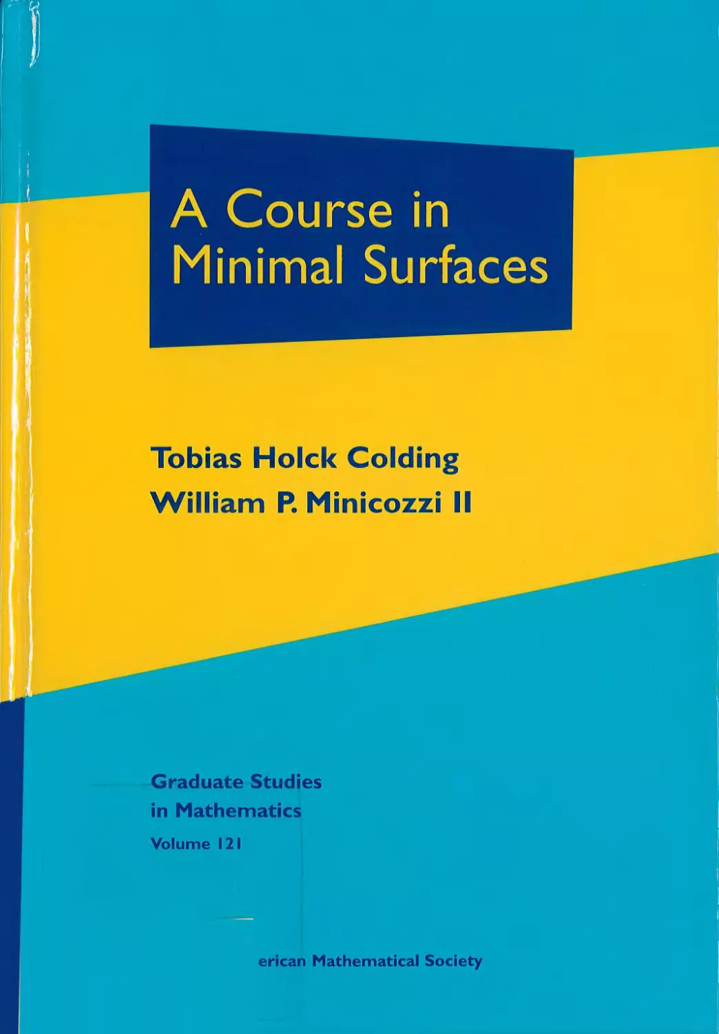
                    A Course in
Minimal Surfaces
Tobias Hoick Colding
William P. Minicozzi II
Graduate Studies
in Mathematics
Volume 121
erican Mathematical Society

A Course in Minimal
Surfaces

A Course in Minimal
Surfaces
Tobias Hoick Colding
William R Minicozzi II
Graduate Studies
in Mathematics
Volume 121
I American Mathematical Society
.^Jf Providence, Rhode Island

Editorial Board
David Cox (Chair)
Rafe Mazzeo
Martin Scharlemann
Gigliola Staffilani
2000 Mathematics Subject Classification. Primary 49Q05, 53A10, 53C42, 58E12, 57M50,
57N10, 35J15, 35J60, 83C57.
For additional information and updates on this book, visit
www.ams.org/bookpages/gsm-121
Library of Congress Cataloging-in-Publication Data
Colding, Tobias H.
A course in minimal surfaces / Tobias Hoick Colding, William P. Minicozzi II.
p. cm. - (Graduate studies in mathematics ; v. 121)
Includes bibliographical references and index.
ISBN 978-0-8218-5323-8 (alk. paper)
1. Minimal surfaces. I. Minicozzi, William P. II. Title.
QA644.C648 2011
516.3/62-dc22 2010044373
Copying and reprinting. Individual readers of this publication, and nonprofit libraries
acting for them, are permitted to make fair use of the material, such as to copy a chapter for use
in teaching or research. Permission is granted to quote brief passages from this publication in
reviews, provided the customary acknowledgment of the source is given.
Republication, systematic copying, or multiple reproduction of any material in this publication
is permitted only under license from the American Mathematical Society. Requests for such
permission should be addressed to the Acquisitions Department, American Mathematical Society,
201 Charles Street, Providence, Rhode Island 02904-2294 USA. Requests can also be made by
e-mail to reprint-permissioiiQams.org.
© 2011 by Tobias Hoick Colding and William P. Minicozzi II. All rights reserved.
The American Mathematical Society retains all rights
except those granted to the United States Government.
Printed in the United States of America.
@) The paper used in this book is acid-free and falls within the guidelines
established to ensure permanence and durability.
Visit the AMS home page at http://www.ams.org/
10 9 8 7 6 5 4 3 2 1 16 15 14 13 12 11

Contents
Preface ix
Chapter 1. The Beginning of the Theory 1
§1. The Minimal Surface Equation and Minimal Submanifolds 1
§2. Examples of Minimal Surfaces in R3 8
§3. Consequences of the First Variation Formula 18
§4. The Gauss Map 28
§5. The Theorem of Bernstein 29
§6. The Weierstrass Representation 33
§7. The Strong Maximum Principle 37
§8. Second Variation Formula, Morse Index, and Stability 38
§9. Multi-valued Graphs 50
§10. Local Examples of Multi-valued Graphs 51
Appendix: The Harnack Inequality 60
Appendix: The Bochner formula 60
Chapter 2. Curvature Estimates and Consequences 65
§1. Simons' Inequality 66
§2. Small Energy Curvature Estimates for Minimal Surfaces 72
§3. Curvature and Area 76
§4. Lp Bounds of \A\2 for Stable Hypersurfaces 85
§5. Bernstein Theorems and Curvature Estimates 87
§6. The General Minimal Graph Equation 88
§7. Almost Stability 92

vi
Contents
§8.
§9.
Chapt
§i-
§2.
§3.
§4.
§5.
§6.
Chapt
§i-
§2.
§3.
§4.
§5.
§6.
Chapt'
§i.
§2.
§3.
§4.
§5.
Chapt<
§i.
§2.
§3.
§4.
§5.
Chapt<
§i-
§2.
§3.
§4.
Sublinear Growth of the Separation
Minimal Cones
er 3. Weak Convergence, Compactness and Applications
The Theory of Varifolds
The Sobolev Inequality
The Weak Bernstein-Type Theorem
General Constructions
Finite Dimensionality
Bubble Convergence Implies Varifold Convergence
er 4. Existence Results
The Plateau Problem
The Dirichlet Problem
The Solution to the Plateau Problem
Branch Points
Harmonic Maps
Existence of Minimal Spheres in a Homotopy Class
er 5. Min-max Constructions
Sweepouts by Curves
Birkhoff's Curve Shortening Process
Existence of Closed Geodesies and the Width
Harmonic Replacement
Minimal Spheres and the Width
er 6. Embedded Solutions of the Plateau problem
Unique Continuation
Local Description of Nodal and Critical Sets
Absence of True Branch Points
Absence of False Branch Points
Embedded Solutions of the Plateau Problem
er 7. Minimal Surfaces in Three-Manifolds
The Minimal Surface Equation in a Three-Manifold
Hersch's and Yang and Yau's Theorems
The Reilly Formula
Choi and Wang's Lower Bound for Ai
97
101
105
106
113
119
120
124
128
133
133
137
142
147
148
153
163
163
164
171
176
190
201
201
207
215
217
224
233
233
239
242
243

Contents
vii
§5. Compactness Theorems with A Priori Bounds 244
§6. The Positive Mass Theorem 251
§7. Extinction of Ricci Flow 255
Chapter 8. The Structure of Embedded Minimal Surfaces 261
§1. Disks that are Double-spiral Staircases 261
§2. One-sided Curvature Estimate 276
§3. Generalized Nitsche Conjecture 278
§4. Calabi-Yau Conjectures for Embedded Surfaces 282
§5. Embedded Minimal Surfaces with Finite Genus 288
Exercises 295
Bibliography 299
Index 311

Preface
The motivation for these lecture notes on minimal surfaces is to have a
treatment that begins with almost no prerequisites and ends up with current
research topics. We touch upon some of the applications to other fields
including low dimensional topology, general relativity, and materials science.
Minimal surfaces date back to Euler and Lagrange and the beginning of
the calculus of variations. Many of the techniques developed have played
key roles in geometry and partial differential equations. Examples include
monotonicity and tangent cone analysis originating in the regularity theory
for minimal surfaces, estimates for nonlinear equations based on the
maximum principle arising in Bernstein's classical work, and even Lebesgue's
definition of the integral that he developed in his thesis on the Plateau
problem for minimal surfaces.
The only prerequisites needed for this book are a basic knowledge of
Riemannian geometry and some familiarity with the maximum principle. Of
the various ways of approaching minimal surfaces (from complex analysis,
PDE, or geometric measure theory), we have chosen to focus on the PDE
aspects of the theory.
In Chapter 1, we will first derive the minimal surface equation as the
Euler-Lagrange equation for the area functional on graphs. Subsequently,
we derive the parametric form of the minimal surface equation (the first
variation formula). The focus of the first chapter is on the basic properties
of minimal surfaces, including the monotonicity formula for area and the
Bernstein theorem. We also mention some examples. In the next to last
section of Chapter 1, we derive the second variation formula, the stability
inequality, and define the Morse index of a minimal surface. In the last
section, we introduce multi-valued minimal graphs which will play a major
ix

X
Preface
role later when we discuss results from [CM3]-[CM7]. We will also give a
local example, from [CM18], of spiraling minimal surfaces (like the helicoid)
that can be decomposed into multi-valued graphs but where the rate of
spiraling is far from constant.
Chapter 2 deals with generalizations of the Bernstein theorem. We
begin the chapter by deriving Simons' inequality for the Laplacian of the norm
squared of the second fundamental form of a minimal hypersurface E in W1.
In the later sections, we discuss various applications of this inequality. The
first application is a theorem of Choi and Schoen giving curvature estimates
for minimal surfaces with small total curvature. Using this estimate, we
give a short proof of Heinz's curvature estimate for minimal graphs. Next,
we discuss a priori estimates for stable minimal surfaces in three-manifolds,
including estimates on area and total curvature of Colding and Minicozzi
and the curvature estimate of Schoen. After that, we follow Schoen,
Simon and Yau and combine Simons' inequality with the stability inequality
to show higher IP bounds for the square of the norm of the second
fundamental form for stable minimal hypersurfaces. The higher IP bounds are
then used together with Simons' inequality to show curvature estimates for
stable minimal hypersurfaces and to give a generalization due to De Giorgi,
Almgren, and Simons of the Bernstein theorem proven in Chapter 1. We
introduce a notion of "almost stabilility" that plays a crucial role in
understanding embedded surfaces. Next, we return to multi-valued minimal
graphs and prove an important result from [CM3] which states that the
separation grows sublinearly if the multi-valued graph has enough sheets.
We close the chapter with a discussion of minimal cones in Euclidean space
and the relationship to the Bernstein theorem.
We start Chapter 3 by introducing stationary varifolds as a
generalization of classical minimal surfaces. We next prove the Sobolev inequality of
Michael and Simon. After that, we prove a generalization, due to Colding
and Minicozzi, of the Bernstein theorem for minimal surfaces discussed in
the preceding chapter. Namely, following [CM6], we will show in Chapter
3 that, in fact, a bound on the density gives an upper bound for the
smallest affine subspace that the minimal surface lies in. We will deduce this
theorem from the properties of the coordinate functions (in fact, more
generally, properties of harmonic functions) on A;-rectifiable stationary varifolds
of arbitrary codimension in Euclidean space. Finally, in the last section, we
introduce another notion of weak convergence (called bubble convergence)
that was developed to explain the bubbling phenomenon that occurs in con-
formally invariant problems, including two-dimensional harmonic maps and
J-holomorphic curves. We will show that bubble convergence implies vari-
fold convergence.

Preface
xi
Chapter 4 begins with the solution to the classical Plateau problem for
maps from surfaces. There is a close connection between energy and area in
dimension two and the main issue is to understand the lack of compactness,
called "bubbling", for maps with bounded energy. The first three sections
cover the basic existence results for the Dirichlet and Plateau problems for
maps from disks, while the fourth section discusses branch points. After
that, we turn to the existence of harmonic maps from the two-sphere,
following the approach by Sacks and Uhlenbeck, [SaUh], of first minimizing a
perturbed energy functional and then taking the limit as the perturbation
goes to zero.
In Chapter 5, we use a very general argument, whose basic idea goes back
to H.A. Schwarz in the 1870s and G.D. Birkhoff in the 1910s, to find minimal
spheres on any sphere. The treatment will follow the papers [CM27] and
[CM28] where some of the existence results were new. The idea of both
Schwarz and Birkhoff was to use a min-max argument to show existence
of critical point for variational problems. This allows us, in particular, to
produce minimal surfaces that are not stable. In the min-max construction
of minimal surfaces, one sweeps out the manifold by surfaces keeping track of
the areas of the slices of the sweepout. One then tries to extract a convergent
sequence of maximal slices for which the area of the maximal slice converges
to the infimum of the maximal slices of all sweepouts.
Chapter 6 focuses on the regularity of classical solutions to the Plateau
problem. After some general discussion of unique continuation and nodal
sets, we study the local description of minimal surfaces in a neighborhood
of either a branch point or a point of nontransverse intersection. Following
Osserman and Gulliver, we rule out interior branch points for solutions
of the Plateau problem. In the remainder of the chapter, we prove the
embeddedness of the solution to the Plateau problem when the boundary is
in the boundary of a mean convex domain. This last result is due to Meeks
and Yau.
In Chapter 7, we discuss the theory of minimal surfaces in
three-manifolds. We begin by explaining how to extend the earlier results to this case
(in particular, monotonicity, the strong maximum principle, and some of
the other basic estimates for minimal surfaces). We then prove the results
of Hersch, and Choi and Wang. Next, we prove the compactness theorem
of Choi and Schoen for embedded minimal surfaces in three-manifolds with
positive Ricci curvature. An important point for this compactness result is
that by results of Choi and Wang and Yang and Yau such minimal surfaces
have uniform area bounds. We then prove the positive mass theorem of
Schoen and Yau. In the last section, we prove the Colding-Minicozzi finite
extinction theorem for Ricci flow on a homotopy three-sphere.

xii
Preface
Finally, in Chapter 8, we will present some recent results on embedded
minimal surfaces in R3. We begin with a local result from [CM4] which
shows that an embedded minimal disk is either graphical or, on a slightly
larger scale, contains a double-spiral staircase. We also state the one-sided
curvature estimate from [CM6]. This theorem roughly asserts that an
embedded minimal disk in M3, that lies on one side of a plane and comes close
to it is a graph over the plane. The novel thing about this estimate is that
it does not require any a priori bound unlike all of the classical results for
minimal surfaces discussed in the previous chapters of this book. These
results are the starting point for the structure of embedded minimal surfaces
obtained in the series of papers [CM3], [CM4], [CM5], and [CM6]. We
then describe an application (from [CM10]) of the one-sided curvature
estimate to prove the Generalized Nitsche Conjecture (proven originally by
P. Collin, [Co]). After this, we turn to the resolution of the Calabi-Yau
conjectures for embedded surfaces from [CM24]. Finally, we describe the
main structure theorems from [CM7] for embedded minimal surfaces with
finite genus and several recent uniqueness results that have relied upon the
structure theory of [CM3]-[CM7].
At the end of the book, problems and exercises are given.
It is a pleasure to thank Matthias Weber for creating some of the figures
for this book and Sergei Gelfand for his persistence and encouragement.
Both authors were supported by regular grants and an FRG grant
during the preparation of this book, all of them from the National Science
Foundation. Any opinions, findings, and conclusions or recommendations
expressed are those of the authors and do not necessarily reflect the views
of the National Science Foundation.

Chapter 1
The Beginning of the
Theory
In this chapter, we will first derive the minimal surface equation as the
Euler-Lagrange equation for the area functional on graphs. Subsequently,
we derive the parametric form of the minimal surface equation (the first
variation formula). The focus of the chapter is on some basic properties
of minimal surfaces, including the monotonicity formula for area and the
Bernstein theorem. We also mention some examples. In the next to last
section, we derive the second variation formula, the stability inequality, and
define the Morse index of a minimal surface. In the last section, we introduce
multi-valued minimal graphs which will play a major role later when we
discuss results from [CM3]-[CM7]. We will also give a local example,
from [CM18], of spiraling minimal surfaces (like the helicoid) that can be
decomposed into multi-valued graphs, but where the rate of spiraling is far
from constant.
1. The Minimal Surface Equation and Minimal
Submanifolds
1.1. Graphs and the minimal surface equation. Suppose that u : Cl C
B? —>• R is a C2 function and consider the graph of the function u
(1.1) Graphs = {(xyytu(xty)) | (xyy) € ft} .
Then the area is
(1.2) Area(GraphJ = / |(l,0,O x (0,l,i*y)|
Jn
= [ Jl+ul + v*= f y/\ + | Vn|2 ,
Jn v Jn
1

1. The Beginning of the Theory
and the (upward pointing) unit normal is
/x 3x N= (1,0,1*3-) x (0,1,%) = (-Ms, -%, 1)
' ; 1(1,0,0 x (0,l,iiy)| y/i + |Vn|2 '
Applying this to a one-parameter family of graphs Graphw+t7?, where rj\dQ, =
0 and t is the parameter, we get that
(1.4) Area(Graphu+t„) = / y/l + \Vu + t V77I2 ;
./ft
hence, the directional derivative of the area functional on graphs at u in the
direction 77 is
(Vii, Vt?)
(1-5) ^i=0Area(Graph^) = X7!
+ |Vu|
2
= — / rj div
Jo.
In \y/l + \Vu\2
Therefore, the graph of u is a critical point for the area functional if u
satisfies the divergence form equation
(1.6) divf . VU = 1 =0.
\y/l + \Vu\*J
Equation (1.6) is the divergence form of the minimal surface equation and
can alternatively be written as
(1.7) 0 = (1 + \Vu\2)
2^
UX J I Uy
Vi + ivuiv, \VT+WW/y
= (1 + Uy) UXX + (1 + Ux) Uyy ~2UXUy UXy
Next we want to show that the graph of a function on £1 satisfying the
minimal surface equation is not just a critical point for the area functional
but is actually area-minimizing amongst surfaces in the cylinder QxMcM3.
Let u) be the two-form on Q x R given by that for I, F € M3,
(1.8) u(X, Y) = det(X, Y, N),
where
(-ux, -uy, 1)
(1.9) N =
y/l + |Vu|2 '

1. The Minimal Surface Equation and Minimal Submanifolds
Observe that
(1.10)
(1.11)
and
(1.12)
Hence
(1.13)
and
(1.14)
d d
u
dx' dy
VI + |Vu|2
1
Vi +1 vu|2'
1 0
0 1
0 0
—u
—u.
X
y
d d
uj
dydz) V1 + |Vu|2
0 0
1 0
0 1
—u,
—u
x
y
—u
X
vTTTwp'
d d
u
dx'dzj Vl + |Vu|2
1 0
0 0
0 1
—u,
—u
X
y
u.
y
Vi + |w|2
u =
dx A dy — ux dy Adz — uy dz A dx
x/l + |V«|2
duo =
d
—u
x
d
—U.
y
dx \ Vl + |V^|2y dy \ Vl + |V^|2
= 0,
since u satisfies the minimal surface equation. In sum, the form uj is closed
and, given any orthogonal unit vectors X and Y at a point (x,yy z)y
(i.i5) wx,y)\ <i,
where equality holds if and only if
(!-16) X, y C T{XiyMXiy)) Graphw .
Such a form cj is called a calibration and it can be used to show that Graph
is area-minimizing:
u
Lemma 1.1. If u : Q —> R satisfies the minimal surface equation and
£ c CI x IR is an?/ o£/ier surface with dT, = d Graphw, then
(1.17)
Area(Graphu) < Area(E).

1. The Beginning of the Theory
Proof. Since u is a closed form and Graphw and E are homologous, Stokes'
theorem gives
(1.18) / cj= f cj.
./Graphs JE
Combining this with (1.15) and (1.16) gives
(1.19) Area(GraphJ = / u = / u < Area(E). D
«/Graphu «/E
Throughout, we will use Br(x) to denote the ball in R3 (or in Rn+1)
with radius r and center x\ we will often write BT for the ball Br(0). We
will use Dr for the disk of radius r in R2 centered at 0.
Corollary 1.2. If u : fi, —> R satisfies the minimal surface equation and
Dr C O, then
(1.20) Area(£r n Graphn) < Ar6*(S ) r2 = 2tt r2 .
Proof. Since dBr D Graphu divides dBr into two components at least one
of which has area at most equal to (Area(S2)/2) r2, (1.17) gives (1.20). □
If the domain Q is convex, the minimal graph is absolutely
area-minimizing. To see this, observe first that for a convex set O the nearest point
projection P : R3 —> Q, x R is a distance nonincreasing Lipschitz map that
is equal to the identity on Cl x R. If E c R3 is any other surface with
<9E = d Graphw, then E' = P(E) has Area(E') < Area(E). Applying (1.17)
to E', we see that Area(Graphw) < Area(E') and the claim follows.
Very similar calculations to the ones above show that if Cl C Rn_1 and
u : Q, —> R is a C2 function, then the graph of it is a critical point for the
area functional if and only if u satisfies the equation
(1.21) divf , VU = J =0.
Moreover, as in (1.17), if u satisfies (1.21), then the graph of u is actually
area-minimizing. Consequently, as in (1.20), if fi contains a ball of radius r,
then
(1.22) Vol(5r H GraphJ < Vol^n ^ rn~l.

1. The Minimal Surface Equation and Minimal Submanifolds 5
1.2. The geometry of submanifolds. We could also have looked more
generally for a ^-dimensional submanifold E possibly with boundary and
sitting inside some Riemannian manifold M (with metric g and covariant
derivative V) and which is a critical point for the area functional.
In the following, if X is a vector field on E C M, then we let XT and XN
denote the tangential and normal components, respectively. The covariant
derivative V on M then induces a covariant derivative Ve on E and second
fundamental form A of E. That is, the induced covariant derivative Ve is
given by
(1.23) VE = (V)T,
and the vector-valued bilinear form A on E is given for X, Y G TXT, by
(1.24) A(X,Y) = (VXY)N.
Since the bracket of tangential vector fields is again a tangential vector field,
it is easy to see that A is symmetric, i.e., A(X, Y) = A(Y, X). Observe that
n—k n—k
(1.25) Y, 9(A(X>y)'N') ^ = E 9^xY, Ne) Ne
e=i i=i
n—k
= -Y,9(Y,VxNe)Ne,
e=i
where Ne is an orthonormal basis of vector fields for the normal space to E
in a neighborhood of x.
The mean curvature vector H at x is by definition
k
(1.26) H = YlME»Ei)y
*=i
where Ei is an orthonormal basis for TXE. Furthermore, the norm squared
of the second fundamental form at x is by definition
(1.27) |A|2=^|A(£i,^)|a.
Recall also that the Gauss equations assert that if X, Y G TXE, then
(1.28) Kv(Xt Y) \X A y|2 = KM(X, Y) \X A Y\2
+ g(A(X,X), A(Y,Y))-g(A(X,Y), A(X,Y))9
where \X A Y\2 is given by
(1.29) \X A Y|2 = <?(*, X) ff(y, Y) - g{X, Y)2
and Km(X,Y) and 1?e(X',Y') are the sectional curvatures of M and E,
respectively, in the two-plane spanned by the vectors X and Y. If En_1 C

1. The Beginning of the Theory
Mn is a hypersurface and TV is a unit normal vector field in a neighborhood
of £, then
(1.30) V(.) N:TXE^ TXY,
is a symmetric map (often referred to as the Weingarten map) and its
eigenvalues (tti)i=i,...,n-i are called the principal curvatures. Moreover,
n-l
(1.31) g(H,N) = -Y,*i.
Finally, if X is a vector field defined in a neighborhood of E, then the
divergence of X at x G E is
n-l
(1.32) &YVvX = YJ9{VEiX,Ei),
i=l
where E% is an orthonormal basis for TXE. Notice that div^ satisfies the
Leibniz rule
(1.33) divE(/X) = (Vs/, X) + / divE(X).
We can also use divs to define the Laplace operator As on E by
(1.34) As/ = divs(VE/).
A function / is said to be harmonic on E if As/ = 0.
Remark 1.3. Note that
divEK" = Y,9(Ei,VEiYN) = -J29(YN,VEiEi)
i i
(1.35) =-g(YN,H).
1.3. The first variation formula. Let F:Ex(—e,e) ->Mbea variation
of E with compact support and fixed boundary. That is, F = Id outside a
compact set,
(1.36) F(rr,0) = rr,
and for all x G dE,
(1.37) F(x,t) = x.
The vector field Ft restricted to E is often called the variational vector field.
Now we want to compute the first variation of area for this one-parameter
family of surfaces. Let xi be local coordinates on E. Set
(1.38) 9ij(t)=g(FXi,FXj),
(1.39) i/(*) = Jdet(9ij(t)) ^det(5#(0)),

1. The Minimal Surface Equation and Minimal Submanifolds
where ay denotes the inverse of the matrix a^-. Note that v(t) is well
defined, independent of the choice of a coordinate system on E (since det ((/#(£))
changes by the determinant squared of the differential of a coordinate
transformation while det(gzi(0)) changes by the inverse of this). Furthermore,
the area formula is
(1.40) Vol(F(S,t)) = J v{t) ^/det(sy(0)),
where the integral is over E. Differentiating this gives
<L41> ' i=0Vol(F(E,i)) = /|i=o,WV/detfe(0))-
To evaluate d/dtt=ov(t) at some point x, we may choose the coordinate
system such that at x it is orthonormal, i.e., so that at the point rr,
(1.42) 9ij(0) = Sij = i° *'*'•'
[1 \ii = j.
Using this and the fact that the t and xi derivatives commute (i.e., VFtFXi —
^FXiFt = [FuFXi] = 0), we get at xt
i=l i=l
' k
(1.43) = Y,(VFXiFuFXi) = divEFt.
t=i
We can relate this formula to the mean curvature by writing the vector field
Ft as the sum of its normal and tangential parts to get
, n—k k
<144) m vw = E E<v^ <F*> Nt) Nt> F*J+div^ Ft
alt-° e=i i=i
n—k k
= E E<F<> ^> <V^> FXi) + divE if
e=i i=i
= -(Fi,iJ) + divsFtT.
Here Ni is an orthonormal basis for the normal bundle of E at x. Integrating
(1.43) and (1.44) gives the so-called first variation formula:
(1.45) ^ Vol(*X£, *)) = "/ (*i, H)= f divE Ft.
dtt=o Jy, Je
Note that Stokes' theorem was used to see that Jdivs F^ = 0. As a
consequence of (1.45), we see that E is a critical point for the area functional
if and only if the mean curvature H vanishes identically.

8 1. The Beginning of the Theory
Definition 1.4. (Minimal Submanifold) An immersed submanifold Efc C
Mn is said to be minimal if the mean curvature H vanishes identically.
It follows from the identity (1.45) that a graph in M3 is a minimal surface
if and only if it satisfies the minimal surface equation (1.6).
2. Examples of Minimal Surfaces in Rs
Minimal surfaces are characterized as having mean curvature zero. The
simplest example is when the full second fundamental form (and not just its
trace) vanishes, i.e., when the surface is totally geodesic. Since the second
fundamental form is the derivative of the unit normal, this means that the
normal is constant and, thus, the surface is a plane.
2.1. Topology of surfaces. Compact orientable surfaces without
boundaries are classified by their genus, a nonnegative integer. Genus = 0
corresponds to a sphere, genus = 1 to the torus. A surface of genus = k is
modelled by the surface of a sphere to which fc-handles have been attached.
A compact orientable surface with a boundary is one formed by taking one
of these surfaces and removing a number of disjoint disks. The genus of
the surface with a boundary is the genus of the original object, and the
boundary corresponds to the edges of the surface created by disk removal.
In particular, a surface with genus 0 and nonempty boundary is a planar
domain, i.e., it can be obtained from the disk in the plane by removing a
number of disjoint sub-disks. Sometimes we will talk about surfaces that
are simply connected. By this we will mean that every loop on the surface
can be shrunk (without leaving the surface) to a point curve. One can easily
see that the only simply connected surfaces are the disk and the sphere.
One immediate consequence of the definition of the genus is monotonicity
under inclusion:
Lemma 1.5. IjY, has genus k and Eo C E, then the genus o/Eo is at most
k.
2.2. The helicoid; see Figure 1.1. The helicoid is given as the set xs =
tan-1 (I2); alternatively, it is given in parametric form by
(1.46) (#i,#2,£3) = (t coss,t sins,s),
where s, t € R. It was discovered by Meusnier (a student of Monge) in 1776.
It is complete, embedded, singly-periodic and simply connected.
The helicoid is a ruled surface since its intersections with horizontal
planes {#3 = s} are straight lines. These lines lift and rotate with constant
speed to form a double spiral staircase. In 1842, Catalan showed that the

2. Examples of Minimal Surfaces
9
helicoid is the only (nonflat) ruled minimal surface; see Chapter 8 for further
uniqueness results. A surface is said to be "ruled" if it can be parameterized
by
(1.47) X(s, t) = 0(t) + s 6(t) where s, t € R,
and f3 and 8 are curves in M3. The curve /3(t) is called the "directrix" of the
surface, and a line having 8(t) as a direction vector is called a "ruling". For
the standard helicoid, the #3-axis is a directrix, and for each fixed t the line
s —>• (scos£,s sin£, t) is a ruling.
.-.V ■:
Figure 1.1. The helicoid, with the ruling pictured.
Credit: Matthias Weber, www.indiana.edu/~minimal.
2.3. The catenoid. The catenoid, shown in Figure 1.2, is the only nonflat
minimal surface of revolution. It was discovered by Euler in 1744 and shown
to be minimal by Meusnier (a student of Monge) in 1776. It is a complete
embedded topological annulus (i.e., genus zero and two ends) and is given as
the set where x\ + x\ = cosh2 (#3) in M3. It is easy to see that the catenoid
has finite total curvature.

10
1. The Beginning of the Theory
/
S
\ \
, i w
/
I
\
\
\
Figure 1.2. The catenoid given by revolving x\ = cosh £3 around the
#3-axis. Credit: Matthias Weber, www.indiana.edu/~minimal.
2.4. Scherk's doubly-periodic surface. Approximately 70 years later
and despite considerable work1 by Monge, Legendre and Poisson, in 1835,
Scherk, [Sk], discovered the next complete minimal surface.
Scherk's surface was a doubly-periodic minimal surface defined as a
graph over the white squares of a checkerboard with vertical lines at the
corners. A fundamental domain of Scherk's surface is given as a graph over
the square \x\\ < ir/2 and \x2\ < tt/2 of
(1.48)
X3 = log
COS (#2)
cos(#i)
If we quotient out by the translations to get a minimal surface in T2 x
the resulting surface has genus 0 and 4 annular ends.
1See [Os5] for more on the history.

2. Examples of Minimal Surfaces 11
Let us check that Scherk's surface is, in fact, a minimal surface. We
need only check that xs = xs (#1,22) satisfies the minimal surface equation.
Clearly,
dXiX3 = tan(xi),
#c2£3 = -tan(rr2),
dXlXlX3 = l + tan2(#i),
#C2X2£3 = -1 - tan2(z2),
dXlx2x3 = 0.
Hence, xs satisfies the minimal surface equation (1.7).
Figure 1.3. Scherk's doubly-periodic surface.
Credit: Matthias Weber, www.indiana.edu/~minimal.
2.5. Scherk's singly-periodic surface. Also in 1835, Scherk, [Sk],
discovered a singly-periodic minimal surface that looks like the desingulariza-
tion of a pair of orthogonal planes. This surface is still one of the most

12 1. The Beginning of the Theory
important examples, as it plays a critical role in gluing and desingulariza-
tion constructions for minimal and constant mean curvature surfaces; see
Kapouleas, [Kal, and Traizet, fTrll.
Figure 1.4. Scherk's singly-periodic surface.
Credit: Matthias Weber, www.indiana.edu/~minimal.
2.6. The Riemann Examples. Around 1860, Riemann, [Ri], classified
all minimal surfaces in R3 that are foliated by circles and straight lines in
horizontal planes. He showed that the only such surfaces are the plane, the
catenoid, the helicoid, and a two-parameter family that is now known as
the Riemann examples. The surfaces that he discovered formed a family
of complete embedded minimal surfaces that are singly-periodic and have
genus zero. Each of the surfaces has infinitely many parallel planar ends
connected by necks ("pairs of pants").
Modulo rigid motions, this is a 2-parameter family of minimal surfaces.
The parameters are:
• Neck size.
• Angle between period vector and the ends.

2. Examples of Minimal Surfaces
13
Figure 1.5. The Riemann examples.
Credit: Matthias Weber, www.indiana.edu/~minimal.
If we keep the neck size fixed and allow the angle to become vertical (i.e.,
perpendicular to the planar ends), the family degenerates to a pair of
oppositely oriented helicoids. On the other hand, as the angle goes to zero, the
family degenerates to a catenoid.
2.7. Enneper's surface. In 1864, Enneper, [E], discovered a minimal
surface parameterized by
(1.49) (a*, x2i x3) = {s- s3/3 + st2, -t - sH + t3/3, s2 - t2),
where s, t £ M. Unlike the earlier examples, Enneper's surface is not
embedded. Like the catenoid, Enneper has finite total curvature.
2.8. The Costa-Hoffman-Meeks surfaces. In 1984, C. Costa, [Cc],
discovered a new minimal surface with finite total curvature, genus one and
three ends, each of which was embedded. This surface was constructed by
the Weierstrass representation using clever choices of data on the torus. In

14
1. The Beginning of the Theory
Figure 1.6. The Riemann examples: starting to degenerate to helicoids.
Credit: Matthias Weber, www.indiana.edu/~minimal.
1985, D. Hoffman and W. Meeks, [HoMel], proved that Costa's surface was
embedded; this surface is now known as the Costa-Hoffman-Meeks surface.
Moreover, Hoffman and Meeks showed that Costa's surface was just the
first in a family of surfaces with three ends and increasing genus. As the
genus goes to infinity, the surfaces converge (at least as sets) to the union
of a plane and a catenoid.
2.9. The Weber-Wolf surfaces. M. Weber and M. Wolf, [WeWo2],
constructed a series of embedded minimal surfaces with two catenoidal ends (the
top and bottom ends), any number of planar ends in the middle, and at least
as many handles as there are planar ends. These surfaces are conjectured
to be at the boundary of what is possible:
Conjecture 1.6 (Hoffman-Meeks). If Ti is a complete embedded minimal
surface in R3 with k ends and genus g, then k < g + 2.

2. Examples of Minimal Surfaces 15
Figure 1.7. A small piece of Enneper's surface that is embedded; it extends to
cross itself. Credit: Matthias Weber, www.indiana.edu/~minimal.
2.10. The genus one helicoid. In 1993, Hoffman-Karcher-Wei gave
numerical evidence for the existence of a complete embedded minimal surface
with genus one that is asymptotic to a helicoid; they called it a "genus
one helicoid". In [HoWW], Hoffman, Weber and Wolf constructed such
a surface as the limit of "singly-periodic genus one helicoids", where each
singly-periodic genus one helicoid was constructed via the Weierstrass
representation. Later, Hoffman and White constructed a genus one helicoid
variationally in [HoWhl].
2.11. Building blocks for embedded surfaces. The Riemann
examples, the genus one helicoid and the Costa-Hoffman-Meeks surface are all
embedded minimal surfaces with finite genus and each can be thought of as
being built out of pieces of planes, helicoids and catenoids. In Chapter 8, we
will discuss the key Colding-Minicozzi structure result for embedded
minimal surfaces. This result, from [CM3]-[CM7], proved that any embedded

16 1. The Beginning of the Theory
Figure 1.8. The original Costa-Hoffman-Meeks surface.
Credit: Matthias Weber, www.indiana.edu/~minimal,
minimal surface with finite genus can be built out of planes, helicoids and
catenoids.
2.12. Schwarz's triply periodic minimal surfaces. In the late 19th
century, H.A. Schwarz (of the Schwarz alternating method discussed in
Chapter 5) and his students, including Neovius, [Ne], discovered five triply
periodic minimal surfaces in K3; see [Sz2], [Sz3]. All of these surfaces have
infinite genus, but their quotients by the crystallographic group have
finite genus. In 1970, A. Schoen, [Sea], constructed many new families of
triply periodic minimal surfaces, including the gyroid. These were
rigorously shown to exist by Karcher in 1989, [Kr]. The gyroid was proven to be
embedded by K. Grosse-Brauckmann and M. Wohlgemuth in 1996, [GrW].
Triply periodic minimal surfaces play a role in the sciences; see [AHHT].
The gyroid structure, for instance, is found in certain block copolymers.

2. Examples of Minimal Surfaces
17
">^fe
Figure 1.9. The Costa-Hoffman-
Meeks surface with many
handles. Credit: Matthias Weber,
www.indiana.edu/~minimal.
Figure 1.10. As the number of
handles gets large, one can see
a bent version of Scherk's singly-
periodic surface. Credit: Matthias
Weber, www.indiana.edu/~minimal.
The fundamental domain for the Schwarz D-surface, discovered in 1865,
solves the Plateau problem with boundary contained in the edges of a cube.
The fundamental domain for the Schwarz P-surface, discovered in the 1880s,
can also be constructed by solving a Plateau problem, this time with
boundary equal to a 4-gon with corners at the vertices of a regular octahedron.
This idea of solving a Plateau problem with a polygonal boundary and then
using reflection has been used with great success, including H.B. Lawson's
construction of minimal surfaces in the round 3-sphere, [Lai]; cf. subsection
6.2.
2.13. The Chen-Gackstatter surface. In 1981, Chen and Gackstatter,
[CcG], discovered the first complete immersed minimal surface of genus one
with finite total curvature. The Chen-Gackstatter surface has one end and
this is of Enneper type.
M. Weber and M. Wolf, [WeWol], showed that one can add handles
to the Chen-Gackstatter surface to get surfaces with arbitrarily high genus
and one Enneper end. In her thesis, [Ks], S. Kim proved that the Weber-
Wolf examples converge to Scherk's singly-periodic surface as the number of
handles goes to infinity.
2.14. The higher dimensional catenoid. There is a higher dimensional
analog of the catenoid given as a minimal surface of revolution around an
axis. We refer to section 2 of [TZ] for its main properties. The most
important ones from our point of view are:

18 1. The Beginning of the Theory
v— \ \ / __ /
_ " ■ • ^
!■?■* •&'*:%.;* :
<C-
V
^,
/-jt
.-*'
Figure 1.11. The Weber-Wolf surface of genus 4 with 5 ends.
Credit: Matthias Weber, www.indiana.edu/~minimal.
• It is a complete, embedded minimal hypersurface.
• The n-dimensional catenoid is given by revolving a curve around
an axis and, thus, it is topologically R x Sn_1. In particular, it is
simply connected for n > 2.
• The volume of the n-dimensional catenoid in a ball of radius R is
bounded by twice the volume of Br c W1 and it converges to this
as R goes to infinity.
• When n > 3, the catenoids lie in a slab between two parallel hy-
perplanes.
3. Consequences of the First Variation Formula
In this section, we will collect some important consequences of the first
variation formula. The most important of these is the monotonicity formula,

3. Consequences of the First Variation Formula
19
•:f-w*=*L
>v
4^
N, _.-_ ;^._^
Figure 1.12. The genus one he-
licoid. Credit: Matthias Weber,
www. indiana. edu/ ~ minimal.
Figure 1.13. A periodic minimal
surface asymptotic to the helicoid,
whose fundamental domain has
genus one. Credit: Matthias
Weber, www.indiana.edu/~minimal.
r
-—JL
\ \
\
j
- /
i
\
\
\
V
v
^
\
Figure 1.14. The Schwarz D-
surface. Credit: Matthias Weber,
www.indiana.edu/~minimal.
Figure 1.15. The Schwarz P-
surface. Credit: Matthias Weber,
www.indiana.edu/~minimal.
Proposition 1.12. In later chapters, we will return to this subject. In
Chapter 3, we extend these results to stationary varifolds, and in Chapter 5 to
minimal surfaces in a three-manifold.

20
1. The Beginning of the Theory
-v T
v. ■
C*
,•/ ?•
I-
V.V^CiV
^ . --* •
te -;'
^
Figure 1.16. A fundamental
domain of Neovius's minimal
surface. Credit: Matthias Weber,
www.indiana.edu/~minimal.
Figure 1.17. The triply
periodic Neovius surface, discovered
in 1883. Credit: Matthias Weber,
www.indiana.edu/~minimal.
■^
v
pi ,^\*
\":.
4 ■%■ Jv! '
1
• *
<* "*
Figure 1.18. A fundamental
domain of Schwarz's CLP
surface. Credit: Matthias Weber,
www.indiana.edu/~minimal.
Figure 1.19. The triply periodic
CLP surface. Credit: Matthias
Weber, www.indiana.edu/~minimal.
Prom (1.45), we see that E is minimal if and only if for all vector fields
X with compact support and vanishing on the boundary of E,
(1.50)
/divEX = 0.

3. Consequences of the First Variation Formula
21
*-=*<&.
-. * *.
r
M
~r
"7 ' " *'•• V"
♦r
-s __.
■\iry
Figure 1.20. A fundamental
domain of Schwarz's H-surface.
Credit: Matthias Weber,
www.indiana.edu/~minimal.
Figure 1.21. The triply periodic
Schwarz H-surface. Credit: Matthias
Weber, www.indiana.edu/~minimal.
' 5 f; '>**
V
! ■
Figure 1.22. The Chen-Gackstatter
surface. Credit: Matthias Weber,
www.indiana.edu/~minimal.
Figure 1.23. Adding handles to
the Chen-Gackstatter surface. It
looks more and more like Scherk's
singly-periodic surface.
Credit: Matthias Weber,
www.indiana.edu/~minimal.
This equation is known as the first variation formula. It has the benefit that
(1.50) makes sense as long as we can define the divergence on E. (This will
later allow us to define a notion of "weak solution" for minimal surfaces.)
In the rest of this section, if xq g W1 is fixed, then we let Bs = Bs(xo)
be the Euclidean ball of radius s centered at xq.

22 1. The Beginning of the Theory
3.1. Harmonicity of the coordinate functions. As a consequence of
(1.50), we will show the following proposition:
Proposition 1.7. Efc C Rn is minimal if and only if the restrictions of the
coordinate functions of W1 to E are harmonic functions.
Proof. Let e* = Vtn^ be the i-th coordinate vector field on Kn and let n
be a smooth function on E with compact support that vanishes on dT, (if E
has boundary).
Since e* is a constant vector field, the divergence of the compactly
supported vector field n e* is given by
(1.51) divE(?? e») = (VE?7, e%) = (VE?7, Vs^) ,
so we see that
(1.52) - /\neuH) = J divs^e*) = MVE?7, VErci> = - / ^AE^.
Prom this, the claim follows easily. □
As a consequence, we can define a Flux homomorphism from (k — 1)-
dimensional homology classes to Mn:
Corollary 1.8. IfY,k C Rn is minimal, then there is a well defined "Flux
homomorphism" F from (k — 1)-dimensional homology classes to Rn given
by
(1.53) ^([7])= [(rh>*i)>
where n7 is the oriented conormaf to 7.
Proof. This mapping is clearly linear, so it suffices to show that it depends
only on the homology class of 7. However, if 71 and 72 are homologous, then
together they bound a &-chain Cl in E. Thus, minimality and the divergence
theorem give
(1.54) / (n71,ei)- / (n72,ei)= / divEei = 0,
j7i J72 Jn
completing the proof. □
Another very useful consequence of (1.50) is a formula for the Laplacian
of I x 12 on a ^-dimensional minimal surface E. Namely, since for any vector
v we have
(1.55) VvXi = (v, e»>,
2The conormal is the vector that is tangent to S, but normal to 7.

3. Consequences of the First Variation Formula 23
we see that
(1.56) divs(a;i,... yxn) = k .
Combining (1.56) and (1.50) (actually we just use that div^ YN = 0 for any
Y) gives
(1.57) Ae|#|2 = 2 divs(^i,..., xn)T = 2 divs(a;i, • • •> xn) = 2k .
Recall that if S C Mn is a compact subset, then the smallest convex set
containing S (the convex hull, Conv(S)) is the intersection of all half-spaces
containing S. In [Os6], Osserman showed that the maximum principle forces
a minimal submanifold to lie in the convex hull of its boundary:
Proposition 1.9 (Convex Hull Property, [Os6]). IJT,k Cln is a compact
minimal submanifold, then E C Conv(dE).
Proof. A half-space H C Rn can be written as
(1.58) H = {xeRn\(x,e) < a} ,
for a vector e € Sn_1 and constant a € K. By Proposition 1.7, the function
u(x) = (e,x) is harmonic on E and hence attains its maximum on <9E by
the maximum principle. □
The argument in the proof of the convex hull property can be rephrased
to say that as we translate a hyperplane towards a minimal surface, the first
point of contact must be on the boundary.
The convex hull property gives monotonicity of topology for minimal
submanifolds. The simplest version of this is for minimal disks:
Corollary 1.10. 7/E2 C Mn is a compact minimal disk and K is a compact
convex set with K D dE = 0, then K D E is simpy connected.
Proof. Suppose instead that there is a closed curve 7 C i^DE that does
not bound a disk in K D E. Since E is simply connected, 7 bounds a disk
r C E. However, the minimal disk Y now violates the convex hull property
since dT = 7 lies inside K, but V does not. □
More generally, one gets monotonicity of the (k — l)-st homology group:
Lemma 1.11. //Efc C Kn is a compact minimal submanifold and K is a
compact convex set with K D dT, = 0, then the inclusion of K HE into E is
an injection on the (k — l)-st homology group.
Proof. If not, then Br(0) DE contains a (k — l)-cycle 7 that does not bound
in Br(0)C\E but does bound T C E. However, V then contradicts the convex
hull property. □

24 1. The Beginning of the Theory
3.2. Monotonicity. Before we state and prove the monotonicity formula
of volume for minimal submanifolds, we will need to recall the coarea
formula. This formula asserts (see, for instance, [Fe] or [KP] for a proof) that
if E is a manifold and
h: E-^M
is a proper (i.e., /i-1((—oo, t]) is compact for all t G R) Lipschitz function
on E, then for all locally integrable functions / on E and t€i,
(1.59) / f\VEh\= [ f fdr.
J{h<t} J-oo Jh=r
Proposition 1.12 (The Monotonicity Formula). Suppose that Efc C Rn is
a minimal submanifold and x$ G M.n; then for allO < s <t,
Vo\(Bt(xo) n E) Vo\(Bs(xq) n E)
J(Bt(x0)\Bs(xo))r\i: \x-x0\K^
Proof. Define the function / on E by f(x) = \x — xo\. Since E is minimal,
(1.61) AE/2 = 2 divs(z - x0) = 2k.
By Stokes' theorem integrating this gives
(1.62) 2kVo\({f<s})= f AE/2 = 2/ \(x-x0)T\.
J{f<s} J{f=s}
The coarea formula (i.e., (1.59)) gives
(1.63) Vol({/ <*})=/ |Vs/I"11VS/| = [' [ |Vs/I"1 dr.
J{f<S} J0 Jf=T
Combining this with (1.62), an easy calculation gives
± (,-> Vol({/ < .») = -*.— Vol({/ < .}) + ."» f{f__s) ]^F]
= s
-fc-1 /
J{f=s}
\(x-x0y
\(x-x0)N\2
{x-x0)T\
Integrating and applying the coarea formula once again gives the claim. □
Notice that (x — xo)N vanishes precisely when E is conical about xo, i.e.,
when E is invariant under dilations about xq. As a corollary, we get the
following:

3. Consequences of the First Variation Formula 25
Corollary 1.13. Suppose that Efc c Kn is a minimal submanifold and xq €
W1; then the function
(i.65) e,o(5) = Vol^^nE)
Vol(£s C
is a nondecreasing function of s. Moreover, Oxo(s) is constant in s if and
only if E is conical about xq.
Finally, if xq G S, then ®Xo(s) > 1; if for some s > 0, Oxo(s) = 1, then
BSC\T, is a ball in some k-dimensional plane.
Proof. Proposition 1.12 directly shows that O^ (s) is monotone
nondecreasing. Since E is smooth and proper, it is infinitesimally Euclidean and hence
(1.66) limexo(s) > 1.
Combining monotonicity of GXo(s) with (1.66) shows that Oxo(s) > 1. If we
have @Xo(s) = 1> then G^ is constant in s so that, by (1.60), (x — xo)N is
identically zero. Clearly, this implies that E is dilation invariant, and since
E is smooth, E is contained in a fc-plane. □
For later reference, we will record some consequences of Corollary 1.13.
Let E be a minimal submanifold and define the density at xq by
(1.67) 9x0 = 11^6^(5).
This limit, which exists since Oxo(s) is monotone, is always at least 1 for
xo G E by (1.66). In fact, so long as E is smooth, Oxo is a nonnegative
integer equal to the multiplicity of E at xq. Note that if E is not embedded,
then this multiplicity can be greater than one.
The next result, which is an elementary consequence of monotonicity,
shows that this multiplicity is upper semicontinuous.
Corollary 1.14. IfT,k C Rn is a minimal submanifold, then the density Qx
is an upper semicontinuous function on Kn. Consequently, for any A > 0,
the set
(1.68) {x e E | Ox > A}
is closed.
Proof. We need to show that if Xj is a sequence of points going to #, then
(1.69) Gx > lim sup QXj,.
COj t CO
Given any 8 > 0, there exists an s > 0 such that
(1.70) Ox>Ox(25)-<5,

26 1. The Beginning of the Theory
and we can choose 0 < e < s so that
(1.71) ex>(l + s_1 e)kex(2s) -2S.
For any Xj with \x — Xj\ < e,
d.72) e„ < e„(s) < V^(^E) = (i + 3-1 €)fc e,(, + «)
< 25 + ex,
where the last inequality follows from (1.71). Since S was arbitrarily small,
(1.72) implies (1.69) and hence G is upper semicontinuous. It follows
immediately that the set defined in (1.68) must be closed. □
3.3. The mean value inequality.
Proposition 1.15 (The Mean Value Inequality). If Efc C Rn is a minimal
submanifold and f is a function on E, then
(1.73) r* f / - s~k [ f
JBtCtZ JBsnT,
r \ N\2 i ft f
= frm + U T I ^2 ~ M2)A^dT
Proof. Observe that the monotonicity formula will be the special case where
/ = 1. Since E is minimal, integration by parts gives
(1.74) 2k f f=f /As|z|2
JBsnE JBsnE
= [ N2As/ + 2/ f\xT\-s2[ AE/.
JBsni: JdBar\s JBar\n
Using this and the coarea formula (i.e., (1.59)) gives
(1.75) -f (,-> f f
= -ks-k-lf f + s~k [ f
JB»riz JdB»ni:
JV|2
= s-fc-
r wls\z 1 r
rd£snE l* I * ^bsde
Integrating and using the coarea formula gives the claim. □
For future reference, we next record a general mean value inequality
which follows from Proposition 1.15.

3. Consequences of the First Variation Formula 27
Corollary 1.16. Suppose that Efc cRn is a minimal submanifold, xq G E,
and s > 0 satisfy Bs(xo)ndTi = 0. If f is a nonnegative function on E with
As/> -As"2/, toen
Proof. If we define g(t) by
(1-77) 9(t) = t~k [ f,
JBt(xo)ni:
then Proposition 1.15 implies that
(1.78) ^)>_^-2ti-* / / = ~s-2^(t).
We can rewrite (1.78) as
(1.79) ^> * -2t> *
V } g(t) ~ 2 " 2s
Prom (1.79), it is obvious that eXt^2s^ g(t) is monotone nondecreasing and
(1.76) follows immediately. □
A function / is said to be subharmonic on E if As/ > 0. We get
immediately the following mean value inequality for the special case of nonnegative
subharmonic functions:
Corollary 1.17. Suppose that Efe C M.n is a minimal submanifold, xq G W1,
and f is a nonnegative subharmonic function on E; then
(1.80) s~h f f
JBs(x0)ni:
is a nondecreasing function of s. In particular, if xq G E, then for all s > 0,
f f
v ■ J MUj- Vo\(Bs c Rk)
In Chapter 3, we will need a general mean value inequality when E is
not minimal. We record this next:
Lemma 1.18. J/En C Rn+1 is a hypersurface with mean curvature H and
f is a nonnegative function on E, then for s <t,
(1.82) t~k [ f-s~k [ f> ( r-""1 / (x,Vf + fHN)dT.
JBtnE JBsni: Js JBTns
Proof. The proof follows as in Proposition 1.15, except that we keep track
of the terms involving H and throw away the nonnegative (and thus only
helpful) terms involving xN. We leave the details as an exercise. □

28 1. The Beginning of the Theory
4. The Gauss Map
Let E2 C R3 be a surface. The Gauss map is a continuous choice of a unit
normal
(1.83) TV : E -» S2 C R3.
Observe that there are two choices of such a map TV and —TV corresponding
to a choice of orientation of E. Moreover, the differential of the map TV can
be identified with the Weingarten map defined above. To see this, suppose
that E\,E2 is an orthonormal frame on E. Since the unit normal to S2
at N(x) is just N(x) itself, E\,E<i also gives an orthonormal frame on the
image. Using this identification, the differential dN is given by
(1.84) (dN(Ei), Ej) = {VEiN, Ej) = -(N, VEiEj) = -Ay .
In the last equality, we identified the normal vector A{j with its inner product
with TV (since E is a hypersurface).
If E is minimal, then the Gauss map is an (anti) conformal map since
the eigenvalues of the Weingarten map are k,i and k?, = —k\. Moreover, for
a minimal surface
(1.85) |dTV|2 = \A\2 = k\ + k\ = -2 Kl k2 = -2 K = -2 det(dTV),
and the area of the Gauss map is a multiple of the total curvature. This
conformality of the Gauss map for a minimal surface in R3, namely (1.85),
can be used to prove the classical Bernstein theorem described in the next
section.
4.1. Local coordinates on a graph. We conclude this section by
calculating the metric, curvature, and second fundamental form of a graph. If
E C R3 is the graph of a function u = u(x, y), then, as we have already seen,
we can take
(1.86) TV =
(-ux,-uy,l)
x/l + |Vn|2 '
Using (a;, y) as coordinates on the graph, we may express the induced metric
9 as
(1.87) gxx = (l + ul), gxy = 9yx = uxuy , gyy = (1 + u2y).
By direct calculation, the eigenvalues of the matrix g are 1 and (1 + |Vit|2).
This can also easily be seen geometrically. Similarly, the inverse matrix is
given by
(1 RR) nxx - 1+Uy nxy - nVx - ~UxUV nVV - 1 + Ux
U ' 9 " 1 + |Vn|2 ' 9 ~9 " 1 + |Vu|2 ' 9 ~ 1 + IW|2 •

5. The Theorem of Bernstein
29
By the Gauss equation, the Gauss curvature of the graph of u is given
by
K= = (NXi (1, 0, tig)) (Ny, (0, 1, Uy)) - (NX, (0, 1, Uy))2
Kl*2 |(l,0,ux)x(0,l,%)|2
/, RQX _ ((-Uxx, ~UyX, 0), (1, 0, UX)) {(-UXy, -Uyy, 0) , (0, 1, Uy))
[ } ~ (l + |Vu|2)2
_ ((-UXX, -Uxy, 0), (0, 1, Uy))2 _ UXX Uyy ~ u\y
(l + |Vu|2)2 " (l + |Vu|2)2 '
Therefore,
(1.90) Kd Area = "** Uyy " ^ dxAdy.
(1 + |W|2)§
Similarly, we may express the second fundamental form A in the coordinates
(x, y) as
(1.91) Axx = (V(1)0,Wx)(l,0,ux), N) = ((0,0,11**), N) = ^—T •
(1 + \Vu\2)2
Thus, this (and similar calculations) give
uxx
**-xx — l >
(1+|V^|2)2
*»-"**-(1 +1 Vtt|2)r
_ Uyy
I\yy — , .
(1+|VU|2)2
Recall that (by (1.27)) the norm squared of A is the sum of the squares of
the entries in an orthonormal frame; in a general frame, this is given by
(1.93) \A\2 = AijAkl^^.
The expression for the second fundamental form and the bound on the
eigenvalues of g (see (1.87)) together imply
(!-94) JH^L < \m2 < 21|He^l,22 •
v J (l + |Vu|2)3 - ' ' - i + |Vu|2
5. The Theorem of Bernstein
Before we prove the famous theorem of Bernstein, we will give a bound
for the total curvature of a minimal graph. We will later see that, with
some more work, this bound can be used to give local curvature estimates
for minimal graphs. Such a local curvature estimate was proven originally
by Heinz [He] using complex analysis and provided a generalization of the
theorem of Bernstein.

30 1. The Beginning of the Theory
Lemma 1.19. Ifu : fl C M? —> R is a solution to the minimal surface
equation, then for all nonnegative Lipschitz functions n with support contained
inflxR,
(1-95) / \A\2lf<C f | VQraph^l2 •
*/Graphu */Graphu
Proof. Let u denote the area two-form on the unit sphere S2. Since the
upper hemisphere is contractible, we can find a (smooth) one-form a on the
upper hemisphere so that
(1.96) da = u.
As before, let N denote the Gauss map. Since E is minimal and the
differential d commutes with pull-backs, we see that
(1.97) \A\2d Area = -2KdArea, = 2N*u = 2dN*a.
Moreover, since a is a one-form, there is a constant Ca so that
(1.98) \N*a\ < Ca \dN\ = Ca \A\.
Set E = Graphw. By (1.97), Stokes' theorem, and (1.98), we get
/ n2 \A\2 dArea = 2 f n2dN*a = -4, f ndnAN*a
(1.99) <4Ca J r)\Vvn\\A\dAxeb.
<4Ca ( f r)2\A\2dArea\2 ( f |Vs^|2rfAreaJ ,
where the last inequality used the Cauchy-Schwarz inequality. Finally,
squaring this and dividing both sides by f^n2 \A\2 gives
(1.100) fr,2\A\2<UC2a /"iVEvI2.
This proves the lemma. □
5.1. The logarithmic cutoff trick. The previous lemma shows that we
can bound the total curvature in terms of the energy of a cutoff function rj.
When the graph E is entire (i.e., defined over all of M2), we will see that it
is possible to choose a sequence of n's that converge to one but has energy
going to zero. This is possible when E has quadratic area growth and is
known as the "logarithmic cutoff trick".

5. The Theorem of Bernstein
31
To see this, fix a large integer N and define 77 on Be2N C R by
1 if r < eN ,
(1.101) 77 = <( 2 - log(r)/iV if eN<r<e2N,
0 ife2iV<r,
where r = \x\. Since |V?7| = ^ is radial, the energy of 77 is
(1.102) = ^ [log(e2") - log(e")] = ^ .
In particular, by taking a sequence of APs going to infinity, we get a sequence
of cutoffs that converges to one and has energy going to 0. Clearly, the same
argument applies with r equal to the distance to a fixed point on a manifold
E satisfying
Vo\(dBr) <Cr
for any fixed constant C. However, the argument can be pushed through
when E has quadratic area growth
Vol(Br)<Cr2
by breaking the integral up into integrals over annuli with bounded ratio
between the inner and outer circles. Namely, using that
sup |V77|2<AT2e2-2*,
£eA£e£-i
we get
27V
/W< £ / fiV"2 e2"2' Vol(£e<)
e=N+lJBet\Be*-l
(1.103) <Ce2AT2 J^ J
n at 1 1 J £
2N * Ce2
We next combine the previous lemma and the logarithmic cutoff trick
to get a total curvature bound for a minimal graph.
Corollary 1.20. If u : Q, C K —> R is a solution to the minimal surface
equation, k > 1, and CI contains a ball of radius kR centered at the origin,
then
C
(1.104) / \A\2 <
DnGraDh..
s^flnGraphu
log ft

32 1. The Beginning of the Theory
Proof. Set E = Graphw. Define the cutoff function n on all of R3 and then
restrict it to the graph of u as follows: Let r denote the distance to the
origin in R3 and define 77 by
!1 ifr2<Ac#2,
2-2 log(r R'1)/ log ac if ac i?2 < r2 < ac2 R2 ,
0 ifr2>Ac2#2.
Since |Vs^| < |Vr| = 1, we have
2
(1.106) |VE7?|< .
r log Ac
Applying Lemma 1.19 with this cutoff function 77 and using the area bound
(1.20), we get
T-2
(1.107) <77^o Y, f r
- (log «)*£:„ J(J
-2
< 71 To > 27re^<— .
(log ac r Z--',, log ac
V 6 > £=(log«)/2 6
(Here, for simplicity, we assumed that (logAc)/2 is an integer.) □
As mentioned above, this argument, i.e., integration by parts with this
particular choice of 77, is often referred to as "a logarithmic cutoff argument".
It is quite useful when the surface has at most quadratic area growth.
As a consequence of this corollary, we get the following theorem of
S. Bernstein [Be] from 1916:
Theorem 1.21 (Bernstein, [Be]). // u : R2 —> R is an entire solution to
the minimal surface equation, then u(x, y) = ax + by + c for some constants
a,b,ce R.
Proof. By the previous corollary, we have for all R > 1,
C
(1.108) / \A\2 <
JB /^nGraph,,
fi^DGraph,
logiT
Letting R —> 00, we conclude that \A\2 = 0; hence 0 = uxx = uxy = uyy and
therefore u = ax + by + c for some constants a, 6, c €R. □
The previous proof (due to L. Simon [Si5]) of the theorem of Bernstein
relied on minimality for two facts:

6. The Weierstrass Representation 33
• The area bound for minimal graphs, (1.20).
• The conformality of the Gauss map, (1.85).
This proof can actually be applied to a wider class of differential equations
where the conformality is replaced by quasi-conformality. We will briefly
return to this later (in (7.7), where we also define quasi-conformality), but
we will not discuss estimates for quasi-conformal maps in these notes. A
detailed discussion may be found in Chapter 16 of [GiTr].
Furthermore, the argument of Lemma 1.19 applies any time that the
Gauss map omits an open set in S2. Using this, it is then not hard to extend
the Bernstein theorem to complete minimal surfaces whose Gauss maps omit
an open set; this was a conjecture of L. Nirenberg and was proven by
R. Osserman (by a different method), [Os4].
6. The Weierstrass Representation
The classical Weierstrass representation takes holomorphic data (a Riemann
surface, a meromorphic function, and a holomorphic one-form) and
associates a minimal surface in R3. To be precise, given
• a Riemann surface Q,
• a meromorphic function ^onfi,
• a holomorphic one-form <f> on Q,
then we get a (branched) conformal minimal immersion F : Cl —>• R3 by
(1.109)
F(z) = Re / (\ {g-\Q - g(Q), \ {g~\Q + g(Q), l) 0(C) •
Here zq g fi is a fixed base point and the integration is along a path jZOfZ
from zq to z. The choice of zq changes F by adding a constant. In general,
the map F may depend on the choice of path (and hence may not be well
defined); this is known as "the period problem" (see M. Weber and M. Wolf,
[WeWo2], for the latest developments).
Lemma 1.22. J//1,/2,/3 are holomorphic functions on CI C C and F =
(F1, F2, F3) : n -> M3 is given by
(1.110) F(z) = Re f (Z1,/2,/3)^,
J^lz0,z
then for each i = 1,2,3 we get
dFl dFl

34 1. The Beginning of the Theory
Proof. If g = u + i v is holomorphic, then the Cauchy-Riemann equations
are
du dv
(1.112)
dx dy'
du dv
<U13> ST"*-
In particular, we get
( . ,_ dg .dg _ (du dv\ . (du dv
dx dy \dx dy) \dy dx
(du .du\
~ \dx dy) '
As an immediate consequence of Lemma 1.22, we see that the Weier-
strass representation gives a conformal mapping (see (1.116) below). Since
harmonic functions are conformally invariant in dimension two, it follows
that the restrictions of the coordinate functions to the image of a Weier-
strass representation are harmonic. Consequently, we see that the image is
in fact a minimal surface.
The unit normal AT, metric ds2, and Gauss curvature K of the resulting
surface are then
(2Re(?,2Imc7,|<7|2-l)
(1.115) N =
M2 + l
(1.116) (to2 = i^(M-1 + M):
(1 117) K = - [_!!MkL'
Since the pullback F*{dxz) is Re 0 by (1.109), <fr is usually called the height
differential. By (1.115), g is the composition of the Gauss map followed by
stereographic projection.
The standard constructions of minimal surfaces from Weierstrass data
are
(1.118) g(z) = 2, (j>(z) = dz/z, CI = C \ {0} giving a catenoid,
(1.119) g(z) = ezz, <j)(z) = dz,Cl = C giving a helicoid,
(1.120) g(z) = \/zy <j){z) = 2zdz, fi, = C giving Enneper's surface.
The representation (1.109) gives an obvious way to deform a minimal
immersion. Namely, multiplying the one-form </> by a unit complex number
e%e gives another minimal immersion. Moreover, since the metric ds2 only
depends on |</>|, this new surface is isometric to the original one. When

6. The Weierstrass Representation 35
9 = 7r/2, the new surface is called the conjugate minimal surface; for general
values of 9, these are called associate minimal surfaces. Using a change of
variables, it is not hard to see that the helicoid and the (universal cover of
the) catenoid are conjugate minimal surfaces.
The Weierstrass representation is particularly useful for constructing
immersed minimal surfaces. For example, in [Nal], Nadirashvili used it to
construct a complete immersed minimal surface in the unit ball in M3. In
particular, Nadirashvili's surface is not proper, i.e., the intersections with
compact sets are not necessarily compact.
Typically, it is rather difficult to prove that the resulting immersion is an
embedding (i.e., is 1-1), although there are some interesting cases where this
can be done. The first modern example was [HoMel] where D. Hoffman
and W. Meeks proved that the surface constructed by Costa was embedded;
this was the first new complete finite topology properly embedded minimal
surface discovered since the classical catenoid, helicoid, and plane. This led
to the discovery of many more such surfaces (see [HoK], [Os2], and [Ro]
for more discussion).
6.1. Finite total curvature. A surface E2 C Kn is said to have finite
total curvature if
[ \A\2<oo.
When E C I3 is minimal, the Gauss equation implies that this is equivalent
to
[ \Kz\ = ~ [ Kx<oo.
In 1964, R. Osserman, [Os3], showed that a complete minimal surface in M3
is conformally equivalent to a closed Riemann surface with a finite number
of points removed and the Gauss map extends meromorphically across the
punctures.
6.2. The Schwarz reflection principle. The Schwarz reflection principle
gives a way to extend solutions of a differential equation past the boundary,
assuming that the solution has a nice form along the boundary. We will see
versions of this for harmonic functions, holomorphic functions, and minimal
surfaces.
We begin with the reflection principle for harmonic functions. The
first observation is that harmonic functions inherit the symmetries of their
boundary data:
Lemma 1.23. Suppose that v : D —>• IR is harmonic and continuous on D.
(1) If v(x,y) = v{x,—y) ondD, then v(x,y) = v(x,—y) on D.

36 1. The Beginning of the Theory
(2) Ifv(x,y) = —v(x,—y) on dD, thenv(x,y) = —v(x,—y) on D.
Proof. Define a reflected function w : D —>• R by w(x,y) = v(x,—y). It
follows from the chain rule that w is also harmonic. In the first case, we
have that w equals v on dD, so the maximum principle implies that w = v
on D. The same argument in the second case gives that w = — v on D. □
Let D+ = D\ D {y > 0} denote the upper half-unit disk. We can now
prove the reflection principle for harmonic functions.
Lemma 1.24. Ifu : D+ —> R is harmonic and u(x,0) = 0, then extending
u to all of D by
(1.121) u(x, y) = -u(x, -y)
gives a harmonic function on all of D.
Proof. Define u on D by (1.121) and let v : D —> R be the harmonic
function that is equal to u on the boundary.3 We will show that v = u on
D.
Observe that the construction of u guarantees that w(x, y) = —w(x, —y)
on dD and, thus by (2) in Lemma 1.23, that w(x,y) = —w(x, —y) on all of
D. In particular, this gives that
w(x,0) = 0.
Therefore, w and u are harmonic functions on D+ that agree on dD+ (they
obviously agree on dD+ D dD and both vanish on the remaining part of
dD+). By the maximum principle, w = u on D+. The same argument
applies in D \ D+ and the lemma follows. □
A similar argument (see page 172 of [A]) shows that if / is holomorphic
on D+ and takes only real values on {y = 0}, it can be extended to a
holomorphic function on all of D by setting
m=W)-
Schwarz developed a version of the reflection principle for minimal
surfaces and used it in the construction of triply periodic minimal surfaces. We
will state a version from Lawson, [La2], and refer there for the proof:
Proposition 1.25 (Schwarz Reflection). Suppose that u : D+ —> RN is a
minimal surface and u maps {y = 0} to a line 7. Then reflection across 7
gives a minimal surface u : D —> RN.
3The function u is given by solving the Dirichlet problem; see [GiTV], [A], or Chapter 4.

7. The Strong Maximum Principle 37
7. The Strong Maximum Principle
First note that the difference of two solutions of the minimal surface equation
satisfies a uniformly elliptic divergence form equation (where the bound
on the ellipticity depends on the bounds for the gradients of the minimal
graphs):
Lemma 1.26. If u\ and u2 are solutions of the minimal surface equation
on a domain Q cW1, then v = u2 — u\ satisfies an equation of the form
(1.122) div(aitj Vv) = 0,
where the eigenvalues of matrix o»j = a^j (x) satisfy
(1.123) 0 < fJL < Ai < • • • < An < 1//JL .
The constant fi depends only on the upper bounds for the gradients of \Vui\.
Proof. Define the mapping F : Rn -> Rn by
(L124) F{x) = (i + w») v. •
By the fundamental theorem of calculus and the chain rule, we can write
-,,, dt
— ui)dt
f1 d
F(Vu2) - F(Vui) = / -j7(F(Vt*i + *(Vii2-Vui)))
Jo at
(1.125) = / dF(Vui+t{Vu2-Vu1))V{u2-ui)
Jo
dF(Vui + t(Vu2 - Vui)) dt) V{u2-ui).
o J
From this, we conclude that v = u2 — u\ satisfies an equation of the form
(1.126) div(aij Vv) = 0,
where the matrix aij is given by (1.125).
Given a unit vector V G Sn_1 and I G Kn, we see that
<U27> dnx)v=^w^-J^mx-
In particular, taking the inner product with V gives
(1 + |X|2)3/2 (V, dF{X) V) = (l + \X\2) - (X, V)2
(1.128) >(1 + |X|2)-|X|2 = 1.
It follows that ctij is a weighted average of positive definite matrices and
thus also positive definite, completing the proof. □
The following corollary is the local version of the strong maximum
principle for minimal hypersurfaces:

38 1. The Beginning of the Theory
Corollary 1.27. Let Q. <Z W1 be an open connected neighborhood of the
origin. Ifu\,U2'.$l^R are solutions of the minimal surface equation with
u\ < u<i and ui(0) = U2(0), then u\ = U2.
Proof. Since the matrix a^j given by Lemma 1.26 is positive definite, we
can apply the maximum principle for linear equations to v = U2 — u\ (see,
for instance, [HaLi] or Theorem 3.5 of [GiTr]). □
By writing a hypersurface locally as the graph of a function, we see that
Corollary 1.27 has the following immediate consequence:
Corollary 1.28 (The Strong Maximum Principle). If Si, E2 C Rn are
complete connected minimal hypersurfaces (without boundaries), Ei D £2 ¥"
0, and E2 lies on one side 0/E1, then Ei = E2.
As an application of the strong maximum principle, we next prove a
generalization due to Schoen of a famous theorem of Rado (cf. Theorem
6.14).
Theorem 1.29 (Schoen, [Sc2]). Let fici2 be strictly convex and trCl3
a simple closed curve which is a graph over dCl with bounded slope. Then
any minimal surface E C M3 with <9E = a must be graphical over Cl and
hence unique.
Proof. We show that E is graphical and leave the uniqueness to the reader.
By the maximum principle, the interior of E is contained in the interior of
the cylinder 0, x R. Given a plane {#3 = £}, we divide E into the portions
E+ above and E^~ below the plane. Reflecting E* below the plane gives
a new minimal surface E+ below the plane. By the maximum principle,
there cannot be a first t where E^~ and E/" have an interior point of contact.
Since <9E is a graph, there cannot be a boundary point of contact. It follows
then that the projection of E to the plane {#3 = 0} must be one to one, as
desired. □
The combination of the maximum principle and reflection used above
is known as "the method of moving planes". It was originally developed
by Alexandrov to prove that a closed embedded constant mean curvature
hypersurface in IRn must be a round sphere.
8. Second Variation Formula, Morse Index, and Stability
8.1. The second variation formula. Suppose now that Efc C Mn is a
minimal submanifold; we want to compute the second derivative of the area
functional for a variation of E. Therefore, again let F be a variation of E

8. Second Variation Formula, Morse Index, and Stability 39
with compact support. In fact, we will assume that F is a normal variation,
that is, on E we have
(1.129) F? = Q.
As before, let xi be local coordinates on E and set
(1.130) 9ij(t)=9(FXi,FXj),
(1.131) u(t) = yjdet(9ij(t)) ^/det(^"(0)).
Differentiating the measure v(t) gives
(1.132) -£- Vol(F(E, t)) = /^(=/W y/totfaiO)).
Recall that the first derivative of the measure v{t) can be written as
(1.133) 2 |i/(t) = TV(^(t)ff*»(t)) !/(*),
where the trace here means J2i j #ijW#uW- To see this, recall that
(1.134) —— det(Sij +1 dij) = Tr((Hj).
dtt=o
To evaluate d2/dt2=0i/(t) at some point x € E, we may choose the
coordinate system X{ to be orthonormal at x. Differentiating (1.133) then gives
81 b X ^
Jj-v(t) = 1*($(0)) - TV(^(0) <U0)) + I ™"''™'2
Since E is minimal, we have Tr(g'(0)) = 0 and, therefore, we get
(1.136) 2 Jj-„(i) = Tr(g"(0)) - Tr(g'(0)g'(0)) = Tr(g"(Q)) - \g'(0)\2,
where the last equality used Tr(M2) = \M\2 for a symmetric matrix M.
Lemma 1.30. At the point x, we get
(1.137) |9'(0)|2 = 4|(A(-,-),F(>|2,
Tr(/(0)) = 2 \{A(-, ■),Ft)\2 + 2 |VgF(|2 + 2 IV<RM(-,Ft)Fu•>
(1.138) + 2 div2(Ftt).
Proof. An easy calculation gives
(1.139) <4-(0) = (FXit, FXj) + (FXi,FXjt) = -2 {A(FXi, FXj), Ft).
Since gij is the identity at x, the vectors FXi give an orthonormal basis for
TE at x and, thus, we get (1.137).

40 1. The Beginning of the Theory
To get (1.138), we compute
k k
(1.140) Tr/(0) = 2^(^
itt,FXi) +
Next, use the definition4 of the Riemann curvature tensor Rm of M to get
AC *C /C
£<*■«,«, .p*> = E<V«V«F-F*> = E<V*V^F'F**>
ife fc
= Yt^M{FXi>Ft)Ft,FXi) + YJ^FXiVFtFuFXi)
i=\ i=\
k
(1.141) = Y,(n>M(FXi,Ft)FuFXi) + divs(F«).
Combining these and using again that FXi is an orthonormal frame gives
IV g"(0) = 2 £<**, i£t) + 2 £«t> *&)
k
+ 2 ^(RM(^, Ft)Fu FXi) + 2 divE(F«)
= 2|(i4(v),Ft)\2 + 2|VE/Ft|2 + 2Trs (RM(-,Ft)Fu •) + 2divs(F«).
D
Therefore, we get at re,
(1.142) ^-^) = -|(A(.,.),Ft)|2
+ |V£Ft|2 - Tr£(RM(^,Ft)4Ft) + divE(F«).
Note that we used the skew symmetry of Rm to reverse the sign. Observe
that the right-hand side of (1.142) is independent of the choice of
coordinates. Inserting (1.142) into (1.132), integrating and using the minimality
of E and Stokes' theorem, we get
^-Vol(F(S,t)) = -^|(/l(,-),Ft)|2
+ /|V£Ft|2- [ Trs(RM(; Ft); Ft)
(1.143) =-f(FuLFt).
4 As on page 89 of [dC2], set RM(U, V)W = VyVVW - VVVVW + V[U>V]W.

8. Second Variation Formula, Morse Index, and Stability 41
The self-adjoint operator L is the so-called stability operator (or Jacobi
operator) defined on a normal vector field X to E by
(1.144) LX = A%X + Tt\R.u(;X)-] + A(X),
where A is Simons' operator defined by
k
(1.145) A(X) = J2 g(A(Ei,Ej),X)A(Ei,Ej)
and A^ is the Laplacian on the normal bundle, that is,
(1.146) A£ X = £(VBiVEiX)N - £(V(VEiEi)rX)N.
i=l i=l
A normal vector field X with L X = 0 is said to be a Jacobi field.
We will say that E has a trivial normal bundle if there is a global or-
thonormal basis for the normal bundle. When E is a hypersurface, this is
equivalent to saying that E is two-sided.
For a hypersurface with a trivial normal bundle, the stability operator
simplifies significantly since, in this case, it becomes an operator on
functions. Namely, if we identify a normal vector field X = n N with n, then
(1.147) Ln = A^n +\A\2 n + RicM(N,N)rj,
where RicM is the Ricci tensor of M (see, e.g., page 97 in [dC2]).
We will adopt the convention that A is a (Dirichlet) eigenvalue of L on
ft C E if there exists a nontrivial normal vector field X which vanishes on
dCl so that
(1.148) LX + \X = 0.
Definition 1.31. The Morse index of a compact minimal surface E is the
number of negative eigenvalues of the stability operator L (counted with
multiplicity) acting on the space of smooth sections of the normal bundle
which vanish on the boundary.
The second variation formula shows that if Efc C Mn is a minimal sub-
manifold, then the Hessian of the area functional at E is given by
(1.149) -/(•,£•>•
It follows that we could have equivalently defined the Morse index of E to
be the index of E as a critical point for the area functional.

42 1. The Beginning of the Theory
8.2. Stability. We say that a minimal submanifold Efc C Mn is stable if
for all variations F with boundary fixed
(1.150) -£- Vol(F(E,*)) = - / (FuLFt) > 0.
Observe that stability is the same as requiring the stability operator to be
negative semidefinite (i.e., Morse index zero). Note also that if En_1 C Kn
is the graph of a function satisfying the minimal surface equation, then E
is stable since E is, in fact, area-minimizing. A complete (possibly non-
compact) minimal submanifold without boundary is said to be stable if all
compact subdomains are stable.
For stable minimal hypersurfaces, we have the following useful
inequality:
Lemma 1.32 (The Stability Inequality). Suppose that En_1 C Mn is a
stable minimal hypersurface with trivial normal bundle, then for all Lipschitz
functions n with compact support
(1.151) / (inf RicM +|A|2) V2 < [ I VE77|2 .
Proof. Since E is stable,
(1.152) 0<- / r}Lr) = - [ {rj A^n + \A\2V2 + RicM(AT, N)r}2).
Integrating by parts gives
(1.153) / (RicM(AT, N) + |A|2) r?< f \V^\2 .
This proves the lemma. □
The stability inequality gives restrictions on a stable minimal
hypersurface when we have some positivity of the curvature of M. The next corollary
records two versions of this (the first due to J. Simons and the second to
Schoen and Yau):
Corollary 1.33. Suppose that En_1 C Mn is a closed stable minimal
hypersurface with trivial normal bundle.
• IfRicM > 0, then E is totally geodesic and Ricm(N,N) = 0 on E.
• // ScalM > 0 and n = 3, then E is an S2 or an MP2 and
(1.154) AscalAf+|A|2)<87r.

8. Second Variation Formula, Morse Index, and Stability 43
Proof. Since E is compact and has no boundary, we can use the constant
function n = 1 in the stability inequality to get
(1.155) / (RicM(AT, N) + \A\2) < 0.
The first conclusion follows immediately. For the second, let
Eu E2, and E3 = N
be an orthonormal basis along E. Since #3333 = 0, the normal Ricci
curvature is given by
(1.156) RicM(AT, N) = #1313 + #2323 .
Similarly, we have Ricm(Ei,Ei) = #1212 + #1313 and RicM(^2,-^2) =
#1212 + #2323- Thus, the scalar curvature is given by
(1.157) ScaW = RIcmOEi, #i) + RicM(#2, E2) + RicM(N, N)
(1.158) = 2 (#1212 + #1313 + #2323) = 2 RicM(AT,iV) + 2 #1212 .
The Gauss equation and minimality give that Ky, = #1212 + det(A) =
#1212 - |^4|2/2, so we get that
(1.159) RicM(N, N) = 1/2 ScalM - KE -1/2 \A\2 .
Substituting this into (1.155), we get that
(1.160) 1/2 / (ScalM+|^4|2)< / KE = 2n X(E),
where x(^)ls the Euler characteristic of E and the equality used the Gauss-
Bonnet formula (see page 274 of [dCl]). It follows that x(E) > 0, giving
the claim. □
By using Lemma 1.32 and a logarithmic cutoff argument (as in the proof
of Theorem 1.21), it is easy to give a second proof of Theorem 1.21. We will
return to this point of view in the next chapter.
8.3. A characterization of stability. We will close this section with some
useful characterizations of stability for minimal hypersurfaces with trivial
normal bundle and we will derive some consequences. This will require
more background in PDE than in the rest of these notes; when this occurs,
precise references will be given.
For minimal hypersurfaces with trivial normal bundle, we saw that
stability was equivalent to Ai(Q, L) > 0 for every ficS where
(1.161) Ai(ft,L) = inf J- fnLn | rj € Cg°(ft) and f rj2 = l| .

44 1. The Beginning of the Theory
For smooth functions u, we define the W1,2-norm by
(1.162) h\\2m,2 = J u2 + J \Vu\2.
1 9
The Sobolev space W0' (^) is the closure of the space of compactly
supported smooth functions on Cl with respect to the W1,2-norm. Similarly,
W1,2(fl) is the closure of the space of smooth functions on Q, with respect
to the W^-norm.
By standard elliptic theory, see, for instance, [HaLi] or [GiTr], we get
the following:
Lemma 1.34. If L and O C S are as above and X\ = Ai(Q, L), then
(1.163) A, = inf { J'V^'2 - WJ- RiC^' ^ | , 6 WJ>V)
Moreover, ifu€W0' (CI) satisfies
(1.164) fVzu\2-\A\y-KcM(N,NW = x
Ju2
then u is smooth and Lu = —X\u.
Proof. Set / equal to the right-hand side of (1.163). To keep the notation
short, define the function V on E by
(1.165) V(x) = \A\2{x) + RicM(N, N)(x).
Since the divergence theorem gives that J | Ve^|2 = — / rj A^r) when r\ is C2
with compact support, we always have that
(1.166) / < Ai.
1 9
For the other direction, choose a minimizing sequence r)j 6 W0' (Q) with
(1.167) — ^ J-<I + -.
After multiplying rjj by a constant, we can assume that f rfi = 1. By
Rellich's compactness theorem (theorem 7.22 in [GiTr]), we can pass to a
subsequence (still denoted by rjj) so that:
• rjj converges weakly in W1,2 to a function rj € W0' .
• rjj converges strongly in L2 to rj and, in particular, f rj2 = 1.
Moreover, energy is lower semi-continuous under weak convergence, so that
/"|VE»/|2<liminf /iVe^I2.

8. Second Variation Formula, Morse Index, and Stability 45
Using that V is a continuous function, it follows that 77 satisfies
By the definition of /, we must have equality in (1.168) and, in particular,
77 realizes the infimum /.
1 2
Both claims will follow from showing that any 77 € W0' that satisfies
equality in (1.168) is smooth and satisfies Lrj = —Irf. We prove this next.
Suppose therefore that 77 € W0' satisfies equality in (1.168) and is
normalized so that
/
„2 = i
If tp is a smooth function with compact support in ft and
(1.169) /^77 = 0,
then, obviously,
(1.170) L> + ^2 = °-
By (1.170) and the definition of /, we must have
0=£ [\Vx(v + ti>)\2-V(V + tTP)2
dtt=o J
(1.171) = 2 Avsr7, VsV>> - Vrffp.
By approximation, equation (1.171) holds for any ip € W0' (ft) satisfying
(1.169). In particular, given any <j> € W01,2(ft), then (1.171) holds for
(1.172) 1> = 4>-V f(<h),
and thus
(1.173) y<vEJ?, vE</-> -vn<i>= U(4>v)) J |vst?|2 - Vn2 = 1 J{<h),
where the last equality used that r] satisfies equality in (1.168) and Jr/ = 1.
1 0
bince (1.173) holds for all </> <E W01,jS(ft), 77 is a weak solution to
L77 = (AE + y)77 = -/77.
Thus, by elliptic regularity (theorem 8.8 of [GiTr]), 77 must be smooth and
must satisfy Lrj = —lrj. Since 77 is smooth, it is a valid test function in the
definition of Ai, so we see that
(1.174) Ai<7.

46 1. The Beginning of the Theory
Combining this with the (easy) opposite inequality shows that Ai = /, giving
the first claim of the lemma. Since we have already shown that n is smooth
and Lrj = —In, the second claim now also follows. □
Combining Lemma 1.34 and the Harnack inequality, we see in the next
lemma that any eigenfunction for the first eigenvalue cannot change sign.
Lemma 1.35. If u is a smooth function on Cl that vanishes on dCl and
Lu = —X\u where Ai = Ai(Q, L), then u cannot change sign in Cl.
Proof. We may assume that u is not identically zero. Since u vanishes
on d£l, so does \u\. In fact, it is easy to see that \u\ also achieves the
minimum in (1.164) and hence, by Lemma 1.34, we have that \u\ is smooth
and L \u\ = — Ai \u\. Since \u\ > 0 and \u\ is not identically zero, the Harnack
inequality, Lemma 1.46, implies that \u\ > 0 in Cl and the lemma follows. □
Since the eigenfunctions with different eigenvalues are all orthogonal to
each other, Lemma 1.35 implies that only the lowest eigenfunction does not
change sign and, in fact, the first eigenvalue has multiplicity one. As a
consequence, we see that if E C M is a stable minimal hypersurface with
trivial normal bundle and without boundary, then E C Mis also stable
where
(1.175) G:M->M
is a covering map, E = G?_1(E), and M is given the pullback metric. On the
other hand, easy examples show that a cover of a stable minimal submanifold
is not in general stable (consider, for instance, RP2 C RP3).
More generally, we have the following version of Barta's theorem, [Ba]:
Lemma 1.36. Let E be a minimal hypersurface with trivial normal bundle,
L its stability operator, and Q C E a bounded domain. If there exists a
positive function u onQ, with Lu = 0, then Cl is stable.
Proof. Set q = \A\2 + RicM(N,N) so that L = As + q. Since u > 0,
w = log u is well denned and satisfies
(1.176) Asw = -q- |VEw|2 •
Let / be a compactly supported smooth function on £1. Multiplying both
sides of (1.176) by f2 and integrating by parts gives
(1.177) j f2q + j f2 |VEw|2 = " j f Aew < 2 J \f\ |Vs/| |VEti/|
<|/2|VeH2 + /|Ve/|2,

8. Second Variation Formula, Morse Index, and Stability 47
where the second inequality follows from the Cauchy-Schwarz inequality.
Cancelling the J f2 |Vew|2 term from both sides of (1.177), we see that
(1.178) -JfLf>0.
Since this is true for any such /, the lemma follows. □
Note that if E is closed or, more generally, if u vanishes on dE, then
Lemma 1.36 follows immediately from Lemma 1.35.
The variation F : R3 x R -> R3 given by
(1.179) F(-,t) : (xi,x2,x3) -> (xux2,x3 + t)
is a one-parameter group of isometries of R , and hence for any surface
E C R3 we have that Area F(E, t) is constant. The variation vector field
is Ft = (0,0,1). If E is minimal, then the second variation formula implies
that (TV, (0,0,1)) (the normal component of the variation vector field) is a
Jacobi field. Furthermore, when E = Graphw
(1.180) (AT, (0,0,1)) =
yjl + |VR2U|2 '
is therefore a positive Jacobi field. Consequently, Lemma 1.36 gives another
way to see that minimal graphs are stable.
A manifold E is said to be parabolic if any positive superharmonic
function u (i.e., A^u < 0) is constant. The next proposition uses the logarithmic
cutoff trick to see that quadratic volume growth implies parabolicity. In this
proposition, we will let Bf = Bf(p) denote an intrinsic (geodesic) ball in
E.
Proposition 1.37. If^E is a complete surface so that for all s > 0 we have
(1.181) Area(BsE) < C s2 ,
then E is parabolic.
Proof. Suppose that u > 0 and A-^u < 0 and set
(1.182) w = logu,
so that |Vsw|2 < — A-£W. Let r denote the distance to p and define the
cutoff function rj by
ifr2 <R,
(1.183) ^2-^ UR<r2<R2,
0 if r2>R2.

48 1. The Beginning of the Theory
By Stokes' theorem and the absorbing inequality (2ab < \o? + 262), we get
(1.184) J r? |Vsw|2 < " fv2 Ae^ < 2 f ri\V^\ |Vsw|
<\ /V|VeH2 + 2 /|VSr?|2.
Substituting the definition of n and the area bound gives
/ |VEw|2< /V|VeH2<4 /|Vs^|2
(1-185) ^TTlf^ E /- - r
16 ^ ~ SC&
- (log#)2 f^ e - logR
!=±logR
Letting R —> oo, we get that w is constant. □
Applying Proposition 1.37, we see that an entire two-dimensional
minimal graph E is parabolic. This follows since the intrinsic distance is bounded
from below by the Euclidean distance and therefore the area bound (1.20)
implies that minimal graphs have quadratic area growth. Setting
(1.186) u= (AT, (0,0,1))
as in (1.180) gives a positive Jacobi field. In particular,
(1.187) AEu = -(\A\2 + RicRs(N,N))u= - |A|2^ < 0,
so that u is a positive superharmonic function. By Proposition 1.37, u must
be constant so that A-^u = 0 and hence \A\2 = 0. In other words, any
complete minimal graph defined on R2 must be flat. This yields another
proof of the Bernstein theorem, Theorem 1.21.
Remark 1.38. It follows from Osserman's theorem that all minimal
surfaces of finite total curvature are parabolic. The helicoid and the classical
examples of Riemann have infinite total curvature, but are also parabolic.
We will next give a characterization of stability for complete noncompact
minimal hypersurfaces with trivial normal bundle due to Fischer-Colbrie and
Schoen (cf. [Ba] and [Du]). We will assume that the boundary is smooth
if it is nonempty.
Proposition 1.39 (Fischer-Colbrie and Schoen, [FiSc]). If Y, is a
complete noncompact minimal hypersurface with trivial normal bundle, then the

8. Second Variation Formula, Morse Index, and Stability 49
following are equivalent:
(1.188) Ai(Q, L) > 0 for every bounded domain OcE.
(1.189) Ai(Q, L) > 0 for every bounded domain OcS.
(1.190) There exists a positive function u with Lu = 0.
Proof. By Lemma 1.36, (1.190) implies (1.188).
Clearly (1.189) implies (1.188). To see the equivalence of (1.188) and
(1.189), given any bounded domain ^o C E choose a strictly larger bounded
domain Qi. The variational characterization of eigenvalues, (1.161), implies
that
(1.191) Ai(fto,L) > Ai(J2i,L) > 0,
where the second inequality follows from (1.188). Let uq denote the first
eigenfunction for L on (]o> and define u\ on Q,\ by
(1.192) u1(x) = iMx) ifx€n°'
I 0 otherwise.
If we had equality in (1.191), then, by Lemma 1.34, Lu\ = — Xiui on Cli
and, by Lemma 1.35, u\ > 0 on Cli. This is not possible since u\ vanishes
on Qi \ fio, and thus the equivalence of (1.188) and (1.189) follows.
It remains to show that (1.189) implies (1.190). To do this, fix p G E
and for each r > 0 let
(1.193) B? = Bf{p) = {q e E | distE(p, q) < r} .
Since Ai(jB^,L) > 0, by the Predholm alternative (see theorem 6.15 of
[GiTr]), there exists a unique function vr with
(1.194) Lvr = -\A\2 - RicM(N,N) on B? and vr = 0 on dB? .
Setting ur = vr + 1, (1.194) gives
(1.195) Lur = 0 on B? and nr = lon^rs.
We claim that
(1.196) ur>0onB?.
By the Harnack inequality, Lemma 1.46, it suffices to show that ur > 0 in
B^. If this fails, then we can choose a nonempty connected component Q,
of the open set
(1.197) {xeB^\ ur(x) < 0} .
By construction, we have ur < 0 in Cl and ur = 0 on dCl, and Lemma 1.35
implies that Ai(fi, L) = 0. This contradiction implies that (1.196) holds.

50 1. The Beginning of the Theory
For each r, we define a positive function wr by
(1.198) wr = (ur(p))~l ur
and observe that Lwr = 0 and wr(p) = 1.
Now, let K be any compact set with K c #JL- Applying the Harnack
inequality (see theorem 8.27 of [GiTr] for the estimates up to <9E), we get
for any r > 2Ro that
(1.199) swpwr<CK.
K
The interior and boundary Schauder estimates (theorems 6.2 and 6.6 of
[GiTr]) imply that
(1.200) KIC2,« <C'K.
In other words, if K C BRv, we have uniform C£ estimates for every wr for
r > 2Rq. By the Arzela-Ascoli theorem, we can choose a subsequence of the
wr that converges uniformly in C >* on compact sets to a function w. This
convergence guarantees that w satisfies Lw = 0. Since each wr was positive
and wr(p) = 1, w is nonnegative and has w(p) = 1. Finally, the Harnack
inequality implies that w is also positive, which completes the proof. □
We can use Proposition 1.39 to give a slight generalization of the
Bernstein theorem.
Corollary 1.40. //Eel3 is a complete, connected, stable, parabolic, 2-
sided minimal surface without boundary, then it must be a plane.
Proof. Since E is orientable and stable, Proposition 1.39 implies that there
exists a function u > 0 with
(1.201) AEw = -(\A\2 + RicM3(iV, JV))u = - |A|2^ < 0.
Since E is parabolic, u must be constant. Hence (1.201) implies that \A\ = 0
and the corollary follows. □
9. Multi-valued Graphs
The simplest minimal surfaces are minimal graphs, where the entire surface
can be written as the graph of a function over a domain in a plane. More
generally, each point in a surface could have a neighborhood where it is a
graph over a fixed plane, but the projection from the surface to the plane
may not be one-to-one. In this case, the surface fails to be a graph, but
is instead a "multi-valued graph". The analysis of embedded multi-valued
graphs played an important role in [CM2]-[CM7].
Intuitively, an (embedded) multi-valued graph is a surface such that over
each point of an annulus in the plane, the surface consists of N graphs. To

10. Local Examples of Multi-valued Graphs 51
make this notion precise, let Dr be the disk in the plane centered at the
origin and of radius r and let V be the universal cover of the punctured
plane C \ {0} with global polar coordinates (p, 9) so p > 0 and 9 G R.
Following [CM2], an N-valued graph on the annulus Ds \ Dr is a single
valued graph of a function u over
(1.202) {(p,9)\r<p<s, \9\< Nir}.
For working purposes, we generally think of the intuitive picture of a multi-
sheeted surface in R3, and we identify the single-valued graph over the
universal cover with its multi-valued image in R3.
The multi-valued graphs that we will consider will all be embedded,
which corresponds to a nonvanishing separation between the sheets (or the
floors). Following [CM2], the separation is the function (see Figure 1.25)
(1.203) w(p, 9) = u(p, 9 + 2tt) - u(p, 9).
If E is the helicoid, then E \ {x$ — axis} = Ei U E2, where Ei, E2 are co-
valued graphs on C \ {0}. Ei is the graph of the function wi(p, 9) = 9 and
E2 is the graph of the function U2(p,9) = 9 + 7r. (Ei is the subset where
s > 0 in (1.46) and E2 the subset where s < 0.) In either case the separation
w = 2-7T. A multi-valued minimal graph is a multi-valued graph of a function
u satisfying the minimal surface equation.
Note that for an embedded multi-valued graph, the sign of w determines
whether the multi-valued graph spirals in a left-handed or right-handed
manner, in other words, whether upwards motion corresponds to turning in a
clockwise direction or in a counterclockwise direction.
It is easy to see that a multi-valued graph must be stable. Namely,
the function (AT, (0,0,1)) is a nonvanishing Jacobi field so stability follows
immediately from Lemma 1.36.
Finally, we note that the separation w satisfies a reasonably nice
divergence form equation. Namely, Lemma 1.26 implies that
(1.204) divKj Vw) = 0,
where the matrix aij is bounded and positive definite. In fact, the
eigenvalues of uniformly bounded in terms of the maximum of the gradient
of the multi-valued function u. Note that this is enough to get a Harnack
inequality for w so long as the gradient of u is uniformly bounded.
10. Local Examples of Multi-valued Graphs
We will use the Weierstrass representation to construct a sequence of disks
(1.205) Y,icB1 = B1{0) CR3

52 1. The Beginning of the Theory
)
Figure 1.24. Multi-valued graphs. The helicoid is obtained by gluing
together two oo-valued graphs along a line. Credit: Matthias Weber,
www.indiana.edu/~minimal.
where the curvatures blow up only at 0 (see (1) and (2) in Theorem 1.41
below) and Ej \ {a^-axis} consists of two multi-valued graphs for each i;
see (3). Furthermore (see (4)), Ej \ {#3 = 0} converges to two embedded
minimal disks E~ C {xs < 0} and E+ c {#3 > 0} each of which spirals into
{xz = 0} and thus is not proper; see Figure 1.26.
Theorem 1.41 (Colding-Minicozzi, [CM18]). There is a sequence of
compact embedded minimal disks 0 € Ej c B\ c K3 with dT>i C dBi and
containing the vertical segment {(0,0, t) \ \t\ < 1} C E* so:
(1) lim^oo|ASi|2(0) = oo.
(2) supisups^ |^eJ2 < 00 for all S > 0.
(3) Ej \ {xs-axis} = Ei^ U E2,i for multi-valued graphs Ei^ and E2,i-
(4) Ei \ {xs = 0} converges to two embedded minimal disks E1*1 c
{±x3 > 0} with E± \ E± = £1 fl {x3 = 0}. Moreover, E± \
{xs-axis} = Ej U E2 for multi-valued graphs T>f and E2 each of
which spirals into {#3 = 0}; see Figure 1.26.

10. Local Examples of Multi-valued Graphs
53
t^-axis
Figure 1.25. The separation w for a multi-valued minimal graph; see (1.203).
It follows from (4) that £* \ {0} converges to a lamination of B\ \ {0}
(with leaves S~, £+, and B\ D {#3 = 0} \ {0}) which does not extend to a
lamination of B\. Namely, 0 is not a removable singularity.
/
E?
+
\
A#3-axis
/^
\
sr
x3 = 0
Figure 1.26. A schematic picture of the examples in Theorem 1.41. Removing
the #3-axis disconnects the surface into two multi-valued graphs; one of these is
in bold.
To show Theorem 1.41, we first construct a one-parameter family (with
parameter a e (0,1/2)) of minimal immersions Fa by making a specific

54
1. The Beginning of the Theory-
choice of Weierstrass data g = etha (where ha = ua + i va), </> = dz, and
domain f2a to use in (1.109). We show in Lemma 1.43 that this one-parameter
family of immersions is compact. Lemma 1.44 shows that the immersions
Fa : Cla —> R3 are embeddings.
The next lemma records the differential of F.
Lemma 1.42. IfF is given by (1.109) with g(z) = ei («(*)+*>(*)) and </> = dz,
then
(1.206)
(1.207)
dxF = (sinhv cosw, sinh-y sinu, 1),
dyF = (cosh v sin u, — cosh v cos u, 0)
y = (x2+a2)V4/2
y-axis
a:-axis
x =1/2
Figure 1.27. The domain Q,a.
| 2/ = M3/2/2
'°°+ ,=
x-axis
= 1/2
Figure 1.28. O0 = f|a>o Q<* \ {°> and
its two components Q,q and Q,q .
For each 0 < a < 1/2, set (see Figure 1.27)
(1.208) ha(z) = - arctan (-)
a \a/
on the domain
(1.209) £la = {(*, y) | \x\ < 1/2, \y\ < (x2 + a2ffA/2) .
Note that ha is well denned since Cla is simply connected and ±ia £ Qa,
For future reference
(1.2io) dzha{z) = ^- = *2 + «2-v2-**y
(1.211)
K0(*) =
zz + a2 (x2 + a2 — y2)2 + 4x22/2 '
-\dzha\2
-\z2 + a2\~2
cosh4va cosh4 (Im arctan(^/a)/a)
Here (1.211) used (1.117). Note that, by the Cauchy-Riemann equations,
dzha = (dx - idy)(ua + iva)/2 = dxua - idyua
(1.212) = dyVa + % dxva.
In the rest of this section, we let Fa : Qa —> R6 be from (1.109) with
g = elha, <j> = dz, and z$ = 0. Set ^o = naQa \ {0} so that
(1.213) n0 = {(x,y)\0< \x\ < 1/2, \y\ < \x\3'2/2}.

10. Local Examples of Multi-valued Graphs 55
(See Figure 1.28.) The family of functions ha is not compact since
lim |/ia|(^) = o°
a—>0
for z 6 £V However, the next lemma shows that the family of immersions
Fa is compact.
Lemma 1.43. If aj —>■ 0, then there is a subsequence ai so Fai converges
uniformly in C2 on compact subsets of Oq •
Proof. Since ha and —1/z are holomorphic and
o2
(1.214) \dzha(z) - dz(-\/z)\ = ,- ,
we get easily that
(1.215) limV/*0 = V(-l/s),
a—>0
where the convergence is uniform on compact subsets of f2o- Since each
^a(^)O) = 0, the fundamental theorem of calculus gives that the i>a's
converge uniformly in C1 on compact subsets of £V (Unfortunately, the iia's
do not converge.)
Let fij = {±x > 0} D f2o be the two components of Clo; see Figure 1.28.
Set bf = ua.(1/2) and b~ = wa.(—1/2) and choose a subsequence ai so
both 6~ and bf converge modulo 2ir (this is possible since T2 = R2/(2irZ2)
is compact). Arguing as above, hai — bf converges uniformly in C1 on
compact subsets of Oj. Therefore, by Lemma 1.42, the minimal immersions
corresponding to Weierstrass data g = el^hai ~b* \ <\> = dz converge uniformly
in C2 on compact subsets of Cl J as i —>■ oo. D
vertical line F Fa(t,-)
X—U
Plane x3 = t. Bro(Fa(t,0))
Figure 1.29. A horizontal slice in Lemma 1.44.
The main difficulty in proving Theorem 1.41 is showing that the
immersions Fa : Qa -> R3 are embeddings. This will follow easily from (A) and
(B) below. Namely, we show in Lemma 1.44 (see Figures 1.29 and 1.30) that
for |t| < 1/2:
(A) The horizontal slice {#3 = t} n Fa(Cla) is the image of the vertical
segment {x = t} in the plane, i.e., xs(Fa(x)y)) = x\ see (PI).

56
1. The Beginning of the Theory
(B) The image Fa ({x = t} D f2a) is a graph over a line segment in the
plane {#3 = t} (the line segment will depend on t); see (P2).
(C) The boundary of the graph in (B) is outside the ball Bro(Fa(t,0))
for some ro > 0 and all a; see (P3).
Cylinder x\ + x^= r£.
Figure 1.30. Horizontal slices of Fa(Cla) in Lemma 1.44.
Lemma 1.44. The immersions Fa have the following properties:
(PI) For each x,y, we have xs(Fa(x,y)) = x.
(P2) For each x, the curve
(x2 + a2)3/4 (z2 + a2)3/4'
Fa(xt •) :
2 7 2
is a graph.
(P3) There exists 7*0 > 0 so that for every a we have
{x2 + a2)3/4
-> {x3 = x}
Fa U,±-
-Fa(xt0)
> r0
Proof. Since z$ = 0 and </> = dz, we get (PI) from (1.109). Using y2 <
(x2 + a2)/4 on fta, (1.210) and (1.212) give
(1.216)
(1.217)
|^yWo(«,2/)| =
dyva{x,y) =
2\xy\
<
A\xy\
(x2 + a2 - y2)2 + 4x2y2 " (x2 + a2)2 '
3
x2 + a2 - 2/2
>
(z2 + a2 - 2/2)2 + Ax2y2 8{x2 + a2)
Set yx%a = (z2 + a2)3/4/2. Integrating (1.216) gives
"ya.o 4|aj|t
max
/•1
: \ua(x,y) -ua(x,0)\ < I
,a JO
(1.218)
(x2 + a2)2
\x\
dt
2(x2 + a2)V2
<1

10. Local Examples of Multi-valued Graphs 57
Set 7x,a(2/) = Fa(x,y). Since va(x,0) = 0 and cos(l) > 1/2, combining
(1.207) and (1.218) gives
<7i,a(2/)>7i,a(°)) = coshva(x,y) cos(ua(x,y)-ua(x,0))
(1.219) >coshva(x,y)/2.
Here 1x,a(y) = dyFa(x,y). By (1.219), the angle between ix,a{y) and t£|O(0)
is always less than 7r/2; this gives (P2).
Since va(x,0) = 0, integrating (1.217) gives
3/s,q
(1.220) min ka(£>v)l > / ttt-?; ^ = —7-7, ^7777.
V ; y*,a/2<\y\<yx,a l aK 'yn~ Jo S(x2 + a2) 32(z2 + a2)V4
Integrating (1.219) and using (1.220) gives
(1.221) <7,,0fe,a) - 7*,a(0),7;a(0)> > ^ \f)3/* e^+"2)-V4/n .
Since limbos3 es /n = 00, (1.221) and its analog for jx,a(—yx,a) give
(P3). ' ' □
Corollary 1.45. See Figure 1.30. Let ro be given by (P3).
(i) Fa is an embedding.
(ii) Fo(t,0) = (0,0,t) for |*| < 1/2.
(hi) {0 < xf + x| < Tq} fl Fa(Oa) = Ei>a U £2,0. /or multi-valued graphs
Si>a, ^2,a over Dro \{0}.
Proof. Properties (PI) and (P2) immediately give (i).
Since 20 = 0, F(0,0) = (0,0,0). Integrating (1.206) and using va(x, 0) =
0 then gives (ii).
By (1.115), Fa is "vertical", i.e., (AT, (0,0,1)) = 0, when \ga\ = 1.
However, \ga(x, y)\ = 1 exactly when y = 0 so that, by (ii), the image is graphical
away from the X3-axis. Combining this with (P3) gives (iii). □
Corollary 1.45 constructs the embeddings Fa that will be used in
Theorem 1.41 and shows property (3). To prove Theorem 1.41, we need therefore
only to show (1), (2), and (4).
Proof of Theorem 1.41. By scaling, it suffices to find a sequence £* C Br
for some R > 0. Corollary 1.45 gives minimal embeddings Fa : Qa —>■
with Fo(*,0) = (0,0, t) for |t| < 1/2 and so (3) holds for any R < r0. Set
(1.222) R = min{r0/2,1/4} ,
(1.223) Xi = BR Ci Fating,
where the sequence a* is to be determined.

58 1. The Beginning of the Theory
To get (1), simply note that, by (1.211),
(1.224) | Ka |(0) = a-4 -► oo as a -> 0.
We next show (2). First, by (1.211),
(1.225) sup sup |Ka| < oo
a {\x\>6}nna
for all 8 > 0. Combined with (3) and Heinz's curvature estimate for minimal
graphs (Theorem 2.3 in the next chapter), this gives (2).
To get (4), use Lemma 1.43 to choose ai —>• 0 so the mappings Fai
converge uniformly in C2 on compact subsets to Fo : tto —> M3. Hence,
by Lemma 1.44, Si \ {#3 = 0} converges to two embedded minimal disks
E* C Fo(ftJ) with
(1.226) E* \ {z3-axis} = Ef U Y%
for multi-valued graphs Y,f. To complete the proof, we show that each graph
Ef is 00-valued (and, hence, spirals into {#3 = 0}). Note that, by (3) and
(1.207), the level sets {#3 = x}C\Y,j are graphs over the line in the direction
(1.227) lim (sinwo(a;,0), — cos^a(#,0),0) .
a->0
Therefore, since an easy calculation for 0 < t < 1/4 gives that
(1.228) lim \ua(tt 0) - ua(2t, 0)| = l/(2t),
a—>0
we see that {t < \x$\ < 2t) n Tij contains an embedded iV^-valued graph
where
(1.229) Nt&- >ooast->0.
Aixt
It follows that S^ must spiral into {#3 = 0}, completing (4). D
Prior to this example, the only local example of a sequence of embedded
minimal disks with curvatures blowing up was the sequence of rescaled
helicoids where the blow up occurs along a line segment (namely, along the axis
of the helicoid). There are now a number of related examples with more
complicated blow up sets, including [De2], [HoWh2], [Kh], and [Kl].
In each of these local examples, the singular sets where the curvature
blows up is a subset of a vertical line. The Colding-Minicozzi limit
lamination theorem of [CM3]-[CM6] implies that the singular set is contained
in a Lipschitz curve (see Chapter 8). In [MeWe], Meeks and Weber
constructed sequences of bent helicoids where the surfaces are twisted around a
bent curve, just as the helicoid is twisted around its axis. Taking a sequence
of these with an increasing number of twists, gives a sequence of embedded
minimal surfaces where the curvature blows up along the bent curve. These

10. Local Examples of Multi-valued Graphs
59
surfaces are only embedded in a neighborhood of the curve, where they
form double-spiral staircases. This local double-spiral staircase structure
turns out to hold in complete generality; this was proven in [CM3]-[CM6].
V
\
O
Figure 1.31. A Meeks-Weber
bent helicoid with four twists.
Credit: Matthias Weber,
www.indiana.edu/~minimal.
Figure 1.32. A bent helicoid
with seven twists.
Credit: Matthias Weber,
www.indiana.edu/~minimal.
~%\
'?-A
NN
'/'
i V
>\>
N
Figure 1.33. As the twists
increase, the curvature gets large
along a circle.
Credit: Matthias Weber,
www. indiana. edu/ ~ minimal.
Figure 1.34. The limit will
foliate a bent cylinder with the
singular circle removed.
Credit: Matthias Weber,
www.indiana.edu/~minimal.

60 1. The Beginning of the Theory
Appendix: The Harnack Inequality
We will next recall the Harnack inequality for nonnegative solutions of
uniformly elliptic equations. The version that we will use is contained in
theorem 8.20 of [GiTr] and applies to a very general class of operators. For the
next lemma, let C be a second-order linear differential operator on Rn given
by
(1.230) Cu= J2 ^(a»(x)^ + bi(x)u)+J2ci(x)^ + d(x)u,
where the coefficients ay', 6*,c*,<i are measurable functions.
Lemma 1.46. Let C be a second-order linear differential operator on O C
W1 with bounded measurable coefficients a%:> ,bl, cl, d as in (1.230) satisfying
n
(1.231) ]T aijXiXj > X\x\2
for some A > 0 and
n
(1.232) ^(a^')2<A,
n
(1.233) A"2 ^(^(z)!2 + Ic^aOl2) + A"V(^)I < ^ ,
for some A, v < oo. Suppose that u € C°(0) D W1,2(Q) satisfies u > 0 in Q
and Cu = 0 weakly in O. Then, for any ball B±n{y) C O, we have
(1.234) sup u<C inf ii,
where C = C(n> ^, vR) < oo.
By using local coordinates and a covering argument with chains of balls
we can extend the Harnack inequality of Lemma 1.46 to elliptic equations
on bounded domains in a Riemannian manifold.
Appendix: The Bochner formula
On Euclidean space Mn, partial derivatives commute and, thus,
(1.235) \ A|Vii|2 = |Hessu|2 + (Vit, VAu).
On a Riemannian manifold M, derivatives do not commute and (1.235)
does not hold in general. However, the failure of derivatives to commute is

Appendix: The Bochner formula 61
measured by the Riemann curvature tensor. Using this, Bochner proved the
following extremely useful formula:
Proposition 1.47 (Bochner formula). On a Riemannian manifold M, we
have
(1.236) - A|Vu|2 = |Hessu|2 + (Via, VAw) + RicM(Vu, Vu).
In the proof, we will use the symmetry of the Hessian Hessw. The Hessian
is the two-tensor given by taking the covariant derivative of the gradient Vu.
Given vector fields V and W, we have
(1.237) Hessw(F, W) = (VVu) (V, W) = (VyVu, W).
Using metric compatibility of the connection and the definition of the
gradient, we have
(1.238) V(W(u)) = V(Vut W) = (Vy Vu, W) + (Via, VvW) ,
so that the bracket [V, W] of V and W applied to u is
(1.239)
[V, W]u = V(W(u)) - W(V(u))
= Hessw(V, W) + (Vu, VVW) - Hessu(W, V) - (Vu, VWV)
= Hessw(V, W) - Hessu(VT, V) + [V, W]u,
where the last equality used the symmetry of the connection (i.e., used that
[V,W] = VVW-VWV).
Proof of Proposition 1.47. Let e% be a local orthonormal frame for M,
so that
(1.240) Av = J2 V2v(e*, a) = ^ (V*Vv, a).
i i
Set v = \ |Vu|2. We have
(Vu, ej) = {Vej Vw, Vu) = Hessu(ej, Vu) = Hessw(Vu, e^) = (Vy^Vu, e^),
where the second and fourth equalities are the definition of Hessu and the
third equality is the symmetry of Hessu. Since this is true for any ej, we
conclude that
(1.241) Vv = V^uVu.
Using this in (1.240) gives
Av = ^(VeiVvnV^,ei)
i
(1.242) = ^T<(vvwVeiVu - V[v„|Ci] Vu + i?M(Vw, ei)Vti), e»>,

62 1. The Beginning of the Theory
where Rm is the Riemann curvature tensor of M and the second equality
is the definition of Rm(Sui Ci)Vw. The last term in the sum is precisely
RicM(Vii, Via). The first term can be rewritten as
^(VvuV^Vi*,^) = Y Vw(VeiVw,ei) - Y^(V^u, VVuei)
i i i
(1.243) = (Via, VAu) - ^(V6iVia, VVwei).
i
Using the symmetry of the Hessian of u and then the symmetry of the
connection, the second term becomes
" X^tw.e,] Vu, e*) = - ^T(Vei Via, [Via, e,])
i i
= ^(Ve, Via, VeiVu - VVuei)
i
(1.244) = |Hessw|2 - ]T(Vei Via, VVwei).
Putting the formulas for the three terms back into (1.242) gives
Av = |Hessw|2 + (Via, VAu) + RicM(V*A, Vu)
(1.245) - 2 ^(VeiVw, VVuei).
i
To complete the proof, we will show that
(1.246) ]T<Ve<Vw'Vv^>=0-
i
The quickest way to prove (1.246) is to note that this quantity does not
depend on the particular choice of frame (since none of the other quantities
in (1.245) do) and it is zero in normal coordinates where Veje% = 0 at a
given point. Since this proof is a little mysterious, so we will give a direct
proof of (1.246). To do this, expand Vef Via and Vy^e* in the basis as
(1.247) VeiViA = ^aijej,
3
(1.248) VvuCi = $3 &<j Cj ,
3
so that the left-hand side of (1.246) is just J2ij(aij &y)- The proof of (1.246)
now follows from three facts:
(1) a,ij = (VeiVu,ej) is symmetric, i.e., a%j = a^.
(2) bij = (Vvuei,ej) is skew-symmetric, i.e., by = —bj%.
(3) If dij is symmetric and by is skew-symmetric, then J2i j(aij hj) = 0.

Appendix: The Bochner formula 63
Fact (1) is just symmetry of the Hessian of u. Fact (2) follows from metric
compatibility since Vu(e^ej) = 0. To prove (3), note that
(1.249) X^(%- bij) = Y,(aH bJi) = ~ Ylf&i 6*i)'
ij iJ i,3
so this term vanishes, completing the proof. □

Chapter 2
Curvature Estimates
and Consequences
In this chapter, we will give various generalizations of the Bernstein
theorem discussed in Chapter 1. We begin by deriving Simons' inequality for
the Laplacian of the norm squared of the second fundamental form of a
minimal hypersurface E in Rn. In the later sections, we will discuss
various applications of such an inequality. Our first application is to a theorem
of Choi and Schoen giving curvature estimates for minimal surfaces with
small total curvature. Using this estimate, we give a short proof of Heinz's
curvature estimate for minimal graphs. Next, we discuss a priori estimates
for stable minimal surfaces in three-manifolds, including estimates on area
and total curvature of Colding and Minicozzi and the curvature estimate of
Schoen. After that, we follow Schoen, Simon and Yau and combine Simons'
inequality with the stability inequality to show higher LP bounds for the
norm squared of the second fundamental form for stable minimal hypersur-
faces. The higher LP bounds are then used together with Simons' inequality
to show curvature estimates for stable minimal hypersurfaces and to give
a generalization due to De Giorgi, Almgren, and Simons of the Bernstein
theorem proven in Chapter 1. We introduce a notion of "almost-stabilility"
that plays a crucial role in understanding embedded surfaces. Next, we
return to multi-valued minimal graphs and prove an important result from
[CM3] which states that the separation grows sublinearly if the multi-valued
graph has enough sheets. We close the chapter with a discussion of minimal
cones in Euclidean space and the counterexample of Bombieri, De Giorgi
and Giusti to the Bernstein theorem in dimension greater than seven.
65

66 2. Curvature Estimates and Consequences
1. Simons' Inequality
In this section, we will derive a very useful differential inequality for the
Laplacian of the norm squared of the second fundamental form of a minimal
hypersurface E in Rn. In the later sections of this chapter, we will discuss
various applications of such an inequality. This inequality, originally due
to J. Simons [Sim], asserts in its most general form that for a minimal
hypersurface En_1 C Mn,
(2.1) AE|^1|2>-C(1 + |A|2)2,
where C depends on the curvature of M and its covariant derivative.
We will now derive Simons' inequality in its original form, see [ScSiYa]
for the more general inequality described above.
Lemma 2.1 (Simons' Inequality, [Sim]). Suppose that En_1 C W1 is a
minimal hypersurface; then
(2.2) Ab\A\2> -2|^ + 2(l + -A_) |VE|7l||2.
Note that this can equivalently be expressed as
(2.3) WAs|yl|+|yl|4>_l_|vE|yl||2.
Before proving the lemma, we briefly recall the definition of the Riemann
curvature R and the Gauss equation which expresses R in terms of the second
fundamental form. Namely, if E{ is an orthonormal frame for a manifold E
with metric g and connection Vs, then the curvature R is given by
(2.4) Rijki = g(R(Ei, Ej)Eky Eg)
= 9&%V\Ek - V|V| Ek + V== E vE EEk, Et).
When E is a hypersurface in W1 with the induced metric and connection,
then the Gauss equation expresses the curvature R in terms of the second
fundamental form of E:
(2.5) Rijke — &ik a-ji — a>jk cue >
where a^ = (A(Ej,Ejc),En) and En is a unit normal.

1. Simons'Inequality 67
Proof of Lemma 2.1. Let Ei for i = l,...,n be a locally denned
orthonormal frame in a neighborhood of some xGS such that En is normal
to E. Let a be the symmetric two-tensor on E given by
(2.6) o(X, Y) = (A(X, Y), En) = {VXY, En) = -{VxEn, Y),
and set a^ = — (V^-En,^-). That is,
n-l
(2.7) a = ]P aij Oi ® Oj ,
where Gi is the dual (to Ei) orthonormal frame. Let a k and o-ij & be denned
by
n-l
(2.8) a .,* = ]P a^ Gi 0 Gj = V^a.
Since a is a symmetric two-tensor, it follows that a.Mfc is also a symmetric two-
tensor. Since the curvature R of M.n vanishes, we get the Codazzi equation:
a>ij,k = (VSfc a) {Ei, Ej)
= Ek a(Ei, Ej) - a(VlkEu Ej) - a(Eiy V^Ej)
(2.9) = ~Ek (^EiEn, Ej) + (Vvt E.En, Ej) + (VEiEn, VEkEj)
= -(VEk^EiEn,Ej) + (Vvt EEn,Ej)
= -{^E^EkEn, Ej) + (VyT^-En, £?) = Ofcj.i •
Note that the second equality above is just the Leibniz rule, the third is the
definition of A, and the last uses that Riknj vanishes on Rn. Therefore, let
a..,, be the symmetric three-tensor given by
n-l
(2.10) a..,. = ]JjT cnjik Gi <g> Oj ® Gfc .
i,j,k=l
Next, we define a symmetric three-tensor a..v£ by
n-l
(2.11) a .,.* = ^2 avM ®* ® ®j ® ®* = V^a..v .
i,j,fc=l

68 2. Curvature Estimates and Consequences
Using the Leibniz rule, we compute that
<kj,ke = ^Ee a..,-(^5 Eh Ek)
= Eza..y(Ei,Ej,Ek) - a..>#(VEiEi,Ej,Ek)
(2.12) - ajEhVleEj,Ek) - ajE^Ej^Ek)
= Ee a..,k(Ei> -Sj) - a..^(V^-Si, ify)
- Q>..,k{Ei, ^EeEj) - Vv£ Eka(Ei> Ej) •
Et
Applying the Leibniz rule again then gives
Oy,M = ^ -Efc o(-^i, Ej) - Ee a>{^EkEii Ej) ~ Ee a(Ei> ^ EkEj)
Ek a(VltEi, Ej) + a(V%kVltEu Ej) + a(V%eEu VTEkEj)
(2.13) - Ek a(Eit VTEiEj) + a(VTEkEu V£^) + a(Eh V^V^)
- VTEiEk a(Eh Ej) + a(Vl^EkEh Ej) + a{Eu V^t^Ej)
n—l n—1
= ^ij,Ck i / j ^Ckim Q"mj ~r / j ^Ckjm Q"mi •
ra=l m=l
(To see the last equality, notice that most of the terms come in obvious
symmetric pairs — 1 and 10, 2 and 4, 3 and 7, 6 and 8 — and the remaining
terms — 5 and 11, 9 and 12 — give the curvature terms.) Note that this
computation holds for any symmetric two-tensor a.

1. Simons'Inequality 69
Using the Gauss equations (2.5), we can rewrite (2.13) as
n—1 n—1
(2.14) 0>ikjk = &ik,kj + 2_^ Rkjim amk "r / ^ ^kjkm ami
ra=l ra=l
n-1
771=1
n-1
H~ / ^ (,afcfc %'m — ajk akm) ami •
771=1
Finally, we are ready to show Simons' equation. Using (2.14), we get that
(2.15)
1 n—1 n—1
- AE |;4|2 = Y^ (Hj AEOij + ^ iVEOij |2
ij=l ij=l
n—1 n—1 n—1 n—1
= Z_j °"ij aij,kk + 2^ tty,fc = ^ a*7 aifcJfc + ^ %',&
ij,fc=l ij,k=l hj,k=l ij,k=l
n—1 n—1
= / ^ aij akk,ij H" / ^ aij (afci %m — flji akm) amk
ij,k=l ij,fc,77i=l
n—1 n—1
"r / ^ aij (afcfc ajm — ajk akm) ami + / ^ aij,k
ij,fc,77i=l ij,k=l
n—1 n—1
ij,fc,77i=l ij,k=l
Note that the last equality used that J2kakk = 0 (i.e., that E is minimal)
and used the symmetry of a^ to cancel two of the sums. Therefore, we get
(2.16) As|^l|2 = -2|J4|4 + 2 £ a%M
i,j,k=l
which is Simons' equation.
We will now see how to obtain Simons' inequality from this. Observe
first that, since a is symmetric, we may choose E{, i = l,...,n — 1, such
that at x we have
yl.Yl) Q,ij = A{ Oij .

70 2. Curvature Estimates and Consequences
Since V\A\2 = 21;4| V|j4|, we have
(2.18) 4 \A\2 \V\A\\2 = \W\A\2\2 = £[(£ 4).]2
= 4j2(J2aii,k\i)2<4\A\2J2al,k,
where the third equality used (2.17) and the inequality used that the inner
product of the vectors (an^,..., an-i,n-i,A;) and (Ai,..., An_i) is bounded
by the product of their lengths. Hence (2.18) gives
(2-19) |VH|2<£afa.
Therefore, by minimality and (2.19),
n—1 n—1
iv|ah2 < e 4,^ = J2ah + E°*.<
i,k=l i^k i=l
2
(2.20) =E4,* + EI£aw)
n-1
< E 4* + (n - 2) E E ah = (" - 1) E alfc
The second inequality in (2.20) used the algebraic fact that
/n-2 \ n-2
(2.2i) E6^ <(n-2)E6:
2
Prom (2.19) and (2.20), we get
i,fc=l i^/e i^A;
n-1
(2-22) < E 4,*-

1. Simons'Inequality 71
Combining (2.22) with Simons' equation (i.e., (2.16)) yields Simons'
inequality. D
1.1. Simons' equation for surfaces. The following is a consequence of
this lemma:
If n = 3 and E2 c M3 is a minimal surface, then
(2.23) A log W» = ^!!Z^ = -2|AP.
This follows since, for a surface, Simons' equation actually implies the
equation
(2.24) A|A|2 = -2|A|4 + 4|V|A||2
and not just an inequality. This is easily seen since, in the case of a surface,
the Cauchy-Schwarz inequalities applied above are equalities by minimality.
Equation (2.23) has the nice geometric interpretation that
(2-25) \A\{-,-)
is a flat (possibly singular) metric on E. Namely, if (E, g) is a Riemann
surface and / is a positive function on E, then the curvature of (E, f2 g) is
given by
(2.26) Kg = &g\ogf + f2Kf2g.
Taking / = \A\* in this formula, where |>1| > 0, and using Simons' equation
in dimension two yields, by minimality,
(2.27) -|A\2 = 2KE = AE log |A\ + 2 \A\ K]A] E
= -\A\2 + 2\A\KlA^.
This clearly implies that \A\ (•, •) is a flat metric on E where \A\ > 0.
The formula for the curvature of the conformally changed metric (i.e.,
formula (2.26)) can easily be proven using moving frames. Namely, for
x € E, let Ei and E% be an orthonormal frame of (E, g) in a neighborhood
x and let Gi be the dual orthonormal coframe. Then O* = f &i is an
orthonormal coframe for (E, f2g). Further from the Cartan equations we
see that
(2.28) 0)1,2 = wi,2 - E2(log/) 0i + £i(log/) 02

72 2. Curvature Estimates and Consequences
and therefore
fti,2 = <toi,2 = dwi,2 + [^1(^1 (log/)) + E2(E2(\og f))] 0i A 02
(2.29) - £2(log/) d0i + Eiilogf) dS2
AglOgf = =
= fii,2 + —^2— Oi a e2,
and the claim follows.
2. Small Energy Curvature Estimates for Minimal Surfaces
In this section, we will obtain a priori interior curvature bounds for minimal
surfaces which have small total curvature. This will be our basic curvature
estimate and it will be used in proving other more general curvature
estimates, e.g., for minimal graphs, stable minimal surfaces, minimal surfaces
with small area, etc.
We will next prove the "small total curvature" estimate of Choi and
Schoen [CiSc]. This is one example of a type of estimate that has been
quite important in geometric analysis. It should be compared with
similar estimates of J. Sacks and K. Uhlenbeck [SaUh] (for harmonic maps),
M. T. Anderson [An], and B. White [Whl].
Theorem 2.2 (Choi-Schoen, [CiSc]). There exist e,p > 0 (depending on
M) so that if ro < p, E2 c M is a compact minimal surface with dT, c
dBro(x), 0 < 5 < 1, and
(2.30) / \A\2<5e,
then for all 0 < a < ro and y G Bro-a(x),
(2.31) a2\A\2(y)<6.
Proof. We shall give the proof for the case Mn = Rn and leave the necessary
modifications for the general case to the reader; cf. Chapter 7.
Set F = (ro — r)2 \A\2 on Bro C\ E and observe that F vanishes on dBro.
Let xo € E be a point where F achieves its maximum and note that it is
enough to show that F(xo) < S. We will show that F(xo) > S leads to a
contradiction for e > 0 sufficiently small.
Define a > 0 by
(2.32) a2 \A\2(x0) = i .

2. Small Energy Curvature Estimates for Minimal Surfaces 73
In particular, since F(xo) > 5, we see that
(2.33) 2cr <r0-r(x0).
Consequently, by the triangle inequality, we have on Ba(xo) that
1< ro~r <2,
2 r0 - r(x0)
Since F achieves its maximum at x$, we conclude that
(r0-r(x0))2 sup \A\2 < 4 sup F(x)=4F(x0)
5a(x0)nE B(7(x0)nE
(2.34) =4(ro-r(x0))2\A\2(xo).
Dividing through by (r*o — r(xo))2 and using the definition of a gives
(2.35) sup \A\2 <4\A\2{x0) = Sa-2.
Ba(xo)nE
After rescaling Ba(xo) fl E to unit size (and still calling it E!), we have
(2.36) sup \A\2 <4\A\2(x0) = S< 1.
Bi(x0)nE
By Simons' inequality on Bi(xo) C\ E,
(2.37) A|A|2>-2|A|2.
The desired contradiction now follows from the mean value inequality. Namely,
Corollary 1.16 implies that
(2.38) i = l4|2(*o) < e/b'(*0)'^ <-*e,
4 7T 7T
which is a contradiction provided that e is chosen sufficiently small. □
2.1. Heinz's curvature estimate for minimal graphs. As an
immediate application, we next prove E. Heinz's curvature estimate for minimal
graphs. For this, let Dro be a disk in R2 of radius tq.
Theorem 2.3 (Heinz, [He]). Ifu : Dro —> R satisfies the minimal surface
equation, then for E = Graphw and 0 < a < ro,
(2.39) a2 sup \A\2 <C.
Uvq — a
Proof. Clearly, it suffices to prove the case where a = ro. We have already
shown in Corollary 1.20 of the previous chapter that, for any « > 1,
(2.40) / \A\2 < -2-.
7Sro/v^nGraphu log«
We choose k > 1 so that
(2.4i) r^-<£>

74 2. Curvature Estimates and Consequences
where e is given by Theorem 2.2 and the theorem now easily follows. □
So far we have seen that both minimal surfaces with small total curvature
and minimal graphs satisfy a priori curvature estimates. We will see below
that small area also implies a curvature estimate (see Theorem 2.15).
2.2. Estimates for intrinsic balls. For this, it will be convenient to let
B^(x) denote the intrinsic ball in E of radius r centered at x:
(2.42) B?(x) = {y € E | distE(x, y) < r} .
Obviously, we always have that B^(x) C Br{x). We will use this notation
for the remainder of this section.
We will use the following elementary lemma which shows that small
intrinsic balls in E are graphical when there is a curvature bound.
Lemma 2.4 (Small Curvature Implies Graphical). Let E2 c W1 be an
immersed surface with
(2.43) 16s2sup|,4e|2 < 1.
If x € E and dists(#,<9E) > 2 s, then
(1) B^s(x) can be written as a graph of a function u over TXT, with
\Vu\ < 1 and y/2s | Hessu | < 1;
(2) The connected component of Bs(x) n E containing x is contained
inB$s(x).
Part (2) of the lemma is a chord-arc bound that relates intrinsic and
extrinsic distances.
Proof of Lemma 2.4. Within this lemma, we define
(2.44) dx,y = dists»-i (N(x), N(y)).
Recall that |VAT| < \A\ by (1.84). Therefore, given y e E, integrating (2.43)
along the geodesic joining x and y gives
1 7T
(2.45) sup dXyV <-<-.
yeBg(x) l 4
Since dXyV < 7r/2 on this set, it follows that Bfs(x) is contained in the graph
of a function u over (a subset of) TXE. Moreover, using (1.3), we have that
(2.46) 1 + |Vu\2 = (N(x), N(y))~2 = cos"2 dx,y ,
so that (2.45) implies |Vw| < 1. The Hessian estimate on u comes from the
gradient and curvature bounds together with (1.94):
(2.47) | Hessw |2 < (1 + |Vu|2)2 \A\3 < 8-^ .

2. Small Energy Curvature Estimates for Minimal Surfaces 75
Finally, to show that the component of Bs(x) n E containing x is
contained in #£(#), we will show that dBfs(x) lies outside of Bs(x). By
elementary geometry, we know that each point on dBfs(x) is the endpoint of
an intrinsic geodesic in E that starts at x and has length 2s. Let
7 : [0,2s] -> E
be one such geodesic parametrized by arclength. Observe that
(2.48) |<MV(t),V(0)>| < \A\(y{t)) < l/4s.
Since (7/(0),7/(0)) = 1, integrating this from 0 to t for any t < 2s gives
(2.49) <VW,V(0)>>l-£>l/2.
4s 7 2
Integrating this from 0 to 2s gives
(2.50) <[7(*)-7(0)],V(0))>/"
Jo
It follows that 7(2s) lies outside of B3s/2(x). Since this holds for any such
7, we get that
(2.51) B3s/2(x)ndBg(x) = $,
which completes the proof. D
Note that, if we replace the bound 1 on the right-hand side of (2.43) by
some S < 1, then we would get that
(2.52) supdX)y < - .
yet z
If 0<s< J, then
d .-2 „ o „:- - «_-3
(2.53) — cos z s = 2 sin s cos s < 4,
OS
so that cos_2s < 1 + 4s. Therefore, (2.46) and (2.52) imply that
(2.54) \Vu\2<46.
We can now see that:
Remark 2.5. Theorem 2.2 holds with intrinsic balls instead of extrinsic
balls (with slightly different constants).
To see this, let r denote the intrinsic distance instead, replace extrinsic
balls with intrinsic balls, and follow the argument verbatim up to (2.37). At
this point, arguing as in Lemma 2.4, (2.36) implies that Bf(xo) contains the
connected component of #1/2(#o) which contains x$. We can now replace
B\{xq) with Bif2{xo) and apply the mean value inequality to complete the
proof as before.

76 2. Curvature Estimates and Consequences
2.3. Estimates on higher derivatives. By Lemma 2.4, the curvature
bounds of the previous result, (2.31) imply that the connected components
of Ba/A{y) D E are graphical with bounded gradient and Hessian. This
implies that the associated minimal surface equation is a uniformly elliptic
divergence form equation with C1 coefficients. Standard elliptic theory then
yields uniform estimates (see, for instance, corollary 16.7 of [GiTr]). This
will be used later in Chapter 7 when we study compactness theorems for
minimal surfaces.
3. Curvature and Area
In this section, we will prove a number of two-dimensional results that rely
on estimates for area and total curvature. The basic ideas are simple, but
are still quite useful. The results from this section are taken from the papers
[CM2] and [CM4].
The starting point is the next lemma relating area growth and total
curvature:
Lemma 2.6. If B^Q(x) C E2 is disjoint from the cut locus of x, then
pro r
(2.55) Length(<9£rE0) - 27rr0 = - / / KE,
JO JBf
pro pr r
(2.56) Area(B= (x)) -nr20 = - / / KE .
JO Jo JBf{x)
Proof. For 0 < t < ro, by the Gauss-Bonnet theorem (see page 274 of
[dCl]),
(2.57) ± [ 1= [ k9 = 2n- f KE,
dtJdBf JdB? JBf
where kg is the geodesic curvature of dBf. Integrating (2.57) gives the
lemma. □
The next corollary from [CM4] specializes Lemma 2.6 to the case where
E is minimal.
Corollary 2.7. // E2 C M3 is immersed and minimal, B^Q c E2 is a disk,
and BfQ n <9E = 0, then
C f pro rr p
t* / |A|2 < / |A|2 (r0 - r)2/2 = / / / \A\
jBfn-2t Jb?o Jo j* jb?{x)
2
(2.58) = 2 (Area (B%) - n r02) < r0 Length(&B^) - 2n r20 .

3. Curvature and Area
77
Proof. Since E is minimal, the Gauss equation gives \A\2 = —2 Ke and
hence, by Lemma 2.6, we get
r rro—t p pro rr r
t2 I \Af<t I |A|2</ / / |A|2
(2.59) = 2 (Area (£rE0) - n r02).
The first equality in (2.58) follows from the coarea formula and integration
by parts twice:
pro pro
(2.60) / f(t)g"(t)dt= / f"(t)g(t)dt,
Jo Jo
with f{t) = ft JBf \A\2 and g(t) = (r„ - tf/2).
To get the last inequality in (2.58), note that J^Length{dBf) > 0 by
(2.57) hence
t —Length(&B?) > Length(&B?)
at
and, consequently,
jt (Length(0B?)/t) > 0.
Prom this it follows easily. □
3.1. Estimates for stable minimal surfaces. For stable minimal
surfaces in three-manifolds, no assumption on the total curvature, area, or
topology is needed to get curvature estimates. This is not known in higher
dimensions. We will limit the discussion to surfaces in M3 for simplicity and
clarity.
The starting point is a uniform area bound for 2-sided stable minimal
surfaces in
Theorem 2.8 (Colding-Minicozzi [CM2]). IfY? C M3 is stable and2-sided
and B^Q is simply connected, then
A/jr
(2.61) Area(B=)<Tr^.
Proof. Let r be the intrinsic distance function to the center of B^0.
Combining Corollary 2.7 and then the stability inequality (Lemma 1.32) gives
4 (Area (B?0) - wr2) = / \A\2 (r0 -rf<( |Vr|2
(2.62) = Area(B£),
where the last equality used that IVrl = 1. The theorem follows. D

78 2. Curvature Estimates and Consequences
As an immediate consequence, we can let ro —>■ oo in Theorem 2.8 to
obtain Bernstein-type theorems (see [FiSc] or [dCP]):
Corollary 2.9. // T,z c R is complete, stable and 2-sided, then it is flat.
Proof. By Proposition 1.39, the universal cover of E is also stable, so we
may assume that E is simply connected. Since E has nonpositive curvature
(by the Gauss equation), geodesic balls in E are simply connected and,
thus, Theorem 2.8 implies that E has quadratic area growth. Proposition
1.37 then implies that E is parabolic. Finally, Corollary 1.40 implies that E
is flat. □
Following [CM2], we can use Theorem 2.8 to prove the following
estimate of R. Schoen:
Theorem 2.10 ([Scl]). J/E2 c M3 is an immersed stable minimal surface
with trivial normal bundle and B^Q = B^Q(x) C E \ dH, where \Km\ < k2
and ro < pi(7r/k, k), then for some C = C(k) and all 0 < a < ro,
(2.63) sup \A\2 <Ca
-2
r0-a
Proof. We will give the proof from [CM2] for M = R3 and leave the easy
modifications to the reader. We begin with two observations. The first
observation is that it suffices to prove (2.63) with cr = ro, i.e., to prove that
(2.64) \A\2{x)<Cr^2.
Second, we may as well assume that E is a topological disk since Proposition
1.39 implies that the universal cover of E is also stable.
Since E has nonpositive curvature and we can assume that it is a disk,
Theorem 2.8 applies to give Are&(Bf(x)) < 4^ s2 for every s < ro. This
quadratic area bound allows us to use the logarithmic cutoff trick to get
small total curvature on a sub-ball. Namely, let r denote the distance in E
to x, fix a large integer n > 0 to be chosen, and define r\ by
!1 if r < e-n ro ,
'O6ro-'°sr if e-"r0<r<r0,
0 if r > ro .
Since |Vr| = 1, we have |V?7| < ^ and |V?7| is supported in the annulus
between e~nro and ro. Applying the stability inequality (i.e., Lemma 1.32)

3. Curvature and Area
79
with the cutoff function rj and using the above area bound, we get
/ \A\2< fV2\A\2< /W<n"2 /
(2.66) < n~2 ^ J r~2
e=-n^B%i rQ\Bfe rQ)
. -2T4 2 47re2
- n 2^ q ^e
r"2
3 3n
Therefore, when n is sufficiently large, the intrinsic version of the Choi-
Schoen small total curvature estimate (Theorem 2.2 and Remark 2.5) gives
(2.64). □
Since intrinsic balls are contained in extrinsic balls:
Corollary 2.11 (R. Schoen [Scl]). If E2 c Bro = Bro(x) C M3 is an
immersed stable minimal surface with trivial normal bundle, where \Km\ <
k2, ro < pi(ir/k,k), and <9£ c dBro, then for some C = C(k) and all
0 < a < ro,
(2.67) sup \A\2 <Ca~2.
R. Schoen has conjectured that this should be true also for stable hy-
persurfaces in M4:
Conjecture 2.12 (Schoen). // S3 c M4 is a complete immersed stable
minimal hypersurface with trivial normal bundle, then £ is flat.
Conjecture 2.13 (Schoen). // S3 c Bro = Bro(x) C M4 is an immersed
stable minimal hypersurface with trivial normal bundle where \Km\ < k2,
ro < Pii^/h, k), and dY, c dBro, then for some C = C(k) and all 0 < a <
ro,
(2.68) sup \A\2 <Ca~2.
DVQ — O
See [CM2] for a generalization of Theorem 2.10 to surfaces that are
stable for a parametric elliptic integrand. Before going on, we will briefly
discuss this generalization.
Let M3 be a Riemannian three-manifold. Given a function </> > 1 on
the unit sphere bundle of M, we can define a functional $ on an immersed
oriented surface £ in M by
(2.69) $(£)=/ <j){x,N{x))dx.

80 2. Curvature Estimates and Consequences
The restriction to (f> > 1 is a convenient normalization. By analogy with the
area functional (i.e., where </> = 1), a surface is said to be $-stationary if
it is a critical point for $. A 3>- stationary surface is $-stable if its second
variation is nonnegative for deformations of compact support. See [A12] for
more on the first and second variation of a parametric integrand. $ is elliptic
if there is some A > 0 such that, for each x G M, v —>• [</>(#, v/\v|) — X]\v\ is
a convex function of v G TXM.
Curvature estimates continue to hold for ^-stable surfaces. Namely, let
D\4> and D^fy denote the derivatives of </> with respect to the first and second
components, respectively; then we have the following:
Theorem 2.14 (Colding-Minicozzi [CM2]). There exist e,p > 0, and C,
where p,C depend on |0|^2,a, \D2<j>\c^<*, so that ifro < p, \D2<I>\ + \D2<I>\ < e,
and BfQ = B^0(x) is a ball in an immersed oriented ^-stable surface E C
with B?ondY, = 0, then for all 0 < a < r0,
(2.70) sup \A\2 <C<7
-2
ro-
As for the minimal surface equation, standard elliptic theory then implies
higher derivative estimates (see [Si2]; cf. chapter 16 of [GiTr]).
We note that many of the standard tools for minimal surfaces do not hold
for general $. In particular, monotonicity of area (i.e., Proposition 1.12)
and Simons' inequality (i.e., Lemma 2.1) no longer hold. This introduces
significant complications. For instance, Simons' inequality and an iteration
argument were used in [Scl] to estimate the conformal factor for a stable
immersion.
3.2. A small excess curvature estimate. We next prove curvature
estimates for (smooth) minimal surfaces with small excess following [CM2].
Allard's regularity theorem [All] shows that this estimate holds more
generally without assuming smoothness.
Let E2 c B\ be a smooth minimal surface with <9E C dB\. Given
0 < s < 1 and x G B\-s n E, the excess for E in Bs(x) is defined to be
(2.71) 9x(s)-l = A™{Bsi?nE)-l.
IT SZ
Monotonicity (i.e., Proposition 1.12) implies that the excess is nonnegative
and monotone increasing in s.
Theorem 2.15. There exist e > 0 and C < oo such that ifO G E2 C i?2ro is
a smooth compact minimal surface with <9E c dB2r0 and for all y G Bro n S,
(2.72) ey(r0)-l<€,

3. Curvature and Area
81
then for all 0 < a < r$ and y G Bro-a(x),
(2.73) <r2 \A\2(y) < 1.
Proof. First, note that, by monotonicity, (2.72) implies that for all s < ro
and y € Bro D E,
(2.74) Gy(s)-1<6.
Defining F = (ro—r)2 \A\2 on BroDS, it suffices to show that F < 1. Suppose
not and argue as in the proof of Theorem 2.2, so that after rescaling E we
have
(2.75) \A\\x0) = \
and
(2.76) sup |A\2 < 1.
Bi(x0)nE
Furthermore, (2.74) implies that for any s < 1,
(2.77) Area(Es(xo) n E) < n(l + e)s2 .
To complete the proof, we will show that (2.75), (2.76), and (2.77) lead to
a contradiction for e > 0 sufficiently small.
First, applying Theorem 2.2, (2.75) implies that
(2.78) irC< [ \A\2,
Jb i (xo)ns
where C comes from Theorem 2.2. By Lemma 2.4, Bi/%(xo) fl E is a graph
with gradient bounded by 1. In particular, it is simply connected and for
z,2/e£1/8(x0)nE,
(2.79) \x - y\ < distE(z, y) <V2\x-y\.
In the remainder of this proof, Bf will denote the intrinsic ball in E of
radius s centered at xq. Combining (2.78) and (2.79), we get
(2.80) irC< J \A\2.
Applying Corollary 2.7 with ro = 1/8 and t = 1/32 gives
(2.81) (1/32)2 / \A\2 < 2 (Area^f/g) - tt(1/8)2) ,
so we get that
(2.82) Area(BF) > * (l + gU .

82 2. Curvature Estimates and Consequences
Finally, (2.79) and (2.77) give
(2.83) Area(E?) < Area(Ei (x0) nE)< ^J~ ^ ,
8 8 04
which contradicts (2.82) for e sufficiently small. This contradiction
completes the proof. □
The above proof shows that, for surfaces, Theorem 2.2 implies the smooth
version of Allard's estimate. In fact, these estimates can be shown to be
equivalent by a similar argument. This, and related results, are discussed in
more detail in [CM2].
3.3. Curvature estimates for simply connected surfaces. In fact, for
simply connected embedded minimal surfaces, any bound at all on the area
or total curvature implies a curvature estimate. This applies more generally
to surfaces with quasi-conformal Gauss maps (cf. (7.6)), but we will restrict
to minimal surfaces.
The first result of this type was an estimate of Schoen and Simon for
extrinsic balls in an embedded minimal disk:
Theorem 2.16 (Schoen-Simon [ScSi]). Let 0 6 E2 c Bro = Bro(0) C
be an embedded simply connected minimal surface with <9E C dBro. If \x > 0
and either
(2.84) Area(E) <(ir%, or
(2.85) J\A\2<ii,
then for the connected component E' of BrQf2 PI E with 0 G E' we have
(2.86) sup|^l|2<Cr^2
E'
for some C = C(/j,).
As an immediate consequence, letting r*o —> oo gives Bernstein-type
theorems for embedded simply connected minimal surfaces with either bounded
density or finite total curvature. Note that Enneper's surface shows that
embeddedness is essential.
Instead of proving Theorem 2.16, we will prove a stronger result for
intrinsic balls in an embedded minimal disk that is due to Colding and
Minicozzi in [CM4]. This stronger estimate for intrinsic balls is crucial
for applications and immediately gives Theorem 2.16 as a corollary. We will
state it only for bounds on |^4|, but note that it also holds with scale-invariant
area bounds because of Corollary 2.7.

3. Curvature and Area
83
Theorem 2.17 (Colding-Minicozzi [CM4]). Given a constant Ci, there
exists Cp so that if BY,2s C £ CK3 is an embedded minimal disk with
(2.87) / \A\2<CIy
then
sup\A\2 <Cps~2.
This theorem will follow easily from the next lemma that gives a
curvature estimate for intrinsic balls in an embedded minimal disk with small
total curvature in an annulus.
Lemma 2.18 (Colding-Minicozzi [CM4]). Given C, there exists e > 0 so
that if i?E9S C £ C M3 is an embedded minimal disk with
(2.88) / |,4|2<C and f \A\2 <e,
Jb*9s Jb*9s\bzs
then
s\ip\A\2 < s~2.
b*s
Proof. Observe first that for e small, the Choi-Schoen curvature estimate,
Theorem 2.2, and (2.88) give
(2.89) sup \A\2<C2es-2.
B*8s\B*2s
Combining (2.55) and the first inequality in (2.88) gives
(2.90) Length(&BE2s) < (4tt + C) s.
We will next use (2.89) and (2.90) to show that, after rotating M3, B*8s \
B^2s is (locally) a graph over {#3 = 0} and, furthermore,
(2.91) |n(<9£E8s)| >3s.
Combining these two facts with embeddedness, the lemma will then follow
easily from Rado's theorem.
By (2.90), we have the diameter bound
diam(£E8s \ £E2s) < (12 + 2tt + C/2)s.
Consequently, since
|Vdists2(7V(x),iV)| < |;4|,
integrating (2.89) gives
(2.92) sup distS2(iV(a/), N(x)) < Cx e1/2 (12 + 2tt + C/2).
x,x'€Bs8s\BE2s

84 2. Curvature Estimates and Consequences
^(yy(*),yy(o)>
< lit
9
We can therefore rotate M6 so that
(2.93) sup | Vx3| < C2 e1/2 (1 + C).
Given y G dBI'2s, let 7y be the outward normal geodesic from y to dB^ss
parametrized by arclength on [0,6s]. Integrating (2.89) along 7^ gives
(2.94) I \kf\<[ MKCieWt/s,
where k^- is the geodesic curvature of 7y as a curve in R3. Since
dt
integrating (2.94) gives a bound for the oscillation of the unit normal 7^
<V,(0.V,(0))>1-C3e1/2.
Integrating again gives that the endpoints of jy project to distant points on
the line in the 7^(0) direction
(2.95) (Ty(6s) - 7j,(0),7;(0)> > (1 - C8 e1/2) 6s.
Since 7y(0) G i?E2s C B2S and (2.93) implies that 7^(0) is nearly horizontal,
we see that, for e small, (2.95) implies
|II(&BE8s)|>3s.
For the next step, see Figure 2.2. Combining |II(<9i?E8s)| > 3s and
(2.93), it follows that, for e small,
U-1(dD2a)nBliss
is a collection of immersed multi-valued graphs over dD2S> Since B^ss is
embedded, Ii~1(dD2S) H BE$s consists of disjoint embedded circles which
are graphs over dD2S\ this is the only use of embeddedness. Since x\ + x\
is subharmonic on the disk BE$S, these circles bound disks in BEgs which
are then graphs by Rado's theorem, i.e., Theorem 1.29.
The curvature bound and gradient bound for the graphs over dD2S easily
imply that the total geodesic curvature is close to 2tt and, thus, Gauss-
Bonnet gives that the total curvature on the spanning disks is small (and
goes to zero as e does). The lemma follows from Theorem 2.2. □
Proof of Theorem 2.17. Let e > 0 be given by Lemma 2.18 with C = Ci
and then let N be the least integer greater than C//e. Given x G -BES, there

4. Lp Bounds of \ A\2 for Stable Hypersurfaces
85
The solid cylinder
Figure 2.1. Proof of Lemma 2.18:
By (2.93) and (2.94), each ^v
is almost a horizontal line
segment of length 65. Therefore,
|n(&BE8s)| > 35.
Figure 2.2. Proof of Lemma 2.18:
U~1(dD2s) n B^ss is a union of
graphs over dD2S- Each bounds a
graph in E over £>2S by Rado's
theorem.
exists 1 < j < N with
(2.96)
/
\A\> < §
,(*)\*V;» N
<€.
Ql-JaVM"' g-3 sy
Combining (2.87) and (2.96), Lemma 2.18 gives that
\A\2(x)<(9-js)-2<92Ns-\
D
It seems likely that there is a generalization of this to higher dimensions,
though clearly one will need to assume more than simply connected. We
conjecture that:
Conjecture 2.19. A complete embedded minimal hypersurface in M4 that
is contractible and has cubic volume growth must be flat.
This conjecture would of course follow from the following stronger
conjecture:
Conjecture 2.20. Prove a curvature estimate for intrinsic balls in an
embedded minimal hypersurface in M4 that are contractible and have bounded
volume. (Namely, generalize Theorem 2.17.,)
4. Lp Bounds of \A\2 for Stable Hypersurfaces
In this section, we combine Simons' inequality with the stability inequality to
show higher IP bounds for the square of the norm of the second fundamental
form for stable minimal hypersurfaces. In the next section, we will use this
bound together with Simons' inequality to show curvature estimates for
stable minimal hypersurfaces.

86 2. Curvature Estimates and Consequences
Theorem 2.21 (Schoen-Simon-Yau [ScSiYa]). Suppose that S""1 C W1 is
an orientable stable minimal hypersurface. For all p G [2,2+ y/2/(n — 1))
and each nonnegative Lipschitz function <j) with compact support
(2.97) / \A\2»tf* < C(n,p) f |V0|*.
Proof. If we insert rf = \A\1+q f in the stability inequality (i.e., Lemma
1.32) for 0 < q < y/2/(n-l), we get
J | A|4+2g /2 < / |/ v| A\1+« + | A|1+« V/|2
(2.98) = (1 + q)2 J f2WA\\2 \A\2« + f |A|2+2«|V/|2
+ 2(l + q)Jf\A\1+2«(Vf,V\A\).
We will use this inequality twice. The key step is the first use of (2.98)
where we combine it with Simons' inequality to bound the term on the right
involving |V|A||2. We then substitute this bound into (2.98) to prove the
theorem.
Multiply Simons' inequality
(2.99) \A\±\A\ + \A\*>-?-WA\\2,
n — 1
by |j4|2?/2 and integrate to get
^-y J \V\A\\2 \A\2"f2 < J \A\4+2"f + J f2\A\1+2«A\A\
(2.100) = f\A\4+2"f2-2 f f\A\1+2*(Vf,V\A\)
-(l + 2q)Jf2\A\2*\V\A\\2.
Combining (2.98) and (2.100) gives
(2.101) (^-^ - q2^j J \a\2" \v\a\\2 f
(2.102) < J \A\2+2" | V/|2 + 2qff\A\1+2" (V/, V|A|>
j \A\w«\Vf\2 + eq J f^WAW2 + \ [\Vf\2\A\2+2i,
where the last inequality used the absorbing inequality 2xy < ex2 + y2/e.
Hence, we get that
(2.103) (-?-[-q2-eq\Jf2\A\2«\V\A\\2< (l + 1) J \Vf?\A\2+2*.

5. Bernstein Theorems and Curvature Estimates
87
|2p*P
This completes the first step.
Applying the Cauchy-Schwarz inequality to absorb the cross-term in
(2.98) and then substituting (2.103) gives (for any e < Vfo-i)-?3)
J |A|4+2g/2 < 2(1 + q)2 f /2|A|2g|V|A||2 + 2 / |A|2g+2|V/|2
(2.104) < ^(i+^a+g/o + 2W | A|2+2g|v/|2 b
If we set p = 2 + g and / = <£?, then 2 < p < 2 + ^/(n - 1) and Holder's
inequality gives
[ |A|2p</>2p < c J |A|2p-202p-2|V0|2
p-1 1
(2.105) < c (y |X| Vj P (I |W|;
for some c = c(n,p). D
5. Bernstein Theorems and Curvature Estimates
In this section, we will first show a generalization of the Bernstein theorem
proven in Chapter 1.
Theorem 2.22 (Schoen-Simon-Yau, [ScSiYa]). //E71"1 C W1 is a complete
two-sided stable minimal hypersurface, n < 6, and there exists V < oo so
that
/01flM Vo\(BR n E) ^ T/
(2.106) sup —i < V,
R>o Bn L
then E is flat.
Proof. For each r > 0 let </> be the cutoff function with <t>\Br = 1, </>|i?2r =
0 and such that <j> decays linearly in the radial direction on the annulus
B<2r \Br. By combining the IP bound of |A|2 from Theorem 2.21 for this
cutoff function and
(2.107) 2p = 4 + ^/7/5<4+^/S/J:^l)
with the volume bound (2.106), we get
f \A\4+y/y* < C(ntp) r-4"^ Vol(E2r n E)
^Brns
(2.108) < C(n,p)2n-1Vrn-5-VVs.
Since n — 5 — \/7/5 < 0, by letting r go to infinity we get that \A\2 = 0.
The claim now easily follows. D

88 2. Curvature Estimates and Consequences
Since minimal graphs are stable and, by (1.22), satisfy the area bound
(2.106), we get the following Bernstein theorem:
Theorem 2.23 (S. Bernstein [Be] for n = 3, E. De Giorgi [DG] for n = 4,
F. J. Almgren, Jr. [Ami] for n = 5, and J. Simons [Sim] for n < 8). //
u : Rn_1 —> M is an entire solution to the minimal surface equation and
n < 8, then u is a linear function.
Proof. When n < 6, this follows immediately from Theorem 2.22. See
[Sim] for n = 7 and 8. D
In fact, a variation on this argument gives curvature estimates for stable
minimal surfaces with bounded area and for minimal graphs. We will give
the statement only for graphs, but the statement and proofs are similar in
the stable case except that one must assume the area bound. Namely, we
have the following:
Theorem 2.24 (E. Heinz [He] for n = 3, Schoen-Simon-Yau [ScSiYa] for
n < 6, and L. Simon [Sil] for n < 8). Ifu : Dro c Mn_1 —> R is a solution
to the minimal surface equation on the (n— 1)-dimensional disk of radius ro
and n < S, then for 0 < a < ro,
(2.109) sup \A\2 <C(n)a
-2
Dr0-<
Proof. (Again, we prove this only for n < 6.) The proof closely follows that
of Theorem 2.3. Namely, taking 2p = n in Theorem 2.21 and letting </> be a
logarithmic cutoff function (as in the proof of Corollary 1.20), we get that
the area bounds for minimal graphs imply that
(2.110) / \A\n < ^,
where C\ = Ci(n), k > 1, and kR < ro. On the other hand, Simons'
inequality implies that
(2.111) A|A|n>-C2|A|n+2,
so we can argue as in Theorem 2.2 to get a corresponding curvature estimate.
□
6. The General Minimal Graph Equation
The main result of this section, Proposition 2.25, gives a useful criterion for
stability of a minimal surface EcR3. The rough idea is that a minimal
surface that can be approached on one side by a sequence of minimal surfaces
must be stable. A quantitative version of this result played an important role
in analyzing the local structure of embedded minimal surfaces in [CM4].

6. The General Minimal Graph Equation 89
To make this precise, define the graph of a function u over a surface E
by
(2.112) {x + u(x) N{x) | x e E} ,
where AT is a unit normal to E. When E is a plane, this is just the usual
notion of a graph.
Proposition 2.25. Let E be a minimal surface. If there is a sequence
Uj so the graphs of Uj over E are minimal, the Uj 's are never zero, and
\uj\ + \Vuj\ -» 0, then E is stable.
The key point for proving the proposition is that the functions Uj nearly
satisfy the Jacobi equation on E.
Lemma 2.26. There is a constant C so that if E is a minimal surface,
the graph of u over E is also minimal, and max{|w| \A\, |V^|} < 1, then u
satisfies the equation
(2.113) div [(/ + L)Vu] + (1 + Q) \A\2 u + QijAij = 0,
whereL < C(\u\ \A\+\Vu\), \Q\ < C(\u\ \A\+\Vu\)2, and\Q{j\ < C(\u\ \A\+
|Vu|)2.
Proof. Let x be the position vector, N the unit normal for E, and let
{ei, e2} be an orthonormal frame along E. We will extend w, ei, e2, and N
to a small neighborhood of E by making all of them constant in the normal
direction. Thus, Vu is tangent to E and
(2.114) VNei = VNN = 0.
Set Aij = (A(ei, e^), iV), so that at any point in E we have
(2.115) VeiN = -Aijej.
Using the minimality of E and the symmetry of A, it is easy to see that
(2.116) AijAjk = ±\A\26ik.
The graph of u over E is given by
(2.117) x -+ X{x) =x + u{x) N,
so the tangent is spanned by X\ and X2 where
(2.118) Xi = VeiX = ei + UiN- uAik ek .
Here we used (2.115) to differentiate N and we used that Vvx = v for any
vector v.

90 2. Curvature Estimates and Consequences
Using (2.118), we compute the metric gij for the graph:
gij = {Xi, Xj) = Sij + UiUj + u2AikAjk - 2uAij
(2.119) = (1 + LL w2 j Si. + ^ _ 2^
Since we will consider solutions where \Vu\ + \u\ \A\ is small, we will often
write this as
(2.120) gtj = S^ - 2 uAij + Q^,
where Qij denotes a matrix that is quadratic in \Vu\ and \u\ \A\ (and will
be allowed to vary from line to line). More precisely, there exists C so that
if max{|ii| \A\, |Vi*|} < 1, then
(2.121) \Qij(x)\<C(\u\\A\ + \Vu\)\
It follows that the inverse metric is given by
(2.122) gij = Sij + 2 uA{j + Qtj .
It follows from (2.120) that
(2.123) det g^ = (1 - 2uAu)(l - 2uA22) + Q = 1 + Q,
where the second equality used minimality (i.e., An + A22 = 0) and Q this
time is a scalar quadratic term. Whenever J(s) is a differentiable path of
matrices, the derivative at 0 of the determinant is given by
(2.124) — |s=0 det J(s) = det J(0) Trace (J_1(0) Jx(0)) .
Applying this with J(s) = gij(s) where gij(s) is computed with (u + sv) in
place of u, we get
— A det Oj,-
= (1 + Q) (Sij + 2 wAy + Qy) (|i4|2wv(5y - 2v Aij + ^Vj + UjVi)
(2.125) = 2(Vii, Vv) - 2 (1 + 0) |A|2 wv + Q^^- v + (LVii, Vv>,
where in the last term L is a matrix that is linearly bounded in | Vu\ +1 A\ \u\
(again assuming that max{|w| | A\, \Vu\} < 1) and we also used (1+Q) Qij =
Qij. Hence, if the graph of u is minimal, then we get for every v with compact
support that
(2.126) 0 = / ((/ + £)Vu, Vv) - (1 + Q) \A\2 uv + QijAijV.
Integrating by parts to take V off of v, we get that u satisfies (2.113). D

6. The General Minimal Graph Equation 91
Proof of Proposition 2.25. By Proposition 1.39, it suffices to construct a
nonvanishing Jacobi field w on an arbitrary open connected subset Ko cY,
with compact closure. Fix a point p in the interior of Kq and let K\ be a
connected open set containing Kq that also has compact closure.
Since \A\ is bounded on compact subsets of E and
(2.127) M + |Vtv| ->0,
Lemma 2.26 gives C so that Uj satisfies
(2.128) div [(/ + Lj)Vuj] + (1 + Qj) \A\2 uj + Q, = 0,
where
(2.129) \Lj\2 + \Qj\ + \Qj\ <C(\u\ \A\ + |Vw|)2 .
In particular, the Uj's satisfy a uniform Harnack inequality:
(2.130) sup Uj < C\ ir&Uj < C\ Uj(p).
In two dimensions, the above equation also implies Holder continuity of the
gradient of Uj (see theorem 12.4 in [GiTr]) which then allows us to apply
the Schauder estimates (theorem 6.2 in [GiTr]) to get
(2.131) IMIc2,«(/r0) < C2Uj{p).
In particular, if we define functions Wj by
(2.132) ^^ = 2i-
then each Wj(p) = 1, the Wj's are positive, and
(2.133) ll^'llc2.«(/iro) — ^2-
We can therefore apply Azela-Ascoli to extract a subsequence (still called Wj)
that converges uniformly in C2 to a limiting function w with w(p) = 1 and
w > 0. Multiplying (2.128) by l/uj(p) and using the uniform convergence,
we can pass to limits to get that
(2.134) divVw+|A|2w = 0,
where we used (2.129) and the fact that Uj + \Vuj\ —>• 0 to get rid of the
higher order terms in the limit. Finally, w also has a Harnack inequality so
it must also be positive. □
There are quantitative versions of this too, where one shows that if two
minimal surfaces with bounded curvature come close, but don't touch, then
each of them is almost stable. We explore this next.

92 2. Curvature Estimates and Consequences
7. Almost Stability
The estimates for stable minimal surfaces can be extended to surfaces that
are "almost stable" in a precise sense of [CM4] that we give below. This
extension plays a crucial role since it is possible to show that nearby, but
disjoint, minimal surfaces with bounded curvature are almost stable, but
are not necessarily stable in the usual sense. The results of this section are
taken from [CM4].
We begin with a generalization of stability:
Definition 2.27 (^-stability). Given 8S > 0, set
(2.135) L6s = A + (1 - 5S)\A\\
so Lq is the usual Jacobi operator on E. A domain HcEis 5s-stable if
<t>L5s(j><0
for any compactly supported Lipschitz function <\> (i.e., (p € C0' (O),).
/
It follows that Cl is £s-stable if and only if, for all <j> € C0' (O), we have
the ^-stability inequality:
(2.136) (1 - 6S) f \A\2<fi2 < f \V<fi\2.
Since the Jacobi equation is the linearization of the minimal graph
equation over E by Lemma 2.26, standard calculations give:
Lemma 2.28. There exists 5g > 0 so that z/E is minimal and u is a positive
solution of the minimal graph equation over E (i.e., {x+u(x) N-^(x) \ x € E}
is minimal) with
\Vu\ + \u\ \A\ < Sg ,
then w = log u satisfies on E
(2.137) Aw = -\Ww\2 + div(aVw) + (Vw, aVw) + (6, Vw) + (c - l)\A\2 ,
for functions aij,bj,c on E with |a|, \c\ < 3 \A\ |^| + |Vii| and \b\ < 2 \A\ \Vu\.
Proof. This follows easily from Lemma 2.26. D
The following slight modification of Proposition 1.39 gives a useful
sufficient condition for ^-stability of a domain:
Lemma 2.29 (Colding-Minicozzi, [CM4]). There exists 8 > 0 so that if
E is minimal and u > 0 is a solution of the minimal graph equation over
O C E with
|Vu| + H|i4| <S,
then 0 is l/2-stable.

+
7. Almost Stability 93
Proof. Set w = logu and choose a cutoff function 4> G C0' (Q). Applying
Stokes' theorem to
div{(f)2Vw - <j>2 aVw),
substituting (2.137), and using |a|, \c\ < 3(5, |6| < 2(5 \Vw\ gives
(1-3(5) [(j)2\A\2 <- [<t>2\Vw\2+ J<j)2{Vw,b + aVw)
2 / (j>{V(j),Vw-aVw)
(2.138) < (5*5-1) /V|Vw|2 + 2(l + 3(5) f \</>Vw\\V<l>\.
The lemma follows from the absorbing inequality 2xy < ex2 + y2/e. D
We will use Lemma 2.29 to see that disjoint embedded minimal surfaces
that are close are nearly stable (Corollary 2.31 below).
We will need a sharpening of Lemma 2.4 which showed that bounds on
\A\ give graphical regions. As in the proof of Lemma 2.4, the starting point
is integrating
(2.139) |VdistS2(Ar(x),A0| < 1^1
on geodesies to get
(2.140) sup distS2(N(x'),N(x)) <s sup \A\.
By (2.140), we can choose 0 < p2 < 1/4 so:
If BE2s{x) C S, s supBs2s(x) \A\ < 4p2, and t < s, then
the component EX)* of Bt{x) D E with x G EXjt is a graph
over TXT, with gradient < t/s and
(2-141) i"f , .-'f 7,1a > 9/10 ■
x'eB*2s{x) aists(^,^ )
One consequence is that if t < s and we translate TXE so that x 6 TXE, then
(2.142) sup |a/ - TXE| < t2/s.
x'GBEt(x)
The next lemma shows that two disjoint minimal surfaces with bounded
curvature that come near each other can be written as graphs over each
other of functions that nearly satisfy the Jacobi equation. The lemma is
stated so that it can be applied either to two everywhere disjoint surfaces,
or to two subsets of a single embedded surface where the sub domains are
intrinsically far enough apart.

94 2. Curvature Estimates and Consequences
Lemma 2.30 (Colding-Minicozzi, [CM4]). There exist Co,po > 0 so that
the following holds:
If Pi < niin{po> P%} and ^i> ^2 C K3 are oriented minimal surfaces with
\A\2 < 4 on each Ei so that
ze£i\7iP2(<9£i),
yeBpl{x)f\Y,2\TAP2{dY,2)1
then BEP2(y) is the graph {z+u(z) N(z)} over a domain containing BEp2/2(x)
with u^O and \Vu\ + 4 \u\ < Co pi.
Proof. Since p\ < p2, (2.141) implies that
5s2p2Wn5s2p2(i/) = i
If t < 9p2/5, then \A\2 < 4 implies that the components EX)£, XJy $
Si, Bt(y)nT,2, respectively, with x G EX)t, y e E^, are graphs with gradient
< t/(2p2) over TxY,\,TyY,2 and have
E*,i C BE2p2(a;), Ey,t C Bs2p2(2/).
The last conclusion implies that E^nE^ = 0. It now follows that EX)t, T,Vtt
are graphs over the same plane. Namely, if we set
0 = d3BtS2(N(x),{N(y),-N(y)})i
then (2.142), \x — y\ < pi, and EX)* n E^t = 0 imply that
(2.143) pi - (t/2 - pi) sin(9 + *2/(2p2) > -t2/(2p2).
Hence,
sin9 < Pl/(t/2 - ^ + t2/[(t/2 - Pl)p2].
For po/p2 small, B^P2(y) is a graph with bounded gradient over TXY,\. The
lemma now follows easily using the Harnack inequality. □

7. Almost Stability
95
Figure 2.3. Corollary 2.31: Two
sufficiently close disjoint minimal
surfaces with bounded curvatures
must be nearly stable.
Figure 2.4. The set VB in
(2.148). Here x eVB and
yeZ\VB.
Combining Lemmas 2.29 and 2.30 gives the next corollary:
Corollary 2.31 (Colding-Minicozzi, [CM4]). See Figure 2.3. Given C0, S >
0, there exists e(Co,S) > 0 so that if pi € Ej C M3 (i = 1,2) are embedded
minimal surfaces with
SinS2 = 0, £E2flte) n <9£i = 0, \Pl-p2\<eR
and
(2.144)
sup |A|2<C0ir2,
then B^n(pi) c Si is S-stable where pi is the point over pi in the universal
cover Si of Si.
7.1. Finding large almost stable regions. The next result gives a
decomposition of an embedded minimal surface with bounded curvature into
a portion with bounded area and a union of disjoint 1/2-stable domains.
This result is more technical, but will be useful in later chapters when we
study the local structure of embedded minimal disks near a point of large
curvature (as in [CM4]).
Lemma 2.32 (Colding-Minicozzi, [CM4]). There exists C\ so that:
If 0 € S c B2R C R3 is an embedded minimal surface with <9S C dB2R,
and \A\2 < 4, then there exist disjoint 1/2-stable subdomains Qj C S and a
function x < 1 which vanishes on Br D S \ U/Qj so that
(2.145)
(2.146)
Area({z € BR D S | X{x) < 1}) < Ci R3 ,
|VX|2<Ci#3.
/

96 2. Curvature Estimates and Consequences
Proof. We can assume that R> p2 (otherwise BrH E is stable). Let S > 0
be from Lemma 2.29 and Co, po be from Lemma 2.30. Set
(2.147) pi=min<| £>,_*-,!}
Co Cq
Given x e B2R-Pl n E, let Ex be the component of Bpi (x) n E with
xGSj and let B+ be the component of Bpi(x) \EX which N(x) points into.
See Figure 2.4. Set
(2.148) VB = {x € BR n E | B+ n E \ £E4pi (x) = 0}
and let {fij} be the components of BrnS\ VB. Choose a maximal disjoint
collection
(2.149) {BBPAVi)} \<%<U
of balls centered in VB. Hence, the union of the balls
(2.150) {Bs2pi(yi)} Ki<u
covers the set VB. Further, the "half-balls"
(2.151) Bpij2(yi) n B+
are pairwise disjoint. To see this, suppose that \yi — yj\ < pi but yj (fc
BE2Pl(yi). Then, by (2.141), Vj £ B^Spi(yi) so B*4pi(yj) £ B+ and
BE4P1 (yi) £ B+.; the triangle inequality then implies that
Bpi/2(yi) HB+n Bpi/2(yj) n B+ = 0,
as claimed. By (2.140)-(2.142), we see that each Bpi/2(yi) n5j has volume
approximately p\ and is contained in B2R so that v < C R3. Define the
function % on E by
!0 if x e VB ,
distE(z, VB)/Pl iixeTPl (VB) \ VB,
1 otherwise .
Since TPl{VB) c [fi=l ^E3Plfei), |A|2 < 4, and 1/ < C#3, we get (2.145).
Combining (2.145) and |Vx| < Pi1 gives (2.146) (taking C\ larger).
It remains to show that each Clj is 1/2-stable. Fix j. By construction, if
x e Qj, then there exists yx 6 B+C\'E\BE4Pl(x) minimizing \x — yx\ in B+C)
E. In particular, by Lemma 2.30, B^P2(yx) is the graph {z + ux(z) N(z)}
over a domain containing B^p2^(x) with ux > 0 and
(2.153) \Vux\ + 4 |ux| < min{(5,p0} .

8. Sublinear Growth of the Separation 97
Choose a maximal disjoint collection of balls B^p2^6(xi) with xi € Qj and
let uXi > 0 be the corresponding functions defined on B^p2/2(xi). Since £
is embedded (and compact) and \uXi\ < po> Lemma 2.30 implies that
uXi(x) = min{# + tN(x) G £}
for z<E£Ep2/20ri). Hence, uXii(x)=uXi2(x) for xeB11 ^^{x^nB^ p2/2{xi2).
Note that TP2/e(Clj) C Ui ^p2/2(xi)- We conclude that the uXi's give a well
defined function Uj > 0 on TP2/q(CIj) with
(2.154) |Vuj| + |uj||A| <6.
Finally, Lemma 2.29 implies that each Clj is 1/2-stable. D
8. Sublinear Growth of the Separation
As we have seen, the separation is constant for the multi-valued graphs
coming from each half of the helicoid. This can be viewed as a type of
Liouville Theorem reflecting the conformal properties of an infinite-valued
graph. In [CM3], we gave a corresponding gradient estimate for positive
solutions of the minimal graph equation defined on a multi-valued graph:
Theorem 2.33 (Colding-Minicozzi, [CM3]). Given a > 0, there exist Sp >
0,Ng > 5 so that the following holds:
IjYi is a Ng -valued minimal graph of a function u on Dqn9 r \ De-Ng R
with | Vu\ < 1 and 0 < w < 8PR is a solution of the minimal graph equation
over E with \Vw\ < 1, then for R < s < 2 R,
(2.155) sup \Az\ + sup \Vw\/w < a/(±R),
yjO,27T y,0,27T
jrL,2jTL jrL,2jTL
(2.156) sup w < (s/R)a sup w.
yjO,27T y.0,27T
RyS JrtyJFt
We will prove this theorem in this section.
One important consequence of (2.156) is that, for a < 1, the separation
grows sublinearly. This plays an important role in [CM3] for extending
multi-valued graphs and again in [CM6] in the proof of the one-sided
curvature estimate (see Chapter 8). See [CM8] for sharper logarithmic
estimates for multi-valued graphs with a growing number of sheets; cf. [CM29].
When the multi-valued graph is part of an embedded minimal disk, then one
can say much more; see [CM8].
Let V be the universal cover of the punctured plane C \ {0} with global
polar coordinates (p, 6) so p > 0 and 0 eR.

98 2. Curvature Estimates and Consequences
8.1. An analog for harmonic functions. Before we prove Theorem 2.33,
we will give an indication of why it is true in this subsection.
The function w is almost a solution of the linearized equation (which is
the Jacobi equation in this case). Since the graphs have bounded gradient,
this equation is not too far from the Laplace equation. To give an indication
of why (2.156) holds, we will give an elementary proof when u and w are
harmonic.
Proof of Theorem 2.33 when u is harmonic. After rescaling, we can
assume that R=l. By making the conformal change of coordinates
(2.157) (p,0)->(logp,0)
we get a positive harmonic function
(2.158) w{x,y) = w{ex,y)
defined on the square [—Ng, Ng] x [—Ng, Ng]. Since the chain rule gives
(2.159) Vlogw(l,0) = Vlogw(0,0),
applying the Euclidean gradient estimate to w yields
(2.160) |Vlogti/(l,0)| = |Vlogw(0,0)| < C/Ng.
This gives the sublinear gradient estimate for w if Ng is sufficiently large.
The bound on Hessw follows similarly. □
8.2. Constructing good cutoff functions. The next lemma and
corollary construct the cutoff function needed in the gradient estimate Theorem
2.33. The material from this subsection and the next is all from [CM3].
Lemma 2.34. Given N > 36/(1—e-1/3)2, there exists a function 0 < </> < 1
on V with J |V0|2 < An/logN and
1 ifR/e<P<e R and \0\ <3tt,
0 if p <e~N R or eN R<p or \0\ > nN
(2'161) *=i~ -Nu^„N
Proof. After rescaling, we may assume that R = 1. Since energy is con-
formally invariant on surfaces, composing with z3N implies that (2.161) is
equivalent to E((f>) < 47r/logiV and
(2 162) 6=il tfUosH^ASAOandl^Tr/TV,
10 if | log p| > 1/3 or |0| > tt/3 .

8. Sublinear Growth of the Separation 99
This is achieved (with E(4>) = 27r/log[AT(l - e_1/3)/6]) by setting
(2.163)
1 on%(l,0),
*=<1-!2S^SiS^fl on ^.^3(1,0) \D6/N(1,0),
0 otherwise. D
Given an N-valued graph E, let SrJ,Vj C E be the subgraph over
(2.164) {(p, 6) | r3 < p < r4, $i < 9 < 6>2} .
Transplanting the cutoff function from Lemma 2.34 to a multi-valued
graph gives the next corollary:
Corollary 2.35. Given eo,r > 0, there exists N > 0 so if E C Mr is an
N-valued graph over DeN R \ De-N r of u with \Vu\ < r, then there is a
cutoff function 0 < (f> < 1 on E with J |V0|2 < eo, </>|aE = 0; o,nd
(2.165) <t> = 1 on V%*m ■
Proof. Since E^ £R ,2 C E^, ^'e^ and the projection from E to V is bi-
Lipschitz with bi-Lipschitz constant bounded by y/1 + r2, the corollary
follows from Lemma 2.34. □
8.3. The gradient estimate. If u > 0 is a solution of the Jacobi equation
Au = — \A\2u on E, then w = logw satisfies
(2.166) Aw = -|Vw|2-|,4|2.
The Bochner formula (Proposition 1.47), (2.166), KE = -|A|2/2, and the
Cauchy-Schwarz inequality give
A|Vw\2 = 2 | Hessw |2 + 2(V«/, VAw) - \A\2 \Vw\2
> 21 Hessw |2 - 41Vw\2 | Hessw | - 41Vw| \A\ \VA\ - \A\2 \Vw\2
(2.167) > -2 \Vw\4 - 3 |A|2 \Ww\2 - 21VA|2 .
Using that the Jacobi equation is the linearization of the minimal graph
equation over E, Lemma 2.28 gave that analogs of (2.166) and (2.167) hold
for solutions of the minimal graph equation over E.
Proof of Theorem 2.33. Fix ce > 0 (to be chosen depending only on a).
Corollary 2.35 gives N (depending only on ce) and a function 0 < (f> < 1
with compact support on Y,~_]fR*N R,
(2.168) / |V0|2 < eE and </> = 1 on E
—7T,37T
R/2,5R/2

100 2. Curvature Estimates and Consequences
Set Ng = N + l, so that
distE(E;_™^il,aS) > e"" R/2
and hence Heinz's curvature estimate gives that
\A?\ <CeN /R
Tp-Nn,Nn
°n Zje~NR,e^R'
n 9tt
Now fix a; G E^2i?. Since multi-valued graphs are stable by Lemma
1.36, we can use </> in the stability inequality to get
/-„,. \A\2< f \A?\24>2< f\V<t>\2<€E,
where the last inequality used (2.168). Hence, we can apply the mean value
inequality to get
(2.169) sup (R2 |VAE|2 + |AE|2) < CeER~2 .
B fa/si*)
Since E and the graph of w are (locally) graphs with bounded gradient, it
is easy to see that
(2.170) sup |Vw| < C eN sup \w\/R <C eN 6P.
y.-NTT.iVTT S
Set v = logw. Choose 8P > 0 (depending only on N)> so that (2.170) implies
that w satisfies (2.137) on ^q-n^^qN R with
|a|,|6|/|A|,|c|<l/4.
Applying Stokes' theorem to
div(^2Vv - (j?oS/v)
and using the absorbing inequality gives
(2.171) / |Vv|2< / (f)2\Vv\2 < CE(4>) < C6e .
JbI/2{x) J
Combining (2.137) and (2.169), an easy calculation (as in (2.167)) shows
that on BfR,8(x)
(2.172) A\Vv\2 > -C \Vv\4 -CeE R~2 \Vv\2 - C eE R~4 .
By the rescaling argument used to prove Theorem 2.2, (2.171) and (2.172)
imply a pointwise bound for \Vv\2 on B^,4(x); combining this with (2.169)
gives (2.155) for eE small.

9. Minimal Cones
101
To get the (2.156), integrate |Vlog \w\\ < a/p along each ray 9 = 6o to
get
(2.173) iog^|ol<ar%-ldp = log(^a(
w(rue0) Jri \rij
and then use the elementary inequality
(s-R)/R<2 \og(s/R). D
9. Minimal Cones
We close this chapter with a discussion of minimal cones in Euclidean space.
The study of these cones has been important both in the generalizations of
the theorem of Bernstein and on issues of local regularity.
If TV*1-1 is a (smooth) submanifold of Sn_1 C Mn, then the cone over N
will be denoted by C(N) and, as a set,
(2.174) C(N) = {x <E Rn | x/\x\ <E N}.
Therefore C(N) is a smooth fc-dimensional submanifold away from the origin
(which is the vertex of the cone). By definition, cones are invariant under
dilations about the origin. First, we have the following simple lemma whose
proof is left for the reader:
Lemma 2.36. A submanifold Nk_1 C Sn_1 is minimal if and only if its
Euclidean mean curvature is everywhere normal to Sn_1 C M.n.
Let x = (xi,..., xn) denote the position vector in W1 and set r = \x\. It
follows from this lemma that if Nk_1 C Sn_1 is minimal, then the Euclidean
mean curvature of N is given by the vector field
(2.175) Ax = (Azi,..., Axn),
where A is the metric Laplacian on N.
We now get the following lemma:
Lemma 2.37. If Nk_1 c Sn_1 is a minimal submanifold, then the
coordinate functions are eigenfunctions with eigenvalue k — 1.
Proof. Since N is minimal, Ax is normal to Sn_1 and, thus, points in the
same direction as the position vector x. It follows that
(2.176) Ax = xf
for some function /. Since x G Sn_1, \x\2 = 1 and hence
(2.177) 0 = A\x\2 = 2 (x, Ax) + 2|Vx\2 = 2 / + 2(fc - 1),
so the function / is equal to the constant (1 — fc), giving the lemma. □

102 2. Curvature Estimates and Consequences
Example 2.38. If Sk x is a totally geodesic (k — l)-sphere in Sn \ then
C(Sk~1) is a fc-dimensional plane through the origin in Rn.
Let Nk_1 C Sn_1 be an immersed submanifold (not necessarily
minimal). Since
(2.178) VC(w)U = r-1 V^"1 •) + ■£ ^ ,
a direct computation shows that the Laplacians of N and C(N) are related
by the following simple formula at x ^ 0:
d d2
(2.179) Ac(AOu = r^ANuir'1 x) + (k - 1) r"1 ^-i* + tt2u '
Lemma 2.39. If Nk_1 C Sn_1 is a minimal submanifold, then C(N) C Rn
is minimal.
Proof. It suffices to show that each coordinate function x\ is harmonic on
C(N). We write xi = ru{ where ui is independent of r and so that Xi and
m agree on N C Sn_1. Lemma 2.37 and (2.179) give
d d2
(2.180) AC(N)Xi = t^AnUi + m(k- 1) r~1-^-r + wi ~^ir
= -(k - 1) r^Ui + (fc - 1) r" V = 0. D
Minimal cones arise in the generalizations of Bernstein's original theorem
and in the study of local regularity for minimal submanifolds. The key fact
here is that since cones are invariant under dilations, the ratio
(2.181) VoKCWnft)
is constant.
Conversely, if Efc is minimal and this ratio is constant, then we have
equality in the monotonicity formula. It follows that V\x\2 is tangent to E
almost everywhere and hence that E is invariant under dilations.
Suppose now that Efc is an area-minimizing minimal hypersurface.
Arguing as we did in (1.22) for minimal graphs in Chapter 1, the density V%
is uniformly bounded. If rj —> 0, then the sequence Y,j = rj E of dilated
surfaces is also area-minimizing. The bound on V^. implies the existence
of a convergent subsequence (say, as area-minimizing currents or
stationary varifolds); see the next chapter for more on this. The (not necessarily
unique) limit is denoted by Eqq and is also area-minimizing. It follows from
the monotonicity formula that V^ = Ve is also equal to the density of
Eqo at the origin. Therefore, we have equality in the monotonicity formula
and consequently E^ is an area-minimizing minimal cone. This argument,

9. Minimal Cones
103
which dates back to W. Fleming [Fl], allows one to prove the Bernstein
theorem by showing the nonexistence of area-minimizing cones.
Theorem 2.40 (Fleming, [Fl]). If there is a nonlinear entire solution of the
minimal surface equation on Rn, then there is a singular area-minimizing
cone in Rn+1.
Shortly after Fleming's result, E. De Giorgi showed in [DG] that the
minimal cone given by Theorem 2.40 was in fact cylindrical. Here cylindrical
means that the cone, as a subset of Mn, splits off a line isometrically, that
is,
(2.182) C(N) = Rx C(N') c Rn .
This implied that there actually existed a singular area-minimizing cone in
Rn.
The significance of this approach is that cones are much simpler to
analyze. This connection is fundamental in the modern theory of regularity; an
important illustration of this is the so-called dimension reduction argument
of Federer. For instance, in dimension two such a cone must be a collection
of planes through the origin; it is easy to see that this can only be
minimizing when there is just a single plane. F. J. Almgren, Jr. showed that
in dimension three such a cone was also a hyperplane. Finally, J. Simons
proved the same theorem for n < 7.
Theorem 2.41 (F. J. Almgren, Jr. [Ami] for n = 3 and J. Simons [Sim]
for n < 7). The hyperplanes are the only stable minimal hypercones in Rn
for n < 7.
However, in 1969 Bombieri, De Giorgi, and Giusti [BDGG] gave an
example of an area-minimizing singular cone in R8. In fact, they showed
that for m > 4 the cones
(2.183) Cm = {{XU • • • , X2m) \ x\ + • • • + Xm = Xm+1 + • • • + X%m} C R2m
are area-minimizing.

Chapter 3
Weak Convergence,
Compactness and
Applications
In this chapter, we will introduce a notion of weak convergence, called vari-
fold convergence, for submanifolds where the submanifold is identified with
a measure that one can integrate against. We will see that there is a natural
generalization of minimal submanifolds and that much of the classical
theory can be extended to this setting. We will next prove the Michael-Simon
Sobolev inequality. We will then prove a generalization from [CM 16] of the
classical Bernstein theorem for minimal surfaces discussed in the previous
chapters.
The various Bernstein theorems imply that, through dimension seven,
area-minimizing hypersurfaces must be affine. A weaker form of this is true
in all dimensions by the Allard regularity theorem [All]. Namely, there
exists
(3.1) 6 = 6{k,n)>0
such that if Efc C M.71 is a fc-dimensional complete immersed minimal
submanifold with
(3.2) Vo\(Br(x) H E) < (1 + S) Vo\(Br c Rk)
for all x and r, then E is an affine fc-plane. More generally, this theorem
holds even when E has singularities, for instance, when E is a stationary
integral fc-varifold (see Definitions 3.3, 3.4, and 3.10 below).
105

106 3. Weak Convergence, Compactness and Applications
In this chapter, we will show that, in fact, a bound on the density (see
(3.34) for the definition of the density for a varifold) gives an upper bound
for the dimension of the smallest affine subspace containing the minimal
surface. We will deduce this theorem from the properties of the coordinate
functions (in fact, more generally, from properties of harmonic functions)
on fc-rectifiable stationary varifolds of arbitrary codimension in Euclidean
space. We refer to the original paper [CM16] for further discussion and
more general results.
Finally, in the last section of this chapter, we will discuss another notion
of weak convergence, called bubble convergence, that is related to work of
Sacks and Uhlenbeck and Gromov. We will then show that bubble
convergence implies varifold convergence.
1. The Theory of Varifolds
We will begin by briefly describing the basic theory of varifolds. For
convenience of notation, we will restrict ourselves to varifolds in W1; without
much further work we could consider varifolds in smooth n-dimensional
manifolds. Varifolds should be thought of as a generalization of submanifolds.
This class of generalized submanifolds is broad enough to give general
compactness results and allow for singularities but is narrow enough to still have
geometric significance. For instance, we can define the first variation for a
varifold.
In the theory of varifolds, surfaces are identified with certain Radon
measures. The basic compactness result will then follow from the compactness
theorem for Radon measures.
Definition 3.1. Let X be a locally compact separable space. A Radon
measure \x is a Borel regular measure which is finite on compact subsets of
X.
The following standard compactness result will be the main benefit of
viewing submanifolds as Radon measures:
Theorem 3.2 (Compactness of Radon Measures). Let X be a locally
compact separable space and /j,j a sequence of Radon measures on X such that
(3.3) s\ipfij(U) < oo
3
for any open set U with compact closure. Then there exists a Radon measure
\x and a subsequence [iy such that \iy —> fi; that is, if f is a continuous
function on X with compact support, then
(3.4) lim / / dfiji = / / dfj,.
j'-j-oo Jx Jx

1. The Theory of Varifolds 107
Let Efc c ln be a smooth properly embedded submanifold. There is an
obvious way to associate to E a Radon measure /i] namely, let
(3.5) fi(A) = Vol(A n E)
on a Borel set A C Rn. Theorem 3.2 gives compactness for submanifolds
(or the associated measures) as long as the submanifolds have uniform local
area bounds. That is, suppose that C < oo and Ej C Rn is a sequence of
fc-dimensional submanifolds with
(3.6) VolOBi^nE;) <C
for all xGln and all j. We define associated Radon measures fij as in (3.5).
By Theorem 3.2, there exists a subsequence / and a Radon measure /j, so
that the ny converge weakly to \i.
The price that we have to pay for viewing a sequence of submanifolds
as measures is that the limit is merely a measure (and need not exhibit
any geometry). In particular, if we were attempting to extract an area-
minimizing submanifold from a minimizing sequence, then we would not be
able to say that the limit was minimal (i.e., had zero first variation).
Let G(fc, n) be the space of (unoriented) fc-planes through the origin in
Rn (so that G(n — l,n) is projective (n — 1) space). Let
(3.7) 7T: Rn x G(k, n) -> Rn
denote projection n(x, w) = x. Note that n is proper. We will also define the
divergence and gradient with respect to a fc-dimensional plane u) at x € Mn
as follows: If X is a C1 vector field, then we define the divergence with
respect to (#, uj) by
k
(3.8) divu,X = J2(Ei>VEiX),
i=l
where Ei is an orthonormal basis for uj and V is the Euclidean derivative.
Likewise, if u is a C1 function, then we set
k
(3.9) V0Ju = ^Ei{u)Ei.
i=l
Definition 3.3 (Varifold). A k-varifold T on Rn is a Radon measure on
Rn x G(k,n). The weight fir of T is the Radon measure on Rn given by
/j,t(E) = T(tt~1E), the support of T is the support of /j,t, and the mass of
T on a set U C Rn is just fiT(U).
Once again, let Ek c Rn be a smooth properly embedded submanifold.
Define TE c Rn x G(kyn) by (x,u) <E TE if lj is the tangent /c-plane to E

108 3. Weak Convergence, Compactness and Applications
at x. E gives rise to a k-varifold T defined by
(3.10) T(A) = Vo\(ir(A n TE))
on a Borel set icKnx G(k, n). Here Vol is fc-dimensional volume. In this
case, the mass of T on a set U is simply the volume of E in U.
With this definition, it is easy to see how varifolds behave under
mappings. Namely, if F : Rn ->■ Rn is a C2 mapping (so that F and dF are C1),
then F induces a C1 map T from Rn x G(k, n) to Rn x U^<fc G(£, n):
(3.11) T(x, u>) = (F(x)y dFx(u)).
If T is a fc-varifold and the mapping F is proper on the support of T, then
we define the (weighted) push-forward varifold F(T) by
(3.12) F(T)(A) = f J„F{x) dT(x,u>),
where JuF(x) is the Jacobian factor given by
(3.13) JuF(x) = (detidF^Y o (dFx\u)) * .
The integrand (3.13) vanishes on the set where T~x is not defined, and hence
the push-forward varifold F(T)(A) given by (3.12) is well defined. When
T comes from a smooth surface E, JU)F(x) is just the square root of the
determinant of the pullback metric and then (3.12) is just the usual area
formula (see, for instance, [Fe]).
Using this transformation rule for varifolds, we can compute the first
variation of "mass" for a varifold. Suppose that
(3.14) F(x,t) :MnxM->IRn
is a one-parameter family of C2 diffeomorphisms such that F(-,0) is the
identity and F(-,t) is the identity outside of a fixed compact set K. Let
Ft(x) denote the vector field ^-(x, 0) (so that Ft vanishes outside a compact
set K) and suppose that K c U cRn. Differentiating under the integral
sign in (3.12) and arguing precisely as in Chapter 1, we get
(3.15) ^ HF{Ttt){U) = ( divw Ft(x) dT(x,u).
«**=0 JUxG(k,n)
We will say that a varifold is stationary if it has zero first variation for
any compactly supported C1 vector field.
Definition 3.4. A varifold T is stationary if for any compactly supported
C1 vector field X we have
(3.16) / d^ X dT(x, w) = 0.
JRnxG(k,n)

1. The Theory of Varifolds 109
Note that, by (3.15), this definition is equivalent to requiring that the
varifold is a critical point for the mass functional for all compactly
supported C2 variations. Observe also that if a varifold arises from a smooth
submanifold, then the first variation formula implies that it is stationary if
and only if it has zero mean curvature.
An important consequence of this definition is the following supplement
to the compactness theorem for varifolds discussed earlier:
Proposition 3.5. If Tj is a sequence of stationary varifolds which converges
weakly to a varifold T, then T is also stationary.
Proof. Given a C1 vector field X with compact support, we can define a
compactly supported continuous function / by
(3.17) f(x,u) = divuX.
Since the Tj are stationary,
(3.18) / f(x,u))dTj(x,u)= J divOJXdTj{x,oj) = 0.
JRnxG(k,n) JRnxG(k,n)
Therefore by varifold convergence and by the compact support of / on Rn x
G(fc,n), we get
/ dWu XdT{x,u)= [ fdT(x,u>)
jRnxG(k,n) JRnxG(k,n)
(3.19) = lim / fdTj{x,u)) = 0.
j^°° JR"xG(k,n)
□
Many of the earlier results about smooth minimal surfaces can be
extended to stationary varifolds by inserting appropriate choices of vector fields
in (3.16). We will give the arguments for two of these extensions below:
the harmonicity of the coordinate functions and the monotonicity formula.
These results should be compared with those of Chapter 1, and with
Propositions 1.7, 1.12, and 1.15, in particular.
A function u on Rn is said to be weakly harmonic on a varifold T if, for
any smooth function n with compact support,
(3.20) / (Vw?7, Vo/it) dT(x, u) = 0.
JRnxG(k,n)
Similarly we say that a function u on Rn is weakly subharmonic on a varifold
T if, for any smooth nonnegative function n with compact support,
(3.21) / (Vw?7, Vo/u) dT(x, u)<0.
JRnxG(k,n)

110 3. Weak Convergence, Compactness and Applications
Proposition 3.6 (Harmonicity of the Coordinate Functions). A varifold
rpk (- 2£n ^s a stationary varifold if and only if the coordinate functions Xi
are weakly harmonic.
Proof. Let n be a smooth function with compact support and set e* = Vx{.
For any unit vector Ej we have VEj{vei) — (^EjV)eu and hence for any
fc-plane oj
(3.22) div^rjei) = (V^, e*) = {V^n, V^a*),
where Vurf is the projection of V77 to u. Therefore,
(3.23) / div^T? a) dT(x,u)= (Vw
jRnxG(k,n) JRnxG(k,n)
The claim easily follows from (3.23). □
Similarly, the monotonicity formula may be generalized to this setting.
Let n : R —>■ 1R be a nonnegative function and set r = \x\. Given any vector
Ey we have
(3.24) VEx = E,
where x = (xi,..., xn). For uj a fc-plane with orthonormal basis Ei, we use
(3.24) to compute
k
(3.25) divM(r)x) = Y,(Ei,VEi(v(r)x))
= k n(r) + r)'(r) (Vwr, x) = k rj(r) + r n'{r) |Vwr|2 .
Let uN denote the orthogonal (n — k)-plane to u). We have
(3.26) 1 = IVr|2 = |Vwr|2 + |Vwivr|2 .
Proposition 3.7 (Monotonicity for Stationary Varifolds). Suppose that
rpk c jjn is a stationary varifold and xo e Rn; then for allO < s <t
(3.27) t~k tiT(Bt(xo)) - s~k fiT(Bs(x0))
= / r~k\V(JjNr\2dT{x^).
J(Bt(xo)\Bs(xo))xG{k,n)
Proof. After a translation, it suffices to assume that xo = 0. Let 0 be a
nonnegative cutoff function with (j>'(s) < 0 which is identically one on [0, ^]
and supported on [0,1]. Fix s for the moment and let r)(r) = (f>(^) so that
(3.28) "fU—£(*£))■

1. The Theory of Varifolds 111
Since T is stationary, integrating (3.25) and using (3.26) gives
(3.29) 0 = / divu}(r)(r)x) dT(x, w)
= / {kr)(r) + rr)'(r)) dT(x,u) - / rr/(r) |Vwjvr|2dT(xyuj).
Substituting (3.28) into (3.29) gives
(3.30) /**G)-'|(*©)«n,<*'w>
Multiplying through by s~fc_1, we may rewrite (3.30) as
(3.3i) 7r(s~k /^(") ^fo")
= s
If we let 0 increase to the characteristic function of [0,1] and apply the
monotone convergence theorem to (3.31), we get
(3.32) j- (s-k fiT(Bs)) = s~k-f ( [ |VwWr|2 dT(x, u)
ds \ I dS \JB,xG(k.n)
Ml
ds \JE
BsxG(k,n)
r~k\VU)Nr\2dT{x,uj)
BsxG(k,n)
Equation (3.32) holds both in the sense of distributions and for almost every
s. To see this, we use the monotonicity of both /j,t(Bs) and the integral on
the right-hand side of (3.32). Integrating (3.32) from s to t yields
(3.33) t~k t*r(Bt) - s~k iit(Bs)
r-*|Vwivr|2dr(a;,w). □
/.
(Bt\B8)xG(ktn)
In Chapter 1, we denned the density for a minimal submanifold. We
can now extend this to stationary varifolds. Namely, given a stationary
fc-varifold Tk cRn, xo eW1, and s > 0, we define the density by
(3'34) Qx°{s) = Vol(BscR«)'
A simple modification of the argument in Proposition 1.12 implies that
Oxo(s) is a nondecreasing function of s.

112 3. Weak Convergence, Compactness and Applications
Similarly, the more general mean value inequality also extends to
stationary varifolds. The necessary modifications will be left to the reader.
Proposition 3.8 (The Mean Value Inequality for Stationary Varifolds).
IfTcW1 is a stationary k-varifold, xo 6 M.n, f is a nonnegative weakly
subharmonic function on T, and 0 < s < t, then
(3.35) t~k [ fdfj,T>s~k [ fdf*r.
Thus far we have been discussing the theory of general varifolds. The
varifolds which come from smooth submanifolds have a good deal of
additional structure. In particular, the associated measures are supported on
smooth submanifolds which have tangent spaces at every point. The class
of varifolds known as rectifiable varifolds have similar additional structure.
Let %k denote fc-dimensional Hausdorff measure.
Definition 3.9. A set S C W1 is said to be k-rectifiable if S C So U Si,
where y,k(So) = 0 and S\ is the image of Rk under a Lipschitz map.
More generally, S is said to be countably k-rectifiable if S C lj£>o ^»
where Hk(So) = 0 and for £ > 1 each Sg is the image of Rk under a Lipschitz
map.
One advantage of working with rectifiable sets is that they have tangent
spaces at almost every point by Rademacher's theorem [Fe]. Consequently,
we may associate a varifold to a rectifiable set, just as we did for smooth
submanifolds. Rectifiable varifolds are then varifolds which are supported
on rectifiable sets.
Definition 3.10 (Rectifiable Varifold). Let S be a countably fc-rectifiable
subset of W1 with %k{S) < oo and let 9 be a positive locally W,k integrable
function on S. Set T equal to the varifold associated to the set S (exactly as
if S were a smooth submanifold). The associated varifold T' = 6 T is called
a rectifiable varifold. If 0 is integer-valued, then T' is an integral varifold.
Henceforth, Y,k C Rn will be a stationary rectifiable fc-varifold.
Associated to each such S is a Radon measure ^s; abusing notation slightly,
we will also use E to denote the (Hausdorff fc-dimensional rectifiable) set
on which the measure is supported. We shall make the standard
assumption that the density is at least 1 on the support. Note that this class of
generalized minimal submanifolds includes the case of embedded minimal
submanifolds equipped with the intrinsic Riemannian metric.
1.1. Varifold distance. Fix a closed manifold M and let
n : GkM -> M

2. The Sobolev Inequality 113
be the Grassmanian bundle of (un-oriented) fc-planes, that is, each fiber
n_1(p) is the set of all fc-dimensional linear subspaces of the tangent space
of M at p. Since GkM is compact, we can choose a countable dense subset
{hn} of all continuous functions on G^M with supremum norm at most one
(dense with respect to the supremum norm).1 If (Xo,Fo) and (Xi,Fi) are
two compact (not necessarily connected) surfaces Xo, X\ with measurable
maps
Ft : Xi -> GkM
so that each ft = II o Fi is in the Sobolev space W1,2(Xi,M) (of maps
that are square-integrable and whose gradients are also square-integrable)
and J fa is the Jacobian of ft, then the varifold distance between them is by
definition
(3.36) dv(F0, Fi) = Y, 2"n / hn°Fo J/o - / hnoFr Jh
m J Xc\ J X\
n
It follows easily that a sequence Xi = (Xi,Fi) with uniformly bounded
areas converges to (X, F), if and only if it converges weakly, that is, if for
all h e C°(G2M) we have
(3.37) [ hoFiJfi-> [ hoFJf.
JXi JX
For instance, when M is a three-manifold, then G2M, G\M, and T1M/{±v}
are isomorphic. (Here TXM is the unit tangent bundle.) If Hi is a sequence
of closed immersed surfaces in M converging to a closed surface E in the
usual Ck topology, then we can think of each surface as being embedded in
TlM/{±v} = G2M by mapping each point to plus-minus the unit normal
vector, ±JV, to the surface. It follows easily that the surfaces with these
inclusion maps converge in the varifold distance. More generally, if X is
a compact surface and f : X -> M is a, W1,2 map, where M is no longer
assumed to be 3-dimensional, then we let F : X -> G2M be given by
that F(x) is the linear subspace df(TxX). (When M is 3-dimensional, then
we may think of the image of this map as lying in T1M/{±v}.) Strictly
speaking, this is only defined on the measurable space where J/ is nonzero;
we extend it arbitrarily to all of X since the corresponding Radon measure
on G2M given by h -> Jx h o F Jf is independent of the extension.
2. The Sobolev Inequality
We will next prove the Sobolev inequality of Michael and Simon, [MiSi]:
This is a corollary of the Stone-Weierstrass theorem; see corollary 35 on page 213 of [R].

114 3. Weak Convergence, Compactness and Applications
Theorem 3.11. There exists Cn depending only on n so that if u > 0 is a
Lipschitz function with compact support on a hypersurface £ C Rn+1, then
n-l
(3.38) ffu^J U <cn f (\Vu\+u\H\) .
The above Sobolev inequality is, in fact, the extreme case of a family
of inequalities. However, all of these inequalities follow from Theorem 3.11
and Holder's inequality as we will see next.
Corollary 3.12. There exists cn depending only on n so that if u > 0 is
a Lipschitz function with compact support on a hypersurface £ C Rn+1 and
p G [l,ra), then
(3.39) IMI^ < cn (^f IIVuHi, + llu^Hip) •
Proof. Given r > 1, apply Theorem 3.11 to the function ur to get
n-l
(3.40) IMI^ = ( f u^J <Cn J (rur-1\Vu\+ur\H\) .
Applying Holder's inequality with exponents /n_1^/r_1x and nH^T_1 gives
(n-l)(r-l) / n+r-1
nr \ nr
J ur~l\Vu\< ( f u^ J ^ ( f \Vu\n
_ i+r-1
rE / VE '
(n-l)(r-l) y _ n+r-1
nr \ nr
J UT\H\ < ( J U^\ ^ ( f (U\H\) n+r-1
Using these two bounds for the terms on the right-hand side of (3.40) and
dividing through by
Jn
(n-l)(r-l)
nr ,
\r— 1
U™-1 = \\U\\ nr
then gives
\\u\\L^ < Cn (r HVul^-^,. + \\uH\\L_nz^} .
Setting p = ^zj, so that r = ^^ and ^ = ^, gives the corollary.
D
The Michael-Simon Sobolev inequality was generalized by Hoffman and
Spruck, [HoSp], to submanifolds of a general Riemannian manifold.

2. The Sobolev Inequality 115
2.1. The proof of the Sobolev inequality. We will need the following
covering lemma (theorem 3.3 in [Si3]):
Lemma 3.13. If B is a family of closed balls in a metric space with
sup{diam(£) | B e B} < oo,
then there is a pairwise disjoint subcollection B' C B so that
U C (J 5B,
where 5B is the ball with the same center as B but with 5 times the radius.
Proof. Set d = sup{diam(i?) \B e B} and subdivide B into disjoint
collections Bi,#2,... with
Bj = {BeB\ diam(B) € (2~jd,21_J'd)} .
Let B[ be any maximal pairwise disjoint subcollection of balls in B\. Next,
let B'2 be a maximal pairwise disjoint subcollection of
{B € B2 | B n B' = 0 for every B' 6 B[} .
Continue inductively by letting B'a be any maximal pairwise disjoint
subcollection of balls in
{B € Bj | B n B' = 0 for every B' e [j B[} .
i<j
Now define B' = \JiB!i. This is clearly pairwise disjoint.
Given B € B, then it must be contained in some Bj. Clearly, we are
done if B G Bj, so we may assume that it is not. By maximality of the
collection Bp there must be some i < j and a ball B' € B% with
The fact that i < j implies that diami? < 2 diamBx. It now follows from
the triangle inequality that B C 5B\ completing the proof. □
We will follow Leon Simon's proof of the Sobolev inequality in [Si3]. Let
E C Mn+1 be a hypersurface and define J(r) by
(3.41) J(r) = ^ / h,
where un is the volume of the unit ball in Rn and h is a nonnegative function
with compact support. The mean value inequality of Lemma 1.18 gives
(3.42) rn+1J'(r) >— f (x,Vh+hHN) > -— [ (\Vh\+h\H\).

116 3. Weak Convergence, Compactness and Applications
Integrating this gives for 0 < a < p that
(3.43) J (a) < J(p) + [P (r~n — [ (\Vh\ + h \H\)) dr.
Jo \ un JBrC\T, J
The next ingredient is a calculus lemma (cf. 18.7 in [Si3]):
Lemma 3.14. Suppose /, g > 0 are bounded, nondecreasing, with
(3.44) Klimsup^,
and for any 0 < a < p,
(3.45) m<m + £f~g(t)*.
Set /oo = hm^oo/(£) and po = 2(/00)1/n. Then there exists p G (0,po)
with
(3.46) /(5p)<yPos(p)-
Proof. We will argue by contradiction, so suppose instead that (3.46) fails
for every p 6 (0, po). Combining this with (3.45) gives
sup ^<^+rr#*
(3.47) ^ + ^ol *^'<">*•
To bound the second integral, make the change of variables s = 5t to get
2 f5po
^- / t-nf(bt)dt=— / s-nf(s)ds
>nA) Jo 5A) Jo
= i— / s-nf(s)ds+— s-nf(s)ds
opo Jo 5Po 7po
<H sup /W i 2 ,-n f
" 5 .X) «r» + 5 (n - 1) *> /o° •
Substituting this back into (3.47) gives
f(<r) ^ /oo ^ 2 f(a) 2 /«,
<r€(o,p0) g Po ° <r€(o,p0) ^ o^n ij p0
and subtracting the second term on the right from both sides gives
t%A*\ 3 /W.5n-3/« 5n-3 n
(3-48) 5 ff6X, "^ " 6(^1) 75 = 6(^1) 2
—n

2. The Sobolev Inequality 117
The last equality used the definition of po- Multiplying by 5/3 and noting
that
5n-3
5(n
zfy < 7/5 since n > 2, we get
(3.49) sup M<72-n<?-<l,
°e(o,po) G 3 12
but this contradicts (3.44) and, thus, proves the lemma. □
If y € E is a point with h(y) > 1, then (3.44) and (3.45) both hold with
f(p) = ±- f h,
9(P) = ^~ [ (\Vh\ + h\H\).
(We use (3.43) to show that (3.45) holds; to get (3.44), note that limp^.0 f(p)
is just h{y) times the multiplicity of E at y.) With this choice of /, we have
foo = ^-J^h<oo (since h has compact support) so that
As a consequence, Lemma 3.14 gives a radius py with
(3.50) f h<^-ffh\nf (|V*| + *|ff|).
JB5py(y)ni: LJn/n \JZ J JBPy(y)nZ
Let S C E be the set where h > 1:
S = {yeX\h(y)>l}.
Using the 5-times covering lemma, Lemma 3.13, we can choose disjoint balls
Bi satisfying (3.50) and so that
(3.51) ScUjb(Bj).
It follows that
(3-52) Lh^«(LhT L{m+hm-
Fix some e > 0 and a monotone function ^(t) with *y(t) = 1 for t > e
and j(t) = 0 for t < 0. Given any t > 0, we set
(3.53) At = {xeE\ u{x) > t} .
Let /j, be the volume measure on E. Applying (3.52) with h(x) = 7(u(#) — t)
gives
(3.54) »(At+e) < -^ {^At))l'n j (| Vu| 7> - *) + 7(« " *) \H\) •

118 3. Weak Convergence, Compactness and Applications
Multiplying through by (t + e)™-1 gives
(t + €)n-lfM(At+e)
5
^ ((* + e)^M(^))1/n [ (\VuW(u-t)+<y(u-t)\H\)
wiA" x ' jv
(3-55) * S (/=(tt+e) *)'" (/,'Vu| y(u -4)+i» •
l/n
where the last inequality used the trivial inequality tfi({v > t}) < J v for
any nonnegative function v.
The last lemma that we will need is a standard application of Pubini's
theorem:
Lemma 3.15. Suppose that v is a measure on a space X, f > 0 is in Ll(v),
At = {x | f(x) > t}, and a > 0. Then
(3.56) - j f«dv= j if*'1 v{At) dt.
It follows that if to > 0, then
(3.57) - / (fa-tg)dv= rV"1 u(At) dt.
a JAt0 Jt0
Proof. The lemma follows from applying Pubini's theorem to the product
space X x [to,oo). □
We can now complete the proof of the Sobolev inequality.
Proof of Theorem 3.11. Integrating (3.55) in t and applying Lemma 3.15
(with v = /i, to = e, and a — 1 = ^j, so that a = ^jy) to the first term
gives
n — 1 f ( _jl_ _n_\
(3.58)
=^(L{u+^YLilvul+um>
where the equality used the fundamental theorem of calculus (and Pubini's
theorem to change the order of integration) to evaluate the 7' term and

3. The Weak Bernstein-Type Theorem 119
Lemma 3.15 (with v = \H\ /i, to = 0, and a = 1) to evaluate the last term.
Letting e go to zero, we get
(3.59) 2Z1 ju* < J^ ^y" |s (|V„|+„|*|) ,
and this gives the theorem with
n 5n n
3. The Weak Bernstein-Type Theorem
We will refer to the following result as the weak Bernstein-type theorem.
Theorem 3.16 (Colding-Minicozzi, [CM16]). 7/E* cRn is a k-rectifiable
stationary varifold with (volume) density at least 1 almost everywhere and
bounded from above byVz, then E must be contained in some affine subspace
of dimension at most (k + 1) ^- e8 2k+4 Vs.
The constant in Theorem 3.16 is not sharp, and is not the best
constant which can be obtained from the arguments of [CM16]. However, the
geometric dependence is sharp (namely, the bound is linear in Vs which is
optimal).
Notice that Theorem 3.16 bounds the number of linearly independent
coordinate functions on E in terms of its volume. When Ve is sufficiently
small, Allard's theorem implies that Efe is planar and hence that there are
only k independent coordinate functions. We note that it follows from
Theorem 3.16 that the 8 in the Allard regularity theorem is independent of
n.
A calibration argument (see [Fe] or [Mr]), cf. (1.15) and (1.16), shows
that complex submanifolds of Cn = R2n are absolutely area-minimizing (and
hence minimal). Using this, it is easy to see that affine algebraic varieties
are examples of stationary rectifiable varifolds with bounded density.
We saw earlier that the coordinate functions are weakly harmonic on E
(Proposition 3.6; cf. Proposition 1.7). Theorem 3.16 will follow from a bound
for the dimensions of certain spaces of harmonic functions on E, namely the
so-called harmonic functions of polynomial growth.
Definition 3.17 (Harmonic Functions of Polynomial Growth). We will
define %d(E) to be the linear space of harmonic functions with polynomial
growth of order at most d. That is, u G Kd(E) if u is harmonic and there
exists some C < oo so that \u(x)\ < C(l + \x\d).

120 3. Weak Convergence, Compactness and Applications
With this definition, the coordinate functions x\ are in Ki(E). For
example, on the catenoid Y?c C M3 centered on the #3-axis, the function x$
grows slower than any power of the intrinsic distance; however, it is not in
Hd(Sc,M) for any d< 1.
Theorem 3.18 (Colding-Minicozzi, [CM16]). Let Efe be a stationary k-
rectifiable varifold with density at least 1 almost everywhere and bounded
from above by Vs < oo. For any d > 1,
(3.60) dim ftd(E) < C VE dk~x,
where C = {k + 1) ^ e8 2k+4 .
The proofs of the finite dimensionality results here consist of the
following two independent steps. First, we will reduce the problem to bounding
the number of L2(Br n E)-orthonormal harmonic functions on E with a
uniform bound on the L2(Bnr n E)-norm for r > 0 and Cl > 1. Next, we will
use the linearity of the space of harmonic functions to form a "Bergman
kernel". That is, if ui,... ,un are the harmonic functions, set
(3.61) K(x) = Y,\ui(x)\2-
i=l
Combining some standard linear algebra with the mean value inequality, we
obtain pointwise bounds for K(x) depending on O and the L2(Bqt D E)-
norm but independent of Af. Integrating this over BrnT, gives a bound on
Af which depends on Cl.
To bound the dimension of Hdi^) polynomially in d, we choose ft to
be approximately 1 + 3. The resulting estimates are then polynomial in d
where the degree depends on both the rate of blowup at the boundary of
the mean value inequality and the regularity of the volume measure.
See [CM16] for related and more general results in this direction. For
results on harmonic functions with polynomial growth in other contexts, see
[CM14], [CM15], and the references therein. Finally, see Calle, [Ca], for a
generalization to mean curvature flow.
4. General Constructions
In this section, we will study the growth and independence properties of
spaces of functions following [CM16]. To begin with, the following lemma
illustrates the usefulness of the assumption on the growth rates of functions.
Lemma 3.19. Suppose that /1,..., /2s we nonnegative nondecreasing
functions on (0,00) such that none of the fi vanishes identically and for some

4. General Constructions
121
do , K > 0 and all i,
(3.62) fi(r) < K(rd° + 1).
For all ti > 1, £/iere ea;is£ s of these functions /<*i > • • • >/c*s and infinitely
many integers, m > 1, swc/i £/m£ /or £ = 1,..., s
(3.63) /a,(irB+1)<na*/aj(nm).
Proof. Since the functions are nondecreasing and none of them vanish
identically, we may suppose that for some R > 0 and any r > R, fi(r) > 0 for
all i.
We will show that there are infinitely many m such that there is some
rank s subset of {fa} (where the subset could vary with m) satisfying (3.63).
This will suffice to prove the lemma; since there are only finitely many rank
s subsets of the 2s functions, one of these rank s subsets must be repeated
infinitely often.
For r > R, note that
2s
(3.64) g(r) = J] fi(r) < K2s(r^ + l)2s ,
and g is a positive nondecreasing function. Assume that there are only
finitely many m > ^^ satisfying (3.63). Let rao — 1 be the largest such m;
for all j > 1 we have that
(3.65) n^'+Vg^+j-l) < g(Qrno+jj #
Iterating this and applying (3.64) gives for any j > 1,
(3.66) ft2d°(s+1^0(fimo) < g(Qmo+j) < c (<V)2sd° ,
where c = c{s,mo,Q.,K). Since Cl > 1, taking j large yields the
contradiction. □
For r > 0, Br = {\x\ < r} C Mn, and functions u and t>, let
(3.67) Iu(r) = [ u2
JBrnx
and
(3.68) Jr(u>v) = I
Je
uv.
£rnE
Note that Jr is an inner product and I(r) is the corresponding quadratic
form. Furthermore, if u € %j(E), then Iu(r) < C(l + r2d+k).
Given a linearly independent set of functions in %(£), we will
construct functions of one variable which reflect the growth and independence
properties of this set.

122 3. Weak Convergence, Compactness and Applications
We begin with two definitions. The first constructs the functions whose
growth properties will be studied.
Definition 3.20 (wi r and fa). Suppose that linearly
independent functions. For each r > 0 we will now define an Jr-orthogonal spanning
set u)i>r and functions fa. Set w\^r = w\ = u\ and /i(r) = IWl(r). Define
Wi>r by requiring it to be orthogonal to Uj\Br for j < i with respect to the
inner product Jr and so that
i-l
(3.69) Ui = ^2 ^ji(r) u3 + wi,r •
3=1
Note that A^(r) is not uniquely defined if the ui\Br are linearly dependent.
However, since the ui are linearly independent on E, \ij{r) will be uniquely
defined for r sufficiently large.
In any case, the following quantity is well defined for all r > 0 (and, in
fact, is positive for r sufficiently large)
(3.70) fa(r) = f
JBr
\m,r\
In the next proposition, we will record some key properties of the
functions fa from Definition 3.20.
Proposition 3.21 (Properties of fa, [CM16]). Ifu\,...,us £ %(E) are
linearly independent, the fa from Definition 3.20 have the following four
properties: There exists a constant K > 0 (depending on the set {ui}) such
that for i = 1,..., s
(3.71) fi(r) < K(r2d+k + 1),
(3.72) fa is a nondecreasing function,
(3.73) fa is nonnegative and positive for r sufficiently large, and
(3.74) fa(r) = IWitr(r) and fa(t) < IWi>r(t) fort<r.
Proof. Note first that fa(r) < IUi(r); thus we get (3.71). Furthermore, for
s <r,
i-l
fa(s) = / \ui - yZXji(s)Uj\2 = IWi>s(s)
j=i
i-l
(3.75) < f k-X>^M^I2 = Ws)
J Bs •_ 1
3=1
i-l
^ / \ui ~ ^2 X3i(r) uj\2 = ^(r) = fair),
JBr j=l

4. General Constructions
123
where the first inequality of (3.75) follows from the orthogonality of Wiir to Uj
for j < i, and the second inequality of (3.75) follows from the monotonicity
of /. Prom (3.75) and the linear independence of the Ui, we get (3.72) and
(3.73). Finally, (3.75) also contains (3.74). □
In the following proposition, we will apply Lemma 3.19 to the functions
fi from Definition 3.20:
Proposition 3.22 (Colding-Minicozzi, [CM16]). Suppose thatui,...,U2S £
y,ci(M) are linearly independent. Given Cl > 1 and mo > 0, there exist
m > Trio, an integer £ > ^Q~4d~2k s, and functions vi,..., V£ in the linear
span of the U{ such that for i,j = 1,..., £,
(3.76) Jnm+1 (vi, Vj) = Si j
and
(3.77) -Cl~4d-2k < IVi(ftm).
Proof. By (3.71), (3.72), and (3.74) of Proposition 3.21, applying Lemma
3.19 to the fi of Definition 3.20 implies that there exist m > rao and a subset
/«!»•••> fas such that for i = 1,..., s,
(3.78) 0 < f^ (Ctm+1) < n4d+2kfai (nm).
Let u)aiiQm+i, i = 1,..., s, be the corresponding functions in the linear span
of the Ui as in Definition 3.20.
Consider the s-dimensional linear space spanned by the functions
waijQm+i with inner product J^m+i. On this space there is also the
positive semidefinite bilinear form J^m. Let v\,..., vs be an orthonormal basis
for Jftm+i which diagonalizes Jam. We will now evaluate the trace of Jo,™
with respect to these two bases. First, with respect to the orthogonal basis
wai)Qm+i we get by (3.74) and (3.78),
(3.79) sn-4d~2k<
-4d-2k < V- Iwai,n^+'(^m)
Since the trace is independent of the choice of basis, we get when evaluating
this on the orthonormal basis v^
s
(3.80) s Q-4d~2k < ^ IVi (ft™) •
Combining this with
(3.81) 0<IVi(nm)<l,

124 3. Weak Convergence, Compactness and Applications
which follows from the monotonicity of /, we get that there exist at least
t > § Cl~Ad~2k of the Vi such that for each of these
(3.82) i n-*d~2k < iVi(n™) < iVi(nm+1) = i .
This shows the proposition. □
5. Finite Dimensionality
In this section, we will show how to bound the dimension of the space of
polynomial growth functions which satisfy a mean value inequality following
[CM16]. The bound on the dimension will be polynomial in the rate of
growth with the exponent determined by the boundary blowup of the mean
value inequality.
Following [CM16], we will say E has the e-volume regularity property if
for 0 < € < 1 and 1 < Cw < oo, given any 0 < S < \ we get an Ro > 0 such
that for all r > Ro,
(3.83) Vol(£r \ B{1_6)r n E) < Cw Se Vol(Br n E).
This is sometimes also called micro-doubling.
For example, it follows immediately that any A;-dimensional cone has
the 1-volume regularity property. We will not use it here, but note that
lemma 3.3 in [CM16] shows that the geodesic metric spaces with a volume
doubling satisfy this volume regularity; see [Ch], [NrPy], [NrTa], and [Te]
for related results and applications.
Stationary fc-rectifiable varifolds with density bounded above and below
have the 1-volume regularity property. To see this, let E be a stationary
fc-rectifiable varifold with density at least 1 almost everywhere and such that
(3.84) Vs= lim O0(r) <oo.
r->oo
Given 0 < S < \, choose R$ such that for R > Ro/2,
(3.85) VE-e0(#)<<5Vs,
so that for R > Ro we have
VolC^!.^ n E) = O0((l - S)R) Vol(£i c Rk) (1 - S)k Rk
(3.86) > VE Vol(£i c Rk) (1 - S)k+1 Rk .
Consequently, for R> Ro,
(3.87) Vo\(BR \ B{1_5)R n E) < VE Vol(£i c Rk) (l - (1 - <5)fc+1) Rk
<2{k + l)6 Vo\(BR n E).

5. Finite Dimensionality
125
The following proposition will be used in combination with the results
of Section 4:
Proposition 3.23 (Colding-Minicozzi, [CM16]). Let T,k be a stationary
k-rectifiable varifold with density at least 1 almost everywhere and bounded
above by VE < oo. Suppose that 0 < a < 1 is fixed, r > 2 Ro, and i>i,..., v■//
are harmonic and Jr-orthonormal. Given any d > 1 such that for any
R> Ro (3.87) holds for any S > ^ and for all i,
(3.88) a < IVi{{\ - (2d)~1)r);
then
(3.89) Af<Cdk~\
where C = VE (k + 1) ^ a"1 2k+1.
Proof. Since d > 1, we can choose a positive integer N with d < N < 2d.
For each x € i?r, set
AT
(3.90) K(aO = ^M2(aO.
Note that, since each V{ € L2oc(M), K(x) must be finite by the mean value
inequality. By construction, K(x) is the trace of the symmetric bilinear
form
(3.91) (v,w) -> (v,w)(x)
for any v, w in the span of the v».
Recall that a symmetric matrix can always be diagonalized by an
orthogonal change of basis. Therefore, given x € Br, we can choose a new
orthonormal basis {wi} for the inner product space (span{i>j}, Jr) such that
at most one of the wi, say tui, is nonvanishing at #. Using the invariance of
the trace under orthogonal change of basis, we have that
M
(3.92) K(x) = J2 H20*0 = WiO*0 •
i=l
Now, since each W{ has L2-norm one on Br, the mean value inequality gives
for 0 < s < \ and any x £ -B(i_s)r,
(3-93) K|2(a:) * Voi(Bsrc^) /«.,„w? * VoI(lfnE) •
Combining (3.92) and (3.93), we get
(3.94) Vol(£r n E) #(*) = Vol(£r n E) K|2(*) < VE
— K

126 3. Weak Convergence, Compactness and Applications
for each j = 1,... ,N and any x £ ^(i-:;/(2d))r-
We break down the integral of K to get
(3.95) / K= f K+Y1 ( K'
We will now bound each of the two terms in the right-hand side of (3.95).
Since d < N < 2d, -B(i-7v/(2d))r C -Br, by (3.94) we have
i\-* voicing) ^r ^
Ib,. „> "~ ^ W Vol(BrnE)
(3-96) /" tf < VE | ^ ) „ ,'/r,2„^' < VE 2" .
Bounding the integral of K on each annulus above in terms of its maximum,
(3.94) yields
N-i ,
Nzi Vo\(B(l_±)r \ B(l_m)r n E) / . x -*
(3.97) < VE Y^ \Lj>d)L V ™)r f 1_ \
K } ~ ii Vol(£rnE) \2d4
N-l / 1 v / • \ -A:
<vE£2(* + i) (h){i
where the second inequality follows from (3.87) (the volume regularity
property). Using the elementary inequality
(3.98) £r* = l+£r*<l+/ 8-kd8 = ^_
(3.97) implies that
N-l
(3.99) Y<l #<Vs(fc + l)
Substituting (3.96) and (3.99) into (3.95) yields
(3.100) / K < VE 2k (1 + (k + 1) —^- dk~l
k 2kdk~x
Jb, x
( M * k~1
<Vx2k+l(k + l)-^-dk-1
k — 1
since d > 1 and A; > 1.

5. Finite Dimensionality 127
Combining (3.88) and (3.100), we get
aT1 J K <
jBd-±,)r
(3.101) A/" < a"1 / K < Vs (k + 1) t^- a"1 2fc+1 dk~l. D
*/ i \ k 1
Theorem 3.18 now follows directly.
Proof of Theorem 3.18. Set Cl = (1 — l/(2d))_1 and choose a positive
integer mo such that Qm° > Ro. Suppose that ^i,...,W2s € %(£) are
linearly independent. By Proposition 3.22, there exist N > mo, an integer
£with
e"4
(3.102) 3<£t
and Jr-orthonormal functions f\,..., ft in the linear span of the ui such
that for i = 1,... ,^,
(3.103) ?^<//4((i_(2d)-i)r),
where we have set r = ClN+1. Proposition 3.23 (with a = e-4/2) implies
that
(3.104) £ < VE (k + 1) -\ e4 2fc+2 rf^"1.
Combining (3.102) and (3.104),
(3.105) dimHd(E) < VE (k + 1) ^-^r e8 2fc+4 dk~l. D
fc — 1
We will close this chapter with a very brief discussion relating the
problems in this chapter to results on minimal cones in Euclidean space.
We leave the proof of the following elementary lemma to the reader (see,
for instance, [CM11] and [CM15] for more discussion):
Lemma 3.24 (cf. (2.179) in Chapter 2). If g is an eigenfunction with
eigenvalue A on Nk_1 and p2 + (k — 2)p = \, then rp g is a harmonic function on
C(N). In fact, rpg <E UP{C(N)).
As a consequence of this lemma we see that spectral properties of N are
equivalent to properties of harmonic functions which grow polynomially on
the cone C{N). Prom this point of view, Theorem 3.18 is roughly an analog
of Weyl's asymptotic formula. See [CM15] for further developments on this
point of view in a related context.
The spectral properties of spherical minimal submanifolds have been
studied in their own right (see, for instance, Cheng, Li and Yau [CgLiYa],
Choi and Wang [CiWa] (Theorem 7.11), and Li and Tian [LiTi]).

128 3. Weak Convergence, Compactness and Applications
6. Bubble Convergence Implies Varifold Convergence
In this section, we will recall the notion of bubble convergence for a sequence
of maps from S2 and then show that bubble convergence implies varifold
convergence. This was proven in [CM27]. This fact will be used later when
we prove the existence of minimal two-spheres by a min-max argument.
6.1. Bubble convergence. We will need a notion of convergence for a
sequence v* of W1,2 maps to a collection {ito,..., um} of W1,2 maps which
is similar in spirit to the convergence in Gromov's compactness theorem for
pseudo holomorphic curves, [G]. The notion that we will use is a slight
weakening of the bubble tree convergence developed by Parker and Wolfson
for J-holomorphic curves in [PkW] and used by Parker for harmonic maps
in [Pk]. In our applications, the ^'s will be approximately harmonic while
the limit maps Ui will be harmonic. We will need the next definition to make
this precise.
S+ and S~ will denote the northern and southern hemispheres in S2
and p+ = (0,0,1) and p~ = (0,0, —1) the north and south poles.
Definition 3.25. Given a ball Br(x) C S2, the conformal dilation taking
Br(x) to S~ is the composition of translation x -> p~ followed by dilation
ofS2 about p~ taking Br(p~) to S~.
The standard example of a conformal dilation comes from applying stere-
ographic projection
(3.106) n:S2\{(0,0,l)}->R2,
then dilating E2 by a positive A ^ 1, and applying IT-1.
In the definition below of convergence, the map uq will be the standard
W1,2-weak limit of the r^'s (see (Bl)), while the other u^s will arise as weak
limits of the composition of the v* 's with a divergent sequence of conformal
dilations of S2 (see (B2)). The condition (B3) guarantees that these limits all
arise in genuinely distinct ways, and the condition (B4) means that together
the Ui$ account for all of the energy.
Definition 3.26. Bubble convergence. We will say that a sequence v^ :
S2 -> M ofW1,2 maps converges to a collection ofW1,2 maps uq, ... ,um :
S2 —> M if the following hold:
(Bl) The yi's converge weakly to u$ in W1,2 and there is a finite set
So = {xq, ... ,x00} C S2 so that the v^'s converge strongly to uq in
Wl>2(K) for any compact K C S2 \ <S0.
(B2) For each i > 0, we get a point x^ G So and a sequence of balls
Bnj(yij) with yij -> x^ and r^j -> 0. Furthermore, if Dij :

6. Bubble Convergence Implies Varifold Convergence 129
S2 —> S2 is the conformal dilation taking the southern hemisphere
to Brij(yij), then the maps v3 o Dij converge to ui as in (Bl).
Namely, v3 o Dij -> Ui weakly in W1,2(S2) and there is a finite
set Si so that the v3 o Dij's converge strongly in W1,2(K) for any
compact K C S2\Si.
(B3) Ifh ± *2, then ^ + ^l + ^'^ -» oo.
(B4) We get the energy equality Y^Lo E(ui) = lim-j->°o E{v3).
6.2. Two simple examples of bubble convergence. The simplest non-
trivial example of bubble convergence is when each map v3' = u o tyj is the
composition of a fixed harmonic map u : S2 -> M with a divergent sequence
of dilations S&j : S2 -» S2. In this case, the v3's converge to the constant
map uq = u(p+) on each compact set of S2 \ {p~} and all of the energy
concentrates at the single point p- = So. Composing the i^'s with the
divergent sequence ^J1 of conformal dilations gives the limit u\ = u.
For the second example, let
(3.107) II:S2\{(0,0,1)}->K2
be stereographic projection and let z = x + iy be complex coordinates on
R2 = C. If we set
(3.108) fj{z) = 1/{jz) + z=^LJly
then the maps
(3.109) vj = n_1 o fj o n : S2 -> S2
are conformal and, therefore, also harmonic. Since each v3 is a rational map
of degree two, we have F,(v3) = Area(^) = Stt. Moreover, the vJ's converge
away from 0 to the identity map which has energy 47r. The other 4n of
energy disappears at 0 but can be accounted for by a map u\ by composing
with a divergent sequence of conformal dilations; u\ must also have degree
one. In this case, the conformal dilations take fj to
(3.110) fj(z) = fj(z/j) = l/z + z/j
which converges to the conformal inversion about the circle of radius one.
6.3. Bubble convergence implies varifold convergence.
Proposition 3.27 (Colding-Minicozzi, [CM27]). // a sequence v3 of
W1,2(S2,M) maps bubble converges to a finite collection of smooth maps
^o> • • • >^m : S2 -» M, then it also varifold converges.

130 3. Weak Convergence, Compactness and Applications
Before getting to the proof, recall that a sequence of functions fj is said
to converge in measure to a function / if for all S > 0 the measure of
(3.111) {x\\fj-f\(x)>5}
goes to zero as j -> oo; see [R], page 95. Clearly, L1 convergence implies
convergence in measure. Furthermore, if fj —> / in measure and h is uniformly
continuous, then
ho fj -^ ho f
in measure. Finally, we will use the following general version of the
dominated convergence theorem which combines theorem 17 on page 92 of [R]
and proposition 20 on page 96 of [R]:
(DCT) If fj -» / in measure, gj -» g in L1, and \fj\ < gj, then f fj -» / /.
We will also use that the map Vu —> Ju is continuous as a map from L2
to L1 and, thus, Area(it) is continuous with respect to E(u). To be precise,
iiu,veW^2(S2,M), then
(3.112) | Jtt - J„| < V2 \Vu - Vv\1/2 max{|Vw|3/2, |Vu|3/2} .
This follows from the linear algebra fact2 that if S and T are N x 2 matrices,
then
(3.113) |det(5r5)-det(frT)| < 2 |T - S\ max{|5|3, |T|3},
where l^l2 is the sum of the squares of the entries of S and ST is the
transpose.
Proof of Proposition 3.27. For each ^, we will let VJ' denote the
corresponding map to G2M. Similarly, for each Ui, let Ui denote the
corresponding map to G2M.
It follows from (B1)-(B4) that we can choose ra+1 sequences of domains
are pairwise disjoint for each j and so that for each
i = 0,..., m applying D^j to fij gives a sequence of domains converging to
S2 \ Si and accounts for all the energy, that is,
(3.114) lim / |V^'|2 = 0.
2Note that \STT\ < \S\ \T\, |1V (STT)\ < \S\ \T\, and if Xt is a path of 2 x 2 matrices, then
dt detXt = Tr (Xf dtXt) where X£ is the cofactor matrix given by swapping diagonal entries
and multiplying off-diagonals by -1. Applying this to Xt = (S + t (T - S))T (S + t(T- S)) and
using the mean value theorem gives (3.113).

6. Bubble Convergence Implies Varifold Convergence 131
By (3.114), the proposition follows from showing for each i and any h in
C°{G2M) that
/ ho Ui JUi = lim / ho V3 Jvj
Js2 J^°° Jnl
(3.115) = lim / hoVJ oDijJrVJoD u
where the last equality is simply the change of variables formula for
integration.
To simplify notation in the proof of (3.115), for each i and j, let v\ denote
the restriction of vJ o Dij to D^J (Qp{ J and let V? denote the corresponding
map to G2M.
Observe that J j -> JUi in LX(S2) by (3.112). Given e > 0 and i, define
i
n\ = {jUi > e}.
Since h is bounded and J j -> JUi in LX(S2), (3.115) would follow from
i
(3.116) lim / hoV?J<= f hoUiJUi.
However, given any S > 0, W1,2 convergence implies that the measure of
(3.117) {x € Cl\ I J j > ^ and \V? - U{\ > 6}
goes to zero as j -> 00. Since L1 convergence of Jacobians implies that
the measure of {# G Cl\ \ J j < |} goes to zero, it follows that the maps
V? converge in measure to Ui on Cl\. Therefore, the h oV?Js converge in
measure to ho Ui on Q\. Consequently, the general version of the dominated
convergence theorem (DCT) gives (3.116) and, thus, also (3.115). □

Chapter 4
Existence Results
This chapter, focuses on the solution to the classical Plateau problem for
maps from surfaces. There is a close connection between energy and area in
dimension two and the main issue is to understand the lack of compactness,
called "bubbling", for maps with bounded energy. The first three sections
cover the basic existence results for the Dirichlet and Plateau problems for
maps from disks, while the fourth section discusses branch points. After
that, we turn to the existence of harmonic maps from the two-sphere,
following the approach by Sacks and Uhlenbeck, [SaUh], of first minimizing a
perturbed energy functional and then taking the limit as the perturbation
goes to zero.
1. The Plateau Problem
The following fundamental existence problem for minimal surfaces is known
as the Plateau problem:
Given a closed curve T, find a minimal surface with
boundary r.
This problem was first formulated by Lagrange in 1760 and was
studied extensively by the Belgian physicist Plateau in the 19th century. This
question has led to many significant developments in geometry and partial
differential equations, including:
• Lebesgue's 1902 thesis where he constructed the Lebesgue integral
in an effort to solve the Plateau problem.
• Early work on existence and regularity theory for partial differential
equations of Courant, Morrey, and others.
133

134
4. Existence Results
• The regularity theory of De Giorgi, Reifenberg, and others.
• The development of geometric measure theory by Federer, Fleming,
Almgren, and others.
There are various solutions to this problem depending on the exact
definition of a surface (parameterized disk, integral current, Z2 current, or
rectifiable varifold). We shall consider the version of the Plateau problem
for parameterized disks; this was solved independently by J. Douglas [Do]
and T. Rado [Ral].
Theorem 4.1. Given a piecewise C1 closed Jordan curve rcR3, there
exists a map u : D C M2 to R3 so that
(1) u : dD -> r is monotone1 and onto.
(2) u e C°(D) n W^2{D) and is C°° on D.
(3) The image of u minimizes area among all maps from disks with
boundary T.
The generalization to Riemannian manifolds is due to C. B. Morrey
[Mol].
The most natural approach to this problem would be to take a sequence
of mappings whose areas are going to the infimum and attempt to extract
a convergent subsequence. There are two serious difficulties with this.
First, since the area only depends on the image and not the
parameterization, the noncompactness of the diffeomorphism group of the disk is
a major problem. Namely, let 4>k : D -» D be a noncompact sequence of
diffeomorphisms of the disk and fix u : D -> R3. The sequence of maps
u{<t>k) has the same image but does not converge.
The second difficulty is that a bound on the area of a map does not give
much control on the map. Since long thin tubes can have arbitrarily small
area, it is possible to construct a sequence of surfaces in R3 with boundary
3D CM2 C R3 with area close to n whose closure is all of R3. Namely, we
can do the following:
Example 4.2. Let T(xJyJh,k) denote the cylindrical "tentacle" centered
at (x,y) of height h and width k (with the top closed off with a disk). This
has excess area irhk. For each positive integer ^, let E^ be the topological
disk with the tentacles T(a/2e,P/2\l,2~u), \a\2 + \/3\2 < 22e, attached.
The area of E^ is less than tt + 22^(7r2-3^) = 7r(l + 2-^), and hence E^ is a
minimizing sequence. However, it is obvious that this sequence of surfaces
does not converge.
1 Monotone is defined below.

1. The Plateau Problem
135
Instead of minimizing area, we will minimize energy (the L2-norm of the
differential of the map). Then we will show that the energy minimizer both
minimizes area and finds a good parameterization.
Before giving a proof of this existence result, we shall need a few
preliminaries.
wi,2 = wx>2(D) will denote the Sobolev space of functions / such that
/ and |V/| are square integrable on the disk £>, and the W1,2-norm of / is
(4-1) !/&.,*= /l/|2+ /|V/|2.
Jd Jd
We set Cqd(D) equal to the space of smooth functions with compact support
on £>, and then let W01,2(D) C W^2{D) denote the closure of C§°{D) with
respect to the W1,2-noim.
Let {x,y) be coordinates on R2 and suppose that u = {ul,u2,v?) is a
map from D C R2 to R3.
If u is in W1,2(D), the energy is denned by
(4.2) E(ti) = - / \Vu\2dxdy = - I {\ux\2 + \uy\2) dxdy,
* Jd * Jd
where V is the Euclidean gradient. The area (or two-dimensional Hausdorff
measure) of the image of u is
(4.3) Area(w) = / (\ux\2\uy\2 — (ux,uy)2)2 dxdy.
Jd
We then have that
(4.4) Area(w) < E(u),
with equality if and only if (ux, uy) and l^l2-1%|2 are zero (as Ll functions).
In the case of equality, we say that u is almost conformaL If u is an almost
conformal immersion, then u is conformaL
One of the key advantages of working in two dimensions is the existence
of isothermal coordinates. Namely, given u as above, then there exists a
diffeomorphism (j>: D -> D such that u(4>) : D —>• R3 is almost conformal (see
Morrey [Mo2] or Chern [Ch2] for a proof). Since the area depends only on
the image (and not the parameterization), we have Area(,a((/>)) = Area(w).
Remark 4.3. In fact, in theorem 3 of [Mo2], Morrey showed that if ds2 is a
bounded piecewise smooth metric on D, then there exists a homeomorphism
(j> : D -> D with 0, |V</>|, |V2</>| in L2 and such that <p is almost conformal.
This stronger result will be applied later in Theorem 6.20.

136
4. Existence Results
Let r C R3 be a piecewise C1 closed Jordan curve. A map / : dD -» T is
said to be monotone if the inverse image of every connected set is connected.
We define the class
Xr ={ip : D -> E3 | <0 € C°(D) n Wl>\D) and
ip\dD • 0-D -» T is monotone and onto}.
Define
(4.5) Ay = inf Area(^) and Er = inf E(i/>).
ipeXr ipeXr
The existence of isothermal coordinates gives the following lemma:
Lemma 4.4. Ay = Ey.
Proof. It follows immediately from (4.4) that Ay < Ey.
The other direction follows from the existence of isothermal coordinates
(see Remark 4.3), although some care needs to be taken at the points where
the mappings fail to be immersions. Given e > 0, choose some u € Xy with
Area(w) = / A/det gij < Ay + e/2,
Jd
where gij = {u^Uj) is the (possibly degenerate) pullback metric on D and
Tr<7=|Vu|2.
The existence of isothermal coordinates requires that the metric be non-
degenerate. To deal with this, define the perturbed map us : D -> E5 =
E3 x E x E by
us(x,y) = (u(x,y),sxisy).
The pullback metric for us is
9ij — 9ij ' s °ij -
For future reference, we record that
detg = det (g{j + s2 <%) = detg + s2 (Trg) + s4 = det^ + s2 \Vu\2 + s4
(4.6) < (y/detg + s \Vu\ + s2) .
The existence of isothermal coordinates (see [Mo2] or [Ch2]) gives a
conformal diffeomorphism (f> : (D,5ij) -> {D,g), so we conclude that us o (f>
is conformal. By construction, we have
E(u o c/>) < E(us o (/>) = Avea,(us o</>) = Area(ws),
where the first equality uses conformality and the last uses that </> is a
diffeomorphism so does not change the area of the image.

2. The Dirichlet Problem
137
We will show next that we can make the area of us as close as we like
to the area of u by taking s small. Namely, (4.6) gives
Area (us) = / y/detg < / (yj&etg + s \Vu\ + s2\
< Area(w) + n s2 + s / \Vu\.
Since u € W1,2, we can choose s to make this less than Area(w) +e. Putting
things together, we get that
Er < E(u o <j)) < Area(w) + e < AT + 2 e,
which proves the lemma since e > 0 is arbitrary. □
We shall prove Theorem 4.1 in two steps. First, we prove that for each
parameterization of the boundary curve V there is an energy-minimizing map
from the disk with these boundary values. Each such map is harmonic. Since
the target is Euclidean, this means that the components ul are harmonic
functions. This is, of course, the classical Dirichlet problem. Second, we
will minimize energy over the possible parameterizations of the boundary
to obtain the energy minimizer which will also solve the Plateau problem.
Of course, to extract a limit here we will need uniform estimates for the
solutions in the sequence. The key estimate for doing this is the Courant-
Lebesgue lemma below.
2. The Dirichlet Problem
We will use the following version of the solution to the well-known Dirichlet
problem for harmonic maps:
Proposition 4.5. Ifw € C°(D) nWx>2(D), then there is a unique (energy-
minimizing) harmonic u £ C°(D) n W1,2(D) n C°°(D) with u = w on dD.
The rest of this section will deal with the proof of Proposition 4.5. There
are a number of different possible approaches (using Fourier series, the Pois-
son kernel, the Perron process, etc.). We will use a variational approach,
where we take a sequence of functions whose energy goes to the infimum
and obtain a limiting energy minimizer.
2.1. Interior regularity of weakly harmonic functions. Before
proving the proposition, we need some preliminaries. We shall use the following
weak compactness result for W1'2 functions (see theorem 7.22 of [GiTr] for
a proof):

138
4. Existence Results
Lemma 4.6 (Rellich Compactness). If Uk is a sequence in W1,2(D) with
sup ||ufc||iyi.2 < oo,
k
then there is a subsequence u^ and u £ W1,2(D) so that Uk> -» u strongly
in L2, Vuk> -» Vw weakly in L2, and
(4.7) / |Vu|2<liminf / \Vuk\2.
JD JD
1 2
Moreover, if each Uk is in W0' , then so is u.
The last part of Lemma 4.6 is a special case of Sobolev space trace
theory; see section 5.5 of [Ev] for more on this.
We will also need the following Dirichlet Poincare inequality for the disk:
Lemma 4.7 (Dirichlet Poincare Inequality). There exists C < oo such that
ifue Wq'2(D), then
(4.8) [ u2<C [ \Vu\2 .
JD JD
Proof. By density, we may assume that u is smooth and has compact
support in D. The Sobolev inequality (see Chapter 3) gives a constant c so
that
f u2 <c ( f |Vti| j <ctt f \Vu\2,
where the second inequality is Cauchy-Schwarz. □
A function v € W1,2(D) is said to be weakly harmonic if for every smooth
ip with compact support in D,
(4.9) / (Vv, V</>)
JD
dx dy = 0.
It follows immediately from integration by parts that smooth harmonic
functions are weakly harmonic.
We shall also need the following elementary regularity result for
harmonic functions on the disk:
Lemma 4.8 (Weyl's Lemma). If v : D -> K is in W1,2 and is weakly
harmonic, then v is C°° on the interior of D.
Of course, this result follows from standard regularity theory (see, for
instance, theorem 2.10 of [GiTr]), but we will give the proof because of its
simplicity. The proof relies on convolution with an approximate identity, so
we briefly recall this technique.

2. The Dirichlet Problem
139
Let ip : [0,1] -» E be a smooth nonnegative monotone nonincreasing
function, that is constant on [0, g], has support on [0, |], and has
(4.10) 2tt / ip(t)tdt = l.
Jo
Define </>* : E2 -» E by
(4.11) fa{x) = r2^{\x\/t).
Hence, fa is a nonnegative smooth radially symmetric which is supported
on Dt and has total integral one.
Fix some t < 1 for the moment and let vt : Pi-t -> E be the convolution
of v and </>£. That is, given y with |y| < (1 — t) we have
(4.12) vt(y)= / v(y + x)^(x)cte.
This integral is well defined since fa is supported on a ball of radius t. The
importance of this construction is that vt is smooth. To see this, we do a
change of variables z = y + x and write (4.12) as
(4.13) vt(y)= f v(z) fa(z - y) dz.
We can now differentiate (4.13) under the integral sign and the smoothness
of vt follows from the smoothness of fa (see, for instance, section 7.2 of
[GiTr] for further discussion).
Proof of Lemma 4.8. Since vt is smooth, the lemma will follow once we
show that vt = v.
To see this, we use the radial symmetry of fa and the mean value
property for weakly harmonic functions which follows easily from Proposition
1.15. That is, Proposition 1.15 gives for a weakly harmonic function v and
any r,
/•2tt
(4.14) / v(y + (r cos0,r sm$))dO = 2nv(y).
Je=o
Writing (4.12) in polar coordinates, we get
pt r2ir
vt(y) = / / v(y + (r cos 0,r sin 0))fa(r cos 0,r sin 9)rd6dr
Jr=o J e=o
(4.15) = / r2ip(-) [ v(y+(r cos 0,r sin 9)) rdOdr
Jr=0 ^^ J 6=0
= 2nv(y)t~2 tp (-) rdr = v(y). D
Jr=o ^t'

140
4. Existence Results
Note that the argument actually gives interior estimates for v and all of
its derivatives. It is easy to see that the harmonic function is real analytic.
Corollary 4.9. Ifv:D -» M. is a smooth harmonic function, then v is real
analytic in D.
Proof. The complex-valued function v = ux — i uy is smooth and we
compute that
(4.16) vx = uxx - iuyx,
(4.17) Vy =UXy-iUyy.
Equations (4.16) and (4.17) imply that v satisfies the Cauchy-Riemann
equations and is hence holomorphic. Therefore the real and imaginary parts of
v, namely ux and uy, are real analytic. Integrating this shows that u is itself
real analytic. □
2.2. Boundary regularity. The previous subsection established interior
regularity of weakly harmonic functions. We show next that harmonic
functions are continuous on the closed disk when the boundary values are
continuous. This was first proven by H.A. Schwarz and was important in the
proof of the Schwarz reflection principle. For simplicity, we restrict to the
simple case of the disk in R2.
Lemma 4.10. Suppose that w € C° (D) CiW1,2 (D). Ifu is weakly harmonic
on D and (u-w) € Wq'2(D), then u € C°(D).
Proof. We have already shown interior regularity, so it remains only to
show that v is continuous at each point of 3D. By symmetry of dD, it
suffices to show continuity at x = 1, y = 0. We will do this using the notion
of a barrier. The function (1 — x) is called a barrier at (1,0) € dD because
it satisfies:
• (1 — x) vanishes at (1,0) and is positive in D \ (1,0).
• (1 — x) is continuous on D and super harmonic2 in D.
Fix any e > 0. By the continuity of w, there exists 8 > 0 so that
\w(z) - tu(l, 0)| < e for all z € ~D D Bs(l, 0).
Since (1 — x) > 0 on D \ (1,0) and S > 0, there exists k so that
k{l-x)(z) > 2sup|w| for all z <£ 15 n £$(1,0).
D
We now define continuous harmonic functions w+ and w~ by
w± = w(l,0)±(c + fc(l-a;)),
Of course, (1 — x) is actually harmonic, but superharmonic is all that is needed.

2. The Dirichlet Problem
141
so that on D (and, thus, on dD)
w~ <w< w+.
The maximum principle (see theorem 8.1 in [GiTr] for a version that allows
the harmonic functions to be in W1,2) gives that on D we have
(4.18) w~<u<w+.
Since (1 — x) is continuous and vanishes at (1,0), we can choose 8$ > 0 (and
less than S) so that
fe(l-x) <eonDnft0(l,0).
Finally, we conclude from (4.18) that
\u-u(l,0)\ <2conBnBj0(l,0).
Since e > 0 was arbitrary, this gives the desired continuity and, thus,
completes the proof. □
2.3. The solution of the Dirichlet problem. We are now prepared to
solve the Dirichlet problem by the direct method in the calculus of variations:
we show that a minimizing sequence converges to a weakly harmonic function
which is then regular.
1 9
Proof of Proposition 4.5. Let Ww' denote the space of functions in / €
W1'2 such that (/ - w) is in W01,2, i.e.,
w$k = {feW1*\U-w)ewl>2}
and let Ew be the infimum of the energy
EW = M U \Vu\2\ueWlA .
We use the direct method to get an energy-minimizer. Namely, choose
1 2
a minimizing sequence of functions U£ £ Ww' with
(4.19) / |Vti<|J
JD
Integrating the parallelogram law
<EW + -.
V
(Ui - Uj)
+
V
(U{ + Uj)
over the disk D gives
i/jv(«,-«,)!' + /
V
(Ui + Uj)
(4.20)
= \ |Vui|2 + \ |V^|2
=\L™2+\kvui
<Ew + -(l/i + l/j).

142
4. Existence Results
The function \{ui + Uj) agrees with w on the boundary, so it has energy at
least Ew and subtracting Ew from both sides gives
J j^|V(tu-u,)|2<|(l/t + l/j).
1 9
Since (ui — Uj) € W0' , Lemma 4.7 implies that
(4.21) f (ui-Uj)2<C [ \V(ui-Uj)\2 <2C(l/i+l/j).
Jd Jd
We conclude that the sequence U£ is Cauchy in W1,2 and therefore converges
strongly in W1,2 to a function i> € W1'2 with
/,
The sequence of W0* (D) functions (v,£ — w) converges to (v — w), so we
conclude (by the last part of Rellich's compactness, Lemma 4.6) that (v —
w) € Wq (D). Hence, v G Ww' and the definition of Ew implies that
L
\Vv\z>Ew.
D
We conclude that JD \Vv\2 = Ew and v is energy-minimizing.
Uniqueness follows immediately from the strong convergence of any minimizing
sequence, without having to pass to subsequences. (It will also follow
immediately from the maximum principle once we show that v is harmonic.)
We show next that v is weakly harmonic. Since v is energy-minimizing,
we have for any smooth ip with compact support in D that
E(v) = - I \Vv\2< - E(v + tip) = - I (Vv + tVip, Vv + tVil>).
^ JD * * JD
Differentiating this at t = 0 gives
(4.22) 0 = ±E(v + tiP)\t=0 = j (V«, W).
Since this holds for any smooth ip with compact support in D, we conclude
that v is weakly harmonic. Hence, by Lemma 4.8, v is smooth on the interior
of the disk. Finally, Lemma 4.10 gives that v is continuous on the closed
disk D, completing the proof. □
3. The Solution to the Plateau Problem
We will now apply the solution of the Dirichlet problem in the previous
section to solve the Plateau problem by minimizing over the possible boundary
parameterizations.

3. The Solution to the Plateau Problem
143
Given any point p £ D, for each p > 0 we define the set
Cp = {qeD\\p-q\=p}.
Given a map u : D —>• E3, let d(Cy be the diameter of the image of the
curve Cpj and L(CP) to be the length of the image of the curve Cp.
Lemma 4.11 (Courant-Lebesgue lemma). // u : D —>• K3, u € C°(D) n
W^1,2(.D) and E(w) < K/2, then, for every 5 < 1, £/iere eziste p £ [5, \/5]
(4.23) (d(Cp))2 < 2ires,
where e$ = **Jfs; in particular, e$ —>• 0 as £ —>• 0.
Proof. By the usual density and regularization arguments (see, for instance,
chapter 5 of [Ev]), it suffices to prove the lemma assuming that u is C1. In
this case, we will bound L(CP) and this immediately implies a bound on
d(Cp).
Define the quantity p(r) by
(4.24) p(r)=r f \Vu\2 ds}
JCr
where ds is arclength measure on Cr. We have
ry/S r\/8 j r
(4.25) / p(r)d(\ogr)= / p{r) — < / \Vu\2dxdy<K.
J5 J5 r JD
Consequently, by the mean value theorem in one-variable calculus, there
exists some p between 5 and y/5 such that
(4.26) pW<£^«< 2K
ffd(logr) ~^S-
Given any r 6 [<5, ^/S], the Cauchy-Schwarz inequality gives
(4.27) (L(Cr))2 <([ \Vu\ ds) < 2<Kp(r).
Combining (4.26) and (4.27) gives (L(CP))2 < 4fep, as claimed. D
There is one final difficulty to overcome: the noncompactness of the
conformal group of D. Recall that a diffeomorphism </>:£>—>• D which
takes the boundary to the boundary is conformal if it preserves angles. This
is equivalent to {(j>xAy) = 0 and \4>x\2 = |<^/|2- The noncompactness of
the conformal group is a problem since energy is conformally invariant in
dimension two.

144
4. Existence Results
Lemma 4.12. If u € W1,2(D) and (f> : D —>• D is a conformal diffeomor-
phism, then E(u) = E{u{(j))).
Proof. Let gij denote the pullback under <j> of the Euclidean metric Sij. The
conformality of </> gives that
(4.28) ^. = (^,^.) = i|V0|2%.
Metrics which are related by a scalar factor in this way are said to be
conformal. Next, we will observe that energy is invariant under conformal changes
of metric. Suppose that gij = A2 Sij. We have
(4.29) Eg(u) = - / gtJUiUj(detgij)^dxdy
* Jd
= \ [ A"2 \Vu\2 A2 dx dy = E(u). □
2 Jd
We will use that the conformal group of D is the group of linear fractional
transformations. This group acts triply-transitively on the boundary, that
is, given two triples of distinct points on the boundary, there exists a linear
fractional transformation taking one to the other. However, the energy and
area are both invariant under conformal reparameterizations of the domain;
hence, we need to mod out this action.
For the remainder of this section, we fix three distinct points qi in V and
three distinct points p? in 3D. We have shown the following:
Lemma 4.13. // u : D -+ R3 is in C°(D) D W^2(D), u : 3D -» T is
monotone and onto, then there is a linear fractional transformation (j) :
D —>• D so that uo (f> satisfies:
(1) E(u) = E{u o <j>).
(2) uo(j)eC°(D)r\W^2{D).
(3) u : dD —>■ T is monotone and onto.
(4) For each i = 1,2,3, we have u o <f>(pi) = q^.
Proof. The first three properties follow from the conformal invariance of
energy and the fact that linear fractional transformations are conformal
diffeomorphisms of the disk. The last property uses that u is onto Y and
the linear fractional transformations are triply transitive on dD. □
We can now use the Courant-Lebesgue lemma to show that fixing the
images of these three points and bounding the energy implies equicontinuity
on the boundary:
Lemma 4.14. For any constant K, define the family of maps T = Tk to
be alii): D -> R3 with

3. The Solution to the Plateau Problem
145
(1) ip € C°(D) fl W^2{D) has E(ip) < K/2.
(2) tp : dD -> T is monotone and onto.
(3) For each i = 1,2,3, we have tp(pi) = q%.
Then T is equicontinuous on dD. Hence, by the Arzela-Ascoli theorem, T
is compact in the topology of uniform convergence on 3D.
Proof. Suppose that we are given e > 0; without loss of generality, we can
take e smaller than min \qi — qj\.
Since T is a simple closed curve of finite length, it follows that there
exists some d > 0 such that if p, q € T with 0 < \p — q\ < d, then
F \ {p, q} has exactly one component with diameter at most e.
Choose some 5 < 1 such that y/2ires < d and such that given any p G dD
at least two of the pi are not in the ball of radius Vd about p.
Now, given any p G dD, the Courant-Lebesgue lemma, i.e., Lemma
4.11, implies that there is some p between S and y/S such that d(Cp) < d.
The curve Cp divides dD into two components, A1 and A2, with the larger
one (say, A2) containing at least two of the base points pi. Denote the
corresponding arcs on T by A1 and A2. Since the image of the endpoints
of Cp are connected by a curve of length less than d, one of A1 and A2 has
diameter less than e. Note that this component cannot contain two of the
base points % and we can thus conclude that A1 has diameter less than e.
Since A1 is the image of A1, this completes the proof of equicontinuity. □
We are now prepared to solve the Plateau problem.
Proof of Theorem 4.1. We observe first that Er < oo. Namely, since T
is piecewise C1, we have a piecewise C1 monotone, onto, map w : dD —> V.
Working in polar coordinates (p, 0), we set
w(pt6) =n(p)w(0),
where r\ is a smooth function with n(l) = 1 and n(p) = 0 for all p < 1/2.
This gives a Lipschitz, and thus finite energy, map; therefore Er < oo.
By Proposition 4.5, there exists a minimizing sequence {uj} of harmonic
maps that are in C°(D) n W1,2(D), so that Uj : dD -> T is monotone and
onto, and so that
E(uj) -> Er •
Moreover, Lemma 4.13 allows us to take each Uj € J-'.
By Rellich's compactness, Lemma 4.6, there is a weakly convergent
subsequence Uk -» u € W1,2 with
E(u) < \immf{E(uk)} = Er .

146
4. Existence Results
The Courant-Lebesgue Lemma and its corollary, Lemma 4.14, imply that
the boundary values of the Uj's form an equicontinuous family of functions
on dD. Thus, Arzela-Ascoli gives a subsequence that converges uniformly
on dD to a continuous function. Moreover, since each Uj is harmonic, so is
(uj — Uk) and the maximum principle gives that
sup \uj — Uk\ = max \uj — Uk\.
D dD
Consequently, the uniform convergence on dD implies uniform convergence
on D. We conclude that
E(u) = Er
and u is harmonic. Moreover, the uniform convergence also implies that u :
dD -» T is monotone and onto. Finally, Lemma 4.4 implies that Area(w) =
Ay and that u is almost conformal. □
Recall that map u is said to be monotone on dD if the inverse image of
a connected set is connected. For future reference, it is convenient to make
the following definition:
Definition 4.15. Let T be a piecewise C1 closed Jordan curve and let
u : D -> E3 be the C0(D)C\Wli2(D) almost conformal harmonic map whose
restriction to dD is a monotone and onto map to F. If u minimizes energy
among all such maps, we will say that u is a solution of the Plateau problem.
It remains to discuss the regularity of u up to the boundary dD. General
arguments for boundary regularity (applied in a wide variety of settings)
were given by S. Hildebrandt in [Hi]. Since our primary concern is with
the case of minimal surfaces in E3, we recall the following result of J. C. C.
Nitsche [Nil]:
Theorem 4.16 (Nitsche, [Nil]). If F is a regular Jordan curve of class
Ck,a where k > 1 and 0 < a < 1, then a solution u of the Plateau problem
is Ck>a on all of D.
The book [Ni2] contains a proof of Theorem 4.16 and an extensive
discussion of boundary regularity.
3.1. Mappings from planar domains. The Plateau problem can be
generalized to mappings from other planar domains with more than one
boundary component. The simplest case is for maps from an annulus, where Meeks
and Yau proved the following:
Theorem 4.17 (Meeks-Yau, [MeYl]). Let F\ and T2 be simple closed
curves. Let A\ and Ai be the areas of the least area disks with boundary Ti
and T2, respectively. If there is an annulus S with <9E = Ti U T2 and
Area(S) < A1+A2,

4. Branch Points
147
then there is a least area annulus with boundary Y\ U T2.
We refer the reader to theorem 1 of [MeYl] for a proof of this and its
generalization to other planar domains.
4. Branch Points
We will next show that the solution to the Plateau problem given in the
previous section is, in fact, immersed. In this book, a branch point for a
minimal surface
u : D -> K3
is a point where the differential of u vanishes; these are precisely the points
where u fails to be an immersion. Thus, we wish to show that solutions
to the Plateau problem do not have branch points; in contrast, there are
minimal surfaces with branch points, but they cannot be energy minimizing
maps from a disk.
Since u is automatically almost conformal, branch points of a minimal
surface have the structure of branched conformal maps z —>• zk for k > 1
in complex analysis (see, e.g., [A]) but they also have additional structure
coming from the third coordinate function of the immersion.
Figure 4.1. A minimal surface Figure 4.2. Half of a minimal
near a branch point. Figure surface near a branch point. Fig-
courtesy of Michael Beeson. ure courtesy of Michael Beeson.
To see that the solutions to the Plateau problem are immersed, we first
show that branch points are isolated (which is true for any minimal surface).
Then, using the minimizing property, we show that interior branch points
do not exist. It follows that the solution is an immersed surface.
If we let z = (x+iy) be the complex coordinate on D, then we saw in the
proof of Corollary 4.9 that the harmonicity of u implies that v = ux — iuy

148
4. Existence Results
is a (vector-valued) holomorphic function. Furthermore, we have
(4.30) \v\2 = \ux\2 + \uy\2 ,
and hence v vanishes precisely at the branch points of u. Since the zeros of
a nonconstant holomorphic function on D must be isolated, this gives the
following:
Corollary 4.18. An almost conformal harmonic map u : D -> R3 has
isolated branch points.
As mentioned above, one can prove quite a bit more. R. Osserman
showed that the image surface was immersed (namely, that there are no
interior geometric branch points). R. Gulliver proved the definitive result:
The solution has no interior branch points (so that not only is the image an
immersed surface, but the parameterization does not introduce any branch
points); cf. H. W. Alt. We will prove these results in Chapter 6.
5. Harmonic Maps
In the next two sections, M will be a closed Riemannian manifold isomet-
rically embedded into some Euclidean space RN. Given a surface £ and a
map
(4.31) u:£->M,
the energy E(u) of the map u is denned to be
(4.32) E(t») = | J |V«|2,
where V is the gradient on E. The map u is harmonic if it is a critical point
for E with respect to compactly supported variations that map into M.
Arguing as in the proof of Lemma 4.12, it is easy to see that the energy
of a map is conformally invariant in two dimensions:
Corollary 4.19. If $ :T -» £ is a conformal diffeomorphism and u : E ->
M is harmonic, then uo$ : T -> M is also harmonic and E(ia) = E(^o $).
5.1. The harmonic map equation. We next derive the Euler-Lagrange
equation for the energy functional; this is called the harmonic map equation.
Lemma 4.20. A harmonic map u : E —> M satisfies
(4.33) {Auf = 0,
where (Au) is the tangential projection to M. In particular,
(4.34) AMu* = g^A* (djU, dku) ,

5. Harmonic Maps 149
where ul are the components of u, gjk is the metric on £, and A^,x\ is the
i-th component of the second fundamental form of M at the point u(x).
Proof. Let u>:ExR->Mbea one-parameter family of maps with
w(x, 0) = u(x). Differentiating the energy gives
_0 E«, t)) = f (Vw(., 0), Vftti;(., 0))
(4.35) =- /(An, ft™(., 0)),
where the second equality used the divergence theorem. The only constraint
on dtw(',0) is that it must be tangent to M since w always maps into M,
so we get (4.33).
The derivation of (4.34) follows since Riemannian geometry implies that
the normal part of Au always can be expressed this way (this does not use
the first equation). Namely, if AT is a normal vector field along M, we have
(Au, Nou) = -j= (dj (g>k V/deT^wfc) , N o u)
(4.36) =-gik{uk,dj {Nov)),
where the second equality used metric compatibility and that uk is tangent
to M while N is normal to M. The chain rule implies that
(4.37) dj (Nou) = VUjN,
so we can rewrite this as
(4.38) (Atx, N o u) = -g* (uki VUjN) = gik {VUjuk, N),
and this gives (4.34). □
Using this, we can derive a differential inequality for \Vu\2 that plays
the same role for harmonic maps that Simons' inequality does for minimal
surfaces.
Lemma 4.21. If u : E -> M is harmonic, then there exists C depending
only on M and a lower bound for Rics so that
(4.39) A |W|2 > -C (\Vu\2 + |Vu|4) .
Proof. Throughout the proof C will be a constant depending only on M
and a lower bound for Rics and will be allowed to change from line to line.

150
4. Existence Results
We start with the Bochner formula (Proposition 1.47) which gives
(applied to each component of u) that
- A |Vu\2 = |Hessw|2 + RicE(Vu, Vu) + (Vu, VAu)
(4.40) > |Hessw|2 - C \Vu\2 - \Vu\ | VAu| ,
where the inequality used that E is compact and thus has bounded Ricci
curvature. Differentiating the harmonic map equation (4.34) gives that
|VAu| < \S7(A o u)\ |Vu|2 + 2 \A\ \Vu\ |Hessu|
(4.41) < C \Vu\3 + C |Vt*| |Hessw| ,
where the second inequality used that \A\ and \VA\ are bounded for the
closed manifold M C RN. Therefore, the absorbing inequality gives
\Vu\ \VAu\ < C \Vu\4 + C|Vu|2 |Hessw|
(4.42) <C |W|4 + |Hessw|2 .
Finally, substituting this back into (4.40) and noting that the hessian terms
cancel, gives the lemma. □
5.2. A priori estimates for harmonic maps. Using the differential
inequality from Lemma 4.21 and arguing as in proof of Theorem 2.2, we get
the small energy estimate of Sacks and Uhlenbeck, [SaUh]:
Theorem 4.22 (Sacks-Uhlenbeck, [SaUh]). Given E and M, there exist
e,p> 0 so that if ro < p, u : E -» M is harmonic and
(4.43) / |Vu|2<<Se,
then
(4.44) \Vu\2(y) < A .
ro
Proof. Set F = (ro — r)2 |Vw| on B^Jy) where r is the distance to y and
r0'
observe that F vanishes on dB^Q (y). Let x$ € E be a point where F achieves
its maximum and note that it is enough to show that F(x$) < S. We will
show that F(xo) > S leads to a contradiction for e > 0 sufficiently small.
Define a > 0 by
(4.45) a2 \Vu\2(x0) = 5- .
In particular, since F(x$) > 5, we see that
(4.46) 2 a <r0-r(x0).

5. Harmonic Maps 151
Consequently, by the triangle inequality, we have on B^(xo) that
1< ro~r <2.
2 r0 - r(z0)
Since F achieves its maximum at #o> we conclude that
(r0-r(x0))2 sup |Vu|2<4 sup F(x) = 4F(x0)
B2(x0) B?(x0)
(4.47) =4(r0-r{x0))2\Vu\2(x0).
Dividing through by (ro — r(xo))2 and using the definition of a gives
(4.48) sup \Vu\2 <4\Vu\2(x0) = 5o--2.
After rescaling B%{xq) to unit size (and still calling it £!), we have
sup \Vu\2 <4|W|2(x0) = S< 1.
Bf(«o)
By Lemma 4.21 on Bf (xo),
A|Vu|2>-2C|Vu|2,
where C depends only on M and the lower bound for Ric^. The desired
contradiction now follows from the mean value inequality. Namely, a
variation on Corollary 1.16 (see [LiSc] for the precise mean value inequality)
gives
(4.49) -A = \Vu\2(x0) <d [ \Vu\2 < d6e,
where C\ depends only on M and the lower bound for the Ric^. This is a
contradiction provided that e is chosen sufficiently small. □
Remark 4.23. The previous estimate was proven for smooth harmonic
maps. F. Helein proved in [Hf2] that weakly harmonic maps are
automatically smooth; cf. [Rt], [RtSt].
Note that estimates on higher derivatives follow immediately from the
L°° estimate on iVi^l and linear elliptic theory. Namely, the equation then
implies that Au is in L°°, so linear elliptic theory (theorem 9.11 in [GiTr])
imply that u is in W2,p for any p < oo. The derivative of the nonlinearity
(4.50) Aou(Vu,Vu)
is bounded by (a constant times)
(4.51) |Vu|3 + |Vu|2|Hessw|
which is in LP. It follows that Au is in WliP and thus u is in W3>p (this is
called "boot-strapping"); see theorem 9.19 in [GiTr]. Repeating this shows

152
4. Existence Results
that u is in Wk'p for every k. The Morrey-Sobolev embedding theorem
(theorem 7.26 in [GiTr]) implies that u is smooth.
5.3. The Hopf differential. In this section, we will show that every finite
energy harmonic map from M2 must also be conformal and, thus, gives a
minimal surface in the target space M. Because of the conformal invariance
of energy, it follows that the same is true for harmonic maps from S2.
The key is that the failure to be conformal is measured by a holomorphic
differential called the Hopf differential and these must vanish on S2 or
(with a growth bound).
We will need the following simple lemma:
Lemma 4.24. If 4> is an L1 holomorphic function on E2, then 0 = 0.
Proof. If / and g are the real and imaginary parts of 0, then
V(/2 + <72)5/
M„x IV/I2 + IVffl2 l/V/ + gVg|2
(4-52) = —: — — rr- >
(/2 + <?2)5 (/2 + 52)5
where the second equality used that / and g are harmonic. The Cauchy
Riemann equations give that V/ and Vg are perpendicular and |V/| = \Vg\.
Using this in the expression for A\</>\ gives
(4.53) AW = 2|V/I2i _ IV/I2 (/2+/) _ IV/I2
(/2 + <72)5 (/2 + 52)5 (/2 + <?2)5
It follows that A10| > 0, so the mean value inequality of Corollary 1.17
implies that either <j> = 0, or the L1 (Br) norm grows at least quadratically
in R. The lemma follows. □
The next lemma shows that finite energy harmonic maps from K2 are
conformal; by the conformal invariance of energy in dimension two, it
follows that harmonic maps from S2 are conformal. This is due to Sacks and
Uhlenbeck (corollary 1.7 in [SaUh]).
Lemma 4.25 (Sacks-Uhlenbeck, [SaUh]). Ifu:R2-}Mis harmonic and
E(u) < oo, then u is almost conformal and minimal
Proof. Consider the complex-valued function
(4.54) </>(xty) = (\ux\2 - \uy\2) - 2i(ux,uy).

6. Existence of Minimal Spheres in a Homotopy Class 153
We will see that <j) is holomorphic. We compute
(4.55) (\ux\2 - \uy\2)x = 2(ux,uxx) -2(uy,uXy),
(4.56) (|^|2 - \Uy\2)y = 2(UXyUXy) ~ 2 (Uy, Uyy) ,
(4.57) ((UX,Uy))x = (UXX,Uy) + (UX,UyX) ,
(4.58) {(Ux,Uy))y = (UXyyUy) + (uXyUyy) .
Putting these into the Cauchy-Riemann equations gives
\\UX\ ~ \Uy\ )X ~ \~^ \U>X, Uy)) = 2 (\UX) UXX) — \UyjUXy)
~r\uxyiuy) ~r \uxiuyy))
(4.59) =2(&u,ux) =0,
where the last equality used that ux is tangential to M and A^ is
perpendicular to M by the harmonic map equation. Similarly, we get that
(4.60) flUa-l2 - \Uy\2)y + (-2 (ux,Uy))x = ~2{^U,Uy) =0,
so we conclude that <j) is holomorphic. Since E(u) < oo, the function <$> is in
L^M2). Finally, by Lemma 4.24, 0 = 0 and we conclude that u is almost
conformal. □
5.4. Removable singularities. We will use the following removable
singularity result for harmonic maps from surfaces:
Theorem 4.26 (Sacks-Uhlenbeck, [SaUh]). Ifu:Bi\ {0} -> M, where
B\ C M2, is a smooth harmonic map with finite energy, then u extends
smoothly as a harmonic map from B\ to M.
We refer to theorem 3.6 in [ScYa2] for the proof.
6. Existence of Minimal Spheres in a Homotopy Class
In this section, we will prove that every closed manifold M with nontrivial
7T2(M) must contain a minimal sphere. This was proven by Sacks and Uhlen-
beck in [SaUh] and we will follow their approach of finding minimizers for
perturbed functionals and taking the limit as the perturbation goes to zero.
The argument of Sacks and Uhlenbeck gives existence when 7r^(M) ^ 0 for
some k > 2:
Theorem 4.27 (Sacks-Uhlenbeck, [SaUh]). If M is a closed manifold and
nk(M) ^ 0 for some k > 2, then there is a nontrivial harmonic map u :
S2 —> M. The map u is almost conformal and its image is minimal.
The rest of this section will be devoted to proving Theorem 4.27 in the
case 7T2(M) ^ 0. We will not do the case nk{M) ^ 0 for k > 2 here since this

154
4. Existence Results
result (and in fact much more) follows from the min-max existence results
in the next chapter.
When 7T2(M) ^ 0, the natural approach would be to minimize energy in
the homotopy class. However, the space of W1,2 maps with bounded energy
is not compact and a minimizing sequence need not converge (even after
passing to a subsequence). We already saw this lack of compactness in the
Plateau problem for disks, where it came from the noncompactness of the
group of conformal automorphisms of the disk. The same is true for maps
from S2 where the group of Mobius transformations is noncompact.
Sacks and Uhlenbeck overcame this difficulty by first minimizing a
perturbed functional Ea that is not invariant under the conformal group and
where a minimizing sequence must converge to a minimizer in the same
homotopy class. The main point will be to get uniform control on the min-
imizers of the perturbed functionals so that we can take the limit.
6.1. The perturbed functionals. We will next define the perturbed
functionals of Sacks and Uhlenbeck and deduce the Euler-Lagrange equation for
these functionals. Namely, given a > 1 and a map u : S2 -> M, define a
perturbed energy function
(4.61) Ea(u) = J^(l + \Vu\2y .
Clearly, when a = 1, we have E\{u) = 4ir + 2E(u) so the critical points of
E\ are precisely the harmonic maps.
Following Lemma 4.20, we compute the Euler-Lagrange equation for Ea.
Lemma 4.28. If the map w.Y, -> M is a critical point for Ea, then
(4.62) (div ((1 + IV^I2)*-1 Vu))T = 0,
where (•) is the tangential projection to M. In particular,
(4.63) Atf + (« - 1) (V1l^"l!7,y2"') = <^4(*) ($«, dku) ,
1 + \vu\ v '
where u% are the components of u, g^ is the metric on £, and A% t ^ is the
i-th component of the second fundamental form of M at the point u(x).
Proof. Let w:ExR-»Mbea one-parameter family of maps with
w(x,0) = u(x). Differentiating Ea gives
Jt |t=o E°«> 0) = « £(! + IvH2(-> O))""1 <Vu>(-, 0), V8tw(-, 0)}
(4.64) = -a [ (div ((1 + | Vul2)"-1 V«), dtw{; 0)),

6. Existence of Minimal Spheres in a Homotopy Class 155
where the second equality used the divergence theorem. The only constraint
on the variation dtw(-,0) is that it must be tangent to M since w always
maps into M, so we get (4.62).
To get (4.63), let AT is a normal vector field along M so that
(div ((1 + | Vuf)"-1 Vu),No u)
= —L= (dj ((1 + | Vu|2)«-y * y/drtjuk) ,Nou)
(4.65) = -g* (1 + | Vul2)""1 (uk} dj (N o u)),
where the second equality used metric compatibility and that uk is tangent
to M while N is normal to M. The chain rule implies that
(4.66) dj (Nou) = VUjN,
so we can rewrite this as
(div ((1 + | Wl2)*-1 Vti), N o u) = -g*k (1 + | Vul2)"-1 (tifc, VUjN)
(4.67) = g>k (1 + |Vul2)""1 (VUjuki N).
Since div ((1 + IV^2)"-1 Vu) is equal to
(4.68) (1 + |Vul2)""1 Au + (a- 1) (1 + |Vw|2)a"2 (V \Vu\2 , Vu),
this gives (4.63). □
The key to obtaining a limiting harmonic map from a sequence of critical
points for the perturbed functionals is to get estimates that are independent
of a. The next lemma gives such an estimate:
Lemma 4.29. Given M and p £ (0, oo), there exist ao > 1 and C so that
if u:S2 -$ M is critical for Ea with a < ojq, then
(4.69) \\u\\W2,P <C
1 +
(suplVul2)2^ (f \Vu\'
p
Proof. The Euler-Lagrange equation gives that
|Ati*| < 2 (a - 1) |V|Vu|| + CM |Vu|2 < 2 (a - 1) |V2u| + CM |Vu|2 ,
where the second inequality used the (vector) Cauchy-Schwarz inequality3
and Cm comes from the second fundamental form of M and does not depend
on u.
3The inequality |V|Vw|| < |V2w| is sometimes called the Kato inequality.

156
4. Existence Results
Given p 6 (l,oo), linear elliptic theory (theorem 9.11 in [GiTr]) gives a
uniform constant C so that for any unit ball B\ C S2 we have
H^lliy2,P(51/2) < & (IMIli»(Bi) + I|Au|Ili»(£i))
<
C (47rdiam(M) +CM (sup I V^l2)^1 (f \Vu\2j
(4.70) +2(a-l)||V2u||LP(i?l)) .
Summing this over i gives
\\u\\w**(B1/2) < Ci N + Ci N (sup|Vu|2)^ (/2lVt*l2)P
(4.71) +CiiV(a-l)||V2^||LP(jBl),
where N is the dimension of the Euclidean space that M sits in and C\
depends only on p and M.
Using that S2 has the K2 volume doubling property, we can cover S2 by
a collection of balls -61/2(2/*) °f radius 1/2 so that
i
where xe is the characteristic function of a set E (so Xe(x) = 1 if x € E
and zero otherwise). Summing (4.71) over these balls gives
I \u\\W2,P(S2) <9dN + 9dN (sup I Vu|2) ^ ( J \Vu\A *
(4.72) +9CiiV(a-l)||V2^||LP(s2).
We choose ao > 1 so that 9C\N (ao — 1) = 1/2. Thus, we can absorb the
||V2w||lp term on the right side of (4.72) to get
(4.73) \\u\\W2,P <1SCiN
l+(sup|Vu|2)V (f \Vu
|2
p
This gives the uniform W2,p estimate for u □
6.2. Minimizers for the perturbed functionals. We will next prove
the existence of minimizers for the perturbed functionals in a homotopy
class.
We start with a simple observation:
Lemma 4.30. Given M, there exists tm > 0 so that ifu and v are
continuous maps from S2 to M and
sup distM{u(x),v(x)) < tm >
xes2
then u and v are homotopic.

6. Existence of Minimal Spheres in a Homotopy Class 157
Proof. Since M is compact and smooth, there exists tm > 0 so that the
exponential map is a diffeomorphism on every closed intrinsic ball of radius
rw Define r C M x M by
r = {(x,y)eM xM\ distM(z, y) < rM} ,
and define a map
by letting H(x,y) : [0,1] -> M be the linear map from x to y.
Setting w(x,t) = H(u(x),v(x))(t) gives the desired homotopy. □
Proposition 4.31. If w : S2 -* M is Lipschitz and a > 1, then there is a
smooth map u : S2 —> M £/m£ minimizes Ea in the homotopy class of w and
satisfies (4.63).
Proof. The Morrey-Sobolev embedding theorem (theorem 7.26 in [GiTr])
yields that any W1'2,01 map is continuous and, in fact, is Holder continuous
with exponent
a
Thus, the homotopy class is well defined. Let i" = /(a, w) be the infimum
of Ea over all W1,2a maps from S2 to M that are homotopic to w.
Let Uj be a sequence of W1,2a maps from S2 to M that are homotopic
to w and have
(4.74) Ea(Uj)<I+-.
q-l
These maps are equicontinuous since they are uniformly C « , so Arzela-
Ascoli gives a subsequence that converges uniformly to a limiting map u.
Thus, by Lemma 4.30, u is homotopic to w. Using weak compactness of
W1,2a and lower semi-continuity of Eai we see that u is also in W1,2a and
(4.75) Ea(u) < \imEa(Uj) = I.
It follows that Ea(u) = /, as claimed.
Since u minimizes Ea relative to any variation (the variation is a
homotopy and thus does not change the homotopy class), Lemma 4.28 implies
that u is a W1,2a weak solution to (4.63). Once we have this, linear elliptic
theory takes over and gives that u is smooth (cf. [Mo2]). This would be
completely standard if u was a scalar-valued function (since the equation
could be written as a perturbation of the Laplacian), but requires some care
here since the system of equations does not decouple when u is vector-valued
and thus standard scalar linear theory does not apply. We will address this
step differently than Sacks and Uhlenbeck. Namely, this can be proven by
modifying the argument in Lemma 4.29 to get that u is in W2,a and then

158
4. Existence Results
bootstrapping to get higher regularity. The main difference from Lemma
4.29 is that we do not bring in sup \Vu\ in the second inequality in (4.70),
but instead use that \Vu\2 € La. □
6.3. Limiting harmonic maps. The next corollary gives the existence
of harmonic maps when there is a sequence of approximate harmonic maps
with a uniform gradient bound.
Corollary 4.32 (Sacks-Uhlenbeck, [SaUh]). Ifui are critical for Eai where
di -> 1 and
(4.76) liminf f sup |Vit»| J < oo,
then there is a subsequence that converges in C1'1/2 to a smooth harmonic
map u : S2 -> M. If the ui's are nontrivial in TT2{M), then so is u.
Proof. After passing to a subsequence, we can assume that \Vui\ < C\ <
oo. Taking p > 3, Lemma 4.29 then gives C^ so that
and the Morrey-Sobolev embedding theorem gives a subsequence (still
denoted by Ui) that converges in C1'1/2 to a limiting function u.
By Lemma 4.28, each Ui solves the divergence form equation
(4.77) div ((1 + IViiil2)*-1 Vtii) = (1 + IVuil2)*-1 A o Ui{Vuu Vm).
Since u% -> u in C1,1/2 and ol% -> 1, the right side of (4.77) converges
uniformly to Aou(Vu, Wu) and the vector field (1+|Vu{\2)ai~1 Vui converges
uniformly to Vw. It follows that u is a C1,1/2 weak solution of the harmonic
map equation
div (Vu) = A o u(Vu, Vu).
As we saw before, linear elliptic theory (theorems 9.11 and 9.19 in [GiTr])
then implies that u is a smooth solution.
Finally, since the Ui's converge to u uniformly, Lemma 4.30 implies that
for i sufficiently large the i^'s are all homotopic to u. □
6.4. Renormalization. The next lemma will give a compactness
theorem for sequences of approximate harmonic maps with uniformly bounded
energy. Following Sacks and Uhlenbeck, compactness will only hold after
composing with a sequence of dilations and there may be energy lost in the
limit.
Lemma 4.33 (Sacks-Uhlenbeck, [SaUh]). Suppose that Ui are critical for
Eoti, i —> 00, where ai -> 1, and the Ui's have bounded energy f |Vi*i|2 < Ce-

6. Existence of Minimal Spheres in a Homotopy Class 159
// supS2 \Vui\ —> oo, then there is a subsequence (still denoted by ui), a
sequence of rotations ofS2, and a sequence of scale factors
(4.78) Xi = sup \Vui\2 -> oo
s2
so that (S2,Aig) —» (R2,5ij) and the ui's converge in C1,1/2 to a smooth
harmonic map u : R2 -> M with |Vi*|(0) = 1 and fR2 \Vu\2 < CE.
Before proving the lemma, we collect some simple facts about the con-
formal metric
9 = ^9
where g is the standard (constant curvature one) metric on S2 and A > 0 is
a constant. Since the dimension is two, the volume element changes by
(4.79) dvg = Xdvg.
If v : S2 -» R is a function, then
(4.80) VgV = - VgV ,
(4.81) div^ = divp ,
(4.82) Asv = - Agv.
A
Using these transformation rules and the change in the metric gives
(4.83) \Vg-v\l = i \Vgv\2g ,
(4.84) \Hes8Bv\29 = jz \Kess9v\2g .
Given q > 1, combining (4.79) and (4.84) shows that
(4.85) / |Hess^ v|| dv5 = A1-9 / |Hess<, v|* dvg .
We are now prepared to prove Lemma 4.33.
Proof of Lemma 4.33. Define conformal metrics
9i = Ai g,
where g is the standard metric on S2 and Xi is defined by (4.78). After
rotating S2, we can assume that the supremum in (4.78) is achieved at the
same point z G S2 for all i. Since Xi -» oo, this sequence of manifolds
converges smoothly to flat Euclidean space; we can assume that z —> 0.
Using the transformation rule (4.83), the map ui satisfies
(4.86) sup \V9iu\9i = \VgiU\gtiz) = 1.
s2

160
4. Existence Results
Given p > 3 and i large enough, Lemma 4.29 gives Cp so that
/ \B.essgUi\pg dvg < Cp ( 1 + sup|V^i|2p-2 / {VgUi^dv^
< Cp(l + A?"1 CE),
where the last inequality used the definition of Aj and the uniform energy
bound for the u^s. Combining this with the transformation rule (4.85) for
the norm of the Hessian, we get
J iHess,, Ui\l dv9i = \]~p J |Hess, u^ dv9 < Cp \}~p (1 + A?"1 CE)
(4.87) <2CPCE,
where the last inequality assumes that Aj > 1 and Ce > 1 (which can be
assumed).
Now that we have a uniform bound on the LP norm of the Hessian for
p > 3, we can proceed as in the proof of Lemma 4.32. Namely, the Morrey-
Sobolev embedding theorem gives a subsequence (still denoted by ui) that
converges in C1,1/2 (on compact subsets) to a limiting map u : K2 —> M.
Furthermore, (4.86) and the uniform convergence of the gradient imply that
|Vw|(0) = 1 and the lower semi-continuity of energy implies that JR2 |Vw|2 <
Ce-
In the remainder of this proof, we will use Cg to denote the harmonic
map operator
Cgvl = Agve - gjk Ae o v(djV, dkv),
so that v is harmonic precisely when Cgv = 0. Similarly, C9i denotes the
harmonic map operator with respect to the metric <#. Using the transformation
rules (4.80) and (4.82), we see that
f^g — A» L9i.
(This is consistent with the conformal invariance of harmonic maps in
dimension two.)
By Lemma 4.28, each U{ satisfies
(Vg\VgUi\2,VgUi)i
'gUi = {1~ ai) l + iv^ij
CgUi = (1 - OLi)
9Ujt\g
Using the transformation rules (4.80) and (4.83) gives
Xi C9iUi = (1 — oti)
1 + AilV^il2

6. Existence of Minimal Spheres in a Homotopy Class 161
so we conclude that
\r u\<(1 a.x2^lv*^l*lHeM*t*l*
\L,giu%\ s ^i a%)
(4.88) <2(l-ai)|Hessfttii|^.
Since c^ —>• 1, it follows from (4.87) that the right side of (4.88) goes to
zero in LP. Thus, we have that
C9iUi -» 0 in LP.
On the other hand, it is easy to see that C9iUi -» C^2U weakly on each
compact set O C K2. Namely, the C1,1/2 convergence of Ui to u implies
that the nonlinearities converge uniformly and that the (divergence form
operators) A9iUi converge weakly to AK2W. Therefore, we conclude that u
is a C1'1/2 weak solution of C$2U = 0. As we saw before, linear elliptic
theory (theorems 9.11 and 9.19 in [GiTr]) then implies that u is a smooth
solution. □
We can now prove the Sacks-Uhlenbeck existence theorem:
Proof of Theorem 4.27 when TT2{M) ^ 0. Since ^{M) ^ 0, we can
choose a Lipschitz map w : S2 -> M that is homotopically nontrivial. In
particular, for every a £ [1,2] we have
(4.89) Ea(w) = / (1 + |Vw|2r < 4tt (1 + sup |Vw|2)2 .
For each j > 0, Proposition 4.31 gives a smooth map Uj : S2 —> M that
minimizes .E1+2 in the homotopy class of w and satisfies (4.63). In particular,
j
the minimizing property and (4.89) give
(4.90) / |V^f< / (1 + lV^I2)1? <Ei±i(w) <4tt(1+sup|Vw|2)2.
Js2 Js2 j
We will divide into two cases, depending on whether or not the Uj's are
blowing up.
Case 1: Suppose first that
liminf ( sup \Vuj\ 1 < 00.
j->-00 \ g2 /
In this case, Corollary 4.32 gives a subsequence that converges in C1'1/2 to
a smooth harmonic map u : S2 —> M that is homotopic to w. In particular,
u is nontrivial since the homotopy class is nontrivial.
Case 2: Suppose now that
liminf I sup |V^,| ) = 00 .
j->oo V S2 J

162
4. Existence Results
In this case, Lemma 4.33 gives a subsequence (still denoted by Uj), a
sequence of rotations of S2, and a sequence of scale factors
Xj = sup \Vuj\ —>• oo
s2
so that (S2,\jg) -» (E2,^) and the u^s converge in C1,1/2 to a smooth
harmonic map u : R2 —>• M with |Vw|(0) = 1 and
(4.91) f |Vw|2<47r(l + sup|Vw;|2)2.
JR2
The energy bound comes from (4.90) and the conformal invariance of energy.
Using stereographic projection and conformal invariance, u gives a non-
trivial harmonic map from S2 \ {p} -> M with finite energy where p is the
point at infinity. By the removable singularity theorem, Theorem 4.26, u
extends to a harmonic map on all of S2. □
As mentioned earlier, their argument actually works when 7Tfc(M) ^ 0 for
some k > 2. In this case, one would use a variational argument to get higher
index critical points for the perturbed functionals (which satisfy the Palais-
Smale Condition (C)) and then apply the rest of the argument without
change. We will prove a stronger existence result in the next chapter.

Chapter 5
Min-max
Constructions
In this chapter, we use a very general argument, whose basic idea goes
back to H.A. Schwarz in the 1870s in his work on harmonic functions and
G.D. Birkhoff in the 1910s in his work on closed geodesies, to find minimal
spheres on any sphere. The treatment that we give here will follow the
papers [CM27] and [CM28] where some of the existence results were new.
The idea of both Schwarz and Birkhoff was to use a min-max argument
to show existence of critical points for variational problems. In this chapter,
this idea allows us, in particular, to produce minimal surfaces that are not
stable. In the min-max construction of minimal surfaces, one sweeps out the
manifold by surfaces keeping track of the areas of the slices of the sweepout.
One then tries to extract a convergent sequence of maximal slices for which
the area of the maximal slices converge to the infimum of the maximal slices
of all sweepouts. The idea is that, if this is done right, then such a sequence
of maximal slices should converge in a weak topology to a nontrivial minimal
surface. Even though such a construction is often referred to as a min-max
construction it should in reality be called an inf-max construction as one
takes the infimum over the maximum of the areas of all sweepouts.
1. Sweepouts by Curves
Given a Riemannian metric on the 2-sphere, sweep the 2-sphere out by a
continuous one-parameter family of closed curves starting and ending at
point curves. Pull the sweepout tight by, in a continuous way, pulling each
curve as tight as possible yet preserving the sweepout.
163

164
5. Min-max Constructions
Finding closed geodesies on the 2-sphere by using sweepouts goes back
to Birkhoff in 1917; see [Bl], [B2] and section 2 in [Cr] for more about
Birkhoff 's ideas. The argument works equally well on any closed manifold,
but only produces nontrivial closed geodesies when the width, which is
defined in (5.23) below, is positive. For instance, when M is topologically
a 2-sphere, the width is, loosely speaking, up to a constant the square of
the length of the shortest closed curve needed to "pull over" M. Birkhoff's
argument gives that 2ir times the width is realized as the length squared of
a closed geodesic.
Throughout this chapter, M will be a closed Riemannian manifold iso-
metrically embedded into some Euclidean space RN. It will be convenient
to scale RN, and thus M, by a constant so that it satisfies the following
three properties:
(Ml) supM \A\ < 1/16, where \A\2 is the norm squared of the second
fundamental form of M;
(M2) the injectivity radius of M is at least 87r and the curvature is at
most 1/64, so that every geodesic ball of radius at most 4tr in M
is strictly geodesically convex;
(M3) if x,y e M with \x - y\ < 1, then distM(x,y) < 2\x - y\.
The last property is a chord-arc relating intrinsic and extrinsic distances.
2. Birkhoff's Curve Shortening Process
Let W1,2 be the space of W1,2 maps from S1 to M, where we identify S1
with R/27rZ. We will use the distance and topology on W1,2 given by the
W1,2 (Sobolev) norm. Recall that the square of the W1,2 norm of a map
/ : S1 -> RN is
/ (l/|2 + l/'|2).
Js1
We will use two basic facts about the space of curves in the W1,2 norm.
The first basic fact is that the W1,2 norm implies Holder regularity. To
see this, suppose that x, y € S1 and use the fundamental theorem of calculus
and Cauchy-Schwarz to get
(5.1) <\x-y\ f |/f •
is1
Thus, we see that / is in Cz. Thus, if /,# are W1,2 close, then applying
this to (/ — g) shows that they are C° close.

2. Birkhoff's Curve Shortening Process 165
The second basic estimate that we will use repeatedly is the Wirtinger
inequality. This is just the usual Dirichlet Poincare inequality which bounds
the I? norm in terms of the L2 norm of the derivative; i.e.,
PIT Li fK Li
/ fdt<L2 (f'fdt,
Jo Jo
provided /(0) = f(n L) = 0. Note that equality is achieved in Wirtinger's
inequality when f(t) = a sm(t/L) for a constant a.
2.1. The space of curves and the curve shortening process. Fix a
large positive integer L and let A denote the space of piecewise linear maps
from S1 to M with exactly L breaks (possibly with unnecessary breaks)
such that the length of each geodesic segment is at most 27r, parametrized
by a (constant) multiple of arclength, and with Lipschitz bound L. By
a linear map, we mean a (constant speed) geodesic. Let G C A denote
the set of immersed closed geodesies in M of length at most 2itL. (The
energy of a curve in A is equal to its length squared divided by 27r. In other
words, energy and length are essentially equivalent.) Note that A is finite
dimensional with the dimension given in terms of L and the dimension of
M.
We will use the distance and topology on A given by the W1'2 norm on
the space of maps from S1 to M.
The curve shortening is a map \I> : A —> A so that1:
(1) ^(7) is homotopic to 7 and Length(\I>(7)) < Length^).
(2) ^(7) depends continuously on 7.
(3) There is a continuous function <j> : [0,00) —> [0,00) with </>(0) = 0
so that
(4) Given e > 0, there exists S > 0 so that if 7 G A with dist(7, G) > e,
then Length (#(7)) < Length (7) - S.
Versions of these properties were known to Birkhoff, but the strong forms
that we give here are proven in [CM28].
2.2. Defining the curve shortening \I>. To define \I/, we will fix a
partition of S1 by choosing 2L consecutive evenly spaced points2
(5.2) XQiXiiX2i...iX2L = #0 ^ S1,
1This map is essentially what is usually called Birkhoff's curve shortening process; see section
2 of [Cr] or [CM28].
2 Note that this is not necessarily where the piecewise linear maps have breaks.

166
5. Min-max Constructions
so that \xj — Xj+\\ = J. ^(7) is given in three steps. First, we apply step 1
to 7 to get a curve 7e, then we apply step 2 to je to get a curve 7G. In the
third and final step, we reparametrize 70 to get ^(7).
Step 1: Replace 7 on each even interval, i.e., [x2j,X2j+2], by the linear
map with the same endpoints to get a piecewise linear curve 7e : S1 —> M.
Namely, for each j, we let 7eL , be the unique shortest (constant
speed) geodesic from j(x2j) to j(x2j+2)-
Step 2: Replace je on each odd interval by the linear map with the same
endpoints to get the piecewise linear curve j0 : S1 —> M.
Step 3: Reparametrize 70 (fixing 7o(#o)) to get the desired constant speed
curve #(7) : S1 ->• M.
It is easy to see that ^ maps A to A and has property (1); cf. section 2
of [Cr].
To prove (2) and (3), it will be useful to observe that there is an
equivalent, but more symmetric, way to construct ^(7) using four steps:
{A\) Follow step 1 to get ye.
(Bi) Reparametrize je (fixing the image of xo) to get the constant speed
curve %. This reparametrization moves the points Xj to new points
Xj (i.e., 7e\xj) = 7e{Xj)).
(A2) Do linear replacement on the odd Xj intervals to get %.
(B2) Reparametrize % (fixing the image of xo) to get the constant speed
curve ^(7).
The reason that this gives the same curve is that % is just a
reparametrization of 7o. We will also use that each of the four steps is energy non-
increasing. This is obvious for the linear replacements, since linear maps
minimize energy. It follows from the Cauchy-Schwarz inequality for the
reparametrizations, since for a curve a : S1 —> M we have
(5.3) Length2{a) < 2nE(a),
with equality if and only if Icr'l = Length(cr)/(27r) almost everywhere.
2.3. Property (3) for #. Using the alternative way of defining #(7) in
four steps, we see that (3) follows from the triangle inequality once we bound
dist(7,7e) and dist(7e,7e) in terms of the decrease in length (as well as the
analogs for steps (A2) and (-62))-
The bound on dist(7, je) follows directly from the following lemma:
Lemma 5.1. There exists C so that if I is an interval of length at most
2ir/L, a\ : I —>• M is a Lipschitz curve with \o~[\ < L, and <J2 : I —► M is

2. Birkhoff's Curve Shortening Process 167
the minimizing geodesic with the same endpoints, then
(5.4) distVi,<j2) < C {E{(ji) - E(a2)) .
We will need a simple consequence of (Ml) and (M3):
Lemma 5.2. If x,y € M, then | (x — y)1-1 < \x — y\2, where (x — y)1- is the
normal component to M at y.
Proof. If \x — y\ > 1, then the claim is clear. Assume therefore that
\x-y\ < 1
and a : [0,^] —> M is a minimizing unit speed geodesic from y to x with
£ <2\x — y\. Let V be the unit normal vector
v= ix~y)L
\{*-y)LV
so (c/(0), V) = 0, and observe that
(5.5) \(x-y)±\= f (a'{s)JV)ds= [ (c/(0) + / a" (t) dt ,V) ds
JO JO JO
/ f \a"{t)\dtds< f f \A(a(t))\dtds
Jo Jo Jo Jo
<
<^2sup|A|<|x-y|2. D
Proof of Lemma 5.1. Integrating by parts and using that a\ and a2 are
equal on dl gives
(5.6) /HI2-/KI2- [\(<n-v2)'\2 = -2 J((<n-o2),a'l) = K.
The lemma will follow by bounding \k\ by ^ Jj K^i — 0"2)'| and appealing
to Wirtinger's inequality.
Since a2 is a geodesic on M, a2 is normal to M and \a2\ < Icr^2 supM \A\ <
W I2
^^p. Thus, Lemma 5.2 gives
4I2 < ,„. „. |2Kl2
(5.7) |<(<Tl - <T2),<72')| < I(<71 - «S)X| ^ < kl - ^2
Integrating (5.7), using that \<t'2\ is constant with |<t2| Length(J) < 2ir, and
applying Wirtinger's inequality gives
,„, , , ^ KI2 /", ,2 ^ K|2 /Length(/)\2 /\, ,,l2
(5.8) |.| < if- ^ k, - a2|2 < if- (^^J I \(<n ~ a2)f

168
5. Min-max Constructions
Applying Lemma 5.1 on each of the L intervals in step (Ai) gives
dist2(7,7e)<C(E(7)-E(7e))
(5.9) < £ (Length2(7) - Length2(*(7))) .
This gives the desired bound on dist(7,7e) since Length(\I/(7)) < 2ir L.
In bounding dist(7e,7e), we will use that 7e is just the composition
7e o P, where P : S1 —>> S1 is a monotone piecewise linear map.3 Using that
\%\ = Length(7e)/(27r) (away from the breaks) and that the integral of P'
is 27r, an easy calculation gives
/(P-i)2=/(pr-2^/(^L)2-2.
_ 47T2 f{<i2 _ _ o_ E(7e) - E(7e)
(5.10) < 2tt
Length2 {%) J "el E(7e)
E(7) - E(*(7))
B(*(7»
Since je and 7e agree at xq = X2L> the Wirtinger inequality bounds dist2(7e, %)
in terms of
(5.11) \ J iaop)'-^|2<f\(.t°p)p'-%°p\2 + \t°p-t
We will bound both terms on the right-hand side of (5.11) in terms of
/ \P' — 1|2 and then appeal to (5.10). To bound the first term, use that Y)'e\
is (a constant) < L to get
(5.12) j\tfeop)p'-%op\2<L? yy-if.
To bound the second integral, we will use that when x and y are points in
S1 that are not separated by a break point, then % is a geodesic from x to
y and, thus, 7" is normal to M and
w:\ < |7:i2 sup \a\<£.
M 10
Therefore, integrating 7" from re to yogives
L2
(5.13) |7e(*) - 7efe)l <\*-v\ sup |7e I < yg \x - y\.
Divide S1 into two sets, ^i and £2, where 5i is the set of points within
distance (tt J \P' — lp)1/2 of a break point for %. Since P(xq) = xq, arguing
'The map P is Lipschitz, but the inverse map P 1 may not be if 7e is constant on an interval.

2. Birkhoff's Curve Shortening Process 169
as in (5.1) gives
\P(x)-x\< (n f\P'-l\A .
Thus, if a; £ £2, then % is smooth between x and P(x). Consequently,
(5.13) gives
(5.14) JjK°P-*f<£js2\P(s)-s?<£f\P<-lf,
where the last inequality used the Wirtinger inequality. On the other hand,
(5.15) / |7e o P - 7^|2 < 4L2 Length^) <SL3 U f \P' - 1|2 j ,
completing the proof of property (3).
2.4. Property (4). To prove property (4), we will argue by contradiction.
Suppose therefore that there exist e > 0 and a sequence jj G A with
(5.16) E(¥(7i))>E(7i)-l/j,
(5.17) dist(7?-,G) >e>0.
Note that the second condition implies a positive lower bound for E(7j).
Observe next that the space A is compact since a £ A depends continuously
on the images of the L break points in the compact manifold M. Therefore,
a subsequence of the 77's must converge to some 7 G A. Since property (3)
implies that
dist(7i,^(7i))->0,
the ^(7j)'s also converge to 7. The continuity of \I/, i.e., property (2) of \I/,
then implies that ^(7) = 7. However, this implies that 7 G G since the only
fixed points of # are immersed closed geodesies. This last fact, which was
used already by Birkhoff (see section 2 in [Cr]), follows immediately from
Lemma 5.1 and (5.10). However, this would contradict that the j^s remain
a fixed distance from any such closed immersed geodesic, completing the
proof of (4).
2.5. Property (2): The continuity of #.
Lemma 5.3. Let 7 : S1 ->■ M be a W1*2 map with E(j) < L. If je and
7e are given by applying steps (Ai) and (B\) to 7, then the map 7 -> % is
continuous from W1,2 to A equipped with the W1,2 norm.
Proof. It follows from (5.1) and the energy bound that
(5.18) distM(7(^2j),7(^+2)) < 27r
for each j and thus we can apply step (A\). The lemma will follow easily
from two observations:

170
5. Min-max Constructions
(CI) Since W1,2 close curves are also C° close, it follows that the points
le(%2j) = l(%2j) are continuous with respect to the W1,2 norm.
(C2) Define T C M x M by
V = {(x,y) e M x M\ distM(a>y) < 47r} ,
and define a map
H:r-+C1([0il]iM)
by letting H(x, y) : [0,1] -» M be the linear map from a; to y.
Then the map H is continuous on I\ Furthermore, the map t ->
H(x,y)(t) has uniformly bounded first and second derivatives
|ftff(x,2/)|<47r,
|^(X,2/)|<7T2.
The second derivative bound comes from (Ml).4
To prove the lemma, suppose that 71 and j2 are nonconstant curves in A
(continuity at the constant maps is obvious). For i = 1,2 and j = 1,..., L,
let alj be the distance in M from Jl{x2j) to 7*(#2^+2)• Let S% = -^ ^lj=\ a)
be the speed of 7*, so that |(7j)'| = S% except at the L break points. By
(CI), the ays are continuous functions of 7* and, thus, so are S1 and S2.
Moreover, (CI) and (C2) imply that 7* and 7^ are C1-close on each interval
[x2j,X2j+2\- Thus, we have shown that 7 -> 7e is continuous.
To show that 7e -> 7e is also continuous, we will show that the 7g's
are close when the 7*'s are. Since the point x$ = X2L is fixed under the
reparametrization, this will follow from applying Wirtinger's inequality to
(7e — 7e) — (7e — 7e)(xo) once we show that Jsi \{^l — 7e)'|2 can be made
small.
The piecewise linear curve 7* is linear on the intervals
r =
X3
ei Z2a^ ~qi Z2°^
(5.19)
I .T —— O'
Set Ij = ij D I2. Observe first that since the intervals H in (5.19) depend
continuously on 7*, the measure of the complement S1 \ Uf=i-0
made small, so that
(5.20) / I a1 - 7e2)f < 4 L2 Length (s1 \ [|J IA )
can be
(Ml) is defined in the beginning of the chapter.

3. Existence of Closed Geodesies and the Width
171
can also be made small. We will divide the Ij's into two groups, depending
on the size of aj. Fix some e > 0 and suppose first that a}- < e; by continuity,
we can assume that a| < 2e. For such a j, we get
j U-ii)'\2<2 J ia1)f+2/ ia2)f
3 3 3
(5.21) <2L (a} + a)) <6eL.
Since there are at most L breaks, summing over these intervals contributes
at most 6eL2 to the energy of (7* — j2).
The last case to consider is an Ij with ak > e; by continuity, we can
assume that a2 > e/2. In this case, 7* can be written on Ij as the composition
7* o Pi where |(PJ)'| = 2tt S*/(La)). Furthermore, Pj and Pf both map Ij
into [x2j)X2j+2] and
(5.22) jf |(7i - 7e2)f = / H ° ^ - %2 ° ^)f •
Finally, this can be made small since the speed CRj)' is continuous5 in 7*
and the 7g's are C2 bounded and C1 close on [x2j, ^2^+2]- Therefore, the
integral over these intervals can also be made small since there are at most
L of them. □
3. Existence of Closed Geodesies and the Width
Let Cl be the set of continuous maps
a : S1 x [0,1] -> M
so that:
• For each t the map <r(-,£) is in W1,2.
• The map t -> 0"(-,£) is continuous from [0,1] to W1,2.
• a maps S1 x {0} and S1 x {1} to points.
Given a map £ G O, the homotopy class Q.^ is defined to be the set
of maps <j € fi that are homotopic to <r through maps in Cl. The width
W = W(&) associated to the homotopy class Cl^- is defined by taking inf of
max of the energy of each slice. That is, set
(5.23) W= inf max E(4,t)),
v ' <rena te[o,i]
where the energy is given by E(<j(-,£)) = Jgl \dxa(x,t)\ dx. The width is
always nonnegative and is positive if a is in a nontrivial homotopy class.
5The speed is continuous because of the lower bound for the a%- 's.

172
5. Min-max Constructions
point
curve
M2
S1 x [0,1]
Figure 5.1. A sweepout.
A particularly interesting example is when Mis a topological 2-sphere
and the induced map from S2 to M has degree one. In this case, the width is
positive and realized by a nontrivial closed geodesic. To see that the width is
positive on nontrivial homotopy classes, observe that if the maximal energy
of a slice is sufficiently small, then each curve <j(-, t) is contained in a convex
geodesic ball in M. Hence, a geodesic homotopy connects cr to a path of
point curves, so cr is homotopically trivial.
The main theorem of this section, Theorem 5.6, of which almost maximal
slices in the tightened sweepouts are almost geodesies, is proven in subsection
3.4. The proof of this theorem as well as the construction of the sequence
of tighter and tighter sweepouts uses a curve shortening map that is defined
in the next subsection.
3.1. The width is continuous in the metric. It is not hard to see that
the width is continuous in the metric, but the min-max curve that realizes
it may not be; see the example below. In fact, elaborating on this example
one can easily see that the width is not in general more than continuous in
the metric.
Lemma 5.4. The width is continuous on a smooth one-parameter family of
metrics {gt}te[o,i\ on a fixed closed surface.
Proof. The continuity follows immediately from the following:
Given e > 0, there exists a S > 0 such that if t € [0,1] and \s — t\ < 5,
then
W(gs) < W(gt) + e. □

3. Existence of Closed Geodesies and the Width
173
Initial sweepout
Tightened sweepout
Figure 5.2. Birkhoff's idea of pulling the sweepout tight to obtain a closed geodesic.
Figure 5.3. Three snapshots of a one-parameter family of "dumbbell" metrics.
The geodesic realizing the width jumps from one bell to the other. The jump
occurs in the middle picture where the geodesic is not unique.
3.2. The curve shortening and sweepouts. The next result shows that
# preserves the homotopy class of a sweepout.
Lemma 5.5. Let 7 6 Cl satisfy max* #(7 (•,£)) < L. If ^e and% are given
by applying steps (A\) and (A2) to each 7(-,£)> then 7, 7e and % are all
homotopic in Cl.

174
5. Min-max Constructions
Proof. Given x,y e M with distA/(^,y) < 47r, let H(x,y) : [0,1] -> M be
the linear map from x to y as in (C2). It follows that
(5.24) F(xtt,s) = H(<y(x,t)^e(x,t))(s)
is an explicit homotopy with F(-, -,0) = 7 and F(-, •, 1) = 7e.
For each £ with Length (7e (•,£)) > 0, 7e is given by 7e(-,£) = 7e(*,0 °
Pt where Pt is a monotone reparametrization of S1 that fixes xq = x^l-
Moreover, Pt is continuous by (5.10) and Pt depends continuously on t by
Lemma 5.3. Since a? —>• (1 — s)Pt{x) + sx gives a homotopy from Pt to the
identity map on S1, we conclude that
(5.25) G(x, t, s) = 7e ((1 - s)Pt(x) + sx, t)
is an explicit homotopy with £?(•, -,0) = je and G(-, •, 1) = -%. Note that Pt
is not defined when Length (7e (•,£)) = 0, but the homotopy G is. □
3.3. Defining the sweepouts. Choose a sequence of maps <jj £ n«j with
(5.26) max E (**(•,*)) < W + - .
*e[o,i] J
Observe that (5.26) and the Cauchy-Schwarz inequality imply a uniform
bound for the length and uniform C1/2 continuity for the slices, that are
both independent of t and j. The first follows immediately and the latter
follows from
\<ji(x,t) - a%t)|2 < (jV\ds&i(s,t)\ ds
(5.27) <\y-x\ \dsaj(s,t)\ ds <\y - x\(W+ 1)
Jx
We will replace the a^s by sweepouts 0^ that, in addition to satisfying
(5.26), also satisfy that the slices crJ(-,£) are in A. We will do this by using
local linear replacement similar to step 1 of the construction of \I>. Namely,
the uniform C1/2 bound for the slices allows us to fix a partition of points
2/0>--->2/7V = 2/0 hi S1 so that each interval [yi,yi+i] is always mapped to
a ball in M of radius at most 4ir. Next, for each t and each j, we replace
^'(•» *) I r 1 by the linear map (geodesic) with the same endpoints and call
the resulting map cr-7(•,£). Reparametrize a^(^t) to have constant speed to
get a^(-jt). It is easy to see that each cr^^t) satisfies (5.26). Furthermore,
the length bound for <ri{;,t) also gives a uniform Lipshitz bound for the
linear maps; let L be the maximum of N and this Lipshitz bound.

3. Existence of Closed Geodesies and the Width
175
It remains to check that <ji is continuous in the transversal direction,
i.e., with respect to £, and homotopic to & in Cl.6 However, this follows
immediately from Lemmas 5.3 and 5.5.
Finally, applying the replacement map ^ to each a^(-^t) gives a new
sequence of sweepouts rf = ^(cr^). (By Lemmas 5.3 and 5.5, ^ depends
continuously on t and preserves the homotopy class Cl^; it is clear that ^
fixes the constant maps at t = 0 and t = 1.)
3.4. Almost maximal implies almost critical. We show the following
useful property; see Theorem 5.5 below and cf. [CM19], [CM27], proposition
3.1 of [CD], proposition 3.1 of [Pi], and 12.5 of [Am3]:
Each curve in the tightened sweepout whose length is close
to the length of the longest curve in the sweepout must
itself be close to a closed geodesic. In particular, there are
curves in the sweepout that are close to closed geodesies.
The above useful property is virtually always implicit in any sweepout
construction of critical points for variational problems yet it is not always
recorded since most authors are only interested in the existence of one critical
point.
As an application, we show that this sequence 7-? of sweepouts is tight.
Namely, we have the following theorem of [CM28]:
Theorem 5.6 (Colding-Minicozzi, [CM28]). Given W > 0 and e > 0,
there exist S > 0 so that if j > 1/8 and for some to,
(5.28) 2TrE(y>(;to)) = Length2 {jj{-,t0)) > 2<k (W - S),
then for this j we have dist (7J'(*, to)» G) < e.
As an immediate consequence, we get the existence of nontrivial closed
geodesies for any metric on S2; this is due to Birkhoff. See [LzWl] for an
alternative proof using the harmonic map heat flow.
The next lemma, which combines properties (3) and (4) of the curve
shortening #, is the key to producing the desired sequence of sweepouts.
Lemma 5.7. Given W > 0 and e > 0, there exists S > 0 so that if j G A
and
(5.29) 2tt (W-S)< Length2 (tf (7)) < Length2 (7) < 2tt (W + 5),
thendist(V(j),G) < e.
6These facts were established already by Birkhoff (see [Bl], [B2] and section 2 of [Cr]).

176
5. Min-max Constructions
Proof. If W < e2/6, the Wirtinger inequality gives the lemma with 8 =
€2/6.
Assume next that W > e2/6. The triangle inequality gives
(5.30) dist(#(7),G) < dist(tf(7),7) +dist(7,G).
Since ^ does not decrease the length of 7 by much, property (4) of ^ allows
us to bound dist(7, G) by e/2 as long as 8 is sufficiently small. Similarly,
property (3) of # allows us to bound dist(\I/(7),7) by e/2 as long as 8 is
sufficiently small. □
Proof of Theorem 5.6. Let 8 be given by Lemma 5.7. By (5.28), (5.26),
and using that j > 1/8, we get
(5.31) 2tt(W-8) < Length2 (7J'(-, t0)) < Length2 (<r*(•,*<>)) <2n(W + 8).
Thus, since 7J(-,£o) — ^(^'('j *()))> Lemma 5.7 gives dist(7J'(-,$o) > G) < e,
as claimed. □
3.5. Parameter spaces. Instead of using the unit interval, [0,1], as the
parameter space for the circles in the sweepout and assuming that the curves
start and end in point curves, we could have used any compact set V and
required that the curves are constant on dV (or that dV = 0). In this case,
let Qv be the set of continuous maps a : S1 x V —> M so that for each
t eV the curve cr(-,t) is in W1,2, the map t —>• cr(-,£) is continuous from V
to W1,2, and finally a maps dV to point curves. Given a map a G nv, the
homotopy class Cl? C Clv is defined to be the set of maps a G Ctv that are
homotopic to a through maps in Clv. Finally, the width W = W(&) is
(5.32) W= inf maxE((j(-,t)).
Theorem 5.6 holds for these general parameter spaces; the proof is virtually
the same with only trivial changes.
4. Harmonic Replacement
We turn next to maps from S2. The rough idea is the same as for curves: We
define an energy decreasing "discrete gradient flow" and show that it strictly
decreases energy away from harmonic maps. The energy decreasing map will
again be constructed by local replacement, but this time we use replacement
by harmonic (energy-minimizing) maps on balls with small energy. This
is often referred to as harmonic replacement and is reminiscent of H.A.
Schwarz's alternating method for solving the Dirichlet problem for harmonic
functions.

4. Harmonic Replacement 177
4.1. The properties of harmonic replacement. In this subsection, we
will summarize the key properties of harmonic replacement. These
properties were proven in [CM27] and we refer to the original paper for their
proofs.
The first key property that makes harmonic replacement useful is that
the energy functional is strictly convex on small energy maps. This is a
convexity theorem for harmonic maps. The precise statement of this is given
by the following result of Colding-Minicozzi, [CM27]:
Theorem 5.8 (Colding-Minicozzi, [CM27]). There exists a constant e\ > 0
(depending on M) so that if u and v are W1,2 maps from B\ C R2 to M, u
and v agree on dB\, and v is weakly harmonic with energy at most e\, then
(5.33) / \Vu\2 - f \Vv\2 > i / \Vv - Vu\2 .
An immediate corollary of Theorem 5.8 is uniqueness of solutions to the
Dirichlet problem for small energy maps (and also that any such harmonic
map minimizes energy). This theorem relies upon estimates of Helein, [Hfl]
and [Hf2], for weakly harmonic maps as well as compensated compactness
techniques dating back to Wente's work in [W].
Corollary 5.9 (Colding-Minicozzi, [CM27]). Let e\ > 0 be as in Theorem
5.8. Ifu\ andu2 are W1,2 weakly harmonic maps from B\ C R2 to M, both
with energy at most e\, and they agree on dB\, then u\ = U2.
The second consequence of Theorem 5.8 is that harmonic replacement is
continuous as a map from C°(Bi) n W1,2(Bi) to itself if we restrict to small
energy maps. (The norm on C°{B\) D W1,2(B\) is the sum of the sup norm
and the W1,2 norm.)
Corollary 5.10. Let e\ > 0 be as in Theorem 5.8 and set
(5.34) M = {ue C°(B{, M) n W^2(BUM) | E(u) < ci} .
Given u £ M, there is a unique energy minimizing map w equal to u on
dB\ and w is in M. Furthermore, there exists C depending on M so that if
u\,U2 £ M. with corresponding energy minimizing maps w\,W2, and we set
E = E(m) + E(u2), then
(5.35) \E(Wl) - E(w2)\ < C\\u1-u2\\co(s^ E+C \\Vu1-Vu2\\L2{Bl) Ex'2 .
Finally, the map from u to w is continuous as a map from C°(Bi)nWli2(Bi)
to itself
It will be convenient to introduce some notation for the next lemma.
Namely, given a C° fl W1'2 map u from S2 to M and a finite collection B
of disjoint closed balls in S2 so the energy of u on \J^B is at most ei/3,

178
5. Min-max Constructions
let H(u, B) : S2 —> M denote the map that coincides with u on S2 \ (JB B
and on (jB B is equal to the energy minimizing map from (JB B to M that
agrees with u on |JS dB. To keep the notation simple, we will set
(5.36) H(utBuB2) = H(H(uiB1)iB2).
Finally, if a € (0,1], then aB will denote the collection of concentric balls
but whose radii are shrunk by the factor a.
In general, H(u,Bi^B2) is not the same as H(u,B2,Bi). This matters
in the proof of Theorem 5.23, where harmonic replacement on either \B\ or
\B2 decreases the energy of u by a definite amount. The next lemma (see
(5.37)) shows that the energy goes down a definite amount regardless of the
order in which we do the replacements. The second inequality bounds the
possible decrease in energy from applying harmonic replacement on H(u, B\)
in terms of the possible decrease from harmonic replacement on u.
Lemma 5.11. There is a constant k, > 0 (depending on M) so that if
u : S2 —>• M is in C°nW1,2 andB\, B2 are each finite collections of disjoint
closed balls in S2 so that the energy of u on each |Jg. B is at most ei/3,
then
(5.37) E(u) - E[H(u,BuB2)} > k (e(u) - E
Furthermore, for any \x G [1/8,1/2], we have
(m-E[HM)])^+E{u)_E[H{u
K,
(5.38) > £[ff(ti,Bi)] - E[H(u,BuvB2)} .
4.2. Compactness of almost harmonic maps. Our notion of almost
harmonic relies on two important properties of harmonic maps from S2 to
M. The first is that harmonic maps from S2 are conformal and, thus, energy
and area are equal; see (A) below. The second is that any harmonic map
from a surface is energy minimizing when restricted to balls where the energy
is sufficiently small; see (B) below.
In the proposition, esu > 0 (depending on M) is the small energy
constant from Theorem 4.22, so that we get interior estimates for harmonic
maps with energy at most esu- In particular, any nonconstant harmonic
map from S2 to M has energy greater than esu-
Proposition 5.12. Suppose that eo, Eq > 0 are constants with esu > ^o and
ui : S2 —)• M is a sequence of C° D W1,2 maps with Eo > E(w>) satisfying:
(A) Area(^) > E(vP) - 1/j.
H(u,-B2)

4. Harmonic Replacement 179
(B) For any finite collection B of disjoint closed balls in S2 with
ill B \^u^\2 < eo there is an energy minimizing map v : \JB \B
M that equals v? on (Jg \dB with
I
U«i*
V^'-V?;|2< 1/j
If (A) and (B) are satisfied, then a subsequence of the v? 's varifold converges
to a collection of harmonic maps v°,..., vm : S2 —>• M.
Varifold convergence is defined in Chapter 3.
One immediate consequence of Proposition 5.12 is a compactness
theorem for sequences of harmonic maps with bounded energy. This was proven
by Jost in lemma 4.3.1 in [Jo]. In fact, Parker proved compactness of
bounded energy harmonic maps in a stronger topology, with C°
convergence in addition to W1'2 convergence; see theorem 2.2 in [Pk]. Therefore,
it is perhaps not surprising that a similar compactness holds for sequences
that are closer and closer to being harmonic in the sense above. However,
it is useful to keep in mind that Parker has constructed sequences of maps
where the Laplacian is going to zero in L1 and yet there is no convergent
subsequence (see proposition 4.2 in [Pk]).
Finally, we point out that Proposition 5.12 can be thought of as a discrete
version of Palais-Smale Condition (C). Namely, if we have a sequence of
maps where the maximal energy decrease from harmonic replacement goes
to zero, then a subsequence converges to a collection of harmonic maps.
The proof of Proposition 5.12 will follow the general structure developed
by Parker and Wolfson in [PkW] and used by Parker in [Pk] to prove
compactness of harmonic maps with bounded energy. The main difficulty is
to rule out loss of energy in the limit (see (B4) in the definition of bubble
convergence; this is known as the energy identity). The rough idea to deal
with this is that energy loss only occurs when there are very small annuli
where the maps are "almost" harmonic and the ratio between the inner and
outer radii of the annulus is enormous. We will use Proposition 5.18 to
show that the map must be "far" from being conformal on such an annulus
and, thus, condition (A) allows us to rule out energy loss. Here "far" from
conformal will mean that the 0-energy of the map is much less than the
radial energy. To make this precise, it is convenient to replace an annulus
Ber2 \ Ben in K2 by the conformally equivalent cylinder [ri,r2] x S1. The
(noncompact) cylinder MxS1 with the flat product metric and coordinates
t and 0 will be denoted by C. For r\ < r2, let Criir2 C C be the product
[n,r2] x S1.

180
5. Min-max Constructions
4.3. Harmonic maps on cylinders. The main result of this subsection is
that harmonic maps with small energy on long cylinders are almost radial.
This implies that a sequence of such maps with energy bounded away from
zero is uniformly far from being conformal and, thus, cannot satisfy (A)
in Proposition 5.12. It will be used to prove a similar result for "almost
harmonic" maps in Proposition 5.18 and eventually be used when we show
that energy will not be lost.
Proposition 5.13. Given S > 0, there exist e<z > 0 and I > 1 depending on
5 (and M) so that if u is a (nonconstant) C3 harmonic map from the flat
cylinder C-u,u = [~3^, 3/] x S1 to M with E(u) < €2, then
(5.39) / \u9\2<6 [ \Vu\2.
To show this proposition, we show a differential inequality which leads
to exponential growth for the 0-energy of the harmonic map on the level sets
of the cylinder. Once we have that, the proposition follows. Namely, if the
0-energy in the "middle" of the cylinder was a definite fraction of the total
energy over the double cylinder, then the exponential growth would force
the 0-energy near the boundary of the cylinder to be too large.
The following standard lemma is the differential inequality for the 9-
energy that leads to exponential growth through Lemma 5.15 below.
Lemma 5.14. For a C3 harmonic map u from Cri r2 C C to M c RN.
(5.40) 8? f\ue\2>l /h,|2-2sup|^|2 /|Vu|4.
Jt z Jt M Jt
Proof. Differentiating ft\ue\2 and integrating by parts in 0 gives
o dt / M2 = / \ute\2 + {uo, uue) = I \ute\2 - (uee, utt)
* Jt Jt Jt Jt Jt
= / \ute\2 - (nee, (Au - uee))
(5.41) > [\uw\2+ f\ued\2-sup\A\ [\uee\\Vu\2,
Jt Jt M Jt
where the last inequality used that |Aw| < |Vw|2 supM \A\ by the harmonic
map equation, (4.34). The lemma follows from applying the absorbing
inequality 2ab < a2/2 + 262 and noting that ft uq = 0 so that Wirtinger's
inequality gives /, \uq\2 < ft \uee\2. □
We will need a simple ODE comparison lemma:

4. Harmonic Replacement 181
Lemma 5.15. Suppose that f is a nonnegative C2 function on [—21, 2£] c M
satisfying
(5.42) f">f-a,
for some constant a > 0. 7/max[_^] / > 2a, then
r2e
(5.43) / / > 2a/2 a sinh(^/A/2).
J-2C
Proof. Fix some xo £ [—£>£\ where / achieves its maximum on [—£,£].
Since the lemma is invariant under reflection x —> —x, we can assume that
xo > 0. If xo is an interior point, then f(xo) = 0; otherwise, if xo = A then
f'(%o) > 0- In either case, we get f'(xo) > 0. Since f(xo) > 2a, (5.42) gives
/"(#o) > a > 0 and, hence, /' is strictly increasing at xo.
We claim that f'(x) > 0 for all x in (#o,2£]. If not, then there would
be a first point y > xo with f'{y) = 0. It follows that /' > 0 on [xo,y]
so that / > f(xo) > 2a on [xo,y] and, thus, that /" > a > 0 on [#o>2/]>
contradicting that f'(y) < f'(xo).
By the claim, / is monotone increasing on [#o,2£] so that (5.42) gives
(5.44) /">^/on[x0,2^].
By a standard Riccati comparison argument using f'{xo) > 0 and (5.44)
(see, e.g., corollary A.9 in [CDM]), we get for t £ [0,2£ — xo],
(5.45) f{x0 + t)> f(x0) cosh(t/V2) > 2 a cosh(*/V2).
Finally, integrating (5.45) on [0,£] gives (5.43). □
Proof of Proposition 5.13. Since we will choose £ > 1 and e^ < esu, the
small-energy interior estimates for harmonic maps (see Theorem 4.22) imply
that
(5.46) sup |Vu\2 < CSU f I Vu|2 < Csu e2 .
Set f(t) = ft\v#\2. It follows from Lemma 5.14 that
/"(*) > | /(*) - 2 sup \A\2 Csu 62 /(Kl2 + l«d2)
^ M Jt
(5.47) >f(t)-Ce2 f(\ut\2-\ue\2),
where C = 2 Csu supM \A\2 and we have assumed that C e^ < 1/4 in the
second inequality.

182
5. Min-max Constructions
We will use that Jt(h|2 — h|2) is constant in t. To see this, differentiate
to get
2d* /(M2 _ M2) = / ((uuutt) ~ (ue,ute))
(5.48) = J{ut,(utt + uee))=0,
where the second equality used integration by parts in 6 and the last equality
used that uu + u$e = Au is normal to M while ut is tangent. Bound this
constant by
(5.49) /(h|2 - h|2) = 1 / (h|2 - h|2) < I / \Vu\2 .
By (5.47) and (5.49), Lemma 5.15 with a = ^ fc \Vu\2 implies
that either
^ K/<2irl,,JVw|2'
or
*2£
(5.51) / \us\2=f f(t)dt>2V2Ce2SinH^/2) / |Vu|2.
The second possibility cannot occur as long as £ is sufficiently large so that
we have
(5.52) 2^2Si°y >1.
Using the upper bound (5.50) for / on [—£,£} to bound the integral of /
gives
(5.53) f h|2 < 2£ max f < Ce2 f \Vu\2.
The proposition follows by choosing 62 > 0 so that Ce2 < min{l/4, 5} and
then choosing £ so that (5.52) holds. □
4.4. Weak compactness of almost harmonic maps. We will need a
compactness theorem for a sequence of maps v? in W1,2(S2, M) which have
uniformly bounded energy and are locally well approximated by harmonic
maps. Before stating this precisely, it is useful to recall the situation for
harmonic maps. Suppose therefore that v? : S2 -> M is a sequence of
harmonic maps with E(vP) < Eq for some fixed Eq. After passing to a

4. Harmonic Replacement
183
subsequence, we can assume that the measures |VitJ'|2 dx converge and there
is a finite set S of points where the energy concentrates so that:
(5.54)
(5.55)
If x £ <S, then inf
r>0
If x 4. S, then inf
^ r>0
lim / |W|2
_J->°° JBr{x) J
lim / |V^'|2
O^oo JBr(x) J
> ^SU-
< est/.
The constant est/ > 0 comes from Theorem 4.22, so that (5.55) implies
uniform C2'a estimates on the u^s in some neighborhood of x. Hence,
Arzela-Ascoli and a diagonal argument give a further subsequence of the
v?'s C2-converging to a harmonic map on every compact subset of S2 \ S.
We will need a more general version of this, where v? : S2 —>• M is a sequence
of W1,2 maps with E(vP) < Eo that are eo-almost harmonic in the following
sense:
(£?o) If B C S2 is any ball with JB \VvP\2 < eo, then there is an energy
minimizing map v : IB —>• M with the same boundary values as v?
on d\B with
/,
Vuj-Vv\ <l/j.
Lemma 5.16. Let eo > 0 be less than esu- Ifv? • S2 —>• M is a sequence of
W1,2 maps satisfying (Bo) and with E(v?) < Eq, then there exists a finite
collection of points {#i,..., Xk}, a subsequence still denoted by vP, and a
harmonic map u : S2 —► M so that v? —>• u weakly in W1'2 and if K C
S2 \ {xij..., x^} is compact, then v? —)• u in W1,2(K). Furthermore, the
measures \Vv?\2 dx converge to a measure v with eo < v(xi) and i^(S2) < ^o-
Proof. After passing to a subsequence, we can assume that:
• The i^'s converge weakly in W1,2 to a W1,2 map u : S2 —>• M.
• The measures \Vu^\2dx converge to a limiting measure v with
KS2) < Eo.
It follows that there are at most Eq/eq points ici,... ,Xk with
(5.56) lim v (Br(xj)) > eo .
r-K)
We will show next that away from the x^s the convergence is strong in
W1,2 and u is harmonic. To see this, consider a point x £ {X\y..., x^}.
By definition, there exist rx > 0 and Jx so that JB / * |V^|2 < eo for
j > Jx. In particular, (Bo) applies so we get energy minimizing maps

184
5. Min-max Constructions
vi : i Brx(x) —> M that agree with u3 on <9| Brx(x) and satisfy
8
(5.57)
/
8 Brx («0
Vvx-Vuj\ <l/j
(Here | BTx (x) is the ball in S2 centered at x so that the stereographic
projection Ux which takes x to 0 € M2 takes | BTx (x) and i?rx (x) to balls
centered at 0 whose radii differ by a factor of 8.) Since E(vi) < eo < est/, it
follows from Theorem 4.22 that a subsequence of the i^'s converges strongly
in W1,2(§ Brx(x)) to a harmonic map vx : \BTx{x) —> M. Combining this
with the triangle inequality and (5.57), we get
/
\Vuj-VvT\ <2
X\ _2'
3^x(x)
/
kBrx{x)
Vu3 - Vv3x
I,
Vvl - Vn
X
0
(5.58) + 2
7>Brx(x)
Similarly, this convergence, the triangle inequality, (5.57), and the Dirichlet
Poincare inequality (theorem 3 on page 265 of [Ev]; this applies since v3x
equals v? on d\ BTx(x)) give
/
lBrx(x)
U3 -Vx
<2
/,
kBrx(x)
v? — v3x
(5.59)
+ 2
/
BrxW
VJx~Vx
->0.
Combining (5.58) and (5.59), we see that the u3's converge to vx strongly
in W1,2(hBrx(x)). In particular, u\i R , . = vx. We conclude that u
9 Brx (x)
is harmonic on S2 \ {a^i,..., Xk}. Furthermore, since any compact K C
S2 \ {#i,..., Xk} can be covered by a finite number of such ninth-balls, we
get that u3 —> u strongly in W1,2(K).
Finally, since u has finite energy, it must have removable singularities at
each of the x^s and, hence, u extends to a harmonic map on all of S2 (see
theorem 3.6 in [SaUh]). □
4.5. Almost harmonic maps on cylinders. The main result of this
subsection, Proposition 5.18 below, extends Proposition 5.13 from harmonic
maps to "almost harmonic" maps. Here "almost harmonic" is made precise
in Definition 5.17 below and roughly means that harmonic replacement on
certain balls does not reduce the energy by much.
Definition 5.17. Given v > 0 and a cylinder Critr2, we will say that a
W1,2(Cri)r2, M) map u is v-almost harmonic if for any finite collection of
disjoint closed balls B in the conformally equivalent annulus Ber2 \Ben c M2

4. Harmonic Replacement 185
there is an energy minimizing map v : |Jg ^B —> M that equals u on (jB \dB
and satisfies
(5.60) / i \Vu-Vv\2 <V- J \Vu\2.
We have used a slight abuse of notation, since our sets will always be
thought of as being subsets of the cylinder; i.e., we identify Euclidean balls
in the annulus with their image under the conformal map to the cylinder.
In this subsection and the two that follow it, given 8 > 0, the constants
l > 1 and 62 > 0 will be given by Proposition 5.13; these depend only on M
and 8.
Proposition 5.18. Given 8 > 0, there exists v > 0 (depending on 8 and M)
so that if m is a positive integer and u is v-almost harmonic from C_^m+z)e,3e
to M with E(u) < 62, then
(5.61) J \ue\2<78 f |V«|2.
We will prove Proposition 5.18 by using a compactness argument to
reduce it to the case of harmonic maps and then appeal to Proposition 5.13.
A key difficulty is that there is no upper bound on the length of the cylinder
in Proposition 5.18 (i.e., no upper bound on m), so we cannot directly
apply the compactness argument. This will be taken care of by dividing the
cylinder into subcylinders of a fixed size and then using a covering argument.
4.6. The compactness argument. The next lemma extends Proposition
5.13 from harmonic maps on C-z^zi to almost harmonic maps. The main
difference from Proposition 5.18 is that the cylinder is of a fixed size in
Lemma 5.19.
Lemma 5.19. Given 6 > 0, there exists \x > 0 (depending on 8 and M)
so that if u is a ^-almost harmonic map from C-^u to M with E(u) < 62,
then
(5.62) / \ue\2<8 f \Vu\2.
Proof. We will argue by contradiction, so suppose that there exists a
sequence v? of 1/j-almost harmonic maps from C-^u t° M with E(vP) < 62
and
(5.63) / \4\2>8 f |W|2.

186
5. Min-max Constructions
We will show that a subsequence of the vP's converges to a nonconstant
harmonic map that contradicts Proposition 5.13. We will consider two separate
cases, depending on whether or not E(uJ) goes to 0.
Suppose first that limsupJ^>00E(^:7) > 0. The upper bound on the
energy combined with being 1/j-almost harmonic (and the compactness of
M) allows us to argue as in Lemma 5.16 to get a subsequence that converges
in W1,2 on compact subsets of C-ztM to a nonconstant harmonic map u :
C-zil,zi ~> M. Furthermore, using the W1,2 convergence on C-i£ together
with the lower semi-continuity of energy, (5.63) implies that
(5.64) J \ue\2 > S f |V£|'
JC—P p JC—it ip
| V'U,
'C-e,e JC-mm
This contradicts Proposition 5.13.
Suppose now that E(u3) -» 0. Replacing v? by
(5-65) v = (emF
gives a sequence of maps to
5.66 Mj = \fc
(E(^)))1/2
with E(t^) = 1 and, by (5.63), fc_ee\vJd\2 > 5 > 0. Furthermore, the t^'s
are also 1/j-almost harmonic (this property is invariant under dilation), so
we can still argue as in Lemma 5.16 to get a subsequence that converges in
W1,2 on compact subsets of C-^zt to a harmonic map v : S2 -» RN (here
we are using that a subsequence of the M^s converges to an affme space).
As before, (5.63) implies that
(5.67) / \ve\2 > S J |Vv|:
JC—p p J C—ip ip
| vc
fC-e,e JC-m,m
This time our normalization gives fc_ \ve\2 > 5 so that v contradicts
Proposition 5.13, completing the proof. □
4.7. The proof of Proposition 5.18.
Proof of Proposition 5.18. For each integer j = 0, ...,ra, let C(J) =
C_(:/+3)^)(3_:/)^ and let \x > 0 be given by Lemma 5.19. We will say that the
j-th cylinder C(j) is good if the restriction of u to C(j) is /x-almost harmonic;
otherwise, we will say that C(j) is bad.
On each good C(j), we apply Lemma 5.19 to get
(5.68) j \ue\2<5 f |V«|2,

4. Harmonic Replacement 187
so that summing this over the good j's gives
(5.69)
£ / \ue\2<8 J2 [ |Vu|2<6*/ |Vu|2,
j good ^c-U+i)e,(i-j)e jgood ^c^ ^c-(m+3)e,3e
where the last inequality used that each C^i+i is contained in at most 6 of
the C(jYs.
We will complete the proof by showing that the total energy (not just
the 0-energy) on the bad C(jYs is small. By definition, for each bad C(j),
we can choose a finite collection of disjoint closed balls Bj in C(j) so that if
v : \Bj -» M is any energy-minimizing map that equals u on d^Bj, then
(5.70) / \Vu-Vv\2>aj>/j, [ \Vu\2.
Since the interior of each C(j) intersects only the C(fc)'s with 0 < \j — k\ < 5,
we can divide the bad C(j)'s into ten subcollections so that the interiors of
the C(jYs in each subcoUection are pairwise disjoint. In particular, one of
these disjoint subcollections, call it T, satisfies
jer j bad j bad Jcw
where the last inequality used (5.70).
However, since Ujer &j *s itself a finite collection of disjoint closed balls
in the entire cylinder C_(m+3)^ and u is z/-almost harmonic on C-(m+3)^3^,
we get that
(5-72) is £ / iVw|2 -" / 'Vu|2 •
j bad JcW JC-(m+3)e,3e
To get the proposition, combine (5.69) with (5.72) to get
(5.73) / \ue\2<U& + —) j |V«|2.
Finally, choosing v sufficiently small completes the proof. □
4.8. Bubble compactness. We will now prove Proposition 5.12 using a
variation of the renormalization procedure developed in [PkW] for pseudo-
holomorphic curves and later used in [Pk] for harmonic maps. A key point
in the proof will be that the uniform energy bound, (A), and (B) are all
dilation invariant, so they apply also to the compositions of the v? s with
any sequence of conformal dilations of S2.
Proof of Proposition 5.12. We will use the energy bound and (B) to
show that a subsequence of the vP's converges in the sense of (Bl), (B2),

188
5. Min-max Constructions
and (B3) of Definition 3.26 to a collection of harmonic maps. We will then
come back and use (A) and (B) to show that the energy equality (B4) also
holds. Hence, the subsequence bubble converges and, thus by Proposition
3.27, also varifold converges.
Set 8 = 1/21 and let I > 1 and €2 > 0 be given by Proposition 5.13. Set
63 = min{eo/2,e2}.
Step 1: Initial compactness. Lemma 5.16 gives a finite collection of
singular points <So C S2, a harmonic map vq : S2 —> M, and a subsequence
(still denoted v?) that converges to vq weakly in W1,2(S2) and strongly in
W1,2(K) for any compact subset K C S2 \ So. Furthermore, the measures
\VvP\2dx converge to a measure vq with ^o(S2) < E$ and each singular
point in x e <So has vo(x) > eo-
Step 2: Renormalizing at a singular point. Suppose that x G Sq is a
singular point from the first step. Fix a radius p > 0 so that x is the only
singular point in B2P(x) and jB ,* |V^o|2 < €3/3. For each j, let rj > 0 be
the smallest radius so that
(5.74) inf / |V^'|2 = e3,
yeBp-rj(x) JBp(x)\Brj(y)
and choose a ball Brj(yj) c Bp(x) with
(5.75) / |V^'|2 = e3.
JBp{x)\Brj{yj)
Since the u^s converge to vq on compact subsets of Bp(x) \ {z}, we get that
yj —>• x and rj —>■ 0. For each j, let
(5.76) Vj : R2 -)- R2
be the "dilation" that takes Brj(yj) to the unit ball .Bi(O) cl2. By dilation
invariance, the dilated maps u{ = v? o tyj1 still satisfy (B) and have the
same energy. Hence, Lemma 5.16 gives a subsequence (still denoted by u{),
a finite singular set <Si, and a harmonic map v\ so that the u[ oil's converge
to vi weakly in W1,2(S2) and strongly in W1,2(K) for any compact subset
K C S2 \ S\. Moreover, the measures |Vtt{ o n|2 dx converge to a measure
1/1.
The choice of the balls Brj(yj) guarantees that v\(S2 \ {p+}) < vo{x)
and ^i(»S'-) < vo(x) — €3. (Recall that stereographic projection n takes the
open southern hemisphere S~ to the open unit ball in IR2.) The key point
for iterating this is the following claim:
(*) The maximal energy concentration at any y e Si \ {p+} is at most
"ofa) - €3/3.

4. Harmonic Replacement 189
Since the energy at a singular point or the energy for a nontrivial harmonic
map is at least eo > ^3, the only way that (*) could possibly fail is if v\
is constant, S\ is exactly two points p+ and y, and at most 63/3 of vo(x)
escapes at p+. However, this would imply that all but at most 2e3/3 of the
Ib (x) \^u^\2 1S m BtjiVj) with ^ —>> 0 which contradicts the minimality of
r/
Step 3: Repeating this. We repeat this blowing up construction at the
remaining singular points in <So, as well as each of the singular points Si in
the southern hemisphere, etc., to get new limiting harmonic maps and new
singular points to blow up at. It follows from (*) that this must terminate
after at most 3 E^/e^ steps.
Step 4: The necks. We have shown that the vP'& converge to a collection
of harmonic maps in the sense of (Bl), (B2), and (B3). It remains to show
(B4), i.e., that the v^s accounted for all of the energy in the sequence v?
and no energy was lost in the limit.
To understand how energy could be lost, it is useful to re-examine what
happens to the energy during the blow up process. At each stage in the
blow up process, energy is "taken from" a singular point x and then goes to
one of two places:
• It can show up in the new limiting harmonic map of a singular
point in S2 \ {p+}.
• It can disappear at the north pole p+ (i.e., z/i(S2 \ {p+}) < vo{x)).
In the first case, the energy is accounted for in the limit or survives to a
later stage. However, in the second case, the energy is lost for good, so this
is what we must rule out.
We will argue by contradiction, so suppose that
(5.77) i/1(S2\{p+})< v0(x)-5
for some 5 > 0. (Note that we must have 8 < €3.) Using the notation in
step 1, suppose therefore that Aj = BSj(yj) \ Bt^yj) are annuli with
(5.78) Sj; ->> 0, -1 -+ 00, and / |V^|2 > 5 > 0.
There is obviously quite a bit of freedom in choosing Sj and tj. In particular,
we can choose a sequence Xj —>• 00 so that the annuli
(5.79) Aj = Bp/2(yj)\Btj/Xj(yj)

190
5. Min-max Constructions
also satisfy this, i.e., A^ Sj —>■ 0 and tj/(\jTj) —>• oo. It follows from (5.78)
and the definition of the r/s that
(5.80) / |V^'|2<€3<e2.
However, combining this with Proposition 5.18 (with 5 = 1/21) shows that
the area must be strictly less than the energy for j large, contradicting (A),
and thus completing the proof. □
5. Minimal Spheres and the Width
We will next define a two-dimensional width, analogous to the
one-dimensional width defined earlier, and use it to produce minimal spheres.
5.1. Width. We will now define a two-dimensional version of the width
defined earlier for sweepouts by curves. We sometimes call this the 2-width,
but, when there is no possible confusion, then we will just call it the width.
Let Q, be the set of continuous maps
a : S2 x [0,1] -► M
so that:
• For each t € [0,1] the map <r(-, t) is in C° n W1'2.
• The map t —¥ cr(-, t) is continuous from [0,1] to C° D W1,2.
• a maps S2 x {0} and S2 x {1} to points.
Given a map ^Gfi, the homotopy class Qp is defined to be the set of maps
aGft that are homotopic to /3 through maps in Q. We will call any such /?
a sweepout; some authors use a more restrictive notion where f$ must also
induce a degree one map from S3 to M. We will, in fact, be most interested
in the case where ft induces a map from S3 to M in a nontrivial class7 in
7T3(M). The reason for this is that the width is positive in this case and, as
we will see, equal to the area of a nonempty collection of minimal 2-spheres.
The (energy) width We = We(P,M) associated to the homotopy class
ftp is defined by taking the infimum of the maximum of the energy of each
slice. That is, set
(5.81) WE= inf max E(<t(-,*)),
o-Gfy? te[o,i]
where the energy is given by
(5.82) E(a(-,t)) = i / \Vx<r{x,t)\2dx.
2 ./s2
For example, when M is a homotopy 3-sphere and the induced map has degree one.

5. Minimal Spheres and the Width 191
Even though this type of construction is always called min-max, it is really
inf-max. That is, for each (smooth) sweepout one looks at the maximal
energy of the slices and then takes the infimum over all sweepouts in a
given homotopy class. The width is always nonnegative by definition, and
positive when the homotopy class of j3 is nontrivial. Positivity can, for
instance, be seen directly using [Jo]. Namely, page 125 in [Jo] shows that if
max£E(cr(•,£)) is sufficiently small (depending on M), then a is homotopi-
cally trivial.8
One could alternatively define the width using area rather than energy
by setting
(5.83) Wa= inf max Area(cr(-,£)).
aefy te[o,i]
The area of a W1,2 map u : S2 —>• RN is by definition the integral of the
Jacobian
(5.84) Ju = yjdet (duT du),
where du is the differential of u and duT is its transpose. That is, if ei, e*i is
an orthonormal frame on D C S2, then
(5.85) Ju = (Kil2 K2|2 - (wci, wC2>2)5 < g \du\2
and
(5.86) Area(w|D) = Ju < E(u|D).
Jd
Consequently, area is less than or equal to energy with equality if and only if
(uei, ue2) and \uei |2 — \ue212 are zero (as L1 functions). In the case of equality,
we say that u is almost conformal; see (5.86). As in the classical Plateau
problem (see Theorem 4.1 in Chapter 4), energy is somewhat easier to work
with in proving the existence of minimal surfaces. The next proposition
shows that We = Wa as for the Plateau problem (clearly, Wa < We by the
discussion above). Therefore, we will drop the subscript and just write W.
Proposition 5.20 (Colding-Minicozzi, [CM27]). WE = WA-
By (5.86), Proposition 5.20 follows once we show that We < Wa- The
corresponding result for the Plateau problem is proven by taking a
minimizing sequence for area and reparametrizing to make these maps conformal,
i.e., choosing isothermal coordinates. There are a few technical difficulties
in carrying this out since the pullback metric may be degenerate and is only
in L1, while the existence of isothermal coordinates requires that the
induced metric be positive and bounded; see, e.g., proposition 5.4 in [ScW].
Corollary 5.10 can be used to give a different proof.

192
5. Min-max Constructions
We will follow the same approach here, the difference is that we need the
reparametrizations to vary continuously with t.
5.2. Density of smooth mappings. The next lemma observes that the
regularization using convolution of Schoen and Uhlenbeck in the proposition
in section 4 of [ScU2] is continuous.
Lemma 5.21. Given 7 G Cl and e > 0, there exists a regularization 7 G ft7
so that
(5.87) max ||^y(-,*) - l{;t)\\w^ < c,
each slice j{-,t) is C2, and the map t —>■ 7(-,£) is continuous from [0,1] to
C2(S2,M).
Proof. Since M is smooth, compact and embedded, there exists a 8 > 0 so
that for each x in the ^-tubular neighborhood M§ of M in RN, there is a
unique closest point H(x) G M and so the map x —>• II(x) is smooth. II is
called nearest point projection.
Given y in the open ball Bi(0) C R3, define Ty : S2 -► S2 by Ty(x) =
]fEjff' Since each Ty is smooth and these maps depend smoothly on 2/, it
follows that the map (2/, /) —>> / o Ty is continuous from
(5.88) Bi(0) xC°n ^^(S2,^) -> C° n W1'2(S2,IRiV)
(this is clear for / G C1 and follows for C° D W1,2 by density). Therefore,
since T0 is the identity, given / G C° n VF1'2(S2, M^) and /x > 0, there exists
r > 0 so that
(5.89) sup ||/ory-/||conH/i,2 </i.
\y\<r
Applying this to 7(-, t) for each t and using that £ —>• 7(*, £) is continuous to
C° fl W1,2 and [0,1] is compact, we get f > 0 with
(5.90) sup sup \\Ty^(-,t)-j{',t)\\conWi,2 <fi.
te[o,i] \y\<f
Next fix a smooth radial mollifier </> > 0 with integral one and compact
support in the unit ball in M3. For each r G (0,1), define 4>r{x) = r~3 <j)(x/r)
and set
(5.91) 7r(M)= / 4>r{y)l{Ty{x) ,t) dy = f <t>r{x - y)^(f- ,t)dy.
JBr(0) JBr(x) \y\
We have the following standard properties of convolution with a mollifier
(see, e.g., section 5.3 and appendix C.4 in [Ev]): First, each 7r(-, t) is smooth

5. Minimal Spheres and the Width 193
and for each k the map t —>■ 7r(-,£) is continuous from [0,1] to Ck(S2,RN).
Second,
(5.92) ll7rM-7(-,*)lloo < sup ||ry7M)-7M)llco>
\v\<r
l|V7r(-,t)-V7(-,i)||L.< sup ||ry7(-,t)-7(-,*)llia.
Ivl<r
It follows from (5.92) and (5.90) that for r < f and all t we have
(5.93) ll7r(-,$)-7(->*)llc*rwi.2 <M-
The map 7r(-,£) may not land in M, but it is in M$ when \i is small
by (5.93). Hence, the map 7(2,t) = II o^r{x^t) satisfies (5.87), each slice
7(-,£) is C2, and t ->• 7(-,t) is continuous from [0,1] to C2(S2,M). Finally,
5 —> 7sr is an explicit homotopy connecting 7 and 7. □
5.3. Equivalence of energy and area. We will also need the existence of
isothermal coordinates, taking special care on the dependence on the metric.
Let S20 denote the round metric on S2 with constant curvature one.
Lemma 5.22. Given a C1 metric g on S2, there is a unique orientation
preserving C1,1/2 conformal diffeomorphism hg : S20 —¥ S? that fixes 3 given
points.
Moreover, if g\ and §2 are two C1 metrics that are both > ego for some
e > 0, then
(5.94) \\hgi - hg2\\conWi,2 < C\\gi - h\\c° ,
where the constant C depends on e and the maximum of the C1 norms of
the gi 's.
Proof. The Riemann mapping theorem for variable metrics (see theorem
3.1.1 and corollary 3.1.1 in [Jo]; cf. [ABe] or [Mo2]) gives the conformal
diffeomorphism hg : S20 —► S|.
We will separately bound the C° and W1,2 norms. First, lemma 17 in
[ABe] gives
(5.95) Wh^ - hg2\\co < C\ \\g\ - faWc*»
where C\ depends on e and the C° norms of the metrics. Second, theorem
8 in [ABe] gives a uniform IP bound for ^{hgx — hg2) on any unit ball in
S2 where p > 2 by (8) in [ABe]
(5.96) l|V(^ - hg2)\\LP{Bl) < C2 \\gi - fellers*),
where C<i depends on e and the C° norms of the metrics. Covering S2 by
a finite collection of unit balls and applying Holder's inequality gives the
desired energy bound. □

194
5. Min-max Constructions
We can now prove the equivalence of the two widths.
Proof of Proposition 5.20. By (5.86), we have that Wa < We- To prove
that We < Wa, given e > 0, let 7 G ftp be a sweepout with
(5.97) max Area (7O, t)) <WA + e/2.
te[o,i]
By Lemma 5.21, there is a regularization 7 € Clp so that each slice 7(-,£) is
C2, the map t —>• 7(-,£) is continuous from [0,1] to C2(S2,M), and (also by
(3.112))
(5.98) max Area(7(-,i)) <WA + e-
The maps 7(-, £) induce a continuous one-parameter family of pullback
(possibly degenerate) C1 metrics g(t) on S2. Lemma 5.22 requires that the
metrics be nondegenerate, so define perturbed metrics g(t) = g(t) + 8go. For
each t, Lemma 5.22 gives C1,1/2 conformal diffeomorphisms ht : S20 —>> S~,tx
that vary continuously in C°n W1,2(S2, S2). The continuity of t ->• 7(-, t)oht
as a map from [0,1] to C° n Wly2(S2,M) follows from this, the continuity
of t —> 7(-, t) in C2, and the chain rule.
We will now use the conformality of the map ht to control the energy of
the composition as in proposition 5.4 of [ScW]. Namely, we have that
E(7(., t) o h) = E (A, : S*0 -> Sjw) < E(ftt : 8% -► S|(t))
(5.99) = Area(S?(t)) = JJdetfo1 g(t)) + 5 Tr^1 g(t)) + i1]1*2dud*
< Area(Sj(4)) + 4;r[52 + 25 sup |sf»5(*)|]1/2.
Choose 5 > 0 so that 4tt [52 + 2 5 supt l^1 #(£)|]1/2 < e.
We would be done if 7(-, t)oht was homotopic to 7. However, the space of
orientation preserving diffeomorphisms of S2 is homotopic to MP3 by Smale's
theorem. To get around this, note that t —>> ||7(-,£)||c2 is continuous and
zero when t = 1, thus for some r < 1,
(5.100) sup||7(-,t)lb» < — CM. „2 •
Consequently, if we set ht equal to ^ = h(t) on [0,r] and equal to h(r(l —
t)/(l - r)) on [r, 1], then (5.99) and (5.100) imply that
(5.101) max E (7^, t) o ht) < WA + 2 e.
*e[o,i]
Moreover, the map j(',t) oht is also in Q. Finally, replacing r by sr and
taking s —>> 0 gives an explicit homotopy in O, from 7(-, t) o ht to 7(-, t). □

5. Minimal Spheres and the Width 195
5.4. The energy decreasing map on sweepouts. Now that we have
developed the basic properties of harmonic replacement, we will define an
energy decreasing map from Cl to itself that preserves the homotopy class
(i.e., maps each Qp to itself) and record its key properties. This should be
thought of as a generalization of Birkhoff's curve shortening process that
plays a similar role when tightening a sweepout by curves.
Theorem 5.23 (Colding-Minicozzi, [CM27]). There is a constant eo > 0
and a continuous function \I> : [0, oo) —>• [0, oo) with \I/(0) = 0, both depending
on M, so that given any 7 Gfi without nonconstant harmonic slices and
W > 0, there exists 7 G ^ so that i£(7(-,£)) < i£(7(-,£)) for each t and so
for each t with E(j(-,t)) > W/2:
(By) If B is any finite collection of disjoint closed balls in S2 with
ill B l^7(*'^)l2 < €o and v : (JB ^B —>• M is an energy minimizing
map equal to 7(-,£) on \JB \dB, then
I IV7(«, t)-Vv\2<V [£(7(-, t)) - £(7(-, *))] •
We will construct 7(-, t) from 7(-, t) by harmonic replacement on a family
of balls in S2 varying continuously in t. The balls will be chosen in Lemma
5.25 below. Throughout this subsection, ei > 0 will be the small energy
constant (depending on M) given by Theorem 5.8.
Given a G Cl and e G (0, ei], define the maximal improvement from
harmonic replacement on families of balls with energy at most e by
(5.102) ea,e(t) = sup {E(<7(., t)) - E(H(a(., t), \b))} ,
where the supremum is over all finite collections B of disjoint closed balls
where the total energy of cr(-,t) on B is at most e. Observe that eai€(t) is
nonnegative, monotone nondecreasing in e, and is positive if o-(-,t) is not
harmonic.
Lemma 5.24. If a(-,t) is not harmonic and e G (0,ei]; then there is an
open interval I1 containing t so that ea^/2{s) < 2eay€(t) for all s in the
double interval 2Il.
Proof. By (5.35) in Corollary 5.10, there exists 5i > 0 (depending on t) so
that if
(5.103) ||(j(-,t)-cr(-,s)||conH/i,2 < <5i

196
5. Min-max Constructions
and B is a finite collection of disjoint closed balls where both a(-,t) and
<j{',s) have energy at most €1, then
(5.104)
E(H(a(.,s)^B))-E(H(a(.,t)^B))
< e*At)/2
Here we have used that ea^e{t) > 0 since cr('yt) is not harmonic. Since
t —>■ cr(-,t) is continuous as a map to C° n VK1,2, we can choose I1 so that
for all s G 2P (5.103) holds and
(5.105) \ Js2 ||Va(.,0l2- |Va(,S)|2| < min {|,^} .
Suppose now that s G 2/* and the energy of <j(-->s) is at most e/2 on a
collection B. It follows from (5.105) that the energy of <j(-,£) is at most e
on B. Combining (5.104) and (5.105) gives
(5.106)
|e(<t(., s)) - E(H(v(., a), \B)) - E(a(., t)) + E(fT((7(., i), ±B)) I < e^i).
Since this applies to any such B, we get that ea^/2{s) < 2ea^{t). D
Given a sweepout with no harmonic slices, the next lemma constructs
finitely many collections of balls so that harmonic replacement on at least
one of these collections strictly decreases the energy. In addition, each
collection consists of finitely many pairwise disjoint closed balls.
Lemma 5.25. If W > 0 and 7 G Cl has no non-constant harmonic slices,
then we get an integer m (depending on y), m collections of balls B\,..., Bm
in S2 where the balls in each collection Bj are pairwise disjoint, and m
continuous functions r*i,..., rm : [0,1] —>> [0,1] so that for each t:
(1) At most two rj(t)'s are positive and X}#e£ \ Ir (t)B l^7(*'^)l2 <
€i/3 for each j.
(2) If i£(7(-,£)) > W/2, then there exists j(t) so that harmonic
replacement on -Z^p- Bj(t) decreases energy by at least e^ei/8(^)/8.
Proof. Since the energy of the slices is continuous in t, the set
(5.107) I = {t I E(7(., t)) > W/2}
is compact. For each t G 7, choose a finite collection B1 of disjoint closed
balls in S2 with \ J^ |V7(-,£)|2 < ei/4 so
(5.108) E(7(-, t)) - E(ff(7(-, t), \ 5*)) > ^^ > 0.
Lemma 5.24 gives an open interval I1 containing t so that for all s G 27*
(5.109) e^ei/8(s)<2e^ei/4(t).

5. Minimal Spheres and the Width 197
Using the continuity of 7(-, s) in C°n W1,2 and Corollary 5.10, we can shrink
P so that 7(«, s) has energy at most ei/3 in Bl for s G 2P and, in addition,
|e(7(-, «)) - ECff(7(-,«), |fi*)) - E(7(-,*)) + E(H(7(-, t), \&))\
(5.110) < ^-ei4/4(t) .
Since I is compact, we can cover 7 by finitely many Il,s, say P1,..., Pm.
Moreover, after discarding some of the intervals, we can arrange that:
Claim: Each t is in at least one closed interval Pj , each
Pj intersects at most two other I** 's, and the Pk 's
intersecting Pj do not intersect each other.
We will prove this by giving a recipe for choosing the sets. First, if P1 is
contained in the union of two other intervals, then throw it out. Otherwise,
consider the intervals whose left endpoint is in P1, find one whose right
endpoint is largest and discard the others (which are already contained in
these). Similarly, consider the intervals whose right endpoint is in P1 and
throw out all but one whose left endpoint is smallest. Next, repeat this
process on P2 (unless it has already been discarded), etc. After at most m
steps, we get the desired cover, thus proving the claim.
For each j = 1,..., m, choose a continuous function rj : [0,1] —>• [0,1] so
that:
• rj M = 1 on Pi and rj (t) is zero for t $. 2P*.
• rj (t) is zero on the intervals that do not intersect P*.
Property (1) follows directly and (2) follows from (5.108), (5.109), and
(5.110). □
Proof of Theorem 5.23. Let #i,..., Bm and ri,..., rm : [0,1] —>> [0, it)
be given by Lemma 5.25. We will use an m step replacement process to
define 7. Namely, first set 70 = 7 and then, for each k = 1,..., ra, define 7^
by applying harmonic replacement to 7fc-1(-,£) on the k-th family of balls
rk(t)Bk; i.e, set
(5.111) 1>(',t) = H(<f-1(.,t),rk(t)Bk).
Finally, we set 7 = 7m.
A key point in the construction is that property (1) of the family of
balls gives that only two rk(tys are positive for each t. Therefore, the energy
bound on the balls given by property (1) implies that each energy minimizing
map replaces a map with energy at most 2ei/3 < €1. Hence, Corollary 5.10
implies that these depend continuously on the boundary values, which are

198
5. Min-max Constructions
themselves continuous in £, so that the resulting map 7 is also continuous in
t. Finally, it is clear that 7 is homotopic to 7 since continuously shrinking
the disjoint closed balls on which we make harmonic replacement gives an
explicit homotopy. Thus, 7 G O^ as claimed.
For each t with E(7(-, t)) > W/2, property (2) of the family of balls gives
some j(t) so that harmonic replacement for 7(-, t) on ^^ Bj^ decreases the
energy by at least 7'n8/8—. Thus, even in the worst case where rj(t) B^t) is
the second family of balls that we do replacement on at i, (5.37) in Lemma
5.11 gives
(5.112) E(7(-,*))-E(7(-,*))>k(^5W^ .
To establish (By), suppose that B is a finite collection of disjoint closed balls
in S2 so that the energy of 7(-, t) on B is at most ei/12. We can assume that
7fe(-,£) has energy at most ei/8 on B for every k since otherwise Theorem
5.8 implies a positive lower bound for E(j(-,t)) — E(*y(-,t)). Consequently,
we can apply (5.38) in Lemma 5.11 twice (first with fi = 1/8 and then with
fi = 1/4) to get
E(7(-,t))-E
H(<y(.,t),±B)
<E(7(-,t))-E
H(^t)^B)
+ ^(E(7(-^))-E(7(^)))1/2
(5.113) <e W+ (E(7(,t))-E(7(^)))1/2 .
Combining (5.112) and (5.113) with Theorem 5.8 gives {By) and, thus,
completes the proof. □
5.5. Existence of good sweepouts. The next result gives the existence
of a sequence of good sweepouts.
Theorem 5.26 (Colding-Minicozzi, [CM27]). Given a metric g on M and
a map ^efi representing a nontrivial class in tt^(M), there exists a sequence
of sweepouts 7^ G Qp m£/i maxsG[0,i] MTs) ~*" W(g), and so that given e > 0,
there exist j and S > 0 so that if j > j and
(5.114) Area(y (-, s)) > W(g) - 5,
then there are finitely many harmonic maps Ui : S2 —>> M with
(5.115) dvW(.,s),\J{ui})<6.
i
In (5.115), we have identified each map Ui with the varifold associated
to the pair (wi,S2) and then taken the disjoint union of these S2's to get

5. Minimal Spheres and the Width 199
Uii^i}- The distance dy in (5.115) is the varifold distance defined in (3.36)
in Chapter 3.
Theorem 5.26 will be proven in subsection 5.6.
One immediate consequence of Theorem 5.26 is that if Sj is any sequence
with Area(7-7(-, sj)) converging to the width W(g) as j —>> oo, then a
subsequence of 7-7(-, Sj) converges to a collection of harmonic maps from S2 to M.
In particular, the sum of the areas of these maps is exactly W(g) and, since
the maps are automatically conformal, the sum of the energies is also W{g).
The existence of at least one nontrivial harmonic map from S2 to M was first
proven in [SaUh], but they allowed for loss of energy in the limit; cf. also
[St]. Ruling out this possible energy loss in various settings is known as the
"energy identity" and it can be rather delicate. This energy loss was ruled
out by Siu and Yau, using also arguments of Meeks and Yau (see Chapter
VIII in [ScYa2]). This was also proven later by Jost in theorem 4.2.1 of
[Jo] which gives at least one min-max sequence converging to a collection of
harmonic maps. The convergence in [Jo] is in a different topology that, as
we will see, implies varifold convergence. See [Pk], [DiTi], [Lt], [LfWcl]
and [LfWc2] for further results on the energy identity.
5.6. Constructing good sweepouts from the energy decreasing map
on Cl. Given Theorem 5.23 and Proposition 5.12, we will prove Theorem
5.26. Let Qw+1 be the set of collections of harmonic maps from S2 to M so
that the sum of the energies is at most W + 1.
Proof of Theorem 5.26. Choose a sequence of maps 7? € ftp with
(5.116) max EfW-,*)) < W + - ,
*e[o,i] 3
and so that 7J(-,t) is not harmonic unless it is a constant map.9 We can
assume that W > 0 since otherwise Area^'(•,£)) < E^ (•,£)) -¥ 0 and the
theorem follows trivially.
Applying Theorem 5.23 to the 7^'s gives a sequence 7^ G Q.p where each
7J(-, t) has energy at most that of t*(-, t). We will argue by contradiction to
9To do this, first use Lemma 5.21 (density of C2-sweepouts) to choose 7^ G ttp so t —>•
7i(-,t) is continuous from [0,1] to C2 and maxtG[0ii] E(7^(-,<)) < W + ^j. Using stereographic
projection, we can view il(-,t) as a map from R2. Now fix a j. The continuity in C2 gives a
uniform boundsupter011 supBl |V^y^(•,t)|2 < CforsomeC. Choose R > 0 with4nCR2 < l/(2j).
Define a map $ : R2 -> E2 in polar coordinates by: $(r,0) = (2r,0) for r < R/2, $(r,0) = (R,0)
for R/2 < r < R, and <E>(r, 0) = (r,6) for R < r. Note that $ is homotopic to the identity, is
conformal away from the annulus Br \ £,r/2> and on Br \ Br/2 has \dr$\ = 0 and |cM>| < 2. It
follows that 7^(-,t) = 7i(-,t) o $ is in Qp, satisfies (5.116), and has dr^{-,t) = 0 on Br \ BR/2.
Since harmonic maps from S2 are conformal by Lemma 4.25, any harmonic 7^(-, t) is constant on
Br \ Br/2 and, thus, constant on S2 by unique continuation (theorem 1.1 in [Sj]).

200
5. Min-max Constructions
show that the 7^'s have the desired property. Suppose, therefore, that there
exist jk —>• 00 and sk G [0,1] with
Wfc(^*),0W+1)>e>O,
Area(7:/fe(-, sk)) >W -1/k.
Thus, by (5.116) and the fact that E(-) > Area(-), we get
E(f'fc(-,^)) -E(t>* (-,**)) < E(f*(.,Sfc)) " Area(y'fc (•,**))
(5.117) <l/k + l/jk-*0,
and, similarly,
E (y*(-, **)) " Area (y'*(., sfc)) -► 0.
Using (5.117) in Theorem 5.23 gives
(B) If B is any collection of disjoint closed balls in S2 with
ill b \^1^k('isk)\2 < ^o and v : \JB \B -> M is an energy
minimizing map that equals 7^fc(-, sk) on {JB \dB, then
(5.118) / \V<yjk{;sk)-Vv\2 <*{l/k + l/jk) -+0.
Therefore, we can apply Proposition 5.12 to get that a subsequence of the
7:/&(,)Sfc)'s varifold converges to a collection of harmonic maps. However,
this contradicts the lower bound for the varifold distance to Qw+1, thus
completing the proof. □
5.7. Parameter spaces. Instead of using the unit interval, [0,1], as the
parameter space for the maps in the sweepout and assuming that the maps
start and end in point maps, we could have used any compact finite
dimensional topological space V and required that the maps are constant on
dV (or that dV = 0). In this case, let Clv be the set of continuous maps
a : S2 xV -)• M so that for each t G V the map <j(-, t) is in C°n W1'2^2, M),
the map t ->• cr(-, t) is continuous from V to C° n W1,2(S2, M), and finally a
maps dV to point maps. Given a map a G H7', the homotopy class Cl? C Qv
is defined to be the set of maps a G Clv that are homotopic to a through
maps in Clv. Finally, the width W = W(a) is
inf max E(a(',t)).
aenr tev
With only trivial changes, the same proof yields Theorem 5.26 for these
general parameter spaces.10
10The main change is in Lemma 5.25 where the bound 2 for the multiplicity in (1) becomes
dim("P) + 1. This follows from the definition of (covering) dimension; see pages 302-303 in [Mu].

Chapter 6
Embedded Solutions of
the Plateau problem
After some general discussion of unique continuation and nodal sets, we
study the local description of minimal surfaces in a neighborhood of either a
branch point or a point of nontransverse intersection. Following Osserman
and Gulliver, we rule out interior branch points for solutions of the Plateau
problem. In the remainder of the chapter, we prove the embeddedness of
the solution to the Plateau problem when the boundary is in the boundary
of a mean convex domain. This last result is due to Meeks and Yau.
1. Unique Continuation
In studying the local properties of minimal surfaces, it will be useful to have
a good description of their possible self-intersections and branch points.
This can be achieved by using results about strong unique continuation for
solutions of elliptic equations. The results of the next two sections will be
used in the following sections to show first that minimal disks are immersed
and then that (under additional hypotheses) they are embedded.
In particular, we will need the following quantitative version of strong
unique continuation:
Theorem 6.1 (Quantitative Strong Unique Continuation). Suppose that v
is a nonconstant solution on D to
(6.1) 0 = {aij vXj)Xi +biVXi+cv,
where a^ is symmetric, uniformly elliptic, and Lipschitz, and bi,c are
continuous. Then there exists some e = e(aij, &;, c) > 0 and d such that for any
201

202 6. Embedded Solutions of the Plateau problem
2t<e,
(6.2) \xl=2tV2 <22J+1.
J\x\=tV
In particular, there exists some integer d < d such that v vanishes precisely
to order d at the origin.
In fact, it will follow from the proof of Theorem 6.1 that d may be
estimated from above in terms of the growth of v from De to £>i/2.
Remark 6.2. In particular, Theorem 6.1 implies that v cannot vanish to
infinite order at any point. An operator which has this property is said to
satisfy strong unique continuation. Note that if L has this strong unique
continuation property, Lv = 0 on a connected domain O, and v vanishes on
an open subset of fi, then necessarily v = 0 on ft.
In the case where Oy = <% and bi = c = 0, this theorem is closely related
to Hadamard's three circles theorem from complex analysis.
1.1. Almgren's frequency function. We will first prove Theorem 6.1 in
the case of the Laplacian on Rn using Almgren's frequency function; this
proof can easily be modified to work in the general case.
Suppose that Au = 0onRn and let ur = ^ denote its radial derivative.
Given r > 0, define scale invariant quantities /(r), E(r), and the frequency
function U(r) (cf. Almgren, [Am2]) by
(6.3) I(r) = r1-n [
Jd
(6.4) E{r)=r2~n [ \Vu\2 = r2~n [
JBr Jd
(6.5) U(r) =
dBr
it—t 19. 9—t) /
uur,
dBr
E(r)
Differentiating / gives
(6.6) I'{r) = 2r1-n [ uur = ^^-,
JdBr r
where the last equality used the divergence theorem since div(uVu) = \Vuf
for the harmonic function u.
Lemma 6.3. The derivative of E is
(6.7) E'(r) = 2r2-n f
Jd
\ur\2

1. Unique Continuation 203
When u is harmonic on the two-dimensional disk, Lemma 6.3 can be
proven by writing u = Re/ (where / is holomorphic), using the Cauchy-
Riemann equations, and integrating by parts.
Proof of Lemma 6.3. Using the coarea formula (i.e., (1.59)) to
differentiate E gives
(6.8) Ef{r) = ?—^E{r)+r2-n f \Vu\2.
r JdBr
Set r2 = \x\2 on Br c Mn, so that the Hessian (r2)ij = 25{j and observe
that
(r2)jUjUk- -u2{r2)k
1
2"'
= {2-n)\Vu\2 + 2rur Au.
(6.9) div
Apply the divergence theorem to get
(6.10) (2-n) / \Vu\2 = 2R [ u2 - R f \Vu\2.
JBR JdBR JdBR
Substituting (6.10) into the formula for E'{r) gives the lemma. □
Lemma 6.4. Differentiating \ogU{r) gives
(6.11) Aiogt/(r) = ^/ (rur-U(r)u)2>0.
dr E(r) JdBr
Proof. Differentiating \ogU(r) gives and substituting the derivatives of I
and D gives
d E'(r) I'(r)
Trl°gU{r) = m ~ W)
2 &(r)
(6i2) =w){r2~nLK
]dBr
r I(r)
Note that
rE2(r)
T" \Ur\" —
I(r)
(6.13) / (rur-U(r)u)2= [ ~2i- |2
JdBr JdBr
Substituting this into (6.12) gives the lemma. □
Example 6.5. Suppose that v(x) is a homogeneous harmonic polynomial
of degree d. It is easy to see that rvr = dv and hence that E(t) = dl(t).
Consequently, in this case, U(t) = d. More generally, suppose that w =
w\ + W2 is a harmonic function where wi is homogeneous of degree d and
the Taylor series of W2 starts at degree d+1. Using the orthogonality of the
spherical harmonics, we see that U(t) > d in this case.

204 6. Embedded Solutions of the Plateau problem
Although we will not use it, we note that if v is harmonic and the
frequency is constant, then v must be homogeneous and hence a spherical
harmonic. Namely, we have the following:
Lemma 6.6. If v is harmonic on D and the frequency function U(t) is
constant (say U(t) = d), then v is a homogeneous harmonic polynomial of
degree d.
Proof. Since U(t) = d is constant, Lemma 6.4 gives that
(6.14) vr{x) = d\x\~l v{x).
It follows from (6.14) that v is homogeneous of degree d and is hence a
spherical harmonic. □
We are now prepared to prove Theorem 6.1 when Av = 0. In fact, we
will prove a stronger statement in this case which will cover Theorem 6.12
stated below.
Proof of Theorem 6.1 for Av = 0. We will show this from the mono-
tonicity of the frequency function. Differentiating log/(t) (see (6.6)) gives
(6.15) (log I)'(t) = 2^-.
Therefore, using the monotonicity of £/(£), we can write
(6.16) W = *s\ ^dt > emi)w = 4f(j).
Again using the monotonicity of U> we see by (6.16) that U(t) is uniformly
bounded for t < \. Consequently, integrating (6.15) and using the uniform
bound on U(t)> we see that for 0 < 2s < t < J,
The estimate (6.17) is known as a doubling estimate. Iterating (6.17) bounds
the order of vanishing at the origin (which gives quantitative strong unique
continuation). Consequently, the Taylor polynomial for v at the origin does
not vanish identically; let v1 denote the first nonzero Taylor polynomial
(which has degree d > 1). Since v is harmonic, v\ and v — v\ are harmonic.
By construction, v — v\ vanishes to order at least d + 1 and the theorem
follows. □

1. Unique Continuation 205
1.2. Frequency functions for general operators. The key to proving
this strong unique continuation theorem was obtaining the doubling
estimate (6.17). This doubling estimate was an immediate consequence of a
uniform bound on the frequency. When Av = 0 on the disk, we deduced
this bound on the frequency from the monotonicity of the frequency. For
more general equations, as in Theorem 6.1, we can write down a frequency
function U(t), but it is not necessarily monotone. However, if the
coefficients are sufficiently regular, then there will exist some constant A such
that eAt U(t) is monotone. This gives enough control to establish a uniform
bound on U(t) for small t and hence the doubling estimate.
As an example, consider the case where a^- = f 8ij with /(0) = 1,
|V/| < A, and bi = c = 0. Suppose that v is a nonconstant solution on D to
(6.18) div(/Vv) = 0.
It will be clear to the reader how to modify these arguments when bi and
c do not vanish. Furthermore, equations of the form (6.18) (including the
cases where bi and c appear) will suffice for all of our applications.
Remark 6.7. As noted at the end of section 2 of [GaLf], equations of the
form (6.1) can be transformed into the form (6.18) by making a suitable
change of metric (see [GaLf] for details).
In general, the above transformation involves introducing a new metric
and hence perturbation terms. In two dimensions, this can be avoided by
using the existence of isothermal coordinates.
Example 6.8 (Laplacian for a Riemannian Metric). l£ gij is a Riemannian
metric in a coordinate chart in M2, the associated Laplacian Ag is given by
(6.19) A^ = -5=(V59ij^k,
where g and g%i are the determinant and inverse matrix of gij. The existence
of isothermal coordinates allows us, after a change of coordinates, to suppose
that g^ = f Sij for a positive function /. In this case, (6.19) becomes
1
7
For 0 < t < 1, define I(t) and E(t) by
(6.20) &gV= -7VXiXi.
(6.21) I(t) = t-1 [ fv
J\x\=t
x\=t
2\ _ o/lY7*,|2
Using Stokes' theorem and the formula div(/V*u2) = 2f\Vv\2 (by (6.18)),
we get
(6.22)
E(t)= f f\Vv\2= f fvrv.
J\x\<t J\x\=t

206
6. Embedded Solutions of the Plateau problem
Once again, we define the frequency U = I/E as in (6.5).
Henceforth, we assume that £, \x\ < ^ so that \ < f(x) < |.
Differentiating I(t) gives
(6.23)
I,{t) = 2t~1 [ fvvr + r1 [ frv\
J\x\=t J\x\=t
so Stokes' theorem and the bound |V/| < 2A/ give
E{t)
(6.24)
I'(t) - 2-
<2\I{t).
The definition of U(t) and (6.24) give the differential inequality
U(t)
(6.25)
(log/)'(*)-2-
<2A.
The coarea formula (i.e., (1.59)) gives
(6.26) E'(t)= [ f\Vv\2.
J\x\=t
Applying Stokes' theorem to (6.26) as before, we get
(6.27) E'{t)= f f\Vv\2=r1j (f \Vv\Wx\-1 x)
J\x\=t J\x\=t
= 2t~1E(t)+t-1 f Xj (fvXivXi)Xj,
J\x\<t
since
(6.28)
£Ci
div(/ \Vv\2x) = {fvl.Xj)Xj = Xj (fvXivXi)Xj + 2fv
Since {fvXi)Xi = 0, vx.Xj = vXjXi, and (xi)Xj = <5^,
%j \jVxi Vxi) Xj = %j Jxj VXi VXi + 4XjJ VXi VXj Xi
(6.29) = XjfXjvXivXi + 2{xjfvXivXj)Xi - 2xjVXj{fvXi)Xi - 2fv
= XjfXjvXivXi + 2(xjfvXivXj)Xi - 2fv.
CC*
Substituting equation (6.29) into (6.27), integrating by parts, and using
the bound |V/| < 2A/ yields
(6.30)
E'{t)-2 [ fv.
J\x\=t
<4XE(t).
Combining (6.25) and (6.30), differentiating \ogU(t) gives
2
(6.31)
(log £/)'(*)-
E(t)
f fv,
J\x\=t
,+2m
t
<6A.

2. Local Description of Nodal and Critical Sets 207
Using Cauchy-Schwarz gives
(6-32) ° *W i
2 f fv?-2^
3 T t
\x\=t
Combining (6.31) and (6.32), we see that e6Xt U(t) is monotone nondecreas-
ing. In particular, for all 0 < t < ^,
1
(6.33) U{t) <ebAt U(t) <e6 U
2A
Combining the uniform bound on the frequency, (6.33), and the differential
inequality (6.25), we obtain the desired bound on the order of vanishing of
v. This completes the proof of Theorem 6.1 for equations of the form (6.18).
2. Local Description of Nodal and Critical Sets
Using the results of the previous section, we will obtain a useful local
description of solutions to elliptic equations on the disk D. We will focus primarily
on obtaining local asymptotic expansions and on the consequences of these
expansions for the nodal and critical sets.
Definition 6.9 (Nodal and Critical Sets). Given a function u, the nodal
set of u is the set {u = 0} where u vanishes. The critical set of u is the set
{u = 0} fl {Vu = 0} where u and Vu both vanish.
Before we get to the main results of this section, we will need some
background material on elliptic estimates. As we saw in Chapter 1, the mean
value inequality bounds the maximum of a harmonic function by its average
on a larger ball. Combining this with the reverse Poincare inequality, one
can then control all higher derivatives similarly. For more general equations,
similar arguments give the following lemma (see theorem 8.8 of [GiTr] or
[HaLi] for a proof):
Lemma 6.10. Let v be a solution to (6.1) on D, and suppose further that
aij,bi,c are smooth. Then there exists constants e > 0 and C < oo which
depend on a^, 6j, c such that for \x\ < e,
(6.34) \v(x)\2 + \x\2 \Vv(x)\2 + |z|4 \V2v(x)\2 < C \x\~2 f v'
J Bo i ~ i
c-2
'B2\x\
Combining Theorem 6.1 and Lemma 6.10 gives the following corollary:
Corollary 6.11. Let v be a solution to (6.1) on D, and let d be the bound
on the order of vanishing given by Theorem 6.1. Suppose further that aij,
bi, and c are smooth. Then there exists constants e > 0 and C < oo which
depend on Ojj, &;, c and d such that for \x\ < e,
(6.35) \v{x)\2 + \x\2 \Vv{x)\2 + |x|4 |VVa;)|2 < CI(\x\).

208 6. Embedded Solutions of the Plateau problem
Proof. By Theorem 6.1, the frequency U(t) is uniformly bounded by Jon
some ball {\x\ < 2e}. Consequently, we have for any s < e that
(6.36) I(2s) <22dI{s).
Integrating the bound (6.36) (and using the trivial monotonicity of I(t))
gives
(6.37) / v2 = f f v2dt< f t I(t) dt < Ci s21(s).
J\x\<2s Jt=0 J\x\=t Jt=0
The estimate (6.35) now follows by combining (6.34) and (6.37). □
Theorem 6.12 (Local Asymptotics, [Ber]). Let v be a solution to (6.1), let
d and d be the bound on the order of vanishing and the order of vanishing
at 0, respectively, given by Theorem 6.1. Suppose further that aij,bi, and c
are smooth. There exists a linear transformation T such that after rotating
by T we can write
(6.38) v(x) = pd(x) + q(x),
where pd is a homogeneous harmonic polynomial of degree d and
(6.39) \q(x)\ + \x\ \Vq(x)\ + • • • + \x\d \Vdq(x)\ < C\x\d+1
for some C < oo which depends on aij, 6j, c and d.
Proof. After a linear transformation, we may assume that aij(0) = 5ij and
a>ij(x) — Sij = Cij(x) where |cij(a;)| < A \x\. We can then write (6.1) as
(6.40) Av = -(aj vXj)Xi -biVXi-cv
= ~Ci,3 ^XiXj ~ °i Vxi ~ CV ,
where b'{ = bi + (cij)Xj.
By Theorem 6.1, v(x) vanishes precisely to order d at the origin.
Therefore the limit
(6.41) \imt-2dI(t)
exists and is not zero. In fact, if Pd(x) denotes the degree d Taylor polynomial
for v at the origin, then
(6.42) }imi-MI(i) = Jim*"*1-1 / p2d.
*-^° t-*0 J\x\=t
Define the error term q by q(x) = v(x) — Pd(x) so that q vanishes to order
at least d + 1 at the origin.
Since v satisfies (6.40), we have
(6.43) lim \x\d~2Av = - lim \x\d~2 {c%jVXiXj - b'ivXi - cv) .

2. Local Description of Nodal and Critical Sets 209
The bound on the frequency implies that the estimate (6.35) applies to v.
Hence the limits of the second two terms in (6.43) are both zero and vXi Xj
is of order |#|d~2. However, \cij\ < X \x\ so the last term on the right-hand
side also goes to zero. Consequently,
(6.44) |Av| < Cla;^-1.
On the other hand, since v—pd is of order at least d+1 the Hessian V2(v— pd)
is of order at least d — 1. Therefore (6.44) implies that Apd is of order at
least d — 1.
However, pd is homogeneous of degree d and hence Apd is a homogeneous
degree d — 2 polynomial. A homogeneous degree d — 2 polynomial which is
of order at least d — 1 must vanish identically, and hence pd is a spherical
harmonic.
Substituting the definition of q into (6.40), we see that q itself satisfies
an elliptic equation
(6.45) Aq = A(v - pd) = Av = -cy vXi Xj - 6- vXi-cv.
As we have already verified, the right-hand side of (6.45) vanishes to order at
least d+1. Lemma 6.10 then yields the higher-order estimates in (6.39). □
We will use Theorem 6.12 repeatedly to describe the local behavior of
minimal surfaces and their almost conformal parameterizations.
In two dimensions, a spherical harmonic Pd{x) of degree d can be written
as a constant times the real part of e%e (xi+ix2)d for some 0 G [0, 2tt). The
real part of a complex vector-valued function / will be denoted by Re /.
Lemma 6.13. Suppose that
(6.46) v(x) =Pd(x) + q{x),
where pd is a nontrivial homogeneous harmonic polynomial of degree d, and
there is a constant C such that
(6.47) \q{x)\ + \x\\Vq{x)\<C\x
id+l
then there exists a neighborhood UofO and a C1 diffeomorphism F : U —> D
with F(0) = 0 such that F(Uf){v = 0}) is equal to the 2d smooth arcs given
by
(6.48) ctj(t) =te d
for t G [0, e] and j = 1,..., 2d.

210 6. Embedded Solutions of the Plateau problem
Proof. Since we are in two dimensions, Pd(x) can be written as a constant
times the real part of ete zd where z = x\ + ix2. After a rotation, we may
suppose that 0 = 0 so that
(6.49) v(z) = Ke(zd + q(z)).
The estimate (6.47) implies that the map
(6.50) F(z)=z(l + z~dq(z))1d
is well defined for \z\ < ^. The complex derivative of F is given by
(6.51) Fz(z) = (1 + z~d q(z))*
+ ^(l + z-dq(z))1^(z-dqz(z)-dz-d-1q(z)).
Applying (6.47) again, we see that F is C1 and Fz(0) = 1. The implicit
function theorem gives the desired neighborhoods and a C1 inverse F-1.
Composing with the diffeomorphism F, we see that v(x) = Ke(F(z))d.
The description (6.48) follows immediately. □
2.1. Rado's theorem. The first application of Theorem 6.12 of Bers will
be to obtain a result of Rado.
Theorem 6.14 (Rado, [Ra2]). Suppose that ft C M? is a convex subset
and a Cl3 is a simple closed curve which is graphical over dCl. Then any
minimal disk E C K3 with <9E = a must be graphical over ft and hence
unique by the maximum principle.
Proof. Suppose that E is such a minimal disk that is not graphical. Then
the projection to the (xi,a;2)-plane cannot be an immersion. Consequently,
there exists some x € E such that at x Ve#i and Vs#2 are linearly
dependent. In other words, there exists (a, b) ^ (0,0) such that
(6.52) Vs(aa;i + bx2)(x) = 0.
By Proposition 1.7, ax\ + bx2 is harmonic on E (since it is a linear
combination of coordinate functions). We may therefore apply Theorem 6.12,
and it follows from (6.52) and Lemma 6.13 that the nodal line
(6.53) ax\+bx2 = (axi+bx2)(x)
has a singularity at x where at least four different curves meet. If two of these
nodal curves were to meet again, then there would be a closed nodal curve
which must bound a disk (since E is a disk). By the maximum principle,
a x\ + b X2 would have to be constant on this disk and hence constant on E
by unique continuation. This would imply that a = <9E is contained in the
plane given by (6.53). Since this is impossible, we conclude that all of these
curves go to the boundary without intersecting again.

2. Local Description of Nodal and Critical Sets 211
In other words, the plane in M3 given by (6.53) intersects a in at least
four points. However, since £1 C K2 is convex, dCl intersects the line given
by (6.53) in exactly two points. Finally, since a is graphical over <9Q, a
intersects the plane in M3 given by (6.53) in exactly two points, which gives
the desired contradiction. □
2.2. Normal forms for harmonic maps. We will next apply Theorem
6.12 to obtain a normal form for a harmonic map u : D —>• M3.
Lemma 6.15. Let u : D —>> M3 be a nonconstant harmonic map with u(0) =
0 and Vu(0) = 0. The following local asymptotic expansion holds:
2d-l
(6.54) u(x) = Re JJ a,j(x\ + ix<i)i + q(x),
j=d
where d>2, each aj € C3, a^ ^ 0, and
(6.55) \q(x)\ + |z| \Vq(x)\ < C\x\2d.
Proof. Since the components of u are actually harmonic functions on D,
Theorem 6.1 implies that u vanishes to some finite order d > 2 there. Let
u1 denote the first d terms in this expansion (so that u1 has terms of degree
d to 2d — 1 and the degree d term is nontrivial). We can then write
u(x) = ul{x) + q(x)
where q(x) satisfies (6.55), and the claim follows. □
2.3. Branch points. Suppose now that u : D —>> M3 is an almost conformal
harmonic map (so that the image is minimal). We saw in Chapter 4 that
u is an immersion away from the (isolated) branch points where uXl and
uX2 both vanish. We are interested in giving a description of u near such a
branch point. Our presentation will roughly follow the arguments of Gulliver
in [Gu].
We let z = x\ + 1x2 be the complex coordinate on D. Since u is almost
conformal,
(6.56) (uz,uz) = 0.
Note that this gives two equations (namely, that the real and imaginary
parts both vanish). Applying this to the local representation (6.54), we get
that {a^ ad) = 0 and (ad,ad+i) = 0. This first condition implies that the
real and imaginary parts of ad are orthogonal and of equal length. After a
rotation, we can assume that ad = (a, —i a, 0) where a > 0. After dilating,
we can take a = 1 so that ad = (1, — i, 0). Since (a^, a<H-i) = 0, we can write
a>d+i = (c, —iCyd). Substituting this back into (6.55), we get
(6.57) m{z) + iu2{z) = zd + czd+1 + G(z),

212 6. Embedded Solutions of the Plateau problem
where d > 2 and
(6.58) |*| \u3(z)\ + \G(z)\ + |*| |VG(*)| < C \z\d+2 .
Equations (6.57) and (6.58) give a sort of normal form for minimal surfaces
near a branch point. It will be convenient to obtain an even more canonical
representation by choosing a nice reparameterization of D.
Lemma 6.16. Suppose that (6.57) and (6.58) hold. Then there exist
neighborhoods U and V o/OGZ) and a C1 diffeomorphism F :V -> U such that
for z G V,
(6.59) ul^iu2 = {F{z))d
and u$ = <f)(F(z)), where
(6.60) \<j>(z)\ + |*| |V</>(*)| + \z\2 \V2<j>(z)\ < C\z\d+1.
If u is real analytic, then F and <p are real analytic away from 0.
Note that C in (6.60) is not the same as in (6.58). The fact that we can
take F and (j) to be real analytic will not be used until we study false branch
points.
Proof. The estimate (6.58) on G(z) implies that for small *,
(6.61) |*|-d|G(*)|<l.
We can therefore define
-d
(6.62) F(z) = z(l + z~aG{z))d .
Clearly, with this definition (6.59) is satisfied.
The estimate (6.58) implies that F is C1 and the derivative at the origin
is the identity. Consequently, the implicit function theorem gives the desired
neighborhoods U and V and a C1 inverse F-1. The estimate (6.60) follows
immediately from (6.58).
If u is real analytic, then so is G. It follows immediately from (6.62)
that F is real analytic away from 0. Since </> is the composition of a real
analytic function with F it is real analytic where F is (namely, away from
0). □
The image minimal surface is locally a multi-valued graph over the plane
X3 = 0. We will next analyze the height function </>. Taking into account
the parameterization (6.59), we can write the minimal surface equation for
<t> from Lemma 6.16 as
(6.63) div (?£j = 0,

2. Local Description of Nodal and Critical Sets 213
where
<«.«> -=(>*)!-
When d = 1, (6.63) is the classical minimal surface equation (described in
Chapter 1). For d > 2, (6.60) implies that W is bounded so that (6.63) is
again a uniformly elliptic equation.
Lemma 6.17. Suppose that d > 1 is fixed, </>i and (f>2 are solutions on
D to (6.63) with W as in (6.64), &(0) = 0, and \<f>i(z)\ < C0\z\d+1. If
$ = 0i — </>2 is not identically zero, then there exists an integer n > d + 1
(in fact, n > d + 2) and an asymptotic expansion
(6.65) ${z)=Reczn + p(z),
where c ^ 0 and
(6.66) \p(z)\ + \z\\Vp(z)\<C\z\n+€
for some e > 0 and C < oo.
Proof. As in the proof of the strong maximum principle (Lemma 1.27), we
conclude that $ satisfies an equation of the form
(6.67) 0 = (aij $Xj )xi + W $Xi + c $ ,
where CLi j) Oi) C Eire smooth, a^- is symmetric, uniformly elliptic, and ^(0) =
Oij.
We are now in a position to apply Theorem 6.12 to $. We conclude that
if $ does not vanish identically, then there is an asymptotic expansion of
the form (6.65) since $(0) = 0. □
The cases d > 2 of Lemma 6.17 will be applied to study branch points
of minimal surfaces. In later sections, we will apply Lemma 6.17 to the
minimal surface equation (that is, the case d = 1) when we analyze the
intersections of immersed minimal surfaces.
Suppose now that £ is a d-th root of unity (that is, (d = 1). Then
<j>c(z) = 0(C z) also satisfies (6.63). Moreover, the self-intersections of the
minimal surface are the points where <f>£ and </> agree (as we allow all possible
values of £). Fixing ( for now, define the function $ by
(6.68) $(z) = 4>{(z) - </>(z).
By Lemma 6.17, if $ is not identically zero, we get an asymptotic expansion
of the form
(6.69) ${z) = Reczn + p{z),

214 6. Embedded Solutions of the Plateau problem
where c ^ 0 and
(6.70) \p(z)\ + \z\\Vp{z)\<C\z\n+e
for some e > 0.
Arguing exactly as in Lemma 6.16, we can make a C1 change of
coordinates F which is conformal at the origin such that on some ball Bro we can
represent $ as
(6.71) $(z) = ReF(z)n.
Finally, the representation (6.71) allows us to give a good description of
u near a branch point.
Theorem 6.18. Let u : D —>■ M6 be an almost conformal harmonic map (so
that the image is minimal). There exists some neighborhood V containing
the origin such that either u(V) is an immersed surface or there exist simple
C1 arcs 7i : [0,1] -► D with 7<(0) = 0, |7-(0)l = 1, 7i(0) + V2(0), u(7i(*)) =
u{^2{t)) for all t, and such that the tangent spaces to the image of u meet
transversely along the images of the 7*.
Proof. We may suppose that u has a branch point at 0 (otherwise the first
option holds trivially). By Lemma 6.16, there is a neighborhood V such
that, after a coordinate change, we have the representation u\ + iv.2 = zn
and u3(z) = <j>(z) where (6.60) holds. Let C = e27ri/n and $ = 0C - <j>.
If $ is identically zero, then (j){z) = </>(£ z) for all z and hence 4>{z) =
4>(zn) for a smooth function </>. We can then reparametrize the image u(V)
by taking u(z) = u{zl/n). The image of u is an immersed surface and it
clearly coincides with the image of u.
Otherwise, if $ does not vanish identically, then we have the
representation (6.71) for $ in the coordinates given by F. In these coordinates,
(6.72) $(te5*) = Re(i*n) = 0
for 0 < t < ro. Since, by definition, $ vanishes when </> and </>£ agree, (6.72)
implies that
, v . * 7TJ v , . 7TX v , . 57TJ v
(6.73) <t>(te^) = <t>{(te*z) = (/)(te^)
for 0 < t < ro. Therefore, in the coordinates given by F, the curves 7* are
given by the rays from the origin in Bro with angles ^ and |^.
Finally, since {|VRe2:n| = 0} = {0}, the representation (6.71) implies
that V<I> does not vanish along the 7$ (except at the origin). Consequently,
the tangent spaces to the image of u meet transversely along the images of
the 7i. □

3. Absence of True Branch Points
215
Definition 6.19. If 0 is a branch point of u but there exists some
neighborhood V containing the origin such that u(V) is an immersed surface, then
we say that 0 is a false branch point If there exists some neighborhood V
containing the origin and simple C1 arcs 7$ : [0,1] —>■ D with 7»(0) = 0,
|7{(0)| = 1, tJ(0) + 72(0), u(ji(t)) = u(-y2(t)) for all t> and such that the
tangent spaces to the image of u meet transversely along the images of the
7i, then 0 is a true branch point.
False branch points come from the parameterization whereas true branch
points are visible in the geometry of the image surface. For this reason, it is
significantly easier to rule out true branch points for area-minimizing disks.
We will return to this in the next section.
3. Absence of True Branch Points
In this section, we will prove that a least area map u : D -¥ R3 does not have
any true branch points; in other words, the image of u must be an immersed
surface. In particular, if u is a solution to the Plateau problem (see Definition
4.15), then u(D) is an immersed surface. True branch points were ruled out
by R. Osserman in [Osl]. This leaves open the possibility that u has false
branch points (where the problem is with the parameterization and not the
surface). This will be addressed in the next section.
Theorem 6.20 (Osserman, [Osl]). If u : D -> M? is an almost conformal
harmonic map with a true branch point at the origin, then there exists a
map v : D -» M3 such that u and v have the same image, u and v are
homeomorphic on 3D, and v is not stationary for the energy functional
with respect to some compactly supported smooth variation.
As an immediate consequence, we see that if u has a true branch point
it cannot be area-minimizing.
Corollary 6.21 (Osserman, [Osl]). If u : D —>• M3 is a solution to the
Plateau problem, then it cannot have any true branch points.
Proof. If u had a true branch point, then Theorem 6.20 would give a new
map with the same energy which is not minimizing. This gives a
contradiction. □
In the proof of Theorem 6.20, we will use the existence of a true branch
point to construct a map (via cut-and-paste arguments) with the same
energy which now folds along a curve. Since stationary maps from the disk
have isolated singularities, the new map cannot be stationary.

216 6. Embedded Solutions of the Plateau problem
Proof of Theorem 6.20. As promised we will construct an almost con-
formal map v with the same image as u so that
(6.74) Ev = Area*, = Areau = Eu
and such that v is not stationary for the energy. Before doing this, we
will construct a map v with the same image as u that is continuous and
is an immersion away from a set of measure zero. Morrey's version of the
uniformization theorem guarantees that we can reparametrize v to get the
almost conformal map v.
Suppose that 0 is a true branch point of u : D —>> R3 and let 7$, i = 1,2,
and V be given by Theorem 6.18. We may suppose that dV is smooth and
that each curve 7$ intersects dV transversally. In fact, after reparameterizing
the 7j, we can arrange that
(6.75) lindV = <yi(e)
for some e > 0.
Choose a homeomorphism F : De —► V which is C2 away from the origin
with F(it) = 7i(*) and F(-it) = <y2(t) for 0 < t < e.
We will next construct a map G : De —>■ De with the following properties.
First, G is the identity on dD€ and continuous in a neighborhood of dD€.
Second, for — | < t < |,
(6.76) lim G(t + is) = 2i\t\
s—>0+
and
(6.77) lim G(t + is) = -2i\t\.
s—>0-
Third, even though G will not be continuous across the real axis, u(F(G)) is
continuous everywhere. This is possible since (6.76) and (6.77) imply that
u(F(G(t))) = ^(7i(|£|)). Fourth, u(F(G)) is piecewise C2 and an immersion
almost everywhere.
There is clearly a great deal of freedom in constructing the map G.
We describe one possible construction. Choose a discontinuous map G :
De —► De such that the negative and positive parts of the imaginary axis are
mapped to — ie and ze, respectively, — | and | are taken to the origin, the
segments of discontinuity [— | ,0] and [0, |] are mapped according to (6.76)
and (6.77), G is the identity on dDe and continuous on a neighborhood of
dDe, and G is a diffeomorphism on each connected component of
(6.78) i>«\([-|.0]U[0,|]U[-i€,t«]).
The map G was constructed so that u(F(G)) is continuous and piecewise
C2.

4. Absence of False Branch Points
217
Define a new map v by
(6.79) v(z) = u(F(G(F-\z)))) for z € V and
v(z) = u(z) for z £ V.
The map v is continuous, piecewise C2 and is an immersion away from a set
of measure zero.
Morrey's version of the uniformization theorem (see Remark 4.3) implies
that there is homeomorphism T : D —>• D€ in W2 (so that its Hessian is in
L2) such that v = voT is almost conformal. By construction, the images of
u and v are identical so that they have equal area.
However, the transversality of the image minimal surface along the 7»
implies that the map v now has branch points along two entire segments.
Therefore v cannot be stationary for energy since, by Corollary 4.18, the
branch points for a stationary map are isolated. □
4. Absence of False Branch Points
The main result of this section, Theorem 6.23, shows that a solution to the
Plateau problem u : D —>• Q, C M3, where Q is mean convex and u(dD) is
embedded, does not have any false branch points. Combined with Osser-
man's result from the previous section, it follows that the energy-minimizing
map u is an immersion.
The most general version of this result is due to R. Gulliver, theorem
8.2 of [Gu] (see also H. W. Alt [Alt]). Recall that u is said to be a solution
to the Plateau problem with boundary r if u minimizes energy among all
maps whose restriction to 3D is a monotone map to T (see Definition 4.15).
Theorem 6.22 (Absence of False Branch Points, [Gu]; cf. [Alt]). Let M3
be a three-dimensional C3 Riemannian manifold and T C M a piecewise
Cl Jordan curve. Ifu : D -+R3 is a solution of the Plateau problem with
boundary T, then u is an immersion on D. That is, u has no interior branch
points.
Since our primary interest will be in the special case where the boundary
of u(D) lies in a mean convex domain, we will not further discuss Theorem
6.22. The question of boundary branch points is not completely solved
except in the case of real analytic boundary by Gulliver and F. Leslie, [GuLe].
On the other hand, the definitive boundary regularity result was proven for
minimizing currents by Hardt and Simon in [HaSi] (see [Wh2] for the latest
developments in the study of boundary regularity for minimal surfaces).
The main theorem of this section is the following:

218 6. Embedded Solutions of the Plateau problem
Theorem 6.23 (Absence of False Branch Points). Let Q be a bounded mean
convex region with smooth boundary and suppose that u : D —» O C K3 is
a solution of the Plateau problem as in Definition 4.15. If u(dD) C dQ is
embedded and u(D) D Q ^ 0, then u(D) C Cl and u has no false branch
points.
Let u : D —>• Cl C K3 be a solution to the Plateau problem so that u is
almost conformal, harmonic, and u : dD —>• dCl is monotone. In Corollary
6.21 (in the previous section), we saw that the image u(D) is an immersed
surface.
By Lemma 6.16, after a C1 change of coordinates which is real analytic
away from 0, there exists a neighborhood V of 0 € D and an integer d < oo
such that for z € V,
(6.80) m + iu2 = zd
and t^3 = </>(z)> where
(6.81) |0(^)| + |*| \V<t>(z)\ + M2 |V20(*)| < C\z\d+1.
If d > 2, then 0 is a branch point for u. In this case, 0 is a false branch
point if
(6.82) <l>(z) = 4>(Cdz)
for all z G V and for any d-th root of unity Q. By the results of the previous
section, all interior branch points are false.
Of course, if 0 is not a branch point, then we have (6.80) and (6.81) with
d=l.
Before proving the theorem, we will need some preliminary lemmas.
Lemma 6.24. Given any z € D and compact set K C D, the set K n
u~1(u(z)) is finite.
Proof. For any point Zj € K n u~l(u(z)) C D, the representation (6.80)
implies there is a neighborhood VZj of Zj such that
(6.83) VZj fl vrl(u(z)) = {zj} .
Since u is continuous on Z), the set u~1(u(z)) is compact and so is K C\
u~1{u{z)). Therefore, there is a finite set of distinct points zi,...,Zk such
that
k
(6.84) Knu-l{u{z))d [)VXj.
Combining (6.83) and (6.84), we have KC\u~l{u{z)) = {^}j=i,...,fc and the
lemma follows. □

4. Absence of False Branch Points
219
We will now specialize to the case where the boundary of the minimal
surface is contained in the boundary of a mean convex region. This situation
will be the focus of the next section.
If the region is actually convex, then things are simpler, as the following
example illustrates:
Example 6.25. Suppose that u : D —► B\ C M3 is a continuous (on D)
harmonic map (not necessarily almost conformal) with u(dD) C dB\ and
u(D) fl Bi ^ 0. Define v : D -» R by v(z) = 1 - \u(z)\2. Since v > 0,
v(dD) = 0, and Av < 0, the strong maximum principle implies that v is
positive in D. In other words, u(D) C B\. Furthermore, the Hopf boundary
point lemma implies that the normal derivative to v does not vanish on 3D.
liu is, in addition, almost conformal and C1 on5, this nonvanishing implies
that there are no branch points in a neighborhood of dD.
In the next lemma (Lemma 6.26), we will generalize this example to
the case where u : D —>■ Cl C M3 is an almost conformal harmonic map with
u(dD) C dCt and dCl is mean convex. To do this we will need to compute the
Hessian of the distance function to the boundary of a mean convex region.
Let Cl c M3 be a mean convex region in M3 and let p denote the distance
to the boundary, that is,
(6.85) p(x) = dist(dft, x).
For y G dCl, let Ki(y) < ^{y) denote the principal curvatures of dCl. Since
the boundary dCl is mean convex, we have
(6.86) 0< mjn[/ci(y) + /C2(y)].
Since dQ is smooth and compact,
(6.87) max [|«i(y)| + M</)|] < « < oo.
yedfl
Combining (6.86) and (6.87), for any y G dCl and t < 1/6, we get
«i (2/) + K2(y)-2t ki {y) k2 {y)
(6.88) 0 <
(l-m(y)t)(l-K2(y)t)
If K\{y) < 0, then (6.88) is immediate. If 0 < ^1(2/), we use the fact that
t < l/fi and hence
(6.89) 2tKi(y) K2{y) < t (k\{v) + K22(y)) < Kl(y) + K2(y).
By (6.87), there is a tubular neighborhood £1$ = {p < 6} C\ O, such that
each x G Cl$ has a unique closest point x' G dCl. In other words, the normal
exponential map is a diffeomorphism onto O5. We can therefore use the

220 6. Embedded Solutions of the Plateau problem
Riccati equation to compute the Hessian of the distance function to dCt on
Qs (this is done on page 355 of [GiTr]). Given x e Q, with
dist(<9n, x) = t < S,
then |Vp| = 1 (Vp is the unit normal to the level set {p = t}). If x' € dCt
is the closest point to x, then the eigenvalues of the Hessian of p at x are
given by
(sw\ ~Kl(-x>) ~K2(X>) o
( ' 1-^(0*' l-K2(x')t'
Given any C2 function / : M —> M, the Hessian of / o p is
(6.91) (f(p))XiXj = f"(p) pXi pXj + f'(p) pXiXj ■
If f(t) = 2at — t2 for some constant a > 0, so that f o p = 2ap — p2, then
f(t) = 2a - 2t and f"(t) = -2. Combining (6.90) and (6.91), if x' e dCl is
the closest point to x, then the eigenvalues of the Hessian of 2 ap — p2 at x
are given by
Lemma 6.26. Let Q be a bounded mean convex region with smooth
boundary, and suppose that u : D —>• H C K3 is continuous, almost conformal, and
harmonic. Ifu(dD) C dCl and u(D) HO ^ 0, then u(D) C Q and \Vu\ does
not vanish on dD.
Notice that this implies that u(D) intersects the boundary transversely.
Proof. Choose a > 0 small enough so that
(6.93) aR<-\
then for t < S\ = min{5, ^=} we have
(6.94) (a - t) —^- < 1.
1 — Kt
Set
(6.95) f(t) = 2at-t2
and
(6.96) v(z) = f o p{u{z)).
Combining (6.92) and (6.94), we get that the eigenvalues of Ress fop(y) for
p{y) < Si are
(6.97) -2<-2{a-t)-^-<-2{a-t)-^4-,

4. Absence of False Branch Points
221
where y G dCl is the closest point to y.
We will show that v(z) is superharmonic if u(z) is in some tubular
neighborhood of dft. Using this, it will again follow that u(D) C ft and that the
normal derivative of u does not vanish at the boundary.
Let z = x\ + ix2 be coordinates for D and 2/1,2/2 > 2/3 be coordinates for
K3. Using the chain rule and the fact that Au = 0, we get
Av(z) = VXiXi{z) = (/ O p)yjyk(u{z)) {Uj)Xi(z) {Uk)xi(z)
(6.98) +(fop)yj(u(z))(Uj)XiXi(z)
= (/ ° P)yjyk(u(z)) (uj)xi(z) (uk)xi(z).
If we let Uz denote the two-plane spanned by uXl(z) and uX2(z), then
(6.98) together with the fact that u is almost conformal gives
(6.99) Av(z) = Eessfop(u{z)) {uXi{z),uXi(z))
= \uXl(z)\2 TrEessfop(u(z))\Uz.
Suppose now that p(u(z)) = t < Si so that (6.97) applies and hence
(6.100) max TrEessfop(u(z))L
two-planes IT u
= -2(a-t)(, Kl{y), +-^M-)<0,
v ; \l-Kl(y)t 1-K2(y)tj ~
where the last inequality follows from (6.88) and y is the closest point in dCt
to u(z).
Combining (6.99) and (6.100), v is superharmonic so long as
p(u(z)) < min {£1, a} .
Since v is nonnegative, vanishes on the boundary, and u(D) n ft =^ 0, it
must be strictly positive on D by the maximum principle. By the definition
of v this implies that u(D) C ft. Finally, since v achieves its minimum on
every point of the boundary, the Hopf boundary point lemma implies that
the normal derivative ^ is strictly negative on the boundary. Combining
this with the chain rule, we get that in the weak sense
(6.101) 0<^ = (/o,W„)^=2«(vp(«),|;
and hence Vn does not vanish on the boundary. □
As a consequence, we see that the restriction of u to the boundary is an
embedding and u can have at most finitely many interior branch points.
Corollary 6.27. Let ft be a bounded mean convex region with <9ft smooth,
and suppose that u : D —>• ft C M3 is C1 on D, almost conformal, and
harmonic. Let Bq denote the branch points ofu and define B = u~1{u{Bq)).

222 6. Embedded Solutions of the Plateau problem
If u(dD) C 30, and u(D) DO 7^ 0, then B is finite and there is a compact
set K C D such that B C K. In particular, the restriction of u to 3D is an
embedding.
Proof. The previous lemma (see (6.101)) gives that |Vw| > 0 on 3D and
hence, since u is almost conformal, there are no branch points on the
boundary of D. Since u G C1(^), this implies that Vw does not vanish on a
neighborhood of the boundary (so that there are no branch points in a
neighborhood of the boundary). Therefore, we have that the branch points
are compactly contained in D. Since the local description (6.80) implies
that they are isolated there can be only finitely many. Let
(6.102) B0 = {zu...,zk}
denote the branch points and let
(6.103) B = u~l{u{{zu ..., zk})).
The previous lemma implies that u~1(u(zj)) C D for each j. Since
u is continuous, this implies that u~1(u(zj)) is compactly contained in D.
Therefore, Lemma 6.24 implies that u~1(u(zj)) is a finite set. Doing this for
each j = 1,..., fc, we get that B is a finite set of points which is compactly
contained in D. □
We are now prepared to prove the main theorem of this section.
Proof of Theorem 6.23. We will suppose that 0 is a false branch point
for u of order d > 2 and that u(D) is not contained in a plane and deduce
a contradiction.
We begin by showing that there is some two-plane II through u(0) such
that II intersects u(D) transversely and
(6.104) U f] u(B) = {u{0)} .
Let ft denote the set of two-planes in K3 through u(0) such that (6.104)
holds.
Since u(B) is a finite set of points, there is some finite set of lines through
u(0) which intersect u(B) \ {u(0)}. Each of these lines is contained in a one-
parameter family of two-planes through u(0) so that ft is an open set with
full measure.
Define the map P : S1 x (-f, J)xR2-> M3 by
(6.105) P(0i, 02, (ai, a2)) = u(0) + ai (- sin0i, cos0X, 0)
+ a2 (cos 0i cos 02, sin 9\ cos 02, — sin 02)
so that for each (0i,02) we get an affine map whose image is a two-plane
through u(0). Since the differential of P is surjective at every point (as a

4. Absence of False Branch Points
223
map to M3), the parametric version of Sard's theorem applies. Consequently,
for any compact immersed submanifold N C M3 the set of (#i, #2) for which
(6.106) P(0i,02,M2)
intersects N transversely is of full measure. In particular, we can find a
two-plane II G ft which intersects u(D) transversely.
After a rotation of M3 fixing u(0) and a translation, we may suppose
that u(0) = 0 and that II is given by y\ = 0. The fact that II and u(D)
intersect transversely implies that
(6.107) Vwp)2/i^0,
and hence the nodal set {y\ = 0}C\u(D) is a collection of compact immersed
arcs. Let 7 denote the connected component of {y\ = 0} D u(D) which
contains u(0). We can write
e
(6.108) 7=U^''
where each 7^ is a compact immersed curve which is either closed or has two
endpoints. Suppose that u(0) G 71 and hence 0 G ^_1(7i) C {u\ = 0}.
Moreover, (6.104) and (6.107) imply that w_1(7i) is a connected curve
which is smooth away from 0. Since 0 is a branch point of order d > 2, we
have the description (6.80) for u. Therefore, in a neighborhood of 0, w_1(7i)
is the union of 2d disjoint arcs.
Next, we claim that these 2d arcs can never intersect again. If any two
did, then we would have a bounded nodal domain for the harmonic function
u\. In that case, u\ would have to be identically zero by the maximum
principle implying that u(D) would be contained in the plane {y\ = 0}.
Therefore these 2d arcs stay disjoint to the boundary. Each of these arcs
begins at 0 and ends in dD (here we used Lemma 6.26 again). The 2d
endpoints of these curves in dD are mapped by u into the 2 endpoints of 71.
We conclude that two distinct arcs ai and 0:2 satisfy
(6.109) u(oi(0)) = u(0) and u(c*i(l)) = u(ot2(l)),
where ^(ai(l)) G du(D). Let a denote the portion of dD between ol\(1)
and 0:2(1). Since the map u is monotone on the boundary and the curve
u(dD) is embedded, u~x(u(ai(l))) is connected and hence u(a) = u(ai(l)).
Therefore, the maximum principle implies that u\ vanishes on the domain
bounded by ai, a2, and a. By unique continuation, u\ vanishes identically
on D, giving the desired contradiction. □

224 6. Embedded Solutions of the Plateau problem
5. Embedded Solutions of the Plateau Problem
In this section, we will see that in certain cases the solution to the Plateau
problem must be embedded. Following Meeks and Yau, we will see that
if the boundary curve is embedded and lies on the boundary of a smooth
convex set (and it is null-homotopic in this convex set), then the minimizing
solution is embedded. In the previous section, we saw that the solution had
to be immersed in this case. Note that some restriction on the boundary
curve is certainly necessary to prove such an embeddedness theorem. For
instance, if the boundary curve was knotted (for instance, the trefoil), then
it could not be spanned by any embedded disk (minimal or otherwise).
Theorem 6.28 (Meeks-Yau, [MeYl]). Let M3 be a compact Riemannian
three-manifold whose boundary is mean convex and let 7 be a simple closed
curve in dM which is null-homotopic in M; then 7 is bounded by a least
area disk and any such least area disk is properly embedded.
Theorem 6.28 is contained in their results (see [MeYl] and [MeY2]
and references therein for additional results).
We will consider the special case of the above theorem where M is a
compact mean convex region in M3.
Theorem 6.29 (Meeks-Yau, [MeYl]). Let Q, be a bounded mean convex
region in M3 with smooth boundary and T C dQ, a C1 simple closed curve.
IfTis null homotopic in Q, then the solution u : D —>• Cl of the Plateau
problem is a proper embedding.
Note that Rado's theorem, Theorem 6.14, can be viewed as a special
case of Theorem 6.29. In this case, the boundary curve is on the boundary
of a convex cylinder. In general, a curve is said to be extremal if it lies on
the boundary of its convex hull. Prior to the work of Meeks and Yau,
embeddedness was known for extremal boundary curves in M3 with small total
curvature by the work of Gulliver and J. Spruck, [GuSp]. Subsequently,
Almgren and Simon, [AmSi], and Tomi and A. J. Tromba, [ToTr], proved
the existence of some embedded solution for extremal boundary curves in
M3 (but not necessarily for the Douglas-Rado solution produced in Section
3).
By the results of Chapter 4 and the previous sections in this chapter,
there exists a solution u to the Plateau problem which is a smooth proper
immersion such that its restriction to 3D is an embedding. For the
remainder of this section, u will always be assumed to have these properties.
5.1. Embeddedness near the boundary. The following lemma shows
that u is an embedding in a neighborhood of the boundary:

5. Embedded Solutions of the Plateau Problem
225
Lemma 6.30. With u as above there exists some 8,8 > 0 such that u :
D \ Dis -^ Cl is an embedding and u(D) is embedded in a 8 neighborhood
of on.
Proof. We will show that u(u>i) ^ u(w2) for any iui, W2 in D\Dis so long
as 8 is sufficiently small.
Since u is an immersion and is C1 on D, there is an eo > 0 such that
(6.110) u(Deo(z0)nD)
is an embedded surface for any z$ G D. Consequently, we may assume that
\w\ -W2\ > eo.
Since u is C1 on Z), there is a constant Co such that for any z\, z<i € D
(6.111) \u(z\) — u(z2)\ < Cq\z\ — Z2\.
The fact that u restricted to dD is a C1 embedding implies that there is
some constant C\ > 0 such that for any z\t Z2 € dD,
(6.112) Ci |*i - *2| < \u(zi) - u(z2)\.
Choose z\,Z2 G 5-D with \u>i — Z{\ < 8. By the triangle inequality together
with (6.111) and (6.112),
(6.113) \u(wi) - u(w2)\ > \u(zi) - u(z2)\ - 2C08 > d \zx - z2\ -2C08
>Ci{e0-28)-2C08.
Equation (6.113) implies that the restriction of u to D\Dis is an embedding
so long as 8 < Cx eo/{2(C0 + Ci)).
By Lemma 6.26 of the previous section, if
v = fopou
where f(t) = 2at — t2 for some a > 0 and p is the distance to dfl, then v
is superharmonic if v(z) < 8o for some 8o > 0 and there exists /? > 0 such
that for all z G dD,
(6.114) £w>/?-
Since u is C1 on D, there exists 5s > 0 so that (6.114) holds if \z\ > 1 — 83.
Therefore, there exist 8\, 82 > 0 and U C D so that Di-§1 C £/" and v(dU) =
82 < 80. As in the previous section, the maximum principle implies that
v(U) > 82. Therefore, there is some 8 > 0 such that
(6.115) u-\{x € ft I dist (re,5ft) <5})cD\ £>i_5 .
The second claim now follows from the first. □

226 6. Embedded Solutions of the Plateau problem
5.2. Density and the double points. Recall that for a point x G 0 the
density of u(D) at x is given by
(6.116) 9, = lim V°«Bs(*)nuP)) .
s-+0 TV Sz
If x G u(D), then (since u(D) is an immersed submanifold) in any
sufficiently small ball, Be(x), we have that Be(x) C\u(D) consists of (possibly
several) minimal surfaces intersecting at #. By monotonicity, as in
Corollaries 1.13 and 1.14, we see that O^ is equal to the number of preimages of
x. That is,
(6.117) Qx = \u~1{x)\ .
Clearly, if x $. u(D), then 6^ = 0. In either case, (6.117) holds.
Consequently, the set of double points V is the set of x G Cl with
(6.118) Sx>2.
By (6.117), V is the smallest set such that u(D) \ V is embedded. Lemma
6.30 implies that
(6.119) V c {x G O | dist (z, dty > 5} .
Using monotonicity, Proposition 1.12, and Lemma 6.30, (6.117) yields a
quantitative form of Lemma 6.24. Namely, there exists
(6.120) C2 = C2(Vo\(u(D)), 5)<oo
such that each point in u(D) has muliplicity at most C2.
Lemma 6.31. With u as above, the set of double points V c u(D) is
compact.
Proof. Lemma 6.30 shows that V is contained in the interior of u(D) so we
can apply monotonicity to u(D) in a neighborhood of each point of V.
By Corollary 1.14, the density is upper semicontinuous and V is closed.
Since it is also bounded, V is compact. □
5.3. Nontransverse double points. Using the local description of a
solution to an elliptic equation, we will show that the set of nontransverse
self-intersections, V C P, is a finite set of points. By definition, x is in V
if and only if there are points z\ ^ z2 in u~1(x) with neighborhoods V\ of
z\ and V2 of z2 such that u{V\) and u(V2) intersect tangentially at x.
Furthermore, we may suppose that each u(Vi) is a graph of a function fa over
a ball Be in its tangent plane at x.

5. Embedded Solutions of the Plateau Problem
227
We can now apply Lemma 6.17 to get an asymptotic expansion for $ =
01— 02 (which is not identically zero by unique continuation). Namely, there
exists an integer n > 2 and an asymptotic expansion
(6.121) $(z)=Reczn + p{z),
where c ^ 0 and
(6.122) \p(z)\ + \z\\Vp(z)\<C\z\n+<*,
for some a > 0. It follows immediately from a slight variation of Lemma
6.13 that u(Vi) n u{V2) is homeomorphic to 2n arcs meeting at x.
Lemma 6.32. With u and V as above, letVcV denote the set of double
points with a nontransverse self-intersection; then V is a finite set of points.
Proof. Suppose that x G V with
(6.123) u~l(x) = {*i, ...,zfe}cD.
We will argue for the case in which all of the nontransverse sheets have the
same tangent plane. The modifications for the general case are clear.
Since u is a C1 immersion, there are neighborhoods V% of Z{ such that
u(Vi) is graphical over Pi, where P; is the tangent plane to u(Vi) at x for
each i = 1,..., fc.
Since u is proper, there exists some eo > 0 such that
k
(6.124) u-^B^clJVj.
By the definition of Z>, we may suppose that Pi,..., Pi all agree up to
orientation and there is a definite separation between ±.P\ and Pe+i,..., Pfc.
Therefore, there is some e\ > 0 such that for any jo < £ < ji, Bei (x) Du(Vj0)
and Bei(x) DuCV^) intersect transversely.
Finally, the discussion preceding the lemma gives some ej0^ > 0 for
each jo 7^ ji < ^ so that B€j . (x) n u(Vj0) and B€j ^ (x) n ^(V^) intersect
transversely away from x. If we now let e > 0 be the minimum of eo, €1, and
all of the ejo^, then
(6.125) Be{x)nf> = {x}
and hence V is an isolated set of points.
It remains to show that V is compact. To see this, suppose that Xj G V
and let z%, G u~1(xj) for i = 1,2 be the points whose neighborhoods intersect
tangentially at Xj. Since u is a C1 immersion, there is an eo > 0 such that
(6.126) \zj~*j\ >eo.

228 6. Embedded Solutions of the Plateau problem
By Lemma 6.30, the Zj are compactly contained in Q and hence have limit
points zx,z2 € D which also satisfy (6.126) (and hence z\ ^ z<i).
Since u is C1, the fact that u{z)) = u(z]) and \N(zj)\ = \N(z])\ for
each j implies that u{zl) = u(z2) and |A/'(^1)| = |iV(^1)|, and thus u{zl) =
u(z2) G V since z\ ^ Z2. The fact that zj —>> z\ and u is continuous implies
that Xj —>• u{z\) and hence V is compact. □
By the previous lemma, it follows that V is a collection of compact
immersed curves which branch at the finite set of points V.
Corollary 6.33. With u and V as above, we can write
n
(6.127) £>=IK,
3 = 1
where each rjj is a compact immersed curve.
Proof. The implicit function theorem implies that V \ V is a union of C1
immersed curves. Therefore, since Lemma 6.32 gives that V is a finite set of
points and Lemma 6.31 gives that V is compact, the corollary follows. □
5.4. Folding curves. The final preliminary that we will need is the notion
of a folding curve used by Meeks and Yau.
Definition 6.34. Let / : Dr —>■ M3 be a Lipschitz map such that the
restriction of / to either x\ > 0 or x\ < 0 is a C1 immersion up to the
boundary. If for each X2 either of the following two possibilities occurs, then
we say that / has a folding curve along the ^2-axis:
First, the plane spanned by fX2{®ix2) and limzi->-0-i- /rci(^i?^2) is
transverse to the plane spanned by /x2(0,#2) and \\mXl-+Q_ fXi(xi,X2)- Second,
the vector lim^-^)- fx\ (#i> #2) is a negative multiple of lim^^o-i- fxi (^i? #2)-
The main point of folding curves is that they cannot arise in least area
maps, as is shown by the following lemma:
Lemma 6.35. If f is a Lipschitz and piecewise Cl map from a disk D
into M3 which has a folding curve, then there is a piecewise C1 Lipschitz
variation vector field W which is area decreasing. In particular, f cannot be
area-minimizing.
Proof. Suppose / is least area. Then it has zero mean curvature where it
is an immersion. The definition of folding curve allows us to construct an
area decreasing variation vector field W along the fold.
Since / is Lipschitz on D and the restriction of / to either {^i > 0}
or {x\ < 0} is a C1 immersion up to the boundary, fX2 is well defined

5. Embedded Solutions of the Plateau Problem
229
everywhere. On the other hand, the angle between \imXl^o+ fXl(xi,X2)
and lim^^o- — fxi(xi^x2) is less than 7r. Consequently, we can choose a
compactly supported Lipschitz vector field W which is piecewise C1 such
that, on the one hand,
(6.128) Urn (W(f(xux2))JXl(xux2)) > 0,
but, on the other hand,
(6.129) lim (W(f(xux2)),-fXl(xux2)) > 0,
x\->0-
and finally
(6.130) {W(f(0,x2)),fX2) = 0.
It follows immediately that, if we take W as the variation vector field, then
the first variation of area is negative. □
The analog of Lemma 6.35 in one dimension less is: Given a piecewise
C1 curve 7 with an interior discontinuity of the tangent 7', then there is one-
parameter deformation which fixes the endpoints but decreases the length.
It follows immediately that a minimizing geodesic between two points in a
complete Riemannian manifold cannot have such a "fold."
We will first discuss how to use the notion of folding curves to prove
the embeddedness result in the special case where u(D) intersects itself
transversely. The proof in the general case will combine these ideas with a
perturbation argument.
The next result that we need is a purely topological result for self-
transverse maps from the disk. Suppose that v : D —>■ K3 is a C1 proper
immersion (not necessarily minimal) in general position such that the
restriction of v to 3D is an embedding.
We can still define the set of double points in the obvious way (namely
points with more than one preimage). Since v is in general position, the
image of v intersects itself transversely along a finite union V of immersed
curves. Let t/i,..., Un denote the connected components of D \ i;_1(I>) so
that the restriction of v to each Uj is an embedding.
The disk D is given by the disjoint union of the closures of the Uj together
with a series of identifications of the boundaries dUj. These identifications
are compatible with v in the sense that v has the same value at any two
points which are identified.
The point of Proposition 6.37 below is that there is another way of
identifying the boundaries of the dUj to construct D in this manner which
is compatible with v and such that v is now a piecewise C1 embedding which
fails to be C1 at V. After doing this, the new map has self-intersections along

230 6. Embedded Solutions of the Plateau problem
V but does not cross itself. By doing this, we have introduced folding curves
along V. The following example in one dimension less illustrates this:
Example 6.36. Let v : [—7r, 7r] ->• R2 be given by
(6.131) v(t) = (2t/ir-smt,cost).
Then the double set is given by (0,0), its inverse image is {—§,§}, and we
have U\ = (—7r, -f), U2 = (—§,§), and U3 = (f,7r). Initially, [—7r,7r] is
given by taking the union of the (relative) closures of the Ui and identifying
-f e Th with -f G Th and § e Th with § € Th.
On the other hand, we can also construct the interval [—7r, 7r] by
identifying -f e Th with f € Th and -f € I/2 with f € C/3. With this
identification, v is still continuous since v(—f) = u(§) (this is what we mean by
saying that the identification is compatible with v). By construction, the
image of v is the same.
Clearly, v is no longer C1 across — f and |. However, the image of v does
not cross itself, although it does still have a self-intersection at a singular
point (this is what we mean by saying that v is a piecewise C1 embedding).
We can now deform v to an embedding by making an arbitrarily small C°
deformation in a neighborhood of (0,0). This operation, which is known as
"rounding off", will reduce the length of the image of v.
We shall need the following topological proposition. See Freedman, [Pr],
for the proof which uses the tower construction from topology. This
construction goes back to Papakyriakopolous, [Pa].
Proposition 6.37. Suppose that v : D —> M3 is a C1 proper immersion in
general position such that the restriction ofv to dD is an embedding. IfV is
the set of double points as above, let U\,..., Un denote the connected
components of D\v~1(V). By constructing appropriate identifications compatible
with v, we can form a new disk D' = U?=i Uj w^ the following properties.
The map w : D' -¥ M3 given by w^ = ^\iJi is a Lipschitz continuous piece-
wise C1 embedding. The maps w and v have the same image and agree on
dD = dD'. Finally, w is arbitrarily close in C° to an embedding, and each
component of dUi \ dD is a folding curve.
The proof of Theorem 6.29 in the case where u(D) is self-transverse
is now clear. Namely, we use Proposition 6.37 to produce a folding curve
for a map with the same area and boundary values. Lemma 6.35 implies
that this new map is not area-minimizing and, hence, neither was u. This
contradiction implies that u must have been an embedding in the first place.

5. Embedded Solutions of the Plateau Problem
231
Using ideas of Preedman, [Pr], and Preedman, Hass and Scott, [FHS],
we can obtain the general case by combining the above approach with a
perturbation argument.
Lemma 6.38. With u and V as above, there exist e > 0 and x\ € V such
that Be(x\) C\V has only transverse self-intersections.
Proof. This follows immediately since the nontransverse self-intersections
are isolated. □
Before continuing, we will recall the local description of immersed
minimal surfaces near points of self-intersection. This result is a direct
consequence of the analytic results on nodal and critical sets of elliptic equations
(similar to the arguments in Section 2).
Lemma 6.39 (Preedman, Hass, and Scott, [FHS]). Let U C D be a
neighborhood of 0, u\, U2 be smooth functions on U, and suppose that v = u\ — u<i
satisfies v = cRezd+q(x) where c ^ 0 and q satisfies (6.39). Let h : U —► V
be a C1 diffeomorphism where V C D is a neighborhood of 0 such that
cRezd(h(x)) = v(x) for x eU.
Let r > 0 be such that Dr C U and ip be a smooth function on U with
support in Dr such that ip(x) = 1 for \x\ < |. For t > 0 set ut(x) =
u\{x) + tip(x); then there exists to > 0 such that for 0 < t < to the graphs
of ut and U2 meet transversely.
Remark 6.40. Notice that since the intersection is not changed above dDr,
the new curves of intersection have the same endpoints as the original
(singular) curves.
5.5. Embeddedness. We are now prepared to prove the main result of
this section.
Proof of Theorem 6.29. Thus far, we have shown that the solution u :
D —>• Q, of the Plateau problem is a proper smooth immersion which is an
embedding in a neighborhood of the boundary. It remains to show that the
set of double points V is empty. We will assume that V ^ 0 and obtain a
contradiction from this.
By Lemma 6.38, there exist ei > 0 and x\ G V such that Bei(x\) D V
has only transverse self-intersections. It follows from Corollary 6.33 that
are only finitely many possible cut-and-paste operations (as in Proposition
6.37) to make Bei(x\) D u(D) embedded. By Lemma 6.35, each of these
cut-and-paste operations reduces the area of u(D) by at least some €2 > 0
(by perturbing along the resulting folding curves).

232 6. Embedded Solutions of the Plateau problem
Lemma 6.30 implies that there is some 8 > 0 such that u(Di-$) DV = 0.
Consequently, the local description, Lemma 6.39, allows us to perturb the
map u in
(6.132) Di_Ati_1(5ei(a;i))
by an arbitrarily small amount to produce a new map u which is in general
position. In particular, we may assume that
(6.133) Area,{u(D)) < Area,(u(D)) + j .
By Proposition 6.37, we may cut-and-paste D to obtain a new disk D'
such that the identifications are compatible with u. The piecewise smooth
embedding w : D' -¥ Q, has the same image, and thus the same area, as
u and these maps agree on the boundary. Since these images agree, the
identifications made in u~1(B€l(xi)) must be among those listed above. In
particular, by perturbing along one of the resulting folding curves in Bei (x\)
we may reduce the area of w(D') by at least €2. Together with (6.133) this
contradicts the minimality of Area(u(£>)), and the proof is complete. □

Chapter 7
Minimal Surfaces in
Three-Manifolds
In this chapter, we discuss the theory of minimal surfaces in three-manifolds.
We begin by explaining how to extend the earlier results to this case (in
particular, monotonicity, the strong maximum principle, and some of the
other basic estimates for minimal surfaces). In the next section, we prove
eigenvalue estimates of Hersch, and Yang and Yau. After that, we turn
to an integral formula of Reilly and the Choi-Wang eigenvalue estimate for
embedded minimal surfaces. Next, we prove the compactness theorem of
Choi and Schoen for embedded minimal surfaces in three-manifolds with
positive Ricci curvature. An important point for this compactness result is
that, by the results of Choi and Wang, and Yang and Yau, such minimal
surfaces have uniform area bounds. In the next section, we prove the positive
mass theorem of Schoen and Yau. Finally, in the last section, we prove
the Colding-Minicozzi estimate for the extinction time of Ricci flow on a
homotopy sphere.
1. The Minimal Surface Equation in a Three-Manifold
In this section, we will first describe the modifications necessary to discuss
minimal surfaces in general Riemannian three-manifolds. The local picture
is very similar to that of minimal surfaces in M3. In fact, many regularity
results for minimal surfaces in arbitrary three-manifolds can be reduced to
the corresponding global result in M3 by means of a rescaling argument.
In the following, Mn will denote a complete n-dimensional
Riemannian manifold with sectional curvature bounded by k (i.e., \Km\ < k) and
injectivity radius bounded below by io > 0. We will usually take n = 3.
233

234
7. Minimal Surfaces in Three-Manifolds
In order to establish the necessary local results relating curvature and
area for minimal surfaces, we shall need to recall some preliminary geometric
facts. The standard Hessian comparison theorem implies the following:
Lemma 7.1. For r < min{io, -4=} and any vector X with \X\ = 1,
(7.1)
Hessr(X, X)--(X- (X, Dr)Dr, X - (X, Dr)Dr)
< Vk.
Proof. The Hessian of the distance function vanishes in the radial
direction. By the Hessian comparison theorem, the remaining eigenvalues of the
Hessian are bounded above and below by Vk cothVkr and Vk cot Vkr,
respectively. Using this, the bound (7.1) follows from elementary
inequalities. □
Let xGS2cM3 with E minimal. When M is Mn, the minimality of E
implies that
(7.2) Ar2 = 4.
This fact is the key to proving the monotonicity formula for minimal surfaces,
i.e., Proposition 1.12. In the general case, using minimality and (7.1), we
get that
(7.3) |Ar2-4| <4Vkr
for r < min{io, -4=}. Applying the coarea formula (i.e., (1.59)) and using
Stokes' theorem gives
(7.4) a -£ Area(Bs n E) = / -?- > ± f Ar2 .
Combining (7.3) and (7.4) implies that for s < min{zo, 4r},
(7.5) ^- (e2^s s~2 Area(£s nS))>0.
We could argue similarly, as in Proposition 1.15, to obtain a mean value
inequality for minimal surfaces in a three-manifold.
When M = M3, the Gauss map of a minimal surface is conformal. More
generally, the Gauss equation and minimality together imply that
(7.6) Kv=KM-\\A\2,
so that
(7.7) \A\2 <2k-2Kx.
In particular, (7.6) implies that the Gauss map is quasi-conformal. A map
F : (Mi, #i) —>■ (M2, #2) is said to be quasi-conformal if there exists a
constant A < 00 such that for all x G M\ the ratio of the maximum and

1. The Minimal Surface Equation in a Three-Manifold 235
minimum eigenvalues of F*g2 are bounded by A. Note that a conformal
map is necessarily quasi-conformal (with A = 1).
In the rest of this section, we will work in local coordinates (^i,^,^)
with a metric gij on M. Set ei equal to the vector field ^- so that (e*, ej) =
gij. We will use Tfj to denote the Christoffel symbols of the corresponding
Riemannian connection.
Suppose that u : £1 C M2 -> K. is a C2 function and consider the graph
of the function u:
(7.8) E = Graphw = {{x\,X2,u{xi,X2)) | (£1,2:2) € 0}.
We will first derive the minimal surface equation for E in these coordinates.
In order to do this, we need to express the mean curvature of E in terms of
u.
For i = 1,2 we define vector fields Ei and linear maps T™ by
(7.9) Ei = ei + uXiez = T?en,
so that (^1,^2) give a basis for the tangent space to E. Let hy = (E^Ej)
denote the induced metric on E. It is convenient to define W by
(7.10) W2 = l + gijuXiuXj.
If N denotes the upward pointing unit normal to E, then (N,Ei) = 0.
Therefore, for i = 1,2,
(7.11) (*,«) = -%
and
(7.12) (N,e3) = ±.
The mean curvature is given by
(7.13) ti'iNiVEkEj).
Using (7.9), we compute that
(7.14) W = gij - W-2gingjluXnuXl
and
(7.15) Vjs.fi, = IfVen^e( = If TJVenei + (lfVen3J) e,
= 7f Tjr>m + Ei{Tl) c, = If Tjr£em + uXiXje3.
Combining (7.11), (7.12), and (7.15), we get
1 2 1
(7.16) (N.VxEj) = -— Y, («*»2?^r3) + w (u*i*,+7?TlAi) ■
m=l

236
7. Minimal Surfaces in Three-Manifolds
Multiplying through by W and /&*■*', we get the minimal surface equation
2
(7.17) o = fc« (uXiXj + if Tjrty - J2 («*. fcyz? rjrs).
m=l
Substituting in the definition of T™ = 5? + u^ <5J, we can write
(7.18) Tf T\TZ = (<5,n + uXi SS) $ + uXj <5<)T%
= Vfj+ uXiT?j + uXjT?3 + uXiuXjT^.
Substituting in (7.18) into (7.17),
(7.19) o = hij (uXiXj + r?. + uXi r|, + uXj r% + uXi uXj r333)
2
- £ UxjF (1$ + t^rg + uXjTf3 + uXiuXjr?3) .
m=l
We next use this to define a function F : R9 —>• K given by
F(xuX2,u,puP2,Pij) = hij (Pij + T^j + pJij + PjT% + !HPjT%)
2
(7.20) - £ Pm^' (rg+Piv% + Pirs+PiPj-rS),
m=l
where r?- = TfAxi,X2,u) and hy' is the inverse matrix to
hij = 9ij(xi,X2,u) +Pi9j3(xuX2yU)+Pj9zi{xiiX2iu)+pipj933(xi1X2iu) .
By construction, if u is a solution to the minimal surface equation, then
(7.21) F(xiiX2,u,uXl,uX2iuXiXj) = 0.
If Vu is bounded, then (7.21) is uniformly elliptic. Thus, if | V^| is bounded,
then we get C2'a estimates for u in terms of the maximum of \u\.
We will give two further implications of the form of (7.21), first a
removable singularities result and then a local description for the intersection
of two minimal surfaces.
The following removable singularities result is far from optimal. In fact,
results on removable singularities are much stronger for the minimal surface
equation than for linear elliptic equations (see, for instance, chapter 10 of
[Os2]). However, this result will suffice for our later applications.
Lemma 7.2. Let u be a C1 function on B\ c M2 with
(7.22) \u\ + |Vu| <C onBi.
If u is a C2(B\ \ {0}) solution to the minimal surface equation, then u is a
smooth solution on all of B\.

1. The Minimal Surface Equation in a Three-Manifold 237
Proof. The assumption (7.22) implies that the minimal surface equation
is uniformly elliptic with bounded coefficients. Writing this equation in
divergence form, the uniform gradient bound (7.22) and the fact that u is a
C2 solution away from 0 imply that u is a W1,2 weak solution on all of B\.
Elliptic estimates (theorem 8.8 of [GiTr]) imply that u is in H2(B\) so that
|Vw| € Wl^2{B1). □
Suppose now that u and v are both smooth solutions to (7.21). Let
w = v — u and for 0 < s < 1 define
(7.23) G(xi,x2,s) = F(xi>X2iu+8w>(u + 8w)Xl,(u + sw)X2>(u+8w)XiXj).
By the fundamental theorem of calculus and the chain rule,
f1 d
(7.24) 0 = G(xux2,l)-G(xux2,0) = / —G(x1,x2,s)ds
Js=o ds
= Fuw + FPi wXi + FPij wXiXj ds ,
Js=0
where each partial derivative of F is evaluated at
(7.25) (xiiX2iu + swiuXl +swXliuX2 +swX2,uXiXj + swXiXj).
In particular, (7.24) shows that w itself satisfies a partial differential equation
where the coefficients are integrals of partial derivatives of F.
This description of the minimal surface equation allows us to apply Bers'
theorem, i.e., Theorem 6.12, to decribe the intersections of minimal surfaces
in a three-manifold.
Theorem 7.3 (Local Description for the Intersections of Minimal Surfaces).
Suppose that Ef, E| C M^ are smooth connected immersed minimal surfaces
that do not coincide on an open set. Then Ei and T,2 intersect transversely
except at an isolated set of points V. Given j/GD there exists an integer d >
2 and a neighborhood y G U where the intersection consists of 2d embedded
arcs meeting at y.
Proof. We may assume that y € V is a point of nontransverse intersection.
Choose coordinates such that y = (0,0,0). We may suppose that Ei and E2
are graphs of functions u and v over their common tangent plane at (0,0,0).
We have that u,v,uXi,vXi all vanish at (0,0). Define w to be u — v.
First, we show that w satisfies a uniformly elliptic differential equation
with smooth coefficients
(7.26) a,ijWXiXj + biWXi + cw = 0.
Since we are interested in local properties, we may assume that u, v, and
their derivatives are uniformly bounded. It follows immediately that the

238
7. Minimal Surfaces in Three-Manifolds
coefficients in (7.24) are smooth and bounded and that a^- is symmetric. In
order to check ellipticity, we need to compute
(7.27) dij = / FPij(xiiX2iu+8Wi(u+8w)Xl,(u+8w)X2i(u+sw)XiXj)ds.
Js=0
By the mean value theorem (of calculus), for each (£1,22) there exists some
0 < t < 1 such that if / = u + tw, then
(7.28) aij(xiiX2) = FPij(xux2, fJXlJX2, fXiXj).
It is easy to see that FPij = h%i, where h^ is the inverse matrix to
(7.29) hij = gij + fXi gjs + fXjgzi + fXi fXj 933
and where
9nl = 9ra(xuX2,f(xi,X2)) .
Clearly, W is uniformly elliptic if and only h^ is. Finally, since g^ is
uniformly elliptic by definition and we may assume that fXi is arbitrarily
small, we may conclude that a^- is uniformly elliptic in some neighborhood
U CR2. Since w satisfies (7.26), Theorem 6.12 implies that either w vanishes
identically or there exists a linear transformation T such that after rotating
by T we can write
(7.30) w(xux2) = Pd(xux2) + q(xux2),
where p^ is a homogeneous harmonic polynomial of degree d < oo and
(7.31) \q(x)\ + |x| \Vq(x)\ + • • • + \x\d \Vdq(x)\ < C\x\d+1.
In particular, this implies that the points of nontransverse intersection are
isolated. Finally, it follows immediately from a slight variation of Lemma
6.13 that u(U) D v(U) is homeomorphic to 2d arcs meeting at x. □
Theorem 7.3 and its variation in the case where E^ is branched (cf.
Theorem 6.18), can be used to extend the results of Chapter 4 to minimal
surfaces in a three-manifold M3.
As an application of Theorem 7.3, we will prove a result of J. Hass on
minimal surfaces in three-manifolds with minimal foliations.
Before we explain this result we will need the definition of a lamination
(cf., for instance, chapter 8 of W. P. Thurston [Th], D. Gabai [Ga], or
D. Calegari [Ci]).
Definition 7.4 (Lamination). A codimension one lamination of M3 is a
collection C of disjoint smooth connected surfaces (called leaves) such that
Uag£ A is closed. Moreover, for each x G M there exists an open
neighborhood U of x and a local coordinate chart, (£/, $), with $(U) C M3 such that
in these coordinates the leaves in C pass through the chart in slices of the
form(R2 x{t})n$(U).

2. Hersch 's and Yang and Yau 's Theorems 239
A foliation is a lamination for which the union of the leaves is all of M.
The foliation is said to be oriented if the leaves are oriented. The foliation
is minimal if all of the leaves are minimal submanifolds.
Theorem 7.5 (J. Hass, [Ha]). If M3 has an oriented codimension one
minimal foliation without compact leaves, then M does not contain an immersed
minimal S2.
Proof. We will suppose that an immersed minimal sphere E C M exists
and deduce a contradiction. Since none of the leaves are compact, E is
not contained in a leaf. Therefore, Theorem 7.3 implies that if p G E with
p G A G C has TpE = TpA, then there is a neighborhood p G U where
they intersect transversely in U \ {p}. In particular, the restriction of the
foliation to E gives rise to a singular foliation whose vector field vanishes
at isolated points (of nontransverse intersection). Applying Theorem 7.3,
we see that the index of the zeros of the vector field is negative at each
zero. The Poincare-Hopf formula implies that the sum of these indices is
the Euler characteristic of E (which is two). This gives a contradiction, and
the theorem follows. □
Clearly, variations of this argument can be applied more generally to give
similar results. Furthermore, certain topological assumptions on M3 make
it possible to prove that a minimal immersed sphere must exist. Chapters
4 and 5 describe some existence results for branched minimal immersions,
while Chapter 6 describes how to rule out branch points in certain cases.
Using a completely different approach F. Smith proved in [Sm] that S3 (with
an arbitrary metric) always admits an embedded minimal S2; see also [CD].
In these cases, Theorem 7.5 implies that every minimal foliation of M has
compact leaves (see [Ha] for more in this direction).
Finally, note that minimal foliations are interesting for topological
reasons. In 1979, Dennis Sullivan, [Du], proved that a codimension one
foliation is taut if and only if there exists a Riemannian metric that makes each
leaf minimal. A codimension-one foliation of a three-manifold is said to be
"taut" if there is a single transverse circle intersecting every leaf, where a
"transverse circle" is a closed loop that is always transverse to the tangent
field of the foliation.
2. Hersch's and Yang and Yau's Theorems
In 1970, J. Hersch proved that round metrics on S2 maximized the product
of the first eigenvalue and the area. The key point was a clever balancing
argument that allowed him to use the coordinate functions of a conformal
map to the round sphere as test functions in the Rayleigh quotient. This

240
7. Minimal Surfaces in Three-Manifolds
idea was extended to general Riemann surfaces by P. Yang and S.T. Yau in
[YgYa].
Theorem 7.6 (Hersch, [Her]). 7/E2 is a topological S2 with a Riemannian
metric, then
(7.32) Ai(E) Area(E) < Ai(S2) Area(S2) = 8tt,
with equality if and only if the metric is round.
Proof. By the uniformization theorem (cf. Lemma 5.22), there exists a
conformal diffeomorphism
$:E4S2Ct3.
For each i = 1,2,3, set fa = XiO $. Given x G S2, let -kx : S2 \ {x} ->> C be
the stereographic projection and let
(7.33) ^x,t(y) = *x1(tMy)))>
then for each t, x this can be extended to a conformal map on S2. Define
# : S2 x (0,1) -> G, where G is the group of conformal transformations of
S2, by #(£,£) = ipx,i/{\-t)' Since ^(x,0) = idg2 for each x G S2, \I> can be
thought of as a continuous map on £?i(0) = S2 x (0, l)/(x,0) = (t/,0). Set
(7-34) ■«•<*•«» = A^(E) (//* ° *<*•«> ° •) WA,
SO
(7.35) ^ : J3i(0) -> R3 and lim ,4(tt(y, «)) = «.
(v»*)-K*.i)
In particular, *4 extends to d.Bi to a map with degree one. Therefore, by
elementary topology, (after possibly replacing $ by ip o <£) we can assume
that for each i,
(7.36) / fa = 0;
rE
that is, each fa is orthogonal to the constant functions. It follows from the
usual variational description of the first eigenvalue that for each i,
(7.37) / \Vfa\2 > Ai(E) f d>l
Summing over i and using that $(E) c S2 (so YLi $ = 1), we get
3 r
(7.38) S^ / \Vfa\2 > Ai(E) Area(E).
*=i ^

2. Hersch's and Yang and Yau's Theorems 241
Now, obviously, since $ is conformal (so that it preserves energy) and since
each Xi is an eigenfunction on S2 c M3 with eigenvalue Ai(S2), so we get
(7.39) / |V&|2 = / \Vxi\2 = Ai(S2) / xf.
JT, JS2 JS2
Combining (7.38) with (7.39) we get
3 3
Ai(S2) Area(S2) = £ Ax(S2) / x\ = £ f |V*<
i=l ^s2 i=l ^s2
3 r
(7.40) = ]T / |V(/>i|2 > Ai(E) Area(E).
|2
In the case of equality in (7.32), we see that equality holds in (7.37) for
each i, so we must have
(7.41) A& + Ai(E)& = 0.
Using once again that J2i=i 4% = 1> we Set
3 3 3
(7.42) O = A^02 = 2^</>iA0i + 2^|V0i|2
i=l i=l i=\
3 3 3
= -2A1(E)^02 + 2^|V</>i|2 = -2A1(E) + 2^|V0i|2.
Hence,
(7.43) Ai(E) = 2^|V&
|V(^t| •
i=l
Now, since $ is conformal, we see easily from (7.43) that
(7.44) 2(d*)*0S2 = Ai(E)0Ej
proving the claim. □
Theorem 7.7 (Yang-Yau, [YgYa]). Suppose that E is a surface with a
Riemannian metric and $ : E —>> S2 C R3 is a (branched) conformal map
with deg(3>) > 0, then
(7.45) Ai(E) Area(E) < deg($) Ai(S2) Area(S2) = 8tt deg($),
with equality if and only if E is isometric to a round sphere.
Proof. For i = 1,2,3 set (pi = X{ o $. By the argument given in the
beginning of the proof of Hersch's theorem and since $ is nonconstant, we

242
7. Minimal Surfaces in Three-Manifolds
can assume that (7.36) holds for each i. The only difference from the proof
of Hersch's theorem is now that instead of (7.39) we have that
(7.46) / | V0i|2 = deg($) / \Vxi\2 = deg(<S>) AX(S2) / x2 .
JT, JS2 JS2
Carrying through this change proves the theorem. □
Lemma 7.8 (Page 124 of [FK]). Let E be a closed surface with genus g.
There exists a (branched) conformal map $ : E —» S2 with degree at most
,~ ,„s / x f a/2 +1 if g is even ,
(7.47) ^)< ' ,/9 ./. ,.
I (7/2 + 3/2 if g is odd .
Combining Theorem 7.7 with Lemma 7.8 we get:
Theorem 7.9 (Yang-Yau [YgYa]). Let E2 be a surface with genus g and a
Riemannian metric, then
(7.48) Ai(E) Area(E) < 4tt (g + 5/2 - (-1)72) < 8tt(1 + g),
with equality in the first inequality if and only if T, is a round sphere.
It is known that if E is a Riemann surface with constant negative
curvature, then
(7.49) Ai (E) Area(E) < ir g - ir.
3. The Reilly Formula
In [Ry], R. Reilly discovered a useful integral version of the Bochner formula
for domains Cl with boundary d£l.
Lemma 7.10 (Reilly, [Ry]). If u is a smooth function on the bounded
domain Cl, then
i(
i2, .2
IV*ia|" + Ric(Vu, Via) - (Aw)2)
(7.50) = / (A((Vuf, (Via)t) - 2un Adnu + Hu2n) ,
JdQ.
where un is the normal derivative and H = —A(ei, ej) is the mean curvature
of dQ..
Proof. The starting point is the Bochner formula (Proposition 1.47)
1
?2,
2
(7.51) - A|V< = \Vzu\ + Ric(Vw, Via) + (Via, VAia) .
Combining this with
(7.52) div {Au Vu) = (Au)2 + (VtA, VAu),

4. Choi and Wang's Lower Bound for Ai 243
we get that
(7.53) div (i V\Vu\2 - AuVuj = \V2u\2 + Ric(Vu, Vti) - (Aw)2 .
Therefore, we can apply Stokes' theorem to get
/ (fa\Vu\2-AuVuYdn)
(7.54) = / (| V2u|2 + Ric(Vu, Vu) - (Aw)2) ,
where dn is the outward pointing unit normal to dCl.
Let e% be an orthonormal frame for dQ,. Using the symmetry of the
Hessian, we have
(7.55) - (V|Vu|2, dn) = (VdnVu, Vu) = (VVwVu, dn),
so we compute
<VeiVu,<9n> = (Vei(Vuf,dn) + <Vei(Vu)\<9n>
(7.56) = A(eu (Vu)T) + e^n ,
where the last equality also used that (Veidn,dn) = 0. It follows that
(VVWVU, dn) = Un (Vdn VtA, dn) + A((Vu)T\ (Vuf)
(7.57) + <(Vu)r, (Vunf).
Likewise, we compute
Au = (VdnVu,dn) + (Vei(Vu)T,ei) + (Ve.tVti)1,^)
(7.58) = (V#n Vw, dn) + A^u - j4(e», e») wn •
Finally, combining all of this gives an expression for the boundary terms:
l- dn\Vu\2 - Auun\ = A((Vuf, (Vuf) + <(Vu)T, (Vunf)
(7.59) -unAdQU + Hul,
where H = —Afe, e») is the mean curvature of dQ. The lemma now follows
after integrating by parts on the ((Vw)T, (Vun)T) term on dCt. D
4. Choi and Wang's Lower Bound for Ai
In this section, we follow Choi and Wang's application of Reilly's formula to
prove a lower bound for the first eigenvalue of a closed embedded minimal
hypersurface in a manifold with positive Ricci curvature.

244
7. Minimal Surfaces in Three-Manifolds
Suppose now that dQ, is minimal (i.e., has H = 0). Let A be the first
Dirichlet eigenvalue of A^ and let / be a corresponding eigenfunction, so
that
(7.60) A5n/ = -A/and / f2 = 1.
Jdo.
Let u be the solution of the Dirichlet problem on Q, with boundary data /,
so that
(7.61) Aqu = 0 and u\dn = f.
We will use this function u in Lemma 7.10. The solid integral becomes
(7.62) J (\V2u\2 + Ric (Vu, Vu)) > / Ric (Vu, Via).
Meanwhile, the boundary integral becomes
/ (A({Vuf,(Wu)T)-2unAdQu)= f (A{(Vuf,(Vu)T)+2\unu)
JdQ, JdQ,
(7.63) = / A((Vu)T,(Vu)T)+2\ f \Wu\2 .
Combining the boundary and interior terms gives
(7.64) 2A / \Vu\2 > (minRic) / \Vu\2 - f A{(Vuf,{Vu)T).
To finish the argument, note that the A term switches sign if we replace ft
by its complement. Thus, we get the theorem of Choi and Wang, [CiWa]:
Theorem 7.11 (Choi-Wang, [CiWa]). If M is a simply connected closed
manifold with Ricm > k and E C M is a closed embedded minimal hyper-
surface, then the first eigenvalue of E is at least |.
Finally, note that Choi and Schoen, [CiSc], used a covering argument
to extend Theorem 7.11 to all closed M's with positive Ricci curvature (i.e.,
they removed the assumption that M is simply connected).
5. Compactness Theorems with A Priori Bounds
In this section, we will prove the following compactness theorem of Choi and
Schoen [CiSc]:
Theorem 7.12 (Choi-Schoen, [CiSc]). The space of closed embedded
minimal surfaces of genus g in a smooth closed three-manifold M3 with positive
Ricci curvature is compact in the smooth topology.

5. Compactness Theorems with A Priori Bounds 245
The proof of this result uses the positivity of the Ricci curvature to
obtain an a priori upper bound on the area of an embedded minimal surface
in terms of its genus. Namely, by combining Theorem 7.11 with the earlier
Theorem 7.9, Choi and Wang obtained the following corollary:
Corollary 7.13 (Choi-Wang, [CiWa]). If M3 has RicM > A > 0 and
E2 C M is a closed embedded minimal surface with genus g, then
(7.65) Area(Sg)<167r(^ + g).
Integrating (7.7) and applying the Gauss-Bonnet formula, we get
(7.66) I \A\-
<2k Area(E9) + 8tt {g - 1) < S2nk^ + 9) +Sn^g_1^
where the second inequality follows from (7.65). The importance of (7.65)
and (7.66) is that the area and total curvature of E are bounded uniformly
in terms of the genus. This is essential in obtaining a smooth compactness
theorem. Note that the area bound alone is enough to give compactness in
the space of integral varifolds (see Section 1).
The next proposition shows how to use the bounds (7.65) and (7.66) in
combination with Theorem 2.2 to obtain a compactness theorem for minimal
surfaces (see [CiSc] and cf. M. T. Anderson [An] and B. White [Whl]).
Proposition 7.14. Let M3 be a closed three-manifold and Ej C M a
sequence of closed embedded minimal surfaces of genus g with
(7.67) Area(Ei) < Cx
and
(7.68) / \AEi\2<C2.
There exists a finite set of points S C M and a subsequence E^ that
converges uniformly in the Ce topology (any t < oo,) on compact subsets of
M \S to a minimal surface E C M. The subsequence also converges to E
in (extrinsic) Hausdorff distance. E is smooth in M, has genus at most g,
and satisfies (7.67) and (7.68).
Proof. We shall give a proof when I = 2 since this implies the general
case (by standard elliptic theory). Within this proof, e = e(M) > 0 and
ro = ro(M) > 0 will be from Theorem 2.2. Let r\ be such that, by (7.5), for
s < t < r\ and any minimal surface T C M, we have
(7.69) -s"2 Area(£s n T) < t~2 Areo,(Bt n E).

246
7. Minimal Surfaces in Three-Manifolds
In order to find the set <S, we define measures v% by
(7.70) Ui(U) = J \Ai\
2
<C2,
where U C M and Ai = A^. The general compactness theorem for Radon
measures, i.e., Theorem 3.2, implies that there is a subsequence v^ which
converges weakly to a Radon measure v with
(7.71) i/(M) < C2 .
For ease of notation, replace i/» with v^. We define the set
S = {xeM\ u{x) > e} .
It follows immediately from (7.71) that S contains at most C2 e_1 points.
Given any y G M\S we have v{y) < e. Since v is a Radon measure and
hence Borel regular, there exists some 0 < 10 s < min{ro,ri} (depending
on y) such that
(7.72) v(Bi0a(y))<e.
Since the 14 —>• z^, (7.72) implies that for £ sufficiently large
(7.73) / \Ai\2<e.
«/Bios(j/)nEi
This allows us to apply Theorem 2.2 uniformly to each Bios(y) n E». It
follows that for i sufficiently large and z G B$s{y) n E*,
(7.74) 25s2|Ai|2(^)< 1.
By (a slight variation of) Lemma 2.4, (7.74) implies that for each z € -Bs(2/)n
Ei the connected component of Bs(z) D E» containing 2 is a graph over
t/j C T^Ei of a function u\ with |Vuf| < 1 and 2 s |V2uf I ^ *• The bounds
on |Vitf I and |V2t^f| imply that u\ satisfies a uniformly elliptic equation
with Lipschitz coefficients (cf. (7.19)). The usual elliptic estimates (see, for
instance, corollary 6.3 of [GiTr]) give an a > 0 and uniform C2>a estimates
for u\ on Bsj2 C T^Ej.
By monotonicity, i.e., (7.69), each connected component of Bs(y) D E;
that intersects Bsf2{y) has area at least | s2. Let cy denote the number of
these. By monotonicity, (7.69), and (7.67), we get
(7.75) ^ r? cy < d .
In particular, the number of connected components of Bs(y) n E^ which
intersect B§. (y) is bounded independently of both i and y.
Since we have a uniform estimate on the number of components together
with uniform C2yCC estimates on the graphs, the Arzela-Ascoli theorem gives
another subsequence rji which converges uniformly in Bs(y) in the C '*

5. Compactness Theorems with A Priori Bounds 247
topology. Since we can cover M \ S by countably many balls like this,
a diagonal argument finishes off the convergence to a (possibly immersed)
surface E which is smooth in M\S. This implies also that E satisfies (7.67)
and (7.68). Furthermore, the uniform C2,"2 estimates imply that E satisfies
the same differential equation; that is, E is minimal.
We may also suppose that Ej converge as integral varifolds to a varifold
supported in E. By the constancy theorem this must be a multiple of E
(theorem 41.1 of [Si4]). This convergence implies that monotonicity, i.e.,
(7.69), applies to the limit E. Combining this with the area bound, for any
y G M and r < r\ we have
(7.76) r~2 Area,(Br(y) n E) < 2 Cx.
Monotonicity also implies that the E^ converge to E in Hausdorff distance.
To see this, note that if we have y G E* with dist(?/, E) > 2(5, then
monotonicity implies that Bs(y)nTli has area at least C S2. Since varifold convergence
implies that the area measures converge, we see that the Ej must converge
to E in Hausdorff distance.
Since each E^ was embedded and the convergence is smooth, E cannot
cross itself. However, the local description of Theorem 7.3 implies then that
E must be embedded.
It remains to show that EU<S is an embedded minimal surface. In other
words, we must show that each x G S is a removable singularity of E. Let
A denote the second fundamental form of E, so that \A\2 is an L1 function
on E (using (7.68)). The monotone convergence theorem implies that
(7.77) lim/ \A\2 = 0.
Hence, given any 0 < S < 1 there exists some 0 < rx < r§ with
(7.78) / \A\2<5e.
JB2 rx (z)D£
Applying Theorem 2.2 to E itself, if r < rx and z G Br(x) \ J3r/2(a;), then
(7.79) r2\A\2{z)<45.
For the moment, fix r < rx and z\ G dB^rj/^x). A slight variation of
Lemma 2.4 and (2.54) imply that, for 8 sufficiently small, the component
of Br^(zi) fl E containing z is a minimal graph with gradient bounded by
C VS over TZT,. If we repeat this argument for some
z2 G dB3r/4(x) n dBr/8(zi)
in this minimal graph, then we see that the connected component of
Br/4(z2) fl E

248
7. Minimal Surfaces in Three-Manifolds
containing z is also a minimal graph with bounded gradient. The area bound
(7.76) implies that after iterating this argument around dB3r^(x)
approximately C\ times we must close up. Taking 8 sufficiently small (depending
only on Ci), we see that the connected component of (Br{x) \ Br/2(x)) D E
containing z\ is a graph over a fixed tangent plane with gradient bounded
by C VS and Hessian bounded by 2 y/Sr-1 (see Lemma 2.4).
With 8 > 0 small and rx > 0 as above, let Ex be a component of
Brx(x) fl E with x e Ex. The above discussion shows that E^ is a minimal
graph of a function u over a fixed tangent plane with | Vit| < C VS. We will
next see that Vu has a limit at x. To see this, note that for any 8C > 0 we
may argue as in (7.78) and (7.79) to find some 0 < rc < rx such that for
any r < rc we have for z G dBr(x) fl Ex,
(7.80) r2 | Hessw | < 4r2 \A\2(z) <168c.
Integrating this around dBr(x), and using the fact that dBr(x) fl E^ is
graphical with bounded gradient, we see that
(7.81) sup \Vu{zi) - Vu(z2)\ < 16tt v^-
zi,Z2€dBr(x)n?2x
It follows immediately that Vu has a limit at x. In particular, u can be
extended to a C1 solution of the minimal surface equation with uniformly
small gradient. We can now apply Lemma 7.2 to conclude that E^ U {x} is
a smooth minimal surface.
Repeating this for each element of <S, we see that E U S is a smooth
minimal surface which is embedded away from S. The local description, i.e.,
Theorem 7.3, then implies that it is embedded everywhere. This completes
the proof. □
We are now prepared to prove Theorem 7.12. Since we have area and
total curvature bounds in this case, Proposition 7.14 implies that any sequence
of closed embedded minimal surfaces of fixed genus will have a subsequence
which converges away from finitely many points to a smooth embedded
minimal surface. The main remaining point is to show that the convergence
holds even across these points. There are now several ways to do this, but
we will use the lower bound on Ai as in the original proof of [CiSc].
Proof of Theorem 7.12. By Myers' theorem, since RicM > 0, M has
finite 7Ti so that, after passing to a finite cover, we may suppose that M
is simply connected. It suffices to show that given any sequence E; C M
of closed embedded minimal surfaces with genus #, there is a subsequence
which converges in the C2,oc topology for some a > 0.
Since RicM > 0, (7.65) and (7.66) hold. Hence, we can apply
Proposition 7.14. Consequently, there exists a finite set of points S C M and a

5. Compactness Theorems with A Priori Bounds 249
subsequence Ej/ that converges uniformly in the C2,a topology on compact
subsets of M\S to a minimal surface EcM. E is smooth and embedded in
M, has genus at most #, and satisfies (7.65) and (7.66). Since M is simply
connected and E is embedded, the normal bundle to E is trivial.
It remains to show that the convergence is smooth across the points
S. We will see that this is equivalent to showing that the convergence
is multiplicity one (this equivalence also follows from Allard's regularity
theorem). First, we will use Theorem 7.11 to see that the convergence is
multiplicity one.
Given any e > 0, there exists i$ = io(e) such that for any i > i$ we have
that
m
(7.82) E<\ |J B€»(*J)=|jE<,B,
Xj€S n=l
where each E;)n is a disjoint minimal graph with bounded gradient over E.
The facts that the Ej are embedded and that the normal bundle to E is
trivial imply that we may choose a top graph which we label E^i.
Consequently, if the convergence is not multiplicity one, then for large i
the minimal surface E^ consists of large graphical pieces connected in small
sets. Using this description, we will construct a test function which is
constant except near these small sets. This will be shown to violate the lower
bound on Ai.
Define a Lipschitz function <j> on £» by
4>(x) = 1 for x G Ei,i \ (J Be(xj),
m = logd^^^logc for x € E^ n Be{xj) ^ BAxj)
<j>{x) = 0 for x € Eifi fl j (J B€2(xj) J ,
\xjfES J
loge- 21oge ' J
cj)(x) = — 1 for n > 1 and x G E^n \ M Be(xj).
Xj£S
Set c = JE. (j> so that ip = 4> — c has integral zero. Clearly, we have that
(7.83) M > 1 + \c\ > 1

250
7. Minimal Surfaces in Three-Manifolds
on at least one of the sheets, and hence
(7.84) lim / ip2 > Area(E).
On the other hand, Vip = V</> and hence the coarea formula (i.e., (1.59))
gives
(7.85) f |Vt/f < 77±^ V) f l^fi
— yf€f
|Vrj-|
where rj(x) = dist^a^). We can estimate this using Stokes' theorem and
monotonicity to get
(7.86) f ]*2! 1,-3/- Ar2
J{rj=i}C\Zi l z JBt{xj)nY,i
< St~2 Area,(Bt{xj) n E*) < 3Ci £-1.
Substituting (7.86) into (7.85) and integrating,
(7.87) Jj^<3C1\S\^J'2\dt = 3C1
\S\
loge
Therefore, taking e sufficiently small, the test function ip violates Theorem
7.11. This contradiction shows that m = 1, that is, the convergence is
multiplicity one.
Using this, we will get uniform curvature estimates for the Ej in a
neighborhood of each Xj. As before, combining this with the Arzela-Ascoli
theorem will imply smooth convergence even across S.
Given Xj G S and 0 < e, since E is smooth we may choose an 0 < 5
such that B2s(xj) n E is a minimal graph with gradient bounded by e. For
i sufficiently large we may suppose that
(B2s(xj)\Bs(xj))n^i
is the graph over E of a function U{ with
s-1M + |Vu| < 2e.
Since the E; —>• E in Hausdorff distance, for i sufficiently large we also have
Ej contained in an J tubular neighborhood. Note that the fact that the
convergence was multiplicity one was used to conclude that this was a single
graph. Since Ej is contained in the tubular neighborhood, the boundary of

6. The Positive Mass Theorem
251
B2S{xj) n Ej is dB2S(xj) n Sj. Using this description as a graph with small
gradient and applying Stokes' theorem to AetJ, we get
(7.88) Area(B2sfe)nS0<1 + c
4 ITS2 ~
By monotonicity, (7.88) implies that for any z € B3(xj) n Si we have
(7.89) Area(^)nSi)<l +
Finally, the smooth version of Allard's regularity theorem, i.e., Theorem
2.15, yields uniform curvature estimates for e > 0 sufficiently small, and the
proof is complete. □
6. The Positive Mass Theorem
In this section, we will prove the positive mass theorem of Schoen and Yau,
[ScYal]. The proof, which roughly follows [ScYal], is an application of
minimal surface theory to general relativity.
Let M be asymptotically flat with ScalM3 > 0. We assume that M has
only one end; the modifications for the general case are straightforward. In
particular, there is a compact set O c M with M \ f2 is K3 \ Br(0) and the
metric on M \ O, can be written as
(7.90) 9ij =(l + ^| J 5i:i + pij ,
where
(7.91) \x\2 \Pij\ + \x\3 \DPij\ + \x\4 \D2Pij\ < C.
M is the mass of M. When pij = 0, M \ Q is isometric to a constant-time
(space-like) slice in the Schwarzschild space-time of mass M.
A tensor h is said to be 0(|#|_p) if
\x\p\h\ + \x\v+1\Dh\<C.
For example,
(7.92) 9ij = (1 + 2M/\x\) Sij + 0(\x\~2),
y/g = V^etgij = 1 + SM |x|_1 + 0(\x\~2).
We can now state the positive mass theorem of Schoen and Yau:
Theorem 7.15 (Positive mass theorem; [ScYal]). If M is as above, then
M>0.
Theorem 7.16 (Uniqueness; [ScYal]). // |V3p^-| = 0(\x\~5) and M = 0
in 7.15, then M =

252
7. Minimal Surfaces in Three-Manifolds
We have stated only the 3-dimensional version, but Schoen and Yau
proved the analogous results through dimension seven; the restriction on
dimension comes from the regularity theory of area-minimizing hypersurfaces
which allows codimension seven singularities. Witten, [Wi], gave a later
proof that M. > 0 using spinors that worked in all dimensions, but only
when M has a spin structure (a topological condition on M).
Finally, we note that Penrose conjectured a stronger inequality when
M admits a closed minimal surface, where the mass M is bounded below
by J y^j: where A is the area of the outer-most closed minimal surface.
This Penrose inequality was proven by T. Ilmanen and G. Huiskin, [Hul],
using inverse mean curvature flow. Shortly after, H. Bray, [Br], gave a
very different proof using the positive mass theorem and giving a stronger
estimate when the outer-most minimal surface had multiple components.
6.1. The proof of the positive mass theorem. We will prove Theorem
7.15 by showing that M < 0 leads to a contradiction.
We begin with some calculations. Recall that the Christoffel symbol Yl-k
is defined by
(7.93) V9<9j = T%dk,
so that the Hessian of a function / is given by
(7.94) Vijf = /y - T*fk .
Using (7.90), (7.91) and di\x\ = Xi/\x\, we compute that
(7.95) I* = (l/2)/m (gimJ + gjmii - gijttn)
= -M(xj 8ik + Xi 5jk - xk Sij) \x\~3 + 0(|x|~3).
We conclude that, for such a metric,
(7-96) \x\2 \Fjk\ + \x\3 \IVjU\ < C.
Lemma 7.17. If M < 0, ScalM > 0, and M asymptotically flat, we can
replace g with a new asymptotically flat metric with Scal^/ > 0, Scal^/ > 0
for \x\ large, and mass M/2.
Sketch of proof. By an easy calculation, A|cc|-1 < 0 for \x\ large. This
allows us to "round off" and obtain <p > 0 with A0 > 0, Acf> > 0 for \x\
large, and </> asymptotic to 1 — A^/(4 \x\). Replace g with </>4 g. □
Lemma 7.18. If M. < 0 and M is asymptotically flat, then there exist
Ro,h> 0 so that for r > Ro the sets
(7.97) Cr = {\x\2 <r2,-h<x3<h}
have strictly mean convex boundary.

6. The Positive Mass Theorem
253
Proof. Using (7.94) and (7.95), we compute that
(7.98) V^af = 2Sij - 2xk I* = 2<^ + 0(\x\~l).
Hence, \x\2 is strictly convex for r > Rq; in particular, {\x\2 = r2} is strictly
convex for r > Rq. Let v be the unit normal to the slices {#3 = t}; we have
(7.99) v = (1 - 2M/\x\)d3 + 0(|:rr2).
Since y/g = 1 + 3./W/|a;| + 0(|#|-2) and \x\i = Xi/\x\, we compute that
divM = y/g-^y/di = (1 + 0(M_1) ((1 - 2A4/|x|)ft3 + 0(|rr|-2)).
(7.100) = -2M x3 \x\~3 + 0{\x\~3).
Using now that M < 0, there exists /i > 0 so that the "sandwich"
(7.101) {-h <x3<h}
has mean convex boundary. □
Proof of Theorem 7.15. By Lemma 7.17, we can assume that M < 0,
Scaljtf > 0, and ScaW > 0 for |rc| > R. We will construct a complete
asymptotically flat stable minimal surface E as a limit of solutions to Plateau
problems. Let /i, Ro be from Lemma 7.18 and fix a curve
(7.102) a c {-h <x3<h}\BR
from {x3 = — h} to {23 = h}. For s > Ro, set
(7.103) 7S = {x\ + x\ = s2 , x3 = 0} .
7S has a nonzero linking number with a.
Solve the Plateau problem (see Chapters 4 and 6) to get area-minimizing
embedded minimal disks
(7.104) ESCCS,
with <9ES = 7S. By a linking argument,
Es n a + 0.
Since the Es's are area minimizing, the standard comparison argument gives
uniform density bounds: If y € Hs, t > R + 2h + \y\, and -B*(2/) C Cs, then
(7.105) Area,(Bt(y) n Es) < Area(Cs n ftBtfo))
+ max {Area({z3 = h} n Bt(y)), Area({z3 = -h] n 5«(j/))}
< 4/iTT^ + O(t) + TTt2 + O(t) < TTt2 + 0(*) •
Finally, the curvature estimate for stable surfaces (see Chapter 2) gives
(7.106) \x\2 \A(x)\2 < C.

254
7. Minimal Surfaces in Three-Manifolds
Since E c {\xs\ < /i}, (7.106) implies that (for \x\ large) each component of
E is a graph with small gradient; we will sharpen this next. By (7.94) and
(7.95),
(7.107) VijX3 = -r?- = (1 + x3) 0(\x\~3).
Since E is minimal and \x3\ < h on E, (7.107) implies that
(7.108) Asa;3 = 0(|^r3).
Therefore, combining (7.106) with \x3\ < /&, elliptic theory (e.g., corollary
6.3 of [GiTr]) gives
(7.109) |x| IVe^sI + \x\2 |V|z3| < Ch + 0(\x\~l).
For graphs with bounded gradient, the Hessian of x3 and the second
fundamental form are essentially equivalent (they are bounded above and below),
so we conclude that
(7.110) \x\4 \A{x)\2 < C .
The estimates (7.105)-(7.110) allow us to extract a convergent subsequence
and stable limit E which also satisfies (7.105), (7.109), (7.110), and the
linking condition E n a ^ 0. Since each Es is embedded, so is E (by the
strong maximum principle). Combining (7.105) and (7.109) yields
(7.111) f\A\2<oo.
Combining this with (7.96) and the Gauss equation, we also have
(7.112) f\KE\<oo.
Since E has quadratic area growth (i.e., (7.105)), we get (logarithmic) cutoff
functions 0 < 4>j < 1 with
(7.113) E(</>j) < 1/j ->• 0 and ^ = 1 on {\x\ < j} n E.
Applying the stability inequality with <j>j gives
(7.114) j (\A\2/2 + ScalM - KE)^2 < E{<j>j) < 1/j.
Using (7.111), (7.112), and letting j ->• oo, (7.114) gives
(7.115) 0 < / {\A\2/2 + ScalM) < / KE < oo.
It remains to deduce a contradiction. The key point is that M < 0 implies
that E is "asymptotically larger than" M2, contradicting (7.115). We will
use the Gauss-Bonnet theorem to make this precise.
For \x\ large, each component of E is a graph over {#3 = 0} so the area
of E in large balls is given by the number of components. By (7.105), there

7. Extinction of Ricci Flow
255
is only one component; i.e., for \x\ large, E is a single-valued graph over
{xz = 0} of a function u. By (7.109),
(7.116) \x\2 \V2u\ + |z| \Vu\ +u = 0(1).
Set crs = {x\ + x\ = s2} fl E = {(s cos0, s sinO,u(s cos#, s sin#)}. Using
(7.96) and (7.116), the geodesic curvature of as (in M) is s-1 + 0(s~2).
Combined with (7.110), the geodesic curvature kg of as (in E) is also s-1 +
0(s~2) and hence
(7.117) / ^ = (2 7rs + 0(l))(s-1 + 0(5-2)) = 27r + 0(s-1).
J(Js
On the other hand, for s large, the Gauss-Bonnet theorem gives that
(7.118) [ kg = 2ir- [ K.
For s sufficiently large, (7.115) and (7.118) contradict (7.117), completing
the proof. □
7. Extinction of Ricci Flow
In this section, we show that on any homotopy three-sphere the Ricci flow
becomes extinct in finite time. This result is due to Colding-Minicozzi,
[CM19], and Perelman, [Pel]. The proof here follows [CM19]. The idea
of the proof is to estimate the rate of change of width (defined in Subsection
5.1) and show that the width becomes zero in finite time, thus giving
extinction. Theorem 5.26, which proves the existence of good sweepouts, will
play a key role in estimating the rate of change of the width.
Let M3 be a smooth closed orientable three-manifold and g(t) a one-
parameter family of metrics on M evolving by Hamilton's Ricci flow, [Hal],
so
(7.119) dtg = -2 RicMt .
A three-manifold M is prime if it cannot be written as a connected sum
in a nontrivial way (a connected sum with S3 is trivial). M is aspherical if
all higher homotopy groups vanish; otherwise, it is nonaspherical. Finally,
M is a homotopy three-sphere if it has the same homotopy groups as S3.
When M is prime and nonaspherical, then it follows by standard
topology that tts(M) is nontrivial (see, e.g., [CM19]). For such an M, fix a
nontrivial homotopy class (3 G Ct. It follows that the width
W(g(t)) = W(p,g(t))
is positive for each metric g(t). This positivity is the only place where the
assumption on the topology of M is used in the theorem below giving an
upper bound for the derivative of the width under the Ricci flow. As a

256
7. Minimal Surfaces in Three-Manifolds
consequence, we get that the solution of the flow becomes extinct in finite
time (see paragraph 4.4 of [Pel] for the precise definition of extinction time
when surgery occurs).
Theorem 7.19 (Colding-Minicozzi, [CM19]). Let M3 be a closed ori-
entable prime nonaspherical three-manifold equipped with a metric g = g(0).
Under the Ricci flow, the width W(g(t)) satisfies
(7.120) jt W(g(t)) < -4tt + ^A_ W{g{t)) t
in the sense of the limsup of forward difference quotients. Hence, g(t)
becomes extinct in finite time.
The Air in (7.120) comes from the Gauss-Bonnet theorem and the 3/4
comes from the bound on the minimum of the scalar curvature that the
evolution equation implies. Both of these constants matter, whereas the
constant C > 0 depends on the initial metric and the actual value is not
important.
To see that (7.120) implies finite extinction time rewrite (7.120) as
(7.121) | (W(g(t)) (t + C)'3'*) < -4» (t + <7)"3/4
and integrate to get
(7.122)
(T + C)"3/4 W(g(T)) < C~3'A W(g(0)) - 16 tt [(T + C)1/4 - Cl^\
Since W > 0 by definition and the right-hand side of (7.122) would become
negative for T sufficiently large, we get the claim.
Theorem 7.19 shows, in particular, that the Ricci flow becomes extinct
for any homotopy 3-sphere. In fact, we get as a corollary finite extinction
time for the Ricci flow on all three-manifolds without aspherical summands
(see 1.5 of [Pel] or section 4 of [CM19] for why this easily follows):
Corollary 7.20 (Colding-Minicozzi, [CM19]; Perelman, [Pel]). Let M3
be a closed orientable three-manifold whose prime decomposition has only
nonaspherical factors and is equipped with a metric g = g(0). Under the
Ricci flow with surgery, g(t) becomes extinct in finite time.
Part of Perelman's interest in the question about finite time extinction
comes from the following: If one is interested in geometrization of a
homotopy 3-sphere (or, more generally, a three-manifold without aspherical
summands) and knew that the Ricci flow became extinct in finite time, then
one would not need to analyze what happens to the flow as time goes to
infinity. Thus, in particular, one would not need collapsing arguments.

7. Extinction of Ricci Flow
257
One of the key ingredients in the proof of Theorem 7.19 is the existence
of a sequence of good sweepouts of M, where each map in the sweepout
whose area is close to the width (i.e., the maximal energy of any map in
the sweepout) must itself be close to a collection of harmonic maps. This is
given by Theorem 5.26.
We will use two notions of closeness and convergence of maps from S2
into a manifold. The first (and weaker) is the varifold distance dy defined
in (3.36) of Chapter 3. The second is bubble convergence defined in the
last section of Chapter 3; Proposition 3.27 shows that bubble convergence
implies varifold convergence.
7.1. Upper bounds for the rate of change of width. Throughout this
subsection, let M3 be a smooth closed prime and nonaspherical orientable
three-manifold and let g(t) be a one-parameter family of metrics on M
evolving by the Ricci flow. We will prove Theorem 7.19 giving the upper
bound for the derivative of the width W(g(t)) under the Ricci flow. To do
this, we need three things.
One is that the evolution equation for the scalar curvature R = R(t)
(see page 16 of [Ha2])
(7.123) dtR = AR + 2| Ric |2 > AR + \ R2 ,
implies by a straightforward maximum principle argument that at time t >
0,
(7.124) R(t) > 1/[minjR(0)] _ 2t/s ~ 2{j. + c) •
The curvature is normalized so that on the unit S3 the Ricci curvature is
2 and the scalar curvature is 6. In the derivation of (7.124) we implicitly
assumed that mini?(0) < 0. If this was not the case, then (7.124) trivially
holds for any C > 0, since, by (7.123), mm R{t) is always nondecreasing.
This last remark is also used when surgery occurs. This is because by
construction any surgery region has large (positive) scalar curvature.
The second thing that we need in the proof is the observation that if
{Sj} is a collection of branched minimal 2-spheres and / G W1,2(S2,M)
with dy (/, (J* E{) < e, then for any smooth quadratic form Q on M we have
(the unit normal Nf is defined where J/ ^ 0)
f[Tr(Q) - Q(Nf,Nf)] - W pr(Q) - QiN^N*)]
Jf i J*i
(7.125) <Ce||Q||ci Area(/).

258
7. Minimal Surfaces in Three-Manifolds
The last thing is an upper bound for the rate of change of area of minimal
2-spheres. Suppose that X is a closed surface and / : X —>• M is a W1,2
map, then using (7.119) an easy calculation gives (cf. pages 38-41 of [Ha2])
(7.126) ju=oAxea,g(t)(f) = -J[R-KicM(Nf,N/)}.
J
If E C M is a closed immersed minimal surface, then
(7-m) l« Area««(s)=- L Ke -5 /E(|yi12+*] •
Here Ke is the (intrinsic) curvature of E. To get (7.127) from (7.126), we
used that if Km is the sectional curvature of M on the two-plane tangent
to E, then the Gauss equations and minimality of E give Ks = Km — \\A\2.
The next lemma gives the upper bound.
Lemma 7.21. //EcM3 is a branched minimal immersion of the 2-sphere,
then
— Area0^(E) < -4ir ^ .
dtt=o mK ' ~ 2 m
(7.128) — Area5(t)(E) < -4tt m\_± minjR(0).
Proof. Let {pi} be the set of branch points of E and bi > 0 the order of
branching. By (7.127),
(7-i29)|«Area»«(E^-/EKs-Ufl=-4,r-2,r^6«-Ufl>
where the equality used the Gauss-Bonnet theorem with branch points (this
equality also follows from the Bochner type formula for harmonic maps
between surfaces given on page 10 of [ScYa2] and the second displayed
equation on page 12 of [ScYa2] that accounts for the branch points). Note
that branch points only help in the inequality (7.128). □
Using these three things, we can show the upper bound for the rate of
change of the width.
Proof of Theorem 7.19. Fix a time r. Below, C denotes a constant
depending only on r but will be allowed to change from line to line. Let 7J'(r)
be the sequence of sweepouts for the metric g(r) given by Theorem 5.26.
We will use the sweepout at time r as a comparison to get an upper bound
for the width at times t > r. The key for this is the following claim: Given
e > 0, there exist j and h > 0 so that if j > j and 0 < h < h, then
(7.130) Area5(r+/l)(7^'(r)) - max Area^^r))
< [-4tt + C e + + max Area^(r) (-yj, (r))] h + Ch2.

7. Extinction of Ricci Flow
259
To see why (7.130) implies (7.120), use the equivalence of the two definitions
of widths to get
(7.131) W(g(r + h)) < max Ate&g(T+h)(^(r)),
and take the limit as j —>• oo (so that1 maxSo Area5(T)(7^0(r)) —>> W(g(r)))
in (7.130) to get
(7.132) ^r + »)-yto(r))^ + g( S gh-
Taking e -> 0 in (7.132) gives (7.120).
It remains to prove (7.130). First, let 8 > 0 and j, depending on e (and
on r), be given by Theorem 5.26. If j > j and
Are&g{T)('ri(T))>W(g)-6i
then let Ui^si(r) be the collection of minimal spheres given by Theorem
5.26. Combining (7.126), (7.125) with Q = RIcm, and Lemma 7.21 gives
^Area^r)) < ^ Area^dJ^M)
i
+ Ce || RicM He1 Al>ea^(T)(7s(T))
(7.133) < -47r-Area^(^(T)) minfl(r) + (7e.
2 M
Substituting the lower bound (7.124) for R(r) gives
/719. d A , ,-, vv . . , 3maxso Area^(r)(7^0(r)) ~
( ^ d*t=r Are^W(7^r)) " "47r + 4(r + (?)
Since the metrics p(£) vary smoothly and every sweepout ^ has uniformly
bounded energy, it is easy to see that Area^+h) (7^ (r)) is a smooth function
of h with a uniform C2 bound independent of both j and s near h = 0 (cf.
(7.126)). In particular, (7.134) and Taylor expansion give h > 0
(independent of j) so that (7.130) holds for s with
Are*g{T)('yi(T))>W(g)-6.
In the remaining case, we have
Area,(ji(r))<W(g)-S
so the continuity of g(t) implies that (7.130) automatically holds after
possibly shrinking h > 0. □
1This follows by combining three facts. First, Areaff(T)(7s0(r)) < E9(T)(7i0(r)) by (5.86),
second, maxSo E9(t) (7^,(7-)) -+ W(g(r)), and, third, W(g(r)) < maxSo Area9(T)(7i0(r)) by the
equivalence of the two definitions of width.

260
7. Minimal Surfaces in Three-Manifolds
7.2. When surgeries occur. There are two main points when there are
surgeries. The first is that the scalar curvature is positive in the surgery
regions and, thus, the lower bound R > — 2(t+c) ^or *ne scalar curvature is
still valid in the presence of surgeries. The second is that inequality (7.122)
is still valid if there are surgeries. Namely, suppose that M is as in
Corollary 7.20 and in addition irreducible. Prom a surgery one can construct a
degree-one map from the presurgery manifold to a component of the post-
surgery manifold (throwing away the irrelevant "Geometric" components).
With Perelman's surgery method (see [Pe2]) the map is (1 + £)-Lipschitz
for a function £ which is described in remark 73.6 of [KL]. The function
£(t) depends on the time t of the presurgery manifold, and vanishes as t
approaches the surgery time.

Chapter 8
The Structure of
Embedded Minimal
Surfaces
We will present some recent results on embedded minimal surfaces in R3.
The first section proves a local result from [CM4] which shows that an
embedded minimal disk is either graphical or, on a slightly larger scale,
contains a double-spiral staircase. The next section states the one-sided
curvature estimate from [CM6]. In the third section, we describe an application
(from [CM10]) of the one-sided curvature estimate to prove the Generalized
Nitsche Conjecture (proven originally by P. Collin, [Co]). After this, we turn
to the resolution of the Calabi-Yau conjectures for embedded surfaces from
[CM24]. Finally, we describe the main structure theorems from [CM7] for
embedded minimal surfaces with finite genus and several recent uniqueness
results that have relied upon the structure theory of [CM3]-[CM7].
1. Disks that are Double-spiral Staircases
We will describe first the local classification of properly embedded minimal
disks that follows from [CM3]-[CM6]. This is the key step for
understanding embedded minimal surfaces with finite genus since these can be
decomposed into pieces that are disks or pairs of pants. This decomposition
uses the monotonicity of topology from Lemmas 1.5 and 1.11.
There are two classical models for embedded minimal disks. The first is
a minimal graph over a simply-connected domain in M2 (such as the plane
itself), while the second is a double spiral staircase like the helicoid. A double
261

262
8. The Structure of Embedded Minimal Surfaces
spiral staircase consists of two staircases that spiral around one another so
that two people can pass each other without meeting.
In [CM3]-[CM6], we showed that these are the only possibilities and,
in fact, every embedded minimal disk is either a minimal graph or can
be approximated by a piece of a rescaled helicoid. It is graph when the
curvature is small and is part of a helicoid when the curvature is above a
certain threshold.
The results of [CM3]-[CM6], for disks as well as for other topological
types, require only a piece of a minimal surface. In particular, the surfaces
may well have boundaries and when, for instance, we say in the next
theorem, "Any embedded minimal disk in M3 is either a graph of a function
or part of a double spiral staircase", then we mean that if the surface is
contained in a Euclidean ball of radius ro and the boundary is contained in
the boundary of that ball, then in a concentric Euclidean ball with radius a
fixed (small) fraction of ro, any component of the surface is either a graph of
a function or part of a double spiral staircase. That the surfaces are allowed
to have boundaries is a major point and makes the results particularly
useful. Note also that as the conclusion is for a "fixed fraction of the surface"
this is an interior estimate.
The following is the main structure theorem for embedded minimal
disks1:
Theorem 8.1 (Colding-Minicozzi, [CM3]-[CM6]). Any embedded minimal
disk in M3 is either a graph of a function or part of a double spiral staircase.
In particular, if for some point the curvature is sufficiently large, then the
surface is part of a double spiral staircase (it can be approximated by a piece
of a rescaled helicoid). On the other hand, if the curvature is below a certain
threshold everywhere, then the surface is a graph of a function.
The proof of Theorem 8.1 has the following three main steps:
A. Fix an integer N (the "large" of the curvature in what follows will depend
on N). If an embedded minimal disk E is not a graph (or equivalently if
the curvature is large at some point), then it contains an TV-valued minimal
graph which initially is shown to exist on the scale of l/max|A|. That is,
the AT-valued graph is initially shown to be defined on an annulus with both
inner and outer radius inversely proportional to max \A\.
B. Such a potentially small N-valued graph sitting inside E can then be seen
to extend as an N-valued graph inside E almost all the way to the boundary.
That is, the small TV-valued graph can be extended to an N-valued graph
defined on an annulus where the outer radius of the annulus is proportional
1See [CM3]-[CM6] for the precise statements, as well as proofs.

1. Disks that are Double-spiral Staircases 263
to R. Here R is the radius of the ball in M3 that the boundary of E is
contained in.
C. The AT-valued graph not only extends horizontally (i.e., tangent to the
initial sheets) but also vertically (i.e., transversally to the sheets). That is,
once there are N sheets there are many more and, in fact, the disk E consists
of two multi-valued graphs glued together along an axis.
Figure 8.1. Proving Theorem 8.1: A. Finding a small AT-valued graph in E.
B. Extending it in E to a large N-valued graph. C. Extend the number of sheets.
The proof is beyond the scope of this book, but we will give the proof
of A, relying on some of the material about stable and almost-stable minimal
surfaces that we proved in Chapter 2 and results about multi-valued graphs
from Chapter 1.
The precise statement of A is that if an embedded minimal disk in a
ball has large curvature at a point, then it contains a small almost flat
multi-valued graph nearby, that is:
Theorem 8.2 (Colding-Minicozzi, [CM4]). Given N,u > 1, and e > 0,
there exists C = C(N,u),e) > 0 so that the following holds:
Let 0 G E2 c Br c K3 be an embedded minimal disk with <9E C OBr. If
for some 0 < ro < R we have
sup |A|2<4|A|2(0) = 4C2r^2,
Brons
then there exist R < ro/uj and (after a rotation of M?) an N-valued graph
EjCS over Dw£ \ Dr with gradient < e, and dists(0, E^) < 4.R.
Recall that by the middle sheet EM of an N-valued graph E we mean
the portion over
(8.1) {(p,0) eV\r1<p<r2andO<0<2ir}.

264
8. The Structure of Embedded Minimal Surfaces
1.1. Total curvature and area of embedded minimal disks. Using
the decomposition of Lemma 2.32 from Chapter 2, we next obtain
polynomial bounds for the area and total curvature of intrinsic balls in embedded
minimal disks with bounded curvature.
Lemma 8.3. There exists C\ so that if 0 £ E C B^r is an embedded
minimal disk with <9E C dB^R and \A\2 < 4, then
(8.2) f f f \A\2 ds dt = 2(Area,(B%) - ir R2) <6irR2 + 20C1R5.
Jo Jo JBf
Proof. Let the constant C\, the cutoff function %, and the set |L fy De
given by Lemma 2.32, so that each £lj is \-stable. Define ip on B^ by
il> = V>(distE(0, •)) = !- dists(0, -)/R,
so x^ vanishes off of the union |L % °f the ^-stable subdomains. Using
X& in the 1/2-stability inequality (see (2.136)), the absorbing inequality and
(2.146) give
j |A|2xV < 2 J |V(X^)|2 = 2 j (x2|V^|2 + 2X^(Vx, W>> + V>2|VX|2)
(8.3) < 6Ci R3 + 3 /x2|V^|2 < 6Ci #3 + 3iT2 Area(Bg).
Using (2.145) and |A|2 < 4, we get
(8.4) j |A| V < 4 Ci #3 + /" | A|2xV < 10 Ci R3 + 3 IT2 Area (£§).
The lemma follows from (8.4) and Corollary 2.7 that relates area and total
curvature for disks. □
The polynomial growth proven in Lemma 8.3 allows us to find large
intrinsic balls with a fixed doubling bound on two different scales:
Corollary 8.4. There exists C2 so that given (3,Ro > 1, we get R2 so that
the following holds:
//OgSc Br2 is an embedded minimal disk with <9£ C 8Br2 and
sup|A|2<4|A|2(0) = 4,
E
then there exists Ro < R < R2/(2/3) with
(8.5) j \A\2 + /T10 j \A\2 < C2 R-2 Area (B^).
'3R "^20R

1. Disks that are Double-spiral Staircases 265
Proof. Set A(s) = Avea,(Bf). Given ra, Lemma 8.3 gives
(8 6) ( min ^(W^o) V" < MW)2™K) < w ,4/«10m „B
(8'6) Un<mI((4^=^)J " A(Ro) ~ Cl m •R°-
Fix m with CJijg < 2m and set i?2 = 2(40)2mRo. By (8.6), there exists
i?i = (4/3)2n_2 Ro with 1 < n < ra so
For simplicity, assume that /3 = 49 for <? G Z+. As in (8.6), (8.7), we get
0 < j < q with
(8.8) 4£1*> <
'4(4/3 fli)l1/(*+1)
< 2«+! 4
10
A(4?Ri) ~ [ A(Ri)
Set R = 4? Ri. Combining (8.7), (8.8), and Corollary 2.7 gives (8.5). □
1.2. Intrinsic sectors. We will show next that sufficiently large "intrinsic
sectors" that are almost stable must contain multi-valued graphs. The
notion of "almost stable" that we will use is <5-stable as in section 2 of [CM4]
(see Definition 2.27).
There are two consequences of almost-stability that will be used. The
first is the ^-stability inequality (2.136). The second is the following
curvature estimate for 1/2-stable surfaces that follows from the argument of
[CM2] (cf. Theorem 2.10):
Lemma 8.5. There exists C so that if E C M3 is a two-sided 1/2-stable
minimal surface and B^(x) n <9£ = 0, then
|A|2(x) < -g.
Proof. This follows from the proof of Theorem 2.10 with trivial
modifications. See [CM2]. □
We will need the notion of an "intrinsic sector" over a subcurve of the
boundary of an intrinsic ball. These sectors allow us to subdivide annuli
into subsets, similar to subdividing Euclidean annuli in polar coordinates
depending on the 9 coordinate. Namely, given 7 C dB^, define the intrinsic
sector; see Figure 8.2,
(8.9) Sr^) = {exp0(v) I r < \v\ < r + R and exp0(r v/\v\) G 7} .
Given R > Ri > r, it is convenient to set
(8.10) SRuR(l) = SR(j)\SRl(1).
We will need a few geometric observations about these intrinsic sectors
that come from analyzing the Riccati equation:

266
8. The Structure of Embedded Minimal Surfaces
(
\
\
s
Radius r
Radius r+R
Figure 8.2. The intrinsic sector Sr(j) over a curve 7 C dBf denned in (8.9).
Lemma 8.6. Suppose that E is an embedded minimal disk containing 0,
is a compact connected curve, and
B?+R fl <9E = 0.
Define the normal exponential map
$ : [0, R] x 7 -> SR(i)
by setting <P(p,x) = jx(p) where jx is the unit speed geodesic starting at x
and (outward) normal to dB^. Then:
(1) $ is a diffeomorphism and so is $(/o, •) : 7 —> Sr(j) D dB^+p.
(2) If we give the cylinder [0,R] x 7 the warped product metric dp2 +
(p/r + l)2 dx2, then $ is distance nondecreasing.
(3) If kg is the geodesic curvature of the level sets of p, then kg > -^.
(4) //sup{pG(3s/4)S)} \A\2p2 < CA, then
, ^CA + 8
sup kg < .
{p=s} S
(5) The integral Jrp=t\ kg is a monotone nondecreasing function oft.
Proof. Since E is a disk with nonpositive curvature and Bf+R fl <9E = 0,
the (standard) exponential map exp0 is a diffeomorphism from Br+R C M2
to B^+R. The Gauss lemma states that the geodesies in E starting at 0 are
orthogonal to the intrinsic distance spheres centered at 0. This implies that

1. Disks that are Double-spiral Staircases 267
if v € K with r < \v\ < r + R and exp0(r v/\v\) G 7, then
(8.11) exp0(v) = $(|v| - r,exp0(rv/\v\)).
It follows that $ is also a diffeomorphism, giving (1), and standard
comparison theorems for nonpositive curvature give (2) and (3).
To see (4), fix a unit-speed geodesic
a: [0,r + R] -> E
with cr(0) = 0 and set f(t) = kg o a(t). Using that the exponential map is a
diffeomorphism and E is a surface, a standard calculation gives
(8.12) f(t) = -f{t) - KS o a(t) = -fit) + I \A\2 o a(t),
where the last equality used the Gauss equation and minimality. The
assumption in (4) gives for t € [r + 3s/4, r + s] that
(8.13) f{t) < -}\t) + ^CA s~2 < -fit) + CA s-2 .
We now consider two cases:
Case 1: Suppose first that there is some i € [r + 3s/4, r + s] with
(8.14) fit) < VfU^
s
,-2
Since (8.13) implies that f(t) < Cas on [t,r + s], the fundamental
theorem of calculus gives
(8.15) /(r + ,)</(t-) + (r + 8-t)^<^ + g<^±l)
where the last inequality used that i/2CU = 2 \JCaI^ < C^/2 + 1.
Case 2: Suppose instead that /(*) > ^y^ for all fe[r + 3s/4, r + s],
It follows from (8.13) that, on this interval,
(8.16) / <_/* + ££ <_*/*.
Since /(£) > j, 1// makes sense and we compute from (8.16) that
— > -
/2-2
so the fundamental theorem of calculus gives that
(8'18) 7FT7)-f(r + 3s/4) + S8-S8'
We conclude that f(r + s) < §.
Thus, we see that in either case f(r + s) < °A*8 and (4) follows.
(8.17) (l//)' = -42>o.

268
8. The Structure of Embedded Minimal Surfaces
The last property, (5), follows immediately from the Gauss-Bonnet
theorem with corners (see page 274 of [dCl]), the Gauss lemma (that gives the
angles at the corners), and the nonpositivity of the curvature that comes
from the Gauss equation and minimality. □
1.3. Almost stable sectors contain multi-valued graphs. In the next
lemma, we use Ts(Cl) to denote the s-tubular neighborhood of a set Q:
Ts(Cl) = {x e £ | dists(x, ft) < s} .
The next lemma is a slight generalization of a result from [CM3] that
controls the area growth of almost-stable sectors. It is modeled on the results
of [CM2] (see Chapter 2) for stable disks.
Lemma 8.7 (Colding-Minicozzi, [CM3]). There exists C, so that i/OGS
is an embedded minimal disk containing a curve 7 C dB^ with
• Xy ^9 < Com and Length^) < Snmri,
• 7r 1/8(£#1(7)) is 1/2-stable and disjoint from dYi,
then for any t G (2ri, 3i?i/4) we have
Length(^rE1+tn5^(7)) ^ (.„ . 1N Ri
(8.19) / kg < 7 < C I (C0 + l)m +
Furthermore, for any ft > 2, we get
n
(8.20) / \A\2 < C (— +
Jsn r, (7) V n
"i.*
log ft
Proof. Within this proof, we will write St for the sector ^(7) to keep
notation short. It is also convenient to define a function p on S^ by
p(aj) = dist5jli(x,7).
By Lemma 8.6, the p here agrees with the p there.
Define the functions £(t) and K{t) by
(8.21) £(t) = Length ({p = t}),
(8.22) K(t)= [ |A|2.
Jst
Since the exponential map is an embedding and the geodesies normal to
dj are perpendicular to the level sets of p (by the Gauss lemma), the first
variation formula for arc-length gives
(8.23) £'(t) = f
kg>0.
{P=t}

1. Disks that are Double-spiral Staircases 269
Let dp, be 1-dimensional Hausdorff measure on the level sets of p. The Jacobi
equation gives
l(kgdn) = -Ksdl,= 1-^2
where the second equality uses minimality and the Gauss equation. Define
K(t) to be the integral of K(t):
(8.24) -(kg dp) = -KE dp=^-dp,
K{t) = f K{s) ds.
Jo
Integrating (8.24) twice, (8.23) yields
(8.25) £(t) = £(0) + J (Jkg + ^) ds = Length(7) + t J kg + ^
Since K(t) > 0, this gives the first inequality in (8.19). Using the coarea
formula and \Vp = 1| and then integrating (8.25) gives
Area(gfll) _ J_ /*' Length(7) f ^ J_ /*' K(t)
R\ ~ R\h [)~ Ri +77 2 + R\]0 2
1 1 fRl K(t)
(8.26) <37rm+-C0m + -^2 / -^,
where the last inequality used the (assumed) bounds on the length and total
curvature of 7.
We will use 1/2-stability to control the total curvature, but this
introduces new terms that we did not need to deal with when we proved curvature
estimates for stable intrinsic balls in Chapter 2. We need cutoff functions
for the "inner boundary" 7, the "outer boundary" {p = Ri} and the "sides"
(i.e., the geodesies perpendicular to dj).
Define a function i/j on Srx by
i/> = i/>{p) = 1 - p/Ri.
Next, let 7a and 75 be the geodesies perpendicular to dj and set
ds = dist<sfii(-,7aU76).
Define functions xi > X2 on Srx by
fQ ov\ (a \ \dsln if 0 < ds < n ,
(8.27) Xi =Xi(ds) = < 1 ., .
| 1 otherwise,
/qoqn / n ,p/ri if0<p<ri,
(8.28) X2 =X2(P) = { n +, .
I otherwise.

270
8. The Structure of Embedded Minimal Surfaces
Set x — XiX2- Since Bf ,8(x) is 1/2-stable for every point x G Sr1^ the
curvature estimate of Lemma 8.7 gives
(8.29) sup \A\2 <Cr^2.
SRl
Using this and standard comparison theorems to bound the area of a tubular
neighborhood of 7 U 7a U %, we get
(8.30) Are&(SRl D {x < 1}) < C (#1 n+m r2).
Combining this area bound with (8.29) gives
(8.31) / |VX|2+/ \A\2<c(^+m
At the end of the proof, we will need the following bound for xi (which we
used to get (8.31)):
(8.32) / |VXi|2+/ |A|2<<7^.
JsRl JsRln{Xi<i} ri
Substituting \ty into the 1/2-stability inequality, the absorbing
inequality 2ab < ea2 + \ b2 and (8.31) give
\ J WW < JIv(xV)l2 = J (x2|v^|2 + 2X^(vx, vi>) + ^2|vx|2)
(8.33) <C(l + l/e) ^+m)+(l+e)|xW
fli , \ , (1 + e) 'Rl
<C(l + l/c) —+ro +
- e) fni
Y1 / l{t)dt,
1 Jo
n 7 R\
where all integrals, except the last, are over Srx .
Using that (ip2)" = 2/R2 and then integrating by parts (in one variable)
twice gives
4 P m = [Rl K(t)a>r=- [Rl K(t)o>2r = f w v
Ki Jo Jo Jo JsRl
(8.34) < C (— + m) + / \A\\V
V ri / JsRl
<C(3 + 2/e) (^+m\+2(l + e)Ri2 [ * i(t),
where the first inequality used (8.31) and the last inequality used (8.33).
(There is a slight abuse of notation in regarding i\) as a function on both
[0, Ri] and S^. The third equality used the coarea formula and |Vp| = 1
to differentiate K(t).)

1. Disks that are Double-spiral Staircases 271
Setting e = \ and combining (8.26) and (8.34) gives
4 fRl 2 Z*^1
jg e{t)<12<jrm + 2C0m+-^ K(t)
(8.35) <(127T + 2C0)ra+-^ f \(t) + 7C (— +m
The crucial point is that the integral of £(t) turns up on both sides, but with
a smaller constant on the right, so this gives a bound. Namely, (8.35) gives
(8.36) Ri2 Avea,(SRl) = R~2 f ' £(t) < CA (— + ro(l + C0) J .
Since £(t) is monotone increasing (by (8.23)), (8.36) gives the second
inequality in (8.19) for t = SRi/A. Since the above argument applies with R\
replaced by t where 1r\ < t < Ri, we get (8.19) for 2r\ < t < 3Ri/4.
To prove the last claim, we will use the stability inequality together with
the logarithmic cutoff trick to take advantage of the quadratic area growth.
Define a cutoff function ipi by
log(p/ri)/logO on Srunri,
1 on SnriyRl/n,
- \og(p/Ri)/ log 0 on SRl/nyRl,
0 otherwise.
(8.37) Vi=V>i(p)=<
Using (8.19) and (8.36) (as in (1.107)), we get
As in (8.33), we apply the 1/2-stability inequality to Xi^i to Set
\(\A?x\ti<[ |V(^iXi)|2<2/ (|V^i|2 + |VXi|2)
(8.39) < 2g((go + 1)w + fli/'-i) + ?Cft
~~ logQ r\ '
Finally, combining (8.32) and (8.39) gives (8.20). □
The next result from [CM3] shows that a large almost stable intrinsic
sector must contain a multi-valued graph. The idea is that the previous
lemma gives subsectors with small total curvature, thus locally graphical,
and these contain multi-valued graphs if they are sufficiently "wide".
Proposition 8.8 (Colding-Minicozzi, [CM3]). Given u > 8,1 > e > 0,C0,
and N, there exist mi,Cli so that the following holds:
IfOeTiisan embedded minimal disk containing a curve 7 C dB^ with

272
8. The Structure of Embedded Minimal Surfaces
• I^^9 < Co mi and Length^) = miri,
n
T'ri/8{Sn'2ujri(/y)) is 1/2-stable and disjoint from <9E,
then (after a rotation ofM?) Sq2 w r (7) contains an N-valued graph En over
Aufim \ Dnin with gradient < e, \A\ < e/r, and
(8.40) dists 2 (7) (7, BN) < 4 fti n .
Proof. As in the previous proof, define a function p by
p(x) = dists^ri(x^).
We will choose Qi > 12 and then set rai = cjOf logOi. By Lemma 8.7
(with Q = fti/6, i?i = Of cjri, and m = 32rai/3),
Partition 7 into 7712 « mi/(Sir (N + 1)) curves 71,..., 7m2 C 7 with
Length^) = 8 tt (TV + 1) n .
Since we have partitioned the sector over 7 into 7712 subsectors whose
interiors are pairwise disjoint, at least one of the 7^'s satisfies
/ \a\2 < — /
—V-L^Sliwri 11/' 1 1
W2
(7)
(8.42) < (3 + 2Cb)C8ir(* + l) ,
V J logOi
where the last inequality used (8.41).
Equation (8.42) gives a very flat sector as long as we choose Qi much
larger than N. We will use this flatness to get the desired N-valued graph.
Property (3) in Lemma 8.6 implies that
1
/
kg>- Length(7i/2) = 4tt (TV + 1),
7i/2 rl
while property (5) in Lemma 8.6 implies that
/.
^wri(7i/2)n{P=t}
Kg

1. Disks that are Double-spiral Staircases 273
is monotone nondecreasing in t. Combining these, we can choose a connected
curve 7 C 7i/2 with
(8.43) / kg = 2ir{N + l).
^2wri(7)n{p=ftir!/3}
Set S = SQiri/3)3QlU}ri(j) and 7 = Sf) {p = Oin/3}.
Next, we use the Gauss-Bonnet theorem, (8.42), and (8.43), (for Qi
large) to get that
(8.44) 2ir(N + l) < [ kg < 2n {N + 1) + i / \A\2 < 2ir (N + 2).
Jsn{p=t} 2 Js
Combining the upper bound for the total curvature with the pointwise lower
bound kg > —^r from Lemma 8.6, gives the length bound
Lengthen {p = t}) < 2ir {N + 2) (t + n) <4?r(iV + 2)t.
Finally, observe that, by stability, (8.42), and using (2) in Lemma 8.6, the
mean value theorem gives for y € 5,
(8.45) sup |A|2< °\N n ■
Integrating (8.45) along rays and level sets of p, we get
C2(logu + N)VN
(8.46) maxdistS2(iV(x),iV(2/))< ^_^
(The logo; term comes from integrating over the rays, since the ratio of
the outer to inner radii is « w. The other term is from integrating along
a level set p = t which has length at most 4ir(N -\- 2)t and \A\ at most
« yiV/logftir1.)
We can now combine these facts to get the proposition; this is quite
similar to the proof of Theorem 2.18 in Chapter 2. Choose Q\ so that
C2(logu> + N)VN <c £
Vlog^i
where C3 is a small constant to be chosen later. For C3 sufficiently small,
after rotating M3, S is locally a graph over {#3 = 0} with gradient < e/2.
Since 7 C 52n and fti > 12, we have
7 C B2ri+niri/3 C #fiiri/2 •
Choosing fti even larger and combining (3) in Lemma 8.6, (8.44), (8.45),
and (8.46), we see that (the orthogonal projection) 11(7) is a convex planar
curve with total curvature at least (2N +1) 7r, so that its Gauss map covers

274 8. The Structure of Embedded Minimal Surfaces
S1 at least N times. Given x £ 7, set jx = S n jx. By (8.45), % has total
(extrinsic geodesic) curvature at most
C2VN logo; <(J ^
Vlog^i
and hence 7^ lies in a narrow cone centered on its tangent ray at x = % D 7.
For Cs small, this implies that % does not rotate and
(8.47) |n(2) - n(7« n {P = t}) \ > ^ (t - ^) .
Hence, 11(^7!; \ {x}) £ ^^fiiri which gives E^ and also
distSn;„nW^'E<')<2nlrl- D
1.4. The local structure near the axis. The key for proving Theorem
8.2 is to find n large intrinsic sectors with a scale-invariant curvature bound.
To do this:
• We first use the curvature estimate for intrinsic balls in a minimal
disk, i.e., Theorem 2.17, to bound Length(dBfy/R from below for
R > Rq.
• Corollary 8.4 gives R3 > Ro and n long disjoint curves 7* C dB^
so the sectors over 7i have bounded J \A\2.
• Theorem 2.17 gives the scale-invariant curvature bound.
• Once we have these sectors, for n large, two must be close in R3
and hence, by Lemmas 2.29 and 2.30 from Chapter 2, 1/2-stable.
• Finally, the TV-valued graph is then given by corollary II. 1.34 of
[CM3] (see Proposition 8.8).
The inner curved generating the sector.
Figure 8.3. Equation (8.51) divides a punctured ball into sectors Si.

1. Disks that are Double-spiral Staircases 275
Proof of Theorem 8.2. Rescale £ by C/r0 so that \A\2(0) = 1 and
\A\2 < 4 on Bc.
Let C2 be from Corollary 8.4 and then let mi,Q.\ > tt be given by
Proposition 8.8 with Co there = 2C2 + 2. Fix ao large (to be chosen).
Since we have the lower bound |A|(0) = 1, the curvature estimate for
embedded minimal disks in Theorem 2.17 implies that the total curvature
in Bf can be made arbitrarily large by taking s sufficiently large. Using
this and Corollary 2.7 to relate total curvature and the length, there exists
Ro = Ro(ao) so that for any R3 > Rq,
(8.48) a0R3<R3/A [ \A\2 < Length^S).
Jb%/2
Set p = 2Sl\u. Corollaries 2.7 and 8.4 give R2 = R2{R0,(3) so if C > R2,
then there is Rq < R3 < R2/(2(3) with
/ |A|2 + /r10/ \A\2<C2R3-2Avez(B%3)
Length(9B|3)
3 R3 "2 0 R3
Length(d£E
(8.49) < C2 &^ .
Using (8.48), choose n so that
(8.50) a0 R3 < 4 mi n R3 < Length^E^) < 8 mi nR3,
and fix 2n disjoint curves 7$ C dB^3 with length 2miR3. Define the intrinsic
sectors (see Figure 8.3)
(8.51) Si = {exp0(v) I 0 < |v| < 2(3R3 and exp0(R3v/\v\) e 7i} .
Since the S^s are disjoint, combining (8.49) and (8.50) gives
(8.52) V ( / IA\2 + /T10 / IA\2) < 4C2min.
fcl VB?R3™i J Si J
Hence, after reordering the 7i, we can assume that for 1 < i < n,
(8.53) / JA|2 + /T10 f \A\2<4 C2 mi.
Using (2) in Lemma 8.6, there are curves 7* C dBfR C\Si with length 2 mi R3
so that iiy € Si = %R3(7i) C £», then
(8-54) ^)/2(rici
Hence, by the curvature estimate, Theorem 2.17, for embedded disks and
(8.53), we get for y € Si and i < n,
(8.55) sup \A\2 < C3 dist^2(0, y),
#distE(0,y)/4(2/)

276 8. The Structure of Embedded Minimal Surfaces
where C3 = Cs(P^mi). For i < n, (8.53) and the Gauss-Bonnet theorem
yield
(8.56) J kg < 2ir + 2C2mi < (2C2 + 2)mi.
By (8.55) and (4) in Lemma 8.6, there exists C4 = C^Cs) so that for i < n,
(8.57) l/{2Rs) < minkg < ma,xkg < C4/R3.
Applying Lemma 2.30 repeatedly (and using (8.55)), it is easy to see
that there exists a > 0 so that if i\ < %2 < n and
(8.58) distal ([o,2mi],R3)
then
{z + u(z)N(z) I z e TR3/4(Sh)} c ^yeSi2B^{0)y)/4(y)
for a function u ^ 0 with
(8.59) |Vu| + |A| |u| < C0 distcr^fo^^j^s)
Here dist(7i/r0)2mi],iR3) {ih/Rz, 712/^3) *s the scale-invariant C^-distance
between the curves.
Next, we use compactness to show that (8.58) must hold for n large.
Namely, since each J1/R3 C B<z is parametrized by arclength on [0,2rai]
and has a uniform C1,1 bound by (8.57), this set of maps is compact by the
Arzela-Ascoli theorem. Hence, there exists no so that if n > no, then (8.58)
holds for some i\ < 12 < n. In particular, (8.59) and Lemma 2.29 imply
that Six is 1/2-stable for n large (now choose ao, i?o> -#2)- After rotating M3,
Proposition 8.8 gives the AT-valued graph Y,g C S^ over £>2wf2i R3 \ £>2fii R3
with gradient < e, |>1| < e/r, and
distE(0,S^) <8fti#3.
Rescaling by ro/C, the theorem follows with R = 2£li Rsro/C. D
2. One-sided Curvature Estimate
One of the key tools used to understand embedded minimal surfaces is the
one-sided curvature estimate of [CM6]. The two sections that follow will use
this estimate to prove two very different long-standing conjectures, the
Generalized Nitsche Conjecture and the Calabi-Yau Conjectures for embedded
surfaces.
The one-sided curvature estimate roughly states that an embedded
minimal disk that lies on one side of a plane, but comes close to the plane, has
bounded curvature. Alternatively, it says that if the curvature is large at
(liL Hi) < a
7ii 7i
11
Rs'Rs

2. One-sided Curvature Estimate
277
the center of a ball, then the minimal disk propagates out in all directions
so that it cannot be contained on one side of any plane that passes near the
center of the ball.
Theorem 8.9 (Colding-Minicozzi, [CM6]). There exists eo > 0 so that the
following holds. Let y £ R3, tq > 0 and
(8.60) E2 c B2ro(y) n {x3 > x3(y)} c M3
be a compact embedded minimal disk with <9E C dB2ro(y)- For any connected
component E' of Bro(y) n E with B€oro(y) n E' ^ 0,
(8.61) sup|AE/|2 <Tq2.
E'
The one-sided curvature estimate is proven in [CM6], using results from
[CM3]-[CM6].
Figure 8.4. The one-sided curvature estimate.
The example of a rescaled catenoid shows that simply connected and
embedded are both essential hypotheses for the one-sided curvature
estimate. More precisely, the height of the catenoid grows logarithmically in
the distance to the axis of rotation. In particular, the intersection of the
catenoid with Bro lies in a slab of thickness « log ro and the ratio of
(8.62) -^^ -> 0 as r0 -)• oo.
Thus, after dilating the catenoid by i, we get a sequence of minimal surfaces
in the unit ball that converges as sets to {#3 = 0} as j —>• 00. However, the
catenoid is not flat, so these rescaled catenoids have |A| —> 00 and (8.61)
does not apply for j large.
We will later come back to an intrinsic version of the one-sided curvature
estimate that was proven in [CM24].

278
8. The Structure of Embedded Minimal Surfaces
Rescaled Catenoid
V
*3 = 0
A rescaled catenoid shows that simply-connected is
essential.
Figure 8.5. Rescaled catenoids.
3. Generalized Nitsche Conjecture
This section studies the ends of a properly embedded complete minimal
surface E2 c M3 with finite topology. In particular, we prove the
Generalized Nitsche Conjecture as an application (from [CM10]) of the one-sided
curvature estimate. The original proof is due to Collin, [Co].
Given a properly embedded minimal surfaces with finite topology, each
end has a representative E which is a properly embedded minimal annulus.
If E has finite total curvature, it is asymptotic to either a plane or half
of a catenoid. On the other hand, the helicoid provides the only known
example of an end with finite topology and infinite total curvature. Clearly,
no representative for the end of the helicoid can be disjoint from an end of
a plane or catenoid.
The main result of [CM10] is that any complete properly embedded
minimal annulus which lies above a sufficiently narrow downward sloping
cone must have finite total curvature. This is closely related to a result of
P. Collin [Co] described below.
In [HoMe2], D. Hoffman and W. Meeks proved that E has at most two
ends with infinite total curvature. Further, they conjectured that if E as
above has at least two ends, then E must have finite total curvature (this is
the "finite total curvature conjecture"; cf. [Mel]).
If E has at least two ends, then there is either an end of a plane or a
catenoid disjoint from E by lemma 5 of [HoMe2]. Therefore, to prove the
finite total curvature conjecture, it suffices to show that a properly embedded
minimal annular end E which lies above the bottom half of a catenoid has
finite total curvature.
In this direction, W. Meeks and H. Rosenberg [MeRl] showed that
if E has at least two ends, then E is conformally equivalent to a compact

3. Generalized Nitsche Conjecture 279
Riemann surface with finitely many points removed. Using this, they showed
that an annular end E arising in the finite total curvature conjecture lies
in a half-space. In fact, they showed that E is either asymptotically planar
(with finite total curvature) or satisfies the hypotheses of the "generalized
Nitsche conjecture."
Conjecture 8.10 (Generalized Nitsche Conjecture, [MeRl]; Collin's
Theorem, [Co]). For t > 0 let Pt = {x3 = t}cl3. Suppose that E C {x3 > 0}
is a properly embedded minimal annulus with dE C Po and that E intersects
every Pt for t > 0 in a simple closed curve; then E has finite total curvature.
P. Collin proved this conjecture in [Co], thereby showing, using [MeRl],
that, for properly embedded complete minimal surfaces with at least two
ends, finite topology is equivalent to finite total curvature. An example of
a properly immersed minimal cylinder in M3 with infinite total curvature,
constructed by H. Rosenberg and E. Toubiana [RoTo], shows that embed-
dedness is a necessary hypothesis in both the finite total curvature and
generalized Nitsche conjectures. Well-known examples show that properness is
also necessary.
Let x\,X2,x3 be the standard coordinates on M3. Given any e G R we
let Ce C M3 denote the conical region
(8.63) Ce = I x3 > e y/xl + x\\ .
With this definition, Co is a half-space and Ce is convex if and only if e > 0.
Theorem 8.11 (Colding-Minicozzi [CM10]). There exists e > 0 such that
any complete properly embedded minimal annular end E C C-e has finite
total curvature.
The generalized Nitsche conjecture follows directly from Theorem 8.11
since {x3 > 0} = Co c C-e. In fact, since the height of the catenoid
only grows logarithmically, the finite total curvature conjecture also follows
directly from Theorem 8.11.
The one-sided curvature estimate, Theorem 8.9, will be the key to the
proof.
The following lemma will be used in the proof to find "low points" in
the end E.
Lemma 8.12. With E as in the theorem above and any S > 0, there exists
a sequence of points yj € E\ C$ with \yj\ —> oo.
Proof. If this fails for 8 > 0, we may rescale to get dE C B\ and
(8.64) E\£i(0) CC6.

280
8. The Structure of Embedded Minimal Surfaces
Since E is proper and 8 > 0, a curve <jq C E connects B\ to {#3 = 200}.
Since 6 > 0, there exists so < 0 so that cosh-1(£) + so < 5t for all t > 1;
hence
(8.65) Cat(O,O,so)n£ = 0.
By the strong maximum principle, there cannot be a first s > so with
Cat(0,0,s) fl E ^ 0 (since dE C Bi). In particular,
(8.66) E C {x\ + x\ < 1} .
Again by the strong maximum principle, there cannot be a first 0 < s < 10
so that
(8.67) Cat(s, 0,100) fl E + 0.
This gives the contradiction since Cat(10,0,100) separates B\ from {#3 =
200} in {re? + x§ < 1}. D
In the proof of the theorem, we will use intrinsic balls in addition to the
usual extrinsic balls Ba(y). The intrinsic ball in E of radius s about a point
y € E will be denoted Bs{y).
Proof of Theorem 8.11. By elementary topology, there is a connected
curve P C C-e \ E with one endpoint in dE and the other at the origin.
Since the statement of the theorem is scale invariant, we may suppose that
(8.68) dEuPcBiDC-t.
Lemma 8.12 yields a sequence of points yj G E\ Ce with 4 < \yj\ —)> 00. By
Sard's theorem, we may choose a sequence Tj with
(8.69) |j/j|-2<6ri<|j/i|-l
so that Brj(yj) and B2rj(yj) intersect E transversely.
For each j> we define a function fj on R3 by
(8.70) fj(x) = 2{x.yj - 2fe|)2 - | \Vj\ x - 2Vj\2 ,
and note that fj is superharmonic on any minimal surface, so that
(8.71) AEfj<0.
Let T,j denote the connected component of B^rjiVj) H E containing yj. If
Ej is not a disk, then there exists a minimal annulus Yj with boundary
components rjj C B\ and 77? C B^rjiVj)- Since fj is positive on 77J and 77?,
the maximum principle implies fj > 0 on Tj. This is a contradiction since
r)j and rjj are in different connected components of {fj > 0}, and hence Ej
is a disk.
By construction, we have xs(yj) < 12erj and
(8.72) B2r.{yj)r\Y,j C B2rj(yj)nC-e C {x3 > -14erj}.

3. Generalized Nitsche Conjecture 281
We conclude that the one-sided curvature estimate, Theorem 8.9, applies.
In particular, if 26 e < eo, then
(8.73) sup|^Ei|2<r72,
EJ j
where Sj is the connected component of Brj(yj) fl Ej containing yj.
The curvature estimate (8.73) allows us to apply the Harnack inequality,
[CgYa], to the positive harmonic function xs + 14erj on Brj(yj) C Ej. We
get that
(8.74) sup (x3 + Uerj)<Ch(x3 + Uerj)(yj)<26Cherj1
-£■
where Ch comes from the Harnack estimate. Applying the gradient estimate,
we have
(8.75) sup |V^3|<C5(26C'/le),
#5r7- (Vj)
where Cg comes from the gradient estimate, [CgYa]. For e > 0 small,
(8.75) implies that Bsr^tyj) is a graph with small gradient over xs = 0. In
8
particular, there is a point
(8.76) y) € dBM n {(*! - Xl(yj))2 + (x2 - x2(Vi)f = r?/4} n B^ fa).
8
By (8.74), if 26(7/^6 < eo, we may now apply the preceding argument with
yj in place of yj.
After iterating this at most 48 tt + 1 times, we go entirely around the
cylinder
(8.77) dBM n {-e \Vj\ <x3< Cfff+1 (6e \Vj\)} .
If e > 0 is small enough, then the one-sided curvature estimate applies in
this entire cylinder. Therefore, so long as e is sufficiently small, iterating
this gives a curve
(8.78) 7,- C dBM n {-e|W| < x3 < C™**1 (6e|j/,|)} nE,
so that 7j is graphical over {xs = 0}. Since jj is embedded, it either spirals
indefinitely or is closed and linked with the ^3-axis. Since E is proper, jj is
compact and hence must be closed.
Let Ej C E be the connected component of B\y.\ fl E containing dE.
By the maximum principle, Ej is an annulus and the other components of
B\y.\ n E are disks.
We will show next that dEj = dE U Gj where
(8.79) Uj C 8BM fl {-e |Vi| <x3< Cf*+1 (6 e \Vj\)} .

282
8. The Structure of Embedded Minimal Surfaces
This is immediate if 7? C Ej by (8.78). On the other hand, if 7? <f. Ej, then
the component of B\y.\ n E bounded by 7^ must be a disk Fj C £. In this
case, (8.78) and the maximum principle imply that
(8.80) Fj C {-€\ui\ <x3< C*"+1 (6e\Vi\)} .
Since dFj is graphical and Fj is a disk, (8.80) implies that Fj separates dC-e
and {x3 > C*87r+1 (6e |^|)} in B\y.\. Since £ is embedded and Fj fl 0 = 0,
we conclude that (8.79) holds.
As above, (8.79) allows us to apply Theorem 8.9 to prove that Oj is
graphical with uniformly small gradient and, furthermore, that there is a
uniform scale-invariant bound on \A\ on a neighborhood of the graph cfj.
As in the proof of the positive mass theorem in the previous chapter, this
implies a uniform bound for the total geodesic curvature of (jj. Thus, since
the other boundary component dE of Ej is independent of j and every Ej
has the same topology, the Gauss-Bonnet theorem (with boundary) gives
that
(8.81) / \A\2<CU
JEj
where C\ < 00 and Ej does not depend on j. Since the Ej's exhaust E as
j —> 00, (8.81) and the monotone convergence theorem imply that
(8.82) / \A\2 < d ,
JE
completing the proof. □
4. Calabi-Yau Conjectures for Embedded Surfaces
Recall that an immersed submanifold in W1 is proper if the preimage of any
compact subset of W1 is compact in the surface. This property has played
an important role in the theory of minimal submanifolds and many of the
classical theorems in the subject assume properness. It is easy to see that
any compact submanifold is automatically proper. On the other hand, there
is no reason to expect a general immersion (or even embedding) to be proper.
For example, the noncompact curve parametrized in polar coordinates by
p(t) = 7r + arctan(£),
9(t) = t
spirals infinitely between the circles of radius tt/2 and Stt/2. However, it
was long thought that a minimal immersion (or embedding) should be better
behaved. This principle was captured by the Calabi-Yau conjectures, dating
back to the 1960s. Much work has been done on them over the past four
decades. Their original form was given in 1965 in [Ce] where E. Calabi made

4. Calabi-Yau Conjectures for Embedded Surfaces 283
the following two conjectures about minimal surfaces (see also S.S. Chern,
page 212 of [Chi] and S.T. Yau's 1982 problem list, [Ya4]):
Conjecture 8.13. "Prove that a complete minimal hypersurface in M.n must
be unbounded."
Calabi continued: "It is known that there are no compact minimal sub-
manifolds of Rn (or of any simply connected complete Riemannian manifold
with sectional curvature < 0). A more ambitious conjecture is":
Conjecture 8.14. "A complete [nonflat] minimal hypersurface in M.n has
an unbounded projection in every (n — 2)-dimensional flat subspace."
The immersed versions of these conjectures turned out to be false.
Namely, Jorge and Xavier, [JXa2], constructed nonflat minimal immersions
contained between two parallel hyperplanes in 1980, giving a
counterexample to the immersed version of the more ambitious Conjecture 8.14; see
also [RoTo]. Another significant development came in 1996, when N. Nadi-
rashvili, [Nal], constructed a complete immersion of a minimal disk into the
unit ball in M3, showing that Conjecture 8.13 also failed for immersed
surfaces; see [MaMol], [LMaMol], [LMaMo2], for other topological types
than disks.
It is clear from the definition of proper that a proper minimal surface
in M3 must be unbounded, so the examples of Nadirashvili are not proper.
Much less obvious is that the plane is the only complete proper immersed
minimal surface in a halfspace. This is, however, a consequence of the strong
half-space theorem of D. Hoffman and W. Meeks:
Theorem 8.15 (Hoffman-Meeks, [HoMe3]). A complete connected
properly immersed minimal surface contained in {x$ > 0} C K3 must be a
horizontal plane {xs = Constant}.
In [CM24], it was shown that the Calabi-Yau Conjectures were true for
embedded surfaces. We will describe this more precisely below.
The main result of [CM24] is an effective version of properness for
disks, giving a chord-arc bound. Obviously, intrinsic distances are larger
than extrinsic distances, so the significance of a chord-arc bound is the
reverse inequality, i.e., a bound on intrinsic distances from above by extrinsic
distances. This is accomplished in the next theorem:
Theorem 8.16 (Colding-Minicozzi, [CM24]). There exists a constant C >
0 so that if £ C M3 is an embedded minimal disk, BfR = BfR(0) is an
intrinsic ball in £\d£ of radius 2R, and i/supBs \A\2 > r$ where R> ro,
then for x £ B^,
(8.83) C dists(x, 0) < \x\ + r0 .

284
8. The Structure of Embedded Minimal Surfaces
The assumption of a lower curvature bound, supBs \A\2 > r^2, in the
theorem is a necessary normalization for a chord-arc bound. This can easily
be seen by rescaling and translating the helicoid.
Properness of a complete embedded minimal disk is an immediate
consequence of Theorem 8.16. Namely, by (8.83), as intrinsic distances go to
infinity, so do extrinsic distances. Precisely, if E is flat, and hence a plane,
then obviously E is proper and if it is nonflat, then supBs \A\2 > r^~2 for
some ro > 0 and hence E is proper by (8.83).
A consequence of Theorem 8.16 together with the one-sided curvature
estimate of [CM6] (i.e., theorem 0.2 in [CM6]) is the following version of
that estimate for intrinsic balls:
Corollary 8.17 (Colding-Minicozzi, [CM24]). There exists e > 0, so that
if
(8.84) E C {x3 > 0} C R3
is an embedded minimal disk, B^R(x) C E \ <9E, and \x\ < eR, then
(8.85) sup |As|2 <R~2.
As a corollary of this intrinsic one-sided curvature estimate we get that
the second, and "more ambitious", of Calabi's conjectures is also true for
embedded minimal disks.
In fact, [CM24] proved both of Calabi's conjectures and properness also
for embedded surfaces with finite topology. Recall that a surface E is said to
have finite topology if it is homeomorphic to a closed Riemann surface with
a finite set of points removed or "punctures". Each puncture corresponds
to an end of E.
The following generalization of the half-space theorem gives Calabi's
second, more ambitious, conjecture for embedded surfaces with finite topology:
Theorem 8.18 (Colding-Minicozzi, [CM24]). The plane is the only
complete embedded minimal surface with finite topology in R3 in a half-space.
Theorem 8.19 (Colding-Minicozzi, [CM24]). A complete embedded
minimal surface with finite topology in R3 must be proper.
There have been several properness results for Riemannian
three-manifolds. W. Meeks and H. Rosenberg, [MeR3], generalized this to get a local
version in Riemannian three-manifolds; they also extended it to embedded
minimal surfaces with finite genus and positive injectivity radius in R3. In
[Cb], B. Coskunuzer proved properness for area minimizing disks in
hyperbolic three-space, assuming that there is at least one C1 point in the
boundary at infinity.

4. Calabi-Yau Conjectures for Embedded Surfaces 285
There has been extensive work on both properness and the half-space
property assuming various curvature bounds. Jorge and Xavier, [JXal]
and [JXa2], showed that there cannot exist a complete immersed minimal
surface with bounded curvature in Hii^i > 0}> later Xavier proved that the
plane is the only such surface in a half-space, [Xa]. Recently, G.P. Bessa,
Jorge and G. Oliveira-Filho, [BJO], and H. Rosenberg, [Ro], have shown
that if a complete embedded minimal surface has bounded curvature, then
it must be proper. This properness was extended to embedded minimal
surfaces with locally bounded curvature and finite topology by Meeks and
Rosenberg in [MeR2]; finite topology was subsequently replaced by finite
genus in [MePRsl] by Meeks, J. Perez and A. Ros.
Inspired by Nadirashvili's examples, F. Martin and S. Morales
constructed in [MaMo2] a complete bounded minimal immersion which is
proper in the (open) unit ball. That is, the preimages of compact
subsets of the (open) unit ball are compact in the surface and the image
of the surface accumulates on the boundary of the unit ball. They
extended this in [MaMo3] to show that any convex, possibly noncompact or
nonsmooth, region of M3 admits a proper complete minimal immersion of
the unit disk. There are a number of interesting related results, including
[AFM], [MaMeNa], and [ANa].
4.1. Higher dimensions. In higher dimensions, very little is known about
the Calabi-Yau Conjectures for hypersurfaces. The counterexamples to the
immersed versions all rely upon Weierstrass techniques that do not extend
to higher dimensions and there are no known counterexamples to Calabi's
first conjecture. However, we conjecture that such counterexamples exist:
Conjecture 8.20. For all n > 3, there is a complete immersed minimal
hypersurface contained in the unit ball of W1.
For embedded hypersurfaces, at least assuming some bounds on topology
as in [CM24], we conjecture the following:
Conjecture 8.21. If n > 3 and £ C W1 is a complete embedded minimal
hypersurface that is contractible, then it is unbounded.
Moreover, we conjecture that properness holds:
Conjecture 8.22. Ifn>3 and £ C M.n is a complete embedded minimal
hypersurface that is contractible, then it is properly embedded.
These conjectures are already very interesting when n = 4.
Higher dimensional catenoids show that Calabi's more ambitious
conjecture does not hold when n > 3. Higher dimensional catenoids are embedded,
are not flat, but are contained between two parallel planes. The difference

286
8. The Structure of Embedded Minimal Surfaces
between n = 3 and n > 3 is essentially coming from the difference in
harmonic function theory between surfaces and higher dimensions. Namely, the
Green's function goes to infinity at infinity on M2, but it remains bounded
on Rk for k > 2. This is relevant because the coordinate functions are
harmonic.
4.2. Outline of the proof of properness. The proof of the Calabi-Yau
conjectures for embedded surfaces is beyond the scope of this book, but
we will give an idea of the proof using the one-sided curvature estimate in
addition to some of the results on almost-stable minimal surfaces that we
have described earlier.
The proof that complete embedded minimal disks are proper in [CM24]
consists roughly of the following three main steps:
(1) Show that if the surface is compact in a ball, then in this ball we
have good chord-arc bounds.
(2) Show that if each component of the intersection of each ball of
a certain size is compact (so that by the first step we have good
estimates), then each intersection with double the Euclidean balls
is also compact. Initially possibly with a much worse constant but
then by the first step with a good constant.
(3) Iterate the above two steps.
Step 1 above relies on [CM3]-[CM6] for properly embedded minimal
disks. We will outline here the proof of step 2 assuming step 1.
Suppose, therefore, that all intersections of the given disk with all
Euclidean balls of radius r are compact and have good chord-arc bounds. We
will show the same for all Euclidean balls of radius 2r.
If not; then there are two points x, y € B^r n E in the same connected
component of B^r HE but with dists(#,y) > Cr for some large constant C.
Let 7 be an intrinsic geodesic in £?2r fl E connecting x and y. By dividing
7 into segments, we conclude that there must be a pair of points xq and yo
on 7 in £?2r which are intrinsically far apart yet extrinsically close. We will
start at these two points and build out showing that xo and yo could not
connect in £?2r H E. This will be the desired contradiction.
By the assumption, each component of Br(xo) D E is compact and by
step 1 has good chord-arc bounds; hence xo and yo must lie in different
components. Thus we have two compact components of Br(xo)nT, which are
extrinsically close near the center. Earlier results (the one-sided curvature
estimate of [CM6]; see theorem 0.2 there) show that half of each of these
two components must have curvature bounds. Since this bound for the

4. Calabi-Yau Conjectures for Embedded Surfaces 287
curvature is in terms of the size of the relevant balls, then it follows that
a fixed fraction of these components must be almost flat — again relative
to its size. In fact, it now follows easily that these two almost flat regions
contain intrinsic balls centered at xo and yo and with radii a fixed fraction
of r. We can, therefore, go to the boundary of these almost flat intrinsic
balls and find two points x\ and y\\ one point in each intrinsic ball which
are extrinsically close yet intrinsically far apart.
Repeat the argument with x\ and y\ in place of xo and yo to get points
X2 and ?/2- Iterating gives large regions in the surface centered at xo and
yo with a priori curvature bounds. Once we have a priori curvature bounds
then improvements involving stability show that even these large regions
are almost flat and thus could not combine in B<ir> This is the desired
contradiction and hence completes the outline of step 2 above of the proof
that embedded minimal disks are proper.
4.3. Chord-arc assuming bounded curvature. In the overview of step
2 of the proof of the Calabi-Yau Conjectures, the one-sided curvature
estimate came in naturally to give a curvature bound for the nearby, but
disjoint, pieces of £. The next lemma shows how to use this curvature
bound to prove the desired "chord-arc" type result (relating extrinsic and
intrinsic distances).
Given a surface E containing 0 and a radius R > 0, we let £<),# denote
the connected component of Br(0) C\ E that contains 0.
Lemma 8.23 (Colding-Minicozzi, lemma//.2.1 in [CM6]). Given Rq, there
exists R\ so that the following holds:
If 0 £ E C Brx is an embedded minimal surface with <9E C dB^ and
(8.86) sup|^|2<4,
BR
then
(8.87) E0)JRo C BRl.
Proof. Let E be the universal cover of E and
(8.88) ft : E -> E
the covering map. With the definition of <5-stable as in section 2 of [CM4]
(see Definition 2.27), the argument of [CM2] (i.e., curvature estimates for
1/2-stable surfaces; cf. Theorem 2.10) gives C > 10 so that if ^^^{z) C £
is 1/2-stable and tl{z) = z, then
(8-89) ft : Bf^z) -* Bf^z)

288 8. The Structure of Embedded Minimal Surfaces
is one-to-one and Bf^ (z) is a graph with
(8.90) BARo(z)ndBfRo(z) = 9.
Corollary 2.13 in [CM4] (see Corollary 2.31) gives e = e(CR0) > 0 so that
if \z\ — z<i\ < e and \A\2 < 4 on (the disjoint balls) ^^(^i), then each
(8.91) ScU/ate) <= S
is 1/2-stable where Tl(zi) = z%.
We claim that there exists n so that
Suppose not; we get a curve a C £o,.Ro c Bro fr°m 0 to dB%n+1*CRo. For
i = 1,..., n, fix points ^ £ dB^iCBjQ n a. It follows that the intrinsic balls
• are disjoint;
have centers in Brq C M3;
•
• have \A\2 < 4.
In particular, there exist i\ and ^2 with
(8.93) 0 < \zh - zi21 < C" R0 n"1/3 < e,
and, by corollary 2.13 in [CM4] (see Corollary 2.31), each B^^^z^) C S
is 1/2-stable where ri(£i,) = Ziy By (8.90), each Bf^z^) is a graph with
(8.94) B4Ro(zij)ndB%io{ziJ) = 9.
In particular,
(8.95) BR,ndBfR^(zij) = iD.
This contradicts that a C B^ connects z^ to dB^^z^). D
5. Embedded Minimal Surfaces with Finite Genus
We next describe two main structure theorems from [CM7] for "nonsimply
connected" embedded minimal surfaces with finite genus. These results, as
well as the results for disks described earlier, have played a key role in much
of the recent development in minimal surface theory. We will first discuss
planar domains (i.e., genus zero) and then turn to the case of finite genus.

5. Embedded Minimal Surfaces with Finite Genus 289
5.1. Uniformly locally simply connected (ULSC). Sequences of
planar domains that are not simply connected are, after passing to a
subsequence, naturally divided into two separate cases depending on whether or
not the topology is concentrating at points. To distinguish between these
cases, we will say that a sequence of surfaces £? C M3 is uniformly locally
simply connected (or ULSC) if for each xGl3, there exists a constant ro > 0
(depending on x) so that for all r < ro, and every surface £;,
(8.96) each connected component of Br(x) n Si is a disk.
For instance, a sequence of rescaled helicoids is ULSC, whereas a sequence
of rescaled catenoids where the necks shrink to zero is not. Applying the
above structure theory of [CM3]-[CM6] for disks to ULSC sequences gives
that there are only two local models for such surfaces. That is, locally in a
ball in M3, one of following holds:
• The curvatures are bounded and the surfaces are locally graphs
over a plane.
• The curvatures blow up and the surfaces are locally double spiral
staircases.
Both of these cases are illustrated by taking a sequence of rescalings of the
helicoid; the first case occurs away from the axis, while the second case
occurs on the axis. If we take a sequence £{ = a* E of rescaled helicoids
where ai —>> 0, then the curvature blows up along the vertical axis but is
bounded away from this axis. Thus, we get that:
• The intersection of the rescaled helicoids with a ball away from the
vertical axis gives a collection of graphs over the plane {#3 = 0}.
• The intersection of the rescaled helicoids with a ball centered on
the vertical axis gives a double spiral staircase.
5.2. Planar domains. We next describe two main structure theorems
from [CM7] for "nonsimply connected" embedded minimal planar domains.
(Precise statements of these results and their proofs are in [CM7].) The first
of these asserts that any such surface without small necks can be obtained by
gluing together two oppositely oriented double spiral staircases. Note that
when one glues two oppositely oriented double spiral staircases together,
then one remains at the same level if one circles both axes. The second
gives a "pair of pants" decomposition of any such surface when there are
small necks, cutting the surface along a collection of short curves. After the
cutting, we are left with graphical pieces that are defined over a disk with
either one or two subdisks removed (a topological disk with two subdisks

290
8. The Structure of Embedded Minimal Surfaces
removed is called a pair of pants). Both structures occur as different
extremes in the two-parameter family of minimal surfaces known as Riemann
examples.
When the sequence is no longer ULSC, then there are other local models
for the surfaces. The simplest example is a sequence of rescaled catenoids.
A sequence of rescaled catenoids converges with multiplicity two to the flat
plane. The convergence is in the smooth topology except at the origin, where
\A\ —> oo. This sequence of rescaled catenoids is not ULSC because the
simple closed geodesic on the catenoid, i.e., the unit circle in the {#3 = 0}
plane, is noncontractible, and the rescalings shrink it down to the origin.
One can get other types of curvature blow-up by considering the family
of embedded minimal planar domains known as the Riemann examples.
Modulo translations and rotations, this family is a two-parameter family of
periodic minimal surfaces, where the parameters can be thought of as the
size of the necks and the angle from one fundamental domain to the next.
By choosing the two parameters appropriately, one can produce sequences
of Riemann examples that illustrate both structure theorems:
(1) If we take a sequence of Riemann examples where the neck size is
fixed and the angles go to |, then the surfaces with angle near |
can be obtained by gluing together two oppositely-oriented double
spiral staircases; see Figure 1.6. Each double spiral staircase looks
like a helicoid. This sequence of Riemann examples converges to
a foliation by parallel planes. The convergence is smooth away
from the axes of the two helicoids (these two axes are the singular
set where the curvature blows up). The sequence is ULSC since
the size of the necks is fixed and thus illustrates the first structure
theorem.
(2) If we take a sequence of examples where the neck sizes go to zero,
then we get a sequence that is not ULSC. However, the surfaces
can be cut along short curves into collections of graphical pairs of
pants; see Figure 8.7. The short curves converge to points and
the graphical pieces converge to flat planes except at these points,
illustrating the second structure theorem.
We next describe the two main structure theorems for nonsimply
connected embedded minimal planar domains. Each of these theorems has a
compactness theorem as a consequence. The first structure theorem deals
with surfaces without small necks.
Theorem 8.24 (Colding-Minicozzi, [CM7]). Any nonsimply connected
embedded minimal planar domain without small necks can be obtained from
gluing together two oppositely oriented double spiral staircases. Moreover, if

5. Embedded Minimal Surfaces with Finite Genus
291
for some point the curvature is large, then the separation between the sheets
of the double spiral staircases is small. Note that because the two double
spiral staircases are oppositely oriented, then one remains at the same level
if one circles both axes.
The following compactness result, or limit lamination theorem, is a
consequence:
Corollary 8.25 (Colding-Minicozzi, [CM7]). A ULSC (but not simply
connected) sequence of embedded minimal surfaces with curvatures blowing up
has a subsequence that converges smoothly to a foliation by parallel planes
away from two lines. The two lines are disjoint and orthogonal to the leaves
of the foliation, and the two lines are precisely the points where the curvature
is blowing up.
This corollary is similar to the case of disks, except that we get two
singular curves for nondisks as opposed to just one singular curve for disks.
Moreover, locally around each of the two lines the surfaces look like a helicoid
around the axis, and the orientation around the two axes are opposite. The
precise statement for disks is often called the limit lamination theorem:
Theorem 8.26 (Colding-Minicozzi, [CM6]). Let £» C BRi = BRi{0) C R3
be a sequence of embedded minimal disks with dE* C dBj^ where Ri —> oo.
7/supBinS. \A\2 —)> oo, then there exists a subsequence, Y,j, and a Lipschitz
curve S : R —> R3 such that after a rotation of R3:
L. xs(S(t)) = t. (That is, S is a graph over the xs-axis.)
2i Each Ej consists of exactly two multi-valued graphs away from S
(which spiral together).
3± For each 1 > a > 0, T,j \ S converges in the Ca-topology to the
foliation, T = {xs = t}t, ofR3.
L supBr(<s(t))nEj \A\2 -* oo for allr>0,te R.
In [Me2], Meeks used [CM3]-[CM6] and [MeR2] to show that the
singular curve S in the limit lamination theorem must be orthogonal to the
limit planes; it follows that S is a straight line.
Despite the similarity of Corollary 8.25 to the case of disks, it is worth
noting that the results for disks do not alone give this result. Namely, even
though the ULSC sequence consists locally of disks, the compactness result
for disks was in the global case where the radii go to infinity. One might
wrongly assume that Corollary 8.25 could be proven by using the results for
disks and a blow-up argument. However, one can construct local examples
that show the difficulty of such an argument. See Chapter 1 for the local

292
8. The Structure of Embedded Minimal Surfaces
One half of E. The other half.
Figure 8.6. The limit lamination theorem for minimal disks. The singular
set S and the two multi-valued graphs are shown schematically.
examples constructed in [CM18]; other examples can be found in [CaL],
[HoWh2], [Kh], [Kl] and [MeWe].
The second structure theorem deals with surfaces with small necks and
gives a pair of pants decomposition.
Theorem 8.27 (Colding-Minicozzi, [CM7]). Any nonsimply connected
embedded minimal planar domain with a small neck can be cut along a collection
of short curves. After the cutting, we are left with graphical pieces that are
defined over a disk with either one or two subdisks removed (a topological
disk with two subdisks removed is called a pair of pants). Moreover, if for
some point the curvature is large, then all of the necks are very small.
The following compactness result is a consequence:
Corollary 8.28 (Colding-Minicozzi, [CM7]). A sequence of embedded
minimal planar domains that are not ULSC, but with curvatures blowing up, has
a subsequence that converges to a collection of flat parallel planes.
5.3. Uniqueness theorems.
5.3.1. The uniqueness of the helicoid. Using the one-sided curvature
estimate and the structure theorems for embedded minimal disks of [CM3]-
[CM6], Meeks Rosenberg, [MeR2], proved the uniqueness of the helicoid:
Theorem 8.29 (Meeks-Rosenberg, [MeR2]). The plane and the helicoid
are the only complete properly embedded simply connected minimal surfaces
inR3.
The assumption of properness in Theorem 8.29 was later removed by
Colding-Minicozzi in [CM24]; see Section 4. Catalan proved in 1842 that
any complete ruled minimal surface is either a plane or a helicoid.
5.3.2. Genus-one helicoid: Structure results for general finite genus. As
described in Chapter 1, Weber, Hoffman and Wolf, [HoWW], recently
constructed a new complete embedded minimal surface in M3. They showed

5. Embedded Minimal Surfaces with Finite Genus 293
A genus zero minimal surface
Cut along necks to get a pair of pants
Each end is asymptotic to a plane
Ends are connected by necks
Figure 8.7. The pair of pants decomposition.
Credit: Matthias Weber, www.indiana.edu/~minimal.
that there exists a properly embedded minimal surface of genus one with
a single end asymptotic to the end of the helicoid. This minimal surface
is called a genus-one helicoid. Under scalings, the sequence of genus one-
surfaces £{ = di E, where a* —> 0, converges to the foliation of flat parallel
planes in M3 just like a sequence of rescaled helicoids with curvatures
blowing up. This convergence is in fact a consequence of a general result that the
theorems in the previous section, stated for planar domains, also hold for
sequences with fixed genus with minor changes (see [CM7] for the precise
statements).
Using the structure results for finite genus minimal surfaces from [CM7],
J. Bernstein and C. Breiner (cf. Meeks and Rosenberg, [MeR2]) proved that
any complete properly embedded minimal surface with finite genus and one
end must be asymptotic to the helicoid:
Theorem 8.30 (Bernstein-Breiner, [BB2]; cf. [MeR2]). A complete
properly embedded minimal surface with finite genus and one end must be
asymptotic to the helicoid.

294
8. The Structure of Embedded Minimal Surfaces
5.3.3. The uniqueness of the Riemann examples. Very recently, Meeks,
Perez and Ros used the structure results of [CM3]-[CM7] as well as
an analytic result from [CDM] to prove the uniqueness of the Riemann
examples:
Theorem 8.31 (Meeks-Perez-Ros, [MePRs4]). The Riemann examples
are the unique complete properly embedded minimal planar domains with
infinitely many ends.

Exercises
Ex 1. Prove that the area functional on graphs is convex.
Ex 2. Prove that the catenoid and helicoid are minimal surfaces.
Ex 3. Verify that the Weierstrass representation
F(z) = Re f f-9-te-1(0-^(C))4(^1(C)+p(0),i) HO,
where g(z) = z, (j)(z) = dz/z, Cl = C \ {0} gives a catenoid.
Ex 4. Derive the formulas (1.115)—(1.117) for the unit normal, metric, and
curvature of a minimal surface from its Weierstrass data.
Ex 5. Compute the total curvature, i.e.. f K. of the catenoid.
Ex 6. Find all rotationally symmetric solutions of the minimal surface
equation on R2 \ D\.
Ex 7. Prove that Enneper's surface is not embedded but its unit normal is
asymptotically vertical (i.e., like a graph). What does Enneper's surface look
like asymptotically?
Ex 8. Suppose that M is a three-manifold with sectional curvatures at most
-1.
• Prove that there is no minimal immersion ofS2 into M.
• Prove an area bound for a minimal immersion of a surface of genus
g into M.
295

296
Exercises
Ex 9. Suppose that u : D\ —> R satisfies the minimal surface equation and
\Du\ < 1 on D\. Use standard elliptic theory to prove a uniform bound
\D2u\(0)<C.
Ex 10. Find a sequence of functions Uj : D\ —> R satisfying the minimal
surface equation with \Duj\ < 1 on D\ but supjDl |jD2u.;| —>• oo.
Ex 11. Show that the flux homomorphism defined in Corollary 1.8
determines the orientation (i.e., the direction of the axis of rotation) and the
scale of a catenoid.
Ex 12. Fill in the details for the proof of Lemma 1.18.
Ex 13. Prove that any positive harmonic function on a catenoid must be
constant.
Ex 14. Suppose that E is a minimal annulus whose boundary components
are circles {x2 -\-y2 = 1, z = H} and {x2 + y2 = 1, z = —H}. Prove that H
cannot be too large.
Ex 15. Suppose that E is a complete minimal surface so that for all R,
Areo,(BR fl E) < 2irR2 .
Prove that either E is embedded or the union of two planes.
Ex 16. Define the divergence form operator
Lu = div(f(\Vu\2)Vu)
for a nonnegative function f (e.g., f(s) = (1 + s)-1/2 gives the minimal
surface equation). For which functions f does L have a strong maximum
principle ?
Ex 17. Complete the proof of Theorem 1.29 by showing uniqueness of
minimal graphs.
Ex 18. What is the Morse index of the catenoid?
Ex 19. Prove that the Morse index of the helicoid is infinite. Can you divide
the helicoid into two stable pieces?
Ex 20. Prove Lemma 3.24.
Ex 21. What is the Morse index of Enneper's surface?

Exercises
297
Ex 22. Classify all complete immersed minimal surfaces in M3 that have a
one-to-one Gauss map.
Ex 23. Prove Lemma 1.18.
Ex 24. Let E be the unit sphere in R3. Use (2.4) to compute the curvature
tensor Rijki •
Ex 25. Suppose that E C R3 is a minimal surface. What is the curvature
of the conformal metric \A\2 (•, •) ?
Ex 26. Suppose that E is a minimal graph and set v = (1 + IV^i^2)1'2
(i.e., the inverse of the third component of the unit normal). Compute
AS(|A|V).
Use this to estimate |A|2(0) by the maximum principle.
Ex 27. Use scaling to prove the following "small energy estimate:"
There exists e > 0 so that if Au = —u5 on Br C R3 and
f u6<e,
Jbr
then |u(0)| < iT1/2.
Ex 28. Redo the previous exercise using integral methods (i.e., integration
by parts and the Sobolev inequality) instead of scaling.
Ex 29. Prove that there exists e > 0 so that i/tt:l24S2Cl3 satisfies
the "harmonic map equation"
Au = -\Vu\2u
and has small energy
J\VU\2<€,
then u is constant.
Ex 30. Suppose that E2 C S3 is an immersed minimal (topological) S2.
Prove that E is totally geodesic (and hence "round"). Hint: Show that A
can be regarded as a holomorphic quadratic differential.
Ex 31. Prove the following sharpening of Heinz }s estimate:
There exists a constant C so that if the graph ofu is minimal over D\ cl2,
then the curvature |A|2 at (the point over) 0 is bounded by
CHI + |V«(0)|2).

298
Exercises
Ex 32. Prove that the least possible area of a closed minimal surface in S3
is 4-7T.
For the next three exercises, define a functional F on hypersurfaces E
in Rn+1 by
(8.97) F(E) = ^exp(-!^) .
Ex 33. Compute the first variation of F and the Euler-Lagrange equation
for critical points of F. (These critical points are called self-shrinkers and
come up in mean curvature flow; see [Hu], [CM25] and [CM6] for more
details.)
Ex 34. Compute the second variation ofF for a compactly supported normal
variation.
Ex 35. Show that there are no closed hypersurfaces that are stable critical
points for F.

Bibliography
[A] L. Ahlfors, Complex analysis. An introduction to the theory of analytic functions
of one complex variable. Third edition. International Series in Pure and Applied
Mathematics. McGraw-Hill Book Co., New York, 1978.
[ABe] L. Ahlfors and L. Bers, Riemann's mapping theorem for variable metrics, Ann. of
Math. (2) 72 (1960) 385-404.
[AFM] A. Alarcon, L. Ferrer, and F. Martin, Density theorems for complete minimal
surfaces in R3, Geom. Funct. Anal. 18 (2008), no. 1, 1-49.
[ANa] A. Alarcon and N. Nadirashvili, Limit sets for complete minimal immersions, Math.
Z. 258 (2008), no. 1, 107-113.
[All] W. K. Allard, On the first variation of a varifold, Ann. of Math. 95 (1972) 417-491.
[A12] W. K. Allard, On the first and second variation of a parametric integral, Amer. J.
Math. 105 (1983) 1255-1276.
[Ami] F. J., Jr. Almgren, Some interior regularity theorems for minimal surfaces and an
extension of Bernstein's theorem, Ann. of Math. 84 (1966) 277-292.
[Am2] F. J., Jr. Almgren, Q-valued functions minimizing DirichleVs integral and the
regularity of area-minimizing rectifiable currents up to codimension 2, preprint.
[Am3] F.J. Almgren, The theory of varifolds, Mimeographed notes, Princeton, 1965.
[AmScSi] F. J., Jr. Almgren, R. Schoen, and L. Simon, Regularity and singularity
estimates on hypersurfaces minimizing parametric elliptic variational integrals, I, II,
Acta Math. 139 (1977) 217-265.
[AmSi] F. J., Jr. Almgren and L. Simon, Existence of embedded solutions of Plateau's
problem, Ann. Scuola Norm. Sup. Pisa 6 (1979) 447-495.
[Alt] H. W. Alt, Verzweigungspunkte von H-Flachen II, Math. Ann. 201 (1973) 33-55.
[AltTo] H. W. Alt and F. Tomi, Regularity and finiteness of solutions to the free boundary
problem for minimal surfaces, Math. Z. 189 (1985) 227-237.
[AHHT] D. M. Anderson, C. Henke, D. Hoffman, E. L. Thomas, Periodic area-minimizing
surfaces in block copolymers, Nature 334(6184) (1988, Aug 18 issue), 598-601.
[An] M. Anderson, Curvature estimates and compactness theorems for minimal surfaces
in 3-manifolds, Ann. Sci. Ecole Norm. Sup., IV Ser. 18 (1985) 89-105.
299

300 Bibliography
[Ba] J. Barta, Sur la vibration fundamental dune membrane, C. R. Acad. Sci. 204 (1937),
472-473.
[BB1] J. Bernstein and C. Breiner, Distortions of the helicoidy Geom. Dedicata 137 (2008),
143-147.
[BB2] J. Bernstein and C. Breiner, Conformal Structure of Minimal Surfaces with Finite
Topology, Crelle, to appear.
[Be] S. Bernstein, Uber ein geometrisches Theorem und seine Anwendung auf die par-
tiellen Differentialgleichungen vom ellipschen Typos. Math. Zeit. 26 (1927) 551-558
(translation of the original version in Comm. Soc. Math. Kharkov 2-erne ser. 15
(1915-17) 38-45).
[Ber] L. Bers, Local behavior of solutions of general linear elliptic equations, Comm. Pure
Appl. Math. 8 (1955) 473-496.
[BJO] G.P. Bessa, L. Jorge and G. Oliveira-Filho, Half-space theorems for minimal
surfaces with bounded curvature, J. Diff. Geom. 57 (2001) 493-508.
[Bl] G.D. Birkhoff, Dynamical systems with two degrees of freedom. TAMS 18 (1917),
no. 2, 199-300.
[B2] G.D. Birkhoff, Dynamical systems, AMS Colloq. Publ. vol 9, Providence, RI, 1927.
[BDGG] E. Bombieri, E. De Giorgi, and E. Giusti, Minimal cones and the Bernstein
problem, Invent. Math. 7 (1969) 243-268.
[BG] E. Bombieri, and E. Giusti, Harnack}s inequality for elliptic differential equations
on minimal surfaces, Invent. Math. 15 (1972) 24-46.
[Br] H. Bray, Proof of the Riemannian Penrose inequality using the positive mass theorem,
J. Differential Geom. 59 (2001), no. 2, 177-267.
[Ca] M. Calle, Bounding dimension of ambient space by density for mean curvature flow,
Math. Z. 252 (2006), no. 3, 655-668.
[Ce] E. Calabi, Problems in differential geometry, Ed. S. Kobayashi and J. Eells, Jr.,
Proceedings of the United States-Japan Seminar in Differential Geometry, Kyoto,
Japan, 1965. Nippon Hyoronsha Co., Ltd., Tokyo (1966) 170.
[Ci] D. Calegari, Foliations and the geometry of 3-manifolds. Oxford Mathematical
Monographs. Oxford University Press, Oxford, 2007.
[CaL] M. Calle and D. Lee, Non-proper helicoid-like limits of closed minimal surfaces in
3-manifolds, Math. Z. 261 (2009), no. 4, 725-736.
[Ch] J. Cheeger, Differentiability of Lipschitz functions on metric measure spaces, Geom.
Funct. Anal. 9 (1999), no. 3, 428-517.
[ChC] J. Cheeger and T. H. Colding, On the structure of spaces with Ricci curvature
bounded below; I, J. Differential Geom, 46 (1997) 406-480.
[CcG] C. Chen and F. Gackstatter, Elliptische und hyperelliptische Funktionen und
vollstandige Minimalflachen vom Enneperschen Typ., Math. Ann. 259 (1982), no.
3, 359-369.
[CgLiYa] S.Y. Cheng, P. Li, and S.T. Yau, Heat equations on minimal submanifolds and
their applications, Amer. J. Math. 106 (1984) 1033-1065.
[CgYa] S.Y. Cheng and S.T. Yau, Differential equations on Riemannian manifolds and
their geometric applications, Comm. Pure Appl. Math. 28 (1975) 333-354.
[Chi] S.S. Chern, The geometry of G-structures, Bull. Amer. Math. Soc. 72 (1966) 167-
219.
[Ch2] S.S. Chern, Complex manifolds without potential theory, 2nd ed., Universitext,
Springer-Verlag, New York-Heidelberg, 1979.

Bibliography 301
[CiSc] H.I. Choi and R. Schoen, The space of minimal embeddings of a surface into a three-
dimensional manifold of positive Ricci curvature, Invent. Math. 81 (1985) 387-394.
[CiWa] H.I. Choi and A.N. Wang, A first eigenvalue estimate for minimal hypersurfaces,
J. Differential Geom. 18 (1983) 559-562.
[CD] T.H. Colding and C. De Lellis, The min-max construction of minimal surfaces.
Surveys in differential geometry, Vol. 8, Lectures on Geometry and Topology held in
honor of Calabi, Lawson, Siu, and Uhlenbeck at Harvard University, May 3-5, 2002,
Sponsored by JDG, (2003) 75-107, math.AP/0303305.
[CDM] T.H. Colding, C. De Lellis, and W.P. Minicozzi II, Three circles theorems for
Schrodinger operators on cylindrical ends and geometric applications, Comm. Pure
Appl. Math. 61 (2008), no. 11, 1540-1602.
[CM1] T.H. Colding and W.P. Minicozzi II, Minimal surfaces, Courant Lecture Notes in
Math., v. 4, 1999.
[CM2] T.H. Colding and W.P. Minicozzi II, Estimates for parametric elliptic integrands,
International Mathematics Research Notices, no. 6 (2002) 291-297.
[CM3] T.H. Colding and W.P. Minicozzi II, The space of embedded minimal surfaces of
fixed genus in a 3-manifold I; Estimates off the axis for disks, Ann. of Math., (2)
160 (2004), no. 1, 27-68.
[CM4] T.H. Colding and W.P. Minicozzi II, The space of embedded minimal surfaces of
fixed genus in a 3-manifold II; Multi-valued graphs in disks, Ann. of Math., (2) 160
(2004), no. 1, 69-92.
[CM5] T.H. Colding and W.P. Minicozzi II, The space of embedded minimal surfaces of
fixed genus in a 3-manifold III; Planar domains, Ann. of Math., (2) 160 (2004), no.
2, 523-572.
[CM6] T.H. Colding and W.P. Minicozzi II, The space of embedded minimal surfaces of
fixed genus in a 3-manifold IV; Locally simply connected, Ann. of Math., (2) 160
(2004), no. 2, 573-615.
[CM7] T.H. Colding and W.P. Minicozzi II, The space of embedded minimal surfaces of
fixed genus in a 3-manifold V; fixed genus, preprint.
[CM8] T.H. Colding and W.P. Minicozzi II, Multi-valued minimal graphs and properness
of disks, International Mathematics Research Notices, no. 21 (2002) 1111-1127.
[CM9] T.H. Colding and W.P. Minicozzi II, On the structure of embedded minimal annuli,
International Mathematics Research Notices, no. 29 (2002) 1539-1552.
[CM10] T.H. Colding and W.P. Minicozzi II, Minimal annuli with and without slits, Jour,
of Symplectic Geometry, vol. 1, issue 1 (2001) 47-61.
[CM11] T.H. Colding and W.P. Minicozzi II, Harmonic functions with polynomial growth,
J. Diff. Geom., v. 46, no. 1 (1997) 1-77.
[CM12] T.H. Colding and W.P. Minicozzi II, Sharp estimates for mean curvature flow of
graphs, J. Reine Angew. Math. 574 (2004), 187-195.
[CM13] T.H. Colding and W.P. Minicozzi II, Generalized Liouville properties of manifolds,
Math. Res. Lett., 3 (1996) 723-729.
[CM14] T.H. Colding and W.P. Minicozzi II, Harmonic functions on manifolds, Ann. of
Math. (2), 146, no. 3 (1997) 725-747.
[CM15] T.H. Colding and W.P. Minicozzi II, Weyl type bounds for harmonic functions,
Inventiones Math., 131 (1998) 257-298.
[CM16] T.H. Colding and W.P. Minicozzi II, Liouville theorems for harmonic sections
and applications, Comm. Pure Appl. Math., 52 (1998) 113-138.

302
Bibliography
[CM17] T.H. Colding and W.P. Minicozzi II, Disks that are double spiral staircases,
Notices of the AMS, Vol. 50, no. 3, March (2003) 327-339.
[CM18] T.H. Colding and W.P. Minicozzi II, Embedded minimal disks: Proper versus
nonproper - global versus local, Transactions of the AMS, 356 (2004), 283-289,
math.DG/0210328.
[CM19] T.H. Colding and W.P. Minicozzi II, Estimates for the extinction time for the
Ricci flow on certain 3-manifolds and a question of Perelmany J. Amer. Math. Soc.
18 (2005), no. 3, 561-569.
[CM20] T.H. Colding and W.P. Minicozzi II, Examples of embedded minimal tori without
area bounds, International Mathematics Research Notices, 99, no. 20 (1999) 1097-
1100.
[CM21] T.H. Colding and W.P. Minicozzi II, Complete properly embedded minimal
surfaces in R3, Duke Math. J. 107 (2001) 421-426.
[CM22] T.H. Colding and W.P. Minicozzi II, Embedded minimal disks, The Proceedings
of the Clay Mathematics Institute Summer School on the Global Theory of Minimal
Surfaces, MSRI, math.DG/0206146.
[CM23] T.H. Colding and W.P. Minicozzi II, Volumes for eigensections, Geom. Ded., 102
(2003), 19-24.
[CM24] T.H. Colding and W.P. Minicozzi II, The Calabi-Yau conjectures for embedded
surfaces, Ann. of Math. (2) 167 (2008), no. 1, 211-243.
[CM25] T.H. Colding and W.P. Minicozzi II, Smooth compactness of self-shrinkers,
Comm. Math. Helv., to appear, http://arxiv.org/pdf/0907.2594.
[CM26] T.H. Colding and W.P. Minicozzi II, Generic mean curvature flow I; generic
singularities, preprint, http://lanl.arxiv.org/abs/0908.3788.
[CM27] T.H. Colding and W.P. Minicozzi II, Width and finite extinction time of Ricci
flow, Geom. Topol. 12 (2008), no. 5, 2537-2586.
[CM28] T.H. Colding and W.P. Minicozzi II, Width and mean curvature flow, Geom.
Topol. 12 (2008), no. 5, 2517-2535.
[CM29] T.H. Colding and W.P. Minicozzi II, An excursion into geometric analysis.
Surveys in differential geometry. Vol. IX, 83-146, Surv. Differ. Geom., IX, Int. Press,
Somerville, MA, 2004.
[Co] P. Collin, Topologie et courbure des surfaces minimales proprement plongees de M3,
Ann. of Math. (2) 145 (1997) 1-31.
[CoRo] P. Collin and H. Rosenberg, Notes sur la demonstration de N. Nadirashvili des
conjectures de Hadamard et Calabi-Yau, Bull. Sci. Math. 123 (1999), no. 7, 563-575.
[Cb] B. Coskunuzer, Least area planes in hyperbolic 3-space are properly embedded,
Indiana Univ. Math. J. 58 (2009), no. 1, 381-392.
[Cc] C. Costa, Example of a complete minimal immersion in R3 of genus one and three
embedded ends, Bol. Soc. Brasil. Mat. 15 (1984), no. 1-2, 47-54.
[Cr] C.B. Croke, Area and the length of the shortest closed geodesic, J. Diff. Geom., 27
(1988), no. 1, 1-21.
[DG] E. De Giorgi, Frontiere orientate di misura minima, Sem. Mat. Scuola Norm. Sup.
Pisa (1961) 1-56.
[Del] B. Dean, Compact embedded minimal surfaces of positive genus without area bounds,
Geom. Ded., 102 (2003), 45-52.
[De2] B. Dean, Embedded minimal disks with prescribed curvature blowup, Proc. Amer.
Math. Soc. 134 (2006), no. 4, 1197-1204.

Bibliography
303
[DiTi] W. Y. Ding, G. Tian, Energy identity for a class of approximate harmonic maps
from surfaces, Comm. Anal. Geom., 3 (1995), 543-554.
[dCl] M. do Carmo, Differential geometry of curves and surfaces, Prentice-Hall, Inc.,
Englewood Cliffs, NJ, 1976.
[dC2] M. do Carmo, Riemannian geometry. Mathematics: Theory &; Applications.
Birkhauser Boston, Inc., Boston, MA, 1992.
[dCP] M. do Carmo and C. K. Peng, Stable complete minimal surfaces in R3 are planes,
Bull. Amer. Math. Soc. (N.S.) 1 (1979), no. 6, 903-906.
[DF] H. Donnelly and C. Fefferman, Nodal domains and growth of harmonic functions on
noncompact manifolds, J. Geom. Anal. 2 (1992) 79-93.
[Do] J. Douglas, Solution of the problem of Plateau, Trans. Amer. Math. Soc. 34 (1932)
731-756.
[Du] R. J. Duffin, Lower bounds for eigenvalues, Physical Rev. (2) 71, (1947). 827-828.
[E] A. Enneper, Analytisch-geometrische Untersuchungen, Z. Math. Phys. 9, 96-125,
1864
[Ev] L. C. Evans, Partial differential equations. Graduate Studies in Mathematics 19,
American Mathematical Society, Providence, 1998.
[FK] H. Farkas and I. Kra, Riemann surfaces, Graduate Texts in Math. 71, Springer-
Verlag, 2nd Ed., (1992).
[Fe] H. Federer, Geometric measure theory, Springer-Verlag, Berlin-Heidelberg-New
York, 1969.
[Fi] R. Finn, On equations of minimal surface type, Ann. of Math. (2), 60 (1954) 397-416.
[FiSc] D. Fischer-Colbrie and R. Schoen, The structure of complete stable minimal surfaces
in 3-manifolds of nonnegative scalar curvature, Comm. Pure Appl. Math. 33 (1980)
199-211.
[Fl] W. Fleming, On the oriented Plateau problem, Rend. Circ. Mat. Palermo 11 (1962)
69-90.
[Fr] M. Freedman, A conservative Dehn}s Lemma, Low-Dimensional Topology, vol. 20 in
Contemporary Mathematics (1983) 121-130.
[FHS] M.H. Freedman, J. Hass, and P. Scott, Least area incompressible surfaces in 3-
manifolds, Invent. Math. 71 (1983), no. 3, 609-642.
[Ga] D. Gabai, Foliations and 3-manifolds, Proceedings of the ICM, vol. 1 (1990) 609-619.
[GaLf] N. Garofalo and F.H. Lin, Monotonicity properties of variational integrals, Ap
weights and unique continuation, Indiana Univ. Math. J. 35 (1986) 245-267.
[GiTr] D. Gilbarg and N. Trudinger, Elliptic Partial Differential Equations of Second
Order, Springer-Verlag, 2nd Ed., (1983).
[G] M. Gromov, Pseudo holomorphic curves in symplectic manifolds, Invent Math., 85
(1985) 307-347.
[GrW] K. Grosse-Brauckmann and M. Wohlgemuth, The gyroid is embedded and has
constant mean curvature companions, Calc. Var. Partial Differential Equations 4 (1996),
no. 6, 499-523.
[Gu] R. Gulliver, Regularity of minimizing surfaces of prescribed mean curvature, Ann. of
Math. (2) 97 (1973) 275-305.
[GuLe] R. Gulliver and F. Leslie, On the boundary branch points of minimizing surfaces,
Arch. Rational Mech. Anal. 52 (1973) 20-25.

304
Bibliography
[GuSp] R. Gulliver and J. Spruck, On embedded minimal surfaces, Ann. of Math. (2) 103
(1976) 331-347; Ann. of Math. (2) 109 (1979) 407-412.
[Hal] R. Hamilton, Three-manifolds with positive Ricci curvature, JDG 17 (1982) 255-306.
[Ha2] R. Hamilton, The formation of singularities in the Ricci flow, Surveys in differential
geometry, Vol. II (Cambridge, MA, 1993), 7-136, Int. Press, Cambridge, MA, 1995.
[HaLi] Q. Han and F.H. Lin, Elliptic Partial Differential Equations, Courant Lecture
Notes in Math., v. 1, 1997.
[HaSi] R. Hardt and L. Simon, Boundary regularity and embedded solutions for the
oriented Plateau problem, Ann. of Math. 110 (1979) 439-486.
[Ha] J. Hass, Minimal surfaces in foliated manifolds, Comment. Math. Helv. 61 (1986)
1-32.
[He] E. Heinz, Uber die Losungen der Minimalflachengleichung, Nachr. Akad. Wiss.
Gottingen Math.-Phys. Kl, II (1952) 51-56.
[Hfl] F. Helein, Harmonic maps, conservation laws, and moving frames. Cambridge Tracts
in Mathematics, 150. Cambridge University Press, Cambridge, 2002.
[Hf2] F. Helein, Regularite des applications harmoniques entre une surface et une variete
riemannienne, CRAS, 312 (1991) 591-596.
[Hem] J. Hempel, 3-manifolds, Annals of Math. Studies 86, Princeton University Press,
Princeton, N.J., 1976.
[Her] J. Hersch, Quatre proprietes isoperimetriques de membranes spheriques homogenes,
C. R. Acad. Sci. Paris Ser. A-B 270 (1970), A1645-A1648.
[Hi] S. Hildebrandt, Boundary behavior of minimal surfaces, Arch. Rational Mech. Anal.
35 (1969) 47-82.
[HoK] D. Hoffman and H. Karcher, Complete embedded minimal surfaces with finite total
curvature, Geometry V (R. Osserman, ed.) Encyclopaedia Math. Sci. 90, Springer-
Verlag, New York (1997) 5-93.
[HoMel] D. Hoffman and W. Meeks III, A complete embedded minimal surface in M3 with
genus one and three ends, J. Diff. Geom. 21 (1985) 109-127.
[HoMe2] D. Hoffman and W. Meeks III, The asymptotic behavior of properly embedded
minimal surfaces of finite topology, J. Amer. Math. Soc, 2, no. 4 (1989) 667-682.
[HoMe3] D. Hoffman and W. Meeks III, The strong half space theorem for minimal
surfaces, Invent. Math., 101 (1990) 373-377.
[HoSp] D. Hoffman, and J. Spruck, Sobolev and isoperimetric inequalities for Riemannian
submanifolds, Comm. Pure Appl. Math. 27 (1974), 715-727.
[HoWW] D. Hoffman, M. Weber, and M. Wolf, An embedded genus-one helicoid, Ann. of
Math. (2) 169 (2009), no. 2, 347-448.
[HoWhl] D. Hoffman and B. White, Genus-one helicoids from a variational point of view,
Comment. Math. Helv. 83 (2008), no. 4, 767-813.
[HoWh2] D. Hoffman and B. White, Sequences of embedded minimal disks whose
curvatures blow up on a prescribed subset of a line, arXiv:0905.0851v2.
[Hu] G. Huisken, Asymptotic behavior for singularities of the mean curvature flow, J.
Differential Geom. 31 (1990), no. 1, 285-299.
[Hul] G. Huisken and T. Ilmanen, The inverse mean curvature flow and the Riemannian
Penrose inequality, J. Differential Geom. 59 (2001), no. 3, 353-437.
[Jp] P. Jones, A complete bounded complex submanifold of C3, Proc. Amer. Math. Soc.
76 (1979), no. 2, 305-306.

Bibliography 305
[JXal] L. Jorge and F. Xavier, On the existence of complete bounded minimal surfaces in
Rn, Bol. Soc. Brasil. Mat., 10 (1979), no. 2, 171-173.
[JXa2] L. Jorge and F. Xavier, A complete minimal surface in R3 between two parallel
planes, Annals of Math., (2) 112 (1980) 203-206.
[JXa3] L. Jorge and F. Xavier, An inequality between the exterior diameter and the mean
curvature of bounded immersions, Math. Zeit., 178 (1981), no. 1, 77-82.
[Jo] J. Jost, Two-dimensional geometric variational problems, J. Wiley and Sons,
Chichester, N.Y. (1991).
[Ka] N. Kapouleas, Complete embedded minimal surfaces of finite total curvature, J. Diff.
Geom., 47 (1997) 95-169.
[Kr] H. Karcher, The triply periodic minimal surfaces of Alan Schoen and their constant
mean curvature companions, Manuscripta Math. 64 (1989), no. 3, 291-357.
[Kh] S. Khan, A Minimal Lamination of the Unit Ball with Singularities along a Line
Segment, Illinois J. Math., Volume 53, Number 3 (2009), 833-855.
[Ks] S. Kim, Limits of minimal surfaces with increasing genus, thesis, Rice University
2007.
[Kl] S. Kleene, A Minimal Lamination with Cantor Set-Like Singularities,
arXiv:0910.0199.
[KL] B. Kleiner and J. Lott, Notes on Perelman's papers, Geom. Topol. 12 (2008), no. 5,
2587-2855.
[KP] S. Krantz and H. Parks, Geometric integration theory. Cornerstones. Birkhauser
Boston, Inc., Boston, MA, 2008.
[Lt] T. Lamm, Energy identity for approximations of harmonic maps from surfaces,
TYans. Amer. Math. Soc. 362 (2010), 4077-4097.
[Lai] H.B. Lawson, Complete minimal surfaces in S3, Ann. of Math. (2) 92 1970 335-374.
[La2] H.B. Lawson, Lectures on minimal submanifolds, vol. I, Publish or Perish, Inc,
Berkeley, 1980.
[Li] P. Li, Linear growth harmonic functions on Kahler manifolds with non-negative
Ricci curvature, Math. Res. Lett. 2 (1995) 79-94.
[LiSc] P. Li and R. M. Schoen, LP and mean value properties of subharmonic functions
on Riemannian manifolds, Acta Math. 153 (1984) 279-301.
[LiTal] P. Li and L.F. Tarn, Linear growth harmonic functions on a complete manifold,
J. Diff. Geom. 29 (1989) 421-425.
[LiTa2] P. Li and L.F. Tarn, Complete surfaces with finite total curvature, J. Diff. Geom.
33 (1991) 139-168.
[LiTi] P. Li and G. Tian, On the heat kernel of the Bergman metric on algebraic varieties,
JAMS 8 (1995) 857-877.
[LfWcl] F. H. Lin, C. Y. Wang, Energy identity of harmonic map flows from surfaces at
finite singular time, Calc. Var. & PDE, 6 (1998), 369-380.
[LfWc2] F. H. Lin, C. Y. Wang, Harmonic and quasi-harmonic spheres, Part II, Comm.
Anal. Geom., 10 (2002), 341-375.
[LzWl] L. Lin and L. Wang, Existence of good sweepouts on closed manifolds, Arxiv
preprint arXiv:0907.2724.
[LMaMol] F. Lopez, F. Martin, and S. Morales, Adding handles to Nadirashvili's surfaces,
J. Diff. Geom. 60 (2002), no. 1, 155-175.

306 Bibliography
[LMaMo2] F. Lopez, F. Martin, and S. Morales, Complete nonorientable minimal surfaces
in a ball ofR3, Trans. Amer. Math. Soc, 358 (2006), no. 9, 3807-3820.
[MaMeNa] F. Martin, W. Meeks, and N. Nadirashvili, Bounded domains which are
universal for minimal surfaces, Amer. J. Math. 129 (2007), no. 2, 455-461.
[MaMol] F. Martin and S. Morales, A complete bounded minimal cylinder in R3, Michigan
Math. J. 47 (2000), no. 3, 499-514.
[MaMo2] F. Martin and S. Morales, On the asymptotic behavior of a complete bounded
minimal surface in R3, Trans. AMS, 356 (2004), no. 10, 3985-3994.
[MaMo3] F. Martin and S. Morales, Complete proper minimal surfaces in convex bodies,
Duke Math. J. 128 (2005), no. 3, 559-593.
[Mel] W. Meeks III, The geometry, topology, and existence of periodic minimal surfaces,
Proc. Sympos. Pure Math., 54, Part 1, American Mathematical Society, Providence,
1993.
[Me2] W. Meeks III, The regularity of the singular set in the Colding and Minicozzi
lamination theorem, Duke Math. J. 123 (2004), no. 2, 329-334.
[Me3] W. Meeks III, The limit lamination metric for the Colding-Minicozzi minimal
lamination, Illinois J. Math. 49 (2005), no. 2, 645-658.
[MePRsl] W. Meeks III, J. Perez, and A. Ros, The geometry of minimal surfaces of finite
genus I. Curvature estimates and quasiperiodicity, J. Differential Geom. 66 (2004),
no. 1, 1-45.
[MePRs2] W. Meeks III, J. Perez, and A. Ros, The geometry of minimal surfaces of finite
genus II. Nonexistence of one limit end examples, Invent. Math. 158 (2004), no. 2,
323-341.
[MePRs3] W. Meeks III, J. Perez, and A. Ros, The geometry of minimal surfaces of finite
genus HI; bounds on the topology and index of classical minimal surfaces, preprint.
[MePRs4] W. Meeks III, J. Perez, and A. Ros, Properly embedded minimal planar domains,
preprint.
[MeRl] W. Meeks III and H. Rosenberg, The geometry and conformal structure of properly
embedded minimal surfaces of finite topology in M3, Invent. Math. 114, no. 3 (1993)
625-639.
[MeR2] W. Meeks III and H. Rosenberg, The uniqueness of the helicoid, Ann. of Math.
(2) 161 (2005), no. 2, 727-758.
[MeR3] W. Meeks III and H. Rosenberg, The minimal lamination closure theorem, Duke
Math. J. 133 (2006), no. 3, 467-497.
[MeWe] W.H. Meeks and M. Weber, Bending the helicoid, Math. Ann. 339 (2007), no. 4,
783-798.
[MeSiY] W. Meeks III, L. Simon, and S.T. Yau, Embedded minimal surfaces, exotic spheres
and manifolds with positive Ricci curvature, Ann. of Math. (2) 116 (1982) 621-659.
[MeYl] W. Meeks III and S.T. Yau, The classical Plateau problem and the topology of
three dimensional manifolds, Topology 21 (1982) 409-442.
[MeY2] W.H. Meeks and S.T. Yau, The existence of embedded minimal surfaces and the
problem of uniqueness, Math. Z. 179 (1982) 151-168.
[MeY3] W.H. Meeks and S.T. Yau, Topology of three-dimensional manifolds and the
embedding problems in minimal surface theory, Ann. of Math. (2) 112 (1980), no. 3,
441-484.
[MiSi] J. Michael and L. Simon, Sobolev and mean-value inequalities on generalized sub-
manifolds of Rn. Comm. Pure Appl. Math. 26 (1973), 361-379.

Bibliography 307
[Mr] F. Morgan, Geometric measure theory: A beginner's guide) 2nd ed. Academic Press
Inc., San Diego, C.A., 1995.
[Mol] C.B. Morrey, The problem of Plateau in a Riemann manifold, Ann. of Math. 49
(1948) 807-851.
[Mo2] C.B. Morrey, Multiple integrals in the calculus of variations, Grundlehren Math.
Wiss. 130, Springer-Verlag, New York, 1966.
[Mu] J. R. Munkres, Topology: A First Course, Prentice-Hall, 1975.
[Nal] N. Nadirashvili, Hadamard's and Calabi-Yau}s conjectures on negatively curved and
minimal surfaces, Invent. Math. 126 (1996) 457-465.
[Na2] N. Nadirashvili, An application of potential analysis to minimal surfaces, Mosc.
Math. J. 1 (2001), no. 4, 601-604, 645.
[NrPy] A. Naor and Y. Peres, Lp compression, traveling salesmen, and stable walks, Duke
Math. J., to appear.
[NrTa] A. Naor and T. Tao, Random martingales and localization of maximal inequalities,
Journal of Functional Analysis 259 (2010) 731-779.
[Ne] E. R. Neovius, Bestimmung zweier spezieller periodischer Minimalachen, Akad. Ab-
handlungen, Helsingfors, 1883.
[Nil] J.C.C. Nitsche, The boundary behavior of minimal surfaces. Kellogg}s theorem and
branch points on the boundary, Invent. Math. 8 (1969) 313-333.
[Ni2] J.C.C. Nitsche, Lectures on Minimal Surfaces, vol. 1, Introduction, Fundamentals,
Geometry, and Basic Boundary Value Problems (English translation), Cambridge
University Press, Cambridge, 1989.
[Osl] R. Osserman, A proof of the regularity everywhere of the classical solution to
Plateau's problem, Ann. of Math. (2) 91 (1970) 550-569.
[Os2] R. Osserman, A survey of minimal surfaces, Dover, 2nd. edition (1986).
[Os3] R. Osserman, Global properties of minimal surfaces in E3 and En, Ann. of Math.
(2) 80 (1964) 340-364.
[Os4] R. Osserman, Proof of a conjecture of Nirenberg, Comm. Pure Appl. Math. 12 (1959)
229-232.
[Os5] R. Osserman, Global properties of classical minimal surfaces, Duke Math. J. 32
(1965) 565-573.
[Os6] R. Osserman, The convex hull property of immersed manifolds, J. Diff. Geom., 6
(1971/72) 267-270.
[OsS] R. Osserman and M. SchifFer, Doubly-connected minimal surfaces, Arch. Rat. Mech.
Anal. 58 (1975) 285-307.
[Pa] CD. Papakyriakopoulous, On Dehn's Lemma and asphericity of knots, Ann. of
Math. (2) 66 (1957) 1-26.
[Pk] T. Parker, Bubble tree convergence for harmonic maps, JDG 44 (1996) 595-633.
[PkW] T. Parker and J. Wolfson, Pseudo-holomorphic maps and bubble trees, JGA 3
(1993) 63-98.
[Pel] G. Perelman, Finite extinction time for the solutions to the Ricci flow on certain
three-manifolds, math.DG/0307245.
[Pe2] G. Perelman, Ricci flow with surgery on three-manifolds, math.DG/0303109.
[Pi] J.T. Pitts, Existence and regularity of minimal surfaces on Riemannian manfolds,
Princeton University Press, Princeton, NJ; University of Tokyo Press, Tokyo 1981.

308 Bibliography
[PiRul] J.T. Pitts and J.H. Rubinstein, Existence of minimal surfaces of bounded
topological type in three-manifolds, Proc. Centre Math. Anal. Austral. Nat. Univ. 10 (1985)
163-176.
[PiRu2] J.T. Pitts and J.H. Rubinstein, Applications of minimax to minimal surfaces and
the topology of three-manifolds, Proc. Centre Math. Anal. Austral. Nat. Univ. 12
(1987) 137-170.
[QTi] J. Qing, G. Tian, Bubbling of the heat flows for harmonic maps from surfaces,
Comm. Pure Appl. Math., 50 (1997), 295-310.
[Ral] T. Rado, On Plateau's problem, Ann. of Math. 31 (1930) 457-469.
[Ra2] T. Rado, On the problem of Plateau, Ergebnisse der Mathematic und ihrer Gren-
zgebiete, vol. 2. Springer-Verlag, Berlin (1953).
[Re] E.R. Reifenberg, Solution of the Plateau Problem for m-dimensional surfaces of
varying topological type. Acta Math. 104 1960 1-92.
[Ry] R. Reilly, Applications of the Hessian operator in a Riemannian manifold, Indiana
Univ. Math. J. 26 (1977), no. 3, 459-472.
[Ri] B. Riemann, Uber die Flache vom kleinsten Inhalt bei gegebener Begrenzung, Abh.
Konigl. d. Wiss. Gottingen, Mathem. CI., 13, 3-52 (1867).
[Rt] T. Riviere, Conservation laws for conformal invariant variational problems, Invent.
Math. 168 (2007), no. 1, 1-22
[RtSt] T. Riviere and M. Struwe, Partial regularity for harmonic maps and related
problems, Comm. Pure Appl. Math. 61 (2008), no. 4, 451-463.
[Ro] H. Rosenberg, Some recent developments in the theory of properly embedded minimal
surfaces in R3, Seminare Bourbaki 1991/92, Asterisque No. 206 (1992) 463-535.
[RoTo] H. Rosenberg and E. Toubiana, A cylindrical type complete minimal surface in a
slab o/R3, Bull. Sci. Math. Ill (1987) 241-245.
[R] H. Roy den, Real Analysis, 3rd edition, Macmillan, London, 1988.
[Ru] J. H. Rubinstein, An Algorithm to Recognize the 3-Sphere, Proceedings of the ICM
(1994) 601-611.
[SaUh] J. Sacks and K. Uhlenbeck, The existence of minimal immersions of 2-spheres,
Ann. of Math. (2) 113 (1981) no. 1, 1-24.
[Sj] J. H. Sampson, Some properties and applications of harmonic mappings, Ann. Scient.
Ec. Norm. Sup. 11 (1977) 211-228.
[Sk] H. F. Scherk, Bemerkungen uber die kleinste Flache innerhalb gegebener Grenzen,
J. Reine Angew. Math. 13 (1835) 185-208.
[Sea] A. Schoen, Infinite periodic minimal surfaces without self-intersections, Technical
Note TN D-5541, NASA, 1970.
[Scl] R. Schoen, Estimates for stable minimal surfaces in three-dimensional manifolds,
In Seminar on Minimal Submanifolds, Ann. of Math. Studies, vol. 103, 111-126,
Princeton University Press, Princeton, N.J., 1983.
[Sc2] R. Schoen, Uniqueness} symmetry, and embeddedness of minimal surfaces, J. Diff.
Geom. 18 (1983), no. 4, 791-809.
[ScSi] R. Schoen and L. Simon, Regularity of simply connected surfaces with quasi-
conformal Gauss map, In Seminar on Minimal Submanifolds, Annals of Math.
Studies, vol. 103, 127-145, Princeton University Press, Princeton, N.J., 1983.
[ScSiYa] R. Schoen, L. Simon, and S.T. Yau, Curvature estimates for minimal hyper
surfaces, Acta Math. 134 (1975) 275-288.

Bibliography
309
[ScUl] R. Schoen and K. Uhlenbeck, A regularity theory for harmonic maps, JDG, 17
(1982), no. 2,307-335.
[ScU2] R. Schoen and K. Uhlenbeck, Boundary regularity and the Dirichlet problem for
harmonic maps, JDG, 18 (1983), no. 2, 253-268.
[ScW] R. Schoen and J. Wolfson, Minimizing area among Lagrangian surfaces: the
mapping problem, JDG, 58 (2001) 1-86.
[ScYal] R. Schoen and S.T. Yau, On the proof of the positive mass conjecture in general
relativity, Comm. Math. Phys. 65 (1979), no. 1, 45-76.
[ScYa2] R. Schoen and S.T. Yau, Lectures on harmonic maps, Int. Press (1997).
[Szl] H. A. Schwarz, Uber einen GrenzUbergang durch altirneirendes Verfahren, Viertel-
jahrsschrift der Naturforschenden Gesellschaft in Zurich, (1870) 15, 272-286.
[Sz2] H. A. Schwarz, Gesammelete Mathematische Abhandlungen, Springer, Berlin, 1890.
[Sz3] H. A. Schwarz, Uber Minimalflachen, Motatsber. Berlin Akad., Apr 1865.
[Se] S. Semmes, Chord-arc surfaces with small constant II: Good parameterizations, Adv.
Math. 88 (1991) 170-199.
[ShTa] K. Shiohama and M. Tanaka, The length function of geodesic parallel circles,
Progress in differential geometry, Adv. Stud. Pure Math., 22, Math. Soc. Japan,
Tokyo, (1993) 299-308.
[Sil] L. Simon, Remarks on curvature estimates for minimal hyper surf aces, Duke Math.
J. 43, no. 3, (1976) 545-553.
[Si2] L. Simon, Equations of mean curvature type in 2 independent variables, Pacific J.
Math. 69 (1977) 245-268.
[Si3] L. Simon, Lectures on Geometric Measure Theory, Proc. Centre Math. Anal. Austral.
Nat. Univ. 3, 1983.
[Si4] L. Simon, Survey lectures on minimal submanifolds, In Seminar on Minimal Subman-
ifolds, Ann. of Math. Studies, vol. 103, 3-52, Princeton University Press, Princeton,
N.J., 1983.
[Si5] L. Simon, The minimal surface equation, Geometry, V, 239-272, Encyclopaedia of
Mathematical Sciences 90, Springer, Berlin, 1997.
[Sim] J. Simons, Minimal varieties in Riemannian manifolds, Ann. of Math. 88 (1968)
62-105.
[SiY] Y.-T. Siu and S.T. Yau, Compact Kahler manifolds of positive bisectional curvature,
Invent. Math, 59 (1980) 189-201.
[Sm] F. Smith, On the existence of embedded minimal 2-spheres in the 3-sphere, endowed
with an arbitrary metric, thesis, University of Melbourne, Melbourne, 1986.
[Sp] M. Spivak, A comprehensive introduction to differential geometry, vol. II, 2nd ed.,
Publish or Perish, Inc., Wilmington, DE, 1979.
[St] M. Struwe, On the evolution of harmonic mappings of Riemannian surfaces, CMH
60 (1985) 558-581.
[Du] D. Sullivan, A homological characterization of foliations consisting of minimal
surfaces, Comment. Math. Helvetici 54 (1979), 218-223.
[Te] R. Tessera, Volume of spheres in doubling metric measured spaces and in groups of
polynomial growth, Bull. Soc. Math. Prance 135 (2007), no. 1, 47-64.
[TZ] L.-F. Tarn, and D. Zhou, Stability properties for the higher dimensional catenoid in
Rn+1., Proc. Amer. Math. Soc. 137 (2009), no. 10, 3451-3461.

310 Bibliography
[Th] W.P. Thurston, The Geometry and Topology of Three-Manifolds, Princeton
University, Princeton, N.J., 1980, preprint.
[Ti] G. Tinaglia, Multi-valued graphs in embedded constant mean curvature disks, Trans.
Amer. Math. Soc. 359 (2007), no. 1, 143-164.
[ToTr] F. Tomi and A.J. Tromba, Extreme curves bound embedded minimal surfaces of
the type of the disc, Math. Z. 158 (1978) 137-145.
[To] T. Toro, Geometric conditions and existence of bi-Lipschitz parameterizations. Duke
Math. J. 77 (1995), no. 1, 193-227.
[Trl] M. Traizet, Construction de surfaces minimales en recollant des surfaces de Scherk,
Ann. Inst. Fourier (Grenoble) 46 (1996), no. 5, 1385-1442.
[Tr2] M. Traizet, Adding handles to Riemannys minimal surfaces, J. Inst. Math. Jussieu
1 (2002) 145-174.
[WeWol] M. Weber and M. Wolf, Minimal surfaces of least total curvature and moduli
spaces of plane polygonal arcs, Geom. Funct. Anal. 8 (1998), no. 6, 1129-1170.
[WeWo2] M. Weber and M. Wolf, Teichmiiller theory and handle addition for minimal
surfaces, Ann. of Math. (2), 156 (2002) 713-795.
[W] H. Wente, An existence theorem for surfaces of constant mean curvature, J. Math.
Anal. Appl., 26 (1969), 318-344.
[Whl] B. White, Curvature estimates and compactness theorems for surfaces that are
stationary for parametric elliptic functional, Invent. Math. 88 (1987) 243-256.
[Wh2] B. White, Classical area minimizing surfaces with real-analytic boundaries, Acta
Math. 179 (1997) 295-305.
[Wi] E. Witten, A new proof of the positive energy theorem, Comm. Math. Phys. 80 (1981)
381-402.
[Xa] F. Xavier, Convex hulls of complete minimal surfaces, Math. Ann. 269 (1984) 179-
182.
[YgYa] P. Yang and S.T. Yau, Eigenvalues of the Laplacian of compact Riemannian
surfaces and minimal submanifolds, Ann. Scuola Norm. Sup. Pisa 7 (1980) 55-63.
[Y] S.D. Yang, A connected sum construction for complete minimal surfaces of finite
total curvature, Comm. Anal. Geom. 9 (2001), no. 1, 115-167.
[Yal] S.T. Yau, Nonlinear analysis in geometry, L'Eseignement Mathematique (2) 33
(1987) 109-158.
[Ya2] S.T. Yau, Open problems in geometry, Proc. Sympos. Pure Math., 54, Part 1,
American Mathematical Society, Providence, 1993.
[Ya3] S.T. Yau, Harmonic functions on complete Riemannian manifolds, Comm. Pure
Appl. Math. 28 (1975) 201-228.
[Ya4] S.T. Yau, Problem section, Seminar on Differential Geometry, Ann. of Math.
Studies, v. 102, Princeton University Press (1982) 669-706.
[Ya5] S.T. Yau, Review of geometry and analysis, Mathematics: frontiers and perspectives,
Amer. Math. Soc, Providence, RI, (2000) 353-401.

Index
absorbing inequality, 48, 93
Allard regularity theorem, 105, 119
almost conformal, 135, 191
almost maximal, 175
almost stable, 92
almost stable sectors, 268, 271
alternating method, 176
area estimate for stable surfaces, 77
aspherical, 255
asymptotically flat, 251
barrier, 140
Barta's theorem, 46, 48
bent helicoids, 59
Bernstein's theorem, 32, 48, 50, 78, 88,
101, 103
Bers' theorem, 208, 237
BirkhofF's curve shortening, 165
Bochner formula, 61, 99, 150, 242
branch point, 147
false, 215
true, 215
bubble compactness, 179
bubble convergence, 128
Calabi's more ambitious conjecture, 283
Calabi-Yau conjectures, 283
calculus of variations
direct method, 141
calibration, 3, 119
catenoid, 9, 34
Cauchy-Riemann equations, 34
Chen-Gackstatter surface, 17
Choi-Schoen theorem, 244
Choi-Wang theorem, 244, 245
chord-arc, 74, 287
assuming bounded curvature, 287
Christoffel symbols, 235
CLP surface, 20
coarea formula, 24
Codazzi equation, 67
cone, 101
conformal
map, 143
metric, 144
conformal dilation, 128
conjugate minimal surface, 35
convex hull property, 23
convexity theorem for harmonic maps,
177
Costa-Hoffman-Meeks surface, 14
Courant-Lebesgue lemma, 143
covering lemma
five times, 115
critical set, 207
curvature
Riemann, 66
curvature estimate
embedded disks, 82, 83
graphs, 73, 88
small excess, 80
small total curvature, 72
stable, 78
Dirichlet problem, 137

312
Index
Disks that are double spiral staircases,
262
divergence, 6
double spiral staircases, 289
eigenvalue, 41
embedded minimal disk
curvature estimate, 82
embedded minimal disks
structure theorem, 262
embedding, 35
energy, 148
conformal invariance on surfaces, 148
of a curve, 165
perturbed, 154
energy identity, 179, 199
Enneper's surface, 13, 34
excess, 80
existence of closed geodesies, 175
Finite dimensionality of harmonic
functions, 120, 124
finite extinction, 255
finite total curvature, 35, 48
finite total curvature conjecture, 278
first variation formula, 7, 108
flux, 22
folding curve, 228
foliation, 239
minimal, 239
taut, 239
frequency function, 202
Gauss equations, 5
Gauss lemma, 266
Gauss map, 28
Gauss-Bonnet, 43, 76, 258, 268
Generalized Nitsche conjecture, 279
genus, 8
genus one helicoid, 15
gradient estimate, 281
Gromov's compactness theorem, 128
gyroid, 16
Hadamard's three circles theorem, 202
harmonic function, 6, 22, 119
conformal invar iance on surfaces, 148
polynomial growth, 119
harmonic map, 148
equation, 148
on cylinders, 180
small energy estimate, 150
harmonic replacement, 176
Harnack inequality, 60
helicoid, 8, 34, 51, 292
Hersch's theorem, 240
Hessian comparison theorem, 234
Hoffman-Meeks conjecture, 14
homotopy three-sphere, 255
Hopf boundary point lemma, 221
Hopf differential, 152
intrinsic sector, 265
inverse mean curvature flow, 252
Jacobi field, 41
Jacobian, 108, 191
Jorge-Xavier's example, 283
Kato inequality, 155
lamination, 238
Laplacian, 6, 205
limit lamination theorem, 59
for disks, 291
for ULSC, 291
linear fractional transformations, 144
logarithmic cutoff, 32, 78
mean convex, 224
mean curvature, 5
mean curvature flow, 298
mean value inequality, 26, 112, 125, 151
Meeks-Yau exchange roundoff, 231
method of moving planes, 38
micro-doubling, 124
min-max, 163, 191
minimal graph equation
general, 89
minimal surface, 8
minimal surface equation, 2, 236
monotone map, 136
monotonicity formula, 24, 110
Morse index, 41
multi-valued graph, 51, 271
stability, 51
Nadirashvili's example, 283
nearest point projection, 192
Neovius surface, 20
nodal set, 207
nonaspherical, 255
one-sided curvature estimate, 277, 281,
284
pair of pants, 292

Index
313
Palais-Smale Condition (C), 179
parabolic, 47
parametric elliptic integrand, 79
Penrose inequality, 252
period problem, 33
planar domain, 8
planar domains, 289
Plateau problem, 133
Poincare inequality, 138
Poincare-Hopf formula, 239
polynomial growth, 119, 264
Positive mass theorem, 251
prime, 255
proper, 35, 282, 286
quadratic volume growth, 47
quasi-conformal, 234
Rado's theorem, 38, 210
rate of change of width, 256, 258
Reilly's formula, 242, 244
Rellich compactness, 138
removable singularity, 236
harmonic map, 153
minimal lamination, 53
minimal surface, 247
Ricci flow, 255
with surgeries, 256, 260
Riemann examples, 12
Riemann mapping theorem, 193
rounding off, 230
Sacks-Uhlenbeck, 153
Sard's theorem, 223
Schauder estimates, 91
Scherk's surface
doubly periodic, 11
singly periodic, 11
Schwarz D-surface, 19
Schwarz H-surface, 21
Schwarz P-surface, 19
Schwarz reflection principle, 36
Schwarzschild space-time, 251
second fundamental form, 5
norm squared, 5
second variation formula, 40
self-shrinkers, 298
separation, 51
sublinear growth, 97
Simons' equation, 69
Simons' inequality, 66, 86, 149
simply connected, 8
Smale's theorem, 194
Sobolev inequality, 113, 138
spherical harmonic, 203, 209
spinors, 252
stability inequality, 42
stability operator, 41
stable, 42
stationary, 108
strong half-space theorem, 283
strong maximum principle, 37
subharmonic, 27
sublinear growth of the separation, 97
Sullivan's theorem, 239
sweepouts, 171, 190
tower construction, 230
trivial normal bundle, 41
tubular neighborhood, 268
two-sided, 41
ULSC, 289
unique continuation, 201
uniqueness theorems, 261, 292, 294
variational vector field, 6
varifold, 107
distance, 113
rectifiable, 112
volume doubling, 124
volume regularity property, 124
weak Bernstein-type theorem, 119
weakly harmonic, 138
Weber-Wolf surface, 18
Weierstrass representation, 51
Weyl's asymptotic formula, 127
Weyl's lemma, 138
width, 171, 190
Wirtinger inequality, 165
Yang-Yau's theorem, 241

Titles in This Series
121 Tobias Hoick Colding and William P. Minicozzi II, A course in minimal surfaces,
2011
120 Qing Han, A basic course in partial differential equations, 2011
119 Alexander Korostelev and Olga Korosteleva, Mathematical statistics: asymptotic
minimax theory, 2011
118 Hal L. Smith and Horst R. Thieme, Dynamical systems and population persistence,
2010
117 Terence Tao, An epsilon of room, I: pages from year three of a mathematical blog. A
textbook on real analysis, 2010
116 Joan Cerda, Linear functional analysis, 2010
115 Julio Gonzalez-Diaz, Ignacio Garcia-Jurado, and M. Gloria Fiestras-Janeiro, An
introductory course on mathematical game theory, 2010
114 Joseph J. Rotman, Advanced modern algebra: Second edition, 2010
113 Thomas M. Liggett, Continuous time Markov processes: An introduction, 2010
112 Predi Troltzsch, Optimal control of partial differential equations: Theory, methods and
applications, 2010
111 Simon Brendle, Ricci flow and the sphere theorem, 2010
110 Matthias Kreck, Differential algebraic topology: Prom stratifolds to exotic spheres, 2010
109 John C. Neu, Training manual on transport and fluids, 2010
108 Enrique Outerelo and Jesus M. Ruiz, Mapping degree theory, 2009
107 Jeffrey M. Lee, Manifolds and differential geometry, 2009
106 Robert J. Daverman and Gerard A. Venema, Embeddings in manifolds, 2009
105 Giovanni Leoni, A first course in Sobolev spaces, 2009
104 Paolo Aluffi, Algebra: Chapter 0, 2009
103 Branko Griinbaum, Configurations of points and lines, 2009
102 Mark A. Pinsky, Introduction to Fourier analysis and wavelets, 2009
101 Ward Cheney and Will Light, A course in approximation theory, 2009
100 I. Martin Isaacs, Algebra: A graduate course, 2009
99 Gerald Teschl, Mathematical methods in quantum mechanics: With applications to
Schrodinger operators, 2009
98 Alexander I. Bobenko and Yuri B. Suris, Discrete differential geometry: Integrable
structure, 2008
97 David C. Ullrich, Complex made simple, 2008
96 N. V. Krylov, Lectures on elliptic and parabolic equations in Sobolev spaces, 2008
95 Leon A. Takhtajan, Quantum mechanics for mathematicians, 2008
94 James E. Humphreys, Representations of semisimple Lie algebras in the BGG category
0, 2008
93 Peter W. Michor, Topics in differential geometry, 2008
92 I. Martin Isaacs, Finite group theory, 2008
91 Louis Halle Rowen, Graduate algebra: Noncommutative view, 2008
90 Larry J. Gerstein, Basic quadratic forms, 2008
89 Anthony Bonato, A course on the web graph, 2008
88 Nathanial P. Brown and Narutaka Ozawa, C*-algebras and finite-dimensional
approximations, 2008
87 Srikanth B. Iyengar, Graham J. Leuschke, Anton Leykin, Claudia Miller, Ezra
Miller, Anurag K. Singh, and Uli Walther, Twenty-four hours of local cohomology,
2007
86 Yulij Ilyashenko and Sergei Yakovenko, Lectures on analytic differential equations,
2007
85 John M. Alongi and Gail S. Nelson, Recurrence and topology, 2007
84 Charalambos D. Aliprantis and Rabee Tourky, Cones and duality, 2007

TITLES IN THIS SERIES
83 Wolfgang Ebeling, Functions of several complex variables and their singularities
(translated by Philip G. Spain), 2007
82 Serge Alinhac and Patrick Gerard, Pseudo-differential operators and the Nash-Moser
theorem (translated by Stephen S. Wilson), 2007
81 V. V. Prasolov, Elements of homology theory, 2007
80 Davar Khoshnevisan, Probability, 2007
79 William Stein, Modular forms, a computational approach (with an appendix by Paul E.
Gunnells), 2007
78 Harry Dym, Linear algebra in action, 2007
77 Bennett Chow, Peng Lu, and Lei Ni, Hamilton's Ricci flow, 2006
76 Michael E. Taylor, Measure theory and integration, 2006
75 Peter D. Miller, Applied asymptotic analysis, 2006
74 V. V. Prasolov, Elements of combinatorial and differential topology, 2006
73 Louis Halle Rowen, Graduate algebra: Commutative view, 2006
72 R. J. Williams, Introduction the the mathematics of finance, 2006
71 S. P. Novikov and I. A. Taimanov, Modern geometric structures and fields, 2006
70 Sean Dineen, Probability theory in finance, 2005
69 Sebastian Montiel and Antonio Ros, Curves and surfaces, 2005
68 Luis Caffarelli and Sandro Salsa, A geometric approach to free boundary problems,
2005
67 T.Y. Lam, Introduction to quadratic forms over fields, 2004
66 Yuli Eidelman, Vitali Milman, and Antonis Tsolomitis, Functional analysis, An
introduction, 2004
65 S. Ramanan, Global calculus, 2004
64 A. A. Kirillov, Lectures on the orbit method, 2004
63 Steven Dale Cutkosky, Resolution of singularities, 2004
62 T. W. Korner, A companion to analysis: A second first and first second course in
analysis, 2004
61 Thomas A. Ivey and J. M. Landsberg, Cartan for beginners: Differential geometry via
moving frames and exterior differential systems, 2003
60 Alberto Candel and Lawrence Conlon, Foliations II, 2003
59 Steven H. Weintraub, Representation theory of finite groups: algebra and arithmetic,
2003
58 Cedric Villani, Topics in optimal transportation, 2003
57 Robert Plato, Concise numerical mathematics, 2003
56 E. B. Vinberg, A course in algebra, 2003
55 C. Herbert Clemens, A scrapbook of complex curve theory, second edition, 2003
54 Alexander Barvinok, A course in convexity, 2002
53 Henryk Iwaniec, Spectral methods of automorphic forms, 2002
52 Ilka Agricola and Thomas Priedrich, Global analysis: Differential forms in analysis,
geometry and physics, 2002
51 Y. A. Abramovich and C. D. Aliprantis, Problems in operator theory, 2002
50 Y. A. Abramovich and C. D. Aliprantis, An invitation to operator theory, 2002
49 John R. Harper, Secondary cohomology operations, 2002
48 Y. Eliashberg and N. Mishachev, Introduction to the /i-principle, 2002
47 A. Yu. Kitaev, A. H. Shen, and M. N. Vyalyi, Classical and quantum computation,
2002
For a complete list of titles in this series, visit the
AMS Bookstore at www.ams.org/bookstore/.

Minimal surfaces date back to Euler and
Lagrange and the beginning of the calculus
of variations. Many of the techniques
developed have played key roles in geometry
and partial differential equations. Examples
include monotonicity and tangent cone anal- - ~-^
ysis originating in the regularity theory for • i
minimal surfaces, estimates for nonlinear
equations based on the maximum principle
arising in Bernstein's classical work, and even Lebesgue's definition of the integral
that he developed in his thesis on the Plateau problem for minimal surfaces.
This book starts with the classical theory of minimal surfaces and ends up with
current research topics. Of the various ways of approaching minimal surfaces (from
complex analysis, PDE, or geometric measure theory), the authors have chosen
to focus on the PDE aspects of the theory. The book also contains some of the
applications of minimal surfaces to other fields including low dimensional topology,
general relativity, and materials science.
The only prerequisites needed for this book are a basic knowledge of Riemannian
geometry and some familiarity with the maximum principle.
ISBN 978-0-8218-5323-8
9»780821 "853238
GSM/121
For additional information
~=ssss. and updates on this book, visit
www.ams.org/bookpages/gsm-121
AMS on the Web
www.ams.org