FIRST-ORDER
LOGIC
Raymond M. Smullyan

FIRST-ORDER LOGIC
Raymond M. SmuIIyan
This completely self-contained study, widely considered the best book in the field,
is intended to serve both as an introduction to quantification theory and as an
exposition of new results and techniques in "analytic'* or "cut-free" methods.
Impressed by the simplicity and mathematical elegance of the tableau point of
view, the author focuses on it here.
After preliminary material on trees (necessary for the tableau method). Part I deals
with prepositional logic from the viewpoint of analytic tableaux, covering such
topics as formulas of prepositional logic. Boolean valuations and truth sets, the
method of tableaux and compactness.
Part II covers first-order logic, offering detailed treatment of such matters as
first-order analytic tableaux, analytic consistency, quantification theory, magic sets
and analytic versus synthetic consistency properties.
Part III continues coverage of first-order logic. Among the topics discussed are
Gentzen systems, elimination theorems, prenex tableaux, symmetric completeness
theorems and systems of linear reasoning.
Raymond M. Smullyan is a well-known logician and inventor of mathematical/
logical puzzles. In this book he has written a stimulating and challenging exposition
of first-order logic that will be welcomed by logicians, mathematicians and anyone
interested in the field.
Unabridged, corrected Dover (1995) republication of the work originally published
by Springer-Verlag, New York, 1968. Preface. Preface to the Dover Edition.
Bibliography. Index. 144 black-and-white illustrations, xii + 158pp. 5% x 8/2.
Paperbound.
See every Dover book in print at www.doverpublications.com
*1D-TS USA
*lt,-SD CANADA
PRINTED IN THE U.S.A.
ISBN-13:978-0-486-68370-6
ISBN-10:0-486-68370-2
5 1095
78048611683706

DOVER BOOKS ON MATHEMATICS
Vectors, Tensors and the Basic Equations of Fluid Mechanics, Rutherford
Aris. (0-486-66110-5)
The Malliavin Calculus, Denis R. Bell. (0-486-44994-7)
Asymptotic Expansions of Integrals, Norman Bleistein and Richard A.
Handelsman. (0-486-65082-0)
Non-Euclidean Geometry, Roberto Bonola. (0-486-60027-0)
Introduction to Partial Differential Equations, Arne Broman.
(0-486-66158-X)
An Introduction to Ordinary Differential Equations, Earl A. Coddington.
(0-486-65942-9)
Matrices and Linear Transformations, Charles G. Cullen. (0-486-66328-0)
Introduction to Nonlinear Differential and Integral Equations, H. T Davis.
(0-486-60971-5)
Some Theory of Sampling, V^. Edwards Deming. (0-486-64684-X)
Introduction to Linear Algebra and Differential Equations, John W.
Dettman. (0-486-65191-6)
Linear Programming and Economic Analysis, Robert Dorfman, Paul A.
Samuelson and Robert M. Solow. (0-486-65491-5)
Theory of H^ Spaces, Peter L. Duren. (0-486-41184-2)
The Thirteen Books of Euclid's Elements, translated with an introduction
and commentary by Sir Thomas L. Heath. (0-486-60088-2,
0-486-60089-0, 0-486-60090-4) Three-volume set
Calculus of Variations with Applications, George M. Ewing. (0-486-64856-7)
Differential Forms with Applications to the Physical Sciences, Harley
Flanders. (0-486-66169-5)
An Introduction to the Calculus of Variations, Charles Fox. (0-486-65499-0)
Foundations of Modern Analysis, Avner Friedman. (0-486-64062-0)
Technical Calculus with Analytic Geometry, Judith L. Gersting.
(0-486-67343-X)
Introduction to Difference Equations, Samuel Goldberg. (0-486-65084-7)
Probability: An Introduction, Samuel Goldberg. (0-486-65252-1)
Topoi, Robert Goldblatt. (0-486-45026-0)
Differential Geometry, William C. Graustein. (0-486-45011-2)
Differential Geometry, Heinrich W. Guggenheimer. (0-486-63433-7)
Numerical Methods for Scientists and Engineers, Richard Hamming.
(0-486-65241-6)
Probability: Elements of the Mathematical Theory, C. R. Heathcote.
(0-486-41149-4)
Building Models by Games, Wilfrid Hodges. (0-486-45017-1)
Ordinary Differential Equations, E. L. Ince. (0-486-60349-0)
Lie Algebras, Nathan Jacobson. (0-486-63832-4)
Greek Mathematical Thought and the Origin of Algebra, Jacob Klein.
(0-486-27289-3)
(continued on back flap)

First-Order Logic
Raymond M. SmuUyan
City University of New York
and Indiana University
Dover Publications, Inc.
New York

The research of this study was sponsored
by the Information Research Division, Air Force Office
of Scientific Research, under Grant No. 433-65
Copyright
Copyright © 1968, 1995 by Raymond M. SmuUyan.
All rights reserved under Pan American and International Copyright
Conventions.
Bibliographical Note
This Dover edition, first published in 1995, is an unabridged, corrected
republication of the work first published by Springer-Verlag, New York,
1968 ("Band 43" of the series "Ergebnisse der Mathematik und ihrer
Grenzgebiete"). The author has written a new Preface for this edition, as
well as providing a number of corrections.
Library of Congress Cataloging-in-Publication Data
Smullyan, Raymond M.
First-order logic / Raymond M. Smullyan.
p. cm.
"An unabridged, corrected republication of the work first published
by Springer-Verlag, New York, 1968 ('Band 43' of the series 'Ergebnisse
der Mathematik und ihrer Grenzgebiete')"—T.p. verso.
Includes bibliographical references (p. - ) and index.
ISBN 0-486-68370-2 (pbk.)
1. First-order logic. I. Title.
QA9.S57 1994
511.3—dc20 94-39736
CIP
Manufactured in the United States of America
Dover Publications, Inc., 31 East 2nd Street, Mineola, N.Y. 11501

To Blanche

Preface to the Dover Edition
Virtually all the improvements in the edition are due to Dr. Perry Smith, who
made many corrections to the earlier edition and provided some very valuable
suggestions. He also called my attention to the fact that the first published paper
on analytic tableaux was that of Lis [1].
ElkaPark,N.Y. R.M.S,
September 1993

Preface to the First Edition
Except for this preface, this study is completely self-contained. It
is intended to serve both as an introduction to Quantification Theory
and as an exposition of new results and techniques in "analytic" or
"cut-free" methods. We use the term "analytic" to apply to any proof
procedure which obeys the subformula principle (we think of such a
procedure as "analysing" the formula into its successive components).
Gentzen cut-free systems are perhaps the best known example of
analytic proof procedures. Natural deduction systems, though not usually
analytic, can be made so (as we demonstrated in [3]). In this study, we
emphasize the tableau point of view, since we are struck by its simplicity
and mathematical elegance.
Chapter I is completely introductory. We begin with preliminary
material on trees (necessary for the tableau method), and then treat the
basic syntactic and semantic fundamentals of prepositional logic. We
use the term "Boolean valuation" to mean any assignment of truth
values to all formulas which satisfies the usual truth-table conditions
for the logical connectives. Given an assignment of truth-values to all
prepositional variables, the truth-values of all other formulas under this
assignment are usually defined by an inductive procedure. We indicate
in Chapter I how this inductive definition can be made explicit—to this
end we find useful the notion of a formation tree (which we discuss
earlier).
In Chapter II we give a detailed presentation of our version of the
tableau method for prepositional logic. Our tableaux—^which we term
analytic tableaux—combine certain features of the semantic tableaux
of Beth with the tableaux of Hintikka. Our tableaux, unlike those of
Beth, use only one tree instead of two. Hintikka's tableau method also
uses only one tree, but each point of the tree is a finite set of formulas,
whereas in ours, each point consists of a single formula. The resulting
combination has many advantages—^indeed we venture to say that if
this combination had been hit on earlier, the tableau method would by
now have achieved the popularity it so richly deserves.
Chapter III is devoted exclusively to the Compactness Theorem for
prepositional logic—^namely that a denumerable set of formulas is
(simultaneously) satisfiable providing all its finite subsets are satisfiable. We
discuss several different proofs because they are analogues of different
completeness proofs for First-Order Logic.

VIII Preface to the First Edition
Chapter IV consists of purely introductory material for First-Order
Logic. Chapter V treats tableaux for First-Order Logic. There we give
proofs of the well known completeness theorem, compactness theorem
(for First-Order Logic) and the Skolem-Lowenheim theorem.
Chapter VI is devoted to the unifying principle which we sketched
in [2]. Some of the applications of the principle are treated in subsequent
chapters.
Chapter VII is devoted to one theorem which should be far more
widely known and appreciated than it appears to be. We refer to this
as the Fundamental Theorem of Quantification Theory. It easily yields
the Completeness Theorem and far more! It is difficult to credit this
theorem to any one author. It is Herbrand-like in character, but it also
incorporates many ideas due to Henkin, Hasenjaeger and Beth.
In Chapter VIII we show how our earlier completeness results can
be used to etablish the completeness of the more usual Hilbert-type
axiom systems for First-Order Logic. We start with a system Q^ which
is much like a standard system, though it incorporates some new
features—viz. avoidance of worry about collision of quantifiers. We then
consider several other systems, each of which is ostensibly (but not
really) weaker than the preceding, ending with a system gf of
particular interest. The rules of Q% are all 1-premise rules, and it is not
immediately obvious that the set of theorems of Q* is closed under modus
ponens. The completeness of Ql might come as somewhat of a shock
to those not already familiar with the Fundamental Theorem, but the
completeness of Q% is really just about tantamount to the Fundamental
Theorem. The system Q%, though a Hilbert-type system, has features
reminiscent of Gentzen's Extended Hauptsatz. It obeys something rather
close to the subformula principle, and the only way a sentence can
possibly be proved in this system is by starting with a tautology and
then applying purely quantificational rules. A modification of Q^ is
given in Chapter XVI, which yields a new proof of the Craig Interpolation
Lemma, reducing it to the propositional case without appeal to prenex
normal form.
In Chapter IX we consider a modernized version of the Henkin-
Hasenjaeger completeness proof, using an idea due to Beth, with a
touch of pepper and salt thrown in by the author. It proceeds in a
slightly more direct manner than any other version we have seen, as
does also the proof there of the Skolem-Lowenheim theorem.
The material of Chapter X will, we hope, prove of expository value
even to the experts. There we try to gain some insight into the essential
differences and similarities between completeness proofs along the
Lindenbaum-Henkin lines and completeness proofs of cut-free systems.
We conclude the chapter with a new completeness proof, incorporating

Preface to the First Edition IX
an idea suggested verbally by Henkin to the author, and modified so as
to be applicable to cut-free systems.
In Chapter XI we study Gentzen systems for propositional logic
and quantification theory. Using our unified "a, j8, y, 5" notation, we
are able to formulate these systems in a uniform manner—i. e. in such
a way that the logical connectives and quantifiers do not appear
explicitly in any of the postulates. This allows a particularly attractive
treatment of the metatheory, since 12 cases can then be collapsed into 4.
Chapter XII consists of Gentzen's Hauptsatz and related results.
Our unified notation pays off further in simplifying the proofs.
Chapter XIII treats the tableau method for prenex formulas. For
prenex formulas, the tableaux need no branching! The resulting
completeness proof is substantially that of Dreben-Quine (cf appendix to
Quine [1])—or of Patton [1]. This is very closely related to Gentzen's
Extended Hauptsatz (as we see in the next chapter). In concluding
Chapter XIII, we sketch an interesting alternative completeness proof
which avoids appeal to any systematic construction of the tree, but
rather utilizes the Henkin-Hasenjaeger principle in a somewhat different
context. [In general, we strive throughout this study to consider various
inter-relationships among the ideas of many authors.]
Chapter XIV contains new material on Gentzen systems. After first
relating Gentzen's Extended Hauptsatz to the Dreben-Quine
completeness proof, we then consider a new version of the Extended Hauptsatz
which does not require appeal to prenex normal form. Then we
consider a Gentzen-type system which satisfies a principle stronger than the
usual subformula principle—i. e. the system is such that if any sequent
U2^V2 is used in a proof of a sequent U -^ V, then every term of U2 is
a subformula of some term of U and every term of V2 is a subformula
of some term of V. This feature is crucial for applications in the
remaining three chapters.
In Chapter XV we use this new Gentzen-type system to obtain a
very easy proof of the Craig Interpolation Lemma. For the benefit of
the non-experts, this chapter concludes with the usual derivation of the
Beth definability theorem as a consequence of Craig's lemma.
In Chapter XVI we consider new and stronger versions of the
completeness theorem which we call "symmetric completeness theorems".
These occured to the author as a consequence not of Craig's Interpolation
Lemma itself, but rather of certain ideas used in some proofs of the
Interpolation Lemma.
Our final chapter contains new systems of Linear Reasoning. We
consider 3 such systems—each of which is related to one of the 3 "symmetric"
completeness theorems of the preceding chapter. The first system (which
we treat in greater detail than the others) does not require appeal to

X Preface to the First Edition
prenex normal form, and uses the idea of "configurations" introduced
by the author in [2]. Our second system comes somewhat closer to the
original system of Craig (and does appeal to prenex normal form). The
third system uses neither prenex normal form nor configurations, and
is closely related to the Fundamental Theorem proved in the preceding
chapter.
The author wishes to express his warmest thanks to Sue Ann Walker,
Robert Cowen, Melvin Fitting and Edwin and Steven Rosenberg for
much valuable help in the preparation of this manuscript.

Contents
Part I. Propositional Logic from the Viewpoint of Analytic Tableaux
Chapter I. Preliminaries 3
§ 0. Foreword on Trees 3
§1. Formulas of Propositional Logic 4
§ 2. Boolean Valuations and Truth Sets 9
Chapter IL Analytic Tableaux 15
§1. The Method of Tableaux 15
§ 2. Consistency and Completeness of the System 25
Chapter IIL Compactness 30
§ 1. Analytic Proofs of the Compactness Theorem 30
§ 2. Maximal Consistency: Lindenbaum's Construction 36
§3. An Analytic Modification of Lindenbaum's Proof 38
§ 4. The Compactness Theorem for Deducibility 40
Fart IL First-Order Logic
Chapter IV. First-Order Logic. Preliminaries 43
§ 1. Formulas of Quantification Theory 43
§ 2. First-Order Valuations and Models 46
§3. Boolean Valuations vs. First-Order Valuations 51
Chapter V. First-Order Analytic Tableaux 52
§1. Extension of Our Unified Notation 52
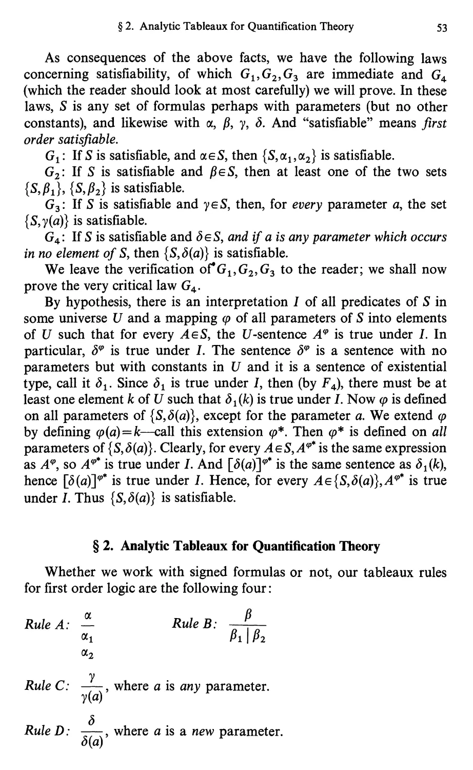
§ 2. Analytic Tableaux for Quantification Theory 53
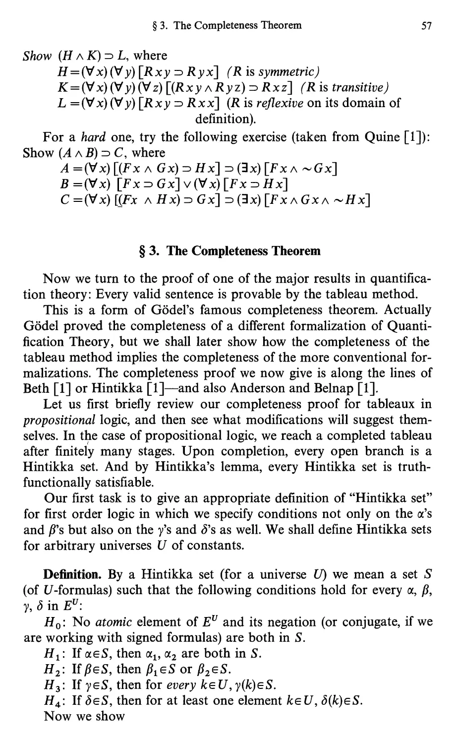
§ 3. The Completeness Theorem 57
§ 4. The Skolem-Lowenheim and Compactness Theorems for First-Order Logic 63
Chapter VL A Unifying Principle 65
§1. Analytic Consistency 65
§ 2. Further Discussion of Analytic Consistency 67
§ 3. Analytic Consistency Properties for Finite Sets 69
Chapter VIL The Fundamental Theorem of Quantification Theory 70
§1. Regular Sets 71
§ 2. The Fundamental Theorem 73
§ 3. Analytic Tableaux and Regular Sets 75
§ 4. The Liberalized Rule D 78
Chapter VIIL Axiom Systems for Quantification Theory 79
§ 0. Foreword on Axiom Systems 80

XII Contents
§1. The System gi 81
§2. The Systems 22,6* 84
Chapter IX. Magic Sets 86
§1. Magic Sets 87
§ 2. Applications of Magic Sets 89
Chapter X. Analytic versus Synthetic Consistency Properties 91
§1. Synthetic Consistency Properties 91
§ 2. A More Direct Construction 96
Part III. Further Topics in First-Order Logic
Chapter XL Gentzen Systems 101
§1. Gentzen Systems for Propositional Logic 101
§ 2. Block Tableaux and Gentzen Systems for First-Order Logic 109
Chapter XII. Elimination Theorems 110
§1. Gentzen's Hauptsatz 110
§ 2. An Abstract Form of the Hauptsatz Ill
§3. Some Applications of the Hauptsatz 115
Chapter XIII. Prenex Tableaux 117
§1. Prenex Formulas 117
§2. Prenex Tableaux 118
Chapter XIV. More on Gentzen Systems 121
§1. Gentzen's Extended Hauptsatz 121
§2. A New Form of the Extended Hauptsatz 122
§3. Symmetric Gentzen Systems 124
Chapter XV. Craig's Interpolation Lemma and Beth's Definability Theorem ... 127
§1. Craig's Interpolation Lemma 127
§2. Beth's Definability Theorem 131
Chapter XVI. Symmetric Completeness Theorems 133
§1. Clashing Tableaux 133
§2. Clashing Prenex Tableaux 136
§3. A Symmetric Form of the Fundamental Theorem 136
Chapter XVII. Systems of Linear Reasoning 141
§ 1. Configurations 142
§2. Linear Reasoning 151
§3. Linear Reasoning for Prenex Formulas 153
§ 4. A System Based on the Strong Symmetric Form of the Fundamental
Theorem 154
References 156
Subject Index 157

Parti
Propositional Logic from the Viewpoint of Analytic Tableaux

Chapter I
Preliminaries
§ 0. Foreword on Trees
Trees will play an important role throughout this work, so we
shall commence with some pertinent definitions:
By an unordered tree, ^, we shall mean a collection of the following
items:
(1) A set S of elements called points,
(2) A function, ^, which assigns to each point x a positive integer
f(x) called the level of x.
(3) A relation xRy defined in 5, which we read "x is a predecessor
of y" or "y is a successor of jc". This relation must obey the following
conditions:
Ci: There is a unique point ai of level 1. This point we call the origin
of the tree.
C2: Every point other than the origin has a unique predecessor.
C3: For any points x, y, if y is a successor of x, then ^(y)=^(x)+1.
We shall call a point x an end point if it has no successors; a simple
point if it has exactly one successor, and a junction point if it has more
than one successor. By a path we mean any finite or denumerable
sequence of points, beginning with the origin, which is such that each term
of the sequence (except the last, if there is one) is the predecessor of the
next. By a maximal path or branch we shall mean a path whose last
term is an end point of the tree, or a path which is infinite.
It follows at once from C^, C2, C3 that for any point x, there exists a
unique path P^ whose last term is x. If y lies on P^, then we shall say that
y dominates x, or that x is dominated by y. If x dominates y and XT^y,
then we shall say that x is (or lies) above y, or that y lies below x. We
shall say that x is comparable with y if x dominates y or y dominates x.
We shall say that y is between x and z if y is above one of the pair {x,z}
and below the other.
By an ordered tree, ^, we shall mean an unordered tree together with
a function Q which assigns to each junction point z a sequence 0(z) which
contains no repetitions, and whose set of terms consists of all the
successors of z. Thus, if z is a junction point of an ordered tree, we can speak
of the P^2'''^,..., n^^... successors of z (for any n up to the number of
successors of z) meaning, of course, the V^,T'^,..,,Yt^,.,. terms of 0(z).

4 I. Preliminaries
For a simple point x, we shall also speak of the successor of x as the
sole successor of x.
We shall usually display ordered trees by placing the origin at the
top and the successor(s) of each point x below x, and in the order, from
left to right, in which they are ordered in the tree. And we draw a line
segment from x to j; to signify that 3; is a successor of x.
We shall have occasion to speak of adding "new" points as successors
of an end point x of a given tree ^, By this we mean more precisely the
following: For any element 3; outside ^, by the adjunction of y as the
sole successor of x, we mean the tree obtained by adding 3; to the set S,
and adding the ordered pair <x,);> to the relation R (looked at as a set
of ordered pairs), and extending the function f by defining f{y)=f(x) +1.
For any distinct elements y^,..., >;„, each outside S, by the adjunction of
);i,...,);„ as respective P^2"^...,n^^ successors of x, we mean the tree
obtained by adding the y^ to S, adding the pairs <x,3;i> to R and extending
f by setting f(y^)=,..=f{y^=f{x)-\-l, and extending the function 0
by defining d{x) to be the sequence (yi,...,)^„). [It is obvious that the
extended structure obtained is really a tree].
A tree is called finitely generated if each point has only finitely many
successors. A tree, ^, is called finite if ^ has only finitely many points,
otherwise the tree is called infinite. Obviously, a finitely generated tree
may be infinite.
We shall be mainly concerned with ordered trees in which each
junction point has exactly 2 successors. Such trees are called dyadic trees.
For such trees we refer to the first successor of a junction point as the
left successor, and the second successor as the right successor.
[Exercise: In a dyadic tree, define x to be to the left of y if there is a
junction point whose left successor dominates x and whose right successor
dominates y. Prove that if x is to the left of y and y is to the left of z,
then X is to the left of z].
§ 1. Formulas of Propositional Logic
We shall use for our undefined logical connectives the following 4
symbols:
(1) - [read "not"], (2) a [read "and"],
(3) V [read "or"], (4) 3 [read "implies"].
These symbols are respectively called the negation, conjunction,
disjunction, and implication symbols. The last 3 are collectively called binary
connectives, the first (^) the unary connective.

§ 1. Formulas of Prepositional Logic 5
Other symbols shall be:
(i) A denumerable set Pi,P2> •••?Pn> ••• of symbols called propositional
variables.
(ii) The two symbols (,), respectively called the left parenthesis and
the right parenthesis (they are used for purposes of punctuation). Until
we come to First-Order Logic, we shall use the word "variable" to mean
propositional variable.
We shall use the letters "p", "^", "r", "s" to stand for any of the variables
Pi ? P2 > • • • > Pn> • • • • The notion of formula is given by the following recursive
rules, which enable us to obtain new formulas from those already
constructed :
Fq : Every propositional variable is a formula.
Fi: If A is a formula so is ^A.
F2,F^,F^: If A, B are formulas so are (A a B), {A v B), (A 3 B).
This recursive definition of "formula" can be made explicit as follows.
By a formation sequence we shall mean any finite sequence such that each
term of the sequence is either a propositional variable or is of the form
^ A, where A is an earlier term of the sequence, or is of one of the forms
(A A B), (A V B), (A =) B), where A, B are earlier terms of the sequence.
Now we can define ^4 to be a formula if there exists a formation sequence
whose last term is A. And such a sequence is also called a formation
sequence for A.
For any formula A, by the negation of A we mean '^A. It will
sometimes prove notationally convenient to write A' in place of '^A. For
any 2 formulas A, B, we refer to {A a B), (A v B), (A ■=> B) as the conjunction,
disjunction, conditional of A, B respectively. In a conditional formula
(A =) B), we refer to A as the antecedent and B as the consequent.
We shall use the letters "^", "5", "C", "X", "7", "Z" to denote
formulas. We shall use the symbol "6" to denote any of the binary
connectives a , v, =>; and when "6" respectively denotes a , v, => then
(XbY) shall respectively mean (XaY), (XvY), (XzdY). We can thus
state the formation rules more succinctly as follows:
Fq : Every propositional variable is a formula.
Fi: If X is a formula so is '^X.
F2'' If X, Y are formulas, then for each of the binary connectives b,
the expression (XbY) is a, formula.
In displaying formulas by themselves (i.e. not as parts of other
formulas), we shall omit outermost parentheses (since no ambiguity can
result). Also, for visual perspicuity, we use square brackets [ ]
interchangeably with parentheses, and likewise braces { }. Usually we shall
use square brackets as exterior to parentheses, and braces as exterior to
square brackets.

6 I. Preliminaries
Example. Consider the following formula:
{{(iP^q)^(q^r))zD{pvr))zD -(^vs)).
It is easier to read if displayed as follows:
{[{p:^q)A{qvr)']zD{pvr)}zD ^(qvs).
^iconJitiona/-we use "X^F'as an abbreviation for (X zd Y) a (Yzd X).
The formula X<r^Y is called the biconditional of X, Y. It is read "X if and
only if r' or "X is equivalent to Y".
Uniqueness of Decomposition. It can be proved that every formula
can be formed in only one way—i. e. for every formula X, one and only
one of the following conditions holds :
(1) X is a propositional variable.
(2) There is a unique formula Y such that X= T.
(3) There is a unique pair X^, X2 and a unique binary connective b
such that X = (Xi 6X2).
Thus no conjunction can also be a disjunction, or a conditional; no
disjunction can also be a conditional. Also none of these can also be a
negation. And, e.g., (X1AX2) can be identical with {Y^aY2) only if
Xi = Yi and X2=y2 (and similarly with the other binary connectives).
We shall not prove this here; perfectly good proofs can be found, e. g. in
Church [1] or Kleene [1].
In our discussion below, we shall consider a more abstract approach
in which this combinatorial lemma can be circumvented.
*Discussion. First we wish to mention that some authors prefer the
following formation rules for formulas:
Fq'. Same as Fq.
F\: If X is a formula, so is '^(X).
F2: If X, y are formulas, so is {X)b(Y).
This second set of rules has the advantage of eliminating, at the outset,
outermost parentheses, but has the disadvantage of needlessly putting
parentheses around variables.
It seems to us that the following set of formation rules, though a bit
more complicated to state, combines the advantages of the two preceding
formulations, and involves using neither more nor less parentheses than
is necessary to prevent ambiguity:
Fq : Same as before.
F'[: If X is a formula but not a propositional variable and p is a
propositional variable, '-'(X) and ^p are formulas.

§1. Formulas of Prepositional Logic 7
f 2: liX,Y are both formulas, but neither X nor 7 is a propositional
variable, and if p, q are propositional variables, then the following
expressions are all formulas:
(a) {X)biY),
(b) {X)bq,
(c) pb(.n
(d) pbq.
In all the above 3 approaches, one needs to prove the unique
decomposition lemma for many subsequent results. Now let us consider
yet another scheme (of a radically different sort) which avoids this.
First of all, we delete the parentheses from our basic symbols. We
now define the negation of X, not as the symbol ^ followed by the first
symbol of X, followed by the second symbol of X, etc. but simply as the
ordered pair whose first term is "^" and whose second term is X. And
we define the conjunction of X, Y as the ordered triple whose first term
is X, whose second term is " a " and whose third term is Y. [In contrast,
the conjunction of X and Y, as previously defined, is a sequence of
n + m + 3 terms, where n, m are the respective number of terms of X, Y.
The "3" additional terms are due to the left parenthesis, right parenthesis
and " A "]. Similarly we define the disjunction (conditional) of X, Y as
the ordered triple {X,b,Yy where b is the binary connective in question.
Under this plan, a formula is either a (propositional) variable, an
ordered pair (if it is a negation) or an ordered triple. Now, no ordered
pair can also be an ordered triple, and neither one can be a single symbol.
Furthermore, an ordered pair uniquely determines its first and second
elements, and an ordered triple uniquely determines its first, second and
third elements. Thus the fact that a formula can be formed in "only one
way" is now immediate.
We remark that with this plan, we can (and will) still use parentheses
to describe formulas, but the parentheses are not parts of the formula.
For example, we write X a{YvZ) to denote the ordered triple whose
first term is X, whose second term is " a ", and whose third term is itself
the ordered triple whose first, second and third terms are respectively,
Y, V ,Z. But (under this plan) the parentheses themselves do not belong
to the object language^) but only to our metalanguage^).
The reader can choose for himself his preferred notion of "formula",
since subsequent developments will not depend upon the choice.
^) The term object language is used to denote the language talked about (in this case
the set of formal expressions of propositional logic), and the term metalanguage is used to
denote the language in which we are talking about the object language (in the present case
English augmented by various common mathematical symbols).

8 I. Preliminaries
Subformulas. The notion of immediate subformula is given explicitly
by the conditions:
Iq : Propositional variables have no immediate subformulas.
/i: ^X has X as an immediate subformula and no others.
72-/4: The formulas XaY, XvY, X:dY have X, Y as immediate
subformulas and no others.
We shall sometimes refer to X, Y respectively as the left immediate sub-
formula, right immediate subformula of X aY, Xv Y, X :d Y.
The notion of subformula is implicitly defined by the rules:
Si: If X is an immediate subformula of Y, or if X is identical with 7,
then Z is a subformula of 7.
S2: If X is a subformula of 7 and 7 is a subformula of Z, then X is
a subformula of Z.
The above implicit definition can be made explicit as follows: 7 is
a subformula of Z iff (i.e. if and only if) there exists a finite sequence
starting with Z and ending with 7 such that each term of the sequence
except the first is an immediate subformula of the preceding term.
The only formulas having no immediate subformulas are
propositional variables. These are sometimes called atomic formulas. Other
formulas are called compound formulas. We say that a variable p occurs in
a formula X, or that p is one of the variables of X, if p is a subformula
ofX.
Degrees; Induction Principles. To facilitate proofs and definitions by
induction, we define the degree of a formula as the number of occurrences
of logical connectives. Thus:
Do: A variable is of degree 0.
Di: If Z is of degree n, then ^X is of degree n+1.
D2 — D4.: If X, 7 are of degrees n^,n2, then X a 7, X v 7, X =) 7 are
each of degree n^ + ^2 +1 •
Example.
pA{qv^r)isof degree 3.
p A (^ V r) is of degree 2.
We shall use the principle of mathematical induction (or of finite
descent) in the following form. Let S be a set of formulas (S may be
finite or infinite) and let P be a certain property of formulas which we
wish to show holds for every element of S. To do this it suffices to show
the following two conditions:
(1) Every element of S of degree 0 has the property P.
(2) If some element of S of degree > 0 fails to have the property P,
then some element of S of lower degree also fails to have property P.
Of course, we can also use (2) in the equivalent form:
(2)' For every element X of S of positive degree, if all elements of S
of degree less than that of X have property P, then X also has property P.

§ 2. Boolean Valuations and Truth Sets
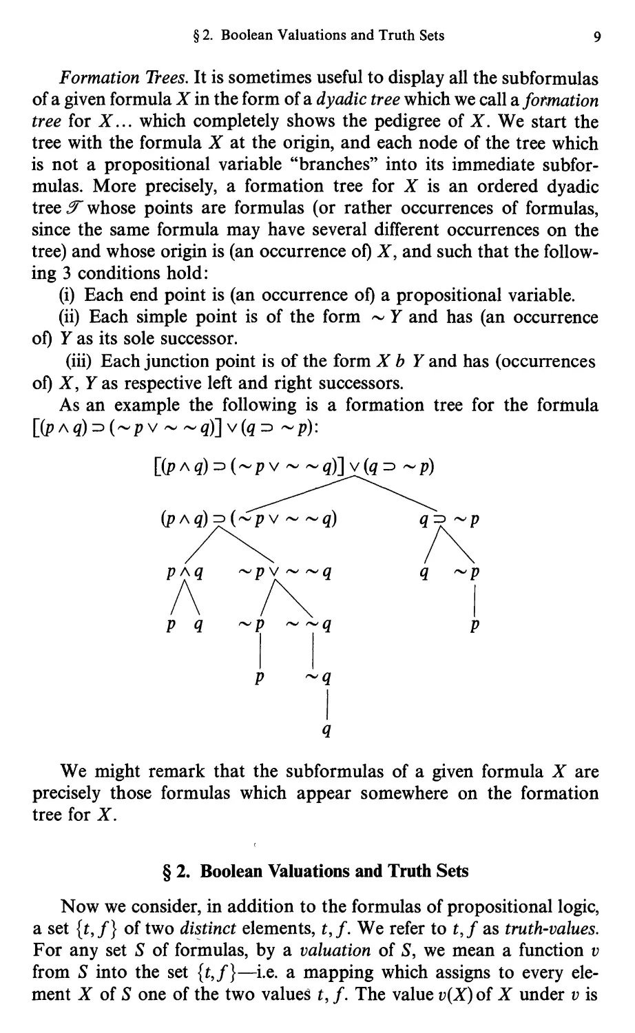
Formation Trees. It is sometimes useful to display all the subformulas
of a given formula X in the form of a dyadic tree which we call a, formation
tree for X... which completely shows the pedigree of X. We start the
tree with the formula X at the origin, and each node of the tree which
is not a propositional variable "branches" into its immediate
subformulas. More precisely, a formation tree for X is an ordered dyadic
tree ^ whose points are formulas (or rather occurrences of formulas,
since the same formula may have several different occurrences on the
tree) and whose origin is (an occurrence of) X, and such that the
following 3 conditions hold:
(i) Each end point is (an occurrence of) a propositional variable.
(ii) Each simple point is of the form ^ Y and has (an occurrence
of) Y as its sole successor.
(iii) Each junction point is of the form X b Y and has (occurrences
of) X, Y as respective left and right successors.
As an example the following is a formation tree for the formula
[(pA^)=)(-pv--^)]v(^=) -p):
[(pA^)=)(-pv
ip^q)
We might remark that the subformulas of a given formula X are
precisely those formulas which appear somewhere on the formation
tree for X.
§ 2. Boolean Valuations and Truth Sets
Now we consider, in addition to the formulas of propositional logic,
a set {t,f} of two distinct elements, t,f. We refer to t,/ as truth-values.
For any set S of formulas, by a valuation of 5, we mean a function v
from S into the set {t,f}—i.e. a mapping which assigns to every
element X of 5 one of the two valued t, f. The value v{X) of X under v is

10 I. Preliminaries
called the truth value of X under v. We say that X is true under v if
v{X) = t, and false under v if v{X) = /.
Now we wish to consider valuations of the set E of all formulas of
propositional logic. We are not really interested in all valuations of E,
but only in those which are "faithful" to the usual "truth-table" rules
for the logical connectives. This idea we make precise in the following
definition.
Definition 1. A valuation y of £ is called a Boolean valuation if for
every X, Y in E, the following conditions hold:
B^: The formula ^X receives the value t if X receives the value/
and f if X receives the value t,
B2: The formula X aY receives the value tifX, Y both receive the
value t, otherwise X aY receives the value /.
B3: The formula XvY receives the value t if at least one of X, Y
receives the value t, otherwise XvY receives the value /
B4: The formula X:dY receives the value f if X, Y receive the
respective values t, f, otherwise X :d Y receives the value t.
This concludes our definition of a Boolean valuation. We say that two
valuations agree on a formula X if Z is either true in both valuations or
false in both valuations. And we say that 2 valuations agree on a set S
of formulas if they agree on every element of the set S.
If Si is a subset of S2 and if v^, V2 are respective valuations of S^, S2,
then we say that V2 is an extension of y^ if ^2? ^i agree on the smaller set 5i.
It is obvious that if 2 Boolean valuations agree on X then they agree
on ^X (why?), and if they agree on both X, Y they must also agree on
each of Za Y, Xy Y, Z=)F(why?). By mathematical induction it follows
that if 2 Boolean valuations of E agree on the set of all atomic elements
of E (i. e., on all propositional variables) then they agree on all of E.
Stated otherwise, a valuation Vq of the set of all atomic elements of E
can be extended to at most one Boolean valuation of E.
By an interpretation of a formula X is meant an assignment of truth
values to all of the variables which occur in X. More generally, by an
interpretation of a set W (of formulas) is meant an assignment of truth
values to all the variables which occur in any of the elements of W. We
can thus rephrase the last statement of the preceding paragraph by
saying that any interpretation Vq of E can be extended to at most one
Boolean valuation of E. That Vq can be extended to at least one Boolean
valuation of E will be clear from the following considerations.
Consider a single formula X and an interpretation Vq of X—or for
that matter any assignment Vq of truth values to a set of propositional
variables which include at least all variables of X (and possibly others).
It is easily verified by induction on the degree of X that there exists one

§ 2. Boolean Valuations and Truth Sets 11
and only one way of assigning truth values to all subformulas of X such
that the atomic subformulas of X (which are propositional variables)
are assigned the same truth values as under Vq, and such that the truth
value of each compound subformula 7 of X is determined from the
truth values of the immediate subformulas of Y by the truth-table rules
B1—B4.. [We might think of the situation as first constructing a formation
tree for X, then assigning truth values to the end points in accordance
with the interpretation Vq, and then working our way up the tree,
successively assigning truth values to the junction and simple points, in terms
of truth values already assigned to their successors, in accordance with
the truth-table rules]. In particular, X being a subformula of itself
receives a truth value under this assignment; if this value is t then we
say that X is true under the interpretation Vq, otherwise false under ^o-
Thus we have now defined what it means for a formula X to be true
under an interpretation.
Now consider an interpretation, Vq, for the entire set E. Each element,
X, of E has a definite truth value under Vq (in the manner we have just
indicated); we let v be that valuation which assigns to each element of E
its truth value under the interpretation ^o- The valuation v is on the
entire set E, and it is easily verified that y is a Boolean valuation, and of
course, v is an extension of Vq. Thus it is indeed the case that every
interpretation of E can be extended to one (and only one) Boolean valuation
ofE.
Tautologies. The notion of tautology is perhaps the fundamental
notion of propositional logic.
Definition 2. Z is a tautology iff X is true in all Boolean valuations
ofE.
Equivalently, X is a tautology iff X is true under every interpretation
of E. Now it is obvious that the truth value of X under an interpretation
of E depends only on the truth values assigned to the variables which
occur in X. Therefore, Z is a tautology if and only if Z is true under every
interpretation of X. Letting n be the number of variables which occur
in X, there are exactly 2" distinct interpretations of X. Thus the task of
determining whether X is or is not a tautology is purely a finite and
mechanical one—just evaluate its truth value under each of its 2"
interpretations (which is tantamount to the familiar truth-table analysis).
Definitions. A formula X is called (truth-functionally) satisfiable
iff X is true in at least one Boolean valuation. A set S of formulas is said
to be (simultaneously) truth-functionally satisfiable iff there exists at
least one Boolean valuation in which every element of S is true. Such a
valuation is said to satisfy S.

12 I. Preliminaries
Definition 4. A set S truth-functionally implies a formula X, or X is
truth-functionally implied by S, or is a truth-functional consequence of S
if X is true in every Boolean valuation which satisfies S. We also say
that Y is truth-functionally implied by X if 7 is truth functionally implied
by the unit set {X} ... i. e. if 7 is true in every Boolean valuation in which
X is true.
Definition 5. Two formulas X, Y are called truth functionally
equivalent iff Z, y are true in the same Boolean valuations. [The reader
should note that X truth-functionally implies 7 iff Z =) 7 is a tautology,
and that X is truth-functionally equivalent to 7 iff the formula X<^Y
is a tautology].
Truth Sets. Let y be a Boolean valuation, and let S be the set of all
formulas which are true under v. It is immediate from the definition of a
Boolean valuation that the set S obeys the following conditions (for
everyZ, 7):
S^: Exactly one of the pair {X, ^X) belongs to S. Stated otherwise
(^x)esmxts.
S2: (Z A 7) is in S iff X, 7 are both in S.
S3: {XvY)ismSiff Xe Sot YeS.
S4: (X=)7)isinSiffZ^Sor YeS.
A set S obeying the above conditions will be called saturated or
will be said to be a truth set. Thus for any Boolean valuation, the set of
all sentences true under the valuation is saturated. Indeed, if v is an
arbitrary valuation, and if S is the set of all sentences which are true
under v, then the following 2 conditions are equivalent:
(1) y is a Boolean valuation,
(2) S is saturated.
Now suppose that we start with a set S, and we define v^ to be that
valuation which assigns t to every member of S, and / to every formula
outside S. [The function v^ is sometimes referred to as the characteristic
function of the set S.] It is again obvious that S is saturated iff v^ is a
Boolean valuation.
Now the set of all sentences true under v^ is obviously S itself. Thus a
set is saturated iff it is the set of all sentences true under some Boolean
valuation. Thus a formula Z is a tautology iff it is an element of every
truth set; stated otherwise, the set of tautologies is the intersection of all
truth sets and a formula X is satisfiable iff it is an element of some truth
set. Stated otherwise, the set of satisfiable sentences is the union of all
truth sets. Likewise a set S truth-functionally implies X iff X belongs to
every truth set which includes S.
We thus see that we really do not need to "import" these "foreign"
elements t, f in order to define our basic semantic notions. In some

§ 2. Boolean Valuations and Truth Sets 13
contexts it is technically more convenient to use t and / and Boolean
valuations; in other it is simpler to use truth sets.
Exercise 1 [Truth Functional Equivalence]. We shall use "c^^" in
our metalanguage and write X ^^^ 7 to mean that X is equivalent to Y—
i. e. that the formula X<-^Yis a tautology.
Now suppose that X^(^X2. Prove the following equivalences:
Zi A 7^X2 A 7;
Xi V 7^X2 V 7;
Xi 3 7^X2 3 7;
7AXi^7AX2,
7vXi-7vZ2,
7=)Zi-7^Z2.
Using these facts, show that for any formula Z which contains X^
as a part, if we replace one or more occurrences of the part X^ by X2,
the resulting formula is equivalent to Z.
Exercise 2 - [Important for Ch. XV!]. In some formulations of
propositional logic, one uses "t", "/" as symbols of the object language
itself; these symbols are then called propositional constants. And a
Boolean valuation is redefined by adding the condition that t must be
given the value truth 3,nd f falsehood. [Thus, e. g. t by itself is a tautology;
/ is unsatisfiable; X =) t is a tautology; /=) Z is a tautology. Also, under
any Boolean valuation t =) 7 has the same truth value as 7; Z =)/ has
the opposite value to X. Thus t =) 7 is a tautology iff 7 is a tautology;
X =)/ is a tautology iff X is unsatisfiable.]
Prove the following equivalences:
{l)XAt^X; Za/-/,
(2) Xvt^t; Zv/^X,
(3) X^tc^t; t^X^X,
(4) X^f^^X; f^X^t,
(5) ^t^/; ^/^t,
(6) Xa7^7aX; XvYc^YvX.
Using these facts show that every formula X with propositional
constants is either equivalent to a formula 7 which contains no pro-
positional constants or else it is equivalent to t or to /
Exercise 3. It is convenient to write a conjunction {..{X^a X2) a ... a X„)
as Xi AX2 a...aX„, and the formulas Xi,X2,...,X„ are called the
components of the conjunction. [Similarly we treat disjunctions.] By a
basic conjunction is meant a conjunction with no repetitions of
components such that each component is either a variable or the negation of a
variable, but no variable and its negation are both components. [As an
example, p^ a ^P2 /^Pa is a basic conjunction—so is ^Pi Ap2 a ^^3—
so is ^Pi AP2 /^Pa-] By a disjunctive normal formula is mean a formula
Ci V... V Q, where each C,. is a basic conjunction. [As an example the

14 I. Preliminaries
formula (p^ a ^Pi^^Pa) v(^Pi Ap2/^Pa) v(^Pi Ap2 Apj) is a
disjunctive normal formula.] A disjunctive normal formula is also sometimes
referred to as a formula in disjunctive normal form. If v^^e allov^^ pro-
positional constants t, f into our formal language, then the formula / is
also said to be a disjunctive normal formula.
Prove that every formula can be put into disjunctive normal form—
i.e. is equivalent to some disjunctive normal formula. [Hint: Make a
truth-table for the formula. Each line of the table v^^hich comes out "T"
v^^ill yield one of the basic conjunctions of the disjunctive normal form.]
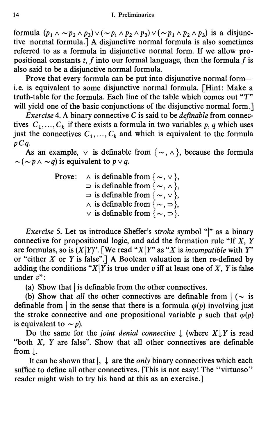
Exercise 4. A binary connective C is said to be definable from
connectives Ci,..., Q if there exists a formula in tv^^o variables p, q v^^hich uses
just the connectives C^,..., Cjt and v^^hich is equivalent to the formula
pCq.
As an example, v is definable from {^, a}, because the formula
^ (^ p A ^ ^) is equivalent to p v ^.
Prove: a is definable from {^
=) is definable from {^
=) is definable from { ^
A is definable from {^
V is definable from { ^
V},
A},
V},
-}.
Exercise 5. Let us introduce Sheffer's stroke symbol "|'' as a binary
connective for propositional logic, and add the formation rule "If X, Y
are formulas, so is {X\Y)'\ [We read "X|r' as "X is incompatible v^^ith F'
or "either Z or 7 is false".] A Boolean valuation is then re-defined by
adding the conditions "X|y is true under v iff at least one of X, 7 is false
under y":
(a) Shov^^ that | is definable from the other connectives.
(b) Shov^^ that all the other connectives are definable from | (^ is
definable from | in the sense that there is a formula (p{p) involving just
the stroke connective and one propositional variable p such that (p{p)
is equivalent to ^p).
Do the same for the joint denial connective [ (v^^here XIY is read
"both X, Y are false". Shov^^ that all other connectives are definable
from |.
Itcanbeshov^^nthat |, i are the onfy binary connectives which each
suffice to define all other connectives. [This is not easy! The "virtuoso"
reader might wish to try his hand at this as an exercise.]

§1. The Method of Tableaux 15
Chapter II
Analytic Tableaux
We now describe an extremely elegant and efficient proof procedure
for propositional logic which we will subsequently extend to first order
logic, and which shall be basic to our entire study. This method, which
we term analytic tableaux, is a variant of the "semantic tableaux" of
Beth [1], or of methods of Hintikka [1]. (Cf. also Anderson and
Belnap [1].) Our present formulation is virtually that which we
introduced in [1]. Ultimately, the whole idea derives from Gentzen [1], and
we shall subsequently study the relation of analytic tableaux to the
original methods of Gentzen.
§ 1. The Method of Tableaux
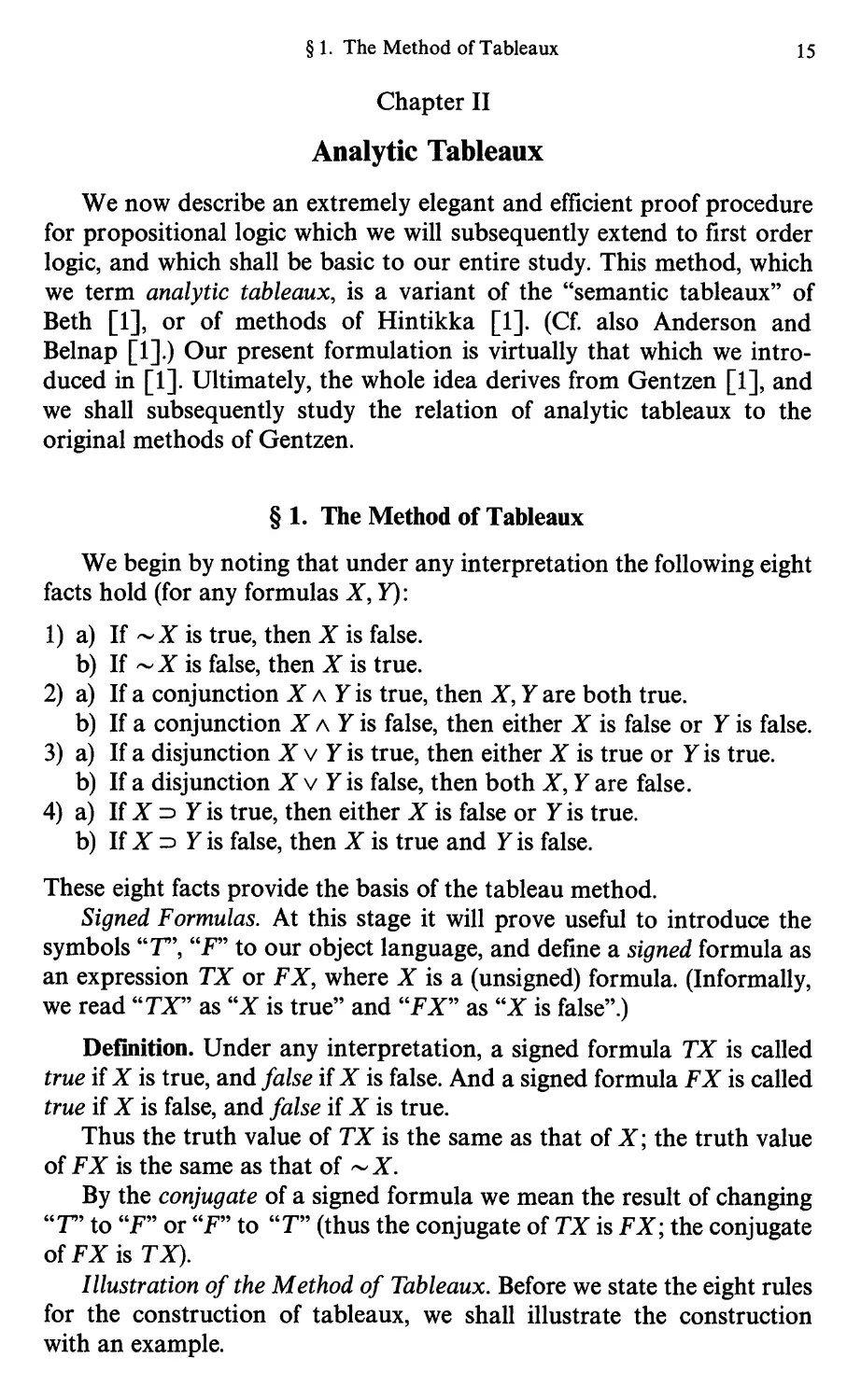
We begin by noting that under any interpretation the following eight
facts hold (for any formulas X, Y):
1) a) If ^Z is true, then X is false,
b) If ^X is false, then X is true.
2) a) If a conjunction X aYis true, then X, Y are both true.
b) If a conjunction X aYis false, then either X is false or Y is false.
3) a) If a disjunction XvYis true, then either X is true or Yis true,
b) If a disjunction XvYis false, then both X, Y are false.
4) a) If X =) y is true, then either X is false or Yis true,
b) If X =) yis false, then X is true and yis false.
These eight facts provide the basis of the tableau method.
Signed Formulas. At this stage it will prove useful to introduce the
symbols "T", "F" to our object language, and define a signed formula as
an expression TX or FX, where X is a (unsigned) formula. (Informally,
we read "TX" as "X is true" and "FX" as "Z is false".)
Definition. Under any interpretation, a signed formula TX is called
true if X is true, and false if X is false. And a signed formula FX is called
true if X is false, and false if X is true.
Thus the truth value of TX is the same as that of X; the truth value
of FX is the same as that of ^X.
By the conjugate of a signed formula we mean the result of changing
"r' to "F" or "F" to "T" (thus the conjugate of TX is FX; the conjugate
ofFXisTX).
Illustration of the Method of Tableaux. Before we state the eight rules
for the construction of tableaux, we shall illustrate the construction
with an example.

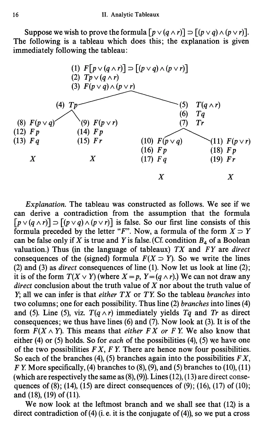
16 11. Analytic Tableaux
Suppose we wish to prove the formula [p v (^ a r)] =) [(p v ^) a (p v r)].
The following is a tableau which does this; the explanation is given
immediately following the tableau:
(l)F[pv(qAr)]=.
(2) Tpv(«Ar)
(3) F{pvq)A(j>vr]
(4) Tp"-^""""^
^\
(8)F(pv«r \9)F(pvr)
(12) Fp
(13) Fq
X
(14) Fp
(15) Fr
X
[(pvq)A{p
1
(10) F(pC
(16) Fp
(17) Fq
vr)]
-(5)
(6)
(7)
'«)
T(qAr)
Tg
Tr
^^(11) Fipvr)
(18) f p
(19) Fr
Explanation. The tableau was constructed as follows. We see if we
can derive a contradiction from the assumption that the formula
[p V (^ A r)] =3 [(p V ^) A (p V rj] is false. So our first line consists of this
formula preceded by the letter "F". Now, a formula of the form X:d Y
can be false only if X is true and Y is false. (Cf. condition B4. of a Boolean
valuation.) Thus (in the language of tableaux) TX and FY are direct
consequences of the (signed) formula F{X =) Y). So we write the lines
(2) and (3) as direct consequences of line (1). Now let us look at line (2);
it is of the form T{X v Y) (where X=p, Y= {q a r).) We can not draw any
direct conclusion about the truth value of X nor about the truth value of
Y; all we can infer is that either TX or TY. So the tableau branches into
two columns; one for each possibility. Thus line (2) branches into lines (4)
and (5). Line (5), viz. T{q a r) immediately yields Tq and Tr as direct
consequences; we thus have lines (6) and (7). Now look at (3). It is of the
form F{XA Y). This means that either FX or FY. We also know that
either (4) or (5) holds. So for each of the possibilities (4), (5) we have one
of the two possibilities FX, FY There are hence now four possibilities.
So each of the branches (4), (5) branches again into the possibilities FX,
F Y More specifically, (4) branches to (8), (9), and (5) branches to (10), (11)
(which are respectively the same as (8), (9)). Lines (12), (13) are direct
consequences of (8); (14), (15) are direct consequences of (9); (16), (17) of (10);
and (18), (19) of (11).
We now look at the leftmost branch and we shall see that (U) is a
direct contradiction of (4) (i. e. it is the conjugate of (4)), so we put a cross

§ 1. The Method of Tableaux 17
after (13) to signify that this branch leads to a contradiction. Similarly,
(14) contradicts (4), so we "close" the branch leading to (15)—i.e. we
put a cross after (15). The next branch is closed by virtue of (17) and (6).
Finally, the rightmost branch is closed by virtue of (19) and (7). Thus all
branches lead to a contradiction, so line (1) is untenable. Thus
[p V (^ A r)] =) [(p V ^) A (p V r)] can never be false in any interpretation,
so it is a tautology.
Remarks, (i) The numbers put to the left of the lines were only for the
purpose of identification in the above explanations; we do not need
them for the actual construction.
(ii) We could have closed some of our branches a bit earlier; lines
(13), (15) are superfluous. In subsequent examples we shall close a branch
as soon as a contradiction appears (a contradiction that is of the form of
two formulas FX, TX).
Rules for the Construction of Tableaux. We now state all the rules in
schematic form; explanations immediately follow. For each logical
connective there are two rules; one for a formula preceded by "T", the
other for a formula preceded by "F":
1)
2)
3)
4)
T^X
FX
T{XaY)
fx
TY
T{XvY)
TX\TY
T{X^ Y)
FX\TY TX
FY
F^X
TX
F{XaY)
FX\FY
F{XvY)
FX
FY
F{X:^Y)
Some Explanations. Rule 1) means that from T--Z we can directly
infer FX (in the sense that we can subjoin FX to any branch passing
through T-Z) and that from F-X we can directly infer TX. Rule 2)
means that T{Xa Y) directly yields both TX, TY, whereas F{XaY)
branches into FX, F Y. Rules 3) and 4) can now be understood analogously.
Signed formulas, other than signed variables, are of two types;
(A) those which have direct consequences (viz. F^X, T^X, T{X a Y),
F{XvY), F{X^ y)); (B) those which branch (viz. F{X a Y), T{XwY),
T{X ID Y)).

18
II. Analytic Tableaux
It is practically desirable in constructing a tableau, that when a line
of type (A) appears on the tableau, we simultaneously subjoin its
consequences to all branches which pass through that line. Then that line
need never be used again. And in using a line of type (B), we divide all
branches which pass through that line into sub-branches, and the line
need never be used again. For example, in the above tableau, we use (1)
to get (2) and (3), and (1) is never used again. From (2) we get (4) and (5),
and (2) is never used again. Line (3) yields (8), (9), (10), (11) and (3) is
never used again, etc.
If we construct a tableau in the above manner, it is not difficult to
see, that after a finite number of steps we must reach a point where
every line has been used (except of course, for signed variables, which
are never used at all to create new lines). At this point our tableau is
complete (in a precise sense which we will subsequently define).
One way to complete a tableau is to work systematically
downwards i.e. never to use a line until all lines above it (on the same branch)
have been used. Instead of this procedure, however, it turns out to be
more efficient to give priority to lines of type (A)—i.e. to use up all
such lines at hand before using those of type (B). In this way, one will
omit repeating the same formula on different branches; rather it will
have only one occurrence above all those branch points.
As an example of both procedures, let us prove the formula
[p=)(^=) r)] =) [(p=) ^)=)(p=) r)]. The first tableau works
systematically downward; the second uses the second suggestion. For the
convenience of the reader, we put to the right of each line the number of
the line from which it was inferred.
First Tableau
(2)Tp =
(3)F(p:
(4)Fp(2)
(6)T(p=>g)(3)
(7)f(p^r)(3)
(10) Fp (6)
(12) Tp (7)
X
ill) Tq (6)
(13) Tp (7)
X
3 (g =3 r)] =3 [(p =) g) ID (p ID r)]
>«)=>(p=.r)(l)
{5)T{q^r){2)
(8)T(p:D«)(3)
(9)F(p:D/-)(3)
{14) Fq (5)
(16) Fp (8)
(20) Tp (9)
X
(17)Tq(8)
X
(15) Tr (5)
(18) Fp (8)
(21) Tp (9)
X
(19)Tq(8)
(22) Tp (9)
(23) Fr (9)
X

§ 1. The Method of Tableaux
19
Second Tableau
(1) F [p =>(«=> r)] ID [(p^q)=.(p ID r)]
(2) Tp^{q^r)(l)
{3)F(p^q)^(p^r){l)
(4) T(p=>q)(3)
{5)F(p^r){3)
(6) Tp (5)
(7) Fr (5)
(8) Fp (2)
X
(9) T(«=>r)(2)
(10) Fp (4)
X
(11) Tq (4)
(12) Fq (9) 1 (13) Tr (9)
X X
It is apparent that Tableau (2) is quicker to construct than Tableau (1),
involving only 13 rather than 23 lines.
As another practical suggestion, one might put a check mark to the
right of a line as soon as it has been used. This will subsequently aid
tjie eye in hunting upward for lines which have not yet been used. (The
check marks may be later erased, if the reader so desires.)
The method of analytic tableaux can also be used to show that a
given formula is a truth functional consequence of a given finite set of
formulas. Suppose we wish to show that Z => Z is a truth-functional
consequence of the two formulas X => 7, 7 => Z. We could, of course,
simply show that \(X^Y)a{Y^ Z)] id (X id Z) is a tautology.
Alternatively, we can construct a tableau starting with
nXiDY),
F{X ID Z)
and show that all branches close.
In general, to show that 7is truth-functionally implied by Xi,...,X„,
we can construct either a closed analytic tableau starting with
F{Xi A... A X^ ID y, or one starting with
TX,
FY

20 II. Analytic Tableaux
Tableaux using unsigned formulas. Our use of the letters "T" and
"F", though perhaps heuristically useful, is theoretically quite
dispensable—simply delete every "T" and substitute "--" for "F". (In which
case, incidentally, the first half of Rule 1) becomes superfluous.) The
rules then become:
'' X
2) ^^
' X
Y
3) ^
'' X\Y
4) ^^^
^> ~X\Y
~{XaY)
~X\~Y
~{XwY)
~X
~Y
~iX=>Y)
X
In working with tableaux which use unsigned formulas, "closing"
a branch naturally means terminating the branch with a cross, as soon
as two formulas appear, one of which is the negation of the other. A
tableau is called closed if every branch is closed.
By a tableau for a formula X, we mean a tableau which starts with X.
If we wish to prove a formula X to be a tautology, we construct a tableau
not for the formula X, but for its negation ^X.
A Unifying Notation. It will save us considerable repetition of
essentially the same arguments in our subsequent development if we use the
following unified notation which we introduced in [2].
We use the letter "a" to stand for any signed formula of type A—i.e.
of one of the five forms T{XaY), F{XvY), F{X id Y), T-X, F-X.
For every such formula a, we define the two formulas a^ and a2 as follows:
If a = T{X A y), then oc^ = TX and a2 = TY.
If a = F{X V y), then a^ = FX and a2 = F Y.
If a = F{X ID y), then oc^ = TX and a2 = F y.
I/a = T- X, then oc^ = FX and a2 = FX.
If a = F-Z, then a^ = TX and a2 = TX.
For perspicuity, we summarize these definitions in the following
table:

§ 1. The Method of Tableaux
21
a
T{XaY)
F{XvY)
F{X^ Y)
T^X
F^X
ai
TX
FX
TX
FX
TX
(X2
TY
FY
FY
FX
TX
We note that under any interpretation, a is true iff ai, a2 are both true.
Accordingly, we shall also refer to an a as a formula of conjunctive type.
We use "j5" to stand for any signed formula of type B—i.e. one of the
three forms F{X a Y), T(X v Y), T{X id Y). For every such formula p,
we define the two formulas p^, P2 ^s in the following table:
p
FiXAY)
TiXvY)
T{X =5 Y)
/?.
FX
TX
FX
P2
FY
TY
TY
In any interpretation, P is true iff at least one of the pair jSj, P2 is true.
Accordingly, we shall refer to any j5-type formula as a formula of
disjunctive type.
We shall sometimes refer to (Xi as the first component of a and (X2 as
the second component of a. Similarly, for p.
By the degree of a signed formula TX or FX we mean the degree
of X. We note that aj, (X2 are each of lower degree than a, and P^, P2 are
each of lower degree than p. Signed variables, of course, are of degree 0.
We might also employ an a, j5 classification of unsigned formulas
in an analogous manner, simply delete all "T", and replace "F" by "--".
The tables would be as follows:
a
XaY
'^(XwY)
^{X^Y)
--Z
ai
X
-X
X
X
(X2
Y
-y
-y
X
p
~(XaF)
XvY
X^Y
h
~X
X
~x
P2
~Y
Y
Y

22 II. Analytic Tableaux
Let us now note that whether we work with signed or unsigned
formulas, all our tableau rules can be succinctly lumped into the following
two:
Rule A - oi RuleB- p
^APi
N.B. In working with signed formulas, there arise situations in which
it is better to regard signed formulas of the form T^X or F^X as of
both the a-type and the j5-type. If we agree to let j5 be such a formula,
it still remains true that under any interpretation, j5 is true iff at least
one of j^i, j52 is true (for in such a case, p^ and p2 ^^e identical
expressions). Under this extended use of "j5". Rule B when applied to an
expression T^X or F^X would yield two identical branches. So in
practice, we need consider only one. Indeed, in practice we need
consider only one branch even in other cases when j^i and ^2 ^^^ identical—
e.g. if j5 = T{X V X) it would be pointless to divide the tableau into two
branches, TZ and TX\
Some Properties of Conjugation. One reason for the desirability of
using "j5" in the extended manner which we just discussed, is that our
operation of conjugation obeys the following pleasant symmetric laws:
Jo"- {a) X is distinct from X\
(b) X = X.
Ji'. [a) The conjugate of any a is some j5.
{h) The conjugate of any j5 is some a.
J2- (a) (a)i=ai_; (a)2 = a^;
Law Ji - (a) would fail under the original definition of j5.
Law J2 says that if we take any signed formula X other than a signed
variable, if we first conjugate X and then take the first (second)
component of this conjugate, we obtain the same result as if we first take the
first (respectively second) component of X and then conjugate it. (For
example, suppose a = F(X ID Y). Then a = T(X id Y), (a)i = FX, (a)2 = TY,
On the other hand, a^ = TX, 0^2 = FY, so a^ = FX, ^2 = TY). The reader
can verify the remaining four cases for a and similarly the cases for p.
We note that J2 can be equivalently stated as follows: If a is the
conjugate of j5, then aj is the conjugate of j^i and (X2 is the conjugate of j52.
Tf-uth Sets re-visited. For the moment let us work with unsigned
formulas (interpreting "a" and "jS" accordingly). Let 5 be a set of unsigned
formulas. We leave it to the reader to verify that 5 is a truth set (as defined
in Chapter I) if and only if S has the following three properties (for
every X, a, j5):

§ 1. The Method of Tableaux 23
(0) Exactly one ofX,--Z belongs to S.
(A) a belongs to S if and only if a^, a2 both belong to S.
(B) p belongs to S if and only if at least one of j^i, p2 belong to S.
We shall also refer to a set S of signed formulas as a valuation set
or truth set if it obeys conditions (A), (B) above and in place of (0), the
condition "exactly one of TX, FX belongs to 5". We shall also refer to
valuation sets of signed formulas as saturated sets.
Exercise. Show that if a set S of unsigned formulas satisfies (^4), (B)
above and in place of (0) the weaker condition "for every propositional
variable p, exactly one of p, --p lies in 5" then it follows that for every
formula X, exactly one of Z, ^X lies in S—i.e. that S is then a truth
set. State and prove an analogous result for signed formulas.
We have defined a set S of signed formulas to be a truth set if it
satisfies the laws:
(0) For any X, exactly one of X, Z belongs to S.
(a) (xeS iff (x^eS and 01,2^8.
(b) peSiff p^eSoT p2^S.
We wish to point out that (b) is superfluous in the presence of (0)
and (a) and also that (a) is superfluous in the presence of (0) and (b). Let
us prove that (b) follows from (0) and (a)—in doing this it will shorten
our work to use our laws Jq — J2 on conjugation. Assume now that S
satisfies conditions (0), (a). We must show that jS belongs to S iff j^i
belongs to S or p2 belongs to S. Suppose that peS.lf neither p^ nor P2
belonged to S, then P^ and P2 would belong to S (since by (0) at least
one of pi, pi belongs to S and at least one of P2, P2 belongs to S). Now
we use the fact that P is some a, and j^i = a^, JS2 = a2. So ai, a2 both belong
to S. Then by (a), a belongs to S—^i. e. P belongs to S. This would mean
that p, P both belong to S, contrary to condition (0). This proves the
first half. Conversely, suppose at least one of pi,p2 belongs to S—let
us say /3i (a perfectly analogous argument works for P2). If P fails to
belong to S, then p belongs to S.^But P is some a, hence by (a), 0)^ and
(P)2 belong to S—Whence (by J2) Pi belongs to S. This implies p^ and P^
both belong to S, contrary to condition (0). This concludes the proof.
We leave it to the reader to verify that it is likewise possible to obtain
(a) from (0) and (b). We also remark that the same result holds for truth
sets of unsigned formulas (but the verification can not be carried out as
elegantly, since we have no conjugation operation satisfying Jq,Ji,J2;
the proof must be ground out by considering all cases separately).
Exercise. Call a set downward closed if for every a and p, (1) if a is
in S, then (Xi,(X2 are both in S; (2) if p is in 5, then at least one of Pi,p2
is in S. Call a set upward closed if the converse conditions hold—^i.e. (1)
if ai,a2 are both in 5, so is a; (2) if either Pi or p 2 is in S, so is p. Show that
any downward closed set satisfying condition (0) (viz. that for every X,

24 II. Analytic Tableaux
exactly one of X,X is in iS) is a truth set. Show that any upward closed
set satisfying (0) is a truth set.
Precise Definition of Tableaux. We have deliberately waited until
the introduction of our unified notation in order to give a precise
definition of an analytic tableau, since the definition can now be given more
compactly.
Definition. An analytic tableau for X is an ordered dyadic tree, whose
points are (occurrences of) formulas, which is constructed as follows.
We start by placing X at the origin. Now suppose ^ is a tableau for X
which has already been constructed; let Y be an end point. Then we
may extend ^ by either of the following two operations.
(A) If some a occurs on the path Py, then we may adjoin either aj
or (X2 as the sole successor of Y. (In practice, we usually successively
adjoin oc^ and then a2.)
(B) If some j5 occurs on the path Py, then we may simultaneously
adjoin pi as the left successor of Y and P2 ^s the right successor of Y
The above inductive definition of tableau for X can be made expHcit
as follows. Given two ordered dyadic trees ^i and ^2? whose points
are occurrences of formulas, we call ^2 ^ direct extension of c^i if ^2
can be obtained from ^i by one appUcation of the operation (A) or (B)
above. Then ^ is a tableau for X iff there exists a finite sequence
{^i,^2^"-^'^n = ^) such that ^1 is a 1-point tree whose origin is X
and such that for each i<n,^^+i is a direct extension of c^^.
To repeat some earlier definitions (more or less informally stated)
a branch 0 of a tableau for signed (unsigned) formulas is closed if it
contains some signed formula and its conjugate (or some unsigned
formula and its negation, if we are working with unsigned formulas.) And ^
is called closed if every branch of ^ is closed. By a proof of (an unsigned
formula) X is meant a closed tableau for FZ(or for ^X, if we work with
unsigned formulas.)
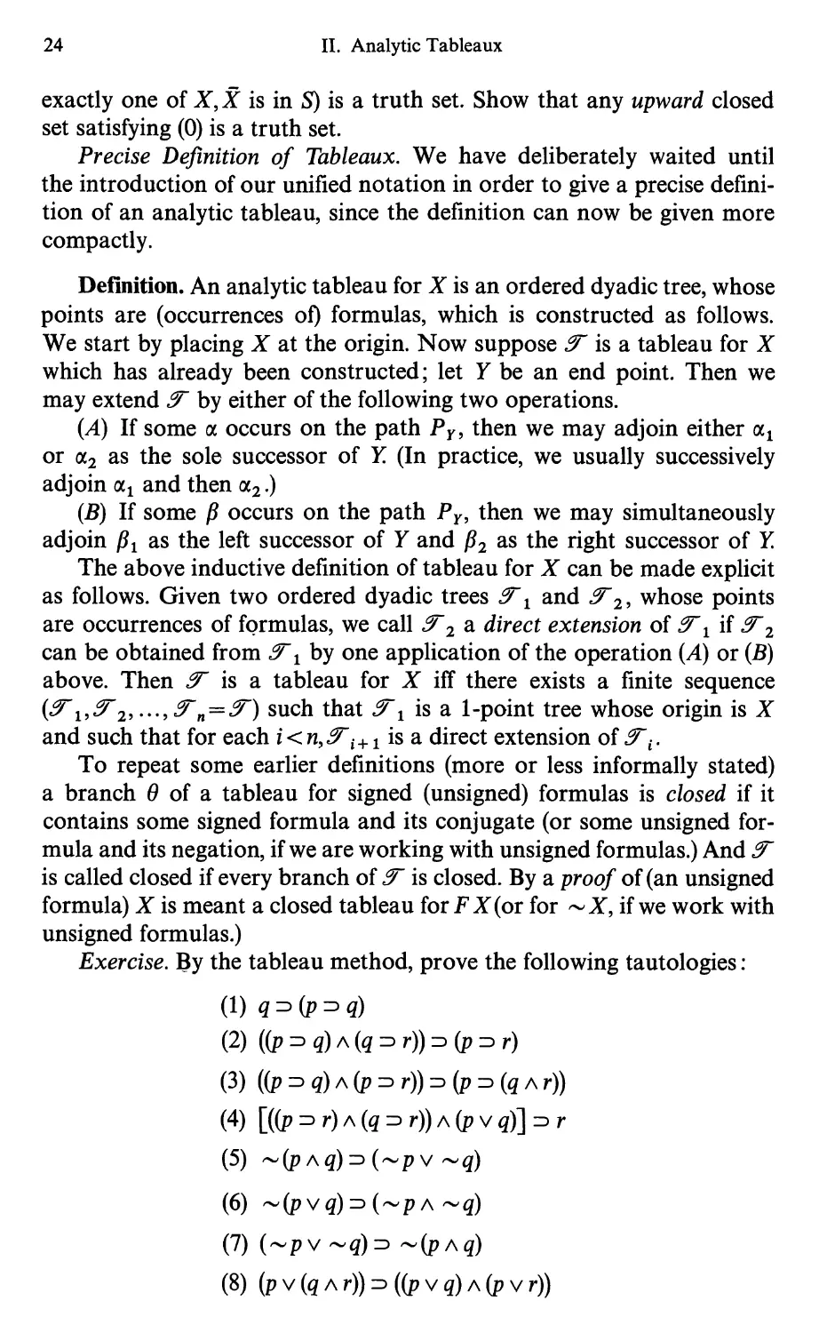
Exercise. By the tableau method, prove the following tautologies :
(1) q:^{p^q)
(2) ((p ID g) A (^ ID r)) ID (P ID r)
(3) ((p:^^)A(piDr))iD(piD(^Ar))
(4) [{{p ^ r) A{q^ r)) A{pv q)]:^ r
(5) ^{pAq)^{^pv ^q)
(6) -(pv^)iD(-pA-^)
(7) (-pv-^)iD ^{pAq)
(8) (pv(^Ar))iD((pvg)A(pvr))

§ 2. Consistency and Completeness of the System 25
§ 2. Consistency and Completeness of the System
Consistency. It is intuitively rather obvious that any formula provable
by the tableau method must be a tautology—equivalently, given any
closed tableau, the origin must be unsatisfiable. This intuitive conviction
can be justified by the following argument.
Consider a tableau ^ and an interpretation Vq whose domain
includes at least all the variables which occur in any point of ^. Let us
call a branch ^ of ^ true under Vq if every term of 6 is true under Vq .
And we shall say that the tableau ^ (as a whole) is true under Vq iff at
least one branch of ^ is true under Vq.
The next step is to note that if a tableau ^2 is an immediate extension
of ^1, then ^2 ^^^st be true in every interpretation in which ^1 is true.
For if c^i is true, it must contain at least one true branch 6. Now ^2
was obtained from ^^ by adding one or two successors to the end point
of some branch ^1 of ^1; if ^1 is distinct from 6, then 6 is still a branch
of c^2j hence ^2 contains the true branch 6, so ^2 is true. On the other
hand, suppose 6 is identical with 6^—i.e. suppose 6 is the branch of c^i
which was extended in ^2- If ^ was extended by operation (A), then
some a appears as a term in 6, and 6 has been extended either to (^i,ai)
or to {9i,(X2), so either {6i,0Ci) or (^i,a2) is a branch of ^2- ^^t (Xi,(X2
are both true since a is, hence ^2 contains the true branch (^i,ai) or
{91,01,2). If 9 was extended by operation (B), then some p occurs in 9 and
both (^1, j^i) and {91,^2) ^^^ branches of ^2- But since p is true, then at
least one of j5i,j52 is true, hence one of the branches {9i,pi) or {91,^2)
of ^2 is true, so again ^2 is true.
We have thus shown that any immediate extension of a tableau which
is true (under a given interpretation) is again true (under the given
interpretation). From this it follows by mathematical induction that for any
tableau ^, if the origin is true under a given interpretation Vq, then ^
must be true under Vq. Now a closed tableau ^ obviously cannot be
true under any interpretation, hence the origin of a closed tableau cannot
be true under any interpretation—i. e. the origin of any closed tableau
must be unsatisfiable. From this it follows that every formula provable
by the tableau method must be a tautology. It therefore further follows
that the tableau method is consistent in the sense that no formula and its
negation are both provable (since no formula and its negation can both
be tautologies).
Completeness. We now consider the more delicate converse situation:
Is every tautology provable by the method of tableaux? Stated otherwise,
if X is a tautology, can we be sure that there exists at least one closed
tableau starting with FX? We might indeed ask the following bolder
question: If Z is a tautology, then will every complete tableau for FX

26 II. Analytic Tableaux
close? An affirmative answer to the second question would, of course,
be even better than an affirmative answer to the first, since it would mean
that any single completed tableau ^ for FAT would decide whether X
is a tautology or not.
Before the reader answers the question too hastily, we should consider
the following. If we delete some of the rules for the construction of
tableaux, it will still be true that a closed tableau for ¥X always indicates
that Z is a tautology. But if we delete too many of the rules, then we
may not have left enough power to always derive a closed tableau for FX
whenever X is a tautology. (For example, if we delete the first half of
the conjunction rule, then it would be impossible to prove the tautology
(p A ^) =) p, though it would still be possible to prove p => [^ => (p a g)].
If we delete the second half but retain the first half, then we could prove
the first tautology above, but not the second.) The question, therefore, is
whether our present set of rules is sufficient to do this. Our present
purpose is to show that they are sufficient.
We shall give the proof for tableaux using signed formulas (the
modifications for tableaux using unsigned formulas are obvious—or
indeed the result for tableaux for unsigned formulas follows directly
from the result for tableaux with signed formulas.)
We are calling a branch ^ of a tableau complete if for every a which
occurs in 6, both ai and (X2 occur in 6, and for every p which occurs in 6,
at least one of j5i,j52 occurs in 6. We call a tableau ^ completed if every
branch of ^ is either closed or complete. We wish to show that if ^ is
any completed open tableau (open in the sense that at least one branch is
not closed), then the origin of 3" is satisfiable. More generally, we shall
show
Theorem 1. Any complete open branch of any tableau is
(simultaneously) satisfiable.
We shall actually prove something stronger. Suppose ^ is a complete
open branch of a tableau c^; let S be the set of terms of 6. Then the set S
satisfies the following three conditions (for every a, p):
Hq\ No signed variable and its conjugate are both in S^).
H^\ If aeS, thena^eS and a2eS.
H2: IfjS6S,thenjSi6SorjS2eS.
Sets S—whether finite or infinite—obeying conditions Hq,Hi,H2
are of fundamental importance—we shall call them Hintikka sets (after
Hintikka who studied their properties explicitly). We shall also refer to
^) Indeed no signed formula and its conjugate appear in S, but we do not need to involve
this stronger fact.

§ 2. Consistency and Completeness of the System 27
Hintikka sets as sets which are saturated downwards. We shall also
call any finite or denumerable sequence 9 a Hintikka sequence if its set of
terms is a Hintikka set.
Let us pause for a moment to compare the notion of downward
saturation with that of saturation discussed earlier (cf. the preceding
section on truth sets re-visited). The definition of a, saturated set differs
from that of a Hintikka set in that in H^,H2 "if is replaced by "if and
only if, and Hq is strengthened to condition (0). So every saturated set is
obviously also a Hintikka set. But a Hintikka set need not be saturated
(e.g. any set of signed variables which contains no signed variable and its
conjugate vacuously satisfies H^,H2, but such a set is certainly not
saturated.)
Theorem 1 is substantially to the effect that every finite Hintikka set
S is satisfiable. The finiteness of 5, however, is not needed in the proof
(nor does it even simplify the proof), so we shall prove
Hintikka's Lemma. Every downward saturated set S (whether finite
or infinite) is satisfiable.
We remark that Hintikka's lemma is equivalent to the statement that
every Hintikka set can be extended to a (i.e. is a subset of some) saturated
set. We remark that Hintikka's lemma also holds for sets of unsigned
formulas (where by a Hintikka set of unsigned formulas we mean a
set S satisfying H^,H2 and in place of//q, the condition that no variable
and its negation are both elements of S).
Proof of Hintikka's Lemma. Let aS be a Hintikka set. We wish to
find an interpretation in which every element of S is true. Well, we
assign to each variable p, which occurs in at least one element of 5, a
truth value as follows :
(1) If TpeS, give p the value true.
(2) If FpG 5, give p the value false.
(3) If neither Tp nor Fp is an element of 5, then give p the value true
or false at will (for definiteness, let us suppose we give it the value true.)
We note that the directions (1), (2) are compatible, since no Tp and
Fp both occur in S (by hypothesis Hq). We now show that every element
of S is true under this interpretation. We do this by induction on the
degree of the elements.
It is immediate that every signed variable which is an element of S
is true under this interpretation (the interpretation was constructed to
insure just this). Now consider an element Z of 5 of degree greater than 0,
and suppose all elements of S of lower degree than X are true. We wish
to show that X must be true. Well, since X is of degree greater than zero,
it must be either some a or some j8.

28 II. Analytic Tableaux
Case 1. Suppose it is an a. Then ai,a2 must also be in S (by Hi).
But ai,a2 are of lower degree than a. Hence by inductive hypothesis
ai and a2 are both true. This implies that a must be true.
Case 2. Suppose X is some p. Then at least one of j^i, ^^2 is in S (by H2)'
Whichever one is in S, being of lower degree than P, must be true (by
inductive hypothesis). Hence P must be true. This concludes the proof.
Remark. If we hadn't used the unifying "a, jS" notation, we would have
had to analyze eight cases rather than two.
Having proved Hintikka's lemma, we have, of course, also proved
Theorem 1. This in turn implies
Theorem 2. (Completeness Theorem for Tableaux)
(a) If X is a tautology, then every completed tableau starting with
FX must close.
(b) Every tautology is provable by the tableau method.
To derive statement (a) from Theorem 1, suppose ^ is a complete
tableau starting with FX. If 5" is open, then FX is satisfiable (by
Theorem 1), hence X cannot be a tautology. Hence if X is a tautology then 5"
must be closed.
Let us note that for S a finite Hintikka set, the proof of Hintikka's
lemma effectively gives us an interpretation which satisfies S. Therefore,
if X is not a tautology, then a completed tableau for FX provides us
with a counterexample to X (i. e. an interpretation in which X is false).
Example. Let X be the formula (p v ^) 3 (p a ^). Let us construct a
completed tableau for FX:
(1) F(pvq):D(pAq)
(2) T{pvq)(l)
(3) F{pAq)(l)
(4) Tp(2)
(6) Fp{3)
X
(1) Fq{3)
(5) T^(2)
(8) Fp(3)
(9) Fq(3)
X
This tableau has two open branches. Let us consider the branch
whose end point is (7). Acording to the method of Hintikka's proof,
if we declare p true and q false, we have an interpretation which satisfies
all lines of this branch. The reader can verify this by successively showing
that (3), (2), (1) are true under this interpretation. Hence F(p v ^) => (p a ^)
is true under this interpretation, which means (pyq)^{pAq) is false
under this interpretation. Likewise the open branch terminating in (8)
gives us another interpretation (viz. q is true, p is false) which is a
counterexample to X.

§2. Consistency and Completeness of the System 29
Tableaux for Finite Sets. If S is a finite set {Xi,..., X„}, by a tableau
for S is meant a tableau starting with
X^
and then continued using Rules A, B.
We leave it to the reader to modify our previous arguments for
tableaux for single formulas, and prove:
Theorem. A finite set S is unsatisfiable iff there exists a closed tableau
forS.
We shall consider tableaux for infinite sets in a subsequent chapter.
Exercise. There is another way of proving the completeness theorem
which does not use Hintikka's lemma.
Show (without use of the completeness theorem): (1) If there exists a
closed tableau for Su{ai,a2} then there exists a closed tableau for
Su{a}; (2) if there exist closed tableaux for Su{Pi} and for Su{P2},
then there exists a closed tableau for Su{P}; (3) if all elements of S
are of degree 0, and S is unsatisfiable, then there exists a closed tableau
for S (trivial!).
Now define the degree of a finite set S to be the sum of the degrees of
the elements of S. Using (1), (2), (3) above, show by induction on the
degree of S that if S is unsatisfiable, then there exists a closed tableau for S.
Atomically Closed Tableaux. Let us call a tableau atomically closed
if every branch contains some atomic element and its conjugate. [By
an atomic element we mean a propositional variable, if we are working
with unsigned formulas, and a signed propositional variable if we are
working with signed formulas. If we are working with unsigned formulas,
then by an atomically closed tableau we mean a tableau in which every
branch contains some propositional variable and its negation.]
Suppose we construct a completed tableau ^ for a set S, and declare
a branch "closed" only if it is atomically closed. Now suppose ^ contains
an (atomically) open branch B. Then the set of elements of B is still a
Hintikka set (because condition Hq requires only that the set contain no
atomic elements and its conjugate), hence is satisfiable (by Hintikka's
lemma). We thus have:
Theorem. // S is unsatisfiable, then there exists an atomically closed
tableau for S.
Corollary. // there exists a closed tableau for S, then there exists an
atomically closed tableau for S.

30 III. Compactness
We remark that the above corollary can be easily proved directly
(i.e. without appeal to any completeness theorem)—cf. Ex. 1 below.
Exercise 1. (a) Show directly by induction on the degree of X that
there exists an atomically closed tableau for any set S which contains
both X and its conjugate X.
(b) Using (a), show that any closed tableau can be further extended
to an atomically closed tableau.
Exercise 2. Tableaux also provide a method of putting (unsigned)
formulas into disjunctive normal form (cf. Ex. 3, end of Chapter I).
Suppose ^ is an open but completed tableau for (the unsigned
formula) X. Let 5i,..., 5„ be the open branches of ^, and for each i^n,
let Ci be the conjunction of the variables which appear in B^ and those
negations ^p (of variables) which appear in B^ (the order of the
conjunction is immaterial). Show that C^v -"VCn is a disjunctive normal
form for X.
Exercise 3. Suppose we take Sheffer's stroke symbol | as our sole
connective for propositional logic (cf. Ex. 5 end of Chapter I). Show that
the following tableau rules give a complete and correct system for pro-
positional logic.
FX\Y TX\Y
Rulel: —-^ Rule 2: '
TX FX\FY
TY
What are the corresponding two rules if we use [ instead of | (cf. Exercise 5
at end of Chapter I)?
Chapter III
Compactness
§ 1. Analytic Proofs of the Compactness Theorem
Let us consider a finite or denumerable set S of formulas. We recall
that a Boolean valuation v is said to satisfy S iff all the elements of S
are true under v, and that S is satisfiable iff S is satisfied by at least one
Boolean valuation.
We now consider the following question. Suppose that S is a de-
numerably infinite set such that every finite subset of S is satisfiable.
Does it necessarily follow that S is satisfiable? In other words, if for
every finite subset So of S there is a Boolean valuation which satisfies So,
does it follow that there is a Boolean valuation under which all the
elements of S are simultaneously true?

§ 1. Analytic Proofs of the Compactness Theorem 31
We can pose the question in another way. Consider S arranged in
some denumerable sequence Xi,X2,...,X„,.... To say that every finite
subset of S is satisfiable is to say nothing more nor less than that for
each n, the set {Xj,..., X„} is satisfiable. For clearly, if all finite subsets
of S are satisfiable, then for any n, the finite set {Xj,..., X„} is satisfiable.
Conversely, suppose that for each n, the set {Xi,...,X„} is satisfiable.
Then any finite subset So of S is a subset of {Xi,..,,X„} for some n,
and hence is satisfiable.
We can thus look at the question as follows. Suppose that there is
some Boolean valuation v^ in which X^ is true, and that there is a Boolean
valutation V2 (but not necessarily the same as v^!) in which X^ and X2
are both true, and for each n there is a Boolean valuation v„ in which
the first n terms are true. Does there necessarily exist one Boolean
valuation v in which all the X^ are simultaneously true?
We shall call a set S consistent if every finite subset of S is satisfiable
(this is equivalent to saying that no formal contradiction can be derived
from S by the tableau method, i.e. there exists no finite number of elements
Xi,...,X„ such that there is a closed tableau for T{Xi aX2 a • • • aX„).
So the compactness question rephrased is whether a consistent infinite
set is necessarily satisfiable—in other words, if it is impossible to derive
a formal contradiction from S, is there necessarily an interpretation in
which every element of S is true? We shall return to this problem shortly.
Konig's Lemma. We first wish to consider a related problem, not
about formulas of propositional logic, but about trees. Suppose ^ is a
tree in which every branch is finite. Does it necessarily follow that ^
contains a branch of maximal length? Stated otherwise, if there exists
no finite branch of maximal length, must ^ necessarily contain an
infinite branch? Stated yet another way, if for every finite n, there is at
least one point of level n, does ^ necessarily contain an infinite branch?
The answer for trees in general is "no", but for finitely generated
trees (i.e. for trees in which each point has only finitely many successors)
the answer is "yes".
A simple example of an infinitely generated tree for which the answer
is "no" is the following:
«2
1
1
«22
fl3
1
1
«32
1
1
«33
1
1
«n2
1
1
«n3
1
Clnn

32 III. Compactness
In this tree, Qq branches to infinitely many points a^,a2,...,a„,...
Every branch of this tree is finite, yet for each positive integer n, there
is a branch of length greater than n (the branch going through fl„+i).
Now Konig's lemma is to the effect that for a finitely generated tree,
if for each n there is at least one point of level n, then the tree must
contain at least one infinite branch. Let us first observe that for a finitely
generated tree ^, the statement that for every n there is at least one point
of level n is equivalent to the statement that ^ has infinitely many points.
(The first statement obviously implies the second, and conversely if ^
has infinitely many points, they must be scattered at infinitely many
levels, since each level of a finitely generated tree contains only finitely
many points.) We thus shall prove Konig's lemma in the following
equivalent form.
Konig's Lemma. Every finitely generated tree ^ with infinitely many
points must contain at least one infinite branch.
Many proofs of Konig's lemma exist in the hterature. We shall give
Konig's original proof, which is perhaps the shortest.
Proof. Call a point of ^ good if it has infinitely many descendents
(i.e. if it dominates infinitely many points) and bad if it has only finitely
many descendents. By hypothesis there are infinitely many points on ^
and thfey are all dominated by the origin; hence the origin is good.
We next observe that if all successors of a point are bad, then the
point must be bad (since by hypothesis it has only finitely many
successors). Thus a good point must have at least one good successor. Thus
the origin Aq has a good successor a^, which in turn has a good
successor fl2> which in turn has a good successor a^, etc. In this way we
generate an infinite branch (flo> ^i* ^i? • • > ^n-• •)•
Remarks. (1) For unordered trees, the axiom of choice is needed in
the above proof, since at each stage we must choose a good successor.
For ordered trees, the axiom of choice is not needed, since at each stage
we can always choose the leftmost good successor.
(2) The crucial place where we used the hypothesis that ^ is finitely
generated was in the statement that a good point necessarily has a good
successor. This statement fails in general for infinitely generated trees—
e. g. in the counterexample we considered a while back, the origin a^ is
good, but each of its successors a^,a2,...,an,... is bad.
The Compactness Problem Resumed. The answer to the compactness
question is "yes"—i.e. if all finite subsets of S are satisfiable, then S is
satisfiable.
This theorem will be basic for our subsequent study of first order
logic, and it will be profitable to consider several proofs of this result.

§ 1. Analytic Proofs of the Compactness Theorem 33
Roughly speaking, the proofs fall into two main lines. Suppose all finite
subsets of S are satisfiable. The proofs along the first line show that S
can then be extended to a Hintikka set, which in turn (by Hintikka's
lemma) can be extended to a truth set. In the second type of proof (along
the lines of Lindenbaum), we extend S directly to a truth set^).
We now consider a proof along the first line—^in this proof we use
analytic tableaux and Konig's lemma.
Let S be arranged in some denumerable sequence X^, X2,..., X„,...
and suppose that for each n, the set {X^,...,X„} is satisfiable. Run a
complete analytic tableau for X^. This tableau cannot close since X^
is satisfiable. Now "tack on" X2 to the end of every open branch, and
continue the tableau to completion. Again we must have at least one
open branch, for otherwise {X^, X2} would not be satisfiable. So tack
on X3 to the end of each open branch, and continue this process
indefinitely (successively tacking on X4, X5, etc.). At no stage can the
tableau close, for otherwise for some finite n, the set {Xj,...,X„} would
not be satisfiable. We thus obtain an infinite tree. Then by Konig's
lemma, the tableau contains at least one infinite branch 9, which clearly
must be open. It is obvious that 6 contains all the X^, and the set of
terms of 6 is easily seen to be a Hintikka set. Then by Hintikka's lemma,
this set is satisfiable, hence also the subset S. This concludes the proof.
Discussion. The above construction has shown something about
tableaux which is of interest on its own account. We have previously
defined a tableau for a single formula X. Let us now define a tableau
for a set S (whether finite or infinite) as a tree constructed as follows.
We begin by placing any element of S at the origin. Then at any stage
we may extend the tableau by Rule A or Rule B or we may add any
element of S to the end of any open branch. This completes the
definition of a tableau for S. Call a point of a tableau fulfilled if it is either of
degree 0, or it is an a and ai, CC2 both appear on every open branch
passing through the point, or it is a j5 and every open branch passing
through the point contains either P^ or ^2- To say that a tableau is
complete (as defined in Chapter II) is to say that every point is fulfilled.
Our proof above provided a scheme for constructing a complete tableau
for any denumerably infinite set S.
Many such schemes could be given. Here is another one (which
incidentally comes closer to something we shall do in First Order Logic).
Start the tableau with X^. Then fulfill the origin, and then append X2
to every open branch. This concludes the first stage. Next fulfill all
*) The 2 proofs generalize to distinct theorems in a more abstract setting. We discuss
this and related topics in Smullyan, [4].

34 III. Compactness
points of level 2, then append X^ to every open branch. This concludes
the second stage. Then fulfill all points of level 3, append X^, to all open
branches, etc. Obviously every point of this tableau gets fulfilled.
We now wish to point out that although we used both analytic
tableaux and Konig's lemma in our proof of the compactness theorem,
neither is really essential, as the following construction will show.
We employ the following notation. For any set S and formula X,
by {S, X} we mean Skj{X}—i.e. the set whose elements are X and those
of S. By {S,X, Y} we mean Su{X, Y}—i.e. the set whose elements
are X, Y and those of S. More generally we write {S,Xi,...,X„} to
mean Su{Xi,...,X„}.
We have defined a set to be consistent if all its finite subsets are satis-
fiable. We say that S is inconsistent if S is not consistent—equivalently,
if some finite subset of S is unsatisfiable. Obviously any extension
(superset) of an inconsistent set is inconsistent; any subset of a consistent
set is consistent. It is almost immediate that consistency satisfies the
following conditions (for any set S and any a, P).
Cq'. No set containing a propositional variable and its negation is
consistent.
Ci: If {S, a} is consistent, so is {S, a^, 01,2}.
€2'. If {S,P} is consistent, then at least one of the sets {S,Pi} or
{S, P2} is consistent.
We can equivalently state Cq, C^, C2 in the following forms.
Iq-. Any set containing a propositional variable and its negation is
inconsistent (i.e. not consistent).
11: If {S, a^, 0C2} is inconsistent, so is {S, a}.
12'' If {S, Pi} and {S, P2} ^^^ t)oth inconsistent, so is {S, P}.
Iq is immediate, since for any propositional variable p, the set
{S, p, ^p} has the unsatisfiable finite subset {p, ^p}.
As for 11, suppose {S, ai,a2} is inconsistent. Then there must be a
finite subset S^ of S such that {Si, a^, a2} is unsatisfiable (because there
is a finite subset So of {S, aj, 0C2} which is unsatisfiable, hence {Sq, a^, 0C2}
is unsatisfiable, and we can take Si to be the elements of So other than
oci,oc2, SO that {Si,oii,oc2} is the same as {So,ai,a2} but Si is a subset
of S). Then {Si, 01] is unsatisfiable (because in any interpretation in
which a is true, a^, 01,2 must also be true). Furthermore {Si, a} is a finite
subset of {S, a} so {S, a} is inconsistent.
As for 12, suppose {S,Pi} and {S,P2} ^^^ t)oth inconsistent. Then
there must be finite subsets Si,S2 of S such that {Si,Pi} and {S2,P2}
are both unsatisfiable. (Cf. second statement in the above proof of I^.)
Let S3 be the union S1US2. Then {S^, Pi} and {S2,P2} are both
unsatisfiable. Hence {S^,P} is unsatisfiable (why?), but S3 is a finite subset
of S, so {S3, jS} is a finite subset of {S, j8}. Therefore {S, j8} is inconsistent.

§ 1. Analytic Proofs of the Compactness Theorem 35
Remark. Of course Co, Cj, C2 are immediate consequences of the
compactness theorem, since the compactness theorem implies that
consistency is the same as satisfiability (and obviously Cq, C^, C2 hold
replacing "consistent" by "satisfiable"). But we wish to use Cq, C^, C2 to
give an alternative proof of the compactness theorem.
We remark that conditions Cq, C^, C2 are the only properties of
consistency which we shall need for our proof. That is to say, given
any other definition of "consistency" satisfying Cq, C^, C2, it will still
hold that any S which has this "consistency" property is satisfiable.
(This fact will be of particular importance later' on when we discuss an
abstract treatment of consistency.)
Now for the construction. Let S be a consistent set arranged in some
denumerable sequence X^,X2,..., X„ We wish to generate an
infinite Hintikka sequence 9 whose terms include each Xj-. At each stage
of our construction, we will have generated a finite number k^n of
terms Yi,...,Yj, such that SulY^,..., Yj is consistent, and our next act
will consist of adding 1, 2, or 3 more terms in such a manner that the
union of the enlarged set of terms with S is still consistent. Specifically,
our generation process is given by the following inductive scheme.
We start the sequence by taking X^ as the first term. This concludes
the first stage.
Now suppose that we have completed the nth stage, and have at
hand a finite sequence X^, Y2,...,Y„+i(i^0% which we will call 9„, such
that On is consistent with S (in the sense that {S, Y^, Y2,..., Y^+J is
consistent). Now we look at the nth term Y„, and our next act is as
follows.
(a) If y„ is an a, then we take ^„+i to be the sequence (Yj, Y2,..., Y„+p
ai, a2, X„+j) (in other words we adjoin both a^ and 0C2 and also add the
element X„+j^ from our set S). It follows readily from condition C^ that
6„+i is again consistent with S.
(b) If y„ is some j] then it follows from C2 that either {0„,Pj^,X„+^
(i.e. (Yi, 72,..., y„+^,iSi,Z„+i)) is consistent with S or (e„,p2,X„+i) is
consistent with S. We let 6„+^ be the former, if consistent with S, or the
latter otherwise.
(c) If Y„ is neither an a nor a P (i.e. if it is either a propositional
variable or its negation), then we merely adjoin X„+i to 6„ (i.e. O^+i
=(^1, 72,..., y„+i,x„+i)).
This concludes the scheme of our construction. Each X„ is introduced
during the nth stage, so every Xi appears in 6. It is obvious that
conditions Hi, /f2 of a Hintikka set are fulfilled (for each a which appears
as some nth term of 0, a^, 0C2 are both added to 6 at stage n +1, and for
each p which appears as some nth term, either P^ or P2 is added at
stage n+1). It remains to verify condition Hq. Well, since each 6^ is

36 III. Compactness
consistent with S, then it follows from Cq that no propositional variable
and its negation both occur in 6„. Hence no propositional variable and
its negation both appear in 6. This concludes the proof.
Discussion. The above proof nowhere uses Konig's lemma, nor does
it explicitly appeal to analytic tableaux. However the above
construction in effect generates the leftmost infinite branch of the complete
tableau for S obtained by the second of our earlier constructions. The point
is that we can generate this branch without considering the other
branches at all.
Exercise. Suppose S is a set such that for any interpretation ^o, there
is always at least one element of S which is true under Vq. Show that
there is a finite subset {Xi,...,X„} of S such that the disjunction
(XiV"'vX„) is a tautology. (Hint: This can be shown as an almost
immediate consequence of the compactness theorem. It is not necessary
to duplicate (or rather "dualize") the construction we made in order to
prove the compactness theorem.)
§ 2. Maximal Consistency: Lindenbaum's Construction
A set M (of formulas) is called maximally consistent if it is consistent
and if no proper extension of M is consistent. (By a proper extension
of a set S we mean a superset of S which contains at least one element
not in S). Any truth set W is obviously consistent (since it, and hence
each of its subsets, is satisfiable). And every element outside a truth set
is false, hence cannot be adjoined to P^ without destroying consistency.
So any truth set is maximally consistent. We now wish to show
Lemma 1. Any maximally consistent set is a truth set.
Our proof uses the following properties of consistency (which indeed
are the only properties of consistency which we need):
Lo: If S is consistent, then every finite subset of S is satisfiable.
L^: If S is consistent, then for any formula X, at least one of the
two sets {S, X}, {S, '^X} is consistent.
Lq is immediate from the definition of consistency. As for Lj, suppose
that {S,X} and {S, '^X} are both inconsistent. Then there is a finite
subset Si of S such that {Si,X} is unsatisfiable, and there is a finite
subset ^2 of S such that {S2, '^X} is unsatisfiable. Let 53 = SiuS2.
Then {S3, X} and {S3, ^X} are both unsatisfiable, hence S3 is
unsatisfiable, but S3 is a finite subset of S. Therefore S is inconsistent.

§ 2. Maximal Consistency: Lindenbaum's Construction 37
Li at once implies
£1: If M is maximally consistent, then for any X either XeM or
^XeM.
Now we turn to the
Proof of Lemma 1. Let M be maximally consistent. Since M is
consistent, then for any formula X, at least one oi X, ^X lies outside M
(by Lq). But byZ!i, at least one of X, ^X lies in M. Thus our first
condition (0) of truth sets is satisfied (cf. Chapter II, the section called "truth
sets revisited"). It remains to show that for any a, a belongs to S iff a^, 0L2
both belong to S (for as we pointed out in Chapter II, it then follows
from (0), (a) that j5 is in S iff at least one of j5i, P2 is in S). Well, suppose
oleM. Then ('^a^) is not in M (by Lq, since {a, ^a^} is not satisfiable).
Hence ol^eM (by £1). Similarly 0L2EM. Conversely suppose ol^eM,ol2eM.
Then {^ol)$M (by Lq, since {a^, a2, '^a} is not satisfiable). Hence oleM
(by £1). This concludes the proof.
Lindenbaum's Theorem. Every consistent set can be extended to a
maximally consistent set.
Before discussing Lindenbaum's proof, we note that the following
properties of consistency are trivial.
Fi: A finite set is consistent iff it is satisfiable.
F2: A (possibly finite) set is consistent iff all its finite subsets are
consistent.
Fi holds, because if a finite set is consistent, then (by definition) all
its finite subsets, including itself, are satisfiable. Conversely, if all finite
subsets of a finite set S are satisfiable, then by definition S is consistent.
F2 then follows immediately from F^.
A property P of sets is said to be of finite character if for any set S,
it has the property P iff all finite subsets of S have the property P.
Condition F2 thus says that consistency is a property of finite character.
The fact that consistency is of finite character is actually the only property
of consistency used in Lindenbaum's proof. Indeed Lindenbaum's
theorem can be looked at as a special case of Tukey's lemma, which we
now discuss.
Consider an arbitrary universe (set) U of objects (maybe finite,
denumerable or non-denumerable). By "set" let us temporarily understand
"subset of [/". Consider now a property P of these sets. By a maximal
set having property P is meant a set S having the property but such
that no proper extension of S (still within XJ) has the property. Tukey's
lemma says that if P is oi finite character then any set having property P
can be extended to a maximal set having property P. This lemma (for
arbitrary universe U) is well known to be equivalent to the Axiom of
Choice. Of course, for a denumerable universe C/, the Axiom of Choice is

38 III. Compactness
not needed. We shall therefore use what is essentially Lindenbaum's
argument and show
Theorem. (Tukey's lemma for the denumerable case). For any denumer-
able universe U and any property P of subsets of U of finite character
any set S (of elements of U) having property P can be extended to a
maximal subset of U having property P.
Proof. (After Lindenbaum). We first arrange all elements of U (not
just those of S) in some denumerable sequence ¥^,¥2,...,¥„,.... Now we
generate a denumerable sequence So,5i,S2,...,S„,... of sets by the
following inductive scheme. We set So = S. Now assume S„ has been
defined. We then determine S„+1 as follows. If S„ u {y„+ J has property P,
we let S„+1 = S„ u { ¥„+^}. If not, then we let S„+1 = S„.
It is obvious that we have Sq ^ 5^ ^ S2 ^ •• ^ S„ ^ S„+i ^ ..., and
that each Si has property P. We now let M be the union of all the sets
Si—i.e. an element XofU belongs to M iff X belongs to at least one S^.
Obviously M is an extension of Sq, and we assert that M is a maximal
set having property P.
First we must show that M has property P. Well, let K be any finite
subset of M. Then K, being finite, must be a subset of some Si (why?).
Since Si has property P and P is of finite character, then K has property P.
Thus every finite subset X of M has property P, therefore M has
property P (since P is of finite character).
As to maximality, take any 5^ such that M u {5^} has property P.
We must show that 5^ lies in M. Since M u { YJ} has property P, so does
the subset S^ u {YJ} (for any property P of finite character, if a set S has
the property, so does any subset S\ since all finite subsets of S' are also
subsets of S). Then YJeSf +1, so YJ belongs to M. This concludes the proof.
Exercise. Call a set S complete if every formula or its negation is in S.
We have already shown that every maximally consistent set is complete.
Show that any consistent complete set must be maximally consistent
(and thus a consistent set is maximally consistent if and only if it is
complete).
§ 3. An Analytic Modification of Lindenbaum's Proof
We proved the compactness theorem in § 1 by showing how to
extend a consistent set 5 to a Hintikka set. Furthermore, the elements of
the Hintikka set of the construction were all subformulas of elements
of 5—or at worst negations of such subformulas. In this sense, we say
that the methods of § 1 are analytic. (We use the term "analytic" in a
way which rather corresponds to the use of the phrase "cut free" in

§ 3. An Analytic Modification of Lindenbaum's Proof 39
Gentzen's work; we will subsequently study the relationship quite
closely.) By contrast, the maximally consistent set M obtained by
Lindenbaum's construction contains every formula X or its negation
(even if neither is a subformula of some element of S).
Lindenbaum's construction is rather simpler than the construction
of § 1, which involves a rather careful scheme for generating the infinite
Hintikka branch 6. We now wish to show how Lindenbaum's
construction can be modified along analytic lines (which will have applications
further on).
We must first get out of the way a certain detail about subformulas
and their negations. Define 7 to be a direct descendant of X if either X is
some a and Y is a^ or 0C2, or X is some j5 and Y is P^ or ^2- And define
y to be a descendant of X if there exists a finite sequence beginning with X
and ending with Y such that each term of the sequence (other than the
first) is a direct descendant of the preceding term. It is easily verified
that if y is a descendant of X, then Y is either a subformula of X or the
negation of a subformula of X (though it is not in general the case that
the negation of a subformula of X is a descendant of X—e.g. '^X is the
negation of a subformula of X aY, but it is not a descendant of X aY).
We shall define S^ to be the set of all descendants of elements of S. Our
earlier remark that the constructions of § 1 use only subformulas of
elements of S and their negations can really be sharpened to the fact that
the constructions use only elements of S^.
Now suppose S is consistent. Since consistency is of finite character,
we can extend S to a maximally consistent subset of S^—i. e. to a consistent
subset of S^ such that no proper extension contained within S^ is
consistent. Now this maximally consistent subset of S^ is in general not a
truth set. But we show
Theorem. Every maximally consistent subset of S^ is a Hintikka set.
The proof follows directly from the properties Co,Ci,C2 of consistency
which we used in § 1. Let M be a maximally consistent subset of S^.
Since M is consistent, then M contains no variable and its negation
(by Co). This proves Hq. As to H^, suppose oceM. Then Mu{a} = M,
so Mu{a} is consistent. Then, by Ci,Mu{oc^} is consistent, hence
oc^eM (by maximality, since a^eS^). Likewise 0C2eM. As to H2, suppose
PeM. Then M = Mu {j5}, and Mu {j5} is consistent. Then by C2, either
M u {j5i} or M u {P2} is consistent, so P^ (respectively P2) belongs to M
(again since M is a maximal consistent subset of S^ and ^1,^2 certainly
belong to S^). This completes the proof.
Exercise. There is another proof of the compactness theorem, which
is well known and probably the simplest of all. (We did not emphasize
it because the principles involved will not be as useful to us in other

40 III. Compactness
contexts as the principles of § 1, § 2). Arrange all the propositional variables
in a denumerable sequence pi, P2> • • > Pn> • • • • Define the sequence
J5i,B2,...,J5„ of sets by the following inductive scheme. If Su{pi} is
consistent, let B^ = {pj, otherwise let B^ = { ^Pi}. Suppose B„ is defined.
Then let B„+ ^ = J5„ u {p„+ J if S u B„ u {p„+ J is consistent, otherwise let
J5„+1 = J5„u {'^p„+1}. Then let B be the union of B^,^2,..., jB„, .... Show
that there is exactly one interpretation which satisfies B, and that all
elements of S are true under this interpretation (and hence that S is
satisfiable).
§ 4. The Compactness Theorem for Deducibility
We shall find the compactness theorem particularly useful in the
following form. We shall say that X is deducible from a set S if there are
finitely many elements Xi,...,X„ of S such that the formula
(Xi A... A X„) 3> X is a tautology. Equivalently, X is deducible from S
if '^X is inconsistent with S (or equivalently with some finite subset of S).
Compactness Theorem. (Second Form). If X is true in all Boolean
valuations which satisfy S, then X is deducible from S.
Proof. By hypothesis {S, '^X} is unsatisfiable. Then by the
compactness theorem, some finite subset Sq of {S, '^X} is unsatisfiable. Letting
Xi,...,X„ be those elements of Sq other than '^X (if ^X happens to
be in Sq), then {Xi,..., X„, '^X} is unsatisfiable, so (X^ a ... a X„) 3 X
is a tautology.
Exercise. A set S is called deductively closed if every formula which
is deducible from S lies in S. Prove Tarski's theorem: A consistent
deductively closed set is the intersection of all its complete consistent
extensions (complete in the sense that every formula or its negation
belongs to the set).

Part II
First-Order Logic

Chapter IV
First-Order Logic. Preliminaries
§ 1. Formulas of Quantification Theory
For first order logic (quantification theory) we shall use the following
symbols :
(a) The symbols of propositional logic other than propositional
variables.
(b) V [read "for all"],
3 [read "there exists"].
(ci) A denumerable list of symbols called individual variables.
(C2) A denumerable list of symbols (not in c^) called individual
parameters.
(d) For each positive integer n, a denumerable list of symbols called
n-ary predicates, or predicates of degree n.
The symbols "V" and "3" are respectively called universal and
existential quantifiers. The term "variable" shall henceforth mean
individual variable (they should not be confused with the propositional
variables used earlier). We shall use small letters "x", "3;", "z" to denote
arbitrary individual variables. We shall use "a", "b", with or without
subscripts to denote individual parameters (henceforth called just
"parameters"). We shall use capital letters "P", "Q", "i^", with or without
subscripts to denote predicates; their degree will always be clear from
the context. We shall use the term "individual symbols" collectively for
(individual) variables and parameters.
Atomic Formulas. By an atomic formula (of quantification theory)
we mean an (n +1)-tuple Pci,...,c„, where P is any predicate of degree n
and Ci,..., c„ are any individual symbols (variables or parameters).
Formulas. Starting with the atomic formulas, we build the set of all
formulas (of quantification theory) by the formation rules of propositional
logic, together with the rule:
(1) If y4 is a formula and x is a variable, then both (Vx)^ and (3x)A
are formulas; these are respectively called the universal quantification
of y4 with respect to x and the existential quantification of ^4 with respect
to X.
The above recursive definition of "formula" can be made explicit
as follows: ^ is a formula iff there is a finite sequence of expressions which
terminates with A and is such that each term is either an atomic formula

44 IV. First-Order Logic. Preliminaries
or is the negation, conjunction, disjunction or conditional of 1 or 2
earlier terms, or is the existential or universal quantification of some
earlier term with respect to some variable x. Such a sequence is again
called a formation sequence for A.
Pure Formulas. By a pure formula, we mean one with no parameters.
Degrees. By the degree d{A) of a formula A we mean the number of
occurrences of logical connectives and quantifiers. Thus
(1) Every atomic formula is of degree 0.
(2) d{^A) = d{A)-^l
d{AAB) = d{AvB) = d{A^B)=^d(A)-]-d{B)-\-l
(3) d({yx)A) = d{A)+l
d((3x)A) = d{A)-\-l
Substitution. For every formula A, variable jc, and parameter a, we
define the formula AJ by the following inductive scheme:
(1) If A is atomic, then A^ is the result of substituting a for every
occurrence of x in A.
(2) [AaB]^ = A>B^
[AvB]^ = AJvBJ
[A3B]^ = AJ3BJ
[^A]>^[AJ]
(3) [(Vx)A]j = (Vx)A
[(3x)A]X3x)A
But for a variable y distinct from x
[(Vx)A]>=(Vx)[^^]
[(3x)^]J = (3x)[/ta
Example. If A is the formula {\fx)PxV'^(3y)Qxy, then
A^ = (Vx)Pxv-(33;)Q(a,y).
We refer to A^ as the result of substituting a for every free occurrence
of X in A (cf discussion below).
By a closed formula or a sentence we mean a formula A such that
for every variable x and every parameter a, AJ = A. [This is equivalent
to saying, in more usual terms, that no variable has a free occurrence in A
—cf. following discussion.]
Discussion. In the way we are treating quantification theory, it is
not necessary to define the notions of "free occurrences" and "bound
occurrences". But to make better contact with the more conventional
treatments, some remarks are in order. An expression (Vx), or (3x) we
shall call a quantified variable. [It is more usually called a "quantifier",
but we prefer the latter term for the symbols V, 3 themselves.]
In any formula A, by the scope of an occurrence of a quantified
variable, is meant the smallest formula which follows that occurrence.

§ 1. Formulas of Quantification Theory 45
Examples. Consider the following 3 formulas:
(a) ((yx)Px)zDl{\fx)QxyvRx]
(b) (Vx)[Px3[(Vx)Qx3;vi^x]]
(c) (Vx)[Px3(Vx)((2x3;Ailx)]
In each of these, there are 2 occurrences of "(Vx)"; let Oi be the first
(leftmost) one, and O2 be the second occurrence. In (a), the scope of 0^
is Px. In (c) the scope of 0^ is {Px^(\f x)(Qxy aRx)). The scope of O2
in both (a) and (b) is Qxy; the scope of O2 in (c) is (Qx3; v Kx).
We define an occurrence of a variable x in a formula A to be bound
if it is either within the scope of some occurrence of (Vx) or (3x), or
else is itself immediately preceded by V or 3. An occurrence of x in ^
is called free if it is not bound. Finally x is said to have a free occurrence
in A if at least one occurrence of x in ^4 is free.
In the above examples, x has no free occurrence in either (b) or (c),
and has only one free occurrence in (a). All occurrences of y in (a), {b),
(c) are free.
The semantical significance of the notion of free and bound occurrences
can be illustrated by the following example:
Consider the expression
(1) x = 5y.
The truth or falsity of (1) depends both on a choice of value for x and
a choice for y. This reflects the purely syntactical fact that x and y each
have a free occurrence in (1).
Now consider:
(2) (33^)[x = 53;].
The truth or falsity of (2) depends on x, but not on any choice for y.
Indeed, we could restate (2) in a form in which the variable y does not
even occur; viz. "x is divisible by 5". And this reflects the fact that x has
a free occurrence in (2) but y does not.
We remark that A^ is indeed the result of substituting a for every
free occurrence of x in A—this can be verified by induction on the
degree of A.
We also remark that it is possible to define what it means for x to
have a free occurrence in A without having to define the notion of
"occurrence". Using our substitution operation, we can say that x has a
free occurrence in A if for some parameter a (or equivalently for every
parameter a) A"^ is distinct from A. Without using the substitution
operation, we can alternatively characterize the notion "x has a free
occurrence in A'' by the following inductive rules:
(1) X has a free occurrence in an atomic formula Pc^,..., c„ iff x is
identical with one of the symbols c^,..., c„.

46 IV. First-Order Logic. Preliminaries
(2) For each of the binary connectives b, x has a free occurrence
in ^ b B iff X has a free occurrence in at least one of A, B. And x has a free
occurrence in '^ ^4 iff x has a free occurrence in A,
(3) If y,x are distinct variables then y has a free occurrence in (Vx)^
[and likewise (3x)^] iff 3; has a free occurrence in A, And x does not
have a free occurrence in {\fx)A, nor in (3x)y4.
Subformulas and Formation Trees. "Formula" will henceforth mean
"closed formula", unless specified to the contrary. The notion of immediate
subformula (in the sense of quantification theory) is given explicitly by
the rules:
(1) A,B are immediate subformulas ofAAB, AvB, Azd B, and A
is an immediate subformula of ^ A.
(2) For any parameter a, variable x, formula A, A"^ is an immediate
subformula of (Vx)y4 and of {3x)A.
The definition of "subformula" is like that of Chapter I, but
construing "immediate subformula" in the above sense.
By a formation tree (in the sense of first order logic) is meant a tree
in which each end point is atomic, and such that for every other point
one of the following conditions holds:
(1) It is of the form AbB, and has A, B for its 1st, 2nd successors,
and it has no other successors, or it is of the form '^A, and has A for its
sole successor.
(2) It is of the form {\fx)A or (3x)y4 and it has ^4^^, ^4^^, ...,A5„,...
as its successors (say as the 1st, 2nd,... nth ... respectively, though the
order is not of any real significance).
Since we have denumerably many parameters, formation trees for
quantification theory are not finitely generated (they involve infinite
branching) unlike the case for propositional logic. [However, it is
obvious that all branches are finite—^indeed the length of each branch
is bounded by 1 + the degree of the formula at the origin.]
Again we call ^ a formation tree for ^4 if ^ is a formation tree with A
at the origin. And again, the subformulas of A are precisely the formulas
which occur in at least one place of the formation tree for A.
§ 2. First-Order Valuations and Models
Formulas with Constants in U. We let U be any non-empty set. We
shall call U a universe of individuals—more briefly, a universe or a
domain. We now wish to define the notions of formulas with constants
in U—or more briefly "U-formulas".
By an atomic \J -formula, we shall mean an ordered (n+l)-tuple
P^i,..., <^„ (also written PS'^... O? where P is an n-ary predicate, and

§ 2. First-Order Valuations and Models 47
each Si is either a variable or an element of U. [Note that we do not
allow any Si to be a parameter.] Having defined the atomic U-formulas,
we can then define the set of all U-formulas by the formation rules given
in § 1. Thus a U-formula is like a formula with parameters, except that it
contains elements of U in place of parameters. This includes the "pure"
formulas—^i.e. those with no parameters, and no constants in U—as
special cases. For any element fceU we define the formula FJ in exactly
the same manner as we define FJ, where a is a parameter. If F is a U-for-
mula, so is FJ. We also define the notion of a U-subformula, analogous
to that of "subformula", and "formation trees" for U-formulas in again
an analogous manner [however, we do not require any ordering of U;
formation trees are not required to be ordered trees]. We let E^ be the
set of all closed U-formulas. By a first order valuation v of E^ we mean an
assignment of truth values to all elements of F^ such that for every A
in E^ and every variable x, the following conditions hold:
Fi: t; is a Boolean valuation of E^.
^2' if) (Vx)^ is true under v iff for every fceUj^J is true under v.
(b) {3x)A is true under v iff for at least one element /cgU, A^
is true under v.
By a first order truth set (with respect to the universe U) we mean a
subset S of F^ which satisfies all the conditions of a truth set as defined
in propositional logic, as well as the conditions:
(a) {\fx)A belongs to S iff for every fceU, ^J belongs to S.
(b) (Bx)A belongs to S iff for at least one k in U, A^ belongs to S.
Again it is immediate that S is a first order truth set iff the characteristic
function of S is a first order valuation. [By the characteristic function
of S we mean, of course, relative to F^—i.e., the function which assigns
t to every element of S and / to every element of F^ which is not in S.]
Atomic Valuations. By an atomic valuation of F^ we mean an
assignment of truth values to all atomic elements of F^. If two first order
valuations agree on all atomic elements of F^, then they must agree on
every element of A of F^ (this is easily seen by induction on the degree
of A). Thus an atomic valuation Vq of F^ can be extended to at most one
first order valuation i; of F^, also Vq can always be extended to at least one
first order valuation v of F^ by the following considerations (which are
obvious analogues of the propositional case). By a valuation tree for A
(with respect to the universe U) is meant a formation tree for A together
with an assignment of truth values to all points of ^ such that the truth
values of each point (other than an end point) is determined from the
truth values of its successors by the conditions Fi,F2. (Cf. definition of a
first order valuation). One easily shows by induction on the degree of A
that for any atomic valuation Vq there exists exactly one valuation tree
for A whose end points receive the values given by VqI in this valuation

48 rV. First-Order Logic. Preliminaries
tree, A receives a unique value. We define v{A) to be this value. Thus v
is a valuation of the entire set E^, and it is easily seen to be a first-order
valuation. N.B. Unlike the case for propositional logic, valuation trees
do not provide any effective method for determining the truth value of a
formula under a given atomic valuation, since (in general) some points
of the tree have infinitely many successors, so we can not in general
actually know the truth value of such a point unless we know the truth-
values of its infinitely many successors. However, even though the
valuation procedure is non-effective it is mathematically well defined.
[To formalize the argument would require using a language stronger
than first order logic; it can be done, e.g. in set theory, or in the language
known as second-order arithmetic]
Interpretations. In propositional logic, we used the term
"interpretation" to mean an atomic valuation. In first order logic, the term
"interpretation" is traditionally used in the following different (but very closely
related) sense.
We let E be the set of all pure closed formulas of quantification theory.
By an interpretation / of £ in a universe U is meant a function which
assigns to each n-ary predicate P an n-place relation P* of elements of U.
An atomic U-sentence P^i,...,^„ is called true under / if the n-tuple
^1,..., ^„ stands in the relation P*. In this manner, the interpretation /
induces a unique atomic valuation Vq. And we say that an arbitrary
element of £^ (not necessarily atomic) is true under the interpretation /
if it is true under the induced atomic valuation Vq.
Conversely, if we start with an atomic valuation Vq on a universe U,
we associate with it that interpretation which defines each P* as the
set of all n-tuples ^i,...,^„ such that P^i,...,^„ is true under Vq. It is
obvious that this interpretation / induces Vq back again, and is the only
interpretation which induces Vq.
Thus, there is no essential difference between the points of view of
interpretations and of atomic valuations, and we shall use whichever
notion is more convenient at the moment.
Example. Let U be the domain of natural numbers. Consider the
formula {\/x){3y)Pxy. It is meaningless to ask whether this formula is
true or false before we are given an interpretation which tells us what
P* is. Suppose we interpret Px,y to mean "x is less than /'—i.e., suppose
we consider any interpretation in which P* is the relation <. Under
such an interpretation the above formula is clearly true. On the other
hand, if we interpret P to be the greater than relation, then the formula is
false.
We have so far been using the letter "£" to denote the set of formulas
built from all predicates of quantification theory. We shall sometimes
consider the case when E is rather the set of all formulas built from some

§ 2. First-Order Valuations and Models 49
subset of the predicates, in which case the definitions of £^, atomic
valuation of £^, first order valuation of E^ and interpretation of £ in U
are the same as before (except that we take into consideration only those
predicates which occur in at least one element of E^).
Example. Let P be a predicate of degree 1 and g be a predicate of
degree 2. Let E be the set of all formulas containing no predicates other
than P and Q. Let U be the finite universe {1,2,3}. The following is an
example of an atomic valuation of E^:
True False
PI
P3
eu
21,3
62,3
P2
eu
62,2
63,3
62,1
63,1
63,2
The truth value of any element of E^ is now completely determined
by the above table (since we have specified which atomic elements are
true and which are false). We have thus determined a y?rst order valuation
defined on the entire set £^.
Alternatively, we could have determined v by the following
interpretation (of the predicates P, Q):
P: The set {1,3}.
Q: The set of ordered pairs
{<1,2>,<1,3>,<2,3>}
equivalently the less than relation restricted to U.
Models. An interpretation / in which every element of a given set S
is true is sometimes call a model of the set S.
Validity and Satisfiability. A pure formula A is called valid if it is
true under every interpretation (in every universe). Equivalently, A is
valid if for every universe U, ^ is true under every first order valuation
of£u.
A formula A is called (first order) satisfiable if it is true in at least one
interpretation in at least one universe—equivalently if for at least one
universe U there is at least one first order valuation in which A is true.
More generally, a set S of pure formulas is called satisfiable (more
generally, simultaneously first order satisfiable) if there is at least one
interpretation in which all elements of S are true.
One sometimes speaks of validity and satisfiability within a specific
universe U. A formula is called valid in U if it is true in all interpretations

50 IV. First-Order Logic. Preliminaries
in U, and satisfiable in U if it is true in at least one interpretation in U.
And a set S is called satisfiable in U if there is at least one interpretation
in U which satisfies every element of S.
Thus A is valid iff A is valid in every universe; A is satisfiable iff it is
satisfiable in at least one universe.
Lowenheim proved the celebrated result that if A is satisfiable at all,
then A must be satisfiable in some denumerable domain. Skolem
subsequently extended this result, and showed that if a denumerable set S of
closed formulas is simultaneously satisfiable, then it is simultaneously
satisfiable in a denumerable domain. This result (the so-called "Skolem-
Lowenheim theorem") has a profound impact on the foundations of
mathematics. We shall subsequently consider several proofs of this
theorem.
Exercise 1. Show that the validity or satisfiability of a formula in a
universe U depends only on the cardinality of U.
Exercise 2. Show that if a formula is satisfiable in U, then it is
satisfiable in any larger domain (i. e. in any superset of U). Show that if A is
valid in U, then it is valid in any smaller domain (subset of U).
Exercise 3. Construct an example of a formula satisfiable in a
denumerable universe, but not in any finite universe.
Exercise 4, Show that A is valid iff —A is not satisfiable. Show that
A is satisfiable iff ~A is not valid.
Sentences with Parameters. We have so far defined validity and
satisfiability just for pure sentences (sentences with no parameters).
Consider now a sentence A(<3i,..., a„) containing exactly the parameters
ai,...,a„. For any universe U and any elements fci,...,fc„ of U by
A(fci,...,fc„) we mean the result of simultaneously substituting k^ for
<3i,..., fc„ for a„ in A(ai,..., a„). Given an interpretation / of the predicates
of A(ai,...,a„) in the universe U, we say that A{a^,...,a„) is satisfiable
under I if there exists at least one n-tuple <fci,...,k„> of U such that
A(fci,..., /c„) is true under /, and we say that A(ai,..., a„) is valid under I
if for every /c^,..., fc„ of U, A(fci,..., fc„) is true under /. Then we say A is
valid (satisfiable) in U if A is valid (satisfiable) under all interpretations
(at least one interpretation) in U. And we say that A(ai,..., aj is valid
(satisfiable) if A(ai,..., a„) is valid (satisfiable) in all (at least one) universe.
The definition of simultaneous satisfiability of a set S of sentences
with parameters should now be obvious. Consider any mapping (p from
the set of parameters of S (i.e. which occur in at least one element of S)
into a universe U. For any AgS, by A"^ we mean the result of substituting
for each parameter a^ of A its image (p{ai) under (p. Now we say that S is
(simultaneously) satisfiable in U if there exists an interpretation / of the
predicates of S and there exists a ''substitution'' cp mapping the parameters
of S into elements of U such that for any AgS, A"^ is true under /.

§ 3. Boolean Valuations vs. First-Order Valuations 51
Exercise. Let x^,..., x„ be variables which do not occur mA{ai,...,a„);
let X(xi,...,x„) be the result of substituting x^ for (3i,...,x„ for a„.
Show that A{a^,...,a„) is valid iff the pure sentence (Vxi).-.(VxJ
y4(xi,...,xj is valid, and that A{ai,...,a„) is satisfiable iff the pure
sentence (3Xi),..., (3xj A(xi,..., XJ is satisfiable.
§ 3. Boolean Valuations vs. First-Order Valuations
By a Boolean atom we shall mean a sentence which is not the negation
of any other sentence nor the conjunction, disjunction or conditional of
other sentences. Equivalently, a sentence is a Boolean atom iff it is either
an atomic sentence P a^,..., a„ or is of one of the forms (V x) A or (3 x) A.
Consider now the universe V whose elements are the parameters
themselves. We can talk about Boolean valuations of E^ and also about
first order valuations of E^; these are not the same thing. Obviously
every first order valuation of E^ is also a Boolean valuation of E^, but a
Boolean valuation of E^ may fail to be a first order valuation of E^.
All our results about Boolean valuations of propositional logic go
over almost intact to Boolean valuations in quantification theory. For
example, any assignment of truth values to all Boolean atoms of E^
can be extended to one and only one Boolean valuation of E^ (but in
general this Boolean valuation fails to be a first-order valuation). Also
the following version of the compactness theorem can be proved exactly
as in propositional logic: If S is an infinite subset of £^ such that every
finite subset of S is truth-functionally satisfiable (i. e. true in at least one
Boolean valuation of E^) then the whole set S is truth-functionally
satisfiable. [This can be proved by any of the methods of Chapter III,
everywhere replacing "propositional variable" by "Boolean atom"].
There is, however, another compactness theorem for first order logic—
a much deeper result which we shall subsequently prove—which says
that if every finite subset of S is first-order satisfiable (i. e. true in at
least one first order valuation) then S is first-order satisfiable.
We must similarly distinguish valid sentences from tautologies. A
valid sentence is true under all first-order valuations; a tautology is true
under all Boolean valuations (even those which are not first order
valuations). For example, the following sentence is not only valid, but even a
tautology. [(Vx)Pxa(Vx)(2x] =5(Vx)Px. This sentence is of the form
{pAq)^p, which is a tautology of propositional logic.
However, the following sentence, though vahd is not a tautology:
(Vx)[PxaQx]id(Vx)Px.
Exercise 1. Why is the last sentence not a tautology?

52 V. First-Order Analytic Tableaux
Exercise 2. Give an example of a sentence which is truth-functionally
satisfiable but not first order satisfiable.
Exercises. \_Importantr\ Show that a quantifier-free sentence (i.e.
a sentence with no quantifiers) which is truth-functionally satisfiable
must also be first order satisfiable.
Show therefore that if a quantifier-fi-ee sentence is valid, then it must
be a tautology [this is a semantic version of Hilbert's first e-theorem].
More generally, show that any S (finite or infinite) of quantifier-fi-ee
sentences which is (simultaneously) truth-functionally satisfiable is also
(simultaneously) first order satisfiable [Hint: Take any Boolean valuation
of E which satisfies S. This Boolean valuation induces a certain
interpretation / of the predicates of S (in a manner we have discussed earlier).
Show that every element X of S is true under this interpretation / (use
induction on the degree of X)].
Chapter V
First-Order Analytic Tableaux
§ 1. Extension of Our Unified Notation
'P" exactly as we did for propositional logic (only now
construing "formula" to mean "closed formula of quantification theory").
We now add two more categories y and d as follows.
For the moment let us work with unsigned formulas. Then "y" shall
denote any formula of one of the two forms (Vx)A, ^^(3^)^, and for
any parameter a, by y(a) we mean ^J, ^Al respectively.
We use "^" to denote any formula of one of the two forms (3x)A,
'^(Vx)^, and by d{a) we respectively mean AJ, '^(^J)- W® refer to
y-formulas as of universal type, and ^-formulas as of existential type.
In working with signed formulas, y shall be any signed formula of
one of the forms T(Vx)^, F(3x)A, and y(a) is respectively TAJ, FA^.
And (3 shall be any signed formula of one of the forms T{3x)A, F(Vx) A,
and d{a) is respectively TAl.FA^.
In considering sentences with constants in the universe I/, we use y,
d in the same manner and for any fcel/, we define y(fc), d{k) similarly.
Under any interpretation in a universe I/, the following facts clearly
hold:
Fi: a is true iff ai,a2 are both true.
F2: j5 is true iff at least one of jS^, ^2 is true.
F3: y is true iff y(/c) is true for every keU.
F4,: 3 is true iff S{k) is true for at least one keU.

§ 2. Analytic Tableaux for Quantification Theory 53
As consequences of the above facts, we have the following laws
concerning satisfiability, of which Gi,G2,G3 are immediate and G4
(which the reader should look at most carefully) we will prove. In these
laws, S is any set of formulas perhaps with parameters (but no other
constants), and likewise with a, j5, y, S. And "satisfiable" means first
order satisfiable.
G^: If S is satisfiable, and aeS, then {S,ai,a2} is satisfiable.
G2: If S is satisfiable and jSgS, then at least one of the two sets
{S,j5i},{S,jS2} is satisfiable.
G3: If S is satisfiable and yeS, then, for every parameter a, the set
{S,y(a)} is satisfiable.
G4: If S is satisfiable and SgS, and if a is any parameter which occurs
in no element of S, then {S,S{a)} is satisfiable.
We leave the verification orGi,G2,G3 to the reader; we shall now
prove the very critical law G4.
By hypothesis, there is an interpretation / of all predicates of S in
some universe U and a mapping (p of all parameters of S into elements
of U such that for every AgS, the [/-sentence A"^ is true under /. In
particular, S"^ is true under /. The sentence 3"^ is a sentence with no
parameters but with constants in U and it is a sentence of existential
type, call it ^1. Since S^ is true under /, then (by F4), there must be at
least one element kofU such that S^ik) is true under /. Now (p is defined
on all parameters of {S,S{a)}, except for the parameter a. We extend cp
by defining q){a) — k—call this extension cp*. Then cp* is defined on all
parameters of {S,d{a)}. Clearly, for every ^gS, A*'"* is the same expression
as A"^, so A"^* is true under /. And [^(a)]**"* is the same sentence as ^i(fc),
hence [5(a)]*'"* is true under /. Hence, for every AG[S,d{a)],A'^* is true
under /. Thus {S,d(a)} is satisfiable.
§ 2. Analytic Tableaux for Quantification Theory
Whether we work with signed formulas or not, our tableaux rules
for first order logic are the following four:
Rule A: — RuleB: ^
y
Rule C: ——, where a is any parameter.
y(a)
d
d
Rule D: ——, where a is a new parameter.

54 V. First-Order Analytic Tableaux
Rules A, B are the same as in prepositional logic. The new rules C, D
(for eliminating quantifiers), are direct rules; the only one of the four
rules which is a branching rule is Rule B. In signed notation, Rules C, D
are as follows:
RuleC:
T{\/x)A F{3x)A
T{lx)A
Rule D: , with proviso (that a is new)
TAl
F{\fx)A . ,
, with same proviso
RuleC
Using unsigned formulas, our quantificational rules are:
{\/x)A ^{3x)A
^ '■n
Rule D: , with proviso
~(yx)A
, With proviso
-A
Discussion concerning Rule D. This rule is a formalization of the
following informal argument used constantly in mathematics. Suppose
in the course of an argument we have proved that there exists an element x
having a certain property P—i.e. we have proved the statement (3x)Px.
We then say, "let a be such an x" and we write Pa. Of course, we are not
asserting that P holds for every a, but just for at least one. If we subsequently
show that for another property Q, there exists an x such that Qx, we
cannot legitimately say "let a be such an x", because we have already
committed the symbol "a" to being the name of some x such that Px
and we do not know that there is any single x having both the properties P
and Q. Thus we take a new parameter b, and say "let b be such an x",
and we write Qb. This is the reason for the proviso in Rule D.
Actually we can liberalize Rule D by replacing the clause "providing
a is new", by "providing a is new, or else a has not been previously
introduced by Rule D, and does not occur in 3, and no parameter of S
has been previously introduced by Rule D". Under this liberahzation,
proofs can sometimes be shortened (cf. Example 2 below.)

§ 2. Analytic Tableaux for Quantification Theory 55
The idea behind this liberalization is this. Suppose in the course
of an argument we prove a sentence (Vx)Px (which is of type y). Then
we conclude Pa. We have not really committed "a" to being the name
of any particular individual; Pa holds for every value of a. So if we
subsequently prove a sentence (3x)gx, we can legitimately say, "let a
be such an x", and for the same value of a, Pa will also hold.
The above discussion is but an informal foreshadowing of a precise
argument showing the consistency of the tableau method for first order
logic. Actually, if we stick to the strict version of Rule D, the consistency
is almost immediate from the conditions Gj, G2, G3, G4 of satisfiability
which we stated in § 1.
For suppose ^ is a branch of a tableau and that 6 is satisfiable. If we
extend 6 by rule A, C or D then the resulting extension is again
satisfiable (by Gi, G3, G4, respectively). If we simultaneously extend 6 to
2 branches 0^, 62 by one application of rule B, then at least one of 6^, 62
is again satisfiable (by G2). Thus any immediate extension of a tableau
which is satisfiable (in the sense that at least one of its branches is
satisfiable) is again satisfiable. Therefore (by induction) if the origin of a
tableau is satisfiable, then at least one branch of the tableau is
satisfiable and hence open. Therefore if a tableau closes, then the origin is
indeed unsatisfiable—stated otherwise, every provable sentence is vahd.
The precise justification of the liberalized version of Rule D is a bit
more dehcate; we shall return to this later. Meanwhile we wish to get
on with some concrete working familarity with First Order Tableaux.
Example 1. The following tableau is a proof of the sentence
(1)
(2)
(3)
(4)
(5)
(6)
(7)
(8)
(9)
(Vx)[Px=.ex]=>
[(Vx)Pxid(Vx)Qx]
~[(Vx)[Px ID Qx] =. [(Vx)Px =) (Vx)ex]]
(Vx)(PxiDex)
~[(Vx)PxiD(Vx)ex]
(Vx)Px
~(Vx)ex
-Qa
Pa
Pa^Qa
~Pa (8)
X
(10) Qa
X
(1)
(1)
(3)
(3)
(5)
(4)
(2)
(8)
Example 2. We wish to give 2 different proofs of the sentence
{3y) [(3x) Px ID Py]. The first proof uses the strict form of Rule D, and
the second (which is shorter) uses the liberalized version of Rule D:

56 V. First-Order Analytic Tableaux
Proof 1. (1) F(3y)[_(3x)Pxz:>Py']
(2) F(3x)Px=.Pa (1)
(3) T(3x)Px (2)
(4) FPa (2)
(5) TPb (3)
(6) F(lx)Px=>Pb (1)
(7) FPb
X
Proof!. (1) F(3y)[(3x)Px=.P3;]
(2) F(3x)Px=.Pa (1)
(3) T(3x)Px (2)
(4) FPa (2)
(5) TPa (3)
X
Exercises. Prove the following formulas :
{\/y)l\fx)Px^Py']
{\fx)PxzD{3x)Px
{3y)lPy^{\/x)Px]
-(3y)Py=^[(V);)((3x)Px=DPy)]
{'Bx)PxiD{3y)Py
(Vx)[PxaQx] = (Vx)Pxa(Vx)Qx]
[(Vx)Px V (Vx)Qx] ID (Vx) [Px V Qx]
(the converse is not valid!)
(3x)(Pxv ex) = ((3x)Pxv(3x)ex)
(3x)(PxAQx)iD((3x)PxA(3x)gx)
(the converse is not valid).
In the next group, C is any closed formula—or at least the variable x
does not occur free in it:
(Vx) [Px V C] = [(Vx)Px V C]
(3x)[PxaC] = [(3x)PxaC]
(3x)C = C
{\fx)C^C
(3x) [C ID Px] = [C 3 (3x)Px]
(3X) [Px D C] = [(VX)PX ID C]
(Vx) [C ID Px] = [C ID (Vx)Px]
(Vx) [Px D C] = [(3x)Px ID C]

§ 3. The Completeness Theorem 57
Show (if A X) =3 L, where
H = {\/x){yy)\_RxyzDRyx] (R is symmetric)
K = {\/x) (Vy) (Vz) [(i^xy ARyz)z:> Rxz'] (Ris transitive)
L ={\f x) {Vy) \^Rxy ZD Rxx~\ {R is reflexive on its domain of
definition).
For a /larti one, try the following exercise (taken from Quine [1]):
Show {AaB)zdC, where
A =(Vx) [{Fx A Gx) =) //x] =) (3x) [Fx a -Gx]
B =(Vx) [Fx =) Gx] v(Vx) [Fx =) Hx]
C=(Vx)[(Fjc a//x)=)Gx] =)(3x)[FxaGxa -//x]
§ 3. The Completeness Theorem
Now we turn to the proof of one of the major results in
quantification theory: Every valid sentence is provable by the tableau method.
This is a form of Godel's famous completeness theorem. Actually
Godel proved the completeness of a different formalization of
Quantification Theory, but we shall later show how the completeness of the
tableau method implies the completeness of the more conventional
formalizations. The completeness proof we now give is along the lines of
Beth [1] or Hintikka [1]—and also Anderson and Belnap [1].
Let us first briefly review our completeness proof for tableaux in
propositional logic, and then see what modifications will suggest
themselves. In the case of propositional logic, we reach a completed tableau
after finitely many stages. Upon completion, every open branch is a
Hintikka set. And by Hintikka's lemma, every Hintikka set is truth-
functionally satisfiable.
Our first task is to give an appropriate definition of "Hintikka set"
for first order logic in which we specify conditions not only on the a's
and j5's but also on the y's and (5's as well. We shall define Hintikka sets
for arbitrary universes U of constants.
Definition. By a Hintikka set (for a universe U) we mean a set S
(of L/-formulas) such that the following conditions hold for every a, j5,
y, d in E^:
Hq : No atomic element of E^ and its negation (or conjugate, if we
are working with signed formulas) are both in S.
H^: If aeS, then a^, a2 are both in S.
H2'. If pes, then l^^eS or ^^265.
H^: If yeS, then for every keU,y{k)eS.
H4,: If deS, then for at least one element kelJ, d{k)ES.
Now we show

58 V. First-Order Analytic Tableaux
Lemma (Hintikka's lemma for first order logic). Every Hintikka set S
for a domain U is (first order) satisfiable—indeed in the domain U.
Proof. We must find an atomic valuation of E^ in which all elements
of S are true. We do this exactly as we did propositional logic—viz., for
every atomic sentence P^i,...,^„of £^, give it the value t if TP(^i,..., ^„
is an element of S, f if FP^^,...,^„ is an element of S, and either t or /
at will if neither is an element of S. We must show that each element X
of S is true under this atomic valuation. Again we do this by induction
on the degree of Z. If Z is of degree 0, it is immediate that X is true
(under this valuation). Now suppose that X is of positive degree and
that every element of S of lower degree is true. We must show X is true.
Since X is not of degree 0, then it is either some a, j5, y or (5. If it is an
a or a j5, then it is true for exactly the same reasons as in the proof of
Hintikka's lemma for propositional logic (viz. if it is an a, then a^, (X2 are
both in S, hence both true (by induction hypothesis), hence a is true;
if it is a j5, then at least one of j^i, 1^2 is in S, and hence true, so P is
true). Thus the new cases to consider are y, (5.
Suppose it is a 7. Then, for every keU, y{k)ES (by H^), but every y{k)
is of lower degree than y, hence true by inductive hypothesis. Hence y
must be true.
Suppose it is a (5. Then for at least one keU,d{k)ES (by H^). Then d{k)
is true by inductive hypothesis, hence d is true.
We next consider how we can use Hintikka's lemma for our
completeness proof. In propositional logic, tableaux terminate after finitely
many steps. But a tableau for first order logic may run on infinitely
without ever closing. Suppose this should happen. Then we generate
an infinite tree ^, and by Konig's Lemma, ^ contains an infinite branch 6.
Clearly 6 is open, but do the elements of 6 necessarily constitute a
Hintikka set? The answer is "no" as the following considerations will
show.
For any Z on a branch 0 of degree > 0, define X to be fulfilled on 6
if either: (f) Z is an a, and a^, 0L2 are both on d\ (ii) Z is a j5 and at least
one of j5i, ^2 is on 6; (Hi) Z is a y and for every parameter a, y(a) is on 6;
(iv) Z is a (5 and for at least one parameter a, S(a) is on 6. Now suppose ^
is a finite tableau and that a branch contains two y-sentences—call
them yi and y2. Now suppose we use y^ and successively adjoin yi(ai),
yi(fl2)j---j'yi(fljj---j for M the parameters 0^,02,...,fl„,.... We thus
generate an infinite branch and we have clearly taken care of fulfilling y^,
but we have totally neglected y2. Or it is possible to fulfill a y-formula
on a branch but neglect one or several a, j5, or S formulas on the branch.
Thus there are many ways in which an infinite tableau can be generated
without all—or even any—open branches being Hintikka sets. The key

§ 3. The Completeness Theorem 59
problem is to find a systematic procedure which will guarantee that
any tableau constructed according to the procedure is such that if it
runs on infinitely, every open branch will have to be a Hintikka sequence.
Many such procedures exist in the literature; the reader should at
this point try to work out such a procedure for himself before reading
further.
The following systematic procedure seems to be as simple and direct
as any. In this procedure of generating the tree, at each stage certain
points of the tree are declared to have been "used" (as a practical
bookkeeping device, we can put a check mark to the right of a point of the
tableau as soon as we have used it).
Now for a precise description of the procedure. We start the tableau
by placing the formula whose satisfiability we are testing at the origin.
This concludes the first stage. Now suppose we have concluded the
nth stage. Then our next act is determined as follows. If the tableau
already at hand is closed, then we stop. Also, if every non-atomic point
on every open branch of the tableau at hand has been used, then we
stop. If neither, then we pick a point X of minimal level (i.e. as high up
on the tree as possible) which has not yet been used and which appears
on at least one open branch^), and we extend the tableau at hand as
follows: we take every open branch 6 passing through the point X, and
1) If X is an a, we extend 6 to the branch {6, a^, a2).
2) If X is a j5 then we simultaneously extend 6 to the 2 branches
(^,ft)and(0,i52).
3) If X is a (5 then we take the first parameter a which does not
appear on the tree and we extend 6 to (6, (5(a)).
4) If X is a y (and this is the delicate case!), then we take the first
parameter a such that y{a) does not occur on 6, and we extend 6 to
{6, y{a), y). (In other words we add y{a) as an endpoint to 6 and then
we repeat an occurrence of y!)
Having performed acts 1—4 (depending on whether X is respectively
an a, p, y, d), we then declare the point X to be used, and this concludes
the stage n+1 of our procedure.
Discussion. To describe the above procedure more informally, we
systematically work our way down the tree, automatically fulfilling all
a, j5 and S formulas which come our way. As to the y-formulas, when
we use an occurrence of y on a branch 6 to subjoin an instance y{a),
the purpose of repeating an occurrence of y is that we must sooner or
later come down the branch 6 and use this repeated occurrence, from
which we adjoin another instance y{b) and repeat an occurrence of y
^) If the reader wishes to make the procedure completely deterministic he can, e. g.
pick the leftmost such unused point of minimal level.

60 V. First-Order Analytic Tableaux
again, which we in turn use again, and so forth. In this way, we are
certain of fulfilling all y formulas (as well as the a, j5, and d formulas).
There are two cases in which a first-order tableau can have a, finite
open branch on which every non-atomic point has been used (so that the
branch is a Hintikka sequence). One is when no y-formulas occur on the
branch; the other is when each y that occurs has a vacuous quantifier,
so that y(a) is the same sentence for every parameter a and y has to be
used only once.
We should also remark that strictly speaking, the tree generated by
our procedure is not literally a tableau, since there are no tableau rules
allowing for arbitrary repetitions of y-formulas (or any other formulas
for that matter). However it is trivial to verify that if we should
subsequently delete these repetitions, then the resulting tree is indeed a
tableau. Or to put it another way, if it is possible to close a tableau
allowing arbitrary repetitions, then we could close the tableau without
these arbitrary repetitions (for anything subjoined using these repetitions
could just as well have come from the originals higher up on the tree).
We shall use the term "systematic tableau", to mean a tableau
constructed by the above systematic procedure. By a finished systematic
tableau we shall mean a systematic tableau which is either infinite, or
else finite but cannot be extended further by continuing the systematic
procedure (in other words, for each open branch, all non-atomic elements
have already been used). From our discussion above, we have:
Theorem 1. For any finished systematic tableau, every open branch is
a Hintikka sequence (for the denumerable universe V of parameters).
From Theorem 1 and Hintikka's lemma for first order logic, we at
once have:
Theorem 2. In any finished systematic tableau ^, every open branch
is simultaneously (first order) satisfiable.
Theorem 2 in turn yields:
Theorem 3. (Completeness Theorem for First Order Tableaux). If X
is valid, then X is provable—i.e., there exists a closed tableau for FX.
Indeed, if X is valid, then the systematic tableau for FX must close after
finitely many steps.
Proof. Suppose X is valid. Let ^ be the finished systematic tableau
starting with FX.lf ^ contained an open branch 6 then by theorem 2,
6 would be satisfiable, hence FX, being a term of 6, would be satisfiable,
contrary to the hypothesis that X is valid. Thus X is provable.

§ 3. The Completeness Theorem 61
Concerning the second statement, by Konig's lemma, a closed
infinite tableau is impossible, because if ^ is closed, then every branch
of ^ is of finite length, hence ^ must be finite.
Theorem 2 also yields:
Theorem 4. (Lowenheim's Theorem). // X is satisfiable at all, then
X is satisfiable in a denumerable domain.
Proof. Let .^ be a finished systematic tableau starting with X. We have
shown earlier that if ^ were closed, then X could not be satisfiable.
Hence ^ contains at least one open branch 6. Then by theorem 2, there
is an interpretation in a denumerable domain in which all elements
of 6—^in particular X itself—are true. This concludes our proof.
Discussion of Systematic Tableaux. In general, systematic tableaux
may take much longer to close than a tableau constructed using some
ingenuity. The whole point of considering systematic tableaux is that
they are bound to close if the origin is unsatisfiable, whereas a tableau
constructed at random may fail to close even though the origin is
unsatisfiable. Yet it is still true that if X is unsatisfiable, a cleverly
constructed tableau for X may close faster than the systematic tableau. Thus
if the reader is in a very lazy mood, and if he wishes to test the
satisfiability of X, he can mechanically run a systematic tableau for X,
confident in the knowledge that if X is unsatisfiable, then the tableau will
eventually close. On the other hand, if he is in a brighter and more
creative mood, then he can be alert and seize the first opportunity—or
indeed plan clever strategies—for closing the tableau quickly, even
though he disregards the systematic procedure.
We assume the reader has already worked several of the exercises
at the end of § 2. It is highly unlikely that any of the tableaux constructed
therein are systematic. At this point, the reader should really try one
or two of these exercises using systematic tableaux, and should compare
the length of the proof with the non-systematic tableau he has already
constructed.
The particular systematic procedure we have given is by no means
the best as a practical proof procedure. The following procedure, though
a bit more difficult to justify, is better from the viewpoint of getting
shorter proofs.
Instead of always using the highest unused point of a given branch,
do the following: At any given stage first use all the a and S points.
(This clearly must terminate after finitely many steps.) Then use up all
the j5 points (and again this must terminate after finitely many steps).
Then use a y-point of maximal height (i.e., maximal level) in the manner
indicated in the first procedure.

62 V. First-Order Analytic Tableaux
A few working examples will convince the reader of the practical
superiority of this procedure. Needless to say, it is still capable of many
further improvements; such a study is a subject in itself known as
"mechanical theorem proving". This subject—^which is of relatively
recent origin—^investigates proof procedures from the viewpoint of
speed. These procedures are sometimes programmed on computing
machines.
Atomic Closure. As in propositional logic, we call a tableau atomically
closed if every branch contains some atomic element and its conjugate.
If we modify our systematic procedure by replacing "closed" by
"atomically closed" and "open" by "atomically open" (meaning "not
atomically closed"), then for any finished tableau constructed by this modified
procedure, each branch is either atomically closed or is a Hintikka set.
Thus if X is unsatisfiable then there not only exists a closed tableau
for X, but even an atomically closed tableau for X. This fact will be
important later on.
Again we proved the above fact using a model-theoretic argument.
But it is equally simple to give a purely systematic proof that any closed
tableau can be further extended to an atomically closed tableau; viz. by
showing by induction on X that there is an atomically closed tableau
for any finite set which contains both X and X. Thus any closed branch
of a tableau can be extended to an atomically closed tableau. Therefore,
any closed tableau can be extended to an atomically closed tableau. [In
verifying this last statement, do not overlook what happens with Rule D!]
Satisfiability in a Finite Domain. Suppose that in constructing a
tableau, we reach a stage in which the tableau is not closed, yet there is at
least one branch 6 whose elements constitute a Hintikka set for the
finite domain of those parameters which occur in at least one element of 6.
It is then pointless to continue the tableau further, for by Hintikka's
Lemma, the set 6 (and hence in particular the origin) is satisfiable in a
finite domain.
Example. We have asserted that the formula [(Vx)Pxv(Vx)gx]
=) (Vx)[PxvQx] is valid, but that its converse (Vx)[PxvQx]
=) [(Vx)Pxv(Vx)Qx] is not valid. In other words the signed formula
P(V x) [Px V Q x] =) [(V x)Px V (V x) g x] is satisfiable. Let us show this by
the tableau method. Consider the following tableau:
(1) F{yx){Px vQx) =) ((Vx)Px V (Vx)Qx)
(2) T{yx){PxvQx) (1)
(3) P(Vx)Pxv(Vx)Qx (1)
(4) Fiyx)Px (3)
(5) F(Vx)Qx (3)
(6) FPa (4)
(7) FQb (5)

§ 4. The Skolem-Lowenheim and Compactness Theorems for First-Order Logic 63
(8)
(9)
(10)
TPa (8)
X
TPavQa
TPbvQb
(11) TQa
(12) TPb
(2)
(2)
(9)
(8)
(13) TQb (9)
The above tableau has one open branch 6. In this branch the a-points
(1), (3) are both fulfilled; the j5-points (8), (9) are both fulfilled; the (5-points
(4), (5) are both fulfilled; and the y-point (2) is fulfilled for the 2 element
domain {a,b}. Then the proof of Hintikka's lemma shows us that all
elements of 6 are true under the following atomic valuation:
Pa — false
Pb — true
Qa — true
Qfo —false
Equivalently, (1) is satisfied by the interpretation in which P is the
set whose only element is b, and Q is the set whose only element is a.
The reader can easily verify that all elements of 6—^in particular (1)
itself—are true under this finite interpretation.
We thus see how tableaux not only can be used to show certain
formulas to be unsatisfiable (or equivalently to show certain formulas
to be valid), but also can sometimes be used to show certain formulas to
be satisfiable (when these formulas happen to be satisfiable in a finite
domain). The real "mystery class" consists of those formulas which are
neither unsatisfiable nor satisfiable in any finite domain. If we construct
a tableau—even a systematic one—for any such formula, the tableau
will run on infinitely, and at no finite stage will we ever know that the
formula is or is not satisfiable. There are formulas which are satisfiable
but not in any finite domain (cf. exercise below). However, the
demonstration of their satisfiability cannot be accomplished within the
framework of analytic tableaux.
Exercise: Let H be the conjunction of the following three sentences:
1) iyx){ly)iRx,y)
2) '^{3x)Rx,x
3) {\fx)Ofy){\fz)l{Rx,yARy,z)z,Rx,z-]
Clearly H is true in the domain of the natural numbers if we interpret
"R" to be the less than relation. Prove that H is not satisfiable in any
finite domain. [This solves Ex. 3, p. 50.]
§ 4. The Skolem-Lowenheim and Compactness Theorems
for First-Order Logic
We have already proved Lowenheim's theorem that every satisfiable
formula is satisfiable in a denumerable domain. Our proof rested on

64 V. First-Order Analytic Tableaux
the method of systematic tableaux for a single formula. To prove the
Skolem-Lowenheim theorem (viz. that every simultaneously satisfiable
denumerable set S is satisfiable in a denumerable domain), we must
extend our method and consider systematic tableaux for sets S of formulas.
We shall restrict ourselves for a while to pure sets S,—^i. e., sets of closed
formulas with no parameters. First of all, by a (first-order) tableau for S
we mean a tree constructed as follows. We start by placing any element
of S Sit the origin. Then at any stage, we can either use Rule A, B, C, D
or we may adjoin any element of S to the end of any open branch; the
elements so adjoined shall sometimes be referred to as the premises of
the tableau (we might think of the process of constructing a tableau
for S as a test for whether the assumption of all elements of S as premises
leads to a contradiction).
By a complete tableau for S we mean a tableau for S such that every
open branch is a Hintikka set^) (for the universe K of parameters) and
also contains all elements of S. (In particular, every closed tableau for S
is vacuously a complete tableau for S.)
Theorem 5. For any S, there exists a complete tableau for S.
Proof. We modify our "systematic" construction of a tableau for a
single formula as follows. We first arrange S in some denumerable
sequence Xi,Z2,...,X„,.... Then we begin by placing X^ at the origin.
This concludes the first stage. Now suppose we have concluded the nth
stage. Then we proceed exactly as before (i. e., as in the case of a systematic
tableau for a single formula), but then before we conclude the {n + l)th
stage, we adjoin Z„+ ^ to the end of every open branch.
This concludes our definition of a systematic tableau for S. It is
obvious that such a tableau must be a complete tableau for S.
Remark. If S should be a finite rather than a denumerable set, then,
of course, we arrange S in a finite sequence X^,..., X^, and carry through
the construction as above through the /cth stage, and from then on,
proceed as in the construction for a single formula.
We leave the proof of the following to the reader:
Lemma. // there exists a closed tableau for (a pure) set S, then some
finite subset of S—to wit, the set of premises of the tableau—is unsatis-
fiable^). Stated otherwise, if all subsets of S are (first order) satisfiable,
then no tableau for S can close.
^) When we refer to a branch 6 (which is really a sequence rather than a set) as being a
Hintikka set, we mean, of course, that the set of elements of 6 constitutes a Hintikka set.
^) We remind the reader that if a tableau is closed, then (by Konig's lemma) it must be
finite and hence its set of premises is finite.

§ 1. Analytic Consistency 65
We now have all the pieces necessary for the following theorem, which
simultaneously yields the Skolem-Lowenheim theorem and the
compactness theorem for first-order logic.
Theorem 6. // all finite subsets of (a pure) set S are satisfiable then
the entire set S is simultaneously satisfiable in a denumerable domain.
Proof. By theorem 5, there exists a complete tableau ^ for S. By
hypothesis and the above lemma, ST cannot be closed; let 6 be an open
branch. Then ^ is a Hintikka set (for the denumerable universe of
parameters), and all elements of S are terms of 6. The result then follows by
Hintikka's lemma.
Hintikka's lemma, together with Theorem 5, also yields:
Theorem 7. // no tableau for S can close, then S is satisfiable in a
denumerable domain.
Chapter VI
A Unifying Principle
At this point we wish to discuss a principle which we introduced
in [2] and which simultaneously yields several of the major results in
Quantification Theory. The mathematical content of this principle is
not really very different from that of our last theorem (Theorem 7,
Chapter V), but it is in a form which makes no reference to the particular
formal system of tableaux (or to any other specific formal system, for
that matter). We believe that this is a good point to discuss this principle
while the tableau method is still fresh in the reader's mind. We shall
apply the principle several times in the further course of this study.
§ 1. Analytic Consistency
The word "set" shall (in this chapter) mean set of sentences (of
Quantification Theory). We shall let'T" denote any property of sets which is of
finite character (which we recall means that a set S has the property F
iff all finite subsets of S have the property F). To avoid circumlocution
(as well as for other reasons which will subsequently become manifest),
we shall say that a set S is F-consistent if S has the property F, and F-
inconsistent if S does not have the property F.

66 VI. A Unifying Principle
Now we define F to be an analytic consistency property^) (for first
order logic) if for every T-consistent set S, the following conditions hold:
^0- -^ contains no atomic element and its conjugate (or no atomic
element and its negation, if we are working with unsigned formulas).
A^: If (xeS, then {S,ai} and {S,a2} (and hence also {S,(x 1,01.2}) are
r-consistent.
^2- If P^S, then either {S,Pi} is T-consistent or {8,^2} is T-consis-
tent.
A3: If yeS, then {S,y{a)} is T-consistent.
A4: If 8eS, then {S,8(a)} is T-consistent, provided a does not occur
in 5.
It will sometimes be convenient to use conditions Aq — A^ in the
following equivalent form:
A'q : Any set containing an atomic element and its conjugate (negation)
is r-inconsistent.
A^: If {S,a,ai} is T-inconsistent, or if {S,a,a2} is T-inconsistent, so is
{S,a}.
A'2'' If [S,Pi} and [8,^2] ^^^ t)oth T-inconsistent, so is {S,j5}.
A'2'. If {S,y,y(fl)} is T-inconsistent, so is {S,y}.
A'^\ If {S,(5(fl)} is r-inconsistent, and if a does not occur in {5,(5},
then {5,(5} is T-inconsistent.
Examples. Suppose we define r{S) to mean that all finite subsets of
S are satisfiable. It is easily verified that this property F is an analytic
consistency property. Another important example of an analytic
consistency property F is this: Define S to be T-consistent if no analytic
tableau for S can close. This is quite trivially an analytic consistency
property.
In what follows, we shall let'T" stand for any analytic consistency
property. Suppose that a set S is T-consistent, and that .^ is a finite
tableau containing a branch 0 which is T-consistent with S (by which
we mean that the union of S with the set of terms of 0 is T-consistent).
If we extend ^ to a branch 0* by an application of Rule A, C or D, then
0* is again T-consistent with S (by conditions A^.A^.A^ respectively).
If we extend d to 0* by adjoining an element of S (as a premise of the
tableau), then trivially, 0* is again T-consistent with S. If we
simultaneously extend 0 to two branches ^^, ^2 by Rule B, then either d^ is T-consis-
tent with S or O2 is T-consistent with S (by condition A2). If we extend
some other branch of ^ (by a tableau rule), then ^ still contains the
branch 0 which is T-consistent with S. It follows by an obvious induction
^) This differs in minor details from what we called an "abstract consistency property"
in [2]. The present definition seems to us a slight improvement.

§ 2. Further Discussion of Analytic Consistency 67
that if <S is r-consistent, then at any stage of the construction of a tableau
for S, we must always have at least one branch 6 which is T-consistent
with S. Then this branch 9 must certainly be open (by condition Aq).
We have thus proved
Lemma 1. For any pure set S, if S is F-consistent (where F is any
analytic consistency property) then no tableau for S can close.
Remark. The lemma for Theorem 6 of the last chapter is a special
case of the above lemma, taking for F the property "all finite subsets are
satisfiable".
The above lemma and Theorem 7 of the last chapter at once yield:
Theorem I. [^ Unifying Principle}. For any pure set S, if S is F-
consistent (where F is any analytic consistency property), then S is
simultaneously satisfiable in a denumerable domain.
Exercise. Prove Theorem I for a set S not necessarily pure but such
that only finitely many parameters occur in iS.
Let us now call an unsigned sentence X F-provable if the unit set
[FX] is T-inconsistent. Theorem I at once yields
Corollary. If X is valid, then X is F-provable.
§ 2. Further Discussion of Analytic Consistency
We have proved Theorem I using analytic tableaux, yet Theorem I
is not stated with reference to tableaux. We wish to point out that
although we need Theorem 7 (Chapter V) to prove Theorem I, both
Theorem 6 and Theorem 7 of Chapter V can be looked at as special cases
of Theorem I (the former by defining F{S) to mean that all finite subsets
of S are satisfiable; the latter by defining F{S) to mean that no tableau
for S can close). Thus the Compactness Theorem for First Order Logic,
the Skolem-Lowenheim theorem and the Completeness Theorem for
tableaux can all be looked at as special cases of our Unifying Principle.
And (as we remarked earUer), we shall subsequently see that several
other basic results of Quantification Theory can be looked at as special
cases of this principle.
In [2] we proved this principle without using analytic tableaux, nor
did we use Konig's lemma (which we used in Chapter V to prove Theorem
7, which in turn we just used to prove Theorem I). The method we used
in [2] was to show how a T-consistent set S could be embedded in a

68 VI. A Unifying Principle
Hintikka sequence 6. The sequence 6 in question is really the leftmost
infinite branch of a systematic tableau ^ for S, but it can be generated
without consideration of the other branches of ^—or without considering
trees at all. [The situation is highly analogous to what we did in Chapter III.
We first used tableaux to prove the Compactness theorem for Proposi-
tional Logic, and then we showed how the essential idea of the
construction could be carried out without use of tableaux.]
Here is the construction we used in [2]. We shall now only consider
the case when S is denumerable (the construction for a finite S is even
simpler, and the necessary modification should be obvious to the reader.)
Suppose S is r-consistent (and pure). Arrange S in some denumerable
sequence Xi,X2,...,X„,... We take X^ as the first term of 9. This
concludes the first stage of the construction. Now suppose we have
completed the nth stage, and that we have at hand a finite sequence 6„
of length ^ n and that 0„ is T-consistent with S. We then look at the nth
term Y. If it is an a, then we extend 6„ to 0„,(x^,a2,X„+i (and the resulting
sequence 6„+j^ has at least n+1 terms and is T-consistent with S by A^).
If y is a P, then either 9„,Pi,X„+i or d^^Pi^^n+i is T-consistent with S
(by ^2)9 so we let O^+i be the former, if T-consistent with S, and the
latter if otherwise (this really corresponds to going down the leftmost
r-consistent branch of the systematic tableau). If Y is of the form d, then
we take the first parameter a which is new to 0„, and we extend 0„ to
(0„,5(a),X„+i) (which is again T-consistent with S by A^. If 7 is of the
form 7, then we take the first parameter a such that y{a) is not a term of
0„, and we extend 0„ to (0„,7(a),y,X„+i) (which is again T-consistent with
S by ^3). This concludes stage n + 1 of the construction. Since each 0„
is r-consistent with S, it cannot contain any element and its conjugate
(by Aq). Thus the infinite sequence d which we generate cannot contain
any element and its conjugate. The other four properties of the definition
of a Hintikka sequence readily follow from the nature of the construction
of 9. So 9 is denumerably satisfiable (by Hintikka's lemma), and every
element of S occurs in at least one place in 9. This proves Theorem I.
We see that the above proof nowhere uses Konig's lemma. So since
Theorems 6 and 7 of Chapter V follow from Theorem I, we now see that
Konig's lemma is a convenience rather than a necessity for their proofs.
The above proof of the Unifying Principle is strikingly similar to
our third analytic proof of the Compactness Theorem for Propositional
Logic given in Chapter III. It is indeed possible to reduce both
constructions to a common construction.
There are other ways to prove the Unifying Principle (and hence also
the Completeness, Compactness and Skolem-Lowenheim theorems)
which make no appeal to the rather careful process for generating an
appropriate Hintikka sequence. We shall study this in Chapter X.

§ 3. Analytic Consistency Properties for Finite Sets 69
§ 3. Analytic Consistency Properties for Finite Sets
For most of the subsequent applications of the Unifying Principle,
we will be dealing with properties F defined just on finite sets. A property
r defined just on finite sets will be called an analytic consistency property
(for finite sets) if conditions Aq — A^. hold for all Jinite sets S (and this
definition does not require that F be of finite character). If T is an analytic
consistency property of finite sets, and if a finite set S is T-consistent, then
no tableau for S can close, hence S is satisfiable.
Remarks. There is of course, a corresponding unifying principle for
propositional logic. Define a property F of sets of formulas of pro-
positional logic to be an analytic consistency property (in the sense of
propositional logic) if conditions Aq,Ai,A2, hold. Then it is similarly
provable that for such a property T, if a set S has the property F, then S
is truth-functionally satisfiable. This result simultaneously yields the
completeness theorem for propositional tableaux and the Compactness
theorem for propositional logic (why?). It can be used to establish the
completeness of any of the many well known Hilbert-type axiom systems
for propositional logic.
The following exercises anticipate, in part, some results of subsequent
chapters.
Exercise 1. [A Dual Form of the Unifying Principle]. Let P be a
property of finite sets S. Call P an analytic provability property if the
following conditions hold (for every finite set S and every X,(x,P,y,d):
Bo'. {S,X,X} has the property P.
Bj^: If {S,jSi} has the property P, so does {S,P}; if {8,^2} has the
property P, so does {S,P}.
B2'' If {S,ai} and {<S,a2} both have the property P, so does {<S,a}.
^3: If {S,d{a)] has the property P, so does {S,d},
B4.: If {S,y{a)} has the property P and if a does not occur in {S,y}
then {S,y} has the property P.
Define a set S to be disjunctively valid if for every interpretation I,
at least one element of S is true under I. [Note that S is disjunctively valid
iff the set S of conjugates of elements of S is unsatisfiable.]
(a) Show that disjunctive validity is an analytic provability property.
(b) Show the following dual form of the Unifying Principle: If P
is an analytic provability property then every finite set S which is
disjunctively valid has the property P.
Exercise 2. [A Symmetric Form of the Unifying Principle]. Consider
a binary relation h between finite sets—^we shall write U h V to mean

70 VII. The Fundamental Theorem of Quantification Theory
that the set U stands in the relation h to V. Define h to be a symmetric
Gentzen relation if the following conditions hold (for every U, V, AT, a, j8, y,
5):
Co: \J,X\-y,X
\j,x,x\-y_
uhv,A:,x
Ci: (a) IfU,a,hV then U,ahV [i=l,2]
(b) If UhV,j5,thenUhV,i5[i=l,2]
C2: (a) If U,j5ihV andU,j52i-V then U,i5hV
(/?) If U h V,ai and U h V ,a2 then U h V ,a
C3: (a) If U,^^^ V then U,'yhV
(b) If Uh V,(5(a)thenUhV,(5
C4: (a) If U,6(a)h V then U,6h V, provided a does not occur in
(^) If U,hV,y(a)then U l-V,y,provided a does not occur in
U,V,y
Now define U I-q V to mean that every interpretation which satisfies
all elements of U also satisfies at least one element of V.
(a) Show that ho is a symmetric Gentzen relation.
{b) Show that for any symmetric Gentzen relation h and for any 2
finite sets U, V if U ho V then U hV.
Chapter VII
The Fundamental Theorem of Quantification Theory
There is one very basic result in Quantification Theory which
appears to be less widely known and appreciated than it should be.
It results from the cumulative efforts of such workers as Herbrand,
Godel, Gentzen, Henkin, Hasenjaeger and Beth. We have referred to
it in [2] as a form of Herbrand's theorem, though this is perhaps unfair
to the other workers mentioned above. This theorem is indeed Herbrand-
like in that it gives a procedure which associates with every valid formula
of Quantification Theory a formula of propositional logic which is a
tautology. This theorem easily yields the completeness theorem for the
more conventional axiomatization of First Order Logic (which we
study in the next chapter), but it yields far more. The beauty of this
theorem is that it makes absolutely no reference to any particular formal
system of logic; it is stated purely in terms of a certain basic relationship
between first order satisfiability and truth-functional satisfiability. In
view of all those considerations, we feel justified in referring to this
theorem as the Fundamental Theorem of Quantification Theory.

§ 1. Regular Sets 71
§ 1. Regular Sets
In preparation for even the statement of the FundamentalTheorem,
we must first motivate and then define the notion of a regular set.
In this chapter, we will be working only with unsigned formulas, and
we construe "y" ^^^ "^" accordingly. By a regular (unsigned) formula
we shall mean a closed formula which is either of the form y ^ y{a) or
of the form 8 ^ 8{a) where a does not occur in 8. We shall refer to
regular formulas of the form, y^y{a) as regular formulas of type C, and
regular formulas of the form S:d S{a) as regular formulas of type D.
Lemma 1. Let She a set of sentences (maybe with parameters) which
is (first order) satisfiable. Then
(a) For every parameter a, the set {S,y ^ y{a)} is satisfiable.
(b) For any parameter a which occurs neither in d nor any element of S,
the set {S,5 =) d{a)} is satisfiable.
Proof. Since y^y{a) is valid, the proof of (a) is immediate. We turn
to the proof of (b).
Suppose {S,d:Dd{a)} were unsatisfiable. Then each of the sets
{S,'^5} and {S,S{a)} would be unsatisfiable (because each of the
formulas ^3 and d{a) impHes the formula 5 ^ S{a)). But since a does not
occur in {S,S}, the unsatisfiabihty of the set {S,d{a)} implies the unsatis-
fiability of the set {S,S} (by an argument of the last chapter, if {S,d} is
satisfiable, and a does not occur in {S,d}, then {S,S,S{a)} is satisfiable
and hence also the subset {<S,5}). Thus both the sets {S, ^5} and {S,d}
would be unsatisfiable, hence the set {S} would be unsatisfiable, contrary
to hypothesis.
Discussion. We have proved (b) of Lemma 1 appealing to a fact proved
in Chapter V. The following alternative proof proceeds directly (and is
very similar to the proof of the corresponding fact in Chapter V).
Suppose S is satisfiable. Let / be any interpretation of all predicates
and parameters of S which satisfies S. Extend / to any interpretation /*
of the set {S,d} (i.e. assign to the predicates and parameters of S which
do not already occur in S any values whatever). Under /*, 3 has a definite
truth value, but 3{a) does not (since we have not yet assigned to the
parameter a any value in the universe U of the interpretation /*). If 3
is false under /*, then we can assign any value of U to the parameter a,
and 3 =) 3{a) will then be true. If 3 is true under /*, then for some keU,3{k)
is true under /*, so we take any such k as the value of a, and 3 =3 3{a) is
then true. We have thus extended /* to an interpretation /** of all
predicates and parameters of {S,3:d 3(a)} in which all elements of this
set are true. Hence {S,3 ^ 3{a)} is satisfiable.
We shall henceforth use the letter "g" to denote any y or 3, and by
Q{a) we respectively mean y(a), 3{a).

72 VII. The Fundamental Theorem of Quantification Theory
By a regular sequence we shall mean a finite (possibly empty) sequence
<2i^6i(«iK62^62(«2)»---»6n=^6n(«n)> such that eveiy term is
regular and such that for each i<n, if Qf+i is a ^-formula, then the
parameter a^+i does not occur in any of the earlier terms 2i => 6i(«iX-v»
Qi ^ Qii^i)' By ^ regular set R we shall mean a finite set whose members
can be arranged in some regular sequence. We can alternatively
characterize a regular set as any finite set constructed according to the
following rules:
Rq : The empty set 0 is regular.
R^: If R is regular, so is {R,y =3 y{a)}.
R2' IfR is regular, so is {R,8z)8(a)}, provided a does not occur in 8
nor in R.
Since the empty set is vacuously satisfiable, the conditions R^, R2,
and Lemma 1 at once yield (by an obvious induction argument) that every
regular set is satisfiable—^indeed, if S is any satisfiable set of pure sentences
and if R is regular, then SuR is again satisfiable (for if we successively
adjoin the elements of 1^ to S, at no stage do we destroy satisfiability (by
Lemma 1)). We can say something stronger.
We henceforth shall use "R" always to denote a regular set. We shall
say that a parameter a occurs critically in R, or that a is a critical
parameter of R if there is at least one 3 such that S =3 d{a) is an element of R.
Then our induction argument above really yields:
Theorem 1, If S is satisfiable and if no critical parameter of R occurs
in S, then RuS is satisfiable.
By R we shall mean the conjunction of the elements of R (in any
order and parenthesized in any way).
Corollary. If R:d X is valid, and if no critical parameter of R occurs
in X, then X is valid. In particular, for any pure sentence X, if R:d X is
valid, so is X.
Proof. Assume hypothesis. Since R^X is valid, then {R,'^X} is
unsatisfiable. Hence {^^X} is unsatisfiable (by Theorem 1, since no
critical parameter of-R occurs in {'^X}), so X is valid.
Discussion. Theorem 1, of course, implies that every regular set is
satisfiable (just take S in Theorem 1 to be the empty set). Actually regular
sets have a property which is stronger than satisfiability. Let us call a
set S sound if for every interpretation of the predicates of S in a
universe U, there exists a choice of values in U for all parameters of S which
makes all elements of S true. (This notion of soundness is, so to speak,
intermediate in strength between satisfiability and validity.) Now a
regular set is not only satisfiable, but even sound. In fact a regular set R
has even the following stronger property: For every interpretation of all

§2. The Fundamental Theorem 73
predicates of R and all non-critical parameters of R, there exists a choice
of values of the critical parameters of 1^ which makes all elements of 1^ true.
Exercise. Prove the last statement above.
Quasi-Regular Sequences. We will subsequently need:
Lemma 2. Suppose R is regular and that a does not occur in d and that
a does not occur critically in R (but it may occur non-critically in R), and
that furthermore no critical parameter of R occurs in 5. Then {R,d :d d{a)}
is regular.
Proof. It is not immediately obvious that we can adjoin 5 ^ d{a) to
R without destroying regularity (since a might occur in R) but we are
saved by the other hypothesis. Let R^ be the set of elements of R of
type D and arranged in some regular sequence 8iz)8i{ai),..., 8n^dn{an),
and let R2 be the elements of R of type C. By hypothesis, none of the
parameters a^,..., a„ occur in S, and also each of them is distinct from a
(since a does not occur critically in R). Therefore, none of the parameters
«!,...,«„ occurs in the formula S =3 S(a). Hence it follows that the sequence
(3 ^ d{aX Si =3 5i(ai),..., ^„ => ^nW) inust be regular. Therefore,
Rj^u{S:d d{a)} is a regular set, hence R2uR^u{S:d S{a)} is regular
(singe all elements of 1^2 ^^^ of type C). Thus {R,d =3 d{a)} is regular.
We now define a quasi-regular sequence as a sequence
gi =) gi(ai), ...,g„=3 g„(a„) of regular formulas such that for each
/ < n, either Qi+i is of type y or fl/+i does not occur at all in any earlier
term Qi=d gi(ai), ..., Qi^Qiiai), or else a/+i occurs only non-critically
in some eariier terms and no critical parameter of any earUer term occurs
in Qi+i (and hence also not in Qi+iiai+i)). By an obvious induction.
Lemma 2 yields:
Lemma 3. Any quasi-regular sequence can be re-arranged to form a
regular sequence. Stated otherwise, the set of terms of any quasi-regular
sequence is a regular set.
§ 2. The Fundamental Theorem
We shall first state the following weak form of the fundamental
theorem.
Theorem 2. Every valid pure sentence X is truth-functionally implied
by some regular set R. Stated otherwise, for any valid pure sentence X,
there exists a regular set R such that R^ X is a tautology.
Theorems 1 and 2 jointly imply that a pure sentence X is valid if and
only if it is truth-functionally implied by some regular set. This is easily
seen to be equivalent to the statement that a finite set S of pure sentences

74 VII. The Fundamental Theorem of Quantification Theory
is unsatisfiable if and only if there exists a regular set R such that RuS is
truth-functionally unsatisfiable.
As we shall later see, Theorem 2 is enough to yield the completeness
theorem for the usual axiomatizations of Quantification theory, but for
other completeness proofs (which we shall want), we need the full force
of the fundamental theorem which is as follows.
Before stating this theorem, we wish to henceforth avoid tiresome
use of the phrase "subformula or the negation of a subformula of, and
so by a weak subformula of X we shall mean a subformula of X or the
negation of a subformula of X.
Theorem 2* [The Fundamental Theorem]. Every pure valid sentence X
is truth-functionally implied by a regular set R with the additional property
that for each member Q^ Q{a) of R,Qis a weak subformula of X.
A set R obeying the conclusion of Theorem 2* will be called an
associate of the formula ^X. More generally, for any finite set S of
sentences, by an associate of S we shall mean a set R satisfying the
following 4 conditions:
(1) R is regular.
(2) For each member Q^Q{a) of R, g is a weak subformula'of some
element of S.
(3) No critical parameter of R occurs in S.
(4) RuS is truth-functionally unsatisfiable.
The fundamental theorem can be equivalently stated thus: Every
unsatisfiable pure finite set S has an associate. [We also note that if S
has an associate, then S is unsatisfiable by Theorem 1.]
We shall give several proofs of the fundamental theorem in the
course of this study. We shall now establish it as a consequence of our
Unifying Principle.
Define r{S) to mean that S has no associate—or put otherwise, call S
r-inconsistent if S has an associate. It only remains to verify that this F is
an analytic consistency property. It will be somewhat more convenient
to use the definition of "analytic consistency property" in the form of the
conditions A'q-A'^ rather than A^ — A^ (cf § 1 of the preceding chapter).
So we verify A'^ — A'^, reading "S has an associate" for "<S is T-inconsis-
tent".
(0) - If S contains some atomic element and its negation, then S is
already truth-functionally unsatisfiable, in which case the empty set 0 is
an associate of S.
(1) - If {5,a,ai} or {5,a,a2} has an associate R, then R is also an
associate of {S,a}.
(2) - Suppose /?i is an associate of {5,j8i} and Ri is an associate of
{5,j82}. If no critical parameter of R\ occurs in Ri or J82, and no critical

§ 3. Analytic Tableaux and Regular Sets 75
parameter of R2 occurs in /?i or j8i, then Ri [} R2 is regular and is an
associate of {5,j8} (verify!). If there are critical parameters ai, ..., a„ of
Ri which also occur in R2, then we take parameters bi, ..., bn which
occur nowhere in /?i U /?2 U {5,j8} and we everywhere replace ai, ..., an
by bi, ..., bn respectively in Ri, and let Rf be the resulting set. Then
Rf is obviously also an associate of {5,j8i} and has no critical parameter
which occurs in R2. Then R1[ U R2 is an associate of {5,j8}.
(3)—IfR is an associate of{S,y,yia)} then {R,yz)y{a)} is an associate
of{5,r}.
To see this, we first note the obvious fact that {R,yz:>yia)} is regular.
Secondly, y is a subformula of some element of {S,y} )viz. y), and for
every Q zd Q{b) in /?, Q is a weak subformula of (some element of) the
set {5,y,y(a)}, and if it is a weak subformula of y(a), it is also a weak
subformula of y). Thirdly, the critical parameters of {/?,7=) y{a)} are the
same as those oiR. Since R is an associate of {5,y,y(a)}, none of them
occur in {S,y,y{a)}, so none of them occur in {5,y)}. Fourthly, the set
{R, 7=3 y{a),S,y} must be truth-functionally unsatisfiable, because the
conjunction of its elements truth-functionally implies that all elements
of {R,S,y,y{a)} are true, but this latter set is by hypothesis not truth-
functionally satisfiable, hence the former set is truth-functionally
unsatisfiable.
(4) - Suppose R is an associate of {S,d{a)] and that a does not occur
in S nor 5, then {R,d =3 d{a)] is an associate of {<S,5}.^^^
To see this, the delicate point to verify is that the set {R,d =) d{a)}
is actually regular. But this follows from Lemma 2 of § 1, since our
present hypothesis says that a does not occur in 6 nor critically in R
(since no parameter of {S,d(a)} does) nor does any critical parameter
of R occur in d (because it does not occur in {<S,5(a)}, hence also not in
d{a\ and hence also not in d). Therefore, the hypothesis of Lemma 2
holds, so {R,dzD d{a)] is regular. The verification of the remaining 3
points necessary to show that {R,d =3 d{a)] is an associate of {3,6} is
essentially the same as in (3) (though the one new feature in the
verification that no critical parameter of [R,d :::> d(a)} occurs in {S,d] is
the fact that a, though a critical parameter of [R,6^6{a)} does not
occur in {8,6} by hypothesis). This concludes the proof.
§ 3. Analytic Tableaux and Regular Sets
Suppose we have a closed tableau ^ for a finite set S of pure
sentences. Then S must be unsatisfiable, hence by the Fundamental Theorem,
S must have an associate R. Now, given the tableau ^, how can we
0 Assuming a occurs in 8{a) (otherwise R itself is an associate of {5, 5}).

76
VII. The Fundamental Theorem of Quantification Theory
effectively find such an Rl The answer is delightfully simple—just take
for R the set of all formulas Q^Q{a) such that Q{a) was inferred from
Q (by Rule C or D) on the tableau ^! We easily show that this R is an
associate of S (and without use of the Fundamental Theorem, so we
also have another proof of the Fundamental Theorem using the
Completeness theorem for tableaux).
That R is regular is immediate from the restriction in Rule D. Also,
for any element Q^ Q{a) of R, the formula Q occurs as a point on the
tableau ^, hence must be a weak subformula of some element of S.
Since S contains no parameters, then of course, no critical parameter
of R occurs in S. It thus remains to show that SuR is truth-functionally
unsatisfiable. We shall do this by showing how to construct a closed
tableau ^ for the set SuR which uses only the truth-functional rules
(Rules A and B).
Before doing this, we pause to discuss a point (which perhaps we
should have discussed earlier) concerning the use of Modus Ponens
within tableaux. The rule of modus ponens—a common rule in most
logical systems—says "From X and Z =3 7 to infer Y\ Suppose we add
this to our tableaux rules in the form "given a branch doi^ containing X
and Z =3 y as terms, we may adjoin Y as an end point to d—^i.e., we may
extend d to 0, Y\ Does this additional rule increase the class of provable
formulas? The answer is quite trivially "no", for given a branch 9
containing X and X =3 1^ since it contains X:dY, then we can (by Rule B)
simultaneously extend it to the two branches d.'^X and 0, Y, but the left
extended branch d.'^X is immediately closed (since d contains X\ so
we have, in effect, extended dio d,Y.
Looked at diagramatically, whereas by modus ponens we do this:
X
X:d Y
without modus ponens we do this:
X
X:dY
^x I y
X

§ 3. Analytic Tableaux and Regular Sets 77
Let us now return to the problem of showing RuS to be truth-
functionally unsatisfiable by constructing the tableau «^ for RuS
using only Rules A, B.
We simply change ^ to .^ as follows. Whereas in ^ we could freely
infer Q{a) from Q by a quantificational rule, in ^q, when we have a
branch 01,2,^2 ^^^ we wish to infer Q{a\ we first adjoin Q 3 Q[a) (as a
premise of the tableau, since it occurs in R and hence in R^S) and
then infer Q{d) by modus ponens. Looked at diagrammatically, in ^ we
have the following: . >.
qU
2(a) [by Rule C or D]
We alter this in ^ as follows: : -\
qU
Q ^ Qia)
Qia)
Or more completely (without use of Modus Ponens):
Q = G(«) [element of R]
X
Thus the set i? u S is truth-functionally unsatisfiable.
If X is a valid pure sentence and if R is an associate of {^X}, let us
refer to the tautology R => AT as an associated tautology ofX. It is
instructive and often curious to see what the associated tautology looks like.
We have just given a procedure whereby we can find an associated
tautology for X given a closed tableau for {~X}. Let us consider an
example. The formula (3 x) [Px v Q x] => [(3 x) Px v (3 x) Q x]—which we
will call A—^is valid; the following is a closed tableau for its negation:
(1) ~[(3x)(Pxvgx)=>((3x)Pxv(3x)ex)]
(2) (3x)(Pxvex) (1)
(3) ~((3x)Pxv(3x)Sx) (1)
(4) ~(3x)Px (3)
(5) ~(3x)ex (3)
(6) PavQa (2)
(7) -^^Pa (4)
(S) ~Qa (5)
(9) Pa (6) I (10) Qa (6)

78 VII. The Fundamental Theorem of Quantification Theory
We have used the quantification rules (C&D) to infer (6) from (2),
(7) from (4) and (8) from (5). Accordingly, our derived R is the set:
that is,
i(4)^(7)V
(.(5)=>(8)J
'1
({3x){PxvQx)zD {PavQay
R=< ^{3x)PxzD ^Pa
l^{3x)QxzD ^Qa
According to our theory, it should truth functionally imply
A = {3x)(PxvQx)zd({3x)Pxv{'^x)Qx).
To see this more perspicuously, let us abbreviate all Boolean atoms
involved by propositional variables. We let
p^={3x){PxvQx)
P2 = Pa
P3 = Qa
P4=(3x)Px
P5 = (3x)Qx
then we have
I -P5ID -P3 J
>4=P1=^(P4VP5).
Without even knowing what "Pi", ../'Ps" stand for, the reader can
see that R^ Aisa, tautology.
§4. The Liberalized Rule £>
Now we are in a good position to justify the soundness of the liberalized
version of Rule D for tableaux. We shall refer to this liberalized rule as
Rule £)*, and we recall that it says "from 8 we may infer 8(a) provided
that either a is new, or else the following 3 conditions all hold: (1) a does
not occur in S; (2) a has not been previously introduced by Rule D*;
(3) no parameter which has been previously introduced by Rule D*
occurs in S'\
Suppose ST is a tableau for 5. Again let R be the set of all formulas
Q ID Q{a) such that Q(a) was inferred from Q on the tableau ST, and
let R be the sequence <Gi => QiC^i),..., Q„ 3 2„(a„)> of elements of R

§4. The Liberalized Rule Z) 79
arranged in the order in which the rules C and D were applied in the
tableaux (i.e. in ST we first inferred Qi(ai) from QuQ2(a2) from
62? • • • J QnM from Q„). Now if ^ was constructed using the strict Rule D,
then not only is the set R regular, but the sequence Risa, regular sequence.
If, however, ^ was constructed using the liberalized Rule D*, then the
sequence R is not necessarily regular, but it must be quasi-regular.
Therefore the set R is still a regular set (by Lemma 3). Furthermore RuS is
truth-functionally unsatisfiable (by the same argument we used for
tableaux constructed according to the strict Rule D—^i. e., we can construct
a closed tableau for RuS using only Rules A, B). If now 5 is a pure set
then S is unsatisfiable (by theorem 1).
Let us call a tableau ^ constructed using Rule D* a liberalized
tableau and let us refer to those parameters of ^ which were introduced
by Rule D* as the critical parameters of ^—we also say that they occur
or were introduced critically in 5".
We have so far considered only tableaux for pure sets S. However,
our above argument shows the following (where now S may contain
parameters).
Theorem, (a) If there exists a closed liberalized tableau for S, and
if no parameter of S was introduced critically in the tableau, then S is
unsatisfiable.
(b) - If X is provable by a liberalized tableau, and if no parameter
of X occurs critically in the tableau, then X is valid.
Chapter VIII
Axiom Systems for Quantification Theory
We now wish to show how we can use our earlier completeness results
to establish the completeness of the more usual formalizations of First
Order Logic. We first consider an axiom system Qi which (except for
rather minor details) is a standard axiom system. Its completeness is
easily obtained as a consequence of our Unifying Principle. We prefer,
however, to emphasize a completeness proof along the following lines.
We consider a succession of axiom systems, starting with Q^ and ending
with a system Qf each of which seems ostensibly weaker than the
preceding. The completeness of Q| easily implies the completeness of Qi, but
it is not immediately obvious that everything provable in Q^ is provable

80 VIII. Axiom Systems for Quantification Theory
in Qf. However, the completeness of Q| is an almost immediate
consequence of the (strong form of) the Fundamental Theorem. The
arguments of this chapter are wholly constructive. We give an effective
procedure whereby given any associate of {^X}, a proof of X can be
found in Q^ (and hence also in Q^). We also know from the preceding
chapter how given a closed tableau for {'^ X}, we can find an associate of
{^X}. Combining these two constructions, we see how given any proof
of X by the tableau method, we can find a proof of X in each of the axiom
systems of this chapter.
§ 0. Foreword on Axiom Systems
By an axiom system ja/is meant a domain D of elements called/orma/
objects together with a subset ^4 of D whose elements are called the axioms
of the system together with a set of relations (of elements of D) called
rules of inference or inference rules. If R is an inference rule and if
R(X^,...,X„,Y) holds, then we say that <Xi,...,X„,7) is an application
of the rule R, and that 7 is a direct consequence of Xi,...,X„ under R,
or that 7 is directly derivable from X ^,..., X„ under R. In any application
<Xi,...,X„,7> of i^, the elements X^,...,X„ are called the premises of
the application and 7 is called the conclusion of the application. By a
proof in J?/is meant a finite sequence X^,...,X„ such that each term Xj
is either an axiom of ja/or is directly derivable from one or more earlier
terms of the sequence under one of the inference rules of s^. A proof
7i, ..., Ynin siis also called a proof of its last term Yn and finally an
element X is called provable in s^ or a, theorem of ja/if there exists a proof
of X in s/.
In the so-called Hilbert-type axiom systems for propositional logic
(quantification theory) the formal objects are formulas of propositional
logic (respectively quantification theory.) In this chapter we consider
only Hilbert-type systems. [In chapter XI we shall consider the so-called
Gentzen-type systems in which the formal objects are of a slightly more
complex nature.]
Following Kleene [1] we use the term "postulate" collectively for
axioms and inference rules. We do not require that the set of axioms be
finite. One sometimes displays an infinite set of axioms by means of a
so-called axiom scheme which specifies the set of all expressions of such
and such form. [An example of a typical axiom scheme for propositional
logic is the set of all formulas of the form (X a 7) 3 X. An example of
an axiom scheme for quantification theory—one which we will use in
our system Q^—is the set of all sentences of the form (Vx)X 3 XJ.]

§ 1. The System (gi 81
Inference rules being usually displayed in the form of a figure in which
a horizontal hne is drawn, the premises are written above the line and
the conclusion below the line. For example, the rule of modus ponens is
displayed thus:
X,XzD Y
It is read "7 is directly derivable from the two premises X,X ^ 7" or
''fTomX,XzD 7".
Many axiom systems for propositional logic exist in the literature in
which modus ponens is the only rule of inference. In the older axiomatic
treatments of quantification theory, it was customary to give axioms for
propositional logic in addition to axioms for the quantifiers. In more
modern versions, one often takes all tautologies as axioms (in addition
to the quantification axioms). This is the course we shall adopt, since an
axiomatic analysis of logic (along Hilbert-type Hnes) at the propositional
level is not needed for any purposes considered in this study. [Later,
though, we will consider Gentzen-type axiom systems at the propositional
level, and these will be useful]
§ 1. The System Q^
In displaying the axiom schemata and inference rules of this system,
we shall use the following notation: (p{x) is to be any formula which has
no free variable other than x, and (p{a) is to be the result of substituting
the parameter a for every free occurrence of x in (p{x).
Axiom Schemata: I. All closed tautologies
II. (^x)(p{x)^ cp{a), (p{a)^{3x)cp{x)
X X ^ Y
Inference Rules: I. (Modus Ponens)
II. (Generahzation Rules)
X =3 (p{a) (p{a) =3 X
X^i\fx)(p{x) (3x)(p{x)z^X
provided a does not occur in X nor in (p{x).
Remarks. The reader might find it of interest to compare the system
Qi with say the systems given in Church [1] or Kleene [1]. To the
reader familiar with these systems, we wish to point out that in our
version Qi, we have arranged matters so that we completely avoid the
bothersome trouble of collision of quantifiers. Roughly speaking, we

82 Vlii. Axiom Systems for Quantification Theory
have done this by weakening Axiom Scheme II and strengthening the
GeneraUzation Rules.
Exercise 1. Show that the above generahzation rules preserve validity
—^i.e. if X 3 (p{a) is valid then X ^ (Vx)(^(x) is valid, and if (p{a)zDX is
valid, then (Bx)(p(x)zD X is valid. It is, of course, obvious that all axioms
of Qi are valid, and that modus ponens preserves vahdity—^i.e. if X and
Z 3 y are both vaHd, then Y is valid. Show therefore that the system Q^
is correct in the sense that everything provable in Qi is actually vaHd.
Show that Qi is consistent in the sense that no formula and its negation
are both provable in d.
Exercise 2. Give the following finitary proof of the consistency of
Qi: Show that all axioms of Qi are valid in a 1-element domain, and that
the inference rules all preserve validity in a 1-element domain. Show
therefore, that every theorem of Qi is valid in a 1-element domain. Show
therefore that Qi is consistent.
Before proceeding further we wish to point out that any axiom
system which contains all tautologies as axioms and which has modus
ponens as one of its inference rules, must be closed under truth-functional
implication—^i. e. if X^,..., X„ are provable in the system and if Yis truth-
functionally implied by {Xi,...,X„}, then Y is provable in the system.
For suppose the system does contain all tautologies as axioms (or for
that matter, all tautologies as theorems) and that the system has modus
ponens as an inference rule (or for that matter, we only require that the
systems be closed under modus ponens—i. e., for every X and Y, if X,
X3 y are both theorems, so is Y), Now suppose that X^,..,,X„ are
theorems of the system and that Y is truth-functionally impHed by
{Xi,..., X„}. Then X^ 3 {X2 3 (••• id (X„ 3 y)...) is a tautology, hence
is a theorem of the system. Since this and X^ are both theorems, so is
X2 =5 (• • • =5 (X„ 3 y)...) (by closure under modus ponens). Since this and
X2 are both theorems, so is X3 3 (••• 3 {X„ 3 Y)...). After n rounds of
this reasoning, we see that Y must be a theorem of the system. Let us
record this fact as
Lemma 1. Any axiom system which contains all tautologies as theorems
and which is closed under modus ponens must be closed under truth-
functional implication.
We next wish to consider a trivial variant Qi of Q^ which enables us
to handle the quantifiers in the unified "y,(5" manner. To obtain Q\ we
replace the right half of Axiom Scheme II (viz. (p{a):D3x(p{x) by
^{3x)(p{x)zD '^q){a\ and we replace the left half of the Generalization
Rule (viz. "from X:=>cp{a) to infer X 3 (Vx)<p(x) (with proviso)"by "from
^q){a)zDX to infer ^iyx)q)(x):=>X (with same proviso)". Thus the
postulates of Q\ are as follows:

§1. The System (gi 83
F: All closed tautologies
IF: Modus Ponens
IIF: (^x)(p{x)^(p{a) '^(Bx)(p{x):^ ^(p{a)
yy,. ^(pia)^X (p{a) 3 X
' ^{\fx)(p{x)^X {3x)(p{x)zDX
(with proviso)
We can now rewrite IIF and IV' in unified notation as follows:
IIF: y 3 y{a)
IV': —5^—^7-j provided a does not occur in 5 nor in X.
o ^A
We leave to the reader the trivial verification (using Lemma 1) that
the systems Qi, Q'l are equivalent (in the sense that a formula is provable
in the one system iff it is provable in the other).
Next we consider a variant Q'l of Q\ which allows a certain useful
symmetry. The postulates of Q'( are:
I": All closed tautologies
II": Modus Ponens
TTT.. y(^) ^ X
'''"• y^X
III'^: , -^ providing a does not occur in S nor in X.
0 ^ X
Thus the only axioms of Q'l are the closed tautologies — the other
postulates are all inference rules. The sole difference between Q^ and
Q'i is that Q'[ contains the inference rule IIF^ in place of the axiom scheme
IIF of the system Q'l.
The equivalence of the systems Q\ and Q'[ is easily seen as follows.
First of all y{a) =5 (y => y{a)) is a tautology, hence is a theorem (indeed an
axiom) of Q'[. Therefore by IIF^ (taking y 3 y{a) for X), y=:>{yzD y{a)) is a
theorem of Qj. But y ^ y{a) is truth-functionally implied by y 3 (y 3 y{a)),
hence y^y(a) is a, theorem of Q'[ (by Lemma 1). From this it is immediate
that everything provable in Q\ is provable in Q'[.
To show that everything provable in Q'i is provable in Q\, we need
merely show that Rule III'^ is derivable in Q\ in the sense that in any
application of the rule, if the premise is provable in Q\, so is the conclusion.
Thus we must show that ify{a) 3 X is provable in Q\, so is X. So suppose
y{a) 3 X is provable in Q\. Obviously y 3 y{a) is also provable in Q'l
(it is an axiom). Hence y 3 X is provable in Q\ by Lemma 1, since yz^X
is truth-functionally impHed by {y 3 y(a), y(a) 3 X}. We thus see that
the systems Qi, Q\, Ql are quite trivially equivalent.

84 VIII. Axiom Systems for Quantification Theory
It will be convenient to unite rules III'^ and lll'l, as follows:
III": —r—:^, where Q is of type D and a does not occur in Q 3 X,
or Q is of type C.
§ 2. The Systems Q2, Ql
We now turn to a system which in some ways is more interesting.
The postulates of Q2 ^"^^ ^s follows:
A^\ All closed tautologies
. [y =^ y(a)] ==> X
B,. ^
B2: ^^ rr , provided a does not occur m 5 nor m X.
We emphasize that modus ponens is not an inference rule of Q2—
indeed both rules 8^,82 are one-premise rules. Thus it is not immediately
obvious that the set of theorems of Q2 is closed under truth-functional
implication.
It will be convenient to rewrite our postulates as follows:
A: All closed tautologies
B: ——^Y^ , provided Q is of type D and a does not occur
in Q nor X, or Q is of type C.
Theorem 1. Everything provable in Q2 is provable in Q[ (and hence
also in Q\ and in Qi).
Proof. It suffices to show that jB is a derived rule of Q[—i.e. that in
any appHcation, if the premise is provable in Q'[, so is the conclusion.
So suppose that \_Q 3 Q(a)] 3 X is provable in Ql and that the proviso
of Rule B holds. Then the proviso of Rule III" of Q'[ also holds. Since
[2 ^ 2W] => X is provable in Q'[, so are both -g ^ X, Q{a) 3 X (by
Lemma 1). Since Q(a) 3 X is provable in Ql and a does not occur in Q
nor in X if Q is of type D, then Q 3 X is provable in Q'[ (by Rule III").
Thus ^QzD X and Qzd X sltq both provable in Q'[, hence (by Lemma 1)
X is provable in Q^. This concludes the proof.
Next we consider the system Ql whose postulates are as follows:
A*: Same as A.
B*: Like B with the additional proviso that Q be a weak subformula
ofX.

§ 2. The Systems Q2, Qi 85
Of course Q2 is immediately a subsystem of Q2 ii^ the strong sense
that any proof in Q2 is already a proof in Q2.
Theorem 2. Gii?en an associate of ^X, a proof of X in Ql can be
found.
Proof. Let R be an associate of -^X.lf R is empty, then Z is a
tautology, hence we immediately have a proof of X in Q^. If R is non-empty,
then we arrange R in an inverse regular sequence Y^,...,Y„, (i.e. each Yi
is of the form Qi 3 Qiiai), where Q^ is a weak subformula of X and, if of
type D, then a^ does not occur in any of Yi+i,...,Y„,X). Also
y^ ID (72 3 •• 3 (1^ 3 X)...) is a tautology, hence is a theorem (indeed an
axiom) of Ql. Then by our sole inference rule of Q2J ^2 =^ ' =^ (^ =^ ^) • • •)
is a theorem of Q^. If n>l, then another appHcation of the inference
rule (B) gives a proof of 73 3 (••• id (7^ 3 X)...). In this manner we
successively eliminate Yi,...,Y„ and obtain a proof of X. In other words,
the following sequence of lines is a proof of X inQl:
7i3(72 3...3(7„3X)...)
72 3(...3(7„z3X)...)
X
This concludes the proof.
Now Theorem 2 and the Fundamental Theorem of Quantification
Theory at once yields.
Theorem 3. (A strong completeness theorem). Every valid sentence is
provable in Q\.
Now by Theorems 1 and 3 (and the fact that Q2 is a subsystem of Q2)
we have
Theorem 4. (GbdeVs Completeness Theorem)^). Every valid sentence is
provable inQ^.
Discussion. The completeness of Ql is a better result than the
completeness of Qi—^it is closely related to the work of Herbrand. The system
Ql has a feature reminiscent of Gentzen's Extended Hauptsatz (which
we shall subsequently study)—^viz. that any sentence provable in Q2 can
be proved by first using truth-functional rules and then quantificational
ones. (Indeed this is the only way a sentence can be proved in this particular
system Q2!)
^) Proved by Godel for a slightly different system than Qi-

86 IX. Magic Sets
There is a way of modifying the system Ql, which preserves the above
mentioned feature, and has the additional feature that many proofs use
only weak subformulas of the sentence to be proved. This can be done
as follows. For any Q of the form (V x) X, (3 x) X, define Q to be ^ (V x) X,
^(3x)X respectively. And for any Q of the form ^{\fx)X, '^(3x)X,
define Q to be (Vx)X, (3x)X respectively. Now let Q*2 be Q2 with rule B
replaced by the following (2-premise) rule:
-y , provided 2 is a weak subformula of X, and
that if Q is of the (5-type, then a does
not occur in Q nor X.
The reader should find it a profitable exercise to prove the
completeness of Q*2. The reader is also urged to look at the following exercises:
Exercise 1. Define a finite set {Xj,..., X„} to be refutable or
inconsistent in 2i(Gi,2i) if the sentence ^{...(X^ aX2)a ••• aXJ is provable
in 2i(2i,Gi)- EstabUsh the completeness of QiiQuQT) as a corollary
of the Unifying Principle (Chapter VI) by showing directly that
consistency in 2i(2i,2i) is an analytic consistency property (for finite sets).
Exercise 2. Modify the above argument to give an alternative (and
possibly more direct) process for translating a proof by analytic tableaux
to a proof in 2i(Gi,2i)- More specifically, call a tableau ^ (for unsigned
formulas) refutable in QiiQuQ'D if (the set of elements of) each branch
of ^ is refutable in QiiQuQi)- Obviously a closed tableau is refutable
in Qi (why?). Now suppose ^' is an immediate extension of ^ (by one
appHcation of Rule A, B, C, or D)—show how a refutation of ^' in
QiiQuQi) leads to a refutation of ^ in Qi{QuQ[). Then by induction,
show the origin of any closed tableau can be refuted in QiiQuQD-
Chapter IX
Magic Sets
There is another approach to the Completeness, Compactness and
Skolem-Lowenheim theorems along very different Hnes which is most
striking in its simpHcity. It is an outgrowth of the completeness proofs of
Henkin and Hasenjaeger and we shall study its relation to those
methods in the next chapter. There are certain key sets involved which
have almost "magical" properties, and which we accordingly call magic
sets.^) [They are closely related to the methods of Hilbert's 8-calculus.]
^) The use of the term "magic" in mathematics is not totally new; one speaks, e. g. of
"magic squares".

§ 1. Magic Sets 87
§ 1. Magic Sets
In this chapter we will be working exclusively with unsigned formulas.
Also Boolean valuations and First Order valuations will always be
understood as referring to valuations of the set E^ of all closed formulas
using only denumerably many parameters.
Definition. By a magic set we shall mean a set M of sentences with
(or without) parameters such that:
M^: Every Boolean valuation satisfying M is also a First Order
valuation.
M2 '• For a,ny finite set Sq of pure sentences and for QWQvy finite subset
Mq of M, if 5o is (first-order) satisfiable, then so is SquMq.
The first surprising fact about magic sets is that they exist (which we
will subsequently show). One importance of magic sets emerges from
the following considerations.
We shall say that a formula X is truth-fiinctionally deducible from a
set S if there exists 3, finite subset Sq of 5 such that X is truth-fiinctionally
implied by Sq (or stated otherwise, that the formula Sq => X is a tautology).
We shall say that a set B constitutes a truth-fiinctional basis for
Quantification Theory if for every pure sentence X, X is valid if and only if X is
truth-functionally deducible from B. Now our first theorem is
Theorem 1. Every magic set M is a truth-functional basis for
Quantification Theory.
Proof. Let M be a magic set.
(a) Suppose X is valid. We assert that X must be true in all Boolean
valuations which satisfy M. For consider any Boolean valuation v which
satisfies M. Then v is also a First Order valuation (by M^). Hence X
must be true under v (becausr a valid formula, by definition, is true under
all First Order valuations).
Thus X is indeed true under all Boolean valuations which satisfy M.
Then by the Compactness theorem for propositional logic (in the second
form for deducibility—cf. § 4 of Chapter III), X must be truth-functionally
deducible from M.
(b) Conversely suppose X is truth-functionally deducible from M,
and that X has no parameters. Then X is truth-functionally implied by
some finite subset Mq of M, hence the set Mqu{^X} is not truth-
functionally satisfiable. A fortiori, Mqu{^X} is not first order
satisfiable (why?). Then {'^X} fails to be first-order satisfiable (because if it
were, then MqKj{'^X} would also be, by property M2), which means
that X is valid. This concludes the proof.

88 IX. Magic Sets
We now define an infinite set to be regular if every finite subset is
regular. A regular set M will be called complete if for every y, the sentence
737(0) is in M for every parameter a, and for every S, there is at least
one parameter a such that S 3 S{a) is in M.
Theorem 2. There exists a complete regular set M, and every such
set is a magic set.
Before proving Theorem 2, we wish to explicitly note:
Lemma 1. Let vbe a Boolean valuation with the following 2 properties
(for every y,S):
(1) If y is true under v, then for every parameter a, y{a) is true under v.
(2) If S is true under v, then for at least one parameter a, S{a) is true
under v.
Then t; is a first-order valuation.
Proof. We shall use the conventional notation 'V W" for ^^y formula
containing no free variables other than (possibly) x, and for any
parameter a, 'V(^)" denotes Icpix)]^.
(a) Suppose {\fx)q){x) is true under v. Then by (1), for every
parameter a, q){a) is true under v. We must show that conversely, if for every a,
q){a) is true under v, then (Vx)(j9(x) is true under v. This is equivalent to
saying that if (Vx)(^(x) is false (under v) then for at least one parameter a,
q){a) is false. So suppose that (Vx)(j9(x) is false. Then the formula -^(Vx)
(p{x) must be true (since i; is a Boolean valuation). Then by (2), there is a
parameter a such that the formula '^ (p{a) is true. Then q){a) must be false.
{b) If (3 x)(p{x) is true (under v) then for at least one a, q){a) is true
(by (2)). If (3 x) q){x) is false, then ^ (3 x)(p{x) is true, hence (by (1)) -^ (p{a) is
true for every parameter a, hence (p{a) is false for every a. Thus if for
some a, (p{a) is true, then (3x)(^(x) is true. This concludes the proof
For future reference, we wish to point out that Lemma 1 can be
formulated in the following equivalent form: Call a set 5 a Boolean truth
set if it is a truth set in the sense of propositional logic (i. e. its characteristic
function is a Boolean valuation). We might remark that condition M^
of the definition of a magic set is equivalent to the condition that every
Boolean truth set which includes M is a First-Order truth set. Lemma 1
is thus equivalent to the following:
Lemma V. Let S be a Boolean truth set with the following 2
properties (for every y,S):
(1) If yeS, then for every parameter a, y{a)eS.
(2) If SeS, then for at least one parameter a, S{a)eS.
Then S is a first-order truth set.

§ 2. Applications of Magic Sets 89
Now we return to the proof of Theorem 2. We use the following
method of pre-assigned parameters. We enumerate all ^-sentences in some
denumerable sequence 3^^,62,...,S„,... and we also consider all our
parameters given in some fixed enumeration 6i,62,...,6„,... Now we
define a^ to be the first parameter (of the sequence {6J) which does not
occur in ^1, ^2 the next parameter which does not occur in ^^ nor 62,
% the next parameter which does not occur in ^i,^2j^3j • -^^n+i the
first parameter after a^,...,a„ which does not occur in ^1,^2j • • j ^nj^n+ ij
etc. Let R^ be the set ^i=>^i(fli), ^2^^2i^2\-",^n^^ni^n\--' Clearly,
R^ is regular. Let R2 be the set of all sentences y =5 y{a) (for every y and
every a). Then 7?i U 7?2 is obviously completely regular, and this will be
our desired set M.
To prove (MJ (of our definition of a magic set), suppose i; is a Boolean
valuation satisfying M. Suppose y is true under v. Now for any a,y^ y{a)
is true under v (because yz^y{a) is an element of M). Then y(a) must be
true under v (because 7, y => y{a) both are true under v and i; is a Boolean
valuation). Thus hypothesis (1) of Lemma 1 is satisfied. To prove
hypothesis (2), if ^ is true under v, then for at least one a,S^ S{a) is true (since
it belongs to M), hence 3 (a) is true. Thus hypothesis (2) of Lemma 1
holds, so V is indeed a first-order valuation.
As for condition (M2), any finite subset R of M is regular, hence if S
is a finite (or for that matter even infinite) pure set which is satisfiable,
then RuSis again satisfiable by Theorem 1, Chapter VIL This concludes
the proof of Theorem 2.
§ 2. Applications of Magic Sets
The mere existence of a magic set (even one which is not regular)
immediately yields the First Order Compactness Theorem and the
Skolem-Lowenheim Theorem as consequences of the Compactness
Theorem for propositional logic by the following beautiful argument.
We first note the trivial:
Lemma 2. Any superset S of M (where M is any magic set) which is
truth'functionally satisfiable is also first-order satisfiable in a denumerable
domain.
Proof. By hypothesis there is a Boolean valuation (of E^) which
satisfies S. Then of course, v also satisfies M. Then v must be a first-order
valuation (since M is a magic set). So S is satisfied by the first-order
valuation v (of the denumerable set E^). This concludes the proof.
Now for the remarkable proof of the Compactness and Skolem-
Lowenheim theorems.
Suppose that S is a set of pure sentences such that every finite subset
of S is (first-order) satisfiable. Let M be any magic set. We first assert

90 IX. Magic Sets
that every finite subset X of M u S is satisfiable. For K is the union of a
finite subset Mq of M with a finite subset Sq of S. By hypothesis, Sq is
satisfiable. Therefore, Mq u Sq is satisfiable (by property M2 of magic
sets). Since K is first-order satisfiable, then a fortiori K is truth-func-
tionally satisfiable (since any First Order valuation satisfying K is also
a Boolean valuation satisfying K). Thus we have shown that every finite
subset of M u S is truth-functionally satisfiable. Then by the Compactness
Theorem for propositional logic, the entire set MuS is truth-functionally
satisfiable. Then by the above lemma, the set MuS—and hence also the
subset S—^is first-order satisfiable in a denumerable domain. This
concludes the proof.
Now we point out that the existence of 3, regular magic set immediately
yields an alternative proof of the weak form of the Fundamental
Theorem. For suppose X is valid; let M be a regular set. Then by Theorem 1,
M includes a finite subset R which truth-functionally implies X, and of
course, jR is a regular finite set. Thus every valid X is truth-functionally
implied by a finite regular set.
We know that even the weak form of the Fundamental Theorem is
enough to yield the completeness of the axiom system g^. Thus the
completeness of Q^ can be alternatively proved by the use of magic sets
(rather than by our earlier analytic methods).
Next we wish to show how we can use complete regular sets to give
an alternative (and simple) proof of the strong form of the Fundamental
Theorem. Let us first note that property Mi of the definition of "magic
sets" can be alternatively stated thus: For any Boolean valuation v
satisfying M, the set of all sentences true under v is 2i first-order truth set. What
we now need is the following closely related fact.
Lemma 3. Let M be a complete regular set, and for any sentence
X, let Mx be the set of all elements Qz::>Q{a) ofM such that Q is a weak
subformula ofX. Let v be any Boolean valuation which satisfies Mx and
let Tx be the set of all weak subformulas of X which are true under v.
Then Tx is a Hintikka set.
Proof. We leave to the reader the trivial verification that Tx has
properties Hq, H^, H2 of Hintikka sets. As for H^, suppose yeTx. Then
y is both true (under v) and is a weak subformula of X. By the latter fact,
7 =) 'y(a) belongs to Mx (for every a), hence is true under v, so y{a) is true
under v. Also y{a) must be a weak subformula of X (since y is), so y{a)eTx.
Proof of /f 4 is analogous, and is left to the reader.
Now, to prove the strong form of the Fundamental Theorem using
complete regular sets, we reason as follows. Let M be a complete regular
set and let X be any pure valid sentence. Define Mx as in Lemma 3. Let

§1. Synthetic Consistency Properties 91
V be any Boolean valuation satisfying Mx- We wish to show that X is
true under v. Let Tx be the set of all weak subformulas of X which are
true under v; we are to show that AT is a member of Tx. Since Z, ~Z are
both weak subformulas of A" and since exactly one of AT, —AT is true under
V, then exactly one of X, —AT lies in Tx. Now Tx is a Hintikka set (by
Lemma 3), hence every element of Tx is first-order satisfiable (indeed Tx
is simultaneously satisfiable by Hintikka's lemma). But —AT is not first-
order satisfiable (since X is valid), hence ---AT cannot lie in Tx. Thus it
must be X that Hes in Tx, so X is true under v.
We have thus shown that for any valid pure sentence X, X is truth-
functionally implied by Mx. Then by the Compactness Theorem for
propositional logic, X must be truth-functionally implied by some finite
subset R of Mx. It is immediate from the definition of Mx that R is not
only regular, but that jR is an associate of {^^X}. This concludes the
proof
Exercise. In our construction of a complete regular set M, the set of
parameters a^,a2,...,a„,.,. may fail to exhaust all members of {6J. Can
you modify the construction so that every parameter appears as one of
the a:l
Chapter X
Analytic versus Synthetic Consistency Properties
We have remarked earlier that magic sets emerged from the
completeness proofs of Henkin and Hasenjaeger. In this chapter we wish
to discuss the Henkin and Hasenjaeger completeness proofs and their
relationship to the completeness proofs of earlier chapters. We conclude
this chapter with a new proof of the Unifying Principle—^which
circumvents the necessity of appealing to systematic tableaux—and we discuss
the essential differences and similarities of what are basically two types
of completeness proofs; the one along the lines of Lindenbaum-Henkin,
the other along the lines of Godel-Herbrand-Gentzen.
§ 1. Synthetic Consistency Properties
We have earlier spoken much about analytic consistency properties
r. Now let J be a property of sets (of sentences) which again is of finite
character. And again we shall call a set S J-consistent (J-inconsistent)
if S does (does not) havejthe property A, and we shall call a sentence
X ^-provable if the set {X} is ^-inconsistent. Now we define A to be

92 X. Analytic versus Synthetic Consistency Properties
a synthetic consistency property if the following conditions hold (for
every S,y,^):
Bq'. If 5 is truth'functionally inconsistent (i.e. if some finite subset of
S is truth-functionally unsatisfiable), then S is /I-inconsistent.
B^: If {S,y} is zl-consistent, so is {S,y,y{a)}.
B4,: If {S,S} is zd-consistent and if a does not occur in {S,S}, then
{S,d,d{a)} is zl-consistent. _
B5: If {S,X) is ^-inconsistent and if {S,X} is ^-inconsistent, then
S is zl-inconsistent. Stated otherwise, if S is zl-consistent, then for every
sentence X, at least one of the sets {S^X} or {S,X} is ^-consistent.
We have purposely skipped the subscripts 1, 2 in our numbering of
conditions Bq — B^ to allow us to compare them more easily with the
conditions Aq — A^ defining analytic consistency properties.
Condition Bq is an obvious strengthening of ^q- Conditions A^, A2
have no counterpart in the definition of synthetic consistency properties.
Conditions B3, B4 (for the quantifiers) are the same as A^, A^ respectively.
And condition B5 is totally absent from the definition of analytic
consistency. We shall refer to this very important condition B5 as the cut
condititon.
Conditions Bq, B^ at once imply the following condition which we
will call B^'. If iS is zl-consistent and if some finite subset of S truth-
functionally implies X, then {S,X} is Zl-consistent.
Proof. If {S,X} were not ^-consistent, then {S,X} would be zl-con-
sistent (by B^\ but this is contrary to Bq (since by hypothesis some finite
subset of {5,AT} is not truth-functionally satisfiable).
Let us now note
Theorem 1. Every synthetic consistency property is also an analytic
consistency property.
Proof. It remains to show that conditions A^, A2 hold (reading "zl"
for "r').
(1): Suppose {S.ol} is zl-consistent. Since a truth-functionally implies
ai, then {S,a,ai} is zl-consistent (by B^). Again since a truth-functionally
implies 0L2, then {S,a,ai,a2} is Zl-consistent (by B^).
(2): Suppose {S,jS} is zl-consistent. Then either {S,p,Pi} or {S,p,'^i}
is zl-consistent (by B^). If the former, then certainly at least one of {S, jS, j^i}
or {8,1^,^2} is zl-consistent and we have won our point. So suppose the
latter—i.e. that {S,^,^^} is zl-consistent. We then wish to show that
{S,p,p2} is Zl-consistent. Well either, {S,p,^^,p2} or {^jMuPi} is
zl-consistent (why?), but the latter is impossible (since {^,^1,^2} is not
truth-functionally satisfiable). Therefore {S,P,Pi,P2} is Zl-consistent,
hence so is its subset {S, p, ^2} (because zl-consistency is of finite character).
This concludes the proof.

§ 1. Synthetic Consistency Properties 93
We have earlier asked the reader to verify that consistency in the
axiom system g^ is an analytic consistency property. Actually it is just
about as easy to verify that consistency in Q^ is even a synthetic consistency
property.
Now Henkin's completeness proof is for systems like 2i, in which
consistency within the system is immediately a synthetic consistency
property. We henceforth let "J" stand for any synthetic consistency
property. Suppose iS is a pure set which is Zl-consistent. Henkin's idea is
to show that S can be extended to a first-order truth set. Of course, we
can speak of maximal J-consistency, but in general it is not the case that
a maximal J-consistent set is a first-order truth set! There is another
condition needed, which we now discuss.
We shall call a set S E-complete (existentially complete) if for every
SeS, there is at least one parameter a such that d{a)eS. Now we assert
Theorem 2. // M is both maximally A-consistent and E-complete, then
M is a first-order truth set.
Proof. Suppose M is maximally J-consistent and ^-complete. That M
is a Boolean truth set can be proved exactly as in Lemma 1 (preceding
Lindenbaum's Theorem)—Chapter III (indeed conditions Bq, B^ are
exactly Lq, L^ discussed immediately following the statement of this
lemma). Next we show that the hypotheses of Lemma V of Chapter IX
hold for M. Well, suppose yeM. Then {M,y}=M, so {M,y} is Zl-con-
sistent. Then for every parameter a, {M,y,y{a)} is Zl-consistent (by B^).
But, [M,y,y{a)] = {M,y{a)} is J-consistent. Then y{a)eM (since M is
maximally J-consistent). Thus yeM implies that for every a,y{a)eM.
Thus M has the first of the two properties required by Lemma V
(Chapter IX). The second property is simply ^-completeness. Thus by
Lemma T, M is a first-order truth set.
Remark. The reader may wonder why ^-completeness is not a
consequence of maximal J-consistency. Well, suppose M is maximally
Zl-consistent and that deM. Now, if there is any parameter a which
occurs in no element of M, then indeed by B^ and the maximal
Zl-consistency of M, d{a) would have to be an element of M. But it may be
that every parameter occurs in some element of M, in which case we
have no assurance that for some a, {M,d{a)} is again zl-consistent.
Now, Henkin's idea is to show how a zd-consistent pure set S can be
extended to a set which is simultaneously maximally zl-consistent and
E-complete. He does this by the following ingenious method.
We partition our denumerable set of parameters into denumerably
many sets yli,yl2, ...,^„,..., each of which is denumerable—or rather
we look at the denumerable sequence A^,A2,...,An,... (without repeti-

94 X. Analytic versus Synthetic Consistency Properties
tions) where each Ai is itself a denumerable sequence di,a\,...,a\,.., of
parameters (without repetitions). We let Eq be the set of all ipure
sentences, and for each n>0, let £„ be the set of all sentences using
parameters just from A^Kj"'Kj A^. We let E^ be the set of all sentences, and
we note that E^^^E^kjE^kj-'-kjE^kj-" .
Call a set S ^-complete relative to a subset S' if, for all SeS\ there
is a parameter a such that S{a)eS.
Lemma. Any A-consistent subset S of £„ can be extended to a subset
of E„+i which is again A-consistent and also E-complete relative to S.
Proof. Arrange all ^-type elements of S in a denumerable sequence
^1, ^2 J • • •»^n» • • • (or ^ finite sequence, if there are only finitely many such
elements). Now all parameters of ^„+i are new to S, and ^„+i is a
sequence 6i,62,...,^„,... • Also each b^+i is new to {iS,6i,...,6J. By
property B4, the set {S,S^{bi)} is J-consistent. Then again by B4,, the
set {S,Sj^{bi), ^2(^2)} is -d-consistent. By an obvious induction argument,
for each n>0, the set {S,Si{b^X...,S„{b„)} is J-consistent. This implies
that the set {S, d^ibi),..., S„{b„),...} is J-consistent (because J is a
property of finite character). And this set {S, ^1(61),..., ^„(6„),...} is obviously
E-complete relative to S (and also a subset of En+1). This concludes the
proof.
Now for Henkin's construction. Let iS be a pure set which is J-con-
sistent. By the above lemma, we can extend S to a subset S^ of E^ which
is J-consistent and ^-complete relative to S, Of course, Si may fail to be
a maximally J-consistent subset of E^, but by Lindenbaum's construction
(or Tukey's lemma—cf. Chapter III), S^ can be extended to a maximally
zd-consistent subset SI of E^. However SI may fail to be ^-complete
relative to S (because in extending S^ to SI we might have added some S
without adding any d{a)!). But by the above lemma, we can extend SJ to a
Zl-consistent subset S2 of £2 which is ^-complete relative to SI. However,
1S2, though J-consistent, may fail to be a maximally J-consistent subset
of £2 J so we extend it to a maximally J-consistent subset SI of £2- We
thus alternate between Lindenbaum's construction and the construction
of the above lemma, and generate a denumerable ascending sequence
S,Sj^,Sl,S2,S*2,...,Si,S*i,... (ascending in the sense that S^S^^Sl^
"•^Si^S* ^"') such that for each z, Si+^ is ^-complete relative to
Sf and Sf is a maximally Zl-consistent subset of £,-. Then Henkin takes
the union S U5iU 5^ U • • US.US; U ••. We leave it to the reader to
verify that this union is both E-complete and maximally zl-consistent
(i.e. is a maximally zl-consistent subset of EJ. Then by Theorem 2, this
union is a first-order truth set, so the subset S is first-order satisfiable
(indeed in a denumerable domain). This concludes Henkin's proof.

§ 1. Synthetic Consistency Properties 95
The Henkin-Hasenjaeger Proof. A simplification of Henkin's proof
—^which avoids alternating between Lindenbaum's construction and
E-completion—^was discovered independently by Hasenjaeger, Henkin
(and apparently also by Beth, and probably several others).
The key fact needed is the following
Lemma. Suppose S is A-consistent. Then
(1) {S,y => y{a)} is A-consistent.
(2) {S,S =5 d{a)} is A-consistent, providing a is new to {S,S}.
Proof. Suppose S is J-consistent. Now consider any sentence
Q ZD Q{a), where Q is either some y or some S such that a is new to {S,Q].
We wish to show that {S,Q zd Q{a)} is J-consistent. Since S is A-con-
sistent, then either {S,Q} or {S, -Q} is Zl-consistent (by B^). If {S,Q} is
J-consistent, so is {S,Q,Q{a)} (by B^, if Q is some y, or by B^ if Q is
some S—since in this case we are assuming that a is new to {S,Q}), and
hence the subset {S, Q{a)} is J-consistent. Thus either {S,^Q} or {S, Q{a)}
is J-consistent. If the former, then {S,Q:=:> Q{a)} is J-consistent (by
property B^, since '^Q truth-functionally implies Q zd Q{a)). If the latter,
then again {S,Q^ Q{a)} is J-consistent (by B^, since Q{a)
truth-functionally implies Q ^ Q{a)). Thus in either case, {S,Q ^ Q{a)} is J-con-
sistent.
Remark. The proof of the above lemma is essentially the same thing
as the proof that everything provable in the system Q2 is provable in
the system Q'l—^indeed one can obtain both results from a common
construction (how?).
Now we consider the Henkin-Hasenjaeger proof Suppose S is a
pure set which is J-consistent. Arrange all ^-sentences (not just those
in S\) in some denumerable sequence ^i,^2j-»^nj- • • ^Y the above
lemma, we can take any parameter a^ not in S^, and adjoin to S the
sentence 3^ =5 ^i(fli), and the resulting set S^ is again J-consistent. Then
take a parameter ^2 not in {3^,62} and -S^0(^2=^ ^2(^2)} is again
zl-consistent. So we inductively define the sequence iS^,..., iS„,... by the
conditions: Sq = S; Si+i = SiU{Si+i^Si + i{ai+i)} where a^- is some
parameter (say the first in some fixed enumeration) which does not occur in
{Si,di+i}. Then each Si is zl-consistent, so their union S* is zl-consistent.
Now, S* has the property that any superset S^ ofS* which is closed under
truth-functional implication must be E-complete (because if SeS^, then
for some parameter a, S^ S(a)eS^, hence by the closure under
truth-functional implication, S{a)eS% Now take for S^ a maximally consistent
extension of S*. Then S^ must be closed under truth-functional
implication (why?), hence S^ is ^-complete. Hence S^ is a first-order truth set.

96 X. Analytic versus Synthetic Consistency Properties
Discussion. In effect, the Henkin-Hasenjaeger construction
manufactures "half of a magic set in the course of the proof, and adjoins it to
S and obtains S*. At this point, one could modify the remainder of the
proof as follows: Instead of extending S* to a maximal consistent set,
we could alternatively add to S* all sentences of the form y zd y{a); the
resulting set S** is again consistent by (1) of the Lemma. Then S** is
truth-functionally satisfiable, so we take a Boolean valuation v satisfying
S** and then the set S*** of all sentences true under i; is a first-order truth
set (because S** is a superset of a magic set). Essentially, therefore, the
Henkin-Hasenjaeger proof boils down to the facts: (f) for any Zl-con-
sistent pure set S and any magic set M, the set SuM is again J-con-
sistent (and this follows.from the above Lemma by induction); (ii) any
truth-functionally satisfiable superset of a magic set is first-order
satisfiable.
§ 2. A More Direct Construction
Professor Henkin has pointed out to the author another
completeness proof which is strikingly direct. And this proof can be modified to
yield another proof of our Unifying Principle (and hence also of the
Completeness Theorem for tableaux) which completely avoids the
necessity for considering "systematic" tableaux.
The problem, as before, is how to extend a Zl-consistent pure set S
to a first-order truth set. Let us recall Lindenbaum's construction: We
first enumerate all sentences in a sequence X^,..., Z„,..., and at the n-th
stage of our construction, we take the set S„ already at hand, and we
adjoin Xn+i provided that this does not destroy ^-consistency,
otherwise we leave X„+^ out. Now Henkin suggests the following
modification: If we do adjoin X„+i, and if X„+i happens to be some S, then we
also throw in S{a) for some a new to iS„. Then the union iSuSiU-uS„u--
is without further ado both maximally Zl-consistent and ^-complete
(verify!).
Thus in one construction, we have simultaneously achieved maximal
consistency and E-completeness. It is hard to imagine a more direct
completeness probf!
Now for the modification of the proof for analytic consistency
properties r. Of course we can perform the same construction, and the
resulting set SuS^u -uS^u- • will indeed be both maximally
T-consistent and E-complete. But such a set is not necessarily a first-order
truth set! However, we have the following:
Theorem. Let S^ be the set of all subformulas of a pure set 5, and
let M be a maximally F-consistent subset ofS^ which is also E-complete.
Then M is a Hintikka set.

§ 2. A More Direct Construction 97
Proof. The proof that M satisfies the truth-functional conditions
Hq^HiMi of the definition of "Hintikka set" is the same as that of
the theorem of § 3, Chapter III. As for H3,, suppose yeM. Then for every
a, the set {M,y(a)} is T-consistent. But y(a)eS^ (since yeS% so y{a)eM
(by the fact that M is maximally T-consistent relative to S^). This proves
H3. Condition H4 is immediate from the hypothesis of E-completeness.
This concludes the proof.
Remark. Strictly speaking, the above theorem is correct for the case
when we are working with signed formulas. If we work with unsigned
formulas, then we must introduce the notion of "descendant" in First-
Order Logic, as we did for propositional logic (cf. §3, Chapter III). We
do this by simply adding to the definition of direct descendant (§ 3,
Chapter III) "or X is some y and Y is y{a) for some a, or X is some 6 and Y
is d{a) for some a". Then the above theorem is correct, reading
"descendant" for "subformula".
Now the modification of Henkin's idea should be obvious. Suppose
iS is a r-consistent pure set. Let S^ be the set of all subformulas (or
descendents, if we are working with unsigned formulas) of elements of
iS, and enumerate S^ in a denumerable sequence Xi,...,X„,.... Then
carry out the same construction, and the resulting set S u iS^ u • • u iS„ u • •
will be maximally T-consistent relative to S^ and ^-complete. By the
above theorem it is a Hintikka set, hence by Hintikka's lemma it is
satisfiable, hence the subset S is satisfiable (and indeed in a denumerable
domain).
We now see clearly that there are basically two types of
completeness proofs. The first (along the Lindenbaum-Henkin lines) extends the
"consistent" set directly to a truth set, and for this we need the full force
of synthetic consistency properties (in particular the cut condition plays
an essential role). And this method is directly applicable to the usual
Hilbert-type formalization of First-Order Logic (such as the system QJ.
The second type of completeness proof (which we term "analytic", and
is along the lines of Godel, Herbrand, Gentzen) extends the
"consistent" set, not directly to a truth set, but to a Hintikka set, which then
can be further extended to a truth set. And for this method to work, we
do not need the cut condition for synthetic consistency properties, but
only the conditions of analytic consistency properties.

Part III
Further Topics in First-Order Logic

Chapter XI
Gentzen Systems
§ 1. Gentzen Systems for Propositional Logic
We have written this section so that it can be read directly following
Chapter II.
Block Tableaux. Preparatory to the main subject of this chapter, it
will be convenient to consider a variant of the tableau method.
Our method of analytic tableaux is a variant of the tableau method
of Beth. The block tableaux, to which we now turn, are substantially
the tableaux of Hintikka [1]. In these tableaux, the "points" of the tree
are finite sets of formulas rather than single formulas. And what we can
do at any stage of the construction is dependent solely on the end points
of the tree.
By a block tableau for a finite set K, we mean a tree constructed by
placing the set K at the origin, and then continuing according to the
following rules:
A:
B:
S,a
S,(Xi
S,Pi
s,p
/\
S,a.
8,0.2
sA
In words the rules above are:
A: To any end point [S.ol] we may adjoin [S.oii] as sole successor, or
we may adjoin {S,oi2] ^s sole successor.
B: To any end point {S,P] we may simultaneously adjoin [S.^i] as left
successor and [8,^2] ^s right successor.
We call a block tableau closed if each end point contains some
element and its conjugate, and atomically closed if each end point contains
some atomic element and its conjugate.
Let us carefully note that in Rule A, we allow the possibility that
a may be an element of S, and in Rule B, that j5 may be an element of S.

102 XL Gentzen Systems
Thus the following rules are but special cases of rules A and B:
A': \S,(x
S,(x
iS,a,ai S,oi,a2
B':
1 s,M, 1 1 s,pj, 1
Example of a Block Tableau. The formula p =) r is truth-functionally
implied by the set p =) ^, q^ r—equivalently, the set {Tp^ q, Tq^ r,
Fp =) r} is unsatisfiable. The following is a closed block tableau for this
set:
Tp ^ q,Tq^r,Fp^r
Tp =^q,Tq^ r, Fp =) r, Tp
Tp^q,Tq^r,Tp,Fr
Fp,TqzDr,Tp,Fr
Tq,Tq=^r,Tp,Fr
Tq,Fq,Tp,Fr
Tq,Tr,Tp,Fr
Completeness. Converting a closed analytic tableau for a set S into a
closed block tableau for 5 is a very easy matter. Consider first the case
that S contains only one sentence X; let ^ be a closed analytic tableau
for {X}. Then if we simply replace each point of ^ by the set consisting
of the point itself together with all points above it on the branch, the
resulting tree B is closed block tableau for {X}.
Example. The following is a closed analytic tableau for F{p vq)^{qyp)
(1) F{pvq)zD(qvp)
(2) Tipvq)
(3) F{qvp)
(4) Fq
(5) Fp
(6) Tp (7) Tq

§ 1. Gentzen Systems for Prepositional Logic
The following is its corresponding block tableau:
103
(1) F(pvq)^{qvp)
(2) \F{pvq)^{qvp),T{pvq)
(3) \F{pvq)^{qvpXTpvq,Fqvp
(4) I F(pvq)^(qvp),Tpvq,Fqvp,Fq
(5) \ F{pvq)^{qvpXTpvq,Fqvp,Fq,Fp
(6) I F(pvq)=^(qvp),Tpvq,Fqvp,Fq,Fp,Tp
(7) I F(pvq)=^{qvp),Tpvq,Fqvp,Fq,Fp,Tq
We have just shown how to convert a closed analytic tableau for a
single formula into a closed block tableau for that formula. Now let S
be a finite set {Xi,...,X„} (where perhaps n>l), and let^be a closed
analytic tableau for S. To obtain a closed block tableau for S, we proceed
as before, but we then delete the origin {X^}, its successor {Xi,X2},...,
its successor {Xi,...,X„_^}.
Example. The following is a closed analytic tableau for the set
{TpAq,Fp}:
(1) TpAq
(2) Fp
(3) Tp
Replacing each point of the tree by the set of all points which
dominate it, we obtain the tree:
(1) 1 TpAq\
(2) 1 TpAq,Fp\
(3) I TpAq,Fp,Tp
This is not a block tableau for {Tp a q,Fp}, but if we delete point (1),
we obtain the desired block tableau:
TpAq,Fp
TpAq,Fp,Tp

104
XI. Gentzen Systems
Modified Block Tableaux. The following modification of block
tableaux will be useful.
Rule A of our rules for constructing block tableaux is really 2 rules
(one for a^ and one for a2). Let us now replace this by the following
single rule:
S,a
S,(Xi,0L2
Call a tree constructed using modified Rule A in place of the original
Rule A a modified block tableau.
Any closed modified block tableau for S can be easily converted into
a closed block tableau for S by replacing each part of the tree:
R,a
by
R,ai,a2
R,(x
R,(x,(x,i
R,ai,a2
(In other words, 2 applications of the original Rule A can be used to
accomplish the same thing as one application of the modified Rule A).
To convert a closed block tableau ^ for S into a closed modified
block tableau for S, we replace each point {R,oLi} of ^ which was
obtained from its predecessor {R, a} by Rule A by the point {R,oli, 0L2} ^^^
also add a2 to each point of the tree below that point. The resulting^'
is not quite a modified tableau, since certain points instead of being
derived from their predecessors by Rule A or RuleB may simply be
repetitions of their predecessors. But if we simply delete these repetitions
from the tree, the resulting tree ^" is then a modified block tableau for
S. And of course, .^" is closed (assuming^ is closed).
Gentzen Sequents. By a sequent we shall mean an ordered pair <L/, V}
of finite sets of unsigned formulas. We shall use the more suggestive
notation U-^V for the sequent <L/,F>. Informally we read U^V as
saying "if all elements of U are true, then at least one element of V is
true". More precisely, we say that a sequent U-^V is true under an
interpretation (or Boolean valuation) / if either some element of U is
false under / or some element of V is true under /—or what is the same
thing, if all elements of U are true under /, then at least one element of

§ 1. Gentzen Systems for Prepositional Logic 105
V is true under /. Thus under any interpretation, the sequent Jfi, ...,X„
->Yi,..., 1^ (i.e. the sequent ({Xi,...,X„}, {Yi,..., Yj,}}) has the same
truth value as the formula (... (Xi a X2) a • • • a Jf„) =) (...(Yi v 72) v • • • v 1^).
We call U-> V Si tautology iff it is true under all interpretations; satisfiable
iff it is true in at least one.
The elements of U and the elements of V are called the terms of the
sequent U-^V. We allow the case that one or both sides of the arrow
(i.e. one or both of the sets L/, V) may be the empty set </>. Following
Gentzen we use -^ Yj,..., 1^ to mean </>^ 7^,..., 1^, and X^,..., X„^ to
mean X^, ...,X„^</>, and finally -^ to mean </>-^</>. We note that -^V
is true (under a given interpretation) iff at least one element of V is true;
L/^ is true iff at least one element of U is false, and finally -^ is false in
any interpretation (because the left side contains no member which is
false—indeed it contains no members at all—and the right side contains
no member which is true). Thus the sequent </> ^ </> is unsatisfiable.
By a tableau for a sequent X^,..., X^^Yi,..., Yit is meant a tableau
for the set {TXi,..., rX„,FYi,..., FYJ. Note that the sequent X^, ...,X„
-> Yi,..., Yfc is a tautology iff the set {TXi,..., rX„,FYi, ...,FYfc} is
unsatisfiable. Accordingly, a closed tableau for the set {TXi,..., rX„,
FYi,...,FYj is also called a tableau-proof of the sequent X^, ...,X„
-> Yi,..., Y^.
The Axiom System ^q- Now we consider an axiom system ^0 ^^ which
the formal objects are sequents. This system is a somewhat modernized
version of Gentzen's original (cf. the discussion at the end of §1). We
have one axiom scheme, and eight inference rules—2 for each of the
logical connectives; one for the introduction of the connective in the
antecedent (left side of the arrow) and one for the introduction in the
succedent (right side of the arrow). The postulates are as follows:
Axioms. U,X^V,X
The rules are:
Conjunction C^:
Disjunction D^:
D2-
U,X,Y-^V
U,XaY^V
U^V,X U-^V,Y
U^V,XaY
U^V,X,Y
U^V,XvY
U,X^V U,Y^V
U,XvY^V

U^V,X=>Y
U^V,X U,Y^V
U,X=>Y^V
U,X-->-V
[/^F,~X
U^V,X
106 XI. Gentzen Systems
Implication 11:
Negation N^:
^- u,^x^v
It is obvious that the axioms of ^q ^^e tautologies, and we leave it
to the reader to verify that all the inference rules preserve tautologies—
indeed in any application of any inference rule, the conclusion is truth-
functionally implied by its premises. Therefore all theorems of ^q are
tautologies. We will shortly prove the completeness of ^q—^i.e. that every
sequent L/^F which is a tautology is provable in ^q.
The System ^q in Uniform Notation. Now we shall again exploit our
unifying "a, j5" notation, which will enable us to collapse the eight
inference rules of ^0 to two.
Let S be a set {TX^,...,TX„,FY^,...,FYk} of signed formulas. By
IiS| we shall mean the sequent X^,..., X„ ^ Yi,..., 1^. The correspondence
between sets S of signed formulas and their corresponding sequents
|iS| is obviously 1 — 1.
Now we can reformulate the postulates of ^q in uniform notation
as follows:
Axioms. \S,TX,FX\
Inference Rules.
\S,0Li,0L2\
To see that this really is the system ^q, we let U be the set of all X
such that TX lies in S, and V the set of all Y such that FY lies in S. We
also let Xi,..., X„ be the members of U andY^,..., 7^ the members of V
(thuss={rXi,...,rx„,Fyi,...,Fy,},and|5|=Xi,...,x„,-^yi,...,yj.
Then the axioms are all sequents of the form | TX^,..., TX„, FY^,..., Fl^,
TX, FX|—i.e. all sequents X,,.,.,X„,X^Y^,...,Yj„X—which is all
sequents U,X-^V,X.

§ 1. Gentzen Systems for Propositional Logic
107
As for the inference rules, we must consider separately the various a
and j8 cases. Suppose, for example, that a = TX a Y. This case of Rule A
is then "|TXi,...,TX„,TX,Ty,Fyi,...,Fy,| yields |TXi,...,TX„,
T{XaYI FY^,...,FYj,\'\ which is "L/,X,y-^F yields U,XAY^r\
which is rule C^. The reader can now easily verify that if we take FX vY,
FX^ y, F^X for a, we respectively get rules D^J^^N^. If we take
FX A y, TX V y, TXz) y, T-X for j8, we respectively get rules C2,D2.
I2,N2' (Also if we take T^X for a, we get N2; if we take F^X for j5,
we get iVi.) Thus our uniform presentation of ^q is correct.
We might remark that in our uniform presentation of ^0, we needed
only one metalinguistic variable "5", whereas in the prior formulation
we needed two metalinguistic variables "L/", "F".
Completeness of ^q. Suppose Xi,...,X„^yi,..., y^ is a tautology.
Let ^ be a closed modified block tableau for the set {TX^, ...,TX„,
FYi,...,FYk}, To transfer ^ into a proof (in tree form) of Xi,...,X„
->yi,..., y^ in the axiom system ^0 ^11 we need do is replace each point
5 of ^ by the sequent |5| (but the resulting proof tree is usually
displayed upside down—^i. e. with the origin at the bottom). Thus the system
^0 is complete.
Example. The following is a closed modified block tableau for the
sequent p => q^ ^q => ^p:
|Tp =
q,F~qz> ^p\
\Tp=^
q,T~q,F~p \
|Tp =
q,Fq,F~p\
\Tp=>
q,Fq,Tp\
Fp,Fq,Tp
Tq,Fq,Tp
Its corresponding proof in ^0 is as follows:
p^^.p p,q-^q
p,p^q^q
p^q^q,^p
p^q,^q,->^p
p^q^^q^ ^p
Discussion. We have remarked that the system ^q is a modification
of the original system of Gentzen—it is substantially that which appears
in Lyndon [7]. In the original Gentzen formulation, he worked with

108 XI. Gentzen Systems
sequents U^V in which U,V instead of being finite sets of formulas
are finite sequences of formulas. Instead of the axiom scheme U,X-^V,X,
Gentzen used the simpler scheme X^X. But also Gentzen added the
following three so-called structural rules:
Thinning:
Contraction:
Interchange:
U^V U^V
U^V,X U,X^V
u--^v,x,x u,x,x^v
u^v,x u,x^v
U^V,,Y,X,V2 U,,Y,X,U2^V
The system—call it ^^—^is equivalent to ^o ^^ the following sense:
LetO, r be finite sequences of formulas; let U be the set of terms of O
and V be the set of terms of F. ThenO^r is provable in % iff U^Vis
provable in ^q.
Several modifications of ^o exist. For example, let ^i be the system
obtained from ^q by replacing rules Ci, D^ as follows: C^ is replaced
by the two rules:
U,X^V U,Y^V
U,XaY^V U,XaY^V
Di is replaced by the two rules:
U^V,X U^V,Y
U^V,XvY U-^V,XvY
The system ^i is not uniform—i.e. it is not possible to present the
inference rules of ^i in the uniform a, j5-notation. It can be made uniform
by also replacing Rule /i by the two rules:
U,X-^V U^V,Y
The resulting system—call it ^2—^is uniform—^it can be presented
uniformly by replacing Rule A by the two rules:
|S,aJ \S,oi2\
The system ^2 bears roughly the same relationship to block tableaux
as ^0 does to modified block tableaux. Indeed, if in a closed block
tableau we replace each point S by the sequent |<S|, the resulting tree is
a proof in ^2-

§ 2. Block Tableaux and Gentzen Systems for First-Order Logic 109
§ 2. Block Tableaux and Gentzen Systems for First-Order Logic
To extend the system of block tableaux (either modified or
unmodified) to Quantification Theory, we add the rules:
D:
1 S,y,y(a) \
1 S,8ia) 1
provided a is new.
The procedure for converting a closed analytic tableau for S into a
closed block tableau for S is exactly the same as for propositional logic.
To extend the Gentzen system % to First-Order Logic, we add the
following rules {(p{x) is any sentence, (p{a) is the result of substituting a
for all free occurrences of x in (p{x)):
U,:
3i:
U,(Vx)(^(x)-^K
U--yV,{3x)(p{x)
U,
U^V,(p{a)
U^V,(Vx)(p{x)
(provided a does not
occur in the conclusion)
U,{3x)(p{x)^V
(with same proviso)
In uniform notation, the quantificational rules are:
C:
D:
\SMa)\
\SMa)\
, provided a does not occur
in anv term of (S.^l.
We shall use the letter "^" for the above system. The completeness
of ^ can be proved from the completeness of modified block tableaux in
exactly the same manner as in propositional logic: If in a closed modified
block tableau for K we replace each point S by the sequent |S|, we obtain
a proof in ^ of the sequent \K\.
Of course, one can alternatively obtain the completeness of ^ directly
as a consequence of our unifying principle: Define S to be consistent if

110 XII. Elimination Theorems
the sequent |S| is not provable in ^. It is immediate from the postulates
of ^ that we then have an analytic consistency property.
For subsequent applications, it is important to note that the system ^
remains complete if we restrict our axiom scheme, U,X^V,X to the
case that X is atomic. For we know that if S is unsatisfiable, then there is
an atomically closed modified block tableau for S. The corresponding
proof of Is I in ^ will then use only this weaker axiom scheme.
Chapter XII
Elimination Theorems
§ 1. Gentzen's Hauptsatz
Call X eliminable if for every finite set S, if there exists a closed tableau
for {S,X} and a closed tableau for {S,X}, then there exists a closed
tableau for S. It is an immediate corollary of the Completeness theorem
for tableaux that every X is eliminable. For suppose there is a closed
tableau for {S,X} and a closed tableau for {S,X}. Then both {S,X} and
{S,X} are unsatisfiable, hence S is unsatisfiable (because in any
interpretation at least one of Z, X is true). Then by the Completeness theorem,
there must be a closed tableau for S.
Gentzen's Hauptsatz (or rather its counterpart for tableaux) is that
every X is eliminable. The above proof—using the Completeness
theorem—^is of course non-constructive. It provides no direct method
whereby given a closed tableau /^ for {S,X} and a closed tableau /2
for {S,X} we can find a closed tableau / for S. Of course, given a closed
tableau /i for {S,X} and a closed tableau /2 for {S,X} we could simply
ignore /^ and /2 ^^^ set to work constructing a systematic tableau for <S,
and we know (by the Completeness theorem) that sooner or later our
systematic tableau will close. But we have absolutely no idea of how long
the systematic tableau for S will run before closing. By contrast, Gentzen's
proof of the Hauptsatz provides a wholly constructive upper bound for
the complexity of ^, as a, function cp of the complexity of the given tableaux
Gentzen, of course, proved the Hauptsatz not for tableaux (which
were developed later), but for Gentzen systems. More specifically,
consider the system ^ of the last chapter. Gentzen's form of the
Hauptsatz is to the effect that ifU,X^V and U^X,V are both provable in ^,
^) For readers with some familiarity with recursive function theory, Gentzen's method
provides a primitive recursive function (p rather than a general recursive (p.

§ 2. An Abstract Form of the Hauptsatz 111
then U^V is provable in ^ (in fact more generally: if Ui,X^Vi and
U2 -^X, V2 are both provable in ^, then U^, 1^2^^i» ^2 is provable in
^). To be more accurate, Gentzen considered a system ^* like ^
together with the following rule:
,^ , p , , UuX^V, U2^X,V2
A proof in ^* is called cut-free if it does not employ the cut rule. The
precise form of Gentzen's formulation is that any sequent provable in ^*
has a cut-free proof in ^* (i.e. a proof in ^).
The Hauptsatz for tableaux easily implies the Hauptsatz for Gentzen
systems (by using constructive translation processes from proofs by
tableaux to proofs in Gentzen systems, and vice versa). We find
tableaux more pleasant to deal with than Gentzen systems, hence our
proof of the Hauptsatz (which is basically that of Gentzen, but rather
more simple in many respects) will be motivated largely by tableau
considerations. Actually we shall prove the Hauptsatz in a more abstract
form, which simultaneously yields the results both for tableaux and
Gentzen's systems without necessitating translation devices.
§ 2. An Abstract Form of the Hauptsatz
All sets S with which we now deal will be assumed finite. We shall
say that S is closed if S contains some element and its conjugate. We shall
say that S closes if there exists a closed tableau for S. For any natural
number k, we shall say that S closes with weight k if there is a closed
tableau .^for S such that k is the number of points of ^ exclusive of the
elements of S. Thus, e.g., a set S is closed iff S closes with weight 0.
For any /c>0, we shall say that S closes via Y with weight k if there
is a closed tableau ^ for S of weight k such that Y is the element of S
which was first used in the construction of ^. Obviously for any /c>0,
if S closes with weight k, then there must be an element 7 of S such that S
closes via Y with weight k (but the 7 is not necessarily unique, since there
might be two different closed tableaux «^i, ^2 for ^^ both of weight k, and
Yi may be the element of S first used in ^^ and Y2 may be the element of S
first used in ^).
Now we wish to consider a purely abstract 3-place relation C{S, Y, k)
between finite sets 5, elements Yand positive integers k, which we read
"S closes via Y with weight /c". Define "<S closes with weight k" to mean
that either k=0 and S is closed, or k>0 and there exists some non-
atomic Ye S such that S closes via Y with weight k. And define "5 closes"

112 XII. Elimination Theorems
to mean that there is some k such that S closes with weight k. Now
define C to be an abstract Gentzen relation if the following conditions
hold:
Pi: The property "<S does not close" is an analytic consistency
property—or equivalently, the property "<S closes" is an analytic inconsistency
property. In detail:
(a) If {S,a,ai} or {S,a,a2} closes, so does {<S,a}.
(b) If {S,ftj5i} and {8,^,^2} both close, so does {S,p}.
(c) If {S,y,y{a)} closes, so does {S,y}.
(d) If {S,S,S{a)} closes for a new to {S,S} then {S,S} closes.
P2'' (a) If {<S,a} closes via a with weight /c, then either {<S,a,ai} or
{<S,a,a2} closes with weight <k.
(b) If {S,P} closes via P with weight /c, then both {S,j5,j5i} and
{S,P,P2} close with weight </c.
(c) If {5,7} closes via y with weight /c, then for some parameter a,
{<S,7,7(a)} closes with weight <k.
(d) If {S,S} closes via ^ with weight /c, then for some parameter a
which is new to {S,S}, the set {S,S,S{a)} closes with weight </c.
P3: If S closes with weight k, then any (finite) superset of S closes
with weight k.
P4.: If {S,S{a)} closes with weight /c, where a is new to {S,S} then for
ei?er}; parameter b, {S,^(b)} closes with weight k.
Before we proceed further with our abstract development, let us
stop and verify that P1-P4 all hold for the tableau interpretation of
"S closes via Y with weight /c". Well, we already know Pi. Condition P2
is really quite obvious—e.g. (a) holds, because if {S,a} closes via a with
weight k, then there is a closed tableau ^ for S, of weight k, and a is the
element of S first used in the construction of ^. Then a was used either
to adjoin ai or (X2—let us assume it was (x^. Then ^ is also a tableau for
{S,a,ai} of weight k—1. Similarly, we can verify (b), (c), (d) of P2.
As for P3, let us remark that if 5" is a tableau for <S, and if <S' is a
superset of S, then ^ is not necessarily a tableau for S' (because we may
in ^ have used Rule D to introduce a parameter which though new to
S may not be new to S'). But given a closed tableau ^ for S of weight /c,
we can obviously construct a closed tableau ^' for <S of weight k in
which all newly introduced parameters lie outside of S' (since S' is finite).
Then ^' will be a closed tableau for S' of weight k.
As for P4, the verification is a bit more delicate. Suppose {S,S{a)]
closes with weight k. Then we construct a closed tableau 5^ for {S,S{a)} of
weight /c in which all newly introduced parameters are distinct from
both a and b. In this tableau, for every sentence X, let Zg be the result of

§ 2. An Abstract Form of the Hauptsatz 113
substituting b for every occurrence of a in X and let ^l be the result of
replacing each point X of 5" by XI. We assert that ^l is a closed tableau
(cf. remarks below). Furthermore, for each XeS, XI = X (because a
does not occur in S) and [_S{ay]l = S{b) (because a does not occur in S),
hence ^l is a closed tableau for {S,S{b)}.
Remarks. A detailed verification of our assertion can be helped by
first verifying the following:
For any X, let X' = Xl Then for any (x,p,y,S:
(a) (a'), = (a,)' [i=l,2]
(c) For c ^ a, [7(c)]' = Y{c\ but [y{a)J = y'{b).
(d) For c ^ a, [^(c)]' = S\cl but [^(a)]' = 6\b).
Then it is easily verified that if a point Y of ^ comes from X by
Rule A, B, C, D, then Y' legitimately comes from X' in 5"^ t)y an apph-
cation of the same rule.
Now we return to our abstract development. As with the special caje
of tableaux, we call X eliminable if for every set <S, if {S,X} and {S,X}
both close, then S closes. We wish to prove:
Theorem 1. (An abstract form of GentzerCs Hauptsatz). Every X is
eliminable.
This theorem will follow from the following "auxiliary" theorem by
a sort of "double induction" argument. First of all, we shall say of two
sets <Si,<S2 that they close with combined weight k if there are integers
fci,/c2 such that S^ closes with weight k^,S2 closes with weight /c2, and
^1 + ^2 =_^- Now we call X k-eliminable if for every (finite) set <S, if {S,X}
and {S,X} close with combined weight k, then S closes. To say that X
is eliminable is to say that for every /c, X is /c-eliminable. So our task is
to show that for every X and every k, X is fc-eliminable. This is done by
a double induction on the degree n of X and the integer k. More
specifically we show
Auxiliary Theorem. Let n,kbe integers with the following 2 properties:
Ci: Every Y of degree < n is eliminable.
C2: For every Y of degree n, and for every k'<k, Y is /c'-eliminable.
Then every X of degree n is /c-eliminable.
Proof of Auxiliary Theorem. Assume that n, k satisfy conditions Cj,
C2. Let X be of degree n, and let {5,X} close with weight k^ and {S,X}
close with weight /c2, where /cj + /c2 = /c. We must show that S closes.

114 XII. Elimination Theorems
We first make the preliminary observation that if either k^ or /c2 = 0,
then S must certainly close. For suppose k^=0. Then {S,X} is already
closed. Then for some Y, {S,X} contains both 7, Y.lf Y^X, thenY, Y
both belong to S, so S is closed (and hence closes). If 7= X, then XeS,
hence {S,X} = S, so S closes. Similarly if/c2 = 0, then S closes.
So we now assume that k^ ^ 1, /c2 ^ 1. Then for some Ye {S,X}, {S,X}
closes via Y with weight k^ and for some Ze{S,X}, {S,X} closes via Z
with weight /c2. There are now two main cases to consider: {A) Yi^X
or Zi^X\ (B) Y=X and Z=X.
Case A. We assume Y^^X (the case Zt^X is obviously handled
similarly). Now, {S} = {<S, 7} and so {S,Y,X] closes via Y with weight
/ci. Now we appeal to property P2 (of the definition of an abstract Gentzen
relation). If Y is either some a, 7 or S, then by (a), (c), (d) of P2 there is some
Yi such that {S,X,Y,Yi} closes with weight <k^, and furthermore if
y=a, then Y^ = (x^ or Y^ = a2; if Y=y, then for some a, Y^=yia); if 7=^,
then for some a new to {S, X, 7}, Yi = ^(a). Since {<S, X} closes with weight
/C2, then {S, Y,X} closes with weight /c2 (because YeS), hence {S,Y, Y^,X}
closes with weight fc2 (by P3), Thus {S,Y,Yi,X} and {S,Y,Yi,X} close
with combined weight </c, hence by condition C2, {S,Y,Y^} closes.
Therefore {<S, Y} closes (by P^), thus S closes.
If Y is some p, then {S,X,P,P^} and {S,X,p,P2} each closes with
weight </ci. Also {S,Xj^} closes with weight /C2, so {S,X,P,P^} and
{S,X,P,P2} each closes with weight /c2 (by P3). Thus {S,j5,j5i,X} and
{S,P,Pi,X} close with combined weight <k, hence {S,P,P^} closes.
Likewise {8,^,^2^^} ^^^ {^^P^Pi^^} close with combined weight </c,
so {S,p,p2} closes. Hence {s/pj^} and {S,p,p2} both close, so {S,j5}
closes (by P^)—^i.e. S closes. This concludes Case A.
Case B^ Y=X and Z = X. Then {S,X} closes via X with weight
/ci and {S,X} closes via X with weight /c2. Now one of X, X is some a or
some 7, and the other is respectively some P or some S. We will assume
it is X that is some a or some y (the case that X is some a or some y
is obviously handled similarly).
Suppose that X is some a. Then we have that {<S,a} closed via a with
weight k^ and {<S,a} closed via a with weight /c2. By P2~(^)» one of the
sets {5,a,ai}, {iS,a,a2} closed with weight <ki. We shall assume it is
{S,a,ai} which closed with weight <k^ (the case that it is {S,a,a2} is
obviously handled similarly). Since {<S,a} closes with weight /c2, so does
{<S,a,ai} (by P3). Hence {S,ai,a} and {S,ai,a} close with combined
weight </c, therefore {S,ai} closes (by hypothesis C2). Also, since {<S,a}
closes with weight /c2, then {S,a,ai} (as well as {S,a,a2}) closes with
weight </c2 (by P2 —(b), since a is some P). And {S,a,ai} closes with
weight /ci (by P3, since {<S,a} closes with weight /cj, hence {S,ai,a} and
{S,ai,a} close with combined weight <k. Therefore (again by C2) {S,dii}

§ 3. Some Applications of the Hauptsatz 115
closes. So {S,(Xi} and {<S,ai} both close. But a^ is of degree <n, therefore
by hypothesis C^, <S closes.
It remains to consider the case that X is some 7. Then {S,y} closes
via y with weight k^ and {S,y} closes via y with weight /c2. By P2, there is
some parameter b such that {S,7,7(b)} closes with weight <k^. Since
{5,7} closes with weight fc2, then {S,y,y{b)} closes with weight /c2.
Therefore {S,y{bXy} and {S,7(b),7} close with combined weight <k, hence
{S,y{b)} closes (by C2). Also {S,y} closes via 7 with weight /c2, so by P2,
{S,7,7(a)} closes with weight /c2, for some a new to {S,y}. Then by P4,
for any parameter c, {S,7,7(c)} closes with weight </c2. In particular,
{S,y,y{b)} closes with weight </c2. Also {S,y,y(b)} closes with weight k^
(by P3), since {S,y} closes with weight /c^. So {S,y{b),y} and {S,7(b),7}
close with combined weight <k, hence {S,y{b)} closes (by C2). Thus
{S,y{b)} and {S,7(b)} both close, hence S closes (by hypothesis C^,
because 7(b) is of degree <n). This concludes the proof of the auxiliary
theorem.
Proof of Hauptsatz (Theorem I). Suppose some X were non-elimin-
able. Then there would have to be a smallest integer n such that some X
of degree n were non-eliminable. Then there would have to be a smallest
integer k such that some X of degree n is not /c-ehminable. We then
have: (1) every X of degree <n is eliminable; (2) every X of degree n is
/c'-eliminable for all k' < k. Then by the auxiliary theorem, every X of
degree n is /c-eliminable. This contradicts the assertion that some X of
degree n is not /c-eliminable.
§ 3. Some Applications of the Hauptsatz
Corollary 1. // {S^.X} and {S2,X} both close, then S^ uS2 closes.
Proof. Suppose {S^,X} and {S2,X} both close. Since {Si,X} closes,
so does {Si,S2,X} (by P3). Since {S2,X} closes, so does {8^,82,X}
(again by P3). Then {Si,S2} closes by Theorem I.
Next we obtain a wholly constructive proof of
Corollary 2. The set of (unsigned) sentences provable by tableaux is
closed under modus ponens—i.e. ifX, X^Y are both provable, so is Y.
Proof. Suppose X,X:dY are both provable. Then {FX} and {F X =d 7}
both close. Since {FX =d 7} closes, so does {F Y,FX =d Y}. Since {FX}
closes, so does {FY^TX z,Y,FX}. Also {FXTXz^XTY} closes (because
it is closed). Therefore {F Y, TX =d Y} closes (by Pi -(b), taking TX =d 7
for p). So {FY,FXzD 7} and {FY,TXzdY} both close, hence by the
Hauptsatz, F Y closes—i.e. Y is provable.

116 XII. Elimination Theorems
N.B.: Corollary 2 should not be confused with the relatively trivial
fact (discussed in Chapter VII) that the addition of modus ponens to the
tableau rules does not increase the class of provable formulas.
The next 3 corollaries are more in the character of lemmas.
Corollary 3. (a) If {<S,a} closes, so does {S,(Xi,(X2}- (b) If {S,P} closes,
then {S,Pi} and {8,^2} both close.
Proof, (a) Suppose {S,a} closes. Then {S,a,ai,a2} closes. Now,
{<S,a,ai,a2,ai} and {S,a,ai,a2,a2} are both closed, hence they both
close. Therefore {<S,a,ai,a2} closes (by P^—{b)). So {S,ai,a2,a} and
{<S,ai,a2,a} both close, so {<S,ai,a2} closes by the Hauptsatz.
(b) Suppose {S,P} closes. Then {S,p,p^} closes. Now {S^p^^pJ^} is
closed, hence closes, so {S,Pi,p} closes (by P^—{a)). Thus {S,Pi,p} and
{S,j5i,j§} both close, so {S,Pi} closes (by the Hauptsatz). A similar
argument shows that {8,^2} closes.
Corollary 4. (a) If {S,y} and {S,y{a)} both close, then S closes, (b) If
{S,d) and {S,d{a)} both close, and if a is new to {S,S} then S closes.
Proof.(a) Suppose {S,y} and {S,y{a)} both close. Since {S,y{a)} closes,
so does {S,y} (because since {S,y{a)} closes, then {S,y,y{a)} closes, hence
{S,y} closes by P^—{c)). Thus {S,y} and {S,y} both close, so S closes.
(b) Proof like (a), using Pi — (d) in place of Pi — (c).
Corollary 5. (a) // {S,y => y{a)} closes, so does S.
(b) // {S,S =) S{a)} closes, and if a is new to {S,S}, then S closes.
Proof, (a) If {S,y => y{a)} closes, then by Corollary 3-(b), {S,y} and
{S,y(a)} both close. The result then follows by Corollary 4-(fl).
(b) Proof like (a), using Corollary 4-{b) in place of Corollary 4-{a).
From Corollary 5 follows by an obvious induction:
Theorem 2. IfR is finite and regular and if no critical parameter of
R occurs in S and ifR U S closes, then S closes.
In Chapter VII we gave a wholly constructive method of obtaining
an associate i^ of <S given a closed tableau for S. Now we can do the
converse.
Theorem 3. // S has an associate, then S closes.
Proof. Let R be an associate of S. Then i^ u S is truth-functionally
unsatisfiable, hence there is a closed tableau for i^ u S using only Rules
A, B. (This by the completeness theorem for propositional logic, which,
though semantical, is wholly constructive.) Then S closes by Theorem 2.
We now know by purely constructive arguments that S closes iff S
has an associate. Thus we now have

§ 1. Prenex Fonnulas 117
Theorem 4. (A syntactic form of HerbrancTs Theorem) {a) If {S,X}
and {S,X} both have associates, then S has an associate.
(b) The set of all X such that {^^X} has an associate is closed under
modus ponens.
Chapter XIII
Prenex Tableaux
§ 1. Prenex Formulas
By a prenex formula is meant a formula of the form {qiXi)'"(q„x„) (M),
where each qi is one of the quantifier symbols "V", "3", and x^^^Xp for
i^j, and M is a quantifier-free formula (i.e. M contains no quantifiers
at all). One sometimes refers to M as the matrix of the prenex formula
{qiXi)"-{q„x„)(M), and {qiX^)'"(q„x„) is called the prefix.
It is a well-known result of Quantification Theory that any formula X
can be put into prenex normal form—^i.e. X is equivalent to some prenex
formula Y. The proof is based on the following basic equivalences (in
these equivalences, (p(x) is any formula, i/^ is a formula, y is a variable
which has no free occurrence in (p{x) or ij/, and (p(y) is the result of
substituting y for all occurrences of x in (p(x)):
^ (Vx)(p(x) ^(lix)^ (p(x)
^(3x)(plx)c^(Vx)^(p{x)
(Vx)(p{x) A i/^ - (Vy) l(p(y) A lA]
il/ A {\fx)(p(x)^{\fy) [ij/ A (p(y)]
{3x)(p{x)Ail/c^(3y)[(p{y)Ail/^
ij/ A{lx)(p(x)^{ly)lil/ A(p{y)]
(Vx) (p{x)vil/:^ (Vy) l(p(y) v i/^]
i// V (Vx) (p (x) ^ (Vy) [il/ V (p(y)']
(3x)(p(x)vil/:^(ly)l(p(y)vil/]
il/v{3x)(p(x)^{3y)[il/v(p(y)]
(A3(3x)9(x)^(3y)[,A3(^(y)]
(3 x) (]f7(x) 3 (/^ - (Vy) [(p(y) 3 ij/^
ij/ 3 (Vx) (j9(x) - (Vy) [ij/ 3 (p(y)]
(Vx) (if7(x) 3 (/^ - (3 y) [(j9(y) 31/^]
These equivalences enable us to move interior quantifiers to the front
of a formula. A complete proof that any formula can be put into prenex
form can be found in virtually any introductory text (e.g. Church [1],
Kleene [1], Mendelson [1]), though the reader not familiar with the
proof should have no difficulty working one out using the exercises below.

118 XIII. Prenex Tableaux
Exercise 1. Suppose A, B are respectively equivalent to Ai,Bi. Prove:
(1) ^>1 is equivalent to ^>li,
(2) (qx)A is equivalent to {qx)Ai (where ^ is V or 3).
(3) For each of the binary connectives o, AoB is equivalent to AioB^.
(4) (qx)A is equivalent to A, if x has no free occurrence in A.
Exercise 2. Suppose A, B are prenex formulas. Using Exercise 1 and
the basic equivalences given previously, show by induction on the number
of quantifiers in the prefixes of A, B, that:
(1) '^A can be put into prenex form.
(2) AoB can be put into prenex form.
(3) (Vx)A and {3x)A can be put into prenex form.
Exercise 3. Using Exercise 2, show that any formula A can be put
into prenex form (use induction on the number of logical connectives and
quantifiers in A).
§ 2. Prenex Tableaux
We now describe a proof procedure^) for prenex sentences, which is
like tableaux, except that we need no branching!
Let 5 be a finite set of prenex sentences. By a prenex-tableau for S
we mean a tableau for S which uses only the quantificational rules C, D.
Since we do not use rule B, then naturally a prenex tableau has only one
branch.
We call a prenex tableau P-closed if the set of formulas of (the one
branch of) the tableau is truth-functionally unsatisfiable.
Of course, given a P-closed prenex tableau for 5, we can further
extend it—using just the truth-functional rules A, B—to an ordinary
tableau which is closed (in the ordinary sense). (This follows from the
completeness theorem for tableaux for propositional logic.) We thus have
Theorem 1. Given a P-closed prenex tableau for 5, we can construct a
closed tableaux for S in which all applications of the quantificational rules
precede all applications of the truth-functional rules.
Our main theorem now is
Theorem 2. (Completeness theorem for prenex tableaux). If a finite
set S of prenex sentences is unsatisfiable, then there exists a P-closed
prenex tableau for S.
^) This procedure is essentially that given in the Appendix to Quine [1].

§2. Prenex Tableaux 119
To prove Theorem 2, we modify (in the obvious manner) our
"systematic" construction of tableaux. Specifically, we start our tableau with the
elements of S (in any order). This concludes the 0-th stage. Now suppose
we have completed the n-th stage. If the tableau at hand is already
inclosed, or if all lines which are y's or d's have been used, then we stop.
Otherwise we take the highest unused line which is a 7 or d, and use it in
the same manner as in the systematic procedure for ordinary tableaux.
This concludes stage n-h 1.
Suppose the tableau runs on infinitely without P-closing. We wish to
show that the set K of sentences on the tableau is satisfiable. Clearly K
has the following properties:
Pq'. K is truth-functionally consistent (i.e. every finite subset of K is
truth-functionally satisfiable).
Pi: IfyeK, then for every parameter a, y(a)GK,
P2'' If (5gX, then for at least one parameter a, (5(a)eX.
We might call a set K having properties Pq? ^i» ^2 ^ P-Hintikka set.
(Note that Pi, P2 are respectively conditions if 3, ii4 and Pq is a
strengthening of condition iio defining a Hintikka set.) We now obviously need:
Lemma. (Analogue for prenex sentences of Hintikka's lemma). Every
P-Hintikka set is (first-order) satisfiable.
We first explicitly state and prove:
Sub-lemma. Every quantifier-free set M which is truth-functionally
satisfiable is first-order satisfiable.
Proof of Sub-lemma. Let i; be a Boolean valuation which satisfies M.
Let vq be the restriction of v to all atomic sentences (thus vq is an
atomic valuation). We know that every atomic valuation can be uniquely
extended to a first-order valuation, so let v' be the first-order valuation
which extends Vq. Then v' is also a Boolean valuation, and v' agrees
with V on the set Mq of all atomic subformulas of elements of M. Therefore
v' agrees with i; on M (this by induction, since Boolean valuations
agreeing on X agree on ^X, and 2 Boolean valuations agreeing on X
and Y must also agree on X a 7, X v 7, and X 3 7). Thus all elements
of M are true under the first-order valuation v\ so M is first-order
satisfiable.
Proof of Lemma. Let X be a P-Hintikka set. Let Kq be the set of
elements of K which contain no quantifiers. By hypothesis Pq, all finite
subsets of K are truth-functionally satisfiable, so obviously all finite
subsets of Xq are truth-functionally satisfiable. Thus by the Compactness
Theorem for prepositional logic, Kq is truth-functionally satisfiable.

120 XIII. Prenex Tableaux
Then by the sub-lemma, Kq is first-order satisfiable. Let i; be a first-
order valuation which satisfies Kq. We assert that every element X of X
is true under v. We prove this by induction on the number n of quantifiers
ofX.
If n = 0, then XgKq, hence X is true under v.
Now suppose that every element of K with (n — 1) quantifiers is true
under v. (a) Suppose yeK and y has n quantifiers. Then yia^), 7(02),...,
y(ai),..., are all in K, and they all have (n —1) quantifiers. Then by the
inductive hypothesis, 7(^1),..., y(ai),..., are all true under v. Hence y
is true under v. (b) Suppose SgK and 3 has n quantifiers. Then for at
least one parameter a, 5(a)gK; also d{a) has (n — 1) quantifiers. Then by
the inductive hypothesis, 3 (a) is true under v. Hence X is true under v.
This concludes the proof.
We have now shown that if a systematic P-tableau for S is infinite,
then S is satisfiable. Suppose now that a systematic P-tableau for S
terminates without P-closing (which, incidentally, can happen only if all
quantifiers of the prefix are existential). Then S is satisfiable in the finite
domain {ai,...,a„} of the parameters which were introduced (this by an
obvious modification of the proof of the above lemma, which we leave to
the reader). Thus if S is unsatisfiable, then the systematic P-tableau for S
must P-close. This proves Theorem 2.
Theorems 1 and 2 at once yield:
Theorem 3. (Semantical version of Gentzen's Extended Hauptsatz
modified for tableaux). // a set S of prenex sentences is unsatisfiable, then
there exists a closed tableau for S in which all applications of Rules C, D
precede all applications of Rules A, B.
By Theorem 3 and the fact that a closed tableau for S implies the
unsatisfiability of S, we have
Theorem 3'. (Syntactical version of Gentzen's Extended Hauptsatz
modified for tableaux). If there exists a closed tableau for S, where S is a
set of prenex sentences, then there exists a closed tableau for S in which
all applications of Rules C, D precede all applications of Rules A, B.
Although Theorem 3' is purely syntactic, we have proved it by a
model-theoretic argument. It can also be proved by a purely syntactic
argument.
Discussion. It has occurred to us that the P-tableau method can be
modified in such a manner that the corresponding completeness proof
does not require any appeal to a systematic tableau. This can be done by
incorporating the Henkin-Hasenjaeger idea in the following manner.

§1. Gentzen's Extended Hauptsatz 121
Consider the complete regular set M of Chapter IX. Replace rule D
by the following rule:
Rule D':
Siiad
Now consider a finite set S of prenex sentences. Let 5* be the closure
of S under operations C and D'—i.e. the intersection of all supersets of S
which are closed under applications of rules C, D'. If 5* is truth-func-
tionally inconsistent, then S is unsatisfiable (why?). If S* is truth-func-
tionally consistent, then 5* is a P-Hintikka set (verify!), in which case S
is satisfiable. Therefore S is satisfiable iff 5* is truth-functionally
consistent. Thus S is unsatisfiable iff 5 can be extended to a truth-functionally
unsatisfiable set using only finitely many applications of Rules C, D'.
Put otherwise, S is unsatisfiable iff there exists a P-closed prenex tableau
for S using rules C, D'. This gives a completeness proof for this modified
tableau system which does not appeal to any systematic construction.
Chapter XIV
More on Gentzen Systems
In § 1 of this chapter, we discuss Gentzen's Extended Hauptsatz.
In § 2 we establish a new form of this extension which does not appeal to
prenex normal form. In § 3 we consider some variants of Gentzen systems
which will play a key role in all 3 subsequent chapters.
§ 1. Gentzen's Extended Hauptsatz
Suppose the sequent X^,...,X„ -^ Yi,..., 1^ is provable in ^, and that
Xi,...,X„, Yi,...,l^ are prenex sentences. Then the set {rXi,...,TX„,
FY^,...,FY^ is unsatisfiable. Hence by Theorem 3 of the last chapter,
there is a closed analytic tableau for this set in which all applications of
the quantificational rules precede all applications of the truth-functional
rules. If we translate this tableau into a proof in ^ of X^,..., X„ -^ 7i,..., 7^
(in the manner of Chapter XI), we obtain a proof in which all
applications of the truth-functional rules precede all applications of the
quantificational rules (we recall that proof trees are displayed upside
down!). We thus have

122 XIV. More on Gentzen Systems
Theorem 1. (Gentzen's Extended Hauptsatz). If U-^V is provable in
^*, where U, V are sets of prenex sentences, then there exists a proof of
JJ-^V in ^ in which all applications of the truth-functional rules precede
all applications of the quantificational rules.
§ 2. A New Form of the Extended Hauptsatz
Now we consider a further extension of Gentzen's Extended
Hauptsatz which makes no appeal to prenex normal form.
We let ^' be the system obtained from ^ by replacing the
quantificational rules by the following rules:
UMa)-^y U-^V,(\fx)(p(x)
provided (\fx)(p{x) is a subformula of (some term oO U-^ V
U-^VMci) U,(yx)(p(x)-^V
provided the same as above and also that a does not occur in
U-^V.
U-^V,(p(a) U,{^x)(p{x)-^V
provided that (lx)(p(x) is a subformula of U-^V.
U,(p{a)-^y U-^V,{3x)(p{x)
with the same proviso as 3^ and the same proviso as U2.
The quantificational rules of ^' are in the spirit of cut rules (combined
with the quantificational rules of ^), but proofs in ^' nevertheless obey
the subformula principle because of the proviso that (Vx) (p{x)
(respectively (3 x) (p(x)) must be a subformula of C/->F.
In uniform notation, the quantificational rules of ^' are as follows:
|S,y(a)| \S,y\
|S| '
provided y is a subformula of some element of S.
\S,d{a)\ \S,d\
u;:
u;
3',:
3'2
D':
\S\ '
provided 6 is a subformula of some element of S and a does not
occur in any element of S.

§ 2. A New Form of the Extended Hauptsatz 123
By a normal proof in ^' we shall mean a proof in which all
applications of the truth-functional rules precede all applications of the
quantificational rules. We wish to prove
Theorem!. (A new form of Gentzen's Extended Hauptsatz). Every
valid sequent U^V has a normal proof in ^'.
We note that Theorem 2 is asserted for all sequents U-^V, not just
those in which the terms ofU-^V are prenex sentences. We will establish
Theorem 2 as a consequence of the Fundamental Theorem modified for
signed formulas as follows.
We now use "7" and "(5" for signed formulas, and "Q" for either
some y or some S. The notation Q^Q{a) now makes no sense, since we
do not put logical connectives between signed formulas. We shall
however define the signed formula Q=>Q(a) as follows:
T(\fx)(p{x)=>T(p(a) = afT(yx)(p(x) id (p(a)
F(yx) (p(x)^ F (p(a) = dfT(p(a) => (Vx)(p(x)
T(3x)(p{x)=>T(p(a) = dfT(3x)cp(x) 3 (p(a)
F(3x)(p(x)=>F(p(a) = ^j'T(p{a) z) {lx)(p{x)
Our definition of => is reasonable in the sense that under any
interpretation, Q=>Q(a) is true iff either Q is false or Q{a) is true. Now we
define a regular set R of signed formulas in the same manner as for
unsigned formulas, only replacing Q^ Q{a) in the definition by Q=>Q(a).
And similarly we define an associate R of a, set S of signed formulas
(only replacing "weak subformula" by "subformula"). Now if ^ is a
closed analytic tableau for a set S of signed formulas, then the set R of
all elements Q=>Q(a) such that Q(a) was inferred from Q in ^ is an
associate of S (the proof is the same as the case for unsigned formulas).
Now for the proof of Theorem 2. Let us first note that a set {5, Q=>Q{a)}
is truth-functionally unsatisfiable iff each of the 2 sets {S,Q}, {S,Q(a)}
is truth-functionally unsatisfiable; a set {S,Q^^Q^(a^), Qi^^QiS^i)} is
truth-functionally unsatisfi_able iff each of the 4 sets {S,Qi,Q2},
{S^QuQiiaz)}, {S,Qi{a,XQ2}, {5,ei(fli),e2(«2)} is truth-functionally
unsatisfiable—and in general, {S,Qx=>Qi(ai),...,Q„=>Q„(a„)} is truth-
functionally unsatisfiable iff each of the 2" sets {S,Ai,...,A„} is
unsatisfiable, where A^ is either Q^ or Qi(ai), A2 is Q2 or Q2(<^2X ...,>4„ is
either Q„ or Q„{a„).
Now suppose a sequent U^V is valid; let S be the set of signed
formulas such that |iS| is the sequent U-^V. Then S is unsatisfiable, so S
has an associate R. We arrange /? is a regular sequence <2i=>2i(fli),
22=>22(«2)i--.2n=>2n(««)>- Letting A^ be either 2i or Qi(a^),...,A„
be either Q„ or Q„(a„), for each of the 2" choices of the sequence

124 XIV. More on Gentzen Systems
<^i,>l2» •••» ^n>> the set {S,Ai,.,.,A„} is truth-functionally unsatisfiable,
hence the sequent \S,A^,...,Aj^ is a, tautology, and hence obviously has
a normal proof in ^'. This means that for each of the possible 2"~^
sequences (A2,...,A„}, both \S,Qi,A2,...,A„\ and \S,Qi{ai),A2,...,A„\
have a normal proof in ^'. Then by an application of Rule C or D'
(depending respectively on whether Q^ is some y or some d) we obtain
a normal proof of \S,A2,...,A„\. Thus for each of the 2""^ choices of
A2,...,A„, the sequent |5,>42, ...,^„| has a normal proof. This means
that for each of the 2"~ ^ choices ofA2,...,A„, the sequent |iS, Q2,A2,...,A„\
and the sequent |iS, Q2{ci2)i ^3»• • •»^n| have normal proofs. Another
application of either Rule C or D' gives a normal proof of |iS,>l3,...,>l„|.
Continuing in this manner, we finally obtain a normal proof of |iS|.
§ 3. Symmetric Gentzen Systems
In some of the inference rules of ^ (more specifically the negation
and implication rules) one transfers a formula from one side of the arrow
to the other (or more accurately, one incorporates it into some formula
on the other side). We shall need some Gentzen-type systems in which
this does not happen. As a result, the systems to which we now turn will
possess a valuable feature: In any proof of a sequent U-^V, for each
sequent Ui-^Vi used in the proof, each term of U^ will be a subformula
of some term of U, and each term of V^ will be a subformula of some
term of V. We might refer to this condition as the 2-sided subformula
principle. (By contrast, in a proof of C/-^F in ^, if C/i->Fi is used in the
proof, some term of U^ may be a subformula of some term of V but not
of U, or some term of V^ may be a subformula of some term of U rather
than of V.)
The System Sf. We shall now consider sequents X-^L in which X,
L are (finite) sets of signed formulas! The postulates of Sf (in uniform
notation) are as follows:
Axioms:
Rules:
K,X^L,X
K,X,X-^L
K^L,X,X
where X is atomic
->-L K^L, «! K^L, 0.2
K^L,oi

(C)
(D)
§ 3. Symmetric Gentzen Systems 125
K,y{a)-^L K-^L,d{a)
K,y-^L K-^L,5
K,5{a)-^L K-^L,y(a)
K,d-^L K-^Uy
(provided a does not occur in the conclusion).
We establish the completeness of y as follows. By a variant of a
sequent K-^L\vq shall mean any sequent obtained from X-^L by
transferring any number of terms from one side of the arrow to the other but at
the same time changing their signs. (Thus, e.g. TX, FY-^TZ is a variant
of FZ,TX-^TY, also a variant of -^FX,TY,TZ, also a variant of
TX-^ TY, TZ.) Clearly if K'-^L is a variant of K^L, then both sequents
are equivalent—^i.e. true under the same interpretations. We note that
for a set S of signed formulas, the sequent S-^is equivalent to the sequent
|iS| (where terms are unsigned formulas). Thus S-^ is valid iff |iS| is valid
iff the set S is unsatisfiable. By a variant of the set S we shall mean a
variant of the sequent 5-^, and we shall also refer to any such variant
as a variant of |iS|.
Let us now consider the system ^ in uniform notation. We know
that ^ is complete even restricting the axiom scheme |iS,X,X| to the
case that X is atomic. Now the set of axioms of ^is precisely the set of
all variants of all these axioms |iS,X,X|. And in any application of an
inference rule of ^, if all variants of the premises are provable in 6^,
then all variants of the conclusion are provable in 6^. It follows then by
induction that all variants of all theorems of ^ are theorems of ^. Now
suppose that K-^L is valid. Then the set XuL is unsatisfiable (where
by L we mean the set of conjugates of the elements of L). Then the
sequent \K,L\ (of unsigned formulas) is provable in ^ (by the
completeness of ^). But K-^L is a variant of \K,L\. Therefore K-^L is provable
in 5^. Thus 6^ is complete.
It is, of course, possible to have an alternative version 5^' in which
the elements of our sequents are unsigned formulas—just use the now
familiar device of deleting all "r"s and replacing all "F"s by "^"s in all
terms of the sequents of the axioms and inference rules (and, of course,
reinterpret "a", "j8", "7", "^" accordingly). Then if a sequent K-^L is
provable in Sf, its corresponding sequent U-^ V (of unsigned formulas) is,
provable in 5^'. This gives the completeness of 5^', because if X^,...,X„
-^ Yi,..., Yfc is valid, then TX^,..., TX„-^ 77^,..., TYj, is provable in 5^,
hence X^,...,X„-^ Yi,..., 1^ is provable in 6^'.
Exercise 1. Suppose we delete either the second axiom scheme
K,X,X-^Lor the third axiom scheme K,-^L,X,X and also delete the

126 XIV. More on Gentzen Systems
left halves of rules A, B, C, D or the right halves, but we add the postulate:
E:
L-^K
Show that we obtain an equivalent system.
The System ^* of Stroke Sequents. It will prove convenient to
consider another system ^* even though it is Httle more than a notational
variant of 6^.
We shall use Sheffer's stroke symbol "|" and define a stroke sequent
as an ordered triple <X,|,L>—which we write more simply as X|L. We
define X|L to be true under an interpretation if at least one element of
X U L is false. Stated otherwise, K\L is equivalent to the Gentzen sequent
K-^L. We now convert our system 6^ for Gentzen sequents to a
complete system 6^* for stroke sequents by replacing in all postulates all
Gentzen sequents K-^L by the stroke sequent K\L. In detail, the
postulates of .5^* are as follows:
Axioms. K,X\L,X^
K,X,X\L> where X is atomic
K\L,X,X]
K,(Xi,(X2\L K\L,(x^,(X2
Rules. A^:
B,: '^"_, „_"^' B,
C,:
K,a|L
K,Pi\L K,
K,p\L
KMa)\L
K,y\L
K,d(a)\L
P2\L
K\L,(x
K\L,p, K\L,p2
K\L,p
KlLMa)
^1- ^7^^ ^2'
K\L,y
K\L,d(a)
K,d\L '"' K\L,d
(providing a is new to the conclusion)
Two sets are called incompatible if their union is unsatisfiable. It is
obvious that K-^L is provable in 6^ iff X|L is provable in 6^*. Hence if X
is incompatible with L, then K^L is valid, hence provable in ^, and so
K\L is provable in ^*. Thus 5^* is complete in the sense that if K is
incompatible with L(i.e. if X|Lis valid) then X|Lis provable in 6^*.
The system ^* is completely symmetric (the system ^ might be
aptly described as skew-symmetric!). We could, of course, have used just
rules A^^, B^, C^, D^ (or alternatively A2, B2, C2, D2) and just one of the

§ 1. Craig's Interpolation Lemma 127
second and third axiom schemata, had we added the postulate:
E: ^^.
L\K
The purpose of introducing the systems ^,^* will become apparent
in the next three chapters.
Chapter XV
Craig's Interpolation Lemma and Beth's Definability Theorem
§ 1. Craig's Interpolation Lemma
A formula Z is called an interpolation formula for a formula X 3 7
if all predicates and parameters of Z occur both in X and in Y, and if
X =5 Z, Z =5 y are both valid. Craig's celebrated Interpolation lemma
says that for any valid sentence X :=> Y: (i) if X, Y have at least one
predicate in common, then there exists an interpolation sentence for
X =5 7; (»■) if X, Y have no predicates in common, then either Y is valid
or X is unsatisfiable.
We will now adjoin the propositional constants t, f to our object
language (cf. Exercise 2, end of Chapter I), and so case (//) can be
subsumed under case (/) as follows. If Yis valid, thenXz)t, t :=)Yare both
valid, so then t is an interpolation formula for Z=5 F. If Z is unsatisfiable,
then Z=d/, /=5 F are both valid, so then/is an interpolation formula for
There is a corresponding interpolation lemma for propositional logic:
If X =5 y is a tautologous formula of propositional logic, then there
exists a formula Z (again called an interpolation formula for X =5 F) of
propositional logic such that all propositional variables of Z occur in X
and in F and such that X =5 Z, Z =5 F are both tautologies. [For example,
q is an interpolation formula for (p a ^) => (p v q).']
Returning to First-Order Logic, a formula Z is called an interpolation
formula for a sequent U-^Vif every predicate and parameter of Z occurs
in at least one element of U and at least one element of V and if both
sequents U-^Z, Z-»Kare valid. Obviously Z is an interpolation formula
for the sequent X^,...,X„-» F^,..., 1^ iff Z is an interpolation formula for
the sentence (X^ a ... a X„) =5 (F^ v . • • v F^), so the existence of
interpolation formulas for all valid sequents is equivalent to the existence of
interpolation formulas for all valid sentences X =5 F So we shall consider
Craig's lemma in the equivalent form that there exist interpolation
formulas for all vahd sequents.

128 XV. Craig's Interpolation Lemma and Beth's Definability Theorem
Proof of Craig s Lemma. We can obtain the interpolation lemma as a
consequence of our Unifying Principle as follows: Define r{S) to mean
that there exist two sets S^, S2 such that S = SiU §2, and there exists
no interpolation formula for the sequent 81-^82. (Equivalently, 8 is
r-inconsistent if for any two sets 8^,82 such that S^u 82 = 8, there exists
an interpolation formula for 8^-^82.) Then Craig's lenmia can be
obtained by verifying that this F is an analytic consistency property.
However, it is a bit more direct to use the results of Exercise 2, end of
Chapter VI, and define 1/ h K to mean that there exists an interpolation
formula for the sequent U-^V, and then verify that h is a symmetric
Gentzen relation. This is practically tantamount to taking the symmetric
Gentzen system ^ (which we introduced in the last chapter) and
showing: (i) there exists an interpolation formula for all the axioms;
(ii) in any application of an inference rule, if there exist interpolation
formulas for the premises, then there exists an interpolation formula for
the conclusion. This is the course we shall take. Also our proof will be
wholly constructive in the sense that we shall specify outright
interpolation formulas for the axioms, and for any application of an inference rule,
given interpolation formulas for the premises, we explicitly exhibit an
interpolation formula for the conclusion. Thus given any proof of U -^
V in &", an interpolation formula forU-^V can be explicitly found. This
implies (by earlier results) that given any closed tableau for U -^ V, an
interpolation formula forU-^V can be explicitly found.
It makes no great difference whether we work with the system 5^
(which uses signed formulas) or the system ^' (which uses unsigned
formulas) (cf. remark below). Perhaps it might be a bit easier to first
work with 9".
Now for the proof. We shall write U^Vto mean that X is an
interpolation formula for U-^V.
Verification for the Axioms. It is obvious that X is an interpolation
formula for U,X-^V,X; f is an interpolation formula for U,X,'^X-^V;
t is an interpolation formula for U-^V,X,'--^X. In other words we have:
(z) U,X^V,X
(ii) U,X,^X^V
(m) U-^V,X,'^X
Verification for the Truth Functional Rules.
A: If l/,ai,a2^K, then also U,(x^V
If U^V,P 1,1^2 then also U^V,p.
B: If l/,j9i^Kand U,P2-^V, then (7,j5^^ V.
lfU^V,(x, and l/^K,a2,then U^^V,(x.

§ 1. Craig's Interpolation Lemma 129
Before proceeding further, let us note that we have now proved
Craig's lemma for propositional logic (because the system 5^' without
rules C, D constitutes a complete system for propositional logic).
Verification for the Quantiflcational Rules.
C: Suppose U,y(a)^V. Then certainly U,y-^X and X-^Kare both
valid, but X may fail to be an interpolation formula for U,y-^V, because
the parameter a might occur in X but not in U,y. If a doesn't occur in X,
then X will be an interpolation formula for U,y-^V. Or if a occurs in
U,y then X is still an interpolation formula for U,y-^V.lfa occurs in X
but not in U,y, then take any variable x which does not occur in X, and
let X^ be the result of substituting x for every occurrence of a in X.
Then (Vx)XJ will be an interpolation formula for U,y-^V. Reason:
(Vx)XJ is a sentence y' of type C and a does not occur in y' and y'{a) = X.
We already know that U,y-^Y{a) (which is the same as U,y-^X) is valid,
but since a does not occur in U,y,y', then U,y-^y' is valid (indeed U,y--^y'
is derivable from U,y-^Y{a) by one appHcation of Rule D of our system
5^').Thus U,y-^y' is valid. Also y'{a)-^Vis valid (by hypothesis), so y'-^V
is valid (cf. Rule C of 5^', taking K to be empty). Thus, U,y-^y' and y'-^V
are valid, and certainly all predicates and parameters of y' are both in
U,y and in K(because a does not occur in y'). Thus y'—i.e. (Vx)X^—is
an interpolation formula for U,y-^V.
The reader can similarly verify that if U^V,d{a), then (i) if a does
not occur in X, or if a occurs in X and in V, d, then U^V,d', (ii) if a occurs
in X but not in V,d, then U^^^^^V.d.
D: Suppose U,d{a)^V, and that a does not occur in U,3, V. Then a
cannot occur in X either, hence U, 3^ V.
Likewise if U^V,y{a), then also U^V,y. This completes the proof.
Remark. If we prefer to work with sequents l/-»K whose terms are
signed formulas, then the easiest way to modify the above proof is to
define an unsigned formula X to be an interpolation formula for U-^V
if the signed formula TX is an interpolation formula for U-^V. Then
given a proof of l/-» K in the system, we can find an unsigned
interpolation formula X for U, V exactly as in the proof for £^', and then TX will
be a (signed) interpolation formula for (7->K
Also, if we work with 5^ rather than £^\ we could have halved our
labor, appealing to Exercise 1 of the last chapter. Checking for Postulate E
is trivial; if X is an interpolation formula for U-^V, then '^X is an
interpolation formula for V-^ U.
Exercise 1. Let us define a Craig sequent as an ordered triple (U, X, V),
where U, V are finite sets of sentences and X is a single sentence, and X
is an interpolation formula for U, V. Let us also write U-^X-^V for
{U,X, V). Now consider the following axiom system for Craig sequents:

130 XV. Craig's Interpolation Lemma and Beth's Definability Theorem
Axioms:
Rules: A:
B:
C:
U,X-^X-^V,X
U,X,-X-^f-^ V
U-^t-^V.X-X
l/,ai,a2->X-^K
U,a-^X-^V
U,P,-^X-^V U,P2-^Y-^V
U,P-^XvY-^V
U,y(a)-^X-^V
u^x^v^p^i
u-^x-^v,p
U-^X-^V,a^ U-^Y-^V,QC2
U-^XaY-^V,(x
U-^X-^V,3{a)
D:
U,y-^X-^V U-^X-^V,d
provided that either a does not occur in X or that a occurs
in U,y or V,d
U, y{a) -^ y'(a) -^ V U-^ S'(a)-^ V,S(a)
provided that a does provided that a does
not occur in U,y,y'. not occur in V,S,S'.
U,3(a)->X-^V U-^X-^V,y{ci)
U,3-^X-^V U-^X-^V,y
provided that a does not occur in the conclusion.
Now define X to be a special interpolation formula for U-^ V if the Craig
sequent U-^X-^V is provable in the above system. Show that if U-^V
is valid, then there exists a special interpolation formula for U-^V.
Exercise 2. The following conditions recursively define the notion
of a predicate occurring positively in a formula and negatively in a
formula:
(1) P occurs positively in an atomic formula Pa^,,..,an; P occurs
negatively in -^Pai,...,a„.
(2) If P occurs positively (negatively) in a i or in a2, it occurs
positively (respectively negatively) in a; if P occurs positively (negatively)
in j^i or in ^2^ it again occurs the same way in p.
(3) If P occurs positively (negatively) in y(a), it occurs the same way
in y. Likewise with "(5" in place of "y".
It is possible for a predicate to occur both positively and negatively in
the same formula—e.g. P occurs both positively and negatively in the
formula {Pav '^Pb),
Now call an interpolation formula XfovU-^Va, Lyndon interpolation
formula (for U->V) if every predicate which occurs positively in X occurs
positively in both U and V, and every predicate which occurs negatively
in X occurs negatively in both U and V. Prove Roger Lyndon's stronger

§2. Beth's Definability Theorem 131
form of Craig's Interpolation Lemma (sometimes known as the Craig-
Lyndon interpolation lemma): For any valid sequent U-^V there
exists a Lyndon interpolation formula. (Hint: Show that every special
interpolation formula for 1/ -^ K is a Lyndon interpolation formula for
Exercise 3. An (unsigned) formula Fis said to be in negation normal
form if " =5" does not occur in Y and if all occurrences of negation signs
immediately precede atomic formulas. Show that every unsigned formula
X is equivalent to a formula Y in negation normal form. Hint: Verify and
use the following equivalences:
-(XAy)^-xv-y
-(Xvy)--XA-y
X:=> Y^^XvY
-(Vx)X^(3x)-X
-(3x)X^(Vx)-X
Now suppose Y is in negation normal form obtained from X using
the above equivalences. Prove that a predicate P occurs positively in X
iff P has at least one occurrence in F which is not immediately preceded
by a negation sign, and that P occurs negatively in Z iff P has at least
one occurrence in Y which is immediately preceded by a negation sign.
§ 2. Beth's DefinabUity Theorem
One important use of Craig's Interpolation Lemma is that it yields a
remarkably elegant proof of Beth's DefinabiHty Theorem which we now
discuss.
Consider a set A of closed formulas without parameters. Let us refer
to y4 as a (first-order) theory. We refer to the elements of A as the axioms
of A. For the time being, let A be finite. We write A\-X to mean that X
is true in all interpretations which satisfy A, or equivalently that there
exists a closed tableau for {A^'^X}, or equivalently that the sequent
A-^X is provable, or equivalently that if we adjoin the elements of A
as additional axioms of the system Q, then X becomes provable. If any
of these equivalent conditions hold, then X is said to be a theorem of
the theory A.
Now let P, Pi,...,P„ be the predicates which occur in A, and let us
presently assume that P is of degree one. P is said to be explicitly definable
from Pi,...,P„ in the theory A if there exists a formula (p{x) with just one
free variable x, whose predicates are all in the set Pi,...,P„ (so P is not a
predicate of (p{x)) and such that
A\-(\fx)[P(x)^(p(x)'],

132 XV. Craig's Interpolation Lemma and Beth's Definability Theorem
And such a formula (p(x) is said to constitute an explicit definition
of P from Pi,..., P„ in the theory A.
Now we say that the axioms of A implicitly define P from Pi,...,P„
or that P is implicitly definable from Pi,..., P„ in the theory A if the
following condition holds: Take a 1-place predicate P' which does not occur
in A, and let A' be the result of substituting P' for P in every element of A.
Then P is called implicitly definable from Pi,...,P„ in A if
AuA'l-(Vx)[P(x)^P'(x)]
Using the completeness theorem, this condition is equivalent to the
condition that any two interpretations of Pi,...,P„, P which satisfy A
and which agree on Pi,...,P^ must also agree on P—or stated otherwise,
given any values of Pi,...,P„, there is at most one value of P which
satisfies the axioms of A. (Why is this equivalent?)
It is obvious that if A defines P explicitly from Pi,...,P„, then it
defines P implicitly from Pi,..., P„. For suppose P is explicitly definable
from Pi,..., P„ in A. Then we have ^l-(Vx) [P(x)<-^9(x)]. Then of course,
we also have (for any new predicate F) A'\-{yx)[F{x)^(p{x)]. Hence
AuA')r{\fx)[P(x)^(p{x)'] A{\fx)lF{x)^(p(x)l hence Auyl'l-(Vx)[P(x)
^P'(x)] (why?).
Beth's definability theorem says the converse—i.e. if A implicitly
defines P from Pi,..., P„, then A explicitly defines P from Pi,..., P„.
Now we shall prove Beth's theorem using Craig's lemma. Without loss
of generality, we can assume that A consists of just one sentence
(otherwise we can work with the conjunction of the elements of A). Thus we are
given A, A'H^x) lP{x)<-^F{x)']. Since the sequent A, A'-^(\fx) [P{x)^F{x)']
is valid, so is the sequent A, A'-^(P{a)<^P\a)) (for any parameter a).
Hence the sequent A, A'-^{P{a) =) F{a)) is valid. This sequent is truth-
functionally equivalent to the sequent A, P(a)-^(^'=5 P'(a)), hence this
latter sequent is valid. In this sequent P does not occur on the right and
P' does not occur on the left. Now we take an interpolation formula X
for A, P(a)->(A'=) P'(a)). Since all predicates of X occur both on the left
and right side of the sequent, then P does not occur in X—indeed all
predicates of X are in the set Pi,..., P„. Also X contains no parameters
except (possibly) a; let x be a variable new to X and let (p(x) = X^^, so that
(p{a) = X. Then (p{a) is an interpolation formula for A, P(a)^{A'z:> F{a)).
Hence
(1) A,P{a)hcp{a)
(2) (piaHA'^Fia)).
From (1) we have A[-{P(a) => (p{a)). From (2) we have A'\-{(p{a) =) F(a)).
Hence also A\-{(p{a) zd P{a)). Hence A\-{P{a) zd (p{a)) and A\-{{(p{a) =) P{a)),
so A]-{P{a)^(p{a)). Therefore A\-{\fx)[P{x)^(p{x)'], so that (p{x) does

§1. Clashing Tableaux 133
explicitly define P from Pi,...,P„ in the theory A. This concludes the
proof of Beth's theorem.
Exercise. Show Beth's theorem for the case that .4 is a denumerable
set (interpreting AhX to mean that X is true in all interpretations which
satisfy A, or equivalently that for some finite subset Aq of A, the sequent
Aq-^X is provable).
Chapter XVI
Symmetric Completeness Theorems
In this chapter we estabhsh some new and stronger versions of
completeness theorems considered earlier. These are closely related to Craig's
Interpolation lemma, and they will play a key role in our final chapter
on linear reasoning.
§ 1. Clashing Tableaux
Suppose we jointly construct a pair (^1,^2) of analytic tableaux,
o^i for a finite set S^ and J2 for a finite set S2, alternating between the
constructions (though not necessarily methodically—i.e. we may carry
out any finite number of steps on one tree, then any finite number of
steps on the other, then back to the first, etc.), and respecting Rule D in
the sense that if d{a) is inferred from d in either tree, the parameter a
must be new to both trees. Call such a pair {J^, J2) ^ joint pair of tableaux
for Si,S2orforSi|S2.
If the reader would Hke us to be more precise, then by a joint pair
(^1,0^2) for 8^,82, we mean a pair constructed as follows: we start J^
with the set S^ (in any order) and J^2 with S2 (in any order). Now suppose
(^1,^2) is a joint pair for 81,82 already constructed. Then we may
extend the pair by either of the following operations:
(1) If Jl is an immediate extension of Jj^ by Rule A, B,or C, then {^1,^2)
is a joint pair for 8^,82', if -^2 is an immediate extension of J2 t>y Rule
A, B, or C, then (J^, J^ is a joint pair for S^, S2.
(2) If J[ is an immediate extension of ^^ by an application —— of Rule D,
d{a)
and if a is new both to J^ and to ^2^ then {J[, J2) is a joint pair for 8^, 82.
Likewise, if Jn is an immediate extension of Jo by an application ——
of Rule D and if a is new to both J^^ and 0^2-
This defines the notion of a joint pair (^1,^2) of tableaux for 8^,82.

134 XVI. Symmetric Completeness Theorems
We shall say that two sets clash—or that one clashes with the other—
if their union contains some atomic element and its conjugate. We shall
say that J'l clashes with J^2—or that ^1,-^2 dash—if every branch of J^
clashes with every branch of ^2- And by a clashing pair of tableaux for
81,82, we mean a joint pair (^1,^2) of tableaux for 8^,82 such that J^
clashes with ^2-
It is obvious that if there exists a clashing pair (0^1,^2) for 8^,82,
then 81^82 must be unsatisfiable (why?). We now wish to prove the
converse (which is sort of a "double analogue"—or a "symmetric form"—
of the completeness theorem)—viz. that if S1US2 is unsatisfiable, then
there exists a clashing pair (^1, ^2) for S^, S2.
We could, of course, prove this model-theoretically by making the
appropriate changes in our completeness proof for analytic tableaux.
More specifically, it should be obvious how to modify our systematic
constructions of single tableaux to systematic constructions of joint pairs
of tableaux. Now if we systematically construct a joint pair for 8^,82
and if after no finite stage do we obtain a clash, then we get two trees
Ji,J^2 (either or both of which may be infinite) and an open branch B^
of J^ and an open branch B2 of J2 such that B^ does not clash with ^2.
Then B^ UB2 will be a Hintikka set, hence S^ US2 will be satisfiable.
Thus if S1US2 is unsatisfiable, then a systematically constructed pair for
81,82 must eventually clash.
To carry out the above proof in detail essentially involves repetition
of the labor of our completeness proof for single tableaux. Alternatively,
we can obtain our completeness theorem for pairs of tableaux as a
consequence of our Unifying Principle as follows: Define r{8) to mean
that there exist sets 8^, 82 such that SiuS2 = S and such that there exists
no clashing pair (^1,-^2) for 8^,82. Then verify that this F is an analytic
consistency property.
Either of the above methods establishes:
Theorem 1. If 8^kj 82 is unsatisfiable, then there exists a clashing pair
{J„J2)for8„82-
Theorem 1 of course implies
Theorem 1'. // there is a closed tableau J> for Sj US2, then there is a
clashing pair {J^, J2) fa^ ^u ^2-
We will shortly discuss a purely syntactic proof of Theorem 1'.
One can of course consider joint pairs of tableaux for propositional
logic—just ignore rules C, D. Clashing tableaux provide a pleasant proof
procedure. We shall consider two examples—the first from propositional
logic, the second from Quantification Theory. By a clashing pair for a
sequent X^,..., X^-^Yi,..., 7^, we shall mean a clashing pair for
({TX„...,TX„},{FY„...,FY,}).

§1. Clashing Tableaux 135
Example 1. The following is a clashing pair for pzD q,q:=) r-^p zd r:
Tp:=> q Fp:=>r
Tq^r Tp
Fp
Tq Fr
FqlTr
Example 2. The following is a clashing pair for the sequent
(yx)(Px:=^Qx),{\fx)Px-^{\fx)Qx:
(1)
(2)
(5)
(6)
T(\fx){Px=>Qx)
T(^x)Px
TPa
TPa^Qa
(3)
(4)
F(yx)Qx
FQa
(7) FPa\{S) TQa
Note that (8) is the conjugate of (4); (7) is the conjugate of (5).
Clashing Block Tableaux. It is obvious how we should define a joint
pair <^i,^2> of block tableaux or of modified block tableaux for 3^,82,
and how to obtain a clashing pair of modified block tableaux for 8^^,82
from a clashing pair of analytic tableaux for Si,S2. Theorems 1 and V thus
hold if J^,J>2^J are modified block tableaux rather than analytic
tableaux.
A Constructive Proof of Theorem 1'. Though Theorem V is purely
syntactic, the preceding proof is model-theoretic (since it appeals to the
notion of validity). We now wish to sketch an effective procedure for
transforming a closed tableau for S^ US2 into a clashing pair for S^, 52-
To this end, the symmetric system ^* will be useful. Given a closed
tableau for S1US2, we know how to obtain a proof of the Gentzen
sequent 8^-^82 in Sf, and hence trivially how to obtain a proof of SJS2
in 5^*. The problem then reduces to showing how from a proof of 8^82
in 5^*, we can obtain a clashing pair (^1,^2) of tableaux for 8^82-
This is done by showing that there exists a clashing pair for each
axiom of 5^*, and in any appHcation of the inference rules, if there are
clashing pairs for each premise, then there is a clashing pair for the
conclusion. We remark that only the left halves A^.B^.C^.D^ of rules
A, B, C, D need be checked, if we use Postulate E. And Postulate E can
be immediately checked by noting that if (-^1,0^2) is a clashing pair for
S1IS2, then (^2j-^i) is a clashing pair for S2IS1. We rely on the reader to
check on the details of the proof Having done this, we obtain (via the
system S^*) an effective procedure for obtaining a clashing pair for S^, <S2
given a closed tableau for S1US2.

136 XVI. Symmetric Completeness Theorems
§ 2. Clashing Prenex Tableaux
Let 81,82 be finite sets of prenex sentences. By a joint pair (^1,-^2)
of prenex tableaux for Si\82 we mean a pair of trees constructed using
just rules C, D of the preceding section. And we say that 0^1,^2 ^re
P-clashing if for the branch Bi of ^1 and the branch B2 of 3>2, the
set BI kjB2 is truth-functionally unsatisfiable.
We leave it to the reader to give an appropriate definition of a
systematic pair (0^1,0^2) for 8^\82, and to show that if (0^1,0^2) is a completed
systematic pair for 8^\82 which is not P-clashing, then for any branch
J5i of ^1 and any branch B2 of .^2 such that B^uB2 is truth-functionally
satisfiable, B^\jB2 is a P-Hintikka set. And P-Hintikka sets are satis-
fiable (cf. §2 of Chapter XIII). Thus we have
Theorem 2. // U\V is valid, where U, V are sets of prenex sentences,
then there is a P-clashing pair of prenex tableaux for U\V.
We leave it to the reader to show that Theorem 2 implies.
Theorem 2'—(A symmetric form of Gentzen's Extended Hauptsatz)—
If U-^V is provable in the system 9", where U,V are sets of prenex
sentences, then 1/->K has a proof in 9" in which all applications of truth-
functional rules precede all applications of quantificational rules.
§ 3. A Symmetric Form of the Fundamental Theorem
We shall call an ordered pair <JRi,JR2> ^ joint associate of an ordered
pair <Si, ^2) if the following conditions hold:
(1) JR1UJR2 is an associate of the set 81^82-
(2) For each element Qi => 2i(ai) of JRi,2i is a weak subformula of
some element of Si, and for each element Q2 =5 62(^2) of R2, Qi is a
weak subformula of some element of S2.
We wish to prove:
Theorems. (A Symmetric Form of the Fundamental Theorem). If
81KJ82 is unsatisfiable, then there is a joint associate (JR^, JR2> of {Si, 82}.
One proves Theorem 3 using the Completeness theorem for clashing
tableaux (Theorem 1) in much the same way as one proves the
Fundamental Theorem using the Completeness theorem for (single) tableaux.
To be specific, let (J^, J2) be a clashing pair of tableaux for S^, S2. Let
Ri be the set of all Q^ :d 2i(«i) such that Qiia^) was inferred from Qi
in J^; let JR2 be the set of all Q2 =5 62(^2) such that 62(^2) was inferred
from Q2 in ^2- Then <JRi, JR2> is a joint associate of (8^,82} (verify!).
We remark that Theorem 3 holds both for unsigned and signed
formulas (for the latter we must, of course, in our definition of joint associate

§ 3. A Symmetric Form of the Fundamental Theorem 137
everywhere replace "2 =5 2(a)" by "2=>2(a)" and "weak subformula"
by "subformula" (cf. §2 of Chapter XIV).
A Stronger Form of the Fundamental Theorem. We now discuss a
still stronger form of both the Fundamental Theorem and the Symmetric
Form of the Fundamental Theorem.
We wish to simultaneously consider the treatment for both signed
and unsigned formulas. Accordingly, if Q is a signed formula, we define
2=>2(a) in the manner of §2 of Chapter XIV; if Q is an unsigned
formula, then we shall take Q=>Q{a) to be 2 =^ 2(a).
By a Boolean descendant of a formula X we shall mean a descendant
of X in the sense of propositional logic (cf. Chapter III)—^i.e. the set of
Boolean descendants of X is the smallest set which contains X and which
contains with each a, both ai,a2, and with each p both iSi,jS2. For
unsigned formulas, every Boolean descendant of X is also a weak
Boolean subformula of X, but not conversely. For signed formulas,
every Boolean descendant of X is a subformula of X, but not conversely
(we call a signed formula n^ X^—where n^ is "T" or "F"—a subformula
of 712 ^2 if Xi is a subformula of X2).
Now we shall call R a strong associate of 5' if K is an associate of S,
and if in addition, R can be arranged in a regular sequence
2l^2l(«l),- .,2n^2n(«n)
such that 2i is a Boolean descendant of some element of 5', Q2 is a Boolean
descendant of some element of {5', 21 (^i)},..., 2n is a Boolean descendant
of some element of {5',2i(ai),..., 2n-i(«n-i)}-
Now suppose o^ is a closed analytic tableau for S. Let R be the
associate of S obtained from J^ by the method of § 3 of Chapter VII—i.e. R
is the set of all formulas Q=>Q{a) such that Q{a) was inferred from Q on
the tableau y. We assert that R is not only an associate of S, but even a
strong associate of S. We can see this as follows.
Let Qi,Q2,-',Qn^^ the y- and <5-formulas which were used in the
construction of ^ and in the order in which they were used. Let
2i(ai),..., Q„{a„) be the formulas which were respectively inferred from
2i5 •••5 2n (thus R can be arranged in the regular sequence <2i=^2i(^iX
...,2„=^2n(^n)))- Now before 2i was used, only truth-functional rules
were applied in y, hence 2i niust be a Boolean descendant of some
element of S. Now let S^ be the set of all formulas which occur on the
tableau as of the stage that 2i(^i) was first inferred from Q^. No further
apphcation of a quantificational rule was made until we inferred 22(^2)
from 22 5 therefore 22 niust be a Boolean descendant of some element
of 5'i. But every element of S^ except possibly 21(^1) is a Boolean
descendant of some element of 5'. And any Boolean descendant of a Boolean

138 XVI. Symmetric Completeness Theorems
descendant of some element of S is again a Boolean descendant of some
element of S. Therefore Q2 must be a Boolean descendant of some
element of {5',Qi(ai)}. Similarly gg is a Boolean descendant of some
element of {S,^i{a^),Q2{a2)},...,Q„ is a Boolean descendant of some
element of {5',gi(ai),..., 2n-i(^n-i)}- Thus R is indeed a strong
associate of 5'.
An analogous result goes through for the symmetric version. We
define <Ri,R2) to be a strong joint associate of <5i, ^'2) if:
(1) R1UR2 is an associate of S^uS2.
(2) R^ can be arranged in a regular sequence <2i=>6i(fli),..., 6„=>2n(^n))
such that for each i<n, 2i+i is a Boolean descendant of some element
of {Si, 2i(^i),..., Qi(cii)}—and similarly R2 can be arranged in a regular
sequence bearing the same relationship to ^'2.
Now, if (0^1,0^2) is a clashing pair for 81,82, and if R^ is the set of
all Q^Q{a) such that Q{a) was inferred from Q on y^, and if R2 is the
set of all Q=>Q{a) such that g(a) was inferred from g in ^2? then the
reader can verify that {R^, R2} is a strongf joint associate of <5'i, 5'2>.
We have thus proved
Theorem 3*. (a) If 8 is unsatisfiable, then 8 has a strong associate,
(b) If 81U82 is unsatisfiable, then (^81,82} has a strong joint associate.
Applications. Consider the Hilbert-type axiom system gf of Chapter
VIII. Suppose we weaken the inference rules by requiring that Q be not
only a subformula of X, but a Boolean descendant of X. The resulting
system would still be complete by virtue of (a) of Theorem 3*.
Next we consider the following "symmetric" version of this system
which we will term "22". We shall use Sheffer's stroke symbol (it is not
too important whether it is taken as an additional primitive or defined
in terms of other logical connectives).
Axioms: AW tautologies of the form X\ Y.
{ly^y{a)-]AX)\Y ^|([7 =^ 7^] a 7)
Rules: C:
D:
X\Y X\Y
provided 7 is a Boolean provided 7 is a Boolean
descendant of X descendant of Y
([<5 3 <5(fl)] A X)\ Y X|([<5 3 <5(fl)] A Y)
provided <5 is a Boolean provided <5 is a Boolean
descendant of X and a descendant of Y and a
does not occur in X| 7 does not occur in X| 7

D:
§3. A Symmetric Form of the Fundamental Theorem 139
The system QQ is complete in the sense that for any two sentences
X, Y which are incompatible, Z|y is provable in QQ. This is proved
using (b) of Theorem 3* in virtually the same manner as we proved the
completeness of the system Qi, using the Fundamental Theorem.
The system QQ could have been alternatively presented as a Gentzen
type system of stroke sequents as follows (the system works if U, V are
construed as sets of signed or unsigned formulas).
Axioms: AW tautologies U\V.
^ , ^ U,y^y{a)\V U\V,y^y{a)
Rules: C: ^|^ t/|F
provided y is a Boolean provided y is a Boolean
descendant of some descendant of some
element of U element of V
U,d^S(a)\V U\V,S^S{a)
u\v u\v
provided (5 is a Boolean provided ^ is a Boolean
descendant of some descendant of some
element of U and a does element of V and a does
not occur in t/| F not occur in C/| K
The system QQ in the above Gentzen-type formulation is complete in
the sense that every vahd stroke sequent is provable.
The completeness of the system QQ affords another proof of Craig's
Interpolation lemma, reducing it to the case for Propositional Logic.
(Craig's lemma for propositional logic can be proved in a different
method—perhaps more simple—than that of the preceding chapter; we
shall do this in the next chapter.) First of all, by an interpolation formula
for a stroke sequent U\Vwc shall mean a formula X such that all
predicates and parameters of X occur both in U and in V, and U-^X,
V-^X are both valid. Alternatively, an interpolation formula for a stroke
sequent U\ V is the same as an interpolation formula for the Gentzen
sequent^ C/->F (because the validity of X->Kis equivalent to the validity
of V-^X). Thus the existence of interpolation formulas for all valid stroke-
sequents is equivalent to the existence of interpolation formulas for all
vaUd Gentzen sequents.
Now, assume the Interpolation Lemma for propositional logic. To
prove the Interpolation Lemma for First Order Logic, it suffices (by
virtue of the completeness of QQ) to show that there is an interpolation
formula for each of the axioms, and in any application of an inference rule,
if there is an interpolation formula for the premise, then there is an

140 XVI. Symmetric Completeness Theorems
interpolation formula for the conclusion. Since we are taking all
tautologies as axioms, then the existence of interpolation formulas for all
axioms is simply the interpolation lemma for propositional logic. Now
for the inference rules:
C: Suppose X is an interpolation formula for U,y=> y{a)\V, where y
is a Boolean descendant of (some element of) U. We assert that if a does
not occur in X, or if a does occur in some element of U, then X is an
interpolation formula for U\V;if a does not occur in U but does occur
in X, (Vx)XJ is an interpolation formula for C/| F (where x is any variable
which has no free occurrence in X). To verify this, the key point is that
since 7 is a Boolean descendant of some element of U, then not only does
every predicate of y occur in U (which would be the case even if y were
only a descendant of U) but also every parameter of y occurs in U. The
detailed verification is as follows. Since U,y^y(a)-^X is valid, so is
U^X (because 7 => 7(a) is valid). And we are given that V^^X is
valid. Suppose that a does not occur in X or that a occurs in U. Every
predicate P of X occurs in C/ or in 7 => 7(a); if P occurs in 7 => 7(a) then P
occurs in 7, and hence in U. So all predicates of X occur in U. As for the
parameters, we are assuming that if a is in X, it is also in U. Now consider
any parameter b of X distinct from a. We know that b is in U or in
7 ID y{a). Suppose b is in 7 3 7(a). Then b must be in 7 or in 7(a). Since a
is the only parameter which could be in y{a) but not in 7, then bey. But
all parameters of 7 are in U. Thus bell. So all parameters of X are in U,
hence X is indeed an interpolation formula for U\V.
Now consider the case that a is in X but not in U. Since U^X is
valid and a does not occur in U, then C/->(Vx)XJ is valid. Since V^'^X
is valid, then K->'^(Vx)X^ is valid. Every predicate of (Vx)X^ is also a
predicate of X, and we already know that all predicates of X are in both
U and V. As for the parameters, let b be any parameter of (Vx)XJ. Then
b^a (because a does not occur in (Vx)X^. Since b occurs in (Vx)XJ,
then b occurs in X. Hence b occurs in {U,y=D y{a)}. Then b must occur
in U for the same reason as before. Also b occurs in V, since it occurs in X.
Thus we have all the conditions of (Vx)XJ being an interpolation formula
forl/|F.
We have thus verified the left half of Rule C. The right half then easily
results by the following argument. Suppose there is an interpolation
formula X for U\V,y=>y{a) and that 7 is a Boolean descendant of V.
Then '^X is an interpolation formula for F,7 => y{a)\U. Hence by our
previous argument for the left half of Rule C, there is an interpolation
formula 7 for F|C/ (7 is either -X or (Vx)(-X)^). Then -7 is an
interpolation formula for U\V.
D: Suppose X is an interpolation formula for C/,<5 3 <5(a)|Fand that
<5 is a Boolean descendant of U, and that a does not occur in U nor V.

§3. A Symmetric Form of the Fundamental Theorem 141
Then X is an interpolation formula for U\ V. Reason: Since all parameters
of X occur in V and a does not occur in V, then a does not occur in X.
Now, U,S^ S(a)-^X is valid and a does not occur in U nor X, hence
U-^X is valid. All predicates of X are in U by the same argument
as for Rule C. Let b be any parameter of X. Then Z? 7^ a (since b occurs
in V and a doesn't), and b must occur in U by the same argument as for
Rule C. Also, of course, y-> ~Zis valid and all predicates and parameters
of X occur in V. So Z is an interpolation formula for U \ V. This proves
the left half of Rule D. The right half is then derivable from the left half
in a manner similar to the argument for Rule C.
Chapter XVII
Systems of Linear Reasoning
In Craig's paper "Linear Reasoning" [1] he considered a system of
Quantification Theory in which there are no axioms, but only inference
rules, and all rules are 1-premise rules. In each of these rules, the premise
vahdly impHes the conclusion. By a derivation of Y from X in the system
is meant a finite sequence of lines
X, i = X)
x„ (=y)
such that for each i<n, the line X^+i is a direct consequence of the
preceding line Xi by one of the inference rules.
His system is complete in the sense that for any conjunction X of
prenex sentences and any disjunction Y of prenex sentences, if X 3 7 is
vahd, then there exists a derivation of 7 from X—moreover one in which
some intermediate line Xi is an interpolation formula for XzdYI
(This constituted the first known proof of Craig's interpolation lemma. It
was subsequent authors who extricated the proof of the interpolation
lemma from the completeness theorem for Craig's system of linear
reasoning, the latter being a far more complicated matter.)
In this chapter, we will not study Craig's original system, but will
rather present other systems of linear reasoning which arise very naturally
from the tableau point of view. The system which we first consider—
which we tend to regard as the "basic" system—does not require appeal
to prenex normal form. We obtain yet another approach to prepositional
logic and quantification theory, somewhat like tableaux, but without use

142
XVII. Systems of Linear Reasoning
of trees. The completeness proof for the system is based primarily on the
completeness theorem for clashing tableaux which we proved in the last
chapter. Then we consider some alternative systems based on our
previous results on P-clashing tableaux and the strong symmetric form
of the fundamental theorem.
§ 1. Configurations
By a configuration ^ we shall mean a finite collection of finite sets of
sentences. If ^ = {Bi,...,B„} we also write ^ in the form
B,
B,
B„
and we refer to the elements jBi,...,jB„ of ^ as the blocks of the
configuration. We shall sometimes write
B
to mean the configuration whose
only element is the set B—such a configuration is a 1-block configuration.
Informally we read ^ as saying "either all the elements of B^ are true
or all the elements of B2 are true or ... or all the elements of B„ are true."
More precisely, we define ^ to be true under an interpretation (or
valuation) / if ^ contains at least one block all of whose elements are
true under /. (In particular, the empty configuration is always false,
whereas the configuration whose only block is the empty set is always
true) Then we define a configuration to be valid if it is true in all
interpretations, and satisfiable if it is true in at least one. We define two
configurations ^1, ^2 to be equivalent if they are true in the same
interpretations. We say that ^1 implies ^2 if ^2 is true in every interpretation
in which ^^ is true. Let us note that if we remove one or more elements
from any block of a configuration ^1, the resulting configuration ^2 is
imphed—indeed truth-fiinctionally implied—by ^^ (i.e. ^2 is true in all
Boolean valuations which satisfy ^1).
Let ^ be a configuration \B^
BA in which the blocks consists of
unsigned formulas. Then the configuration ^ is equivalent to the single
formula B^w-wB^ (i^^i is empty, then by B^ we shall mean t). We
shall refer to jB^ v • • • v jB„ as a translation of the configuration ^. If ^ is
empty, then we define its translation to be /.
For any finite set S of signed formulas, by S we shall mean the result
of first unsigning the formulas (i.e. deleting "T"s and replacing "F's by
"'^"s) and then taking the conjunction (the order is immaterial). Then
for a configuration LB J • • jB„ whose blocks Bi consist of signed formulas,
we again call the formula jB^ v • • • v jB„ a translation of the configuration

§ 1. Configurations
143
^
^
We remark that the translation of a configuration is not
unique, but any two translations are equivalent—^indeed truth-function-
ally equivalent—and contain the same predicates and parameters.
Now we define ^2 to be a reduction of ^1 if ^2 can be obtained from
^1 by finitely many of the following operations:
A: Replace any block IS, a by [5, a 1,02] ;
B: Replace any block | S,P by 5',j5i 5',j52 (i.e. we
replace | S,P \ by the two blocks | S,Pi |, | ^',^^2
C: Replace any block \ S,y \ by S,y,y(a)
D: Replace any block S,S
by
S,S{a) \, provided that a is
new to the configuration.
If ^ is a configuration | S^ \'"\Sf/\, then by ^ \^j we mean
[^•••[5^[y];by^ [J] [V] we mean ["^••-[Xl [^ f^, etc.
We thus can display our reduction operation in the following schematic
form:
A:
S,a
S,a^,(X2
B:
s,p
S,Pi S,P2
C:
s,y
^ S,y,y(^)
D:
^ S,S
^ S,S{a)
provided a is new to ^ 5,<5
We call a block closed if it contains some element X and its conjugate
X. If the block contains some atomic X and X, then we call the block

144 XVII. Systems of Linear Reasoning
atomically closed. We call a configuration closed if each of its blocks is
closed, and atomically closed if each of its blocks is atomically closed.
A closed configuration is obviously unsatisfiable.
We leave it to the reader to verify that any reduction of a satisfiable
configuration is again satisfiable. Therefore if ^ is reducible to a closed
configuration, then ^ is unsatisfiable. In particular, if a 1-block configura-
is reducible to a closed configuration, then S must be unsatis-
tion
fiable.
Next we wish to show that if S is unsatisfiable, then 1^ is reducible
to an atomically closed configuration. This "completeness" theorem is an
easy consequence of the completeness theorem for modified block
tableaux. For any modified block tableau 5", define its corresponding
configuration ^ to be the set of end points of ^. Now, it is obvious that if ^
is the corresponding configuration of ^, then ^ is a reduction of the
origin of ^ And if .^is atomically closed, so is ^. Now, if S is
unsatisfiable, then there is an atomically closed tableau for S. Hetice the
corresponding configuration ^ of ^ is an atomically closed reduction of S.
This proves:
Theorem 1. S is unsatisfiable iff\ S | is reducible to an atomically closed
configuration.
Exercise 1. Define S to be inconsistent if | S \ is reducible to an
atomically closed configuration. Establish Theorem 1 as a consequence of
the Unifying Principle.
Exercise 2.. Show that a configuration ^ (with possibly more than
one block) is unsatisfiable iff ^ is reducible to a closed configuration.
Clashing Configurations. We shall say that an ordered pair <^i,^i) of
configurations is reducible to an ordered pair <^„,^^> if there exists a
finite sequence <^i, ^i >,..., <^„, ^^>—which we call a reduction sequence—
such that for each i < n, either ^+1 is obtained from % or ^+1 is obtained
from ^'i by (one appUcation of) one of the operations A, B, C, D and
moreover if it is operation D, then the parameter a must be new to both
% and %. If <^i,^i> is reducible to {%,^i}, and if the former pair is
jointly satisfiable (i.e. if there is an interpretation in which %,^i are both
true) then the latter pair is also jointly satisfiable (why?). We shall say
that a pair <^,^'> of configurations clash if for each block B of ^ and each
block B' of ^', BuB' is atomically closed. Obviously a clashing pair of
configurations is not jointly satisfiable, hence any pair of configurations
which is reducible to a clashing pair is not jointly satisfiable.
If <o^i,o^2) is a joint pair of modified block tableaux for Si\S2, and
if %, % are the configurations corresponding to J^, J2 respectively.

§ 1. Configurations 145
then <^i,^2) is a reduction of <| S^ \, \ S2 |> (verify!). We know from § 1
of the last chapter that if 5'i is incompatible with ^'2, then there does
exist a clashing pair <^i,^2> of modified block tableaux for 5'i|5'2.
The corresponding configurations ^i,% obviously clash. We have
thus shown:
Theorem 2. S^ is incompatible with S2 iff <| S^ \, \ S2 |> is reducible
to a clashing pair of configurations.
Remarks. We wish to discuss how a clashing pair <^i,^2) which
is a reduction of <| S^ \, \_S2_P yields an interpolation formula for the
stroke sequent 5'i|5'2. In the case of propositional logic, the matter is
quite simple. Of course in propositional logic, our reduction procedure
uses only operations A and B, and clearly if ^^ is reducible to ^2 using
only operations A and B, then the configuration ^1 is equivalent to the
configuration ^2- We might also make the following remark: In both
propositional logic and quantification theory, if <^i,^2) is a reduction
of (^1,^2)5 then certainly ^\ is a reduction of ^1 and ^2 is a reduction
of ^2- Now suppose conversely that ^\ is a reduction of ^^ and ^2 is
a reduction of ^2- Then in quantification theory, <^i,^2) is generally
not a reduction of (^1,^2) (because of operation D\ but in the case of
propositional logic, it is a reduction.
Now let 8^,82 be (finite) sets of signed formulas of propositional
logic, and let (^1,^2) be a reduction of < 5'i , ^'2 > which clashes.
To find an interpolation formula for 5'i|5'2 we proceed as follows. First
we delete all closed blocks from ^^; the resulting configuration ^\ is
obviously equivalent to ^j. Then we delete all non-atomic elements from
all blocks of ^\, and also all atomic elements X such that X does not
occur in any block of ^2- Then the resulting configuration—call it
^it^2—still clashes with ^2 (why?), and is implied by ^1, and all pro-
positional variables which occur in any block Bi of ^it^2 ^^ust occur
in ^2> hence they occur in both Si and in 5'2. Now let X be a translation
of ^it^2 and consider the signed formula TX. Clearly S^^TX holds.
And since ^11^2 clashes with ^2? ^^^ ^2 is equivalent to [ ^'2 | and TX
is equivalent to ^it^2 5 then TX is incompatible with 5'2—i.e. S2^FX
holds. And all propositional variables of X occur in both S^ and ^'2. So
TX is an interpolation formula for Si\S2'
Further Remarks. At the propositional level, the use of configurations
to obtain interpolation formulas is tantamount to reduction to
disjunctive normal form (cf Exercise 3, end of Chapter I). Indeed, suppose X is
truth-functionally incompatible with Y. Let Cj v ••• v C„ be a reduction

146 XVII. Systems of Linear Reasoning
of X to disjunctive normal form. If in each C^ we delete all conjunctive
components that do not occur in Y, the resulting disjunctive normal
formula Ci V ••• V CA is still incompatible with Y, and is still implied by X,
and is hence an interpolation formula for Z => (~ 7).
Quantified Configurations. For Quantification Theory, the use of
clashing configurations to obtain interpolation formulas is more com-
pHcated. The trouble is this: In propositional logic, our "reduction"
operations A, B are such that any reduction of a configuration ^ is
equivalent to ^, but (as we have already remarked), this is not the case
in quantification theory because of operation D. We now remedy the
situation as follows.
By a parameter prefix—which we will also refer to just as a "prefix"—
we shall mean an expression (^iai)(^2^2)"'*(^n^nX which we also write
as ^ifli^2^2---^n^n5 whcrc ai,...,a„ are distinct parameters and each qi
is one of the symbols "V", "3" (e.g. Va^ 3 a'^a-^^a^^ is a parameter
prefix). We also allow the empty prefix. Now consider a prefix qiai...q„a„
and an unsigned formula X and consider the expression q^ai...q„a„X.
Strictly speaking, this expression is not a formula, since our formation
rules do not allow quantifying parameters. But for our present purposes,
it will be convenient to "pretend" that aj,..., a„ are variables rather than
parameters. To be precise, let x^,..., x„ be variables which do not occur
in X (and such that x^^Xj for It^j); let X' be the result of substituting x^
for a^,..., x„ for a„ in X. Call ^^ x^... ^„x„X' a translation ofqi a^... q„a„X.
By an interpretation / of the expression q^ai...q„anX we mean an
assignment of values to all predicates of X and to all parameters of X
other than a^,..., a„. Now we define the expression qiai...q„a„X to be
true under / if a translation q^x^...q„x„X' is true under /.
By a quantified configuration we shall mean an ordered pair <(t,^>
—also written a^—where ^ is a configuration and (t is a prefix such
that every parameter which occurs in a also occurs in ^ (i.e. in at least
one element of at least one block of ^). (It will prove technically
convenient to arrange matters so that we never have "vacuous" quantifiers
in our prefix.) By a translation of (t^ we shall mean a translation of aX,
where X is a translation of ^. By an interpretation / of (T^ we mean an
interpretation of aX, where X is a translation of ^, and we call a^ true
under I if a X is true under /.
Preparatory to our consideration of "reduction" operations for
quantified configurations, we make the following observations.
Consider two prefixes (7i,o"2 which contain exactly the same parameters.
For such a pair we shall say that a^ implies a2, or that 02 is weaker than
(Ti, if for any formula X with the same parameters as (t^ (or G2), (TiX
implies (T2 X. Let us note the following implications of prefixes:

§ 1. Configurations
147
(1) ^/a'^b implies \fh^a.
(2) 3 aVb implies \/b3 a (but not conversely).
(3) 3 a3b implies 3 hi a.
(4) Va implies 3 a.
generally:
(1) (TiVaVb (72
(2) (71 3aVb(T2
(3) (7^3 a3 b (72
(4) (TiVa (72
implies
implies
implies
implies
(7iVb Va(72.
a^^fh 3a(T2-
G^3b3 aG2'
(71 3 a (72.
This means that in a prefix, if we move a universal quantifier any
number of places to the left, or move an existential quantifier any number
of places to the right, or if we change a universal quantifier to an
existential quantifier, we weaken the prefix. Thus (7^ (72 Va implies both (7^ Va (72
and (7i 3 a a2. Using our notation "^" to mean either "V" or "3", we
can say cr^ (72 Va implies (7^qaG2, regardless of whether q is "V" or " 3 ".
The following are our reduction operations for quantified
configurations ;
A\
B:
(7^
S,oc
(7^ S,(Xi,(X2
(}(£ 1 S,iS 1
<j<€ 1 S,;6i 1 1 ^,^^ 1
(7^
5,7
a'<€ I 5,7,7(a) f
where cr' is defined as follows: If a is in cr or in
S,7 or not in ^ 5,7,7(a) , then a' = 0.
Otherwise, a' is any prefix obtained by inserting
either Va or 3 a anywhere in (7.
D\
(7^ 5,(5
(7'^ I S,(^(a)
S,^
and (7'
where a does not occur in b nor in
is defined as follows: If a does not occur in b(a),
then (7' = (7. Otherwise (7' = (7 3 a.
We remark that in operations A, B, D the conclusion is equivalent to
the premise. As for operation C, if the first case holds (i. e. if a is in (7
or in ^I 5,7 I or not in ^| iS,7,7(a) |), then the conclusion is equivalent

148 XVII. Systems of Linear Reasoning
to the premise. In the second case, then a^\ S,y \ is equivalent to (xVa
S,y,y{a) \, which in turn implies cr'^| S,y,y{a) |. Thus in all four
operations, the premise always implies the conclusion.
An unquantified configuration ^ is a logically distinct object from
the quantified configuration ^^ (where ^ is the empty prefix) even
though they are true under precisely the same interpretations. In
particular, by a reduction of ^ we mean a reduction using the original
operations A, B,C,D; by Si reduction of ^^ is meant a reduction using the new
operations A, B, C, D. Thus a reduction of ^ is not in general implied
by ^, whereas a reduction of ^^ is implied by ^.
We similarly define a reduction of an ordered pair <0'i^i,cr2^2> (^^t
in using operation D, the parameter a must be new to both quantified
configurations). More precisely, to perform a reduction operation on an
ordered pair <cri^i,(72^2) we mean the act of performing the operation
on just the first or second member of the pair, doing nothing to the other
member, and if the operation is D, we demand that the principal
parameter a must be new to both ^^ and %.
For any prefixes a^, a2, by (Ti\(T2 we mean the result of deleting
from (Ti all quantifiers qa such that a does not occur in a2. (E.g. if
cri = Va3b 3cVrfandcr2= 3e\/a 3/Vc, then cti f (72 = Va 3c, and (72tcrj
= Va V c.) By the dual a^ of a prefix a is meant the result of changing each
"V" to "3" and each "3" to "V" (e.g. the dual of Va3bVc is 3 aVb3c).
Obviously (Ti\(T2 is the same as cr^f(72. We shall call a pair ((7^,(72) of
prefixes a special pair if (Ti\(T2 is the dual of (72tcri—equivalently, if
^1 \ ^2 = (^2 \ ^iT' The following lemma is basic.
Lemma I. // (^1,^2) ^^ reducible to <^i,^2) ^^^ ^fi^i^^i) ^^ special,
then there is a special pair (iAij'A2) such that <o'i ^1,(72^2) ^s reducible to
Proof. By an obvious induction argument, it suffices to prove the lemma
for the case that <^i,^2> is obtained from <^i,^2) by just one reduction
step. If the step is operation A or B, then we obviously take i/^i to be cr^
and 1/^2 to be (72. Now suppose the step is an application of operation C—
applied say to the left member ^^ (a similar argument would apply if the
application were to the right member ^2)- Let a be the principal parameter
of the application. Of course we take 1/^2 to be (72- As for i/^i, if the first
case holds, then we have no choice but to take ij/^ to be (7^, in which case
certainly (1^1,1/^2) is special. Suppose the second case holds (i.e. a is not
in a I nor ^1 but is in y{a)). If a does not occur in (72, then ((7i Va, (T2) is
again a special pair, so we then take i/^^ to be (7^ Va. If a is in (72, then we
take q to be "3" if Va occurs in a2 or "V" if 3 a occurs in a2', then we

§ 1. Configurations 149
must put qa somewhere in the prefix a^ so that the resulting prefix ij/^
will be such that (ip 1,(72) is again special. We do this as follows. Let q^b
be the rightmost quantifier of a^ such that b is to the left of a in (73 and
let ^2 c t)e the leftmost quantifier of (Xi such that c occurs to the right of a
in (72. Then we can insert qa anyhere in (t^ between q^b and q2C. This
takes care of operation C. As to operation D, there is little to prove!
We must take 1/^2 = ^2 ^^^ 'Ai to be (Ti^^ if a does not occur in d{a), or
cr3 a otherwise. In the first case, {il/i,il/2) = {<^i,<^2) hence is special. In the
second case, since a does not occur in (T2 (because it does not occur in ^2),
then ((Ti 3 0,(72) is again special. This concludes the proof.
Next we consider, in addition to the reduction operations A, B, C, D,
the following two operations:
E: (Existential Generalization)
(7^
(73a^
F: (Deletion)
(7^
7^
, provided a occurs in ^ but not in a.
where ^' is the result of either removing a closed block from
^ or removing an element from an open block of ^, and a'
is the result of deleting from (t all quantifiers qa such that a
does not occur in ^'.
In operations E and F, the premise implies the conclusion (verify!).
To perform operation E or F on an ordered pair <(71^1,(72^2) of
configurations, we mean the act of performing E, Fon either (t^^i or (72^2-
The main result we wish to show is that if Sj is incompatible with ^2,
then by using operations A, B, C, D, E, F it is possible to reduce <<P | S^ |,
<p| S2 |) to a pair <(7i^i,(72^2> which satisfies the following four
conditions:
(1) ^1 clashes with ^2-
(2) All blocks of % and of ^2 contain only atomic elements.
(3) An element occurs in some block of ^^ iff its conjugate occurs in ^2-
(4) a2 is the dual of (7i.
A pair <(7i ^1,(72^2) satisfying conditions (1), (2), (3), (4) above we
shall call a basic pair. Such a pair is incompatible (i.e. not jointly satisfi-
able) (why?). We re-state the result we wish to prove as
Theorems. // S^ is incompatible with S2, then {0\ S^ |, ^| ^2 |>
is A — F reducible (i.e. reducible using operations A, B, C, D, E, F) to
a basic pair <(7i ^1,(72^2)-

150 XVII. Systems of Linear Reasoning
Proof. Suppose S^ is incompatible with ^2. Then by Theorem 2,
<| Si |, I ^2 |> is reducible to a clashing pair <^i,^2>- Let ai,...,a„ be
the parameters (in any order) of S ^ which do not occur in S2; let b i,..., Z?,
be the parameters common to S^, S2, and let Ci,...,c^ be the parameters
of ^2 which do not occur in S^. Let ij/i be the prefix 3 «!,..., 3 a„; let 1/^2
be the prefix 3 Ci,...,3cj. Now <^ 5^ L 0 ^2 > is reducible to
i^i |_^ij' ^21 S2 |) using operation E. Since ^Ai? ^^2 contain no common
parameters, then (1/^1,1^2) is obviously a special pair of prefixes. And
(| Si |, I iS2 |> is reducible to <^i,^2>j so by Lemma I there is a special
pair (1/^1,i^i) such that <i/^J -S^ ,1/^2 -^^2 > is A, B, C, D reducible to
<i/^;^i,iA'2^2>- Hence <cP Si L cP S2 > is A, B, C, D, E reducible to
<i/^i ^1,1/^2 ^2>• Now let ^1 be the result of first deleting all closed blocks
from ^1, then all non-atomic elements from the remaining blocks, and
all atomic elements whose conjugates do not occur in any blocks of 2)2.
Let (Ti be the result of deleting all quantifiers q a from i/rl such that a does
not occur in ^1. Similarly we define %2 and 0-2. Now {ij/i^i, ilf'i^i) is
reducible to {(t{^\,(T2^2) by operation F. It remains to show that
{(t{%\,(T2%2) is a basic pair.
Clearly ^1, ^2 satisfy conditions (1), (2), (3) of our definition of a
basic pair; the point now is to verify that a2 is the dual of cti . Well, since
(1/^1,1/^2) is a special pair, so is (cti, 02) (why?). Since (oi, (T2) is special, it
remains only to show that (Ti, (T2 contain exactly the same parameters
(and this will imply that (72 = cr5). Well suppose /c is a parameter of (7^.
Then k is in^i, but k is not in the SQt {bi,...,bj} (why?). The parameters
of ^1 are obviously the same as the parameters of ^2? hence k is in %.
Hence k is in ^2- ^^t k is not in the set {bi,..,,bj}, therefore k must be
in the prefix 1/^2 (why?). Now the only parameters of 1/^2 ^^^ ^^ ^2 are
those of ^2 iiot in ^2- ^^t k is in ^2? so ^ is in a2. Thus all parameters of
(Tj are in (72. A similar argument shows that all parameters of (T2 are in (Xi.
This concludes the proof
Discussion. Suppose ((P | S^ |, 4>| ^2 |) is ^ —F reducible to a
basic pair <(Ti ^1, (J2^2)\ l^t X^ be a translation of a^ ^^ and X2 be a
translation of (72^2- We assert that X^ must be an interpolation
formula for the stroke sequent S^ \ S2 (and thus Theorem 3 affords yet
another proof of Craig's interpolation lemma—rather closer in spirit to
the original proof of Craig). For we know that ^1, ^2 contain the same
predicates and parameters; (x^, a2 contain the same parameters, hence
the predicates of X^, X2 are the same, and the parameters of X^ are

§ 2. Linear Reasoning 151
those of ^1 not in a^; the parameters of X2 are those of ^2 ^^^ ^^ <^i,
hence Xj, X2 contain the same parameters. All predicates and
parameters of Xi are in S^\ all predicates and parameters of X2 are in iS2,
thus all predicates and parameters of X^ are in both Sj and ^2- Finally, S^
implies X^, iS2 implies X2, but Xj is incompatible with X2, so ^2
implies ^ Xi. Thus Xi is an interpolation formula for 5^ | ^2.
§ 2. Linear Reasoning
Theorem 3 can be converted to a theorem on linear reasoning in
the following manner.
By a dual configuration we shall mean an ordered pair <^, 0>—also
written ^^—where ^ is a configuration. The "label" 0 is to be thought
of as directions for interpreting the configuration differently—i.e.
reading the comma inside the blocks as " v " rather than " a ", and
interpreting juxtaposition of blocks as " a " rather than " v ". To be more
precise, let ^ be a configuration LB^ •• LB„ . Then we say that
is true under a given interpretation / if every block of ^ contains at
least one element which is true under /. And we define a translation
of ^^ not as BiV'V B„ (which is a translation of ^), but rather as
^1 A • • A^„. We shall sometimes write {B^]-"{B„} for (| B^ \ • • • | B„ |f.
Note that a one-block configuration | X | whose block contains
only one element is equivalent to the dual configuration {X} (i.e. to | X | ^).
Note also that if ^ is closed, the translation of ^ is truth-functionally
unsatisfiable, whereas the translation of ^^ is a tautology.
For any configuration ^, by its conjugate configuration ^ we mean
the result of replacing every element X of every block by its conjugate
X. We note the following facts:
(a) Under any interpretation, ^ has the opposite truth-value to ^^.
(b) ^1 implies ^2 iff ^1 is incompatible with ^2-
(c) (Ti ^; implies a2 ^l iff al ^2 implies (x? ^1.
We shall collectively refer to operations A, B, C, D, E, F—as applied
to single quantified configurations—as L^-operations. Now we shall
define the "duals" of Lj-operations; these are to be applied to quantified
dual configurations. We shall say that (72^2 is obtainable from a^^^hy
a rfwa/ Li-operation iff cr J ^^ is obtainable from 0% ^2 ^Y that L^-operation.
We shall refer to dual Lj-operations as L2-operations. In detail, the
L2-operations are
B":
a'if°{S,oc}

152 XVII. Systems of Linear Reasoning
C": —;—-^ r—, where a is defined as follows:
a'^ {S,o} (j) jf ^ (Jq^s jiQt occur in a, then (j' = (j.
(ii) if a occurs in ^^ {S,d}, then a' = (x.
{Hi) if qa occurs in a but a does not occur in
^^{S,d} then a' is the result of deleting qa
from cr.
(TVa^o{S,7(a)} (T^o{S,7(a)}
,0.
where a does not where a does not occur in ^^{S,y} nor in
occur in ^^{5,7} y{a).
E^: (Universal Instantiation)
(7^?
X . ^ Q , where ^2 is the result of adding a closed block to ^^ or
^^2 adding an arbitrary element to some block of ^1 and a'
is the result of taking those parameters ai,...,a„ which
occur in ^2 t>ut not in a and for each a^, inserting either
Va^ or 3 a^ anywhere in the prefix a.
In addition to the L^-operations and L2-operations, we finally
consider the operation
S: (Switching Operation)
(7^1
—Q , where ^1 strongly clashes with ^2-
We use the term "I^operations" collectively for Li,L2 and S
operations. We say that (72^2 is I^deducible from ai^i if there exists a
sequence of lines (called an /^deduction of (T2 ^2 fro^^ ^1 ^i)> starting
with (Ti^i and ending with (72^2» such that each line (except the first)
is obtainable from the preceding line by an application of an /^operation.
(Every L-deduction must obviously begin with Li-steps, then comes
just one 5-step, and then come L2-steps.) In all L-operations, the
premise implies the conclusion, hence if ^I 52 1° is L-deducible from (p| S^ |,
then the sequent 5i -^ ^2 is valid. Theorem 3 now easily yields
Theorem 4. (Completeness of Linear Reasoning). If 81-^82 is valid.
then there exists an L-deduction of^\ S2 f from ^\ Si

§3. Linear Reasoning for Prenex Formulas 153
Proof. Suppose 81^82 is valid. Then S^ is incompatible with 52-
Then by Theorem 3, {^\ S^ L ^ -^2 > is ^ —F reducible to a basic
pair <cr^i, cr^^2>-.This means that a^^ is Li-deducible from ^| S^ \
(i.e. L-deducible using L^-operations) and (t^^2 is Lj-deducible from
. Since ^^ strongly clashes with ^2^ then (7(^2)^ is obtainable from
^
S2
(7^1 by an S-step. Since cr^^2 is Lj-deducible from(P| ^2 |, then 0
is L2-deducible from (7(^2)^^ which in turn is S-deducible from a^i,
which in turn is L^-deducible from ^| S^ |. Thus(p|s^^ is Irdeducible
from(p| Si 1.
Remark. Consider an Irdeduction of (p| iS2 f from (?>| S^ |; let a^
be the last configuration of the deduction (the next line is the first dual
configuration). Then any translation of (x^ is an interpolation formula
for the sequent 81^82 (cf. the discussion following the proof of
Theorem 3).
The completeness of our system of linear reasoning derives ultimately
from our completeness theorem for clashing tableaux. Two other new
systems of linear reasoning—^which arise naturally from our completeness
theorem for clashing prenex tableaux and from the strong symmetric
form of the fundamental theorem—are presented below.
§ 3. Linear Reasoning for Prenex Formulas
If we consider only prenex formulas, then we need to use only
configurations (and dual configurations) with only one block. (This is a
counterpart to the fact that prenex tableaux have only one branch.) We shall now
identify a set S (of prenex sentences) with the 1-block configuration
(and by S^ we shall mean the dual configuration S r). Using the
completeness theorem for P-clashing prenex tableaux, one easily proves
Theorem 5. // S^, S2 are incompatible sets of prenex sentences, then
<iSi,iS2) is C, D reducible (i.e. reducible using just operations C, D) to a
pair <iSi,52> such that S\\j S'2 is truth-functionally unsatisfiable.
Next it is easily verified that Lemma I (preceding Theorem 3) holds,
reading "C—D reducible" for "reducible". We again consider operation E,
and in place of operation F, the following operation:
(TlSi
F'\ , provided *Si 3 *S2 is a tautology, and all predicates and
^2'S'2 parameters of iS2 occur in S^, and a2 results from a^ by
deleting all quantifiers qa such that a does not occur in ^2.

154 XVII. Systems of Linear Reasoning
The following is the analogue of Theorem 3 for prenex formulas:
Theorem 6. // 81,82 are incompatible sets of prenex sentences, then
{08^,082} is C, D, E, F' reducible to a pair {(t 18^,(7282} such that
8'i\j8'2 is truth-functionally unsatisfiable, and 8^,82 contain the same
predicates and parameters, and a2 is the dual ofa^.
Theorem 6 is proved much in the manner of Theorem 3, using
Theorem 5 in place of Theorem 2, and also using Craig's Interpolation
Lemma for propositional logic (verify!).
Next we consider in place of operation 8, the following operation:
g8i
8': —Q, where Si =) iS2 is a tautology.
082
By the dual F'^ of operation F' we mean:
a 8^
^ ^, provided 5i =) *S2 is a tautology, and all predicates and param-
^2'S^2 eters of S\ are in ^2, and all parameters in 0-2 occur in 5§,
and (T\ is the result of deleting from (12 all quantifiers q a
such that a does not occur in S\.
Now Theorem 6 easily yields
Theorem 7. (A Completeness Theorem for Linear Reasoning for
Prenex Formulas). If S\-^ 82 is valid, then ^55 is deducible from <PSi
using operations C, D, E, F' and their duals, and operation S'.
The reader might find it of interest to compare this system with the
original system of Craig [1].
§ 4. A System Based on the Strong Symmetric Form
of the Fundamental Theorem
This system (perhaps the simplest of all) again uses 1-block
configurations but does not appeal to prenex normal form. It is like the preceding
system except that we replace operations C, D by the following operations:
C: —. , where 7 is a Boolean descendant of some element
8,y^ y(a) \ of 8, and a' is cr if a is in cr or S or not in 7(a);
otherwise a' is the result of putting 3 a or V a
anywhere in a.
D'\
-s
where ^ is a Boolean descendant of some element
8,d^ d(a^ of 8, a does not occur in 8 nor in d, and a' is a or
(7 3 a depending respectively upon whether a
does or does not occur in d{a).
The definition of the dual operations C'^, D'^ should be obvious.

§ 4. A System Based on the Strong Symmetric Form of the Fundamental Theorem 155
Theorem 8. For any sets Si,S2 of sentences (not necessarily prenex),
if 81-^82 is valid, then S2 is deducible from Si using operations C, D', E, F'
and their duals and the operation S'.
The proof of Theorem 8 should be easily obtainable by the reader—it
uses in place of Theorem 3 the strong symmetric form of the
Fundamental Theorem (or more directly, the completeness of the system QQ in the
Gentzen type formulation (cf. end of preceding chapter)) as well as
Craig's Interpolation Lemma for propositional logic.

References
Anderson, A. R,, and Nuel D. Belnap, Jr.: [1] A simple proof of Godel's Completeness
theorem (abstract). J. S. L. 24, 4, 320 (1959).
Beth, E. W.: [1] The Foundations of Mathematics. North Holland 1959.
Church, A.: [1] Introduction to Mathematical Logic I. Princeton 1956.
Craig, W.: [1] Linear Reasoning. A New Form of the Herbrand-Gentzen theorem. J. S. L.
22,250-268 (1957).
Gentzen, G.: [1] Untersuchungen uber das logische Schliefien. Mathematische Zeitschrift.
39, 176-210, 405^31 (1935).
Hintikka, K. J. J.: [1] Form and content in quantification theory. Acta Philosophica Fen-
nica. 8, 7-55 (1955).
Kleene, S. C: [1] Introduction to Metamathematics. Princeton: Van-Nostrand 1952.
Lis, Z.: [1] Wynikanie semantyczne a wynikanie formalne ("Logical consequence, semantic and
formal"). Studia Logica 10, 39-60 (1960).
Lyndon, R. C: [1] Notes on Logic. Princeton: Van-Nostrand 1966.
Mendelson, E.: [1] Introduction to Mathematical Logic. Princeton: Van-Nostrand 1964.
Patton, T.: [1] A system of quantificational deduction. Notre Dame Journal of Formal
Logic. IV, 3, (1963).
Quine: [1] Methods of Logic. New York: Henry Holt and Co. 1959.
Smullyan, R. M.: [1] Trees and Nest Structures. J. S. L. 31, 303-321 (1966).
— [2] A Unifying Principle in Quantification Theory. Proceedings of the National
Academy of Sciences, June 1963.
— [3] Analytic natural deduction. J. S. L. 30, 123-139 (1965).
— [4] Abstract Quantification Theory. Proc. Conference on Intuitionism and Proof Theory. North
HoUand 1969.

Subject Index
Analytic Consistency 65, 66, 69
/\nalytic Tableaux
For Propositional Logic 15
For Quantification Theory 53
Relation to Regular Sets 75
Associate 74
Atomic Valuations 47
Axiom Systems 80
fii 81
Q\ 82
fii 83
Qi 84
Qi 85
QQ 138, 139
Go 105
Beth-Definability T heorem 131
Block Tableaux 101, 102, 109
Boolean
Atoms 51
Descendent 130
Valuations 10
Clashing
Configurations 144
Prenex tableaux 136
Tableaux 133, 134
Closed branch (tableau) 17, 24
Compactness Theorem
For propositional logic 30,31,32
For deducibility 40
For First-Order Logic 63, 65
Complete branch 26
Complete Regular Set 88
Completeness Theorem 60
Configurations 142, 143, 144
Craig Interpolation Lemma 127,
128, 129
Critical Parameters 72
zl-consistency 91
Degrees (of formulas) 8,44
Disjunctive Normal Form 13
Dual Configurations 151
Dual of a prefix 148
E-complete 91
Elimination Theorems
110
First-Order
Analytic Tableaux 52
Truth Sets 47
Valuations 47
Formation Sequence 4
Formation Trees 9, 46
Formulas 4,43
Fundamental Theorem 47, 73, 137
r-Consistency 66
Properties for finite sets 69
Gentzen
Extended Hauptsatz 120, 121,
122, 123
Hauptsatz 110,113
Systems 105, 109
Godel's Completeness Theorem 60
Henkin Completeness Proof 94
Henkin-Hasenjaeger Completeness
Proof 95
Hintikka
Lemmas 27, 58
Sets 27,57
Interpretations 10,48
Junction Point 3
Konig's Lemma 32
Liberalized Rule D 78
Lindenbaum Construction 37
Linear Reasoning 141, 151, 153
For prenex formulas 153
Lowenheim Theorem 61
Lyndon-Craig Interpolation Lemma
130,131
Magic Sets 87
Maximal Consistency 36
Modified Block Tableaux 104

158
Subject Index
Open Branch (tableau)
Ordered Trees 3
26
Parameters 43
P-Hintikka Sets
Prefixes 146
Prenex formulas
Prenex tableaux
119
117
118
Quantified Configurations 146
Regular sets 72
Regular Sequences 72
Satisfiability 11,49
Signed Formulas 15
Skolem Lowenheim Theorem 64,65
Special (pair of prefixes) 148
Strong associate 137
Subformulas 8,46
Symmetric Completeness Theorems
133
Synthetic Consistency 92
Symmetric Gentzen Systems
126
Systematic Tableaux 59
Tableaux 15,52,118,133
Propositional Rules 17
Quantification Rules 53
Tautologies 11
Trees 3
Truth Functional Satisfiability
Truth Sets 12,47
Tukey's Lemma 38
U-formulas 46
Unified Notation 20, 52
Unifying Principle 65
Validity 49
Weak subformula 74
124,
51

A CATALOG OF SELECTED
DOVER BOOKS
IN SCIENCE AND MATHEMATICS
m

CATALOG OF DOVER BOOKS
Astronomy
BURNHAM'S CELESTIAL HANDBOOK, Robert Burnhamjr. Thorough guide
to the stars beyond our solar system. Exhaustive treatment. Alphabetical by
constellation: Andromeda to Cetus in Vol. 1; Chamaeleon to Orion in Vol. 2; and Pavo to
Vulpecula in Vol. 3. Hundreds of illustrations. Index in Vol. 3. 2,000pp. 6'^ x 9/4.
Vol. I: 0-486-23567-X
Vol. II: 0-486-23568-8
Vol. Ill: 0-486-23673-0
EXPLORING THE MOON THROUGH BINOCULARS AND SMALL
TELESCOPES, Ernest H. Cherrington, Jr. Informative, profusely illustrated guide to
locating and identifying craters, rills, seas, mountains, other lunar features. Newly revised
and updated with special section of new photos. Over 100 photos and diagrams.
240pp. 8V4 X 11. 0-486-24491-1
THE EXTRATERRESTRIAL LIFE DEBATE, 1750-1900, Michael J. Crowe. First
detailed, scholarly study in English of the many ideas that developed from 1750 to
1900 regarding die existence of intelligent extraterrestrial life. Examines ideas of
Kant, Herschel, Voltaire, Percival Lowell, many other scientists and thinkers. 16
illustrations. 704pp. 5% x S'L 0-486-40675-X
THEORIES OF THE WORLD FROM ANTIQUITY TO THE COPERNICAN
REVOLUTION, Michael J. Crowe. Newly revised edition of an accessible,
enlightening book recreates the change from an earth-centered to a sun-centered
conception of the solar system. 242pp. 5% x U. 0-486-41444-2
A HISTORY OF ASTRONOMY, A. Pannekoek. Well-balanced, carefully reasoned
study covers such topics as Ptolemaic theory, work of Copernicus, Kepler, Newton,
Eddington's work on stars, much more. Illustrated. References. 521pp. 5% x S^L
0-486-65994-1
A COMPLETE MANUAL OF AMATEUR ASTRONOMY: TOOLS AND
TECHNIQUES FOR ASTRONOMICAL OBSERVATIONS, R Clay Sherrod
with Thomas L. Koed. Concise, highly readable book discusses: selecting, setting up
and maintaining a telescope; amateur studies of the sun; lunar topography and occul-
tations; observations of Mars, Jupiter, Saturn, the minor planets and die stars; an
introduction to photoelectric photometry; more. 1981 ed. 124 figures. 25 halftones.
37 tables. 335pp. 6'y^ x 9'L 0-486-40675-X
AMATEUR ASTRONOMER'S HANDBOOK, J. B. Sidgwick. Timeless,
comprehensive coverage of telescopes, mirrors, lenses, mountings, telescope drives,
micrometers, spectroscopes, more. 189 illustrations. 576pp. 5% x S^L (Available in U.S. only.)
0-486-24034-7
STARS AND RELATIVITY, Ya. B. Zel'dovich and I. D. Novikov. Vol. 1 of Relativistic
Astrophysics by famed Russian scientists. General relativity, properties of matter under
astrophysical conditions, stars, and stellar systems. Deep physical insights, clear
presentation. 1971 edition. References. 544pp. 5% x S'L 0-486-69424-0

CATALOG OF DOVER BOOKS
Chemistry
THE SCEPTICAL CHYMIST: THE CLASSIC 1661 TEXT, Robert Boyle. Boyle
defines the term "element," asserting that all natural phenomena can be explained by
the motion and organization of primary particles. 1911 ed. viii+232pp. 5% x 8/^.
0-486-42825-7
RADIOACTIVE SUBSTANCES, Marie Curie. Here is the celebrated scientist's
doctoral thesis, the prelude to her receipt of the 1903 Nobel Prize. Curie discusses
establishing atomic character of radioactivity found in compounds of uranium and
thorium; extraction from pitchblende of polonium and radium; isolation of pure
radium chloride; determination of atomic weight of radium; plus electric, photographic,
luminous, heat, color effects of radioactivity. ii-l-94pp. 5% x 8/^. 0-486-42550-9
CHEMICAL MAGIC, Leonard A. Ford. Second Edition, Revised by E. Winston
Grundmeier. Over 100 unusual stunts demonstrating cold fire, dust explosions,
much more. Text explains scientific principles and stresses safety precautions.
128pp. 5% X S'L 0-486-67628-5
THE DEVELOPMENT OF MODERN CHEMISTRY, Aaron J. Ihde.
Authoritative history of chemistry from ancient Greek theory to 20th-century innovation.
Covers major chemists and their discoveries. 209 illustrations. 14 tables.
Bibliographies. Indices. Appendices. 851pp. 5% x S^L 0-486-64235-6
CATALYSIS IN CHEMISTRY AND ENZYMOLOGY, William R Jencks.
Exceptionally clear coverage of mechanisms for catalysis, forces in aqueous solution,
carbonyl- and acyl-group reactions, practical kinetics, more. 864pp. 5% x S^L
0-486-65460-5
ELEMENTS OF CHEMISTRY, Antoine Lavoisier. Monumental classic by founder
of modem chemistry in remarkable reprint of rare 1790 Kerr translation. A must for
every student of chemistry or the history of science. 539pp. 5% x S^L 0-486-64624-6
THE HISTORICAL BACKGROUND OF CHEMISTRY, Henry M. Leicester.
Evolution of ideas, not individual biography. Concentrates on formulation of a
coherent set of chemical laws. 260pp. 5% x S'L 0-486-61053-5
A SHORT HISTORY OF CHEMISTRY, J. R. Partington. Classic exposition
explores origins of chemistry, alchemy, early medical chemistry, nature of
atmosphere, theory of valency, laws and structure of atomic theory, much more. 428pp.
5% X 8'y^. (Available in U.S. only.) 0-486-65977-1
GENERAL CHEMISTRY, Linus Pauling. Revised 3rd edition of classic first-year
text by Nobel laureate. Atomic and molecular structure, quantum mechanics,
statistical mechanics, thermodynamics correlated with descriptive chemistry. Problems.
992pp. 5% X S'L 0-486-65622-5
FROM ALCHEMY TO CHEMISTRY, John Read. Broad, humanistic treatment
focuses on great figures of chemistry and ideas that revolutionized the science. 50
illustrations. 240pp. 5% x S'L 0-486-28690-8

CATALOG OF DOVER BOOKS
Engineering
DE RE METALLICA, Georgius Agricola. The famous Hoover translation of
greatest treatise on technological chemistry, engineering, geology, mining of early
modern times (1556). All 289 original woodcuts. 638pp. 6% x 11. 0-486-60006-8
FUNDAMENTALS OF ASTRODYNAMICS, Roger Bate et al. Modem approach
developed by U.S. Air Force Academy. Designed as a first course. Problems,
exercises. Numerous illustrations. 455pp. 5% x 8'y^. 0-486-60061-0
DYNAMICS OF FLUIDS IN POROUS MEDIA, Jacob Bear. For advanced
students of ground water hydrology, soil mechanics and physics, drainage and irrigation
engineering and more. 335 illustrations. Exercises, with answers. 784pp. 6^k x 9/4.
0-486-65675-6
THEORY OF VISCOELASTICITY (Second Edition), Richard M. Christensen.
Complete consistent description of the linear theory of the viscoelastic behavior of
materials. Problem-solving techniques discussed. 1982 edition. 29 figures.
xiv-F364pp. 6% X 9%. 0-486-42880-X
MECHANICS, J. P. Den Hartog. A classic introductory text or refresher. Hundreds
of applications and design problems illuminate fundamentals of, trusses, loaded
beams and cables, etc. 334 answered problems. 462pp. 5% x S^L 0-486-60754-2
MECHANICAL VIBRATIONS, J. R Den Hartog. Classic textbook offers lucid
explanations and illustrative models, applying theories of vibrations to a variety of
practical industrial engineering problems. Numerous figures. 233 problems,
solutions. Appendix. Index. Preface. 436pp. 5% x 8'y^. 0-486-64785-4
STRENGTH OF MATERIALS, J. P. Den Hartog. Full, clear treatment of basic
material (tension, torsion, bending, etc.) plus advanced material on engineering
methods, applications. 350 answered problems. 323pp. 5% x S^L 0-486-60755-0
A HISTORY OF MECHANICS, Rene Dugas. Monumental study of mechanical
principles from antiquity to quantum mechanics. Contributions of ancient Greeks,
Galileo, Leonardo, Kepler, Lagrange, many others. 671pp. 5% x 8'y^. 0-486-65632-2
STABILITY THEORY AND ITS APPLICATIONS TO STRUCTURAL
MECHANICS, Clive L. Dym. Self-contained text focuses on Koiter postbuckling
analyses, with mathematical notions of stability of motion. Basing minimum energy
principles for static stability upon dynamic concepts of stability of motion, it
develops asymptotic buckling and postbuckling analyses from potential energy
considerations, with applications to columns, plates, and arches. 1974 ed. 208pp. 5% x S^L
0-486-42541-X
METAL FATIGUE, N. E. Frost, K. J. Marsh, and L. R Pook. Definitive, clearly
written, and well-illustrated volume addresses all aspects of the subject, from the
historical development of understanding metal fatigue to vital concepts of the cyclic stress
that causes a crack to grow. Includes 7 appendixes. 544pp. 5% x S^L 0-486-40927-9

CATALOG OF DOVER BOOKS
A TREATISE ON ELECTRICITY AND MAGNETISM, James Clerk Maxwell.
Important foundation work of modern physics. Brings to final form Maxwell's
theory of electromagnetism and rigorously derives his general equations of field theory.
1,084pp. 5% X S'L Two-vol. set. Vol. I: 0-486-60636-8 Vol. II: 0-486-60637-6
QUANTUM MECHANICS: PRINCIPLES AND FORMALISM, Roy McWeeny.
Graduate student-oriented volume develops subject as fundamental discipline,
opening with review of origins of Schrodinger's equations and vector spaces. Focusing on
main principles of quantum mechanics and their immediate consequences, it
concludes with final generalizations covering alternative "languages" or representations.
1972 ed. 15 figures. xi-M55pp. 5% x S'L 0-486-42829-X
INTRODUCTION TO QUANTUM MECHANICS With Applications to
Chemistry, Linus Pauling & E. Bright Wilson, Jr. Classic undergraduate text by Nobel
Prize winner applies quantum mechanics to chemical and physical problems.
Numerous tables and figures enhance the text. Chapter bibliographies. Appendices.
Index. 468pp. 5% x S'L 0-486-64871-0
METHODS OF THERMODYNAMICS, Howard Reiss. Outstanding text focuses
on physical technique of thermodynamics, typical problem areas of understanding,
and significance and use of thermodynamic potential. 1965 edition. 238pp. 5% x 8/4.
0-486-69445-3
THE ELECTROMAGNETIC FIELD, Albert Shadowitz. Comprehensive
undergraduate text covers basics of electric and magnetic fields, builds up to
electromagnetic theory. Also related topics, including relativity. Over 900 problems. 768pp.
5% X S'A. 0-486-65660-8
GREAT EXPERIMENTS IN PHYSICS: FIRSTHAND ACCOUNTS FROM
GALILEO TO EINSTEIN, Morris H. Shamos (ed.). 25 crucial discoveries: Newton's
laws of motion, Chadwick's study of the neutron. Hertz on electromagnetic waves,
more. Original accounts clearly annotated. 370pp. 5% x 8/4. 0-486-25346-5
EINSTEIN'S LEGACY, Julian Schwinger. A Nobel Laureate relates fascinating
story of Einstein and development of relativity theory in well-illustrated,
nontechnical volume. Subjects include meaning of time, paradoxes of space travel, gravity and
its effect on light, non-Euclidean geometry and curving of space-time, impact of radio
astronomy and space-age discoveries, and more. 189 b/w illustrations. xiv-l-250pp.
8% x Q'L 0-486-41974-6
STATISTICAL PHYSICS, Gregory H. Wannier. Classic text combines
thermodynamics, statistical mechanics and kinetic theory in one unified presentation of thermal
physics. Problems with solutions. Bibliography. 532pp. 5% x S^L 0-486-65401-X
Paperbound unless otherwise indicated Available at your book dealer, online at
www.doverpublications.coin, or by writing to Dept. GI, Dover Publications, Inc., 31 East
2nd Street, Mineola, NY 11501. For current price information or for free catalogues (please
indicate field of interest), write to Dover Publications or log on to www.doverpublications.coni
and see every Dover book in print. Dover publishes more than 500 books each year on science,
elementary and advanced mathematics, biology, music, art, literary history, social sciences, and
other areas.

(continued from front flap)
Theory and Application of Infinite Series, Konrad Knopp. (0-486-66165-2)
Applied Analysis, Cornelius Lanczos. (0-486-65656-X)
An Introduction to Algebraic Structures, Joseph Landin. (0-486-65940-2)
Finite Difference Equations, H. Levy and F. Lessman. (0-486-67260-3)
Games and Decisions: Introduction and Critical Survey, R. Duncan Luce
and Howard Raiffa. (0-486-65943-7)
First Order Mathematical Logic, Angelo Margaris. (0-486-66269-1)
Introduction to Topology, Bert Mendelson. (0-486-66352-3)
The World of Mathematics, James R. Newman (ed.). (0-486-41153-2,
0-486-41150-8, 0-486-41151-6, 0-486-41152-4) Four-volume set
Geometry: A Comprehensive Course, Dan Pedoe. (0-486-65812-0)
Functional Analysis, Frigyes Riesz and Bela Sz.-Nagy. (0-486-66289-6)
Applied Probability Models with Optimization Applications, Sheldon M.
Ross. (0-486-67314-6)
Introduction to the Calculus of Variations, Hans Sagan. (0-486-67366-9)
Matrices and Linear Algebra, Hans Schneider and George Phillip Barker.
(0-486-66014-1)
Group Theory, W. R. Scott. (0-486-65377-3)
Lectures on Classical Differential Geometry (Second Edition), Dirk J.
Struik. (0-486-65609-8)
Ordinary Differential Equations, Morris Tenenbaum and Harry Pollard.
(0-486-64940-7)
Modern Algebra, Seth Warner. (0-486-66341-8)
Advanced Calculus, David V. Widder. (0-486-66103-2)
Challenging Mathematical Problems with Elementary Solutions,
A. M. Yaglom and I. M. Yaglom. (0-486-65536-9, 0-486-65537-7)
Two-volume set
• Introduction to Partial Differential Equations with Applications,
E.C. Zachmanoglou and Dale W Thoe. (0-486-65251-3)
Uses of Infinity, Leo Zippin. (0-486-41178-8)
Paperbound unless otherwise indicated. Available at your book dealer,
online at www.doverpublications.com, or by writing to Dept. 23, Dover
Publications, Inc., 31 East 2nd Street, Mineola, NY 11501. For current price
information or for free catalogs (please indicate field of interest), write to
Dover Publications or log on to www.doverpublications.com and see
every Dover book in print. Each year Dover publishes over 500 books on
fine art, music, crafts and needlework, antiques, languages, literature,
children's books, chess, cookery, nature, anthropology, science,
mathematics, and other areas.
Manufactured in the USA