


Текст
A First Course in String Theory.
Solutions for problems in Part I.
The following pages contain the solutions for all the problems to be found in Part I of the
textbook A First Course in String Theory. The handwritten solutions are all due to Jeffrey
Goldstone. They are clear and elegant, and I hope that he will publish them someday. If you
distribute some solutions to students please let them know that they are due to Goldstone.
The rest of the solutions have been typeset. They were mostly written by me, with some
help by Stefanos Marnerides and Ian Ellwood.
Barton Zwiebach
MIT
Cambridge, MA
June 2004
Quick Calculation 2.3.
Since we are leaving the coordinates x2 and x3 invariant, we only consider boosts along
the x1 axis, for which
To get
*"■ =
we would need
7 = —= , and C = — 1,
V2
which is not possible given that 7 = 1/л/1 — /32.
More conceptually, under boosts —(x'°J + (ж'1J = -(ж0J + (ж1J ф -(х+J + (ж
The last equality would be needed if there was a boost that set (x'°,x11) = (ж+,ж~).
2.1. Exercises with units
(a) By definition, two charges of one esu each placed a distance lcm from each other, repel
with a force of magnitude 1 dyne. Let q denote the charge in Coulombs that is equivalent
to one esu. We use the equations
Щ with ^ ^
8.99xlO^
4тгб0 С
and since 1 dyne is equivalent to 10~5 Newtons,
1CT5N = 8.99 x 10⁹^^-—%—- -y q = 3.334 x 1СГ10С.
С A0-2mJ
Prom this we conclude that 1 esu is equivalent to 3.34xlO~10 Coulombs, or alternatively, 1
Coulomb is equivalent to 2.998 xlO9 esu.
(b) The fundamental temperature r is defined from - = dS/дЕ where S is entropy (unitless)
and E is energy. So, the fundamental temperature has units of energy. The Kelvin temper-
temperature T arises from r = kBT, so [kBT] = [E]. The constant kB can be measured once we fix
the Kelvin scale. This is done by specifying arbitrarily the value for the temperature Ttp of
the triple point of water: Ttp = 273.16K. Then kB can be measured, say from PV = NkBT,
and from measurements on a dilute gas kB ~ 1.38 x 10~16erg/K. Just as Coulombs always
appear with e0, so that Coulombs always cancel in formulae, Kelvin temperature T always
appears with kB, and К cancels.
(c) Recall that [e] = M^L^T'1, Щ = ML2T-\ and [c] = LT'1. Therefore [he] =
ML3T-2 = [e2] ande2/ftcisdimensionless. With e = 4.802xl(r10esu, h= 1.504xlCT27erg-s,
and с = 2.997 x 1010cm/s, we find
&- = 7.297 x 1СГ3 * -i- .
he 137
This is the fine structure constant.
2.2. Lorentz Transformation for light cone coordinates.
(a) The nontrivial Lorentz tranformations for this boost are:
x'° = 7(ж° - f3xl)
xn = ф1 - fix0) .
We then find
r0/ _|_ „/1 _
±x 7
/2 л/2
Therefore,
ж+ , x =
_ /2 2 /3 3
x , a/ = ж\ ж А = xA ,
The light-cone coordinates x+ and ж do not mix under boosts along ж1!
(b)
A)
Figure 1: A rotation of coordinates.
The new, rotated coordinates are given by
x'° = x°
xn = cos в x1 + sin в x2
x'2 = — sin в x1 + cos в x2
ж'3 = ж3 .
After some algebra, we find
= -A + cos e)x+ + -(l- cos6)x
2 '2
A + cos e)x + (l cos6)x + ^x,
2 '2 \[2
x'~ = -A - cos 9)x+ + -A + cos 9) x~ - ^=x2,
2 2 у 2
ж'2 = ^ж+ H —x~ + cos 61 x2,
V2 V2
x13 = x3 .
(c) For a boost with velocity parameter C along x3, the Lorentz transformations are:
x'1 = x1
x'2 = x2
x'3 = ф3 - Cx°)
Therefore
x'1 j(x° - Px3) + x1
/+ _
V2 V2
2
■'- ГУ® О T, Л ГГ.'3
Working similarly for x' , x'2, and x'3 we obtain
x12 = x2,
x13 = Tx3 - ^{x
л/2
сц =
^c y-° ^ ^
j
' —
"f
P
f
(О
U
p
a,
"О
7.
;
1 0
f
0
- к
Ь) Г
««К.
О
='Л " ^
,0 О-
.
"^
i
r
о*, о
"О
1 *
Д.
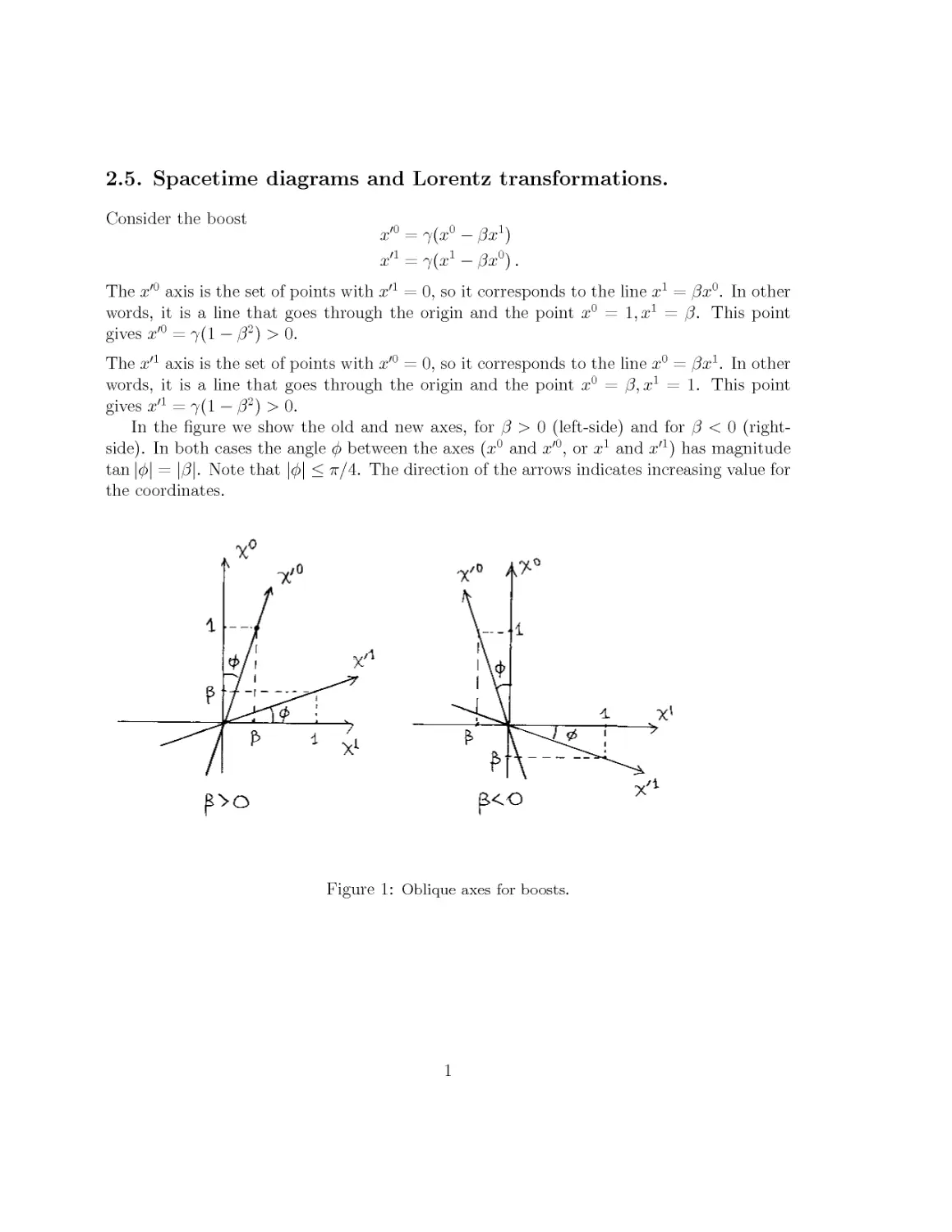
2.5. Spacetime diagrams and Lorentz transformations.
Consider the boost
x'° = ф° - Px1)
xn =
The x'° axis is the set of points with x'1 = 0, so it corresponds to the line x1 = f3x°. In other
words, it is a line that goes through the origin and the point x° = \,хг = [3. This point
gives x'° = 7A -/32) >0.
The x'1 axis is the set of points with x'° = 0, so it corresponds to the line x° = /Зх1. In other
words, it is a line that goes through the origin and the point x° = C, x1 = 1. This point
gives ж'1 =7(l-/32) > 0.
In the figure we show the old and new axes, for f3 > 0 (left-side) and for C < 0 (right-
side). In both cases the angle ф between the axes (x° and x'°, or x1 and xn) has magnitude
tan \ф\ = \C\. Note that \ф\ < тг/4. The direction of the arrows indicates increasing value for
the coordinates.
1
\
—
A
h
t
i
X
p>o
Figure 1: Oblique axes for boosts.
2.6. Light-like compactification
(a) We use the above to compute
x+ = —%3- ~ —=(ct- 2-kR + x + 2ttR) = x
л/2 л/2К
-(ct- 2irR -x- 2irR) = x~ - 2ir(V2R).
/2 ' '
x = ^
л/2 л/2
We therefore have the light-cone identifications
x+ ~ x+ , x~ ~ x~ - 2ж(л/2К) .
The compactification does not involve the light-cone time x+.
(b) With the Lorentz transformations x' = 7B; — /3ct) and ct' = ^(ct — /3x), we find
x' ~ j(x + 2irR - /3[ct - 2irR}) = x' + 2тгД7A + /3)
ct' ~ j(ct - 2irR - P[x + 2тгД]) = ct' - 2irRj(l + /3)
thus
Comparing with A) we learn that in the boosted frame the effective radius of compactification
is increased.
Now consider the compactification
Kct) \ct) \ -R
(c) We search for a frame (x1, ct')
x' = j(x — Cct)
ct' = 7(ct - /3x)
in which this compactification is standard. For this we need ct' ~ ct'. So,
ct' ~ 7(ct - 2ttR - 13 [x + 2тгл/й2 + R2S]
= ct' - 7Bтг)(Д
Thus, we need R + /Зл/R2 + R2S = 0, so
0 = --
R
Now examine the x' identification to find the radius:
x' ~ j(x
x'
Simplify,
C)
Thus, х' ~ ж' + 2ttRs. The radius of compactification is i?s. It is interesting to note that
7 = л/Д2 + R?s/Rs. In the limit as Д, is small, this is a very large Lorentz factor 7 ~ R/Rs.
(d) The required spacetime diagram is shown in Figure 1.
Ct
Figure 1: The heavy dots are identified so that the x' axis must go through them. The world line
of the origin of the primed system is the ct' line. This origin is moving in the negative x-direction,
as the sign of C indicates.
(e) Light like compactification with radius R arises by boosting a standard compactification
with radius Rs with Lorentz factor 7 ~ R/Rs, in the limit as Rs —> 0.
2
2.7. A spacetime orbifold in two-dimensions.
(a) Prom Problem 2.2 we know that under a boost with velocity parameter /3 along the x1
direction, x+ and x~ transform as
x+ and x'
x .
Since these positive scale factors are inverses of each other we may define
A is called the rapidity. Given two boosts with rapidities Ai and A2, the rapidity of the
combined transformation is clearly Ai + Ai. The range — сю < A < oo arises because C €
(—1,1), so ex € @, oo). We can write the identification as
For arbitrary A the orbifold fixed point is the origin x+ = x~ = 0.
(b) Below we plot curves of constant a2 for two values of a2. Note that there are upper and
lower branches.
-'v ( line of constant a2
Note that x+x is invariant under boosts since x+ and x get multiplied by e л and ел,
respectively. Since the signs of x+ and x~ are not changed under boosts, the identification
equates points on the same x+x~ = a2 curve.
1
(c) We have x+ = a2/x~ so that dx+ = -(^Jdx+. This yields
-ds2 = -2dx+dx- = 2( — ) {dx'J > 0.
Thus ds2 < 0 and the curve is spacelike.
(d) Prom part (c) we have that — ds2 = 2a2{^-J so the appropriate root is
To find the invariant length of the circle we must integrate the above differential from a
given x~ to its immediate image exx~. This gives an invariant length
у/2 а
= V2alog(ex) = y/2a\.
2.8. Extra dimensions and statistical mechanics.
(a) The states of the system are labeled by к and / and the partition function is given by
Z(a,R) = y>xpi-/3( —
2m
Here к = 1,..., сю, while / = 0,1,..., oo. Due to the degeneracy of the energy levels we
must include an extra factor of 2 for each term in the / sum for / > 0. Defining
we have that
Z(a, R) = Z(a) 1 + 2Z(ttR) .
A)
We need to evaluate Z(r) for small C. In this case, the terms in the sum vary very slowly
with к and many of them are nearly equal to one making the total sum very large. It is thus
possible to replace the sum with an integral that runs from zero to infinity:
B)
/0 1 2m\r/J V 27Г/ЗЯ2
For sufficiently small /3, B) applies both for r = a and r = 2irR. So A) gives:
Z(a,R) ~Z(a)-2ZGrR) ~
/т(тгЛJ
2irphz
2тгВП2
This partition function is just the product of two familiar factors, one using the length a and
the other using 2ttR. For high temperature the partition function is approximately that of
a particle in a two-dimensional box with sides a and 2ttR.
(b) The stated regime implies that the thermal energy kT satisfies the inequalities
h2 kT r?_
mR? ma2
We can use the high-temperature result B) for Z(a), but not for Z(ttR):
Bh2
Z(a,R) =
2Z(ttR)
The leading correction arises from the first term in the sum that defines Z(ttR). This is a
"low-temperature" small correction; the argument of the exponential is large and negative.
1
3.1. Lorentz covariance for motion in electromagnetic fields
We rearrange the indices by raising the fi in equation A) of the problem statement:
= q F^ dxv
ds с ds
Multiplying both sides of the equation by ds/dt we find
= q piiV dxv
dt с dt
We test this equation using F^v, as given in the text, and ^ = (—c,vx,vy,vz):
= qEx + 4vyBz - vzBy)
-vxBj good!
<& = q-(F™{-c) + F21vx + F23vz) = qEy + %ZBX - vxBz)
dt с с
= q( Ё + -vx В] good!
V c Jy
^ = \(F30(-c) + F^vx + F*\) = qEz + \{vxBy - vyBx)
+ -vxBj good!
The last equation is
<¥_ = qpOl <^i = cIe-v
dt с dt с
With p° = E/c, it becomes
—— = (qE) ■ v = force x velocity
(L
The rate of change of the particle energy equals the rate at which the fields do work on the
particle. The magnetic force is perpendicular to the velocity and does not do work.
3.2. Maxwell equations in four dimensions
(a) T is totally antisymmetric, so T vanishes unless all the indices are different. This yields
four equations: T012 = О, Т013 = 0, T023 = 0, and Т12з = О. The first three of them give
T012 = 0 ->• d0F12 + d1F20 + d2F01 = 0
1д Я + д F д F П
с at dx dy
T013 = 0
T023 = 0
dEy
dx
d0F13 +
dz
d0F23 +
1д(в
cdty
dEz
dEx
dy
dlF3° +d
3W +dlX
dx
d2F30 +
d
+ ~д~У
dEy
1
с
d3F01
1
с
d3F02
с
'z d
1
dBz
dt
= 0
дВу
dt
= 0
~z y
dBx
ду dz с dt
They are the three components of V x Ё = -\Щ. Finally Ti23 = 9iF23 + d2F31 + d3F12 = 0
gives
+ + „ . VB 0.
ox dy dz
(b) Test values for /i in the equation dF^/dx" = fjc. For /i = 0:
70
—
dxl с
F 70
= — = p which is V • E = p.
dxl с
/i = г: To do the 3 indices at once note that Fli = el^kBk where 6 is totally antisymmetric
and e123 = 1. For example F12 = e12kBk = e123B3 = B3. Using this, we have
1 dFl° dFlJ f ldEl d . ... .. f
1 = — -^ 1 r(e 3 В ) = —
с dt dxi с с dt dxi с
A little rearrangement gives
iik d , j1 ldE1 n . n . _ -*. fj
iVIllCIl Id I V X
+ whichis (VxB); ( + ^
с с dt \c с dt
3.3 Electromagnetism in three dimensions
(a) Using equation C.9) and noting that there are no currents nor velocity in the z direction,
we have
Bx = By = 0, Ez = 0, jz = 0, vz = 0.
Maxwell's equations then become
Maxwell's
equations
down to 3D
dET dR,
dx
dEy
dx
dBz
dy
dBz
dy
dEx
dy
i
с
_jy ,
p
1
с
1
\dBz
с dt
dEx
dt
dEy
from V • E = p
1 On
from V x Ё =
с dt
dx с с dt
с с dt
while we get nothing from V • В = 0. The force law gives nontrivial equations only for the
т ялН ti mninnnpntfi1
x and у components:
Vy R\ d'Py n(T? Vx
-Bz), — = q{Ey--
(b) In three dimensions we have A* = (Ф, A1, A2), A^ = (-Ф, A1, A2), and j^ = (cp,]1,]2).
Moreover, F^v = d^Av — dvA^, so
FOl = -
d<S> dAv dAx
■ + -— = -Ег, F12 = -^- - -^— = Bz just a name!
с dt dx1 dx dy
Thus the field strength looks like
-ET -R,
F \iv
piiv _
Ey -Bz
0
-Ex
-Ey
Ex
0
-bz
Ey
Bz
0
The above 3-dimensional F can be viewed as the 4-dimensional one with Ez = Bx = By = 0.
The 3-dimensional j can be viewed as the 4-dimensional j with jz = 0. The Maxwell
equations that arise in 3 dimensions are therefore the truncation to Ez = Bx = By = 0 and
jz = 0 of the original four-dimensional ones. Those are simply the ones given in part (a), so
there is no need to check anything further.
The force law
dt
dt
gives
dt с с ~ i
so everything is as expected. Also,
dp0 qF°l q - dE
—— = Vi = -E ■ v => — = qE ■ v tamiliar result!
at с с dt
3.4 Electric fields and potentials of point charge
(a) TOij = doFij + diFj0 + djFOi. For time-independent fields doFij = 0, so TOij = 0 implies
9^-9,^ = 0 -► diEj-djEi = {). A)
E = —УФ says Ei = —d^, so condition A) is satisfied since дiдjФ = djd^.
(b) With d spatial dimensions and a point charge q at x = 0,
Ё^) = Щ^к (equation C.73)) .
/7Г2 '
Since E(r) = -f(r),
Г(|) 9 1
Ф(г) =
setting Ф = Oat r = oo for d> 2. Since Г(ж + 1) = жГ(ж), Г(|) = (|-1)Г(|-1), so we get
3.5 Calculating the divergence in higher dimensions.
The thin shell has volume vol(S"i^1(r)) dr, so applying the divergence theorem we find
(V • /) vol(Sd-\r)) dr = f(r + dr) vol(Sd-\r + dr)) - f(r) vol(Sd-\r)).
The left-hand side is the volume integral of the divergence of / over the shell. The right-hand
side is the net flux of / out of the shell. Dividing both sides of this equation by vol(S"i^1(r) dr
and taking the limit dr —» 0, we find
Since vol(Sd г(г)) ~ rd 1, with a constant of proportionality that cancels out between the
numerator and the denominator, we have
This is the final formula. For d = 3 it gives V • /= 4, fr{r2f{r)) = f + ;/(>).
3.6 Analytic continuation for gamma functions.
We begin by breaking up the integral into two pieces
dte-Hz~1+ / die"***-1. A)
Ji
The second term converges for any z since the problematic region of integration near t = 0
has been removed; whatever the value of z, we have e~btz~l —> 0 for t —> oo. Using the
expansion for e~*, the first term in A) can be written as
t dte~t1f-l= tdtt^yt^. B)
^
nl
Note that in the sum the nth term converges for $l(z) > —те. If we remove the first N terms,
the remaining sum from N + 1 to oo will converge for 9?(z) > — (N + 1). We thus rewrite
B) as
—I +
The first term can be rewritten as
N
In the second term we can perform the integration assuming that $l(z) > 0. This gives
1 N s \ N , s i N , s
*-~* те! t-^ те! /n ^ те! z + n
71 = 0 71 = 0 "/U 71 = 0
Putting all the terms together, we have
T(z)= [\^
те! z + n J1
While this was derived for $l(z) > 0, the integrals converge for $l(z) > —N — 1, so the
right-hand side provides the analytic continuation. The result is a meromorphic function,
namely, a function with poles. These arise from the term
N (-л\п 1
C)
те! z + n
71 = 0
which is just a sum of simple poles at the integers те = 0, —f, —2,..., N. Since we can take
N to be arbitrarily large we see that T(z) has a simple pole at every integer, n < 0. Finally
we may read off the residue of the poles from C)
(-1)"
те!
3.7 Simple quantum gravity effects are small.
(a) The standard Bohr radius
ti2 e2
a0 = = 5.29 x lCT9cm, arises from the potential V = .
т„ег г
In the gravitational case, the potential is V = —Gmemp/r2, so, the "gravitational" Bohr
with Gmemp:
h2 h2 ( e2
radius uq is obtained by replacing e2 with Gmemp:
a9 = —
0 me(Gmemp) mee2 \Gmemp J
The ratio between the "gravitational" and the conventional Bohr radius is therefore
< = ^_ = D-8 x ICT^J ^227xlO39
a0 Gmemp F.67 x 1С)-8)@.911 х 1С)-27)A.672 х 1С)-24)
This gives
a90 = 1.20 x 1031cm.
Since 1 light year ps 9.5 x 1017cm, a90 = 1.3 x 10¹³ light years !! The universe is about 1010
years old, so this distance is fantastically large.
(b) We introduce factors of G, c, and h into the formula, with exponents a, C, and 7 to be
determined:
8тгМ 8тгМ
Since [kT] = [E] = ML2/T2, using [G] = tfM^T-2, [c] = LT, and [Щ = ML2T-\ we
find
М^ _ r3a+/3+27 jw— a+7-1 rp-2a-C—f
т2
This gives three equations for three unknowns:
3a + /3 + 27 = 2 , — a + 7 = 2 , — 2a — C — 7 = —2 .
The solution is a = —1, /3 = 3, and 7=1. As a result,
he3 ,hc, c2 mLc2
hT = = ( — \ —
G' 8irM 8irM '
where mP = 2.17 x 10~5gr is the Planck mass. For a mass with million solar masses M =
106Msun w 2 x 1039gr,
kT^ B.17 x 10-^C xlO1OJ.843xlo-3oeV ^ rw6.lxl0-uK.
8тг 2 x 1039
This is much colder than the nanokelvins attained by Ketterle et al. in Bose-Einstein con-
condensation experiments. For a room temperature black hole, T ~ 300 K, and we find
M^^^Sx 1039 gr «4.1 x 10²⁰ kg,
w
hich is approximately 6.8 x 10 5Mearth or 5.6 x 10 3Mmoon.
3.8 Planetary motion in four and higher dimensions.
Figure 1: Motion in the plane described with polar coordinates.
We begin by deriving the usual results concerning effective potentials for the motion in a
centrar force field. Using time-dependent unit vectors eT(t) and ee(t) in the radial and in
the tangential direction we have:
x(t) = r(t)er(t)
ic{t) = rer(t) + r9ee(t)
'x(t) = [r- r92]er + [2r9 + r9]ee
If the force is central (along er) we have
2r0 + r6> = 0-► ^-(r29) = 0.
The constancy of r29 implies the constancy of the angular momentum L = mr29. We thus
have
9 '
with L a constant of motion. Let F be the gravitational (central) force associated to the
potential energy V^:
Together
with
A)
this equation
L2
m2r3
gives
1 dVgT
m dr
д
дг
\ m
effective
L2
2m2r2
potential
This completes our derivation of the effective potential. Noting that the gravitational po-
potential energy Vgr divided by the mass is simply the gravitational potential Vg, we have the
familiar result
V- = V + L" B)
eff g 2m2r2 ' У >
\
\
\
\
\
r
Figure 2: Effective potential for four-dimensional planetary motion.
In four dimensions
D) GM L2
Г
As seen by the shape of the potential in Figure 2, the radial motion is stable around the
equilibrium position r0. Indeed
^eff
dr
GM L2 L2
= -\ ^ 7-^7 = 0 ^> r0 = _,, r—- orbit radius .
о
GMm2
Computing the second derivative of the potential at the critical point we confirm it is a
minimum:
d2VF
eff
dr2
2GM 3L2 2GM 3GM GM
'0 la '0 '0 '0 '0
> 0 —*• stable!
Our familiar world has the additional property that non-circular closed orbits exist, but we
can't see that from the effective potential.
In five dimensions
т/E) -
aUyu'lVl L2
2m2 r
Irr.2 '
Figure 3: Five spacetime dimensions and L > Lq. Planet will go out to r —> oo
Figure 4: Five spacetime dimensions and L < Lo. Planet will fall into the star at r = 0.
with a > 0, a dimensionless constant that can be determined using Gauss' law. Note that
both terms have the same r dependence! There is a critical Lo which makes V"eff vanish:
Ll =
In terms of Lo the potential is
V
2r2
-Ll)
For L > Lo, see Figure 3. For L < Lo, see Figure 4. The orbits are unstable. They can
exist for any radius if L = Lo exactly, but any small perturbation that changes the angular
momentum will either make the planet spiral in or out.
3
For spacetime dimensions D > 5
2m2r2
Since D — 3 > 2, V"eff is as in Figure 5. An unstable circular orbit is possible with an
L-dependent radius r0.
Figure 5: Effective potential for D > 6 spacetime dimensions.
3.9 Gravitational field of a point mass in compactified five-dimensional
world.
(a) We examine the gravitational equation
for a point particle of mass M fixed at the origin r = л/ж2 + у2 + z2 + w2 = 0 of a five
dimensional spacetime. Consider a four-dimensional ball BA(r) that contains the mass. The
boundary of this ball is the 3-sphere S3(r). Integrating the above equation over BA(r):
I d(Vol) V • VV;E) = 4тгСE)М .
Using the divergence theorem the left-hand side can be written as
/ d(Vol) Flux of VKE) = / d(Vol)—— = VolE3(r)) — (r)
Jsz(r) 9 Js^r) dr Br
because Wg is radial and of constant magnitude over the three sphere. Since Vol(S<3(r)) =
2vr2r3 we get
2,v wm .
Br Br 7Г
Integrating, with zero potential at infinity, we find
(b) We consider the compactification w ~ w + 2тта of the w direction into a circle of radius
a (see Figure 1). Note that the potential at the point P with coordinates (x,y,z,0) cannot
just be
1 G^M
VP(x, y,z,0) = not true
9 7Г X2 + y2 + Z2
as if we could use A) when the space is compactified. If A) could be used directly, for a
point P' displaced vertically from P by 2тга we would also write
1
Vg KX, У, Z, 27Г«) = 2 ,
y 7г хл +
But then, the potentials at P and P' would be different, in contradiction with the compact-
compactification statement that P and P' are the same point.
1
x,y,z
Figure 1:
To implement the w periodicity implied by the compactification we must introduce a periodic
array of masses; a mass at each w = 2тта, for every integer n € Z. This is an infinite number
of masses! Note that with periodic masses the potential will also be periodic. As shown in
Figure 2, the observer actually "sees" the additional masses because the light rays wrap
around the cylinder. Adding the contributions of each mass using A), we find the potential:
1
x2 + у2 + z2 + BтгпаJ
1
R2 + BтгтааJ
where R2 = x2 + y2 + z2. We thus have
R2
B)
(с) Let us evaluate the above Vg when |<1. In this case the terms in the sum are slowly
varying and
Letting те = т^-х,
Back in B) we get
Figure 2:
dn
Bт»2 ■
E
n = — oo
1
R
1 + Bvrf nJ 2vm J^ l + x2 2a
R
7Г R2 2a \2iraJ R '
that is, V" = — ^jf with G = -^-, which is exactly what we wanted to show!
3.10 Exact answer for gravitational potential.
(a) Using the cited identity with x = 2a/R, the potential in equation B) of Problem 3.9
becomes:
G{S)M 1 R \ R~\ /GE)\M \ R~\
V}5)(x, y, z, 0) = — coth — = - — coth — (exact) .
9 y 'y' ' ' 7Г R2 2a [2a\ \2ira J R [2a\ y '
(b) We can do an asymptotic expansion of coth |4 for R ^> a:
coth | —
2a
oosh I — л л
LUbI1 ha\ e1^ + e~2^
sinh 7Г-
1 + e-f
1-е-?
ъ — в 2a
_ Л
So the potential with its first leading correction is
Correction is 1% when 2e~? = ^. This gives f = In 200 ~ 5.3.
(c) When R <§; a, we are near the mass. For small x, coth(x) ~ i + | + O(x3). So we have
coth
R_
2a
2a R 2a ( R
R 6a R\ 12a2 '
We then find
R2
9 2ira R R\ 12a2 J irR2
1
R2
12a2
The leading term gives the 5-dimensional answer (see equation A) of Problem 3.9). This
makes sense; very near the mass the effects of compactification must be negligible.
/_
4.2 Longitudinal waves on strings.
Let r/(x, t) denote the longitudinal displacement at x, for any time t. One may then ask,
what is the tension T(x, £)? Given the definition of the coefficient of tension, we can write
T(x, t) = To + r0 — .
Lj
To evaluate the second term on the right-hand side, we look at a small piece of parameter
space from x — e to x + 6. The corresponding piece of static string has length L = 2e, and
it is stretched AL = r/(x + e,t) — r/(x — e,t). So
Д 7~ -| *~)
—— (r}(x + 6 t) 7](x et)) ~
As a result, we find
Д 7~ -| *~)
—— = — (r}(x + 6, t) - 7](x — e,t)) ~ — , when
Lj 2c V / ox
A)
This gives the tension at any point on the string. Now consider the piece of string associated
with the parameter space interval from x to x + dx. The mass of this piece of string is
fiodx, its average acceleration is |^, and the net force acting on it is T(x + dx) — T(x). So,
Newton's law gives
(tiodx) -7^ = T(x + dx) - T(x) = —dx.
Cancelling the common factor of dx and using A), we find
d2r] d2r]
ot2 ox2
This takes the form of the familiar wave equation for transverse oscillations, with the tension
To replaced by the coefficient of tension tq. The velocity v of the longitudinal waves is
v = лАо/^о- You can also prove that the tension T(x, t) satisfies exactly the same wave
equation.
„.
-I-
Г)
JL
n
О
vU Л*С1,Г)
t vt*- *^*"
■ 3
J.
-г-
)
J
U
JL. 4Л
f-
\\ u
,,
^
,».
л
= о
4.4 A configuration with two joined strings.
The equation for the oscillation frequencies breaks into two equations
^У± El yi(x) = о , for 0<ж<а,
^ + J y
ахг То
-\ и? У2(х) = 0 , for a < x < 2a .
ахг То
Here у\(х) = y(x) for x € [0, a] and y2{x) = y(x) for x € [a, 2a]. We let
л 2 А*1 2 i л 2 A4 2 2
A^ = — w and Aj = — и .
To To
With this notation, the two equations take similar form
Since у(ж = 0) = y(x = 2a) = 0 we write
yi(x) = Asin(Aix), and 2/20*0 = -Bsin(A2Ba — x)),
which satisfy the differential equation and the boundary conditions at x = 0 and ж = 2а.
(a) Since the string does not break at x = a, we must have y\(a) = У2(а). Since the there is
no mass at the joining point the slopes must agree too: y[(a) = y'2(a).
(b) Applying the boundary conditions in (a) we find
v4sinAia= В sinA2a,
AAi cos Ai<x = —BX2 cos A2a.
These two equations can be written as
(sinAia — sinA2a\ I A\ _
AicosAia A2cosA2aj \B I
Since we need solutions where both A and В are not zero, the determinant of the above
matrix must vanish:
A2 sin Ai<x cos A2a + Ai cos X^a sin A2a = 0 . A)
This equation can be used to find the oscillation frequencies. As a check, assume //1 = //2 =
/io, in which case Ai = A2 = A. The condition becomes sinBAa) = 0, which gives ABa) = тетг.
This gives the familiar frequencies.
1
(с) With /i! = fi0 and /i2 = 2//0 we write
= w— cj = A and A2 = W -=- uj = v l\.
Equation A) then gives
л/2 sin Aa cos л/2~Аа + cos Aa sin л/2~Аа = 0 .
Solving this equation numerically we find that the lowest root is Аа ~ 1.26567. This gives
the lowest frequency
[и 1.26567 [и 2.53134
Ba)
Note that uL is bounded as
\To тг/л/2
Ba)
/To 7Г
Ba) '
The lower and upper bounds are the lowest frequencies of strings of constant mass density
2//0 and /i0, respectively (тг/л/2 ~ 2.22144).
о
VjU-tK
wt- flJ***-^
f
', "а
/
"Те Л
Л<_ = 0
fi
Jt ■*.* О
00
И
3
-2-
H y< s ч
О u
V^*^
ot
- 4
4.6. Deriving Euler-Lagrange equations.
(a) Under a variation 6q(t) of the coordinate, the variation 6q(t) of the velocity is -^. Since
the Lagrangian L depends on q and q, the full variation is
Г Q I J, J Г I '-^ v^-l/ v^ |
The second term in the brackets is rewritten in terms of a total time derivative and a term
proportional to Sq:
The total time derivative does not contribute when we set the variations to vanish at the
initial and final times (we always assume this). The variation SS is therefore
L d fd
If this variation is to vanish for all 5q(t) we must have
d fd
This is the Euler-Lagrange equation.
(b) Under a variation дф(х) of the field, the variation 5(д^ф) of the field derivative is equal
to дцEф). Since the Lagrangian density С depends on ф and д^ф, the full variation is
SS = /dMl£
J [дф
дф
The total derivatives (middle term) do not contribute if the variations vanish at infinity or,
more precisely, if 6ф(х°,х1,х'2,... ,xd) vanishes when any of its arguments is equal to plus
or minus infinity. Consider, for example, the term with \i = 1:
dx°dxldx2 ...dxd-^-{ -^—5ф )= I dx°dx2... dxd
dC
д{дгф)
if 5ф(х°, x1 = ±oo, x2,..., xd) = 0. Back to the variation, we therefore have
5<b\ = 0,
дф
which is the Euler-Lagrange equation for the field.
1 RU, пЛЖч «ч гЛ>О 4
XV .о -г-
u*.
5.2 Particle equation of motion with arbitrary parameterization.
We are told to vary х^(т) —> х^(т) + 5х^(т) in the action
The variation gives
6S=-mc
S = —me
Tf 1 _
dx^ dxv
(IT
dr.
dxv
_ dx^dxH
lap dr dr
dx" dx?
laP dr dr
dr.
Integrating by parts and dropping total derivatives (&г^
^ = 0) we find
SS= -
d
me-
dxu
The action is stationary if
vac
dr
dxa dxP
dr dr
dxa dxP
laP dr dr
= 0 .
A)
This is the equation of motion for the particle in "manifestly" reparameterization invariant
form. Indeed, the object between the brackets is clearly reparameterization invariant:
me-
dxu
me-
dxu
P dr dr
P dr' dr'
(This follows immediately using the chain rule ^ = ^- j{p .) The derivative in front of the
brackets (see A)) does not spoil the reparameterization invariance since:
d
dr' d
d
When we choose т equal to s
dxv
x^ dxv _ (dsJ
ds ds (dsJ
Equation A) then becomes the familiar
d г dx
ds
t* | _ з_м _ q
ds
•л ■£
44 •
= Д
Cr
s - Ji« 11 pr ?» - т 1* *'
-r>
u
5.5 Equations of motion for a charged particle.
We are interested in the variation of the action
ф
S=-mc ds + -I, 1= dr Afi(x(T))—(т), A)
Jv c Jv d,T
when we let x^(r) —> х^(т) + 6х^(т). We note that
j) + 6x(t) ) - Afi I x(t) ) = —-f 5xv{t) ,
/ V / СУХ
where ^£ is calculated at x = х(т). We therefore have
51 = I dT -
Jv 6xv dT Jv r~ (It
We exchange \i ^ v in the first term and rewrite the second using a total derivative:
f dAv dxv f \ d dAu,
51 = dT бх11 \- dT \ —(А^бх11) — бх11—-
Jv dx^ dT Jv ydr dT
We assume that 5x vanishes at the ends of V, so the total derivative (first term in brackets)
vanishes. Using the chain rule for the second term in brackets we find
/ ft /л f\rf'^ I fi /a H rf'^
I oj\v ax lieu и/±цax
61= dr 6x^ ' ri^ ЯггР-—n
jv ю' dT Jp dxv dT
The two terms can now be combined to write
Jp \ dx^ dxv J dT Jp ^ dT
This concludes our computation of the variation of /. The variation of the first term in A)
was calculated in the textbook (equation E.29)). The total variation is therefore
dr с Jp dT
dxv
F
dr
Setting the variation equal to zero, we find the expected equation of motion
dpp, _q p dxv
7 ^ игу T
dr с dr
5.6 Electromagnetic field dynamics with a charged point particle.
Write
с jv ат
Since
Л I ti т11 — / d Tn (t — t[t-| I A (t\
we have
if \ Г
Sint = -o / dDxA^(x)\qc / dr 5D(x - х(т))
dr
where jfi(x) is the current of Problem 5.3. Under a variation SA^(x) of the gauge field
1
с
Let now
s =_1
'-'em л
4c.
We then have
j-fdDx2- F^SF^ = -^ J dDx
aq — / c]ur о • F^SF — / r/ r • F^v\ В ()A — 8 SA
= +- f dDx F^ ^^ (since F^ = -F^)
с J oxv
= — / dDx5A^ —— (throwing away boundary terms).
Collecting variations we have
SSmt + SSem = -- fdDx6A
Setting the total variation to vanish we find the field equations
dxv ~ с
5.7 Point particle action in curved space.
Our starting point is the variation
SS = -me I S(ds).
With the path parameterized by an arbitrary r we have
(as) = —g^AxiT))— ;—(dTj .
dr dr
Under a variation х(т) —> х(т) + дх(т) the variation of the metric is
A)
B)
so the variation of B) gives
= д^(х + 5х) - д^
dr^ drv
х) = -^Sxa{
dxa dr dr dr dr
Dividing by 2ds and cancelling one factor of dr, we find
1 dg^v a dx^ dxv dx^ dSxa
Back into A), we have
5S = mc dr -
dSxc
2 9ж«
ds dr
ds dr
Integrating by parts and dropping total derivatives that vanish since Sx = 0 at the endpoints
of the world-line
2 dxa ds dr dr
ds
It is now convenient to choose the arbitrary parameter r equal to s, so that
'1 Bn
oo = me / as ож (
2 9
drv
(is ds
(is
[Note: if we had used s as a parameter from the start, we might worry about the change in
the range of s when the path changes.] The equation of motion simply requires the vanishing
of the object inside parentheses. Expanding it out
У
dxv
dxv
fia
ds2
ds ds 2 <Эжа ds ds
1
^ •
The last two terms in the left-hand side can be combined:
d2x» 1 f дд^ _ дд^Л dx^dx^
2 \ d" d" ) d d
Э11а ds2 2\ dxv дха J ds ds
Since the expression in parenthesis multiplies ^-^-, which is symmetric in fi, v, we rewrite
it in a form which is also symmetric in fi, u, to get
d2x'x lfdg^a dgva dg^^dx11 dxv
Multiplying the equation by gXa and recalling that gXag^a = <^, we have
xv
1 Xafdga^ dgav dg^\dx^ dxv _
2 29 V dxv dx» dxa) ds ds '
ds2 29 V dxv dx» dxa) ds ds
The equation has taken the form
d2xx
л
s ds ° '
as we wanted to show. [For the quoted form let A —» /i, /i —» a, and г/
6.1 Stretched string and a nonrelativistic limit.
We are told to consider the string action in the form
A)
The second integral here is simply an integral along the string; it is not appropriate to write
limits of integration because the integration variable has not been chosen yet.
We describe the motion using the function y(t,x), where ж is a (horizontal) coordinate
along the equilibrium direction of the string and у represents transverse displacement. To
perform the integral along the string in A), we examine the contribution from the piece of
string that stretches between x and x + dx. This piece is represented by the spatial vector
(dx , dX2,..., dXd) = (dx, dy). The length ds of this small piece of string is given by the
Pythagorean theorem:
ds2 = dx2 + dy • dy.
This implies that
where we used the small-oscillation approximation | J^| <C 1. Additionally, since the string is
almost horizontal everywhere and at all times (||^| <C 1, again) the perpendicular velocity
is approximately equal to the vertical velocity Ц, so we write
Since \vj_\ «С с (problem statement) we can approximate
1 ,uu^ C)
Using B) and C) in A), we find
2\dxJ J V 2c2V9t
Since the terms in brackets and parentheses are of the form 1 + e, with 6 a small correction,
multiplying out we only keep terms linear in the corrections
1--^ - 1--^ ^ 1-
The action thus becomes
S ~ / dt(-Toa) + / dt dx
'и Jti Jo
lTn
ITo/cfyy t (dy
dy\-
This can be compared with the action in equation D.36). We have indeed obtained the
action of a nonrelativistic string with tension To and mass density /i0 = T0/c2. The additional
constant corresponds to a potential energy Toa, namely tension times the length of the string.
6.2 Alternative derivation of the non-relativistic limit.
In this problem we work in the static gauge X° = ct = ст supplemented by the additional
gauge condition X1 = x = aa/ai. The other embedding coordinates Х1(т, a), with i =
2,3, ...d can then be viewed as functions Xl(t,x) of parameters t and x. They will be
collectively denoted as y(t,x). The nonrelativistic approximation is based on
\дху\<&1 and -<9ty<l. A)
We begin with the action
5 = -^ /'dr Г daJCaX ■ 3TXJ - (dTXJ {daX)\
c J Jo
Because of reparameterization invariance we can replace r by t and и by ж to get:
S = -To j' dt £dxJ(dxX -l-dtx\ -±(dtXJ(dxXJ. B)
Noting that dxX° = 0 and d^1 = 1, we have
dxx--cdtx\ =
The term in the last line does not contribute since, on account of A), it is a fourth power of
a small number. The terms in the first two lines will contribute; each contains corrections
quadratic in the small number. We can approximate S in B) by action as
+ (dxy]
Multiplying out, keeping only quadratic terms, and using \J\ + 6 ~ 1 + ^e we find the
nonrelativistic action we derived previously in Problem 6.1:
S c^ j dt £ d
6.3 Planar motion for open string with attached endpoints.
To solve this problem we must find an expression for v\ in terms of y. Since the motion
occurs in two spatial dimensions, the location of the string is described by
X = (x, y(x,t)).
Associated with an infinitesimal dx we have the small string segment dX given by
dX = (dx,y'dx) = (l,y')dx,
where prime denotes x derivative. The length ds of this piece of string is
ds =\dX\ = л/l + y'2 dx .
We now find
dX _ dx dX _ 1
~~ds ~ ~ds ~dx ~ y/\ +~j/2 ^ }У'}
and we note that
£=<••»>•
Using the formula for v\ from the notes
fdX dXy
\dt ds J '
and evaluating the dot products using C) and D) we get
2 2
,2 У2 У'2
y2
/l+y'V 1+у'2 l+y'2'
Finally, using B) and E), we find that the string Lagrangian becomes
= -To / dxJl + y>2-^.
A)
B)
C)
D)
E)
— i —
i«% ^F^
Ju
» О
LW^-*-1
• c vJ><^ >
К '
_ о »-
Tf
JLJk
JL
Q
ь i- awao £Wv
ftb
1 T
xa=o
v*jz>*£
i
\
О
с.
S -
f
\
"
IP -
ui
«Lr-
O*"
-a. I©
i
«Л И -
-> <A%
I
H-
I-
^^aO5C^
„^ JtL ,«b «• /-^^
г "С
С?
е
аи
- \
JLJL
r
—к*
V
+
(его) Juk Uu> t-
IP
UvsS>
t>\
О
I.e.
и-
.£«—
X
i
«-
A,
-эх"'* О <>l"T
i
U'\ O5 ем
Is
C
W st<^-f
■s
•*
i
Г
- \-
fcwb гы>-**Д1д/"
■<JT
-z-
о J О О
S
j -
к
/
A
9
vr
К
A
It. o
- О.988
7.-2»
IL***_,
-4-
i. OL p^-
cfT .
- \ -
rv*>A~o
At b- o, V
a.
-U
'
О
X
&
X4) V
= v C
- 2 -
Л-Ь
&- ul
* u
JL
1
j _
Y
у ,
t
V - U
1 " ~7T
у - U
Г
^Y
7.5 Planar motion for an open string with fixed endpoints.
(a) We check first that |F'(u)|2 = 1. We readily confirm that it holds:
,->., .|2 o/ 7TUN . 2/ 7TU\
\r (u)| = cos ( 7 cos — ) + sin I 7 cos — ) = 1. A)
The other condition is
F(u + 2a1)-F(u) = Ba,0). B)
Differentiating both sides with respect to и gives the periodicity condition
F'(u + 2a) = F'(u) ,
which holds since F"(u) is a function of cos ^ only. In full detail, condition B) requires
duF'{u) = Ba, 0),
which implies a relation among the constants a, 7, and <7i, to be discussed in part (d).
(b) We have
where we used F"(u) = F"(—u). This gives
dy . / 7ГСГ\
— = sm 7 cos — .
da V G\/
Below we plot dy/da for 7 = тг/10 and a\ = тт.
C)
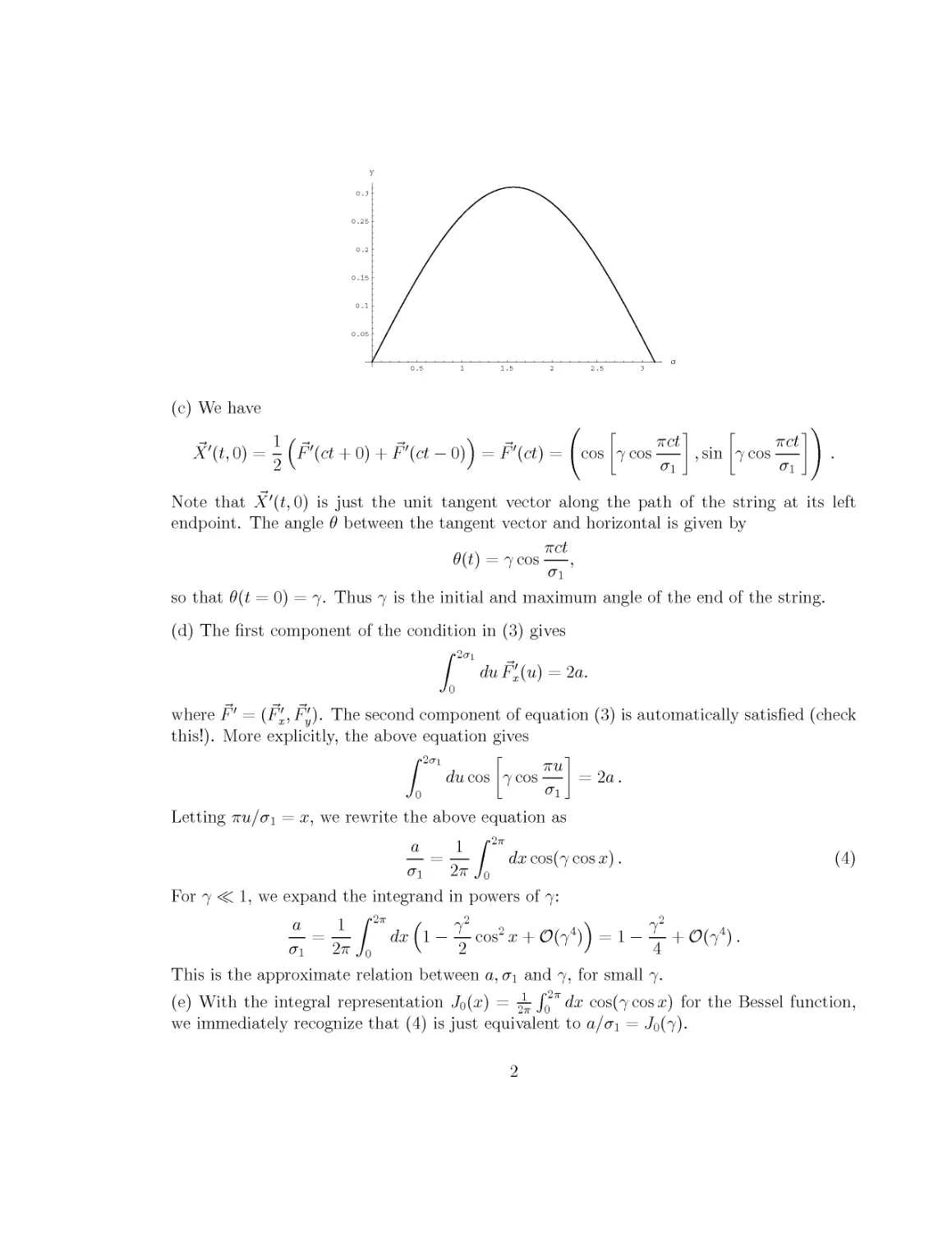
Integrating dy/da gives у (a), as shown in the following figure:
С с) We have
X'
'(£, 0) = - (F'(ct + 0) + F'(ct - 0)) = F'(ct) = I cos
TTCt
7 cos ■
, sin 7 cos ■
TTCt
0"!
Note that X'(t, 0) is just the unit tangent vector along the path of the string at its left
endpoint. The angle в between the tangent vector and horizontal is given by
TTCt
6(t) = 7 cos ,
so that 9(t = 0) = 7. Thus 7 is the initial and maximum angle of the end of the string,
(d) The first component of the condition in C) gives
/ duF'x(u) = 2a.
Jo
where F" = (F'x,F'y). The second component of equation C) is automatically satisfied (check
this!). More explicitly, the above equation gives
Г" Я \ Н 9
/ аи cos 7 cos — \ = Za .
J I ° \
D)
Letting тти/ai = x, we rewrite the above equation as
a _ 1 Г2ж
^=2Wo XC0SG
For 7 <C 1, we expand the integrand in powers of 7:
a _ 1 Г27Г / 72 2
(Ti 2тг Jo \ 2
This is the approximate relation between a, a\ and 7, for small 7.
(e) With the integral representation Jq(x) = ^J^rfi cosGcosx) for the Bessel function,
we immediately recognize that D) is just equivalent to aja\ = JqG).
7.6 Planar motion (continued) and the formation of cusps.
(a) We have that
B'X 1
and
F'(it) = cos
vra
7 cos —
, sin
vra
7 cos ■
Consider the ж component of equation A):
1
= - cos 17 cos
ir(ct + a)
+ -COS
7 cos ■
vr(ct —
It is convenient to define
vr(ct±cr) _
7 COS ■
With this notation,
7TCt 7П7 7TCt 7Г<7
= /3 =F a , so p = 7cos cos—, a = 7sin sin —
^. = - (cos(/3 — a) + cos(/3 + a)) = cos a cos [3 .
A)
B)
Similarly,
X'y = - (sin(/3 — a) + sin(/3 + a)) = cos a sin /3 .
Assembling together these results,
X'(t, a) = cos a (cos /3, sin /3 ) = cos ( 7 sin sin — ) (cos /3, sin [3]. C)
Note that when ct = <7i/2, we obtain /3 = 0 so that
X' = cos I 7 sin — sin — ) A, 0) = cos I 7 sin — ) A, 0).
V 2 CTi ) \ CTi )
Since X' points along the x axis for all a, the string is horizontal,
(b) We have
Ш—
There is only one sign difference between this expression and that for X'. Thus we get
immediately that
-—£T~ = 9 (cos(/3 — a) — cos(/3 + a)) = sin a sin /3 ,
1 dXv 1
and similarly,
1 dXv 1 / . ^ . . ^ . \
——-1 = - ( sm(p — a) — sm(p + a) ) = — cos p sin a .
Together, the above equations give
1 OX
1 OX . / \
—— = sm a sin p, — cos p .
с at V /
It follows that
sina =
7TCt 7Г<7
sm I 7 sin sin —
which is what we wanted to show.
At t = 0 the velocity is clearly zero. When 7 < тг/2, we have
7Г
TTCt 7Г<7
i
7Г
so sm
< 7 sm sm — = a < — ,
< 1 and the velocity of any point on the string at any time is strictly smaller
than c. For 7 = vr/2 and ct = <7i/2 we have
ldX
~с~ЬТ
7Г
sm I — sm
2
At the midpoint of the string, a = <7i/2 this gives
(c) Setting 7 = \/2(У/2) and ct = a1/4 we have
1 dX\
с dt I
~c~dt
• / AT71" • ж ■ 7ra\
sm I v 2 — sm — sm —
2 4 G\ I
sin ^ I = 1.
/-7Г 7Г(Т\
sm I — sm —
2 0"i /
This is the same formula that we found for the case 7 = vr/2 and ct = <7i/2, so we again find
that only one point, a = cr1/2 has reached the speed of light.
Setting 7 = \/2(тг/2) and ct = <7i/3 we have
ldX
~c~dt
This equals one when
I 1— 7Г 7Г 7П7
sin ( v 2 — sin — sin —
2 3 <7i
О 7Г 7ГСГ
sm | a / - — sin —
2 2 (Ti
7ГСГ /2
sm — = W - ,
0-1 V 3
which occurs at two values <j/, crr of u:
and
7T0V
= 7Г — sm
-1
3 '
To see that these points are cusps, we examine X' near a = ai using equation C):
/ 7Г /3 7П7 \ ( „ Л
os I -W- sin— I (^cos/3, sin/JJ .
X'{t = — ,a) =cos ( -xf- sin— ) (cos/5, sin/5) . D)
Here
7TCt 7Га 7Г 1 7Га
/3 = 7 cos cos — = — cos — .
a-i a-i 2
We note that at a = o\ the value /3i of /3 is completely regular:
We can therefore set /3 = /3i in equation D). The prefactor on the right-hand side of D) is
more delicate. Putting a = o\ + 5a we have to lowest order in 5a that
sin "V"^ -> =J^ + ^^5a + ОEа2) .
Therefore,
7Г /З . 7Г(<7; + J<j) 7Г 1 7Г
^ V 2 Sm а~г ~ 2 +
which implies that
2
тг [3 . 7r(ai+5a)\ 1 тг 2
W sm ^5a + OEa )
/тг [3 . 7r(ai+5a)\ 1 тг 2
cos — W- sm —^ = ——5a + OEa ).
\2 V 2 o- У /2<7
Finally, back in D), we have
X'(t = —,at + 5a) =5a(—l——) fcos/3b sin
V 3c /V y/2 ci / V
Near ai the tangent vector X' to the string is equal to a constant vector V\ times 5a. For a
slightly smaller than a\ and growing we are approaching the cusp, 5a < 0, and the tangent
points along +V/. For a slightly larger than a\ we are moving away from the cusp, 5a > 0
and the tangent points along (—Vi). The tangent to the string reverses direction at ai, and
it does so discontinuously. This is a cusp. Note that Д is simply the angle that the cusp
makes with respect to the horizontal.
(d) Setting a = 1, requires
~ 10.154868.
For these values of a\ and 7 we plot the strings that occur for ct = 0, a^/4, and
(Х-
A
О
П
О
8.2 A generalization for charges and a special case for currents.
(a) With several coordinates qa and symmetry parameters ё, the variations are written as
We now claim that the charges are
This time the Euler-Lagrange and invariance equations are
d (dL\ dL n dL . a dL d
A)
B)
We verify conservation as in the book: we compute the time derivative of the charges in B)
and then use equations C) to find that
%dQ% d(dL\ dLd dL dL d
e-df = m (wNq + w&m = WJq + w*m = °- D)
Since the ё are independent parameters, we conclude that
dQl
dt
= 0.
E)
(b) The index a can only take the value zero - there is just £°, which plays the role of time
in this world. The field фа is only a function of time. The action becomes
The quoted equations become
s=
(б)
*=■*?■
where the last equation is "obtained" because there are no spatial coordinates to integrate
over; since there is no space, the charge density j° is really just a charge. The second equation
in G) is charge conservation, in correspondence with E). The first equation in G), takes
the form of B), once we note that do is really a dot derivative, and that qa and фа are the
labels of the corresponding dynamical variables, both of which depend only on time.
q/3
£rriLbi*Lkr«iUo P
YV4C-
Ut
гЛ-
Jk
W*
%
\
о
С-
U-
dUTT
>Y
,
UO.U,
^
)UvtO-
о
lit-
8.4 Simple estimates regarding a/, To, and £s.
We know that
To = and £s = Нсл/а'.
2тга' Не
Moreover, for quick estimates we can use
he = 198 MeV x 1СГ15т = 1.98 x 1СГ14 GeV • cm,
together with
—— = 1.6 x 1CT8N ~ 1.63 x 1СГ12 ton.
cm
(a) For a' ~ 0.95 GeV, we get
To = 1 ^ с 8.47 x 10¹² ^ с 13.8 ton.
2-3.14-0.95-1.98 x 10⁻¹⁴ cm cm
The string length is then
4 = 1.98 x 1СГ14 x \/CL95 cm = 1.93 x 1СГ14 cm.
(b) With 4 ~ 1СГ30ст, we have
Since the string tension is inversely proportional to a' we have
To = 13.8 ton x ( °'95GeV Л = 5.14 x 1033 ton .
V2.55x 10-33 GeV-2y
This is a fantastically large force. The gravitational force which keeps the Earth in orbit
around the sun is about 3.6 x 10¹⁸ ton. The above string tension is about 2.6 million times
larger than the "weight" of the sun (the mass of the sun is ~ 2 x 1030 kg).
8.5 Angular momentum of Kasey's jumping rope.
Prom the solution to the jumping rope problem we have
(X1,X2) = — tan7 sin — (coscut, smut) , A)
7Г <7i
and, moreover,
7ГС E L0
lv = —cosj, (T1 = — = . B)
Lo To cos 7
The momentum density is computed using A) and B)
7 = ^r —» (>1,>9 = S1I17 Sin (— Sill Wt , COS Ujt) C
c2 dt с (Ti
We compute the z-component Jz of the angular momentum of the string, measured with
respect to the origin:
Jz = M12 = / da {X{Pl - X2VT) ■ D)
Jo
Using A) and C) we find
To _. fai л_„.„2 7Г(Т LoTqcti sin 7 ^o / -^u \ _._ 2
Jz = — tan 7 — sin 7 / da sin — = = sin 7 . E
7Г С Jo ^l 27ГС COS 7 °-~l """ " '
We express this result in terms of energy using B):
Jo tii . о
Equivalently,
—г = — -Б2 sin2 7 = sin2 7 a'E2 . F)
/г 2тг To nc
The above Jz/h is smaller than a'E2, the value of the angular momentum of a rigidly rotating
straight open string of the same energy.
RXL €.6
/
? ,
L
с "
8.7 Generalizing the construction of conserved currents.
To show that the current is conserved we take its divergence
We now use the equations of motion that follow from the Lagrangian
dC dL_
ад(дафа) ~ ~d&
to simplify the first term of A). We then find
1 дфа д(дафа) 1
The first two terms on the right-hand side are simply the variation 5C of the Lagrangian
under the symmetry transformation. By equation A) of the problem statement we have
£ldaja = 5C — 6ldaAa = 0 .
Since the parameters ё are independent constants, the currents ji are conserved.
We now consider а С with no dependence on the coordinates £@. Under a change фа —>
фа _|_ ePQ^a^ the variation of the Lagrangian is given by
«: = •£
+
д(дафа)
We therefore recognize that
where we also used the constancy of the e'3. Relabelling indices
^ = ^c) = ^5^) = ^y^) with
We then have, using equation B) of the problem statement
as desired. For a = C = 0
where 7i is the Hamiltonian density of the system. This is clear because the first term on the
right-hand side is the product of the canonical momentum associated with the coordinate
фа times the velocity of the coordinate фа.
1
у. l
- О * rV"-
-til sp-
L
7
rj.l
о
t
U^ ^*Н^
1
г
L*_ «*• <"-
U
V
fic
= о, о •
./
£ <w
kJb
^х1
%
Ысь, sv-A^n ггг"
'
•■
тк
о
4 j
О
1ХЦ r
О I
t- L и
) X =
-Г »
1
с
М
4Pi
-Г J
i
- О
wu
л
С
JL)
l.e.
■r
f
f
OL
o/^^ "
CO H -
.JL
И =
I
у
1
i
л-
JL
V
К
+■
f
f
P
ч,
се..
JU, '
= О
v\.
x'-o,
Г *
^
.t\.iQ--"
К"
xr U
/
К - ь -
л-
X3 - -
U>
I
fAL Ю. I
-* Z7>
^
-Ь
TT
- О
P-
= a.
I
a
\
u
r*AL~
V
UuV»-1-^-
-ао
V
f
•so
"\)V
Г
-it-nf* t
V
1
U.
Problem 10.3. Light-cone components of Lorentz tensors.
(a) Since every component of A equals the corresponding component of B, we have that
A± = -^{А° ± А1) = -^{В° ± В1) = B±
V 2 2
The fact that A1 = B1 follows from A^ = B^ setting /i = /.
(b) The fact that our definition works for tensors of the form R^ = A^B" implies that
R++ = A+B+ = -i(i° + A1) -^=(B° + B1)
у/2 л/2
= -(A°B° + A^B1 + A'B0 + A'B1)
Similarly,
A+B- = -4(Л° + A1) -^-(B0 - B1)
л/2 л/2
-(A°B° - A^B1 + A'B0 - A'B1)
= -^(A° - A1) -^(B° +
л/2 л/2
° + A0Bl - AlB° - AlBl)
R— = A~B- = -^(A° - A1) -^-(B° - B1)
= 1(A°B° - A^B1 - A'B0 + A'B1)
In general we may write the change of coordinates of a vector field as A^ = M^AV where
the hatted index is a light-cone index and M^ = -4= and M^ = ±4= and Mj = Sj. Since
each index of a tensor transforms like a vector, we can write
This immediately implies that if B?v = S^ that
(c) We have
V01
- v01 + v10 - v11) = \(-i - о + о -1) = -l
v~+ = \(v00 + v01 - vw - v11) = \(-i + о - о -1) = -l
V- = ^00 - г]01 - г]10 + г?11) = ±(-1 - 0 - 0 + 1) = О
(d) We find
F+~ = -(F00 — F01 + F10 — F11) = F10 = — Ex.
Similarly
X X
F+J ( rpOI i T7^I\ / rpl i Ли D \
— ^\-^ \ -Г ) — ^\-^ ^T £ -D J J
Vz v z
and
F-J = ^(Fo/ - F11) = ^-(E1 - e1IJBj)
v2 V2
Finally, there is only one non-zero component of FIJ given by F23 = — F32 = 5Ж
la 4
. о
Й.
-
J
^ 6
'ТА
,
Л-
\o. 5
л
И
i.e.
р
r, .
r
Г/
г
U-
>€.y
£/- dbJy&f-
Problem 10.7. Massive vector field.
We have been given the action
S = I' dDx(--dpAv d^Av + -д„Ац d^Av - -m'A^A» - -д^ф д^ф - (д ■ А)тф) . A)
The first two terms can be written as —\{dilAv — dvA^) d^Av = —jFllvFtlv, so the action is
S= I' dDx (-If^F"" - ^rrfApA" - ^дцф д^ф - C ■ А)тф) . B)
(a) We consider the candidate gauge transformations
SA^ = д^е , дф = b m e .
The variation of the action is computed using B), in which the first term inside the paren-
parentheses is gauge invariant. We find
SS=
д^ф_- (д\)тф-Ь(д ■ A)m?e\ .
We integrate by parts the derivatives that appear in the underlined terms to find:
SS = I dDx(m2ed-A + bт(д2е) ф - (д2е)тф - Ъ(д ■ А)т2Л .
То get SS = 0 we need 6=1. So the gauge transformations are
SAp = д^е, 5ф= те. C)
(b) The variation of the action B) gives:
SS = I dDx(д„FАц) F^ - m2(SA^A» - д^ф) д^ф - {дI5А11)тф - (д ■ А)т6ф\ .
We integrate by parts all derivatives that act on variations:
SS = f dDx(-6АцdvF^v - SA^m2 A» + SA^тд^ф + 5фд2ф - 5фтд ■ A\ .
The equations of motion are therefore
= 0, д2ф-тд-А = 0. D)
1
One readily verifies that the equations of motion are gauge invariant. This is good, but not
strictly necessary; it suffices for consistency if the variations vanish when the equations of
motion hold.
(c) The gauge transformation дф = me allows us to gauge away ф: setting 6 = —ф/т, one
finds ф —> ф + em = 0. With ф = 0 the equations of motion D) become:
-dvF^ - m2A'x = 0 , д ■ A = 0 .
More explicitly:
-9*(d ■ A) + d2A» - m2A» = 0 , д ■ A = 0 .
This is equivalent to
d2A^ - m2A^ = 0 , д ■ A = 0 . E)
The above are the equations of motion in the gauge where the scalar field has disappeared.
(d) In momentum space equations E) become
(p2+m2)A^ = 0, p-A = 0. F)
When p2 ф —m2 the first equation gives A'x(p) = 0. Consider now p2 = —m2, in which case
the first equation is satisfied for arbitrary A^(p). Using a suitable Lorentz transformation
any timelike vector p11 can be rotated into a vector with only a time component. We can
thus assume that p11 = (m, 0) since this ansatz satisfies p2 = —m2. The second equation
gives p ■ A = poA° + p ■ A = —mA° = 0. So we conclude that A0 = 0. The remaining D — 1
components A1 with г = 1,... D — 1 remain unconstrained. We have shown that the massive
vector field has D — 1 degrees of freedom.
r
J
■л
у
7h
р Н*
UflB-
мь
tVAb
и
_ьИЬ
11 -1-
,fc> =
О~£_г
Т
О
M_£U
и
Mz
е^>
О
11.3 Classical dynamics in Hamiltonian language.
As stated, to derive the classical equations of motion in Hamiltonian language we vary
Jt- ^ ' Jt- У dt dt dp dq )
with independent variations 5q(t) and 5p(t) that vanish at £; and tf. Replacing
dSq d(Sqp) dp
P—r~ = ; oq—r ,
dt dt dt
and integrating the total derivative, the variation becomes
rts / vdn ftHi vdp
The terms at initial and final times vanish because of the boundary conditions on the vari-
variations, and the condition that the variations vanish for otherwise arbitrary 5q(t) and 5p(t)
give
dq dH dp dH
— = , and — = .
dt op dt dq
Using these equations we readily find that
dv dv dv dq dv dp dv dv dH dv dH dv
~dt ~ ~dt + ~dq~di + ~dp~dt ~ ~dt + ~dq~~dp ~ 'dp'dq ~ ~dt + ^' *'
This is what we wanted to show. The Hamiltonian generates time evolution in classical
mechanics via the Poisson brackets.
RILU4-
v- 4
Л"ЗГ ^ A "^
PAL п.
JL
/*■
М к^З
[м", м
^:
f н
■+Х'
= L
- о
и.С
н
-з:
f
1
Р
J
' f
. Г
o.
RAL
1
н+~ н
_■*•— \
-V--
о.
^
_|
-Г
« — ь
f
H
+—
х jrT | ^ О
^- t£erf
бег <
,1
ir
* £"
L * n.^ h"x = ^ p1- °<?f
?
Л . ;,ГОХЛ
т- _1_ "" I W Oil
"[f
Г T
Ui.
; J
[М
I
о
,
Д-
3L w*-"
T
<%«*~ »* ~ ~ \
■х
Р
н1
лг
П.\5 —
Ь
//
-г
\ v
;
PAU
X
) О
X
1
A.
П+о
Х-
= О
= О
ц 4А
V ' Г
; "T" J—Д_ ^Vrtifp-e^
v/Ч
w\
-с
х: ^
I
yn#O
ТГ
- f А
ПЛ"
12.4 Analytic continuation of the zeta function.
Replacing the integration variable t with nt in the definition of F(s) gives
T(s) = / d(nt)e"ntnsts = ns
oo
o
OO OO „oo „oo OO
->• r(s)C(s) = V r(s)n-s = V / dte-^t"-1 = / rft t8-1 V e""*.
n=l n=lJ° J° n=l
The geometric series gives J^^Li e~nt = i_e-* = ?~Г> so we Se^
()С() / p
jo e — i
We now consider the expansion of l/(e* — 1) around t = 0. Expanding the exponential,
1 1 1 1 1 1 t . 2n
= 1 u O(t )
* 2 12 V h
where we used -^— = 1 — x + x2 — .... We now write r(s)£(s) in A) as
/s~l Г°°
Jo e- - i jl e- - i
Only the first integral on the right hand side may diverge near t = 0. We rewrite it as
Jo
f1 , s-l ( l 11 * \ 1 1 1
/0 ** Vet-l~I + 2~12/+s-l~2s + 12(s + 1) "
Hence, as quoted in the problem statement, B) becomes
l / 1 11 t Л 1 1 1
47 5I5J s + ijjTm)^ *-
The last integral is convergent for all s. Since the terms enclosed by the large parentheses
are of order t2, the first integral is of the form Jo dtts+l and converges for Щв) > —2.
We recall that F(s) has a simple pole at s = 0 with residue one and a simple pole at
s = — 1 with residue —1 [ the general result is that the residue at s = —n < 0, with n integer
1
is (—1)п/те!]. Equation C) shows that r(s)£(s) also has simple poles at s = 0 and s = —1.
We therefore deduce that £(s) is regular for s = 0, — 1, and
Rese=_n(r(s)C(s)) = (Ress=_nr(s)) C(-n) , n = 0,1.
Reading off the residue at s = — I from C) we get the celebrated result:
Similarly, reading off the residue at s = 0 we find that
~=(i)C(o) - C(o) = ~.
It is interesting to note in C) that r(s)£(s) has a simple pole at s = I. Since F(s) has no
pole at s = I, C(s) does. The pole at s = I, with residue one, is in fact the only singularity
of the zeta function ((s).
n i 1
А
(X
Oil \1
[к.
9
sVJu * n-
Л
о
Аф
,
fi
(гЛ^ч
))
Ll°>
L
1
-v-
o(
■f -' -*
<J>= О^>О
POL a.
1 L _к С "
}
4-
L U- L 3
№'Л J
С (П. 152)
1 L
П
°7
Я я
i
QiX.
As
s *- r
«fc^ ytbi^j u ^ ^"Г^ ^^r
iC-tf^O
о *w
.
;e<L.
еГ)
Ы
ife
С
.
^4^
5
0
li UkUW»*. «-t
.Vе
я ^я°
a
«O
Jb
J
V
If
v «о
/
г
-2l
■00
-1
_ 2
RAL \ъ. \
T
* —п>0 -гг
as-,
и«б"*
w.
Jbr
-TT
^«лСй.
ПлГ
t
и
к*0
J
^ й k<- u^tr pW
U
- - -Wb
>-.
sr-
X.
yfcr).
i -ч
.
V ^
к
\u
—-Y4
Jl
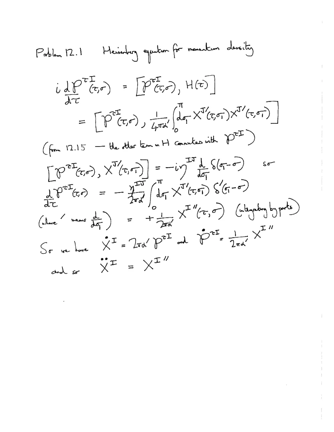
PAU 13 Л
?*
\U-o
?
О
j
Sf
x-
x-
^v/r~ tt*
13.4 Lq — Lq as world-sheet momentum. (Continued)
(b) With 8X1 = ed^X1 we find:
SC =
With a little rearrangement we write
Since the variation of С is a total derivative, the u-translation 5X1 = ed^X1 is a symmetry.
In the notation of equation A) of Problem 8.7, and letting (£°,£1) = (r, a) we write
with Л0 = 0 and Л1 = ^e ((9TXJJ - aX1J) • A)
The conserved current is (equation B) in Problem 8.7):
so the charge density j° is
0 1 y^y1
— Л — A A
2'
OidoX1) a 2vra'
Note that Ла, computed to prove that we had a symmetry, does not enter into the charge
density since Л0 = 0. The conserved charge Q is
Q= f daj° = ^—f daXJXJ/ = -{L± - Ц),
/о ^nLX Jo
comparing with the result stated in part (a) of the problem.
d.
X
1
jt а, и J- ***>*) ^ "*
\
i^^r -i-Ь^
и
cu»
RAL
В
ас
А
Г
*■>-
U4 О .
A2C-
JtLt
t.
u\
jrarSlm Л- /\ ,
О ч^ *
0
ъ
U
L
— Ь .
i
f>-
-e-
-TI
-*■
f
^
. ff■
0