


![III The Free Groups
1. The free group F[A]](https://djvu.online/jpg1/b/j/x/bjxy5hTwQL9tH/039.webp)


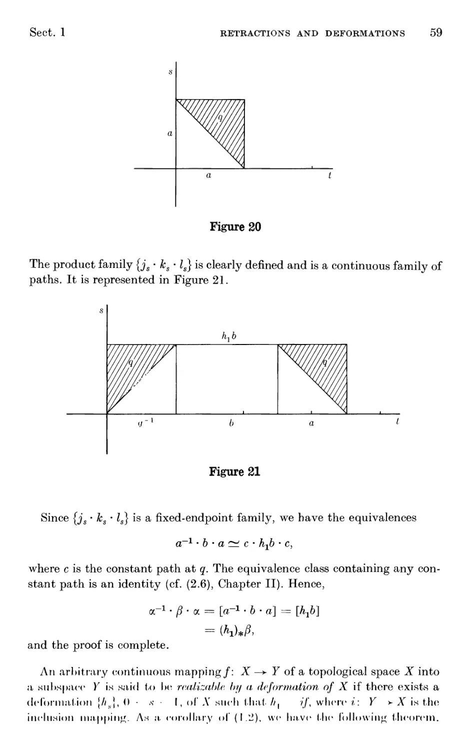


Текст
Richard H. Crowell
Ralph Η. Fox
Introduction to
Knot Theory
S
Springer- Vcrlag
New York Heidelberg Berlin
R. H. Crowell
Department of Mathematics
Dartmouth College
Hanover, New Hampshire 03755
R. H. Fox
Formerly of Princeton University
Princeton, New Jersey
Editorial Board
P. R. Halmos
Managing Editor
Department of Mathematics
University of California
Santa Barbara,
California 93106
F. W. Gehring
Department of Mathematics
University of Michigan
Ann Arbor, Michigan 48104
С. С. Moore
Department of Mathematics
University of California
at Berkeley
Berkeley, California 94720
AMS Subject Classifications: 20E40, 55A05, 55A25, 55A30
Library of Congress Cataloging in Publication Data
Crowell, Richard H.
Introduction to knot theory.
(Graduate texts in mathematics ; 57)
Bibliography: p.
Includes index.
1. Knot theory. I. Fox, Ralph Hartzler,
1913- joint author. II. Title. III. Series.
QA612.2.C76 1977 514Л224 77-22776
ISBN
All rights reserved
No part of this book may be translated or reproduced in any form
without written permission from Springer Verlag
© 1963 by R. H. Crowell and C. Fox
I'riniod in tho United States of America
9 H7li 5 4
ISBN 0 :tK7 90*272 Λ S|n-iNtf"r-Vorljitf Now York
ISBN .Ί MO 90272 I Sprin^i- VnrlRtf Bni-lin И.ч.МЬгг^
To the memory of
Richard C. Blanchfield and Roger H. Kyle
and
RALPH H. FOX
Preface to the
Springer Edition
This book was written as an introductory text for a one-semester course
and, as such, it is far from a comprehensive reference work. Its lack of
completeness is now more apparent than ever since, like most branches of
mathematics, knot theory has expanded enormously during the last fifteen
years. The book could certainly be rewritten by including more material and
also by introducing topics in a more elegant and up-to-date style.
Accomplishing these objectives would be extremely worthwhile. However, a significant
revision of the original work along these lines, as opposed to writing a new
book, would probably be a mistake. As inspired by its senior author, the late
Ralph H. Fox, this book achieves qualities of effectiveness, brevity, elementary
character, and unity. These characteristics would be jeopardized, if not lost,
in a major revision. As a result, the book is being republished unchanged,
except for minor corrections. The most important of these occurs in Chapter
III, where the old sections 2 and 3 have been interchanged and somewhat
modified. The original proof of the theorem that a group is free if and only
if it is isomorphic to F\s/~\ for some alphabet stf contained an error, which
has been corrected using the fact that equivalent reduced words are equal.
I would like to include a tribute to Ralph Fox, who has been called the
father of modern knot theory. He was indisputably a first-rate mathematician
of international stature. More importantly, he was a great human being. His
students and other friends respected him, and they also loved him. This
edition of the book is dedicated to his memory.
Richard H. Crowell
Dartmouth College
1977
Preface
Knot theory is a kind of geometry, and one whose appeal is very direct
because the objects studied are perceivable and tangible in everyday physical
space. It is a meeting ground of such diverse branches of mathematics as
group theory, matrix theory, number theory, algebraic geometry, and
differential geometry, to name some of the more prominent ones. It had its
origins in the mathematical theory of electricity and in primitive atomic
physics, and there are hints today of new applications in certain branches of
chemistry.1 The outlines of the modern topological theory were worked out
by Dehn, Alexander, Reidemeister, and Seifert almost thirty years ago. As
a subfield of topology, knot theory forms the core of a wide range of problems
dealing with the position of one manifold imbedded within another.
This book, which is an elaboration of a series of lectures given by Fox at
Haverford College while a Philips Visitor there in the spring of 1956, is an
attempt to make the subject accessible to everyone. Primarily it is a
textbook for a course at the junior-senior level, but we believe that it can be used
with profit also by graduate students. Because the algebra required is not
the familiar commutative algebra, a disproportionate amount of the book
is given over to necessary algebraic preliminaries. However, this is all to the
good because the study of noncommutativity is not only essential for the
development of knot theory but is itself an important and not overcultivated
Hold. Perhaps the most fascinating aspect of knot theory is the interplay
between geometry and this noncommutative algebra.
For the past thirty years Kurt Reidemeister's Ergebnisse publication
/\ notentheorie has been virtually the only book on the subject. During that
lime many important advances have been made, and moreover the
combinatorial point of view that dominates Knotentheorie has generally given way
to a strictly topological approach. Accordingly, we have emphasized the
topological invariance of the theory throughout.
There is no doubt whatever in our minds but that the subject centers
;iround the concepts: knot group, Alexander matrix, covering space, and our
presentation is faithful to this point of view. We regret that, in the interest
of keeping the material at as elementary a level as possible, we did not
introduce and make systematic use of covering space theory. However, had
\vc done so, this honk would have become much longer, more difficult, and
1 M.L. l4is.li nn.l L. WiiHMrniiiili. Vlirmirnl Topology/'./. . | ш. ('/нт. Кос., Η'Λ ( НИМ )
Vlll PREFACE
presumably also more expensive. For the mathematician with some maturity,
for example one who has finished studying this book, a survey of this central
core of the subject may be found in Fox's "A quick trip through knot theory"
(1962).1
The bibliography, although not complete, is comprehensive far beyond the
needs of an introductory text. This is partly because the field is in dire need
of such a bibliography and partly because we expect that our book will be
of use to even sophisticated mathematicians well beyond their student days.
To make this bibliography as useful as possible, we have included a guide
to the literature.
Finally, we thank the many mathematicians who had a hand in reading
and criticizing the manuscript at the various stages of its development.
In particular, we mention Lee Neuwirth, J. van Buskirk, and R. J. Aumann,
and two Dartmouth undergraduates, Seth Zimmerman and Peter Rosmarin.
We are also grateful to David S. Cochran for his assistance in updating the
bibliography for the third printing of this book.
1 Nno liihln>fjM'R|>hy
Contents
Prerequisites ........... 1
Chapter I · Knots and Knot Types
1. Definition of a knot ......... 3
2. Tame versus wild knots ......... 5
3. Knot projections .......... 6
4.. Isotopy type, amphicheiral and invertible knots .... 8
Chapter Π · The Fundamental Group
Introduction . . . . . . . . . . .13
1. Paths and loops . . . . . . · .14
2. Classes of paths and loops . . . . . ... .15
3. Change of basepoint . . . . . . . .21
4. Induced homomorphisms of fundamental groups . . . .22
5. Fundamental group of the circle ....... 24
Chapter Ш · The Free Groups
Introduction . . . . . . . . .31
1. The free group F[s/] 31
2. Reduced words .......... 32
3. Free groups ........... 35
Chapter IV · Presentation of Groups
Introduction ........... 37
1. Development of the presentation concept ψ . . . . 37
2. Presentations and presentation types ...... 39
3. The Tietze theorem . . . . . . .43
4. Word subgroups and the associated homomorphisms . . .47
5. Free abelian groups ......... 50
Chapter V · Calculation of Fundamental Groups
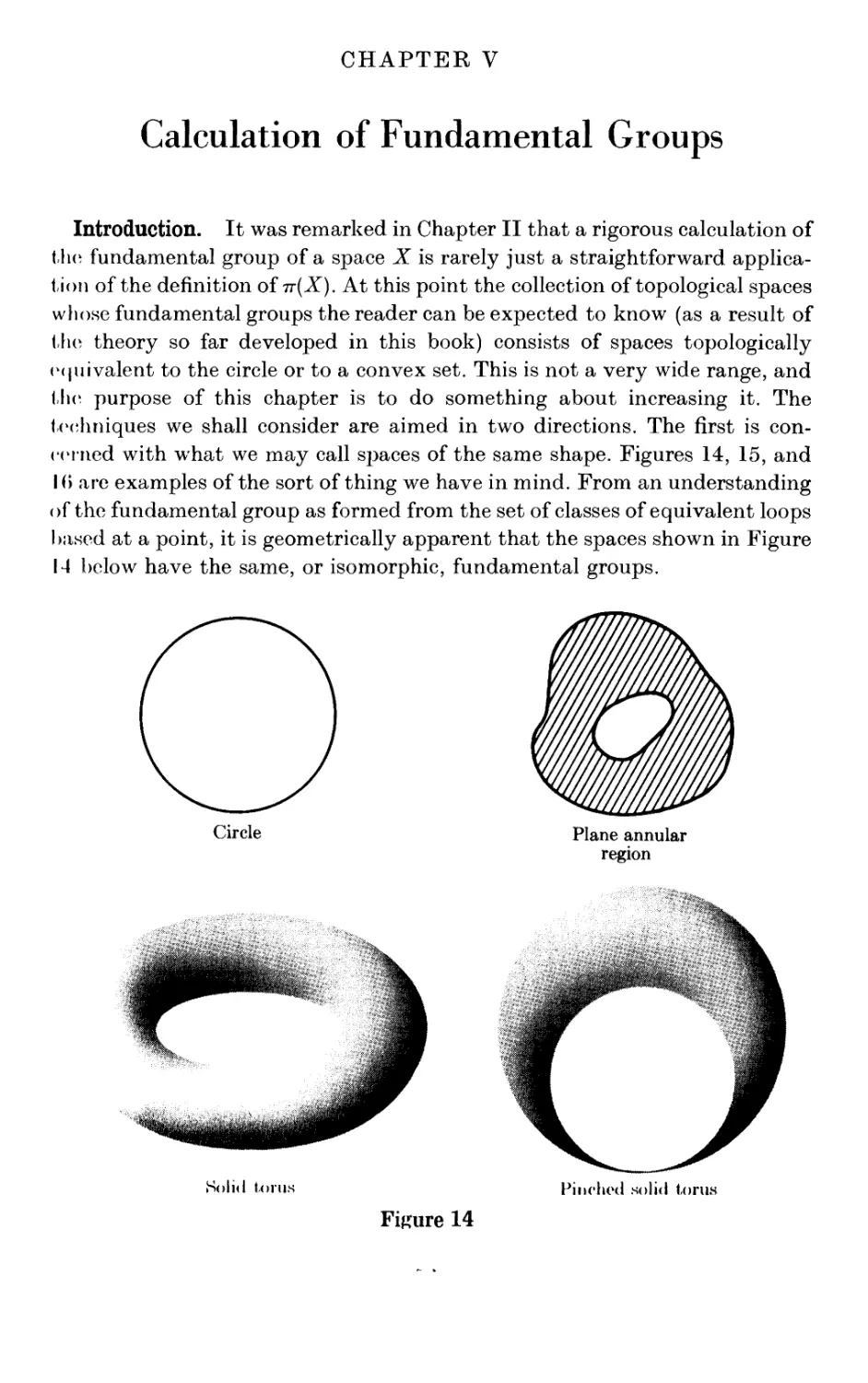
Introduction ........... 52
1. Retractions and deformations ....... 54
2. Homotopv type .......... 02
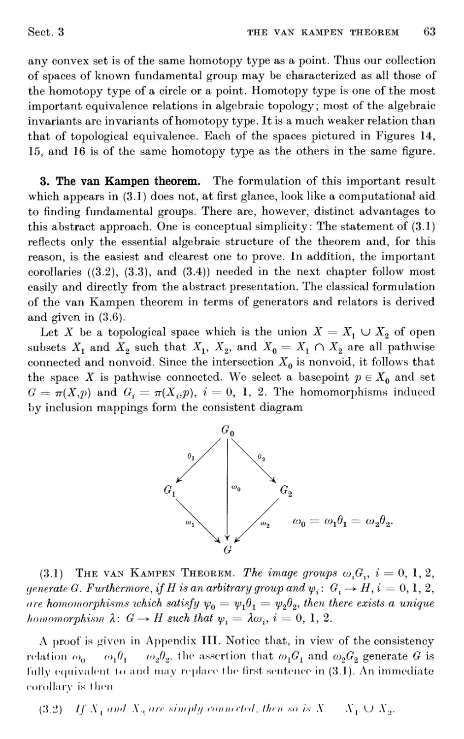
3. The van Kampen theorem ........ 03
X CONTENTS
Chapter VI · Presentation of a Knot Group
Introduction ......
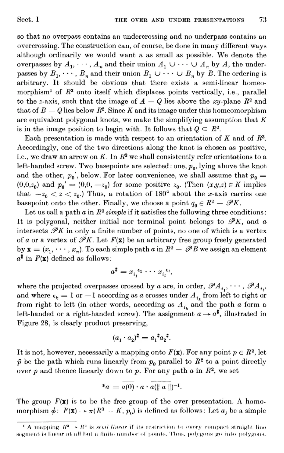
1. The over and under presentations
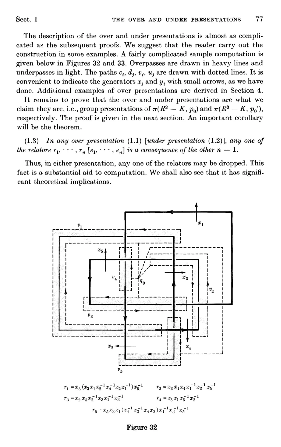
2. The over and under presentations, continued
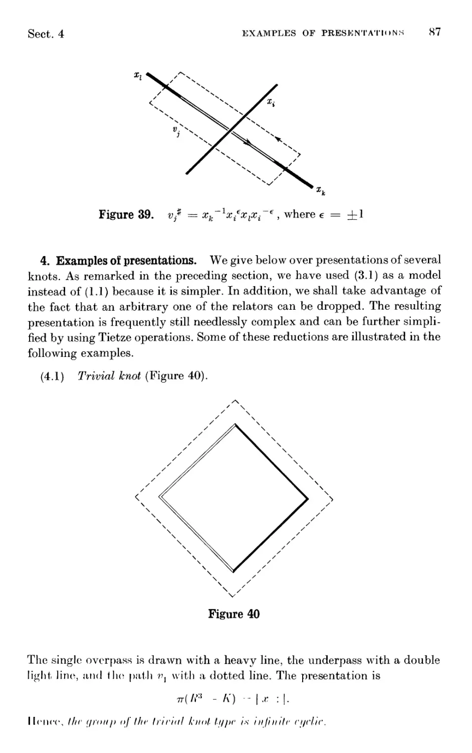
3. The Wirtinger presentation
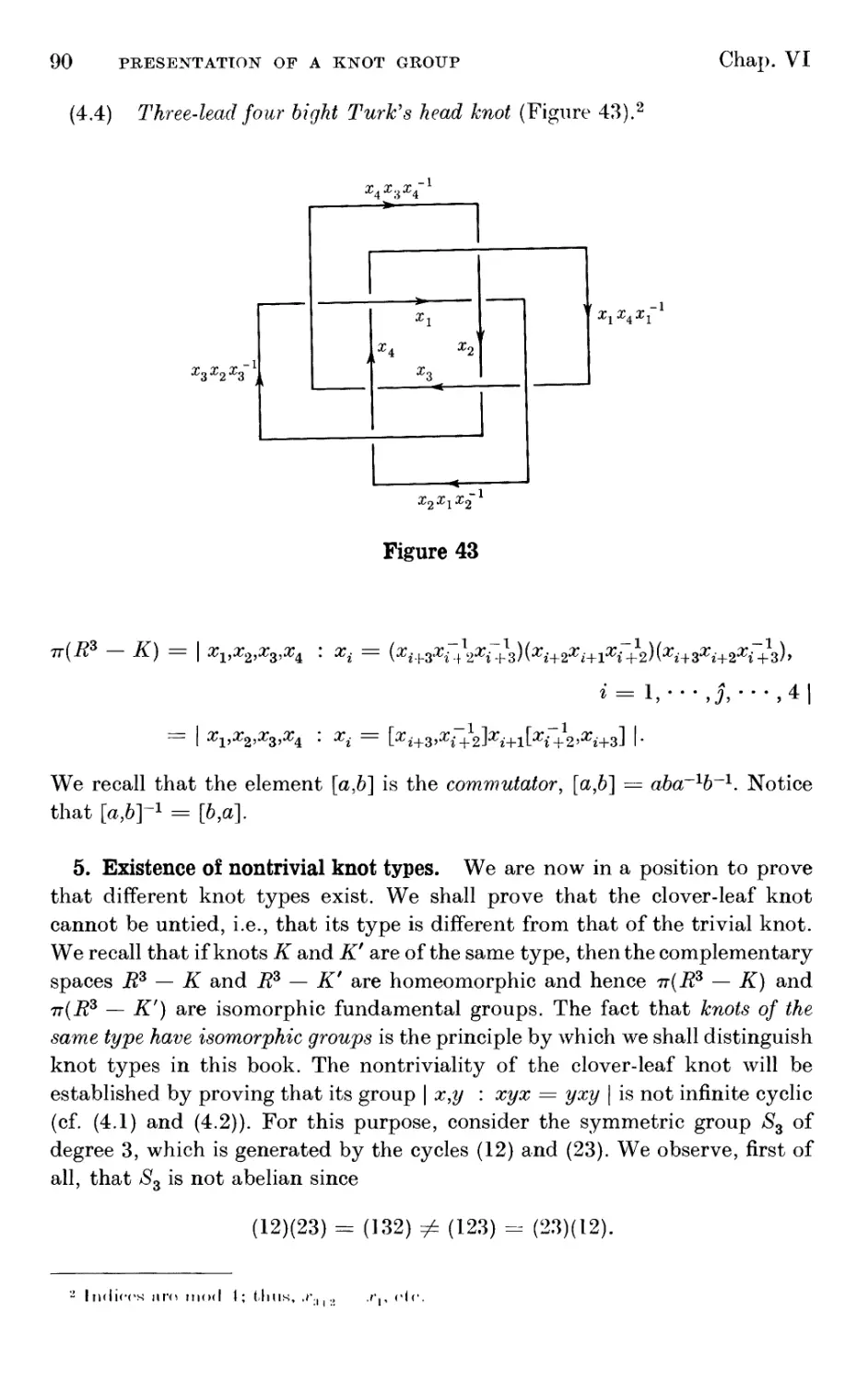
4. Examples of presentations
5. Existence of nontrivial knot types .
72
72
78
86
87
90
Chapter VII · The Free Calculus and the Elementary Ideals
Introduction .
1. The group ring
2. The free calculus .
3. The Alexander matrix
4. The elementary ideals
94
94
96
100
101
Chapter VIII · The Knot Polynomials
Introduction ......
1. The abelianized knot group
2. The group ring of an infinite cyclic group .
3. The knot polynomials ....
4. Knot types and knot polynomials .
110
111
113
119
123
Chapter IX · Characteristic Properties of the Knot Polynomials
Introduction ........... 134
1. Operation of the trivializer . . . . . . . .134
2. Conjugation ........... 136
3. Dual presentations. . . . . . . . . .137
Appendix I. Differentiable Knots are Tame
Appendix II. Categories and groupoids
Appendix III. Proof of the van Kampen theorem
Guide to the Literature ....
Bibliography . . . . .
Index .......
147
153
156
161
165
178
Prerequisites
For an intelligent reading of this book a knowledge of the elements of
modern algebra and point-set topology is sufficient. Specifically, we shall
assume that the reader is familiar with the concept of a function (or mapping)
and the attendant notions of domain, range, image, inverse image, one-one,
onto, composition, restriction, and inclusion mapping; with the concepts
of equivalence relation and equivalence class; with the definition and
elementary properties of open set, closed set, neighborhood, closure, interior,
induced topology, Cartesian product, continuous mapping, homeomorphism,
compactness, connectedness, open cover(ing), and the Euclidean n-dimen-
sional space Rn; and with the definition and basic properties of homomor-
phism, automorphism, kernel, image, groups, normal subgroups, quotient
groups, rings, (two-sided) ideals, permutation groups, determinants, and
matrices. These matters are dealt with in many standard textbooks. We may,
for example, refer the reader to A. H. Wallace, An Introduction to Algebraic
Topology (Pergamon Press, 1957), Chapters I, II, and III, and to G. Birkhoff
and S. MacLane, A Survey of Modern Algebra, Revised Edition (The Mac-
millanCo.,NewYork, 1953), Chapters III, §§1-3, 7, 8; VI, §§4-8, 11-14; VII,
§5; X, §§1, 2; XIII, §§1-4. Some of these concepts are also defined in the
index.
In Appendix I an additional requirement is a knowledge of differential and
integral calculus.
The usual set theoretic symbols e, <=, =^, =, U, Π, and — are used. For
the inclusion symbol we follow the common convention: А с: В means that
ρ Ε Β whenever ρ Ε A. For the image and inverse image of A under / we
write either JA and/_1^4, or/(^4) and/_1(^4). For the restriction of/ to A we
write/ | A, and for the composition of two mappings/: X —> Υ and g: Υ -> Ζ
we write gf.
When several mappings connecting several sets are to be considered at the
same time, it is convenient to display them in a (mapping) diagram, such as
X"< * Υ or
i/
11'each clrmcnl. in each set displayed in a diagram has at most one ima^e
element» in any jj;ivrn set of Mir diagram, Mir diagram is said In br amxi.sl<'nf.
2 PREREQUISITES
Thus the first diagram is consistent if and only if gf = 1 and fg = 1, and the
second diagram is consistent if and only if bf = a and eg = b (and hence
cgf = a).
The reader should note the following "diagram-filling" lemma, the proof of
which is straightforward.
// h: G -> Η and k: G -> К are homomorphisms and h is onto, there
exists a (necessarily unique) homomorjphism f: Η -> К making the diagram
Η > К
consistent if and only if the kernel of h is contained in the kernel of k.
CHAPTER I
Knots and Knot Types
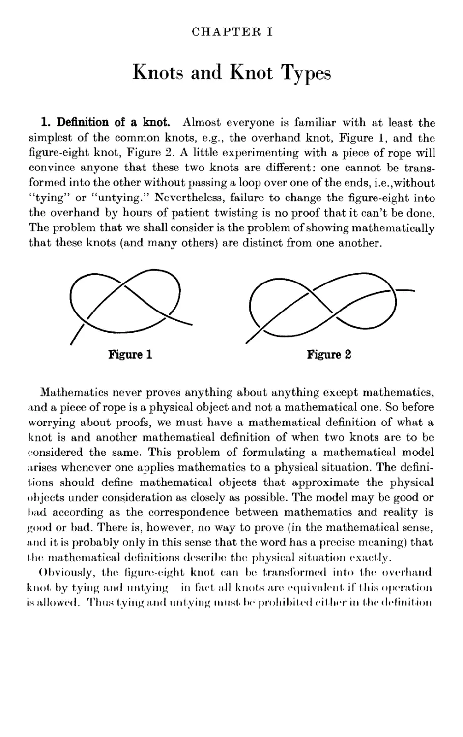
1. Definition of a knot. Almost everyone is familiar with at least the
simplest of the common knots, e.g., the overhand knot, Figure 1, and the
figure-eight knot, Figure 2. A little experimenting with a piece of rope will
convince anyone that these two knots are different: one cannot be
transformed into the other without passing a loop over one of the ends, i.e., without
"tying" or "untying." Nevertheless, failure to change the figure-eight into
the overhand by hours of patient twisting is no proof that it can't be done.
The problem that we shall consider is the problem of showing mathematically
that these knots (and many others) are distinct from one another.
$29. 0гх
Figure 1 Figure 2
Mathematics never proves anything about anything except mathematics,
and a piece of rope is a physical object and not a mathematical one. So before
worrying about proofs, we must have a mathematical definition of what a
knot is and another mathematical definition of when two knots are to be
considered the same. This problem of formulating a mathematical model
arises whenever one applies mathematics to a physical situation. The
definitions should define mathematical objects that approximate the physical
objects under consideration as closely as possible. The model may be good or
had according as the correspondence between mathematics and reality is
good or bad. There is, however, no way to prove (in the mathematical sense,
and it is probably only in this sense that the word has a precise meaning) that
the mathematical definitions describe the physical situation exactly.
Obviously, the figure-eight knot can be transformed into the overhand
knot by tying and untying in fact all knots are equivalent it this operation
is allowed. Thus lying and untying must he prohibited either in the delinition
•I KNOTS AND KNOT TYPES
Chap. I
of when two knots are to be considered the same or from the beginning in the
very definition of what a knot is. The latter course is easier and is the one
we shall adopt. Essentially, we must get rid of the ends. One way would be to
prolong the ends to infinity; but a simpler method is to splice them together.
Accordingly, we shall consider a knot to be a subset of 3-dimensional space
which is homeomorphic to a circle. The formal definition is: К is a knot if there
exists a homeomorphism of the unit circle С into 3-dimensional space R3
whose image is K. By the circle С is meant the set of points (x,y) in the plane
li2 which satisfy the equation x2 + y2 = 1.
The overhand knot and the figure-eight knot are now pictured as in Figure
3 and Figure 4. Actually, in this form the overhand knot is often called the
clover-leaf knot. Another common name for this knot is the trefoil. The figure-
eight knot has been called both the four-knot and Listing's knot.
Figure 3 Figure 4
We next consider the question of when two knots Kx and K2 are to be
considered the same. Notice, first of all, that this is not a question of whether or
not Kx and К2 are homeomorphic. They are both homeomorphic to the unit
circle and, consequently, to each other. The property of being knotted is not
an intrinsic topological property of the space consisting of the points of
the knot, but is rather a characteristic of the way in which that space is
imbedded in R3. Knot theory is a part of 3-dimensional topology and not of
1-dimensional topology. If a piece of rope in one position is twisted into
another, the deformation does indeed determine a one-one correspondence
between the points of the two positions, and since cutting the rope is not
allowed, the correspondence is bicontinuous. In addition, it is natural to
think oi the motion of the- rope as accompanied by a motion of the surrounding
air molecules which thus determines a bicontinuous permutation of the points
of space. This picture su^esls l,hc deiinilion: Knots /\'( and /\\> are vqalvuloil
if (here exists a hnmcomorphism of /»':t onto ilself which maps /\ , onto A.,.
Sect. 2
TAME VERSUS WILD KNOTS 5
It is a triviality that the relation of knot equivalence is a true equivalence
relation. Equivalent knots are said to be of the same type, and each
equivalence class of knots is a knot type. Those knots equivalent to the unknotted
circle x2 + y2 = 1, ζ = 0, are called trivial and constitute the trivial type.1
Similarly, the type of the clover-leaf knot, or of the figure-eight knot is
defined as the equivalence class of some particular representative knot. The
informal statement that the clover-leaf knot and the figure-eight knot are
different is rigorously expressed by saying that they belong to distinct knot
types.
2. Tame versus wild knots. A polygonal knot is one which is the union of a
finite number of closed straight-line segments called edges, whose endpoints
are the vertices of the knot. A knot is tame if it is equivalent to a polygonal
knot; otherwise it is wild. This distinction is of fundamental importance. In
fact, most of the knot theory developed in this book is applicable (as it stands)
only to tame knots. The principal invariants of knot type, namely, the
elementary ideals and the knot polynomials, are not necessarily defined for a
wild knot. Moreover, their evaluation is based on finding a polygonal
representative to start with. The discovery that knot theory is largely confined to
the study of polygonal knots may come as a surprise—especially to the reader
who approaches the subject fresh from the abstract generality of point-set
topology. It is natural to ask what kinds of knots other than polygonal are
tame. A partial answer is given by the following theorem.
(2.1) If a knot parametrized by arc length is of class C1 (i.e., is continuously
differentiable), then it is tame.
A proof is given in Appendix I. It is complicated but straightforward, and
it uses nothing beyond the standard techniques of advanced calculus. More
explicitly, the assumptions on К are that it is rectifiable and given as the image
of a vector-valued function p(s) = (x(s), y(s), z(s)) of arc length s with
continuous first derivatives. Thus, every sufficiently smooth knot is tame.
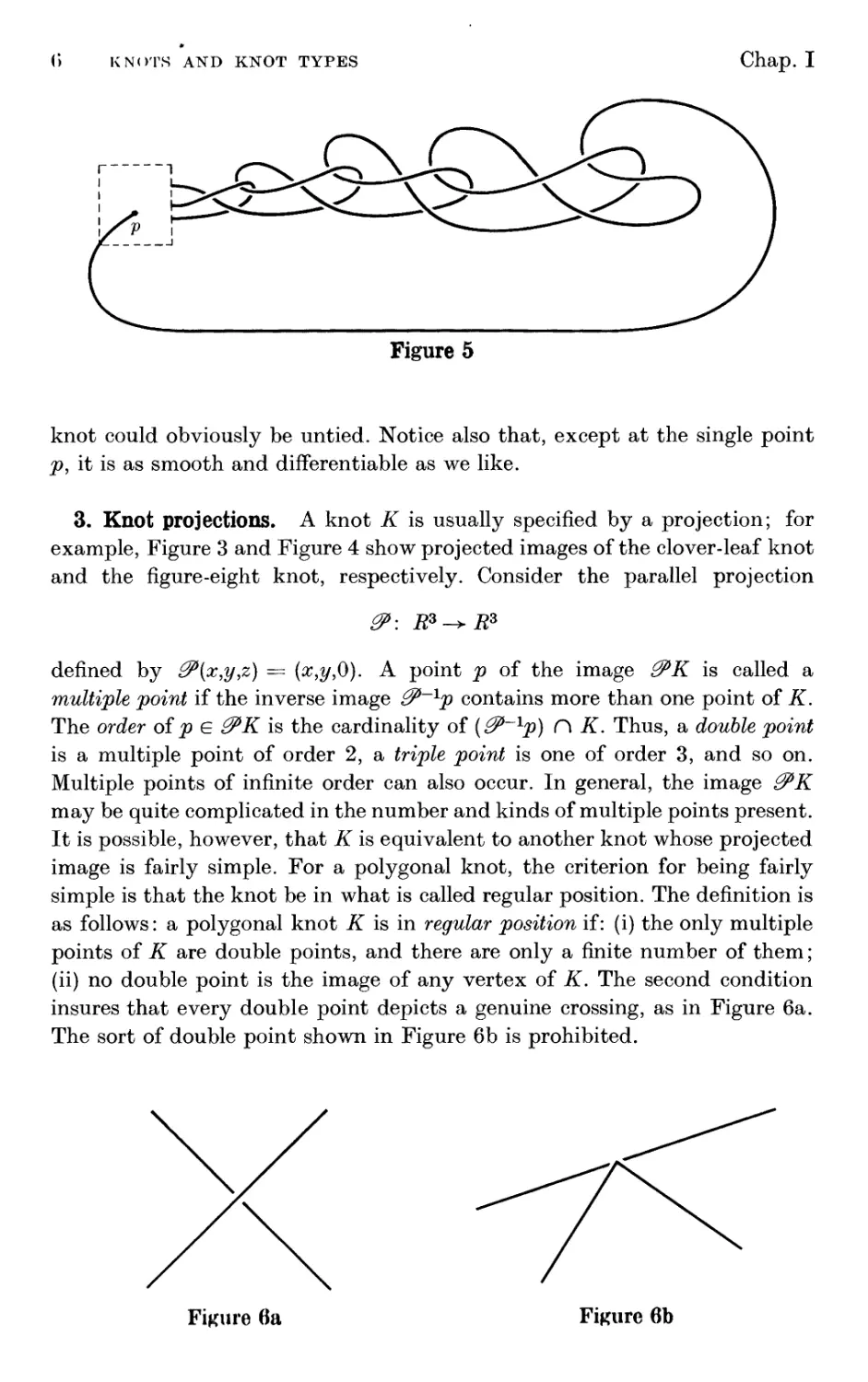
It is by no means obvious that there exist any wild knots. For example,
no knot that lies in a plane is wild. Although the study of wild knots is a corner
of knot theory outside the scope of this book, Figure 5 gives an example
of a knot known to be wild.2 This knot is a remarkable curve. Except for the
fact that the number of loops increases without limit while their size decreases
without limit (as is indicated in the figure by the dotted square about p), the
1 Any knot, which lies in a plane is necessarily Irivial. This is a well known and deep
theorem (>Г plane fopolojj;\. See Л. II. Newinnii, elements of I he ΊΌρο/ο</ι/ of Г1ппс Sets of
I'oinls, Second edition (( 'nmhridcv University Press, ( 'anihrid^e, Р.)Г>1), p. I 7.4.
·'■ I!. II. Ι'Ό\, ll \ lleiimrknNe Simple Closed Curve," Annuls of Miilht inofics. Vol. .'>()
(P.Ml»), pp. LMil. W>.
() KNOTS AND KNOT TYPES
Chap. I
Figure 5
knot could obviously be untied. Notice also that, except at the single point
p, it is as smooth and differentiable as we like.
3. Knot projections. A knot К is usually specified by a projection; for
example, Figure 3 and Figure 4 show projected images of the clover-leaf knot
and the figure-eight knot, respectively. Consider the parallel projection
defined by £P(x,y,z) = (x,y,0). A point ρ of the image 3PK is called a
multiple point if the inverse image 2P~xp contains more than one point of K.
The order of ρ e @PK is the cardinality of {3P~xp) Π Κ. Thus, a double point
is a multiple point of order 2, a triple point is one of order 3, and so on.
Multiple points of infinite order can also occur. In general, the image &K
may be quite complicated in the number and kinds of multiple points present.
It is possible, however, that К is equivalent to another knot whose projected
image is fairly simple. For a polygonal knot, the criterion for being fairly
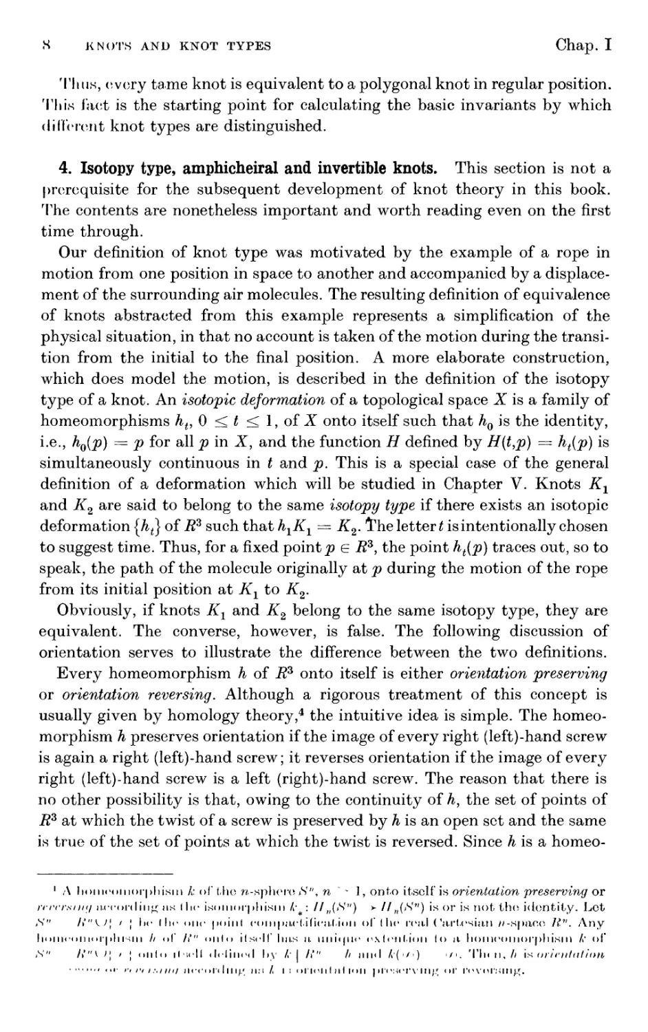
simple is that the knot be in what is called regular position. The definition is
as follows: a polygonal knot К is in regular position if: (i) the only multiple
points of К are double points, and there are only a finite number of them ;
(ii) no double point is the image of any vertex of K. The second condition
insures that every double point depicts a genuine crossing, as in Figure 6a.
The sort of double point shown in Figure 6b is prohibited.
Figure 6a
Figure 6b
Sect. 3
KNOT PROJECTIONS 7
Each double point of the projected image of a polygonal knot in regular
position is the image of two points of the knot. The one with the larger
z- coordinate is called an overcrossing, and the other is the corresponding
undercrossing.
(3.1) Any polygonal knot К is equivalent under an arbitrarily small rotation
of Rz to a polygonal knot in regular position.
Proof. The geometric idea is to hold К fixed and move the projection.
Every bundle (or pencil) of parallel lines in Rz determines a unique parallel
projection of i?3 onto the plane through the origin perpendicular to the bundle.
We shall assume the obvious extension of the above definition of regular
position so that it makes sense to ask whether or not К is in regular position
with respect to any parallel projection. It is convenient to consider R3 as a
subset3 of a real projective 3-space P3. Then, to every parallel projection we
associate the point of intersection of any line parallel to the direction of
projection with the projective plane P2 at infinity. This correspondence is
clearly one-one and onto. Let Q be the set of all points of P2 corresponding to
projections with respect to which К is not in regular position. We shall show
that Q is nowhere dense in P2. It then follows that there is a projection 0O
with respect to which К is in regular position and which is arbitrarily close
to the original projection 0* along the z-axis. Any rotation of Rz which
transforms the line ^0_1(0,0,0) into the z-axis will suffice to complete the proof.
In order to prove that Q is nowhere dense in P2, consider first the set of all
straight lines which join a vertex of К to an edge of K. These intersect P2 in a
finite number of straight-line segments whose union we denote by Qv Any
projection corresponding to a point of P2 — Q± must obviously satisfy
condition (ii) of the definition of regular position. Furthermore, it can have at
most a finite number of multiple points, no one of which is of infinite order.
It remains to show that multiple points of order η > 3 can be avoided, and
this is done as follows. Consider any three mutually skew straight lines, each
of which contains an edge of K. The locus of all straight lines which intersect
these three is a quadric surface which intersects P2 in a conic section.
(See the reference in the preceding footnote.) Set Q2 equal to the union of all
such conies. Obviously, there are only a finite number of them. Furthermore,
the image of К under any projection which corresponds to some point of
P2 — (Qi ^ Q2) nas no multiple points of order η > 3. We have shown that
P2 - (Q, и Q2) cz ρ2 - ρ.
Thus Q is a subset of Qx KJ ζ)2, which is nowhere dense in P2. This completes
the proof of (3.1). I '.
л Ког ни n.ccoiiii!, of llin coiicopls nsod in (his proof, moo (). Vohlon 11ml .1. VV. Yoiin^,
rrojcrlinr (U'omctrif ((riim and Company, lioslon, MjimmjicIiiimoLI.m, MHO), Vol. I pp. II,
2!M)', :toi.
К KNOTS AND KNOT TYPES
Chap. I
Thus, (ivory tame knot is equivalent to a polygonal knot in regular position.
This fact is the starting point for calculating the basic invariants by which
different knot types are distinguished.
4. Isotopy type, amphicheiral and invertible knots. This section is not a
prerequisite for the subsequent development of knot theory in this book.
The contents are nonetheless important and worth reading even on the first
time through.
Our definition of knot type was motivated by the example of a rope in
motion from one position in space to another and accompanied by a
displacement of the surrounding air molecules. The resulting definition of equivalence
of knots abstracted from this example represents a simplification of the
physical situation, in that no account is taken of the motion during the
transition from the initial to the final position. A more elaborate construction,
which does model the motion, is described in the definition of the isotopy
type of a knot. An isotopic deformation of a topological space X is a family of
homeomorphisms ht,Q<t<l,ofX onto itself such that h0 is the identity,
i.e., h0(p) = ρ for all ρ in X, and the function Η defined by H(t,p) = ht(p) is
simultaneously continuous in t and p. This is a special case of the general
definition of a deformation which will be studied in Chapter V. Knots Κλ
and K2 are said to belong to the same isotopy type if there exists an isotopic
deformation {AJ of R2 such that h1K1 = K2. The letter £ is intentionally chosen
to suggest time. Thus, for a fixed pointy e Rz, the point ht(p) traces out, so to
speak, the path of the molecule originally at ρ during the motion of the rope
from its initial position at Kx to K2.
Obviously, if knots Kx and K2 belong to the same isotopy type, they are
equivalent. The converse, however, is false. The following discussion of
orientation serves to illustrate the difference between the two definitions.
Every homeomorphism h of J?3 onto itself is either orientation preserving
or orientation reversing. Although a rigorous treatment of this concept is
usually given by homology theory,4 the intuitive idea is simple. The
homeomorphism h preserves orientation if the image of every right (left)-hand screw
is again a right (left)-hand screw; it reverses orientation if the image of every
right (left)-hand screw is a left (right)-hand screw. The reason that there is
no other possibility is that, owing to the continuity of h, the set of points of
R3 at which the twist of a screw is preserved by h is an open set and the same
is true of the set of points at which the twist is reversed. Since h is a homeo-
1 Л lioiii(M»ii)()i'|)bism /: of the π-sphere *V", η ~ - 1, onto itself is orientation preserving or
rrrcrsnn/ according ns I lie isomoi'idiisiii /^ : //,,(<S'") у //ri(Sv) is or is not the identity. Let
>S'" /i'"U[ / I Im· Ihr one point enmpaetiiieatiiHi of (he гем.1 ('artesian //-space llv. Any
Ι κ >ι ι к ·« > 11 it »i-| >11 i-4i 11 // of It" niilu ilsrlf has a uiihjiK' «wlrntinn (o a lioineomorphisin k of
N" /»'"v >; ' J un(u ii'icll «IrlinoJ l>v /.· | /.'" // ninl /»■(-'-) "· Tin η, Λ is orirnhition
' «"■ >■· iu ι :.i mi iin'Di ■< Ι Μ ι// мм /. I : < amii Ι μ Ι κ hi | η < >м< м'\ in ij; or ΓονηΐΜΐη^.
Sect. 4 isotopy type, amphicheiral and invertible knots 9
morphism, every point of R3 belongs to one of these two disjoint sets; and
since R3 is connected, it follows that one of the two sets is empty. The
composition of homeomorphisms follows the usual rule of parity:
h
preserving
reversing
preserving
reversing
h2
preserving
preserving
reversing
reversing
KK
preserving
reversing
reversing
preserving
Obviously, the identity mapping is orientation preserving. On the other
hand, the reflection (x,y,z) —> (x,y, — z) is orientation reversing. If Λ is a
linear transformation, it is orientation preserving or reversing according as its
determinant is positive or negative. Similarly, if both h and its inverse are C1
differentiable at every point of R3, then h preserves or reverses orientation
according as its Jacobian is everywhere positive or everywhere negative.
Consider an isotopic deformation {ht} of R3. The fact that the identity is
orientation preserving combined with the continuity of H(t,p) = ht(p),
suggests that ht is orientation preserving for every t in the interval 0 < t < 1.
This is true.5 As a result, we have that a necessary condition for two knots to
be of the same isotopy type is that there exist an orientation preserving
homeomorphism of R3 on itself which maps one knot onto the other.
A knot К is said to be amphicheiral if there exists an orientation reversing
homeomorphism h of R3 onto itself such that hK = K. An equivalent
formulation of the definition, which is more appealing geometrically, is provided
by the following lemma. By the mirror image of a knot К we shall mean the
image of К under the reflection 0t defined by (x,y,z) —> (x,y, — z). Then,
(4.1) A knot К is amphicheiral if and only if there exists an orientation
preserving homeomorphism of R3 onto itself which maps К onto its mirror image.
Proof. If К is amphicheiral, the composition 3%h is orientation preserving
and maps К onto its mirror image. Conversely, if h' is an orientation
preserving homeomorphism of R3 onto itself which maps К onto its mirror image, 1 lie
composition &h' is orientation reversing and (&h')K = K. [ \
It is not hard to show that the figure-eight knot is amphicheiral. The
experimental approach is the best; a rope which has been tied as a figure-right
and then spliced is quite rasily twisted into its mirror image. Thr operation is
illustrated in Figure 7. On the other hand, the clover-leaf knot is not amphi-
r' Any isotopic deformation ]/>,}, <> · / ' I, <»f Mm ('artesian η space /ι" delinitoly
possesses a ιιηίψιο extension loan isot opie dcforniat ion {/»"/},*> ' f ' I, of (lie// sphere
Λ'", i.e.. A", | /»'" /i,, tind A,(/ ) <t . |Л»г end ι /, I ho lionieoinorpliisni /,·, is homo lop ir to
the identity, mid so tlm induced isomorphism (/·,) on //ri(.S'") is the idmilily. 11 lollovvs
thai- Λ, is onenliil юп ptv,er\ iii^ tor nil / in О / · I. (Sir iiImi IihiImdIm I.)
10 knots and knot types Chap. I
d) (2) (3)
(4) (5) (6)
Figure 7
cheiral. In this case, experimenting with a piece of rope accomplishes nothing
except possibly to convince the skeptic that the question is nontrivial.
Actually, to prove that the clover-leaf is not amphicheiral is hard and requires
fairly advanced techniques of knot theory. Assuming this result, however, we
have that the clover-leaf knot and its mirror image are equivalent but not of
the same isotopy type.
It is natural to ask whether or not every orientation preserving homeo-
morphism / of Rz onto itself is realizable by an isotopic deformation, i.e.,
given/, does there exist {ht}, 0 < t < 1, such that/ = Λχ? If the answer were
no, we would have a third kind of knot type. This question is not an easy one.
The answer is, however, yes.6
Just as every homeomorphism of Rz onto itself either preserves or reverses
orientation, so does every homeomorphism / of a knot К onto itself. The
geometric interpretation is analogous to, and simpler than, the situation in
3-dimensional space. Having prescribed a direction on the knot, / preserves or
reverses orientation according as the order of points of К is preserved or
reversed under/. A knot К is called invertible if there exists an orientation
preserving homeomorphism h of Ег onto itself such that the restriction h | К
is an orientation reversing homeomorphism of К onto itself. Both the clover-
" (J. Μ . I'MmIhu-, "()ιι Ι.Ι10 (jmii|» of nil I lomooinurpliinmM of η Manifold," ff'mn.s<tc/i.onx of
the Ammnin Malhrmntmd Soncty, Vol. 1)7 (l!M»0), j>|>. M.K1 i!IU.
Sect. 4
ISOTOPY TYPE, AMPHICHEIEAL AND INVERTIBLE KNOTS
11
leaf and figure-eight knots are invertible. One has only to turn them over
(cf. Figure 8).
Figure 8
Until recently no example of a noninvertible knot was known. Trotter
solved the problem by exhibiting an infinite set of noninvertible knots, one
of which is shown in Figure 9.7
3
Figure 9
EXERCISES
1. Show that any simple closed polygon in R2 belongs to the trivial knot
type.
2. Show that there are no knotted quadrilaterals or pentagons. What knot
types are represented by hexagons? by Heptagons?
7 II. ΙΛ Trottor, "Noniiivortihlo knots oxi.4t.,> Ί'υρυΙ,υ,/μ, vol. 2 (МММ), |>|>. 27Г> 2H0.
PJ KNOTS AND KNOT TYPES
Chap. I
.4. I )evise a method for constructing a table of knots, and use it to find the
ten knots of not more than six crossings. (Do not consider the question of
whether these are really distinct types.)
I. Determine by experiment which of the above ten knots are obviously
amphicheiral, and verify that they are all invertible.
Γ). Show that the number of tame knot types is at most countable.
(). (Brunn) Show that any knot is equivalent to one whose projection has
at most one multiple point (perhaps of very high order).
7. (Tait) A polygonal knot in regular position is said to be alternating
if the undercrossings and overcrossings alternate around the knot. (A knot
typo is called alternating if it has an alternating representative.) Show that if
/v is any knot in regular position there is an alternating knot (in regular
position) that has the same projection as K.
8. Show that the regions into which R2 is divided by a regular projection
can be colored black and white in such a way that adjacent regions are of
opposite colors (as on a chessboard).
9. Prove the assertion made in footnote 4 that any homeomorphism h of Rn
onto itself has a unique extension to a homeomorphism к of Sn = Rn U {oo}
onto itself.
10. Prove the assertion made in footnote 5 that any isotopic deformation
{ht}9 0 < t < 1, of Rn possesses a unique extension to an isotopic deformation
{kt}, 0 <t < 1, of Sn. (Hint: Define F(p, t) = (ht(p),t), and use invariance of
domain to prove that F is a homeomorphism of Rn X [0, 1] onto itself.)
CHAPTER II
The Fundamental Group
Introduction. Elementary analytic geometry provides a good example of
the applications of formal algebraic techniques to the study of geometric
concepts. A similar situation exists in algebraic topology, where one associates
algebraic structures with the purely topological, or geometric, configurations.
The two basic geometric entities of topology are topological spaces and
continuous functions mapping one space into another. The algebra involved, in
contrast to that of ordinary analytic geometry, is what is frequently called
modern algebra. To the spaces and continuous maps between them are made
to correspond groups and group homomorphisms. The analogy with analytic
geometry, however, breaks down in one essential feature. Whereas the
coordinate algebra of analytic geometry completely reflects the geometry, the
algebra of topology is only a partial characterization of the topology. This
means that a typical theorem of algebraic topology will read: If topological
spaces X and Υ are homeomorphic, then such and such algebraic conditions
are satisfied. The converse proposition, however, will generally be false. Thus,
if the algebraic conditions are not satisfied, we know that X and Υ are
topological^ distinct. If, on the other hand, they are fulfilled, we usually can
conclude nothing. The bridge from topology to algebra is almost always a
one-way road; but even with that one can do a lot.
One of the most important entities of algebraic topology is the fundamental
group of a topological space, and this chapter is devoted to its definition and
elementary properties. In the first chapter we discussed the basic spaces and
continuous maps of knot theory: the 3-dimensional space R3, the knots
themselves, and the homeomorphisms of i?3 onto itself which carry one knot onto
another of the same type. Another space of prime importance is the
complementary space Es — К of a knot K, which consists of all of those points of i?3
that do not belong to K. All of the knot theory in this book is a study of the
properties of the fundamental groups of the complementary spaces of knots,
and this is indeed the central theme of the entire subject. \\\ this chapter,
however, the development of the fundamental group is made* for an arbitrary
topological space Л' and is independent· of our later applications of the
fundamental group to knot theory.
II ΤΗΙί FUNDAMENTAL GROUP
Chap. II
1. Paths and loops. A particle moving in space during a certain interval
of time describes a path. It will be convenient for us to assume that the motion
brains at time t = 0 and continues until some stopping time, which may differ
lor different paths but may be either positive or zero. For any two real
numbers χ and у with χ < у, we define [x,y] to be the set of all real numbers t
satisfying χ < t < y. A path α in a topological space X is then a continuous
mapping
α: [0,||α||]->Χ.
The number || a || is the stopping time, and it is assumed that || a || > 0. The
points a(0) and a(\\ a ||) in X are the initial point and terminal point,
respectively, of the path a.
It is essential to distinguish a path a from the set of image points a(t) in X
visited during the interval [0,|| a ||]. Different paths may very well have the
same set of image points. For example, let X be the unit circle in the plane,
given in polar coordinates as the set of all pairs {r,6) such that r = 1. The two
paths
a(t) = (l,i), 0 < t < 2тг,
6(0 = (1,20, 0 <t <2tt-,
are distinct even though they have the same stopping time, same initial and
terminal point, and same set of image points. Paths a and b are equal if and
only if they have the same domain of definition, i.e., || a || = || b ||, and, if for
every t in that domain, a(t) = b(t).
Consider any two paths a and b in X which are such that the terminal point
of α coincides with the initial point of δ, i.e., a(\\ a ||) = b(0). The product a · b
of the paths a and b is defined by the formula
(ait), 0 < t < || a II,
(a · b)(t) = {
W- || α ||), || α || < t < || a \\ + \\ b ||.
It is obvious that this defines a continuous function, and a ♦ b is therefore a
path in X. Its stopping time is
II α· δ II = 11 « II + 11 δ II·
We emphasize that the product of two paths is not defined unless the terminal
point of the first is the same as the initial point of the second. It is obvious that
the three assertions
(i) a · b and Ь · с are defined,
(ii) a · (b · c) is defined,
(iii) (a ■ b) ■ с is defined,
are equivalent and that whenever one of them holds, the associative law,
a · (b · c) (a ■ b) ■ (\
is valid.
A path a is railed an identity path, or simply an identity, if if has stopping
time || a \\ 0. This terminology relleefs the faef flint the set of all identify
Sect. 2
CLASSES OF PATHS AND LOOPS 15
paths in a topological space may be characterized as the set of all
multiplicative identities with respect to the product. That is, the path e is an identity
if and only if e · a = a and b · e = b whenever e · a and b · e are defined.
Obviously, an identity path has only one image point, and conversely, there
is precisely one identity path for each point in the space. We call a path whose
image is a single point a constant path. Every identity path is constant; but
the converse is clearly false.
For any path a, we denote by a-1 the inverse path formed by traversing a
in the opposite direction. Thus,
a-^t) = a{\\ a \\ — t), 0 <t < \\ a ||.
The reason for adopting this name and notation for a-1 will become apparent
as we proceed. At present, calling a-1 an inverse is a misnomer. It is easy to
see that a · a-1 is an identity e if and only if α = e.
The meager algebraic structure of the set of all paths of a topological space
with respect to the product is certainly far from being that of a group. One
way to improve the situation algebraically is to select an arbitrary point ρ in
X and restrict our attention to paths which begin and end at p. A path whose
initial and terminal points coincide is called a loop, its common endpoint
is its basepoint, and a loop with basepoint ρ will frequently be referred to as
p-based. The product of any two ^э-based loops is certainly defined and is
again a j9-based loop. Moreover, the identity path at ρ is a multiplicative
identity. These remarks are summarized in the statement that the set of all
p-based loops in X is a semi-group with identity.
The semi-group of loops is a step in the right direction; but it is not a group.
Hence, we consider another approach. Returning to the set of all paths, we
shall define in the next section a notion of equivalent paths. We shall then
consider a new set, whose elements are the equivalence classes of paths. The
fundamental group is obtained as a combination of this construction with the
idea of a loop.
2. Classes of paths and loops. A collection of paths hs in X, 0 < s < 1, will
be called a continuous family of paths if
(i) The stopping time || hs || depends continuously on s.
(ii) The function h defined by the formula h(s,t) = hs(t) maps the closed
region 0 < s < 1, 0 < t < || hs || continuously into X.
Tt should be noted that a function of two variables which is continuous at
every point of its domain of definition with respect to each variable is not
necessarily continuous in both simultaneously. The function / defined on the
unit square 0 < s < \, 0 < t < 1 by the formula
fl, if a· /, 0,
- , nf.hrrwiMtv
vV· ι μ
Н> ТИК FUNDAMENTAL GROUP
Chap. II
is η,η example. The collection of paths {/J defined by fs(t) = f(s,t) is not,
therefore, a continuous family.
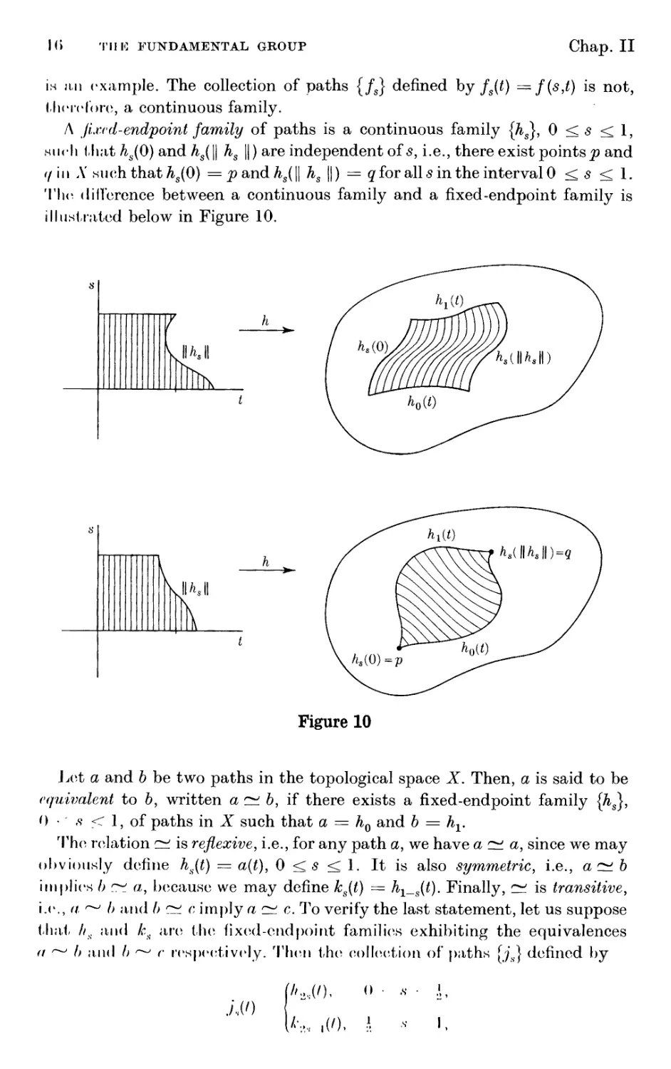
A Jurd-endpoint family of paths is a continuous family {hs}, 0 < s < 1,
such that hs(0) and hs(\\ hs ||) are independent of s, i.e., there exist points^ and
ί/in Л' such that hs(0) = p8indhs(\\ hs ||) = q for all 5 in the interval 0 < s < 1.
The difference between a continuous family and a fixed-endpoint family is
illustrated below in Figure 10.
Мь
Figure 10
Let a and δ be two paths in the topological space X. Then, a is said to be
equivalent to b, written a ~ b, if there exists a fixed-endpoint family [hs],
0 · 'ft < 1, of paths in X such that a = h0 and δ = hv
The relation ^ is reflexive, i.e., for any path a, we have a c^. a, since we may
obviously define hs(t) — α(ί), 0 <s < 1. It is also symmetric, i.e., a c^ b
implies b ^ a, because we may define ks(t) = h1_s(t). Finally, ^ is transitive,
i.e., α ^ /> and /> c^ с imply a c^ c. To verify the last statement, let us suppose
that //А. and ks are the fixed-end point families exhibiting the equivalences
a r^j b and b ~ r respectively. Then the collection of paths [js] defined by
un
Sect. 2
CLASSES OF PATHS AND LOOPS 17
is a fixed-endpoint family proving α ^ с. То complete the arguments, the
reader should convince himself that the collections defined above in showing
reflexivity, symmetry, and transitivity actually do satisfy all the conditions
for being path equivalences: fixed-endpoint, continuity of stopping time, and
simultaneous continuity in s and t.
Thus, the relation c^ is a true equivalence relation, and the set of all paths
in the space X is therefore partitioned into equivalence classes. We denote
the equivalence class containing an arbitrary path a by [a]. That is, [a] is the
set of all paths δ in Ζ such that a c^. b. Hence, we have
[a] = [b] if and only if a ~ b.
The collection of all equivalence classes of paths in the topological space X
will be denoted by Γ(Χ). It is called the fundamental groupoid of X. The
definition of a groupoid as an abstract entity is given in Appendix II.
Geometrically, paths a and b are equivalent if and only if one can be
continuously deformed onto the other in X without moving the endpoints.
The definition is the formal statement of this intuitive idea. As an example,
let X be the annular region of the plane shown in Figure 11 and consider five
loops e (identity), av a2, a3, a4 in X based at p. We have the following
equivalences
However, it is not true that
αλ ~ α3.
Figure 11 shows that certain fundamental properties of X are reflected in the
equivalence structure of the loops of X. If, for example, the points lying
inside the inner boundary of X had been included as a part of X, i.e., if the
Figure 11
Μι III К FUNDAMENTAL GROUP
Chap. II
In·!· were filled in, then all loops based at ρ would have been equivalent to the
i<l<κ! ιf.ν loop e. It is intended that the arrows in Figure 11 should imply that
• ι ι llir interval of the variable t is traversed for each a{, the image point runs
«inhiiid the circuit once in the direction of the arrow. It is essential that the
κΙγ,ί of at as a function be maintained. The image points of a path do not
nperify the path completely; for example, аъф α3 · α3, and furthermore, we
<!<> not even have, аъ^ az- a3.
We shall now show that path multiplication induces a multiplication in the
fundamental groupoid Г(Х). As a result we shall transfer our attention from
paths and products of paths to consideration of equivalence classes of paths
and the induced multiplication between these classes. In so doing, we shall
obtain the necessary algebraic structure for defining the fundamental group.
(2.1) For any paths a, a , b, b' in X, if a · b is defined and a c^. a and
b c^ b', then a! · b' is defined and a · b c^ a · b''.
Proof. If {hs} and {ks} are the fixed-endpoint families exhibiting the
equivalences a c^ a and b ^ b', respectively, then the collection of paths
{hs · ks] is a fixed-endpoint family which gives a · b c± a · b'. We observe,
first of all, that the products hs · ks, are defined for every s in 0 < s < 1
because
A.(ll К ||) = A0(|| К ||) = «(H a ||) = 6(0) = i0(0) = *,(0).
In particular, a · b' = hx- kx is defined. It is a straightforward matter to
verify that the function h · k defined by
(h · k)(s,t) = (hs · k,)(t), 0 < s < 1, 0 < t < \\h8 || + || *e ||,
is simultaneously continuous in s and t. Since || hs · ks || = || hs || + || ks \\
is a continuous function of s, the paths hs · ks form a continuous family. We
have
(K ' *.)(0) = Ae(0) = a(0),
and
(Αβ·*β)(Ι|Λβ·Α;β||) = *β(||*β||) = 6(||6||)>
so that {As · ks}, 0 < 5 < 1, is a fixed-endpoint family. Since h0· k0 = a · b
and hx- k± = a' · b', the proof is complete.
Consider any two paths a and b in X such that a · δ is defined. The product
of the equivalence classes [a] and [b] is defined by the formula
[a] · [Ь] = [a ■ b].
Multiplication in Γ(Χ) is well-defined as a result of (2.1).
Since all paths belonging to a single equivalence class have the same initial
point and the same terminal point, we may define the initial point and
terminal point- of an element α in V(X) to he those of an arbitrary
representative path in or. The product- α · // of two elements a and /i in Γ(Λ') is then
Sect. 2
CLASSES OF PATHS AND LOOPS 19
defined if the terminal point of α coincides with the initial point of β. Since
the mapping a -> [a] is product preserving, the associative law holds in Γ(Χ)
whenever the relevant products are defined, exactly as it does for paths.
An element e in T(X) is an identity if it contains an identity path. Just as
before, we have that an element e is an identity if and only if e · α = α and
β · € = β whenever e · α and β - € are defined. This assertion follows almost
trivially from the analogous statement for paths. For, let e be an identity, and
suppose that e · α is defined. Let e be an identity path in e and a a
representative path in a. Then, e · a = a, and so e · α = α. Similarly, β · e = β.
Conversely, suppose that e is not an identity. To prove that there exists an α
such that e · α is defined and e · ol-Φ a, select for a the class containing the
identity path corresponding to the terminal point of e. Then, e · α is defined,
and, since α is an identity, e · α = e. Hence, if e · α = α, the class e is an
identity, which is contrary to assumption. This completes the proof. We
conclude that Γ(Χ) has at least as much algebraic structure as the set of paths in
X. The significant thing, of course, is that it has more.
(2.2) For any path a in X, there exist identity paths ex and e2 such that
a · a-1 c^ ex and a-1 · a f^± e2.
Proof. The paths ex and e2 are obviously the identities corresponding to
the initial and terminal points, respectively, of a. Consider the collection of
paths {hs}, 0 < s < 1, defined by the formula
*.(*)
(a(t), 0 < t <s || a ||,
[a(2s || a \\ - t), s \\ a \\ < t <2s \\ a ||.
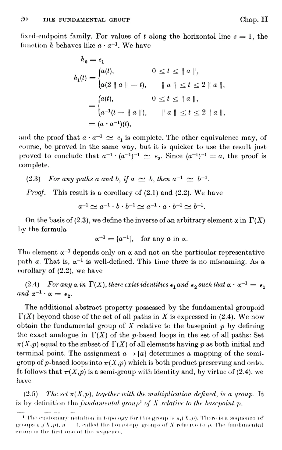
The domain of the mapping h defined by h(s,t) = hs(t) is the shaded area
shown in Figure 12. On the line t = 0, i.e., on the s-axis, h is constantly equal
to a(0). The same is true along the line t = 2s\\a\\. Hence the paths hs form a
Figure 12
20 тле fundamental group Chap. II
lixcd-cndpoint family. For values of t along the horizontal line 5=1, the
function h behaves like a · a-1. We have
hQ = e1
(a(t), 0 <t <\\a\\,
[a(2 || α || - f), || a \\ < t < 2 || a ||,
_(a(t), 0 <t < || a ||,
~[a-Ht- || a ||), || a \\ < t < 2 || a ||,
= (a · a-x)W,
and the proof that a · α-1 ^ ех is complete. The other equivalence may, of
course, be proved in the same way, but it is quicker to use the result just
proved to conclude that a-1 · (or1)-1 ^ e2. Since (a-1)-1 = a, the proof is
complete.
(2.3) For any paths a and b, if a ^ b, then a-1 c± 6_1.
Proof. This result is a corollary of (2.1) and (2.2). We have
or1 ^ or1 · δ · δ-1 ~ a'1 - a - δ-1 ~ δ-1.
On the basis of (2.3), we define the inverse of an arbitrary element α in Γ(Χ)
by the formula
a-1 = [a-1], for any α in a.
The element a-1 depends only on a and not on the particular representative
path a. That is, a-1 is well-defined. This time there is no misnaming. As a
corollary of (2.2), we have
(2.4) For any α in Γ(Χ), there exist identities ex and e2 such that α · α-1 = ex
and or1 · α = e2.
The additional abstract property possessed by the fundamental groupoid
T(X) beyond those of the set of all paths in X is expressed in (2.4). We now
obtain the fundamental group of X relative to the basepoint ρ by defining
the exact analogue in Γ(Χ) of the j9-based loops in the set of all paths: Set
π(Χ,ρ) equal to the subset of Γ(Χ) of all elements having^ as both initial and
terminal point. The assignment a —> [a] determines a mapping of the
semigroup of £>-based loops into π(Χ,ρ) which is both product preserving and onto.
it follows that π(Χ,ρ) is a semi-group with identity and, by virtue of (2.4), we
have
(2.5) The. set n(X,'p), together with the, multiplication defined, is a group. It
is by definition the fu.nda'metilal group1 of X relative to the basepoint p.
1 Tim cumj о тагу ι ml nl inn in I npnlo^y for I Ins дгопр is я,(.\\/>). Thorn is α .чп<цнчн!о of
j-Mou|>m // fl( .V ,/>), // I , culled Mm Imiiinl <>|>y ^гппрм of X ivlnl ι\ η In />. Tim Γη in In nmn I a.I
L'l'uin» in Mm lir.'tl <>im <>| llm Mrmmimn.
Sect. 3 CHANGE OF BASEPOINT 21
We conclude this section with the useful observation that as far as
equivalence classes go, constant paths are the same as identity paths.
(2.6) Every constant path is equivalent to an identity path.
Proof. Let к be an arbitrary constant path in X defined by
k(t) = p, 0 < t < || к ||, for some ρ e X.
Obviously, the collection of paths hs defined by the formula
hs(t) =p, 0 < t < s || к ||
is a fixed-endpoint family, and hx = к and h0 = e, where e is the identity path
corresponding to p.
3. Change of basepoint. The fundamental group π(Χ,ρ) of X is defined
with respect to and depends on the choice of basepoint p. However we shall
now show that if X is pathwise connected the fundamental groups of X
defined for different basepoints are all isomorphic. A topological space X is
pathwise connected2 if any two of its points can be joined by a path lying in X.
(3.1) Let α be any element of Γ(Χ) having initial point ρ and terminal point
p\ Then, the assignment
β —* α-1 · β · α for any β in π(Χ,ρ)
is an isomorphism of π(Χ,ρ) onto π(Χ,ρ').
Proof. The product α-1 · β · a is certainly defined, and it is clear that
α"1 · β · a e π(Χ,ρ'). For any βν β2 e π(Χ,ρ)
βι ' β2 - α-ι · (βχ·β2) · α = (α"1 · β, · α) · (or* · β2 · α).
So the mapping is a homomorphism. Next, suppose α-1 · β · a = 1 (= e).
Then,
β = a · a-1 · β · a * a-1 = a · a-1 = 1,
and we may conclude that the assignment is an isomorphism. Finally, for any
γ in π(Χ,ρ'), α · γ · α-1 e π(Χ,ρ). Obviously,
α · γ · α-1 -> γ.
Thus the mapping is onto, and the proof is complete.
" This r Iff in it ion should he coul insl <ч1 vvil.h I lull oi" i'onniiiitodiHiKX.
Л topological splice is connrcferf if il. is no!- the union of two disjoint- nonempty open
set s. 11 is ensy t о show I I in I n, put h wise connect ed s pi ice is necessn rily connected, hut that
n. connected spnee is no|. neci· iin ill \ pnlhwise connected.
22 THE FUNDAMENTAL GROUP Chap. II
It is a corollary of (3.1) that the fundamental group of a pathwise connected
space is independent of the basepoint in the sense that the groups defined for
any two basepoints are isomorphic. For this reason, the definition of the
fundamental group is frequently restricted to pathwise connected spaces for
which it is customary to omit explicit reference to the basepoint and to speak
simply of the fundamental group π(Χ) of X. Occasionally this omission can
cause real confusion (if one is interested in properties of π(Χ,ρ) beyond those
it possesses as an abstract group). In any event, π(Χ) always means π(Χ,ρ)
for some choice of basepoint ρ in X.
4. Induced homomorphisms of fundamental groups. Suppose we are given a
continuous mapping/: X -> Υ from one topological space X into another Y.
Any path a in X determines a path fa in Υ given by the composition
[0,||α||]-!*Χ-^Γ,
i.e.,fa(t) = f(a(t)). The stopping time of fa is obviously the same as that of a,
i.e., ||/a || = || a ||. Furthermore, the assignment α—>/α is product-
preserving :
(4.1) // the product a · b is defined, so is fa - fb, and f(a · b) = fa · fb.
The proof is very simple. Since a · b is defined, a(\\ a ||) = b(0). Consequently,
/a(||/a||)=/a(||a||)=/(a(||a||))
= /(6(0)) =/6(0),
and the product fa · fb is therefore defined. Furthermore,
f(a-b)(t)=f((a-b)(t))
_(f(a(t)), 0<ί<||α||,
1/(δ(<-||α||)), II «II <i<||«|| + ||MI,
_(fa(t), 0<ί<||/α||,
~U(i-ll/e||), IIMl <^IIMI + 11 Ml,
= (fa-fb)(t).
It is obvious that,
(4.2) // e is an identity, so is fe.
Furthermore,
(4.3) /a-i = (/a)-'.
Proof.
/«-»(<) =/(«-1(0)-/ИИ« II -0)
/"(IIMl i) (./'") '(<)·
Sect. 4 INDUCED HOMOMORPHISMS OF FUNDAMENTAL GROUPS 23
For any continuous family of paths {hs}, 0 < s < 1, in X, the collection of
paths {fhs} is also a continuous family. In addition, {fhs} is a fixed-endpoint
family provided {hs} is. Consequently,
(4.4) If a~ b, then fa ~ fb.
Thus, / determines a mapping/* of the fundamental groupoid Γ(Χ) into the
fundamental groupoid Γ( Υ) given by the formula
/ли) = [/«]·
The basic properties of the function Д are summarized in
(4.5)
(i) // e is an identity, then so is Де.
(ii) // the product α · β is defined, then so is Да · Д/S and Д(а · β) =
(iii) // /: X -> X is the identity function, i.e., f(x) = x, then Д is also
the identity function, i.e., Да = a.
(iv) // X > Υ > Ζ are continuous mappings and gf: X -> Ζ is the
composition, then {gf)% = g*f*.
The proofs of these propositions follow immediately from (4.1), (4.2), and the
associativity of the composition of functions, i.e., (gf)a = g(fa).
It is obvious that, for any choice of basepointj9 in X,f%(n(X,p)) <= n(Y,fp).
Thus, the function defined by restricting Д to π(Χ,ρ) (which we shall also
denote by Д) determines a homomorphism
Д: 7T{X,p)-+7T{Y,fp),
which is called the homomorphism induced by f. Notice that if X is pathwise
connected, the algebraic properties of the homomorphism/* are independent
of the choice of basepoint. More explicitly, for any two points^, q e X, choose
α e T(X) with initial point ρ and terminal point q. Then the homomorphisms
π(Χ,ρ)±+π(Υ,/ρ)
(4.6)
γ—И/* <*) М/*°0
n(X,q)±+MYJq)
form a consistent diagram and the vertical mappings are isomorphisms onto
(cf (3.1)). Thus, for example, if either one of the homomorphisms Д is one-
one or onto, so is the other.
As we have indicated in the introduction to this chapter, the notion of a
homomorphism induced by a continuous mapping is fundamental to algebraic
topology. The homomorphism of the fundamental group induced by a
continuous mapping provides the bridge from topology to algebra in knot theory.
24 THE FUNDAMENTAL GROUP
Chap. II
The following important theorem shows how the topological properties of the
function / are reflected in the homomorphism Д.
(4.7) Theorem. ///: X-+Υ is a homeomorphism of X onto Y, the
induced homomorphism Д : π(Χ,ρ) -> π( Y,fp) is an isomorphism onto for any
basepoint ρ in X.
The proof is a simple exercise using the properties formulated in (4.5). The
functions
/ /_1
X—> Υ —+X
induce homomorphisms
π(Χ,ρ) ±+ n(Y,fp) ^V π(Χ,ρ).
But the compositions / -1/ and jf _1 are identity maps. Consequently, so are
(/"У)* = f~1*f* and (#-1)* = /*/~V Xt follows from this fact that/* is
an isomorphism onto, which finishes the proof.
Thus, if pathwise connected topological spaces X and Υ are homeomorphic,
their fundamental groups are isomorphic. It was observed in consideration of
Figure 11 that certain of the topological characteristics of X were reflected
in the equivalence classes of loops of X. Theorem (4.7) is a precise formulation
of this observation.
Suppose we are given two knots К and K' and we can show that the groups
7г( R3 — K) and tt(R3 — К') are not isomorphic. By the fundamental Theorem
(4.7), it then follows that R3 — К and R3 — Kr are not topologically
equivalent spaces. But if К and K' were equivalent knots, there would exist a
homeomorphism of J?3 onto R3 transforming К onto K'. This mapping
restricted to R3 — К would give a homeomorphism of R3 — К onto R3 — Kr.
We may conclude therefore that К and K! are knots of different type. It is by
this method that many knots can be distinguished from one another.
5. Fundamental group of the circle. With a little experience it is
frequently rather easy to guess correctly what the fundamental group of a not-
too-complicated topological space is. Justifying one's guess with a proof,
however, is likely to require topological techniques beyond a simple knowledge
of the definition of the fundamental group. Chapter V is devoted to a discussion
of some of these methods.
An exception to the foregoing remarks is the calculation of the fundamental
group of any convex set. A subset of an w-dimensional vector space over the
real or complex numbers is called convex if any two of its points can be joined
by a straight line segment which is contained in the subset. Any /?-based loop
in such a set is equivalent to a constant path. To prove this wo have only to
sot
//,(/) sp I (I *),/(/), 0 / · || r/ ||, 0 ,s - ' I.
Sect. 5
FUNDAMENTAL GROUP OF THE CIRCLE 25
The deformation is linear along the straight line joinings and a(t). A path wise
connected space is said to be simply-connected if its fundamental group is
trivial. As a result we have
(5.1) Every convex set is simply-connected.
We next consider the problem of determining the fundamental group of the
circle. Our solution is motivated by the theory of covering spaces,3 one of the
topological techniques referred to in the first paragraph of this section. Let
the field of real numbers be denoted by R and the subring of integers by J.
We denote the additive subgroup consisting of all integers which are a
multiple of 3 by 3J. The circle, whose fundamental group we propose to
calculate, may be regarded as the factor group R/3J with the identification
topology, i.e., the largest topology such that the canonical homomorphism
φ: R -> R/3J is a continuous mapping. A good way to picture the situation
is to regard R/3J as a circle of circumference 3 mounted like a wheel on the
real line R so that it may roll freely back and forth without skidding. The
possible points of tangency determine the many-one correspondence φ (cf.
Figure 13). Incidentally, the reason for choosing R/3J for our circle instead of
R\J (or RjxJ for some other x) is one of convenience and will become apparent
as we proceed.
\ 4
\Pq у
-1 U 1 2 3 4
Figure 13
(5.2) The image under φ of any open subset of R is an open subset of R/3J.
Proof. For any subset В of R/3J, В is open if and only if φ~λ(Β) is open.
Furthermore, for any subset X of R,
φ-ψΧ) = U (3n + X),
neJ
where 3n + X is the set of all real numbers 3n + χ with χ e X. Since
translation along R by a fixed amount is a homeomorphism, and the union of any
collection of open sets is open, our contention follows.
The mapping φ restricted to any interval of R of length less than 3 is one-
one and, by virtue of (5.2), is therefore also a homeomorphism on that interval.
:| II. ttoiiort and W. TliroH'all, Ijvhrhitch <lcr Topoloijiv, (Toubnor, Loip/.ijj; and Horlin,
ИШ). V\\. VIII. 1<о|>гт1<ч1 by Ihr ( Ί.οΙμ,μι. INiLlinhin^ < V, Now York, \\\ΓΛ.
26 THE FUNDAMENTAL GROUP
Chap. II
Thus, φ is locally a homeomorphism. For any integer n, we define the set Cn
to be the image under φ of the open interval (n — 1, η + 1). It follows from
(5.2) that each Cn is open and from the above remarks that the mapping
φη: (n-l,n + l)^Cn
defined by setting φη{χ) = ф(х), η — I < χ < η -\- I, is a homeomorphism.
The sets Cn form an open cover of the circle. However, this cover consists of
only three distinct sets because, as is easily shown,
Cn — Cm if and only if ф(п) = ф(т).
Moreover, the three points
П = <A(0), pl = φ(1), p2 = φ{2),
are the only distinct members of the image set фЗ. Geometrically, of course,
p0, pv p2, are three equally spaced points on the circle (cf. Figure 13), (70 is the
open, connected arc of length 2 running from p1to p2 and containing p0, etc.
We next define a sequence of continuous functions ψη by composing φη~λ
with the inclusion mapping into R.
-l,n + l)
R
The important properties of these mappings are summarized in
(5.3)
(i) φψη(ρ) = ρ, whenever ψη(ρ) is defined.
(ii) // ψη(ρ) and ym(p) are defined, then they are equal if and only if
| η — m | < 2.
(iii) For any real χ and integer n, if ф(х) е Cn, there is exactly one integer
m = η (mod 3) such that
Ч>тФ(х) = χ·
Proof, (i) is immediate, so we pass to (ii). In one direction the result is
obvious since, if | η — m\ > 2, the images of ψη and ψπι are disjoint. The other
direction may be proved by proving that if ρ e Cn Π Cn+V then ψη(ρ) =
ψη+ι(ρ). By (i), we have that
Ρ = Φψη(ρ) = Φψη+ι(ρ)·
Hence ψη(ρ) = ψη+ι(Ρ) + %r for some integer r. Since ψη(ρ) and ψη^ρ) e
(n — 1, η -\- 2), it follows that r — 0, and the proof of (ii) is complete. In
proving (iii), we observe first of all that uniqueness is an immediate con-
srquence of (ii). Kxistence is proved as follows: \ϊ φ(χ) ( (?tl, th<ui ф(х) ф(у)
for some //( (и I,// | I). Then, χ // | 3/·, for souk* integer r, and
Sect. 5
FUNDAMENTAL GROUP OF THE CIRCLE 27
x e (3r + η — 1, 3r + η + 1). Hence,
Ψ*τ+ηΦ(Χ) = χ,
and we may set m = η + 3r. This completes the proof.
Consider two arbitrary non-negative real numbers a and τ and the rectangle
Ε consisting of all pairs (s,t) such that 0 < s < a and 0 < t < т. The major
step in our derivation of the fundamental group of the circle is the following:
(5.4) For any continuous mapping h: Ε —* R/3J and real number χ e R
such that φ(χ) = h(0,0), there exists one and only one continuous function
h: Ε —> R such that h(0,0) = χ and h = φΊι.
Proof of uniqueness. Suppose there are two continuous mappings h and Ъ!
satisfying h = φΊι = φΊι' and χ = Λ(0,0) = ^(0,0). Let E0 be the set of all
points (s,t) gE for which h(s,t) = h'(s,t). Since J? is a Hausdorff space, it is
clear that E0 is a closed subset of E. Moreover, E0 contains the point (0,0) and
is therefore nonvoid. We contend that E0 is also open. Suppose h(s0,t0) =
h'(s0,t0) = x0. For some integer n, x0 e (n — 1, η + 1) and consequently
there exist open subsets U and U' of Ε containing (s0,t0) such that both
hU and h'U' are subsets of (n — I, n + 1). Then, for any (s,t) e U Π U',
h(s,t),hf(s,t) G(n — l,n + 1),
and
φηΚ(*ί) = Η*,*) = ФгР(*>*)·
Since фп is a homeomorphism, h(s,t) = hf(s,t), and our contention is proved.
Since Ε is connected, it follows that E0 = E, and the proof of uniqueness is
complete.
Proof of existence. We first assume that the rectangle Ε is not degenerate,
i.e., that both a and τ are positive. Consider a subdivision
0 = s0 < вг < · · · < sk = a,
0 = го < h < ' ' ' < h = T
which is so fine that each elementary rectangle E{j defined by the inequalities
si_1 < s < si and tj_1 < t < tj is contained in one of the open sets h~~xCn.
(Were no such subdivision to exist, there would have to be a point of Ε
contained in rectangles of arbitrarily small diameter, no one of which would
lie in any set of h~~xCn, and this would quickly lead to a contradiction.4) Then
there exists a function v(i,j) = 0, 1,2, such that
г —- 1, · · · , к,
>'(Я„) с avittJ)
1 Μ. II. Λ. Nowiium, Hlrmrntti of flic '1\)\h)Uhju of Пат- Sets of Points, Socond I'Uilion,
(('ambrid^n \ InivofMi'ly Гп^мл, ( 'μ,πιΙμκΙ^ο, 1(.>Г»1), |». К).
28 THE FUNDAMENTAL GROUP Chap. II
The function h is constructed bit by bit by defining its values on a single
elementary rectangle at a time. Starting with En, we have
ф(х) = Л(0,0) е Cvihl).
Hence, by (5.3) (iii), there exists a unique integer μ(1,1) = ν(1,1) (mod 3)
such that
YV<U>fe(0'0) = χ·
We define h(s,t) = W μα,Λ.)Μ8 J) > f°r апУ (s»0 e-^n· We next assume that A is
extended by adjoining elementary rectangles to its domain in some order
subject only to the restriction that Ei}_1 and Ε{_χί are always adjoined before
E{j. To extend to Eip we use (5.3) (iii) again to obtain a unique integer
μ(ί^) = v(i,j) (mod 3) such that
and define h(s,t) = ψμα^Μ^,ή, for any (s,t) sE{j. That the extension fits
continuously with the previous construction is proved by using the point
h{si-v h-i) anc^ (^-3) (n) ^n one direction in order to conclude that
l/*(»-U)-/iMI<2,
\μ(*,1-1)-μ(4)\ <2.
Then, from (5.3) (ii) in the other direction, it follows that h is well-defined on
the left and bottom edges of Eiy In this manner h is extended to all of E. The
proof for a degenerate Ε is a corollary of the result for a nondegenerate
rectangle. For example, if a = 0 and τ > 0, we choose an arbitrary a' > 0
and define
h'(sj) = h(0,t), 0 < t < τ, 0 < s < a .
The existence of h! is assured and we set
h(0,t) = Λ'(Ο,ί), 0 < t < т.
The proof of (5.4) is complete.
Consider a loop a in the circle based at p0 = φ(0). Its domain [0, || a ||] is a
degenerate rectangle. It follows from (5.4) that there exists one and only
one path a covering a and starting at 0, i.e., a = φα and a(0) = 0. Since
Φ&{\\ a II) = Φ(®)> we know that ά(|| a ||) = 3r for a uniquely determined
integer r = ra, which we call the winding number of a. Geometrically, ra is the
algebraic number of times the loop a wraps around the circle.
(5.5) ra.b = ra + rb.
Proof. Let a and b be the paths starting at 0 and covering a and b,
respectively. The function с defined by
Ш), 0 ■ I ■ || n||,
щг IMI) I -K* II " II · * II «II I II Ml·
Sect. 5
FUNDAMENTAL GROUP OF THE CIRCLE 29
is obviously a path with initial point 0 and covering the product a · b. Since
there is only one such path, it follows immediately that
3r„.6 = c(|| о || + l|6|l) = S(llb|l) + 3re
= 3(r6 + r„).
(5.6) Loops with equal winding numbers are equivalent.
Proof. This result is an immediate consequence of the obvious fact that all
paths in R with the same initial point and the same terminal point are
equivalent. Let a and b be two £>0-based loops in the circle whose winding
numbers are equal and defined by paths a and 5 in R. The images hs = <f>hs,
0 < s < 1, of any fixed-endpoint family {hs} which exhibits the equivalence
of a and b constitute a continuous family which proves that a is equivalent
to b.
(5.7) Equivalent loops have equal winding numbers.
Proof. It is here that the full force of (5.4) is used. We consider a
continuous family of £>0-based loops hs, 0 < s < 1, in the circle. Let τ be an upper
bound of the set of real numbers || hs ||, 0 < s < 1. We define a continuous
function h by
hs(t), 0 < s < 1 and 0 < t < || hs ||,
*.(|IM), 0 <s <land ||Λβ|| <t <τ.
Then, where h is the unique function covering h, i.e., φΚ — h and^(0,0) = 0,
we have
#(в,||А.||) = Л.(||Л.||)=1>о = *(0).
Hence, the set of image points h(s, || hs ||), 0 < s < 1, is contained in the
discrete set 3J. But a continuous function which maps a connected set into a
discrete set must be constant on that set. With this fact and the uniqueness
property of covering paths we have
3rfte = &(0,||A0||) = *(l>||A1||) = 3rfti>
arid the proof is complete.
By virtue of (5.7), we may unambiguously associate to any element of
n(R/3J,p0) the winding number of any representative loop. The definition of
multiplication in the fundamental group and (5.5) show that this association
is a homomorphism into the additive group of integers. (5.6) proves that the
homomorphism is, in fact, an isomorphism. With the observation that there
exists a loop whoso winding number equals any given integer vv(^ complete the
proof of the following theorem.
h{s,t) =
(Γ>.Κ) Thr fiuitlmtinihil (/roup of fhc circle is infinite сцсИс.
30 THE FUNDAMENTAL GROUP
Chap.II
EXERCISES
1. Compute the fundamental group of the union of two cubes joined at one
corner and otherwise disjoint.
2. Compute the fundamental group of a five-pointed star (boundary plus
interior).
3. Prove that if α,β G π(Χ,ρ) and a G a, b G β, then the loops a and b are
freely equivalent (also called freely homotopic) if and only if α and β are
conjugate in π(Χ,ρ). (The definitions of "conjugate" and "freely homotopic"
are given in the index.)
4. Show that if X is a simply connected space and/ and g are paths from
ρ G X to q G X, then/ and g belong to the same fixed-endpoint family.
5. Let/: X —* Υ be a continuous mapping, and/*: π(Χ,ρ) —* n(Y,fp) the
induced homomorphism. Are the following statements true or false?
(a) If/ is onto, then/* is onto.
(b) If/is one-one, then/* is one-one.
6. Prove that if X, Y, and Χ Π F are nonvoid, open, pathwise
connected subsets oflU Γ and if X and Υ are simply-connected, then X U У
is also simply-connected.
7. Let the definition of continuous family of paths be weakened by
requiring that the function h be continuous in each variable separately instead
of continuous in both simultaneously. Define the "not so fundamental group"
π(Χ,ρ) by using this weaker definition of equivalence. Show that the "not so
fundamental group" of a circle is the trivial group.
CHAPTER III
The Free Groups
Introduction. In many applications of group theory, and specifically in
our subsequent analysis of the fundamental groups of the complementary
spaces of knots, the groups are described by ' 'defining relations," or, as we are
going to say later, are "presented". We have here another (and completely
different) analogy with analytic geometry. In analytic geometry a coordinate
system is selected, and the geometric configuration to be studied is defined by
a set of one or more equations. In the theory of group presentations the role
that is played in analytic geometry by a coordinate system is played by a
free group. Therefore, the study of group presentations must begin with a
careful description of the free groups.
1. The free group F[s/]. Let us assume that we have been given a set si of
cardinality a. The elements a,b,c of s/ may be abstract symbols or they may
be objects derived from some other mathematical context. We shall call s/
an alphabet and its members letters. By a syllable we mean a symbol an where
α is a letter of the alphabet s/ and the exponent η is an integer. By a word
we mean a finite ordered sequence of syllables. For example b'^a^c^c1 is a
seven-syllable word. In a word the syllables are written one after another in
the form of a formal product. Every syllable is itself a word—a one-syllable
word. A syllable may be repeated or followed by another syllable formed from
the same letter. There is a unique word that has no syllables; it is called the
empty word, and we denote it by the symbol 1. The syllables in a word are to
be counted from the left. Thus in the example above a1 is the third syllable.
For brevity a syllable of the form a1 is usually written simply as a.
In the set W(s/) of all words formed from the alphabet s/ there is defined
a natural multiplication: the product of two words is formed simply by writing
one after the other. The number of syllables in this product is the sum of the
number of syllables in each word. It is obvious that this multiplication is
associative and that the empty word 1 is both a left and a right identity.
Thus W(s/) is a semi-group.
However 1У(.я/) is by no means a group, ΐη fact, the only element of W(.oi)
that has an inverse is I. In order to form a group we collect the words together
into equivalence classes, using a process analogous to that by which the
fundamental group is obtained from the semi group of phased loops.
'Л2 THE FREE GROUPS
Chap.Ill
I fa word и is of the form w1a°w29 where wl and w2 are words, we say that the
word /; = wxw2 is obtained from и by an elementary contraction of type I or that
// is obtained from ν by an elementary expansion of type I. If a0 is the nth
syllable of the word u, the contraction occurs at the nth syllable.
If a word и is of the form w1apaQw2, where w1 and w2 are words, we say that
the word ν = w1av+Qw2 is obtained from и by an elementary contraction of type
11 or that и is obtained from ν by an elementary expansion of type II. The
contraction occurs at the nth syllable if aq is the nth syllable.
Words и and ν are called equivalent (the relation is written и ~ v) if one
can be obtained from the other by a finite sequence of elementary expansions
and contractions. It is trivial that this is actually an equivalence relation;
W(si) is thus partitioned into equivalence classes. As before, we denote by
\u\ the equivalence class represented by the word u. Thus, [u] ~ [v] means
the same as и ~ v. We denote by F[sf] the set of equivalence classes of words.
It is easy to verify that if ν is obtained from?; by an elementary contraction,
then uv' is also obtained from uv by an elementary contraction, and that if
и is obtained from и by an elementary contraction, then uv' is also obtained
from uv' by an elementary contraction. From this it is easy to deduce that if
и ~ и and ν ~ г/, then uv ~ u'v'. In other words F[stf~\ inherits the
multiplication of W(sf), and the inherited multiplication is defined as follows:
|м|[г;] = [uv]. The associativity of the multiplication in F[s/] follows
immediately from the associativity of the multiplication in W(s/). The
equivalence class [1] is both a left and right identity. Thus F[sf] inherits from
W(s/) its semi-group structure. However in F[s/] every element also has an
inverse: the inverse [u]~* of the class [u] is represented by the word й that is
obtained from и by reversing the order of its syllables and changing the sign
of the exponent of each syllable. For example, if и = Ъ~*сРа}с2с2аРс1, then
й — с laQc~2c~2a~1a°bz. This shows that the semi-group F[s/] is actually a
group; it is called the free group on the alphabet si. Note that we allow the
empty alphabet; the resulting free group is trivial. The free group on an
alphabet of just one letter is an infinite cyclic group. The abstract definition of
a free group will be given in the third section, and it will be shown that the
group F[s/] is, in fact, free according to this definition. The name "free
group on the alphabet s/" anticipates these developments.
2. Reduced words. It is important to be able to decide whether or not
i wo given words и and ν in W(s/) are equivalent. Of course, if one tries to
transform и into ν by elementary expansions and contractions and succeeds,
then that is all there is to it, but if one fails, the question of equivalence
remains unanswered. What is wanted is a procedure, or algorithm, for
making this decision. The problem of finding .such a uniform procedure is
usually called the word problem for the free groups Ат|.с/|. Л solution to the
problem is presented in the remainder of this sect ion.
Λ word iv is called reduced if it is not possible to apply any elementary
Sect. 2
REDUCED WORDS 33
contraction to it, i.e., if no syllable of w has exponent 0 and no two
consecutive syllables are on the same letter. It is obvious, since elementary
contraction always reduces the number of syllables, that each equivalence
class of words contains at least one word that is reduced. We propose now to
show that there is only one.
For any word w, the word p(w) is defined as follows: If w is reduced, then
p(w) = w. If w is not reduced, then p(w) is the word obtained from w by an
elementary contraction at the first possible syllable of w, i.e., the word p(w)
is obtained from w by an elementary contraction at the jth. syllable of w,
where no elementary contraction is possible at the kth syllable for any
к < j. Note that it may be possible to apply an elementary contraction of
both types at the Jth syllable of w. However, this situation causes no
ambiguity, for w must then be of the form w = uapa°v where ua? is a reduced
word containing j — I syllables, and so either type of reduction yields
p{w) = uapv. Clearly,
(2.1) w is reduced if and only if p{w) = w.
(2.2) // и is not reduced, then p(uv) = p(u)v.
The standard reduction of a word w is defined to be the sequence
w — p°(w), /o(w), p2(w),
If a word is not reduced, an application of p reduces the number of syllables
by 1. Hence, in the standard reduction of any word w there exists a smallest
nonnegative integer r = r(w) such that pr(w) = pr+1(w). This number r is
the reduction length of w, and we define w* = pr(w). Note that p(w%) = w*
and therefore w* is a reduced word. In addition, the standard reduction
becomes constant, i.e.,
pi(w) = w%, for every i > r(w).
Since p(w) r*~> w, we conclude that
(2.3) w# is reduced and w ~ w#.
Moreover,
(2.4) w is reduced if and only if w = w%.
The central proposition in our solution of the word problem is
(2.5) и r^, ν if and only if u* = v#.
Proof. If и* = я*, then we have
и ^ u* = v* ~ v,
and so и ~ v. In proving the converse, we may assume that ν is obtained
from и by an elementary contraction.
(Uise. Г. и 1Ш{)н>' and ■/; wu/.
Let к equal the reduction length of w. We contend that
34 the free groups Chap. Ill
The proof is by induction on k. First, suppose that к = 0, i.e., that w is
reduced. Then,
p(u) = ww' — v.
Next, assume that к > 0. By (2.2), we have
p(u) = p(w)a°w', p(v) = p(w)w''.
The reduction length of p(w) is к — 1. So the inductive hypothesis yields
ptp(u) = pk~lp(v),
and the contention is proved. Since the words in the standard reductions of
и and ν are eventually the same, it follows that u* = v^.
Case П. и = waPcflw' and ν = wap+Qw'.
Again, let к equal the reduction length of w. We contend that
p*+2(W) = p*+l(i;).
The proof is by induction on k. First, assume that к = 0, i.e., that w is reduced.
We consider two possibilities.
(a) The last syllable of w is not on the letter a. Then,
p(u) = wap+Qw' = v,
рЦи) = p(v).
(b) w = w"ar. Then w" is reduced and the last syllable of w" is not on a.
Hence,
p(u) = w"ar+paflw',
рЦи) = w"ar+P+*w' = p(v)9
p2(u) = p(v).
Next, suppose that к > 0. By (2.2), we have
p(u) = p(w)apaPw', p(v) — p(w)ap+^w''.
The reduction length of p(w) is к — 1. Hence, the hypothesis of induction
gives
pMp(U) = pkp(v),
which is
p*+2(M) = pM(v).
Thus, the contention is proved. As in Case 1, we conclude that щ = v#. This
completes the proof.
It follows directly from the preceding three propositions that
(2.6) Each equivalence class of words contains one and only one reduced word.
Furthermore, any sequence of elementary contractions of и must lead to the same
reduced word u+.
Thus we have a finite algorithm for determining whether or not и and ν
represent t he same element of A'|.c/ |; one has only to find //„, and n+ and
compare (hem syllable l>\ syllable.
Sect. 3
FREE GROUPS 35
3. Free groups. Let G be an arbitrary group, and consider a subset Ε of
G. The collection of subgroups of G that contain Ε is not vacuous since the
improper subgroup 6r is a member of it. It is easily verified that the
intersection of this collection is itself a subgroup that contains E; it is called the
subgroup generated by E. If Ε φ 0, then the subgroup generated by Ε
consists of all elements of G of the form ginigon2 - · -gfi, where дъ g2, · · ·, giG Ε
and пъп2, - · ·, Щ are integers. On the other hand, the subgroup of G
generated by the empty set is trivial. If the subgroup generated by Ε is G
itself, Ε is called a generating set of elements of G.
In the group F [si] each element can be written (in many ways) as a product
of integral powers of [a], [b], [c], · · · . For example, [a2b3c~2] = [a]2[bf[c]~2.
Thus the elements [a], [b], [c], · · · constitute a generating set of elements of
F[si]. We denote this generating set by [si].
Let us call a generating set Ε of elements of a group G a free basis if, given
any group H, any function φ: Ε —► Η can be extended to a homomorphism
of G into H. (Since Ε generates G, such an extension is necessarily unique.)
A group that has a free basis will be called free. The simplest free group is the
trivial group 1; the empty set Ε = 0 is a free basis of it.
(3.1) Λ group is free if and only if it is isomorphic to F[si] for some si.
Proof. The group F[<vi] is free because [s/] is a free basis of it. To show
this, consider a function φ: [si] —► H. Denote by φ' the induced mapping of
si into H. Extend φ' to a homomorphism into Η of the semi-group W(si) of
words by defining
ф'(атЪ» · · · ) = (ф'(а)Г(ф'(Ъ))»
and observe that if ^ —' ν then ф'{и) = φ'(ν). It follows that φ' induces a
homomorphism of F[si] into H. This homomorphism is clearly an extension
of the function φ: [si] —► H\ thus [si] is a free basis of F[si]. If now G is
any group that is mapped onto F[si] by an isomorphism Я, then Ε = λ~1[s/]
is obviously a free basis of G, so that G must be a free group.
Conversely let G be a free group, and let Ε be a free basis of G. Let F[si] be
the free group on an alphabet si whose cardinality is the same as that of E.
Every element of si is a reduced word. It follows that if α Φ b, then [α] Φ [b],
and so there exists a natural one-one correspondence between si and [si].
Hence, there exists a one-one correspondence κ: Ε -> [si]. Since Ε is a free
basis, the correspondence к extends to a homomorphism φ of G into F[si].
Since [si] is a free basis of F[si], the function #c_1: [si] -> Ε extends to a
homomorphism φ of F\si] into G. The homomorphisms φφ: F[si]-^> F[si]
and φφ: G -> G are extensions of the respective functions κκ~χ\ [si] -> [si]
and κ~ικ: Ε --*■ E. Since these functions are identities, they extend to the
identity automorphisms of //7|^/| and G respectively. Since such extensions
are unique, it, follows that φφ and φφ are identity automorphisms. Thus
</> maps (! isomorphieally onto /''I·'/) and φ φ '. This shows that d is
isomorphic to A'|.t/|, and we arc (inished.
36 THE FREE GROUPS
Chap. Ill
The above proof shows also that the cardinality of the free basis Ε of G is
equal to the cardinality α of the alphabet s/. Thus free groups G, G' are
certainly isomorphic if they respectively have free bases Ε, Ε' of the same
cardinality. It will be shown (cf. (4.2) Chapter IV) that converse^, if free
groups G, G' have bases Ε, Ε' of different cardinalities, then they are not
isomorphic. Granting this, it follows that to each free group G there
corresponds a number η such that each free basis of G has cardinality exactly n.
The cardinal number η is called the rank of the free group G.
(3.2) Any group is a homomorphic image of some free group.
This fact is of the utmost importance for the theory of group presentations;
it means that, using free groups as "coordinate systems," any group can be
coordinatized. Its proof is, of course, quite trivial: Let Ε be any set of
generators of a given group G, and let F[s/] be any free group on an alphabet s/
whose cardinality α is equal to or greater than the cardinality of E. Let
A: [s/] —► Ε be any function whose image is all of E. Since [stf] is a free basis
of F[s/], the function λ extends to a homomorphism of the free group F[si\
onto G.
EXERCISES
1. In how many ways can the word α_2δδ_1α7δδ_1α_1 be reduced to a4
by elementary contractions?
2. Develop a finite algorithm for determining whether or not two given
words represent conjugate elements of F[sf].
3. Develop a finite algorithm for determining whether or not a given word
represents the nth power of an element of F[s/].
4. Prove that the elements y, xyx~l, x2yx~2, · · · constitute a free basis of
the subgroup of F(x,y) which they generate. Deduce that the free group of
any given finite rank η can be mapped isomorphically into the free group
of any given rank m > 2.
5. Prove that the free group of rank η cannot be generated by fewer than
η elements.
6. It is known (Nielsen, Schreier, etc.1) that every subgroup of a free group
is free. Using this fact, prove that in a free group:
(a) There are no elements of finite order (other than the identity).
(b) If two elements commute they are powers of a third element.
(c) If umd = vnd, where m and η are relatively prime, then there is an
element w such that и = wn, ν = wm.
(d) If uvu = ν then и = 1.
7. In Exercise 6 prove (a), (b), (c), (d) directly without using the Nielsen
theorem.
<S. Show that if u,i\u\v' are elements of a free group such that uvu~lv~l =
и'г'(н') l(r') l / I, then // and //' need not commute.
1 S.'n K. II Knx, 'Ί'Ίνη DiIWimiIihI Culmlus III. Subgroups," Annuls of ΜuthrnuUics,
V..I <»l ( 1<ЬГ>), p. IOK.
CHAPTER IV
Presentation of Groups
Introduction. In this chapter we give a firm foundation to the concept of
defining a group by generators and relations. This is an important step; for
example, if one is not careful to distinguish between the elements of a group
and the words that describe these elements, utter confusion is likely to ensue.
The principal problem which arises is that of recognizing when two sets of
generators and relations actually present the same group. Theoretically a
solution is given by the Tietze theorem. However, this leads to practical results
only when coupled with some kind of systematic simplification of the groups
involved. Such systematic simplification is accomplished very neatly by the
so-called word subgroups, which are going to be introduced toward the end of
this chapter.
1. Development of the presentation concept. The concept of an abstract
group was derived from the concept of a permutation group (or substitution
group as it was called), and this was, naturally, a finite group. Thus, when
workers began to develop a theory of abstract groups they centered attention
almost exclusively on finite groups, and so a group was usually described by
exhibiting its Cayley group table. Of course, the use of a group table is not
usually possible for an infinite group, nor even very practical for a finite group
of large order. Furthermore the group table contains redundant information,
so that it is not a very efficient device. For example, the table
1 a b
1
a
b
1
a
b
a
b
1
b
1
a
has nine entries, but, using the fact (obtained from the middle entry) that
h = a2, we can reduce the information necessary to determine the group to the
statement that the elements of the group are 1, a, and a2 and the fact that
rr3 = 1. Thus the group in question is more efficiently depicted if we note that
the element a generates the group, that the equation a3 = 1 is satisfied, and
that neither of the equations a2 = 1 or a = 1 is satisfied.
This loads to the method of describing a group by giving generators and
relations for it. As introduced by Dyek in 1КК2-.Ч, it- ran about like this: a
group (i is determined if there is given a set of elements f/,, f/.,, * · · , called
wi
IIS rKMSKNTATION OF GROUPS
Chap. IV
(jcncnttors, that generate the group, and a set of equations ^(дх, g2, · · ·) = 19
/.»(ί/ι, ί/o, ' ' ' ) = 1, * * *, called defining equations or defining relations, that
have the property that every true relation that subsists among the elements
f/,, f/o, · · · is an algebraic consequence of the given equations.
Now from a stricter point of view this procedure is somewhat vague in that
1 lie left-hand sides of the equations do not have true existence. What kind of
an object is/,-^!, g2, * * *)? It cannot be an element of 6r, for if it were in 67, it
would have to be the identity element 1. In order to write down such
equations we must postulate the existence of some realm in which fi(gv g2, ' ' ')
has an independent existence. Clearly, the object required is just the free
group. Thus we are led to the following reformation of the method of
description.
Let F be a free group with free basis xl9 x2, - - - in one-one correspondence
with the generators g1, g2, · · · of G. Let φ be the homomorphism of F onto G
defined by φχό = gj9 j = 1, 2, · · · . For each of the defining equations
SMlvth* · · 0 = 1» set
ri =/<(*i, *2> " " *), г = 1,2, · · · .
That is, ri is the element of F obtained by replacing each occurrence of
(jr j — 1, 2, · · · , in the expression /{(дг, g2, ' ' ') by x3·. For example, if the
/fh equation is g\g2g^xg<fx = 1, then ri = x1x2x1~1x2~1. The assertion that the
equation/г(дг15 g2, · · ·) = 1 holds in G is then equivalent to the statement that
'/·, is in the kernel of φ. Thus,
1 = ФГг =Μ9ΐ>92> * * О·
The elements rv r2, · · · are called relators.
It is now easy to say exactly what it means for an equation to be an
algebraic consequence of some others. Remembering that we have replaced each
equation/Дд^, g2, · · ·) = 1 by a group element ri9 we see that the following
must be meant. An element/of an arbitrary group Q is called a consequence of
a set of elements/l5/2, · · · in Q if every homomorphism ψ ofQ into any group
// that maps each of the elements fv /2, · · · into 1 also maps the element /
info 1. Since every homomorphism of Q determines a normal subgroup, i.e.,
the kernel of the homomorphism, and conversely, since every normal
subgroup of Q determines a homomorphism of which it is the kernel; the
definition can be rephrased as follows: An element/ of Q is a consequence of elements
/,,/a, · * * if/is contained in every normal subgroup of Q that contains all the
elements fv /2, · · · . Let us call the set of all consequences of fv /2, · · · the
гон.sequence offvf2, * * * · Then what we have found is that the consequence is
the intersection of all the normal subgroups of Q which contain all the ele-
menfs/j,/,, · · · . Since the intersection of any collection of normal subgroups
is ilselfa normal subgroup, we can also say thai, 1 he consequence of J\, f2, ' ' '
is I he smallest normal subgroup ol7,> which contains all the elements/,,/,, · · ·.
YVe can determine the consequences ol J\,J\>, ''' even more explicitly.
Sect. 2
PRESENTATIONS AND PRESENTATION TYPES 39
Observe that any product of transforms of powers of these elements; i.e., any
element к of the form
Π »4V
3 = 1
is mapped into 1 by any homomorphism that maps each oifvf2, · · · into 1.
Hence every such element & is a consequence of f1, f2, · · · . It is easy to see
that the set of all such elements к constitutes a normal subgroup К of Q; thus
К is contained in the consequence of/x, /2, · · · . On the other hand, К is a
normal subgroup of Q which contains all the elements f1,f2, ' ' ' , and so it is
one of the normal subgroups belonging to the collection whose intersection is
the consequence of fv /2, · · · . It follows that the consequence of fv f2,'·'
is just K. We have therefore shown that an element of Q is a consequence of
/x, /2, * * * if and only if it is of the form
π Α,/ί&ν1.
3 = 1
We shall have occasion to use the following theorem.
(1.1) Let gv g2, · · · be a set of elements of a group G, and let φ be a
homomorphism, of G onto a group H. Then φ maps the consequence of gv g2, · · · onto
the consequence of the set фдг, фд2, · · · of elements of H.
Proof. Denote the consequence of gv g2, · · · by KG and the consequence of
hx = фд17 h2 = фд2, · · · by KH. Since фКа contains all the elements hx, h2, · · ·
and is normal, фК0 must contain KH\ To prove the reverse inclusion,
consider any element h οϊφΚ0 and select an element g e KG such that фд = h.
If ψ is any homomorphism of Η that maps each of the elements hv h2, · · ·
into 1, then ψφ must map each of the elements gv g2, · · · into 1. Since g e KG,
we must have грфд = 1, that is to say, \ph = 1. Since h is mapped into 1 by
every such homomorphism, h must belong to KH. This shows that фКа is
contained in KH, and therefore фКа = KH. This completes the proof, рл
Φ
Returning now to the homomorphism F —>■ G, we denote by R the
consequence of the relators rv r2, · · · . The assertion that the equations
fi(9i>92> ···) = !, г = 1,2, · · · ,
constitute a defining set of relations for G from which all others can be derived
is simply the assertion that R equals the kernel of φ. In this case the group G
is determined by the free basis xv x2, · · · and the elements rv r2, · · · because
G is isomorphic to the factor group FjR.
2. Presentations and presentation types. The following definitions forma-
lize tho id(kas of the рпч;<ч1т# section. Let F be a free group with a free basis Ε
that is supposed to be lar«j;c enough io include an inexhaustible supply of basic
elements.
10 HUONKNTATION OF GROUPS
Chap. IV
The set Ε is called the underlying set of generators. A group presentation,
denoted by (x : r), is an object that consists of a subset X of the underlying
hH of generators and a subset Γ of the subgroup F(x) generated in F by x.
Notice that F(x) is isomorphic to the free group F[x] on the alphabet x. It is
important to observe that F(x) is itself a free group and X is a free basis of it;
this follows directly from the definition of free basis (without appealing to the
deep Niolsen-Schreier theorem that asserts that any subgroup of a free group
is free). The set χ is called the set of generators of the presentation and the set
г is called the set of relators of the presentation. The group of, or defined by, a
I indentation (x : r) is the factor group | χ : r | = F(x)/R, where R is the
consequence in F(x) of Г.
Л presentation of a group G consists of a group presentation (x : r) and
an isomorphism t of the group | χ : r | onto G. Clearly, any homomorphism φ
о I* the free group F(x) onto a group G whose kernel is the consequence of r
determines a presentation of G. Conversely, any presentation of G determines
such a homomorphism. That is, if у denotes the canonical homomorphism of
F(x) upon F(x)/E in the consistent diagram, then either one of φ and ι
determines the other uniquely. When the extra precision is desired, we write
F(x)
Ί >s*
\x:v\-^+G
(x : r)^ to indicate that (x : r) is a presentation of the group G with respect
to the homomorphism φ.
The name "presentation" was selected to describe the situation in which a
group G is studied by mapping a known group (the free group F(x)) onto it
because it was felt that this is in some way dual to the situation in which a
group G is studied by mapping it into a known group (e.g. a group of
permutations); the latter mappings are what are called "representations" of G.
Although there is no logical necessity for it we shall now reintroduce the
concept of relation. The reason for doing this is that the manipulation of
relations fits more easily into our accustomed patterns of thought than the
manipulation of relators. For example, it is easy to see that if α and δ commute,
then the fact that (ab)2 = 1 implies that a2b2 = 1, but it is not quite so easy
to show that a2b2 is a consequence of the two relators aba^b'1 and (ab)2.
(In fact, a2b2 = b-1{aba-lb-l)-lb-b-l{ab)2b.) It is not difficult to put the
"relation" concept on a sound footing as in the following: by the formula
и ν is meant what would more properly be written ?/ - ν (mod /I), i.e.,
///' ' ( l\. This is, of course, always with reference to a given presentation
(X : r). On occasion we might, even write (x : ///> ' I, · · ·) or (x : //, /;,
• ■ ·) meaning the snme 111 i 11 д as (X : ///' ', · · ·). 'There is no use in frying to be
more precise aboil! if , nn 1 he only ml vim! age of I he use of rclalions in the
nlacc of relators lies in the mformnhlv I liaf is aehie\ ed.
Sect. 2
PRESENTATIONS AND PRESENTATION TYPES 41
The presentation notation may be used consistently even when the set of
relators is empty. Thus (x :) is a presentation of the free group F(x). Although
it is unlikely that the occasion should often arise, we might even denote by
(:) an especially simple presentation of the trivial group.
A presentation (x : r) is finitely generated if X is finite, finitely related if r is
finite. A finite presentation is one that is both finitely generated and finitely
related. A group is said to be finitely generated if it has at least one finitely
generated presentation, finitely related if it has at least one finitely related
presentation, finitely presented if it has at least one finite presentation.
Although nonfinite presentations are common enough and by no means
pathological, we shall be primarily concerned with finite sets χ and r.
Just as the equations of a curve or of a surface take on different forms in
different coordinate systems, so a group has many different presentations.
For example, it may be shown that
| x,y : xyx = уху I *& \ a,b : a3 = b2 |,
and that
| x,y : xy2 = уъх, ух2 — з?у | я^ | : |.
The problem of determining whether or not two presentations determine
isomorphic groups is the isomorphism problem. It is not possible to give a
general solution of this problem1, but partial solutions can be found, and these
are of great importance. These are usually of the nature of conditions on
presentations that must be fulfilled if the groups presented are to be
isomorphic. Such conditions are of importance because they are the means of
showing that certain groups are not isomorphic. The methodology of finding
such partial solutions of the isomorphism problem will now be considered.
A mapping f: (X : r) —* (y : S) of presentations consists of the two
presentations (x : r) and (y : s) and a homomorphism/: F(x) —>■ F(y) wrhich satisfies
the condition that the image/(r) of r under/ is contained in the consequence
of S.
Ever}' presentation mapping /: (x : r) —* (y : s) determines uniquely a
group homomorphism /#: | χ : r | —* | у : S | satisfying f#y = yf, where the
canonical homomorphisms F(x) —► | X : г | and F(y) —* | у : S | are both
denoted by the symbol y.
F(x) ~^> F(y)
-4 , J-
|x : r|-^> |y : s|
1 There are a number of similar problems which are known Ι ο have no genera! solut ion:
deciding whether or not I he дroup defined by а Д1 ven presentation is t rivial (I he t ri via lily
problem), is finite, is abelian, is free, ete; deciding whether or not n. ^ivon word is a
consequence of a j^iven .sot of won Is (the won I problem); and many others. Son JV1. ().
Rabin, "Recursive I ^solvability of ( Jroup Theoretic Problems,1' Annuls of Mathematics,
Vol. 117 (M).r>8), pp. 172 MM.
42 PRESENTATION OF GROUPS Chap. IV
Composition of presentation maps is defined in the natural way. If we are
given mappings/: (x : r) —* (y : S)and^: (y : s) —> (z : t), the composition
gf consists of (x : r) and (z : t) and the homomorphism gf: F(x) —► F(z).
The associative law holds and there are identity mappings. Thus the
collection of presentations and presentation mappings forms a category. Moreover,
1* = 1 and (gf)* = g*f*.
Presentation mappings /l5/2: (Χ · Γ) —* (y : S) are homotopic, written
fx ~ /2, if, for every χ in x, the elementf1(x)f2{x~'1) belongs to the consequence
of s.
The condition for homotopy of presentation mappings can be restated:
yf^u) = y/2(w) f°r every и e F(x). Since the definition of induced mapping
gives /ΐ*γ(η) = yfb{u), г = 1, 2, we have shown
(2Л) Λ — h if and onlV *//i* = /2*·
Furthermore,
(2.2) Iffx ~ /2 and gx ~ g2, then gj± ~ gj2
We have seen that a presentation map/ determines a homomorphism/*.
Conversely,
(2.3) For each homomorphism Θ: |x : г | —^ | у : s|, there exists a
presentation map f: (x : r) —► (y : S) such that f* = Θ. Furthermore, any two
such presentation maps are homotopic.
Proof. Consider the diagram
F(x) ^(У)
|X : г I—>\У : S|.
Since γ is onto, we can assign to each χ e X an element f(x) e F(y) in such a
way that yf{x) — Θγ(χ). Since F(x) is a free group with basis χ this assignment
may be extended to a homomorphism /: F(x) —► F(y) such that yf — θγ. The
image /r is contained in the consequence of s; hence / is a presentation
mapping, and/* = Θ. The uniqueness of/ up to homotopy follows from (2.1). Π
Thus the homotopy classes of presentation maps are in one-one
correspondence with the homomorphisms between the groups presented. In
addition, the correspondence is composition preserving.
Presentations (x : r) and (y : s) are of the same type if there exist mappings
f
(x : r) ~^~Z^ (y : s) such that gf 2^ I and fg c^L 1. The pair of mappings f,g
и
(or either one separately) is called a presentation (or hotn.otopy) equivalence.
(2.-1) 7T//»o presentation* are of the same type if and only if their groups arc
fsontor/>/ue.
Sect. 3
THE TIETZE THEOREM 43
Proof. If f,g is a presentation equivalence, then
9*f* = W)* = 1* = 1,
f*9* = Ш* = 1* = 1;
hence Д maps | χ : г | isomorphically upon | у : s | (and g+ — Д-1).
Conversely, if Θ maps | χ : г | isomorphically upon | у : s | and/* = Θ, g+ = #_1,
then
(Α/)* = ^*/*=β-1β = 1=(1)*, hence ^/-1,
Ш* = /*£* = ^_1 = 1 = (1)*, hence fg~ 1.
3. The Tietze theorem. Among presentation equivalences special
importance is attached to the Tietze equivalences Ι, Γ, II, IT which will now be
considered.
Let (x : r) be any presentation and let s be any consequence of r. Consider
the presentation (y : s) made up of у = χ and s = г U s. In this case the
consequence of r equals the consequence of s. Hence (x : r), (y : s), and the
identity automorphism 1 : F(x) —► F(y) define a presentation mapping
I : (X : r) -► (y : s). Similarly, (y : s), (X : r), and the identity 1 define a
presentation mapping I' : (y : s) —► (X : r). The pair of mappings I and
Γ is trivially a presentation equivalence.
Starting again from an arbitrary presentation (x : r) let у be any member
of the underlying set of generators that is not contained in x, and let ξ be any
element of F(x). Consider the presentation (y : s) made up of у = χ \J у and
S = r KJyξ-1. The homomorphism II: F(x) —► F(y), defined by the rule
TL(x) — χ for any χ e X, maps r into the consequence of s so that (x : r),
(y : s), and II: F(x) —► F{y) define a presentation map Π: (χ : г) —► (у : s).
Also the homomorphism IT: F{y) -> F{x) defined by the rule IL'(x) = χ for
any χ e x and TL'(y) = ξ maps s onto rul and hence into the consequence of
r. It follows that (y : s), (X : r), and Π': F(y) -► F{x) define a presentation
map ΙΓ: (y : s) —► (x : r). The composition ΠΉ is the identity. Also for
every χ e x, II W(x) · x'1 = 1, and II U!(y) · y~l = 11(f) · y1 = ξ^1 =
^ξ'1)'1 which belongs to the consequence of s, so that IIΙΓ ^ 1. Thus the
pair Π,ΙΓ is a presentation equivalence. Note that Π: F(x) —> F(y) is an
inclusion and ΙΓ: F(y) -> F(x) is a retraction.2
Although theoretically I and Γ are completely trivial and Π and IT
somewhat less so, in practice the opposite is true. Actually checking that an
element, or proposed relation, is a consequence of certain others can be quite
difficult. (It is a special case of the word problem, cf. footnote 1 on page 41.)
The same difficulty occurs in the proof of the fundamental Tietze theorem
that we are getting ready to prove. It is precisely in order to verify the use
of I and I' in that proof that the following lemma is needed.
(3.1) Let X and у be, disjoint setx of underlying basis elements, and let 0 be
a retraction of F(x {J y) onto A'(x). Let (X : r)^ be a presentation of a group (7.
2 A rclravlinn is any ma|>|Hii^/: Л' ► У hihIi llml У < Л'нп<1/(/>) /; for ovory/м )'.
44 presentation of groups Chap. IV
Then the kernel of the homomorphism φθ: F(x VJ y) —> G is the consequence С
of the union of r and the set of all elements у · в(у)~1, ?/еу.
Proof. Clearly, фд{г) — ф(г) — 1 for any r El. Since 0 is a retraction,
Θ2 = Θ, and hence фО(у · %)-*) = ф(в(у) · %)-*) = ф(1) = 1. Thus С is
contained in the kernel of φθ.
To prove the converse, we consider the canonical homomorphism γ of
F(x U у) onto the factor group F(x U y)jC and its restriction γ' = γ | J^(x).
J?(x U у) -^-> JF(x) -^-> G
i^(x U y)/C
We have y'0(:r) = }/(#) — γ(χ) for .τ e x. Moreover, for yey, we have
УЫ * /%)_1 = y{y) ' yOiy)'1 = y(y ' %)_1) = 1, hence /%) = y(y). This
shows that y'0 = y. Suppose now that и Ε F(x U y) such that фд(и) = 1.
Then у(г* · θ^)'1) = у'д{и · fl(^)-1) = γ'(θ(η) · 0(г*)-1) = /(1) = 1, and so
и · θ(^)_1 е С. But, фд(и) = 1, so that 0(w) is in the consequence of Г and
therefore lies in С We conclude that и = и · θ(^)_1 · 0(и) Ε С. f
/
(3.2) Tietze Theorem. Suppose that (χ : г) < * (у : s) is α presentation
9
equivalence and that the presentations (x : r) and (y : s) are both finite. Then
there exists a finite sequence Tv T±\ · · · ; Tt, T/ of Tietze equivalences such
that f=T1---Tlandg=Tl'-· Tx'.
Proof. :j W7e shall first prove this under the assumption that x and у are
disjoint sets. We consider the following diagram
F{x и у)
F(x) ч_ > F(j)
f*
>
where t and о are inclusions, and ρ and a are retractions defined so that p(y)
g(y) for у ε у, and σ(χ) = f(x) for χ ex.
Tt is apparent that the presentation equivalence
(X : Γ) 7'_> (X U У : Г U b),
Sect. 3
THE TIETZE 'ПИНии KM 46
whereb = {y · p(y)~x}, canbe factored into Τ in I /<♦ II equivalences V',,'/','; · · · ;
Tm,Tm\ where mis thenumber of elementsol Ними! у, ко that ι = V, · · · Tm,
ρ = Tm' · · · Tx'. Similarly the presentation eqm\ м Inm-
о
(у : s)T~^ (x u у : sua).
о
where a = [x · а(х)~г), canbefactoredintoTietzellequivMlrmvn N, >','; · · · ;
Sn,Sn\ where η is the number of elements of the set X, so Mm I »» N, · · · tfw,
σ = /Sn' · · · /S/.
Now it follows from (3.1) that the kernel of the homomorphiMin y^ и llm
consequence of r U b. But yp = g+γσ, and ya(S U a) = 1; henee ν ι Mi m
contained in the consequence of Г U b. By the same argument г U b ш »<>n
tained in the consequence of s U a. Hence the presentation equivalrnern
α /5
(x и у : г и b) т^ (х^У :rusuaub) ±=£ (χ и у : s и а)
а' [У
carried by the identity automorphism of F(x U y) can be factored into
Tietzel equivalences UXiU^\ · · ; Uq+niUq+na,nd Vl9V^\ · · ■ ; Vp+m,V'p+m
respectively, where ρ is the number of elements of the set Γ and q is the number
of elements of the set S. Then, а = U1 · · · UQ+n, a' = Uq+n · · · J7/, β =
Vl'" Vv^ β' = K+rn ' * * Vl> and SO
/ = σβ'η = Sn'··· S^V'p+m · · · V^U, · · · и,+пТг -"Tm,
g = ρα'βο = Tm'··· Тг'и'я+п · · · C7/V · · V9+mSl ■ ■ ■ Sn.
} ; If x and у are not disjoint, we select from the underlying set of generators
a subset ζ which is disjoint from χ U у and is in one-one correspondence with
x. This correspondence induces an isomorphism h± of F(x) onto F(z) and the
inverse isomorphism h2 = hx~l of F(z) onto F(x). Let t = йх(г), kx = fh2, and
k2 = кгд, so that / = kxhx and g = h2k2.
(z : t)
(x : Г) < > (У : S)
о
Clearly hvh2 is a presentation equivalence. We claim that kvk2 is also a
presentation equivalence. Let the consequences of r, S, and t be denoted
respectively by R, S, and T. Then Ιφ) = fh2(t) =/(r) с S and /φ)
h1g(s) с Ь\(Щ ~ rI\ s<> that k\ and k2 are presentation maps; furthermore
kjcx -■-- hx(jjh2 ~ 1ιΥ\Ιι2 I and kxh\> JhJi\<f ~ fit r^J '· Now we can apply
1 he lirsl partol'lhe proof tu iee and we are finished.
•Ill ntusHNTATiON of groups Chap. IV
The importance of the Tietze theorem is that it reduces the problem of
nlinuing that a given function of group presentations depends only on the
j_4<hi|> presented to one of checking that it is unaltered by the Tietze opera-
I тин I and II. For example, in Chapter VII we shall show how to compute a
rrrljiin sequence of so-called elementary ideals from each finite group pre-
Menlnlion. Since presentations that differ by the two Tietze operations will be
mIiowii to give isomorphic sequences, we shall conclude that the elementary
ideals are group invariants.
As an example of how Tietze equivalences are used to obtain one
presentation from another, let us show that the groups | x,y,z : xyz = yzx ] and
| .r,//,a : χα = ax \ are isomorphic:
(x,y,z : xyz(yzx)~1)
I II
(x,y,z,a : xyz{yzx)~\ aiyz)'1)
Ι ι
(x,y,z,a : ха(ах)~г, a(yz)~1, xyz(yzx)~1)
\ г
(x,y,z,a : xa(ax)~x, a(yz)~x)
l ι
(x,y,z,a : ха(ах)~г, z(y~1a)~1, a(yz)~1)
i г
(x,y,a,z : ха(ах)~г, z(y~1a)~1)
| ΙΓ
(x,y,a : xa(ax)~1).
As another example let us show that | x,y : xyx = уху | is isomorphic to
| a,b : a3 = b2 \. To see how this could be done, we begin by noticing that if
we multiply both sides of xyx = уху on the left by xyx, we get (xyx)(xyx) =
(xy)(xy)(xy). Then we set a = xy and b = xyx and observe that these last two
relations can be solved for χ and y. This reasoning leads us to the following
sequence of Tietze equivalences, which we now write in the informal style:
(x,y : xyx = уху)
\ II (twice)
(x,y,a,b : xyx = уху, a = xy, b = xyx)
j I (thrice)
(x,y,a,b : xyx = уху, α3 = b2, a = xy, b = xyx, χ = а~гЬ, у = Ь~га2)
I Г (thrice)
(x,y,a,b : ая b2, χ — a~lb, у — fr~V2)
\ ΙΓ (twice)
(a9b : dA fr).
Sect. 4 WORD SUBGROUPS AND THE ASSOCIATED HOMOMORPHISMS 47
4. Word subgroups and the associated homomorphisms. If one wishes to
find necessary conditions in the isomorphism problem, one is almost forced to
find some uniform method of simplifying groups. To accomplish this we are
going to make use of the "word subgroups," as will now be explained.
To define a word subgroup we begin by selecting a subset W of some free
group F(x). (The elements of W are represented by words in the underlying
set of generators, and this is the origin of the term "word subgroup.") Given
any group G we consider the set Ω = Q(G) of all possible homomorphisms
ω of F(x) into G, and we denote by W(G) the subgroup of G generated by all
the elements co(w), w e W, ω eQ. Such a subgroup W(G), which is called a
word subgroup, is necessarily a normal subgroup since it is unaltered by any
inner automorphism of G. In fact W(G) has an even stronger property—it is
mapped into itself by every endomorphism of G (such subgroups are called
fully normal). For if α is any endomorphism of G and if ω 6 Ω, then αω 6 Ω
so that ol(W{G)) с W(G).
The simplest examples of word subgroups are the commutator subgroup and
the power. To obtain the commutator subgroup we select χ = {x,y} and W
the subset of F(x,y) consisting of the single element [x,y] = xyx~xy~x. The
resulting word subgroup W(G) is called the commutator subgroup and may be
denoted [G,G]. It is the subgroup of G generated by all elements of the form
9ι92@ι~192~1' The quotient group G/[G,G] is called the commutator quotient
group or the abelianized group, and the canonical homomorphism G —> G/[G,G]
is called the abelianizer. The commutator quotient group is xn abelian group;
abelianization just has the effect of making everything commute.
To obtain the nth power (n > 0) of G we select χ = {χ} and W the subset
of F(x) consisting of the single element xn. The resulting word subgroup W(G)
is called the nth power of G and may be denoted Gn. It is the subgroup of G
generated by all elements of the form gn. It should be clear that G° = 1,
G1 = G, and that Gm с Gn whenever m is divisible by n. Also it may be noted
that [G,G] с G2; in fact, g&g^g^1 = (дгд2)2' (g2~19i~192)2' &T2> and this
means that GjG2 is always abelian.
If φ: G1 —► G2 is a group homomorphism and W is any subset of a free
group, then (^W{G1) с W(G2) since (f>ajEQ.(G2) for any ωθΩ^).
Consequently, there is induced a unique homomorphism φ* such that
Φ
G1 >■ G2
ι ι
G1IW{G1)^G2IW{G2)
is a consistent diagram. It is straightforward to prove that
(4.1) (a) If φ is the identity, so is φ*, (b) Given the composition Gx —>■ G2 —>-
G:l, then, (</></>)* '/ν/**· ((>) If Φ ls (,fd'n,,SY> 'is Φ*· W U Φ i's atl isomorphism onto,
so is f/)+.
IS PRESENTATION OF GROUPS Chap. IV
Vov example, if (a) and (b) have been verified, (d) follows by simply
observing
identity = (φφ-1)* = φ*(φ~%
= (Ф~гф)* = (Ф~г)*Ф*·
Notice that if (d) is altered by the omission of the word "onto," the result is
I also.
Using (4.1), we can prove a result that was promised in Chapter III.
(4.2) // m and η are distinct cardinal numbers, then the free groups of rank
m and η are not isomorphic.
Proof. Consider free groups Fm and Fn of rank m and η respectively, and
assume that they are isomorphic. Then by (4.1) we must have an isomorphism
о Г Fm/Fm2 onto Fn/Fv2. However the elements of these groups can be exhibited
explicitly and counted; since Fm/Fm2 is abelian its elements are just the
products x^x^2 · · · xm6m, where xv · · · , xm is a basis for Fm, <5f = 0 or 1,
and only a finite number of the exponents δ{ are different from 0. Thus the
number of elements of Fm/Fm2 is just the number of finite subsets of a set
of cardinality m; it is 2m for finite m and m for infinite m. If Fm/Fm2 ъ Fn/Fn2,
then m and rt must be both finite or both infinite, and hence m = П. р
Krom (4.1) there follows the most elementary of all necessary conditions
in the isomorphism problem:
(4..Ч) In order that G1 and G2 be isomorphic it is necessary that their
commutator quotient groups GJIG^G-^ and G2/[G2,G2] be isomorphic.
The commutator quotient group G/[G,G] of any group G is the largest
abelian group which is a homomorphic image of G. This idea is expressed
rigorously in the following way. Consider an arbitral homomorphism θ of G
into an abelian group K. Then, there exists a unique homomorphism d'
mapping G/[G,G] into К which is consistent with Θ and the abelianizer
a: G^Gj\G,G].
в
G >K
A /ζ Θ = Θ'α
G/[G,G]
To prove this assertion, consider an arbitrary commutator
I .</■ ,.'/21 r/ii/a'/i "V/2~J > .'/ι th G °-
Since К is ;il>elian,
%,.</·.! I%,.«r/al l,
and, therefore the consequence of the commute 1 <и\ч of (I is contained in the
Sect. 4 WORD SUBGROUPS AND THE ASSOCIATED HOMOMORPHISMS 49
kernel of д. The group [G,G] generated by the commutators of G is ipso facto
contained in their consequence; hence 0' is well-defined by
d'ag = 0g, ge G.
The uniqueness of d' follows trivially. Notice that since [G,G] is a normal
subgroup of G it actually equals the consequence of the commutators of G.
The result just proved is succinctly summarized in the statement
(4.4) Any homomorphism of a group into an abelian group can be factored
through the commutator quotient group.
(4.5) If a group G is generated by gv g2, · · · , then its commutator subgroup
[G,G] is the consequence of the commutators [g^g^, i, j = 1, 2, · · · .
Proof. The consequence К of the commutators [gi3gj] is contained in
every normal subgroup of G that contains {[&,£,]}. Hence К с: [G,G]. To
prove the converse we have to show that the commutator [u,v] of any two
elements of G lies in K.
For every element g e G, let 1(g) denote the smallest non-negative integer
η for which there exist ev e2, ' ' · , en = ±1 such that g = И7£=1дк€к.
Obviously 1(g) = 0 if and only if g — 1. Our proof of the above proposition is by
induction on l(u) + l(v), If either l(u) =0 or l(v)= 0 then [u,v] = 1 e K. If
l(u) = l(v) = 1 the commutator [u,v] is one of the following:
[9г>9зЪ
[^Г1] = ЯГЧЯрЯгЬ,,
ЬГ1^-1] = Яг^ЯГ^ЯнЯАЯоЯг'
and each of these must belong to K. Assume next that either l(u) or l(v) is
greater than 1. As a result of the identity
[u,v] = [v^]-1,
we may assume that it is l(u) that is greater than 1. Then и = иги2 where
1(иг) < l(u) and l(u2) < ^(г*). By the inductive hypothesis
[иги2,г] = u1[u23v]u1~1[uvv] e K,
and this completes the proof.
(4.6) If (χ : τ) is any group presentation, then (x : r U {[хг·,^·], i,j =
], 2, · · ·}) is a presentation of the abelianized group of \ X : r |.
Proof. Let γ denote the canonical homomorphism of the free group F(x)
onto the factor дтпр | X : r |. The ahelianizer of | X : r | is denoted as before
by a. We now have !o show lhal \\\v keinel of αγ is the consequence К of
Г \J {\'i'rJ'j\\. Th;i.t A' is соп1-;пп(м1 in this kei-nel is trivial. To prove the
50 PRESENTATION OF GROUPS
Chap. IV
π ι verse inclusion select any element и of F(x) such that ayu = 1. By (4.5)
γα is contained in the consequence of {[γχ^γχ^] = {y[%i}Xj\}· But, by (1.1),
this is the image under γ of the consequence of {[ж^]}. Thus γη = γν for
some consequence ν of {[x^Xj]}. Hence и = vw for some consequence w of r,
and the proof is complete. p
5. Free abelian groups. In the theory of abelian groups, one encounters
>i nothcr kind of free group, which is quite analogous to, but different from,
the lice group as it is defined in this book. Specifically, a/ree abelian group of
rank η is any group which is isomorphic to the abelianized group of a free
group of rank n. Since the only commutative free groups are those of rank 0
and 1, i.e., the trivial groups and the infinite cyclic groups, it is clear that the
two notions overlap but do not coincide. Generally speaking, a free abelian
group is not a free group. For both types, however, the rank is a complete
invariant. Thus,
(5.1) Two free abelian groups are isomorphic if and only if they have the
same rank.
11 is not hard to construct a proof based on the same result for free groups,
(I.'5), and the technique used in proving (4.2) (cf. Exercise 2 below).
There is an abstract characterization of the free abelian groups which is
entirely analogous to that of the free groups. A generating set Ε of elements
of an abelian group G is a basis if, given any abelian group H, any function
(/>: F —>■ Η can be extended to a homomorphism of G into H. Then,
(5.2) An abelian group is free abelian if and only if it has a basis.
Λ proof based on (4.4) is straightforward.
Because of (4.6) it is an easy matter to give simple presentations of the free
abelian groups. For example (x,y : xy = yx) and (x,y,z : xy = yx, yz = zy9
zx xz) present the free abelian groups of rank 2 and 3 respectively.
EXERCISES
1. Prove the following addendum to (4.1): If φ is an isomorphism into, then
</>* need not be an isomorphism into. (One solution: Gx = (x:), G2 = (u,v:),
ф(.с) - шт-Ч-\ W(G) = [G,G].)
2. If Fn denotes the free group and An the free abelian group of rank n,
show that FJFn2 ъ AJAn2. Deduce (5.1) from this.
:*. Prove (5.2).
\. How many different homomorphisms are there of the free group of rank
2 onto the cyelie group of order 4?
5. Show that the presentations (ajt : ar 1, h:t I, <ih ha) ;ind
(r : rn I) describe the same group.
Sect. 5
FREE ABELIAN GROUPS 51
6. Show that the group presented by (x,y : xy2 = y3x, yx2 = xzy) is the
trivial group. (This is a hard problem.)
7. In the presentation (a,b,c,d : b = c~xac, с = dbd'1, d = а~гса, a = bdb~x)
verify that any one of the relations is a consequence of the others.
8. Show that the presentation (a,b : a3 = 1, b2 = 1, ab = ba2) describes
the symmetric group of degree 3.
9. Describe the word subgroup W(G) of an arbitrary group G for (i) W = xy,
(ii) W = Л/9, (iii) W = хуху~г.
10. Is theorem (1.1) necessarily true if φ is not onto?
11. Show that (4.5) is false if the words "consequence of" are replaced by
the words "subgroup generated by".
CHAPTER V
Calculation of Fundamental Groups
Introduction. It was remarked in Chapter II that a rigorous calculation of
the fundamental group of a space X is rarely just a straightforward
application of the definition οίπ(Χ). At this point the collection of topological spaces
whose fundamental groups the reader can be expected to know (as a result of
the theory so far developed in this book) consists of spaces topologically
equivalent to the circle or to a convex set. This is not a very wide range, and
the purpose of this chapter is to do something about increasing it. The
techniques we shall consider are aimed in two directions. The first is
concerned with what we may call spaces of the same shape. Figures 14, 15, and
l(> are examples of the sort of thing we have in mind. From an understanding
of the fundamental group as formed from the set of classes of equivalent loops
based at a point, it is geometrically apparent that the spaces shown in Figure
N below have the same, or isomorphic, fundamental groups.
Circle Plane annular
region
Soli* 1 torus
Figure 14
Pinched solid torus
INTRODUCTION 53
Similarly for Figure 15.
Sphere
Spiny sphere
Figure 15
And again in Figure 16.
Ellipses with one
point in common
Spectacle frames
Double plane annulus
Figure 16
We have purposely chosen these examples so that no two are topologically
equivalent. (This fact is not obvious.1) Nevertheless, all spaces included in the
1 Most of the above spaces under the same figure are distinguishable from one another
because of the fact that the dimension of a topological space in the neighborhood of a
point is a topological invariant-, i.e., under a homeomorphism the local dimension for any
point- i.s the same as that of its imago under the homeomorphism. See W. Hurewicz and
If. Wiillnuui, Dimension. Theory, (Princeton University Press, Princeton, Now Jersey,
I!) IK).
54 CALCULATION OF FUNDAMENTAL GROUPS
Chap. V
same figure have isomorphic fundamental groups and, in some sense, are of
the same shape. In the first two sections of this chapter we shall study some
of the mathematical terminology used in describing this concept precisely and
its relation to the fundamental group. The definitions introduced will be
those οΓ retraction, deformation, deformation retract, and homotopy type. The
relation of homotopy type is the rigorous replacement of our vague notion of
s|wires of the same shape.
The second over-all topic of this chapter is the calculation of the
fundamental groups of spaces which are built up in a systematic way from simpler
spaces whose fundamental groups are known. As a simple example, consider
the space consisting of the union of two circles X and Υ which have a single
point ρ in common. Now it is very reasonable—and also correct—to guess
that π(Χ U Υ) is the free group on two generators: one generating π(Χ) and
the other 77(Y). However, this conclusion is certainly not an obvious corollary
of any techniques so far developed. Clearly, it would be of tremendous
importance to have a general procedure for cementing together the fundamental
groups which correspond to the spaces that are being joined. For a wide
variety of spaces such a procedure exists; it is derived from the van Kampen
theorem. Most spaces encountered in topology, specifically the so-called
complexes, do exhibit a decomposition as the union of structurally simple subsets.
By repeated application of the van Kampen theorem to these components the
collection of spaces whose fundamental groups are readily calculable is
enormously enlarged. In Section 3 we shall give a precise statement of this all
important tool and discuss its application in several examples. A proof for it
appears in Appendix III.
1. Retractions and deformations. A retraction of a topological space X
onto a subspace У is a continuous mapping p: X —>· Υ such that, for any
ρ in Υ, p(p) = p. A space Υ is called a retract οι Χ if there exists a retraction
ρ: Χ-> Υ.
As an example, consider the square Q in 2-dimensional Euclidean space
R2 defined by 0 < # < 1, 0 < у < I. A retraction of Q onto the edge Ε
defined by0<a:<l,y = 0is given by
p(x,y) = (x,0), 0 < x,y < 1.
By restricting the domain of this function to the set Q consisting of all (x,y)
in Q such that xy(x — \){y — 1) = 0 (at least one of the factors must equal
zero), we obtain a retraction of the boundary of the square onto the edge E.
In addition, the origin (0,0) is a retract of the square, of its boundary Q, and
also of the edge E. The retraction, with domain suitably chosen in each case,
is <i;iven by the function
/'К'/) (<M>).
Sect. 1
RETRACTIONS AND DEFORMATIONS 55
More generally, for any point ρ of an arbitrary topological space X, the
constant mapping ρ: X —>- ρ is a retraction. A point is therefore a retract of any
space that contains it.
It follows from the above that any interior point ρ of a closed circular disc
D is a retract of the disc. By projecting radially outward from ρ onto the
boundary D of the disc, we see that D is a retract of the complementary space
D — p. Analogous results hold in 3 dimensions. If ρ is the center of D and if
D is rotated about a diameter to form a 3-cell B, then ρ is a retract of B, and
the boundary sphere is a retract of В — p. If the disc D is rotated about a line
lying in its exterior, D describes a solid torus V and ρ describes a circle C.
We may conclude that C, forming the core of the solid torus, is a retract of V,
Similarly the torus that constitutes the boundary of V is a retract of V — C,
It is equally important, of course, to give examples of subspaces which are
not retracts of their containing spaces. These are also readily available. The
boundary of a square is not a retract of the square. Similarly, D is not a
retract of the disc D. There is no retraction of 3-space Rz onto the solid torus
V nor onto its core C. The equator is not a retract of the surface of the earth.
Well, how do we know? How can one possibly prove the nonexistence of a
retraction? An answer is given in the following theorem.
(1.1) If ρ: Χ -+ Υ is a retraction and X is pathwise connected, then, for
any basepoint ρ e X, the induced homomorphism ρ%: π(Χ,ρ) —> π(Υ,ρρ) is
onto.
Proof. It was observed in Chapter II (cf. (4.6) and accompanying
discussion) that the algebraic properties of any homomorphism induced by a
continuous mapping of a pathwise connected space are independent of the
choice of basepoint. For this reason, it is sufficient to check (1.1) for a base-
point ρ Ε Υ. Consider the induced homomorphisms
π(Υ,ρ)^π(Χ,ρ)-?1+π(Υ,ρ),
where i: Υ —* X is the inclusion. Since ρ is a retract, the composition pi
is the identity. Hence (cf. (4.5), Chapter II), we have (pi)* = p*i* = identity,
and it follows that p* is onto, and we are finished.
The continuous image of a pathwise connected space is pathwise connected.
Thus, the space Υ appearing in (1.1) is connected too. Without the provision
that X be pathwise connected, (1.1) would be false.
The square, the disc, and the space Rz are convex sets and hence possess
trivial fundamental groups. It is true that a proof of the fact that the
fundamental group of the sphere is trivial is not given until the end of this chapter.
However, the fact that all loops on the sphere having a common basepoint
can be contracted to that point certainly sounds plausible. Incidentally, the
word "sphere" alone always menus the surface of the solid cell. Thus, in all
56 CALCULATION OF FUNDAMENTAL GROUPS
Chap.V
the examples mentioned in the paragraph preceding (1.1), the fundamental
group of the containing space X is the trivial group. The subspace Y, however,
in each example has an infinite cyclic fundamental group. A group containing
only one element can obviously not be mapped onto one containing more
than one, and the contentions of that paragraph are therefore proved.
We turn now to the notion of a deformation. The intuitive idea here is
almost self-explanatory. A topological space X is deformable into a subspace
Υ if X can be continuously shrunk into Y. The words "into" and "onto" have
their usual meaning. If the result of the shrinking is a set not only contained in
Υ but equal to Y, then we say X is deformable onto Y. For example, a square
is deformable onto one of its edges. The appropriate definitions are: A
deformation of a topological space X is a family of mappings hs: X ^ X, 0 < s < 1,
such that h0 is the identity, i.e., h0(p) = ρ for all ρ in X, and the function h
defined by h(s,p) = hs(p) is simultaneously continuous in the two variables
5 and p.2 A deformation of a space X into (or onto) a subspace Υ is a
deformation {hs} of X such that the image h±X is contained in (or equal to) Y. We say
that X is deformable into, or onto, a subspace Υ if such a deformation exists.
A square, for example, can be deformed onto an edge; a deformation in R2
is given by
(i) hs(x,y) = (x, (1 — s)y), 0 < x,y,s < 1.
The family of functions
(ii) hs(x,y) = ((1 — s)x, (1 — s)y), 0 < x,y,s < 1,
is a deformation of the square onto the corner (0,0). The disc D defined with
respect to polar coordinates by the inequality 0 < r < 1 is deformed onto its
center by the functions
(0 <r,s < 1,
(iii) h8{r,d) = (r(l - s), Θ),
V / s\ ) V V h h (θ < 0 < 277.
The complementary space consisting of all points of D except the center can
be deformed onto the boundary D of the disc. The deformation is given by
i0 < r < 1,
(iv) h8{r,d) = (r(l - s) + s, 0), 0 < s < 1,
(θ < θ < 2π.
The reader should check that for0<r<l, 0 < s < 1, the inequalities
r < r(l — s) -f- s < 1 are satisfied. Notice also that (iv) cannot be extended
to a deformation of D onto D. As before, we may extend our considerations
of a disc into 3 dimensions and conclude, for example, that a solid torus V
'·'■ Λ ^i'linnili/.iil.hMi is (lm ιInlinil ion <>| я <ΙηίοπιιιιΙ ion of Λ' in.it con.hiin.in<j xpacc Ζ as a
family ol* mn|>|>m^s //,,: X >· Ζ, Ο · .ν I, xalixlyin^ //0(/<) /» for nil /» in X and I.ho
condil inn o| iiinnll nnooii i eonl niml \. Tim mom mil nrl»м I dolimlion of (Informal ion
f.4\nn nhovo in Minlahln lor our |>иг|>очпч.
Sect. 1
RETRACTIONS AND DEFORMATIONS 57
can be deformed onto a circle С forming its core, and that V — С can be
deformed onto the torus that forms the boundary of V.
A deformation of a disc onto its boundary can be constructed as follows:
Let the disc D be defined with respect to polar coordinates to be the set of all
points (τ,θ) that satisfy 0 < r < sin Θ. (See Figure 17.) The boundary t) is
Figure 17
the set of points defined by r = sin Θ. The deformation occurs in two steps:
In the interval 0 < s < J, the entire disc is shrunk to the origin p. Then, in
\ < s < 1, points are moved along the boundary D in the counterclockwise
direction with increasing r and s. Specifically, for any ordered pair (τ,θ) such
that 0 < r < sin Θ, we set
Ka(rfi) =
Ml - 2s), Θ),
(sin nr(2s — 1)
77T(2S - 1)),
for 0 < в < £,
for \ <s < 1.
It is not hard to convince oneself that this family of functions satisfies the
requirement of simultaneous continuity prescribed by the definition of a
deformation. This example is particularly interesting because we know from
(1.1) that the boundary D is not a retract of the disc D.
We have just seen an example of a topological space X which can be
deformed onto a subspace which is not a retract of X. It is natural to ask
whether, conversely, there exist retracts which cannot be obtained by
deformation. The answer is yes, and a good tool for finding examples is Theorem
(1.3) below. We prove first, as a lemma,
(1.2) // {^s}, 0 < s < 1, is a deformation of X, then, for any basepoint ρ
in X, the homonmrphism (Л1)5(с: π(Χ,ρ) —* tt(XJix{p)) is an isomorphism onto.
Proof. Wo driino ;i path a with initial point/; and terminal pointy = hx(p)
by tho formula
4(1) /<,{/>), О / ■ . I .
58 CALCULATION OF FUNDAMENTAL GROUPS Chap. V
LH. the equivalence class of paths in X containing a be denoted by a. We
.shall show that, for any β in π(Χ,ρ),
(КШ) = α-1 · β ■ α,
and the result then follows from (3.1), Chapter II. Consider therefore an
arbitrary element β in π(Χ,ρ) and representative loop b in β. Set
ks(t) = hs(b(t)l 0 <s <1, 0 <t < || δ II·
The collection {ks} is certainly a continuous family of loops; its domain is
conveniently pictured in Figure 18.
s
a
}hb
I
6
a
—II *» II t
Figure 18
Another continuous family of paths is defined as follows and represented
in Figure 19.
a(l - (t - «)), 0 <s <t < 1,
.q, 0 < t < s < 1.
s
///r/////
α"1
α
/
Figure 19
Λ final continuous family of paths is represented in Figure 20 and defined by
7, .s' | /. ·!,()· sj ■ I.
Λ(ί)
w
Sect. 1
RETRACTIONS AND DEFORMATIONS 59
Figure 20
The product family {js · ks · ls} is clearly defined and is a continuous family of
paths. It is represented in Figure 21.
Figure 21
Since {js · ks · ls} is a fixed-endpoint family, we have the equivalences
a-1 · b · a ~ с · к±Ь · c,
where с is the constant path at q. The equivalence class containing any
constant path is an identity (cf. (2.6), Chapter II). Hence,
α-1 · β · a = [a-1 · b · a]
= (^ι)*β>
and the proof is complete.
[*i4
An arbitrary continuous mapping/: X —>■ 7 of a topological space X into
a subspacc Υ is said to be realizable by a deformation of X if there exists a
deformation {//J, О · s ■ I, of Л" such that //, '//', where *: Υ > X is the
inclusion mapping. As a eorollary of (I/J), we have the following theorem.
60 CALCULATION OF FUNDAMENTAL GROUPS
Chap. V
(1.3) If a continuous mapping f: X —> Υ is realizable by a deformation of
X, then, for any basepoint ρ in X, the induced homomorphism Д: π(Χ,ρ) —>■
π( YJp) is an isomorphism into.
Proof. Let i: Υ —>■ X be the inclusion mapping and {hs} a deformation of
X such that hx = г/. Since (A^* — г*/* and since (h-j)^ is an isomorphism
by (1.2), we may conclude that/* is also an isomorphism. Note that/* is, in
general, not an onto mapping even though (h^)^ is.
Obviously, a space X is deformable into a subspace Υ if and only if there
exists a mapping /: X -> У which is realizable by a deformation of X.
Consequently, by virtue of Theorem (1.3), it is easy to find examples of
retracts which cannot be obtained by deformation. As we have seen, an edge
Ε of a square Q is a retract of the boundary Q of the square. However, Q
cannot be deformed into E. The fundamental group tt{Q) is infinite cyclic and
tt{E) is trivial, so no mapping of tt{Q) into π(Ε) can be an isomorphism.
Similarly, Q cannot be deformed onto a point. In contrast to a similar
statement we observed to hold for retracts, it is certainly false that an arbitrary
space X is deformable onto any point in X.
We are now ready to combine the notions of retraction and deformation
into a single definition. A subspace У of a topological space X is a deformation
retract of X if there exists a retraction ρ: X — > Υ which is realizable by a
deformation of X.
Since hx defines a retraction in each of the formulas (i), (ii), (Hi), (iv), each
exhibits a deformation retract. Thus, both an edge of a square and a corner
point are deformation retracts of the square. An interior point ρ of a disc D
is a deformation retract of D, and the boundary of D is a deformation retract
of D — p. In the following theorem, which is a direct corollary of (1.1) and
(1.3), we obtain an important property of deformation retracts.
(1.4) If a subspace Υ is a deformation retract of a pathwise connected
topological space X, then π(Χ) is isomorphic to 77(F).
Notice in this theorem that Υ must also be pathwise connected. A more
informative statement of (1.4) is the following:
If X is pathwise connected and the retraction p: X —>■ Υ is realizable by a
deformation and if i: Υ —>■ X is the inclusion mapping, then, for any points
ρ in X and q in Y, both induced homomorphisms
ρ*: π(Χ,ρ)-+π(Υ,ρρ),
4- 7T(Y,q)-+n(X,q),
are isomorphisms onto.
The liist result is a direct corollary of (1.1) and (1.3). To prove the second,
consider· The mappings
тг(Л',7) ''* ν /t( )\t[) '* > n(X,q).
Sect. 1
RETRACTIONS AND DEFORMATIONS 61
We have already noted that p% is an isomorphism onto. Moreover, we know
that there exists a deformation {hs} of X such that Ηλ = ip. By (1.2), (h^)^ =
i*p* is an isomorphism onto, and it follows immediately that i% is also an
isomorphism onto. The big difference between the two statements of Theorem
(1.4) is that the latter not only says that two groups are isomorphic, but also
says explicitly what the two relevant isomorphisms are.
The concepts of retraction, deformation, and deformation retract can be
nicely summarized with the example of a square Q. Since there exists a
homeomorphism of Q onto the circular disc D that carries the boundary Q
onto the boundary D, we may conclude that the square, like the disc, may be
deformed onto its boundary. We thus have the following diagram:
Q (square)
deformation
retract
ρ (corner point) < Ε (edge).
deformation retract v °
Let the closed disc defined by the polar coordinate inequality 0 < r < 1
be denoted by D, and its center by p. The open disc, defined by 0 < r < 1,
is denoted by D. Notice that D = D — D. The deformation (iv) of D — ρ
onto D can be extended as follows: For any r,s,6 such that 0 < r, 0 < s < 1,
0 < θ < 2тг, set
(r(l —8) + 8,θ), if 0 <r < 1,
s l(r,0), if 1 < r.
This extended deformation shows that the complement R2 — D of the open
disc in the plane is a deformation retract of the punctured plane R2 — p. By
rotating the disc D about an axis lying outside D, as we have done before,
we obtain a solid torus V, whose surface and interior are denoted by V and V
respectively. The point ρ describes a circle С under the rotation, and it is
obvious that the torus V is a deformation retract of the complement V — С
Consider next a topological imbedding of the closed solid torus V into the
3-dimensional space R3. The image of С under the imbedding is a knot K. The
knotted torus which is the image of V and which contains К as a core, we
denote by W. Its surface and interior are denoted by W and W, respectively.
It can be proved that the imbedding of V into R3 must carry V onto W and
V onto W. Consequently, it follows that W is a deformation retract of W — K;
.since the points of W remain fixed throughout the deformation, we may
extend the mapping to all of IP К and conclude that A>:< W isadefonnation
62 CALCULATION OF FUNDAMENTAL GROUPS
Chap. V
retract of Rz — K. Thus, Ег — К and R3 — W have isomorphic fundamental
groups.3 It is obvious that any knot of tame type is the core of such an open
toroidal neighborhood. It has been proved4 that conversely, any knot which
possesses such a toroidal neighborhood is tame.
The following theorem, with which we conclude this section, is perhaps an
unexpected result. At first glance, one is very likely to guess that it is false.
As a matter of fact, the proof is almost a triviality.
(1.5) If the space X can be deformed into Υ and if there also exists a
retraction ρ of X onto Υ, then Υ is a deformation retract of X; moreover, ρ can be
realized by a deformation.
Proof. Let {hs} be a deformation of X into Y. We define a new
deformation {ks} of X as follows. For any point ρ in X,
jh2s(p), 0 < s < J,
Then, k0(p) = h0(p) = p. The condition of simultaneous continuity in s &ηάρ
is satisfied because the two definitions of k^ agree. Using the top line, we get
k^(p) = h^p). Since hx{p) is by assumption in Y, we obtain from the second
line ks(p) = ph±(p) = hd(p). The retraction ρ is realized by the deformation
because кг(р) = ph0(p) = p(p).
2. Homotopy type. Topological spaces X and Υ are of the same homotopy
type if there exists a finite sequence
of topological spaces such that, for each i = 1, * · · , n, either Xi is topologi-
cally equivalent to Х{_г, or Xi is a deformation retract of Xt_v or vice-versa.5
The relation of belonging to the same homotop}T type is obviously an
equivalence relation. From (1.4) above, and (4.7) of Chapter II, we conclude that
(2.1) If X and Υ are pathwise connected spaces of the same homotopy type,
then π{Χ) is isomorphic to π(Υ).
Any point in a convex set С is a deformation retract of C. It follows that
3 However, the fundamental groups of it!3 — К and R3 — W may not be isomorphic
(the torus W may be "horned"); See J. W. Alexander, "An Example of a Simply
Connected Surface Bounding a Region which is not Simply Connected," Proceedings of the
National Academy of Sciences, Vol. 10 (1924), pp. 8-10.
4 E. Moise, "Affine Structures in 3-Manifolds, V. The Triangulation Theorem and
Hauptvermutung," Ann. of Math. Vol. 56 (1952), pp. 96-114.
5 For the usual definition of homotopy type see P. J. Hilton, An Introduction to
Jfomofopi/ ΊΊκόγι/, Cambridge Tracts in Mai hematics and Mathematical Physics, No. 43
(Ciimhridgn University Press, Cambridge, И)Г>3). I'\>r proofl hal I hi! <>n\s definil ion is the
same им ours see K. II. К<>\, "On Homotopy Typo and I )efornml ion Kolraels," Ann. of
Math. Vol. I 1 (l!)i:i), pp. 10 Ы).
Sect. 3
THE VAN KAMPEN THEOREM 63
any convex set is of the same homotopy type as a point. Thus our collection
of spaces of known fundamental group may be characterized as all those of
the homotopy type of a circle or a point. Homotopy type is one of the most
important equivalence relations in algebraic topology; most of the algebraic
invariants are invariants of homotopy type. It is a much weaker relation than
that of topological equivalence. Each of the spaces pictured in Figures 14,
15, and 16 is of the same homotopy type as the others in the same figure.
3. The van Kampen theorem. The formulation of this important result
which appears in (3.1) does not, at first glance, look like a computational aid
to finding fundamental groups. There are, however, distinct advantages to
this abstract approach. One is conceptual simplicity: The statement of (3.1)
reflects only the essential algebraic structure of the theorem and, for this
reason, is the easiest and clearest one to prove. In addition, the important
corollaries ((3.2), (3.3), and (3.4)) needed in the next chapter follow most
easily and directly from the abstract presentation. The classical formulation
of the van Kampen theorem in terms of generators and relators is derived
and given in (3.6).
Let X be a topological space which is the union X = Χλ U X2 of open
subsets Χλ and X2 such that Xv X2, and X0 = Χλ C\ X2 are all pathwise
connected and nonvoid. Since the intersection X0 is nonvoid, it follows that
the space X is pathwise connected. We select a basepoint ρ e X0 and set
G = π(Χ,ρ) and Gi = π(Χ{,ρ), i = 0, 1, 2. The homomorphisms induced
by inclusion mappings form the consistent diagram
ωΛυΛ = ω ο
(3.1) The van Kampen Theorem. The image groups ωβζ, г = 0, 1,2,
generate G. Furthermore, if Η is an arbitrary group and ψ{: Gt —* H, i = 0, 1, 2,
are homomorphisms which satisfy ψ0 = ψ1θ1 = ψ202, then there exists a unique
/tonwmorphism λ: G —> Η such that ψι = λω^ г = 0, 1,2.
Л proof is given in Appendix III. Notice that, in view of the consistency
relation o{} ro/j, οβ^ *n(i ft^wtion that o>1G1 and oj2G2 generate G is
I'm My equivalent, to and may replace the first, sentence in (3.1). An immediate
corollary is t hen
(3.2) //' A', ami A'., arc simply runmefn/, tlan so is \ A', U A.,.
64 CALCULATION OF FUNDAMENTAL GROUPS Chap. V
As will be shown in detail among other examples at the end of this chapter,
the next corollary of the van Kampen theorem solves the problem of
determining the fundamental group of two circles joined at a point (cf. Figure 22).
(3.3) IJGqIs trivial and Gx and G2 are free groups with free bases (αΐ5 α2, · · ·}
and {βν β2, · · ·}, respectively, then G is free and {ωλοίν ω1οί2, ' ' ' , ω2βν
ω2β2, - - -} is a free basis.
Proof. Let Я be a free group with free basis {xv x2, · · · , yv y2, · · ·} such
that the functions щ and ψ2 defined by
ΨΛ- = xp j = 1, 2, · · ·,
уФъ = Уъ &= 1, 2, ·· ·,
are one-one correspondences between {olv a2, * * "} and {xv x2, · · ·} and
between {βν β2, · · ·} and {yv y2, · · ·}, respectively. Since G1 and G2 are free,
these correspondences extend to homomorphisms
fi:G(-^H, t = l,2.
Since G0 is trivial, there is a corresponding trivial homomorphism ψ0: G0-+ H,
and, in addition ψ0 = ψ1Θι = ψ2Θ2. By the van Kampen theorem, there exists
a homomorphism λ: G -> Η such that ψί = λω^ г = 0, 1, 2. Consequently
ΛωΛ· = Ψ& = χρ j = 1, 2, · · · ,
Ха>фк = уфк = ук, к = 1, 2, · · · .
Since Η is free, there exists a homomorphism μ: Η -> G defined by
μχ. = ωχοίρ j = 1, 2, · · · ,
№ = ωΦ^ Α = 1, 2, · · · .
Obviously, both compositions λμ and μλ are identity mappings. Hence, both
are isomorphisms onto and inverses of each other, and the proof is complete.
(3.4) // X2 is simply-connected, then the homomorphism ωλ is onto. Further-
more, if {οίχ, α2> ' ' '} generates G0, then the kernel of ωχ is the consequence of
{Vi> Aia2> · ' ·}·
Proof. Since G2 is trivial, the image group w±Gx generates G. No group
can be generated by a proper subgroup; so wxGx = G. Turning to the second
assertion, we observe that
ωΑαί — ω2^2α; = 1' J = 1> 2, · · · .
Hence, the consequence of {01olv 0xol2, · · ·} is contained in the kernel of ωχ.
Conversely, consider an arbitrary element β in the kernel of (ox and the
canonical homomorphism y;,: rV, > //, where // is the quotient group
GJ (consequence ol' {0lal, Ο,ίχ.π · · ·}). The composition y',0,, which wc denote
by V'o» i·4- °' <,<>,MMr1 trivial. Denoting the trivial homomorphism oif/,, into //
Sect. 3
THE VAN KAMPEN THEOREM 65
by y*2> we obtain the consistency relations ψ0 = ιρφχ = ψ2θ2· By the van
Kampen theorem, there exists a homomorphism λ: G —►■ Η such that
ψι = Ясог Therefore
Ψιβ = λωχβ = 1,
and it follows that β is a consequence of (б^о^, θ^, * * ·}. This completes the
proof. p;
We are now in a position to calculate the fundamental groups of some
interesting topological spaces. One drawback, however, will be the condition
imposed on Χλ and X2 by the van Kampen theorem that they be open sets.
Most of the common examples don't come that way naturally, and we shall
have to do a little prodding. Actually, under certain conditions, the van
Kampen theorem holds for closed sets Xv X2 and could be applied to all our
examples directly.6 However, without introducing a good bit more
terminology, it is difficult to describe the proper generalization succinctly. What has
to be done in each case will become clear as we proceed.
(i) The η-leafed rose. This space, denoted by C(n), is the union of η
topological circles Xv · · · , Xn joined at a point ρ and otherwise disjoint (cf.
Figure 22). The fundamental group of C{n) is free of rank n. More fully, if xi
X5
Figure 22
(l K. K. van KiunpiMi, "On 1.1m Ooiiiinrl.ion Ix'l.woon Urn ΚιιικΙιιιικιιιΙ,ιιΙ («roups of Komo
Rolaiod Spawns," American Journal of M<tthcnntticx,\u\. Г>Г> (1<Ш), pp. !>(>! 1>(>7; P.Oluin,
"Nonaholian Cohomology and van КатршГн ΊΊιοοΓοιη," Ann. of Moth., Vol. (>K (1<)Г>Н),
pp. 0Γ>8 liliK.
66 CALCULATION OF FUNDAMENTAL GROUPS
Chap. V
is a generator of the infinite cyclic group 77 (Хг), and сог-
induced by inclusion, then
π{Χ<)^π{0Μ)ΪΒ
»(£<η>) = \ωΙΧν
■■ ι.
The proof is by induction on n. The space C(1) is a circle, whose group has been
shown in Chapter II to be infinite cyclic, i.e., free of rank 1. Consider
C(n+1) = C(rc) U Xn+V
{p} = cin) η xn+v
Except for the fact that C{n), Xn+V and {p} are not open subsets of C{n+1), the
desired conclusion follows immediately from (3.3). To get around the
difficulty, consider an open neighborhood N of ρ in C{n+1) consisting of ρ and the
union of 2(n + 1) disjoint, open arcs each of which has ρ as one of itsendpoints
(cf. Figure 23). Then (7(w), Xn+V and {p} are deformation retracts of C{n) U N,
\ I '
ν
Figure 23
Xn+1 U N, and {p} U Ν, respectively. The latter are open subsets of Cin+1),
and (3.3) may be applied to complete the proof. In particular, for η = 2, we
obtain the answer to the problem posed in the introduction to this chapter—
that of computing the fundamental group of two circles joined at a point.
(ii) The sphere. Let X0 be an open equatorial band dividing the sphere X
into north and south polar caps. Sot Хг equal to the union of X{) and the
north polar cap and Л'^, the union of X() and the south polar cap. Clearly,
Λ7, Π Λ\, are open, path wise eonneeted, and nonvoid in
Λ',, Λ'.,, η ml Λ'0
Л'
Л', w \.л. Μ ο π
(.he нраеея Л'( ;их1 Л\> are homenmnrphie to convex
Sect. 3
THE VAN KAMPEN THEOREM 67
discs and hence are simply-connected. By (3.2), it follows that the sphere is
also simply-connected.
(iii) The sphere with η > 1 holes. By stretching one hole to an equator and
projecting the result on a plane, one can see that the sphere with η > 1 holes,
denoted by S{n), is topologically equivalent to a disc with η — 1 holes. If
η > 1, the disc contains an (n — l)-leafed rose as a deformation retract
(cf. Figure 24). We conclude that π($(η)) is a free group of rank η — 1. (The
trivial group is free of rank 0.)
Figure 24
(iv) The torus. We shall exhibit the torus X as the union of two open
subsets Χλ and X2 such that X2 is a disc and Xx contains a 2-leafed rose as a
deformation retract. The decomposition is pictured in Figure 25. The subspace
Χλ is the torus minus a closed disc (or hole) D, and X2 is an open disc of X
which contains D. The intersection X0 = Χλ Γ\ Χ2 is an open annulus,
and its fundamental group is therefore infinite cyclic. That Xx is of the
Figure 25
68 CALCULATION OF FUNDAMENTAL GROUPS
Chap. V
homotopy type of a 2-leafed rose can be seen by stretching the hole D as
indicated in Figure 26. Hence, π(Χχ) is free of rank 2. A generator of 77(X0)
is represented by a path с running around the edge of Χλ and X2. From
Figure 26 it is clear that such a path is equivalent in Χλ to one running first
Figure 26
around a, then b, then a in the opposite direction, and finally around b in the
opposite direction. Hence
[с] = [а][Ъ][а}-\Ы\
where I lie brackets indieafe equivalence classes in Xv Another good way to
visualize (his relation is to eut (lie torus along a arid h and flatten it out as in
figure t>7. The subsets ,Y, and A\> are shown as I he shaded regions, and it is
едму Го read (he above relation inmi the third |>iefure of Kigure 27. гГо
Sect. 3
THE VAN KAMPEN THEOKEM 69
X..
ΧγνΧ2=Χ
Figure 27
summarize: п(Хг) is a free group and χ = [a] and у = [b] constitute a free
basis, X2 is simply-connected, and π(Χ0) is generated by an element whose
image in π(Χ^) under the homomorphism induced by inclusion is xyx~ly~l. It
follows from (3.4) that the homomorphism ωί: п(Хг) -^π(Χ) induced by
inclusion is onto and that its kernel is the consequence oixyx~xy~l. Thus, the
group of the torus has the presentation
(x,y : xyx~ly-1)
or, in the language of relations,
(x,y : xy = yx).
This group is the free abelian group of rank 2.
The final objective of this chapter is to derive from (3.1) a formulation of
the van Kampen theorem in terms of group presentations. The spaces X
and Xi3 i = 0, 1, 2, are assumed to satisfy all the conditions imposed in the
paragraph preceding (3.1), and the notation for the various fundamental
groups and homomorphisms induced by inclusion is also the same. In addition,
we assume given group presentations
(3.5)
a,
Ix ·· r I./.,
* ·· Η,...
70 CALCULATION OF FUNDAMENTAL GROUPS Chap. V
The problem is to find a group presentation of G, and the solution is stated in
(3.6).
We denote by Fv F2, and F0 the free groups which are the domains of
φν φ2, and φ0, respectively. It is convenient to assume that x and у are
disjoint and that their union is a free basis of a free group F. Thus, Fx and F2
are subgroups of F. There exists a unique honiomorphism φ: F -> G such
that
φ\Fi = ωгφi, * = 1,2.
Notice that φτ = фй = 1. Inasmuch as F0 is free, the mappings Θλ and Θ2
can be lifted to the free groups, i.e., there exist homomorphisms dt: F0 —►■ Fi9
i = 1, 2, so that
\Φι \Φο \Φ2
6τι ■< Сгл —^ 6τ9
h θ2
is a consistent diagram. Where ζ = {zv z2, · · ·}, consider the set of all
elements QiZkd2zk~x, к = 1, 2, · · · , in F. Clearly,
= (ω1θ10ο^)(ω2θ20ο^-1)
= ^о^о(%-1) = 1-
Thus, the consequence of Г U S U {&iZkd2zk~1} is contained in the kernel of φ.
We contend that the converse is also true. To prove it, consider an arbitrary
homomorphism ψ: F -> II which maps г U S U {S1zkS2zk~1} onto 1. It is then
obvious that there exist homomorphisms ψ{: G^^-^H, i = 1, 2, so that
Ψ I Fi
is consistent. Furthermore, since трв^к = ip02zk, к = 1, 2, · · · , it follows by
diagram chasing that
ψΑΦοζκ = ψ2θ2Φοζ*> & = 1, 2, · · · .
Since the elements φ0ζν φ0ζ2, · · · generate G0, we may conclude that the
homomorphism ip0 is well-defined by
V'o Ψ\°ι - V'A·
l>V the viin ΚηηψΓπ Ι,Ιιΐ'οιπιι (·Μ), ίΊπΊν exists a hoinoinorphisin A: f/ ν//
Sect. 3
THE VAN KAMPEN THEOREM 71
such that ψί = λωρ г = О, 1, 2. Consider, finally, an arbitrary element
щеЖ» i = 1, 2. Then,
Wi = V>i<f>iUi = ^гФгиг = Циг>
and hence
ψ = λφ.
It follows that anything in the kernel of φ is also in the kernel of ψ, and our
contention is proved. Thus, the kernel of φ equals the consequence of
г и s и {в^Д
and we have proved
(3.6) Alternative Formulation of the van Kampen Theorem. //
the groups Gv G2, and G0 have the presentations (3.5), then
G=\x,y : r,s, {fl^AV-1} \φ·
EXERCISES
1. Consider the closed circular disc D with center ρ and boundary D as
shown in Figure 17. We have seen that the complement in the plane R2 of the
open disc D = D — JD is a deformation retract of the punctured plane
R2 — p. Prove that the complement R2 — D is not a deformation retract of
R2 — p, but that R2 — D and R2 — ρ are of the same homotopy type.
2. Prove that if X is a deformation retract of Y, and У is a deformation
retract of Z, then X is a deformation retract of Z.
3. Find a presentation for the fundamental group of (a) a Klein bottle,
(b) a double torus.
4. Prove that the three spaces pictured in Figure 16 belong to the same
homotopy type but to distinct topological types.
5. What is the fundamental group of the complement R3 — X for (a)
X = circle; (b) X = union of two separated circles; (c) X = union of two
simply linked circles?
CHAPTER VI
Presentation of a Knot Group
Introduction. In this chapter we return to knot theory. The major
objective here is the description and verification of a procedure for deriving from
any polygonal knot К in regular position two presentations of the group of
K, which are called respectively the over and under presentations. The
classical Wirtinger presentation is obtained as a special case of the over
presentation. In a later section we calculate over presentations of the groups
of four separate knots explicitly, and the final section contains a proof of the
existence of nontrivial knots, in that it is shown that the clover-leaf knot
can not be untied. The fact that our basic description in this chapter is
concerned with a pair of group presentations represents a concession to later
theory. It is of no significance at this stage. One presentation is plenty, and,
for this reason, Section 4 is limited to examples of over presentations. The
existence of a pair of over and under presentations is the basis for a duality
theory which will be exploited in Chapter IX to prove one of the important
theorems.
If К is any knot in 3-dimensional space R3 and p0 is any point in R3 — K,
then the fundamental group n(R3 — K,p0) is called the group of K. Since
R3 — К is connected, different choices of basepoint yield isomorphic groups.
For this reason, it is common practice to omit explicit reference to the base-
point p0 and speak simply of the group n(R3 — K) of the knot K. Nevertheless,
the precise meaning of "the group of K" is always "the group tt{R3 — K, p0)
for some basepoint £>0." It will be clear that the particular over and under
presentations obtained from a given knot in regular position depend not only
on the knot but also on a number of arbitrary choices. Hence, the terminology
"the over and under presentations of the knot K" exemplifies to an even
greater degree the same abuse of language as the phrase "the fundamental
group of the space X." A knot in regular position has many pairs of over
and under presentations. All of these will be seen to be of the same type.
1. The over and under presentations. Let К be a polygonal knot in regular
position and 3P the projection &*(x,y,z) = (x,y,0) (cf. Chapter I, Section 3).
For some positive integer n, we select a subset Q of К containing exactly 2n
points no one of which is either an overcrossing or an undercrossing. These
divide К into two classes of closed, connected segmented arcs, the overpasses
and the utideryyawx, which alternate around the knot, i.e., each point in Q
belongs to one overpass and one underpass. The subdivision is to he chosen
Tl
Sect. 1
THE OVER AND UNDER PRESENTATIONS Ί\\
so that no overpass contains an undercrossing and no underpass contains an
overcrossing. The construction can, of course, be done in many different ways
although ordinarily we would want η as small as possible. We denote the
overpasses by Av · · · , An and their union Αλ U · · · U An by A, the
underpasses by Bv - - · , Bn and their union Вг U · · · U Bn by B. The ordering is
arbitrary. It should be obvious that there exists a semi-linear homeo-
morphism1 of Rz onto itself which displaces points vertically, i.e., parallel
to the 2-axis, such that the image of A — Q lies above the xy-jA&ne R2 and
that of В — Q lies below R2. Since К and its image under this homeomorphism
are equivalent polygonal knots, we make the simplifying assumption that К
is in the image position to begin with. It follows that Q cz R2,
Each presentation is made with respect to an orientation of К and of Rz.
Accordingly, one of the two directions along the knot is chosen as positive,
i.e., we draw an arrow on K. In R3 we shall consistently refer orientations to a
left-handed screw. Two basepoints are selected: one,£>0, lying above the knot
and the other, p0', below. For later convenience, we shall assume that^p0 =
(0,0,20) and Pq — (0,0, — z0) for some positive z0. (Then (x,y,z) e К implies
that — z0 < ζ < ζ0.) Thus, a rotation of 180° about the ar-axis carries one
basepoint onto the other. Finally, we choose a point q0e R2 — &K.
Let us call a path a in R2 simple if it satisfies the following three conditions:
It is polygonal, neither initial nor terminal point belongs to &K, and a
intersects &K in only a finite number of points, no one of which is a vertex
of α or a vertex of SPK. Let F(x) be an arbitrary free group freely generated
by X = (xv · · · , xn). To each simple path a in R2 — 2PB we assign an element
eft in F(x) defined as follows :
a% = χ_€, . . . χ^^
where the projected overpasses crossed by a are, in order, ^>Ai , · · · , ^At ,
and where ek = 1 or — 1 according as a crosses under A f from left to right or
from right to left (in other words, according as Ai and the path a form a
left-handed or a right-handed screw). The assignment a -> oft, illustrated in
Figure 28, is clearly product preserving,
It is not, however, necessarily a mapping onto F(x). For any pointy e R2, let
p be the path which runs linearly from p0 parallel to R2 to a point directly
over ρ and thence linearly down to p. For any path a in R2, we set
% = φ) · α · α(|| а Ц)"1.
The group 7^(x) is to be the free group of the over presentation. A homo-
morphism φ: F(x) > 7г(/£3 К, р{)) is defined as follows: Let a} be a simple
1 Л mapping Λ>:ι »- Н'л is sctn-i linear if ils loslrirlion Lo ovory rompm-i, sbniiglii, lino
sn^monb is liiinur ai, all l>ul a. iiniln mitnbnr ι>|" poinls. Thus, polygons jj^o iul-o polygons.
74 PRESENTATION OF A KNOT GROUP
Chap. VI
ι
---"7
/
/
/
/
/
/
A*
г ' '
л2
/
1
1
/ Аг
i 3
Al
Figure 28. a* = x^x^x^x ^x^1
path in R2 — SPB such that a/ = xvj = 1, · · · , n. We define
фх. = [%.], j = ir.. уЩ
where the square brackets indicate the equivalence class in R3 — К of the
£>0-based loop *«,·. It is obvious that фх§ is independent of the particular
choice of representative path ay The homomorphism φ is the unique
extension to the entire group F(x) of this assignment on the generators, xv · · · , xn.
It follows that
φα* = [*α],
for any path a in R2 — &B. It is our contention that the homomorphism φ
is onto or, in other words, that φχν · · · , φχη generate n{Rz — K, pQ). The
proof is deferred until the next section; but it should be pointed out that the
result is a very natural one. As suggested by Figure 29, it is geometrically
almost obvious that every £>0-based loop in J?3 — К is equivalent to a product
Sect. 1
THE OVER AND UNDER PRESENTATIONS 75
of the loops *α;·, j = 1, · · · , n, and their inverses. It is hard to see what could
go wrong.
The generators for the under presentation are chosen in an entirely
analogous manner: Let F(y) be a free group freely generated by у = (yv · · · , yn).
To each simple path b in R2 — 0>A we assign № in F(y) defined by
bb = y*l ... у 6m
where the projected underpasses crossed by b are in order SPBj , · · · , 0>Bj ,
and dk = 1 or — 1 according as b crosses over Βό from left to right or from
right to left (i.e., according as Bjk and b form a right-handed or a left-handed
screw). The assignment δ —>- ^ is illustrated in Figure 30.
β3
--"^
I
—>
1
*4
\
\
\
\
\
\y
\>B2
У
У
Τ
Figure 30 bb = у3у+у2у± ly2 1
A homomorphism φ': F(y) —>· n(R3 — K, p0') is defined in the same way:
Where 0t is the reflection &(x,y,z) = (x,y,—z) and a is any path in R2, we set
^a = £&*a. Let b{ be a simple path in R2 — SPA with b^ = y^ i = 1, · · · , n.
Then,
Ф'Уг = Ubil г = 1, · · · ,n,
where the square brackets indicate the equivalence class in tt{Rz — K,p0').
Again, we contend that the extension of this assignment on the generators is
a homomorphism onto.
The images &В^ i = 1, · · · , η of the underpasses are disjoint segmented
arcs. Hence we may select disjoint, simply-connected, open sets Vv · · · , Vn
in R2 such that '2РВ{ с Vt, г = 1, · · · , η, and such that their boundaries
are the disjoint images of simple loops vv · · · , vn which run counterclockwise
(from above) around K1? · · · , V n, respectively. Similarly, we choose simply -
connected, disjoint, open sets Uv · · · , Utl in R2 such that &A3 с U p j —
I,···,//, wilh boundaries that are t lie; disjoint images of simple loops
//,, · · · , иir which run clockwise (from above) around //,, · · · , Πir
respectively. We also insist Ihal the previously chosen point. <f{) lie outside the
closures oi all 1 he regions \ r I' /, j I ,···,//. Next, we select, a set, of
76
PRESENTATION OF A KNOT GROUP
Chap. VI
simple paths cv · · · , cn such that each c{ has initial point g0 and terminal
η
point 1^(0), and c^t) e R2 — (J Yk unless t = \\ c{\\. (Yk is the closure of Vk.)
k=l
Similarly, we choose a set of simple paths dv · · · , dn such that dj(0) = g0,
η
and аД dj ||) = i*,(0), and dfi) e #2 — (J Ϊ7Λ unless ί = || ^ ||. These paths
k = l
may, of course, be chosen in several ways. Examples that illustrate these
regions and paths are shown in Figures 32, 33, and 34.
We are now in a position to describe the two presentations. The over
presentation of n(Rz — K, p0) is
(1-1) (*!,···,*„ : г19---,гп)ф,
where ri — (ci · v{ · c^-1)*, г = 1, · · ·, п. The corresponding under presentation
of tt(#3- if, p0') is
(1-2) (2/i> ·" ' >Уп : sv ··- >*п)ф'>
where ss — (d^ · u^ · df1)^, j = 1, · · · , n. The validity of the equations
<^r^ = 1 and (fr'sj = 1, г, j = 1, · · · , n, is geometrically easy to see. We have
Фи = [*(сг * vi * СГ1)]> t = 1, · · · , w,
and
</>4· = [*№ * uim drx)l j = ι, · · ·, n.
The contraction of a typical loop *(c{ · t^ · c^-1) by sliding it below Bi is
illustrated in Figure 31. The analogous picture can, of course, be drawn for
the under presentation. Incidentally, we do not claim that it is obvious that
the relators rv · · · , rn and sv · · · , sn constitute defining sets.
?V-^
(i)
](5)
(3)
ν
'(4)
Figure 31
Sect. 1
THE OVER AND UNDER PRESENTATIONS 77
The description of the over and under presentations is almost as
complicated as the subsequent proofs. We suggest that the reader carry out the
construction in some examples. A fairly complicated sample computation is
given below in Figures 32 and 33. Overpasses are drawn in heavy lines and
underpasses in light. The paths ci5 d^ v^ u^ are drawn with dotted lines. It is
convenient to indicate the generators xj and yt with small arrows, as we have
done. Additional examples of over presentations are derived in Section 4.
It remains to prove that the over and under presentations are what we
claim they are, i.e., group presentations of 7r(R3 — K, p0) and tt(Rz — K, p0'),
respectively. The proof is given in the next section. An important corollary
will be the theorem.
(1.3) In any over presentation (1.1) [under presentation (1.2)], any one of
the relators rv - · · , rn [sv - · · , sn] is a consequence of the other η — 1.
Thus, in either presentation, any one of the relators may be dropped. This
fact is a substantial aid to computation. We shall also see that it has
significant theoretical implications.
«el
■; ι r~
! ! /r-
\ ; / ι
ι / >--
* I / /
if·
*3
I
Ι ι
rl ~ Xb (3% x\ x2 x4 X2X\ 'Xb
r2 ~x3 x\x±x\ XS x5
= x2 x§ x2 хз xi
ГЪ ~ ΧΤ\Χ'ΛΧ\\ΧΛ Χ'Λ χ4χ2/Χ1 xli xh
Figure 32
78 PRESENTATION OF A К1*Рй* GROUP
Chap. VI
Ул —
"5 I
-! /
I
u2\
I /
r_J /
/
\ /
χ 'η
f'l'
1 * ι
1
^3 ι
| 1
1
1
'
1
1 L_
L__
\US
-J
«1 = 2/2 (2/4 2/1 2/2-1 2/3 X 2/2 2/1 1)У2}
s3 = 2/2 2/i 2/2 1УзУ&1Уз1
i2/5 2/i 1y3 lVt *
«4 ^2/3 (2/52/22/5 1У\ 1)Уз1
S5 = 2/4 2/3 2/4" У 2
Figure 33
2. The over and under presentations, continued. In this section we shall
prove that the over and under presentations (1.1) and (1.2) are in fact group
presentations of π(Ξ3 — К, p0) and π{Ξ* — К, p0'), respectively. In so doing,
we shall also obtain Theorem (1.3). We observe, first of all, that it is not
necessary to give separate proofs for both presentations. An under
presentation can be characterized in terms of an over presentation by simply reversing
the orientation of К and interchanging the roles of up and down. More
explicitly, let h: R3 —► i?3 be the rotation of 180° about the #-axis defined by
h(z,y,z) = (x, — y,—z). Define K' = hK. The homeomorphism h induces the
isomorphism h*: n(R3 — К', p0) —► π(R3 — К, р0'). We take as the positive
direction along K' the opposite of that induced by h from the orientation on
К that was used in defining (1.1). Simply speaking, we turn К over and
reverse the arrow. Let
(//i> ' ' ' *?/„
•-.«Jc
Im' any over presentation of π( /\*n /\\ pl}) const meted in the нате, way as
(I.I). We assume 1 h;it I lie /th overpass of Л' is // lit and I hat the /fh relator is
obtained by rending aroiind i'/*h.\t and, finally, thai ln({) is (he emnnion base-
Sect. 2 THE OVER AND UNDER PR STATIONS, CONTINUED 79
point in R2 of the loops determining the relators. Then,
I У1» " ' > У» · h> ' ' ' » *· Ia,c = M^3 - ^Ю
obviously coincides with (1.2). To see that it is obvious, try an example.
Figure 34 shows the over presentation obtained by rotating the knot of
Figures 32 and 33 by 180° and reversing the arrow. As a result of these remarks,
we shall restrict our attention to the over presentation in the remainder of
this section.
Иг*"
\ *
\ I
I N
/
■*—#"
si =2/2 (2/4 2/12/2 Уз 2/2 2/Г ) 2/2 «2 = 2/з 2/i 2/5 2/i 2/з 2/4 J
s3 = 2/2 2/i 2/2_12/3 2/5_12/з~]
S4 = 2/3 (2/5 2/2 2/5" 1Vl~1) 2/3 *
s5= 2/4 2/3 2/4 ^г"1
Figure 34
Consider a closed square # (boundary plus interior) parallel to the plane
J?2, lying below K, and such that
(2.1)
&K U {<70} U U У г с ^.
For any subset /7 of A', we denote by L+ the union of А', Л', and the set of all
points (.r,//,;:) which lie between Λ'ηικΙ A, i.e., which satisfy zy ■ ζ ,г\,, where
(.'%//,~,) ί >S', (.г,//,;;,,) ι A. For example, Q+ is the union of А, Л', and the 2м
80 PRESENTATION OF A KNOT GROUP
Chap. VI
vertical segments joining 8 to Q, the set of points of the original subdivision
which separates the knot into overpasses and underpasses. The set K+ for a
typical clover-leaf knot is illustrated in Figure 35.
Figure 35
The derivation is a sequence of applications of the van Kampen theorem. The
space R3 — K* is first shown to be simply-connected. Next, the set K+ — B+
is adjoined to R3 — K+, and it is proved that n(R3 — B#, p0) is a free group
of rank n. A final application of the van Kampen theorem fills in B% — К and
yields an over presentation of n(R3 — Kyp0).
(2.2) The space R3 — K# is simply-connected.
Proof. The result is geometrically obvious (cf. Figure 35), but a formal
proof using the van Kampen theorem can be given: Let X be the set of all
points of R3 — К# which do not He below 8. That is, if S' is the set of all
points (xyyyz) such that (x,y,z) e 8 and ζ < ζ, then
X = (Л» - К.) - 8'.
It is not only intuitively apparent but also easy to prove that X is simply-
connected. In fact, the basepoint p0 = (0,0,z0) is a deformation retract of X.
This fact is obtained from the following two deformations:
hs(x,y,z) = {x, y, (1 — s)z + sz0), 0 < s < 1,
Κ(χΜ>ζο) = ((! — *)x> (l — s)y> zo)> 0 < 5 < 1,
The first, {hs}, is a vertical deformation of X onto the horizontal plane
containing p0; the second, {&J, collapses this plane onto pQ (cf. Exercise 2,
Chapter V to justify composition of these deformations). Next, set Υ equal
to the simply-connected space consisting of all points lying below the
horizontal plane that contains the square 8. Clearly,
Λ' u Υ -. Η3 Λ*.
Sect. 2 THE OVER AND UNDER PRESENTATIONS, CONTINUED 81
The sets X, У, and Χ Π Υ are nonvoid, open, and pathwise connected in
X U 7. It follows from the van Kampen theorem, or more specifically
Corollary (3.2), Chapter V, that X U 7 is simply-connected, and the proof
of (2.2) is complete.
The set K* — B* is the disjoint union of η open topological discs Fv · · · ,
Fn, which we order so that Fi consists of those points lying between Aj — Q
and S, minus any points that happen also to lie on or below an underpass
(cf. Figure 36). For each j, j = 1, · · · , n, let a} be a simple path in R2 — 0>B
71 III III I II II I I I II I II In
Figure 36
which crosses under Ai once, from left to right. The loop *a, intersects F9 once
and is otherwise contained in R3 — K*. Let Wi be an open neighborhood of
the union of Fi and the set of image points of *a5 chosen so that:
(i) Wj is pathwise connected, and the group π(Ψρρ0) is infinite cyclic
and generated by the equivalence class of *af in Wr
(ii) W, ПК* = F,.
(Hi)
Wj — K* is simply-connected.
That these sets can be constructed is geometrical^ obvious. Each Wj is
just the union of Fj and the image of *a,-—both slightly "thickened" to an
open set in R3. More explicitly, let с > 0 be so small that the open e-neighbor-
hood W/ of the image of *af satisfies W/ Π Κ+ <= F5. Set W " equal to the
set of all points whose distance from F0 is less than e and which are closer to
F} than to K* — Fjt Proving that W} = W/ U W " satisfies the above
conditions (i), (ii), and (iii) would be admittedly tedious, but presumably
possible.
(2.3) R3 — B% is pathwise connected and tt(R3 — B#, p0) is a free group.
Furthermore, the set of equivalence classes xv
is a free basis.
xn of the loops *%, · · · , *an
Proof. Sot
Xn - /P
A'*.
Λ', Λ', , U Wr j I, ···,//.
82 PRESENTATION OF A KNOT GROUP Chap. VI
Since Wj П #* = Fp
(R* - K.) и W, = Д3 - (K,, - W,) =
= (R* - К J U F„
and so
x. = (л» _ ζφ) и и ^. i
& = 1
In particular,
Zn = (Д» - Ζ J U (Ζ* -
= л» - в*,
and so the sequence terminates in the right space. Furthermore, since
FtnWi = K^nWknWi = FknFi = 0, k^j,
it follows that
= w,- к*,
and thus, by (iii), that Х^г П Wj is simply-connected. Lemma (2.2) states
that X0 is simply-connected, and we take as an inductive hypothesis that
Xj_i is pathwise connected, π(Χ}_ΐ9ρ0) is a free group, and the set of
equivalence classes of *al9 · · · , *α,·_! in XJ_1 is a free basis. Since Xd_l9 W jy and
Xj-ι Π Wj are pathwise connected, nonvoid, open subsets of X,· = Х^г U
И^, it follows by (i) above and by (3.3) of Chapter V, that the set of
equivalence classes in Xj of *al9 · · · , *a,· is a free basis of π(Χρρ0). Induction
completes the proof.
The elements xl9 · · · , xn introduced in the preceding lemma are to be the
generators of the over presentation. In other words, the group π(Β3 — B%, p0)
is to be taken as the free group of the presentation. Notice that, where
(2.4) φ: π(Β*- В» p0) - π(Β* - Ky p0)
is the homomorphism induced by inclusion, the element φχ5, j = 1, · · · , n,
is the equivalence class in B3 — К of the loop *ajm Thus, to within an
isomorphism, φ is identical with the homomorphism denoted by the same symbol
in Section 1. For any simple path a in B2 — &By the element a* will be
understood to be a member of π(Β3 — B%y p0). In fact, o? is just the
equivalence class in B3 — B% of the loop *a. It is our final contention, which
completes the derivation, that φ is onto and that its kernel is the consequence
of any η — 1 of the relators rl9 · · · , rv that occur in (1.1). Notice that this
proposition includes Theorem (].*$).
A proof is obtained by the same technique that was used to determine
the ^roup π ( /»>:l />*, />0). I>y adjoining to the space w hose <j;roup is known an
Mppropri.'itc open neighborhood ol the set lo he filled in (here, /»ψ Λ'), tin»
link now η croup μ Ι π ι eh ι re is obtained by an a pp hca I ion о I 1 he van К am pen
' ' '" - l:<·1 <-м,м llifMniiiiroS'
B* - (K* - Fj)
- 1, · · · , n.
Sect. 2
THE OVER AND UNDER PRESENTATIONS, CONTINUED 83
in its interior and the knot К in its exterior. Topologically, Τ is just a sphere;
but for convenience it will be assumed to be thin and flat with two faces parallel
to S. Let W be an open neighborhood of B* — К chosen so that:
(iv) W is simply-connected and contains p0.
(v) W Π Κ = 0.
(vi) Τ — В* is a deformation retract of W — B*.
Such a set can be constructed in many ways. For instance, connect Τ to p0
with a polygonal arc Ε which is disjoint to K*. Let W' be the union of an
c-neighborhood of Τ U Ε and the points inside T. Set W" equal to the set of
all points whose distance from B* is less than с and which are closer to
B* — К than to K. For sufficiently small c, the set W' U W" may be taken
as W.
The goal of this section is the following theorem.
(2.5) The knot group of К has the over presentation
n(R3 -Κ,ρ0) = \χν··'9ζη : rv · · · , rk, · · · , г п\ф
where rk indicates the deletion of the &th relator rk and φ is the homomorphism
(2.4).
Proof. We shall apply the van Kampen theorem to the groups of R3 — B%,
W, and (R3 — B+) C\W.We first observe that
Β*-Ψ=(Κυ(Β+- Κ)) - W
= (K- W) и ((В* -K)-W) = K.
Hence,
(R3 - B*) U W = R3 - (B* - W) = R3 - K,
and so this union is the space whose group we are after. Also,
(R3 - В*) Г\ W = W - B*
and Τ — B+ belong to the same homotopy type. The space Τ — В* is a box
with η knife cuts in the top; it is therefore of the homotopy type of a sphere
with η holes and its fundamental group is free of rank η — 1 (cf. Example
(iii), Chapter V, Section 3). In greater detail: Let h be the vertical projection
of the plane R2 upon the plane containing the top of T. It is a consequence of
(2.1) that
{hq0}u (J hVt)cz T.
i = 1 /
Since the closures ΫΛ, · · · , Vfl of the regions VXi · · · , Vn are pairwise
disjoint,, we in;iy select a set of polygonal paths r,, · · ■ , сtl in Τ - |J'·' , hVt
with the common initial point /t</0 and subject to the following restrictions:
Kneh path ν t is ;in arc (i.e., a homenmorphism) ami its terminal point is
//(e (0)) (i с , I he i ma ее under A of I he hasepoinf of I he loop which hounds Г ).
84 PRESENTATION OF A KNOT GROUP
Chap. VI
Figure 37
The images of ev · · · , en are, except for the point hq0, pairwise disjoint and
are contained, except for their terminal points, in Τ — (J?=i ^\ (c^· Figure
37).
Set
w. = e. · hvt · e,"1, г = 1, · · · , п.
Clearly, the union of the images of the loops wv · · · , wn is of the homotopy
type of an ^-leafed rose (cf. Example (iii), Chapter V). Furthermore, the
union of the images of any η — 1 of wv · · · , wn is a deformation retract of
Τ — В*. Although a completely rigorous proof of this fact would admittedly
be a nontrivial affair, the geometric idea is simple: First, widen all the knife
cuts and push them back onto the curves hv^ Then, choose one of the holes
and starting from it, push the rest of the box onto the remaining η — 1 loops
wv In any event, we conclude that π(Τ — B%, hq0) is a free group and the
equivalence classes of any η — 1 of wv · · · , wn constitute a free basis. It
follows that the same is true of the group tt{W — B%, hq0), and finally, where
α is a path in W — B% which runs from p0 to hq0, the set of equivalence classes
of any η — 1 ofa · wi· a-1, i = 1, · · · , n, is a free basis oftt(W — B%, p0).
It is then a direct consequence of Corollary (3.4), Chapter V, of the van
Kampen theorem that the homomorphism φ is onto and that its kernel is the
consequence of any η — 1 of the equivalence classes in R3 — B* of the loops
a· wi· a-1, i = 1, · · · , n. Thus we obtain
n{R3 — K, p0) = | xv · · · , xn : [a · wi · a"1], i = 1, · · · , fc, · · · , η \φ.
The proof is completed with the observation that, for each i = 1, · · · , n,
the element [a · w{ · a-1] is conjugate to v/ and, thence, to r^ To prove this,
consider a path b{ (analogous to and equivalent to v^O)) which runs in a
straight horizontal line from p0 to the point directly over ν{(0) and thence
straight down to hv{(0). It is obvious (cf. Figure 38) that in R3 — B* a valid
(Mjuivalonce is
*/>, ~ bt ' fn\ - ht ', /' I, · · · , ·//.
Sect. 2 THE OVER AND UNDER PRESENTATIONS, CONTINUED 85
Figure 38
Consequently,
a · w{ · a-1 = (a · e{) · hvi · (a · e,·)"1
~ (a · e< · br1) ' bt · hvt · b^ · {a · e< · δ,"1)"1
where ji = (a · ei · b^1). As a result,
\a · wi · a-1] = [/Jv/f/J-1, i = 1, ■ ■ ■ , n.
Since vf is in turn conjugate to rt-, the kernel of 0 is the consequence of
ri> ' * ' > *a> ' ' ' > r«> an(^ ^Пе Pro°f of (2.5) is complete.
It is not unlikely that an intelligent reader, having worked his way through
this section, will be unsatisfied. In the first place, the derivation is long and
complicated. What is more unsettling, however, may be the feeling that, in
spite of its length, it is still incomplete. At three places the existence of the
complicated geometric construction essential to the argument is assumed
without proof. In the interests of both economy and elegance, would it not
' be better simply to assume the desired conclusion and be done with it? The
most honest answer is that there are degrees of the obvious. The first section
of this chapter leaves two real questions unanswered: How do we really know
that the elements φχν · · · , φχη generate the knot group? And the harder one:
Why do any η -- L of /*,, · · · , ru constitute a defining set of relators? Γη
contrast, the assertions whose details we omitted are of a different sort. One
wonders perhaps how to prove them in the best way, but not whether or not
86 PRESENTATION OF A KNOT GROUP
Chap. VI
they are true. In spite of this preamble, the main point of this paragraph is
not to present an apology. It is rather to call attention to the fact that,
although these omitted details are intricate, they are not profound. The
reason simply stems from our exclusive use of finite polygonal constructions.
Everything can be chopped up into a finite number of triangles and tetra-
hedra, and these can be studied one at a time. It is tempting to try to
eliminate these restrictions of linearity—if for no other reason than that it is
unnatural to draw segmented knots. To some degree this can be done.
However, the existence of wild knots whose groups are not finitely generated
means that more is involved than simply convenience.
3. The Wirtinger presentation. An essential feature of any pair of
corresponding over and under presentations is the common basepoint, denoted in
Section 1 by q0, of the 2n simple paths in R2 whose images under # and b
constitute the relators of the two presentations. The necessity of having a
common point will only become clear when the precise duality between over and
under presentation is studied in Chapter IX. Notice, however, that whatever
the reason may be, it has nothing to do with presentation type. The
presentation
(3.1) (xv· ·· ,zn : V> *·· >νη)φ
of n(R3 — K, p0) is obtained from the over presentation (1.1) by η
applications of Tietze operations I and I'. (We recall that v{ is the loop in R2 — 0>B
around the projected underpass &В{.) The main advantage of (3.1) over (1.1)
is simply that there is less work in calculating it; one need not bother finding
the elements c/, · · · , cj. Therefore, we have used this modified form of the
over presentation exclusively in the examples in the next section. Of course,
it is also true of (3.1) that any one of the relators v^, · · · , vj* is a consequence of
the remaining η — 1 of them and therefore may be omitted.
A presentation (3.1) of the group of a given knot is called a Wirtinger
presentation if each underpass contains exactly one undercrossing and each
path vi cuts the projected overpasses in just four places. These two
conditions can always be imposed unless, of course, the knot has no under-
crossings. That they are natural restrictions to make is evidenced by the fact
that historically this presentation of a knot group was one of the first to be
studied, and it is certainly the commonest one encountered in the literature.
The presentations of the clover-leaf knot and of the figure-eight knot in the
next section are examples. An attractive feature of the Wirtinger presentation
is that the relators are particularly simple: written as a relation, each one is
of the form xk — xfxpf*, e — | 1 (cf. figure 39). Notice, however, that
unless the knot- projection is alternating (i.e., «'is one traverses the knot,
undererossin<^s and overerossin^s alternate), the Wirtinger presentation is not
the most, economical in the number of generators mid relators which mi^ht
he obtained.
Sect. 4
EXAMPLES OF PRESENTATIONS 87
Figure 39. v$ = xlc~lxi€xlxi~€ , where e = ±1
4. Examples of presentations. We give below over presentations of several
knots. As remarked in the preceding section, we have used (3.1) as a model
instead of (1.1) because it is simpler. In addition, we shall take advantage of
the fact that an arbitrary one of the relators can be dropped. The resulting
presentation is frequently still needlessly complex and can be further
simplified by using Tietze operations. Some of these reductions are illustrated in the
following examples.
(4.1) Trivial knot (Figure 40).
Figure 40
The single overpass is drawn with a heavy line, the underpass with a double
light line, and Ню path v{ with a dotted line. The presentation is
π(№ - К) ~\x :|.
I lencc, (he (jrouf) of \hi' tririftl knot, li/pr is in/im'tr ci/clic.
88 PRESENTATION OF A KNOT GROUP Chap. VI
(4.2) Clover-leaf knot (Figure 41). Again, the overpasses are shown in
heavy lines and the loops vv v2, v3 are drawn with dotted lines around the
underpasses. We choose generators x,y,z such that
χ = а/, у = a2*, ζ = a3#.
У
Figure 41
Clearly,
v^ — x~xyzy"x
v£ = y~xzxz~x
v£ = z~xxyx~x.
Consequently, we obtain for the group тт{Еъ — К) of the clover-leaf knot К
the presentation
(x,y,z : x~~xyzy~x, y'hxz"1),
where v^ has been dropped.
Suppose we include in the presentation all three relators obtained by
reading around the underpasses. Writing relations instead of the more formal
relators, we get
7т(Ег — К) = I χ,у,ζ : χ = угу~г, у = zxz~l, ζ = хухгл [.
Substitution οϊ ζ — хух~л in 1.1 ю other two relations yields
7r(A>u K) I л\у : .r //.'*//·'' '// ',// .**//.**// xx ' |.
Sect. 4
EXAMPLES OF PRESENTATIONS 89
If the second relation is multiplied through on the right by xyx~1y~1f one
obtains the first. This is empirical verification of the claim that any one of the
relations obtained by reading around the underpasses of an over presentation
is a consequence of the others. Finally, therefore, we obtain the following
common presentation of the group n(R3 — K) of the clover-leaf knot:
{x,y : xyx = уху).
(4.3) Figure-eight knot (Figure 42). Figure 42 shows a different projection
Figure 42
of the figure-eight knot from the ones given in Figures 4 and 7 of Chapter I.
Using either a piece of string or a pencil and paper, one can easily show that
the knot type represented below is the same. A Wirtinger presentation is
(x,y,z,w : χ = z~xwz, у = wocw~1i ζ — х~гух).
Substituting ζ = х~гух in the other two relations, we obtain
π(Μ3 — К) = I x,y,w : χ = x~xy~xxwx~xyx, у = wxvr1 |.
The first relation now gives w = x~xyxy~xx. Substitution in the second yields
n(R3 — K) = | x,y : у = x~xyxy~xxyx~xy~xx |.
Finally,
ττ{1\'λ К) - I x,y : yx~1yxy~~1 = x~xyxy~xx |.
90 PRESENTATION OF A KNOT GROUP Chap. VI
(4.4) Three-lead four bight Turk's head knot (Figure 43).2
*^4 ^3*^4
Τ JO-I ds λ Xf -I
3/П Js | JsO
Figure 43
TT\K K) = | Χΐ5Χ2^33^4 : xi = (жг [-3,Гг4 2^г-ЬЗ/(^гЧ2^г'+Л'+2)('ГгЧЗ'Гг+2'Гг+3/>
г = 1, — ,j, — , 4 I
— Ι %\>χ2}χζ&\ ' Хг = 1Хг+3^Х1-\-2\Хг+1\-Х1-\-2^Хг+з\ I*
We recall that the element [a,b] is the commutator, [a,b] = abarxb~~x. Notice
that [afiY1 = [b,a].
5. Existence of nontrivial knot types. We are now in a position to prove
that different knot types exist. We shall prove that the clover-leaf knot
cannot be untied, i.e., that its type is different from that of the trivial knot.
We recall that if knots К and K' are of the same type, then the complementary
spaces Ег — К and R? — K' are homeomorphic and hence n(Rz — K) and
7r(J?3 — K') are isomorphic fundamental groups. The fact that knots of the
same type have isomorphic groups is the principle by which we shall distinguish
knot types in this book. The nontriviality of the clover-leaf knot will be
established by proving that its group | x,y : xyx = уху | is not infinite cyclic
(cf. (4.1) and (4.2)). For this purpose, consider the symmetric group Sz of
degree 3, which is generated by the cycles (12) and (23). We observe, first of
all, that #3 is not abelian since
(12)(23) - (132) φ (123) = (23)(12).
- Indirrs urn mod 1; thus, ,r;i (., r,, He.
Sect. 5
EXISTENCE OF NONTRIVIAL KNOT TYPES 91
The over presentation (4.2) of the clover-leaf knot consists of a homomorphism
φ of the free group F, for which χ and у constitute a free basis, onto the knot
group, and the kernel of φ is the consequence of xyx(yxy)~1. The
homomorphism Θ of F onto Sz defined by
0(*) = (12) %) = (23),
induces a homomorphism of the knot group onto S3 provided d{xyx) = Θ (уху).
But
д(хух) = θ(χ) %) θ(χ) = (12)(23)(12) = (13),
д{уху) = ^Ы 0(ζ) %) = (23)(12)(23) = (13).
Thus, the knot group of the clover-leaf knot can be mapped homomorphically
onto a nonabelian group. It follows that the knot group itself is nonabelian,
and hence it is certainly not infinite cyclic. We conclude that the clover-leaf
knot cannot be untied.
Likewise, in order to prove that the clover-leaf is distinct from the figure-
eight knot, it is sufficient to show that their groups are not isomorphic. These
groups are presented in (4.2) and (4.3). Unfortunately, there is no general
procedure for determining whether or not two presentations determine
isomorphic groups. We do know, from the Tietze theorem, that if two groups are
isomorphic, their finite presentations are related by the Tietze operations.
However, attempting to show directly that the presentations given in (4.2)
and (4.3) are not related by Tietze operations does not seem a potentially easy
job.3 What is needed are some standard procedures for deriving from a group
presentation some easily calculable algebraic quantities which are the same
for isomorphic groups and hence are so-called group invariants. That is, the
group of a knot type is usually too complicated an invariant, and so we must
pass to one that is simpler and easier to handle. In so doing there is a danger
of throwing the baby away with the bath water. In passing to simpler
invariants one invariably loses some information. What we want to do is to
achieve readily distinguishable invariants which are still fine enough to
distinguish the groups of at least a large number of different knots. The next
two chapters are devoted to just this problem.
3 Actually, the clover-leaf (group G) and the figure-eight knot (group G') can be
distinguished by the same method we used in demonstrating the nontriviality of the
clover-leaf. Ιΐ G m G', there must exist a homomorphism ξ mapping G' onto the
symmetric jrroiip>S':i. Usin^ the presentation (V - \x,i/ : t/x'h/xy'1 = x~hjxy-xx\, and by simply ex-
Im.ustine; the unite mniihnr of possibilities, on» can chock that no assignment of a; and у
into Л'., ox I ends to a homoniorpliism off/7 onf.o S.v (However 111 is does not si low that the
li^uro-ni^lil. knot cannot, ho milled, nltlinii^li llu's will he shown line in Chapter VTTI.)
92 PRESENTATION OF A KNOT GROUP
Chap. VI
EXERCISES
1. For each of the following knots find a presentation of the group of the
knot that has just two generators.
t/ ж
(d) (e)
Figure 44
2. For each of the uve knots considered in Exercise 1, determine the
representations into the symmetric group of degree 3.
3. A torus knot Kpq of type p,q (where ρ and q are relatively prime
integers) is a curve on the surface of the "unknotted" torus (r — 2)2 + z2 = 1
that cuts a meridian in ρ points and a longitude in q points. It is represented
by the equation r = 2 + cos (qd/p), ζ = sin (qd/p). By dividing Вг — К
into the part not interior to the torus and the part not exterior to it and
applying van Kampen's theorem, prove that a presentation of the group of
KPtqk{afi : a* = b«).
4. (a) Show geometrically that the clover-leaf knot is the torus knot K2 3.
(b) Draw a picture of the torus knot K25.
5. Prove that the presentation of the group of the clover-leaf knot derived
in (4.2) is of the same type as (a,b : a2 = №).
6. Let us say that a knot diagram has property I if it is possible to color the
projected overpasses in three colors, assi^ninjr a color to each edge in such a
way thai, (a) the three overpasses that meet at a, crossing are either all colored
the same or are all colored differently; (h) all three colors are actually used.
EXERCISES 93
Show that a diagram of a knot К has property I if and only if the group of
К can be mapped homomorphically onto the symmetric group of degree 3.
7. Show that property I is equivalent to the following: It is possible to
assign an integer to each edge in such a way that the sum of the three edges
that meet at any crossing is divisible by 3.
8. Show that no knot group can be represented upon the fundamental
group of the Klein bottle.
9. Using the fact that the group G of the overhand knot has a presentation
(a,b : a2 = b3) find all (classes of) representations of G onto the alternating
group A 5 of degree 5.
CHAPTER VII
The Free Calculus and the Elementary Ideals
Introduction. In the last chapter a method was developed for calculating
a presentation of the group of any knot in regular position. Unfortunately, it
does not follow, as was pointed out, that it is now a simple matter to
distinguish knot groups, and thus knot types. There is no general algorithm for
deciding whether or not two presentations define isomorphic groups, and even
in particular examples the problem can be difficult. We are therefore
concerned with deriving some powerful, yet effectively calculable, invariants of
group presentation type. Such are the elementary ideals. In this chapter we
shall study the necessary algebraic machinery for defining these invariants.
Specialization to presentations of knot groups in Chapter VIII then leads
naturally to the knot polynomials. With these invariants we can easily
distinguish many knot types.
1. The group ring. With any multiplicative group G there is associated its
group ring JG with respect to the ring J of integers. The elements of JG are
the mappings v: G-+J which satisf}^ v(g) = 0 except for at most a finite
number of g e G. Addition and multiplication in JG are defined respectively
by
К + v2)g = vtf + ν29
(ViV2)9 = Σ(νιΗ)(ν2^Χ9)
heG
for any vlfv2e JG and g e G. It is a straightforward matter to verify that JG
is a ring with respect to these two operations. Multiplication by an integer
n, which is defined in any ring, satisfies the equation
(nv)g = n(vg)
for any ν e JG and g e G.
There exists a mapping G —* JG which assigns to each g e G the function
</* defined by
This 111:11 > | > i η <jf is one one and pnxluH .-preserving. Since I he inline <>Γ any
Sect. 1
THE GROUP RING !)Γ>
product-preserving mapping of a group into a ring is a group, we conclude
that the mapping g —>g* is a group isomorphism of G onto its image. Where
e G G denotes the identity, the element e* is a nonzero multiplicative identity
for the ring JG.
Let ν be an arbitrary nonzero element oiJG. Let gv · · · , gk, к > 1, be the
elements of G for which vig^ Φ 0 and let
Ъ = vfai), i = 1, · · · , k.
Then
ν = ntfj* + · · · + nkgk*.
That is, the image of G under the mapping g —* g* generates the additive
group JG. Henceforth we identify g and g* and write elements of JG as finite
integral combinations of elements of G. It then becomes obvious, for example,
that
(1.1) JG is a commutative ring if and only if G is a commutative group.
It is trivial to prove that if n1g1 + · · · + nkgk = 0 and gv · · · , gk are
distinct, then n± = · · · = nk = 0. It follows that a nonzero element of JG
can be written as a finite sum of distinct group elements with nonzero
coefficients in one and only one way. This fact implies that, as an additive
group, JG satisfies the analogue of the characteristic property of free groups
that was discussed in Chapter III :
(1.2) An arbitrary mapping φ of G into an additive abelian group A has a
unique extension to an additive homomorphism φ: JG —► A. Moreover, if A is a
ring and φ preserves products on G, the extension is a ring homomorphism.
Proof. Set φ0 = 0. Every nonzero element of JG has a unique expression
n1g1 + * * * + nkgk where ni φ 0, i = 1, · · · , k, and gv · · · , gk are distinct.
To obtain the extension, we define
Φ(ηι9ι + * * ' + nk9k) = ni<f>9i + * * * + пкфдк.
Next, we observe that if this equation holds under the imposed conditions,
it also holds for arbitrary integers nv · · · , nk and group elements gv · · · , gk.
But then, φ is trivially addition-preserving. Since any extension of φ to an
additive homomorphism JG —> A must satisfy this equation, the uniqueness
of the extension is assured. Finally, if A is a ring and φ is product-preserving
in G,
Φ(Σηι$ίΣη/93') = Φ(Σηίη/9#/)
--= Σν,η/Φα,Φν/ = ΣηιΦ9ΐΣη3'Φο/
ϋ i J
(ΦΣ"#ι)(ΦΣ"/ν/)>
and I he prool" is complete ' ' \\
As an a<l<lilivr πιοπμ, therefore, JG is IVee ahelia.n and 1 he subset (I is ,\,
96 THE FREE CALCULUS AND THE ELEMENTARY IDEALS Chap. VII
basis. (Cf. Section 5, Chapter IV.) Another corollary of (1.2) is
(1.3) Every group homomorphism φ: G —> G' has a unique extension to a
ring homomorphism φ: JG —>■ JG'.
Notice that if any one of the restrictions; (i) φ is the identity mapping;
(ii) φ is onto; (iii) φ is one-one, is satisfied by the group homomorphism
φ: G-+G', then it also holds for the ring homomorphism φ: JG —* JG'.
Two homomorphisms defined on the group ring of every group come up
sufficiently often to warrant special mention and notation. The first of these is
the abelianizer, which was introduced in Section 4 of Chapter IV as the
canonical homomorphism of a group onto its commutator quotient group.
By the abelianizer we shall now mean either the group homomorphism
a: G-> G/[G,G], as before, or its unique extension on the group ringsVThe
second homomorphism is the trivializer. For any group G consider the mapping
t: G -> J defined by t(g) = 1, for all g G G. The trivializer is the unique
extension oft to the ring homomorphism t: JG -+J. Clearly,
i г
We conclude this section with the observation that the mapping J —* JG
defined by η —* ne, where e g G is the identity, is a ring isomorphism. Hence,
both G and J are considered as subsets of the group ring JG.
2. The free calculus. By a derivative in a group ring JG will be meant any
mapping D: JG —* JG which satisfies
(2.1) D(vx + v2) = Dvx + Dv2,
(2.2) D(Vlv2) = (DvJtivJ + v,Dv2,
where t is the trivializer and vv v2 sJG. For elements of G, (2.2) takes the
simpler form
(2.3) ЩдхЯ2) = Dgx + gxDg2, gv g2 e G.
In fact, in view of (1.2), a derivative may be defined as the unique linear
extension to JG of any mapping D of G into JG which satisfies (2.3). Obviously,
the constant mapping oiJG onto the element 0 is a derivative. The question
of whether or not nontrivial derivatives always exist in an arbitrary group
ring is settled by the observation that the mapping g —> g — 1, for any g gG,
determines a derivative. Moreover, if D and D' are two derivatives in JG and
vQ G JG is an arbitrary element, it is easy to check that the mappings D + D'
and D ° v{) defined respectively by
(2,1) (I) | /)> · I)v -| P'v)
ν r JG
(/>-!'„)'' V>r)v* )
ли· iilso <lrnvji! ivr.4 in JG.
Sect. 2
THE FREE CALCULUS 1)7
It is worthwhile to note some of the coii/iequcnees of the axioms for a
derivative:
(2.5) D&nj,t) = Znfig,
(2.6) Dn = 0, for any integer v.
(2.7) Dg-1 = —g^Dg, for any g < G.
The first follows from the fact that D is an additive homomorphism. Since
2)1 = 2)(1·1) = 2)1 + 2)1, we conclude that 2)1=0 and, more generally,
that (2.6) holds. Lastly, the equations 0 = Dig'1 g) = Dg ' If/' l></ esfab-
lish (2.7). It is useful to define, for any g e G and integer n, the group ling
element
9-1
It follows that
(2.8)
Dgn
o,
w-1
i = 0
-l9\
i=n
gn — 1
= 2)
if η = 0,
if η > 0,
if η < 0.
a.
The proof is by induction on the absolute value of n. For η = 0, +1, — 1,
the assertion reduces respectively to 2)1 =0, Dg = Dg, and Dg~x = —g~xDg,
Next assume | η | > 1. If η is positive, (2.3) and the hypothesis of induction
У1еИ Dg^1 = Dgn + £n2ty
= lglDg + 0я Л?
г = 0
Similarly, for negative n,
9n+1 ~ 1
9-1
Dg.
Dg"-1 = Dgn + gnDg~1
-1
= -I 9{Dg - fl--1^
gn~x - ι
and the proof is complete.
£7-1
Щ,
Another consequence of the axioms is the fact that any derivative is
uniquely determined by its values on any generating subset of G.
Although we have introduced the notion of a derivative in an arbitrary
group ring, we are here really interested in, and henceforth shall confine our
ί>Η ТИН FREE CALCULUS AND THE ELEMENTARY IDEALS Chap. VII
s\\ I en I.ion to, derivatives in the group ring of a free group (hence the title of
I hi.ч .section). Suppose i^is a free group with a free basis of elements xv x2, · · ·.
An nihil тагу element of the group ring JF is a finite sum of finite products of
powers of these x's, and it is natural to think of such elements as polynomials
in I he variables xv x2, · · · . Of course they are not true polynomials since
ne^iil.ivo powers may occur and, what is more important, the variables do not
commute. Nevertheless, an element oiJF will be called a, free polynomial and
will 1)0 denoted generically as/(a;) = Ση^, ui e F. The action of the trivial-
i/er t on a free polynomial is indicated by writing tf(x) = /(1).
(2.9) To each free generator xj there corresponds a unique derivative
D, = d/dxj
in JF, called the derivative with respect to xj9 which has the property
dx{
— = d{j (Kronecker delta).
OXj
Proof. Since the values of the derivative d\dxj are specified on a
generating subset of F, uniqueness is automatic. In order to prove existence, we
consider an arbitrary set A of elements av a2, · · · in one-one correspondence
with xv x2, · · · under the assignment Θα{ = x{. From the results of Chapter
III we know that θ extends to a product-preserving mapping of the semi-group
W(A) of words onto the group F under which equivalent words in W(A) map
onto the same group element in F. We propose to define, for each xj9 a
mapping Λ,·: W(A) -+JF which will induce the derivative djdxr The definition
is by induction on the number of syllables in a word and is given by
Γ~Λ,·1 = 0 (where 1 denotes the empty word),
(*) ΛΑη = 7-^^
[_Λ,(α,-ηα) = kfi? + x?Kfl, α ε W(A).
The reason for retreating to the semi-group W(A) for the basic definition
should be clear. With the absence of any cancellation law in W(A), the
function Λ,- is unambiguously defined by (*). We contend that
(**) Λ,-(αδ) = Λ,α + θα · Afi, a,b e W(A).
The proof is by induction on the number of syllables in ab. If a is the empty
word, the result holds trivially; so we assume that a contains at least one
syllable. Hence, a — atnc and by (*)
Л>/>) Л>#"г'>) А///' I .г/'ЛДгЛ).
Kv I.he hypothesis of induct.ion, therefore,
A,(ah) A//f" | .rf"A/· | .r/'Oc-AJ» Л// | (hi · Л/л
Sect. 2
THE FREE CALCULUS 99
We next assert that if two words are equivalent, then their images under A,-
are equal. The proof amounts to verifying
А0{ааг%) = Λ,(αδ),
A5{aa™+nb) = А^аагтагпЬ).
With (**) available, these identities follow easily. For the first, we have
А0{аагЩ = Λ,·(αα/>) + д{аа?) · Afi
= Α μ + da · Afi
= А,{аЬ).
For the second, we note first that
x™ + n _ l xm _ ] χη _ γ
г г ' x .m —
Thus, A,<+w = A,-(afmafn); hence>
Αό{αα™ +nb) = Αό{αα™+η) + θ(αα?+η) · Ар
= Afl + да · A,(afmafn) + Θ(ααгтагп) · Afi
= А,(аа™а{"Ъ),
and the assertion is proved. The mapping Э/Эж,·: F -^JF is now defined by
Э
(***) —- Θα = Ал, for any a e ЩЛ).
The function Э/Эа;,· is well-defined because Θ is onto and because if Θα = db,
then a and 6 are equivalent words and so Afl = Afi. (Notice that the proof
that Αό depends only on equivalence classes of words depends on the fact that
the same is true of θ.) It follows immediately from (***) that dxjdxj = dtj.
To check that d\dxj determines a derivative in JF, we have only to verify
Axiom (2.3): For any и = θα and ν = db in F,
д д д д
—— (uv) = -—d{ab) = AAab) = Ал + uAfi = -г— и + и — ν,
axj 0Xj 0Xj 0Xj
and the proof of (2.9) is complete.
The preceding theorem is a remarkable result in that it reveals the entire
structure of the set of derivatives in a free group ring. This assertion is
formulated explicitly in the following important corollary:
(2.10) For any free polynomials hx(x), h2(x), · · · , there is one and only one
derivative J) in J F Midi that Dx0 = hj(x), j = 1, 2, · · ·. Moreover, for any
f(x)c-Jb\
^ <V
100 THE FREE CALCULUS AND THE ELEMENTARY IDEALS Chap. VII
Proof. Again, uniqueness is automatic. It should next be checked that the
above sum is a finite one. We leave it to the reader to prove that if the
df{x)
generator x^ does not occur in the free polynomial f(x), then —— = 0. (cf.
Exercise 5). It then follows that the mapping f(x) -^ 2, z— h^x) is a deriva-
j dxj
tive in JF (cf. (2.4)) with the desired property, and the proof is complete.
We have already remarked that the mapping f (x) —►/(#) — /(1) is a
derivative in JF. As a corollary of (2.10), we thus obtain the fundamental
formula
(2Л1) f(x)-f(l) = lM-(* ,-1).
j dxj
It follows that a free polynomial is determined by its derivatives and its value
at 1. The analogy with the familiar law of the mean is obvious and is
also capable of further interesting generalization.
3. The Alexander matrix. The free calculus is the principal mathematical
tool in our construction of useful invariants of group presentation types.
Consider a group presentation (x : r). The set χ = (χν x2, · · ·) is a free basis of
the free group F, and the group of the presentation is the factor group
| χ : r | = FjR <?- F
where R is the consequence of r = (rl9 r2, · · · ) and γ is the canonical homo-
morphism. Both γ and the abelianizer α possess unique extensions to homo-
morphisms of their respective group rings. Denoting the abelianized group of
| χ : r | by H, we thus have the composition
д
JF i^> JF -U J | χ : r | -1> JH. /Г! g Ρ [
The Alexander matrix of (x : r) is the matrix || a{j || defined by the formula
a«= ау{ц) ■
The effect ofay on drjdxj is an immense simplification. The homomorphism
γ carries elements oiJF into J\ χ : Г | where every consequence of Г equals 1.
Even more important is the fact that α then takes everything into a
commutative ring. In a commutative ring one can define determinants, and
furthermore, for knot groups, J Η is particularly simple.
It should bo remarked that the definition of the Alexander matrix assumes
an ordering of liie ^enrrators and relators whereas the original definition of a
group presentation in Chapter IV did not. This is true hut unimportant.. We
mImiII sec in the next .section that· two matrices which differ only by a permu-
Sect. 4
THE ELEMENTARY IDEALS 101
tation of the rows or of the columns are considered equivalent anyway. The
additional property of order could, of course, have been ascribed to group
presentations in the first place. It is, however, (for us) an inessential feature
and the definition seems simpler without it.
4. The elementary ideals. Let R be an arbitrary commutative ring with a
nonzero multiplicative identity 1, and consider an m (row) χ η (column)
matrix A with entries in R. For any non-negative integer k, we define the
kth elementary ideal Ek(A) of A as follows:
If0<n — k < m, then Ek(A) is the ideal generated by the determinants of
all (n — k) χ (n — k) submatrices of A.
If η — к > m, then Ek(A) = 0.
Ifn-k < 0, then Ek(A) = R.
Since the determinant of any matrix can be expanded as a combination of
the cofactors of the elements of any row or column, we have immediately
(4.1) The elementary ideals of A form an ascending chain
E0(A) с EM) c · · · c En(A) = En+1(A) = · · · = R.
If A and A' are two matrices with entries in R, we define A to be equivalent
to i', denoted A ~ A', if there exists a finite sequence of matrices
A = А19 · · · , An = A ,
such that Ai+1 is obtained from Av or vice-versa, by one of the following
operations:
(г) Permuting rows or permuting columns.
II A ||
(гг) Adjoining a row of zeros, A —* .
(Hi) Adding to a row a linear combination of other rows.
(iv) Adding to a column a linear combination of other columns,
(v) Adjoining a new row and column such that the entry in the intersection
of the new row and column is 1, and the remaining entries in the new row and
column are all 0, A —Μ η ·
It is not hard to show that a matrix A is equivalent to the matrix obtained
from A by adjoining a new row and column such that the entry in the
intersection of the new row and column is 1, the remaining entries in the new
column are all 0, and the remaining entries in the new row are arbitrary.
Urnee, (/;) may be replaced by the stronger
" A ~ "4 ι
α I
lOU ТИК FREE CALCULUS AND THE ELEMENTARY IDEALS Chap. VII
The proof of this assertion is obtained in one application of (v) and η
applications of (Iv), where η is the number of columns in A. Thus,
(v)
A 0
0 1
(iv)
A 0
a 1
The present definition of matrix equivalence differs from the one we usually
enroiinter in linear algebra most notably in respect to (ii) and (v). The familiar
operations of multiplication of a row and of a column by a unit e of the ring R,
however, still preserve equivalence. They may be accomplished as follows:
("*')
(vii)
\A
a
(ii)
\A\
a
0
(Hi)
>
\A
a
1 ea 1
d)
—>
\A\
lea
1 a
(Hi)
A
ea
-e"1 ea
(U)
A a
(V)
(i)
(vi)
A
0
A
0
A
0
a
о 1
-e-1 1 |
ea a
0 -e-1
ea 0
0 1
(iv)
> ι
(iv)
>
(v) 1
/
A a
0 -e-1
1 A ea
|0 0 -
1 ea
ea
о [I
0 1
-е-1]
It should also be observed that matrix equivalence, as we have defined it, is
trivially reflexive, symmetric, and transitive. That is, it is a true equivalence
relation.
(4.2) Equivalent matrices define the same chain of elementary ideals.
Proof. The proof depends on the well-known elementary facts of
determinant manipulation. Incidentally, these are purely combinatorial in nature
and hold in any commutative ring. We must prove that Ek(A) = Ek(A')
where A' is obtained from A by any one of the above operations (г), · · · , (ν).
For (г), (Hi), and (iv), the result is immediatef For example, consider (Hi): Any
generator of Ek(A') is either already a generator οϊEk(A) or, by expansion by
the minors of a row, is a linear combination of generators of Ek(A). The same
expansion shows that the converse proposition is valid.
Next, consider operation (гг): Since η = η' and m = m + 1, we see that
if 0 < η — к < m, then 0 < η — к < т', and in this range we have
Ek(A) = Ek(A'). The only other possibility that is not definitionally
immediate is η — к = т'. In this case, Ek(A) = 0 follows trivially and Ek(Af) is
generated by the determinants of the m' χ m' submatrices of A'. Since the
last row of each of these submatrices contains all zeros, Ek(Af) = 0 holds as
well.
Initially, we must, check operation (/>). Here n' n | I and -m! ~ m \ 1.
If // /' ///, then //' /· (// | I) /· ■ /// | I ///' and the
identifies А;л(,1) Кк(.\') 0 ίΐιν iininedmt.c. If // /· 0, then
Sect. 4
THE ELEMENTARY IDEALS 103
n' — к < 1. In this case, Ek(A) = R follows trivially, and the same is true
for A' except when n' — к = 1. But E^^A') is the ideal generated by the
elements of A'. Since one of these elements is 1, we conclude E^^A') = R.
The remaining range is 0 < η — к < т. Any (η — к) χ (η — к) sub-
matrix of A can be enlarged to an (nf — k) χ {η — к) submatrix of A' by
adjoining appropriate elements of the new row and column of A' including
thereby the element 1 in the intersection. Expansion by the minors of the new
column shows that the determinants of these two submatrices are equal,
except possibly for sign. Thus, Ek(A) с Ек(А'). Conversely, consider any
(nf — k) X (nf — k) submatrix of A' whose rows may or may not include the
new row of A' (note n' — к > 2). If they do, expansion by minors of the
row shows that its determinant is a generator of Ek(A) and, consequently,
belongs to Ek(A). If its rows do not include the new row of Af, its determinant
belongs to Ек_г(А), which by (4.1) is contained in Ek(A). We conclude that,
under operation (v), Ek(A) => Ek(Af), and the proof is complete.
Consider an arbitrary ring homomorphism φ: R —► R' where R and Rf are
any two commutative rings containing multiplicative identities. If Л = || au ||
is a matrix with entries in R, we define the image matrix
фА = || φ(αϋ) ||.
A useful result is
(4.3) // φ is onto, then фЕк(А) = Ек(фА).
Proof. Of course, ф(0) = 0 automatically; but the equation φR = R',
which is needed if η — к < 0, is just the hypothesis that φ is onto.
Obviously, the image of the set of determinants of all (n — k) χ (η — к) sub-
matrices of A equals the set of all determinants of all (n — k) χ (η — к)
submatrices of фА. Thus, we have only to ask whether the image of an ideal
generated by a set of elements av · · · , ar in R is the ideal generated by the
images ф(а1), · · · , ф(аг) in R'. The answer is easily seen to be yes; but, again,
only if φ is onto.
For any finite group presentation (x : r) and non-negative integer k, we
define the &th elementary ideal of (x : r) to be the &th elementary ideal of the
Alexander matrix of (x : r). By virtue of (4.2), of course, the elementary ideals
of a presentation may be calculated from any matrix equivalent to the
Alexander matrix. In any specific example one naturally uses the simplest
matrix one can find.
The elementary ideals, defined for any finite group presentation, represent
a generalization of the knot polynomials which we shall define in the next
chapter for presentations of knot groups. There arc several reasons for
introducing the ideals before the polynomials. Kirst of all, whereas the ideals
are defined for arbitrary finitely presented groups, !-hr polynomials exist and
are unique only for a more restricted ehss of groups satisfying certain
ΙΟΙ ΊΊΙΚ FREE CALCULUS AND THE ELEMENTARY IDEALS Chap. VII
nl^ebraie conditions. In the next chapter we shall discuss these conditions
μ ml show that any tame knot group satisfies them. Furthermore, it is, if
anylliin^, easier to prove the invariance of the ideals than of the polynomials.
Since the latter can be characterized in terms of the former, we can kill two
bin Is with one stone. Finally, even where the polynomials do exist, the ideals
eon lain more information. We shall exhibit two knots in Chapter VIII which
are not distinguishable by their polynomials, but which do have different
elementary ideals.
The immediate problem is to prove that the elementary ideals of a finite
presentation are invariants of the type of the presentation. The proof is based
on the Tietze theorem, which reduces the problem to checking the invariance
of the ideals under Tietze operations I and II. The essential part of the proof,
Therefore, is simply examining the effect on the Alexander matrices of each
of these operations. For a clear understanding of the formulation of the
invariance theorem which appears below, the reader may wish to review
the basic definitions and results on presentation mappings and the Tietze
theorem in Chapter IV.
If/: (X : r) -> (y : s) is an arbitrary presentation mapping, there is induced
a homomorphism/^: |x:r|->|y:s|on the groups of the presentations. This
mapping in turn induces a homomorphism f^* of the abelianized group of
| χ : Г | into that of | у : S | (cf. (4.1), Chapter IV). If (x : r) and (y : s) are known
to be of the same type, there exists a presentation equivalence (x : r) —>■
(У : S) -%- (X : r) and
identity = (fg)* = f*g*,
identity = (/*£*)* =/**£**.
Similarly, g**f** is the identity. Thus,
(4.4) If the pair f, g is a presentation equivalence, then each of /^ and g%^
is an isomorphism onto and the inverse of the other.
Notice that the same conclusion holds for the extensions of /** and g%^ to
their respective ring homomorphisms on the appropriate group rings.
We recall that if the pair of mappings f,g is a presentation equivalence,
then each of/ and g may be called a presentation equivalence separately. To
speak of one alone, however, always implies the existence of a mate. The
statement that the elementary ideals of a finite group presentation are
invariants of the presentation type is the following theorems
(4.5) The Invariance of the Elementary Ideals. If (x : r) and (y : s)
are finite group presentations and
/: (x : Г) ► (y : s)
is a presentation eqtft rale нес, then the kilt elenienianj ideal of (X : Г) /л* mapped
^///** onto the Idh eletneniarif ideal of (y : s).
Sect. 4
THE ELEMENTARY IDEALS 105
Proof. As a result of the Tietze theorem, the proof immediately reduces to
checking only the Tietze equivalences I, I', II, and IT. Also observe that,
in view of (4.4), if (4.5) holds for one member of a pair of presentation
equivalences, it holds automatically for the other. So we need check only Tietze
I and II.
Tietze I. This is the presentation mapping
(X : r) —> (X : Γ U s),
where X — (xl9 · · · , xn), Γ = (rl9 · · · , rM), the element s is a consequence of r,
and I: F(x) -> F(x) is the identity mapping. It follows that I* and I** are
also identities. Hence, the argument is completed by simply showing that
(X : r) and (x : Г U s) have equivalent Alexander matrices. Since s is a
consequence of r, we have
ρ
в = Пг*л*а*г**"1'
k = l
ds д д
0Xj 0Xj l l dXj 2
jfc = l * OX л "
But since
However,
Э
and
(*V,
y®=l1y(^(tv^e»"i})·
9% r, a* — 1 3r, ^ 9%
%-x) - Д-5 + % τ ^ - %4 *^ я~
dx,- rijt — 1 dXj * 0Xj
У
Hence,
(|."",.4-1) = w<%>r(|r·)·
Setting OLkay{uk) = ck, we obtain finally
\9ay k = \ k \dxjl
Thus, the Alexander matrix of (x : r U л) is like that of (x : r) except for having
one additional row which is a linear combination of the other rows. So the two
matrices are equivalent and the first part of the proof is complete.
им;
ТНК FREE CALCULUS AND THE ELEMENTARY IDEALS Chap. VII
TiHzv. II. This is the presentation mapping
(χ:Γ)Λ(χυί/:Γϋ νξ-1),
whno χ = (xv · · · , zn), r = (rv · · · , rm) <= jP(x), ξ e i^x), у is a member of
I.I in underlying set of generators not contained in x, and II: F(x) —► F(x,y) is
\.\w, inclusion mapping. Setting
G = | x : r | , and £' = | χ U у : r U у ξ'1 | ,
and Я and #' equal to the abelianized groups of О and G' respectively, we
have the following array of homomorphisms:
JF(x)—>JF(x \Jy)
1 1
JG "· > JO'
y'U = Щу,
α'Π* = Π**α.
•ι ι
We denote the Alexander matrices of (x : r) and (xUy:rU У ζ-1) by
^ = || a{j || and A' = \\ a{/ \\ , respectively. Then
г = 1, · · · , m,
j = 1, · · · ,n,
and
= ay(fe)=e«'·
Clearly,
and
Эу
(2/I-1) = ι. _
So, if we denote the row of elements
iy(^H,i =
1, · · · , n, by a', we have
A' =
|n„4 ol
Hence, by matrix operation (г/) of page 101,
A' r
^ΠΛΛ4.
it follows from (4.2) and (4.3) that
к„(Л') л;(П^/1) π,,ΛΜ),
jiikI the proof of the: invariaiMn Uirorrm is complolc
Sect. 4
THE ELEMENTARY IDEALS 107
A characteristic of the techniques of Chapter IV and of our approach to the
Alexander matrix and the elementary ideals in this chapter has been the
construction of a theory of group presentations independent of the particular
groups from which the presentations may have come (e.g., in knot theory
from the fundamental groups). Thus, we have defined both the Alexander
matrix and the elementary ideals of a presentation rather than of a presentation
of a group G. Similarly, the Tietze theorem asserts the existence of a
factorization of presentation mappings; it is not given as a statement about
presentations of the same group. We feel that the style which we have adopted is not
only conceptually simpler but also corresponds more exactly to the actual
computation of examples in knot theory. The alternative approach, however,
is easily described: Consider a presentation
of a group G. The Alexander matrix is defined to be the matrix || a{j || of
elements
*« = аф(щ) v-
(a is, of course, the abelianizer of G), and the elementary ideals are those of
this matrix. The invariance theorem then becomes
(4.6) The elementary ideals are invariants of any finitely presented group G,
i.e., any two finite presentations of G have the same chain of ideals.
A proof of (4.6) from (4.5) is a simple exercise involving only the most basic
properties of homomorphisms and factor groups.
EXERCISES
1. In the group ring of the free group F(x,y,z) calculate the following
derivatives:
r) r) 7) Я
(a) — (xyzhr4rhr% (b) - (xyz*arhrhr*)9 (c) — [z*»,y], (d) — [x,y]»,
ox oz ox ox
д д
(e) 5- [xm,y]n, (f) -r- [[x,ym],ynl
ox oy
2. Prove that if F is a free group with free basis (xv x2, ' ' ') and if there
η
exist finitely many elements av · · · , an in JF such that ^ аг(хг ~ 1) = 0>
then ax = - · · = an = 0. ϊ==1
3. If r/L, r/2, · · · generate (7, show directly that for any ν с J(* there exists a
unite set, of elements r,, · · · , νtl in JG such that ν \ν ^ vMh ')·
(Korcwiunple, ί/,ί/ο I f/,(i/.> I) I (f/, I).) ' '
108 THE FREE CALCULUS AND THE ELEMENTARY IDEALS Chap. VII
4. One cannot help feeling that our proof of Theorem (2.9) is not quite as
good as it might be because it relies essentially on the structure of the free
group as it is derived from the semi- group of words. Is it not, after all, possible
to give an elegant proof of (2.9) based on the definition of a free group as a
group that has a free basis? For example a possible approach would be to
prove Exercise 2 above independently of the existence of djdxj and then to
combine this result with Exercise 3. Thus from Exercise 3 we get/(#) — /(1)
= Σαλχί ~ 1) ^ог some aj £JF. If one knew that the elements aj were
j df
uniquely determined by f(x), one could simply define —— to be a ·. Wrestle
их ■
with this a bit! j
5. Using only (2.1), (2.2), and (2.9), prove that if the generator xj does not
df
occur in the free polynomial f(x), then —— = 0. Note that this is a problem
OXj
about elements of a free group, not about words.
6. Calculate the derivatives of w = [[a,6],[c,d]]. What would be the effect
on the Alexander matrix of adjoining to a presentation the relation w = 1 ?
7. Denoting by G' the commutator subgroup of a group G and therefore by
G" the commutator subgroup of G', discuss the relationship between the
Alexander matrices of G and of G\G".
8. By constructing the chain of elementary ideals, give another proof of
the fact that the free groups of distinct finite ranks m and η are not
isomorphic.
9. Suppose θ maps a group Gx homomorphically onto a group G2 in such a
way that its kernel is contained in the commutator subgroup Gx' of Gv Prove
that the induced homomorphism Θ* of GJG^ onto G2jG2 is an isomorphism,
and that, for each d, Ed{Gx) is contained in Ed{G2). {Ed{G) is the dth. ideal of
the Alexander matrix of any of the presentations of G.)
10. Calculate the chain of elementary ideals for the free abelian group of
rank n, and conclude that, for η > 1, the free group of rank η is not abelian.
11. Calculate the chain of elementary ideals for:
(a) The fundamental group of a Klein bottle | a,b : abarxb = 1 |;
(b) The group \afi : b2 = 1 |;
(c) The group \ a,b : b2 = 1, ab = ba\;
and use the result to show that these groups are not isomorphic.
12. Calculate the chain of elementary ideals for the metacyclic group
| a,x : av - 1, χν~~Λ — 1, xaxr1 = ak \, where ρ is an odd prime and & is a
jnimilivo root, modulo y> (see the index for a definition of this term). Deduce
l.liitl. Ι.Ιπη <_»;n>u|> i.s not abelian.
1.4. ('nleulnle (lie ehain of elemenl nry ideals for 1 lie Ciindatnenl.al дгоир of
EXERCISES JO!)
h
the orientable surface of genus Д, | </,,/>,,··· , <ilr hh : JJ [аг-Д] = 1 |, and
deduce that if u > 2 this group is ncillirr Ιϊτγ nor nbclian.
14. Calculate the chain of elementnry idmlM for | xjj : (ζ?/)71 = {yx)n |,
and deduce that, for η > 2, this group is ncilhrr lice nor abelian.
15. Calculate the chain of elementary ideals ΙΌι· (.he group
I W : [[ЗГ1,*],*] = [[z~\yU\ \\x '..|,//| I |,
and deduce that this group is neither free nor я he I тип
16. Calculate the chain of elementary ideals lor the bin id groups1
Ι σΐ9 · · · , ση : aiaMai = σί+1σ{σί+1 (г Ι , ■ · · , // I) J
I aiaj = σρί9 \i - j\ / I J .
17. Prove that if the free group of rank η can be mapped hoinomorphically
onto a group G then En(G) = (1).
18. Given any finite set of integral polynomials f^t), · · · ,/„(0 sueh that
(/i(l), · · · ,/n(l)) = 1, construct a group G such that (1\W (l\) and
Ех(0) = {U(t), ···,/„(<))-
1 E. Artin, "The Theory of Braids," American Scientist, Vol. 38, No. 1 (1950), pp.
112-119; F. Bohnenblust, "The Algebraical Braid Group," Annals of Mathematics, Vol.
48 (1947), pp. 127-136.
CHAPTER VIII
The Knot Polynomials
Introduction. The underlying knot-theoretic structure developed in this
hook is a chain of successively weaker invariants of knot type. The sequence
of knot polynomials, to which this chapter is devoted, is the last in the chain
knot type of К
presentation type of tt{Rz — K)
\
sequence of elementary ideals _,._
i
sequence of knot polynomials.
The only complete invariant is the first, i.e., the knot type itself. It is complete
for the not very profound reason that two knots are of the same type if and
only if they are of the same type. If we stop here, we have a definition but no
theory. For all we know, all knots are equivalent. The next step is the major
advance. The theorem that knots of the same type possess isomorphic groups
reduces the topological problem to a purely algebraic one. The remaining
invariants are aimed at the very difficult problem of recognizing when two
presentations present nonisomorphic groups. It is important to realize that
at each step in the chain information is lost. In fact, for each invariant, we
have given at the end of this chapter a pair of knots whose type is distinguished
by that invariant but not by the succeeding one. The compensating gain is in
the decision problem, i.e., the question of recognizing whether two values of
an invariant are the same or different. As we have remarked elsewhere, this
problem is unsolvable for group presentations in general. For the knot
polynomials, however, it is a triviality.
The knot polynomials can be defined in terms of the elementary ideals
(cf. (3.2)). Unlike the ideals, however, which are defined for all finite
presentations, the knot polynomials depend for their existence and uniqueness on
the special algebraic properties of the abelianized group of a knot group. For
this reason, the first section of this chapter is devoted to proving the theorem
that l.hr abeliani/ed group of any knot group is infinite cyclic. The second
section establishes the necessary algebraic properties of the group ring of an
inlinile cyclic group. We then define the knot polynomials, cheek their
ι m
Sect. 1
THE ABELIANIZED 1?ЪГОТ GROUP 111
existence, uniqueness, and invariance, and study some of ^their properties.
The final section contains examples of different knot types distinguished by
calculation of their polynomials and ideals. It should be emphasized that we
restrict ourselves throughout to knots whose groups we know possess over
presentations. By a knot group, therefore, we mean now a fundamental group
of the complement of a tame knot.
1. The abelianized knot group. Our contention is that the abelianized
group of every knot group is infinite cyclic. The proof is based on consideration
of the over presentation of a knot group.
Let G be a knot group and (xv · · · , xn : rv · · · ,гп)ф an over presentation of
G. A typical example of how a relator r{ is derived by reading around an
underpass is shown below in Figure 45. (It obviously doesn't really matter, but
Figure 45. ri = хкШ x2 1х3хМг]х3 гх2
for simplicity we have used the modified over presentation (3.1), Chapter VI,
instead of (1.1), Chapter VI.) For any element и in the free group F generated
by xv · · · , xn, we define the jth. exponent sum of и to be the sum of the
exponents of Xj at all occurrences of xi in u. We already have an expression for
du
this quantity; the jth exponent sum of и is the image of —— under the
OXj
trivializer t: JF —* J. Let xK{i) and xX{i) be the generators corresponding to the
two overpasses adjacent to the underpass with respect to which ri is defined.
To be specific, we assume that, with respect to the orientation of the knot, the
overpass corresponding to xK{i) precedes the overpass corresponding to xl{iy
The example shown in Figure 45 illustrates the fact that the к(г)ЬЪ. and A(i)th
exponent sums of ri are respectively +1 and — 1 whereas the exponent sum
of ri with respect to any other generator is 0. Hence, if 0 is any homomorphism
of G into an abelian group, we have
' Ч>; (»<к,„)(«'Ь„)) '·
Since every knot projection is connected, we conclude that ^</>.гг Офх) for
THE KNOT POLYNOMIALS
Chap. VIII
every pair of generators xi and xy Thus any element in the image group BG is
a power of the single element t — Βφχρ j = 1, · · · , n. We have proved
(1.1) Every abelian homomorphic image of a knot group is cyclic.
Furthermore, the generators of any over presentation are all mapped onto a single
generator.
In particular, the abelianized group of any knot group is cyclic. It remains
to prove that it cannot be finite. To prove this, consider again the over
presentation of G, and denote by (t) an infinite cyclic group generated by t.
Since F is a free group, the assignment ζχί — t, j = 1, · · · , η can be extended
to a homomorphism of F onto (t). It is easy to show that there exists
a homomorphism θ of G onto (t) such that the diagram
F~^->(t)
is consistent. For, clearly,
tfi = ts\ i = 1, · · · , n,
where s{ is the sum over j of the exponent sums of ri with respect to xy We
have
si = Σt тэт = Σ (кф) - δΐΆι)) = °·
j=i σχ3 j=i
Thus, ζ^ = 1, г = 1, · · · , n, and the consequence of ri9 · · · , rk, · · · , rn,
which is the kernel of φ, is contained in the kernel of ζ. It follows that θ is
well-defined by
θφα = ζη, ue F.
Since ζ is onto, so is Θ. Consider next the abelianizer a: G —>(?/[(?,G]. We
recall the important fact that any homomorphism of a group into an abelian
group can be factored through the commutator quotient group (cf. (4.4),
Chapter IV). As a result, there exists a homomorphism Θ' such that the diagram
Gj[G,G]
is consistent. Since 0 is onto, so is 0'. A function whose image is infinite cannot
have а unite domain; so we conclude that ('l\G,G\ is infinite. Combining this
result, with (1.1), we obtain
(\.)1) Thv ahelianiicd group of any knot group /.s infinite cyclic.
Sect. 2
THE GROUP RING OF AN INFINITE CYCLIC GROUP 113
Another way of arriving at (1.2) is by reducing a presentation by Tietze
operations. If one begins, for example, with a Wirtinger presentation of G,
then G/[G,G] has the presentation (cf. (4.6), Chapter IV)
(xv , xn : #г- + 1#л-($)#1#вд, VxiixjU 1>J = !>'**> n)>
which one can then reduce to
(xv · · · , xn : х{+1х{-\ i = 1, * * * , η) ~ (t :).
Notice that this approach is based on the theorem (cf. (4.5), Chapter IV) that
the consequence of the set of commutators [g^g^, where gv g2, · · · generate
a group, is the whole commutator subgroup.
2. The group ring of an infinite cyclic group. A knowledge of some of the
basic algebraic properties of the group ring of an infinite cyclic group Η is
necessary for a proper understanding of the knot polynomials. In this section,
therefore, we shall review some of the elementary concepts of divisibility in
rings and integral domains in general and see how they apply to the group ring
JH.
Let R be an arbitrary ring having a multiplicative identity 1. An element
и of R is called a unit if it has a left and a right inverse, i.e., if there exist
v,w e R such that uv = wu^= 1. The associative law implies that
w = w(uv) = (wu)v = v.
Hence, an equivalent definition is that a unit is an element having an inverse,
which, by the same reasoning, must be unique. Since the product of any two
units is again a unit, it is easy to see that the set of units of R is a multiplicative
group. For example, the only units of the ring of integers are +1 and —1. In
a group ring, all group elements and their negatives are obviously units. They
are the so-called trivial units of the group ring. The possibility of the existence
of nontrivial units will be considered briefly somewhat later in this section.
For any elements a and δ of a commutative ring R, we say that a divides
b, written α | δ, if there exists с e R such that b — ac. Elements a and b are
associates if a | b and Ъ\а. This relation is an equivalence relation provided
R contains an identity 1. The only associate of 0 is 0 itself. A commutative
ring is called an integral domain if it contains at least two elements and has
the property that if α φ 0 and b φ 0, then ab φ 0.
(2.1) Two elements in an integral domain with identity 1 are associates if and
only if one is a unit multiple of the other.
Proof. Ha and b are associates, there exist elements с and d such that
a — be and b ad. Consequently, a adc and
<t(\ dr) 0.
Ill nil·: knot polynomials
Chap. VIII
Since I hr ring is an integral domain, either α or (1 — dc) is 0. If a = 0 it must
also Im- Inic that b = 0, and we are done. If 1 — dc = 0, then d and с are
unit::, and the desired conclusion again follows. Conversely, suppose a — ub
for some unit u. Then,δ = w_1aand α and b are associates, and we are finished.
A commutative ring R will be said to be associate to a subring Q of R if there
c\i:<lx a mapping p: R -> Q such that, for any a, b e R, the elements a and
f>a are associates, and p{ab) = {pa)(pb). It is immediate that
(1M) If Q is an integral domain, then so is R.
f'mof. Consider nonzero elements a and b in R. Any associate of a
nonzero element must also be nonzero; hence pa and pb are nonzero. Since Q
is an integral domain, p(ab) = papb φ 0, and therefore ab φ 0.
An element d of a commutative ring R is called a greatest common divisor,
abbreviated g.c.d., of a finite set of elements av · · · , an e R if d | a{, i = 1,
• · · , n, and, for any e e R, if e j a{, i = 1, · · · , n, then e | d. Obviously, any
two g.c.d.'s of the same finite set are associates. There is no reason for
supposing that every finite set of elements in an arbitrary commutative ring
has a g.c.d. A counter-example to this conjecture is provided by the ring of all
complex numbers m + nv — 3 where m and η are integers. Since it is a non-
trivial subring of the field of complex numbers, this ring is automatically an
integral domain. The only units are 1 and —1. It is not difficult to show that
any common divisor of 4 and 2(1 + V—3) is one of the numbers 1, 2,
1 + ν — 3, 1 — ν—3, and their negatives. Since no one of these numbers is
divisible by all of the others, it follows that 4 and 2(1 + V—3) have no
greatest common divisor. A ring will be called a g.c.d. domain if it is an integral
domain and every finite set of elements has a g.c.d.
(2.3) If a commutative ring R is associate to a subring Q which is a g.c.d.
domain, then R is also a g.c.d. domain.
Proof. It follows from (2.2) that R is an integral domain. The product-
preserving mapping of R into Q is denoted, as before, by ρ: R —>- Q. Consider
any finite set of elements av · · · , an in R, and let d be a g.c.d. in Q of pav · · · ,
pan. We contend that d is a g.c.d. in R of av · · · , an. First of all, since d | pai
and pai | a^ we have d | аг, г = 1, · · · , п. Next suppose e | a{, i = 1, · · · , n.
Then, at = Ьге and pat = pb{pe; so pe divides pai in Q. Since d is a g.c.d.,
pe divides d in Q and therefore also in R. Thus, e I pe and pe I d, and so e I d.
This completes the proof. Г >
In a.n iiH-c^i'al domain wil.h identify, any two <j\c.d.\s of the same finite set
are unit multiples of each o! her. As a. result, in such a, rinj^ it is customary to
Sect. 2
THE GROUP RING OF AN INFINITE CYCLIC GROUP 115
speak of any greatest common divisor d of a finite set av · · · , an as the
greatest common divisor and to write d = g.c.d.(a1; · · · , an).
The concepts of unique factorization and of a prime are also relevant to
the present discussion. An element ρ in an integral domain with identity is
a prime if ρ is not a unit and if ρ = ab implies that either α or δ is a unit. A
unique factorization domain is an integral domain with identity in which every
element which is neither zero nor a unit has an essentially unique
factorization into primes. To say that factorization into primes is essentially unique
means that, for any primes pt, qpi = 1, · · · , m, j = 1, · · · , n, if px · · · pm —
Qi' ' ' Qni then m = η and, for a suitable ordering, pi and qi are associates,
i = 1, · · · , n. The statement that the ring of integers is a unique
factorization domain is just the famous Fundamental Theorem of Arithmetic.
(2.4) Every unique factorization domain is a g.c.d. domain.
Proof. If a is any nonzero element of a unique factorization domain R,
the primes which are associates may be combined and a factorization
a^7 uPini " ' РшПт^ m >0,
obtained in which no two of pv · · · , pm are associates, the ηό are positive
integers, and г* is a unit. Any divisor of a has a factorization up\^ · · · p™™
where u' is a unit and the n/ are integers such that 0 < η/ < ηό. Similarly,
if av · · · , an are nonzero elements of R, there exist primes pv · · · , pm,
m > 0, no two of which are associates, such that
a. = UiPf*·· -p^r, i = l,-",n,
where the ηίό are integers > 0, and the ut are units. The element
d = Plni · · · pmn™, n, = min (wfi),
is obviously a greatest common divisor of av · · · , an. An integral domain in
which every finite set of nonzero elements has a g.c.d. is a g.c.d. domain;
so the proof is complete.
We assume that the reader has some familiarity with the definition and
elementary facts about the ring R[t\ of polynomials in one variable t with
coefficients in an integral domain R. For example,1 it is easy to show that if
R is an integral domain, then R[t] is an integral domain whose only units are
the units of R. A deeper result, the key point in the proof of which is due to
Gauss, is the following theorem.2
(2.5) // R is a unique factorization domain, then so is R\t\.
1 Sen N. .Iiicol)soii, fycctures in Abstract Ahjrhru, Vol. I (I), win Nosir.-nul Γοιιψηπν,
Inc.; IVinrHon, N..I., 1!>Г>1), Clm.|>. 15, Seels. Ι, Γ», <*,.
a Sen N. .Iiirohsoii, Lrrt nrrs ι η Abstract Aftfiftnt, V<>|, Ι (Ι). 4Μιι Nnslrnml C<mi|»m\,
Inc.; ГпмсНоп. N..I.. I i».»I), Ππ4>. I. Seel. ('».
ΙΙΓ) the knot polynomials Chap. VIII
We return now to the group ring of the infinite cyclic group i/. For a choice
of a generator t of H, an arbitrary element a oiJH has a unique representation
CO
a = %antn,
— CO
where all but a finite number of integers an are equal to zero. It follows that
11 ηϊ polynomial ring J[t] is a subring oiJH. For every nonzero element a in
,///, we define μ(α) to be the smallest integer η such that an φ 0. For
example,
μψ> + 2ί - 7Г5) = -5, μ(1) = 0.
If α = 0, we set μ(α) = со with the usual convention that 00 + 00=00 and
./> I 7i = n+oo = oo. Then,
(2.6) μ(αδ) = μ{α) + μφ), for a,b e JH.
Proof. If either a = 0 or b = 0, our convention gives the result; so we
jisstimc that both are nonzero. Let с = ab. Then, if
00 OO CO
β = Σβ»'"· 6 = 26«*я. and c = 2c/.
we have
00 OO
Cn= Σ aPn-i = Σ агЪп-г-
г = — oo i = μ(α)
IГ >г < //(α) + μφ) and г > //(α), then η — г < η — μ(α) < μφ) and so
a-lbn_i = 0. Hence,
cn = 0 for /ι < μ(α) + μ(δ).
If η ■= μ(α) + μφ) and г > μ(α), then η — г < η — μ(α) = μφ) and so
<,Ί!>η_. = 0. Thus,
СМа) + М6) = αμ(α)ύμφ) Φ 0
because the ring of integers is an integral domain. This completes the proof. Г)
With the convention that t ~ °° = 0, it is apparent that, for any a e JH, the
clement αί~μ{α) is a polynomial. Hence, the function given by pa = αί~μ{α)
drlines a mapping of JH into the subring J[t] of polynomials. The fact that
;шу power of t is a unit of JH implies that, for any a eJH, a and pa are
associates. Since Γ^α)Γ^(ί>) = «-<"(а,+'|(&)) for any α, beJH, it is a corollary of
(2.0) that ρ is product-preserving. We conclude that J Η is associate to the
si 1 bring J[t] of polynomials. As a consequence of the Fundamental Theorem
of Arithmetic and Lemmas (2.5) and (2.4), it follows that J[t] is a g.c.d.
domain. Hence, by (2.3), we obtain our main theorem:
(2.7) The group ritxj of an infinite, cyclic у roup is' a y.c.d. domain.
It is worth noting \\w\A.JII is an integral dninmn as a trivial consequence of
(2.f>). An example of a дгоир ιΐημ; which is not, an inl-e^ml domain is flic дгоир
Sect. 2
THE GROUP RING OF ΛΝ INFINITE CYCLIC GROUP 117
ring of a cyclic group of order 2, in which
(t + l)(f - 1) = t2 - I = 0
is a valid equation. Another important result is
(2.8) The group ring of an infinite cyclic group has only trivial units, i.e.,
the powers of a generator t and their negatives.
Proof. Let α be a unit, of J Η and b its inverse. Then, ah -- I and
(pa)(pb) = pl = l.
The only units of the polynomial ring J[t] are 1 and —1. Hence,
pa = αί~μ{α) = ±1,
a = ±t^a\
and the proof is complete.
For an example of nontrivial units in a group ring, consider the group
ring of the cyclic group of order 5 generated by t. Then,
(1 - i2 + *4)(1 - t + $>ψ = (1 - t + fi - t5 + t6)t*
= (1 - t + i3 - 1 + t)fi
= P=l.
Our conclusions about the group ring of an infinite cyclic group are actually
valid for the group ring of any finitely generated free abelian group. The
proof is the same. Let К be a free abelian (multiplicative) group of rank m
generated by tv · · · , tm. Then, an arbitrary element a of J К has a unique
representation
00
°= Σ αη1,···,»„Ί*1···'™*"'.
П1,''-,Пт= — оо
where all but a finite number of the integers an ... уП are zero. For α φ 0,
we define μ^α) to be the smallest power of ti which occurs in a. The function
ρ given by
(at-^ia) · · · t~^a\ α φ Ο,
pa =
[0, a = 0,
defines a product-preserving mapping of J К into the polynomial ring in m
variables J[tv · · · , tm\. Clearly, every element is associate to its image under
p, and so J К is associate to J[tv · · · , tm]. Starting with the ring of integers,
we obtain after m applications of Theorem (2.5) the fact that J[tv · · · , tm]
is a unique factorization domain, and a similar argument shows that the only
units are 1 and — 1. Lemmas (2.4) and (2.3) together with the obvious
analogue of (2.S) then complete the proof of
(2.!)) ΊΊκ> group ring of a free abelian group of rank tn ^- 0 is a, g.c.d.
domain irhoxc only units ore group clement* and their negatives.
118 THE KNOT POLYNOMIALS
Chap. VIII
The notion of a greatest common divisor can be elegantly described in
terms of ideals. We recall that, in a commutative ring R with identity 1,
the ideal Ε generated by a subset S is the set of all finite sums
2>A> а{Ев,Ь{е R.
i
An equivalent characterization of Ε is as the smallest ideal containing S.
By this is meant the intersection of all ideals of R which contain S. Since any
ideal which contains S must contain the ideal generated by S, the equivalence
of the two characterizations is obvious. An ideal is called a principal ideal if it
is generated by a single element. It is a simple matter to check that any two
associates generate the same ideal in R, and, conversely, any two generators of a
principal ideal of R are associates. A notion we shall find useful is that of the
smallest principal ideal containing a given finite set of elements. The only
trouble is that, for commutative rings in general, there isn't any such thing.
The smallest principal ideal containing аг, · · · , an means the intersection of
all principal ideals of the given ring which contain av · · · , an. This
intersection is an ideal all right; but it doesn't have to be a principal ideal.
(2.10) If R is a commutative ring with identity and av · · · , an e R, then d
is a g.c.d. of av · · · , an if and only if the intersection of all principal ideals of
R which contain av · · · , an is itself a principal ideal generated by d.
Proof. Suppose first that the smallest principal ideal D containing
av · · · , an does exist and that d is a generator. Then we certainly have
d\a{, i = 1, · · · , n. Consider next an arbitrary e e R such that e | at,
i = 1, · · · , n. The principal ideal Ε generated by e contains av · · · , an and,
therefore, also contains D. Thus d e Ε and so e I d. We conclude that d is a
g.c.d. of av · · · , an. Conversely, suppose d is given as a g.c.d. of av · · · , an
and generates the principal ideal D. Since d\at, i — 1, · · · , n, it follows
that D contains av · · · , an. Consider next any principal ideal Ε containing
av · · - , an. If e is a generator of E, we have e I аг·, i = 1, · · · , n. Consequently,
e | d and this implies that Ε contains D. Any member of a collection of sets
which is a subset of every set in the collection must itself equal the
intersection of the collection. It follows that D is the smallest principal ideal
containing av · · · , an, and the proof of (2.10) is complete.fAs a corollary, we
have
(2.11) In a g.c.d. domain with identity, the g.c.d. of any finite set of elements
is the generator of the smallest principal ideal that contains them.
The generator of a principal ideal in such a ring is, of course, determined
only to within unit, multiples, and the same j^oes for the <^.c.d. 'Thus this last
result is true insofar as it makes sense; slriefly speaking, it- is the equivalence
classes whieh are equal.
Sect. 3
Till·: KNOT POLYNOMIALS II!)
3. The knot polynomials. The group ring <>l ли infinite cyclic group
becomes, upon selection of a generator t of the. group, what may be called a
ring of h-polynomials in t. The letter "L" is suggested by Mir Laurent power
series with negative exponents which arises in the theory of complex variables.
More generally, a ring of L-polynomials in η variables /,,, ···,/„ is I he group
ring of a free abelian group of rank η generated by tv · ■ ■ , Iu. Notice that,
for one variable, the notion of L-polynomial coincides with thai, of free,
polynomial which was introduced in the last chapter. This is simply because
an infinite cyclic group happens to be both free and free abelian. It should be
emphasized that the ring of L-polynomials is not determined by the group
ring alone. An element of the group ring of an infinite cyclic group generally
has two representations as an L-polynomial, e.g.,
3t2 - Ы + Г3 and i3 - 5Г1 + ЗГ2,
depending on which of the two generators is set equal to t. Nevertheless, we
commonly refer to an element of the group ring of a free abelian group as an
L-polynomial. In fact, the following definition of the knot polynomials is an
example of this practice.
For any integer к > 0, the kth knot polynomial Δ7. of a finite presentation
(x : r) = (xv · · · , xn : rv · · · , rm) of a knot group is the g.c.d. of the
determinants of all (n — h) X (n — k) submatrices of the Alexander matrix
of (X : r) where it is understood that
Ak = 0 if η — к > m,
\ = 1 if η — Г < 0.
The group | χ : r | is canonically isomorphic to the knot group it presents;
hence, by (1.2), the abelianized group is certainly infinite cyclic. It follows
from (2.7) and (2.8) that the group ring of the abelianized group of | χ : r |
is a g.c.d. domain with only trivial units. We conclude that
(3.1) The knot polynomials exist and are unique to within ±tn, where η is
any integer and t is a generator of the infinite cyclic abelianized group of the
presentation (x : r) of the knot group.
The smallest principal ideal containing a given finite set of elements is the
smallest principal ideal containing the ideal generated by this finite set of
elements. Hence, as a consequence of (2.11) and the definitions of the
polynomial /\k and the elementary ideal Ek, we obtain the following
characterization of the knot polynomials.
(3.2) Each knot polynomial Afc is the generator of the smallest principal ideal
containing the elementary ideal Ek.
A very important practical corollary of (3.2) and our result that equivalent
matrices have the same- elementary ideals is the fact that the knot poly-
120 the knot polynomials Chap. VIII
nomials of a presentation, like the elementary ideals, can be calculated from
any matrix equivalent to the Alexander matrix. One naturally uses the
simplest matrix one can find.
(3.3) Δ,+1|Δ,.
Proof. We shall use a corollary of (3.2) and the fact that the elementary
ideals form an ascending chain (cf. (4.1), Chapter VII). Let (Δ^) and (Afc+1)
denote the principal ideals generated by Δ^ and ΔΛ+1, respectively. We have
(Δ*+ι) = ^-+i = Еь-
Since (Δ^) is the smallest principal ideal containing Ek,
(Δ*+ι) => (Δ*)·
Thus, Δ, = αΔ,+1, or Δ,+1 Ι Δ,.
The next theorem is the analogue for knot groups of the in variance theorem
for the elementary ideals, (4.5) of Chapter VII. Its essential content is that
the knot 'polynomials are invariants of knot type.
(3.4) Invariance of the knot polynomials. // (x : r) and (y : s) are
finite presentations of knot groups and
f: (x : r) -> (y : s)
is a presentation equivalence, then, to within units, the kth knot polynomial Δ^
of (x : r) is mapped by f** onto the kth knot polynomial Δ/ of (y : s).
Proof. We shall use a corollary of (3.2) and the Invariance Theorem (4.5)
of Chapter VII. We recall that/** is the linear extension to the group rings
of an induced isomorphism of the abelianized group of | χ : r | onto that of
| у : S | (cf. (4.4) and preceding paragraph in Chapter VII). Denote by (Δ^.)
and (Δ^') the principal ideals generated by /\k and Δ^', respectively, and by
Ek and Ekr the elementary ideals of (x : r) and (y : s), respectively. Then,
Ek с (Δ,) and Ek' с (Δ,') and f„Ek = Ek'.
Now, an isomorphic image of a principal ideal is principal, and /^(Δ*.) -3
f**Ejc -
By the
and so
= Ek'.
. Since {/\k)
same argument,
is minimal,
/„(Δ*) з (Δ,').
/**_1(Δ*')
/**(Δ/,·)
=> (\)
(Δ,/).
Si nee /'^.(Д,.) is generated 1>у/+ + Ал, llie elements Δ/ ;ιικΙ/+Η(ΔΑ дге associate's
,ίιηΙ Ihet'elore iinil mull iples oleneh oilier ΊΊιι; eonipleles lite proof.
Sect. 3
THE KNOT POLYNOMIALS 121
The preceding theorem is of fundamental importance. It implies directly
that the knot polynomials are invariants of knot type. We recall the basic
principles: (1) If two knots represent the same knot type, their groups are
isomorphic (cf. (4.7) and the subsequent discussion in Chapter II). (2) Two
presentations of isomorphic groups are of the same presentation type, and,
hence, there exists a presentation equivalence between them (cf. (2.4) and
accompanying discussion in Chapter IV). Let us see how this invariance
theorem applies to a fictitious example. Suppose we are given two knots К
and K', known to be of the same type, and are asked to obtain, for some integer
k, their respective polynomials Afc and Afc\ We determine an over presentation
of K, possibly simplify it, calculate the matrix of derivatives, select a
generator t of the abelianized group, and obtain the Alexander matrix. We then
manage to find a g.c.d. of all determinants of order η — к and, finally, end up
with an L-polynomial, say Afc = 3£3 — Ы2 + t. Since the knot polynomials
are unique only up to units, it is natural to normalize Δ^ to the polynomial
&k = 3i2- Ы + 1,
i.e., no negative powers of t and a positive constant term. Notice, however,
that the form of the normalized polynomial Afc depends on the choice of
generator of the abelianized group of the presentation. For if we select the
other generator s = i_1, the final normalized polynomial is
Afc = s2 - 5s + 3,
which is not of the same form as Ш2 — Ы + 1 but is, in the ring JH, an
associate of it. The next question is: If we go through a similar calculation
for K' and obtain Δ7/, what must it look like? Let us assume that we have
picked a generator χ so that Δ/ is an L-polynomial in x. Since К and K' are of
the same type, their knot groups are isomorphic and there exists an
isomorphism/** between the abelianized groups of the presentations of the knot
groups. Notice that regardless of how difficult it may be to describe the
isomorphism between the knot groups, the mapping/** is very simple. There
are only two ways to map one infinite cyclic group isomorphically onto
another: either/**(£) = χ or/**(£) = x~x. In our example, therefore, either
/**Afc = 3x2 — 5x + 1 or 3x~2 — Sx-1 + 1.
By the Invariance Theorem (3.4), we have/**Afc = ±xn&k'. Hence, if ΔΛ/ is
normalized, there are just the two possibilities
Ak' = Ъх2 - 5x + 1 or x2 — bx + 3.
As wo have indicated above, these two reciprocal forms of the polynomial arc
equally good.
The above fictitious example is very iictitions indeed. We shall prove in
the next chapter that if ΔΑ.(/) rjn \ сti ,/" ' | ··· | r0 is an arbilrarv
normalized knot polynomial, I.hen с с i Ο, · · · , //. As a result, ol I his
122 THE KNOT POLYNOMIALS
Chap. VIII
symmetry, it follows that the normalized form of a knot polynomial is an
invariant of knot type. Specifically, if the normalized knot polynomials
ΔΑ and Дд/ of respective knots К and K' are not identical for every к > 0,
then К and K' represent distinct knot types.
In any over presentation of a knot group any relator is a consequence of
the others and therefore can be dropped (cf. (1.3), Chapter VI). Thus, every
knot group has a presentation whose Alexander matrix is (n — 1) χ η.
Consequently,
(3.5) The 0th elementary ideal and polynomial of a knot group are trivial:
This is actually a special case of the more general fact that the 0th
elementary ideal of a finite presentation is trivial if and only if the abelianized
group of the presentation is infinite.
Let (x : r) = (xv · · · , xn : rv · · · , rrn) be a presentation of a given knot
group. We denote by γ the homomorphism of the free group generated by
xv · · · , xn onto the factor group | χ : r |, and by α the abelianizer of | χ : г |.
Suppose that all the generators of the presentation are mapped by αγ onto a
single element, i.e.,
(3.6) αγχ{ = αγχρ i,j = 1, · · · , η.
This condition is in fact satisfied by any over presentation (cf. (1.1)). The
entries of the Alexander matrix A = \\ atj || of (x : r) are defined by
/dr\
aij = аУ\~я~ Ь i = 1,' · · ,m and j = 1, · · · , n.
By the fundamental formula (cf. (2.11), Chapter VII),
" - ■ -д (I) <* - "·
Since yr{ = 1,
n (dr\
° = ?1βΚ^)(α^-1)·
Since αγχ1 = θίγχρ j = 1, · * · , η, we сап write
η
3=1
The element αγχχ is a generator of the infinite cyclic abelianized group of
| X : r |; so {αγχχ — 1)^0. Since the group ring of an infinite cyclic group is
an integral domain, n
<> - -1 «„.
■i ι
i.e., Ui<· sum oC the column vectors of I lie Alexander matrix is the zero vector.
Sect. 4
KNOT TYPES AND KNOT POLYNOMIALS 123
Hence,
(3.7) The Alexander matrix A of any finite presentation of a knot group
which satisfies (3.6) is equivalent to the matrix obtained by replacing any column
of A with a column of zeros.
Suppose (X : r) is an over presentation with η generators and η — 1
relators. As remarked above, (3.6) holds, and so (3.7) is applicable. In this
case, however, A is an (n — 1) Χ η matrix. If one column is replaced by
zeros, there remains at most one (n — 1) X (n — 1) submatrix with
nonzero determinant. Since equivalent matrices define the same elementary
ideals, it follows that the 1st elementary ideal of (X : r) is principal. Hence, by
(3.2),
(3.8) The 1st elementary ideal of a knot group is a principal ideal generated
by the 1st knot polynomial Δχ.
The 1st knot polynomial Δχ is the most important member of the sequence
of knot polynomials. It is called the Alexander polynomial of the knot group
and is commonly written without the subscript. Thus,
Δ(ί) = Δ^ί).
It also follows, of course, that the determinant of any one of the (n — 1) χ
(η — I) submatrices of A may be taken to be the polynomial ΔΓ
4. Knot types and knot polynomials. The following examples illustrate the
power of the knot polynomials. It will become apparent that these invariants
provide a systematic tool for distinguishing knot types on quite a respectable
scale. The computational procedure is based on the results of the preceding
sections. For example, it is a consequence of (1.1) that the Alexander matrix
of an over presentation can be obtained from the matrix of derivatives simply
by setting all generators xi equal to t. On the other hand, it is usually to one's
advantage to simplify an over presentation before starting to compute
derivatives. However, if all the generators of one presentation of a knot group are
mapped by αγ onto a single generator of the abelianized group, the same will
be true for any other presentation obtained from the first by means of Tietze
operations I, I', and ΙΓ. So one may still set all generators xt equal to t after
simplifying an over presentation provided no new generators have been
introduced in the process. Notice, moreover, that (3.7) is valid for such
presentations. This fact obviously offers a substantial computational shortcut.
More often than not, a group presentation is written with relations rather
than the more formal relators:
(! I 'V " ' ' 'Λ, : r\ V " "
''rm λ'μ|·
124 the knot polynomials Chap. VIII
The relation r{ = s{ corresponds to the relator r^f1. We have
дуг1 = &±_ -i ^fi
дх^ dxj г г dxj
Since the canonical homomorphism γ maps every relator onto 1, computation
of the entries atj of the Alexander matrix is simplified by the observation that
a» = aA-i^J=ar^{ri-Si)-
In the examples which follow we consider first those knots for which we
have already computed group presentations in Chapter VI.
(4.1) Trivial knot (Figure 46).
Figure 46. tt(№ - K) = |x :[
Rather than talk about a matrix with one column and no rows, we observe
that the presentation (x :) is of the same type as (x : I). Hence, the
Alexander matrix is simply A = || 0 || and
Afc = 1 for к > 1.
(4.2) Clover-leaf knot (Figure 47).
Figure 47. π(1\'λ К) | .г,// : .гу.г угу |
Sect. 4 knot types and knot polynomials 125
The two entries of the Alexander matrix A = || an a12 || are
a
an = <*y ^ (**/* — 2W) = ay(l + ^ — 2/),
а
ai2 ^ауг (^ — У^У) = ay(x — l — Vх)·
ду
Setting αγχ = йуу = t, we obtain
A = || 1 —t + t2 -1 + f-i2 ||.
Hence,
Δχ = 1 - ί + *2 and ΔΛ = 1 for jfc > 2.
So the clover-leaf knot cannot be untied. We have, however, already proved
this fact in Chapter VI.
(4.3) Figure-eight knot. A Wirtinger presentation in which χ and у
correspond to the overpasses shown in Figure 48 can be simplified to give
тг(Я3 — К) = \ χ,у : ух~хуху~1 — x~lyxy~xx |.
Figure 48
Again, we set αγχ = ayy = t. The computation is halved by the observation
that since (3.7) holds for the above presentation, either one of the two entries
of the Alexander matrix may be set equal to the polynomial Av Thus
д
Ax — αγ — (i/x луху г — χ hjxy~lx)
ox
- I t t ] - I - I = t - 3 -f t-1.
Nonnaliziiiu, we obtain
Λ, r- :ι/ ι ι.
< )l>\ ioiisly, A, I lor /,· :' \\ <· coik-IikIc licit I In· limine ci^hl knot is not
I rivial find is о Г a dill·· rent I \ |><· In mm I Ik· <·|<>\ ci· lea I
20 the knot polynomials Chap. VIII
(4.4) Three-lead four bight Turk's head knot (Figure 49).
tt(K K) = I xvx2,x3,x^ : xi = [#г+3, ^+2Ft+iL3;i+2» xi+zh
i = 1, · · · , 4 integers mod 4 I.
{
1
C4 X3 X4~
χ4 χ2λ
4 1
X%X\X2
Figure 49
Υ X\ X^ X\
τ
1
As can be read from Figure 49, this presentation is obtained by simplifying a
Wirtinger presentation; the generators 3/jj , Хл are four of the original
eight. Accordingly, we set αγχ{ = t, i = 1, · · · , 4. The Alexander matrix
A = || ais || is given by
aij — аУ ЗГ~ (xi ~ [^г+З' xi + 2~\xi+llxi + 2> xi+zl)·
OXj
Hence,
«M+2 = -f + 2 - Г1
г = 1, · · · , 4; indices
are integers mod 4.
Any one of the four relations is a consequence of the other three and may be
discarded. As a result, we may drop the 4th row of the matrix and obtain
/
/ ,
1
1
·>
·)
! / '
/ ■
/
2
1
1
2 ' / '
/
3
2
I
I
/ '
/
/
4
о
->
1
rl
/ ■
Sect. 4
KNOT TYPES AND KNOT POLYNOMIALS 127
The reader should check the operations in the following reduction of A to an
equivalent matrix of simpler form.
1
t — 2 + t-1
0
1
t - 2 + Г1
0
0
t - 3 + t~l
0
-1
1
t - 1 + t-1
0
0
t - 1 + Г1
0
0
f - 1 + Г
(t - 3 + ί-^ί-ί + 1 - f-1)
0
0
(t - 3 + *-*)(* - 1 + Г1)
0
—t + 2 — Г1
-1
0
—ί + 2 — Г1
-1
0
—t + 1 - Г1
-1
0
0
0
f - 1 + Г1
ί - 1 + Г1
0
1
0
ol
0
0
Hence, the normalized polynomials are
Δι = (*2 _ 3t + l)(i2 _ 4 + 1)2?
Δ2 = *2 - ί + 1,
Δ* = 1 for к > 3.
So this knot is neither trivial, nor the clover-leaf, nor the figure-eight. Notice
that the elementary ideals Ex and E2 are both principal ideals: Ex generated
by Δχ and E2 by Δ2.
(4.5) Stevedore's knot (Figure 50).
χ and у are Wirtinger generators, and we set αγχ = ayy = t. Using (3.7),
we have immediately
d#
- «-2 -| 2/ -|- ί -- (-2ί -}- 2ί2)
2//~ Ι Γ)/ 2.
128 THE KNOT POLYNOMIALS
Chap. VIII
Figure 50. π(№ - К) = \ x,y : (xy-l)-*y(xy-lfx = yixy-^-hjixy-1)2 \
The higher polynomials are, of course, all equal to 1. On normalizing, we
obtain
Лх = 2t2 - 5i + 2,
Δλ = 1 for к > 2.
The higher elementary ideals are also trivial.
Ег = (2t2 — Ы + 2),
Ek = (1) for к >2.
(4.6) (Figure 51).
Figure 51
Sect. 4
KNOT TYPES AND KNOT POLYNOMIALS 129
We omit the details; but one can simplify a Wirtinger presentation and obtain
7t(#3 — K) = | z,y,z : rvr2 |
where x, y, ζ are the Wirtinger generators indicated in Figure 51, and the
relators νλ and r2 correspond to the following relations.
тг : y^xyx V
χ~Λ-ζχ~Λ-ζχζ~±χ.
X~LZXZ~XX
lnr- ~ У~^гУг~\
Under the mapping αγ the generators x, y, ζ are each sent into t, and the
Alexander matrix of the presentation can be written down quite easily. We
get
«bi = "И^ = *-'- 3
ГЧ-2
2ί"! + 1
α-=4Ι2)=ί_ι-2
*» = αΗ"^Ι =°·
-<-
Consequently,
II ЗГ1 - 3 -Г1 + 2 -
-2Г1 + 1 |
Ι —Г1 + 2 t'1 - 2 0 I
|| 3 — 3t — 1 + 2t 0
I) — 1 + 2t 1 — 2t 0
1 2 - t 0 01
1 0 1 — 2f 0 1
Since 2 — £ and 1 — 2t are distinct irreducibles, their g.c.d. is 1. Hence,
Дг = (2 -0(1 -2t) = 2 - 5t + 2t2,
Δ/Γ I for k - 2.
The second elementary ideal ΛΛ, is generated by 2 / and 21 I. That this
ideal is not I.he* whole <чоп|> \\w\i .111 ofl.hr aheliani/ed *_м< >u | > of Uie presenla,
130 THE KNOT POLYNOMIALS
Chap. VIII
tion may be seen by mapping JH homomorphically onto the integers J by
setting t —* — 1, t'1 —* —1. Under this homomorphism the ideal E2 is mapped
onto the integral ideal generated by 3 since
2-f ->3,
1 -2t ->3.
We conclude
Ex = (2t2 -Ы + 2),
E2 = (2 — t, I — 2t) is not a principal ideal,
Ek=(l) for k>3.
Comparison with the preceding example shows that the two knots exhibited
in Figures 50 and 51 have the same knot 'polynomials but distinct elementary
ideals. These examples verify the contention made in Chapter VII and in the
introduction to this chapter that the elementary ideals are stronger invariants
than the polynomials.
(4.7) (Figures 52 and 53).
Figure 52
The Alexander matrix of each of these knot types is equivalent to the matrix
||4ί2-7ί + 4 0||.
Thus, the methods developed in the last two chapters fail to distinguish them. Their
groups can, however, be shown to be nonisomorphie by other methods.3
:t I >\ I lie linking invariant, of I he second cyclic branched covering; el. II. tteifert, " I )ie
\ cr .chlinj-iiii/j· in viirmnl on der /,\ I. use hen К nol.enuhorln^onin^en," Π a nth. . \h/i. I I ( I !Wf>)
|>|> SI ΙΟΙ
Sect. 4 knot types and knot polynomials 131
(4.8) Granny knot and Square knot (Figures 54 and 55).
Figure 54
Figure 55
It can be shown by more advanced techniques that the knots shown in
Figure 54 and Figure 55 represent distinct knot types.4 However, the
methods of this book fail to distinguish them from the very outset. Not only
do they have equivalent Alexander matrices, but they even possess isomorphic
groups. For each, we have
77-(J?3 — K) = | x,y,a : a~xxa = хах~г, a~xya — yay~x |.
EXERCISES
1. For each of the uve knots in Exercise 1 of Chapter VI, find an Alexander
matrix with one row and two columns. Compute the elementary ideals and
knot polynomials.
4 R. П. Fox, "On Lho Coinplnmontary Domains of" a Certain Pair of Inoquivalont
Knots;' Ned. Afoulvmiv Wrfrnsrl,., Iiulmj. Math. Vol. 14 (1952), pp. 37-40; H. Soifort,
"Vw'HrlilinKiititfHitivanatiloti," ,S\ H. Ггги.ч.ч. Afoul. Wins, lierlin Vol. 2C> (10,43), pp.
.41 I К2.Ч.
132 THE KNOT POLYNOMIALS
Chap. VIII
2. Compute the elementary ideals and knot polynomials for each of the
following four knots.
(a) True lover's knot. (b) False lover's knot.
(c) Chinese button knot. (d) Bowline knot.
Figure 56a
Figure 56b
Figure 56c
Figure 56d
3. Using the presentation of the group of the torus knot Kpq given in
Chapter VI, Exercise 3, show that the Alexander polynomial is
Δ(*) =
(Ρ
l)(f-l)
(t» — l)(tQ - 1)'
and Ε *
1.
4. Prove that the degree of the normalized Alexander polynomial of a knot
is not greater than the number of crossings of any of its diagrams.
5. Show that the Alexander matrix class of the knot in Figure 57 is the
same as that of a trivial knot.
(). Prove that the group of the figure-eight cannot be mapped homomorphi-
елПу upon the group of the overhand knot.
7. If we tie two knots on the same piece of string, the result is called a
composite knot. Prove (.hat the Alexander polynomial of a composite knot is
1 he product ol the polynomials ol the constituent knots.
EXERCISES 133
Figure 57
8. Let к and η be positive integers and let us try to assign to each overpass
xi of a regular knot projection an integer λ} in such a way that corresponding
to each crossing xj >· I >■ xj+1 the relation k{Xk — Α,) ξξξ Xk — Xj+1 (mod n)
та*
holds. Prove that this can be done nontrivially if and only if Δ(&) ^ 0
(mod n).
9. Prove that the group of a knot can be mapped homomorphically upon
the group of Chapter VII, Exercise 12, if and only if Δ(&) =0 (mod p).
10. Let f(t) be an integral polynomial and let us try to assign to each
overpass xi of a regular knot projection an integral polynomial Aj(t) in such
a way that corresponding to each crossing as shown in Exercise 8 the relation
t(Ak(t) — Aj(t)) = Ak(t) — Aj+1(t) (mod /(*)) holds. Prove that this can be
done nontrivially if and only if f(t) divides Δ(£)·
CHAPTER IX
Characteristic Properties of the
Knot Polynomials
Introduction. A survey of the knot polynomials ΔΑ(£) computed at the end
of the preceding chapter shows that, for each of them, Afc(l) = ^1. A proof
that this equation holds for all knot polynomials is the objective of the first
section of the present chapter. The survey also substantiates the assertion
that all knot polynomials are reciprocal polynomials, i.e., for every knot
polynomial Afc(£), there exists an integer η such that Ak(t) = i^A^i""1). Thus,
if Ak(t) = cntn + cn_1tn~1 + · · · + c0, the coefficients exhibit the symmetry
c{ = cn_i9 i = 0, · · · , n. As was pointed out in Section 3 of Chapter VIII,
this property is essential to our conclusion that knots of the same type possess
identical polynomials. It is therefore important to close this gap in the theory.
The proof that knot polynomials are reciprocal polynomials will be effected in
Sections 2 and 3 by introducing the notion of dual group presentations, the
crucial examples of which are the over and under presentations of knot groups
defined in Chapter VI. It should be emphasized that our arguments apply only
to tame knots, and throughout this chapter "knot" always means "tame knot."
It is known1 that the two properties
Δ1(1) = ±1,
Δχ(ί) is a reciprocal polynomial,
characterize the 1st polynomial or Alexander polynomial Δχ(ί) of a knot; in
other words any L-polynomial that has these two properties is the 1st
polynomial of some knot.
1. Operation of the trivializer. An element a of the group ring J Η of an
infinite cyclic group Η has a representation as an L-polynomial
00
— 00
where all but a finite number of the integers an are equal to zero. The image of α
1 II. Sri fori,, "Obor das Uosohlert von ΚηοΙ,οη," Math. Ann. Vol. 110 (1034), pp. 571-
Γ>ί)1ί; ({. Ύοιτομ and \i. II. Kox, "Dual IVoMonl-ations of" Iho (Jroup of a Knol.," Ann. of
Math. Vol. Γ»!> (M>M), pp. 2 I I !>|K.
i:m
Sect. 1 OPERATION OF THE TRIVIALIZER 135
under the trivializing homomorphism t : J Η -> J is obtained by setting t = 1
(cf. Section 1, Chapter VII). Thus, we write ta = a(l). An invariant of knot
type, simpler than the knot polynomials ΔΛ(ί), is the sequence of integers
| Afc(l) |, & = 1, 2, · · ·. Although each knot polynomial is specified only to
within a unit factor ±tn, the absolute value | Afc(l) | is uniquely determined
by the isomorphism class of the knot group. This invariant, however, is useless
as a tool for distinguishing knot types. In this section we shall prove the
interesting theorem that, for any knot group,
(1.1) |Δ»(1)| = 1, 4 = 1,2,.··.
An equivalent result is
(1.2) For any finite presentation (χ : τ) of a knot group and integer к > 1,
the image of the elementary ideal Ek of (x : r) under the trivializer t is the entire
ring of integers, i.e., tEk = J, к = 1, 2 · · ·.
It is easy to show that (1.1) and (1.2) are equivalent. Observe, first of all,
that since /\k+1 | Afc(cf. (3.3), Chapter VIII), (1.1) is equivalent to the statement
that | Δ^Ι) | = 1· Similarly, the elementary ideals form an ascending chain,
and so (1.2) is equivalent to the equation tE± = J. We have shown that Ex is
a principal ideal generated by Δχ. It follows that \Ελ is generated by
tAj = Δ^Ι). Thus, if | Δ^Ι) | = 1, then tEx=J. Conversely, since the
generator of an ideal in an integral domain is unique to within units, if {Ελ = J,
then | Ax(l) | = 1.
We now prove (1.2). Let (x : r) = (xv · · · , xn : rv · · · , rn) be a finite
presentation of a knot group and A its Alexander matrix. As a result of (4.6) of
Chapter IV, the abelianized group of the knot group can be presented by
(X : r, [x^Xj], i, j = 1, * * * , n). Denote the Alexander matrix of this
presentation by A'. Since the abelianized group of any knot group is infinite cyclic,
(X : r, [x{,Xj], i,j = 1, · * · , n) is of the same presentation type as (x :). The
elementary ideals of the latter are E0 = (0), Ελ = E2 = · · · = (1). It follows
from the fundamental invariance theorem for elementary ideals (cf. (4.5),
Chapter VII) that
F(A'\ i<0)' * = °'
Ek{A) = \(l), k>l.
The ideal (1), generated by the identity 1, is, of course, the entire ring. We
next observe that the image of any Alexander matrix under the trivializer is
identical with the image of the original matrix of free derivatives under the
trivializer. Furthermore,
Э
— [xt,x,] - dik(l - x^x-1) + д}к(х{ - XiXjXr-ixfi).
And so,
д
i \-rr-r,\ ^i *, h к — I, · · · , n.
(lvh
\*M\ CHARACTERISTIC PROPERTIES OF THE KNOT POLYNOMIALS Chap. IX
Ν,η
Using the results of this paragraph and (4.2) and (4.3) of Chapter VII, we
obtain
tEk(A) = E№) = E№) = Wh(A')
_ i(0), if& = 0,
~~ [J, iik > 1,
and the proof of (1.2) is complete.
2. Conjugation. The immediate objective of this and the next section is
the theorem :
(2.1) For any knot polynomial Afc(£), there exists an even integer η such that
Ak(t) = i"At([).
Notice that if (2.1) holds for a polynomial ΔΛ(ί), it also holds for any unit
multiple of ΔΛ(ί)·
The degree of an arbitrary L-polynomial a(t) = Σ " ет amtm (am = 0 for all but
a finite number of values) is the difference between the largest and smallest
values of m for which am φ 0. Since this number is unaffected by
multiplication by a unit factor ±tk or by the change of variable s = £-1, the degree
of a knot polynomial is a well-defined invariant of knot type. If the
polynomial Ak(t) is chosen in normalized form (no negative powers of t and a
positive constant term), then the integer η which appears in the statement of
(2.1) above is obviously the degree of ΔΛ(ί)· Thus, in addition to stating that
knot polynomials are reciprocal polynomials, (2.1) implies that
(2.2) Every knot polynomial is of even degree.
The mapping ( )_1: G —► G which assigns to every element g of an arbitrary
group G its inverse gr1, is one-one and onto but not an isomorphism (unless G
is abelian). Since it is product-reversing instead of preserving, i.e.,
(gh)-1 = h-ig-1, g, heG,
it is called an anti-isomorphism. An important fact, albeit trivially verifiable,
is that ( )" 1 is consistent with homomorphisms: Given any homomorphism
φ: G > ΪΙ, the mapping diagram is consistent. The unique linear extension
1 1
Sect. 3 DUAL PRESENTATIONS 137
of ( )_1 to the group ring JG (cf. (1.2), Chapter VII) will be called conjugation
and denoted by a bar. Thus,
Σαί9ί = Σαί(9ζ)~\ ai £J> Яг е G-
Using the theory of dual presentations developed in the next section, we shall
prove the important theorem
(2.3) The elementary ideals Ek of any finite presentation of a knot group are
invariant under conjugation, i.e., Ек = Ek, к = 0, 1, 2, · · · .
Theorem (2.1) is a corollary of (2.3) and (1.1). The proof is as follows:
Denote by (Afc) the principal ideal generated by the knot polynomial /\k. We
recall that (Afc) is the smallest principal ideal containing Ek. Since Ek с (\),
Ек = Ёк<= (Kj.
In the group ring of an abelian group, conjugation is a ring isomorphism.
Hence, (Afc) is a principal ideal, and (Afc) = (Afc). Since (Afc) is minimal,
(Δ,) <= (ΔΛ <= (Δ^) = (Δ,).
We conclude that __
(Δ*) = (Δ*)·
Generators of a principal ideal in an integral domain are unique to within
units; hence,
ΔΛ(ί) = €ί»ΔΛ
where e = ±1. (Of course, Ak(t) = /\k and ΔΛΙ-Ι = ΔΛ.) For к = 0, both
sides of the equation are zero, and the value of e doesn't much matter. For
к > 0, we know from (1.1) that Afc(l) φ 0. Hence, substituting t = 1 gives
immediately e = 1. Writing kk(t) = c0 + c±t + · · · + cntn, we have ci = cn_i5
г = 0, · · · , п. If η were odd, we would have by (1.1)
|A,(l)| = l=2|c0+--- + C(n_1)/a|,
which is impossible. Hence, η is even, and the proof of (2.1) from (2.3) and
(1.1) is complete.
3. Dual presentations. The definition of dual presentations is conveniently
expressed using the terminology of congruences. If /: R -> R' is any ring
homomorphism and ava2 e R, we write αλ ξξ α2 (mod/), translated ax is
congruent to a2 'modulo f, whenever fal — fa2. (The expression appears most
commonly in consideration of the homomorphism of the integers»/ onto the
ring »/n of residue classics.) Two (initio group presentations (X : r)
(:*:,, · · ■ , .r„ : /',, · · · , rtl) and (y : s) (//,, · · · . //„ : .ч,, · · · , sH) eonsti
©■
138 CHARACTERISTIC PROPERTIES OF THE KNOT POLYNOMIALS Chap. IX
tute a pair of dual presentations if there exists a presentation equivalence
Θ: (X : Г) -> (У : S) such that
(i) Bxi ξι/γ1 (mod ay),
1,
^(χ.-ΐή^Λ^-ΐ) (moday), i,j=l,-
n.
The homomorphism γ is the extension to the group ring of the canonical
homomorphism of the free group generated by yv · · · , yn onto the factor
group | у : s |, and α is the abelianizer.
Dual presentations are ipso facto of the same type, and it therefore makes
sense to speak of dual presentations of a given group. It is our contention
that the group of any knot has a pair of dual presentations. Specifically, we
shall prove that the over and under presentations (1.1) and (1.2), Chapter VI,
are mutually dual. We assume that К is a polygonal knot in regular position
situated as described in Section 1, Chapter VI, and that overpasses,
underpasses, orientations, basepoints, generators, etc. have been selected as there
described. The notation will be the same. The presentations (1.1) and (1.2)
are abbreviated (x : r) and (y : s) respectively, and the canonical homo-
morphisms of F(x) and F(y) onto the factor groups | χ : r | and | у : s |
are both denoted by γ. Let α be the equivalence class of a path in R3 — К
with initial point p0' and terminal point p0. The mapping η defined by
ηβ
α
■β·
α
-ι
for all β G n(Rz — K,p0) is an isomorphism of n(Rz — K, p0) onto
77(i?3 — K,p0'), cf. (3.1), Chapter II. This isomorphism induces a natural
isomorphism θ% of | χ : г | onto | у : s | which is realizable by a presentation
equivalence 0: (x : r)-> (y : s) (cf. (2.3) and (2.4), Chapter IV). All of
these actually very simple ideas are summed up in the following completely
consistent diagram.
n(R* - K,n) -L> n(R3 - K,p0')
Consider an arbitrary underpass Bk adjacent to an overpass Ay Where β
is the equivalence class of the path shown in Figure 58 below, it is clear that
and that
ηφχ, = (α · β-1) · (β ■ фх, ■ β'1) ■ (β ■ α-1),
Ρ·φχ,·(1 ' (ф'ук) '.
DUAL PRESENTATIONS 139
Hence,
ηφχ, = (α · /Η) · (f 2/Γ1) · (β ■ α"1),
and so
θ*Υ*ί = ν * (УУаГ1) * σ"1,
where σ is the image of (α · β-1) under the isomorphism π(Ε3 — K,p0') ъ
| У : s |. We denote the abelianizer on | χ : r | and on | у : s | by the same
letter a. Finally, therefore,
αγθχό = αθ*γχό = α[σ · (yyfc_1) * σ1"1] = <Wfc-1·
This coupled with the fact (cf. (1.1), Chapter VIII) that
(3.1) x{ = Xj (mod αγ), i,j= 1, * · · , n,
implies
®xk = Ук'1 (mod <*y),
and Condition (г) of the definition of dual presentations is established.
It is a corollary of the preceding two equations that
(3.2) y{ = yi (mod αγ), г, j = 1, · · · , п.
Moreover (ef. (I.I) and (1.2), Chapter VIII), the infinite eyclie aheliani/ed
group of | У : S | is generated by the single element .v 0 }'?//, i I, · · · , //.
140 CHARACTERISTIC PROPERTIES OF THE KNOT POLYNOMIALS Chap. IX
In order to establish (n), we shall need the following lemma:
(3.3) Let a and 6 be any two simple paths in R2 — SPB and R2 — SPA,
respectively, having the same initial and terminal points (i.e., a(0) = 6(0) and
a( || a || ) = 6( || 6 || ). Then,
θα* == (б^)-1 (mod αγ).
Proof. As a result of (3.1) and (3.2), we have
α# = χλι (mod ay), for some integer Z,
6b = yxm (mod αγ), for some integer m.
Next, choose a simple path с in R2 — SPA with the same initial and terminal
points as a and 6 such that
& = yxl (mod αγ).
There are several ways to pick c. For example, one may simply follow along a
as closely as possible skirting around every projected overpass encountered
(cf. Figure 59). Suppose, for example, that the path a crosses under the
Figure 59
overpass Aj so that the resulting contribution to a* is z*. Then, as is
illustrated in Figure 59, in skirting around SPA^ the contribution to с obtained by
crossing underpasses is
(Уг*1 ' * ' Ух*9)Ук\УГ9*9 * * ' Уг~€1)-
Thus the exponent sum of aff and cb must he equal. Since cb~l is a closed
path which cuts no projected overpasses, we have
</>'И'>") ') ι.
Sect. 3
DUAL PRESENTATIONS III
Hence,
cP = bb (mod ay),
und so
Ух = У\ш (mod αγ).
Since ay2/x generates an infinite cyclic group, we conclude that I = m. Finally,
using Condition (г), we obtain
θα* = Ъх™ = y^m = (Ь*)-1 (mod ay),
and the proof is complete. Notice, incidentally, that (3.3) includes (г) as a
special case.
The presentations (x : r) and (y : s) are unaffected by the size and shape
of the regions Vv · · · , Vn and Uv · · · , Un. Consequently, we shall assume
that the points of each one remain close to the particular projected underpass
or overpass covered. Consider an arbitrary pair of integers i, j = 1, · · · , //.
We have (cf. (1.1) and (1.2), Chapter VI) ri = c* · v* · (c,*)"1 and
Sj = d> · u> · (df)-1. Notice that
— - 9c/s^/_5ci* ^ c*E!i! (mod )
dxj dxj г dxj dxj г дх^
and similarly
ψ· = *ϊψ- (mod у).
дуг ду,
Thus, in checking (ii), we need only consider occurrences of x5 in r* and ///
in u}K We shall say that the overpass Ai is adjacent to the underpass II t if
they have an endpoint in common, i.e., if they occur consecutively alon^ К.
The different cases may be classified as follows:
Case (1) The overpass Αό neither crosses over nor is adjacent to the underpass
Bt. In this case, v$ does not contain x3 and u^ does not contain yr Hence,
dr. ds,
IT^-JT^0 (mody).
dxj dyi
Case (2) The overpass Αό crosses over Bi at least once, but w not adjacent \<>
B{. We include the possibility that Aj crosses Bt several times. However,
dr,
each intersection of t\ with &A} contributes a monomial term lo —- , and
d>\ . ,. . Эх, д-''>
-— is just the sum of these contributions. Similarly, — is the sum ol the
OX j ' ' Off,
monomials contributed by the intersect ions of η} and ;//>,. 'Thus we may
study one crossing at a, time. The sil nation at a. single crossing of II by A
is show n in figure (JO.
I 12 (ulAltACTERlSTlC PROPERTIES OF THE KNOT POLYNOMIALS Chap. IX
V ^
[/ 4*
/ N \ / I
ν /
I
1
!i
I
1
1
1
x) ,
'
4$
/
t
j v' j
^ !
г
/*
ч .·'
/\
\ /
Then,
Hence,
Therefore,
Figure 60
ri = c^xffxftfKc*)-1,
s. = d№y№yr*Hd>)-\
-iL = (C.#e# - сУх^хГ) ^^ + ·
OXj Xj — 1
p = (djW - dbhWlfiyc*) ^4 +
^ (χ, - 1) = c<*e*(l -/*)(x* - 1) + ·
~ (y<-i) = ^(i -fcb)(y/-i) +
By the lemma (3.3)
(mod ay),
(mod αγ).
вс?е* = (dthl·)-1 (mod αγ),
Of* = г/г_<5 (mod ay),
θχ] ξ= (fc>)-i (mod ay).
Hence,
0
(mod αγ),
and il, follows lli.il
/<■■
o\
γι)! f)/ (.'/, О (nxxlnj').
Sect. 3
DUAL PRESENTATIONS 143
Case (3) The overpass Aj is adjacent to B{. The situation is illustrated in
Figure 61.
We have
Hence,
Figure 61
r-L(Xj-l) = CiW(x*-l) +
p-(yi-D = d>gHyi€-l) +
By the Lemma (3.3),
and so
в(сУ) = (dfg9)-1 (mod ay),
0χ? =Уг~€ (mod ay),
K£(Xj ~~i)) ξ {а>ьдЬ){у* ~~i)+■ ■ ■ (m°d ay)·
We have already observed in Case (2) that the contribution from the crossings
of Aj over B{ yield terms that cancel in pairs (mod ay). It follows that
„ /dr.· \ dsi
\d£.{Xi "^т^"1' (mod α^·
and the proof that (X : r) and (y : s) are dual presentations is complete. We
have proved
(3.4) Correspond! ihj over and under presentations of the, (/roup of a knot arc,
dual prese η tat ion s.
144 CHARACTERISTIC PROPERTIES OF THE KNOT POLYNOMIALS Chap. IX
rV\\r iii variance under conjugation of the elementary ideals of a knot group,
i.e., (2.3), i** an easy corollary of Theorem (3.4). In view of (3.1) and (3.2) and
Condition (г), we have the stronger result
(дгЛ dsj
\Эж"/ Y~ (moday) μ = i, ···,%.
rrhat is, if A and В are the Alexander matrices of (x : r) and (y : s),
respectively, then
(3.5) в„А = Ш.
(The | indicates the transposed matrix.) The transpose of a square matrix
obviously has the same elementary ideals as the original. Let us denote the
kth elementary ideals of (x : r) and (y : s) by Екг) and Ek2\ respectively.
The kth ideal of an arbitrary matrix Μ we denote by Ek(M). Thus E{k1] =
Ek(A) and E[2) = Ek(B). Finally, therefore (cf. Chapter VII, (4.3) and (4.5)),
= Ek(B) = Ek(B)
Hence Theorem (2.3) of this chapter is proved.
EXERCISES
1. Show that there exists an automorphism of the group G of the clover-
leaf knot that induces conjugation on the group ring of the abelianized group
GjG\
2. Use the result of Exercise 1 to prove directly (i.e., without using dual
presentations) that the elementary ideals of the group of the clover-leaf knot
are invariant under conjugation.
3. Prove directly (i.e., without using dual presentations) that the
elementary ideals of any invertible knot are invariant under conjugation.
4. Show that the Alexander polynomial Δ(ί) of any knot can be written in the
form
Δ(0 = th + c/^l - tf + c/-2(l - 04 + * * * + ch(l - t)*h,
and that, conversely, given any set of integers cv * · · , ch there is a knot whose
Alexander polynomial is
h
i ι
Г). Prove that, then» is no knot- whoso дгоир is
EXERCISES 145
6. Prove that Δ( —1) is always an odd integer.
7. If the Alexander polynomial Δ(ί) of a knot is of degree 2h and e is a
complex number on the unit circle, show that Д(б)/€л is real.
8. If the Alexander polynomial Δ(£) of a knot is of degree 2h and ω is a
primitive cube root of unity, show that Δ(ω)/ωΛ is an integer.
9. (See Exercise 8.) Show that Δ(ω)/ωΛ = Δ(ω2)/ω2\ and hence that
Δ(ω)Δ(ω2) is the square of an integer.
10. Prove similarly that if i is a primitive fourth root of unity, then
Δ(ί)Δ( — г) is the square of an integer.
APPENDIX I
Differentiable knots are tame. Let К be a knot in 3-dimensional space R3
which is rectifiable and which is given as the image of a periodic vector-
valued function p(s) = (x(s), y(s), z(s)) of arc length s whose derivative
p'(s) = (x'(s), y'{s), z'(s)) exists and is continuous for all s. The period I is the
length of K. We shall prove that К is tame, i.e., equivalent to a polygonal
knot.
We denote the norm, or length, of a vector ρ e R3 by \\ ρ || and the dot
product of two vectors pv p2 e R3 by px · p2. If neither px nor p2 is zero, the
angle between them is given by
Рх'Рг
< (PvPz) = cos"1
Pi II II P2
Consider any three parameter values s0, sv s2 which satisfy s0 < s± < s2.
From
p'(u) du = p'(s0) du + (p'(u) — p'(s0)) du
follows
(1) P(s2) ~ P(s1) = («, - WW + Q),
where
1 fs2
Q = (P (v>) - P (s0)) du,
S2 S1 Js1
Since parametrization is made with respect to arc length, we have || p'(s0) || = 1.
Hence,
li-ll Q\\ I <: II i>'(«0) + G II <i + ll<3ll,
and so
II *>'(*„) + Q II = ι + q
for some number q which satisfies \ q \ < \\ Q ||. Thus,
(2) \\p(s2)-p(s1)\\=(s2-s1)(l+q).
Choose an arbitrary positive e < \. Since the derivative p(s) is continuous
and hence uniformly continuous, there exists δ > 0 so that if | s — s' \ < <5,
then || p'(s) — p\s) || < €. Accordingly, we impose the restriction s2 — s0 < δ.
Then,
(*2 - si) II G II = II Γ V(") - /M ^ II
Js1
< (*2 — «i)€,
and
№ ы - и <? и · - *.
I 17
148 APPENDIX I
Dividing (1) by (2), we obtain
p(s9) — pis-,)
|| p(s2) - p(sx) ||
where
p = Q — чр\ч)
i + q
Since q > — e > — J, we have 1/(1 + q) < 2. Hence,
(5) || Ρ || < 2 || Q - qp'(80) || < 2(|| Q || + | q |) < 4e.
We shall draw two conclusions from the equations of the preceding
paragraph. The first, an immediate corollary of (2) and (3), is the well-known fact
(LI) The ratio of chord length to arc length along К approaches 1 as the
latter approaches 0.
The second conclusion is the principal lemma on which our proof of the
tameness of К depends.
(1.2) For any angle α > 0, there exists δ > 0 such that, for any s, s', и, и'
in an interval of length δ and such that s < s' and и < и',
< (Pis') - p(s), p(uf) - p(u)) < a.
Proof. This lemma is a consequence of (4) and (5). For if
50 = min [s, s', и, и'},
then
Hence,
where
Consequently,
p(s') - p(s)
: Ρ (s0) + P, II ^ II < 4*>
■.p'(s0) + P\ UP'II <*e.
p(uf) — p(u) =l ,-
P(s') ~ P(s) || ' || p(uf) - p(u) || " Ъ
q=p'(s0)-(P+P') + P-P'.
q\ < II Ρ II + ΙΙΡΊΙ + 11 Ρ II \\P'\\ <8e+16e2,
II Pis') -
p(u') -
II *>(«') -
p(s')
-*>(«) II
-p(u)
- v(u) 1!
— p(s)
which can be made arbitrarily small. Thus, cos <£ (p(s') — p(s), p(u') — p(u))
can be made arbitrarily near 1, and (1.2) follows.
We now turn to the main argument that К is tame. Vov any two points
/>, // ( Л\ let hiv (/;,'//) he the shorter are length between them alon^ A\
Note that it | л· л' | · //:», where / is the total length of the knot, then
APPENDIX I 149
arc (p(s),p(sf)) = | s — s' |. Consider the function/: Κ Χ Κ —> iu defined by
II 2> - 2>' II/arc Qr>,/), ρ ^ /,
1, i>=2>'.
We have shown that the ratio of chord length to arc length approaches 1 as
the latter approaches 0. Consequently,/is continuous. Since it is positive and
its domain is compact, it has a positive minimum value m. Thus,
(6) || ρ — ρ' || > m arc (p,p'), p,p'eK.
We next select a positive angle a0 < 7r/4 such that tan a0 < w/2. For
this angle a0, choose δ in accordance with Lemma (1.2). Let η be a positive
integer so large that Ijn < δ/2, and select parameter values {st}?L _ «, such
that si+1 — Si = Ijn. Notice that р(в{) = p(Sj) if and only if г z= j (mod n),
so that the set {p(Si)}?L _ «, consists of exactly η points of the knot. For each
s{, we form the double solid cone C{ with apex angle a0 whose axis is the
chord joining p(s{) and p(si+1) (cf. Figure 62).
Figure 62
The following four propositions are corollaries of (1.2) and (6).
(1.3) Adjacent cones intersect only at their common apex.
Proof. Since si+2 — s{ = (si+2 — si+1) + (si+1 — з{) < δ it follows that
the acute angle between the axes of the cones Ci and Ci+1 is less than a0, which
in turn is less than 77/4. The apex angle of the cones is a0. Thus, there is no
chance of intersection except at the apex.
(1.4) // st < s < si+v then p(s) e C{.
Proof. We have
<£ {p{s) - p(*it),p{si+l) - p{St)) < Oq,
·)' (?'Kn) A>(*)i/>K,i) - 7'W) ' ' ao<
whence (1.4) follows immediately.
/ (P>P')
150 APPENDIX I
(1.5) For every perpendicular cross section D of any cone C{, there is
exactly one s in the interval [Si,sM] such that p(s)eD.
Proof. The existence of s follows from (1.4) and the continuity of the
function p. To get uniqueness, suppose that si < s < s' < si+l and that p(s)
and p(s') lie on a single plane perpendicular to the axis of C{. Then the angle
<£ (p(s') — p(s), p(si+i) — p(Si)) must, on the one hand, be equal to π/2 and,
on the other hand, be less than oCq. This is a contradiction.
(1.6) Nonadjacent cones are disjoint.
Proof. Suppose otherwise, i.e., we assume that there exist nonadjacent
cones Ci and Cj and a point ρ in their intersection, cf. Figure 63. ~Letp(s) be
Figure 63
the point with si < s < si+1 on the plane which contains ρ and is normal to
the axis of Сг. The analogous point for Cj is p(s'). Then,
|| p(s) - ρ || < (-1 tan a0,
and the same inequality holds for p(s'). Since C{ and Cj are not adjacent along
/
K, we know that - < arc {p{s),p(s )). Thus,
η
II Pi*) - p(s') || < 2 arc {p{s), p{s')) tan a() -: w arc (p(.s·), p{s')).
ΊΊπη contnidicts (()), and (1.6) is provcul.
AITINIHX I 151
The proof that К is tamo is virtually complete. It only ι шин to verify
that, for each double cone (!r Minv exists а потеопюфЫмт ht <>f С{ onto
itself which is the identity on tin* boundary of the conn η ι и Ι ιιιπμπ Λ' Π Ct
onto the axis. In view of (J.4) and (Ι i>). I he construction of hi и I» u inn |>|нпд is
not hard. Consider an arbitrary Hoard circular disc D with ιίμι1< ι />(), We
include the possibility that J) is <1<у,гп<чп1,г, i.e., D = {j>0}. For rvn у mln ior
point 2> of i), a mapping gD : /> ► /> ia defined by mapping any t ay ιοπιιημ;
ρ to a point q on the circumference of /> linearly onto the ray joining />() !o 7
so that ρ -+p0 and q —► <? (cf. Figure Ul). 11» is obvious that gDp ia a honiro
Figure 64. Perpendicular cross section of a cone
morphism of D onto itself which leaves the circumference fixed and maps
ρ onto p0. Furthermore, gDjP{p) is simultaneously continuous in ρ and p'.
Returning to the double cone, we consider an arbitrary point ρ e C^ Let
p(s) be the intersection of the knot К with the plane containing ρ and normal
to the axis of C{. This plane intersects Ci in a disc (degenerate at the end-
points) which we denote by Ds. The desired homeomorphism h{: Ci —► C^ is
now defined by
The existence and uniqueness of p(s) as an interior point of Ds are
consequences of (1.5) and the proof of (1.4). The final step is the extension of the
homeomorphisms Лг to a single mapping h of R3 onto itself which is defined by
h(p)
Ρ if Pt\)Cit
i
h(P) if VtCi-
That h is a well-defined homeomorphism follows from (Γ.3) and (Γ.0) and the
152 APPENDIX I
fact that the homeomorphisms hi are the identity on the boundaries of the
cones. We conclude
(1.7) Theorem. The knot К is tame.
There are two interesting ramifications of this theorem which are worth
mentioning. The first is that the cones Ci can clearly be chosen arbitrarily
small, i.e., so that the maximum diameter is less than any preassigned e. As
a result, the knot К is what is called €-equivalent to a polygonal knot. For
any e > 0, there is a homeomorphism h of Rz onto itself so that hK is polygonal
and || h(p) — ρ || < e for all ρ e Rz. Furthermore, h moves only points lying
within a distance e of the knot. The second remark is that h is realizable by
an isotopic deformation of E3. This is simply because the mapping gDp is
isotopic to the identity. Using vector notation, we may set
9D,p,t == aD,t(p-p0)+p0-
Thus differentiable knots (as defined in the first paragraph of the appendix)
are tame in the strongest possible sense.
The question of when a knot is tame has been studied by several authors.
For example Milnor1 defines the total curvature к of an arbitrarily closed curve
and proves (among other results) that if the total curvature of a knot is finite,
the knot is tame. He also shows that if a closed curve С is given as the image
of a function p(s) of arc length s with continuous 2nd derivative, then к is
given by the usual integral formula
* =j II P"(s) II ds.
1 J. W. Milnor, "On the Total Curvature of Knots," Ann. of Math. Vol. 52 (1950),
pp. 248-257.
APPENDIX II
Categories and groupoids. The tendency of modern mathematics to isolate
almost any set of properties from its original context, to name, and to develop
an abstract theory has produced an amazing vocabulary and array of
definitions. Obviously, these definitions differ widely in the scope of their
applicability and in the depth of the concomitant abstract theories. A few, like that
of a group or of a topological space, have a fundamental importance to the
whole of mathematics that can hardly be exaggerated. Others are more in the
nature of convenient, and often highly specialized, labels which serve
principally to pigeonhole ideas. As far as this book is concerned, the notions of
category and groupoid belong to the latter class.1 It is an interesting curiosity
that they provide a convenient systematization of the ideas involved in
developing the fundamental group.
A set С is a category if, for some pairs of elements α, β in С, а product a · β
in С is defined which satisfies Axioms (г) and (ii) below. An element € in С
is an identity if, for any α in C, whenever € · α (or α · e) is defined, then
€ · α = α (or α · e = α).
(г) The product α · (β · γ) is defined if and only if ία · β) · γ is defined.
When either is defined the associative law holds:
α·(β·γ) = (α·β)·γ.
Furthermore, a · β · γ is defined (parentheses are dropped by virtue of
associativity) if and only if both products a · β and β · γ are defined.
(ii) For any element a in C, there exist identities €x and €2 in С such that
€x · a and a · e2 are defined.
The reader will recognize that we have come across these properties
before. In fact a fair amount of the material in the beginning of Chapter II
can be summarized in the following: Both the set of all paths in a topological
space X and the fundamental groupoid Г(Х) are categories. The mapping of the
former category into the latter which assigns to each path a its equivalence class
[a] is onto, product-preserving, and carries the identities of one category onto
those of the other.
We may now observe how the constructions carried out in our development
of the fundamental group may be paralleled in abstracto. We prove first
(II. 1) For each α in the category C, the identities ex and e2 such that ex · α
and α · e2 are defined, are unique.
1 The idea of a category plays a basic role in the axiomatic development of homology
theory, in fact tho definition and Lemma (TT.l) above are taker» directly from Chapter IV
ofS. Kilonbor^ and N. S teen rod, Foundations of Algebraic To-poloyu ( Princeton University
Press; IYincoton, N.J., Ι!)Γ>2).
Ι Γ)· I APPENDIX II
Proof. Suppose there exist identities ex and ex' in С such that ex · α and
€,' · α are defined. Then €x' · (ex · α) is defined since ex · α = α. Consequently,
ί/ · et is defined, and hence e/ — e/ · ex — ev Similarly e2 *s unique.
For any category С and identity e in (7, we denote by C€ the set of all
elements α in С such that e · α and α · e are defined.
(11.2) C€ is a semi-group with identity e.
Proof. The product of any identity with itself is always defined. Hence,
e e Ce. Consider next arbitrary elements α and β in Ce. Since α · e and € · β
are defined, (a · e) · β is defined, and (a · e) · β = a · β. Thus, the product
of any two elements of Ce is defined. Since the associative law is known to
hold, the proof is complete.
The set of all ^>-based loops in X and the fundamental group π(Χ,ρ) are,
of course, both examples of sets C€ in their respective categories.
An element a-1 in a category С is an inverse of an element α if there exist
identities ex and e2 in С such that α · α-1 --= €l and a-1 · a = €2.
(11.3) The products e± · a, a · €2, €2 · a-1, and or1 · ег are defined.
Proof. Since e± · €x is defined, the products e± · a · a-1 and α · α-1 · €x are
defined. It follows that el · α and a-1 · e± are defined. The analogous argument
holds for α · e2 and e2 · a-1.
(11.4) If an inverse exists, it is unique.
Proof. Suppose β and /?' are inverses of a. It follows from (II.3) and (II. 1)
that the identities €1 and e2 whose existence follows from the assumption of
the existence of an inverse of α are uniquely determined by a. Consequently,
we have
α · β = α · β' = e± and β · α
Since, by (П.З), €2 · β' is defined, we have
β' = €2 * β' = β * α * β' =
and we are done.
A groupoid is a category in which every element has an inverse. In view of
(2.4) of Chapter II, it is apparent that the set Γ(Χ) of equivalence classes of
paths in X does satisfy the requirements of being a groupoid.
(11.5) If С is a groupoid and e is any identity, then C€ is a group.
Proof. Consider any α in C€. Since С is a groupoid, α has an inverse a-1,
and there exist identities e, and e2 in С such that
α · α ' e,, α ' ■ α e2,
and (he prndnets « , ■ or, a · «.,, «2· α ', and α '·(, are defined. Since an'(1
= /J' · α = €2.
•-β-4 = β,
APPENDIX II 155
however, the products e · α and α · e are defined, and we may therefore
conclude from (II. 1) that e = ег = e2. Consequently, a-1 e C€. This conclusion,
together with (II.2), completes the proof.
The abstract parallel of Theorem (3.1), Chapter II, also holds. The proof
is in all essentials identical:
(II.6) Suppose С is a groupoid, e± and e2 are any two identities in C, and
<xis an arbitrary element of С such that e1 · α and α · e2 are defined. Then, for any
β in Ce , the product α-1 · β · a is defined, and the assignment β —> a-1 · β · a is
an isomorphism of С' onto С' .
APPENDIX III
Proof of the van Kampen theorem. This is stated in theorem (3.1) of
Chapter V. There are two things to be proved:
(ΙΠ.1) The image groups ωβ^ г = О, 1,2, generate G.
Proof. Consider an arbitrary non-trivial element ex. G G and a p-based loop
a: [0, || a \\ ] -> X representing a. Since α φ 1, we know that || a || > 0. We
construct a subdivision
0 = f0 < h < · · · < tn = || a ||
such that1 each difference tt — f^ is contained in at least one of the inverse
images α~γΧ^ i = 0, 1, 2. We then choose an index function μ mapping the
integers 1, · · · , η onto 0, 1, 2 such that
aPi-i>*<] <= XMv), г = 1,··· ,w.
For each point t{, i = 0, · · · , η, of the subdivision we select a path bt in X
subject to the conditions:
(i) bi(0)=P<™dbi(\\bi\\) = a(ti).
(ii) If a(t€) = p, then b{(t) = ρ for all t.
(Hi) bt(t) e XMi) η Χμ{ί+ί), 0 < t < II bt || and г = 1, · · · , η - 1.
Notice that Condition (Hi) may be satisfied because Χμ^ Π X/i(l + 1)is one of
the subspaces Z0, Xl5 and X2, and each of these is path wise-connected. Next,
consider paths a{: [0,^ — ^_x] -> X, i = 1, · · · ,n, defined by at(t) = α(ί + ^_2).
Clearly я
α = Π αν
i = l
Since each product 6^_х · α^ · &г·-1 is defined and b0 and bn are identity paths,
a - Π &<-l * «г ' V1.
г = 1
Each path Ь{_± · α^ · δ^-1 is ар-based loop whose image lies entirely in Χμ^) and
which, therefore, is a representative loop of ωμ(ί)α^ for some 0Lt G 67^)· Thus
« = n
and the proof of (III.l) is complete
г = 1
1 S. LofHchotz, Alffebrnic Topoloyy (American Maihomatical Society Colloquium
Publications Vol. 27; Now York, HMl>), |>. ,47.
APPENDIX III 157
The second part of the van Kampen theorem is
(III.2) // Η is an arbitrary group and ψ{: Gi -> H, i = 0, 1, 2, are homo-
morphisms which satisfy ψ0 = ψίθι = ψ202, then there exists a unique homomor-
phism λ: G —► Η such that ,ψί = λωί9 г = 0, 1, 2.
Proof. The uniqueness of λ is no problem. If it exists, the relations
ψ. = χω^ г = 0, 1, 2, together with the conclusion of (III.l) imply that it is
unique. The only question is of existence, and there is an obvious construction.
Let α be an arbitrary element of G. We have shown that
η
α = Π ωμ«)α<·
г=1
So we define
η
λ* = Π Ψμϋ)<*4·
г = 1
The hard problem is to prove that λ is well-defined. If it is, we are finished;
for the preceding formula implies both that Я is a homomorphism and that it
satisfies ψί = λω^, г = 0, 1, 2. The problem clearly amounts to proving that,
for any finite set of elements 0Lt e G^, where i = 1, · · · , r and μ is any
mapping of the integers 1, · · · , r into 0, 1,2, then
r r
Π ω^^ = 1 implies JJ V>M(i)*i = L
г=1 ί=1
Verification of this proposition is the objective of the remainder of the proof.
We select representative loops at e αί? i — 1, · · · , r. Then the product
r
a = TI ωμ(ί)αί
г = 1
is equivalent to the identity path. (For simplicit}^ we shall denote an inclusion
mapping and its induced homomorphism of the fundamental groups by tho
same symbol.) The equivalence is effected by a fixed-endpoint family {Дч}
or, what amounts to the same thing, a continuous mapping h: R —> X,
where
R = [0, || a || ] χ [0, 11,
which satisfies
Λ(ί,0) = a(t),
Λ(0,β) = h(t,l) = h( || a ||,s) = p.
г
The vertical lines t = ^ \\ ak \\, i = \, · · · , r, provide a decomposition of
k = l
the rectangle R, and wo consider a refinement
<>-*„<*, -···■-/,„ || «||,
О .v0 · ' .s, -
I,
158 APPENDIX III
into subrectangles Rip so fine1 that each RiS is contained in at least one of the
inverse images h~1Xi, i — 0, 1, 2. Each subrectangle RiS consists of all pairs
(t,s) satisfying the inequalities ^_x < t <ti and Sj_x < s < s^ i = 1, · · · , η
and j = 1, · · · , m. The subdivision has been chosen so fine that there exists
an index function v(i,j) such that
hR{j с Xv(iti), i = 1, ' ' ' , η and j = 1, · · · , m.
For each lattice point (t^Sj), we select a path etj in X subject to the conditions:
(iv) The initial and terminal points of e{j are ρ and htf^Sj), respectively.
(v) If hty^Sj) = p, then etj(t) = ρ for all t.
(vi) The image of the path e{j is contained in
Xvdj) Π Xv(i+u) Π Xviij+l) Π Xv(i+iii+i)·
(Assume XvU j} = Xifi = 0orn-{- 1, or if j = 0 or m + 1.)
j -1 j
(vii) If 2 II 4 II < h-i < h < Σ Wak h then the image of ei0 is a
k=l k=l
subset of Χμ(ί).
Conditions (iv), (v), and (vi) are entirely analogous to (i), (ii), and (Hi),
i >
>'j
1
c.J-i
4
Figure 65
respectively; (vii) is an additional complexity. We next define paths, (cf.
Figure 65)
Cij(t) = h(t + t,_v *,), 0 < t < tt - tt_v
dij(s) = h(ti9 s + Vi)> 0 < s < sj- ss_v
and set
aa = ei-ij ' ca ' егГг> i = 1, · · · , n and j = 0, · · · , m,
ba = eij-i * da * вгГ1» г = 0, · · ■ , w and j = 1, · · · , m.
It is a consequence of (vi) that the image points of the loops ati, btJ, altJ_v and
bi , j all lie in A'v(i ,>. Ilenee, they define group (elements «,r //,;, a,/, and β,/,
respectively, in (/,.(, ,>. ΊΊηϊ product, α, ; \'l>,)'(in l ' b, Ί,/ ls contraetible
APPENDIX III 159
(i.e., equivalent to the identity path) in X; moreover, since the image of R{j
as well as the images of the four paths lies in Xv(itJ), the product is also
contracture in Xv(ij). We conclude that
(i) ««'/WW)"1 = i·
The central idea in the proof of (III.2) is the fact that if group elements α e Gi
and β g Gj, i,j = 0, 1, 2, possess a common representative loop, then ψ{οί = ψβ.
The proof is easy: Since Xt Π Xj = Xk for some к = 0, 1, or 2, each of
the two inclusion mappings
Α· < JLk > Λ.j
is either an identity mapping or one of θχ and θ2. As a result, the induced
homomorphisms
Сгг. <— trfc —> о-
must be consistent with the homomorphisms ψ0, ψν and ψ2, i.e.,
ΨΜι = Wk = ΨΜ2-
The assertion that α and /8 possess a common representative loop states that
there exists a p-based loop с in Xk such that ηχο e α and ??2c e /?. Thus, if с
defines у е (rfc, we have
W = a> W = /3.
Hence,
and the assertion is proved.
Applying this result, we obtain
(2) | ^v(U)aO· = Vv(z,J+l)ai,j+l»
Ι Ψν(ί,3)βί3 — Wv(i+l,j)Hi + l,j·
Now apply the homomorphism ^(ij) ^° (1)· ^е equation obtained says that
the result of reading counterclockwise around each Rti under ψν^\ is the
identity. Equations (2) show that edges of adjacent rectangles will cancel.
It follows (by induction) that the result of reading around the circumference
of the large rectangle R is the identity. Furthermore, only the elements along
the bottom edge, s = 0, are nontrivial. We conclude, therefore, that
η
Tly>v(i,l)<*il = L
г = 1
3
Since each of the numbers ^ \\ (^k \\, j = I, ' ' ' , r, is a member of [tv · · · , /„},
there exists an index function i(j) such that г(0) — 0 and
tan £ll"JI> 3 ι, ···.*·.
к I
160 APPENDIX III
Then, as a result of Conditions (iv) and (v), we have
Hi)
Π аг0 — ωμϋ)αΡ j=l,'-' ,Г.
By virtue of (vii), we may assume that the equivalence is in Χμ^γ Thus, each
loop ai0, i = i(j — 1 )+ 1, ' * * , i(j), determines a group element a/ e 0 ^
and
Π < = ai
<=г0"-1) + 1
Since осг1' and a/ possess a common representative loop ai0, it follows from
our central assertion that
W(j)a/ = Ψνϋ,ΐ)<*·η> i = г*0' - 1) + 1, · · · , i(j).
Finally, therefore,
1 = Π Π Ψ«,ι>< =Π Π Ψμω«ή
г / ъ(з) \ г
= Π Ψμϋ) Π «/ I = Π W(i>*>'
and the proof of (IIL2) is complete.
The above proof of the van Kampen theorem can be used to prove a more
general theorem,2 from which the present proof is virtually copied. Instead of
regarding X as the union of just two subspaces Хг and X2, we consider an
arbitrary collection of path wise-connected, open subsets Xi (i may range
over any index set whatever) which is closed under finite intersections and
which satisfies
χ = \jXi
ρ e C\Xi, for some p.
Let Gi — тг{Х^р) and G = π(Χ,ρ) and consider all homomorphisms
®a: @i ~* @j and (o{: Gi —> G induced by inclusion (the existence of θ^
presupposes that X{ с Xj). Then, the conclusions of the van Kampen
theorem hold: The groups ωβί generate G, and, for any group Η and
homomorphisms ψί: Gi-^H which satisfy ψ{ = \ρβφ there exists a unique homomor-
phism λ: G -> Η such that ψ{ = λω{.
This generalization may be used to calculate the fundamental group of the
union of an increasing nest of open sets each of whose groups is known. This
result can be used to obtain presentations of the groups of wild knots and
other wild imbeddings.3
2 \i. II. Oowoll/4)n tbo van Kampon Uioorom," Vacijic, ,ϊ. Math. Vol. 9, No. 1 (1959),
pi>. \:\ r.o.
:| II. II. !<\>x mid I']. Artin, "ttomo Wild ('oils and Sphorns in Thron-dirnonsional ftpaeo."
Ann. <>f Math. Vol. 19 (19 IK), pp. 979 990.
Guide to the Literature
The literature of knot theory is scattered, and some of it is difficult reading.
The only comprehensive book on the subject is [Reidemeister 1932], and the
literature has more than tripled since then. The following notes are intended
to help the student find some of the more easily accessible papers and to
orient him in the field. For the most part, the papers quoted are recent ones.
The references are to the subsequent Bibliography, which is a chronological
listing. Such references as [Fox 1954], [Brody I960'], and [Murasugi 1958"]
refer respectively to the first, second, and third paper of the author within
the year indicated. Many important earlier papers that are not quoted
in the Guide can be found in the Bibliography and in the bibliographies
of the quoted papers.
The problem with which we have been concerned in this book is a special
case of the 'problem of placement: Given topological spaces X and Y, what
are the different ways of imbedding X in Y1 The case that we have studied
is X = S1, Υ = Rz. Its significance is that it is the simplest interesting case
and that the methods used to study it have, mutatis mutandis, general
validity.
Thus we may always consider the group G = π(Υ — X) of a placement
X <= Y. If this group is finitely presented it has Alexander matrices and
elementary ideals [Fox 1954], but if the group cannot be finitely presented
its Alexander matrices are infinite matrices and things get more complicated
[Brody I960'].
If X is a link of μ components, i.e., the union of μ mutually disjoint simple
closed curves in Υ = Rs, the commutator quotient group GjG' is free
abelian of rank μ, so that we must deal with L-polynomials in μ variables.
If the link is tame, a polynomial Δ(£χ ,···,£) can be defined even when
μ > 2, and it has properties analogous to the Alexander polynomial in one
variable [Reidemeister and Schumann 1934, Fox 1954, Torres and Fox 1954,
Hosokawa 1958, Fox I960']. If X is just any one-dimensional complex in
Υ = R3, then the group G/G', though free abelian, may no longer have a
preferred basis, and this causes special difficulties [Kinoshita 1958', 1959].
A natural generalization of knot theory is the case X an га-sphere, or
union of μ (> 2) mutually disjoint ж-spheres, and Υ --·- Rn (n * m). It is
reasonably well-established that the ease of a single ш-sphere (knotting) is
really interesting only if m η 2, while the case of .several m-spheres
K)l
162 GUIDE TO THE LITERATURE
(linking) is not interesting unless < m < η — 2 [Μ. Brown 1960,
Stallings 1961, Zeeman 1960]. If m = η — 2, GjG' is free abelian of rank μ,
and the theory is very similar to that of knots and links in R3 [Artin 1925',
van Kampen 1928, Andrews and Curtis 1959, Fox and Milnor 1957, Terasaka
1959, Zeeman 1960, Kinoshita 1961], however for η > 3 the reciprocal
character of the polynomial Δ no longer holds in general. Naturally the case
η = 4 has received the most attention. If X is a surface other than #2 in
i?4, GjG' may have elements of finite order, and this causes new difficulties
[Fox I960', Kinoshita 196Γ]. Knots and links in arbitrary 3-dimensional
manifolds have been considered [Blanchfield 1957, Brody 1960] although
much remains to be done. This is an especially interesting case because of
the possibility of applying it to the yet unsolved problem of classifying the
3-manifolds. The group itself is a more powerful invariant than the
polynomial, so naturally less is known about its properties [Fox 1948, Torres and
Fox 1954, Rapport 1960, Neuwirth 1959].
Placement of surfaces, with or without boundary, in R3 has some
interesting and difficult problems that are relevant to knot theory [Alexander
1924, Fox 1948, Kyle 1955]. Especial attention should be paid to the Dehn
lemma, whose solution was one of topology's recent important breakthroughs
[Papakyriakopoulos 1957, Shapiro and Whitehead 1958, Papakyriakopoulos
1958]. An immediate consequence of Dehn's lemma is the fact that a tame
knot (in R3) is trivial if and only if its group is cyclic [Dehn 1910].
A simple and elegant construction shows that a tame knot can always be
spanned by an orientable surface, and this fact can be used to give an
especially practical form of the Alexander matrix [Seifert 1934, Wendt 1937,
Fox 1960].
One of the most important chapters of knot theory has to do with covering
spaces. Unbranched covering spaces are described, for example, in the book
of Seifert and Threlfall 1934, and the description of branched ones has been
recently formalized [Fox 1957]. Every closed orientable 3-manifold is a
branched covering space of S3 [Alexander 1919 together with Clifford 1877].
By means of the branched cyclic covering spaces of a knot (or link) new
geometric meaning can be attached to the various aspects of the Alexander
matrix, and even more powerful invariants can be defined [Seifert 1933',
1935, Blanchfield and Fox 1951, Kyle 1954, 1959, Fox 1956, 1960].
The theory of companionship of knots includes the multiplication
(composition), doubling, and cabling of knots [Schubert 1953, 1954, Whitehead
1937, Seifert 1949]. To multiply two knots you simply tie one after the other
in the same piece of string. Under this operation the tame knot types form a
commutative semigroup S in which factorization is unique [Schubert 1949].
In (Jus semigroup only the trivial type has an inverse; this proves that it is
impossible to tie two knots in a piece of string in such a way that they Vaneel'.
The problem "Which knot types can appear when я (locally Hat) S2 in №
GUIDE TO THE LITKKATUKK МУЛ
is cut by a hyperplane i?3?" leads to a classification of knot types such that
these classes of types, with multiplication induced from S, form a group
[Fox and Milnor 1957, Terasaka 1959]. Not much is known, as yet, about
this group.
There are interesting problems of knot theory centered about knot-
diagrams, i.e., regular projections of knots. Thus alternating knots, i.e., those
that have projections whose crossings are alternately under and over around
the knot, have some surprising properties [Murasugi 1958, 1958', 1958",
1960, Crowell 1959, 1959'], one of which virtually amounts to a pun: the
Alexander polynomial of an alternating knot is alternating. The problem of
recognizing from their diagrams whether two knots are equivalent is in
general unsolved, but a method has recently been given for deciding from a
diagram whether a knot is trivial [Haken 1961], and the solutions of similar
problems for alternating knots and links were already known [Crowell 1959].
If a knot has a diagram in which there is only one overpass it is obviously
trivial; those knots that have diagrams containing just two overpasses have
been completely classified [Schubert 1956]. It is known that any tame knot
has a certain kind of diagram called a plat [Reidemeister I960]; the simplest
case is that of a plat with four strings (Viergeflechte) and this has received
some attention [Bankwitz and Schumann 1934].
The homotopy groups -nk (k — 1, 2, · · ·) generalize the fundamental group
π = πχ, so it is natural to examine the homotopy groups of Υ — X for a
placement of X in Y. It is now known [Papakyriakopoulos 1957] that
nk(S3 — X) is trivial for A: > 2 for any tame knot X, and that if X is a link
7T2{S3 — X) is trivial if and only if X cannot be "pulled apart into two
pieces". An earlier investigation into this problem led to some highly
interesting algebraic problems but no general solution [Whitehead 1939, Higman
1948]. If X is an (n — 2)-sphere in Sn or a union of mutually disjoint
(n — 2)-spheres in Sn, then π2($η — X) may or may not be trivial and some
interesting problems arise [Andrews and Curtis 1959, Epstein 1960].
The most venerable invariant of knot theory is the linking number of a
link of two components; this was first considered over a hundred years ago
[Gauss 1833]. Its value can be read from a diagram [Brunn 1892] or from its
polynomial [Reidemeister and Schumann 1934, Torres and Fox 1954]. It has
been generalized in various ways that deserve further study [Pannwitz 1933,
Eilenberg 1937, Milnor 1954, 1957, Plans 1957].
Can the set of fixed points of a transformation of R3 of finite period ρ be
a (tame) knot? This problem is unsolved, although some results on it have
been obtained [Montgomery and Samelson 1955, Kinoshita 1958', Fox 1958).
A related problem concerns the knots that can be mapped on themselves by
transformations of period ρ [Trotter 1961], and it is also only slightly solved.
The connections between knot theory and differential geometry | Fary
1949, Milnor 1950, 1953, Fox I950J and between knot theory and algebraic
geometry |/ai isk ι 1935, Reeve 1955 | deserve further exploration.
164 GUIDE TO THE LITERATURE
There is a bewildering array of papers on wild knots and on wildness, of
which we can indicate only a sampling [Borsuk 1947, Fox and Artin 1948,
Fox 1949, Blankinship and Fox 1950, Kirkor 1958, 1958', Bing 1958,
Debrunner and Fox 1960, Brody I960'].
Finally we must mention the closely related theory of braids [Artin 1925,
1947, 1947', 1950, Newman 1942, Markoff 1935, Weinberg 1939, Fox and
Neuwirth 1962] and several provocative papers of mysterious significance
[Fox 1958', Kinoshita and Terasaka 1957, Hashizume and Hosokawa 1958,
Curtis 1959].
The standard table of (prime) knots of 9 or fewer crossings may be found
in the book of Reidemeister, 1932, pp. 25, 31, 41, 70-72. The tables on pp.
70-72 were extended by various workers in the 19th century up through 10
crossings and through the alternating 11 crossings. The corresponding
extension of the table on p. 41 of Δ(£) has been made by machine but has not
yet been published. No corresponding tables of links have ever been made.
The Ashley book of knots [Ashley 1944] is an immense compendium of
knots, as the term is understood by sailors, weavers, etc. With a little
patience one can find in it all sorts of provocative examples of knots and
links.
Bibliography
This bibliography contains only the most important papers on knot theory.
References to papers that are false, trivial, or of specialized or peripheral interest
have been suppressed. Abbreviations J.F.M., Zbl., and M.R. are for the titles of
the reviewing journals Jahrbuch ilber die Fortschritte der Mathematik, Zentralblatt
fur Mathematik, and Mathematical Reviews.
1833 Gauss, K. F. "Zur mathematischen Theorie der electrodynamischon
Wirkungen." Werke. Koniglichen Gesellschaft der Wissenschaften zu
Gottingen. 1877, vol. 5, p. 605.
1877 Clifford, W. K. "On the canonical form and dissection of a Riemann's
surface." Proceedings of the London Mathematical Society, vol. 8, pp.
292-304; J.F.M. 9, 391.
1877- Tait, P. G. "On knots." Scientific Paper, 7. (Cambridge University Press,
1885 1898, London), pp. 273-347; J.F.M. 9, 392; 11, 362; 17, 521.
1890 Little, C. N. "Alternate ± knots of order 11." Trans. Roy.Soc. Edinburgh,
vol. 36, pp. 253-255 (with two plates); J.F.M. 22, 562.
1892 Brunn, H. "Topologische Betrachtungen." Zeitschrift fur Mathematik
und Physik, vol. 37, pp. 106-116; J.F.M. 24, 507.
1900 Little, C. N. "Non-alternate ± knots." Trans. Roy. Soc. Edinburgh, vol.
39, pp. 771-778 (with three plates); J.F.M. 31, 481.
1910 Dehn, M. "Uber die Topologie des drei-dimensionalen Raumes." Mathe-
matische Annalen, vol. 69, pp. 137-168; J.F.M. 41, 543.
1914 Dehn, M. "Die beiden Kleeblattschlingen." Math. Ann., vol. 75, pp.
402-413.
1919 Alexander, J. W. "Note on Riemann spaces." Bulletin of the American
Mathematical Society, vol. 26, pp. 370-372. J.F.M. 47, 529.
1921 Antoine, L. "Sur l'homeomorphie de deux figures et de leurs voisinage.s."
Journal de Mathematique, series 8, vol. 4, pp. 221-325; J.F.M. 48, 650.
1923 Schreier, O. "Uber die Gruppen AaBb = 1." Abhandlungen aus de/m
Mathematischen Seminar der Universitat, Hamburg, vol. 3, pp. 167-НИ,);
J.F.M. 50, 70.
1924 Alexander, J. W. "On the subdivision of 3-space by a polyhedron."
Proceedings of the National Academy of Sciences of the United States of
America, vol. 10, pp. 6-8; J.F.M. 50, 659.
Alexander, J. W. "An example of a simply connected surface bounding
a region which is not simply connected." Proc. Nat. Acad., vol. 10,
pp. 8-10; J.F.M. 50, 661.
Alexander, J. W. "Remarks on a point set constructed by Antoinn."
Proc. Nat. Acad., vol. 10, pp. 10-12; J.F.M. 50, 661.
1925 Artin, E. "Theorie der Zopfe." Hamburg Abh., vol. 4, pp. 47 72; Л.К.М.
51, 450.
Artin, E. "Zur Tsol-opie /wcidimonHionalrr Fhichon in ι R4." Hamburg
Abh. vol. 4, pp. 174 177; .J.KM. 51, 450.
Μ if»
166
BIBLIOGRAPHY
1926 Reidemeister, К. "Knoten und Gruppen." Hamburg Abh., vol. 5, pp.
7-23; J.F.M. 52, 578.
Reidemeister, K. "Elementare Begrundung der Knotentheorie." Hamburg
Abh., vol. 5, pp. 24-32; J.F.M. 52, 579.
Reidemeister, K. "Uber unendliche diskrete Gruppen." Hamburg Abh.,
vol. 5, pp. 33-39; J.F.M. 52, 112.
Schreier, O. "Die Untergruppen der freien Gruppen." Hamburg Abh., vol.
5, pp. 233-244; J.F.M. 53, 110.
1927 Alexander, J. W. and Briggs, G. B. "On types of knotted curves." Annals
of Mathematics, series 2, vol. 28, pp. 562-586; J.F.M. 53, 549.
1928 Alexander, J. W. "Topological invariants of knots and links."
Transactions of the American Mathematical Society, vol. 30, pp. 275-306;
J.F.M. 54, 603.
Reidemeister, K. "Uber Knotengruppen." Hamburg Abh., vol. 6, pp. 56-64;
J.F.M. 54, 603.
van Kampen, E. R. "Zur Isotopie zweidimensionaler Flachen im R4."
Hamburg Abh., vol. 6, p. 216; J.F.M. 54, 602.
1929 Kneser, H. "Geschlossene Flachen in dreidimensionalen Mannigfaltig-
keiten." Jahresbericht der Deutschen Mathematiker Vereinigung, vol. 38,
pp. 248-260; J.F.M. 551, 311.
Reidemeister, K. "Knoten und Verkettungen." Mathematische Zeitschrift,
vol. 29, pp. 713-729; J.F.M. 552, 973.
1930 Bankwitz, C. "Uber die Torsionszahlen der zyklischen Uberlagerungs-
raume des Knotenraumes." Ann. of Math., vol. 31, pp. 131-133; J.F.M.
562, 1133.
Frankl, F. and Pontrjagin, L. "Ein Knotensatz mit Anwendung auf die
Dimensionstheorie." Math. Ann., vol. 102, pp. 785-789; J.F.M. 561, 503.
1931 Magnus, W. "Untersuchungen uber einige unendliche diskontinuierliche
Gruppen." Math. Ann., vol. 105, pp. 52-74; J.F.M. 571, 151.
1932 Alexander, J. W. "Some problems in topology." Verhandlungen des
Internationallen Mathematiker-Kongress Zurich, vol. 1, pp. 249-257;
J.F.M. 581, 621; Zbl. 6, 421.
Burau, W. "Uber Zopfinvarianten." Hamburg Abh., vol. 9, pp. 117-124;
J.F.M. 581, 614; Zbl. 6, 34.
Burau, W. "Kennzeichnung der Schlauchknoten." Hamburg Abh., vol.
9, pp. 125-133; J.F.M. 581, 615; Zbl. 6, 34.
Reidemeister, K. KNOTENTHEORIE in Ergebnisse der Mathematik, vol.
1, no. 1 (reprint Chelsea, 1948, New York); J.F.M. 582, 1202; Zbl. 5, 120.
1933 Goeritz, L. "Knoten und quadratische Formen." Math. Z., vol. 36, pp.
647-654; J.F.M. 592, 1237; Zbl. 6, 422.
Pannwitz, E. "Eine elementargeometrische Eigenschaft von Versch-
lingungen und Knoten." Math. Ann., vol. 108, pp. 629-672; J.F.M.
591, 557; Zbl. 7, 231.
Seifert, H. "Topologie dreidimensionaler gefaserter Raume." Acta
Mathematica, vol. 60, pp. 147-238; J.F.M. 592, 1241; Zbl. 6, 83.
kSeifert, H. "Verschlingungsinvarianten." Sitzungsberichte der preussischen
Akademie. der Wissenschaften, vol. 26, pp. 811-828; J.F.M. 592, 1238;
Zbl. 8, 181.
van Kuinpcn, К II. "On I,hi» connection between the fundamental groups
of some related spaces.11 Amm'ran ,1 ounial of Μathematicx, vol. Γ>Γ>, pp.
U<>l 2Γ>7; J. KM. ГИ.И, Г>77; Zbl. f>, ll.r>.
BIBLIOGRAPHY 167
1934 Bankwitz, С. and Schumann, H. G. "Uber Viergeflechte." Hamburg Abh.y
vol. 10, pp. 263-284; J.F.M. 601, 527; Zbl. 9, 230.
Burau, W. "Kennzeichnung der Schlauchverkettungen." Hamburg Abh.,
vol. 10, pp. 285-297; J.F.M. 601, 525; Zbl. 9, 231.
Goeritz, L. "Die Betti'schen Zahlen der zyklischen Uberlagerungsraumo
der Knotenaussenraume." Amer. J. Math., vol. 56, pp. 194-198;
J.F.M. 601, 524; Zbl. 9, 39.
Goeritz, L. "Bemerkungen zur Knotentheorie." Hamburg Abh., vol. 10,
pp. 201-210; J.F.M. 601, 525; Zbl. 9, 230.
Reidemeister, K. and Schumann, H. G. "L-Polynome von Verkettungen."
Hamburg Abh., vol. 10, pp. 256-262; J.F.M. 601, 526; Zbl. 9, 230.
Seifert, H. "Uber das Geschlecht von Knoten." Math. Ann., vol. 110, pp.
571-592; J.F.M. 601, 523; Zbl. 10, 133.
Seifert, H. and Threlfall, W. LEHRBUCH DER TOPOLOGIE. (Teubnor,
1934, Leipzig und Berlin); J.F.M. 601, 496; Zbl. 9, 86.
1935 Bankwitz, C. "Uber Knoten und Zopfe in gleichsinniger Verdrillung."
Math. Z., vol. 40, pp. 588-591; J.F.M. 612, 1352.
Burau, W. "Uber Verkettungsgruppen." Hamburg Abh.y vol. 11, pp.
171-178; J.F.M. 612, 1021; Zbl. 11, 177.
Burau, W. "Uber Zopfgruppen und gleichsinnig verdrillte Verkettungcn."
Hamburg Abh., vol. 11, pp. 179-186; J.F.M. 611, 610; Zbl. 11, 178.
Markoff, A. "Uber die freie Aquivalenz geschlossener Zopfe." Recue.il
Mathematique Moscou, Vol. 1, pp. 73-78; J.F.M. 621, 658; Zbl. 14, 42.
Seifert, H. "Die Verschlingungsinvarianten der zyklischen Knoteniiber-
lagerungen." Hamburg Abh., vol. 11, pp. 84-101; J.F.M. 611, 609; Zbl.
11, 178.
Zariski, O. ALGEBRAIC SURFACES in Ergebnisse der Mathematik, vol.
3, no. 5, Springer, Berlin (reprinted Chelsea, 1948, New York); J.F.M.
611, 704.
1936 Eilenberg, S. "Sur les courbes sans noeuds." Fundamenta Mathematicae
vol. 28, pp. 233-242; Zbl. 16, 138.
Seifert, H. "La theorie des noeuds." L·enseignement Math., vol. 35, pp.
201-212; J.F.M. 621, 659; Zbl. 15, 84.
1937 Eilenberg, S. "Sur les espaces multicoherents, II." Fund. Math., vol. 29,
pp. 101-122; Zbl. 17, 40.
Newman, M. H. A. and Whitehead, J. H. C. "On the group of a certain
linkage." Quarterly Journal of Mathematics (Oxford series), vol. 8,
pp. 14-21; J.F.M. 63\ 552; Zbl. 16, 278.
Wendt, H. "Die gordische Auflosung von Knoten." Math. Z., vol. 42, pp.
680-696; J.F.M. 631, 552; Zbl. 16, 420.
Whitehead, J. H. C. "On doubled knots." Journal of the London
Mathematical Society, vol. 12, pp. 63-71; J.F.M. 631, 552; Zbl. 16, 44.
1939 Vietoris, L. "Uber m-gliedrige Verschlingungen." Jahresbe/rieht Deutsche
Mathematiker Vereinigung, vol. 49, Abt. 1, pp. 1-9; Zbl. 20, 407.
Weinberg, N. "Sur l'equivalence libre des tresses ferrnees." Cnmpfcs
Rendus (Doklady) de Γ Academic des Sciences de ΓΙ/RSS, vol. 23, pp.
215-216; Zbl. 21, 357.
Whitehead, Л. Н. С "On the uspherieily of regions in я 3-sphere." /''und.
Math. vol. 32, pp. 149 !<><>; Zbl. 21, 1(12.
1942 Ni'winiiii, 14. II. A. "On u string problem of I linir.",/. /,nn<l<>n Math. Sac,
vol. 17, pp. 173 177; /hi. 2K, 1M; MM. Ι, 2Γ>2.
168 BIBLIOGRAPHY
Tietze, Η. EIN KAPITEL TOPOLOGIE. Zur Einfuhrung in die Lehre
von den verknoteten Linien. Teubner, Leipzig und Berlin (Hamburger
Mathematische Einzelschriften 36); M. R. 8, 285.
1944 Ashley, C. W. THE ASHLEY BOOK OF KNOTS. Doubleday and Co.,
N.Y.
1947 Artin, E. "Theory of braids." Ann. of Math., vol. 48, pp. 101-126; Zbl.
30, 177; M.R. 8, 367.
Artin, E. "Braids and permutations." Ann. of Math., vol. 48, pp. 643-649;
Zbl. 30, 178; M.R. 9, 6.
Bohnenblust, F. "The algebraical braid group." Ann. of Math., vol. 48,
pp. 127-136; Zbl. 30, 178; M.R. 8, 367.
Borsuk, K. "An example of a simple arc in space whose projection in
every plane has interior points." Fund. Math., vol. 34, pp. 272-277;
Zbl. 32, 314; M.R. 10, 54.
1948 Borsuk, K. "Sur la courbure totale des courbes fermees." Annates de la
societe Polonaise de mathematique, vol. 20, pp. 251-265; M.R. 10, 60.
Chow, W. L. "On the algebraical braid group." Ann. of Math., vol. 49,
pp. 654-658; Zbl. 33, 10; M.R. 10, 98.
Fox, R. H. "On the imbedding of polyhedra in 3-space." Ann. of Math.,
vol. 49, pp. 462-470; Zbl. 32, 125; M.R. 10, 138.
Fox, R. H. and Artin, E. "Some wild cells and spheres in three-dimensional
space." Ann. of Math. vol. 49, pp. 979-990; Zbl. 33, 136; M.R. 10, 317.
Higman, G. "A theorem on linkages." Quart. J. of Math. (Oxford series),
vol. 19, pp. 117-122; Zbl. 30, 322; M.R. 9, 606.
1949 Burger, E. "Uber Schnittzahlen von Homotopie-ketten." Math. Z., vol.
52, pp. 217-255; Zbl. 33, 307; M.R. 12, 43.
Fary, I. "Sur la courbure totale d'une courbe gauche faisant un noeud."
Bulletin de la Societe Mathematique de France, vol. 77, pp. 128-138;
M.R. 11, 393.
Fox, R. H. "A remarkable simple closed curve." Ann. of Math., vol. 50,
pp. 264-265; Zbl. 33, 136; M.R. 11, 45.
Schubert, H. "Die eindeutige Zerlegbarkeit eines Knotens in Primknoten."
Sitzungsberichte der Heidelberger Akademie der Wissenschaften Mathe-
matisch-Naturwissenschaftliche Klasse, No. 3, pp. 57-104; Zbl. 31, 286;
M.R. 11, 196.
Seifert, H. "Schlingknoten." Math. Z., vol. 52, pp. 62-80; Zbl. 33, 137;
M.R. 11, 196.
1950 Artin, E. "The theory of braids." American Scientist, vol. 38, pp. 112-119;
M.R. 11, 377.
Blankinship, W. A. and Fox, R. H. "Remarks on certain pathological
open subsets of 3-space and their fundamental groups." Proceedings
of the American Mathematical Society, vol. 1, pp. 618-624; Zbl. 40, 259;
M.R. 13, 57.
Burger, E. "Uber Gruppen mit Verschlingungen." Journal fur die Reine
und Angewandte Mathematik, vol. 188, pp. 193-200; Zbl. 40, 102; M.R.
13, 204.
Fox, R. H. "On the total curvature of some tame knots." Ann. of Math.
vol. 52, pp. 258-260; Zbl. 37, 390; M.R. 12, 373.
(irjLoub, W. "Die semilinearen Abbildimpon." S.-H. Heidelberger Akad.
ΙΓ/.s'.s·. Math. Nat. kl., pp. 205 272; M.R. 13, 152.
Miliior, .1. VV. "On I.ho ininl nirvat.iiiv of knots." Ann. of Math., vol. 52,
pp. IMS ^57; Zbl. 37, 3K<); MM. !2, 373.
BIBLIOGRAPHY 169
Seifert, Η. "On the homology invariants of knots." Quart. J. Math.
Oxford, vol. 1, pp. 23-32; Zbl. 35, 111; M.R. 11, 735.
Seifert, H. and Threlfall, W. "Old and new results on knots." Canadian
Journal of Mathematics, vol. 2, pp. 1-15; Zbl. 35, 251; M.R. 11, 450.
1951 Blanchfield, R. C. and Fox, R. H. "Invariants of self-linking." Ann. of
Math., vol. 53, pp. 556-564; Zbl. 45, 443; M.R. 12, 730.
Blankinship, W. A. "Generalization of a construction of Antoine." Ann.
of Math., vol. 53, pp. 276-297; Zbl. 42, 176; M.R. 12, 730.
Chen, К. Т. "Integration in free groups." Ann. of Math., vol. 54, pp. 147-
162; Zbl. 45, 301; M.R. 13, 105.
Torres, G. "Sobre las superficies orientables extensibles en nudos."
Boletin de la Sociedad Matematica Mexicana, vol. 8, pp. 1-14; M.R. 13,
375.
1952 Chen, К. Т. "Commutator calculus and link invariants." Proc. A.M.S.
vol. 3, pp. 44-55; Zbl. 49, 404; M.R. 13, 721.
Chen, K. T. "Isotopy invariants of links." Ann. of Math., vol. 56, pp.
343-353; Zbl. 49, 404; M.R. 14, 193.
Fox, R. H. "On the complementary domains of a certain pair of inequiva-
lent knots." Koninklijke Nederlandse Akademie van Wetenschappen.
Proceedings, series A, vol. 55 (or equivalently, Indagationes Mathematical
ex Actis Quibus Titulis vol. 14), pp. 37-40; Zbl. 46, 168; M.R. 13, 966.
Fox, R. H. "Recent development of knot theory at Princeton."
Proceedings of the International Congress of Mathematics, Cambridge, 1950,
vol. 2, pp. 453-457; Zbl. 49, 130; M.R. 13, 966.
Moise, E. E. "Affine structures in 3-manifolds, V. The triangulation
theorem and Hauptvermutung." Ann. of Math., vol. 56, pp. 96-114; Zbl.
48, 171; M.R. 14, 72.
1953 Fox, R. H. "Free differential calculus, I. Derivation in the free group
ring." Ann. of Math., vol. 57, pp. 547-560; Zbl. 50, 256.
Gugenheim, V. Κ. Α. Μ. "Piecewise linear isotopy and embedding of
elements and spheres. I, II." Proc. Lond. Math. Soc, series 2, vol. 3,
pp. 29-53, 129-152; Zbl. 50, 179; M.R. 15, 336.
Kneser, M. and Puppe, D. "Quadratische Formen und Verschlingungsin-
varianten von Knoten." Math. Z., vol. 58, pp. 376-384; Zbl. 50, 398;
M.R. 15, 100.
Milnor, J. "On the total curvatures of closed space curves." Mathematica
Scandinavica, vol. 1, pp. 289-296; Zbl. 52, 384; M.R. 15, 465.
Plans, A. "Aportacion al estudio de los grupos de homologia do los ro-
cubrimientos ciclicos ramificados correspondientes a un nudo." Hamsta
de la Real Academia de Ciencias Exactas, Fisicas у Naturales de Mddrid,
vol. 47, pp. 161-193; Zbl. 51, 146; M.R. 15, 147.
Schubert, H. "Knoten und Vollringe." Acta Math., vol. 90, pp. 131 28<>;
Zbl. 51, 404; M.R. 17, 291.
Torres, G. "On the Alexander polynomial." Ann. of Math., vol. Г>7, pp.
57-89; Zbl. 50, 179; M.R. 14, 575.
1954 Bing, R. H. "Locally tame sets are tame." Ann. of Math., vol. 59, pp.
145-158; Zbl. 55, 168; M.K. 15, 816.
Fox, li. H. "Free differential calculus, II. Tho isomorphism problem."
Ann. of Math., vol. r>9, pp. 196 210; M.K. 1.1, 931.
Ношша, Т. "On I,ho existence of unknotted polygons on 2-тшиГоИм in
КЛ" Ositht Mnthemutivul JtmrnaL vol. 6, pp. 129 13-1; Zbl. Ы), 421;
M.K. Hi, 160.
170 BIBLIOGRAPHY
Kyle, R. H. "Branched covering spaces and the quadratic forms of
a link." Ann. of Math., vol. 59, pp. 539-548; Zbl. 55, 421; M.R. 15,
979.
Milnor, J. "Link groups." Ann. of Math., vol. 59, pp. 177-195; Zbl. 55,
169; M.R. 17, 70.
Moise, Ε. Ε. "Affine structures in 3-manifolds VII, invariance of the knot
types; local tame imbedding." Ann. of Math., vol. 59, pp. 159-170;
Zbl. 55, 168; M.R. 15, 889.
Schubert, H. "Uber eine numerische Knoteninvariante." Math. Z., vol.
61, pp. 245-288; Zbl. 58, 174; M.R. 17, 292.
Torres, G. and Fox, R. H. "Dual presentations of the group of a knot."
Ann. of Math., vol. 59, pp. 211-218; Zbl. 55, 168; M.R. 15, 979.
1955 Kyle, R. H. "Embeddings of Mobius bands in 3-dimensional space."
Proceedings of the Royal Irish Academy, Section A, vol. 57, pp. 131-136;
Zbl. 66, 171; M.R. 19, 976.
Montgomery, D. and Samelson, H. "A theorem on fixed points of
involutions in S3." Canadian J. Math., vol. 7, pp. 208-220; Zbl. 64, 177;
M.R. 16, 946.
Papakyriakopoulos, C. D. "On the ends of knot groups." Ann. of Math.,
vol. 62, pp. 293-299; Zbl. 67, 158; M.R. 19, 976.
Reeve, J. E. "A summary of results in the topological classification of
plane algebroid singularities." Rendiconti del Seminario Matematico di
Torino, vol. 14, pp. 159-187.
1956 Aumann, R. J. "Asphericity of alternating knots." Ann. of Math., vol.
64, pp. 374-392; Zbl. 78, 164; M.R. 20, 453.
Bing, R. H. "A simple closed curve that pierces no disk." Journal de
Mathematiques Pures et Appliquees series 9, vol. 35, pp. 337-343; Zbl.
70, 402; M.R. 18, 407.
Fox, R. H. "Free differential calculus, III. Subgroups." Ann. of Math.,
vol. 64, pp. 407-419; M.R. 20, 392.
Schubert, H. "Knoten mit zwei Brucken." Math. Z., vol. 65, pp. 133-170;
Zbl. 71, 390; M.R. 18, 498.
1957 Bing, R. H. "Approximating surfaces with polyhedral ones." Ann. of
Math., vol. 65, pp. 456-483; M.R. 19, 300.
Blanchfield, R. C. "Intersection theory of manifolds with operators with
applications to knot theory." Ann. of Math., vol. 65, pp. 340-356;
Zbl. 80, 166; M.R. 19, 53.
Conner, P. E. "On the action of a finite group on Sn X Sn." Annals of
Math., vol. 66, pp. 586-588; M.R. 20, 453.
Fox, R. H. "Covering spaces with singularities." Lefschetz symposium.
Princeton Mathematical Series, vol. 12, pp. 243-257; Zbl. 79, 165; M.R.
23, 106.
Fox, R. H. and Milnor, J. W. "Singularities of 2-spheres in 4-space and
equivalence of knots." Bull. A. M. S., vol. 63, p. 406.
Kinoshita, S. and Terasaka, H. "On unions of knots." Osaka Math. J.,
vol. 9, pp. 131-153; Zbl. 80, 170; M.R. 20, 804.
Milnor, J. "Isotopy of links." Lefschetz symposium. Princeton Math. Ser.,
vol. 12, pp. 280-306; Zbl. 80, 169; M.R. 19, 1070.
Papiikyriakopoulos, ('. I). "On Dohn's Ininnnianil t.hr asphcrictity of knots."
/W. NuL Acad. Sri. U.S.A., vol. Ί.Ί, |>|>. 1(H) 172; Ann. of Math., vol.
<>(>, |>|к I 2(i; Zbl. 7K, НИ; M.U. IK, 500; I!), 7(>l.
BIBLIOGRAPHY 171
Plans, A. "Aportacion a la homotopia de sistemas de nudos." Revista
Matematica Ηispano-Americana, Series 4, vol. 17, pp. 224-237; M.K.
20, 803.
1958 Bing, R. H. "Necessary and sufficient conditions that a 3-manifold be
S3." Ann. of Math., vol. 68, pp. 17-37; Zbl. 81, 392; M.R. 20, 32Γ>.
Fox, R. H. "On knots whose points are fixed under a periodic
transformation of the 3-sphere." Osaka Math. J., vol. 10, pp. 31-35; Zbl. 84, 395.
Fox, R. H. "Congruence classes of knots." Osaka Math. J., vol. 10, pp.
37-41; Zbl. 84, 192.
Fox, R. H., Chen, К. Т., and Lyndon, R. C. "Free differential calculus,
IV. The quotient groups of the lower central series." Ann. of Math.y
vol. 68, pp. 81-95; M.R. 21, 247.
Hashizume, Y. "On the uniqueness of the decomposition of a link."
Osaka Math. J., vol. 10, pp. 283-300, vol. 11, p. 249; M.R. 21, 308.
Hashizume, Y. and Hosokawa, F. "On symmetric skew unions of knots."
Proceedings of the Japan Academy, vol. 34, pp. 87-91; M.R. 20, 804.
Hosokawa, F. "On V-polynomials of links." Osaka Math. J., vol. 10, pp.
273-282; M.R. 21, 308.
Kinoshita, S. "On Wendt's theorem of knots II." Osaka Math. J., vol.
10, pp. 259-261.
Kinoshita, S. "On knots and periodic transformations." Osaka Math.,/.,
vol. 10, pp. 43-52; M.R. 21, 434.
Kinoshita, S. "Alexander polynomials as isotopy invariants, I." Osaka
Math. J., vol. 10, pp. 263-271; M.R. 21, 308.
Kirkor, A. "A remark about Cartesian division by a segment." Bulletin
de V Academic Polonaise des Sciences, vol. 6, pp. 379-381; M.R. 20, 580.
Kirkor, A. "Wild O-dimensional sets and the fundamental group." Fund.
Math., vol. 45, pp. 228-236; Zbl. 80, 168; M.R. 21, 300.
Murasugi, K. "On the genus of the alternating knot, I." Journal of the
Mathematical Society of Japan, vol. 10, pp. 9Ф-105; M.R. 20, 1010.
Murasugi, K. "On the genus of the alternating knot, II." J. Math. Soc.
Japan, vol. 10, pp. 235-248; M.R. 20, 1010.
Muxasugi, K. "On the Alexander polynomial of the alternating knot."
Osaka Math. J., vol. 10, pp. 181-189; M.R. 20, 1010.
Papakyriakopoulos, C. D. "Some problems on 3-dimensional manifolds."
Bull. A. M. S., vol. 64, pp. 317-335; M.R. 21, 307.
Rabin, M. O. "Recursive unsolvability of group theoretic problems."
Annals of Math., vol. 67, pp. 172-194.
Shapiro, A. and Whitehead, J. H. C. "A proof and extension of Dohn's
lemma." Bull. A. M. S., vol. 64, pp. 174-178; M.R. 21, 432.
Whitehead, J. H. C. "On 2-spheres in 3-manifolds." Bull. A. M. S., vol.
64, pp. 161-166; M.R. 21, 432.
1959 Andrews, J. J. and Curtis, M. L. "Knotted 2-sphercs in the 4-sphuro."
Ann. of Math., vol. 70, pp. 565-571; M.R. 21, 1111.
Anger, A. L. "Machine calculation of knot polynomials." Princeton
senior thesis.
Connor, P. K. "Transformation groups on a N(77-, I)." Michigan
Mathematics Journal, vol. 6, pp. 413 417; M.R. 23, I 13.
(Vowoll, R. N. "Non-iilt.iM'iuitinjr links." Illinois Journal of Mathematics,
vol. 3, pp. 101 120; M.K,. 20, 1010.
(Ynwrll, K. II. "On l.ho vim Knmprn t.hnoi'nm." Paci/i< Journal of
Mathematics vol. 1), |)|>. 13 Г>0; M.K. 21. 713.
172 BIBLIOGRAPHY
Crowell, R. Η. "Genus of alternating link types." Ann. of Math., vol. 69,
pp. 258-275; M.R. 20, 1010.
Curtis, M. L. "Self-linked subgroups of semigroups." Amer.J. Math., vol.
81, pp. 889-892; M.R. 21,1343.
Goblirsch, R. P. "On decomposition of 3-space by linkages." Proc. A. M. S.
10, pp. 728-730; M.R. 22, 507.
Homma, T. "On tame imbeddings of O-dimensional compact sets in E3."
Yokohama Mathematics Journal, vol. 7, pp. 191-195; M.R. 23, 241.
Kinoshita, S. "Alexander polynomials as isotopy invariants, II." Osaka
Math. J., vol. 11, pp. 91-94; M.R. 22, 170.
Kyle, R. H. "Branched covering spaces and the quadratic forms of links,
II." Ann. of Math. vol. 69, pp. 686-699; M.R. 21, 1111.
Neuwirth, L. "Knot groups." Princeton Ph. D. Thesis.
Terasaka, H. "On null-equivalent knots." Osaka Math. J., vol. 11, pp.
95-113; M.R. 22, 1447.
1960 Brody, E. J. "The topological classification of the lens spaces." Ann. of
Math., vol. 71, pp. 163-184; M.R. 22, 1215.
Brody, E. J. "On infinitely generated modules." Quart. J. Oxford, vol. 11,
pp. 141-150; M.R. 22, 1701.
Brown, M. "A proof of the generalized Schoenflies theorem." Bull. A. M.S.y
vol. 66, pp. 74-76; M.R. 22, 1441.
Debrunner, H. and Fox, R. H. "A mildly wild imbedding of an n-frame."
Duke MathematicalJoumal, vol. 27, pp. 425-429; M.R. 22, 1939.
Epstein, D. B. A. "Linking spheres." Proceedings of the Cambridge
Philosophical Society, vol. 56, pp. 215-219; M.R. 22, 1448.
Fisher, G. M. "On the group of all homeomorphisms of a manifold."
Trans. A. M. S., vol. 97, pp. 193-212; M.R. 22, 1443.
Fox, R. H. "The homology characters of the cyclic coverings of the knots
of genus one." Ann. of Math., vol. 71, pp. 187-196; M.R. 22, 1702.
Fox, R. H. "Free differential calculus, V. The Alexander matrices
reexamined." Ann. of Math., vol. Tl, pp. 408-422; M.R. 22, 444.
Hosokawa, F. and Kinoshita, S. "On the homology group of the branched
cyclic covering spaces of links." Osaka Math. J., vol. 12, pp. 331-355.
Hotz, G. "Arkadenfadendarstellung von Knoten und eine neue Darstellung
der Knotengruppe. Hamburg Abh., vol. 24, pp. 132-148; M.R. 22,
337.
Kinoshita, S. "On diffeomorphic approximations of polyhedral surfaces
in 4-space." Osaka Math. J., vol. 12, pp. 191-194.
Murasugi, K. "On alternating knots." Osaka Math. J., vol. 12, pp. 277-303.
Neuwirth, L. "The algebraic determination of the genus of knots." Amer.
J. Math., vol. 82, pp. 791-798; M.R. 22, 1946.
Noguchi, H. "The smoothing of combinatorial η-manifolds in (n + 1)-
space." Ann. of Math., vol. 72, pp. 201-215.
Rapaport, E. S. "On the commutator subgroup of a knot group." Ann. of
Math., vol. 71, pp. 157-162; M.R. 22, 1159.
Reidemeister, K. "Knoten und Geflechte." Akademie der Wissenschaft in
Gottingen Mathematisch-physikalische Klasse. Nachrichten . . . Mathe-
matisch-physikalisch-chemische Abteilung, Vol. 5, pp. 105-115; M.R.
22, 337.
ToniHuka, H. "On the non-triviality of somo kinds of кпоЫ." Osaka Math.
,/., vol. 12, pp. 113 144.
Тпшмнкп., N. "Musuhimn no riron." (.lapnnosn) Suyaku, vol. 12, pp. I 20.
BIBLIOGRAPHY 173
Zeeman, Ε. С. "Unknotting spheres." Ann. of Math., vol. 72, pp. 350-361;
M.R. 22, 1447.
Zeeman, E. C. "Linking spheres." Hamburg Abh., vol. 24, pp. 149-153;
M.R. 22, 1448.
Zeeman, E. C. "Unknotting spheres in five dimensions." Bull. A. M. S.,
vol. 66, p. 198; M.R. 22, 1447.
1961 Bing, R. H. "Tame Cantor sets in E3." Pacific J. Math., vol. 2, pp.
435-446.
Crowell, R. H. "Knots and wheels." N.C.T.M. Yearbook.
Crowell, R. H. "Corresponding group and module sequences." Nagoya
MathematicalJournal, vol. 19, pp. 27-40.
Debrunner, H. "Links of Brunnian type." Duke Math. J., vol. 28, pp.
17-23.
Epstein, D. B. A. "Projective planes in 3-manifolds." Proc. London Math.
Soc., vol. 11, pp. 469-484.
Fadell, E. and van Buskirk, J. "On the braid groups of E2 and S2." Bull.
A. M. S., vol. 67, pp. 211-213.
Gassner, M. J. "On braid groups." Hamburg Abh., vol. 25, pp. 10-12.
Gay, D. A. "A problem involving certain knots often and eleven crossings."
Princeton senior thesis.
Gluck, H. "The embedding of two-spheres in the four-sphere." Bull.
A. M. S., vol. 67, pp. 586-589.
Gluck, H. "Orientable surfaces in four-space." Bull. A. M. S., vol. 67,
pp. 590-592.
Haken, W. "Theorie der Normalflachen." Acta Math., vol. 105, pp.
245-375.
Keldysh, L. V. "Some problems of topology in Euclidean spaces." Russian
Mathematical Surveys, vol. 16, pp. 1-15.
Kervaire, J. and Milnor, J. "On 2-spheres in 4-m#nifolds." Proc. Nat.
Acad., vol. 47, pp. 1651-1657.
Kinoshita, S. "On the Alexander polynomial of 2-spheres in a 4-sphere."
Ann. of Math., vol. 74, pp. 518-531.
Lipschutz, S. "On a finite matrix representation of the braid group."
Archiv der Mathematik, vol. 12, pp. 7-12.
Murasugi, K. "On the definition of the knot matrix." Proc. Japan Acad.,
vol. 37, pp. 220-221.
Murasugi, K. "Remarks on torus knots." Proc. Japan Acad., vol. 37,
p. 222.
Murasugi, K. "Remarks on knots with two bridges." Proc. Japan Acad.,
vol. 37, pp. 294-297.
Neuwirth, L. "The algebraic determination of the topological type of tho
complement of a knot." Proc. A. M. S.9 vol. 12, pp. 904-906.
Neuwirth, L. "A note on torus knots and links determined by thoir
groups." Duke Math. J., vol. 28, pp. 545-551.
Schubert, H. "Bestimmung der Primfaktorzerlegung von Vorkettungon."
Math. Zeitschrift, vol. 76, pp. 116-148.
Terasaka, H. and Hosokawa, F. "On the unknotted sphere S2 in K4"
Osaka Math. J., vol. 13, pp. 265-270.
Trotter, H. "Periodic automorphisms of-groups and knots." Duke Math.
J., vol. 28, pp. 553 557.
19C>2 All'ord, VV. K. "Somo "nico" wild 2-.чр1мчон in KV toiolouy or
174 BIBLIOGRAPHY
3-manifolds. Proceedings of the 1961 Topology Institute at the University
of Georgia, Prentice-Hall, pp. 29-33.
Ball, B. J. "Penetration indices and applications." Proc. Top. Inst.,
pp. 37-39.
Bing, R. H. "Decompositions of E3." Proc. Top. Inst., pp. 5-21.
Brown, M. "Locally flat imbeddings of topological manifolds." Ann. of
Math., vol. 75, pp. 331-341.
Dahm, D. M. "A generalization of braid theory." Princeton Ph.D. thesis.
Doyle, P. H. "Tame, wild, and planar sets in E3." Proc. Top. Inst.,
pp. 34-36.
Edwards, C. H. "Concentric tori and tame curves in S3." Proc. Top.
Inst., pp. 39-41; M.R. 23, 107.
Fadell, E. and Neuwirth, L. "Configuration spaces". Math. Scand., vol.
10, pp. 111-118.
( Fox, R. H. "A quick trip through knot theory." Proc. Top. Inst., pp.
. 120-167.
Fox, R. H. "Some problems in knot theory." Proc. Top. Inst., pp.
168-176.
Fox, R. H. "Knots and periodic transformations." Proc. Top. Inst., pp.
177-182.
Fox, R. H. and Harrold, O. G. "The Wilder arcs." Proc. Top. Inst., pp.
184-187.
Fox, R. H. "Construction of simply connected 3-manifolds." Proc. Top.
Inst., pp. 213-216.
Fox, R. H. and Neuwirth, L. "The braid groups." Math. Scand., vol. 10,
pp. 119-126.
Gluck, H. "Rotational symmetry of 3-manifolds." Proc. Top. Inst., pp.
104-106.
Gluck, H. "The reducibility of embedding problems." Proc. Top. Inst.,
pp. 182-183.
Haefliger, A. "Knotted (4k — l)-spheres in 6k-space." Ann. of Math.,
vol. 75, pp. 452-466.
Haefliger, A. "Differentiable links." Topology, vol. 1, pp. 241-244.
Haken, W. "Ueber das Homoomorphieproblem der 3-Mannigfaltigkeiten I."
Math. Zeitschr., vol. 80, pp. 89-120.
Harrold, O. G. "Combinatorial structures, local unknottedness, and loeal
peripheral unknottedness." Proc. Top. Inst., pp. 71-83.
Hempel, J. "Construction of orientable 3-manifolds." Proc. Top. Inst.,
pp. 207-212.
Kinoshita, S. "On quasi-translations in 3-space." Proc. Top. Inst., pp.
223-226.
Kinoshita, S. "A note on the genus of a knot." Proc. A.M.S., vol. 13, p. 451.
Mazur, B. "Symmetric homology spheres." III. J. Math., vol. 6, pp. 245-250.
Milnor, J. "A unique decomposition theorem for 3-manifolds." Am. J.
Math., vol. 84, pp. 1-7.
Milnor, J. "A duality theorem for Reidemeister torsion." Ann. of Math.,
vol. 76, pp. 137-147.
Moise, E. "Periodic homeomorphisms of the 3-sphore." III. J. Math.,
vol. 6, pp. 206-225.
Murnxutfi, K. "Non-amphieheimlity of Mir spatial alternating links." Proc.
A.M.S., vol. 13, pp. 771 776.
Sheppenl, .1. Λ. Μ. "ΠπικΙκ which сип l>e plaited will» 1 hen· threads Lied
blether ill nil end." I'mccrfiings of the /\<>i/<tl *SW/V///, vol. A 265, pp.
BIBLIOGRAPHY 175
Stallings, J. "On fibering certain 3-manifolds." Proc. Top. Inst., pp. 95-100.
Stoel, Т. В. "An attempt to distinguish certain knots of ten and eleven
crossings." Princeton senior thesis.
Trotter, H. F. "Homology of group systems with applications to knot
theory." Ann. of Math., vol. 76, pp. 464-498.
Yajima, T. "On the fundamental groups of knotted 2-manifolds in the
4-space." J. Osaka Math., vol. 13, pp. 63-71.
Zeeman, E. C. "Isotopies and knots in manifolds." Proc. Top. Inst.,
pp. 187-193.
Zeeman, E. C. "Unknotting 3-spheres in six dimensions." Proc. A.M.S.,
vol. 13, pp. 753-757.
1963 Burde, G. "Zur Theorie der Zopfe." Math. Ann., vol. 151, pp. 101-107.
Crowell, R. H. "The group G'/G" of a knot group G." Duke Math. J.,
vol. 30, pp. 349-354.
Crowell, R. H. and Trotter, H. F. "A class of pretzel knots." Duke Math. J.,
vol. 30, pp. 373-377.
Gluck, H. "Unknotting S1 in S4." Bull. A.M.S., vol. 69, pp. 91-94.
Haefliger, A. "Plongement differentiable dans le domaine stable." Comm.
Math. Helv., vol. 37, pp. 155-176.
Hammer, G. "Kin Verfahren zur Bestimmung von Begleitknoten." Math.
Z., vol. 81, pp. 395-413.
Hudson, J. F. P. "Knotted tori." Topology, vol. 2, pp. 11-22.
Lipschutz, S. "Note on a paper by Shepperd on the braid group." Proc.
A.M.S., vol. 14, pp. 225-227.
Murasugi, K. "On a certain subgroup of the group of an alternating link."
Amer. J. Math., vol. 85, pp. 544-550.
Neuwirth, L. "On Stallings fibrations." Proc. A.M.S., vol. 14, pp. 380-381.
Neuwirth, L. "A remark on knot groups with a center." Proc. A.M.S.,
vol. 14, pp. 378-379.
Neuwirth, L. "Interpolating manifolds for knots in S3." Topology, vol. 2,
pp. 359-365.
Noguchi, H. "A classification of orientable surfaces in 4-space." Proc.
Japan Acad., vol. 39, pp. 422-423.
Schmid, J. "Ueber eine Klasse von Verkettungen." Math. Z., vol. 81,
pp. 187-205.
Stallings, J. "On topologically unknotted spheres." Ann. of Math., vol. 77,
pp. 490-503.
Takase, R. "Note on orientable surfaces in 4-space." Proc. Japan Acad.,
vol. 39, p. 424.
Zeeman, E. "Unknotting combinatorial falls." Math. Ann., vol. 78, pp.
501-520.
1964 Andrews, J. and Dristy, F. "The Minkowski units of ribbon knots." Proc.
A.M.S., vol. 15, pp. 856-864.
Bing, R. and Klee, V. "Every simple closed curve in V? is unknotted in KV
J. London Math. Soc, vol. 39, pp. 86 94.
Bomdman, .1. "Sonic embeddingx of 2-xphcivs in 4-ιη>ιηίΓ<>Ι<!κ." I'mc. Camlt.
Phi.L s<><\, vol. 60, pp. :\гл :т>.
(Yowoll, 1С. II. "On the miniliihitor of a, knot modulo.11 f*roc. A.M.S.,
vol. ΙΓ), pp. 606 700.
Кох, 1С. II. iiimI Smyllir, N. u/\n nloiil clnss invanmit of knots." Гг<н\
AM S., \м|. Ii>, pi>. 707 701).
176 BIBLIOGRAPHY
Krotenheerdt, О. "Ueber einen speziellen Тур- alternierender Knoten."
Math. Ann., vol. 153, pp. 270-284.
Milnor, J. "Most knots are wild." Fund. Math., vol. 54, pp. 335-338.
Murasugi, K. "The center of a group with one defining relation." Math.
Ann., vol. 155, pp. 246-251.
Trotter, H. F. "Noninvertible knots exist." Topology, vol. 2, pp. 275-280.
Yajima, T. "On simply knotted spheres in R4." J. Osaka Math., vol. 1,
pp. 133-152.
Yanagawa, T. "Brunnian systems of 2-spheres in 4-space." J. Osaka Math.,
vol. 1, pp. 127-132.
1965 Brown, E. M. and Crowell, R. H. "Deformation retractions of 3-manifolds
into their boundaries." Ann. of Math., vol. 82, pp. 445-458.
Crowell, R. H. "Torsion in link modules." J. Math. Mech., vol. 14, pp.
289-298.
Haefliger, A. and Steer, B. "Symmetry of linking coefficients." Comment.
Math. Helv., vol. 39, pp. 259-270.
Levine, J. "A characterization of knot polynomials." Topology, vol. 4,
pp. 135-141.
Levine, J. "A classification of differentiable knots." Ann. of Math., vol. 82,
pp. 15-51.
Murasugi, K. "On a certain numerical invariant of link types." Trans.
A.M.S., vol. 117, pp. 387-422.
Murasugi, K. "On the Minkowski unit of slice links." Trans. A.M.S.,
vol. 114, pp. 377-383.
Murasugi, K. "Remarks on rosette knots." Math. Ann., vol. 158, pp.
290-292.
Murasugi, K. "On the center of the group of a link." Proc. A.M.S., vol. 16,
pp. 1052-1057.
Neuwirth, L. KNOT GROUPS, Annals of Mathematics Studies, No. 56,
Princeton University Press, Princeton, N.J.
Robertello, R. "An invariant of knot cobordism." Comm. Pure Appl.
Math., vol. 18, pp. 543-555.
Zeeman, E. "Twisting spin knots." Trans. A.M.S., vol. 115, pp. 471-495.
1966 Brown, E. M. and Crowell, R. H. "The augmentation subgroup of a link."
J. Math. Mech., vol. 15, pp. 1065-1074.
Burde, G. and Zieschang, H. "Eine Kennzeichnung der Torusknoten."
Math. Ann., vol. 167, pp. 169-176.
Feustel, C. D. "Homotopic arcs are isotopic." Proc. A.M.S., vol. 17,
pp. 891-896.
Fox, R. H. "Rolling." Bull. A.M.S., vol. 72, pp. 162-164.
Fox, R. H. and Milnor, J. "Singularities of 2-spheres in 4-space and
cobordism of knots." Osaka J. Math., vol. 3, pp. 257-267.
Giffen, C. "The generalized Smith conjecture." Amer. J. Math., vol. 88,
pp. 187-198.
Holmes, R. and Smythe, N. "Algebraic invariants of isotopy of links."
Amer. J. Math., vol. 88, pp. 646 654.
Kinoshitii, S. "On Kox's property of α surface in n 3-m»mifoM." J)uka
iMttfh. ,/., vol. :П, pp. 71)1 7!M.
Lovin<\ .1. "Polynomial invarmnls oI'UmoIm (tf ('(κΙιιικίιηκιιι (wo.11 Aim. of
ΛΛ////., vol HI, pp. Г>.Ч7 b.M.
BIBLIOGRAPHY 177
Murasugi, К. "On Milnor's invariants for links." Trans. A.M.S., vol. 124,
pp. 94-110.
Schaufele, С. В. "A note on link groups." Bull. A.M.S., vol. 72, pp. 107-110.
Smythe, N. "Boundary links." topology seminar Wisconsin, Annals
of Mathematics Studies, No. 60, Princeton University Press, pp. 69-72.
1967 Burde, G. and Zieschang, H. "Neuwirthsche Knoten und Flachenab-
bildungen," Abh. Math. Sem. Univ. Hamburg, vol. 31, pp. 239-246.
Burde, G. "Darstellungen von Knotengruppen." Math. Ann., vol. 173,
pp. 24-33.
Fox, R. H. "Two theorems about periodic transformations of the 3-sphere."
Michigan Math. J., vol. 14, pp. 331-334.
Gamst, J. "Linearisierung von Gruppendaten mit Anwendungen auf
Knotengruppen." Math. Z., vol. 97, pp. 291-302.
Giffen, C. "On transformations of the 3-sphere fixing a knot." Bull. A.M.S.,
vol. 73, pp. 913-914.
Giffen, C. "Cyclic branched coverings of doubled curves in 3-manifolds."
Illinois J. Math., vol. 11, pp. 644-646.
Hosakawa, F. "A concept of cobordism between links." Ann. of Math.,
vol. 86, pp. 362-373.
Levine, J. "A method for generating link polynomials." Amer. J. Math.,
vol. 89, pp. 69-84.
Magnus, W. and Peluso, A. "On knot groups." Comm. Pure Appl. Math.,
vol. 20, pp. 749-770.
Massey, W. S. ALGEBRAIC TOPOLOGY: AN INTRODUCTION. Har-
court, Brace & World, Inc.
Murasugi, K. "Errata to: On the center of the group of a link." Proc.
A.M.S., vol. 18, p. 1142.
Schaufele, С. В. "Kernels of free abelian representations of a link group."
Proc. A.M.S., vol. 18, pp. 535-539.
Schaufele, С. В. "The commutator group of a doubled knot." Duke Math.
J., vol. 34, pp. 677-682.
Smythe, N. "Isotopy invariants of links and the Alexander matrix."
Amer. J. Math., vol. 89, pp. 693-703.
Smythe, N. "Trivial knots with arbitrary projection." J. Australian Math.
Soc, vol. 7, pp. 481-489.
Index
Cross references are indicated by italics. The numbers refer to pages.
abelianized group
abelianizer 47, 96
adjacent 141
Alexander matrix
Alexander polynomial
algebraic geometry 163
alphabet 31
alternating group 93
alternating knot 12, 163, 164
alternating polynomial 163
amphicheiral 9, 11
anti-isomorphism 136
apex 149
arc length 147, 148
associates 113
associate to a subring 114
associative law 14, 19, 32, 153
basepoint 15, 21, 22
basis 50, 161
—, free, 35,36, 81,84, 107
Begleitung — companionship
bowline knot 132
braid 164
braid group 109, 164
branched covering space 130, 162
Bracken — overpasses
cabling 162
calculus 1, о
—, free, 96ff
canceling of knots 162
cardinality 35,36,48, 108
category 153-155
Cayley group table 37
Chinese button knot
clover leaf knot
coniinnl я! or 49, 90
quotient, group, 17, <1K, -19, 161
subgroup, 17, I OH
4OIII|Ulllll>nslll|> H< '\ ',l<' ί I I I II)', M>2
<·< )ΐ))|)Ιι·ιΐΜ·ηΙ ol a knot, I 4
complementary space 13
complex 54, 161
component of a link 161
composition of knots 132, 162
composition of presentation maps 42
confusion, utter 37
congruence 137
cone 149
conic section 7
conjugate 30, 36
Elements α and β of a group are
conjugate if β — yocy-3 for some
element γ of the group.
conjugation 137, 144
connected 1, 8, 21, 29
A space is connected if it is not the
union of two disjoint, nonempty,
open subsets.
—, pathwise, 21, 22, 55, 60, 62
A space is pathwise connected if any
two of its points can be joined by a
path in that space.
—, simply, 25, 30, 63, 80
consequence 38
consistency relation 63, 65
consistent mapping diagram 1
constant path 15
continuous family of paths 15
contraction 32, 34
convex set 24, 52, 55, 62
core 55, 61, 62
cover(ing), open 1
An open cover (or covering) of a subset
of a space is a collection of open sets
whose union contains the subset.
covering path 27, 28
(Jivon a mapping φ, a path/ covers a
path </ if</;/ g.
covering space 25, 1 62
crossing 6
crossings, number oi, 1.42, 161
nirviiliiiv, total. 1.40, I 52
174
Ι Ν Ι) Ν X
170
cyclic covering 130, 162
cyclic group
defining equation 38
defining relation 31, ,ЧН, 39
deformablo 56
deformation 54, 56, 61
—, isotopic, 8, 10, 152
— retract 54, 60, 62, 71
degree of Alexander polynomial 132
degree of knot polynomial 136
degree of L-polynomial 1,46
Dehn Lemma 162
dense, nowhere, 7
A subset of a space is nowhere dense
if the complement of its closure is
dense in the entire space,
derivative 96, 98ff, 107, 108
diagram of a knot 163
diagram of maps 1
differentiable curve 5, 147
differentiable knot 5, 6, 147-152
differential geometry 163
dimension 53
divisor 113
—, greatest common, 114, 118
domain
—, integral, 113
—, greatest common divisor, 114
—, unique factorization, 115
double point 6, 7
double torus 71
doubling of a knot 162
dual group presentations 134, 138,
143
edge 5, 7
elementary contractions 32
elementary expansions 32
elementary ideals
empty word 31
endomorphism 47
equality of paths 14
equation, defining, 38
equivalent knots 4, 8, 24, 163
equivalent matrices 101
equivalent paths 16
equivalent presentations 42, 104, 120
equivalent words 32
Euclidean piano 5, 6
Euclidean 3-нраео 4
expansion 32
exponent huh» I I I
I'lM't.nrr/.iit.inii, ιιηίψιο, Ι Ι Γ», 162
1'iilnn lovmYi knot
family, contiinioiiH, 15, 16, 30
ii^nni night knot
limtnly gnnonifod 41, 86
finitely presented 41, 161
finitely related 4 I
iixod-ondpoinf family 16, 30
fixed point not of a transformation 163
Hat, locally, 162
Klnmish knot
lour' knot
froo abolian group
free basis
free calculus 96ff
free group
free homotopy
free polynomial 98
fully normal 47
fundamental formula 100
fundamental group 20, 52
fundamental groupoid 17ff, 153
generating set 35
generator 37, 38, 40, 82, 112
granny knot
greatest common divisor 114
greatest common divisor domain 114,
118
group 1, 163
—, abelianized, 47, 49, 111-113, 144
—, alternating, 93
—, braid, 109
—, commutator quotient, 47, 48, 49,
161
—, cyclic, 50, 112, 162
—, free, 31, 32, 35, 36, 50, 64, 81, 84,
107, 108, 109, 111
—, free abelian, 50, 69, 108, 161, 162
—, fundamental, 20, 52
—, knot, 72, 111
—, infinite cyclic, 29, 56, 87, 111-118
—, metacyclic, 108
—, power of a, 47
—, symmetric, 51, 90, 92, 93
group of a placement 161
group presentation 40, 50, 51, 69- 7 I
group ring 94, 113 118
group table 37
groupoid 154, 155
A groupoid is a category in which
every element has an inverse.
, fundamental, 17IT, 153
180 INDEX
homotopy 42
—, free, 30
Two loops are called freely homotopic
if they belong to a continuous family
of loops (not necessarily having a
common basepoint).
homotopy group 20, 42, 163
homotopy type 54, 62, 71
hyperplane 163
ideal 1, 118
—, elementary, 5, 94, 10Ш, 103, 104,
108, 109, 110, 119, 122, 123, 131-132,
135, 137, 144, 161
—, principal, 118, 130
identification topology 25
identity 19, 31, 153
identity path 14
imbedding 161
inclusion 1
induced homomorphism 23, 30
infinite matrices 161
initial point 14, 18
integral domain 113
inverse 20, 31, 32, 154, 162
inverse path 15
invertible 10, 11, 144
isomorphism problem 41, 110
isotopic deformation 8, 10, 152
isotopy type 8
Jacobian 9
Klein bottle 71, 93, 108
knot 4, 61, 62, 162
—, alternating, 12, 163, 164
—, amphicheiral, 9
—, bowline, 132
—, Chinese button, 132
—, clover leaf, 3, 4, 6, 9, 10, 72, 80, 88,
90, 91, 92, 93, 124, 127, 132, 144
— diagram, 163
—, differentiable, 5, 6, 147-152
— equivalence, 4, 8, 24, 163
—, false lover's, 132
—, figure eight, 3, 4, 6, 9, 11, 89, 91,
125, 127, 132
—, four - figure eight
—, Flemish figure eight
, granny, I 3 I
group, 72, I I I
, invert,iMn, 10, I I, III
—, Listing's = figure eight
—, noninvertible, 11
—, overhand = clover leaf
—, polygonal, 5
— polynomial
—, prime, 164
A knot type is prime if it is not the
composition of two nontrivial knot
types.
— projection, 6
—, simple = clover leaf
—, single = clover leaf
—, square, 131
—, stevedore's, 127
— table, 11
—, tame
—, torus, 134
—, trefoil = clover leaf
—, trivial, 5, 11, 87, 90, 91, 124, 132,
162, 163
—, true lover's, 132
—, Turk's head, 90, 126
— type, 5, 24, 110
—, wild, 5, 86, 160, 164
knotted sphere 161-163
knotted torus 61
length, arc
letter 31
link 161, 162, 163
—, tame, 161
linked spheres 162
linking invariant 130, 162
linking number 163
link polynomial 161, 163
link table 164
Listing's knot
locally flat 162
loop 15
L-polynomial 119, 134, 161
machine calculation of knot
polynomials 164
manifold 162
mapping of presentations 41
matrices, equivalent
matrix 1
—, Alexander, 100, 108, 123, 131-132,
135, 101, 102
, infinite, 1 61
metaeyelic group 108
mirror imago 9
multiple point (i, 7, I 2
INDEX 181
multiplication of knots = composition
of knots
Nielsen theorem 36
noninvertible 11
norm of a vector 147
normal, fully, 47
normalized knot polynomial 121
nowhere dense
number of crossings 132
open cover(ing)
order of a point 6
orientation preserving 8, 9, 10
orientation reversing 8, 9, 10
overcrossing 7, 12, 73, 78ff
overhand knot
overpass 72, 73, 133, 163
overpresentation 72, 76ff, 83, 111, 134,
143
paths 14
—, constant, 15
—, continuous family of, 15
—, equality of, 14
—, equivalence of, 16
—, fixed-endpoint family of, 16
—, identity, 14
—, inverse, 15
—, product of, 14
—, simple, 73
pathwise connected
placement 161, 162, 163
plane 5
plat 163
point
—, base, 15, 21, 22
—, double, 6, 7
—, initial, 14, 18
—, multiple, 6
—, terminal, 14, 18
—, triple, 6
polygonal knot 5, 7, 86
polynomial
—, alternating, 12, 163, 164
—, Alexander, 123, 131-133, 134,
144-145, 161, 163
—, free, 98
—, knot, 5, 94, 110, 119, 122, 123,
131-133, 134-145, 162
--, L-, 119, 134, 161
— , reciprocal, 134, 162
portion, n^ular, 6, 7, 72
power of a group 47
presentation equivalence 42, 104, 120
presentations 31, 40, 50, 51, 69-71,
107, 160
—, dual group, 134, 138, 143
—, mapping of, 41
presentation type 42, 110
prime 115
— knot
primitive root 108
An integer к is a primitive root
modulo a prime ρ if к generates the
multiplicative group of residue classes
1, 2, · · · 9p ~ 1.
principal ideal
product of knots = composition of
knots
product of paths 14
product of words 31
projection of a knot 6, 72, 163
projective plane 7
projective space 7
quadric surface 7
rank 36,48,50, 108, 161
real projective space 7
reciprocal polynomial 134, 162
reduced word 32, 33, 34, 35
reduction 33, 34
reflection 9, 75
region 12
regular position 6, 7, 12, 72
relation 37, 40
—, defining, 31, 38, 39
relator 38, 40
representation 40
retract 54, 57
—, deformation, 54, 60, 61, 62, 71
retraction 43, 54, 61
ring 1
—, group,94, 113-118
rose 65, 84
Schlauchknoten = cable knots
Schlingknoten = doubled knots
semigroup 15, 31, 108, 154, 162
A semigroup is a category that has
only one identity,
semilincar 73
simple path 73, 140
simplo knot
Hi'tnply -connected
182 INDEX
single knot
skew lines 7
solid torus 55, 61
space
—, covering
—, Euclidean, 1, 8
—, projective, 7
sphere 5o, 66, 161-163
splice 4
splittable link 163
square knot
standard reduction 33
stopping time 14
stevedore's knot
subgroup 1
—, commutator, 47, 108
—, fully normal, 47
—, word, 37, 47
sum, exponent, 111
surface 109, 162
syllable 31
symmetric group 51, 90, 92, 93
table
—, group, 37
—, knot, 11, 164
—, link, 164
tame knot 5, 11, 62, 111, 147-152, 162,
163
tame link 161
terminal point 14, 18
time, stopping, 14
Tietze equivalence 43, 91, 105, 106, 123
Tietze theorem 37, 43ff, 44, 104, 113
toroidal neighborhood 62
torus 55, 61, 67, 132
—, double, 71
torus knot 92
total curvature
transformation of finite period 163
transpose of a matrix 144
trefoil = clover leaf knot
triple point 6, 7
trivial knot
trivial unit 117
triviality problem 41
trivializer 96, 134-136
true lover's knot
Turk's head knot
tying 3
type
—, alternating, 12
—, homotopy
—, isotopy, 8
—, knot
—, presentation
—, tame, 5, 11
—, trivial, 5, 11
—, wild, 5
unbranched covering space 162
undercrossing 7, 12, 73
underlying set of generators 40
underpass 72, 73
underpresentation 72, 76ff, 134, 143
unique factorization domain 115, 162
unit 113
—, trivial, 117
untying 3, 6
van Kampen theorem 54, 63, 65, 69-71
80,156-160
Verkettung = link
Verschlingung = link
vertex of a knot 5, 6, 7
Viergeflechte 163
wild knot
wildness 164
winding number 28
Wirtinger presentation 72, 86, 113
words 31
—, empty, 31
—, equivalent, 32
—, product of, 31
—, reduced, 32, 33, 34, 35
word problem 32, 41, 47
word subgroup 47, 51
Zopf = braid