See discussions, stats, and author profiles for this publication at: https://www.researchgate.net/publication/305978340

On the total length of the random minimal directed spanning tree
Article in Advances in Applied Probability · June 2006
DOI: 10.1017/S0001867800001002

CITATIONS

READS

16

54

2 authors, including:
Andrew R. Wade
Durham University
48 PUBLICATIONS 443 CITATIONS
SEE PROFILE

Some of the authors of this publication are also working on these related projects:

Convex hulls of random walks View project

All content following this page was uploaded by Andrew R. Wade on 05 November 2019.
The user has requested enhancement of the downloaded file.

arXiv:math.PR/0409201 v1 13 Sep 2004

On the total length of the random minimal
directed spanning tree
Mathew D. Penrose1 and Andrew R. Wade2
September 2004
Abstract
In Bhatt and Roy’s minimal directed spanning tree (MDST) construction for a
random partially ordered set of points in the unit square, all edges must respect the
“coordinatewise” partial order and there must be a directed path from each vertex
to a minimal element. We study the asymptotic behaviour of the total length of
this graph with power weighted edges. The limiting distribution is given by the sum
of a normal component away from the boundary and a contribution introduced by
the boundary effects, which can be characterized by a fixed point equation, and is
reminiscent of limits arising in the probabilistic analysis of certain algorithms. As
the exponent of the power weighting increases, the distribution undergoes a phase
transition from the normal contribution being dominant to the boundary effects
dominating. In the critical case where the weight is simple Euclidean length, both
effects contribute significantly to the limit law. We also give a law of large numbers
for the total weight of the graph.
Key words and phrases: Spanning tree; nearest neighbour graph; weak convergence; fixed-point equation; phase transition; fragmentation process.

1

Introduction

Recent interest in graphs, generated over random point sets consisting of independent uniform points in the unit square by connecting nearby points according to
some deterministic rule, has been considerable. Such graphs include the geometric
graph, the nearest neighbour graph and the minimal-length spanning tree. Many
aspects of the large-sample asymptotic theory for such graphs, when they are locally
determined in a certain sense, are by now quite well understood. See for example
[9, 14, 17, 18, 23, 24, 25].
1

Department of Mathematical Sciences, University of Bath, Bath, BA2 7AY, England:
m.d.penrose@bath.ac.uk
2
Department of Mathematical Sciences, University of Durham, South Road, Durham DH1 3LE, England: a.r.wade@durham.ac.uk

1

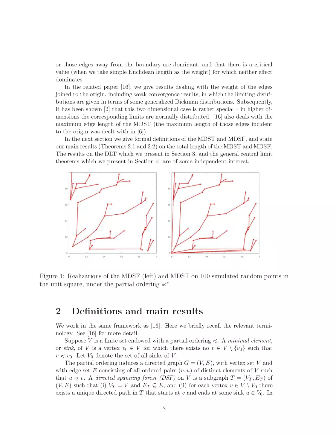
One such graph is the minimal directed spanning tree (or MDST for short),
which was introduced by Bhatt and Roy in [6]. In the MDST, each point x of a
finite (random) subset S of (0, 1]2 is connected by a directed edge to the nearest
y ∈ S ∪ {(0, 0)} such that y 6= x and y 4∗ x, where y 4∗ x means that each
component of x − y is nonnegative. See Figure 1 for a realisation of the MDST on
simulated random points.
Motivation comes from the modelling of communications or drainage networks
(see [6, 16, 20]). For example, consider the problem of designing a set of canals to
connect a set of hubs, so as to minimize their total length subject to a constraint
that all canals must flow downhill. The mathematical formulation given above for
this constraint can lead to significant boundary effects due to the possibility of
long edges occurring near the lower and left boundaries of the unit square; these
boundary effects distinguish the MDST qualitatively from the standard minimal
spanning tree and the nearest neighbour graph for point sets in the plane. Another
difference is the fact that there is no uniform upper bound on vertex degrees in the
MDST.
In the present work, we consider the total length of the MDST on random points
in (0, 1]2 , as the number of points becomes large. We also consider the total length
of the minimal directed spanning forest (MDSF), which is the MDST with edges
incident to the origin removed (see Figure 1 for an example). In [6], Bhatt and Roy
mention that the total length is an object of considerable interest, although they
restrict their analysis to the length of the edges joined to the origin (subsequently
also examined in [16]). A first order result for the total length of the MDST or
MDSF is a law of large numbers; we derive this in Theorem 2.1 for a family of
MDSFs indexed by partial orderings on R2 , which include 4∗ as a special case.
This paper is mainly concerned with establishing second order results, i.e., weak
convergence results for the distribution of the total length, suitably centred and
scaled. For the length of edges from points in the region away from the boundary,
we prove a central limit theorem. The boundary effects are significant, and near
the boundary the MDST can be described in terms of a one-dimensional, on-line
version of the MDST which we call the directed linear tree (DLT), and which we
examine in Section 3. In the DLT, each point in a sequence of independent uniform
random points in an interval is joined to its nearest neighbour to the left, amongst
those points arriving earlier in the sequence. This DLT is of separate interest in
relation to, for example, network modelling and molecular fragmentation (see [5],
[4], and references therein).
In Theorem 3.1 we establish that the limiting distribution of the centred total
length of the DLT is characterized by a distributional fixed-point equation, which resembles those encountered in the probabilistic analysis of algorithms such as Quicksort [7]. Such fixed-point distributional equalities, and the so-called ‘divide and
conquer’ or recursive algorithms from which they arise, have received considerable
attention recently; see, for example, [8, 13, 21, 22].
We consider power-weighted edges. Our weak convergence results (Theorem
2.2) demonstrate that, depending on the value chosen for the weight exponent of
the edges, there are two regimes in which either the boundary effects dominate

2

or those edges away from the boundary are dominant, and that there is a critical
value (when we take simple Euclidean length as the weight) for which neither effect
dominates.
In the related paper [16], we give results dealing with the weight of the edges
joined to the origin, including weak convergence results, in which the limiting distributions are given in terms of some generalized Dickman distributions. Subsequently,
it has been shown [2] that this two dimensional case is rather special – in higher dimensions the corresponding limits are normally distributed. [16] also deals with the
maximum edge length of the MDST (the maximum length of those edges incident
to the origin was dealt with in [6]).
In the next section we give formal definitions of the MDST and MDSF, and state
our main results (Theorems 2.1 and 2.2) on the total length of the MDST and MDSF.
The results on the DLT which we present in Section 3, and the general central limit
theorems which we present in Section 4, are of some independent interest.

Figure 1: Realizations of the MDSF (left) and MDST on 100 simulated random points in
the unit square, under the partial ordering 4∗ .

2

Definitions and main results

We work in the same framework as [16]. Here we briefly recall the relevant terminology. See [16] for more detail.
Suppose V is a finite set endowed with a partial ordering 4. A minimal element,
or sink, of V is a vertex v0 ∈ V for which there exists no v ∈ V \ {v0 } such that
v 4 v0 . Let V0 denote the set of all sinks of V .
The partial ordering induces a directed graph G = (V, E), with vertex set V and
with edge set E consisting of all ordered pairs (v, u) of distinct elements of V such
that u 4 v. A directed spanning forest (DSF) on V is a subgraph T = (VT , ET ) of
(V, E) such that (i) VT = V and ET ⊆ E, and (ii) for each vertex v ∈ V \ V0 there
exists a unique directed path in T that starts at v and ends at some sink u ∈ V0 . In

3

the case where V0 consists of a single sink, we refer to any DSF on V as a directed
spanning tree (DST) on V . If we ignore the orientation of edges then [16] a DSF on
V is indeed a forest and, if there is just one sink, then any DST on V is a tree.
Suppose the directed graph (V, E) carries a weight function onPits edges, i.e.,
a function w : E → [0, ∞). If T is a DSF on V , we set w(T ) := e∈ET w(e). A
minimal directed spanning forest (MDSF) on V (or, equivalently, on G), is a directed
spanning forest T on V such that w(T ) ≤ w(T ′ ) for every DSF T ′ on V . If V has
a single sink, then a minimal directed spanning forest on V is called a minimal
directed spanning tree (MDST) on V .
For v ∈ V , we say that u ∈ V \ {v} is a directed nearest neighbour of v if u 4 v
and w(v, u) ≤ w(v, u′ ) for all u′ ∈ V \ {v} such that u′ 4 v. For each v ∈ V \ V0 ,
let nv denote a directed nearest neighbour of v (chosen arbitrarily if v has more
than one directed nearest neighbour). Then [16] the subgraph (V, EM ) of (V, E),
obtained by taking EM := {(v, nv ) : v ∈ V \ V0 }, is a MDSF of V . Thus, if all
edge-weights are distinct, the MDSF is unique, and is obtained by connecting each
non-minimal vertex to its directed nearest neighbour.
For what follows, we consider a general type of partial ordering of R2 , denoted
θ,φ

4 , specified by the angles θ ∈ [0, 2π) and φ ∈ (0, π] ∪ {2π}. For x ∈ R2 , let Cθ,φ (x)
be the closed cone with vertex x and boundaries given by the rays from x at angles
θ and θ + φ, measuring anticlockwise from the upwards vertical. The partial order
is such that, for x1 , x2 ∈ R2 ,
θ,φ

x1 4 x2 iff x1 ∈ Cθ,φ (x2 ).

(1)
π/2,π/2

We shall use 4∗ as shorthand for the special case 4 , which is of particular
interest, as in [6]. In this case u 4∗ v for u = (u1 , u2 ), v = (v1 , v2 ) ∈ E if and only
if u1 ≤ v1 and u2 ≤ v2 . The symbol 4 will denote a general partial order on R2 .
We do not permit here the case φ = 0, which would almost surely give us
a disconnected point set. Nor do we allow π < φ < 2π, since in this case the
directional relation (1) is not a partial order, since the transitivity property (if
u 4 v and v 4 w then u 4 w) fails for π < φ < 2π. We shall, however, allow the
case φ = 2π which leads to the standard nearest neighbour (directed) graph.
The weight function is given by power-weighted Euclidean distance, i.e., for
(u, v) ∈ E we assign weight w(u, v) = ku − vkα to the edge (u, v), where k · k denotes
the Euclidean norm on R2 , and α > 0 is an arbitrary fixed parameter. Thus, when
α = 1 the weight of an edge is simply its Euclidean length. Moreover, we shall
assume that V ⊂ R2 is given by V = S or V = S 0 := S ∪ {0}, where 0 is the
origin in R2 and S is generated in a random manner. The random point set S will
usually be either the set of points given by a homogeneous Poisson point process Pn
of intensity n on the unit square (0, 1]2 , or a binomial point process Xn consisting
of n independent uniformly distributed points on (0, 1]2 .
Note that in this random setting, each point of S almost surely has a unique
directed nearest neighbour, so that V has a unique MDSF, which does not depend

4

on the choice of α. Denote by Lα (S) the total weight of all the edges in the MDSF
on S, and let L̃α (S) := Lα (S) − E[Lα (S)], the centred total weight.
Our first result presents laws of large numbers for the total edge weight for the
θ,φ

general partial order 4 and general 0 < α < 2. We state the result for n points
uniformly distributed on (0, 1]2 , but the proof carries through to other distributions
(see the start of Section 5).
θ,φ

Theorem 2.1 Suppose 0 < α < 2. Under the general partial order 4 , with 0 ≤
θ < 2π and 0 < φ ≤ π or φ = 2π, it is the case that
L1

n(α/2)−1 Lα (Xn ) −→ (2/φ)α/2 Γ(1 + α/2),

as n → ∞.

(2)

Also, when the partial order is 4∗ , (2) remains true with the addition of the origin,
i.e. with Xn replaced by Xn0 .
p
Remark. In the special case α = 1, the limit in (2) is π/(2φ). This limit is 1
when φ = π/2. Also, for φ = 2π we have the standard nearest neighbour (directed)
graph (that is, every point is joined to its nearest neighbour by a directed edge),
and this limit is then 1/2. This result (for α = 1, φ = 2π) is stated without proof
(and attributed to Miles [12]) in [1], but we have not previously seen the limiting
constant derived explicitly, either in [12] or anywhere else.
Our main result (Theorem 2.2) presents convergence in distribution for the case
where the partial order is 4∗ ; the limiting distributions are of a different type in
the three cases α = 1 (the same situation as [6]), 0 < α < 1, and α > 1. We define
these limiting distributions in Theorem 2.2, in terms of distributional fixed-point
equations. These fixed-point equations are of the form
D

X=

k
X

Ar X {r} + B,

(3)

r=1

where k ∈ N, X {r} , r = 1, . . . , k, are independent copies of the random variable X,
and (A1 , . . . , Ak , B) is a random vector, independent of (X {1} , . . . , X {k} ), satisfying
the conditions
E

k
X
r=1

|Ar |2 < 1,

E[B] = 0,

E[B 2 ] < ∞.

(4)

Theorem 3 of Rösler [21] (proved using the contraction mapping theorem; see also
[13, 22]) says that if (4) holds, there is a unique square-integrable distribution with
mean zero satisfying the fixed-point equation (3), and this will guarantee uniqueness
of solutions to all the distributional fixed-point equalities considered in the sequel.
Define the random variable D̃1 , to have the distribution that is the unique solution to the distributional fixed-point equation
D

{1}

D̃1 = U D̃1

{2}

+ (1 − U )D̃1

+ U log U + (1 − U ) log(1 − U ) + U,

5

(5)

where U is uniform on (0, 1) and independent of the other variables on the right. We
shall see later (in Propositions 3.5 and 3.6) that E[D̃1 ] = 0 and Var[D̃1 ] = 2 − π 2 /6;
higher order moments are given recursively by eqn (14).
For α > 1, let D̃α denote a random variable with distribution characterized by
the fixed-point equation
D

D̃α = U α D̃α{1} + (1 − U )α D̃α{2} +

1
1
α
Uα +
(1 − U )α −
,
α−1
α−1
α−1

(6)

where again U is uniform on (0, 1) and independent of the other variables on the
right. Also for α > 1, let F̃α denote a random variable with distribution characterized by the fixed-point equation
D

F̃α = U α F̃α + (1 − U )α D̃α +

(1 − U )α
1
Uα
+
−
,
α(α − 1)
α−1
α(α − 1)

(7)

where U is uniform on (0, 1), D̃α has the distribution given by (6), and the U , D̃α
and F̃α on the right are independent. In Section 3 we shall see that the random
variables D̃α , F̃α for α > 1 arise as centred versions of random variables (denoted
Dα , Fα respectively) satisfying somewhat simpler fixed point equations. Thus D̃α
and F̃α both have mean zero; their variances are given by eqns (38) and (40) below.
Let N (0, s2 ) denote the normal distribution with mean zero and variance s2 .
Theorem 2.2 Suppose the weight exponent is α > 0 and the partial order is 4∗ .
There exist constants 0 < t2α ≤ s2α such that, for normal random variables Yα ∼
N (0, s2α ) and Wα ∼ N (0, t2α ):
(i) As n → ∞,
D

D

n(α−1)/2 L̃α (Pn0 ) −→ Yα and n(α−1)/2 L̃α (Xn0 ) −→ Wα
D

{1}
L̃1 (Pn0 ) −→ D̃1
D
L̃α (Pn0 ) −→

+

{2}
D̃1

D

+ Y1 and L̃1 (Xn0 ) −→

{1}
D̃1

+

{2}
D̃1

D

D̃α{1} + D̃α{2} and L̃α (Xn0 ) −→ D̃α{1} + D̃α{2}

(0 < α < 1); (8)
+ W1 ;
(α > 1).

(9)
(10)

{i}

Here all the random variables in the limits are independent, and D̃α , i = 1, 2 are
independent copies of the random variable D̃α defined at (5) for α = 1 and (6) for
α > 1.
(ii) As n → ∞,
D

D

n(α−1)/2 L̃α (Pn ) −→ Yα and n(α−1)/2 L̃α (Xn ) −→ Wα
D

{1}

L̃1 (Pn ) −→ D̃1

D

{2}

+ D̃1

D

{1}

+ Y1 and L̃1 (Xn ) −→ D̃1
D

{2}

+ D̃1

L̃α (Pn ) −→ F̃α{1} + F̃α{2} and L̃α (Xn ) −→ F̃α{1} + F̃α{2}

(0 < α < 1); (11)
+ W1 ;
(α > 1) .
{i}

(12)
(13)

Here all the random variables in the limits are independent, and D̃1 , i = 1, 2,
{i}
are independent copies of D̃1 with distribution defined at (5), and for α > 1, F̃α ,
i = 1, 2, are independent copies of F̃α with distribution defined at (7).

6

Remarks. The normal random variables Yα or Wα arise from the edges away from
the boundary (see Section 6). The non-normal variables (the D̃s and F̃ s) arise from
the edges very close to the boundary, where the MDSF is asymptotically close to
the ‘directed linear forest’ discussed in Section 3.
Theorem 2.2 indicates a phase transition in the character of the limit law as
α increases. The normal contribution (from the points away from the boundary)
dominates for 0 < α < 1, while the boundary contributions dominate for α > 1.
In the critical case α = 1, neither effect dominates and both terms contribute
significantly to the asymptotic behaviour.
Noteworthy in the case α = 1 is the fact that by (9) and (12), the limiting
distribution is the same for L̃1 (Pn ) as for L̃1 (Pn0 ), and the same for L̃1 (Xn ) as for
L̃1 (Xn0 ). Note, however, that the difference L̃1 (Pn ) − L̃1 (Pn0 ) is the (centred) total
length of edges incident to the origin, which is not negligible, but itself converges
in distribution (see [16]) to a non-degenerate random variable, namely a centred
generalized Dickman random variable with parameter 2 (see (28) below). As an
extension of Theorem 2.2, it should be possible to show that the joint distribution
of (L̃1 (Pn ), L̃1 (Pn0 )) converges to that of two coupled random variables, both having
the distribution of D̃1 , whose difference has the centred generalized Dickman distribution with parameter 2. Likewise for the joint distribution of (L̃1 (Xn ), L̃1 (Xn0 )).
Of particular interest is the distribution of the variable D̃1 appearing in Theorem
2.2. In Section 3.4, we give a plot (Figure 2) of the probability density function of
this distribution, estimated by simulation. Also, we can use the fixed-point equation
(5) to calculate the moments of D̃1 recursively. Writing
f (U ) := U log U + (1 − U ) log(1 − U ) + U,
and setting mk := E[D̃1k ], we obtain
mk = E[(f (U ))k ] +

i  
k  X
X
i
k
i=2

i

j=0

j

E[(f (U ))k−i U j (1 − U )i−j ]mj mi=j .

(14)

The fact that m1 = 0 simplifies things a little, and we can rewrite this as

k  
X
k 
mi E[(f (U ))k−i (U i + (1 − U )i )]
mk = E[(f (U ))k ] +
i
i=1

i−2  
X
i
+
E[(f (U ))k−i U j (1 − U )i−j ]mj mi−j  .
j
j=2

So, for example, when k = 3 we obtain m3 ≈ 0.15411, which shows D̃1 is not Gaussian and is consistent with the skewness of the plot in Figure 2.
The remainder of this paper is organized as follows. After discussion of the DLT
in Section 3, in Section 4 we present general limit theorems in geometric probability,
which we shall use in obtaining our main results for the MDST. Theorem 2.1 is

7

proved in Section 5 (this proof does not use the results of Section 3). The proof of
Theorem 2.2 is prepared in Sections 6 and 7, and completed in Section 8. In these
proofs, we repeatedly use Slutsky’s theorem (see e.g. [14]) which says that if Xn → X
in distribution and Yn → 0 in probability, then Xn + Yn → X in distribution.

3

The directed linear forest and tree

The directed linear forest (DLF) and directed linear tree (DLT) are for us a tool
for the analysis of the limiting behaviour of the contribution to the total weight of
the random MDSF/MDST from edges near the boundary of the unit square. In
the present section we derive the properties of the DLF that we need (in particular,
Theorem 3.1); subsequently, in Theorem 7.1, we shall see that the total weight of
edges from the points near the boundaries, as n → ∞, converges in distribution to
the limit of the total weight of the DLF.
The DLT is also of some intrinsic interest. It is a one-dimensional directed
analogue of the so-called ‘on-line nearest neighbour graph’, which is of interest
in the study of networks such as the world wide web (see, e.g. [5]; and [15] for
more on the on-line nearest neighbour graph). Moreover, it is constructed via a
fragmentation process similar to those seen in, for example, [4]; the tree provides a
historical representation of the fragmentation process.
For any finite sequence Tm = (x1 , x2 , . . . , xm ) ∈ (0, 1]m , we construct the directed
linear forest (DLF) as follows. We start with the unit interval (0, 1] and insert the
points xi in order, one at a time, starting with i = 1. At the insertion of each
point, we join the new point to its nearest neighbour among those points already
present that lie to the left of the point (provided that such a point exists). In
other words, for each point xi , i ≥ 2, we join xi by a directed edge to the point
max{xj : 1 ≤ j < i, xj < xi }. If {xj : 1 ≤ j < i, xj < xi } is empty, we do not add
any directed edge from xi . In this way we construct a ‘directed linear forest’, which
we denote by DLF (Tm ). We denote the total weight (under weight function with
exponent α) of DLF (Tm ) by Dα (Tm ), that is, we set
Dα (Tm ) :=

m
X
(xi − max{xj : 1 ≤ j < i, xj < xi })α 1{min{xj : 1 ≤ j < i} < xi }.
i=2

Further, given Tm , let Tm0 be the sequence (x0 , x1 , . . . , xm ) where the initial term
is x0 := 0. Then the DLF on Tm0 is constructed in the same way, where now for
each i ≥ 1, we join xi by an edge to the point max{xj : 0 ≤ j < i, xj < xi }. But
now we see that x1 will always be joined to x0 = 0, and x2 will be joined either to
x1 (if x2 > x1 ) or to x0 , and so on. In this way we construct a ‘directed linear tree’
(DLT) on vertex set {x0 , x1 , . . . , xm } with m edges. Denote the total weight of this
tree with weight exponent α by Dα (Tm0 ); that is, set
D

α

Tm0




m
X
(xi − max{xj : 0 ≤ j < i, xj < xi })α .
:=
i=1

8

We shall be mainly interested in the case where Tm is a random vector in (0, 1]m .
α (T )] the centred total weight of the
In this case, set D̃
α (Tm ) := D
α (Tm) − E [D

m
DLF, and D̃ α Tm0 = D α Tm0 − E Dα Tm0 the centred total weight of the DLT.
We take Tm to be a vector of uniform variables. Let (X1 , X2 , X3 , . . .) be a
sequence of independent uniformly distributed random variables in (0, 1], and for
0 ). For these
m ∈ N set Um := (X1 , X2 , . . . , Xm ). We consider Dα (Um ) and D α (Um
variables, we establish asymptotic behaviour of the mean value in Propositions 3.1
and 3.2, along with the following convergence results, which are the principal results
of this section.
For α > 1, let Dα denote a random variable with distribution characterized by
the fixed-point equation
D

Dα = U α Dα{1} + (1 − U )α Dα{2} + U α ,

(15)

where U is uniform on (0, 1) and independent of the other variables on the right.
Also for α > 1, let Fα denote a random variable with distribution characterized by
the fixed-point equation
D

Fα = U α Fα + (1 − U )α Dα ,

(16)

where U is uniform on (0, 1), Dα has the distribution given by (15), and the U , Dα
and Fα on the right are independent. The corresponding centred random variables
D̃α := Dα − E[Dα ] and F̃α := Fα − E[Fα ] satisfy the fixed-point equations (6) and
(7) respectively. The solutions to (6) and (7) are unique by the criterion given at
(4), and hence the solutions to (15) and (16) are also unique.
L2

L2

0 ) −→ D̃ and D̃ 1 (U ) −→ F̃
Theorem 3.1 (i) As m → ∞ we have D̃ 1 (Um
1
m
1
where D̃1 has the distribution given by the fixed-point equation (5), and F̃1 has
the same distribution as D̃1 . Also, the variance of D̃1 (and hence also of F̃1 )
is 2 − π 2 /6 ≈ 0.355066. Finally, Cov(D̃1 , F̃1 ) = (7/4) − π 2 /6 ≈ 0.105066.

0 ) → D , almost surely and in L2 ,
(ii) For α > 1, as m → ∞ we have D α (Um
α
L2

and Dα (Um ) −→ Fα , almost surely and in L2 , where the distributions of Dα ,
Fα are given by the fixed-point equations (15) and (16) respectively. Also,
E[Dα ] = (α − 1)−1 and E[Fα ] = (α(α − 1))−1 , while Var(Dα ) and Var(Fα ) are
given by (38) and (40) respectively.

Proof. Part (i) follows from Propositions 3.5, 3.6 and 3.7 below. Part (ii) follows
from Propositions 3.3 and 3.4 below. We prove these results in the following sections. 
An interesting property of the DLT, which we use in establishing fixed-point
equations for limit distributions, is its self-similarity (scaling property). In terms of
the total weight, this says that for any t ∈ (0, 1), if Y1 , . . . , Yn are independent and
uniformly distributed on (0, t], then the distribution of Dα (Y1 , . . . , Yn ) is the same
as that of tα Dα (X1 , . . . , Xn ).

9

3.1

The mean total weight of the DLF and DLT

0 . For m = 1, 2, 3, . . . denote
First we consider the rooted case, i.e. the DLT on Um
by Zm the random variable given by the gain in length of the tree on the addition
of one point (Xm ) to an existing m − 1 points in the DLT on a sequence of uniform
0
random variables Um−1
, i.e. with the conventions D1 (U00 ) = 0 and X0 = 0, we set
0
0
Zm := D 1 (Um
) − D 1 (Um−1
) = Xm − max{Xj : 0 ≤ j < m, Xj < Xm }.

(17)

α.
Thus, with weight exponent α, the mth edge to be added has weight Zm

Lemma 3.1 (i) Zm has distribution function Fm given by Fm (t) = 0 for t < 0,
Fm (t) = 1 for t > 1, and Fm (t) = 1 − (1 − t)m for 0 ≤ t ≤ 1.
α has expectation and variance
(ii) For α > 0, Zm


m!Γ(1 + α) 2
m!Γ(1 + 2α)
m!Γ(1 + α)
α
α
. (18)
, Var[Zm ] =
−
E[Zm ] =
Γ(1 + α + m)
Γ(1 + 2α + m)
Γ(1 + α + m)
In particular,
E[Zm ] =

1
m
; Var[Zm ] =
.
m+1
(m + 1)2 (m + 2)

(19)

(iii) For α > 0, as m → ∞ we have



α
α
E[Zm
] ∼ Γ(α + 1)m−α , Var[Zm
] ∼ Γ(2α + 1) − (Γ(α + 1))2 m−2α .

(20)

(iv) As m → ∞, mZm converges in distribution, to an exponential with parameter 1.
Proof. For 0 ≤ t ≤ 1 we have

P [Zm > t] = P [Xm > t and none of X1 , . . . , Xm−1 lies in (Xm − t, Xm )] = (1 − t)m ,
and (i) follows. We then obtain (ii) since for any α > 0 and for k = 1, 2,
Z 1
Z 1
m!Γ(1 + kα)
1/(kα)
kα
.
(1 − t1/kα )m dt =
P [Zm > t
]dt =
E[Zm ] =
Γ(1 + kα + m)
0
0
Then (iii) follows by Stirling’s formula, which yields
kα
] = Γ(1 + kα)m−kα (1 + O(m−1 )).
E[Zm

For (iv), we have from (i) that, for t ∈ [0, ∞), and m large enough so that (t/m) ≤ 1,
 


t
t m
P [mZm ≤ t] = Fm
→ 1 − e−t , as m → ∞.
=1− 1−
m
m

But 1 − e−t , t ≥ 0 is the exponential distribution function with parameter 1. 

The following result gives the asymptotic behaviour of the expected total weight
of the DLT. Let γ denote Euler’s constant, so that
!
k
X
1
− log k = γ + O(k−1 ).
(21)
i
i=1

10

Proposition 3.1 As m → ∞ the expected total weight of the DLT under α-power
0 satisfies
weighting on Um
Γ(α + 1) 1−α
m
(0 < α < 1);
1−α
0
E[D 1 (Um
)] − log m → γ − 1;
1
0
+ O(m1−α ) (α > 1).
E[D α (Um
)] =
α−1
0
E[D α (Um
)]

∼

(22)
(23)
(24)

Proof. We have
E[D

α

0
(Um
)]

=

m
X

E[D

α

i=1

(Ui0 )]

− E[D

α

0
(Ui−1
)]




=

m
X

E[Ziα ].

i=1

In the case where α = 1, E[Zi ] = (i + 1)−1 by (19), and (23) follows by (21). For
general α > 0, α 6= 1, from (18) we have that
E[D

α

0
(Um
)]

= Γ(1 + α)

m
X
i=1

Γ(i + 1)
1
Γ(1 + α)Γ(m + 2)
=
−
.
Γ(1 + α + i)
α − 1 (α − 1)Γ(m + 1 + α)

(25)

By Stirling’s formula, the last term satisfies
−

Γ(1 + α)Γ(m + 2)
Γ(1 + α) 1−α
=−
m
(1 + O(m−1 )),
(α − 1)Γ(m + 1 + α)
α−1

(26)

which tends to zero as m → ∞ for α > 1, to give us (24). For α < 1, we have (22)
from (25) and (26). 
Now consider the unrooted case, i.e., the directed linear forest. For Um as above
the total weight of the DLF is denoted D α (Um ), and the centred total weight is
D̃α (Um ) := D α (Um ) − E[D α (Um )]. We then see that
0
0
Dα (Um
) = D α (Um ) + Lα0 (Um
),

(27)

0 ) is the total weight of edges incident to 0 in the DLT on U 0 .
where Lα0 (Um
m
0 ) converges to a random variable that has
The following lemma says that Lα0 (Um
the generalized Dickman distribution with parameter 1/α (see [16]), that is, the
distribution of a random variable X which satisfies the distributional fixed-point
equation
D

X = U α (1 + X),

(28)

where U is uniform on (0, 1) and independent of the X on the right. We recall from
Proposition 3 of [16] that if X satisfies (28) then
E[X] = 1/α, and E[X 2 ] = (α + 2)/(2α2 ).

11

(29)

Lemma 3.2 Let α > 0. There is a random variable Lα0 with the generalized
Dickman distribution with parameter 1/α, such that as m → ∞, we have that
0 ) → Lα , almost surely and in L2 .
Lα0 (Um
0
0 ) denote the degree of the origin in the directed linear tree on
Proof. Let δD (Um
0 , so that δ (U 0 ) is the number of lower records in the sequence (X , . . . , X ).
Um
1
m
D m
Then
0
α
Lα0 (Um
) = U1α + (U1 U2 )α + · · · + (U1 · · · UδD (Um
0 )) ,

(30)

where (U1 , U2 , . . .) is a certain sequence of independent uniform random variables on
(0, 1), namely the ratios between successive lower records of the sequence (Xn ). The
sum U1α + (U1 U2 )α + (U1 U2 U3 )α + · · · has nonnegative terms and finite expectation,
so it converges almost surely to a limit which we denote Lα0 . Then Lα0 has the
generalized Dickman distribution with parameter 1/α (see Proposition 2 of [16]).
0 ) tends to infinity almost surely as m → ∞, we have Lα (U 0 ) → Lα
Since δD (Um
m
0
0
0 ))2 ≤ (Lα )2 for all
almost surely. Also, E[(Lα0 )2 ] < ∞, by (29), and (Lα0 − Lα0 (Um
0
0 ) − Lα )2 ] → 0 by the dominated convergence theorem, and so
m. Thus E[(Lα0 (Um
0
2
we have the L convergence as well. 
Proposition 3.2 As m → ∞ the expected total weight of the DLF under α-power
weighting on Um satisfies
Γ(α + 1) 1−α
m
(0 < α < 1);
1−α
E[D 1 (Um )] − log m → γ − 2;
1
E[D α (Um )] →
(α > 1).
α(α − 1)
E[D α (Um )]

∼

(31)
(32)
(33)

0 )] − E[Lα (U 0 )]. By Lemma 3.2
Proof. By (27) we have E[D α (Um )] = E[D α (Um
m
0
and (29),
0
E[Lα0 (Um
)] −→ E[Lα0 ] = 1/α.

We then obtain (31), (32) and (33) from Proposition 3.1. 

3.2

Orthogonal increments for α = 1

In this section we shall show (in Lemma 3.5) that when α = 1, the variables Zi , i ≥ 1
are mutually orthogonal, in the sense of having zero covariances, which will be used
later on to establish convergence of the (centred) total length of the DLT. To prove
this, we first need further notation.
Given X1 , . . . , Xm , let us denote the order statistics of X1 , . . . , Xm , taken in increasing
order,
as
m
m
m
m
m
m
X(1) , X(2) , . . . , X(m) . Thus (X(1) , X(2) , . . . , X(m) ) is a nondecreasing sequence, forming a permutation of the original (X1 , . . . , Xm ). Denote the existing m + 1 intervals

12



m
m
between points by Ijm := X(j−1)
, X(j)
for j = 1, 2, . . . , m + 1, where we set
m
m
X(0) := 0 and X(m+1) := 1. Let the widths of these intervals (the spacings) be
m
m
− X(j−1)
,
Sjm := Ijm = X(j)

P
m
for 1 ≤ j ≤ m + 1. Then 0 ≤ Sjm < 1 for 1 ≤ j ≤ m + 1, and m+1
j=1 Sj = 1. That


m
belongs to the m-dimensional simplex, ∆m . Note
is, the vector S1m , S2m , . . . , Sm+1
m
that only m of the Sj are required to specify the vector.
We can arrange the spacings themselves (Sjm , 1 ≤ j ≤ m + 1) into increasing
m
m , Sm , . . . , Sm
order to give S(1)
(2)
(m+1) . Then let FS denote the sigma field generated
by these ordered spacings, so that


m
m
.
(34)
FSm = σ S(1)
, . . . , S(m+1)

The following interpretation of FSm may be helpful. The set (0, 1) \ {X1 , . . . , Xm }
consists almost surely of m + 1 connected components (‘fragments’) of total length
1, and FSm is the σ-field generated by the collection of lengths of these fragments,
ignoring the order in which they appear.
m , . . . , Sm
By definition, the value of Zm must be one of the (ordered) spacings S(1)
(m+1) .
The next result says that, given the values of these spacings, each of the possible
values for Zm are equally likely.
Lemma 3.3 For m ≥ 1 we have
i
h
m
P Zm = S(i)
FSm =

1
m+1

a.s., for i = 1, . . . , m + 1.

(35)

Hence,

E [Zm |FSm ]

m+1
1 X m
1
=
S(i) =
.
m+1
m+1

(36)

i=1



m , . . . , Xm
Proof. First we note that X(1)
(m) is uniformly distributed over
{(x1 , . . . , xm ) : 0 ≤ x1 ≤ x2 ≤ . . . ≤ xm ≤ 1} .

Now








S1m
S2m
S3m
..
.
m
Sm





 
 
 
=
 
 

1
0
−1 1
0 −1
..
..
.
.
0
0

  Xm
(1)
m

X
(2)


  Xm
  (3)
 .
  ..
m
0 . . . −1 1
X(m)

0
0
1
..
.

...
...
...
..
.

0
0
0
..
.

0
0
0
..
.






.




m ) is uniform over
The m by m matrix here has determinant 1. Hence (S1m , . . . , Sm


m


X
xj ≤ 1; xj ≥ 0, ∀ 1 ≤ j ≤ m .
(x1 , . . . , xm ) :


j=1

13



m
is uniform over the m-dimensional simplex ∆m . In particular,
Then S1m , . . . , Sm+1
m , . . . , Sm
m
the Sjm are exchangeable. Thus given S(1)
(m+1) , i.e. FS , the actual values
m , . . . , Sm
m
are equally likely to be any permutation of S(1)
of S1m , . . . , Sm+1
(m+1) , and
m (but
m
m
m
given S1 , . . . , Sm+1 the value of Zm is equally likely to be any of S1 , . . . , Sm
m ).
cannot be Sm+1
m , . . . , Sm
m
Hence, given S(1)
(m+1) the probability that Zm = S(i) is (1/m) × m/(m +
P
m
1) = 1/(m + 1), i.e. we have (35), and then (36) follows since m+1
j=1 S(j) = 1. 
Lemma 3.4 Let 1 ≤ m < ℓ. Given FSm , Zℓ and Zm are conditionally independent.

m , . . . , Sm
Proof. Given FSm , we have S(1)
(m+1) , and by (35), the (conditional) distrim
m
bution of Zm is uniform on {S(1) , . . . , S(m+1)
}. The conditional distribution of Zℓ ,
m
m
m
ℓ > m, given FS , depends only on S(1) , . . . , S(m+1)
and not which one of them Zm
happens to be. Hence Zm and Zℓ are conditionally independent. 

Lemma 3.5 For 1 ≤ m < ℓ, the random variables Zm , Zℓ satisfy Cov [Zm , Zℓ ] = 0.
Proof. From Lemmas 3.4 and 3.3,
E [Zm Zℓ |FSm ] = E [Zm |FSm ] E [Zℓ |FSm ] =

1
E [Zℓ |FSm ] ,
m+1

and by taking expectations we obtain
E [Zm Zℓ ] =

1
1
1
E [Zℓ ] =
·
= E[Zm ] · E[Zℓ ].
m+1
m+1 ℓ+1

Hence the covariance of Zm and Zℓ is zero. 
Remarks. (i) Calculations yield, for example, that E[D 1 (U10 )] = E[Z1 ] = 1/2,
E[D 1 (U20 )] = 5/6, and Var[Z1 ] = 1/12, Var[Z2 ] = 1/18, Var[D 1 (U20 )] = 5/36.
α is unique to the α = 1 case. For
(ii) The orthogonality structure of the Zm
example, it can be shown that, for α > 0,


2
1
2Γ(α + 2)2
α α
E[Z1α ]E[Z2α ] =
,
and
E[Z
Z
]
=
1
+
.
1 2
(1 + α)2 (2 + α)
2(1 + α)2
Γ(2α + 3)

Then
Cov[Z1α , Z2α ] =

(α − 2)Γ(2α + 3) + 2(α + 2)Γ(α + 2)2
,
2(α + 1)2 (α + 2)Γ(2α + 3)

and this quantity is zero only if α = 1; it is positive for α > 1 and negative for
0 < α < 1.

14

3.3

Limit behaviour for α > 1

We now consider the limit distribution of the total weight of the DLT and DLF.
In the present section we consider the case of α-power weighted edges with α > 1;
that is, we prove part (ii) of Theorem 3.1. To describe the moments of the limiting
0 ) and D α (U ), we introduce the notation
distribution of Dα (Um
m
Z

J(α) :=

0

1

√ Γ(α + 1)
.
uα (1 − u)α du = 2−1−2α π
Γ(α + 3/2)

(37)

0 )), and subsequently consider the unrooted
We start with the rooted case (D α (Um
α
case (D (Um )).

Proposition 3.3 Let α > 1. Then there exists a random variable Dα such that as
0 ) → D almost surely and in L2 . Also, the random variable
m → ∞ we have Dα (Um
α
Dα satisfies the distributional fixed-point equality (15). Further, E[Dα ] = 1/(α − 1)
and
Var[Dα ] =

α (α − 2 + 2(2α + 1)J(α))
.
(α − 1)2 (2α − 1)

(38)

Proof.PLet Zi be the length of the ith edge of the DLT, as defined at (17). Let
α
Dα := ∞
i=1 Zi . The sum converges almost surely since it has non-negative terms
and, by (20), has finite expectation for α > 1. By (20) and Cauchy-Schwarz, there
exists a constant 0 < C < ∞ such that
E[Dα2 ] =

∞ X
∞
X
i=1 j=1

E[Ziα Zjα ] ≤ C

∞ X
∞
X
i=1 j=1

i−α j −α < ∞,

since α > 1. The L2 convergence then follows from the dominated convergence
theorem.
Taking U = X1 here, by the self-similarity of the DLT we have that
D

0
α
0
α
0
D α (Um
) = U α D{1}
(UN
) + (1 − U )α D{2}
(Um−1−N
) + U α,

(39)

α (U 0 ) and D α (U 0
where N ∼ Bin(m−1, U ), given U , and, given U and N , D{1}
N
{2} m−1−N )
α
0
α
0
are independent with the distribution of D (UN ) and D (Um−1−N ), respectively.
As m → ∞, N and m − N both tend to infinity almost surely, and so, by taking
m → ∞ in (39), we obtain the fixed-point equation (15).
The identity E[Dα ] = (α − 1)−1 is obtained either from (24) of Proposition 3.1,
or by taking expectations in (15). Next, if we set D̃α = Dα − E[Dα ], (15) yields (6).
Then, using the definition (37) of J(α), the fact that E[D̃α ] = 0, and independence,
we obtain from (6) that

E[D̃α2 ] =

α2 + 1
2αJ(α)
1
2E[D̃α2 ]
+
+
−
,
2
2
2α + 1
(α − 1) (2α + 1) (α − 1)
(α − 1)2

15

and rearranging this gives (38). 
Recall from Lemma 3.2 that Lα0 is the limiting weight of edges attached to the
origin in the DLT on uniform points. Combining this fact with Proposition 3.3, we
obtain a similar result to the latter for the unrooted case as follows:
Proposition 3.4 Let α > 1. There is a random variable Fα , satisfying the distributional fixed-point equality (16), such that Dα (Um ) → Fα , as n → ∞, almost
surely and in L2 . Further, E[Fα ] = 1/(α(α − 1)), and
Var[Fα ] =

α + 2(2α + 1)J(α) − 2
1
Var[Dα ] +
,
2α
2α2 (α − 1)2

(40)

where J(α) is given by (37) and Var[Dα ] by (38).
Proof. By Lemma 3.2 and Proposition 3.3, there are random variables Dα and
L2

L2

0 ) −→ D and Lα (U 0 ) −→ Lα , also with
Lα0 such that as m → ∞ we have Dα (Um
α
m
0
0
almost sure convergence in both cases. Hence, setting Fα := Dα − Lα0 , we have by
(27) that
0
0
D α (Um ) = D α (Um
) − Lα0 (Um
) → Fα ,

a.s. and in L2 .

(41)

Next, we show that Fα satisfies the distributional fixed-point equality (16). The
self-similarity of the DLT implies that
D

0
),
D α (Um ) = U α D α (UN ) + (1 − U )α D α (Um−1−N

(42)

0
where N ∼ Bin(m−1, U ), given U , and D α (UN ) and Dα (Um−1−N
) are independent,
given U and N . As m → ∞, N and m − N both tend to infinity almost surely, so
taking m → ∞ in (42), using Proposition 3.3 and eqn (41), we obtain the fixed-point
equation (16).
The identity E[Fα ] = α−1 (α − 1)−1 is obtained either by (33), or by taking
expectations in (16) and using the formula for E[Dα ] in Proposition 3.3. Then with
F̃α := Fα − E[Fα ], we obtain (7) from (16), and using independence and the fact
that E[F̃α ] = E[D̃α ] = 0 we obtain

2α
E[D̃α2 ]
2αJ(α) − 1
α2 + 1
E[F̃α2 ] =
+ 2
+
,
2α + 1
2α + 1
α (α − 1)2
α2 (α − 1)2 (2α + 1)
which yields (40). 
Examples. When α = 2 we have that E[D2 ] = 1 and J(2) = 1/30, so that
Var[D2 ] = 2/9. Also, E[F2 ] = 1/2 and Var[F2 ] = 7/72 ≈ 0.0972.

16

3.4

Limit behaviour for α = 1

0 ) diverges
Unlike in the case α > 1, for α = 1 the mean of the total weight D1 (Um
as m → ∞ (see Proposition 3.1), so clearly there is no limiting distribution for
0 ). Nevertheless, by using the orthogonality of the increments of the sequence
D1 (Um
1
0 ), m ≥ 1), we are able to show that the centred total weight D̃ 1 (U 0 ) does
(D (Um
m
converge in distribution (in fact, in L2 ) to a limiting random variable, and likewise
for the unrooted case; this is our next result.
Subsequently, we shall characterize the distribution of the limiting random variable (for both the rooted and unrooted cases) by a fixed-point identity, and thereby
complete the proof of Theorem 3.1 (i).
0 ) converges in L2
Proposition 3.5 (i) As m → ∞, the random variable D̃ 1 (Um
to a limiting random
D̃1 , with E[D̃1 ] = 0 and Var[D̃1 ] = 2 − π 2 /6. In

 1 0variable
particular, Var D (Um ) → 2 − π 2 /6 as m → ∞.
(ii) As m → ∞, D̃1 (Um ) converges in L2 to the limiting random variable F̃1 :=
D̃1 − L10 + 1.

Proof. Adopt the convention D1 (U00 ) = 0. By the orthogonality of the Zj (Lemma
3.5) and (19), for 0 ≤ ℓ < m,
h

Var D̃

1

0
(Um
)−

D̃

1

i

(Uℓ0 )

= Var

m
X

j=ℓ+1

=

m
X

j=ℓ+1

(Zj − E[Zj ])

j
−→ 0 as m, ℓ → ∞.
(j + 1)2 (j + 2)

0 ) is a Cauchy sequence in L2 , and so converges in L2 to a limiting
Hence D̃1 (Um
0 )] = 0, and
random variable, which we denote D̃1 . Then E[D̃1 ] = limm→∞ E[D̃1 (Um
∞
h
i X
0
Var[D̃1 ] = lim Var D̃1 (Um
) =

j
(j + 1)2 (j + 2)
j=1
 2

 X
∞ 
∞
X
π
2
π2
1
2
−
=
1
−
−
1
=
2
−
.
−
=
j+1 j+2
(j + 1)2
6
6
m→∞

j=1

j=1

It remains to prove part (ii), the convergence for the centred total length of the
DLF D̃ 1 (Um ). We have by (27) that
L2

0
0
0
D̃1 (Um ) = D̃ 1 (Um
) − L10 (Um
) + E[L10 (Um
)] −→ D̃1 − L10 + 1,

where the convergence follows by Lemma 3.2 and part (i). Thus D̃1 (Um ) converges
in L2 as m → ∞. 
For the next few results it is more convenient to consider the DLF defined on
a Poisson number of points. Let (X1 , X2 , . . .) be a sequence of independent uniformly distributed random variables in (0, 1], and let (N (t), t ≥ 0) be the counting

17

process of a homogeneous Poisson process of unit rate in (0, ∞), independent of
(X1 , X2 , . . .). Thus N (t) is a Poisson variable with parameter t. As before, let
0
Um = (X1 , . . . , Xm ), and (for this section only) let Pt := UN (t) . Let Pt0 := UN
(t) , so
0
that Pt = (0, X1 , X2 , . . . , XN (t) ).
We construct the DLF and DLT on X1 , X2 , . . . , XN (t) as before. Let D̃ 1 (Pt0 ) =




D1 (Pt0 ) − E D 1 (Pt0 ) and D̃1 (Pt ) = D1 (Pt ) − E D 1 (Pt ) . We aim to show that
0 ), and likewise in the
the limit distribution for D̃ 1 (Pt0 ) is the same as for D̃ 1 (Um
unrooted case. We shall need the following result.
Lemma 3.6 As t → ∞,

1
d
1
d
E[D 1 (Pt )] = + O(t−2 ); and
E[D 1 (Pt0 )] = + O(t−2 ).
(43)
dt
t
dt
t
Proof. The point set {X1 , . . . , XN (t) } is a homogeneous Poisson point process in
(0, 1), so we have
d
E[D 1 (Pt )] = E[length of new arrival]
dt
Z 1
=
duE[dist. to next pt. to the left of u in Pt ]
0
Z u
Z 1

 e−t
1
2
ste−ts ds = + 2 e−t − 1 +
du
=
t
t
t
0
0


1
=
+ O t−2 .
t
Similarly,
Z 1
d
E[D 1 (Pt0 )] =
duE[dist. to next pt. to the left of u in Pt ∪ {0}]
dt
0
Z u
Z 1
P [dist. to next pt. to the left > s]ds
du
=
0
0
Z u
Z 1
1 e−t − 1
e−ts ds = +
du
=
t
t2
0
0


1
=
+ O t−2 . 
t

Lemma 3.7 (i) As t → ∞, D̃1 (Pt0 ) converges in distribution to D̃1 , the L2 large-m
0 ).
limit of D̃ 1 (Um
(ii) As t → ∞, D̃ 1 (Pt ) converges in distribution to F̃1 , the L2 large-m limit of
1
D̃ (Um ).
L2

0 ) −→ D̃ as m → ∞. Let
Proof. (i) From Proposition 3.5, we have D̃ 1 (Um
P 1
Pm
1
0
1
0
−1
at := E[D (Pt )] and µm := E[D (Um )]. Since µm = E m
i=1 Zi =
i=1 (1 + i)
by (19), for any positive integers ℓ, m we have
max(m,ℓ)

|µm − µℓ | =

X

j=min(m,ℓ)+1

1
≤ log
j+1



max(m, ℓ) + 1
min(m, ℓ) + 1

18



= log



m+1
ℓ+1



.

(44)

Note the distributional equalities




0
L D 1 (Pt0 )|N (t) = m = L D 1 (Um
) ;




0
L D1 (Pt0 ) − µN (t) |N (t) = m = L D̃1 (Um
) .

(45)
m

First we aim to show that at − µ⌊t⌋ → 0 as t → ∞. Set pm (t) := e−t tm! . Then
we can write
at − µ⌊t⌋ =
=

∞
X

m=0

pm (t)(µm − µ⌊t⌋ )

X

pm (t)(µm − µ⌊t⌋ ) +

|m−⌊t⌋|≤t3/4

X

pm (t)(µm − µ⌊t⌋ ). (46)

|m−⌊t⌋|>t3/4

We examine these two sums separately. First consider the sum for |m − ⌊t⌋| ≤ t3/4 .
By (44), we have
!
!

⌊t⌋ + 1
⌊t⌋ + 1 + t3/4
, log
sup
µm − µ⌊t⌋ ≤ max log
⌊t⌋ + 1
⌊t⌋ + 1 − t3/4
m:|m−⌊t⌋|≤t3/4


= O t−1/4 → 0 as t → ∞.

Hence the first sum in (46) tends to zero as t → ∞. To estimate the second sum,
observe that
X
X
pm (t)(µm − µ⌊t⌋ ) ≤
pm (t)(m + t)
|m−⌊t⌋|>t3/4

|m−⌊t⌋|>t3/4

h
i
= E (N (t) + t)1{|N (t) − ⌊t⌋| > t3/4 }
i1/2
 
h

≤
E (N (t) + t)2 · P |N (t) − ⌊t⌋| > t3/4
.(47)

By Chernoff bounds on the tail probabilities of a Poisson random variable (e.g. Lemma
1.4 of [14]), the expression (47) is O(t exp(−t2 /18)) and so tends to zero. Hence the
second sum in (46) tends to zero, and thus
at − µ⌊t⌋ → 0 as t → ∞.

(48)

D

Now we show that D̃1 (Pt0 ) −→ D̃1 as t → ∞. We have






D̃ 1 (Pt0 ) = D 1 (Pt0 ) − µN (t) + µN (t) − µ⌊t⌋ + µ⌊t⌋ − at .

(49)

The final bracket tends to zero, by (48). Also, by (45) and the fact that N (t) →
∞ a.s. as t → ∞, we have
D

D 1 (Pt0 ) − µN (t) −→ D̃1 .

19

Finally, using (44), we have
µN (t) − µ⌊t⌋

≤

log

N (t) + 1 P
−→ 0,
⌊t⌋ + 1

P

as t → ∞, since N (t)/⌊t⌋ −→ 1. So Slutsky’s theorem applied to (49) yields
D

D̃1 (Pt0 ) −→ D̃1 as t → ∞, completing the proof of (i)
The proof of (ii) follows in the same way as that of (i), except that in (44) the
first equals sign is replaced by an inequality ≤. This does not affect the rest of the
proof. 
The next two propositions complete the proof of Theorem 3.1.
Proposition 3.6 The limiting random variable D̃1 of Proposition 3.5 (i) satisfies
the fixed-point equation (5).
Proof. For integer n > 0, let Tn := min{s : N (s) ≥ n}, the nth arrival time of the
Poisson process with counting process N (·). Set T := T1 , and set U := X1 (which
is uniform on (0, 1)).
By the Marking Theorem for Poisson processes [10], the two-dimensional point
process Q := {(Xn , Tn ) : n ≥ 1} is a homogeneous Poisson process of unit intensity
on (0, 1) × (0, ∞). Given the value of (U, T ), the restriction of Q to (0, U ] × (T, ∞)
and the restriction of Q to (U, 1] × (T, ∞) are independent homogeneous Poisson
processes on these regions. Hence, by scaling properties of the Poisson process
1 (·), i = 1, 2 for
(see the Mapping Theorem in [10]) and of the DLT, writing D{i}
independent copies of D1 (·), we have


D
0
1
1
)
+
U
1{t > T }. (50)
(P(1−U
(PU0 (t−T ) ) + (1 − U )D{2}
D 1 (Pt0 ) =
U D{1}
)(t−T )

Let as = 0 for s ≤ 0, and as = E[D 1 (Ps0 )] for s > 0. Then D̃ 1 (Pt0 ) = D 1 (Pt0 ) − at ,
so that by (50),


D
1
1
0
D̃1 (Pt0 ) =
U D̃{1}
(PU0 (t−T ) ) + (1 − U )D̃{2}
(P(1−U
)
+
U
1{t > T }
)(t−T )




(51)
+U aU (t−T ) − at + (1 − U ) a(1−U )(t−T ) − at .

From Lemma 3.6 we have
at − aU (t−T ) =
and hence as t → ∞,

Z

dat
dt

t

U (t−T )

=

1
t

+ O(t−2 ). Hence, if T < t, then



das
ds = log t − log{U (t − T )} + O (U (t − T ))−1 ,
ds

at − aU (t−T ) → − log U,

a.s..

(52)

Since P [T < t] tends to 1, by making t → ∞ in (51) and using Slutsky’s theorem
we obtain (5). 

20

Proposition 3.7 The limiting random variable F̃1 of Proposition 3.5 (ii) satisfies the fixed-point equation (5), and so has the same distribution as D̃1 . Also,
Cov(F̃1 , D̃1 ) = (7/4) − π 2 /6.
Proof. The proof follows similar lines to that of Proposition 3.6. Once more let
as = E[D 1 (Ps0 )], for s ≥ 0, and as = 0 for s < 0. Let bs = E[D 1 (Ps )] for s > 0, and
bs = 0 for s ≤ 0, and let T := min{t : N (t) ≥ 1}, Then


D
1
1
0
D 1 (Pt ) =
U D{1}
(PU (t−T ) ) + (1 − U )D{2}
(P(1−U
)
1{t > T }, (53)
)(t−T )

1 (·) and D 1 (·) are independent copies of D 1 (·). Then D̃ 1 (P ) = D 1 (P )−
where D{1}
t
t
{2}

bt and D̃ 1 (Pt0 ) = D 1 (Pt0 ) − at , so that (53) yields


D
1
1
0
D̃ 1 (Pt ) =
U D̃{1}
(PU (t−T ) ) + (1 − U )D̃{2}
(P(1−U
)
1{t > T }
)(t−T )




+U bU (t−T ) − bt + (1 − U ) a(1−U )(t−T ) − bt .

From Lemma 3.6 we have
at (52),

dbt
dt

=

1
t

(54)

+ O(t−2 ). Hence, by the same argument as used

bt − bU (t−T ) → − log U a.s.
0
1
Also, at − bt = E[L0 (Pt )] by (27), so that limt→∞ (at − bt ) = 1, by
the fact that E[L10 ] = 1 (eqn (29)). Using also (52) we find that as

Lemma 3.2 and
t → ∞,

a(1−U )(t−T ) − bt = (a(1−U )(t−T ) − at ) + (at − bt ) → 1 + log (1 − U ),

a.s.

Taking t → ∞ in (54), and using Slutsky’s theorem, we obtain
D

F̃1 = U F̃1 + (1 − U )D̃1 + U log U + (1 − U ) log (1 − U ) + (1 − U ).

(55)

The change of variable (1 − U ) 7→ U then shows that D̃1 as defined at (5) satisfies
(55), and so by the uniqueness of solution, F̃1 has the same distribution as D̃1 and
satisfies (5).
To obtain the covariance of F̃1 and D̃1 , observe from Proposition 3.5 (ii) that
1
L0 = D̃1 − F̃1 + 1, and therefore by (29), we have that
1/2 = Var[L10 ] = Var[D̃1 ] + Var[F̃1 ] − 2Cov(D̃1 , F̃1 ).

(56)

2 − π 2 /6

Since Var[F̃1 ] = Var[D̃1 ] =
by Proposition 3.5 (i), rearranging (56) we find
2
that Cov(D̃1 , F̃1 ) = (7/4) − π /6. 
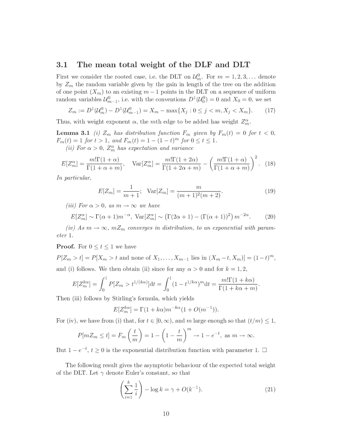
Remark. Figure 2 is a plot of the estimated probability density function of D̃1 .
This was obtained by performing 106 repeated simulations of the DLT on a sequence of 103 uniform (simulated) random points on (0, 1]. For each simulation,
the expected value of D1 (U103 ) (which is precisely (1/2) + (1/3) + · · · (1/1001) by
Lemma 3.1) was subtracted from the total length of the simulated DLT to give an
approximate realization of D̃1 . The density function was then estimated from the
sample of 106 approximate realizations of D̃1 , using a window width of 0.0025. The
simulated sample from which the density estimate for D̃1 was taken had sample
mean ≈ −2 × 10−4 and sample variance ≈ 0.3543, which are reasonably close to the
expectation and variance of D̃1 .

21

Figure 2: Estimated probability density function for D̃1 .

4

General results in geometric probability

Notions of stabilizing functionals of point sets have recently proved to be a useful
basis for a general methodology for establishing limit theorems for functionals of
random point sets in Rd . In particular, Penrose and Yukich [17, 18] provide general
central limit theorems and laws of large numbers for stabilizing functionals. One
might hope to apply these results in the case of the MDSF weight. In fact we shall
obtain our law of large numbers (Theorem 2.1) by application of a result from [18],
but to obtain the central limit theorem for edges away from the boundary in the
MDSF and MDST, we need an extension of the general result in [17]. It is these
general results that we describe in the present section.
For our general results, we use the following notation. Let d ≥ 1 be an integer.
For X ⊂ Rd , constant a > 0, and y ∈ Rd , let y + aX denote the transformed set
{y + ax : x ∈ X }. Let diam(X ) := sup{kx1 − x2 k : x1 , x2 ∈ X }, and let card(X )
denote the cardinality (number of elements) of X (when finite).
For x ∈ Rd and r > 0, let B(x; r) denote the closed Euclidean ball with centre
x and radius r, and let Q(x; r) denote the corresponding l∞ ball, i.e., the d-cube
x + [−r, r]d . For bounded measurable R ⊂ Rd let |R| denote the Lebesgue measure
of R, let ∂R denote the topological boundary of R and for r > 0, set ∂r R :=
∪x∈∂R Q(x; r), the r-neighbourhood of the boundary of R.

4.1

A general law of large numbers

Let ξ(x; X ) be a measurable R+ -valued function defined for all pairs (x, X ), where
X ⊂ Rd is finite and x ∈ X . Assume ξ is translation invariant, that is, for all
y ∈ Rd , ξ(y + x; y + X ) = ξ(x; X ). When x ∈
/ X , we abbreviate the notation

22

ξ(x; X ∪ {x}) to ξ(x; X ).
For our general law of large numbers, we use a notion of stabilization defined as
follows. For any locally finite point set X ⊂ Rd and any ℓ ∈ N define
!
ξ + (X ; ℓ) := sup

k∈N

ess sup {ξ(0; (X ∩ B(0; ℓ)) ∪ A} , and

−

ξ (X ; ℓ) := inf

k∈N

ℓ,k




ess inf {ξ(0; (X ∩ B(0; ℓ)) ∪ A} ;
ℓ,k

where ess supℓ,k is the essential supremum, with respect to Lebesgue measure on
Rdk , over sets A ⊂ Rd \B(0; ℓ) of cardinality k. Define the limit of ξ on X by
ξ∞ (X ) := lim sup ξ + (X ; k).
k→∞

We say the functional ξ stabilizes on X if
lim ξ + (X ; k) = lim ξ − (X ; k) = ξ∞ (X ).

k→∞

k→∞

(57)

For τ ∈ (0, ∞), let Hτ be a homogeneous Poisson process of intensity τ on Rd .
The following general law of large numbers is due to Penrose and Yukich [18]. We
shall use it to prove Theorem 2.1.
Lemma 4.1 [18] Suppose q = 1 or q = 2. Suppose ξ is almost surely stabilizing on
Hτ , with limit ξ∞ (Hτ ), for all τ ∈ (0, ∞). Let f be a probability density function on
Rd , and let Xn be the point process consisting of n independent random d-vectors
with common density f . If ξ satisfies the moments condition
p i
h 
< ∞,
(58)
sup E ξ n1/d X1 ; n1/d Xn
n∈N

for some p > q, then as n → ∞,
n−1

X

x∈Xn

Lq

ξ(n1/d x; n1/d Xn ) −→

Z

Rd




E ξ∞ Hf (x) f (x)dx,

(59)

and the limit is finite.

4.2

General central limit theorems

In the course of the proof of Theorem 2.2, we shall use a modified form of a general
central limit theorem obtained for functionals of geometric graphs by Penrose and
Yukich [17]. We recall the setup of [17]. As in Section 4.1, let ξ(x; X ) be a translation
invariant real-valued functional defined for finite X ⊂ Rd and x ∈ X . Then ξ induces
a translation invariant functional H(X ; S) defined on all finite point sets X ⊂ Rd
and all Borel-measurable regions S ⊆ Rd by
X
H(X ; S) :=
ξ(x; X ).
(60)
x∈X ∩S

23

It is this ‘restricted’ functional that interests us here, while [17] is concerned rather
with the global functional H(X ; Rd ). In our particular application (the length of
edges of the MDST on random points in a square), the global functional fails to
satisfy the conditions of the central limit theorems in [17], owing to boundary effects.
Here we generalize the result in [17] to the ‘restricted’ functional H(X ; S). It is this
generalized result that we can apply to the MDST, when we take S to be a region
‘away from the boundary’ of the square in which the random points are placed.
We use a notion of stabilization for H which is related to, but not equivalent to,
the notion of stabilization of ξ used in Section 4.1. Loosely speaking, ξ is stabilizing
if when a point inserted at the origin into a homogeneous Poisson process, only
nearby Poisson points affect the inserted point; for H to be stabilizing we require
also that the the inserted point affects only nearby points.
For B ⊆ Rd , let ∆(X ; B) denote the ‘add one cost’ of the functional H on the
insertion of a point at the origin,
∆(X ; B) := H(X ∪ {0}; B) − H(X ; B).
Let P := H1 (a homogeneous Poisson point process of unit intensity on Rd ). Let
Qn := P ∩ Rn (the restriction of P to Rn ). Adapting the ideas of [17], we make the
following definitions.
Definition 4.1 We say the functional H is strongly stabilizing if there exist almost
surely finite random variables R (a radius of stabilization) and ∆(∞) such that, with
probability 1, for any B ⊇ B(0; R),
∆(P ∩ B(0; R) ∪ A; B) = ∆(∞), ∀ finite A ⊂ Rd \ B(0; R).
We say that the functional H is polynomially bounded if, for all B ∋ 0, there
exists a constant β such that for all finite sets X ⊂ Rd ,
|H(X ; B)| ≤ β (diam(X ) + card(X ))β .

(61)

We say that H is homogeneous of order γ if for all finite X ⊂ Rd and Borel
B ⊆ Rd , and all a ∈ R, H(aX ; aB) = aγ H(X ; B).
Let (Rn , Sn ), for n = 1, 2, . . ., be a sequence of ordered pairs of bounded Borel
subsets of Rd , such that Sn ⊆ Rn for all n. Assume that for all r > 0, n−1 |∂r Rn | → 0
and n−1 |∂r Sn | → 0 (the vanishing relative boundary condition). Assume also that
|Rn | = n for all n, and |Sn |/n → 1 as n → ∞; that Sn tends to Rd , in the sense that
∪n≥1 ∩m≥n Sm = Rd ; and that there exists a constant β such that diam(Rn ) ≤ βnβ
for all n (the polynomial boundedness condition on (Rn , Sn )n≥1 ). Subject to these
conditions, the choice of (Rn , Sn )n≥1 is arbitrary.
Let U1,n , U2,n , . . . be i.i.d. uniform random vectors on Rn . Let
Um,n = {U1,n , . . . , Um,n }
(a binomial point process), and for Borel A ⊆ Rd with 0 < |A| < ∞, let Um,A be
the binomial point process of m i.i.d. uniform random vectors on A.

24

Let R be the collection of all pairs (A, B) with A, B ⊂ Rd of the form (A, B) =
(x + Rn , x + Sn ) with x ∈ Rd and n ∈ N. That is, R is the collection of all the
(Rn , Sn ) and their translates.
We say that the functional H satisfies the uniform bounded moments condition
on R if
!
{E[∆(Um,A ; B)4 ]}

sup

sup

(A,B)∈R:0∈A

|A|/2≤m≤3|A|/2

< ∞.

(62)

We now state the general results, which extend those of Penrose and Yukich
(Theorem 2.1 and Corollary 2.1 in [17]).
Theorem 4.1 Suppose that H is strongly stabilizing, is polynomially bounded (61),
and satisfies the uniform bounded moments condition (62) on R. Then there exist
constants s2 , t2 , with 0 ≤ t2 ≤ s2 , such that as n → ∞,
(i) n−1 Var (H (Qn ; Sn )) → s2 ;



D
(ii) n−1/2 (H (Qn ; Sn ) − E [H (Qn ; Sn )]) −→ N 0, s2 ;

(iii) n−1 Var (H (Un,n ; Sn )) → t2 ;

D

(iv) n−1/2 (H (Un,n ; Sn ) − E [H (Un,n ; Sn )]) −→ N (0, t2 ).

Also, s2 and t2 are independent of the choice of the (Rn , Sn ). Further, if the distribution of ∆(∞) is nondegenerate, then s2 ≥ t2 > 0.
Let R0 be a fixed bounded Borel subset of Rd with |R0 | = 1 and |∂R0 | = 0. Let
(S0,n , n ≥ 1) be a sequence of Borel sets with S0,n ⊆ R0 such that |S0,n | → 1 as
n → ∞ and for all r > 0 we have |∂n−1/d r S0,n | → 0 as n → ∞
Let R0 be the collection of all pairs of the form (x + n1/d R0 , x + n1/d S0,n ) with
n ≥ 1 and x ∈ Rd . Let Xn be the binomial point process of n i.i.d. uniform random
vectors on R0 , and let Pn be a homogeneous Poisson point process of intensity n on
R0 .
Corollary 4.1 Suppose H is strongly stabilizing, satisfies the uniform bounded moments condition on R0 , is polynomially bounded and is homogeneous of order γ.
Then with s2 , t2 as in Theorem 4.1 we have that, as n → ∞
(i) n(2γ/d)−1 Var (H (Pn ; S0,n )) → s2 ;



D
(ii) n(γ/d)−1/2 (H (Pn ; S0,n ) − E [H (Pn ; S0,n )]) −→ N 0, s2 ;

(iii) n(2γ/d)−1 Var (H (Xn ; S0,n )) → t2 ;



D
(iv) n(γ/d)−1/2 (H (Xn ; S0,n ) − E [H (Xn ; S0,n )]) −→ N 0, t2 .

Proof. The corollary follows from Theorem 4.1 by taking Rn = n1/d R0 and Sn =
n1/d S0,n (or suitable translates thereof), and scaling, since H is homogeneous of
order γ. 

25

4.3

Proof of Theorem 4.1: the Poisson case

Let P be a Poisson process of unit intensity on Rd . We say the functional H is
weakly stabilizing on R if there is a random variable ∆(∞) such that
a.s.

∆(P ∩ A; B) −→ ∆(∞),

(63)

as (A, B) → Rd through R, by which we mean (63) holds whenever (A, B)
R-valued sequence of the form (An , Bn )n≥1 , such that ∪n≥1 ∩m≥n Bm = Rd .
that strong stabilization of H implies weak stabilization of H.
We say the functional H satisfies the Poisson bounded moments condition
if
 

sup
E ∆(P ∩ A; B)4 < ∞.

is an
Note
on R
(64)

(A,B)∈R:0∈A

Theorem 4.2 Suppose that H is weakly stabilizing on R (63) and satisfies (64).
Then there exists s2 ≥ 0 such that as n → ∞, n−1 Var[H(Qn ; Sn )] → s2 and
D

n−1/2 (H(Qn ; Sn ) − E[H(Qn ; Sn )]) −→ N (0, s2 ).

Before proving Theorem 4.2, we require further definitions and a lemma. Let P ′ be
an independent copy of the Poisson process P. For x ∈ Zd , set


P ′′ (x) = (P \ Q(x; 1/2)) ∪ P ′ ∩ Q(x; 1/2) .
Then given a translation invariant functional H on point sets in Rd , define
∆x (A; B) := H(P ′′ (x) ∩ A; B) − H(P ∩ A; B);
this is the change in H(P∩A; B) when the Poisson points in Q(x; 1/2) are resampled.
Lemma 4.2 Suppose H is weakly stabilizing on R. Then for all x ∈ Zd , there is a
random variable ∆x (∞) such that for all x ∈ Zd ,
a.s.

∆x (A; B) −→ ∆x (∞),

(65)

as (A, B) → Rd through R. Moreover, if H satisfies (64), then


E (∆x (A; B))4 < ∞.
sup

(66)

(A,B)∈R,x∈Zd

Proof. Set C0 = Q(0; 1/2). By translation invariance, we need only consider the
case x = 0, and thus it suffices to prove that the variables H(P ∩ A; B) − H(P ∩
A \ C0 ; B) converge almost surely as (A, B) → Rd through R.
The number N of points of P in C0 is Poisson with parameter 1. Let V1 , V2 , . . . , VN
be the points of P ∩ C0 , taken in an order chosen uniformly at random from the N !
possibilities. Then, provided C0 ⊆ A,
H(P ∩ A; B) − H(P ∩ A \ C0 ; B) =

26

N
−1
X
i=0

δi (A; B),

where
δi (A; B) := H((P ∩A\C0 )∪{V1 , . . . , Vi+1 }; B)−H((P ∩A\C0 )∪{V1 , . . . , Vi }; B).
Since N is a.s. finite, it suffices to prove that each δi (A; B) converges almost surely as
(A, B) → Rd through R. Let U be a uniform random vector on C0 , independent of
P. The distribution of the translated point process −Vi+1 + {V1 , . . . , Vi } ∪ (P \ C0 )
is the same as the conditional distribution of P given that the number of points in
−U + C0 is equal to i, an event of strictly positive probability. By assumption, this
satisfies weak stabilization, which proves (65).
Next we prove (66). If Q(x; 1/2) ∩ A = ∅ then ∆x (A; B) is zero with probability
1. By translation invariance, it suffices to consider the x = 0 case, that is, to prove
h
i
sup
E (∆0 (A; B))4 < ∞.
(67)
(A,B)∈R:C0 ∩A6=∅

The proof of this now follows the proof of (3.4) of [17], but with δi (A) replaced by
δi (A; B) everywhere. 
Proof of Theorem 4.2. Here we can assume, without loss of generality, that
Qn = P ∩ Rn . For x ∈ Zd , let Fx denote the σ-field generated by the points of P in
∪y∈Zd :y≤x Q(y; 1/2), where the order in the union is the lexicographic order on Zd .
Let Rn′ be the set of points x ∈ Zd such that Q(x; 1/2) ∩ Rn 6= ∅. Let kn =
card(Rn′ ). Then we have that
[
Rn ⊆
Q(x; 1/2) ⊆ Rn ∪ ∂1 (Rn ),
x∈R′n

so that
|Rn | ≤ kn ≤ |Rn | + |∂1 (Rn )|.
The vanishing relative boundary condition then implies that kn /n → 1 as n → ∞.
Define the filtration (G0 , G1 , . . . , Gkn ) as follows: let G0 be the trivial σ-field,
label the elements of Rn′ in lexicographic order as
Pkxn1 , . . . , xkn and let Gi = Fxi for
1 ≤ i ≤ kn . Then H(Qn ; Sn ) − E[H(Qn ; Sn )] = i=1 Di , where we set

Di = E[H(Qn ; Sn )|Gi ] − E[H(Qn ; Sn )|Gi−1 ] = E[−∆xi (Rn ; Sn )|Fxi ].
(68)
P n 2
Di . By this
By orthogonality of martingale differences, Var[H(Qn ; Sn )] = E ki=1
fact, along with a CLT for martingale differences (Theorem 2.3 of [11] or Theorem
2.10 of [14]), it suffices to prove the conditions

n
o2 
sup E max kn−1/2 |Di |
< ∞,
(69)
n≥1

1≤i≤kn

P

kn−1/2 max |Di | −→ 0,
1≤i≤kn

27

(70)

and for some s2 ≥ 0,
kn−1

kn
X
i=1

L1

Di2 −→ s2 .

(71)

Using (66), and the representation (68) for Di , we can verify (69) and (70) in
just the same manner as for the equivalent estimates (3.7) and (3.8) in [17].
We now prove (71). By (65), for each x ∈ Zd the variables ∆x (A; B) converge
almost surely to a limit, denoted ∆x (∞), as (A, B) → Rd through R. For x ∈ Zd
and (A, B) ∈ R, let
Fx (A; B) = E[∆x (A; B)|Fx ];

Fx = E[∆x (∞)|Fx ].

Then (Fx , x ∈ Zd ) is a stationary family of random variables. Set s2 = E[F02 ]. We
claim that the ergodic theorem implies
X
L1
(72)
Fx2 −→ s2 .
kn−1
x∈R′n

The proof of this follows, with minor modifications, the proof of the corresponding
result (3.10) in [17].
We need to show that Fx (Rn ; Sn )2 approximates to Fx2 . We consider x at the
origin 0. For any (A, B) ∈ R, by Cauchy-Schwarz,

1/2

1/2
E[|F0 (A; B)2 − F02 |] ≤ E[(F0 (A; B) + F0 )2 ]
E[(F0 (A; B) − F0 )2 ]
. (73)

By the definition of F0 and the conditional Jensen inequality,
i
h
E[(F0 (A; B) + F0 )2 ] = E (E[∆0 (A; B) + ∆0 (∞)|F0 ])2
= E[(∆0 (A; B) + ∆0 (∞))2 ],

≤ E[E[(∆0 (A; B) + ∆0 (∞))2 |F0 ]]

which is uniformly bounded by (65) and (66). Similarly,
E[(F0 (A; B) − F0 )2 ] ≤ E[(∆0 (A; B) − ∆0 (∞))2 ],

(74)

which is also uniformly bounded by (65) and (66). For any R-valued sequence
(An , Bn )n≥1 with ∪n≥1 ∩m≥n Bn = Rd , the sequence (∆0 (An ; Bn ) − ∆0 (∞))2 tends
to 0 almost surely by (65), and is uniformly integrable by (66), and therefore the
expression (74) tends to zero so that by (73), E[|F0 (An ; Bn )2 − F02 |] → 0.
Returning to the given sequence (Rn , Sn ), let ε > 0. By the vanishing relative
boundary condition, we can choose Kn so that limn→∞ Kn = ∞ and |∂Kn Sn | ≤ εn
for all n. Let Sn′ be the set of x ∈ Zd such that Q1/2 (x) has non-empty intersection
with Sn \ ∂Kn (Sn ). Using the conclusion of the previous paragraph and translation
invariance, it is not hard to deduce that
lim sup E[|Fx (Rn ; Sn )2 − Fx2 |] = 0.

n→∞ x∈S ′

n

28

(75)

Also, since we assume |Sn | ∼ n we have card(Sn′ ) ≥ |Sn | − εn ≥ (1 − 2ε)n for large
enough n. Using this with (75), the uniform boundedness of E[|Fx (Rn ; Sn )2 − Fx2 |]
and the fact that ε can be taken arbitrarily small in the above argument, it is routine
to deduce that
X
L1
(Fx (Rn ; Sn )2 − Fx2 ) −→ 0,
kn−1
x∈R′n

and therefore (72) remains true with Fx replaced by Fx (Rn ; Sn ); that is, (71) holds
and the proof of Theorem 4.2 is complete. 

4.4

Proof of Theorem 4.1: the non-Poisson case

In this section we complete the proof of Theorem 4.1. The first step is to show that
the conditions of Theorem 4.1 imply those of Theorem 4.2, as follows.
Lemma 4.3 If H satisfies the uniform bounded moments condition (62) and is
polynomially bounded, then H satisfies the Poisson bounded moments condition (64).
Proof. The proof follows, with minor modifications, that of Lemma 4.1 of [17]. 
It follows from Lemma 4.3 that if H satisfies the conditions of Theorem 4.1, then
Theorem 4.2 applies and we have the Poisson parts of Theorem 4.1. To de-Poissonize
these limits we follow [17]. Define
Rm,n := H(Um+1,n ; B) − H(Um,n ; B).
We use the following coupling lemma.
Lemma 4.4 Suppose H is strongly stabilizing. Let ε > 0. Then there exists δ > 0
and n0 ≥ 1 such that for all n ≥ n0 and all m, m′ ∈ [(1 − δ)n, (1 + δ)n] with m < m′ ,
there exists a coupled family of variables D, D′ , R, R′ with the following properties:
(i) D and D ′ each have the same distribution as ∆(∞);
(ii) D and D ′ are independent;
(iii) (R, R′ ) have the same joint distribution as (Rm,n , Rm′ ,n );
(iv) P [{D 6= R} ∪ {D ′ 6= R′ }] < ε.
Proof. Since we assume |Sn |/|Rn | → 1, the probability that a random d-vector
uniformly distributed over Rn lies in Sn tends to 1 as n → ∞. Using this fact the
proof follows, with some minor modifications, that of the corresponding result in
[17], Lemma 4.2. 
Lemma 4.5 Suppose H is strongly stabilizing and satisfies the uniform bounded
moments condition (62). Let (h(n))n≥1 be a sequence with n−1 h(n) → 0 as n → ∞.

29

Then
lim

sup

n→∞ |n−m|≤h(n)

lim

|ERm,n − E∆(∞)| = 0;

sup

n→∞ n−h(n)≤m<m′ ≤n+h(n)

lim

sup

n→∞ |n−m|≤h(n)

(76)

ERm,n Rm′ ,n − (E∆(∞))2 = 0;

2
ERm,n
< ∞.

(77)
(78)

Proof. The proof follows that of Lemma 4.3 of [17]. 
Proof of Theorem 4.1 Theorem 4.1 now follows in the same way as Theorem 2.1
in [17], replacing H( · ) with H( · ; Sn ). 

5 Proof of Theorem 2.1: Laws of large numbers
We now derive our law of large numbers for the total weight of the random MDSF
θ,φ

on the unit square. We consider the general partial order 4 , for 0 ≤ θ < 2π and
θ,φ

0 < φ ≤ π or φ = 2π. Recall that y 4 x if y ∈ Cθ,φ (x), where Cθ,φ (x) is the cone
formed by the rays at θ and θ + φ measured anticlockwise from the upwards vertical.
We consider the random point set Xn , the binomial point process of n independent uniformly distributed points on (0, 1]2 . However, the result (2) also holds
(with virtually the same proof) if the points of Xn are uniformly distributed on an
arbitrary convex set in R2 of unit area. If the points are distributed in R2 with a
density function f that has convex support and isRbounded away from 0 and infinity
on its support, then (2) holds with a factor of R2 f (x)(2−α)/2 dx introduced into
the right hand side (cf. eqn (2.9) of [18]).
For the general partial order given by θ, φ we apply Lemma 4.1 to obtain a
law of large numbers for Lα (Xn ). As a special case, we thus obtain a law of large
numbers under the partial order 4∗ given by θ = φ = π/2. This method enables
us to evaluate the limit explicitly, unlike methods based on the subadditivity of the
functional which may also be applicable here (see the remark at the end of this
section).
In applying Lemma 4.1 to the MDSF functional, we take the dimension d in the
lemma to be 2, and take f (x) (the underlying probability density function in the
lemma) to be 1 for x ∈ (0, 1]2 and zero elsewhere. We take ξ(x; X ) to be d(x; X )α ,
where d(x; X ) is the distance from point x to its directed nearest neighbour in X
θ,φ

under 4 , if such a neighbour exists, or zero otherwise. Thus in our case
ξ(x; X ) = (d(x; X ))α

with

d(x; X ) := min {kx − yk : y ∈ X \ {x}, y 4 x} (79)

with the convention that min{} = 0. We need to show this choice of ξ satisfies the
conditions of Lemma 4.1. As before, Hτ denotes a homogeneous Poisson process on
Rd of intensity τ , now with d = 2.

30

Lemma 5.1 Let τ > 0. Then ξ is almost surely stabilizing on Hτ , in the sense of
(57), with limit ξ∞ (Hτ ) = (d(0; Hτ ))α .
Proof. Let R be the (random) distance from 0 to its directed nearest neighbour
in Hτ , i.e. R = d(0; Hτ ). Since φ > 0 and τ > 0, we have 0 < R < ∞ almost
surely. But then for any ℓ > R, we have ξ(0; (Hτ ∩ B(0; ℓ)) ∪ A) = Rα , for any
finite A ⊂ Rd \ B(0; ℓ). Thus ξ stabilizes on Hτ with limit ξ∞ (Hτ ) = Rα . 
Before proving that our choice of ξ satisfies the moments condition for Lemma
4.1, we give a geometrical lemma. For B ⊆ R2 with B bounded, and for x ∈ B,
write dist(x; ∂B) for sup{r : B(x; r) ⊆ B}, and for s > 0, define the region
Aθ,φ (x, s; B) := B(x; s) ∩ B ∩ Cθ,φ (x).

(80)

Lemma 5.2 Let B be a convex bounded set in R2 , and let x ∈ B. If Aθ,φ (x, s; B) ∩
∂B(x; s) 6= ∅, and s > dist(x, ∂B), then
|Aθ,φ (x, s; B)| ≥ s sin(φ/2)dist(x, ∂B)/2.
Proof. The condition Aθ,φ (x, s; B) ∩ ∂B(x; s) 6= ∅ says that there exists y ∈
B ∩ Cθ,φ (x, s) with ky − xk = s. The line segment xy is contained in the cone
Cθ,φ (x); take a half-line h starting from x, at an angle φ/2 to the line segment xy
and such that h is also contained in Cθ,φ (x). Let z be the point in h at a distance
dist(x, ∂B) from x. Then the interior of the triangle xyz is entirely contained in
Aθ,φ (x, s), and has area s sin(φ/2)dist(x, ∂B)/2. 
Lemma 5.3 Suppose α > 0. Then ξ given by (79) satisfies the moments condition
(58) for any p ∈ (1/α, 2/α].
Proof. Setting Rn := (0, n1/2 ]2 , we have
h
p i dx
p i Z
h 
1/2
1/2
.
E ξ(x; n1/2 Xn−1 )
=
E ξ n X1 ; n X n
n
Rn

(81)

For x ∈ Rn set m(x) := dist(x, ∂Rn ). Let us divide Rn into three regions
Rn (1) := {x ∈ Rn : m(x) ≤ n−1/2 };

Rn (3) := {x ∈ Rn : n

−1/2

Rn (2) := {x ∈ Rn : m(x) > 1};

< m(x) ≤ 1}.

For all x ∈ Rn , we have ξ(x; n1/2 Xn−1 ) ≤ (2n)α/2 , and hence, since Rn (1) has area
at most 4, we can bound the contribution to (81) from x ∈ Rn (1) by
Z
h
p i dx
≤ 4n−1 (2n)pα/2 = 22+pα/2 n(pα−2)/2 ,
(82)
E ξ(x; n1/2 Xn−1 )
n
x∈Rn (1)
which is bounded provided pα ≤ 2.

31

Now, for x ∈ Rn , with Aθ,φ (·) defined at (80), we have
h
i
h
i
P d(x; n1/2 Xn−1 ) > s ≤ P n1/2 Xn−1 ∩ Aθ,φ (x, s; Rn ) = ∅


|Aθ,φ (x, s; Rn )| n−1
=
1−
n
≤ exp(1 − |Aθ,φ (x, s; Rn )|),

(83)

since |Aθ,φ (x, s; Rn )| ≤ n. For x ∈ Rn and s > m(x), by Lemma 5.2 we have
|Aθ,φ (x, s; Rn )| ≥ sin(φ/2)sm(x)/2

if Aθ,φ (x, s; Rn ) ∩ ∂B(x; s) 6= ∅,

and also
P [d(x; n1/2 Xn−1 ) > s] = 0 if

Aθ,φ (x, s; Rn ) ∩ ∂B(x; s) = ∅.

For s ≤ m(x), we have that |Aθ,φ (x, s; Rn )| = φ2 s2 ≥ sin(φ/2)s2 . Combining these
observations and (83), we obtain for all x ∈ Rn and s > 0 that
h
i
P d(x; n1/2 Xn−1 ) > s ≤ exp (1 − sin(φ/2)s min(s, m(x))/2) , x ∈ Rn .
Setting c = (1/2) sin(φ/2), we therefore have for x ∈ Rn that
Z ∞ h
i
i
h
1/2
p
P ξ(x; n1/2 Xn−1 )p > r dr
=
E ξ(x; n Xn−1 )
Z0 ∞ h
i
P d(x; n1/2 Xn−1 ) > r 1/(αp) dr
=
0

≤

Z

m(x)αp

0

+

Z

∞



dr exp 1 − cr 2/(αp)



dr exp 1 − cm(x)r 1/(αp)

m(x)αp

= O(1) +

Z

∞

e1−cu αpuαp−1 m(x)−pα du

m(x)2

= O(1) + O(m(x)−αp ).

(84)

For x ∈ Rn (2), this bound is O(1), and the area of Rn (2) is less than n, so that the
contribution to (81) from Rn (2) satisfies
Z
h
p i dx
1/2
lim sup
E ξ(x; n Xn−1 )
< ∞.
(85)
n
n→∞
Rn (2)

Finally, by (84), there is a constant c′ such that if αp > 1, the contribution to (81)
from Rn (3) satisfies
Z
Z 1
h
p i dx
E ξ(x; n1/2 Xn−1 )
≤ c′ n−1/2
y −αp dy
n
−1/2
Rn (3)
y=n
!
′
−1/2
cn
n(αp−1)/2
≤
αp − 1

32

which is bounded provided αp ≤ 2. Combined with the bounds in (82) and (85),
this shows that the expression (81) is uniformly bounded, provided 1 < αp ≤ 2. 
Following notation from Section 4.2, for k ∈ N, and for a < b and c < d let
Uk,(a,b]×(c,d] denote the point process consisting of k independent random vectors
uniformly distributed on the rectangle (a, b] × (c, d]. Before proceeding further, we
recall that if M (X ) denotes the number of minimal elements (under the ordering
4∗ ) of a point set X ⊂ R2 , then
E[M (Uk,(a,b]×(c,d] )] = E[M (Xk )] = 1 + (1/2) + · · · + (1/k) ≤ 1 + log k.

(86)

The first equality in (86) comes from some obvious scaling which shows that the
distribution of M (Uk,(a,b]×(c,d] ) does not depend on a, b, c, d. For the second equality
in (86), see [3] or the proof of Theorem 1.1(a) of [6].
Proof of Theorem 2.1. Suppose α < 2, and set f (·) to be the indicator of the
unit square (0, 1]2 . By Lemmas 5.1 and 5.3, our functional ξ, given at (79), satisfies
the conditions of Lemma 4.1 with p = 2/α and q = 1, with this choice of f . So by
Lemma 4.1, we have that
X
ξ(n1/2 x; n1/2 Xn )
n(α/2)−1 Lα (Xn ) = n−1
x∈Xn

L1

−→

Z

R2




E ξ∞ (Hf (x) ) f (x)dx = Eξ∞ (H1 ).

(87)

Since the disk sector Cθ,φ (x) ∩ B(x; r) has area (φ/2)r 2 , by Lemma 5.1 we have

h
i

P [ξ∞ (H1 ) > s] = P H1 ∩ Cθ,φ (0) ∩ B(0; s1/α ) = ∅ = exp −(φ/2)s2/α .

Hence, the limit in (87) is
Z ∞
P [ξ∞ (H1 ) > s] ds = α2(α−2)/2 φ−α/2 Γ(α/2),
E [ξ∞ (H1 )] =
0

θ,φ

and this gives us (2). Finally, in the case where 4 =4∗ , (2) remains true when Xn
is replaced by Xn0 , since
E[n(α/2)−1 |Lα (Xn0 ) − Lα (Xn )|] ≤ 2α/2 n(α/2)−1 E[M (Xn )],

(88)

where M (Xn ) denotes the number of minimal elements of Xn . By (86), E[M (Xn )] ≤
1 + log n, and hence the right hand side of (88) tends to 0 as n → ∞ for 0 < α < 2.
This gives us (2) with Xn0 under 4∗ . 
Remark. A law of large numbers for Euclidean functionals of many random geometric structures can be treated by the boundary functional approach of Yukich [25].
It can be shown that the MDSF satisfies some, but possibly not all, of the appropriate conditions that would allow this approach to be successful. The MDSF functional is subadditive, its corresponding boundary functional is superadditive, and

33

the functional and its boundary functional are sufficiently ‘close in mean’. However,
it is not clear that the functional is ‘smooth’, since the degree of the graph is not
bounded.

6 Central limit theorem away from the boundary
While it should be possible to adapt the argument of the present section to more
general partial orders, from now on we take the partial order 4 on R2 to be 4∗ . For
each n, define the region S0,n := (nε−1/2 , 1]2 , where ε ∈ (0, 1/2) is a small constant
to be chosen later. In this section, we use the general central limit theorems of
Section 4.2 to demonstrate a central limit theorem for the contribution to the total
weight of the MDSF, under 4∗ , from edges away from the boundary, that is from
points in the region S0,n .
Given α > 0, consider the MDSF total weight functional H = Lα on point sets
in R2 . For x ∈ X , let the directed nearest neighbour distance d(x; X ) and the
corresponding α-weighted functional ξ(x; X ) be given by (79), where now we take
4 to be 4∗ . For R ⊆ R2 , set
X
Lα (X ; R) =
ξ(x; X ),
(89)
x∈X ∩R

and set Lα (X ) := Lα (X ; R2 ).
Let Xn be the binomial point process of n i.i.d. uniform random vectors on (0, 1]2 ,
and let Pn be the homogeneous Poisson process of intensity n on (0, 1]2 . The main
result of this section is the following.
Theorem 6.1 Suppose that α > 0 and the partial order is 4∗ . Then there exist
constants 0 < tα ≤ sα , not depending on the choice of ε, such that, as n → ∞,
(i) nα−1 Var [Lα (Xn ; S0,n )] → t2α ;



D
(ii) n(α−1)/2 L̃α (Xn ; S0,n ) −→ N 0, t2α ;

(iii) nα−1 Var [Lα (Pn ; S0,n )] → s2α ;



D
(iv) n(α−1)/2 L̃α (Pn ; S0,n ) −→ N 0, s2α .

The following corollary states that Theorem 6.1 remains true in the rooted cases
too, i.e. with Xn replaced by Xn0 and Pn replaced by Pn0 .
Corollary 6.1 Suppose that α > 0 and the partial order is 4∗ . Then, with tα , sα
as given in Theorem 6.1, we have that as n → ∞,



(i) nα−1 Var Lα Xn0 ; S0,n → t2α ;

 D


(ii) n(α−1)/2 L̃α Xn0 ; S0,n −→ N 0, t2α ;



(iii) nα−1 Var Lα Pn0 ; S0,n → s2α ;

34


 D


(iv) n(α−1)/2 L̃α Pn0 ; S0,n −→ N 0, s2α .

Proof. For each region R ⊆ [0, 1]2 and point set S ⊂ [0, 1]2 with 0 ∈ S, let Lα0 (S; R)
denote the total weight of the edges incident to 0 in the MDST on S from points
in R. Then Lα (Pn0 ; S0,n ) equals Lα (Pn ; S0,n ) + Lα0 (Pn0 ; S0,n ), so that
Var[Lα (Pn0 ; S0,n )] − Var[Lα (Pn ; S0,n )] = 2Cov[Lα (Pn ; S0,n ), Lα0 (Pn0 ; S0,n )]
+Var[Lα0 (Pn0 ; S0,n )].

(90)

Let Nn denote the number of points of Pn , and let En denote the event that at
least one point of Pn ∩ S0,n is joined to 0 in the MDST on Pn0 . Then
h
i
P [En ] ≤ P (0, nε−1/2 ]2 ∩ Pn = ∅ = exp(−n2ε ),

and Lα0 (Pn0 ; S0,n ) ≤ 2α/2 Nn 1En . Thus by the Cauchy-Schwarz inequality, for some
finite constant C we have




Var Lα0 (Pn0 ; S0,n ) ≤ E Lα0 (Pn0 ; S0,n )2 ≤ Cn2 exp(−n2ε /2),
(91)

and combining this with (90), Theorem 6.1 (iii) and the Cauchy-Schwarz inequality
shows that


nα−1 (Var Lα (Pn0 ; S0,n ) − Var [Lα (Pn ; S0,n )]) → 0,

so that from Theorem 6.1 (iii)
 we obtain the corresponding rooted result (iii). Also,
since (91) implies nα−1 Var Lα0 (Pn0 ; S0,n ) tends to zero, from Theorem 6.1 (iv) and
Slutsky’s theorem we obtain the corresponding rooted result (iv).
The binomial results (i) and (ii) follow in the same manner as above, with slight
modifications. 
To prove Theorem 6.1, we demonstrate that our functional Lα satisfies suitable
versions of the conditions of Theorem 4.1 and Corollary 4.1. First, we see that Lα
is polynomially bounded (see (61)), since
Lα (X ; B) ≤ (diam(X ))α card(X ).
Also, Lα is homogeneous of order α.
Lemma 6.1 Lα is strongly stabilizing, in the sense of Definition 4.1.
Proof. To prove stabilization it is sufficient to show that there exists an almost
surely finite random variable R, the radius of stabilization, such that the add one
cost is unaffected by changes in the configuration at a distance greater than R from
the added point. We show that there exists such an R.
For s > 0 construct eight disjoint triangles Tj (s), 1 ≤ j ≤ 8, by splitting the
square Q(0; s) into eight triangles via drawing in the diagonals of the square and
the x and y axes. Label the triangle with vertices (0, 0), (0, s), (s, s) as T1 (s) and then
label increasingly in a clockwise manner. See Figure 3. Note that Tj (t) ⊂ Tj (s)

35

(0, s)
T8 (s)

(s, s)

T1 (s)

T7 (s)

T2 (s)
(s, 0)

0
T6 (s)

T3 (s)

T5 (s)

T4 (s)

Figure 3: The triangles T1 (s), . . . , T8 (s), s > 0.
for t < s. Let the random variable S be the minimum s such that the triangles
Tj (s), 1 ≤ j ≤ 8, each contain at least one point of P. Then S is almost surely
finite.
We claim that R = 3S is a radius of stabilization for Lα , that is any points at
distance d ≥ 3S from the origin have no impact on the set of added or removed
edges when a point is inserted at the origin.
First, 0 can have no point at a distance of at least 3S away as its directed nearest
√
neighbour, since there will be points in T5 and T6 within a distance of at most 2S
of 0.
We now need to show that no point at a distance at least 3S from 0 can have
the origin as its directed nearest neighbour. Clearly, for the partial order 4∗ , we
need only consider points in the region (0, ∞)2 .
Consider a point (x, y) in the first quadrant, such that k(x, y)k ≥ 3S. Consider
the disk sector
D(x,y) := B ((x, y), k(x, y)k) ∩ {w : w 4∗ (x, y)} .
We aim to show that given any (x, y) of the above form, at least one of the Tj (S),
j = 1, . . . , 8, is contained in D(x,y) , which implies that the origin cannot be the
directed nearest neighbour of (x, y). To demonstrate this, we show that given such
an (x, y), D(x,y) contains all three vertices of at least one of the Tj (S).
First suppose x > S, y > S. Then we have that T1 (S) and T2 (S) are in D(x,y) ,
since we have, for example,




k(x, y) − 0k2 − k(x, y) − (0, S)k2 = x2 + y 2 − x2 + (y − S)2
= S(2y − S) > 0.

By symmetry, the only other situation
we need consider is when 0 < x ≤ S. Then
√
y 2 ≥ 9S 2 − x2 ≥ 8S 2 , so y ≥ 2 2S. Then we have that T8 (S) is in D(x,y) , since




k(x, y) − 0k2 − k(x, y) − (−S, S)k2 = x2 + y 2 − (x + S)2 + (y − S)2

36

√
= 2S(y − x − S) ≥ 4S 2 ( 2 − 1) > 0.
This completes the proof. 
Lemma 6.2 The distribution of ∆(∞) is non-degenerate.
Proof. We demonstrate the existence of two configurations that occur with strictly
positive probability and give rise to different values for ∆(∞). Note that adding a
point at the origin causes some new edges to be formed (namely those incident to
the origin), and the possible deletion of some edges (namely the edges from points
which have the origin as their directed nearest neighbour after its insertion).
Let η > 0, with η < 1/3. Later we shall impose further conditions on η. Again
we refer to the construction in Figure 3. Let E1 denote the event that for each i,
1 ≤ i ≤ 8, there is a single point of P, denoted Wi , in each of Ti (η), and that there
are no other points in [−1, 1]2 . Suppose that E1 occurs. Then, on addition of the
origin, the only edges that can possibly be removed are those from W1 and from
√
W2 (see the proof of Lemma 6.1). These removed edges have length at most η 8,
and hence
√
∆ ≥ −2(η 8)α := δ1 ,
on E1 .
(92)
Now let E2 denote the event that there is a single point of P, denoted Z1 , in
the square (η, 2η) × (0, η), a single point denoted Z2 in the square (0, η) × (η, 2η), a
single point denoted W in the square (−1 − η, −1) × (−η, 0), and no other point in
[−3, 3]2 . See Figure 4.
3

2η
Z2
η
−1 − η
−3

0011

−1
0

1100
0011

W

Z1

η

2η

3

−3

Figure 4: A possible configuration for event E2 .

37

Suppose that E2 occurs. Now, on addition of the origin, an edge of length at
most 1 + 2η is added from the origin to W. On the other hand, for i = 1, 2 the edge
from Zi to W (of length at least 1) is replaced by an edge from Zi to the origin (of
length at most 3η). It is also possible that some other edges from points outside
[−3, 3]2 are replaced by shorter edges from these points to the origin. Combining
the effect of all these additions and replacements of edges, we find that
∆ ≤ (1 + 2η)α + 2((3η)α − 1) := δ2 ,

on E2 .

(93)

Given α, by taking η small enough we can arrange that δ1 > −1/4 and δ2 < −3/4.
With such a choice of η, events E1 and E2 both have strictly positive probability
which shows that the distribution of ∆ is non-degenerate. 
For the next lemma, we set R0 := (0, 1]2 , recalling that S0,n := (nε−1/2 , 1]2
throughout this section, and let R0 be as defined just before Corollary 4.1.
Lemma 6.3 Lα satisfies the uniform bounded moments condition (62) on R0 .
Proof. Choose some (A, B) ∈ R0 such that 0 ∈ A, i.e., such that for some n ∈ N
the set A is a translate of (0, n1/2 ]2 containing the origin and B is the corresponding
translate of n1/2 S0,n = (nε , n1/2 ]2 . Note that |A| = n, and choose m ∈ [n/2, 3n/2].
Denote the m independent random vectors on A comprising Um,A by V1 , . . . , Vm .
For contributions to ∆(Um,A ; B) we are only interested in edges from points in the
region B away from the boundary of A, although the origin can be inserted anywhere
in A. Contributions to ∆(Um,A ; B) come from the edges that are added or deleted
on the addition of 0. We split ∆(Um,A ; B) into two parts: the positive contribution
from added edges, ∆+ (Um,A ; B), and the negative contribution, ∆− (Um,A ; B), from
removed edges.
By construction of the MDSF, the added edges are those that have 0 as an
end-point after it has been inserted. Thus an upper bound on ∆+ (Um,A ; B) is
Lαmax δ(0)+Lα0 , where Lmax is the length of the longest edge from a point of Um,A ∩B
to 0, and δ(0) is the number of such edges (or zero if no such edge exists), and L0
is the length of the edge from 0, or zero if no such edge exists.
For w ∈ A and x ∈ B, with w 4∗ x, define the region
R(w, x) := {y ∈ A : y 4∗ x, ky − xk ≤ kw − xk}.

Since points in B are distant at least 1 from the lower or left boundary of A, by
Lemma 5.2 there exists a constant 0 < C < ∞ such that
|R(w, x)| ≥ Ckx − wk, for all w ∈ A, x ∈ B with w 4∗ x and kx − wk ≥ 1. (94)

Suppose there is a point at x with 0 4∗ x. Then, the probability of the event E(x)
that x is joined to the origin in the MDSF on Um,A ∪ {0} is


|R(0, x)| m−1
P [E(x)] = P [R(0, x) empty] = 1 −
|A|



|R(0, x)|
≤ exp (1 − m)
≤ exp (1 − |R(0, x)|/2),
(95)
n

38

since m ≥ n/2 and |R(0, x)| ≤ n.
We have that Lαmax δ(0) ≤ maxi=1,...,m Wi , where
Wi = kVi kα card(B(0; kVi k)∩Um,A ∩{y : 0 4∗ y}) 1{Vi joined to 0 and Vi ∈ B}.
Let N (x) denote the number of points of Um−1,A in B(0; kxk) ∩ {y : 0 4 y}. Then
we obtain
Z
m
X
dx
4
4
.
kxk4α E[(N (x) + 1)4 1{E(x)}]
W
=
m
E[L4α
δ(0)
]
≤
E
i
max
|A|
B
i=1

By the Cauchy-Schwarz inequality and the fact that m ≤ 3|A|/2 by assumption,
Z
3
4
E[L4α
δ(0)
]
≤
kxk4α (E[(N (x) + 1)8 ])1/2 P [E(x)]1/2 dx.
(96)
max
2 B
The mean of N (x) is bounded by a constant times kxk2 so E[(N (x) + 1)8 ] =
O(max(kxk16 , 1)). This follows from the binomial moment generating function for
Bin(n, p), from which we have for β > 0 that E[X β ] ≤ k1 (E[X])β if pn > 1 and
E[X β ] ≤ k2 E[X] if pn < 1, for some constants k1 , k2 > 0.
4
Combined with (94), (95) and (96), this shows that E[L4α
max δ(0) ] is bounded by
a constant times
Z
Z
4α+8
kxk4α dx,
kxk
exp (−Ckxk/4)dx +
x∈B:kxk≤1

x∈B:kxk≥1

which is bounded by a constant that does not depend on the choice of (A, B).
We need to consider L0 only when 0 ∈ B. For x ∈ R2 with x 4∗ 0, let E ′ (x)
denote the event that R(x, 0) is empty (i.e., contains no point of Um−1,A ). By (94)
and (95), for 0 ∈ B we have
Z
dx
4α
kxk4α P [E ′ (x)]
E[L0 ] ≤ m
|A|
x∈A:x4∗ 0
#
"Z
Z
3
kxk4α dx
kxk4α exp(1 − Ckxk/2)dx +
≤
2 x∈A:x4∗ 0,kxk≥1
x∈A:x4∗ 0,kxk≤1
which is bounded by a constant. Thus ∆+ (Um,A ; B) has bounded fourth moment.
Now consider the set of deleted edges. As at (79), let d(x; Um,A ) denote the
distance from x to its directed nearest neighbour in Um,A , or zero if no such point
exists. Again use E(x) for the event that x becomes joined to 0 on the addition of
the origin, and let E ′′ (Vi ) := E(Vi ) ∩ {Vi ∈ B}. Then
E[∆− (Um,A ; B)4 ] =
α

×d(Vk ; Um,A )

m X
m
m X
m X
X

E[d(Vi ; Um,A )α d(Vj ; Um,A )α

i=1 j=1 k=1 ℓ=1
α
d(Vℓ ; Um,A ) 1{E ′′ (Vi ) ∩ E ′′ (Vj )

39

∩ E ′′ (Vk ) ∩ E ′′ (Vℓ )}].

(97)

For i, j, k, ℓ distinct, the (i, j, k, ℓ)th term of (97) is bounded by
Z Z Z Z
dw dx dy dz
E[dm−4 (w)α dm−4 (x)α dm−4 (y)α dm−4 (z)α
B B B B n n n n
×1{Em−4 (w) ∩ Em−4 (x) ∩ Em−4 (y) ∩ Em−4 (z)}],

(98)

where dm−4 (x) := d(x, Um−4,A ∪ {w, x, y, z}) (using the notation of (79)), and
Em−4 (x) is the event that 0 is the directed nearest neighbour of x in the set Um−4,A ∪
{0, x}.
Let Im−4 (x) denote the indicator variable of the event that x is a minimal
element of Um−4,A ∪{x}. An upper bound for dm−4 (x) is provided by d(x; Um−4,A ∪x)
except when this is zero, so that
dm−4 (x)8α ≤ d(x; Um−4,A ∪ {x})8α + d(x; {w, x, y, z})8α Im−4 (x).

(99)

For x ∈ B, it can be shown, by a similar argument to the one used above for L0 ,
that there is a constant C ′ such that
E[(d(x; Um−4,A ∪ {x}))8α ] < C ′ .

(100)

Moreover, if w ∈ A with w 4 x and kx − wk = t > 0, then by a similar argument
to that at (95), and (94), we have that
E[Im−4 (x)] ≤ exp(4 − |R(w, x)|/2) ≤ exp(4 − Ct/2),

t ≥ 1,

and hence, uniformly over A, B and {w, x, y, z} ⊂ A with x ∈ B, we have




8α
8α
E[d(x; {w, x, y, z}) Im−4 (x)] ≤ max sup t exp(4 − Ct/2) , 1 .
t≥1

Combining this with (100), we see from (99) that E[dm−4 (x)8α ] is bounded by a
constant. Also, by a similar argument to (95) and (94), it can be shown that
P [Em−4 (x)] ≤ exp(4 − Ckxk/2) for kxk ≥ 1. Therefore, by Hölder’s inequality, the
expression (98) is bounded by a constant times
Z Z Z Z
−4
n
dwdxdydz exp(−C(kwk + kxk + kyk + kzk)/16)
and therefore is O(n−4 ). Since the number of distinct (i, j, k, ℓ) in the summation
(97) is bounded by m4 , and hence by (3/2)4 n4 , this shows that the contribution to
(97) from i, j, k, ℓ distinct is uniformly bounded.
Likewise, the number of terms (i, j, k, ℓ) with only three distinct values (e.g.,
i = j with i, k, ℓ distinct) is O(n3 ). Such a term is bounded by an expression like
(98) but now with a triple integral, which by a similar argument is O(n−3 ). Hence
the contribution to (97) of these terms is also bounded. Similarly, the contribution
to (97) from (i, j, k, ℓ) with two distinct values has O(n2 ) terms which are O(n−2 ),
and so is bounded. Likewise the contribution to (97) from terms with i = j = k = ℓ
is bounded. Thus the expression (97) is uniformly bounded.

40

Hence ∆(Um,A ; B) has bounded fourth moments, uniformly in A, B, m. 
Proof of Theorem 6.1. By Lemmas 6.1, 6.2, 6.3 and the fact that Lα is homogeneous of order α, we can apply Corollary 4.1, taking R0 := (0, 1]2 and S0,n :=
(nε−1/2 , 1]2 , to obtain Theorem 6.1. 
Remark. An alternative method for proving central limit theorems in geometrical
probability is based on dependency graphs. Such a method was employed by Avram
and Bertsimas [1] to give central limit theorems for nearest neighbour graphs and
other random geometrical structures. A general version of this method is provided
by [19]. By a similar argument to [1], one can show that, under 4∗ , the total weight
(for α > 2/3) of edges in the MDST from points in the region (εn , 1)2 (for εn given
below) satisfies a central limit theorem, where
εn =

r

n
c log n

−1

.

Such an approach can be suitably adapted to show that a central limit theorem
also holds under the more general partial order specified by θ, φ, in the region
(εn , 1− εn )2 . The benefit of this method is that it readily yields rates of convergence
bounds for the CLT. The martingale method employed has the advantage of yielding
the convergence of the variance.

7

The edges near the boundary

Next in our analysis of the MDST on random points in the unit square, we consider
the length of the edges close to the boundary of the square. The limiting structure
of the MDSF and MDST near the boundaries is described by the directed linear
forest model discussed in Section 3.
Initially we consider the ‘rooted’ case where we insert a point at the origin. Later
we analyse the multiple sink (or ‘unrooted’) case, where we do not insert a point at
the origin, in a similar way.
Fix σ ∈ (1/2, 2/3). Let Bn denote the L-shaped boundary region (0, 1]2 \
−σ
(n , 1]2 . Recall from (89) that Lα (X ; R) denotes the contribution to the total
weight of the MDST on X from edges starting at points of X ∩ R. When X is a
random point set, set L̃α (X ; R) := Lα (X ; R) − ELα (X ; R).
Theorem 7.1 Suppose the partial order is 4∗ . Then as n → ∞ we have
D

L̃α (Pn0 ; Bn ) −→ D̃α{1} + D̃α{2}
D

L̃α (Xn0 ; Bn ) −→ D̃α{1} + D̃α{2}

{1}

{2}

(α ≥ 1);

(101)

(α ≥ 1),

(102)

where D̃α , D̃α are independent random variables with the distribution of D̃α
given by the fixed-point equation (5) for α = 1 and by (6) for α > 1. Also, as

41

n → ∞,
D

L̃α (Pn ; Bn ) −→ F̃α{1} + F̃α{2}
D

L̃α (Xn ; Bn ) −→ F̃α{1} + F̃α{2}

{1}

(α ≥ 1);

(103)

(α ≥ 1),

(104)

{2}

where F̃α , F̃α are independent random variables with the same distribution as
D̃1 for α = 1 and with the distribution given by the fixed-point equation (7) for
α > 1. Also, as n → ∞,
L1

n(α−1)/2 Lα (Pn ; Bn ) −→ 0
L1

n(α−1)/2 Lα (Pn0 ; Bn ) −→ 0

(0 < α < 1);

(105)

(0 < α < 1).

(106)

The idea behind the proof of Theorem 7.1 is to show that the MDSF near each
of the two boundaries is close to a DLF system defined on a sequence of uniform
random variables coupled to the points of the MDSF. To do this, we produce two
explicit sequences of random variables on which we construct the DLF coupled to
Pn , a Poisson process of intensity n on (0, 1]2 , on which the MDSF is constructed.
Let Bnx be the rectangle (n−σ , 1] × (0, n−σ ], let Bny be the rectangle (0, n−σ ] ×
(n−σ , 1], and let Bn0 be the square (0, n−σ ]2 ; see Figure 5. Then Bn = Bn0 ∪ Bnx ∪ Bny .
Define the point processes
1

y
Bn

0
Bn

x
Bn

0
n−σ

Figure 5: The boundary regions
Vnx := Pn ∩ (Bnx ∪ Bn0 ),

Vny := Pn ∩ (Bny ∪ Bn0 ), and Vn0 := Pn ∩ Bn0 .

(107)

Let Nnx := card(Vnx ), Nny := card(Vny ) and Nn0 := card(Vn0 ). List Vnx in order of
increasing y-coordinate as Xxi , i = 1, 2, . . . , Nnx . In coordinates, set Xxi = (Xix , Yix )
for each i. Similarly, list Vny in order of increasing x-coordinate as Xyi = (Xiy , Yiy ),
i = 1, . . . , Nny . Set Unx = (Xix , i = 1, 2, . . . , Nnx ) and Uny = (Yiy , i = 1, 2, . . . , Nny ).
Then Unx and Uny are sequences of uniform random variables in (0, 1], on which we

42

x ),
may construct a DLF. Also, we write Unx,0 for the sequence (0, X1x , X2x , . . . , XN
x
n

and Uny,0 for the sequence (0, Y1y , Y2y , . . . , YNy y ).
n
With the total DLF/DLT weight functional Dα (·) defined in Section 3 for random finite sequences in (0, 1), the DLF weight Dα (Unx ) is coupled in a natural way to
the MDSF contribution Lα (Vnx ), and likewise for Dα (Uny ) and Lα (Vny ), for Dα (Unx,0 )
and Lα (Vnx ∪ {0}), and for D α (Uny,0 ) and Lα (Vny ∪ {0}).
Lemma 7.1 For any α ≥ 1, as n → ∞,
L2

L2

Lα (Vnx ) − D α (Unx ) −→ 0, and Lα (Vny ) − D α (Uny ) −→ 0;
L2

L2

Lα (Vnx ∪ {0}) − D α (Unx,0 ) −→ 0, and Lα (Vny ∪ {0}) − D α (Uny,0 ) −→ 0.
Further, for 0 < α < 1, as n → ∞,
i
h


E |Lα (Vnx ) − D α (Unx )|2 = O n2−2σ−2ασ ,

(108)
(109)

(110)

and the corresponding result holds for Vny and Uny , and for the rooted cases (with the
addition of the origin).

Proof. We approximate the MDSF in the region Bn by two DLFs, coupled to the
MDSF. Consider Vnx ; the argument for Vny is entirely analogous.
We have the set of points Vnx = {(Xix , Yix ), i = 1, . . . , Nnx }. We construct the
MDSF on these points, and construct the DLF on the x-coordinates, Unx = (Xix , i =
1, . . . , Nnx ). Consider any point (Xix , Yix ). For any single point, either an edge exists
from that point in both constructions, or in neither. Suppose an edge exists, that
x , D(i) < i in the DLF model, and (X x , Y x )
is suppose Xix is joined to a point XD(i)
i
i
x
x
to a point (XN (i) , YN (i) ) in the MDST (we do not necessarily have N (i) = D(i)).
x | ≤ |X x − X x
By construction, we know that |Xix − XD(i)
i
N (i) |, since N (i) < i by the
order of our points. It then follows that
x
x
α
x
x
α
x
x
α
k(Xix , Yix ) − (XN
(i) , YN (i) )k ≥ |Xi − XN (i) | ≥ |Xi − XD(i) | ,

and so we have established that, for all α > 0,
D α (Unx ) ≤ Lα (Vnx ); and D α (Unx,0 ) ≤ Lα (Vnx ∪ {0}).
Now, by the construction of the MDST, we have that
x
x
x
x
x
x
k(Xix , Yix ) − (XN
(i) , YN (i) )k ≤ k(Xi , Yi ) − (XD(i) , YD(i) )k.

(111)

If (x, y) ∈ (0, 1]2 then k(x, y)k ≤ x + y, and by the Mean Value Theorem for the
function t 7→ tα , for α ≥ 1,
k(x, y)kα − xα ≤ (x + y)α − xα ≤ α2α−1 y

(α ≥ 1).

Hence, for α ≥ 1,
x
x
x
x
k(Xix , Yix ) − (XD(i)
, YD(i)
)kα − (Xix − XD(i)
)α ≤ α2α−1 (Yix − YD(i)
).

43

(112)

Then (111) and (112) yield, for α ≥ 1,
x
x
α
x
x
α
α−1
x
k(Xix , Yix ) − (XN
(Yix − YD(i)
).
(i) , YN (i) )k − (Xi − XD(i) ) ≤ α2

Hence, for α ≥ 1,
x

Nn
X
x
α
x
α
x
α−1
(Yix − YD(i)
).
0 ≤ L (Vn ) − D (Un ) ≤ α2
i=1

Thus, for α ≥ 1,
0 ≤ Lα (Vnx ) − D α (Unx ) ≤ α2α−1 Nnx n−σ ;

0 ≤ Lα (Vnx ∪ {0}) − D α (Unx,0 ) ≤ α2α−1 Nnx n−σ .


We have Nnx ∼ Po n1−σ , so that since σ > 1/2, we have
and

E[(Lα (Vnx ∪ {0}) − D α (Unx,0 ))2 ] ≤ α2 22α−2 n−2σ E[(Nnx )2 ] → 0,

(113)

α ≥ 1.

An entirely analogous argument leads to the same statement for Uny and Vny , and we
obtain (108), and (109) in identical fashion.
We now consider 0 < α < 1. By the concavity of the function t 7→ tα for α < 1,
we have for x > 0, y > 0 that
k(x, y)kα − xα ≤ (x + y)α − xα ≤ y α

(0 < α < 1).

Then, by a similar argument to (113) in the α ≥ 1 case, we obtain
0 ≤ Lα (Vnx ) − D α (Unx ) ≤ Nnx n−ασ .


Then (110) follows since Nnx ∼ Po n1−σ , and the rooted case is similar. 

Lemma 7.2 Suppose D̃1 has distribution given by (5), D̃α , α > 1, has distribution
given by (6), and F̃α , α > 1, has distribution given by (7). Then as n → ∞,
D

L̃1 (Vnx ∪ {0}) −→ D̃1 ,
D

L̃α (Vnx ∪ {0}) −→ D̃α ,

and

and

D

L̃1 (Vnx ) −→ D̃1 ;
D

L̃α (Vnx ) −→ F̃α

(α > 1).

(114)

(115)

Moreover, (114) and (115) also hold with Vnx replaced by Vny .
Proof. As usual we present the argument for Vnx only, since the result for Vny follows
in the same manner. First consider the α > 1 case. We have the distributional
equality




0
L D α (Unx,0 ) Nnx = m = L D α (Um
) ;
L ( Dα (Unx )| Nnx = m) = L (D α (Um )) .

44

But Nnx is Poisson with mean n1−σ , and so tends to infinity almost surely. Thus
D

D

by Theorem 3.1 (ii), Dα (Unx,0 ) −→ Dα and D α (Unx ) −→ Fα as n → ∞, and so by
Lemma 7.1 and Slutsky’s theorem, we obtain
D

Lα (Vnx ∪ {0}) −→ Dα

D

and Lα (Vnx ) −→ Fα as n → ∞.

(116)

Also, E[D α (Unx,0 )] → (α − 1)−1 by (24), so by Lemma 7.1 and Proposition 3.3,
E[Lα (Vnx ∪ {0})] → (α − 1)−1 = E[Dα ]. Similarly, by (33), Lemma 7.1 and Proposition 3.4, E[Lα (Vnx )] → (α(α − 1))−1 = E[Fα ]. Hence, (116) still holds with the
centred variables, i.e., (115) holds.
Now suppose α = 1. Since Nnx is Poisson with parameter n1−σ , Lemma 3.7 (i),
D

with t = n1−σ , then shows that D̃1 (Unx,0 ) −→ D̃1 as n → ∞. Slutsky’s theorem
D

with Lemma 7.1 then implies that L̃1 (Vnx ∪ {0}) −→ D̃1 . In the same way we obtain
D

L̃1 (Vnx ) −→ D̃1 , this time using part (ii) instead of part (i) of Lemma 3.7, along
with Proposition 3.7. 
Note that Dα (Unx ) and D α (Uny ) are not independent. To deal with this, we define
Ṽnx := Pn ∩ Bxn , and Ṽny := Pn ∩ Byn .
Also, recall the definition of Vn0 at (107). Let Ñnx := card(Ṽnx ) and Ñny := card(Ṽny ).
Since Bnx and Bny are disjoint, Lα (Ṽnx ) and Lα (Ṽny ) are independent, by the spatial
independence property of the Poisson process Pn .
Lemma 7.3 Suppose α > 0. Then:
(i) As n → ∞,
L1

L1

Lα (Vnx ) − Lα (Ṽnx ) −→ 0, and Lα (Vny ) − Lα (Ṽny ) −→ 0;
L1

(117)
L1

Lα (Vnx ∪ {0}) − Lα (Ṽnx ∪ {0}) −→ 0, and Lα (Vny ∪ {0}) − Lα (Ṽny ∪ {0}) −→ 0.(118)
L1

L1

(ii) As n → ∞, we have Lα (Vn0 ) −→ 0, and Lα (Vn0 ∪ {0}) −→ 0.

Proof. We first prove (i). We give only the argument for Vnx ; that for Vny is
analogous. Set ∆ := Lα (Vnx ) − Lα (Ṽnx ). Let β = (σ + (1/2))/2. Then 1/2 < β < σ.
Assume without loss of generality that Pn is the restriction to (0, 1]2 of a homogeneous Poisson process Hn of intensity n on R2 . Let X− = (X − , Y − ) be the
point of Hn ∩ ((0, n−β ] × (0, ∞)) with minimal y-coordinate. Then X − is uniform
on (0, n−β ]. Let En be the event that X − > 3n−σ ; then P [Enc ] = 3nβ−σ for n large
enough.
−β
Let ∆1 be the the contribution to ∆ from edges starting at points in (0,
√ n −β] ×
−σ
(0, n ]. Then the absolute value of ∆1 is bounded by the product of ( 2n )α
and the number of points of Pn in (0, n−β ] × (0, n−σ ]. Hence, for any α > 0,
h

i
√
E [|∆1 |] ≤ ( 2n−β )α E card Pn ∩ ((0, n−β ] × (0, n−σ ])
= 2α/2 n1−β−σ−αβ → 0.

45

(119)

Let ∆2 := ∆ − ∆1 , the contribution to ∆ from edges starting at points in
(n−β , 1] × (0, n−σ ]. Then by the triangle inequality, if En occurs then these edges
are unaffected by points in Bn0 , so that ∆2 is zero if En occurs. Also, only minimal
elements of Pn ∩(n−β , 1]×(0, n−σ ] can possibly have their directed nearest neighbour
in (0, n−σ ] × (0, n−σ ]; hence, if Mn denotes the number of such minimal elements
then |∆2 | is bounded by 2α/2 Mn . Hence, using (86), we obtain
E[|∆2 |] ≤ 2α/2 P [Enc ]E[Mn ] = O(nβ−σ log n)
which tends to zero. Combined with (119), this gives us (117). The same argument
gives us (118).
For (ii), note that
√


E Lα (Vn0 ) ≤ ( 2n−σ )α E[Nn0 ] = 2α/2 n1−2σ−σα → 0, as n → ∞,
L1

L1

for any α > 0. Thus Lα (Vn0 ) −→ 0, and similarly Lα (Vn0 ∪ {0}) −→ 0. 

In proving our next lemma (and again later on) we use the following elementary
fact. If N (n) is Poisson with parameter n, then as n → ∞ we have
E[|N (n) − n| log max(N (n), n)] = O(n1/2 log n).

(120)

To see this, set Yn := |N (n) − n| log max(N (n), n). Then Yn 1{N (n)≤2n} ≤ |N (n) −
n| log(2n), and the expectation of this is O(n1/2 log n) by Jensen’s inequality since
Var(N (n)) = n. On the other hand, the Cauchy-Schwarz inequality shows that
E[Yn 1{N (n)>2n} ] → 0, and (120) follows.
We now state a lemma for coupling Xn and Pn . The α ≥ 1 part will be used in
the proof of Theorem 7.1. The 0 < α < 1 part will be needed later, in the proof of
Theorem 2.2. As in Section 6, let S0,n denote the ‘inner’ region (nε−1/2 , 1]2 , with
ε ∈ (0, 1/2) a constant. The boundary region Bn is disjoint from S0,n ; let Cn denote
the intermediate region (0, 1]2 \ (Bn ∪ S0,n ), so that Bn ∪ Cn = (0, 1]2 \ S0,n .
Lemma 7.4 There exists a coupling of Xn and Pn such that:

(i) For 0 < α < 1, provided ε < (1 − α)/2, we have that as n → ∞,
n(α−1)/2 E[|Lα (Xn ; Bn ∪ Cn ) − Lα (Pn ; Bn ∪ Cn )|] → 0

(121)

n(α−1)/2 E[|Lα (Xn0 ; Bn ∪ Cn ) − Lα (Pn0 ; Bn ∪ Cn )|] → 0.

(122)

and

(ii) For α ≥ 1, we have that as n → ∞,
E[|Lα (Xn ; Bn ) − Lα (Pn ; Bn )|] → 0

(123)

E[|Lα (Xn0 ; Bn ) − Lα (Pn0 ; Bn )|] → 0.

(124)

and

46

Proof. We couple Xn and Pn in the following standard way. Let X1 , X2 , X3 , . . .
be independent uniform random vectors on (0, 1]2 , and let N (n) ∼ Po(n) be independent of (X1 , X2 , . . .). For m ∈ N (and in particular for m = n) set Xm :=
{X1 , . . . , Xm }; set Pn := {X1 , . . . , XN (n) }.
For each m ∈ N, let Ym denote the in-degree of vertex Xm in the MDST on
Xm . Suppose Xm = x. Then an upper bound for Ym is provided by the number of
minimal elements of the restriction of Xm−1 to the rectangle {y ∈ (0, 1]2 : x 4∗ y}.
Hence, conditional on Xm = x and on there being k points of Xm−1 in this rectangle,
the expected value of Ym is bounded by the expected number of minimal elements
in a random uniform sample of k points in this rectangle, and hence (see (86))
by 1 + log k. Hence, given the value of Xm , the conditional expectation of Ym is
bounded by 1 + log m.
First we prove the statements in part (i) (0 < α < 1). Suppose ε < (1 − α)/2.
Then
|Lα (Xm ; Bn ∪ Cn ) − Lα (Xm−1 ; Bn ∪ Cn )| ≤ 2α/2 (Ym + 1)1{Xm ∈ Bn ∪ Cn }. (125)
Since Bn ∪ Cn has area 2nε−1/2 − n2ε−1 , we obtain
E[(Ym + 1)1{Xm ∈ Bn ∪ Cn }] ≤ (2 + log m)2nε−1/2 .
Hence, by (125) there is a constant C such that
n(α−1)/2 E[(|Lα (Pn ; Bn ∪ Cn ) − Lα (Xn ; Bn ∪ Cn )|)|N (n)]

≤ C|N (n) − n| log(max(N (n), n))n(α+2ε−2)/2 ,

and since we assume α + 2ε < 1, by (120) the expected value of the right hand side
tends to zero as n → ∞, and we obtain (121). Likewise in the rooted case (122).
Now we prove part (ii). For α ≥ 1, we have
|Lα (Xm ; Bn ) − Lα (Xm−1 ; Bn )| ≤ 2α/2 (Ym + 1)1{Xm ∈ Bn }.

(126)

Since Bn has area 2n−σ − n−2σ , by (126) there is a constant C such that
E[(|Lα (Pn ; Bn ) − Lα (Xn ; Bn )|)|N (n)] ≤ C|N (n) − n| log(max(N (n), n))n−σ ,
and since σ > 1/2, by (120) the expected value of the right hand side tends to zero
as n → ∞, and we obtain (123). We get (124) similarly. 
Proof of Theorem 7.1. Suppose α ≥ 1. We have that
L̃α (Ṽnx ) = L̃α (Vnx ) + (L̃α (Ṽnx ) − L̃α (Vnx )).
The final bracket converges to zero in probability, by Lemma 7.3 (i). Thus by Lemma
D

D

7.2 and Slutsky’s theorem, we obtain L̃α (Ṽnx ) −→ F̃α (where we have F̃1 = D̃1 ).
Now
L̃α (Vnx ) + L̃α (Vny ) = L̃α (Ṽnx ) + L̃α (Ṽny ) + (L̃α (Vnx ) − L̃α (Ṽnx )) + (L̃α (Vny ) − L̃α (Ṽny )).

47

The last two brackets converge to zero in probability, by Lemma 7.3 (i). Then the
independence of L̃α (Vnx ) and L̃α (Vny ) and another application of Slutsky’s theorem
yield
D
L̃α (Vnx ) + L̃α (Vny ) −→ F̃α{1} + F̃α{2} ,
{1}

where F̃α

{2}

and F̃α

are independent copies of F̃α . Similarly,
D

L̃α (Vnx ∪ {0}) + L̃α (Vny ∪ {0}) −→ D̃α{1} + D̃α{2} .
Finally, since L̃α (Pn ; Bn ) = L̃α (Vnx ) + L̃α (Vny ) − L̃α (Vn0 ) (with a similar statement
including the origin) Lemma 7.3 (ii) and Slutsky’s theorem complete the proof of
(101) and (103).
To deduce (102) and (104), assume without loss of generality that Xn and Pn are
coupled in the manner of Lemma 7.4. Then L̃α (Pn ; Bn ) − L̃α (Xn ; Bn ) tends to zero
in probability by (123), and L̃α (Pn0 ; Bn ) − L̃α (Xn0 ; Bn ) tends to zero in probability
by (124). Hence by Slutsky’s theorem, the convergence results (101) and (103) carry
through to the binomial point process case, i.e., (102) and (104) hold.
Now suppose 0 < α < 1. Then (110) gives us




2
(127)
= O n(α+1)(1−2σ) ,
E n(α−1)/2 (Lα (Vnx ) − D α (Unx ))
which tends to 0 as n → ∞, since σ > 1/2. Likewise for the rooted case,





2
(α−1)/2
α
x
α
x,0
L (Vn ∪ {0}) − D (Un )
E n
= O n(α+1)(1−2σ) ,

(128)

By Proposition 3.2 we have

E[n(α−1)/2 Dα (Unx )] = O(n(α−1)/2 E[(Nnx )1−α ]) = O(n(α−1)(σ−1/2) ) → 0,
and combined with (127) this completes the proof of (105). Similarly, by Proposition
3.1,
E[n(α−1)/2 D α (Unx,0 )] = O(n(α−1)/2 E[(Nnx )1−α ]) = O(n(α−1)(σ−1/2) ) → 0,
and combined with (128) this gives us (106). 

8

Proof of Theorem 2.2

Let σ ∈ (1/2, 2/3). Let ε > 0 with
ε < min(1/2, (1 − σ)/3, (3 − 4σ)/10, (2 − 3σ)/8).

(129)

In addition, if 0 < α < 1, we impose the further condition that ε < (1 − α)/2. As
in Section 6, denote by S0,n the region (nε−1/2 , 1]2 . As in Section 7, let Bn denote
the region (0, 1]2 \ (n−σ , 1]2 , and let Cn denote (0, 1]2 \ (Bn ∪ S0,n ).

48

We know from Sections 6 and 7 that, for large n, the weight of edges starting
in S0,n satisfies a central limit theorem, and the weight of edges starting in Bn can
be approximated by the directed linear forest. We shall show in Lemmas 8.2 and
8.3 that (with a suitable scaling factor for α < 1) the contribution to the total
weight from points in Cn has variance converging to zero. To complete the proof of
Theorem 2.2 in the Poisson case, we shall show that the lengths from Bn and S0,n are
asymptotically independent by virtue of the fact that the configuration of points in
Cn is (with probability approaching one) sufficient to ensure that the configuration
of points in Bn has no effect on the edges from points in S0,n . To extend the result to
the binomial point process case, we shall use a de-Poissonization argument related
to that used in [17].
First consider the region Cn . We naturally divide this into three regions. Let
Cnx := (nε−1/2 , 1] × (n−σ , nε−1/2 ], Cny := (n−σ , nε−1/2 ] × (nε−1/2 , 1],

Cn0 := (n−σ , nε−1/2 ]2 .

Also, as in Section 7, let
Bnx := (n−σ , 1] × (0, n−σ ], Bny := (0, n−σ ] × (n−σ , 1], Bn0 := (0, n−σ ]2 .
We divide the Cn and Bn into rectangular cells as follows (see Figure 6.) We leave
Cn0 undivided. We set
kn := ⌊n1−σ−2ε ⌋

(130)

and divide Cnx lengthways into kn cells. For each cell,
height = nε−1/2 − n−σ ∼ nε−1/2 . (131)

width = (1 − nε−1/2 )/kn ∼ n2ε+σ−1 ;

Label these cells Γxi for i = 1, 2, . . . , kn from left to right. For each cell Γxi , define
the adjoining cell of Bnx , formed by extending the vertical edges of Γxi , to be βix .
The cells βix then have width (1 − nε−1/2 )/kn ∼ n2ε+σ−1 and height n−σ .
In a similar way we divide Cny into kn cells Γyi of height (1 − nε−1/2 )/kn and
width nε−1/2 − n−σ , and divide Bny into the corresponding cells βiy , i = 1, . . . , kn .
x
For i = 2, . . . , kn , let Ex,i denote the event that the cell βi−1
contains at least
y
one point of Pn , and let Ey,i denote the event that βi−1 contains at least one point
of Pn .
Lemma 8.1 For n sufficiently large, and for 1 ≤ j < i ≤ kn with i − j > 3, if Ex,i
(respectively Ey,i ) occurs then no point in the cell Γxi (respectively Γyi ) has a directed
nearest neighbour in the cell Γxj or βjx (Γyj or βjy ).
Proof. Consider a point X, say, in cell Γxi in Cnx . Given Ex,i , we know that there
x
is a point, Y say, in the cell βi−1
to the left of the βix cell immediately below Γxi ,
∗
such that Y 4 X, but the difference in x-coordinates between X and Y is no more
than twice the width of a cell. So, by the triangle inequality, we have
kX − Y k ≤ 2(1 − nε−1/2 )/kn + nε−1/2 ∼ 2n2ε+σ−1 ,

49

(132)

1

(1 − nε−1/2 )/kn

S0,n
βjy

Γy
j

Γx
i

0
Cn

nε−1/2 − n−σ

βix

n−σ
0
n−σ

Figure 6: The regions of [0, 1]2.
since σ > 1/2. Now, consider a point Z in a cell Γxj or βjx with j ≤ i − 4. In this
case, the difference in x-coordinates between X and Z is at least the width of 3
cells, so that
kX − Zk ≥ 3(1 − nε−1/2 )/kn ∼ 3n2ε+σ−1 .

(133)

Comparing (132) and (133), we see that X is not connected to Z, which completes
the proof. 
Recall from (89) that for a point set S ⊂ R2 and a region R ⊆ R2 , Lα (S; R)
denotes the total weight of edges of the MDSF on S which originate in the region
R.
Lemma 8.2 As n → ∞, we have that
Var[Lα (Pn ; Cn )] → 0 and Var[Lα (Pn0 ; Cn )] → 0

(α ≥ 1);

(134)

Var[n(α−1)/2 Lα (Pn ; Cn )] → 0

(0 < α < 1);

(135)

Var[n(α−1)/2 Lα (Pn0 ; Cn )] → 0

(0 < α < 1).

(136)

50

Proof. For ease of notation, write Xi = Lα (Pn ; Γxi ) and Yi = Lα (Pn ; Γyi ), for
i = 1, 2, . . . , kn . Also let Z = Lα (Pn ; Cn0 ). Then
#
"
kn
kn
X
X
(137)
Yi .
Xi +
Var[Lα (Pn ; Cn )] = Var Z +
i=1

i=1

Let Nix , Niy , N0 , respectively, denote the number of points of Pn in Γxi , Γyi , Cn0 ,
respectively. Then by (131), Nix is Poisson with parameter asymptotic to n3ε+σ−1/2 ,
while N1x + N1y + N0 is Poisson with parameter asymptotic to 2n3ε+σ−1/2 ; hence as
n → ∞ and we have
E[(Nix )2 ] ∼ n6ε+2σ−1 ,

E[(N1x + N1y + N0 )2 ] ∼ 4n6ε+2σ−1 .

(138)

Edges from points in Γx1 ∩ Γy1 ∩ Cn0 are of length at most 2n2ε+σ−1 , and hence,
Var[X1 + Y1 + Z] ≤ (2n2ε+σ−1 )2α E[(N1x + N1y + N0 )2 ]
∼ 22+2α n6ε+2σ−1+2α(2ε+σ−1) .

(139)

For α ≥ 1, since ε is small (129), the expression (139) is O(n10ε+4σ−3 ) and in fact
tends to zero, so that
Var(X1 + Y1 + Z) → 0 (α ≥ 1).

(140)

By Lemma 8.1 and (132), given Ex,i , an edge from a point of Γxi can be of length
no more than 3n2ε+σ−1 . Thus using (138) we have
Var[Xi 1{Ex,i }] ≤ E[Xi2 1{Ex,i }] ≤ (3n2ε+σ−1 )2α E[(Nix )2 ]
= O(n6ε+2σ−1+2α(2ε+σ−1) ).

(141)

Next, observe that Cov[Xi 1{Ex,i }, Xj 1{Ex,j }] = 0 for i − j > 3, since by Lemma
8.1, Xi 1{Ex,i } is determined by the restriction of Pn to the union of the regions
Γxℓ ∪ βℓx , i − 3 ≤ ℓ ≤ i. Thus by (130), Cauchy-Schwarz and (141), we obtain
Var

"k
n
X
i=2

#

Xi 1{Ex,i }

=

kn
X

Var[Xi 1{Ex,i }]

i=2
kn
X

X

+

Cov[Xi 1{Ex,i }, Xj 1{Ex,j }]

i=2 j:1≤|j−i|≤3

= O(n4ε+σ+2α(2ε+σ−1) ).

(142)

For α ≥ 1, the bound in (142) tends to zero as n → ∞, since 1/2 < σ < 2/3 and ε
is small (129).
By (130), the cells βix , i = 1, . . . , kn , have width asymptotic to n2ε+σ−1 and
height n−σ , so the mean number of points of Pn in one of these cells is asymptotic
to n2ε ; hence for any cell βix or βiy , i = 1, . . . , kn , the probability that the cell

51

contains no point of Pn is given by exp{−n2ε (1 + o(1))}. Hence for n large enough,
c ] ≤ exp(−nε ), and hence by (138),
and i = 2, . . . , kn , we have P [Ex,i
c
c
c
c
Var[Xi 1{Ex,i
}] ≤ E[Xi2 |Ex,i
]P [Ex,i
] ≤ 2α E[(Nix )2 ]P [Ex,i
]

= O(n6ε+2σ−1 exp(−nε )).

(143)

Hence by Cauchy-Schwarz we have
#
"k
kn
n
X
X
X
c
c
c
c
Var[Xi 1{Ex,i
}] +
Cov[Xi 1{Ex,i
}, Xj 1{Ex,j
}]
Xi 1{Ex,i }
=
Var
i=2

i=2

= O

i6=j


2 6ε+2σ−1
kn n
exp(−nε )

→ 0,

(144)

as n → ∞. Then by (142), (144), and the analogous estimates for Yi , along with
the Cauchy-Schwarz inequality, we obtain for α ≥ 1 that
#
"k
kn
kn
kn
n
X
X
X
X
c
c
Yi 1{Ey,i } → 0, (145)
Xi 1{Ex,i } +
Yi 1{Ey,i } +
Xi 1{Ex,i } +
Var
i=2

i=2

i=2

i=2

as n → ∞. By (137) with (140), (145), and Cauchy-Schwarz again, we obtain the
first part of (134). The argument for Pn0 is the same as for Pn , so we have (134).
Now suppose 0 < α < 1. We obtain (135) and (136) in a similar way to (134),
since (139) implies that
Var(n(α−1)/2 (X1 + Y1 + Z)) = O(n6ε+2σ−2+α(4ε+2σ−1) )
and (142) implies
Var n

(α−1)/2

kn
X
i=2

!

Xi 1{Ex,i }

= O(n4ε+σ−1+α(4ε+2σ−1) ),

and both of these bounds tend to zero when 0 < α < 1, 1/2 < σ < 2/3, and ε is
small (129). 
To prove those parts of Theorem 2.2 which refer to the binomial process Xn , we
need further results comparing the processes Xn and Pn when they are coupled as
in Lemma 7.4.
Lemma 8.3 Suppose α ≥ 1. With Xn and Pn coupled as in Lemma 7.4, we have
that as n → ∞
L1

L1

Lα (Xn ; Cn ) − Lα (Pn ; Cn ) −→ 0 and Lα (Xn0 ; Cn ) − Lα (Pn0 ; Cn ) −→ 0.

(146)

Proof. Let Pn and Xm (m ∈ N) be coupled as described in Lemma 7.4. Given n,
for m ∈ N define the event
Em,n := ∩1≤i≤kn ({Xm−1 ∩ βix 6= ∅} ∩ {Xm−1 ∩ βiy 6= ∅}),

52

with the sub-cells βix and βiy of Bn as defined near the start of Section 8. Then by
c ] above, we have
similar arguments to those for P [Ex,i
c
P [Em,n
] = O(n1−σ−2ε exp(−nε /2)),

m ≥ n/2 + 1.

As in the proof of Lemma 7.4, let Ym denote the in-degree of vertex Xm in the
MDST on Xm . Then


c
|Lα (Xm ; Cn ) − Lα (Xm−1 ; Cn )| ≤ (Ym +1)1{Xm ∈ Cn } (3n2ε+σ−1 )α + 2α/2 1{Em,n
} .
Thus, given N (n),

|Lα (Xn ; Cn ) − Lα (Pn ; Cn )| ≤

Pmax(N (n),n)

m=min(N (n),n)

(Ym + 1)1{Xm ∈ Cn }


c
× 3α nα(2ε+σ−1) + 2α/2 1{Em,n
} .

Since Cn has area less than 2nε−1/2 , by (86) there exists a constant C such that,
for n sufficiently large and N (n) ≥ n/2 + 1,
E [ (|Lα (Xn ; Cn ) − Lα (Pn ; Cn )|)| N (n)] ≤ 2α/2 n1{N (n)<n/2+1}

+C|N (n) − n| log(max(N (n), n))nα(2ε+σ−1)+ε−1/2 1{N (n)≥n/2+1} .

(147)

By tail bounds for the Poisson distribution, we have nP [N (n) < n/2 + 1] → 0 as
n → ∞, and hence, taking expectations in (147) and using (120), we obtain
E [|Lα (Xn ; Cn ) − Lα (Pn ; Cn )|] = O(nα(2ε+σ−1)+ε log n) + o(1),
which tends to zero since α ≥ 1, 1/2 < σ < 2/3 and ε is small (see (129)). So we
obtain the unrooted part of (146). The argument is the same in the rooted case. 
Lemma 8.4 Suppose Xn and Pn are coupled as described in Lemma 7.4, with
N (n) := card(Pn ). Let ∆(∞) be given by Definition 4.1 with H = L1 , and set
α1 := E[∆(∞)]. Then as n → ∞ we have
L2

L1 (Pn ; S0,n ) − L1 (Xn ; S0,n ) − n−1/2 α1 (N (n) − n) −→ 0;
L2

L1 (Pn0 ; S0,n ) − L1 (Xn0 ; S0,n ) − n−1/2 α1 (N (n) − n) −→ 0.

(148)
(149)

Proof. The proof of the first part (148) follows that of eqn (4.5) of [17], using our
Lemma 4.5 and the fact that the functional L1 is homogeneous of order 1, is strongly
stabilizing by Lemma 6.1, and satisfies the moments condition (62) by Lemma 6.3.
As shown in the proof of Corollary 6.1 (see in particular eqn (91)), we have that
1
L (Pn0 ; S0,n ) − L1 (Pn ; S0,n ) converges to zero in L2 and L1 (Xn0 ; S0,n ) − L1 (Xn ; S0,n )
converges to zero in L2 . Therefore the second part (149) follows from (148). 
We are now in a position to prove Theorem 2.2. We divide the proof into two
cases: α 6= 1 and α = 1. In the latter case, to prove the result for the Poisson

53

process Pn , we need to show that L1 (Pn ; Bn ) and L1 (Pn ; S0,n ) are asymptotically
independent; likewise for Pn0 . We shall then obtain the results for the binomial process Xn and for Xn0 from those for Pn and Pn0 via the coupling described in Lemma
7.4.
Proof of Theorem 2.2 for α 6= 1. First suppose 0 < α < 1. For the Poisson case,
we have
n(α−1)/2 L̃α (Pn ) = n(α−1)/2 L̃α (Pn ; S0,n ) + n(α−1)/2 L̃α (Pn ; Bn )
+n(α−1)/2 L̃α (Pn ; Cn ).

(150)

The first term in the right hand side of (150) converges in distribution to N (0, s2α )
by Theorem 6.1 (iv), and the other two terms converge in probability to 0 by eqns
(105) and (135). Thus Slutsky’s theorem yields the first (Poisson) part of (11). To
obtain the second (binomial) part of (11), we use the coupling of Lemma 7.4. We
write
n(α−1)/2 L̃α (Xn ) = n(α−1)/2 L̃α (Xn ; S0,n ) + n(α−1)/2 (L̃α (Pn ; Bn ∪ Cn ))
+n(α−1)/2 (L̃α (Xn ; Bn ∪ Cn ) − L̃α (Pn ; Bn ∪ Cn )).

(151)

The first term in the right side of (151) is asymptotically N (0, t2α ) by Theorem 6.1
(ii). The second term tends to zero in probability by (105) and (135). The third
term tends to zero in probability by (121). Thus we have the binomial case of (11).
The rooted case (8) is similar. Now, for the first (Poisson) part of (8), we use
Corollary 6.1 (iv) with (106) and (136), and Slutsky’s theorem. The second part of
(8) follows from the analogous statement to (151) with the addition of the origin,
using Corollary 6.1 (ii) with (106), (136), (122), and Slutsky’s theorem again.
Next, suppose α > 1. We have
L̃α (Pn ) = L̃α (Pn ; S0,n ) + L̃α (Pn ; Cn ) + L̃α (Pn ; Bn ).

(152)

The first term in the right hand side converges to 0 in probability, by Theorem 6.1
(iii). The second term also converges to 0 in probability, by the first part of (134).
Then by (103) and Slutsky’s theorem, we obtain the first (Poisson) part of (13). To
obtain the rooted version, i.e. the first part of (10), we replace Pn by Pn0 in (152),
and combine (101) with Corollary 6.1 (iii) and the second part of (134), and apply
Slutsky’s theorem again.
To obtain the binomial versions of the results (10) and (13), we again make use
of the coupling described in Lemma 7.4. We have
L̃α (Xn ) = L̃α (Xn ; S0,n ) + L̃α (Xn ; Cn ) + L̃α (Xn ; Bn ).

(153)

The first term in the right hand side converges in probability to zero by Theorem
6.1 (i). The second term converges in probability to zero by the first part of (134)
{1}
{2}
and the first part of (146). The third part converges in distribution to F̃α + F̃α
by by (104). Hence, Slutsky’s theorem yields the binomial part of (13).

54

Similarly, by replacing Pn by Pn0 and Xn by Xn0 in (153), and using Corollary 6.1
(i), the second part of (134) and of (146), (102) and Slutsky’s theorem, we obtain
the binomial part of (10). This completes the proof for α 6= 1.
Proof of Theorem 2.2 for α = 1: the Poisson case. We now prove the first
part of (9) and the first part of (12). Given n, set qn := 4⌊nε+σ−1/2 ⌋. Split each
cell Γxi of Cnx into 4qn rectangular sub-cells, by splitting the horizontal edge into
qn segments and the vertical edge into 4 segments by a rectangular grid. Similarly,
split each cell Γyi by splitting the vertical edge into qn segments and the horizontal
edge into 4 segments. Finally, add a single square sub-cell in the top right-hand
corner of Cn0 , of side (1/4)nε−1/2 , and denote this “the corner sub-cell”.
The total number of all such sub-cells is 1 + 8kn qn ∼ 32n(1/2)−ε . Each of the
sub-cells has width asymptotic to (1/4)nε−1/2 and height asymptotic to (1/4)nε−1/2 ,
and so the area of each cell is asymptotic to (1/16)n2ε−1 . So for large n, for each
of these sub-cells, the probability that it contains no point of Pn is bounded by
exp(−nε ).
Let En be the event that each of the sub-cells described above contains at least
one point of Pn . Then


P [Enc ] = O n(1/2)−ε exp(−nε ) → 0.
(154)

Suppose x lies on the lower boundary of S0,n . Consider the rectangular sub-cell of
Γxi lying just to the left of the sub-cell directly below x (or the corner sub-cell if that
lies just to the left of the sub-cell directly below x). All points y in this sub-cell
satisfy y 4∗ x, and for large n, satisfy ky − xk < (3/4)nε−1/2 , whereas the nearest
point to x in Bn is at a distance at least (3/4)nε−1/2 . Arguing similarly for x on the
left boundary of S0,n , and using the triangle inequality, we see that if En occurs, no
point in S0,n can be connected to any point in Bn , provided n is sufficiently large.
For simplicity of notation, set Xn := L̃1 (Pn ; Bn ) and Yn := L̃1 (Pn ; S0,n ). Also,
{1}
{2}
set X := D̃1 + D̃1 and Y ∼ N (0, s21 ), independent of X, with s1 as given in
D

Theorem 6.1. We know from Theorem 7.1 and Theorem 6.1 that Xn −→ X and
D
Yn −→ Y as n → ∞.
D
We need to show that Xn + Yn −→ X + Y , where X and Y are independent
random variables. We show this by convergence of the characteristic function,
E[exp (it(Xn + Yn ))] −→ E[exp (itX)]E[exp (itY )].

(155)

With ω denoting the configuration of points in Cn , we have
Z
h
i


E eitXn eitYn ω dP (ω) + E eit(Xn +Yn ) 1Enc
E [exp (it(Xn + Yn ))] =
ZEn
h
i
 


E eitXn E eitYn ω dP (ω) + E eit(Xn +Yn ) 1Enc ,
=
En

where we have used the fact that Xn and Yn are conditionally independent, given
ω ∈ En , for n sufficiently large, and that Xn is independent of the configuration in

55

Cn . Then E[eit(Xn +Yn ) 1Enc ] → 0 as n → ∞, since P [Enc ] → 0. So

 

E [exp (it(Xn + Yn ))] − E eitXn E eitYn 1En → 0,

and we obtain (155) since E[eitYn 1En ] = E[eitYn ] − E[eitYn 1Enc ], E[eitYn 1Enc ] → 0,
E[eitXn ] → E[eitX ], and E[eitYn ] → E[eitY ] as n → ∞.
We can now prove the first (Poisson) part of (12). We have the α = 1 case of
(152). The contribution from Cn converges in probability to 0 by the first part of
(134). Slutsky’s theorem and (155) then give the first (Poisson) part of (12). The
rooted Poisson case (9) follows from the rooted version of (152), this time applying
the argument for (155) taking Xn := L̃1 (Pn0 ; Bn ), Yn := L̃1 (Pn0 ; S0,n ) and X, Y as
before, and then using the second part of (134) and Slutsky’s theorem again. Thus
we obtain the first (Poisson) part of (9).
Proof of Theorem 2.2 for α = 1: the binomial case. It remains for us
to prove the second part of (9) and the second part of (12). To do this, we use
the coupling of Lemma 7.4 once more. Considering first the unrooted case, we
here set Xn := L1 (Xn ; Bn ) and Yn := L1 (Xn ; S0,n ). Set Xn′ := L1 (Pn ; Bn ) and
Yn′ := L1 (Pn ; S0,n ) (note that all these random variables are uncentred).
{1}
{2}
Set Y ∼ N (0, s21 ) with s1 as given in Theorem 6.1. Set X := D̃1 + D̃1 ,
independent of Y . Then by (155) we have (in our new notation)
D

Xn′ − EXn′ + Yn′ − EYn′ −→ X + Y.

(156)

P

By (123), we have Xn − Xn′ −→ 0 and EXn − EXn′ → 0. Also, with α1 as defined
in Lemma 8.4, eqn (148) of that result gives us
L2

Yn′ − Yn − n−1/2 α1 (N (n) − n) −→ 0

(157)

so that E[Yn′ ] − E[Yn ] → 0. Combining these observations with (156), and using
Slutsky’s theorem, we obtain
D

Xn − EXn + Yn − EYn + n−1/2 α1 (N (n) − n) −→ X + Y.

(158)

By Theorem 6.1 (iii) we have Var(Yn′ ) → s21 as n → ∞. By (157), and the independence of N (n) and Yn , we have
s21 = lim Var[Yn + n−1/2 α1 (N (n) − n)] = lim (Var[Yn ] + α21 )
n→∞

n→∞

(159)

so that α21 ≤ s21 . Also, n−1/2 α1 (N (n) − n) is independent of Xn + Yn , and asymptotically N (0, α21 ). Since the N (0, s2 ) characteristic function is exp(−s2 t2 /2), for
all t ∈ R we obtain from (158) that
E[exp(it(Xn − EXn + Yn − EYn ))] → exp(−(s21 − α21 )t2 /2)E[exp(itX)]
so that
D

Xn − EXn + Yn − EYn −→ X + W,

56

(160)

where W ∼ N (0, s21 − α21 ), and W is independent of X.
We have the α = 1 case of (153). By the first part of (134) and the first part of
(146), the contribution from Cn tends to zero in probability. Hence by (160) and
Slutsky’s theorem, we obtain the second (binomial) part of (12).
For the rooted case, we apply the argument for (160), now taking Xn :=
1
L (Xn0 ; Bn ), Yn := L1 (Xn0 ; S0,n ), with X, Y and W as before. The rooted case
P

of (156) follows from the rooted case of (155), and now we have Xn − Xn′ −→ 0 and
EXn − EXn′ → 0 by (124). In the rooted case (157) still holds by (149), and then
we obtain the rooted case of (160) as before.
To obtain the second (binomial) part of (9), we start with the rooted version of
the α = 1 case of (153). By the second part of (134) and of (146), the contribution
from Cn tends to zero in probability. Hence by the rooted version of (160) and
Slutsky’s theorem, we obtain the second part of (9).
This completes the proof of the α = 1 case, and hence the proof of Theorem 2.2
is complete. 

Acknowledgements
The first author began this work while at the University of Durham, and was also
supported by the Isaac Newton Institute for Mathematical Sciences, Cambridge.
The second author was supported by the EPSRC.

References
[1] Avram, F. and Bertsimas, D. (1993) On central limit theorems in geometrical
probability, Ann. Appl. Probab., 3, 1033–1046.
[2] Bai, Z., Lee, S. and Penrose, M. D. (2004) Rooted edges in a minimal directed
spanning tree, preprint.
[3] Barndorff-Nielsen, O. and Sobel, M. (1966) On the distribution of the number
of admissible points in a vector random sample, Theory Probab. Appl. 11, 249–
269.
[4] Bertoin, J. and Gnedin, A. (2004) Asymptotic laws for nonconservative selfsimilar fragmentations. Preprint, available from arXiv:math.pr/0402227.
[5] Berger, N., Bollobás, B., Borgs, C., Chayes, J., and Riordan, O. (2003) Degree distribution of the FKP model, Automata, Languages and Programming:
30th International Colloquium, ICALP 2003, Lecture Notes in Computer Science 2719, eds. J.C.M. Baeten, J.K. Lenstra, J. Parrow, and G.J. Woeginger,
Springer, Heidelberg, 725–738.
[6] Bhatt, A. G. and Roy, R. (2004) On a random directed spanning tree, Adv.
App. Probab., 36, 19–42.
[7] Hoare, C. A. R. (1961) Algorithm 64: Quicksort, Comms. of the ACM, 4, 321.

57

[8] Hwang, H.-K. (1998) Asymptotics of divide-and-conquer recurrences: Batcher’s
sorting algorithm and a minimum Euclidean matching heuristic, Algorithmica,
22, 529–546.
[9] Kesten, H. and Lee, S. (1996) The central limit theorem for weighted minimal
spanning trees on random points. Ann. Appl. Probab. 6 495-527.
[10] Kingman, J. F. C. (1993) Poisson Processes, Oxford Studies in Probability, 3,
Oxford University Press, Oxford.
[11] McLeish, D. L. (1974) Dependent central limit theorems and invariance principles, Ann. Probab., 2, 620–628.
[12] Miles, R. E. (1970) On the homogeneous planar Poisson point process. Math.
Biosci. 6, 85–127.
[13] Neininger, R. and Rüschendorf, L. (2004) A general limit theorem for recursive
algorithms and combinatorial structures, Ann. App. Probab., 14, 378–418.
[14] Penrose, M. (2003) Random Geometric Graphs, Oxford Studies in Probability,
6, Clarendon Press, Oxford.
[15] Penrose, M. D. (2004) Multivariate spatial central limit theorems with
applications to percolation and spatial graphs, preprint available from
http://www.maths.bath.ac.uk/MATHEMATICS/preprints.html
[16] Penrose, M. D. and Wade, A. R. (2004) Random minimal directed spanning
trees and Dickman-type distributions, Adv. App. Probab, 36, 691–714.
[17] Penrose, M. D. and Yukich, J. E. (2001) Central limit theorems for some graphs
in computational geometry, Ann. Appl. Probab., 11, 1005–1041.
[18] Penrose, M. D. and Yukich, J. E. (2003) Weak laws of large numbers in geometric probability, Ann. Appl. Probab., 13, 277–303.
[19] Penrose, M. D. and Yukich, J. E. (2004) Normal approximation in geometric
probability, preprint.
[20] Rodriguez-Iturbe, I. and Rinaldo, A. (1997) Fractal River Basins: Chance and
Self-Organization, Cambridge University Press, Cambridge.
[21] Rösler, U. (1992) A fixed point theorem for distributions, Stochastic Process.
Appl. 42, 195–214.
[22] Rösler, U. and Rüschendorf, L. (2001) The contraction method for recursive
algorithms, Algorithmica, 29, 3–33.
[23] Seppäläinen, T. and Yukich, J. E. (2001) Large deviation principles for Euclidean functionals and other nearly additive processes, Probability Theory and
Related Fields 120, 309-345.
[24] Steele, J. M. (1997) Probability Theory and Combinatorial Optimization, Society for Industrial and Applied Mathematics, Philadelphia.
[25] Yukich, J. E. (1998) Probability Theory of Classical Euclidean Optimization
Problems, Lecture Notes in Mathematics, 1675, Springer, Berlin.

58

View publication stats