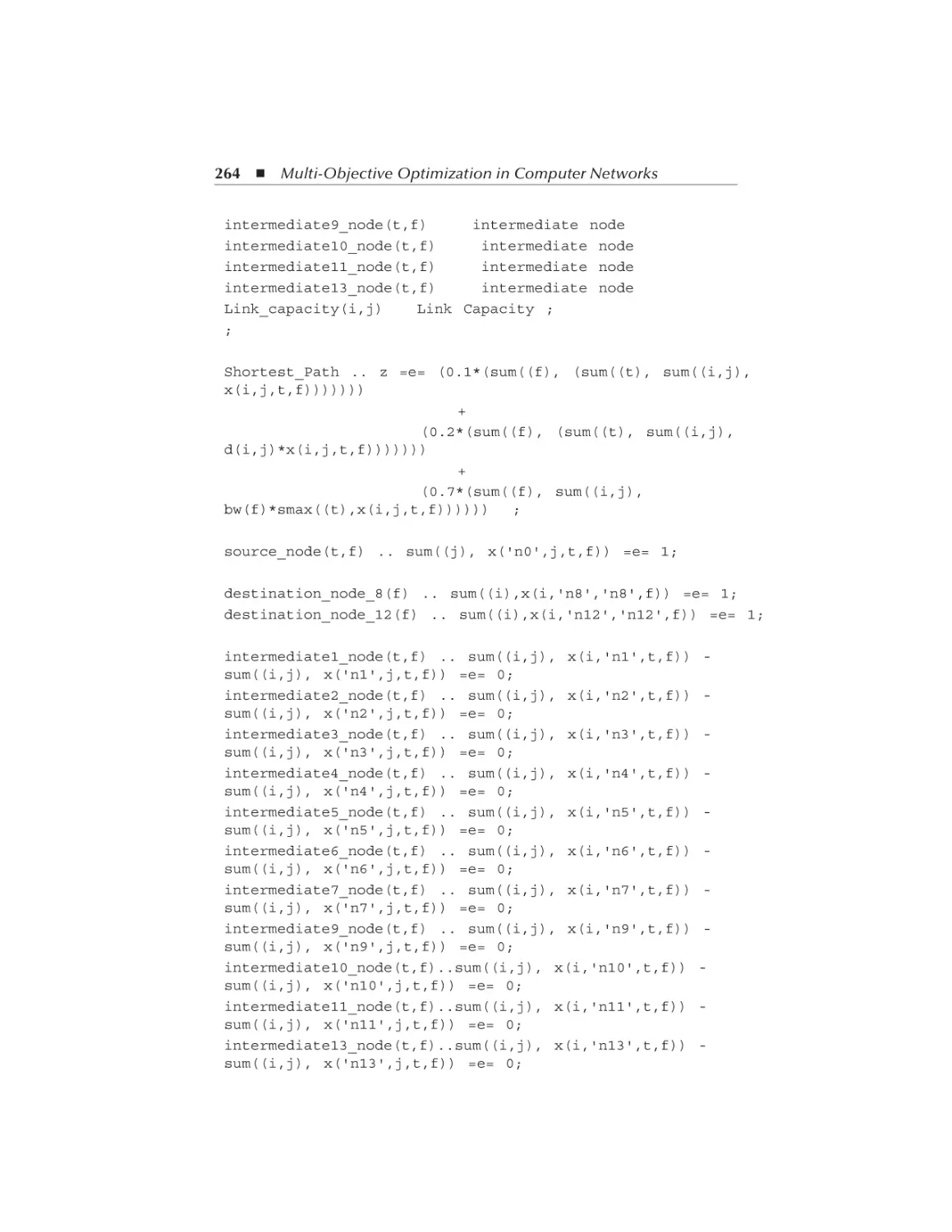
/


Автор: Donoso Y.
Теги: programming languages programming networks wireless networks wireless mesh networks
ISBN: 0-8493-8084-7
Год: 2007


Текст
AU8084_C000.fm Page i Friday, February 16, 2007 6:19 AM
Multi-Objective
Optimization
in Computer
Networks Using
Metaheuristics
AU8084_C000.fm Page ii Friday, February 16, 2007 6:19 AM
OTHER TELECOMMUNICATIONS BOOKS FROM AUERBACH
Architecting the Telecommunication
Evolution: Toward Converged Network
Services
Vijay K. Gurbani and Xian-He Sun
ISBN: 0-8493-9567-4
Business Strategies for the
Next-Generation Network
Nigel Seel
ISBN: 0-8493-8035-9
Security in Distributed, Grid, Mobile,
and Pervasive Computing
Yang Xiao
ISBN: 0-8493-7921-0
TCP Performance over UMTS-HSDPA
Systems
Mohamad Assaad and Djamal Zeghlache
ISBN: 0-8493-6838-3
Testing Integrated QoS of VoIP:
Packets to Perceptual Voice Quality
Vlatko Lipovac
ISBN: 0-8493-3521-3
Chaos Applications in
Telecommunications
Peter Stavroulakis
ISBN: 0-8493-3832-8
Context-Aware Pervasive Systems:
Architectures for a New Breed of
Applications
Seng Loke
ISBN: 0-8493-7255-0
Fundamentals of DSL Technology
Philip Golden, Herve Dedieu, Krista S Jacobsen
ISBN: 0-8493-1913-7
Introduction to Mobile Communications:
Technology, Services, Markets
Tony Wakefield
ISBN: 1-4200-4653-5
IP Multimedia Subsystem: Service
Infrastructure to Converge NGN,
3G and the Internet
Rebecca Copeland
ISBN: 0-8493-9250-0
MPLS for Metropolitan Area Networks
Nam-Kee Tan
ISBN: 0-8493-2212-X
Performance Modeling and Analysis of
Bluetooth Networks: Polling, Scheduling,
and Traffic Control
Jelena Misic and Vojislav B Misic
ISBN: 0-8493-3157-9
A Practical Guide to Content Delivery
Networks
Gilbert Held
ISBN: 0-8493-3649-X
The Handbook of Mobile Middleware
Paolo Bellavista and Antonio Corradi
ISBN: 0-8493-3833-6
Traffic Management in IP-Based
Communications
Trinh Anh Tuan
ISBN: 0-8493-9577-1
Understanding Broadband over
Power Line
Gilbert Held
ISBN: 0-8493-9846-0
Understanding IPTV
Gilbert Held
ISBN: 0-8493-7415-4
WiMAX: A Wireless Technology
Revolution
G.S.V. Radha Krishna Rao, G. Radhamani
ISBN: 0-8493-7059-0
WiMAX: Taking Wireless to the MAX
Deepak Pareek
ISBN: 0-8493-7186-4
Wireless Mesh Networking: Architectures,
Protocols and Standards
Yan Zhang, Jijun Luo and Honglin Hu
ISBN: 0-8493-7399-9
Wireless Mesh Networks
Gilbert Held
ISBN: 0-8493-2960-4
Resource, Mobility, and Security
Management in Wireless Networks
and Mobile Communications
Yan Zhang, Honglin Hu, and Masayuki Fujise
ISBN: 0-8493-8036-7
AUERBACH PUBLICATIONS
www.auerbach-publications.com
To Order Call: 1-800-272-7737 • Fax: 1-800-374-3401
E-mail: orders@crcpress.com
AU8084_C000.fm Page iii Friday, February 16, 2007 6:19 AM
Multi-Objective
Optimization
in Computer
Networks Using
Metaheuristics
Yezid Donoso
Ramon Fabregat
Boca Raton New York
Auerbach Publications is an imprint of the
Taylor & Francis Group, an informa business
AU8084_C000.fm Page iv Friday, February 16, 2007 6:19 AM
Auerbach Publications
Taylor & Francis Group
6000 Broken Sound Parkway NW, Suite 300
Boca Raton, FL 33487-2742
© 2007 by Taylor & Francis Group, LLC
Auerbach is an imprint of Taylor & Francis Group, an Informa business
No claim to original U.S. Government works
Printed in the United States of America on acid-free paper
10 9 8 7 6 5 4 3 2 1
International Standard Book Number-10: 0-8493-8084-7 (Hardcover)
International Standard Book Number-13: 978-0-8493-8084-6 (Hardcover)
This book contains information obtained from authentic and highly regarded sources. Reprinted
material is quoted with permission, and sources are indicated. A wide variety of references are
listed. Reasonable efforts have been made to publish reliable data and information, but the author
and the publisher cannot assume responsibility for the validity of all materials or for the consequences of their use.
No part of this book may be reprinted, reproduced, transmitted, or utilized in any form by any
electronic, mechanical, or other means, now known or hereafter invented, including photocopying,
microfilming, and recording, or in any information storage or retrieval system, without written
permission from the publishers.
For permission to photocopy or use material electronically from this work, please access www.
copyright.com (http://www.copyright.com/) or contact the Copyright Clearance Center, Inc. (CCC)
222 Rosewood Drive, Danvers, MA 01923, 978-750-8400. CCC is a not-for-profit organization that
provides licenses and registration for a variety of users. For organizations that have been granted a
photocopy license by the CCC, a separate system of payment has been arranged.
Trademark Notice: Product or corporate names may be trademarks or registered trademarks, and
are used only for identification and explanation without intent to infringe.
Library of Congress Cataloging-in-Publication Data
Donoso, Yezid.
Multi-objective optimization in computer networks using metaheuristics /
Yezid Donoso, Ramon Fabregat.
p. cm.
Includes bibliographical references and index.
ISBN 0-8493-8084-7 (alk. paper)
1. Computer networks. 2. Mathematical optimization. I. Fabregat, Ramon,
1963- II. Title.
TK5105.5.D665 2007
004.6--dc22
Visit the Taylor & Francis Web site at
http://www.taylorandfrancis.com
and the Auerbach Web site at
http://www.auerbach-publications.com
2007060385
AU8084_C000.fm Page v Friday, February 16, 2007 6:19 AM
Dedication
To my wife, Adriana
For her love and tenderness and for our future together
To my children, Andres Felipe, Daniella, Marianna,
and the following with Adry
… a gift of God to my life
Yezid
To my wife, Telvys, and my children
… “continuarem caminant cap a Ìtaca”
Ramon
AU8084_C000.fm Page vi Friday, February 16, 2007 6:19 AM
AU8084_C000.fm Page vii Friday, February 16, 2007 6:19 AM
Contents
1
Optimization Concepts........................................................................... 1
1.1
1.2
1.3
1.4
1.5
2
Local Minimum.......................................................................................... 2
Global Minimum ........................................................................................ 3
Convex and Nonconvex Sets...................................................................... 3
Convex and Concave Functions................................................................. 5
Minimum Search Techniques.................................................................... 11
1.5.1 Breadth First Search ..................................................................... 11
1.5.2 Depth First Search ........................................................................ 12
1.5.3 Best First Search........................................................................... 14
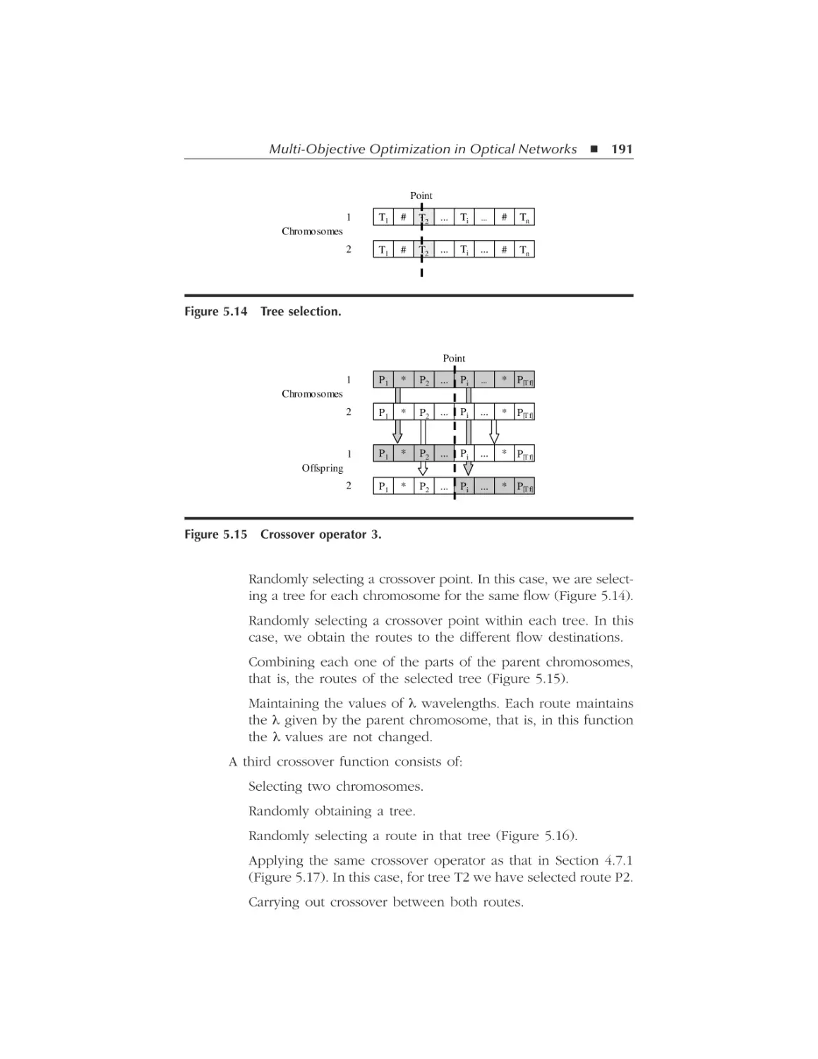
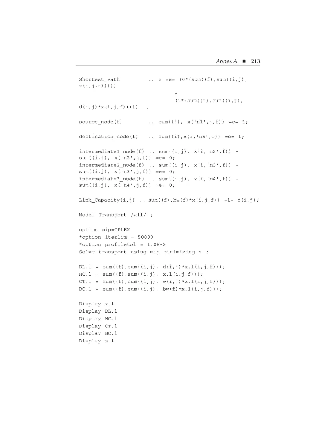
Multi-Objective Optimization Concepts ............................................ 15
2.1
2.2
2.3
Single-Objective versus Multi-Objective Optimization............................. 17
Traditional Methods .................................................................................. 19
2.2.1 Weighted Sum............................................................................... 19
2.2.2 ε-Constraint................................................................................... 23
2.2.3 Distance to a Referent Objective Method.................................... 26
2.2.4 Weighted Metrics.......................................................................... 28
2.2.5 The Benson Method ..................................................................... 30
Metaheuristics............................................................................................ 32
2.3.1 Convergence Toward Optimal ...................................................... 33
2.3.2 Optimal Solutions Not Withstanding Convexity of
the Problem ..................................................................................... 33
2.3.3 Avoiding Local OptimaL.............................................................. 33
2.3.4 Polynomial Complexity of Metaheuristics................................... 34
2.3.5 Evolutionary Algorithms .............................................................. 35
2.3.5.1 Components of a General Evolutionary Algorithm......... 36
2.3.5.2 General Structure of an Evolutionary Algorithm ......... 38
2.3.6 Ant Colony.................................................................................... 40
2.3.6.1 General Structure of an Ant Colony Algorithm ........... 40
2.3.7 Memetic Algorithm....................................................................... 42
vii
AU8084_C000.fm Page viii Friday, February 16, 2007 6:19 AM
viii Contents
2.4
3
42
43
44
45
46
49
50
51
52
53
53
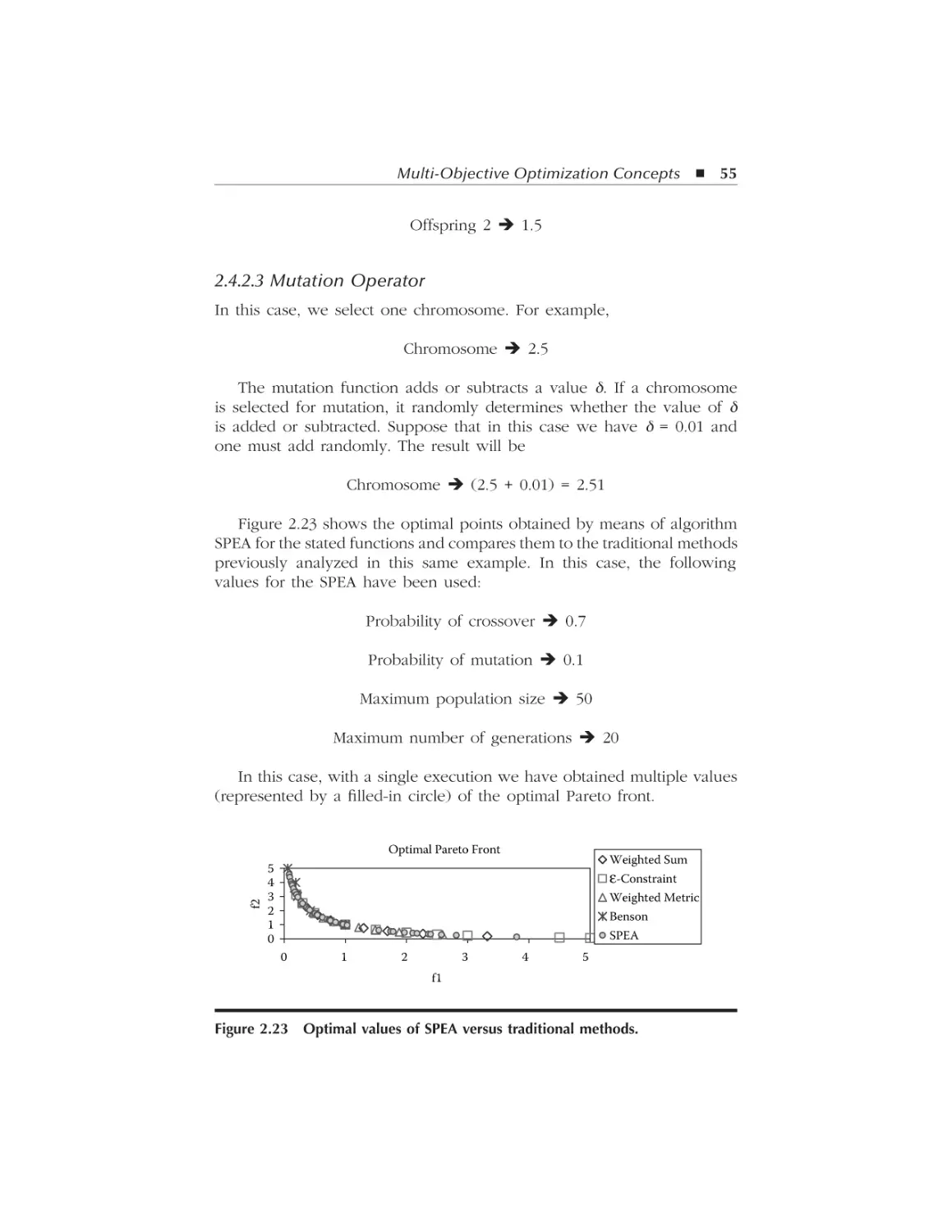
55
Computer Network Modeling ............................................................. 57
3.1
3.2
4
2.3.7.1 Local Searches...............................................................
2.3.7.2 General Structure of a Memetic Algorithm ..................
2.3.8 Tabu Search...................................................................................
2.3.8.1 General Structure of a Tabu Search ..............................
2.3.9 Simulated Annealing.....................................................................
2.3.9.1 General Structure of Simulated Annealing ...................
Multi-Objective Solution Applying Metaheuristics..................................
2.4.1 Procedure to Assign Fitness to Individuals..................................
2.4.2 Reducing the Nondominated Set Using Clustering.....................
2.4.2.1 Representation of the Chromosome..............................
2.4.2.2 Crossover Operator........................................................
2.4.2.3 Mutation Operator .........................................................
Computer Networks: Introduction ............................................................ 57
3.1.1 Reference Models ......................................................................... 57
3.1.1.1 OSI Reference Model.................................................... 58
3.1.1.2 TCP/IP Reference Model .............................................. 59
3.1.2 Classification of Computer Networks Based on Size.................. 60
3.1.2.1 Personal Area Networks (PANs)................................... 61
3.1.2.2 Local Area Networks (LANs) ....................................... 61
3.1.2.3 Metropolitan Area Networks (MANs) .......................... 62
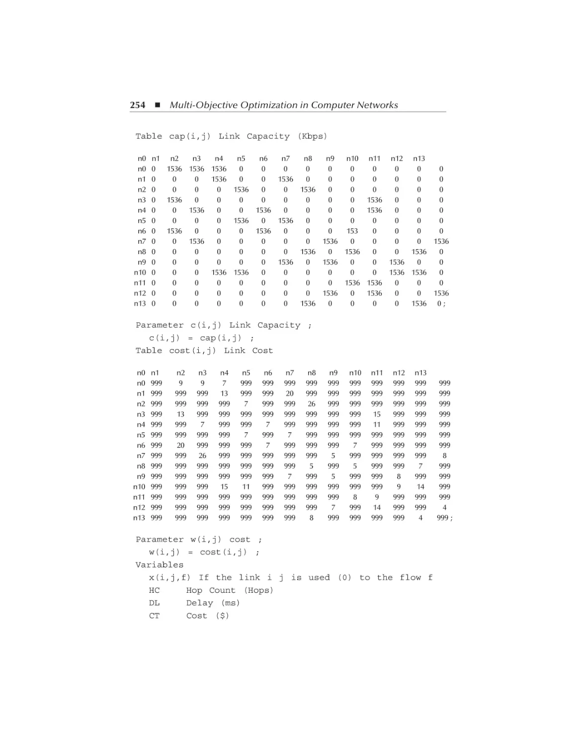
3.1.2.4 Wide Area Networks (WANs)....................................... 62
3.1.3 Classification of Computer Networks Based on
Type of Transmission...................................................................... 64
3.1.3.1 Unicast Transmissions ................................................... 64
3.1.3.2 Multicast Transmissions ................................................ 64
3.1.3.3 Broadcast Transmissions ............................................... 64
Computer Network Modeling.................................................................. 65
3.2.1 Introduction to Graph Theory ...................................................... 65
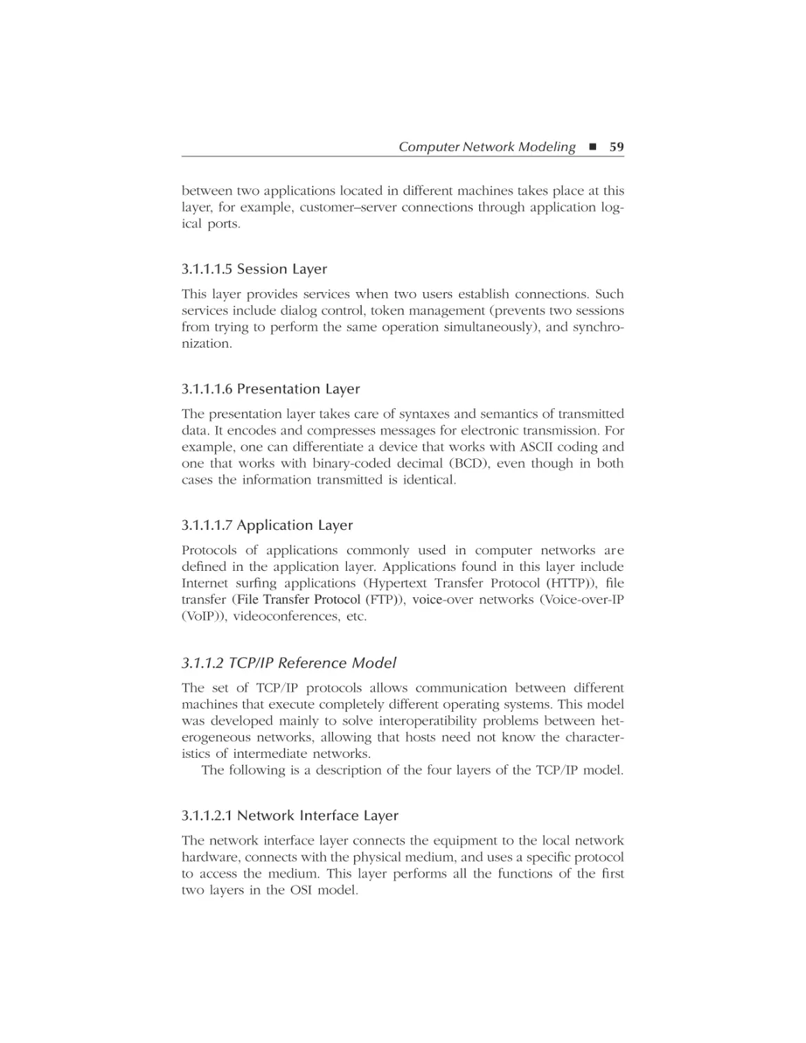
3.2.2 Computer Network Modeling in Unicast Transmission .............. 66
3.2.3 Computer Networks Modeling in Multicast Transmission.......... 68
Routing Optimization in Computer Networks.................................. 71
4.1
4.2
Concepts ..................................................................................................... 71
4.1.1 Unicast Case ................................................................................. 71
4.1.2 Multicast Case .............................................................................. 72
Optimization Functions ............................................................................. 74
4.2.1 Hop Count .................................................................................... 74
4.2.1.1 Unicast Transmission..................................................... 74
4.2.1.2 Multicast Transmission.................................................. 75
4.2.2 Delay ............................................................................................. 78
4.2.2.1 Unicast Transmission..................................................... 78
4.2.2.2 Multicast Transmission.................................................. 80
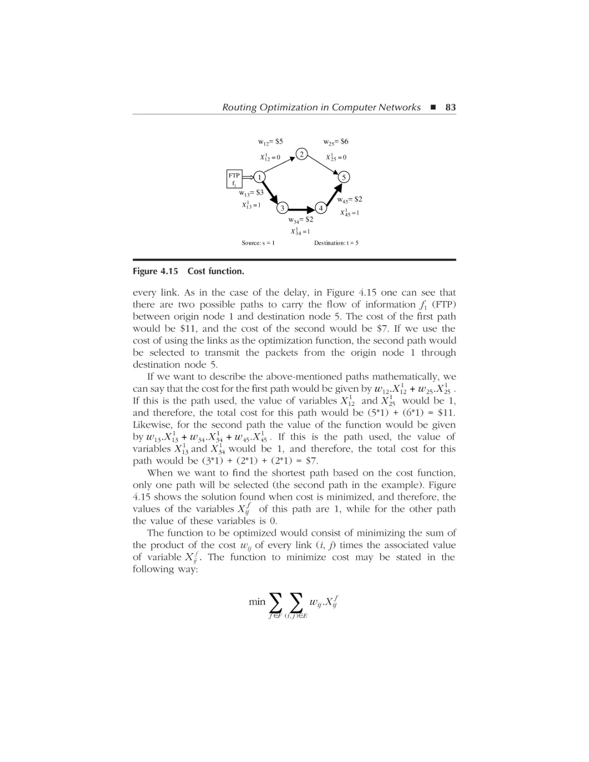
4.2.3 Cost ............................................................................................... 82
4.2.3.1 Unicast Transmission..................................................... 82
4.2.3.2 Multicast Transmission.................................................. 84
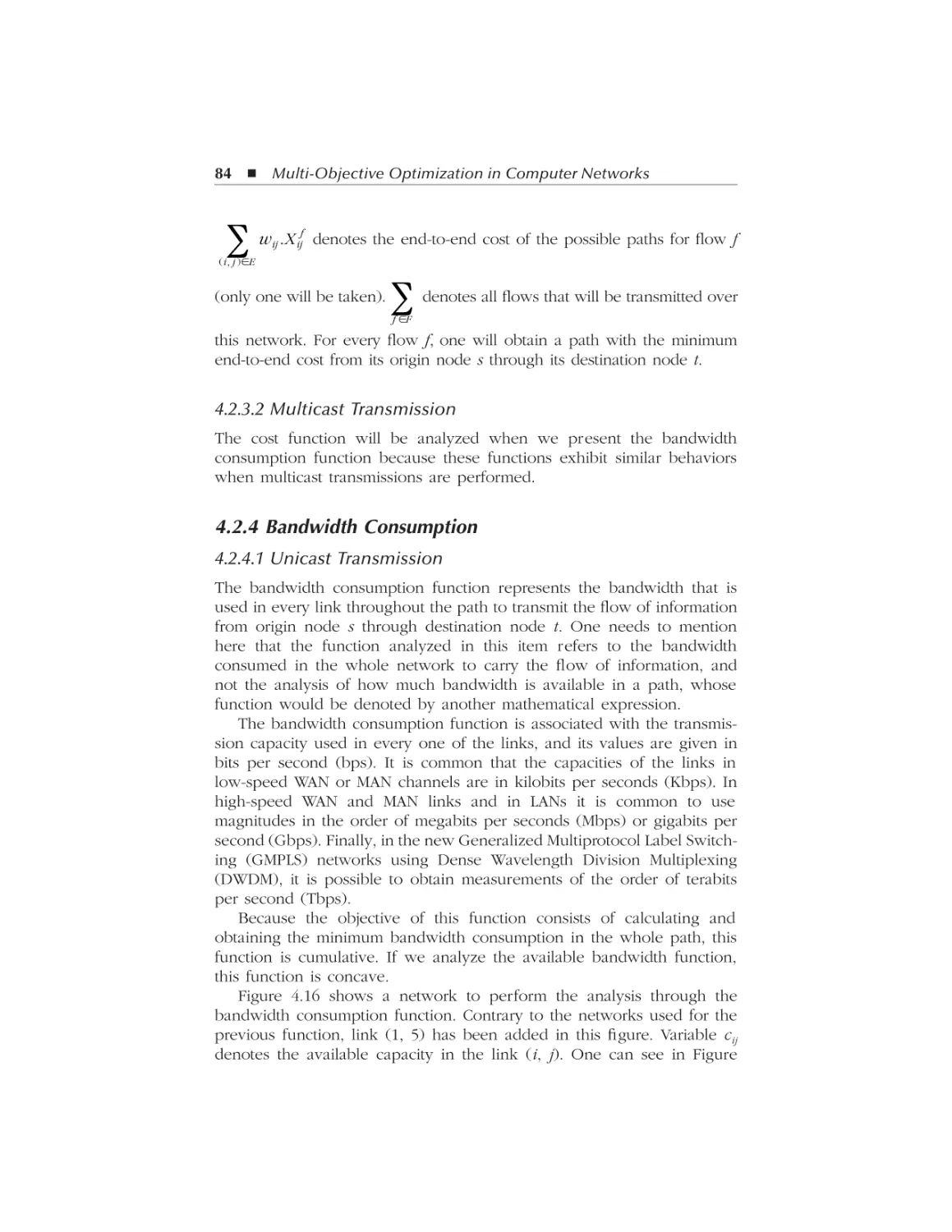
4.2.4 Bandwidth Consumption .............................................................. 84
AU8084_C000.fm Page ix Friday, February 16, 2007 6:19 AM
Contents ix
4.3
4.4
4.5
4.6
4.7
4.2.4.1 Unicast Transmission..................................................... 84
4.2.4.2 Multicast Transmission.................................................. 86
4.2.5 Packet Loss Rate........................................................................... 89
4.2.6 Blocking Probability..................................................................... 90
4.2.6.1 Unicast Transmission..................................................... 90
4.2.6.2 Multicast Transmission.................................................. 92
4.2.7 Maximum Link Utilization........................................................... 92
4.2.7.1 Unicast Transmission..................................................... 92
4.2.7.2 Multicast Transmission.................................................. 94
4.2.8 Other Multicast Functions ............................................................ 95
4.2.8.1 Hop Count Average ....................................................... 95
4.2.8.2 Maximal Hop Count...................................................... 96
4.2.8.3 Maximal Hop Count Variation ...................................... 96
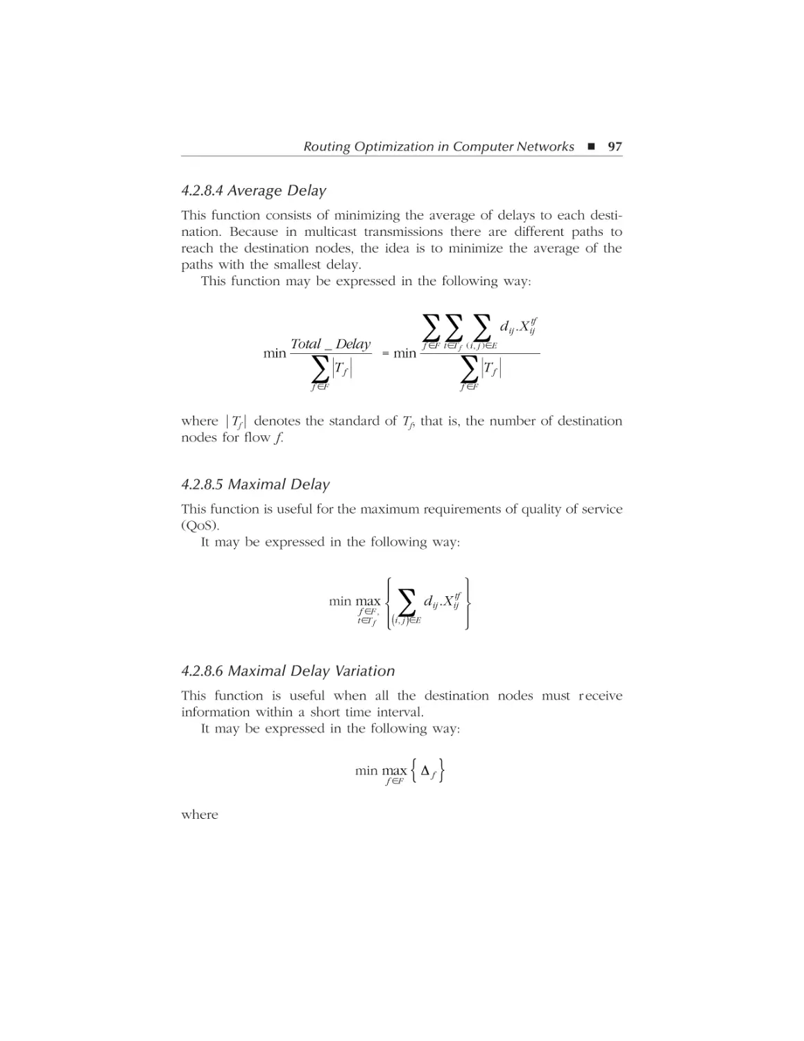
4.2.8.4 Average Delay ............................................................... 97
4.2.8.5 Maximal Delay .............................................................. 97
4.2.8.6 Maximal Delay Variation .............................................. 97
4.2.8.7 Average Cost.................................................................. 98
4.2.8.8 Maximal Cost ................................................................ 98
Constraints ................................................................................................. 98
4.3.1 Unicast Transmission.................................................................... 98
4.3.2 Multicast Transmission............................................................... 100
Functions and Constraints....................................................................... 102
4.4.1 Unicast Transmissions ................................................................ 102
4.4.2 Multicast Transmissions ............................................................. 102
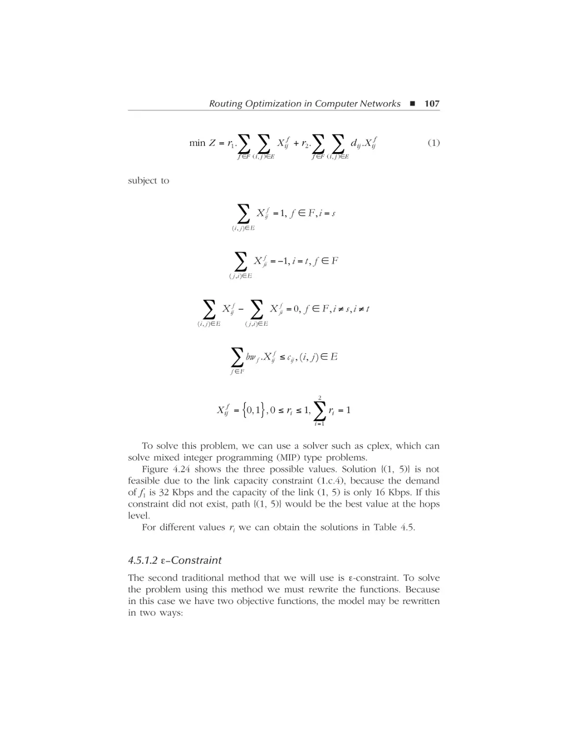
Single-Objective Optimization Modeling and Solution ......................... 102
4.5.1 Unicast Transmission Using Hop Count and Delay.................. 106
4.5.1.1 Weighted Sum.............................................................. 106
4.5.1.2 ε-Constraint.................................................................. 107
4.5.1.3 Weighted Metrics......................................................... 110
4.5.1.4 Benson Method............................................................ 113
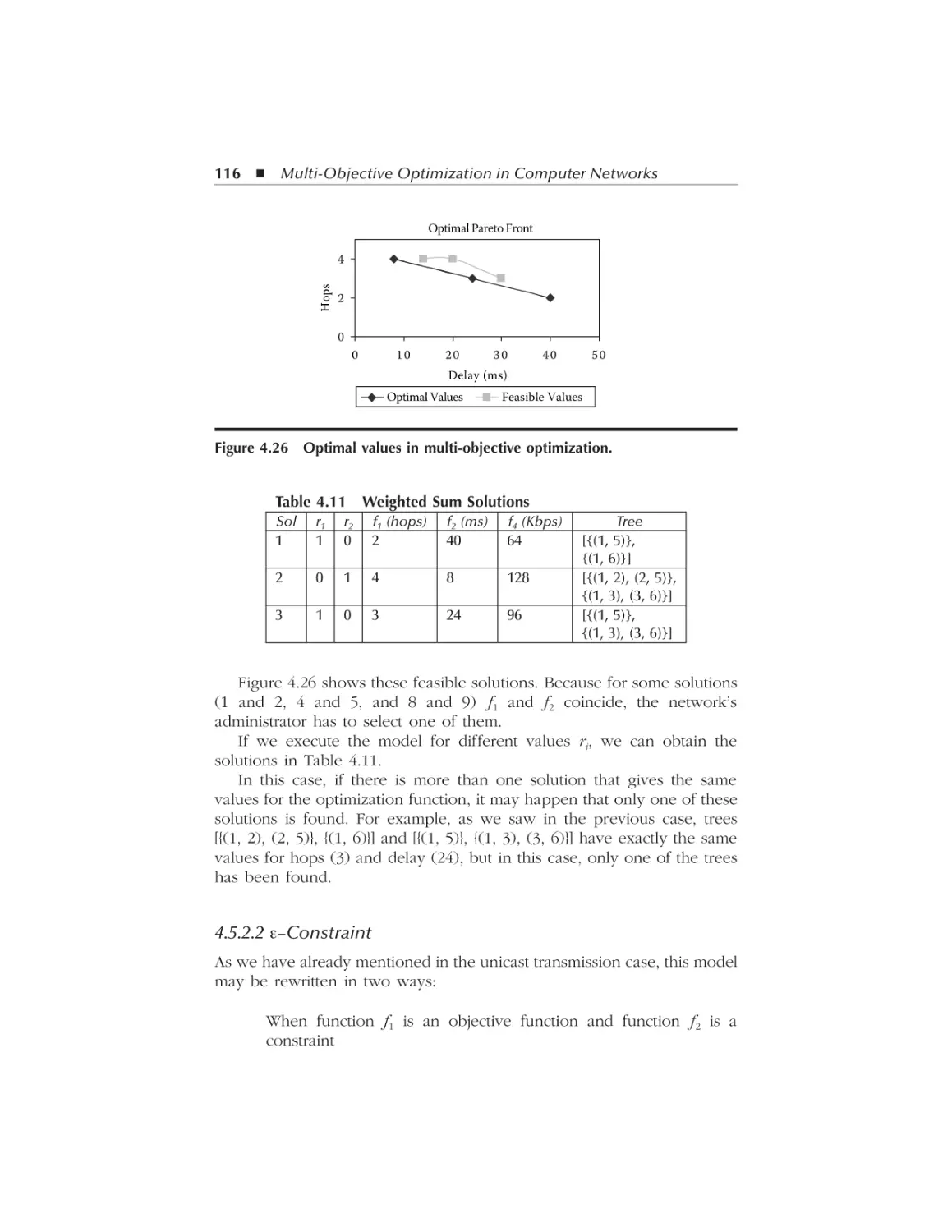
4.5.2 Multicast Transmission Using Hop Count and Delay ............... 114
4.5.2.1 Weighted Sum.............................................................. 114
4.5.2.2 ε-Constraint.................................................................. 116
4.5.2.3 Weighted Metrics......................................................... 119
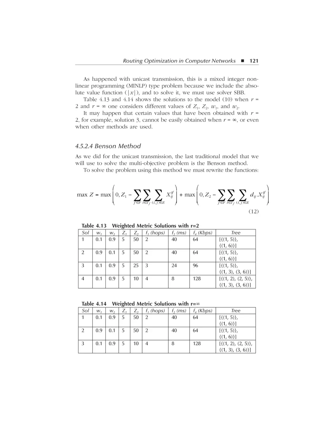
4.5.2.4 Benson Method............................................................ 121
4.5.3 Unicast Transmission Using Hop Count, Delay, and
Bandwidth Consumption............................................................... 123
4.5.4 Multicast Transmission Using Hop Count, Delay, and
Bandwidth Consumption............................................................... 126
4.5.5 Unicast Transmission Using Hop Count, Delay,
Bandwidth Consumption, and Maximum Link Utilization ..............129
4.5.6 Multicast Transmission Using Hop Count, Delay,
Bandwidth Consumption, and Maximum Link Utilization ............. 133
Multi-Objective Optimization Modeling ................................................ 138
4.6.1 Unicast Transmission.................................................................. 138
4.6.2 Multicast Transmission............................................................... 140
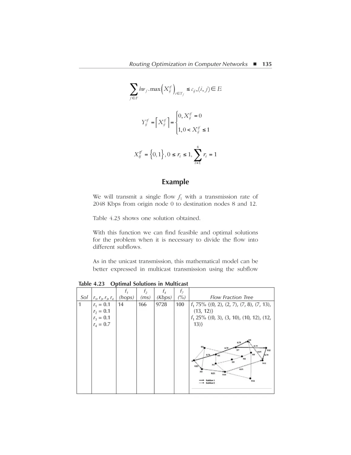
Obtaining a Solution Using Metaheuristics............................................ 142
AU8084_C000.fm Page x Friday, February 16, 2007 6:19 AM
Contents
x
4.7.1
4.7.2
4.7.3
4.7.4
4.7.5
4.7.6
5
Unicast for the Hop Count and Delay Functions ...................... 143
4.7.1.1 Coding of a Chromosome ........................................... 143
4.7.1.2 Initial Population ......................................................... 144
4.7.1.3 Selection ...................................................................... 144
4.7.1.4 Crossover ..................................................................... 144
4.7.1.5 Mutation....................................................................... 145
Multicast for the Hop Count and Delay Functions ................... 146
4.7.2.1 Coding of a Chromosome ........................................... 146
4.7.2.2 Initial Population ......................................................... 148
4.7.2.3 Selection ...................................................................... 148
4.7.2.4 Crossover ..................................................................... 148
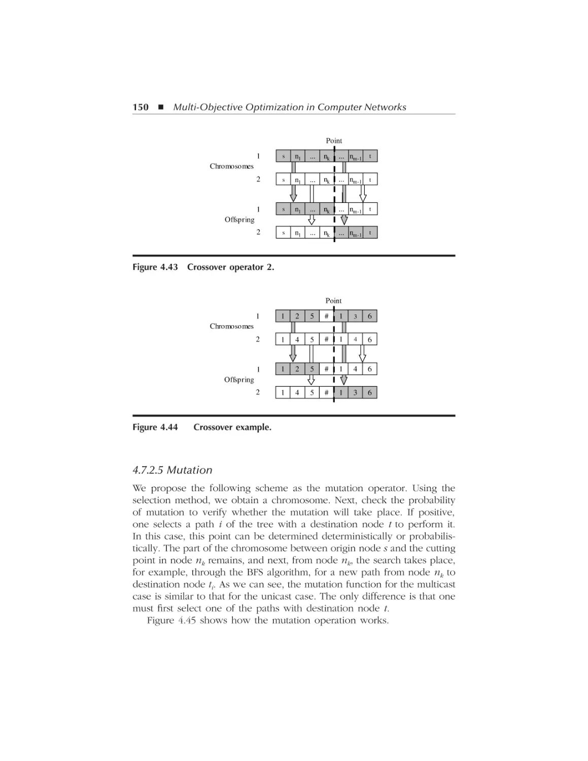
4.7.2.5 Mutation....................................................................... 150
Unicast Adding the Bandwidth Consumption Function ............ 151
4.7.3.1 Coding of a Chromosome ........................................... 151
4.7.3.2 Initial Population ......................................................... 151
4.7.3.3 Selection ...................................................................... 152
4.7.3.4 Crossover ..................................................................... 152
4.7.3.5 Mutation....................................................................... 152
Multicast Adding the Bandwidth Consumption Function ......... 153
4.7.4.1 Coding of a Chromosome ........................................... 154
4.7.4.2 Initial Population ......................................................... 154
4.7.4.3 Selection ...................................................................... 154
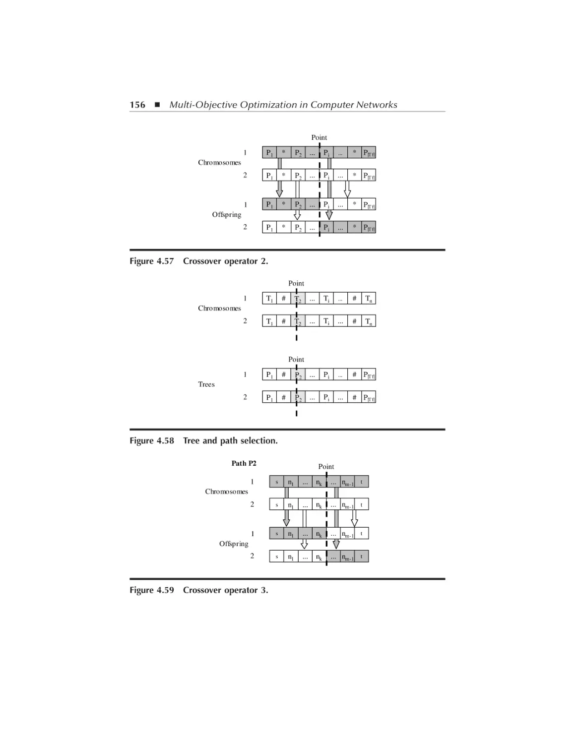
4.7.4.4 Crossover ..................................................................... 155
4.7.4.5 Mutation....................................................................... 157
Unicast Adding the Maximum Link Utilization Function......... 157
4.7.5.1 Coding of a Chromosome ........................................... 157
4.7.5.2 Initial Population ......................................................... 158
4.7.5.3 Selection ...................................................................... 158
4.7.5.4 Crossover ..................................................................... 158
4.7.5.5 Mutation....................................................................... 159
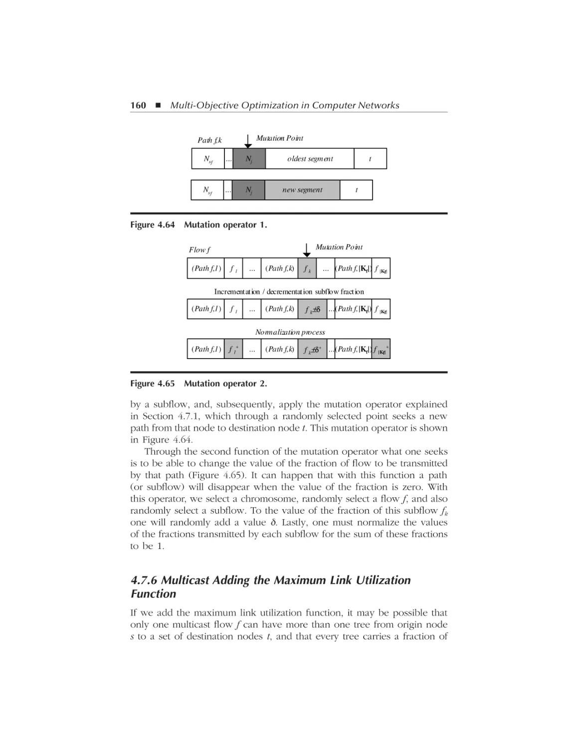
Multicast Adding the Maximum Link Utilization Function......... 160
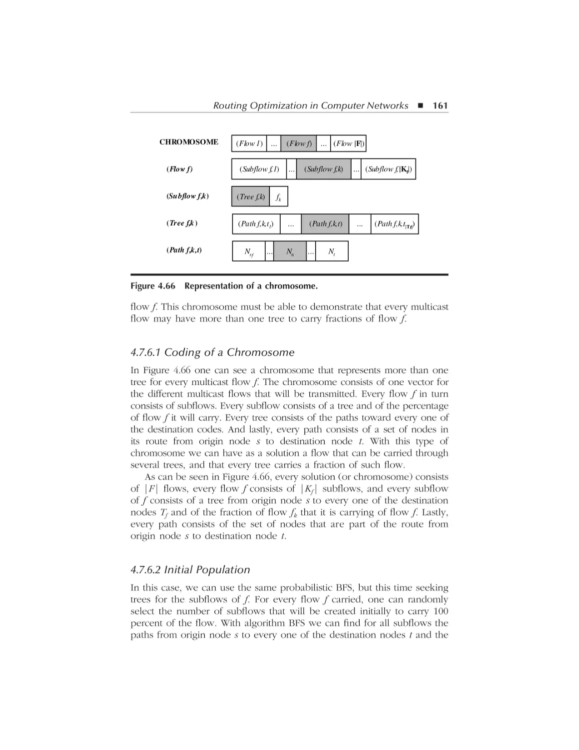
4.7.6.1 Coding of a Chromosome ........................................... 161
4.7.6.2 Initial Population ......................................................... 161
4.7.6.3 Selection ...................................................................... 162
4.7.6.4 Crossover ..................................................................... 162
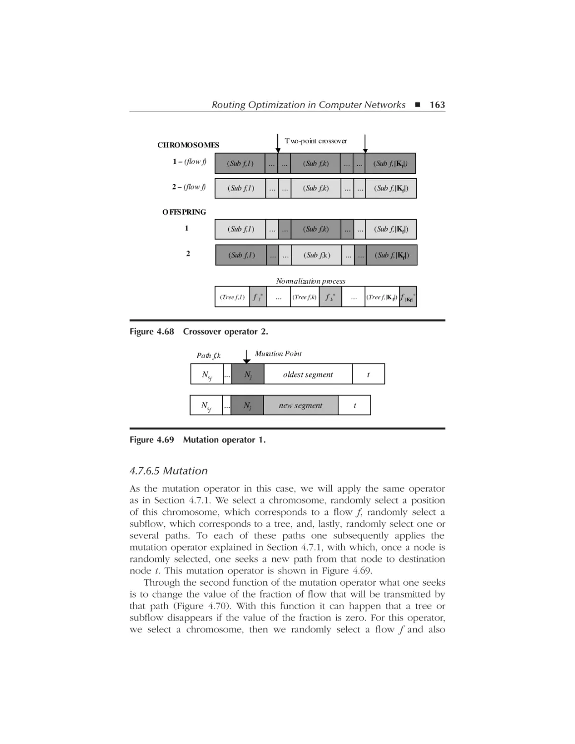
4.7.6.5 Mutation........................................................................ 163
Multi-Objective Optimization in Optical Networks ....................... 165
5.1
5.2
Concepts ..................................................................................................
5.1.1 Multiplexing of the Network......................................................
5.1.2 Multiprotocol l Switching Architecture (MPlS) ........................
5.1.3 Optical Fiber ...............................................................................
5.1.3.1 Types of Fibers ...............................................................
New Optimization Functions ..................................................................
5.2.1 Number of l ...................................................................................
5.2.1.1 Unicast .........................................................................
5.2.1.2 Multicast ......................................................................
165
167
167
167
168
168
170
171
171
AU8084_C000.fm Page xi Friday, February 16, 2007 6:19 AM
Contents xi
5.2.2
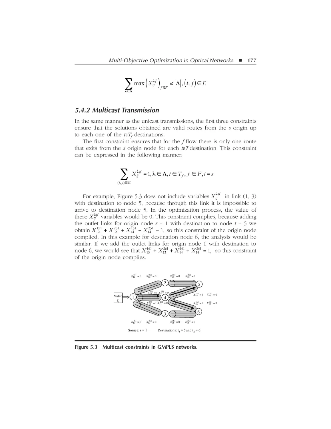
5.3
5.4
5.5
5.6
5.7
6
Optical Attenuation.....................................................................
5.2.2.1 Unicast .........................................................................
5.2.2.2 Multicast ......................................................................
Redefinition of Optical Transmission Functions ....................................
5.3.1 Unicast ........................................................................................
5.3.2 Multicast .....................................................................................
Constraints ...............................................................................................
5.4.1 Unicast Transmission..................................................................
5.4.2 Multicast Transmission...............................................................
Functions and Constraints.......................................................................
5.5.1 Unicast Transmissions ................................................................
5.5.2 Multicast Transmissions .............................................................
Multi-objective Optimization Modeling .................................................
5.6.1 Unicast Transmissions ................................................................
5.6.2 Multicast Transmissions .............................................................
Obtaining a Solution Using Metaheuristics............................................
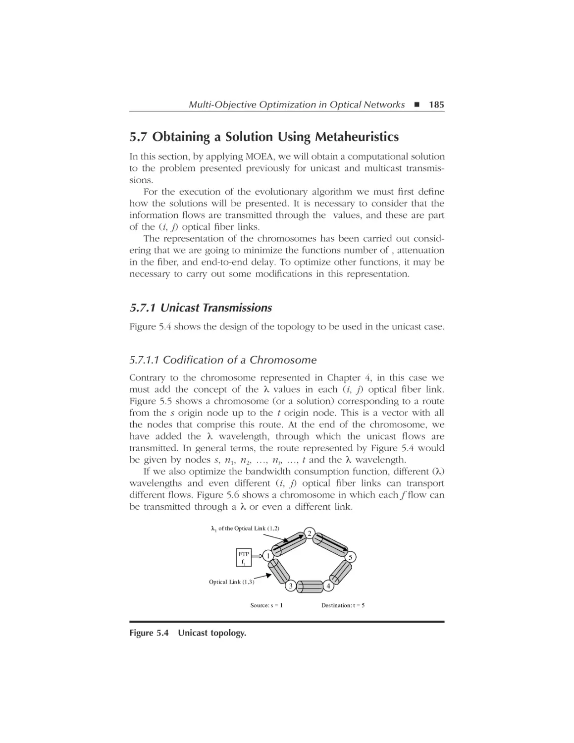
5.7.1 Unicast Transmissions ................................................................
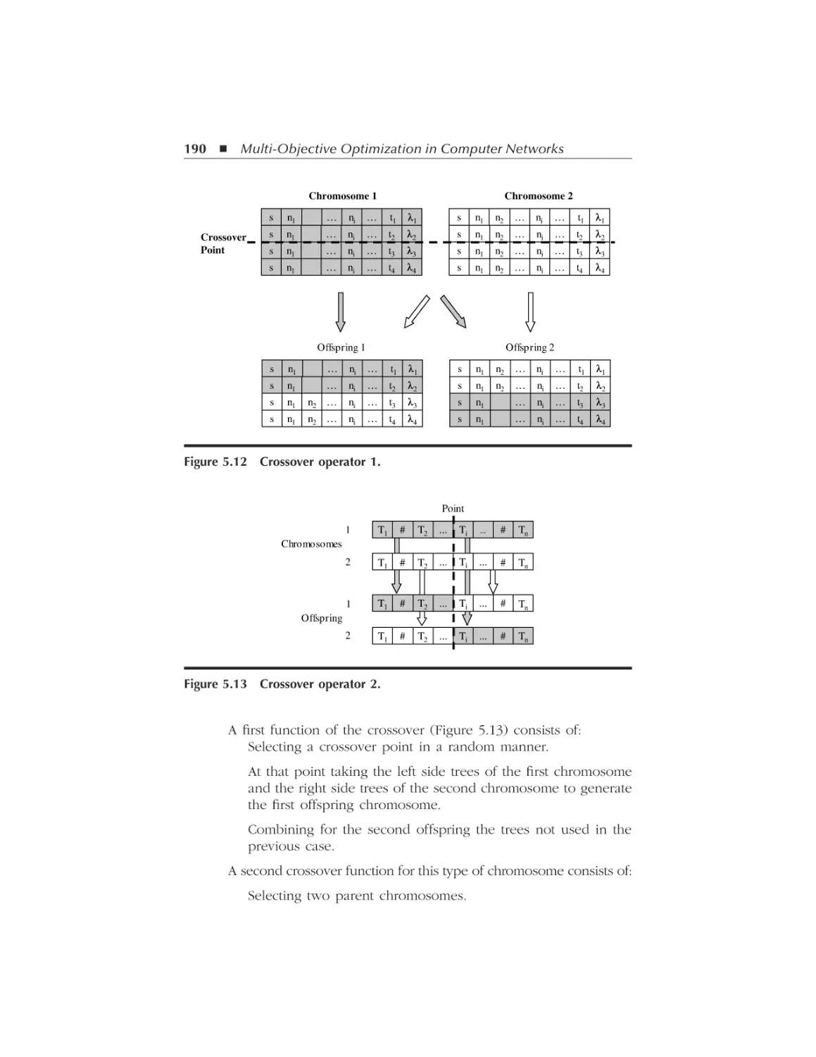
5.7.1.1 Codification of a Chromosome ...................................
5.7.1.2 Initial Population .........................................................
5.7.1.3 Selection ......................................................................
5.7.1.4 Crossover .....................................................................
5.7.1.5 Mutation.......................................................................
5.7.2 Multicast Transmissions .............................................................
5.7.2.1 Codification of a Chromosome ...................................
5.7.2.2 Initial Population .........................................................
5.7.2.3 Selection ......................................................................
5.7.2.4 Crossover .....................................................................
5.7.2.5 Mutation.......................................................................
171
171
172
172
172
172
175
175
177
179
179
179
179
179
184
185
185
185
186
186
186
187
187
187
188
189
189
192
Multi-Objective Optimization in Wireless Networks ..................... 195
6.1
6.2
6.3
6.4
6.5
6.6
Concepts ..................................................................................................
New Optimization Function....................................................................
6.2.1 Free Space Loss..........................................................................
6.2.1.1 Unicast .........................................................................
6.2.1.2 Multicast ......................................................................
Constraints ...............................................................................................
6.3.1 Unicast Transmission..................................................................
6.3.2 Multicast Transmission...............................................................
Function and Constraints ........................................................................
6.4.1 Unicast Transmissions ................................................................
6.4.2 Multicast Transmissions .............................................................
Multi-Objective Optimization Modeling ................................................
6.5.1 Unicast Transmission..................................................................
6.5.2 Multicast Transmission...............................................................
Obtaining a Solution Using Metaheuristics............................................
195
196
196
197
197
198
198
199
200
200
200
200
200
203
204
AU8084_C000.fm Page xii Friday, February 16, 2007 6:19 AM
xii Contents
Annex A....................................................................................................... 205
Annex B....................................................................................................... 275
Bibliography ............................................................................................... 435
Index............................................................................................................ 441
AU8084_C000.fm Page xiii Friday, February 16, 2007 6:19 AM
Preface
Many new multicast applications emerging from the Internet, such as
Voice-over-IP (VoIP), videoconference, TV over the Internet, radio over
the Internet, video streaming multipoint, etc., have the following resource
requirements: bandwidth consumption, end-to-end delay, delay jitter,
packet loss ratio, and so forth. It is therefore necessary to formulate a
proposal to specify and provide the resources necessary for these kinds
of applications so they will function properly.
To show how these new applications can comply with these requirements, the book presents a multi-objective optimization scheme in which
we will analyze and solve the problems related to resources optimization
in computer networks. Once the readers have studied this book, they will
be able to extend these models by adding new objective functions, new
functions that act as restrictions, new network models, and new types of
services or applications.
This book is for an academic and scientific setting. In the professional
environment, it is focused on optimization of resources that a carrier needs
to know to profit from computer resources and its network infrastructure.
It is very useful as a textbook mainly for master’s- or Ph.D.-level courses,
whose subjects are related to computer networks traffic engineering, but
it can also be used for an advanced or specialized course for the senior
year of an undergraduate program. On the other hand, it can be of great
use for a multi-objective optimization course that deals with graph theory
by having represented the computer networks through graphs.
The book structure is as follows:
Chapter 1: Analyzes the basic optimization concepts, as well as
several techniques and algorithms for the search of minimals.
xiii
AU8084_C000.fm Page xiv Friday, February 16, 2007 6:19 AM
xiv Preface
Chapter 2: Analyzes the basic multi-objective optimization concepts
and the ways to solve them through traditional techniques and
several metaheuristics.
Chapter 3: Shows how to analytically model the computer network
problems dealt with in this book.
Chapter 4: The book’s main chapter — it shows the multi-objective
models in computer networks and the applied way in which we
can solve them.
Chapter 5: An extension of Chapter 4, applied to optical networks.
Chapter 6: An extension of Chapter 4, applied to wireless networks.
Lastly, Annex A provides the source code to solve the mathematical
model problems presented in this book through solvers. Annex B includes
some source codes programmed in C language, which solve some of the
multi-objective optimization problems presented. These source files are
available online at http://www.crcpress.com/e—products/downloads/
default.asp
AU8084_C000.fm Page xv Friday, February 16, 2007 6:19 AM
The Authors
Yezid Donoso, Ph.D., is a professor at the Universidad del Norte in
Barranquilla, Colombia, South America. He teaches courses in computer
networks and multi-objective optimization. He is also a director of the
computer network postgraduate program and the master program in
system and computer engineering. In addition, he is a consultant in
computer network and optimization for Colombian industries. He earned
his bachelor’s degree in system and computer engineering from the
Universidad del Norte, Barranquilla, Colombia, in 1996; M.Sc. degree in
system and computer engineering from the Universidad de los Andes,
Bogotá, Colombia, in 1998; D.E.A. in information technology from Girona
University, Spain, in 2002; and Ph.D. (cum laude) in information technology from Girona University in 2005.
Dr. Donoso is a senior member of IEEE as well as a distinguished
visiting professor (DVP) of the IEEE Computer Society. His biography has
been published in Who’s Who in the World (2006) and Who’s Who in
Science and Engineering (2006) by Marquis, U.S.A. and in 2000 Outstanding Intellectuals of the 21st Century (2006) by International Biographical
Centre, Cambridge, England. His awards include the title of distinguished
professor from the Universidad del Norte (October 2004) and the National
Award of Operations research from the Colombian Society of Operations
Research (2004).
Ramon Fabregat, Ph.D., earned his degree in computer engineering from
the Universitat Autónoma de Barcelona (UAB), Spain, and his Ph.D. in
information technology (1999) from Girona University, Spain. Currently, he
is a professor in the electrical engineering, computer science, and automatic
control departments and a researcher at the Institute of Informatics and
Applications at Girona University. His teaching duties include graduate- and
postgraduate-level courses on operating systems, computer communication
xv
AU8084_C000.fm Page xvi Friday, February 16, 2007 6:19 AM
xvi The Authors
networks, and the performance evaluation of telecommunication systems.
His research interests are in the fields of management and performance
evaluation of communication networks, network management based on
intelligent agents, MPLS and GMPLS, and adaptive hypermedia systems.
He coordinated the participation of broadband communications and
distributed systems research group (BCDS) in the ADAPTPlan project (a
Spanish national research project). He is a member of the Spanish Network
of Excellence in MPLS/GMPLS networks, which involves several Spanish
institutions. He has participated in the technical program committees of
several conferences and has coauthored several papers published in
international journals and presented at leading international conferences.
AU8084_C001.fm Page 1 Wednesday, February 7, 2007 5:46 AM
Chapter 1
Optimization Concepts
In the field of engineering, solving a problem is not enough; the solution
found must be the best solution possible. In other words, one must find
the optimal solution to the problem. We say that this is the best possible
solution because in the real world this problem may have certain constraints by which the solutions found may be feasible (they can be
implemented in practice) and unfeasible (they cannot be implemented).
In engineering, one speaks of optimization when one wants to solve
complex problems. Such complexity may be associated with the kind of
problem one wants to solve (i.e., if the problem is nonlinear) or the kind
of solution one wishes to get (i.e., whether the solution is exact or an
approximation).
There are five basic ways to solve such problems: analytically, numerically, algorithmically through heuristics, algorithmically through metaheuristics, or through simulation. Analytical solutions are practically possible
for simple problems, but complex or large-sized problems are very difficult
and require too much computational time. When the analytical model is
very complex, problems can be solved by approximation using numerical
methods. To obtain such optimal approximate values, functions analyzed
must usually meet a series of conditions. If such conditions are not met,
the numerical method may converge toward the optimal value. In any
event, these techniques are very useful when the problems are monoobjective, whether linear or not.
However, when a problem is multi-objective, numerical methods are
susceptible of being nonconvergent, depending on the model used. For
example, if one attempts to solve a multi-objective optimization scheme
1
AU8084_C001.fm Page 2 Wednesday, February 7, 2007 5:46 AM
2 Multi-Objective Optimization in Computer Networks
by means of numerical methods using the mono-objective scheme of the
weighted sum of the functions (which will be explained later), in addition
to the conditions that the functions must meet for the specific numerical
method, such a multi-objective scheme would present inconveniences if
the search space is not convex, because one might not find many solutions.
One can also find the solution applying computational algorithms called
heuristics. In this case, heuristics presents a computational scheme that
can reach the optimal value in an computational time. But the search of
solutions with this type of algorithm may exhibit serious problems if, for
example, the spaces are nonconvex or if the nature of the problem is of
combined solution analysis. Furthermore, heuristics may present serious
computational time problems when the problem is NP-Hard. A recognition
problem P1 is said to be NP-Hard if all other problems in the class NP
polynomially to P1, and we say that a recognition problem P1 is in the
class NP if for every yes instance of P1, there is a short (i.e., polynomial
length) verification that the instance is a yes instance [AHU93].
To overcome these inconveniences, metaheuristics have been created,
which obtain an approximate solution to practically any kind of problem
that is NP-Hard and complex or combined analysis solutions. Among
existing metaheuristics we can mention genetic algorithms, Tabu search,
ant colony, simulated annealing, memetic algorithms, etc. Many of these
metaheuristics have been redesigned to provide solutions to multi-objective problems, which are the main interest of this book.
This chapter provides an introduction to fundamentals of local and
global minimal and some existing techniques to search for such minimal.
1.1 Local Minimum
When optimizing a function f(x), one wants to find the minimum value
in an [a, b] interval; that is, a ≤ x ≤ b. This minimum value is called the
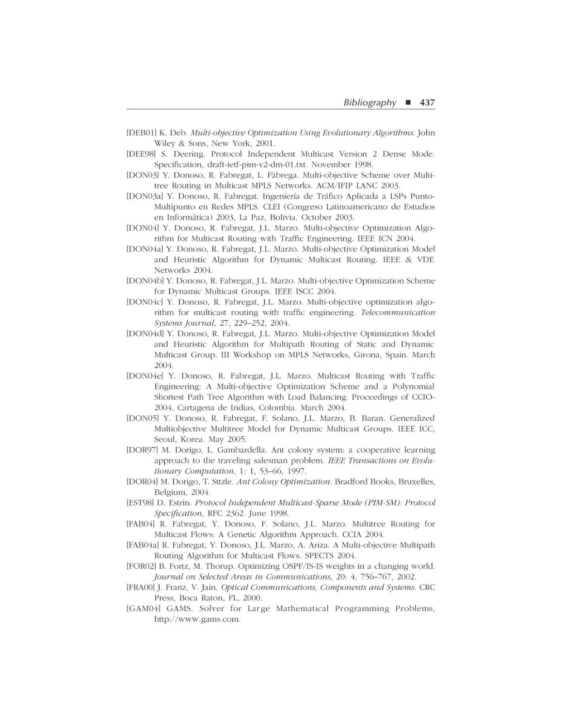
local minimum (Figure 1.1).
f(x)
f(x*)
f(x**)
[
a
Figure 1.1 Local minimum.
]
x* b
x**
x
AU8084_C001.fm Page 3 Wednesday, February 7, 2007 5:46 AM
Optimization Concepts 3
If given function f(x), we want to find the minimum value, but only
in the (a ≤ x ≤ b) interval. The resulting f(x*) value is called the local
minimum of function f(x) in interval [a, b]. As shown in Figure 1.1, this
f(x*) value is the minimum value in the [ a, b] interval, but is not the
minimum value of function f(x) in the (–∞, ∞) interval.
Traditionally, search techniques for local minima are simpler than
search techniques for global minima due, among many reasons, to the
complexity generated in the search space when the interval is (–∞, ∞).
1.2 Global Minimum
When the function minimized is not constrained to a specific interval of
the function, then one says that the value found is a global minimum. In
this case, the search space interval is associated with (–∞, ∞).
Even though in Figure 1.1 the value of function f(x*) is a minimum,
we can see that f(x**) < f(x*). If there is no other value f(x'), so that f(x')
< f(x**) in the (–∞, ∞) interval, then one says that f(x**) is a global minimum
of function f(x).
To find the global maximum value of a function, the analysis would be
exactly the same, but in this case there should not exist another f(x') value
so that f(x') > f(x**) in the (–∞, ∞) interval.
1.3 Convex and Nonconvex Sets
Definition 1
A set S of ℜn is convex if for any pairs of points P1, P2 ε S and for every λ
ε [0, 1] one proves that P = λP1 + (1 − λ ) P2 ε S. Point P is a linear combination of points P1 and P2.
A set S ⊆ ℜn is convex if the linear combination of any two points in
S also belongs to S.
On the other hand, a set is nonconvex if there is at least one point P in
set S that cannot be represented by a linear combination.
Taking into account these definitions, Figure 1.2 represents convex
solution sets and Figure 1.3 represents nonconvex solution sets.
Below are examples of convex sets.
Exercise
a. Is set S =
{( x , x ) ∈ℜ
1
2
2
/ x 2 ≥ x1
}
convex?
AU8084_C001.fm Page 4 Wednesday, February 7, 2007 5:46 AM
4 Multi-Objective Optimization in Computer Networks
P2
S
S
P1
P
P2
P
P2
P
P1
P1
Figure 1.2 Convex sets.
P
P1
P1
S
P2
P1
S
P
P
P2
P2
Figure 1.3 Nonconvex sets.
Proof:
Let x = (x1, x2), y = (y1, y2), and x, y ε S. We must prove that for
every λ ε [0, 1], z = (z1, z2) = λx + (1 – λ)y ε S. In this case, we
must prove that z2 ≥ z1.
λx + (1 – λ)y = (λx1 + (1 – λ)y1, λx2 + (1 – λ)y2)
Because x, y ε S, x2 ≥ x1, y2 ≥ y1, and λ ≥ 0 y (1 – λ) ≥ 0.
Then λx2 ≥ λx1 y (1 – λ)y2 ≥ (1 – λ)y1.
Adding both inequalities, we have
λx2 + (1 – λ)y2 ≥ λx1 + (1 – λ)y1
Because z ε S, z2 = λx2 + (1 – λ)y2 y z1 = λx1 + (1 – λ)y1.
Replacing in the foregoing inequality we have that z2 ≥ z1; therefore
we have proven that S is a convex set.
{
}
b. Let S = x ∈ℜ / x ≤ 1 . Is it convex?
AU8084_C001.fm Page 5 Wednesday, February 7, 2007 5:46 AM
Optimization Concepts 5
Proof:
Let x, y ε S, that is, |x| ≤ 1 and |y| ≤ 1. We must prove that for
every λ ε[0, 1], z = λx + (1 – λ)y ε S. In this case, we must prove
that |z| ≤ 1.
Because z = λx + (1 – λ)y, applying || to the equality and taking
into account the properties of this function — that λ ε [0, 1], |x|
≤ 1, and |y| ≤ 1 — we have that → |z| = |λx + (1 – λ)y| = |λx|
+ |(1 – λ)y| = λ|x| + (1 – λ)|y| ≤ 1, and therefore S is convex.
1.4 Convex and Concave Functions
Definition 2
Let S be a convex, unempty subset of ℜn and f a defined function of S in
ℜ. Function f is convex in S if and only if for any pair of points P1, P2 ε S
and for every λ ε[0, 1] one proves that f(λP1 + (1 – λ) P2) ≤ λf (P1) + (1 – λ) f (P2).
Definition 3
Let S be a convex, unempty subset of ℜn and f a defined function of S in
ℜ. Function f is concave in S if and only if for any pair of points P1, P2 ε
S and for every λ ε[0, 1] one proves that f(λP1 + (1 – λ) P2) ≤ λf (P1) + (1 –
λ) f (P2).
Definition 4
Let S be a convex, unempty subset of ℜn and f a defined function of S in
ℜ. Function f is strictly convex in S if and only if for any pair of points P1,
P2 ε S and for every λ ε[0, 1] one proves that f(λP1 + (1 – λ) P2) ≤ λf (P1) +
(1 – λ) f (P2).
Definition 5
Let S be a convex, unempty subset of ℜn and f a defined function of S in
ℜ. Function f is strictly concave in S if and only if for any pair of points
P1, P2 ε S and for every λ ε[0, 1] one proves that f(λP1 + (1 – λ) P2) ≤ λf (P1)
+ (1 – λ) f (P2).
AU8084_C001.fm Page 6 Wednesday, February 7, 2007 5:46 AM
6 Multi-Objective Optimization in Computer Networks
Exercise
Probe whether the following functions are concave or convex.
a. Let y = f(x) = ax + b, in ℜ, with a, b ε ℜ.
Proof:
Let
f(λx + (1 – λ)y) = a[x + (1 – λ)y] + b
= aλx + a(1 – λ)y + b
= λax + (1 – λ)ay + b + b – λb
= λax + b + (1 – λ)ay + b – λb
= λ[ax + b] + (1 – λ)ay + (1 – λ)b
= λ[ax + b] + (1 – λ)[ay + b]
= λf(x) + (1 – λ)f(y)
Consequently, function y = f(x) = ax + b is convex and concave.
n
b. Let y = f ( x ) =
∑ c .x , of ℜ
i
i
n
in ℜ, with ci, xi positive.
i =1
Proof: Due to the function we are stating, in this case the inequality
< does not apply, because these types of functions are not convex.
Let
n
f (λx + (1 – λ)y) ≥
∑ c . (λx + (1 − λ ) y )
i
i
i
i =1
n
≥
∑
i =1
n
λci xi +
∑ (1 − λ )c y
i
i =1
i
AU8084_C001.fm Page 7 Wednesday, February 7, 2007 5:46 AM
Optimization Concepts 7
n
≥λ
∑
n
ci xi + (1 − λ )
i =1
∑c y
i
i
i =1
≥ λf(x) + (1 – λ)f(y)
n
Consequently, function y = f ( x ) =
∑ c .x
i
is concave.
i
i =1
The following definitions can be used when function f is differentiable.
Definition 6
Let S be a convex, unempty subset of ℜn and f a defined differential function
of S in ℜ. Then, function f is convex in S if and only if for any pair of
points P1, P2 ε S one proves that ⎡⎣∇f ( y ) − ∇f ( x )⎤⎦ y − x ≥ 0.
(
)
Definition 7
Let S be a convex, unempty subset of ℜn and f a defined differential function
of S in ℜ. Then, function f is strictly convex in S if and only if for any pair
of points P1, P2 ε S one proves that ⎡⎣∇f ( y ) − ∇f ( x )⎤⎦ y − x > 0.
(
)
Definition 8
Let S be a convex, unempty subset of ℜn and f a defined differential function
of S in ℜ. Function f is concave in S if and only if for any pair of points
P1, P2 ε S one proves that ⎡⎣ ∇f ( y ) − ∇f ( x )⎤⎦ y − x ≤ 0.
(
)
Definition 9
Let S be a convex, unempty subset of ℜn and f a defined differential function
of S in ℜ. Function f is strictly concave in S if and only if for any pair of
points P1, P2 ε S one proves that ⎡⎣ ∇f ( y ) − ∇f ( x )⎤⎦ y − x < 0.
(
)
Exercise
Show whether the following functions are concave or convex.
n
c. Let y = f ( x ) =
∑x
i =1
2
i
, of ℜn in ℜ.
AU8084_C001.fm Page 8 Wednesday, February 7, 2007 5:46 AM
8 Multi-Objective Optimization in Computer Networks
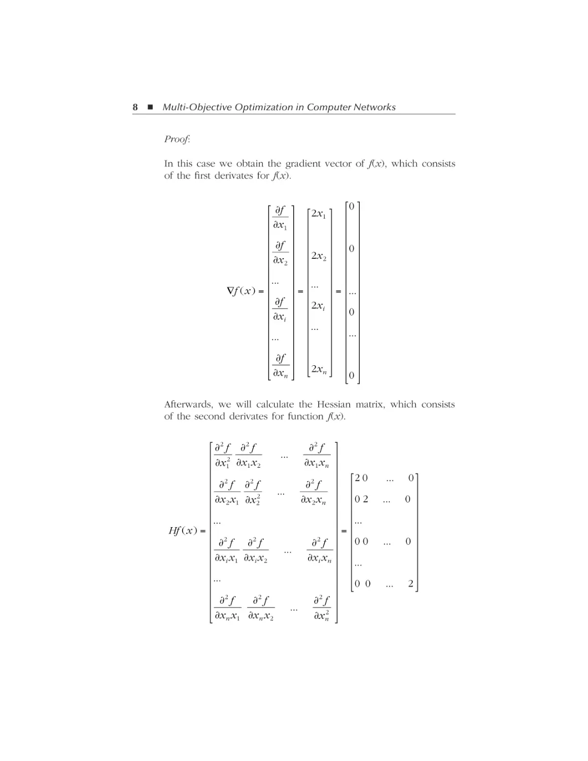
Proof:
In this case we obtain the gradient vector of f(x), which consists
of the first derivates for f(x).
⎡ ∂f ⎤
⎢ ∂x ⎥
⎢ 1⎥
⎢ ∂f ⎥
⎥
⎢
⎢ ∂x 2 ⎥
⎥
⎢
⎢... ⎥
⎥=
∇f ( x ) = ⎢
⎢ ∂f ⎥
⎢
⎥
⎢ ∂xi ⎥
⎢
⎥
⎢... ⎥
⎢
⎥
⎢ ∂f ⎥
⎢⎣ ∂xn ⎥⎦
⎡2x1 ⎤
⎢
⎥
⎢
⎥
⎢
⎥
⎢2x 2 ⎥
⎢
⎥
⎢
⎥
⎢... ⎥
⎢
⎥=
⎢2xi ⎥
⎢
⎥
⎢... ⎥
⎢
⎥
⎢
⎥
⎢
⎥
⎢2x ⎥
⎣ n⎦
⎡0 ⎤
⎢ ⎥
⎢ ⎥
⎢ ⎥
⎢0 ⎥
⎢ ⎥
⎢ ⎥
⎢ ⎥
⎢...⎥
⎢ ⎥
⎢0 ⎥
⎢ ⎥
⎢ ⎥
⎢...⎥
⎢ ⎥
⎢ ⎥
⎢ ⎥
⎢⎣0 ⎥⎦
Afterwards, we will calculate the Hessian matrix, which consists
of the second derivates for function f(x).
⎡ ∂2 f ∂2 f
∂2 f ⎤
...
⎥
⎢ 2
∂x1 xn ⎥
⎢ ∂x1 ∂x1 x 2
⎥
⎢ 2
2
∂2 f ⎥
⎢ ∂ f ∂ f
...
⎢ ∂x 2 x 1 ∂x 22
∂x 2 xn ⎥
⎥
⎢
⎥
⎢...
⎥=
Hf ( x ) = ⎢
⎢ 2
⎥
2
2
∂ f ⎥
⎢ ∂ f ∂ f
...
⎢ ∂xi x1 ∂xi x 2
∂xi xn ⎥
⎢
⎥
⎢...
⎥
⎢
⎥
2
2
⎢ ∂2 f
∂ f
∂ f ⎥
...
⎢
⎥
∂xn2 ⎥⎦
⎢⎣ ∂xn x1 ∂xn x 2
⎡2 0
⎢
⎢0 2
⎢
⎢....
⎢
⎢0 0
⎢
⎢...
⎢
⎢0 0
⎣
...
...
...
...
0⎤
⎥
0 ⎥
⎥
⎥
⎥
0⎥
⎥
⎥
⎥
2 ⎥⎦
AU8084_C001.fm Page 9 Wednesday, February 7, 2007 5:46 AM
Optimization Concepts 9
n
Because the Hessian matrix is positive, function y = f ( x ) =
∑x
2
i
i =1
is convex.
d. Let f(x) = ex.
Proof:
Substituting the value of the function in definition ⎡⎣ ∇f ( y ) − ∇f ( x )⎤⎦
y − x we get:
(
)
[∇f(y) – ∇f(x)] (y – x) = [ey – ex] (y – x)
Because x ≠ y, if x > y, we have ex > ey, and if y > x, we have ey > ex.
Then, the sign of [eye – ex] is the same sign of (y – x), the product
[eye – ex] (y – x) will always be positive, and therefore, function
f(x) = ex is strictly convex.
e. Let f(x) = ln x, with x > 0.
Proof:
Substituting the value of the function in definition ⎡⎣ ∇f ( y ) − ∇f ( x )⎤⎦
y − x we get:
(
)
[∇f(y) – ∇f(x)] (y – x) = [1/y – 1/x] (y – x)
=
( x − y )( y − x )
xy
( x − y )( y − x )
xy
will always be negative, and therefore, function f(x) = ln x is strictly
concave.
Because x ≠ y, if x > y or y > x, then the statement
AU8084_C001.fm Page 10 Wednesday, February 7, 2007 5:46 AM
10 Multi-Objective Optimization in Computer Networks
Proposition 1
(
)( )
ℜ; H is a convex
If f is
g f
If f is
g f
If f is
g f
If f is
g f
convex and g is increasing and convex, then function
Let g f x with f: H ⊂ ℜn
M and g: M ⊂ ℜ
subset of ℜn and M an interval of ℜ. Then:
(
(
(
(
)( x ) is convex.
convex and g is increasing and concave,
)( x ) is concave.
concave and g is increasing and convex,
)( x ) is convex.
concave and g is increasing and concave,
)( x ) is concave.
then function
then function
then function
Exercise
Probe whether the following functions are concave or convex.
⎛ n
⎞
f. Let y = f ( x ) = ln ⎜
xi ⎟ , of ℜn, with x positive.
⎝ i =1 ⎠
Proof:
∑
n
Because we have previously proven that function
∑x
i
is concave,
i =1
because function ln x is increasing and concave, applying propo-
⎛
sition 1, we have that y = f ( x ) = ln ⎜
⎝
⎛
g. Let y = f ( x ) = ⎜
⎝
Proof:
n
∑
i =1
n
∑
i =1
⎞
xi ⎟ is a concave function.
⎠
2
⎞
x i2 ⎟ , with x ε ℜn.
⎠
n
Because we have proven that function
∑x
2
i
is convex and func-
i =1
tion x2 is an increasing convex function, by proposition 1, we have
⎛
that y = f ( x ) = ⎜
⎝
n
∑
i =1
2
⎞
x ⎟ is a convex function.
⎠
2
i
AU8084_C001.fm Page 11 Wednesday, February 7, 2007 5:46 AM
Optimization Concepts 11
1.5 Minimum Search Techniques
Given a graph that could, for example, represent a computer network
connectivity scheme, there are different search techniques to find optimal
values to get from one point of the graph to another. The following section
is a discussion of how some of these search techniques work, more
specifically, the breadth first search, depth first search, and best first search
techniques.
1.5.1 Breadth First Search
This method (Figure 1.4) consists of expanding the search through the
neighboring nodes. In this case, the algorithm begins searching all the
directly connected nodes. The nodes through which it passes to reach
the goal node are stored in a queue, and once the last connected node
is reached, it starts removing from the queue and continues executing the
algorithm, expanding successively.
Figure 1.4 The different steps of a tree search using the Breadth First Search
method.
AU8084_C001.fm Page 12 Wednesday, February 7, 2007 5:46 AM
12 Multi-Objective Optimization in Computer Networks
The following is an example of the Breadth First Search algorithm:
Algorithm BFS(G, s)
L0
NULL
L0 insert_Last(s)
setLabel(s, VISITED)
i
0
while ¬Li.isEmpty()
NULL
Li +1
for all v ∈ Li.elements()
for all e ∈ G.incidentEdges(v)
if getLabel(e) = UNEXPLORED
w
opposite(v,e)
if getLabel(w) = UNEXPLORED
setLabel(e, DISCOVERY)
setLabel(w, VISITED)
Li +1.insertLast(w)
else
setLabel(e, CROSS)
i
i +1
end BFS
1.5.2 Depth First Search
This method (Figure 1.5) consists of expanding the search for the deepest
nonterminal node. This algorithm begins its search on a tree branch until
a goal node is reached. The nodes through which it passes to reach the
goal node are stored in a queue, and once it reaches the goal node, it
starts removing from the queue and continues executing the algorithm,
expanding in depth successively.
The Depth First Search algorithm is as follows:
Algorithm DFS(G, v)
Input graph G and a start vertex v of G
Output labeling of the edges of G
in the connected component of v
AU8084_C001.fm Page 13 Wednesday, February 7, 2007 5:46 AM
Optimization Concepts 13
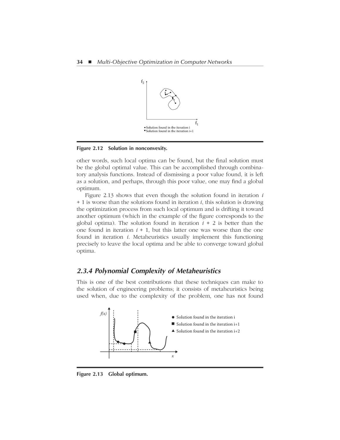
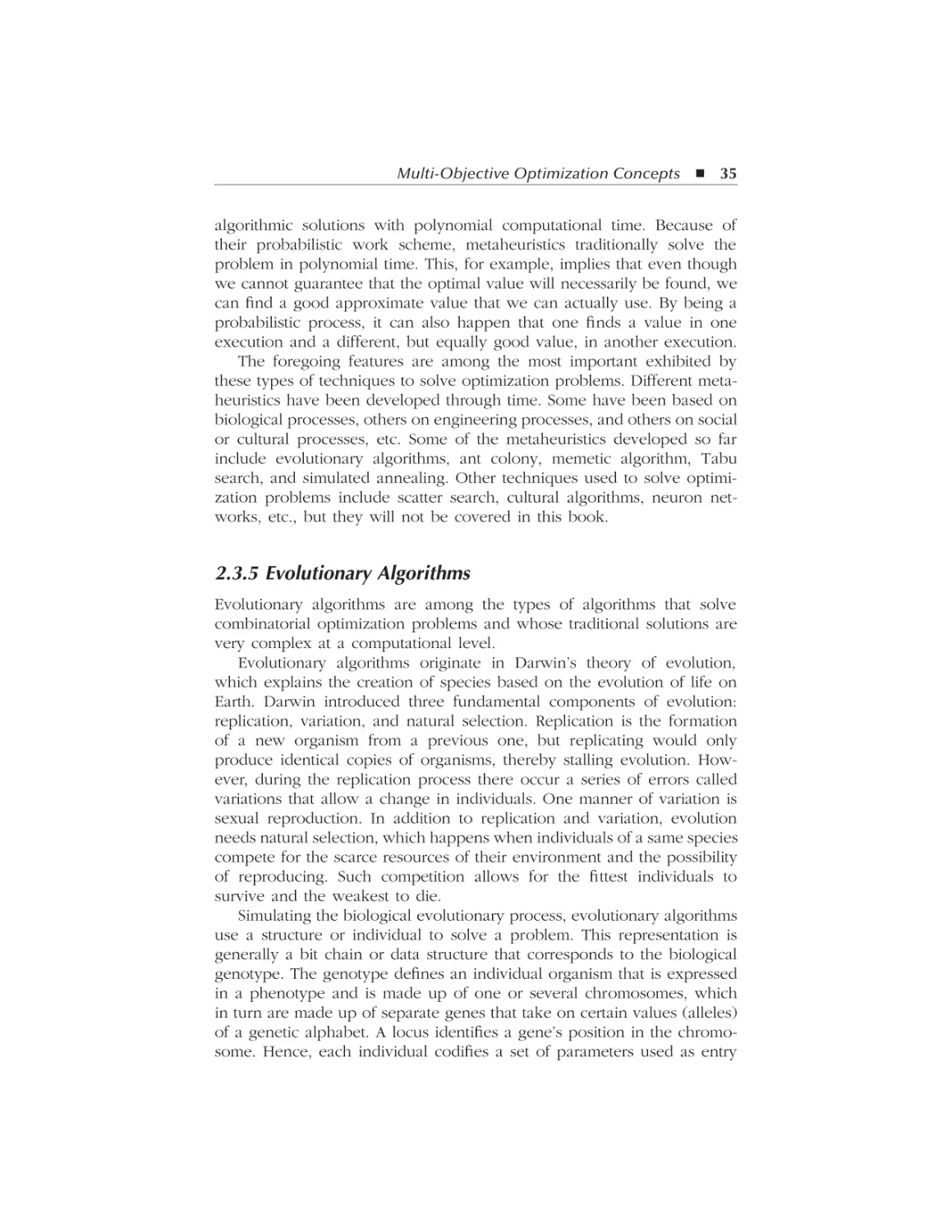
Figure 1.5 The different steps of searching a tree using the Depth First Search
method.
as discovery edges and back edges
setLabel(v, VISITED)
for all e
G.incidentEdges(v)
if getLabel(e) = UNEXPLORED
w
opposite(v,e)
if getLabel(w) = UNEXPLORED
setLabel(e, DISCOVERY)
DFS(G, w)
else
setLabel(e, BACK)
end DFS
AU8084_C001.fm Page 14 Wednesday, February 7, 2007 5:46 AM
14 Multi-Objective Optimization in Computer Networks
1.5.3 Best First Search
This technique (Figure 1.6) expands the search of the most promising
node; it can be considered an improved Breadth First Search. In this case,
each tree branch will have an associated weight, and the decision on
which direction to take in the search will be based on the value of such
weight.
Figure 1.6 The different steps of a tree search using the Best First Search.
AU8084_C002.fm Page 15 Thursday, February 15, 2007 5:24 AM
Chapter 2
Multi-Objective
Optimization Concepts
Optimization problems are normally stated in a single-objective way. In
other words, the process must optimize a single-objective function complying with a series of constraints that are based on constraints given by
the real world. A single-objective optimization problem may be stated as
follows:
Optimize [minimize/maximize]
f(X)
(1)
subject to
H(X) = 0
G(X) ≤ 0
In this case, the function to be optimized (minimize or maximize) is
f(X), where vector X is the set of independent variables. Functions H(X)
and G(X) are the constraints of the model.
For this problem we can define three sets of solutions:
1. The universal set, which in this case is all possible values of X,
whether feasible or nonfeasible.
15
AU8084_C002.fm Page 16 Thursday, February 15, 2007 5:24 AM
16 Multi-Objective Optimization in Computer Networks
2. The set of feasible solutions, which are all the values of X that comply
with the H(X) and G(X) constraints. In the real world, these variables
would be all possible solutions that can be performed.
3. The set of optimal solutions, which are those values of X that, in
addition to being feasible, comply with the optimal value (minimum
or maximum) of function f(X), whether in a specific [a, b] interval
or in a global context (–∞, ∞). In this case, one says that the set of
optimal solutions may consist of a single element or several elements,
provided that the following characteristic is met: f(x) = f(x'), where
x ≠ x'. In this case, we can say that there are two optimal values
to the problem when vector X = {x, x'}.
But in real life, it is possible that when wanting to solve a problem,
we may need to optimize more than one objective function. When this
happens, we speak of multi-objective optimization.
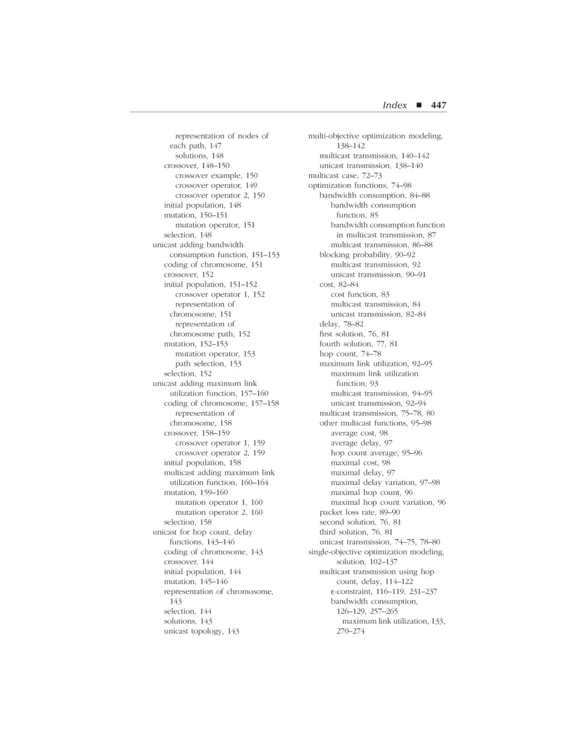
Figure 2.1 illustrates the topology of a network with five nodes and
five links, each with a specific cost, on which one wishes to transmit a
File Transfer Protocol (FTP) package from node 1 to node 5. The problem
consists of determining which of the two possible paths one must take
to transmit this package. In Figure 2.1, a cost has assigned between each
pair of nodes (link).
An analysis of Figure 2.1 shows that if we take the path given by links
(1, 2) and (2, 5), we would have a 2 jump path and a cost of 20 units.
If we take the path given by links (1, 3), (3, 4) and (4, 5), however, we
would have a 3 jump path and a cost of 15 units. In this specific case,
we can identify 2 feasible paths: the first one given by links (1, 2) and
(2, 5) and the second given by links (1, 3), (3, 4) and (4, 5). If we only
want to optimize (in this case minimize) the number of jumps, we can
see that the minimum value is 2 jumps, and it is given by path (1, 2) and
(2, 5). On the other hand, if we only want to minimize the cost objective
function, the minimum value would be 15 units and would be given by
path (1, 3), (3, 4) and (4, 5). This example shows that the optimal solution
2
10
FTP
10
1
5
5
5
3
Figure 2.1 Network topology.
5
4
AU8084_C002.fm Page 17 Thursday, February 15, 2007 5:24 AM
Multi-Objective Optimization Concepts 17
and value obtained depend on the objective function optimized, but with
the drawback that other results will only be contemplated as feasible
solutions, and not as optimal solutions.
In the previous example mentioned, if we optimize the number of
jumps function, we will be paying the highest cost of transporting the
package on this network. But it can also happen that the network
administrator wants to use the path with fewer jumps. For this reason,
we will state a model with more than one objective function, in which
the solution will consist of a set of optimal solutions, not a single optimal
solution.
A multi-objective optimization model may be stated as follows:
Optimize [minimize/maximize]
F(X) = {f1(X), f2(X), …, fn(X)}
(2)
subject to
H(X) = 0
G(X) ≥ 0
In this case, the functions to be optimized (whether minimize or
maximize) are the set of functions F(X), where the vector X is the set of
independent variables. Functions H(X) and G(X) are the constraints of the
model. The solutions found solve the objective solutions even when they
are conflicting, that is, when minimizing one function may worsen other
functions.
Stating and solving multi-objective optimization problems applied to
computer networks is the purpose of this book.
The first part of this chapter does a comparative analysis between
performing single-function and multiple-function optimization pr ocesses. Next, the chapter shows some of the traditional methods used
to solve multi-objective optimization problems, and finally, the last
section shows some metaheuristics to solve multi-objective optimization
processes.
2.1 Single-Objective versus Multi-Objective Optimization
When the optimization process is performed on a single-objective problem,
only one function will be minimized or maximized, and therefore, it will
AU8084_C002.fm Page 18 Thursday, February 15, 2007 5:24 AM
18 Multi-Objective Optimization in Computer Networks
be necessary to find a minimum or maximum, whether local or global,
for that objective function. When we speak of multiple objective functions,
we wish to find the set of values that minimize or maximize each of these
functions. Moreover, a typical feature of this type of problem is that these
functions may conflict with each other; in other words, when a function
is optimized, other functions may worsen. In multi-objective optimizations
we may find the following situations:
Minimize all objective functions.
Maximize all objective functions.
Minimize some and maximize others.
The following example, which serves as an introduction to the formal
theory of multi-objective optimization, explains the difference between optimizing a single function and optimizing multiple functions simultaneously.
Suppose you want to go from one city to another and there are different
means of transportation to choose from: airlines, with or without a nonstop
flight, train, automobile, etc. The actual duration and cost of the trip will
vary according to the option selected.
Table 2.1 and Figure 2.2 show cost and trip duration data for each,
independent of the means of transportation used.
An analysis of Table 2.1 or Figure 2.2 shows that by minimizing the
time function only, we will reach the city of destination in 1 h, but at the
highest cost ($600). By minimizing the cost function only, we will obtain
the most inexpensive solution ($100), but the duration of the trip will be
the longest (16 h).
By optimizing a single function, we obtain a partial view of the results,
when in the real problem it could happen that more than one function
influences the decision of which option to select.
However, if the problem is analyzed in a multi-objective context, the
idea of this optimization process is that the result is shown as a set of
optimal solutions (optimal Pareto front) for the different objective functions
jointly. This can be seen in the table. Later on, we will show that all of
these points are optimal in the multi-objective context. Therefore, if we
were to optimize both functions simultaneously, these would be the values
obtained.
Table 2.1
Multi-Objective Example
Option
1
2
3
4
5
6
7
8
9
10
Cost ($)
600
550
500
450
400
300
250
200
150
100
Time (hours)
1
2
3
4
5
6
8
10
14
16
AU8084_C002.fm Page 19 Thursday, February 15, 2007 5:24 AM
Multi-Objective Optimization Concepts 19
Time (Hours)
Optimal Pareto Front
20
15
10
5
0
0
100
200
300
400
500
600
700
Cost ($)
Figure 2.2 Optimal values in multi-objective optimization.
2.2 Traditional Methods
Solving the previous scheme can be quite complex. It requires optimizers
that instead of providing a single optimal solution, yield as a result a set
of optimal solutions, and such optimizers do not exist. In this section we
will introduce some methods to solve multi-objective optimization problems in a single-objective context. This way, we can use the existing
traditional optimizers. We will also show their drawbacks and constraints
when finding the multiple solutions.
There are several methods that can be used to solve multi-objective
problems using single-objective approximations. Some of them are
weighted sum, ε-constraint, weighted metrics, Benson, lexicographic, and
min-max, among others. All of these methods try to find the optimal
Pareto front using different approximation techniques.
Later on we will analyze methods that use metaheuristics to solve
multi-objective optimization problems in a real multi-objective context.
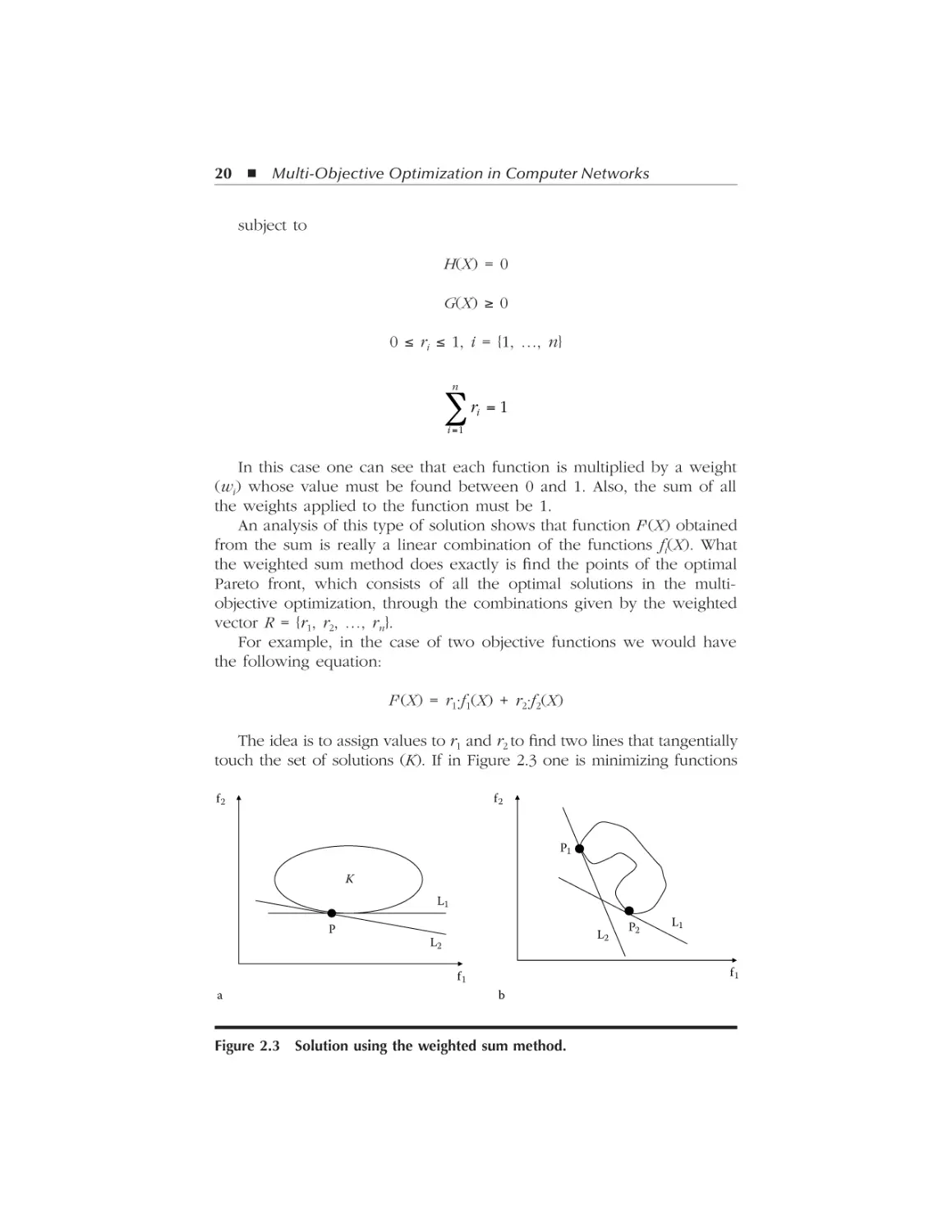
2.2.1 Weighted Sum
This method consists of creating a single-objective model by weighing
the n objective functions by assigning a weight to each the functions.
Through the weighted sum method, the multi-objective model (2) can
be restated in the following way:
Optimize [minimize/maximize]
n
'
F (X ) =
∑r * f (X )
i
i =1
i
(3)
AU8084_C002.fm Page 20 Thursday, February 15, 2007 5:24 AM
20 Multi-Objective Optimization in Computer Networks
subject to
H(X) = 0
G(X) ≥ 0
0 ≤ ri ≤ 1, i = {1, …, n}
n
∑r = 1
i
i =1
In this case one can see that each function is multiplied by a weight
(wi) whose value must be found between 0 and 1. Also, the sum of all
the weights applied to the function must be 1.
An analysis of this type of solution shows that function F'(X) obtained
from the sum is really a linear combination of the functions fi(X). What
the weighted sum method does exactly is find the points of the optimal
Pareto front, which consists of all the optimal solutions in the multiobjective optimization, through the combinations given by the weighted
vector R = {r1, r2, …, rn}.
For example, in the case of two objective functions we would have
the following equation:
F'(X) = r1·f1(X) + r2·f2(X)
The idea is to assign values to r1 and r2 to find two lines that tangentially
touch the set of solutions (K). If in Figure 2.3 one is minimizing functions
f2
f2
P1
K
L1
P
L2
L2
L1
f1
f1
a
P2
b
Figure 2.3 Solution using the weighted sum method.
AU8084_C002.fm Page 21 Thursday, February 15, 2007 5:24 AM
Multi-Objective Optimization Concepts 21
F1 and F2 through weights (r1, r2), by means of this method the optimization
process will find the crossing point P of the the two lines (linear combinations) L1 and L2. This point (P) would be the optimal solution found by
means of this method with weights (r1, r2) and that belongs to the optimal
Pareto front in the multi-objective context. If we were to change the values
of (r1, r2), we would find another point P that would also belong to the
optimal Pareto front.
If the set of solutions K is convex, any element of the optimal Pareto
front may be found by changing the values of weight vector R (r1 and
r2) in the example in Figure 2.3a. But this is only true when the set of
solutions K is convex. If solution set K is nonconvex (Figure 2.3b), there
are points of K that cannot be represented by a linear combination, and
therefore, such points cannot be found by means of this method.
For this method to work completely, the search space for the set of
solutions must be convex; otherwise, we cannot guarantee that all optimal
Pareto front points will be found. In a convex set of solutions, all elements
of the optimal Pareto front would have a p > 0 probability of being found,
but in nonconvex sets of solutions, this probability could be 0 for certain
elements of the optimal Pareto front.
Another drawback of this method deals with the range of values that
can be obtained in the functions optimized. The problem arises when the
ranges of the functions (a ≤ f1 ≤ b, c ≤ f2 ≤ d) have different magnitudes,
and especially when such differences are very large. If this happens, the
function having the highest range values will predominate in the result.
For example, if 0 < f1 < 1 and 0 < f2 < 1000, all solutions would be biased
to function f2, which is the function with the larger-sized range.
To solve the previous drawback, it would be necessary to normalize
the values of all objective functions, and this would generate a greater
effort to obtain the results of the optimization model.
Example
The following shows how we can apply this method to solve a
simple problem with two objective functions that we want to
minimize:
f1(x) = x4
f2(x) = (x – 2)4
subject to
–4 ≤ x ≤ 4
AU8084_C002.fm Page 22 Thursday, February 15, 2007 5:24 AM
22 Multi-Objective Optimization in Computer Networks
Functions
1400
1200
1000
F(X)
800
600
400
f2(x)
200
f1(x)
0
–4
–3
–2
–1
0
X
1
2
3
4
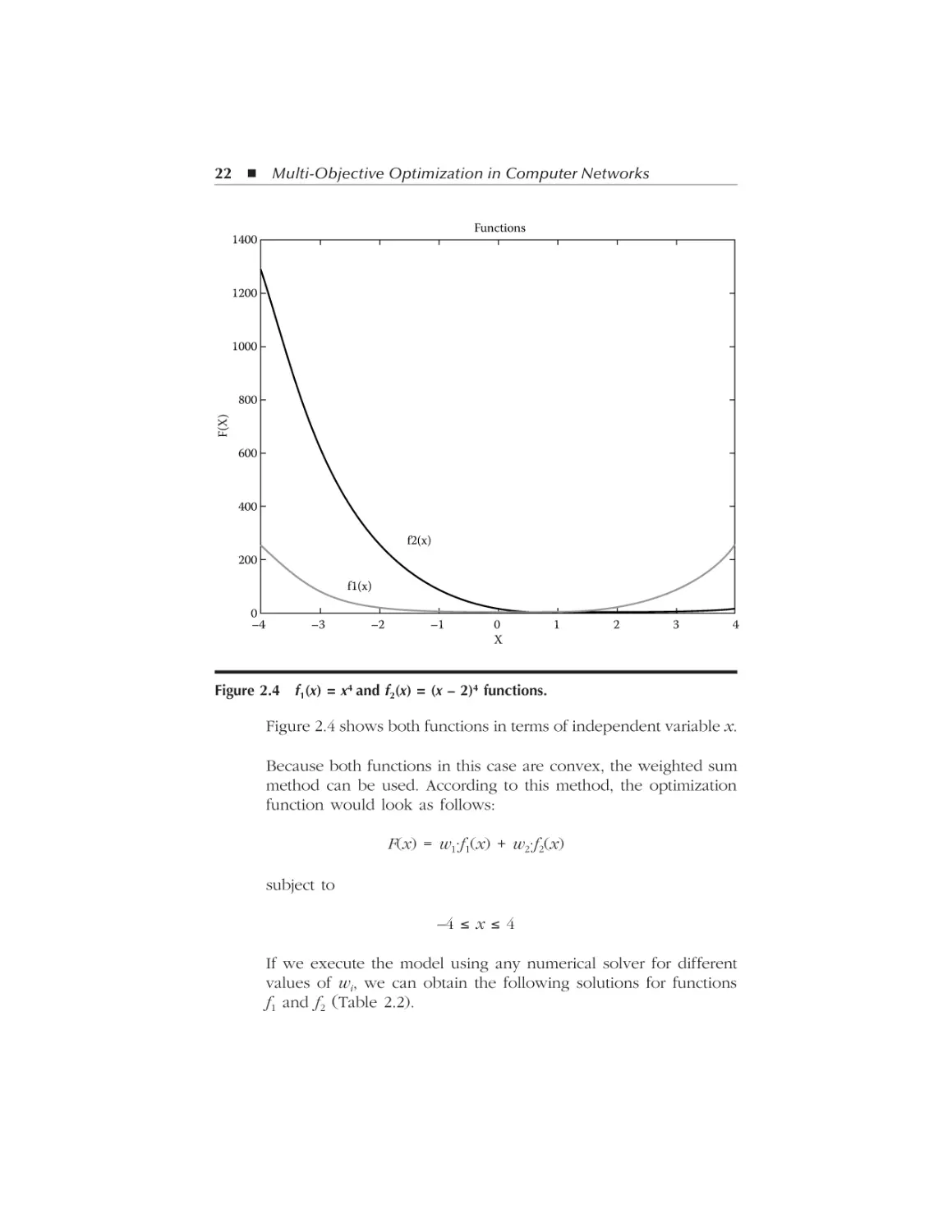
Figure 2.4 f1(x) = x4 and f2(x) = (x – 2)4 functions.
Figure 2.4 shows both functions in terms of independent variable x.
Because both functions in this case are convex, the weighted sum
method can be used. According to this method, the optimization
function would look as follows:
F(x) = w1·f1(x) + w2·f2(x)
subject to
–4 ≤ x ≤ 4
If we execute the model using any numerical solver for different
values of wi, we can obtain the following solutions for functions
f1 and f2 (Table 2.2).
AU8084_C002.fm Page 23 Thursday, February 15, 2007 5:24 AM
Multi-Objective Optimization Concepts 23
Table 2.2
Sol
Optimal Values with Weighted Sum
w1
w2
f1
f2
x
1
0
1
16.0
0
2.0
2
0.1
0.9
3.32
0.18
1.35
3
0.2
0.8
2.27
0.36
1.23
4
0.3
0.7
1.69
0.55
1.14
5
0.4
0.6
1.30
0.76
1.07
6
0.5
0.5
1
1
1
7
0.6
0.4
0.76
1.30
0.93
8
0.7
0.3
0.55
1.69
0.86
9
0.8
0.2
0.36
2.27
0.77
10
0.9
0.1
0.18
3.33
0.649
11
1
0
0
16
0
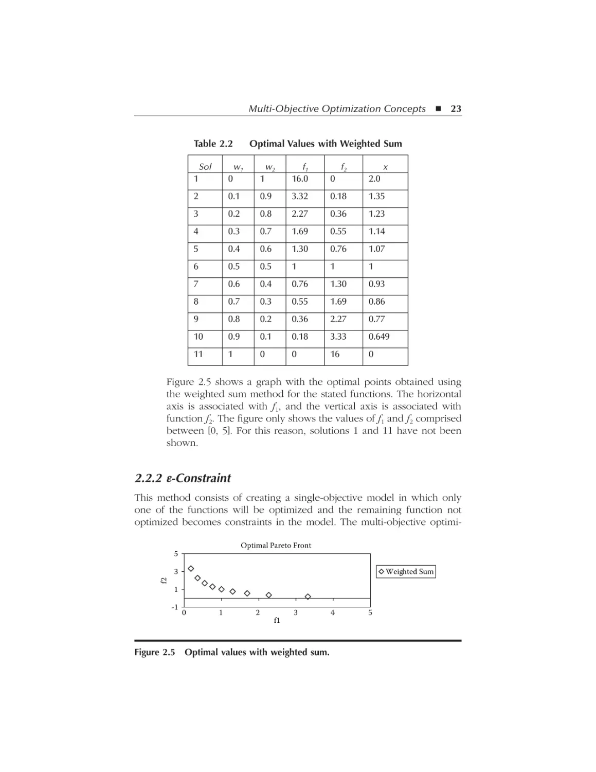
Figure 2.5 shows a graph with the optimal points obtained using
the weighted sum method for the stated functions. The horizontal
axis is associated with f1, and the vertical axis is associated with
function f2. The figure only shows the values of f1 and f2 comprised
between [0, 5]. For this reason, solutions 1 and 11 have not been
shown.
2.2.2 ε-Constraint
This method consists of creating a single-objective model in which only
one of the functions will be optimized and the remaining function not
optimized becomes constraints in the model. The multi-objective optimiOptimal Pareto Front
5
3
f2
Weighted Sum
1
-1
0
1
2
3
f1
Figure 2.5 Optimal values with weighted sum.
4
5
AU8084_C002.fm Page 24 Thursday, February 15, 2007 5:24 AM
24 Multi-Objective Optimization in Computer Networks
zation model shown above (2) can be restated through the ε-constraint
model as follows:
Optimize [minimize/maximize]
fi ( X )
(4)
subject to
fk(X) ≤ εk, k = 1, …, n and k ≠ i
H(X) = 0
G(X) ≤ 0
In this case, function fi(X) is the only one optimized; the other n – 1
functions become constraints and are limited by their corresponding
values.
The objective in this method consists of changing the values of ε of
each of the functions and, in this way, obtaining different optimization
values in function f i ( X ).
Figure 2.6 shows an example in which two functions (f1 and f2) are
optimized using the ε-constraint model. In the example, f2 is optimized
and f1 has become a constraint.
For the two solutions P1a and P1b shown in Figure 2.6, one observes
that when function f1 is a constraint with upper limit ε1a , the optimization
point found for f2 is P1a . When in the model the constraint value for f1 is
changed to εb1 , the optimization value found for f2 is P1b .
If we change the constraint value for f1, we can obtain different values
for f2, and therefore obtain the values of the optimal Pareto front.
One can also optimize the other functions by changing the objective
function to be optimized. In this case, the model would be
f2
P1a
P1b
ε1a
ε1b
Figure 2.6 Solution using the ε-constraint method.
f1
AU8084_C002.fm Page 25 Thursday, February 15, 2007 5:24 AM
Multi-Objective Optimization Concepts 25
Optimize [minimize/maximize]
f j(X )
(5)
subject to
fk(X) ≤ εk, k = 1, …, n and k ≠ j
H(X) = 0
G(X) ≤ 0
Here, function fi(X) is now a constraint and function fj(X) is the objective
function. In this case, if the values of the functions that act as constraint
are modified, one can find new values of the optimal Pareto front.
Through this method one can solve problems with convex and nonconvex solution spaces. The drawback is that one must know the problem
and the ε values for the results obtained in the optimization to be true
solutions to the specific problem.
Now we will show how this method can be applied to solve a simple
problem with two objective functions. As in the previous section, we need
to minimize both functions.
Example
Apply the ε-constraint method to the two previous functions.
Considering f2 as the objective function and f1 as the constraint,
the model would be
Min f2(x) = (x – 2)4
Min f2(x) = (x – 2)4
Subject to
x4 ≤ ε1
–4 ≤ x ≤ 4
In this case, given different values of ε1, we can obtain the following
solutions, again using any numerical solver, such as sparse nonlinear optimizer (SNOPT). (Table 2.3)
AU8084_C002.fm Page 26 Thursday, February 15, 2007 5:24 AM
26 Multi-Objective Optimization in Computer Networks
Table 2.3
Sol
Optimal Values with ε-Constraint
f1
ε1
f2
X
1
20.0
16
0
2
2
5.0
5
0.06
1.50
3
4.5
4.5
0.09
1.46
4
3.0
3.0
0.22
1.32
5
2.5
2.5
0.3
1.26
6
2.0
2.0
0.43
1.19
7
1.5
1.5
0.64
1.11
8
1.0
1.0
1.0
1.0
9
0.5
0.5
1.81
0.84
10
0.3
0.3
2.52
0.74
11
0.2
0.2
3.14
0.67
12
0
0
15.67
0.01
Figure 2.7 shows the optimal points obtained using the weighted
sum method and the ε-constraint method for the functions
discussed.
2.2.3 Distance to a Referent Objective Method
This method, like the weighted sum method, allows one to transform a
multi-objective optimization problem into a single-objective problem. The
function traditionally used in this method is distance.
Optimal Pareto Front
5
Weighted Sum
ε-Constraint
f2
3
1
-1
0
1
2
3
4
5
f1
Figure 2.7 Optimal values with ε-constraint versus weighted sum.
AU8084_C002.fm Page 27 Thursday, February 15, 2007 5:24 AM
Multi-Objective Optimization Concepts 27
Through the distance to a referent objective method, the multi-objective
method (2) can be rewritten as follows:
Optimize [minimize/maximize]
1r
⎡ n
r ⎤
'
F (X ) = ⎢
Z i − fi ( X ) ⎥
⎢⎣ i = 1
⎥⎦
∑
(6)
subject to
H(X) = 0
G(X) ≥ 0
1≤ r< ∞
In this method, one must set a Zi value for each of the functions. These
Zi values serve as referent points to find the values of the optimal Pareto
front by means of the distance function, as shown in Figure 2.8. Another
value that must be set is r, which will tell us the distance function to be
used. For example, if r = 1 is a solution equivalent to the weighted sum
method but without normalizing the values of the functions; if r = 2 one
would be using the Euclidean distance and if r
∞ the problem is called
the min-max or Tchebychev problem.
In the specific case of r
∞, the formula of the method can be
written as
Optimize [minimize/maximize]
F ' ( X ) = max ni =1 ⎡⎣ Zi − f i ( X ) ⎤⎦
(7)
subject to
H(X) = 0
G(X) ≤ 0
1≤r< ∞
Figure 2.8 shows examples of this method with two functions and
using r with values 1, 2, and ∞.
AU8084_C002.fm Page 28 Thursday, February 15, 2007 5:24 AM
28 Multi-Objective Optimization in Computer Networks
f2
f2
f2
A
A
A
Z
Z
B
B
f1
f1
a
Z
B
C
f1
b
c
Figure 2.8 Solution using the distance to a referent objective method.
As can be seen in Figure 2.8, this method is sensitive to the values of
Zi and r. In Figure 2.8a and 2.8b, one can see that through this method
it is not possible to find certain values of the optimal Pareto front between
A and B. However, through Figure 2.8c (with r
∞), it is possible to
find such points.
It may not be possible to find solutions in the optimal Pareto front for
certain values of r when the set of solutions is nonconvex. Therefore, if
the solution space is nonconvex or one is uncertain of it being convex,
one should use the method with r
∞. Finally, analyzing the graphs in
Figure 2.8, one can see that it is necessary to provide a good value of Z
as point of reference. Providing a poor point Z may result in divergence
instead of convergence toward optimal. This can be a problem due to
ignorance of the set of solutions.
2.2.4 Weighted Metrics
This method is similar to the previous one, with the difference that each
of the functions is normalized with respect to a weight. Using the weighted
metrics method, the multi-objective model (2) can be rewritten by adding
a weight-multiplying factor to each function to normalize their values.
Optimize [minimize/maximize]
1r
⎡ n
r ⎤
F (X ) = ⎢
w i Z i − fi ( X ) ⎥
⎢⎣ i = 1
⎥⎦
'
∑
Subject to
H(X) = 0
G(X) ≤ 0
(8)
AU8084_C002.fm Page 29 Thursday, February 15, 2007 5:24 AM
Multi-Objective Optimization Concepts 29
1≤ r< ∞
0 ≤ wi ≤ 1, i = {1, …, n}
n
∑w
i
=1
i =1
∞, the formula of the method can be
In the specific case of r
rewritten in the following way:
Optimize [minimize/maximize]
F ' ( X ) = max ni =1 ⎡⎣w i Zi − f i ( X ) ⎤⎦
(9)
Subject to
H(X) = 0
G(X) ≥ 0
1≤ r< ∞
0 ≤ wi ≤ 1, i = {1, …, n}
n
∑w
i
=1
i =1
This method has the same drawbacks as the method pr eviously
mentioned.
Example
Apply this method when r
functions:
∞ to the two previous objective
f1(x) = x4 y f2(x) = (x – 2)4
Min z = max [w1·|z1 – f1(x)|, w2·|z2 – f2(x)|]
Subject to
–4 ≤ x ≤ 4
If we execute the different values of wi and zi, we obtain the
following solutions: (Table 2.4)
AU8084_C002.fm Page 30 Thursday, February 15, 2007 5:24 AM
30 Multi-Objective Optimization in Computer Networks
Table 2.4
Sol
1
2
3
4
5
6
7
8
9
10
11
Optimal Values with Weighted Metrics
w1
w2
0
0.1
0.2
0.3
0.4
0.5
0.6
0.7
0.8
0.9
1
1
0.9
0.8
0.7
0.6
0.5
0.4
0.3
0.2
0.1
0
z1
0
0
0
0
0
0
0
0
0
0
0
z2
0
0
0
0
0
0
0
0
0
0
0
f1
f2
x
15.87
2.59
1.88
1.49
1.22
1
0.81
0.64
0.47
0.29
0
0
0.29
0.47
0.64
0.81
1
1.22
1.49
1.88
2.59
16
2.0
1.27
1.17
1.11
1.05
1
0.95
0.89
0.83
0.73
0
Figure 2.9 shows the optimal points obtained using the weighted
metrics method for the given functions and compares them with
the methods previously analyzed for this same example.
2.2.5 The Benson Method
This method is similar to the weighted metrics method, but in this case
the Z reference value has to be a feasible solution. Using the Benson
method, one can rewrite the multiobjective model (2) the following way:
Maximize
n
F '( X ) =
∑ max (0, Z − f ( X ))
i
i
i =1
Optimal Pareto Front
5
Weighted Sum
ε-Constraint
Weighted Metric
f2
3
1
-1
0
1
2
3
4
5
f1
Figure 2.9 Optimal values with weighted metric versus ε-constraint versus
weighted sum.
AU8084_C002.fm Page 31 Thursday, February 15, 2007 5:24 AM
Multi-Objective Optimization Concepts 31
Subject to
fi(X) ≤ Zi, i = 1, 2, …, n
H(X) = 0
G(X) ≤ 0
As can be seen, instead of minimizing, one is maximizing the resulting
function F' because this method works this way. In this case, objective
functions will be constraints by vector Z. Using this method, one can
obtain the Pareto front values in a nonconvex solution space. The drawback consists of finding good values for Z to find the points in the Pareto
front. One must know the space of feasible solutions of the problem being
solved or, in lack of it, generate such values randomly.
Example
Apply this method to the two objective functions already mentioned:
Min z = max [0, z1 – f1(x)] + [0, z2 – f2(x)]
Subject to
x4 ≤ z1
(x – 2)4 ≤ z2
–4 ≤ x ≤ 4
If we execute the method for different values of wi and zi, we
obtain the following solutions (Table 2.5):
Table 2.5
Method
Optimal Values with the Benson
Sol
1
2
3
4
5
z1
5
5
3
2
1
z2
2
1
4
5
3
f1
0.43
1
0.19
0.06
0.22
f2
2
1
4
5
3
x
0.81
1
0.59
0.51
0.68
AU8084_C002.fm Page 32 Thursday, February 15, 2007 5:24 AM
32 Multi-Objective Optimization in Computer Networks
Figure 2.10 shows the optimal points obtained using the weighted
metrics method for the given functions and compares them with
the methods previously analyzed for this same example.
f2
Optimal Pareto Front
Weighted Sum
ε-Constraint
Weighted Metric
Benson
5
4
3
2
1
0
0
1
2
3
4
5
f1
Figure 2.10 Optimal Benson values versus other methods.
After analyzing the different methods and applying them to a simple
case, we can say that these methods converge toward the optimal Pareto
front, although one must take into consideration the specific drawbacks
of each.
There are other traditional methods that can be used to solve these
multi-objective problems. They include the Keeney–Raiffa, compromise,
goal attainment, lexicographic, proper equality constraints, and goal programming methods and others that belong to the group of interactive
methods and will not be considered in this book.
2.3 Metaheuristics
Metaheuristics are considered high-level algorithmic strategies that are
used to guide other heuristics or algorithms in their search of the space
of feasible solutions of the optimal value (in the single-objective case)
and the set of optimal values (in the multi-objective case).
Traditionally, metaheuristics are good techniques to solve optimization
problems in which to accomplish convergence toward optimum one must
perform combinatorial analysis of solutions. The way to find some new
solutions that are unknown thus far and that belong to the set of feasible
solutions is done through the solutions previously known. These techniques accomplish the following functional features.
AU8084_C002.fm Page 33 Thursday, February 15, 2007 5:24 AM
Multi-Objective Optimization Concepts 33
2.3.1 Convergence toward Optimal
As the algorithm is executed, feasible solutions found must converge
toward the optimal value.
Figure 2.11 shows that when both functions (f1 and f2) are minimized,
the solutions found in iteration i + 1, compared to solutions found in
iteration i, converge to the optimal Pareto front. This does not mean that
every new solution obtained has to be better than the previous one, but
this process does have to show this behavior.
2.3.2 Optimal Solutions Not Withstanding Convexity
of the Problem
When metaheuristics function through combinatory analysis, any solution
belonging to the set of feasible solutions must have a probability p > 0
of being found. If a metaheuristic meets this requirement, then any optimal
solution may be found. In this case, it does not matter whether the set
of solutions is convex, because this technique will always find the optimal
solution.
Figure 2.12 shows that despite having a nonconvex set of solutions,
the solutions of iteration i + 1 can be found through combinatorial analysis
of the solutions obtained in iteration i.
2.3.3 Avoiding Local Optimal
There are heuristic algorithms that can find local optimal. If the problem
consists of finding local optima, one does not need to use metaheuristic
techniques to solve it. If the problem consists of finding global optimal,
such metaheuristic techniques are required to not fall in local optimal; in
f2
Solution found in the iteration i
Solution found in the iteration i+1
Figure 2.11 Convergence toward optimal.
f1
AU8084_C002.fm Page 34 Thursday, February 15, 2007 5:24 AM
34 Multi-Objective Optimization in Computer Networks
f2
Solution found in the iteration i
Solution found in the iteration i+1
f1
Figure 2.12 Solution in nonconvexity.
other words, such local optima can be found, but the final solution must
be the global optimal value. This can be accomplished through combinatory analysis functions. Instead of dismissing a poor value found, it is left
as a solution, and perhaps, through this poor value, one may find a global
optimum.
Figure 2.13 shows that even though the solution found in iteration i
+ 1 is worse than the solutions found in iteration i, this solution is drawing
the optimization process from such local optimum and is drifting it toward
another optimum (which in the example of the figure corresponds to the
global optima). The solution found in iteration i + 2 is better than the
one found in iteration i + 1, but this latter one was worse than the one
found in iteration i. Metaheuristics usually implement this functioning
precisely to leave the local optima and be able to converge toward global
optima.
2.3.4 Polynomial Complexity of Metaheuristics
This is one of the best contributions that these techniques can make to
the solution of engineering problems; it consists of metaheuristics being
used when, due to the complexity of the problem, one has not found
f(x)
Solution found in the iteration i
Solution found in the iteration i+1
Solution found in the iteration i+2
x
Figure 2.13 Global optimum.
AU8084_C002.fm Page 35 Thursday, February 15, 2007 5:24 AM
Multi-Objective Optimization Concepts 35
algorithmic solutions with polynomial computational time. Because of
their probabilistic work scheme, metaheuristics traditionally solve the
problem in polynomial time. This, for example, implies that even though
we cannot guarantee that the optimal value will necessarily be found, we
can find a good approximate value that we can actually use. By being a
probabilistic process, it can also happen that one finds a value in one
execution and a different, but equally good value, in another execution.
The foregoing features are among the most important exhibited by
these types of techniques to solve optimization problems. Different metaheuristics have been developed through time. Some have been based on
biological processes, others on engineering processes, and others on social
or cultural processes, etc. Some of the metaheuristics developed so far
include evolutionary algorithms, ant colony, memetic algorithm, Tabu
search, and simulated annealing. Other techniques used to solve optimization problems include scatter search, cultural algorithms, neuron networks, etc., but they will not be covered in this book.
2.3.5 Evolutionary Algorithms
Evolutionary algorithms are among the types of algorithms that solve
combinatorial optimization problems and whose traditional solutions are
very complex at a computational level.
Evolutionary algorithms originate in Darwin’s theory of evolution,
which explains the creation of species based on the evolution of life on
Earth. Darwin introduced three fundamental components of evolution:
replication, variation, and natural selection. Replication is the formation
of a new organism from a previous one, but replicating would only
produce identical copies of organisms, thereby stalling evolution. However, during the replication process there occur a series of errors called
variations that allow a change in individuals. One manner of variation is
sexual reproduction. In addition to replication and variation, evolution
needs natural selection, which happens when individuals of a same species
compete for the scarce resources of their environment and the possibility
of reproducing. Such competition allows for the fittest individuals to
survive and the weakest to die.
Simulating the biological evolutionary process, evolutionary algorithms
use a structure or individual to solve a problem. This representation is
generally a bit chain or data structure that corresponds to the biological
genotype. The genotype defines an individual organism that is expressed
in a phenotype and is made up of one or several chromosomes, which
in turn are made up of separate genes that take on certain values (alleles)
of a genetic alphabet. A locus identifies a gene’s position in the chromosome. Hence, each individual codifies a set of parameters used as entry
AU8084_C002.fm Page 36 Thursday, February 15, 2007 5:24 AM
36 Multi-Objective Optimization in Computer Networks
of the function under consideration. Finally, a set of chromosomes is
called the population. Just as in nature, varied evolutionary operators
function in the algorithm population trying to produce better individuals.
The three operators most used in evolutionary algorithms are mutation,
recombination, and selection.
2.3.5.1 Components of a General Evolutionary Algorithm
An evolutionary algorithm consists of the individuals, the population of
such individuals, and the fitness of each of the individuals and of the
genetic operators. We will explain in a very simple manner what each of
these components consists of.
2.3.5.1.1 Individual
As previously mentioned, an individual is the representation of a solution
to the problem. It includes bit chains, trees, graphs, or any data structure
adjusted to the problem being solved.
2.3.5.1.2 Population
A population is the set of individuals used by the algorithm to perform
the evolutionary process. The initial population generally is generated
randomly. Subsequently, it is modified iteratively by the operators with
the purpose of improving the individuals.
2.3.5.1.3 Aptitude Function (Fitness)
The aptitude function assigns each individual a real value that shows how
good such an individual’s adaptation is to its environment. In many
algorithms, especially those that optimize an objective, this fitness is equal
to the function optimized. In multi-objective algorithms, however, it is a
more elaborate function that takes into account other important factors in
this type of problem, for example, how many individuals are close among
them or how many individuals dominate a specific individual from another
population.
2.3.5.1.4 Genetic Operators
Genetic operators are applied on individuals of the population, modifying
them to obtain a better solution. The concept of population improvement
is very dependent on the problem. In a multi-objective problem, as
AU8084_C002.fm Page 37 Thursday, February 15, 2007 5:24 AM
Multi-Objective Optimization Concepts 37
previously mentioned, it is important to obtain a Pareto front as close to
the real one as possible. The three most common operators used in an
evolutionary algorithm are selection, recombination, and mutation.
2.3.5.1.4.1 Selection Operator — To obtain the next population,
genetic operators are applied to the best or fittest individuals (set of
parents). The roulette and tournament methods are the two most common
selection operators.
Roulette Method — Let Ω be the set of individuals that represent the
feasible solutions to the problem and f : Ω → ℜ the fitness function.
If x ∈Ω , then p( x ) =
f (x )
∑
f ( y)
defines the probability of individual x being
y ∈I
part of the set of parents.
Tournament Method — Let Ω be the set of individuals representing the
feasible solutions to the problem and f : Ω → ℜ the fitness function. The
set of parents S ⊂ Ω will be made by elements
x ∈ S such that
f ( x ) = max( f ( y )) y ∈S . To select the elements that will make up the set of
parents in this method, form small subsets (usually randomly).
2.3.5.1.4.2 Crossover Operator — Let Ω be the set of individuals
representing the feasible solutions to the problem. A crossover operator
is a function λ : Ωx Ω → χρ( Ω ) , where ρ( Ω ) is the set of all subsets of
Ω . The crossover function combines two elements of the current population to produce one or more offspring.
Figure 2.14 illustrates an example of the crossover operator, where,
by selection of two chromosomes (parents), one produces two offspring
chromosomes. It is possible that operators select more than two parents
and also produce more than two offspring.
2.3.5.1.4.3 Mutation Operator — Let Ω be the set of individuals representing the feasible solutions to the problem. A mutation operator is a
function β : Ω → Ω that takes an individual and transforms it into another.
Figure 2.15 illustrates an example of the mutation operator, where the
selected chromosome is altered to produce a new chromosome. Mutation
operators may alter more than one value in the chromosome.
AU8084_C002.fm Page 38 Thursday, February 15, 2007 5:24 AM
38 Multi-Objective Optimization in Computer Networks
Chromosome 1
Offspring 1
Chromosome 2
Offspring 2
Figure 2.14 Crossover function.
Chromosome
Chromosome
Figure 2.15 Mutation function.
2.3.5.2 General Structure of an Evolutionary Algorithm
In this book we will show other methaheuristics that are also used to
solve optimization problems, although greater emphasis will be placed
on evolutionary algorithms.
Figure 2.16 is the general structure of an evolutionary algorithm to
solve an optimization algorithm. Population P0 initiates in line 2. These
individuals are usually generated randomly.
Normally, the end condition of these algorithms is the performance of
a constant number of iterations. In certain cases, additional conditions are
introduced to control convergence of the algorithm to the optimal value
sought.
In P' one assigns the individuals that the selection operator takes from
Pt (line 4). In line 5 one selects from P' the individuals that will be the
parents of the next generation, that is, upon which one will apply the
crossover operators.
In line 6 one assigns a P'' to all the individuals produced with the
crossover operator. To a subset of such individuals one applies the
mutation operator (line 7). In line 9 one determines all the individuals of
the next generation (Pt+1). The individuals that continue into the next
generation are usually the individuals produced with the crossover and
mutation operators. However, certain algorithms maintain high-quality
individuals from previous generations.
Evolutionary algorithms comply with the following metaheuristic characteristics:
AU8084_C002.fm Page 39 Thursday, February 15, 2007 5:24 AM
Multi-Objective Optimization Concepts 39
t: iteration number.
Pt: Population in iteration t.
pc: Probability of performing crossover.
pm: Probability of performing mutation.
: Crossover operator.
ß: Mutation operator.
S: is a subset of the merger P’ and P’ obtained randomly
W: is a subset of P’’ obtained randomly
Selection Operator(): selection operator.
Begin:
1.
t=0
2.
Initialize P0
3.
While (condition of completion = = false)
4.
P’=Selection_Operator(Pt)
5.
Select a Subset S
6.
P' ' = { ( x) | x
7.
Select a Subset W
8.
P' ' ' = { ( x) | x W }
9.
Pt +1 = M
10.
t=t+1
11.
Pt
P' xP'
S}
P' '
P ' ' P' ' '
EndWhile
End.
Figure 2.16 Evolutionary algorithm.
Convergence to optimum: In the multi-objective case, this usually
takes place through the elitist or dominant functions. This way, one
can eliminate the poor individuals in each generation, while only
the good individuals remain. Because the process is iterative, one
expects each generation to present better individuals, guaranteeing
convergence toward optimal.
AU8084_C002.fm Page 40 Thursday, February 15, 2007 5:24 AM
40 Multi-Objective Optimization in Computer Networks
Optimal solutions not withstanding convexity of the problem: This
feature is accomplished by means of the combinatory analysis produced through the crossover and mutation operators.
Avoid local optima: This feature is accomplished through the values
of crossover and mutation probabilities. If the mutation probability
is high, the algorithm may converge toward local optima. Normally,
one recommends a value of 0.05 or 0.1 as a maximum. Another fact
that can help accomplish this feature is that there may be nonoptimal
individuals in the population, confirming what is illustrated in Figure
2.8 — that operators can produce a good individual from bad
individuals.
Polynomial complexity of metaheuristics: Being a probabilistic algorithm, its consequence is that its execution is nonexhaustive. For
more information about evolutionary algorithms, read [BAC00] and
[DEB01].
2.3.6 Ant Colony
Optimization based on ant colonies (ACO) is a metaheuristic approach to
solve combinatorial optimization problems. This metaheuristic is based on
the foraging behavior of certain ant species. The ants cooperate among
them to find food quickly. This cooperation is possible due to the indirect
communication of the ants.
Initially, scouting ants start searching for food sources. As they return
to the colony, they leave markers, called pheromones, on the path leading
to the food, which will lead other ants on the right track. The amount of
pheromones tells other ants how good a path is. When others follow the
path, they leave their own markers. As time goes by and more ants take
the path, the pheromones increase and, therefore, there is greater probability of the path being taken. In the absence of pher omones, ants
randomly scout for paths.
To explain this behavior, Dorigo [DOR04] designed an experiment that
served as a starting point for combinatorial optimization algorithms based
on ant colonies. This experiment established two paths, one long and
one short, between the colony and the food source. During these experiments he observed that ants tend to take the shorter path.
2.3.6.1 General Structure of an Ant Colony Algorithm
Figure 2.17 shows the pseudo-code of an algorithm based on ant colony.
Three procedures must be implemented: construct ant solutions, update
pheromones, and daemon actions. Dorigo et al. [DOR97] and [DOR04]
say that this metaheuristic does not specify whether these procedures
AU8084_C002.fm Page 41 Thursday, February 15, 2007 5:24 AM
Multi-Objective Optimization Concepts 41
Procedure ACOMetaheuristic
1.
ScheduleActivities
2.
ConstructAntsSolutions
3.
UpdatePheromones
4.
DaemonActions
5.
End-ScheduleActivities
end-Procedure
Figure 2.17 Ant colony algorithm.
must be executed fully parallel and independently or some sort of synchronization is needed.
2.3.6.1.1 Ant-Based Solution Contruction
This is the procedure responsible for managing the ants that concurrently
and asynchronically visit the adjacent states of the problem considered,
moving through the neighbors of the construction graph. The transition
from one state to the next is done using the pheromone trace and the
heuristic information of how to recalculate the value of the pheromones.
In this fashion, the ants construct the solutions that will later be evaluated
with the objective, so that the pheromone update can decide what amount
of pheromone to add.
2.3.6.1.2 Pheromone Trail Update
This is the procedure by which pheromone trails are modified. The
pheromone trail in the link, in the case of application to computer
networks, can increase by pheromone addition from passing ants or
decrease due to pheromone evaporation. From a practical point of view,
an increase in the amount of pheromone increases the possibility of an
ant using a component or link to build the solution. On the other hand,
pheromone evaporation is used to avoid too rapid convergence toward
suboptimal regions in the space of solutions, and would therefore favor
the exploration of new areas in the search space.
2.3.6.1.3 Daemon Actions
This procedure is used to implement centralized actions that cannot be
performed by ants. For example, local searches and processes that take
AU8084_C002.fm Page 42 Thursday, February 15, 2007 5:24 AM
42 Multi-Objective Optimization in Computer Networks
the best solutions and deposit additional pheromone on the links or
components.
For more information about ant colonies, read [DOR04].
2.3.7 Memetic Algorithm
A memetic algorithm is a combination of an evolutionary algorithm and
a local search. This combination is used to accomplish algorithms that
comply mainly with the following two characteristics: flexibility to incorporate specific heuristics to the problem and specialized operators, and
efficiency to produce acceptable solutions in less time.
Some authors see memetic algorithms as a simulation of cultural
evolution. This simulation is conceived as the transmission, imitation,
modification, and selection of the ideas, trends, methods, and all information that defines a culture. The minimum unit of cultural transmission
is called memes, and it is the equivalent of genders in biological evolution.
In the context of cultural evolution, memetic algorithms are defined as
those that make an analogy of cultural evolution.
Because the general scheme is basically the same, generically memetic
algorithms can be conceived as a hybrid of evolutionary algorithms and
local search, and the simulation of cultural evolution.
2.3.7.1 Local Searches
Before introducing the general structure of a memetic algorithm, one must
explain local searches.
A neighborhood function can be defined as follows: Let ( X , f ) (where
X is the set of feasible solutions and f is the function to be optimized)
be an instance of a combinatorial optimization problem. One neighborhood function is a mapping ξ : X → ρ( X ) (where ρ( X ) is the set of all
subsets of X), which defines for every solution i ∈ X a set ξ( i ) ⊆ X of
solutions that are in a certain sense close to i. The set ξ( i ) is the
neighborhood of solutions of i, and every
j ∈ξ( i ) is a neighbor of i.
One must assume that i ∈ξ( i ) is met for i ∈ X .
Once the neighborhood function is defined, one says that a local search
is a method that, starting from a solution, continually tries to find the best
solutions, searching among the neighbors (obtained by the neighborhood
function) of such solution.
AU8084_C002.fm Page 43 Thursday, February 15, 2007 5:24 AM
Multi-Objective Optimization Concepts 43
t: number of the iteration.
Pt: Population in iteration t.
pc: probability of performing a crossover.
pm: probability of performing a mutation.
: crossover operator.
ß: mutation operator.
: local search.
Selection Operator(): this is the selection operator.
Local_Search();
Begin:
1.
t=0
2.
Initialize P0
3.
While(Condition of Completion == false)
4.
P’=Selection_Operator(Pt)
5.
Select a Subset c
6.
P' ' = { ( x) | x
S}
7.
L = { ( x) | x
P' '}
7.
Select a Subset W
8.
P' ' ' = { ( x) | x W }
9.
L' = { ( x) | x
P' ' '}
9.
Pt +1 = M
L
10.
t=t+1
11.
Pt
P' '
L'
EndWhile
End.
Figure 2.18 Memetic algorithm.
2.3.7.2 General Structure of a Memetic Algorithm
Figure 2.18 is a general structure of a memetic algorithm. Operators used
in memetic algorithms are the same operators used in evolutionary algorithms. Memetic algorithms have the same characteristics as evolutionary
algorithms because they operate similarly, except for the local search
added to find better solutions in less time.
AU8084_C002.fm Page 44 Thursday, February 15, 2007 5:24 AM
44 Multi-Objective Optimization in Computer Networks
For more information about memetic algorithms, read [MER00] and
[MOS03].
2.3.8 Tabu Search
Tabu search (TS) is a metaheuristic procedure used for a local search
heuristic algorithm to explore the space of solutions beyond the simple
local optimum. It has been applied to a wide range of practical optimization applications, producing an accelerated growth of Tabu search
algorithms in recent years. Using TS or TS hybrids with other heuristics
or algorithmic procedures, one can establish new records to find better
solutions in programming, sequencing, resource assignment, investment
planning, telecommunications problems, etc.
Tabu search is based on the premise that to rate the solution to a
problem as intelligent, it must incorporate adaptative memory and sensible
exploration (responsive). Adaptative memory is the mechanism by which
the Tabu search technique ensures that solutions already found in previous
steps are not repeated. This mechanism stores solutions or steps taken to
find such solutions in a temporary memory. The use of adaptative memory
contrasts with “forgetful” designs, like the ones inspired on physics or
biology metaphors; with “rigid memory” designs, such as those exemplified
by branching and delimitation; and with its “cousins” in artificial intelligence (AI), which are normally not managed with this type of memory
schemes.
The importance of sensible exploration in Tabu search, whether in a
deterministic or probabilistic implementation, is based on the assumption
that a poor strategic selection may produce more information than a good
random selection.
In a memory-using system, a poor selection based on a strategy may
provide useful clues on how to make beneficial modifications to the
strategy.
The basis for a Tabu search (TS) can be described as follows. Given
a function f(x) to be optimized in a set X, TS starts as any local search,
going iteratively from one point (solution) to another until meeting a given
stopping criteria. Each x ∈ X has an associated neighborhood (or vicinity) N ( x ) ⊆ X , and every solution x ' ∈ N ( x ) can be reached from x by
means of an operation called movement.
TS exceeds local search using a modification strategy of N(x) as the
local search continues, replacing it by a neighborhood N*(x). As said in
our previous discussion, a key aspect in Tabu search is the use of memory
structures that help determine N*(x), and thus organize the way the space
is explored.
AU8084_C002.fm Page 45 Thursday, February 15, 2007 5:24 AM
Multi-Objective Optimization Concepts 45
The solutions admitted in N*(x) by these memory structures are determined in several ways. Specifically, the one that gives its name to Tabu
search identifies solutions found on a specified horizon (and, implicitly,
certain solutions identified with them) and excludes them from N*(x),
classifying them as Tabu. In principle, the Tabu terminology implies a
type of inhibition that incorporates a cultural connotation (i.e., something
that is subject to the influence of history and context), which can be
overcome under appropriate conditions.
The process by which solutions acquire a Tabu status has several facets
designed to promote an aggressive examination guided by new points.
One useful way to visualize and implement this process is to replace the
original evaluation of solutions by Tabu evaluations, which introduce
penalties to significantly discourage the election of Tabu solutions (i.e.,
that will preferably be excluded from the N*(x) neighborhood, according
to their dependence with the elements that make up the Tabu status).
Further, Tabu evaluations also periodically include incentives to stimulate
the selection of other types of solutions as a result of aspiration levels
and long-term influence.
TS profits from memory (and hence form the learning process) to
perform these functions. Memory used in TS may be explicit or based on
attributes, although both modes are not excluding. Explicit memory conserves complete solutions and typically consists of an elite list of solutions
visited during the search (or highly attractive but unexplored neighborhoods for such solutions). These special solutions are strategically introduced to expand N*(x), and thus present useful options not found in N(x).
The memory in TS is also designed to introduce a more subtle effect
in the search by means of a memory based on attributes that saves
information about solution attributes that change when moving from one
solution to another. For example, in a graph or network context, attributes
may consist of added nodes or arcs that are added, deleted, or replaced
by the movements executed. In more complex problem formulations,
attributes may represent function values. Sometimes attributes can also be
strategically combined to create other attributes through hashing procedures or IA-related segmentations, or by vocabulary construction methods.
2.3.8.1 General Structure of a Tabu Search
Figure 2.19 is the general structure of an algorithm through Tabu search.
This algorithm randomly finds an initial solution. Subsequently, and
although the exit condition has not been met, one finds new solutions
based on the existing one. These new solutions must be neighbors of the
current solution and also cannot be in the Tabu list. The Tabu list is used
AU8084_C002.fm Page 46 Thursday, February 15, 2007 5:24 AM
46 Multi-Objective Optimization in Computer Networks
F represents feasible solutions
x’ is the best solution found so far
c: iteration counter
T set of “tabu” movements
N(x) is the neighborhood function
1. Select x
F
2. x’ = x
3. c = 0
4. T =
5. If {N(x)
T} = , goto step 2
6. Otherwise, c
Select nc
c+1
{N(x)
T} such that: nc(x) = opt(n(x) : n
{N(x)
T)}
opt() is an evaluation function defined by the user
7. x
nc(x)
If f(x) < f(x’) then x’
x
8. Check stopping conditions:
Maximum number of iterations has been reached
N(x)
T=
after reaching this
step directly from step 2.
9. If stopping conditions are not met, update T
and return to step 2
Figure 2.19 Tabu search algorithm.
to ensure that solutions that have been visited are not visited again. For
more information about Tabu search, read [GLO97].
2.3.9 Simulated Annealing
Simulated annealing uses concepts originally described for statistical
mechanics. According to Aarts [AAR1989], annealing is a thermal process
AU8084_C002.fm Page 47 Thursday, February 15, 2007 5:24 AM
Multi-Objective Optimization Concepts 47
in which, through a thermal bath, low energy status is produced in a
solid. This physical process of annealing first softens the solid by heating
it at a high temperature and then cools it down slowly until the particles
rearrange themselves in a solid configuration. For each temperature
reached in the annealing process, the solid can reach thermal balance if
the heating occurs slowly. If cooling is done correctly, the solid reaches
its fundamental state in which particles form perfect reticulate and the
system is at its lowest energy level. However, if cooling takes place too
rapidly, the solid may reach metastable status, in which there are defects
in the form of high-energy structures.
The evolution of a solid in the thermal bath can be simulated using
the Metropolis algorithm based on the Monte Carlos techniques. In this
algorithm, thermal balance, described by the Boltzmann distribution, at a
given temperature is obtained by generating an elevated number of
transitions. Very briefly, the algorithm transitions from one step to the
next according to the following rules: if the energy in the produced state
is lower than the current state, then it accepts the produced state as the
current state; however, the produced state will be accepted with a determined probability (based on the Boltzmann distribution). This acceptance
probability is a function of temperature and the difference between the
two energy levels. The lower the temperature, the lower the probability
of transformation into a higher energy state, and the greater the energy
in the new state, the lower the probability of it being accepted. Therefore,
there is a possibility for every state to be reached, but with a different
probability, depending on temperature.
Simulated annealing can be seen as an iterative Metropolis algorithms
process that is executed with decreasing control parameter values (temperature). Conceptually, it is a search method by neighborhoods, in which
the selection criteria are the rules of transition of the Metropolis algorithm:
The algorithm randomly selects a candidate from the group that makes
up the neighborhood of the current solution. If the candidate is better
than it in terms of evaluation criteria, then it is accepted as the current
solution; however, it will be accepted with a probability that decreases
as the difference in cost between the candidate solution and the current
solution increases. When a candidate is rejected, the algorithm randomly
selects another candidate and the process is repeated.
Randomization in the selection of the next solution has been designed
to reduce the probability of being trapped in a local optimum. One has
been able to prove, as will be seen later, that simulated annealing is
capable of finding (asymptotically) the optimal solution with one probability. Although guaranteed, optimality will only be reached after an infinite
number of steps in the worst of cases. Therefore, asymptotic convergence
of the algorithm can only be approximated in practice, which, fortunately,
AU8084_C002.fm Page 48 Thursday, February 15, 2007 5:24 AM
48 Multi-Objective Optimization in Computer Networks
is done in polynomial time. Good functioning of the metaheuristic will
depend largely on the design of the neighborhood structure, the cooling
pattern, and the data structure.
In the early 1980s, working in the design of electronic circuits, Kirkpatrick et al. [KIR83] (and Cerny [CER85] doing independent work researching the Transmission Control Protocol (TCP)) considered applying the
Metropolis algorithm to some of the combinatorial optimization minimization problems that appear in these types of designs. They felt it was
possible to establish an analogy between the parameters in the thermodynamics simulation and the local optimization methods. Thus, they
related the following:
Thermodynamic
Configuration
Fundamental configuration
Energy of configuration
Temperature
Optimization
⇔
⇔
⇔
⇔
Feasible solution
Optimum solution
Cost of solution
?
A real meaning in the field of optimization does not correspond to
the physical concept of temperature; rather, it has to be considered a
parameter, T, which will have to be adjusted. In a similar way, one could
imagine the processes that take place when the molecules of a substance
start moving in the different energy levels searching for a balance at a
given temperature and those that occur in minimization (or maximization)
processes in local optimization. In the first case, once the temperature is
fixed, distribution of the particles in the dif ferent levels follows the
Boltzmann distribution; therefore, when a molecule moves, this movement
will be accepted in the simulation if the energy decreases, or will be
accepted with a probability that is proportional to the Boltzmann factor
in the opposite case. When speaking of optimization, once the T parameter
is set, we produce an alteration and directly accept the new solution when
its cost decreases. If the cost does not decrease, it is accepted with a
probability that is proportional to the Boltzmann factor.
This is the key of simulated annealing, as it is basically a local search
heuristic strategy where the selection of the new element in the neighborhood N(s) is done randomly. As was seen previously, the drawback
of this strategy is that if it falls in a local optimum during the search, it
is unable to leave it. To avoid this, simulated annealing allows certain
probability (lesser every time as we approach the optimal solution) passage
to worst solutions. Indeed, analyzing the behavior of the Boltzmann factor
as a function of temperature, we see that as temperature decreases, the
AU8084_C002.fm Page 49 Thursday, February 15, 2007 5:24 AM
Multi-Objective Optimization Concepts 49
probability of us accepting a solution that is worse than the previous one
also decreases rapidly.
The strategy that we will follow in simulated annealing will start with
a high temperature (with which we will allow changes to worse solutions
during the first steps, when we are still far from the global optimum),
and subsequently, we will decrease the temperature (reducing the possibility of changes to worse solutions once we are closer to the optimum
sought). This procedure gives rise to the name of the algorithm: annealing
is a metallurgical process (used, for example, to eliminate internal stress
in cold laminated steel) through which the material is rapidly heated and
then slowly cooled for hours in a controlled way.
2.3.9.1 General Structure of Simulated Annealing
Figure 2.20 shows the general structure of the algorithm through simulated
annealing. Input parameters for this algorithm are the initial temperature,
To, and the cooling velocity, α. This cooling velocity is associated with
Input (To, , Tf)
1. T
To
2. Sact
Initial_Solution
3. While T
Tf do
4.
Begin
5.
For cont
1 to L(T) do
6.
Begin
7.
Scand
8.
cost(Scand) – cost(Sact)
If (U(0,1) < e(-
9.
10.
Sact
11.
/T)
) or ( < 0) Then
Scand
End
12.
T
13.
End
14.
Select_Solution_N(Sact)
(T)
Write the best solutions of Sact visited.
Figure 2.20 Simulated annealing algorithm.
AU8084_C002.fm Page 50 Thursday, February 15, 2007 5:24 AM
50 Multi-Objective Optimization in Computer Networks
the way we update the value Ti+1 from Ti when the temperature decreases
after L(T) iterations.
An initial solution that belongs to the solution space Ω is generated
and, until the end of the process is reached, for every T one calculates,
a number L(T) tells the number of iterations (before the temperature
reduction) that a solution will combine. These new solutions found must
be in the neighborhood N(Sact) of the current one, which will replace
the current solution if it costs less or has a probability e(–δ/T). To calculate
this probability, generate a uniform random number [0, 1) that is represented as U(0, 1). Finally, the solution offered will be the best of all the
Sact visited. For more information about simulated annealing, read
[VAN89].
2.4 Multi-Objective Solution Applying Metaheuristics
As we have seen in previous sections, the use of traditional techniques
allows us to obtain optimal Pareto front points, yet some of these techniques have certain constraints. Something to bear in mind is that computer
network problems are usually NP problems. Hence, to obtain an optimal
solution one resorts to metaheuristics. Also bear in mind that the metaheuristics explained previously are aimed at providing a solution to singleobjective problems, and therefore must be adjusted to solve multi-objective
problems.
In the case of evolutionary algorithms, the Multi-Objective Evolutionary
Algorithm (MOEA) is an adaptation to solve multi-objective problems.
Similarly, other metaheuristic techniques can be adapted to address multiobjective problems. In this section we will discuss the MOEA technique.
There are different MOEA algorithms, which can be divided into elitist
(SPEA, PAES, NSGA II, DPGA, MOMGA, etc.) and nonelitist (VEGA, VOES,
MOGA, NSGA, NPGA, etc.). They can also be classified based on the
generation in which they were developed. The first generation includes
those that do not work with Pareto dominance (VEGA, among others)
and those that do work with the Pareto dominance concept (MOGA,
NSGA, NPGA, and NPGA 2, among others). The second generation
includes PAES, PESA, PESA II, SPEA, SPEA 2, NSGA II, MOMGA, and
MOMGA II, among others.
Because the purpose of this book is to show how metaheuristics solve
computer network problems, we will not provide an analysis of the
different evolutionary algorithms. One can consult some of these algorithms in books by [DEB01] and [COE02]. We will concentrate on the
application of the SPEA algorithm to solve multi-objective pr oblems
through MOEA.
AU8084_C002.fm Page 51 Thursday, February 15, 2007 5:24 AM
Multi-Objective Optimization Concepts 51
SPEA is a combination of new and previously used techniques to find
different optimal Pareto and parallel solutions. It shares the following
characteristics with other algorithms previously proposed: It saves the
nondominated solutions it has found so far in an external population,
thus implementing elitism. It uses the concept of Pareto dominance to
assign a fitness value to individuals. It does clustering [MOR80] to reduce
the number of nondominated solutions it has stored without destroying
the characteristics of the Pareto front outlined so far.
On the other hand, SPEA exclusively uses the following concepts: It
combines the above-mentioned three characteristics in a single algorithm
(so far they had always been proposed separately). It determines fitness
of an individual based solely on the solutions found in the population of
nondominated individuals; this way it is not relevant that members of the
general population dominate one another — all solutions are part of the
external set of nondominant solutions that participate in the selection. It
suggests a new method for inducing the formation of niches within the
population, thus preserving genetic diversity; this method is based on the
Pareto concept and does not require previous knowledge or determination
of any distance parameter (as in the radius of the niche in SF (sharing
function).
Figure 2.21 shows a pseudoalgorithm by means of SPEA.
2.4.1 Procedure to Assign Fitness to Individuals
One of SPEA’s characteristics is the way it assigns fitness to each individual.
The process in carried out so that the dominant and most characteristic
individuals have better fitness values. At the same time, the process is
thought to induce maintenance of genetic diversity and the obtaining of
solutions distributed in the complete Pareto front.
1. Begin
2.
Generate randomly the initial population P0 with size N
3.
Initialize the set PE as an empty set
4.
Initialize the generation t counter to 0
5.
While t < gmax
6.
Evaluate the objectives on the members of Pt and PEt
7.
Calculate the fitness of each of the individuals in Pt and PEt
8.
Make the environmental selection to conform the new extern population PEt+1
9.
Apply the selection operator by binary tournament with replacement on PEt+1.
10.
Apply the crossover and mutation operators on the selected population.
11.
Assign the new population to Pt+1.
12.
t t +1
13.
End While
14. End
Figure 2.21 SPEA algorithm.
AU8084_C002.fm Page 52 Thursday, February 15, 2007 5:24 AM
52 Multi-Objective Optimization in Computer Networks
The fitness assignment process takes place in two stages: First, a fitness
value is assigned to the individuals in set P' (external, nondominated set).
The members of P (set of general solutions) are then evaluated.
To assign fitness to members of the dominant set, each solution i ∈
P' is assigned a real value s i ∈[ 0, 1) , called strength, which is proportional
to the number of individuals j ∈P for which i j (that is, it is a measure
of the individuals dominated by i). Let n be the number of individuals in
P that are dominated by i, and let us assume that N is the size of P. Then
s i is defined as s i =
strength: F (i) =
n
. The fitness of i is inversely equal to its
N +1
1
.
si
The strength of an individual j ∈P is calculated as the sum of strengths
of all external, nondominated solutions i ∈ P' that dominate j. Add 1 to
that total to ensure that members of P' have better strength than the
members of P. Hence, the fitness of individual j is stated as f j =
1
1+
∑
si
,
ij j
where s j ∈[1, N ) .
The idea that underlies this mechanism is to always prefer individuals
that are closer to the optimal Pareto front and at the same time distribute
them through the whole feasible surface.
2.4.2 Reducing the Nondominated Set Using Clustering
In certain problems, the optimal Pareto front can be very large and may
even contain an infinite number of solutions. However, from the standpoint
of the network administrator, once a reasonable limit is reached, no
advantage is added by considering all the nondominated solutions found
until that point.
Furthermore, the size of the external population of nondominated
solutions alters the assignment procedure used by the algorithm. When
the external dominant set exceeds the established limit, the algorithm no
longer finds good solutions and also has greater probability of becoming
stagnant in a local minimum. For these reasons, a purge of the external
dominant set may not only be necessary, but even mandatory.
AU8084_C002.fm Page 53 Thursday, February 15, 2007 5:24 AM
Multi-Objective Optimization Concepts 53
One method that has been applied successfully to this problem and
has been studied extensively in the same context is the cluster analysis
[MOR80]. Overall, the cluster analysis partitions a collection of p elements
in q groups of homogenous elements, where q < p. Next, a characteristic
or centroid element for the cluster is selected.
The average link method [MOR80] has been shown to be an adequate
behavior in this problem and is the chosen one in [ZIT99] for the SPEA.
For this, it is also the method used in the implementations subsequently
described to control size of the external population of SPEA and prevent
losing good and significant solutions already found.
The clustering procedure is expressed in the following pseudocode
(Figure 2.22). In it we will show how SPEA can be applied to solve a
simple problem with the same two objective functions worked with the
traditional methods. As in the previous cases, we will minimize both
functions but, in this case, in a real multi-objective context.
Min F(X) = [f1(x) = x4, f2(x) = (x – 2)4]
Subject to
–4 ≤ x ≤ 4
2.4.2.1 Representation of the Chromosome
In this case, one chromosome stands exactly for a value of x in the
mathematical model. For this reason, it would be represented by a real
value. For example,
Chromosome
2.5
As selection operator we have chosen the roulette method, by means
of which we can obtain the chromosomes to execute the crossover and
mutation operators.
2.4.2.2 Crossover Operator
By means of the roulette method we select, for example, the following
chromosomes:
Chromosome 1
2.5
Chromosome 2
1.3
AU8084_C002.fm Page 54 Thursday, February 15, 2007 5:24 AM
54 Multi-Objective Optimization in Computer Networks
C: union of all clusters
i: one P’ chromosome
P’: nondominated population
P: dominated population
1. Clustering Procedure()
2. Begin
3. Initialize the set of clusters C; each individual i
Hence: C
i
P’ constitutes a different cluster.
i .
4. While C > N’
5.
d
Calculate the distance of all possible pairs of clusters where distance
1
c1 c 2
i
1
i1 c1 ,i2 c2
i2 of the two clusters c1 and c 2
between pairs of individuals of these 2 clusters. Metrics
C is the average distance
reflects the distance
between 2 individuals i1 e i2
6.
Determine two clusters c1 and c2 with minimum distance d and join them to
create a single one.
7. End While
8. Compute the reduced nondominated set, selecting an individual that is characteristic
of each cluster. The centroid (the point with minimum average distance with respect to
all other cluster points) is the characteristic solution.
9. End
Figure 2.22 Clustering procedure.
The crossover function takes the complete part of chromosome 1 (2)
and the decimal part of chromosome 2 (.3), combining these two values
to create the first offspring.
Offspring 1
2.3
The second offspring is created taking the complete part of chromosome 2 (1) and the decimal part of chromosome 1 (.5).
AU8084_C002.fm Page 55 Thursday, February 15, 2007 5:24 AM
Multi-Objective Optimization Concepts 55
Offspring 2
1.5
2.4.2.3 Mutation Operator
In this case, we select one chromosome. For example,
Chromosome
2.5
The mutation function adds or subtracts a value δ. If a chromosome
is selected for mutation, it randomly determines whether the value of δ
is added or subtracted. Suppose that in this case we have δ = 0.01 and
one must add randomly. The result will be
Chromosome
(2.5 + 0.01) = 2.51
Figure 2.23 shows the optimal points obtained by means of algorithm
SPEA for the stated functions and compares them to the traditional methods
previously analyzed in this same example. In this case, the following
values for the SPEA have been used:
Probability of crossover
0.7
Probability of mutation
0.1
Maximum population size
50
Maximum number of generations
20
In this case, with a single execution we have obtained multiple values
(represented by a filled-in circle) of the optimal Pareto front.
f2
Optimal Pareto Front
Weighted Sum
5
4
3
2
1
0
ε-Constraint
Weighted Metric
Benson
SPEA
0
1
2
3
4
5
f1
Figure 2.23 Optimal values of SPEA versus traditional methods.
AU8084_C002.fm Page 56 Thursday, February 15, 2007 5:24 AM
AU8084_C003.fm Page 57 Wednesday, February 7, 2007 6:31 AM
Chapter 3
Computer Network
Modeling
This chapter briefly introduces computer networks. Readers will learn
basic concepts and fundamentals that will allow them to understand the
application of metaheuristic techniques in multi-objective problems in
computer networks.
3.1 Computer Networks: Introduction
A computer network can be defined as a set of computers that interact
among the individual computers, sharing resources or information. Reference models have been developed in computer networks to establish the
functions of certain layers in the network for proper performance. The
following section introduces two reference models: the Open Systems
Interconnection (OSI) model established by the International Organization
for Standardization (ISO) and the Transmission Control Protocol/Internet
Protocol (TCP/IP) model.
3.1.1 Reference Models
Designing, implementing, and manufacturing computer networks and
related devices are very complex activities. Therefore, in order for this
technology to be successful and massively used, the manufacturers’ com57
AU8084_C003.fm Page 58 Wednesday, February 7, 2007 6:31 AM
58 Multi-Objective Optimization in Computer Networks
munity saw the need to follow a series of standards and common models,
allowing interoperability among the products of different brand names.
3.1.1.1 OSI Reference Model
The OSI reference model was developed by the ISO for international
standardization of protocols used at various layers. The model uses welldefined descriptive layers that specify what happens at each stage of data
processing during transmission. It is important to note that this model is
not a network architecture because it does not specify the exact services
and protocols that will be used in each layer.
The OSI model has seven layers. Each of the layers is described next.
3.1.1.1.1 Physical Layer
The physical layer is responsible for transmitting bits over a physical
medium. It provides services at the data-link layer, receiving the blocks
the latter generates when emitting messages or providing the bit chains
when receiving information. At this layer it is important to define the type
of physical medium to be used, the type of interfaces between the medium
and the device, and the signaling scheme.
3.1.1.1.2 Data-Link Layer
The data-link layer is responsible for transferring data between the ends
of a physical link. It must also detect errors, create blocks made up of
bits, called frames, and control data flow to reduce congestion. Additionally, the data-link layer must correct problems resulting from damaged,
lost, or duplicate frames. The main function of this layer is switching.
3.1.1.1.3 Network Layer
The network layer provides the means for connecting and delivering data
from one end to another. It also controls interoperability problems between
intermediate networks. The main function performed at this layer is
routing.
3.1.1.1.4 Transport Layer
The transport layer receives data from the upper layers, divides it in
smaller units if necessary, transfers it to the network layer, and ensures
that all the information arrives correctly at the other end. Connection
AU8084_C003.fm Page 59 Wednesday, February 7, 2007 6:31 AM
Computer Network Modeling 59
between two applications located in different machines takes place at this
layer, for example, customer–server connections through application logical ports.
3.1.1.1.5 Session Layer
This layer provides services when two users establish connections. Such
services include dialog control, token management (prevents two sessions
from trying to perform the same operation simultaneously), and synchronization.
3.1.1.1.6 Presentation Layer
The presentation layer takes care of syntaxes and semantics of transmitted
data. It encodes and compresses messages for electronic transmission. For
example, one can differentiate a device that works with ASCII coding and
one that works with binary-coded decimal (BCD), even though in both
cases the information transmitted is identical.
3.1.1.1.7 Application Layer
Protocols of applications commonly used in computer networks ar e
defined in the application layer. Applications found in this layer include
Internet surfing applications (Hypertext Transfer Protocol (HTTP)), file
transfer (File Transfer Protocol (FTP)), voice-over networks (Voice-over-IP
(VoIP)), videoconferences, etc.
3.1.1.2 TCP/IP Reference Model
The set of TCP/IP protocols allows communication between different
machines that execute completely different operating systems. This model
was developed mainly to solve interoperatibility problems between heterogeneous networks, allowing that hosts need not know the characteristics of intermediate networks.
The following is a description of the four layers of the TCP/IP model.
3.1.1.2.1 Network Interface Layer
The network interface layer connects the equipment to the local network
hardware, connects with the physical medium, and uses a specific protocol
to access the medium. This layer performs all the functions of the first
two layers in the OSI model.
AU8084_C003.fm Page 60 Wednesday, February 7, 2007 6:31 AM
60 Multi-Objective Optimization in Computer Networks
3.1.1.2.2 Internet Layer
This is a service of datagrams without connection. Based on a metrics,
the Internet layer establishes the routes that the data will take. This layer
uses IP addresses to locate equipment on the network. It depends on the
routers, which resend the packets over a specific interface depending on
the IP address of the destination equipment. Is equivalent to layer 3 of
the OSI model.
3.1.1.2.3 Transportation Layer
The transportation layer is based on two protocols: the User Datagram
Protocol (UDP) and the Transmission Control Protocol (TCP).
The UDP is a protocol that is not connection oriented: it provides
nonreliable datagram services (there is no end-to-end detection or correction of errors), it does not retransmit any data that has not been
received, and it requires little overcharge. For example, this protocol is
used for real-time audio and video transmission, where it is not possible
to perform retransmissions due to the strict delay requirements one has
in these cases.
The TCP is a connection-oriented protocol that provides reliable data
transmission, guarantees exact and orderly data transfer, retransmits data
that has not been received, and provides guarantees against data duplication. TCP does the task of layer 4 in the OSI model. All applications
working under this protocol require a value called port, which identifies
an application in an entity and through which the connection is made
with another application in another entity. TCP supports many of the most
popular Internet applications, including HTTP, Simple Mail Transfer Protocol (SMTP), FTP, and Secure Shell (SSH).
3.1.1.2.4 Application Layer
The application layer is similar to the OSI application layer, serving as a
communication interface, providing specific application services. There
are many protocols in this layer, among them FTP, HTTP, Internet Message
Access Protocol (IMAP), Internet Relay Chat (IRC), Network File System
(NFS), Network News Transport Protocol (NNTP), Network Time Protocol
(NTP), Post Office Protocol version 3 (POP3), SMTP, Simple Network
Management Protocol (SNMP), SSH, Telnet, etc.
3.1.2 Classification of Computer Networks Based on Size
Computer networks may be classified in several ways according to the
context of the study being conducted. The following is a classification by
AU8084_C003.fm Page 61 Wednesday, February 7, 2007 6:31 AM
Computer Network Modeling 61
Bluetooth
Cellular Network
Internet
Cellular
PC
Figure 3.1 PAN design.
size. Later we will specify to which of the networks we will apply the
concepts of this book.
3.1.2.1 Personal Area Networks (PANs)
Personal area networks are small home computer networks. They generally
connect the home computers to share other devices, such as printers,
stereo equipment, etc. Technologies such as Bluetooth are included in
PANs.
A typical example of a PAN is the connection to the Internet through
a cellular network. Here, the PC is connected via Bluetooth to the cell
phone, and through this cell phone we connect to the Inter net, as
illustrated in Figure 3.1.
3.1.2.2 Local Area Networks (LANs)
Local area networks generally connect businesses, public institutions,
libraries, universities, etc., to share services and resources such as Internet,
databases, printers, etc. They include technologies such as Ethernet (in
any of its speeds, today reaching up to 10 Gbps), Token Ring, 100VGAnyLan, etc.
The main structure of a LAN traditionally consists of a switch to which
one connects the switches where office PCs are connected. Corporate
servers and other main equipment are also connected to the main switch.
Traditionally, this main switch can be a third-layer switch or can go through
a router connected to the main switch, which connects the LAN to the
Internet. This connection from the LAN to the carrier, or Internet service
provider (ISP), is called the last mile.
Figure 3.2 shows a traditional LAN design.
AU8084_C003.fm Page 62 Wednesday, February 7, 2007 6:31 AM
62 Multi-Objective Optimization in Computer Networks
Core Switch
(Chassis)
Ethernet
Last Mile /
Man Connection
Edge Switch
PCs
Servers
PCs
Figure 3.2 LAN design.
3.1.2.3 Metropolitan Area Networks (MANs)
Metropolitan area networks cover the geographical area of a city, interconnecting, for instance, different offices of an organization that are within
the perimeter of the same city. Within these networks one finds technologies such as Asynchronous Transfer Mode (ATM), Frame Relay, xDSL
(any type of Digital Subscriber Line), cable modem, Integrated Services
Digital Network (ISDN), and even Ethernet.
A MAN can be used to connect different LANs, whether among them
or with a wide area network (WAN) such as Internet. LANs connect to
MANs with what is called the last mile, through technologies such as
ATM/Synchronous Digital Hierar chy (SDH), ATM/SONET, Frame
Relay/xDSL, ATM/T1, ATM/E1, Frame Relay/T1, Frame Relay/E1,
ATM/Asymmetrical Digital Subscriber Line (ADSL), Ethernet, etc. Traditionally, the metropolitan core is made up of high-velocity switches, such
as ATM switchboards over an SDH ring or SONET. The new technological
platforms establish that MAN or WAN rings can work over Dense Wave
Length Division Multiplexing (DWDM); they can go from a 10-Gbps current
to transmission velocities of 1.3 Tbps. These high-velocity switches can
also be layer 3 equipment, and therefore may perform routing.
Figure 3.3 shows a traditional MAN design.
3.1.2.4 Wide Area Networks (WANs)
Wide area networks span a wide geographical area. They typically connect
several local area networks, providing connectivity to devices located in
different cities or countries. Technologies applied to these networks are
the same as those applied to MANs, but in this case, a larger geographical
AU8084_C003.fm Page 63 Wednesday, February 7, 2007 6:31 AM
Computer Network Modeling 63
Metropolitan Backbone
Switch
ATM / Sonet
ATM / SDH
Last Mile /
Man Connection
(ATM, Frame Relay, etc.)
ADM
Sonet or SDH
Wan Connection
Figure 3.3 MAN design.
area is spanned, and therefore, a larger number of devices and greater
complexity in the analysis is required to develop the optimization process.
The most familiar case of WANs is the Internet, as it connects many
networks worldwide. A WAN design may consist of a combination of twolayer (switches) and three-layer (routers) equipment, and the analysis
depends exclusively on the layer under consideration. Traditionally, in
this type of network, it is normally analyzed under a layer 3 perspective.
Figure 3.4 shows a traditional WAN design.
In this book we will work with several kinds of networks. Chapters 4
and 5 discuss MANs and WANs. Said chapters do not include LANs because
problems found therein are simpler than problems found in MANs and
Wan Backbone
Switch / Router
Man Connections
Figure 3.4 WAN design.
AU8084_C003.fm Page 64 Wednesday, February 7, 2007 6:31 AM
64 Multi-Objective Optimization in Computer Networks
2
FTP
Server
FTP
Client
s=1
t=5
MAN / WAN
LAN
3
4
LAN
Figure 3.5 Unicast transmission.
WANs. Because Ethernet applies to both LANs and MANs, the same analysis
for the WANs can be used for the LANs. Chapter 6 covers wir eless
networks. Wireless networks do not use physical cables. This type of
analysis can be applied on PANs, LANs, MANs, and WANs.
3.1.3 Classification of Computer Networks Based on Type of
Transmission
Based on the type of transmission, computer networks fall into the
following classifications.
3.1.3.1 Unicast Transmissions
A transmission between a single transmitter and a single receiver is a
unicast transmission (Figure 3.5). Examples include applications such as
HTTP, FTP, Telnet, VoIP, point-to-point videoconferences, etc.
3.1.3.2 Multicast Transmissions
Transmission of information between one or several transmitters and
several receivers is called multicast transmission (Figure 3.6). Applications
such as multipoint videoconferences, video streaming, etc., are examples
of multicast transmissions.
3.1.3.3 Broadcast Transmissions
Transmission of information between a transmitter and all receivers in a
computer network is a broadcast transmission. Usually, these are control
messages or messages sent by certain applications for proper operation.
AU8084_C003.fm Page 65 Wednesday, February 7, 2007 6:31 AM
Computer Network Modeling 65
LAN
MAN / WAN
2
Video
Server
s=1
Video
Client 1
t1=5
4
Video
Client 2
LAN
3
t2=6
LAN
Figure 3.6 Multicast transmission.
This book will focus on unicast and multicast transmissions because
they are traditionally the ones intentionally generated by computer network users.
3.2 Computer Network Modeling
A computer network can be represented in a graph where the nodes
represent the devices for network interconnection, such as routers,
switches, modems, satellites, and others, where the edges represent the
physical connection links between such devices. In this book, the nodes
will represent the routers or switches (in Internet analysis they would be
routers).
The links will represent the media and physical transmission technologies between such routers or switches, for example, optical fiber, copper,
satellite links, microwaves, etc. In the case of communications, the nodes
could be the satellites and the links, the uplink and downlink.
In the next section we will introduce graph theory to represent and
model computer networks as graphs and, consequently, be able to apply
different graph algorithms to computer networks.
3.2.1 Introduction to Graph Theory
Graphs are a type of data structure that consists basically of two components: vertices or nodes, and the edges or links that connect them.
Graphs are divided into undirected graphs and directed graphs. Undirected graphs are made up of a set of nodes and a set of links that are
AU8084_C003.fm Page 66 Wednesday, February 7, 2007 6:31 AM
66 Multi-Objective Optimization in Computer Networks
Node
2
3
1
Link
6
4
5
Figure 3.7 Graph.
Node
2
3
1
Link
6
4
5
Figure 3.8 Directed graph.
not ordered node pairs. Figure 3.7 shows a undirected graph with six
nodes and eight links, in which we refer indistinctly, for example, to link
(1, 2) or (2, 1).
Directed graphs are a set of nodes and a set of edges whose elements
are ordered pairs of different nodes. Figure 3.8 shows a directed graph
(also with six nodes and eight links) with the following links: {(1, 2), (1,
4), (2, 3), (2, 5), (3, 6), (4, 3), (4, 6), (5, 6)}. In this case, we see that
there is a link (1, 2) but not a link (2, 1). For link (2, 1) to exist, it would
have to be explicit in the set of links.
Because we can represent a computer network through graphs, we
can use different algorithms applied to graphs (shortest path, shortest path
tree, minimum spanning tree, maximum flow, breadth first search, depth
first search, etc.) to optimize resources in the computer networks.
3.2.2 Computer Network Modeling in Unicast Transmission
In the unicast case the network is modeled as a directed graph G = ( N , E ),
where N is the set of nodes and E is the set of links. n denotes the
AU8084_C003.fm Page 67 Wednesday, February 7, 2007 6:31 AM
Computer Network Modeling 67
number of network nodes, i.e., n = N . Among the nodes, we have a
source s ∈ N (ingress node) and a destination t ∈ N (egress node).
Let (i, j ) ∈ E be the link from node i to node j. Let f ∈ F be any unicast
flow, where F is the flow set. We denote the number of flows by |F|.
Let cij be the weight of each link (i, j). Let bwf be the traffic demand of
a flow f from the ingress node s to the egress node t.
Figure 3.9a illustrates a computer network for unicast transmissions.
We can see that the set of nodes N is {1, 2, 3, 4, 5}, and therefore, n =
|N| = 5. The set of links E is {(1, 2), (1, 3), (2, 5), (3, 4), (4, 5)}. Because
this graph is a directed graph, there is no possibility of transmitting from
node 2 to node 1, because link (2, 1) is not a part of set E. G = (N, E)
is the graph that represents the network. The nodes, for example, would
represent the routers and the links, the fiber optics or the terrestrial or
satellite microwave connections. In this example, the origin or transmitter
node is node 1 (labeled s) and the destination node or receiver is node
5 s (labeled t).
In this type of network we suppose that origin as well as destination
nodes are connected to a LAN such as Ethernet, for example, to which
are connected the clients or servers that are transmitting the information.
In Figure 3.9b, both the origin node s and the destination node t are
connected to an Ethernet LAN, whether through a hub or a switch.
Each link in the networks is assigned a weight. In this example, cij
stands for the weight of each link. The weight can mean a delay in
transmission on such link, the linking capacity, the available capacity, the
cost of transmitting the information through that link, etc.
Finally, we find that computer networks transmit the traffic produced
by certain applications. In this book, when we talk about applications,
we generally refer to applications over IP, because this is the transmission
protocol on the Internet. For example, these unicast applications can be
FTP for file transfers, HTTP for surfing, Telnet to emulate terminals, HTTPsecure, HTTP, SSH-secure Telnet, VoIP for telephone call transfer over IP,
videoconferences over IP, video streaming, etc. In this example, we have
established a single flow |F| = 1, which is an FTP transmission from the
2
c12
FTP
f1
c25
s=1
a
c34
c45
3
4
FTP
Client
t=5
c13
c45
3
c25
s=1
t=5
c13
2
c12
FTP
Server
c34
4
b
Figure 3.9 Computer network modeling in unicast transmission.
AU8084_C003.fm Page 68 Wednesday, February 7, 2007 6:31 AM
68 Multi-Objective Optimization in Computer Networks
origin node s to destination node t. The FTP flow is shown as f1, and the
set of flows would consist of a single element, that is, F = {f1}.
The path through which the flow will be transmitted from the emitting
node to the receiving node will be determined by a routing algorithm.
In this section, we have shown how the topology of computer networks
transmitting unicast applications through graphs can be represented. In
later chapters, this modeling will help us develop the optimization models
at the routing level.
3.2.3 Computer Networks Modeling in Multicast Transmission
As we had previously mentioned, there are other types of applications
that transmit their data to several destination modes. These transmissions
are called multicast transmissions.
In the multicast case, the network can be modeled as a dir ected
graph G = ( N , E ) , where N is the set of nodes and E is the set of links.
n denotes the number of network nodes, i.e., n = N . Among the nodes,
we have a source s ∈ N (ingress node) and some destinations T (the set
of egress nodes). Let t ∈T be any egress node. Let (i, j ) ∈ E be the link
from node i to node j. Let f ∈ F be any multicast flow, where F is the
flow set and T f is the egress node subset for the multicast flow f. We
use|F|to denote the number of flows. Note that T =
Tf .
∪
f ∈F
Figure 3.10a shows a computer network for multicast transmission. In
this figure we can see that the set of nodes N is {1, 2, 3, 4, 5, 6}, and
therefore, n = |N| = 6. The set of links e is {(1, 2), (1, 3), (1, 4), (2, 5),
(3, 6), (4, 5), (4, 6)}. The graph that represents the networks is G = (N,
E). In this example, the origin or transmitter is node 1 (labeled s) and the
set of destination or receiving nodes consists of nodes 5 and 6 (labeled
t1 and t2, respectively).
c12
Video
f1
s=1
c14
2
4
c25
t1=5
c45
s=1
c14
2
4
c46
Video
Client 1
t1=5
c45
c46
c13
Video
Client 2
c13
3
a
c12
Video
Server
c25
c36
t2=6
3
c36
t2=6
b
Figure 3.10 Computer network modeling in multicast transmission.
AU8084_C003.fm Page 69 Wednesday, February 7, 2007 6:31 AM
Computer Network Modeling 69
As in the unicast case, in this type of network we assume that the
origin and destination nodes are connected to a LAN such as, for example,
Ethernet, to which are connected the clients or servers performing the
transmission of information (Figure 3.10b). The origin router s and the
destination routers t1 and t2 are connected to a LAN Ethernet network
through a hub or switch. Like in the unicast case, the weight of each link
is represented by cij.
Examples of multicast applications include multipoint videoconferences, multipoint video streaming, multipoint audio conferences, etc. In
this example, we have one single flow |F| = 1 that is a video-streaming
transmission from origin node s to destination nodes t1 and t2. This videostreaming flow we represent as f1; the set of flows F would consist of a
single element F = {f1} and T = Tf.
One can see that the modeling of a network for multicast transmission
is similar to the unicast case, with the difference that the flow of information will be received by multiple destinations.
AU8084_C003.fm Page 70 Wednesday, February 7, 2007 6:31 AM
AU8084_C004.fm Page 71 Friday, February 16, 2007 5:49 AM
Chapter 4
Routing Optimization in
Computer Networks
4.1 Concepts
4.1.1 Unicast Case
To solve an optimization problem in computer networks, we need to
define a variable that will tell us the route through which the flow of
information will be transmitted. We will define the variables vector X ijf
as follows:
⎧⎪1, if link ( i , j ) is used for flow f
X ijf = ⎨
⎪⎩0, if link ( i , j ) is not used for flow f
This means that the variables vector X ijf is 1 if link ( i, j) is used to
transmit flow f; if it cannot be used, the vector is 0. In Figure 4.1 we
see that there are two possible routes to go from origin node 1 to
destination node 5. The first route is through links (1, 2) and (2, 5).
The second path is through links (1, 3), (3, 4), and (4, 5). Assuming
the first path ((1, 2), (2, 5)) has been selected as the r oute through
1
1
which to transmit flow f1, X 12
= 1 and X 25
= 1. Because links (1, 3), (3,
4), and (4, 5) are not used, the values of vector X ijf for these equal 0
(Figure 4.1).
Table 4.1 summarizes the parameters used for the unicast case.
71
AU8084_C004.fm Page 72 Friday, February 16, 2007 5:49 AM
72 Multi-Objective Optimization in Computer Networks
1
X 12
1
FTP
f1
X 125 1
2
1
1
X 13
5
0
3
4
1
X 34
X 145
0
0
Figure 4.1 Computer network optimization in unicast transmission.
Table 4.1
Parameters Used for the Unicast Case
Terms
Definition
G (N, E)
N
E
s
t
(i, j)
F
f
Graphs of the topology
Set of nodes
Set of links
Ingress node
Egress node
Link from node i to node j
The flow set
Any unicast flow
Indicates whether the link (i, j) is used for flow f with destination
to the egress node t
The available capacity of each link (i, j)
The traffic demand of a flow f
X ijf
cij
bwf
4.1.2 Multicast Case
For the multicast case, we must also define a variable that shows us
whether the link is used to transmit a specific flow.
We will define the variables vector X ijtf as follows:
⎧⎪1, if link ( i , j ) is used for flow f with destination t
X ijtf = ⎨
⎪⎩0, if link ( i , j ) is not used for flow f with destination t
This means that variable X ijtf is 1 if link (i, j) is used to transmit multicast
flow f with destination node t, which belongs to the set of destination
nodes Tf. If it is not used, it is 0. In Figure 4.2 we can see that there are
four possible trees to go from origin node 1 to destination nodes 5 and
6. The first tree consists of paths {(1, 2), (2, 5)} and {(1, 3), (3, 6)}. The
second tree consists of {(1, 4), (4, 5)} and {(1, 4), (4, 6)}. The third tree
AU8084_C004.fm Page 73 Friday, February 16, 2007 5:49 AM
Routing Optimization in Computer Networks 73
51
X 25
0
51
X 12
Video
f1
1
61
X 13
Source: s = 1
2
0
51
1
X 14
61
1
X 14
0
4
5
51
1
X 45
61
1
X 46
3
61
0
X 36
6
Destinations: t 1 = 5 and t 2 = 6
Figure 4.2 Computer network optimization in multicast transmission.
consists of paths {(1, 2), (2, 5)} and {(1, 4), (4, 6)}. Finally, the fourth tree
consists of paths {(1, 4), (4, 5)} and {(1, 3), (3, 6)}. Assuming that the
second tree was selected ({(1, 4), (4, 5)} and {(1, 4), (4, 6)}) as the tree
51
61
to transmit multicast flow f1, X 14
= 1 and X 14
= 1 , because both links are
used to transmit flow f1 with destination nodes 5 and 6. Because links (1,
2), (2, 5), (1, 3), and (3, 6) are not being used, the values of vector X ijtf
for these links for both destination nodes 5 and 6 (Figure 4.2) are zero.
Variables corresponding to the links through which one cannot reach a
specific destination are not shown in Figure 4.2; for example, vari61
able X 45
= 0 , because it is impossible to reach node 6 through link (4, 5).
Table 4.2 summarizes the parameters used for the multicast case.
Table 4.2
Parameters Used for the Multicast Case
Terms
Definition
G(N, E)
N
E
S
T
(i, j)
F
f
Tf
Graphs of the topology
Set of nodes
Set of links
Ingress node
Set of egress nodes or any egress node
Link from node i to node j
The flow set
Any multicast flow
The egress node subset for the multicast flow f
Indicates whether the link (i, j) is used for flow f with destination
to the egress node t
The available capacity of each link (i, j)
The traffic demand of a flow f
X ijtf
cij
bwf
AU8084_C004.fm Page 74 Friday, February 16, 2007 5:49 AM
74 Multi-Objective Optimization in Computer Networks
4.2 Optimization Functions
In this section we will define certain functions that will later be used for
multi-objective optimization. This book will show some of the functions
most commonly used, but we are not attempting an exhaustive analysis
of all possible functions that can be considered.
4.2.1 Hop Count
4.2.1.1 Unicast Transmission
The first function to be analyzed is hop count. This function represents
the number of links through which packets must pass from the time they
leave the origin node until they reach the destination node.
Figure 4.3 shows that there are two possible paths to carry the flow
of information f1 (File Transfer Protocol (FTP)) between origin node 1
and destination node 5: The first path is formed by links (1, 2) and (2,
5), and therefore, the number of hops to be taken by the packets is 2.
The second path is formed by links (1, 3), (3, 4), and (4, 5) and, in this
case, the number of hops is 3.
If we use the number of hops as an optimization function, then the
path chosen to transmit the packets from origin node 1 to destination
node 5 will be the first path.
The routing protocol that works with the hops function to calculate
the shortest path is called the Routing Internet Protocol (RIP). This protocol
is used mainly in small metropolitan area networks (MANs) or wide area
networks (WANs) or in routing in local area networks (LANs) through the
virtual LANs (VLANs).
To mathematically describe the hop count function we will use an
example. In Figure 4.3 we have the variables X ijf describing the paths. If
we want to describe the paths mentioned above under these variables,
we could say that the number of hops for the first path would be given
1
X 12
1
FTP
f1
X 125 1
2
1
1
X 13
5
0
3
4
1
X 34
Source: s = 1
X 145
0
0
Destination: t = 5
Figure 4.3 Hop count function in unicast transmission.
AU8084_C004.fm Page 75 Friday, February 16, 2007 5:49 AM
Routing Optimization in Computer Networks 75
1
1
by X 12
+ X 25
. If this is the path used, the value of these variables would
be 1 and the sum would yield 2. Similarly, for the second path, the value
1
1
1
of the function would be given by X 13
, and if this is the path
+ X 34
+ X 45
used, the value of each of these variables would be 1, and therefore, the
sum would yield 3.
When we want to find the shortest path based on the hop count
function, only one path will be selected. For the example shown previously, it would be the path given by links (1, 2) and (2, 5).
The function to be optimized would consist of minimizing the sum of
all the paths, but only the variables X ijf of one path would have a value
of 1. Therefore, the hop count function can be stated the following way:
min
∑∑
X ijf
f ∈F ( i , j ) ∈E
∑
X ijf denotes the possible paths for flow f (of which only one will
( i , j )∈E
be taken).
∑
denotes all the flows that will be transmitted over the
f ∈F
network. In the solution, for every flow f, one will get a path with the
minimum number of hops from its origin node s through its destination
node t.
4.2.1.2 Multicast Transmission
In this section we will analyze how we can mathematically express the
hop count function when we perform multicast flow transmissions, that
is, when the information is sent to a set of destination nodes.
Figure 4.4 shows that there are four possible trees to carry the flow
of information f1 (video) between node 1 and destination nodes 5 and 6:
The first tree (Figure 4.5) is formed by paths {(1, 2), (2, 5)} and {(1, 3),
(3, 6)}, and therefore, the number of total hops for this tree will be the
sum of the number of hops in each path. Because there are 2 hops in
the first path and also 2 hops in the second path, the total number of
hops in the tree is 4. The second tree (Figure 4.6) is formed by paths {(1,
4), (4, 5)} and {(1, 4), (4, 6)}, and therefore, the total number of hops in
this tree is 4. The third tree (Figure 4.7) is formed by paths {(1, 2), (2, 5)}
and {(1, 4), (4, 6)}, and therefore, the total number of hops is 4. The
fourth tree (Figure 4.8) is formed by paths {(1, 4), (4, 5)} and {(1, 3), (3,
6)}, and therefore, the total number of hops is 4.
AU8084_C004.fm Page 76 Friday, February 16, 2007 5:49 AM
76 Multi-Objective Optimization in Computer Networks
2
Video
f1
5
4
1
3
Source: s = 1
6
Destinations: t 1 = 5 and t 2 = 6
Figure 4.4 Hop count function in multicast transmission.
51
X 25
1
2
51
X 12
1
Video
f1
51
X 14
61
X 14
1
0
0
61
1
X 13
Source: s = 1
5
4
3
51
X 45
0
61
X 46
0
6
61
1
X 36
Destinations: t 1 = 5 and t 2 = 6
Figure 4.5 First solution.
51
0
X 25
51
X 12
Video
f1
0
51
X 14
1
s=1
61
X 13
2
61
X 14
1
0
Source: s = 1
5
51
1
X 45
4
61
1
X 46
3
61
0
X 36
6
Destinations: t 1 = 5 and t 2 = 6
Figure 4.6 Second solution.
51
1
X 25
51
X 12
Video
f1
1
61
X 13
Source: s = 1
Figure 4.7 Third solution.
2
1
51
X 14
61
X 14
0
0
1
5
4
3
51
X 45
0
61
X 46
1
6
61
X 36
0
Destinations: t 1 = 5 and t 2 = 6
AU8084_C004.fm Page 77 Friday, February 16, 2007 5:49 AM
Routing Optimization in Computer Networks 77
51
0
X 25
51
X 12
Video
f1
51
X 14
61
X 14
1
61
X 13
Source: s = 1
2
0
1
1
0
5
51
X 45
1
4
61
X 46
3
0
6
61
1
X 36
Destinations: t 1 = 5 and t 2 = 6
Figure 4.8 Fourth solution.
Because we are using the total number of hops as the optimization
function, it is possible to take any of the four trees as the optimal tree.
In multicast transmissions, the routing protocol that works based on this
hop count function is called the Distance Vector Multicast Routing Protocol
(DVMRP).
To mathematically describe the hop count function for the multicast
case we will use an example. In the previous figures one can see the
variables X ijtf that describe the trees. The number of hops for the first tree
51
51
61
61
would be given by: X 12
. If this is the tree used,
+ X 25
+ X 13
+ X 36
the value of these variables would be 1, and therefore, the sum would
be 4. We can calculate for the other three trees in a similar way.
When we want to find the shortest path tree based on the hop count
function, only one tree will be selected for transmission of the multicast
flow, but any of these four trees could be used.
The function to be optimized would consist of minimizing the sum of
all the paths with destination node t. The hop count function for multicast
transmission can be stated in the following way:
(
) (
min
∑∑ ∑
)
X ijtf
f ∈F t ∈T f ( i , j ) ∈E
∑
X ijtf denotes one of the possible paths for flow f with destination
( i , j )∈E
node t.
∑
denotes that one must find a path for each of the nodes t
t ∈T f
of flow f.
∑
f ∈F
denotes all multicast flows transmitted over the network.
AU8084_C004.fm Page 78 Friday, February 16, 2007 5:49 AM
78 Multi-Objective Optimization in Computer Networks
For each flow f one will get a tree with the minimum number of hops
from its origin node s through the set of destination nodes T.
4.2.2 Delay
4.2.2.1 Unicast Transmission
There are different kinds of delay that are complementary among each
other. Some authors showed that delay has three basic components:
switching delay, queuing delay, and propagation delay. The switching
delay is a consistent value and can be added to the propagation value.
The queuing delay is already reflected in the bandwidth consumption.
The authors state that the queuing delay is used as an indirect measure
of buffer overflow probability (to be minimized). Other computational
studies have shown that it makes little difference whether the cost function
used in routing includes the queuing delay or the much simpler form of
link utilization.
Because later in this book we will analyze the bandwidth consumption function, we will only analyze the propagation delay here. The
unit associated to the delay function is time, and it is usually expressed
in milliseconds (ms). Because the objective of this function is to
calculate and obtain the minimum delay end to end, this function is
cumulative.
Using the same network of previous examples, we will analyze how
the delay function can change the result of the shorter path. Figure 4.9
shows a graph for the analysis by means of the delay function. A weight
dij has been added to each link; it denotes the propagation delay between
node i and node j. As in the previous example, Figure 4.9 shows that
there are two possible paths to carry the flow of information f1 (FTP)
d12 = 5
1
X 12
FTP
f1
0
2
d25=6
X 125
1
5
d13 =3
1
1
X 13
0
d45 =2
3
4
d34 =2
X 145 1
1
1
X 34
Source: s = 1
Figure 4.9 Delay function.
Destination: t = 5
AU8084_C004.fm Page 79 Friday, February 16, 2007 5:49 AM
Routing Optimization in Computer Networks 79
between origin node 1 and the destination node 5: The first path is formed
by links (1, 2) with a delay d12 of 5 ms and (2, 5) with a delay d25 of 6
ms. Because this is a cumulative function, the end-to-end delay experienced by the packets during transmission using this path would be 11
ms. The second path is formed by links (1, 3) with a delay of 3 ms, (3,
4) with a delay of 2 ms, and (4, 5) with a delay of 2 ms; the end-to-end
delay is 7 ms. If we use the end-to-end delay as the optimization function,
the second path will be selected to transmit the packets from origin node
1 to destination node 5.
If we compare this result with the analysis using the hop count function
(Figure 4.3), we see that the best path is different in every case. By means
of multi-objective optimization, we can find all of these solutions when
the functions are in conflict.
Among the unicast routing protocols that can work with this type of
function are Open Shortest Path First (OSPF), Interior Gateway Routing
Protocol (IGRP), Enhanced Interior Gateway Routing Protocol (EIGRP),
Intermediate System to Intermediate System (IS-IS), and Border Gateway
Protocol (BGP).
To mathematically describe the end-to-end delay function we will use
an example (Figure 4.9). In this case, the delay for the first path would
1
1
be given by d 12 .X 12
. If this is the path used, the variables
+ d 25 .X 25
1
1
X 12 = 1 and X 25 = 1 would be 1, and therefore, the end-to-end delay for
this path would be (5*1) + (6*1) = 11 ms. Likewise, for the second path
1
1
1
the value of the function would be given by d 13 .X 13
.
+ d 34 .X 34
+ d 45 .X 45
f
If this is the path used, the value of these variables X ij would be 1;
therefore, the calculation would be (3*1) + (2*1) + (2*1) = 7 ms.
When we want to find the shortest path based on the end-to-end delay
function, only one path will be selected (the second path in this example.)
Figure 4.9 shows the solution found, and therefore, the values of variables X ijf of the second path are 1, while for the other path the value of
these variables is 0.
The function to be optimized would consist of minimizing the sum of
the product of the delay dij of each link (i, j) times the value associated
with variable X ijf . The function to minimize the end-to-end delay can be
stated the following way:
min
∑ ∑ d .X
ij
f ∈F ( i , j ) ∈E
f
ij
AU8084_C004.fm Page 80 Friday, February 16, 2007 5:49 AM
80 Multi-Objective Optimization in Computer Networks
∑ d .X
ij
f
ij
denotes the end-to-end delay value of the possible paths for
( i , j )∈E
flow f (only one will be taken).
∑
denotes all flows that will be
f ∈F
transmitted over this network. For each flow f, one will get a path with
the minimum end-to-end delay from its origin node s to its destination
node t.
4.2.2.2 Multicast Transmission
In this section we will analyze how we can mathematically express the
end-to-end delay function when we transmit multicast flows.
Figure 4.10 shows that there are four possible trees to carry the flow
of information f1 (video) between node 1 and destination nodes 5 and 6.
Figure 4.11 to Figure 4.14 show the same four possible trees shown
previously in the hop count function to carry flow of information f1 (video)
between origin node 1 and destination nodes 5 and 6. In this case, for
each tree the total end-to-end delay would be 8 ms (Figure 4.11), 20 ms
(Figure 4.12), 14 ms (Figure 4.13), and 14 ms (Figure 4.14), respectively.
Therefore, in this case, the solution would be given by the tree formed
by paths {(1, 2), (2, 5)} and {(1, 3), (3, 6)}.
Other multicast routing protocols that can work with this type of
function are, among others, Protocol Independent Multicast — Dense
Mode (PIM-DM), Multicast Open Shortest Path First (MOSPF), and Border
Gateway Multicast Protocol (BGMP).
In this book we do not analyze the analytical model for the case of
transmission with shared trees, which is how the Protocol Independent
Multicast — Sparse Mode (PIM-SM) works, but with some minor changes,
it could be implemented. In this case, the change would consist of creating
a unicast shortest path (would be the same model of the delay function
2
Video
f1
1
4
3
Source: s = 1
5
6
Destinations: t 1 = 5 and t 2 = 6
Figure 4.10 Delay function in multicast transmission.
AU8084_C004.fm Page 81 Friday, February 16, 2007 5:49 AM
Routing Optimization in Computer Networks 81
d25 =2
2
d12 =2
Video
f1
1
d14 =5
d13 =2
4
5
d45 =5
d46 =5
3
6
d36 =2
Source: s = 1
Destinations: t 1 = 5 and t 2 = 6
Figure 4.11 First solution.
2
d12 =2
Video
f1
1
d14 =5
d13 =2
4
3
Source: s = 1
d25 =2
5
d45 =5
d46 =5
6
d36 =2
Destinations: t 1 = 5 and t 2 = 6
Figure 4.12 Second solution.
2
d12 =2
Video
f1
1
d14 =5
d13 =2
Source: s = 1
d25 =2
5
d45 =5
4
d46 =5
3
6
d36 =2
Destinations: t 1 = 5 and t 2 = 6
Figure 4.13 Third solution.
2
d12 =2
Video
f1
1
d14 =5
d13 =2
4
d25 =2
5
d45 =5
d46 =5
3
6
d36 =2
Source: s = 1
Figure 4.14 Fourth solution.
Destinations: t 1 = 5 and t 2 = 6
AU8084_C004.fm Page 82 Friday, February 16, 2007 5:49 AM
82 Multi-Objective Optimization in Computer Networks
in the unicast case) between origin node s and node RP (rendezvous
point), which works as the root of the shared tree and, subsequently,
performs the shortest path tree (would be the same model of the delay
function for the multicast case) between node RP and every one of the
destination nodes Tf.
To mathematically describe the end-to-end delay function we will use
an example (Figure 4.11). In this case, the total delay would be given
51
51
61
61
by d 12 .X 12
. If this tree is used, the value
+ d 25 .X 25
+ d 13 .X 13
+ d 36 .X 36
of the variables would be 1, and therefore, the value would be ((2*1) +
(2*1)) + ((2*1) + (2*1)) = 8 ms. The calculation for the other three trees
can be done in the same way.
The function to be optimized would consist of minimizing the sum of
all the paths. The function to minimize the end-to-end delay for multicast
transmission can be stated as follows:
(
) (
min
)
∑ ∑ ∑ d .X
ij
tf
ij
f ∈F t ∈T f ( i , j ) ∈E
4.2.3 Cost
4.2.3.1 Unicast Transmission
The cost of the transmission function may be correlated to the delay
function. In this section, we will analyze the cost function because there
will be cases where the cost of transmission will not necessarily be
correlated with other objective functions such as delay or hops. The
analysis of the cost function is similar to the analysis performed with the
delay function.
The unit of the cost function is associated with money; for example,
the cost of each link may be associated with the cost of using the links
in a clear channel transmission with Point-to-Point Protocol (PPP) or HighLevel Data-Link Control (HDLC) technology, or may be associated with
the use of a commuted operator through a virtual circuit with Asynchronous Transfer Mode (ATM) technology or ATM or Frame Relay, or through
a local service provider (LSP) in Multi-Protocol Label Switching (MPLS)
technology. Because the objective of this function is to calculate and
obtain the minimum end-to-end cost, this function is also cumulative.
Figure 4.15 shows a network to perform the analysis by means of the
cost function. In this figure one sees that a weight wij, which denotes the
cost of transmitting any flow between nodes i and j, has been added to
AU8084_C004.fm Page 83 Friday, February 16, 2007 5:49 AM
Routing Optimization in Computer Networks 83
w12 = $5
1
X 12
FTP
f1
w25 = $6
2
0
X 125
1
0
5
w13 = $3
w45 = $2
1
1
X 13
3
4
X 145 1
w34 = $2
1
X 34
1
Source: s = 1
Destination: t = 5
Figure 4.15 Cost function.
every link. As in the case of the delay, in Figure 4.15 one can see that
there are two possible paths to carry the flow of information f1 (FTP)
between origin node 1 and destination node 5. The cost of the first path
would be $11, and the cost of the second would be $7. If we use the
cost of using the links as the optimization function, the second path would
be selected to transmit the packets from the origin node 1 through
destination node 5.
If we want to describe the above-mentioned paths mathematically, we
1
1
can say that the cost for the first path would be given by w 12 .X 12
.
+ w 25 .X 25
1
1
If this is the path used, the value of variables X 12 and X 25 would be 1,
and therefore, the total cost for this path would be (5*1) + (6*1) = $11.
Likewise, for the second path the value of the function would be given
1
1
1
by w 13 .X 13
. If this is the path used, the value of
+ w 34 .X 34
+ w 45 .X 45
1
1
variables X 13 and X 34 would be 1, and therefore, the total cost for this
path would be (3*1) + (2*1) + (2*1) = $7.
When we want to find the shortest path based on the cost function,
only one path will be selected (the second path in the example). Figure
4.15 shows the solution found when cost is minimized, and therefore, the
values of the variables X ijf of this path are 1, while for the other path
the value of these variables is 0.
The function to be optimized would consist of minimizing the sum of
the product of the cost wij of every link (i, j) times the associated value
of variable X ijf . The function to minimize cost may be stated in the
following way:
min
∑ ∑ w .X
ij
f ∈F ( i , j ) ∈E
f
ij
AU8084_C004.fm Page 84 Friday, February 16, 2007 5:49 AM
84 Multi-Objective Optimization in Computer Networks
∑ w .X
ij
f
ij
denotes the end-to-end cost of the possible paths for flow f
( i , j )∈E
(only one will be taken).
∑ denotes all flows that will be transmitted over
f ∈F
this network. For every flow f, one will obtain a path with the minimum
end-to-end cost from its origin node s through its destination node t.
4.2.3.2 Multicast Transmission
The cost function will be analyzed when we present the bandwidth
consumption function because these functions exhibit similar behaviors
when multicast transmissions are performed.
4.2.4 Bandwidth Consumption
4.2.4.1 Unicast Transmission
The bandwidth consumption function represents the bandwidth that is
used in every link throughout the path to transmit the flow of information
from origin node s through destination node t. One needs to mention
here that the function analyzed in this item refers to the bandwidth
consumed in the whole network to carry the flow of information, and
not the analysis of how much bandwidth is available in a path, whose
function would be denoted by another mathematical expression.
The bandwidth consumption function is associated with the transmission capacity used in every one of the links, and its values are given in
bits per second (bps). It is common that the capacities of the links in
low-speed WAN or MAN channels are in kilobits per seconds (Kbps). In
high-speed WAN and MAN links and in LANs it is common to use
magnitudes in the order of megabits per seconds (Mbps) or gigabits per
second (Gbps). Finally, in the new Generalized Multiprotocol Label Switching (GMPLS) networks using Dense Wavelength Division Multiplexing
(DWDM), it is possible to obtain measurements of the order of terabits
per second (Tbps).
Because the objective of this function consists of calculating and
obtaining the minimum bandwidth consumption in the whole path, this
function is cumulative. If we analyze the available bandwidth function,
this function is concave.
Figure 4.16 shows a network to perform the analysis through the
bandwidth consumption function. Contrary to the networks used for the
previous function, link (1, 5) has been added in this figure. Variable cij
denotes the available capacity in the link (i, j). One can see in Figure
AU8084_C004.fm Page 85 Friday, February 16, 2007 5:49 AM
Routing Optimization in Computer Networks 85
c12 = 64 Kbps
c25 =64 Kbps
1
X 12
1
FTP
f1
bwf1 = 32 Kbps
1
X 125 1
2
1
X 15
0
5
c15 =16 Kbps
c13 =64 Kbps
1
X 13
0
c45 =64 Kbps
3
4
c34 =64 Kbps
1
X 34
Source: s = 1
X 145
0
0
Destination: t = 5
Figure 4.16 Bandwidth consumption function.
4.16 that there are three possible paths to carry the flow of information
f1 (FTP) between origin node 1 and destination node 5. In this example,
the first path is formed by links (1, 2), with a capacity of 64 Kbps, and
(2, 5), with a capacity of 64 Kbps. Because this function is cumulative,
the application has a traffic demand bwf1 of 32 Kbps, and because it must
pass through the two links, the bandwidth consumption when transmitting
the flow through this path would be 64 Kbps: 32 Kbps consumed by (1,
2) plus 32 Kbps consumed by (2, 5). The second path consists only of
link (1, 5), but there is a drawback to this link: it cannot transmit flow f1
because flow f1 (bwf1) demands a capacity of 32 Kbps and the capacity
of channel c15 is only 16 Kbps. The third path is formed by links (1, 3),
with a capacity of 64 Kbps, (3, 4), with a capacity of 64 Kbps, and (4,
5), with a capacity of 64 Kbps; as for the first path, the value of the
bandwidth consumption in the complete path would be 96 Kbps.
If we use bandwidth consumption as the optimization function, the
first path would be selected to transmit the packets from origin node 1
to destination node 5, with a bandwidth consumption of 64 Kbps.
Comparing this result obtained with the means of the hop count
function (see Figure 4.3), it could be that both functions are correlated.
However, in this last example one can see that if we only minimize the
hop count function, the result is feasible because the second path, even
though it only has 1 hop, does not have enough capacity to carry the
demand of flow f1.
When we analyze this same function in multicast transmission, we will
see that it will be very useful due to the nature of the multicast transmission
of creating tree transmission.
To mathematically describe the bandwidth consumption function we
will use an example (Figure 4.16). In this case, the bandwidth consumption
1
1
for the first path would be given by bw 1 .X 12
. If this is the path
+ bw 1 .X 25
1
1
used, the value of the variables X 12 and X 25 would be 1, and therefore,
AU8084_C004.fm Page 86 Friday, February 16, 2007 5:49 AM
86 Multi-Objective Optimization in Computer Networks
the value for this path would be (32*1) + (32*1) = 64 Kbps. Similarly, for
1
the second path the value of the function would be given by bw1 .X 15
. If
this is the path used, the value of variable X 11 would be 1, and therefore,
the calculation would be 32*1 = 32 Kbps. But because the capacity of
this channel is only 16 Kbps, this path is not a feasible solution for the
problem. For the third path, the value of the function would be given
1
1
1
by bw 1 .X 13
; now, if this is the path used, the value
+ bw 1 .X 34
+ bw 1 .X 45
1
1
1
of the variables X 13 , X 34 , and X 45
would be 1, and therefore, the value
would be (32*1) + (32*1) + (32*1) = 96 Kbps.
When we want to find the shortest path based on the bandwidth
consumption function, only one path will be selected, and for the example
previously shown, it would be the first path given by links (1, 2), and (2,
5). Figure 4.16 shows the solution found when minimizing bandwidth
consumption, and therefore, the values of variables X ijf of this path are
1, while for the other paths the value of these variables is 0.
The function to be optimized would consist of minimizing the sum of
the product of the demand bwf for each flow f times the value associated
with variable X ijf and can be expressed in the following way:
min
∑ ∑ bw .X
f
f
ij
f ∈F ( i , j ) ∈E
∑ bw .X
f
f
ij
denotes the value of the bandwidth consumption of the
( i , j )∈E
possible paths for flow f (only one will be taken).
∑
denotes all flows
f ∈F
that will be transmitted over this network. For each flow f, one will obtain
a path with the minimum bandwidth consumption from its origin node s
through its destination node t.
4.2.4.2 Multicast Transmission
This function makes an interesting contribution in multicast transmission.
As discussed in previous chapters for multicast transmissions, when one
wants to send a packet to more than one destination, if packages whose
destinations are different pass through the same link, only one is transmitted through such link. The router will copy this package to be able
to transmit and resend it through more than one exit port.
Figure 4.17 shows that there are four possible trees to transmit flow
f1 from origin node s to destination nodes t1 and t2. The first tree would
AU8084_C004.fm Page 87 Friday, February 16, 2007 5:49 AM
Routing Optimization in Computer Networks 87
cij
64 Kbps ,
2
d 15 = 2
Video
f1
bwf1 = 32 Kbps
1
d 15 = 5
i, j
d 15 = 2
4
E
5
d 15 = 5
d 15 = 5
d 15 = 2
3 d =2
15
Source: s = 1
6
Destinations: t 1 = 5 and t 2 = 6
Figure 4.17 Bandwidth consumption function in multicast transmission.
be formed by paths {(1, 2), (2, 5)} and {(1, 3), (3, 6)}. As we have seen
previously, functions hops, total delay, and bandwidth consumption would
give the following values: 4 hops, 8-ms delay, and 128-Kbps bandwidth
consumption, respectively. In this case, calculation of the bandwidth
consumption function would be given by 32 Kbps of flow f1 passing
through links (1, 2) and (2, 5) to reach destination t1, and another 32
Kbps passing through links (1, 3) and (3, 6) to reach destination t2.
Therefore, total consumption would be the sum of the demand of flow
f1 (32 Kbps) passing through the four links, that is, 32 Kbps * 4 = 128 Kbps.
The second tree would be formed by paths {(1, 4), (4, 5)} and {(1, 4),
(4, 6)}. In this tree the values would be 4 hops for the hop count and 20
ms for the delay. But because the transmission is multicast, only one
packet would pass through link (1, 4) to destinations t1 and t2, instead of
one for each of the destinations, and therefore, the bandwidth consumption function in link (1, 4) would only be 32 Kbps. These packets would
arrive at nodes t1 and t2 because at node 4, such packets would be copied
to exit through links (4, 5) and (4, 6), consuming 32 Kbps at each of
them. Therefore, the value of the bandwidth consumption function when
transmitting such flow through this tree would be 32 Kbps * 3 = 96 Kbps.
If we compare this tree with the first tree, we can see that for the delay
function, the first tree is better; for the hops count function, both trees
have the same value; and for the bandwidth consumption function, the
second tree shows a better value than the first. At the multi-objective
optimization level these two trees would be noncomparable solutions.
The third tree would be formed by paths {(1, 2), (2, 5)} and {(1, 4),
(4, 6)}. In this case, the values of the functions would be 4 hops, 14 ms,
and 128 Kbps.
Finally, the fourth tree would be formed by paths {(1, 4), (4, 5)} and
{(1, 3), (3, 6)}, and the values would be 4 hops, 14 ms, and 128 Kbps.
AU8084_C004.fm Page 88 Friday, February 16, 2007 5:49 AM
88 Multi-Objective Optimization in Computer Networks
We can see that if we minimize this function, one tends to find trees
with paths that intercept each other to reach the destination nodes, and
this way profit from the functionality of the multicast transmissions.
If we optimize a unicast transmission, the function can be expressed
in the following way:
min
∑ ∑ ∑ bw .X
f
tf
ij
f ∈F t ∈T f ( i , j ) ∈E
But in the case of a multicast transmission, the mathematical for mula
would be expressed differently. Once again, let us take the second tree
that we previously analyzed, which showed the best value for the band51
61
51
61
, X 14
, X 45
, X 46
X ijtf would be
width consumption function. Variables X 14
1, and the value of the rest of the variables X ijtf would be 0. In this case,
51
61
variables X 14
and X 14
would both have a value of 1, showing that the
multicast packets of flow f1 that travel to destinations 5 and 6 are passing
through the same link, (1, 4). But, as we had mentioned pr eviously,
duplicate packets do not pass through this link, and we can use the max
function to determine the maximum value of the variables that pass
through this link for the same multicast flow, but for different destinations.
51
61
, X 14
= 1, 1 = 1 . By
Hence, the value would be given by max X 14
means of the previous scheme, we would mathematically express in the
model that the packets are not transmitted in duplicate for every link that
shares a same multicast flow. Therefore, the bandwidth consumption
function for multicast transmissions can be restated in the following way:
{
}
{
min
} { }
∑ ∑ bw . max ( X )
f
tf
ij
t ∈T f
f ∈F ( i , j ) ∈E
If we analyze the cost function, the behavior would be similar to the
bandwidth consumption function because the same link is used to reach
several destinations; only one packet is transmitted, and the cost would
be associated to the transmittal of such packet. Therefore, the cost function
in multicast transmissions can be expressed as
min
∑ ∑ w . max ( X )
ij
f ∈F ( i , j ) ∈E
where wij is the cost of (i, j).
tf
ij
t ∈T f
AU8084_C004.fm Page 89 Friday, February 16, 2007 5:49 AM
Routing Optimization in Computer Networks 89
4.2.5 Packet Loss Rate
Packet loss rate in transmission consists of calculating and obtaining the
minimum end-to-end packet loss rate. Being a probabilistic value at each
link, this function is multiplicative.
Figure 4.18 shows a network to perform the analysis through the packet
loss rate function. In this figure one can see that the variable plrij, which
is between nodes i and j, has been added to each link. As in the previous
case, in Figure 4.18 one can see that there are two possible paths to carry
the flow of information f1 (FTP) between the origin node 1 and the
destination node 5.
The first path is formed by link (1, 2), with a packet loss rate plr12 of
0.5, and link (2, 5), with a packet loss rate plr25 of 0.6. Because it is a
multiplicative function, the packet loss rate that the packets would experience when transmitted through this path would be 0.6*0.5 = 0.3.
The second path is formed by links (1, 3), with a packet loss rate of
0.2; (3, 4), with a packet loss rate of 0.2; and (4, 5), with a packet loss
rate of 0.2, and in this case, the end-to-end value of the packet loss rate
would be 0.2*0.2*0.2 = 0.008.
If we use the end-to-end packet loss rate as the optimization function,
the second path would be selected to transmit the packets from origin
node 1 through destination node 5.
To mathematically describe the end-to-end packet loss rate function
we will use an example (Figure 4.18). In this example, the packet loss
1
1
rate for the first path would be given by plr12 .X 12
. If this is the
* plr25 .X 25
1
1
path used, the values of X 12 and X 25 would be 1, and therefore, the
calculation for this path would be (0.5*1)*(0.6*1) = 0.3. Similarly, for the
second path, the value of the function would be given
1
1
1
by plr13 .X 13
; now, if this is the path used, the value
* plr34 .X 34
* plr45 .X 45
plr12 = 0.5
1
X 12
FTP
f1
plr25 =0.6
2
0
X 125
1
5
plr13 =0.2
1
X 13
1
0
plr45 =0.2
3
4
plr34 =0.2
X 145 1
1
1
X 34
Source: s = 1
Figure 4.18 Packet loss rate function.
Destination: t = 5
AU8084_C004.fm Page 90 Friday, February 16, 2007 5:49 AM
90 Multi-Objective Optimization in Computer Networks
of these X ijf variables would be 1; hence, the calculation would be
(0.2*1)*(0.2*1)*(0.2*1) = 0.008.
When we want to find the shortest route based on the packet loss
rate function, only one path will be selected, and in the example previously
shown, it would be the second path, given by links (1, 3), (3, 4), and (4,
5). Figure 4.18 shows the solution when minimizing packet loss rate, and
therefore, the values of variables X ijf of this path are 1, whereas for the
other path the value of such variables is 0.
The function to minimize packet loss rate may be expressed in the
following way:
min
∑ ∏ plr .X
ij
f
ij
f ∈F ( i , j ) ∈E
∏ plr .X
ij
f
ij
denotes the end-to-end packet loss rate value of the pos-
( i , j )∈E
sible paths for the flow f (only one will be taken).
The packet loss rate at every link may be calculated in the following
way: if Packettx_i is the number of packets transmitted through node i and
Packetrx_j is the number of packets received through node j using link (i,
j), we can express packet loss rate at link (i, j) as
plrij =
Packet rx _ j
Packet tx _ i
4.2.6 Blocking Probability
4.2.6.1 Unicast Transmission
The next function that we can optimize is the blocking probability function.
This function behaves like the packet loss function with the difference
that while in the packet loss function one analyzes the packets received
versus packets transmitted, in the blocking probability function one analyzes the number of connections (flows f) that can actually be transmitted
versus the total number of flows requesting transmission (|F|).
To calculate the value of the blocking probability function, we can
establish the following definitions. If Connectiontotal = |F| is the total
number of connections that one wishes to establish and Connectionreal is
the amount of connections that can actually be established due to the
AU8084_C004.fm Page 91 Friday, February 16, 2007 5:49 AM
Routing Optimization in Computer Networks 91
network’s bandwidth resources, we can express the blocking probability
as 1 – BP, where
BP =
Connectionreal
connectiontotal
The expression Connectionreal can be defined as Connectionreal =
∑ max ( X )
f
ij
f ∈F
( i , j )∈E
as a function of variables X ijf . Optimization of this
function would be associated with the maximum flow theory.
The max function calculates the maximum value for the variables X ijf
in the path from origin node s through destination node t for every flow
f. If for a flow f there is a path to transmit such flow, the value of the
corresponding variables X ijf will be 1, and therefore, the value of
( )
max X ijf
(i , j ) ∈
will also be 1. But if for a flow f one cannot build a path
due to lack of network broadband width availability, the value of the
( )
variables X ijf will be 0, and therefore, the value of max X ijf
be 0.
(i , j ) ∈
will also
∑ denotes all the flows that will be transmitted over the network,
f ∈F
and therefore will tell us how many flows can actually be transmitted
with the curr ent characteristics of the bandwidth r esources.
Because Connectionreal ≤ Connectiontotal ,
∑ max ( X )
f
ij
( i , j ) ∈E
f ∈F
fore, the function to optimize may be
min 1 − BP , where BP =
Connectionreal
connectiontotal
or
max Connectionreal =
∑ max ( X )
f
ij
f ∈F
( i , j )∈E
≤ F , and there-
AU8084_C004.fm Page 92 Friday, February 16, 2007 5:49 AM
92 Multi-Objective Optimization in Computer Networks
4.2.6.2 Multicast Transmission
For this function we can refer to the analysis performed on unicast
transmissions. The function to be optimized would consist of maximizing the number of connections, that is, the number of flows f that can
be transmitted on the network, and the function to minimize the
probability of blocking for multicast transmissions can be expressed in
the following way:
min 1 − BP , where BP =
Connectionreal
connectiontotal
or
max Connectionreal =
∑ max ( X )
tf
ij
f ∈F
( i , j )∈, t ∈T f
where Connectiontotal = |F| would be equally defined in the unicast
transmission.
4.2.7 Maximum Link Utilization
4.2.7.1 Unicast Transmission
When we analyze the bandwidth consumption function we see that the
path given by link {(1, 5)} would be a nonfeasible solution because the
capacity of the link was 16 Kbps and the demand of flow f1 was 32 Kbps.
However, paths {(1, 2), (2, 5)} and {(1, 3), (3, 4), (4, 5)} were feasible
solutions because the capacity of all their links was 64 Kbps, and the flow
f1 could be transmitted through them.
But if the origin node wishes to transmit an application f1 at a rate of
128 Kbps (Figure 4.19), there would not be a feasible solution on this
network, and the problem would not have a solution.
If we somehow split flow f1 into two subflows of, for example, 64
Kbps, one subflow could be transmitted through path {(1, 2), (2, 5)} and
the other subflow through path {(1, 3), (3, 4), (4, 5)}, and then there would
be a feasible solution. It is important to note that for the split considered,
path {(1, 5)} was not considered.
This technique is called load balancing, and it is precisely through
the maximum link utilization function that one can obtain solutions of
this type.
AU8084_C004.fm Page 93 Friday, February 16, 2007 5:49 AM
Routing Optimization in Computer Networks 93
c12 = 64 Kbps
1
X 12
FTP
f1
bwf1 = 128 Kbps
c25 =64 Kbps
0.5
c15 =16 Kbps
1
1
X 15
c13 =64 Kbps
1
X 13
X 125
2
0.5
0.5
5
0
3
4
c45 =64 Kbps
X 145
c34 =64 Kbps
1
X 34
Source: s = 1
0.5
0.5
Destination: t = 5
Figure 4.19 Maximum link utilization function.
In this case, the vector of variables X ijf ∈ℜ, X ijf ∈ ⎡⎣ 0, 1 ⎤⎦ will indicate
the fraction of flow f that is transmitted through link (i, j).
To mathematically describe the maximum link utilization function we
will use an example (Figure 4.19). Here, the maximum link utilization for
the first path would be given by max
{(bw .X
1
1
12
)(
1
c12 , bw 1 .X 25
c25
)} . If
1
1
this is the path used, the value of variables X 12
and X 25
would be 0.5
because paths in this example transmit up to 50 percent of the demand
of flow f1, and therefore, the value for this path would be max{(128*0.5/64),
(128*0.5/64)} = 1. Similarly, for the second path, the value of the function
would be given by max
{(bw .X
1
1
13
)(
)(
1
1
c13 , bw 1 .X 34
c34 , bw 1 .X 45
c45
)} . If
1
1
1
this is the path used, the value of variables X 13
, X 34
, and X 45
would also
be 0.5, and therefore, the value would be max{(128*0.5/64), (128*0.5/64),
(128*0.5/64)} = 1. Because no others are feasible, because none of the
paths have enough capacity to transmit the demand of flow f1, which is
128 Kbps, the maximum link utilization for the whole network would be
α = max ( MLU _ path1, MLU _ Path2 ) = max(1, 1 ) = 1 , where MLU is
maximum link utilization.
In this solution the links of paths {(1, 2), (2, 5)} and {(1, 3), (3, 4), (4,
5)} are used completely, and therefore, MLU = 1 in them. However, link
1
(1, 5) has not been used, the value of variable X 15
would be 0, and,
consequently, MLU = 0.
The function to be optimized would consist of minimizing (the
maximum utilization in the links of the whole network). This function
may be expressed in the following way:
AU8084_C004.fm Page 94 Friday, February 16, 2007 5:49 AM
94 Multi-Objective Optimization in Computer Networks
min
α
where
∑ bw .X
f
{ }
α = max α ij , where α ij =
∑ bw .X
f
f
ij
f
ij
f ∈F
c ij
denotes the value of total traffic demand for all flows f ∈ F
f ∈F
that are transmitted through link (i, j). When one divides the previous
value by the capacity of this link (i, j), we obtain the percentage of usage
on link (i, j), which is denoted by αij. Because the objective is to minimize
{ }
the maximum usage value, we define α = max αij .
Suppose we have a link (i, j) with a capacity Cij (Figure 4.20a). When
the maximum link utilization is used, one establishes a new upper limit
(α·cij) in this link so that it does not use its full capacity (Figure 4.20b).
This way, when the new upper limit is surpassed, the flow of information
will be transmitted through other paths instead of using the total capacity
of this link. This way we will be performing a load-balancing function.
4.2.7.2 Multicast Transmission
To analyze this function we can resort to the bandwidth consumption
function in multicast transmissions and maximum link utilization in unicast
transmission. In multicast transmissions, we had expressed the bandwidth
consumption function as min
∑ ∑ bw . max ( X )
tf
ij
f
f ∈F ( i , j ) ∈E
t ∈T f
. In unicast
transmissions, we had expressed the maximum link utilization function
as min α, where
cij
a.cij
Figure 4.20 (a) Normal channel. (b) Channel with the function.
cij
AU8084_C004.fm Page 95 Friday, February 16, 2007 5:49 AM
Routing Optimization in Computer Networks 95
∑ bw .X
f
{ }
α = max α ij , where α ij =
f
ij
f ∈F
c ij
As had been discussed in the bandwidth consumption function in
multicast transmissions, when one uses a same link to send information
to more than one destination, only one packet is sent through that link.
( )
Therefore, one has to add the function max X ijtf
t ∈T f
to the maximum link
utilization function for multicast transmissions, through which we can
express the previous functioning. Hence, the maximum link utilization
function in multicast transmissions would be represented by the following
mathematical statement:
min
α
where
∑ bw .max ( X )
f
ij
f
{ }
α = max α ij , where α ij =
f ∈F
t ∈T f
c ij
4.2.8 Other Multicast Functions
We can define other functions for multicast transmission that can be based
in the functions mentioned above, for example, hop count average,
maximal hop count, maximal hop count variation, average delay, maximal
delay, maximal delay variation, average cost, maximal cost, etc. These
new functions can be associated with the functions analyzed in previous
sections, but in real situations they may be very useful for network
administrators and designers.
4.2.8.1 Hop Count Average
Hop count average consists of minimizing the average of the number of
hops. Because in multicast transmissions there are different paths to reach
the destination nodes, the idea would be to minimize the average of the
shortest paths to each destination.
AU8084_C004.fm Page 96 Friday, February 16, 2007 5:49 AM
96 Multi-Objective Optimization in Computer Networks
This function may be expressed in the following way:
min
Total _ Hop _ Count
∑T
∑∑ ∑
= min
∑T
X ijtf
f ∈F t ∈T f ( i , j ) ∈E
f
f
f ∈F
f ∈F
where |Tf| denotes the standard of Tf, which is the number of destination
nodes for flow f.
4.2.8.2 Maximal Hop Count
This function is useful for the maximum requirements of quality of service
(QoS).
It may be expressed in the following way:
⎫
⎧
⎪
⎪
X ijtf ⎬
min max ⎨
f ∈F ,
⎪⎭
t ∈T f ⎪
⎩(i , j )∈E
∑
4.2.8.3 Maximal Hop Count Variation
This function is useful when all destination nodes must receive information
within a short time interval.
It may be expressed in the following way:
{ }
min max Η f
f ∈F
where
⎫
⎫
⎧
⎧
⎪
⎪
⎪
⎪
X ijtf ⎬ − min ⎨
X itfj ⎬
Η f = max ⎨
t ∈T f
t ∈T f
⎪⎭
⎪⎭
⎪⎩(i , j )∈E
⎪⎩(i , j )∈E
∑
∑
AU8084_C004.fm Page 97 Friday, February 16, 2007 5:49 AM
Routing Optimization in Computer Networks 97
4.2.8.4 Average Delay
This function consists of minimizing the average of delays to each destination. Because in multicast transmissions there are different paths to
reach the destination nodes, the idea is to minimize the average of the
paths with the smallest delay.
This function may be expressed in the following way:
∑ ∑ ∑ d .X
= min
∑T
ij
min
Total _ Delay
∑T
f ∈F
f
tf
ij
f ∈F t ∈T f ( i , j ) ∈E
f
f ∈F
where |Tf| denotes the standard of Tf, that is, the number of destination
nodes for flow f.
4.2.8.5 Maximal Delay
This function is useful for the maximum requirements of quality of service
(QoS).
It may be expressed in the following way:
⎧
⎪
d ij .X ijtf
min max ⎨
f ∈F ,
t ∈T f ⎪
⎩(i , j )∈E
∑
⎫
⎪
⎬
⎪⎭
4.2.8.6 Maximal Delay Variation
This function is useful when all the destination nodes must r eceive
information within a short time interval.
It may be expressed in the following way:
{ }
min max Δ f
f ∈F
where
AU8084_C004.fm Page 98 Friday, February 16, 2007 5:49 AM
98 Multi-Objective Optimization in Computer Networks
⎧
⎪
Δ f = max ⎨
d ij .X ijtf
t ∈T f
⎪⎩(i , j )∈E
∑
⎫
⎧
⎪
⎪
−
min
d ij .X ijtf
⎬ t ∈T ⎨
f
⎪⎭
⎪⎩(i , j )∈E
∑
⎫
⎪
⎬
⎪⎭
4.2.8.7 Average Cost
This function consists of minimizing the average of costs to each destination.
It may be expressed in the following way:
∑ ∑ w . max ( X )
= min
∑T
tf
ij
ij
min
Total _ Cost
∑T
f
f ∈F
f ∈F ( i , j ) ∈E
t ∈T f
f
f ∈F
4.2.8.8 Maximal Cost
This function is useful for the maximum requirements of quality of service
(QoS).
It may be expressed in the following way:
⎧
⎪
max X ijtf
min max ⎨
f ∈F
⎪⎩(i , j )∈E
∑
( )
t ∈T f
⎫
⎪
⎬
⎪⎭
4.3 Constraints
In this section we will introduce the fundamental constraints that are
necessary for the solutions found to be feasible.
4.3.1 Unicast Transmission
The first three constraints are the flow conservation constraints, which
guarantee that the solutions obtained are valid paths from the origin s to
the destination t. Variable X ijf tells us whether link (i, j) is used by flow
f. We will consider this a positive variable when the link leaves the node,
and negative in the opposite case.
AU8084_C004.fm Page 99 Friday, February 16, 2007 5:49 AM
Routing Optimization in Computer Networks 99
The first constraint ensures that for every flow f only one path exits
from origin node s. The equation that models this constraint is given by
the following expression:
∑X
f
ij
= 1, f ∈ F , i = s
( i , j )∈ E
In Figure 4.21, adding the links that exit origin node s = 1, we
1
1
obtain X 12
+ X 13
= 1 , and therefore, this constraint is met.
The second constraint ensures that for every flow f only one path
reaches the destination node t. The equation that models this constraint
is given by the following expression:
∑X
f
ji
= −1, i = t , f ∈ F
( j , i )∈ E
In Figure 4.21, adding the links that reach destination node t = 5, we
1
1
obtain − X 25
− X 45
= −1 , and therefore, this constraint is met.
The third constraint ensures that for every flow f everything that reaches
an intermediate node (is not origin node s or destination node t) also
exits that node through another link. That is, if for every flow f we add
the exit links and subtract the entry links of an intermediate node, the
value must be 0. The equation that models this constraint is given by the
following expression:
∑X −∑X
f
ij
( i , j )∈ E
f
ji
= 0, f ∈ F , i ≠ s , i ≠ t
( j , i )∈ E
In Figure 4.21 the intermediate nodes are nodes 2, 3, and 4. For node
1
1
2, if we add its exits and subtract its entries, we obtain X 25
− X 12
=0.
1
X 12
1
FTP
f1
2
X 125 1
1
1
X 13
5
0
3
4
1
X 34
Figure 4.21 Unicast constraints.
0
X 145
0
AU8084_C004.fm Page 100 Friday, February 16, 2007 5:49 AM
100 Multi-Objective Optimization in Computer Networks
1
1
For node 3, we would obtain X 34
− X 13
= 0 , and, finally, for node 4, we
1
1
obtain X 45 − X 34 = 0 . Therefore, this constraint is met for all intermediate
nodes.
On the other hand, because in the models shown we have analyzed
the demand of traffic necessary for each flow of data and the capacity of
the links, one needs to define a constraint to prevent sending a demand
of traffic larger than the link’s capacity. This constraint can be expressed
in the following way:
∑ bw .X
f
f
ij
≤ c ij ,( i , j ) ∈ E
f ∈F
∑ bw .X
f
f
ij
denotes all the demand for flow (for all flows f) in bits per
f ∈F
second (bps) that is transmitted in a link (i, j ) ∈ E . The expression ≤ cij
does not allow the demand to be higher than the capacity of link cij.
4.3.2 Multicast Transmission
Just like in unicast transmissions, the first three constraints ensure that the
solutions obtained are valid paths from origin s through every one of the
destinations t ε Tf. We will also consider that variable X ijf is positive when
the link exits the node, and negative in the opposite case.
The first constraint ensures that for every destination t ε Tf and for
flow f, only one path leaves from origin node s. The equation that models
this constraint is given by the following expression:
∑X
tf
ij
= 1, t ∈ T f , f ∈ F , i = s
( i , j )∈ E
In Figure 4.22, for example, one has not put variables X ijtf on link (1,
3) with destination node 5, because it is impossible to reach destination
node 5 through such a link. In the optimization process, the value of
these variables X ijtf would be 0. This constraint is met because adding
the exit links for origin node s = 1 with destination node t = 5, we
51
51
obtain X 12
+ X 14
= 1 , and adding the exit links for origin node s = 1 with
61
61
destination node T = 6, we obtain X 13
+ X 14
=1 .
The second constraint ensures that for every flow f only one path
reaches each of the destination nodes t. The equation that models this
constraint is given by the following expression:
AU8084_C004.fm Page 101 Friday, February 16, 2007 5:49 AM
Routing Optimization in Computer Networks 101
51
0
X 25
51
X 12
Video
f1
1
61
X 13
2
0
51
1
X 14
61
X 14
1
0
4
5
51
X 45
1
61
X 46
1
3
6
61
0
X 36
Source: s = 1
Destinations: t1 = 5 and t 2 = 6
Figure 4.22 Multicast constraints.
∑X
tf
ji
= −1, i = t , t ∈ T f , f ∈ F
( j , i )∈ E
In Figure 4.22, adding the entry links for destination nodes t = 5, we
51
51
61
61
obtain − X 25
− X 46
= −1 , and therefore, this con− X 45
= −1 and − X 36
straint is met.
The third constraint ensures that for every flow f, everything that enters
an intermediate node also exits such node through another link. This
means that if we add the exit links and subtract the entry links in an
intermediate node, the value must be 0 for every flow f. The equation
that models this constraint is given by the following expression:
∑
( i , j )∈ E
X ijtf −
∑
X tfji = 0, t ∈ T f , f ∈ F , i ≠ s , i ∉ T f
( j , i )∈ E
In Figure 4.22 the intermediate nodes are nodes 2, 3, and 4. For node
51
51
2, if we add the exits and subtract its entries, we obtain X 25
− X 12
=0 .
51
51
For node 3, we obtain X 36 − X 13 = 0 , and, finally, for node 4, we
51
51
61
61
obtain X 45
− X 14
= 0 and X 46
− X 14
= 0 . Therefore, this constraint is met
for all intermediate nodes.
With the previous constraints we ensure that for every flow the multicast transmissions generate a single feasible path for its trajectory between
the origin node s and every one of the destination nodes t. It is important
to note that the set of all these paths creates a tree.
On the other hand, because in the models discussed we have analyzed
the traffic demand needed for each flow of data and the capacity of the
channels, one needs to define a constraint to avoid sending a traffic
demand larger than the capacity of the link. This constraint can be
expressed in the following way:
AU8084_C004.fm Page 102 Friday, February 16, 2007 5:49 AM
102 Multi-Objective Optimization in Computer Networks
∑ bw .max ( X )
f
tf
ij
f ∈F
∑ bw . max ( X )
f
f ∈F
tf
ij
t ∈T f
t ∈T f
≤ c ij ,( i , j ) ∈ E
denotes the complete demand of flow (for all
multicast flows f) in bps that is transmitted in a link (i, j) ∈ E. This
mathematical expression was analyzed in the bandwidth consumption
function for multicast transmissions. The expression ≤ cij does not allow
this flow demand to exceed the capacity of link cij.
It may happen that on certain jobs some optimization functions will
be used as constraints. This is true of the maximum delay function or the
maximum hops function. But because the purpose of this book is to
perform a multi-objective analysis, these functions will be used exclusively
as objective functions and not as constraints.
4.4 Functions and Constraints
In this section we will summarize the functions and constraints discussed
above.
4.4.1 Unicast Transmissions
Table 4.3 is a summary of the functions previously defined for the unicast
transmissions case.
4.4.2 Multicast Transmissions
Table 4.4 is a summary of the functions previously defined for the multicast
transmissions case.
4.5 Single-Objective Optimization Modeling
and Solution
In this section we will introduce varied models to solve multi-objective
problems using traditional methods that convert the multi-objective problem into a single-objective approximation. In the first cases, we will show
how the single-objective approximation is formulated through the different
methods, as well as the source code to solve such problem through a
solver. For problems with more functions we will only use the weighted
AU8084_C004.fm Page 103 Friday, February 16, 2007 5:49 AM
Routing Optimization in Computer Networks 103
Table 4.3
Objective Functions
Function
f1
Hop count
f2
End-to-end delay
Expression
∑∑X
f
ij
f ∈F ( i , j )∈E
∑ ∑ d .X
ij
f
ij
f ∈F ( i , j )∈E
f3
Cost
∑ ∑ w .X
ij
f
ij
f ∈F ( i , j )∈E
f4
Bandwidth consumption
∑ ∑ bw .X
f
ij
∑ ∏ plr .X
f
ij
f
f ∈F ( i , j )∈E
f5
Packet loss rate
ij
f ∈F ( i , j )∈E
f6
Blocking probability
min 1 − BP , where BP =
max Connection real =
Connection real
or
connection total
∑ max ( X )
f
ij
f ∈F
f7
Maximum link utilization
min α where
( i , j )∈
∑bw .X
f
{ }
α = max α ij , where α ij =
f
ij
f ∈F
c ij
Constraints
Name
c1
Source node
Expression
∑X
f
ij
= 1, f ∈ F , i = s
∑X
f
ji
= −1, i = t , f ∈ F
( i , j )∈ E
c2
Destination node
( j , i )∈ E
c3
Intermediate node
∑X −∑X
f
ij
( i , j )∈ E
c4
Link capacity
= 0, f ∈ F , i ≠ s , i ≠ t
( j , i )∈ E
∑bw .X
f
f ∈F
f
ji
f
ij
≤ c ij , ( i , j ) ∈ E
AU8084_C004.fm Page 104 Friday, February 16, 2007 5:49 AM
104 Multi-Objective Optimization in Computer Networks
Table 4.4
Objective Functions
Function
f1
Expression
Hop count
min
∑∑ ∑ X
tf
ij
f ∈F t ∈T f ( i , j )∈E
f2
End-to-end delay
min
∑ ∑ ∑ d .X
ij
tf
ij
f ∈F t ∈T f ( i , j )∈E
f3
Cost
min
∑ ∑ w .max ( X )
tf
ij
ij
t ∈T f
f ∈F ( i , j )∈E
f4
Bandwidth consumption
min
∑ ∑ bw .max ( X )
tf
ij
f
f ∈F ( i , j )∈E
f5
Blocking probability
min 1 − BP, where BP =
max Connection real =
t ∈T f
Connection real
connection totaal
∑ max ( X )
tf
ij
f ∈F
f6
( i , j )∈,t ∈T f
Maximum link utilization
min α where
∑ bw .max ( X )
f
ij
f
{ }
α = max α ij , where α ij =
Other multicast functions
Hop count average
f7
min
Total _ Hop _ Count
∑T
f
f ∈F
∑∑ ∑ X
= min
∑T
f ∈F t ∈T f ( i , j )∈E
f
f ∈F
f8
or
Maximal hop count
⎧
⎪
X ijtf
min max ⎨
f ∈F ,
t ∈T f ⎪
⎩( i , j )∈E
∑
⎫
⎪
⎬
⎪⎭
tf
ij
f ∈F
cij
t ∈Tf
AU8084_C004.fm Page 105 Friday, February 16, 2007 5:49 AM
Routing Optimization in Computer Networks 105
Table 4.4
f9
Objective Functions (continued)
Maximal hop count
variation
{ }
min max Η f
f ∈F
where
⎧
⎪
X ijtf
Η f = max ⎨
t ∈T f
⎪⎩( i , j )∈E
∑
f10
Average delay
⎫
⎧
⎪
⎪
X itfj
⎬ − min
⎨
t ∈T f
⎪⎭
⎪⎩( i , j )∈E
∑
⎫
⎪
⎬
⎪⎭
∑ ∑ ∑ d .X
Total _ Delay
min
= min
T
∑
∑T
ij
tf
ij
f ∈F t ∈T f ( i , j )∈E
f
f
f ∈F
f ∈F
f11
Maximal delay
∑
⎫
⎪
⎬
⎪⎭
{ }
where
⎧
⎪
d ij .X ijtf
min max ⎨
f ∈F ,
t ∈T f ⎪
⎩( i , j )∈E
f12
Maximal delay variation
min max Δ f
f ∈F
⎧
⎪
d ij .X ijtf
Δ f = max ⎨
t ∈T f
⎪⎩( i , j )∈E
∑
f13
Average cost
min
Total _ Cost
∑T
f
f ∈F
f14
⎫
⎧
⎪
⎪
d ij .X ijtf
⎬ − min
⎨
t ∈T f
⎪⎭
⎪⎩( i , j )∈E
∑
∑ ∑ w .max ( X )
min
∑T
f ∈F ( i , j )∈E
f
f ∈F
Maximal cost
⎧
⎪
min max ⎨
max X ijtf
f ∈F
⎪⎩( i , j )∈E
∑
( )
t ∈T f
⎫
⎪
⎬
⎪⎭
Constraints
Name
c1
Source node
Expression
∑X
( i , j )∈ E
tf
ij
tf
ij
ij
=
⎫
⎪
⎬
⎪⎭
= 1, t ∈ T f , f ∈ F , i = s
t ∈T f
AU8084_C004.fm Page 106 Friday, February 16, 2007 5:49 AM
106 Multi-Objective Optimization in Computer Networks
Table 4.4
c2
Objective Functions (continued)
Destination node
∑X
tf
ji
= −1, i = t , t ∈ T f , f ∈ F
( j , i )∈ E
c3
Intermediate node
∑X −∑X
tf
ij
( i , j )∈ E
c4
Link capacity
tf
ji
= 0, t ∈ T f , f ∈ F , i ≠ s , i ∉ T f
( j , i )∈ E
∑bw .max ( X )
tf
ij
f
f ∈F
t ∈T f
≤ c ij , ( i , j ) ∈ E
sum method from among the traditional methods that we explained in
previous chapters. As in Chapter 5, we will only use metaheuristics to
solve the problems discussed.
4.5.1 Unicast Transmission Using Hop Count and Delay
To understand the multi-objective optimization process, in this section we
will use several traditional methods to analyze the hop count (f1) and
delay (f2) functions in a unicast transmission in a very simple network
topology (Figure 4.23). In the results, one will add the values of the
bandwidth consumption function (f4) so that these results may later be
analyzed when function f4 is also optimized.
4.5.1.1 Weighted Sum
The first traditional method we will use is the weighted sum method.
To solve the problem using this method we must rewrite the functions
that we are going to optimize:
d12 = 5
c12 = 64 Kbps
FTP
f1
bwf1 = 32 Kbps
1
c13 =64 Kbps
d13 =3
Figure 4.23 Example 1.
2
d15 =20
d25 =6
c25 =64 Kbps
5
c15 =16 Kbps
c45 =64 Kbps
3
4
c34 =64 Kbps
d34 =2
d45 =2
AU8084_C004.fm Page 107 Friday, February 16, 2007 5:49 AM
Routing Optimization in Computer Networks 107
∑∑
∑ ∑ d .X
X ijf + r2 .
min Z = r1 .
f ∈F ( i , j ) ∈E
ij
f
ij
(1)
f ∈F ( i , j ) ∈E
subject to
∑X
f
ij
= 1, f ∈ F , i = s
f
ji
= −1, i = t , f ∈ F
( i , j )∈ E
∑X
( j , i )∈ E
∑X −∑X
f
ij
( i , j )∈ E
f
ji
= 0, f ∈ F , i ≠ s , i ≠ t
( j , i )∈ E
∑ bw .X
f
f
ij
≤ c ij , ( i , j ) ∈ E
f ∈F
2
X = {0, 1} , 0 ≤ ri ≤ 1,
f
ij
∑r = 1
i
i =1
To solve this problem, we can use a solver such as cplex, which can
solve mixed integer programming (MIP) type problems.
Figure 4.24 shows the three possible values. Solution {(1, 5)} is not
feasible due to the link capacity constraint (1.c.4), because the demand
of f1 is 32 Kbps and the capacity of the link (1, 5) is only 16 Kbps. If this
constraint did not exist, path {(1, 5)} would be the best value at the hops
level.
For different values ri we can obtain the solutions in Table 4.5.
4.5.1.2 ε−Constraint
The second traditional method that we will use is ε-constraint. To solve
the problem using this method we must rewrite the functions. Because
in this case we have two objective functions, the model may be rewritten
in two ways:
AU8084_C004.fm Page 108 Friday, February 16, 2007 5:49 AM
108 Multi-Objective Optimization in Computer Networks
Optimal Pareto Front
5
Hops
4
Infeasible
Solution
3
2
1
0
0
5
10
15
20
Delay (ms)
25
30
Figure 4.24 Optimal values in multi-objective optimization.
Table 4.5
Sol
1
2
3
4
5
6
7
Weighted Sum Solutions
r1
r2
1
0
0.5
0.1
0.9
0.8
0.7
0
1
0.5
0.9
0.1
0.2
0.3
f1
(hops)
f2
(ms)
f4
(Kbps)
2
3
3
3
2
2
3
11
7
7
7
11
11
7
64
96
96
96
64
64
96
Path
{(1, 2), (2, 5)}
{(1, 3), (3, 4), (4, 5)}
{(1, 3), (3, 4), (4, 5)}
{(1, 3), (3, 4), (4, 5)}
{(1, 2), (2, 5)}
{(1, 2), (2, 5)}
{(1, 3), (3, 4), (4, 5)}
When function f1 is an objective function and function f2 is a
constraint
When function f2 is objective and function f1 is a constraint
When function f1 is an objective function, the model is
min Z =
∑∑
X ijf
f ∈F ( i , j ) ∈E
subject to
∑ ∑ d .X
ij
f ∈F ( i , j )∈E
f
ij
≤ ε2
(2)
AU8084_C004.fm Page 109 Friday, February 16, 2007 5:49 AM
Routing Optimization in Computer Networks 109
∑X
f
ij
= 1, f ∈ F , i = s
f
ji
= −1, i = t , f ∈ F
( i , j )∈ E
∑X
( j , i )∈ E
∑X −∑X
f
ij
( i , j )∈ E
f
ji
= 0, f ∈ F , i ≠ s , i ≠ t
( j , i )∈ E
∑ bw .X
f
f
ij
≤ c ij ,( i , j ) ∈ E
f ∈F
X ijf = {0, 1}
When function f2 is an objective function, the model is
min Z =
∑ ∑ d .X
ij
f
ij
f ∈F ( i , j ) ∈E
subject to
∑∑
X ijf ≤ ε1
f ∈F ( i , j )∈E
∑X
f
ij
= 1, f ∈ F , i = s
f
ji
= −1, i = t , f ∈ F
( i , j )∈ E
∑X
( j , i )∈ E
∑X −∑X
f
ij
( i , j )∈ E
( j , i )∈ E
f
ji
= 0, f ∈ F , i ≠ s , i ≠ t
(3)
AU8084_C004.fm Page 110 Friday, February 16, 2007 5:49 AM
110 Multi-Objective Optimization in Computer Networks
∑ bw .X
f
f
ij
≤ c ij ,( i , j ) ∈ E
f ∈F
X ijf = {0, 1}
We can use cplex, which can solve MIP type problems, to solve this
problem using the ε-constraint method.
Table 4.6 and 4.7 show the solutions to the model (2) when different
values ε1 and ε2 are considered.
4.5.1.3 Weighted Metrics
The third traditional model that we will use is the weighted metrics model.
To solve the problem using this method we must rewrite the functions.
First, we will consider a value of r = 2 and then a value of r = ∞.
When r = 2, the model is
⎡
min Z = ⎢⎢w 1 . Z1 −
⎢⎣
2
2
∑∑
X ijf
+ w 2. Z2 −
f ∈F ( i , j ) ∈E
∑ ∑ d .X
ij
f ∈F ( i , j ) ∈E
f
ij
Table 4.6 ε-Constraint Solution 1
Sol
1
2
3
4
5
2
30
20
10
7
6
f1 (hops)
f2 (ms)
f4 (Kbps)
2
2
3
3
11
11
7
7
64
64
96
96
Path
{(1, 2), (2, 5)}
{(1, 2), (2, 5)}
{(1, 3), (3, 4), (4, 5)}
{(1, 3), (3, 4), (4, 5)}
Solution not feasible
Table 4.7 ε-Constraint Solution 2
Sol
1
2
3
4
5
1
10
5
3
2
1
f1 (hops)
f2 (ms)
f4 (Kbps)
3
3
3
2
7
7
7
11
96
96
96
64
1/2
⎤
⎥
⎥
⎥⎦
Path
{(1, 3), (3, 4), (4, 5)}
{(1, 3), (3, 4), (4, 5)}
{(1, 3), (3, 4), (4, 5)}
{(1, 2), (2, 5)}
Solution not feasible
(4)
AU8084_C004.fm Page 111 Friday, February 16, 2007 5:49 AM
Routing Optimization in Computer Networks 111
subject to
∑X
f
ij
= 1, f ∈ F , i = s
f
ji
= −1, i = t , f ∈ F
( i , j )∈ E
∑X
( j , i )∈ E
∑X −∑X
f
ij
( i , j )∈ E
f
ji
= 0, f ∈ F , i ≠ s , i ≠ t
( j , i )∈ E
∑ bw .X
f
f
ij
≤ c ij ,( i , j ) ∈ E
f ∈F
X ijf = {0, 1}
1 ≤ r< ∞
0 ≤ wi ≤ 1, i = {1, …, 2}
2
∑w
i
=1
i =1
and when r = ∞, the model is rewritten in the following way:
⎡
min Z = max ⎢w 1 . Z1 −
⎢
⎣
∑∑
X ijf , w 2 . Z 2 −
f ∈F ( i , j ) ∈E
subject to
∑X
( i , j )∈ E
f
ij
= 1, f ∈ F , i = s
⎤
d ij .X ijf ⎥ (5)
⎥
( i , j )∈E
⎦
∑∑
f ∈F
AU8084_C004.fm Page 112 Friday, February 16, 2007 5:49 AM
112 Multi-Objective Optimization in Computer Networks
∑X
f
ji
= −1, i = t , f ∈ F
( j , i )∈ E
∑X −∑X
f
ij
( i , j )∈ E
f
ji
= 0, f ∈ F , i ≠ s , i ≠ t
( j , i )∈ E
∑ bw .X
f
f
ij
≤ c ij ,( i , j ) ∈ E
f ∈F
X ijf = {0, 1}
0 ≤ wi ≤ 1, i = {1, …, 2}
2
∑w
i
=1
i =1
To solve this method, we can use a solver such as the standard branch
and bound (SBB), which can solve mixed integer nonlinear programming
(MINLP) type problems, because we include the absolute value function (|x|).
Table 4.8 shows the solutions to model (4) when r = 2, and different
values Z1, Z2, w1, and w2 are considered.
For r = ∞ one obtains exactly the same results.
Table 4.8
Weighted Metric Solution with r=2 and r=∞
Sol
w1
w2
1
2
3
4
5
6
7
8
9
10
11
0.9
0.9
0.8
0.1
0.1
0.5
0.9
0.1
0.9
0.5
0.1
0.1
0.1
0.2
0.9
0.9
0.5
0.1
0.9
0.1
0.5
0.9
Z1
Z2
f1
(hops)
f2
(ms)
f4
(Kbps)
5
1
1
2
3
3
3
3
1
1
1
20
20
20
20
20
3
3
3
1
1
1
3
2
2
2
2
3
3
3
2
3
3
7
11
11
11
11
7
7
7
11
7
7
96
64
64
64
64
96
96
96
64
96
96
Path
{(1, 3), (3, 4), (4, 5)}
{(1, 2), (2, 5)}
{(1, 2), (2, 5)}
{(1, 2), (2, 5)}
{(1, 2), (2, 5)}
{(1, 3), (3, 4), (4, 5)}
{(1, 3), (3, 4), (4, 5)}
{(1, 3), (3, 4), (4, 5)}
{(1, 2), (2, 5)}
{(1, 3), (3, 4), (4, 5)}
{(1, 3), (3, 4), (4, 5)}
AU8084_C004.fm Page 113 Friday, February 16, 2007 5:49 AM
Routing Optimization in Computer Networks 113
4.5.1.4 Benson Method
The last traditional method that we will use to solve the multi-objective
problem is the Benson method. To solve the problem using this method,
we must rewrite the functions in the following way:
⎛
max Z = max ⎜ 0, Z1 −
⎜⎝
⎞
⎛
X ijf ⎟ + max ⎜ 0, Z 2 −
⎟⎠
⎜⎝
∑∑
f ∈F ( i , j ) ∈E
⎞
d ij .X ijf ⎟
⎟⎠
( i , j ) ∈E
(6)
∑∑
f ∈F
subject to
∑∑
X ijf ≤ Z1
f ∈F ( i , j )∈E
∑ ∑ d .X
ij
f
ij
≤ Z2
f ∈F ( i , j )∈E
∑X
f
ij
= 1, f ∈ F , i = s
f
ji
= −1, i = t , f ∈ F
( i , j )∈ E
∑X
( j , i )∈ E
∑X −∑X
f
ij
( i , j )∈ E
f
ji
= 0, f ∈ F , i ≠ s , i ≠ t
( j , i )∈ E
∑ bw .X
f
f
ij
≤ c ij ,( i , j ) ∈ E
f ∈F
X ijf = {0, 1}
Table 4.9 shows the solutions to the model for the values Z1 and Z2,
for which a solution was found.
AU8084_C004.fm Page 114 Friday, February 16, 2007 5:49 AM
114 Multi-Objective Optimization in Computer Networks
Table 4.9
Benson Solutions
Sol
Z1
Z2
f1 (hops)
f2 (ms)
f4 (Kbps)
1
2
3
4
5
5
2
3
3
4
20
20
20
7
10
2
2
2
3
3
11
11
11
7
7
64
64
64
96
96
Path
{(1,
{(1,
{(1,
{(1,
{(1,
2),
2),
2),
3),
3),
(2,
(2,
(2,
(3,
(3,
5)}
5)}
5)}
4), (4, 5)}
4), (4, 5)}
4.5.2 Multicast Transmission Using Hop Count and Delay
As we did in the previous section for unicast transmission, we will use
several traditional methods to analyze the hop count (f1) and delay (f2)
functions in a multicast transmission in a very simple network topology
(Figure 4.25).
4.5.2.1 Weighted Sum
To solve the problem with this method, we must rewrite the functions in
the following way:
∑∑ ∑
∑ ∑ ∑ d .X
X ijtf + r2 .
min Z = r1 .
f ∈F t ∈T f ( i , j ) ∈E
ij
f ∈F t ∈T f ( i , j ) ∈E
d15=20
s=1
d15=5
d15=2
cij = 64 Kbps, (i,j)Є E
4
d15=5
3
d15=20
Figure 4.25 Example 1.
t1=5
d15=5
A
Video
f1
bwfl = 32 Kbps
d15=2
2
d15=2
d15=2
t2=6
tf
ij
(7)
AU8084_C004.fm Page 115 Friday, February 16, 2007 5:49 AM
Routing Optimization in Computer Networks 115
subject to
∑X
tf
ij
= 1, t ∈ T f , f ∈ F , i = s
( i , j )∈ E
∑X
tf
ji
= −1, i = t , t ∈ T f , f ∈ F
( j , i )∈ E
∑X −∑X
tf
ij
( i , j )∈
∈E
tf
ji
= 0, t ∈ T f , f ∈ F , i ≠ s , i ≠ t
( j , i )∈ E
∑ bw .max ( X )
tf
ij
f
f ∈F
t ∈T f
≤ c ij ,( i , j ) ∈ E
(7.c.4)
2
X ijtf = {0, 1} , 0 ≤ ri ≤ 1,
∑r = 1
i
i =1
If we remove the link capacity constraint (7.c.4), the problem is of the
mixed integer programming (MIP) type and we can use the cplex as
solver. Considering the link capacity constraint, because a max function
is included, we have a DNLP (nonlinear programming with discontinuous
derivatives) type problem, and in this case, one must use solvers such as
Sparse Nonlinear Optimizer (SNOPT) or Constraint Nonlinear Optimizer
(COMOPT).
Table 4.10 shows these solutions.
Table 4.10
Optimal and Feasible Solutions
Sol
f1 (hops)
f2 (ms)
f4 (Kbps)
1
2
3
4
5
6
7
8
9
3
3
4
4
4
2
4
3
3
30
30
20
14
14
40
8
24
24
96
96
96
128
128
64
128
96
96
Tree
[{(1,
[{(1,
[{(1,
[{(1,
[{(1,
[{(1,
[{(1,
[{(1,
[{(1,
5)}, {(1, 4), (4, 6)}]
4), (4, 5)}, {(1, 6)}]
4), (4, 5)}, {(1, 4), (4, 6)}]
2), (2, 5)}, {(1, 4), (4, 6)}]
4), (4, 5}, {(1, 3), (3, 6)}]
5)}, {(1, 6)}]
2), (2, 5)}, {(1, 3), (3, 6)}]
5)}, {(1, 3), (3, 6)}]
2), (2, 5)}, {(1, 6)}]
AU8084_C004.fm Page 116 Friday, February 16, 2007 5:49 AM
116 Multi-Objective Optimization in Computer Networks
Optimal Pareto Front
Hops
4
2
0
0
10
20
30
40
50
Delay (ms)
Optimal Values
Feasible Values
Figure 4.26 Optimal values in multi-objective optimization.
Table 4.11
Weighted Sum Solutions
Sol
r1
r2
f1 (hops)
f2 (ms)
f4 (Kbps)
1
1
0
2
40
64
2
0
1
4
8
128
3
1
0
3
24
96
Tree
[{(1, 5)},
{(1, 6)}]
[{(1, 2), (2, 5)},
{(1, 3), (3, 6)}]
[{(1, 5)},
{(1, 3), (3, 6)}]
Figure 4.26 shows these feasible solutions. Because for some solutions
(1 and 2, 4 and 5, and 8 and 9) f1 and f2 coincide, the network’s
administrator has to select one of them.
If we execute the model for different values ri, we can obtain the
solutions in Table 4.11.
In this case, if there is more than one solution that gives the same
values for the optimization function, it may happen that only one of these
solutions is found. For example, as we saw in the previous case, trees
[{(1, 2), (2, 5)}, {(1, 6)}] and [{(1, 5)}, {(1, 3), (3, 6)}] have exactly the same
values for hops (3) and delay (24), but in this case, only one of the trees
has been found.
4.5.2.2 ε−Constraint
As we have already mentioned in the unicast transmission case, this model
may be rewritten in two ways:
When function f1 is an objective function and function f2 is a
constraint
AU8084_C004.fm Page 117 Friday, February 16, 2007 5:49 AM
Routing Optimization in Computer Networks 117
When function f2 is an objective function and function f1 is a
constraint
When function f1 is the objective function, the model is
min Z =
∑∑ ∑
X ijtf
(8)
f ∈F t ∈T f ( i , j ) ∈E
subject to
∑ ∑ ∑ d .X
ij
tf
ij
≤ ε2
f ∈F t ∈T f ( i , j )∈E
∑X
tf
ij
= 1, t ∈ T f , f ∈ F , i = s
( i , j )∈ E
∑X
tf
ji
= −1, i = t , t ∈ T f , f ∈ F
( j , i )∈ E
∑X −∑X
tf
ij
( i , j )∈
∈E
tf
ji
= 0, t ∈ T f , f ∈ F , i ≠ s , i ≠ t
( j , i )∈ E
∑ bw .max ( X )
tf
ij
f
f ∈F
t ∈T f
≤ c ij ,( i , j ) ∈ E
X ijtf = {0, 1}
When function f2 is the objective function, the model is
min Z =
∑ ∑ ∑ d .X
ij
f ∈F t ∈T f ( i , j ) ∈E
subject to
∑∑ ∑
f ∈F t ∈T f ( i , j )∈E
X ijtf ≤ ε1
tf
ij
(9)
AU8084_C004.fm Page 118 Friday, February 16, 2007 5:49 AM
118 Multi-Objective Optimization in Computer Networks
∑X
tf
ij
= 1, t ∈ T f , f ∈ F , i = s
( i , j )∈ E
∑X
tf
ji
= −1, i = t , t ∈ T f , f ∈ F
( j , i )∈ E
∑X −∑X
tf
ij
( i , j )∈
∈E
tf
ji
= 0, t ∈ T f , f ∈ F , i ≠ s , i ≠ t
( j , i )∈ E
∑ bw .max ( X )
tf
ij
f
f ∈F
t ∈T f
≤ c ij ,( i , j ) ∈ E
X ijtf = {0, 1}
As we have already mentioned, if we remove the link capacity (7.c.4)
constraint, the problem is of the MIP type, and if we consider the link
capacity constraint, we have a DNLP type problem.
When f1 and f2 are the objective function, for different values ε2 we
can obtain the solutions in Table 4.11 and 4.12.
We can see that when we optimize f1 we find tree [{(1, 2), (2, 5)}, {(1,
6)}], and when we optimize f2 we find tree [{(1, 5)}, {(1, 3), (3, 6)}], where
the values of the functions are the same. This shows us that if we optimize
all functions, we can find more solutions than when we used the weighted
sum method, where only one of these trees was found.
Table 4.11 ε-Constraint Solution
f1 (hops)
f2 (ms)
f4 (Kbps)
1
Sol
50
2
2
40
64
2
30
3
24
96
3
20
4
8
128
Tree
[{(1, 5)},
{(1, 6)}]
[{(1, 2), (2, 5)},
{(1, 6)}]
[{(1, 2), (2, 5)},
{(1, 3), (3, 6)}]
AU8084_C004.fm Page 119 Friday, February 16, 2007 5:49 AM
Routing Optimization in Computer Networks 119
Table 4.12 ε-Constraint Solution
f1 (hops)
f2 (ms)
f4 (Kbps)
1
Sol
10
1
4
8
128
2
3
3
24
96
3
2
2
40
64
Tree
[{(1, 2), (2, 5)},
{(1, 3), (3, 6)}]
[{(1, 5)},
{(1, 3), (3, 6)}]
[{(1, 5)},
{(1, 6)}]
4.5.2.3 Weighted Metrics
To solve the problem with this method, we must rewrite the functions.
First, we will consider a value of r = 2 and then a value of r = ∞.
When r = 2, the model is
⎡
⎢
min Z = ⎢w 1 . Z1 −
⎢⎣
2
∑∑ ∑
X ijtf
2
+ w 2. Z2 −
f ∈F t ∈T f ( i , j ) ∈E
∑ ∑ ∑ d .X
ij
f ∈F t ∈T f ( i , j ) ∈E
subject to
∑X
tf
ij
= 1, t ∈ T f , f ∈ F , i = s
( i , j )∈ E
∑X
tf
ji
= −1, i = t , t ∈ T f , f ∈ F
( j , i )∈ E
∑X −∑X
tf
ij
( i , j )∈
∈E
tf
ji
= 0, t ∈ T f , f ∈ F , i ≠ s , i ≠ t
( j , i )∈ E
∑ bw .max ( X )
f
f ∈F
tf
ij
t ∈T f
≤ c ij ,( i , j ) ∈ E
X ijtf = {0, 1}
tf
ij
1/2
⎤
⎥
⎥
⎥⎦
(10)
AU8084_C004.fm Page 120 Friday, February 16, 2007 5:49 AM
120 Multi-Objective Optimization in Computer Networks
1≤ r< ∞
0 ≤ wi ≤ 1, i = {1, …, 2}
2
∑w
i
=1
i =1
When r = ∞, the model is
⎡
min Z = max ⎢w 1 . Z1 −
⎢
⎣
∑∑ ∑
X ijtf , w 2 . Z 2 −
f ∈F t ∈T f ( i , j ) ∈E
⎤
d ij .X ijtf ⎥
⎥
( i , j )∈E
⎦
(11)
∑∑ ∑
f ∈F t ∈T f
subject to
∑X
tf
ij
= 1, t ∈ T f , f ∈ F , i = s
( i , j )∈ E
∑X
tf
ji
= −1, i = t , t ∈ T f , f ∈ F
( j , i )∈ E
∑X −∑X
tf
ij
( i , j )∈
∈E
tf
ji
= 0, t ∈ T f , f ∈ F , i ≠ s , i ≠ t
( j , i )∈ E
∑ bw .max ( X )
tf
ij
f
f ∈F
t ∈T f
≤ c ij ,( i , j ) ∈ E
X ijtf = {0, 1}
0 ≤ wi ≤ 1, i = {1, …, 2}
2
∑w
i =1
i
=1
AU8084_C004.fm Page 121 Friday, February 16, 2007 5:49 AM
Routing Optimization in Computer Networks 121
As happened with unicast transmission, this is a mixed integer nonlinear programming (MINLP) type problem because we include the absolute value function (|x|), and to solve it, we must use solver SBB.
Table 4.13 and 4.14 shows the solutions to the model (10) when r =
2 and r = ∞ one considers different values of Z1, Z2, w1, and w2.
It may happen that certain values that have been obtained with r =
2, for example, solution 3, cannot be easily obtained when r = ∞, or even
when other methods are used.
4.5.2.4 Benson Method
As we did for the unicast transmission, the last traditional model that we
will use to solve the multi-objective problem is the Benson method.
To solve the problem using this method we must rewrite the functions:
⎛
max Z = max ⎜ 0, Z1 −
⎜⎝
∑∑ ∑
f ∈F t ∈T f ( i , j ) ∈E
⎛
⎞
X ijtf ⎟ + max ⎜ 0, Z 2 −
⎜⎝
⎟⎠
⎞
d ij .X ijtf ⎟
( i , j ) ∈E
⎠⎟
∑∑ ∑
f ∈F t ∈T f
(12)
Table 4.13
Weighted Metric Solutions with r=2
Sol
w1
w2
Z1
Z2
f1 (hops)
f2 (ms)
f4 (Kbps)
1
0.1
0.9
5
50
2
40
64
2
0.9
0.1
5
50
2
40
64
3
0.1
0.9
5
25
3
24
96
4
0.1
0.9
5
10
4
8
128
Table 4.14
Tree
[{(1, 5)},
{(1, 6)}]
[{(1, 5)},
{(1, 6)}]
[{(1, 5)},
{(1, 3), (3, 6)}]
[{(1, 2), (2, 5)},
{(1, 3), (3, 6)}]
Weighted Metric Solutions with r=∞
Sol
w1
w2
Z1
Z2
f1 (hops)
f2 (ms)
f4 (Kbps)
1
0.1
0.9
5
50
2
40
64
2
0.9
0.1
5
50
2
40
64
3
0.1
0.9
5
10
4
8
128
Tree
[{(1, 5)},
{(1, 6)}]
[{(1, 5)},
{(1, 6)}]
[{(1, 2), (2, 5)},
{(1, 3), (3, 6)}]
AU8084_C004.fm Page 122 Friday, February 16, 2007 5:49 AM
122 Multi-Objective Optimization in Computer Networks
subject to
∑∑ ∑
X ijtf ≤ Z1
f ∈F t ∈T f ( i , j )∈E
∑ ∑ ∑ d .X
ij
tf
ij
≤ Z2
f ∈F t ∈T f ( i , j )∈E
∑X
tf
ij
= 1, t ∈ T f , f ∈ F , i = s
( i , j )∈ E
∑X
tf
ji
= −1, i = t , t ∈ T f , f ∈ F
( j , i )∈ E
∑X −∑X
tf
ij
( i , j )∈
∈E
tf
ji
= 0, t ∈ T f , f ∈ F , i ≠ s , i ≠ t
( j , i )∈ E
∑ bw .max ( X )
f
tf
ij
f ∈F
t ∈T f
≤ c ij ,( i , j ) ∈ E
X ijtf = {0, 1}
Table 4.15 shows the solutions to the model (12) for different values
of Z1 and Z2.
Table 4.15
Benson Method Solutions
Sol
Z1
Z2
f1 (hops)
f2 (ms)
f4 (Kbps)
1
5
50
4
8
128
2
5
25
4
8
128
3
3
24
3
24
96
4
2
50
2
40
64
Tree
[{(1, 2), (2, 5)},
{(1, 3), (3, 6)}]
[{(1, 2), (2, 5)},
{(1, 3), (3, 6)}]
[{(1, 2), (2, 5)},
{(1, 6)}]
[{(1, 5)},
{(1, 6)}]
AU8084_C004.fm Page 123 Friday, February 16, 2007 5:49 AM
Routing Optimization in Computer Networks 123
4.5.3 Unicast Transmission Using Hop Count, Delay,
and Bandwidth Consumption
For this case, we will use the functions hop count (f1), delay (f2), and
bandwidth consumption (f4) in a unicast transmission.
In this section we will consider the weighted sum traditional method
to subsequently be able to compare the results with a metaheuristic.
To solve the problem using this method, we must rewrite the functions
in the following way:
∑∑
min Z = r1 .
∑ ∑ d .X
X ijf + r2 .
f ∈F ( i , j ) ∈E
ij
f
ij
∑ ∑ bw .X
+ r3 .
f ∈F ( i , j ) ∈E
f
f
ij
f ∈F ( i , j ) ∈E
(13)
subject to
∑X
f
ij
= 1, f ∈ F , i = s
f
ji
= −1, i = t , f ∈ F
( i , j )∈ E
∑X
( j , i )∈ E
∑X −∑X
f
ij
( i , j )∈ E
f
ji
= 0, f ∈ F , i ≠ s , i ≠ t
( j , i )∈ E
∑ bw .X
f
f
ij
≤ c ij ,( i , j ) ∈ E
f ∈F
3
X ijf = {0, 1} , 0 ≤ ri ≤ 1,
∑r = 1
i
i =1
The problem is a MIP type problem, and therefore, we can use Cplex
to solve it.
Figure 4.27 shows the topology considered. In this case, the links are
T1, and therefore, the capacity considered is 1536 Kbps.
AU8084_C004.fm Page 124 Friday, February 16, 2007 5:49 AM
124 Multi-Objective Optimization in Computer Networks
N8
5
N1
9
9
8
26
20
N7
N2
13
7
N9
7
7
N0
N13
5
7
7
N4
7
4
N6
N5
N12
14
11
8
N3
15
N10
9
N11
Figure 4.27 Example 2 network.
Example 1
Table 4.16 shows the solutions for different values ri when we
transmit a single 512-Kbps flow f1 from node 0 to node 12.
In this table we can see that notwithstanding the values of ri,
there is only one path that simultaneously optimizes the three
functions.
Example 2
Table 4.17 shows the solutions for different values ri when we
transmit a single 512-Kbps flow f1 from node 0 to node 13.
Table 4.16
Sol
1
2
3
4
Example 1 Solutions
r1
r2
r3
0
0
1
0.3
0
1
0
0.3
1
0
0
0.4
f1 (hops)
f2 (ms)
f4 (Kbps)
3
3
3
3
36
36
36
36
1536
1536
1536
1536
Path
{(0,
{(0,
{(0,
{(0,
3),
3),
3),
3),
(3,
(3,
(3,
(3,
10),
10),
10),
10),
(10,
(10,
(10,
(10,
12)}
12)}
12)}
12)}
AU8084_C004.fm Page 125 Friday, February 16, 2007 5:49 AM
Routing Optimization in Computer Networks 125
Table 4.17
Sol
1
2
3
4
Example 2 Solutions
r1
r2
r3
0
0
1
0.3
0
1
0
0.3
1
0
0
0.4
f1
(hops)
3
4
3
3
f2
(ms)
43
40
43
43
f4
(Kbps)
1536
2048
1536
1536
Path
{(0,
{(0,
{(0,
{(0,
2),
3),
2),
2),
(2,
(3,
(2,
(2,
7), (7, 13)}
10), (10, 12), (12, 13)}
7), (7, 13)}
7), (7, 13)}
Example 3
Table 4.18 shows the solutions for different values ri when we
transmit three flows, f1, f2, and f3, of 512 Kbps from node 0 to
node 13.
Table 4.18
Sol
1
2
3
4
Example 3 Solutions
r1
r2
r3
0
0
1
0.3
0
1
0
0.3
1
0
0
0.4
f1
(hops)
f2
(ms)
f4
(Kbps)
9
12
9
9
129
120
129
129
4608
6144
4608
4608
Path
{(0,
{(0,
{(0,
{(0,
2),
3),
2),
2),
(2,
(3,
(2,
(2,
7), (7, 13)}
10), (10, 12), (12, 13)}
7), (7, 13)}
7), (7, 13)}
Example 4
Table 4.19 shows the solutions for different values ri when we
transmit two 1024-Kbps flows f1 and f2 from node 0 to node 13.
Table 4.19
Sol
r1
Example 4 Solutions
r2
r3
f1
(hops)
f2
(ms)
f4
(Kbps)
1
0
0
1
7
83
7168
2
0
1
0
7
83
7168
3
1
0
0
7
83
7168
4
0.3
0.3
0.4
7
83
7168
Flow Path
f1 {(0, 3), (3, 10), (10, 12), (12, 13)}
f2 {(0, 2), (2, 7), (7, 13)}
f1 {(0, 3), (3, 10), (10, 12), (12, 13)}
f2 {(0, 2), (2, 7), (7, 13)}
f1 {(0, 3), (3, 10), (10, 12), (12, 13)}
f2 {(0, 2), (2, 7), (7, 13)}
f1 {(0, 3), (3, 10), (10, 12), (12, 13)}
f2 {(0, 2), (2, 7), (7, 13)}
AU8084_C004.fm Page 126 Friday, February 16, 2007 5:49 AM
126 Multi-Objective Optimization in Computer Networks
Example 5
Lastly, if in the previous example we consider an additional
third flow f3 with the same transmission rate of 1024 Kbps, any
solution that one obtains is nonfeasible due to the link capacity
constraint. Using the maximum link utilization function, the
flows can be fractioned through the different paths and it would
be possible to find feasible solutions. In this case, as we have
seen previously, the variables X ijf = ⎡⎣ 0, 1 ⎤⎦ .
4.5.4 Multicast Transmission Using Hop Count, Delay, and
Bandwidth Consumption
In this section we will do the analysis using the functions hop count,
delay, and bandwidth consumption in a multicast transmission over the
topology of Figure 4.27. As we did in the previous section, we will use
the weighted sum traditional method and then compare the results with
a metaheuristic.
To solve the problem with this method, we must rewrite the functions
in the following way:
∑∑ ∑ X
min Z = r1 .
f ∈ F t ∈ T f ( i , j )∈ E
tf
ij
∑ ∑ ∑ d .X
+ r2 .
ij
f ∈ F t ∈ T f ( i , j )∈ E
∑ ∑ bw .max ( X )
+ r3 .
f
f ∈ F ( i , j )∈ E
tf
ij
t ∈T f
subject to
∑X
tf
ij
= 1, t ∈ T f , f ∈ F , i = s
( i , j )∈ E
∑X
tf
ji
= −1, i = t , t ∈ T f , f ∈ F
( j , i )∈ E
∑X −∑X
tf
ij
( i , j )∈
∈E
( j , i )∈ E
tf
ji
= 0, t ∈ T f , f ∈ F , i ≠ s , i ≠ t
tf
ij
(14)
AU8084_C004.fm Page 127 Friday, February 16, 2007 5:49 AM
Routing Optimization in Computer Networks 127
∑ bw .max ( X )
tf
ij
f
f ∈F
t ∈T f
≤ c ij ,( i , j ) ∈ E
3
X ijtf = {0, 1} , 0 ≤ ri ≤ 1,
∑r = 1
i
i =1
Example 1
We will transmit a 512-Kbps single multicast flow f1 from node
0 to nodes 8 and 12.
In this case we will need a solver DNLP (nonlinear programming
with discontinuous derivatives) because the bandwidth consumption function uses the max function.
Table 4.20 shows the solutions for different values ri.
In solutions 1 and 2 we see that only one function has been
minimized, hop count and delay, respectively, and in both
cases, the resulting tree is the same (Figure 4.28). In this case,
SNOPT was used as the solver.
In solution 3 only the bandwidth function has been optimized
(Figure 4.29). The resulting tree is a different tree that tried to
use the same links for both destinations and, in this way,
Table 4.20
Sol
r1
Example 1 Solution
r2
r3
f1 (hops) f2 (ms) f4 (Kbps)
1
1
0
0
6
76
3072
2
0
1
0
6
76
3072
3
0
0
1
7
79
2048
4
0.5 0.49 0.01 7
79
2048
5
0.5 0.5
76
3072
0
6
Tree
[{(0, 2), (2, 7), (7, 8)},
{(0, 3), (3, 10), (10, 12)}]
[{(0, 2), (2, 7), (7, 8)},
{(0, 3), (3, 10), (10, 12)}]
[{(0, 3), (3, 10), (10, 12), (12, 8)},
{(0, 3), (3, 10), (10, 12)}]
[{(0, 3), (3, 10), (10, 12), (12, 8)},
{(0, 3), (3, 10), (10, 12)}]
[{(0, 2), (2, 7), (7, 8)},
{(0, 3), (3, 10), (10, 12)}]
AU8084_C004.fm Page 128 Friday, February 16, 2007 5:49 AM
128 Multi-Objective Optimization in Computer Networks
N8
5
N1
9
9
8
26
20
N7
N2
13
7
7
N5
7
4
N6
7
N4
N9
7
7
N0
N13
5
N12
14
11
8
N3
15
N10
9
N11
Figure 4.28 Minimizing hop count or delay.
N8
5
N1
9
9
8
26
20
N7
N2
7
7
N0
13
7
7
7
N4
N9
7
4
N6
N5
N12
14
11
N3
N13
5
8
15
N10
9
N11
Figure 4.29 Minimizing bandwidth consumption.
minimize the bandwidth consumption used. CONOPT was used
as the solver in this case.
In solution 4 we can see that even though the value of the
weight associated with the bandwidth consumption function is
low (r3 = 0.01), the result still slants toward that function.
Lastly, in solution 5 we see that if we remove the bandwidth
consumption function, the optimization process will try to find
AU8084_C004.fm Page 129 Friday, February 16, 2007 5:49 AM
Routing Optimization in Computer Networks 129
Table 4.21
Example 2 Solution
Sol
r1
r2
r3
f1 (hops)
f2 (ms)
f4 (Kbps)
1
0
1
0
18
228
9216
Tree
[{(0, 2), (2, 7), (7, 8)},
{(0, 3), (3, 10), (10, 12)}]
the tree with the minimum value of hop count and delay, and
the solution corresponds to the one previously found in 1 and 2.
Example 2
We will transmit three 512-Kbps multicast flows, f1, f2, and f3,
each of them from origin node 0 to destination nodes 8 and 12.
Table 4.21 shows the only solution that was found in the tests
performed with different values ri.
4.5.5 Unicast Transmission Using Hop Count, Delay,
Bandwidth Consumption, and Maximum Link Utilization
In this section we will use the hop count (f1), delay (f2), bandwidth
consumption (f4), and maximum link utilization (f7) functions in a unicast
transmission to find a feasible solution for the case analyzed in the latter
part of Section 4.5.3, where there was no feasible solution to the problem
due to the capacity of the links. By adding the maximum link utilization
function we are using a technique known as load balancing, through
which each flow f may be divided and transmitted through different paths.
In this case, the value of variables X ijf passes from binary to real between
0 and 1. If we use the maximum link utilization function with r eal
variables X ijf , the hop count (f1) and delay (f2) functions must be redefined.
We must define a new vector of variables Yijf in the following way:
⎧0 , X f = 0
ij
f ⎤ ⎪
⎡
Yij = ⎢ X ij ⎥ = ⎨
⎪⎩1, 0 < X ijf ≤ 1
f
where Yijf denotes whether link (i, j) is used (1) or not (0) for the unicast
transmission of flow f.
Then, the hop count function would be redefined as
AU8084_C004.fm Page 130 Friday, February 16, 2007 5:49 AM
130 Multi-Objective Optimization in Computer Networks
∑∑Y
f
ij
f ∈F ( i , j )∈E
and the delay function as
∑ ∑ d .Y
ij
f
ij
f ∈F ( i , j )∈E
To solve the problem with this method, we must rewrite the functions
in the following way:
∑∑Y
min Z = r1 .
ij
f
∑ ∑ d .Y
+ r2 .
f ∈F ( i , j ) ∈E
ij
f
ij
∑ ∑ bw .X
+ r3 .
f ∈F ( i , j ) ∈E
f
f
ij
+ r4 .α
f ∈F ( i , j ) ∈E
(15)
subject to
∑ bw .X
f
{ }
α = max αij , where αij =
∑X
f
ij
f ∈F
f
ij
= 1, f ∈ F , i = s
f
ji
= −1, i = t , f ∈ F
cij
( i , j )∈ E
∑X
( j , i )∈ E
∑X −∑X
f
ij
( i , j )∈ E
f
ji
= 0, f ∈ F , i ≠ s , i ≠ t
( j , i )∈ E
∑ bw .X
f
f ∈F
f
ij
≤ c ij ,( i , j ) ∈ E
AU8084_C004.fm Page 131 Friday, February 16, 2007 5:49 AM
Routing Optimization in Computer Networks 131
⎧0 , X f = 0
ij
f ⎤ ⎪
⎡
Yij = ⎢ X ij ⎥ = ⎨
⎪⎩1, 0 < X ijf ≤ 1
f
4
X = {0, 1} , 0 ≤ ri ≤ 1,
f
ij
∑r = 1
i
i =1
Example
Between origin node 0 and destination node 13 we will transmit
three flows, f1, f2, and f3, with a transmission rate of 1024 Kbps
each.
Table 4.22 shows the solutions obtained for different values ri.
Table 4.22
Sol
r1, r2,
r3, r4
Optical Solutions in Unicast
f1
(hops)
f2
(ms)
f4
(Kbps)
f7
(%)
1
r4 = 1
14
166
10752
100
2
r3 = 1
14
166
10752
100
3
r2 = 1
16
178
11776
100
4
r1 = 1
16
178
11776
100
Flow Fraction Path
f1 100% {(0, 3), (3, 10), (10, 12),
(12, 13)}
f2 50% {(0, 2), (2, 7), (7, 13)}
f2 50% {(0, 3), (3, 10), (10, 12),
(12, 13)}
f3 100% {(0, 2), (2, 7), (7, 13)}
f1 100% {(0, 3), (3, 10), (10, 12),
(12, 13)}
f2 50% {(0, 2), (2, 7), (7, 13)}
f2 50% {(0, 3), (3, 10), (10, 12),
(12, 13)}
f3 100% {(0, 2), (2, 7), (7, 13)}
f1 100% {(0, 2), (2, 7), (7, 13)}
f2 50% {(0, 1), (1, 6), (6, 9), (9,
8), (9, 8), (8, 12), (12, 13)}
f2 50% {(0, 2), (2, 7), (7, 13)}
f3 100% {(0, 3), (3, 10), (10, 12),
(12, 13)}
f1 100% {(0, 2), (2, 7), (7, 13)}
f2 50% {(0, 1), (1, 6), (6, 9), (9,
8), (9, 8), (8, 12), (12, 13)}
f2 50% {(0, 2), (2, 7), (7, 13)}
f3 100% {(0, 3), (3, 10), (10, 12),
(12, 13)}
AU8084_C004.fm Page 132 Friday, February 16, 2007 5:49 AM
132 Multi-Objective Optimization in Computer Networks
As we can see, with the maximum link utilization function we
can find feasible solutions. In this case, the unicast flow must
be divided through several paths.
This mathematical model can better be expressed using the
subflow concept. In this case, the set of flows is denoted by
F. Every flow f ε F can be divided into Kf subflows that, once
normalized, can be denoted as fk, where k = 1, …, |Kf|. Under
this denomination, fk shows the fraction of flow f ε F that is
carried by subflow k. For each flow f ε F we have an origin
node sf ε N and a destination node tf. It is necessary to include
kf
the constraint
∑f
k
= 1 to normalize the values fk.
k =1
In this new mathematical formula the vector of variables X ijf
is replaced by the new denotation X ijfk . X ijfk denotes a fraction
of the flow f that is transmitted by subflow k through link (i,
j). Similarly, one redefines Yijfk ,
Yij
fk
⎧0 , X f k = 0
ij
fk ⎤ ⎪
⎡
= ⎢ X ij ⎥ = ⎨
⎪⎩1, 0 < X ijf k ≤ 1
To solve the problem with this method, we must rewrite the
functions in the following way adding the new index k:
∑∑ ∑ Y
min Z = r1 .
ij
fk
f ∈ F k ∈ K f ( i , j )∈ E
∑∑ ∑
+ r3 .
∑ ∑ ∑ d .Y
+ r2 .
ij
f ∈ F k ∈ K f ( i , j )∈ E
bw f .X ijf k + r4 .α
f ∈ F k ∈ K f ( i , j )∈ E
subject to
∑ ∑ bw .X
f
{ }
α = max α ij , where α ij =
f ∈F k ∈K f
c ij
fk
ij
ij
fk
(16)
AU8084_C004.fm Page 133 Friday, February 16, 2007 5:49 AM
Routing Optimization in Computer Networks 133
∑ ∑X
fk
ij
= 1, f ∈ F , i = s f
( i , j )∈ E k ∈ K f
∑ ∑X
fk
ji
= −1, i = t f , f ∈ F
( j , i )∈ E k ∈ K f
∑X
fk
ij
−
( i , j )∈ E
∑X
fk
ji
= 0, f ∈ F , k ∈ K f , i ≠ s f , i ≠ t f
( j , i )∈ E
∑ ∑ bw .X
f
fk
ij
≤ c ij ,( i , j ) ∈ E
f ∈F k∈K f
Yij
fk
⎧0 , X f k = 0
ij
fk ⎤ ⎪
⎡
= ⎢ X ij ⎥ = ⎨
⎪⎩1, 0 < X ijf k ≤ 1
4
X
fk
ij
= {0, 1} , 0 ≤ ri ≤ 1,
∑r = 1
i
i =1
This new mathematical model facilitates denotation of the flow
of traffic that is transmitting every one of the subflows. In
addition, it will allow for each of these subflows to be an LSP
path in the MPLS technology.
4.5.6 Multicast Transmission Using Hop Count, Delay,
Bandwidth Consumption, and Maximum Link Utilization
In this case, we will use the hop count ( f1), delay (f2), bandwidth
consumption (f4), and maximum link utilization (f7) functions in a multicast
transmission. Variables X ijtf also pass from binary to real between 0 and
1, and every multicast flow f can be divided and transmitted through
different trees. If we use the maximum link utilization function with these
real variables X ijtf , the hop count and delay functions must be redefined.
Let us define a new vector of variables Yijtf :
⎧0, X tf = 0
ij
⎪
Y = ⎡⎢ X ⎤⎥ = ⎨
⎪⎩1, 0 < X ijtf ≤ 1
tf
ij
tf
ij
AU8084_C004.fm Page 134 Friday, February 16, 2007 5:49 AM
134 Multi-Objective Optimization in Computer Networks
that represent whether link (i, j) is used (1) or not (0) for the multicast
transmission of flow f.
Due to the above, the hop count function would be redefined as
∑∑ ∑ Y
tf
ij
f ∈F t ∈T f ( i , j )∈E
and the delay function as
∑ ∑ ∑ d .Y
tf
ij
ij
f ∈F t ∈T f ( i , j )∈E
To solve the problem with this method, we must rewrite the functions:
∑∑ ∑ Y
tf
ij
min Z = r1 .
∑ ∑ ∑ d .Y
+ r2 .
f ∈ F t ∈ T f ( i , j )∈ E
ij
f ∈ F t ∈ T f ( i , j )∈ E
∑ ∑ bw .max ( X )
+ r3 .
tf
ij
tf
ij
f
f ∈ F ( i , j )∈ E
t ∈T f
(17)
+ r4 .α
subject to
∑ bw .max ( X )
tf
ij
f
{ }
α = max α ij , where α ij =
∑X
tf
ij
f ∈F
t ∈Tf
cij
= 1, t ∈ T f , f ∈ F , i = s
( i , j )∈ E
∑X
tf
ji
= −1, i = t , t ∈ T f , f ∈ F
( j , i )∈ E
∑X −∑X
tf
ij
( i , j )∈
∈E
( j , i )∈ E
tf
ji
= 0, t ∈ T f , f ∈ F , i ≠ s , i ≠ t
AU8084_C004.fm Page 135 Friday, February 16, 2007 5:49 AM
Routing Optimization in Computer Networks 135
∑ bw .max ( X )
tf
ij
f
f ∈F
t ∈T f
≤ c ij ,( i , j ) ∈ E
⎧0, X tf = 0
ij
⎪
Y = ⎡⎢ X ⎤⎥ = ⎨
⎪⎩1, 0 < X ijtf ≤ 1
tf
ij
tf
ij
4
X ijtf = {0, 1} , 0 ≤ ri ≤ 1,
∑r = 1
i
i =1
Example
We will transmit a single flow f1 with a transmission rate of
2048 Kbps from origin node 0 to destination nodes 8 and 12.
Table 4.23 shows one solution obtained.
With this function we can find feasible and optimal solutions
for the problem when it is necessary to divide the flow into
different subflows.
As in the unicast transmission, this mathematical model can be
better expressed in multicast transmission using the subflow
Table 4.23
Sol
1
Optimal Solutions in Multicast
r1, r2, r3, r4
r1
r2
r3
r4
=
=
=
=
0.1
0.1
0.1
0.7
f1
(hops)
14
f2
(ms)
166
f4
(Kbps)
9728
f7
(%)
100
Flow Fraction Tree
f1 75% {(0, 2), (2, 7), (7, 8), (7, 13),
(13, 12)}
f1 25% {(0, 3), (3, 10), (10, 12), (12,
13)}
AU8084_C004.fm Page 136 Friday, February 16, 2007 5:49 AM
136 Multi-Objective Optimization in Computer Networks
concept. In this case, the set of multicast flows is denoted by
F. For every flow f ε, F can be divided into Kf subflows and,
once normalized, can be denoted as fk, where k = 1, …, |Kf|.
Under this denomination, fk shows the fraction of the multicast
flow f ε F that is carried by subflow k. For every flow f ε F we
have an origin node sf ε N and a set of destination nodes Tf ⊂
N associated to such flow. In this case, a destination node t of
a flow meets with t ε Tf and also T =
∪T
f
.
f ∈F
kf
One must include the constraint
values fk.
∑f
k
= 1 to normalize the
k =1
In this mathematical formula the vector of variables X ijtf is
replaced by the new denotation X ijtfk . X ijtfk denotes the fraction
of the flow f transmitted by subflow k with destination node t
through link (i, j). Similarly, it is redefined Yijtfk , where
tf k
ij
Y
⎧0, X tf k = 0
ij
⎪
= ⎡⎢ X ⎤⎥ = ⎨
⎪⎩1, 0 < X ijtf k ≤ 1
tf k
ij
For the case of multicast flow transmission through different
subflows it is necessary to add a new constraint, a subflow
uniformity constraint, to ensure that a subflow fk always carries
the same information:
⎧ X f k = max
X ijf kt , if Yij f kt = 1
⎪
t ∈ T f , (i , j ) ∈ E
X ijf kt = ⎨
, (i , j ) ∈ E, t ∈ T f
f kt
if
Y
=
0
⎪⎩
ij
0,
{
}
Without this constraint, X ijf kt > 0 may differ from X i ′fjk′t ′ > 0, and
therefore, the same subflow fk may not carry the same data to
different destinations t and t'. As a consequence of this new
constraint, mapping subflows to LSPs is easy.
To solve the problem with this method, we must rewrite the
functions with the addition of the new index k:
AU8084_C004.fm Page 137 Friday, February 16, 2007 5:49 AM
Routing Optimization in Computer Networks 137
∑∑∑ ∑ Y
tf k
ij
min Z = r1 .
∑ ∑ ∑ ∑ d .Y
+ r2 .
f ∈ F k ∈ K f t ∈ T f ( i , j )∈ E
ij
f ∈ F k ∈ K f t ∈ T f ( i , j )∈ E
∑ ∑ ∑ bw .max ( X )
+ r3 .
tf k
ij
tf k
ij
f
f ∈ F k ∈ K f ( i , j )∈ E
+ r4 .α
t ∈T f
subject to
∑ ∑ bw .max ( X )
tf k
ij
f
{ }
α = max α ij , where α ij =
f ∈F k ∈K f
t ∈T f
c ij
∑ ∑X
tf k
ij
= 1, t ∈ T f , f ∈ F , i = s f
∑ ∑X
tf k
ji
= −1, i = t , t ∈ T f , f ∈ F
( i , j )∈ E k ∈ K f
( j , i )∈ E k ∈ K f
∑X
( i , j )∈ E
tf k
ij
−
∑X
tf k
ji
= 0, t ∈ T f , f ∈ F , k ∈ K f , i f ≠ s f , i f ≠ t
( j ,ii ) ∈ E
⎧ X f k = max
X ijf kt , if Yij f kt = 1
⎪
t ∈ T f , (i , j ) ∈ E
X ijf kt = ⎨
, (i , j ) ∈ E, t ∈ T f
f kt
if
Y
=
0
⎪⎩
ij
0,
{
}
∑ ∑ bw .max ( X )
f
f ∈F k∈K f
tf k
ij
Y
tf k
ij
t ∈T f
≤ c ij ,( i , j ) ∈ E
⎧0, X tf k = 0
ij
tf k ⎤ ⎪
⎡
= ⎢ X ij ⎥ = ⎨
⎪⎩1, 0 < X ijtf k ≤ 1
4
X
tf k
ij
= {0, 1} , 0 ≤ ri ≤ 1,
∑r = 1
i
i =1
(18)
AU8084_C004.fm Page 138 Friday, February 16, 2007 5:49 AM
138 Multi-Objective Optimization in Computer Networks
4.6 Multi-Objective Optimization Modeling
In this section we will present the model by means of a real multi-objective
scheme.
In this case, functions are handled as independent functions and no
approximation is made through a single-objective method. In other words,
we are going to rewrite the vector of objective functions instead of a
single-objective approximation. Constraints remain exactly the same.
4.6.1 Unicast Transmission
If we are going to optimize the functions hop and delay, the vector of
the objective functions would be given by
⎡
=⎢
X ijf ,
⎢
⎣ f ∈ F ( i , j )∈ E
( ) ∑∑
F X
f
ij
⎤
d ij .X ⎥
⎥
f ∈ F ( i , j )∈ E
⎦
∑∑
f
ij
If, in addition, we want to optimize the bandwidth consumption
function, the vector of objective functions would be given by
⎡
=⎢
X ijf ,
⎢
⎣ f ∈ F ( i , j )∈ E
⎤
bw f .X ⎥
d ij .X ,
⎥
f ∈ F ( i , j )∈ E
f ∈ F ( i , j )∈ E
⎦
( ) ∑∑
F X
f
ij
∑∑
f
ij
∑∑
subject to
∑X
f
ij
= 1, f ∈ F , i = s
f
ji
= −1, i = t , f ∈ F
( i , j )∈ E
∑X
( j , i )∈ E
∑X −∑X
f
ij
( i , j )∈ E
( j , i )∈ E
f
ji
= 0, f ∈ F , i ≠ s , i ≠ t
f
ij
(19)
AU8084_C004.fm Page 139 Friday, February 16, 2007 5:49 AM
Routing Optimization in Computer Networks 139
∑ bw .X
f
f
ij
≤ c ij ,( i , j ) ∈ E
f ∈F
X ijf = {0, 1}
This way, we can add the functions that we need to optimize without
interfering in the analytical model to be solved.
If, in addition, we want to optimize the maximum link utilization, the
model would be the following (in this case, it has been necessary to add
some constraints):
⎡
F X ijf k = ⎢
Yij f k ,
⎢
⎣ f ∈F k ∈K f ( i , j )∈E
( ) ∑∑ ∑
∑∑ ∑
d ij .Yij f k ,
f ∈F k ∈K f ( i , j )∈E
⎤
bw f .X ijf k , α ⎥
⎥
f ∈F k ∈K f ( i , j )∈E
⎦
(20)
∑∑ ∑
subject to
∑ ∑ bw .X
f
{ }
α = max α ij , where α ij =
∑ ∑X
fk
ij
fk
ij
f ∈F k ∈K f
c ij
= 1, f ∈ F , i = s f
( i , j )∈ E k ∈ K f
∑ ∑X
fk
ji
= −1, i = t f , f ∈ F
( j , i )∈ E k ∈ K f
∑X
( i , j )∈ E
fk
ij
−
∑X
fk
ji
= 0, f ∈ F , k ∈ K f , i ≠ s f , i ≠ t f
( j , i )∈ E
∑ ∑ bw .X
f
f ∈F k∈K f
fk
ij
≤ c ij ,( i , j ) ∈ E
AU8084_C004.fm Page 140 Friday, February 16, 2007 5:49 AM
140 Multi-Objective Optimization in Computer Networks
Yij
⎧0 , X f k = 0
ij
fk ⎤ ⎪
⎡
= ⎢ X ij ⎥ = ⎨
⎪⎩1, 0 < X ijf k ≤ 1
fk
4
X
fk
ij
= {0, 1} , 0 ≤ ri ≤ 1,
∑r = 1
i
i =1
From these models we can include any other objective function that
we wish to optimize or any other constraint that we need to add.
4.6.2 Multicast Transmission
If we are going to optimize the functions hop and delay, the vector of
the objective functions would be given by
⎡
F X ijtf = ⎢
⎢ f ∈F
⎣
( ) ∑∑ ∑
X ijtf ,
t ∈T f ( i , j ) ∈E
⎤
d ij .X ijtf ⎥
⎥
( i , j ) ∈E
⎦
∑∑ ∑
f ∈F t ∈T f
(21)
If, in addition, we want to optimize the bandwidth consumption
function, the vector of the objective functions would be given by
⎡
F X ijtf = ⎢
X ijtf ,
⎢
⎣ f ∈F t ∈T f ( i , j )∈E
( ) ∑∑ ∑
∑∑ ∑
f ∈F t ∈T f ( i , j )∈E
d ij .X ijtf ,
∑∑
f ∈F ( i , j )∈E
( )
bw f .max X ijtf
t ∈T f
(22)
subject to
∑X
tf
ij
= 1, t ∈ T f , f ∈ F , i = s
( i , j )∈ E
∑X
( j , i )∈ E
tf
ji
= −1, i = t , t ∈ T f , f ∈ F
⎤
⎥
⎥
⎦
AU8084_C004.fm Page 141 Friday, February 16, 2007 5:49 AM
Routing Optimization in Computer Networks 141
∑X −∑X
tf
ij
( i , j )∈
∈E
tf
ji
= 0, t ∈ T f , f ∈ F , i ≠ s , i ≠ t
( j , i )∈ E
∑ bw .max ( X )
tf
ij
f
f ∈F
t ∈T f
≤ c ij ,( i , j ) ∈ E
X ijtf = {0, 1}
And if we want to optimize the maximum link utilization function, the
model would be the following:
⎡
=⎢
⎢
⎣ f ∈F k∈K f
( ) ∑ ∑ ∑ ∑ Y , ∑ ∑ ∑ ∑ d .YY
F X
tf k
ij
tf k
ij
t ∈ T f ( i , j )∈ E
ij
tf k
ij
,
f ∈ F k ∈ K f t ∈ T f ( i , j )∈ E
(23)
∑ ∑ ∑ bw .max ( X )
f
tf k
ij
f ∈ F k ∈ K f ( i , j )∈ E
⎤
, α⎥
⎥
t ∈T f
⎦
subject to
∑ ∑ bw .max ( X )
tf k
ij
f
{ }
α = max α ij , where α ij =
f ∈F k ∈K f
t ∈T f
c ij
∑ ∑X
tf k
ij
= 1, t ∈ T f , f ∈ F , i = s f
∑ ∑X
tf k
ji
= −1, i = t , t ∈ T f , f ∈ F
( i , j )∈ E k ∈ K f
( j , i )∈ E k ∈ K f
∑X
( i , j )∈ E
tf k
ij
−
∑X
( j ,ii ) ∈ E
tf k
ji
= 0, t ∈ T f , f ∈ F , k ∈ K f , i f ≠ s f , i f ≠ t
AU8084_C004.fm Page 142 Friday, February 16, 2007 5:49 AM
142 Multi-Objective Optimization in Computer Networks
⎧ X f k = max
X ijf kt , if Yij f kt = 1
⎪
t ∈ T f , (i , j ) ∈ E
X ijf kt = ⎨
, (i , j ) ∈ E, t ∈ T f
f kt
if
Y
=
0
⎪⎩
ij
0,
{
}
∑ ∑ bw . max ( X )
f
f ∈F k ∈K f
tf k
ij
Y
tf k
ij
t ∈T f
, (i , j ) ∈ E
≤ cij
⎧0, X tf k = 0
ij
tf k ⎤ ⎪
⎡
= ⎢ X ij ⎥ = ⎨
⎪⎩1, 0 < X ijtf k ≤ 11
4
X
tf k
ij
= {0, 1} , 0 ≤ ri ≤ 1,
∑r = 1
i
i =1
4.7 Obtaining a Solution Using Metaheuristics
To solve multi-objective optimization problems applied to computer networks, one can use certain types of metaheuristics. In this section we will
discuss the source codes developed in C language of a metaheuristic,
which solve the optimization problem under a simple solution and do
not have the intention of being the most effective and efficient algorithm
to provide this solution. If readers want to analyze advanced algorithms
to solve these types of problems, they can review some of the works and
books recommended in the bibliography. Even though some of the
metaheuristics mentioned in Chapter 2 can be used, we will concentrate
on working with the Multi-objective Evolutionary Algorithm (MOEA).
Specifically, we will work with the methodology proposed by the Strength
Pareto Evolutionary Algorithm (SPEA) to solve the stated problems.
In this section we will obtain a computational solution to the problem
previously stated for unicast as well as multicast transmissions.
To execute the evolutionary algorithm, one must first define how the
solutions are going to be represented — in other words, what is the
structure of a chromosome. In addition, one must define how the search
process of the initial population is going to take place, how the chromosome selection process will be developed, what the crossover function
will be, and, lastly, what the mutation function will be.
AU8084_C004.fm Page 143 Friday, February 16, 2007 5:49 AM
Routing Optimization in Computer Networks 143
4.7.1 Unicast for the Hop Count and Delay Functions
Figure 4.30 shows the topology that we will use in the unicast case.
4.7.1.1 Coding of a Chromosome
Figure 4.31 shows a chromosome (or a solution) corresponding to a path
from origin node s to destination node t. It is a vector that contains all
the nodes that form that path. Overall, the path represented by Figure
4.31 would be given by nodes s, n1, n2, …, ni, …, t.
Figure 4.32 shows a representation of chromosomes corresponding to
the five solutions that can be considered in Figure 4.30.
2
FTP
f1
1
5
3
4
Source: s = 1
Destination: t = 5
Figure 4.30 Unicast topology.
Path
s
n1
n2
...
ni
...
Figure 4.31 Representation of a chromosome.
Figure 4.32 Solutions.
Path 1
1
2
Path 2
1
5
Path 3
1
3
4
5
Path 4
1
2
4
5
Path 5
1
3
5
5
t
AU8084_C004.fm Page 144 Friday, February 16, 2007 5:49 AM
144 Multi-Objective Optimization in Computer Networks
4.7.1.2 Initial Population
To establish the initial population we use the breadth first search (BFS)
graph search algorithm, which was explained in Chapter 1. Here, the
algorithm will be executed probabilistically. Given a path to destination
t, if probability P is not met, such path will not be explored. Because it
is probabilistic, the search of this algorithm would not be exhaustive. The
idea is to find several paths from origin node s to destination node t to
consider them as the initial population. The paths not found by algorithm
BFS will be found by the crossover and mutation procedures of the MOEA.
This way, we will obtain a population of feasible paths to solve the
problem.
4.7.1.3 Selection
Selection of a chromosome is done probabilistically. The value associated
with the selection probability is given by the chromosome’s fitness, which
tells how good this chromosome is compared with others in its population.
This algorithm is simple; the idea is to select all chromosomes that are
not dominated in a generation, that is, in an iteration of the algorithm.
These chromosomes form an elitist population called Pnd. The other
chromosomes are dominated by population Pnd and form a population
called P. The fitness value of each chromosome, both in population Pnd
as in P, is calculated by the SPEA to ensure that the worst fitness value
of the elitist Pnd is better than the best value in population P. Hence,
chromosomes in Pnd have a greater probability of being selected. Once
fitness values are found for all chromosomes, one uses the roulette
selection operator or the binary tournament (explained in Chapter 2) on
the junction of both populations Pnd and P to select one chromosome at
a time every time needed.
4.7.1.4 Crossover
The crossover and mutation functions are subject to combinatorial analysis
to find new chromosomes from existing chromosomes.
We propose the following scheme as the crossover operator. Using the
selection procedure, one selects two chromosomes from which the offspring
chromosomes will be produced. Next, one checks the crossover probability
to determine whether the crossover will take place. If possible, one selects
a cutting point, which can be obtained randomly, in any position past the
origin node s and prior to destination node t. The crossover function
considered in this book only has one cutting point, but one could consider
crossover functions with more than one cutting point.
AU8084_C004.fm Page 145 Friday, February 16, 2007 5:49 AM
Routing Optimization in Computer Networks 145
Point
1
s
n1
...
ni
...
nm-1 t
2
s
n1
...
ni
...
nm-1 t
1
s
n1
...
ni
...
nm-1 t
2
s
n1
...
ni
...
nm-1 t
Chromosomes
Offspring
Figure 4.33
Crossover operator.
Point
1
1
2
...
5
2
1
3
...
4
5
1
1
2
...
4
5
2
1
3
...
5
Chromosomes
Offspring
Figure 4.34 Crossover example.
Once the cutting point is determined, one obtains the offspring in the
following way: the left part of the first parent chromosome is selected,
the right part of the second parent chromosome is selected, and then
both are combined to produce a new offspring. An additional crossover
can be done to produce another offspring; in this case, the left part of
the second parent chromosome is combined with the right side of the
first parent chromosome (see Figure 4.33). Lastly, one must verify that the
offspring created (one or two) are really feasible solutions to the problem.
Figure 4.34 shows how from two existing paths in the initial population
(parent chromosomes) one obtains two new paths (offspring chromosomes). The crossover point has been selected in the second position.
Finally, we must verify that both paths are feasible in the topology shown
in Figure 4.10.
4.7.1.5 Mutation
We propose the following scheme as the mutation operator. By means of
the selection method we obtain a chromosome. Next, one checks the
AU8084_C004.fm Page 146 Friday, February 16, 2007 5:49 AM
146 Multi-Objective Optimization in Computer Networks
Point
Chromosome
s
n1
...
ni
...
nm-1 t
New Path
New Chromosome
s
n1
...
ni
...
...
nm-1 t
Figure 4.35 Mutation operator.
Point
Chromosome
1
2
New Chromosome
1
2
...
5
New Path
4
5
Figure 4.36 Mutation example.
probability of mutation to verify whether the mutation will take place. If
positive, one selects a cutting point to perform it. This point can be
deterministic, for example, always in the center of the chromosome, or it
can be selected probabilistically, this being most recommended. The part
of the chromosome between origin node s and cutting point ni is maintained, and as from node ni, one performs, for example, through the BFS
algorithm, the search of a new path between node ni and the destination
node t.
Figure 4.35 shows how the mutation operator works.
Figure 4.36 shows how in the topology analyzed (Figure 4.30), from
existing path {(1, 2), (2, 5)}, one obtains the new path {(1, 2), (2, 4), (4,
5)}. In this case, the mutation point is in the second position, and through,
for example, the BFS algorithm, one has found the new path {(2, 4), (4,
5)} between nodes 2 and 5. Finally, we must verify that this path corresponds to a feasible path in the topology considered.
4.7.2 Multicast for the Hop Count and Delay Functions
Figure 4.37 shows the topology that we will use in the multicast case.
4.7.2.1 Coding of a Chromosome
Figure 4.38 shows a chromosome (or a solution) corresponding to a tree
from origin node s to each of the destination nodes t. It is a vector with
AU8084_C004.fm Page 147 Friday, February 16, 2007 5:49 AM
Routing Optimization in Computer Networks 147
2
Video
f1
5
4
1
3
Source: s = 1
6
Destinations: t 1 = 5 and t2 = 6
Figure 4.37 Multicast topology.
Tree
P1
#
P2
...
Pi
...
#
Pn
Figure 4.38 Representation of a chromosome.
Tree
s
n1
...
ni
...
P1
#
P2
t1
#
s
n1
…
ni
...
t2
Figure 4.39 Representation of the nodes of each path.
n paths (one to each of the destination nodes). Each of these n paths Pi,
with i = 1, …, n is separated by the special character #.
As we have considered for the unicast case, every path Pi is formed
by the nodes that are part of such path. Figure 4.39 shows the tree that
corresponds to a multicast transmission with two destination nodes (t1
and t2).
The tree could also be represented using matrices. In this case, each
row represents a path with one destination node t.
There are other ways to represent these trees, for example, with
dynamic structures that would optimize the use of memory in PCs. In this
book we will use the tree representation shown in Figure 4.39 and Figure
4.40.
Figure 4.41 shows some of the trees that can be obtained in the
topology of Figure 4.37 for a multicast flow from origin node 1 to
destination nodes 5 and 6.
AU8084_C004.fm Page 148 Friday, February 16, 2007 5:49 AM
148 Multi-Objective Optimization in Computer Networks
P1
Tree
P2
s
n1
...
ni
...
t1
s
n1
…
ni
...
t2
Figure 4.40 Representation in matrix form.
Tree 1
1
5
#
1
6
Tree 2
1
2
5
#
1
3
6
Tree 3
1
4
5
#
1
4
6
Tree 4
1
2
5
#
1
4
6
Tree 5
1
4
5
#
1
3
6
Figure 4.41 Solutions.
4.7.2.2 Initial Population
To establish the initial population, we use the BFS algorithm probabilistically. Here, the idea is to find the initial population formed by several
trees from origin node s to the set of destination nodes t.
4.7.2.3 Selection
The chromosome selection process (which in the multicast case represents
a tree) can be done the same way as for the unicast case.
4.7.2.4 Crossover
By means of the crossover and mutation functions one can perform
combinatorial analysis to find new chromosomes from existing chromosomes.
As the crossover operator we propose the following scheme. Using
the selection procedures, select two chromosomes with which one will
create the offspring chromosome. Next, check the crossover probability
to verify whether the crossover will effectively take place. In the multicast
AU8084_C004.fm Page 149 Friday, February 16, 2007 5:49 AM
Routing Optimization in Computer Networks 149
Point
1
P1
#
P...2
...
Pi
...
#
Pn
2
P1
#
Pi
...
Pi
...
#
Pn
Chromosomes
<
1
P1
#
P...2
...
Pi
...
#
Pn
2
P1
#
P...2
...
Pi
...
#
Pn
Offspring
Figure 4.42 Crossover operator.
case, one can define two crossover functions. The first one consists of
randomly selecting the path that we will use as the cutting point. As
previously mentioned, we are using a single cutting point, but more than
one could be used.
The offspring are created in the following way (Figure 4.42): from the
first parent chromosome select the left part of the chromosome, and from
the second parent chromosome select the right part; then combine the
two parts to create a new offspring. The crossover taking place here is
interchanging paths of the two trees and also ensuring that both offspring
trees have paths to reach all destination nodes t. An offspring could also
be obtained by combining the left part of the second parent chromosome
with the right part of the first parent chromosome.
The second crossover function consists of selecting a path i of each
chromosome, with the constraint that all of these paths have the same
node t as destination. In this case, the crossover is done like in the unicast
case, dividing each of the chromosome paths by a randomly selected
cutting point and interchanging both parts of the path between the two
partial chromosomes considered.
In Figure 4.43 one can see how the two paths i (1 and 2 in Figure
4.43) of each of the two chromosomes selected crossed, as from the
selected cutting point.
Figure 4.44 shows how, for the multicast case, from the two existing
trees in the initial population (parent chromosomes) one obtains two new
trees (offspring chromosomes) by means of the first crossover function.
We consider parent chromosomes trees [{(1, 2), (2, 5)}, {(1, 3), (3, 6)}] and
[{(1, 4), (4, 5)}, {(1, 4), (4, 6)}], and the crossover point is selected after
the first path. Doing the crossover function explained previously, the
offspring chromosomes would be trees [{(1, 2), (2, 5)}, {(1, 4), (4, 6)}], and
[{(1, 4), (4, 5)}, {(1, 3), (3, 6)}].
AU8084_C004.fm Page 150 Friday, February 16, 2007 5:49 AM
150 Multi-Objective Optimization in Computer Networks
Point
1
s
n1
...
...
nk
... nm-1 t
2
s
n1
...
...
nk
... nm-1 t
1
s
n1
...
...
nk
... nm-1 t
2
s
n1
...
...
nk
... nm-1 t
Chromosomes
Offspring
Figure 4.43 Crossover operator 2.
Point
1
1
2
...
5
#
1
3
6
2
1
4
...
5
#
1
4
6
1
1
2
...
5
#
1
4
6
2
1
4
...
5
#
1
3
6
Chromosomes
Offspring
Figure 4.44
Crossover example.
4.7.2.5 Mutation
We propose the following scheme as the mutation operator. Using the
selection method, we obtain a chromosome. Next, check the probability
of mutation to verify whether the mutation will take place. If positive,
one selects a path i of the tree with a destination node t to perform it.
In this case, this point can be determined deterministically or probabilistically. The part of the chromosome between origin node s and the cutting
point in node nk remains, and next, from node nk, the search takes place,
for example, through the BFS algorithm, for a new path from node nk to
destination node ti. As we can see, the mutation function for the multicast
case is similar to that for the unicast case. The only difference is that one
must first select one of the paths with destination node t.
Figure 4.45 shows how the mutation operation works.
AU8084_C004.fm Page 151 Friday, February 16, 2007 5:49 AM
Routing Optimization in Computer Networks 151
Point
Chromosome
s
n1
...
ni
...
New Chromosome
s
n1
...
ni
...
nm-1 t
New Path
nm-1 t
...
Figure 4.45 Mutation operator.
4.7.3 Unicast Adding the Bandwidth Consumption Function
As mentioned in Section 4.5.3, when the bandwidth consumption function
is added, it is possible that one solution may consist of more than one path.
For this reason, the chromosome specified in Section 4.7.1 must be modified
to represent a solution in which more than one path is found as a solution
to the problem. In these solutions, a flow may be carried completely (100
percent) by one path, but another flow from the same origin to the same
destination might also be carried completely (100 percent) by a different
path, and therefore, one must redefine this chromosome.
4.7.3.1 Coding of a Chromosome
Figure 4.46 shows a chromosome that can represent more than one path.
As in the multicast case, the character # separates the different paths, but
in this case, each path goes from origin node s to destination node t,
transmitting a specific flow. In other words, path P1 carries flow f1, path
Pi carries flow fi, and so on. With this type of chromosome we can have
a solution in which the same path carries more than one flow.
Now, as can be seen in Figure 4.47, every path Pi consists of the nodes
through which the packets from origin node s to destination node t must
be transmitted.
4.7.3.2 Initial Population
To establish the initial population, we can once again use the probabilistic
BFS algorithm.
Chromosome
P1
#
P...2
...
Pi
Figure 4.46 Representation of a chromosome.
...
#
Pn
AU8084_C004.fm Page 152 Friday, February 16, 2007 5:49 AM
152 Multi-Objective Optimization in Computer Networks
Path
n1
s
n2
...
ni
t
...
Figure 4.47 Representation of a chromosome path.
Point
1
P1
#
P...2
...
Pi
...
#
Pn
2
P1
#
P...2
...
Pi
...
#
Pn
1
P1
#
P...2
...
Pi
...
#
Pn
2
P1
#
P...2
...
Pi
...
#
Pn
Chromosomes
Offspring
Figure 4.48 Crossover operator 1.
4.7.3.3 Selection
This process is done in the same way as the SPEA, explained previously
in Section 2.4.
4.7.3.4 Crossover
As crossover operator we propose two possible crossover functions. The
first one consists of selecting two parent chromosomes, randomly selecting
a crossing point, and combining each of the parts of the parent chromosomes (Figure 4.48). Another possibility would be to select |F| chromosomes and create offspring selecting a path Pi associated with flow fi from
each parent chromosome. This way, with the |F| parent chromosomes
one obtains a new offspring.
The second crossover function consists of selecting two chromosomes
and randomly selecting a path as the crossover point (Figure 4.49), using
the same crossover operator explained in Section 4.7.1.
4.7.3.5 Mutation
In this case, we will apply the same operator explained in Section 4.7.1
as the mutation operator. One selects a chromosome, randomly selects a
position on this chromosome, which corresponds to a path, and applies
the mutation operator explained in Section 4.7.1. For example, Figure 4.50
shows that in the chromosome selected one has chosen the position
corresponding to path P2, and subsequently, on this path (P2) one selects
AU8084_C004.fm Page 153 Friday, February 16, 2007 5:49 AM
Routing Optimization in Computer Networks 153
Point
1
P1
#
P...2
...
Pi
...
#
Pn
2
P1
#
P...2
...
Pi
...
#
Pn
Chromosomes
Figure 4.49 Path selection.
Point
Chromosome
1
P1
#
P...2
...
Pi
#
...
Pn
Figure 4.50 Path selection.
Point
Path (P2)
s
n1
...
ni
...
nm-1 t
New Sub Path
New Path (P2 )
s
n1
...
ni
...
...
nm-1 t
Figure 4.51 Mutation operator.
a point from which one performs the search of a new path to destination
node t (Figure 4.51).
This way, by means of the mutation operator from an existing path,
we would find new paths for a flow f.
4.7.4 Multicast Adding the Bandwidth Consumption Function
As was seen when the bandwidth consumption function was added to
multicast transmissions, it is possible for a solution to consist of more
than one tree. With these types of solutions, a multicast flow can be
completely carried (100 percent) by one tree, but another flow could also
be carried completely (100 percent) by a different tree. For this reason,
this chromosome must be redefined the same way as the unicast case
was redefined.
AU8084_C004.fm Page 154 Friday, February 16, 2007 5:49 AM
154 Multi-Objective Optimization in Computer Networks
4.7.4.1 Coding of a Chromosome
Figure 4.52 shows a chromosome that can represent more than one tree,
and the character # separates the different trees. In this case, for each
multicast flow f there is a tree that goes from origin node s to a set of
destination nodes Tf. In other words, tree T1 carries flow f1, tree Ti carries
flow fi, and so on. In this case, we can have a chromosome in which the
same tree carries more than one multicast flow.
Each tree consists of |Tf| paths, as many as the number of destination
nodes that flow f has. Figure 4.53 shows a tree Ti that goes from origin
node s to a set of destination nodes Tf; it is formed by a vector where
each path with a destination node t ε Tf is separated by the special character
*. Hence, if we have |Tf| destination nodes, we would represent the |Tf|
paths toward each of the destination nodes.
In addition, as with the unicast case, every path Pi is formed by the
nodes that make up such path. Figure 4.54 shows that every path consists
of the set of nodes and, for this specific case, where only two destination
nodes exist.
4.7.4.2 Initial Population
To determine the initial population, we will once again use the probabilistic BFS algorithm, and for every flow f, we will obtain a tree.
4.7.4.3 Selection
The selection process of a chromosome in the multicast case can be done
in the same way as in the unicast case.
Chromosome
T1
#
T2
...
Ti
...
#
Tn
Figure 4.52 Representation of a chromosome (trees).
Tree
P1
*
P2
...
Pi
...
* P|T f|
Figure 4.53 Representation of a chromosome (paths of the tree Ti).
Path 1
s
n1
...
ni
...
t1
Path 2
s
n1
…
ni
...
t2
Figure 4.54 Representation of the paths.
AU8084_C004.fm Page 155 Friday, February 16, 2007 5:49 AM
Routing Optimization in Computer Networks 155
4.7.4.4 Crossover
As crossover operator we propose three possible crossover functions. The
first consists of selecting two parent chromosomes, selecting a crossover
point, and combining each of the parts (Figure 4.55). With this crossover
function we can exchange different trees in the offspring chromosome.
The second crossover function consists of selecting two parent chromosomes and randomly selecting a crossover point (Figure 4.56). In this
case, we would be selecting a tree from each chromosome for the same
flow. Subsequently, one randomly selects a crossover point within each
tree, and we would obtain the paths to the different destinations of the
flow. Finally, one combines each of the parts of the parent chromosomes,
that is, of the paths of the selected tree (Figure 4.57).
The third crossover function consists of selecting two chromosomes,
randomly obtaining a tree, and, from this selected tree, randomly obtaining
a path to which we will apply the same crossover operator that was
explained in Section 4.7.1.
In Figure 4.58 we see an example where we have selected path P2 of
tree T2 of multicast flow f, and from this point on we apply the crossover
operator explained in Section 4.7.1.
Figure 4.59 shows the third crossover function.
Point
1
T1
#
T...2
...
Ti
...
#
Tn
2
T1
#
T...2
...
Ti
...
#
Tn
1
T1
#
T...2
...
Ti
...
#
Tn
2
T1
#
T...2
...
Ti
...
#
Tn
Chromosomes
Offspring
Figure 4.55 Crossover operator 1.
Point
1
T1
#
T...2
...
Ti
...
#
Tn
2
T1
#
T...2
...
Ti
...
#
Tn
Chromosomes
Figure 4.56 Tree selection.
AU8084_C004.fm Page 156 Friday, February 16, 2007 5:49 AM
156 Multi-Objective Optimization in Computer Networks
Point
1
P1
*
P...2
...
Pi
...
* P|T f|
2
P1
*
P...2
...
Pi
...
* P|T f|
1
P1
*
P...2
...
Pi
...
* P|T f|
2
P1
*
P...2
...
Pi
...
* P|T f|
Chromosomes
Offspring
Figure 4.57 Crossover operator 2.
Point
1
T1
#
T...2
...
Ti
...
#
Tn
2
T1
#
T...2
...
Ti
...
#
Tn
Chromosomes
Point
1
P1
#
P...2
...
Pi
...
# P|T f|
2
P1
#
P...2
...
Pi
...
# P|T f|
Trees
Figure 4.58 Tree and path selection.
Path P2
Point
1
s
n1
...
...
nk
... nm-1 t
2
s
n1
...
...
nk
... nm-1 t
1
s
n1
...
...
nk
... nm-1 t
2
s
n1
...
...
nk
... nm-1 t
Chromosomes
Offspring
Figure 4.59 Crossover operator 3.
AU8084_C004.fm Page 157 Friday, February 16, 2007 5:49 AM
Routing Optimization in Computer Networks 157
Point
Chromosome
T1
#
T...2
...
Ti
...
#
Tn
...
Pi
...
* P|T f|
Point
Tree T2
P1
*
P...2
Figure 4.60 Tree and path selection.
4.7.4.5 Mutation
As mutation operator, in this case we will apply the same operator as
in Section 4.7.1. We select a chromosome and randomly select a position
of this chromosome, tree T2 in the example in Figure 4.60. Within tree
T2 we randomly select a path (for example, P2) and, subsequently, apply
the mutation operator explained in Section 4.7.1. This way, by means
of the mutation operator, we would find new paths for a flow f from
an existing path.
4.7.5 Unicast Adding the Maximum Link Utilization Function
By adding the maximum link utilization function, it is possible that a
single flow f may have more than one path from origin node s to
destination node t, and that every path carries a fraction of flow f. For
this reason, one must redefine the chromosome in order for it to represent
these fractions of flow f.
4.7.5.1 Coding of a Chromosome
Figure 4.61 shows a chromosome that can represent more than one path
for every flow f. The main structure of the chromosome consists of a
vector for the different unicast flows that are transmitted. In addition,
every flow f consists of subflows, and every subflow consists of a path
and the percentage of flow f that it carries. As in the previous cases, every
path consists of the set of nodes from origin node s to destination node
t. With this chromosome a flow can be carried through several paths, and
every path carries a fraction of this flow.
Every solution (or chromosome) consists of |F| flows, every flow f
consists of |Kf| subflows, and every subflow f consists of a path from
origin node s to destination node t and of the fraction of flow fk that it
is carrying of flow f (Figure 4.61).
AU8084_C004.fm Page 158 Friday, February 16, 2007 5:49 AM
158 Multi-Objective Optimization in Computer Networks
CHROMOSOME
(Flow f)
(Subflow f,k)
(Path f,k,t)
(Flow 1)
...
(Subflow f,1)
(Path f,k)
s
(Flow f)
...
... (Flow |F|)
(Subflow f,k)
... (Subflow f,|Kf|)
fk
...
i
...
t
Figure 4.61 Representation of a chromosome.
4.7.5.2 Initial Population
In this case, we can use the same BFS algorithm, but now seeking paths
for subflows of f. For every flow f one can randomly select the number
of subflows that will be created initially to carry 100 percent of the flow,
and subsequently, for every subflow with algorithm BFS we find a path
from origin node s to destination node t and the percentage of flow that
this path will carry.
4.7.5.3 Selection
This process is done in the same way as the SPEA, previously explained.
4.7.5.4 Crossover
Two crossover functions can be used as the crossover operator. The first
consists of selecting |F| parent chromosomes, sequentially selecting a
flow from every parent chromosome, and combining all |F| parent
chromosomes to create an offspring chromosome. With this process one
can obtain several offspring, and we take different flows from every parent
chromosome (Figure 4.62).
The second crossover function consists of selecting two chromosomes
and the flow f that will be used for the crossover function. Subsequently,
one takes the same flow f of both chromosomes, randomly selects two
crossover points, and crosses them as shown in Figure 4.63. Here, two
offspring have been created. By means of this crossover function we
would be changing the paths for every flow f, and additionally, we would
be reducing or increasing the number of paths or subflows through which
flow f will be transmitted. Lastly, we must normalize the values of the
AU8084_C004.fm Page 159 Friday, February 16, 2007 5:49 AM
Routing Optimization in Computer Networks 159
CHROMOSOMES
1
(Flow 1)
(Flow 2)
...
(Flow |F|)
2
(Flow 1)
(Flow 2)
...
(Flow |F|)
...
|F|
O FFSPRING
(Flow 1)
(Flow 2)
...
(Flow |F|)
(Flow 1)
(Flow 2)
...
(Flow |F|)
Figure 4.62 Crossover operator 1.
T wo-point crossover
CHROMOSOMES
1 – (flow f)
(Sub f,1)
... ...
(Sub f,k)
... ...
(Sub f,|Kf|)
2 – (flow f)
(Sub f,1)
... ...
(Sub f,k)
... ...
(Sub f,|Kf|)
1
(Sub f,1)
... ...
(Sub f,k)
... ...
(Sub f,|Kf|)
2
(Sub f,1)
... ...
(Sub f,k)
... ...
(Sub f,|Kf|)
O FFSPRING
Normalization process
(Path f,1)
f
*
1
...
(Path f,k)
f k*
...
(Path f,|Kf |)
f |Kf|*
Figure 4.63 Crossover operator 2.
fraction to transmit for every subflow in order for the sum of the fraction
to continue to be 1.
4.7.5.5 Mutation
In this case, we will apply as mutation operator the same operator that
we explained in Section 4.7.1. We select a chromosome, then randomly
select a position of this chromosome, which corresponds to the path used
AU8084_C004.fm Page 160 Friday, February 16, 2007 5:49 AM
160 Multi-Objective Optimization in Computer Networks
Mutation Point
Path f,k
Nsf
...
Nj
Ns f
...
Nj
oldest segment
new segment
t
t
Figure 4.64 Mutation operator 1.
Mutation Point
Flow f
(Path f,1)
f1
...
(Path f,k)
fk
... (Path f,|Kf|) f |Kf|
Incrementation / decrementation subflow fraction
(Path f,1)
f1
...
(Path f,k)
...(Path f,|Kf|) f |Kf|
fk
Normalization process
(Path f,1)
f 1*
...
(Path f,k)
fk
*
...(Path f,|Kf|) f |Kf|*
Figure 4.65 Mutation operator 2.
by a subflow, and, subsequently, apply the mutation operator explained
in Section 4.7.1, which through a randomly selected point seeks a new
path from that node to destination node t. This mutation operator is shown
in Figure 4.64.
Through the second function of the mutation operator what one seeks
is to be able to change the value of the fraction of flow to be transmitted
by that path (Figure 4.65). It can happen that with this function a path
(or subflow) will disappear when the value of the fraction is zero. With
this operator, we select a chromosome, randomly select a flow f, and also
randomly select a subflow. To the value of the fraction of this subflow fk
one will randomly add a value δ. Lastly, one must normalize the values
of the fractions transmitted by each subflow for the sum of these fractions
to be 1.
4.7.6 Multicast Adding the Maximum Link Utilization
Function
If we add the maximum link utilization function, it may be possible that
only one multicast flow f can have more than one tree from origin node
s to a set of destination nodes t, and that every tree carries a fraction of
AU8084_C004.fm Page 161 Friday, February 16, 2007 5:49 AM
Routing Optimization in Computer Networks 161
CHROMOSOME
(Flow f)
(Flow 1)
...
(Subflow f,1)
(Subflow f,k)
(Tree f,k)
(Tree f,k )
(Path f,k,t1)
(Path f,k,t)
Ns f
(Flow f)
... (Flow |F|)
...
(Subflow f,k)
...
(Path f,k,t)
Nn
...
... (Subflow f,|Kf|)
fk
...
...
(Path f,k,t|T f|)
Nt
Figure 4.66 Representation of a chromosome.
flow f. This chromosome must be able to demonstrate that every multicast
flow may have more than one tree to carry fractions of flow f.
4.7.6.1 Coding of a Chromosome
In Figure 4.66 one can see a chromosome that represents more than one
tree for every multicast flow f. The chromosome consists of one vector for
the different multicast flows that will be transmitted. Every flow f in turn
consists of subflows. Every subflow consists of a tree and of the percentage
of flow f it will carry. Every tree consists of the paths toward every one of
the destination codes. And lastly, every path consists of a set of nodes in
its route from origin node s to destination node t. With this type of
chromosome we can have as a solution a flow that can be carried through
several trees, and that every tree carries a fraction of such flow.
As can be seen in Figure 4.66, every solution (or chromosome) consists
of |F| flows, every flow f consists of |Kf| subflows, and every subflow
of f consists of a tree from origin node s to every one of the destination
nodes Tf and of the fraction of flow fk that it is carrying of flow f. Lastly,
every path consists of the set of nodes that are part of the route from
origin node s to destination node t.
4.7.6.2 Initial Population
In this case, we can use the same probabilistic BFS, but this time seeking
trees for the subflows of f. For every flow f carried, one can randomly
select the number of subflows that will be created initially to carry 100
percent of the flow. With algorithm BFS we can find for all subflows the
paths from origin node s to every one of the destination nodes t and the
AU8084_C004.fm Page 162 Friday, February 16, 2007 5:49 AM
162 Multi-Objective Optimization in Computer Networks
CHROMOSOMES
1
(Flow 1)
(Flow 2)
...
(Flow |F|)
2
(Flow 1)
(Flow 2)
...
(Flow |F|)
...
|F|
O FFSPRING
(Flow 1)
(Flow 2)
...
(Flow |F|)
(Flow 1)
(Flow 2)
...
(Flow |F|)
Figure 4.67 Crossover operator 1.
percentage of flow that this tree will carry. The sum of all subflows for
a multicast flow f must total 1.
4.7.6.3 Selection
This process is done in the same way as the SPEA, which was previously
explained.
4.7.6.4 Crossover
We propose two possible crossover functions as the crossover operator.
The first one consists of selecting parent |F| chromosomes, sequentially
selecting one flow of every parent chromosome, and combining the |F|
parent chromosomes to create an offspring chromosome. With this process
one can obtain several offspring, taking different flows from every parent
chromosome (Figure 4.67).
The second crossover function consists of selecting two chromosomes
and one flow f that will be used for the crossover function. Subsequently,
one takes the same flow f of both chromosomes and randomly selects
two crossover points to later cross them as shown in Figure 4.68. In
this case, one has created two offspring. Through this crossover function
we would be changing the paths for every flow f and also would be
reducing or increasing the number of paths or subflows through which
flow f will be transmitted. Lastly, we must normalize the values of the
fraction to be transmitted by every subflow in order for the sum of the
fractions to be 1.
AU8084_C004.fm Page 163 Friday, February 16, 2007 5:49 AM
Routing Optimization in Computer Networks 163
T wo-point crossover
CHROMOSOMES
1 – (flow f)
(Sub f,1)
... ...
(Sub f,k)
... ...
(Sub f,|Kf|)
2 – (flow f)
(Sub f,1)
... ...
(Sub f,k)
... ...
(Sub f,|Kf|)
1
(Sub f,1)
... ...
(Sub f,k)
... ...
(Sub f,|Kf|)
2
(Sub f,1)
... ...
(Sub f,k)
... ...
(Sub f,|Kf|)
O FFSPRING
Normalization process
(Tree f,1)
f 1*
...
(Tree f,k)
f k*
...
(Tree f,|K f|)
f |Kf|*
Figure 4.68 Crossover operator 2.
Mutation Point
Path f,k
Nsf
...
Nj
Nsf
...
Nj
oldest segment
new segment
t
t
Figure 4.69 Mutation operator 1.
4.7.6.5 Mutation
As the mutation operator in this case, we will apply the same operator
as in Section 4.7.1. We select a chromosome, randomly select a position
of this chromosome, which corresponds to a flow f, randomly select a
subflow, which corresponds to a tree, and, lastly, randomly select one or
several paths. To each of these paths one subsequently applies the
mutation operator explained in Section 4.7.1, with which, once a node is
randomly selected, one seeks a new path from that node to destination
node t. This mutation operator is shown in Figure 4.69.
Through the second function of the mutation operator what one seeks
is to change the value of the fraction of flow that will be transmitted by
that path (Figure 4.70). With this function it can happen that a tree or
subflow disappears if the value of the fraction is zero. For this operator,
we select a chromosome, then we randomly select a flow f and also
AU8084_C004.fm Page 164 Friday, February 16, 2007 5:49 AM
164 Multi-Objective Optimization in Computer Networks
Mutation Point
Flow f
(Tree f,1)
f1
...
(Tree f,k)
fk
... (Tree f,|Kf|) f |Kf|
Incrementation / decrementation subflow fraction
(Tree f,1)
f1
...
(Tree f,k)
... (Tree f,|Kf|) f |Kf|
fk
Norm alization process
(Tree f,1)
f 1*
...
(Tree f,k)
fk
*
...(Tree f,|Kf|) f |Kf|*
Figure 4.70 Mutation operator 2.
randomly select a subflow. To the value of the fraction of this subflow fk
one will randomly add or subtract a value δ. Finally, one must normalize
the values of the fractions transmitted by every subflow.
To conclude, we want to mention that three different chromosomes
have been defined with their respective evolutionary operators. Every type
of chromosome solves the optimization of different objective functions.
Other objective functions mentioned in this book (or not mentioned) can
be added to the chromosomes that we have analyzed, and even with
slight changes, the source codes may serve to execute the respective
optimization processes both at the traditional methods level and at the
metaheuristic by means of the MOEA.
AU8084_C005.fm Page 165 Wednesday, February 7, 2007 10:28 AM
Chapter 5
Multi-Objective
Optimization in
Optical Networks
5.1 Concepts
Even though optical fiber was manufactured during the 1970s, the complete capacity of this technology is not being used, largely due to the fact
that in the past there were no applications that demanded facilities for
large traffic. Lately, progress in the computer and network world, such as
videoconferences, telemedicine, video, and image and text files distribution, demands the development of optical networks in extensive areas.
Not all the networks that use optical fiber are optical networks. We
will define optical networks as telecommunications networks whose transmission links are optical fibers and whose architecture is designed to
make the most of fiber characteristics. The objective is to have a network
with a totally optical core (optical network node (ONN)), with the links
connected through optical nodes, and in the end of such core there should
be access stations to the network, called network attached storage (NAS),
which serve as the interface, so that the user terminals and other optical
systems can connect to the optical network.
NAS provides terminal points (emitters and receptors) for travel of the
optical signals within the physical layer. Communications outside of the
purely optical part of the network continue in an electrical manner,
165
AU8084_C005.fm Page 166 Wednesday, February 7, 2007 10:28 AM
166 Multi-Objective Optimization in Computer Networks
whether ending in a final accessory (for example, user terminals) or going
through electronic commutation equipment (for example, Asynchronous
Transfer Mode (ATM) switches). The ONNs carry out commutation and
routing functions, which control the travel of the optical signals, and they
are configured to create emitting/destination connections.
The performance of a network is constrained by the quantity and
functionality of its physical resources. Below, we will explain the different
functions carried out in an optical network, emphasizing the role of optical
resources for supplying connectivity and flow of information.
In terms of hardware, the interface between the logical layer and the
physical layer is found in the external ports (electrical) and NAS. As
indicated, the optical connections end in the access stations and serve as
the interface between the electronic and optical equipment. On the optical
side, each NAS is connected to an ONN through an access link that consists
of one or more pairs of fiber. The optical signals are interchanged between
the station and the network through the station transmitters’ receptors.
Each node is connected to its neighboring nodes through a pair of fibers,
which constitute the intermodal links of the network. A very long link
can have one or more optical amplifiers to compensate the attenuation
experienced by the fiber.
The sublayers of the optical layer work according to the way in which
the optical spectrum is partitioned. The smallest entity is the partition in
channels, each one of which is assigned a different wavelength. These
are the basic information bearers in the physical layer. It is expected that
λ channels will be independently commuted by the ONNs.
Each point-to-point optical connection is carried out through a λ
created on two steps. The first step in a channel assigns the λ wavelength
to the transmitter of the emitting node and to the receptor of the destination
node. The second step establishes an optical route (OP) through a node
sequence to carry this wavelength from the source to the destination.
The unidirectional connection between external nodes of a pair of
NASs is called logic connection (LC). This connection carries a logical
signal in a determined electrical format. All the LCs use the resources of
the physical layer, and each LC is transmitted through an optical connection
by the transmission channel. The transmission channel carries out the
conversion of the logical signal into a transmission signal. This conversion
is carried out at the transmission processor (TP). The same inverse option
is carried out in the reception processor (RP). Additionally, the transmission
signal must be limited to the bandwidth that can be managed by the
optical transmitter (OT) and the optical receptor (OR), and the spectrum
allowed by the channel that carries the signal. The main reason for the
optical layer to divide into sublayers is the operation of the multiplexer
— in other words, the handling of multiple accesses and the commuting.
AU8084_C005.fm Page 167 Wednesday, February 7, 2007 10:28 AM
Multi-Objective Optimization in Optical Networks 167
5.1.1 Multiplexing of the Network
A large number of simultaneous connections can be supported in a link
of an optical network, using the multiplexing technique. There are different
multiplexing techniques. Among them we can mention multiplexing by
division of time, space, and frequency. In this chapter we will suppose
that we use dense wavelength division multiplexing (DWDM). DWDM
uses a smaller separation between the wavelengths than WDM.
Using DWDM, each fiber will have different connections in different
wavelengths (channels ). The wavelengths have to be sufficiently separated
to avoid them from superimposing themselves, which would produce
interference in the optical receiver signal. That is why in DWDM the
wavelengths are normally separated among themselves by 1 or 0.1 nm.
A network that uses DWDM with channels in m wavelengths, λ1, λ2,
…, λm, can be considered at the level of point-to-point connection as m
copies in the network, each one with the same physical topology. An
optical connection between two stations uses an optical route in the
network copy corresponding to channel λ assigned to that connection. In
an optical network, a route that communicates emitter/destination must
use the same channel λ for all the links in the route.
5.1.2 Multiprotocol λ Switching Architecture (MPλS)
MPλS architecture was designed for optical networks by the Inter net
Engineering Task Force (IETF) based on Multi-Protocol Label Switching
(MPLS). MPS tries to correlate an MPLS label to a specific wavelength in
such a way that the optical nodes do not need to process the MPLS label,
but can make decisions based on the wavelengths. This allows switching
without the need for converting the optical signal to an electric signal,
because there is no need to read contents of the package. A generalized
MPLS (GMPLS) is a set of technical specifications of how MPLS would
work under different technologies in the network, for example, the optical
networks.
5.1.3 Optical Fiber
As mentioned previously, not all networks that use optical fiber are optical
networks, but all optical networks use optical fiber. For this reason, we
will explain how light propagates through optical fiber.
In optical communications the fiber is simply the transmission medium
that transmits a light pulse generated by the optical transmitter. The
presence of a pulse means the bit is worth 1, and its absence, 0.
AU8084_C005.fm Page 168 Wednesday, February 7, 2007 10:28 AM
168 Multi-Objective Optimization in Computer Networks
5.1.3.1 Types of Fibers
There are three types of optical fibers depending on the diameter of the
core and its refraction index. Light travels differently in each of these fiber
types. The diameters of the core are measured in microns (a micron is a
micrometer, which is the millionth part of a meter).
5.1.3.1.1 Step Index Multimode Fiber
In the multimode fibers, the diameter of the core varies from 50 to 100
microns. Additionally, the light rays enter through a finite number of
angles and travel through a finite number of routes. The other possible
routes interact with one another and are destroyed by a process of
interference. They are called step index because the refraction index of
the core is constant.
5.1.3.1.2 Graded Index Multimode Fiber
This fiber has the same characteristics as the step index multimode fiber
with respect to the core diameter and the light rays entering from different
angles. The difference between the two is that in graded index multimode
fiber the core has a variable refraction index — thus the name graded
index. The nearer it is to the center, the greater the refraction index of
the core.
5.1.3.1.3 Step Index Monomode Fiber
In these fibers the diameter of the core goes from 7 to 9 microns, that is,
it is considerably thinner than in the multimode fibers. This is possible
because in these fibers the light does not bounce, but travels in a straight
line, so only one light ray passes through, and there is almost no distortion.
5.2 New Optimization Functions
In the case of optical transmissions, we must again specify the meaning
of each one of the variables for the unicast case as well as for the multicast
one.
As explained in the case of unicast traffic for the nonoptical networks,
we define the following variables:
G = (N, E) is the graph that models this optical network, with N
being the set of nodes and E the set of links.
AU8084_C005.fm Page 169 Wednesday, February 7, 2007 10:28 AM
Multi-Objective Optimization in Optical Networks 169
F is the set of data flows that are transmitted in the network.
s and t are the source and destination flows for f flow.
(i, j) ∈ E is the link between nodes i and j.
dij is the delay of link (i, j).
bwf is the demand of f flow.
In the case of optical networks we must define other variables:
λ ∈ Λ is the wavelength (λ) used, with Λ the set of values that
support the network. In this case, binary variable X ijλf takes the
value of 1 if the λ wavelength of link (i, j) is used to transport f
flow from the s origin node up to the t destination node. If it is
not used, it takes the value of 0.
Pi is the power of laser in node i.
Lij is the distance of node i to node j.
Aij is the attenuation factor of the fiber between nodes i and j.
bw is the bandwidth of λ.
For the multicast traffic we define the following variables:
G = (N, E) is the graph that models the optical network, with N
being the set of nodes and E the set of links.
F is the set of data flows that are transmitted in the network.
s is the flow source node f.
Tf is the set of nodes exiting from flow f.
(i, j) ∈ E is the link between nodes i and j.
dij is the delay of link (i, j).
bwf is the demand of flow f.
λ ∈ Λ is the wavelength (λ) used, with Λ being the set of all the Λ
values supported by the network. In this case, binary variable X ijλft takes
the value of 1 if the λ wavelength of link (i, j) is used by the tree to
transport f flow from the s origin node up to destination node t. If it is
not used, it takes the value 0, where:
Pi is the laser power in node i.
AU8084_C005.fm Page 170 Wednesday, February 7, 2007 10:28 AM
170 Multi-Objective Optimization in Computer Networks
Lij is the distance of node i to node j.
Aij is the attenuating factor of the fiber between nodes i and j.
cij is the wavelength of λ in fiber-optical link (i, j).
In Figure 5.1 we can see that in transmissions through GMPLS the
information would be transmitted through a λ, which goes through a fiberoptical link (i, j).
5.2.1 Number of λ
The first function to optimize is the quantity of λ used. This problem arises
because at present, optical commutation equipment can only work with up
to 128 different λ values, and this presents a restriction. Another restriction
is that normally present optical commutation equipment does not carry out
a change of λ. When the equipment receives a specific λ through an optical
port, commutation consists in that same λ1 being transferred through another
optical port. If the optical commuter would carry out a change of λ values
when this equipment receives a specific λ1 through an optical port, it could
transfer a different λ2 through another port. Due to these characteristics, the
GMPLS(DWDM) Network
IP/MPLS
128 λ = 1.3Tbps
Figure 5.1 GMPLS network.
AU8084_C005.fm Page 171 Wednesday, February 7, 2007 10:28 AM
Multi-Objective Optimization in Optical Networks 171
function of the number of λ used is an important factor in this type of
network.
5.2.1.1 Unicast
The function may be expressed in the following manner:
min
∑ max( X
λf
ij
) f ∈F ,( i , j ) ∈E
λ
The max( X ijλf ) function allows us to determine whether a specific λ
is used in a network link. The addition allows us to calculate how many
λ values are used.
5.2.1.2 Multicast
For multicast transmissions, the function may be expressed in the following
manner:
min
∑ max( X
λft
ij
) f ∈F , t ∈T f ,(i , j ) ∈E
λ
5.2.2 Optical Attenuation
Attenuation of an optical fiber link (i, j) is the loss of signal due to:
Aij attenuation in the link, which is a physical characteristic of the
fiber that is used
The power of transmitter Pi
The distance covered by fiber Lij
(
− A * L / 10
)
The mathematical expression for the attenuation is 10 ij ij * Pi .
In this case, we want to minimize the maximum attenuation in each link
of a route, from the s origin node up to the t destination node.
5.2.2.1 Unicast
The function may be expressed in the following manner:
AU8084_C005.fm Page 172 Wednesday, February 7, 2007 10:28 AM
172 Multi-Objective Optimization in Computer Networks
⎧
⎫
− A * L / 10
min ⎨ max ⎡⎢ 10 ij ij * Pi * X ijλf ⎤⎥
⎣
⎦ f ∈F , λ ∈Λ,,(i , j )∈E ⎬⎭
⎩
(
)
As mentioned previously, the objective consists of minimizing the
maximum attenuation of the links in a specific route. Through the max
function we achieve this objective.
5.2.2.2 Multicast
For multicast transmissions, the function may be expressed in the following
manner:
⎧⎪
⎡ − A * L / 10
min ⎨ max ⎢ 10 ij ij * Pi * max X ijλft
⎣
⎩⎪
(
)
( )
t ∈T f
⎫⎪
⎤
⎬
⎥⎦
f ∈F , λ ∈Λ, (i , j ) ∈E ⎭
⎪
In this case, we minimize maximum attenuation for each one of the t
destination nodes. As explained in Chapter 4, it is necessary to use the
(
function max X ijλff
)
as it is transmitting multicast flow.
5.3 Redefinition of Optical Transmission Functions
The functions that were analyzed in Chapter 4 can also be implemented
in GMPLS networks. It would practically consist of adding variable λ and
the corresponding additions in the functions.
5.3.1 Unicast
In the case of unicast transmissions, the functions would remain as shown
in Table 5.1.
5.3.2 Multicast
In the case of multicast transmissions, the functions would remain as
shown in Table 5.2.
AU8084_C005.fm Page 173 Wednesday, February 7, 2007 10:28 AM
Multi-Objective Optimization in Optical Networks 173
Table 5.1
Objective Functions
Function
f1
Expression
Number of λ
min
∑ max( X
λf
ij
) f ∈F ,( i , j )∈E
λ
f2
Optical attenuation
⎫⎪
⎪⎧
− A *L /10
min ⎨max ⎡⎢ 10 ij ij * Pi * X ijλf ⎤⎥
⎬
⎣
⎦
f ∈F , λ ∈Λ,,( i , j )∈E ⎪
⎪⎩
⎭
(
f3
Hop count
)
∑∑ ∑ X
fλ
ij
f ∈F λ ∈Λ ( i , j )∈E
f4
End-to-end delay
∑ ∑ ∑ d .X
ij
fλ
ij
f ∈F λ ∈Λ ( i , j )∈E
f5
Cost
∑ ∑ ∑ w .X
ij
fλ
ij
f ∈F λ ∈Λ ( i , j )∈E
f6
Bandwidth consumption
∑ ∑ ∑ bw .X
fλ
ij
∑ ∑ ∏ plr .X
fλ
ij
f
f ∈F λ ∈Λ ( i , j )∈E
f7
Packet loss rate
ij
f ∈F λ ∈Λ ( i , j )∈E
f8
Blocking probability
max BP =
Connection real
or
connection total
max Connection real =
∑ max ( X )
f
ij
f ∈F
f9
Maximum link utilization
λ ∈Λ ,( i , j )∈
min α, where
∑ ∑ bw .X
f
{ }
α = max α ij , where α ij =
f ∈F λ ∈Λ
Λ .λ _ bw
fλ
ij
AU8084_C005.fm Page 174 Wednesday, February 7, 2007 10:28 AM
174 Multi-Objective Optimization in Computer Networks
Table 5.2
Objective Functions
Function
f1
Expression
Number of
min
∑ max( X
λft
ij
) f ∈F ,t ∈T f ,( i , j )∈E
λ
f2
f3
Optical
attenuation
⎧⎪
⎡ − A *L /10
min ⎨max ⎢ 10 ij ij * Pi * max X ijλft
⎣
⎩⎪
(
)
( )
t ∈T f
⎫⎪
⎤
⎬
⎥
⎦ f ∈F ,λ∈Λ ,( i , j )∈E ⎭⎪
Hop count
min
∑∑∑ ∑ X
λtf
ij
f ∈F t ∈T f λ ∈Λ ( i , j )∈E
f4
End-to-end
delay
min
∑ ∑ ∑ ∑ d .X
ij
λtf
ij
f ∈F t ∈T f λ ∈Λ ( i , j )∈E
f5
Cost
min
∑ ∑ ∑ w .max ( X )
λtf
ij
ij
t ∈T f
f ∈F λ ∈Λ ( i , j )∈E
f6
Bandwidth
consumption
min
∑ ∑ ∑ bw .max ( X )
λtf
ij
f
f ∈F λ ∈Λ ( i , j )∈E
f7
Packet loss rate
min
∑ ∑ ∑ ∏ plr .X
ij
t ∈T f
λtf
ij
f ∈F t ∈T f λ ∈Λ ( i , j )∈E
f8
Blocking
probability
max BP =
Connection real
or
Connection total
max Connection real =
∑ max ( X )
λtf
ij
f ∈F
f9
Maximum link
utilization
λ ∈Λ ,( i , j )∈,t ∈T f
min α , where
∑ ∑ bw .max ( X )
f
{ }
α = max α ij , where α ij =
f ∈F λ ∈Λ
Λ .λ _ bw
λtf
ij
AU8084_C005.fm Page 175 Wednesday, February 7, 2007 10:28 AM
Multi-Objective Optimization in Optical Networks 175
5.4 Constraints
5.4.1 Unicast Transmission
In the case of transmissions with optical commutation, we must establish
the following premise when a switch port receives a package through
wavelength λ1: the switch will commute and use the same value λ1 for
one of the outlet ports. This section will not analyze what happens when
it is possible to make the change of λ values within the switch.
As with the transmissions without optical commutation, the first three
constraints ensure that the solutions obtained are valid routes from the s
origin up to the t destination.
The first constraint ensures that for each f flow there is a route from
the s origin node. The equation that models this constraint is given by
the following expression:
∑∑X
λf
ij
= 1, f ∈ F , i = s
λ ∈ Λ ( i , j )∈ E
In Figure 5.2 we can observe that in each link (i, j) there are two
wavelengths, λ1 and λ2. In this case, adding the outlet links of the s origin
11
21
11
21
node, we realize that X 12
+ X 12
+ X 13
+ X 13
= 1 , and therefore, this constraint complies. It is important to remember that in this model we have
added an index that identifies wavelength λ.
The second constraint ensures that for each f flow there is a route up
to the t destination node. The equation that models this constraint is given
by the following expression:
∑∑X
λf
ji
= −1, i = t , f ∈ F
λ ∈ Λ ( j , i )∈ E
11
X 12
1 X 1221 0
FTP
f1
11
X 13
0
2
11
1
X 25
1
X 1321
0
5
11
X 45
0
3
11
X 34
Source: s = 1
21
X 25
4
0
21
X 34
0
Destination: t = 5
Figure 5.2 Unicast constraints in GMPLS networks.
0
21
X 45
0
AU8084_C005.fm Page 176 Wednesday, February 7, 2007 10:28 AM
176 Multi-Objective Optimization in Computer Networks
In Figure 5.2, for example, adding up the arrival links for destination
11
21
11
21
5, we observe that − X 25
− X 25
− X 45
− X 45
= −1 , and therefore, we comply with this constraint.
The third constraint ensures that for each f flow, everything that arrives
to an intermediate node — in other words, that does not belong to the
s origin node or to the t destination node — also exits from this intermediate node through any other link. In this case, if we add the outlets
and subtract the inlets in an intermediate node, the value should be 0 for
each f flow. The equation that models this constraint is
∑ ∑ X −∑ ∑ X
λf
ij
λ ∈ Λ ( i , j )∈ E
λf
ji
= 0, f ∈ F , i ≠ s , i ≠ t
λ ∈ Λ ( j , i )∈ E
In Figure 5.2, the intermediate nodes are nodes 2, 3, and 4. For node 2,
21
11
if we add its outlets and subtract its inlets, we would find that X 25
+ X 25
11
11
21
11
21
– X 12
+ X 1221 = 0. For node 3 we would find that X 34
+ X 34
− X 13
+ X 13
=0,
11
21
11
21
and, finally, for node 4 we would find that X 45
+ X 45
− X 34
+ X 34
=0.
Therefore, this constraint also complies.
On the other hand, as in the models presented, we have analyzed the
traffic demand necessary for each data flow and the capacity of each λ
belonging to a (i, j) fiber channel, and it is necessary to define a constraint
to avoid sending a traffic demand larger than the capacity of the link.
This constraint may be expressed in the following manner:
∑ bw .X
f
λf
ij
≤ c λij ,( i , j ) ∈ E , λ ∈ Λ
f ∈F
∑ bw .X
f
λf
ij
represents, in bits per second (bps), the total demand flow
f ∈F
(for all f flows) that is transmitted by the λ wavelength in optical fiber
link (i, j ) ∈ E . The expression ≤ cλij does not permit the total flow
demand to be superior to the capacity of λ in link (i, j).
For optical transmissions with λ commutations, it is necessary to define
a new restriction.
This new constraint limits the number of λ used in the link to the
number of λ defined in network |Λ|. This constraint can be expressed
in the following manner:
AU8084_C005.fm Page 177 Wednesday, February 7, 2007 10:28 AM
Multi-Objective Optimization in Optical Networks 177
∑ max ( X )
λf
ij
f ∈F
≤ Λ , (i, j ) ∈ E
λ ∈Λ
5.4.2 Multicast Transmission
In the same manner as the unicast transmissions, the first three constraints
ensure that the solutions obtained are valid routes from the s origin up
to each one of the tεTf destinations.
The first constraint ensures that for the f flow there is only one route
that exits from the s origin node for each tεT destination. This constraint
can be expressed in the following manner:
∑X
λtf
ij
= 1, λ ∈ Λ , t ∈ T f , f ∈ F , i = s
( i , j )∈ E
For example, Figure 5.3 does not include variables X ijλtf in link (1, 3)
with destination to node 5, because through this link it is impossible to
arrive to destination node 5. In the optimization process, the value of
these X ijλtf variables would be 0. This constraint complies, because adding
the outlet links for origin node s = 1 with destination to node t = 5 we
151
251
151
251
obtain X 12
+ X 12
+ X 14
+ X 14
= 1, so this constraint of the origin node
complied. In this example for destination node 6, the analysis would be
similar. If we add the outlet links for origin node 1 with destination to
161
161
node 6, we would see that X 13
+ X 13261 + X 14
+ X 14261 = 1, so this constraint
of the origin node complies.
151
X 12
0
251
X 12
X 151
25
0
0
251
X 25
0
2
Video
f1
151
X 14
1
251
X 14
1
5
0
X 151
45
4
161
X 14
261
1 X 14
X 161
46
0
6
3
161
X 13
0
261
X 13
Source: s = 1
0
161
X 36
0
261
X 36
0
Destinations: t 1 = 5 and t 2 = 6
Figure 5.3 Multicast constraints in GMPLS networks.
1
251
X 45
0
1
261
X 46
0
AU8084_C005.fm Page 178 Wednesday, February 7, 2007 10:28 AM
178 Multi-Objective Optimization in Computer Networks
The second constraint ensures that for each f flow there is only one
route to each one of the t destination nodes. This constraint may be
expressed in the following manner:
∑X
λtf
ji
= −1, i = t , λ ∈ Λ , t ∈ T f , f ∈ F
( j , i )∈ E
In Figure 5.3, adding the arrival links for destination nodes 5 and 6
161
161
151
251
151
251
we find that − X 25
− X 36261 − X 46
−
− X 25
− X 45
− X 45
= −1 and − X 36
261
X 46 = −1 , respectively. Therefore, this constraint complies.
The third constraint ensures that for each f flow everything that arrives
to an intermediate node also leaves that node through any other link.
This means that if we add the outlet links and subtract the inlet links in
an intermediate node, the value should be 9 for each f flow. This constraint
can be expressed in the following manner:
∑X
λtf
ij
∑X
−
( i , j )∈ E
λtf
ji
= 0, λ ∈ Λ , t ∈ T f , f ∈ F , i ≠ s , i ∉ T f
( j , i )∈ E
In Figure 5.3 intermediate nodes are nodes 2, 3, and 4. For node 2, if
we add the outlets and subtract the inlets, we see that
151
151
151
251
151
251
X 25
+ X 25
− X 12
− X 12
= 0 . For node 3 we see that X 36
+ X 36251 − X 13
151
251
− X 13251 = 0 , and, fi nally, for node 4 we see that X 45
+ X 45
−
151
251
161
261
161
261
X 14 − X 14 = 0 and X 46 + X 46 − X 14 − X 14 = 0 . Therefore, this constraint also complies.
In the models presented, we have analyzed the traffic demand necessary for each multicast data flow and the capacity of each λ belonging to
an (i, j) optical fiber channel. However, it is necessary to define a constraint
to avoid sending a larger traffic demand than the capacity of the link.
This constraint can be expressed in the following manner:
∑ bw .max ( X )
f
f ∈F
∑ bw . max ( X )
f
f ∈F
λtf
ij
t ∈T f
λtf
ij
t ∈T f
≤ c λij ,( i , j ) ∈ E , λ ∈ Λ
represents, in bps, the total flow demand (for
all f flows) that is transmitted by the λ wavelength in the (i, j ) ∈ E optical
AU8084_C005.fm Page 179 Wednesday, February 7, 2007 10:28 AM
Multi-Objective Optimization in Optical Networks 179
fiber link. The expression ≤ cλij does not allow all this flow of demand to
be greater than the capacity of λ in link (i, j).
As we did in the case of unicast transmissions, we defi ne a new
constraint in the multicast transmissions. This new constraint limits the
number of λ used in a link to the number of λ defined in the |Λ| network.
This constraint for the case of multicast can be expressed in the following
manner:
∑ max ( X )
λtf
ij
λ ∈Λ
t ∈T f , f ∈F
≤ Λ , (i, j ) ∈ E
5.5 Functions and Constraints
In this section we summarize the functions and constraints presented.
5.5.1 Unicast Transmissions
Table 5.3 presents a summary of the functions that were defined previously
for unicast transmissions in GMPLS optical networks.
5.5.2 Multicast Transmissions
Table 5.4 presents a summary of the functions that were previously defined
for the multicast transmissions in GMPLS optical networks.
5.6 Multi-objective Optimization Modeling
This section presents a real multi-objective scheme to minimize the functions number of λ, attenuation, and delay for unicast and multicast
transmissions. In this case, the functions are managed as independent
functions and no approximation is carried out through a single-objective
method.
5.6.1 Unicast Transmissions
( ) { ( ) ( ) ( )}
F X ijλf = f1 X ijλf , f 2 X ijλf , f 3 X ijλf
AU8084_C005.fm Page 180 Wednesday, February 7, 2007 10:28 AM
180 Multi-Objective Optimization in Computer Networks
Table 5.3
Objective Functions
Function
f1
Expression
Number of λ
min
∑ max( X
λf
ij
) f ∈F ,( i , j )∈E
λ
f2
Optical attenuation
⎫⎪
⎪⎧
− A *L /10
min ⎨max ⎡⎢ 10 ij ij * Pi * X ijλf ⎤⎥
⎬
⎣
⎦
f ∈F , λ ∈Λ,,( i , j )∈E ⎭
⎪
⎩⎪
(
f3
Hop count
)
∑∑ ∑ X
fλ
ij
f ∈F λ ∈Λ ( i , j )∈E
f4
End-to-end delay
∑ ∑ ∑ d .X
ij
fλ
ij
f ∈F λ ∈Λ ( i , j )∈E
f5
Cost
∑ ∑ ∑ w .X
ij
fλ
ij
f ∈F λ ∈Λ ( i , j )∈E
f6
Bandwidth
consumption
∑ ∑ ∑ bw .X
fλ
ij
∑ ∑ ∏ plr .X
fλ
ij
f
f ∈F λ ∈Λ ( i , j )∈E
f7
Packet loss rate
ij
f ∈F λ ∈Λ ( i , j )∈E
f8
Blocking probability
max BP =
Connection real
or
Connection total
max Connection real =
∑ max ( X )
f
ij
f ∈F
f9
Maximum link
utilization
λ ∈Λ ,( i , j )∈
min α, where
∑ ∑ bw .X
f
{ }
α = max α ij , where α ij =
f ∈F λ ∈Λ
Λ .λ _ bw
fλ
ij
AU8084_C005.fm Page 181 Wednesday, February 7, 2007 10:28 AM
Multi-Objective Optimization in Optical Networks 181
Table 5.3
Objective Functions (continued)
Constraints
Name
c1
Expression
Source node
∑∑X
λf
ij
= 1, f ∈ F , i = s
∑∑X
λf
ji
= −1, i = t , f ∈ F
∑∑X
λf
ij
−
λ ∈ Λ ( i , j )∈ E
c2
Destination node
λ ∈ Λ ( j , i )∈ E
c3
Intermediate node
λ ∈ Λ ( i , j )∈ E
c4
Link capacity
∑bw .X
f
∑∑X
λf
ji
= 0, f ∈ F , i ≠ s , i ≠ t
λ ∈ Λ ( j , i )∈ E
λf
ij
≤ c λij , ( i , j ) ∈ E , λ ∈ Λ
f ∈F
c5
Number of
∑ max ( X )
λf
ij
f ∈F
( )
≤ Λ , i, j ∈E
λ ∈Λ
where
( ) ∑ max( X
f1 X ijλf =
λf
ij
) f ∈F ,( i , j ) ∈E
λ
⎧
⎫
− A * L / 10
f 2 X ijλf = ⎨ max ⎡⎢ 10 ij ij * Pi * max X ijλf ⎤⎥
⎣
⎦ f ∈F , λ ∈Λ,(i , j )∈E ⎬⎭
⎩
( )
(
)
( )
( ) ∑ ∑ ∑ d .X
f 3 X ijλf =
ij
f ∈F λ ∈Λ ( i , j ) ∈E
subject to
∑∑X
λ ∈ Λ ( i , j )∈ E
λf
ij
= 1, f ∈ F , i = s
fλ
ij
AU8084_C005.fm Page 182 Wednesday, February 7, 2007 10:28 AM
182 Multi-Objective Optimization in Computer Networks
Table 5.4
Objective Functions
Function
f1
Expression
Number of λ
min
∑ max( X
λft
ij
) f ∈F ,t ∈T f ,( i , j )∈E
λ
f2
f3
Optical
attenuation
⎧⎪
⎡ − A *L /10
min ⎨max ⎢ 10 ij ij * Pi * max X ijλft
⎣
⎩⎪
(
Hop count
min
)
∑∑∑ ∑ X
( )
t ∈T f
⎫⎪
⎤
⎬
⎥
⎦ f ∈F ,λ∈Λ ,( i , j )∈E ⎭⎪
λtf
ij
f ∈F t ∈T f λ ∈Λ ( i , j )∈E
f4
End-to-end
delay
min
∑ ∑ ∑ ∑ d .X
ij
λtf
ij
f ∈F t ∈T f λ ∈Λ ( i , j )∈E
f5
Cost
min
∑ ∑ ∑ w .max ( X )
λtf
ij
ij
t ∈T f
f ∈F λ ∈Λ ( i , j )∈E
f6
Bandwidth
consumption
min
∑ ∑ ∑ bw .max ( X )
λtf
ij
f
f ∈F λ ∈Λ ( i , j )∈E
f7
Packet loss rate
min
∑ ∑ ∑ ∏ plr .X
ij
t ∈T f
λtf
ij
f ∈F t ∈T f λ ∈Λ ( i , j )∈E
f8
Blocking
probability
max BP =
Connection real
or
Connection total
max Connection real =
∑ max ( X )
λtf
ij
f ∈F
f9
Maximum link
utilization
λ ∈Λ ,( i , j )∈,t ∈T f
min α, where
∑ ∑ bw .max ( X )
f
{ }
α = max α ij , where α ij =
f ∈F λ ∈Λ
Λ .λ _ bw
λtf
ij
AU8084_C005.fm Page 183 Wednesday, February 7, 2007 10:28 AM
Multi-Objective Optimization in Optical Networks 183
Table 5.4
Objective Functions (continued)
Constraints
Name
c1
Expression
Source node
∑X
λtf
ij
= 1, λ ∈ Λ , t ∈ T f , f ∈ F , i = s
∑X
λtf
ji
= −1, i = t , λ ∈ Λ , t ∈ T f , f ∈ F
∑X
λtf
ij
−
( i , j )∈ E
c2
Destination
node
( j , i )∈ E
c3
Intermediate
node
Link capacity
∑bw .max ( X )
λtf
ij
f
f ∈F
c5
Number of
λtf
ji
= 0, λ ∈ Λ , t ∈ T f , f ∈ F , i ≠ s , i ∉ T f
( j , i )∈ E
( i , j )∈ E
c4
∑X
t ∈T f
∑ max ( X )
λtf
ij
t ∈T f , f ∈F
λ ∈Λ
∑∑X
λf
ji
≤ c λij , ( i , j ) ∈ E , λ ∈ Λ
( )
≤ Λ , i, j ∈E
= −1, i = t , f ∈ F
λ ∈ Λ ( j , i )∈ E
∑ ∑ X −∑ ∑ X
λf
ij
λ ∈ Λ ( i , j )∈ E
λf
ji
= 0, f ∈ F , i ≠ s , i ≠ t
λ ∈ Λ ( j , i )∈ E
∑ bw .X
f
λf
ij
≤ c λij ,( i , j ) ∈ E , λ ∈ Λ
f ∈F
∑ max ( X )
λf
ij
f ∈F
≤ Λ , (i, j ) ∈ E
λ ∈Λ
X ijλf = {0, 1}
AU8084_C005.fm Page 184 Wednesday, February 7, 2007 10:28 AM
184 Multi-Objective Optimization in Computer Networks
5.6.2 Multicast Transmissions
) { (
(
) (
) (
F X ijλtf = f1 X ijλtf , f 2 X ijλtf , f 3 X ijλtf
)}
where
( ) ∑ max( X
f1 X ijλft =
λft
ij
) f ∈F , t ∈T f ,(i , j ) ∈E
λ
⎧⎪
⎡ − A * L / 10
f 2 X ijλft = ⎨ max ⎢ 10 ij ij * Pi * max X ijλft
⎣
⎪⎩
(
( )
)
( )
t ∈T f
( ) ∑ ∑ ∑ ∑ d .X
f 3 X ijλft =
ij
⎫⎪
⎤
⎬
⎥⎦
f ∈F , λ ∈Λ, (i , j ) ∈E ⎪
⎭
λtf
ij
f ∈F t ∈T f λ ∈Λ ( i , j ) ∈E
subject to
∑X
λtf
ij
= 1, λ ∈ Λ , t ∈ T f , f ∈ F , i = s
( i , j )∈ E
∑X
λtf
ji
= −1, i = t , λ ∈ Λ , t ∈ T f , f ∈ F
( j , i )∈ E
∑X
λtf
ij
−
( i , j )∈ E
∑X
λtf
ji
= 0, λ ∈ Λ , t ∈ T f , f ∈ F , i ≠ s , i ∉ T f
( j , i )∈ E
∑ bw .max ( X )
f
λtf
ij
f ∈F
∑ max ( X )
λtf
ij
λ ∈Λ
t ∈T f
≤ c λij ,( i , j ) ∈ E , λ ∈ Λ
t ∈T f , f ∈F
≤ Λ , (i, j ) ∈ E
X ijλtf = {0, 1}
AU8084_C005.fm Page 185 Wednesday, February 7, 2007 10:28 AM
Multi-Objective Optimization in Optical Networks 185
5.7 Obtaining a Solution Using Metaheuristics
In this section, by applying MOEA, we will obtain a computational solution
to the problem presented previously for unicast and multicast transmissions.
For the execution of the evolutionary algorithm we must first define
how the solutions will be presented. It is necessary to consider that the
information flows are transmitted through the values, and these are part
of the (i, j) optical fiber links.
The representation of the chromosomes has been carried out considering that we are going to minimize the functions number of , attenuation
in the fiber, and end-to-end delay. To optimize other functions, it may be
necessary to carry out some modifications in this representation.
5.7.1 Unicast Transmissions
Figure 5.4 shows the design of the topology to be used in the unicast case.
5.7.1.1 Codification of a Chromosome
Contrary to the chromosome represented in Chapter 4, in this case we
must add the concept of the λ values in each (i, j) optical fiber link.
Figure 5.5 shows a chromosome (or a solution) corresponding to a route
from the s origin node up to the t origin node. This is a vector with all
the nodes that comprise this route. At the end of the chromosome, we
have added the λ wavelength, through which the unicast flows are
transmitted. In general terms, the route represented by Figure 5.4 would
be given by nodes s, n1, n2, …, ni, …, t and the λ wavelength.
If we also optimize the bandwidth consumption function, different (λ)
wavelengths and even different (i, j) optical fiber links can transport
different flows. Figure 5.6 shows a chromosome in which each f flow can
be transmitted through a λ or even a different link.
1
of the Optical Link (1,2)
FTP
f1
1
Optical Lin k (1,3)
Source: s = 1
Figure 5.4 Unicast topology.
2
5
3
4
Destination: t = 5
AU8084_C005.fm Page 186 Wednesday, February 7, 2007 10:28 AM
186 Multi-Objective Optimization in Computer Networks
Path
s
n1
n2
…
ni
…
t
Figure 5.5 Representation of a chromosome.
f1
s
n1
n2 …
ni
…
t
1
f2
s
n1
n2 …
ni
…
t
2
fi
s
n1
n2 …
t
i
t
|F|
…
…
ni
…
f |F|
s
n1
n2 …
…
…
ni
…
Figure 5.6 Representation of a chromosome.
5.7.1.2 Initial Population
To establish the initial population, we use the probabilistic breadth first
search (BFS) algorithm. In this case, once we have found a route, a λ
value is randomly selected for that route with 1 ≤ λ ≤ |Λ|. The idea is to
find several routes from the s origin node up to the t destination node to
consider them as the initial population. The routes that are not found by
the BFS algorithm can be found by MOEA’s crossover and mutation
procedures.
The probabilistic BFS algorithm will give us a population of feasible
routes to resolve the problem.
5.7.1.3 Selection
This process is carried out in the same manner as the SPEA, explained
previously in Chapter 4.
5.7.1.4 Crossover
This process is carried out in a manner similar to that of the SPEA,
explained previously in Chapter 4. In this case, it is also necessary to
determine which of the two wavelengths of the parent chromosomes is
used in each of the two possible descendants. Figure 5.7 shows the
function of the crossover operator.
AU8084_C005.fm Page 187 Wednesday, February 7, 2007 10:28 AM
Multi-Objective Optimization in Optical Networks 187
Point
1
s
n1
...
ni
...
nm-1 t
1
2
s
n1
...
ni
...
nm-1 t
2
1
s
n1
...
ni
...
nm-1 t
2
2
s
n1
...
ni
...
nm-1 t
1
Chromosomes
Offspring
Figure 5.7 Crossover operator.
Point
Path
s
n1
...
ni
...
New Path
s
n1
...
ni
...
nm-1 t
New Sub Path
...
nm-1 t
Figure 5.8 Mutation operator.
5.7.1.5 Mutation
This process is carried out in a manner similar to that of the SPEA,
explained previously in Chapter 4. In this case, we maintain the same λ
wavelength. Figure 5.8 shows the function of the mutation operator.
5.7.2 Multicast Transmissions
Figure 5.9 shows the design of topology used in the multicast case.
5.7.2.1 Codification of a Chromosome
In this case, we must also add the λ values through which the multicast
flow is transmitted in each (i, j) fiber-optical link. The chromosome
represents a tree that goes from the s origin node up to the set of tεTf
destination nodes (Figure 5.10). It is comprised of a matrix in which each
file represents a route from the s origin node up to the t destination node.
At the end of each file, a λ has been added, over which the flow is
transmitted for that destination node. Because we have |Tf| destination
AU8084_C005.fm Page 188 Wednesday, February 7, 2007 10:28 AM
188 Multi-Objective Optimization in Computer Networks
1
of the Optical Link (1,4)
Video
f1
2
1
5
4
6
3
Optical Lin k (1,3)
Source: s = 1
Destinations: t 1 = 5 and t 2 = 6
Figure 5.9 Multicast topology.
s
n1
n2
…
ni
…
t1
1
s
n1
n2 …
ni
…
t2
2
s
n1
n2 …
…
…
ni
… t|T f |
|F|
Figure 5.10 Representation of chromosome 1.
nodes, the chromosome will be made up of |Tf| files. In general terms,
each file — in other words, each route — is represented by nodes s, n1,
n2, …, ni, …, t and the λ wavelength. This representation is valid if all
the f flows are transmitted through the same multicast tree.
If we optimize the bandwidth consumption function, it is possible, just
like we analyzed in Chapter 4, for different flows to be transmitted through
different trees, through the different λ values or even through different
(i, j) optical fibers. In this case, Figure 5.11 shows a chromosome that
demonstrates that each f multicast flow can be transmitted through a
different tree. In this case, it would be |F| trees. Each Ti tree has a |Tf|
set of routes to carry the information to each one of the tεTf destination
nodes. Finally, each Pi paid is comprised of the set of nodes from the s
origin node up to one of the t destination nodes and the corresponding
λ value for that route.
5.7.2.2 Initial Population
To establish the initial population, we use probabilistic algorithm BFS. In
this case, once we have found a route, a λ value is randomly selected
for that route with 1 ≤ λ ≤ |Λ|. As the flow is multicast, the idea is to find
AU8084_C005.fm Page 189 Wednesday, February 7, 2007 10:28 AM
Multi-Objective Optimization in Optical Networks 189
Point
Chromosome
T1
#
T2
...
Ti
...
#
T|F|
Point
Tree Ti
P1
*
P2
...
Pi
...
* P|T f|
Path Pi
s
n1
n2
…
ni
…
t1
i
Figure 5.11 Representation of chromosome 2.
several routes from the s origin node up to each of the t destination nodes.
Upon finalizing execution of this procedure, we will obtain a tree population feasible to solve the problem.
5.7.2.3 Selection
The selection process of a chromosome for the case of multicast can be
carried out in the same manner as the multicast case presented in Chapter 4.
5.7.2.4 Crossover
The crossover operator depends on the representation used. If we use
the chromosome represented in Figure 5.10, which comprises only one
tree, the crossover functions consists of:
Randomly selecting a crossover point
Generating a first descendant, taking the first routes of the first
chromosome and the last routes of the crossover point of the
second chromosome
Generating, if this possibility is contemplated, the second descendant, taking the second part of the first chromosome and the first
part of the second
Figure 5.11 shows the proposed crossover scheme.
If we are optimizing the bandwidth consumption function and are
therefore using Figure 5.12 as a representation of the chromosome, we
can define the following crossover operators:
AU8084_C005.fm Page 190 Wednesday, February 7, 2007 10:28 AM
190 Multi-Objective Optimization in Computer Networks
Chromosome 1
Crossover
Point
Chromosome 2
s
n1
n2
…
ni
…
t1
1
s
n1
n2
…
ni
…
t1
1
s
n1
n2 …
ni
…
t2
2
s
n1
n2
…
ni
…
t2
2
s
n1
n2 …
ni
…
t3
3
s
n1
n2
…
ni
…
t3
3
s
n1
n2 …
ni
…
t4
4
s
n1
n2
…
ni
…
t4
4
Offspring 1
Offspring 2
s
n1
n2
…
ni
…
t1
1
s
n1
n2
…
ni
…
t1
1
s
n1
n2 …
ni
…
t2
2
s
n1
n2
…
ni
…
t2
2
s
n1
n2 …
ni
…
t3
3
s
n1
n2
…
ni
…
t3
3
s
n1
n2 …
ni
…
t4
4
s
n1
n2
…
ni
…
t4
4
Figure 5.12 Crossover operator 1.
Point
1
T1
#
T...2
...
Ti
...
#
Tn
2
T1
#
T...2
...
Ti
...
#
Tn
1
T1
#
T...2
...
Ti
...
#
Tn
2
T1
#
T...2
...
Ti
...
#
Tn
Chromosomes
Offspring
Figure 5.13 Crossover operator 2.
A first function of the crossover (Figure 5.13) consists of:
Selecting a crossover point in a random manner.
At that point taking the left side trees of the first chromosome
and the right side trees of the second chromosome to generate
the first offspring chromosome.
Combining for the second offspring the trees not used in the
previous case.
A second crossover function for this type of chromosome consists of:
Selecting two parent chromosomes.
AU8084_C005.fm Page 191 Wednesday, February 7, 2007 10:28 AM
Multi-Objective Optimization in Optical Networks 191
Point
1
T1
#
T...2
...
Ti
...
#
Tn
2
T1
#
T...2
...
Ti
...
#
Tn
Chromosomes
Figure 5.14 Tree selection.
Point
1
P1
*
P...2
...
Pi
...
* P|T f|
2
P1
*
P...2
...
Pi
...
* P|T f|
1
P1
*
P...2
...
Pi
...
* P|T f|
2
P1
*
P...2
...
Pi
...
* P|T f|
Chromosomes
Offspring
Figure 5.15 Crossover operator 3.
Randomly selecting a crossover point. In this case, we are selecting a tree for each chromosome for the same flow (Figure 5.14).
Randomly selecting a crossover point within each tree. In this
case, we obtain the routes to the different flow destinations.
Combining each one of the parts of the parent chromosomes,
that is, the routes of the selected tree (Figure 5.15).
Maintaining the values of λ wavelengths. Each route maintains
the λ given by the parent chromosome, that is, in this function
the λ values are not changed.
A third crossover function consists of:
Selecting two chromosomes.
Randomly obtaining a tree.
Randomly selecting a route in that tree (Figure 5.16).
Applying the same crossover operator as that in Section 4.7.1
(Figure 5.17). In this case, for tree T2 we have selected route P2.
Carrying out crossover between both routes.
AU8084_C005.fm Page 192 Wednesday, February 7, 2007 10:28 AM
192 Multi-Objective Optimization in Computer Networks
Point
1
T1
#
T...2
...
Ti
...
#
Tn
2
T1
#
T...2
...
Ti
...
#
Tn
Chromosomes
Point
1
P1
#
P...2
...
Pi
...
# P|T f|
2
P1
#
P...2
...
Pi
...
# P|T f|
Trees
Figure 5.16 Tree and path selection.
Point
1
s
n1
...
ni
...
nm-1 t
1
2
s
n1
...
ni
...
nm-1 t
2
1
s
n1
...
ni
...
nm-1 t
2
2
s
n1
...
ni
...
nm-1 t
1
Chromosomes
Offspring
Figure 5.17 Crossover operator 4.
Assigning a λ wavelength to the offspring. It can be from the
first parent, as well as from the second. In case there is a second
offspring, the wavelength of the other parent must be the one
assigned. For example, in Figure 5.17, to the first offspring we
have assigned the λ of the second parent.
5.7.2.5 Mutation
Through the crossover operators previously defined, we have been able
to carry out the necessary combinations for flows, trees, and routes.
Therefore, the mutation operator can work as the operator presented in
the unicast transmissions. In this case, a mutation point is selected, and
AU8084_C005.fm Page 193 Wednesday, February 7, 2007 10:28 AM
Multi-Objective Optimization in Optical Networks 193
Point
Path
s
n1
...
ni
...
nm-1 t
New Sub Path
New Path
s
n1
...
ni
...
...
nm-1 t
Figure 5.18 Mutation operator.
as of that mutation point, a new route is searched up to the t destination
node. In this function, the λ value can be randomly changed for that route.
Figure 5.18 shows the functioning of the mutation operator.
AU8084_C005.fm Page 194 Wednesday, February 7, 2007 10:28 AM
AU8084_C006.fm Page 195 Thursday, February 15, 2007 5:26 AM
Chapter 6
Multi-Objective
Optimization in Wireless
Networks
This chapter presents an extension of the optimization scheme proposed
in Chapter 4 for wireless networks.
6.1 Concepts
The term wireless means “without wires” and includes devices capable of
transmitting and receiving data without a physical connection between
them, more specifically, those using radio signals. A wireless network is
a system capable of connecting terminals to the data network without the
need to use communication wires. Wireless networks are very useful. The
most common one is the portable office, which is ideal for people with
a business that requires constant traveling. Another use is that of satellite
surveillance, where, for example, fleets of trucks communicate with their
base station to inform about their accurate position, speed, and distance
traveled during a specific period. Another important use of wireless
transmissions is connectivity in metropolitan or extended networks at the
microwave and satellite levels.
The availability of wireless connections and networks can broaden the
users’ freedom as far as the hour in which the people can solve problems
related to fixed wire networks and, in some cases, even reduce networks’
implementation expenses.
195
AU8084_C006.fm Page 196 Thursday, February 15, 2007 5:26 AM
196 Multi-Objective Optimization in Computer Networks
6.2 New Optimization Function
Wireless networks present new challenges given that data travels through
the air as radio waves. Other challenges result from the unique possibilities
of wireless networks, which allow freedom to move, achieved through
the removal of wires. For example, the users can walk from one room
to the next, from building to building, from city to city, etc., with uninterrupted wireless connection at all times.
The complexity of wireless networks increases by embedding characteristics and metrics, which are added to configuration parameters.
This chapter introduces a new parameter used for the optimization of
wireless networks: free space loss.
To solve optimization problems in wireless networks, we will be using
the same definition for the X ijf variable vector defined in the traditional
unicast transmissions model of Chapter 4. The X ijf vector shall be defined
as follows:
⎧⎪1, if link ( i , j ) is used for flow f
X ijf = ⎨
⎩⎪0, if link ( i , j ) is not used for flow f
This means that the X ijf variable vector is 1 if the (i, j) wireless link
is used to transmit the f flow; otherwise, it is 0.
As they have been defined for unicast transmissions, the X ijtf variables
for the case of multicast will be defined as follows:
⎧⎪1, if link ( i , j ) is used for flow f with destination t
X ijtf = ⎨
⎩⎪0, if link ( i , j ) is not used for flow f with destination t
This means that the X ijtf variable is equal to 1 if the wireless link (i,
j) is used for transmitting the f multicast flow with destination node t,
which belongs to the set of Tf nodes; otherwise, it is 0.
Below there is a new function related to wireless means.
6.2.1 Free Space Loss
In a communication system, free space loss is considered the attenuation
suffered by the electromagnetic waves on their way from the transmitter
to the receiver (Figure 6.1). This means that the transmitter sends the
signal at a certain intensity and the receiver receives at a lower one.
In an ideal propagation in free space, the free space loss is the result of
AU8084_C006.fm Page 197 Thursday, February 15, 2007 5:26 AM
Multi-Objective Optimization in Wireless Networks 197
Router
Modem Transmitter
Antenna
Receiver
Antenna
Modem
Router
Figure 6.1 Free space loss.
⎛ 4 πd ⎞
FSL = ⎜
⎝ λ ⎟⎠
2
where λ is the wavelength and d is the distance between the antennas.
6.2.1.1 Unicast
For unicast transmission, the function may be expressed as follows:
∑ max ( FSL
ij
)
* X ijf (i , j )∈E
f ∈F
where
⎛ 4 πd ij ⎞
FSLij = ⎜
⎟
⎝ λij ⎠
2
In this case, the objective would consist of minimizing the maximum
free space loss presented by a link along the path toward the destination
node.
6.2.1.2 Multicast
For multicast transmissions, the function could be expressed as follows:
∑ max ⎛⎜⎝ FSL
ij
f ∈F
( )
* max X ijtf
t ∈T f
⎞
⎟⎠ (i , j )∈E
AU8084_C006.fm Page 198 Thursday, February 15, 2007 5:26 AM
198 Multi-Objective Optimization in Computer Networks
where
⎛ 4 πd ij ⎞
FSLij = ⎜
⎟
⎝ λij ⎠
2
In this case, we would be minimizing the maximum attenuation for
each one of the t destination nodes.
6.3 Constraints
This section presents the basic constraints that are necessary for the
solutions found to be feasible.
6.3.1 Unicast Transmission
Like the constraints presented in Chapter 4, the first three constraints
ensure that the solutions obtained are feasible paths from origin s to
destination t.
The first constraint makes sure that for each f flow there is only one
path from origin s. The equation that models this constraint is given by
the following expression:
∑X
f
ij
= 1, f ∈ F , i = s
( i , j )∈ E
The second constraint makes sure that for each f flow there is only
one path from the t destination node. The equation that models this
constraint is given by
∑X
f
ji
= −1, i = t , f ∈ F
( j , i )∈ E
The third constraint makes sure that for each f flow what arrives at
an intermediate node also leaves this node from any other link. This
means that if for each f flow we add the outlets and subtract the inlets
in an intermediate node, the value should be 0. The equation that models
this constraint is given by
AU8084_C006.fm Page 199 Thursday, February 15, 2007 5:26 AM
Multi-Objective Optimization in Wireless Networks 199
∑X −∑X
f
ij
( i , j )∈ E
f
ji
= 0, f ∈ F , i ≠ s , i ≠ t
( j , i )∈ E
With the above constraints we make sure that unicast transmissions in
wireless networks create only one feasible path in its route from the s
origin node to the t destination node.
Because in all these models we have analyzed the necessary traffic
demand for each data flow and channel capacity, it is necessary to define
a constraint that does not allow sending a greater traffic demand than the
link is capable of receiving. The equation that models this constraint is
∑ bw .X
f
f
ij
≤ c ij ,( i , j ) ∈ E
f ∈F
6.3.2 Multicast Transmission
As in the unicast transmissions presented in Chapter 4, the first three
constraints ensure that the obtained solutions are feasible paths from the
s origin to each one of the tεTf destinations.
The first constraint makes sure that only one path comes out from the
s node origin to each tεTf destination for the f flow. The equation that
models this constraint is
∑X
tf
ij
= 1, t ∈ T f , f ∈ F , i = s
( i , j )∈ E
The second constraint makes sure that for each f flow there is only
one path going to each one of the t destinations. The equation that models
this constraint is given by
∑X
tf
ji
= −1, i = t , t ∈ T f , f ∈ F
( j , i )∈ E
The third constraint makes sure that for each f flow, what arrives at
an intermediate node also leaves this node by any other link. This means
that if at an intermediate node for each f flow we add the outlets and
subtract the inlets, the value should be 0. The equation that models this
constraint is given by
AU8084_C006.fm Page 200 Thursday, February 15, 2007 5:26 AM
200 Multi-Objective Optimization in Computer Networks
∑X −∑X
tf
ij
( i , j )∈ E
tf
ji
= 0, t ∈ T f , f ∈ F , i ≠ s , i ∉ T f
( j , i )∈ E
With the above constraints, we make sure that for multicast transmitters
only one feasible path is created between the s origin node and each one
of the t destination nodes.
Because in all these models we have analyzed the necessary traffic
demand for each data flow and channel capacity, it is necessary to define
a constraint that does not allow sending a greater traffic demand than the
link is capable of receiving. The equation that models this constraint is
∑ bw .max ( X )
tf
ij
f
f ∈F
t ∈T f
≤ c ij ,( i , j ) ∈ E
6.4 Function and Constraints
This section recapitulates only the new functions for transmissions in
wireless networks and the presented constraints.
6.4.1 Unicast Transmissions
Table 6.1 is a summary of the functions defined for each unicast transmission case in wireless networks.
6.4.2 Multicast Transmissions
Table 6.2 is a summary of the functions defi ned for each multicast
transmission case in wireless networks.
6.5 Multi-Objective Optimization Modeling
6.5.1 Unicast Transmission
If we are to optimize free space loss and delay functions, the vector for
objective functions would be given by
⎡
F X ijf = ⎢
max FSL ij * X ijf (i , j ) ∈ E ,
⎢
⎣ f ∈F
( ) ∑
(
)
⎤
d ij .X ijf ⎥
⎥
f ∈ F ( i , j )∈ E
⎦
∑∑
AU8084_C006.fm Page 201 Thursday, February 15, 2007 5:26 AM
Multi-Objective Optimization in Wireless Networks 201
Table 6.1
Function Summary for Unicast Transmission
Objective Functions
Function
f1
Expression
Free space loss
∑ max ( FSL
ij
)
* X ijf ( i , j )∈E where
f ∈F
⎛ 4 πd ij ⎞
FSL ij = ⎜
⎟
⎝ λ ij ⎠
2
Constraints
Name
c1
Expression
Source node
∑X
f
ij
= 1, f ∈ F , i = s
∑X
f
ji
= −1, i = t , f ∈ F
( i , j )∈ E
c2
Destination node
( j , i )∈ E
c3
Intermediate node
∑X −∑X
f
ij
( i , j )∈E
c4
Link capacity
f
ji
= 0 , f ∈F ,i ≠ s,i ≠ t
( j , i )∈E
∑bw .X
f
f
ij
≤ c ij
,( i , j ) ∈ E
f ∈F
subject to
⎛ 4 πd ij ⎞
FSLij = ⎜
⎟
⎝ λij ⎠
∑X
( i , j )∈ E
f
ij
2
= 1, f ∈ F , i = s
AU8084_C006.fm Page 202 Thursday, February 15, 2007 5:26 AM
202 Multi-Objective Optimization in Computer Networks
Table 6.2
Function Summary for Multicast Transmission
Objective Functions
Function
f1
Expression
Free space loss
∑ max ⎛⎜⎝ FSL
ij
( )
* max X ijtf
f ∈F
⎛ 4 πd ij ⎞
FSL ij = ⎜
⎟
⎝ λ ij ⎠
t ∈T f
⎞
⎟⎠ ( i , j )∈E , where
2
Constraints
Name
c1
Expression
Source node
∑X
tf
ij
= 1, t ∈ T f , f ∈ F , i = s
∑X
tf
ji
= −1, i = t , t ∈ T f , f ∈ F
( i , j )∈ E
c2
Destination node
( j , i )∈ E
c3
Intermediate node
∑X −∑X
tf
ij
( i , j )∈ E
c4
Link capacity
= 0, t ∈ T f , f ∈ F , i ≠ s , i ∉ T f
( j , i )∈ E
∑bw .max ( X )
tf
ij
f
f ∈F
∑X
tf
ji
f
ji
t ∈T f
≤ c ij , ( i , j ) ∈ E
= −1, i = t , f ∈ F
( j , i )∈ E
∑X −∑X
f
ij
( i , j )∈ E
( j , i )∈ E
f
ji
= 0, f ∈ F , i ≠ s , i ≠ t
AU8084_C006.fm Page 203 Thursday, February 15, 2007 5:26 AM
Multi-Objective Optimization in Wireless Networks 203
∑ bw .X
f
f
ij
≤ c ij ,( i , j ) ∈ E
f ∈F
X ijf = {0, 1}
In this case, the functions are managed as independent functions and
no approach is made through a single-objective method. In other words,
we are rewriting a new vector for objective functions instead of a singleobjective approach. The constraints remain the same.
To conclude, we can state that the model presented in Chapter 4 can
be used to carry out optimizations in wireless networks and add some
additional functions that have not been anticipated in this book.
6.5.2 Multicast Transmission
If we are to optimize free space loss and delay functions in multicast
transmissions, the vector of objective functions would be given by
∑ max ⎛⎜⎝ FSL
ij
f ∈F
⎡
⎛
=⎢
max ⎜ FSLij * max X ijtf
⎢
⎝
⎢⎣ f ∈F
( ) ∑
F X
tf
ij
⎞
⎟ i , j ∈E
t ∈T f ⎠ ( )
( )
* max X ijtf
⎞
⎟
t ∈T f ⎠
( )
,
(i , j )∈E
∑∑ ∑
f ∈F t ∈T f
subject to
⎛ 4 πd ij ⎞
FSLij = ⎜
⎟
⎝ λij ⎠
∑X
tf
ij
2
= 1, t ∈ T f , f ∈ F , i = s
( i , j )∈ E
∑X
( j , i )∈ E
tf
ji
⎤
d ij .X ⎥
⎥
( i , j ) ∈E
⎥⎦
= −1, i = t , t ∈ T f , f ∈ F
tf
ij
AU8084_C006.fm Page 204 Thursday, February 15, 2007 5:26 AM
204 Multi-Objective Optimization in Computer Networks
∑X −∑X
tf
ij
( i , j )∈
∈E
tf
ji
= 0, t ∈ T f , f ∈ F , i ≠ s , i ≠ t
( j , i )∈ E
∑ bw .max ( X )
f
f ∈F
tf
ij
t ∈T f
≤ c ij ,( i , j ) ∈ E
X ijtf = {0, 1}
6.6 Obtaining a Solution Using Metaheuristics
The only difference between this chapter’s model and the one presented
in Chapter 4 is that the links (i, j) represent wireless connections. Consequently, this chapter has defined a new function related to this type of
transmission means. Given that the other characteristics presented in
Chapter 4 are the same as this chapter’s, the designed chromosomes and
operators specified in Chapter 4 work properly and can be equally used
for this type of network. Therefore, if we wish to solve a problem with
this new function related to wireless networks, we must refer to Chapter
4, specifically to Section 4.7, on obtaining a solution using metaheuristics.
AU8084_A001.fm Page 205 Thursday, February 15, 2007 5:32 AM
Annex A1
File in GAMS of Section 2.2.1
**************************************************
***
Multi-Objective Optimization
***
***
***
***
Yezid E. Donoso Meisel
***
**************************************************
Variables
x
Value of x
f
minimization
f1
function 1
f2
function 2
w1
Multiplication factor f1
w2
Multiplication factor f2
;
Positive Variable w1;
Positive Variable w2;
Equations
optimal
Objective function
constraint1
constraint
constraint2
constraint
weight
Weight constraint
value_w1
value w1
value_w2
value w2
1 These source files are available online at http://www.crcpress.com/e products/
—
downloads/default.asp
205
AU8084_A001.fm Page 206 Thursday, February 15, 2007 5:32 AM
206 Multi-Objective Optimization in Computer Networks
value_f1
value_f2
;
value f1
value f2
optimal ..
f =e= (w1*power(x,4)) + (w2*power(x-2,4));
constraint1 ..
constraint2 ..
weight
..
x =l= 4;
x =g= -4;
w1 + w2 =e= 1;
value_w1
value_w2
..
..
w1 =e= 1.0;
w2 =e= 0.0;
value_f1
value_f2
..
..
f1 =e= power(x,4);
f2 =e= power(x-2,4);
Model Transport /all/ ;
*option dnlp=CONOPT
*option dnlp=MINOS
option nlp=SNOPT
*option lp=CPLEX
*option iterlim = 50000
*option profiletol = 1.0E-2
Solve transport using nlp minimizing f ;
Display
Display
Display
Display
Display
Display
x.l, x.m
f.l, f.m
w1.l, w1.m
w2.l, w2.m
f1.l, f1.m
f2.l, f2.m
File in GAMS of Section 2.2.2
**************************************************
***
Multi-Objective Optimization
***
***
***
***
Yezid E. Donoso Meisel
***
**************************************************
Variables
AU8084_A001.fm Page 207 Thursday, February 15, 2007 5:32 AM
Annex A 207
x
f
f1
f2
z1
z2
;
Equations
optimal
Value of x
minimization
function 1
function 2
feasible value f1
feasible value f2
Objective function
restriction_f1
restriction_f2
value_z1
value_z2
restriction function 1
restriction function 2
value z1
value z2
value_f1
value_f2
value f1
vallor f2
;
optimal .. f =e= (max(0,(z1-power(x,4)))+max(0,(z2power(x-2,4))));
restriccion_f1
restriccion_f2
..
..
power(x,4) =l= z1;
power(x-2,4) =l= z2;
value_z1
value_z2
..
..
z1 =e= 0.4;
z2 =e= 3;
value_f1
value_f2
..
..
f1 =e= power(x,4);
f2 =e= power(x-2,4);
Model Transport /all/ ;
*option dnlp=CONOPT
*option dnlp=MINOS
option nlp=SNOPT
AU8084_A001.fm Page 208 Thursday, February 15, 2007 5:32 AM
208 Multi-Objective Optimization in Computer Networks
*option lp=CPLEX
*option iterlim = 50000
*option profiletol = 1.0E-2
Solve transport using nlp maximizing f ;
Display
Display
Display
Display
Display
Display
x.l, x.m
f.l, f.m
f1.l, f1.m
f2.l, f2.m
z1.l, z1.m
z2.l, z2.m
File in GAMS of Section 2.2.4
**************************************************
***
Multi-Objective Optimization
***
**
***
***
Yezid E. Donoso Meisel
***
*************************************************
Variables
x
Value of x
f
minimization
f1
function 1
f2
function 2
w1
Multiplication factor f1
w2
Multiplication factor f2
z1
Reference Point f1
z2
Reference Point f2
;
Positive Variable w1;
Positive Variable w2;
Equations
optimal
Objective function
weight
value_w1
value_w2
value_z1
Weight constraint
value w1
value w2
value z1
AU8084_A001.fm Page 209 Thursday, February 15, 2007 5:32 AM
Annex A 209
value_z2
value_f1
value_f2
value z2
value f1
value f2
;
optimal
.. f =e= max((w1*abs(z1-power(x,4))),
(w2*abs(z2-power(x-2,4))));
weight
..
w1 + w2 =e= 1;
value_w1
value_w2
..
..
w1 =e= 1.0;
w2 =e= 0.0;
value_z1
value_z2
..
..
z1 =e= 0.0;
z2 =e= 0.0;
value_f1
value_f2
..
..
f1 =e= power(x,4);
f2 =e= power(x-2,4);
Model Transport /all/ ;
*option dnlp=CONOPT
*option dnlp=MINOS
option nlp=SNOPT
*option lp=CPLEX
*option iterlim = 50000
*option profiletol = 1.0E-2
Solve transport using nlp minimizing f ;
Display
Display
Display
Display
Display
Display
x.l, x.m
f.l, f.m
w1.l, w1.m
w2.l, w2.m
f1.l, f1.m
f2.l, f2.m
AU8084_A001.fm Page 210 Thursday, February 15, 2007 5:32 AM
210 Multi-Objective Optimization in Computer Networks
File in GAMS of Section 2.2.5
**************************************************
***
Multi-Objective Optimization
***
***
***
***
Yezid E. Donoso Meisel
***
**************************************************
Variables
x
f
f1
f2
z1
z2
;
Equations
optimal
Value of x
minimization
function 1
function 2
feasible value f1
feasible value f2
Objective function
restriction_f1
restriction_f2
value_z1
value_z2
restriction function 1
restriction function 2
value z1
value z2
value_f1
value_f2
value f1
value f2
;
optimal
.. f =e= (max(0,(z1power(x,4)))+max(0,(z2-power(x-2,4))));
restriction_f1
restriction_f2
..
..
power(x,4) =l= z1;
power(x-2,4) =l= z2;
value_z1
value_z2
..
..
z1 =e= 0.4;
z2 =e= 3;
value_f1
value_f2
..
..
f1 =e= power(x,4);
f2 =e= power(x-2,4);
Model Transport /all/ ;
AU8084_A001.fm Page 211 Thursday, February 15, 2007 5:32 AM
Annex A 211
*option dnlp=CONOPT
*option dnlp=MINOS
option nlp=SNOPT
*option lp=CPLEX
*option iterlim = 50000
*option profiletol = 1.0E-2
Solve transport using nlp maximizing f ;
Display
Display
Display
Display
Display
Display
x.l, x.m
f.l, f.m
f1.l, f1.m
f2.l, f2.m
z1.l, z1.m
z2.l, z2.m
File in GAMS of Section 4.5.1.1
**************************************************
***
***
***
Multi-Objective Ej01
***
***
***
***
Objective Functions:
***
***
Hop Count
***
***
Delay
***
***
***
***
Eng. Yezid E. Donoso Meisel, Ph.D.
***
**************************************************
Sets
i
ingress node / n1, n2, n3, n4, n5 /
j
egress node / n1, n2, n3, n4, n5 /
f
Flows / f1 / ;
Parameter
bw(f) Transmission rate (Kbps)
/ f1 32 / ;
Table delay(i,j) Link Delay
n1
n2
n3
n4
n1
999
5
3
999
n2
999
999
999
999
n5
20
6
AU8084_A001.fm Page 212 Thursday, February 15, 2007 5:32 AM
212 Multi-Objective Optimization in Computer Networks
n3
999
999
999
2
999
n4
999
999
999
999
2
n5
999
999
999
999
999 ;
Parameter d(i,j) delay ;
d(i,j) = delay(i,j) ;
Table cap(i,j) Link Capacity (Kbps)
n1
n2
n3
n4
n5
n1
0
64
64
0
16
n2
0
0
0
0
64
n3
0
0
0
64
0
n4
0
0
0
0
64
n5
0
0
0
0
0 ;
Parameter c(i,j) Link Capacity ;
c(i,j) = cap(i,j) ;
Table cost(i,j) Link Cost
n1
n2
n3
n4
n5
n1
999
5
3
999
20
n2
999
999
999
999
6
n3
999
999
999
2
999
n4
999
999
999
999
2
n5
999
999
999
999
999 ;
Parameter w(i,j) delay ;
w(i,j) = cost(i,j) ;
Variables
x(i,j,f) if the link i j is usd (0) to the flow f
HC
Hop Count (Hops)
DL
Delay (ms)
CT
Cost ($)
BC
Bandwidth Consumption (Kbps)
z
minimization ;
Binary Variable x;
Equations
Shortest_Path
Objective function
source_node(f)
source node
destination_node(f)
destination node
intermediate1_node(f) intermediate node
intermediate2_node(f) intermediate node
intermediate3_node(f) intermediate node
Link_capacity(i,j)
Link Capacity ;
AU8084_A001.fm Page 213 Thursday, February 15, 2007 5:32 AM
Annex A 213
Shortest_Path
x(i,j,f)))))
.. z =e= (0*(sum((f),sum((i,j),
+
(1*(sum((f),sum((i,j),
d(i,j)*x(i,j,f)))))
;
source_node(f)
.. sum((j), x('n1',j,f)) =e= 1;
destination_node(f)
.. sum((i),x(i,'n5',f)) =e= 1;
intermediate1_node(f) .. sum((i,j), x(i,'n2',f)) sum((i,j), x('n2',j,f)) =e= 0;
intermediate2_node(f) .. sum((i,j), x(i,'n3',f)) sum((i,j), x('n3',j,f)) =e= 0;
intermediate3_node(f) .. sum((i,j), x(i,'n4',f)) sum((i,j), x('n4',j,f)) =e= 0;
Link_Capacity(i,j) .. sum((f),bw(f)*x(i,j,f)) =l= c(i,j);
Model Transport /all/ ;
option mip=CPLEX
*option iterlim = 50000
*option profiletol = 1.0E-2
Solve transport using mip minimizing z ;
DL.l
HC.l
CT.l
BC.l
=
=
=
=
Display
Display
Display
Display
Display
Display
sum((f),sum((i,j),
sum((f),sum((i,j),
sum((f),sum((i,j),
sum((f),sum((i,j),
x.l
DL.l
HC.l
CT.l
BC.l
z.l
d(i,j)*x.l(i,j,f)));
x.l(i,j,f)));
w(i,j)*x.l(i,j,f)));
bw(f)*x.l(i,j,f)));
AU8084_A001.fm Page 214 Thursday, February 15, 2007 5:32 AM
214 Multi-Objective Optimization in Computer Networks
File in GAMS of Section 4.5.1.2 (f2)
**************************************************
***
***
***
Multi-Objective Ej01
***
***
***
***
E-Constraint
***
***
***
***
Objective Functions:
***
***
Hop Count
***
***
Delay
***
***
***
***
Eng. Yezid E. Donoso Meisel, Ph.D.
***
**************************************************
Sets
i
ingress node / n1, n2, n3, n4, n5 /
j
egress node / n1, n2, n3, n4, n5 /
f
Flows / f1 / ;
Parameter
bw(f) Transmission rate (Kbps)
/ f1 32 / ;
Table delay(i,j) Link Delay
n1
n2
n3
n4
n1
999
5
3
999
n2
999
999
999
999
n3
999
999
999
2
n4
999
999
999
999
n5
999
999
999
999
Parameter d(i,j) delay ;
d(i,j) = delay(i,j) ;
Table cap(i,j) Link Capacity (Kbps)
n1
n2
n3
n4
n1
0
64
64
0
n2
0
0
0
0
n3
0
0
0
64
n4
0
0
0
0
n5
0
0
0
0
Parameter c(i,j) Link Capacity ;
c(i,j) = cap(i,j) ;
n5
20
6
999
2
999 ;
n5
16
64
0
64
0 ;
AU8084_A001.fm Page 215 Thursday, February 15, 2007 5:32 AM
Annex A 215
Table cost(i,j) Link Cost
n1
n2
n3
n4
n1
999
5
3
999
n2
999
999
999
999
n3
999
999
999
2
n4
999
999
999
999
n5
999
999
999
999
Parameter w(i,j) delay ;
w(i,j) = cost(i,j) ;
Variables
x(i,j,f)
if the link i j is used (0) to the
HC
Hop Count (Hops)
DL
Delay (ms)
CT
Cost ($)
BC
Bandwidth Consumption (Kbps)
z
minimization ;
Binary Variable x;
Equations
Shortest_Path
Objective function
e_constraint_f2
constraint function f2
source_node(f)
source node
destination_node(f)
destination node
intermediate1_node(f) intermediate node
intermediate2_node(f) intermediate node
intermediate3_node(f) intermediate node
Link_capacity(i,j)
Link Capacity ;
n5
20
6
999
2
999 ;
flow f
Shortest_Path .. z =e= sum((f),sum((i,j), x(i,j,f)));
e_constraint_f2 .. sum((f),sum((i,j), d(i,j)*x(i,j,f)))
=l= 15;
source_node(f) .. sum((j), x('n1',j,f)) =e= 1;
destination_node(f) .. sum((i),x(i,'n5',f)) =e= 1;
intermediate1_node(f) .. sum((i,j), x(i,'n2',f)) sum((i,j), x('n2',j,f)) =e= 0;
intermediate2_node(f) .. sum((i,j), x(i,'n3',f)) sum((i,j), x('n3',j,f)) =e= 0;
AU8084_A001.fm Page 216 Thursday, February 15, 2007 5:32 AM
216 Multi-Objective Optimization in Computer Networks
intermediate3_node(f) .. sum((i,j), x(i,'n4',f)) sum((i,j), x('n4',j,f)) =e= 0;
Link_Capacity(i,j) .. sum((f),bw(f)*x(i,j,f)) =l= c(i,j);
Model Transport /all/ ;
option mip=CPLEX
*option iterlim = 50000
*option profiletol = 1.0E-2
Solve transport using mip minimizing z ;
DL.l
HC.l
CT.l
BC.l
=
=
=
=
Display
Display
Display
Display
Display
Display
sum((f),sum((i,j),
sum((f),sum((i,j),
sum((f),sum((i,j),
sum((f),sum((i,j),
d(i,j)*x.l(i,j,f)));
x.l(i,j,f)));
w(i,j)*x.l(i,j,f)));
bw(f)*x.l(i,j,f)));
x.l
DL.l
HC.l
CT.l
BC.l
z.l
File in GAMS of Section 4.5.1.2 (f1)
**************************************************
***
***
***
Multi-Objective Ej01
***
***
***
***
E-Constraint Function f2
***
***
***
***
Objective Functions:
***
***
Hop Count
***
***
Delay
***
***
***
***
Eng. Yezid E. Donoso Meisel, Ph.D.
***
**************************************************
AU8084_A001.fm Page 217 Thursday, February 15, 2007 5:32 AM
Annex A 217
Sets
i
ingress node / n1, n2, n3, n4, n5 /
j
egress node / n1, n2, n3, n4, n5 /
f
Flows / f1 / ;
Parameter
bw(f) Transmission rate (Kbps)
/ f1 32 / ;
Table delay(i,j) Link Delay
n1
n2
n3
n4
n5
n1
999
5
3
999
20
n2
999
999
999
999
6
n3
999
999
999
2
999
n4
999
999
999
999
2
n5
999
999
999
999
999 ;
Parameter d(i,j) delay ;
d(i,j) = delay(i,j) ;
Table cap(i,j) Link Capacity (Kbps)
n1
n2
n3
n4
n5
n1
0
64
64
0
16
n2
0
0
0
0
64
n3
0
0
0
64
0
n4
0
0
0
0
64
n5
0
0
0
0
0 ;
Parameter c(i,j) Link Capacity ;
c(i,j) = cap(i,j) ;
Table cost(i,j) Link Cost
n1
n2
n3
n4
n5
n1
999
5
3
999
20
n2
999
999
999
999
6
n3
999
999
999
2
999
n4
999
999
999
999
2
n5
999
999
999
999
999 ;
Parameter w(i,j) delay ;
w(i,j) = cost(i,j) ;
Variables
x(i,j,f) if the link i j is used (0) to the flow f
HC
Hop Count (Hops)
DL
Delay (ms)
CT
Cost ($)
BC
Bandwidth Consumption (Kbps)
AU8084_A001.fm Page 218 Thursday, February 15, 2007 5:32 AM
218 Multi-Objective Optimization in Computer Networks
z
minimizacion ;
Binary Variable x;
Equations
Shortest_Path
Objective function
e_constraint_f1
constraint function f2
source_node(f)
source node
destination_node(f)
destination node
intermediate1_node(f) intermediate node
intermediate2_node(f) intermediate node
intermediate3_node(f) intermediate node
Link_capacity(i,j)
Link Capacity ;
Shortest_Path
..
z =e=
sum((f),sum((i,j),d(i,j)*x(i,j,f)));
e_constraint_f1
=l= 2;
..
sum((f),sum((i,j), x(i,j,f)))
source_node(f)
=e= 1;
..
sum((j), x('n1',j,f))
destination_node(f)
=e= 1;
..
sum((i),x(i,'n5',f))
intermediate1_node(f)
- sum((i,j), x('n2',j,f))
intermediate2_node(f)
- sum((i,j), x('n3',j,f))
intermediate3_node(f)
- sum((i,j), x('n4',j,f))
..
sum((i,j), x(i,'n2',f))
=e= 0;
..
sum((i,j), x(i,'n3',f))
=e= 0;
..
sum((i,j), x(i,'n4',f))
=e= 0;
Link_Capacity(i,j) .. sum((f),bw(f)*x(i,j,f)) =l= c(i,j);
Model Transport /all/ ;
option mip=CPLEX
*option iterlim = 50000
*option profiletol = 1.0E-2
Solve transport using mip minimizing z ;
AU8084_A001.fm Page 219 Thursday, February 15, 2007 5:32 AM
Annex A 219
DL.l
HC.l
CT.l
BC.l
=
=
=
=
Display
Display
Display
Display
Display
Display
sum((f),sum((i,j),
sum((f),sum((i,j),
sum((f),sum((i,j),
sum((f),sum((i,j),
d(i,j)*x.l(i,j,f)));
x.l(i,j,f)));
w(i,j)*x.l(i,j,f)));
bw(f)*x.l(i,j,f)));
x.l
DL.l
HC.l
CT.l
BC.l
z.l
File in GAMS of Section 4.5.1.3 (r = 2)
**************************************************
***
***
***
Multi-Objective Ej01
***
***
***
***
Metric Weight r=2
***
***
***
***
Objective Functions:
***
***
Hop Count
***
***
Delay
***
***
***
***
Eng. Yezid E. Donoso Meisel, Ph.D.
***
***************************************************
Sets
i
ingress node / n1, n2, n3, n4, n5 /
j
egress node / n1, n2, n3, n4, n5 /
f
Flows / f1 / ;
Parameter
bw(f) Transmission rate (Kbps)
/ f1 32 / ;
Table delay(i,j) Link Delay
n1
n2
n3
n4
n1
999
5
3
999
n2
999
999
999
999
n5
20
6
AU8084_A001.fm Page 220 Thursday, February 15, 2007 5:32 AM
220 Multi-Objective Optimization in Computer Networks
n3
999
999
999
2
n4
999
999
999
999
n5
999
999
999
999
Parameter d(i,j) delay ;
d(i,j) = delay(i,j) ;
Table cap(i,j) Link Capacity (Kbps)
n1
n2
n3
n4
n1
0
64
64
0
n2
0
0
0
0
n3
0
0
0
64
n4
0
0
0
0
n5
0
0
0
0
Parameter c(i,j) Link Capacity ;
c(i,j) = cap(i,j) ;
Table cost(i,j) Link Cost
n1
n2
n3
n4
n1
999
5
3
999
n2
999
999
999
999
n3
999
999
999
2
n4
999
999
999
999
n5
999
999
999
999
Parameter w(i,j) delay ;
w(i,j) = cost(i,j) ;
Variables
x(i,j,f)
If the link i j is used (0) to the
HC
Hop Count (Hops)
DL
Delay (ms)
CT
Cost ($)
BC
Bandwidth Consumption (Kbps)
z
minimization ;
Binary Variable x;
Equations
Shortest_Path
Objective function
source_node(f)
source node
destination_node(f)
destination node
intermediate1_node(f)
intermediate node
intermediate2_node(f)
intermediate node
intermediate3_node(f)
intermediate node
Link_capacity(i,j)
Link Capacity ;
999
2
999 ;
n5
16
64
0
64
0 ;
n5
20
6
999
2
999 ;
flow f
AU8084_A001.fm Page 221 Thursday, February 15, 2007 5:32 AM
Annex A 221
Shortest_Path
..
z =e= sqrt((0.5*sqr(abs(3(sum((f),sum((i,j), x(i,j,f)))))))
+
(0.5*sqr(abs(3(sum((f),sum((i,j), d(i,j)*x(i,j,f)))))))) ;
source_node(f) .. sum((j), x('n1',j,f)) =e= 1;
destination_node(f) .. sum((i),x(i,'n5',f)) =e= 1;
intermediate1_node(f) .. sum((i,j), x(i,'n2',f)) sum((i,j), x('n2',j,f)) =e= 0;
intermediate2_node(f) .. sum((i,j), x(i,'n3',f)) sum((i,j), x('n3',j,f)) =e= 0;
intermediate3_node(f) .. sum((i,j), x(i,'n4',f)) sum((i,j), x('n4',j,f)) =e= 0;
Link_Capacity(i,j) .. sum((f),bw(f)*x(i,j,f)) =l= c(i,j);
Model Transport /all/ ;
option minlp=SBB
*option iterlim = 50000
*option profiletol = 1.0E-2
Solve transport using minlp minimizing z ;
DL.l
HC.l
CT.l
BC.l
=
=
=
=
Display
Display
Display
Display
Display
Display
sum((f),sum((i,j),
sum((f),sum((i,j),
sum((f),sum((i,j),
sum((f),sum((i,j),
x.l
DL.l
HC.l
CT.l
BC.l
z.l
d(i,j)*x.l(i,j,f)));
x.l(i,j,f)));
w(i,j)*x.l(i,j,f)));
bw(f)*x.l(i,j,f)));
AU8084_A001.fm Page 222 Thursday, February 15, 2007 5:32 AM
222 Multi-Objective Optimization in Computer Networks
File in GAMS of Section 4.5.1.3 (r = ∞)
**************************************************
***
***
***
Multi-Objective Ej01
***
***
***
***
Metric Weight r=INF
***
***
***
***
Objective Functions:
***
***
Hop Count
***
***
Delay
***
***
***
***
Eng. Yezid E. Donoso Meisel, Ph.D.
***
**************************************************
Sets
i
ingress node / n1, n2, n3, n4, n5 /
j
egress node / n1, n2, n3, n4, n5 /
f
Flows / f1 / ;
Parameter
bw(f) Transmission rate (Kbps)
/ f1 32 / ;
Table delay(i,j) Link Delay
n1
n2
n3
n4
n1
999
5
3
999
n2
999
999
999
999
n3
999
999
999
2
n4
999
999
999
999
n5
999
999
999
999
Parameter d(i,j) delay ;
d(i,j) = delay(i,j) ;
Table cap(i,j) Link Capacity (Kbps)
n1
n2
n3
n4
n1
0
64
64
0
n2
0
0
0
0
n3
0
0
0
64
n4
0
0
0
0
n5
0
0
0
0
Parameter c(i,j) Link Capacity ;
c(i,j) = cap(i,j) ;
n5
20
6
999
2
999 ;
n5
16
64
0
64
0 ;
AU8084_A001.fm Page 223 Thursday, February 15, 2007 5:32 AM
Annex A 223
Table cost(i,j) Link Cost
n1
n2
n3
n1
999
5
3
n2
999
999
999
n3
999
999
999
n4
999
999
999
n5
999
999
999
Parameter w(i,j) delay ;
w(i,j) = cost(i,j) ;
Variables
x(i,j,f)
If the link i j is used (0)
HC
Hop Count (Hops)
DL
Delay (ms)
CT
Cost ($)
BC
Bandwidth Consumption (Kbps)
z
minimization ;
Binary Variable x;
Equations
Shortest_Path
Objective function
source_node(f)
source node
destination_node(f)
destination node
intermediate1_node(f) intermediate node
intermediate2_node(f) intermediate node
intermediate3_node(f) intermediate node
Link_capacity(i,j)
Link Capacity ;
n4
999
999
2
999
999
n5
20
6
999
2
999 ;
to the flow f
Shortest_Path
..
z =e= max((0.9*abs(1(sum((f),sum((i,j), x(i,j,f)))))),
(0.1*abs(20-(sum((f),sum((i,j),
d(i,j)*x(i,j,f))))))) ;
source_node(f) .. sum((j), x('n1',j,f)) =e= 1;
destination_node(f) .. sum((i),x(i,'n5',f)) =e= 1;
intermediate1_node(f) .. sum((i,j), x(i,'n2',f)) sum((i,j), x('n2',j,f)) =e= 0;
intermediate2_node(f) .. sum((i,j), x(i,'n3',f)) sum((i,j), x('n3',j,f)) =e= 0;
AU8084_A001.fm Page 224 Thursday, February 15, 2007 5:32 AM
224 Multi-Objective Optimization in Computer Networks
intermediate3_node(f) .. sum((i,j), x(i,'n4',f)) sum((i,j), x('n4',j,f)) =e= 0;
Link_Capacity(i,j) .. sum((f),bw(f)*x(i,j,f)) =l= c(i,j);
Model Transport /all/ ;
option minlp=SBB
*option iterlim = 50000
*option profiletol = 1.0E-2
Solve transport using minlp minimizing z ;
DL.l
HC.l
CT.l
BC.l
=
=
=
=
Display
Display
Display
Display
Display
Display
sum((f),sum((i,j),
sum((f),sum((i,j),
sum((f),sum((i,j),
sum((f),sum((i,j),
d(i,j)*x.l(i,j,f)));
x.l(i,j,f)));
w(i,j)*x.l(i,j,f)));
bw(f)*x.l(i,j,f)));
x.l
DL.l
HC.l
CT.l
BC.l
z.l
File in GAMS of Section 4.5.1.4
**************************************************
***
***
***
Multi-Objective Ej01
***
***
***
***
Benson
***
***
***
***
Objective Functions:
***
***
Hop Count
***
***
Delay
***
***
***
***
Eng. Yezid E. Donoso Meisel, Ph.D.
***
**************************************************
AU8084_A001.fm Page 225 Thursday, February 15, 2007 5:32 AM
Annex A 225
Sets
i
ingress node / n1, n2, n3, n4, n5
j
egress node / n1, n2, n3, n4, n5
f
Flows / f1 / ;
Parameter
bw(f) Transmission rate (Kbps)
/ f1 32 / ;
Table delay(i,j) Link Delay
n1
n2
n3
n1
999
5
3
n2
999
999
999
n3
999
999
999
n4
999
999
999
n5
999
999
999
Parameter d(i,j) delay ;
d(i,j) = delay(i,j) ;
Table cap(i,j) Link Capacity (Kbps)
n1
n2
n3
n1
0
64
64
n2
0
0
0
n3
0
0
0
n4
0
0
0
n5
0
0
0
Parameter c(i,j) Link Capacity ;
c(i,j) = cap(i,j) ;
Table cost(i,j) Link Cost
n1
n2
n3
n1
999
5
3
n2
999
999
999
n3
999
999
999
n4
999
999
999
n5
999
999
999
Parameter w(i,j) delay ;
w(i,j) = cost(i,j) ;
Variables
x(i,j,f)
If the link i j is used (0)
HC
Hop Count (Hops)
DL
Delay (ms)
CT
Cost ($)
BC
Bandwidth Consumption (Kbps)
/
/
n4
999
999
2
999
999
n5
20
6
999
2
999 ;
n4
0
0
64
0
0
n5
16
64
0
64
0 ;
n4
999
999
2
999
999
n5
20
6
999
2
999 ;
to the flow f
AU8084_A001.fm Page 226 Thursday, February 15, 2007 5:32 AM
226 Multi-Objective Optimization in Computer Networks
z
minimizacion ;
Binary Variable x;
Equations
Shortest_Path
Objective function
e_constraint_f1
constraint function f1
e_constraint_f2
constraint function f2
source_node(f)
source node
destination_node(f)
destination node
intermediate1_node(f) intermediate node
intermediate2_node(f) intermediate node
intermediate3_node(f) intermediate node
Link_capacity(i,j)
Link Capacity ;
Shortest_Path
x(i,j,f))))))
..
z =e= max(0,(3-(sum((f),sum((i,j),
+
max(0,(7-(sum((f),sum((i,j),
d(i,j)*x(i,j,f))))))
;
e_constraint_f1 .. sum((f),sum((i,j), x(i,j,f))) =l= 4;
e_constraint_f2 .. sum((f),sum((i,j), d(i,j)*x(i,j,f)))
=l= 10;
source_node(f)
.. sum((j), x('n1',j,f)) =e= 1;
destination_node(f) .. sum((i),x(i,'n5',f)) =e= 1;
intermediate1_node(f).. sum((i,j), x(i,'n2',f)) sum((i,j), x('n2',j,f)) =e= 0;
intermediate2_node(f) .. sum((i,j), x(i,'n3',f)) sum((i,j), x('n3',j,f)) =e= 0;
intermediate3_node(f) .. sum((i,j), x(i,'n4',f)) sum((i,j), x('n4',j,f)) =e= 0;
Link_Capacity(i,j) .. sum((f),bw(f)*x(i,j,f)) =l= c(i,j);
Model Transport /all/ ;
option minlp=SBB
*option iterlim = 50000
AU8084_A001.fm Page 227 Thursday, February 15, 2007 5:32 AM
Annex A 227
*option profiletol = 1.0E-2
Solve transport using minlp maximizing z ;
DL.l
HC.l
CT.l
BC.l
=
=
=
=
Display
Display
Display
Display
Display
Display
sum((f),sum((i,j),
sum((f),sum((i,j),
sum((f),sum((i,j),
sum((f),sum((i,j),
d(i,j)*x.l(i,j,f)));
x.l(i,j,f)));
w(i,j)*x.l(i,j,f)));
bw(f)*x.l(i,j,f)));
x.l
DL.l
HC.l
CT.l
BC.l
z.l
File in GAMS of Section 4.5.2.1
**************************************************
***
***
***
Multi-Objective Ej01
***
***
***
***
Objective Functions:
***
***
Hop Count
***
***
Delay
***
***
***
***
Eng. Yezid E. Donoso Meisel, Ph.D.
***
**************************************************
Sets
i
ingress node / n1, n2, n3, n4, n5, n6 /
j
egress node / n1, n2, n3, n4, n5, n6 /
f
Flows / f1 /
t
destination nodes / n5, n6 / ;
Parameter
bw(f) Transmission rate (Kbps)
/ f1 32 / ;
Table delay(i,j) Link Delay
n1
n2
n3
n4
n5
n6
AU8084_A001.fm Page 228 Thursday, February 15, 2007 5:32 AM
228 Multi-Objective Optimization in Computer Networks
n1
999
2
2
5
20
20
n2
999
999
999
999
2
999
n3
999
999
999
999
999
2
n4
999
999
999
999
5
5
n5
999
999
999
999
999
999
n6
999
999
999
999
999
999 ;
Parameter d(i,j) delay ;
d(i,j) = delay(i,j) ;
Table cap(i,j) Link Capacity (Kbps)
n1
n2
n3
n4
n5
n6
n1
0
64
64
64
64
64
n2
0
0
0
0
64
0
n3
0
0
0
0
0
64
n4
0
0
0
0
64
64
n5
0
0
0
0
0
0
n6
0
0
0
0
0
0 ;
Parameter c(i,j) Link Capacity ;
c(i,j) = cap(i,j) ;
Table cost(i,j) Link Cost
n1
n2
n3
n4
n5
n6
n1
999
2
2
5
20
20
n2
999
999
999
999
2
999
n3
999
999
999
999
999
2
n4
999
999
999
999
5
5
n5
999
999
999
999
999
999
n6
999
999
999
999
999
999 ;
Parameter w(i,j) delay ;
w(i,j) = cost(i,j) ;
Variables
x(i,j,t,f) If the link i j is used (0) to the flow f
with destination node t
HC
Hop Count (Hops)
DL
Delay (ms)
CT
Cost ($)
BC
Bandwidth Consumption (Kbps)
r1
r1
r2
r2
z
minimization ;
*Binary Variable x;
Positive Variable x;
AU8084_A001.fm Page 229 Thursday, February 15, 2007 5:32 AM
Annex A 229
*Positive Variable r1;
*Positive Variable r2;
Equations
Shortest_Path
source_node(t,f)
destination_node_5(f)
destination_node_6(f)
intermediate1_node(t,f)
intermediate2_node(t,f)
intermediate3_node(t,f)
*Link_capacity(i,j)
*c1
*c2
*rs
;
Objective function
source node
destination node
destination node
intermediate node
intermediate node
intermediate node
Link Capacity ;
c1
c2
rs
*Shortest_Path
.. z =e= (r1*(sum((f), (sum((t),
sum((i,j), x(i,j,t,f)))))))
*
+
*
(r2*(sum((f), (sum((t),
sum((i,j), d(i,j)*x(i,j,t,f))))))) ;
Shortest_Path .. z =e= (1*(sum((f), (sum((t), sum((i,j),
x(i,j,t,f)))))))
+
(0*(sum((f), (sum((t), sum((i,j),
d(i,j)*x(i,j,t,f))))))) ;
source_node(t,f)
.. sum((j), x('n1',j,t,f)) =e= 1;
destination_node_5(f) .. sum((i),x(i,'n5','n5',f)) =e= 1;
destination_node_6(f) .. sum((i),x(i,'n6','n6',f)) =e= 1;
intermediate1_node(t,f) ..sum((i,j), x(i,'n2',t,f)) sum((i,j), x('n2',j,t,f)) =e= 0;
intermediate2_node(t,f) .. sum((i,j), x(i,'n3',t,f)) sum((i,j), x('n3',j,t,f)) =e= 0;
intermediate3_node(t,f) .. sum((i,j), x(i,'n4',t,f)) sum((i,j), x('n4',j,t,f)) =e= 0;
AU8084_A001.fm Page 230 Thursday, February 15, 2007 5:32 AM
230 Multi-Objective Optimization in Computer Networks
*Link_Capacity(i,j) .. sum((f),bw(f)*smax((t),x(i,j,t,f)))
=l= c(i,j);
*c1
.. (sum((f), (sum((t), sum((i,j),
x(i,j,t,f)))))) =e= 3;
*c2
.. (sum((f), (sum((t), sum((i,j),
d(i,j)*x(i,j,t,f)))))) =e= 24;
*rs
.. r1+r2 =e= 1;
Model Transport /all/ ;
*option dnlp=SNOPT
option mip=CPLEX
*option iterlim = 50000
*option profiletol = 1.0E-2
solve transport using mip minimizing z ;
*solve transport using dnlp minimizing z ;
DL.l = sum((f), sum((t), sum((i,j), d(i,j)*x.l(i,j,t,f))));
HC.l = sum((f), sum((t), sum((i,j), x.l(i,j,t,f))));
CT.l = sum((f), sum((t), sum((i,j), w(i,j)*x.l(i,j,t,f))));
*BC.l = sum((f),sum((i,j),bw(f)*smax((t),x.l(i,j,t,f))));
Display x.l
Display DL.l
Display HC.l
Display CT.l
*Display r1.l
*Display r2.l
*Display BC.l
Display z.l
AU8084_A001.fm Page 231 Thursday, February 15, 2007 5:32 AM
Annex A 231
File in GAMS of Section 4.5.2.2 (f1)
**************************************************
***
***
***
Multi-Objective Ej01
***
***
***
***
Objective Functions:
***
***
Hop Count
***
***
Delay
***
***
***
***
Eng. Yezid E. Donoso Meisel, Ph.D.
***
**************************************************
Sets
i
ingress node / n1, n2, n3, n4, n5, n6 /
j
egress node / n1, n2, n3, n4, n5, n6 /
f
Flows / f1 /
t
destination nodes / n5, n6 / ;
Parameter
bw(f) Transmission rate (Kbps)
/ f1 32 / ;
Table delay(i,j) Link Delay
n1
n2
n3
n4
n5
n1
999
2
2
5
20
n2
999
999
999
999
2
n3
999
999
999
999
999
n4
999
999
999
999
5
n5
999
999
999
999
999
n6
999
999
999
999
999
Parameter d(i,j) delay ;
d(i,j) = delay(i,j) ;
Table cap(i,j) Link Capacity (Kbps)
n1
n2
n3
n4
n5
n1
0
64
64
64
64
n2
0
0
0
0
64
n3
0
0
0
0
0
n4
0
0
0
0
64
n5
0
0
0
0
0
n6
0
0
0
0
0
n6
20
999
2
5
999
999
n6
64
0
64
64
0
0 ;
;
AU8084_A001.fm Page 232 Thursday, February 15, 2007 5:32 AM
232 Multi-Objective Optimization in Computer Networks
Parameter c(i,j) Link Capacity ;
c(i,j) = cap(i,j) ;
Table cost(i,j) Link Cost
n1
n2
n3
n4
n5
n6
n1
999
2
2
5
20
20
n2
999
999
999
999
2
999
n3
999
999
999
999
999
2
n4
999
999
999
999
5
5
n5
999
999
999
999
999
999
n6
999
999
999
999
999
999 ;
Parameter w(i,j) delay ;
w(i,j) = cost(i,j) ;
Variables
x(i,j,t,f) If the link i j is used (0) to the flow f
with destination node t
HC
Hop Count (Hops)
DL
Delay (ms)
CT
Cost ($)
BC
Bandwidth Consumption (Kbps)
r1
r1
r2
r2
z
minimization ;
Binary Variable x;
*Positive Variable x;
*Positive Variable r1;
*Positive Variable r2;
Equations
Shortest_Path
Objective function
e_constraint_f1
constraint function f2
source_node(t,f)
source node
destination_node_5(f)
destination node
destination_node_6(f)
destination node
intermediate1_node(t,f)
intermediate node
intermediate2_node(t,f)
intermediate node
intermediate3_node(t,f)
intermediate node
*Link_capacity(i,j)
Link Capacity ;
*c1
c1
*c2
c2
*rs
rs
;
AU8084_A001.fm Page 233 Thursday, February 15, 2007 5:32 AM
Annex A 233
*Shortest_Path
.. z =e= (r1*(sum((f), (sum((t),
sum((i,j), x(i,j,t,f)))))))
*
+
*
(r2*(sum((f), (sum((t),
sum((i,j), d(i,j)*x(i,j,t,f))))))) ;
Shortest_Path .. z =e= sum((f), (sum((t), sum((i,j),
d(i,j)*x(i,j,t,f))))) ;
e_constraint_f1
.. (sum((f), (sum((t), sum((i,j),
x(i,j,t,f)))))) =l= 2;
source_node(t,f)
.. sum((j), x('n1',j,t,f)) =e= 1;
destination_node_5(f) .. sum((i),x(i,'n5','n5',f)) =e= 1;
destination_node_6(f) .. sum((i),x(i,'n6','n6',f)) =e= 1;
intermediate1_node(t,f).. sum((i,j), x(i,'n2',t,f)) sum((i,j), x('n2',j,t,f)) =e= 0;
intermediate2_node(t,f) .. sum((i,j), x(i,'n3',t,f)) sum((i,j), x('n3',j,t,f)) =e= 0;
intermediate3_node(t,f) .. sum((i,j), x(i,'n4',t,f)) sum((i,j), x('n4',j,t,f)) =e= 0;
*Link_Capacity(i,j) .. sum((f),bw(f)*smax((t),x(i,j,t,f)))
=l= c(i,j);
*c1
.. (sum((f), (sum((t), sum((i,j),
x(i,j,t,f)))))) =e= 3;
*c2
.. (sum((f), (sum((t), sum((i,j),
d(i,j)*x(i,j,t,f)))))) =e= 24;
*rs
.. r1+r2 =e= 1;
Model Transport /all/ ;
*option dnlp=SNOPT
option mip=CPLEX
*option iterlim = 50000
*option profiletol = 1.0E-2
AU8084_A001.fm Page 234 Thursday, February 15, 2007 5:32 AM
234 Multi-Objective Optimization in Computer Networks
solve transport using mip minimizing z ;
*solve transport using dnlp minimizing z ;
DL.l = sum((f), sum((t), sum((i,j), d(i,j)*x.l(i,j,t,f))));
HC.l = sum((f), sum((t), sum((i,j), x.l(i,j,t,f))));
CT.l = sum((f), sum((t), sum((i,j), w(i,j)*x.l(i,j,t,f))));
*BC.l = sum((f), sum((i,j),
bw(f)*smax((t),x.l(i,j,t,f))));
Display x.l
Display DL.l
Display HC.l
Display CT.l
*Display r1.l
*Display r2.l
*Display BC.l
Display z.l
File in GAMS of Section 4.5.2.2 (f2)
**************************************************
***
***
***
Multi-Objective Ej01
***
*** ***
***
Objective Functions:
***
***
Hop Count
***
***
Delay
***
***
***
***
Eng. Yezid E. Donoso Meisel, Ph.D.
***
**************************************************
Sets
i
ingress node / n1, n2, n3, n4, n5, n6 /
j
egress node / n1, n2, n3, n4, n5, n6 /
f
Flows / f1 /
t
destination nodes / n5, n6 / ;
Parameter
bw(f) Transmission rate (Kbps)
/ f1 32 / ;
AU8084_A001.fm Page 235 Thursday, February 15, 2007 5:32 AM
Annex A 235
Table delay(i,j) Link Delay
n1
n2
n3
n4
n5
n6
n1
999
2
2
5
20
20
n2
999
999
999
999
2
999
n3
999
999
999
999
999
2
n4
999
999
999
999
5
5
n5
999
999
999
999
999
999
n6
999
999
999
999
999
999 ;
Parameter d(i,j) delay ;
d(i,j) = delay(i,j) ;
Table cap(i,j) Link Capacity (Kbps)
n1
n2
n3
n4
n5
n6
n1
0
64
64
64
64
64
n2
0
0
0
0
64
0
n3
0
0
0
0
0
64
n4
0
0
0
0
64
64
n5
0
0
0
0
0
0
n6
0
0
0
0
0
0 ;
Parameter c(i,j) Link Capacity ;
c(i,j) = cap(i,j) ;
Table cost(i,j) Link Cost
n1
n2
n3
n4
n5
n6
n1
999
2
2
5
20
20
n2
999
999
999
999
2
999
n3
999
999
999
999
999
2
n4
999
999
999
999
5
5
n5
999
999
999
999
999
999
n6
999
999
999
999
999
999 ;
Parameter w(i,j) delay ;
w(i,j) = cost(i,j) ;
Variables
x(i,j,t,f) If the link i j is used (0) to the flow f
with destination node t
HC
Hop Count (Hops)
DL
Delay (ms)
CT
Cost ($)
BC
Bandwidth Consumption (Kbps)
r1
r1
r2
r2
z
minimization ;
AU8084_A001.fm Page 236 Thursday, February 15, 2007 5:32 AM
236 Multi-Objective Optimization in Computer Networks
Binary Variable x;
*Positive Variable x;
*Positive Variable r1;
*Positive Variable r2;
Equations
Shortest_Path
e_constraint_f2
source_node(t,f)
destination_node_5(f)
destination_node_6(f)
intermediate1_node(t,f)
intermediate2_node(t,f)
intermediate3_node(t,f)
*Link_capacity(i,j)
*c1
*c2
*rs
;
Objective function
constraint function f2
source node
destination node
destination node
intermediate node
intermediate node
intermediate node
Link Capacity ;
c1
c2
rs
*Shortest_Path
.. z =e= (r1*(sum((f), (sum((t),
sum((i,j), x(i,j,t,f)))))))
*
+
*
(r2*(sum((f), (sum((t),
sum((i,j), d(i,j)*x(i,j,t,f))))))) ;
Shortest_Path .. z =e= (sum((f), (sum((t), sum((i,j),
x(i,j,t,f)))))) ;
e_constraint_f2
.. sum((f), (sum((t), sum((i,j),
d(i,j)*x(i,j,t,f))))) =l= 10;
source_node(t,f)
.. sum((j), x('n1',j,t,f)) =e= 1;
destination_node_5(f) .. sum((i),x(i,'n5','n5',f)) =e= 1;
destination_node_6(f) .. sum((i),x(i,'n6','n6',f)) =e= 1;
intermediate1_node(t,f) .. sum((i,j), x(i,'n2',t,f)) sum((i,j), x('n2',j,t,f)) =e= 0;
intermediate2_node(t,f) .. sum((i,j), x(i,'n3',t,f)) sum((i,j), x('n3',j,t,f)) =e= 0;
AU8084_A001.fm Page 237 Thursday, February 15, 2007 5:32 AM
Annex A 237
intermediate3_node(t,f) .. sum((i,j), x(i,'n4',t,f)) sum((i,j), x('n4',j,t,f)) =e= 0;
*Link_Capacity(i,j) .. sum((f),bw(f)*smax((t),x(i,j,t,f)))
=l= c(i,j);
*c1
.. (sum((f), (sum((t), sum((i,j),
x(i,j,t,f)))))) =e= 3;
*c2
.. (sum((f), (sum((t), sum((i,j),
d(i,j)*x(i,j,t,f)))))) =e= 24;
*rs
..
r1+r2 =e= 1;
Model Transport /all/ ;
*option dnlp=SNOPT
option mip=CPLEX
*option iterlim = 50000
*option profiletol = 1.0E-2
solve transport using mip minimizing z ;
*solve transport using dnlp minimizing z ;
DL.l = sum((f), sum((t), sum((i,j), d(i,j)*x.l(i,j,t,f))));
HC.l = sum((f), sum((t), sum((i,j), x.l(i,j,t,f))));
CT.l = sum((f), sum((t), sum((i,j), w(i,j)*x.l(i,j,t,f))));
*BC.l = sum((f), sum((i,j),
bw(f)*smax((t),x.l(i,j,t,f))));
Display x.l
Display DL.l
Display HC.l
Display CT.l
*Display r1.l
*Display r2.l
*Display BC.l
Display z.l
AU8084_A001.fm Page 238 Thursday, February 15, 2007 5:32 AM
238 Multi-Objective Optimization in Computer Networks
File in GAMS of Section 4.5.2.3 (r = 2)
**************************************************
***
***
***
Multi-Objective Ej01
***
***
***
***
Objective Functions:
***
***
Hop Count
***
***
Delay
***
***
***
***
Eng. Yezid E. Donoso Meisel, Ph.D.
***
**************************************************
Sets
i
ingress node / n1, n2, n3, n4, n5, n6 /
j
egress node / n1, n2, n3, n4, n5, n6 /
f
Flows / f1 /
t
destination nodes / n5, n6 / ;
Parameter
bw(f) Transmission rate (Kbps)
/ f1 32 / ;
Table delay(i,j) Link Delay
n1
n2
n3
n4
n5
n1
999
2
2
5
20
n2
999
999
999
999
2
n3
999
999
999
999
999
n4
999
999
999
999
5
n5
999
999
999
999
999
n6
999
999
999
999
999
Parameter d(i,j) delay ;
d(i,j) = delay(i,j) ;
Table cap(i,j) Link Capacity (Kbps)
n1
n2
n3
n4
n5
n1
0
64
64
64
64
n2
0
0
0
0
64
n3
0
0
0
0
0
n4
0
0
0
0
64
n5
0
0
0
0
0
n6
0
0
0
0
0
Parameter c(i,j) Link Capacity ;
n6
20
999
2
5
999
999
n6
64
0
64
64
0
0 ;
;
AU8084_A001.fm Page 239 Thursday, February 15, 2007 5:32 AM
Annex A 239
c(i,j) = cap(i,j) ;
Table cost(i,j) Link Cost
n1
n2
n3
n4
n5
n6
n1
999
2
2
5
20
20
n2
999
999
999
999
2
999
n3
999
999
999
999
999
2
n4
999
999
999
999
5
5
n5
999
999
999
999
999
999
n6
999
999
999
999
999
999 ;
Parameter w(i,j) delay ;
w(i,j) = cost(i,j) ;
Variables
x(i,j,t,f) If the link i j is used (0) to the flow f
with destination node t
HC
Hop Count (Hops)
DL
Delay (ms)
CT
Cost ($)
BC
Bandwidth Consumption (Kbps)
r1
r1
r2
r2
z
minimization ;
Binary Variable x;
*Positive Variable x;
*Positive Variable r1;
*Positive Variable r2;
Equations
Shortest_Path
Objective function
source_node(t,f)
source node
destination_node_5(f)
destination node
destination_node_6(f)
destination node
intermediate1_node(t,f)
intermediate node
intermediate2_node(t,f)
intermediate node
intermediate3_node(t,f)
intermediate node
*Link_capacity(i,j)
Link Capacity ;
*c1
c1
*c2
c2
*rs
rs
;
AU8084_A001.fm Page 240 Thursday, February 15, 2007 5:32 AM
240 Multi-Objective Optimization in Computer Networks
Shortest_Path .. z =e= sqrt((0.1*sqr(abs(5-(sum((f),
(sum((t), sum((i,j), x(i,j,t,f)))))))))
+
(0.9*sqr(abs(10-(sum((f),
(sum((t), sum((i,j), d(i,j)*x(i,j,t,f)))))))))) ;
source_node(t,f)
.. sum((j), x('n1',j,t,f)) =e= 1;
destination_node_5(f) .. sum((i),x(i,'n5','n5',f)) =e= 1;
destination_node_6(f) .. sum((i),x(i,'n6','n6',f)) =e= 1;
intermediate1_node(t,f) .. sum((i,j), x(i,'n2',t,f)) sum((i,j), x('n2',j,t,f)) =e= 0;
intermediate2_node(t,f) .. sum((i,j), x(i,'n3',t,f)) sum((i,j), x('n3',j,t,f)) =e= 0;
intermediate3_node(t,f) .. sum((i,j), x(i,'n4',t,f)) sum((i,j), x('n4',j,t,f)) =e= 0;
*Link_Capacity(i,j) .. sum((f),bw(f)*smax((t),x(i,j,t,f)))
=l= c(i,j);
*c1
.. (sum((f), (sum((t), sum((i,j),
x(i,j,t,f)))))) =e= 3;
*c2
.. (sum((f), (sum((t), sum((i,j),
d(i,j)*x(i,j,t,f)))))) =e= 24;
*rs
.. r1+r2 =e= 1;
Model Transport /all/ ;
*option dnlp=SNOPT
*option mip=CPLEX
option minlp=SBB
*option iterlim = 50000
*option profiletol = 1.0E-2
solve transport using minlp minimizing z ;
*solve transport using dnlp minimizing z ;
AU8084_A001.fm Page 241 Thursday, February 15, 2007 5:32 AM
Annex A 241
DL.l = sum((f), sum((t), sum((i,j), d(i,j)*x.l(i,j,t,f))));
HC.l = sum((f), sum((t), sum((i,j), x.l(i,j,t,f))));
CT.l = sum((f), sum((t), sum((i,j), w(i,j)*x.l(i,j,t,f))));
*BC.l = sum((f), sum((i,j),
bw(f)*smax((t),x.l(i,j,t,f))));
Display x.l
Display DL.l
Display HC.l
Display CT.l
*Display r1.l
*Display r2.l
*Display BC.l
Display z.l
File in GAMS of Section 4.5.2.3 (r = ∞)
**************************************************
***
***
***
Multi-Objective Ej01
***
***
***
***
Objective Functions:
***
***
Hop Count
***
***
Delay
***
***
***
***
Eng. Yezid E. Donoso Meisel, Ph.D.
***
**************************************************
Sets
i
ingress node / n1, n2, n3, n4, n5, n6 /
j
egress node / n1, n2, n3, n4, n5, n6 /
f
Flows / f1 /
t
destination nodes / n5, n6 / ;
Parameter
bw(f) Transmission rate (Kbps)
/ f1 32 / ;
Table delay(i,j) Link Delay
AU8084_A001.fm Page 242 Thursday, February 15, 2007 5:32 AM
242 Multi-Objective Optimization in Computer Networks
n1
n2
n3
n4
n5
n6
n1
999
2
2
5
20
20
n2
999
999
999
999
2
999
n3
999
999
999
999
999
2
n4
999
999
999
999
5
5
n5
999
999
999
999
999
999
n6
999
999
999
999
999
999 ;
Parameter d(i,j) delay ;
d(i,j) = delay(i,j) ;
Table cap(i,j) Link Capacity (Kbps)
n1
n2
n3
n4
n5
n6
n1
0
64
64
64
64
64
n2
0
0
0
0
64
0
n3
0
0
0
0
0
64
n4
0
0
0
0
64
64
n5
0
0
0
0
0
0
n6
0
0
0
0
0
0 ;
Parameter c(i,j) Link Capacity ;
c(i,j) = cap(i,j) ;
Table cost(i,j) Link Cost
n1
n2
n3
n4
n5
n6
n1
999
2
2
5
20
20
n2
999
999
999
999
2
999
n3
999
999
999
999
999
2
n4
999
999
999
999
5
5
n5
999
999
999
999
999
999
n6
999
999
999
999
999
999 ;
Parameter w(i,j) delay ;
w(i,j) = cost(i,j) ;
Variables
x(i,j,t,f) If the link i j is used (0) to the flow f
with destination node t
HC
Hop Count (Hops)
DL
Delay (ms)
CT
Cost ($)
BC
Bandwidth Consumption (Kbps)
r1
r1
r2
r2
z
minimization ;
Binary Variable x;
AU8084_A001.fm Page 243 Thursday, February 15, 2007 5:32 AM
Annex A 243
*Positive Variable x;
*Positive Variable r1;
*Positive Variable r2;
Equations
Shortest_Path
source_node(t,f)
destination_node_5(f)
destination_node_6(f)
intermediate1_node(t,f)
intermediate2_node(t,f)
intermediate3_node(t,f)
*Link_capacity(i,j)
*c1
*c2
*rs
;
Objective function
source node
destination node
destination node
intermediate node
intermediate node
intermediate node
Link Capacity ;
c1
c2
rs
Shortest_Path
.. z =e= max((0.1*abs(3-(sum((f),
(sum((t), sum((i,j), x(i,j,t,f)))))))),
(0.9*abs(24-(sum((f), (sum((t),
sum((i,j), d(i,j)*x(i,j,t,f))))))))) ;
source_node(t,f)
.. sum((j), x('n1',j,t,f)) =e= 1;
destination_node_5(f) .. sum((i),x(i,'n5','n5',f)) =e= 1;
destination_node_6(f) .. sum((i),x(i,'n6','n6',f)) =e= 1;
intermediate1_node(t,f) .. sum((i,j), x(i,'n2',t,f)) sum((i,j), x('n2',j,t,f)) =e= 0;
intermediate2_node(t,f) .. sum((i,j), x(i,'n3',t,f)) sum((i,j), x('n3',j,t,f)) =e= 0;
intermediate3_node(t,f) .. sum((i,j), x(i,'n4',t,f)) sum((i,j), x('n4',j,t,f)) =e= 0;
*Link_Capacity(i,j) .. sum((f),bw(f)*smax((t),x(i,j,t,f)))
=l= c(i,j);
AU8084_A001.fm Page 244 Thursday, February 15, 2007 5:32 AM
244 Multi-Objective Optimization in Computer Networks
*c1
.. (sum((f), (sum((t), sum((i,j),
x(i,j,t,f)))))) =e= 3;
*c2
.. (sum((f), (sum((t), sum((i,j),
d(i,j)*x(i,j,t,f)))))) =e= 24;
*rs
.. r1+r2 =e= 1;
Model Transport /all/ ;
*option dnlp=SNOPT
*option mip=CPLEX
option minlp=SBB
*option iterlim = 50000
*option profiletol = 1.0E-2
solve transport using minlp minimizing z ;
*solve transport using dnlp minimizing z ;
DL.l = sum((f), sum((t), sum((i,j), d(i,j)*x.l(i,j,t,f))));
HC.l = sum((f), sum((t), sum((i,j), x.l(i,j,t,f))));
CT.l = sum((f), sum((t), sum((i,j), w(i,j)*x.l(i,j,t,f))));
*BC.l = sum((f), sum((i,j),
bw(f)*smax((t),x.l(i,j,t,f))));
Display x.l
Display DL.l
Display HC.l
Display CT.l
*Display r1.l
*Display r2.l
*Display BC.l
Display z.l
AU8084_A001.fm Page 245 Thursday, February 15, 2007 5:32 AM
Annex A 245
File in GAMS of Section 4.5.2.4
**************************************************
***
***
***
Multi-Objective Ej01
***
***
***
***
Objective Functions:
***
***
Hop Count
***
***
Delay
***
***
***
***
Eng. Yezid E. Donoso Meisel, Ph.D.
***
**************************************************
Sets
i
ingress node / n1, n2, n3, n4, n5, n6 /
j
egress node / n1, n2, n3, n4, n5, n6 /
f
Flows / f1 /
t
destination nodes / n5, n6 / ;
Parameter
bw(f) Transmission rate (Kbps)
/ f1 32 / ;
Table delay(i,j) Link Delay
n1
n2
n3
n4
n5
n1
999
2
2
5
20
n2
999
999
999
999
2
n3
999
999
999
999
999
n4
999
999
999
999
5
n5
999
999
999
999
999
n6
999
999
999
999
999
Parameter d(i,j) delay ;
d(i,j) = delay(i,j) ;
Table cap(i,j) Link Capacity (Kbps)
n1
n2
n3
n4
n5
n1
0
64
64
64
64
n2
0
0
0
0
64
n3
0
0
0
0
0
n4
0
0
0
0
64
n5
0
0
0
0
0
n6
0
0
0
0
0
n6
20
999
2
5
999
999
n6
64
0
64
64
0
0 ;
;
AU8084_A001.fm Page 246 Thursday, February 15, 2007 5:32 AM
246 Multi-Objective Optimization in Computer Networks
Parameter c(i,j) Link Capacity ;
c(i,j) = cap(i,j) ;
Table cost(i,j) Link Cost
n1
n2
n3
n4
n5
n6
n1
999
2
2
5
20
20
n2
999
999
999
999
2
999
n3
999
999
999
999
999
2
n4
999
999
999
999
5
5
n5
999
999
999
999
999
999
n6
999
999
999
999
999
999 ;
Parameter w(i,j) delay ;
w(i,j) = cost(i,j) ;
Variables
x(i,j,t,f) If the link i j is used (0) to the flow f
with destination node t
HC
Hop Count (Hops)
DL
Delay (ms)
CT
Cost ($)
BC
Bandwidth Consumption (Kbps)
r1
r1
r2
r2
z
minimization ;
Binary Variable x;
*Positive Variable x;
*Positive Variable r1;
*Positive Variable r2;
Equations
Shortest_Path
Objective function
e_constraint_f1
constraint function f1
e_constraint_f2
constraint function f2
source_node(t,f)
source node
destination_node_5(f)
destination node
destination_node_6(f)
destination node
intermediate1_node(t,f)
intermediate node
intermediate2_node(t,f)
intermediate node
intermediate3_node(t,f)
intermediate node
*Link_capacity(i,j)
Link Capacity ;
*c1
c1
*c2
c2
*rs
rs
;
AU8084_A001.fm Page 247 Thursday, February 15, 2007 5:32 AM
Annex A 247
Shortest_Path .. z =e= max(0,(3-(sum((f), (sum((t),
sum((i,j), x(i,j,t,f))))))))
+
max(0,(24-(sum((f), (sum((t),
sum((i,j), d(i,j)*x(i,j,t,f)))))))) ;
e_constraint_f1
.. sum((f), (sum((t), sum((i,j),
x(i,j,t,f))))) =l= 5;
e_constraint_f2
.. sum((f), (sum((t), sum((i,j),
d(i,j)*x(i,j,t,f))))) =l= 25;
source_node(t,f)
.. sum((j), x('n1',j,t,f)) =e= 1;
destination_node_5(f) .. sum((i),x(i,'n5','n5',f)) =e= 1;
destination_node_6(f) .. sum((i),x(i,'n6','n6',f)) =e= 1;
intermediate1_node(t,f) .. sum((i,j), x(i,'n2',t,f)) sum((i,j), x('n2',j,t,f)) =e= 0;
intermediate2_node(t,f) .. sum((i,j), x(i,'n3',t,f)) sum((i,j), x('n3',j,t,f)) =e= 0;
intermediate3_node(t,f) .. sum((i,j), x(i,'n4',t,f)) sum((i,j), x('n4',j,t,f)) =e= 0;
*Link_Capacity(i,j) .. sum((f),bw(f)*smax((t),x(i,j,t,f)))
=l= c(i,j);
*c1
.. (sum((f), (sum((t), sum((i,j),
x(i,j,t,f)))))) =e= 3;
*c2
.. (sum((f), (sum((t), sum((i,j),
d(i,j)*x(i,j,t,f)))))) =e= 24;
*rs
.. r1+r2 =e= 1;
Model Transport /all/ ;
*option dnlp=SNOPT
*option mip=CPLEX
AU8084_A001.fm Page 248 Thursday, February 15, 2007 5:32 AM
248 Multi-Objective Optimization in Computer Networks
option minlp=SBB
*option iterlim = 50000
*option profiletol = 1.0E-2
solve transport using minlp maximizing z ;
*solve transport using dnlp minimizing z ;
DL.l = sum((f), sum((t), sum((i,j), d(i,j)*x.l(i,j,t,f))));
HC.l = sum((f), sum((t), sum((i,j), x.l(i,j,t,f))));
CT.l = sum((f), sum((t), sum((i,j), w(i,j)*x.l(i,j,t,f))));
*BC.l = sum((f), sum((i,j),
bw(f)*smax((t),x.l(i,j,t,f))));
Display x.l
Display DL.l
Display HC.l
Display CT.l
*Display r1.l
*Display r2.l
*Display BC.l
Display z.l
File in GAMS of Section 4.5.3 (Examples 1 and 2)
**************************************************
***
***
***
Multi-Objective NSF Network
***
***
***
***
Objective Functions:
***
***
Hop Count
***
***
Delay
***
***
Bandwidth Consumption
***
***
***
***
Eng. Yezid E. Donoso Meisel, Ph.D.
***
**************************************************
Sets
i
ingress node / n0, n1, n2, n3, n4, n5, n6, n7, n8,
n9, n10, n11, n12, n13 /
AU8084_A001.fm Page 249 Thursday, February 15, 2007 5:32 AM
Annex A 249
j
egress node / n0, n1, n2, n3, n4, n5, n6, n7,
n8, n9, n10, n11, n12, n13 /
f
Flows / f1 / ;
Parameter
bw(f) Transmission rate (Kbps)
/ f1 512 / ;
Table delay(i,j) Link Delay
n0
n0
n1
n2
n3
n4
n5
n6
n7
n8
n9
n10
n11
n12
n13
n1
999
999
999
999
999
999
999
999
999
999
999
999
999
999
n2
9
999
999
13
999
999
20
999
999
999
999
999
999
999
n3
9
999
999
999
7
999
999
26
999
999
999
999
999
999
n4
7
13
999
999
999
999
999
999
999
999
15
999
999
999
n5
999
999
7
999
999
7
999
999
999
999
11
999
999
999
n6
999
999
999
999
7
999
7
999
999
999
999
999
999
999
n7
999
20
999
999
999
7
999
999
999
7
999
999
999
999
n8
999
999
26
999
999
999
999
999
5
999
999
999
999
8
n9
999
999
999
999
999
999
999
5
999
5
999
999
7
999
n10
999
999
999
999
999
999
7
999
5
999
999
8
999
999
n11
999
999
999
15
11
999
999
999
999
999
999
9
14
999
n12
999
999
999
999
999
999
999
999
999
8
9
999
999
999
n13
999
999
999
999
999
999
999
999
7
999
14
999
999
4
999
999
999
999
999
999
999
8
999
999
999
999
4
999 ;
Parameter d(i,j) delay ;
d(i,j) = delay(i,j) ;
Table cap(i,j) Link Capacity (Kbps)
n0
n0
n1
n2
n3
n4
n5
n6
n7
n8
n9
n10
n11
n12
n13
n1 n2
0
1536
0
0
0
0
0
1536
0
0
0
0
0
1536
0
0
0
0
0
0
0
0
0
0
0
0
0
0
n3
1536
0
0
0
1536
0
0
1536
0
0
0
0
0
0
n4
n5
n6
n7
n8
n9
n10 n11 n12 n13
1536
0
0
0
0
0
0
0
0
0
0
1536
0
0
1536
0
0
0
0
0
0
0
0
1536
0
0
1536
0
0
0
0
0
0
0
0
0
0
0
0
0
1536
0
0
0
0
0
1536
0
0
0
0
1536
0
0
0
0
1536
0
1536
0
0
0
0
0
0
0
0
0
1536
0
0
0
1536
0
0
0
0
0
0
0
0
0
1536
0
0
0
0
1536
0
0
0
0
1536
0
1536
0
0
1536
0
0
0
0
1536
0
1536
0
0
1536
0
0
1536 1536
0
0
0
0
0
0
1536 1536
0
0
0
0
0
0
0
1536 1536
0
0
0
0
0
0
0
0
1536
0
1536
0
0
1536
0
0
0
0
1536
0
0
0
0
1536 0 ;
Parameter c(i,j) Link Capacity ;
AU8084_A001.fm Page 250 Thursday, February 15, 2007 5:32 AM
250 Multi-Objective Optimization in Computer Networks
c(i,j) = cap(i,j) ;
Table cost(i,j) Link Cost
n0
n0
n1
n2
n3
n4
n5
n6
n7
n8
n9
n10
n11
n12
n13
999
999
999
999
999
999
999
999
999
999
999
999
999
999
n1
9
999
999
13
999
999
20
999
999
999
999
999
999
999
n2
9
999
999
999
7
999
999
26
999
999
999
999
999
999
n3
7
13
999
999
999
999
999
999
999
999
15
999
999
999
n4
999
999
7
999
999
7
999
999
999
999
11
999
999
999
n5
999
999
999
999
7
999
7
999
999
999
999
999
999
999
n6
999
20
999
999
999
7
999
999
999
7
999
999
999
999
n7
999
999
26
999
999
999
999
999
5
999
999
999
999
8
n8
999
999
999
999
999
999
999
5
999
5
999
999
7
999
n9
999
999
999
999
999
999
7
999
5
999
999
8
999
999
n10
999
999
999
15
11
999
999
999
999
999
999
9
14
999
n11
999
999
999
999
999
999
999
999
999
8
9
999
999
999
n12
999
999
999
999
999
999
999
999
7
999
14
999
999
4
n13
999
999
999
999
999
999
999
8
999
999
999
999
4
999 ;
Parameter w(i,j) cost ;
w(i,j) = cost(i,j) ;
Variables
x(i,j,f) If the link i j is used (0) to the flow f
HC
Hop Count (Hops)
DL
Delay (ms)
CT
Cost ($)
BC
Bandwidth Consumption (Kbps)
z
minimization ;
Binary Variable x;
Equations
Shortest_Path
Objective function
source_node(f)
source node
destination_node(f)
destination node
intermediate1_node(f)
intermediate node
intermediate2_node(f)
intermediate node
intermediate3_node(f)
intermediate node
intermediate4_node(f)
intermediate node
intermediate5_node(f)
intermediate node
intermediate6_node(f)
intermediate node
intermediate7_node(f)
intermediate node
intermediate8_node(f)
intermediate node
intermediate9_node(f)
intermediate node
AU8084_A001.fm Page 251 Thursday, February 15, 2007 5:32 AM
Annex A 251
intermediate10_node(f)
intermediate node
intermediate11_node(f)
intermediate node
intermediate12_node(f)
intermediate node
Link_capacity(i,j)
Link Capacity ;
Shortest_Path
x(i,j,f)))))
.. z =e= (0.3*(sum((f),sum((i,j),
+
(0.3*(sum((f),sum((i,j),
d(i,j)*x(i,j,f)))))
+
(0.4*(sum((f),sum((i,j),
bw(f)*x(i,j,f))))) ;
source_node(f)
.. sum((j), x('n0',j,f)) =e= 1;
destination_node(f)
.. sum((i),x(i,'n13',f)) =e= 1;
intermediate1_node(f) .. sum((i,j),
sum((i,j), x('n1',j,f)) =e= 0;
intermediate2_node(f) .. sum((i,j),
sum((i,j), x('n2',j,f)) =e= 0;
intermediate3_node(f) .. sum((i,j),
sum((i,j), x('n3',j,f)) =e= 0;
intermediate4_node(f) .. sum((i,j),
sum((i,j), x('n4',j,f)) =e= 0;
intermediate5_node(f) .. sum((i,j),
sum((i,j), x('n5',j,f)) =e= 0;
intermediate6_node(f) .. sum((i,j),
sum((i,j), x('n6',j,f)) =e= 0;
intermediate7_node(f) .. sum((i,j),
sum((i,j), x('n7',j,f)) =e= 0;
intermediate8_node(f) .. sum((i,j),
sum((i,j), x('n8',j,f)) =e= 0;
intermediate9_node(f) .. sum((i,j),
sum((i,j), x('n9',j,f)) =e= 0;
intermediate10_node(f).. sum((i,j),
sum((i,j), x('n10',j,f)) =e= 0;
intermediate11_node(f).. sum((i,j),
sum((i,j), x('n11',j,f)) =e= 0;
intermediate12_node(f).. sum((i,j),
sum((i,j), x('n12',j,f)) =e= 0;
x(i,'n1',f)) x(i,'n2',f)) x(i,'n3',f)) x(i,'n4',f)) x(i,'n5',f)) x(i,'n6',f)) x(i,'n7',f)) x(i,'n8',f)) x(i,'n9',f)) x(i,'n10',f)) x(i,'n11',f)) x(i,'n12',f)) -
AU8084_A001.fm Page 252 Thursday, February 15, 2007 5:32 AM
252 Multi-Objective Optimization in Computer Networks
Link_Capacity(i,j)
c(i,j);
.. sum((f),bw(f)*x(i,j,f)) =l=
Model Transport /all/ ;
option mip=CPLEX
*option iterlim = 50000
*option profiletol = 1.0E-2
Solve transport using mip minimizing z ;
DL.l
HC.l
CT.l
BC.l
=
=
=
=
Display
Display
Display
Display
Display
Display
sum((f),sum((i,j),
sum((f),sum((i,j),
sum((f),sum((i,j),
sum((f),sum((i,j),
d(i,j)*x.l(i,j,f)));
x.l(i,j,f)));
w(i,j)*x.l(i,j,f)));
bw(f)*x.l(i,j,f)));
x.l
DL.l
HC.l
CT.l
BC.l
z.l
File in GAMS of Section 4.5.3 (Examples 3 and 4)
**************************************************
***
***
***
Multi-Objective NSF Network
***
***
***
***
Objective Functions:
***
***
Hop Count
***
***
Delay
***
***
Bandwidth Consumption
***
***
***
***
Eng. Yezid E. Donoso Meisel, Ph.D.
***
**************************************************
Sets
AU8084_A001.fm Page 253 Thursday, February 15, 2007 5:32 AM
Annex A 253
i
ingress node / n0, n1, n2, n3, n4, n5, n6, n7, n8,
n9, n10, n11, n12, n13 /
j
egress node / n0, n1, n2, n3, n4, n5, n6, n7,
n8, n9, n10, n11, n12, n13 /
f
Flows / f1, f2 / ;
Parameter
bw(f) Transmission rate (Kbps)
/ f1 1024
f2 1024 / ;
Table delay(i,j) Link Delay
n0
n0
n1
n2
n3
n4
n5
n6
n7
n8
n9
n10
n11
n12
n13
n1
999
999
999
999
999
999
999
999
999
999
999
999
999
999
n2
9
999
999
13
999
999
20
999
999
999
999
999
999
999
n3
9
999
999
999
7
999
999
26
999
999
999
999
999
999
n4
7
13
999
999
999
999
999
999
999
999
15
999
999
999
n5
999
999
7
999
999
7
999
999
999
999
11
999
999
999
n6
999
999
999
999
7
999
7
999
999
999
999
999
999
999
Parameter d(i,j) delay ;
d(i,j) = delay(i,j) ;
n7
999
20
999
999
999
7
999
999
999
7
999
999
999
999
n8
999
999
26
999
999
999
999
999
5
999
999
999
999
8
n9
999
999
999
999
999
999
999
5
999
5
999
999
7
999
n10
999
999
999
999
999
999
7
999
5
999
999
8
999
999
n11
999
999
999
15
11
999
999
999
999
999
999
9
14
999
n12
999
999
999
999
999
999
999
999
999
8
9
999
999
999
n13
999 999
999 999
999 999
999 999
999 999
999 999
999 999
999
8
7
999
999 999
14 999
999 999
999
4
4 999 ;
AU8084_A001.fm Page 254 Thursday, February 15, 2007 5:32 AM
254 Multi-Objective Optimization in Computer Networks
Table cap(i,j) Link Capacity (Kbps)
n0
n0
n1
n2
n3
n4
n5
n6
n7
n8
n9
n10
n11
n12
n13
n1 n2
n3
n4
n5
n6
n7
n8
n9
n10 n11 n12 n13
0
1536 1536 1536
0
0
0
0
0
0
0
0
0
0
0
0
0
1536
0
0
1536
0
0
0
0
0
0
0
0
0
0
0
1536
0
0
1536
0
0
0
0
0
0
0
1536
0
0
0
0
0
0
0
0
1536
0
0
0
0
0
1536
0
0
1536
0
0
0
0
1536
0
0
0
0
0
0
0
1536
0
1536
0
0
0
0
0
0
0
0
1536
0
0
0
1536
0
0
0
153
0
0
0
0
0
0
1536
0
0
0
0
0
1536
0
0
0
0
1536
0
0
0
0
0
0
0
1536
0
1536
0
0
1536
0
0
0
0
0
0
0
1536
0
1536
0
0
1536
0
0
0
0
0
1536 1536
0
0
0
0
0
0
1536 1536
0
0
0
0
0
0
0
0
0
0
1536 1536
0
0
0
0
0
0
0
0
0
0
0
1536
0
1536
0
0
1536
0
0
0
0
0
0
0
1536
0
0
0
0
1536 0 ;
Parameter c(i,j) Link Capacity ;
c(i,j) = cap(i,j) ;
Table cost(i,j) Link Cost
n0
n0
n1
n2
n3
n4
n5
n6
n7
n8
n9
n10
n11
n12
n13
n1
999
999
999
999
999
999
999
999
999
999
999
999
999
999
n2
9
999
999
13
999
999
20
999
999
999
999
999
999
999
n3
9
999
999
999
7
999
999
26
999
999
999
999
999
999
n4
7
13
999
999
999
999
999
999
999
999
15
999
999
999
n5
999
999
7
999
999
7
999
999
999
999
11
999
999
999
n6
999
999
999
999
7
999
7
999
999
999
999
999
999
999
n7
999
20
999
999
999
7
999
999
999
7
999
999
999
999
n8
999
999
26
999
999
999
999
999
5
999
999
999
999
8
n9
999
999
999
999
999
999
999
5
999
5
999
999
7
999
n10
999
999
999
999
999
999
7
999
5
999
999
8
999
999
n11
999
999
999
15
11
999
999
999
999
999
999
9
14
999
n12
999
999
999
999
999
999
999
999
999
8
9
999
999
999
n13
999
999
999
999
999
999
999
999
7
999
14
999
999
4
Parameter w(i,j) cost ;
w(i,j) = cost(i,j) ;
Variables
x(i,j,f) If the link i j is used (0) to the flow f
HC
Hop Count (Hops)
DL
Delay (ms)
CT
Cost ($)
999
999
999
999
999
999
999
8
999
999
999
999
4
999 ;
AU8084_A001.fm Page 255 Thursday, February 15, 2007 5:32 AM
Annex A 255
BC
Bandwidth Consumption (Kbps)
z
minimization ;
Binary Variable x;
Equations
Shortest_Path
Objective function
source_node(f)
source node
destination_node(f)
destination node
intermediate1_node(f)
intermediate node
intermediate2_node(f)
intermediate node
intermediate3_node(f)
intermediate node
intermediate4_node(f)
intermediate node
intermediate5_node(f)
intermediate node
intermediate6_node(f)
intermediate node
intermediate7_node(f)
intermediate node
intermediate8_node(f)
intermediate node
intermediate9_node(f)
intermediate node
intermediate10_node(f)
intermediate node
intermediate11_node(f)
intermediate node
intermediate11_node(f)
intermediate node
Link_capacity(i,j)
Link Capacity ;
Shortest_Path
x(i,j,f)))))
.. z =e= (0.3*(sum((f),sum((i,j),
+
(0.3*(sum((f),sum((i,j),
d(i,j)*x(i,j,f)))))
+
(0.4*(sum((f),sum((i,j),
bw(f)*x(i,j,f))))) ;
source_node(f)
.. sum((j), x('n0',j,f)) =e= 1;
destination_node(f)
.. sum((i),x(i,'n13',f)) =e= 1;
intermediate1_node(f) .. sum((i,j), x(i,'n1',f)) sum((i,j), x('n1',j,f)) =e= 0;
intermediate2_node(f) .. sum((i,j), x(i,'n2',f)) sum((i,j), x('n2',j,f)) =e= 0;
intermediate3_node(f) .. sum((i,j), x(i,'n3',f)) sum((i,j), x('n3',j,f)) =e= 0;
AU8084_A001.fm Page 256 Thursday, February 15, 2007 5:32 AM
256 Multi-Objective Optimization in Computer Networks
intermediate4_node(f) .. sum((i,j), x(i,'n4',f)) - sum((i,j),
x('n4',j,f)) =e= 0;
intermediate5_node(f) .. sum((i,j), x(i,'n5',f)) - sum((i,j),
x('n5',j,f)) =e= 0;
intermediate6_node(f) .. sum((i,j), x(i,'n6',f)) - sum((i,j),
x('n6',j,f)) =e= 0;
intermediate7_node(f) .. sum((i,j), x(i,'n7',f)) - sum((i,j),
x('n7',j,f)) =e= 0;
intermediate8_node(f) .. sum((i,j), x(i,'n8',f)) - sum((i,j),
x('n8',j,f)) =e= 0;
intermediate9_node(f) .. sum((i,j), x(i,'n9',f)) - sum((i,j),
x('n9',j,f)) =e= 0;
intermediate10_node(f) .. sum((i,j), x(i,'n10',f)) sum((i,j), x('n10',j,f)) =e= 0;
intermediate10_node(f) .. sum((i,j), x(i,'n11',f)) sum((i,j), x('n11',j,f)) =e= 0;
intermediate12_node(f) .. sum((i,j), x(i,'n12',f)) sum((i,j), x('n12',j,f)) =e= 0;
Link_Capacity(i,j)
.. sum((f),bw(f)*x(i,j,f)) =l= c(i,j);
Model Transport /all/ ;
option mip=CPLEX
*option iterlim = 50000
*option profiletol = 1.0E-2
Solve transport using mip minimizing z ;
DL.l
HC.l
CT.l
BC.l
=
=
=
=
Display
Display
Display
Display
Display
Display
sum((f),sum((i,j),
sum((f),sum((i,j),
sum((f),sum((i,j),
sum((f),sum((i,j),
x.l
DL.l
HC.l
CT.l
BC.l
z.l
d(i,j)*x.l(i,j,f)));
x.l(i,j,f)));
w(i,j)*x.l(i,j,f)));
bw(f)*x.l(i,j,f)));
AU8084_A001.fm Page 257 Thursday, February 15, 2007 5:32 AM
Annex A 257
File in GAMS of Section 4.5.4 (Example 1)
**************************************************
***
***
***
Multi-Objective NSF Network
***
***
***
***
Objective Functions:
***
***
Hop Count
***
***
Delay
***
***
Bandwidth Consumption
***
***
***
***
Eng. Yezid E. Donoso Meisel, Ph.D.
***
**************************************************
Sets
i
ingress node / n0, n1, n2, n3, n4, n5, n6, n7, n8,
n9, n10, n11, n12, n13 /
j
egress node / n0, n1, n2, n3, n4, n5, n6, n7,
n8, n9, n10, n11, n12, n13 /
f
Flows / f1 /
t
destination nodes / n8, n12 / ;
Parameter
bw(f) Transmission rate (Kbps)
/ f1 512 / ;
Table delay(i,j) Link Delay
n0
n0
n1
n2
n3
n4
n5
n6
n7
n8
n9
n10
n11
n12
n13
n1
999
999
999
999
999
999
999
999
999
999
999
999
999
999
n2
9
999
999
13
999
999
20
999
999
999
999
999
999
999
n3
9
999
999
999
7
999
999
26
999
999
999
999
999
999
n4
7
13
999
999
999
999
999
999
999
999
15
999
999
999
n5
999
999
7
999
999
7
999
999
999
999
11
999
999
999
n6
999
999
999
999
7
999
7
999
999
999
999
999
999
999
Parameter d(i,j) delay ;
n7
999
20
999
999
999
7
999
999
999
7
999
999
999
999
n8
999
999
2
999
999
999
999
999
5
999
999
999
999
8
n9
999
999
999
999
999
999
999
5
999
5
999
999
7
999
n10
999
999
999
999
999
999
7
999
5
999
999
8
999
999
n11
999
999
999
15
11
999
999
999
999
999
999
9
14
999
n12
999
999
999
999
999
999
999
999
999
8
9
999
999
999
n13
999
999
999
999
999
999
999
999
7
999
14
999
999
4
999
999
999
999
999
999
999
8
999
999
999
999
4
999 ;
AU8084_A001.fm Page 258 Thursday, February 15, 2007 5:32 AM
258 Multi-Objective Optimization in Computer Networks
d(i,j) = delay(i,j) ;
Table cap(i,j) Link Capacity (Kbps)
n0
n0
n1
n2
n3
n4
n5
n6
n7
n8
n9
n10
n11
n12
n13
n1 n2
n3
n4
n5
n6
n7
n8
n9
n10 n11 n12 n13
0
1536 1536 1536
0
0
0
0
0
0
0
0
0
0
0
0
0
1536
0
0
1536
0
0
0
0
0
0
0
0
0
0
0
1536
0
0
1536
0
0
0
0
0
0
0
1536
0
0
0
0
0
0
0
0
1536
0
0
0
0
0
1536
0
0
1536
0
0
0
0
1536
0
0
0
0
0
0
0
1536
0
1536
0
0
0
0
0
0
0
0
1536
0
0
0
1536
0
0
0
1536
0
0
0
0
0
0
1536
0
0
0
0
0
1536
0
0
0
0
1536
0
0
0
0
0
0
0
1536
0
1536
0
0
1536
0
0
0
0
0
0
0
1536
0
1536
0
0
1536
0
0
0
0
0
1536 1536
0
0
0
0
0
0
1536 1536
0
0
0
0
0
0
0
0
0
0
1536 1536
0
0
0
0
0
0
0
0
0
0
0
1536
0
1536
0
0
1536
0
0
0
0
0
0
0
1536
0
0
0
0
1536 0 ;
Parameter c(i,j) Link Capacity ;
c(i,j) = cap(i,j) ;
Table cost(i,j) Link Cost
n0
n0
n1
n2
n3
n4
n5
n6
n7
n8
n9
n10
n11
n12
n13
n1
999
999
999
999
999
999
999
999
999
999
999
999
999
999
n2
9
999
999
13
999
999
20
999
999
999
999
999
999
999
n3
9
999
999
999
7
999
999
26
999
999
999
999
999
999
n4
7
13
999
999
999
999
999
999
999
999
15
999
999
999
n5
999
999
7
999
999
7
999
999
999
999
11
999
999
999
n6
999
999
999
999
7
999
7
999
999
999
999
999
999
999
n7
999
20
999
999
999
7
999
999
999
7
999
999
999
999
n8
999
999
26
999
999
999
999
999
5
999
999
999
999
8
n9
999
999
999
999
999
999
999
5
999
5
999
999
7
999
n10
999
999
999
999
999
999
7
999
5
999
999
8
999
999
n11
999
999
999
15
11
999
999
999
999
999
999
9
14
999
n12
999
999
999
999
999
999
999
999
999
8
9
999
999
999
n13
999
999
999
999
999
999
999
999
7
999
14
999
999
4
999
999
999
999
999
999
999
8
999
999
999
999
4
999 ;
Parameter w(i,j) cost ;
w(i,j) = cost(i,j) ;
Variables
x(i,j,t,f) If the link i j is used (0) to the flow f
with destination node t
HC
Hop Count (Hops)
DL
Delay (ms)
AU8084_A001.fm Page 259 Thursday, February 15, 2007 5:32 AM
Annex A 259
CT
Cost ($)
BC
Bandwidth Consumption (Kbps)
r1
r1
r2
r2
z
minimizacion ;
Positive Variable x;
Equations
Shortest_Path
Objective function
source_node(t,f)
source node
destination_node_8(f)
destination node
destination_node_12(f)
destination node
intermediate1_node(t,f)
intermediate node
intermediate2_node(t,f)
intermediate node
intermediate3_node(t,f)
intermediate node
intermediate4_node(t,f)
intermediate node
intermediate5_node(t,f)
intermediate node
intermediate6_node(t,f)
intermediate node
intermediate7_node(t,f)
intermediate node
intermediate9_node(t,f)
intermediate node
intermediate10_node(t,f)
intermediate node
intermediate11_node(t,f)
intermediate node
intermediate13_node(t,f)
intermediate node
Link_capacity(i,j)
Link Capacity ;
;
Shortest_Path.. z =e= (0.5*(sum((f), (sum((t), sum((i,j),
x(i,j,t,f)))))))
+
(0.5*(sum((f), (sum((t), sum((i,j),
d(i,j)*x(i,j,t,f)))))))
+
(0.0*(sum((f), sum((i,j),
bw(f)*smax((t),x(i,j,t,f)))))) ;
source_node(t,f)
.. sum((j), x('n0',j,t,f)) =e= 1;
destination_node_8(f) .. sum((i),x(i,'n8','n8',f)) =e= 1;
destination_node_12(f) .. sum((i),x(i,'n12','n12',f)) =e= 1;
intermediate1_node(t,f) .. sum((i,j), x(i,'n1',t,f)) sum((i,j), x('n1',j,t,f)) =e= 0;
AU8084_A001.fm Page 260 Thursday, February 15, 2007 5:32 AM
260 Multi-Objective Optimization in Computer Networks
intermediate2_node(t,f) .. sum((i,j), x(i,'n2',t,f)) sum((i,j), x('n2',j,t,f)) =e= 0;
intermediate3_node(t,f) .. sum((i,j), x(i,'n3',t,f)) sum((i,j), x('n3',j,t,f)) =e= 0;
intermediate4_node(t,f) .. sum((i,j), x(i,'n4',t,f)) sum((i,j), x('n4',j,t,f)) =e= 0;
intermediate5_node(t,f) .. sum((i,j), x(i,'n5',t,f)) sum((i,j), x('n5',j,t,f)) =e= 0;
intermediate6_node(t,f) .. sum((i,j), x(i,'n6',t,f)) sum((i,j), x('n6',j,t,f)) =e= 0;
intermediate7_node(t,f) .. sum((i,j), x(i,'n7',t,f)) sum((i,j), x('n7',j,t,f)) =e= 0;
intermediate9_node(t,f) .. sum((i,j), x(i,'n9',t,f)) sum((i,j), x('n9',j,t,f)) =e= 0;
intermediate10_node(t,f) .. sum((i,j), x(i,'n10',t,f)) sum((i,j), x('n10',j,t,f)) =e= 0;
intermediate11_node(t,f) .. sum((i,j), x(i,'n11',t,f)) sum((i,j), x('n11',j,t,f)) =e= 0;
intermediate13_node(t,f) .. sum((i,j), x(i,'n13',t,f)) sum((i,j), x('n13',j,t,f)) =e= 0;
Link_Capacity(i,j) .. sum((f),bw(f)*smax((t),x(i,j,t,f))) =l=
c(i,j);
Model Transport /all/ ;
*option dnlp=CONOPT
option dnlp=SNOPT
*option iterlim = 50000
*option profiletol = 1.0E-2
solve transport using dnlp minimizing z ;
DL.l
HC.l
CT.l
BC.l
=
=
=
=
Display
Display
Display
Display
sum((f),
sum((f),
sum((f),
sum((f),
x.l
DL.l
HC.l
CT.l
sum((t), sum((i,j), d(i,j)*x.l(i,j,t,f))));
sum((t), sum((i,j), x.l(i,j,t,f))));
sum((t), sum((i,j), w(i,j)*x.l(i,j,t,f))));
sum((i,j), bw(f)*smax((t),x.l(i,j,t,f))));
AU8084_A001.fm Page 261 Thursday, February 15, 2007 5:32 AM
Annex A 261
Display BC.l
Display z.l
File in GAMS of Section 4.5.4 (Example 2)
**************************************************
***
***
***
Multi-Objective NSF Network
***
***
***
***
Objective Functions:
***
***
Hop Count
***
***
Delay
***
***
Bandwidth Consumption
***
***
***
***
Eng. Yezid E. Donoso Meisel, Ph.D.
***
**************************************************
Sets
i
ingress node / n0, n1, n2, n3, n4, n5, n6, n7, n8,
n9, n10, n11, n12, n13 /
j
egress node / n0, n1, n2, n3, n4, n5, n6, n7,
n8, n9, n10, n11, n12, n13 /
f
Flows / f1, f2 /
t
destination nodes / n8, n12 / ;
Parameter
bw(f) Transmission rate (Kbps)
/ f1 1024
f2 1024 / ;
AU8084_A001.fm Page 262 Thursday, February 15, 2007 5:32 AM
262 Multi-Objective Optimization in Computer Networks
Table delay(i,j) Link Delay
n0
n0
n1
n2
n3
n4
n5
n6
n7
n8
n9
n10
n11
n12
n13
n1
999
999
999
999
999
999
999
999
999
999
999
999
999
999
n2
9
999
999
13
999
999
20
999
999
999
999
999
999
999
n3
9
999
999
999
7
999
999
26
999
999
999
999
999
999
n4
7
13
999
999
999
999
999
999
999
999
15
999
999
999
n5
999
999
7
999
999
7
999
999
999
999
11
999
999
999
n6
999
999
999
999
7
999
7
999
999
999
999
999
999
999
n7
999
20
999
999
999
7
999
999
999
7
999
999
999
999
n8
999
999
26
999
999
999
999
999
5
999
999
999
999
8
n9
999
999
999
999
999
999
999
5
999
5
999
999
7
999
n10
999
999
999
999
999
999
7
999
5
999
999
8
999
999
n11
999
999
999
15
11
999
999
999
999
999
999
9
14
999
n12
999
999
999
999
999
999
999
999
999
8
9
999
999
999
n13
999
999
999
999
999
999
999
999
7
999
14
999
999
4
999
999
999
999
999
999
999
8
999
999
999
999
4
999 ;
Parameter d(i,j) delay ;
d(i,j) = delay(i,j) ;
Table cap(i,j) Link Capacity (Kbps)
n0 n1 n2
n3
n4
n5
n6
n7
n8
n9
n10 n11 n12 n13
n0 0 1536 1536 1536
0
0
0
0
0
0
0
0
0
0
n1 0
0
0
1536
0
0
1536
0
0
0
0
0
0
0
n2 0
0
0
0
1536
0
0
1536
0
0
0
0
0
0
n3 0 1536
0
0
0
0
0
0
0
0
1536
0
0
0
n4 0
0
1536
0
0
1536
0
0
0
0
1536
0
0
0
n5 0
0
0
0
1536
0
1536
0
0
0
0
0
0
0
n6 0 1536
0
0
0
1536
0
0
0
1536
0
0
0
0
n7 0
0
1536
0
0
0
0
0
1536
0
0
0
0
1536
n8 0
0
0
0
0
0
0
1536
0
1536
0
0
1536
0
n9 0
0
0
0
0
0
1536
0
1536
0
0
1536
0
0
n10 0
0
0
1536 1536
0
0
0
0
0
0
1536 1536
0
n11 0
0
0
0
0
0
0
0
0
1536 1536
0
0
0
n12 0
0
0
0
0
0
0
0
1536
0
1536
0
0
1536
n13 0
0
0
0
0
0
0
1536
0
0
0
0
1536 0 ;
Parameter c(i,j) Link Capacity ;
c(i,j) = cap(i,j) ;
AU8084_A001.fm Page 263 Thursday, February 15, 2007 5:32 AM
Annex A 263
Table cost(i,j) Link Cost
n0
n0
n1
n2
n3
n4
n5
n6
n7
n8
n9
n10
n11
n12
n13
n1
999
999
999
999
999
999
999
999
999
999
999
999
999
999
n2
9
999
999
13
999
999
20
999
999
999
999
999
999
999
n3
9
999
999
999
7
999
999
26
999
999
999
999
999
999
n4
7
13
999
999
999
999
999
999
999
999
15
999
999
999
n5
999
999
7
999
999
7
999
999
999
999
11
999
999
999
n6
999
999
999
999
7
999
7
999
999
999
999
999
999
999
n7
999
20
999
999
999
7
999
999
999
7
999
999
999
999
n8
999
999
26
999
999
999
999
999
5
999
999
999
999
8
n9
999
999
999
999
999
999
999
5
999
5
999
999
7
999
n10
999
999
999
999
999
999
7
999
5
999
999
8
999
999
n11
999
999
999
15
11
999
999
999
999
999
999
9
14
999
n12
999
999
999
999
999
999
999
999
999
8
9
999
999
999
n13
999
999
999
999
999
999
999
999
7
999
14
999
999
4
999
999
999
999
999
999
999
8
999
999
999
999
4
999 ;
Parameter w(i,j) cost ;
w(i,j) = cost(i,j) ;
Variables
x(i,j,t,f) If the link i j is used (0) to the flow f
with destination node t
HC
Hop Count (Hops)
DL
Delay (ms)
CT
Cost ($)
BC
Bandwidth Consumption (Kbps)
r1
r1
r2
r2
z
minimization ;
Positive Variable x;
Equations
Shortest_Path
Objective function
source_node(t,f)
source node
destination_node_8(f)
destination node
destination_node_12(f)
destination node
intermediate1_node(t,f)
intermediate node
intermediate2_node(t,f)
intermediate node
intermediate3_node(t,f)
intermediate node
intermediate4_node(t,f)
intermediate node
intermediate5_node(t,f)
intermediate node
intermediate6_node(t,f)
intermediate node
intermediate7_node(t,f)
intermediate node
AU8084_A001.fm Page 264 Thursday, February 15, 2007 5:32 AM
264 Multi-Objective Optimization in Computer Networks
intermediate9_node(t,f)
intermediate node
intermediate10_node(t,f)
intermediate node
intermediate11_node(t,f)
intermediate node
intermediate13_node(t,f)
intermediate node
Link_capacity(i,j)
Link Capacity ;
;
Shortest_Path .. z =e= (0.1*(sum((f), (sum((t), sum((i,j),
x(i,j,t,f)))))))
+
(0.2*(sum((f), (sum((t), sum((i,j),
d(i,j)*x(i,j,t,f)))))))
+
(0.7*(sum((f), sum((i,j),
bw(f)*smax((t),x(i,j,t,f)))))) ;
source_node(t,f) .. sum((j), x('n0',j,t,f)) =e= 1;
destination_node_8(f) .. sum((i),x(i,'n8','n8',f)) =e= 1;
destination_node_12(f) .. sum((i),x(i,'n12','n12',f)) =e= 1;
intermediate1_node(t,f) .. sum((i,j), x(i,'n1',t,f))
sum((i,j), x('n1',j,t,f)) =e= 0;
intermediate2_node(t,f) .. sum((i,j), x(i,'n2',t,f))
sum((i,j), x('n2',j,t,f)) =e= 0;
intermediate3_node(t,f) .. sum((i,j), x(i,'n3',t,f))
sum((i,j), x('n3',j,t,f)) =e= 0;
intermediate4_node(t,f) .. sum((i,j), x(i,'n4',t,f))
sum((i,j), x('n4',j,t,f)) =e= 0;
intermediate5_node(t,f) .. sum((i,j), x(i,'n5',t,f))
sum((i,j), x('n5',j,t,f)) =e= 0;
intermediate6_node(t,f) .. sum((i,j), x(i,'n6',t,f))
sum((i,j), x('n6',j,t,f)) =e= 0;
intermediate7_node(t,f) .. sum((i,j), x(i,'n7',t,f))
sum((i,j), x('n7',j,t,f)) =e= 0;
intermediate9_node(t,f) .. sum((i,j), x(i,'n9',t,f))
sum((i,j), x('n9',j,t,f)) =e= 0;
intermediate10_node(t,f)..sum((i,j), x(i,'n10',t,f))
sum((i,j), x('n10',j,t,f)) =e= 0;
intermediate11_node(t,f)..sum((i,j), x(i,'n11',t,f))
sum((i,j), x('n11',j,t,f)) =e= 0;
intermediate13_node(t,f)..sum((i,j), x(i,'n13',t,f))
sum((i,j), x('n13',j,t,f)) =e= 0;
-
AU8084_A001.fm Page 265 Thursday, February 15, 2007 5:32 AM
Annex A 265
Link_Capacity(i,j)..sum((f),bw(f)*smax((t),x(i,j,t,f)))
=l= c(i,j);
Model Transport /all/ ;
option dnlp=CONOPT
*option dnlp=SNOPT
*option iterlim = 50000
*option profiletol = 1.0E-2
solve transport using dnlp minimizing z ;
DL.l
HC.l
CT.l
BC.l
= sum((f), sum((t), sum((i,j), d(i,j)*x.l(i,j,t,f))));
= sum((f), sum((t), sum((i,j), x.l(i,j,t,f))));
= sum((f), sum((t), sum((i,j), w(i,j)*x.l(i,j,t,f))));
= sum((f), sum((i,j), bw(f)*smax((t),x.l(i,j,t,f))));
Display
Display
Display
Display
Display
Display
x.l
DL.l
HC.l
CT.l
BC.l
z.l
File in GAMS of Section 4.5.5
**************************************************
***
***
***
Multi-Objective NSF Network
***
***
***
***
Objective Functions:
***
***
Hop Count
***
***
Delay
***
***
Bandwidth Consumption
***
***
Maximum Link Utilization
***
***
***
***
Eng. Yezid E. Donoso Meisel, Ph.D.
***
**************************************************
AU8084_A001.fm Page 266 Thursday, February 15, 2007 5:32 AM
266 Multi-Objective Optimization in Computer Networks
Sets
i
ingress node / n0, n1, n2, n3, n4, n5, n6, n7, n8,
n9, n10, n11, n12, n13 /
j
egress node / n0, n1, n2, n3, n4, n5, n6, n7,
n8, n9, n10, n11, n12, n13 /
f
Flows / f1, f2, f3 / ;
Parameter
bw(f) Transmission rate (Kbps)
/ f1 1024
f2 1024
f3 1024/ ;
Table delay(i,j) Link Delay
n0
n0
n1
n2
n3
n4
n5
n6
n7
n8
n9
n10
n11
n12
n13
n1
999
999
999
999
999
999
999
999
999
999
999
999
999
999
n2
9
999
999
13
999
999
20
999
999
999
999
999
999
999
n3
9
999
999
999
7
999
999
26
999
999
999
999
999
999
n4
7
13
999
999
999
999
999
999
999
999
15
999
999
999
n5
999
999
7
999
999
7
999
999
999
999
11
999
999
999
n6
999
999
999
999
7
999
7
999
999
999
999
999
999
999
Parameter d(i,j) delay ;
d(i,j) = delay(i,j) ;
n7
999
20
999
999
999
7
999
999
999
7
999
999
999
999
n8
999
999
26
999
999
999
999
999
5
999
999
999
999
8
n9
999
999
999
999
999
999
999
5
999
5
999
999
7
999
n10
999
999
999
999
999
999
7
999
5
999
999
8
999
999
n11
999
999
999
15
11
999
999
999
999
999
999
9
14
999
n12
999
999
999
999
999
999
999
999
999
8
9
999
999
999
n13
999
999
999
999
999
999
999
999
7
999
14
999
999
4
999
999
999
999
999
999
999
8
999
999
999
999
4
999 ;
AU8084_A001.fm Page 267 Thursday, February 15, 2007 5:32 AM
Annex A 267
Table cap(i,j) Link Capacity (Kbps)
n0
n0
n1
n2
n3
n4
n5
n6
n7
n8
n9
n10
n11
n12
n13
n1 n2
n3
n4
n5
n6
n7
n8
n9
n10 n11
0 1536 1536 1536
0
0
0
0
0
0
0
0
0
0
1536
0
0
1536
0
0
0
0
0
0
0
0
1536
0
0
1536
0
0
0
0 1536
0
0
0
0
0
0
0
0
1536
0
0
1536
0
0
1536
0
0
0
0
1536
0
0
0
0
1536
0
1536
0
0
0
0
0 1536
0
0
0
1536
0
0
0
1536
0
0
0
1536
0
0
0
0
0
1536
0
0
0
0
0
0
0
0
0
1536
0
1536
0
0
0
0
0
0
0
1536
0
1536
0
0
0
0
0
1536 1536
0
0
0
0
0
0
0
0
0
0
0
0
0
0
0
1536 1536
0
0
0
0
0
0
0
0
1536
0
1536
0
0
0
0
0
0
0
1536
0
0
0
n12
0
0
0
0
0
0
0
0
0
1536
1536
0
0
0
n13
0
0
0
0
0
0
0
0
0
0
0
0
0
0
0
1536
1536
0
0
0
1536
0
0
0
0
1536
1536 0 ;
Parameter c(i,j) Link Capacity ;
c(i,j) = cap(i,j) ;
Table cost(i,j) Link Cost
n0
n0
n1
n2
n3
n4
n5
n6
n7
n8
n9
n10
n11
n12
n13
n1
999
999
999
999
999
999
999
999
999
999
999
999
999
999
n2
9
999
999
13
999
999
20
999
999
999
999
999
999
999
n3
9
999
999
999
7
999
999
26
999
999
999
999
999
999
n4
7
13
999
999
999
999
999
999
999
999
15
999
999
999
n5
999
999
7
999
999
7
999
999
999
999
11
999
999
999
n6
999
999
999
999
7
999
7
999
999
999
999
999
999
999
n7
999
20
999
999
999
7
999
999
999
7
999
999
999
999
n8
999
999
26
999
999
999
999
999
5
999
999
999
999
8
n9
999
999
999
999
999
999
999
5
999
5
999
999
7
999
n10
999
999
999
999
999
999
7
999
5
999
999
8
999
999
n11
999
999
999
15
11
999
999
999
999
999
999
9
14
999
n12
999
999
999
999
999
999
999
999
999
8
9
999
999
999
n13
999
999
999
999
999
999
999
999
7
999
14
999
999
4
999
999
999
999
999
999
999
8
999
999
999
999
4
999 ;
Parameter w(i,j) cost ;
w(i,j) = cost(i,j) ;
Variables
x(i,j,f)
If the link i j is used (0) to the flow f
HC
Hop Count (Hops)
DL
Delay (ms)
CT
Cost ($)
BC
Bandwidth Consumption (Kbps)
AU8084_A001.fm Page 268 Thursday, February 15, 2007 5:32 AM
268 Multi-Objective Optimization in Computer Networks
a
MLU Value
alpha(i,j) MLU Value in each link
z
minimization ;
Positive Variable x;
Equations
Shortest_Path
Objective function
MLU_Link(i,j)
MLU Link Value
MLU
MLU Total Value
source_node(f)
source node
destination_node(f)
destination node
intermediate1_node(f)
intermediate node
intermediate2_node(f)
intermediate node
intermediate3_node(f)
intermediate node
intermediate4_node(f)
intermediate node
intermediate5_node(f)
intermediate node
intermediate6_node(f)
intermediate node
intermediate7_node(f)
intermediate node
intermediate8_node(f)
intermediate node
intermediate9_node(f)
intermediate node
intermediate10_node(f)
intermediate node
intermediate11_node(f)
intermediate node
intermediate12_node(f)
intermediate node
Link_capacity(i,j)
Link Capacity ;
Shortest_Path .. z =e= (1.0*(sum((f),sum((i,j),
ceil(x(i,j,f))))))
+
(0.0*(sum((f),sum((i,j),
d(i,j)*ceil(x(i,j,f))))))
+
(0.0*(sum((f),sum((i,j),
bw(f)*x(i,j,f)))))
+
(0.0 * a) ;
MLU_Link(i,j)
bw(f)*x(i,j,f)));
.. c(i,j)*alpha(i,j) =e= (sum((f),
MLU
.. a =e= smax((i,j), alpha(i,j));
AU8084_A001.fm Page 269 Thursday, February 15, 2007 5:32 AM
Annex A 269
source_node(f) .. sum((j), x('n0',j,f)) =e= 1;
destination_node(f) .. sum((i),x(i,'n13',f)) =e= 1;
intermediate1_node(f) .. sum((i,j), x(i,'n1',f)) sum((i,j), x('n1',j,f)) =e= 0;
intermediate2_node(f) .. sum((i,j), x(i,'n2',f)) sum((i,j), x('n2',j,f)) =e= 0;
intermediate3_node(f) .. sum((i,j), x(i,'n3',f)) sum((i,j), x('n3',j,f)) =e= 0;
intermediate4_node(f) .. sum((i,j), x(i,'n4',f)) sum((i,j), x('n4',j,f)) =e= 0;
intermediate5_node(f) .. sum((i,j), x(i,'n5',f)) sum((i,j), x('n5',j,f)) =e= 0;
intermediate6_node(f) .. sum((i,j), x(i,'n6',f)) sum((i,j), x('n6',j,f)) =e= 0;
intermediate7_node(f) .. sum((i,j), x(i,'n7',f)) sum((i,j), x('n7',j,f)) =e= 0;
intermediate8_node(f) .. sum((i,j), x(i,'n8',f)) sum((i,j), x('n8',j,f)) =e= 0;
intermediate9_node(f) .. sum((i,j), x(i,'n9',f)) sum((i,j), x('n9',j,f)) =e= 0;
intermediate10_node(f) .. sum((i,j), x(i,'n10',f)) sum((i,j), x('n10',j,f)) =e= 0;
intermediate11_node(f) .. sum((i,j), x(i,'n11',f)) sum((i,j), x('n11',j,f)) =e= 0;
intermediate12_node(f) .. sum((i,j), x(i,'n12',f)) sum((i,j), x('n12',j,f)) =e= 0;
Link_Capacity(i,j) ..sum((f),bw(f)*x(i,j,f)) =l= c(i,j);
Model Transport /all/ ;
option dnlp=SNOPT
*option iterlim = 50000
*option profiletol = 1.0E-2
Solve transport using dnlp minimizing z ;
DL.l = sum((f),sum((i,j), d(i,j)*ceil(x.l(i,j,f))));
HC.l = sum((f),sum((i,j), ceil(x.l(i,j,f))));
CT.l = sum((f),sum((i,j), w(i,j)*x.l(i,j,f)));
AU8084_A001.fm Page 270 Thursday, February 15, 2007 5:32 AM
270 Multi-Objective Optimization in Computer Networks
BC.l = sum((f),sum((i,j), bw(f)*x.l(i,j,f)));
Display
Display
Display
Display
Display
Display
Display
x.l
DL.l
HC.l
CT.l
BC.l
a.l
z.l
File in GAMS of Section 4.5.6
**************************************************
***
***
***
Multi-Objective
Network
***
***
***
***
Objective Functions:
***
***
Hop Count
***
***
Delay
***
***
Bandwidth Consumption
***
***
Maximum Link Utilization
***
***
***
***
Eng. Yezid E. Donoso Meisel, Ph.D.
***
**************************************************
Sets
i
ingress node / n0, n1, n2, n3, n4, n5, n6, n7, n8,
n9, n10, n11, n12, n13 /
j
egress node / n0, n1, n2, n3, n4, n5, n6, n7,
n8, n9, n10, n11, n12, n13 /
f
Flows / f1 /
t
destination nodes / n8, n12 / ;
Parameter
bw(f) Transmission rate (Kbps)
/ f1 2048 /
;
AU8084_A001.fm Page 271 Thursday, February 15, 2007 5:32 AM
Annex A 271
Table delay(i,j) Link Delay
n0
n0
n1
n2
n3
n4
n5
n6
n7
n8
n9
n10
n11
n12
n13
n1
999
999
999
999
999
999
999
999
999
999
999
999
999
999
n2
9
999
999
13
999
999
20
999
999
999
999
999
999
999
n3
9
999
999
999
7
999
999
26
999
999
999
999
999
999
n4
7
13
999
999
999
999
999
999
999
999
15
999
999
999
n5
999
999
7
999
999
7
999
999
999
999
11
999
999
999
n6
999
999
999
999
7
999
7
999
999
999
999
999
999
999
n7
999
20
999
999
999
7
999
999
999
7
999
999
999
999
n8
999
999
26
999
999
999
999
999
5
999
999
999
999
8
n9
999
999
999
999
999
999
999
5
999
5
999
999
7
999
n10
999
999
999
999
999
999
7
999
5
999
999
8
999
999
n11
999
999
999
15
11
999
999
999
999
999
999
9
14
999
n12 n13
999 999
999 999
999 999
999 999
999 999
999 999
999 999
999 999
999
7
8
999
9
14
999 999
999 999
999
4
999
999
999
999
999
999
999
8
999
999
999
999
4
999 ;
Parameter d(i,j) delay ;
d(i,j) = delay(i,j) ;
Table cap(i,j) Link Capacity (Kbps)
n0 n1 n2
n3
n4
n5
n6
n7
n8
n9
n10 n11 n12 n13
n0 0 1536 1536 1536
0
0
0
0
0
0
0
0
0
0
n1 0
0
0
1536
0
0
1536
0
0
0
0
0
0
0
n2 0
0
0
0
1536
0
0
1536
0
0
0
0
0
0
n3 0 1536
0
0
0
0
0
0
0
0 1536
0
0
0
n4 0
0
1536
0
0
1536
0
0
0
0 1536
0
0
0
n5 0
0
0
0
1536
0
1536
0
0
0
0
0
0
0
n6 0 1536
0
0
0
1536
0
0
0
1536
0
0
0
0
n7 0
0
1536
0
0
0
0
0
1536
0
0
0
0 1536
n8 0
0
0
0
0
0
0
1536
0
1536
0
0
1536
0
n9 0
0
0
0
0
0
1536
0
1536
0
0
1536
0
0
n10 0
0
0
1536 1536
0
0
0
0
0
0
1536 1536
0
n11 0
0
0
0
0
0
0
0
0
1536 1536
0
0
0
n12 0
0
0
0
0
0
0
0
1536
0
1536
0
0
1536
n13 0
0
0
0
0
0
0
1536
0
0
0
0
1536 0 ;
Parameter c(i,j) Link Capacity ;
c(i,j) = cap(i,j) ;
AU8084_A001.fm Page 272 Thursday, February 15, 2007 5:32 AM
272 Multi-Objective Optimization in Computer Networks
Table cost(i,j) Link Cost
n0
n0
n1
n2
n3
n4
n5
n6
n7
n8
n9
n10
n11
n12
n13
n1
999
999
999
999
999
999
999
999
999
999
999
999
999
999
n2
9
999
999
13
999
999
20
999
999
999
999
999
999
999
n3
9
999
999
999
7
999
999
26
999
999
999
999
999
999
n4
7
13
999
999
999
999
999
999
999
999
15
999
999
999
n5
999
999
7
999
999
7
999
999
999
999
11
999
999
999
n6
999
999
999
999
7
999
7
999
999
999
999
999
999
999
n7
999
20
999
999
999
7
999
999
999
7
999
999
999
999
n8
999
999
26
999
999
999
999
999
5
999
999
999
999
8
n9
999
999
999
999
999
999
999
5
999
5
999
999
7
999
n10
999
999
999
999
999
999
7
999
5
999
999
8
999
999
n11
999
999
999
15
11
999
999
999
999
999
999
9
14
999
n12
999
999
999
999
999
999
999
999
999
8
9
999
999
999
n13
999
999
999
999
999
999
999
999
7
999
14
999
999
4
999
999
999
999
999
999
999
8
999
999
999
999
4
999 ;
Parameter w(i,j) cost ;
w(i,j) = cost(i,j) ;
Variables
x(i,j,t,f) If the link i j is used (0) to the flow f
with destination node t
HC
Hop Count (Hops)
DL
Delay (ms)
CT
Cost ($)
BC
Bandwidth Consumption (Kbps)
a
MLU Value
alpha(i,j) MLU Value in each link
z
minimization ;
Positive Variable x;
Equations
Shortest_Path
Objective function
MLU_Link(i,j)
MLU Link Value
MLU
MLU Total Value
source_node(t,f)
source node
destination_node_8(f)
destination node
destination_node_12(f)
destination node
intermediate1_node(t,f)
intermediate node
intermediate2_node(t,f)
intermediate node
intermediate3_node(t,f)
intermediate node
intermediate4_node(t,f)
intermediate node
intermediate5_node(t,f)
intermediate node
AU8084_A001.fm Page 273 Thursday, February 15, 2007 5:32 AM
Annex A 273
intermediate6_node(t,f)
intermediate node
intermediate7_node(t,f)
intermediate node
intermediate9_node(t,f)
intermediate node
intermediate10_node(t,f)
intermediate node
intermediate11_node(t,f)
intermediate node
intermediate13_node(t,f)
intermediate node
Link_capacity(i,j)
Link Capacity ;
;
Shortest_Path
.. z =e= (0.1*(sum((f), (sum((t),
sum((i,j), ceil(x(i,j,t,f))))))))
+
(0.1*(sum((f), (sum((t),
sum((i,j), d(i,j)*ceil(x(i,j,t,f))))))))
+
(0.1*(sum((f), sum((i,j),
bw(f)*smax((t),x(i,j,t,f))))))
+
(0.7*a) ;
MLU_Link(i,j)
.. c(i,j)*alpha(i,j) =e= (sum((f),
bw(f)*smax((t),x(i,j,t,f))));
MLU
.. a =e= smax((i,j), alpha(i,j));
source_node(t,f)
.. sum((j), x('n0',j,t,f)) =e= 1;
destination_node_8(f) .. sum((i),x(i,'n8','n8',f)) =e= 1;
destination_node_12(f) .. sum((i),x(i,'n12','n12',f)) =e=
1;
intermediate1_node(t,f) .. sum((i,j),
sum((i,j), x('n1',j,t,f)) =e= 0;
intermediate2_node(t,f) .. sum((i,j),
sum((i,j), x('n2',j,t,f)) =e= 0;
intermediate3_node(t,f) .. sum((i,j),
sum((i,j), x('n3',j,t,f)) =e= 0;
intermediate4_node(t,f) .. sum((i,j),
sum((i,j), x('n4',j,t,f)) =e= 0;
intermediate5_node(t,f) .. sum((i,j),
sum((i,j), x('n5',j,t,f)) =e= 0;
x(i,'n1',t,f)) x(i,'n2',t,f)) x(i,'n3',t,f)) x(i,'n4',t,f)) x(i,'n5',t,f)) -
AU8084_A001.fm Page 274 Thursday, February 15, 2007 5:32 AM
274 Multi-Objective Optimization in Computer Networks
intermediate6_node(t,f) .. sum((i,j), x(i,'n6',t,f)) sum((i,j), x('n6',j,t,f)) =e= 0;
intermediate7_node(t,f) .. sum((i,j), x(i,'n7',t,f)) sum((i,j), x('n7',j,t,f)) =e= 0;
intermediate9_node(t,f) .. sum((i,j), x(i,'n9',t,f)) sum((i,j), x('n9',j,t,f)) =e= 0;
intermediate10_node (t,f) .. sum((i,j), x(i,'n10',t,f)) sum((i,j), x('n10',j,t,f)) =e= 0;
intermediate11_node(t,f) .. sum((i,j), x(i,'n11',t,f)) sum((i,j), x('n11',j,t,f)) =e= 0;
intermediate13_node(t,f) .. sum((i,j), x(i,'n13',t,f)) sum((i,j), x('n13',j,t,f)) =e= 0;
Link_Capacity(i,j)
..
sum((f),bw(f)*smax((t),x(i,j,t,f))) =l= c(i,j);
Model Transport /all/ ;
option dnlp=CONOPT
*option dnlp=SNOPT
*option iterlim = 50000
*option profiletol = 1.0E-2
solve transport using dnlp minimizing z ;
DL.l = sum((f), sum((t), sum((i,j),
d(i,j)*ceil(x.l(i,j,t,f)))));
HC.l = sum((f), sum((t), sum((i,j), ceil(x.l(i,j,t,f)))));
CT.l = sum((f), sum((t), sum((i,j), w(i,j)*x.l(i,j,t,f))));
BC.l = sum((f), sum((i,j), bw(f)*smax((t),x.l(i,j,t,f))));
Display
Display
Display
Display
Display
Display
Display
x.l
DL.l
HC.l
CT.l
BC.l
a.l
z.l
AU8084_A002.fm Page 275 Thursday, February 15, 2007 5:34 AM
Annex B1
Program in C to Section 4.7.1
/-------------------------------------------------------/*
Program: MOEA - UNICAST
*/
#include <vcl.h>
#pragma hdrstop
#include
#include
#include
#include
#include
<stdlib.h>
<math.h>
<stdio.h>
<conio.h>
<time.h>
//------------------------------------------------------//Basic Definitions
#define WHITE 0
#define GRAY 1
#define BLACK 2
#define MAX_NODES 50
1
These source files are available online at http://www.crcpress.com/e—products/
downloads/default.asp
275
AU8084_A002.fm Page 276 Thursday, February 15, 2007 5:34 AM
276 Multi-Objective Optimization in Computer Networks
#define MAX_POPULATION 50
#define MAX_GENERATIONS 1
#define SIZE_COMPARISON 1.0
#define CROSS_OVER_PROBABILITY 0.75
#define MUTATION_PROBABILITY 0.1
#define ERROR 0.00001
#define oo 1000000000
#define oof 10000.0
#define zero 0.000001
#define DOMINATED 0
#define NONDOMINATED 1
#define BOTH_NONDOMINATED 2
#define MAX_NONDOMINATED_SOLUTIONS 3
//End basic declaration
//Declarations
float Prob[100][4];
// for roulette selection
float Jprob[100][3];
// for roulette selection
int num_prob;
// for roulette selection
float Ci[100][9];
// for roulette selection
int clusters[100][500];
// Needed for Clustering
int n; // number of nodes
int e; // number of edges
int d; // number of sinks
int demand; //demand of the flow
int num_paths; //number of paths in the paths array
int max_paths; //indicate the destination node with maximum
number of paths
int num_population; //number of elements of the population
int num_population_initial ; //number of elements of the
population
int new_num_population; //number of elements of the
population
int new_num_population1; //number of elements of the
population
int new_num_population2; //number of elements of the
population
int new_num_population3; //number of elements of the
population
int size_comparison_set; //size of the comparison set
int maxNondominated;// maximum size of external
nondominated set
AU8084_A002.fm Page 277 Thursday, February 15, 2007 5:34 AM
Annex B 277
int f1_max_value,f1_min_value;//Are the bounds of the
function f1
int f2_max_value,f2_min_value;//Are the bounds of the
function f2
int del_path[MAX_NODES];//path to be removed by a constraint
int color[MAX_NODES]; // needed for breadth-first search
int pred[MAX_NODES]; // array to store augmenting path
int dest[MAX_NODES]; // array to store the sink nodes
float strength[MAX_NODES][2]; // array to store the
strength
int capacity[MAX_NODES][MAX_NODES]; //array to store the
link capacity
int delay[MAX_NODES][MAX_NODES]; //array to store the
link delay
int visited[MAX_NODES][MAX_NODES]; //array to store
information about the link visited in the paths search
int num_paths_by_destination[MAX_NODES][3]; //array to
indicate the number of paths by each destination
// 0 : destination
node
// 1 :
number of paths to this destination
// 2 :
number of the row where is the first position for
this destination
int paths[MAX_NODES][MAX_NODES]; //array to store the paths
to all destinations
// 0 : destination node
// 1 to (-1) : nodes of this path
// with (-1) values identify the
end of this path
int population[MAX_POPULATION][MAX_POPULATION]; //array
to store the population
int new_population[MAX_POPULATION][MAX_POPULATION];
//array to store the population
int new_population1[MAX_POPULATION][MAX_POPULATION];
//array to store the population for binary tournament
selection
int new_population2[MAX_POPULATION][MAX_POPULATION];
//array to store the population
AU8084_A002.fm Page 278 Thursday, February 15, 2007 5:34 AM
278 Multi-Objective Optimization in Computer Networks
int new_population3[MAX_POPULATION][MAX_POPULATION];
//array to store the population
int temp_population[MAX_POPULATION][MAX_POPULATION];
float fitness[MAX_POPULATION][2];//array to store fitness
of the chromosomes of the population
// 0 : hop count
// 1 : delay
int comparison_set[MAX_POPULATION][MAX_POPULATION];
//array to store the comparison set
int count_generations; //Generation Counter
clock_t time1, time2, time3;
//A Queue for Breadth-First Search--------------------int head,tail;
int q[MAX_NODES+2];
void enqueue (int x) {
q[tail] = x;
tail++;
color[x] = GRAY;
}
int dequeue () {
int x = q[head];
head++;
color[x] = BLACK;
return x;
}
//-----------------------------------------------------//Breadth-First Search---------------------------------int bfs (int start, int target) {
int u,v;
for (u=0; u<n; u++) {
color[u] = WHITE;
}
head = tail = 0;
enqueue(start);
pred[start] = -1;
while (head!=tail) {
u = dequeue();
// Search all adjacent white nodes v. If the capacity
AU8084_A002.fm Page 279 Thursday, February 15, 2007 5:34 AM
Annex B 279
// from u to v in the residual network is positive,
// enqueue v.
for (v=0; v<n; v++) {
if (color[v]==WHITE && visited[u][v] == 1) {
enqueue(v);
pred[v] = u;
}
}
}
// If the color of the target node is black now,
// it means that we reached it.
return color[target]==BLACK;
}
int ai=0,aj=0;
//End Breadth First Search-------------------------------#define MAX_PATHS 500 //Needed for backtracking generation
paths
int s=0,ind=0,kk=1,target,a=1,kn=0; //Needed for backtracking generation paths
int path[MAX_PATHS][MAX_NODES],ant[50][2]; //Needed for
backtracking generation paths
//-------Search Paths for Initial Population----------void update_population(){ //Update Backtracking population
int w=0;
while(path[num_population_initial -1][w]!=-1){
population[num_population_initial1][w]=path[num_population_initial-1][w];
w++;
}
if(path[num_population_initial-1][w]==-1){
population[num_population_initial1][w]=path[num_population_initial-1][w];
}
}
//-----------------------------------------------------void move(int ii)
{ int u;
for(u=ii;u<kk;u++)
{
path[num_paths-1][u]=path[num_paths-1][u+1];
AU8084_A002.fm Page 280 Thursday, February 15, 2007 5:34 AM
280 Multi-Objective Optimization in Computer Networks
}
path[num_paths-1][u]=-1;
}
//-----------------------------------------------------void del_visited(int base){ //Analyze visited nodes
for(int ii=kk;ii>0;ii--)
{
if(visited[path[num_paths-1][ii-1]][path[num_paths1][ii]]!=1)
{
move(ii-1);
}
}
while(ant[a-1][1]!=base)
{ ant[a-1][0]=ant[a][0];
ant[a-1][1]=ant[a][1];
ant[a][0]=0;
ant[a][1]=0;
a--;
}
}
//-----------------------------------------------------bool visit(int node,int c){
int sw=0;
for(int ii=0;ii<kn;ii++)
{
if(path[c][ii]==node)
sw=1;
}
if(sw==0)
return true;
else
return false;
}
//-----------------------------------------------------void update_path(int ii){ //Update backtracking paths
int jj=0;
AU8084_A002.fm Page 281 Thursday, February 15, 2007 5:34 AM
Annex B 281
while((path[num_paths-1][jj]!=ii)&&(jj<MAX_NODES))
{path[num_paths][jj]=path[num_paths-1][jj];
jj++; kk++;
}
path[num_paths][jj]=path[num_paths-1][jj];
}
//------------------------------------------------------//------------------------------------------------------int Count(int i,int num_paths){ //Count nodes in a path
int cont=0;
int np=0;
np=num_paths;
while(path[np][cont]!=i)
{
cont++;
}
return cont+1;
}
//------------------------------------------------------//backtracking search paths-----------------------------void Search_Paths(int i)
{
if(i<n)
{
for(int j=ind;j<=n;j++)
{
if(visited[i][j]==1)
{
if(kk==1)
kn=Count(i,num_paths-1);
else
kn=Count(i,num_paths);
int np=0;
if(kk>1)
np=num_paths;
AU8084_A002.fm Page 282 Thursday, February 15, 2007 5:34 AM
282 Multi-Objective Optimization in Computer Networks
else
np=num_paths-1;
if(visit(j,np))
{
if((kk==1)&&(num_paths>0))
update_path(i);
path[num_paths][kk]=j;
if(j!=target)
{
ant[a][0]=i;
ant[a][1]=j;
a++;
kk++;
ind=0;
Search_Paths(j);
}else{
path[num_paths][kk+1]=-1;
num_population_initial++;
num_paths++;
ant[a][0]=i;
ant[a][1]=j;
a++;
i=ant[a-1][0];
ind=ant[a-1][1]+1;
j=ind;
ant[a][0]=0;
ant[a][1]=0;
a--;
del_visited(i);
update_population();
kk=1;
}//end else
}//end visit
}//end population
}//end for
}
}
//End backtracking search paths--------------------------
AU8084_A002.fm Page 283 Thursday, February 15, 2007 5:34 AM
Annex B 283
//Remove paths function 2-------------------------------void remove_path_2(int i_del){
for(int i=i_del;i<num_population-1;i++){
int j=0;
while(population[i+1][j]!=-1)
{
population[i][j]=population[i+1][j];
j++;
}
for(int k=j;k<MAX_NODES;k++)
{population[i][k]=-1;}
}
num_population--;
int n=population[0][0];
}
//------------------------------------------------------//Delete repeated paths---------------------------------void repetition(int p[MAX_POPULATION][MAX_POPULATION],int
ii,int n){
int v=0;
for(int i=ii+1;i<num_population;i++){
int j=0;v=0;
while (population[i][j] != -1) {
if(population[i][j]==p[ii][j])
v++;
else
v=0;
j++;
}
if(v==j)
{remove_path_2(i);
i--;
}
}
}
AU8084_A002.fm Page 284 Thursday, February 15, 2007 5:34 AM
284 Multi-Objective Optimization in Computer Networks
//------------------------------------------------------//Path Feasibility analysis-----------------------------void feasibility(int j){
int fit=0;
int k=0;
while (population[j][k+1] != -1) {
fit = fit + capacity[population[j][k]]
[population [j][k+1]]; //capacity
k++;
}
if(fit<demand){
remove_path_2(j);
}
}
//------------------------------------------------------//initial population-------------------------------------void initial_population() {
int i,j,i1,j1,j2;
int num_paths_by_destination_tmp[MAX_NODES][2];
for (i=0; i<MAX_POPULATION; i++) {
for (j=0; j<MAX_POPULATION; j++) {
new_population[i][j] = -1;
new_population2[i][j] = -1;
new_population3[i][j] = -1;
}
}
for(int ii=0;ii<=num_population;ii++)
repetition(population,ii,num_population);
for(int i=0;i<num_population;i++)
feasibility(i);
i=0;
while(population[i][0]!=-1 && population[i][1]!=0){
i++;
}
AU8084_A002.fm Page 285 Thursday, February 15, 2007 5:34 AM
Annex B 285
num_population=i;
num_population_initial=i;
}
//end initial_population()-------------------------------//SetFit()----------------------------------------------void SetFit(int p,int i, int s){
strength[i][p]=s;
}
//end SetFit()-------------------------------------------//GetFit()----------------------------------------------float GetFit(int p,int i){
return strength[i][p];
}
//end GetFit()-------------------------------------------//dominatesOrEqual--------------------------------------bool dominatesOrEqual(int i,int j,int
cam1[MAX_NODES][MAX_NODES],int
cam2[MAX_NODES][MAX_NODES]){
int k=0,l,state1,state2;
int win,loss,tie;
int fit[2][2];
fit[0][0]=0;
fit[0][1]=0;
fit[1][0]=0;
fit[1][1]=0;
while (cam1[i][k+1] != -1) {
fit[0][0] = fit[0][0]+1;//hop count
fit[0][1] = fit[0][1] + delay[cam1[i][k]][cam1[i][k+1]];
//delay
k++;
}
k=0;
while (cam2[j][k+1] != -1) {
fit[1][0] = fit[1][0]+1;//hop count
fit[1][1] = fit[1][1] +
AU8084_A002.fm Page 286 Thursday, February 15, 2007 5:34 AM
286 Multi-Objective Optimization in Computer Networks
delay[cam2[j][k]][cam2[j][k+1]];//delay
k++;
}
win
= 0;
loss = 0;
tie = 0;
if (fit[0][0] < fit[1][0])
win++;
else if (fit[0][0] == fit[1][0])
tie++;
else
loss++;
if (fit[0][1] < fit[1][1])
win++;
else if (fit[0][1] == fit[1][1])
tie++;
else
loss++;
if(win>loss)
return true;
else
if(win==loss)
return true;
else
return false;
}
//end dominatesOrEqual-----------------------------------//Calculate Non-Dominated Fitness-----------------------void calcStrengths()
{
int
int
i, j;
domCount,pop_count;
for (i = new_num_population1 - 1; i >= 0; i--) {
domCount = 0;
AU8084_A002.fm Page 287 Thursday, February 15, 2007 5:34 AM
Annex B 287
pop_count=0;
for (j = num_population - 1; j >= 0; j--){
if(population[j][0]!=-1){
pop_count++;
if (dominatesOrEqual(i,j,new_population1,
population)){
domCount++;
}
}
}
SetFit(0,i, 1/(double(domCount) / double(pop_count +
1))); //num_population
}
}
//end calcStrengths()------------------------------------//Calculate dominated fitness---------------------------void calcFitness()
{
int
i, j;
double fitness1;
for (i = num_population - 1; i >= 0; i--) {
fitness1 = 0.0;
if(population[i][0]!=-1){
for (j = new_num_population1 - 1; j >= 0; j--) {
if (dominatesOrEqual(j,i,new_population1,population))
fitness1 += GetFit(0,j);
}
SetFit(1,i, 1.0 + fitness1);
}
}
}
//end calcFitness()--------------------------------------//Distance calculate-------------------------------------double IndDistance(int i,int j,int
cam1[MAX_NODES][MAX_NODES])
{
double distance;
distance=0;
int fit[2][2],k=0;
AU8084_A002.fm Page 288 Thursday, February 15, 2007 5:34 AM
288 Multi-Objective Optimization in Computer Networks
fit[0][0]=0;
fit[0][1]=0;
fit[1][0]=0;
fit[1][1]=0;
while (cam1[i][k+1] != -1) {
fit[0][0] = fit[0][0]+1;//hop count
fit[0][1] = fit[0][1] +
delay[cam1[i][k]][cam1[i][k+1]];//delay
k++;
}
k=0;
while (cam1[j][k+1] != -1) {
fit[1][0] = fit[1][0]+1;//hop count
fit[1][1] = fit[1][1] +
delay[cam1[j][k]][cam1[j][k+1]];//delay
k++;
}
distance = sqrt(
(pow(fit[0][0] - fit[1][0], 2)) +
(pow(fit[0][1] - fit[1][1], 2))
);
return distance;
}
//End distance-------------------------------------------//Cluster distance---------------------------------------double ClusterDistance(int ic1, int ic2)
{
double sum = 0;
int numOfPairs = 0;
int ik1=0;
while(clusters[ic1][ik1]!=-1)
{
int ik2=0;
while(clusters[ic2][ik2]!=-1){
numOfPairs++;
sum += IndDistance(ic1,ic2,new_population);
ik2++;
}
AU8084_A002.fm Page 289 Thursday, February 15, 2007 5:34 AM
Annex B 289
ik1++;
}
if(sum<0) sum=sum*-1;
return (sum / double(numOfPairs));
}
//End clusters distance---------------------------------//Join Clusters------------------------------------------void JoinClusters(int cluster1, int cluster2, int&
numOfClusters)
{
int k=0;
while(clusters[cluster1][k]!=-1)
{
k++;
}
int kk=0;
while(clusters[cluster2][kk]!=-1)
{clusters[cluster1][k]=clusters[cluster2][kk];
k++;kk++;
}
k=0;
while(clusters[cluster2][k]!=-1)
{clusters[cluster2][k]=-1;k++;}
numOfClusters--;
}
//End Join Clusters-------------------------------------//Find Cluster Centroid---------------------------------void ClusterCentroid(int cluster)
{
int cluster_value[200][2],k=0,prom1=0,prom2=0;
for(int i=0;i<100;i++)
AU8084_A002.fm Page 290 Thursday, February 15, 2007 5:34 AM
290 Multi-Objective Optimization in Computer Networks
{cluster_value[i][0]=0;cluster_value[i][1]=0;}
int num_cam=0;
while(clusters[cluster][k]!=-1){
int cl=clusters[cluster][k];
int kk=0;
while (new_population[cl][kk+1] != -1) {
cluster_value[cluster][0] =
cluster_value[cluster][0]+1;//hop count
cluster_value[cluster][1] = cluster_value
[cluster][1]+delay[new_population[cl][kk]][new_population
[cl][kk+1]];//delay
kk++;
}
num_cam++;
prom1=cluster_value[cluster][0];
prom2=cluster_value[cluster][1];
k++;
}
prom1=prom1/num_cam;
prom2=prom2/num_cam;
for(int i=0;i<100;i++)
{cluster_value[i][0]=0;cluster_value[i][1]=0;}
int min_dist=1000,selected=0;
float dist=0;
k=0;
while(clusters[cluster][k]!=-1){
kk=0;
int cl=clusters[cluster][k];
cluster_value[cluster][0]=0;
cluster_value[cluster][1]=0;
while (new_population[cl][kk+1] != -1) {
cluster_value[cluster][0] = cluster_value
[cluster][0]+1;
//hop count
cluster_value[cluster][1] = cluster_value
AU8084_A002.fm Page 291 Thursday, February 15, 2007 5:34 AM
Annex B 291
[cluster][1] +
delay[new_population[cl][kk]][new_population[cl][kk+1]];
//delay
kk++;
}
dist=sqrt(pow(cluster_value[cluster][0]prom1,2)+pow(cluster_value[cluster][1]-prom2,2));
if(dist<min_dist)
{
selected=clusters[cluster][k];
min_dist=dist;
}
k++;
}
clusters[cluster][0]=selected;
k=1;
while(clusters[cluster][k]!=-1){
clusters[cluster][k]=-1;
k++;
}
k=0;
while(new_population[clusters[cluster][0]][k]!=-1){
new_population1[new_num_population1][k]=new_population
[clusters[cluster][0]][k];
k++;
}
new_population1[new_num_population1][k]=-1;
new_num_population1++;
}
//End Cluster Centroid----------------------------------//Reduce Non-Dominated-----------------------------------void clustering(void)
{
int i;
for (i = 0 ; i < new_num_population; i++){
clusters[i][0]=i;
}
AU8084_A002.fm Page 292 Thursday, February 15, 2007 5:34 AM
292 Multi-Objective Optimization in Computer Networks
int population_clusters=new_num_population;
while(population_clusters>maxNondominated){
float minDist=100;
int join1,join2;
int numOfClusters = new_num_population;
for (int c = 0; c < numOfClusters; c++) {
for (int d = c + 1; d < numOfClusters; d++) {
if(clusters[c][0]!=-1 && clusters[d][0]!=-1)
{
double dist=ClusterDistance(c,d);
//clusters[c][0],clusters[d][0]);
if (dist < minDist) {
minDist = dist;
join1 = c;
join2 = d;
}}
}
}
JoinClusters(join1, join2, population_clusters);
}
int c=0,ind=0;
while(c<population_clusters)
{
if(clusters[ind][0]!=-1)
{
ClusterCentroid(ind);
c++;
}
ind++;
}
}
//End Reduce Non-Dominated------------------------------//Bubble_Sort-------------------------------------------void Bubble_Sort()
{
int i,j;
float temp1=0,temp2=0;
AU8084_A002.fm Page 293 Thursday, February 15, 2007 5:34 AM
Annex B 293
for(i=0;i<new_num_population1;i++){
for(j=i+1;j<new_num_population1;j++){
if(Prob[i][0]>Prob[j][0])
{
temp1=Prob[i][0];
temp2=Prob[i][1];
Prob[i][0]=Prob[j][0];
Prob[i][1]=Prob[j][1];
Prob[j][0]=temp1;
Prob[j][1]=temp2;
}
}
}
for(i=0;i<num_prob;i++){
for(j=i+1;j<num_prob;j++){
if(Prob[i][2]>Prob[j][2])
{
temp1=Prob[i][2];
temp2=Prob[i][3];
Prob[i][2]=Prob[j][2];
Prob[i][3]=Prob[j][3];
Prob[j][2]=temp1;
Prob[j][3]=temp2;
}
}
}
}
//End Bubble_Sort----------------------------------------//Join_Prob---------------------------------------------void Join_Prob()
{
int temp1=0,temp2=0,i,j,ii=0;
Jprob[0][0]=0;
Ci[0][7]=0;
Ci[0][8]=0;
AU8084_A002.fm Page 294 Thursday, February 15, 2007 5:34 AM
294 Multi-Objective Optimization in Computer Networks
for(i=0;i<num_prob;i++){
if(i==0){
Jprob[i][0]=Prob[i][2];
}else{
Jprob[i][0]=Jprob[i-1][0]+Prob[i][2];
}
Jprob[i][1]=1;
Jprob[i][2]=Prob[i][3];
}
j=i;
for(i=0;i<new_num_population1;i++){
Jprob[j][0]=Jprob[j-1][0]+Prob[i][0];
Jprob[j][1]=0;
Jprob[j][2]=Prob[i][1];
j++;
}
}
//End Join_Prob------------------------------------------//Set_new_population------------------------------------void Set_new_population(int p,int i)
{
int k;
if(p==0){
k=0;
while(new_population1[i][k]!=-1)
{
new_population[new_num_population][k]=new_population1[i][
k];
k++;
}
new_population[new_num_population][k]=-1;
new_num_population++;
}else{
k=0;
while(population[i][k]!=-1)
{
new_population[new_num_population][k]=population[i][k];
AU8084_A002.fm Page 295 Thursday, February 15, 2007 5:34 AM
Annex B 295
k++;
}
new_population[new_num_population][k]=-1;
new_num_population++;
}
}
//Set_new_population------------------------------------//Roulette_Selection------------------------------------void Roulette_Selection()
{
float num_random,sum_fitness=0,sum_ci=0,prob[100][3];
int i,j;
for(i=0;i<MAX_NODES;i++)
{
for(j=0;j<MAX_NODES;j++)
{
new_population[i][j]=-1;
}
}
new_num_population=0;
for(i=0;i<new_num_population1;i++){
sum_fitness=sum_fitness+GetFit(0,i);
Ci[i][0]=0;
}
for(i=0;i<num_population;i++){
if(population[i][0]!=-1){
sum_fitness=sum_fitness+GetFit(1,i);
Ci[i][1]=0;
}
}
for(i=0;i<new_num_population1;i++){
Ci[i][0]=1-double(GetFit(0,i)/sum_fitness);
sum_ci=sum_ci+Ci[i][0];
}
for(i=0;i<num_population;i++){
if(population[i][0]!=-1){
AU8084_A002.fm Page 296 Thursday, February 15, 2007 5:34 AM
296 Multi-Objective Optimization in Computer Networks
Ci[i][1]=1-double(GetFit(1,i)/sum_fitness);
sum_ci=sum_ci+Ci[i][1];
}
}
for(i=0;i<new_num_population1;i++){
Prob[i][0]=Ci[i][0]/sum_ci;
Prob[i][1]=i;
}
j=0;
for(i=0;i<num_population;i++){
if(population[i][0]!=-1){
Prob[j][2]=Ci[i][1]/sum_ci;
Prob[j][3]=i;
j++;
}
}
num_prob=j;
Bubble_Sort();
Join_Prob();
new_num_population=0;
for(i=0;i<(num_prob+new_num_population1)/2;i++){
num_random=rand()/32300.0;
int sw=0;
j=0;
while((j<num_population+new_num_population11)&&(sw==0)){
if(Jprob[0][0]>num_random){
Set_new_population(Jprob[0][1],Jprob[0][2]);
sw=1;
}else{
if((Jprob[j+1][0]>=num_random)&&(Jprob[j][0]<num_random))
{
Set_new_population(Jprob[j+1][1],Jprob[j+1][2]);
sw=1;
}
j++;
AU8084_A002.fm Page 297 Thursday, February 15, 2007 5:34 AM
Annex B 297
}
}
}
}
//end Roulette_Selection---------------------------------void select_non_dominated() {
for (int i=0; i<MAX_POPULATION; i++) {
for (int j=0; j<MAX_POPULATION; j++) {
new_population[i][j] = -1;
}
}
int i,j,sw,k,l,state1,state2;
int win,loss,tie;
new_num_population = 0;
for(i=0; i<num_population; i++) {
j=0;
sw=0;
if(population[i][0]!=-1)
{
while((j<num_population)&&(sw==0)){
win
= 0;
loss = 0;
tie = 0;
if (fitness[i][0] < fitness[j][0])
win++;
else if (fitness[i][0] == fitness[j][0])
tie++;
else
loss++;
if (fitness[i][1] < fitness[j][1])
win++;
else if (fitness[i][1] == fitness[j][1])
tie++;
else
loss++;
AU8084_A002.fm Page 298 Thursday, February 15, 2007 5:34 AM
298 Multi-Objective Optimization in Computer Networks
if (win > 0) {
if (loss == 0) {
state1 = NONDOMINATED;
state2 = DOMINATED;
}
else {
state1 = BOTH_NONDOMINATED;
state2 = BOTH_NONDOMINATED;
}
}
else {
if (loss > 0) {
sw=1;
state1 = DOMINATED;
state2 = NONDOMINATED;
}
else {
state1 = BOTH_NONDOMINATED;
state2 = BOTH_NONDOMINATED;
}
}
if (tie == 4) {
state1 = NONDOMINATED;
state2 = DOMINATED;
}
j++;
}
}
if(sw==0){
k=0;
while (population[i][k] != -1) {
new_population[new_num_population][k] =
population[i][k];
population[i][k]=-1;
k++;
}
new_population[new_num_population][k] =
population[i][k];
AU8084_A002.fm Page 299 Thursday, February 15, 2007 5:34 AM
Annex B 299
population[i][k]=-1;
k++;
new_num_population++;
}
}
for(i=0; i<num_population; i++){
if(population[i][k]==-1)
{
j=i;
while(j<num_population){
k=0;
while(population[j+1][k]!=-1){
population[j][k]=population[j+1][k];
k++;
}
population[j][k]=-1;
j++;
}
num_population--;
}
}
if (num_population == 1) {
k=0;
for (l=0; l < d; l++) {
while (population[0][k] != -1) {
new_population[0][k] = population[0][k];
population[i][k]=-1;
k++;
}
new_population[0][k] = population[0][k];
population[i][k]=-1;
k++;
}
new_num_population++;
}
}
//SPEA--------------------------------------------------void SPEA()
{
AU8084_A002.fm Page 300 Thursday, February 15, 2007 5:34 AM
300 Multi-Objective Optimization in Computer Networks
int i,k;
select_non_dominated();
if (new_num_population > maxNondominated){
new_num_population1=0;
clustering();
}else{
new_num_population1=0;
for(i=0;i<new_num_population;i++){
k=0;
while(new_population[i][k]!=-1){
new_population1[new_num_population1][k]=new_population[i]
[k];
k++;
}
new_population1[new_num_population1][k]=-1;
new_num_population1++;
}
}
calcStrengths();
calcFitness();
}
//End SPEA-----------------------------------------------//Functions Calculate ----------------------------------void function_calculate(int
pop[MAX_POPULATION][MAX_NODES], int num_pop) {
int i,j,k,max,min,max2,min2;
max=0;
min=1000;
max2=0;
min2=1000;
float alpha;
for (i=0; i<num_pop; i++) {
for (j=0; j<2; j++) {
fitness[i][j] = 0.0;
}
}
for (i=0; i<num_pop; i++) {
AU8084_A002.fm Page 301 Thursday, February 15, 2007 5:34 AM
Annex B 301
k=0;
for (j=0; j < d; j++) {
while (pop[i][k+1] != -1) {
fitness[i][0] = fitness[i][0] + 1;//hop
count
fitness[i][1] = fitness[i][1] +
delay[pop[i][k]][pop[i][k+1]];//delay
k++;
}
}
}
}
//end functions calculate-------------------------------//remove path--------------------------------------------void remove_path(int i_del,int paths-tmp
[MAX_NODES][MAX_NODES],int num){
for(int k=0;k<i_del;k++)
{
for(int j=0;j<num;j++){
paths-tmp[del_path[k]][j]=0;
}
for(int i=del_path[k];i<num-1;i++){
int j=0;
while(paths-tmp[i][j]!=-1)
{
paths-tmp[i][j]=paths-tmp[i+1][j];
j++;
}
}
num--;
}
}
//------------------------------------------------------//end remove path---------------------------------------//Constraint--------------------------------------------void restriction(int paths-tmp[MAX_NODES][MAX_NODES],int
num){
AU8084_A002.fm Page 302 Thursday, February 15, 2007 5:34 AM
302 Multi-Objective Optimization in Computer Networks
for(int i=0;i<num;i++){
int j=0,sw=0;
while((paths-tmp[i][j]!=-1)&&(sw==0)){
if(capacity[paths-tmp[i][j]][pathstmp[i][j+1]]<demand)
{
if(capacity[paths-tmp[i][j]][pathstmp[i][j+1]]!=0){
for(int ii=i;ii<=num;ii++){
int jj=0;
while(paths-tmp[ii][jj]!=-1)
{
paths-tmp[ii][jj]=paths-tmp[ii+1][jj];
jj++;
}
}
sw=1;
}
}
j++; }
}
}
//end constraint-----------------------------------------//cross-over pointer-------------------------------------int crossover_position(int i){ //Obtain the position-Cut
of a path
int sw=0,j=0;
while(sw==0){
if((new_population[i][j]==1)||(new_population[i+1][j]==-1)){
sw=1;
}
j++;
}
return j-2;
}
//end cross-over pointer---------------------------------
AU8084_A002.fm Page 303 Thursday, February 15, 2007 5:34 AM
Annex B 303
//verify_path-------------------------------------------bool verify_path(int pop[MAX_NODES][MAX_NODES], int
indice){
int j=0,sw=0;
while(pop[indice][j+1]!=-1)
{
if(capacity[pop[indice][j]][pop[indice][j+1]]==0)
sw=1;
j++;
}
if(sw==0)
return false;
else
return true;
}
//end verify_path----------------------------------------//remove_path_3-----------------------------------------void remove_path_3(int indice, int
pop[MAX_NODES][MAX_NODES],int size){
int i=0,j;
for(i=indice;i<MAX_NODES;i++)
pop[indice][i]=-1;
for(i=indice;i<size-1;i++){
j=0;
while(pop[i+1][j]!=-1)
{
pop[i][j]=pop[i+1][j];
j++;
}
for(int k=j;k<MAX_NODES;k++){pop[i][k]=-1;}
}
}
AU8084_A002.fm Page 304 Thursday, February 15, 2007 5:34 AM
304 Multi-Objective Optimization in Computer Networks
//end remove path---------------------------------------//Repeated_nodes ----------------------------------------bool Repeated_nodes(int pop[MAX_NODES][MAX_NODES], int
indice){
int i=0,j=0,sw=0;
while(pop[indice][i+1]!=-1)
{
j=0;
while(pop[indice][j]!=-1){
if(i!=j){
if(pop[indice][i]==pop[indice][j]){
sw=1;
}
}
j++;
}
i++;
}
if(sw==0)
return false;
else
return true;
}
//End Repeated_nodes -----------------------------------//cross over -------------------------------------------void cross_over() {
for (int i=0; i<MAX_POPULATION; i++) {
for (int j=0; j<MAX_POPULATION; j++) {
new_population2[i][j] = -1;
}
}
int i,l,k,k1,k2,k3,cross_over_position;
float num_random;
new_num_population2 = 0;
AU8084_A002.fm Page 305 Thursday, February 15, 2007 5:34 AM
Annex B 305
if(new_num_population == 1){
k3=0;
while(new_population[0][k3]!= -1){
new_population2[0][k3]=new_population[0][k3];
k3++;
}
new_population2[0][k3]=new_population[0][k3];
}else{
for(i=0; i<new_num_population-1; i++){
num_random = rand()/32300.0;
//Evaluate CrossOver
Prob
if (num_random <= CROSS_OVER_PROBABILITY) {
cross_over_position=random(crossover_position(i));
if(cross_over_position==0){
cross_over_position=1;
}
k=0;k1=0;k2=0;
while(k<cross_over_position){
new_population2[new_num_population2][k]
= new_population[i][k];
new_population2[new_num_population2+1][k]
= new_population[i+1][k];
k++;
}
k1=k;
k2=k;
while(new_population[i+1][k1]!= -1){
new_population2[new_num_population2][k1]=new_population[i
+1][k1];
k1++;
}
new_population2[new_num_population2][k1]=new_population[i
+1][k1];
AU8084_A002.fm Page 306 Thursday, February 15, 2007 5:34 AM
306 Multi-Objective Optimization in Computer Networks
while(new_population[i][k2]!= -1){
new_population2[new_num_population2+1][k2]=new_population
[i][k2];
k2++;
}
new_population2[new_num_population2+1][k2]=new_population
[i][k2];
new_num_population2=new_num_population2+2;
}
}
}
for(i=0; i<new_num_population; i++){
int k4=0;
while(new_population[i][k4]!= -1){
new_population2[new_num_population2][k4]=new_population[i
][k4];
k4++;
}
new_population2[new_num_population2][k4]=new_population[i
][k4];
k4++;
new_num_population2++;
}
for(k=0;k<new_num_population2;k++)
{
if(Repeated_nodes(new_population2,k))
{remove_path_3(k,new_population2,new_num_population2);
new_num_population2--;
k--;
}else{
if(verify_path(new_population2,k))
{remove_path_3(k,new_population2,new_num_population2);
AU8084_A002.fm Page 307 Thursday, February 15, 2007 5:34 AM
Annex B 307
new_num_population2--;
k--;
}
}
}
}
//end cross_over()---------------------------------------//mutation----------------------------------------------int m_position(int i){ //Obtain the position-Cut of a path
int sw=0,j=0;
while(sw==0){
if(new_population[i][j]==-1){
sw=1;
}
j++;
}
return j-2;
}
//end_mutation_position---------------------------------//mutation----------------------------------------------void mutation() {
for (int i=0; i<MAX_POPULATION; i++) {
for (int j=0; j<MAX_POPULATION; j++) {
new_population3[i][j] = -1;
}
}
int i,l,k,k1,k2,u,i2,mutation_position,p;
float num_random;
int paths_tmp[MAX_NODES];
new_num_population3 = 0;
for(i=0; i<new_num_population2-1; i++){
num_random = rand()/32300.0;
if (num_random <= MUTATION_PROBABILITY){
mutation_position=random(m_position(i));
AU8084_A002.fm Page 308 Thursday, February 15, 2007 5:34 AM
308 Multi-Objective Optimization in Computer Networks
if(mutation_position==0){
mutation_position=1;
}
k=0;k1=0;
while(k<mutation_position){
new_population3[new_num_population3][k]
= new_population2[i][k];
k++;
}
if(bfs(new_population2[i][k1],dest[0])){
paths_tmp[0] = dest[0];
for (u=dest[0]; pred[u]>=0; u=pred[u]) {
k1++;
paths_tmp[k1] = pred[u];
visited[pred[u]][u] = 0;
}
new_population3[new_num_population3][k] =
pred[u];
for (int i1 = k1-1; i1>=0; i1--) {
new_population3[new_num_population3][k]=paths_tmp[i1];
k++;
}
new_num_population3++;
}
}
}
for(k=0;k<new_num_population3;k++)
{
if(Repeated_nodes(new_population3,k))
{remove_path_3(k,new_population3,new_num_population3);
new_num_population3--;
AU8084_A002.fm Page 309 Thursday, February 15, 2007 5:34 AM
Annex B 309
k--;
}else{
if(verify_path(new_population3,k))
{remove_path_3(k,new_population3,new_num_population3);
new_num_population3--;
k--;
}
}
}
}
//end mutation()-----------------------------------------bool rest(int p[MAX_POPULATION][MAX_POPULATION],int i)
{
bool val=true;
int j=0;
while (p[i][j] != -1) {
if(capacity[p[i][j]][p[i][j+1]]<demand)
{
if(capacity[p[i][j]][p[i][j+1]]>0)
{
val=false;
}
}
j++;
}
return val;
}
//------------------------------------------------------void Clear_cluster(){
for(int i=0;i<100;i++){
for(int j=0;j<500;j++){
clusters[i][j]=-1;
}
}
}
//UpDate new populations--------------------------------void update_new_population() {
int i,j,k,l;
int num_temp_population=0;
AU8084_A002.fm Page 310 Thursday, February 15, 2007 5:34 AM
310 Multi-Objective Optimization in Computer Networks
for (i=0; i<MAX_POPULATION; i++) {
for (j=0; j<MAX_POPULATION; j++) {
temp_population[i][j] = -1;
}
}
int ii=0;
for (i=0; i<num_population; i++) {
j=0;
if(population[i][0]!=-1){
while(population[i][j]!=-1){
temp_population[ii][j]=population[i][j];
j++;
}
temp_population[ii][j]=-1;
ii++;
}
}
num_temp_population=ii;
for (i=0; i<MAX_POPULATION; i++) {
for (j=0; j<MAX_POPULATION; j++) {population[i][j]=
-1;}}
num_population = 0;
for(i=0;i<new_num_population1;i++){
j=0;
if(new_population1[i][j]!=-1)
{
while(new_population1[i][j]!=-1){
population[num_population][j]=new_population1[i][j];
j++;
}
population[num_population][j]=-1;
num_population++;
}
}
for(i=0; i<new_num_population2; i++) {
k=0;
while (new_population2[i][k] != -1) {
AU8084_A002.fm Page 311 Thursday, February 15, 2007 5:34 AM
Annex B 311
population[num_population][k] =
new_population2[i][k];
k++;
}
population[num_population][k] =
new_population2[i][k];
k++;
num_population++;
}
for(i=0; i<new_num_population3; i++) {
k=0;
while (new_population3[i][k] != -1) {
population[num_population][k] =
new_population3[i][k];
k++;
}
population[num_population][k] =
new_population3[i][k];
k++;
num_population++;
}
for (i=0; i<MAX_POPULATION; i++) {
for (j=0; j<MAX_POPULATION; j++) {
new_population[i][j] = -1;
new_population1[i][j] = -1;
new_population2[i][j] = -1;
new_population3[i][j] = -1;
temp_population[i][j] = -1;
}
}
Clear_cluster();
}
//end update_new_population()----------------------------//population_view()-------------------------------------void population_view(int
population_v[MAX_POPULATION][MAX_POPULATION], int
AU8084_A002.fm Page 312 Thursday, February 15, 2007 5:34 AM
312 Multi-Objective Optimization in Computer Networks
size_population,int count_generations ,String title) {
//char *title
int i,k,l,g,h;
printf("\n\n%s\n\n",title);
printf("GENERATION \tPOPULATION\n");
for(i=0; i < size_population; i++) {
k=0;
printf("%d \t\t",count_generations);
while (population_v[i][k] != -1) {
printf("%d,",population_v[i][k]);
k++;
}
printf("\n");
k++;
}
}
//end population_view()----------------------------------//FITNESS VIEW-------------------------------------------void fitness_view(int generation, int tam) {
int i;
printf("\FUNCTION VALUES\n\n");
printf("CHROMOSOME \t FUNCTIONS \t GENERATION\n");
for(i=0; i < tam; i++) {
printf("Chromosome %d \t Hop Count \t %f\n",i,
fitness[i][0]);
printf("Chromosome %d \t Delay
\t %f\n",i,
fitness[i][1]);
}
printf("\n");
}
//end fitness_view()-------------------------------------//------------------------------------------------------void B_INPUTFILE()
{
int a,b,c,h,i,j;
FILE* input = fopen("mf_MOEA.in","r");
// read number of nodes, edges and sinks
fscanf(input,"%d %d %d\n",&n,&e,&d);
AU8084_A002.fm Page 313 Thursday, February 15, 2007 5:34 AM
Annex B 313
// initialize empty capacity matrix
for (i=0; i<n; i++) {
num_paths_by_destination[i][0] = 0;
num_paths_by_destination[i][1] = 0;
for (j=0; j<n; j++) {
capacity[i][j] = 0;
delay[i][j] = 0;
visited[i][j] = 0;
}
}
for (i=0; i<MAX_POPULATION; i++) {
for (j=0; j<MAX_POPULATION; j++) {
population[i][j] = 0;
}
}
// read sink nodes
printf("SINK NODE: ");
for (i=0; i<d; i++) {
fscanf(input,"%d",&dest[i]);
printf("%d\n",dest[i]);
target=dest[i];
}
// read demand of the multicast flow (kbps)
printf("DEMAND FLOW(kbps): ");
fscanf(input,"%d\n",&demand);
printf("%d\n\n",demand);
// read edge capacities
printf("Edge Capacities \n");
for (i=0; i<e; i++) {
fscanf(input,"%d %d %d %d",&a,&b,&c,&h);
printf("%d %d %d %d\n",a,b,c,h);
capacity[a][b] = c;
delay[a][b] = h;
visited[a][b] = 1;
}
AU8084_A002.fm Page 314 Thursday, February 15, 2007 5:34 AM
314 Multi-Objective Optimization in Computer Networks
int r=0;
r=visited[8][12];
fclose(input);
}
//------------------------------------------------------void OUTFILE(int size_population,int
population_v[MAX_POPULATION][MAX_POPULATION]){
FILE* output = fopen("OUTPUT_FILE.txt","w");
// read number of nodes, edges and sinks
fprintf(output,"%s\n\n","FINAL POPULATION");
fprintf(output,"GENERATION \tPOPULATION\n\n");
int i,k;
for(i=0; i < size_population; i++) {
k=0;
fprintf(output,"%d \t\
t",count_generations);
while (population_v[i][k] != -1) {
fprintf(output,"%d,",population_v[i][k]);
k++;
}
fprintf(output,"\n");
k++;
}
fprintf(output,"\nFUNCTION VALUES\n\n");
fprintf(output,"CHROMOSOME \t FUNCTIONS \t
GENERATION\n\n");
for(i=0; i < size_population; i++) {
fprintf(output,"Chromosome %d \t Hop Count\t %f\
n",i,fitness[i][0]);
fprintf(output,"Chromosome %d \t Delay
\t %f\
n",i,fitness[i][1]);
}
fprintf(output,"\n");
fclose(output);
}
//------------------------------------------------------int main ()
{
AU8084_A002.fm Page 315 Thursday, February 15, 2007 5:34 AM
Annex B 315
B_INPUTFILE();
maxNondominated = MAX_NONDOMINATED_SOLUTIONS;
int nondominatedSetUpperBound = num_population
+ maxNondominated;
time1 = clock();
Search_Paths(0);
initial_population();
population_view(population,num_population_initial
,0,"INITIAL POPULATION");
num_population=num_population_initial ;
count_generations = 0;
while (count_generations < MAX_GENERATIONS) {
function_calculate(population,num_population);
Clear_cluster();
SPEA();
Roulette_Selection();
cross_over();
population_view(new_population2,new_num_population2,count
_generations,"POPULATION AFTER CROSSOVER");
mutation();
population_view(new_population3,new_num_population3,count
_generations,"POPULATION AFTER MUTATION ");
update_new_population();
count_generations++;
}
for(int ii=0;ii<num_population;ii++)
repetition(population,ii,num_population);
function_calculate(population,num_population);
select_non_dominated();
population_view(new_population,new_num_population,4,"FINAL
POPULATION");
function_calculate(new_population,new_num_population);
AU8084_A002.fm Page 316 Thursday, February 15, 2007 5:34 AM
316 Multi-Objective Optimization in Computer Networks
fitness_view(count_generations,new_num_population);
time2 = clock();
printf("\nMOEA running time : %f \n",(float)(time2time1)/CLK_TCK*1000);
OUTFILE(new_num_population,new_population);
getch();
return 0;
}
//------------------------------------------------------Input File (mf_MOEA.in)
14 40 1
12
256
0 1 1536 9
0 2 1536 9
0 3 1536 7
1 0 1536 9
2 0 1536 9
3 0 1536 7
1 3 1536 13
1 6 1536 20
3 1 1536 13
6 1 1536 20
2 4 1536 7
2 7 1536 26
4 2 1536 7
7 2 1536 26
3 10 1536 15
10 3 1536 15
4 5 1536 7
4 10 1536 11
5 4 1536 7
10 4 1536 11
5 6 1536 7
6 5 1536 7
6 9 1536 7
9 6 1536 7
7 8 1536 5
/*
/*
/*
/*
nodes Links Number of Destinations */
Destination Node */
Demand of the flow (Kbps) */
Node i Node j Link Capacity Delay */
AU8084_A002.fm Page 317 Thursday, February 15, 2007 5:34 AM
Annex B 317
8 7 1536 5
7 13 1536 8
13 7 1536 8
8 9 1536 5
9 8 1536 5
8 12 1536 7
12 8 1536 7
9 11 1536 8
11 9 1536 8
10 12 1536 14
12 10 1536 14
10 11 1536 9
11 10 1536 9
12 13 1536 4
13 12 1536 4
Example 1
Destination node: 12
SOURCE
TARGET
0
12
SOL
1
CHROMOSOME
0,3,10,12
FUNCTIONS
HOP
DELAY
3
36
5
Hops
4
3
2
1
0
0
10
20
Delay
Opt. Pareto Front
30
40
AU8084_A002.fm Page 318 Thursday, February 15, 2007 5:34 AM
318 Multi-Objective Optimization in Computer Networks
Topology
N8
5
N1
9
9
8
26
20
N7
N2
7
7
N0
13
7
7
N9
N5
7
4
N6
7
N4
N13
5
N12
14
11
8
N3
15
N10
9
N11
Example 2
Destination node: 13
SOURCE
TARGET
0
13
SOL
1
2
FUNCTIONS
HOP
DELAY
3
43
4
40
CHROMOSOME
0,2,7,13
0,3,10,12,13
5
Hops
4
3
2
1
0
39
40
41
42
Delay
Opt. Pareto Front
43
44
AU8084_A002.fm Page 319 Thursday, February 15, 2007 5:34 AM
Annex B 319
Topology
First solution:
N8
5
N1
9
9
8
26
20
N7
N2
13
7
7
N5
7
4
N6
7
N4
N9
7
7
N0
N13
5
N12
14
11
8
N3
15
N10
9
N11
Second solution:
N8
5
N1
9
9
8
26
20
N7
N2
7
7
N0
13
7
7
7
N4
N9
7
4
N6
N5
N12
14
11
N3
N13
5
8
15
N10
9
N11
Program in C to Section 4.7.2
//------------------------------------------------------/*
Program: MOEA - MULTICAST
*/
AU8084_A002.fm Page 320 Thursday, February 15, 2007 5:34 AM
320 Multi-Objective Optimization in Computer Networks
#include <vcl.h>
#pragma hdrstop
#include <stdlib.h>
#include <math.h>
#include <stdio.h>
#include <conio.h>
#include <time.h>
//-------------------------------------------------------------------------//Basic Definitions
#define WHITE 0
#define GRAY 1
#define BLACK 2
#define MAX_NODES 50
#define MAX_POPULATION 50
#define MAX_GENERATIONS 5
#define SIZE_COMPARISON 1.0
#define CROSS_OVER_PROBABILITY 0.7
#define MUTATION_PROBABILITY 0.3
#define ERROR 0.00001
#define oo 1000000000
#define oof 10000.0
#define zero 0.000001
#define DOMINATED 0
#define NONDOMINATED 1
#define BOTH_NONDOMINATED 2
#define MAX_NONDOMINATED_SOLUTIONS 3
//
//Declarations
float Prob[100][4]; //Needed for roulette selection
float Jprob[100][3]; //Needed for roulette selection
int num_prob;
//Needed for roulette selection
float Ci[100][9];
//Needed for roulette selection
int clusters[100][500]; //Needed for Clustering
int n; // number of nodes
int e; // number of edges
int d; // number of sinks
int demand; //demand of the flow
AU8084_A002.fm Page 321 Thursday, February 15, 2007 5:34 AM
Annex B 321
int num_paths; //number of paths in the paths array
int max_paths; //indicate the destination node with maximum
number of paths
int num_population; //number of elements of the population
int num_population_initial ; //number of elements of the
population
int new_num_population; //number of elements of the
population
int new_num_population1; //number of elements of the
population
int new_num_population2; //number of elements of the
population
int new_num_population3; //number of elements of the
population
int size_comparison_set; //size of the comparison set
int maxNondominated;// maximum size of external
nondominated set
int f1_max_value,f1_min_value;//Are the bounds of the
function f1
int f2_max_value,f2_min_value;//Are the bounds of the
function f2
int del_path[MAX_NODES];//path to be removed by a constraint
int color[MAX_NODES]; // needed for breadth-first search
int pred[MAX_NODES]; // array to store augmenting path
int dest[MAX_NODES]; // array to store the sink nodes
float strength[MAX_NODES][2]; // array to store the
strength
int capacity[MAX_NODES][MAX_NODES]; //array to store the
link capacity
int delay[MAX_NODES][MAX_NODES]; //array to store the
link delay
int visited[MAX_NODES][MAX_NODES]; //array to store
information about the link visited in the paths search
int num_paths_by_destination[MAX_NODES][3]; //array to
indicate the number of paths by each destination
// 0 : destination node
// 1 : number
of paths to this destination
// 2 : number
of the row where is the first position for this destination
AU8084_A002.fm Page 322 Thursday, February 15, 2007 5:34 AM
322 Multi-Objective Optimization in Computer Networks
int paths[MAX_NODES][MAX_NODES]; //array to store all paths
to all destinations
// 0 : destination node
// 1 to (-1) : nodes of
this path
// with (-1) values
identify the end of this path
int population[MAX_POPULATION][MAX_NODES][MAX_NODES];
//array to store the population
int population_branch[MAX_POPULATION][MAX_NODES]; //array
to store the population
int new_population[MAX_POPULATION][MAX_NODES][MAX_NODES];
//array to store the population
int new_population1[MAX_POPULATION][MAX_NODES][MAX_NODES];
//array to store the population for binary tournament
selection
int new_population2[MAX_POPULATION][MAX_NODES][MAX_NODES];
//array to store the population
int new_population3[MAX_POPULATION][MAX_NODES][MAX_NODES];
//array to store the population
int temp_population[MAX_POPULATION][MAX_NODES][MAX_NODES];
float fitness[MAX_POPULATION][2];//array to store fitness
of the chromosomes of the population
// 0 : hop count
// 1 : delay
int count_generations;
clock_t time1, time2, time3;
//A Queue for Breadth-First Search----------------------int head,tail;
int q[MAX_NODES+2];
void enqueue (int x) {
q[tail] = x;
tail++;
color[x] = GRAY;
}
int dequeue () {
int x = q[head];
head++;
color[x] = BLACK;
AU8084_A002.fm Page 323 Thursday, February 15, 2007 5:34 AM
Annex B 323
return x;
}
//------------------------------------------------------//Breadth-First Search-----------------------------------int bfs (int start, int target) {
int u,v;
for (u=0; u<n; u++) {
color[u] = WHITE;
}
head = tail = 0;
enqueue(start);
pred[start] = -1;
while (head!=tail) {
u = dequeue();
// Search all adjacent white nodes v. If the capacity
// from u to v in the residual network is positive,
// enqueue v.
for (v=0; v<n; v++) {
if (color[v]==WHITE && visited[u][v] == 1) {
enqueue(v);
pred[v] = u;
}
}
}
// If the color of the target node is black now,
// it means that we reached it.
return color[target]==BLACK;
}
int ai=0,aj=0;
#define MAX_PATHS 500
int s=0,ind=0,kk=1,target,a=1,kn=0;//Needed for
Backtracking search paths
int path[MAX_PATHS][MAX_NODES],ant[50][2];//Needed for
Backtracking search paths
//------------------------------------------------------void clear_branch(){//Clear branchs
int i,j;
AU8084_A002.fm Page 324 Thursday, February 15, 2007 5:34 AM
324 Multi-Objective Optimization in Computer Networks
s=0;ind=0;kk=1;a=1;kn=0;
for(i=0;i<MAX_PATHS;i++){
for(j=0;j<MAX_NODES;j++){
path[i][j]=0;
}
}
for(i=0;i<50;i++){
for(j=0;j<2;j++){
ant[i][j]=0;
}
}
for(i=0;i<MAX_POPULATION;i++){
for(j=0;j<MAX_NODES;j++){
population_branch[i][j]=0;
}
}
num_population_initial
num_paths=0;
=0;
}
//------------------------------------------------------//-------Search Paths for Initial Population------------void update_population(){// Update backtracking population
int w=0;
while(path[num_population_initial -1][w]!=-1){
population_branch[num_population_initial1][w]=path[num_population_initial-1][w];
w++;
}
if(path[num_population_initial-1][w]==-1){
population_branch[num_population_initial1][w]=path[num_population_initial-1][w];
}
}
//-------------------------------------------------------
AU8084_A002.fm Page 325 Thursday, February 15, 2007 5:34 AM
Annex B 325
void move (int ii)
{ int u;
for(u=ii;u<kk;u++)
{
path[num_paths-1][u]=path[num_paths-1][u+1];
}
path[num_paths-1][u]=-1;
}
//------------------------------------------------------void del_visited(int base){
for(int ii=kk;ii>0;ii--)
{
if(visited[path[num_paths-1][ii-1]][path[num_paths1][ii]]!=1)
{
move (ii-1);
}
}
while(ant[a-1][1]!=base)
{ ant[a-1][0]=ant[a][0];
ant[a-1][1]=ant[a][1];
ant[a][0]=0;
ant[a][1]=0;
a--;
}
}
//------------------------------------------------------bool visit(int node,int c){
int sw=0;
for(int ii=0;ii<kn;ii++)
{
if(path[c][ii]==node)
sw=1;
}
if(sw==0)
return true;
else
AU8084_A002.fm Page 326 Thursday, February 15, 2007 5:34 AM
326 Multi-Objective Optimization in Computer Networks
return false;
}
//------------------------------------------------------update_path(int ii){//Update backtracking paths
int jj=0;
while((path[num_paths-1][jj]!=ii)&&(jj<MAX_NODES))
{path[num_paths][jj]=path[num_paths-1][jj];
jj++; kk++;
}
path[num_paths][jj]=path[num_paths-1][jj];
}
//------------------------------------------------------int Count(int i,int num_paths){
int cont=0;
int np=0;
np=num_paths;
while(path[np][cont]!=i)
{
cont++;
}
return cont+1;
}
//------------------------------------------------------Search_Paths(int i) //Backtracking search paths
{
if(i<n)
{
for(int j=ind;j<=n;j++)
{
if(visited[i][j]==1)
{
if(kk==1)
kn=Count(i,num_paths-1);
else
AU8084_A002.fm Page 327 Thursday, February 15, 2007 5:34 AM
Annex B 327
kn=Count(i,num_paths);
int np=0;
if(kk>1)
np=num_paths;
else
np=num_paths-1;
if(visit(j,np))
{
if((kk==1)&&(num_paths>0))
update_path(i);
path[num_paths][kk]=j;
if(j!=target)
{
ant[a][0]=i;
ant[a][1]=j;
a++;
kk++;
ind=0;
Search_Paths(j);
}else{
path[num_paths][kk+1]=-1;
num_population_initial ++;
num_paths++;
ant[a][0]=i;
ant[a][1]=j;
a++;
i=ant[a-1][0];
ind=ant[a-1][1]+1;
j=ind;
ant[a][0]=0;
ant[a][1]=0;
a--;
del_visited(i);
update_population();
kk=1;
AU8084_A002.fm Page 328 Thursday, February 15, 2007 5:34 AM
328 Multi-Objective Optimization in Computer Networks
}//end else
}//end visit
}//end population
}//end for
}
}
//------------------------------------------------------void remove_path_2(int i_del){
for(int i=i_del;i<num_population-1;i++){
for(int h=0;h<d;h++){
int j=0;
while(population[i+1][h][j]!=-1)
{
population[i][h][j]=population[i+1][h][j];
j++;
}
for(int k=j;k<MAX_NODES;k++){population
[i][h][k]=-1;}
}
}
num_population--;
int n=population[0][0][0];
}
//-------End Search Paths for Initial Population--------void repetition(int
p[MAX_POPULATION][MAX_NODES][MAX_NODES],int ii,int
n){//Delete repeated paths
int v=0;
for(int i=ii+1;i<num_population;i++){
int v=0,k=0;
for(int h=0;h<d;h++){
int j=0;
while (population[i][h][j] != -1) {
if(population[i][h][j]==p[ii][h][j])
v++;
else
AU8084_A002.fm Page 329 Thursday, February 15, 2007 5:34 AM
Annex B 329
v=0;
j++;k++;
}
}
if(v==k)
{remove_path_2(i);
i--;
}
}
}
//------------------------------------------------------void feasibility(int j){//feasibility Analysis
int fit=0;
int k=0,h;
for(h=0;h<d;h++){
while (population[j][h][k+1] != -1) {
fit = fit + capacity[population[j][h][k]]
[population[j][h][k+1]]; //capacity
k++;
}
if(fit<demand){
remove_path_2(j);h=d;
}
}
}
//initial population-------------------------------------void initial_population() {
int i,j,i1,j1,j2,k;
int num_paths_by_destination_tmp[MAX_NODES][2];
for (i=0; i<MAX_POPULATION; i++) {
for(k=0;k<d;k++){
for (j=0; j<MAX_POPULATION; j++) {
new_population[i][k][j] = -1;
AU8084_A002.fm Page 330 Thursday, February 15, 2007 5:34 AM
330 Multi-Objective Optimization in Computer Networks
new_population2[i][k][j] = -1;
new_population3[i][k][j] = -1;
}
}
}
for(int ii=0;ii<=num_population;ii++)
repetition(population,ii,num_population);
for(int i=0;i<num_population;i++)
feasibility(i);
i=0;
while(population[i][0][0]!=-1 && population[i][0][1]!=0)
{i++;
}
num_population=i;
num_population_initial =i;
}
//end initial_population()-------------------------------//SetFit()----------------------------------------------void SetFit(int p,int i, int s){
strength[i][p]=s;
}
//end SetFit()-------------------------------------------//GetFit()----------------------------------------------float GetFit(int p,int i){
return strength[i][p];
}
//end GetFit()-------------------------------------------//dominatesOrEqual--------------------------------------bool dominatesOrEqual(int i,int j,int
cam1[MAX_POPULATION][MAX_NODES][MAX_NODES],int
cam2[MAX_POPULATION][MAX_NODES][MAX_NODES]){
int k=0,l,state1,state2,h;
int win,loss,tie;
AU8084_A002.fm Page 331 Thursday, February 15, 2007 5:34 AM
Annex B 331
int fit[2][2];
fit[0][0]=0;
fit[0][1]=0;
fit[1][0]=0;
fit[1][1]=0;
for(h=0;h<d;h++){
while (cam1[i][h][k+1] != -1) {
fit[0][0] = fit[0][0]+1;//hop count
fit[0][1] = fit[0][1] +
delay[cam1[i][h][k]][cam1[i][h][k+1]];//delay
k++;
}
}
k=0;
for(h=0;h<d;h++){
while (cam2[j][h][k+1] != -1) {
fit[1][0] = fit[1][0]+1;//hop count
fit[1][1] = fit[1][1] +
delay[cam2[j][h][k]][cam2[j][h][k+1]];//delay
k++;
}
}
win
= 0;
loss = 0;
tie = 0;
if (fit[0][0] < fit[1][0])
win++;
else if (fit[0][0] == fit[1][0])
tie++;
else
loss++;
if (fit[0][1] < fit[1][1])
win++;
else if (fit[0][1] == fit[1][1])
tie++;
else
loss++;
AU8084_A002.fm Page 332 Thursday, February 15, 2007 5:34 AM
332 Multi-Objective Optimization in Computer Networks
if(win>loss)
return true;
else
if(win==loss)
return true;
else
return false;
}
//end dominatesOrEqual-----------------------------------//calc. Strengths and fitness for non-dominated population-----------------void calcStrengths()
{
int
int
i, j;
domCount,pop_count;
for (i = new_num_population1 - 1; i >= 0; i--) {
domCount = 0;
pop_count=0;
for (j = num_population - 1; j >= 0; j--){
if(population[j][0][0]!=-1){
pop_count++;
if (dominatesOrEqual(i,j,new_population1,
population)){
domCount++;
}
}
}
if(domCount==0)pop_count=domCount=1;
SetFit(0,i, 1/(double(domCount) / double(pop_count +
1))); //num_population
}
}
//end calcStrengths()------------------------------------//calc.Fitness for dominated population-----------------void calcFitness()
AU8084_A002.fm Page 333 Thursday, February 15, 2007 5:34 AM
Annex B 333
{
int
double
i, j;
fitness1;
for (i = num_population - 1; i >= 0; i--) {
fitness1 = 0.0;
if(population[i][0][0]!=-1){
for (j = new_num_population1 - 1; j >= 0; j--) {
if (dominatesOrEqual(j,i,new_population1,population))
fitness1 += GetFit(0,j);
}
SetFit(1,i, 1.0 + fitness1);
}
}
}
//end calcFitness()--------------------------------------//Distance calculate-------------------------------------double IndDistance(int i,int j,int
cam1[MAX_POPULATION][MAX_NODES][MAX_NODES])
{
double distance;
distance=0;
int fit[2][2],k=0,h;
fit[0][0]=0;
fit[0][1]=0;
fit[1][0]=0;
fit[1][1]=0;
for(h=0;h<d;h++){
k=0;
while (cam1[i][h][k+1] != -1) {
fit[0][0] = fit[0][0]+1;//hop count
fit[0][1] = fit[0][1] +
delay[cam1[i][h][k]][cam1[i][h][k+1]];//delay
k++;
}
AU8084_A002.fm Page 334 Thursday, February 15, 2007 5:34 AM
334 Multi-Objective Optimization in Computer Networks
}
for(h=0;h<d;h++){
k=0;
while (cam1[j][h][k+1] != -1) {
fit[1][0] = fit[1][0]+1;//hop count
fit[1][1] = fit[1][1] +
delay[cam1[j][h][k]][cam1[j][h][k+1]];//delay
k++;
}
}
distance = sqrt(
(pow(fit[0][0] - fit[1][0], 2)) +
(pow(fit[0][1] - fit[1][1], 2))
);
return distance;
}
//End distance-------------------------------------------------------------//Cluster distance---------------------------------------------------------double ClusterDistance(int ic1, int ic2)
{
double sum = 0;
int numOfPairs = 0;
int ik1=0;
while(clusters[ic1][ik1]!=-1)//clusters[ic1][ik1]
{
int ik2=0;
while(clusters[ic2][ik2]!=-1){
numOfPairs++;
sum += IndDistance(ic1,ic2,new_population);
ik2++;
}
ik1++;
}
AU8084_A002.fm Page 335 Thursday, February 15, 2007 5:34 AM
Annex B 335
if(sum<0) sum=sum*-1;
return (sum / double(numOfPairs));
}
//End clusters distance---------------------------------//Join Clusters------------------------------------------void JoinClusters(int cluster1, int cluster2, int&
numOfClusters)
{
int k=0;
while(clusters[cluster1][k]!=-1)
{
k++;
}
int kk=0;
while(clusters[cluster2][kk]!=-1)
{clusters[cluster1][k]=clusters[cluster2][kk];
k++;kk++;
}
k=0;
while(clusters[cluster2][k]!=-1)
{clusters[cluster2][k]=-1;k++;}
numOfClusters--;
}
//End Join Clusters-------------------------------------//Find Cluster Centroid---------------------------------int ClusterCentroid(int cluster)
{
int cluster_value[200][2],k=0,prom1=0,prom2=0;
for(int i=0;i<100;i++)
{cluster_value[i][0]=0;cluster_value[i][1]=0;}
int num_cam=0;
AU8084_A002.fm Page 336 Thursday, February 15, 2007 5:34 AM
336 Multi-Objective Optimization in Computer Networks
while(clusters[cluster][k]!=-1){
int cl=clusters[cluster][k];
int kk=0;
for(int h=0;h<d;h++){
while (new_population[cl][h][kk+1] != -1) {
cluster_value[cluster][0] =
cluster_value[cluster][0]+1;//hop count
cluster_value[cluster][1] = cluster_value
[cluster][1]+delay[new_population[cl][h][kk]][new_
population[cl][h][kk+1]];//delay
kk++;
}
}
prom1=cluster_value[cluster][0];
prom2=cluster_value[cluster][1];
num_cam++;
k++;
}
prom1=prom1/num_cam;
prom2=prom2/num_cam;
for(int i=0;i<100;i++)
{cluster_value[i][0]=0;cluster_value[i][1]=0;}
int min_dist=1000,selected=0;
float dist=0;
k=0;
while(clusters[cluster][k]!=-1){
kk=0;
int cl=clusters[cluster][k];
cluster_value[cluster][0]=0;
cluster_value[cluster][1]=0;
for(int h=0;h<d;h++){
while (new_population[cl][h][kk+1] != -1) {
cluster_value[cluster][0] =
cluster_value[cluster][0]+1;//hop count
AU8084_A002.fm Page 337 Thursday, February 15, 2007 5:34 AM
Annex B 337
cluster_value[cluster][1] = cluster_value
[cluster][1] +
delay[new_population[cl][h][kk]][new_population[cl][h][kk
+1]];//delay
kk++;
}
}
dist=sqrt(pow(cluster_value[cluster][0]prom1,2)+pow(cluster_value[cluster][1]-prom2,2));
if(dist<min_dist)
{
selected=clusters[cluster][k];
min_dist=dist;
}
k++;
}
clusters[cluster][0]=selected;
k=1;
while(clusters[cluster][k]!=-1){
clusters[cluster][k]=-1;
k++;
}
for(int h=0;h<d;h++){
k=0;
while(new_population[clusters[cluster][0]][h][k]!=-1){
new_population1[new_num_population1][h][k]=new_population
[clusters[cluster][0]][h][k];
k++;
}
new_population1[new_num_population1][h][k]=-1;
}
new_num_population1++;
}
//End Cluster Centroid----------------------------------//Reduce Non-Dominated------------------------------------
AU8084_A002.fm Page 338 Thursday, February 15, 2007 5:34 AM
338 Multi-Objective Optimization in Computer Networks
void
{
clustering(void)
int i;
for (i = 0 ; i < new_num_population; i++){
clusters[i][0]=i;
}
int population_clusters=new_num_population;
while(population_clusters>maxNondominated){
float minDist=100;
int join1,join2;
int numOfClusters = new_num_population;
for (int
for (int
c = 0; c < numOfClusters; c++) {
d = c + 1; d < numOfClusters; d++) {
if(clusters[c][0]!=-1 && clusters[d][0]!=-1)
{
double dist=ClusterDistance(c,d);//
clusters[c][0],clusters[d][0]);
if (dist < minDist) {
minDist = dist;
join1 = c;
join2 = d;
}}
}
}
JoinClusters(join1, join2, population_clusters);
}
int c=0,ind=0;
while(c<population_clusters)
{
if(clusters[ind][0]!=-1)
{
AU8084_A002.fm Page 339 Thursday, February 15, 2007 5:34 AM
Annex B 339
ClusterCentroid(ind);
c++;
}
ind++;
}
}
//End Reduce Non-Dominated------------------------------//Bubble_Sort-------------------------------------------void Bubble_Sort()
{
int i,j;
float temp1=0,temp2=0;
for(i=0;i<new_num_population1;i++){
for(j=i+1;j<new_num_population1;j++){
if(Prob[i][0]>Prob[j][0])
{
temp1=Prob[i][0];
temp2=Prob[i][1];
Prob[i][0]=Prob[j][0];
Prob[i][1]=Prob[j][1];
Prob[j][0]=temp1;
Prob[j][1]=temp2;
}
}
}
for(i=0;i<num_prob;i++){
for(j=i+1;j<num_prob;j++){
if(Prob[i][2]>Prob[j][2])
{
temp1=Prob[i][2];
temp2=Prob[i][3];
Prob[i][2]=Prob[j][2];
Prob[i][3]=Prob[j][3];
Prob[j][2]=temp1;
Prob[j][3]=temp2;
AU8084_A002.fm Page 340 Thursday, February 15, 2007 5:34 AM
340 Multi-Objective Optimization in Computer Networks
}
}
}
}
//End Bubble_Sort----------------------------------------//Join_Prob---------------------------------------------void Join_Prob()
{
int temp1=0,temp2=0,i,j,ii=0;
Jprob[0][0]=0;
Ci[0][7]=0;
Ci[0][8]=0;
for(i=0;i<num_prob;i++){
if(i==0){
Jprob[i][0]=Prob[i][2];
}else{
Jprob[i][0]=Jprob[i-1][0]+Prob[i][2];
}
Jprob[i][1]=1;
Jprob[i][2]=Prob[i][3];
}
j=i;
for(i=0;i<new_num_population1;i++){
Jprob[j][0]=Jprob[j-1][0]+Prob[i][0];
Jprob[j][1]=0;
Jprob[j][2]=Prob[i][1];
j++;
}
}
//End Join_Prob------------------------------------------//Set_new_population------------------------------------void Set_new_population(int p,int i)
AU8084_A002.fm Page 341 Thursday, February 15, 2007 5:34 AM
Annex B 341
{
int k,h;
if(p==0){
for(h=0;h<d;h++){
k=0;
while(new_population1[i][h][k]!=-1)
{
new_population[new_num_population][h][k]=new_population1[
i][h][k];
k++;
}
new_population[new_num_population][h][k]=-1;
}
new_num_population++;
}else{
for(h=0;h<d;h++){
k=0;
while(population[i][h][k]!=-1)
{
new_population[new_num_population][h][k]=
population[i][h][k];
k++;
}
new_population[new_num_population][h][k]=-1;
}
new_num_population++;
}
}
//Set_new_population------------------------------------//Roulette_Selection------------------------------------void Roulette_Selection()
{
float num_random,sum_fitness=0,sum_ci=0,prob[100][3];
int i,j,k;
AU8084_A002.fm Page 342 Thursday, February 15, 2007 5:34 AM
342 Multi-Objective Optimization in Computer Networks
for(i=0;i<MAX_POPULATION;i++)
{
for(k=0;k<MAX_NODES;k++){
for(j=0;j<MAX_NODES;j++)
{
new_population[i][k][j]=-1;
}
}
}
new_num_population=0;
for(i=0;i<new_num_population1;i++){
sum_fitness=sum_fitness+GetFit(0,i);
Ci[i][0]=0;
}
for(i=0;i<num_population;i++){
if(population[i][0][0]!=-1){
sum_fitness=sum_fitness+GetFit(1,i);
Ci[i][1]=0;
}
}
for(i=0;i<new_num_population1;i++){
Ci[i][0]=1-double(GetFit(0,i)/sum_fitness);
sum_ci=sum_ci+Ci[i][0];
}
for(i=0;i<num_population;i++){
if(population[i][0][0]!=-1){
Ci[i][1]=1-double(GetFit(1,i)/sum_fitness);
sum_ci=sum_ci+Ci[i][1];
}
}
for(i=0;i<new_num_population1;i++){
Prob[i][0]=Ci[i][0]/sum_ci;
Prob[i][1]=i;
AU8084_A002.fm Page 343 Thursday, February 15, 2007 5:34 AM
Annex B 343
}
j=0;
for(i=0;i<num_population;i++){
if(population[i][0][0]!=-1){
Prob[j][2]=Ci[i][1]/sum_ci;
Prob[j][3]=i;
j++;
}
}
num_prob=j;
Bubble_Sort();
Join_Prob();
new_num_population=0;
for(i=0;i<(num_prob+new_num_population1)/2;i++){
num_random=rand()/32300.0;
int sw=0;
j=0;
while((j<num_population+new_num_population11)&&(sw==0)){
if(Jprob[0][0]>num_random){
Set_new_population(Jprob[0][1],Jprob[0][2]);
sw=1;
}else{
if((Jprob[j+1][0]>=num_random)&&(Jprob[j][0]<num_random))
{
Set_new_population(Jprob[j+1][1],Jprob[j+1][2]);
sw=1;
}
j++;
}
}
}
AU8084_A002.fm Page 344 Thursday, February 15, 2007 5:34 AM
344 Multi-Objective Optimization in Computer Networks
}
//end Roulette_Selection---------------------------------void select_non_dominated() {
for (int i=0; i<MAX_POPULATION; i++) {
for(int h=0;h<MAX_NODES;h++){
for (int j=0; j<MAX_NODES; j++) {
new_population[i][h][j] = -1;
}
}
}
int i,j,sw,k,l,h,state1,state2;
int win,loss,tie;
new_num_population = 0;
for(i=0; i<num_population; i++) {
j=0;
sw=0;
if(population[i][0][0]!=-1)
{
while((j<num_population)&&(sw==0)){
win
= 0;
loss = 0;
tie = 0;
if (fitness[i][0] < fitness[j][0])
win++;
else if (fitness[i][0] == fitness[j][0])
tie++;
else
loss++;
if (fitness[i][1] < fitness[j][1])
win++;
else if (fitness[i][1] == fitness[j][1])
tie++;
else
loss++;
AU8084_A002.fm Page 345 Thursday, February 15, 2007 5:34 AM
Annex B 345
if (win > 0) {
if (loss == 0) {
state1 = NONDOMINATED;
state2 = DOMINATED;
}
else {
state1 = BOTH_NONDOMINATED;
state2 = BOTH_NONDOMINATED;
}
}
else {
if (loss > 0) {
sw=1;
state1 = DOMINATED;
state2 = NONDOMINATED;
}
else {
state1 = BOTH_NONDOMINATED;
state2 = BOTH_NONDOMINATED;
}
}
if (tie == 4) {
state1 = NONDOMINATED;
state2 = DOMINATED;
}
j++;
}
}
if(sw==0){
h=0;
while(h<d){
k=0;
while (population[i][h][k]
!= -1) {
new_population[new_num_population][h][k]
= population[i][h][k];
AU8084_A002.fm Page 346 Thursday, February 15, 2007 5:34 AM
346 Multi-Objective Optimization in Computer Networks
population[i][h][k]=
-1;
k++;
}
new_population[new_num_population][h][k] =
population[i][h][k];
population[i][h][k]=-1;
k++;
h++;
}
new_num_population++;
/* int jjj=i;
while(jjj<num_population-1){
for(h=0;h<d;h++){
k=0;
while(population[jjj+1][h][k]!=-1){
population[jjj][h][k]=
population[jjj+1][h][k];
k++;
}
population[jjj][h][k]=-1;
}
jjj++;
}
num_population--;
*/
}
}
for(i=0; i<num_population; i++){
if(population[i][0][0]==-1)
{
j=i;
while(j<num_population){
for(h=0;h<d;h++){
AU8084_A002.fm Page 347 Thursday, February 15, 2007 5:34 AM
Annex B 347
k=0;
while(population[j+1][h][k]!=-1){
population[j][h][k]=
population[j+1][h][k];
k++;
}
population[j][h][k]=-1;
}
j++;
}
num_population--;
}
}
if (num_population == 1) {
k=0;
for (l=0; l < d; l++) {
while (population[0][l][k] != -1) {
new_population[0][l][k] =
population[0][l][k];
population[0][l][k]=-1;
k++;
}
new_population[0][l][k] = population[0][l][k];
population[0][l][k]=-1;
k++;
}
new_num_population++;
}
}
//SPEA--------------------------------------------------void SPEA()
{
int i,k,h;
select_non_dominated();
if (new_num_population > maxNondominated){
new_num_population1=0;
clustering();
AU8084_A002.fm Page 348 Thursday, February 15, 2007 5:34 AM
348 Multi-Objective Optimization in Computer Networks
}else{
new_num_population1=0;
for(i=0;i<new_num_population;i++){
for(h=0;h<d;h++){
k=0;
while(new_population[i][h][k]!=-1){
new_population1[new_num_population1][h][k]=new_population
[i][h][k];
k++;
}
new_population1[new_num_population1][h][k]=-1;
}
new_num_population1++;
}
}
calcStrengths();
calcFitness();
}
//End SPEA-----------------------------------------------//Functions Calculate ----------------------------------void Functions_calculate(int
pop[MAX_POPULATION][MAX_NODES][MAX_NODES],int num_pop) {
int i,j,k,max,min,max2,min2;
max=0;
min=1000;
max2=0;
min2=1000;
float alpha;
for (i=0; i<num_pop; i++) {
for (j=0; j<2; j++) {
fitness[i][j] = 0.0;
}
}
for (i=0; i<num_pop; i++) {
k=0;
for (j=0; j < d; j++) {
AU8084_A002.fm Page 349 Thursday, February 15, 2007 5:34 AM
Annex B 349
k=0;
while (pop[i][j][k+1] != -1) {
fitness[i][0] = fitness[i][0] + 1;//hop
count
fitness[i][1] = fitness[i][1] +
delay[pop[i][j][k]][pop[i][j][k+1]];//delay
k++;
}
k++;
}
}
}
//end Functions calculate----------------------------------------------------//end restriction----------------------------------------------------------void restriction(int paths-tmp
[MAX_POPULATION][MAX_NODES][MAX_NODES],int num){
for(int i=0;i<num;i++){
for(int h=0;h<d;h++){
int j=0,sw=0;
while((paths-tmp[i][h][j]!=-1)&&(sw==0)){
if(capacity[paths-tmp[i][h][j]][pathstmp[i][h][j+1]]<demand)
{
if(capacity[paths-tmp[i][h][j]][pathstmp[i][h][j+1]]!=0){
for(int ii=i;ii<=num;ii++){
for(int hh=0;hh<d;hh++){
int jj=0;
while(paths-tmp[ii][hh][jj]!=-1)
{
AU8084_A002.fm Page 350 Thursday, February 15, 2007 5:34 AM
350 Multi-Objective Optimization in Computer Networks
paths-tmp[ii][hh][jj]=pathstmp[ii+1][hh][jj];
jj++;
}
}
}
sw=1;
}
}
j++; }
}
}
}
//end restriction----------------------------------------//cross-over pointer-------------------------------------int crossover_position(int i,int des){
int sw=0,j=0;
while(sw==0){
if((new_population[i][des][j]==
-1)||(new_population[i+1][des][j]==-1)){
sw=1;
}
j++;
}
return j-2;
}
//end cross-over pointer--------------------------------//verify_path-------------------------------------------bool verify_path(int
pop[MAX_POPULATION][MAX_NODES][MAX_NODES], int indice){
int sw;
for(int h=0;h<d;h++){
int j=0;sw=0;
while(pop[indice][h][j+1]!=-1)
AU8084_A002.fm Page 351 Thursday, February 15, 2007 5:34 AM
Annex B 351
{
if(capacity
[pop[indice][h][j]][pop[indice][h][j+1]]==0)
{sw=1;h=d;}
j++;
}
}
if(sw==0)
return false;
else
return true;
}
//end verify_path----------------------------------------//remove_path_3-----------------------------------------void remove_path_3(int indice, int
pop[MAX_POPULATION][MAX_NODES][MAX_NODES],int size){
int i=0,j,h;
for(h=0;h<d;h++){
for(i=indice;i<MAX_NODES;i++)
{pop[indice][h][i]=-1;}
}
for(i=indice;i<size-1;i++){
for(h=0;h<d;h++){
j=0;
while(pop[i+1][h][j]!=-1)
{
pop[i][h][j]=pop[i+1][h][j];
j++;
}
for(int k=j;k<MAX_NODES;k++){pop[i][h][k]=-1;}
}
}
}
//end remove path---------------------------------------//Repeated_nodes -----------------------------------------
AU8084_A002.fm Page 352 Thursday, February 15, 2007 5:34 AM
352 Multi-Objective Optimization in Computer Networks
bool Repeated_nodes(int
pop[MAX_POPULATION][MAX_NODES][MAX_NODES], int indice){
int i=0,j=0,sw=0,h;
for(h=0;h<d;h++){
while(pop[indice][h][i+1]!=-1)
{
j=0;
while(pop[indice][h][j]!=-1){
if(i!=j){
if(pop[indice][h][i]==pop[indice][h][j]){
sw=1;
h=d;
}
}
j++;
}
i++;
}
}
if(sw==0)
return false;
else
return true;
}
//End Repeated_nodes -----------------------------------//cross over -------------------------------------------// Figure 4.33
void cross_over() {
for (int i=0; i<MAX_POPULATION; i++) {
for(int h=0;h<d;h++){
for (int j=0; j<MAX_POPULATION; j++) {
new_population2[i][h][j] = -1;
AU8084_A002.fm Page 353 Thursday, February 15, 2007 5:34 AM
Annex B 353
}
}
}
int i,l,k,k1,k2,k3,cross_over_position,dest_rand;
float num_random;
new_num_population2 = 0;
if(new_num_population == 1){
for(int h=0;h<d;h++){
k3=0;
while(new_population[0][h][k3]!= -1){
new_population2[0][h][k3]=new_population[0][h][k3];
k3++;
}
new_population2[0][h][k3]=new_population[0][h][k3];
}
}else{
for(i=0; i<new_num_population-1; i++){
num_random = rand()/32300.0;
if (num_random <= CROSS_OVER_PROBABILITY) {
for(int h=0;h<d;h++){
cross_over_position=
random(crossover_position(i,h));
if(cross_over_position==0){
cross_over_position=1;
}
k=0;k1=0;k2=0;
while(k<cross_over_position){
new_population2[new_num_population2][h][k]
= new_population[i][h][k];
new_population2[new_num_population2+1][h][k]
= new_population[i+1][h][k];
AU8084_A002.fm Page 354 Thursday, February 15, 2007 5:34 AM
354 Multi-Objective Optimization in Computer Networks
k++;
}
k1=k;
k2=k;
while(new_population[i+1][h][k1]!= -1){
new_population2[new_num_population2][h][k1]=new_population
[i+1][h][k1];
k1++;
}
new_population2[new_num_population2][h][k1]=new_population
[i+1][h][k1];
while(new_population[i][h][k2]!= -1){
new_population2[new_num_population2+1][h][k2]=new_population
[i][h][k2];
k2++;
}
new_population2[new_num_population2+1][h][k2]=new_populat
ion[i][h][k2];
}
new_num_population2=new_num_population2+2;
}
}
}
for(i=0; i<new_num_population; i++){
for(int h=0;h<d;h++){
int k4=0;
while(new_population[i][h][k4]!= -1){
new_population2[new_num_population2][h][k4]=new_population
[i][h][k4];
k4++;
}
AU8084_A002.fm Page 355 Thursday, February 15, 2007 5:34 AM
Annex B 355
new_population2[new_num_population2][h][k4]=new_population
[i][h][k4];
k4++;
}
new_num_population2++;
}
for(k=0;k<new_num_population2;k++)
{
if(Repeated_nodes(new_population2,k))
// repeated
remove
{remove_path_3(k,new_population2,new_num_population2);
new_num_population2--;
k--;
}else{
if(verify_path(new_population2,k))
// Path
Feasible
{remove_path_3(k,new_population2,new_num_population2);
new_num_population2--;
k--;
}
}
}
}
//end cross_over()---------------------------------------//mutation position-------------------------------------int m_position(int i,int des){
int sw=0,j=0;
while(sw==0){
if(new_population[i][des][j]==-1){
sw=1;
}
j++;
}
return j-2;
}
AU8084_A002.fm Page 356 Thursday, February 15, 2007 5:34 AM
356 Multi-Objective Optimization in Computer Networks
//end_mutation_position---------------------------------//mutation----------------------------------------------// Figure 4.35
void mutation() {
for (int i=0; i<MAX_POPULATION; i++) {
for(int h=0;h<d;h++){
for (int j=0; j<MAX_POPULATION; j++) {
new_population3[i][h][j] = -1;
}
}
}
int
i,l,k,k1,k2,u,i2,mutation_position,p,mutation_rand,h;
float num_random;
int paths_tmp[MAX_NODES];
new_num_population3 = 0;
for(i=0; i<new_num_population2-1; i++){
num_random = rand()/32300.0;
if (num_random <= MUTATION_PROBABILITY){
mutation_rand=random(d);
mutation_position=
random(m_position(i,mutation_rand));
if(mutation_position<=1){
mutation_position=2;
}
k=0;k1=0;
while(k<mutation_position){
new_population3[new_num_population3][mutation_rand][k] =
new_population2[i][mutation_rand][k];
k++;
}
AU8084_A002.fm Page 357 Thursday, February 15, 2007 5:34 AM
Annex B 357
if(bfs(new_population2[i][mutation_rand][k],dest[mutation
_rand])){
paths_tmp[0] = dest[mutation_rand];
for (u=dest[mutation_rand]; pred[u]>=0;
u=pred[u]) {
k1++;
paths_tmp[k1] = pred[u];
visited[pred[u]][u] = 0;
}
new_population3[new_num_population3][mutation_rand][k] =
pred[u];
for (int i1 = k1; i1>=0; i1--) {
new_population3[new_num_population3][mutation_rand][k]=
paths_tmp[i1];
k++;
}
new_population3[new_num_population3][mutation_rand][k]=
-1;
for(h=0;h<d;h++){
if(h!=mutation_rand)
{
k=0;
while(new_population2[i][h][k]!=
-1){
new_population3[new_num_population3][h][k]=new_population
2[i][h][k];
k++;
}
new_population3[new_num_population3][h][k]=-1;
}
}
AU8084_A002.fm Page 358 Thursday, February 15, 2007 5:34 AM
358 Multi-Objective Optimization in Computer Networks
new_num_population3++;
}
}
}
for(k=0;k<new_num_population3;k++)
{
if(Repeated_nodes(new_population3,k))
{remove_path_3(k,new_population3,new_num_population3);
new_num_population3--;
k--;
}else{
if(verify_path(new_population3,k))
{remove_path_3(k,new_population3,new_num_population3);
new_num_population3--;
k--;
}
}
}
}
//end mutation()-----------------------------------------void Clear_cluster(){
for(int i=0;i<100;i++){
for(int j=0;j<500;j++){
clusters[i][j]=-1;
}
}
}
//UpDate new populations--------------------------------void update_new_population() {
int i,j,k,l;
int num_temp_population=0;
for (i=0; i<MAX_POPULATION; i++) {
AU8084_A002.fm Page 359 Thursday, February 15, 2007 5:34 AM
Annex B 359
for(l=0;l<d;l++){
for (j=0; j<MAX_POPULATION; j++) {
temp_population[i][l][j] = -1;
}
}
}
int ii=0;
for (i=0; i<num_population; i++) {
if(population[i][0][0]!=-1){
for(l=0;l<d;l++){
j=0;
while(population[i][l][j]!=-1){
temp_population[ii][l][j]=
population[i][l][j];
j++;
}
temp_population[ii][l][j]=-1;
}
ii++;
}
}
num_temp_population=ii;
for (i=0; i<MAX_POPULATION; i++) {
for(l=0;l<d;l++){
for (j=0; j<MAX_POPULATION; j++)
{population[i][l][j]=-1;}}}
num_population = 0;
for(i=0;i<new_num_population1;i++){
if(new_population1[i][0][j]!=-1)
{
AU8084_A002.fm Page 360 Thursday, February 15, 2007 5:34 AM
360 Multi-Objective Optimization in Computer Networks
for(l=0;l<d;l++){
j=0;
while(new_population1[i][l][j]!=-1){
population[num_population][l][j]=new_population1[i][l][j];
j++;
}
population[num_population][l][j]=-1;
}
num_population++;
}
}
for(i=0; i<new_num_population2; i++) {
for(l=0;l<d;l++){
k=0;
while (new_population2[i][l][k] != -1) {
population[num_population][l][k] =
new_population2[i][l][k];
k++;
}
population[num_population][l][k] =
new_population2[i][l][k];
k++;
}
num_population++;
}
for(i=0; i<new_num_population3; i++) {
for(l=0;l<d;l++){
k=0;
while (new_population3[i][l][k] != -1) {
population[num_population][l][k] =
new_population3[i][l][k];
k++;
}
population[num_population][l][k] =
new_population3[i][l][k];
k++;
AU8084_A002.fm Page 361 Thursday, February 15, 2007 5:34 AM
Annex B 361
}
num_population++;
}
for (i=0; i<MAX_POPULATION; i++) {
for(l=0;l<d;l++){
for (j=0; j<MAX_POPULATION; j++) {
new_population[i][l][j] = -1;
new_population1[i][l][j] = -1;
new_population2[i][l][j] = -1;
new_population3[i][l][j] = -1;
temp_population[i][l][j] = -1;
}
}
}
Clear_cluster();
}
//end update_new_population()----------------------------//population_view()-------------------------------------void population_view(int
population_v[MAX_POPULATION][MAX_NODES][MAX_NODES], int
size_population,int count_generations ,String title) {
//char *title
int i,k,l,g,h;
printf("\n\n%s\n\n",title);
printf("GENERATION \tPOPULATION\n");
for(i=0; i < size_population; i++) {
k=0;
printf("%d \t\t",count_generations);
for(l=0;l<d;l++){
k=0;
while (population_v[i][l][k] != -1) {
printf("%d,",population_v[i][l][k]);
k++;
}
AU8084_A002.fm Page 362 Thursday, February 15, 2007 5:34 AM
362 Multi-Objective Optimization in Computer Networks
printf("\n\t\t");
}
printf("\n");
k++;
}
}
//end population_view()----------------------------------//FITNESS VIEW-------------------------------------------void fitness_view(int tam,int generation) {
int i;
printf("\FUNCTION VALUES\n\n");
printf("CHROMOSOME \t FUNCTIONS \t GENERATION\n");
for(i=0; i < tam; i++) {
printf("Chromosome %d \t Hop Count \t %f\n",i,
fitness[i][0]);
printf("Chromosome %d \t Delay
\t %f\n",i,
fitness[i][1]);
}
printf("\n");
}
//end fitness_view()-------------------------------------//------------------------------------------------------//------------------------------------------------------void B_INPUTFILE()
{
int a,b,c,h,i,j,l;
FILE* input = fopen("mf_MOEA.in","r");
// read number of nodes, edges and sinks
fscanf(input,"%d %d %d\n",&n,&e,&d);
//printf("%d %d\n",n,e);
// initialize empty capacity matrix
for (i=0; i<n; i++) {
num_paths_by_destination[i][0] = 0;
num_paths_by_destination[i][1] = 0;
for (j=0; j<n; j++) {
capacity[i][j] = 0;
AU8084_A002.fm Page 363 Thursday, February 15, 2007 5:34 AM
Annex B 363
delay[i][j] = 0;
visited[i][j] = 0;
}
}
for (i=0; i<MAX_POPULATION; i++) {
for(l=0;l<MAX_NODES;l++){
for (j=0; j<MAX_NODES; j++) {
population[i][l][j] = 0;
}
}
}
// read sink nodes
printf("SINKS NODES:\t");
for (i=0; i<d; i++) {
fscanf(input,"%d",&dest[i]);
printf("%d , ",dest[i]);
target=dest[i];
}
// read demand of the multicast flow (kbps)
printf("\nDEMAND FLOW:\t");
fscanf(input,"%d\n",&demand);
printf("%d Kbps\n\n",demand);
// read edge capacities
printf("EDGE CAPACITIES\n");
for (i=0; i<e; i++) {
fscanf(input,"%d %d %d %d",&a,&b,&c,&h);
printf("%d %d %d %d\n",a,b,c,h);
capacity[a][b] = c;
delay[a][b] = h;
visited[a][b] = 1;
}
int r=0;
r=visited[8][12];
AU8084_A002.fm Page 364 Thursday, February 15, 2007 5:34 AM
364 Multi-Objective Optimization in Computer Networks
fclose(input);
}
//------------------------------------------------------void OUTFILE(int size_population,int
population_v[MAX_POPULATION][MAX_NODES][MAX_NODES]){
FILE* output = fopen("OUTPUT_FILE.txt","w");
// read number of nodes, edges and sinks
fprintf(output,"%s\n\n","FINAL POPULATION");
fprintf(output,"GENERATION \tPOPULATION\n\n");
int i,k,l;
for(i=0; i < size_population; i++) {
fprintf(output,"%d \t\
t",count_generations);
for(l=0;l<d;l++){
k=0;
while (population_v[i][l][k] != -1) {
fprintf(output,"%d,",population_v[i][l][k]);
k++;
}
fprintf(output,"\n\t\t");
}
fprintf(output,"\n\n");
k++;
}
fprintf(output,"\nFUNCTION VALUES\n\n");
fprintf(output,"CHROMOSOME \t FUNCTIONS \t
GENERATION\n\n");
for(i=0; i < size_population; i++) {
fprintf(output,"Chromosome %d \t Hop Count\t %f\
n",i,fitness[i][0]);
fprintf(output,"Chromosome %d \t Delay
\t %f\
n",i,fitness[i][1]);
}
fprintf(output,"\n");
fclose(output);
}
//-------------------------------------------------------
AU8084_A002.fm Page 365 Thursday, February 15, 2007 5:34 AM
Annex B 365
void sort_best(){
int i,j,k,salt1,salt2,temp;
for(i=0;i<num_population_initial ;i++){
k=0;
salt1=0;
while(population_branch[i][k]!=-1){
salt1++;
k++;
}
for(j=i+1;j<num_population_initial;j++){
k=0;
salt2=0;
while(population_branch[j][k]!=-1){
salt2++;
k++;
}
if(salt2<salt1){
k=0;
while(k<=salt1){
temp=population_branch[i][k];
population_branch[i][k]=population_branch[j][k];
population_branch[j][k]=temp;
k++;
}
salt1=salt2;
population_branch[j][k]=-1;
population_branch[i][k]=-1;
}
}
}
}
//------------------------------------------------------void Search_trees(){
int h,k,i,npi=1000;
for(h=0;h<d;h++){
target=dest[h];
Search_Paths(0);
// Source node : node 0
AU8084_A002.fm Page 366 Thursday, February 15, 2007 5:34 AM
366 Multi-Objective Optimization in Computer Networks
sort_best();
for(i=0;i<num_population_initial ;i++){
k=0;
while(population_branch[i][k]!=-1)
{
population[i][h][k]=population_branch[i][k];
k++;
}
population[i][h][k]=-1;
}
if(npi>num_population_initial)
npi=num_population_initial;
num_population_initial=0;
clear_branch();
}
num_population_initial=npi;
}
//------------------------------------------------------int main ()
{
B_INPUTFILE();
maxNondominated = MAX_NONDOMINATED_SOLUTIONS;
int nondominatedSetUpperBound = num_population
+ maxNondominated;
time1 = clock();
Search_trees();
initial_population();
population_view(population,
num_population_initial,0,"INITIAL POPULATION");
num_population=num_population_initial-1;
count_generations = 0;
while (count_generations < MAX_GENERATIONS) {
AU8084_A002.fm Page 367 Thursday, February 15, 2007 5:34 AM
Annex B 367
//printf("\n\nGeneration: %d\n\
n",count_generations+1);
Functions_calculate(population,num_population);
//fitness_view(tringGrid10,count_generations);
Clear_cluster();
SPEA();
Roulette_Selection();
cross_over();
population_view(new_population2,new_num_population2,count
_generations,"POPULATION AFTER CROSSOVER");
mutation();
population_view(new_population3,new_num_population3,count
_generations,"POPULATION AFTER MUTATION ");
update_new_population();
population_view(population,num_population,count_generations,"NEW POPULATION");
count_generations++;
}
for(int ii=0;ii<num_population;ii++)
repetition(population,ii,num_population);
Functions_calculate(population,num_population);
select_non_dominated();
population_view(new_population,new_num_population,4,
"FINAL POPULATION");
Functions_calculate(new_population,new_num_population);
fitness_view(new_num_population,count_generations);
time2 = clock();
printf("\nMOEA running time : %f \n",(float)(time2time1)/CLK_TCK*1000);
OUTFILE(new_num_population,new_population);
getch();
return 0;
}
//-------------------------------------------------------
AU8084_A002.fm Page 368 Thursday, February 15, 2007 5:34 AM
368 Multi-Objective Optimization in Computer Networks
Input File (mf_MOEA.in)
14 40 2 /* Nodes
Links
Destination Nodes */
8
/* Destination node 1 */
12
/* Destination node 2 */
256
/* Demand of the flow */
0 1 1536 9/* Node i
Node j
Link Capacity
Delay */
0 2 1536 9
0 3 1536 7
1 0 1536 9
2 0 1536 9
3 0 1536 7
1 3 1536 13
1 6 1536 20
3 1 1536 13
6 1 1536 20
2 4 1536 7
2 7 1536 26
4 2 1536 7
7 2 1536 26
3 10 1536 15
10 3 1536 15
4 5 1536 7
4 10 1536 11
5 4 1536 7
10 4 1536 11
5 6 1536 7
6 5 1536 7
6 9 1536 7
9 6 1536 7
7 8 1536 5
8 7 1536 5
7 13 1536 8
13 7 1536 8
8 9 1536 5
9 8 1536 5
8 12 1536 7
12 8 1536 7
9 11 1536 8
11 9 1536 8
10 12 1536 14
12 10 1536 14
10 11 1536 9
AU8084_A002.fm Page 369 Thursday, February 15, 2007 5:34 AM
Annex B 369
11 10 1536 9
12 13 1536 4
13 12 1536 4
Example 1
Destination nodes: 8 and 12
SOURCE
TARGET
0
8,12
SOL
CHROMOSOME
0,2,7,8
0,3,10,12
1
FUNCTIONS
HOP
DELAY
6
76
8
Hops
6
4
2
0
0
20
40
60
80
Delay
Opt. pareto Front
Topology
N8
5
N1
9
9
8
26
20
N7
N2
7
7
N0
13
7
7
7
N4
N9
4
N12
8
15
7
N6
N5
14
11
N3
N13
5
N10
9
N11
AU8084_A002.fm Page 370 Thursday, February 15, 2007 5:34 AM
370 Multi-Objective Optimization in Computer Networks
Example 2
Destination nodes: 8 and 13
SOURCE
TARGET
0
8,13
SOL
FUNCTIONS
HOP
DELAY
CHROMOSOME
0,2,7,8
0,2,7,13
0,1,6,9,8
0,3,10,12,13
1
2
6
83
8
81
10
8
Hops
6
4
2
0
80
81
82
83
84
85
Delay
Opt. pareto Front
First solution:
N8
5
N1
9
9
8
26
20
N7
N2
7
7
N0
13
7
7
7
N4
N9
N5
4
N12
8
15
7
N6
14
11
N3
N13
5
N10
9
N11
AU8084_A002.fm Page 371 Thursday, February 15, 2007 5:34 AM
Annex B 371
Second solution:
N8
5
N1
9
9
8
26
20
N7
N2
7
7
N0
13
7
7
7
N4
N9
7
4
N6
N5
N12
14
11
N3
N13
5
8
15
N10
9
N11
Program in C to Section 4.7.1 (Adding Several Flows f)
//------------------------------------------------------/*
Program: MOEA - UNICAST - MULTI FLOWS
*/
#include <vcl.h>
#pragma hdrstop
#include <stdlib.h>
#include <math.h>
#include <stdio.h>
#include <conio.h>
#include <time.h>
//------------------------------------------------------//Basic Definitions
#define WHITE 0
#define GRAY 1
#define BLACK 2
#define MAX_NODES 50
#define MAX_FLOWS 3
#define MAX_POPULATION 400
AU8084_A002.fm Page 372 Thursday, February 15, 2007 5:34 AM
372 Multi-Objective Optimization in Computer Networks
#define
#define
#define
#define
#define
#define
#define
#define
#define
#define
#define
#define
//
MAX_GENERATIONS 5
SIZE_COMPARISON 1.0
CROSS_OVER_PROBABILITY 0.85
MUTATION_PROBABILITY 0.2
ERROR 0.00001
oo 1000000000
oof 10000.0
zero 0.000001
DOMINATED 0
NONDOMINATED 1
BOTH_NONDOMINATED 2
MAX_NONDOMINATED_SOLUTIONS 3
//Declarations
float Prob[MAX_POPULATION][4]; //Needed for roulette
selection
float Jprob[MAX_POPULATION][3]; //Needed for roulette
selection
int num_prob;
//Needed for roulette selection
float Ci[MAX_POPULATION][9];
//Needed for roulette
selection
int clusters[MAX_POPULATION][MAX_POPULATION]; //Needed for
Clustering
int n; // number of nodes
int e; // number of edges
int d; // number of sinks
int flows; // number of flows
int demand[MAX_FLOWS]; //demand of the flow
int num_paths; //number of paths in the paths array
int max_paths; //indicate the destination node with maximum
number of paths
int num_population; //number of elements of the population
int num_population_initial ; //number of elements of the
population
int new_num_population; //number of elements of the
population
int new_num_population1; //number of elements of the
population
int new_num_population2; //number of elements of the
population
AU8084_A002.fm Page 373 Thursday, February 15, 2007 5:34 AM
Annex B 373
int new_num_population3; //number of elements of the
population
int size_comparison_set; //size of the comparison set
int maxNondominated;// maximum size of external
nondominated set
int f1_max_value,f1_min_value;//Are the bounds of the
function f1
int f2_max_value,f2_min_value;//Are the bounds of the
function f2
int del_path[MAX_NODES];//path to be removed by a constraint
int color[MAX_NODES]; // needed for breadth-first search
int pred[MAX_NODES]; // array to store augmenting path
int dest[MAX_NODES]; // array to store the sink nodes
float strength[MAX_NODES][2]; // array to store the
strength
int capacity[MAX_NODES][MAX_NODES]; //array to store the
link capacity
int temp_capacity[MAX_NODES][MAX_NODES]; //array to store
the temporal link capacity
int delay[MAX_NODES][MAX_NODES]; //array to store the
link delay
int visited[MAX_NODES][MAX_NODES]; //array to store
information about the link visited in the paths search
int num_paths_by_destination[MAX_NODES][3]; //array to
indicate the number of paths by each destination
// 0 : destination node
// 1 : number
of paths to this destination
// 2 : number
of the row where is the first position for this destination
int paths[MAX_NODES][MAX_NODES]; //array to store all paths
to all destinations
// 0 : destination node
// 1 to (-1) : nodes of
this path
/*
// with (-1) values
identify the end of this path
int population[MAX_POPULATION][MAX_NODES][MAX_NODES];
//array to store the population
int population_branch[MAX_POPULATION][MAX_NODES]; //array
to store the population
AU8084_A002.fm Page 374 Thursday, February 15, 2007 5:34 AM
374 Multi-Objective Optimization in Computer Networks
int new_population[MAX_POPULATION][MAX_NODES][MAX_NODES];
//array to store the population
int new_population1[MAX_POPULATION][MAX_NODES][MAX_NODES];
//array to store the population for binary tournament
selection
int new_population2[MAX_POPULATION][MAX_NODES][MAX_NODES];
//array to store the population
int new_population3[MAX_POPULATION][MAX_NODES][MAX_NODES];
//array to store the population
int temp_population[MAX_POPULATION][MAX_NODES][MAX_NODES];
*/
int population[MAX_POPULATION][MAX_FLOWS][MAX_NODES];
//array to store the population
int first_population[MAX_POPULATION][MAX_NODES];
int new_population[MAX_POPULATION][MAX_FLOWS][MAX_NODES];
//array to store the population
int new_population1[MAX_POPULATION][MAX_FLOWS][MAX_NODES];
//array to store the population for binary tournament
selection
int new_population2[MAX_POPULATION][MAX_FLOWS][MAX_NODES];
//array to store the population
int new_population3[MAX_POPULATION][MAX_FLOWS][MAX_NODES];
//array to store the population
int temp_population[MAX_POPULATION][MAX_FLOWS][MAX_NODES];
float fitness[MAX_POPULATION][3];//array to store fitness
of the chromosomes of the population
// 0 : hop count
// 1 : delay
int count_generations;
clock_t time1, time2, time3;
//A Queue for Breadth-First Search----------------------int head,tail;
int q[MAX_NODES+2];
void enqueue (int x) {
q[tail] = x;
tail++;
color[x] = GRAY;
AU8084_A002.fm Page 375 Thursday, February 15, 2007 5:34 AM
Annex B 375
}
int dequeue () {
int x = q[head];
head++;
color[x] = BLACK;
return x;
}
//------------------------------------------------------//Breadth-First Search-----------------------------------int bfs (int start, int target) {
int u,v;
for (u=0; u<n; u++) {
color[u] = WHITE;
}
head = tail = 0;
enqueue(start);
pred[start] = -1;
while (head!=tail) {
u = dequeue();
// Search all adjacent white nodes v. If the capacity
// from u to v in the residual network is positive,
// enqueue v.
for (v=0; v<n; v++) {
if (color[v]==WHITE && visited[u][v] == 1) {
enqueue(v);
pred[v] = u;
}
}
}
// If the color of the target node is black now,
// it means that we reached it.
return color[target]==BLACK;
}
int ai=0,aj=0;
#define MAX_PATHS 500
int s=0,ind=0,kk=1,target,a=1,kn=0;//Needed for
Backtracking search paths
AU8084_A002.fm Page 376 Thursday, February 15, 2007 5:34 AM
376 Multi-Objective Optimization in Computer Networks
int path[MAX_PATHS][MAX_NODES],ant[50][2];//Needed for
Backtracking search paths
//------------------------------------------------------void clear_branch(){//Clear branchs
/*
int i,j;
s=0;ind=0;kk=1;a=1;kn=0;
for(i=0;i<MAX_PATHS;i++){
for(j=0;j<MAX_NODES;j++){
path[i][j]=0;
}
}
for(i=0;i<50;i++){
for(j=0;j<2;j++){
ant[i][j]=0;
}
}
for(i=0;i<MAX_POPULATION;i++){
for(j=0;j<MAX_NODES;j++){
population_branch[i][j]=0;
}
}
num_population_initial
num_paths=0;*/
=0;
}
//------------------------------------------------------//-------Search Paths for Initial Population------------void update_population(){// Update backtracking population
int w=0;
while(path[num_population_initial-1][w]!=-1){
first_population[num_population_initial1][w]=path[num_population_initial-1][w];
w++;
}
AU8084_A002.fm Page 377 Thursday, February 15, 2007 5:34 AM
Annex B 377
if(path[num_population_initial-1][w]==-1){
first_population[num_population_initial1][w]=path[num_population_initial-1][w];
}
}
//------------------------------------------------------void move (int ii)
{ int u;
for(u=ii;u<kk;u++)
{
path[num_paths-1][u]=path[num_paths-1][u+1];
}
path[num_paths-1][u]=-1;
}
//------------------------------------------------------void del_visited(int base){
for(int ii=kk;ii>0;ii--)
{
if(visited[path[num_paths-1][ii-1]][path[num_paths1][ii]]!=1)
{
move(ii-1);
}
}
while(ant[a-1][1]!=base)
{ ant[a-1][0]=ant[a][0];
ant[a-1][1]=ant[a][1];
ant[a][0]=0;
ant[a][1]=0;
a--;
}
}
//------------------------------------------------------bool visit(int node,int c){
int sw=0;
for(int ii=0;ii<kn;ii++)
{
if(path[c][ii]==node)
AU8084_A002.fm Page 378 Thursday, February 15, 2007 5:34 AM
378 Multi-Objective Optimization in Computer Networks
sw=1;
}
if(sw==0)
return true;
else
return false;
}
//------------------------------------------------------//Sort Paths by Hop Count
void initial_sort(){
int i,j,k,hops1,hops2,temp;
hops1=0;hops2=0;
for(i=0;i<num_population_initial ;i++){
k=0;
while(first_population[i][k]!=-1){
k++;
}
hops1=k;
for(j=i+1;j<num_population_initial;j++){
k=0;
while(first_population[j][k]!=-1){
k++;
}
hops2=k;
if(hops1>hops2)
{ k=0;
while(k<hops1)
{
temp=first_population[i][k];
first_population[i][k]=first_population[j][k];
first_population[j][k]=temp;
k++;
}
first_population[i][k]=-1;
first_population[j][k]=-1;
hops1=hops2;
}
AU8084_A002.fm Page 379 Thursday, February 15, 2007 5:34 AM
Annex B 379
}
}
}
//
//----------------------------------------------------------------------------update_path(int ii){//Update backtracking paths
int jj=0;
while((path[num_paths-1][jj]!=ii)&&(jj<MAX_NODES))
{path[num_paths][jj]=path[num_paths-1][jj];
jj++; kk++;
}
path[num_paths][jj]=path[num_paths-1][jj];
}
//------------------------------------------------------int Count(int i,int num_paths){
int cont=0;
int np=0;
np=num_paths;
while(path[np][cont]!=i)
{
cont++;
}
return cont+1;
}
//------------------------------------------------------Search_Paths(int i) //Backtracking search paths
{
if(i<n)
{
for(int j=ind;j<=n;j++)
{
if(visited[i][j]==1)
{
AU8084_A002.fm Page 380 Thursday, February 15, 2007 5:34 AM
380 Multi-Objective Optimization in Computer Networks
if(kk==1)
kn=Count(i,num_paths-1);
else
kn=Count(i,num_paths);
int np=0;
if(kk>1)
np=num_paths;
else
np=num_paths-1;
if(visit(j,np))
{
if((kk==1)&&(num_paths>0))
update_path(i);
path[num_paths][kk]=j;
if(j!=target)
{
ant[a][0]=i;
ant[a][1]=j;
a++;
kk++;
ind=0;
Search_Paths(j);
}else{
path[num_paths][kk+1]=-1;
num_population_initial ++;
num_paths++;
ant[a][0]=i;
ant[a][1]=j;
a++;
i=ant[a-1][0];
ind=ant[a-1][1]+1;
j=ind;
ant[a][0]=0;
ant[a][1]=0;
a--;
AU8084_A002.fm Page 381 Thursday, February 15, 2007 5:34 AM
Annex B 381
del_visited(i);
update_population();
kk=1;
}//end else
}//end visit
}//end population
}//end for
}
}
//------------------------------------------------------void remove_path_2(int i_del){
for(int i=i_del;i<num_population-1;i++){
for(int h=0;h<flows;h++){
int j=0;
while(population[i+1][h][j]!=-1)
{
population[i][h][j]=population[i+1][h][j];
j++;
}
population[i][h][j]=-1;j++;
for(int k=j;k<MAX_NODES;k++){population[i][h][k]=-1;}
}
}
num_population--;
int n=population[0][0][0];
}
//-------End Search Paths for Initial Population--------void repetition(int
p[MAX_POPULATION][MAX_FLOWS][MAX_NODES],int ii,int
n){//Delete repeated paths
int v=0;
for(int i=ii+1;i<num_population;i++){
int v=0,k=0;
for(int h=0;h<flows;h++){
int j=0;
while (population[i][h][j] != -1) {
AU8084_A002.fm Page 382 Thursday, February 15, 2007 5:34 AM
382 Multi-Objective Optimization in Computer Networks
if(population[i][h][j]==p[ii][h][j])
v++;
else
v=0;
j++;k++;
}
}
if(v==k)
{
remove_path_2(i);
i--;
}
}
}
//------------------------------------------------------void feasibility(int j){//feasibility Analysis
int fit=0,sw=0;
int k=0,h;
for(h=0;h<flows;h++){
while ((population[j][h][k+1] != -1)&&(sw==0)) {
fit = fit + capacity[population[j][h][k]]
[population[j][h][k+1]]; //capacity
k++;
if(fit<demand[h]){
remove_path_2(j);h=flows;sw=1;
}
}
}
}
//verify capacity----------------------------------------bool verify_capacity(int i,int j,int k){
bool sw=true;
AU8084_A002.fm Page 383 Thursday, February 15, 2007 5:34 AM
Annex B 383
if(j!=-1)
{
if(temp_capacity[i][j]>=demand[k])
{sw=true;
temp_capacity[i][j]=temp_capacity[i][j]-demand[k];
}
else
sw=false;
}
return sw;
}
//temp_capacity-----------------------------------------void restart_capacity(){
for (int i=0; i<n; i++) {
for (int j=0; j<n; j++) {
temp_capacity[i][j] = capacity[i][j];
}
}
}
//initial population-------------------------------------void initial_population() {
restart_capacity();
int i,j,i1,j1,j2,k,sh;
int num_paths_by_destination_tmp[MAX_NODES][2];
for (i=0; i<MAX_POPULATION; i++) {
for(k=0;k<flows;k++){
for (j=0; j<MAX_POPULATION; j++) {
new_population[i][k][j] = -1;
new_population2[i][k][j] = -1;
new_population3[i][k][j] = -1;
}
}
}
AU8084_A002.fm Page 384 Thursday, February 15, 2007 5:34 AM
384 Multi-Objective Optimization in Computer Networks
j1=0;
for (i=0; i<num_population_initial /4; i++) {
for(k=0;k<flows;k++){
j=0;
while(first_population[i][j]!=-1){
population[j1][k][j]=first_population[i][j];
j++ ;
}
population[j1][k][j]=-1;
}
j1++;
}
if(flows>1){
for (i=0; i<num_population_initial /4; i++) {
j2=i;
while(j2<num_population_initial/4){
for(k=0;k<flows;k++){
j=0;
if(k==0){
while(first_population[i][j]!=-1){
population[j1][k][j]=first_population[i][j];
j++ ;
}
population[j1][k][j]=-1;
}else{
while(first_population[j2][j]!=-1){
population
[j1][k][j]=first_population[j2][j];
j++ ;
}
population[j1][k][j]=-1;
}
AU8084_A002.fm Page 385 Thursday, February 15, 2007 5:34 AM
Annex B 385
j2++;
}
j1++;
}
}
}
num_population=j1;
for(int ii=0;ii<=num_population;ii++)
repetition(population,ii,num_population);
for(int i=0;i<num_population;i++)
feasibility(i);
for (i=0; i<num_population; i++) {
int y=0;
for(k=0;k<flows;k++){
j=0;sh=0;
while(population[i][k][j]!=-1 && sh==0){
if(verify_capacity( population[i][k][j],
population[i][k][j+1],k))
{
j++ ;
}else{
remove_path_2(i);
sh=1;
k=flows;
i--;
restart_capacity();
}
}
}
j1++;
AU8084_A002.fm Page 386 Thursday, February 15, 2007 5:34 AM
386 Multi-Objective Optimization in Computer Networks
}
/*
i=0;
while(population[i][0][0]!=-1 && population[i][0][1]!=0)
{i++;
}
num_population=i; */
num_population_initial =num_population;
}
//end initial_population()-------------------------------//SetFit()----------------------------------------------void SetFit(int p,int i, int s){
strength[i][p]=s;
}
//end SetFit()-------------------------------------------//GetFit()----------------------------------------------float GetFit(int p,int i){
return strength[i][p];
}
//end GetFit()-------------------------------------------//dominatesOrEqual--------------------------------------bool dominatesOrEqual(int i,int j,int
cam1[MAX_POPULATION][MAX_FLOWS][MAX_NODES],int
cam2[MAX_POPULATION][MAX_FLOWS][MAX_NODES]){
int k=0,l,state1,state2,h;
int win,loss,tie;
int fit[2][2];
fit[0][0]=0;
fit[0][1]=0;
fit[0][2]=0;
fit[1][0]=0;
fit[1][1]=0;
fit[1][2]=0;
AU8084_A002.fm Page 387 Thursday, February 15, 2007 5:34 AM
Annex B 387
for(h=0;h<flows;h++){
while (cam1[i][h][k+1] != -1) {
fit[0][0] = fit[0][0] + 1;//hop count
fit[0][1] = fit[0][1] +
delay[cam1[i][h][k]][cam1[i][h][k+1]];//delay
fit[0][2] = fit[0][2] + demand[h];
k++;
}
}
k=0;
for(h=0;h<flows;h++){
while (cam2[j][h][k+1] != -1) {
fit[1][0] = fit[1][0]+1;//hop count
fit[1][1] = fit[1][1] +
delay[cam2[j][h][k]][cam2[j][h][k+1]];//delay
fit[1][2] = fit[1][2] + demand[h];
k++;
}
}
win
= 0;
loss = 0;
tie = 0;
if (fit[0][0] < fit[1][0])
win++;
else if (fit[0][0] == fit[1][0])
tie++;
else
loss++;
if (fit[0][1] < fit[1][1])
win++;
else if (fit[0][1] == fit[1][1])
tie++;
else
loss++;
if (fit[0][2] < fit[1][2])
win++;
else if (fit[0][2] == fit[1][2])
AU8084_A002.fm Page 388 Thursday, February 15, 2007 5:34 AM
388 Multi-Objective Optimization in Computer Networks
tie++;
else
loss++;
if(win>loss)
return true;
else
if(win==loss)
return true;
else
return false;
}
//end dominatesOrEqual-----------------------------------//calc. Strengths and fitness for non-dominated population-----------------void calcStrengths()
{
int
int
i, j;
domCount,pop_count;
for (i = new_num_population1 - 1; i >= 0; i--) {
domCount = 0;
pop_count=0;
for (j = num_population - 1; j >= 0; j--){
if(population[j][0][0]!=-1){
pop_count++;
if (dominatesOrEqual(i,j,new_population1,
population)){
domCount++;
}
}
}
if(domCount==0)pop_count=domCount=1;
AU8084_A002.fm Page 389 Thursday, February 15, 2007 5:34 AM
Annex B 389
SetFit(0,i, 1/(double(domCount) / double(pop_count +
1))); //num_population
}
}
//end calcStrengths()------------------------------------//calc.Fitness for dominated population------------------void calcFitness()
{
int
double
i, j;
fitness1;
for (i = num_population - 1; i >= 0; i--) {
fitness1 = 0.0;
if(population[i][0][0]!=-1){
for (j = new_num_population1 - 1; j >= 0; j--) {
if (dominatesOrEqual(j,i,new_population1,population))
fitness1 += GetFit(0,j);
}
SetFit(1,i, 1.0 + fitness1);
}
}
}
//end calcFitness()--------------------------------------//Distance calculate-------------------------------------double IndDistance(int i,int j,int
cam1[MAX_POPULATION][MAX_FLOWS][MAX_NODES])
{
double distance;
distance=0;
int fit[2][2],k=0,h;
fit[0][0]=0;
fit[0][1]=0;
fit[0][2]=0;
fit[1][0]=0;
fit[1][1]=0;
fit[1][2]=0;
AU8084_A002.fm Page 390 Thursday, February 15, 2007 5:34 AM
390 Multi-Objective Optimization in Computer Networks
for(h=0;h<flows;h++){
k=0;
while (cam1[i][h][k+1] != -1) {
fit[0][0] = fit[0][0]+1;//hop count
fit[0][1] = fit[0][1] +
delay[cam1[i][h][k]][cam1[i][h][k+1]];//delay
fit[0][2] = fit[0][2] + demand[h];
k++;
}
}
for(h=0;h<flows;h++){
k=0;
while (cam1[j][h][k+1] != -1) {
fit[1][0] = fit[1][0]+1;//hop count
fit[1][1] = fit[1][1] +
delay[cam1[j][h][k]][cam1[j][h][k+1]];//delay
fit[1][2] = fit[1][2] + demand[h];
k++;
}
}
distance = sqrt(
(pow(fit[0][0] - fit[1][0], 2)) +
(pow(fit[0][1] - fit[1][1], 2)) +
(pow(fit[0][2] - fit[1][2], 2))
);
return distance;
}
//End distance-------------------------------------------//Cluster distance---------------------------------------double ClusterDistance(int ic1, int ic2)
{
double sum = 0;
int numOfPairs = 0;
int ik1=0;
while(clusters[ic1][ik1]!=-1)//clusters[ic1][ik1]
{
AU8084_A002.fm Page 391 Thursday, February 15, 2007 5:34 AM
Annex B 391
int ik2=0;
while(clusters[ic2][ik2]!=-1){
numOfPairs++;
sum += IndDistance(ic1,ic2,new_population);
ik2++;
}
ik1++;
}
if(sum<0) sum=sum*-1;
return (sum / double(numOfPairs));
}
//End clusters distance---------------------------------//Join Clusters------------------------------------------void JoinClusters(int cluster1, int cluster2, int&
numOfClusters)
{
int k=0;
while(clusters[cluster1][k]!=-1)
{
k++;
}
int kk=0;
while(clusters[cluster2][kk]!=-1)
{clusters[cluster1][k]=clusters[cluster2][kk];
k++;kk++;
}
k=0;
while(clusters[cluster2][k]!=-1)
{clusters[cluster2][k]=-1;k++;}
numOfClusters--;
}
//End Join Clusters-------------------------------------//Find Cluster Centroid----------------------------------
AU8084_A002.fm Page 392 Thursday, February 15, 2007 5:34 AM
392 Multi-Objective Optimization in Computer Networks
int
{
ClusterCentroid(int cluster)
int cluster_value[200][2],k=0,prom1=0,prom2=0;
for(int i=0;i<100;i++)
{cluster_value[i][0]=0;cluster_value[i][1]=0;}
int num_cam=0;
while(clusters[cluster][k]!=-1){
int cl=clusters[cluster][k];
int kk=0;
for(int h=0;h<d;h++){
while (new_population[cl][h][kk+1] != -1) {
cluster_value[cluster][0] =
cluster_value[cluster][0]+1;//hop count
cluster_value[cluster][1] = cluster_value
[cluster][1]+delay[new_population[cl][h][kk]][new_
population[cl][h][kk+1]];//delay
kk++;
}
}
prom1=cluster_value[cluster][0];
prom2=cluster_value[cluster][1];
num_cam++;
k++;
}
prom1=prom1/num_cam;
prom2=prom2/num_cam;
for(int i=0;i<100;i++)
{cluster_value[i][0]=0;cluster_value[i][1]=0;}
int min_dist=1000,selected=0;
float dist=0;
k=0;
while(clusters[cluster][k]!=-1){
AU8084_A002.fm Page 393 Thursday, February 15, 2007 5:34 AM
Annex B 393
kk=0;
int cl=clusters[cluster][k];
cluster_value[cluster][0]=0;
cluster_value[cluster][1]=0;
for(int h=0;h<flows;h++){
while (new_population[cl][h][kk+1] != -1) {
cluster_value[cluster][0] =
cluster_value[cluster][0]+1;//hop count
cluster_value[cluster][1] = cluster_value
[cluster][1] +
delay[new_population[cl][h][kk]][new_population[cl][h][kk
+1]];//delay
kk++;
}
}
dist=sqrt(pow(cluster_value[cluster][0]prom1,2)+pow(cluster_value[cluster][1]-prom2,2));
if(dist<min_dist)
{
selected=clusters[cluster][k];
min_dist=dist;
}
k++;
}
clusters[cluster][0]=selected;
k=1;
while(clusters[cluster][k]!=-1){
clusters[cluster][k]=-1;
k++;
}
for(int h=0;h<flows;h++){
k=0;
while(new_population[clusters[cluster][0]][h][k]!=-1){
new_population1[new_num_population1][h][k]=new_population
[clusters[cluster][0]][h][k];
AU8084_A002.fm Page 394 Thursday, February 15, 2007 5:34 AM
394 Multi-Objective Optimization in Computer Networks
k++;
}
new_population1[new_num_population1][h][k]=-1;
}
new_num_population1++;
}
//End Cluster Centroid----------------------------------//Reduce Non-Dominated-----------------------------------void clustering(void)
{
int i;
for (i = 0 ; i < new_num_population; i++){
clusters[i][0]=i;
}
int population_clusters=new_num_population;
while(population_clusters>maxNondominated){
float minDist=100;
int join1,join2;
int numOfClusters = new_num_population;
for (int c = 0; c < numOfClusters; c++) {
for (int dd = c + 1; dd < numOfClusters; dd++) {
if(clusters[c][0]!=-1 && clusters[dd][0]!=-1)
{
double dist=ClusterDistance(c,dd);
//clusters[c][0],clusters[d][0]);
if (dist < minDist) {
minDist = dist;
join1 = c;
join2 = dd;
}}
}
}
JoinClusters(join1, join2, population_clusters);
AU8084_A002.fm Page 395 Thursday, February 15, 2007 5:34 AM
Annex B 395
}
int c=0,ind=0;
while(c<population_clusters)
{
if(clusters[ind][0]!=-1)
{
ClusterCentroid(ind);
c++;
}
ind++;
}
}
//End Reduce Non-Dominated------------------------------//Bubble_Sort-------------------------------------------void Bubble_Sort()
{
int i,j;
float temp1=0,temp2=0;
for(i=0;i<new_num_population1;i++){
for(j=i+1;j<new_num_population1;j++){
if(Prob[i][0]>Prob[j][0])
{
temp1=Prob[i][0];
temp2=Prob[i][1];
Prob[i][0]=Prob[j][0];
Prob[i][1]=Prob[j][1];
Prob[j][0]=temp1;
Prob[j][1]=temp2;
}
}
}
for(i=0;i<num_prob;i++){
for(j=i+1;j<num_prob;j++){
if(Prob[i][2]>Prob[j][2])
AU8084_A002.fm Page 396 Thursday, February 15, 2007 5:34 AM
396 Multi-Objective Optimization in Computer Networks
{
temp1=Prob[i][2];
temp2=Prob[i][3];
Prob[i][2]=Prob[j][2];
Prob[i][3]=Prob[j][3];
Prob[j][2]=temp1;
Prob[j][3]=temp2;
}
}
}
}
//End Bubble_Sort----------------------------------------//Join_Prob---------------------------------------------void Join_Prob()
{
int temp1=0,temp2=0,i,j,ii=0;
Jprob[0][0]=0;
Ci[0][7]=0;
Ci[0][8]=0;
for(i=0;i<num_prob;i++){
if(i==0){
Jprob[i][0]=Prob[i][2];
}else{
Jprob[i][0]=Jprob[i-1][0]+Prob[i][2];
}
Jprob[i][1]=1;
Jprob[i][2]=Prob[i][3];
}
j=i;
for(i=0;i<new_num_population1;i++){
Jprob[j][0]=Jprob[j-1][0]+Prob[i][0];
Jprob[j][1]=0;
Jprob[j][2]=Prob[i][1];
j++;
AU8084_A002.fm Page 397 Thursday, February 15, 2007 5:34 AM
Annex B 397
}
}
//End Join_Prob------------------------------------------//Set_new_population------------------------------------void Set_new_population(int p,int i)
{
int k,h;
if(p==0){
for(h=0;h<flows;h++){
k=0;
while(new_population1[i][h][k]!=-1)
{
new_population[new_num_population][h][k]=new_population1[
i][h][k];
k++;
}
new_population[new_num_population][h][k]=-1;
}
new_num_population++;
}else{
for(h=0;h<flows;h++){
k=0;
while(population[i][h][k]!=-1)
{
new_population[new_num_population][h][k]=
population[i][h][k];
k++;
}
new_population[new_num_population][h][k]=-1;
}
new_num_population++;
}
}
AU8084_A002.fm Page 398 Thursday, February 15, 2007 5:34 AM
398 Multi-Objective Optimization in Computer Networks
//Set_new_population------------------------------------//Roulette_Selection------------------------------------void Roulette_Selection()
{
float num_random,sum_fitness=0,sum_ci=0,prob[100][3];
int i,j,k;
for(i=0;i<MAX_POPULATION;i++)
{
for(k=0;k<MAX_FLOWS;k++){
for(j=0;j<MAX_NODES;j++)
{
new_population[i][k][j]=-1;
}
}
}
new_num_population=0;
for(i=0;i<new_num_population1;i++){
sum_fitness=sum_fitness+GetFit(0,i);
Ci[i][0]=0;
}
for(i=0;i<num_population;i++){
if(population[i][0][0]!=-1){
sum_fitness=sum_fitness+GetFit(1,i);
Ci[i][1]=0;
}
}
for(i=0;i<new_num_population1;i++){
Ci[i][0]=1-double(GetFit(0,i)/sum_fitness);
sum_ci=sum_ci+Ci[i][0];
}
for(i=0;i<num_population;i++){
if(population[i][0][0]!=-1){
Ci[i][1]=1-double(GetFit(1,i)/sum_fitness);
sum_ci=sum_ci+Ci[i][1];
AU8084_A002.fm Page 399 Thursday, February 15, 2007 5:34 AM
Annex B 399
}
}
for(i=0;i<new_num_population1;i++){
Prob[i][0]=Ci[i][0]/sum_ci;
Prob[i][1]=i;
}
j=0;
for(i=0;i<num_population;i++){
if(population[i][0][0]!=-1){
Prob[j][2]=Ci[i][1]/sum_ci;
Prob[j][3]=i;
j++;
}
}
num_prob=j;
Bubble_Sort();
Join_Prob();
new_num_population=0;
for(i=0;i<(num_prob+new_num_population1)/2;i++){
num_random=rand()/32300.0;
int sw=0;
j=0;
while((j<num_population+new_num_population11)&&(sw==0)){
if(Jprob[0][0]>num_random){
Set_new_population(Jprob[0][1],Jprob[0][2]);
sw=1;
}else{
if((Jprob[j+1][0]>=num_random)&&(Jprob[j][0]<num_random))
{
Set_new_population(Jprob[j+1][1],Jprob[j+1][2]);
AU8084_A002.fm Page 400 Thursday, February 15, 2007 5:34 AM
400 Multi-Objective Optimization in Computer Networks
sw=1;
}
j++;
}
}
}
}
//end Roulette_Selection---------------------------------void select_non_dominated() {
for (int i=0; i<MAX_POPULATION; i++) {
for(int h=0;h<MAX_FLOWS;h++){
for (int j=0; j<MAX_NODES; j++) {
new_population[i][h][j] = -1;
}
}
}
int i,j,sw,k,l,h,state1,state2;
int win,loss,tie;
if (num_population == 1) {
k=0;
for (l=0; l < flows; l++) {
while (population[0][l][k] != -1) {
new_population[0][l][k] = population[0][l][k];
population[0][l][k]=-1;//ojo
k++;
}
new_population[0][l][k] = population[0][l][k];
population[0][l][k]=-1;//ojo
k++;
}
new_num_population++;
}else{
new_num_population = 0;
for(i=0; i<num_population; i++) {
j=0;
sw=0;
AU8084_A002.fm Page 401 Thursday, February 15, 2007 5:34 AM
Annex B 401
if(population[i][0][0]!=-1)
{
while((j<num_population)&&(sw==0)){
win
= 0;
loss = 0;
tie = 0;
if (fitness[i][0] < fitness[j][0])
win++;
else if (fitness[i][0] == fitness[j][0])
tie++;
else
loss++;
if (fitness[i][1] < fitness[j][1])
win++;
else if (fitness[i][1] == fitness[j][1])
tie++;
else
loss++;
if (fitness[i][2] < fitness[j][2])
win++;
else if (fitness[i][2] == fitness[j][2])
tie++;
else
loss++;
if (win > 0) {
if (loss == 0) {
state1 = NONDOMINATED;
state2 = DOMINATED;
}
else {
state1 = BOTH_NONDOMINATED;
state2 = BOTH_NONDOMINATED;
}
}
else {
AU8084_A002.fm Page 402 Thursday, February 15, 2007 5:34 AM
402 Multi-Objective Optimization in Computer Networks
if (loss > 0) {
sw=1;
state1 = DOMINATED;
state2 = NONDOMINATED;
}
else {
state1 = BOTH_NONDOMINATED;
state2 = BOTH_NONDOMINATED;
}
}
if (tie == 6) {
state1 = NONDOMINATED;
state2 = DOMINATED;
}
j++;
}
}
if(sw==0){
h=0;
while(h<flows){
k=0;
while (population[i][h][k]
!= -1) {
new_population[new_num_population][h][k]
= population[i][h][k];
population[i][h][k]=-1;
k++;
}
new_population[new_num_population][h][k] =
population[i][h][k];
population[i][h][k]=-1;
k++;
h++;
}
new_num_population++;
AU8084_A002.fm Page 403 Thursday, February 15, 2007 5:34 AM
Annex B 403
/* int jjj=i;
while(jjj<num_population-1){
for(h=0;h<d;h++){
k=0;
while(population[jjj+1][h][k]!=-1){
population[jjj][h][k]=
population[jjj+1][h][k];
k++;
}
population[jjj][h][k]=-1;
}
jjj++;
}
num_population--;
*/
}
}
for(i=0; i<num_population; i++){
if(population[i][0][0]==-1)
{
j=i;
while(j<num_population){
for(h=0;h<flows;h++){
k=0;
while(population[j+1][h][k]!=-1){
population[j][h][k]=
population[j+1][h][k];
k++;
}
population[j][h][k]=-1;
}
j++;
}
num_population--;
}
}
AU8084_A002.fm Page 404 Thursday, February 15, 2007 5:34 AM
404 Multi-Objective Optimization in Computer Networks
}
}
//SPEA--------------------------------------------------------------------void SPEA()
{
int i,k,h;
select_non_dominated();
if (new_num_population > maxNondominated){
new_num_population1=0;
clustering();
}else{
new_num_population1=0;
for(i=0;i<new_num_population;i++){
for(h=0;h<flows;h++){
k=0;
while(new_population[i][h][k]!=-1){
new_population1[new_num_population1][h][k]=new_population
[i][h][k];
k++;
}
new_population1[new_num_population1][h][k]=-1;
}
new_num_population1++;
}
}
calcStrengths();
calcFitness();
}
//End SPEA-----------------------------------------------//Functions Calculate ----------------------------------void Functions_calculate(int
pop[MAX_POPULATION][MAX_FLOWS][MAX_NODES],int num_pop) {
int i,j,k,max,min,max2,min2;
max=0;
min=1000;
max2=0;
AU8084_A002.fm Page 405 Thursday, February 15, 2007 5:34 AM
Annex B 405
min2=1000;
float alpha;
for (i=0; i<num_pop; i++) {
for (j=0; j<3; j++) {
fitness[i][j] = 0.0;
}
}
for (i=0; i<num_pop; i++) {
k=0;
for (j=0; j < flows; j++) {
k=0;
while (pop[i][j][k+1] != -1) {
fitness[i][0] = fitness[i][0] + 1;//hop
count
fitness[i][1] = fitness[i][1] +
delay[pop[i][j][k]][pop[i][j][k+1]];//delay
fitness[i][2] =
fitness[i][2] + demand[j];
k++;
}
k++;
}
}
}
//end Functions calculate-------------------------------//end restriction----------------------------------------void restriction(int paths-tmp
[MAX_POPULATION][MAX_FLOWS][MAX_NODES],int num){
for(int i=0;i<num;i++){
for(int h=0;h<flows;h++){
int j=0,sw=0;
while((paths-tmp[i][h][j]!=-1)&&(sw==0)){
if(capacity[paths-tmp[i][h][j]][pathstmp[i][h][j+1]]<demand[h])
AU8084_A002.fm Page 406 Thursday, February 15, 2007 5:34 AM
406 Multi-Objective Optimization in Computer Networks
{
if(capacity[paths-tmp[i][h][j]][pathstmp[i][h][j+1]]!=0){
for(int ii=i;ii<=num;ii++){
for(int hh=0;hh<flows;hh++){
int jj=0;
while(paths-tmp[ii][hh][jj]!=-1)
{
paths-tmp[ii][hh][jj]=pathstmp[ii+1][hh][jj];
jj++;
}
}
}
sw=1;
}
}
j++; }
}
}
}
//end restriction----------------------------------------//cross-over pointer-------------------------------------int crossover_position(int i,int des){
int sw=0,j=0;
while(sw==0){
if((new_population[i][des][j]==
-1)||(new_population[i+1][des][j]==-1)){
sw=1;
}
j++;
}
AU8084_A002.fm Page 407 Thursday, February 15, 2007 5:34 AM
Annex B 407
return j-2;
}
//end cross-over pointer--------------------------------//verify_path-------------------------------------------bool verify_path(int
pop[MAX_POPULATION][MAX_FLOWS][MAX_NODES], int indice){
int sw;
sw=0;
for(int h=0;h<flows;h++){
int j=0;
while((pop[indice][h][j+1]!=-1)&&(sw==0))
{
if(capacity[pop[indice][h][j]][pop[indice][h][j+1]]==0)
{sw=1;h=flows;}
j++;
}
}
if(sw==0)
return false;
else
return true;
}
//end verify_path----------------------------------------//remove_path_3-----------------------------------------void remove_path_3(int indice, int
pop[MAX_POPULATION][MAX_FLOWS][MAX_NODES],int size){
int i=0,j,h;
for(h=0;h<flows;h++){
for(i=indice;i<MAX_NODES;i++)
{pop[indice][h][i]=-1;}
}
for(i=indice;i<size-1;i++){
for(h=0;h<flows;h++){
j=0;
while(pop[i+1][h][j]!=-1)
AU8084_A002.fm Page 408 Thursday, February 15, 2007 5:34 AM
408 Multi-Objective Optimization in Computer Networks
{
pop[i][h][j]=pop[i+1][h][j];
j++;
}
for(int k=j;k<MAX_NODES;k++){pop[i][h][k]=-1;}
}
}
}
//end remove path---------------------------------------//Repeated_chromosomes ----------------------------------void repeated_chromosomes(){
for (int i=0; i<num_population-1; i++) {
for(int h=0;h<flows;h++){
int j=0;
while(population[i][h][j]!=-1){
for (int ii=0; ii<num_population; ii++) {
int jj=0;
while(population[ii][h][jj]!=-1){
}
}
}
}
}
}
//end Repeated_chromosomes -----------------------------//Repeated_nodes -----------------------------------------
AU8084_A002.fm Page 409 Thursday, February 15, 2007 5:34 AM
Annex B 409
bool Repeated_nodes(int
pop[MAX_POPULATION][MAX_FLOWS][MAX_NODES], int indice){
int i=0,j=0,sw=0,h;
for(h=0;h<flows;h++){
while(pop[indice][h][i+1]!=-1)
{
j=0;
while(pop[indice][h][j]!=-1){
if(i!=j){
if(pop[indice][h][i]==pop[indice][h][j]){
sw=1;
h=d;
}
}
j++;
}
i++;
}
}
if(sw==0)
return false;
else
return true;
}
//End Repeated_nodes -----------------------------------//cross over -------------------------------------------// Figure 4.33
void cross_over() {
for (int i=0; i<MAX_POPULATION; i++) {
for(int h=0;h<flows;h++){
for (int j=0; j<MAX_POPULATION; j++) {
new_population2[i][h][j] = -1;
AU8084_A002.fm Page 410 Thursday, February 15, 2007 5:34 AM
410 Multi-Objective Optimization in Computer Networks
}
}
}
int i,l,k,k1,k2,k3,cross_over_position,dest_rand;
float num_random;
new_num_population2 = 0;
if(new_num_population == 1){
for(int h=0;h<flows;h++){
k3=0;
while(new_population[0][h][k3]!= -1){
new_population2[0][h][k3]=new_population[0][h][k3];
k3++;
}
new_population2[0][h][k3]=new_population[0][h][k3];
}
}else{
for(i=0; i<new_num_population-1; i++){
num_random = rand()/32300.0;
if (num_random <= CROSS_OVER_PROBABILITY) {
for(int h=0;h<flows;h++){
cross_over_position=random(crossover_position(i,h));
if(cross_over_position==0){
cross_over_position=1;
}
k=0;k1=0;k2=0;
while(k<cross_over_position){
new_population2[new_num_population2][h][k]
= new_population[i][h][k];
new_population2[new_num_population2+1][h][k]
= new_population[i+1][h][k];
AU8084_A002.fm Page 411 Thursday, February 15, 2007 5:34 AM
Annex B 411
k++;
}
k1=k;
k2=k;
while(new_population[i+1][h][k1]!= -1){
new_population2[new_num_population2][h][k1]=new_population
[i+1][h][k1];
k1++;
}
new_population2[new_num_population2][h][k1]=new_population
[i+1][h][k1];
while(new_population[i][h][k2]!= -1){
new_population2[new_num_population2+1][h][k2]=new_population
[i][h][k2];
k2++;
}
new_population2[new_num_population2+1][h][k2]=new_population
[i][h][k2];
}
new_num_population2=new_num_population2+2;
}
}
}
for(i=0; i<new_num_population; i++){
for(int h=0;h<flows;h++){
int k4=0;
while(new_population[i][h][k4]!= -1){
new_population2[new_num_population2][h][k4]=new_population
[i][h][k4];
k4++;
}
AU8084_A002.fm Page 412 Thursday, February 15, 2007 5:34 AM
412 Multi-Objective Optimization in Computer Networks
new_population2[new_num_population2][h][k4]=new_population
[i][h][k4];
k4++;
}
new_num_population2++;
}
for(k=0;k<new_num_population2;k++)
{
if(Repeated_nodes(new_population2,k))
// repeated
remove
{remove_path_3(k,new_population2,new_num_population2);
new_num_population2--;
k--;
}else{
if(verify_path(new_population2,k))
// Path
Feasible
{remove_path_3(k,new_population2,new_num_population2);
new_num_population2--;
k--;
}
}
}
}
//end cross_over()---------------------------------------//mutation position-------------------------------------int m_position(int i,int des){
int sw=0,j=0;
while(sw==0){
if(new_population[i][des][j]==-1){
sw=1;
}
j++;
}
return j-2;
AU8084_A002.fm Page 413 Thursday, February 15, 2007 5:34 AM
Annex B 413
}
//end_mutation_position---------------------------------//mutation----------------------------------------------// Figure 4.35
void mutation() {
for (int i=0; i<MAX_POPULATION; i++) {
for(int h=0;h<flows;h++){
for (int j=0; j<MAX_POPULATION; j++) {
new_population3[i][h][j] = -1;
}
}
}
int
i,l,k,k1,k2,u,i2,mutation_position,p,mutation_rand,h;
float num_random;
int paths_tmp[MAX_NODES];
new_num_population3 = 0;
for(i=0; i<new_num_population2-1; i++){
num_random = rand()/32300.0;
if (num_random <= MUTATION_PROBABILITY){
mutation_rand=random(flows);
mutation_position=random(m_position(i,mutation_rand));
if(mutation_position<=1){
mutation_position=2;
}
k=0;k1=0;
while(k<mutation_position){
new_population3[new_num_population3][mutation_rand][k] =
new_population2[i][mutation_rand][k];
k++;
AU8084_A002.fm Page 414 Thursday, February 15, 2007 5:34 AM
414 Multi-Objective Optimization in Computer Networks
}
if(bfs(new_population2[i][mutation_rand][k],dest[0])){
paths_tmp[0] = dest[0];
for (u=dest[0]; pred[u]>=0; u=pred[u]) {
k1++;
paths_tmp[k1] = pred[u];
visited[pred[u]][u] = 0;
}
new_population3[new_num_population3][mutation_rand][k] =
pred[u];
for (int i1 = k1; i1>=0; i1--) {
new_population3[new_num_population3][mutation_rand][k]=pa
ths_tmp[i1];
k++;
}
new_population3[new_num_population3][mutation_rand][k]=
-1;
for(h=0;h<flows;h++){
if(h!=mutation_rand)
{
k=0;
while(new_population2[i][h][k]!=
-1){
new_population3[new_num_population3][h][k]=new_population
2[i][h][k];
k++;
}
new_population3[new_num_population3][h][k]=-1;
}
}
AU8084_A002.fm Page 415 Thursday, February 15, 2007 5:34 AM
Annex B 415
new_num_population3++;
}
}
}
for(k=0;k<new_num_population3;k++)
{
if(Repeated_nodes(new_population3,k))
{remove_path_3(k,new_population3,new_num_population3);
new_num_population3--;
k--;
}else{
if(verify_path(new_population3,k))
{remove_path_3(k,new_population3,new_num_population3);
new_num_population3--;
k--;
}
}
}
}
//end mutation()-----------------------------------------void Clear_cluster(){
for(int i=0;i<100;i++){
for(int j=0;j<500;j++){
clusters[i][j]=-1;
}
}
}
//UpDate new populations--------------------------------------------------void update_new_population() {
int i,j,k,l;
AU8084_A002.fm Page 416 Thursday, February 15, 2007 5:34 AM
416 Multi-Objective Optimization in Computer Networks
int num_temp_population=0;
for (i=0; i<MAX_POPULATION; i++) {
for(l=0;l<flows;l++){
for (j=0; j<MAX_POPULATION; j++) {
temp_population[i][l][j] = -1;
}
}
}
int ii=0;
for (i=0; i<num_population; i++) {
if(population[i][0][0]!=-1){
for(l=0;l<flows;l++){
j=0;
while(population[i][l][j]!=-1){
temp_population[ii][l][j]=
population[i][l][j];
j++;
}
temp_population[ii][l][j]=-1;
}
ii++;
}
}
num_temp_population=ii;
for (i=0; i<MAX_POPULATION; i++) {
for(l=0;l<flows;l++){
for (j=0; j<MAX_POPULATION; j++)
{population[i][l][j]=-1;}}}
num_population = 0;
for(i=0;i<new_num_population1;i++){
AU8084_A002.fm Page 417 Thursday, February 15, 2007 5:34 AM
Annex B 417
if(new_population1[i][0][0]!=-1)
{
for(l=0;l<flows;l++){
j=0;
while(new_population1[i][l][j]!=-1){
population[num_population][l][j]=new_population1[i][l][j];
j++;
}
population[num_population][l][j]=-1;
}
num_population++;
}
}
for(i=0; i<new_num_population2; i++) {
for(l=0;l<flows;l++){
k=0;
while (new_population2[i][l][k] != -1) {
population[num_population][l][k] =
new_population2[i][l][k];
k++;
}
population[num_population][l][k] =
new_population2[i][l][k];
k++;
}
num_population++;
}
for(i=0; i<new_num_population3; i++) {
for(l=0;l<flows;l++){
k=0;
while (new_population3[i][l][k] != -1) {
population[num_population][l][k] =
new_population3[i][l][k];
k++;
}
AU8084_A002.fm Page 418 Thursday, February 15, 2007 5:34 AM
418 Multi-Objective Optimization in Computer Networks
population[num_population][l][k] =
new_population3[i][l][k];
k++;
}
num_population++;
}
for (i=0; i<MAX_POPULATION; i++) {
for(l=0;l<flows;l++){
for (j=0; j<MAX_POPULATION; j++) {
new_population[i][l][j] = -1;
new_population1[i][l][j] = -1;
new_population2[i][l][j] = -1;
new_population3[i][l][j] = -1;
temp_population[i][l][j] = -1;
}
}
}
for(int ii=0;ii<=num_population;ii++)
repetition(population,ii,num_population);
Clear_cluster();
}
//end update_new_population()----------------------------//population_view()-------------------------------------void population_view(int
population_v[MAX_POPULATION][MAX_FLOWS][MAX_NODES], int
size_population,int count_generations ,String title) {
//char *title
int i,k,l,g,h;
printf("\n\n%s\n\n",title);
printf("GENERATION \tPOPULATION\n");
for(i=0; i < size_population; i++) {
k=0;
printf("%d \t\t",count_generations);
AU8084_A002.fm Page 419 Thursday, February 15, 2007 5:34 AM
Annex B 419
for(l=0;l<flows;l++){
k=0;
while (population_v[i][l][k] != -1) {
printf("%d,",population_v[i][l][k]);
k++;
}
printf("\n\t\t");
}
printf("\n");
k++;
}
}
//end population_view()----------------------------------//FITNESS VIEW-------------------------------------------void fitness_view(int tam,int generation) {
int i;
printf("\FUNCTION VALUES\n\n");
printf("CHROMOSOME \t FUNCTIONS \t GENERATION\n");
for(i=0; i < tam; i++) {
printf("Chromosome %d \t Hop Count \t %f\n",i,fitness[i][0]);
printf("Chromosome %d \t Delay
\t %f\n",i,fitness[i][1]);
printf("Chromosome %d \t Bandwidth \t
%f\n",i,fitness[i][2]);
}
printf("\n");
}
//end fitness_view()-------------------------------------//------------------------------------------------------//------------------------------------------------------void B_INPUTFILE()
{
int a,b,c,h,i,j,l;
FILE* input = fopen("mf_MOEA.in","r");
// read number of nodes, edges and sinks
fscanf(input,"%d %d %d %d\n",&n,&e,&d,&flows);
AU8084_A002.fm Page 420 Thursday, February 15, 2007 5:34 AM
420 Multi-Objective Optimization in Computer Networks
//printf("%d %d\n",n,e);
// initialize empty capacity matrix
for (i=0; i<n; i++) {
num_paths_by_destination[i][0] = 0;
num_paths_by_destination[i][1] = 0;
for (j=0; j<n; j++) {
capacity[i][j] = 0;
delay[i][j] = 0;
visited[i][j] = 0;
}
}
for (i=0; i<MAX_POPULATION; i++) {
for(l=0;l<MAX_FLOWS;l++){
for (j=0; j<MAX_NODES; j++) {
population[i][l][j] = 0;
}
}
}
// read sink nodes
printf("SINKS NODES:\t");
for (i=0; i<d; i++) {
fscanf(input,"%d",&dest[i]);
printf("%d , ",dest[i]);
target=dest[i];
}
// read demand of the multicast flow (kbps)
printf("\nNUM. OF FLOWS:\t %d",flows);
printf("\nDEMAND FLOW:\t");
for (i=0; i<flows; i++) {
fscanf(input,"%d\n",&demand[i]);printf("%d Kbps ,
",demand[i]);
}
// read edge capacities
printf("\n\nEDGE CAPACITIES\n");
for (i=0; i<e; i++) {
fscanf(input,"%d %d %d %d",&a,&b,&c,&h);
AU8084_A002.fm Page 421 Thursday, February 15, 2007 5:34 AM
Annex B 421
printf("%d %d %d %d\n",a,b,c,h);
capacity[a][b] = c;
delay[a][b] = h;
visited[a][b] = 1;
}
int r=0;
r=visited[8][12];
fclose(input);
}
//------------------------------------------------------void OUTFILE(int size_population,int
population_v[MAX_POPULATION][MAX_FLOWS][MAX_NODES]){
FILE* output = fopen("OUTPUT_FILE.txt","w");
// read number of nodes, edges and sinks
fprintf(output,"%s\n\n","FINAL POPULATION");
fprintf(output,"GENERATION \tPOPULATION\n\n");
int i,k,l;
for(i=0; i < size_population; i++) {
fprintf(output,"%d \t\
t",count_generations);
for(l=0;l<flows;l++){
k=0;
while (population_v[i][l][k] != -1) {
fprintf(output,"%d,",population_v[i][l][k]);
k++;
}
fprintf(output,"\n\t\t");
}
fprintf(output,"\n\n");
k++;
}
fprintf(output,"\nFUNCTION VALUES\n\n");
fprintf(output,"CHROMOSOME \t FUNCTIONS \t
GENERATION\n\n");
for(i=0; i < size_population; i++) {
AU8084_A002.fm Page 422 Thursday, February 15, 2007 5:34 AM
422 Multi-Objective Optimization in Computer Networks
fprintf(output,"Chromosome %d \t Hop Count\t %f\
n",i,fitness[i][0]);
fprintf(output,"Chromosome %d \t Delay
\t %f\
n",i,fitness[i][1]);
fprintf(output,"Chromosome %d \t
Bandwidth\t %f\n",i,fitness[i][2]);
}
fprintf(output,"\n");
fclose(output);
}
//------------------------------------------------------/*void sort_best(){
int i,j,k,salt1,salt2,temp;
for(i=0;i<num_population_initial ;i++){
k=0;
salt1=0;
while(population_branch[i][k]!=-1){
salt1++;
k++;
}
for(j=i+1;j<num_population_initial;j++){
k=0;
salt2=0;
while(population_branch[j][k]!=-1){
salt2++;
k++;
}
if(salt2<salt1){
k=0;
while(k<=salt1){
temp=population_branch[i][k];
population_branch[i][k]=population_branch[j][k];
population_branch[j][k]=temp;
k++;
}
salt1=salt2;
AU8084_A002.fm Page 423 Thursday, February 15, 2007 5:34 AM
Annex B 423
population_branch[j][k]=-1;
population_branch[i][k]=-1;
}
}
}
}
//-------------------------------------------------------------------------void Search_trees(){
int h,k,i,npi=1000;
for(h=0;h<d;h++){
target=dest[h];
Search_Paths(0);
// Source node : node 0
sort_best();
for(i=0;i<num_population_initial;i++){
k=0;
while(population_branch[i][k]!=-1)
{
population[i][h][k]=population_branch[i][k];
k++;
}
population[i][h][k]=-1;
}
if(npi>num_population_initial)
npi=num_population_initial;
num_population_initial=0;
clear_branch();
}
num_population_initial=npi;
}
*/
//------------------------------------------------------int main ()
{
AU8084_A002.fm Page 424 Thursday, February 15, 2007 5:34 AM
424 Multi-Objective Optimization in Computer Networks
B_INPUTFILE();
maxNondominated = MAX_NONDOMINATED_SOLUTIONS;
int nondominatedSetUpperBound = num_population
+ maxNondominated;
time1 = clock();
Search_Paths(0);
initial_sort();
initial_population();
population_view(population,num_population_initial,0,"INITIAL POPULATION");
num_population=num_population_initial;
count_generations = 0;
while (count_generations < MAX_GENERATIONS) {
//printf("\n\nGeneration: %d\n\
n",count_generations+1);
Functions_calculate(population,num_population);
//fitness_view(tringGrid10,count_generations);
Clear_cluster();
SPEA();
Roulette_Selection();
cross_over();
population_view(new_population2,new_num_population2,count
_generations,"POPULATION AFTER CROSSOVER");
mutation();
population_view(new_population3,new_num_population3,count
_generations,"POPULATION AFTER MUTATION ");
update_new_population();
population_view(population,num_population,count_generations,"NEW POPULATION");
count_generations++;
}
for(int ii=0;ii<num_population;ii++)
repetition(population,ii,num_population);
AU8084_A002.fm Page 425 Thursday, February 15, 2007 5:34 AM
Annex B 425
population_view(population,num_population,count_generations,"NEW POPULATION");
Functions_calculate(population,num_population);
select_non_dominated();
population_view(new_population,new_num_population,4,"FINAL
POPULATION");
Functions_calculate(new_population,new_num_population);
fitness_view(new_num_population,count_generations);
time2 = clock();
printf("\nMOEA running time : %f \n",(float)(time2time1)/CLK_TCK*1000);
OUTFILE(new_num_population,new_population);
getch();
return 0;
}
//------------------------------------------------------Input File (mf_MOEA.in)
14 40 1 2 /* Nodes Links Number of Destination Number of
flows */
13
/* Destination node */
512
/* Demand of the flow 1 */
512
/* Demand of the flow 2 */
0 1 1536 9
0 2 1536 9
0 3 1536 7
1 0 1536 9
2 0 1536 9
3 0 1536 7
1 3 1536 13
1 6 1536 20
3 1 1536 13
6 1 1536 20
2 4 1536 7
2 7 1536 26
4 2 1536 7
7 2 1536 26
3 10 1536 15
AU8084_A002.fm Page 426 Thursday, February 15, 2007 5:34 AM
426 Multi-Objective Optimization in Computer Networks
10 3 1536 15
4 5 1536 7
4 10 1536 11
5 4 1536 7
10 4 1536 11
5 6 1536 7
6 5 1536 7
6 9 1536 7
9 6 1536 7
7 8 1536 5
8 7 1536 5
7 13 1536 8
13 7 1536 8
8 9 1536 5
9 8 1536 5
8 12 1536 7
12 8 1536 7
9 11 1536 8
11 9 1536 8
10 12 1536 14
12 10 1536 14
10 11 1536 9
11 10 1536 9
12 13 1536 4
13 12 1536 4
Example 1
Number of flows: 1 (512 Kbps)
Destination node: 12
SOURCE
TARGET
SOL
1
0
12
CHROMOSOME
0,3,10,12
HOP
3
FUNCTIONS
DELAY
BAND. COMP
36
1536
AU8084_A002.fm Page 427 Thursday, February 15, 2007 5:34 AM
Annex B 427
2100
BANDWIDTH
2000
1900
1800
1700
1600
1500
40
35
4
3.8
30
3.6
3.4
25
20
DELAY
3.2
3
HOP COUNT
N8
5
N1
9
9
8
26
20
N7
N2
7
7
N0
13
7
7
7
N4
N9
7
4
N6
N5
N12
14
11
N3
N13
5
8
15
N10
9
N11
Example 2
Number of flows: 1 (512 Kbps)
Destination node: 13
SOURCE
TARGET
0
13
SOL
1
2
CHROMOSOME
0,2,7,13
0,3,10,12,13
HOP
3
4
FUNCTIONS
DELAY
BAND. COMP
43
1536
40
2048
AU8084_A002.fm Page 428 Thursday, February 15, 2007 5:34 AM
428 Multi-Objective Optimization in Computer Networks
2100
BANDWIDTH
2000
1900
1800
1700
1600
1500
43
42.5
4
42
3.8
41.5
3.6
41
3.4
40.5
40
DELAY
3.2
3
HOP COUNT
First solution:
N8
5
N1
9
9
8
26
20
N7
N2
7
7
N0
13
7
7
7
N4
N9
4
N12
8
15
7
N6
N5
14
11
N3
N13
5
N10
9
N11
AU8084_A002.fm Page 429 Thursday, February 15, 2007 5:34 AM
Annex B 429
Second solution:
N8
5
N1
9
9
8
26
20
N7
N2
7
7
N0
13
7
7
7
N4
N9
7
4
N6
N5
N12
14
11
N3
N13
5
8
15
N10
9
N11
Example 3
Number of flows: 2 (512 Kbps every 1)
Destination node: 12
SOURCE
TARGET
0
12
SOL
CHROMOSOME
0,3,10,12
0,3,10,12
1
HOP
6
FUNCTIONS
DELAY
BAND. COMP
72
3072
AU8084_A002.fm Page 430 Thursday, February 15, 2007 5:34 AM
430 Multi-Objective Optimization in Computer Networks
2100
BANDWIDTH
3072.5
3072
3071.5
3071
73
72.5
7
6.5
72
6
71.5
5.5
71
DELAY
5
HOP COUNT
Solution:
N8
5
N1
9
9
8
26
20
N7
N2
7
7
N0
13
7
7
7
N4
N9
N5
N10
9
N11
Example 4
Number of flows: 2 (512 Kbps every 1)
4
N12
8
15
7
N6
14
11
N3
N13
5
AU8084_A002.fm Page 431 Thursday, February 15, 2007 5:34 AM
Annex B 431
Destination node: 13
SOURCE
TARGET
0
13
SOL
CHROMOSOME
0,2,7,13
0,2,7,13
0,3,10,12,13
0,3,10,12,13
0,2,7,13
0,3,10,12,13
1
2
3
FUNCTIONS
DELAY
BAND. COMP
HOP
6
86
3072
8
80
4096
7
83
3584
4200
BANDWIDTH
4000
3800
3600
3400
3200
3000
86
85
8
84
7.5
83
82
7
81
DELAY
80
6.5
6
HOP COUNT
AU8084_A002.fm Page 432 Thursday, February 15, 2007 5:34 AM
432 Multi-Objective Optimization in Computer Networks
First solution:
N8
5
N1
9
8
26
20
9
N7
N2
13
7
7
7
N4
7
N9
7
7
N0
N13
5
4
N6
N5
N12
14
11
8
N3
15
N10
9
N11
Second solution:
N8
5
N1
9
9
8
26
20
N7
N2
7
7
N0
13
7
7
7
N4
N9
N5
4
N12
8
15
7
N6
14
11
N3
N13
5
N10
9
N11
AU8084_A002.fm Page 433 Thursday, February 15, 2007 5:34 AM
Annex B 433
Third solution:
N8
5
N1
9
9
8
26
20
N7
N2
7
7
N0
13
7
7
7
N4
N9
4
N12
8
15
7
N6
N5
14
11
N3
N13
5
N10
9
N11
AU8084_A002.fm Page 434 Thursday, February 15, 2007 5:34 AM
AU8084_C007.fm Page 435 Thursday, February 8, 2007 7:19 AM
Bibliography
[AAR89] E. Aarts. Simulated Annealing and Boltzman Machines: A Stochastic
Approach to Combinatorial Optimization and Neutral Computing. John
Wiley and Sons, New York, 1989.
[ABO98] E. Aboelela, C. Douligeris. Fuzzy Generalized Network Approach for
Solving an Optimization Model for Routing in B-ISDN, IEEE CCECE
1998/CCGEI 1998.
[ABR02] H. Abrahamsson, B. Ahlgren, J. Alonso, A. Andersson, P. Kreuger. A Multi
Path Routing Algorithm for IP Networks Based on Flow Optimisation, LCNS
2511. QoFIS 2002.
[AHU93] R. Ahuja, T. Magnanti, J. Orlin. Network Flows: Theory, Algorithms and
Applications. Prentice-Hall, Englewood Cliffs, NJ, 1993.
[AHU97] R. Ahuja, M. Kodialam, A. Mishra, J. Orlin. Theory and methodology,
computational investigations of maximum flow algorithms. European Journal of Operational Research, 97, 509–542, 1997.
[ALO02] S. Alouf, E. Altman, P. Nain. Optimal On-line Estimation of the Size of a
Dynamic Multicast Group. IEEE INFOCOM 2002.
[APP03] D. Applegate, M. Thorup. Load Optimal MPLS Routing with N+M Labels.
IEEE INFOCOM 2003.
[ASH02] J. Ash, M. Girish, E. Gray, B. Jamoussi, G. Wright. Applicability Statement
for CR-LDP, RFC 3213. January 2002.
[ASH02a] J. Ash, Y. Lee, P. Ashwood-Smith, B. Jamoussi, D. Fedyk, D. Skalecki,
L. Li. LSP Modification Using CR-LDP, RFC 3214. January 2002.
[AWD01] D. Awduche, L. Berger, D. Gan, T. Li, V. Srinivasan, G. Swallow. RSVPTE: Extensions to RSVP for LSP Tunnels, RFC 3209. December 2001.
[BAC00] T. Back, D. Fogel, T. Michalewicz. Evolutionary Computation 1. IOP
Publishing, Bristol, UK., 2000.
[BAL97] A. Ballardie. Core Based Trees (CBT version 2) Multicast Routing, RFC
2189. September 1997.
[BAL97a] A. Ballardie. Core Based Trees (CBT) Multicast Routing Architecture, RFC
2201. September 1997.
435
AU8084_C007.fm Page 436 Thursday, February 8, 2007 7:19 AM
436 Multi-Objective Optimization in Computer Networks
[BAN01] N. Banerjee, S. Das. Fast Determination of QoS Multicast Routes in
Wireless Networks Using Genetic Algorithm. IEEE ICC 2001.
[BAR04] B. Baran, R. Fabregat, Y. Donoso, F. Solano, J.L. Marzo. Generalized
Multiobjective Multitree Model, Research Report. Girona University, 2004.
[BAZ90] M. Bazaraa, J. Jarvis, H. Sherali. Linear Programming and Network Flows,
2nd ed. John Wiley & Sons, New York, 1990.
[BAZ93] M. Bazaraa, H. Sherali, C. Shetty. Nonlinear Programming, Theory and
Algorithms. John Wiley & Sons, New York, 1993.
[BHA02] S. Bhatnagar, S. Ganguly, B. Nath. Label Space Reduction in Multipointto-Point LSPs for Traffic Engineering. ECUMN 2002.
[CAO00] Z. Cao, Z. Wang, E. Zegura. Rainbow Fair Queueing: Fair Bandwidth
Sharing without Per-Flow. IEEE INFOCOM 2000.
[CAO00a] Z. Cao, Z. Wang, E. Zegura. Performance of Hashing-Based Schemes
for Internet Load Balancing. IEEE INFOCOM 2000.
[CER04] S. Cerav-Erbas. Traffic Engineering in MPLS Networks with Multiple
Objectives: Modeling and Optimization. Ph.D. thesis, Aachen, Germany,
2004.
[CER85] V. Cerny. Thermodynamical approach to the traveling salesman problem:
an efficient simulated algorithm. Journal of Optimization Theory and Applications. 45, 41–45, 1985.
[CET04] C. Cetinkaya, E. Knightly. Opportunistic Traffic Scheduling over Multiple
Network Paths. IEEE INFOCOM 2004.
[CHA03] D. Chakraborty, G. Chakraborty, N. Shiratori. A dynamic multicast routing
satisfying multiple QoS constraints. International Journal of Network Management, 13:5, 321–335, 2003.
[CHE01] J. Chen, S. Chan. Multipath Routing for Video Unicast over BandwidthLimited Networks. IEEE GLOBECOM 2001.
[CHO03] H. Cho, J. Lee, B. Kim. Multi-path Constraint-Based Routing Algorithms
for MPLS Traffic Engineering. IEEE ICC 2003.
[COE02] C. Coello, D. Van Veldhuizen, G. Lamont. Evolutionary Algorithms for
Solving Multi-objective Problems. Kluwer Academic Publishers, New York,
2002.
[COH78] J. Cohon. Multiobjective Programming and Planning. Academic Press,
New York, 1978.
[COL03] Y. Collette, P. Siarry. Multiobjective Optimization, Principles and Case
Studies. Springer, Berlin, 2003.
[CRI04] J. Crichigno, B. Barán. A Multicast Routing Algorithm Using Multiobjective
Optimization. IEEE ICT 2004.
[CRI04a] J. Crichigno, B. Barán. Multiobjective Multicast Routing Algorithm. IEEE
ICT 2004.
[CRI04b] J. Crichigno, B. Barán. Multiobjective Multicast Routing Algorithm for
Traffic Engineering. IEEE ICCCN 2004.
[CUI03] X. Cui, C. Lin, Y. Wei. A Multiobjective Model for QoS Multicast Routing
Based on Genetic Algorithm. ICCNMC 2003.
[CUI03a] Y. Cui, K. Xu, J. Wu. Precomputation for Multi-constrained QoS Routing
in High-Speed Networks. IEEE INFOCOM 2003.
AU8084_C007.fm Page 437 Thursday, February 8, 2007 7:19 AM
Bibliography 437
[DEB01] K. Deb. Multi-objective Optimization Using Evolutionary Algorithms. John
Wiley & Sons, New York, 2001.
[DEE98] S. Deering. Protocol Independent Multicast Version 2 Dense Mode.
Specification, draft-ietf-pim-v2-dm-01.txt. November 1998.
[DON03] Y. Donoso, R. Fabregat, L. Fàbrega. Multi-objective Scheme over Multitree Routing in Multicast MPLS Networks. ACM/IFIP LANC 2003.
[DON03a] Y. Donoso, R. Fabregat. Ingeniería de Tráfico Aplicada a LSPs PuntoMultipunto en Redes MPLS. CLEI (Congreso Latinoamericano de Estudios
en Informática) 2003, La Paz, Bolivia. October 2003.
[DON04] Y. Donoso, R. Fabregat, J.L. Marzo. Multi-objective Optimization Algorithm for Multicast Routing with Traffic Engineering. IEEE ICN 2004.
[DON04a] Y. Donoso, R. Fabregat, J.L. Marzo. Multi-objective Optimization Model
and Heuristic Algorithm for Dynamic Multicast Routing. IEEE & VDE
Networks 2004.
[DON04b] Y. Donoso, R. Fabregat, J.L. Marzo. Multi-objective Optimization Scheme
for Dynamic Multicast Groups. IEEE ISCC 2004.
[DON04c] Y. Donoso, R. Fabregat, J.L. Marzo. Multi-objective optimization algorithm for multicast routing with traffic engineering. Telecommunication
Systems Journal, 27, 229–252, 2004.
[DON04d] Y. Donoso, R. Fabregat, J.L. Marzo. Multi-objective Optimization Model
and Heuristic Algorithm for Multipath Routing of Static and Dynamic
Multicast Group. III Workshop on MPLS Networks, Girona, Spain. March
2004.
[DON04e] Y. Donoso, R. Fabregat, J.L. Marzo. Multicast Routing with Traffic
Engineering: A Multi-objective Optimization Scheme and a Polynomial
Shortest Path Tree Algorithm with Load Balancing. Proceedings of CCIO2004, Cartagena de Indias, Colombia. March 2004.
[DON05] Y. Donoso, R. Fabregat, F. Solano, J.L. Marzo, B. Baran. Generalized
Multiobjective Multitree Model for Dynamic Multicast Groups. IEEE ICC,
Seoul, Korea. May 2005.
[DOR97] M. Dorigo, L. Gambardella. Ant colony system: a cooperative learning
approach to the traveling salesman problem. IEEE Transactions on Evolutionary Computation, 1: 1, 53–66, 1997.
[DOR04] M. Dorigo, T. Sttzle. Ant Colony Optimization. Bradford Books, Bruxelles,
Belgium, 2004.
[EST98] D. Estrin. Protocol Independent Multicast-Sparse Mode (PIM-SM): Protocol
Specification, RFC 2362. June 1998.
[FAB04] R. Fabregat, Y. Donoso, F. Solano, J.L. Marzo. Multitree Routing for
Multicast Flows: A Genetic Algorithm Approach. CCIA 2004.
[FAB04a] R. Fabregat, Y. Donoso, J.L. Marzo, A. Ariza. A Multi-objective Multipath
Routing Algorithm for Multicast Flows. SPECTS 2004.
[FOR02] B. Fortz, M. Thorup. Optimizing OSPF/IS-IS weights in a changing world.
Journal on Selected Areas in Communications, 20: 4, 756–767, 2002.
[FRA00] J. Franz, V. Jain. Optical Communications, Components and Systems. CRC
Press, Boca Raton, FL, 2000.
[GAM04] GAMS. Solver for Lar ge Mathematical Pr ogramming Problems,
http://www.gams.com.
AU8084_C007.fm Page 438 Thursday, February 8, 2007 7:19 AM
438 Multi-Objective Optimization in Computer Networks
[GHA03] R. Ghanea-Hercock. Applied Evolutionary Algorithms in Java. Springer,
Berlin, 2003.
[GLO97] F. Glover, M. Laguna. Tabu Search. Kluwer Academic Publishers, Dordrecht, The Netherlands, 1997.
[GOL89] D. Goldberg. Genetic Algorithms in Search, Optimization and Machine
Learning. Addison-Wesley Publishing, Reading, MA, 1989.
[GUP03] A. Gupta, A. Kumar, R. Rastogi. Exploring the Trade-Off between Label
Size and Stack Depth in MPLS Routing. IEEE INFOCOM 2003.
[HER03] R. Hernandez, C. Fernandez, P. Baptista. Metodología de la Investigación,
3rd ed. McGraw-Hill, New York, 2003.
[HOR97] J. Horn. Multicriteria decision making and evolutionary computation. In
T. Baeck, D.B. Fogel, Z. Michalewicz, Eds., Handbook of Evolutionary
Computation. Institute of Physics Publishing, Bristol, U.K., 1997.
[IM95] Y. Im, Y. Lee, S. Wi, K. Lee, Y. Choi, C. Kim. Multicast Routing Algorithms
in High Speed Networks. IEEE 1995.
[INA99] J. Inagaki, M. Haseyama, H. Kitajima. A genetic algorithm for determining
multiple routes and its applications. Circuits and Systems, 6, 137–140, 1999.
[IZM02] R. Izmailov, D. Niculescu. Flow Splitting Approach for Path Provisioning
and Path Protection Problems. HPSR 2002.
[KIM02] C. Kim, Y. Choi, Y. Seok, Y. Lee. A Constrained Multipath Traffic Engineering Scheme for MPLS Networks. IEEE ICC 2002.
[KIM04] J. Kim, C. Kim, S. Seok, C. Kang. Traffic Engineering Using Adaptive
Multipath-Forwarding against Dynamic Traffic in MPLS Networks. IEEE ICN
2004.
[KIR83] S. Kirkpatrick, C. Gelatt, M. Vecchi, Optimization by simulated annealing.
Science Journal, 220, 680, 1983.
[KOY04] A. Koyama, L. Barolli, K. Matsumoto, B. Apduhan. A GA-Based Multipurpose Optimization Algorithm for QoS Routing. IEEE AINA 2004.
[LAG03] M. Laguna, R. Martí. Scatter Search. Methodology and Implementations in
C. Kluwer Academic Publishers, Dordrecht, The Netherlands, 2003.
[LAY04] L. Layuan, L. Chunlin. QoS Multicast Routing in Networks with Uncertain
Parameter. IEEE IPDPS 2004.
[LEE02] L. Lee, Y. Seok, Y. Choi, C. Kim. A Constrained Multipath Traffic Engineering Scheme for MPLS Networks. IEEE ICC 2002.
[LEU98] Y. Leung, G. Li, Z. Xu. A genetic algorithm for the multiple destination
routing problems. IEEE Transactions on Evolutionary Computation, 2:4,
150–161, 1998.
[LI99] Y. Li, Y. Bouchebaba. A New Genetic Algorithm for the Optimal Communication Spanning Tree Problem, LNCS 1829. 1999.
[MED01] A. Medina, A. Lakhina, I. Mata, J. Byers. BRITE: An Approach to Universal
Topology Generation. International Workshop on Modeling, Analysis and
Simulation of Computer and Telecommunications Systems 2001.
[MER00] P. Merz. Memetic Algorithms for Combinatorial Optimization Problems.
Ph.D. thesis, Universitat Gesamthochshule, Siegen, Germany, 2000.
[MON04] D. Montgomery. Diseño y Análisis de Experimentos, 2nd ed. Limusa
Wiley, Mexico DF, Mexico, 2004.
AU8084_C007.fm Page 439 Thursday, February 8, 2007 7:19 AM
Bibliography 439
[MOR80] J. Morse. Reducing the size of the nondominated set: pruning by
clustering. Computers and Operating Research, 7(1–2), 55–66, 1980.
[MOS03] P. Moscato, C. Carlos. Introducción a los Algortimos Meméticos. Universidad de Málaga, Málaga, Spain, 2003.
[MOY94] J. Moy. Multicast Extensions to OSPF, RFC 1584. March 1994.
[OH03] Y. Oh, D. Kim, H. Yoen, M. Do, J. Lee. Scalable MPLS Multicast Using
Label Aggregation in Internet Broadcasting Systems. ICT 2003.
[PAU97] A. Paulraj, C. Papadias. Space-time processing for wireless communications. IEEE Signal Processing Magazine, 14:b, 49–83, 1997.
[POM04] D. Pompili, L. Lopez, C. Scoglio. DIMRO: A DiffServ-Integrated Multicast
Algorithm for Internet Resource Optimization in Source Specific Multicast
Applications. ICC 2004.
[PUS00] T. Pusateri. Distance Vector Multicast Routing Protocol, draft-ietf-idmrdvmrp-v3-10. August 2000.
[RAG99] S. Raghavan, G. Manimaran, C. Siva Ram Murthy. A rearrangeable algorithm for the construction of delay-constrained dynamic multicast trees.
IEEE/ACM Transactions on Networking, 7, 514–529, 1999.
[RAO98] N. Rao, S. Batsell. QoS Routing via Multiple Paths Using Bandwidth
Reservation. IEEE INFOCOM 1998.
[ROS01] E. Rosen, A. Viswanathan, R. Callon. Multiprotocol Label Switching Architecture, RFC 3031. 2001.
[ROY02] A. Roy, N. Banerjee, S. Das. An Efficient Multi-objective QoS-Routing
Algorithm for Wireless Multicasting. IEEE INFOCOM 2002.
[ROY04] A. Roy, S. Das. QM2RP: a QoS-based mobile multicast routing protocol
using multi-objective genetic algorithm. Journal of Mobile Communication,
Computation and Information, Wireless Networks, 10:3, 271–286, 2004.
[SAI00] H. Saito, Y. Miyao, M. Yoshida. Traffic Engineering Using Multiple Multipoint-to-Point LSPs. INFOCOM 2000.
[SEO02] Y. Seok, Y. Lee, Y. Choi, C. Kim. Explicit Multicast Routing Algorithms
for Constrained Traffic Engineering. IEEE ISCC 2002.
[SOL04] F. Solano, R. Fabregat, Y. Donoso. Sub-flow Assignment Model of Multicast
Flows Using Multiple p2mp LSPs. 30th Conferencia Latinoamericana de
Informática (CLEI2004). September 2004.
[SOL04a] F. Solano, R. Fabregat, Y. Donoso, J.L. Marzo. Mapping Subflows to P2MP
LSPs. IEEE International Workshop on IP Operations and Management
(IPOM 2004). Beijing, China, October 2004.
[SOL05] F. Solano, R. Fabregat, Y. Donoso, J.L. Marzo. Asymmetric Tunnels in
P2MP LSPs as a Label Space Reduction Method. IEEE ICC 2005. Seoul,
Korea, May 2005.
[SON03] J. Song, S. Kim, M. Lee, H. Lee, T. Suda. Adaptive Load Distribution over
Multipath in MPLS Networks. IEEE ICC 2003.
[SRI03] A. Sridharan, R. Guerin, C. Diot. Achieving Near-Optimal Traffic Engineering
Solutions for Current OSPF/IS-IS Networks. IEEE INFOCOM 2003.
[STR02] A. Striegel, G. Manimaran. A survey of QoS multicasting issues. IEEE
Communications Magazine, 40:6, 82–87, 2002.
AU8084_C007.fm Page 440 Thursday, February 8, 2007 7:19 AM
440 Multi-Objective Optimization in Computer Networks
[SUN99] Q. Sun. A Genetic Algorithm for Delay-Constrained Minimum-Cost Multicasting, Technical Report, 74/75, 38106. IBR, TU Braunschweig, Butenweg, 1999.
[THA00] D. Thaler. Border Gateway Multicast Protocol (BGMP): Protocol Specification, draft-ietf-bgmp-spec-02.txt. November 2000.
[TRA03] H. Tran, R. Harris. Genetic Algorithm Approach to Rearrangement of QoS
Multicast Tree. 3rd ATcrc Telecommunications and Networking Conference
and Workshop. December 11–12, 2003.
[VAN89] P. Van Laarhoven, E. Aarts. Simulated Annealing: Theory and Applications.
Kluwer Academic Publishers, Dordrecht, The Netherlands, 1989.
[VAN99] D. Van Veldhuizen. Multiobjective Evolutionary Algorithms: Classifications,
Analysis and New Innovations. Ph.D. thesis, Air Force Institute of Technology, 1999.
[VIL99] C. Villamizar. MPLS Optimized Multipath (MPLS-OMP). Internet Draft. 1999.
[VUT00] S. Vutukury, J. Garcia. A Traffic Engineering Approach Based on MinimumDelay Routing. IEEE ICCN 2000.
[XIA99] F. Xiang, L. Junzhou, W. Jieyi, G. Guanqun. QoS routing based on genetic
algorithm. Computer Communications, 22, 1293–1399, 1999.
[WAI88] D. Waitzman. Distance Vector Multicast Routing Protocol, RFC 1075. 1988.
[WAN01] Z. Wang. Internet QoS. Arquitecture and Mechanism for Quality of Service.
Morgan Kaufmann Publishers, San Francisco, 2001.
[WAN01a] Y. Wang, Z. Wang, L. Zhang. Internet Traffic Engineering without Full
Mesh Overlaying. INFOCOM 2001.
[ZIT99] E. Zitzler, L. Thiele. Multiobjective evolutionary algorithm: a comparative
case study and the strength Pareto approach. IEEE Transactions on Evolutionary Computation, 3:4, 257–271, 1999.
AU8084_Index.fm Page 441 Thursday, February 15, 2007 5:34 AM
Index
A
Ant colony, 40–41
ant-based solution contruction, 41
daemon actions, 41–42
pheromone trail update, 41
structure of algorithm, 40–42
B
Benson method, 30–32, 210–211
example, 31
file in GAMS, 210–211, 224–227,
245–248
optimal Benson values versus other
methods, 32
optimal values with, 31
Best First Search, 14
tree search using, steps, 14
Breadth First search, 11–12
algorithm, 12
tree search using, steps, 11
Broadcast transmissions, 64–65
C
Codification of chromosome, 187–188
Computer network modeling, 57–69
graph theory, 65–66
directed graph, 66
graph, 66
local area networks, design, 62
multicast transmission, computer
networks modeling in, 68
OSI reference model, 58–59
application layer, 59
data-link layer, 58
network layer, 58
physical layer, 58
presentation layer, 59
session layer, 59
transport layer, 58–59
overview, 57–65
personal area networks, design, 61
reference models, 57–60
size, classification of computer networks
based on, 60–64
local area networks, 61–62
personal area networks, 61–64
wide area networks, 62–64
TCP/IP reference model, 59–60
application layer, 60
Internet layer, 60
network interface layer, 59–60
transportation layer, 60
type of transmission, classification of
computer networks based on,
64–65
broadcast transmissions, 64–65
multicast transmissions, 64
unicast transmissions, 64
unicast transmission, 64
computer network modeling in,
66–68
wide area networks, design, 63
Concave function, 5
definition 2, 5
441
AU8084_Index.fm Page 442 Thursday, February 15, 2007 5:34 AM
442 Multi-Objective Optimization in Computer Networks
definition 3, 5
definition 4, 5
definition 5, 5
definition 6, 7
definition 7, 7
definition 8, 7
definition 9, 7
exercise, 6–7, 10
proof, 8–10
proposition 1, 10
Convex function, 5
definition 2, 5
definition 3, 5
definition 4, 5
definition 5, 5
definition 6, 7
definition 7, 7
definition 8, 7
definition 9, 7
exercise, 6–7, 10
proof, 8–10
proposition 1, 10
Convex sets, 3–5
definition 1, 3
exercise, 3–5
proof, 4–5
Free space loss, wireless networks, 196–198
multicast, 197–198
unicast, 197
Functions, constraints, 102, 179
multicast transmissions, 102, 179
unicast transmission, 102
unicast transmissions, 179
G
Global maximum, 3
Global minimum, 3
Graded index multimode fiber, 168
Graph theory, 65–66
directed graph, 66
graph, 66
L
LANs. See Local area networks
Local area networks, 61–62
design, 62
Local minimum, 2–3
M
D
Daemon actions, ant colony, 41–42
Depth First Search, 12–13
algorithm, 12–13
tree search using, steps, 13
Distance to referent objective method, 26
solution using distance to referent
objective method, 28
E
Epsilon-constraint, 23–26, 206–208
example, 25
file in GAMS, 206–208, 214–219,
231–237
optimal values with, 26
solution using, 24
F
Fiber types, 168
graded index multimode fiber, 168
step index monomode fiber, 168
step index multimode fiber, 168
Memetic algorithm, 42–44
local searches, 42
structure, 43–44
Metaheuristics, 32–50
avoiding local optimal, 33
convergence toward optimal, 33
solution in nonconvexity, 34
convergence toward optimal, 33
evolutionary algorithms, 35–40
components, 36–38
aptitude function, 36
genetic operators, 36–38
crossover function, 38
crossover operator, 37
mutation function, 38
mutation operator, 37
roulette method, 37
selection operator, 37
tournament method, 27
individual, 36
population, 36
general structure, 38–40
avoid local optima, 40
convergence to optimum, 39
AU8084_Index.fm Page 443 Thursday, February 15, 2007 5:34 AM
Index 443
optimal solutions not
withstanding convexity of
problem, 40
polynomial complexity, 40
multi-objective solution applying, 50–55
procedure to assign fitness to
individuals, 51–52
reducing nondominated set using
clustering, 52
crossover operator, 53–54
clustering procedure, 54
mutation operator, 55
optimal values of SPEA versus
traditional methods, 55
representation of chromosome,
53
SPEA algorithm, 51
obtaining solution using, 142–164, 185–193
multicast adding bandwidth
consumption function, 153–157
coding of chromosome, 154
crossover, 155
crossover operator 1, 155
crossover operator 2, 156
crossover operator 3, 156
tree, path selection, 156–157
tree selection, 155
initial population, 154
mutation, 157
selection, 154
representation of chromosome,
154
representation of chromosome
(trees), 154
representation of paths, 154
multicast adding maximum link
utilization function, 161
coding of chromosome, 161
crossover, 162–163
crossover operator 2, 163
mutation operator 1, 163
initial population, 161–162
crossover operator 1, 162
mutation, 163–164
mutation operator 2, 164
selection, 162
multicast for hop count, delay functions,
146–151
coding of chromosome, 146–148
multicast topology, 147
representation in matrix form, 148
representation of chromosome,
147
representation of nodes of each
path, 147
solutions, 148
crossover, 148–150
crossover example, 150
crossover operator, 149
crossover operator 2, 150
initial population, 148
mutation, 150–151
mutation operator, 151
selection, 148
multicast transmissions, 187–193
codification of chromosome,
187–188
crossover, 189–192
initial population, 188–189
mutation, 192–193
selection, 189
unicast adding bandwidth consumption
function, 151–153
coding of chromosome, 151
crossover, 152
initial population, 151–152
crossover operator 1, 152
representation of chromosome,
151
representation of chromosome
path, 152
mutation, 152–153
mutation operator, 153
path selection, 153
selection, 152
unicast adding maximum link utilization
function, 157–160
coding of chromosome, 157–158
representation of chromosome,
158
crossover, 158–159
crossover operator 1, 159
crossover operator 2, 159
initial population, 158
multicast adding maximum link
utilization function, 160–164
mutation, 159–160
mutation operator 1, 160
mutation operator 2, 160
selection, 158
unicast for hop count, delay functions,
143–146
AU8084_Index.fm Page 444 Thursday, February 15, 2007 5:34 AM
444 Multi-Objective Optimization in Computer Networks
coding of chromosome, 143
crossover, 144
initial population, 144
mutation, 145–146
representation of chromosome, 143
selection, 144
solutions, 143
unicast topology, 143
unicast transmissions, 185–187
crossover, 186–187
initial population, 186
mutation, 187
selection, 186
optimal solutions not withstanding
convexity of problem, 33
polynomial complexity, 34–35
global optimum, 34
Minimum search techniques, 11–14
Best First Search, 14
tree search using, steps, 14
Breadth First search, 11–12
algorithm, 12
tree search using, steps, 11
Depth First Search, 12–13
algorithm, 12–13
tree search using, steps, 13
Multi-objective optimization modeling,
138–142, 179–184
multicast transmission, 140–142
multicast transmissions, 184
unicast transmission, 138–140
unicast transmissions, 179–183
Multicast for hop count, 146–151
program in C, 319–371
Multicast transmission, 177–179
computer networks modeling in, 68
Multicast transmission using hop count,
delay, bandwidth consumption
file in GAMS, 257–265
maximum link utilization, file in GAMS,
270–274
Multicast transmissions, 64, 179, 187–193
codification of chromosome, 187–188
crossover, 189–192
initial population, 188–189
mutation, 192–193
selection, 189
Multiplexing of network, 167
Multiprotocol lambda switching
architecture, 167
N
Network topology, 16
New optimization functions, 168–172
number of lambda, 170–171
multicast, 171
unicast, 171
optical attenuation, 171–172
multicast, 172
unicast, 171–172
Nonconvex sets, 3–5
definition 1, 3
exercise, 3–5
proof, 4–5
Number of lambda, 170–171
O
Optical attenuation, 171–172
multicast, 172
unicast, 171–172
Optical fiber, 167–168
types of fibers, 168
graded index multimode fiber, 168
step index monomode fiber, 168
step index multimode fiber, 168
Optical networks, multi-objective
optimization in, 165–193
constraints, 175–179
multicast transmission, 177–179
unicast transmission, 175–177
functions, constraints, 179
multicast transmissions, 179
unicast transmissions, 179
metaheuristics, obtaining solution using,
185–193
multicast transmissions, 187–193
codification of chromosome,
187–188
crossover, 189–192
initial population, 188–189
mutation, 192–193
selection, 189
unicast transmissions, 185–187
crossover, 186–187
initial population, 186
mutation, 187
selection, 186
multi-objective optimization modeling,
179–184
multicast transmissions, 184
unicast transmissions, 179–183
AU8084_Index.fm Page 445 Thursday, February 15, 2007 5:34 AM
Index 445
multiplexing of network, 167
multiprotocol lambda switching
architecture, 167
new optimization functions, 168–172
number of lambda, 170–171
multicast, 171
unicast, 171
optical attenuation, 171–172
multicast, 172
unicast, 171–172
optical fiber, 167–168
types of fibers, 168
graded index multimode fiber,
168
step index monomode fiber, 168
step index multimode fiber, 168
redefinition of optical transmission
functions, 172–174
multicast, 172–174
unicast, 172
Optimization concepts, 1–14
concave function, 5
definition 2, 5
definition 3, 5
definition 4, 5
definition 5, 5
definition 6, 7
definition 7, 7
definition 8, 7
definition 9, 7
exercise, 6–7, 10
proof, 8–10
proposition 1, 10
convex function, 5
definition 2, 5
definition 3, 5
definition 4, 5
definition 5, 5
definition 6, 7
definition 7, 7
definition 8, 7
definition 9, 7
exercise, 6–7, 10
proof, 8–10
proposition 1, 10
convex sets, 3–5
definition 1, 3
exercise, 3–5
proof, 4–5
global maximum, 3
global minimum, 3
local minimum, 2–3
minimum search techniques, 11–14
Best First Search, 14
tree search using, steps, 14
Breadth First search, 11–12
algorithm, 12
tree search using, steps, 11
Depth First Search, 12–13
algorithm, 12–13
tree search using, steps, 13
nonconvex sets, 3–5
definition 1, 3
exercise, 3–5
proof, 4–5
Optimization functions, 74–98
bandwidth consumption, 84–88
bandwidth consumption function, 85
bandwidth consumption function in
multicast transmission, 87
multicast transmission, 86–88
blocking probability, 90–92
multicast transmission, 92
unicast transmission, 90–91
cost, 82–84
cost function, 83
multicast transmission, 84
unicast transmission, 82–84
delay, 78–82
first solution, 76, 81
fourth solution, 77, 81
hop count, 74–78
maximum link utilization, 92–95
maximum link utilization function,
93
multicast transmission, 94–95
unicast transmission, 92–94
multicast transmission, 75–78, 80
other multicast functions, 95–98
average cost, 98
average delay, 97
hop count average, 95–96
maximal cost, 98
maximal delay, 97
maximal delay variation, 97–98
maximal hop count, 96
maximal hop count variation, 96
packet loss rate, 89–90
second solution, 76, 81
third solution, 76, 81
unicast transmission, 74–75, 78–80
OSI reference model, 58–59
AU8084_Index.fm Page 446 Thursday, February 15, 2007 5:34 AM
446 Multi-Objective Optimization in Computer Networks
application layer, 59
data-link layer, 58
network layer, 58
physical layer, 58
presentation layer, 59
session layer, 59
transport layer, 58–59
Overview of multi-objective optimization,
15–55
ant colony, 40–42
memetic algorithm, 42–44
metaheuristics, 32–50
convergence toward optimal, 33
evolutionary algorithms, 35–40
components of, 27, 36–38
general structure, 38–40
local optimal, avoiding, 33–34
multi-objective solution applying,
50–55
procedure to assign fitness to
individuals, 51–52
reducing nondominated set using
clustering, 52–55
optimal solutions not withstanding
convexity of problem, 33
polynomial complexity of
metaheuristics, 34–35
network topology, 16
set of feasible solutions, 16
set of optimal solutions, 16
simulated annealing, 46–50
versus single-objective versus, 17–19
Tabu search, 44–50
traditional methods, 19
ε-constraint, 23–26, 206–208
Benson method, 30–32, 210–211
distance to referent objective
method, 26, 28
weighted metrics, 28–30, 208–209
weighted sum, 19–23, 205–206
universal set, 15
P
PANs. See Personal area networks
Personal area networks, 61–64
design, 61
Pheromone trail update, ant colony, 41
R
Redefinition of optical transmission
functions, 172–174
multicast, 172–174
unicast, 172
Routing optimization, 71–164
constraints, 98–102
multicast transmission, 100–102
unicast transmission, 98–100
functions, constraints, 102
multicast transmissions, 102
unicast transmission, 102
metaheuristics, obtaining solution using,
142–164
multicast adding bandwidth
consumption function, 153–157
coding of chromosome, 154
crossover, 155
crossover operator 1, 155
crossover operator 2, 156
crossover operator 3, 156
tree, path selection, 156–157
tree selection, 155
initial population, 154
mutation, 157
selection, 154
representation of
chromosome, 154
representation of
chromosome (trees), 154
representation of paths, 154
multicast adding maximum link
utilization function, 161
coding of chromosome, 161
crossover, 162–163
crossover operator 2, 163
mutation operator 1, 163
initial population, 161–162
crossover operator 1, 162
mutation, 163–164
mutation operator 2, 164
selection, 162
multicast for hop count, delay
functions, 146–151
coding of chromosome, 146–148
multicast topology, 147
representation in matrix form,
148
representation of
chromosome, 147
AU8084_Index.fm Page 447 Thursday, February 15, 2007 5:34 AM
Index 447
representation of nodes of
each path, 147
solutions, 148
crossover, 148–150
crossover example, 150
crossover operator, 149
crossover operator 2, 150
initial population, 148
mutation, 150–151
mutation operator, 151
selection, 148
unicast adding bandwidth
consumption function, 151–153
coding of chromosome, 151
crossover, 152
initial population, 151–152
crossover operator 1, 152
representation of
chromosome, 151
representation of
chromosome path, 152
mutation, 152–153
mutation operator, 153
path selection, 153
selection, 152
unicast adding maximum link
utilization function, 157–160
coding of chromosome, 157–158
representation of
chromosome, 158
crossover, 158–159
crossover operator 1, 159
crossover operator 2, 159
initial population, 158
multicast adding maximum link
utilization function, 160–164
mutation, 159–160
mutation operator 1, 160
mutation operator 2, 160
selection, 158
unicast for hop count, delay
functions, 143–146
coding of chromosome, 143
crossover, 144
initial population, 144
mutation, 145–146
representation of chromosome,
143
selection, 144
solutions, 143
unicast topology, 143
multi-objective optimization modeling,
138–142
multicast transmission, 140–142
unicast transmission, 138–140
multicast case, 72–73
optimization functions, 74–98
bandwidth consumption, 84–88
bandwidth consumption
function, 85
bandwidth consumption function
in multicast transmission, 87
multicast transmission, 86–88
blocking probability, 90–92
multicast transmission, 92
unicast transmission, 90–91
cost, 82–84
cost function, 83
multicast transmission, 84
unicast transmission, 82–84
delay, 78–82
first solution, 76, 81
fourth solution, 77, 81
hop count, 74–78
maximum link utilization, 92–95
maximum link utilization
function, 93
multicast transmission, 94–95
unicast transmission, 92–94
multicast transmission, 75–78, 80
other multicast functions, 95–98
average cost, 98
average delay, 97
hop count average, 95–96
maximal cost, 98
maximal delay, 97
maximal delay variation, 97–98
maximal hop count, 96
maximal hop count variation, 96
packet loss rate, 89–90
second solution, 76, 81
third solution, 76, 81
unicast transmission, 74–75, 78–80
single-objective optimization modeling,
solution, 102–137
multicast transmission using hop
count, delay, 114–122
ε-constraint, 116–119, 231–237
bandwidth consumption,
126–129, 257–265
maximum link utilization, 133,
270–274
AU8084_Index.fm Page 448 Thursday, February 15, 2007 5:34 AM
448 Multi-Objective Optimization in Computer Networks
Benson method, 121, 245–248
weighted metrics, 119–121
weighted sum, 114, 227–230
example 1, 114
objective functions, 103–106
unicast transmission using hop
count, delay, 106–114
-constraint, 107–110
bandwidth consumption,
123–126, 248–256
maximum link utilization,
129–133, 265–270
Benson method, 113
weighted metrics, 110–112
weighted sum, 106–107, 211–213
unicast case, 71–72
S
Set of feasible solutions, 16
Set of optimal solutions, 16
Simulated annealing, 46–50
structure, 49–50
Single-objective optimization modeling,
solution, 102–137
multicast transmission using hop count,
delay, 114–122
ε-constraint, 116–119, 231–237
bandwidth consumption, 126–129,
257–265
maximum link utilization, 133,
270–274
Benson method, 121, 245–248
weighted metrics, 119–121
weighted sum, 114, 227–230
example 1, 114
optimal, feasible solutions, 115
optimal values in multi-objective
optimization, 116
weighted sum solutions, 116
objective functions, 103–106
unicast transmission using hop count,
delay, 106–114
ε-constraint, 107–110
bandwidth consumption, 123–126,
248–256
maximum link utilization,
129–133, 265–270
Benson method, 113
weighted metrics, 110–112
weighted sum, 106–107, 211–213
Single-objective versus multi-objective
optimization, 17–19
multi-objective example, 18
optimal values, multi-objective
optimization, 19
Size, classification of computer networks
based on, 60–64
local area networks, 61–62
personal area networks, 61–64
wide area networks, 62–64
Step index monomode fiber, 168
Step index multimode fiber, 168
T
Tabu search, 44–50
structure, 45–46
TCP/IP reference model, 59–60
application layer, 60
Internet layer, 60
network interface layer, 59–60
transportation layer, 60
Type of transmission, classification of
computer networks based on,
64–65
broadcast transmissions, 64–65
multicast transmissions, 64
unicast transmissions, 64
U
Unicast for hop count, 143–146
program in C, 275–319, 371–433
Unicast transmission, 64, 175–177
computer network modeling in, 66–68
Unicast transmission using hop count,
delay, bandwidth consumption
file in GAMS, 248–256
maximum link utilization, file in GAMS,
265–270
Unicast transmissions, 64, 179, 185–187
crossover, 186–187
initial population, 186
mutation, 187
selection, 186
Universal set, 15
W
WANs. See Wide area networks
Weighted metrics, 28–30, 208–209
example, 29
AU8084_Index.fm Page 449 Thursday, February 15, 2007 5:34 AM
Index 449
file in GAMS, 208–209, 219–224,
238–244
optimal values with, 30
Weighted sum, 19–23, 205–206
example, 21–23
file in GAMS, 205–206, 211–213,
227–230
optimal values with, 23
solution using weighted sum method, 20
Wide area networks, 62–64
design, 63
Wireless networks, 195–204
constraints, 198–200
multicast transmission, 199–200
unicast transmission, 198–199
free space loss, 196–198
multicast, 197–198
unicast, 197
function, constraints, 200
multicast transmissions, 200
unicast transmissions, 200
metaheuristics, obtaining solution using,
204
multi-objective optimization modeling,
200–204
multicast transmission, 203–204
unicast transmission, 200–203
new optimization function, 196–198
AU8084_Index.fm Page 450 Thursday, February 15, 2007 5:34 AM