/


Текст
ALGORITHMS
OF INFORMATICS
Volume 1
FOUNDATIONS
mondAt Kiadó
Budapest, 2007
The book appeared with the support of the
Department of Mathematics of Hungarian Academy of Science
Editor: Antal Iványi
Authors: Zoltán Kása (Chapter 1), Zoltán Csörnyei (2), Ulrich Tamm (3),
Péter Gács (4), Gábor Ivanyos, Lajos Rónyai (5), Antal Járai, Attila Kovács (6),
Jörg Rothe (7, 8), Csanád Imreh (9), Ferenc Szidarovszky (10), Zoltán Kása (11),
Aurél Galántai, András Jeney (12), István Miklós (13), László Szirmay-Kalos (14),
Ingo Althöfer, Stefan Schwarz (15), Burkhard Englert, Dariusz Kowalski,
Grzegorz Malewicz, Alexander Allister Shvartsman (16), Tibor Gyires (17), Antal Iványi,
Claudia Leopold (18), Eberhard Zehendner (19), Ádám Balog, Antal Iványi (20),
János Demetrovics, Attila Sali (21, 22), Attila Kiss (23)
Validators: Zoltán Fülöp (1), Pál Dömösi (2), Sándor Fridli (3), Anna Gál (4),
Attila Peth® (5), Lajos Rónyai (6), János Gonda (7), Gábor Ivanyos (8), Béla Vizvári (9),
János Mayer (10), András Recski (11), Tamás Szántai (12), István Katsányi (13),
János Vida (14), Tamás Szántai (15), István Majzik (16), János Sztrik (17),
Dezs® Sima (18, 19), László Varga (20), Attila Kiss (21, 22), András Benczúr (23)
Linguistical validators: Anikó Hörmann and Veronika Vöröss
Translators: Csaba Schneider (1), Milós Péter Pintér (10), László Orosz (14),
Veronika Vöröss (17), Anikó Hörmann (23)
Cover art: Victor Vasarely, Dirac, 1978. With the permission of Museum of Fine Arts,
Budapest. The used
lm is due to GOMA ZRt. Cover design by Antal Iványi
c Ingo Althöfer, Viktor Belényesi, Zoltán Csörnyei, János Demetrovics, Pál Dömösi,
°
Burkhard Englert, Péter Gács, Aurél Galántai, Anna Gál, János Gonda, Tibor Gyires,
Anikó Hörmann, Csanád Imreh, Anna Iványi, Antal Iványi, Gábor Ivanyos, Antal Járai,
András Jeney, Zoltán Kása, István Katsányi, Attila Kiss, Attila Kovács,
Dariusz Kowalski, Claudia Leopold, Kornél Locher, Gregorz Malewicz,
János Mayer, István Miklós, Attila Peth®, András Recski, Lajos Rónyai, Jörg Rothe,
Attila Sali, Stefan Schwarz, Alexander Allister Shvartsman, Dezs® Sima, Tamás Szántai,
Ferenc Szidarovszky, László Szirmay-Kalos, János Sztrik, Ulrich Tamm, László Varga,
János Vida, Béla Vizvári, Veronika Vöröss, Eberhard Zehendner, 2007
ISBN of Volume 1: 978-963-87596-1-0;
ISBN of Volume 1 and Volume 2: 978-963-87596-0-3 Ö
Published by mondAt Kiadó
H-1158 Budapest, Jánoshida u. 18. Telephone/facsimile: +36 1 418-0062
Internet: http://www.mondat.hu/, E-mail: mondat@mondat.hu
Responsible publisher: ifj. László Nagy
Printed and bound by
mondAt Kft, Budapest
Contents
Preface . . . . . . . . . . . . . . . . . . . . . . . . . . . . . . . . . . . . . . .
Introduction . . . . . . . . . . . . . . . . . . . . . . . . . . . . . . . . . . .
8
9
I. AUTOMATA . . . . . . . . . . . . . . . . . . . . . . . . . . . . . . . . .
1. Automata and Formal Languages (Zoltán Kása) . . . . . . . . . .
12
13
1.1.
Languages and grammars . . . . . . . . . . . . . . . . . . . . . . .
1.1.1. Operations on languages . . . . . . . . . . . . . . . . . . . .
1.1.2. Specifying languages . . . . . . . . . . . . . . . . . . . . . .
1.1.3. Chomsky hierarchy of grammars and languages . . . . . . .
1.1.4. Extended grammars . . . . . . . . . . . . . . . . . . . . . .
1.1.5. Closure properties in the Chomsky-classes . . . . . . . . . .
1.2. Finite automata and regular languages . . . . . . . . . . . . . . . .
1.2.1. Transforming nondeterministic
nite automata in deterministic
nite automata . . . . . . . . . . . . . . . . . . . . . .
1.2.2. Equivalence of deterministic
nite automata . . . . . . . . .
1.2.3. Equivalence of
nite automata and regular languages . . . .
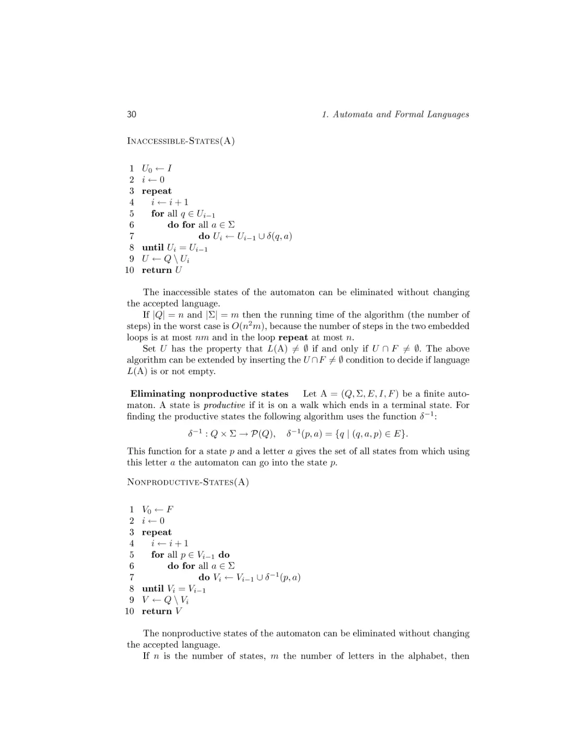
1.2.4. Finite automata with empty input . . . . . . . . . . . . . .
1.2.5. Minimization of
nite automata . . . . . . . . . . . . . . . .
1.2.6. Pumping lemma for regular languages . . . . . . . . . . . .
1.2.7. Regular expressions . . . . . . . . . . . . . . . . . . . . . . .
1.3. Pushdown automata and context-free languages . . . . . . . . . . .
1.3.1. Pushdown automata . . . . . . . . . . . . . . . . . . . . . .
1.3.2. Context-free languages . . . . . . . . . . . . . . . . . . . . .
1.3.3. Pumping lemma for context-free languages . . . . . . . . . .
1.3.4. Normal forms of the context-free languages . . . . . . . . .
2. Compilers (Zoltán Csörnyei) . . . . . . . . . . . . . . . . . . . . . . .
2.1.
2.2.
The structure of compilers . . . . . .
Lexical analysis . . . . . . . . . . . .
2.2.1. The automaton of the scanner
2.2.2. Special problems . . . . . . .
2.3. Syntactic analysis . . . . . . . . . . .
2.3.1. LL(1) parser . . . . . . . . . .
.
.
.
.
.
.
.
.
.
.
.
.
.
.
.
.
.
.
.
.
.
.
.
.
.
.
.
.
.
.
.
.
.
.
.
.
.
.
.
.
.
.
.
.
.
.
.
.
.
.
.
.
.
.
.
.
.
.
.
.
.
.
.
.
.
.
.
.
.
.
.
.
.
.
.
.
.
.
.
.
.
.
.
.
.
.
.
.
.
.
.
.
.
.
.
.
.
.
.
.
.
.
13
14
14
18
22
24
26
31
34
36
41
45
47
50
60
60
69
71
73
80
81
84
85
89
92
94
Contents
4
LR (1) parsing . . . . . . . . . . . . . . . . . . . . . . . . . .
3. Compression and Decompression (Ulrich Tamm) . . . . . . . . . .
3.1. Facts from information theory . . . . . . . . . . . . . . . . . . . . .
3.1.1. The Discrete Memoryless Source . . . . . . . . . . . . . . .
3.1.2. Pre
x codes . . . . . . . . . . . . . . . . . . . . . . . . . . .
3.1.3. Kraft's inequality and noiseless coding theorem . . . . . . .
3.1.4. Shannon-Fano-Elias-codes and the Shannon-Fano-algorithm
3.1.5. The Human coding algorithm . . . . . . . . . . . . . . . .
3.2. Arithmetic coding and modelling . . . . . . . . . . . . . . . . . . .
3.2.1. Arithmetic coding . . . . . . . . . . . . . . . . . . . . . . .
3.2.2. Modelling . . . . . . . . . . . . . . . . . . . . . . . . . . . .
3.3. Ziv-Lempel-coding . . . . . . . . . . . . . . . . . . . . . . . . . . .
3.3.1. LZ77 . . . . . . . . . . . . . . . . . . . . . . . . . . . . . . .
3.3.2. LZ78 . . . . . . . . . . . . . . . . . . . . . . . . . . . . . . .
3.4. The Burrows-Wheeler-transform . . . . . . . . . . . . . . . . . . .
3.5. Image compression . . . . . . . . . . . . . . . . . . . . . . . . . . .
3.5.1. Representation of data . . . . . . . . . . . . . . . . . . . . .
3.5.2. The discrete cosine transform . . . . . . . . . . . . . . . . .
3.5.3. Quantisation . . . . . . . . . . . . . . . . . . . . . . . . . .
3.5.4. Coding . . . . . . . . . . . . . . . . . . . . . . . . . . . . . .
4. Reliable computation (Péter Gács) . . . . . . . . . . . . . . . . . .
4.1. Probability theory . . . . . . . . . . . . . . . . . . . . . . . . . . .
4.1.1. Terminology . . . . . . . . . . . . . . . . . . . . . . . . . . .
4.1.2. The law of large numbers (with large deviations) . . . . .
4.2. Logic circuits . . . . . . . . . . . . . . . . . . . . . . . . . . . . . .
4.2.1. Boolean functions and expressions . . . . . . . . . . . . . .
4.2.2. Circuits . . . . . . . . . . . . . . . . . . . . . . . . . . . . .
4.2.3. Fast addition by a Boolean circuit . . . . . . . . . . . . . .
4.3. Expensive fault-tolerance in Boolean circuits . . . . . . . . . . . . .
4.4. Safeguarding intermediate results . . . . . . . . . . . . . . . . . . .
4.4.1. Cables . . . . . . . . . . . . . . . . . . . . . . . . . . . . . .
4.4.2. Compressors . . . . . . . . . . . . . . . . . . . . . . . . . . .
4.4.3. Propagating safety . . . . . . . . . . . . . . . . . . . . . . .
4.4.4. Endgame . . . . . . . . . . . . . . . . . . . . . . . . . . . .
4.4.5. The construction of compressors . . . . . . . . . . . . . . .
4.5. The reliable storage problem . . . . . . . . . . . . . . . . . . . . . .
4.5.1. Clocked circuits . . . . . . . . . . . . . . . . . . . . . . . . .
4.5.2. Storage . . . . . . . . . . . . . . . . . . . . . . . . . . . . .
4.5.3. Error-correcting codes . . . . . . . . . . . . . . . . . . . . .
4.5.4. Refreshers . . . . . . . . . . . . . . . . . . . . . . . . . . . .
2.3.2.
109
131
132
132
133
135
137
139
141
142
146
153
153
154
155
160
160
161
162
163
169
170
171
172
174
174
176
178
180
184
184
185
188
189
191
194
194
197
198
202
II. COMPUTER ALGEBRA . . . . . . . . . . . . . . . . . . . . . . . . 216
5. Algebra (Gábor Ivanyos, Lajos Rónyai) . . . . . . . . . . . . . . . . 217
5.1.
Fields, vector spaces, and polynomials . . . . . . . . . . . . . . . . 217
5.1.1. Ring theoretic concepts . . . . . . . . . . . . . . . . . . . . 217
Contents
5
5.1.2. Polynomials . . . . . . . . . . . . . . . . . . . . . . . . .
Finite
elds . . . . . . . . . . . . . . . . . . . . . . . . . . . . .
Factoring polynomials over
nite
elds . . . . . . . . . . . . . .
5.3.1. Square-free factorisation . . . . . . . . . . . . . . . . . .
5.3.2. Distinct degree factorisation . . . . . . . . . . . . . . .
5.3.3. The Cantor-Zassenhaus algorithm . . . . . . . . . . . . .
5.3.4. Berlekamp's algorithm . . . . . . . . . . . . . . . . . . .
5.4. Lattice reduction . . . . . . . . . . . . . . . . . . . . . . . . . .
5.4.1. Lattices . . . . . . . . . . . . . . . . . . . . . . . . . . .
5.4.2. Short lattice vectors . . . . . . . . . . . . . . . . . . . .
5.4.3. Gauss' algorithm for two-dimensional lattices . . . . . .
5.4.4. A Gram-Schmidt orthogonalisation and weak reduction
5.4.5. Lovász-reduction . . . . . . . . . . . . . . . . . . . . . .
5.4.6. Properties of reduced bases . . . . . . . . . . . . . . . .
5.5. Factoring polynomials in Q[x] . . . . . . . . . . . . . . . . . . .
5.5.1. Preparations . . . . . . . . . . . . . . . . . . . . . . . .
5.5.2. The Berlekamp-Zassenhaus algorithm . . . . . . . . . .
5.5.3. The LLL algorithm . . . . . . . . . . . . . . . . . . . . .
5.2.
5.3.
.
.
.
.
.
.
.
.
.
.
.
.
.
.
.
.
.
.
.
.
.
.
.
.
.
.
.
.
.
.
.
.
.
.
.
.
221
230
237
237
239
241
242
248
248
251
252
254
256
257
259
260
266
268
6. Computer Algebra (Antal Járai, Attila Kovács) . . . . . . . . . . 275
6.1.
6.2.
Data representation . . . . . . . . . . . . . . . . . . .
Common roots of polynomials . . . . . . . . . . . . .
6.2.1. Classical and extended Euclidean algorithm .
6.2.2. Primitive Euclidean algorithm . . . . . . . . .
6.2.3. The resultant . . . . . . . . . . . . . . . . . .
6.2.4. Modular greatest common divisor . . . . . . .
6.3. Gröbner basis . . . . . . . . . . . . . . . . . . . . . .
6.3.1. Monomial order . . . . . . . . . . . . . . . . .
6.3.2. Multivariate division with remainder . . . . .
6.3.3. Monomial ideals and Hilbert's basis theorem .
6.3.4. Buchberger's algorithm . . . . . . . . . . . . .
6.3.5. Reduced Gröbner basis . . . . . . . . . . . . .
6.3.6. The complexity of computing Gröbner bases .
6.4. Symbolic integration . . . . . . . . . . . . . . . . . .
6.4.1. Integration of rational functions . . . . . . . .
6.4.2. The Risch integration algorithm . . . . . . . .
6.5. Theory and practice . . . . . . . . . . . . . . . . . .
6.5.1. Other symbolic algorithms . . . . . . . . . . .
6.5.2. An overview of computer algebra systems . .
7. Cryptology (Jörg Rothe) . . . . . . . . . . . . . . . . .
7.1. Foundations . . . . . . . . . . . . . . . . . . . . . . .
7.1.1. Cryptography . . . . . . . . . . . . . . . . . .
7.1.2. Cryptanalysis . . . . . . . . . . . . . . . . . .
7.1.3. Algebra, number theory, and graph theory . .
7.2. Diie and Hellman's secret-key agreement protocol .
7.3. RSA and factoring . . . . . . . . . . . . . . . . . . .
.
.
.
.
.
.
.
.
.
.
.
.
.
.
.
.
.
.
.
.
.
.
.
.
.
.
.
.
.
.
.
.
.
.
.
.
.
.
.
.
.
.
.
.
.
.
.
.
.
.
.
.
.
.
.
.
.
.
.
.
.
.
.
.
.
.
.
.
.
.
.
.
.
.
.
.
.
.
.
.
.
.
.
.
.
.
.
.
.
.
.
.
.
.
.
.
.
.
.
.
.
.
.
.
.
.
.
.
.
.
.
.
.
.
.
.
.
.
.
.
.
.
.
.
.
.
.
.
.
.
.
.
.
.
.
.
.
.
.
.
.
.
.
.
.
.
.
.
.
.
.
.
.
.
.
.
.
.
.
.
.
.
.
.
.
.
.
.
.
.
.
.
.
.
.
.
.
.
.
.
.
.
.
.
.
.
.
.
.
.
.
.
.
.
.
.
.
.
.
.
.
.
.
.
.
.
.
.
276
281
281
287
289
296
300
301
303
304
305
307
307
309
310
315
326
327
328
332
333
334
338
339
346
349
Contents
6
7.3.1. RSA . . . . . . . . . . . . . . . . . . . . . . . . .
7.3.2. Digital RSA signatures . . . . . . . . . . . . . . .
7.3.3. Security of RSA . . . . . . . . . . . . . . . . . . .
7.4. The protocols of Rivest, Rabi, and Sherman . . . . . . .
7.5. Interactive proof systems and zero-knowledge . . . . . .
7.5.1. Interactive proof systems, Arthur-Merlin games,
knowledge protocols . . . . . . . . . . . . . . . . .
7.5.2. Zero-knowledge protocol for graph isomorphism .
. . . . . .
. . . . . .
. . . . . .
. . . . . .
. . . . . .
and zero. . . . . .
. . . . . .
349
353
353
355
356
356
359
8. Complexity Theory (Jörg Rothe) . . . . . . . . . . . . . . . . . . . . 364
8.1.
8.2.
8.3.
Foundations . . . . . . . . . . . . . . . . . . . . .
NP-completeness . . . . . . . . . . . . . . . . . .
Algorithms for the satis
ability problem . . . . .
8.3.1. A deterministic algorithm . . . . . . . . .
8.3.2. A randomised algorithm . . . . . . . . . .
8.4. Graph isomorphism and lowness . . . . . . . . . .
8.4.1. Reducibilities and complexity hierarchies .
8.4.2. Graph isomorphism is in the low hierarchy
8.4.3. Graph isomorphism is in SPP . . . . . . .
.
.
.
.
.
.
.
.
.
.
.
.
.
.
.
.
.
.
.
.
.
.
.
.
.
.
.
.
.
.
.
.
.
.
.
.
.
.
.
.
.
.
.
.
.
.
.
.
.
.
.
.
.
.
.
.
.
.
.
.
.
.
.
.
.
.
.
.
.
.
.
.
.
.
.
.
.
.
.
.
.
.
.
.
.
.
.
.
.
.
365
371
373
373
375
378
378
383
386
III. NUMERICAL METHODS . . . . . . . . . . . . . . . . . . . . . . . 394
9. Competitive Analysis (Imreh Csanád) . . . . . . . . . . . . . . . . 395
9.1.
9.2.
9.3.
Notions, de
nitions . . . . . . . . . . . . . .
The k -server problem . . . . . . . . . . . . .
Models related to computer networks . . . .
9.3.1. The data acknowledgement problem
9.3.2. The
le caching problem . . . . . . .
9.3.3. On-line routing . . . . . . . . . . . .
9.4. On-line bin packing models . . . . . . . . .
9.4.1. On-line bin packing . . . . . . . . . .
9.4.2. Multidimensional models . . . . . . .
9.5. On-line scheduling . . . . . . . . . . . . . .
9.5.1. On-line scheduling models . . . . . .
9.5.2. LIST model . . . . . . . . . . . . . .
9.5.3. TIME model . . . . . . . . . . . . .
.
.
.
.
.
.
.
.
.
.
.
.
.
.
.
.
.
.
.
.
.
.
.
.
.
.
.
.
.
.
.
.
.
.
.
.
.
.
.
.
.
.
.
.
.
.
.
.
.
.
.
.
.
.
.
.
.
.
.
.
.
.
.
.
.
.
.
.
.
.
.
.
.
.
.
.
.
.
.
.
.
.
.
.
.
.
.
.
.
.
.
.
.
.
.
.
.
.
.
.
.
.
.
.
.
.
.
.
.
.
.
.
.
.
.
.
.
.
.
.
.
.
.
.
.
.
.
.
.
.
.
.
.
.
.
.
.
.
.
.
.
.
.
.
.
.
.
.
.
.
.
.
.
.
.
.
.
.
.
.
.
.
.
.
.
.
.
.
.
395
397
403
403
405
408
412
412
416
419
419
420
425
10. Game Theory (Ferenc Szidarovszky) . . . . . . . . . . . . . . . . . 429
10.1. Finite games . . . . . . . . . . . . . . . . . . . . . .
10.1.1. Enumeration . . . . . . . . . . . . . . . . . .
10.1.2. Games represented by
nite trees . . . . . . .
10.2. Continuous games . . . . . . . . . . . . . . . . . . . .
10.2.1. Fixed-point methods based on best responses
10.2.2. Applying Fan's inequality . . . . . . . . . . .
10.2.3. Solving the Kuhn-Tucker conditions . . . . .
10.2.4. Reduction to optimization problems . . . . .
10.2.5. Method of
ctitious play . . . . . . . . . . . .
10.2.6. Symmetric matrix games . . . . . . . . . . . .
.
.
.
.
.
.
.
.
.
.
.
.
.
.
.
.
.
.
.
.
.
.
.
.
.
.
.
.
.
.
.
.
.
.
.
.
.
.
.
.
.
.
.
.
.
.
.
.
.
.
.
.
.
.
.
.
.
.
.
.
.
.
.
.
.
.
.
.
.
.
.
.
.
.
.
.
.
.
.
.
430
431
433
437
437
438
440
441
449
450
Contents
10.2.7. Linear programming and matrix games
10.2.8. The method of von Neumann . . . . .
10.2.9. Diagonally strictly concave games . . .
10.3. The oligopoly problem . . . . . . . . . . . . .
7
.
.
.
.
.
.
.
.
.
.
.
.
.
.
.
.
.
.
.
.
.
.
.
.
.
.
.
.
.
.
.
.
.
.
.
.
.
.
.
.
.
.
.
.
.
.
.
.
452
454
457
465
11. Recurrences (Zoltán Kása) . . . . . . . . . . . . . . . . . . . . . . . . 478
11.1. Linear recurrence equations . . . . . . . . . . . . . . . . . . . . . .
11.1.1. Linear homogeneous equations with constant coe
cients . .
11.1.2. Linear nonhomogeneous recurrence equations with constant
coe
cients . . . . . . . . . . . . . . . . . . . . . . . . . . . .
11.2. Generating functions and recurrence equations . . . . . . . . . . . .
11.2.1. De
nition and operations . . . . . . . . . . . . . . . . . . .
11.2.2. Solving recurrence equations by generating functions . . . .
11.2.3. The Z-transform method . . . . . . . . . . . . . . . . . . . .
11.3. Numerical solution . . . . . . . . . . . . . . . . . . . . . . . . . . .
12. Scienti
c Computations (Aurél Galántai, András Jeney) . . . . .
12.1. Floating point arithmetic and error analysis . . . . . . . . . . . . .
12.1.1. Classical error analysis . . . . . . . . . . . . . . . . . . . . .
12.1.2. Forward and backward errors . . . . . . . . . . . . . . . . .
12.1.3. Rounding errors and
oating point arithmetic . . . . . . . .
12.1.4. The
oating point arithmetic standard . . . . . . . . . . . .
12.2. Linear systems of equations . . . . . . . . . . . . . . . . . . . . . .
12.2.1. Direct methods for solving linear systems . . . . . . . . . .
12.2.2. Iterative methods for linear systems . . . . . . . . . . . . .
12.2.3. Error analysis of linear algebraic systems . . . . . . . . . . .
12.3. Eigenvalue problems . . . . . . . . . . . . . . . . . . . . . . . . . .
12.3.1. Iterative solutions of the eigenvalue problem . . . . . . . . .
12.4. Numerical program libraries and software tools . . . . . . . . . . .
12.4.1. Standard linear algebra subroutines . . . . . . . . . . . . . .
12.4.2. Mathematical software . . . . . . . . . . . . . . . . . . . . .
479
479
484
486
486
490
497
500
502
502
502
504
505
510
512
512
523
525
534
537
543
544
547
Bibliography . . . . . . . . . . . . . . . . . . . . . . . . . . . . . . . . . . . 552
Subject Index . . . . . . . . . . . . . . . . . . . . . . . . . . . . . . . . . . 563
Name Index . . . . . . . . . . . . . . . . . . . . . . . . . . . . . . . . . . . . 572
Preface
It is a special pleasure for me to recommend to the Readers the book Algorithms of
Computer Science, edited with great care by Antal Iványi. Computer algorithms form
a very important and fast developing branch of computer science. Design and analysis of large computer networks, large scale scienti
c computations and simulations,
economic planning, data protection and cryptography and many other applications
require eective, carefully planned and precisely analysed algorithms.
Many years ago we wrote a small book with Péter Gács under the title Algorithms. The two volumes of the book Algorithms of Computer Science show how this
topic developed into a complex area that branches o into many exciting directions.
It gives a special pleasure to me that so many excellent representatives of Hungarian
computer science have cooperated to create this book. It is obvious to me that this
book will be one of the most important reference books for students, researchers and
computer users for a long time.
Budapest, July 2007
László Lovász
Introduction
The
rst volume of the book Informatikai algoritmusok (in English: Algorithms of
Informatics ) appeared in 2004, and the second volume of the book appeared in
2005. Two volumes contained 31 chapters: 23 chapters of the present book, and
further chapters on clustering (author: András Lukács), frequent elements in data
bases (author: Ferenc Bodon), geoinformatics (authors: István Elek, Csaba Sidló),
inner-point methods (authors: Tibor Illés, Marianna Nagy, Tamás Terlaky), number
theory (authors: Gábor Farkas, Imre Kátai), Petri nets (authors: Zoltán Horváth,
Máté Tejfel), queueing theory (authors: László Lakatos, László Szeidl, Miklós Telek),
scheduling (author: Béla Vizvári).
The Hungarian version of the
rst volume contained those chapters which were
nished until May of 2004, and the second volume contained the chapters
nished
until April of 2005.
English version contains the chapters submitted until April of 2007. Volume 1
contains the chapters belonging to the fundamentals of informatics, while the second
volume contains the chapters having closer connection with some applications.
The chapters of the
rst volume are divided into three parts. The chapters of
Part 1 are connected with automata: Automata and Formal Languages (written by
Zoltán Kása, Babes-Bolyai University of Cluj-Napoca), Compilers (Zoltán Csörnyei,
Eötvös Loránd University), Compression and Decompression (Ulrich Tamm, Chemnitz University of Technology Commitment), Reliable Computations (Péter Gács,
Boston University).
The chapters of Part 2 have algebraic character: here are the chapters Algebra
(written by Gábor Ivanyos, Lajos Rónyai, Budapest University of Technology and
Economics), Computer Algebra (Antal Járai, Attila Kovács, Eötvös Loránd University), further Cryptology and Complexity Theory (Jörg Rothe, Heinrich Heine
University).
The chapters of Part 3 have numeric character: Competitive Analysis (Csanád
Imreh, University of Szeged), Game Theory (Ferenc Szidarovszky, The University of
Arizona) and Scienti
c Computations (Aurél Galántai, András Jeney, University of
Miskolc).
10
Introduction
The second volume is also divided into three parts. The chapters of Part 4
are connected with computer networks: Distributed Algorithms (Burkhard Englert,
California State University; Dariusz Kowalski, University of Liverpool; Grzegorz Malewicz, University of Alabama; Alexander Allister Shvartsman, University of Connecticut), Network Simulation (Tibor Gyires, Illinois State University), Parallel Algorithms (Antal Iványi, Eötvös Loránd University; Claudia Leopold, University of
Kassel), and Systolic Systems (Eberhard Zehendner, Friedrich Schiller University).
The chapters of Part 5 are Memory Management (Ádám Balogh, Antal Iványi,
Eötvös Loránd University), Relational Databases and Query in Relational Databases
(János Demetrovics, Eötvös Loránd University; Attila Sali, Alfréd Rényi Institute of
Mathematics), Semi-structured Data Bases (Attila Kiss, Eötvös Loránd University).
The chapters of Part 6 of the second volume have close connections with biology: Bioinformatics (István Miklós, Eötvös Loránd University), Human-Computer
Interactions (Ingo Althöfer, Stefan Schwarz, Friedrich Schiller University), and Computer Graphics (László Szirmay-Kalos, Budapest University of Technology and Economics).
The chapters are validated by Gábor Ivanyos, Lajos Rónyai, András Recski,
and Tamás Szántai (Budapest University of Technology and Economics), Sándor
Fridli, János Gonda, and Béla Vizvári (Eötvös Loránd University), Pál Dömösi, and
Attila Peth® (University of Debrecen), Zoltán Fülöp (University of Szeged), Anna
Gál (University of Texas), János Mayer (University of Zürich).
The validators of the chapters which appeared only in the Hungarian version:
István Pataricza, Lajos Rónyai (Budapest University of Economics and Technology),
András A. Benczúr (Computer and Automation Research Institute), Antal Járai
(Eötvös Loránd University), Attila Meskó (Hungarian Academy of Sciences), János
Csirik (University of Szeged), János Mayer (University of Zürich),
The book contains verbal description, pseudocode and analysis of over 200 algorithms, and over 350
gures and 120 examples illustrating how the algorithms work.
Each section ends with exercises and each chapter ends with problems. In the book
you can
nd over 330 exercises and 70 problems.
We have supplied an extensive bibliography, in the section Chapter notes of
each chapter. The web site of the book contains the maintained living version of
the bibliography in which the names of authors, journals and publishers are usually
links to the corresponding web site.
The LATEX style
le was written by Viktor Belényesi. The
gures was drawn or
corrected by Kornél Locher. Anna Iványi transformed the bibliography into hypertext.
The linguistical validators of the book are Anikó Hörmann and Veronika Vöröss. Some chapters were translated by Anikó Hörmann (Eötvös Loránd University),
László Orosz (University of Debrecen), Miklós Péter Pintér (Corvinus University of
Budapest), Csaba Schneider (Budapest University of Technology and Economics),
and Veronika Vöröss (Eötvös Loránd University).
The publication of the book was supported by Department of Mathematics of
Hungarian Academy of Science.
Introduction
11
We plan to publish the corrected and extended version of this book in printed and
electronic form too. This book has a web site: http://elek.inf.elte.hu/EnglishBooks.
You can use this website to obtain a list of known errors, report errors, or make suggestions (using the data of the colofon page you can contact with any of the creators
of the book). The website contains the maintaned PDF version of the bibliography
in which the names of the authors, journals and publishers are usually active links
to the corresponding web sites (the living elements are underlined in the printed
bibliography). We welcome ideas for new exercises and problems.
Budapest, July 2007
Antal Iványi (tony@compalg.inf.elte.hu)
I. AUTOMATA
1. Automata and Formal Languages
Automata and formal languages play an important role in projecting and realizing
compilers. In the
rst section grammars and formal languages are de
ned. The different grammars and languages are discussed based on Chomsky hierarchy. In the
second section we deal in detail with the
nite automata and the languages accepted
by them, while in the third section the pushdown automata and the corresponding
accepted languages are discussed. Finally, references from a rich bibliography are
given.
1.1. Languages and grammars
A
nite and nonempty set of symbols is called an alphabet . The elements of an
alphabet are letters, but sometimes are named also symbols.
With the letters of an alphabet words are composed. If a1 , a2 , . . . , an ∈ Σ, n ≥ 0,
then a1 a2 . . . an a Σ is a word over the alphabet Σ (the letters ai are not necessary
distinct). The number of letters of a word, with their multiplicities, constitutes the
length of the word. If w = a1 a2 . . . an , then the length of w is |w| = n. If n = 0,
then the word is an empty word, which will be denoted by ε (sometimes λ in other
books). The set of words over the alphabet Σ will be denoted by Σ∗ :
©
ª
Σ∗ = a1 a2 . . . an | a1 , a2 , . . . , an ∈ Σ, n ≥ 0 .
For the set of nonempty words over Σ the notation Σ+ = Σ∗ \ {ε} will be used. The
set of words of length n over Σ will be denoted by Σn , and Σ0 = {ε}. Then
Σ∗ = Σ0 ∪ Σ1 ∪ · · · ∪ Σn ∪ · · ·
and
Σ+ = Σ1 ∪ Σ2 ∪ · · · ∪ Σn ∪ · · · .
The words u = a1 a2 . . . am and v = b1 b2 . . . bn are equal (i.e. u = v ), if m = n and
ai = bi , i = 1, 2, . . . , n.
We de
ne in Σ∗ the binary operation called concatenation . The concatenation
(or product) of the words u = a1 a2 . . . am and v = b1 b2 . . . bn is the word uv =
a1 a2 . . . am b1 b2 . . . bn . It is clear that |uv| = |u| + |v|. This operation is associative
but not commutative. Its neutral element is ε, because εu = uε = u for all u ∈ Σ∗ .
Σ∗ with the concatenation is a monoid.
We introduce the power operation. If u ∈ Σ∗ , then u0 = ε, and un = un−1 u for
n ≥ 1.
1. Automata and Formal Languages
14
The reversal (or mirror image ) of the word u = a1 a2 . . . an is u−1 =
an−1
of u sometimes is denoted by uR or ũ. It is clear that
¡an−1
¢−1. . . a1 . The reversal
−1
u
= u and (uv) = v −1 u−1 .
Word v is a pre
x of the word u if there exists a word z such that u = vz . If
z 6= ε then v is a proper pre
x of u. Similarly v is a su
x of u if there exists a word
x such that u = xv . The proper su
x can also be de
ned. Word v is a subword
of the word u if there are words p and q such that u = pvq. If pq 6= ε then v is a
proper subword .
A subset L of Σ∗ is called a language over the alphabet Σ. Sometimes this
is called a formal language because the words are here considered without any
meanings. Note that ∅ is the empty language while {ε} is a language which contains
the empty word.
1.1.1. Operations on languages
If L, L1 , L2 are languages over Σ we de
ne the following operations
• union
L1 ∪ L2 = {u ∈ Σ∗ | u ∈ L1 or u ∈ L2 } ,
• intersection
L1 ∩ L2 = {u ∈ Σ∗ | u ∈ L1 and u ∈ L2 } ,
• dierence
L1 \ L2 = {u ∈ Σ∗ | u ∈ L1 and u 6∈ L2 } ,
• complement
L = Σ∗ \ L ,
• multiplication
L1 L2 = {uv | u ∈ L1 , v ∈ L2 } ,
• power
L0 = {ε},
Ln = Ln−1 L, if n ≥ 1 ,
• iteration or star operation
∞
[
L∗ =
Li = L0 ∪ L ∪ L2 ∪ · · · ∪ Li ∪ · · · ,
• mirror
i=0
L−1 = {u−1 | u ∈ L} .
We will use also the∞notation L+
[
L+ =
Li = L ∪ L2 ∪ · · · ∪ Li ∪ · · · .
i=1
The union, product and iteration are called regular operations .
1.1.2. Specifying languages
Languages can be speci
ed in several ways. For example a language can be speci
ed
using
1) the enumeration of its words,
1.1. Languages and grammars
15
2) a property, such that all words of the language have this property but other
word have not,
3) a grammar.
Specifying languages by listing their elements For example the following
are languages
L1 = {ε, 0, 1},
L2 = {a, aa, aaa, ab, ba, aba}.
Even if we cannot enumerate the elements of an in
nite set in
nite languages can
be speci
ed by enumeration if after enumerating the
rst some elements we can
continue the enumeration using a rule. The following is such a language
L3 = {ε, ab, aabb, aaabbb, aaaabbbb, . . .}.
Specifying languages by properties
The following sets are languages
L4 = {an bn | n = 0, 1, 2, . . .},
L5 = {uu−1 | u ∈ Σ∗ },
L6 = {u ∈ {a, b}∗ | na (u) = nb (u)},
where na (u) denotes the number of letters a in word u and nb (u) the number of
letters b.
Specifying languages by grammars
shortly the grammar .
De
ne the generative grammar or
De
nition 1.1 A grammar is an ordered quadruple G = (N, T, P, S), where
• N is the alphabet of variables (or nonterminal symbols),
• T is the alphabet of terminal symbols, where N ∩ T = ∅,
• P ⊆ (N ∪ T )∗ N (N ∪ T )∗ × (N ∪ T )∗ is a
nite set, that is P is the
nite set
of productions of the form (u, v) , where u, v ∈ (N ∪ T )∗ and u contains at least a
nonterminal symbol,
• S ∈ N is the start symbol.
Remarks. Instead of the notation (u, v) sometimes u → v is used.
In the production u → v or (u, v) word u is called the left-hand side of the
production while v the right-hand side. If for a grammar there are more than one
production with the same left-hand side, then these production
u → v1 , u → v2 , . . . , u → vr
can be written as
u → v1 | v2 | . . . | vr .
We de
ne on the set (N ∪ T )∗ the relation called direct derivation
u =⇒ v,
if
u = p1 pp2 ,
v = p1 qp2
and
(p, q) ∈ P .
In fact we replace in u an appearance of the subword p by q and we get v . Another
notations for the same relation can be ` or |=.
If we want to emphasize the used grammar G, then the notation =⇒ can be
∗
replaced by =⇒. Relation =⇒ is the re
exive and transitive closure of =⇒, while
+
G
∗
=⇒ denotes its transitive closure. Relation =⇒ is called a derivation .
1. Automata and Formal Languages
16
From the de
nition of a re
exive and transitive relation we can deduce the
∗
following: u =⇒ v , if there exist the words w0 , w1 , . . . , wn ∈ (N ∪ T )∗ , n ≥ 0 and
u = w0 , w0 =⇒ w1 , w1 =⇒ w2 , . . . , wn−1 =⇒ wn , wn = v . This can be written
shortly u = w0 =⇒ w1 =⇒ w2 =⇒ . . . =⇒ wn−1 =⇒ wn = v. If n = 0 then u = v .
+
The same way we can de
ne the relation u =⇒ v except that n ≥ 1 always, so at
least one direct derivation will de used.
De
nition 1.2 The language generated by grammar G = (N, T, P, S) is the set
∗
L(G) = {u ∈ T ∗ | S =⇒ u} .
So L(G) contains all words over the alphabet T which can be derived from the start
symbol S using the productions from P .
Example 1.1 Let G = (N, T, P, S) where
N = {S},
T = {a, b},
P = {S → aSb, S → ab}.
It is easy to see than L(G) = {an bn | n ≥ 1} because
S =⇒ aSb =⇒ a2 Sb2 =⇒ · · · =⇒ an−1 Sbn−1 =⇒ an bn ,
G
G
G
G
G
where up to the last but one replacement the
rst production (S → aSb) was used, while
∗
at the last replacement the production S → ab. This derivation can be written S =⇒ an bn .
G
Therefore an bn can be derived from S for all n and no other words can be derived from S .
De
nition 1.3 Two grammars G1 and G2 are equivalent, and this is denoted by
G1 ∼
= G2 if L(G1 ) = L(G2 ).
Example 1.2 The following two grammars are equivalent because both of them generate
the language {an bn cn | n ≥ 1}.
G1 = (N1 , T, P1 , S1 ), where
N1 = {S1 , X, Y }, T = {a, b, c},
P1 = {S1 → abc, S1 → aXbc, Xb → bX, Xc → Y bcc, bY → Y b, aY → aaX, aY →
aa}.
G2 = (N2 , T, P2 , S2 ), where
N2 = {S2 , A, B, C},
P2 = {S2 → aS2 BC, S2 → aBC, CB → BC, aB → ab, bB → bb, bC → bc, cC →
cc}.
∗
First let us prove by mathematical induction that for n ≥ 2 S1 =⇒ an−1 Y bn cn . If n = 2
then
G1
S1 =⇒ aXbc =⇒ abXc =⇒ abY bcc =⇒ aY b2 c2 .
G1
G1
G1
G1
∗
The inductive hypothesis is S1 =⇒ an−2 Y bn−1 cn−1 . We use production aY → aaX , then
G1
(n − 1) times production Xb → bX , and then production Xc → Y bcc, afterwards again
(n − 1) times production bY → Y b. Therefore
∗
S1 =⇒ an−2 Y bn−1 cn−1 =⇒ an−1 Xbn−1 cn−1 =⇒
G1
G1
G1
∗
an−1 bn−1 Xcn−1 =⇒ an−1 bn−1 Y bcn =⇒ an−1 Y bn cn .
G1
G1
1.1. Languages and grammars
17
∗
If now we use production aY → aa we get S1 =⇒ an bn cn for n ≥ 2, but S1 =⇒ abc
G1
G1
by the production S1 → abc, so an bn cn ∈ L(G1 ) for any n ≥ 1. We have to prove in
addition that using the productions of the grammar we cannot derive only words of the
form an bn cn . It is easy to see that a successful derivation (which ends in a word containing
only terminals) can be obtained only in the presented way.
Similarly for n ≥ 2
∗
∗
S2 =⇒ aS2 BC =⇒ an−1 S2 (BC)n−1 =⇒ an (BC)n =⇒ an B n C n
G2
G2
G2
∗
G2
∗
=⇒ an bB n−1 C n =⇒ an bn C n =⇒ an bn cC n−1 =⇒ an bn cn .
G2
G2
G2
G2
Here orderly were used the productions S2 → aS2 BC (n − 1 times), S2 → aBC , CB → BC
(n − 1 times), aB → ab, bB → bb (n − 1 times), bC → bc, cC → cc (n − 1 times). But
∗
S2 =⇒ aBC =⇒ abC =⇒ abc, So S2 =⇒ an bn cn , n ≥ 1. It is also easy to see than other
G2
G2
G2
G2
words cannot be derived using grammar G2 .
The grammars
G3 = ({S}, {a, b}, {S → aSb, S → ε}, S) and
G4 = ({S}, {a, b}, {S → aSb, S → ab}, S)
are not equivalent because L(G3 ) \ {ε} = L(G4 ).
Theorem 1.4 Not all languages can be generated by grammars.
Proof We encode grammars for the proof as words on the alphabet {0, 1}. For a
given grammar G = (N, T, P, S) let N = {S1 , S2 , . . . , Sn }, T = {a1 , a2 , . . . , am } and
S = S1 . The encoding is the following:
the code of Si is 10 |11 .{z
. . 11} 01,
the code of ai is 100 11
. . 11} 001 .
| .{z
i times
i times
In the code of the grammar the letters are separated by 000, the code of the arrow
is 0000, and the productions are separated by 00000.
It is enough, of course, to encode the productions only. For example, consider
the grammar
G = ({S}, {a, b}, {S → aSb, S → ab}, S).
The code of S is 10101, the code of a is 1001001, the code of b is 10011001. The code
of the grammar is
10101
| {z } 0000 1001001
| {z } 000 10101
| {z } 000 10011001
| {z } 00000 10101
| {z } 0000 1001001
| {z } 000
10011001
| {z } .
From this encoding results that the grammars with terminal alphabet T can be
enumerated 1 as G1 , G2 , . . . , Gk , . . . , and the set of these grammars is a denumerable
in
nite set.
1 Let us suppose that in the alphabet {0, 1} there is a linear order <, let us say 0 < 1. The words
which are codes of grammars can be enumerated by ordering them
rst after their lengths, and
inside the equal length words, alphabetically, using the order of their letters. But we can use equally
the lexicographic order, which means that u < v (u is before v ) if u is a proper pre
x of v or there
exists the decompositions u = xay and v = xby 0 , where x, y , y 0 are subwords, a and b letters with
a < b.
18
1. Automata and Formal Languages
Consider now the set of all languages over T denoted by LT = {L | L ⊆ T ∗ },
that is LT = P(T ∗ ). The set T ∗ is denumerable because its words can be ordered.
Let this order s0 , s1 , s2 , . . ., where s0 = ε. We associate to each language L ∈ LT an
in
nite binary sequence b0 , b1 , b2 , . . . the following way:
½
1, if si ∈ L
bi =
i = 0, 1, 2, . . . .
0, if si 6∈ L
It is easy to see that the set of all such binary sequences is not denumerable, because each sequence can be considered as a positive number less than 1 using its
binary representation (The decimal point is considered to be before the
rst digit).
Conversely, to each positive number less than 1 in binary representation a binary
sequence can be associated. So, the cardinality of the set of in
nite binary sequences
is equal to cardinality of interval [0, 1], which is of continuum power. Therefore the
set LT is of continuum cardinality. Now to each grammar with terminal alphabet
T associate the corresponding generated language over T . Since the cardinality of
the set of grammars is denumerable, there will exist a language from LT , without
associated grammar, a language which cannot be generated by a grammar.
1.1.3. Chomsky hierarchy of grammars and languages
Putting some restrictions on the form of productions, four type of grammars can be
distinguished.
De
nition 1.5 De
ne for a grammar G = (N, T, P, S) the following four types.
A grammar G is of type 0 (phrase-structure grammar) if there are no res-
trictions on productions.
A grammar G is of type 1 (context-sensitive grammar) if all of its productions are of the form αAγ → αβγ , where A ∈ N , α, γ ∈ (N ∪ T )∗ , β ∈ (N ∪ T )+ .
A production of the form S → ε can also be accepted if the start symbol S does not
occur in the right-hand side of any production.
A grammar G is of type 2 (context-free grammar) if all of its productions are
of the form A → β , where A ∈ N , β ∈ (N ∪ T )+ . A production of the form S → ε
can also be accepted if the start symbol S does not occur in the right-hand side of
any production.
A grammar G is of type 3 (regular grammar) if its productions are of the form
A → aB or A → a, where a ∈ T and A, B ∈ N . A production of the form S → ε
can also be accepted if the start symbol S does not occur in the right-hand side of
any production.
If a grammar G is of type i then language L(G) is also of type i.
This classi
cation was introduced by Noam Chomsky.
A language L is of type i (i = 0, 1, 2, 3) if there exists a grammar G of type i
which generates the language L, so L = L(G).
Denote by Li (i = 0, 1, 2, 3) the class of the languages of type i. Can be proved
that
L0 ⊃ L 1 ⊃ L 2 ⊃ L 3 .
1.1. Languages and grammars
19
By the de
nition of dierent type of languages, the inclusions (⊇) are evident, but
the strict inclusions (⊃) must be proved.
Example 1.3 We give an example for each type of context-sensitive, context-free and
regular grammars.
Context-sensitive grammar. G1 = (N1 , T1 , P1 , S1 ), where N1 = {S1 , A, B, C}, T1 =
{a, 0, 1}.
Elements of P1 are:
S1
→ ACA,
AC → AACA | ABa | AaB,
B
→ AB | A,
A
→ 0 | 1.
Language L(G1 ) contains words of the form uav with u, v ∈ {0, 1}∗ and |u| 6= |v|.
Context-free grammar. G2 = (N2 , T2 , P2 , S), where N2 = {S, A, B}, T2 = {+, ∗, (, ), a}.
Elements of P2 are:
S → S + A | A,
A → A ∗ B | B,
B → (S) | a.
Language L(G2 ) contains algebraic expressions which can be correctly built using letter
a, operators + and ∗ and brackets.
Regular grammar. G3 = (N3 , T3 , P3 , S3 ), where N3 = {S3 , A, B}, T3 = {a, b}.
Elements of P3 are:
S3 → aA
A → aB | a
B → aB | bB | a | b.
Language L(G3 ) contains words over the alphabet {a, b} with at least two letters a at
the beginning.
It is easy to prove that any
nite language is regular. The productions will
be done to generate all words of the language. For example, if u = a1 a2 . . . an
is in the language, then we introduce the productions: S → a1 A1 , A1 → a2 A2 ,
. . . An−2 → an−1 An−1 , An−1 → an , where S is the start symbol of the language and
A1 , . . . , An−1 are distinct nonterminals. We de
ne such productions for all words
of the language using dierent nonterminals for dierent words, excepting the start
symbol S . If the empty word is also an element of the language, then the production
S → ε is also considered.
The empty set is also a regular language, because the regular grammar G =
({S}, {a}, {S → aS}, S) generates it.
Eliminating unit productions A production of the form A → B is called
a unit production , where A, B ∈ N . Unit productions can be eliminated from a
grammar in such a way that the new grammar will be of the same type and equivalent
to the
rst one.
Let G = (N, T, P, S) be a grammar with unit productions. De
ne an equivalent
grammar G0 = (N, T, P 0 , S) without unit productions. The following algorithm will
construct the equivalent grammar.
20
1. Automata and Formal Languages
Eliminate-Unit-Productions(G)
1 if the unit productions A → B and B → C are in P put also
the unit production A → C in P while P can be extended,
2 if the unit production A → B and the production B → α (α 6∈ N ) are in P
put also the production A → α in P ,
3 let P 0 be the set of productions of P except unit productions
4 return G0
Clearly, G and G0 are equivalent. If G is of type i ∈ {0, 1, 2, 3} then G0 is also of
type i.
Example 1.4
Use the
above algorithm in the case of the grammar G =
{S, A, B, C}, {a, b}, P, S , where P contains
S → A,
A → B,
B → C,
C → B,
D → C,
S → B,
A → D,
C → Aa,
A → aB,
A → b.
Using the
rst step of the algorithm, we get the following new unit productions:
S→D
(because of S → A and A → D),
S→C
(because of S → B and B → C ),
A→C
(because of A → B and B → C ),
B→B
(because of B → C and C → B ),
C→C
(because of C → B and B → C ),
D→B
(because of D → C and C → B ).
In the second step of the algorithm will be considered only productions with A or C in the
right-hand side, since productions A → aB , A → b and C → Aa can be used (the other
productions are all unit productions). We get the following new productions:
S → aB
(because of S → A and A → aB ),
S→b
(because of S → A and A → b),
S → Aa
(because of S → C and C → Aa),
A → Aa
(because of A → C and C → Aa),
B → Aa
(because of B → C and C →Aa).
The new grammar G0 = {S, A, B, C}, {a, b}, P 0 , S will have the productions:
S → b,
A → b,
B → Aa,
C → Aa,
S → aB,
A → aB,
S → Aa
A → Aa,
Grammars in normal forms A grammar is to be said a grammar in normal
form if its productions have no terminal symbols in the left-hand side.
We need the following notions. For alphabets Σ1 and Σ2 a homomorphism is a
function h : Σ∗1 → Σ∗2 for which h(u1 u2 ) = h(u1 )h(u2 ), ∀u1 , u2 ∈ Σ∗1 . It is easy to
see that for arbitrary u = a1 a2 . . . an ∈ Σ∗1 value h(u) is uniquely determined by the
restriction of h on Σ1 , because h(u) = h(a1 )h(a2 ) . . . h(an ).
If a homomorphism h is a bijection then h an isomorphism.
Theorem 1.6 To any grammar an equivalent grammar in normal form can be
associated.
1.1. Languages and grammars
21
Proof Grammars of type 2 and 3 have in left-hand side of any productions only a
nonterminal, so they are in normal form. The proof has to be done for grammars of
type 0 and 1 only.
Let G = (N, T, P, S) be the original grammar and we de
ne the grammar in
normal form as G0 = (N 0 , T, P 0 , S).
Let a1 , a2 , . . . , ak be those terminal symbols which occur in the left-hand side
of productions. We introduce the new nonterminals A1 , A2 , . . . , Ak . The following
notation will be used: T1 = {a1 , a2 , . . . , ak }, T2 = T \ T1 , N1 = {A1 , A2 , . . . , Ak } and
N 0 = N ∪ N1 .
De
ne the isomorphism h : N ∪ T −→ N 0 ∪ T2 , where
h(ai ) = Ai , if
h(X) = X , if
ai ∈ T1 ,
X ∈ N ∪ T2
De
ne the set P 0 of production as
n
o n
o
¯
¯
P 0 = h(α) → h(β) ¯ (α → β) ∈ P ∪ Ai −→ ai ¯ i = 1, 2, . . . , k
∗
∗
G
G
In this case α =⇒ β if and only if h(α) =⇒
h(β). From this the theorem
0
∗
∗
immediately results because S =⇒ u ⇔ S = h(S) =⇒
h(u) = u.
0
G
G
Example 1.5 Let G = ({S, D, E}, {a, b, c, d, e}, P, S), where P contains
S
→ aebc | aDbc
Db → bD
Dc → Ebccd
bE → Eb
aE → aaD | aae
In the left-hand side of productions the terminals a, b, c occur, therefore consider the
new nonterminals A, B, C , and include in P 0 also the new productions A → a, B → b and
C → c.
Terminals a, b, c will be replaced by nonterminals A, B, C respectively, and we get the
set P 0 as
S
→ AeBC | ADBC
DB → BD
DC → EBCCd
BE → EB
AE → AAD | AAe
A
→ a
B
→ b
C
→ c.
Let us see what words can be generated by this grammars. It is easy to see that
∗
aebc ∈ L(G0 ), because S =⇒ AeBC =⇒ aebc.
∗
S =⇒ ADBC =⇒ ABDC =⇒ ABEBCCd =⇒ AEBBCCd =⇒ AAeBBCCd =⇒
0
aaebbccd, so aaebbccd ∈ L(G ).
∗
We prove, using the mathematical induction, that S =⇒ An−1 EB n C(Cd)n−1 for
n ≥ 2. For n = 2 this is the case, as we have seen before. Continuing the derivation we
∗
∗
get S =⇒ An−1 EB n C(Cd)n−1 =⇒ An−2 AADB n C(Cd)n−1 =⇒ An B n DC(Cd)n−1 =⇒
n n
n−1 ∗
n
n+1
n−1
n
n+1
A B EBCCd(Cd)
=⇒ A EB
CCd(Cd)
= A EB
C(Cd)n , and this is what
we had to prove.
1. Automata and Formal Languages
22
∗
∗
But S =⇒ An−1 EB n C(Cd)n−1 =⇒ An−2 AAeB n C(Cd)n−1 =⇒ an ebn c(cd)n−1 . So
a ebn c(cd)n−1 ∈ L(G0 ), n ≥ 1. These words can be generated also in G.
n
1.1.4. Extended grammars
In this subsection extended grammars of type 1, 2 and 3 will be presented.
Extended grammar of type 1. All productions are of the form α → β , where
|α| ≤ |β|, excepted possibly the production S → ε.
Extended grammar of type 2. All productions are of the form A → β , where
A ∈ N, β ∈ (N ∪ T )∗ .
Extended grammar of type 3. All productions are of the form A → uB or
A → u, Where A, B ∈ N, u ∈ T ∗ .
Theorem 1.7 To any extended grammar an equivalent grammar of the same type
can be associated.
Proof Denote by Gext the extended grammar and by G the corresponding equivalent
grammar of the same type.
Type 1. De
ne the productions of grammar G by rewriting the productions
α → β , where |α| ≤ |β| of the extended grammar Gext in the form γ1 δγ2 → γ1 γγ2
allowed in the case of grammar G by the following way.
Let X1 X2 . . . Xm → Y1 Y2 . . . Yn (m ≤ n) be a production of Gext , which is not
in the required form. Add to the set of productions of G the following productions,
where A1 , A2 , . . . , Am are new nonterminals:
X1 X2 . . . Xm
→ A1 X2 X3 . . . Xm
A1 X2 . . . Xm
→ A1 A2 X3 . . . Xm
...
A1 A2 . . . Am−1 Xm
→ A1 A2 . . . Am−1 Am
A1 A2 . . . Am−1 Am
→ Y1 A2 . . . Am−1 Am
Y1 A2 . . . Am−1 Am
→ Y1 Y2 . . . Am−1 Am
...
Y1 Y2 . . . Ym−2 Am−1 Am → Y1 Y2 . . . Ym−2 Ym−1 Am
Y1 Y2 . . . Ym−1 Am
→ Y1 Y2 . . . Ym−1 Ym Ym+1 . . . Yn .
Furthermore, add to the set of productions of G without any modi
cation the
productions of Gext which are of permitted form, i.e. γ1 δγ2 → γ1 γγ2 .
Inclusion L(Gext ) ⊆ L(G) can be proved because each used production of Gext
in a derivation can be simulated by productions G obtained from it. Furthermore,
since the productions of G can be used only in the prescribed order, we could not
obtain other words, so L(G) ⊆ L(Gext ) also is true.
Type 2. Let Gext = (N, T, P, S). Productions of form A → ε have to be eliminated, only S → ε can remain, if S doesn't occur in the right-hand side of productions.
For this de
ne the following sets:
U0 = {A ∈ N | (A → ε) ∈ P }
+
Ui = Ui−1 ∪ {A ∈ N | (A → w) ∈ P, w ∈ Ui−1
}.
Since for i ≥ 1 we have Ui−1 ⊆ Ui , Ui ⊆ N and N is a
nite set, there must
exists such a k for which Uk−1 = Uk . Let us denote this set as U . It is easy to see
1.1. Languages and grammars
23
∗
that a nonterminal A is in U if and only if A =⇒ ε. (In addition ε ∈ L(Gext ) if and
only if S ∈ U .)
We de
ne the productions of G starting from the productions of Gext in the
following way. For each production A → α with α 6= ε of Gext add to the set of
productions of G this one and all productions which can be obtained from it by
eliminating from α one or more nonterminals which are in U , but only in the case
when the right-hand side does not become ε.
It in not di
cult to see that this grammar G generates the same language as
Gext does, except the empty word ε. So, if ε 6∈ L(Gext ) then the proof is
nished.
But if ε ∈ L(Gext ), then there are two cases. If the start symbol S does not occur
in any right-hand side of productions, then by introducing the production S → ε,
grammar G will generate also the empty word. If S occurs in a production in the
right-hand side, then we introduce a new start symbol S 0 and the new productions
S 0 → S and S 0 → ε. Now the empty word ε can also be generated by grammar G.
Type 3. First we use for Gext the procedure de
ned for grammars of type 2 to
eliminate productions of the form A → ε. From the obtained grammar we eliminate
the unit productions using the algorithm Eliminate-Unit-Productions (see page
20).
In the obtained grammar for each production A → a1 a2 . . . an B , where B ∈
N ∪ {ε}, add to the productions of G also the followings
A
→ a1 A1 ,
A1
→ a2 A2 ,
...
An−1 → an B,
where A1 , A2 , . . . , An−1 are new nonterminals. It is easy to prove that grammar G
built in this way is equivalent to Gext .
Example 1.6 Let Gext = (N, T, P, S) be an extended grammar of type 1, where N =
{S, B, C}, T = {a, b, c} and P contains the following productions:
S
→ aSBC | aBC
CB →
BC
aB → ab
bB
→
bb
bC → bc
cC
→ cc .
The only production which is not context-sensitive is CB → BC . Using the method given
in the proof, we introduce the productions:
CB → AB
AB → AD
AD → BD
BD → BC
Now the grammar G = ({S, A, B, C, D}, {a, b, c}, P 0 , S) is context-sensitive, where the elements of P 0 are
S
→ aSBC | aBC
CB → AB
aB → ab
AB → AD
bB → bb
AD → BD
bC → bc
BD → BC
cC → cc.
It can be proved that L(Gext ) = L(G) = {an bn cn | n ≥ 1}.
24
1. Automata and Formal Languages
Example 1.7 Let Gext = ({S, B, C}, {a, b, c}, P, S) be an extended grammar of type 2,
where P contains:
S → aSc | B
B → bB | C
C → Cc | ε.
Then U0 = {C}, U1 = {B, C}, U3 = {S, B, C} = U . The productions of the new grammar
are:
S → aSc | ac | B
B → bB | b | C
C → Cc | c.
The original grammar generates also the empty word and because S occurs in the righthand side of a production, a new start symbol and two new productions will be de
ned:
S 0 → S, S 0 → ε. The context-free grammar equivalent to the original grammar is G =
({S 0 , S, B, C}, {a, b, c}, P 0 , S 0 ) with the productions:
S0 → S | ε
S → aSc | ac | B
B → bB | b | C
C → Cc | c.
Both of these grammars generate language {am bn cp | p ≥ m ≥ 0, n ≥ 0}.
Example 1.8 Let Gext = ({S, A, B}, {a, b}, P, S) be the extended grammar of type 3
under examination, where P :
S → abA
A → bB
B → S | ε.
First, we eliminate production B → ε. Since U0 = U = {B}, the productions will be
S → abA
A → bB | b
B → S.
The latter production (which a unit production) can also be eliminated, by replacing it with
B → abA. Productions S → abA and B → abA have to be transformed. Since, both productions have the same right-hand side, it is enough to introduce only one new nonterminal
and to use the productions S → aC and C → bA instead of S → abA. Production B → abA
will be replaced by B → aC . The new grammar is G = ({S, A, B, C}, {a, b}, P 0 , S), where
P 0:
S → aC
A → bB | b
B → aC
C → bA.
Can be proved that L(Gext ) = L(G) = {(abb)n | n ≥ 1}.
1.1.5. Closure properties in the Chomsky-classes
We will prove the following theorem, by which the Chomsky-classes of languages are
closed under the regular operations, that is, the union and product of two languages
of type i is also of type i, the iteration of a language of type i is also of type i
(i = 0, 1, 2, 3).
Theorem 1.8 The class Li (i = 0, 1, 2, 3) of languages is closed under the regular
operations.
1.1. Languages and grammars
25
Proof For the proof we will use extended grammars. Consider the extended gram-
mars G1 = (N1 , T1 , P1 , S1 ) and G2 = (N2 , T2 , P2 , S2 ) of type i each. We can suppose
that N1 ∩ N2 = ∅.
Union. Let G∪ = (N1 ∪ N2 ∪ {S}, T1 ∪ T2 , P1 ∪ P2 ∪ {S → S1 , S → S2 }, S).
We will show that L(G∪ ) = L(G1 )∪L(G2 ). If i = 0, 2, 3 then from the assumption
that G1 and G2 are of type i follows by de
nition that G∪ also is of type i. If i = 1
and one of the grammars generates the empty word, then we eliminate from G∪ the
corresponding production (possibly the both) Sk → ε (k = 1, 2) and replace it by
production S → ε.
Product. Let G× = (N1 ∪ N2 ∪ {S}, T1 ∪ T2 , P1 ∪ P2 ∪ {S → S1 S2 }, S).
We will show that L(G× ) = L(G1 )L(G2 ). By de
nition, if i = 0, 2 then G× will
be of the same type. If i = 1 and there is production S1 → ε in P1 but there is
no production S2 → ε in P2 then production S1 → ε will be replaced by S → S2 .
We will proceed the same way in the symmetrical case. If there is in P1 production
S1 → ε and in P2 production S2 → ε then they will be replaced by S → ε.
In the case of regular grammars (i = 3), because S → S1 S2 is not a regular
production, we need to use another grammar G× = (N1 ∪ N2 , T1 ∪ T2 , P10 ∪ P2 , S1 ),
where the dierence between P10 and P1 lies in that instead of productions in the
form A → u, u ∈ T ∗ in P10 will exist production of the form A → uS2 .
Iteration. Let G∗ = (N1 ∪ {S}, T1 , P, S).
In the case of grammars of type 2 let P = P1 ∪ {S → S1 S, S → ε}. Then G∗
also is of type 2.
In the case of grammars of type 3, as in the case of product, we will change the
productions, that is P = P10 ∪ {S → S1 , S → ε}, where the dierence between P10
and P1 lies in that for each A → u (u ∈ T ∗ ) will be replaced by A → uS , and the
others will be not changed. Then G∗ also will be of type 3.
The productions given in the case of type 2 are not valid for i = 0, 1, because
∗
when applying production S → S1 S we can get the derivations of type S =⇒ S1 S1 ,
∗
∗
S1 =⇒ α1 β1 , S1 =⇒ α2 β2 , where β1 α2 can be a left-hand side of a production. In
∗
this case, replacing β1 α2 by its right-hand side in derivation S =⇒ α1 β1 α2 β2 , we
can generate a word which is not in the iterated language. To avoid such situations,
rst let us assume that the language is in normal form, i.e. the left-hand side of
productions does not contain terminals (see page 20), second we introduce a new
nonterminal S 0 , so the set of nonterminals now is N1 ∪ {S, S 0 }, and the productions
are the following:
P = P1 ∪ {S → ε, S → S1 S 0 } ∪ {aS 0 → aS | a ∈ T1 } .
Now we can avoid situations in which the left-hand side of a production can extend
over the limits of words in a derivation because of the iteration. The above derivations
∗
can be used only by beginning with S =⇒ S1 S 0 and getting derivation S =⇒ α1 β1 S 0 .
Here we can not replace S 0 unless the last symbol in β1 is a terminal symbol, and
only after using a production of the form aS 0 → aS .
It is easy to show that L(G∗ ) = L(G1 )∗ for each type.
Exercises
©
ª
1.1-1 Give a grammar which generates language L = uu−1 | u ∈ {a, b}∗ and
determine its type.
1. Automata and Formal Languages
26
a1
a2
a3
...
input tape
an
6
control unit
-
yes/no
Figure 1.1. Finite automaton.
1.1-2 Let G = (N, T, P, S) be an extended context-free grammar, where
N = {S, A, C, D}, T = {a, b, c, d, e},
P = {S → abCADe, C → cC, C → ε, D → dD, D → ε, A → ε, A →
dDcCA}.
Give an equivalent context-free grammar.
1.1-3 Show that Σ∗ and Σ+ are regular languages ©over arbitrary alphabet Σ. ª
1.1-4 Give a grammar to generate language L = u ∈ {0, 1}∗ | n0 (u) = n1 (u) ,
where n0 (u) represents the number of 0's in word u and n1 (u) the number of 1's.
1.1-5 Give a grammar to generate all natural numbers.
1.1-6 Give a grammar to generate the following languages, respectively:
L1 = {an bm cp | n ≥ 1, m ≥ 1, p ≥ 1},
L2 = {a2n | n ≥ 1},
L3 = {an bm | n ≥ 0, m ≥ 0 },
L4 = {an bm | n ≥ m ≥ 1}.
1.1-7 Let G = (N, T, P, S) be an extended grammar, where N = {S, A, B, C},
T = {a} and P contains the productions:
S → BAB, BA → BC, CA → AAC, CB → AAB, A → a, B → ε .
Determine the type of this grammar. Give an equivalent, not extended grammar
with the same type. What language it generates?
1.2. Finite automata and regular languages
Finite automata are computing models with input tape and a
nite set of states
(Fig. 1.1). Among the states some are called initial and some
nal. At the beginning
the automaton read the
rst letter of the input word written on the input tape.
Beginning with an initial state, the automaton read the letters of the input word
one after another while change its states, and when after reading the last input letter
the current state is a
nal one, we say that the automaton accepts the given word.
The set of words accepted by such an automaton is called the language accepted
(recognized) by the automaton.
1.2. Finite automata and regular languages
27
0
?
q1
±
2
M
1
1
2
2
0 -
®
q0
i
6
U
j
q2 ¾ 0
1
Figure 1.2. The
nite automaton of Example 1.9.
De
nition 1.9 A nondeterministic
nite automaton (NFA) is a system A =
(Q, Σ, E, I, F ), where
• Q is a
nite, nonempty set of states,
• Σ is the input alphabet,
• E is the set of transitions (or of edges), where E ⊆ Q × Σ × Q,
• I ⊆ Q is the set of initial states,
• F ⊆ Q is the set of
nal states.
An NFA is in fact a directed, labelled graph, whose vertices are the states and
there is a (directed) edge labelled with a from vertex p to vertex q if (p, a, q) ∈ E .
Among vertices some are initial and some
nal states. Initial states are marked by
a small arrow entering the corresponding vertex, while the
nal states are marked
with double circles. If two vertices are joined by two edges with the same direction
then these can be replaced by only one edge labelled with two letters. This graph
can be called a transition graph.
Example 1.9 Let A = (Q, Σ, E, I, F ), where Q = {q0 , q1 , q2 }, Σ = {0, 1, 2},
E = (q0 , 0, q0 ), (q0 , 1, q1 ), (q0 , 2, q2 ),
(q1 , 0, q1 ), (q1 , 1, q2 ), (q1 , 2, q0 ),
(q2 , 0, q2 ), (q2 , 1, q0 ), (q2 , 2, q1 )
I = {q0 }, F = {q0 }.
The automaton can be seen in Fig. 1.2.
In the case of an edge (p, a, q) vertex p is the start-vertex, q the end-vertex and
a the label. Now de
ne the notion of the walk as in the case of graphs. A sequence
(q0 , a1 , q1 ), (q1 , a2 , q2 ), . . . , (qn−2 , an−1 , qn−1 ), (qn−1 , an , qn )
1. Automata and Formal Languages
28
- q1
1- q
2
¾
0,1
0,1
6
0
- q0
- q0
0,1
?
0 - q
1
A
1 - q
2
?
B
Figure 1.3. Nondeterministic
nite automata.
δ
0
1
δ
0
1
q0
q1
{q1 }
∅
∅
{q2 }
q2
{q2 }
{q2 }
q0
q1
q2
{q0 , q1 }
∅
{q2 }
{q0 }
{q2 }
{q2 }
A
B
Figure 1.4. Transition tables of the NFA in Fig. 1.3.
of edges of a NFA is a walk with the label a1 a2 . . . an . If n = 0 then q0 = qn and
a1 a2 . . . an = ε. Such a walk is called an empty walk . For a walk the notation
a
a
a
an−1
a
1
2
3
n
q0 −→
q1 −→
q2 −→
· · · −→ qn−1 −→
qn ,
w
will be used, or if w = a1 a2 . . . an then we write shortly q0 −→ qn . Here q0 is the
start-vertex and qn the end-vertex of the walk. The states in a walk are not necessary
distinct.
A walk is productive if its start-vertex is an initial state and its end-vertex is
a
nal state. We say that an NFA accepts or recognizes a word if this word is the
label of a productive walk. The empty word ε is accepted by an NFA if there is an
empty productive walk, i.e. there is an initial state which is also a
nal state.
The set of words accepted by an NFA will be called the language accepted by
this NFA. The language accepted or recognized by NFA A is
n
o
w
L(A) = w ∈ Σ∗ | ∃p ∈ I, ∃q ∈ F, ∃p −→ q .
The NFA A1 and A2 are equivalent if L(A1 ) = L(A2 ).
Sometimes it is useful the following transition function :
δ : Q × Σ → P (Q),
δ(p, a) = {q ∈ Q | (p, a, q) ∈ E} .
This function associate to a state p and input letter a the set of states in which
the automaton can go if its current state is p and the head is on input letter a.
1.2. Finite automata and regular languages
29
Denote by |H| the cardinal (the number of elements) of H .2 An NFA is a deterministic
nite automaton (DFA) if
|I| = 1 and |δ(q, a)| ≤ 1, ∀q ∈ Q, ∀a ∈ Σ .
In Fig. 1.2 a DFA can be seen.
Condition |δ(q, a)| ≤ 1 can be replaced by
(p, a, q) ∈ E, (p, a, r) ∈ E =⇒ q = r , ∀p, q, r ∈ Q, ∀a ∈ Σ .
If for a DFA |δ(q, a)| = 1 for each state q ∈ Q and for each letter a ∈ Σ then it is
called a complete DFA.
Every DFA can be transformed in a complete DFA by introducing a new state,
which can be called a snare state. Let A = (Q, Σ, E, {q0 }, F ) be a DFA. An equivalent
and complete DFA
will be A0 = (Q ∪ {s}, Σ, E 0 ,ª{q0 },
©
© F ), where s isªthe new state
and E 0 = E ∪ (p, a, s) | δ(p, a) = ∅, p ∈ Q, a ∈ Σ ∪ (s, a, s) | a ∈ Σ . It is easy to
see that L(A) = L(A0 ).
Using the transition function we can easily de
ne the transition table. The rows
of this table are indexed by the elements of Q, its columns by the elements of Σ. At
the intersection of row q ∈ Q and column a ∈ Σ we put δ(q, a). In the case of Fig.
1.2, the transition table is:
δ
0
1
2
q0
{q0 }
{q1 }
{q2 }
q1
q2
{q1 }
{q2 }
{q2 }
{q0 }
{q0 }
{q1 }
The NFA in 1.3 are not deterministic: the
rst (automaton A) has two initial
states, the second (automaton B) has two transitions with 0 from state q0 (to states
q0 and q1 ). The transition table of these two automata are in Fig. 1.4. L(A) is set
of words over Σ = {0, 1} which do not begin with two zeroes (of course ε is in
language), L(B) is the set of words which contain 01 as a subword.
Eliminating inaccessible states Let A = (Q, Σ, E, I, F ) be a
nite automaton.
A state is accessible if it is on a walk which starts by an initial state. The following
algorithm determines the inaccessible states building a sequence U0 , U1 , U2 , . . . of
sets, where U0 is the set of initial states, and for any i ≥ 1 Ui is the set of accessible
states, which are at distance at most i from an initial state.
2 The same notation is used for the cardinal of a set and length of a word, but this is no matter of
confusion because for word we use lowercase letters and for set capital letters. The only exception
is δ(q, a), but this could not be confused with a word.
1. Automata and Formal Languages
30
Inaccessible-States(A)
1
2
3
4
5
6
7
8
9
10
U0 ← I
i←0
repeat
i←i+1
for all q ∈ Ui−1
do for all a ∈ Σ
do Ui ← Ui−1 ∪ δ(q, a)
until Ui = Ui−1
U ← Q \ Ui
return U
The inaccessible states of the automaton can be eliminated without changing
the accepted language.
If |Q| = n and |Σ| = m then the running time of the algorithm (the number of
steps) in the worst case is O(n2 m), because the number of steps in the two embedded
loops is at most nm and in the loop repeat at most n.
Set U has the property that L(A) 6= ∅ if and only if U ∩ F 6= ∅. The above
algorithm can be extended by inserting the U ∩F 6= ∅ condition to decide if language
L(A) is or not empty.
Eliminating nonproductive states Let A = (Q, Σ, E, I, F ) be a
nite automaton. A state is productive if it is on a walk which ends in a terminal state. For
nding the productive states the following algorithm uses the function δ −1 :
δ −1 : Q × Σ → P(Q),
δ −1 (p, a) = {q | (q, a, p) ∈ E}.
This function for a state p and a letter a gives the set of all states from which using
this letter a the automaton can go into the state p.
Nonproductive-States(A)
1
2
3
4
5
6
7
8
9
10
V0 ← F
i←0
repeat
i←i+1
for all p ∈ Vi−1 do
do for all a ∈ Σ
do Vi ← Vi−1 ∪ δ −1 (p, a)
until Vi = Vi−1
V ← Q \ Vi
return V
The nonproductive states of the automaton can be eliminated without changing
the accepted language.
If n is the number of states, m the number of letters in the alphabet, then
1.2. Finite automata and regular languages
31
the running time of the algorithm is also O(n2 m) as in the case of the algorithm
Inaccessible-states.
The set V given by the algorithm has the property that L(A) 6= ∅ if and only if
V ∩ I 6= ∅. So, by a little modi
cation it can be used to decide if language L(A) is
or not empty.
1.2.1. Transforming nondeterministic
nite automata in deterministic
nite automata
As follows we will show that any NFA can be transformed in an equivalent DFA.
Theorem 1.10 For any NFA one may construct an equivalent DFA.
Proof Let A = (Q, Σ, E, I, F ) be an NFA. De
ne a DFA A = (Q, Σ, E, I, F ), where
• Q = P(Q) \ ∅,
• edges
[of E are those triplets (S, a, R) for which R, S ∈ Q are not empty, a ∈ Σ
and R =
δ(p, a),
p∈S
• I = {I},
• F = {S ⊆ Q | S ∩ F 6= ∅}.
We prove that L(A) = L(A).
a) First prove that L(A) ⊆ L(A). Let w = a1 a2 . . . ak ∈ L(A). Then there exists
a walk
ak−1
ak
a1
a2
a3
q0 −→
q1 −→
q2 −→
· · · −→ qk−1 −→
qk , q0 ∈ I, qk ∈ F.
Using the transition function δ of NFA A we construct the sets S0 = {q0 }, δ(S0 , a1 ) =
S1 , . . . δ(Sk−1 , ak ) = Sk . Then q1 ∈ S1 , . . . , qk ∈ Sk and since qk ∈ F we get
Sk ∩ F 6= ∅, so Sk ∈ F . Thus, there exists a walk
a
a
ak−1
a
a
1
2
3
k
S0 −→
S1 −→
S2 −→
· · · −→ Sk−1 −→
Sk , S0 ⊆ I, Sk ∈ F .
There are sets S00 , . . . , Sk0 for which S00 = I , and for i = 0, 1, . . . , k we have Si ⊆ Si0 ,
and
ak−1 0
ak
a1
a2
a3
S00 −→
S10 −→
S20 −→
· · · −→ Sk−1
−→
Sk0
is a productive walk. Therefore w ∈ L(A). That is L(A) ⊆ L(A).
b) Now we show that L(A) ⊆ L(A). Let w = a1 a2 . . . ak ∈ L(A). Then there is a
walk
ak−1
ak
a1
a2
a3
q0 −→
q1 −→
q2 −→
· · · −→ q k−1 −→
q k , q 0 ∈ I, q k ∈ F .
Using the de
nition of F we have q k ∩F 6= ∅, i.e. there exists qk ∈ q k ∩F , that is by the
de
nitions of qk ∈ F and q k there is qk−1 such that (qk−1 , ak , qk ) ∈ E . Similarly, there
are the states qk−2 , . . . , q1 , q0 such that (qk−2 , ak , qk−1 ) ∈ E, . . . , (q0 , a1 , q1 ) ∈ E,
where q0 ∈ q 0 = I , thus, there is a walk
ak−1
ak
a1
a2
a3
q0 −→
q1 −→
q2 −→
· · · −→ qk−1 −→
qk , q0 ∈ I, qk ∈ F,
so L(A) ⊆ L(A).
In constructing DFA we can use the corresponding transition function δ :
[
δ(q, a) =
δ(q, a) , ∀q ∈ Q, ∀a ∈ Σ.
q∈q
1. Automata and Formal Languages
32
1
R
1 S3
0 S2
- S0
¾
0, 1
Figure 1.5. The equivalent DFA with NFA A in Fig. 1.3.
The empty set was excluded from the states, so we used here ∅ instead of {∅}.
Example 1.10 Apply Theorem 1.10 to transform NFA A in Fig. 1.3. Introduce the
following notation for the states of the DFA:
S0 := {q0 , q1 },
S4 := {q0 , q2 },
S1 := {q0 },
S5 := {q1 , q2 },
S2 := {q1 },
S6 := {q0 , q1 , q2 } ,
S3 := {q2 },
where S0 is the initial state. Using the transition function we get the transition table:
δ
0
1
S0
{S2 }
{S3 }
S1
S2
S3
S4
S5
{S2 }
∅
{S3 }
{S5 }
{S3 }
∅
{S3 }
{S3 }
{S3 }
{S3 }
S6
{S5 }
{S3 }
This automaton contains many inaccessible states. By algorithm Inaccessible-states we
determine the accessible states of DFA:
U0 = {S0 },
U1 = {S0 , S2 , S3 },
U2 = {S0 , S2 , S3 } = U1 = U.
Initial state S0 is also a
nal state. States S2 and S3 are
nal states. States S1 , S4 , S5 , S6
are inaccessible and can be removed from the DFA. The transition table of the resulted
DFA is
δ
0
1
S0
S2
S3
{S2 }
∅
{S3 }
{S3 }
{S3 }
{S3 }
The corresponding transition graph is in Fig. 1.5.
The algorithm given in Theorem 1.10 can be simpli
ed. It is not necessary to
consider all subset of the set of states of NFA. The states of DFA A can be obtained
successively. Begin with the state q 0 = I and determine the states δ(q 0 , a) for all
a ∈ Σ. For the newly obtained states we determine the states accessible from them.
This can be continued until no new states arise.
In our previous example q 0 := {q0 , q1 } is the initial state. From this we get
1.2. Finite automata and regular languages
δ(q 0 , 0) = {q1 }, where q 1 := {q1 },
δ(q 1 , 0) = ∅,
δ(q 2 , 0) = {q 2 },
33
δ(q 0 , 1) = {q 2 }, where q 2 := {q2 },
δ(q 1 , 1) = {q 2 },
δ(q 2 , 1) = {q 2 }.
The transition table is
δ
0
1
q0
q1
q2
{q 1 }
∅
{q 2 }
{q 2 }
{q 2 }
{q 2 }
which is the same (excepted the notation) as before.
The next algorithm will construct for an NFA A = (Q, Σ, E, I, F ) the transition
table M of the equivalent DFA A = (Q, Σ, E, I, F ), but without to determine the
nal states (which can easily be included). Value of IsIn(q, Q) in the algorithm is
true if state q is already in Q and is false otherwise. Let a1 , a2 , . . . , am be an ordered
list of the letters of Σ.
Nfa-Dfa(A)
1
2
3
4
5
6
7
q0 ← I
Q ← {q 0 }
i←0
k←0
repeat
¤ i counts the rows.
¤ k counts the states.
for j = 1, 2, .[
..,m
do q ←
δ(p, aj )
¤ j counts the columns.
p∈q i
8
if q 6= ∅
9
then if IsIn(q, Q)
10
then M [i, j] ← {q}
11
else k ← k + 1
12
qk ← q
13
M [i, j] ← {q k }
14
Q ← Q ∪ {q k }
15
else M [i, j] ← ∅
16
i←i+1
17 until i = k + 1
18 return transition table M of A
Since loop repeat is executed as many times as the number of states of new
automaton, in worst case the running time can be exponential, because, if the number
of states in NFA is n, then DFA can have even 2n − 1 states. (The number of subsets
of a set of n elements is 2n , including the empty set.)
Theorem 1.10 will have it that to any NFA one may construct an equivalent DFA.
Conversely, any DFA is also an NFA by de
nition. So, the nondeterministic
nite
automata accepts the same class of languages as the deterministic
nite automata.
1. Automata and Formal Languages
34
1.2.2. Equivalence of deterministic
nite automata
In this subsection we will use complete deterministic
nite automata only. In this
case δ(q, a) has a single element. In formulae, sometimes, instead of set δ(q, a) we
will use its single element. We introduce for a set A = {a} the function elem(A)
which give us the single element of set A, so elem(A) = a. Using walks which begin
with the initial state and have the same label in two DFA's we can determine the
equivalence of these DFA's. If only one of these walks ends in a
nal state, then they
could not be equivalent.
Consider two DFA's over the same alphabet A = (Q, Σ, E, {q0 }, F ) and A0 =
0
(Q , Σ, E 0 , {q00 }, F 0 ). We are interested to determine if they are or not equivalent. We
construct a table with elements of form (q, q 0 ), where q ∈ Q and q 0 ∈ Q0 . Beginning
with the second column of the table, we associate a column to each letter of the
alphabet Σ. If the
rst element of the ith row is (q, q³0 ) then at the cross of ith row and
¡
¢
¡
¢´
the column associated to letter a will be the pair elem δ(q, a) , elem δ 0 (q 0 , a) .
...
...
a
...
(q, q 0 )
...
elem δ(q, a) , elem δ 0 (q 0 , a)
...
...
In the
rst column of the
rst row we put (q0 , q00 ) and complete the
rst row using
the above method. If in the
rst row in any column there occur a pair of states
from which one is a
nal state and the other not then the algorithm ends, the two
automata are not equivalent . If there is no such a pair of states, every new pair is
written in the
rst column. The algorithm continues with the next un
lled row. If
no new pair of states occurs in the table and for each pair both of states are
nal or
both are not, then the algorithm ends and the two DFA are equivalent .
If |Q| = n, |Q0 | = n0 and |Σ| = m then taking into account that in worst
case loop repeat is executed nn0 times, loop for m times, the running time of the
algorithm in worst case will be O(nn0 m), or if n = n0 then O(n2 m).
Our algorithm was described to determine the equivalence of two complete
DFA's. If we have to determine the equivalence of two NFA's,
rst we transform
them into complete DFA's and after this we can apply the above algorithm.
Dfa-Equivalence(A, A0 )
1 write in the
rst column of the
rst row the pair (q0 , q00 )
2 i←0
1.2. Finite automata and regular languages
35
3 repeat
4
i←i+1
5
let (q, q 0 ) be the pair in the
rst column of the ith row
6
for all a ∈ Σ
7
do write in the
associated to a in ´
the ith row
³ column
¡
¢
¡ 0 0 ¢
the pair elem δ(q, a) , elem δ (q , a)
³
¡
¢
¡
¢´
8
if one state in elem δ(q, a) , elem δ 0 (q 0 , a) is
nal and the other not
9
then return no³
¡
¢
¡
¢´
10
else write pair elem δ(q, a) , elem δ 0 (q 0 , a) in the next empty row
of the
rst column, if not occurred already in the
rst column
11 until the
rst element of (i + 1)th row becomes empty
12 return yes
Example 1.11 Determine if the two DFA's in Fig. 1.6 are equivalent or not. The algorithm
gives the table
- q0
- p0 ¾
µ
¸
a
b
b
ª
j
q1
Y
a
b
a
a
~
q2
a
p1
b
p2
±
a
b
ª
¾
b
a
ª
R
- p3
¾
b
Figure 1.6. Equivalent DFA's (Example 1.11).
- q0
- p0 ¾
µ
¸
b
a
b
ª
q1
Y
j
a
a
b
a
~
q2
b
p1
p2
±
a
b
ª
¾
b
a
Figure 1.7. Non equivalent DFA's (Example 1.12).
a
ª
R
- p3
¾
b
1. Automata and Formal Languages
36
a
b
(q0 , p0 )
(q2 , p3 )
(q1 , p1 )
(q2 , p3 )
(q1 , p2 )
(q2 , p3 )
(q1 , p1 )
(q2 , p3 )
(q0 , p0 )
(q1 , p2 )
(q2 , p3 )
(q0 , p0 )
The two DFA's are equivalent because all possible pairs of states are considered and in
every pair both states are
nal or both are not
nal.
Example 1.12 The table of the two DFA's in Fig. 1.7 is:
a
b
(q0 , p0 )
(q1 , p3 )
(q2 , p1 )
(q1 , p3 )
(q2 , p1 )
(q2 , p2 )
(q2 , p2 )
(q0 , p3 )
These two DFA's are not equivalent, because in the last column of the second row in the
pair (q0 , p3 ) the
rst state is
nal and the second not.
1.2.3. Equivalence of
nite automata and regular languages
We have seen that NFA's accept the same class of languages as DFA's. The following
theorem states that this class is that of regular languages.
Theorem 1.11 If L is a language accepted by a DFA, then one may construct a
regular grammar which generates language L.
Proof Let A = (Q, Σ, E, {q0 }, F ) be the DFA accepting language L, that is L =
L(A). De
ne the regular grammar G = (Q, Σ, P, q0 ) with the productions:
• If (p, a, q) ∈ E for p, q ∈ Q and a ∈ Σ, then put production p → aq in P .
• If (p, a, q) ∈ E and q ∈ F , then put also production p → a in P .
Prove that L(G) = L(A) \ {ε}.
Let u = a1 a2 . . . an ∈ L(A) and u 6= ε. Thus, since A accepts word u, there is a
walk
an−1
a1
a2
a3
an
q0 −→
q1 −→
q2 −→
· · · −→ qn−1 −→
qn , qn ∈ F.
Then there are in P the productions
q0 → a1 q1 , q1 → a2 q2 , . . . , qn−2 → an−1 qn−1 , qn−1 → an
(in the right-hand side of the last production qn does not occur, because qn ∈ F ),
so there is the derivation
q0 =⇒ a1 q1 =⇒ a1 a2 q2 =⇒ . . . =⇒ a1 a2 . . . an−1 qn−1 =⇒ a1 a2 . . . an .
Therefore, u ∈ L(G).
1.2. Finite automata and regular languages
37
a
- q0
a
?
b
b
- q1
- q2
?
Figure 1.8. DFA of the Example 1.13.
Conversely, let u = a1 a2 . . . an ∈ L(G) and u 6= ε. Then there exists a derivation
q0 =⇒ a1 q1 =⇒ a1 a2 q2 =⇒ . . . =⇒ a1 a2 . . . an−1 qn−1 =⇒ a1 a2 . . . an ,
in which productions
q0 → a1 q1 , q1 → a2 q2 , . . . , qn−2 → an−1 qn−1 , qn−1 → an
were used, which by de
nition means that in DFA A there is a walk
a
a
an−1
a
a
1
2
3
n
q0 −→
q1 −→
q2 −→
· · · −→ qn−1 −→
qn ,
and since qn is a
nal state, u ∈ L(A) \ {ε} .
If the DFA accepts also the empty word ε, then in the above grammar we introduce a new start symbol q00 instead of q0 , consider the new production q00 → ε and
for each production q0 → α introduce also q00 → α.
Example 1.13 Let A = ({q0 , q1 , q2 }, {a, b}, E, {q0 }, {q2 }) be a DFA, where E = (q0 , a, q0 ),
(q0 , b, q1 ), (q1 , b, q2 ), (q2 , a, q2 ) . The corresponding transition table is
δ
a
b
q0
q1
q2
{q0 }
∅
{q2 }
{q1 }
{q2 }
∅
The transition graph of A is in Fig. 1.8. By Theorem 1.11 we de
ne regular grammar
G = ({q0 , q1 , q2 }, {a, b}, P, q0 ) with the productions in P
q0 → aq0 | bq1 ,
q1 → bq2 | b,
q2 → aq2 | a.
One may prove that L(A) = {am bban | m ≥ 0, n ≥ 0}.
The method described in the proof of Theorem 1.11 easily can be given as an
algorithm. The productions of regular grammar G = (Q, Σ, P, q0 ) obtained from the
DFA A = (Q, Σ, E, {q0 }, F ) can be determined by the following algorithm.
1. Automata and Formal Languages
38
Regular-Grammar-from-Dfa(A)
1
2
3
4
5
6
7
8
9
10
11
P ←∅
for all p ∈ Q
do for all a ∈ Σ
do for all q ∈ Q
do if (p, a, q) ∈ E
then P ← P ∪ {p → aq}
if q ∈ F
then P ← P ∪ {p → a}
if q0 ∈ F
then P ← P ∪ {q0 → ε}
return G
It is easy to see that the running time of the algorithm is Θ(n2 m), if the number
of states is n and the number of letter in alphabet is m. In lines 24 we can consider
only one loop, if we use the elements of E . Then the worst case running time is
Θ(p), where p is the number of transitions of DFA. This is also O(n2 m), since all
transitions are possible. This algorithm is:
Regular-grammar-from-dfa'(A)
1
2
3
4
5
6
7
8
P ←∅
for all (p, a, q) ∈ E
do P ← P ∪ {p → aq}
if q ∈ F
then P ← P ∪ {p → a}
if q0 ∈ F
then P ← P ∪ {q0 → ε}
return G
Theorem 1.12 If L = L(G) is a regular language, then one may construct an
NFA that accepts language L.
Proof Let G = (N, T, P, S) be the grammar which generates language L. De
ne
NFA A = (Q, T, E, {S}, F ):
• Q = N ∪ {Z}, where Z 6∈ N ∪ T (i.e. Z is a new symbol),
• For every production A → aB , de
ne transition (A, a, B) in E .
• For every
production A → a, de
ne transition (A, a, Z) in E .
½
{Z}
if production S → ε does not occur in G,
•F =
{Z, S} if production S → ε occurs in G.
Prove that L(G) = L(A).
Let u = a1 a2 . . . an ∈ L(G), u 6= ε. Then there is in G a derivation of word u:
S =⇒ a1 A1 =⇒ a1 a2 A2 =⇒ . . . =⇒ a1 a2 . . . an−1 An−1 =⇒ a1 a2 . . . an .
This derivation is based on productions
S → a1 A1 , A1 → a2 A2 , . . . , An−2 → an−1 An−1 , An−1 → an .
1.2. Finite automata and regular languages
39
a
-
a
?
b
S
-
b
A
b
~
?
B
a
?
Z
Figure 1.9. NFA associated to grammar in Example 1.14.
Then, by the de
nition of the transitions of NFA A there exists a walk
a
a
an−1
a
a
1
2
3
n
S −→
A1 −→
A2 −→
· · · −→ An−1 −→
Z, Z ∈ F.
Thus, u ∈ L(A). If ε ∈ L(G), there is production S → ε, but in this case the initial
state is also a
nal one, so ε ∈ L(A). Therefore, L(G) ⊆ L(A).
Let now u = a1 a2 . . . an ∈ L(A). Then there exists a walk
a
a
an−1
a
a
1
2
3
n
S −→
A1 −→
A2 −→
· · · −→ An−1 −→
Z, Z ∈ F.
If u is the empty word, then instead of Z we have in the above formula S , which
also is a
nal state. In other cases only Z can be as last symbol. Thus, in G there
exist the productions
S → a1 A1 , A1 → a2 A2 , . . . , An−2 → an−1 An−1 , An−1 → an ,
and there is the derivation
S =⇒ a1 A1 =⇒ a1 a2 A2 =⇒ . . . =⇒ a1 a2 . . . an−1 An−1 =⇒ a1 a2 . . . an ,
thus, u ∈ L(G) and therefore L(A) ⊆ L(G).
Example 1.14 Let G = ({S, A, B}, {a, b}, {S → aS, S → bA, A → bB, A →
b, B → aB, B → a}, S) be a regular grammar.
The NFA associated is
A = ({S, A, B, Z}, {a, b}, E, S, {Z}), where E = (S, a, S), (S, b, A), (A, b, B), (A, b, Z),
(B, a, B), (B, a, Z) . The corresponding transition table is
δ
a
b
S
A
{S}
∅
{A}
{B, Z}
B
E
{B, Z}
∅
∅
∅
The transition graph is in Fig. 1.9. This NFA can be simpli
ed, states B and Z can be
contracted in one
nal state.
Using the above theorem we de
ne an algorithm which associate an NFA A =
(Q, T, E, {S}, F ) to a regular grammar G = (N, T, P, S).
1. Automata and Formal Languages
40
Nfa-from-Regular-Grammar(A)
1
2
3
4
5
6
7
8
9
10
11
12
13
E←∅
Q ← N ∪ {Z}
for all A ∈ N
do for all a ∈ T
do if (A → a) ∈ P
then E ← E ∪ {(A, a, Z)}
for all B ∈ N
do if (A → aB) ∈ P
then E ← E ∪ {(A, a, B)}
if (S → ε) 6∈ P
then F ← {Z}
else F ← {Z, S}
return A
As in the case of algorithm Regular-grammar-from-dfa, the running time is
Θ(n2 m), where n is number of nonterminals and m the number of terminals. Loops
in lines 3, 4 and 7 can be replaced by only one, which uses productions. The running
time in this case is better and is equal to Θ(p), if p is the number of productions.
This algorithm is:
Nfa-from-Regular-Grammar'(A)
1
2
3
4
5
6
7
8
9
10
11
E←∅
Q ← N ∪ {Z}
for all (A → u) ∈ P
do if u = a
then E ← E ∪ {(A, a, Z)}
if u = aB
then E ← E ∪ {(A, a, B)}
if (S → ε) 6∈ P
then F ← {Z}
else F ← {Z, S}
return A
From theorems 1.10, 1.11 and 1.12 results that the class of regular languages
coincides with the class of languages accepted by NFA's and also with class of languages accepted by DFA's. The result of these three theorems is illustrated in Fig.
1.10 and can be summarised also in the following theorem.
Theorem 1.13 The following three class of languages are the same:
• the class of regular languages,
• the class of languages accepted by DFA's,
• the class of languages accepted by NFA's.
Operation on regular languages It is known (see Theorem 1.8) that the set
L3 of regular languages is closed under the regular operations, that is if L1 , L2 are
1.2. Finite automata and regular languages
41
-
Regular grammars
Nondeterministic
nite automata
Y
+
Deterministic
nite automata
Figure 1.10. Relations between regular grammars and
nite automata. To any regular grammar
one may construct an NFA which accepts the language generated by that grammar. Any NFA can
be transformed in an equivalent DFA. To any DFA one may construct a regular grammar which
generates the language accepted by that DFA.
1
- q0
0
?
ε
- q1
1
?
ε
- q2
?
Figure 1.11. Finite automata ²-moves.
regular languages, then languages L1 ∪ L2 , L1 L2 and L∗1 are also regular. For regular
languages are true also the following statements.
The complement of a regular language is also regular. This is easy to prove using
automata. Let L be a regular language and let A = (Q, Σ, E, {q0 }, F ) be a DFA
which accepts language L. It is easy to see that the DFA A = (Q, Σ, E, {q0 }, Q \ F )
accepts language L. So, L is also regular.
The intersection of two regular languages is also regular. Since L1 ∩L2 = L1 ∪ L2 ,
the intersection is also regular.
The dierence of two regular languages is also regular. Since L1 \ L2 = L1 ∩ L2 ,
the dierence is also regular.
1.2.4. Finite automata with empty input
A
nite automaton with ε-moves (FA with ε-moves) extends NFA in such way that
it may have transitions on the empty input ε, i.e. it may change a state without
reading any input symbol. In the case of a FA¡ with ε-moves
A = (Q, Σ, E, I, F ) for
¢
the set of transitions it is true that E ⊆ Q × Σ ∪ {ε} × Q.
The transition¡function¢of a FA with ε-moves is:
δ : Q × Σ ∪ {ε} → P(Q), δ(p, a) = {q ∈ Q | (p, a, q) ∈ E} .
The FA with ε-moves in Fig. 1.11 accepts words of form uvw, where u ∈
{1}∗ , v ∈ {0}∗ and w ∈ {1}∗ .
Theorem 1.14 To any FA with ε-moves one may construct an equivalent NFA
(without ε-moves).
1. Automata and Formal Languages
42
Let A = (Q, Σ, E, I, F ) be an FA with ε-moves and we construct an equivalent NFA
A = (Q, Σ, E, I, F ). The following algorithm determines sets F and E .
For a state q denote by Λ(q) the set of states (including even q ) in which one
may go from q using ε-moves only. This may be extended also to sets
[
Λ(S) =
Λ(q), ∀S ⊆ Q .
q∈S
Clearly, for all q ∈ Q and S ⊆ Q both Λ(q) and Λ(S) may be computed. Suppose in
the sequel that these are given.
The following algorithm determine the transitions using the transition function
δ , which is de
ned in line 5.
If |Q| = n and |Σ| = m,, then lines 26 show that the running time in worst case
is O(n2 m).
Eliminate-Epsilon-Moves(A)
1 F ← F ∪ {q ∈ I | Λ(q) ∩ F 6= ∅}
2 for all q ∈ Q
3
do for all a ∈ Σ [
4
do ∆ ←
δ(p, a)
p∈Λ(q)
5
δ(q, a) ← ∆ ∪
[
Λ(p)
p∈∆
©
ª
6 E ← (p, a, q), | p, q ∈ Q, a ∈ Σ, q ∈ δ(p, a)
7 return A
Example 1.15 Consider the FA with ε-moves in Fig. 1.11. The corresponding transition
table is:
δ
0
1
ε
q0
q1
∅
{q1 }
{q0 }
∅
{q1 }
{q2 }
q2
∅
{q2 }
∅
Apply algorithm Eliminate-Epsilon-Moves.
Λ(q0 ) = {q0 , q1 , q2 }, Λ(q1 ) = {q1 , q2 }, Λ(q2 ) = {q2 }
Λ(I) = Λ(q0 ), and its intersection with F is not empty, thus F = F ∪ {q0 } = {q0 , q2 }.
(q0 , 0) :
∆ = δ(q0 , 0) ∪ δ(q1 , 0) ∪ δ(q2 , 0) = {q1 }, {q1 } ∪ Λ(q1 ) = {q1 , q2 }
δ(q0 , 0) = {q1 , q2 }.
(q0 , 1) :
∆ = δ(q0 , 1) ∪ δ(q1 , 1) ∪ δ(q2 , 1) = {q0 , q2 }, {q0 , q2 } ∪ (Λ(q0 ) ∪ Λ(q2 )) = {q0 , q1 , q2 }
δ(q0 , 1) = {q0 , q1 , q2 }
(q1 , 0) :
∆ = δ(q1 , 0) ∪ δ(q2 , 0) = {q1 }, {q1 } ∪ Λ(q1 ) = {q1 , q2 }
1.2. Finite automata and regular languages
1
- q0
43
0
?
1
0,1 - q
1
?
0,1 - q
2
?
*
0,1
Figure 1.12. NFA equivalent to FA with ε-moves given in Fig. 1.11.
δ(q1 , 0) = {q1 , q2 }
(q1 , 1) :
∆ = δ(q1 , 1) ∪ δ(q2 , 1) = {q2 }, {q2 } ∪ Λ(q2 ) = {q2 }
δ(q1 , 1) = {q2 }
(q1 , 1) : ∆ = δ(q2 , 0) = ∅
δ(q2 , 0) = ∅
(q2 , 1) :
∆ = δ(q2 , 1) = {q2 }, {q2 } ∪ Λ(q2 ) = {q2 }
δ(q2 , 1) = {q2 }.
The transition table of NFA A is:
δ
0
1
q0
q1
q2
{q1 , q2 }
{q1 , q2 }
∅
{q0 , q1 , q2 }
{q2 }
{q2 }
and the transition graph is in Fig. 1.12.
De
ne regular operations on NFA: union, product and iteration. The result will
be an FA with ε-moves.
Operation will be given also by diagrams. An NFA is given as in Fig. 1.13(a).
Initial states are represented by a circle with an arrow,
nal states by a double circle.
Let A1 = (Q1 , Σ1 , E1 , I1 , F1 ) and A2 = (Q2 , Σ2 , E2 , I2 , F2 ) be NFA. The result
of any operation is a FA with ε-moves A = (Q, Σ, E, I, F ). Suppose that Q1 ∩Q2 = ∅
always. If not, we can rename the elements of any set of states.
Union. A = A1 ∪ A2 , where
Q = Q1 ∪ Q2 ∪ {q0 },
Σ = Σ1 ∪ Σ2 ,
I = {q0 },
F = F1 ∪ F2 ,
[ ©
ª
E = E1 ∪ E2 ∪
(q0 , ε, q) .
q∈I1 ∪I2
For the result of the union see Fig. 1.13(b). The result is the same if instead of
a single initial state we choose as set of initial states the union I1 ∪ I2 . In this case
the result automaton will be without ε-moves. By the de
nition it is easy to see that
L(A1 ∪ A2 ) = L(A1 ) ∪ L(A2 ).
1. Automata and Formal Languages
44
A1 ∪ A2
A1
ε
-
-
A2
ε
(a)
-
(b)
Figure 1.13. (a) Representation of an NFA. Initial states are represented by a circle with an
arrow,
nal states by a double circle. (b) Union of two NFA's.
A1 · A2
A1
A∗1
ε
A1
A2
-
R
-
(a)
ε
- ª
ε
(b)
Figure 1.14. (a) Product of two FA. (b) Iteration of an FA.
Product. A = A1 · A2 , where
Q = Q1 ∪ Q2 ,
Σ = Σ1 ∪ Σ2 ,
F = F2 ,
I = I1 ,
[
E = E1 ∪ E2 ∪
p ∈ F1
q ∈ I2
©
ª
(p, ε, q)
For the result automaton see Fig. 1.14(a). Here also L(A1 · A2 ) = L(A1 )L(A2 ).
Iteration. A = A1 ∗ , where
Q = Q1 ∪ {q0 },
Σ = Σ1 ,
F = F1 ∪ {q0 },
I = {q0 }
1.2. Finite automata and regular languages
45
0
1
- q0
¼
0
1
- q1
?
- q2
q5
6
1
1
q3
I
1
0
^ ?
j q ¾
4
0
6
q4
*
q3
*
*
q2
*
*
*
q1
*
*
*
*
*
1
0
q5
µ
q0
0
*
*
Figure 1.15. Minimization of DFA.
E = E1 ∪
[ ©
p∈I1
ª
(q0 , ε, p) ∪
[
©
ª
(q, ε, p) .
q ∈ F1
p ∈ I1
The iteration of¡ an FA¢ can be seen in Fig. 1.14(b). For this operation it is also
∗
true that L(A∗1 ) = L(A1 ) .
The de
nition of these tree operations proves again that regular languages are
closed under the regular operations.
1.2.5. Minimization of
nite automata
A DFA A = (Q, Σ, E, {q0 }, F ) is called minimum state automaton if for any
equivalent complete DFA A0 = (Q0 , Σ, E 0 , {q00 }, F 0 ) it is true that |Q| ≤ |Q0 |. We
give an algorithm which builds for any complete DFA an equivalent minimum state
automaton.
States p and q of an DFA A = (Q, Σ, E, {q0 }, F ) are equivalent if for arbitrary
word u we reach from both either
nal or non
nal states, that is
½
u
u
p −→ r, r ∈ F and q −→ s, s ∈ F or
∗
p ≡ q if for any word u ∈ Σ
u
u
p −→ r, r 6∈ F and q −→ s, s 6∈ F .
If two states are not equivalent, then they are distinguishable. In the following
algorithm the distinguishable states will be marked by a star, and equivalent states
will be merged. The algorithm will associate list of pair of states with some pair
of states expecting a later marking by a star, that is if we mark a pair of states
by a star, then all pairs on the associated list will be also marked by a star. The
algorithm is given for DFA without inaccessible states. The used DFA is complete,
so δ(p, a) contains exact one element, function elem de
ned on page 34, which gives
the unique element of the set, will be also used here.
1. Automata and Formal Languages
46
0
¼
- q0 q3
0
¾
1
- q1 q5
1
-
q2
¾
1
0
1
?
-
q4
¾
0
Figure 1.16. Minimum automaton equivalent with DFA in Fig. 1.15.
Automaton-Minimization(A)
© ª
1 mark with a star all pairs of states p, q for which
p ∈ F and q 6∈ F or p 6∈ F and q ∈ F
© ª
2 associate an empty list with each
pair p, q
© unmarked
ª
3 for all unmarked pair of states
p,¡ q and¢ for all¡ symbol
©
¢ªa ∈ Σ
examine pairs of states elem δ(p, a) , elem δ(q, a)
if any of these pairs is
© marked,
ª
then mark also pair p, q ©withª all the elements on the list before
associated with pair p, q
else if all the above pairs are unmarked
then put
with pairs
© pair
¡ {p, q}¢ on each
¡ list associated
¢ª
elem δ(p, a) , elem δ(q, a) , unless δ(p, a) = δ(q, a)
4 merge all unmarked (equivalent) pairs
After
nishing the algorithm, if a cell of the table does not contain a star,
then the states corresponding to its row and column index, are equivalent and may
be merged. Merging states is continued until it is possible. We can say that the
equivalence relation decomposes the set of states in equivalence classes, and the
states in such a class may be all merged.
Remark. The above algorithm can be used also in the case of an DFA which is
not complete,
©
ª that is there are states for which does not exist transition. Then a
pair ∅, {q} may occur, and if q is a
nal state, consider this pair marked.
Example 1.16 Let be the DFA in Fig. 1.15. We will use a table for marking pairs with
a star. Marking pair {p, q} means putting a star in the cell corresponding to row p and
column q (or row q and column p).
1.2. Finite automata and regular languages
47
First we mark pairs {q2 , q0 }, {q2 , q1 }, {q2 , q3 }, {q2 , q4 } and {q2 , q5 } (because
q2 is the single
nal state). Then consider all unmarked pairs and examine them
as the algorithm
requires. Let us begin with
pair {q0 , q1}. Associate with it pairs
{elem δ(q0 , 0) , elem δ(q1 , 0) }, {elem δ(q0 , 1) , elem δ(q1 , 1) }, that is {q1 , q4 }, {q4 , q2 }.
Because pair {q4 , q2 } is already marked, mark also pair {q0 , q1 }.
In the case of pair {q0 , q3 } the new pairs are {q1 , q5 } and {q4 , q4 }. With pair {q1 , q5 }
associate pair {q0 , q3 } on a list, that is
{q1 , q5 } −→ {q0 , q3 } .
Now continuing with {q1 , q5 } one obtain pairs {q4 , q4 } and {q2 , q2 }, with which nothing are
associated by algorithm.
Continue with pair {q0 , q4 }. The associated pairs are {q1 , q4 } and {q4 , q3 }. None of
them are marked, so associate with them on a list pair {q0 , q4 }, that is
{q1 , q4 } −→ {q0 , q4 },
{q4 , q3 } −→ {q0 , q4 } .
Now continuing with {q1 , q4 } we get the pairs {q4 , q4 } and {q2 , q3 }, and because this latter
is marked we mark pair {q1 , q4 } and also pair {q0 , q4 } associated to it on a list. Continuing
we will get the table in Fig. 1.15, that is we get that q0 ≡ q3 and q1 ≡ q5 . After merging
them we get an equivalent minimum state automaton (see Fig. 1.16).
1.2.6. Pumping lemma for regular languages
The following theorem, called pumping lemma for historical reasons, may be e
ciently used to prove that a language is not regular. It is a su
cient condition for a
regular language.
Theorem 1.15 (pumping lemma). For any regular language L there exists a natural number n ≥ 1 (depending only on L), such that any word u of L with length at
least n may be written as u = xyz such that
(1) |xy| ≤ n,
(2) |y| ≥ 1,
(3) xy i z ∈ L for all i = 0, 1, 2, . . ..
Proof If L is a regular language, then there is such an DFA which accepts L (by
Theorems 1.12 and 1.10). Let A = (Q, Σ, E, {q0 }, F ) be this DFA, so L = L(A).
Let n be the number of its states, that is |Q| = n. Let u = a1 a2 . . . am ∈ L and
m ≥ n. Then, because the automaton accepts word u, there are states q0 , q1 , . . . , qm
and walk
am−1
a1
a2
a3
am
q0 −→
q1 −→
q2 −→
· · · −→ qm−1 −→
qm , qm ∈ F.
Because the number of states is n and m ≥ n, by the pigeonhole principle3 states
q0 , q1 , . . . , qm can not all be distinct (see Fig. 1.17), there are at least two of them
which are equal. Let qj = qk , where j < k and k is the least such index. Then
j < k ≤ n. Decompose word u as:
x = a1 a2 . . . aj
3 Pigeonhole principle: If we have to put more than k objects into k boxes, then at least one box
will contain at least two objects.
1. Automata and Formal Languages
48
qk−1 =
...
qj+1
>
ak w
q2
q1 3
a2
aj
ak+1
qj = qk w
qk+1 - . . . - qm
am
3
- q0
aj+1
- . . . - qj
a3
= 6
a1
Figure 1.17. Sketch of DFA used in the proof of the pumping lemma.
y = aj+1 aj+2 . . . ak
z = ak+1 ak+2 . . . am .
This decomposition immediately yields to |xy| ≤ n and |y| ≥ 1. We will prove that
xy i z ∈ L for any i.
Because u = xyz ∈ L, there exists an walk
x
y
z
q0 −→ qj −→ qk −→ qm , qm ∈ F,
and because of qj = qk , this may be written also as
x
y
z
q0 −→ qj −→ qj −→ qm , qm ∈ F .
y
From this walk qj −→ qj can be omitted or can be inserted many times. So, there
are the following walks:
x
z
q0 −→ qj −→ qm , qm ∈ F ,
x
y
y
y
z
q0 −→ qj −→ qj −→ . . . −→ qj −→ qm , qm ∈ F .
Therefore xy i z ∈ L for all i, and this proves the theorem.
Example 1.17 We use the pumping lemma to show that L1 = {ak bk | k ≥ 1} is not
regular. Assume that L1 is regular, and let n be the corresponding natural number given
by the pumping lemma. Because the length of the word u = an bn is 2n, this word can be
written as in the lemma. We prove that this leads to a contradiction. Let u = xyz be the
decomposition as in the lemma. Then |xy| ≤ n, so x and y can contain no other letters
than a, and because we must have |y| ≥ 1, word y contains at least one a. Then xy i z for
i 6= 1 will contain a dierent number of a's and b's, therefore xy i z 6∈ L1 for any i 6= 1. This
is a contradiction with the third assertion of the lemma, this is why that assumption that
L1 is regular, is false. Therefore L1 6∈ L3 .
Because the context-free grammar G1 = ({S}, {a, b}, {S → ab, S → aSb}, S) generates
language L1 , we have L1 ∈ L2 . From these two follow that L3 ⊂ L2 .
Example 1.18 We show that L2 = u ∈ {0, 1}∗ | n0 (u) = n1 (u) is not regular. (n0 (u)
is the number of 0's in u, while n1 (u) the number of 1's).
1.2. Finite automata and regular languages
49
We proceed as in the previous example using here word u = 0n 1n , where n is the
natural number associated by lemma to language L2 .
Example 1.19 We prove, using the pumping lemma, that L3 = uu | u ∈ {a, b}∗ is not
n
n
a regular language. Let w = a ba b = xyz be, where n here is also the natural number
associated to L3 by the pumping lemma. From |xy| ≤ n we have that y contains no other
letters than a, but it contains at least one. By lemma we have xz ∈ L3 , that is not possible.
Therefore L3 is not regular.
Pumping lemma has several interesting consequences.
Corollary 1.16 Regular language L is not empty if and only if there exists a word
u ∈ L, |u| < n, where n is the natural number associated to L by the pumping lemma.
Proof The assertion in a direction is obvious: if there exists a word shorter than
n in L, then L 6= ∅. Conversely, let L 6= ∅ and let u be the shortest word in L.
We show that |u| < n. If |u| ≥ n, then we apply the pumping lemma, and give
the decomposition u = xyz , |y| > 1 and xz ∈ L. This is a contradiction, because
|xz| < |u| and u is the shortest word in L. Therefore |u| < n.
Corollary 1.17 There exists an algorithm that can decide if a regular language is
or not empty.
Proof Assume that L = L(A), where A = (Q, Σ, E, {q0 }, F ) is a DFA. By consequence 1.16 and theorem 1.15 language L is not empty if and only if it contains a
word shorter than n, where n is the number of states of automaton A. By this it is
enough to decide that there is a word shorter than n which is accepted by automaton
A. Because the number of words shorter than n is
nite, the problem can be decided.
When we had given an algorithm for inaccessible states of a DFA, we remarked
that the procedure can be used also to decide if the language accepted by that
automaton is or not empty. Because
nite automata accept regular languages, we
can consider to have already two procedures to decide if a regular languages is
or not empty. Moreover, we have a third procedure, if we take into account that
the algorithm for
nding productive states also can be used to decide on a regular
language when it is empty.
Corollary 1.18 A regular language L is in
nite if and only if there exists a word
u ∈ L such that n ≤ |u| < 2n, where n is the natural number associated to language
L, given by the pumping lemma.
Proof If L is in
nite, then it contains words longer than 2n, and let u be the shortest
word longer than 2n in L. Because L is regular we can use the pumping lemma, so
u = xyz , where |xy| ≤ n, thus |y| ≤ n is also true. By the lemma u0 = xz ∈ L. But
because |u0 | < |u| and the shortest word in L longer than 2n is u, we get |u0 | < 2n.
From |y| ≤ n we get also |u0 | ≥ n.
Conversely, if there exists a word u ∈ L such that n ≤ |u| < 2n, then using the
pumping lemma, we obtain that u = xyz , |y| ≥ 1 and xy i z ∈ L for any i, therefore
L is in
nite.
50
1. Automata and Formal Languages
Now, the question is: how can we apply the pumping lemma for a
nite regular
language, since by pumping words we get an in
nite number of words? The number
of states of a DFA accepting language L is greater than the length of the longest
word in L. So, in L there is no word with length at least n, when n is the natural
number associated to L by the pumping lemma. Therefore, no word in L can be
decomposed in the form xyz , where |xyz| ≥ n, |xy| ≤ n, |y| ≥ 1, and this is why we
can not obtain an in
nite number of words in L.
1.2.7. Regular expressions
In this subsection we introduce for any alphabet Σ the notion of regular expressions over Σ and the corresponding representing languages. A regular expression is
a formula, and the corresponding language is a language over Σ. For example, if
Σ = {a, b}, then a∗ , b∗ , a∗ + b∗ are regular expressions over Σ which represent respectively languages {a}∗ , {b}∗ , {a}∗ ∪ {b}∗ . The exact de
nition is the following.
De
nition 1.19 De
ne recursively a regular expression over Σ and the language
it represent.
• ∅ is a regular expression representing the empty language.
• ε is a regular expression representing language {ε}.
• If a ∈ Σ, then a is a regular expression representing language {a}.
• If x, y are regular expressions representing languages X and Y respectively,
then (x + y), (xy), (x∗ ) are regular expressions representing languages X ∪ Y , XY
and X ∗ respectively.
Regular expression over Σ can be obtained only by using the above rules a
nite
number of times.
Some brackets can be omitted in the regular expressions if taking into account the
priority of operations (iteration, product, union) the corresponding languages are
not aected. For example instead of ((x∗ )(x + y)) we can consider x∗ (x + y).
Two regular expressions are equivalent if they represent the same language,
that is x ≡ y if X = Y , where X and Y are the languages represented by regular
expressions x and y respectively. Figure 1.18 shows some equivalent expressions.
We show that to any
nite language L can be associated a regular expression
x which represent language L. If L = ∅, then x = ∅. If L = {w1 , w2 , . . . , wn },
then x = x1 + x2 + . . . + xn , where for any i = 1, 2, . . . , n expression xi is a regular
expression representing language {wi }. This latter can be done by the following rule.
If wi = ε, then xi = ε, else if wi = a1 a2 . . . am , where m ≥ 1 depends on i, then
xi = a1 a2 . . . am , where the brackets are omitted.
We prove the theorem of Kleene which refers to the relationship between regular
languages and regular expression.
Theorem 1.20 (Kleene's theorem). Language L ⊆ Σ∗ is regular if and only if
there exists a regular expression over Σ representing language L.
Proof First we prove that if x is a regular expression, then language L which
represents x is also regular. The proof will be done by induction on the construction
1.2. Finite automata and regular languages
(x + y)∗
x+y
(x + y) + z
(xy)z
(x + y)z
x(y + z)
≡ (x∗ + y)∗
(x + y)∗
(x∗ )∗
x∗ x
xx∗ + ε
≡
≡
≡
≡
≡
≡
≡
≡
≡
≡
51
y+x
x + (y + z)
x(yz)
xz + yz
xy + xz
(x + y ∗ )∗ ≡ (x∗ + y ∗ )∗
(x∗ y ∗ )∗
x∗
xx∗
x∗
Figure 1.18. Properties of regular expressions.
1
0
1
? ¼
- q0
?
q1
0
*
Figure 1.19. DFA from Example 1.20, to which regular expression is associated by Method 1.
of expression.
If x = ∅, x = ε, x = a, ∀a ∈ Σ, then L = ∅, L = {ε}, L = {a} respectively. Since
L is
nite in all three cases, it is also regular.
If x = (x1 + x2 ), then L = L1 ∪ L2 , where L1 and L2 are the languages which
represent the regular expressions x1 and x2 respectively. By the induction hypothesis
languages L1 and L2 are regular, so L is also regular because regular languages are
closed on union. Cases x = (x1 x2 ) and x = (x∗1 ) can be proved by similar way.
Conversely, we prove that if L is a regular language, then a regular expression x
can be associated to it, which represent exactly the language L. If L is regular, then
there exists a DFA A = (Q, Σ, E, {q0 }, F ) for which L = L(A). Let q0 , q1 , . . . , qn the
k
states of the automaton A. De
ne languages Rij
for all −1 ≤ k ≤ n and 0 ≤ i, j ≤ n.
k
Rij is the set of words, for which automaton A goes from state qi to state qj without
using any state with index greater than k . Using transition graph we can say: a word
k
is in Rij
, if from state qi we arrive to state qj following the edges of the graph, and
concatenating the corresponding labels on edges we get exactly that word, not using
k
any state qk+1 , . . . qn . Sets Rij
can be done also formally:
−1
Rij = {a ∈ Σ | (qi , a, qj ) ∈ E}, if i 6= j ,
−1
Rii
= {a ∈ Σ | (qi , a, qi ) ∈ E} ∪ {ε},
¡ k−1 ¢∗ k−1
k−1
k−1
k
Rkj for all i, j, k ∈ {0, 1, . . . , n}.
Rij
= Rij
∪ Rik
Rkk
1. Automata and Formal Languages
52
0
0
- q0
1
- q1
0
?
R
- q2
1
1
- q3
µ
Figure 1.20. DFA in Example 1.21 to which a regular expression is associated by Method 1. The
computation are in Figure 1.21.
k
We can prove by induction that sets Rij
can be described by regular expressik
ons. Indeed, if k = −1, then for all i and j languages Rij
are
nite, so they can be
expressed by regular expressions representing exactly these languages. Moreover, if
k−1
for all i and j language Rij
can be expressed by regular expression, then language
k
Rij can be expressed also by regular expression, which can be corresponding constk−1
k−1
k−1
k−1
ructed from regular expressions representing languages Rij
, Rik
, Rkk
and Rkj
k
respectively, using the above formula for Rij .
Finally, if F = {qi1 , qi2 , . . . , qip } is the set of
nal states of the DFA A, then
n
n
n
L = L(A) = R0i
∪R0i
∪. . .∪R0i
can be expressed by a regular expression obtained
1
2
p
n
n
n
from expressions representing languages R0i
, R0i
, . . . , R0i
using operation +.
1
2
p
Further on we give some procedures which associate DFA to regular expressions
and conversely regular expression to DFA.
Associating regular expressions to
nite automata We present here three
methods, each of which associate to a DFA the corresponding regular expression.
Method 1. Using the result of the theorem of Kleene, we will construct the sets
n
n
k
, and write a regular expression which represent the language L = R0i
∪ R0i
∪
Rij
1
2
n
. . . ∪ R0ip , where F = {qi1 , qi2 , . . . , qip } is the set of
nal states of the automaton.
Example 1.20 Consider the DFAin Fig. 1.19.
∗
1
0
0
0
0
L(A) = R00
= R00
∪ R01
R11
R10
0
∗
∗
R00 : 1 + ε ≡ 1
0
R01
: 1∗ 0
0
R11
: 11∗ 0 + ε + 0 ≡ (11∗ + ε)0 + ε ≡ 1∗ 0 + ε
0
R10 : 11∗
Then the regular expression corresponding to L(A) is 1∗ + 1∗ 0(1∗ 0 + ε)∗ 11∗ ≡ 1∗ +
∗
1 0(1∗ 0)∗ 11∗ .
Example 1.21 Find a regular expression associated to DFA in Fig. 1.20. The computations
3
is 11 + (0 + 10)0∗ 1.
are in Figure 1.21. The regular expression corresponding to R03
1.2. Finite automata and regular languages
53
k = −1
k=0
k=1
k=2
k
R00
ε
ε
ε
ε
k
R01
1
1
1
1
k
R02
0
0
0 + 10
(0 + 10)0∗
k
R03
∅
∅
11
11 + (0 + 10)0∗ 1
k
R11
ε
ε
ε
ε
k
R12
0
0
0
00∗
k
R13
1
1
1
1 + 00∗ 1
k
R22
0+ε
0+ε
0+ε
0∗
k
R23
1
1
1
0∗ 1
k
R33
ε
ε
ε
ε
k=3
11 + (0 + 10)0∗ 1
k .
Figure 1.21. Determining a regular expression associated to DFA in Figure 1.20 using sets Rij
Method 2. Now we generalize the notion of
nite automaton, considering words
instead of letters as labels of edges. In such an automaton each walk determine a
regular expression, which determine a regular language. The regular language accepted by a generalized
nite automaton is the union of regular languages determined
by the productive walks. It is easy to see that the generalized
nite automata accept
regular languages.
The advantage of generalized
nite automata is that the number of its edges
can be diminuted by equivalent transformations, which do not change the accepted
language, and leads to a graph with only one edge which label is exactly the accepted
language.
The possible equivalent transformations can be seen in Fig. 1.22. If some of the
1. Automata and Formal Languages
54
x
R
y
1
-
µ
y
x
s
3
z 3
2
xy ∗ z
1
?
3
replaced by
v
u
4
x+y
replaced by
s
5
4
uy ∗ v
- 2
3
uy ∗ z
xy ∗ v
s
- 5
Figure 1.22. Possible equivalent transformations for
nding regular expression associated to an
automaton.
-
ε
1
- ?ª
q0
?
q1
0
ε
?
ε
0
1
1
- ?¾
q0
00∗ 1
-
µ
ε
?
(1 + 00∗ 1)∗
?
Figure 1.23. Transformation of the
nite automaton in Fig. 1.19.
vertices 1, 2, 4, 5 on the
gure coincide, in the result they are merged, and a loop
will arrive.
First, the automaton is transformed by corresponding ε-moves to have only one
initial and one
nal state. Then, applying the equivalent transformations until the
graph will have only one edge, we will obtain as the label of this edge the regular
expression associated to the automaton.
Example 1.22 In the case of Fig. 1.19 the result is obtained by steps illustrated in Fig.
1.23. This result is (1 + 00∗ 1)∗ , which represents the same language as obtained by Method
1 (See example 1.20).
1.2. Finite automata and regular languages
55
0
0
- q0
?
R
- q2
10
1
- q3
*
11
00∗ 1
j
- q0
100∗ 1
- q3
*
11
- q0
00∗ 1 + 100∗ 1 + 11
- q3
Figure 1.24. Steps of Example 1.23.
Example 1.23 In the case of Fig. 1.20 is not necessary to introduce new initial and
nal
state. The steps of transformations can be seen in Fig. 1.24. The resulted regular expression
can be written also as (0 + 10)0∗ 1 + 11, which is the same as obtained by the previous
method.
Method 3. The third method for writing regular expressions associated to
nite
automata uses formal equations. A variable X is associated to each state of the automaton (to dierent states dierent variables). Associate to each state an equation
which left side contains X , its right side contains sum of terms of form Y a or ε,
where Y is a variable associated to a state, and a is its corresponding input symbol.
If there is no incoming edge in the state corresponding to X then the right side of
the equation with left side X contains ε, otherwise is the sum of all terms of the form
Y a for which there is a transition labelled with letter a from state corresponding to
Y to the state corresponding to X . If the state corresponding to X is also an initial
and a
nal state, then on right side of the equation with the left side X will be also
a term equal to ε. For example in the case of Fig. 1.20 let these variable X, Y, Z, U
corresponding to the states q0 , q1 , q2 , q3 . The corresponding equation are
X=ε
Y = X1
Z = X0 + Y 0 + Z0
U = Y 1 + Z1.
1. Automata and Formal Languages
56
If an equation is of the form X = Xα + β , where α, β are arbitrary words not
containing X , then it is easy to see by a simple substitution that X = βα∗ is a
solution of the equation.
Because these equations are linear, all of them can be written in the form X =
Xα + β or X = Xα, where α do not contain any variable. Substituting this in the
other equations the number of remaining equations will be diminuted by one. In
such a way the system of equation can be solved for each variable.
The solution will be given by variables corresponding to
nal states summing
the corresponding regular expressions.
In our example from the
rst equation we get Y = 1. From here Z = 0 + 10 +
Z0, or Z = Z0 + (0 + 10), and solving this we get Z = (0 + 10)0∗ . Variable U can
be obtained immediately and we obtain U = 11 + (0 + 10)0∗ 1.
Using this method in the case of Fig. 1.19, the following equations will be obtained
X = ε + X1 + Y 1
Y = X0 + Y 0
Therefore
X = ε + (X + Y )1
Y = (X + Y )0.
Adding the two equations we will obtain
X + Y = ε + (X + Y )(0 + 1), from where (considering ε as β and (0 + 1) as α)
we get the result
X + Y = (0 + 1)∗ .
From here the value of X after the substitution is
X = ε + (0 + 1)∗ 1,
which is equivalent to the expression obtained using the other methods.
Associating
nite automata to regular expressions
expression r a generalized
nite automaton:
-
r
Associate to the regular
-
After this, use the transformations in Fig. 1.25 step by step, until an automaton
with labels equal to letters from Σ or ε will be obtained.
Example 1.24 Get started from regular expression ε + (0 + 1)∗ 1. The steps of transfor-
mations are in Fig. 1.26(a)-(e). The last
nite automaton (see Fig. 1.26(e)) can be done in
a simpler form as can be seen in Fig. 1.26(f). After eliminating the ε-moves and transforming in a deterministic
nite automaton the DFA in Fig. 1.27 will be obtained, which is
equivalent to DFA in Fig. 1.19.
1.2. Finite automata and regular languages
xy
-
replaced by
57
x
y
-
-
x
x+y
-
R
replaced by
y
µ
x
x∗
-
replaced by
ε
-
? ε
-
Figure 1.25. Possible transformations to obtain
nite automaton associated to a regular expression.
Exercises
1.2-1 Give a DFA which accepts natural numbers divisible by 9.
1.2-2 Give a DFA which accepts the language containing all words formed by
a. an even number of 0's and an even number of 1's,
b. an even number of 0's and an odd number of 1's,
c. an odd number of 0's and an even number of 1's,
d. an odd number of 0's and an odd number of 1's.
1.2-3 Give a DFA to accept respectively the following languages:
L1 = {an bm | n ≥ 1, m ≥ 0},
L2 = {an bm | n ≥ 1, m ≥ 1},
L3 = {an bm | n ≥ 0, m ≥ 0},
L4 = {an bm | n ≥ 0, m ≥ 1}.
1.2-4 Give an NFA which accepts words containing at least two 0's and any number
of 1's. Give an equivalent DFA.
1.2-5 Minimize the DFA's in Fig. 1.28.
1.2-6 Show that the DFA in 1.29.(a) is a minimum state automaton.
1.2-7 Transform NFA in Fig. 1.29.(b) in a DFA, and after this minimize it.
1.2-8 De
ne
nite automaton A1 which accepts all words of the form 0(10)n (n ≥ 0),
and
nite automaton A2 which accepts all words of the form 1(01)n (n ≥ 0). De
ne
the union automaton A1 ∪ A2 , and then eliminate the ε-moves.
1.2-9 Associate to DFA in Fig. 1.30 a regular expression.
1.2-10 Associate to regular expression ab∗ ba∗ + b + ba∗ a a DFA.
1.2-11 Prove, using the pumping lemma, that none of the following languages are
regular: ©
ª
©
ª
©
ª
L1 = an cbn | n ≥ 0 ,
L2 = an bn an | n ≥ 0 ,
L3 = ap | p prím .
1.2-12 Prove that if L is a regular language, then {u−1 | u ∈ L} is also regular.
1.2-13 Prove that if L ⊆ Σ∗ is a regular language, then the following languages are
also regular.
pre(L) = {w ∈ Σ∗ | ∃u ∈ Σ∗ , wu ∈ L}, suf(L) = {w ∈ Σ∗ | ∃u ∈ Σ∗ , uw ∈ L}.
1. Automata and Formal Languages
58
ε
-
ε + (0 + 1)∗ 1
-
j
-
*
(0 + 1)∗ 1
(b)
(a)
ε
-
ε
R
-
-
(0 + 1)∗
-
ε
1
ε
0
1
R
?
-
6
1
(d)
ε
1
-
ε
6
0+1
(c)
R
-
-
-
-
ε
-
?
ε
1
6
1
0
(e)
(f)
Figure 1.26. Associating
nite automaton to regular expression ε + (0 + 1)∗ 1.
1
-
ª
0
6
0
0
R
-
1
6
1
Figure 1.27. Finite automaton associated to regular expression ε + (0 + 1)∗ 1.
1.2. Finite automata and regular languages
a
p
K
a
b
U
- q
+
K
a
b
s
a
- 1
U
j
b
a
6
a
b
r
¾
59
+
b
¾
a
6
a
b
3
Y
- 2
¾
- 4
b
b
Figure 1.28. DFA's to minimize for Exercise 1.2-5
1
?
0
1
q0
66
a
a
?
b
b
Y
?
0,1 - q
?
0,1
?
j
b
q1
- p
q2
a
(b)
(a)
Figure 1.29. Finite automata for Exercises 1.2-6 and 1.2-7
1.2-14 Show that the following languages are all regular.
L1 = {abn cdm | n > 0, m > 0},
L2 = {(ab)n | n ≥ 0},
L3 = {akn | n ≥ 0, k constant}.
0,1
- q0
0,1
?
1 - q1
0 - q2
1 - q3
Figure 1.30. DFA for Exercise 1.2-9
?
0,1 -
?
r
*
1. Automata and Formal Languages
60
a1
a2
...
an
input
tape
6
stack
- zk
...
yes/no ¾
control unit
z1
z0
Figure 1.31. Pushdown automaton.
1.3. Pushdown automata and context-free
languages
In this section we deal with the pushdown automata and the class of languages
the context-free languages accepted by them.
As we have been seen in Section 1.1, a context-free grammar G = (N, T, P, S) is
one with the productions of the form A → β , A ∈ N , β ∈ (N ∪ T )+ . The production
S → ε is also permitted if S does not appear in right hand side of any productions.
∗
Language L(G) = {u ∈ T | S =⇒ u} is the context-free language generated by
G
grammar G.
1.3.1. Pushdown automata
We have been seen that
nite automata accept the class of regular languages. Now
we get to know a new kind of automata, the so-called pushdown automata , which
accept context-free languages. The pushdown automata dier from
nite automata
mainly in that to have the possibility to change states without reading any input
symbol (i.e. to read the empty symbol) and possess a stack memory, which uses the
so-called stack symbols (See Fig. 1.31).
The pushdown automaton get a word as input, start to function from an initial
state having in the stack a special symbol, the initial stack symbol. While working,
the pushdown automaton change its state based on current state, next input symbol
(or empty word) and stack top symbol and replace the top symbol in the stack with
a (possibly empty) word.
There are two type of acceptances. The pushdown automaton accepts a word by
nal state when after reading it the automaton enter a
nal state. The pushdown
automaton accepts a word by empty stack when after reading it the automaton
empties its stack. We show that these two acceptances are equivalent.
De
nition 1.21 A nondeterministic pushdown automaton is a system
V = (Q, Σ, W, E, q0 , z0 , F ),
1.3. Pushdown automata and context-free languages
61
where
• Q is the
nite, non-empty set of states
• Σ is the input alphabet,
• W is the ¡stack alphabet,
¢
• E ⊆ Q × Σ ∪ {ε} × W × W ∗ × Q is the set of transitions or edges,
• q0 ∈ Q is the initial state,
• z0 ∈ W is the start symbol of stack,
• F ⊆ Q is the set of
nal states.
A transition (p, a, z, w, q) means that if pushdown automaton V is in state p,
reads from the input tape letter a (instead of input letter we can also consider the
empty word ε), and the top symbol in the stack is z , then the pushdown automaton
enters state q and replaces in the stack z by word w. Writing word w in the stack is
made by natural order (letters of word w will be put in the stack letter by letter from
left to right).
¡ Instead of¢ writing transition (p, a, z, w, q) we will use a more suggestive
notation p, (a, z/w), q .
Here, as in the case of
nite automata, we can de
ne a transition function
δ : Q × (Σ ∪ {ε}) × W → P(W ∗ × Q) ,
which associate to current state, input letter and top letter in stack pairs of the form
(w, q), where w ∈ W ∗ is the word written in stack and q ∈ Q the new state.
Because the pushdown automaton is nondeterministic, we will have for the transition function
δ(q, a, z) = {(w1 , p1 ), . . . , (wk , pk )} (if the pushdown automaton reads an input
letter and moves to right), or
δ(q, ε, z) = {(w1 , p1 ), . . . , (wk , pk )} (without move on the input tape).
A pushdown automaton is deterministic, if for any q ∈ Q and z ∈ W we have
• |δ(q, a, z)| ≤ 1, ∀a ∈ Σ ∪ {ε} and
• if δ(q, ε, z) 6= ∅, then δ(q, a, z) = ∅, ∀a ∈ Σ.
We can associate to any pushdown automaton a transition table, exactly as in
the case of
nite automata. The rows of this table are indexed by elements of Q, the
columns by elements from Σ ∪ {ε} and W (to each a ∈ Σ ∪ {ε} and z ∈ W will correspond a column). At intersection of row corresponding to state q ∈ Q and column
corresponding to a ∈ Σ ∪ {ε} and z ∈ W we will have pairs (w1 , p1 ), . . . , (wk , pk ) if
δ(q, a, z) = {(w1 , p1 ), . . . , (wk , pk )}.
The transition graph,
in which ¢the label of edge (p, q) will be (a, z/w) corres¡
ponding to transition p, (a, z/w), q , can be also de
ned.
Example 1.25 V1 = ({q0 , q1 , q2 }, {a, b}, {z0 , z1 }, E, q0 , z0 , {q0 }). Elements of E are:
q0 , (a, z0 /z0 z1 ), q1
q1 , (a, z1 /z1 z1 ), q1
q2 , (b, z1 /ε), q2
The transition function:
δ(q0 , a, z0 ) = {(z0 z1 , q1 )}
q1 , (b, z1 /ε), q2
q2 , (ε, z0 /ε), q0 .
1. Automata and Formal Languages
62
¾
(a, z0 /z0 z1 ):
-
q0
q1
(a, z1 /z1 z1 )
(b, z1 /ε)
Y
?
(ε, z0 /ε)
q2
(b, z1 /ε)
¾
Figure 1.32. Example of pushdown automaton.
δ(q1 , a, z1 ) = {(z1 z1 , q1 )}
δ(q2 , b, z1 ) = {(ε, q2 )}
δ(q1 , b, z1 ) = {(ε, q2 )}
δ(q2 , ε, z0 ) = {(ε, q0 )} .
The transition table:
Σ ∪ {ε}
a
W
z0
q0
(z0 z1 , q1 )
q1
q2
b
ε
z1
z1
z0
(z1 z1 , q1 )
(ε, q2 )
(ε, q2 )
(ε, q0 )
Because for the transition function every set which is not empty contains only one element
(e.g. δ(q0 , a, z0 ) = {(z0 z1 , q1 )}), in the above table each cell contains only one element, And
the set notation is not used. Generally, if a set has more than one element, then its elements
are written one under other. The transition graph of this pushdown automaton is in Fig.
1.32.
The current state, the unread part of the input word and the content of stack
constitutes a con
guration of the pushdown automaton, i.e. for each q ∈ Q, u ∈ Σ∗
and v ∈ W ∗ the triplet (q, u, v) can be a con
guration.
If u = a1 a2 . . . ak and v = x1 x2 . . . xm , then the pushdown automaton can change
its con
guration in two ways:
• (q, a¡1 a2 . . . ak , x1 x2 ¢. . . xm−1 xm ) =⇒ (p, a2 a3 . . . ak , x1 , x2 . . . xm−1 w),
if q, (a1 , xm /w), p ∈ E
• (q, a¡1 a2 . . . ak , x1 x2¢ . . . xm ) =⇒ (p, a1 a2 . . . ak , x1 , x2 . . . xm−1 w),
if q, (ε, xm /w), p ∈ E.
∗
The re
exive and transitive closure of the relation =⇒ will be denoted by =⇒.
1.3. Pushdown automata and context-free languages
63
Instead of using =⇒, sometimes ` is considered.
How does work such a pushdown automaton? Getting started with the initial
con
guration (q0 , a1 a2 . . . an , z0 ) we will consider all possible next con
gurations,
and after this the next con
gurations to these next con
gurations, and so on, until
it is possible.
De
nition 1.22 Pushdown automaton V accepts (recognizes) word u by
nal
state if there exist a sequence of con
gurations of V for which the following are
true:
• the
rst element of the sequence is (q0 , u, z0 ),
• there is a going from each element of the sequence to the next element, excepting
the case when the sequence has only one element,
• the last element of the sequence is (p, ε, w), where p ∈ F and w ∈ W ∗ .
Therefore pushdown automaton V accepts word u by
nal state, if and only if
∗
(q0 , u, z0 ) =⇒ (p, ε, w) for some w ∈ W ∗ and p ∈ F . The set of words accepted by
nal state by pushdown automaton V will be called the language accepted by V by
nal state and will be denoted by L(V).
De
nition 1.23 Pushdown automaton V accepts (recognizes) word u by empty
stack if there exist a sequence of con
gurations of V for which the following are
true:
• the
rst element of the sequence is (q0 , u, z0 ),
• there is a going from each element of the sequence to the next element,
• the last element of the sequence is (p, ε, ε) and p is an arbitrary state.
Therefore pushdown automaton V accepts a word u by empty stack if
∗
(q0 , u, z0 ) =⇒ (p, ε, ε) for some p ∈ Q. The set of words accepted by empty stack by
pushdown automaton V will be called the language accepted by empty stack by V
and will be denoted by Lε (V).
Example 1.26 Pushdown automaton V1 of Example 1.25 accepts the language {an bn | n ≥
0} by
nal state. Consider the derivation for words aaabbb and abab.
Word a3 b3 is accepted by the considered pushdown automaton because
(q0 , aaabbb, z0 ) =⇒ (q1 , aabbb, z0 z1 ) =⇒ (q1 , abbb, z0 z1 z1 ) =⇒ (q1 , bbb, z0 z1 z1 z1 )
=⇒ (q2 , bb, z0 z1 z1 ) =⇒ (q2 , b, z0 z1 ) =⇒ (q2 , ε, z0 ) =⇒ (q0 , ε, ε) and because q0 is a
nal
state the pushdown automaton accepts this word. But the stack being empty, it accepts
this word also by empty stack.
Because the initial state is also a
nal state, the empty word is accepted by
nal state,
but not by empty stack.
To show that word abab is not accepted, we need to study all possibilities. It is easy to
see that in our case there is only a single possibility:
(q0 , abab, z0 ) =⇒ (q1 , bab, z0 z1 ) =⇒ (q2 , ab, z0 ) =⇒ (q0 , ab, ε), but there is no further
going, so word abab is not accepted.
Example 1.27 The transition table of the pushdown automaton V2
({q0 , q1 }, {0, 1}, {z0 , z1 , z2 }, E, q0 , z0 , ∅) is:
=
1. Automata and Formal Languages
64
(0, z2 /z2 z1 )
(0, z1 /z1 z1 )
(0, z0 /z0 z1 )
-
q0
(0, z1 /ε)
?
?
q1
(0, z1 /ε)
(1, z2 /ε)
(ε, z0 /ε)
6
6
(1, z0 /z0 z2 )
(1, z1 /z1 z2 )
(1, z2 /z2 z2 )
(1, z2 /ε)
(ε, z0 /ε)
Figure 1.33. Transition graph of the Example 1.27
0
Σ ∪ {ε}
1
ε
W
z0
z1
z2
z0
z1
z2
z0
q0
(z0 z1 , q0 )
(z1 z1 , q0 )
(ε, q1 )
(z2 z1 , q0 )
(z0 z2 , q0 )
(z1 z2 , q0 )
(z2 z2 , q0 )
(ε, q1 )
(ε, q1 )
(ε, q1 )
(ε, q1 )
q1
(ε, q1 )
The corresponding transition
graph can be seen in Fig. 1.33. Pushdown automaton V2
accepts the language uu−1 | u ∈ {0, 1}∗ . Because V2 is nemdeterministic, all the con
gurations obtained from the initial con
guration (q0 , u, z0 ) can be illustrated by a computation tree . For example the computation tree associated to the initial con
guration
(q0 , 1001, z0 ) can be seen in Fig. 1.34. From this computation tree we can observe that,
because (q1 , ε, ε) is a leaf of the tree, pushdown automaton V2 accepts word 1001 by empty
stack. The computation tree in Fig. 1.35 shows that pushdown automaton V2 does not
accept word 101, because the con
gurations in leaves can not be continued and none of
them has the form (q, ε, ε).
Theorem 1.24 A language L is accepted by a nondeterministic pushdown automaton V1 by empty stack if and only if it can be accepted by a nondeterministic
pushdown automaton V2 by
nal state.
Proof a) Let V1 = (Q, Σ, W, E, q0 , z0 , ∅) be the pushdown automaton which accepts
by empty stack language L. De
ne pushdown automaton V2 = (Q ∪ {p0 , p}, Σ, W ∪
{x}, E 0 , p0 , x, {p})
x 6∈ W and
n¡ , where p, p0 6∈¢Q,
o ,n
o
¡
¢¯
E 0 = E ∪ p0 , (ε, x/xz0 ), q0 ∪ q, (ε, x/ε), p ¯ q ∈ Q .
1.3. Pushdown automata and context-free languages
65
(q0 , 1001, z0 )
(q0 , 001, z0 z2 )
(q1 , 1001, ε)
(q0 , 01, z0 z2 z1 )
(q0 , 1, z0 z2 z1 z1 )
(q1 , 1, z0 z2 )
(q0 , ε, z0 z2 , z1 z1 z2 )
(q1 , ε, z0 )
(q1 , ε, ε)
Figure 1.34. Computation tree to show acceptance of the word 1001 (see Example 1.27).
(q0 , 101, z0 )
(q0 , 01, z0 z2 )
(q0 , 1, z0 z2 z1 )
(q1 , 101, ε)
(q1 , 01, z0 )
(q0 , ε, z0 z2 z1 z2 )
Figure 1.35. Computation tree to show that the pushdown automaton in Example 1.27 does not
accept word 101.
Working of V2 : Pushdown automaton V2 with an ε-move
rst goes in the initial
state of V1 , writing z0 (the initial stack symbol of V1 ) in the stack (beside x). After
this it is working as V1 . If V1 for a given word empties its stack, then V2 still has x
in the stack, which can be deleted by V2 using an ε-move, while a
nal state will be
1. Automata and Formal Languages
66
reached. V2 can reach a
nal state only if V1 has emptied the stack.
b) Let V2 = (Q, Σ, W, E, q0 , z0 , F ) be a pushdown automaton, which accepts
language L by
nal state. De
ne pushdown automaton V1 = (Q ∪ {p0 , p}, Σ, W ∪
{x}, E 0 , p0 , x, ∅)
and
n¡, where p0 , p 6∈ Q¢, ox 6∈nW
o
¡
¢¯
E 0 = E ∪ p0 , (ε, x/xz0 ), q0 ∪ q, (ε, z/ε), p ¯ q ∈ F, p ∈ Q, z ∈ W
n¡
o
¢¯
∪ p, (ε, z/ε), p ¯ p ∈ Q, z ∈ W ∪ {x}
Working V1 : Pushdown automaton V1 with an ε-move writes in the stack beside x
the initial stack symbol z0 of V2 , then works as V2 , i.e reaches a
nal state for each
accepted word. After this V1 empties the stack by an ε-move. V1 can empty the
stack only if V2 goes in a
nal state.
The next two theorems prove that the class of languages accepted by nondeterministic pushdown automata is just the set of context-free languages.
Theorem 1.25 If G is a context-free grammar, then there exists such a nondeterministic pushdown automaton V which accepts L(G) by empty stack, i.e.
Lε (V) = L(G).
We outline the proof only. Let G = (N, T, P, S) be a context-free grammar. De
ne
pushdown automaton V = ({q}, T, N ∪ T, E, q, S, ∅), where q 6∈ N ∪ T, and the set
E of transitions is:
• If there is in the set
¡ of productions¢ of G a production of type A → α, then let
put in E the transition q, (ε, A/α−1 ), q ,
¡
¢
• For any letter a ∈ T let put in E the transition q, (a, a/ε), q .
If there is a production S → α in G, the pushdown automaton put in the stack
the mirror of α with an ε-move. If the input letter coincides with that in the top of
the stack, then the automaton deletes it from the stack. If in the top of the stack
there is a nonterminal A, then the mirror of right-hand side of a production which
has A in its left-hand side will be put in the stack. If after reading all letters of the
input word, the stack will be empty, then the pushdown automaton recognized the
input word.
The following algorithm builds for a context-free grammar G = (N, T, P, S) the
pushdown automaton V = ({q}, T, N ∪ T, E, q, S, ∅), which accepts by empty stack
the language generated by G.
From-Cfg-to-Pushdown-Automaton(G)
1 for all production A → α
do put in E the transition
2 for all terminal a ∈ T
do put in E the transition
3 return V
¡
¢
q, (ε, A/α−1 ), q
¡
¢
q, (a, a/ε), q
If G has n productions and m terminals, then the number of step of the algorithm
is Θ(n + m).
Example 1.28 Let G = ({S, A}, {a, b}, {S → ε, S → ab, S → aAb, A → aAb, A →
ab}, S). Then V = ({q}, {a, b}, {a, b, A, S}, E, q, S, ∅), with the following transition table.
1.3. Pushdown automata and context-free languages
67
(q, aabb, S)
(q, aabb, ε)
(q, aabb, bAa)
(q, aabb, ba)
(q, abb, bA)
(q, abb, b)
(q, abb, bbAa)
(q, abb, bba)
(q, bb, bbA)
(q, bb, bb)
(q, bb, bbbAa)
(q, b, b)
(q, bb, bbba)
(q, ε, ε)
Figure 1.36. Recognising a word by empty stack (see Example 1.28).
Σ ∪ {ε}
a
b
W
a
b
S
A
(ε, q)
(ε, q)
(ε, q)
(ba, q)
(bAa, q)
(bAa, q)
(ba, q)
q
ε
Let us see how pushdown automaton V accepts word aabb, which in grammar G can
be derived in the following way:
S =⇒ aAb =⇒ aabb,
where productions S → aAb and A → ab were used. Word is accepted by empty stack (see
Fig. 1.36).
Theorem 1.26 For a nondeterministic pushdown automaton V there exists always
a context-free grammar G such that V accepts language L(G) by empty stack, i.e.
Lε (V) = L(G).
Instead of a proof we will give a method to obtain grammar G. Let V = (Q, Σ, W, E,
q0 , z0 , ∅) be the nondeterministic pushdown automaton in question.
Then G = (N, T, P, S), where
N = {S} ∪ {Sp,z,q | p, q ∈ Q, z ∈ W } and T = Σ.
Productions in P will be obtained as follows.
• For all state q put in P production S → Sq0 ,z0 ,q .
68
1. Automata and Formal Languages
¡
¢
• If q, (a, z/zk . . . z2 z1 ), p ∈ E , where q ∈ Q, z, z1 , z2 , . . . zk ∈ W (k ≥ 1) and
a ∈ Σ ∪ {ε}, put in P for all possible states p1 , p2 , . . . , pk productions
Sq,z,pk¡ → aSp,z1 ,p1 S
¢ p1 ,z2 ,p2 . . . Spk−1 ,zk ,pk .
• If q, (a, z/ε), p ∈ E , where p, q ∈ Q, z ∈ W, and a ∈ Σ ∪ {ε}, put in P
production
Sq,z,p → a.
The context-free grammar de
ned by this is an extended one, to which an equivalent context-free language can be associated. The proof of the theorem is based
on the fact that to every sequence of con
gurations, by which the pushdown automaton V accepts a word, we can associate a derivation in grammar G. This derivation generates just the word in question, because of productions of the form
Sq,z,pk → aSp,z1 ,p1 Sp1 ,z2 ,p2 . . . Spk−1 ,zk ,pk , which were de
ned for all possible states
p1 , p2 , . . . , pk . In Example 1.27 we show how can be associated a derivation to a
sequence of con
gurations. The pushdown automaton de
ned in the example recognizes word 00 by the sequence of con
gurations
(q0 , 00, z0 ) =⇒ (q0 , 0, z0 z1 ) =⇒ (q1 , ε, z0 ) =⇒ (q1 , ε, ε),
which
¡ sequence is based
¢ on the transitions
q
,
(0,
z
/z
z
),
q
0
0
0
1
0
¡
¢ ,
q
,
(0,
z
/ε),
q
0
1
1
¡
¢,
q1 , (ε, z1 /ε), q1 .
To these transitions, by the de
nition of grammar G, the following productions can
be associated
(1) Sq0 ,z0 ,p2 −→ 0Sq0 ,z1 ,p1 Sp1 ,z0 ,p2 for all states p1 , p2 ∈ Q,
(2) Sq0 ,z1 ,q1 −→ 0,
(3) Sq1 ,z0 ,q1 −→ ε.
Furthermore, for each state q productions S −→ Sq0 ,z0 ,q were de
ned.
By the existence of production S −→ Sq0 ,z0 ,q there exists the derivation S =⇒
Sq0 ,z0 ,q , where q can be chosen arbitrarily. Let choose in above production (1) state
q to be equal to p2 . Then there exists also the derivation
S =⇒ Sq0 ,z0 ,q =⇒ 0Sq0 ,z1 ,p1 Sp1 ,z0 ,q ,
where p1 ∈ Q can be chosen arbitrarily. If p1 = q1 , then the derivation
S =⇒ Sq0 ,z0 ,q =⇒ 0Sq0 ,z1 ,q1 Sq1 ,z0 ,q =⇒ 00Sq1 ,z0 ,q
will result. Now let q equal to q1 , then
S =⇒ Sq0 ,z0 ,q1 =⇒ 0Sq0 ,z1 ,q1 Sq1 ,z0 ,q1 =⇒ 00Sq1 ,z0 ,q1 =⇒ 00,
which proves that word 00 can be derived used the above grammar.
The next algorithm builds for a pushdown automaton V = (Q, Σ, W, E, q0 , z0 , ∅)
a context-free grammar G = (N, T, P, S), which generates the language accepted by
pushdown automaton V by empty stack.
1.3. Pushdown automata and context-free languages
69
From-Pushdown-Automaton-to-Cf-Grammar(V, G)
1 for all q ∈ Q
2
do ¡put in P production S
¢ → Sq0 ,z0 ,q
3 for all q, (a, z/zk . . . z2 z1 ), p ∈ E ¤ q ∈ Q, z, z1 , z2 , . . . zk ∈ W (k ≥ 1), a ∈ Σ ∪ {ε}
4
do for all states p1 , p2 , . . . , pk
5
¡ do put in
¢ P productions Sq,z,pk → aSp,z1 ,p1 Sp1 ,z2 ,p2 . . . Spk−1 ,zk ,pk
6 for All q(a, z/ε), p ∈ E
¤ p, q ∈ Q, z ∈ W , a ∈ Σ ∪ {ε}
7
do put in P production Sq,z,p → a
If the automaton has n states and m productions, then the above algorithm
executes at most n + mn + m steps, so in worst case the number of steps is O(nm).
Finally, without proof, we mention that the class of languages accepted by deterministic pushdown automata is a proper subset of the class of languages accepted
by nondeterministic pushdown automata. This points to the fact that pushdown
automata behave dierently as
nite automata.
Example 1.29 As an example, consider pushdown automaton V from the Example 1.28:
V = ({q}, {a, b}, {a, b, A, S}, E, q, S, ∅). Grammar G is:
G = ({S, Sa , Sb , SS , SA , }, {a, b}, P, S) ,
where for all z ∈ {a, b, S, A} instead of Sq,z,q we shortly used Sz . The transitions:
q, (a, a/ε), q ,
q, (b, b/ε), q ,
q, (ε, S/ε), q ,
q, (ε, S/ba), q ,
q, (ε, S/bAa), q ,
q, (ε, A/ba), q ,
q, (ε, A/bAa), q .
Based on these, the following productions are de
ned:
S → SS
Sa → a
Sb → b
SS → ε | Sa Sb | Sa SA Sb
SA → Sa SA Sb | Sa Sb .
It is easy to see that SS can be eliminated, and the productions will be:
S → ε | Sa Sb | Sa SA Sb ,
SA → Sa SA Sb | Sa Sb ,
Sa → a, Sb → b,
and these productions can be replaced:
S → ε | ab | aAb,
A → aAb | ab.
1.3.2. Context-free languages
Consider context-free grammar G = (N, T, P, S). A derivation tree of G is a
nite,
ordered, labelled tree, which root is labelled by the the start symbol S , every interior
vertex is labelled by a nonterminal and every leaf by a terminal. If an interior vertex
labelled by a nonterminal A has k descendents, then in P there exists a production
A → a1 a2 . . . ak such that the descendents are labelled by letters a1 , a2 , . . . ak . The
1. Automata and Formal Languages
70
S
a
A
a
A
a
A
a
b
b
Figure 1.37. Derivation (or syntax) tree of word aaaabb.
result of a derivation tree is a word over T , which can be obtained by reading the
labels of the leaves from left to right. Derivation tree is also called syntax tree .
Consider the context-free grammar G = ({S, A}, {a, b}, {S → aA, S → a, S →
ε, A → aA, A → aAb, A → ab, A → b}, S). It generates language L(G) =
{an bm | n ≥ m ≥ 0}. Derivation of word a4 b2 ∈ L(G) is:
S =⇒ aA =⇒ aaA =⇒ aaaAb =⇒ aaaabb.
In Fig. 1.37 this derivation can be seen, which result is aaaabb.
To every derivation we can associate a syntax tree. Conversely, to any syntax
tree more than one derivation can be associated. For example to syntax tree in Fig.
1.37 the derivation
S =⇒ aA =⇒ aaAb =⇒ aaaAb =⇒ aaaabb
also can be associated.
De
nition 1.27 Derivation α0 =⇒ α1 =⇒ . . . =⇒ αn is a leftmost
derivation, if for all i = 1, 2, . . . , n − 1 there exist words ui ∈ T ∗ ,
βi
∈
(N ∪ T )∗ and productions (Ai
αi = ui Ai βi and
→ γi ) ∈ P , for which we have
αi+1 = ui γi βi .
Consider grammar:
G = ({S, A}, {a, b, c}, {S → bA, S → bAS, S → a, A → cS, A → a}, S).
In this grammar word bcbaa has two dierent leftmost derivations:
S =⇒ bA =⇒ bcS =⇒ bcbAS =⇒ bcbaS =⇒ bcbaa,
S =⇒ bAS =⇒ bcSS =⇒ bcbAS =⇒ bcbaS =⇒ bcbaa.
De
nition 1.28 A context-free grammar G is ambiguous if in L(G) there exists
a word with more than one leftmost derivation. Otherwise G is unambiguous.
The above grammar G is ambiguous, because word bcbaa has two dierent leftmost derivations. A language can be generated by more than one grammar, and
1.3. Pushdown automata and context-free languages
u
v
S
T
A
T 00
A
T0
w
71
x
y
Figure 1.38. Decomposition of tree in the proof of pumping lemma.
between them can exist ambiguous and unambiguous too. A context-free language
is inherently ambiguous, if there is no unambiguous grammar which generates it.
Example 1.30 Examine the following two grammars.
Grammar G1 = ({S}, {a, +, ∗}, {S → S + S, S → S ∗ S, S → a}, S) is ambiguous because
S =⇒ S + S =⇒ a + S =⇒ a + S ∗ S =⇒ a + a ∗ S =⇒ a + a ∗ S + S =⇒ a + a ∗ a + S
=⇒ a + a ∗ a + a
and
S =⇒ S ∗ S =⇒ S + S ∗ S =⇒ a + S ∗ S =⇒ a + a ∗ S =⇒ a + a ∗ S + S =⇒ a + a ∗ a + S
=⇒ a + a ∗ a + a.
Grammar G2 = ({S, A}, {a, ∗, +}, {S → A + S | A, A → A ∗ A | a}, S) is unambiguous.
Can be proved that L(G1 ) = L(G2 ).
1.3.3. Pumping lemma for context-free languages
Like for regular languages there exists a pumping lemma also for context-free languages.
Theorem 1.29 (pumping lemma). For any context-free language L there exists a
natural number n (which depends only on L), such that every word z of the language
longer than n can be written in the form uvwxy and the following are true:
(1) |w| ≥ 1,
(2) |vx| ≥ 1,
(3) |vwx| ≤ n,
(4) uv i wxi y is also in L for all i ≥ 0.
Proof Let G = (N, T, P, S) be a grammar without unit productions, which generates
language L. Let m = |N | be the number of nonterminals, ©and let ` be the maximum
of lengths of right-hand sides of productions, i.e. ` = max |α| | ∃A ∈ N : (A → α) ∈
1. Automata and Formal Languages
72
ª
P . Let n = `m+1 and z ∈ L(G), such that |z| > n. Then there exists a derivation
tree T with the result z . Let h be the height of T (the maximum of path lengths
from root to leaves). Because in T all interior vertices have at most ` descendents,
T has at most `h leaves, i.e. |z| ≤ `h . On the other hand, because of |z| > `m+1 , we
get that h > m + 1. From this follows that in derivation tree T there is a path from
root to a leave in which there are more than (m + 1) vertices. Consider such a path.
Because in G the number of nonterminals is m and on this path vertices dierent
from the leaf are labelled with nonterminals, by the pigeonhole principle, it must be
a nonterminal on this path which occurs at least twice.
Let us denote by A the nonterminal being the
rst on this path from root to
the leaf which
rstly repeat. Denote by T 0 the subtree, which root is this occurrence
of A. Similarly, denote by T 00 the subtree, which root is the second occurrence of A
on this path. Let w be the result of the tree T 0 . Then the result of T 00 is in form
vwx, while of T in uvwxy . Derivation tree T with this decomposition of z can be
seen in Fig. 1.38. We show that this decomposition of z satis
es conditions (1)(4)
of lemma.
Because in P there are no ε-productions (except maybe the case S → ε), we
have |w| ≥ 1. Furthermore, because each interior vertex of the derivation tree has
at least two descendents (namely there are no unit productions), also the root of T 00
has, hence |vx| ≥ 1. Because A is the
rst repeated nonterminal on this path, the
height of T 00 is at most m + 1, and from this |vwx| ≤ `m+1 = n results.
After eliminating from T all vertices of T 00 excepting the root, the result of
∗
obtained tree is uAy , i.e. S =⇒ uAy .
G
∗
Similarly, after eliminating T 0 we get A =⇒ vAx, and
nally because of the
∗
∗
G
G
G
∗
∗
∗
G
∗
∗
G
i
G
G
∗
G
de
nition of T 0 we get A =⇒ w. Then S =⇒ uAy, A =⇒ vAx and A =⇒ w.
∗
∗
G
G
∗
∗
Therefore S =⇒ uAy =⇒ uwy and S =⇒ uAy =⇒ uvAxy =⇒ . . . =⇒ uv i Ax y =⇒
G
G
uv i wxi y for all i ≥ 1. Therefore, for all i ≥ 0 we have S =⇒ uv i wxi y , i.e. for all
i ≥ 0 uv i wxi y ∈ L(G) .
Now we present two consequences of the lemma.
Corollary 1.30 L2 ⊂ L1 .
Proof This consequence states that there exists a context-sensitive language which
is not context-free. To prove this it is su
cient to
nd a context-sensitive language
for which the lemma is not true. Let this language be L = {am bm cm | m ≥ 1}.
To show that this language is context-sensitive it is enough to give a convenient
grammar. In Example 1.2 both grammars are extended context-sensitive, and we
know that to each extended grammar of type i an equivalent grammar of the same
type can be associated.
Let n be the natural number associated to L by lemma, and consider the word
z = an bn cn . Because of |z| = 3n > n, if L is context-free z can be decomposed in
z = uvwxy such that conditions (1)(4) are true. We show that this leads us to a
contradiction.
Firstly, we will show that word v and x can contain only one type of letters.
Indeed if either v or x contain more than one type of letters, then in word uvvwxxy
1.3. Pushdown automata and context-free languages
73
the order of the letters will be not the order a, b, c, so uvvwxxy 6∈ L(G), which
contradicts condition (4) of lemma.
If both v and x contain at most one type of letters, then in word uwy the
number of dierent letters will be not the same, so uwy 6∈ L(G). This also contradicts
condition (4) in lemma. Therefore L is not context-free.
Corollary 1.31 The class of context-free languages is not closed under the intersection.
Proof We give two context-free languages which intersection is not context-free.
Let N = {S, A, B}, T = {a, b, c} and
G1 = (N, T, P1 , S) where P1 :
S → AB ,
A → aAb | ab,
B → cB | c,
and G2 = (N, T, P2 , S), where P2 :
S → AB ,
A → Aa | a,
B → bBc | bc.
Languages L(G1 ) = {an bn cm | n ≥ 1, m ≥ 1} and L(G2 ) = {an bm cm | n ≥ 1, m ≥
1} are context-free. But
L(G1 ) ∩ L(G2 ) = {an bn cn | n ≥ 1}
is not context-free (see the proof of the Consequence 1.30).
1.3.4. Normal forms of the context-free languages
In the case of arbitrary grammars the normal form was de
ned (see page 20) as grammars with no terminals in the left-hand side of productions. The normal form in the
case of the context-free languages will contains some restrictions on the right-hand
sides of productions. Two normal forms (Chomsky and Greibach) will be discussed.
Chomsky normal form
De
nition 1.32 A context-free grammar G = (N, T, P, S) is in Chomsky normal
form, if all productions have form A → a or A → BC , where A, B, C ∈ N ,
a ∈ T.
Example 1.31 Grammar G = ({S, A, B, C}, {a, b}, {S → AB, S → CB, C → AS, A →
a, B → b}, S) is in Chomsky normal form and L(G) = {an bn | n ≥ 1}.
To each ε-free context-free language can be associated an equivalent grammar is
Chomsky normal form. The next algorithm transforms an ε-free context-free grammar G = (N, T, P, S) in grammar G0 = (N 0 , T, P 0 , S) which is in Chomsky normal
form.
1. Automata and Formal Languages
74
Chomsky-Normal-Form(G)
1 N0 ← N
2 eliminate unit productions, and let P 0 the new set of productions
(see algorithm Eliminate-Unit-Productions on page 20)
3 in P 0 replace in each production with at least two letters in right-hand side
all terminals a by a new nonterminal A, and add this nonterminal to N 0
and add production A → a to P 0
4 replace all productions B → A1 A2 . . . Ak , where k ≥ 3 and A1 , A2 , . . . , Ak ∈ N ,
by the following:
B
→ A1 C1 ,
C1
→ A2 C2 ,
...
Ck−3 → Ak−2 Ck−2 ,
Ck−2 → Ak−1 Ak ,
where C1 , C2 , . . . , Ck−2 are new nonterminals, and add them to N 0
5 return G0
Example 1.32 Let G = ({S, D}, {a, b, c}, {S → aSc, S → D, D → bD, D → b}, S). It
is easy to see that L(G) = {an bm cn | n ≥ 0, m ≥ 1}. Steps of transformation to Chomsky
normal form are the following:
Step 1: N 0 = {S, D}
Step 2: After eliminating the unit production S → D the productions are:
S → aSc | bD | b,
D → bD | b.
Step 3: We introduce three new nonterminals because of the three terminals in productions.
Let these be A, B, C . Then the production are:
S → ASC | BD | b,
D → BD | b,
A → a,
B → b,
C → c.
Step 4: Only one new nonterminal (let this E ) must be introduced because of a single
production with three letters in the right-hand side. Therefore N 0 = {S, A, B, C, D, E},
and the productions in P 0 are:
S → AE | BD | b,
D → BD | b,
A → a,
B → b,
C → c,
E → SC .
All these productions are in required form.
Greibach normal form
1mm
De
nition 1.33 A context-free grammar G = (N, T, P, S) is in Greibach normal form if all production are in the form A → aw, where A ∈ N , a ∈ T ,
w ∈ N ∗.
1.3. Pushdown automata and context-free languages
75
Example 1.33 Grammar G = ({S, B}, {a, b}, {S → aB, S → aSB, B → b}, S) is in
Greibach normal form and L(G) = {an bn | n ≥ 1}.
To each ε-free context-free grammar an equivalent grammar in Greibach normal
form can be given. We give and algorithm which transforms a context-free grammar
G = (N, T, P, S) in Chomsky normal form in a grammar G0 = (N 0 , T, P 0 , S) in
Greibach normal form.
First, we give an order of the nonterminals: A1 , A2 , . . . , An , where A1 is the start
symbol. The algorithm will use the notations x ∈ N 0+ , α ∈ T N 0∗ ∪ N 0+ .
Greibach-Normal-Form(G)
1 N0 ← N
2 P0 ← P
3 for i ← 2 to n
¤ Case Ai → Aj x, j < i
4
do for j ← 1 to i − 1
5
do for all productions Ai → Aj x and Aj → α (where α has no Aj
as
rst letter) in P 0 productions Ai → αx,
delete from P 0 productions Ai → Aj x
6
if there is a production Ai → Ai x
¤ Case Ai → Ai x
7
then put in N 0 the new nonterminal Bi ,
for all productions Ai → Ai x put in P 0 productions Bi → xBi
and Bi → x,delete from P 0 production Ai → Ai x,
for all production Ai → α (where Ai is not the
rst letter of α)
put in P 0 production Ai → αBi
8 for i ← n − 1 downto 1
¤ Case Ai → Aj x, j > i
9
do for j ← i + 1 to n
10
do for all productions Ai → Aj x and Aj → α
put in P 0 production Ai → αx and
delete from P 0 productions Ai → Aj x,
11 for i ← 1 to n
¤ Case Bi → Aj x
12
do for j ← 1 to n
13
do for all productions Bi → Aj x and Aj → α
put in P 0 production Bi → αx and
delete from P 0 productions Bi → Aj x
0
14 return G
The algorithm
rst transform productions of the form Ai → Aj x, j < i such
that Ai → Aj x, j ≥ i or Ai → α, where this latter is in Greibach normal form.
After this, introducing a new nonterminal, eliminate productions Ai → Ai x, and
using substitutions all production of the form Ai → Aj x, j > i and Bi → Aj x will
be transformed in Greibach normal form.
1. Automata and Formal Languages
76
Example 1.34 Transform productions in Chomsky normal form
A1 → A2 A3 | A2 A4
A2 → A2 A3 | a
A3 → A2 A4 | b
A4 → c
in Greibach normal form.
Steps of the algorithm:
35: Production A3 → A2 A4 must be transformed. For this production A2 → a is
appropriate. Put A3 → aA4 in the set of productions and eliminate A3 → A2 A4 .
The productions will be:
A1 → A2 A3 | A2 A4
A2 → A2 A3 | a
A3 → aA4 | b
A4 → c
6-7: Elimination of production A2 → A2 A3 will be made using productions:
B2 → A 3 B2
B2 → A 3
A2 → aB2
Then, after steps 67. the productions will be:
A1 → A2 A3 | A2 A4
A2 → aB2 | a
A3 → aA4 | b
A4 → c
B2 → A 3 B2 | A 3
810: We make substitutions in productions with A1 in left-hand side. The results is:
A1 → aA3 | aB2 A3 | aA4 | aB2 A4
1113: Similarly with productions with B2 in left-hand side:
B2 → aA4 B2 | aA3 A4 B2 | aA4 | aA3 A4
After the elimination in steps 813 of productions in which substitutions were made,
the following productions, which are now in Greibach normal form, result:
A1 → aA3 | aB2 A3 | aA4 | aB2 A4
A2 → aB2 | a
A3 → aA4 | b
A4 → c
B2 → aA4 B2 | aA3 A4 B2 | aA4 | aA3 A4
Example 1.35 Language
L = an bk cn+k | n ≥ 0, k ≥ 0, n + k > 0
can be generated by grammar
G = {S, R}, {a, b, c}, {S → aSc, S → ac, S → R, R → bRc, R → bc}, S
First, will eliminate the single unit production, and after this we will give an equivalent
grammar in Chomsky normal form, which will be transformed in Greibach normal form.
Productions after the elimination of production S → R:
S → aSc | ac | bRc | bc
R → bRc | bc.
We introduce productions A → a, B → b, C → c, and replace terminals by the corresponding nonterminals:
1.3. Pushdown automata and context-free languages
77
S → ASC | AC | BRC | BC,
R → BRC | BC,
A → a, B → b, C → c.
After introducing two new nonterminals (D, E ):
S → AD | AC | BE | BC,
D → SC,
E → RC,
R → BE | BC,
A → a, B → b, C → c.
This is now in Chomsky normal form. Replace the nonterminals to be letters Ai as in the
algorithm. Then, after applying the replacements
S replaced by A1 , A replaced by A2 , B replaced by A3 , C replaced by A4 , D replaced
by A5 ,
E replaced by A6 , R replaced by A7 ,
our grammar will have the productions:
A1 → A2 A5 | A2 A4 | A3 A6 | A3 A4 ,
A2 → a, A3 → b, A4 → c,
A5 → A1 A4 ,
A6 → A7 A4 ,
A7 → A3 A6 | A3 A4 .
In steps 35 of the algorithm the new productions will occur:
A5 → A2 A5 A4 | A2 A4 A4 | A3 A6 A4 | A3 A4 A4 then
A5 → aA5 A4 | aA4 A4 | bA6 A4 | bA4 A4
A7 → A3 A6 | A3 A4 , then
A7 → bA6 | bA4 .
Therefore
A1 → A2 A5 | A2 A4 | A3 A6 | A3 A4 ,
A2 → a, A3 → b, A4 → c,
A5 → aA5 A4 | aA4 A4 | bA6 A4 | bA4 A4
A6 → A7 A4 ,
A7 → bA6 | bA4 .
Steps 67 will be skipped, because we have no left-recursive productions. In steps 810
after the appropriate substitutions we have:
A1 → aA5 | aA4 | bA6 | bA4 ,
A 2 → a,
A3 → b,
A4 → c,
A5 → aA5 A4 | aA4 A4 | bA6 A4 | bA4 A4
A6 → bA6 A4 | bA4 A4 ,
A7 → bA6 | bA4 .
Exercises
1.3-1 Give
to accept the following languages:
© pushdown automata
ª
L1 = ©an cbn | n ≥ 0ª ,
L2 = ©an b2n | n ≥ 1ª, ©
ª
L3 = a2n bn | n ≥ 0 ∪ an b2n | n ≥ 0 ,
1.3-2 Give a context-free grammar to generate language L = {an bn cm | n ≥ 0, m ≥
0}, and transform it in Chomsky and Greibach normal forms. Give a pushdown
automaton which accepts L.
78
1. Automata and Formal Languages
1.3-3 What
grammars?
¡ languages are generated by the¢following context-free
¡
G¢1 = {S}, {a, b}, {S → SSa, → b}, S , G2 = {S}, {a, b}, {S → SaS, →
b}, S .
1.3-4 Give a context-free grammar to generate words with an equal number of
letters a and b.
1.3-5 Prove, using the pumping lemma, that a language whose words contains an
equal number of letters a, b and c can not be context-free.
1.3-6 Let the grammar G = (V, T, P, S), where
V = {S},
T = {if, then, else, a, c },
P = {S → if a then S, S → if a then S else S, S → c},
Show that word if a then if a then c else c has two dierent leftmost derivations.
1.3-7 Prove that if L is context-free, then L−1 = {u−1 | u ∈ L} is also context-free.
Problems
1-1 Linear grammars
A grammar G = (N, T, P, S) which has productions only in the form A → u1 Bu2
or A → u, where A, B ∈ N, u, u1 , u2 ∈ T ∗ , is called a linear grammar . If in a
linear grammar all production are of the form A → Bu or A → v , then it is called a
left-linear grammar. Prove that the language generated by a left-linear grammar is
regular.
1-2 Operator grammars
An ε-free context-free grammar is called operator grammar if in the right-hand
side of productions there are no two successive nonterminals. Show that, for all ε-free
context-free grammar an equivalent operator grammar can be built.
1-3 Complement of context-free languages
Prove that the class of context-free languages is not closed on complement.
Chapter notes
In the de
nition of
nite automata instead of transition function we have used the
transition graph, which in many cases help us to give simpler proofs.
There exist a lot of classical books on automata and formal languages. We mention from these the following: two books of Aho and Ullman [5, 6] in 1972 and 1973,
book of Gécseg and Peák [78] in 1972, two books of Salomaa [207, 208] in 1969 and
1973, a book of Hopcroft and Ullman [112] in 1979, a book of Harrison [103] in 1978,
a book of Manna [160], which in 1981 was published also in Hungarian. We notice
also a book of Sipser [228] in 1997 and a monograph of Rozenberg and Salomaa
[206]. In a book of Lothaire (common name of French authors) [153] on combinatorics of words we can read on other types of automata. Paper of Giammarresi and
Montalbano [83] generalise the notion of
nite automata. A new monograph is of
1. Chapter Notes
79
Hopcroft, Motwani and Ullman [111]. In German we recommend the student book of
Asteroth and Baier [13]. The concise description of the transformation in Greibach
normal form is based on this book.
Other books in English: [30, 37, 63, 132, 139, 147, 152, 163, 171, 225, 226, 236,
237].
At the end of the next chapter on compilers another books on the subject are
mentioned.
2. Compilers
When a programmer writes down a solution of her problems, she writes a program
on a special programming language. These programming languages are very dierent
from the proper languages of computers, from the machine languages . Therefore
we have to produce the executable forms of programs created by the programmer. We
need a software or hardware tool, that translates the source language program
written on a high level programming language to the target language program ,
a lower level programming language, mostly to a machine code program.
There are two fundamental methods to execute a program written on higher
level language. The
rst is using an interpreter . In this case, the generated machine
code is not saved but executed immediately. The interpreter is considered as a special
computer, whose machine code is the high level language. Essentially, when we use an
interpreter, then we create a two-level machine; its lower level is the real computer, on
which the higher level, the interpreter, is built. The higher level is usually realized
by a computer program, but, for some programming languages, there are special
hardware interpreter machines.
The second method is using a compiler program. The dierence of this method
from the
rst is that here the result of translation is not executed, but it is saved in
an intermediate
le called target program .
The target program may be executed later, and the result of the program is
received only then. In this case, in contrast with interpreters, the times of translation
and execution are distinguishable.
In the respect of translation, the two translational methods are identical, since
the interpreter and the compiler both generate target programs. For this reason
we speak about compilers only. We will deal the these translator programs, called
compilers (Figure 2.1).
source language
−→
program
translator
−→
Figure 2.1. The translator.
target language
program
2.1. The structure of compilers
81
Our task is to study the algorithms of compilers. This chapter will care for
the translators of high level imperative programming languages; the translational
methods of logical or functional languages will not be investigated.
First the structure of compilers will be given. Then we will deal with scanners,
that is, lexical analysers. In the topic of parsers syntactic analysers , the two most
successful methods will be studied: the LL(1) and the LALR (1) parsing methods.
The advanced methods of semantic analysis use O-ATG grammars, and the task of
code generation is also written by this type of grammars. In this book these topics
are not considered, nor we will study such important and interesting problems as
symbol table handling, error repairing or code optimising. The reader can
nd very
new, modern and e
cient methods for these methods in the bibliography.
2.1. The structure of compilers
A compiler translates the source language program (in short, source program) into
a target language program (in short, target program). Moreover, it creates a list by
which the programmer can check her private program. This list contains the detected
errors, too.
Using the notation program (input)(output) the compiler can be written by
compiler (source program)(target program, list) .
In the next, the structure of compilers are studied, and the tasks of program elements
are described, using the previous notation.
The
rst program of a compiler transforms the source language program into
character stream that is easy to handle. This program is the source handler .
source handler (source program)(character stream).
The form of the source program depends from the operating system. The source
handler reads the
le of source program using a system, called operating system,
and omits the characters signed the end of lines, since these characters have no importance in the next steps of compilation. This modi
ed, poured character stream
will be the input data of the next steps.
The list created by the compiler has to contain the original source language
program written by the programmer, instead of this modi
ed character stream.
Hence we de
ne a list handler program,
list handler (source program, errors)(list) ,
which creates the list according to the
le form of the operating system, and puts
this list on a secondary memory.
It is practical to join the source handler and the list handler programs, since
they have same input
les. This program is the source handler .
source handler (source program, errors)(character stream, list) .
The target program is created by the compiler from the generated target code. It is
2. Compilers
82
source
program
↓
source
handler
−→
←−
?compiler ?
−→
↓
list
code
handler
↓
target
program
Figure 2.2. The structure of compilers.
located on a secondary memory, too, usually in a transferable binary form. Of course
this form depends on the operating system. This task is done by the code handler
program.
code handler (target code)(target program) .
Using the above programs, the structure of a compiler is the following (Figure
2.2):
source handler (source program, errors) (character string, list),
?compiler ? (character stream)(target code, errors),
code handler (target code)(target program) .
This decomposition is not a sequence: the three program elements are executed
not sequentially. The decomposition consists of three independent working units.
Their connections are indicated by their inputs and outputs.
In the next we do not deal with the handlers because of their dependentness
on computers, operating system and peripherals although the outer form, the
connection with the user and the availability of the compiler are determined mainly
by these programs.
The task of the program ?compiler ? is the translation. It consists of two main
subtasks: analysing the input character stream, and to synthetizing the target code.
The
rst problem of the analysis is to determine the connected characters in
the character stream. These are the symbolic items, e.g., the constants, names of
variables, keywords, operators. This is done by the lexical analyser , in short,
scanner . >From the character stream the scanner makes a series of symbols
and during this task it detects lexical errors .
scanner (character stream)(series of symbols, lexical errors) .
This series of symbols is the input of the syntactic analyser , in short, parser .
Its task is to check the syntactic structure of the program. This process is near
to the checking the verb, the subject, predicates and attributes of a sentence by a
language teacher in a language lesson. The errors detected during this analysis are
the syntactic errors . The result of the syntactic analysis is the syntax tree of the
program, or some similar equivalent structure.
parser (series of symbols)(syntactically analysed program, syntactic errors) .
2.1. The structure of compilers
ANALYSIS
83
−→
SYNTHESIS
scanner
↓
parser
code
generator
↓
↓
semantic
analyzer
code
optimizer
Figure 2.3. The programs of the analysis and the synthesis.
The third program of the analysis is the semantic analyser . Its task is to check
the static semantics. For example, when the semantic analyser checks declarations
and the types of variables in the expression a + b, it veri
es whether the variables
a and b are declared, do they are of the same type, do they have values? The errors
detected by this program are the semantic errors .
semantic analyser (syntactically analysed program)(analysed program, semantic
errors) .
The output of the semantic analyser is the input of the programs of synthesis .
The
rst step of the synthesis is the code generation, that is made by the code
generator :
code generator (analysed program)(target code).
The target code usually depends on the computer and the operating system. It is
usually an assembly language program or machine code. The next step of synthesis
is the code optimisation :
code optimiser (target code)(target code).
The code optimiser transforms the target code on such a way that the new code is
better in many respect, for example running time or size.
As it follows from the considerations above, a compiler consists of the next
components (the structure of the ?compiler? program is in the Figure 2.3):
source handler (source program, errors)(character stream, list),
scanner (character stream)(series of symbols, lexical errors),
parser (series of symbols)(syntactically analysed program, syntactic errors),
semantic analyser (syntactically analysed program)(analysed program,
2. Compilers
84
semantic errors),
code generator (analysed program)(target code),
code optimiser (target code)(target code),
code handler(target code)(target program).
The algorithm of the part of the compiler, that performs analysis and synthesis,
is the next:
?Compiler?
1
2
3
4
5
determine the symbolic items in the text of source program
check the syntactic correctness of the series of symbols
check the semantic correctness of the series of symbols
generate the target code
optimise the target code
The objects written in the
rst two points will be analysed in the next sections.
Exercises
2.1-1 Using the above notations, give the structure of interpreters.
2.1-2 Take a programming language, and write program details in which there are
lexical, syntactic and semantic errors.
2.1-3 Give respects in which the code optimiser can create better target code than
the original.
2.2. Lexical analysis
The source-handler transforms the source program into a character stream. The
main task of lexical analyser (scanner) is recognising the symbolic units in this
character stream. These symbolic units are named symbols .
Unfortunately, in dierent programming languages the same symbolic units consist of dierent character streams, and dierent symbolic units consist of the same
character streams. For example, there is a programming language in which the 1.
and .10 characters mean real numbers. If we concatenate these symbols, then the
result is the 1..10 character stream. The fact, that a sign of an algebraic function
is missing between the two numbers, will be detected by the next analyser, doing
syntactic analysis. However, there are programming languages in which this character stream is decomposited into three components: 1 and 10 are the lower and upper
limits of an interval type variable.
The lexical analyser determines not only the characters of a symbol, but the
attributes derived from the surrounded text. Such attributes are, e.g., the type and
value of a symbol.
The scanner assigns codes to the symbols, same codes to the same sort of symbols. For example the code of all integer numbers is the same; another unique code
is assigned to variables.
The lexical analyser transforms the character stream into the series of symbol
2.2. Lexical analysis
85
codes and the attributes of a symbols are written in this series, immediately after
the code of the symbol concerned.
The output information of the lexical analyser is not readable: it is usually a
series of binary codes. We note that, in the viewpoint of the compiler, from this step
of the compilation it is no matter from which characters were made the symbol, i.e.
the code of the if symbol was made form English if or Hungarian ha or German
wenn characters. Therefore, for a program language using English keywords, it is
easy to construct another program language using keywords of another language. In
the compiler of this new program language the lexical analysis would be modi
ed
only, the other parts of the compiler are unchanged.
2.2.1. The automaton of the scanner
The exact de
nition of symbolic units would be given by regular grammar, regular
expressions or deterministic
nite automaton. The theories of regular grammars,
regular expressions and deterministic
nite automata were studied in previous chapters.
Practically the lexical analyser may be a part of the syntactic analysis. The main
reason to distinguish these analysers is that a lexical analyser made from regular
grammar is much more simpler than a lexical analyser made from a context-free
grammar. Context-free grammars are used to create syntactic analysers.
One of the most popular methods to create the lexical analyser is the following:
1. describe symbolic units in the language of regular expressions, and from this
information construct the deterministic
nite automaton which is equivalent
to these regular expressions,
2. implement this deterministic
nite automaton.
We note that, in writing of symbols regular expressions are used, because they are
more comfortable and readable then regular grammars. There are standard programs
as the lex of UNIX systems, that generate a complete syntactical analyser from
regular expressions. Moreover, there are generator programs that give the automaton
of scanner, too.
A very trivial implementation of the deterministic
nite automaton uses multidirectional case instructions. The conditions of the branches are the characters
of state transitions, and the instructions of a branch represent the new state the
automaton reaches when it carries out the given state transition.
The main principle of the lexical analyser is building a symbol from the longest
series of symbols. For example the string ABC is a three-letters symbol, rather than
three one-letter symbols. This means that the alternative instructions of the case
branch read characters as long as they are parts of a constructed symbol.
Functions can belong to the
nal states of the automaton. For example, the
function converts constant symbols into an inner binary forms of constants, or the
function writes identi
ers to the symbol table.
The input stream of the lexical analyser contains tabulators and space characters,
since the source-handler expunges the carriage return and line feed characters only.
2. Compilers
86
/.-,
()*+
?
D
»¼½¾
()*+
/.-,
?ÂÁÀ¿ e
()*+
//.-,
D
D
»¼½¾
/.-,
()*+
ÂÁÀ¿
E
D
Figure 2.4. The positive integer and real number.
In most programming languages it is possible to write a lot of spaces or tabulators
between symbols. In the point of view of compilers these symbols have no importance
after their recognition, hence they have the name white spaces .
Expunging white spaces is the task of the lexical analyser. The description of
the white space is the following regular expression:
(space | tab )∗ ,
where space and the tab tabulator are the characters which build the white space
symbols and | is the symbol for the or function. No actions have to make with
this white space symbols, the scanner does not pass these symbols to the syntactic
analyser.
Some examples for regular expression:
Example 2.1 Introduce the following notations: Let D be an arbitrary digit, and let L
be an arbitrary letter,
D ∈ {0, 1, . . . , 9}, and L ∈ {a, b, . . . , z, A, B, . . . , Z} ,
the not-visible characters are denoted by their short names, and let ε be the name of the
empty character stream. Not (a) denotes a character distinct from a. The regular expressions
are:
1. real number: (+ | − | ε)D+ .D+ (e(+ | − | ε)D+ | ε),
2. positive integer and real number: (D+ (ε | .)) | (D∗ .D+ ),
3. identi
er: (L | _ )(L | D | _ )∗ ,
4. comment: - -(Not (eol ))∗ eol ,
5. comment terminated by ## : ##((# | ε)Not (#))∗ ##,
6. string of characters: ”(Not (”) | ” ”)∗ ”.
Deterministic
nite automata constructed from regular expressions 2 and 3 are in
Figures 2.4 and 2.5.
The task of lexical analyser is to determine the text of symbols, but not all the
characters of a regular expression belong to the symbol. As is in the 6th example, the
rst and the last " characters do not belong to the symbol. To unravel this problem,
2.2. Lexical analysis
87
()*+
//.-,
L|_
.-,
»¼½¾
ÂÁÀ¿
//()*+
e
L|D|_
Figure 2.5. The identi
er.
_
()*+
//.-,
_
.-,
//()*+
()*+
// .-, eol //.-,
()*+
»¼½¾
ÂÁÀ¿
E
Not (eol)
Figure 2.6. A comment.
T (Not (”))
.-,
//()*+
”
()*+
//< .-,q
T (”)
”
()*+
/.-,
»¼½¾
ÂÁÀ¿ |
Figure 2.7. The character string.
a buer is created for the scanner. After recognising of a symbol, the characters
of these symbols will be in the buer. Now the deterministic
nite automaton is
supplemented by a T transfer function, where T (a) means that the character a is
inserted into the buer.
Example 2.2 The 4th and 6th regular expressions of the example 2.1 are supplemented by
the T function, automata for these expressions are in Figures 2.6 and 2.7. The automaton
of the 4th regular expression has none T function, since it recognises comments. The automaton of the 6th regular expression recognises This is a "string" from the character
string "This is a ""string""".
Now we write the algorithm of the lexical analyser given by deterministic
nite
automaton. (The state of the set of one element will be denoted by the only element
of the set).
Let A = (Q, Σ, δ, q0 , F ) be the deterministic
nite automaton, which is the scanner. We augment the alphabet Σ with a new notion: let others be all the characters
not in Σ. Accordingly, we modify the transition function δ :
½
δ 0 (q, a) =
δ(q, a),
∅,
if a 6= others ,
otherwise .
The algorithm of parsing, using the augmented automaton A0 , follows:
2. Compilers
88
Lex-analyse(x#, A0 )
1
2
3
4
5
6
7
8
9
10
11
q ← q0 , a ←
rst character of x
s0 ← analyzing
while a 6= # and s0 = analyzing
do if δ 0 (q, a) 6= ∅
then q ← δ 0 (q, a)
a ← next character of x
else s0 ← error
if s0 = analyzing and q ∈ F
then s0 ← O.K.
else s0 ← ERROR
return s0 , a
The algorithm has two parameters: the
rst one is the input character string
terminated by #, the second one is the automaton of the scanner. In the line 1
the state of the scanner is set to q0 , to the start state of the automaton, and the
rst character of the input string is determined. The variable s0 indicates that the
algorithm is analysing the input string, the text analysing is set in this variable in
the line 2. In the line 5 a state-transition is executed. It can be seen that the above
augmentation is needed to terminate in case of unexpected, invalid character. In line
810 the O.K. means that the analysed character string is correct, and the ERROR
signs that a lexical error was detected. In the case of successful termination the
variable a contains the # character, at erroneous termination it contains the invalid
character.
We note that the algorithm Lex-Analyse recognise one symbol only, and then
it is terminated. The program written in a programming language consists of a lot
of symbols, hence after recognising a symbol, the algorithm have to be continued by
detecting the next symbol. The work of the analyser is restarted at the state of the
automaton. We propose the full algorithm of the lexical analyser as an exercise (see
Exercise 2-1 ).
Example 2.3 The automaton of the identi
er in the point 3 of example 2.1 is in Figure
2.5. The start state is 0, and the
nal state is 1. The transition function of the automaton
follows:
δ
L
0
1
1
1
_
1
1
D
∅
1
The augmented transition function of the automaton:
δ0
L
0
1
1
1
_
1
1
D
others
∅
∅
∅
1
2.2. Lexical analysis
89
The algorithm Lex-Analyse gives the series of states 0111111 and sign O.K. to the input
string abc123#, it gives sign ERROR to the input sting 9abc#, and the series 0111 and sign
ERROR to the input string abcχ123.
2.2.2. Special problems
In this subsection we investigate the problems emerged during running of lexical
analyser, and supply solutions for these problems.
Keywords, standard words All of programming languages allows identi
ers
having special names and prede
ned meanings. They are the keywords . Keywords
are used only in their original notions. However there are identi
ers which also have
prede
ned meaning but they are alterable in the programs. These words are called
standard words .
The number of keywords and standard words in programming languages are
vary. For example, there is a program language, in which three keywords are used
for the zero value: zero, zeros és zeroes.
Now we investigate how does the lexical analyser recognise keywords and standard words, and how does it distinguish them from identi
ers created by the programmers.
The usage of a standard word distinctly from its original meaning renders extra
di
culty, not only to the compilation process but also to the readability of the
program, such as in the next example:
if if then else = then;
or if we declare procedures which have names begin and end:
begin
begin; begin end; end; begin end;
end;
Recognition of keywords and standard words is a simple task if they are written
using special type characters (for example bold characters), or they are between
special pre
x and post
x characters (for example between apostrophes).
We give two methods to analyse keywords.
1. All keywords is written as a regular expression, and the implementation of
the automaton created to this expression is prepared. The disadvantage of
this method is the size of the analyser program. It will be large even if the
description of keywords, whose
rst letter are the same, are contracted.
2. Keywords are stored in a special keyword-table. The words can be determined
in the character stream by a general identi
er- recogniser. Then, by a simple
search algorithm, we check whether this word is in the keyword- table. If this
word is in the table then it is a keyword. Otherwise it is an identi
er de
ned by
the user. This method is very simple, but the e
ciency of search depends on
2. Compilers
90
the structure of keyword-table and on the algorithm of search. A well-selected
mapping function and an adequate keyword-table should be very eective.
If it is possible to write standard words in the programming language, then the
lexical analyser recognises the standard words using one of the above methods. But
the meaning of this standard word depends of its context. To decide, whether it has
its original meaning or it was overde
ned by the programmer, is the task of syntactic
analyser.
Look ahead Since the lexical analyser creates a symbol from the longest character stream, the lexical analyser has to look ahead one or more characters for the
allocation of the right-end of a symbol There is a classical example for this problem,
the next two FORTRAN statements:
DO 10 I = 1.1000
DO 10 I = 1,1000
In the FORTRAN programming language space-characters are not important characters, they do not play an important part, hence the character between 1 and 1000
decides that the statement is a DO cycle statement or it is an assignment statement
for the DO10I identi
er.
To sign the right end of the symbol, we introduce the symbol / into the description of regular expressions. Its name is lookahead operator. Using this symbol
the description of the above DO keyword is the next:
DO / (letter | digit )∗ = (letter | digit )∗ ,
This de
nition means that the lexical analyser says that the
rst two D and O letters
are the DO keyword, if looking ahead, after the O letter, there are letters or digits, then
there is an equal sign, and after this sign there are letters or digits again, and
nally,
there is a , character. The lookahead operator implies that the lexical analyser
has to look ahead after the DO characters. We remark that using this lookahead
method the lexical analyser recognises the DO keyword even if there is an error in
the character stream, such as in the DO2A=3B, character stream, but in a correct
assignment statement it does not detect the DO keyword.
In the next example we concern for positive integers. The de
nition of integer
numbers is a pre
x of the de
nition of the real numbers, and the de
nition of real
numbers is a pre
x of the de
nition of real numbers containing explicit power-part.
pozitív egész :
pozitív valós :
D+
D+ .D+
és D+ .D+ e(+ | − | ε)D+
The automaton for all of these three expressions is the automaton of the longest
character stream, the real number containing explicit power-part.
The problem of the lookahead symbols is resolved using the following algorithm.
Put the character into a buer, and put an auxiliary information aside this character.
This information is it is invalid. if the character string, using this red character, is
2.2. Lexical analysis
91
not correct; otherwise we put the type of the symbol into here. If the automaton is
in a
nal-state, then the automaton recognises a real number with explicit powerpart. If the automaton is in an internal state, and there is no possibility to read a
next character, then the longest character stream which has valid information is the
recognised symbol.
Example 2.4 Consider the 12.3e+f# character stream, where the character # is the endsign
of the analysed text. If in this character stream there was a positive integer number in the
place of character f, then this character stream should be a real number. The content of
the puer of lexical analyser:
1
integer number
12
integer number
12.
invalid
12.3
real number
12.3e
invalid
12.3e+
invalid
12.3e+f
invalid
12.3e+f#
The recognised symbol is the 12.3 real number. The lexical analysing is continued at the
text e+f.
The number of lookahead-characters may be determined from the de
nition of
the program language. In the modern languages this number is at most two.
The symbol table There are programming languages, for example C, in which
small letters and capital letters are dierent. In this case the lexical analyser uses
characters of all symbols without modi
cation. Otherwise the lexical analyser converts all characters to their small letter form or all characters to capital letter form.
It is proposed to execute this transformation in the source handler program.
At the case of simpler programming languages the lexical analyser writes the
characters of the detected symbol into the symbol table, if this symbol is not there.
After writing up, or if this symbol has been in the symbol table already, the lexical
analyser returns the table address of this symbol, and writes this information into
its output. These data will be important at semantic analysis and code generation.
Directives In programming languages the directives serve to control the compiler. The lexical analyser identi
es directives and recognises their operands, and
usually there are further tasks with these directives.
If the directive is the if of the conditional compilation, then the lexical analyser
has to detect all of parameters of this condition, and it has to evaluate the value
of the branch. If this value is false, then it has to omit the next lines until the
else or endif directive. It means that the lexical analyser performs syntactic and
semantic checking, and creates code-style information. This task is more complicate
if the programming language gives possibility to write nested conditions.
Other types of directives are the substitution of macros and including
les into
the source text. These tasks are far away from the original task of the lexical analyser.
The usual way to solve these problems is the following. The compiler executes
2. Compilers
92
a pre-processing program, and this program performs all of the tasks written by
directives.
Exercises
2.2-1 Give a regular expression to the comments of a programming language. In
this language the delimiters of comments are /∗ and ∗/, and inside of a comment
may occurs / and ∗ characters, but ∗/ is forbidden.
2.2-2 Modify the result of the previous question if it is supposed that the programming language has possibility to write nested comments.
2.2-3 Give a regular expression for positive integer numbers, if the pre- and postzero characters are prohibited. Give a deterministic
nite automaton for this regular
expression.
2.2-4 Write a program, which re-creates the original source program from the output of lexical analyser. Pay attention for nice an correct positions of the re-created
character streams.
2.3. Syntactic analysis
The perfect de
nition of a programming language includes the de
nition of its syntax
and semantics.
The syntax of the programming languages cannot be written by context free
grammars. It is possible by using context dependent grammars, two-level grammars
or attribute grammars. For these grammars there are not e
cient parsing methods,
hence the description of a language consists of two parts. The main part of the
syntax is given using context free grammars, and for the remaining part a context
dependent or an attribute grammar is applied. For example, the description of the
program structure or the description of the statement structure belongs to the
rst
part, and the type checking, the scope of variables or the correspondence of formal
and actual parameters belong to the second part.
The checking of properties written by context free grammars is called syntactic
analysis or parsing. Properties that cannot be written by context free grammars
are called form the static semantics. These properties are checked by the semantic
analyser.
The conventional semantics has the name run-time semantics or dynamic semantics. The dynamic semantics can be given by verbal methods or some interpreter methods, where the operation of the program is given by the series of state-alterations
of the interpreter and its environment.
We deal with context free grammars, and in this section we will use extended
grammars for the syntactic analysis. We investigate on methods of checking of properties which are written by context free grammars. First we give basic notions of
the syntactic analysis, then the parsing algorithms will be studied.
∗
De
nition 2.1 Let G = (N, T, P, S) be a grammar. If S =⇒
α and α ∈ (N ∪ T )∗
∗
∗
then α is a sentential form. If S =⇒ x and x ∈ T then x is a sentence of the
language de
ned by the grammar.
2.3. Syntactic analysis
93
The sentence has an important role in parsing. The program written by a programmer is a series of terminal symbols, and this series is a sentence if it is correct,
that is, it has not syntactic errors.
De
nition 2.2 Let G = (N, T, P, S) be a grammar and α = α1 βα2 is a sentential
form (α, α1 , α2 , β ∈ (N ∪ T )∗ ). We say that β is a phrase of α, if there is a symbol
∗
∗
A ∈ N , which S =⇒ α1 Aα2 and A =⇒ β . We say that α is a simple phrase of β ,
if A → β ∈ P .
We note that every sentence is phrase. The leftmost simple phrase has an important role in parsing; it has its own name.
De
nition 2.3 The leftmost simple phase of a sentence is the handle.
The leaves of the syntax tree of a sentence are terminal symbols, other points
of the tree are nonterminal symbols, and the root symbol of the tree is the start
symbol of the grammar.
In an ambiguous grammar there is at least one sentence, which has several syntax
trees. It means that this sentence has more than one analysis, and therefore there are
several target programs for this sentence. This ambiguity raises a lot of problems,
therefore the compilers translate languages generated by unambiguous grammars
only.
We suppose that the grammar G has properties as follows:
+
1. the grammar is cycle free, that is, it has not series of derivations rules A =⇒ A
(A ∈ N ),
2. the grammar is reduced, that is, there are not unused symbols in the grammar,
all of nonterminals happen in a derivation, and from all nonterminals we can
derive a part of a sentence. This last property means that for all A ∈ N
∗
∗
∗
∗
it is true that S =⇒ αAβ =⇒ αyβ =⇒ xyz , where A =⇒ y and |y| > 0
(α, β ∈ (N ∪ T )∗ , x, y, z ∈ T ∗ ).
As it has shown, the lexical analyser translates the program written by a programmer into series of terminal symbols, and this series is the input of syntactic
analyser. The task of syntactic analyser is to decide if this series is a sentence of the
grammar or it is not. To achieve this goal, the parser creates the syntax tree of the
series of symbols. From the known start symbol and the leaves of the syntax tree
the parser creates all vertices and edges of the tree, that is, it creates a derivation
of the program.
If this is possible, then we say that the program is an element of the language.
It means that the program is syntactically correct.
Hence forward we will deal with left to right parsing methods. These methods
read the symbols of the programs left to right. All of the real compilers use this
method.
To create the inner part of the syntax tree there are several methods. One of
these methods builds the syntax tree from its start symbol S . This method is called
top-down method. If the parser goes from the leaves to the symbol S , then it uses
2. Compilers
94
the bottom-up parsing method.
We deal with top-down parsing methods in Subsection 2.3.1. We investigate
bottom-up parsers in Subsection 2.3.2; now these methods are used in real compilers.
2.3.1. LL(1) parser
If we analyse from top to down then we start with the start symbol. This symbol is
the root of syntax tree; we attempt to construct the syntax tree. Our goal is that
the leaves of tree are the terminal symbols.
First we review the notions that are necessary in the top-down parsing. Then
the LL(1) table methods and the recursive descent method will be analysed.
LL(k) grammars Our methods build the syntax tree top-down and read symbols
of the program left to right. For this end we try to create terminals on the left side
of sentential forms.
De
nition 2.4 If A → α ∈ P then the leftmost direct derivation of the sentential form xAβ (x ∈ T ∗ , α, β ∈ (N ∪ T )∗ ) is xαβ , and
xAβ
=⇒
lef tmost
xαβ .
∗
De
nition 2.5 If all of direct derivations in S =⇒
x (x ∈ T ∗ ) are leftmost, then
this derivation is said to be leftmost derivation, and
S
∗
=⇒
lef tmost
x.
In a leftmost derivation terminal symbols appear at the left side of the sentential
forms. Therefore we use leftmost derivations in all of top-down parsing methods.
Hence if we deal with top-down methods, we do not write the text leftmost at the
arrows.
One might as well say that we create all possible syntax trees. Reading leaves
from left to right, we take sentences of the language. Then we compare these sentences with the parseable text and if a sentence is same as the parseable text, then we
can read the steps of parsing from the syntax tree which is belongs to this sentence.
But this method is not practical; generally it is even impossible to apply.
A good idea is the following. We start at the start symbol of the grammar, and
using leftmost derivations we try to create the text of the program. If we use a not
suitable derivation at one of steps of parsing, then we
nd that, at the next step,
we can not apply a proper derivation. At this case such terminal symbols are at the
left side of the sentential form, that are not same as in our parseable text.
For the leftmost terminal symbols we state the theorem as follows.
∗
∗
Theorem 2.6 If S =⇒
xα =⇒ yz (α ∈ (N ∪ T )∗ , x, y, z ∈ T ∗ ) és |x| = |y|, then
x=y .
The proof of this theorem is trivial. It is not possible to change the leftmost terminal symbols x of sentential forms using derivation rules of a context free grammar.
2.3. Syntactic analysis
95
This theorem is used during the building of syntax tree, to check that the leftmost
terminals of the tree are same as the leftmost symbols of the parseable text. If they
are dierent then we created wrong directions with this syntax tree. At this case we
have to make a backtrack, and we have to apply an other derivation rule. If it is
impossible (since for example there are no more derivation rules) then we have to
apply a backtrack once again.
General top-down methods are realized by using backtrack algorithms, but these
backtrack steps make the parser very slow. Therefore we will deal only with grammars such that have parsing methods without backtracks.
The main properties of LL(k) grammars are the following. If, by creating the
∗
∗
leftmost derivation S =⇒ wx (w, x ∈ T ∗ ), we obtain the sentential form S =⇒ wAβ
∗
(A ∈ N, β ∈ (N ∪ T ) ) at some step of this derivation, and our goal is to achieve
∗
Aβ =⇒ x, then the next step of the derivation for nonterminal A is determinable
unambiguously from the
rst k symbols of x.
To look ahead k symbols we de
ne the function First k .
De
nition 2.7 Let Firstk (α) (k ≥ 0, α ∈ (N ∪ T )∗ ) be the set as follows.
∗
∗
Firstk (α) = {x | α =⇒ xβ and |x| = k} ∪ {x | α =⇒ x and |x| < k} (x ∈ T ∗ , β ∈ (N ∪T )∗ ) .
The set Firstk (x) consists of the
rst k symbols of x; for |x| < k , it consists the
∗
full x. If α =⇒ ε, then ε ∈ Firstk (α).
De
nition 2.8 The grammar G is a LL(k) grammar (k ≥ 0), if for derivations
∗
∗
S =⇒ wAβ =⇒ wα1 β =⇒ wx ,
∗
∗
S =⇒ wAβ =⇒ wα2 β =⇒ wy
(A ∈ N, x, y, w ∈ T ∗ , α1 , α2 , β ∈ (N ∪ T )∗ ) the equality
Firstk (x) = Firstk (y)
implies
α1 = α2 .
Using this de
nition, if a grammar is a LL(k) grammar then the k symbol after
the parsed x determine the next derivation rule unambiguously (Figure 2.8).
One can see from this de
nition that if a grammar is an LL(k0 ) grammar then
for all k > k0 it is also an LL(k) grammar. If we speak about LL(k) grammar then
we also mean that k is the least number such that the properties of the de
nition
are true.
Example 2.5 The next grammar is a LL(1) grammar. Let G = ({A, S}, {a, b}, P, S) be a
grammar whose derivation rules are:
S → AS | ε
A → aA | b
We have to use the derivation S → AS for the start symbol S if the next symbol of the
parseable text is a or b. We use the derivation S → ε if the next symbol is the mark #.
2. Compilers
96
S
w
w
w
A
α
β
β
x
7−→k
Figure 2.8. LL(k) grammar.
Example 2.6 The next grammar is a LL(2) grammar. Let G = ({A, S}, {a, b}, P, S) be a
grammar whose the derivation rules are:
S → abA | ε
A → Saa | b
One can see that at the last step of derivations
S→abA
S =⇒ abA =⇒ abSaa =⇒ ababAaa
and
S→ε
S =⇒ abA =⇒ abSaa =⇒ abaa
if we look ahead one symbol, then in both derivations we obtain the symbol a. The proper
rule for symbol S is determined to look ahead two symbols (ab or aa).
There are context free grammars such that are not LL(k) grammars. For example
the next grammar is not LL(k) grammar for any k .
Example 2.7 Let G = ({A, B, S}, {a, b, c}, P, S) be a grammar whose the derivation rules
are:
S→A|B
A → aAb | ab
B → aBc | ac
L(G) consists of sentences ai bi és ai ci (i ≥ 1). If we analyse the sentence ak+1 bk+1 , then
at the
rst step we can not decide by looking ahead k symbols whether we have to use the
derivation S → A or S → B , since for all k Firstk (ak bk ) = Firstk (ak ck ) = ak .
By the de
nition of the LL(k) grammar, if we get the sentential form wAβ using
leftmost derivations, then the next k symbol determines the next rule for symbol A.
This is stated in the next theorem.
Theorem 2.9 Grammar G is a LL(k) grammar i
∗
S =⇒ wAβ, és A → γ | δ (γ 6= δ, w ∈ T ∗ , A ∈ N, β, γ, δ ∈ (N ∪ T )∗ )
implies
Firstk (γβ) ∩ Firstk (δβ) = ∅ .
2.3. Syntactic analysis
97
If there is a A → ε rule in the grammar, then the set Firstk consists the k
length pre
xes of terminal series generated from β . It implies that, for deciding the
property LL(k), we have to check not only the derivation rules, but also the in
nite
derivations.
We can give good methods, that are used in the practice, for LL(1) grammars
only. We de
ne the follower-series, which follow a symbol or series of symbols.
∗
De
nition 2.10 Followk (β) = {x | S =⇒
αβγ and x ∈ Firstk (γ)}, and if ε ∈
Followk (β), then Followk (β) = Followk (β) \ {ε} ∪ {#} (α, β, γ ∈ (N ∪ T )∗ , x ∈ T ∗ )
.
The second part of the de
nition is necessary because if there are no symbols
after the β in the derivation αβγ , that is γ = ε, then the next symbol after β is the
mark # only.
Follow 1 (A) (A ∈ N ) consists of terminal symbols that can be immediately after
the symbol A in the derivation
∗
∗
S =⇒ αAγ =⇒ αAw (α, γ ∈ (N ∪ T )∗ , w ∈ T ∗ ).
Theorem 2.11 The grammar G is a LL(1) grammar i, for all nonterminal A
and for all derivation rules A → γ | δ ,
First1 (γ Follow1 (A)) ∩ First1 (δ Follow1 (A)) = ∅ .
In this theorem the expression First1 (γ Follow1 (A)) means that we have to concatenate to γ the elements of set Follow1 (A) separately, and for all elements of this
new set we have to apply the function First1 .
It is evident that Theorem 2.11 is suitable to decide whether a grammar is LL(1)
or it is not.
Hence forward we deal with LL(1) languages determined by LL(1) grammars,
and we investigate the parsing methods of LL(1) languages. For the sake of simplicity,
we omit indexes from the names of functions First1 és Follow1 .
The elements of the set First (α) are determined using the next algorithm.
First(α)
1 if α = ε
2
then F ← {ε}
3 if α = a, where a ∈ T
4
then F ← {a}
98
2. Compilers
5 if α = A, where A ∈ N
6
then if A → ε ∈ P
7
then F ← {ε}
8
else F ← ∅
9
for all A → Y1 Y2 . . . Ym ∈ P (m ≥ 1)
10
do F ← F ∪ (First(Y1 ) \ {ε})
11
for k ← 1 to m − 1
∗
12
do if Y1 Y2 . . . Yk =⇒
ε
13
then F ← F ∪ (First(Yk+1 ) \ {ε})
∗
14
if Y1 Y2 . . . Ym =⇒
ε
15
then F ← F ∪ {ε}
16 if α = Y1 Y2 . . . Ym (m ≥ 2)
17
then F ← (First(Y1 ) \ {ε})
18
for k ← 1 to m − 1
∗
19
do if Y1 Y2 . . . Yk =⇒
ε
20
then F ← F ∪ (First(Yk+1 ) \ {ε})
∗
21
if Y1 Y2 . . . Ym =⇒
ε
22
then F ← F ∪ {ε}
23 return F
In lines 14 the set is given for ε and a terminal symbol a. In lines 515 we
construct the elements of this set for a nonterminal A. If ε is derivated from A then
we put symbol ε into the set in lines 67 and 1415. If the argument is a symbol
stream then the elements of the set are constructed in lines 1622. We notice that
we can terminate the for cycle in lines 11 and 18 if Yk ∈ T , since in this case it is
not possible to derive symbol ε from Y1 Y2 . . . Yk .
In Theorem 2.11 and hereafter, it is necessary to know the elements of the set
Follow(A). The next algorithm constructs this set.
Follow(A)
1 if A = S
2
then F ← {#}
3
else F ← ∅
4 for all rules B → αAβ ∈ P
5
do if |β| > 0
6
then F ← F ∪ (First(β) \ {ε})
∗
7
if β =⇒
ε
8
then F ← F ∪ Follow(B)
9
else F ← F ∪ Follow(B)
10 return F
The elements of the Follow(A) set get into the set F . In lines 49 we check that,
if the argumentum is at the right side of a derivation rule, what symbols may stand
immediately after him. It is obvious that no ε is in this set, and the symbol # is in
2.3. Syntactic analysis
99
S
x
x
B
ay
S
α
x
x
b
α
ay
Figure 2.9. The sentential form and the analysed text.
the set only if the argumentum is the rightmost symbol of a sentential form.
Parsing with table Suppose that we analyse a series of terminal symbols xay
and the part x has already been analysed without errors. We analyse the text with a
top-down method, so we use leftmost derivations. Suppose that our sentential form
is xY α, that is, it has form xBα or xbα (Y ∈ (N ∪ T ), B ∈ N, a, b ∈ T, x, y ∈
T ∗ , α ∈ (N ∪ T )∗ ) (Figure 2.9).
In the
rst case the next step is the substitution of symbol B . We know the next
element of the input series, this is the terminal a, therefore we can determine the
correct substitution of symbol B . This substitution is the rule B → β for which
a ∈ First(β Follow(B)). If there is such a rule then, according to the de
nition of
LL(1) grammar, there is exactly one. If there is not such a rule, then a syntactic
error was found.
In the second case the next symbol of the sentential form is the terminal symbol
b, thus we look out for the symbol b as the next symbol of the analysed text. If this
comes true, that is, a = b, then the symbol a is a correct symbol and we can go
further. We put the symbol a into the already analysed text. If a 6= b, then here is a
syntactic error. We can see that the position of the error is known, and the erroneous
symbol is the terminal symbol a.
The action of the parser is the following. Let # be the sign of the right end of
the analysed text, that is, the mark # is the last symbol of the text. We use a stack
through the analysing, the bottom of the stack is signed by mark #, too. We give
serial numbers to derivation rules and through the analysing we write the number
of the applied rule into a list. At the end of parsing we can write the syntax tree
from this list (Figure 2.10).
We sign the state of the parser using triples (ay#, Xα#, v). The symbol ay# is
the text not analysed yet. Xα# is the part of the sentential form corresponding to
the not analysed text; this information is in the stack, the symbol X is at the top
of the stack. v is the list of the serial numbers of production rules.
If we analyse the text then we observe the symbol X at the top of the stack,
and the symbol a that is the
rst symbol of the not analysed text. The name of
the symbol a is actual symbol. There are pointers to the top of the stack and to the
actual symbol.
We use a top down parser, therefore the initial content of the stack is S#. If the
initial analysed text is xay , then the initial state of the parsing process is the triple
2. Compilers
100
x
a
y
#
6
X ¾
α
#
parser
?
v
Figure 2.10. The structure of the LL(1) parser.
(xay#, S#, ε), where ε is the sign of the empty list.
We analyse the text, the series of symbols using a parsing table The rows of this
table sign the symbols at the top of the stack, the columns of the table sign the
next input symbols, and we write mark # to the last row and the last column of
the table. Hence the number of rows of the table is greater by one than the number
of symbols of the grammar, and the number of columns is greater by one than the
number of terminal symbols of the grammar.
The element T [X, a] of the table is as follows.
(β, i),
ha X → β az i-th derivation rule ,
a ∈ First(β) or
(ε ∈ First(β) and a ∈ Follow(X)) ,
T [X, a] =
if X = a ,
pop,
if X = # and a = # ,
accept,
error
otherwise .
We
ll in the parsing table using the following algorithm.
LL(1)-Table-Fill-in(G)
1
2
3
4
5
6
7
8
9
10
11
12
13
14
for all A ∈ N
do if A → α ∈ P the i-th rule
then for all a ∈ First(α)- ra
do T [A, a] ← (α, i)
if ε ∈ First(α)
then for all a ∈ Follow(A)
do T [A, a] ← (α, i)
for all a ∈ T
do T [a, a] ← pop
T [#, #] ← accept
for all X ∈ (N ∪ T ∪ {#}) and all a ∈ (T ∪ {#})
do if T [X, a] = empty
then T [X, a] ← error
return T
At the line 10 we write the text accept into the right lower corner of the table. At
2.3. Syntactic analysis
101
the lines 89 we write the text pop into the main diagonal of the square labelled by
terminal symbols. The program in lines 17 writes a tuple in which the
rst element
is the right part of a derivation rule and the second element is the serial number of
this rule. In lines 1213 we write error texts into the empty positions.
The actions of the parser are written by state-transitions. The initial state is
(x#, S#, ε), where the initial text is x, and the parsing process will be
nished if
the parser goes into the state (#, #, w), this state is the
nal state If the text is ay#
in an intermediate step, and the symbol X is at the top of stack, then the possible
state-transitions are as follows.
(ay#, βα#, vi),
ha T [X, a] = (β, i) ,
(y#, α#, v),
ha T [X, a] = pop ,
(ay#, Xα#, v) →
O.K.
,
ha
T [X, a] = accept ,
ERROR,
ha T [X, a] = error .
The letters O.K. mean that the analysed text is syntactically correct; the text ERROR means that a syntactic error is detected.
The actions of this parser are written by the next algorithm.
LL(1)-Parser(xay#, T )
1
2
3
4
5
6
7
8
9
10
11
s ← (xay#, S#, ε), s0 ← analyze
repeat
if s = (ay#, Aα#, v) és T [A, a] = (β, i)
then s ← (ay#, βα#, vi)
else if s = (ay#, aα#, v)
then s ← (y#, α#, v)
else if s = (#, #, v)
then s0 ← O.K.
else s0 ← ERROR
0
0
until s = O.K. or s = ERROR
return s0 , s
¤ Then T [a, a] = pop.
¤ Then T [#, #] = accept.
¤ Then T [A, a] = error.
The input parameters of this algorithm are the text xay and the parsing table
T . The variable s0 describes the state of the parser: its value is analyse, during the
analysis, and it is either O.K. or ERROR. at the end. The parser determines his
action by the actual symbol a and by the symbol at the top of the stack, using the
parsing table T . In the line 34 the parser builds the syntax tree using the derivation
rule A → β . In lines 56 the parser executes a shift action, since there is a symbol
a at the top of the stack. At lines 89 the algorithm
nishes his work if the stack is
empty and it is at the end of the text, otherwise a syntactic error was detected. At
the end of this work the result is O.K. or ERROR in the variable s0 , and, as a result,
there is the triple s at the output of this algorithm. If the text was correct, then we
can create the syntax tree of the analysed text from the third element of the triple.
If there was an error, then the
rst element of the triple points to the position of
the erroneous symbol.
Example 2.8 Let G be a grammar G = ({E, E 0 , T, T 0 , F }, {+, ∗, (, ), i}, P, E), where the
2. Compilers
102
set P of derivation rules:
E → T E0
E 0 → +T E 0 | ε
T → FT0
T 0 → ∗F T 0 | ε
F → (E) | i
>From these rules we can determine the Follow(A) sets. To
ll in the parsing table,
the following sets are required:
First(T E 0 ) = {(, i},
First(+T E 0 ) = {+},
First(F T 0 ) = {(, i},
First(∗F T 0 ) = {∗},
First((E)) = {(},
First(i) = {i},
Follow(E 0 ) = {), #},
Follow(T 0 ) = {+, ), #}.
The parsing table is as follows. The empty positions in the table mean errors
+
E
E0
T
T0
*
i
#
)
(T E 0 , 1)
(+T E 0 , 2)
(ε, 6)
i
(ε, 3)
(∗F T 0 , 5)
#
(T E 0 , 1)
(F T 0 , 4)
F
+
*
(
)
(
(ε, 3)
(F T 0 , 4)
(ε, 6)
((E), 7)
(ε, 6)
(i, 8)
pop
pop
pop
pop
pop
accept
2.3. Syntactic analysis
103
E
E0
T
F
T0
+
i
ε
F
T
E0
T0
ε
F
T0
i
ε
∗
i
Figure 2.11. The syntax tree of the sentence i + i ∗ i.
Example 2.9 Using the parsing table of the previous example, analyse the text i + i ∗ i.
(i + i ∗ i#, S#, ε)
(T E 0 ,1)
−−−−−→
(F T 0 ,4)
(
i + i ∗ i#,
T E 0 #,
1
)
14
)
148
148
)
)
1486
)
14862
14862
)
)
(
i + i ∗ i#,
F T 0 E 0 #,
−−−→
pop
−−→
(
(
i + i ∗ i#,
iT 0 E 0 #,
+i ∗ i#,
T 0 E 0 #,
(ε,6)
(
+i ∗ i#,
E 0 #,
(
(
+i ∗ i#,
+T E 0 #,
i ∗ i#,
T E 0 #,
(
i ∗ i#,
F T 0 E 0 #,
148624
)
(
(
i ∗ i#,
iT 0 E 0 #,
∗i#,
T 0 E 0 #,
1486248
1486248
)
)
(
(
∗i#,
∗F T 0 E 0 #,
i#,
F T 0 E 0 #,
14862485
14862485
)
)
−−−→
pop
−−→
(
(
i#,
iT 0 E 0 #,
#,
T 0 E 0 #,
148624858
148624858
)
)
−−−→
(ε,6)
(
#,
E 0 #,
1486248586
)
(ε,3)
(
#,
#,
14862485863
)
−−−−−→
(i,8)
−−−→
(+T E 0 ,2)
−
−−−−−−
→
pop
−−→
(F T 0 ,4)
−−−−−→
(i,8)
−−−→
pop
−−→
(∗F T 0 ,5)
−−−−−−→
pop
−−→
(i,8)
−−−→
accept
−−−−→
O.K.
The syntax tree of the analysed text is the Figure 2.11.
Recursive-descent parsing method There is another frequently used method
for the backtrackless top-down parsing. Its essence is that we write a real program
2. Compilers
104
for the applied grammar. We create procedures to the symbols of grammar, and
using these procedures the recursive procedure calls realize the stack of the parser
and the stack management. This is a top-down parsing method, and the procedures
call each other recursively; it is the origin of the name of this method, that is,
recursive-descent method.
To check the terminal symbols we create the procedure Check. Let the parameter
of this procedure be the expected symbol, that is the leftmost unchecked terminal
symbol of the sentential form, and let the actual symbol be the symbol which is
analysed in that moment.
procedure Check(a);
begin
if actual_symbol = a
then Next_symbol
else Error_report
end;
The procedure Next_symbol reads the next symbol, it is a call for the lexical
analyser. This procedure determines the next symbol and put this symbol into the
actual_symbol variable. The procedure Error_report creates an error report and
then
nishes the parsing.
We create procedures to symbols of the grammar as follows. The procedure of
the nonterminal symbol A is the next.
procedure
begin
T(A)
end;
A;
where T(A) is determined by symbols of the right part of derivation rule having
symbol A in its left part.
The grammars which are used for syntactic analysis are reduced grammars. It
means that no unnecessary symbols in the grammar, and all of symbols occur at the
left side at least one reduction rule. Therefore, if we consider the symbol A, there is
at least one A → α production rule.
1. If there is only one production rule for the symbol A,
(a) let the program of the rule A → a is as follows: Check(a),
(b) for the rule A → B we give the procedure call B ,
(c) for the rule A → X1 X2 . . . Xn (n ≥ 2) we give the next block:
begin
T(X_1);
T(X_2);
...
T(X_n)
end;
2.3. Syntactic analysis
105
2. If there are more rules for the symbol A:
(a) If the rules A → α1 | α2 | . . . | αn are ε-free, that is from αi (1 ≤ i ≤ n)
it is not possible to deduce ε, then T(A)
case actual_symbol
First(alpha_1) :
First(alpha_2) :
...
First(alpha_n) :
end;
of
T(alpha_1);
T(alpha_2);
T(alpha_n)
where First(alpha_i) is the sign of the set First(αi ).
We note that this is the
rst point of the method of recursive-descent
parser where we use the fact that the grammar is an LL(1) grammar.
(b) We use the LL(1) grammar to write a programming language, therefore it
is not comfortable to require that the grammar is a ε-free grammar. For
the rules A → α1 | α2 | . . . | αn−1 | ε we create the next T(A) program:
case actual_symbol of
First(alpha_1)
:
First(alpha_2)
:
...
First(alpha_(n-1)) :
Follow(A)
:
end;
T(alpha_1);
T(alpha_2);
T(alpha_(n-1));
skip
where Follow(A) is the set Follow(A).
In particular, if the rules A → α1 | α2 | . . . | αn for some i (1 ≤ i ≤ n)
∗
αi =⇒ ε, that is ε ∈ First(αi ), then the i-th row of the case statement is
Follow(A) : skip
In the program T(A), if it is possible, we use if-then-else or while statement
instead of the statement case.
The start procedure, that is the main program of this parsing program, is the
procedure which is created for the start symbol of the grammar.
We can create the recursive-descent parsing program with the next algorithm.
The input of this algorithm is the grammar G, and the result is parsing program P .
In this algorithm we use a Write-Program procedure, which concatenates the new
program lines to the program P . We will not go into the details of this algorithm.
2. Compilers
106
Create-Rec-Desc(G)
1
2
3
4
5
6
7
8
9
10
11
12
13
14
15
16
17
18
19
20
21
22
23
24
P ←∅
Write-Program(
procedure Check(a);
begin
if actual_symbol = a
then Next_symbol
else Error_report
end;
)
for all symbol A ∈ N of the grammar G
do if A = S
then Write-Program(
program S;
begin
Rec-Desc-Stat(S, P )
end.
)
else Write-Program(
procedure A;
begin
Rec-Desc-Stat(A, P )
end;
)
return P
The algorithm creates the Check procedure in lines 29/ Then, for all nonterminals of grammar G, it determines their procedures using the algorithm Rec-DescStat. In the lines 1117, we can see that for the start symbol S we create the main
program. The output of the algorithm is the parsing program.
Rec-Desc-Stat(A, P )
1 if there is only one rule A → α
2
then Rec-Desc-Stat1(α, P )
3
else Rec-Desc-Stat2(A, (α1 , . . . , αn ), P )
4 return P
¤ A → α.
¤ A → α1 | · · · | αn .
The form of the statements of the parsing program depends on the derivation
rules of the symbol A. Therefore the algorithm Rec-Desc-Stat divides the next
tasks into two parts. The algorithm Rec-Desc-Stat1 deals with the case when
there is only one derivation rule, and the algorithm Rec-Desc-Stat2 creates the
program for the alternatives.
2.3. Syntactic analysis
107
Rec-Desc-Stat1(α, P )
1
2
3
4
5
6
7
8
9
10
11
12
13
14
15
16
17
if α = a
then Write-Program(
Check(a)
)
if α = B
then Write-Program(
B
)
if α = X1 X2 . . . Xn (n ≥ 2)
then Write-Program(
begin
Rec-Desc-Stat1(X1 , P )
Rec-Desc-Stat1(X2 , P )
...
;
;
Rec-Desc-Stat1(Xn , P )
return P
end;
Rec-Desc-Stat2(A, (α1 , . . . , αn ), P )
1 if the rules α1 , . . . , αn are ε- free
2
then Write-Program(
3
case actual_symbol of
4
First(alpha_1) : Rec-Desc-Stat1 (α1 , P ) ;
5
...
6
First(alpha_n) : Rec-Desc-Stat1 (αn , P )
7
end;
8
)
9 if there is a ε-rule, αi = ε (1 ≤ i ≤ n)
10
then Write-Program(
11
case actual_symbol of
12
First(alpha_1)
: Rec-Desc-Stat1 (α1 , P ) ;
13
...
14
First(alpha_(i-1)) : Rec-Desc-Stat1 (αi−1 , P ) ;
15
Follow(A)
: skip;
16
First(alpha_(i+1)) : Rec-Desc-Stat1 (αi+1 , P ) ;
17
...
18
First(alpha_n)
: Rec-Desc-Stat1 (α1 , P )
19
end;
20
)
21 return P
These two algorithms create the program described above.
Checking the end of the parsed text is achieved by the recursive- descent parsing
method with the next modi
cation. We generate a new derivation rule for the end
2. Compilers
108
mark #. If the start symbol of the grammar is S , then we create the new rule
S 0 → S#, where the new symbol S 0 is the start symbol of our new grammar. The
mark # is considered as terminal symbol. Then we generate the parsing program
for this new grammar.
Example 2.10 We augment the grammar of the Example 2.8 in the above manner. The
production rules are as follows.
S 0 → E#
E → T E0
E 0 → +T E 0 | ε
T → FT0
T 0 → ∗F T 0 | ε
F → (E) | i
In the example 2.8 we give the necessary First and Follow sets. We use the next sets:
First(+T E 0 ) = {+},
First(∗F T 0 ) = {∗},
First((E)) = {(},
First(i) = {i},
Follow(E 0 ) = {), #},
Follow(T 0 ) = {+, ), #}.
In the comments of the program lines we give the using of these sets. The
rst characters
of the comment are the character pair --.
The program of the recursive-descent parser is the following.
program S';
begin
E;
Check(#)
end.
procedure E;
begin
T;
E'
end;
procedure E';
begin
case actual_symbol of
+
: begin
Check(+);
T;
E'
end;
),#
: skip
end
end;
procedure T;
begin
F;
T'
end;
-- First(+TE')
-- Follow(E')
2.3. Syntactic analysis
procedure T';
begin
case actual_symbol of
*
: begin
Check(*);
F;
T'
end;
+,),# : skip
end
end;
procedure F;
begin
case actual_symbol of
(
: begin
Check(();
E;
Check())
end;
i
: Check(i)
end
end;
109
-- First(*FT')
-- Follow(T')
-- First((E))
-- First(i)
We can see that the main program of this parser belongs to the symbol S 0 .
2.3.2. LR (1) parsing
If we analyse from bottom to up, then we start with the program text. We search
the handle of the sentential form, and we substitute the nonterminal symbol that
belongs to the handle, for this handle. After this
rst step, we repeat this procedure
several times. Our goal is to achieve the start symbol of the grammar. This symbol
will be the root of the syntax tree, and by this time the terminal symbols of the
program text are the leaves of the tree.
First we review the notions which are necessary in the parsing.
To analyse bottom-up, we have to determine the handle of the sentential form.
The problem is to create a good method which
nds the handle, and to
nd the best
substitution if there are more than one possibilities.
De
nition 2.12 If A → α ∈ P , then the rightmost substitution of the sentential form βAx (x ∈ T ∗ , α, β ∈ (N ∪ T )∗ ) is βαx, that is
βAx
=⇒
rightmost
βαx .
∗
De
nition 2.13 If the derivation S =⇒
x (x ∈ T ∗ ) all of the substitutions were
rightmost substitution, then this derivation is a rightmost derivation,
S
∗
=⇒
rightmost
x.
2. Compilers
110
In a rightmost derivation, terminal symbols are at the right side of the sentential
form. By the connection of the notion of the handle and the rightmost derivation, if
we apply the steps of a rightmost derivation backwards, then we obtain the steps of
a bottom-up parsing. Hence the bottom-up parsing is equivalent with the inverse
of a rightmost derivation. Therefore, if we deal with bottom-up methods, we will not
write the text "rightmost" at the arrows.
General bottom-up parsing methods are realized by using backtrack algorithms.
They are similar to the top-down parsing methods. But the backtrack steps make
the parser very slow. Therefore we only deal with grammars such that have parsing
methods without backtracks.
Hence forward we produce a very e
cient algorithm for a large class of contextfree grammars. This class contains the grammars for the programming languages.
The parsing is called LR (k) parsing; the grammar is called LR (k) grammar. LR
means the "Left to Right" method, and k means that if we look ahead k symbols then
we can determine the handles of the sentential forms. The LR (k) parsing method is
a shift-reduce method.
We deal with LR(1) parsing only, since for all LR (k) (k > 1) grammar there is
an equivalent LR(1) grammar. This fact is very important for us since, using this
type of grammars, it is enough to look ahead one symbol in all cases.
Creating LR (k) parsers is not an easy task. However, there are such standard
programs (for example the yacc in UNIX systems), that create the complete parsing
program from the derivation rules of a grammar. Using these programs the task of
writing parsers is not too hard.
After studying the LR (k) grammars we will deal with the LALR (1) parsing
method. This method is used in the compilers of modern programming languages.
LR(k) grammars As we did previously, we write a mark # to the right end of
the text to be analysed. We introduce a new nonterminal symbol S 0 and a new rule
S 0 → S into the grammar.
Let G0 be the augmented grammar belongs to grammar G =
(N, T, P, S), where G0 augmented grammar
De
nition 2.14
G0 = (N ∪ {S 0 }, T, P ∪ {S 0 → S}, S 0 ) .
Assign serial numbers to the derivation rules of grammar, and let S 0 → S be the
0th rule. Using this numbering, if we apply the 0th rule, it means that the parsing
process is concluded and the text is correct.
We notice that if the original start symbol S does not happen on the right side
of any rules, then there is no need for this augmentation. However, for the sake of
generality, we deal with augmented grammars only.
De
nition 2.15
if for derivations
The augmented grammar G0 is an LR(k) grammar (k ≥ 0),
∗
S 0 =⇒ αAw =⇒ αβw ,
0 ∗
S =⇒ γBx =⇒ γδx = αβy
∗
(A, B ∈ N, x, y, w ∈ T , α, β, γ, δ ∈ (N ∪ T )∗ ) the equality
Firstk (w) = Firstk (y)
2.3. Syntactic analysis
111
S0
α
α
S0
γ
w
A
γ
w
β
7−→k
x
B
x
δ
α
β
y
7−→k
Figure 2.12. The LR(k) grammar.
implies
α = γ, A = B és x = y .
The feature of LR (k) grammars is that, in the sentential form αβw, looking
ahead k symbol from w unambiguously decides if β is or is not the handle. If the
handle is beta, then we have to reduce the form using the rule A → β , that results the
new sentential form is αAw. Its reason is the following: suppose that, for sentential
forms αβw and αβy , (their pre
xes αβ are same), Firstk (w) = Firstk (y), and we can
reduce αβw to αAw and αβy to γBx. In this case, since the grammar is a LR (k)
grammar, α = γ and A = B hold. Therefore in this case either the handle is β or β
never is the handle.
Example 2.11 Let G0 = ({S 0 , S}, {a}, P 0 , S 0 ) be a grammar and let the derivation rules
be as follows.
S0 → S
S → Sa | a
This grammar is not an LR(0) grammar, since using notations of the de
nition, in the
derivations
∗
S 0 =⇒ ε S 0 ε =⇒ ε S
α A w
α β
∗
ε,
w
S 0 =⇒ ε S 0 ε =⇒ ε Sa ε =
γ B x
γ δ
x
ε S a,
α β y
it holds that First0 (ε) = First0 (a) = ε, and γBx 6= αAy .
Example 2.12
The next grammar is a LR (1) grammar. G = ({S 0 , S}, {a, b}, P 0 , S 0 ), the derivation
rules are:
S0 → S
S → SaSb | ε
In the next example we show that there is a context-free grammar, such that is
not LR (k) grammar for any k . (k ≥ 0).
2. Compilers
112
Example 2.13 Let G0 = ({S 0 , S}, {a}, P 0 , S 0 ) be a grammar and let the derivation rules
be
S0 → S
S → aSa | a
Now for all k (k ≥ 0)
∗
S 0 =⇒ ak Sak =⇒ ak aak = a2k+1 ,
0
∗
S =⇒ a
and
but
k+1
Sak+1 =⇒ ak+1 aak+1 = a2k+3 ,
Firstk (ak ) = Firstk (aak+1 ) = ak ,
ak+1 Sak+1 6= ak Sak+2 .
It is not sure that, for a LL(k) (k > 1) grammar, we can
nd an equivalent LL(1)
grammar. However, LR (k) grammars have this nice property.
Theorem 2.16 For all LR(k) (k > 1) grammar there is an equivalent LR(1) grammar.
The great signi
cance of this theorem is that it makes su
cient to study the
LR (1) grammars instead of LR (k) (k > 1) grammars.
LR(1) canonical sets
Now we de
ne a very important notion of the LR parsings.
De
nition 2.17 If β is the handle of the αβx (α, β ∈ (N ∪T )∗ , x ∈ T ∗ ) sentential
form, then the pre
xes of αβ are the viable pre
xes of αβx.
Example 2.14 Let G0 = ({E, T, S 0 }, {i, +, (, )}, P 0 , S 0 ) be a grammar and the derivation
rule as follows.
(0) S 0 → E
(1) E → T
(2) E → E + T
(3) T → i
(4) T → (E)
E + (i + i) is a sentential form, and the
rst i is the handle. The viable pre
xes of this
sentential form are E, E+, E + (, E + (i.
By the above de
nition, symbols after the handle are not parts of any viable
pre
x. Hence the task of
nding the handle is the task of
nding the longest viable
pre
x.
For a given grammar, the set of viable pre
xes is determined, but it is obvious
that the size of this set is not always
nite.
The signi
cance of viable pre
xes are the following. We can assign states of a
deterministic
nite automaton to viable pre
xes, and we can assign state transitions
to the symbols of the grammar. From the initial state we go to a state along the
symbols of a viable pre
x. Using this property, we will give a method to create an
automaton that executes the task of parsing.
2.3. Syntactic analysis
113
A
α
.
β
a
Figure 2.13. The [A → α.β, a] LR(1) -item.
De
nition 2.18 If A → αβ is a rule of a G0 grammar, then let
[A → α.β, a] , (a ∈ T ∪ {#}) ,
be a LR(1)-item, where A → α.β is the core of the LR(1)-item, and a is the
lookahead symbol of the LR(1)-item.
The lookahead symbol is instrumental in reduction, i.e. it has form [A → α., a].
It means that we can execute reduction only if the symbol a follows the handle
alpha.
De
nition 2.19 The LR(1)-item [A → α.β, a] is valid for the viable pre
x γα if
∗
S 0 =⇒ γAx =⇒ γαβx (γ ∈ (N ∪ T )∗ , x ∈ T ∗ ) ,
and a is the
rst symbol of x or if x = ε then a = #.
Example 2.15 Let G0 = ({S 0 , S, A}, {a, b}, P 0 , S 0 ) a grammar and the derivation rules as
follows.
(0) S 0 → S
(1) S → AA
(2) A → aA
(3) A → b
∗
Using these rules, we can derive S 0 =⇒ aaAab =⇒ aaaAab. Here aaa is a viable pre
x,
∗
and [A → a.A, a] is valid for this viable pre
x. Similarly, S 0 =⇒ AaA =⇒ AaaA, and
LR(1)-item [A → a.A, #] is valid for viable pre
x Aaa.
Creating a LR (1) parser, we construct the canonical sets of LR (1)-items. To
achieve this we have to de
ne the closure and read functions.
De
nition 2.20 Let the set H be a set of LR(1)-items for a given grammar. The
set closure(H) consists of the next LR(1)-items:
1. every element of the set H is an element of the set closure(H),
2. if [A → α.Bβ, a] ∈ closure(H), and B → γ is a derivation rule of the grammar,
then [B → .γ, b] ∈ closure(H) for all b ∈ First(βa),
3. the set closure(H) is needed to expand using the step 2 until no more items can
be added to it.
2. Compilers
114
S0
δ
A
a
δ
α . B
δ
α .
γ
x
β
a
βa
x
x
Figure 2.14. The function closure([A → α.Bβ, a]).
By de
nitions, if the LR(1)-item [A → α.Bβ, a] is valid for the viable pre
x δα,
then the LR(1)-item [B → .γ, b] is valid for the same viable pre
x in the case of
b ∈ First(βa). (Figure 2.14). It is obvious that the function closure creates all of
LR(1)-items which are valid for viable pre
x δα.
We can de
ne the function closure(H), i.e. the closure of set H by the following
algorithm. The result of this algorithm is the set K.
Closure-Set-of-Items(H)
1 K←∅
2 for all E ∈ H LR(1)-item
3
do K ← K ∪ Closure-Item(E)
4 return K
Closure-Item(E)
1 KE ← {E}
2 if the LR(1)-item E has form [A → α.Bβ, a]
3
then I ← ∅
4
J ← KE
5
repeat
6
for for all LR(1)-items ∈ J which have form [C → γ.Dδ, b]
do for for all rules D → η ∈ P
7
8
do for for all symbols c ∈ First(δb)
9
do I ← I ∪ [D → .η, c]
10
J ←I
11
if I 6= ∅
12
then KE ← KE ∪ I
13
I←∅
14
until J 6= ∅
15 return KE
The algorithm Closure-Item creates KE , the closure of item E . If, in the
argument E , the "point" is followed by a terminal symbol, then the result is this
2.3. Syntactic analysis
115
item only (line 1). If in E the "point" is followed by a nonterminal symbol B , then
we can create new items from every rule having the symbol B at their left side (line
9). We have to check this condition for all new items, too, the repeat cycle is in line
514. These steps are executed until no more items can be added (line 14). The set
J contains the items to be checked, the set I contains the new items. We can
nd
the operation J ← I in line 10.
De
nition 2.21 Let H be a set of LR(1)-items for the grammar G. Then the set
read(H, X ) (X ∈ (N ∪ T )) consists of the following LR(1)-items.
1. if [A → α.Xβ, a] ∈ H, then all items of the set closure([A → αX.β, a]) are in
read(H, X),
2. the set read(H, X) is extended using step 1 until no more items can be added
to it.
The function read(H, X) "reads symbol X " in items of H, and after this operation the sign "point" in the items gets to the right side of X . If the set H contains
the valid LR(1)-items for the viable pre
x γ then the set read(H, X) contains the
valid LR(1)-items for the viable pre
x γX .
The algorithm Read-set-of-items executes the function read. The result is the
set K.
Read-Set-of-Items(H, Y )
1 K←∅
2 for all E ∈ H
3
do K ← K ∪ Read-item(E, Y )
4 return K
Read-Item(E, Y )
1 if E = [A → α.Xβ, a] and X = Y
2
then KE,Y ← Closure-Item([A → αX.β, a])
3
else KE,Y ← ∅
4 return KE,Y
Using these algorithms we can create all of items which writes the state after
reading of symbol Y .
Now we introduce the following notation for LR(1)-items, to give shorter descriptions. Let
[A → α.Xβ, a/b]
be a notation for items
[A → α.Xβ, a] and [A → α.Xβ, b] .
2. Compilers
116
Example 2.16 The LR(1)-item [S 0 → .S, #] is an item of the grammar in the example
2.15. For this item
closure( S 0 → .S, # ) = { S 0 → .S, # , [S → .AA, #] , [A → .aA, a/b] , [A → .b, a/b]} .
We can create the canonical sets of LR(1)-items or shortly the LR (1)-canonical
sets with the following method.
De
nition 2.22 Canonical sets of LR(1)-items H0 , H1 , . . . , Hm are the following.
•
•
•
H0 = closure([S 0 → .S, #]),
Create the set read(H0 , X) for a symbol X . If this set is not empty and it is not
equal to canonical set H0 then it is the next canonical set H1 .
Repeat this operation for all possible terminal and nonterminal symbol X . If we
get a nonempty set which is not equal to any of previous sets then this set is
a new canonical set, and its index is greater by one as the maximal index of
previously generated canonical sets.
repeat the above operation for all previously generated canonical sets and for all
symbols of the grammar until no more items can be added to it.
The sets
H0 , H1 , . . . , Hm
are the canonical sets of LR(1)-items of the grammar G.
The number of elements of LR (1)-items for a grammar is
nite, hence the above
method is terminated in
nite time.
The next algorithm creates canonical sets of the grammar G.
Create-Canonical-Sets(G)
1
2
3
4
5
6
7
8
9
10
11
12
13
14
15
16
i←0
Hi ← Closure-Item([S 0 → .S, #])
I ← {Hi }, K ← {Hi }
repeat
L←K
for all M ∈ I -re
do I ← I \ M
for all X ∈ T ∪ N -re
do J ← Closure-Set-of-Items(Read-Set-of-Items(M, X))
if J 6= ∅ and J 6∈ K
then i ← i + 1
until K = L
return K
Hi ← J
K ← K ∪ {Hi }
I ← I ∪ {Hi }
2.3. Syntactic analysis
117
The result of the algorithm is K . The
rst canonical set is the set H0 in the line
2. Further canonical sets are created by functions Closure-Set-of-Items(ReadSet-of-Items) in the line 9. The program in the line 10 checks that the new set
diers from previous sets, and if the answer is true then this set will be a new
set in lines 1112. The for cycle in lines 614 guarantees that these operations are
executed for all sets previously generated. In lines 314 the repeat cycle generate
new canonical sets as long as it is possible.
Example 2.17 The canonical sets of LR (1)-items for the Example 2.15 are as follows.
H0
= closure([S 0 → .S])
=
{[S 0 → .S, #] , [S → .AA, #] ,
[A → .aA, a/b] , [A → .b, a/b]}
H2
=
read(H0 , S)
read(H0 , A)
H3
=
read(H0 , a)
= closure([A → a.A, a/b])
=
{[A → a.A, a/b] , [A → .aA, a/b] ,
[A → .b, a/b]}
H4
=
= closure([A → b., a/b])
=
{[A → b., a/b]}
H5
=
H6
=
read(H0 , b)
read(H2 , A)
read(H2 , a)
H7
=
H8
=
H1
H9
=
=
read(H2 , b)
read(H3 , A)
read(H3 , a)
read(H3 , b)
read(H6 , A)
read(H6 , a)
read(H6 , b)
= closure([S 0 → S., #])
=
{[S 0 → S., #]}
0
= closure([S → A.A, #])
=
{[S → A.A, #] , [A → .aA, #] ,
[A → .b, #]}
= closure([S → AA., #])
=
{[S → AA., #]}
= closure([A → a.A, #])
=
{[A → a.A, #] , [A → .aA, #] ,
[A → .b, #]}
= closure([A → b., #])
=
{[A → b., #]}
= closure([A → aA., a/b])
=
{[A → aA., a/b]}
=
{[A → aA., #]}
= H3
= H4
= closure([A → aA., #])
= H6
= H7
The automaton of the parser is in Figure 2.15.
LR(1) parser
If the canonical sets of LR (1)-items
H0 , H1 , . . . , Hm
were created, then assign the state k of an automaton to the set Hk . Relation between
the states of the automaton and the canonical sets of LR (1)-items is stated by the
next theorem. This theorem is the great theorem of the LR(1)-parsing .
Theorem 2.23 The set of the LR(1)-items being valid for a viable pre
x γ can be
assigned to the automaton-state k such that there is path from the initial state to
state k labeled by gamma.
This theorem states that we can create the automaton of the parser using canonical sets. Now we give a method to create this LR (1) parser from canonical sets of
LR (1)-items.
2. Compilers
118
@ABC
GFED
?>=<
89:;
> 1
S
GFED
/ @ABC
0
@ABC
GFED
?>=<
89:;
> 5
a
A
A
GFED
/ @ABC
2
°
GFED
/ @ABC
6
a
b
A
@ABC
?>=<
89:;
/ GFED
9
b
à ²
@ABC
GFED
?>=<
89:;
7
a
a
b
» °
@ABC
GFED
3
A
GFED
?>=<
89:;
/ @ABC
8
b
¿ ²
@ABC
GFED
?>=<
89:;
4
Figure 2.15. The automaton of the Example 2.15.
The deterministic
nite automaton can be described with a table, that is called LR (1) parsing table. The rows of the table are assigned to the states of the
automaton.
The parsing table has two parts. The
rst is the action table. Since the operations
of parser are determined by the symbols of analysed text, the action table is divided
into columns labeled by the terminal symbols. The action table contains information
about the action performing at the given state and at the given symbol. These actions
can be shifts or reductions. The sign of a shift operation is sj , where j is the next
state. The sign of the reduction is ri, where i is the serial number of the applied rule.
The reduction by the rule having the serial number zero means the termination of
the parsing and that the parsed text is syntactically correct; for this reason we call
this operation accept.
The second part of the parsing table is the goto table. In this table are informations about shifts caused by nonterminals. (Shifts belong to terminals are in the
action table.)
Let {0, 1, . . . , m} be the set of states of the automata. The i-th row of the table
is
lled in from the LR (1)-items of canonical set Hi .
The i-th row of the action table:
•
if [A → α.aβ, b] ∈ Hi and read(Hi , a) = Hj then action[i, a] = sj ,
•
if [A → α., a] ∈ Hi and A 6= S 0 , then action[i, a] = rl, where A → α is the l-th
rule of the grammar,
•
if [S 0 → S., #] ∈ Hi , then action[i, #] = accept.
The method of
lling in the goto table:
•
if read(Hi , A) = Hj , then goto[i, A] = j .
•
In both table we have to write the text error into the empty positions.
2.3. Syntactic analysis
119
x
a
y
#
6
X k ¾
parser
α
# 0
Figure 2.16. The structure of the LR(1) parser.
These action and goto tables are called canonical parsing tables.
Theorem 2.24 The augmented grammar G0 is LR(1) grammar i we can
ll in
the parsing tables created for this grammar without con
icts.
We can
ll in the parsing tables with the next algorithm.
Fill-in-LR(1)-Table(G)
1 for all LR(1) canonical sets Hi
2
do for all LR(1)-items
3
if [A → α.aβ, b] ∈ Hi and read(Hi , a) = Hj
4
then action [i, a] = sj
5
if [A → α., a] ∈ Hi and A 6= S 0 and A → α the l-th rule
6
then action[i, a] = rl
7
if [S 0 → S., #] ∈ Hi
8
then action[i, #] = accept
9
if read(Hi , A) = Hj
10
then goto[i, A] = j
11
for all a ∈ (T ∪ {#})
12
do if action[i, a] = empty
13
then action[i, a] ← error
for all X ∈ N
14
15
do if goto[i, X] = empty
16
then goto[i, X] ← error
17 return action, goto
We
ll in the tables its line-by-line. In lines 26 of the algorithm we
ll in the
action table, in lines 910 we
ll in the goto table. In lines 1113 we write the error
into the positions which remained empty.
Now we deal with the steps of the LR (1) parsing. (Figure 2.16).
The state of the parsing is written by con
gurations. A con
guration of the
LR (1) parser consists of two parts, the
rst is the stack and the second is the
unexpended input text.
2. Compilers
120
The stack of the parsing is a double stack, we write or read two data with the
operations push or pop. The stack consists of pairs of symbols, the
rst element of
pairs there is a terminal or nonterminal symbol, and the second element is the serial
number of the state of automaton. The content of the start state is #0.
The start con
guration is (#0, z#), where z means the unexpected text.
The parsing is successful if the parser moves to
nal state. In the
nal state the
content of the stack is #0, and the parser is at the end of the text.
Suppose that the parser is in the con
guration (#0 . . . Yk ik , ay#). The next move
of the parser is determined by action[ik , a].
State transitions are the following.
•
If action[ik , a] = sl, i.e. the parser executes a shift, then the actual symbol a and
the new state l are written into the stack. That is, the new con
guration is
(#0 . . . Yk ik , ay#) → (#0 . . . Yk ik ail , y#) .
•
If action[ik , a] = rl, then we execute a reduction by the i-th rule A → α. In this
step we delete |α| rows, i.e. we delete 2|α| elements from the stack, and then we
determine the new state using the goto table. If after the deletion there is the
state ik−r at the top of the stack, then the new state is goto[ik−r , A] = il .
(#0 . . . Yk−r ik−r Yk−r+1 ik−r+1 . . . Yk ik , y#) → (#0 . . . Yk−r ik−r Ail , y#) ,
•
•
where |α| = r.
If action[ik , a] = accept, then the parsing is completed, and the analysed text
was correct.
If action[ik , a] = error, then the parsing terminates, and a syntactic error was
discovered at the symbol a.
The LR (1) parser is often named canonical LR (1) parser.
Denote the action and goto tables together by T . We can give the following
algorithm for the steps of parser.
LR(1)-Parser(xay#, T )
1
2
3
4
5
6
7
8
9
10
11
12
13
s ← (#0, xay#), s0 ← parsing
repeat
s = (#0 . . . Yk−r ik−r Yk−r+1 ik−r+1 . . . Yk ik , ay#)
if action[ik , a] = sl
then s ← (#0 . . . Yk ik ail , y#)
else if action[ik , a] = rl and A → α is the l-th rule and
|α| = r and goto[ik−r , A] = il
then s ← (#0 . . . Yk−r ik−r Ail , ay#)
else if action[ik , a] = accept
then s0 ← O.K.
else s0 ← ERROR
0
0
until s = O.K. or s = ERROR
return s0 , s
2.3. Syntactic analysis
121
The input parameters of the algorithm are the text xay and table T . The variable s0 indicates the action of the parser. It has value parsing in the intermediate
states, and its value is O.K. or ERROR at the
nal states. In line 3 we detail the
con
guration of the parser, that is necessary at lines 68. Using the action table,
the parser determines its move from the symbol xk at the top of the stack and from
the actual symbol a. In lines 45 we execute a shift step, in lines 68 a reduction.
The algorithm is completed in lines 911. At this moment, if the parser is at the end
of text and the state 0 is at the top of stack, then the text is correct, otherwise a
syntax error was detected. According to this, the output of the algorithm is O.K. or
ERROR, and the
nal con
guration is at the output, too. In the case of error, the
rst symbol of the second element of the con
guration is the erroneous symbol.
Example 2.18 The action and goto tables of the LR (1) parser for the grammar of
Example 2.15 are as follows. The empty positions denote errors.
state
0
1
2
3
4
5
6
7
8
9
a
action
b
#
goto
S A
s3
s4
1
2
accept
s6
s3
r3
s7
s4
r3
s6
s7
5
8
r1
9
r3
r2
r2
r2
Example 2.19 Using the tables of the previous example, analyse the text abb#.
(#0,
aab#)
s3
−→
s4
−→
r3
−→
r2
−→
s7
−→
r3
−→
r1
−→
elfogad
rule
(#0a3,
(#0a3b4,
(#0a3A8,
(#0A2,
(#0A2b7,
(#0A2A5,
(#0S1,
bb#)
b#)
b#)
b#)
#)
#)
#)
A→b
A → aA
A→b
S → AA
−−−−→ O.K.
The syntax tree of the sentence is in Figure 2.17.
LALR(1) parser Our goal is to decrease the number of states of the parser,
since not only the size but the speed of the compiler is dependent on the number of
states. At the same time, we wish not to cut radically the set of LR (1) grammars
2. Compilers
122
S0
S
A
A
a
A
b
b
Figure 2.17. The syntax tree of the sentence aab.
and languages, by using our new method.
There are a lot of LR (1)-items in the canonical sets, such that are very similar:
their core are the same, only their lookahead symbols are dierent. If there are two
or more canonical sets in which there are similar items only, then we merge these
sets.
If the canonical sets Hi és a Hj are mergeable, then let K[i,j] = Hi ∪ Hj .
Execute all of possible merging of LR (1) canonical sets. After renumbering the
indexes we obtain sets K0 , K1 , . . . , Kn ; these are the merged LR(1) canonical sets or
LALR(1) canonical sets.
We create the LALR (1) parser from these united canonical sets.
Example 2.20 Using the LR (1) canonical sets of the example 2.17, we can merge the
next canonical sets:
H3 and H6 ,
H4 and H7 ,
H8 and H9 .
In the Figure 2.15 it can be seen that mergeable sets are in equivalent or similar
positions in the automaton.
There is no di
culty with the function read if we use merged canonical sets. If
K = H1 ∪ H2 ∪ . . . ∪ Hk ,
0
0
0
read(H1 , X) = H1 , read(H2 , X) = H2 , . . . , read(Hk , X) = Hk ,
and
0
0
0
K0 = H1 ∪ H2 ∪ . . . ∪ Hk ,
then
read(K, X) = K0 .
We can prove this on the following way. By the de
nition of function read, the
2.3. Syntactic analysis
123
set read(H, X) depends on the core of LR (1)-items in H only, and it is independent
of the lookahead symbols. Since the cores of LR (1)-items in the sets H1 , H2 , . . . , Hk
are the same, the cores of LR (1)-items of
read(H1 , X), read(H2 , X), . . . , read(Hk , X)
are also the same. It follows that these sets are mergeable into a set K0 , thus
read(K, X) = K0 .
However, after merging canonical sets of LR (1)-items, elements of this set can
raise di
culties. Suppose that
K[i,j] = Hi ∪ Hj .
•
After merging there are not shift-shift con
icts. If
[A → α.aβ, b] ∈ Hi
and
[B → γ.aδ, c] ∈ Hj
then there is a shift for the symbol a and we saw that the function read does
not cause problem, i.e. the set read(K[i,j] , a) is equal to the set read(Hi , a) ∪
read(Hj , a).
•
If there is an item
[A → α.aβ, b]
in the canonical set Hi and there is an item
[B → γ., a]
in the set a Hj , then the merged set is an inadequate set with the symbol a, i.e.
there is a shift-reduce con
ict in the merged set.
But this case never happens. Both items are elements of the set Hi and of
the set Hj . These sets are mergeable sets, thus they are dierent in lookahead
symbols only. It follows that there is an item [A → α.aβ, c] in the set Hj . Using
the Theorem 2.24 we get that the grammar is not a LR (1) grammar; we get
shift-reduce con
ict from the set Hj for the LR (1) parser, too.
•
However, after merging reduce-reduce con
ict may arise. The properties of LR (1)
grammar do not exclude this case. In the next example we show such a case.
Example 2.21 Let G0 = ({S 0 , S, A, B}, {a, b, c, d, e}, P 0 , S 0 ) be a grammar, and the derivation rules are as follows.
S0 → S
S → aAd | bBd | aBe | bAe
A→c
B→c
This grammar is a LR (1) grammar. For the viable pre
x ac the LR (1)-items
{[A → c., d] , [B → c., e]} ,
2. Compilers
124
for the viable pre
x bc the LR (1)-items
{[A → c., e] , [B → c., d]}
create two canonical sets.
After merging these two sets we get a reduce-reduce con
ict. If the input symbol is d
or e then the handle is c, but we cannot decide that if we have to use the rule A → c or
the rule B → c for reducing.
Now we give the method for creating a LALR (1) parsing table. First we give the
canonical sets of LR (1)-items
H1 , H2 , . . . , Hm
, then we merge canonical sets in which the sets constructed from the core of the
items are identical ones. Let
K1 , K2 , . . . , Kn (n ≤ m)
be the LALR (1) canonical sets.
For the calculation of the size of the action and goto tables and for
lling in
these tables we use the sets Ki (1 ≤ i ≤ n). The method is the same as it was in
the LR (1) parsers. The constructed tables are named by LALR (1) parsing tables.
De
nition 2.25 If the
lling in the LALR(1) parsing tables do not produce conflicts then the grammar is said to be an LALR(1) grammar.
The run of LALR (1) parser is the same as it was in LR (1) parser.
Example 2.22 Denote the result of merging canonical sets Hi and Hj by K[i,j] . Let [i, j]
be the state which belonging to this set.
The LR (1) canonical sets of the grammar of Example 2.15 were given in the Example
2.17 and the mergeable sets were seen in the example 2.20. For this grammar we can create
the next LALR (1) parsing tables.
állapot
0
1
2
[3, 6]
[4, 7]
5
[8, 9]
a
action
b
s [3, 6]
s [4, 7]
#
S
goto
A
1
2
accept
s [3, 6]
s [3, 6]
r3
s [4, 7]
s [4, 7]
r3
r2
r2
5
[8, 9]
r3
r1
r2
The
lling in the LALR (1) tables are con
ict free, therefore the grammar is an LALR (1)
grammar. The automaton of this parser is in Figure 2.18.
Example 2.23 Analyse the text abb# using the parsing table of the previous example.
2.3. Syntactic analysis
125
GFED
@ABC
?>=<
89:;
> 1
S
@ABC
/ GFED
0
@ABC
GFED
?>=<
89:;
> 5
a
A
A
@ABC
/ GFED
2
a
a
¯
GFED
/ @ABC
3,6
;
A
@ABC
?>=<
89:;
/ GFED
8,9
b
b
b
à ²
@ABC
GFED
89:;
4,7
4 ?>=<
Figure 2.18. The automaton of the Example 2.22.
rule
(#0,
aab#)
s[3,6]
−−−→
s[4,7]
−−−→
r3
−→
r2
−→
s[4,7]
−−−→
r3
−→
r1
−→
elfogad
(#0a [3, 6] ,
(#0a [3, 6] b [4, 7] ,
(#0a [3, 6] A[8, 9],
(#0A2,
(#0A2b [4, 7] ,
(#0A2A5,
(#0S1,
bb#)
b#)
b#)
b#)
A→b
A → aA
#)
#)
#)
A→b
S → AA
−−−−→ O.K.
The syntax tree of the parsed text is in the Figure 2.17.
As it can be seen from the previous example, the LALR (1) grammars are LR (1)
grammars. The converse assertion is not true. In the example 2.21 there is a grammar
which is LR (1), but it is not LALR (1) grammar.
Programming languages can be written by LALR (1) grammars. The most frequently used methods in compilers of programming languages is the LALR (1) method. The advantage of the LALR (1) parser is that the sizes of parsing tables are
smaller than the size of LR (1) parsing tables.
For example, the LALR (1) parsing tables for the Pascal language have a few
hundreds of lines, whilst the LR (1) parsers for this language have a few thousands
of lines.
Exercises
2.3-1 Find the LL(1) grammars among the following grammars (we give their derivation rules only).
1.
S
A
B
→
→
→
ABc
a|ε
b|ε
2.
S
A
B
→
→
→
Ab
a|B|ε
b|ε
2. Compilers
126
3. S
A
B
→
→
→
ABBA
a|ε
b|ε
4. S
A
B
→
→
→
aSe | A
bAe | B
cBe | d
2.3-2 Prove that the next grammars are LL(1) grammars (we give their derivation
rules only).
1. S
B
C
→
→
→
Bb | Cd
aB | ε
cC | ε
2. S
A
→
→
aSA | ε
c | bS
3. S
A
B
→
→
→
AB
a|ε
b|ε
2.3-3 Prove that the next grammars are not LL(1) grammars (we give their derivation rules only).
1. S
A
→
→
2. S
A
→ aAaa | bAba
→ b|ε
3. S
A
→
→
aAa | Cd
abS | c
abA | ε
Saa | b
2.3-4 Show that a LL(0) language has only one sentence.
2.3-5 Prove that the next grammars are LR(0) grammars (we give their derivation
rules only).
1. S 0
S
→
→
S
aSa | aSb | c
2. S 0
S
A
→
→
→
S
aAc
Abb | b
2.3-6 Prove that the next grammars are LR(1) grammars. (we give their derivation
rules only).
1. S 0
S
→
→
S
aSS | b
2. Problems
2.
S0
S
→
→
127
S
SSa | b
2.3-7 Prove that the next grammars are not LR(k) grammars for any k (we give
their derivation rules only).
1.
S0
S
→
→
S
aSa | bSb | a | b
2.
S0
S
→
→
S
aSa | bSa | ab | ba
2.3-8 Prove that the next grammars are LR(1) but are not LALR(1) grammars (we
give their derivation rules only).
1.
S0
S
A
B
→
→
→
→
S
Aa | bAc | Bc | bBa
d
d
2.
S0
S
A
B
C
D
→
→
→
→
→
→
S
aAcA | A | B
b | Ce
dD
b
CcS | CcD
2.3-9 Create parsing table for the above LL(1) grammars.
2.3-10 Using the recursive descent method, write the parsing program for the above
LL(1) grammars.
2.3-11 Create canonical sets and the parsing tables for the above LR(1) grammars.
2.3-12 Create merged canonical sets and the parsing tables for the above LALR(1)
grammars.
Problems
2-1 Lexical analysis of a program text
The algorithm Lex-analyse in Section 2.2 gives a scanner for the text that is
described by only one regular expression or deterministic
nite automaton, i.e. this
scanner is able to analyse only one symbol. Create an automaton which executes
total lexical analysis of a program language, and give the algorithm Lex-analyselanguage for this automaton. Let the input of the algorithm be the text of a
program, and the output be the series of symbols. It is obvious that if the automaton
goes into a
nite state then its new work begins at the initial state, for analysing
the next symbol. The algorithm
nishes his work if it is at the end of the text or a
lexical error is detected.
128
2. Compilers
2-2 Series of symbols augmented with data of symbols
Modify the algorithm of the previous task on such way that the output is the series
of symbols augmented with the appropriate attributes. For example, the attribute
of a variable is the character string of its name, or the attribute of a number is its
value and type. It is practical to write pointers to the symbols in places of data.
2-3 LALR(1) parser from LR (0) canonical sets
If we omit lookahead symbols from the LR (1)-items then we get LR(0)-items .
We can de
ne functions closure and read for LR (0)-items too, doing not care for
lookahead symbols. Using a method similar to the method of LR (1), we can construct
LR(0) canonical sets
I0 , I1 , . . . , In .
One can observe that the number of merged canonical sets is equal to the number of
LR (0) canonical sets, since the cores of LR (1)-items of the merged canonical sets are
the same as the items of the LR (0) canonical sets. Therefore the number of states
of LALR (1) parser is equal to the number of states of its LR (0) parser.
Using this property, we can construct LALR (1) canonical sets from LR (0) canonical sets, by completing the items of the LR (0) canonical sets with lookahead
symbols. The result of this procedure is the set of LALR (1) canonical sets.
It is obvious that the right part of an LR (1)-item begins with symbol point only
if this item was constructed by the function closure. (We notice that there is one
exception, the [S 0 → .S] item of the canonical set H0 .) Therefore it is no need for
all items of LR (1) canonical sets. Let the kernel of the canonical set H0 be the
LR (1)-item [S 0 → .S, #], and let the kernel of any other canonical set be the set of
the LR (1)-items such that there is no point at the
rst position on the right side
of the item. We give an LR (1) canonical set by its kernel, since all of items can be
construct from the kernel using the function closure.
If we complete the items of the kernel of LR (0) canonical sets then we get the
kernel of the merged LR (1) canonical sets. That is, if the kernel of an LR (0) canonical
set is Ij , then from it with completions we get the kernel of the LR (1) canonical set,
Kj .
∗
If we know Ij then we can construct read(Ij , X) easily. If [B → γ.Cδ] ∈ Ij , C →
Aη and A → Xα, then [A → X.α] ∈ read(Ij , X). For LR (1)-items, if [B → γ.Cδ, b] ∈
∗
Kj , C → Aη and A → Xα then we have to determine also the lookahead symbols,
i.e. the symbols a such that [A → X.α, a] ∈ read(Kj , X).
If ηδ 6= ε and a ∈ First(ηδb) then it is sure that [A → X.α, a] ∈ read(Kj , X).
In this case, we say that the lookahead symbol was spontaneously generated for
this item of canonical set read(Kj , X). The symbol b do not play important role in
the construction of the lookahead symbol.
If ηδ = ε then [A → X.α, b] is an element of the set read(Kj , X), and the lookahead symbol is b. In this case we say that the lookahead symbol is propagated
from Kj into the item of the set read(Kj , X).
If the kernel Ij of an LR (0) canonical set is given then we construct the propagated and spontaneously generated lookahead symbols for items of read(Kj , X) by
the following algorithm.
For all items [B → γ.δ] ∈ Ij we construct the set Kj = closure([B → γ.δ, @]),
2. Chapter Notes
129
where @ is a dummy symbol,
•
if [A → α.Xβ, a] ∈ Kj and a 6= @ then [A → αX.β, a] ∈ read(Kj , X) and the
symbol a is spontaneously generated into the item of the set read(Kj , X),
•
if [A → α.Xβ, @] ∈ Kj then [A → αX.β, @] ∈ read(Kj , X), and the symbol @ is
propagated from Kj into the item of the set read(Kj , X).
The kernel of the canonical set K0 has only one element. The core of this element
is [S 0 → .S]. For this item we can give the lookahead symbol # directly. Since the
core of the kernel of all Kj canonical sets are given, using the above method we can
calculate all of propagated and spontaneously generated symbols.
Give the algorithm which constructs LALR (1) canonical sets from LR(0) canonical sets using the methods of propagation and spontaneously generation.
Chapter notes
The theory and practice of compilers, computers and program languages are of the
same age. The construction of
rst compilers date back to the 1950's. The task of
writing compilers was a very hard task at that time, the
rst Fortran compiler took
18 man-years to implement [6]. From that time more and more precise de
nitions
and solutions have been given to the problems of compilation, and better and better
methods and utilities have been used in the construction of translators.
The development of formal languages and automata was a great leap forward,
and we can say that this development was urged by the demand of writing of compilers. In our days this task is a simple routine project. New results, new discoveries
are expected in the
eld of code optimisation only.
One of the earliest nondeterministic and backtrack algorithms appeared in the
1960's. The
rst two dynamic programming algorithms were the CYK (CockeYounger-Kasami) algorithm from 196567 and the Earley-algorithm from 1965. The
idea of precedence parsers is from the end of 1970's and from the beginning of 1980's.
The LR (k) grammars was de
ned by Knuth in 1965; the de
nition of LL(k) grammars is dated from the beginning of 1970's. LALR (1) grammars were studied by De
Remer in 1971, the elaborating of LALR (1) parsing methods were
nished in the
beginning of 1980's [4, 5, 6].
To the middle of 1980's it became obvious that the LR parsing methods are the
real e
cient methods and since than the LALR (1) methods are used in compilers
[4].
A lot of very excellent books deal with the theory and practice of compiles.
Perhaps the most successful of them was the book of Gries [94]; in this book there
are interesting results for precedence grammars. The
rst successful book which
wrote about the new LR algorithms was of Aho and Ullman [5], we can
nd here
also the CYK and the Early algorithms. It was followed by the "dragon book" of
Aho and Ullman[6]; the extended and corrected issue of it was published in 1986 by
authors Aho, Ullman and Sethi [4].
Without completeness we notice the books of Fischer and LeBlanc [69], Tremblay
and Sorenson [243], Waite and Goos [250], Hunter[115], Pittman [192] and Mak
130
2. Compilers
[157]. Advanced achievements are in recently published books, among others in the
book of Muchnick [175], Grune, Bal, Jacobs and Langendoen [96], in the book of
Cooper and Torczon [49] and in a chapter of the book by Louden [154].
3. Compression and Decompression
Algorithms for data compression usually proceed as follows. They encode a text
over some
nite alphabet into a sequence of bits, hereby exploiting the fact that
the letters of this alphabet occur with dierent frequencies. For instance, an e
occurs more frequently than a q and will therefore be assigned a shorter codeword.
The quality of the compression procedure is then measured in terms of the average
codeword length.
So the underlying model is probabilistic, namely we consider a
nite alphabet and a
probability distribution on this alphabet, where the probability distribution re
ects
the (relative) frequencies of the letters. Such a pairan alphabet with a probability
distributionis called a source. We shall
rst introduce some basic facts from Information Theory. Most important is the notion of entropy, since the source entropy
characterises the achievable lower bounds for compressibility.
The source model to be best understood, is the discrete memoryless source. Here
the letters occur independently of each other in the text. The use of pre
x codes,
in which no codeword is the beginning of another one, allows to compress the text
down to the entropy of the source. We shall study this in detail. The lower bound
is obtained via Kraft's inequality, the achievability is demonstrated by the use of
Human codes, which can be shown to be optimal.
There are some assumptions on the discrete memoryless source, which are not
ful
lled in most practical situations. Firstly, usually this source model is not realistic,
since the letters do not occur independently in the text. Secondly, the probability
distribution is not known in advance. So the coding algorithms should be universal
for a whole class of probability distributions on the alphabet. The analysis of such
universal coding techniques is much more involved than the analysis of the discrete
memoryless source, such that we shall only present the algorithms and do not prove
the quality of their performance. Universal coding techniques mainly fall into two
classes.
Statistical coding techniques estimate the probability of the next letters as accurately as possible. This process is called modelling of the source. Having enough
information about the probabilities, the text is encoded, where usually arithmetic
coding is applied. Here the probability is represented by an interval and this interval
will be encoded.
132
3. Compression and Decompression
Dictionary-based algorithms store patterns, which occurred before in the text, in
a dictionary and at the next occurrence of a pattern this is encoded via its position in
the dictionary. The most prominent procedure of this kind is due to Ziv and Lempel.
We shall also present a third universal coding technique which falls in neither
of these two classes. The algorithm due to Burrows and Wheeler has become quite
prominent in recent years, since implementations based on it perform very well in
practice.
All algorithms mentioned so far are lossless, i. e., there is no information lost
after decoding. So the original text will be recovered without any errors. In contrast,
there are lossy data compression techniques, where the text obtained after decoding
does not completely coincide with the original text. Lossy compression algorithms
are used in applications like image, sound, video, or speech compression. The loss
should, of course, only marginally eect the quality. For instance, frequencies not
realizable by the human eye or ear can be dropped. However, the understanding of
such techniques requires a solid background in image, sound or speech processing,
which would be far beyond the scope of this paper, such that we shall illustrate only
the basic concepts behind image compression algorithms such as JPEG.
We emphasise here the recent developments such as the BurrowsWheeler transform and the contexttree weighting method. Rigorous proofs will only be presented
for the results on the discrete memoryless source which is best understood but not a
very realistic source model in practice. However, it is also the basis for more complicated source models, where the calculations involve conditional probabilities. The
asymptotic computational complexity of compression algorithms is often linear in
the text length, since the algorithms simply parse through the text. However, the
running time relevant for practical implementations is mostly determined by the
constants as dictionary size in Ziv-Lempel coding or depth of the context tree, when
arithmetic coding is applied. Further, an exact analysis or comparison of compression algorithms often heavily depends on the structure of the source or the type of
le to be compressed, such that usually the performance of compression algorithms
is tested on benchmark
les. The most well-known collections of benchmark
les are
the Calgary Corpus and the Canterbury Corpus.
3.1. Facts from information theory
3.1.1. The Discrete Memoryless Source
The source model discussed throughout this chapter is the Discrete Memoryless
Source (DMS). Such a source is a pair (X , P ), where X = {1, . . . , m}, is a
nite
alphabet and P = (P (1), . . . , P (m)) is a probability distribution on X . A discrete
memoryless source can also be described by a random variable X , where Prob(X =
x) = P (x) for all x ∈ X . A word xn = (x1 x2 . . . xn ) ∈ X n is the realization of the
random variable (X1 . . . Xn ), where the Xi 's are identically distributed and independent of each other. So the probability P n (x1 x2 . . . xn ) = P (x1 ) · P (x2 ) · · · · · P (xn )
is the product of the probabilities of the single letters.
3.1. Facts from information theory
A
B
C
D
E
F
G
64
14
27
35
100
20
14
H
I
J
K
L
M
T
133
42
63
3
6
35
20
71
N
O
P
Q
R
S
56
56
17
4
49
56
U
V
W
X
Y
Z
31
10
10
3
18
2
Space/Punctuation mark 166
Figure 3.1. Frequency of letters in 1000 characters of English.
Estimations for the letter probabilities in natural languages are obtained by
statistical methods. If we consider the English language and choose for X the latin
alphabet with an additional symbol for Space and punctuation marks, the probability
distribution can be derived from the frequency table in 3.1, which is obtained from
the copy
tting tables used by professional printers. So P (A) = 0.064, P (B) = 0.014,
etc.
Observe that this source model is often not realistic. For instance, in English
texts e.g. the combination `th' occurs more often than `ht'. This could not be the
case, if an English text was produced by a discrete memoryless source, since then
P (th) = P (t) · P (h) = P (ht).
In the discussion of the communication model it was pointed out that the encoder
wants to compress the original data into a short sequence of binary digits, hereby
∞
S
using a binary code, i. e., a function c : X −→ {0, 1}∗ =
{0, 1}n . To each element
n=0
x ∈ X a codeword c(x) is assigned. The aim of the encoder is to minimise the average
length of the codewords. It turns out that the best possible data compression can
be described in terms of the entropy H(P ) of the probability distribution P . The
entropy is given by the formula
H(P ) = −
X
P (x) · lg P (x) ,
x∈X
where the logarithm is to the base 2. We shall also use the notation H(X)
according to the interpretation of the source as a random variable.
3.1.2. Pre
x codes
A code (of variable length) is a function c : X −→ {0, 1}∗ , X = {1, . . . , m}. Here
{c(1), c(2),¡. . . , c(m)} is the set of codewords
, where for x = 1, . . . , m the codeword
¢
is c(x) = c1 (x), c2 (x), . . . , cL(x) (x) where L(x) denotes the length of c(x), i. e.,
the number of bits used to presentc(x).
A code c is uniquely decipherable (UDC) , if every word in {0, 1}∗ is representable by at most one sequence of codewords.
A code c is a pre
x code, if no codeword is pre
x of another one, i.
e., for any two codewords c(x) and c(y), x 6= y , with L(x) ≤ L(y) holds
3. Compression and Decompression
134
¡
¢
¡
¢
c1 (x), c2 (x), . . . , cL(x) (x) 6= c1 (y), c2 (y), . . . , cL(x) (y) . So in at least one of the
rst L(x) components c(x) and c(y) dier.
Messages encoded using a pre
x code are uniquely decipherable. The decoder
proceeds by reading the next letter until a codeword c(x) is formed. Since c(x) cannot
be the beginning of another codeword, it must correspond to the letter x ∈ X .
Now the decoder continues until another codeword is formed. The process may be
repeated until the end of the message. So after having found the codeword c(x) the
decoder instantaneously knows that x ∈ X is the next letter of the message. Because
of this property a pre
x code is also denoted as instantaneous code.
The criterion for data compression is to minimise the average length of the
codewords.
So if we are
¡
¢ given a source (X , P ), where X = {1, . . . , m} and P =
P (1), P (2), . . . , P (m) is a probability distribution on X , the average length L(c)
is de
ned by
X
L(c) =
P (x) · L(x) .
x∈X
The following pre
x code c for English texts has average length L(c) = 3·0.266+
4 · 0.415 + 5 · 0.190 + 6 · 0.101 + 7 · 0.016 + 8 · 0.012 = 4.222.
A −→ 0110,
E −→ 110,
I −→ 0111,
M −→ 001010,
Q −→ 01011010,
U −→ 10000,
B −→ 010111,
F −→ 11111,
J −→ 11110110,
N −→ 1010,
R −→ 1110,
V −→ 0101100,
C −→ 10001,
G −→ 111110,
K −→ 1111010,
O −→ 1001,
S −→ 1011,
W −→ 001011,
Y −→ 010010,
Z −→ 11110111,
SP −→ 000.
D −→ 01001,
H −→ 00100,
L −→ 01010,
P −→ 010011,
T −→ 0011,
X −→ 01011011,
We can still do better, if we do not encode single letters, but blocks of n letters
for some n ∈ N . In this case we replace the source (X , P ) by (X n , P n ) for some
n ∈ N . Remember that P n (x1 x2 . . . xn ) = P (x1 ) · P (x2 ) · · · · · P (xn ) for a word
(x1 x2 . . . xn ) ∈ X n , since the source is memoryless. If e.g. we are given an alphabet
with two letters, X = {a, b} and P (a) = 0.9, P (b) = 0.1, then the code c de
ned
by c(a) = 0, c(b) = 1 has average length L(c) = 0.9 · 1 + 0.1 · 1 = 1. Obviously we
cannot
nd a better code. The combinations of two letters now have the following
probabilities:
P 2 (aa) = 0.81,
P 2 (ab) = 0.09,
P 2 (ba) = 0.09,
P 2 (bb) = 0.01 .
The pre
x code c2 de
ned by
c2 (aa) = 0,
c2 (ab) = 10,
c2 (ba) = 110,
c2 (bb) = 111
has average length L(c2 ) = 1·0.81+2·0.09+3·0.09+3·0.01 = 1.29. So 12 L(c2 ) = 0.645
could be interpreted as the average length the code c2 requires per letter of the
alphabet X . When we encode blocks of n letters we are interested in the behaviour
of
3.1. Facts from information theory
135
1 000
*
00
0
j 01
q 001
1 010
q 011
1 100
* 10
R1
j 11
q 101
1 110
q 111
Figure 3.2. Example of a code tree.
L(n, P ) = min
cU DC
1
n
X
(x1 ...xn
P n (x1 . . . xn )L(x1 . . . xn ) .
)∈X n
It follows from the Noiseless Coding Theorem, which is stated in the next section,
that limn−→∞ L(n, P ) = H(P ) the entropy of the source (X , P ).
In our example for the English language we have H(P ) ≈ 4.19. So the code
presented above, where only single letters are encoded, is already nearly optimal in
respect of L(n, P ). Further compression is possible, if we consider the dependencies
between the letters.
3.1.3. Kraft's inequality and noiseless coding theorem
We shall now introduce a necessary and su
cient condition for the existence of a
pre
x code with prescribed word lengths L(1), . . . , L(m).
Theorem 3.1 (Kraft's inequality). Let X = {1, . . . , m}. A uniquely decipherable
code c : X −→ {0, 1}∗ with word lengths L(1), . . . , L(m) exists, if and only if
X
2−L(x) ≤ 1 .
x∈X
Proof The central idea is to interpret the codewords as nodes of a rooted binary
tree with depth T = maxx∈X {L(x)}. The tree is required to be complete (every path
from the root to a leaf has length T ) and regular (every inner node has outdegree
2). The example in Figure 3.2 for T = 3 may serve as an illustration.
So the nodes with distance n from the root are labeled with the words xn ∈
{0, 1}n . The upper successor of x1 x2 . . . xn is labeled x1 x2 . . . xn 0, its lower successor
is labeled x1 x2 . . . xn 1.
3. Compression and Decompression
136
The shadow of a node labeled by x1 x2 . . . xn is the set of all the leaves which
are labeled by a word (of length T ) beginning with x1 x2 . . . xn . In other words, the
shadow of x1 . . . xn consists of the leaves labeled by a sequence with pre
x x1 . . . xn .
In our example {000, 001, 010, 011} is the shadow of the node labeled by 0.
Now suppose we are given positive integers L(1), . . . , L(m). We further assume
that L(1) ≤ L(2) ≤ · · · ≤ L(m). As
rst codeword c(1) = 00
. . . 0} is chosen. Since
| {z
P
x∈X
L(1)
2T −L(x) ≤ 2T , we have 2T −L(1) < 2T (otherwise only one letter has to be
encoded). Hence there are left some nodes on the T -th level, which are not in the
shadow of c(1). We pick the
rst of these remaining nodes and go back T −L(2) steps
in direction to the root. Since L(2) ≥ L(1) we shall
nd a node labeled by a sequence
of L(2) bits, which is not a pre
x of c(1). So we can choose this sequence as c(2). Now
again, either m = 2, and we are ready, or by the hypothesis 2T −L(1) + 2T −L(2) < 2T
and we can
nd a node on the T -th level, which is not contained in the shadows
of c(1) and c(2). We
nd the next codeword as shown above. The process can be
continued until all codewords are assigned.
T
P −L(x)
P
2
=
Conversely, observe that
wj 2−j , where wj is the number of
j=1
x∈X
codewords with length j in the uniquely decipherable pre
x code and T again denotes
the maximal word length.
The s-th power of this term can be expanded as
s
T ·s
T
X
X
Nk 2−k .
wj 2−j =
Here Nk =
P
i1 +···+is =k
j=1
k=s
wi1 . . . wis is the total number of messages whose coded
representation is of length k.
Since the code is uniquely decipherable, to every sequence of k letters corresponds
T
·s
T
·s
P
P
at most one possible message. Hence Nk ≤ 2k and
Nk 2−k ≤
1 = T ·s−s+1 ≤
T · s. Taking sth root this yields
T
P
j=1
k=s
−j
wj 2
k=s
1
s
≤ (T · s) .
1
Since this inequality holds for any s and lim (T · s) s = 1, we have the desired
s−→∞
result
T
X
j=1
wj 2−j =
X
2−L(x) ≤ 1 .
x∈X
Theorem 3.2 (Noiseless Coding Theorem). For a source (X , P ), X = {1, . . . , m}
it is always possible to
nd a uniquely decipherable code c : X −→ {0, 1}∗ with
average length
H(P ) ≤ L(c) < H(P ) + 1 .
3.1. Facts from information theory
137
Proof Let L(1), . . . , L(m) denote the codeword lengths of an optimal uniquely de−L(x)
cipherable code. Now we de
ne a probability distribution Q by Q(x) = 2 r
for
m
P −L(x)
x = 1, . . . , m, where r =
2
. By Kraft's inequality r ≤ 1.
x=1
For two probability distributions P and Q on X the I-divergence D(P ||Q) is
de
ned by
D(P ||Q) =
X
x∈X
P (x) lg
P (x)
.
Q(x)
I-divergence is a good measure for the distance of two probability distributions.
Especially, always the I-divergence D(P ||Q) ≥ 0. So for any probability distribution
P
X
¡
¢
D(P ||Q) = −H(P ) −
P (x) · lg 2−L(x) · r−1 ≥ 0 .
x∈X
From this it follows
P that
H(P )
P (x) · lg 2−L(x) · r−1
≤−
x∈X
P
=
P (x) · L(x) −
x∈X
P
x∈X
P (x) · lg r−1 = Lmin (P ) + lg r.
Since r ≤ 1, lg r ≤ 0 and hence Lmin (P ) ≥ H(P ).
In order to prove the right-hand side of the Noiseless Coding Theorem for x =
1, . . . , m we de
ne L(x) = d− lg P (x)e. Observe that − lg P (x) ≤ L(x) < − lg P (x)+
1 and hence P
P (x) ≥ 2−L(x)
P . −L(x)
2
and from Kraft's Inequality we know that there
P (x) ≥
So 1 =
x∈X
x∈X
exists a uniquely decipherable code with word lengths L(1), . . . , L(m). This code has
average length
X
X
P (x) · L0 (x) <
P (x)(− lg P (x) + 1) = H(P ) + 1 .
x∈X
x∈X
3.1.4. Shannon-Fano-Elias-codes and the Shannon-Fanoalgorithm
In the proof of the Noiseless Coding Theorem it was explicitly shown how to construct a pre
x code c to a given probability distribution P = (P (1), . . . , P (a)). The
idea was to assign to each x a codeword of length L(x) by choosing an appropriate
vertex in the tree introduced. However, this procedure does not always yield an optimal code. If e.g. we are given the probability distribution ( 31 , 13 , 13 ), we would encode
1 −→ 00, 2 −→ 01, 3 −→ 10 and thus achieve an average codeword length 2. But
the code with 1 −→ 00, 2 −→ 01, 3 −→ 1 has only average length 35 .
Shannon gave an explicit procedure for obtaining codes with codeword lengths
1
e using the binary representation of cumulative probabilities (Shannon redlg P (x)
marked this procedure was originally due to Fano ). The elements of the source are
ordered according to increasing probabilities P (1) ≥ P (2) ≥ · · · ≥ P (m). Then the
3. Compression and Decompression
138
x
P (x)
Q(x)
Q(x)
dlg
1
2
3
4
5
6
7
0.25
0.2
0.11
0.11
0.11
0.11
0.11
0
0.25
0.45
0.56
0.67
0.78
0.89
0.125
0.35
0.505
0.615
0.725
0.835
0.945
2
3
4
4
4
4
4
1
e
P (x)
L
cS (x)
cSF E (x)
00
010
0111
1000
1010
1100
1110
3.3
001
0101
10001
10100
10111
11010
11110
4.3
Figure 3.3. Example of Shannon code and Shannon-Fano-Elias-code.
x
P (x)
c(x)
L(x)
1
2
3
4
5
6
7
0.25
0.2
0.11
0.11
0.11
0.11
0.11
00
01
100
101
110
1110
1111
2
2
3
3
3
4
4
2.77
L(c)
Figure 3.4. Example of the Shannon-Fano-algorithm.
1
codeword cS (x) consists of the
rst dlg P (x)
e bits of the binary expansion of the sum
P
Q(x) = j<x P (j).
This procedure was further developed by Elias. The elements of the source now
may occur in any order. The Shannon-Fano-Elias-code has as codewords
P cSF E (x)
1
the
rst dlg P (x)
e + 1 bits of the binary expansion of the sum Q(x) = j<x P (j) +
1
2 P (x).
We shall illustrate these procedures with the example in Figure 3.3.
A more e
cient procedure is also due to Shannon and Fano. The Shannon-
Fano-algorithm will be illustrated by the same example in Figure 3.4.
The messages are
rst written in order of nonincreasing probabilities. Then the
message set is partitioned into two most equiprobable subsets X0 and X1 . A 0 is
assigned to each message contained in one subset and a 1 to each of the remaining
messages. The same procedure is repeated for subsets of X0 and X1 ; that is, X0 will
be partitioned into two subsets X00 and X01 . Now the code word corresponding to a
message contained in X00 will start with 00 and that corresponding to a message in
X01 will begin with 01. This procedure is continued until each subset contains only
one message.
However, this algorithm neither yields an optimal code in general, since the pre
x
code 1 −→ 01, 2 −→ 000, 3 −→ 001, 4 −→ 110, 5 −→ 111, 6 −→ 100, 7 −→ 101 has
average length 2.75.
3.1. Facts from information theory
p1
p2
p3
p4
p5
P6
p7
0.25
0.2
0.11
0.11
0.11
0.11
0.11
p1
p67
p2
p3
p4
p5
C123
c4567
0
1
0.25
0.22
0.2
0.11
0.11
0.11
c4567
c23
c1
p1
p67
p45
p2
p3
1
00
01
139
0.25
0.22
0.22
0.2
0.11
c23
c1
c67
c45
00
01
10
11
P23
p1
p67
p45
c1
c67
c45
c2
c3
0.31 p4567
0.25 p23
0.22 p1
0.22
01
10
11
000
001
c1
c67
c2
c3
c4
c5
0.44
0.31
0.25
01
10
000
001
110
111
p123
p4567
c1
c2
c3
c4
c5
c6
c7
0.56
0.44
01
000
001
110
111
100
101
Figure 3.5. Example of a Human code.
3.1.5. The Human coding algorithm
The Human coding algorithm is a recursive procedure, which we shall illustrate
with the same example as for the Shannon-Fano-algorithm in Figure 3.5 with px =
P (x) and cx = c(x). The source is successively reduced by one element. In each
reduction step we add up the two smallest probabilities and insert their sum P (m) +
P (m−1) in the increasingly ordered sequence P (1) ≥ · · · ≥ P (m−2), thus obtaining
a new probability distribution P 0 with P 0 (1) ≥ · · · ≥ P 0 (m − 1). Finally we arrive
at a source with two elements ordered according to their probabilities. The
rst
element is assigned a 0, the second element a 1. Now we again blow up the source
until the original source is restored. In each step c(m − 1) and c(m) are obtained by
appending 0 or 1, respectively, to the codeword corresponding to P (m) + P (m − 1).
Correctness
The following theorem demonstrates that the Human coding algorithm always
yields a pre
x code optimal with respect to the average codeword length.
Theorem 3.3 We are given a source (X , P ), where X = {1, . . . , m} and the probabilities are ordered nonincreasingly P (1) ≥ P (2) ≥ · · · ≥ P (m). A new probability
distribution is de
ned by
¡
¢
P 0 = P (1), . . . , P (m − 2), P (m − 1) + P (m) .
¡
¢
Let c0 = c0 (1), c0 (2), . . . , c0 (m − 1) be an optimal pre
x code for P 0 . Now we
de
ne a code c for the distribution P by
3. Compression and Decompression
140
c(x)
= c0 (x) for x = 1, . . . , m − 2 ,
c(m − 1)
= c0 (m − 1)0 ,
c(m)
= c0 (m − 1)1 .
Then c is an optimal pre
x code for P and Lopt (P ) − Lopt (P 0 ) = p(m − 1) +
p(m), where Lopt (P ) denotes the length of an optimal pre
x code for probability
distribution P
Proof For a probability distribution P on X = {1, . . . , m} with P (1) ≥ P (2) ≥
· · · ≥ P (m) there exists an optimal pre
x code c with
i)
ii)
iii)
L(1) ≤ L(2) ≤ · · · ≤ L(m)
L(m − 1) = L(m)
c(m − 1) and c(m) dier exactly in the last position.
This holds, since:
i)
Assume that there are x, y ∈ X with P (x) ≥ P (y) and L(x) > L(y). Then the
code d obtained by interchanging the codewords c(x) and c(y) has average length
L(d) ≤ L(c), since
L(d) − L(c)
ii)
iii)
= P (x) · L(y) + P (y) · L(x) − P (x) · L(x) − P (y) · L(y)
= (P (x) − P (y)) · (L(y) − L(x)) ≤ 0
Assume we are given a code with L(1) ≤ · · · ≤ L(m − 1) < L(m). Because of
the pre
x property we may drop the last L(m) − L(m − 1) bits and thus obtain
a new code with L(m) = L(m − 1).
If no two codewords of maximal length agree in all places but the last, then we
may drop the last digit of all such codewords to obtain a better code.
Now we are ready to prove the statement from the theorem. From the de
nition
of c and c0 we have
Lopt (P ) ≤ L(c) = L(c0 ) + p(m − 1) + p(m) .
Now let d be an optimal pre
x code with the properties ii) and iii) from the
preceding lemma. We de
ne a pre
x code d0 for
P 0 = (P (1), . . . , P (m − 2), P (m − 1) + P (m))
by d0 (x) = d(x) for x = 1, . . . , m − 2 and d0 (m − 1) is obtained by dropping the last
bit of d(m − 1) or d(m).
Now
Lopt (P )
= L(d) = L(d0 ) + P (m − 1) + P (m)
≥ Lopt (P 0 ) + P (m − 1) + P (m)
and hence Lopt (P ) − Lopt (P 0 ) = P (m − 1) + P (m), since L(c0 ) = Lopt (P 0 ).
Analysis
If m denotes the size of the source alphabet, the Human coding algorithm needs
3.2. Arithmetic coding and modelling
141
m − 1 additions and m − 1 code modi
cations (appending 0 or 1). Further we need
m − 1 insertions, such that the total complexity can be roughly estimated to be
O(m lg m). However, observe that with the Noiseless Coding Theorem, the quality
of the compression rate can only be improved by jointly encoding blocks of, say, k
letters, which would result in a Human code for the source X k of size mk . So, the
price for better compression is a rather drastic increase in complexity. Further, the
codewords for all mk letters have to be stored. Encoding a sequence of n letters can
since be done in O( nk · (mk lg mk )) steps.
Exercises
3.1-1 Show that the code c : {a, b} −→ {0, 1}∗ with c(a) = 0 and c(b) = 0| . {z
. . 01} is
n
uniquely decipherable but not instantaneous for any n > 0.
3.1-2 Compute the entropy of the source (X , P ), with X = {1, 2} and P =
(0.8, 0, 2).
3.1-3 Find the Human-codes and the Shannon-Fano-codes for the sources
(X n , P n ) with (X , P ) as in the previous exercise for n = 1, 2, 3 and calculate their
average codeword lengths.
3.1-4 Show that always 0 ≤ H(P ) ≤ lg |X |.
3.1-5 Show that the redundancy ρ(c) = L(c) − H(P ) of a pre
x code c for a source
with probability distribution P can be expressed as a special Idivergence.
3.1-6 Show that the I-divergence D(P ||Q) ≥ 0 for all probability distributions P
and Q over some alphabet X with equality exactly if P = Q but that the I-divergence
is not a metric.
3.2. Arithmetic coding and modelling
In statistical coding techniques as Shannon-Fano- or Human-coding the probability
distribution of the source is modelled as accurately as possible and then the words
are encoded such that a higher probability results in a shorter codeword length.
We know that Human-codes are optimal with respect to the average codeword
length. However, the entropy is approached by increasing the block length. On the
other hand, for long blocks of source symbols, Human-coding is a rather complex
procedure, since it requires the calculation of the probabilities of all sequences of the
given block length and the construction of the corresponding complete code.
For compression techniques based on statistical methods often arithmetic coding is preferred. Arithmetic coding is a straightforward extension of the ShannonFano-Elias-code. The idea is to represent a probability by an interval. In order to do
so, the probabilities have to be calculated very accurately. This process is denoted as
modelling of the source . So statistical compression techniques consist of two stages: modelling and coding. As just mentioned, coding is usually done by arithmetic
coding. The dierent algorithms like, for instance, DCM (Discrete Markov Coding)
and PPM (Prediction by Partial Matching) vary in the way of modelling the source.
We are going to present the context-tree weighting method, a transparent algorithm
for the estimation of block probabilities due to Willems, Shtarkov, and Tjalkens,
3. Compression and Decompression
142
which also allows a straightforward analysis of the e
ciency.
3.2.1. Arithmetic coding
The idea behind arithmetic coding is to represent a messagePxn = (x1 . . . xn ) by
interval I(xn ) = [Qn (xn ), Qn (xn )+P n (xn )), where Qn (xn ) = yn <xn P n (y n ) is the
sum of the probabilities of those sequences which are smaller than xn in lexicographic
order.
A codeword c(xn ) assigned to message xn also corresponds to an interval.
Namely, we identify codeword c = c(xn ) of length L = L(xn ) with interval
J(c) = [bin(c), bin(c) + 2−L ), where bin(c) is the binary expansion of the nominator in the fraction 2cL . The special choice of codeword c(xn ) will be obtained from
P n (xn ) and Qn (xn ) as follows:
L(xn ) = dlg
1
e + 1,
P n (xn )
n
bin(c) = dQn (xn ) · 2L(x ) e .
So message xn is encoded by a codeword c(xn ), whose interval J(xn ) is inside
interval I(xn ).
Let us illustrate arithmetic coding by the following example of a discrete memoryless source with P (1) = 0.1 and n = 2.
xn
00
01
10
11
P n (xn ) Qn (xn ) L(xn )
c(xn )
0.81
0.00
2
00
0.09
0.81
5
11010
0.09
0.90
5
11101
0.01
0.99
8 11111110 .
At
rst glance it may seem that this code is much worse than the Human
code for the same source with codeword lengths (1, 2, 3, 3) we found previously. On
the other hand, it can be shown that arithmetic coding always achieves an average
codeword length L(c) < H(P n ) + 2, which is only two bits apart from the lower
bound in the noiseless coding theorem. Human coding would usually yield an even
better code. However, this negligible loss in compression rate is compensated by
several advantages. The codeword is directly computed from the source sequence,
which means that we do not have to store the code as in the case of Human coding.
Further, the relevant source models allow to easily compute P n (x1 x2 . . . xn−1 xn ) and
Qn (x1 x2 . . . xn−1 xn ) from P n−1 (x1 x2 . . . xn−1 ), usually by multiplication by P (xn ).
This means that the sequence to be encoded can be parsed sequentially bit by bit,
unlike in Human coding, where we would have to encode blockwise.
Encoding: The basic algorithm for encoding a sequence (x1 . . . xn ) by arithmetic
coding works as follows. We assume that P n (x1 . . . xn ) = P1 (x1 ) · P2 (x2 ) · · · Pn (xn ),
(in the case Pi = P for all i the discrete memoryless source arises, but in the
section on modelling more complicated formulae come into play) and hence Qi (xi ) =
P
y<xi Pi (xi )
Starting with B0 = 0 and A0 = 1 the
rst i letters of the text to be compressed determine the current interval [Bi , Bi + Ai ). These current intervals are
successively re
ned via the recursions
3.2. Arithmetic coding and modelling
Bi+1 = Bi + Ai · Qi (xi ),
143
Ai+1 = Ai · Pi (xi ) .
Ai · Pi (x) is usually denoted as augend. The
nal interval [Bn , Bn + An ) =
[Qn (xn ), Qn (xn ) + P n (xn )) will then be encoded by interval J(xn ) as described
above. So the algorithm looks as follows.
Arithmetic-Encoder(x)
1
2
3
4
5
6
7
8
B←0
A←1
for i ← 1 to n
do B ← B + A · Qi (x[i])
A ← A · Pi (x[i])
L ← dlg A1 e + 1
c ← dB · 2L e
return c
We shall illustrate the encoding procedure by the following example from the
literature. Let the discrete, memoryless source (X , P ) be given with ternary alphabet
X = {1, 2, 3} and P (1) = 0.4, P (2) = 0.5, P (3) = 0.1. The sequence x4 = (2, 2, 2, 3)
has to be encoded. Observe that Pi = P and Qi = Q for all i = 1, 2, 3, 4. Further
Q(1) = 0, Q(2) = P (1) = 0.4, and Q(3) = P (1) + P (2) = 0.9.
The above algorithm yields
i
Bi
0
0
1
B0 + A0 · Q(2) = 0.4
2
B1 + A1 · Q(2) = 0.6
B2 + A2 · Q(2) = 0.7
3
4 B3 + A3 · Q(3) = 0.8125
Ai
1
A0 · P (2) = 0.5
A1 · P (2) = 0.25
A2 · P (2) = 0.125
A3 · P (3) = 0.0125 .
Hence Q(2, 2, 2, 3) = B4 = 0.8125 and P (2, 2, 2, 3) = A4 = 0.0125. From this can
be calculated that L = dlg A1 e + 1 = 8 and
nally dB · 2L e = d0.8125 · 256e = 208
whose binary representation is codeword c(2, 2, 2, 3) = 11010000.
Decoding: Decoding is very similar to encoding. The decoder recursively "undoes" the encoder's recursion. We divide the interval [0, 1) into subintervals with
bounds de
ned by Qi . Then we
nd the interval in which codeword c can be found.
This interval determines the next symbol. Then we subtract Qi (xi ) and rescale by
1
.
multiplication by Pi (x
i)
3. Compression and Decompression
144
Arithmetic-Decoder(c)
1 for i ← 1 to n
2
do j ← 1
3
while (c < Qi (j))
4
do j ← j + 1
5
x[i] ← j − 1
6
c ← (c − Qi (x[i]))/Pi (x[i])
7 return x
Observe that when the decoder only receives codeword c he does not know when
the decoding procedure terminates. For instance c = 0 can be the codeword for
x1 = (1), x2 = (1, 1), x3 = (1, 1, 1), etc. In the above pseudocode it is implicit that
the number n of symbols has also been transmitted to the decoder, in which case
it is clear what the last letter to be encoded was. Another possibility would be to
provide a special end-of-
le (EOF)-symbol with a small probability, which is known
to both the encoder and the decoder. When the decoder sees this symbol, he stops
decoding. In this case line 1 would be replaced by
1 while (x[i] 6= EOF)
(and i would have to be increased). In our above example, the decoder would
receive the codeword 11010000, the binary expansion of 0.8125 up to L = 8 bits.
This number falls in the interval [0.4, 0.9) which belongs to the letter 2, hence the
1
rst letter x1 = 2. Then he calculates (0.8075 − Q(2)) P (2)
= (0.815 − 0.4) · 2 = 0.83.
Again this number is in the interval [0.4, 0.9) and the second letter is x2 = 2. In order
1
to determine x3 the calculation (0.83 − Q(2)) P (2)
= (0.83 − 0.4) · 2 = 0.86 must be
1
performed. Again 0.86 ∈ [0.4, 0.9) such that also x3 = 2. Finally (0.86 − Q(2)) P (2)
=
(0.86 − 0.4) · 2 = 0.92. Since 0.92 ∈ [0.9, 1), the last letter of the sequence must be
x4 = 3 .
Correctness
Recall that message xn is encoded by a codeword c(xn ), whose interval J(xn )
n
n
n
is inside interval I(xn ). This follows from dQn (xn ) · 2L(x ) e2−L(x ) + 2−L(x ) <
1
n
−dlg
e
P n (xn )
Qn (xn ) + 21−L(x ) = Qn (xn ) + 2
≤ Qn (xn ) + P n (xn ).
Obviously a pre
x code is obtained, since a codeword can only be a pre
x of
another one, if their corresponding intervals overlap and the intervals J(xn ) ⊂
I(xn ) are obviously disjoint for dierent n-s.
Further, we mentioned already that arithmetic coding compresses down to the
1
entropy up to two bits. This is because for every sequence xn it is L(xn ) < lg P n (x
n) +
2. It can also be shown that the additional transmission of block length n or the
introduction of the EOF symbol only results in a negligible loss of compression.
However, the basic algorithms we presented are not useful in order to compress
longer
les, since with increasing block length n the intervals are getting smaller and
smaller, such that rounding errors will be unavoidable. We shall present a technique
to overcome this problem in the following.
Analysis
The basic algorithm for arithmetic coding is linear in the length n of the sequence to be encoded. Usually, arithmetic coding is compared to Human coding.
3.2. Arithmetic coding and modelling
145
In contrast to Human coding, we do not have to store the whole code, but can obtain the codeword directly from the corresponding interval. However, for a discrete
memoryless source, where the probability distribution Pi = P is the same for all
letters, this is not such a big advantage, since the Human code will be the same
for all letters (or blocks of k letters) and hence has to be computed only once. Human coding, on the other hand, does not use any multiplications which slow down
arithmetic coding.
For the adaptive case, in which the Pi 's may change for dierent letters xi to be
encoded, a new Human code would have to be calculated for each new letter. In
this case, usually arithmetic coding is preferred. We shall investigate such situations
in the section on modelling.
For implementations in practice
oating point arithmetic is avoided. Instead, the
subdivision of the interval [0, 1) is represented by a subdivision of the integer range
0, . . . , M , say, with proportions according to the source probabilities. Now integer
arithmetic can be applied, which is faster and more precise.
Precision problem
In the basic algorithms for arithmetic encoding and decoding the shrinking of
the current interval would require the use of high precision arithmetic for longer
sequences. Further, no bit of the codeword is produced until the complete sequence
xn has been read in. This can be overcome by coding each bit as soon as it is
known and then double the length of the current interval [LO, HI), say, so that
this expansion represents only the unknown part of the interval. This is the case
when the leading bits of the lower and upper bound are the same, i. e. the interval
is completely contained either in [0, 12 ) or in [ 12 , 1). The following expansion rules
guarantee that the current interval does not become too small.
Case 1 ([LO, HI) ∈ [0, 12 )): LO ← 2 · Lo, HI ← 2 · HI .
Case 2 ([LO, HI) ∈ [ 21 , 1)): LO ← 2 · LO − 1, HI ← 2 · HI − 1.
Case 3 ( 14 ≤ LO <
1
2
≤ HI < 34 ): LO ← 2 · LO − 21 , HI ← 2 · HI − 21 .
The last case called under
ow (or follow) prevents the interval from shrinking
too much when the bounds are close to 12 . Observe that if the current interval is
contained in [ 14 , 34 ) with LO < 12 ≤ HI , we do not know the next output bit, but we
do know that whatever it is, the following bit will have the opposite value. However,
in contrast to the other cases we cannot continue encoding here, but have to wait
(remain in the under
ow state and adjust a counter underf lowcount to the number
of subsequent under
ows, i. e. underf lowcount ← underf lowcount + 1) until the
current interval falls into either [0, 21 ) or [ 12 , 1). In this case we encode the leading
bit of this interval 0 for [0, 12 ) and 1 for [ 12 , 1) followed by underf lowcount many
inverse bits and then set underf lowcount = 0. The procedure stops, when all letters
are read in and the current interval does not allow any further expansion.
146
3. Compression and Decompression
Arithmetic-Precision-Encoder(x)
1
2
3
4
5
6
7
8
9
10
11
12
13
14
15
16
17
18
19
20
21
22
23
24
25
26
LO ← 0
HI ← 1
A←1
under
owcount ← 0
for i ← 1 to n
do LO ← LO + Qi (x[i]) · A
A ← Pi (x[i])
HI ← LO + A
while HI − LO < 12 AND NOT (LO < 14 AND HI ≥ 12 )
do if HI < 21
then c ← c||0, under
owcount many 1s
under
owcount ← 0
LO ← 2· LO
HI ← 2· HI
else if LO ≥ 12
then c ← c||1, under
owcount many 0s
under
owcount ← 0
LO ← 2 · LO − 1
HI ← 2 · HI − 1
else if LO ≥ 14 AND HI < 43
then under
owcount ← under
owcount +1
LO ← 2 · LO − 21
HI ← 2 · HI − 12
if under
owcount > 0
then c ← c||0, under
owcount many 1s)
return c
We shall illustrate the encoding algorithm in Figure 3.6 by our example the
encoding of the message (2, 2, 2, 3) with alphabet X = {1, 2, 3} and probability
distribution P = (0.4, 0.5, 0.1). An under
ow occurs in the sixth row: we keep track
of the under
ow state and later encode the inverse of the next bit, here this inverse
bit is the 0 in the ninth row. The encoded string is 1101000.
Precision-decoding involves the consideration of a third variable besides the interval bounds LO and HI.
3.2.2. Modelling
Modelling of memoryless sources with the Krichevsky-Tro
movEstimator In this section we shall only consider binary sequences xn ∈ {0, 1}n
to be compressed by an arithmetic coder. Further, we shortly write P (xn ) instead of
P n (xn ) in order to allow further subscripts and superscripts for the description of the
special situation. Pe will denote estimated probabilities, Pw weighted probabilities,
and P s probabilities assigned to a special context s.
The application of arithmetic coding is quite appropriate if the probability distribution of the source is such that P (x1 x2 . . . xn−1 xn ) can easily be calculated from
3.2. Arithmetic coding and modelling
Current
Interval
[0.00, 1.00)
[0.40, 0.90)
[0.60, 0.85)
[0.20, 0.70)
[0.40, 0.65)
[0.30, 0.80)
[0.75, 0.80)
[0.50, 0.60)
[0.00, 0.20)
[0.00, 0.40)
[0.00, 0.80)
Action
subdivide
subdivide
encode 1
expand [ 21 , 1)
subdivide
under
ow
expand [ 41 , 34 )
subdivide
encode 10
expand [ 21 , 1)
encode 1
expand [ 21 , 1)
encode 0
expand [0, 21 )
encode 0
expand [0, 21 )
encode 0
147
1
Subintervals
2
3
[0.00, 0.40)
[0.40, 0.60)
[0.40, 0.90)
[0.60, 0.85)
[0.90, 1.00)
[0.85, 0.90)
Input
2
2
[0.20, 0.40)
[0.40, 0.65)
[0.65, 0.70)
2
[0.30, 0.50)
[0.50, 0.75)
[0.75, 0.80)
3
Figure 3.6. Example of arithmetic encoding with interval expansion.
P (x1 x2 . . . xn−1 ). Obviously this is the case, when the source is discrete and memoryless, since then P (x1 x2 . . . xn−1 xn ) = P (x1 x2 . . . xn−1 ) · P (xn ).
Even when the underlying parameter θ = P (1) of a binary, discrete memoryless
source is not known, there is an e
cient way due to Krichevsky and Tro
mov to
estimate the probabilities via
P (Xn = 1|xn−1 ) =
b + 12
,
a+b+1
where a and b denote the number of 0s and 1s, respectively, in the sequence
xn−1 = (x1 x2 . . . xn−1 ). So given the sequence xn−1 with a many 0s and b many
b+ 21
1s, the probability that the next letter xn will be a 1 is estimated as a+b+1
. The
estimated block probability of a sequence containing a zeros and b ones then is
Pe (a, b) =
1
2
· · · (a − 21 ) 12 · · · (b − 12 )
1 · 2 · · · (a + b)
with initial values a = 0 and b = 0 as in Figure 3.7, where the values of the
Krichevsky-Tro
mov estimator Pe (a, b) for small (a, b) are listed.
Note that the summand 12 in the nominator guarantees that the probability for
the next letter to be a 1 is positive even when the symbol 1 did not occur in the
sequence so far. In order to avoid in
nite codeword length, this phenomenon has to
be carefully taken into account when estimating the probability of the next letter in
all approaches to estimate the parameters, when arithmetic coding is applied.
3. Compression and Decompression
148
a
0
1
2
3
b
0
1
1/2
3/8
5/16
1
1/2
1/8
1/16
5/128
2
3/8
1/16
3/128
3/256
3
5/16
5/128
3/256
5/1024
4
35/128
7/256
7/1024
5/2048
5
63/256
21/1024
9/2048
45/32768
Figure 3.7. Table of the
rst values for the Krichevsky-Tro
mov-estimator.
θ1
θ10
θ00
???????
0 1 0 0 1 0 0 1 1 1
Figure 3.8. An example for a tree source.
Models with known context tree In most situations the source is not memoryless, i. e., the dependencies between the letters have to be considered. A suitable
way to represent such dependencies is the use of a su
x tree, which we denote as
context tree . The context of symbol xt is su
x s preceding xt . To each context (or
leaf in the su
x tree) s there corresponds a parameter θs = P (Xt = 1|s), which is
the probability of the occurrence of a 1 when the last sequence of past source symbols is equal to context s (and hence 1 − θs is the probability for a 0 in this case).
We are distinguishing here between the model (the su
x tree) and the parameters
(θs ).
Example 3.1 Let S = {00, 10, 1} and θ00 = 12 , θ10 = 31 , and θ1 = 15 . The corresponding
su
x tree jointly with the parsing process for a special sequence can be seen in Figure 3.8.
The actual probability of the sequence '0100111' given the past '. . . 010' is
4
P s (0100111| . . . 010) = (1−θ10 )θ00 (1−θ1 )(1−θ10 )θ00 θ1 θ1 = 32 · 12 · 45 · 23 · 12 · 15 · 15 = 1075
,
since the
rst letter 0 is preceded by su
x 10, the second letter 1 is preceded by
su
x 00, etc.
Suppose the model S is known, but not the parameters θs . The problem now is
to
nd a good coding distribution for this case. The tree structure allows to easily
determine which context precedes a particular symbol. All symbols having the same
context (or su
x) s ∈ S form a memoryless source subsequence whose probability
is determined by the unknown parameter θs . In our example these subsequences are
'11' for θ00 , '00' for θ10 and '011' for θ1 . One uses the Krichevsky-Tro
mov-estimator
for this case. To each node s in the su
x tree, we count the numbers as of zeros and
bs of ones preceded by su
x s. For the children 0s and 1s of parent node s obviously
3.2. Arithmetic coding and modelling
149
a0s + a1s = as and b0s + b1s = bs must be satis
ed.
In our example (aλ , bλ ) = (3, 4) for the root λ, (a1 , b1 ) = (1, 2), (a0 , b0 ) =
(2, 2) and (a10 , b10 ) = (2, 0), (a00 , b00 ) = (0, 2). Further (a11 , b11 ) = (0, 1),
(a01 , b01 ) = (1, 1), (a111 , b111 ) = (0, 0), (a011 , b011 ) = (0, 1), (a101 , b101 ) =
(0, 0),(a001 , b001 ) = (1, 1), (a110 , b110 ) = (0, 0), (a010 , b010 ) = (2, 0), (a100 , b100 ) =
(0, 2), and (a000 , b000 ) = (0, 0). These last numbers are not relevant for our special
source S but will be important later on, when the source model or the corresponding
su
x tree, respectively, is not known in advance.
Example 3.2 Let S = {00, 10, 1} as in the previous example. Encoding a subsequence
is done by successively updating the corresponding counters for as and bs . For example,
when we encode the sequence '0100111' given the past '. . . 010' using the above su
x tree
and KrichevskyTro
movestimator we obtain
Pes (0100111| . . . 010) =
1 1 1 3 3 1 1
3 3 1
9
· · · · · · = · ·
=
,
2 2 2 4 4 4 2
8 8 16
1024
1
where 38 , 38 and 16
are the probabilities of the subsequences '11', '00' and '011' in the
context of the leaves. These subsequences are assumed to be memoryless.
The context-tree weighting method Suppose we have a good coding distribution P1 for source 1 and another one, P2 , for source 2. We are looking for a good
coding distribution for both sources. One possibility is to compute P1 and P2 and
then 1 bit is needed to identify the best model which then will be used to compress
the sequence. This method is called selecting. Another possibility is to employ the
weighted distribution, which is
Pw (xn ) =
P1 (xn ) + P2 (xn )
.
2
We shall present now the context-tree weighting algorithm . Under the assumption that a context tree is a full tree of depth D, only as and bs , i. e. the number
of zeros and ones in the subsequence of bits preceded by context s, are stored in each
node s of the context tree.
Further, to each node s is assigned a weighted probability Pws which is recursively
de
ned as
(
0s 1s
Pe (as ,bs )+Pw
Pw
for 0 ≤ L(s) < D ,
s
2
Pw =
Pe (as , bs )
for L(s) = D ,
where L(s) describes the length of the (binary) string s and Pe (as , bs ) is the estimated
probability using the Krichevsky - Tro
mov estimator.
Example 3.3 After encoding the sequence '0100111' given the past '. . . 010' we obtain
35
the context tree of depth 3 in Figure 3.9. The weighted probability Pw λ = 4096
of the root
node λ
nally yields the coding probability corresponding to the parsed sequence.
Recall that for the application in arithmetic coding it is important that probabilities P (x1 . . . xn−1 0) and P (x1 . . . xn−1 1) can be e
ciently calculated from
3. Compression and Decompression
150
(0,0)
(0,1)
6
(0,1)
011
Pw
11
Pw
= 1/2
= 1/2
(0,0)
(1,1)
(1,1)
(1,2)
(3,4)
(0,0)
(2,0)
010
Pw
= 3/8
(0,2)
100
Pw
1
01
Pw
= 1/8
001
Pw
= 1/8
(2,0)
1
Pw
= 1/16
λ
Pw
= 35/4096
10
Pw
= 3/8
(2,2)
0
Pw
= 21/256
0
= 3/8
(0,0)
(0,2)
00
Pw
= 3/8
?
Figure 3.9. Weighted context tree for source sequence '0100111' with past . . . 010. The pair (as , bs )
denotes as zeros and bs ones preceded by the corresponding context s. For the contexts s =
s = P (0, 0) = 1.
111, 101, 110, 000 it is Pw
e
P (x1 . . . xn ). This is possible with the context-tree weighting method, since the weighted probabilities Pws only have to be updated, when s is changing. This just occurs
for the contexts along the path from the root to the leaf in the context tree preceding
the new symbol xn namely the D + 1 contexts xn−1 , . . . , xn−i for i = 1, . . . , D − 1
and the root λ. Along this path, as = as + 1 has to be performed, when xn = 0, and
bs = bs + 1 has to be performed, when xn = 1, and the corresponding probabilities
Pe (as , bs ) and Pws have to be updated.
This suggests the following algorithm for updating the context tree
CT (x1 , . . . , xn−1 |x−D+1 , . . . x0 ) when reading the next letter xn . Recall that to each
node of the tree we store the parameters (as , bs ), Pe (as , bs ) and Pws . These parameters have to be updated in order to obtain CT (x1 , . . . , xn |x−D+1 , . . . x0 ). We assume
the convention that the ordered pair (xn−1 , xn ) denotes the root λ.
Update-Context-Tree(xn , CT (x1 . . . xn−1 |x−D+1 . . . x0 ))
1 s ← (xn−1 . . . xn−D )
2 if xn = 0
+1/2
3
then Pws ← Pws · aass+b
s +1
4
as ← as + 1
+1/2
5
else Pws ← Pws · abss+b
s +1
6
bs ← bs + 1
3.2. Arithmetic coding and modelling
7 for i ← 1 to D
8
do s ← (xn−1 , . . . , xn−D+i )
9
if xn = 0
10
then Pe (as , bs ) ← Pe (as , bs ) ·
11
as ← as + 1
12
else Pe (as , bs ) ← Pe (as , bs ) ·
13
bs ← bs + 1
14
Pws ← 21 · (Pe (as , bs ) + Pw0s · Pw1s )
15 return Pws
151
as +1/2
as +bs +1
as +1/2
as +bs +1
The probability Pwλ assigned to the root in the context tree will be used for
the successive subdivisions in arithmetic coding. Initially, before reading x1 , the
parameters in the context tree are (as , bs ) = (0, 0), Pe (as , bs ) = 1, and Pws = 1 for all
contexts s in the tree. In our example the updates given the past (x−2 , x−1 , x0 ) =
9
(0, 1, 0) would yield the successive probabilities Pwλ : 21 for x1 = 0, 32
for (x1 x2 ) =
5
13
27
(01), 64 for (x1 x2 x3 ) = (010), 256 for (x1 x2 x3 x4 ) = (0100), 1024 for (x1 x2 x3 x4 ) =
13
13
(01001), 1024
for (x1 x2 x3 x4 x5 ) = (010011), 1024
for (x1 x2 x3 x4 x5 x6 ) = (010011),
35
and
nally 4096 for (x1 x2 x3 x4 x5 x6 x7 ) = (0100111).
Correctness
Recall that the quality of a code concerning its compression capability is measured with respect to the average codeword length. The average codeword length of
the best code comes as close as possible to the entropy of the source. The dierence
between the average codeword length and the entropy is denoted as the redundancy
ρ(c) of code c, hence
ρ(c) = L(c) − H(P ) ,
which obviously is the weighted (by P (xn )) sum of the individual redundancies
ρ(xn ) = L(xn ) − lg
1
.
P (xn )
The individual redundancy ρ(xn |S) of sequences xn given the (known) source S
for all θs ∈ [0, 1] for s ∈ S , |S| ≤ n is bounded by
ρ(xn |S) ≤
|S|
n
lg
+ |S| + 2 .
2
|S|
The individual redundancy ρ(xn |S) of sequences xn using the context-tree weighting algorithm (and hence a complete tree of all possible contexts as model S ) is
bounded by
n
|S|
lg
+ |S| + 2 .
ρ(xn |S) < 2|S| − 1 +
2
|S|
Comparing these two formulae, we see that the dierence of the individual redundancies is 2|S| − 1 bits. This can be considered as the cost of not knowing the
model, i.e. the model redundancy. So, the redundancy splits into the parameter redundancy, i. e. the cost of not knowing the parameter, and the model redundancy.
3. Compression and Decompression
152
It can be shown that the expected redundancy behaviour of the context-tree weighting method achieves the asymptotic lower bound due to Rissanen who could
demonstrate that about 12 lg n bits per parameter is the minimum possible expected
redundancy for n −→ ∞.
Analysis
The computational complexity is proportional to the number of nodes that are
visited when updating the tree, which is about n(D + 1). Therefore, the number of
operations necessary for processing n symbols is linear in n. However, these operations are mainly multiplications with factors requiring high precision.
As for most modelling algorithms, the backlog of implementations in practice
is the huge amount of memory. A complete tree of depth D has to be stored and
updated. Only with increasing D the estimations of the probabilities are becoming
more accurate and hence the average codeword length of an arithmetic code based on
these estimations would become shorter. The size of the memory, however, depends
exponentially on the depth of the tree.
We presented the contexttree weighting method only for binary sequences. Note
that in this case the cumulative probability of a binary sequence (x1 . . . xn ) can be
calculated as
Qn (x1 x2 . . . xn−1 xn ) =
X
P j (x1 x2 . . . xj−1 0) .
j=1,...,n;xj =1
For compression of sources with larger alphabets, for instance ASCII-
les, we
refer to the literature.
Exercises
3.2-1 Compute the arithmetic codes for the sources (X n , P n ), n = 1, 2, 3 with
X = {1, 2} and P = (0.8, 0.2) and compare these codes with the corresponding
Human-codes derived previously.
3.2-2 For the codes derived in the previous exercise compute the individual redundancies of each codeword and the redundancies of the codes.
3.2-3 Compute the estimated probabilities Pe (a, b) for the sequence 0100110 and
all its subsequences using the Krichevsky-Tro
mov-estimator.
3.2-4 Compute all parameters (as , bs ) and the estimated probability Pes for the sequence 0100110 given the past 110, when the context tree S = {00, 10, 1} is known.
What will be the codeword of an arithmetic code in this case?
3.2-5 Compute all parameters (as , bs ) and the estimated probability Pλ for the
sequence 0100110 given the past 110, when the context tree is not known, using the
context-tree weighting algorithm.
3.2-6 Based on the computations from the previous exercise, update the estimated
probability for the sequence 01001101 given the past 110.
Show that for the cumulative probability of a binary sequence (x1 . . . xn ) it is
Qn (x1 x2 . . . xn−1 xn ) =
X
j=1,...,n;xj =1
P j (x1 x2 . . . xj−1 0) .
3.3. Ziv-Lempel-coding
153
3.3. Ziv-Lempel-coding
In 19761978 Jacob Ziv and Abraham Lempel introduced two universal coding algorithms, which in contrast to statistical coding techniques, considered so far, do
not make explicit use of the underlying probability distribution. The basic idea here
is to replace a previously seen string with a pointer into a history buer (LZ77) or
with the index of a dictionary (LZ78). LZ algorithms are widely usedzip and
its variations use the LZ77 algorithm. So, in contrast to the presentation by several
authors, Ziv-Lempel-coding is not a single algorithm. Originally, Lempel and Ziv
introduced a method to measure the complexity of a stringlike in Kolmogorov
complexity. This led to two dierent algorithms, LZ77 and LZ78. Many modi
cations and variations have been developed since. However, we shall present the original
algorithms and refer to the literature for further information.
3.3.1. LZ77
The idea of LZ77 is to pass a sliding window over the text to be compressed. One
looks for the longest substring in this window representing the next letters of the
text. The window consists of two parts: a history window of length lh , say, in which
the last lh bits of the text considered so far are stored, and a lookahead window
of length lf containing the next lf bits of the text. In the simplest case lh and lf
are
xed. Usually, lh is much bigger than lf . Then one encodes the triple (oset,
length, letter). Here the oset is the number of letters one has to go back in the
text to
nd the matching substring, the length is just the length of this matching
substring, and the letter to be stored is the letter following the matching substring.
Let us illustrate this procedure with an example. Assume the text to be compressed
is ...abaabbaabbaaabbbaaaabbabbbabbb..., the window is of size 15 with lh = 10 letters
history and lf = 5 letters lookahead buer. Assume, the sliding window now arrived
at
...aba||abbaabbaaa|bbbaa|| ,
i. e., the history window contains the 10 letters abbaabbaaa and the lookahead
window contains the
ve letters bbbaa. The longest substring matching the
rst
letters of the lookahead window is bb of length 2, which is found nine letters back
from the right end of the history window. So we encode (9, 2, b), since b is the next
letter (the string bb is also found
ve letters back, in the original LZ77 algorithm
one would select the largest oset). The window then is moved 3 letters forward
...abaabb||aabbaaabbb|aaaab|| .
The next codeword is (6, 3, a), since the longest matching substring is aaa of
length 3 found 6 letters backwards and a is the letter following this substring in the
lookahead window. We proceed with
...abaabbaabb||aaabbbaaaa|bbabb|| ,
and encode (6, 3, b). Further
3. Compression and Decompression
154
...abaabbaabbaaab||bbaaaabbab|babbb|| .
Here we encode (3, 4, b). Observe that the match can extend into the lookahead
window.
There are many subtleties to be taken into account. If a symbol did not appear
yet in the text, oset and length are set to 0. If there are two matching strings of
the same length, one has to choose between the
rst and the second oset. Both
variations have advantages. Initially one might start with an empty history window
and the
rst letters of the text to be compressed in the lookahead window - there
are also further variations.
A common modi
cation of the original scheme is to output only the pair (oset,
length) and not the following letter of the text. Using this coding procedure one has
to take into consideration the case in which the next letter does not occur in the
history window. In this case, usually the letter itself is stored, such that the decoder
has to distinguish between pairs of numbers and single letters. Further variations do
not necessarily encode the longest matching substring.
3.3.2. LZ78
LZ78 does not use a sliding window but a dictionary which is represented here as
a table with an index and an entry. LZ78 parses the text to be compressed into a
collection of strings, where each string is the longest matching string α seen so far
plus the symbol s following α in the text to be compressed. The new string αs is
added into the dictionary. The new entry is coded as (i, s), where i is the index of
the existing table entry α and s is the appended symbol.
As an example, consider the string abaabbaabbaaabbbaaaabba. It is divided by
LZ78 into strings as shown below. String 0 is here the empty string.
Input
String Index
Output
a
1
(0, a)
b
aa
bb
2
3
4
(0, b) (1, a) (2, b)
aab
5
(3, b)
ba
aabb
baa
6
7
8
(2, a) (5, b) (6, a)
aabba
9
(7, a) .
Since we are not using a sliding window, there is no limit for how far back strings
can reach. However, in practice the dictionary cannot continue to grow in
nitely.
There are several ways to manage this problem. For instance, after having reached
the maximum number of entries in the dictionary, no further entries can be added
to the table and coding becomes static. Another variation would be to replace older
entries. The decoder knows how many bits must be reserved for the index of the
string in the dictionary, and hence decompression is straightforward.
Correctness
Ziv-Lempel coding asymptotically achieves the best possible compression rate
which again is the entropy rate of the source. The source model, however, is much
more general than the discrete memoryless source. The stochastic process generating
the next letter, is assumed to be stationary (the probability of a sequence does
not depend on the instant of time, i. e. P (X1 = x1 , . . . , Xn = xn ) = P (Xt+1 =
x1 , . . . , Xt+n = xn ) for all t and all sequences (x1 . . . xn )). For stationary processes
3.4. The Burrows-Wheeler-transform
155
the limit limn→∞ n1 H(X1 , . . . Xn ) exists and is de
ned to be the entropy rate.
If s(n) denotes the number of strings in the parsing process of LZ78 for a text
generated by a stationary source, then the number of bits required to encode all
these strings is s(n) · (lg s(n) + 1). It can be shown that s(n)·(lgns(n)+1) converges to
the entropy rate of the source. However, this would require that all strings can be
stored in the dictionary.
Analysis
If we
x the size of the sliding window or the dictionary, the running time of
encoding a sequence of n letters will be linear in n. However, as usually in data compression, there is a tradeo between compression rate and speed. A better compression
is only possible with larger memory. Increasing the size of the dictionary or the window will, however, result in a slower performance, since the most time consuming
task is the search for the matching substring or the position in the dictionary.
Decoding in both LZ77 and LZ78 is straightforward. Observe that with LZ77
decoding is usually much faster than encoding, since the decoder already obtains the
information at which position in the history he can read out the next letters of the
text to be recovered, whereas the encoder has to
nd the longest matching substring
in the history window. So algorithms based on LZ77 are useful for
les which are
compressed once and decompressed more frequently.
Further, the encoded text is not necessarily shorter than the original text. Especially in the beginning of the encoding the coded version may expand a lot. This
expansion has to be taken into consideration.
For implementation it is not optimal to represent the text as an array. A suitable
data structure will be a circular queue for the lookahead window and a binary search
tree for the history window in LZ77, while for LZ78 a dictionary tree should be used.
Exercises
3.3-1 Apply the algorithms LZ77 and LZ78 to the string abracadabra.
3.3-2 Which type of
les will be well compressed with LZ77 and LZ78, respectively?
For which type of
les are LZ77 and LZ78 not so advantageous?
3.3-3 Discuss the advantages of encoding the
rst or the last oset, when several
matching substrings are found in LZ77.
3.4. The Burrows-Wheeler-transform
The Burrows-Wheeler-transform will best be demonstrated by an example. As~ = WHEELER. This text will be mapped to a
sume that our original text is X
~
second text L and an index I according to the following rules.
~ . In
1) We form a matrix M consisting of all cyclic shifts of the original text X
our example
3. Compression and Decompression
156
M =
W
H
E
E
L
E
R
H
E
E
L
E
R
W
E
E
L
E
R
W
H
E
L
E
R
W
H
E
2) From M we obtain a new matrix M 0
lexicographically. Here this yields the matrix
E E L E
E L E R
E R W H
M0 =
H E E L
L E R W
R W H E
W H E E
L
E
R
W
H
E
E
E
R
W
H
E
E
L
R
W
H
E
E
L
E
.
by simply ordering the rows in M
R
W
E
E
H
E
L
W
H
E
R
E
L
E
H
E
L
W
E
E
R
.
~ then is just the last column of the matrix M 0 and
3) The transformed string L
the index I is the number of the row of M 0 , in which the original text is contained.
~ = HELWEER and I = 6 we start counting the the rows with
In our example L
row no. 0.
~ and
This gives rise to the following pseudocode. We write here X instead of X
~ , since the purpose of the vector notation is only to distinguish the
L instead of L
vectors from the letters in the text.
BWT-Encoder(X )
1
2
3
4
5
6
7
8
9
10
11
12
13
14
for j ← 0 to n − 1
do M [0, j] ← X[j]
for i ← 0 to n − 1
do for j ← 0 to n − 1
do M [i, j] ← M [i − 1, j + 1 mod n]
for i ← 0 to n − 1
do row i of M 0 ← row i of M in lexicographic order
for i ← 0 to n − 1
do L[i] ← M 0 [i, n − 1]
i=0
while (row i of M 0 6= row i of M )
do i ← i + 1
I←i
return L and I
It can be shown that this transformation is invertible, i. e., it is possible to re~ from its transform L
~ and the index I . This is because
construct the original text X
3.4. The Burrows-Wheeler-transform
157
these two parameters just yield enough information to
nd out the underlying permutation of the letters. Let us illustrate this reconstruction using the above example
~ we obtain a second string E
~ by simply ordering
again. From the transformed string L
~ in ascending order. Actually, E
~ is the
rst column of the matrix M 0
the letters in L
above. So, in our example
~ = “H
L
~ = “E
E
E
E
L
E
W
H
E
L
E
R
R00
W 00 .
~
~ is the letter in position
Now obviously the
rst letter X(0)
of our original text X
~
~
~
I of the sorted string E , so here X(0) = E(6) = W . Then we look at the position of
~ here there is only one W, which is letter
the letter just considered in the string L
~
no. 3 in L. This position gives us the location of the next letter of the original text,
~
~
~ , hence X(2)
~
~
namely X(1)
= E(3)
= H . H is found in position no. 0 in L
= E(0)
= E.
~
Now there are three Es in the string L and we take the
rst one not used so far, here
~
~
the one in position no. 1, and hence X(3)
= E(1)
= E . We iterate this procedure
~
~
~
~
~
~
and
nd X(4) = E(4) = L, X(5) = E(2) = E , X(6)
= E(5)
= R.
This suggests the following pseudocode.
BWT-Decoder(L, I )
1
2
3
4
5
6
7
8
9
E[0..n − 1] ← sort L[0..n − 1]
pi[−1] ← I
for i ← 0 to n − 1
do j = 0
while (L[j]) 6= E[pi[i − 1]] OR j is a component of pi)
do j ← j + 1
pi[i] ← j
X[i] ← L[j]
return X
This algorithm implies a more formal description. Since the decoder only knows
~ , he has to sort this string to
nd out E
~ . To each letter L(j)
~
L
from the transformed
~
~
string L record the position π(j) in E from which it was jumped to by the process
described above. So the vector pi in our pseudocode yields a permutation π such
~
~
that for each j = 0, . . . , n−1 row j it is L(j)
= E(π(j))
in matrix M . In our example
π = (3, 0, 1, 4, 2, 5, 6). This permutation can be used to reconstruct the original text
~ of length n via X(n
~ − 1 − j) = L(π
~ j (I)), where π 0 (x) = x and π j (x) = π(π j−1 (x))
X
for j = 1, . . . , n − 1.
Observe that so far the original data have only been transformed and are not
~ has exactly the same length as the original string L
~ . So
compressed, since string L
what is the advantage of the Burrows-Wheeler transformation? The idea is that the
transformed string can be much more e
ciently encoded than the original string.
The dependencies among the letters have the eect that in the transformed string
~ there appear long blocks consisting of the same letter.
L
In order to exploit such frequent blocks of the same letter, Burrows and Wheeler
3. Compression and Decompression
158
suggested the following move-to-front-code , which we shall illustrate again with
our example above.
We write down a list containing the letters used in our text in alphabetic order
indexed by their position in this list.
E
0
H
1
L
2
R
3
W
4
~ letter by letter, note the index
Then we parse through the transformed string L
of the next letter and move this letter to the front of the list. So in the
rst step we
note 1the index of the H, move H to the front and obtain the list
H
0
E
1
L
2
R
3
W
4
Then we note 1 and move E to the front,
E
0
H
1
L
2
R
3
W
4
E
1
H
2
R
3
W
4
L
1
E
2
H
3
R
4
W
1
L
2
H
3
R
4
W
1
L
2
H
3
R
4
E
1
W
2
L
3
H
4
note 2 and move L to the front,
L
0
note 4 and move W to the front,
W
0
note 2 and move E to the front,
E
0
note 0 and leave E at the front,
E
0
note 4 and move R to the front,
R
0
So we obtain the sequence (1, 1, 2, 4, 2, 0, 4) as our move-to-front-code. The pseudocode may look as follows, where Q is a list of the letters occuring in the string
~.
L
3.4. The Burrows-Wheeler-transform
159
Move-to-Front(L)
1
2
3
4
5
6
7
8
9
Q[0..n − 1] ← list of m letters occuring in L ordered alphabetically
for i ← 0 to n − 1
do j = 0
while (j 6= L[i])
j ←j+1
c[i] ← j
for l ← 0 to j
do Q[l] ← Q[l − 1 mod j + 1]
return c
The move-to-front-code c will
nally be compressed, for instance by Humancoding.
Correctness
The compression is due to the move-to-front-code obtained from the transformed
~ . It can easily be seen that this move-to-front coding procedure is invertible,
string L
~ from the code obtained as above.
so one can recover the string L
Now it can be observed that in the move-to-front-code small numbers occur more
frequently. Unfortunately, this will become obvious only with much longer texts than
in our examplein long strings it was observed that even about 70 per cent of the
numbers are 0. This irregularity in distribution can be exploited by compressing
the sequence obtained after move-to-front-coding, for instance by Human-codes or
run-length codes.
The algorithm performed very well in practice regarding the compression rate
as well as the speed. The asymptotic optimality of compression has been proven for
a wide class of sources.
Analysis
The most complex part of the Burrows-Wheeler transform is the sorting of the
~ . Due to fast sorting procedures, especially
block yielding the transformed string L
suited for the type of data to be compressed, compression algorithms based on the
Burrows-Wheeler transform are usually very fast. On the other hand, compression is
done blockwise. The text to be compressed has to be divided into blocks of appropriate size such that the matrices M and M 0 still
t into the memory. So the decoder
has to wait until the whole next block is transmitted and cannot work sequentially
bit by bit as in arithmetic coding or Ziv-Lempel coding.
Exercises
3.4-1 Apply the Burrows-Wheeler-transform and the move-to-front code to the text
abracadabra.
~ and the index i of the position in the
3.4-2 Verify that the transformed string L
~
sorted text E (containing the
rst letter of the original text to be compressed) indeed
yield enough information to reconstruct the original text.
3.4-3 Show how in our example the decoder would obtain the string
~ =HELWEER from the move-to-front code (1, 1, 2, 4, 2, 0, 4) and the letters
L
E,H,L,W,R occuring in the text. Describe the general procedure for decoding moveto-front codes.
3. Compression and Decompression
160
3.4-4 We followed here the encoding procedure presented by Burrows and Wheeler.
~ even without constructing the two
Can the encoder obtain the transformed string L
matrices M and M 0 ?
3.5. Image compression
The idea of image compression algorithms is similar to the one behind the BurrowsWheeler-transform. The text to be compressed is transformed to a format which is
suitable for application of the techniques presented in the previous sections, such
as Human coding or arithmetic coding. There are several procedures based on the
type of image (for instance, black/white, greyscale or colour image) or compression
(lossless or lossy). We shall present the basic stepsrepresentation of data, discrete
cosine transform, quantisation, codingof lossy image compression procedures like
the standard JPEG .
3.5.1. Representation of data
A greyscale image is represented as a two-dimensional array X , where each entry
X(i, j) represents the intensity (or brightness) at position (i, j) of the image. Each
X(i, j) is either a signed or an unsigned k -bit integers, i. e., X(i, j) ∈ {0, . . . , 2k − 1}
or X(i, j) ∈ {−2k−1 , . . . , 2k−1 − 1}.
A position in a colour image is usually represented by three greyscale values
R(i, j), G(i, j), and B(i, j) per position corresponding to the intensity of the primary
colours red, green and blue.
In order to compress the image, the three arrays (or channels) R, G, B are
rst
converted to the luminance/chrominance space by the Y Cb Cr -transform (performed entrywise)
Y
0.299
0.587
0.114
R
Cb = −0.169 −0.331
· G
0.5
Cr
0.5
−0.419 −0.0813
B
Y = 0.299R + 0.587G + 0.114B is the luminance or intensity channel, where
the coe
cients weighting the colours have been found empirically and represent the
best possible approximation of the intensity as perceived by the human eye. The
chrominance channels Cb = 0.564(B − Y ) and Cr = 0.713(R − Y ) contain the colour
information on red and blue as the dierences from Y . The information on green is
obtained as big part in the luminance Y .
A
rst compression for colour images commonly is already obtained after application of the Y Cb Cr -transform by removing irrelevant information . Since the
human eye is less sensitive to rapid colour changes than to changes in intensity, the
resolution of the two chrominance channels Cb and Cr is reduced by a factor of 2 in
both vertical and horizontal direction, which results after sub-sampling in arrays of
1
4 of the original size.
The arrays then are subdivided into 8×8 blocks, on which successively the actual
(lossy) data compression procedure is applied.
3.5. Image compression
161
Let us consider the following example based on a real image, on which the steps
of compression will be illustrated. Assume that the 8 × 8 block of 8-bit unsigned
integers below is obtained as a part of an image.
139
144
150
159
159
161
162
161
f =
144
151
155
161
160
161
162
162
149
153
160
162
161
161
161
161
153
156
163
160
161
161
163
161
155
159
158
160
160
160
162
163
155
156
156
159
155
157
157
158
155
156
156
159
155
157
157
158
155
155
156
159
155
157
157
158
3.5.2. The discrete cosine transform
Each 8 × 8 block (f (i, j))i,j=0,...,7 , say, is transformed into a new block
(F (u, v))u,v=0,...,7 . There are several possible transforms, usually the discrete cosine transform is applied, which here obeys the formula
7 X
7
X
1
(2i
+
1)uπ
(2j
+
1)vπ
F (u, v) = cu cv
f (i, j) · cos
cos
4
16
16
i=0 j=0
The cosine transform is applied after shifting the unsigned integers to signed
integers by subtraction of 2k−1 .
DCT(f )
1 for u ← 0 to 7
2 do for v ← 0 to 7
3
do F (u, v) ← DCT - coe
cient of matrix f
4 return F
The coe
cients need not be calculated according to the formula above. They
can also be obtained via a related Fourier transform (see Exercises) such that a Fast
Fourier Transform may be applied. JPEG also supports wavelet transforms, which
may replace the discrete cosine transform here.
The discrete cosine transform can be inverted via
1
f (i, j) =
4
½
where cu =
√1
2
1
Ã
7 X
7
X
(2j + 1)vπ
(2i + 1)uπ
cos
cu cv F (u, v) · cos
16
16
u=0 v=0
for u = 0
for u =
6 0
½
and cv =
constants.
In our example, the transformed block F is
√1
2
1
for v = 0
for v =
6 0
!
,
are normalisation
3. Compression and Decompression
162
F =
235.6 −1.0
−22.6 −17.5
−10.9 −9.3
−7.1 −1.9
−0.6 −0.8
1.8
−0.2
−1.3 −0.4
−2.6
1.6
−12.1
−6.2
−1.6
0.2
1.5
1.6
−0.3
−3.8
−5.2 2.1
−3.2 −2.9
1.5
0.2
1.5
0.9
1.6 −0.1
−0.3 −0.8
−1.5 −0.5
−1.8 1.9
−1.7 −2.7 1.3
−0.1 0.4 −1.2
−0.9 −0.6 −0.1
−0.1 0.0
0.3
−0.7 0.6
1.3
1.5
1.0 −1.0
1.7
1.1 −0.8
1.2 −0.6 −0.4
where the entries are rounded.
The discrete cosine transform is closely related to the discrete Fourier transform
and similarly maps signals to frequencies. Removing higher frequencies results in a
less sharp image, an eect that is tolerated, such that higher frequencies are stored
with less accuracy.
Of special importance is the entry F (0, 0), which can be interpreted as a measure
for the intensity of the whole block.
3.5.3. Quantisation
The discrete cosine transform maps integers to real numbers, which in each case
have to be rounded to be representable. Of course, this rounding already results in
a loss of information. However, the transformed block F will now be much easier to
manipulate. A quantisation takes place, which maps the entries of F to integers
by division by the corresponding entry in a luminance quantisation matrix Q. In our
example we use
Q=
16
12
14
14
18
24
49
72
11
12
13
17
22
35
64
92
10
14
16
22
37
55
78
95
16
19
24
29
56
64
87
98
24 40 51
26 58 60
40 57 69
51 87 80
68 109 103
81 104 113
103 121 120
112 100 103
61
55
56
62
77
92
101
99
.
The quantisation matrix has to be carefully chosen in order to leave the image at
highest possible quality. Quantisation is the lossy part of the compression procedure.
The idea is to remove information which should not be visually signi
cant. Of
course, at this point there is a tradeo between the compression rate and the quality
of the decoded image. So, in JPEG the quantisation table is not included into the
standard but must be speci
ed (and hence be encoded).
3.5. Image compression
163
Quantisation(F )
1 for i ← 0 to 7
2
do for j ← 0 to 7
F (i,j)
}
3
do T (i, j) ← { Q(i,j)
4 return T
F (i,j)
This quantisation transforms block F to a new block T with T (i, j) = { Q(i,j)
},
where {x} is the closest integer to x. This block will
nally be encoded. Observe that
in the transformed block F besides the entry F (0, 0) all other entries are relatively
small numbers, which has the eect that T mainly consists of 0s .
15
0 −1 0 0 0 0 0
−2 −1 0 0 0 0 0 0
−1 −1 0 0 0 0 0 0
0
0
0 0 0 0 0 0
T =
0
0
0 0 0 0 0 0
0
0
0 0 0 0 0 0
0
0
0 0 0 0 0 0
0
0
0 0 0 0 0 0
Coe
cient T (0, 0), in this case 15, deserves special consideration. It is called DC
term (direct current), while the other entries are denoted AC coe
cients (alternate
current).
3.5.4. Coding
Matrix T will
nally be encoded by a Human code. We shall only sketch the
procedure. First the DC term will be encoded by the dierence to the DC term of
the previously encoded block. For instance, if the previous DC term was 12, then
T (0, 0) will be encoded as −3.
After that the AC coe
cients are encoded according to the zig-zag order T (0, 1),
T (1, 0), T (2, 0), T (1, 1), T (0, 2), T (0, 3), T (1, 2), etc.. In our example, this yields the
sequence 0, −2, −1, −1, −1, 0, 0, −1 followed by 55 zeros. This zigzag order exploits
the fact that there are long runs of successive zeros. These runs will be even more
e
ciently represented by application of run-length coding, i. e., we encode the
number of zeros before the next nonzero element in the sequence followed by this
element.
Integers are written in such a way that small numbers have shorter representations. This is achieved by splitting their representation into size (number of bits to
be reserved) and amplitude (the actual value). So, 0 has size 0, 1 and −1 have size
1. −3, −2, 2, and 3 have size 2, etc.
In our example this yields the sequence (2)(3) for the DC term followed by
(1, 2)(−2), (0, 1)(−1), (0, 1)(−1), (0, 1)(−1), (2, 1)(−1), and a
nal (0, 0) as an endof-block symbol indicating that only zeros follow from now on. (1, 2)(−2), for instance, means that there is 1 zero followed by an element of size 2 and amplitude
−2.
These pairs are then assigned codewords from a Human code. There are die-
3. Compression and Decompression
164
rent Human codes for the pairs (run, size) and for the amplitudes. These Human
codes have to be speci
ed and hence be included into the code of the image.
In the following pseudocode for the encoding of a single 8 × 8-block T we shall
denote the dierent Human codes by encode-1, encode-2, encode-3.
Run-Length-Code(T )
1
2
3
4
5
6
7
8
9
10
11
12
13
14
15
16
c ← encode -1(size (DC − T [0, 0]))
c ← c|| encode -3(amplitude (DC − T [00]))
DC ← T [0, 0]
for l ← 1 to 14
do for i ← 0 to l
do if l = 1 mod 2
then u ← i
else u ← l − i
if T [u, l − u] = 0
then run ← run + 1
else c ← c|| encode -2(run, size (T [u, l − u]))
c ← c|| encode -3(amplitude (T [u, l − u])
run ← 0
if run > 0
then encode -2(0,0)
return c
At the decoding end matrix T will be reconstructed. Finally, by multiplication
of each entry T (i, j) by the corresponding entry Q(i, j) from the quantisation matrix
Q we obtain an approximation F to the block F, here
240
0
−10 0 0 0 0 0
−24 −12
0
0 0 0 0 0
−14 −13
0
0 0 0 0 0
0
0
0
0 0 0 0 0
.
F =
0
0
0
0 0 0 0 0
0
0
0
0 0 0 0 0
0
0
0
0 0 0 0 0
0
0
0
0 0 0 0 0
To F the inverse cosine transform is applied. This allows
8 × 8block f of the original image in our example as
144 146 149 152 154 156 156
148 150 152 154 156 156 156
155 156 157 158 158 157 156
160 161 161 162 161 159 157
f =
163 163 164 163 162 160 158
163 164 164 164 162 160 158
160 161 162 162 162 161 159
158 159 161 161 162 161 159
to decode the original
156
156
155
155
156
157
158
158
.
3.5. Image compression
165
Exercises
3.5-1 Find size and amplitude for the representation of the integers 5, -19, and 32.
3.5-2 Write the entries of the following matrix in zig zag order.
5
3
0
2
−1
0
0
0
0
1
−1
1
0
0
0
0
−2
0
0
0
0
0
0
0
0 0 0 0 0
1 0 0 0 0
0 0 0 0 0
0 0 0 0 0
0 0 0 0 0
0 0 0 0 0
0 0 0 0 0
0 0 0 0 0
How would this matrix be encoded if the dierence of the DC term to the previous
one was −2?
3.5-3 In our example after quantising the sequence (2)(3), (1, 2)(−2), (0, 1)(−1),
(0, 1)(−1), (0, 1)(−1), (2, 1)(−1), (0, 0) has to be encoded. Assume the Human
codebooks would yield 011 to encode the dierence 2 from the preceding block's
DC, 0, 01, and 11 for the amplitudes −1, −2, and 3, respectively, and 1010, 00,
11011, and 11100 for the pairs (0, 0), (0, 1), (1, 2), and (2, 1), respectively. What
would be the bitstream to be encoded for the 8 × 8 block in our example? How many
bits would hence be necessary to compress this block?
3.5-4 What would be matrices T , F and f , if we had used
8 6 5 8 12 20 26 31
6 6 7 10 13 29 30 28
7 7 8 12 20 29 35 28
7 9 11 15 26 44 40 31
Q=
9 11 19 28 34 55 52 39
12 18 28 32 41 52 57 46
25 32 39 44 57 61 60 51
36 46 48 49 56 50 57 50
for quantising after the cosine transform in the block of our example?
3.5-5 What would be the zig-zag-code in this case (assuming again that the DC
term would have dierence −3 from the previous DC term)?
3.5-6 For any sequence (f (n))n=0,...,m−1 de
ne a new sequence (fˆ(n))n=0,...,2m−1
by
½
f (n) for n = 0, . . . , m − 1
ˆ
f (n) =
.
f (2m − 1 − n) for n = m, . . . , 2m − 1
This sequence can be expanded to a Fourier-series via
1
fˆ(n) = √
2m
2m−1
X
n=0
2π
ĝ(u)ei 2m nu
with ĝ(u) = √
2m−1
2π
1 X ˆ
f (u)e−i 2m nu ,
2m n=0
i=
√
−1 .
3. Compression and Decompression
166
Show how the coe
cients of the discrete cosine transform
(
m−1
X
√1
for u = 0
(2n + 1)πu
m
, cu =
F (u) = cu
f (n) cos(
√2
for u 6= 0
2m
m
n=0
arise from this Fourier series.
Problems
3-1 Adaptive Human-codes
Dynamic and adaptive Human-coding is based on the following property. A binary
code tree has the sibling property if each node has a sibling and if the nodes can
be listed in order of nonincreasing probabilities with each node being adjacent to its
sibling. Show that a binary pre
x code is a Human-code exactly if the corresponding
code tree has the sibling property.
3-2 Generalisations of Kraft's inequality
In the proof of Kraft's inequality it is essential to order the lengths L(1) ≤ · · · ≤ L(a).
Show that the construction of a pre
x code for given lengths 2, 1, 2 is not possible if
we are not allowed to order the lengths. This scenario of unordered lengths occurs
with the Shannon-Fano-Elias-code and in the theory of alphabetic codes, which are
related to special search problems. Show that in this case a pre
x code with lengths
L(1) ≤ · · · ≤ L(a) exists if and only if
X
1
2−L(x) ≤ .
2
x∈X
If we additionally require the pre
x codes to be also su
x-free i. e., no codeword is
the end of another one, it is an open problem to show that Kraft's inequality holds
with the 1 on the righthand side replaced by 3/4, i. e.,
X
3
2−L(x) ≤ .
4
x∈X
3-3 Redundancy of Krichevsky-Tro
mov-estimator
Show that using the Krichevsky-Tro
mov-estimator, when parameter θ of a discrete
memoryless source is unknown, the individual redundancy of sequence xn is at most
1
n
2 lg n + 3 for all sequences x and all θ ∈ {0, 1}.
3-4 Alternatives to move-to-front-codes
Find further procedures which like move-to-front-coding prepare the text for compression after application of the Burrows-Wheeler-transform.
Chapter notes
The frequency table of the letters in English texts is taken from [254]. The Human
coding algorithm was introduced by Human in [113]. A pseudocode can be found in
3. Chapter Notes
167
[51], where the Human coding algorithm is presented as a special Greedy algorithm.
There are also adaptive or dynamic variants of Human-coding, which adapt the
Human-code if it is no longer optimal for the actual frequency table, for the case
that the probability distribution of the source is not known in advance. The 3/4conjecture on Kraft's inequality for
x-free-codes is due to Ahlswede, Balkenhol,
and Khachatrian [3].
Arithmetic coding has been introduced by Rissanen [198] and Pasco [185]. For a
discussion of implementation questions see [146, 146, 259]. In the section on modelling we are following the presentation of Willems, Shtarkov and Tjalkens in [257].
The exact calculations can be found in their original paper [256] which received the
Best Paper Award of the IEEE Information Theory Society in 1996. The KrichevskyTro
mov-estimator had been introduced in [140].
We presented the two original algorithms LZ77 and LZ78 [263, 264] due to
Lempel and Ziv. Many variants, modi
cations and extensions have been developed
since that concerning the handling of the dictionary, the pointers, the behaviour
after the dictionary is complete, etc. For a description, see, for instance, [23] or
[24]. Most of the prominent tools for data compression are variations of Ziv-Lempelcoding. For example zip and gzip are based on LZ77 and a variant of LZ78 is
used by the program compress.
The Burrows-Wheeler transform was introduced in the technical report [34]. It
became popular in the sequel, especially because of the Unix compression tool bzip
based on the Burrows-Wheeler-transform, which outperformed most dictionary
based tools on several benchmark
les. Also it avoids arithmetic coding, for which
patent rights have to be taken into consideration. Further investigations on the
Burrows-Wheeler-transform have been carried out, for instance in [20, 64, 143].
We only sketched the basics behind lossy image compression, especially the preparation of the data for application of techniques as Human coding. For a detailed
discussion we refer to [241], where also the new JPEG2000 standard is described.
Our example is taken from [251].
JPEGshort for Joint Photographic Experts Groupis very
exible. For instance, it also supports lossless data compression. All the topics presented in the
section on image compression are not unique. There are models involving more basic colours and further transforms besides the Y Cb Cr -transform (for which even
dierent scaling factors for the chrominance channels were used, the formula presented here is from [241]). The cosine transform may be replaced by another operation
like a wavelet transform. Further, there is freedom to choose the quantisation matrix,
responsible for the quality of the compressed image, and the Human code. On the
other hand, this has the eect that these parameters have to be explicitly speci
ed
and hence are part of the coded image.
The ideas behind procedures for video and sound compression are rather similar
to those for image compression. In principal, they follow the same steps. The amount
of data in these cases, however, is much bigger. Again information is lost by removing irrelevant information not realizable by the human eye or ear (for instance by
psychoacoustic models) and by quantising, where the quality should not be reduced
signi
cantly. More re
ned quantising methods are applied in these cases.
Most information on data compression algorithms can be found in literature
168
3. Compression and Decompression
on Information Theory, for instance [52, 100], since the analysis of the achievable
compression rates requires knowledge of source coding theory. Recently, there have
appeared several books on data compression, for instance [24, 101, 177, 210, 211], to
which we refer to further reading. The benchmark
les of the Calgary Corpus and
the Canterbury Corpus are available under [35] or [36].
The book of I. Csiszár and J. Körner [55] analyses dierent aspects of information
theory including the problems of data compression too.
4. Reliable Computation
Any planned computation will be subject to dierent kinds of unpredictable in
uences during execution. Here are some examples:
(1) Loss or change of stored data during execution.
(2) Random, physical errors in the computer.
(3) Unexpected interactions between dierent parts of the system working simultaneously, or loss of connections in a network.
(4) Bugs in the program.
(5) Malicious attacks.
Up to now, it does not seem that the problem of bugs can be solved just with
the help of appropriate algorithms. The discipline of software engineering addresses
this problem by studying and improving the structure of programs and the process
of their creation.
Malicious attacks are addressed by the discipline of computer security. A large
part of the recommended solutions involves cryptography.
Problems of kind (3) are very important and a whole discipline, distributed
computing has been created to deal with them.
The problem of storage errors is similar to the problems of reliable communication, studied in information theory: it can be viewed as communication from the
present to the future. In both cases, we can protect against noise with the help of
error-correcting codes (you will see some examples below).
In this chapter, we will discuss some sample problems, mainly from category (2).
In this category, distinction should also be made between permanent and transient
errors. An error is permanent when a part of the computing device is damaged
physically and remains faulty for a long time, until some outside intervention by
repairmen to it. It is transient if it happens only in a single step: the part of the
device in which it happened is not damaged, in the next step it operates correctly
again. For example, if a position in memory turns from 0 to 1 by accident, but a
subsequent write operation can write a 0 again then a transient error happened. If
the bit turned to 1 and the computer cannot change it to 0 again, this is a permanent
error.
170
4. Reliable Computation
Some of these problems, especially the ones for transient errors, are as old as
computing. The details of any physical errors depend on the kind of computer it is
implemented on (and, of course, on the kind of computation we want to carry out).
But after abstracting away from a lot of distracting details, we are left with some
clean but challenging theoretical formulations, and some rather pleasing solutions.
There are also interesting connections to other disciplines, like statistical physics
and biology.
The computer industry has been amazingly successful over the last
ve decades in
making the computer components smaller, faster, and at the same time more reliable.
Among the daily computer horror stories seen in the press, the one conspicuously
missing is where the processor wrote a 1 in place of a 0, just out of caprice. (It
undisputably happens, but too rarely to become the identi
able source of some
visible malfunction.) On the other hand, the generality of some of the results on
the correction of transient errors makes them applicable in several settings. Though
individual physical processors are very reliable (error rate is maybe once in every
1020 executions), when considering a whole network as performing a computation,
the problems caused by unreliable network connections or possibly malicious network
participants is not unlike the problems caused by unreliable processors.
The key idea for making a computation reliable is redundancy, which might be
formulated as the following two procedures:
(i) Store information in such a form that losing any small part of it is not fatal:
it can be restored using the rest of the data. For example, store it in multiple
copies.
(ii) Perform the needed computations repeatedly, to make sure that the faulty
results can be outvoted.
Our chapter will only use these methods, but there are other remarkable ideas which
we cannot follow up here. For example, method (ii) seems especially costly; it is
desireable to avoid a lot of repeated computation. The following ideas target this
dilemma.
(A) Perform the computation directly on the information in its redundant form:
then maybe recomputations can be avoided.
(B) Arrange the computation into segments such a way that those partial results
that are to be used later, can be cheaply checked at each milestone between
segments. If the checking
nds error, repeat the last segment.
4.1. Probability theory
The present chapter does not require great sophistication in probability theory but
there are some facts coming up repeatedly which I will review here. If you need
additional information, you will
nd it in any graduate probability theory text.
4.1. Probability theory
171
4.1.1. Terminology
A probability space is a triple (Ω, A, P) where Ω is the set of elementary events ,
A is a set of subsets of Ω called the set of events and P : A → [0, 1] is a function.
For E ∈ A, the value P(E) is called the probability of event E . It is required that
Ω ∈ A and that E ∈ A implies Ω r E ∈ A. Further, if a (possibly in
nite) sequence
of sets is in A then so is their union. Also, it is assumed that P(Ω) = 1 and that if
E1 , E2 , . . . ∈ A are disjoint then
³[ ´ X
P
Ei =
P(Ei ) .
i
i
For P(F ) > 0, the conditional probability of E given F is de
ned as
P(E | F ) = P(E ∩ F )/P(F ) .
Events E1 , . . . , En are independent if for any sequence 1 ≤ i1 < · · · < ik ≤ n we
have
P(Ei1 ∩ · · · ∩ Eik ) = P(Ei1 ) · · · P(Eik ) .
Example 4.1 Let Ω = {1, . . . , n} where A is the set of all subsets of Ω and P(E) = |E|/n .
This is an example of a discrete probability space: one that has a countable number of
elements.
More generally, a discrete probability space is P
given by a countable set Ω =
{ω1 , ω2 , . . . }, and a sequence p1 , p2 , . . . with pi ≥ 0,
i pi = 1. The
Pset A of events is
the set of all subsets of Ω, and for an event E ⊂ Ω we de
ne P(E) = ωi ∈E pi .
A random variable over a probability space Ω is a function f from Ω to the
real numbers, with the property that every set of the form { ω : f (ω) < c } is
an event: it is in A. Frequently, random variables are denoted by capital letters
X, Y, Z , possibly with indices, and the argument ω is omitted from X(ω). The event
{ ω : X(ω) < c } is then also written as [ X < c ]. This notation is freely and
informally extended to more complicated events. The distribution of a random
variable X is the function F (c) = P[ X < c ]. We will frequently only specify the
distribution of our variables, and not mention the underlying probability space, when
it is clear from the context that it can be speci
ed in one way or another. We can
speak about the joint distribution of two or more random variables, but only if
it is assumed that they can be de
ned as functions on a common probability space.
Random variables X1 , . . . , Xn with a joint distribution are independent if every
n-tuple of events of the form [ X1 < c1 ], . . . , [ Xn < cn ] is independent.
The expected value of a random variable X taking values x1 , x2 , . . . with probabilities p1 , p2 , . . . is de
ned as
EX = p1 x1 + p2 x2 + · · · .
It is easy to see that the expected value is a linear function of the random variable:
E(αX + βY ) = αEX + βEY ,
4. Reliable Computation
172
even if X, Y are not independent. On the other hand, if variables X, Y are independent then the expected values can also be multiplied:
EXY = EX · EY .
(4.1)
There is an important simple inequality called the Markov inequality , which says
that for an arbitrary nonnegative random variable X and any value λ > 0 we have
P[ X ≥ λ ] ≤ EX/λ .
(4.2)
4.1.2. The law of large numbers (with large deviations)
In what follows the bounds
x
≤ ln(1 + x) ≤ x
1+x
for x > −1
(4.3)
will be useful. Of these, the well-known upper bound ln(1 + x) ≤ x holds since the
graph of the function ln(1 + x) is below its tangent line drawn at the point x = 0.
1
x
The lower bound is obtained from the identity 1+x
= 1 − 1+x
and
µ
1
x
x
− ln(1 + x) = ln
= ln 1 −
≤−
.
1+x
1+x
1+x
Consider n independent random variables X1 , . . . , Xn that are identically distributed, with
P[ Xi = 1 ] = p, P[ Xi = 0 ] = 1 − p .
Let
Sn = X1 + · · · + Xn .
We want to estimate the probability P[ Sn ≥ f n ] for any constant 0 < f < 1. The
law of large numbers says that if f > p then this probability converges fast to 0 as
n → ∞ while if f < p then it converges fast to 1. Let
f
1−f
+ (1 − f ) ln
p
1−p
f
f
> f ln − f = f ln
,
p
ep
D(f, p) = f ln
(4.4)
(4.5)
where the inequality (useful for small f and ep < f ) comes via 1 > 1 − p > 1 − f
f
and ln(1 − f ) ≥ − 1−f
from (4.3). Using the concavity of logarithm, it can be shown
that D(f, p) is always nonnegative, and is 0 only if f = p (see Exercise 4.1-1).
Theorem 4.1 (Large deviations for coin-toss). If f > p then
P[ Sn ≥ f n ] ≤ e−nD(f,p) .
This theorem shows that if f > p then P[ Sn > f n ] converges to 0 exponentially
fast. Inequality (4.5) will allow the following simpli
cation:
µ ¶nf
f
ep
−nf ln ep
P[ Sn ≥ f n ] ≤ e
=
,
(4.6)
f
4.1. Probability theory
173
useful for small f and ep < f .
Proof. For a certain real number α > 1 (to be chosen later), let Yn be the random
variable that is α if Xn = 1 and 1 if Xn = 0, and let Pn = Y1 · · · Yn = αSn : then
P[ Sn ≥ f n ] = P[ Pn ≥ αf n ] .
Applying the Markov inequality (4.2) and (4.1), we get
P[ Pn ≥ αf n ] ≤ EPn /αf n = (EY1 /αf )n ,
where EY1 = pα + (1 − p). Let us choose α =
get EY1 =
1−p
1−f ,
f (1−p)
p(1−f ) ,
this is > 1 if p < f . Then we
and hence
EY1 /αf =
pf (1 − p)1−f
= e−D(f,p) .
f f (1 − f )1−f
This theorem also yields some convenient estimates for binomial coe
cients. Let
h(f ) = −f ln f − (1 − f ) ln(1 − f ) .
This is sometimes called the entropy of the probability distribution (f, 1 − f ) (measured in logarithms over base e instead of base 2). From inequality (4.3) we obtain
the estimate
e
− f ln f ≤ h(f ) ≤ f ln
(4.7)
f
which is useful for small f .
Korollar 4.1 We have, for f ≤ 1/2:
µ ¶f n
n µ 
X
n
e
nh(f )
.
≤e
≤
f
i
(4.8)
i≤f n
In particular, taking f = k/n with k ≤ n/2 gives
µ ¶ µ ¶ µ ¶f n ³ ´
n
n
e
ne k
=
≤
=
.
k
fn
f
k
(4.9)
Proof. Theorem 4.1 says for the case f > p = 1/2:
2−n
n µ 
X
n
= P[ Sn ≥ f n ] ≤ e−nD(f,p) = 2−n enh(f ) ,
i
i≥f n
n µ 
X
n
≤ enh(f ) .
i
i≥f n
Substituting g = 1 − f , and noting the symmetries
gives (4.8).
¡n¢
f
=
¡n¢
g
, h(f ) = h(g) and (4.7)
4. Reliable Computation
174
Remark
4.2 Inequality (4.6) also follows from the trivial estimate P[ Sn ≥ f n ] ≤
¡ ¢
n
fn
pf n combined with (4.9).
Exercises
4.1-1 Prove that the statement made in the main text that D(f, p) is always nonnegative, and is 0 only if f = p.
4.1-2 For f = p + δ , derive from Theorem 4.1 the useful bound
P[ Sn ≥ f n ] ≤ e−2δ
2
n
.
Hint. Let F (x) = D(x, p), and use the Taylor formula: F (p + δ) = F (p) + F 0 (p)δ +
F 00 (p + δ 0 )δ 2 /2, where 0 ≤ δ 0 ≤ δ.
4.1-3 Prove that in Theorem 4.1, the assumption that Xi are independent and
identically distributed can be weakened: replaced by the single inequality
P[ Xi = 1 | X1 , . . . , Xi−1 ] ≤ p .
4.2. Logic circuits
In a model of computation taking errors into account, the natural assumption is
that errors occur everywhere. The most familiar kind of computer, which is separated into a single processor and memory, seems extremely vulnerable under such
conditions: while the processor is not looking, noise may cause irreparable damage
in the memory. Let us therefore rather consider computation models that are parallel : information is being processed everywhere in the system, not only in some
distinguished places. Then error correction can be built into the work of every part
of the system. We will concentrate on the best known parallel computation model:
Boolean circuits.
4.2.1. Boolean functions and expressions
Let us look inside a computer, (actually inside an integrated circuit, with a microscope). Discouraged by a lot of physical detail irrelevant to abstract notions of
computation, we will decide to look at the blueprints of the circuit designer, at
the stage when it shows the smallest elements of the circuit still according to their
computational functions. We will see a network of lines that can be in two states
(of electric potential), high or low, or in other words true or false, or, as we
will write, 1 or 0. The points connected by these lines are the familiar logic components : at the lowest level of computation, a typical computer processes bits .
Integers,
oating-point numbers, characters are all represented as strings of bits,
and the usual arithmetical operations can be composed of bit operations.
De
nition 4.2 A Boolean vector function is a mapping f : {0, 1}n → {0, 1}m .
Most of the time, we will take m = 1 and speak of a Boolean function.
4.2. Logic circuits
175
∧
∨
¬
Figure 4.1. AND, OR and NOT gate.
The variables in f (x1 , . . . , xn ) are sometimes called Boolean variables , Boo-
lean variables or bits .
Example 4.2 Given an undirected graph G with N nodes, suppose we want to study
the question whether it has a Hamiltonian cycle (a sequence (u1 , . . . , un ) listing all vertices
of G such that (ui , ui+1 ) is an edge for each i < n and also (un , u1 ) is an edge). This
question
is described by a Boolean function f as follows. The graph can be described with
N
Boolean variables xij (1 ≤ i < j ≤ N ): xij is 1 if and only if there is an edge between
2
nodes i and j. We de
ne f (x12 , x13 , . . . , xN −1,N ) = 1 if there is a Hamiltonian cycle in G
and 0 otherwise.
Example 4.3 [Boolean vector function] Let n = m = 2k, let the input be two integers
u, v , written as k-bit strings: x = (u1 , . . . , uk , v1 , . . . , vk ). The output of the function is
their product y = u · v (written in binary): if u = 5 = (101)2 , v = 6 = (110)2 then
y = u · v = 30 = (11110)2 .
There are only four one-variable Boolean functions: the identically 0, identically
1, the identity and the negation : x → ¬x = 1 − x. We mention only the following
two-variable Boolean functions: the operation of conjunction (logical AND):
(
1 if x = y = 1 ,
x∧y =
0 otherwise ,
this is the same as multiplication. The operation of disjunction , or logical OR:
(
0 if x = y = 0 ,
x∨y =
1 otherwise .
It is easy to see that x ∨ y = ¬(¬x ∧ ¬y): in other words, disjunction x ∨ y can be
expressed using the functions ¬, ∧ and the operation of composition . The following
two-argument Boolean functions are also frequently used:
x → y = ¬x ∨ y
(implication),
x ↔ y = (x → y) ∧ (y → x)
x ⊕ y = x + y mod 2 = ¬(x ↔ y)
(equivalence),
(binary addition) .
4. Reliable Computation
176
A
nite number of Boolean functions is su
cent to express all others: thus, arbitrarily complex Boolean functions can be computed by elementary operations.
In some sense, this is what happens inside computers.
De
nition 4.3 A set of Boolean functions is a complete basis if every other
Boolean function can be obtained by repeated composition from its elements.
Proposition 4.3 The set {∧, ∨, ¬} forms a complete basis; in other words, every
Boolean function can be represented by a Boolean expression using only these connectives.
The proof can be found in all elementary introductions to propositional logic.
Note that since ∨ can be expressed using {∧, ¬}, this latter set is also a complete
basis (and so is {∨, ¬}).
From now on, under a Boolean expression (formula), we mean an expression
built up from elements of some given complete basis. If we do not mention the basis
then the complete basis {∧, ¬} will be meant.
In general, one and the same Boolean function can be expressed in many ways
as a Boolean expression. Given such an expression, it is easy to compute the value
of the function. However, most Boolean functions can still be expressed only by very
large Boolean expression (see Exercise 4.2-4).
4.2.2. Circuits
A Boolean expression is sometimes large since when writing it, there is no possibility
for reusing partial results. (For example, in the expression
((x ∨ y ∨ z) ∧ u) ∨ (¬(x ∨ y ∨ z) ∧ v),
the part x ∨ y ∨ z occurs twice.) This de
ciency is corrected by the following more
general formalism.
A Boolean circuit is essentially an acyclic directed graph, each of whose nodes
computes a Boolean function (from some complete basis) of the bits coming into it
on its input edges, and sends out the result on its output edges (see Figure 4.2). Let
us give a formal de
nition.
De
nition 4.4 Let Q be a complete basis of Boolean functions. For an integer N
let V = {1, . . . , N } be a set of nodes. A Boolean circuit over Q is given by the
following tuple:
N = (V, { kv : v ∈ V }, { argj (v) : v ∈ V ; j = 1, . . . , kv }, { bv : v ∈ V }) .
(4.10)
For every node v there is a natural number kv showing its number of inputs. The
sources, nodes v with kv = 0, are called input nodes: we will denote them, in
increasing order, as
inpi (i = 1, . . . , n) .
4.2. Logic circuits
177
0
1
∨ 1
1
¬ 0
∧ 0
¬ 1
∧ 1
1
1
Figure 4.2. The assignment (values on nodes, con
guration) gets propagated through all the gates.
This is the computation.
To each non-input node v a Boolean function
bv (y1 , . . . , ykv )
from the complete basis Q is assigned: it is called the gate of node v . It has as many
arguments as the number of entering edges. The sinks of the graph, nodes without
outgoing edges, will be called output nodes: they can be denoted by
outi
(i = 1, . . . , m) .
(Our Boolean circuits will mostly have just a single output node.) To every non-input
node v and every j = 1, . . . , kv belongs a node argj (v) ∈ V (the node sending the
value of input variable yj of the gate of v ). The circuit de
nes a graph G = (V, E)
whose set of edges is
E = { (argj (v), v) : v ∈ V, j = 1, . . . , kv } .
We require argj (v) < v for each j, v (we identi
ed the with the natural numbers
1, . . . , N ): this implies that the graph G is acyclic. The size
|N |
of the circuit N is the number of nodes. The depth of a node v is the maximal
length of directed paths leading from an input node to v . The depth of a circuit is
the maximum depth of its output nodes.
De
nition 4.5 An input assignment, or input con
guration to our circuit
4. Reliable Computation
178
x1
x2
x3
y1,1
x4
x5
y1,2
x6
x7
y1,3
y2,1
x8
y1,4
y2,2
y3,1
Figure 4.3. Naive parallel addition.
N is a vector x = (x1 , . . . , xn ) with xi ∈ {0, 1} giving value xi to node inpi :
valx (v) = yv (x) = xi
for v = inpi , i = 1, . . . , n. The function yv (x) can be extended to a unique con
guration v 7→ yv (x) on all other nodes of the circuit as follows. If gate bv has k
arguments then
yv = bv (yarg1 (v) , . . . , yargk (v) ) .
(4.11)
For example, if bv (x, y) = x ∧ y , and uj = argj (v) (j = 1, 2) are the input nodes
to v then yv = yu1 ∧ yu2 . The process of extending the con
guration by the above
equation is also called the computation of the circuit. The vector of the values
youti (x) for i = 1, . . . , m is the result of the computation. We say that the Boolean
circuit computes the vector function
x 7→ (yout1 (x), . . . , youtm (x)) .
The assignment procedure can be performed in stages: in stage t, all nodes of depth
t receive their values.
We assign values to the edges as well: the value assigned to an edge is the one
assigned to its start node.
4.2.3. Fast addition by a Boolean circuit
The depth of a Boolean circuit can be viewed as the shortest time it takes to compute
the output vector from the input vector by this circuit. Az an example application
of Boolean circuits, let us develop a circuit that computes the sum of its input bits
very fast. We will need this result later in the present chapter for error-correcting
purposes.
4.2. Logic circuits
179
De
nition 4.6 We will say that a Boolean circuit computes a near-majority if
it outputs a bit y with the following property: if 3/4 of all input bits is equal to b
then y = b.
The depth of our circuit is clearly Ω(log n), since the output must have a path
to the majority of inputs. In order to compute the majority, we will also solve the
task of summing the input bits.
Theorem 4.4
(a) Over the complete basis consisting of the set of all 3-argument Boolean functions,
for each n there is a Boolean circuit of input size n and depth ≤ 3 log(n + 1)
whose output vector represents the sum of the input bits as a binary number.
(b) Over this same complete basis, for each n there is a Boolean circuit of input size
n and depth ≤ 2 log(n + 1) computing a near-majority.
Proof. First we prove (a). For simplicity, assume n = 2k − 1: if n is not of this form,
we may add some fake inputs. The naive approach would be proceed according to
Figure 4.3: to
rst compute y1,1 = x1 + x2 , y1,2 = x3 + x4 , . . . , y1,2k−1 = x2k −1 + x2k .
Then, to compute y2,1 = y1,1 + y1,2 , y2,2 = y1,3 + y1,4 , and so on. Then yk,1 =
x1 + · · · + x2k will indeed be computed in k stages.
It is somewhat troublesome that yi,j here is a number, not a bit, and therefore
must be represented by a bit vector, that is by group of nodes in the circuit, not just
by a single node. However, the general addition operation
yi+1,j = yi,2j−1 + yi,2j ,
when performed in the naive way, will typically take more than a constant number
of steps: the numbers yi,j have length up to i + 1 and therefore the addition may
add i to the depth, bringing the total depth to 1 + 2 + · · · + k = Ω(k 2 ).
The following observation helps to decrease
Pk the depth. Let a, b, c be three numbers in binary notation: for example, a = i=0 ai 2i . There are simple parallel formulas to represent the sum of these three numbers as the sum of two others, that is
to compute a + b + c = d + e where d, e are numbers also in binary notation:
di = ai + bi + ci mod 2 ,
ei+1 = b(ai + bi + ci )/2c .
(4.12)
Since both formulas are computed by a single 3-argument gate, 3 numbers can be
reduced to 2 (while preserving the sum) in a single parallel computation step. Two
such steps reduce 4 numbers to 2. In 2(k − 1) steps therefore they reduce a sum of 2k
terms to a sum of 2 numbers of length ≤ k. Adding these two numbers in the regular
way increases the depth by k : we found that 2k bits can be be added in 3k − 2 steps.
To prove (b), construct the circuit as in the proof of (a), but without the last
addition: the output is two k -bit numbers whose sum we are interested in. The
highest-order nonzero bit of these numbers is at some position < k . If the sum is
4. Reliable Computation
180
more than 2k−1 then one these numbers has a nonzero bit at position (k − 1) or
(k − 2). We can determine this in two applications of 3-input gates.
Exercises
4.2-1 Show that {1, ⊕, ∧} is a complete basis.
4.2-2 Show that the function x NOR y = ¬(x ∨ y) forms a complete basis by itself.
4.2-3 Let us
x the complete basis {∧, ¬}. Prove Proposition 4.3 (or look up its
proof in a textbook). Use it to give an upper bound for an arbitrary Boolean function
f of n variables, on:
(a) the smallest size of a Boolean expression for f ;
(b) the smallest size of a Boolean circuit for f ;
(c) the smallest depth of a Boolean circuit for f ;
4.2-4 Show that for every n there is a Boolean function f of n variables such that
every Boolean circuit in the complete basis {∧, ¬} computing f contains Ω(2n /n)
nodes. Hint. For a constant c > 0, upperbound the number of Boolean circuits with
at most c2n /n nodes and compare it with the number of Boolean functions over n
variables.]
4.2-5 Consider a circuit Mr3 with 3r inputs, whose single output bit is computed
from the inputs by r levels of 3-input majority gates. Show that there is an input
vector x which is 1 in only n1/ log 3 positions but with which Mr3 outputs 1. Thus
a small minority of the inputs, when cleverly arranged, can command the result of
this circuit.
4.3. Expensive fault-tolerance in Boolean circuits
Let N be a Boolean circuit as given in De
nition 4.4. When noise is allowed then
the values
yv = valx (v)
will not be determined by the formula (4.11) anymore. Instead, they will be random variables Yv . The random assignment (Yv : v ∈ V ) will be called a random
con
guration .
De
nition 4.7 At vertex v , let
Zv = bv (Yarg1 (v) , . . . , Yargk (v) ) ⊕ Yv .
(4.13)
In other words, Zv = 1 if gate Yv is not equal to the value computed by the noisefree gate bv from its inputs Yargj (v) . (See Figure 4.4.) The set of vertices where Zv
is non-zero is the set of faults.
Let us call the dierence valx (v) ⊕ Yv the deviation at node v .
Let us impose conditions on the kind of noise that will be allowed. Each fault
should occur only with probability at most ², two speci
c faults should only occur
with probability at most ²2 , and so on.
4.3. Expensive fault-tolerance in Boolean circuits
0
181
1
∧
1
Figure 4.4. Failure at a gate.
De
nition 4.8 For an ² > 0, let us say that the random con
guration (Yv : v ∈ V )
is ²-admissible if
(a) Yinp(i) = xi for i = 1, . . . , n.
(b) For every set C of non-input nodes, we have
P[ Zv = 1 for all v ∈ C ] ≤ ²|C| .
(4.14)
In other words, in an ²-admissible random con
guration, the probability of having faults at k dierent speci
c gates is at most ²k . This is how we require that not
only is the fault probability low but also, faults do not conspire. The admissibility
condition is satis
ed if faults occur independently with probability ≤ ².
Our goal is to build a circuit that will work correctly, with high probability,
despite the ever-present noise: in other words, in which errors do not accumulate.
This concept is formalized below.
De
nition 4.9 We say that the circuit N with output node w is (², δ)-resilient if
for all inputs x, all ²-admissible con
gurations Y, we have P[ Yw 6= valx (w) ] ≤ δ .
Let us explore this concept. There is no (², δ)-resilient circuit with δ < ², since
even the last gate can fail with probability ². So, let us, a little more generously,
allow δ > 2². Clearly, for each circuit N and for each δ > 0 we can choose ² small
enough so that N is (², δ)-resilient. But this is not what we are after: hopefully, one
does not need more reliable gates every time one builds a larger circuit. So, we hope
to
nd a function
F (N, δ)
and an ²0 > 0 with the property that for all ² < ²0 , δ ≥ 2², every Boolean circuit N
of size N there is some (², δ)-resilient circuit N 0 of size F (N, δ) computing the same
function as N . If we achieve this then we can say that we prevented the accumulation
of errors. Of course, we want to make F (N, δ) relatively small, and ²0 large (allowing
more noise). The function F (N, δ)/N can be called the redundancy : the factor by
which we need to increase the size of the circuit to make it resilient. Note that the
problem is nontrivial even with, say, δ = 1/3. Unless the accumulation of errors is
prevented we will lose gradually all information about the desired output, and no
4. Reliable Computation
182
δ < 1/2 could be guaranteed.
How can we correct errors? A simple idea is this: do everything 3 times and
then continue with the result obtained by majority vote.
De
nition 4.10 For odd natural number d, a d-input majority gate is a Boolean
function that outputs the value equal to the majority of its inputs.
Note that a d-input majority can be computed using O(d) gates of type AND
and NOT.
Why should majority voting help? The following informal discussion helps understanding the bene
ts and pitfalls. Suppose for a moment that the output is a
single bit. If the probability of each of the three independently computed results
failing is δ then the probability that at least 2 of them fails is bounded by 3δ 2 .
Since the majority vote itself can fail with some probability ² the total probability
of failure is bounded by 3δ 2 + ². We decrease the probability δ of failure, provided
the condition 3δ 2 + ² < δ holds.
We found that if δ is small, then repetition and majority vote can make it
smaller. Of course, in order to keep the error probability from accumulating, we
would have to perform this majority operation repeatedly. Suppose, for example,
that our computation has t stages. Our bound on the probability of faulty output
after stage i is δi . We plan to perform the majority operation after each stage i. Let
us perform stage i three times. The probability of failure is now bounded by
δi+1 = δi + 3δ 2 + ².
(4.15)
Here, the error probabilities of the dierent stages accumulate, and even if 3δ 2 +² < δ
we only get a bound δt < (t − 1)δ . So, this strategy will not work for arbitrarily large
computations.
Here is a somewhat mad idea to avoid accumulation: repeat everything before
the end of stage i three times, not only stage i itself. In this case, the growing
bound (4.15) would be replaced with
δi+1 = 3(δi + δ)2 + ² .
Now if δi < δ and 12δ 2 + ² < δ then also δi+1 < δ , so errors do not accumulate. But
we paid an enormous price: the fault-tolerant version of the computation reaching
stage (i + 1) is 3 times larger than the one reaching stage i. To make t stages faulttolerant this way will cost a factor of 3t in size. This way, the function F (N, δ)
introduced above may become exponential in N .
The theorem below formalizes the above discussion.
Theorem 4.5 Let R be a
nite and complete basis for Boolean functions. If 2² ≤
δ ≤ 0.01 then every function can be computed by an (², δ)-resilient circuit over R.
Proof. For simplicity, we will prove the result for a complete basis that contains the
three-argument majority function and contains not functions with more than three
arguments. We also assume that faults occur independently.
Let N be a noise-free circuit of depth t computing function f . We will prove
that there is an (², δ)-resilient circuit N 0 of depth 2t computing f . The proof is by
4.3. Expensive fault-tolerance in Boolean circuits
183
induction on t. The su
cient conditions on ² and δ will emerge from the proof.
The statement is certainly true for t = 1, so suppose t > 1. Let g be the
output gate of the circuit N , then f (x) = g(f1 (x), f2 (x), f3 (x)). The subcircuits
Ni computing the functions fi have depth ≤ t − 1. By the inductive assumption,
there exist (², δ)-resilient circuits Ni0 of depth ≤ 2t − 2 that compute fi . Let M be a
new circuit containing copies of the circuits Ni0 (with the corresponding input nodes
merged), with a new node in which f (x) is computed as g is applied to the outputs
of Ni0 . Then the probability of error of M is at most 3δ + ² < 4δ if ² < δ since
each circuit Ni0 can err with probability δ and the node with gate g can fail with
probability ².
Let us now form N 0 by taking three copies of M (with the inputs merged) and
adding a new node computing the majority of the outputs of these three copies.
The error probability of N 0 is at most 3(4δ)2 + ² = 48δ 2 + ². Indeed, error will be
due to either a fault at the majority gate or an error in at least two of the three
independent copies of M. So under condition
48δ 2 + ² ≤ δ ,
(4.16)
the circuit N 0 is (², δ)-resilient. This condition will be satis
ed by 2² ≤ δ ≤ 0.01.
The circuit N 0 constructed in the proof above is at least 3t times larger than N .
So, the redundancy is enormous. Fortunately, we will see a much more economical
solution. But there are interesting circuits with small depth, for which the 3t factor
is not extravagant.
Theorem 4.6 Over the complete basis consisting of all 3-argument Boolean func-
tions, for all su
ciently small ² > 0, if 2² ≤ δ ≤ 0.01 then for each n there is an
(², δ)-resilient Boolean circuit of input size n, depth ≤ 4 log(n + 1) and size (n + 1)7
outputting a near-majority (as given in De
nition 4.6).
Proof. Apply Theorem 4.5 to the circuit from part (a) of Theorem 4.4: it gives a
new, 4 log(n + 1)-deep (², δ)-resilient circuit computing a near-majority. The size of
any such circuit with 3-input gates is at most 34 log(n+1) = (n + 1)4 log 3 < (n + 1)7 .
Exercises
4.3-1 Exercise 4.2-5 suggests that the iterated majority vote Mr3 is not safe against
manipulation. However, it works very well under some circumstances. Let the input
to Mr3 be a vector X = (X1 , . . . , Xn ) of independent Boolean random variables
with P[ Xi = 1 ] = p < 1/6. Denote the (random) output bit of the circuit by Z .
Assuming that our majority gates can fail with probability ≤ ² ≤ p/2 independently,
prove
k
P[ Z = 1 ] ≤ max{10², 0.3(p/0.3)2 } .
Hint. De
ne g(p) = ² + 3p2 , g0 (p) = p, gi+1 (p) = g(gi (p)), and prove P[ Z = 1 ] ≤
gr (p). ]
4.3-2 We say that a circuit N computes the function f (x1 , . . . , xn ) in an (², δ)input-robust way, if the following holds: For any input vector x = (x1 , . . . , xn ), for
any vector X = (X1 , . . . , Xn ) of independent Boolean random variables perturbing
it in the sense P[ Xi 6= xi ] ≤ ², for the output Y of circuit N on input X we have
4. Reliable Computation
184
P[ Y = f (x) ] ≥ 1 − δ . Show that if the function x1 ⊕ · · · ⊕ xn is computable on an
(², 1/4)-input-robust circuit then ² ≤ 1/n.
4.4. Safeguarding intermediate results
In this section, we will see ways to introduce fault-tolerance that scale up better.
Namely, we will show:
Theorem 4.7 There are constants R0 , ²0 such that for
F (n, δ) = N log(n/δ) ,
for all ² < ²0 , δ ≥ 3², for every deterministic computation of size N there is an
(², δ)-resilient computation of size R0 F (N, δ) with the same result.
Let us introduce a concept that will simplify the error analysis of our circuits,
making it independent of the input vector x.
De
nition 4.11 In a Boolean circuit N , let us call a majority gate at a node
v a correcting majority gate if for every input vector x of N , all input wires
of node v have the same value. Consider a computation of such a circuit N . This
computation will make some nodes and wires of N tainted. We de
ne taintedness
by the following rules:
The input nodes are untainted.
If a node is tainted then all of its output wires are tainted.
A correcting majority gate is tainted if either it fails or a majority of its inputs
are tainted.
Any other gate is tainted if either it fails or one of its inputs is tainted.
Clearly, if for all ²-admissible random con
gurations the output is tainted with
probability ≤ δ then the circuit is (², δ)-resilient.
4.4.1. Cables
So far, we have only made use of redundancy idea (ii) of the introduction to the
present chapter: repeating computation steps. Let us now try to use idea (i) (keeping
information in redundant form) in Boolean circuits. To protect information traveling
from gate to gate, we replace each wire of the noiseless circuit by a cable of k wires
(where k will be chosen appropriately). Each wire within the cable is supposed to
carry the same bit of information, and we hope that a majority will carry this bit
even if some of the wires fail.
De
nition 4.12 In a Boolean circuit N 0 , a certain set of edges is allowed to be
4.4. Safeguarding intermediate results
185
1 0 0 0 0
∨
0 0 1 0 0
∨
∨
∨
∨
1 0 1 0 0
Figure 4.5. An executive organ.
called a cable if in a noise-free computation of this circuit, each edge carries the
same Boolean value. The width of the cable is its number of elements. Let us
x
an appropriate constant threshold ϑ. Consider any possible computation of the noisy
version of the circuit N 0 , and a cable of width k in N 0 . This cable will be called
ϑ-safe if at most ϑk of its wires are tainted.
Let us take a Boolean circuit N that we want to make resilient. As we replace
wires of N with cables of N 0 containing k wires each, we will replace each noiseless
2-argument gate at a node v by a module called the executive organ of k gates,
which for each i = 1, . . . , k , passes the ith wire both incoming cables into the ith
node of the organ. Each of these nodes contains a gate of one and the same type bv .
The wires emerging from these nodes form the output cable of the executive organ.
The number of tainted wires in this output cable may become too high: indeed,
if there were ϑk tainted wires in the x cable and also in the y cable then there could
be as many as 2ϑk such wires in the g(x, y) cable (not even counting the possible new
taints added by faults in the executive organ). The crucial part of the construction
is to attach to the executive organ a so-called restoring organ : a module intended
to decrease the taint in a cable.
4.4.2. Compressors
How to build a restoring organ? Keeping in mind that this organ itself must also
work in noise, one solution is to build (for an approriate δ 0 ) a special (², δ 0 )-resilient
circuit that computes the near-majority of its k inputs in k independent copies.
Theorem 4.6 provides a circuit of size k(k + 1)7 to do this.
It turns out that, at least asymptotically, there is a better solution. We will look
for a very simple restoring organ: one whose own noise we can analyse easily. What
could be simpler than a circuit having only one level of gates? We
x an odd positive
integer constant d (for example, d = 3). Each gate of our organ will be a d-input
majority gate.
De
nition 4.13 A multigraph is a graph in which between any two vertices there
may be several edges, not just 0 or 1. Let us call a bipartite multigraph with k inputs
4. Reliable Computation
186
minority
restoring organ
smaller minority
Figure 4.6. A restoring organ.
and k outputs, d-half-regular, if each output node has degree d. Such a graph is a
(d, α, γ, k)-compressor if it has the following property: for every set E of at most
≤ αk inputs, the number of those output points connected to at least d/2 elements
of E (with multiplicity) is at most γαk .
The compressor property is interesting generally when γ < 1. For example, in
an (5, 0.1, 0.5, k)-compressor the outputs have degree 5, and the majority operation
in these nodes decreases every error set con
ned to 10% of all input to just 5% of all
outputs. A compressor with the right parameters could serve as our restoring organ:
it decreases a minority to a smaller minority and may in this way restore the safety
of a cable. But, are there compressors?
Theorem 4.8 For all γ < 1, all integers d with
1 < γ(d − 1)/2 ,
(4.17)
there is an α such that for all integer k > 0 there is a (d, α, γ, k)-compressor.
Note that for d = 3, the theorem does not guarantee a compressor with γ < 1.
Proof. We will not give an explicit construction for the multigraph, we will just show
that it exists. We will select a d-half-regular multigraph randomly (each such multigraph with the same probability), and show that it will be a (d, α, γ, k)-compressor
with positive probability. This proof method is called the probabilistic method .
Let
s = bd/2c .
Our construction will be somewhat more general, allowing k 0 6= k outputs. Let us
generate a random bipartite d-half-regular multigraph with k inputs and k 0 outputs
in the following way. To each output, we draw edges from d random input nodes
chosen independently and with uniform distribution over all inputs. Let A be an
input set of size αk , let v be an output node and let Ev be the event that v has s + 1
4.4. Safeguarding intermediate results
187
or more edges from A. Then we have
µ
µ 
d
d s+1
αs+1 =
α
=: p .
P(Ev ) ≤
s+1
s
On the average (in expected value), the event Ev will occur for pk 0 dierent output
nodes v . For an input set A, let FA be the event that the set of nodes v for which
Ev holds has size > γαk 0 . By inequality (4.6) we have
µ
P(FA ) ≤
ep
γα
¶k0 γα
.
The number M of sets A of inputs with ≤ αk elements is, using inequality (4.7),
M≤
X µk ¶ ³ e ´αk
≤
.
i
α
i≤αk
The probability that our random graph is not a compressor is at most as large as
the probability that there is at least one input set A for which event FA holds. This
can be bounded by
0
M · P(FA ) ≤ e−αDk
where
¡
¢
D = −(γs − k/k 0 ) ln α − γ ln (ds) − ln γ + 1 − k/k 0 .
As we decrease α the
rst term of this expression dominates. Its coe
cient is positive
according to the assumption (4.17). We will have D > 0 if
!
¡
¢
γ ln (ds) − ln γ + 1 + k/k 0
α < exp −
.
γs − k/k 0
Ã
Example 4.4 Choosing γ = 0.4, d = 7, the value α = 10−7 will work.
We turn a (d, α, γ, k)-compressor into a restoring organ R, by placing d-input
majority gates into its outputs. If the majority elements sometimes fail then the
output of R is random. Assume that at most αk inputs of R are tainted. Then
(γ + ρ)αk outputs can only be tainted if αρk majority gates fail. Let
pR
be the probability of this event. Assuming that the gates of R fail independently
with probability ≤ ², inequality (4.6) gives
µ ¶αρk
e²
pR ≤
.
(4.18)
αρ
4. Reliable Computation
188
ϑm
ϑm
∨
∨
∨
∨
∨
2ϑm + 0.14ϑm = 2.14ϑm
restoring organ
0.4(2.14ϑm) + 0.14ϑm < ϑm (counting failures)
Figure 4.7. An executive organ followed by a restoring organ.
Example 4.5 Choose γ = 0.4, d = 7, α = 10−7 as in Example 4.4, further ρ = 0.14 (this
−8
will satisfy the inequality (4.19) needed later). With ² = 10−9 , we get pR ≤ e−10 k .
The attractively small degree d = 7 led to an extremely unattractive probability bound
on the failure of the whole compressor. This bound does decrease exponentially with cable
width k, but only an extremely large k would make it small.
Example 4.6 Choosing again γ = 0.4, but d = 41 (voting in each gate of the compressor
over 41 wires instead of 7), leads to somewhat more realistic results. This choice allows
α = 0.15. With ρ = 0.14, ² = 10−9 again, we get pR ≤ e−0.32k .
These numbers look less frightening, but we will still need many scores of wires in the
cable to drive down the probability of compression failure. And although in practice our
computing components fail with frequency much less than 10−9 , we may want to look at
the largest ² that still can be tolerated.
4.4.3. Propagating safety
Compressors allow us to construct a reliable Boolean circuit all of whose cables are
safe.
De
nition 4.14 Given a Boolean circuit N with a single bit of output (for simplicity), a cable width k and a Boolean circuit R with k inputs and k outputs, let
N 0 = Cab(N , R)
be the Boolean circuit that we obtain as follows. The input nodes of N 0 are the same
4.4. Safeguarding intermediate results
189
as those of N . We replace each wire of N with a cable of width k , and each gate of
N with an executive organ followed by a restoring organ that is a copy of the circuit
R. The new circuit has k outputs: the outputs of the restoring organ of N 0 belonging
to the last gate of N .
In noise-free computations, on every input, the output of N 0 is the same as the
output of N , but in k identical copies.
Lemma 4.9 There are constants d, ²0 , ϑ, ρ > 0 and for every cable width k a circuit
R of size 2k and gate size ≤ d with the following property. For every Boolean circuit
N of gate size ≤ 2 and number of nodes N , for every ² < ²0 , for every ²-admissible
con
guration of N 0 = Cab(N , R), the probability that not every cable of N 0 is ϑ-safe
e² ϑρk
is < 2N ( ϑρ
) .
Proof. We know that there are d, α and γ < 1/2 with the property that for all k a
(d, α, γ, k)-compressor exists. Let ρ be chosen to satisfy
and de
ne
γ(2 + ρ) + ρ ≤ 1,
(4.19)
ϑ = α/(2 + ρ).
(4.20)
Let R be a restoring organ built from a (d, α, γ, k)-compressor. Consider a gate v
of circuit N , and the corresponding executive organ and restoring organ in N 0 . Let
us estimate the probability of the event Ev that the input cables of this combined
organ are ϑ-safe but its output cable is not. Assume that the two incoming cables
are safe: then at most 2ϑk of the outputs of the executive organ are tainted due
to the incoming cables: new taint can still occur due to failures. Let Ev1 be the
event that the executive organ taints at least ρϑk more of these outputs. Then
e² ρϑk
P(Ev1 ) ≤ ( ρϑ
) , using the estimate (4.18). The outputs of the executive organ
are the inputs of the restoring organ. If no more than (2 + ρ)ϑk = αk of these are
tainted then, in case the organ operates perfectly, it would decrease the number of
tainted wires to γ(2 + ρ)ϑk . Let Ev2 be the event that the restoring organ taints
e² ρϑk
an additional ρϑk of these wires. Then again, P(Ev2 ) ≤ ( ρϑ
) . If neither Ev1 nor
Ev2 occur then at most γ(2 + ρ)ϑk + ρϑk ≤ ϑk (see (4.19)) tainted wires emerge
from the restoring organ, so the outgoing cable is safe. Therefore Ev ⊂ Ev1 ∪ Ev2
e² ρϑk
and hence P(Ev ) ≤ 2( ρϑ
) .
Let V = {1, . . . , N } be the nodes of the circuit N . Since the incoming cables of
the whole circuit N 0 are safe, the event that there is some cable that is not safe is
e² ρϑk
) .
contained in E1 ∪ E2 ∪ · · · ∪ EN ; hence the probability is bounded by 2N ( ρϑ
4.4.4. Endgame
Proof of Theorem 4.7. We will prove the theorem only for the case when our
computation is a Boolean circuit with a single bit of output. The generalization with
more bits of output is straightforward. The proof of Lemma 4.9 gives us a circuit
e² ρϑk
N 0 whose output cable is safe except for an event of probability < 2N ( ρϑ
) . Let
4. Reliable Computation
190
N log( N/δ)
each gate fails
with prob. ǫ
size N
noiseless
result fails with prob. δ
Figure 4.8. Reliable circuit from a fault-free circuit.
us choose k in such a way that this becomes ≤ δ/3:
k≥
log(6N/δ)
.
ρϑ
ρϑ log e²
0
(4.21)
It remains to add a little circuit to this output cable to extract from it the majority
reliably. This can be done using Theorem 4.6, adding a small extra circuit of size
(k + 1)7 that can be called the coda to N 0 . Let us call the resulting circuit N 00 .
The probability that the output cable is unsafe is < δ/3. The probability that the
output cable is safe but the coda circuit fails is bounded by 2². So, the probability
that N 00 fails is ≤ 2² + δ/3 ≤ δ , by the assumption δ ≥ 3².
Let us estimate the size of N 00 . By (4.21), we can choose cable width k =
O(log(N/δ)). We have |N 0 | ≤ 2kN , hence
|N 00 | ≤ 2kN + (k + 1)7 = O(N log(N/δ)).
Example 4.7 Take the constants of Example 4.6, with ϑ de
ned in equation (4.20): then
²0 = 10−9 , d = 41, γ = 0.4, ρ = 0.14, α = 0.15, ϑ = 0.07, giving
1
ρϑ ln
ρϑ
e²0
≈ 6.75,
4.4. Safeguarding intermediate results
191
so making k as small as possible (ignoring that it must be integer), we get k ≈ 6.75 ln(N/δ).
With δ = 10−8 , N = 1012 this allows k = 323. In addition to this truly unpleasant cable
size, the size of the coda circuit is (k + 1)7 ≈ 4 · 1017 , which dominates the size of the rest
of N 00 (though as N → ∞ it becomes asymptotically negligible).
As Example 4.7 shows, the actual price in redundancy computable from the
proof is unacceptable in practice. The redundancy O(lg(N/δ)) sounds good, since it
is only logarithmic in the size of the computation, and by choosing a rather large
majority gate (41 inputs), the factor 6.75 in the O(·) here also does not look bad;
still, we do not expect the
nal price of reliability to be this high. How much can
this redundancy improved by optimization or other methods? Problem 4-6 shows
that in a slightly more restricted error model (all faults are independent and have
the same probability), with more randomization, better constants can be achieved.
Exercises 4.4-1, 4.4-2 and 4.4-5 are concerned with an improved construction for the
coda circuit. Exercise 4.5-2 shows that the coda circuit can be omitted completely.
But none of these improvements bring redundancy to acceptable level. Even aside
from the discomfort caused by their random choice (this can be helped), concentrators themselves are rather large and unwieldy. The problem is probably with using
circuits as a model for computation. There is no natural way to break up a general
circuit into subunits of non-constant size in order to deal with the reliability problem
in modular style.
4.4.5. The construction of compressors
This subsection is sketchier than the preceding ones, and assumes some knowledge
of linear algebra.
We have shown that compressors exist. How expensive is it to
nd a (d, α, γ, k)compressor, say, with d = 41, α = 0.15, γ = 0.4, as in Example 4.6? In a deterministic
algorithm, we could search through all the approximately dk d-half-regular bipartite
graphs. For each of these, we could check all possible input sets of size ≤ αk : as we
know, their number is ≤ (e/α)αk < 2k . The cost of checking each subset is O(k),
so the total number of operations is O(k(2d)k ). Though this number is exponential
in k , recall that in our error-correcting construction, k = O(log(N/δ)) for the size
N of the noiseless circuit: therefore the total number of operations needed to
nd a
compressor is polynomial in N .
The proof of Theorem 4.8 shows that a randomly chosen d-half-regular bipartite
graph is a compressor with large probability. Therefore there is a faster, randomized
algorithm for
nding a compressor. Pick a random d-half-regular bipartite graph,
check if it is a compressor: if it is not, repeat. We will be done in a constant expected
number of repetititons. This is a faster algorithm, but is still exponential in k , since
each checking takes Ω(k(e/α)αk ) operations.
Is it possible to construct a compressor explicitly, avoiding any search that takes
exponential time in k ? The answer is yes. We will show here only, however, that
the compressor property is implied by a certain property involving linear algebra,
which can be checked in polynomial time. Certain explicitly constructed graphs are
known that possess this property. These are generally sought after not so much for
4. Reliable Computation
192
their compressor property as for their expander property (see the section on reliable
storage).
For vectors v, w, let (v, w) denote their inner product. A d-half-regular bipartite
multigraph with 2k nodes can be de
ned by an incidence matrix M = (mij ),
where mij is the number of edges connecting input j to output i. Let e be the vector
(1, 1, . . . , 1)T . Then M e = de, so e is an eigenvector of M with eigenvalue
d.
P
Moreover, d is the largest eigenvalue of M . Indeed, denoting by |x|1 = i |xi | for
any row vector x = (x1 , . . . , xk ), we have |xM |1 ≤ |x|1 .
Theorem 4.10 Let G be a multigraph de
ned by the matrix M . For all γ > 0,
and
√
µ < d γ/2,
(4.22)
there is an α > 0 such that if the second largest eigenvalue of the matrix M T M is
µ2 then G is a (d, α, γ, k)-compressor.
Proof. The matrix M T M has largest eigenvalue d2 . Since it is symmetric, it has
a basis of orthogonal eigenvectors e1 , . . . , ek of unit length with corresponding nonnegative eigenvalues
λ21 ≥ · · · ≥ λ2k
√
where λ1 = d and e1 = e/ Pk . Recall that in the orthonormal basis {ei }, any vector
f can be written as f = i (f , ei )ei . For an arbitrary vector f , we can estimate
|M f |2 as follows.
|M f |2 = (M f , M f ) = (f , M T M f ) =
X
λ2i (f , ei )2
i
X
(f , ei )2 ≤ d2 (f , e1 )2 + µ2 (f , f )
≤ d (f , e1 ) + µ
2
2
2
i>1
2
2
2
= d (f , e) /k + µ (f , f ).
Let now A ⊂ {1, . . . , k} be a set of size αk and f = (f1 , . . . , fk )T where fj = 1 for
j ∈ A and 0 otherwise. Then, coordinate i of M f counts the number di of edges
coming from the set A to the node i. Also, (f , e) = (f , f ) = |A|, the number of
elements of A. We get
X
k
−1
X
d2i = |M f |2 ≤ d2 (f , e)2 /k + µ2 (f , f ) = d2 α2 k + µ2 αk,
i
(di /d)2 ≤ α2 + (µ/d)2 α.
i
Suppose that there are cαk nodes i with di > d/2, then this says
cα ≤ 4(µ/d)2 α + 4α2 .
Since (4.22) implies 4(µ/d)2 < γ , it follows that M is a (d, α, γ, k, k)-compressor for
small enough α.
4.4. Safeguarding intermediate results
193
It is actually su
cient to look for graphs with large k and µ/d < c < 1 where
d, c are constants. To see this, let us de
ne the product of two bipartite multigraphs
with 2k vertices by the multigraph belonging to the product of the corresponding
matrices.
Suppose that M is symmetric: then its second largest eigenvalue is µ and the
ratio of the two largest eigenvalues of M r is (µ/d)r . Therefore using M r for a
su
ciently large r as our matrix, the condition (4.22) can be satis
ed. Unfortunately,
taking the power will increase the degree d, taking us probably even farther away
from practical realizability.
We found that there is a construction of a compressor with the desired parameters as soon as we
nd multigraphs with arbitrarily large sizes 2k , with symmetric
matrices M k and with a ratio of the two largest eigenvalues of M k bounded by a
constant c < 1 independent of k . There are various constructions of such multigraphs (see the references in the historical overview). The estimation of the desired
eigenvalue quotient is never very simple.
Exercises
4.4-1 The proof of Theorem 4.7 uses a coda circuit of size (k + 1)7 . Once we
proved this theorem we could, of course, apply it to the computation of the
nal
majority itself: this would reduce the size of the coda circuit to O(k log k). Try out
this approach on the numerical examples considered above to see whether it results
in a signi
cant improvement.
4.4-2 The proof of Theorem 4.8 provided also bipartite graphs with the compressor
property, with k inputs and k 0 < 0.8k outputs. An idea to build a smaller coda
circuit in the proof of Theorem 4.7 is to concatenate several such compressors, decreasing the number of cables in a geometric series. Explore this idea, keeping in mind,
however, that as k decreases, the exponential error estimate in inequality (4.18)
becomes weaker.
4.4-3 In a noisy Boolean circuit, let Fv = 1 if the gate at vertex v fails and 0
otherwise. Further, let Tv = 1 if v is tainted, and 0 otherwise. Suppose that the distribution of the random variables Fv does not depend on the Boolean input vector.
Show that then the joint distribution of the random variables Tv is also independent
of the input vector.
4.4-4 This exercise extends the result of Exercise 4.3-1 to random input vectors:
it shows that if a random input vector has only a small number of errors, then the
iterated majority vote Mr3 of Exercise 4.2-5 may still work for it, if we rearrange the
input wires randomly. Let k = 3r , and let j = (j1 , . . . , jk ) be a vector of integers
ji ∈ {1, . . . , k}. We de
ne a Boolean circuit C(j) as follows. This circuit takes input
vector x = (x1 , . . . , xk ), computes the vector y = (y1 , . . . , yk ) where yi = xji (in
other words, just leads a wire from input node ji to an intermediate node i) and
then inputs y into the circuit Mr3 .
Denote the (possibly random) output bit of C(j) by Z . For any
xed input
vector x, assuming that our majority gates can fail with probability ≤ ² ≤ α/2
independently, denote q(j, x) := P[ Z = 1 ]. Assume that the input is a vector
X = (X1 , . . . , Xk ) of (not necessarily independent)
Boolean random variables, with
P
p(x) := P[ X = x ]. Denoting |X| = i Xi , assume P[ |X| > αk ] ≤ ρ < 1. Prove
4. Reliable Computation
194
that there is a choice of the vector j for which
X
k
p(x)q(j, x) ≤ ρ + max{10², 0.3(α/0.3)2 } .
x
The choice may depend on the distribution of the random vector X . Hint. Choose the
vector j (and hence the circuit C(j)) randomly, as a random vector J = (J1 , . . . , Jk )
where the variables Ji are independent and uniformly distributed over {1, . . . , k},
and denote s(j) := P[ J = j ]. Then prove
X
X
k
s(j)
p(x)q(j, x) ≤ ρ + max{10², 0.3(α/0.3)2 }.
j
x
P
For this, interchange the averaging over x and j . Then note that j s(j)q(j, x) is
the probability of Z = 1 when the wires Ji are chosen randomly on the
y during
the computation of the circuit. ]
4.4-5 Taking the notation of Exercise 4.4-3 suppose, like there, that the random
variables Fv are independent of each other, and their distribution does not depend
on the Boolean input vector. Take the Boolean circuit Cab(N , R) introduced in
De
nition 4.14, and de
ne the random Boolean vector T = (T1 , . . . , Tk ) where Ti = 1
if and only if the ith output node is tainted. Apply Exercise 4.4-4 to show that there
is a circuit C(j) that can be attached to the output nodes to play the role of the
coda circuit in the proof of Theorem 4.7. The size of C(j) is only linear in k , not
(k + 1)7 as for the coda circuit in the proof there. But, we assumed a little more
about the fault distribution, and also the choice of the wiring j depends on the
circuit Cab(N , R).
4.5. The reliable storage problem
There is hardly any simpler computation than not doing anything, just keeping the
input unchanged. This task does not
t well, however, into the simple model of
Boolean circuits as introduced above.
4.5.1. Clocked circuits
An obvious element of ordinary computations is missing from the above described
Boolean circuit model: repetition. If we want to repeat some computation steps, then
we need to introduce timing into the work of computing elements and to store the
partial results between consecutive steps. Let us look at the drawings of the circuit
designer again. We will see components like in Figure 4.9, with one ingoing edge and
no operation associated with them; these will be called shift registers . The shift
registers are controlled by one central clock (invisible on the drawing). At each clock
pulse, the assignment value on the incoming edge jumps onto the outgoing edges and
stays in the register. Figure 4.10 shows how shift registers may be used inside a
circuit.
De
nition 4.15 A clocked circuit over a complete basis Q is given by a tuple
4.5. The reliable storage problem
195
t
trigger
s
s
Figure 4.9. A shift register.
x
t
y
-
carry
t
t
Q
s
Q
-
#
XOR
3 "!
@
R#
@
Q
s
Q
- Maj
"!
Figure 4.10. Part of a circuit which computes the sum of two binary numbers x, y. We feed the
digits of x and y beginning with the lowest-order ones, at the input nodes. The digits of the sum
come out on the output edge. A shift register holds the carry.
4. Reliable Computation
196
logic circuit
clock
Figure 4.11. A computer consists of some memory (shift registers) and a Boolean circuit operating on it. We can de
ne the size of computation as the size of the computer times the number
of steps.
just like a Boolean circuit in (4.10). Also, the circuit de
nes a graph G = (V, E)
similarly. Recall that we identi
ed nodes with the natural numbers 1, . . . , N . To each
non-input node v either a gate bv is assigned as before, or a shift register: in this
case kv = 1 (there is only one argument). We do not require the graph to be acyclic,
but we do require every directed cycle (if there is any) to pass through at least one
shift register.
The circuit works in a sequence t = 0, 1, 2, . . . of clock cycles. Let us denote
the input vector at clock cycle t by xt = (xt1 , . . . , xtn ), the shift register states by
t
). The part of the circuit
st = (st1 , . . . , stk ), and the output vector by y t = (y1t , . . . , ym
going from the inputs and the shift registers to the outputs and the shift registers
de
nes two Boolean vector functions λ : {0, 1}k ×{0, 1}n → {0, 1}m and τ : {0, 1}k ×
{0, 1}n → {0, 1}k . The operation of the clocked circuit is described by the following
equations (see Figure 4.11, which does not show any inputs and outputs).
y t = λ(st , xt ),
st+1 = τ (st , xt ) .
(4.23)
Frequently, we have no inputs or outputs during the work of the circuit, so the
equations (4.23) can be simpli
ed to
st+1 = τ (st ) .
(4.24)
How to use a clocked circuit described by this equation for computation? We write
some initial values into the shift registers, and propagate the assignment using the
gates, for the given clock cycle. Now we send a clock pulse to the register, causing
4.5. The reliable storage problem
197
it to write new values to their output edges (which are identical to the input edges
of the circuit). After this, the new assignment is computed, and so on.
How to compute a function f (x) with the help of such a circuit? Here is a possible
convention. We enter the input x (only in the
rst step), and then run the circuit,
until it signals at an extra output edge when desired result f (x) can be received
from the other output nodes.
Example 4.8 This example uses a convention dierent from the above described one: new
input bits are supplied in every step, and the output is also delivered continuously. For the
binary adder of Figure 4.10, let ut and v t be the two input bits in cycle t, let ct be the
content of the carry, and wt be the output in the same cycle. Then the equations (4.23)
now have the form
wt = ut ⊕ v t ⊕ ct , ct+1 = Maj(ut , v t , ct ) ,
where Maj is the majority operation.
4.5.2. Storage
A clocked circuit is an interesting parallel computer but let us pose now a task for it
that is trivial in the absence of failures: information storage. We would like to store
a certain amount of information in such a way that it can be recovered after some
time, despite failures in the circuit. For this, the transition function τ introduced
in (4.24) cannot be just the identity: it will have to perform some error-correcting
operations. The restoring organs discussed earlier are natural candidates. Indeed,
suppose that we use k memory cells to store a bit of information. We can call the
content of this k -tuple safe when the number of memory cells that dissent from the
correct value is under some treshold ϑk . Let the rest of the circuit be a restoring
organ built on a (d, α, γ, k)-compressor with α = 0.9ϑ. Suppose that the input cable
is safe. Then the probability that after the transition, the new output cable (and
therefore the new state) is not safe is O(e−ck ) for some constant c. Suppose we keep
the circuit running for t steps. Then the probability that the state is not safe in
some of these steps is O(te−ck ) which is small as long as t is signi
cantly smaller
than eck . When storing m bits of information, the probability that any of the bits
loses its safety in some step is O(mte−cm ).
To make this discussion rigorous, an error model must be introduced for clocked
circuits. Since we will only consider simple transition functions τ like the majority
vote above, with a single computation step between times t and t + 1, we will make
the model also very simple.
De
nition 4.16 Consider a clocked circuit described by equation (4.24), where
at each time instant t = 0, 1, 2, . . . , the con
guration is described by the bit vector
st = (st1 , . . . , stn ). Consider a sequence of random bit vectors Y t = (Y1t , . . . , Ynt ) for
t = 0, 1, 2, . . . . Similarly to (4.13) we de
ne
Zi,t = τ (Y t−1 ) ⊕ Yit .
(4.25)
Thus, Zi,t = 1 says that a failure occurs at the space-time point (i, t). The sequence
4. Reliable Computation
198
{Y t } will be called ²-admissible if (4.14) holds for every set C of space-time points
with t > 0.
By the just described construction, it is possible to keep m bits of information
for T steps in
O(m lg(mT ))
(4.26)
memory cells. More precisely, the cable Y T will be safe with large probability in any
admissible evolution Y t (t = 0, . . . , T ).
Cannot we do better? The reliable information storage problem is related to
the problem of information transmission : given a message x, a sender wants
to transmit it to a receiver throught a noisy channel . Only now sender and
receiver are the same person, and the noisy channel is just the passing of time.
Below, we develop some basic concepts of reliable information transmission, and
then we will apply them to the construction of a reliable data storage scheme that
is more economical than the above seen naive, repetition-based solution.
4.5.3. Error-correcting codes
Error detection To protect information, we can use redundancy in a way more
e
cient than repetition. We might even add only a single redundant bit to our
message. Let x = (x1 , . . . , x6 ), (xi ∈ {0, 1}) be the word we want to protect. Let us
create the error check bit
x7 = x1 ⊕ · · · ⊕ x6 .
For example, x = 110010, x0 = 1100101. Our codeword x0 = (x1 , . . . , x7 ) will be
subject to noise and it turns into a new word, y . If y diers from x0 in a single
changed (not deleted or added) bit then we will detect this, since then y violates
the error check relation
y1 ⊕ · · · ⊕ y7 = 0 .
We will not be able to correct the error, since we do not know which bit was corrupted.
Correcting a single error To also correct corrupted bits, we need to add
more error check bits. We may try to add two more bits:
x8 = x1 ⊕ x3 ⊕ x5 ,
x9 = x1 ⊕ x2 ⊕ x5 ⊕ x6 .
Then an uncorrupted word y must satisfy the error check relations
y1 ⊕ · · · ⊕ y7 = 0 ,
y1 ⊕ y3 ⊕ y5 ⊕ y8 = 0 ,
y1 ⊕ y2 ⊕ y5 ⊕ y6 ⊕ y9 = 0 ,
4.5. The reliable storage problem
199
encoding
noise (channel)
decoding
Figure 4.12. Transmission through a noisy channel.
or, in matrix notation Hy
1 1
H = 1 0
1 1
mod 2 = 0, where
1
1
0
1
0
0
1
1
1
1
0
1
1
0
0
0 0
1 0 = (h1 , . . . , h9 ) .
0 1
Note h1 = h5 . The matrix H is called the error check matrix , or parity check
matrix .
Another way to write the error check relations is
y1 h1 ⊕ · · · ⊕ y5 h5 ⊕ · · · ⊕ y9 h9 = 0.
Now if y is corrupted, even if only in a single position, unfortunately we still cannot
correct it: since h1 = h5 , the error could be in position 1 or 5 and we could not
tell the dierence. If we choose our error-check matrix H in such a way that the
colum vectors h1 , h2 , . . . are all dierent (of course also from 0), then we can always
correct an error, provided there is only one. Indeed, if the error was in position 3
then
Hy mod 2 = h3 .
Since all vectors h1 , h2 , . . . are dierent, if we see the vector h3 we can imply that
the bit y3 is corrupted. This code is called the Hamming code . For example, the
following error check matrix de
nes the Hamming code of size 7:
1 1 1 0 1 0 0
H = 1 0 1 1 0 1 0 = (h1 , . . . , h7 ).
(4.27)
1 1 0 1 0 0 1
In general, if we have s error check bits then our code can have size 2s − 1, hence the
number of bits left to store information, the information bits is k = 2s − s − 1.
So, to protect m bits of information from a single error, the Hamming code adds
≈ log m error check bits. This is much better than repeating every bit 3 times.
Codes Let us summarize the error-correction scenario in general terms. In order
to
ght noise, the sender encodes the message x by an encoding function φ∗
into a longer string φ∗ (x) which, for simplicity, we also assume to be binary. This
codeword will be changed by noise into a string y. The receiver gets y and applies
to it a decoding function φ∗ .
De
nition 4.17 The pair of functions φ∗ : {0, 1}m → {0, 1}n and φ∗ : {0, 1}n →
{0, 1}m is called a code if φ∗ (φ∗ (x)) = x holds for all x ∈ {0, 1}m . The strings
4. Reliable Computation
200
x ∈ {0, 1}m are called messages, words of the form y = φ∗ (x) ∈ {0, 1}n are called
codewords. (Sometimes the set of all codewords by itself is also called a code.) For
every message x, the set of words Cx = { y : φ∗ (y) = x } is called the decoding set
of x. (Of course, dierent decoding sets are disjoint.) The number
R = m/n
is called the rate of the code.
We say that our code that corrects t errors if for all possible messages x ∈
{0, 1}m , if the received word y ∈ {0, 1}n diers from the codeword φ∗ (x) in at most
t positions, then φ∗ (y) = x.
If the rate is R then the n-bit codewords carry Rn bits of useful information. In
terms of decoding sets, a code corrects t errors if each decoding set Cx contains all
words that dier from φ∗ (x) in at most t symbols (the set of these words is a kind
of ball of radius t).
The Hamming code corrects a single error, and its rate is close to 1. One of the
important questions connected with error-correcting codes is how much do we have
to lower the rate in order to correct more errors.
Having a notion of codes, we can formulate the main result of this section about
information storage.
Theorem 4.11 (Network information storage). There are constants ², c1 , c2 , R >
0 with the following property. For all su
ciently large m, there is a code (φ∗ , φ∗ ) with
message length m and codeword length n ≤ m/R, and a Boolean clocked circuit N of
size O(n) with n inputs and n outputs, such that the following holds. Suppose that at
time 0, the memory cells of the circuit contain string Y 0 = φ∗ (x). Suppose further
that the evolution Y 1 , Y 2 , . . . , Y t of the circuit has ²-admissible failures. Then we
have
P[ φ∗ (Y t ) 6= x ] < t(c1 ²)−c2 n .
This theorem shows that it is possible to store m bits information for time t, in
a clocked circuit of size
O(max(log t, m)) .
As long as the storage time t is below the exponential bound ecm for a certain
constant c, this circuit size is only a constant times larger than the amount m of
information it stores. (In contrast, in (4.26) we needed an extra factor log m when
we used a separate restoring organ for each bit.)
The theorem says nothing about how di
cult it is to compute the codeword
φ∗ (x) at the beginning and how di
cult it is to carry out the decoding φ∗ (Y t ) at
the end. Moreover, it is desireable to perform these two operations also in a noisetolerant fashion. We will return to the problem of decoding later.
Linear algebra Since we will be dealing more with bit matrices, it is convenient
to introduce the algebraic structure
F2 = ({0, 1}, +, ·),
4.5. The reliable storage problem
201
which is a two-element
eld. Addition and multiplication in F2 are de
ned modulo
2 (of course, for multiplication this is no change). It is also convenient to vest the set
{0, 1}n of binary strings with the structure Fn2 of an n-dimensional vector space over
the
eld F2 . Most theorems and algorithms of basic linear algebra apply to arbitrary
elds: in particular, one can de
ne the row rank of a matrix as the maximum number
of linearly independent rows, and similarly the column rank. Then it is a theorem
that the row rank is equal to the colum rank. From now on, in algebraic operations
over bits or bit vectors, we will write + in place of ⊕ unless this leads to confusion.
To save space, we will frequently write column vectors horizontally: we write
x1
..
T
. = (x1 , . . . , xn ) ,
xn
where AT denotes the transpose of matrix A. We will write
Ir
for the identity matrix over the vector space Fr2 .
Linear codes
Let us generalize the idea of the Hamming code.
De
nition 4.18 A code (φ∗ , φ∗ ) with message length m and codeword length n is
linear if, when viewing the message and code vectors as vectors over the
eld F2 ,
the encoding function can be computed according to the formula
φ∗ (x) = Gx,
with an m × n matrix G called the generator matrix of the code. The number m
is called the the number of information bits in the code, the number
k =n−m
the number of error-check bits.
Example 4.9 The matrix H in (4.27) can be written as H = (K, I 3 ), with
1
K = 1
1
1
0
1
1
1
0
0
1 .
1
Then the error check relation can be written as
y1
I4 .
y=
.. .
−K
y4 .
This shows that the bits y1 , . . . , y4 can be taken to be the message bits, or information
bits, of the code, making the Hamming code a linear code with the generator matrix
4. Reliable Computation
202
(I 4 , −K)T . (Of course, −K = K over the
eld F2 .)
The following statement is proved using standard linear algebra, and it generalizes the relation between error check matrix and generator matrix seen in
Example 4.9.
Proposition 4.12 Let k, m > 0 be given with n = m + k.
(a) For every n × m matrix G of rank m over F2 there is a k × n matrix H of rank
k with the property
n
{ Gx : x ∈ Fm
2 } = { y ∈ F2 : Hy = 0 }.
(4.28)
(b) For every k × n matrix H of rank k over F2 there is an n × m matrix G of rank
m with property (4.28).
De
nition 4.19 For a vector x, let |x| denote the number of its nonzero elements:
we will also call it the weight of x.
In what follows it will be convenient to de
ne a code starting from an error-check
matrix H . If the matrix has rank k then the code has rate
R = 1 − k/n.
We can
x any subset S of k linearly independent columns, and call the indices i ∈ S
error check bits and the indices i 6∈ S the information bits . (In Example 4.9,
we chose S = {5, 6, 7}.) Important operations can performed over a code, however,
without
xing any separation into error-check bits and information bits.
4.5.4. Refreshers
Correcting a single error was not too di
cult;
nding a similar scheme to correct 2
errors is much harder. However, in storing n bits, typically ²n (much more than 2)
of those bits will be corrupted in every step. There are ingenious and quite e
cient
codes of positive rate (independent of n) correcting even this many errors. When
applied to information storage, however, the error-correction mechanism itself must
also work in noise, so we are looking for a particularly simple one. It works in our
favor, however, that not all errors need to be corrected: it is su
cient to cut down
their number, similarly to the restoring organ in reliable Boolean circuits above.
For simplicity, as gates of our circuit we will allow certain Boolean functions with
a large, but constant, number of arguments. On the other hand, our Boolean circuit
will have just depth 1, similarly to a restoring organ of Section 4.4. The output of
each gate is the input of a memory cell (shift register). For simplicity, we identify
the gate and the memory cell and call it a cell. At each clock tick, a cell reads its
inputs from other cells, computes a Boolean function on them, and stores the result
(till the next clock tick). But now, instead of majority vote among the input values
cells, the Boolean function computed by each cell will be slightly more complicated.
4.5. The reliable storage problem
203
Our particular restoring operations will be de
ned, with the help of a certain
k × n parity check matrix H = (hij ). Let x = (x1 , . . . , xn )T be a vector of bits. For
some j = 1, . . . , n, let Vj (from vertical) be the set of those indices i with hij = 1.
For integer i = 1, . . . , k , let Hi (from horizontal) be the set of those indices j with
hij = 1. Then
P the condition Hx = 0 can also be expressed by saying that for all
i, we have j∈Hi xj ≡ 0 (mod 2). The sets Hi are called the parity check sets
belonging to the matrix H . From now on, the indices i will be called checks , and
the indices j locations.
De
nition 4.20 A linear code H is a low-density parity-check code with bounds K, N > 0 if the following conditions are satis
ed:
(a) For each j we have |Vj | ≤ K ;
(b) For each i we have |Hi | ≤ N .
In other words, the weight of each row is at most N and the weight of each column
is at most K .
In our constructions, we will keep the bounds K, N constant while the length n
of codewords grows. Consider a situation when x is a codeword corrupted by some
errors. To check whether bit xj is incorrect we may check all the sums
X
si =
xj
j∈Hi
for all i ∈ Vj . If all these sums are 0 then we would not suspect xj to be in error. If
only one of these is nonzero, we will know that x has some errors but we may still
think that the error is not in bit xj . But if a signi
cant number of these sums is
nonzero then we may suspect that xj is a culprit and may want to change it. This
idea suggests the following de
nition.
De
nition 4.21 For a low-density parity-check code H with bounds K, N , the
refreshing operation associated with the code is the following, to be performed
simultaneously for all locations j :
Find out whether more than bK/2c of the sums si are nonzero among
the ones for i ∈ Vj . If this is the case,
ip xj .
Let xH denote the vector obtained from x by this operation. For parameters 0 <
ϑ, γ < 1, let us call H a (ϑ, γ, K, N, k, n)-refresher if for each vector x of length n
with weight |x| ≤ ϑn the weight of the resulting vector decreases thus: |xH | ≤ γϑn.
Notice the similarity of refreshers to compressors. The following lemma shows
the use of refreshers, and is an example of the advantages of linear codes.
Lemma 4.13 For an (ϑ, γ, K, N, k, n)-refresher H , let x be an n-vector and y a
codeword of length n with |x − y| ≤ ϑn. Then |xH − y| ≤ γϑn.
4. Reliable Computation
204
ϑn corrupted symbols
KN -input gate
clock
γϑn + ρϑn ≤ ϑn
Figure 4.13. Using a refresher
Proof. Since y is a codeword, Hy = 0, implying H(x − y) = Hx. Therefore the
error correction
ips the same bits in x − y as in x: (x − y)H − (x − y) = xH − x,
giving xH − y = (x − y)H . So, if |x − y| ≤ ϑn, then |xH − y| = |(x − y)H | ≤ γϑn.
Theorem 4.14 There is a parameter ϑ > 0 and integers K > N > 0 such that
for all su
ciently large codelength n and k = N n/K there is a (ϑ, 1/2, K, N, k, n)refresher with at least n − k = 1 − N/K information bits.
In particular, we can choose N = 100, K = 120, ϑ = 1.31 · 10−4 .
We postpone the proof of this theorem, and apply it
rst.
Proof of Theorem 4.11. Theorem 4.14 provides us with a device for information
storage. Indeed, we can implement the operation x → xH using a single gate gj of
at most KN inputs for each bit j of x. Now as long as the inequality |x − y| ≤ ϑn
holds for some codeword y , the inequality |xH − y| ≤ γϑn follows with γ = 1/2.
Of course, some gates will fail and introduce new deviations resulting in some x0
rather than xH . Let e² < ϑ/2 and ρ = 1 − γ(= 1/2). Then just as earlier, the
probability that there are more than ρϑn failures is bounded by the exponentially
decreasing expression (e²/ρϑ)ρϑn . With fewer than ρϑn new deviations, we will still
have |x0 − y| < (γ + ρ)ϑn < ϑn. The probability that at any time ≤ t the number
of failures is more than ρϑn is bounded by
t(e²/ρϑ)ρϑn < t(6²/ϑ)(1/2)ϑn .
4.5. The reliable storage problem
205
Example 4.10 Let ² = 10−9 . Using the sample values in Theorem 4.14 we can take
N = 100, K = 120, so the information rate is 1 − N/K = 1/6. With the corresponding
values of ϑ, and γ = ρ = 1/2, we have ρϑ = 6.57 · 10−5 . The probability that there are
more than ρϑn failures is bounded by
−5
(e²/ρϑ)ρϑn = (10−4 e/6.57)6.57·10
n
−4
≈ e−6.63·10
n
.
This is exponentially decreasing with n, albeit initially very slowly: it is not really small
until n = 104 . Still, for n = 106 , it gives e−663 ≈ 1.16 · 10−288 .
Decoding? In order to use a refresher for information storage,
rst we need
to enter the encoded information into it, and at the end, we need to decode the
information from it. How can this be done in a noisy environment? We have nothing
particularly smart to say here about encoding besides the reference to the general
reliable computation scheme discussed earlier. On the other hand, it turns out that
if ² is su
ciently small then decoding can be avoided altogether.
Recall that in our codes, it is possible to designate certain symbols as information
symbols. So, in principle it is su
cient to read out these symbols. The question is
only how likely it is that any one of these symbols will be corrupted. The following
theorem upperbounds the probability for any symbol to be corrupted, at any time.
Theorem 4.15 For parameters ϑ, γ > 0, integers K > N > 0, codelength n, with
k = N n/K, consider a (ϑ, 1/2, K, N, k, n)-refresher. Build a Boolean clocked circuit
N of size O(n) with n inputs and n outputs based on this refresher, just as in the
proof of Theorem 4.11. Suppose that at time 0, the memory cells of the circuit contain
string Y 0 = φ∗ (x). Suppose further that the evolution Y 1 , Y 2 , . . . , Y t of the circuit
has ²-admissible failures. Let Y t = (Yt (1), . . . , Yt (n)) be the bits stored at time t.
Then ² < (2.1KN )−10 implies
P[ Yt (j) 6= Y0 (j) ] ≤ c² + t(6²/ϑ)(1/2)ϑn
for some c depending on N, K .
Remark 4.16 What we are bounding is only the probability of a corrupt symbol in
the particular position j . Some of the symbols will certainly be corrupt, but any one
symbol one points to will be corrupt only with probability ≤ c².
The upper bound on ² required in the condition of the theorem is very severe,
underscoring the theoretical character of this result.
Proof. As usual, it is su
cient to assume Y 0 = 0. Let Dt = { j : Yt (j) = 1 }, and
let Et be the set of circuit elements j which fail at time t. Let us de
ne the following
sequence of integers:
b0 = 1,
bu+1 = d(4/3)bu e,
cu = d(1/3)bu e.
It is easy to see by induction
b0 + · · · + bu−1 ≤ 3bu ≤ 9cu .
(4.29)
The
rst members of the sequence bu are 1,2,3,4,6,8,11,15,18,24,32, and for cu they
are 1,1,1,2,2,3,4,5,6,8,11.
4. Reliable Computation
206
Lemma 4.17 Suppose that Yt (j0 ) 6= 0. Then either there is a time t0 < t at which
≥ (1/2)ϑn circuit elements failed, or there is a sequence of sets Bu ⊆ Dt−u for
0 ≤ u < v and C ⊆ Et−v with the following properties.
(a) For u > 0, every element of Bu shares some error-check with some element of
Bu−1 . Also every element of C shares some error-check with some element of
Bv−1 .
(b) We have |Et−u ∩ Bu | < |Bu |/3 for u < v , on the other hand C ⊆ Et−v .
(c) We have B0 = {j0 }, |Bu | = bu , for all u < v , and |C| = cv .
Proof. We will de
ne the sequence Bu recursively, and will say when to stop. If
j0 ∈ Et then we set v = 0, C = {0}, and stop. Suppose that Bu is already de
ned.
0
Let us de
ne Bu+1 (or C if v = u + 1). Let Bu+1
be the set of those j which
00
0
∩ Dt−u−1 . The
= Bu+1
share some error-check with an element of Bu , and let Bu+1
00
refresher property implies that either |Bu+1 | > ϑn or
00
|Bu r Et−u | ≤ (1/2)|Bu+1
|.
In the former case, there must have been some time t0 < t − u with |Et0 | > (1/2)ϑn,
otherwise Dt−u−1 could never become larger than ϑn. In the latter case, the property
|Et−u ∩ Bu | < (1/3)|Bu | implies
00
(2/3)|Bu | < |Bu r Et−u | ≤ (1/2)|Bu+1
|,
00
(4/3)bu < |Bu+1 |.
00
00
00
with
| then let Bu+1 be any subset of Bu+1
| < (1/3)|Bu+1
Now if |Et−u−1 ∩ Bu+1
00
size bu+1 (there is one), else let v = u + 1 and C ⊆ Et−u−1 ∩ Bu+1 a set of size cv
(there is one). This construction has the required properties.
For a given Bu , the number of dierent choices for Bu+1 is bounded by
¶ µ
¶ µ
µ 0
¶b
KN bu
eKN bu u+1
|Bu+1 |
b
b
≤
≤
≤ ((3/4)eKN ) u+1 ≤ (2.1KN ) u+1 ,
bu+1
bu+1
bu+1
where we used (4.9). Similarly, the number of dierent choices for C is bounded by
µ
KN bv−1
cv
≤ µcv with µ = 2.1KN.
It follows that the number of choices for the whole sequence B1 , . . . , Bv−1 , C is
bounded by
µb1 +···+bv−1 +cv .
On the other hand, the probability for a
xed C to have C ⊆ Ev is ≤ ²cv . This way,
we can bound the probability that the sequence ends exactly at v by
pv ≤ ²cv µb1 +···+bv−1 +cv ≤ ²cv µ10cv ,
4.5. The reliable storage problem
207
where we used (4.29). For small v this gives
p0 ≤ ²,
p1 ≤ ²µ,
p2 ≤ ²µ3 ,
p3 ≤ ²2 µ6 ,
p4 ≤ ²2 µ10 ,
p5 ≤ ²3 µ16 .
Therefore
∞
X
v=0
pv ≤
5
X
v=0
pv +
∞
X
²3 µ16
,
(µ10 ²)cv ≤ ²(1 + µ + µ3 ) + ²2 (µ6 + µ10 ) +
1 − ²µ10
v=6
where we used ²µ10 < 1 and the property cv+1 > cv for v ≥ 5. We can bound the
last expression by c² with an appropriate constantb c.
We found that the event Yt (j) 6= Y0 (j) happens either if there is a time t0 < t at
which ≥ (1/2)ϑn circuit elements failed (this has probability bound t(2e²/ϑ)(1/2)ϑn )
or an event of probability ≤ c² occurs.
Expanders We will construct our refreshers from bipartite multigraphs with a
property similar to compressors: expanders.
De
nition 4.22 Here, we will distinguish the two parts of the bipartite (multi)
graphs not as inputs and outputs but as left nodes and right nodes. A bipartite
multigraph B is (N, K)-regular if the points of the left set have degree N and the
points in the right set have degree K . Consider such a graph, with the left set having
n nodes (then the right set has nN/K nodes). For a subset E of the left set of B , let
Nb(E) consist of the points connected by some edge to some element of E . We say
that the graph B expands E by a factor λ if we have |Nb(E)| ≥ λ|E|. For α, λ > 0,
our graph B is an (N, K, α, λ, n)-expander if B expands every subset E of size ≤ αn
of the left set by a factor λ.
De
nition 4.23 Given an (N, K)-regular bipartite multigraph B , with left set
{u1 , . . . , un } and right set {v1 , . . . , vk }, we assign to it a parity-check code H(B)
as follows: hij = 1 if vi is connected to uj , and 0 otherwise.
Now for every possible error set E , the set Nb(E) describes the set of parity
checks that the elements of E participate in. Under some conditions, the lower
bound on the size of Nb(E) guarantees that a su
cient number of errors will be
corrected.
Theorem 4.18 Let B be an (N, K, α, (7/8)N, n)-expander with integer αn. Let
k = N n/K . Then H(B) is a ((3/4)α, 1/2, K, N, k, n)-refresher.
Proof. More generally, for any ² > 0, let B be an (N, K, α, (3/4 + ²)N, n)-expander
with integer αn. We will prove that H(B) is a (α(1 + 4²)/2, (1 − 4²), K, N, k, n)refresher. For an n-dimensional bit vector x with A = { j : xj = 1 }, a = |A| = |x|,
assume
a ≤ nα(1 + 4²)/2 .
(4.30)
Our goal is to show |xH | ≤ a(1 − 4²): in other words, that in the corrected vector
the number of errors decreases at least by a factor of (1 − 4²).
4. Reliable Computation
208
L
R
E
E′
degree N
degree K
Figure 4.14. A regular expander.
Let F be the set of bits in A that the error correction operation fails to
ip,
with f = |F |, and G the set of of bits that were 0 but the operation turns them
to 1, with g = |G|. Our goal is to bound |F ∪ G| = f + g . The key observation is
that each element of G shares at least half of its neighbors with elements of A, and
similarly, each element of F shares at least half of its neighbors with other elements
of A. Therefore both F and G contribute relatively weakly to the expansion of A∪G.
Since this expansion is assumed strong, the size of |F ∪ G| must be limited.
Let
δ = |Nb(A)|/(N a) .
By expansion, δ ≥ 3/4 + ².
First we show |A ∪ G| ≤ αn. Assume namely that, on the contrary, |A ∪ G| > αn,
and let G0 be a subset of G such that |A ∪ G0 | = αn =: p (an integer, according to
the assumptions of the theorem). By expansion,
(3/4 + ²)N p ≤ Nb(A ∪ G0 ).
Each bit in G has at most N/2 neighbors that are not neighbors of A; so,
|Nb(A ∪ G0 )| ≤ δN a + N (p − a)/2.
Combining these:
δa + (p − a)/2 ≥ (3/4 + ²)p,
a ≥ p(1 + 4²)/(4δ − 2) ≥ αn(1 + 4²)/2,
since δ ≤ 1. This contradiction with (4.30) shows |A ∪ G| ≤ αn.
4.5. The reliable storage problem
209
Now |A ∪ G| ≤ αn implies (recalling that each element of G contributes at most
N/2 new neighbors):
(3/4 + ²)N (a + g) ≤ |Nb(A ∪ G)| ≤ δN a + (N/2)g,
(3/4 + ²)(a + g) ≤ δa + g/2,
(3/4 + ²)a + (1/4 + ²)g ≤ δa.
(4.31)
Each j ∈ F must share at least half of its neighbors with others in A. Therefore
j contributes at most N/2 neighbors on its own; the contribution of the other N/2
must be divided by 2, so the the total contribution of j to the neighbors of A is at
most (3/4)N :
δN a = Nb(A) ≤ N (a − f ) + (3/4)N f = N (a − f /4),
δa ≤ a − f /4.
Combining with (4.31):
(3/4 + ²)a + (1/4 + ²)g ≤ a − f /4,
(1 − 4²)a ≥ f + (1 + 4²)g ≥ f + g.
Random expanders Are there expanders good enough for Theorem 4.18? The
maximum expansion factor is the degree N and we require a factor of (7/8)N. It
turns out that random choice works here, too, similarly to the one used in the
construction of compressors.
The choice has to be done in a way that the result is an (N, K)-regular bipartite
multigraph of left size n. We will start with N n left nodes u1 , . . . , uN n and N n
right nodes v1 , . . . , vN n . Now we choose a random matching , that is a set of N n
edges with the property that every left node is connected by an edge to exactly
one right node. Let us call the resulting graph M . We obtain B now as follows: we
collapse each group of N left nodes into a single node: u1 , . . . , uN into one node,
uN +1 , . . . , u2N into another node, and so on. Similarly, we collapse each group of K
right nodes into a single node: v1 , . . . , vK into one node, vK+1 , . . . , v2K into another
node, and so on. The edges between any pair of nodes in B are inherited from the
ancestors of these nodes in M . This results in a graph B with n left nodes of degree
N and nN/K right nodes of degree K . The process may give multiple edges between
nodes of B , this is why B is a multigraph. Two nodes of M will be called cluster
neighbors if they are collapsed to the same node of B .
Theorem 4.19 Suppose
−1
−1
0 < α ≤ e N/8−1 · (22K) 1−8/N .
Then the above random choice gives an (N, K, α, (7/8)N, n)-expander with positive
probability.
4. Reliable Computation
210
Example 4.11 If N = 48, K = 60 then the inequality in the condition of the theorem
becomes
α ≤ 1/6785.
Proof. Let E be a set of size αn in the left set of B . We will estimate the probability
that E has too few neighbors. In the above choice of the graph B we might as well
start with assigning edges to the nodes of E , in some
xed order of the N |E| nodes
of the preimage of E in M . There are N |E| edges to assign. Let us call a node of the
right set of M occupied if it has a cluster neighbor already reached by an earlier
edge. Let Xi be a random variable that is 1 if the ith edge goes to an occupied node
and 0 otherwise. There are
N n − i + 1 ≥ N n − N αn = N n(1 − α)
choices for the ith edge and at most KN |E| of these are occupied. Therefore
P[ Xi = 1 | X1 , . . . , Xi−1 ] ≤
KN |E|
Kα
=
=: p.
N n(1 − α)
1−α
Using the large deviations theorem in the generalization given in Exercise 4.1-3, we
have, for f > 0:
P[
N
αn
X
µ
Xi ≥ f N αn ] ≤ e−N αnD(f,p) ≤
i=1
P
Now, the number of dierent neighbors of E is N αn −
µ
P[ N (E) ≤ N αn(1 − f ) ] ≤
ep
f
¶f N αn
i
µ
=
ep
f
¶f N αn
.
Xi , hence
eKα
f (1 − α)
¶f N αn
.
Let us now multiply this with the number
X µn
≤ (e/α)αn
αn
i≤αn
of sets E of size ≤ αn:
³ e ´αn µ eKα ¶f N αn
=
α
f (1 − α)
Ã
α
µ
f N −1
eK
e
f (1 − α)
¶f N !αn
Ã
≤
where in the last step we assumed α ≤ 0.01. This is < 1 if
µ
−1
α ≤ e f N −1
eK
0.99f
−1
¶ 1−1/(f
N)
Substituting f = 1/8 gives the formula of the theorem.
.
α
f N −1
µ
¶f N !αn
eK
e
,
0.99f
4. Problems
211
Proof of Theorem 4.14. Theorem 4.18 shows how to get a refresher from an
expander, and Theorem 4.19 shows the existence of expanders for certain parameters.
Example 4.11 shows that the parameters can be chosen as needed for the refreshers.
Exercises
4.5-1 Prove Proposition 4.12.
4.5-2 Apply the ideas of the proof of Theorem 4.15 to the proof of Theorem 4.7,
showing that the coda circuit is not needed: each wire of the output cable carries
the correct value with high probability.
Problems
4-1 Critical value
Consider a circuit Mk like in Exercise 4.2-5, assuming that each gate fails with
probability ≤ ² independently of all the others and of the input. Assume that the
input vector is all 0, and let pk (²) be the probability that the circuit outputs a 1.
Show that there is a value ²0 < 1/2 with the property that for all ² < ²0 we have
limk→∞ pk (²) = 0, and for ²0 < ² ≤ 1/2, we have have limk→∞ pk (²) = 1/2. Estimate
also the speed of convergence in both cases.
4-2 Regular compressor
We de
ned a compressor as a d-halfregular bipartite multigraph. Let us call a
compressor regular if it is a d-regular multigraph (the input nodes also have degree
d). Prove a theorem similar to Theorem 4.8: for each γ < 1 there is an integer d > 1
and an α > 0 such that for all integer k > 0 there is a regular (,.α, γ, k)-compressor.
Hint. Choose a random d-regular bipartite multigraph by the following process: (1.
Replace each vertex by a group of d vertices. 2. Choose a random complete matching
betwen the new input and output vertices. 3. Merge each group of d vertices into
one vertex again.) Prove that the probability, over this choice, that a d-regular
multigraph is a not a compressor is small. For this, express the probability with the
help of factorials and estimate the factorials using Stirling's formula.
4-3 Two-way expander
Recall the de
nition of expanders. Call a (d, α, lg, k)-expander regular if it is a dregular multigraph (the input nodes also have degree d). We will call this multigraph
a two-way expander if it is an expander in both directions: from A to B and from
B to A. Prove a theorem similar to the one in Problem 4-2 : for all lg < d there
is an α > 0 such that for all integers k > 0 there is a two-way regular (d, α, lg, k)expander.
4-4 Restoring organ from 3-way voting
The proof of Theorem 4.8 did not guarantee a (,.α, γ, k)-compressor with any
γ < 1/2, <
. 7. If we only want to use 3-way majority gates, consider the following
construction. First create a 3-halfregular bipartite graph G with inputs u1 , . . . , uk
and outputs v1 , . . . , v3k , with a 3-input majority gate in each vi . Then create new
nodes w1 , . . . , wk , with a 3-input majority gate in each wj . The gate of w1 computes
4. Reliable Computation
212
the majority of v1 , v2 , v3 , the gate of w2 computes the majority of v4 , v5 , v6 , and so
on. Calculate whether a random choice of the graph G will turn the circuit with
inputs (u1 , . . . , uk ) and outputs (w1 , . . . , wk ) into a restoring organ. Then consider
three stages instead of two, where G has 9k outputs and see what is gained.
4-5 Restoring organ from NOR gates
The majority gate is not the only gate capable of strengthening the majority. Recall the NOR gate introduced in Exercise 4.2-2, and form NOR2 (x1 , x2 , x3 , x4 ) =
(x1 NORx2 )NOR(x3 NORx4 ). Show that a construction similar to Problem 4-4 can
be carried out with NOR2 used in place of 3-way majority gates.
4-6 More randomness, smaller restoring organs
Taking the notation of Exercise 4.4-3, suppose like there, that the random variables
Fv are independent of each other, and their distribution does not depend on the
Boolean input vector. Apply the idea of Exercise 4.4-5 to the construction of each
restoring organ. Namely, construct a dierent restoring organ for each position:
the choice depends on the circuit preceding this position. Show that in this case,
our error estimates can be signi
cantly improved. The improvement comes, just as
in Exercise 4.4-5, since now we do not have to multiply the error probability by
the number of all possible sets of size ≤ αk of tainted wires. Since we know the
distribution of this set, we can average over it.
4-7 Near-sorting with expanders
In this problem, we show that expanders can be used for near-sorting. Let G be a
regular two-way (d, α, lg, k)-expander, whose two parts of size k are A and B . According to a theorem of K®nig, (the edge-set of) every d-regular bipartite multigraph is
the disjoint union of (the edge-sets of) d complete matchings M1 , . . . , Md . To such
an expander, we assign a Boolean circuit of depth d as follows. The circuit's nodes
are subdivide into levels i = 0, 1, . . . , d. On level i we have two disjoint sets Ai , Bi of
size k of nodes aij , bij (j = 1, . . . , k ). The Boolean value on aij , bij will be xij and
yij respectively. Denote the vector of 2k values at stage i by z i = (xi1 , . . . , yik ). If
(p, q) is an edge in the matching Mi , then we put an ∧ gate into aip , and a ∨ gate
into biq :
xip = x(i−1)p ∧ y(i−1)q ,
yiq = x(i−1)p ∨ y(i−1)q .
This network is trying to sort the 0's to Ai and the 1's to Bi in d stages. More
generally, the values in the vectors z i could be arbitrary numbers. Then if x ∧ y still
means min(x, y) and x ∨ y means max(x, y) then each vector z i is a permutation of
the vector z 0 . Let G = (1 + λ)α. Prove that z d is G-sorted in the sense that for
all m, at least Gm among the m smallest values of z d is in its left half and at least
Gm among the m largest values are in its right half.
4-8 Restoring organ from near-sorters
Develop a new restoring organ using expanders, as follows. First, split each wire
of the input cable A, to get two sets A00 , B00 . Attach the G-sorter of Problem 4-7 ,
getting outputs A0d , Bd0 . Now split the wires of Bd0 into two sets A000 , B000 . Attach the
G-sorter again, getting outputs A00d , Bd00 . Keep only B = A00d for the output cable.
Show that the Boolean vector circuit leading from A to B can be used as a restoring
organ.
4. Chapter Notes
213
Chapter notes
The large deviation theorem (Theorem 4.1), or theorems similar to it, are sometimes
attributed to Cherno or Bernstein. One of its frequently used variants is given in
Exercise 4.1-2.
The problem of reliable computation with unreliable components was addressed
by John von Neumann in [179] on the model of logic circuits. A complete proof of
the result of that paper (with a dierent restoring organ) appeare
rst in the paper
[60] of R. L. Dobrushin and S. I. Ortyukov. Our presentation relied on parts of the
paper [191] of N. Pippenger.
The lower-bound result of Dobrushin and Ortyukov in the paper [59] (corrected
in [189], [197] and [80]), shows that reduncancy of log n is unavoidable for a general
reliable computation whose complexity is n. However, this lower bound only shows
the necessity of putting the input into a redundantly encoded form (otherwise critical
information may be lost in the
rst step). As shown in [191], for many important
function classes, linear redundancy is achievable.
It seems natural to separate the cost of the initial encoding: it might be possible
to perform the rest of the computation with much less redundancy. An important
step in this direction has been made by D. Spielman in the paper [232] in (essentially) the clocked-circuit model. Spielman takes a parallel computation with time t
running on w elementary components and makes it reliable using only (log w)c times
more processors and running it (log w)c times longer. The failure probability will be
texp(−w1/4 ). This is small as long as t is not much larger than exp(w1/4 ). So, the
redundancy is bounded by some power of the logarithm of the space requirement ; the
time requirement does not enter explictly. In Boolean circuits no time- and spacecomplexity is de
ned separately. The size of the circuit is analogous to the quantity
obtained in other models by taking the product of space and time complexity.
Questions more complex than Problem 4-1 have been studied in [190]. The method of Problem 4-2 , for generating random d-regular multigraphs is analyzed for
example in [25]. It is much harder to generate simple regular graphs (not multigraphs) uniformly. See for example [133].
The result of Exercise 4.2-4 is due to C. Shannon, see [221]. The asymptotically
best circuit size for the worst functions was found by Lupanov in [156]. Exercise 4.3-1
is based on [60], and Exercise 4.3-2 is based on [59] (and its corrections).
Problem 4-7 is based on the starting idea of the lg n depth sorting networks
in [8].
For storage in Boolean circuits we partly relied on A. V. Kuznietsov's paper [144]
(the main theorem, on the existence of refreshers is from M. Pinsker). Low density
parity check codes were introduced by R. G. Gallager in the book [74], and their
use in reliable storage was
rst suggested by M. G. Taylor in the paper [242]. New,
constructive versions of these codes were developed by M. Sipser and D. Spielman
in the paper [233], with superfast coding and decoding.
Expanders, invented by Pinsker in [188] have been used extensively in theoretical
computer science: see for example [174] for some more detail. This book also gives
references on the construction of graphs with large eigenvalue-gap. Exercise 4.4-4
and Problem 4-6 are based on [60].
214
4. Reliable Computation
The use of expanders in the role of refreshers was suggested by Pippenger (private communication): our exposition follows Sipser and Spielman in [?]. Random
expanders were found for example by Pinsker. The needed expansion rate (> 3/4
times the left degree) is larger than what can be implied from the size of the eigenvalue gap. As shown in [188] (see the proof in Theorem 4.19) random expanders
have the needed expansion rate. Lately, constructive expanders with nearly maximal
expansion rate were announced by Capalbo, Reingold, Vadhan and Wigderson in [?].
Reliable computation is also possible in a model of parallel computation that
is much more regular than logic circuits: in cellular automata. We cannot present
those results here: see for example the papers [79] and [81].
II. COMPUTER ALGEBRA
5. Algebra
First, in this chapter, we will discuss some of the basic concepts of algebra, such as
elds, vector spaces and polynomials (Section 5.1). Our main focus will be the study
of polynomial rings in one variable. These polynomial rings play a very important
role in constructive applications. After this, we will outline the theory of
nite
elds,
putting a strong emphasis on the problem of constructing them (Section 5.2) and
on the problem of factoring polynomials over such
elds (Section 5.3). Then we
will study lattices and discuss the Lenstra-Lenstra-Lovász algorithm which can be
used to
nd short lattice vectors (Section 5.4). We will present a polynomial time
algorithm for the factorisation of polynomials with rational coe
cients; this was the
rst notable application of the Lenstra-Lenstra-Lovász algorithm (Section 5.5).
5.1. Fields, vector spaces, and polynomials
In this section we will overview some important concepts related to rings and polynomials.
5.1.1. Ring theoretic concepts
We recall some de
nitions introduced in Chapters 3133 of the textbook Introduction
to Algorithms. In the sequel all cross references to Chapters 3133 refer to results in
that book.
A set S with at least two elements is called a ring , if it has two binary operations,
the addition, denoted by the + sign, and the multiplication, denoted by the · sign.
The elements of S form an Abelian group with respect to the addition, and they
form a monoid (that is, a semigroup with an identity), whose identity element is
denoted by 1, with respect to the multiplication. We assume that 1 6= 0. Further,
the distributive properties also hold: for arbitrary elements a, b, c ∈ S we have
a · (b + c) = a · b + a · c and
(b + c) · a = b · a + c · a .
5. Algebra
218
Being an Abelian group with respect to the addition means that the operation
is associative, commutative, it has an identity element (denoted by 0), and every
element has an inverse with respect to this identity. More precisely, these requirements are the following:
associative property : for all triples a, b, c ∈ S we have (a + b) + c = a + (b + c);
commutative property : for all pairs a, b ∈ S we have a + b = b + a;
existence of the identity element: for the zero element 0 of S and for all elements
a of S , we have a + 0 = 0 + a = a;
existence of the additive inverse: for all a ∈ S there exists b ∈ S , such that
a + b = 0.
It is easy to show that each of the elements a in S has a unique inverse. We usually
denote the inverse of an element a by −a.
Concerning the multiplication, we require that it must be associative and that
the multiplicative identity should exist. The identity of a ring S is the multiplicative
identity of S . The usual name of the additive identity is zero. We usually omit the
· sign when writing the multiplication, for example we usually write ab instead of
a · b.
Example 5.1 Rings.
(i) The set Z of integers with the usual operations + and ·.
(ii) The set Zm of residue classes modulo m with respect to the addition and multiplication
modulo m. (iii) The set Rn×n of (n × n)-matrices with real entries with respect to the
addition and multiplication of matrices.
Let S1 and S2 be rings. A map φ : S1 → S2 is said to be a homomorphism , if φ
preserves the operations, in the sense that φ(a±b) = φ(a)±φ(b) and φ(ab) = φ(a)φ(b)
holds for all pairs a, b ∈ S1 . A homomorphism φ is called an isomorphism , if φ is
a one-to-one correspondence, and the inverse is also a homomorphism. We say that
the rings S1 and S2 are isomorphic , if there is an isomorphism between them. If
S1 and S2 are isomorphic rings, then we write S1 ∼
= S2 . From an algebraic point of
view, isomorphic rings can be viewed as identical.
For example the map φ : Z → Z6 which maps an integer to its residue modulo
6 is a homomorphism: φ(13) = 1, φ(5) = 5, φ(22) = 4, etc.
A useful and important ring theoretic construction is the direct sum. The direct
sum of the rings S1 and S2 is denoted by S1 ⊕ S2 . The underlying set of the direct
sum is S1 × S2 , that is, the set of ordered pairs (s1 , s2 ) where si ∈ Si . The operations
are de
ned componentwise: for si , ti ∈ Si we let
(s1 , s2 ) + (t1 , t2 ) := (s1 + t1 , s2 + t2 )
and
(s1 , s2 ) · (t1 , t2 ) := (s1 · t1 , s2 · t2 ) .
Easy calculation shows that S1 ⊕ S2 is a ring with respect to the operations above.
This construction can easily be generalised to more than two rings. In this case, the
elements of the direct sum are the k -tuples, where k is the number of rings in the
direct sum, and the operations are de
ned componentwise.
5.1. Fields, vector spaces, and polynomials
219
Fields A ring F is said to be a
eld , if its non-zero elements form an Abelian
group with respect to the multiplication. The multiplicative inverse of a non-zero
element a is usually denoted a−1 .
The best-known examples of
elds are the the sets of rational numbers, real
numbers, and complex numbers with respect to the usual operations. We usually
denote these
elds by Q, R, C, respectively.
Another important class of
elds consists of the
elds Fp of p-elements where p
is a prime number. The elements of Fp are the residue classes modulo p, and the
operations are the addition and the multiplication de
ned on the residue classes.
The distributive property can easily be derived from the distributivity of the integer
operations. By Theorem 33.12, Fp is a group with respect to the addition, and, by
Theorem 33.13, the set F∗p of non-zero elements of Fp is a group with respect to the
multiplication. In order to prove this latter claim, we need to use that p is a prime
number.
Characteristic, prime
eld In an arbitrary
eld, we may consider the set of
elements of the form m · 1, that is, the set of elements that can be written as the sum
1 + · · · + 1 of m copies of the multiplicative identity where m is a positive integer.
Clearly, one of the two possibilities must hold:
(a) none of the elements m · 1 is zero;
(b) m · 1 is zero for some m ≥ 1.
In case (a) we say that F is a
eld with characteristic zero . In case (b) the
characteristic of F is the smallest m ≥ 1 such that m · 1 = 0. In this case, the
number m must be a prime, for, if m = rs, then 0 = m · 1 = rs · 1 = (r · 1)(s · 1),
and so either r · 1 = 0 or s · 1 = 0.
Suppose that P denotes the smallest sub
eld of F that contains 1. Then P is
said to be the prime
eld of F. In case (a) the sub
eld P consists of the elements
(m · 1)(s · 1)−1 where m is an integer and s is a positive integer. In this case,
P is isomorphic to the
eld Q of rational numbers. The identi
cation is obvious:
(m · 1)(s · 1)−1 ↔ m/s.
In case (b) the characteristic is a prime number, and P is the set of elements
m · 1 where 0 ≤ m < p. In this case, P is isomorphic to the
eld Fp of residue classes
modulo p.
Vector spaces Let F be a
eld. An additively written Abelian group V is said
to be a vector space over F, or simply an F-vector space, if for all elements a ∈ F
and v ∈ V , an element av ∈ V is de
ned (in other words, F acts on V ) and the
following hold:
a(u + v) = au + av, (a + b)u = au + bu ,
a(bu) = (ab)u, 1u = u .
Here a, b are arbitrary elements of F, the elements u, v are arbitrary in V , and the
element 1 is the multiplicative identity of F.
The space of (m × n)-matrices over F is an important example of vector spaces.
Their properties are studied in Chapter 31.
A vector space V over a
eld F is said to be
nite-dimensional if there is a
5. Algebra
220
collection {v1 , . . . , vn } of
nitely many elements in V such that each of the elements
v ∈ V can be written as a linear combination v = a1 v1 + · · · + an vn for some
a1 , . . . , an ∈ F. Such a set {vi } is called a generating set of V . The cardinality
of the smallest generating set of V is referred to as the dimension of V over F,
denoted dimF V . In a
nite-dimensional vector space, a generating system containing
dimF V elements is said to be a basis .
A set {v1 , . . . , vk } of elements of a vector space V is said to be linearly independent , if, for a1 , . . . , ak ∈ F, the equation 0 = a1 v1 + · · · + ak vk implies
a1 = · · · = ak = 0. It is easy to show that a basis in V is a linearly independent set. An important property of linearly independent sets is that such a set can
be extended to a basis of the vector space. The dimension of a vector space coincides
with the cardinality of its largest linearly independent set.
A non-empty subset U of a vector space V is said to be a subspace of V , if it is
an (additive) subgroup of V , and au ∈ U holds for all a ∈ F and u ∈ U . It is obvious
that a subspace can be viewed as a vector space.
The concept of homomorphisms can be de
ned for vector spaces, but in this
context we usually refer to them as linear maps . Let V1 and V2 be vector spaces
over a common
eld F. A map φ : V1 → V2 is said to be linear, if, for all a, b ∈ F
and u, v ∈ V1 , we have
φ(au + bv) = aφ(u) + bφ(v) .
The linear mapping φ is an isomorphism if φ is a one-to-one correspondence and
its inverse is also a homomorphism. Two vector spaces are said to be isomorphic if
there is an isomorphism between them.
Lemma 5.1 Suppose that φ : V1 → V2 is a linear mapping. Then U = φ(V1 )
is a subspace in V2 . If φ is one-to-one, then dimF U = dimF V1 . If, in this case,
dimF V1 = dimF V2 < ∞, then U = V2 and the mapping φ is an isomorphism.
Proof As
φ(u) ± φ(v) = φ(u ± v) and aφ(u) = φ(au),
we obtain that U is a subspace. Further, it is clear that the images of the elements
of a generating set of V1 form a generating set for U . Let us now suppose that φ is
one-to-one. In this case, the image of a linearly independent subset of V1 is linearly
independent in V2 . It easily follows from these observations that the image of a
basis of V1 is a basis of U , and so dimF U = dimF V1 . If we assume, in addition,
that dimF V2 = dimF V1 , then a basis of U is also a basis of V2 , as it is a linearly
independent set, and so it can be extended to a basis of V2 . Thus U = V2 and the
mapping φ must be a one-to-one correspondence. It is easy to see, and is left to the
reader, that φ−1 is a linear mapping.
The direct sum of vector spaces can be de
ned similarly to the direct sum of
rings. The direct sum of the vector spaces V1 and V2 is denoted by V1 ⊕ V2 . The
underlying set of the direct sum is V1 × V2 , and the addition and the action of the
eld F are de
ned componentwise. It is easy to see that
dimF (V1 ⊕ V2 ) = dimF V1 + dimF V2 .
5.1. Fields, vector spaces, and polynomials
221
Finite multiplicative subgroups of
elds Let F be a
eld and let G ⊆ F
be a
nite multiplicative subgroup of F. That is, the set G contains
nitely many
elements of F, each of which is non-zero, G is closed under multiplication, and the
multiplicative inverse of an element of G also lies in G. We aim to show that the
group G is cyclic, that is, G can be generated by a single element. The main concepts
related to cyclic groups can be found in Section 33.3.4. ord(a) of an element a ∈ G
is the smallest positive integer k such that ak = 1.
The cyclic group generated by an element a is denoted by hai. Clearly, |hai| =
ord(a), and an element ai generates the group hai if and only if i and n are relatively
prime. Hence the group hai has exactly φ(n) generators where φ is Euler's totient
function (see Subsection 33.3.2).
The following identity is valid for an arbitrary integer n:
X
φ(d) = n.
d|n
Here the summation index d runs through all positive divisors of n. In order to verify
this identity, consider all the rational numbers i/n with 1 ≤ i ≤ n. The number of
these is exactly n. After simplifying these fractions, they will be of the form j/d
where d is a positive divisor of n. A
xed denominator d will occur exactly φ(d)
times.
Theorem 5.2 Suppose that F is a
eld and let G be a
nite multiplicative subgroup
of F. Then there exists an element a ∈ G such that G = hai.
Proof Suppose that |G| = n. Lagrange's theorem (Theorem 33.15) implies that the
order of an element b ∈ G is a divisor of n. We claim, for an arbitrary d, that there
are at most φ(d) elements in F with order d. The elements with order d are roots
of the polynomial xd − 1. If F has an element b with order d, then, by Lemma 5.5,
xd − 1 = (x − b)(x − b2 ) · · · (x − bd ) (the lemma will be veri
ed later). Therefore
all the elements of F with order d are contained in the group hbi, which, in turn,
contains exactly φ(d) elements of order d.
If G had no element of order n, then the order of each of the elements of G would
be a proper divisor of n. In this case, however, using the identity above and the fact
that φ(n) > 0, we obtain
X
φ(d) < n ,
n = |G| ≤
d|n, d<n
which is a contradiction.
5.1.2. Polynomials
Suppose that F is a
eld and that a0 , . . . , an are elements of F. Recall that an
expression of the form
f = f (x) = a0 + a1 x + a2 x2 + · · · + an xn ,
where x is an indeterminate, is said to be a polynomial over F (see Chapter 32).
The scalars ai are the coe
cients of the polynomial f . The degree of the zero
5. Algebra
222
polynomial is zero, while the degree of a non-zero polynomial f is the largest index
j such that aj 6= 0. The degree of f is denoted by deg f .
The set of all polynomials over F in the indeterminate x is denoted by F[x]. If
f = f (x) = a0 + a1 x + a2 x2 + · · · + an xn
and
g = g(x) = b0 + b1 x + b2 x2 + · · · + bn xn
are polynomials with degree not larger than n, then their sum is de
ned as the
polynomial
h = h(x) = f + g = c0 + c1 x + c2 x2 + · · · + cn xn
whose coe
cients are ci = ai + bi .
The product f g of the polynomials f and g is de
ned as the polynomial
f g = d0 + d1 x + d2 x2 + · · · + d2n x2n
with degree at most 2n whose coe
cients are given by the equations dj =
Pj
k=0 ak bj−k . On the right-hand side of these equations, the coe
cients with index
greater than n are considered zero. Easy computation shows that F[x] is a commutative ring with respect to these operations. It is also straightforward to show that
F[x] has no zero divisors , that is, whenever f g = 0, then either f = 0 or g = 0.
Division with remainder and divisibility The ring F[x] of polynomials over F
is quite similar, in many ways, to the ring Z of integers. One of their similar features
is that the procedure of division with remainder can be performed in both rings.
Lemma 5.3 Let f (x), g(x) ∈ F[x] be polynomials such that g(x) 6= 0. Then there
there exist polynomials q(x) and r(x) such that
f (x) = q(x)g(x) + r(x) ,
and either r(x) = 0 or deg r(x) < deg g(x). Moreover, the polynomials q and r are
uniquely determined by these conditions.
Proof We verify the claim about the existence of the polynomials q and r by
induction on the degree of f . If f = 0 or deg f < deg g , then the assertion clearly
holds. Let us suppose, therefore, that deg f ≥ deg g . Then subtracting a suitable
multiple q ∗ (x)g(x) of g from f , we obtain that the degree of f1 (x) = f (x)−q ∗ (x)g(x)
is smaller than deg f (x). Then, by the induction hypothesis, there exist polynomials
q1 and r1 such that
f1 (x) = q1 (x)g(x) + r1 (x)
and either r1 = 0 or deg r1 < deg g . It is easy to see that, in this case, the polynomials
q(x) = q1 (x) + q ∗ (x) and r(x) = r1 (x) are as required.
It remains to show that the polynomials q and r are unique. Let Q and R be
polynomials, possibly dierent from q and r, satisfying the assertions of the lemma.
That is, f (x) = Q(x)g(x) + R(x), and so (q(x) − Q(x))g(x) = R(x) − r(x). If the
5.1. Fields, vector spaces, and polynomials
223
polynomial on the left-hand side is non-zero, then its degree is at least deg g , while
the degree of the polynomial on the right-hand side is smaller than deg g . This,
however, is not possible.
Let R be a commutative ring with a multiplicative identity and without zero
divisors, and set R∗ := R \ {0}. The ring R is said to be a Euclidean ring if there
is a function φ : R∗ → N such that φ(ab) ≥ φ(a)φ(b), for all a, b ∈ R∗ ; and, further,
if a ∈ R, b ∈ R∗ , then there are elements q, r ∈ R such that a = qb + r, and if r 6= 0,
then φ(r) < φ(b). The previous lemma shows that F[x] is a Euclidean ring where the
rôle of the function φ is played by the degree function.
The concept of divisibility in F[x] can be de
ned similarly to the de
nition
of the corresponding concept in the ring of integers. A polynomial g(x) is said to
be a divisor of a polynomial f (x) (the notation is g | f ), if there is a polynomial
q(x) ∈ F[x] such that f (x) = q(x)g(x). The non-zero elements of F, which are clearly
divisors of each of the polynomials, are called the trivial divisors or units . A nonzero polynomial f (x) ∈ F[x] is said to be irreducible , if whenever f (x) = q(x)g(x)
with q(x), g(x) ∈ F[x], then either q or g is a unit.
Two polynomials f, g ∈ F[x] are called associates , if there is some u ∈ F∗ such
that f (x) = ug(x).
Using Lemma 5.3, one can easily prove the unique factorisation theorem in the
ring of polynomials following the argument of the proof of the corresponding theorem
in the ring of integers (see Section 33.1). The role of the absolute value of integers
is played by the degree of polynomials.
Theorem 5.4
An arbitrary polynomial 0 6= f ∈ F[x] can be written in the form
f (x) = uq1 (x)e1 · · · qr (x)er ,
where u ∈ F∗ is a unit, the polynomials qi ∈ F[x] are pairwise non-associate and
irreducible, and, further, the numbers ei are positive integers. Furthermore, this decomposition is essentially unique in the sense that whenever
f (x) = U Q1 (x)d1 · · · Qs (x)ds
is another such decomposition, then r = s, and, after possibly reordering the factors
Qi , the polynomials qi and Qi are associates, and moreover di = ei for all 1 ≤ i ≤ r.
Two polynomials are said to be relatively prime, if they have no common irreducible divisors.
A scalar a ∈ F is a root of a polynomial f ∈ F[x], if f (a) = 0. Here the value
f (a) is obtained by substituting a into the place of x in f (x).
Lemma 5.5 Suppose that a ∈ F is a root of a polynomial f (x) ∈ F[x]. Then there
exists a polynomial g(x) ∈ F[x] such that f (x) = (x − a)g(x). Hence the polynomial
f may have at most deg f roots.
Proof By Lemma 5.3, there exists g(x) ∈ F[x] and r ∈ F such that f (x) = (x −
a)g(x) + r. Substituting a for x, we
nd that r = 0. The second assertion now follows
by induction on deg f from the fact that the roots of g are also roots of f .
5. Algebra
224
The cost of the operations with polynomials Suppose that f (x), g(x) ∈ F[x]
are polynomials of degree at most n. Then the polynomials f (x)±g(x) can obviously
be computed using O(n)
eld operations. The product f (x)g(x) can be obtained,
using its de
nition, by O(n2 )
eld operations. If the Fast Fourier Transform can be
performed over F, then the multiplication can be computed using only O(n lg n)
eld
operations (see Theorem 32.2). For general
elds, the cost of the fastest known multiplication algorithms for polynomials (for instance the SchönhageStrassen-method)
e
is O(n lg n lg lg n), that is, O(n)
eld operations.
The division with remainder, that is, determining the polynomials q(x) and r(x)
for which f (x) = q(x)g(x) + r(x) and either r(x) = 0 or deg r(x) < deg g(x), can
be performed using O(n2 )
eld operations following the straightforward method
outlined in the proof of Lemma 5.3. There is, however, an algorithm (the Sieveking
e
Kung algorithm) for the same problem using only O(n)
steps. The details of this
algorithm are, however, not discussed here.
Congruence, residue class ring Let f (x) ∈ F[x] with deg f = n > 0, and let
g, h ∈ F[x]. We say that g is congruent to h modulo f , or simply g ≡ h (mod f ),
if f divides the polynomial g − h. This concept of congruence is similar to the
corresponding concept introduced in the ring of integers (see 33.3.2). It is easy to
see from the de
nition that the relation ≡ is an equivalence relation on the set F[x].
Let [g]f (or simply [g] if f is clear from the context) denote the equivalence class
containing g . From Lemma 5.3 we obtain immediately, for each g , that there is a
unique r ∈ F[x] such that [g] = [r], and either r = 0 (if f divides g ) or deg r < n. This
polynomial r is called the representative of the class [g]. The set of equivalence
classes is traditionally denoted by F[x]/(f ).
Lemma 5.6 Let f, f1 , f2 , g1 , g2 ∈ F[x] and let a ∈ F. Suppose that f1 ≡
f2 (mod f ) and g1 ≡ g2 (mod f ). Then
f1 + g1 ≡ f2 + g2 (mod f ) ,
f1 g1 ≡ f2 g2 (mod f ) ,
and
af1 ≡ af2 (mod f ) .
Proof The
rst congruence is valid, as
(f1 + g1 ) − (f2 + g2 ) = (f1 − f2 ) + (g1 − g2 ) ,
and the right-hand side of this is clearly divisible by f . The second and the third
congruences follow similarly from the identities
f1 g1 − f2 g2 = (f1 − f2 )g1 + (g1 − g2 )f2
and
respectively.
af1 − af2 = a(f1 − f2 ) ,
5.1. Fields, vector spaces, and polynomials
225
The previous lemma makes it possible to de
ne the sum and the product of two
congruence classes [g]f and [h]f as [g]f + [h]f := [g + h]f and [g]f [h]f := [gh]f ,
respectively. The lemma claims that the sum and the product are independent of
the choice of the congruence class representatives. The same way, we may de
ne the
action of F on the set of congruence classes: we set a[g]f := [ag]f .
Theorem 5.7 Suppose that f (x) ∈ F[x] and that deg f = n > 0.
(i) The set of residue classes F[x]/(f ) is a commutative ring with an identity under
the operations + and · de
ned above.
(ii) The ring F[x]/(f ) contains the
eld F as a subring, and it is an n-dimensional
vector space over F. Further, the residue classes [1], [x], . . . , [xn−1 ] form a basis of
F[x]/(f ).
(iii) If f is an irreducible polynomial in F[x], then F[x]/(f ) is a
eld.
Proof (i) The fact that F[x]/(f ) is a ring follows easily from the fact that F[x] is a
ring. Let us, for instance, verify the distributive property:
[g]([h1 ]+[h2 ]) = [g][h1 +h2 ] = [g(h1 +h2 )] = [gh1 +gh2 ] = [gh1 ]+[gh2 ] = [g][h1 ]+[g][h2 ] .
The zero element of F[x]/(f ) is the class [0], the additive inverse of the class [g] is
the class [−g], while the multiplicative identity element is the class [1]. The details
are left to the reader.
(ii) The set {[a] | a ∈ F} is a subring isomorphic to F. The correspondence is
obvious: a ↔ [a]. By part (i), F[x]/(f ) is an additive Abelian group, and the action
of F satis
es the vector space axioms. This follows from the fact that the polynomial ring is itself a vector space over F. Let us, for example, verify the distributive
property:
a([h1 ]+[h2 ]) = a[h1 +h2 ] = [a(h1 +h2 )] = [ah1 +ah2 ] = [ah1 ]+[ah2 ] = a[h1 ]+a[h2 ] .
The other properties are left to the reader.
We claim that the classes [1], [x], . . . , [xn−1 ] are linearly independent. For, if
[0] = a0 [1] + a1 [x] + · · · + an−1 [xn−1 ] = [a0 + a1 x + · · · + an−1 xn−1 ] ,
then a0 = · · · = an−1 = 0, as the zero polynomial is the unique polynomial with
degree less than n that is divisible by f . On the other hand, for a polynomial g ,
the degree of the class representative of [g] is less than n. Thus the class [g] can be
expressed as a linear combination of the classes [1], [x], . . . , [xn−1 ]. Hence the classes
[1], [x], . . . , [xn−1 ] form a basis of F[x]/(f ), and so dimF F[x]/(f ) = n.
(iii) Suppose that f is irreducible. First we show that F[x]/(f ) has no zero
divisors. If [0] = [g][h] = [gh], then f divides gh, and so f divides either g or h. That
is, either [g] = 0 or [h] = 0. Suppose now that g ∈ F[x] with [g] 6= [0]. We claim that
the classes [g][1], [g][x], . . . , [g][xn−1 ] are linearly independent. Indeed, an equation
[0] = a0 [g][1]+· · ·+an−1 [g][xn−1 ] implies [0] = [g][a0 +· · ·+an−1 xn−1 ], and, in turn, it
also yields that a0 = · · · = an−1 = 0. Therefore the classes [g][1], [g][x], . . . , [g][xn−1 ]
form a basis of F[x]/(f ). Hence there exist coe
cients bi ∈ F for which
[1] = b0 [g][1] + · · · + bn−1 [g][xn−1 ] = [g][b0 + · · · + bn−1 xn−1 ] .
5. Algebra
226
Thus we
nd that the class [0] 6= [g] has a multiplicative inverse, and so F[x]/(f ) is
a
eld, as required.
We note that the converse of part (iii) of the previous theorem is also true, and
its proof is left to the reader (Exercise 5.1-1).
Example 5.2 We usually represent the elements of the residue class ring F[x]/(f ) by their
representatives, which are polynomials with degree less than deg f .
1. Suppose that F = F2 is the
eld of two elements, and let f (x) = x3 + x + 1. Then
the ring F[x]/(f ) has 8 elements, namely
[0], [1], [x], [x + 1], [x2 ], [x2 + 1], [x2 + x], [x2 + x + 1].
Practically speaking, the addition between the classes is the is addition of polynomials. For
instance
[x2 + 1] + [x2 + x] = [x + 1] .
When computing the product, we compute the product of the representatives, and substitute it (or reduce it) with its remainder after dividing by f . For instance,
[x2 + 1] · [x2 + x] = [x4 + x3 + x2 + x] = [x + 1] .
The polynomial f is irreducible over F2 , since it has degree 3, and has no roots. Hence the
residue class ring F[x]/(f ) is a
eld.
2. Let F = R and let f (x) = x2 − 1. The elements of the residue class ring are the
classes of the form [ax + b] where a, b ∈ R. The ring F[x]/(f ) is not a
eld, since f is not
irreducible. For instance, [x + 1][x − 1] = [0].
Lemma 5.8 Let L be a
eld containing a
eld F and let α ∈ L.
(i) If L is
nite-dimensional as a vector space over F, then there is a non-zero
polynomial f ∈ F[x] such that α is a root of f .
(ii) Assume that there is a polynomial f ∈ F[x] with f (α) = 0, and let g be such
a polynomial with minimal degree. Then the polynomial g is irreducible in F[x].
Further, if h ∈ F[x] with h(α) = 0 then g is a divisor of h.
Proof (i) For a su
ciently large n, the elements 1, α, . . . , αn are linearly dependent
over F. A linear dependence gives a polynomial 0 6= f ∈ F[x] such that f (α) = 0.
(ii) If g = g1 g2 , then, as 0 = g(α) = g1 (α)g2 (α), the element α is a root of either
g1 or g2 . As g was chosen to have minimal degree, one of the polynomials g1 , g2 is a
unit, and so g is irreducible. Finally, let h ∈ F[x] such that h(α) = 0. Let q, r ∈ F[x]
be the polynomials as in Lemma 5.3 for which h(x) = q(x)g(x) + r(x). Substituting
α for x into the last equation, we obtain r(α) = 0, which is only possible if r = 0.
De
nition 5.9 The polynomial g ∈ F[x] in the last lemma is said to be a minimal
polynomial of α.
It follows from the previous lemma that the minimal polynomial is unique up to
a scalar multiple. It will often be helpful to assume that the leading coe
cient (the
coe
cient of the term with the highest degree) of the minimal polynomial g is 1.
Corollary 5.10 Let L be a
eld containing F, and let α ∈ L. Suppose that f ∈ F[x]
is irreducible and that f (α) = 0. Then f is a minimal polynomial of α.
5.1. Fields, vector spaces, and polynomials
227
Proof Suppose that g is a minimal polynomial of α. By the previous lemma, g | f
and g is irreducible. This is only possible if the polynomials f and g are associates.
Let L be a
eld containing F and let α ∈ L. Let F(α) denote the smallest sub
eld
of L that contains F and α.
Theorem 5.11 Let L be a
eld containing F and let α ∈ L. Suppose that f ∈ F[x]
is a minimal polynomial of α. Then the
eld F(α) is isomorphic to the
eld F[x]/(f ).
More precisely, there exists an isomorphism φ : F[x]/(f ) → F(α) such that φ(a) = a,
for all a ∈ F, and φ([x]f ) = α. The map φ is also an isomorphism of vector spaces
over F, and so dimF F(α) = deg f .
Proof Let us consider the map ψ : F[x] → L, which maps a polynomial g ∈ F[x]
into g(α). This is clearly a ring homomorphism, and ψ(F[x]) ⊆ F(α). We claim
that ψ(g) = ψ(h) if and only if [g]f = [h]f . Indeed, ψ(g) = ψ(h) holds if and only
if ψ(g − h) = 0, that is, if g(α) − h(α) = 0, which, by Lemma 5.8, is equivalent
to f | g − h, and this amounts to saying that [g]f = [h]f . Suppose that φ is the
map F[x]/(f ) → F(α) induced by ψ , that is, φ([g]f ) := ψ(g). By the argument
above, the map φ is one-to-one. Routine computation shows that φ is a ring, and
also a vector space, homomorphism. As F[x]/(f ) is a
eld, its homomorphic image
φ(F[x]/(f )) is also a
eld. The
eld φ(F[x]/(f )) contains F and α, and so necessarily
φ(F[x]/(f )) = F(α).
Euclidean algorithm and the greatest common divisor Let f (x), g(x) ∈
F[x] be polynomials such that g(x) 6= 0. Set f0 = f , f1 = g and de
ne the polynomials qi and fi using division with reminder as follows:
f0 (x) = q1 (x)f1 (x) + f2 (x) ,
f1 (x) = q2 (x)f2 (x) + f3 (x) ,
..
.
fk−2 (x) = qk−1 (x)fk−1 (x) + fk (x) ,
fk−1 (x) = qk (x)fk (x) + fk+1 (x) .
Note that if 1 < i < k then deg fi+1 is smaller than deg fi . We form this sequence
of polynomials until we obtain that fk+1 = 0. By Lemma 5.3, this de
nes a
nite
process. Let n be the maximum of deg f and deg g . As, in each step, we decrease
the degree of the polynomials, we have k ≤ n + 1. The computation outlined above
is usually referred to as the Euclidean algorithm . A version of this algorithm for
the ring of integers is described in Section 33.2.
We say that the polynomial h(x) is the greatest common divisor of the
polynomials f (x) and g(x), if h(x) | f (x), h(x) | g(x), and, if a polynomial h1 (x) is a
divisor of f and g , then h1 (x) is a divisor of h(x). The usual notation for the greatest
common divisor of f (x) and g(x) is gcd(f (x), g(x)). It follows from Theorem 5.4 that
gcd(f (x), g(x)) exists and it is unique up to a scalar multiple.
5. Algebra
228
Theorem 5.12 Suppose that f (x), g(x) ∈ F[x] are polynomials, that g(x) 6= 0,
and let n be the maximum of deg f and deg g . Assume, further, that the number k
and the polynomial fk are de
ned by the procedure above. Then
(i) gcd(f (x), g(x)) = fk (x).
(ii) There are polynomials F (x), G(x) with degree at most n such that
fk (x) = F (x)f (x) + G(x)g(x) .
(5.1)
(iii) With a given input f, g , the polynomials F (x), G(x), fk (x) can be computed
using O(n3 )
eld operations in F.
Proof (i) Going backwards in the Euclidean algorithm, it is easy to see that the
polynomial fk divides each of the fi , and so it divides both f and g . The same way,
if a polynomial h(x) divides f and g , then it divides fi , for all i, and, in particular,
it divides fk . Thus gcd(f (x), g(x)) = fk (x).
(ii) The claim is obvious if f = 0, and so we may assume without loss of generality
that f 6= 0. Starting at the beginning of the Euclidean sequence, it is easy to see
that there are polynomials Fi (x), Gi (x) ∈ F[x] such that
Fi (x)f (x) + Gi (x)g(x) = fi (x) .
(5.2)
We observe that (5.2) also holds if we substitute Fi (x) by its remainder Fi∗ (x) after
dividing by g and substitute Gi (x) by its remainder G∗i (x) after dividing by f . In
order to see this, we compute
Fi∗ (x)f (x) + G∗i (x)g(x) ≡ fi (x) (mod f (x)g(x)) ,
and notice that the degree of the polynomials on both sides of this congruence is
smaller than (deg f )(deg g). This gives
Fi∗ (x)f (x) + G∗i (x)g(x) = fi (x) .
(iii) Once we determined the polynomials fi−1 , fi , Fi∗ and G∗i , the polynomials
∗
and G∗i+1 can be obtained using O(n2 )
eld operations in F. Initially we
fi+1 , Fi+1
∗
have F1 = 1 and G∗2 = −q1 . As k ≤ n + 1, the claim follows.
Remark. Traditionally, the Euclidean algorithm is only used to compute the
greatest common divisor. The version that also computes the polynomials F (x) and
G(x) in (5.1) is usually called the extended Euclidean algorithm. In Chapter ??
the reader can
nd a discussion of the Euclidean algorithm for polynomials. It is
relatively easy to see that the polynomials fk (x), F (x), and G(x) in (5.1) can, in
fact, be computed using O(n2 )
eld operations. The cost of the asymptotically best
e .
method is O(n)
The derivative of a polynomial is often useful when investigating multiple factors.
The derivative of the polynomial
f (x) = a0 + a1 x + a2 x2 + · · · + an xn ∈ F[x]
is the polynomial
f 0 (x) = a1 + 2a2 x + · · · + nan xn−1 .
5.1. Fields, vector spaces, and polynomials
229
It follows immediately from the de
nition that the map f (x) 7→ f 0 (x) is an F-linear
mapping F[x] → F[x]. Further, for f (x), g(x) ∈ F[x] and a ∈ F, the equations
(f (x) + g(x))0 = f 0 (x) + g 0 (x) and (af (x))0 = af 0 (x) hold. The derivative of a
product can be computed using the Leibniz rule : for all f (x), g (x) ∈ F[x] we
have (f (x)g(x))0 = f 0 (x)g(x) + f (x)g 0 (x). As the derivation is a linear map, in order
to show that the Leibniz rule is valid, it is enough to verify it for polynomials of
the form f (x) = xi and g(x) = xj . It is easy to see that, for such polynomials, the
Leibniz rule is valid.
The derivative f 0 (x) is sensitive to multiple factors in the irreducible factorisation
of f (x).
Lemma 5.13 Let F be an arbitrary
eld, and assume that f (x) ∈ F[x] and f (x) =
uk (x)v(x) where u(x), v(x) ∈ F[x]. Then uk−1 (x) divides the derivative f 0 (x) of the
polynomial f (x).
Proof Using induction on k and the Leibniz rule, we
nd (uk (x))0 = kuk−1 (x)u0 (x).
Thus, applying the Leibniz rule again, f 0 (x) = uk−1 (x)(ku0 (x)v(x) + uk (x)v 0 (x)).
Hence uk−1 (x) | f 0 (x).
In many cases the converse of the last lemma also holds.
Lemma 5.14 Let F be an arbitrary
eld, and assume that f (x) ∈ F[x] and f (x) =
u(x)v(x) where the polynomials u(x) and v(x) are relatively prime. Suppose further
that u0 (x) 6= 0 (for instance F has characteristic 0 and u(x) is non-constant). Then
the derivative f 0 (x) is not divisible by u(x).
Proof By the Leibniz rule, f 0 (x) = u(x)v 0 (x) + u0 (x)v(x) ≡ u0 (x)v(x) (mod u(x)).
Since deg u0 (x) is smaller than deg u(x), we obtain that u0 (x) is not divisible by u(x),
and neither is the product u0 (x)v(x), as u(x) and v(x) are relatively prime.
The Chinese remainder theorem for polynomials
Using the following
theorem, the ring F[x]/(f ) can be assembled from rings of the form F[x]/(g) where
g | f.
Theorem 5.15 (Chinese remainder theorem for polynomials) Let f1 , . . . , fk ∈ F[x]
pairwise relatively prime polynomials with positive degree and set f = f1 · · · fk . Then
the rings F[x]/(f ) and F[x]/(f1 ) ⊕ · · · ⊕ F[x]/(fk ) are isomorphic. The mapping
realizing the isomorphism is
φ : [g]f 7→ ([g]f1 , . . . , [g]fk ),
g ∈ F[x] .
Proof First we note that the map φ is well-de
ned. If h ∈ [g]f , then h = g + f ∗ f ,
which implies that h and g give the same remainder after division by the polynomial
fi , that is, [h]fi = [g]fi .
The mapping φ is clearly a ring homomorphism, and it is also a linear mapping
between two vector spaces over F. The mapping φ is one-to-one; for, if φ([g]) = φ([h]),
then φ([g − h]) = (0, . . . , 0), that is, fi | g − h (1 ≤ i ≤ k ), which gives f | g − h and
[g] = [h].
The dimensions of the vector spaces F[x]/(f ) and F[x]/(f1 ) ⊕ · · · ⊕ F[x]/(fk )
coincide: indeed, both spaces have dimension deg f . Lemma 5.1 implies that φ is an
5. Algebra
230
isomorphism between vector spaces. It only remains to show that φ−1 preserves the
multiplication; this, however, is left to the reader.
Exercises
5.1-1 Let f ∈ F[x] be polynomial. Show that the residue class ring F[x]/(f ) has no
zero divisors if and only if f is irreducible.
5.1-2 Let R be a commutative ring with an identity. A subset I ⊆ R is said to be
an ideal , if I is an additive subgroup, and a ∈ I , b ∈ R imply ab ∈ I . Show that R
is a
eld if and only if its ideals are exactly {0} and R.
5.1-3 Let a1 , . . . , ak ∈ R. Let (a1 , . . . , ak ) denote the smallest ideal in R that
contains the elements ai . Show that (a1 , . . . , ak ) always exists, and it consists of the
elements of the form b1 a1 + b2 a2 + · · · + bk ak where b1 , . . . , bk ∈ R.
5.1-4 A commutative ring R with an identity and without zero divisors is said to
be a principal ideal domain if, for each ideal I of R, there is an element a ∈ I
such that (using the notation of the previous exercise) I = (a). Show that Z and
F[x] where F is a
eld, are principal ideal domains.
5.1-5 Suppose that S is a commutative ring with an identity, that I an ideal in S ,
and that a, b ∈ S . De
ne a relation on S as follows: a ≡ b (mod I) if and only if
a − b ∈ I . Verify the following:
a.) The relation ≡ is an equivalence relation on S .
b.) Let [a]I denote the equivalence class containing an element a, and let S/I denote
the set of equivalence classes. Set [a]I + [b]I := [a + b]I , and [a]I [b]I := [ab]I . Show
that, with respect to these operations, S/I is a commutative ring with an identity.
Hint. Follow the argument in the proof of Theorem 5.7.
5.1-6 Let F be a
eld and let f (x), g(x) ∈ F[x] such that gcd(f (x), g(x)) = 1. Show
that there exists a polynomial h(x) ∈ F[x] such that h(x)g(x) ≡ 1 (mod f (x)). Hint.
Use the Euclidean algorithm.
5.2. Finite
elds
Finite
elds, that is,
elds with a
nite number of elements, play an important rôle in
mathematics and in several of its application areas, for instance, in computing. They
are also fundamental in many important constructions. In this section we summarise
the most important results in the theory of
nite
elds, putting an emphasis on the
problem of their construction.
In this section p denotes a prime number, and q denotes a power of p with a
positive integer exponent.
Theorem 5.16 Suppose that F is a
nite
eld. Then there is a prime number p
such that the prime
eld of F is isomorphic to Fp (the
eld of residue classes modulo
p). Further, the
eld F is a
nite dimensional vector space over Fp , and the number
of its elements is a power of p. In fact, if dimFp F = d, then |F| = pd .
Proof The characteristic of F must be a prime, say p, as a
eld with characteristic
zero must have in
nitely many elements. Thus the prime
eld P of F is isomorphic
to Fp . Since P is a sub
eld, the
eld F is a vector space over P . Let α1 , . . . , αd be a
5.2. Finite
elds
231
Pd
basis of F over P . Then each α ∈ F can be written uniquely in the form j=1 ai αi
where ai ∈ P . Hence |F| = pd .
In a
eld F, the set of non-zero elements (the multiplicative group of F) is denoted
by F∗ . From Theorem 5.2 we immediately obtain the following result.
Theorem 5.17 If F is a
nite
eld, then its multiplicative group F∗ is cyclic.
A generator of the group F∗ is said to be a primitive element . If |F| = q and
α is a primitive element of F, then the elements of F are 0, α, α2 , . . . , αq−1 = 1.
Corollary 5.18 Suppose that F is a
nite
eld with order pd and let α be a primitive element of F. Let g ∈ Fp [x] be a minimal polynomial of α over Fp . Then g is
irreducible in Fp [x], the degree of g is d, and F is isomorphic to the
eld Fp [x]/(g).
Proof Since the element α is primitive in F, we have F = Fp (α). The rest of the
lemma follows from Lemma 5.8 and from Theorem 5.11.
Theorem 5.19 Let F be a
nite
eld with order q . Then
(i) (Fermat's little theorem) If β ∈ F∗ , then β q−1 = 1.
(ii) If β ∈ F, then β q = β .
Proof (i) Suppose that α ∈ F∗ is a primitive element. Then we may choose an
integer i such that β = αi . Therefore
β q−1 = (αi )q−1 = (αq−1 )i = 1i = 1.
(ii) Clearly, if β = 0 then this claim is true, while, for β 6= 0, the claim follows
from part (i).
Theorem 5.20 Let F be a
eld with q elements. Then
xq − x =
Y
(x − α) .
α∈F
Proof By Theorem 5.19 and Lemma 5.5, the product on the right-hand side is a
divisor of the polynomial xq − x ∈ F[x]. Now the assertion follows, as the degrees
and the leading coe
cients of the two polynomials in the equation coincide.
Corollary 5.21 Arbitrary two
nite
elds with the same number of elements are
isomorphic.
Proof Suppose that q = pd , and that both K and L are
elds with q elements.
Let β be a primitive element in L. Then Corollary 5.18 implies that a minimal
polynomial g(x) ∈ Fp [x] of β over Fp is irreducible (in Fp [x]) with degree d. Further,
L∼
= Fp [x]/(g(x)). By Lemma 5.8 and Theorem 5.19, the minimal polynomial g is
a divisor of the polynomial xq − x. Applying Theorem 5.20 to K, we
nd that the
polynomial xq − x, and also its divisor g(x), can be factored as a product of linear
terms in K[x], and so g(x) has at least one root α in K. As g(x) is irreducible in
Fp [x], it must be a minimal polynomial of α (see Corollary 5.10), and so Fp (α) is
isomorphic to the
eld Fp [x]/(g(x)). Comparing the number of elements in Fp (α)
5. Algebra
232
and in K, we
nd that Fp (α) = K, and further, that K and L are isomorphic.
In the sequel, we let Fq denote the
eld with q elements, provided it exists. In
order to prove the existence of such a
eld for each prime-power q , the following two
facts will be useful.
Lemma
¡ ¢ 5.22 If p is a prime number and j is an integer such that 0 < j < p, then
p|
p
j
.
¡ ¢
is an integer. On the other hand, pj =
p(p − 1) · · · (p − j + 1)/j! is a fraction such that, for 0 < j < p, its numerator is
divisible by p, but its denominator is not.
Proof On the one hand, the number
¡p¢
j
Lemma 5.23 Let R be a commutative ring and let p be a prime such that pr = 0
for all r ∈ R. Then the map Φp : R → R mapping r 7→ rp is a ring homomorphism.
Proof Suppose that r, s ∈ R. Clearly,
Φp (rs) = (rs)p = rp sp = Φp (r)Φp (s) .
By the previous lemma,
p µ 
X
p p−j j
r s = rp + sp = Φp (r) + Φp (s) .
Φp (r + s) = (r + s) =
j
j=0
p
We obtain in the same way that Φp (r − s) = Φp (r) − Φp (s).
The homomorphism Φp in the previous lemma is called the Frobenius endomorphism .
Theorem 5.24 Assume that the polynomial g(x) ∈ Fq [x] is irreducible, and, for a
d
positive integer d, it is a divisor of the polynomial xq − x. Then the degree of g(x)
divides d.
Proof Let n be the degree of g(x), and suppose, by contradiction, that d = tn +
d
s where 0 < s < n. The assumption that g(x) | xq − x can be rephrased as
qd
x
PN≡ x (imod g(x)). However, this means that, for an arbitrary polynomial u(x) =
i=0 ui x ∈ Fq [x], we have
d
u(x)q =
N
X
d
d
uqi xiq =
i=0
N
X
d
ui (xq )i ≡
i=0
N
X
ui xi = u(x) (mod g(x)) .
i=0
Note that we applied Lemma 5.23 to the ring R = Fq [x]/(g(x)), and Theorem 5.19
to Fq . The residue class ring Fq [x]/(g(x)) is isomorphic to the
eld Fqn , which
has q n elements. Let u(x) ∈ Fq [x] be a polynomial for which u(x) (mod g(x))
n
is a primitive element in the
eld Fqn . That is, u(x)q −1 ≡ 1 (mod g(x)), but
u(x)j 6≡ 1 (mod g(x)) for j = 1, . . . , q n − 2. Therefore,
d
u(x) ≡ u(x)q = u(x)q
s
tn+s
nt
s
s
= (u(x)q )q ≡ u(x)q (mod g(x)) ,
and so u(x)(u(x)q −1 − 1) ≡ 0 (mod g(x)). Since the residue class ring Fq [x]/(g(x))
s
is a
eld, u(x) 6≡ 0 (mod g(x)), but we must have u(x)q −1 ≡ 1 (mod g(x)). As
s
n
0 ≤ q − 1 < q − 1, this contradicts to the primitivity of u(x) (mod g(x)).
5.2. Finite
elds
233
Theorem 5.25 For an arbitrary prime p and positive integer d, there exists a
eld
with pd elements.
Proof We use induction on d. The claim clearly holds if d = 1. Now let d > 1 and let
r be a prime divisor of d. By the induction hypothesis, there is a
eld with q = p(d/r)
elements. By Theorem 5.24, each of the irreducible factors, in Fq [x], of the the
r
r
polynomial f (x) = xq −x has degree either 1 or r. Further, f 0 (x) = (xq −x)0 = −1,
and so, by Lemma 5.13, f (x) is square-free. Over Fq , the number of linear factors of
f (x) is at most q , and so is the degree of their product. Hence there exist at least
(q r − q)/r ≥ 1 polynomials with degree r that are irreducible in Fq [x]. Let g(x) be
such a polynomial. Then the
eld Fq [x]/(g(x)) is isomorphic to the
eld with q r = pd
elements.
Corollary 5.26 For each positive integer d, there is an irreducible polynomial f ∈
Fp [x] with degree d.
Proof Take a minimal polynomial over Fp of a primitive element in Fpd .
A little bit later, in Theorem 5.31, we will prove a stronger statement: a random
polynomial in Fp [x] with degree d is irreducible with high probability.
Sub
elds of
nite
elds
nite
eld.
The following theorem describes all sub
elds of a
Theorem 5.27 The
eld F = Fpn contains a sub
eld isomorphic to Fpk , if and
only if k | n. In this case, there is exactly one sub
eld in F that is isomorphic to Fpk .
Proof The condition that k | n is necessary, since the larger
eld is a vector space
over the smaller
eld, and so pn = (pk )l must hold with a suitable integer l.
Conversely, suppose that k | n, and let f ∈ Fp [x] be an irreducible polynomial
with degree k . Such a polynomial exists by Corollary 5.26. Let q = pk . Applying
n
Theorem 5.19, we obtain, in Fp [x]/(f ), that xq ≡ x (mod f ), which yields xp =
l
n
xq ≡ x (mod f ). Thus f must be a divisor of the polynomial xp − x. Using
Theorem 5.20, we
nd that f has a root α in F. Now we may prove in the usual way
that the sub
eld Fp (α) is isomorphic to Fpk .
The last assertion is valid, as the elements of Fq are exactly the roots of xq − x
(Theorem 5.20), and this polynomial can have, in an arbitrary
eld, at most q roots.
The structure of irreducible polynomials
Next we prove an important
property of the irreducible polynomials over
nite
elds.
Theorem 5.28 Assume that Fq ⊆ F are
nite
elds, and let α ∈ F. Let f ∈ Fq [x]
be the minimal polynomial of α over Fq with leading coe
cient 1, and suppose that
deg f = d. Then
d−1
f (x) = (x − α)(x − αq ) · · · (x − αq ) .
Moreover, the elements α, αq , . . . , αq
d−1
are pairwise distinct.
5. Algebra
234
Proof Let f (x) = a0 +a1 x+· · ·+xd . If β ∈ F with f (β) = 0, then, using Lemma 5.23
and Theorem 5.19, we obtain
0 = f (β)q = (a0 +a1 β+· · ·+β d )q = aq0 +aq1 β q +· · ·+β dq = a0 +a1 β q +· · ·+β qd = f (β q ) .
Thus β q is also a root of f .
As α is a root of f , the argument in the previous paragraph shows that so are the
d−1
elements α, αq , . . . , αq . Hence it su
ces to show, that they are pairwise distinct.
i
j
i
Suppose, by contradiction, that αq = αq and that 0 ≤ i < j < d. Let β = αq and
l
l
let l = j−i. By assumption, β = β q , which, by Lemma 5.8, means that f (x) | xq −x.
From Theorem 5.24, we obtain, in this case, that d | l, which is a contradiction, as
l < d.
This theorem shows that a polynomial f which is irreducible over a
nite
eld
cannot have multiple roots. Further, all the roots of f can be obtained from a single
root taking q -th powers repeatedly.
Automorphisms
elds.
In this section we characterise certain automorphisms of
nite
De
nition 5.29 Suppose that Fq ⊆ F are
nite
elds. The map Ψ : F → F is
an Fq -automorphism of the
eld F, if it is an isomorphism between rings, and
Ψ(a) = a holds for all a ∈ Fq .
Recall that the map Φ = Φq : F → F is de
ned as follows: Φ(α) = αq where
α ∈ F.
Theorem 5.30 The set of Fq -automorphisms of the
eld F = Fqd is formed by the
maps Φ, Φ2 , . . . , Φd = id.
Proof By Lemma 5.23, the map Φ : F → F is a ring homomorphism. The map
Φ is obviously one-to-one, and hence it is also an isomorphism. It follows from
Theorem 5.19, that Φ leaves the elements Fq
xed. Thus the maps Φj are Fq automorphisms of F.
Suppose that f (x) = a0 + a1 x + · · · + xd ∈ Fq [x], and β ∈ F with f (β) = 0, and
that Ψ is an Fq -automorphism of F. We claim that Ψ(β) is a root of f . Indeed,
0 = Ψ(f (β)) = Ψ(a0 ) + Ψ(a1 )Ψ(β) + · · · + Ψ(β)d = f (Ψ(β)) .
Let β be a primitive element of F and assume now that f ∈ Fq [x] is a minimal
j
polynomial of β . By the observation above and by Theorem 5.28, Ψ(β) = β q , with
some 0 ≤ j < d, that is, Ψ(β) = Φj (β). Hence the images of a generating element of
F under the automorphisms Ψ and Φj coincide, which gives Ψ = Φj .
The construction of
nite
elds Let q = pn . By Theorem 5.7 and Corollary 5.26, the
eld Fq can be written in the form F[x]/(f ), where f ∈ F[x] is an
irreducible polynomial with degree n. In practical applications of
eld theory, for
example in computer science, this is the most common method of constructing a
nite
eld. Using, for instance, the polynomial f (x) = x3 + x + 1 in Example 5.2,
we may construct the
eld F8 . The following theorem shows that we have a good
chance of obtaining an irreducible polynomial by a random selection.
5.2. Finite
elds
235
Theorem 5.31 Let f (x) ∈ Fq [x] be a uniformly distributed random polynomial
with degree k > 1 and leading coe
cient 1. (Being uniformly distributed means that
the probability of choosing f is 1/q k .) Then f is irreducible over Fq with probability
at least 1/k − 1/q k/2 .
Proof First we estimate the number of elements α ∈ Fqk for which Fq (α) = Fqk .
We claim that the number of such elements is at least
X
|Fqk/r | ,
|Fqk | −
r|k
where the summation runs for the distinct prime divisors r of k . Indeed, if α does
not generate, over Fq , the
eld Fqk , then it is contained in a maximal sub
eld of
Fqk , and these maximal sub
elds are, by Theorem 5.27, exactly the
elds of the form
Fqk/r . The number of distinct prime divisors of k are at most lg k , and so the number
of such elements α is at least q k − (lg k)q k/2 . The minimal polynomials with leading
coe
cients 1 over Fq of such elements α have degree k and they are irreducible.
Such a polynomial is a minimal polynomial of exactly k elements α (Theorem 5.28).
Hence the number of distinct irreducible polynomials with degree k and leading
coe
cient 1 in Fq [x] is at least
(lg k)q k/2
qk
qk
−
≥
− q k/2 ,
k
k
k
from which the claim follows.
If, having Fq , we would like to construct one of its extensions Fqk , then it is
worth selecting a random polynomial
f (x) = a0 + a1 x + · · · + ak−1 xk−1 + xk ∈ Fq [x].
In other words, we select uniformly distributed random coe
cients a0 , . . . , ak−1 ∈ Fq
independently. The polynomial so obtained is irreducible with a high probability (in
fact, with probability at least 1/k − ² if q k is large). Further, in this case, we also
have Fq [x]/(f ) ∼
= Fqk . We expect that we will have to select about k polynomials
before we
nd an irreducible one.
We have seen in Theorem 5.2 that
eld extensions can be obtained using irreducible polynomials. It is often useful if these polynomials have some further nice
properties. The following lemma claims the existence of such polynomials.
Lemma 5.32 Let r be a prime. In a
nite
eld Fq there exists an element which
is not an r-th power if and only if q ≡ 1 (mod r). If b ∈ Fq is such an element, then
the polynomial xr − b is irreducible in Fq [x], and so Fq [x]/(xr − b) is a
eld with q r
elements.
Proof Suppose
rst that r - q − 1 and let s be a positive integer such that sr ≡
1 (mod q − 1). If b ∈ Fq such that b 6= 0, then (bs )r = bsr = bbsr−1 = b, while if
b = 0, then b = 0r . Hence, in this case, each of the elements of Fq is an r-th power.
Next we assume that r | q − 1, and we let a be a primitive element in Fq .
Then, in Fq , the r-th powers are exactly the following 1 + (q − 1)/r elements:
0, (ar )0 , (ar )1 , . . . , (ar )(q−1)/r−1 . Suppose now that rs | q − 1, but rs+1 - q − 1.
5. Algebra
236
Then the order of an element b ∈ Fq \ {0} is divisible by rs if and only if b is not an
r-th power. Let b be such an element, and let g(x) ∈ Fq [x] be an irreducible factor
of the polynomial xr − b. Suppose that the degree of g(x) is d; clearly, d ≤ r. Then
K = Fq [x]/(g(x)) is a
eld with q d elements and, in K, the equation [x]r = b holds.
Therefore the order of [x] is divisible by rs+1 . Consequently, rs+1 | q d − 1. As q − 1
is not divisible by rs+1 , we have r | (q d − 1)/(q − 1) = 1 + q + · · · + q d−1 . In other
words 1 + q + . . . + q d−1 ≡ 0 (mod r). On the other hand, as q ≡ 1 (mod r), we
nd
1 + q + · · · + q d−1 ≡ d (mod r), and hence d ≡ 0 (mod r), which, since 0 < d ≤ r,
can only happen if d = r.
In certain cases, we can use the previous lemma to boost the probability of
nding an irreducible polynomial.
Proposition 5.33 Let r be a prime such that r | q−1. Then, for a random element
b ∈ F∗q , the polynomial xr − b is irreducible in Fq [x] with probability at least 1 − 1/r.
Proof Under the conditions, the r-th powers in F∗q constitute the cyclic subgroup
with order (q −1)/r. Thus a random element b ∈ F∗q is an r-th power with probability
1/r, and hence the assertion follows from Lemma 5.32.
Remark. Assume that r | (q − 1), and, if r = 2, then assume also that 4 | (q − 1).
In this case there is an element b in Fq that is not an r-th power. We claim that
that the residue class [x] is not an r-th power in Fq [x]/(xr − b) ∼
= Frq . Indeed, by the
argument in the proof of Lemma 5.32, it su
ces to show that r2 - (q r − 1)/(q − 1).
By our assumptions, this is clear if r = 2. Now assume that r > 2, and write
q ≡ 1 + rt (mod r2 ). Then, for all integers i ≥ 0, we have q i ≡ 1 + irt (mod r2 ),
and so, by the assumptions,
qr − 1
r(r − 1)
= 1 + q + · · · + q r−1 ≡ r +
rt ≡ r (mod r2 ) .
q−1
2
Exercises
5.2-1 Show that the polynomial xq+1 − 1 can be factored as a product of linear
factors over the
eld Fq2 .
5.2-2 Show that the polynomial f (x) = x4 + x + 1 is irreducible over F2 , that is,
F2 [x]/(f ) ∼
= F16 . What is the order of the element [x]f in the residue class ring? Is
it true that the element [x]f is primitive in F16 ?
5.2-3 Determine the irreducible factors of x31 − 1 over the
eld F2 .
5.2-4 Determine the sub
elds of F36 .
5.2-5 Let a and b be positive integers. Show that there exists a
nite
eld K containing Fq such that Fqa ⊆ K and Fqb ⊆ K. What can we say about the number of
elements in K?
5.2-6 Show that the number of irreducible polynomials with degree k and leading
coe
cient 1 over Fq is at most q k /k .
5.2-7 (a) Let F be a
eld, let V be an n-dimensional vector space over F, and let
A : V → V be a linear transformation whose minimal polynomial coincides with
its characteristic polynomial. Show that there exists a vector v ∈ V such that the
images v, Av, . . . , An−1 v are linearly independent.
5.3. Factoring polynomials over
nite
elds
237
(b) A set S = {α, αq , . . . , αq } is said to be a normal basis of Fqd over Fq , if
α ∈ Fqd and S is a linearly independent set over Fq . Show that Fqd has a normal basis
over Fq . Hint. Show that a minimal polynomial of the Fq -linear map Φ : Fqd → Fqd
is xd − 1, and use part (a).
d−1
5.3. Factoring polynomials over
nite
elds
One of the problems that we often have to solve when performing symbolic computation is the factorisation problem. Factoring an algebraic expression means
writing it as a product of simpler expressions. Experience shows that this can be
very helpful in the solution of a large variety of algebraic problems. In this section,
we consider a class of factorisation algorithms that can be used to factor polynomials
in one variable over
nite
elds.
The input of the polynomial factorisation problem is a polynomial f (x) ∈
Fq [x]. Our aim is to compute a factorisation
f = f1e1 f2e2 · · · fses
(5.3)
of f where the polynomials f1 , . . . , fs are pairwise relatively prime and irreducible
over Fq , and the exponents ei are positive integers. By Theorem 5.4, f determines
the polynomials fi and the exponents ei essentially uniquely.
Example 5.3 Let p = 23 and let
f (x) = x6 − 3x5 + 8x4 − 11x3 + 8x2 − 3x + 1 .
Then it is easy to compute modulo 23 that
f (x) = (x2 − x + 10)(x2 + 5x + 1)(x2 − 7x + 7) .
None of the factors x2 − x + 10, x2 + 5x + 1, x2 − 7x + 7 has a root in F23 , and so they are
necessarily irreducible in F23 [x].
The factorisation algorithms are important computational tools, and so they
are implemented in most of the computer algebra systems (Mathematica, Maple,
etc). These algorithms are often used in the area of error-correcting codes and in
cryptography.
Our aim in this section is to present some of the basic ideas and building blocks
that can be used to factor polynomials over
nite
elds. We will place an emphasis
on the existence of polynomial time algorithms. The discussion of the currently best
known methods is, however, outside the scope of this book.
5.3.1. Square-free factorisation
The factorisation problem in the previous section can e
ciently be reduced to the
special case when the polynomial f to be factored is square-free; that is, in (5.3),
ei = 1 for all i. The basis of this reduction is Lemma 5.13 and the following simple
result. Recall that the derivative of a polynomial f (x) is denoted by f 0 (x).
5. Algebra
238
Lemma 5.34 Let f (x) ∈ Fq [x] be a polynomial. If f 0 (x) = 0, then there exists a
polynomial g(x) ∈ Fq [x] such that f (x) = g(x)p .
P
P
Proof Suppose that f (x) = ni=0 ai xi . Then f 0 (x) = ni=1 ai ixi−1 . If the coe
cient
ai i is zero in Fq then either ai = 0 or p | i. Hence, if f 0 (x) = 0 then f (x) can be
Pk
pd−1
pj
d
written as f (x) =
, we have
j=0 bj x . Let q = p ; then choosing cj = bj
Pk
p
pd
j p
cj = bj = bj , and so f (x) = ( j=0 cj x ) .
If f 0 (x) = 0, then, using the previous lemma, a factorisation of f (x) into
square-free factors can be obtained from that of the polynomial g(x), which has
smaller degree. On the other hand, if f 0 (x) 6= 0, then, by Lemma 5.13, the polynomial f (x)/gcd(f (x), f 0 (x)) is already square-free and we only have to factor
gcd(f (x), f 0 (x)) into square-free factors. The division of polynomials and computing
the greatest common divisor can be performed in polynomial time, by Theorem 5.12.
In order to compute the polynomial g(x), we need the solutions, in Fq , of equations
s−1
of the form y p = a with a ∈ Fq . If q = ps , then y = ap
is a solution of such an
equation, which, using fast exponentiation (repeated squaring, see 33.6.1), can
be obtained in polynomial time.
One of the two reduction steps can always be performed if f is divisible by a
square of a polynomial with positive degree.
Usually a polynomial can be written as a product of square-free factors in many
dierent ways. For the sake of uniqueness, we de
ne the square-free factorisation
of a polynomial f ∈ F[x] as the factorisation
f = f1e1 · · · fses ,
where e1 < · · · < es are integers, and the polynomials fi are relatively prime and
square-free. Hence we collect together the irreducible factors of f with the same
multiplicity. The following algorithm computes a square-free factorisation of f . Besides the observations we made in this section, we also use Lemma 5.14. This lemma,
combined with Lemma 5.13, guarantees that the product of the irreducible factors
with multiplicity one of a polynomial f over a
nite
eld is f /gcd(f, f 0 ).
Square-Free-Factorisation(f )
1
2
3
4
g←f
S←∅
m←1
i←1
5.3. Factoring polynomials over
nite
elds
239
5 while deg g 6= 0
6
do if g 0 = 0
√
7
then g ← p g
8
i←i·p
9
else h ← g/gcd(g, g 0 )
10
g ← g/h
11
if deg h 6= 0
12
then S ← S ∪ (h, m)
13
m←m+i
14 return S
The degree of the polynomial g decreases after each execution of the main loop,
and the subroutines used in this algorithm run in polynomial time. Thus the method
above can be performed in polynomial time.
5.3.2. Distinct degree factorisation
Suppose that f is a square-free polynomial. Now we factor f as
f (x) = h1 (x)h2 (x) · · · ht (x) ,
(5.4)
where, for i = 1, . . . , t, the polynomial hi (x) ∈ Fq [x] is a product of irreducible
polynomials with degree i. Though this step is not actually necessary for the solution
of the factorisation problem, it is worth considering, as several of the known methods
can e
ciently exploit the structure of the polynomials hi . The following fact serves
as the starting point of the distinct degree factorisation.
Theorem 5.35 The polynomial xq − x is the product of all the irreducible polyd
nomials f ∈ Fq [x], each of which is taken with multiplicity 1, that have leading
coe
cient 1 and whose degree divides d.
Proof As (xq − x)0 = −1, all the irreducible factors of this polynomial occur with
d
d
multiplicity one. If f ∈ Fq [x] is irreducible and divides xq −x, then, by Theorem 5.24,
the degree of f divides d.
Conversely, let f ∈ Fq [x] be an irreducible polynomial with degree k such that
d
k | d. Then, by Theorem 5.27, f has a root in Fqd , which implies f | xq − x.
The theorem oers an e
cient method for computing the polynomials hi (x).
First we separate h1 from f , and then, step by step, we separate the product of the
factors with higher degrees.
Distinct-Degree-Factorisation(f )
1 F ←f
3 for i ← 1 to deg f
i
4
do hi ← gcd(F, xq − x)
7
F ← F/hi
8 return h1 , . . . , hdeg f
5. Algebra
240
If, in this algorithm, the polynomial F (x) is constant, then we may stop, as the
i
further steps will not give new factors. As the polynomial xq − x may have large
qi
degree, computing gcd(F (x), x − x) must be performed with particular care. The
i
important idea here is that the residue xq (mod F (x)) can be computed using fast
exponentiation.
The algorithm outlined above is suitable for testing whether a polynomial is
irreducible, which is one of the important problems that we encounter when constructing
nite
elds. The algorithm presented here for distinct degree factorisation
can solve this problem e
ciently. For, it is obvious that a polynomial f with degree
k is irreducible, if, in the factorisation (5.4), we have hk (x) = f (x).
The following algorithm for testing whether a polynomial is irreducible is somewhat more e
cient than the one sketched in the previous paragraph and handles
correctly also the inputs that are not square-free.
Irreducibility-Test(f )
1
2
3
4
5
6
7
n ← deg f
if xp 6≡ x (mod f )
then return "no"
for the prime divisors r of n
n/r
do if xp ≡ x (mod f )
then return "no"
return "yes"
n
In lines 2 and 5, we check whether n is the smallest among the positive integers k
k
for which f divides xq − x. By Theorem 5.35, this is equivalent to the irreducibility
of f . If f survives the test in line 2, then, by Theorem 5.35, we know that f is
square-free and k must divide n. Using at most lg n + 1 fast exponentiations modulo
f , we can thus decide if f is irreducible.
Theorem 5.36 If the
eld Fq is given and k > 1 is an integer, then the
eld
Fqk can be constructed using a randomised Las Vegas algorithm which runs in time
polynomial in lg q and k .
Proof The algorithm is the following.
Finite-Field-Construction(q k )
1 for i ← 0 to k − 1
2
do ai ← a random element (uniformly distributed) of Fq
Pk−1
3 f ← xk + i=0 ai xi
4 if Irreducibility-Test(f ) = "yes"
5
then return Fq [x]/(f )
6
else return "fail"
In lines 13, we choose a uniformly distributed random polynomial with leading
coe
cient 1 and degree k . Then, in line 4, we e
ciently check if f (x) is irreducible.
By Theorem 5.31, the polynomial f is irreducible with a reasonably high probability.
5.3. Factoring polynomials over
nite
elds
241
5.3.3. The Cantor-Zassenhaus algorithm
In this section we consider the special case of the factorisation problem in which q
is odd and the polynomial f (x) ∈ Fq [x] is of the form
(5.5)
f = f1 f2 · · · fs ,
where the fi are pairwise relatively prime irreducible polynomials in Fq [x] with the
same degree d, and we also assume that s ≥ 2. Our motivation for investigating this
special case is that a square-free distinct degree factorisation reduces the general
factorisation problem to such a simpler problem. If q is even, then Berlekamp's
method, presented in Section 5.3.4, gives a deterministic polynomial time solution.
There is a variation of the method discussed in the present section that works also
for even q ; see Exercise 5-2
Lemma 5.37 Suppose that q is odd. Then there are (q 2 − 1)/2 pairs (c1 , c2 ) ∈
(q−1)/2
Fq × Fq such that exactly one of c1
(q−1)/2
and c2
is equal to 1.
Proof Suppose that a is a primitive element in Fq ; that is, aq−1 = 1¡, but ak =
6 1 for
¢
s
(q−1)/2 2
0 < k < q − 1. Then Fq \ {0} = {a |s = 0, . . . , q − 2}, and further, as a
= 1,
but a(q−1)/2 6= 1, we obtain that a(q−1)/2 = −1. Therefore as(q−1)/2 = (−1)s , and
so half of the element c ∈ Fq \ {0} give c(q−1)/2 = 1, while the other half give
c(q−1)/2 = −1. If c = 0 then clearly c(q−1)/2 = 0. Thus there are ((q −1)/2)((q +1)/2)
(q−1)/2
(q−1)/2
6= 1, and, obviously, we have the
= 1, but c2
pairs (c1 , c2 ) such that c1
same number of pairs for which the converse is valid. Thus the number of pairs that
satisfy the condition is (q − 1)(q + 1)/2 = (q 2 − 1)/2.
Theorem 5.38 Suppose that q is odd and the polynomial f (x) ∈ Fq [x] is of
the form (5.5) and has degree n. Choose a uniformly distributed random polynomial u(x) ∈ Fq [x] with degree less than n. (That is, choose pairwise independent, P
uniformly distributed scalars u0 , . . . , un−1 , and consider the polynomial
n−1
i
2d
u(x) =
− 1)/(2q 2d ) ≥ 4/9, the
i=0 ui x .) Then, with probability at least (q
greatest common divisor
q d −1
gcd(u(x) 2 − 1, f (x))
is a proper divisor of f (x).
Proof The element u(x) (mod fi (x)) corresponds to an element of the residue
class
eld F[x]/(fi (x)) ∼
= Fqd . By the Chinese remainder theorem (Theorem 5.15),
choosing the polynomial u(x) uniformly implies that the residues of u(x) modulo
the factors fi (x) are independent and uniformly distributed random polynomials.
By Lemma 5.37, the probability that exactly one of the residues of the polynomial
d
u(x)(q −1)/2 − 1 modulo f1 (x) and f2 (x) is zero is precisely (q 2d − 1)/(2q 2d ). In this
case the greatest common divisor in the theorem is indeed a divisor of f . For, if
d
u(x)(q −1)/2 − 1 ≡ 0 (mod f1 (x)), but this congruence is not valid modulo f2 (x),
d
then the polynomial u(x)(q −1)/2 −1 is divisible by the factor f1 (x), but not divisible
5. Algebra
242
by f2 (x), and so its greatest common divisor with f (x) is a proper divisor of f (x).
The function
q 2d − 1
1
1
= − 2d
2d
2q
2 2q
is strictly increasing in q d , and it takes its smallest possible value if q d is the smallest
odd prime-power, namely 3. The minimum is, thus, 1/2 − 1/18 = 4/9.
The previous theorem suggests the following randomised Las Vegas polynomial
time algorithm for factoring a polynomial of the form (5.5) to a product of two
factors.
Cantor-Zassenhaus-Odd(f, d)
1
2
3
4
5
6
7
8
n ← deg f
for i ← 0 to n − 1
do
u ← a random element (uniformly distributed) of Fq
P i
n−1
u ← i=0 ui xi
d
g ← gcd(u(q −1)/2 − 1, f )
if 0 < deg g < deg f
then return(g, f /g)
else return "fail"
If one of the polynomials in the output is not irreducible, then, as it is of the
form (5.5), it can be fed, as input, back into the algorithm. This way we obtain a
polynomial time randomised algorithm for factoring f .
In the computation of the greatest common divisor, the residue
d
u(x)(q −1)/2 (mod f (x)) should be computed using fast exponentiation.
Now we can conclude that the general factorisation problem (5.3) over a
eld
with odd order can be solved using a randomised polynomial time algorithm.
5.3.4. Berlekamp's algorithm
Here we will describe an algorithm that reduces the problem of factoring polynomials
to the problem of searching through the underlying
eld or its prime
eld. We assume
that
f (x) = f1e1 (x) · · · fses (x) ,
where the fi (x) are pairwise non-associate, irreducible polynomials in Fq [x], and
also that deg f (x) = n. The Chinese remainder theorem (Theorem 5.15) gives an
isomorphism between the rings Fq [x]/(f ) and
Fq [x]/(f1e1 ) ⊕ · · · ⊕ Fq [x]/(fses ).
The isomorphism is given by the following map:
[u(x)]f ↔ ([u(x)]f1e1 , . . . , [u(x)]fses ) ,
where u(x) ∈ Fq [x].
The most important technical tools in Berlekamp's algorithm are the p-th and
5.3. Factoring polynomials over
nite
elds
243
q -th power maps in the residue class ring Fq [x]/(f (x)). Taking p-th and q -th powers
on both sides of the isomorphism above given by the Chinese remainder theorem,
we obtain the following maps:
[u(x)]p
↔ ([u(x)p ]f1e1 , . . . , [u(x)p ]fses ) ,
(5.6)
[u(x)]q
↔
([u(x)q ]f1e1 , . . . , [u(x)q ]fses ) .
(5.7)
The Berlekamp subalgebra Bf of the polynomial f = f (x) is the subring of
the residue class ring Fq [x]/(f ) consisting of the
xed points of the q -th power map.
Further, the absolute Berlekamp subalgebra Af of f consists of the
xed points
of the p-th power map. In symbols,
Bf = {[u(x)]f ∈ Fq [x]/(f ) : [u(x)q ]f = [u(x)]f } ,
Af = {[u(x)]f ∈ Fq [x]/(f ) : [u(x)p ]f = [u(x)]f } .
It is easy to see that Af ⊆ Bf . The term subalgebra is used here, because both
types of Berlekamp subalgebras are subrings in the residue class ring Fq [x]/(f (x))
(that is they are closed under addition and multiplication modulo f (x)), and, in
addition, Bf is also linear subspace over Fq , that is, it is closed under multiplication
by the elements of Fq . The absolute Berlekamp subalgebra Af is only closed under
multiplication by the elements of the prime
eld Fp .
The Berlekamp subalgebra Bf is a subspace, as the map u 7→ uq − u (mod f (x))
is an Fq -linear map of Fq [x]/g(x) into itself, by Lemma 5.23 and Theorem 5.19.
Hence a basis of Bf can be computed as a solution of a homogeneous system of
linear equations over Fq , as follows.
For all i ∈ {0, . . . , n−1}, compute the polynomial hi (x) with degree at most n−1
that satis
es xiq − xi ≡ hi (x) (mod f (x)). For each i, such a polynomial hi can be
determined by fast exponentiation usingPO(lg q) multiplications of polynomials and
n
divisions with remainder. Set hi (x) = j=0 hij xj . The class [u]f of a polynomial
Pn−1
u(x) = i=0 ui xi with degree less than n lies in the Berlekamp subalgebra if and
only if
n−1
X
ui hi (x) = 0 ,
i=0
which, considering the coe
cient of xj for j = 0, . . . , n − 1, leads to the following
system of n homogeneous linear equations in n variables:
n−1
X
hij ui = 0, (j = 0, . . . , n − 1) .
i=0
Similarly, computing a basis of the absolute Berlekamp subalgebra over Fp can be
carried out by solving a system of nd homogeneous linear equations in nd variables
over the prime
eld Fp , as follows. We represent the elements of Fq in the usual
way, namely using polynomials with degree less than d in Fp [y]. We perform the
5. Algebra
244
operations modulo g(y), where g(y) ∈ Fp [y] is an irreducible polynomial with degree
d over the prime
eld Fp . Then the polynomial u[x] ∈ Fq [x] of degree less than n
can be written in the form
n−1
d−1
XX
uij y j xi ,
i=0 j=0
where uij ∈ Fp . Let, for all i ∈ {0, . . . , n − 1} and for all j ∈ {0, . . . , d − 1}, hij (x) ∈
Fq [x] be the unique polynomial with degree at most (n − 1) for which hij (x) ≡
Pn−1 Pd−1
l k
(y j xi )p −y j xi (mod f (x)). The polynomial hij (x) is of the form k=0 l=0 hkl
ij y x .
The criterion
for being a member of the absolute Berlekamp subalgebra of [u] with
Pn−1 P
d−1
u[x] = i=0 j=0 uij y j xi is
n−1
d−1
XX
uij hij (x) = 0 ,
i=0 j=0
which, considering the coe
cients of the monomials y l xk , is equivalent to the following system of equations:
n−1
d−1
XX
hkl
ij uij = 0 (k = 0, . . . , n − 1, l = 0, . . . , d − 1) .
i=0 j=0
This is indeed a homogeneous system of linear equations in the variables uij . Systems
of linear equations over
elds can be solved in polynomial time (see Section 31.4),
the operations in the ring Fq [x]/(f (x)) can be performed in polynomial time, and
the fast exponentiation also runs in polynomial time. Thus the following theorem is
valid.
Theorem 5.39 Let f ∈ Fq [x]. Then it is possible to compute the Berlekamp subalgebras Bf ≤ Fq [x]/(f (x)) and Af ≤ Fq [x]/(f (x)), in the sense that an Fq -basis of Bf
and Fp -basis of Af can be obtained, using polynomial time deterministic algorithms.
By (5.6) and (5.7),
Bf = {[u(x)]f ∈ Fq [x]/(f ) : [uq (x)]f ei = [u(x)]f ei (i = 1, . . . , s)}
(5.8)
Af = {[u(x)]f ∈ Fq [x]/(f ) : [up (x)]f ei = [u(x)]f ei (i = 1, . . . , s)} .
(5.9)
i
i
and
i
i
The following theorem shows that the elements of the Berlekamp subalgebra can
be characterised by their Chinese remainders.
Theorem 5.40
Bf = {[u(x)]f ∈ Fq [x]/(f ) : ∃ci ∈ Fq such that [u(x)]f ei = [ci ]f ei (i = 1, . . . , s)}
i
i
and
Af = {[u(x)]f ∈ Fq [x]/(f ) : ∃ci ∈ Fp such that [u(x)]f ei = [ci ]f ei (i = 1, . . . , s)} .
i
i
5.3. Factoring polynomials over
nite
elds
245
Proof Using the Chinese remainder theorem, and equations (5.8), (5.9), we are only
required to prove that
uq (x) ≡ u(x) (mod g e (x)) ⇐⇒ ∃c ∈ Fq such that u(x) ≡ c (mod g e (x)) ,
and
up (x) ≡ u(x) (mod g e (x)) ⇐⇒ ∃c ∈ Fp such that u(x) ≡ c (mod g e (x))
where g(x) ∈ Fq [x] is an irreducible polynomial, u(x) ∈ Fq [x] is an arbitrary polynomial and e is a positive integer. In both of the cases, the direction ⇐ is a simple
consequence of Theorem 5.19. As Fp = {a ∈ Fq | ap = a}, the implication ⇒ concerning the absolute Berlekamp subalgebra follows from that concerning the Berlekamp
subalgebra, and so it su
ces to consider the latter.
The residue class ring Fq [x]/(g(x)) is a
eld, and so the polynomial xq − x has
at most q roots in Fq [x]/(g(x)). However, we already obtain q distinct roots from
Theorem 5.19, namely the elements of Fq (the constant polynomials modulo g(x)).
Thus
uq (x) ≡ u(x) (mod g(x)) ⇐⇒ ∃c ∈ Fq such that u(x) ≡ c (mod g(x)) .
Hence, if uq (x) ≡ u(x) (mod g e (x)), then u(x) is of the form u(x) = c + h(x)g(x)
where h(x) ∈ Fq [x]. Let N be an arbitrary positive integer. Then
N
N
N
N
N
u(x) ≡ uq (x) ≡ uq (x) ≡ (c + h(x)g(x))q ≡ c + h(x)q g(x)q ≡ c (mod g q (x)) .
If we choose N large enough so that q N ≥ e holds, then, by the congruence above,
u(x) ≡ c (mod g e (x)) also holds.
An element [u(x)]f of Bf or Af is said to be non-trivial if there is no element
c ∈ Fq such that u(x) ≡ c (mod f (x)). By the previous theorem and the Chinese
remainder theorem, this holds if and only if there are i, j such that ci 6= cj . Clearly
a necessary condition is that s > 1, that is, f (x) must have at least two irreducible
factors.
Lemma 5.41 Let [u(x)]f be a non-trivial element of the Berlekamp subalgebra Bf .
Then there is an element c ∈ Fq such that the polynomial gcd(u(x) − c, f (x)) is a
proper divisor of f (x). If [u(x)]f ∈ Af , then there exists such an element c in the
prime
eld Fp .
Proof Let i and j be integers such that ci 6= cj ∈ Fq , u(x) ≡ ci (mod fiei (x)),
e
and u(x) ≡ cj (mod fj j (x)). Then, choosing c = ci , the polynomial u(x) − c is
e
divisible by fiei (x), but not divisible by fj j (x). If, in addition, u(x) ∈ Af , then also
c = ci ∈ Fp .
Assume that we have a basis of Af at hand. At most one of the basis elements
can be trivial, as a trivial element is a scalar multiple of 1. If f (x) is not a power of an
irreducible polynomial, then there will surely be a non-trivial basis element [u(x)]f ,
and so, using the idea in the previous lemma, f (x) can be factored two factors.
Theorem 5.42 A polynomial f (x) ∈ Fq [x] can be factored with a deterministic
algorithm whose running time is polynomial in p, deg f , and lg q .
246
5. Algebra
Proof It su
ces to show that f can be factored to two factors within the given
time bound. The method can then be repeated.
Berlekamp-Deterministic(f )
1 S ← a basis of Af
2 if |S| > 1
3
then u ← a non-trivial element of S
4
for c ∈ Fp
5
do g ← gcd(u − c, f )
6
if 0 < deg g < deg f
7
then return (g, f /g)
8
else return "a power of an irreducible"
In the
rst stage, in line 1, we determine a basis of the absolute Berlekamp
subalgebra. The cost of this is polynomial in deg f and lg q . In the second stage
(lines 28), after taking a non-trivial basis element [u(x)]f , we compute the greatest
common divisors gcd(u(x) − c, f (x)) for all c ∈ Fp . The cost of this is polynomial in
p and deg f .
If there is no non-trivial basis-element, then Af is 1-dimensional and f is the
e1 -th power of the irreducible polynomial f1 where f1 and e1 can, for instance, be
determined using the ideas presented in Section 5.3.1.
The time bound in the previous theorem is not polynomial in the input size, as
it contains p instead of lg p. However, if p is small compared to the other parameters
(for instance in coding theory we often have p = 2), then the running time of the
algorithm will be polynomial in the input size.
Corollary 5.43 Suppose that p can be bounded by a polynomial function of deg f
and lg q . Then the irreducible factorisation of f can be obtained in polynomial time.
The previous two results are due to E. R. Berlekamp. The most important open
problem in the area discussed here is the existence of a deterministic polynomial
time method for factoring polynomials. The question is mostly of theoretical interest,
since the randomised polynomial time methods, such as the a Cantor -Zassenhaus
algorithm, are very e
cient in practice.
Berlekamp's randomised algorithm We can obtain a good randomised algorithm using Berlekamp subalgebras. Suppose that q is odd, and, as before, f ∈ Fq [x]
is the polynomial to be factored.
Let [u(x)]f be a random element in the Berlekamp subalgebra Bf . An argument, similar to the one in the analysis of the Cantor-Zassenhaus algorithm shows
that, provided f (x) has at least two irreducible factors, the greatest common divisor
gcd(u(x)(q−1)/2 − 1, f (x)) is a proper divisor of f (x) with probability at least 4/9.
Now we present a variation of this idea that uses less random bits: instead of choosing
a random element from Bf , we only choose a random element from Fq .
Lemma 5.44 Suppose that q is odd and let a1 and a2 be two distinct elements of
Fq . Then there are at least (q − 1)/2 elements b ∈ Fq such that exactly one of the
5.3. Factoring polynomials over
nite
elds
247
elements (a1 + b)(q−1)/2 and (a2 + b)(q−1)/2 is 1.
Proof Using the argument at the beginning of the proof of Lemma 5.37, one can
easily see that there are (q − 1)/2 elements in the set Fq \ {1} whose (q − 1)/2-th
power is −1. It is also quite easy to check, for a given element c ∈ Fq \ {1}, that
there is a unique b 6= −a2 such that c = (a1 + b)/(a2 + b). Indeed, the required b is
the solution of a linear equation.
By the above, there are (q − 1)/2 elements b ∈ Fq \ {−a2 } such that
µ
¶(q−1)/2
a1 + b
= −1 .
a2 + b
For such a b, one of the elements (a1 + b)(q−1)/2 and (a2 + b)(q−1)/2 is equal to 1 and
the other is equal to −1.
Theorem 5.45 Suppose that q is odd and the polynomial f (x) ∈ Fq [x] has at least
two irreducible factors in Fq [x]. Let u(x) be a non-trivial element in the Berlekamp
subalgebra Bf . If we choose a uniformly distributed random element b ∈ Fq , then,
with probability at least (q − 1)/(2q) ≥ 1/3, the greatest common divisor gcd((u(x) +
b)(q−1)/2 − 1, f (x)) is a proper divisor of the polynomial f (x).
Q
Proof Let f (x) = si=1 fiei (x), where the factors fi (x) are pairwise distinct irreducible polynomials. The element [u(x)]f is a non-trivial element of the Berlekamp
subalgebra, and so there are indices 0 < i, j ≤ s and elements ci 6= cj ∈ Fq such
e
that u(x) ≡ ci (mod fiei (x)) and u(x) ≡ cj (mod fj j (x)). Using Lemma 5.44 with
a1 = ci and a2 = cj , we
nd, for a random element b ∈ Fq , that the probability that
exactly one of the elements (ci + b)(q−1)/2 − 1 and (cj + b)(q−1)/2 − 1 is zero is at least
(q − 1)/(2q). If, for instance, (ci + b)(q−1)/2 − 1 = 0, but (cj + b)(q−1)/2 − 1 6= 0, then
e
(u(x) + b)(q−1)/2 − 1 ≡ 0 (mod fiei (x)) but (u(x) + b)(q−1)/2 − 1 6= 0 (mod fj j (x)),
that is, the polynomial (u(x) + b)(q−1)/2 − 1 is divisible by fiei (x), but not divisible
e
by fj j (x). Thus the greatest common divisor gcd(f (x), (u(x) + b)(q−1)/2 − 1) is a
proper divisor of f .
The quantity (q − 1)/(2q) = 1/2 − 1/(2q) is a strictly increasing function in q ,
and so it takes its smallest value for the smallest odd prime-power, namely 3. The
minimum is 1/3.
The previous theorem gives the following algorithm for factoring a polynomial
to two factors.
Berlekamp-Randomised(f )
1 S ← a basis of Bf
2 if |S| > 1
3
then u ← a non-trivial elements of S
4
c ← a random element (uniformly distributed) of Fq
5
g ← gcd((u − c)(q−1)/2 − 1, f )
6
if 0 < deg g < deg f
7
then return (g, f /g)
8
else return "fail"
9
else return "a power of an irreducible"
5. Algebra
248
Exercises
5.3-1 Let f (x) ∈ Fp [x] be an irreducible polynomial, and let α be an element of the
eld Fp [x]/(f (x)). Give a polynomial time algorithm for computing α−1 . Hint. Use
the result of Exercise 5.1-6
5.3-2 Let f (x) = x7 + x6 + x5 + x4 + x3 + x2 + x + 1 ∈ F2 [x]. Using the DistinctDegree-Factorisation algorithm, determine the factorisation (5.4) of f .
5.3-3 Follow the steps of the Cantor-Zassenhaus algorithm to factor the polynomial
x2 + 2x + 9 ∈ F11 [x].
5.3-4 Let f (x) = x2 − 3x + 2 ∈ F5 [x]. Show that F5 [x]/(f (x)) coincides with the
absolute Berlekamp subalgebra of f , that is, Af = F5 [x]/(f (x)).
5.3-5 Let f (x) = x3 −x2 +x−1 ∈ F7 [x]. Using Berlekamp's algorithm, determine the
irreducible factors of f :
rst
nd a non-trivial element in the Berlekamp subalgebra
Af , then use it to factor f .
5.4. Lattice reduction
Our aim in the rest of this chapter is to present the Lenstra-Lenstra-Lovász algorithm for factoring polynomials with rational coe
cients. First we study a geometric
problem, which is interesting also in its own right, namely
nding short lattice vectors. Finding a shortest non-zero lattice vector is hard: by a result of Ajtai, if this
problem could be solved in polynomial time with a randomised algorithm, then so
could all the problems in the complexity class N P . For a lattice with dimension
n, the lattice reduction method presented in this chapter outputs, in polynomial
time, a lattice vector whose length is not greater than 2(n−1)/4 times the length of
a shortest non-zero lattice vector.
5.4.1. Lattices
First, we recall a couple of concepts related to real vector spaces. Let Rn denote
the collection of real vectors of length n. It is routine to check that Rn is a vector
space over the
eld R. The scalar product of two vectors u = (u1 , . . . , un ) and
n
v = (v1 , . . . , vn ) in R
p is de
ned as the number (u, v) = u1 v1 + u2 v2 + · · · + un vn .
The quantity |u| = (u, u) is called the length of the vector u. The vectors u and
v are said to be orthogonal if (u, v) = 0. A basis b1 , . . . , bn of the space Rn is said
to be orthonormal, if, for all i, (bi , bi ) = 1 and, for all i and j such that i 6= j , we
have (bi , bj ) = 0.
The rank and the determinant of a real matrix, and de
nite matrices are discussed in Section 31.1.
De
nition 5.46 A set L ⊆ Rn is said to be a lattice, if L is a subgroup with
respect to addition, and L is discrete, in the sense that each bounded region of Rn
contains only
nitely many points of L. The rank of the lattice L is the dimension
of the subspace generated by L. Clearly, the rank of L coincides with the cardinality
5.4. Lattice reduction
249
of a maximal linearly independent subset of L. If L has rank n, then L is said to be
a full lattice. The elements of L are called lattice vectors or lattice points.
De
nition 5.47 Let b1 , . . . , br be linearly independent elements of a lattice L ⊆
Rn . If all the elements of L can be written as linear combinations of the elements
b1 , . . . , br with integer coe
cients, then the collection b1 , . . . , br is said to be a basis
of L.
In this case, as the vectors b1 , . . . , br are linearly independent, all vectors of Rn can
uniquely be written as real linear combinations of b1 , . . . , br .
By the following theorem, the lattices are precisely those additive subgroups of
Rn that have bases.
Theorem 5.48 Let b1 , . . . , br be linearly independent vectors in Rn and let L be
the set of integer linear combinations of b1 , . . . , br . Then L is a lattice and the vectors
b1 , . . . , br form a basis of L. Conversely, if L is a lattice in Rn , then it has a basis.
Proof Obviously, L is a subgroup, that is, it is closed under addition and subtraction. In order to show that it is discrete, let us assume that n = r. This assumption
means no loss of generality, as the subspace spanned by b1 , . . . , br is isomorphic to
Rr . In this case, φ : (α1 , . . . , αn ) 7→ α1 b1 + . . . + αn bn is an invertible linear map of
Rn onto itself. Consequently, both φ and φ−1 are continuous. Hence the image of a
discrete set under φ is also discrete. As L = φ(Zn ), it su
ces to show that Zn is
discrete in Rn . This, however, is obvious: if K is a bounded region in Rn , then there
is a positive integer ρ, such that the absolute value of each of the coordinates of the
elements of K is at most ρ. Thus Zn has at most (2bρc + 1)n elements in K .
The second assertion is proved by induction on n. If L = {0}, then we have
nothing to prove. Otherwise, by discreteness, there is a shortest non-zero vector, b1
say, in L. We claim that the vectors of L that lie on the line {λb1 | λ ∈ R} are
exactly the integer multiples of b1 . Indeed, suppose that λ is a real number and
consider the vector λb1 ∈ L. As usual, {λ} denotes the fractional part of λ. Then
0 6= |{λ}b1 | < |b1 |, yet {λ}b1 = λb1 − [λ]b1 , that is {λ}b1 is the dierence of two
vectors of L, and so is itself in L. This, however, contradicts to the fact that b1 was
a shortest non-zero vector in L. Thus our claim holds.
The claim veri
ed in the previous paragraph shows that the theorem is valid
when n = 1. Let us, hence, assume that n > 1. We may write an element of Rn as
the sum of two vectors, one of them is parallel to b1 and the other one is orthogonal
to b1 :
(v, b1 )
v = v∗ +
b1 .
(b1 , b1 )
Simple computation shows that (v ∗ , b1 ) = 0, and the map v 7→ v ∗ is linear. Let
L∗ = {v ∗ |v ∈ L}. We show that L∗ is a lattice in the subspace, or hyperplane,
H ∼
= Rn−1 formed by the vectors orthogonal to b1 . The map v 7→ v ∗ is linear, and
so L∗ is closed under addition and subtraction. In order to show that it is discrete,
let K be a bounded region in H . We are required to show that only
nitely many
points of L∗ are in K . Let v ∈ L be a vector such that v ∗ ∈ K . Let λ be the integer
that is closest to the number (v, b1 )/(b1 , b1 ) and let v 0 = v − λb1 . Clearly, v 0 ∈ L and
5. Algebra
250
v 0∗ = v ∗ . Further, we also have that |(v 0 , b1 )/(b1 , b1 )| = |(v − λb1 , b1 )/(b1 , b1 )| ≤ 1/2,
and so the vector v 0 lies in the bounded region K × {µb1 : − 1/2 ≤ µ ≤ 1/2}.
However, there are only
nitely many vectors v 0 ∈ L in this latter region, and so K
also has only
nitely many lattice vectors v ∗ = v 0∗ ∈ L∗ .
We have, thus, shown that L∗ is a lattice in H , and, by the induction hypothesis,
it has a basis. Let b2 , . . . , br ∈ L be lattice vectors such that the vectors b∗2 , . . . , b∗r
form a basis of the lattice L∗ . P
Then, for an arbitrary lattice vector v ∈ L, the vector
r
v ∗ can be P
written in the form i=2 λi b∗i where the coe
cients λi are integers. Then
r
0
v = v − i=2 λi bi ∈ L and, as the map v 7→ v ∗ is linear, we have v 0∗ = 0. This,
0
however, implies that v 0 is a lattice
Pr vector on the line λb1 , and so v = λ1 b1 with
some integer λ1 . Therefore v = i=1 λi bi , that is, v is an integer linear combination
of the vectors b1 , . . . , br . Thus the vectors b1 , . . . , br form a basis of L.
A lattice L is always full in the linear subspace spanned by L. Thus, without
loss of generality, we will consider only full lattices, and, in the sequel, by a lattice
we will always mean a full lattice .
Example 5.4 Two familiar lattices in R2 :
1. The square lattice is the lattice in R2 with basis b1 = (1, 0), b2 = (0, 1)
√.
2. The triangular lattice is the lattice with basis b1 = (1, 0), b2 = (1/2, ( 3)/2).
The following simple fact will often be used.
Lemma 5.49 Let L be a lattice in Rn , and let b1 , . . . , bn be a basis of L. If we
reorder the basis vectors b1 , . . . , bn , or if we add to a basis vector an integer linear
combination of the other basis vectors, then the collection so obtained will also form
a basis of L.
Proof Straightforward.
Let b1 , . . . , bn be a basis in L. The Gram matrix of b1 , . . . , bn is the matrix
B = (Bij ) with entries Bij = (bi , bj ). The matrix B is positive de
nite, since it is
of the form AT A where A is a full-rank matrix (see Theorem 31.6). Consequently,
det B is a positive real number.
Lemma 5.50 Let b1 , . . . , bn and w1 , . . . , wn be bases of a lattice L and let B and
W be the matrices Bij = (bi , bj ) and Wij = (wi , wj ). Then the determinants of B
and W coincide.
P
Proof For all i = 1, . . . , n, the vector wi is of the form wi = nj=1 αij bj where the
αij are integers. Let A be the matrix with entries Aij = αij . Then, as
(wi , wj )
=
(
n
X
k=1
αik bk ,
n
X
l=1
αjl bl ) =
n
X
k=1
n
X
αik
(bk , bl )αjl ,
l=1
we have W = ABAT , and so det W = det B(det A)2 . The number det W/ det B =
(det A)2 is a non-negative integer, since the entries of A are integers. Swapping the
two bases, the same argument shows that det B/ det W is also a non-negative integer.
This can only happen if det B = det W .
5.4. Lattice reduction
251
De
nition
√ 5.51 (The determinant of a lattice). The determinant of a lattice L is
det L =
det B where B is the Gram matrix of a basis of L.
By the previous lemma, det L is independent of the choice of the basis. The
quantity det L has a geometric meaning, as det L P
is the volume of the solid body,
n
the so-called parallelepiped, formed by the vectors { i=1 αi bi : 0 ≤ α1 , . . . , αn ≤ 1}.
Remark 5.52 Assume that the coordinates of the vectors bi in an orthonormal
basis of Rn are αi1 , . . . , αin (i = 1, . . . , n). Then the Gram matrix B of the vectors
b1 , . . . , bn is B = AAT where A is the matrix Aij = αij . Consequently, if b1 , . . . , bn
is a basis of a lattice L, then det L = | det A|.
P
Proof The assertion follows from the equations (bi , bj ) = nk=1 αik αjk .
5.4.2. Short lattice vectors
We will need a fundamental result in convex geometry. In order to prepare for this,
we introduce some simple notation. Let H ⊆ Rn . The set H is said to be centrally
symmetric, if v ∈ H implies −v ∈ H . The set H is convex, if u, v ∈ H implies
λu + (1 − λ)v ∈ H for all 0 ≤ λ ≤ 1.
Theorem 5.53 (Minkowski's Convex Body Theorem).
Let L be a lattice in Rn
and let K ⊆ R be a centrally symmetric, bounded, closed, convex set. Suppose that
the volume of K is at least 2n det L. Then K ∩ L 6= {0}.
n
Proof By the conditions, the volume of the set (1/2)K := {(1/2)vP: v ∈ K} is at
n
least det L. Let b1 , . . . , bn be a basis of the lattice L and let P = { i=1 αi bi : 0 ≤
α1 , . . . , αn < 1} be the corresponding half-open parallelepiped. Then each of the
vectors in Rn can be written uniquely in the form x + z where x ∈ L and z ∈ P . For
an arbitrary lattice vector x ∈ L, we let
Kx = (1/2)K ∩ (x + P ) = (1/2)K ∩ {x + z : z ∈ P } .
As the sets (1/2)K and P are bounded, so is the set
(1/2)K − P = {u − v : u ∈ (1/2) · K, v ∈ P } .
As L is discrete, L only has
nitely many points in (1/2)K − P ; that is, Kx = ∅,
except for
nitely many x ∈ L. Hence S = {x ∈ L : Kx 6= ∅} is a
nite set, and,
moreover, the set (1/2)K is the disjoint union of the sets Kx (x ∈ S ). Therefore, the
total volume of these sets is at least det L. For a given x ∈ S , we set Px = Kx − x =
{z ∈ P : x + z ∈ (1/2)K}. Consider the closure P and Px of the sets P and Px ,
respectively:
( n
)
X
P =
αi bi : 0 ≤ α1 , . . . , αn ≤ 1
©
i=1
ª
and Px = z ∈ P : x + z ∈ (1/2)K . The total volume of the closed sets Px ⊆ P
is at least as large as the volume of the set P , and so these sets cannot be disjoint:
5. Algebra
252
there are x 6= y ∈ S and z ∈ P such that z ∈ Px ∩ Py , that is, x + z ∈ (1/2)K and
y + z ∈ (1/2)K. As (1/2) · K is centrally symmetric, we
nd that −y − z ∈ (1/2) · K .
As (1/2)K is convex, we also have (x − y)/2 = ((x + z) + (−y − z))/2 ∈ (1/2)K .
Hence x − y ∈ K . On the other hand, the dierence x − y of two lattice points lies
in L \ {0}.
Minkowski's theorem is sharp. For, let ² > 0 be an arbitrary positive number,
and let L = Zn be the lattice of points with integer coordinates in Rn . Let K be
the set of vectors (v1 , . . . , vn ) ∈ Rn for which −1 + ² ≤ vi ≤ 1 − ² (i = 1, . . . , n).
Then K is bounded, closed, convex, centrally symmetric with respect to the origin,
its volume is (1 − ²)n 2n det L, yet L ∩ K = {0}.
Corollary 5.54 √Let√L be a lattice in Rn . Then L has a lattice vector v 6= 0 whose
n
length is at most
n det L.
Proof
Let K be the following centrally symmetric cube with side length s =
√
2 n det L:
K = {(v1 , . . . , vn ) ∈ Rn : − s/2 ≤ vi ≤ s/2, i = 1, . . . , n} .
The volume of the cube K is exactly 2n det L, and so it√contains
a non-zero lattice
√
vector. However, the vectors in K have length at most n n det L.
We remark that, for n > 1, we can
nd an even shorter lattice vector, if we
replace the cube in the proof of the previous assertion by a suitable ball.
5.4.3. Gauss' algorithm for two-dimensional lattices
Our goal is to design an algorithm that
nds a non-zero short vector in a given
lattice. In this section we consider this problem for two-dimensional lattices, which
is the simplest non-trivial case. Then there is an elegant, instructive, and e
cient
algorithm that
nds short lattice vectors. This algorithm also serves as a basis for
the higher-dimensional cases. Let L be a lattice with basis b1 , b2 in R2 .
Gauss(b1 , b2 )
1 (a, b) ← (b1 , b2 )
2 forever
3
do b ← the shortest lattice vector on the line b − λa
4
if |b| < |a|
5
then b ↔ a
6
else return (a, b)
In order to analyse the procedure, the following facts will be useful.
Lemma 5.55 Suppose that a and b are two linearly independent vectors in the
plane R2 , and let L be the lattice generated by them. The vector b is a shortest
non-zero vector of L on the line b − λa if and only if
|(b, a)/(a, a)| ≤ 1/2 .
(5.10)
5.4. Lattice reduction
253
Proof We write b as the sum of a vector parallel to a and a vector orthogonal to a:
b = (b, a)/(a, a)a + b∗ .
(5.11)
Then, as the vectors a and b∗ are orthogonal,
¯2 µ
¯µ
¶2
¯
¯ (b, a)
(b, a)
2
∗¯
¯
|b − λa| = ¯
−λ a+b ¯ =
− λ |a|2 + |b∗ |2 .
(a, a)
(a, a)
This quantity takes its smallest value for the integer λ that is the closest to the
number (b, a)/(a, a). Hence λ = 0 gives the minimal value if and only if (5.10) holds.
Lemma 5.56 Suppose that the linearly independent vectors a and b form a basis
for a lattice L ⊆ R2 and that inequality (5.10) holds. Assume, further, that
|b|2 ≥ (3/4)|a|2 .
(5.12)
Write b, as in (5.11), as the sum of the vector ((b, a)/(a, a))a, which is parallel to a,
and the vector b∗ = b − ((b, a)/(a, a))a, which is orthogonal to a. Then
|b∗ |2 ≥ (1/2)|a|2 .
(5.13)
Further, either b or a is a shortest non-zero vector in L.
Proof By the assumptions,
|a|2 ≤
4 2
4
4
4
2
|b| = |b∗ |2 + ((b, a)/(a, a)) |a|2 ≤ |b∗ |2 + (1/3)|a|2 .
3
3
3
3
Rearranging the last displayed line, we obtain |b∗ |2 ≥ (1/2)|a|2 .
The length of a vector 0 6= v = αa + βb ∈ L can be computed as
2
|αa + βb|2 = |βb∗ |2 + (α + β(b, a)/(a, a)) |a|2 ≥ β 2 |b∗ |2 ≥ (1/2)β 2 |a|2 ,
which implies |v| > |a| whenever |β| ≥ 2. If β = 0 and α 6= 0, then |v| = |α|·|a| ≥ |a|.
Similarly, α = 0 and β 6= 0 gives |v| = |β| · |b| ≥ |b|. It remains to consider the case
when α 6= 0 and β = ±1. As | − v| = |v|, we may assume that β = 1. In this case,
however, v is of the form v = b − λa (λ = −α), and, by Lemma 5.55, the vector b is
a shortest lattice vector on this line.
Theorem 5.57 Let v be a shortest non-zero lattice vector in L. Then Gauss' algorithm terminates after O(1 + lg(|b1 |/|v|)) iterations, and the resulting vector a is
a shortest non-zero vector in L.
Proof First we verify that, during the course of the algorithm, the vectors a and b
will always form a basis for the lattice L. If, in line 3, we replace b by a vector of
the form b0 = b − λa, then, as b = b0 + λa, the pair a, b0 remains a basis of L. The
swap in line 5 only concerns the order of the basis vectors. Thus a and b is always a
basis of L, as we claimed.
By Lemma 5.55, inequality (5.10) holds after the
rst step (line 3) in the loop,
5. Algebra
254
and so we may apply Lemma 5.56 to the scenario before lines 45. This shows that
if none of a and b is shortest, then |b|2 ≤ (3/4)|a|2 . Thus, except perhaps for the
last execution of the
p loop, after each swap in line 5, the length of a is decreased by a
factor of at least 3/4. Thus we obtain the bound for the number of executions of
the loop. Lemma 5.56 implies also that the vector a at the end is a shortest non-zero
vector in L.
Gauss' algorithm gives an e
cient polynomial time method for computing a
shortest vector in the lattice L ⊆ R2 . The analysis of the algorithm gives the following
interesting theoretical consequence.
Corollary 5.58 Let L be a√lattice in R2 , and let a be a shortest non-zero lattice
2
vector in L. Then |a| ≤ (2/ 3) det L.
Proof Let b be a vector in L such that b is linearly independent of a and (5.10)
holds. Then
µ
¶2
(b, a)
1
|a|2 ≤ |b|2 = |b∗ |2 +
|a|2 ≤ |b∗ |2 + |a|2 ,
(a, a)
4
which yields (3/4)|a|2 ≤ |b∗ |2 . The area of the fundamental parallelogram can be
computed using the well-known formula
area = base · height,
and so det L = |a||b∗ |. The number |b∗ | can now be bounded by the previous inequality.
5.4.4. A Gram-Schmidt orthogonalisation and weak reduction
Let b1 , . . . , bn be a linearly independent collection of vectors in Rn . For an index i
with i ∈ {1, . . . , n}, we let b∗i denote the component of bi that is orthogonal to the
subspace spanned by b1 , . . . , bi−1 . That is,
bi = b∗i +
i−1
X
λij bj ,
j=1
where
(b∗i , bj ) = 0
for
j = 1, . . . , i − 1 .
Clearly b∗1 = b1 . The vectors b∗1 , . . . , b∗i−1 span the same subspace as the vectors
b1 , . . . , bi−1 , and so, with suitable coe
cients µij , we may write
bi =
b∗i
+
i−1
X
µij b∗j ,
j=1
and
(b∗i , b∗j ) = 0, if j 6= i .
(5.14)
5.4. Lattice reduction
255
By the latter equations, the vectors b∗1 , . . . , b∗i−1 , b∗i form an orthogonal system, and
so
(bi , b∗j )
µij = ∗ ∗
(j = 1, . . . , i − 1) .
(5.15)
(bj , bj )
The set of the vectors b∗1 , . . . , b∗n is said to be the Gram-Schmidt orthogonalisation of the vectors b1 , . . . , bn .
Lemma 5.59 Let L ⊆ Rn be a lattice with basis b1 , . . . , bn . Then
det L =
n
Y
|b∗i | .
i=1
Proof Set µii = 1 and µij = 0, if j > i. Then b∗i =
(b∗i , b∗j ) =
n
X
µik
k=1
n
X
Pn
k=1
µik bk , and so
(bk , bl )µjl ,
l=1
that is, B ∗ = M BM T where B and B ∗ are the Gram matrices of the collections b1 , . . . , bn and b∗1 , . . . , b∗n , respectively, and M is the matrix with entries µij .
The matrix M is a lower triangular matrix with ones in the main
Qn diagonal, and so
det M = det M T = 1. As B ∗ is a diagonal matrix, we obtain i=1 |b∗i |2 = det B ∗ =
(det M )(det B)(det M T ) = det B .
Qn
Corollary 5.60 (Hadamard inequality).
i=1 |bi | ≥ det L.
Proof The vector bi can be written as the sum of the vector b∗i and a vector
orthogonal to b∗i , and hence |b∗i | ≤ |bi |.
The vector b∗i is the component of bi orthogonal to the subspace spanned by the
vectors b1 , . . . , bi−1 . Thus b∗i does not change if we subtract a linear combination of
the vectors b1 , . . . , bi−1 from bi . If, in this linear combination, the coe
cients are
integers, then the new sequence b1 , . . . , bn will be a basis of the same lattice as the
original. Similarly to the
rst step of the loop in Gauss' algorithm, we can make the
numbers µij in (5.15) small. The input of the following procedure is a basis b1 , . . . , bn
of a lattice L.
Weak-Reduction(b1 , . . . , bn )
1 forj ← n − 1 downto 1
2
do for i ← j + 1 to n
3
bi ← bi − λbj , where λ is the integer nearest the number (bi , b∗j )/(b∗j , b∗j )
4 return (b1 , . . . , bn )
De
nition 5.61 (Weakly reduced basis). A basis b1 , . . . , bn of a lattice is said to
be weakly reduced if the coe
cients µij in (5.15) satisfy
|µij | ≤
1
2
for
1≤j<i≤n.
5. Algebra
256
Lemma 5.62 The basis given by the procedure
duced.
Weak-Reduction
is weakly re-
Proof By the remark preceding the algorithm, we obtain that the vectors b∗1 , . . . , b∗n
never change. Indeed, we only subtract linear combinations of vectors with index less
than i from bi . Hence the inner instruction does not change the value of (bk , b∗l ) with
k 6= i. The values of the (bi , b∗l ) do not change for l > j either. On the other hand,
the instruction achieves, with the new bi , that the inequality |µij | ≤ 1/2 holds:
|(bi − λb∗j , b∗j )| = |(bi , b∗j ) − λ(b∗j , b∗j )| = |(bi , b∗j ) − λ(b∗j , b∗j )| ≤
1 ∗ ∗
(b , b ) .
2 j j
By the observations above, this inequality remains valid during the execution of the
procedure.
5.4.5. Lovász-reduction
First we de
ne, in an arbitrary dimension, a property of the bases that usually
turns out to be useful. The de
nition will be of a technical nature. Later we will see
that these bases are interesting, in the sense that they consist of short vectors. This
property will make them widely applicable.
De
nition 5.63 A basis b1 , . . . , bn of a lattice L is said to be (Lovász-)reduced
if
•
it is weakly reduced,
and, using the notation introduced for the Gram-Schmidt orthogonalisation,
• |b∗i |2 ≤ (/3)|b∗i+1 + µi+1,i b∗i |2 for all 1 ≤ i < n.
Let us observe the analogy of the conditions above to the inequalities that we
have seen when investigating Gauss' algorithm. For i = 1, a = b1 and b = b2 , being
weakly reduced ensures that b is a shortest vector on the line b − λa. The second
condition is equivalent to the inequality |b|2 ≥ (3/4)|a|2 , but here it is expressed in
terms of the Gram-Schmidt basis. For a general index i, the same is true, if a plays
the rôle of the vector bi , and b plays the rôle of the component of the vector bi+1
that is orthogonal to the subspace spanned by b1 , . . . , bi−1 .
Lovász-Reduction(b1 , . . . , bn )
1 forever
2
do (b1 , . . . , bn ) ←Weak-Reduction(b1 , . . . , bn )
3
nd an index i for which the second condition of being reduced is violated
4
if there is such an i
5
then bi ↔ bi+1
6
else return (b1 , . . . , bn )
Theorem 5.64 Suppose that in the lattice L ⊆ Rn each of the pairs of the lattice
5.4. Lattice reduction
257
vectors has an integer scalar product. Then the swap in the 5th line of the Lovászoccurs at most lg4/3 (B1 · · · Bn−1 ) times where Bi is the upper left (i×i)subdeterminant of the Gram matrix of the initial basis b1 , . . . , bn .
Reduction
Proof The determinant Bi is the determinant of the Gram matrix of b1 , . . . , bi , and,
by the observations
we made at the discussion of the Gram-Schmidt orthogonalisaQi
tion, Bi = j=1 |b∗j |2 . This, of course, implies that Bi = Bi−1 |b∗i |2 for i > 1. By
the above, the procedure Weak-Reduction
cannot change the vectors b∗i , and so
Qn−1
it does not change the product j=1 Bj either. Assume, in line 5 of the procedure,
that a swap bi ↔ bi+1 takes place. Observe that, unless j = i, the sets {b1 , . . . , bj }
do not change, and neither do the determinants Bj . The rôle of the vector b∗i is
∗
taken over by the vector
p bi+1 + µi,i+1 bi , whose ∗length, because of the conditions of
the swap, is at most 3/4 times the length of bi . That is, the new Bi is at most 3/4
Qn−1
times the old. By the observation above, the new value of B = j=1 Bj will also
be at most 3/4 times the old one. Then the assertion follows from the fact that the
quantity B remains a positive integer.
Corollary 5.65 Under the conditions of the previous theorem, the cost of the
procedure Lovász-Reduction is at most O(n5 lg nC) arithmetic operations with
rational numbers where C is the maximum of 2 and the quantities |(bi , bj )| with
i, j = 1, . . . , n.
Proof It follows from the Hadamard inequality that
Bi ≤
i q
Y
√
√
(b1 , bj )2 + . . . + (bi , bj )2 ≤ ( iC)i ≤ ( nC)n .
j=1
√
Hence B1 · · · Bn−1 ≤ ( nC)n(n−1) and lg4/3 (B1 . . . Bn−1 ) = O(n2 lg nC). By the
previous theorem, this is the number of iterations in the algorithm. The cost of the
Gram-Schmidt orthogonalisation is O(n3 ) operations, and the cost of weak reduction is O(n2 ) scalar product computations, each of which can be performed using
O(n) operations (provided the vectors are represented by their coordinates in an
orthogonal basis).
One can show that the length of the integers that occur during the run of the
algorithm (including the numerators and the denominators of the fractions in the
Gram-Schmidt orthogonalisation) will be below a polynomial bound.
5.4.6. Properties of reduced bases
Theorem 5.67 of this section gives a summary of the properties of reduced bases
that turn out to be useful in their applications. We will
nd that a reduced basis
consists of relatively short vectors. More precisely, |b1 | will approximate, within a
constant factor depending only on the dimension, the length of a shortest non-zero
lattice vector.
Lemma 5.66 Let us assume that the vectors b1 , . . . , bn form a reduced basis of a
lattice L. Then, for 1 ≤ j ≤ i ≤ n,
(bi∗ , b∗i ) ≥ 2j−i (b∗j , b∗j ) .
(5.16)
5. Algebra
258
In particular,
(b∗i , b∗i ) ≥ 21−i (b∗1 , b∗1 ) .
(5.17)
Proof Substituting a = b∗i , b = b∗i+1 + ((bi+1 , b∗i ))/((b∗i , b∗i )b∗i ), Lemma 5.56 gives,
for all 1 ≤ i < n, that
(b∗i+1 , b∗i+1 ) ≥ (1/2)(b∗i , b∗i ) .
Thus, inequality (5.16) follows by induction.
Now we can formulate the fundamental theorem of reduced bases.
Theorem 5.67 Assume that the vectors b1 , . . . , bn form a reduced basis of a lattice
L. Then
(i) |b1 | ≤ 2(n−1)/4 (det L)(1/n) .
(ii) |b1 | ≤ 2(n−1)/2 |b| for all lattice vectors 0 6= b ∈ L. In particular, the length of
b1 is not greater than 2(n−1)/2 times the length of a shortest non-zero lattice
vector.
(iii) |b1 | · · · |bn | ≤ 2(n(n−1))/4 det L.
Proof (i) Using inequality (5.17),
(det L)2 =
n
Y
(b∗i , b∗i ) ≥
i=1
n
Y
(21−i (b1 , b1 )) = 2
−n(n−1)
2
(b1 , b1 )n ,
i=1
and so assertionP
(i) holds.
n
(ii) Let b = i=1 zi bi ∈ L with zi ∈ Z be a lattice vector. Assume that zj is the
last non-zero coe
cient and write bj = b∗j + v where v is a linear combination of the
vectors b1 , . . . , bj−1 . Hence b = zj b∗j + w where w lies in the subspace spanned by
b1 , . . . , bj−1 . As b∗j is orthogonal to this subspace,
(b, b) = zj2 (b∗j , b∗j ) + (w, w) ≥ (b∗j , b∗j ) ≥ 21−j (b1 , b1 ) ≥ 21−n (b1 , b1 ) ,
and so assertion (ii) is valid.
(iii) First we show that (bi , bi ) ≤ 2i−1 (b∗i , b∗i ). This inequality is obvious if i = 1,
and so we assume that i > 1. Using the decomposition (5.14) of the vector bi and
the fact that the basis is weakly reduced, we obtain that
Ã
!2
i
i−1
i−1
X
(bi , b∗j )
1 X i−j ∗ ∗
1X ∗ ∗
∗ ∗
∗ ∗
∗ ∗
(bi , bi ) =
(b
,
b
)
≤
(b
,
b
)
+
2 (bi , bi )
(b
,
b
)
≤
(b
,
b
)
+
i
i
j j
i
i
(b∗j , b∗j )
4 j=1 j j
4 j=1
j=1
≤
(2i−2 + 1)(b∗i , b∗i ) ≤ 2i−1 (b∗i , b∗i ) .
Multiplying these inequalities for i = 1, . . . , n,
n
Y
i=1
(bi , bi ) ≤
n
Y
i=1
2i−1 (b∗i , b∗i ) = 2
n(n−1)
2
n
Y
(b∗i , b∗i ) = 2
i=1
n(n−1)
2
(det L)2 ,
5.5. Factoring polynomials in Q[x]
259
which is precisely the inequality in (iii).
It is interesting to compare assertion (i) in the previous theorem and Corollary 5.54 after Minkowski's theorem. Here we obtain a weaker bound for the length
of b1 , but this vector can be obtained by an e
cient algorithm. Essentially, the existence of the basis that satis
es assertion (iii) was
rst shown by Hermite using the
tools in the proofs of Theorems 5.48 and 5.67. Using a Lovász-reduced basis, the
cost of
nding a shortest vector in a lattice with dimension n is at most polynomial
2
in the input size and in 3n ; see Exercise 5.4-4.
Exercises
5.4-1 The triangular lattice is optimal. Show that the bound in Corollary 5.58 is
sharp. More precisely, let L ⊆ R2 be a full lattice√and let 0 6= a ∈ L be a shortest
vector in L. Verify that the inequality |a|2 = (2/ 3) det L holds if and only if L is
similar to the triangular lattice.
5.4-2 The denominators of the Gram-Schmidt numbers. Let us assume that the
Gram matrix of a basis b1 , . . . , bn has only integer
entries. Show that the numbers
Qj−1
µij in (5.15) can be written in the form µij = ζij / k=1 Bk where the ζij are integers
and Bk is the determinant of the Gram matrix of the vectors b1 , . . . , bk .
5.4-3 The length of the vectors in a reduced basis. Let b1 , . . . , bn be a reduced basis
of a lattice L and let us assume that the numbers (bi , bi ) are integers. Give an upper
bound depending only on n and det L for the length of the vectors bi . More precisely,
prove that
n(n−1)
|bi | ≤ 2 4 det L .
5.4-4 The coordinates of a shortest lattice vector. Let b1 , . . . , bn be a reducedPbasis
of a lattice L. Show that each of the shortest vectors in L is of the form
zi bi
where zi ∈ Z and |zi | ≤ 3n . Consequently, for a bounded n, one can
nd a shortest
non-zero lattice vector in polynomial time.
P
Hint. Assume, for some lattice vector v = zi bi , that |v| ≤ |b1 |. Let us write v
in the basis b∗1 , . . . , b∗n :
n
n
X
X
v=
(zj +
µij zi )b∗j .
j=1
i=j+1
It follows from the assumption that each of the components of v (in the orthogonal
basis) is at most as long as b1 = b∗1 :
¯
¯
¯
¯
n
X
¯
¯ |b∗1 |
¯zj +
¯≤
µ
z
ij
i
¯
¯ |b∗ | .
¯
¯
j
i=j+1
Use then the inequalities |µij | ≤ 1/2 and (5.17).
5.5. Factoring polynomials in Q[x]
In this section we study the problem of factoring polynomials with rational coe
cients. The input of the factorisation problem is a polynomial f (x) ∈ Q[x]. Our
5. Algebra
260
goal is to compute a factorisation
f = f1e1 f2e2 · · · fses ,
(5.18)
where the polynomials f1 , . . . , fs are pairwise relatively prime, and irreducible over
Q, and the numbers ei are positive integers. By Theorem 5.4, f determines, essentially uniquely, the polynomials fi and the exponents ei .
5.5.1. Preparations
First we reduce the problem (5.18) to another problem that can be handled more
easily.
Lemma 5.68 We may assume that the polynomial f (x) has integer coe
cients
and it has leading coe
cient 1.
Proof Multiplying by the common denominator of the coe
cients, we may assume
that f (x) = a0 + a1 x + · · · + an xn ∈ Z[x]. Performing the substitution y = an x, we
obtain the polynomial
µ 
n−1
X
y
n−1
g(y) = an
f
= yn +
an−i−1
ai y i ,
n
an
i=0
which has integer coe
cients and its leading coe
cient is 1. Using a factorisation of
g(y), a factorisation of f (x) can be obtained e
ciently.
Primitive polynomials, Gauss' lemma
De
nition 5.69 A polynomial f (x) ∈ Z[x] is said to be primitive, if the greatest
common divisor of its coe
cients is 1.
A polynomial f (x) ∈ Z[x] \ {0} can be written in a unique way as the product of
an integer and a primitive polynomial in Z[x]. Indeed, if a is the greatest common
divisor of the coe
cients, then f (x) = a(1/a)f (x). Clearly, (1/a)f (x) is a primitive
polynomial with integer coe
cients.
Lemma 5.70 (Gauss' Lemma). If u(x), v(x) ∈ Z[x] are primitive polynomials,
then so is the product u(x)v(x).
Proof We argue by contradiction andPassume that p is aPprime number that divides
n
m
all the coe
cients of uv . Set u(x) = i=0 ui xi , v(x) = j=0 vj xj and let i0 and j0
be the smallest indices such that p - ui0 and p - vj0 . Let k0 = i0 + j0 and consider
the coe
cient of xk0 in the product u(x)v(x). This coe
cient is
X
i+j=k0
ui vj = ui0 vj0 +
iX
0 −1
i=0
ui vk0 −i +
jX
0 −1
uk0 −j vj .
j=0
Both of the sums on the right-hand side of this equation are divisible by p, while
ui0 vj0 is not, and hence the coe
cient of xk0 in u(x)v(x) cannot be divisible by p
after all. This, however, is a contradiction.
5.5. Factoring polynomials in Q[x]
261
Proposition 5.71 Let us assume that g(x), h(x) ∈ Q[x] are polynomials with
rational coe
cients and leading coe
cient 1 such that the product g(x)h(x) has
integer coe
cients. Then the polynomials g(x) and h(x) have integer coe
cients.
Proof Let us multiply g(x) and h(x) by the least common multiple cg and ch ,
respectively, of the denominators of their coe
cients. Then the polynomials cg g(x)
and ch h(x) are primitive polynomials with integer coe
cients. Hence, by Gauss'
Lemma, so is the product cg ch g(x)h(x) = (cg g(x))(ch h(x)). As the coe
cients of
g(x)h(x) are integers, each of its coe
cients is divisible by the integer cg ch . Hence
cg ch = 1, and so cg = ch = 1. Therefore g(x) and h(x) are indeed polynomials with
integer coe
cients.
One can show similarly, for a polynomial f (x) ∈ Z[x], that factoring f (x) in Z[x]
is equivalent to factoring the primitive part of f (x) in Q[x] and factoring an integer,
namely the greatest common divisor of the coe
cients
Mignotte's bound As we work over an in
nite
eld, we have to pay attention
to the size of the results in our computations.
Pn
De
nition 5.72 The norm of a polynomial
f (x) = i=0 ai xi ∈ C[x] with comppP
n
2
lex coe
cients is the real number kf (x)k =
i=0 |ai | .
The inequality maxni=0 |ai | ≤ kf (x)k implies that a polynomial f (x) with integer
coe
cients can be described using O(n lg kf (x)k) bits.
Lemma 5.73 Let f (x) ∈ C[x] be a polynomial with complex coe
cients. Then, for
all c ∈ C, we have
k(x − c)f (x)k = k(cx − 1)f (x)k ,
where c is the usual conjugate of the complex number c.
P
Proof Let us assume that f (x) = ni=0 ai xi and set an+1 = a−1 = 0. Then
(x − c)f (x) =
n+1
X
(ai−1 − cai )xi ,
i=0
and hence
2
k(x − c)f (x)k
=
n+1
X
|ai−1 − cai |2 =
i=0
=
n+1
X
(|ai−1 |2 + |cai |2 − ai−1 cai − ai−1 cai )
i=0
2
2
kf (x)k + |c|2 kf (x)k −
n+1
X
(ai−1 cai + ai−1 cai ) .
i=0
Performing similar computations with the right-hand side of the equation in the
lemma, we obtain that
(cx − 1)f (x) =
n+1
X
(cai−1 − ai )xi ,
i=0
5. Algebra
262
and so
k(cx − 1)f (x)k
2
n+1
X
=
|cai−1 − ai |2 =
i=0
n+1
X
(|cai−1 |2 + |ai |2 − cai−1 ai − cai−1 ai )
i=0
2
2
= kf (x)k + |c|2 kf (x)k −
n+1
X
(ai−1 cai + ai−1 cai ) .
i=0
The proof of the lemma is now complete.
Theorem 5.74 (Mignotte).
Let us assume that the polynomials f (x), g(x) ∈ C[x]
have complex coe
cients and leading coe
cient 1 and that g(x)|f (x). If deg(g(x)) =
m, then kg(x)k ≤ 2m kf (x)k.
Q
Proof By the fundamental theorem of algebra, f (x) = ni=1 (x − αi ) where
α1 , . . . , αn are the complex roots of the polynomial
Q f (x) (with multiplicity). Then
there is a subset I ⊆ {1, . . . , n} such that g(x) = i∈I (x − αi ). First we claim, for
an arbitrary set J ⊆ {1, . . . , n}, that
Y
|αi | ≤ kf (x)k .
(5.19)
i∈J
If J contains an integer i with αi = 0, then this inequality will trivially hold. Let
us hence assume that αi 6= 0 for every i ∈ J . Set J = {1, . . . , n} \ J and h(x) =
Q
i∈J (x − αi ). Applying Lemma 5.73 several times, we obtain that
°
°
° °
°Y
°
° °Y
Y
°
°
° °
kf (x)k = ° (x − αi )h(x)° = ° (αi x − 1)h(x)° = |
αi | · ku(x)k ,
°
°
° °
i∈J
i∈J
i∈J
Q
where u(x) = i∈J (x−1/αi )h(x). As the leading coe
cient of u(x) is 1, ku(x)k ≥ 1,
and so
Y
Y
|
αi | = |
αi | = kf (x)k / ku(x)k ≤ kf (x)k .
i∈J
i∈J
Let us express the coe
cients of g(x) using its roots:
Y
Y
X
(−1)|J|
g(x) =
(x − αi ) =
αj xm−|J|
i∈I
=
m
X
i=0
j∈J
J⊆I
(−1)m−i
X
Y
αj xi .
J⊆I,|J|=m−i j∈J
For an arbitrary polynomial t(x) = t0 + · · · + tk xk , the inequality kt(x)k ≤ |t0 | +
· · · + |tk | is valid. Therefore, using inequality (5.19), we
nd that
¯
¯
m ¯
X
X
Y ¯¯
¯
¯
kg(x)k ≤
αj ¯¯
¯
¯
i=0 ¯J⊆I,|J|=m−i j∈J
¯
¯
X ¯¯ Y ¯¯
¯
≤
αj ¯¯ ≤ 2m kf (x)k .
¯
¯
J⊆I ¯j∈J
5.5. Factoring polynomials in Q[x]
263
The proof is now complete.
Corollary 5.75 The bit size of the irreducible factors in Q[x] of an f (x) ∈ Z[x]
with leading coe
cient 1 is polynomial in the bit size of f (x).
Resultant and good reduction Let F be an arbitrary
eld, and let f (x), g(x) ∈
F[x] be polynomials with degree n and m, respectively: f = a0 + a1 x + . . . + an xn ,
g = b0 +b1 x+. . .+bm xm where an 6= 0 6= bm . We recall the concept of the resultant
from Chapter 3. The resultant of f and g is the determinant of the ((m+n)×(m+n))matrix
a0 a1 a2
a3
···
an
a0 a1
a2
···
an−1
an
.
.
.
.
.
.
..
..
..
..
..
..
a0
a1
···
an−2 an−1 an
.
bm
M =
(5.20)
b0 b1 · · · bm−1
b
b
·
·
·
b
b
0
1
m−1
m
b0
b1
···
bm−1
bm
..
..
..
..
..
.
.
.
.
.
b0
b1
···
bm−1 bm .
The matrix above is usually referred to as the Sylvester matrix. The blank spaces in
the Sylvester matrix represent zero entries.
The resultant provides information about the common factors of f and g . One
can use it to express, particularly elegantly, the fact that two polynomials are relatively prime:
gcd(f (x), g(x)) = 1 ⇔ Res(f, g) 6= 0 .
(5.21)
Corollary 5.76 Let f (x) = a0 + a1 x + · · · + an xn ∈ Z[x] be a square-free (in Q[x]),
non-constant polynomial. Then Res(f (x), f 0 (x)) is an integer. Further, assume that
p is a prime not dividing nan . Then the polynomial f (x) (mod p) is square-free in
Fp [x] if and only if p does not divide Res(f (x), f 0 (x)).
Proof The entries of the Sylvester matrix corresponding to f (x) and f 0 (x) are
integers, and so is its determinant. The polynomial f has no multiple roots over
Q, and so, by Exercise 5.5-1, gcd(f (x), f 0 (x)) = 1, which gives, using (5.21), that
Res(f (x), f 0 (x)) 6= 0. Let F (x) denote the polynomial f reduced modulo p. Then
it follows from our assumptions that Res(F (x), F 0 (x)) is precisely the residue of
Res(f (x), f 0 (x)) modulo p. By Exercise 5.5-1, the polynomial F (x) is square-free
precisely when gcd(F (x), F 0 (x)) = 1, which is equivalent to Res(F (x), F 0 (x)) 6= 0.
This amounts to saying that p does not divide the integer Res(f (x), f 0 (x)).
Corollary 5.77 If f (x) ∈ Z[x] is a square-free polynomial with degree n, then there
is a prime p = O((n lg n + 2n lg kf k)2 ) (that is, the absolute value of p is polynomial
in the bit size of f ) such that the polynomial f (x) (mod p) is square-free in Fp [x].
5. Algebra
264
Proof By the Prime Number Theorem (Theorem 33.37), for large enough K , the
product of the primes in the interval [1, K] is at least 2(0.9K/ ln K) .
2
Set K = ((n + 1) lg n + 2n lg kf k) . If K is large enough, then
√
K
p1 · · · pl ≥ 2(0.9K/ ln K) > 2
≥ nn+1 kf k
2n
2n−1
≥ nn+1 kf k
|an |
(5.22)
where p1 , . . . , pl are primes not larger than K , and an is the leading coe
cient of f .
Let us suppose, for the primes p1 , . . . , pl , that f (x) (mod pi ) is not square-free
in Fpi [x]. Then the product p1 · · · pl divides Res(f (x), f 0 (x)) · nan , and so
n−1
p1 · · · pl ≤ |Res(f, f 0 )| · |nan | ≤ kf k
n
· kf 0 k · |nan | ≤ nn+1 kf k
2n−1
|an | .
(In the last two inequalities, we used the Hadamard inequality, and the fact that
kf 0 (x)k ≤ n kf (x)k.) This contradicts to inequality (5.22), which must be valid
because of the choice of K .
We note that using the Prime Number Theorem more carefully, one can obtain
a stronger bound for p.
Hensel lifting We present a general procedure that can be used to obtain, given
a factorisation modulo a prime p, a factorisation modulo pN of a polynomial with
integer coe
cients.
Theorem 5.78 (Hensel's lemma). Suppose that f (x), g(x), h(x) ∈ Z[x] are polynomials with leading coe
cient 1 such that f (x) ≡ g(x)h(x) (mod p), and, in addition, g(x) (mod p) and h(x) (mod p) are relatively prime in Fp [x]. Then, for an
arbitrary positive integer t, there are polynomials gt (x), ht (x) ∈ Z[x] such that
• both of the leading coe
cients of gt (x) and ht (x) are equal to 1,
• gt (x) ≡ g(x) (mod p) and ht (x) ≡ h(x) (mod p),
• f (x) ≡ gt (x)ht (x) (mod pt ).
Moreover, the polynomials gt (x) and ht (x) satisfying the conditions above are unique
modulo pt .
Proof From the conditions concerning the leading coe
cients, we obtain that
deg f (x) = deg g(x) + deg h(x), and, further, that deg gt (x) = deg g(x) and
deg ht (x) = deg h(x), provided the suitable polynomials gt (x) and ht (x) indeed exist.
The existence is proved by induction on t. In the initial step, t = 1 and the choice
g1 (x) = g(x) and h1 (x) = h(x) is as required.
The induction step t → t+1: let us assume that there exist polynomials gt (x) and
ht (x) that are well-de
ned modulo pt and satisfy the conditions. If the polynomials
gt+1 (x) and ht+1 (x) exist, then they must satisfy the conditions imposed on gt (x)
and ht (x). As gt (x) and ht (x) are unique modulo pt , we may write gt+1 (x) = gt (x) +
pt δg (x) and ht+1 (x) = ht (x) + pt δh (x) where δg (x) and δh (x) are polynomials with
integer coe
cients. The condition concerning the leading coe
cients guarantees that
deg δg (x) < deg g(x) and that deg δh (x) < deg h(x).
By the induction hypothesis, f (x) = gt (x)ht (x) + pt λ(x) where λ(x) ∈ Z[x]. The
observations about the degrees of the polynomials gt (x) and ht (x) imply that the
5.5. Factoring polynomials in Q[x]
265
degree of λ(x) is smaller than deg f (x). Now we may compute that
gt+1 (x)ht+1 (x) − f (x)
= gt (x)ht (x) − f (x) + pt ht (x)δg (x) +
+ pt gt (x)δh (x) + p2t δg (x)δh (x)
≡ −pt λ(x) + pt ht (x)δg (x) + pt gt (x)δh (x) (mod p2t ) .
As 2t > t + 1, the congruence above holds modulo pt+1 . Thus gt+1 (x) and ht+1 (x)
satisfy the conditions if and only if
pt ht (x)δg (x) + pt gt (x)δh (x) ≡ pt λ(x) (mod pt+1 ) .
This, however, amounts to saying, after cancelling pt from both sides, that
ht (x)δg (x) + gt (x)δh (x) ≡ λ(x) (mod p) .
Using the congruences gt (x) ≡ g(x) (mod p) and ht (x) ≡ h(x) (mod p) we obtain
that this is equivalent to the congruence
h(x)δg (x) + g(x)δh (x) ≡ λ(x) (mod p) .
(5.23)
Considering the inequalities deg δg (x) < deg gt (x) and deg δh (x) < deg ht (x) and
the fact that in Fp [x] the polynomials g(x) (mod p) and h(x) (mod p) are relatively
prime, we
nd that equation (5.23) can be solved uniquely in Fp [x]. For, if u(x) and
v(x) form a solution to u(x)g(x) + v(x)h(x) ≡ 1 (mod p), then, by Theorem 5.12,
the polynomials
δg (x)
= v(x)λ(x) (mod g(x)) ,
δh (x)
= u(x)λ(x) (mod h(x))
and
form a solution of (5.23). The uniqueness of the solution follows from the bounds
on the degrees, and from the fact that g(x) (mod p) and h(x) (mod p) relatively
prime. The details of this are left to the reader.
Corollary 5.79 Assume that p, and the polynomials f (x), g(x), h(x) ∈ Z[x] satisfy the conditions of Hensel's lemma. Set deg f = n and let N be a positive integer.
Then the polynomials gN (x) and hN (x) can be obtained using O(N n2 ) arithmetic
operations modulo pN .
Proof The proof of Theorem 5.78 suggests the following algorithm.
Hensel-Lifting(f, g, h, p, N )
1
2
3
4
5
6
7
8
(u(x), v(x)) ← is a solution, in Fp [x], of u(x)g(x) + v(x)h(x) ≡ 1 (mod p)
(G(x), H(x)) ← (g(x), h(x))
for t ← 1 to N − 1
do λ(x) ← (f (x) − G(x) · H(x))/pt
δg (x) ← v(x)λ(x) reduced modulo g(x) (in Fp [x])
δh (x) ← u(x)λ(x) reduced modulo h(x) (in Fp [x])
(G(x), H(x)) ← (G(x) + pt δg (x), H(x) + pt δh (x)) (in (Z/(pt+1 ))[x])
return (G(x), H(x))
5. Algebra
266
The polynomials u and v can be obtained using O(n2 ) operations in Fp (see
Theorem 5.12 and the remark following it). An iteration t → t + 1 consists of a
constant number of operations with polynomials, and the cost of one run of the
main loop is O(n2 ) operations (modulo p and pt+1 ). The total cost of reaching
t = N is O(N n2 ) operations.
5.5.2. The Berlekamp-Zassenhaus algorithm
The factorisation problem (5.18) was e
ciently reduced to the case in which the polynomial f has integer coe
cients and leading coe
cient 1. We may also assume that
f (x) has no multiple factors in Q[x]. Indeed, in our case f 0 (x) 6= 0, and so the possible
multiple factors of f can be separated using the idea that we already used over
nite
elds as follows. By Lemma 5.13, the polynomial g(x) = f (x)/(f (x), f 0 (x)) is already
square-free, and, using Lemma 5.14, it su
ces to
nd its factors with multiplicity
one. From Proposition 5.71, we can see that g(x) has integer coe
cients and leading
coe
cient 1. Computing the greatest common divisor and dividing polynomials can
be performed e
ciently, and so the reduction can be carried out in polynomial time.
(In the computation of the greatest common divisor, the intermediate expression
swell can be avoided using the techniques used in number theory.)
In the sequel we assume that the polynomial
f (x) = xn +
n−1
X
ai xi ∈ Z[x]
i=0
we want to factor is square-free, its coe
cients are integers, and its leading coe
cient
is 1.
The fundamental idea of the Berlekamp-Zassenhaus algorithm is that we compute the irreducible factors of f (x) modulo pN where p is a suitably chosen prime
and N is large enough. If, for instance, pN > 2 · 2n−1 kf k, and we have already
computed the coe
cients of a factor modulo pN , then, by Mignotte's theorem, we
can obtain the coe
cients of a factor in Q[x].
From now on, we will also assume that p is a prime such that the polynomial
f (x) (mod p) is square-free in Fp [x]. Using linear search such a prime p can be found
in polynomial time (Corollary 5.77). One can even assume that p is polynomial in
the bit size of f (x).
The irreducible factors in Fp [x] of the polynomial f (x) (mod p) can be found
using Berlekamp's deterministic method (Theorem 5.42). Let g1 (x), . . . , gr (x) ∈ Z[x]
be polynomials, all with leading coe
cient 1, such that the gi (x) (mod p) are the
irreducible factors of the polynomial f (x) (mod p) in Fp [x].
Using the technique of Hensel's lemma (Theorem 5.78) and Corollary 5.79, the
system g1 (x), . . . , gr (x) can be lifted modulo pN . To simplify the notation, we assume
now that g1 (x), . . . , gr (x) ∈ Z[x] are polynomials with leading coe
cients 1 such that
f (x) ≡ g1 (x) · · · gr (x) (mod pN )
and the gi (x) (mod p) are the irreducible factors of the polynomial f (x) (mod p) in
Fp [x].
5.5. Factoring polynomials in Q[x]
267
Let h(x) ∈ Z[x] be an irreducible factor with leading coe
cient 1 of the polynomial f (x) in Q[x]. Then there is a uniquely determined set I ⊆ {1, . . . , r} for
which
Y
h(x) ≡
gi (x) (mod pN ) .
i∈I
Let N be the smallestQ
integer such that pN ≥ 2·2n−1 kf (x)k. Mignotte's bound shows
that the polynomial i∈I gi (x) (mod pN ) on the right-hand side, if its coe
cients
are represented by the residues with the smallest absolute values, coincides with h.
We found that determining the irreducible factors of f (x) is equivalent to
nding
minimal subsets I ⊆ {1, . . . , r} for which
Q there is a polynomial h(x) ∈ Z[x] with
leading coe
cient 1 such that h(x) ≡ i∈I gi (x) (mod pN ), the absolute values of
the coe
cients of h(x) are at most 2n−1 kf (x)k, and, moreover, h(x) divides f (x).
This can be checked by examining at most 2r−1 sets I . The cost of examining a
single I is polynomial in the size of f .
To summarise, we obtained the following method to factor, in Q[x], a square-free
polynomial f (x) with integer coe
cients and leading coe
cient 1.
Berlekamp-Zassenhaus(f )
1 p ← a prime p such that f (x) (mod p) is square-free in Fp [x]
and p = O((n lg n + 2n lg kf k)2 )
2 {g1 , . . . , gr } ← the irreducible factors of f (x) (mod p) in Fp [x]
(using Berlekamp's deterministic method)
3 N ← blogp (2deg f · kf k)c + 1
4 {g1 , . . . , gr } ← the Hensel lifting of the system {g1 , . . . , gr } modulo pN
5 I ← the collection
of minimal subsets I 6= ∅ of {1, . . . r} such that
Q
gI ← Q i∈I gi reduced modulo pN divides f
6 return { i∈I gi : I ∈ I}
Theorem 5.80 Let f (x) = xn +
Pn−1
ai xi ∈ Z[x] be a square-free polynomial with
integer coe
cients and leading coe
cient 1, and let p be a prime number such that
the polynomial f (x) (mod p) is square-free in Fp [x] and p = O((n lg n + 2n lg kf k)2 ).
Then the irreducible factors of the polynomial f in Q[x] can be obtained by the
Berlekamp-Zassenhaus algorithm. The cost of this algorithm is polynomial in n,
lg kf (x)k and 2r where r is the number of irreducible factors of the polynomial
f (x) (mod p) in Fp [x].
i=0
Example 5.5 (Swinnerton-Dyer polynomials) Let
f (x) =
Y
(x ±
√
2±
√
√
3 ± · · · ± pl ) ∈ Z[x] ,
where 2, 3, . . . , pl are the
rst l prime numbers, and the product is taken over all possible
2l combinations of the signs + and −. The degree of f (x) is n = 2l , and one can show that
it is irreducible in Q[x]. On the other hand, for all primes p, the polynomial f (x) (mod p)
is the product of factors with degree at most 2. Therefore these polynomials represent hard
5. Algebra
268
cases for the Berlekamp-Zassenhaus algorithm, as we need to examine about 2n/2−1 sets I
to
nd out that f is irreducible.
5.5.3. The LLL algorithm
Our goal in this section is to present the Lenstra-Lenstra-Lovász algorithm (LLL
algorithm) for factoring polynomials f (x) ∈ Q[x]. This was the
rst polynomial
time method for solving the polynomial factorisation problem over Q. Similarly to
the Berlekamp-Zassenhaus method, the LLL algorithm starts with a factorisation of
f modulo p and then uses Hensel lifting. In the
nal stages of the work, it uses lattice
reduction to
nd a proper divisor of f , provided one exists. The powerful idea of the
LLL algorithm is that it replaced the search, which may have exponential complexity,
in the Berlekamp-Zassenhaus algorithm by an e
cient lattice reduction.
Let f (x) ∈ Z[x] be a square-free polynomial with leading coe
cient 1 such that
deg f = n > 1, and let p be a prime such that the polynomial f (x) (mod p) is square
free in Fp [x] and p = O((lg n + 2n lg kf k)2 ).
Lemma 5.81 Suppose that f (x) ≡ g0 (x)v(x) (mod pN ) where g0 (x) and v(x) are
polynomials with integer coe
cients and leading coe
cient 1. Let g(x) ∈ Z[x] with
deg g(x) = m < n and assume that g(x) ≡ g0 (x)u(x) (mod pN ) for some polynomial
u(x) such that u(x) has integer coe
cients and deg u(x) = deg g(x) − deg g0 (x). Let
us further assume that kg(x)kn kf (x)km < pN . Then gcd(f (x), g(x)) 6= 1 in Q[x].
Proof Let d = deg v(x). By the assumptions,
f (x)u(x) ≡ g0 (x)u(x)v(x) ≡ g(x)v(x) (mod pN ) .
Suppose that u(x) = α0 +α1 x+. . .+αm−1 xm−1 and v(x) = β0 +β1 x+. . .+βn−1 xn−1 .
(We know that βd = 1. If i > d, then βi = 0, and similarly, if j > deg u(x), then
αj = 0.) Rewriting the congruence, we obtain
X
X
xd g(x) +
βj xj g(x) −
αi xi f (x) ≡ 0 (mod pN ) .
i
j6=d
Considering the coe
cient vectors of the polynomials xj g(x) and xi f (x), this congruence amounts to saying that adding to the (m + d)-th row of the Sylvester matrix
(5.20) a suitable linear combination of the other rows results in a row in which all
the elements are divisible by pN . Consequently, det M ≡ 0 (mod pN ). The Hadam
n
mard inequality (Corollary 5.60) yields that | det M | ≤ kf k kgk < pN , but this
can only happen if det M = 0. However, det M = Res(f (x), g(x)), and so, by (5.21),
gcd(f (x), g(x)) 6= 1.
The application of lattice reduction
Set
2
2n
N = dlogp (22n kf (x)k )e = O(n2 + n lg kf (x)k) .
Further, we let g0 (x) ∈ Z[x] be a polynomial with leading coe
cient 1 such that
g0 (x) (mod pN ) is an irreducible factor of f (x) (mod pN ). Set d = deg g0 (x) < n.
5.5. Factoring polynomials in Q[x]
269
De
ne the set L as follows:
L = {g(x) ∈ Z[x] : deg g(x) ≤ n − 1, ∃h(x) ∈ Z[x], with g ≡ hg0 (mod pN )} .
(5.24)
Clearly, L is closed under addition of polynomials. We identify a polynomial with
degree less than n with its coe
cient vector of length n. Under this identi
cation,
L becomes a lattice in Rn . Indeed, it is not too hard to show (Exercise 5.5-2) that
the polynomials
pN 1, pN x, . . . , pN xd−1 , g0 (x), xg0 (x), . . . , xn−d−1 g0 (x) ,
or, more precisely, their coe
cient vectors, form a basis of L.
Theorem 5.82 Let g1 (x) ∈ Z[x] be a polynomial with degree less than n such that
the coe
cient vector of g1 (x) is the
rst element in a Lovász-reduced basis of L.
Then f (x) is irreducible in Q[x] if and only if gcd(f (x), g1 (x)) = 1.
Proof As g1 (x) 6= 0, it is clear that gcd(f (x), g1 (x)) = 1 whenever f (x) is irredu-
cible. In order to show the implication in the other direction, let us assume that
f (x) is reducible and let g(x) be a proper divisor of f (x) such that g(x) (mod p)
is divisible by g0 (x) (mod p) in Fp [x]. Using Hensel's lemma (Theorem 5.78), we
conclude that g(x) (mod pN ) is divisible by g0 (x) (mod pN ), that is, g(x) ∈ L.
Mignotte's theorem (Theorem 5.74) shows that
kg(x)k ≤ 2n−1 kf (x)k .
Now, if we use the properties of reduced bases (second assertion of Theorem 5.67),
then we obtain
kg1 (x)k ≤ 2(n−1)/2 kg(x)k < 2n kg(x)k ≤ 22n kf (x)k ,
and so
n
deg g1
kg1 (x)k kf (x)k
n
n
2
2n
≤ kg1 (x)k kf (x)k < 22n kf (x)k
≤ pN .
We can hence apply Lemma 5.81, which gives gcd(g1 (x), f (x)) 6= 1.
Based on the previous theorem, the LLL algorithm can be outlined as follows
(we only give a version for factoring to two factors). The input is a square-free
polynomial f (x) ∈ Z[x] with integer coe
cients and leading coe
cient 1 such that
deg f = n > 1.
5. Algebra
270
LLL-Polynomial-Factorisation(f )
1 p ← a prime p such that f (x) (mod p) is square-free in Fp [x]
and p = O((n lg n + 2n lg kf k)2 )
2 w(x) ← an irreducible factor f (x) (mod p) in Fp [x]
(using Berlekamp's deterministic method)
3 if deg w = n
4
then return "irreducible"
2
5
else N ← dlogp ((22n kf (x)k2n )e = O(n2 + n lg(kf (x)k)
6
(g0 , h0 ) ← Hensel-Lifting(f, w, f /w (mod p), p, N )
7
(b1 , . . . , bn ) ← a basis of the lattice L ⊆ Rn in (5.24)
8
(g1 , . . . , gn ) ← Lovász-Reduction(b1 , . . . , bn )
9
f ∗ ← gcd(f, g1 )
10
if deg f ∗ > 0
11
then return (f ∗ , f /f ∗ )
12
else return "irreducible"
Theorem 5.83 Using the LLL algorithm, the irreducible factors in Q[x] of a polynomial f ∈ Q[x] can be obtained deterministically in polynomial time.
Proof The general factorisation problem, using the method introduced at the dis-
cussion of the Berlekamp-Zassenhaus procedure, can be reduced to the case in which
the polynomial f (x) ∈ Z[x] is square-free and has leading coe
cient 1. By the observations made there, the steps in lines 17 can be performed in polynomial time. In
line 8, the Lovász reduction can be carried out e
ciently (Corollary 5.65). In line 9,
we may use a modular version of the Euclidean algorithm to avoid intermediate
expression swell (see Chapter ??).
The correctness of the method is asserted by Theorem 5.82. The LLL algorithm
can be applied repeatedly to factor the polynomials in the output, in case they are
not already irreducible.
One can show that the Hensel lifting costs O(N n2 ) = O(n4 + n3 lg kf k) operations with moderately sized integers. The total cost of the version of the LLL
algorithm above is O(n5 lg(pN )) = O(n7 + n6 lg kf k).
Exercises
5.5-1 Let F be a
eld and let 0 6= f (x) ∈ F[x]. The polynomial f (x) has no
irreducible factors with multiplicity greater than one if and only if gcd(f (x), f 0 (x)) =
1. Hint. In one direction, one can use Lemma 5.13, and use Lemma 5.14 in the other.
5.5-2 Show that the polynomials
pN 1, pN x, . . . , pN xd−1 , g0 (x), xg0 (x), . . . , xn−d−1 g0 (x)
form a basis of the lattice in (5.24). Hint. It su
ces to show that the polynomials
pN xj (d ≤ j < n) can be expressed with the given polynomials. To show this, divide
pN xj by g0 (x) and compute the remainder.
5. Problems
271
Problems
5-1 The trace in
nite
elds
Let Fqk ⊇ Fq be
nite
elds. The de
nition of the trace map tr = trk,q on Fqk is as
follows: if α ∈ Fqk then
tr(α) = α + αq + · · · + αq
k−1
.
a. Show that the map tr is Fq -linear and its image is precisely Fq . Hint. Use the
fact that tr is de
ned using a polynomial with degree q k−1 to show that tr is
not identically zero.
b. Let (α, β) be a uniformly distributed random pair of elements from Fqk × Fqk .
Then the probability that tr(α) 6= tr(β) is 1 − 1/q .
5-2 The Cantor-Zassenhaus algorithm for
elds of characteristic 2
Let F = F2m and let f (x) ∈ F[x] be a polynomial of the form
(5.25)
f = f1 f2 · · · fs ,
where the fi are pairwise relatively prime and irreducible polynomials with degree
d in F[x]. Also assume that s ≥ 2.
a. Let u(x) ∈ F[x] be a uniformly distributed random polynomial with degree less
than deg f . Then the greatest common divisor
gcd(u(x) + u2 (x) + · · · + u2
md−1
(x), f (x))
is a proper divisor of f (x) with probability at least 1/2.
Hint. Apply the previous exercise taking q = 2 and k = md, and follow the
argument in Theorem 5.38.
b. Using part (a), give a randomised polynomial time method for factoring a polynomial of the form (5.25) over F.
5-3 Divisors and zero divisors
Let F be a
eld. The ring R is said to be an F-algebra (in case F is clear from
the context, R is simply called an algebra), if R is a vector space over F, and
(ar)s = a(rs) = r(as) holds for all r, s ∈ S and a ∈ F. It is easy to see that
the rings F[x] and F[x]/(f ) are F-algebras.
Let R be a
nite-dimensional F-algebra. For an arbitrary r ∈ R, we may consider
the map Lr : R → R de
ned as Lr (s) = rs for s ∈ R. The map Lr is F-linear, and
so we may speak about its minimal polynomial mr (x) ∈ F[x], its characteristic
polynomial kr (x) ∈ F[x], and its trace T r(r) = T r(Lr ). In fact, if U is an ideal in
R, then U is an invariant subspace of Lr , and so we can restrict Lr to U , and we
may consider the minimal polynomial, the characteristic polynomial, and the trace
of the restriction.
5. Algebra
272
a. Let f (x), g(x) ∈ F[x] with deg f > 0. Show that the residue class [g(x)]
is a zero divisor in the ring F[x]/(f ) if and only if f does not divide g and
gcd(f (x), g(x)) 6= 1.
b. Let R be an algebra over F, and let r ∈ R be an element with minimal polynomial
f (x). Show that if f is not irreducible over F, then R contains a zero divisor.
To be precise, if f (x) = g(x)h(x) is a non-trivial factorisation (g, h ∈ F[x]), then
g(r) and h(r) form a pair of zero divisors, that is, both of them are non-zero,
but their product is zero.
5-4 Factoring polynomials over algebraic number
elds
a. Let F be a
eld with characteristic zero and let R be a
nite-dimensional Falgebra with an identity element. Let us assume that R = S1 ⊕ S2 where S1
and S2 are non-zero F-algebras. Let r1 , . . . , rk be a basis of R over F. Show that
there is a j such that mrj (x) is not irreducible in F[x].
Hint. This exercise is for readers who are familiar with the elements of linear
algebra. Let us assume that the minimal polynomial of rj is the irreducible polynomial m(x) = xd − a1 xd−1 + · · · + ad . Let ki (x) be the characteristic polynomial
of Lrj on the invariant subspace Ui (for i ∈ {1, 2}). Here U1 and U2 are the sets
of elements of the form (s1 , 0) and (0, s2 ), respectively where si ∈ Si . Because of
our conditions, we can
nd suitable exponents di such that ki (x) = m(x)di . This
implies that the trace Ti (rj ) of the map Lrj on the subspace Ui is Ti (rj ) = di a1 .
Set ei = dimF Ui . Obviously, ei = di d, which gives T1 (rj )/e1 = T2 (rj )/e2 . If the
assertion of the exercise is false, then the latter equation holds for all j , and so,
as the trace is linear, it holds for all r ∈ R. This, however, leads to a contradiction: if r = (1, 0) ∈ S1 ⊕ S2 (1 denotes the unity in S1 ), then clearly T1 (r) = e1
and T2 (r) = 0.
b. Let F be an algebraic number
eld , that is, a
eld of the form Q(α) where
α ∈ C, and there is an irreducible polynomial g(x) ∈ Z[x] such that g(α) = 0. Let
f (x) ∈ F[x] be a square-free polynomial and set R = F[x]/(f ). Show that R is
a
nite-dimensional algebra over Q. More precisely, if deg g = m and deg f = n,
then the elements of the form αi [x]j (0 ≤ i < m, 0 ≤ j < n) form a basis over
Q.
c. Show that if f is reducible over F, then there are Q-algebras S1 , S2 such that
R∼
= S1 ⊕ S2 .
Hint. Use the Chinese remainder theorem .
d. Consider the polynomial g above and suppose that a
eld F and a polynomial
f ∈ F[x] are given. Assume, further, that f is square-free and is not irreducible
over F. The polynomial f can be factored to the product of two non-constant
polynomials in polynomial time.
Hint. By the previous remarks, the minimal polynomial m(y) over Q of at least
one of the elements αi [x]j (0 ≤ i ≤ m, 0 ≤ j ≤ n) is not irreducible in Q[y]. Using
the LLL algorithm, m(y) can be factored e
ciently in Q[y]. From a factorisation
of m(y), a zero divisor of R can be obtained, and this can be used to
nd a
5. Chapter Notes
273
proper divisor of f in F[x].
Chapter notes
The abstract algebraic concepts discussed in this chapter can be found in many
textbooks; see, for instance, Hungerford's book [114].
The theory of
nite
elds and the related algorithms are the theme of the excellent books by Lidl and Niederreiter [151] and Shparlinski [224].
Our main algorithmic topics, namely the factorisation of polynomials and lattice
reduction are thoroughly treated in the book by von zur Gathen and Gerhard [77].
We recommend the same book to the readers who are interested in the e
cient methods to solve the basic problems concerning polynomials. Theorem 8.23 of that book
estimates the cost of multiplying polynomials by the Schönhage-Strassen method,
while Corollary 11.6 is concerned with the cost of the asymptotically fast implementation of the Euclidean algorithm. Ajtai's result about shortest lattice vectors was
published in [7].
The method by Kaltofen and Shoup is a randomised algorithm for factoring
polynomials over
nite
elds, and currently it has one of the best time bounds among
the known algorithms. The expected number of Fq -operations in this algorithm is
O(n1.815 lg q) where n = deg f . Further competitive methods were suggested by von
zur Gathen and Shoup, and also by Huang and Pan. The number of operations
required by the latter is O(n1.80535 lg q), if lg q < n0.00173 . Among the deterministic
methods, the one by von zur Gathen and Shoup is the current champion. Its cost is
e 2 + n3/2 s + n3/2 s1/2 p1/2 ) operations in Fq where q = ps . An important related
O(n
problem is constructing the
eld Fqn . The fastest randomised method is by Shoup. Its
cost is O∼(n2 +n lg q). For
nding a square-free factorisation, Yun gave an algorithm
e
that requires O(n)
+ O(n lg(q/p))
eld operations in Fq .
The best methods to solve the problem of lattice reduction and that of factoring
polynomials over the rationals use modular and numerical techniques. After slightly
e 3.381 lg2 C) bit
modifying the de
nition of reduced bases, an algorithm using O(n
operations for the former problem was presented by Storjohann. (We use the original de
nition introduced in the paper by Lenstra, Lenstra and Lovász [149].) We
e 6 + n4 lg2 l) bit operations for factoring
also mention Schönhage's method using O(n
polynomials with integer coe
cients (l is the length of the coe
cients).
Besides factoring polynomials with rational coe
cients, lattice reduction can
also be used to solve lots of other problems: to break knapsack cryptosystems and
random number generators based on linear congruences, simultaneous Diophantine
approximation, to
nd integer linear dependencies among real numbers (this problem
plays an important rôle in experiments that attempt to
nd mathematical identities).
These and other related problems are discussed in the book [77].
A further exciting application area is the numerical solution of Diophantine
equations. One can read about these developments in in the books by Smart [230]
and Gaál [73]. The di
culty of
nding a shortest lattice vector was veri
ed in Ajtai's
paper [7].
274
5. Algebra
Finally we remark that the practical implementations of the polynomial methods involving lattice reduction are not competitive with the implementations of the
Berlekamp-Zassenhaus algorithm, which, in the worst case, has exponential complexity. Nevertheless, the basis reduction performs very well in practice: in fact it is
usually much faster than its theoretically proven speed. For some of the problems in
the application areas listed above, we do not have another useful method.
The work of the authors was supported in part by grants T042481 and T042706
of the Hungarian Scienti
c Research Fund.
6. Computer Algebra
Computer systems performing various mathematical computations are inevitable
in modern science and technology. We are able to compute the orbits of planets and
stars, command nuclear reactors, describe and model many of the natural forces.
These computations can be numerical and symbolical.
Although numerical computations may involve not only elementary arithmetical operations (addition, subtraction, multiplication, division) but also more sophisticated
calculations, like computing numerical values of mathematical functions,
nding roots of polynomials or computing numerical eigenvalues of matrices, these operations
can only be carried out on numbers. Furthermore, in most cases these numbers are
not exact. Their degree of precision depends on the
oating-point arithmetic of the
given computer hardware architecture.
Unlike numerical calculations, symbolic and algebraic computations operate on
symbols that represent mathematical objects. These objects may be numbers such as
integers, rational numbers, real and complex numbers, but may also be polynomials,
rational and trigonometric functions, equations, algebraic structures such as groups,
rings, ideals, algebras or elements of them, or even sets, lists, tables.
Computer systems with the ability to handle symbolic computations are called
computer algebra systems or symbolic and algebraic systems or formula manipulation
systems. In most cases, these systems are able to handle both numerical and graphical
computations. The word symbolic emphasises that, during the problem-solving
procedure, the objects are represented by symbols, and the adjective algebraic
refers to the algebraic origin of the operations on these symbolic objects.
To characterise the notion computer algebra, one can describe it as a collection
of computer programs developed basically to perform
•
exact representations of mathematical objects and
•
arithmetic with these objects.
On the other hand, computer algebra can be viewed as a discipline which has been
developed in order to invent, analyse and implement e
cient mathematical algorithms based on exact arithmetic for scienti
c research and applications.
Since computer algebra systems are able to perform error-free computations
with arbitrary precision,
rst we have to clarify the data structures assigned to the
various objects. Subsection 6.1 deals with the problems of representing mathematical
objects. Furthermore, we describe the symbolic algorithms which are indispensable
6. Computer Algebra
276
in modern science and practice.
The problems of natural sciences are mainly expressed in terms of mathematical
equations. Research in solving symbolic linear systems is based on the well-known
elimination methods. To
nd the solutions of non-linear systems,
rst we analyse
dierent versions of the Euclidean algorithm and the method of resultants. In the
mid-sixties of the last century, Bruno Buchberger presented a method in his PhD
thesis for solving multivariate polynomial equations of arbitrary degree. This method
is known as the Gröbner basis method . At that time , the mathematical community
paid little attention to his work, but since then it became the basis of a powerful
set of tools for computing with higher degree polynomial equations. This topic is
discussed in Subsections 6.2 and 6.3.
The next area to be introduced is the
eld of symbolic integration. Although the
nature of the problem was understood long ago (Liouville's principle), it was only
in 1969 that Robert Risch invented an algorithm to solve the following: given an
elementary
function f (x) of a real variable x, decide whether the inde
nite integral
R
f (x)dx is also an elementary function, and if so, compute the integral. We describe
the method in Subsection 6.4.
At the end of this section, we oer a brief survey of the theoretical and practical
relations of symbolic algorithms in Subsection 6.5, devoting an independent part to
the present computer algebra systems.
6.1. Data representation
In computer algebra, one encounters mathematical objects of dierent kinds. In order
to be able to manipulate these objects on a computer, one
rst has to represent and
store them in the memory of that computer. This can cause several theoretical and
practical di
culties. We examine these questions in this subsection.
Consider the integers . We know from our studies that the set of integers is countable, but computers can only store
nitely many of them. The range of values
for such a single-precision integer is limited by the number of distinct encodings
that can be made in the computer word, which is typically 32 or 64 bits in length.
Hence, one cannot directly use the computer's integers to represent the mathematical integers, but must be prepared to write programs to handle arbitrarily large
integers represented by several computer integers. The term arbitrarily large does
not mean in
nitely large since some architectural constraints or the memory size limits in any case. Moreover, one has to construct data structures over which e
cient
operations can be built. In fact, there are two standard ways of performing such a
representation.
•
Radix notationP
(a generalisation of conventional decimal notation), in which n is
k−1
represented as i=0 di B i , where the digits di (0 ≤ i ≤ k −1) are single precision
integers. These integers can be chosen from the canonical digit set {0 ≤ di ≤
B − 1} or from the symmetrical digit set {−bB/2c < di ≤ bB/2c}, where base
B can be, in principle, any positive integer greater than 1. For e
ciency, B is
chosen so that B − 1 is representable in a single computer word. The length k of
6.1. Data representation
•
277
the linear list (d0 , d1 , . . . , dk−1 ) used to represent a multiprecision integer may be
dynamic (i.e. chosen approximately for the particular integer being represented)
or static (i.e. pre-speci
ed
xed length), depending on whether the linear list
is implemented using linked list allocation or using array (sequential) notation.
The sign of n is stored within the list, possibly as the sign of d0 or one or more
of the other entries.
Modular notation, in which n is represented by its value modulo a su
cient
number of large (but representable in one computer word) primes. From the
images one can reconstruct n using the Chinese remainder algorithm.
The modular form is fast for addition, subtraction and multiplication but is
much slower for divisibility tasks. Hence, the choice of representation in
uences
the algorithms that will be chosen. Indeed, not only the choice of representation
in
uences the algorithms to be used but also the algorithms in
uence the choice of
representation.
Example 6.1 For the sake of simplicity, in the next example we work only with natural
numbers. Suppose that we have a computer architecture with machine word 32 bits in
length, i.e. our computer is able to perform integer arithmetic with the integers in range
I1 = [0, 232 − 1] = [0, 4 294 967 295]. Using this arithmetic, we carry out a new arithmetic
by which we are able to perform integer arithmetic with the integers in range I2 = [0, 1050 ].
Using radix representation let B = 104 , and let
n1
=
123456789098765432101234567890 ,
n2
=
2110 .
Then,
n1
=
[7890, 3456, 1012, 5432, 9876, 7890, 3456, 12] ,
n2
=
[2110] ,
n1 + n2
=
[0, 3457, 1012, 5432, 9876, 7890, 3456, 12] ,
n1 · n2
=
[7900, 3824, 6049, 1733, 9506, 9983, 3824, 6049, 2] ,
where the sum and the product were computed using radix notation.
Switching to modular representation we have to choose pairwise relatively prime integers from the interval I1 such that their product is greater than 1050 . Let, for example, the
primes be
m1 = 4294967291, m2 = 4294967279, m3 = 4294967231 ,
m4 = 4294967197, m5 = 4294967189, m6 = 4294967161 ,
Q6
where i=1 mi > 1050 . Then, an integer from the interval I2 can be represented by a
6-tuple from the interval I1 . Therefore,
n1 ≡ 2009436698
(mod m1 ),
n1 ≡ 961831343
n1 ≡ 4253639097
(mod m3 ),
n1 ≡ 1549708
n1 ≡ 2459482973
(mod m5 ),
n1 ≡ 3373507250
(mod m2 ) ,
(mod m4 ) ,
(mod m6 ) ,
furthermore, n2 ≡ 2110 (mod mi ), (1 ≤ i ≤ 6). Hence
n1 + n2
=
[2009438808, 961833453, 4253641207, 1551818, 2459485083, 3373509360] ,
n1 · n2
=
[778716563, 2239578042, 2991949111, 3269883880, 1188708718, 1339711723] ,
6. Computer Algebra
278
where addition and multiplication were carried out using modular arithmetic.
More generally, concerning the choice of representation of other mathematical
objects, it is worth distinguishing three levels of abstraction:
1. Object level. This is the level where the objects are considered as formal mathematical objects. For example 3 + 3, 4 · 4 − 10 and 6 are all representations
of the integer 6. On the object level, the polynomials (x − 1)2 (x + 1) and
x3 − x2 − x + 1 are considered equal.
2. Form level. On this level, one has to distinguish between dierent representations of an object. For example (x − 1)2 (x + 1) and x3 − x2 − x + 1 are considered
dierent representations of the same polynomial, namely the former is a product, a latter is a sum.
3. Data structure level. On this level, one has to consider dierent ways of representing an object in a computer memory. For example, we distinguish between
representations of the polynomial x3 − x2 − x + 1 as
•
•
an array [1, −1, −1, 1] ,
a linked list [1, 0] → [−1, 1] → [−1, 2] → [1, 3] .
In order to represent objects in a computer algebra system, one has to make choices
on both the form and the data structure level. Clearly, various representations are
possible for many objects. The problem of how to represent an object becomes
even more di
cult when one takes into consideration other criteria, such as memory
space, computation time, or readability. Let us see an example. For the polynomial
f (x)
= (x − 1)2 (x + 1)3 (2x + 3)4
= 16x9 − 80x8 + 88x7 + 160x6 − 359x5 + x4 + 390x3 − 162x2 − 135x + 81
the product form is more comprehensive, but the second one is more suitable to
know the coe
cient of, say, x5 . Two other illustrative examples are
•
•
x1000 − 1 and (x − 1)(x999 + x998 + · · · + x + 1) ,
(x + 1)1000 and x1000 + 1000x999 + · · · + 1000x + 1 .
It is very hard to
nd any good strategy to represent mathematical objects satisfying
several criteria. In practice, one object may have several dierent representations.
This, however, gives rise to the problem of detecting equality when dierent representations of the same object are encountered. In addition, one has to be able to
convert a given representation to others and simplify the representations.
Consider the integers. In the form level, one can represent the integers using
base B representation, while at the data structure level they can be represented by
a linked list or as an array.
Rational numbers can be represented by two integers, a numerator and a denominator. Considering memory constraints, one needs to ensure that rational numbers
are in lowest terms and also that the denominator is positive (although other choices,
such as positive numerator, are also possible). This implies that a greatest common
6.1. Data representation
279
divisor computation has to be performed. Since the ring of integers is a Euclidean
domain, this can be easily computed using the Euclidean algorithm. The uniqueness
of the representation follows from the choice of the denominator's sign.
Multivariate polynomials (elements of R[x1 , x2 , . . . , xn ], where R is an integral
domain) can be represented in the form a1 xe1 +a2 xe2 +· · ·+an xen , where ai ∈ R\{0}
e
e
e
and for ei = (ei1 , . . . , ein ), one can write xei for x1i1 x2i2 · · · xnin . In the form level,
one can consider the following levels of abstraction:
1. Expanded or factored representation, where the products are multiplied out
or the expression is in product form. Compare
•
•
2
2
x
¡ y2 − x¢ + y − 1 , and
x + 1 (y − 1) .
2. Recursive or distributive representation (only for multivariate polynomials).
In the bivariate case, the polynomial f (x, y) can be viewed as an element of
the domain R[x, y], (R[x])[y] or (R[y])[x]. Compare
•
•
•
x2 y 2 + x2 + xy 2 − 1 ,
(x2 + x)y 2 + x2 − 1 , and
(y 2 + 1)x2 + y 2 x − 1 .
At the data structure level, there can be dense or sparse representation. Either
all terms are considered, or only those having non-zero coe
cients. Compare x4 +
0x3 + 0x2 + 0x − 1 and x4 − 1. In practice, multivariate polynomials are represented
mainly in the sparse way.
P∞
The traditional approach of representing power series of the form i=0 ai xi is to
truncate at some speci
ed point, and then to regard them as univariate polynomials.
However, this is not a real representation, since many power series can have the
same representation. To overcome this disadvantage, there exists a technique of
representing power series by a procedure generating all coe
cients (rather than by
any
nite list of coe
cients). The generating function is a computable function f
such that f (i) = ai . To perform an operation with power series, it is enough to know
how to compute the coe
cients of the resulting series from the coe
cients of the
operands. For example, the P
coe
cients hi of the product of the power series f and
i
g can be computed as hi = k=0 fk gi−k . In that way, the coe
cients are computed
when they are needed. This technique is called lazy evaluation .
Since computer algebra programs compute in a symbolic way with arbitrary
accuracy, in addition to examining time complexity of the algorithms it is also important to examine their space complexity.1 Consider the simple problem of solving
a linear system having n equations an n unknowns with integer coe
cients which
require ω computer word of storage. Using Gaussian elimination, it is easy to see
that each coe
cient of the reduced linear system may need 2n−1 ω computer words
of storage. In other words, Gaussian elimination suers from exponential growth
1 We consider the running time as the number of operations executed, according to the RAMmodel. Considering the Turing-machine model, and using machine words with constant length, we
do not have this problem, since in this case space is always bounded by the time.
6. Computer Algebra
280
in the size of the coe
cients. Note that if we applied the same method to linear
systems having polynomial coe
cients, we would have exponential growth both in
the size of the numerical coe
cients of the polynomials and in the degrees of the
polynomials themselves. In spite of the observed exponential growth, the
nal result
of the Gaussian elimination will always be of reasonable size because by Cramer's
rule we know that each component of the solution to such a linear system is a ratio
of two determinants, each of which requires approximately nω computer words. The
phenomenon described above is called intermediate expression swell. This often
appears in computer algebra algorithms.
Example 6.2 Using only integer arithmetic we solve the following system of linear equations:
37x + 22y + 22z
=
1,
31x − 14y − 25z
=
97 ,
−11x + 13y + 15z
=
−86 .
First, we eliminate variable x from the second equation. We multiply the
rst row by 31,
the second by −37 and take their sum. If we apply this strategy for the third equation to
eliminate variable x, we get the following system.
37x + 22y + 22z
=
1,
1200y + 1607z
=
−3558 ,
723y + 797z
=
−3171 .
Now, we eliminate variable y multiplying the second equation by 723, the third one by
−1200, then taking their sum. The result is
37x + 22y + 22z
=
1,
1200y + 1607z
=
−3558 ,
205461z
=
1232766 .
Continuing this process of eliminating variables, we get the following system:
1874311479932400x
=
5622934439797200 ,
246553200y
=
−2712085200 ,
205461z
=
1232766 .
After some simpli
cation, we get that x = 3, y = −11, z = 6. If we apply greatest common
divisor computations in each elimination step, the coe
cient growth will be less drastic.
In order to avoid the intermediate expression swell phenomenon, one uses modular techniques. Instead of performing the operations in the base structure R (e.g.
Euclidean ring), they are performed in some factor structure, and then, the result is
transformed back to R (Figure 6.1). In general, modular computations can be performed e
ciently, and the reconstruction steps can be made with some interpolation
strategy. Note that modular algorithms are very common in computer algebra, but
it is not a universal technique.
6.2. Common roots of polynomials
281
modular
problem in R
-
reduction
problem in R/hmi
direct
computations
modular
computations
?
solution
in R
reconstruction
?
solution in
R/hmi
Figure 6.1. The general scheme of modular computations.
6.2. Common roots of polynomials
Let R be an integral domain and let
f (x)
g(x)
= f0 + f1 x + · · · + fm−1 xm−1 + fm xm ∈ R[x], fm 6= 0 ,
= g0 + g1 x + · · · + gn−1 xn−1 + gn xn ∈ R[x], gn 6= 0
(6.1)
(6.2)
be arbitrary polynomials with n, m ∈ N, n + m > 0. Let us give a necessary and
su
cient condition for f and g sharing a common root in R.
6.2.1. Classical and extended Euclidean algorithm
If T is a
eld, then T [x] is a Euclidean domain. Recall that we call an integral domain
R Euclidean together with the function ϕ : R \ {0} → N if for all a, b ∈ R (b 6= 0),
there exist q, r ∈ R such that a = qb + r, where r = 0 or ϕ(r) < ϕ(b); furthermore,
for all a, b ∈ R \ {0}, we have ϕ(ab) ≥ ϕ(a). The element q = a quo b is called the
quotient and r = a rem b is called the remainder . If we are working in a Euclidean
domain, we would like the greatest common divisor to be unique. For this, a unique
element has to be chosen from each equivalence class obtained by multiplying by
the units of the ring R. (For example, in case of integers we always choose the nonnegative one from the classes {0}, {−1, 1}, {−2, 2}, . . .) Thus, every element a ∈ R
has a unique form
a = unit(a) · normal(a) ,
where normal(a) is called the normal form of a. Let us consider a Euclidean
domain R = T [x] over a
eld T . Let the normal form of a ∈ R be the corresponding
normalised monic polynomial, that is, normal(a) = a/lc(a), where lc(a) denotes the
leading coe
cient of polynomial a. Let us summarise these important cases:
6. Computer Algebra
282
•
If R = Z then unit(a) = sgn(a) (a 6= 0) and ϕ(a) = normal(a) = | a |,
•
if R = T [x] (T is a
eld) then unit(a) = lc(a) (the leading coe
cient of polynomial a with the convention unit(0) = 1), normal(a) = a/lc(a) and ϕ(a) = deg a.
The following algorithm computes the greatest common divisor of two arbitrary
elements of a Euclidean domain. Note that this is one of the most ancient algorithms
of the world, already known by Euclid around 300 B.C.
Classical-Euclidean(a, b)
1
2
3
4
5
6
7
c ← normal(a)
d ← normal(b)
while d 6= 0
do r ← c rem d
c←d
d←r
return normal(c)
In the ring of integers, the remainder in line 4 becomes c − bc/dc. When R =
T [x], where T is a
eld, the remainder in line 4 can be calculated by the algorithm
Euclidean-Division-Univariate-Polynomials(c, d), the analysis of which is left
to Exercise 6.2-1.
Figure 6.2 shows the operation of the Classical-Euclidean algorithm in Z
and Q[x]. Note that in Z the program only enters the while loop with non-negative
numbers and the remainder is always non-negative, so the normalisation in line 7 is
not needed.
Before examining the running time of the Classical-Euclidean algorithm, we
deal with an extended version of it.
Extended-Euclidean(a, b)
1
2
3
4
5
6
7
8
9
10
(r0 , u0 , v0 ) ← (normal(a), 1, 0)
(r1 , u1 , v1 ) ← (normal(b), 0, 1)
while r1 6= 0
do q ← r0 quo r1
r ← r0 − qr1
u ← (u0 − qu1 )
v ← (v0 − qv1 )
(r0 , u0 , v0 ) ← (r1 , u1 , v1 )
(r1 , u1 , v1 ) ← (r, u, v)
return (normal(r0 ), u0 /(unit(a) · unit(r0 )), v0 /(unit(b) · unit(r0 )))
It is known that in the Euclidean domain R, the greatest common divisor of
elements a, b ∈ R can be expressed in the form gcd(a, b) = au + bv with appropriate
elements u, v ∈ R. However, this pair u, v is not unique. For if u0 , v0 are appropriate,
then so are u1 = u0 + bt and v1 = v0 − at for all t ∈ R:
au1 + bv1 = a(u0 + bt) + b(v0 − at) = au0 + bv0 = gcd(a, b) .
6.2. Common roots of polynomials
283
iteration
1
2
3
4
(a) The operation of
iteration
1
2
3
r
4x2 − 38
x + 20
3
3
23
− 23
x
+
4
6
0
r
c
d
18
12
6
0
18
30
18
12
6
30
18
12
6
0
Classical-Euclidean(−18, 30).
c
x4
−
17 3
x + 13
x2 − 23
x + 14
3
3
3
3
2 + 7x − 2
x3 − 20
x
3
4x2 − 38
x + 20
3
3
23
− 23
x
+
4
6
d
− 20
x2 + 7x −
3
4x2 − 38
x + 20
3
3
23
− 23
x
+
4
6
x3
2
0
(b) The operation of
Classical-Euclidean(12x4 − 68x3 + 52x2 − 92x + 56 − 12x3 + 80x2 − 84x + 24).
Figure 6.2. Illustration of the operation of the Classical-Euclidean algorithm in Z and Q[x].
In case (a), the input is a = −18, b = 30, a, b ∈ Z. The
rst two lines of the pseudocode compute
the absolute values of the input numbers. The loop between lines 3 and 6 is executed four times,
values r, c and d in these iterations are shown in the table. The Classical-Euclidean(−18,30)
algorithm outputs 6 as result. In case (b), the input parameters are a = 12x4 − 68x3 + 52x2 −
92x + 56, b = −12x3 + 80x2 − 84x + 24 ∈ Q[x]. The
rst two lines compute the normal form of
the polynomials, and the while loop is executed three times. The output of the algorithm is the
polynomial normal(c) = x − 2/3.
The Classical-Euclidean algorithm is completed in a way that beside the greatest
common divisor it outputs an appropriate pair u, v ∈ R as discussed above.
Let a, b ∈ R, where R is a Euclidean domain together with the function ϕ. The
equations
r0 = u0 a + v0 b and r1 = u1 a + v1 b
(6.3)
are obviously ful
lled due to the initialisation in the
rst two lines of the pseudocode Extended-Euclidean. We show that equations (6.3) are invariant under
the transformations of the while loop of the pseudocode. Let us presume that the
conditions (6.3) are ful
lled before an iteration of the loop. Then lines 45 of the
pseudocode imply
r = r0 − qr1 = u0 a + v0 b − q(au1 + bv1 ) = a(u0 − qu1 ) + b(v0 − qv1 ) ,
hence, because of lines 67,
r = a(u0 − qu1 ) + b(v0 − qv1 ) = au + bv.
Lines 89 perform the following operations: u0 , v0 take the values of u1 and v1 , then
u1 , v1 take the values of u and v , while r0 , r1 takes the value of r1 and r. Thus,
the equalities in (6.3) are also ful
lled after the iteration of the while loop. Since
ϕ(r1 ) < ϕ(r0 ) in each iteration of the loop, the series {ϕ(ri )} obtained in lines 89
is a strictly decreasing series of natural numbers, so sooner or later the control steps
6. Computer Algebra
284
out of the while loop. The greatest common divisor is the last non-zero remainder
in the series of Euclidean divisions, that is, r0 in lines 89.
Example 6.3 Let us examine the series of remainders in the case of polynomials
r0
=
r1
=
r2
=
r3
=
r4
=
r5
=
a(x)
=
63x5 + 57x4 − 59x3 + 45x2 − 8 ,
(6.4)
b(x)
=
−77x4 + 66x3 + 54x2 − 5x + 99 .
(6.5)
19 4 59 3 5 2
8
x −
x + x −
,
21
63
7
63
6
54
5
9
x4 − x3 −
x2 +
x− ,
7
77
77
7
6185 3 1016 2 1894
943
x +
x +
x+
,
4851
539
1617
441
771300096 2 224465568
100658427
x +
x+
,
420796475
420796475
38254225
125209969836038125
3541728593586625
−
x−
,
113868312759339264
101216278008301568
471758016363569992743605121
.
180322986033315115805436875
x5 +
The values of the variables u0 , v0 before the execution of line 10 are
u0
=
v0
=
113868312759339264 3 66263905285897833785656224 2
x −
x
125209969836038125
81964993651506870820653125
1722144452624036901282056661
1451757987487069224981678954
−
x+
,
901614930166575579027184375
901614930166575579027184375
113868312759339264 4 65069381608111838878813536 3
−
x −
x
125209969836038125
81964993651506870820653125
178270505434627626751446079 2
6380859223051295426146353
+
x +
x
81964993651506870820653125
81964993651506870820653125
179818001183413133012445617
−
.
81964993651506870820653125
The return values are:
gcd(a, b)
=
u
=
v
=
1,
2580775248128 3
3823697946464 2
x −
x
467729710968369
779549518280615
27102209423483
7615669511954
−
x+
,
2338648554841845
779549518280615
703847794944 4
3072083769824 3
x +
x
155909903656123
779549518280615
301255883677
25468935587159
25249752472633 2
x −
x+
.
−
2338648554841845
779549518280615
2338648554841845
We can see that the size of the coe
cients show a drastic growth. One might ask
why we do not normalise in every iteration of the while loop? This idea leads to
the normalised version of the Euclidean algorithm for polynomials.
6.2. Common roots of polynomials
285
Extended-Euclidean-Normalised(a, b)
1
2
3
4
5
6
7
8
9
10
11
12
13
14
e0 ← unit(a)
(r0 , u0 , v0 ) ← (normal(a), e−1
0 , 0)
e1 ← unit(b)
(r1 , u1 , v1 ) ← (normal(b), 0, e−1
1 )
while r1 6= 0
do q ← r0 quo r1
s ← r0 rem r1
e ← unit(s)
r ← normal(s)
u ← (u0 − qu1 )/e
v ← (v0 − qv1 )/e
(r0 , u0 , v0 ) ← (r1 , u1 , v1 )
¡ (r1 , u1 , v1¢) ← (r, u, v)
return r0 , u0 , v0
Example 6.4 Let us look at the series of remainders and series e obtained in the
Extended-Euclidean-Normalised
algorithm in case of the polynomials (6.4) and (6.5)
19 4 59 3 5 2
8
x −
x + x −
,
21
63
7
63
6
54
5
9
x4 − x3 −
x2 +
x− ,
7
77
77
7
9144
5682
10373
3
2
x +
x +
x+
,
6185
6185
6185
2338183
369080899
x2 +
x+
,
8034376
257100032
166651173
x+
,
5236962760
r0 = x5 +
e0 =63 ,
r1 =
e1 = − 77 ,
r2 =
r3 =
r4 =
r5 = 1,
6185
,
4851
771300096
e3 =
,
420796475
222685475860375
e4 = −
,
258204790837504
156579848512133360531
e5 =
.
109703115798507270400
e2 =
Before the execution of line 14 of the pseudocode, the values of the variables gcd(a, b) =
r0 , u = u0 , v = v0 are
gcd(a, b)
=
u
=
v
=
1,
2580775248128 3
3823697946464 2
x −
x
467729710968369
779549518280615
7615669511954
27102209423483
x+
,
−
2338648554841845
779549518280615
703847794944 4
3072083769824 3
x +
x
155909903656123
779549518280615
301255883677
25468935587159
25249752472633 2
x −
x+
.
−
2338648554841845
779549518280615
2338648554841845
Looking at the size of the coe
cients in Q[x], the advantage of the normalised version
is obvious, but we could still not avoid the growth. To get a machine architecturedependent description and analysis of the Extended-Euclidean-Normalised al-
6. Computer Algebra
286
gorithm, we introduce the following notation. Let
blog2 |a|/wc + 1 if a ∈ Z \ {0}, and λ(0) = 0 ,
max{λ(b), λ(c)} if a = b/c ∈ Q, b, c ∈ Z, gcd(b, c) = 1 ,
X
λ(a) = max{λ(b), λ(a0 ), . . . , λ(an )} if a =
ai xi /b ∈ Q[x] ,
λ(a) =
λ(a) =
0≤i≤n
ai ∈ Z, b ∈ N+ , gcd(b, a0 , . . . , an ) = 1 ,
where w is the word length of the computer in bits. It is easy to verify that if
a, b ∈ Z[x] and c, d ∈ Q, then
λ(c + d) ≤
λ(a + b) ≤
λ(cd), λ(c/d) ≤
λ(ab) ≤
λ(c) + λ(d) + 1 ,
max{λ(a), λ(b)} + 1 ,
λ(c) + λ(d) ,
λ(a) + λ(b) + λ(min{deg a, deg b} + 1) .
We give the following theorems without proof.
Theorem 6.1 If a, b ∈ Z and λ(a) = m ≥ n = λ(b), then the
Classical-
and Extended-Euclidean algorithms require O(mn) machine-word
arithmetic operations.
Euclidean
Theorem 6.2 If F is a
eld and a, b ∈ F [x], deg(a) = m ≥ n = deg(b), then
the Classical-Euclidean, Extended-Euclidean and Extended-EuclideanNormalised algorithms require O(mn) elementary operations in F .
Can the growth of the coe
cients be due to the choice of our polynomials? Let
us examine a single Euclidean division in the Extended-Euclidean-Normalised
algorithm. Let a = bq + e∗ r, where
a =
xm +
b =
xn +
m−1
1 X
ai xi ∈ Q[x] ,
c i=0
n−1
1X
bi xi ∈ Q[x] ,
d i=0
and r ∈ Q[x] are monic polynomials, ai , bi ∈ Z, e∗ ∈ Q, c, d ∈ N+ , and consider the
case n = m − 1. Then
q
=
λ(q) ≤
e∗ r
=
λ(e∗ r) ≤
am−1 d − bn−1 c
,
cd
λ(a) + λ(b) + 1 ,
acd2 − xbcd2 − (am−1 d − bn−1 c)bd
a − qb =
,
cd2
λ(a) + 2λ(b) + 3 .
x+
(6.6)
Note that the bound (6.6) is valid for the coe
cients of the remainder polynomial
r as well, that is, λ(r) ≤ λ(a) + 2λ(b) + 3. So in case λ(a) ∼ λ(b), the size of the
6.2. Common roots of polynomials
287
coe
cients may only grow by a factor of around three in each Euclidean division.
This estimate seems accurate for pseudorandom polynomials, the interested reader
should look at Problem 6-1 The worst case estimate suggests that
λ(rl ) = O(3l · max{λ(a), λ(b)}) ,
where l denotes the running time of the Extended-Euclidean-Normalised algorithm, practically, the number of times the while loop is executed. Luckily, this
exponential growth is not achieved in each iteration of the loop, and altogether the
growth of the coe
cients is bounded polynomially in terms of the input. Later we
will see that the growth can be eliminated using modular techniques.
Summarising: after computing the greatest common divisor of the polynomials
f, g ∈ R[x] (R is a
eld), f and g have a common root if and only if their greatest
common divisor is not a constant. For if gcd(f, g) = d ∈ R[x] is not a constant, then
the roots of d are also roots of f and g , since d divides f and g . On the other hand,
if f and g have a root in common, then their greatest common divisor cannot be a
constant, since the common root is also a root of it.
6.2.2. Primitive Euclidean algorithm
If R is a UFD (unique factorisation domain, where every non-zero, non-unit element
can be written as a product of irreducible elements in a unique way up to reordering and multiplication by units) but not necessarily a Euclidean domain then, the
situation is more complicated, since we may not have a Euclidean algorithm in R[x].
Luckily, there are several useful methods due to: (1) unique factorisation in R[x], (2)
the existence of a greatest common divisor of two or more arbitrary elements.
The
rst possible method is to perform the calculations in the
eld of fractions
of R. The polynomial p(x) ∈ R[x] is called a primitive polynomial if there is
no prime in R that divides all coe
cients of p(x). A famous lemma by Gauss says
that the product of primitive polynomials is also primitive, hence, for the primitive
polynomials f, g , d = gcd(f, g) ∈ R[x] if and only if d = gcd(f, g) ∈ H[x], where
H denotes the
eld of fractions of R. So we can calculate greatest common divisors
in H[x] instead of R[x]. Unfortunately, this approach is not really eective because
arithmetic in the
eld of fractions H is much more expensive than in R.
A second possibility is an algorithm similar to the Euclidean algorithm: in the
ring of polynomials in one variable over an integral domain, a so-called pseudodivision can be de
ned. Using the polynomials (6.1), (6.2), if m ≥ n, then there
exist q, r ∈ R[x], such that
gnm−n+1 f = gq + r ,
where r = 0 or deg r < deg g . The polynomial q is called the pseudo-quotient of f
and g and r is called the pseudo-remainder . The notation is q = pquo(f, g), r =
prem(f, g).
Example 6.5 Let
f (x)
g(x)
=
=
12x4 − 68x3 + 52x2 − 92x + 56 ∈ Z[x] ,
3
2
−12x + 80x − 84x + 24 ∈ Z[x] .
(6.7)
(6.8)
6. Computer Algebra
288
iteration
1
2
3
r
c
d
108x2 − 342x + 108
621x − 414
3x4 − 17x3 + 13x2 − 23x + 14
−3x3 + 20x2 − 21x + 6
6x2 − 19x + 10
−3x3 + 20x2 − 21x + 6
6x2 − 19x + 10
3x − 2
0
3x − 2
0
Figure 6.3. The illustration of the operation of the
Primitive-Euclidean
algorithm with input
a(x) = 12x4 − 68x3 + 52x2 − 92x + 56, b(x) = −12x3 + 80x2 − 84x + 24 ∈ Z[x]. The
rst two lines
of the program compute the primitive parts of the polynomials. The loop between lines 3 and 6 is
executed three times, the table shows the values of r, c and d in the iterations. In line 7, variable
γ equals gcd(4, 4) = 4. The Primitive-Euclidean(a, b) algorithm returns 4 · (3x − 2) as result.
Then pquo(f, g) = −144(x + 1), prem(f, g) = 1152(6x2 − 19x + 10).
On the other hand, each polynomial f (x) ∈ R[x] can be written in a unique form
f (x) = cont(f ) · pp(f )
up to a unit factor, where cont(f ) ∈ R and pp(f ) ∈ R[x] are primitive polynomials.
In this case, cont(f ) is called the content, pp(f ) is called the primitive part of
f (x). The uniqueness of the form can be achieved by the normalisation of units.
For example, in the case of integers, we always choose the positive ones from the
equivalence classes of Z.
The following algorithm performs a series of pseudo-divisions. The algorithm
uses the function prem(), which computes the pseudo-remainder, and it assumes
that we can calculate greatest common divisors in R, contents and primitive parts
in R[x]. The input is a, b ∈ R[x], where R is a UFD. The output is the polynomial
gcd(a, b) ∈ R[x].
Primitive-Euclidean(a, b)
1
2
3
4
5
6
7
8
9
c ← pp(f )
d ← pp(g)
while d 6= 0
do r ← prem(c, d)
c←d
d ← pp(r)
γ ← gcd(cont(a), cont(b))
δ ← γc
return δ
The operation of the algorithm is illustrated by Figure 6.3. The running time of the
Primitive-Euclidean algorithm is the same as the running time of the previous
versions of the Euclidean algorithm.
The Primitive-Euclidean algorithm is very important because the ring
R[x1 , x2 , . . . , xt ] of multivariate polynomials is a UFD, so we apply the algorithm recursively, e.g. in R[x2 , . . . , xt ][x1 ], using computations in the UFDs R[x2 , . . . , xt ], . . . ,
6.2. Common roots of polynomials
289
R[xt ]. In other words, the recursive view of multivariate polynomial rings leads to the
recursive application of the Primitive-Euclidean algorithm in a straightforward
way.
We may note that, like above, the algorithm shows a growth in the coe
cients.
Let us take a detailed look at the UFD Z[x]. The bound on the size of the
coe
cients of the greatest common divisor is given by the following theorem, which
we state without proof.
P
Pn
i
i
Theorem 6.3 (Landau-Mignotte). Let a(x) = m
i=0 ai x , b(x) =
i=0 bi x ∈
Z[x], am 6= 0 6= bn and b(x) | a(x). Then
v
¯
¯uX
n
X
um
¯
¯
b
n ¯t
a2i .
|bi | ≤ 2n ¯¯
am ¯
i=1
i=0
Corollary 6.4 With the notations of the previous theorem, the absolute value of
any coe
cient of the polynomial gcd(a, b) ∈ Z[x] is smaller than
v
v
um
u n
½
¾
X
u
uX
1
1
min{m,n}
2
2
t
t
2
· gcd(am , bn ) · min
a ,
b
.
|am | i=1 i |bn | i=1 i
Proof The greatest common divisor of a and b obviously divides both a and b, and its
degree is at most the minimum of their degrees. Furthermore, the leading coe
cient
of the greatest common divisor divides am and bn , so it also divides gcd(am , bn ).
Example 6.6 Corollary 6.4 implies
√ that the absolute value of the coe
cients of the greatest
common
divisor is at most b32/9 3197c = 201 for the polynomials (6.4), (6.5), and at most
√
b32 886c = 952 for the polynomials (6.7) and (6.8).
6.2.3. The resultant
The following method describes the necessary and su
cient conditions for the common roots of (6.1) and (6.2) in the most general context. As a further advantage, it
can be applied to solve algebraic equation systems of higher degree.
Let R be an integral domain and H its
eld of fractions. Let us consider the smallest extension K of H over which both f (x) of (6.1) and g(x) of (6.2) splits into linear
factors. Let us denote the roots (in K ) of the polynomial f (x) by α1 , α2 , . . . , αm ,
and the roots of g(x) by β1 , β2 , . . . , βn . Let us form the following product:
res(f, g) =
=
n m
fm
gn (α1 − β1 )(α1 − β2 ) · · · (α1 − βn )
·(α2 − β1 )(α2 − β2 ) · · · (α2 − βn )
..
.
·(αm − β1 )(αm − β2 ) · · · (αm − βn )
m Y
n
Y
n m
fm gn
(αi − βj ) .
i=1 j=1
6. Computer Algebra
290
It is obvious that res(f, g) equals to 0 if and only if αi = βj for some i and j , that
is, f and g have a common root. The product res(f, g) is called the resultant of the
polynomials f and g . Note that the value of the resultant depends on the order of f
and g , but the resultants obtained in the two ways can only dier in sign.
n
= gnm fm
res(g, f )
n Y
m
Y
(βj − αi )
j=1 i=1
=
n m
(−1)mn fm
gn
m Y
n
Y
(αi − βj ) = (−1)mn res(f, g) .
i=1 j=1
Evidently, this form of the resultant cannot be applied in practice, since it presumes
that the roots are known. Let us examine the dierent forms of the resultant. Since
f (x)
= fm (x − α1 )(x − α2 ) · · · (x − αm )
g(x)
= gn (x − β1 )(x − β2 ) · · · (x − βn ) (gn 6= 0) ,
(fm 6= 0) ,
hence,
g(αi )
= gn (αi − β1 )(αi − β2 ) · · · (αi − βn )
n
Y
= gn
(αi − βj ) .
j=1
Thus,
res(f, g) =
=
n
fm
n
fm
m µ
n
Y
Y
gn
(αi − βj )
i=1
m
Y
i=1
j=1
g(αi ) = (−1)mn gnm
n
Y
f (βj ) .
j=1
Although it looks a lot more friendly, this form still requires the roots of at least one
polynomial. Next we examine how the resultant may be expressed only in terms of
the coe
cients of the polynomials. This leads to the Sylvester form of the resultant.
Let us presume that polynomial f in (6.1) and polynomial g in (6.2) have a
common root. This means that there exists a number α ∈ K such that
f (α)
= fm αm + fm−1 αm−1 + · · · + f1 α + f0 = 0 ,
g(α)
= gn αn + gn−1 αn−1 + · · · + g1 α + g0 = 0 .
Multiply
these
equations
by
the
numbers
αn−1 , αn−2 ,
m−1
m−2
. . . , α, 1 and α
, α
, . . . , α, 1, respectively. We get n equations from the
rst one and m from the second one. Consider these m + n equations as a
homogeneous system of linear equations in m + n indeterminates. This system has
the obviously non-trivial solution αm+n−1 , αm+n−2 , . . . , α, 1. It is a well-known
fact that a homogeneous system with as many equations as indeterminates has
non-trivial solutions if and only if its determinant is zero. We get that f and g can
6.2. Common roots of polynomials
291
only have common roots if the determinant
fm
D = gn
···
..
.
···
..
.
···
fm
···
..
···
···
g0
f0
···
..
.
.
gn
···
↑
..
.
···
f0
n
↓
↑
(6.9)
m
..
.
···
g0
↓
equals to 0 (there are 0s everywhere outside the dotted areas). Thus, a necessary
condition for the existence of common roots is that the determinant D of order
(m + n) is 0. Below we prove that D equals to the resultant of f and g , hence, D = 0
is also a su
cient condition for common roots. The determinant (6.9) is called the
Sylvester form of the resultant.
Theorem 6.5 Using the above notation
n
D = fm
m
Y
g(αi ) .
i=1
Proof We will precede by induction on m. If m = 0, then f = fm = f0 , so the right-
hand side is f0n . The left-hand side is a determinant of order n with f0 everywhere
in the diagonal, and 0 everywhere else. Thus, D = f0n , so the statement is true. In
the following, presume that m > 0 and the statement is true for m − 1. If we take
the polynomial
∗
∗
f ∗ (x) = fm (x − α1 ) · · · (x − αm−1 ) = fm−1
xm−1 + fm−2
xm−2 + · · · + f1∗ x + f0∗
instead of f , then f ∗ and g ful
l the condition:
∗
fm−1
D∗ =
gn
···
..
.
···
..
.
···
∗
fm−1
···
..
···
···
g0
f0∗
···
..
.
···
f0∗
∗m
= fm−1
.
.
gn
..
···
m−1
Y
g(αi ) .
i=1
..
.
···
g0
Since f = f ∗ (x − αm ), the coe
cients of f and f ∗ satisfy
∗
∗
∗
fm = fm−1
, fm−1 = fm−2
− fm−1
αm , . . . , f1 = f0∗ − f1∗ αm , f0 = −f0∗ αm .
6. Computer Algebra
292
Thus,
∗
fm−1
D=
∗
∗
fm−2
− fm−1
αm
..
.
gn
···
..
.
···
∗
fm−1
···
..
···
−f0∗ αm
···
g0
···
..
.
···
−f0∗ αm
.
.
.
gn
..
···
..
.
···
g0
We transform the determinant in the following way: add αm times the
rst column to
the second column, then add αm times the new second column to the third column,
etc. This way the αm -s disappear from the
rst n lines, so the
rst n lines of D∗ and
the transformed D are identical. In the last m rows, subtract αm times the second
one from the
rst one, and similarly, always subtract αm times a row from the row
right above it. In the end, D becomes
∗
fm−1
D=
gn
···
..
.
···
..
.
···
∗
fm−1
···
..
···
···
g0
f0∗
···
..
.
.
gn
···
gn
..
.
···
f0∗
.
..
.
···
gn αm + gn−1
g0
···
g(αm )
∗
Using
Qmthe last row for expansion, we get D = D g(αm ), which implies D =
n
fm
i=1 g(αi ) by the induction hypothesis.
We get that D = res(f, g), that is, polynomials f and g have a common root in
K if and only if determinant D vanishes.
>From an algorithmic point of view, the computation of the resultant in Sylvester form for higher degree polynomials means the computation of a large determinant. The following theorem implies that pseudo-division may simplify the
computation.
Theorem 6.6 For the polynomials f of (6.1) and g of (6.2), in case of m ≥ n > 0
res(f, g) = 0,
(m−n)(n−1)+d
gn
if prem(f, g) = 0 ,
res(f, g) = (−1)mn res(g, r), if r = prem(f, g) 6= 0 and d = deg(r) .
Proof Multiply the
rst line of the determinant (6.9) by gnm−n+1 . Let q =
qm−n xm−n + · · · + q0 ∈ R[x] and r = rd xd + · · · + r0 ∈ R[x] be the uniquely
determined polynomials with
gnm−n+1 (fm xm + · · · + f0 )
=
(qm−n xm−n + · · · + q0 )(gn xn + · · · + g0 )
+ rd xd + · · · + r0 ,
6.2. Common roots of polynomials
293
where r = prem(f, g). Then multiplying row (n + 1) of the resultant by qm−n ,
row (n + 2) by qm−n−1 etc., and subtracting them from the
rst row we get the
determinant
¯
¯ 0
¯
¯
¯
¯
¯
¯
¯
¯
¯ gn
¯
¯
gnm−n+1 res(f, g) = ¯
¯
¯
¯
¯
¯
¯
¯
¯
¯
¯
¯
···
fm
···
..
.
0
···
..
.
rd
···
fm
···
···
..
···
···
.
..
···
···
···
g0
.
..
r0
···
···
..
f0
···
.
..
..
.
···
···
.
..
.
..
.
gn
···
.
···
···
¯
¯
¯
¯
¯
¯
¯
¯
f0 ¯¯
¯
¯
¯
¯ .
¯
¯
¯
¯
¯
¯
¯
¯
¯
¯
g0 ¯
Here rd is in the (m − d + 1)th column of the
rst row, and r0 is in the (m + 1)th
column of the
rst row.
Similarly, multiply the second row by gnm−n+1 , then multiply rows (n+2), (n+3),
. . . by qm−n , qm−n−1 etc., and subtract them from the second row. Continue the same
way for the third, . . ., nth row. The result is
¯
¯
¯
¯
¯
¯
¯
¯
¯
¯
¯
¯ gn
¯
n(m−n+1)
gn
res(f, g) = ¯¯
¯
¯
¯
¯
¯
¯
¯
¯
¯
¯
¯
rd
···
..
.
···
..
r0
···
..
.
···
..
.
g0
..
..
.
.
rd
···
..
.
..
.
..
.
···
..
.
.
gn
···
···
..
.
···
..
.
···
¯
¯
¯
¯
¯
¯
¯
¯
¯
r0 ¯¯
¯
¯
¯ .
¯
¯
¯
¯
¯
¯
¯
¯
¯
¯
¯
g0 ¯
6. Computer Algebra
294
After reordering the rows
¯
¯ gn
¯
¯
¯
¯
¯
¯
¯
¯
¯
¯
n(m−n+1)
mn ¯
res(f, g) = (−1) ¯
gn
¯
¯
¯
¯
¯
¯
¯
¯
¯
¯
¯
···
..
.
···
..
···
g0
..
.
.
gn
rd
···
..
.
···
..
.
···
gn
···
..
..
.
···
···
r0
g0
···
..
.
.
rd
···
..
.
···
..
.
···
¯
¯
¯
¯
¯
¯
¯
¯
¯
¯
¯
¯
¯
¯ .
g0 ¯¯
¯
¯
¯
¯
¯
¯
¯
¯
r0 ¯
Note that
¯
¯ gn
¯
¯
¯
¯
¯
¯
¯ rd
¯
¯
¯
¯
¯
¯
¯
¯
···
..
.
···
..
.
···
gn
···
..
···
···
r0
g0
···
..
.
.
rd
···
..
.
···
..
.
···
¯
¯
¯
¯
¯
¯
g0 ¯¯
¯
¯ = res(g, r) ,
¯
¯
¯
¯
¯
¯
r0 ¯
thus,
gnn(m−n+1) res(f, g) = (−1)mn gnm−d res(g, r) ,
and therefore
gn(m−n)(n−1)+d res(f, g) = (−1)mn res(g, r) .
(6.10)
Equation (6.10) describes an important relationship. Instead of computing the
possibly gigantic determinant res(f, g), we perform a series of pseudo-divisions and
apply (6.10) in each step. We calculate the resultant only when no more pseudodivision can be done. An important consequence of the theorem is the following
corollary.
Corollary 6.7 There exist polynomials u, v ∈ R[x] such that res(f, g) = f u + gv ,
with deg u < deg g , deg v < deg f .
Proof Multiply the ith column of the determinant form of the resultant by xm+n−i
6.2. Common roots of polynomials
295
and add it to the last column for i = 1, . . . , (m + n − 1). Then
¯
¯ fm · · · · · · f0 · · · xn−1 f
¯
¯
..
..
..
¯
.
.
.
¯
¯
f
·
·
·
·
·
·
f
m
res(f, g) = ¯¯
m−1
g
¯ gn · · · · · · g0 · · · x
¯
..
.
.
..
..
¯
.
¯
¯
gn · · · · · ·
g
¯
¯
¯
¯
¯
¯
¯
¯ .
¯
¯
¯
¯
¯
¯
Using the last column for expansion and factoring f and g , we get the statement
with the restrictions on the degrees.
The most important bene
t of the resultant method, compared to the previously
discussed methods, is that the input polynomials may contain symbolic coe
cients
as well.
Example 6.7 Let
f (x)
=
2x3 − ξx2 + x + 3 ∈ Q[x] ,
g(x)
=
x2 − 5x + 6 ∈ Q[x] .
Then the existence of common rational roots of f and g cannot be decided by variants of
the Euclidean algorithm, but we can decide it with the resultant method. Such a root exists
if and only if
2
res(f, g) =
1
−ξ
2
−5
1
1
−ξ
6
−5
1
3
1
3
6
−5
6
= 36ξ 2 − 429ξ + 1260 = 3(4ξ − 21)(3ξ − 20) = 0 ,
that is, when ξ = 20/3 or ξ = 21/4.
The signi
cance of the resultant is not only that we can decide the existence of
common roots of polynomials, but also that using it we can reduce the solution of
algebraic equation systems to solving univariate equations.
Example 6.8 Let
f (x, y)
=
x2 + xy + 2x + y − 1 ∈ Z[x, y] ,
(6.11)
g(x, y)
=
x2 + 3x − y 2 + 2y − 1 ∈ Z[x, y] .
(6.12)
Consider polynomials f and g as elements of (Z[x])[y]. They have a common root if and
only if
resy (f, g) =
x+1
0
−1
x2 + 2x − 1
x+1
2
0
x2 + 2x − 1
x2 + 3x − 1
= −x3 − 2x2 + 3x = 0 .
Common roots in Z can exist for x ∈ {−3, 0, 1}. For each x, we substitute into
equations (6.11) and (6.12) (already in Z[y]) and get that the integer solutions are
6. Computer Algebra
296
(−3, 1), (0, 1), (1, −1).
We note that the resultant method can also be applied to solve polynomial
equations in several variables, but it is not really eective. One problem is that
computational space explosion occurs in the computation of the determinant. Note
that computing the resultant of two univariate polynomials in determinant form
using the usual Gauss-elimination requires O((m+n)3 ) operations, while the variants
of the Euclidean algorithm are quadratic. The other problem is that computational
complexity depends strongly on the order of the indeterminates. Eliminating all
variables together in a polynomial equation system is much more eective. This
leads to the introduction of multivariate resultants.
6.2.4. Modular greatest common divisor
All methods considered so far for the existence and calculation of common roots of
polynomials are characterised by an explosion of computational space. The natural question arises: can we apply modular techniques? Below we examine the case
a(x), b(x) ∈ Z[x] with (a, b 6= 0). Let us consider the polynomials (6.4), (6.5) ∈ Z[x]
and let p = 13 a prime number. Then the series of remainders in Zp [x] in the
Classical-Euclidean algorithm is
r0
r1
r2
r3
r4
r5
=
=
=
=
=
=
11x5 + 5x4 + 6x3 + 6x2 + 5 ,
x4 + x3 + 2x2 + 8x + 8 ,
3x3 + 8x2 + 12x + 1 ,
x2 + 10x + 10 ,
7x ,
10 .
We get that polynomials a and b are relatively prime in Zp [x]. The following theorem
describes the connection between greatest common divisors in Z[x] and Zp [x].
Theorem 6.8 Let a, b ∈ Z[x], a, b 6= 0. Let p be a prime such that p 6 | lc(a) and
p 6 | lc(b). Let furthermore c = gcd(a, b) ∈ Z[x], ap = a remp, bp = b remp and
cp = c remp.¡ Then
¢
¡
¢
(1) deg gcd(ap , bp ) ≥ deg gcd(a, b) ,
(2) if p 6 | res(a/c, b/c), then gcd(ap , bp ) = cp .
Proof (1): Since cp | ap and cp | bp , thus cp | gcd(ap , bp ). So
¡
¢
¡
¢
deg gcd(ap , bp ) ≥ deg gcd(a, b) mod p .
¡
¢
By the hypothesis p 6 | lc gcd(a, b) , which implies
¡
¢
¡
¢
deg gcd(a, b) mod p = deg gcd(a, b) .
(2): Since gcd(a/c, b/c) = 1 and cp is non-trivial,
gcd(ap , bp ) = cp · gcd(ap /cp , bp /cp ) .
(6.13)
6.2. Common roots of polynomials
297
If gcd(ap , bp ) 6= cp , then the right-hand side of (6.13) is non-trivial, thus
res(ap /cp , bp /cp ) = 0. But the resultant is the sum of the corresponding products of
the coe
cients, so p | res(a/c, b/c), contradiction.
Corollary 6.9 ¡There are at
of primes p such that p 6 | lc(a),
¢ most a
¡
nite number
¢
p 6 | lc(b) and deg gcd(ap , bp ) > deg gcd(a, b) .
In case statement (1) of Theorem 6.8 is ful
lled, we call p a lucky prime. We
can outline a modular algorithm for the computation of the gcd.
Modular-Gcd-Bigprime(a, b)
1 M ← the Landau-Mignotte constant (from Corollary 6.4)
2 H ← {}
3 while true
4
do p ← a prime with p ≥ 2M , p 6∈ H , p 6 | lc(a) and p 6 | lc(b)
5
cp ← gcd(ap , bp )
6
if cp | a and cp | b
7
then return cp
8
else H ← H ∪ {p}
The
rst line of the algorithm requires the calculation of the Landau-Mignotte bound. The fourth line requires a su
ciently large prime p which does not divide
the leading coe
cient of a and b. The
fth line computes the greatest common divisor of polynomials a and b modulo p (for example with the Classical-Euclidean
algorithm in Zp [x]). We store the coe
cients of the resulting polynomials with symmetrical representation. The sixth line examines whether cp | a and cp | b are ful
lled,
in which case cp is the required greatest common divisor. If this is not the case, then
p is an unlucky prime, so we choose another prime. Since, by Theorem 6.8, there
are only
nitely many unlucky primes, the algorithm eventually terminates. If the
primes are chosen according to a given strategy, set H is not needed.
The disadvantage of the Modular-gcd-bigprime algorithm is that the
Landau-Mignotte constant grows exponentially in terms of the degree of the input polynomials, so we have to work with large primes. The question is how we
could modify the algorithm so that we can work with many small primes. Since
the greatest common divisor in Zp [x] is only unique up to a constant factor, we
have to be careful with the coe
cients of the polynomials in the new algorithm. So,
before applying the Chinese remainder theorem for the coe
cients of the modular
greatest common divisors taken modulo dierent primes, we have to normalise the
leading coe
cient of gcd(ap , bp ). If am and bn are the leading coe
cients of a and
b, then the leading coe
cient of gcd(a, b) divides gcd(am , bn ). Therefore, we normalise the leading coe
cient of gcd(ap , bp ) to gcd(am , bn ) mod p in case of primitive
polynomials a and b; and
nally take the primitive part of the resulting polynomial.
Just like in the Modular-gcd-bigprime algorithm, modular values are stored with
symmetrical representation. These observations lead to the following modular gcd
algorithm using small primes.
6. Computer Algebra
298
Modular-Gcd-Smallprimes(a, b)
1
2
3
4
5
6
7
8
9
10
11
12
13
14
15
16
17
18
19
20
21
22
23
24
25
26
27
28
29
30
d ← gcd( lc(a), lc(b))
p ← a prime such that p 6 | d
H ← {p}
P ←p
cp ← gcd(ap , bp )
gp ← (d mod p) · cp
(n, i, j) ← (3, 1, 1)
while true
do if j = 1
then if deg gp = 0
then return 1
(g, j, P ) ← (gp , 0, p)
if n ≤ i
then g ← pp(g)
if g | a and g | b
then return g
p ← a prime such that p 6 | d and p 6∈ H
H ← H ∪ {p}
cp ← gcd(ap , bp )
gp ← (d mod p) · cp
if deg gp < deg g
then (i, j) ← (1, 1)
if j = 0
then if deg gp = deg g
then g1 = Coeff-build(g, gp , P, p)
if g1 = g
then i ← i + 1
else i ← 1
P ←P ·p
g ← g1
Coeff-Build(a, b, m1 , m2 )
1
2
3
4
5
6
7
p←0
c ← 1/m1 mod m2
for i ← deg a downto 0
do r ← ai mod m1
s ← (bi − r) mod m2
p ← p + (r + s · m1 )xi
return p
We may note that the algorithm Modular-Gcd-Smallprimes does not require
as many small primes as the LandauMignotte bound tells us. When the value of
polynomial g does not change during a few iterations, we test in lines 1316 if
g is a greatest common divisor. The number of these iterations is stored in the
6.2. Common roots of polynomials
299
variable n of line six. Note that the value of n could vary according to the input
polynomial. The primes used in the algorithms could preferably be chosen from an
(architecture-dependent) prestored list containing primes that
t in a machine word,
so the use of set H becomes unnecessary. Corollary 6.9 implies that the Modulargcd-smallprimes algorithm always terminates.
The Coeff-build algorithm computes the solution of the equation system obtained by taking congruence relations modulo m1 and m2 for the coe
cients of
identical degree in the input polynomials a and b. This is done according to the
Chinese remainder theorem. It is very important to store the results in symmetrical
modular representation form.
Example 6.9 Let us examine the operation of the Modular-gcd-smallprimes algorithm
for the previously seen polynomials (6.4), (6.5). For simplicity, we calculate with small
primes. Recall that
a(x)
=
63x5 + 57x4 − 59x3 + 45x2 − 8 ∈ Z[x] ,
b(x)
=
−77x4 + 66x3 + 54x2 − 5x + 99 ∈ Z[x] .
After the execution of the
rst six lines of the algorithm with p = 5, we have d = 7, cp =
x2 + 3x + 2 and gp = 2x2 + x − 1. Since j = 1 due to line 7, lines 1012 are executed.
Polynomial gp is not zero, so g = 2x2 + x − 1, j = 0, and P = 5 will be the values after
the execution. The condition in line 13 is not ful
lled, so we choose another prime, p = 7
is a bad choice, but p = 11 is allowed. According to lines 1920, cp = 1, gp = −4. Since
deg gp < deg g , we have j = 1 and lines 2530 are not executed. Polynomial gp is constant,
so the return value in line 11 is 1, which means that polynomials a and b are relatively
prime.
Example 6.10 In our second example, consider the already discussed polynomials
a(x)
=
12x4 − 68x3 + 52x2 − 92x + 56 ∈ Z[x] ,
b(x)
=
−12x3 + 80x2 − 84x + 24 ∈ Z[x] .
Let again p = 5. After the
rst six lines of the polynomials d = 12, cp = x + 1, gp = 2x + 2.
After the execution of lines 1012, we have P = 5, g = 2x + 2. Let the next prime be p = 7.
So the new values are cp = x + 4, gp = −2x − 1. Since deg gp = deg g , P = 35 and the new
value of g is 12x − 8 after lines 2530. The value of the variable i is still 1. Let the next
prime be 11. Then cp = gp = x + 3. Polynomials gp and g have the same degree, so we
modify the coe
cients of g . Then g1 = 12x − 8 and since g = g1 , we get i = 2 and P = 385.
Let the new prime be 13. Then cp = x + 8, gp = −x + 5. The degrees of gp and g are still
equal, thus lines 2530 are executed and the variables become g = 12x − 8, P = 4654, i = 3.
After the execution of lines 1718, it turns out that g | a and g | b, so g = 12x − 8 is
the greatest common divisor.
We give the following theorem without proof.
Theorem 6.10 The
Modular-gcd-smallprimes algorithm works correctly.
The computational complexity of the algorithm is O(m3 (lg m + λ(K))2 ) machine
word operations, where m = min{deg a, deg b}, and K is the LandauMignotte bound for polynomials a and b.
6. Computer Algebra
300
Exercises
6.2-1P Let R be a commutative ring with identity element, a =
Pm
ai xi ∈ R[x],
b=
∈ R[x], furthermore, bn a unit, m ≥ n ≥ 0. The following algorithm
performs Euclidean division for a and b and outputs polynomials q, r ∈ R[x] for
which a = qb + r and deg r < n or r = 0 holds.
n
i
i=0 bi x
i=0
Euclidean-Division-Univariate-Polynomials(a, b)
1
2
3
4
5
6
7
8
r←a
for i ← m − n downto 0
do if deg r = n + i
then qi ← lc(r)/bn
r ← r − qi x i b
else qi ← 0
Pm−n
q ← i=0 qi xi and r
return q
Prove that the algorithm uses at most
(2 deg b + 1)(deg q + 1) = O(m2 )
operations in R.
6.2-2 What is the dierence between the algorithms
Extended-Euclidean and
in Z[x]?
6.2-3 Prove that res(f · g, h) = res(f, h) · res(g, h).
6.2-4 The discriminant of polynomial f (x) ∈ R[x] (deg f = m, lc(f ) = fm ) is
the element
Extended-Euclidean-Normalised
m(m−1)
discrf =
(−1) 2
fm
res(f, f 0 ) ∈ R ,
where f 0 denotes the derivative of f with respect to x. Polynomial f has a multiple
root if and only if its discriminant is 0. Compute discrf for general polynomials of
second and third degree.
6.3. Gröbner basis
Let F be a
eld and R = F [x1 , x2 , . . . , xn ] be a multivariate polynomial ring in n
variables over F . Let f1 , f2 , . . . , fs ∈ R. First we determine a necessary and su
cient
condition for the polynomials f1 , f2 , . . . , fs having common roots in R. We can see
that the problem is a generalisation of the case s = 2 from the previous subsection.
Let
½ X
¾
I = hf1 , . . . , fs i =
qi fi : qi ∈ R
1≤i≤s
6.3. Gröbner basis
301
denote the ideal generated by polynomials f1 , . . . , fs . Then the polynomials
f1 , . . . , fs form a basis of ideal I . The variety of an ideal I is the set
½
¾
n
V (I) = u ∈ F : f (u) = 0 for all f ∈ I .
The knowledge of the variety V (I) means that we also know the common roots of
f1 , . . . , fs . The most important questions about the variety and ideal I are as follows.
•
V (I) 6= ∅ ?
•
How big is V (I)?
•
Given f ∈ R, in which case is f ∈ I ?
•
I=R?
Fortunately, in a special basis of ideal I , in the so-called Gröbner basis, these questions are easy to answer. First let us study the case n = 1. Since F [x] is a Euclidean
ring,
hf1 , . . . , fs i = h gcd(f1 , . . . , fs ) i .
(6.14)
We may assume that s = 2. Let f, g ∈ F [x] and divide f by g with remainder. Then
there exist unique polynomials q, r ∈ F [x] with f = gq + r and deg r < deg g . Hence,
f ∈ hgi ⇔ r = 0 .
Moreover, V (g) = {u1 , . . . , ud } if x − u1 , . . . , x − ud are the distinct linear factors of
g ∈ F [x]. Unfortunately, equality (6.14) is not true in case of two or more variables.
Indeed, a multivariate polynomial ring over an arbitrary
eld is not necessary Euclidean, therefore we have to
nd a new interpretation of division with remainder. We
proceed in this direction.
6.3.1. Monomial order
Recall that a partial order ρ ⊆ S × S is a total order (or simply order) if either aρb
or bρa for all a, b ∈ S . The total order `¹` ⊆ Nn is allowable if
(i) (0, . . . , 0) ¹ v for all v ∈ Nn ,
(ii) v1 ¹ v2 ⇒ v1 + v ¹ v2 + v for all v1 , v2 , v ∈ Nn .
It is easy to prove that any allowable order on Nn is a well-order (namely, every
nonempty subset of Nn has a least element). With the notation already adopted
consider the set
T = {xi11 · · · xinn | i1 , . . . , in ∈ N} .
The elements of T are called monomials . Observe that T is closed under multiplication in F [x1 , . . . , xn ], constituting a commutative monoid. The map Nn → T ,
(i1 , . . . , in ) 7→ xi11 · · · xinn is an isomorphism, therefore, for an allowable total order ¹
on T , we have that
6. Computer Algebra
302
(i) 1 ¹ t for all t ∈ T ,
(ii) ∀ t1 , t2 , t ∈ T t1 ≺ t2 ⇒ t1 t ≺ t2 t.
The allowable orders on T are called monomial orders . If n = 1, the natural order
is a monomial order, and the corresponding univariate monomials are ordered by
their degree. Let us see some standard examples of higher degree monomial orders.
Let
α = xi11 · · · xinn , β = xj11 · · · xjnn ∈ T ,
where the variables are ordered as x1 Â x2 Â · · · Â xn−1 Â xn .
•
Pure lexicographic order.
α ≺plex β ⇔ ∃l ∈ {1, . . . , n} il < jl and i1 = j1 , . . . , il−1 = jl−1 .
•
Graded lexicographic order.
α ≺grlex β ⇔ i1 + · · · + in < j1 + · · · + jn or (i1 + · · · + in = j1 + · · · + jn and
α ≺plex β ).
•
Graded reverse lexicographic order.
α ≺grevlex β ⇔ i1 + · · · + in < j1 + · · · + jn or (i1 + · · · + in = j1 + · · · + jn and
∃l ∈ {1, . . . , n} il > jl and il+1 = jl+1 , . . . , in = jn ).
The proof that these orders are monomial orders is left as an exercise. Observe that
if n = 1, then ≺plex =≺grlex =≺grevlex . The graded reverse lexicographic order is
often called a total degree order and it is denoted by ≺tdeg .
Example 6.11
Let ≺=≺plex and let z ≺ y ≺ x. Then
1
≺
z ≺ z 2 ≺ · · · ≺ y ≺ yz ≺ yz 2 ≺ · · ·
≺
y 2 ≺ y 2 z ≺ y 2 z 2 ≺ · · · x ≺ xz ≺ xz 2 ≺ · · ·
≺
xy ≺ xy 2 ≺ · · · ≺ x2 ≺ · · · .
Let ≺=≺tdeg and again, z ≺ y ≺ x. Then
1
≺
z≺y≺x
≺
z 2 ≺ yz ≺ xz ≺ y 2 ≺ xy ≺ x2
≺
z 3 ≺ yz 2 ≺ xz 2 ≺ y 2 z ≺ xyz
≺
x2 z ≺ y 3 ≺ xy 2 ≺ x2 y ≺ x3 ≺ · · · .
Let a monomial order ≺ be given. Furthermore, we identify thePvector α =
αn
α
1
(α1 , . . . , αn ) ∈ Nn with the monomial xα = xα
1 · · · xn ∈ R. Let f =
α∈Nn cα x ∈
α
R be a non-zero polynomial, cα ∈ F . Then cα x (cα 6= 0) are the terms of polynomial f , mdeg(f ) = max{α ∈ Nn : cα 6= 0} is the multidegree of the polynomial
(where the maximum is with respect to the monomial order), lc(f ) = cmdeg(f ) ∈
F \ {0} is the leading coe
cient of f , lm(f ) = xmdeg(f ) ∈ R is the leading
monomial of f , and lt(f ) = lc(f ) · lm(f ) ∈ R is the leading term of f . Let
lt(0) = lc(0) = lm(0) = 0 and mdeg(0) = −∞.
Example 6.12 Consider the polynomial f (x, y, z) = 2xyz 2 −3x3 +4y 4 −5xy 2 z ∈ Q[x, y, z].
6.3. Gröbner basis
303
Let ≺=≺plex and z ≺ y ≺ x. Then
mdeg(f ) = (3, 0, 0), lt(f ) = −3x3 , lm(f ) = x3 , lc(f ) = −3 .
If ≺=≺tdeg and z ≺ y ≺ x, then
mdeg(f ) = (0, 4, 0), lt(f ) = 4y 4 , lm(f ) = y 4 , lc(f ) = 4 .
6.3.2. Multivariate division with remainder
In this subsection, our aim is to give an algorithm for division with remainder in R.
Given multivariate polynomials f, f1 , . . . , fs ∈ R and monomial order ≺, we want to
compute the polynomials q1 , . . . , qs ∈ R and r ∈ R such that f = q1 f1 +· · ·+qs fs +r
and no monomial in r is divisible by any of lt(f1 ), . . . , lt(fs ).
Multivariate-Division-with-Remainder(f, f1 , . . . , fs )
1
2
3
4
5
6
7
8
9
10
11
r←0
p←f
for i ← 1 to s
do qi ← 0
while p 6= 0
do if lt(fi ) divides lt(p) for some i ∈ {1, . . . , s}
then choose such an i and qi ← qi + lt(p)/lt · (fi )
p ← p − lt(p)/lt(fi ) · fi
else r ← r + lt(p)
p ← p − lt(p)
return q1 , . . . , qs and r
The correctness of the algorithm follows from the fact that in every iteration of the
while cycle of lines 510, the following invariants hold
(i) mdeg(p) ¹ mdeg(f ) and f = p + q1 f1 + · · · + qs fs + r,
(ii) qi 6= 0 ⇒ mdeg(qi fi ) ¹ mdeg(f ) for all 1 ≤ i ≤ s,
(iii) no monomial in r is divisible by any lt(fi ).
The algorithm has a weakness, namely, the multivariate division with remainder is
not deterministic. In line 7, we can choose arbitrarily from the appropriate values of
i.
Example 6.13 Let f = x2 y + xy 2 + y 2 ∈ Q[x, y], f1 = xy − 1, f2 = y 2 − 1, the monomial
order ≺plex , y ≺plex x, and in line 7, we always choose the smallest possible i. Then the
result of the algorithm is q1 = x + y , q2 = 1, r = x + y + 1. But if we change the order
of the functions f1 and f2 (that is, f1 = y 2 − 1 and f2 = xy − 1), then the output of the
algorithm is q1 = x + 1, q2 = x and r = 2x + 1.
As we have seen in the previous example, we can make the algorithm deterministic by always choosing the smallest possible i in line 7. In this case, the
quotients q1 , . . . , qs and the remainder r are unique, which we can express as
r = f rem (f1 , . . . , fs ).
6. Computer Algebra
304
Observe that if s = 1, then the algorithm gives the answer to the ideal membership problem: f ∈ hf1 i if and only if the remainder is zero. Unfortunately, if s ≥ 2,
then this is not true anymore. For example, with the monomial order ≺plex
xy 2 − x rem (xy + 1, y 2 − 1) = −x − y ,
and the quotients are q1 = y , q2 = 0. On the other hand, xy 2 − x = x · (y 2 − 1) + 0,
which shows that xy 2 − x ∈ hxy + 1, y 2 − 1i.
6.3.3. Monomial ideals and Hilbert's basis theorem
Our next goal is to
nd a special basis for an arbitrary polynomial ideal such that
the remainder on division by that basis is unique, which gives the answer to the ideal
membership problem. But does such a basis exist at all? And if it does, is it
nite?
The ideal I ⊆ R is a monomial ideal if there exists a subset A ⊆ Nn such that
I = hxA i = h{xα ∈ T : α ∈ A}i ,
that is, ideal I is generated by monomials.
Lemma 6.11
Let I = hxA i ⊆ R be a monomial ideal, and β ∈ Nn . Then
xβ ∈ I ⇔ ∃α ∈ A
x α | xβ .
Proof The ⇐ direction
is obvious. Conversely, let α1 , . . . , αs ∈ A and q1 , . . . , qs ∈ R
P
such that xβ = i qi xαi . Then the sum has at least one member qi xαi which contains
xβ , therefore xαi | xβ .
The most important consequence of the lemma is that two monomial ideals are
identical if and only if they contain the same monomials.
Lemma 6.12 (Dickson's lemma). Every monomial ideal is
nitely generated, namely, for every A ⊆ Nn , there exists a
nite subset B ⊆ A such that hxA i = hxB i.
Lemma 6.13 Let I be an ideal in R = F [x1 , . . . , xn ]. If G ⊆ I is a
nite subset
such that hlt(G)i = hlt(I)i, then hGi = I .
Proof Let G = {g1 , . . . , gs }. If f ∈ I is an arbitrary polynomial, then division
with remainder gives f = q1 g1 + · · · + qs gs + r, with q1 , . . . , qs , r ∈ R, such that
either r = 0 or no term of r is divisible by the leading term of any gi . But r =
f − q1 g1 − · · · − qs gs ∈ I , hence, lt(r) ∈ lt(I) ⊆ hlt(g1 ), . . . , lt(gs )i. This, together
with Lemma (6.11), implies that r = 0, therefore f ∈ hg1 , . . . , gs i = hGi.
Together with Dickson's lemma applied to hlt(I)i, and the fact that the zero
polynomial generates the zero ideal, we obtain the following famous result.
Theorem 6.14 (Hilbert's basis theorem). Every ideal I ⊆ R = F [x1 , . . . , xn ] is
nitely generated, namely, there exists a
nite subset G ⊆ I such that hGi = I and
hlt(G)i = hlt(I)i.
6.3. Gröbner basis
305
Corollary 6.15 (ascending chain condition). Let I1 ⊆ I2 ⊆ · · · be an ascending
chain of ideals in R. Then there exists an n ∈ N such that In = In+1 = · · · .
Proof Let I = ∪j≥1 Ij . Then I is an ideal, which is
nitely generated by Hilbert's
basis theorem. Let I = hg1 , . . . , gs i. With n = min{j ≥ 1 : g1 , . . . , gs ∈ Ij }, we have
In = In+1 = · · · = I .
A ring satisfying the ascending chain condition is called Noetherian . Speci
cally, if F is a
eld, then F [x1 , . . . , xn ] is Noetherian.
Let ≺ be a monomial order on R and I ⊆ R an ideal. A
nite set G ⊆ I is
a Gröbner basis of ideal I with respect to ≺ if hlt(G)i = hlt(I)i. Hilbert's basis
theorem implies the following corollary
Corollary 6.16 Every ideal I in R = F [x1 , . . . , xn ] has a Gröbner basis.
It is easy to show that the remainder on division by the Gröbner basis G does
not depend on the order of the elements of G. Therefore, we can use the notation
f rem G = r ∈ R. Using the Gröbner basis, we can easily answer the ideal membership problem.
Theorem 6.17 Let G be a Gröbner basis of ideal I ⊆ R with respect to a monomial
order ≺ and let f ∈ R. Then f ∈ I ⇔ f rem G = 0.
Proof We prove that there exists a unique r ∈ R such that (1) f −r ∈ I , (2) no term
of r is divisible by any monomial of lt(G). The existence of such an r comes from
division with remainder. For the uniqueness, let f = h1 + r1 = h2 + r2 for arbitrary
h1 , h2 ∈ I and suppose that no term of r1 or r2 is divisible by any monomial of
lt(G). Then r1 − r2 = h2 − h1 ∈ I , and by Lemma 6.11, lt(r1 − r2 ) is divisible by
lt(g) for some g ∈ G. This means that r1 − r2 = 0.
Thus, if G is a Gröbner basis of R, then for all f, g, h ∈ R,
g = f rem G and h = f rem G ⇒ g = h.
6.3.4. Buchberger's algorithm
Unfortunately, Hilbert's basis theorem is not constructive, since it does not tell us
how to compute a Gröbner basis for an ideal I and basis G. In the following, we
investigate how the
nite set G can fail to be a Gröbner basis for an ideal I .
Let g, h ∈ R be nonzero polynomials, α = (α1 , . . . , αn ) = mdeg(g),
β = (β1 , . . . , βn ) = mdeg(h), and γ = (max{α1 , β1 }, . . . , max{αn , βn }). The Spolynomial of g and h is
S(g, h) =
xγ
xγ
g−
h ∈ R.
lt(g)
lt(h)
It is easy to see that S(g, h) = −S(h, g), moreover, since xγ /lt(g), xγ /lt(h) ∈ R,
therefore S(g, h) ∈ hg, hi.
The following theorem yields an easy method to test whether a given set G is a
Gröbner basis of the ideal hGi.
6. Computer Algebra
306
Theorem 6.18 The set G = {g1 , . . . , gs } ⊆ R is the Gröbner basis of the ideal hGi
if and only if
S(gi , gj ) rem (g1 , . . . , gs ) = 0 for all i (1 ≤ i < j ≤ s) .
Using the S -polynomials, it is easy to give an algorithm for constructing the
Gröbner basis. We present a simpli
ed version of Buchberger's method (1965): given
a monomial order ≺ and polynomials f1 , . . . , fs ∈ R = F [x1 , . . . , xn ], the algorithm
yields a G ⊆ R Gröbner basis of the ideal I = hf1 , . . . , fs i.
Gröbner-basis(f1 , . . . , fs )
1
2
3
4
5
6
7
8
9
10
G ← {f1 , . . . , fs }
P ← {(fi , fj ) | fi , fj ∈ G, i < j, fi 6= fj }
while P 6= ∅
do (f, g) ← an arbitrary pair from P
P ← P \ (f, g)
r ← S(f, g) rem G
if r 6= 0
then G ← G ∪ {r}
P ← P ∪ {(f, r) | f ∈ G}
return G
First we show the correctness of the Gröbner-basis algorithm assuming that the
procedure terminates. At any stage of the algorithm, set G is a basis of ideal I , since
initially it is, and at any other step only those elements are added to G that are
remainders of the S -polynomials on division by G. If the algorithm terminates, the
remainders of all S -polynomials on division by G are zero, and by Theorem (6.18),
G is a Gröbner basis.
Next we show that the algorithm terminates. Let G and G∗ be the sets corresponding to successive iterations of the while cycle (lines 3 − 9). Clearly, G ⊆ G∗
and hlt(G)i ⊆ hlc(G∗ )i. Hence, ideals hlt(G)i in successive iteration steps form an
ascending chain, which stabilises by Corollary (6.15). Thus, after a
nite number of
steps, we have hlt(G)i = hlc(G∗ )i. We state that G = G∗ in this case. Let f, g ∈ G
and r = S(f, g) rem G. Then r ∈ G∗ and either r = 0 or lt(r) ∈ hlt(G∗ )i = hlt(G)i,
and using the de
nition of the remainder, we conclude that r = 0.
Example 6.14 Let F = Q, ≺=≺plex , z ≺ y ≺ x, f1 = x − y − z, f2 = x + y − z 2 , f3 =
x2 + y 2 − 1.
G = {f1 , f2 , f3 } by step one, and P = {(f1 , f2 ), (f1 , f3 ), (f2 , f3 )} by step two.
At the
rst iteration of the while cycle, let us choose the pair (f1 , f2 ). Then P =
{(f1 , f3 ), (f2 , f3 )}, S(f1 , f2 ) = −2y − z + z 2 and r = f4 = S(f1 , f2 ) rem G = −2y − z + z 2 .
Therefore, G = {f1 , f2 , f3 , f4 } and P = {(f1 , f3 ), (f2 , f3 ), (f1 , f4 ), (f2 , f4 ), (f3 , f4 )}.
At the second iteration of the while cycle, let us choose the pair (f1 , f3 ). Then P =
P \ {f1 , f3 }, S(f1 , f3 ) = −xy − xz − y 2 + 1, r = f5 = S(f1 , f3 ) rem G = −1/2z 4 − 1/2z 2 + 1,
hence, G = {fi | 1 ≤ i ≤ 5} and P = {(f2 , f3 ), (f1 , f4 ), . . . , (f3 , f4 ), (f1 , f5 ), . . . , (f4 , f5 )}.
At the third iteration of the while cycle, let us choose the pair (f2 , f3 ). Then P =
P \ {(f2 , f3 )}, S(f2 , f3 ) = xy − xz 2 − y 2 + 1, r = S(f2 , f3 ) rem G = 0.
At the fourth iteration, let us choose the pair (f1 , f4 ). Then P = P \{f1 , f4 }, S(f1 , f4 ) =
6.3. Gröbner basis
307
2y 2 + 2yz + xz − xz 2 , r = S(f1 , f4 ) rem G = 0.
In the same way, the remainder of the S -polynomials of all the remaining pairs on
division by G are zero hence, the algorithm returns with G = {x − y − z, x + y − z 2 , x2 +
y 2 − 1, −2y − z + z 2 , −1/2z 4 − 1/2z 2 + 1} which constitutes a Gröbner basis.
6.3.5. Reduced Gröbner basis
In general, the Gröbner basis computed by Buchberger's algorithm is neither unique
nor minimal. Fortunately, both can be achieved by a little
nesse.
Lemma 6.19 If G is a Gröbner basis of I ⊆ R, g ∈ G and lt(g) ∈ hlt(G \ {g})i,
then G \ {g} is a Gröbner basis of I as well.
We say that the set G ⊆ R is a minimal Gröbner basis for ideal I = hGi if it is a
Gröbner basis, and for all g ∈ G,
•
lc(g) = 1,
•
lt(g) 6∈ hlt(G \ {g})i.
An element g ∈ G of a Gröbner basis G is said to be reduced with respect to G if
no monomial of g is in the ideal hlt(G \ {g})i. A minimal Gröbner basis G for I ⊆ R
is reduced if all of its elements are reduced with respect to G.
Theorem 6.20 Every ideal has a unique reduced Gröbner basis.
Example 6.15 In Example 6.14 not only G but also G0 = {x−y −z, −2y −z +z 2 , −1/2z 4 −
1/2z 2 + 1} is a Gröbner basis. It is not hard to show that Gr = {x − 1/2z 2 − 1/2z, y −
1/2z 2 − 1/2z, z 4 + z 2 − z} is a reduced Gröbner basis.
6.3.6. The complexity of computing Gröbner bases
The last forty years (since Buchberger's dissertation) was not enough to clear up
entirely the algorithmic complexity of Gröbner basis computation. Implementation
experiments show that we are faced with the intermediate expression swell phenomenon. Starting with a few polynomials of low degree and small coe
cients, the
algorithm produces a large number of polynomials with huge degrees and enormous
coe
cients. Moreover, in contrast to the variants of the Euclidean algorithm, the
explosion cannot be kept under control. In 1996, Kühnle and Mayr gave an exponential space algorithm for computing a reduced Gröbner basis. The polynomial
ideal membership problem over Q is EXPSPACE-complete.
Let f, f1 , . . . , fs ∈ F [x1 , . . . , xn ] be polynomials over a
eld F with deg fi ≤ d
(≺=≺tdeg ). If f ∈ hf1 , f2 , . . . fs i, then
f = f1 g1 + · · · + fs gs
for polynomials g1 , . . . , gs ∈ F [x1 , . . . , xn ] for which their degrees are bounded by
n
β = β(n, d) = (2d)2 . The double exponential bound is essentially unavoidable,
6. Computer Algebra
308
which is shown by several examples. Unfortunately, in case F = Q, the ideal membership problem falls into this category. Fortunately, in special cases better results
are available. If f = 1 (Hilbert's famous Nullstellensatz), then in case d = 2, the bound is β = 2n+1 , while for d > 2, the bound is β = dn . But the variety V (f1 , . . . , fs )
is empty if and only if 1 ∈ hf1 , f2 , . . . fs i, therefore the solvability problem of a
polynomial system is in PSPACE. Several results state that under speci
c circumstances, the (general) ideal membership problem is also in PSPACE. Such a criterion
is for example that hf1 , f2 , . . . fs i is zero-dimensional (contains
nitely many isolated
points).
In spite of the exponential complexity, there are many successful stories for
the application of Gröbner bases: geometric theorem proving, robot kinematics and
motion planning, solving polynomial systems of equations are the most widespread
application areas. In the following, we enumerate some topics where the Gröbner
basis strategy has been applied successfully.
•
•
•
•
•
Equivalence of polynomial equations. Two sets of polynomials generate the same
ideal if and only if their Gröbner bases are equal with arbitrary monomial order.
Solvability of polynomial equations. The polynomial system of equations
fi (x1 , . . . , xn ) = 0, 1 ≤ i ≤ s is solvable if and only if 1 6∈ hf1 , . . . , fs i.
Finitely many solutions of polynomial equations. The polynomial system of equations fi (x1 , . . . , xn ) = 0, 1 ≤ i ≤ s has a
nite number of solutions if and only if
in any Gröbner basis of hf1 , . . . , fs i for every variable xi , there is a polynomial
such that its leading term with respect to the chosen monomial order is a power
of xi .
The number of solutions. Suppose that the system of polynomial equations
fi (x1 , . . . , xn ) = 0, 1 ≤ i ≤ s has a
nite number of solutions. Then the number
of solutions counted with multiplicityes is equal to the cardinality of the set of
monomials that are not multiples of the leading monomials of the polynomials
in the Gröbner basis, where any monomial order can be chosen.
Simpli
cation of expressions.
We show an example for the last item.
Example 6.16 Let a, b, c ∈ R be given such that
a + b + c = 3, a2 + b2 + c2 = 9, a3 + b3 + c3 = 24 .
Compute the value of a4 + b4 + c4 . So let f1 = a + b + c − 3, f2 = a2 + b2 + c2 − 9 and
a3 + b3 + c3 − 24 be elements of R[a, b, c] and let ≺=≺plex , c ≺ b ≺ a. Then the Gröbner
basis of hf1 , f2 , f3 i is
G = {a + b + c − 3, b2 + c2 − 3b − 3c + bc, 1 − 3c2 + c3 } .
Since a4 + b4 + c4 rem G = 69, the answer to the question follows.
Exercises
6.3-1 Prove that the orders ≺plex , ≺grlex and ≺tdeg are monomial orders.
6.3-2 Let ≺ be a monomial order on R, f, g ∈ R \ {0}. Prove the following:
6.4. Symbolic integration
309
a. mdeg(f g) = mdeg(f ) + mdeg(g),
b. if f + g 6= 0, then mdeg(f + g) ¹ max{mdeg(f ), mdeg(g)}, where equality
holds if mdeg(f ) 6= mdeg(g).
6.3-3 Let f = 2x4 y 2 z − 3x4 yz 2 + 4xy 4 z 2 − 5xy 2 z 4 + 6x2 y 4 z − 7x2 yz 4 ∈ Q[x, y, z].
a. Determine the order of the monomials in f for the monomial orders ≺plex ,
≺grlex and ≺tdeg with z ≺ y ≺ x in all cases.
b. For each of the three monomial orders from (a.), determine mdeg(f ), lc(f ),
lm(f ) and lt(f ).
6.3-4? Prove Dickson's lemma.
6.3-5 Compute the Gröbner basis and the reduced Gröbner basis of the ideal I =
hx2 + y − 1, xy − xi ⊆ Q[x, y] using the monomial order ≺=≺lex , where y ≺ x. Which
of the following polynomials belong to I : f1 = x2 + y 2 − y, f2 = 3xy 2 − 4xy + x + 1?
6.4. Symbolic integration
The problem of inde
nite integration is the following: given a function f ,
nd a
function gR the derivative of which is f , that is, g 0 (x) = f (x); for this relationship the
notation f (x) dx = g(x) is also used. In introductory calculus courses, one tries to
solve inde
nite integration problems by dierent methods, among which one tries
to choose in a heuristic way: substitution, trigonometric substitution, integration
by parts, etc. Only the integration of rational functions is usually solved by an
algorithmic method.
It can be shown that inde
nite integration in the general case is algorithmically
unsolvable. So we only have the possibility to look for a reasonably large part that
can be solved using algorithms.
The
rst step is the algebraisation of the problem: we discard every analytical
concept and consider dierentiation as a new (unary) algebraic operation connected
to addition and multiplication in a given way, and we try to
nd the inverse of
this operation. This approach leads to the introduction of the concept of dierential
algebra.
r
The integration routines of computer algebra systems (e.g. Maple°
), similarly
to us,
rst try a few heuristic methods. Integrals of polynomials (or a bit more
generally,
nite Laurent-series) are easy to determine. This is followed by a simple
table lookup process (e.g. in case of Maple 35 basic integrals are used). One can, of
course, use integral tables entered from books as well. Next we may look for special
cases where appropriate methods are known. For example, for integrands of the form
eax+b sin(cx + d) · p(x) ,
where p is a polynomial, the integral can be determined using integration by parts.
When the above methods fail, a form of substitution called the derivative-divides
method is tried: if the integrand is a composite expression, then for every subexpression f (x), we divide by the derivative of f , and check if x vanishes from the
result after the substitution u = f (x). Using these simple methods we can determine
a surprisingly large number of integrals. To their great advantage, they can solve
310
6. Computer Algebra
simple problems very quickly. If they do not succeed, we try algorithmic methods.
The
rst one is for the integration of rational functions. As we will see, there is a
signi
cant dierence between the version used in computer algebra systems and the
version used in hand computations, since the aims are short running times even in
complicated cases, and the simplest possible form of the result. The Risch algorithm
for integrating elementary functions is based on the algorithm for the integration of
rational functions. We describe the Risch algorithm, but not in full detail. In most
cases, we only outline the proofs.
6.4.1. Integration of rational functions
In this subsection, we introduce the notion of dierential
eld and dierential extension
eld, then we describe Hermite's method.
Dierential
elds
Let K be a
eld of characteristic 0, with a mapping f 7→ f 0
of K into itself satisfying:
(1) (f + g)0 = f 0 + g 0 (additivity);
(2) (f g)0 = f 0 g + g 0 f (Leibniz-rule).
The mapping f 7→ f 0 is called a dierential operator , dierentiation or derivation , and K is called a dierential
eld . The set C = {c ∈ K : c0 = 0}
0
is the
R
eld of constants or constant sub
eld in K . If fR = g , we also write
f = g . Obviously, for any constant c ∈ C , we have f + c = g . The logarithmic
derivative of an element 0 6= f ∈ K is de
ned as f 0 /f (the derivative of log(f )).
Theorem 6.21 With the notations of the previous de
nition, the usual rules of
derivation hold:
(1) 00 = 10 = (−1)0 = 0;
(2) derivation is C -linear: (af + bg)0 = af 0 + bg 0 for f, g ∈ K , a, b ∈ C ;
(3) if g 6= 0, f is arbitrary, then (f /g)0 = (f 0 g − g 0 f )/g 2 ;
(4) (f n )0 = nf 0 f n−1 for 0 6= f ∈ K and n ∈ Z;
R
R
(5) f g 0 = f g − gf 0 for f, g ∈ K (integration by parts).
Example 6.17 (1) With the notations of the previous de
nition, the mapping f 7→ 0 on
K is the trivial derivation, for this we have C = K .
(2) Let K = Q(x). There exists a single dierential operator on Q(x) with x0 = 1, it is
the usual dierentiation. For this the constants are the elements of Q. Indeed, n0 = 0 for
n ∈ N by induction, so the elements of Z and Q are also constants. We have by induction
that the derivative of power functions is the usual one, thus, by linearity, this is true for
polynomials, and by the dierentiation rule of quotients, we get the statement. It is not
di
cult to calculate that for the usual dierentiation, the constants are the elements of Q.
(3) If K = C(x), where C is an arbitrary
eld of characteristic 0, then there exists
a single dierential operator on K with constant sub
eld C and x0 = 1: it is the usual
dierentiation. This statement is obtained similarly to the previous one.
6.4. Symbolic integration
311
If C is an arbitrary
eld of characteristic 0, and K = C(x) with the usual
dierentiation, then 1/x is not the derivative of anything.
√ (The proof of the statement
is very much like the proof of the irrationality of 2, but we have to work with
divisibility by x rather than by 2.)
The example shows that for the integration of 1/x and other similar functions,
we have to extend the dierential
eld. In order to integrate rational functions, an
extension by logarithms will be su
cient.
Extensions of dierential
elds Let L be a dierential
eld and K ⊂ L
a sub
eld of L. If dierentiation doesn't lead out of K , then we say that K is a
dierential sub
eld of L, and L is a dierential extension
eld of K . If for
some f, g ∈ L we have f 0 = g 0 /g , that is, the derivative of f is the
R logarithmic
derivative of g , then we write f = log g . (We note that log, just like is a relation
rather than a function. In other words, log is an abstract concept here and not
a logarithm function to a given base.) If we can choose g ∈ K , we say that f is
logarithmic over K .
Example 6.18 (1) Let g = x ∈ K = Q(x), L = Q(x,
R f ), where f is a new indeterminate,
and let f 0 = g 0 /g = 1/x, that is, f = log(x). Then 1/x dx = log(x).
(2) Analogically,
√
√
Z
√
√
1
2
2
=
log(x
−
2)
−
log(x + 2)
2
x −2
4
4
√
√
√
is in the dierential
eld Q( 2) x, log(x − 2), log(x + 2) .
(3) Since
Z
1
1
1
1
= log(x) − log(x + i) − log(x − i) = log(x) − log(x2 + 1) ,
x3 + x
2
2
2
the integral can be considered as an element of
Q x, log(x), log(x2 + 1)
or an element of
Q(i) x, log(x), log(x − i), log(x + i)
as well. Obviously, it is more reasonable to choose the
rst possibility, because in this case
there is no need to extend the base
eld.
Hermite's method Let K be a
eld of characteristic
0, f, g ∈ K[x] non-zero
R
relatively prime polynomials. To compute the integral f /g using Hermite's method,
we can
nd polynomials a, b, c, d ∈ K[x] with
Z
Z
c
f
a
= +
,
(6.15)
g
d
b
where deg a < deg b and b is monic and square-free.
The rational function c/d is
R
called the rational part, the expression a/b is called the logarithmic part of
the integral. The method avoids the factorisation of g into linear factors (in a factor
6. Computer Algebra
312
eld or some larger
eld), and even its decomposition into irreducible factors over
K.
Trivially, we may assume that g is monic. By Euclidean division we have f =
pg + h, where deg h < deg g , thus, f /g = p + h/g. The integration of the polynomial
part p is trivial. Let us determine the square-free factorisation of g , that is,
nd monic
and pairwise relatively prime polynomials g1 , . . . , gm ∈ K[x] such that gm 6= 1 and
m
g = g1 g22 · · · gm
. Let us construct the partial fraction decomposition (this can be
achieved by the Euclidean algorithm):
m
i
h X X hi,j
,
=
j
g
i=1 j=1 gi
where every hi,j has smaller degree than gi .
The Hermite-reduction
is the iteration of the following step: if j > 1, then
R
the integral hi,j /gij is reduced to the sum of a rational function and an integral
similar to the original one, with j reduced by 1. Using that gi is square-free, we get
gcd(gi , gi0 ) = 1, thus, we can obtain polynomials s, t ∈ K[x] by the application of the
extended Euclidean algorithm such that sgi + tgi0 = hi,j and deg s, deg t < deg gi .
Hence, using integration by parts,
Z
Z
Z
hi,j
t · gi0
s
=
+
j
j
j−1
gi
gi
giZ
Z
−t
t0
s
=
+
+
(j − 1)gij−1 Z (j − 1)gij−1
gij−1
s + t0 /(j − 1)
−t
+
.
=
(j − 1)gij−1
gij−1
It can be
¡ shown that
¢ using fast algorithms, if deg f, deg g < n, then the procedure
requires O M (n) log n operations in the
eld K , where M (n) is a bound on the
number of operations needed to multiply to polynomials of degree at most n.
Hermite's method has a variant that avoids the partial fraction decomposition
of h/g . If m = 1, then g is square-free. If m > 1, then let
m−1
g ∗ = g1 g22 · · · gm−1
=
g
.
m
gm
0
Since gcd(gm , g ∗ gm
) = 1, there exist polynomials s, t ∈ K[x] such that
0
sgm + tg ∗ gm
=h.
m
Dividing both sides by g = g ∗ gm
and integrating by parts,
Z
Z
−t
s + g ∗ t0 /(m − 1)
h
+
,
=
m−1
m−1
g
(m − 1)gm
g ∗ gm
thus, m is reduced by one.
Note that a and c can be determined by the method of undetermined coe
cients
(Horowitz's method). After division, we may assume deg f < deg g . As it can be
6.4. Symbolic integration
313
m−1
seen from the algorithm, we can choose d = g2 g32 · · · gm
and b = g1 g2 · · · gm .
Dierentiating (6.15), we get a system of linear equations on deg b coe
cients of a
and degd coe
cients of c, altogether n coe
cients. This method in general is not as
fast as Hermite's method.
The algorithm below performs the Hermite-reduction for a rational function f /g
of variable x.
Hermite-Reduction(f, g )
1
2
3
4
5
6
7
8
9
10
11
12
13
14
15
16
17
18
p ← quo(f, g)
h ← rem(f, g)
(g[1], . . . , g[m]) ← Square-free(g)
construct the partial fraction decomposition of (h/g), compute numerators
h[i, j] belonging to g[i]j
rac ← 0
int ← 0
for i ← 1 to m
do int ← int + h[i, 1]/g[i]
for j ← 2 to i
do n ← j
while n > 1
do determine s and t from the equation s · g[i] + t · g[i]0 = h[i, j]
n←n−1
rac ← rac − (t/n)/g[i]n
h[i, n] ← s + t0 /n
int ←
R int +
R h[i, 1]/g[i]
red ← rac + p + int
return red
R
If for some
eld K of characteristic 0, we want to compute the integral a/b,
where a, b ∈ K[x] are non-zero relatively prime polynomials with deg a < deg b,
b square-free Q
and monic, we can proceed by decomposing polynomial b into linear
n
factors, b = k=1 (x − ak ), inPits splitting
eld L, then constructing the partial
n
fraction decomposition, a/b = k=1 ck /(x − ak ), over L,
nally integrating we get
Z
n
¡
¢
a X
=
ck log(x − ak ) ∈ L x, log(x − a1 ), . . . , log(x − an ) .
b
k=1
The disadvantage of this method, as we have seen in the example of the function
1/(x3 + x), is that the degree of the extension
eld L can be too large. An extension
degree as large as n! can occur, which leads to totally unmanageable cases. On the
other hand, it is not clear either if a
eld extension is needed at all: for example, in
case of the function 1/(x2 − 2), can we not compute the integral without extending
the base
eld? The following theorem enables us to choose the degree of the
eld
extension as small as possible.
Theorem 6.22 (Rothstein-Trager integration algorithm).
Let K be a
eld of characteristic 0, a, b ∈ K[x] non-zero relatively prime polynomials, deg a < deg b, b
6. Computer Algebra
314
square-free and monic. If L is an algebraic extension of K , c1 , . . . , ck ∈ L \ K are
square-free and pairwise relatively prime monic polynomials, then the following statements are equivalent:
Z
(1)
k
a X
=
ci log vi ,
b
i=1
(2) The polynomial r = resx (b, a − yb0 ) ∈ K[y] can be decomposed into linear factors
over L, c1 , . . . , ck are exactly the distinct roots of r, and vi = gcd(b, a − ci b0 ) if
i = 1, . . . , k . Here, resx is the resultant taken in the indeterminate x.
R
Example 6.19 Let us consider again the problem of computing the integral 1/(x3 +x) dx.
In this case,
r = resx x3 + x, 1 − y(3x2 + 1) = −4z 3 + 3y + 1 = −(2y + 1)2 (y − 1) ,
the roots of which are c1 = 1 and c2 = −1/2. Thus,
v1
=
v2
=
gcd x3 + x, 1 − (3x2 + 1) = x ,
1
gcd x3 + x, 1 + (3x2 + 1) = x2 + 1 .
2
The algorithm, which can be easily given based on the previous theorem, can be
slightly improved: instead of computing vi = gcd(b, a − ci b0 ) (by calculations over
the
eld L), vi can also be computed over K , applying the Extended-EuclideanNormalised algorithm. This was discovered by Trager, , and independently by
Lazard and Rioboo. It is not di
cult to show¡that the running
time of the complete
¢
integration algorithm obtained this way is O nM (n) lg n if deg f, deg g < n.
Theorem 6.23 (Lazard-Rioboo-Trager-formula). Using the notations of the previous theorem, let e denote the multiplicity of ci as a root of the polynomial
r = resx (b, a − yb0 ). Then
(1) deg vi = e;
(2) if w(x, y) ∈ K(y)[x] denotes the remainder of degree e in the Extendedalgorithm performed in K(y)[x] on b and a − yb0 , then
vi = w(x, ci ).
Euclidean-Normalised
The algorithm below is the improved
R Lazard-Rioboo-Trager version of the
Rothstein-Trager method. We compute a/b for the rational function a/b of indeterminate x, where b is square-free and monic, and deg a < deg b.
6.4. Symbolic integration
315
Integrate-Logarithmic-Part(a, b, x)
1
2
3
4
5
6
7
8
9
10
11
12
13
14
15
16
17
18
Let r(y) ← resx (b, a − yb0 ) by the subresultant algorithm, furthermore
let we (x, y) be the remainder of degree e during the computation
(r1 (y), . . . , rk (y)) ←Square-free(r(y))
int ← 0
for i ← 1 to k
do if ri (y) 6= 1
then w(y) ← the gcd of the coe
cients of wi (x, y)
(l(y), s(y), t(y)) ←
Extended-Euclidean-Normalised(w(y), ri (y))
wi (x, y) ←Primitive-Part(rem(s(y) · wi (x, y), ri (y)))
(ri,1 , . . . , ri,k ) ←Factors(ri )
for j ← 1 to k
do d ← deg(ri,j )
c ←Solve(ri,j (y) = 0, y)
if d = 1
then int ← int + c · log(wi (x, c))
else for n ← 1 to d
do int ← int + c[n] · log(wi (x, c[n]))
return int
R
Example 6.20 Let us consider again the problem of computing the integral 1/(x2 −2) dx.
In this case,
r = resx (x2 − 2, 1 − y · 2x) = −8y 2 + 1 .
The polynomial is
√ irreducible in Q[x], thus, we cannot avoid the extension of Q. The
roots of r are ±1/ 8. From the Extended-Euclidean-Normalised-algorithm over Q(y),
w1 (x, y) = x − 1/(2y), thus, the integral is
Z
√
√
1
1
1
dx = √ log(x − 2) − √ log(x + 2) .
x2 − 2
8
8
6.4.2. The Risch integration algorithm
Surprisingly, the methods found for the integration of rational functions can be
generalised for the integration of expressions containing basic functions (sin, exp etc.)
and their inverse. Computer algebra systems can compute the integral of remarkably
complicated functions, Rbut sometimes they fail in seemingly very simple cases, for
example the expression x/(1+ex ) dx is returned unevaluated, or the result contains
a special non-elementary function, for example the logarithmic integral. This is due
to the fact that in such cases, the integral cannot be given in closed form.
Although the basic results for integration in closed form had been discovered
by Liouville in 1833, the corresponding algorithmic methods were only developed by
Risch in 1968.
6. Computer Algebra
316
Elementary functions The functions usually referred to as functions in closed
form are the ones composed of rational functions, exponential functions, logarithmic
functions, trigonometric and hyperbolic functions, their inverses and n-th roots (or
more generally inverses of polynomial functions, that is, solutions of polynomial
equations); that is, any nesting of the above functions is also a function in closed
form.
R
2
One might note that while 1/(1 + x ) dx is usually given in the form arctg(x),
the algorithm for the integration of rational functions returns
Z
1
i
i
dx = log(x + i) − log(x − i)
1 + x2
2
2
as solution. Since trigonometric and hyperbolic functions and their inverses over
C can be expressed in terms of exponentials and logarithms, we can restrict our
attention to exponentials and logarithms. Surprisingly, it also turns out that the
only extensions needed are logarithms (besides algebraic numbers) in the general
case.
Exponential elements Let L be a dierential extension
eld of the dierential
eld K . If for a θ ∈ L, there exists a u ∈ K such that θ0 /θ = u0 , that is, the
logarithmic derivative of θ equals the derivative of an element of K , then we say
that θ is exponential over K and we write θ = exp(u). If only the following is true:
for an element θ ∈ L, there is a u ∈ K such that θ0 /θ = u, that is, the logarithmic
derivative of θ is an element of K , then θ is called hyperexponential over K .
Logarithmic, exponential or hyperexponential elements may be algebraic or
transcendent over K .
Elementary extensions
eld K . If
Let L be a dierential extension
eld of the dierential
L = K(θ1 , θ2 , . . . , θn ) ,
where for j = 1, 2, . . . , n, θj is logarithmic, exponential or algebraic over the
eld
Kj−1 = K(θ1 , . . . , θj−1 )
(K0 = K ), then L is called an elementary extension of K . If for j = 1, 2, . . . , n,
θj is either transcendental and logarithmic, or transcendental and exponential over
Kj−1 , then L is a transcendental elementary extension of K .
Let C(x) be the dierential
eld of rational functions with the usual dierentiation and constant sub
eld C. An elementary extension of C(x) is called a
eld of
elementary functions, a transcendental elementary extension of C(x) is called a
eld
of transcendental elementary functions.
Example 6.21 The function f = exp(x) + exp(2x) + exp(x/2) can be written in the form
f = θ1 + θ2 + θ3 ∈ Q(x, θ1 , θ2 , θ3 ), where θ1 = exp(x), θ2 = exp(2x), θ3 = exp(x/2).
Trivially, θ1 is exponential over Q(x), θ2 is exponential over Q(x, θ1 ) and θ3 is exponential
over Q(x, θ1 , θ2 ). Since θ2 = θ12 and Q(x, θ1 , θ2 ) = Q(θ1 ), f can be written in the simpler
form f = θ1 + θ12 + θ3 . The function θ3 is not only exponential but also algebraic over
6.4. Symbolic integration
317
1/2
1/2
Q(x, θ1 ), since θ32 − θ1 = 0, that is, θ3 = θ1 . So f = θ1 + θ12 + θ1
can be put in an even simpler form:
1/2
∈ Q(x, θ1 , θ1 ). But f
f = θ32 + θ34 + θ3 ∈ Q(x, θ3 ) .
Example 6.22 The function
q
f=
log(x2 + 3x + 2) log(x + 1) + log(x + 2)
can be written in form f = θ4 ∈ Q(x, θ1 , θ2 , θ3 , θ4 ), where θ1 = log(x2 + 3x + 2), θ2 =
log(x + 1), θ3 = log(x + 2), and θ4 satis
es the algebraic equation θ42 − θ1 (θ2 + θ3 ) = 0. But
f can also be given in the much simpler form f = θ1 ∈ Q(x, θ1 ).
Example 6.23 The function f = exp log(x)/2 can be written in the form f = θ2 ∈
Q(x, θ1 , θ2 ), where θ1 = log(x) and θ2 = exp(θ1 /2), so θ1 is logarithmic over Q(x), and θ2
is exponential over Q(x, θ1 ). But θ22 − x = 0, so θ2 is algebraic over Q(x), and f (x) = x1/2 .
The integration of elementary functions The integral of an element of a
eld
of elementary functions will be completely characterised by Liouville's Principle in
case it is an elementary function. Algebraic extensions, however, cause great di
culty
if not only the constant
eld is extended.
Here we only deal with the integration of elements of
elds of transcendental
elementary functions by the Risch integration algorithm.
In practice, this means an element of the
eld of transcendental elementary
functions Q(α1 , . . . , αk )(x, θ1 , . . . , θn ), where α1 , . . . , αk are algebraic over Q and
the integral is an element of the
eld
Q(α1 , . . . , αk , . . . , αk+h )(x, θ1 , . . . , θn , . . . , θn+m )
of elementary functions. In principle, it would be simpler to choose C as constant
sub
eld but, as we have seen in the case of rational functions, this is impossible, for
we can only compute in an exact way in special
elds like algebraic number
elds;
and we even have to keep the number and degrees of αk+1 , . . . , αk+h as small as
possible. Nevertheless, we will deal with algebraic extensions of the constant sub
eld
dynamically: we can imagine that the necessary extensions have already been made,
while in practice, we only perform extensions when they become necessary.
After the conversion of trigonometric and hyperbolic functions (and their inverses) to exponentials (and logarithms, respectively), the integrand becomes an
element of a
eld of elementary functions. Examples 6.21 and 6.22 show that there
are functions that do not seem to be elements of a transcendental elementary extension at
rst sight, and yet they are; while Example 6.23 shows that there are
functions that seem to be elements of such an extension at
rst sight, and yet
they are not. The
rst step is to represent the integrand as an element of a
eld of
transcendental elementary functions using the algebraic relationships between the
dierent exponential and logarithmic functions. We will not consider how this can
be done. It can be veri
ed whether we succeeded by the following structure theorem
6. Computer Algebra
318
by Risch. We omit the proof of the theorem. We will need a de
nition.
An element θ is monomial over a dierential
eld K if K and K(θ) have
the same constant
eld, θ is transcendental over K and it is either exponential or
logarithmic over K .
Theorem 6.24 (Structure theorem). Let K be the
eld of constants and Kn =
K(x, θ1 , . . . , θn ) a dierential extension
eld of K(x), which has constant
eld K .
Let us assume that for all j , either θj is algebraic over Kj−1 = K(x, θ1 , . . . , θj−1 ),
or θj = wj , with wj = log(uj ) and uj ∈ Kj−1 , or θj = uj , with uj = exp(wj ) and
wj ∈ Kj−1 . Then
1. g = log(f ), where f ∈ Kn \ K , is monomial over Kn if and only if there is no
product
Y k
fk ·
uj j , k, kj ∈ Z, k 6= 0
which is an element of K ;
2. g = exp(f ), where f ∈ Kn \ K , is monomial over Kn if and only if there is no
linear combination
X
f+
cj wj , cj ∈ Q
which is an element of K .
Product and summation is only taken for logarithmic and exponential steps.
The most important classic result of the entire theory is the following theorem.
Theorem 6.25 (Liouville's Principle).
Let K be a dierential
eld with constant
eld C . Let L be a dierential extension
eld of K with the same constant
eld. Let
us assume that g 0 = f ∈ K . Then there exist constants c1 , . . . , cm ∈ C and elements
v0 , v1 , . . . , vm ∈ K such that
f = v00 +
m
X
cj
j=1
that is,
Z
g=
f = v0 +
m
X
vj0
,
vj
cj log(vj ) .
j=1
Note that the situation is similar to the case of rational functions.
We will not prove this theorem. Although the proof is lengthy, the idea of the
proof is easy to describe. First we show that a transcendental exponential extension
cannot be eliminated, that is dierentiating a rational function of it, the new
element does not vanish. This is due to the fact that dierentiating a polynomial of
an element of the transcendental exponential extension, we get a polynomial of the
same degree, and the original polynomial does not divide the derivative, except for
the case when the original polynomial is monomial. Next we show that no algebraic
extension is needed to express the integral. This is essentially due to the fact that
6.4. Symbolic integration
319
substituting an element of an algebraic extension into its minimal polynomial, we get
zero, and dierentiating this equation, we get the derivative of the extending element
as a rational function of the element. Finally, we have to examine extensions by
transcendental logarithmic elements. We show that such an extending element can
be eliminated by dierentiation if and only if it appears in a linear polynomial with
constant leading coe
cient. This is due to the fact that dierentiating a polynomial
of such an extending element, we get a polynomial the degree of which is either
the same or is reduced by one, the latter case only being possible when the leading
coe
cient is constant.
The Risch algorithm Let K be an algebraic number
eld over Q, and Kn =
K(x, θ1 , . . . , θn ) a
eld of transcendental elementary functions. The algorithm is
recursive in n: using the notation θ = θn , we will integrate a function f (θ)/g(θ) ∈
Kn = Kn−1 (θ), where Kn−1 = K(x, θ1 , . . . , θn−1 ). (The case n = 0 is the integration
of rational functions.) We may assume that f and g are relatively prime and g is
monic. Besides dierentiation with respect to x, we will also use dierentiation with
respect to θ, which we denote by d/dθ. In the following, we will only present the
algorithms.
Risch algorithm: logarithmic case Using the notations of the previous paragraph, we
rst presume that θ is transcendental and logarithmic, θ0 = u0 /u, u ∈ Kn−1 .
By Euclidean division, f (θ) = p(θ)g(θ) + h(θ), hence,
Z
Z
Z
f (θ)
h(θ)
= p(θ) +
.
g(θ)
g(θ)
Unlike the integration of rational functions, here the integration of the polynomial
part is more di
cult. Therefore, we begin with the integration of the rational part.
Logarithmic case, rational part
free factorisation of g(θ). Then
m
(θ) be the squareLet g(θ) = g1 (θ)g22 (θ) · · · gm
µ
d
gcd gj (θ), gj (θ)) = 1
dθ
¡
¢
is obvious. It can be shown that the much stronger condition gcd gj (θ), gj (θ)0 = 1
is also ful
lled. By partial fraction decomposition,
m
i
h(θ) X X hi,j (θ)
=
.
g(θ)
g (θ)j
i=1 j=1 i
We use Hermite-reduction: using the extended Euclidean algorithm we get polynomials s(θ), t(θ) ∈ Kn−1 [θ] that satisfy s(θ)gi (θ) + t(θ)gi (θ)0 = hi,j (θ) and
deg s(θ), deg t(θ) < deg gi (θ). Using integration by parts,
Z
Z
Z
hi,j (θ)
s(θ)
t(θ) · gi (θ)0
+
=
gi (θ)j
gi (θ)j−1
gij (θ)
6. Computer Algebra
320
=
=
Z
Z
t(θ)0
s(θ)
−t(θ)
+
+
(j − 1)gi (θ)j−1 Z (j − 1)gi (θ)j−1
gi (θ)j−1
−t(θ)
s(θ) + t(θ)0 /(j − 1)
+
.
j−1
(j − 1)gi (θ)
gi (θ)j−1
Continuing this procedure while j > 1, we get
Z
Z
c(θ)
a(θ)
h(θ)
=
+
,
g(θ)
d(θ)
b(θ)
where a(θ), b(θ), c(θ), d(θ) ∈ Kn−1 [θ], deg a(θ) < deg b(θ) and b(θ) is a square-free
and monic polynomial.
It can beR shown that the Rothstein-Trager method can be applied to compute
the integral a(θ)/b(θ). Let us calculate the resultant
¡
¢
r(y) = res θ b(θ), a(θ) − y · b(θ)0 .
It can be shown that the integral is elementary if and only if r(y) is of the form
r(y) = r(y)s, where r(y) ∈ K[y] and s ∈ Kn−1 . If we compute the primitive part
of r(y), choose it as r(y) and any coe
cient of r(y) is not a constant, then there is
no elementary integral. Otherwise, let c1 , . . . , ck be the distinct roots of r(y) in its
factor
eld and let
¡
¢
vi (θ) = gcd b(θ), a(θ) − ci b(θ)0 ∈ Kn−1 (c1 , . . . , ck )[θ]
for i = 1, . . . , k . It can be shown that
Z
k
¡
¢
a(θ) X
=
ci log vi (θ) .
b(θ)
i=1
Let us consider a few examples.
R
Example 6.24 The integrand of the integral 1/ log(x) is 1/θ ∈ Q(x, θ), where θ = log(x)
. Since
r(y) = res θ(θ, 1 − y/x) = 1 − y/x ∈ Q(x)[y]
is a primitive polynomial and it has a coe
cient that is, not constant, the integral is not
elementary.
Example 6.25 The integrand of the integral
θ = log(x). Here,
R
1/ x log(x) is 1/(xθ) ∈ Q(x, θ), where
r(y) = res θ(θ, 1/x − y/x) = 1/x − y/x ∈ Q(x)[y],
which has primitive part 1 − y . Every coe
cient of this is constant, so the integral is
elementary, c1 = 1, v1 (θ) = gcd(θ, 1/x − 1/x) = θ, so
Z
1
= c1 log v1 (θ) = log log(x) .
x log(x)
6.4. Symbolic integration
321
Logarithmic case, polynomial part
of the polynomial part
The remaining problem is the integration
p(θ) = pk θk + pk−1 θk−1 + · · · + p0 ∈ Kn−1 [θ] .
R
According to Liouville's Principle p(θ) is elementary if and only if
p(θ) = v0 (θ)0 +
k
X
vj (θ)0
,
vj (θ)
cj
j=1
where cj ∈ K and vi ∈ Kn−1 (θ) for j = 0, 1, . . . , m, KC is an extension of K and
Kn−1 = K(x, θ1 , . . . , θn−1 ). We will show that K can be an algebraic extension of K .
A similar reasoning to the proof of Liouville's Principle shows that v0 (θ) ∈ Kn−1 [θ]
and vj (θ) ∈ Kn−1 (that is, independent of θ) for j = 1, 2, . . . , m. Thus,
p(θ) = v0 (θ)0 +
m
X
cj
j=1
vj0
.
vj
We also get, by the reasoning used in the proof of Liouville's Principle, that the
degree of v0 (θ) is at most k + 1. So if v0 (θ) = qk+1 θk+1 + qk θk + · · · + q0 , then
pk θk + pk−1 θk−1 + · · · + p0 = (qk+1 θk+1 + qk θk + · · · + q0 )0 +
m
X
j=1
cj
vj0
.
vj
Hence, we get the following system of equations:
0
pk
pk−1
p1
p0
=
=
=
..
.
=
=
0
qk+1
,
(k + 1)qk+1 θ0 + qk0 ,
0
kqk θ0 + qk−1
,
2q2 θ0 + q10 ,
q1 θ0 + q00 ,
Pm
where q0 = q0 + j=1 cj log(vj ) in the last equation. The solution of the
rst equation
is simply a constant bk+1 . Substituting this into the next equation and integrating
both sides, we get
Z
pk = (k + 1)bk+1 · θ + qk .
Applying the integration procedure recursively, the integral of pk ∈ Kn−1 can be
computed, but this equation can only be solved if the integral is elementary, it uses
at most
R one logarithmic extension, and it is exactly θ = log(u)
R . If this is not ful
lled,
then p(θ) cannot be elementary. If it is ful
lled, then pk = ck θ + dk for some
ck ∈ K and dk ∈ Kn−1 , hence, bk+1 = ck+1 /(k + 1) ∈ K and qk = dk + bk with
an arbitrary integration constant bk . Substituting for qk into the next equation and
rearranging, we get
0
pk−1 − kdk θ0 = kbk θ0 + qk−1
,
6. Computer Algebra
322
so we have
Z ³
pk−1 − kdk
u0 ´
= kbk θ + qk−1
u
after integration. The integrand on the right hand side is in Kn−1 , so we can call
the integration procedure in a recursive way. Just like above, the equation can only
be solved when the integral is elementary, it uses at most one logarithmic extension
and it is exactly θ = log(u). Let us assume that this is the case and
Z ³
u0 ´
pk−1 − kdk
= ck−1 θ + dk−1 ,
u
where ck−1 ∈ K and dk−1 ∈ Kn−1 . Then the solution is bk = ck−1 /k ∈ K and
qk−1 = dk−1 + bk−1 , where bk−1 is an arbitrary integration constant. Continuing the
procedure, the solution of the penultimate equation is b2 = c1 /2 ∈ K and q1 = d1 +b1
with an integration constant b1 . Substituting for q1 into the last equation, after
rearrangement and integration, we get
Z ³
u0 ´
p0 − d1
= b1 θ + q0 .
u
This time the only condition is that the integral should be an elementary function.
If it is elementary, say
Z ³
u0 ´
p0 − d1
= d0 ∈ Kn−1 ,
u
then b1 ∈ K is the coe
cient of θ = log(u) in d0 , q0 = d0 − b1 log(u), and the result
is
Z
p(θ) = bk+1 θk+1 + qk θk + · · · + q1 θ + q0 .
Let us consider a few examples.
Example 6.26 The integrand of the integral
R
the integral is elementary, then
log(x) is θ ∈ Q(x, θ), where θ = log(x). If
Z
θ = b2 θ 2 + q 1 θ + q 0
and 0 = b02R, 1 = 2b2 θ0 + q10 , 0 = qR1 θ0 + q00 . With the unknown constant b2 from the second
equation, 1 = 2b2 θ + q1 . Since 1 = x + b1 , we get b2 =R0, q1 = x + b1 . From
R the third
equation −xθ0 = b1 θ0 +q00 . SinceRθ0 = 1/x, after integration −1 = b1 θ +q0 and −1 = −x,
we get b1 = 0, q0 = −x, hence, log(x) = x log(x) − x.
log log(x) is θ2 ∈ Q(x, θ1 , θ2 ), where
θ1 = log(x) and θ2 = log(θ1 ). If the integral is elementary, then
Z
θ2 = b2 θ22 + q1 θ2 + q0
Example 6.27 The integrand of the integral
R
and 0 = b02R, 1 = 2b2 θ20 + q10 , 0 = qR1 θ20 + q00 . With the unknown constant b2 from the second
equation, 1 = 2b2 θ + q1 . Since 1 = x + b1 , we get b2 = 0, q1 = x + b1 . From the third
6.4. Symbolic integration
323
equation −xθ20 = b1 θ20 + q00 . Since θ20 = θ10 /θ1 = 1/ x log(x) , the equation
Z
−1
= b1 θ2 + q0
log(x)
must hold but we know from Example 6.24 that the integral on the left hand side is not
elementary.
Risch algorithm: exponential case Now we assume that θ is transcendental
and exponential, θ0 /θ = u0 , u ∈ Kn−1 . By Euclidean division, f (θ) = q(θ)g(θ)+h(θ),
hence
Z
Z
Z
f (θ)
h(θ)
= q(θ) +
.
g(θ)
g(θ)
We plan using Hermite's method for the rational part. But we have to face an
unpleasant surprise: although for the square-free factors gj (θ)
µ
d
gcd gj (θ), gj (θ) = 1
dθ
¡
¢
is obviously satis
ed, the much stronger condition gcd gj (θ), gj (θ)0 = 1 is not. For
example, if gj (θ) = θ, then
¡
¢
gcd gj (θ), gj (θ)0 = gcd(θ, u0 θ) = θ .
It can be shown, however,¡ that this unpleasant
phenomenon does not appear if
¢
θ 6 | gj (θ), in which case gcd gj (θ), gj (θ)0 = 1. Thus, it will be su
cient to eliminate
θ from the denominator. Let g(θ) = θ` g(θ), where θ 6 | g(θ), and let us look for
polynomials h(θ), s(θ) ∈ Kn−1 [θ] with h(θ)θ` + t(θ)g(θ) = h(θ), deg h(θ) < deg g(θ)
and deg s(θ) < `. Dividing both sides by g(θ), we get
f (θ)
t(θ) h(θ)
= q(θ) + l +
.
g(θ)
θ
g(θ)
Using the notation p(θ) = q(θ)+t(θ)/θl , p(θ) is a
nite Laurent-series the integration
of which will be no harder than the integration of a polynomial. This is not surprising
if we note θ−1 = exp(−u). Even so, the integration of the polynomial part is more
di
cult here, too. We start with the other one.
Exponential case, rational part
m
Let g(θ) = g1¡(θ)g22 (θ) · · · g¢m
(θ) be the square0
free factorisation of g(θ). Then, since θ 6 | gj (θ), gcd gj (θ), gj (θ) = 1. Using partial
fraction decomposition
m
i
h(θ) X X hi,j (θ)
=
.
g(θ)
g (θ)j
i=1 j=1 i
Hermite-reduction goes the same way as in the logarithmic case. We get
Z
Z
h(θ)
c(θ)
a(θ)
=
+
,
g(θ)
d(θ)
b(θ)
6. Computer Algebra
324
where a(θ), b(θ), c(θ), d(θ) ∈ Kn−1 [θ], deg a(θ) < deg b(θ) and b(θ) is a square-free
and monic polynomial, θ 6 | b(θ).
It can beR shown that the Rothstein-Trager method can be applied to compute
the integral a(θ)/b(θ). Let us calculate the resultant
¢
¡
r(y) = res θ b(θ), a(θ) − y · b(θ)0 .
It can be shown that the integral is elementary if and only if r(y) is of form r(y) =
r(y)s, where r(y) ∈ K[y] and s ∈ Kn−1 . If we compute the primitive part of r(y),
choose it as r(y) and any coe
cient of r(y) is not a constant, then there is no
elementary integral. Otherwise, let c1 , . . . , ck be the distinct roots of r(y) in its
factor
eld and let
¡
¢
vi (θ) = gcd b(θ), a(θ) − ci b(θ)0 ∈ Kn−1 (c1 , . . . , ck )[θ]
for i = 1, . . . , k . It can be shown that
à k
!
Z
k
X
X
¡
¢
a(θ)
=−
ci deg vi (θ) +
ci log vi (θ) .
b(θ)
i=1
i=1
Let us consider a few examples.
R
Example 6.28 The integrand of the integral 1/ 1+ exp(x) is 1/(1 + θ) ∈ Q(x, θ), where
θ = exp(x). Since
r(y) = res θ(θ + 1, 1 − yθ) = −1 − y ∈ Q(x)[y]
is a primitive polynomial which only has constant coe
cients, the integral is elementary,
c1 = −1, v1 (θ) = gcd(θ + 1, 1 + θ) = 1 + θ, thus,
Z
1
= −c1 x deg v1 (θ) + c1 log v1 (θ) = x − log exp(x) + 1 .
1 + exp(x)
Example 6.29 The integrand of the integral
R
where θ = exp(x). Since
x/ 1 + exp(x) is x/(1 + θ) ∈ Q(x, θ),
r(y) = res θ(θ + 1, x − yθ) = −x − y ∈ Q(x)[y]
is a primitive polynomial that has a non-constant coe
cient, the integral is not elementary.
Exponential case, polynomial part
of the polynomial part
p(θ) =
k
X
The remaining problem is the integration
pi θi ∈ Kn−1 (θ) .
i=−`
According to Liouville's Principle
R
p(θ) is elementary if and only if
0
p(θ) = v0 (θ) +
m
X
j=1
cj
vj (θ)0
,
vj (θ)
6.4. Symbolic integration
325
where cj ∈ K and vj ∈ Kn−1 (θ) for j = 0, 1, . . . , m, KC is an extension of K and
Kn−1 = K(x, θ1 , . . . , θn−1 ). It can be shown that K can be an algebraic extension
of K . A similar reasoning to the proof of Liouville's Principle shows that we may
assume without breaking generality that vj (θ) is either an element of Kn−1 (that
is, independent of θ), or it is monic and irreducible in Kn−1 [θ] for j = 1, 2, . . . , m.
Furthermore, it can be shown that there can be no non-monomial factor in the
denominator of v0 (θ), since such a factor would also be present in the derivative.
Similarly, the denominator of vj (θ) (j = 1, 2, . . . , m) can have no non-monomial
factor either. So we get that either vj (θ) ∈ Kn−1 , or vj (θ) = θ, since this is the only
irreducible monic monomial. But if vj (θ) = θ, then the corresponding term of the
sum is cj vj0 (θ)/vj (θ) = cj u0 , which can be incorporated into v0 (θ)0 . Hence, we get
that if p(θ) has an elementary integral, then
0
k
m
X
X
vj0
j
p(θ) =
qj θ
+
cj
,
vj
j=1
j=−`
where qj , vj ∈ Kn−1 and cj ∈ K . The summation should be taken over the same
range as in p(θ) since
(qj θj )0 = (qj0 + ju0 gj )θj .
Comparing the coe
cients, we get the system
pj = qj0 + ju0 qj , ha −` ≤ j ≤ k , j 6= 0 ,
p0 = q00 ,
Pm
whereR q0 = q0 + j=1 cj log(vj ). The solution of Rthe equation p0 = q00 is simply
q0 = p0 ; if this integral is not elementary, then p(θ) cannot be elementary either, but if it is, then we have determined q0 . In the case j 6= 0, we have to solve
a dierential equation called Risch dierential equation to determine qj . The
dierential equation is of the form y 0 + f y = g , where the given functions f and
g are elements of Kn−1 , and we are looking for solutions in Kn−1 . At
rst sight it
looks as if we had replaced the problem of integration with a more di
cult problem,
but the linearity of the equations and that the solution has to be in Kn−1 means
a great
R facility. If any Risch dierential equation fails to have a solution in Kn−1 ,
then p(θ) is not elementary, otherwise
Z
X
p(θ) =
qj θj + q0 .
j6=0
The Risch dierential equation can be solved algorithmically, but we will not go into
details.
Let us consider a few examples.
Example 6.30 The integrand of the integral
R
R
exp(−x2 ) is θ ∈ Q(x, θ), where θ =
exp(−x ). If the integral is elementary, then θ = q1 θ, where q1 ∈ C(x)
R . It is not dif
cult to show that the dierential equation has no rational solutions, so exp(−x2 ) is not
elementary.
2
6. Computer Algebra
326
xx is exp (x log(x) =R θ2 ∈ Q(x, θ1 , θ2 ),
where θ1 = log(x) and θ2 = exp(xθ1 ). If the integral is elementary, then θ2 = q1 θ2 , where
q1 ∈ C(x, θ1 ). Dierentiating both sides, θ2 = q10 θ2 + q1 (θ1 + 1)θ2 , thus, 1 = q10 + (θ1 + 1)q1 .
Since θ1 is transcendental over C(x)R, by comparing the coe
cients 1 = q10 + q1 and 0 = q1 ,
which has no solutions. Therefore, xx is not elementary.
Example 6.31 The integrand of the integral
R
Example 6.32 The integrand of the integral
Z
(4x2 + 4x − 1) exp(x2 ) + 1 exp(x2 ) − 1
(x + 1)2
is
4x2 + 4x − 1 2
(θ − 1) ∈ Q(x, θ) ,
(x + 1)2
R
2
where θ = exp(x ). If the integral is elementary, then it is of the form f (θ) = q2 θ2 + q0 ,
where
f (θ) =
4x2 + 4x − 1
,
(x + 1)2
2
4x + 4x − 1
q00 = −
.
(x + 1)2
The second equation can be integrated and q0 is elementary. The solution of the
rst
equation is q2 = 1/(1 + x). Hence,
Z
(2x + 1)2
1
f (θ) =
exp2 (x2 ) −
+ 4 log(x + 1) .
x+1
x+1
q20 + 4xq2
=
Exercises
6.4-1 Apply Hermite-reduction to the following function f (x) ∈ Q(x) :
441x7 + 780x6 − 286x5 + 4085x4 + 769x3 + 3713x2 − 43253x + 24500
.
9x6 + 6x5 − 65x4 + 20x3 + 135x2 − 154x + 49
R
6.4-2 Compute the integral f , where
f (x) =
f (x) =
36x6 + 126x5 + 183x4 + 13807/6x3 − 407x2 − 3242/5x + 3044/15
∈ Q(x) .
(x2 + 7/6x + 1/3)2 (x − 2/5)3
6.4-3 Apply the Risch integration algorithm to compute the following integral:
Z
2
2
x(x + 1){(x2 e2x − log(x + 1)2 ) + 2xe3x (x − (2x3 + 2x2 + x + 1) log(x + 1))}
dx .
((x + 1) log2 (x + 1) − (x3 + x2 )e2x2 )2
6.5. Theory and practice
So far in the chapter we tried to illustrate the algorithm design problems of computer
algebra through the presentation of a few important symbolic algorithms. Below
the interested reader will
nd an overview of the wider universe of the research of
symbolic algorithms.
6.5. Theory and practice
327
6.5.1. Other symbolic algorithms
Besides the resultant method and the theory of Gröbner-bases presented in this
chapter, there also exist algorithms for
nding real symbolic roots of non-linear
equations and inequalities. (Collins).
There are some remarkable algorithms in the area of symbolic solution of dierential equations. There exists a decision procedure similar to the Risch algorithm
for the computation of solutions in closed form of a homogeneous ordinary dierential equation of second degree with rational function coe
cients. In case of higher
degree linear equations, Abramov's procedure gives closed rational solutions of an
equation withRpolynomial coe
cients, while Bronstein's algorithm gives solutions of
the form exp( f (x)dx). In the case of partial dierential equations Lie's symmetry
methods can be used. There also exists an algorithm for the factorisation of linear
dierential operators over formal power series and rational functions.
Procedures based on factorisation are of great importance in the research of
computer algebra algorithms. They are so important that many consider the birth
of the entire research
eld with Berlekamp's publication on an eective algorithm
for the factorisation of polynomials of one variable over
nite
elds of small characteristic p. Later, Berlekamp extended his results for larger characteristic. In order
to have similarly good running times, he introduced probabilistic elements into the
algorithm. Today's computer algebra systems use Berlekamp's procedure even for
large
nite
elds as a routine, perhaps without most of the users knowing about the
probabilistic origin of the algorithm. The method will be presented in another chapter of the book. We note that there are numerous algorithms for the factorisation of
polynomials over
nite
elds.
Not much time after polynomial factorisation over
nite
elds was solved, Zassenhaus, taking van der Waerden's book Moderne Algebra from 1936 as a base,
used Hensel's lemma for the arithmetic of p-adic numbers to extend factorisation.
Hensel-lifting as his procedure is now called is a general approach for the re
construction of factors from their modular images. Unlike interpolation, which needs
multiple points from the image, Hensel-lifting only needs one point from the image.
The BerlekampZassenhaus-algorithm for the factorisation of polynomials with integer coe
cients is of fundamental importance but it has two hidden pitfalls. First, for
a certain type of polynomial the running time is exponential. Unfortunately, many
bad polynomials appear in the case of factorisation over algebraic number
elds.
Second, a representation problem appears for multivariable polynomials, similar to
what we have encountered at the Gauss-elimination of sparse matrices. The
rst
problem was solved by a Diophantine optimisation based on the geometry of numbers, a so-called lattice reduction algorithm by Lenstra-Lenstra-Lovász [149]; it is
used together with Berlekamp's method. This polynomial algorithm is completed by
a procedure which ensures that the Hensel-lifting will start from a good modular
image and that it will end in time. Solutions have been found for the mentioned
representation problem of the factorisation of multivariable polynomials as well. This
is the second area where randomisation plays a crucial role in the design of eective
algorithms. We note that in practice, the Berlekamp-Zassenhaus-Hensel-algorithm
proves more eective than the Lenstra-Lenstra-Lovász-procedure. As a contrast, the
328
6. Computer Algebra
problem of polynomial factorisation can be solved in polynomial time, while the best
e 1/4 ) (Pollard
proved algorithmic bound for the factorisation of the integer N is O(N
1+o(1)
and Strassen) in the deterministic case √and L(N )
(Lenstra and Pomerance) in
the probabilistic case, where L(N ) = e ln N ln ln N .
In fact, a new theory of heuristic or probabilistic methods in computer algebra
is being born to avoid computational or memory explosion and to make algorithms
with deterministically large running times more eective. In the case of probabilistic
algorithms, the probability of inappropriate operations can be positive, which may
result in an incorrect answer (Monte Carlo algorithms) or although we always get
the correct answer (Las Vegas algorithms) we may not get anything in polynomial time. Beside the above examples, nice results have been achieved in testing
polynomial identity, irreducibility of polynomials, determining matrix normal forms
(Frobenius, Hilbert, Smith), etc. Their role is likely to increase in the future.
So far in the chapter we gave an overview of the most important symbolic algorithms. We mentioned in the introduction that most computer algebra systems are
also able to perform numeric computations: unlike traditional systems, the precision
can be set by the user. In many cases, it is useful to combine the symbolic and
numeric computations. Let us consider for example the symbolically computed power series solution of a dierential equation. After truncation, evaluating the power
series with the usual
oating point arithmetics in certain points, we get a numerical
approximation of the solution. When the problem is an approximation of a physical
problem, the attractivity of the symbolic computation is often lost, simply because
they are too complicated or too slow and they are not necessary or useful, since we
are looking for a numerical solution. In other cases, when the problem cannot be dealt with using symbolic computation, the only way is the numerical approximation.
This may be the case when the existing symbolic algorithm does not
nd a closed
solution (e.g. the integral of non-elementary functions, etc.), or when a symbolic
algorithm for the speci
ed problem does not exist. Although more and more numerical algorithms have symbolic equivalents, numerical procedures play an important
role in computer algebra. Let us think of dierentiation and integration: sometimes traditional algorithms integral transformation, power series approximation,
perturbation methods can be the most eective.
In the design of computer algebra algorithms, parallel architectures will play an
increasing role in the future. Although many existing algorithms can be parallelised easily, it is not obvious that good sequential algorithms will perform optimally
on parallel architectures as well: the optimal performance might be achieved by a
completely dierent method.
6.5.2. An overview of computer algebra systems
The development of computer algebra systems is linked with the development of
computer science and algorithmic mathematics. In the early period of computers,
researchers of dierent
elds began the development of the
rst computer algebra
systems to facilitate and accelerate their symbolic computations; these systems, reconstructed and continuously updated, are present in their manieth versions today.
General purpose computer algebra systems appeared in the seventies, and pro-
6.5. Theory and practice
329
vide a wide range of built-in data structures, mathematical functions and algorithms,
trying to cover a wide area of users. Because of their large need of computational
resources, their expansion became explosive in the beginning of the eighties when
microprocessor-based workstations appeared. Better hardware environments, more
eective resource management, the use of system-independent high-level languages
and, last but not least social-economic demands gradually transformed general purpose computer algebra systems into market products, which also resulted in a better
user interface and document preparation.
Below we list the most widely known general and special purpose computer
algebra systems and libraries.
•
General purpose computer algebra systems: Axiom, Derive, Form, GNUcalc, Jacal, Macsyma, Maxima, Maple, Distributed Maple, MathCAD, Matlab Symbolic Math Toolbox, Scilab, MAS, Mathematica,
Mathview, Mock-Mma, MuPAD, Reduce, Risa.
•
•
•
•
•
Algebra and number theory: Bergman, CoCoA, Felix, Fermat, GRB, Kan,
Macaulay, Magma, Numbers, Pari, Simath, Singular.
Algebraic geometry: Casa, Ganith.
Group theory: Gap, LiE, Magma, Schur.
Tensor analysis: Cartan, FeynCalc, GRG, GRTensor, MathTensor,
RedTen, Ricci, TTC.
Computer algebra libraries: Apfloat, BigNum, GNU MP, Kant, LiDiA,
NTL, Saclib, Ubasic, Weyl, Zen.
Most general purpose computer algebra systems are characterised by
•
•
•
•
•
•
•
•
•
•
interactivity,
knowledge of mathematical facts,
a high-level, declarative2 programming language with the possibility of functional
programming and the knowledge of mathematical objects,
expansibility towards the operational system and other programs,
integration of symbolic and numeric computations,
automatic (optimised) C and Fortran code generation,
graphical user interface,
2- and 3-dimensional graphics and animation,
possibility of editing text and automatic LATEX conversion,
on-line help.
Computer algebra systems are also called mathematical expert systems . Today
we can see an astonishing development of general purpose computer algebra systems,
mainly because of their knowledge and wide application area. But it would be a
mistake to underestimate special systems, which play a very important role in many
research
elds, besides, in many cases are easier to use and more eective due to
2 Declarative programming languages specify the desired result unlike imperative languages, which
describe how to get the result.
6. Computer Algebra
330
their system of notation and the low-level programming language implementation
of their algorithms. It is essential that we choose the most appropriate computer
algebra system to solve a speci
c problem.
Problems
6-1 The length of coe
cients in the series of remainders in a Euclidean
division
Generate two pseudorandom polynomials of degree n = 10 in Z[x] with coe
cients of
l = 10 decimal digits. Perform a single Euclidean division in (in Q[x]) and compute
the ratio of the maximal coe
cients of the remainder and the original polynomial
(determined by the function λ). Repeat the computation t = 20 times and compute
the average. What is the result? Repeat the experiment with l = 100, 500, 1000.
6-2 Simulation of the
Modular-gcd-smallprimes
algorithm
Using simulation, give an estimation for the optimal value of the variable n in the
Modular-gcd-smallprimes algorithm. Use random polynomials of dierent degrees and coe
cient magnitudes.
6-3 Modi
ed pseudo-euclidean division
Let f, g ∈ Z[x], deg f = m ≥ n = deg g . Modify the pseudo-euclidean division in
such a way that in the equation
gns f = gq + r
instead of the exponent s = m − n + 1 put the smallest value s ∈ N such that
q, r ∈ Z[x]. Replace the procedures pquo() and prem() in the Primitive-Euclidean
algorithm by the obtained procedures spquo() and sprem(). Compare the amount of
memory space required by the algorithms.
6-4 Construction of reduced Gröbner basis
Design an algorithm that computes a reduced Gröbner basis from a given Gröbnerbasis G.
6-5 Implementation of Hermite-reduction
Implement Hermite-reduction in a chosen computer algebra language.
6-6 Integration of rational functions
Write a program for the integration of rational functions.
Chapter notes
The algorithms Classical-Euclidean and Extended-Euclidean for nonnegative integers are described in [51]. A natural continuation of the theory of resultants leads to subresultants, which can help in reducing the growth of the coe
cients
in the Extended-Euclidean algorithm (see e.g. [76, 82]).
Gröbner bases were introduced by B. Buchberger in 1965 [33]. Several authors
examined polynomial ideals before this. The most well-known is perhaps Hironaka,
6. Chapter Notes
331
who used bases of ideals of power series to resolve singularities over C. He was
rewarded a Fields-medal for his work. His method was not constructive, however.
Gröbner bases have been generalised for many algebraic structures in the last two
decades.
The bases of dierential algebra have been layed by J. F. Ritt in 1948 [199].
The square-free factorisation algorithm used in symbolic integration can be found
for example in the books [76, 82]. The importance of choosing the smallest possible
extension degree in Hermite-reduction is illustrated by Example 11.11 in [82], where
the splitting
eld has very large degree but the integral can be expressed in an
extension of degree 2. The proof of the Rothstein-Trager integration algorithm can be
found in [76] (Theorem 22.8.). We note that the algorithm was found independently
by Rothstein and Trager. The proof of the correctness of the Lazard-Rioboo-Trager
formula, the analysis of the running time of the Integrate-logarithmic-part
algorithm, an overview of the procedures that deal with the di
culties of algebraic
extension steps, the determination of the hyperexponential integral (if exists) of a
hyperexponential element over C(x), the proof of Liouville's principle and the proofs
of the statements connected to the Risch algorithm can be found in the book [76].
There are many books and publications available on computer algebra and related topics. The interested reader will
nd mathematical description in the following
general works: Caviness [39], Davenport et al. [57], von zur Gathen et al. [76], Geddes
et al. [82], Knuth [134, 135, 136], Mignotte [167], Mishra [170], Pavelle et al. [187],
Winkler [258].
The computer-oriented reader will
nd further information on computer algebra
in Christensen [41], Gonnet and Gruntz [90], Harper et al. [102] and on the world
wide web.
A wide range of books and articles deal with applications, e.g. Akritas [9], Cohen
et al. (ed.) [46, 47], Grossman (ed.) [95], Hearn (ed.) [104], Kovács [138] and Odlyzko
[181].
For the role of computer algebra systems in education see for example the works
of Karian [126] and Uhl [245].
Conference proceedings: Aaecc, Disco, Eurocal, Eurosam, Issac and Symsac.
Computer algebra journals: Journal of Symbolic Computation Academic Press,
Applicable Algebra in Engineering, Communication and Computing SpringerVerlag, Sigsam Bulletin ACM Press.
The Department of Computer Algebra of the Eötvös Loránd University, Budapest takes works [76, 82, 167, 258] as a base in education.
7. Cryptology
This chapter introduces a number of cryptographic protocols and their underlying
problems and algorithms. A typical cryptographic scenario is shown in Figure 7.1
(the design of Alice and Bob is due to Crépeau). Alice and Bob wish to exchange
messages over an insecure channel, such as a public telephone line or via email over
a computer network. Erich is eavesdropping on the channel. Knowing that their
data transfer is being eavesdropped, Alice and Bob encrypt their messages using a
cryptosystem.
Erich
Figure 7.1. A typical scenario in cryptography.
In Section 7.1, various symmetric cryptosystems are presented. A cryptosystem
is said to be symmetric if one and the same key is used for encryption and decryption.
For symmetric systems, the question of key distribution is central: How can Alice
and Bob agree on a joint secret key if they can communicate only via an insecure
channel? For example, if Alice chooses some key and encrypts it like a message
using a symmetric cryptosystem to send it to Bob, then which key should she use
to encrypt this key?
This paradoxical situation is known as the secret-key agreement problem ,
and it was considered unsolvable for a long time. Its surprisingly simple, ingenious
solution by Whit
eld Diie and Martin Hellman in 1976 is a milestone in the history
of cryptography. They proposed a protocol that Alice and Bob can use to exchange
a few messages after which they both can easily determine their joint secret key.
Eavesdropper Erich, however, does not have clue about their key, even if he was able
to intercept every single bit of their transferred messages. Section 7.2 presents the
Diie-Hellman secret-key agreement protocol.
7.1. Foundations
333
It may be considered an irony of history that this protocol, which
nally solved
the long-standing secret-key agreement problem that is so important in symmetric
cryptography, opened the door to public-key cryptography in which there is no
need to distribute joint secret keys via insecure channels. In 1978, shortly after Diie
and Hellman had published their pathbreaking work in 1976, Rivest, Shamir, and
Adleman developed their famous RSA system, the
rst public-key cryptosystem
in the open literature. Section 7.3 describes the RSA cryptosystem and the related
digital signature scheme. Using the latter protocol, Alice can sign her message to
Bob such that he can verify that she indeed is the sender of the message. Digital
signatures prevent Erich from forging Alice's messages.
The security of the Diie-Hellman protocol rests on the assumption that computing discrete logarithms is computationally intractable. That is why modular exponentiation (the inverse function of which is the discrete logarithm) is considered
to be a candidate of a one-way function. The security of RSA similarly rests on
the assumption that a certain problem is computationally intractable, namely on
the assumption that factoring large integers is computationally hard. However, the
authorised receiver Bob is able to e
ciently decrypt the ciphertext by employing the
factorisation of some integer he has chosen in private, which is his private trapdoor
information.
Section 7.4 introduces a secret-key agreement protocol developed by Rivest and
Sherman, which is based on so-called strongly noninvertible associative one-way
functions. This protocol can be modi
ed to yield a digital signature scheme as well.
Section 7.5 introduces the fascinating area of interactive proof systems and zeroknowledge protocols that has practical applications in cryptography, especially for
authentication issues. In particular, a zero-knowledge protocol for the graph isomorphism problem is presented. On the other hand, this area is also central to
complexity theory and will be revisited in Chapter 8, again in connection to the
graph isomorphism problem.
7.1. Foundations
Cryptography is the art and science of designing secure cryptosystems, which are
used to encrypt texts and messages so that they be kept secret and unauthorised
decryption is prevented, whereas the authorised receiver is able to e
ciently decrypt
the ciphertext received. This section presents two classical symmetric cryptosystems.
In subsequent sections, some important asymmetric cryptosystems and cryptographic protocols are introduced. A protocol is dialog between two (or more) parties,
where a party may be either a human being or a computing machine. Cryptographic protocols can have various cryptographic purposes. They consist of algorithms
that are jointly executed by more than one party.
Cryptanalysis is the art and science of (unauthorised) decryption of ciphertexts and of breaking existing cryptosystems. Cryptology captures both these
elds, cryptography and cryptanalysis. In this chapter, we focus on cryptographic
algorithms . Algorithms of cryptanalysis, which are used to break cryptographic
protocols and systems, will be mentioned as well but will not be investigated in
detail.
7. Cryptology
334
7.1.1. Cryptography
Figure 7.1 shows a typical scenario in cryptography: Alice and Bob communicate
over an insecure channel that is eavesdropped by Erich, and thus they encrypt their
messages using a cryptosystem.
De
nition 7.1 (Cryptosystem).
with the following properties:
A cryptosystem is a quintuple (P, C, K, E, D)
1. P , C , and K are
nite sets, where P is the plaintext space, C is the ciphertext space, and K is the key space. The elements of P are called the
plaintexts, and the elements of C are called the ciphertexts. A message is
a string of plaintext symbols.
2. E = {Ek | k ∈ K} is a family of functions Ek : P → C , which are used for
encryption. D = {Dk | k ∈ K} is a family of functions Dk : C → P , which are
used for decryption.
3. For each key e ∈ K, there exists some key d ∈ K such that for each plaintext
p ∈ P,
Dd (Ee (p)) = p .
(7.1)
A cryptosystem is said to be symmetric (or private-key) if either d = e or if d
at least can easily be determined from e. A cryptosystem is said to be asymmetric
(or public-key) if d 6= e and it is computationally infeasible to determine the private
key d from the corresponding public key e.
At times, we may use distinct key spaces for encryption and decryption, with
the above de
nition modi
ed accordingly.
We now introduce some easy examples of classical symmetric cryptosystems.
Consider the alphabet Σ = {A, B, . . . , Z}, which will be used both for the plaintext
space and for the ciphertext space. We identify Σ with Z26 = {0, 1, . . . , 25} so as to
be able to perform calculations with letters as if they were numbers. The number
0 corresponds to the letter A, the 1 corresponds to B, and so on. This coding of
plaintext or ciphertext symbols by nonnegative integers is not part of the actual
encryption or decryption.
Messages are elements of Σ∗ , where Σ∗ denotes the set of strings over Σ. If some
message m ∈ Σ∗ is subdivided into blocks of length n and is encrypted blockwise, as
it is common in many cryptosystems, then each block of m is viewed as an element
of Zn26 .
Example 7.1 [Shift Cipher] The
rst example is a monoalphabetic symmetric cryptosystem. Let K = P = C = Z26 . The shift cipher encrypts messages by shifting every plaintext
symbol by the same number k of letters in the alphabet modulo 26. Shifting each letter in
the ciphertext back using the same key k, the original plaintext is recovered. For each key
k ∈ Z26 , the encryption function Ek and the decryption function Dk are de
ned by:
Ek (m)
=
(m + k) mod 26
Dk (c)
=
(c − k) mod 26 ,
7.1. Foundations
m
c
335
S H I FT EACH L ETTER TO THE L EFT
RGHE S D Z BG KD S S DQ S N S GD KDE S
Figure 7.2. Example of an encryption by the shift cipher.
where addition and subtraction by k modulo 26 are carried out characterwise.
Figure 7.2 shows an encryption of the message m by the shift cipher with key k = 25.
The resulting ciphertext is c. Note that the particular shift cipher with key k = 3 is also
known as the Caesar cipher , since the Roman Emperor allegedly used this cipher during
his wars to keep messages secret.1 This cipher is a very simple substitution cipher in which
each letter is substituted by a certain letter of the alphabet.
Since the key space is very small, the shift cipher can easily be broken. It is
already vulnerable by attacks in which the attacker knows the ciphertext only, simply
by checking which of the 26 possible keys reveals a meaningful plaintext, provided
that the ciphertext is long enough to allow unique decryption.
The shift cipher is a monoalphabetic cryptosystem, since every plaintext letter is
replaced by one and the same letter in the ciphertext. In contrast, a polyalphabetic
cryptosystem can encrypt the same plaintext symbols by dierent ciphertext symbols, depending on their position in the text. Such a polyalphabetic cryptosystem
that is based on the shift cipher, yet much harder to break, was proposed by the
French diplomat Blaise de Vigenère (1523 until 1596). His system builds on previous
work by the Italian mathematician Leon Battista Alberti (born in 1404), the German
abbot Johannes Trithemius (born in 1492), and the Italian scientist Giovanni Porta
(born in 1675). It works like the shift cipher, except that the letter that encrypts
some plaintext letter varies with its position in the text.
Example 7.2 [Vigenère Cipher] This symmetric polyalphabetic cryptosystem uses a socalled Vigenère square , a matrix consisting of 26 rows and 26 columns, see Figure 7.3.
Every row has the 26 letters of the alphabet, shifted from row to row by one position. That
is, the single rows can be seen as a shift cipher obtained by the keys 0, 1, . . . , 25. Which
row of the Vigenère square is used for encryption of some plaintext symbol depends on its
position in the text.
Messages are subdivided into blocks of a
xed length n and are encrypted blockwise,
i.e., K = P = C = Zn26 . The block length n is also called the period of the system. In what
follows, the ith symbol in a string w is denoted by wi .
For each key k ∈ Zn26 , the encryption function Ek and the decryption function Dk ,
both mapping from Zn26 to Zn26 , are de
ned by:
Ek (b)
=
(b + k) mod 26
Dk (c)
=
(c − k) mod 26,
where addition and subtraction by k modulo 26 are again carried out characterwise. That
is, the key k ∈ Zn26 is written letter by letter above the symbols of the block b ∈ Zn26 to be
1 Historic remark: Gaius Julius Caesar reports in his book De Bello Gallico that he sent an
encrypted message to Q. Tullius Cicero (the brother of the famous speaker) during the Gallic Wars
(58 until 50 B.C.). The system used was monoalphabetic and replaced Latin letters by Greek letters;
however, it is not explicitly mentioned there if the cipher used indeed was the shift cipher with key
k = 3. This information was given later by Suetonius.
7. Cryptology
336
0 A B C D E F G
H I J K L M N O P Q R S T U V W X Y Z
1 B C D E F G H
I
J
K
L
M
N
O
P
Q
R
S
T
U
V
W
X
Y
Z
2 C D E F G H
3 D E F G H
4 E F G H
5 F G H
6 G H
7 H
8
I
9 J
10 K
11 L
12 M
13 N
14 O
15 P
16 Q
17 R
18 S
19
I
J
K
L
M
N
O
P
Q
R
S
T
I
J
K
L
M
N
O
P
Q
R
S
T
U
I
J
K
L
M
N
O
P
Q
R
S
T
U
V
I
J
K
L
M
N
O
P
Q
R
S
T
U
V
W
I
J
K
L
M
N
O
P
Q
R
S
T
U
V
W
X
I
J
K
L
M
N
O
P
Q
R
S
T
U
V
W
X
Y
J
K
L
M
N
O
P
Q
R
S
T
U
V
W
X
Y
Z
A
K
L
M
N
O
P
Q
R
S
T
U
V
W
X
Y
Z
A
B
L
M
N
O
P
Q
R
S
T
U
V
W
X
Y
Z
A
B
C
M
N
O
P
Q
R
S
T
U
V
W
X
Y
Z
A
B
C
D
N
O
P
Q
R
S
T
U
V
W
X
Y
Z
A
B
C
D
E
O
P
Q
R
S
T
U
V
W
X
Y
Z
A
B
C
D
E
F
P
Q
R
S
T
U
V
W
X
Y
Z
A
B
C
D
E
F
G
Q
R
S
T
U
V
W
X
Y
Z
A
B
C
D
E
F
G
H
R
S
T
U
V
W
X
Y
Z
A
B
C
D
E
F
G
H
I
S
T
U
V
W
X
Y
Z
A
B
C
D
E
F
G
H
I
J
T
U
V
W
X
Y
Z
A
B
C
D
E
F
G
H
I
J
K
U
V
W
X
Y
Z
A
B
C
D
E
F
G
H
I
J
K
L
V
W
X
Y
Z
A
B
C
D
E
F
G
H
I
J
K
L
M
W
X
Y
Z
A
B
C
D
E
F
G
H
I
J
K
L
M
N
X
Y
Z
A
B
C
D
E
F
G
H
I
J
K
L
M
N
O
Y
Z
A
B
C
D
E
F
G
H
I
J
K
L
M
N
O
P
Z
A
B
C
D
E
F
G
H
I
J
K
L
M
N
O
P
Q
A
B
C
D
E
F
G
H
I
J
K
L
M
N
O
P
Q
R
T U V W X Y Z A B C D E F G H I J K L M N O P Q R S
20 U V W X Y Z A B C D E F G H
21 V W X Y Z A B C D E F G H
22 W X Y Z A B C D E F G H
I
I J
24 Y Z A B C D E F G H I J K
25 Z A B C D E F G H I J K L
23 X Y Z A B C D E F G H
I
J
K
L
M
I
J
K
L
M
N
J
K
L
M
N
O
K
L
M
N
O
P
L
M
N
O
P
Q
M
N
O
P
Q
R
N
O
P
Q
R
S
O
P
Q
R
S
T
P
Q
R
S
T
U
Q
R
S
T
U
V
R
S
T
U
V
W
S
T
U
V
W
X
T
U
V
W
X
Y
Figure 7.3. Vigenère square: Plaintext H is encrypted as A by key T.
k
m
c
TONYTONYT O N YTO NYTON YT ONY T ONY
HUNGAR I AN I S AL L GRE EK TO GERMAN S
A I AE T FVYG WF YE Z T PX S X RH URP F OAQ
Figure 7.4. Example of an encryption by the Vigenère cipher.
encrypted. If the last plaintext block has less than n symbols, one uses less key symbols
accordingly. In order to encrypt the ith plaintext symbol bi , which has the key symbol ki
sitting on top, use the ith row of the Vigenère square as in the shift cipher.
For example, choose the block length n = 4 and the key k = TONY. Figure 7.4 shows
the encryption of the message m, which consists of seven blocks, into the ciphertext c by
the Vigenère cipher using key k.
To the
rst plaintext letter, H, the key symbol T is assigned. The intersection of
the H column with the T row of the Vigenère square yields A as the
rst letter of the
ciphertext, see Figure 7.3.
7.1. Foundations
337
There are many other classical cryptosystems, which will not be described in
detail here. There are various ways to classify cryptosystems according to their properties or to the speci
c way they are designed. In De
nition 7.1, the distinction
between symmetric and asymmetric cryptosystems was explained. The two examples above (the shift cipher and the Vigenère cipher) demonstrated the distinction
between monoalphabetic and polyalphabetic systems. Both are substitution ciphers , which may be contrasted with permutation ciphers (a.k.a. transposition
ciphers ) in which the plaintext letters are not substituted by certain ciphertext
letters but go to another position in the text remaining otherwise unchanged.
Moreover, block ciphers such as the Vigenère system can be contrasted with
stream ciphers , which produce a continuous stream of key symbols depending on
the plaintext context to be encrypted. One can also distinguish between dierent
types of block ciphers. An important type are the a
ne linear block ciphers ,
which are de
ned by a
ne linear encryption functions E(A,~b) and decryption functions D(A−1 ,~b) , both mapping from Znm to Znm . That is, they are of the following
form:
E(A,~b) (~x) =
D(A−1 ,~b) (~y ) =
A~x + ~b mod m ,
A
−1
(7.2)
(~y − ~b) mod m .
Here, (A, ~b) and (A−1 , ~b) are the keys used for encryption and decryption, respectively; A is a (n × n) matrix with entries from Zm ; A−1 is the inverse matrix
for A; ~x, ~y , and ~b are vectors in Znm , and all arithmetics is carried out modulo m.
Some mathematical explanations are in order (see also De
nition 7.2 in Subsection 7.1.3): An (n × n) matrix A over the ring Zm has a multiplicative inverse
if and only if gcd(det A, m) = 1. The inverse matrix for A is de
ned by A−1 =
(det A)−1 Aadj , where det A is the determinant of A, and Aadj = ((−1)i+j det Aj,i )
is the adjunct matrix for A. The determinant det A of A is recursively de
ned:
For n =P1 and A = (a), det A = a; for n > 1 and each i ∈ {1, 2, . . . , n},
n
det A = j=1 (−1)i+j ai,j det Ai,j , where ai,j denotes the (i, j) entry of A and the
(n − 1) × (n − 1) matrix Ai,j results from A by cancelling the ith row and the
j th column. The determinant of a matrix and thus its inverse (if it exists) can be
computed e
ciently, see Problem 7-3 .
For example, the Vigenère cipher is an a
ne linear cipher whose key contains
the unity matrix as its
rst component. If ~b in (7.2) is the zero vector, then it is
a linear block cipher. A classical example is the Hill cipher , invented by Lester
Hill in 1929. Here, the key space is the set of all (n × n) matrices A with entries
in Zm such that gcd(det A, m) = 1. This condition guarantees the invertibility of
those matrices that are allowed as keys, since the inverse matrix A−1 is used for
decryption of the messages encrypted by key A. For each key A, the Hill cipher is
de
ned by the encryption function EA (~x) = A~x mod m and the decryption function
DA−1 (~y ) = A−1 ~y mod m. Thus, it is the most general linear cipher. The permutation
cipher also is linear, and hence is a special case of the Hill cipher.
338
7. Cryptology
7.1.2. Cryptanalysis
Cryptanalysis aims at breaking existing cryptosystems and, in particular, at determining the decryption keys. In order to characterise the security or vulnerability of
the cryptosystem considered, one distinguishes dierent types of attacks according
to the information available for the attacker. For the shift cipher, ciphertext-only
attacks were already mentioned. They are the weakest type of attack, and a cryptosystem that does not resist such attacks is not of much value.
A
ne linear block ciphers such as the Vigenère and the Hill cipher are vulnerable to attacks in which the attacker knows the plaintext corresponding to some
ciphertext obtained and is able to conclude the keys used. These attacks are called
known-plaintext attacks . A
ne linear block ciphers are even more vulnerable to
chosen-plaintext attacks , in which the attacker can choose some plaintext and is
then able to see which ciphertext corresponds to the plaintext chosen. Another type
of attack is in particular relevant for asymmetric cryptosystems: In an encryptionkey attack , the attacker merely knows the public key but does not know any ciphertext yet, and seeks to determine the private key from this information. The dierence
is that the attacker now has plenty of time to perform computations, whereas in the
other types of attacks the ciphertext was already sent and much less time is available to decrypt it. That is why keys of much larger size are required in public-key
cryptography to guarantee the security of the system used. Hence, asymmetric cryptosystems are much less e
cient than symmetric cryptosystems in many practical
applications.
For the attacks mentioned above, the method of frequency counts is often useful.
This method exploits the redundancy of the natural language used. For example, in
many natural languages, the letter E occurs statistically signi
cant most frequently.
On average, the E occurs in long, typical texts with a percentage of 12.31% in
English, of 15.87% in French, and even of 18.46% in German. In other languages,
dierent letters may occur most frequently. For example, the A is the most frequent
letter in long, typical Finnish texts, with a percentage of 12.06%.
That the method of frequency counts is useful for attacks on monoalphabetic
cryptosystems is obvious. For example, if in a ciphertext encrypting a long German
text by the shift cipher, the letter occurring most frequently is Y, which is rather
rare in German (as well as in many other languages), then it is most likely that
Y encrypts E. Thus, the key used for encryption is U (k = 20). In addition to
counting the frequency of single letters, one can also count the frequency with which
certain pairs of letters (so-called digrams) and triples of letters (so-called trigrams)
occur, and so on. This kind of attack also works for polyalphabetic systems, provided
the period (i.e., the block length) is known.
Polyalphabetic cryptosystems with an unknown period, however, provide more
security. For example, the Vigenère cipher resisted each attempt of breaking it for a
long time. No earlier than in 1863, about 300 years after its discovery, the German
cryptanalyst Friedrich Wilhelm Kasiski found a method of breaking the Vigenère
cipher. He showed how to determine the period, which initially is unknown, from
repetitions of the same substring in the ciphertext. Subsequently, the ciphertext can
be decrypted by means of frequency counts. Singh writes that the British eccentric
7.1. Foundations
339
Charles Babbage, who was considered a genius of his time by many, presumably had
discovered Kasiski's method even earlier, around 1854, although he didn't publish
his work.
The pathbreaking work of Claude Shannon (1916 until 2001), the father of modern coding and information theory, is now considered a milestone in the history
of cryptography. Shannon proved that there exist cryptosystems that guarantee
perfect secrecy in a mathematically rigorous sense. More precisely, a cryptosystem
(P, C, K, E, D) guarantees perfect secrecy if and only if |P| = |C| = |K|, the keys
in K are uniformly distributed, and for each plaintext p ∈ P and for each ciphertext c ∈ C there exists exactly one key k ∈ K with Ek (p) = c. That means that
such a cryptosystem often is not useful for practical applications, since in order to
guarantee perfect secrecy, every key must be at least as long as the message to be
encrypted and can be used only once.
7.1.3. Algebra, number theory, and graph theory
In order to understand some of the algorithms and problems to be presented later,
some fundamental notions, de
nitions, and results from algebra and, in particular,
from number theory, group theory, and graph theory are required. This concerns
both the cryptosystems and zero-knowledge protocols in Chapter 7 and some of the
problems to be considered in upcoming Chapter 8. The present subsection may as
well be skipped for now and revisited later when the required notions and results
come up. In this section, most of the proofs are omitted.
De
nition 7.2 (Group, ring, and
eld).
• A group G = (S, ◦) is de
ned by some nonempty set S and a two-ary operation
◦ on S that satisfy the following axioms:
Closure: (∀x ∈ S) (∀y ∈ S) [x ◦ y ∈ S] .
Associativity: (∀x ∈ S) (∀y ∈ S) (∀z ∈ S) [(x ◦ y) ◦ z = x ◦ (y ◦ z)] .
Neutral element: (∃e ∈ S) (∀x ∈ S) [e ◦ x = x ◦ e = x] .
Inverse element: (∀x ∈ S) (∃x−1 ∈ S) [x ◦ x−1 = x−1 ◦ x = e] .
The element e is called the neutral element of the group G. The element
x−1 is called the inverse element for x. G is said to be a monoid if G
satis
es associativity and closure under ◦, even if G has no neutral element or
if not every element in G has an inverse. A group G = (S, ◦) (respectively,
a monoid G = (S, ◦)) is said to be commutative (or abelian) if and only if
x ◦ y = y ◦ x for all x, y ∈ S . The number of elements of a
nite group G is said
to be the order G and is denoted by |G|.
•
H = (T, ◦) is said to be a subgroup of a group G = (S, ◦) (denoted by H ≤ G)
if and only if T ⊆ S and H satis
es the group axioms.
•
A ring is a triple R = (S, +, ·) such that (S, +) is an abelian group and (S, ·) is
a monoid and the distributive laws are satis
ed:
(∀x ∈ S) (∀y ∈ S) (∀z ∈ S) :
7. Cryptology
340
(x · (y + z) = (x · y) + (x · z)) ∧ ((x + y) · z = (x · z) + (y · z)) .
•
•
A ring R = (S, +, ·) is said to be commutative if and only if the monoid (S, ·)
is commutative. The neutral element group (S, +) is called the zero element
(the zero, for short) of the ring R. A neutral element of the monoid (S, ·) is
called the one element (the one, for short) of the ring R.
Let R = (S, +, ·) be a ring with one. An element x of R is said to be invertible
(or a unity of R) if and only if it is invertible in the monoid (S, ·).
A
eld is a commutative ring with one in which each nonzero element is invertible.
Example 7.3 [Group, ring, and
eld]
•
•
Let k ∈ N. The set Zk = {0, 1, . . . , k − 1} is a
nite group with respect to addition modulo k, with neutral element 0. With respect to addition and multiplication modulo k,
Zk is a commutative ring with one, see Problem 7-1 . If p is a prime number, then Zp
is a
eld with respect to addition and multiplication modulo p.
Let gcdn, m denote the greatest common divisor of two integers m and n. For k ∈ N,
de
ne the set Z∗k = {i | 1 ≤ i ≤ k − 1 and gcdi, k = 1}. With respect to multiplication
modulo k, Z∗k is a
nite group with neutral element 1.
If the operation ◦ of a group G = (S, ◦) is clear from the context, we omit
stating it explicitly. The group Z∗k from Example 7.3 will play a particular role in
Section 7.3, where the RSA cryptosystem is introduced. The Euler function ϕ gives
the order of this group, i.e., ϕ(k) = |Z∗k |. The following properties of ϕ follow from
the de
nition:
•
•
ϕ(m · n) = ϕ(m) · ϕ(n) for all m, n ∈ N with gcdm, n = 1, and
ϕ(p) = p − 1 for all prime numbers p.
The proof of these properties is left to the reader as Exercise 7.1-3. In particular,
we will apply the following fact in Subsection 7.3.1, which is a consequence of the
properties above.
Proposition 7.3 If n = p·q for prime numbers p and q , then ϕ(n) = (p−1)(q −1).
Euler's Theorem below is a special case (namely, for the group Z∗n ) of Lagrange's
Theorem, which says that for each group element a of a
nite multiplicative group
G of order |G| and with neutral element e, a|G| = e. The special case of Euler's
theorem, where n is a prime number not dividing a, is known as Fermat's Little
Theorem.
Theorem 7.4 (Euler). For each a ∈ Z∗n , aϕ(n) ≡ 1 mod n.
Corollary 7.5 (Fermat's Little Theorem). If p is a prime number and a ∈ Z∗p ,
then ap−1 ≡ 1 mod p.
In Section 8.4, algorithms for the graph isomorphism problem will be presented.
This problem, which also is related to the zero-knowledge protocols to be introduced
7.1. Foundations
341
in Subsection 7.5.2, can be seen as a special case of certain group-theoretic problems.
In particular, permutation groups are of interest here. Some examples for illustration
will be presented later.
De
nition 7.6 (Permutation group).
• A permutation is a bijective mapping of a set onto itself. For each integer
•
•
•
n ≥ 1, let [n] = {1, 2, . . . , n}. The set of all permutations of [n] is denoted by Sn .
For algorithmic purposes, permutations π ∈ Sn are given as pairs (i, π(i)) from
[n] × [n].
If one de
nes the composition of permutations as an operation on Sn , then Sn
becomes a group. For two permutations π and τ in Sn , their composition πτ is
de
ned to be that permutation in Sn that results from
rst applying π and then
τ to the elements of [n], i.e., (πτ )(i) = τ (π(i)) for each i ∈ [n]. The neutral
element of the permutation group Sn is the identical permutation, which is
de
ned by id(i) = i for each i ∈ [n]. The subgroup of Sn that contains id as its
only element is denoted by id.
For any subset T of Sn , the permutation group hTi generated by T is de
ned
as the smallest subgroup of Sn containing T. Subgroups G of Sn are represented
by their generating sets, sometimes dubbed the generators of G. In G, the orbit
of an element i ∈ [n] is de
ned as G(i) = {π(i) | π ∈ G}.
For any subset T of [n], let STn denote the subgroup of Sn that maps every
element of T onto itself. In particular, for i ≤ n and a subgroup G of Sn , the
(pointwise) stabiliser of [i] in G is de
ned by
G(i) = {π ∈ G | π(j) = j for each j ∈ [i]} .
•
Observe that G(n) = id and G(0) = G.
Let G and H be permutation groups with H ≤ G. For τ ∈ G, Hτ = {πτ | π ∈ H}
is said to be a right coset of H in G. Any two right cosets of H in G are either
identical or disjoint. Thus, the permutation group G is partitioned by the right
cosets of H in G:
G = Hτ1 ∪ Hτ2 ∪ · · · ∪ Hτk .
(7.3)
Every right coset of H in G has the cardinality |H|. The set {τ1 , τ2 , . . . , τk }
in (7.3) is called the complete right transversal of H in G.
The notion of pointwise stabilisers is especially important for the design of algorithms solving problems on permutation groups. The crucial structure exploited
there is the so-called tower of stabilisers of a permutation group G:
id = G(n) ≤ G(n−1) ≤ · · · ≤ G(1) ≤ G(0) = G .
(i)
(i−1)
For each i with
.
Sn−11 ≤ i ≤ n, let Ti be the complete right transversal of G in G
Then, T = i=1 Ti is said to be a strong generator of G, and we have G = hTi.
Every π ∈ G then has a unique factorisation π = τ1 τ2 · · · τn with τi ∈ Ti . The
following basic algorithmic results about permutation groups will be useful later in
Section 8.4.
7. Cryptology
342
Theorem 7.1 Let a permutation group G ≤ Sn be given by a generator. Then, we
have:
1. For each i ∈ [n], the orbit G(i) of i in G can be computed in polynomial time.
2. The tower of stabilisers id = G(n) ≤ G(n−1) ≤ · · · ≤ G(1) ≤ G(0) = G can
be computed in time polynomially in n, i.e., for each i with 1 ≤ i ≤ n, the
complete right transversals Ti of G(i) in G(i−1) and thus a strong generator of
G can be determined e
ciently.
The notions introduced in De
nition 7.6 for permutation groups are now explained for concrete examples from graph theory. In particular, we consider the automorphism group and the set of isomorphisms between graphs. We start by introducing some useful graph-theoretical concepts.
De
nition 7.7 (Graph isomorphism and graph automorphism). A graph G con-
sists of a
nite set of vertices, V (G), and a
nite set of edges, E(G), that connect
certain vertices with each other. We assume that no multiple edges and no loops
occur. In this chapter, we consider only undirected graphs, i.e., the edges are not
oriented and can be seen as unordered vertex pairs. The disjoint union G ∪ H of two
graphs G and H is de
ned as the graph with vertex set V (G) ∪ V (H) and edge set
E(G) ∪ E(H), where we assume that that the vertex sets V (G) and V (H) are made
disjoint (by renaming if necessary).
Let G and H be two graphs with the same number of vertices. An isomorphism
between G and H is an edge-preserving bijection of the vertex set of G onto that
of H. Under the convention that V (G) = {1, 2, . . . , n} = V (H), G and H are isomorphic (G ∼
= H , for short) if and only if there exists a permutation π ∈ Sn such
that for all vertices i, j ∈ V (G),
{i, j} ∈ E(G) ⇐⇒ {π(i), π(j)} ∈ E(H) .
(7.4)
An automorphism of G is an edge-preserving bijection of the vertex set of G onto
itself. Every graph has the trivial automorphism id. By Iso(G, H) we denote the
set of all isomorphisms between G and H, and by Aut(G) we denote the set of all
automorphisms of G. De
ne the problems graph automorphism (GI, for short)
and graph automorphism (GA, for short) by:
GI =
{(G, H) | G and H are isomorphic graphs} ;
GA =
{G | G has a nontrivial automorphism} .
For algorithmic purposes, graphs are represented either by their vertex and edge
lists or by an adjacency matrix, which has the entry 1 at position (i, j) if {i, j} is
an edge, and the entry 0 otherwise. This graph representation is suitably encoded
over the alphabet Σ = {0, 1}. In order to represent pairs of graphs, we use a standard bijective pairing function (·, ·) from Σ∗ × Σ∗ onto Σ∗ that is polynomial-time
computable and has polynomial-time computable inverses.
7.1. Foundations
343
F
1
2
3
G
4
5
3
4
1
2
H
5
2
1
3
4
5
Figure 7.5. Three graphs: G is isomorphic to H , but not to F .
Example 7.4 [Graph isomorphism and graph automorphism] The graphs G and H shown
in Figure 7.5 are isomorphic.
An isomorphism π : V (G) → V (H) preserving adjacency of the vertices according
to (7.4) is given, e.g., by π = (13 24 31 45 52), or in cycle notation by π = (1 3)(2 4 5). There
are three further isomorphisms between G and H , i.e., |Iso(G, H)| = 4, see Exercise 7.1-4.
However, neither G nor H is isomorphic to F . This is immediately seen from the fact that
the sequence of vertex degrees (the number of edges fanning out of each vertex) of G and H ,
respectively, diers from the sequence of vertex degrees of F : For G and H , this sequence is
(2, 3, 3, 4, 4), whereas it is (3, 3, 3, 3, 4) for F . A nontrivial automorphism ϕ : V (G) → V (G)
of G is given, e.g., by ϕ = (12 21 34 43 55), or ϕ = (1 2)(3 4)(5); another one by τ = (11 22 34 43 55), or
τ = (1)(2)(3 4)(5). There are two more automorphisms of G, i.e., |Aut(G)| = 4, see Exercise
7.1-4.
The permutation groups Aut(F ), Aut(G), and Aut(H) are subgroups of S5 . The tower
Aut(G)(5) ≤ Aut(G)(4) ≤ · · · ≤ Aut(G)(1) ≤ Aut(G)(0) of stabilisers of Aut(G) consists
of the subgroups Aut(G)(5) = Aut(G)(4) = Aut(G)(3) = id, Aut(G)(2) = Aut(G)(1) =
h{id, τ }i, and Aut(G)(0) = Aut(G). In the automorphism group Aut(G) of G, the vertices
1 and 2 have the orbit {1, 2}, the vertices 3 and 4 have the orbit {3, 4}, and vertex 5 has
the orbit {5}.
Iso(G, H) and Aut(G) have the same number of elements if and only if G and
H are isomorphic. To wit, if G and H are isomorphic, then |Iso(G, H)| = |Aut(G)|
follows from Aut(G) = Iso(G, G). Otherwise, if G ∼
6 H , then Iso(G, H) is empty but
=
Aut(G) contains always the trivial automorphism id. This implies (7.5) in Lemma 7.8
below, which we will need later in Section 8.4. For proving (7.6), suppose that G
and H are connected; otherwise, we simply consider instead of G and H the cographs G and H , see Exercise 7.1-5. An automorphism of G ∪ H that switches the
vertices of G and H , consists of an isomorphism in Iso(G, H) and an isomorphism
in Iso(H, G). Thus, |Aut(G ∪ H)| = |Aut(G)| · |Aut(H)| + |Iso(G, H)|2 , which implies
7. Cryptology
344
(7.6) via (7.5).
Lemma 7.8 For any two graphs G and H , we have
½
|Iso(G, H)|
=
|Aut(G ∪ H)|
=
|Aut(G)| = |Aut(H)| if G ∼
=H
0
if G ∼
6 H ;
=
½
2 · |Aut(G)| · |Aut(H)| if G ∼
=H
|Aut(G)| · |Aut(H)|
if G ∼
6= H .
(7.5)
(7.6)
If G and H are isomorphic graphs and if τ ∈ Iso(G, H), then Iso(G, H) =
Aut(G)τ . Thus, Iso(G, H) is a right coset of Aut(G) in Sn . Since any two right
cosets are either identical or disjoint, Sn can be partitioned into right cosets of
Aut(G) according to (7.3):
Sn = Aut(G)τ1 ∪ Aut(G)τ2 ∪ · · · ∪ Aut(G)τk ,
(7.7)
where |Aut(G)τi | = |Aut(G)| for all i, 1 ≤ i ≤ k . The set {τ1 , τ2 , . . . , τk } of permutations in Sn thus is a complete right transversal of Aut(G) in Sn . Denoting by
π(G) the graph H ∼
= G that results from applying the permutation π ∈ Sn to the
vertices of G, we have {τi (G) | 1 ≤ i ≤ k} = {H | H ∼
= G}. Since there are exactly
n! = n(n − 1) · · · 2 · 1 permutations in Sn , it follows from (7.7) that
|{H | H ∼
= G}| = k =
|Sn |
n!
=
.
|Aut(G)|
|Aut(G)|
This proves the following corollary.
Corollary 7.9 If G is a graph with n vertices, then there are exactly n!/|Aut(G)|
graphs isomorphic to G.
For the graph G in Figure 7.5 from Example 7.4, there thus exist exactly 5!/4 =
30 isomorphic graphs. The following lemma will be used later in Section 8.4.
Lemma 7.10 Let G and H be two graphs with n vertices. De
ne the set
A(G, H)
= {(F, ϕ) | F ∼
= G and ϕ ∈ Aut(F )} ∪ {(F, ϕ) | F ∼
= H and ϕ ∈ Aut(F )} .
Then, we have
½
|A(G, H)|
=
n!
2n!
if G ∼
=H
if G ∼
6= H .
Proof If F and G are isomorphic, then |Aut(F )| = |Aut(G)|. Hence, by Corollary 7.9, we have
|{(F, ϕ) | F ∼
= G and ϕ ∈ Aut(F )}| =
n!
· |Aut(F )| = n! .
|Aut(F )|
Analogously, one can show that |{(F, ϕ) | F ∼
= H and ϕ ∈ Aut(F )}| = n!. If G and
H are isomorphic, then
{(F, ϕ) | F ∼
= G and ϕ ∈ Aut(F )}
=
{(F, ϕ) | F ∼
= H and ϕ ∈ Aut(F )} .
7.1. Foundations
c1
c2
345
WK L VVHQWHQ F H L VHQFUB S WHGEB F DHVDUVNHB
N UO S J YA Z E EWRO S VHPXYG N R J BPWNK S R L FQEP
Figure 7.6. Two ciphertexts encrypting the same plaintext, see Exercise 7.1-1.
It follows that |A(G, H)| = n!. If G and H are nonisomorphic, then {(F, ϕ) | F ∼
=G
and ϕ ∈ Aut(F )} and {(F, ϕ) | F ∼
= H and ϕ ∈ Aut(F )} are disjoint sets. Thus,
|A(G, H)| = 2n!.
Exercises
7.1-1 Figure 7.6 shows two ciphertexts, c1 and c2 . It is known that both encrypt
the same plaintext m and that one was obtained using the shift cipher, the other one
using the Vigenère cipher. Decrypt both ciphertexts. Hint. After decryption you will
notice that the plaintext obtained is a true statement for one of the two ciphertexts,
whereas it is a false statement for the other ciphertext. Is perhaps the method of
frequency counts useful here?
7.1-2 Prove that Z is a ring with respect to ordinary addition and multiplication.
Is it also a
eld? What can be said about the properties of the algebraic structures
(N, +), (N, ·), and (N, +, ·)?
7.1-3 Prove the properties stated for Euler's ϕ function:
a. ϕ(m · n) = ϕ(m) · ϕ(n) for all m, n ∈ N with gcd(m, n) = 1.
b. ϕ(p) = p − 1 for all prime numbers p.
Using these properties, prove Proposition 7.3.
7.1-4 Consider the graphs F , G, and H from Figure 7.5 in Example 7.4.
a. Determine all isomorphisms between G and H .
b. Determine all automorphisms of F , G, and H .
c. For which isomorphisms between G and H is Iso(G, H) a right coset of Aut(G)
in S5 , i.e., for which τ ∈ Iso(G, H) is Iso(G, H) = Aut(G)τ ? Determine the complete
right transversals of Aut(F ), Aut(G), and Aut(H) in S5 .
d. Determine the orbit of all vertices of F in Aut(F ) and the orbit of all vertices
of H in Aut(H).
e. Determine the tower of stabilisers of the subgroups Aut(F ) ≤ S5 and
Aut(H) ≤ S5 .
f. How many graphs with 5 vertices are isomorphic to F ?
7.1-5 The co-graph G of a graph G is de
ned by the vertex set V (G) = V (G) and
the edge set E(G) = {{i, j} | i, j ∈ V (G) and {i, j} 6∈ E(G)}. Prove the following
claims: a. Aut(G) = Aut(G).
b. Iso(G, H) = Iso(G, H).
c. G is connected if G is not connected.
7. Cryptology
346
Step
1
2
Alice
Erich
ra mod p
rb mod p
3
4
Bob
Alice and Bob agree upon a large prime number p and a primitive root r of p;
both p and r are public
chooses a large, secret number a
chooses a large, secret number b
at random and computes α =
at random and computes β =
α⇒
⇐β
computes kA = β a mod p
computes kB = αb mod p
Figure 7.7. The Diie-Hellman secret-key agreement protocol.
7.2. Diie and Hellman's secret-key agreement
protocol
The basic number-theoretic facts presented in Subsection 7.1.3 will be needed in this
and the subsequent sections. In particular, recall the multiplicative group Z∗k from
Example 7.3 and Euler's ϕ function. The arithmetics in remainder class rings will
be explained at the end of this chapter, see Problem 7-1 .
Figure 7.7 shows the Diie-Hellman secret-key agreement protocol, which is based on exponentiation with base r and modulus p, where p is a prime number and r
is a primitive root of p. A primitive root of a number n is any element r ∈ Z∗n such
that rd 6≡ 1 mod n for each d with 1 ≤ d < ϕ(n). A primitive root r of n generates
the entire group Z∗n , i.e., Z∗n = {ri | 0 ≤ i < ϕ(n)}. Recall that for any prime number
p the group Z∗p has order ϕ(p) = p − 1. Z∗p has exactly ϕ(p − 1) primitive roots, see
also Exercise 7.2-1.
Example 7.5 Consider Z∗5 = {1, 2, 3, 4}. Since Z∗4 = {1, 3}, we have ϕ(4) = 2, and the
two primitive roots of 5 are 2 and 3. Both 2 and 3 generate all of Z∗5 , since:
20 = 1;
30 = 1;
21 = 2;
31 = 3;
22 = 4;
32 ≡ 4 mod 5;
23 ≡ 3 mod 5 ;
33 ≡ 2 mod 5 .
Not every number has a primitive root; 8 is the smallest such example. It is
known that a number n has a primitive root if and only if n either is from {1, 2, 4},
or has the form n = q k or n = 2q k for some odd prime number q .
De
nition 7.11 (Discrete logarithm). Let p be a prime number, and let r be a
primitive root of p. The modular exponential function with base r and modulus p
is the function expr,p that maps from Zp−1 to Z∗p , and is de
ned by expr,p (a) =
ra mod p. Its inverse function is called the discrete logarithm, and maps for
xed p
and r the value expr,p (a) to a. We write a = logr expr,p (a) mod p.
The protocol given in Figure 7.7 works, since (in the arithmetics modulo p)
kA = β a = rba = rab = αb = kB ,
so Alice indeed computes the same key as Bob. Computing this key is not hard, since
7.2. Diie and Hellman's secret-key agreement protocol
347
modular exponentiation can be performed e
ciently using the square-and-multiply
method from algorithm Square-and-Multiply.
Erich, however, has a hard time when he attempts to determine their key, since
the discrete logarithm is considered to be a hard problem. That is why the modular
exponential function expr,p is a candidate of a one-way function, a function that is
easy to compute but hard to invert. Note that it is not known whether or not one-way
functions indeed exist; this is one of the most challenging open research questions
in cryptography. The security of many cryptosystems rests on the assumption that
one-way functions indeed exist.
Square-and-Multiply(a, b, m)
1
¤ m is the modulus, b < m is the base, and a is the exponent
Pk
2 determine the binary expansion of the exponent a = i=0 ai 2i , where ai ∈ {0, 1}
³ i ´2
i
i+1
3 compute successively b2 , where 0 ≤ i ≤ k , using that b2 = b2
Qk
i
4 compute ba = i = 0 b2 in the arithmetics modulo m
ai =1
5
6 return ba
i
i+1
¤ as soon as a factor b2 in the product and b2
are determined,
i
¤ b2 can be deleted and need not be stored
Why can the modular exponential function expr,p (a) = ra mod p be computed
e
ciently? Naively performed, this computation may require many multiplications,
depending on the size of the exponent a. However, using algorithm Square-andMultiply there is no need to perform a−1 multiplications as in the naive approach;
no more than 2 log a multiplications su
ce. The square-and-multiply algorithm thus
speeds modular exponentiation up by an exponential factor.
Note that in the arithmetics modulo m, we have
Pk
ba = b
i=0
ai 2 i
=
k ³
Y
b2
i
´ ai
i=0
=
k
Y
i
b2 .
i=0
ai =1
Thus, the algorithm Square-and-Multiply is correct.
Example 7.6 [Square-and-Multiply in the Diie-Hellman Protocol] Alice and Bob have
chosen the prime number p = 5 and the primitive root r = 3 of 5. Alice picks the secret
number a = 17. In order to send her public number α to Bob, Alice wishes to compute
α = 317 = 129140163 ≡ 3 mod 5. The binary expansion of the exponent is 17 = 1 + 16 =
20 + 24 . Alice successively computes the values:
0
1
2
3
4
32 = 3; 32 = 32 ≡ 4 mod 5; 32 ≡ 42 ≡ 1 mod 5; 32 ≡ 12 ≡ 1 mod 5; 32 ≡ 12 ≡ 1 mod 5 .
0
4
Then, she computes 317 ≡ 32 · 32 ≡ 3 · 1 ≡ 3 mod 5. Note that Alice does not have to
multiply 16 times but merely performs four squarings and one multiplication to determine
α = 3 mod 5.
Suppose that Bob has chosen the secret exponent b = 23. By the same method, he
can compute his part of the key, β = 323 = 94143178827 ≡ 2 mod 5. Now, Alice and Bob
7. Cryptology
348
determine their joint secret key according to the Diie-Hellman protocol from Figure 7.7;
see Exercise 7.2-2.
Note that the protocol is far from being secure in this case, since the prime number
p = 5 and the secret exponents a = 17 and b = 23 are much too small. This toy example
was chosen just to explain how the protocol works. In practice, a and b should have at least
160 bits each.
If Erich was listening very careful, he knows the values p, r, α, and β after Alice
and Bob have executed the protocol. His aim is to determine their joint secret key
kA = kB . This problem is known as the Diie-Hellman problem. If Erich were able to
determine a = logr α mod p and b = logr β mod p e
ciently, he could compute the
key kA = β a mod p = αb mod p = kB just like Alice and Bob and thus would have
solved the Diie-Hellman problem. Thus, this problem is no harder than the problem
of computing discrete logarithms. The converse question of whether or not the DiieHellman problem is at least as hard as solving the discrete logarithm (i.e., whether
or not the two problems are equally hard) is still just an unproven conjecture. As
many other cryptographic protocols, the Diie-Hellman protocol currently has no
proof of security.
However, since up to date neither the discrete logarithm nor the Diie-Hellman
problem can be solved e
ciently, this direct attack is not a practical threat. On the
other hand, there do exist other, indirect attacks in which the key is determined not
immediately from the values α and β communicated in the Diie-Hellman protocol.
For example, Diie-Hellman is vulnerable by the man-in-the-middle attack. Unlike
the passive attack described above, this attack is active, since the attacker Erich aims
at actively altering the protocol to his own advantage. He is the man in the middle
between Alice and Bob, and he intercepts Alice's message α = ra mod p to Bob and
Bob's message β = rb mod p to Alice. Instead of α and β , he forwards his own values
αE = rc mod p to Bob and βE = rd mod p to Alice, where the private numbers c and
d were chosen by Erich. Now, if Alice computes her key kA = (βE )a mod p, which
she falsely presumes to share with Bob, kA in fact is a key for future communications
with Erich, who determines the same key by computing (in the arithmetics modulo p)
kE = αd = rad = rda = (βE )a = kA .
Similarly, Erich can share a key with Bob, who has not the slightest idea that he in
fact communicates with Erich. This raised the issue of authentication, which we will
deal with in more detail later in Section 7.5 about zero-knowledge protocols.
Exercises
7.2-1 a. How many primitive roots do Z∗13 and Z∗14 have?
b. Determine all primitive roots of Z∗13 and Z∗14 , and prove that they indeed are
primitive roots.
c. Show that every primitive root of 13 and of 14, respectively, generates all of
Z∗13 and Z∗14 .
7.2-2 a. Determine Bob's number β = 323 = 94143178827 ≡ 2 mod 5 from Example
7.6 using the algorithm Square-and-Multiply.
b. For α and β from Example 7.6, determine the joint secret key of Alice and
Bob according to the Diie-Hellman protocol from Figure 7.7.
7.3. RSA and factoring
Step
1
2
3
4
5
349
Alice
Erich
Bob
chooses large prime numbers p and q at random and computes n = pq and ϕ(n) = (p −
1)(q − 1), his public key (n, e) and his private
key d, which satisfy (7.8) and (7.9)
⇐ (n, e)
encrypts m as c =
me mod n
c⇒
decrypts c as m = cd mod n
Figure 7.8. The RSA protocol.
7.3. RSA and factoring
7.3.1. RSA
The RSA cryptosystem, which is named after its inventors Ron Rivest, Adi Shamir,
and Leonard Adleman [200], is the
rst public-key cryptosystem. It is very popular
still today and is used by various cryptographic applications. Figure 7.8 shows the
single steps of the RSA protocol, which we will now describe in more detail, see also
Example 7.7.
1. Key generation: Bob chooses two large prime numbers at random, p and q with
p 6= q , and computes their product n = pq . He then chooses an exponent e ∈ N
satisfying
1 < e < ϕ(n) = (p − 1)(q − 1)
and
gcd(e, ϕ(n)) = 1
(7.8)
and computes the inverse of e mod ϕ(n), i.e., the unique number d such that
1 < d < ϕ(n)
and
e · d ≡ 1 mod ϕ(n) .
(7.9)
The pair (n, e) is Bob's public key, and d is Bob's private key.
2. Encryption: As in Section 7.1, messages are strings over an alphabet Σ. Any
message is subdivided into blocks of a
xed length, which are encoded as positive
integers in |Σ|-adic representation. These integers are then encrypted. Let m < n
be the number encoding some block of the message Alice wishes to send to Bob.
Alice knows Bob's public key (n, e) and encrypts m as the number c = E(n,e) (m),
where the encryption function is de
ned by
E(n,e) (m) = me mod n .
3. Decryption: Let c with 0 ≤ c < n be the number encoding one block of the
ciphertext, which is received by Bob and also by the eavesdropper Erich. Bob
decrypts c by using his private key d and the following decryption function
Dd (c) = cd mod n .
7. Cryptology
350
Theorem 7.12 states that the RSA protocol described above indeed is a cryptosystems in the sense of De
nition 7.1. The proof of Theorem 7.12 is left to the
reader as Exercise 7.3-1.
Theorem 7.12 Let (n, e) be the public key and d be the private key in the RSA
protocol. Then, for each message m with 0 ≤ m < n,
d
m = (me ) mod n .
Hence, RSA is a public-key cryptosystem.
To make RSA encryption and (authorised) decryption e
cient, the algorithm
algorithm is again employed for fast exponentiation.
How should one choose the prime numbers p and q in the RSA protocol? First
of all, they must be large enough, since otherwise Erich would be able to factor
the number n in Bob's public key (n, e) using the extended Euclidean algorithm.
Knowing the prime factors p and q of n, he could then easily determine Bob's private
key d, which is the unique inverse of e mod ϕ(n), where ϕ(n) = (p−1)(q−1). To keep
the prime numbers p and q secret, they thus must be su
ciently large. In practice, p
and q should have at least 80 digits each. To this end, one generates numbers of this
size randomly and then checks using one of the known randomised primality tests
whether the chosen numbers are primes indeed. By the Prime Number Theorem,
there are about N/ ln N prime numbers not exceeding N . Thus, the odds are good
to hit a prime after reasonably few trials.
In theory, the primality of p and q can be decided even in deterministic polynomial time. Agrawal et al. [1, 2] recently showed that the primality problem, which
is de
ned by
Square-and-Multiply
PRIMES = {bin(n) | n is prime} ,
is a member of the complexity class P. Their breakthrough solved a longstanding
open problem in complexity theory: Among a few other natural problems such as
the graph isomorphism problem, the primality problem was considered to be one
of the rare candidates of problems that are neither in P nor NP-complete.2 For
practical purposes, however, the known randomised algorithms are more useful than
the deterministic algorithm by Agrawal et al. The running time of O(n12 ) obtained
in their original paper [1, 2] could be improved to O(n6 ) meanwhile, applying a
more sophisticated analysis, but this running time is still not as good as that of the
randomised algorithms.
2 The complexity classes P and NP will be de
ned in Section 8.1 and the notion of NP-completeness
will be de
ned in Section 8.2.
7.3. RSA and factoring
351
Miller-Rabin(n)
1
2
3
4
5
6
7
8
9
10
determine the representation n − 1 = 2k m, where m and n are odd
choose a number z ∈ {1, 2, . . . , n − 1} at random under the uniform distribution
compute x = z m mod n
if (x ≡ 1 mod n)
then return n is a prime number
else for j ← 0 to k − 1
do if (x ≡ −1 mod n)
then return n is a prime number
else x ← x2 mod n
return n is not a prime number
One of the most popular randomised primality tests is the algorithm Millerdeveloped by Rabin [195], which is based on the ideas underlying the deterministic algorithm of Miller [168]. The Miller-Rabin test is a so-called Monte Carlo
algorithm, since the no answers of the algorithm are always reliable, whereas its
yes answers have a certain error probability. An alternative to the Miller-Rabin
test is the primality test of Solovay and Strassen [231]. Both primality tests run in
time O(n3 ). However, the Solovay-Strassen test is less popular because it is not as
e
cient in practice and also less accurate than the Miller-Rabin test.
The class of problems solvable via Monte Carlo algorithms with always reliable
yes answers is named RP, which stands for R andomised P olynomial Time. The
complementary class, coRP = {L | L ∈ RP}, contains all those problems solvable
via Monte Carlo algorithms with always reliable no answers. Formally, RP is de
ned via nondeterministic polynomial-time Turing machines (NPTMs, for short; see
Section 8.1 and in particular De
nitions 8.1, 8.2, and 8.3) whose computations are
viewed as random processes: For each nondeterministic guess, the machine
ips an
unbiased coin and follows each of the resulting two next con
gurations with probability 1/2 until a
nal con
guration is reached. Depending on the number of accepting
computation paths of the given NPTM, one obtains a certain acceptance probability
for each input. Errors may occur. The de
nition of RP requires that the error probability must be below the threshold of 1/2 for an input to be accepted, and there
must occur no error at all for an input to be rejected.
Rabin
De
nition 7.13 (Randomised polynomial time). The class RP consists of exactly
those problems A for which there exists an NPTM M such that for each input x,
if x ∈ A then M (x) accepts with probability at least 1/2, and if x 6∈ A then M (x)
accepts with probability 0.
Theorem 7.14 PRIMES is in coRP.
Theorem 7.14 follows from the fact that, for example, the Miller-Rabin test is a
Monte Carlo algorithm for the primality problem. We present a proof sketch only. We
show that the Miller-Rabin test accepts PRIMES with one-sided error probability as in
De
nition 7.13: If the given number n (represented in binary) is a prime number then
the algorithm cannot answer erroneously that n is not prime. For a contradiction,
7. Cryptology
352
suppose n is prime but the Miller-Rabin test halts with the output: n is not a prime
number. Hence, z m 6≡ 1 mod n. Since x is squared in each iteration of the for loop,
we sequentially test the values
z m , z 2m , . . . , z 2
k−1
m
modulo n. By assumption, for none of these values the algorithm says n were prime.
It follows that for each j with 0 ≤ j ≤ k − 1,
z2
j
m
6≡ −1 mod n .
k
Since n − 1 = 2k m, Fermat's Little Theorem (see Corollary 7.5) implies z 2 m ≡
k−1
1 mod n. Thus, z 2 m is a square roots of 1 modulo n. Since n is prime, there are
only two square roots of 1 modulo n, namely ±1 mod n, see Exercise 7.3-1. Since
k−1
k−1
k−2
z 2 m 6≡ −1 mod n, we must have z 2 m ≡ 1 mod n. But then, z 2 m again is a
k−2
square root of 1 modulo n. By the same argument, z 2 m ≡ 1 mod n. Repeating
this argument again and again, we eventually obtain z m ≡ 1 mod n, a contradiction.
It follows that the Miller-Rabin test works correctly for each prime number. On the
other hand, if n is not a prime number, it can be shown that the error probability of
the Miller-Rabin tests does not exceed the threshold of 1/4. Repeating the number
of independent trials, the error probability can be made arbitrarily close to zero, at
the cost of increasing the running time of course, which still will be polynomially in
log n, where log n is the size of the input n represented in binary.
Example 7.7 [RSA] Suppose Bob chooses the prime numbers p = 67 and q = 11. Thus,
n = 67 · 11 = 737, so we have ϕ(n) = (p − 1)(q − 1) = 66 · 10 = 660. If Bob now chooses the
smallest exponent possible for ϕ(n) = 660, namely e = 7, then (n, e) = (737, 7) is his public
key. Using the extended Euclidean algorithm, Bob determines his private key d = 283, and
we have e · d = 7 · 283 = 1981 ≡ 1 mod 660; see Exercise 7.3-2. As in Section 7.1, we identify
the alphabet Σ = {A, B, . . . , Z} with the set Z26 = {0, 1, . . . , 25}. Messages are strings over
Σ and are encoded in blocks of
xed length as natural numbers in 26-adic representation.
In our example, the block length is ` = blog26 nc = blog26 737c = 2.
More concretely, any block b = b1 b2 · · · b` of length ` with bi ∈ Z26 is represented by
the number
X̀
mb =
bi · 26`−i .
i=1
Since ` = blog26 nc, we have
0 ≤ mb ≤ 25 ·
X̀
26`−i = 26` − 1 < n .
i=1
The RSA encryption function encrypts the block b (i.e., the corresponding number mb ) as
cb = (mb )e mod n. The ciphertext for block b then is cb = c0 c1 · · · c` with ci ∈ Z26 . Thus,
RSA maps blocks of length ` injectively to blocks of length ` + 1. Figure 7.9 shows how to
subdivide a message of length 34 into 17 blocks of length 2 and how to encrypt the single
blocks, which are represented by numbers. For example, the
rst block, RS, is turned into
a number as follows: R corresponds to 17 and S to 18, and we have
17 · 261 + 18 · 260 = 442 + 18 = 460 .
7.3. RSA and factoring
Message
353
RS A I ST HE KE YT OP UB L I CK EY CR YP TO GR AP HY
mb
460
cb
697 387 229 340 165 223 586
8
487 186 264 643 379 521 294
5
62
128
69
639 508 173
15
206
189 600 325 262 100 689 354 665 673
Figure 7.9. Example of an RSA encryption.
Step
1
2
3
4
5
Alice
Erich
Bob
chooses n = pq , her public
key (n, e) and her private key
d just as Bob does in the RSA
protocol in Figure 7.8
(n, e) ⇒
signs the message m by
sigA (m) = md mod n
(m, sigA (m)) ⇒
checks m ≡ (sigA (m))e mod
n to verify Alice's signature
Figure 7.10. Digital RSA signatures.
The resultingP
number cb is written again in 26-adic representation and can have the
length ` + 1: cb = `i=0 ci · 26`−i , where ci ∈ Z26 , see also Exercise 7.3-2. So, the
rst block,
697 = 676 + 21 = 1 · 262 + 0 · 261 + 21 · 260 , is encrypted to yield the ciphertext BAV.
Decryption is also done blockwise. In order to decrypt the
rst block with the private
key d = 283, compute 697283 mod 737, again using fast exponentiation with Squareand-Multiply. To prevent the numbers from becoming too large, it is recommendable to
reduce modulo n = 737 after each multiplication. The binary expansion of the exponent is
283 = 20 + 21 + 23 + 24 + 28 , and we obtain
0
1
3
4
8
697283 ≡ 6972 · 6972 · 6972 · 6972 · 6972 ≡ 697 · 126 · 9 · 81 · 15 ≡ 460 mod 737
as desired.
7.3.2. Digital RSA signatures
The public-key cryptosystem RSA from Figure 7.8 can be modi
ed so as to produce
digital signatures. This protocol is shown in Figure 7.10. It is easy to see that this
protocol works as desired; see Exercise 7.3-2. This digital signature protocol is vulnerable to chosen-plaintext attacks in which the attacker can choose a plaintext
and obtains the corresponding ciphertext. This attack is described, e.g., in [203].
7.3.3. Security of RSA
As mentioned above, the security of the RSA cryptosystem crucially depends on the
assumption that large numbers cannot be factored in a reasonable amount of time.
Despite much eort in the past, no e
cient factoring algorithm has been found until
now. Thus, it is widely believed that there is no such algorithm and the factoring
problem is hard. A rigorous proof of this hypothesis, however, has not been found
either. And even if one could prove this hypothesis, this would not imply a proof
7. Cryptology
354
of security of RSA. Breaking RSA is at most as hard as the factoring problem;
however, the converse is not known to hold. That is, it is not known whether these
two problems are equally hard. It may be possible to break RSA without factoring n.
We omit listing potential attacks on the RSA system here. Rather, the interested
reader is pointed to the comprehensive literature on this subject; note also Problem
7-4 at the end of this chapter. We merely mention that for each of the currently
known attacks on RSA, there are suitable countermeasures, rules of thumb that
either completely prevent a certain attack or make its probability of success negligibly
small. In particular, it is important to take much care when choosing the prime
numbers p and q , the modulus n = pq, the public exponent e, and the private key d.
Finally, since the factoring attacks on RSA play a particularly central role, we
brie
y sketch two such attacks. The
rst one is based on Pollard's (p − 1) method [193]. This method is eective for composite numbers n having a prime factor p
such that the prime factors of p−1 each are small. Under this assumption, a multiple
ν of p − 1 can be determined without knowing p. By Fermat's Little Theorem (see
Corollary 7.5), it follows that aν ≡ 1 mod p for all integers a coprime with p. Hence,
p divides aν − 1. If n does not divide aν − 1, then gcd(aν − 1, n) is a nontrivial divisor
of n. Thus, the number n can be factored.
How can the multiple ν of p − 1 be determined? Pollard's (p − 1) method uses
as candidates for ν the products of prime powers below a suitably chosen bound S :
Y
ν=
qk .
q is prime, q k ≤ S
If all prime powers dividing p − 1 are less than S , then ν is a multiple of p − 1. The
algorithm determines gcd(aν − 1, n) for a suitably chosen base a. If no nontrivial
divisor of n is found, the algorithm is restarted with a new bound S 0 > S .
Other factoring methods, such as the quadratic sieve, are described, e.g., in [205,
234]. They use the following simple idea. Suppose n is the number to be factored.
Using the sieve, determine numbers a and b such that:
a2 ≡ b2 mod n
and a 6≡ ±b mod n .
(7.10)
Hence, n divides a2 −b2 = (a−b)(a+b) but neither a−b nor a+b. Thus, gcd(a−b, n)
is a nontrivial factor of n.
There are also sieve methods other than the quadratic sieve. These methods are
distinguished by the particular way of how to determine the numbers a and b such
that (7.10) is satis
ed. A prominent example is the general number
eld sieve,
see [148].
Exercises
7.3-1 a. Prove Theorem 7.12. Hint. Show (me )d ≡ m mod p and (me )d ≡ m mod q
using Corollary 7.5, Fermat's Little Theorem. Since p and q are prime numbers
d
with p 6= q and n = pq , the claim (me ) ≡ m mod n now follows from the Chinese
remainder theorem.
b. The proof sketch of Theorem 7.14 uses the fact that any prime number n can
have only two square roots of 1 modulo n, namely ±1 mod n. Prove this fact. Hint.
7.4. The protocols of Rivest, Rabi, and Sherman
Step
1
2
3
4
5
Alice
Erich
355
Bob
chooses two large numbers x
and y at random, keeps x secret and computes xσy
(y, xσy) ⇒
chooses a large number z at
random, keeps z secret and
computes yσz
⇐ yσz
computes kA = xσ(yσz)
computes kB = (xσy)σz
Figure 7.11. The Rivest-Sherman protocol for secret-key agreement, based on σ.
It may be helpful to note that r is a square root of 1 modulo n if and only if n
divides (r − 1)(r + 1).
7.3-2 a. Let ϕ(n) = 660 and e = 7 be the values from Example 7.7. Show that the
extended Euclidean algorithm indeed provides the private key d = 283, the inverse
of 7 mod 660.
b. Consider the plaintext in Figure 7.9 from Example 7.7 and its RSA encryption. Determine the encoding of this ciphertext by letters of the alphabet
Σ = {A, B, . . . , Z} for each of the 17 blocks.
c. Decrypt each of the 17 ciphertext blocks in Figure 7.9 and show that the
original message is obtained indeed.
d. Prove that the RSA digital signature protocol from Figure 7.10 works.
7.4. The protocols of Rivest, Rabi, and Sherman
Rivest, Rabi, and Sherman proposed protocols for secret-key agreement and digital
signatures. The secret-key agreement protocol given in Figure 7.11 is due to Rivest and Sherman. Rabi and Sherman modi
ed this protocol to a digital signature
protocol, see Exercise 7.4-1.
The Rivest-Sherman protocol is based on a total, strongly noninvertible, associative one-way function. Informally put, a one-way function is a function that is
easy to compute but hard to invert. One-way functions are central cryptographic
primitives and many cryptographic protocols use them as their key building blocks.
To capture the notion of noninvertibility, a variety of models and, depending on the
model used, various candidates for one-way functions have been proposed. In most
cryptographic applications, noninvertibility is de
ned in the average-case complexity model. Unfortunately, it is not known whether such one-way functions exist;
the security of the corresponding protocols is merely based on the assumption of
their existence. Even in the less challenging worst-case model, in which so-called
complexity-theoretic one-way functions are usually de
ned, the question of whether any type of one-way function exists remains an open issue after many years of
research.
A total (i.e., everywhere de
ned) function σ mapping from N × N to N is
associative if and only if (xσy)σz = xσ(yσz) holds for all x, y, z ∈ N, where
7. Cryptology
356
we use the in
x notation xσy instead of the pre
x notation σ(x, y). This property
implies that the above protocol works:
kA = xσ(yσz) = (xσy)σz = kB ,
so Alice and Bob indeed compute the same secret key.
The notion of strong noninvertibility is not to be de
ned formally here. Informally put, σ is said to be strongly noninvertible if σ is not only a one-way function,
but even if in addition to the function value one of the corresponding arguments
is given, it is not possible to compute the other argument e
ciently. This property
implies that the attacker Erich, knowing y and xσy and yσz , is not able to compute
the secret numbers x and z , from which he could easily determine the secret key
kA = kB .
Exercises
7.4-1 Modify the Rivest-Sherman protocol for secret-key agreement from Fi-
gure 7.11 to a protocol for digital signatures.
7.4-2 (a. Try to give a formal de
nition of the notion of strong noninvertibility
that is de
ned only informally above. Use the worst-case complexity model.
b. Suppose σ is a partial function from N × N to N, i.e., σ may be unde
ned for
some pairs in N × N. Give a formal de
nition of associativity for partial functions.
What is wrong with the following (
awed) attempt of a de
nition: A partial function
σ : N × N → N is said to be associative if and only if xσ(yσz) = (xσy)σz holds for
all x, y, z ∈ N for which each of the four pairs (x, y), (y, z), (x, yσz), and (xσy, z) is
in the domain of σ . Hint. A comprehensive discussion of these notions can be found
in [105, 107, 108].
7.5. Interactive proof systems and zero-knowledge
7.5.1. Interactive proof systems, Arthur-Merlin games, and zeroknowledge protocols
In Section 7.2, the man-in-the-middle attack on the Diie-Hellman protocol was
mentioned. The problem here is that Bob has not veri
ed the true identity of his
communication partner before executing the protocol. While he assumes to communicate with Alice, he in fact exchanges messages with Erich. In other words, Alice's
task is to convince Bob of her true identity without any doubt. This cryptographic
task is called authentication. Unlike digital signatures, whose purpose is to authenticate electronically transmitted documents such as emails, electronic contracts,
etc., the goal now is to authenticate individuals such as human or computer parties
participating in a cryptographic protocol.3
In order to authenticate herself, Alice might try to prove her identity by a secret
information known to her alone, say by giving her PIN ( P ersonal I dentifaction
N umber) or any other private information that no one knows but her. However,
3 Here, an individual or a party is not necessarily a human being; it may also be a computer
program that automatically executes a protocol with another computer program.
7.5. Interactive proof systems and zero-knowledge
357
there is a catch. To prove her identity, she would have to give her secret away to Bob.
But then, it no longer is a secret! Bob, knowing her secret, might pretend to be Alice
in another protocol he executes with Chris, a third party. So the question is how to
prove knowledge of a secret without giving it away. This is what zero-knowledge is all
about. Zero-knowledge protocols are special interactive proof systems, which were
introduced by Goldwasser, Micali, and Racko and, independently, by Babai and
Moran. Babai and Moran's notion (which is essentially equivalent to the interactive
proof systems proposed by Goldwasser et al.) is known as Arthur-Merlin games,
which we will now describe informally.
Merlin and Arthur wish to jointly solve a problem L, i.e., they wish to jointly
decide whether or not a given input x belongs to L. The mighty wizard Merlin is
represented by an NP machine M , and the impatient King Arthur is represented by
a randomised polynomial-time Turing machine A. To make their decision, they play
the following game, where they are taking turns to make alternating moves. Merlin's
intention is always to convince Arthur that x belongs to L (no matter whether or
not that indeed is the case). Thus, each of Merlin's moves consists in presenting a
proof for x ∈ L, which he obtains by simulating M (x, y), where x is the input and
y describes all previous moves in this game. That is, the string y encodes all previous
nondeterministic choices of M and all previous random choices of A.
King Arthur, however, does not trust Merlin. Of course, he cannot check the
mighty wizard's proofs all alone; this task simply exceeds his computational power.
But he knows Merlin well enough to express some doubts. So, he replies with a nifty
challenge to Merlin by picking some details of his proofs at random and requiring
certi
cates for them that he can verify. In order to satisfy Arthur, Merlin must
convince him with overwhelming probability. Thus, each of Arthur's moves consists
in the simulation of A(x, y), where x again is the input and y describes the previous
history of the game.
The idea of Arthur-Merlin games can be captured via alternating existential
and probabilistic quanti
ers, where the former formalise Merlin's NP computation
and the latter formalise Arthur's randomised polynomial-time computation.4 In this
way, a hierarchy of complexity classes can be de
ned, the so-called Arthur-Merlin
hierarchy. We here present only the class MA from this hierarchy, which corresponds
to an Arthur-Merlin game with two moves, with Merlin moving
rst.
De
nition 7.15 (MA in the Arthur-Merlin hierarchy). The class MA contains
exactly those problems L for which there exists an NP machine M and a randomised polynomial-time Turing machine A such that for each input x:
• If x ∈ L then there exists a path y of M (x) such that A(x, y) accepts with
probability at least 3/4 (i.e., Arthur cannot refute Merlin's proof y for x ∈ L,
and Merlin thus wins).
• If x 6∈ L then for each path y of M (x), A(x, y) rejects with probability at least
3/4 (i.e., Arthur is not taken in by Merlin's wrong proofs for x ∈ L and thus
wins).
Analogously, the classes AM, MAM, AMA, . . . can be de
ned, see Exercise 7.5-1.
4 This is similar to the well-known characterisation of the levels of the polynomial hierarchy via
alternating ∃ and ∀ quanti
ers, see Section 8.4 and in particular item 3 Theorem 8.11.
7. Cryptology
358
In De
nition 7.15, the probability threshold of 3/4 for Arthur to accept or to
reject, respectively, is chosen at will and does not appear to be large enough at
rst
glance. In fact, the probability of success can be ampli
ed using standard techniques
and can be made arbitrarily close to one. In other words, one might have chosen even
a probability threshold as low as 1/2 + ε, for an arbitrary
xed constant ε > 0, and
would still have de
ned the same class. Furthermore, it is known that for a constant
number of moves, the Arthur-Merlin hierarchy collapses down to AM:
NP ⊆ MA ⊆ AM = AMA = MAM = · · · .
It is an open question whether or not any of the inclusions NP ⊆ MA ⊆ AM is a
strict one.
A similar model, which can be used as an alternative to the Arthur-Merlin
games, are the interactive proof systems mentioned above. The two notions use
dierent terminology: Merlin now is called the prover and Arthur the veri
er.
Also, their communication is not interpreted as a game but rather as a protocol.
Another dierence between the two models, which appears to be crucial at
rst, is
that Arthur's random bits are public (so, in particular, Merlin knows them), whereas
the random bits of the veri
er in an interactive proof system are private. However,
Goldwasser and Sipser [89] proved that, in fact, it does not matter whether the
random bits are private or public, so Arthur-Merlin games essentially are equivalent
to interactive proof systems.
If one allows a polynomial number of moves (instead of a constant number),
then one obtains the complexity class IP. Note that interactive proof systems are
also called IP protocols. By de
nition, IP contains all of NP. In particular, the graph
isomorphism problem is in IP. We will see later that IP also contains problems from
coNP = {L | L ∈ NP} that are supposed to be not in NP. In particular, the proof of
Theorem 8.16 shows that the complement of the graph isomorphism problem is in
AM and thus in IP. A celebrated result by Shamir [219] says that IP equals PSPACE,
the class of problems solvable in polynomial space.
Let us now turn back to the problem of authentication mentioned above, and
to the related notion of zero-knowledge protocols. Here is the idea. Suppose Arthur
and Merlin play one of their games. So, Merlin sends hard proofs to Arthur. Merlin
alone knows how to get such proofs. Being a wise wizard, he keeps this knowledge
secret. And he uses his secret to authenticate himself in the communication with
Arthur.
Now suppose that malicious wizard Marvin wishes to fool Arthur by pretending
to be Merlin. He disguises as Merlin and uses his magic to look just like him. However, he does not know Merlin's secret of how to produce hard proofs. His magic
is no more powerful than that of an ordinary randomised polynomial-time Turing
machine. Still, he seeks to simulate the communication between Merlin and Arthur.
An interactive proof system has the zero-knowledge property if the information
communicated between Marvin and Arthur cannot be distinguished from the information communicated between Merlin and Arthur. Note that Marvin, who does not
know Merlin's secret, cannot introduce any information about this secret into the
simulated IP protocol. Nonetheless, he is able to perfectly copy the original protocol,
so no one can tell a dierence. Hence, the (original) protocol itself must have the
7.5. Interactive proof systems and zero-knowledge
359
property that it does not leak any information whatsoever about Merlin's secret. If
there is nothing to put in, there can be nothing to take out.
De
nition 7.16 (Zero-knowledge protocol). Let L be any set in IP, and let (M, A)
be an interactive proof system for L, where M is an NPTM and A is a randomised
polynomial-time Turing machine. The IP protocol (M, A) is a zero-knowledge protocol for L if and only if there exists a randomised polynomial-time Turing machine
c, A) simulates the original protocol (M, A) and, for each x ∈ L, the
such that (M
tuples (m1 , m2 , . . . , mk ) and (m
b 1, m
b 2, . . . , m
b k ) representing the information commuc, A), respectively, are identically distributed over the
nicated in (M, A) and in (M
c, A), respectively.
random choices in (M, A) and in (M
The notion de
ned above is called honest-veri
er perfect zero-knowledge in
the literature, since (a) it is assumed that the veri
er is honest (which may not
necessarily be true in cryptographic applications though), and (b) it is required
that the information communicated in the simulated protocol perfectly coincides
with the information communicated in the original protocol. Assumption (a) may
be somewhat too idealistic, and assumption (b) may be somewhat too strict. That
is why also other variants of zero-knowledge protocols are studied, see the notes at
the end of this chapter.
7.5.2. Zero-knowledge protocol for graph isomorphism
Let us consider a concrete example now. As mentioned above, the graph isomorphism
problem (GI, for short) is in NP, and the complementary problem GI is in AM, see the
proof of Theorem 8.16. Thus, both problems are contained in IP. We now describe a
zero-knowledge protocol for GI that is due to Goldreich, Micali, and Wigderson [84].
Figure 7.12 shows this IP protocol between the prover Merlin and the veri
er Arthur.
Although there is no e
cient algorithm known for GI, Merlin can solve this
problem, since GI is in NP. However, there is no need for him to do so in the
protocol. He can simply generate a large graph G0 with n vertices and a random
permutation π ∈ Sn . Then, he computes the graph G1 = π(G0 ) and makes the pair
(G0 , G1 ) public. The isomorphism π between G0 and G1 is kept secret as Merlin's
private information.
Of course, Merlin cannot send π to Arthur, since he does not want to give his
secret away. Rather, to prove that the two graphs, G0 and G1 , indeed are isomorphic,
Merlin randomly chooses an isomorphism ρ under the uniform distribution and a bit
a ∈ {0, 1} and computes the graph H = ρ(Ga ). He then sends H to Arthur whose
response is a challenge for Merlin: Arthur sends a random bit b ∈ {0, 1}, chosen
under the uniform distribution, to Merlin and requests to see an isomorphism σ
between Gb and H . Arthur accepts if and only if σ indeed satis
es σ(Gb ) = H .
The protocol works, since Merlin knows his secret isomorphism π and his random
permutation ρ: It is no problem for Merlin to compute the isomorphism σ between
Gb and H and thus to authenticate himself. The secret π is not given away. Since
G0 and G1 are isomorphic, Arthur accepts with probability one. The case of two
nonisomorphic graphs does not need to be considered here, since Merlin has chosen
isomorphic graphs G0 and G1 in the protocol; see also the proof of Theorem 8.16.
7. Cryptology
360
Step
1
Merlin
Arthur
randomly chooses a permutation ρ on
V (G0 ) and a bit a, computes H =
ρ(Ga )
2
3
H⇒
chooses a random bit b and requests to see an isomorphism
between Gb and H
4
5
⇐b
computes the isomorphism σ satisfying
σ(Gb ) = H as follows:
if b = a then σ = ρ;
if 0 = b 6= a = 1 then σ = πρ;
if 1 = b 6= a = 0 then σ = π −1 ρ.
6
7
σ⇒
veri
es that σ(Gb ) = H and accepts accordingly
Figure 7.12. Goldreich, Micali, and Wigderson's zero-knowledge protocol for GI.
Step
1
2
3
4
5
6
7
Marvin
Arthur
randomly chooses a permutation ρ on
V (G0 ) and a bit a, computes H =
ρ(Ga )
H⇒
chooses a random bit b and requests to see an isomorphism
between Gb and H
⇐b
c deletes all information
if b 6= a then M
communicated in this round; if b = a
c sends σ = ρ
then M
σ⇒
b = a implies σ(Gb ) = H , so
Arthur accepts Marvin's faked
identity
Figure 7.13. Simulation of the zero-knowledge protocol for GI without knowing π.
Now, suppose, Marvin wishes to pretend to be Merlin when communicating
with Arthur. He does know the graphs G0 and G1 , but he doesn't know the secret
isomorphism π . Nonetheless, he tries to convince Arthur that he does know π . If Arthur's random bit b happens to be the same as his bit a, to which Marvin committed
before he sees b, then Marvin wins. However, if b 6= a, then computing σ = πρ or
σ = π −1 ρ requires knowledge of π . Since GI is not e
ciently solvable (and even too
hard for a randomised polynomial-time Turing machine), Marvin cannot determine
the isomorphism π for su
ciently large graphs G0 and G1 . But without knowing π ,
all he can do is guess. His chances of hitting a bit b with b = a are at most 1/2. Of
course, Marvin can always guess, so his success probability is exactly 1/2. If Arthur
challenges him in r independent rounds of this protocol again and again, the probability of Marvin's success will be only 2−r . Already for r = 20, this probability is
negligibly small: Marvin's probability of success is then less than one in one million.
7. Problems
361
It remains to show that the protocol from Figure 7.12 is a zero-knowledge protocol. Figure 7.13 shows a simulated protocol with Marvin who does not know Merlin's
secret π but pretends to know it. The information communicated in one round of
the protocol has the form of a triple: (H, b, σ). If Marvin is lucky enough to choose
a random bit a with a = b, he can simply send σ = ρ and wins: Arthur (or any third
party watching the communication) will not notice the fraud. On the other hand,
if a 6= b then Marvin's attempt to betray will be uncovered. However, that is no
problem for the malicious wizard: He simply deletes this round from the protocol
and repeats. Thus, he can produce a sequence of triples of the form (H, b, σ) that
is indistinguishable from the corresponding sequence of triples in the original protocol between Merlin and Arthur. It follows that Goldreich, Micali, and Wigderson's
protocol for GI is a zero-knowledge protocol.
Exercises
7.5-1 Arthur-Merlin hierarchy:
a. Analogously to MA from De
nition 7.15, de
ne the other classes AM, MAM,
AMA, . . . of the Arthur-Merlin hierarchy.
b. What is the inclusion structure between the classes MA, coMA, AM, coAM,
and the classes of the polynomial hierarchy de
ned in De
nition 8.10 of Section 8.4.1.
7.5-2 Zero-knowledge protocol for graph isomorphism:
a. Consider the graphs G and H from Example 7.4 in Section 7.1.3. Execute
the zero-knowledge protocol from Figure 7.12 with the graphs G0 = G and G1 = H
and the isomorphism π = (13 24 31 45 52). Use an isomorphism ρ of your choice, and try all
possibilities for the random bits a and b. Repeat this Arthur-Merlin game with an
unknown isomorphism ρ chosen by somebody else.
b. Modify the protocol from Figure 7.12 such that, with only one round of the
protocol, Marvin's success probability is less than 2−25 .
Problems
7-1 Arithmetics in the ring Zk
Let k ∈ N and x, y, z ∈ Z. We say x is congruent to y modulo k (x ≡ y mod k , for
short) if and only if k divides the dierence y − x. For example, −10 ≡ 7 mod 17
and 4 ≡ 0 mod 2. The congruence ≡ modulo k de
nes an equivalence relation on Z,
i.e., it is re
exive (x ≡ x mod k ), symmetric (if x ≡ y mod k then y ≡ x mod k ),
and transitive (x ≡ y mod k and y ≡ z mod k imply x ≡ z mod k ).
The set x + kZ = {y ∈ Z | y ≡ x mod k} is the remainder class of x mod k . For
example, the remainder class of 3 mod 7 is
3 + 7Z = {3, 3 ± 7, 3 ± 2 · 7, . . .} = {3, 10, −4, 17, −11, . . .} .
We represent the remainder class of x mod k by the smallest natural number in
x + kZ. For instance, 3 represents the remainder class of 3 mod 7. The set of all
remainder classes mod k is Zk = {0, 1, . . . , k − 1}. On Zk , addition is de
ned by
7. Cryptology
362
(x+kZ)+(y+kZ) = (x+y)+kZ, and multiplication is de
ned by (x+kZ)·(y+kZ) =
(x · y) + kZ. For example, in the arithmetics modulo 7, we have (4 + 7Z) + (5 + 7Z) =
(4 + 5) + 7Z = 2 + 7Z and (4 + 7Z) · (5 + 7Z) = (4 · 5) + 7Z = 6 + 7Z.
Prove that in the arithmetics modulo k :
a.
b.
c.
d.
(Zk , +, ·) is a commutative ring with one;
Z∗k , which is de
ned in Example 7.3, is a multiplicative group;
(Zp , +, ·) is a
eld for each prime number p.
Prove that the neutral element of a group and the inverse of each group element
are unique.
e. Let R be a commutative ring with one. Prove that the set of all invertible
elements in R forms a multiplicative group. Determine this group for the ring Zk .
7-2 Tree isomorphism
The graph isomorphism problem can be solved e
ciently on special graph classes,
such as on the class of trees. An (undirected) tree is a connected graph without
cycles. (A cycle is a sequence of pairwise incident edges that returns to the point of
origin.) The leaves of a tree are the vertices with degree one. The tree isomorphism
problem is de
ned by
TI
= {(G, H) | G and H are isomorphic trees} .
Design an e
cient algorithm for this problem.
Hint. Label the vertices of the given pair of trees successively by suitable number
sequences. Compare the resulting sequences of labels in the single loops of the algorithm. Starting from the leaves of the trees and then working step by step towards
the center of the trees, the algorithm halts as soon as all vertices are labelled. This
algorithm can be found, e.g., in [129].
7-3 Computing the determinant
Design an e
cient algorithm in pseudocode for computing the determinant of a
matrix. Implement your algorithm in a programming language of your choice. Can
the inverse of a matrix be computed e
ciently?
7-4 Low-exponent attack
a. Consider the RSA cryptosystem from Figure 7.8. For the sake of e
ciency, the
public exponent e = 3 has been popular. However, this choice is dangerous.
Suppose Alice, Bob, and Chris encrypt the same message m with the same
public exponent e = 3, but perhaps with distinct moduli, nA , nB , and nC . Erich
intercepts the resulting three ciphertexts: ci = m3 mod ni for i ∈ {A, B, C}.
Then, Erich can easily decrypt the message m. How?
Hint. Erich knows the Chinese remainder theorem, which also was useful in
Exercise 7.3-1.
A recommended value for the public exponent is e = 216 + 1, since its binary
expansion has only two ones. Thus, the square-and-multiply algorithm runs fast
for this e.
7. Chapter Notes
363
b. The attack described above can be extended to k ciphertexts that are related
with each other as follows. Let ai and bi be known, 1 ≤ i ≤ k , and suppose
that k messages ci = (ai m + bi )e mod ni are sent and are intercepted by Erich.
2
Further, suppose that k > e(e + 1)/2 and min(ni ) > 2e . How can attacker Erich
now determine the original message m?
Hint. Apply so-called lattice reduction techniques (see, e.g., Micciancio and Goldwasser [165]). The attack mentioned here is due to Håstad [97] and has been
strengthened later by Coppersmith [50].
c. How can the attacks described above be prevented?
Chapter notes
Singh's book [227] gives a nice introduction to the history of cryptology, from its
ancient roots to modern cryptosystems. For example, you can
nd out there about
recent discoveries related to the development of RSA and Diie-Hellman in the
nonpublic sector. Ellis, Cocks, and Williamson from the Communications Electronics
Security Group (CESG) of the British Government Communications Head Quarters
(GCHQ) proposed the RSA system from Figure 7.8 and the Diie-Hellman protocol
from Figure 7.7 even earlier than Rivest, Shamir, and Adleman and at about the
same time as but independent of Diie and Hellman, respectively. RSA and DiieHellman are described in probably every book about cryptography written since
their invention. A more comprehensive list of attacks against RSA than that of
Section 7.3 can be found in, e.g., [27, 124, 173, 203, 205, 220].
Primality tests such as the Miller-Rabin test and factoring algorithms are also
described in many books, e.g., in [86, 205, 209, 234].
The notion of strongly noninvertible associative one-way functions, on which
the secret-key agreement protocol from Figure 7.11 is based, is due to Rivest and
Sherman. The modi
cation of this protocol to a digital signature scheme is due
to Rabi and Sherman. In their paper [194], they also proved that commutative,
associative one-way function exist if and only if P 6= NP. However, the one-way
functions they construct are neither total nor strongly noninvertible, even if P 6= NP
is assumed. Hemaspaandra and Rothe [108] proved that total, strongly noninvertible,
commutative, associative one-way functions exist if and only if P 6= NP. Further
investigations on this topic can be found in [26, 105, 107, 110].
The notion of interactive proof systems and zero-knowledge protocols is due
to Goldwasser, Micali, and Racko [88]. One of the best and most comprehensive
sources on this
eld is Chapter 4 in Goldreich's book [86]; see also the books [131, 184,
205] and the surveys [87, 85, 203]. Arthur-Merlin games were introduced by Babai
and Moran [18, 17] and have been investigated in many subsequent papers. Variants
of the notion of zero-knowledge, which dier from the notion in De
nition 7.16
in their technical details, are extensively discussed in, e.g., [86] and also in, e.g.,
[85, 87, 203].
8. Complexity Theory
In Chapter 7, e
cient algorithms were introduced that are important for cryptographic protocols. Designing e
cient algorithms of course is a central task in all areas
of computer science. Unfortunately, many important problems have resisted all attempts in the past to devise e
cient algorithms solving them. Well-known examples
of such problems are the satis
ability problem for boolean formulas and the graph
isomorphism problem.
One of the most important tasks in complexity theory is to classify such problems
according to their computational complexity. Complexity theory and algorithmics
are the two sides of the same medal; they complement each other in the following
sense. While in algorithmics one seeks to
nd the best upper bound for some problem,
an important goal of complexity theory is to obtain the best possible lower bound
for the same problem. If the upper and the lower bound coincide, the problem has
been classi
ed.
The proof that some problem cannot be solved e
ciently often appears to be
negative and not desirable. After all, we wish to solve our problems and we wish to
solve them fast. However, there is also some positive aspect of proving lower bounds
that, in particular, is relevant in cryptography (see Chapter 7). Here, we are interested in the applications of ine
ciency: A proof that certain problems (such as the
factoring problem or the discrete logarithm) cannot be solved e
ciently can support
the security of some cryptosystems that are important in practical applications.
In Section 8.1, we provide the foundations of complexity theory. In particular,
the central complexity classes P and NP are de
ned. The question of whether or
not these two classes are equal is still open after more than three decades of intense
research. Up to now, neither a proof of the inequality P 6= NP (which is widely
believed) could be achieved, nor were we able to prove the equality of P and NP.
This question led to the development of the beautiful and useful theory of NPcompleteness.
One of the best understood NP-complete problems is SAT, the satis
ability problem of propositional logic: Given a boolean formula ϕ, does there exist a satisfying
assignment for ϕ, i.e., does there exist an assignment of truth values to ϕ's variables
that makes ϕ true? Due to its NP-completeness, it is very unlikely that there exist
e
cient deterministic algorithms for SAT. In Section 8.3, we present a deterministic
and a randomised algorithm for SAT that both run in exponential time. Even though
8.1. Foundations
365
these algorithms are asymptotically ine
cient (which is to say that they are useless
in practice for large inputs), they are useful for su
ciently small inputs of sizes still
relevant in practice. That is, they outperform the naive deterministic exponentialtime algorithm for SAT in that they considerably increase the input size for which
the algorithm's running time still is tolerable.
In Section 8.4, we come back to the graph isomorphism problem, which was
introduced in Section 7.1.3 (see De
nition 7.7) and which was useful in Section 7.5.2
with regard to the zero-knowledge protocols. This problem is one of the few natural
problems in NP, which (under the plausible assumption that P 6= NP) may be
neither e
ciently solvable nor be NP-complete. In this regard, this problem is special
among the problems in NP. Evidence for the hypothesis that the graph isomorphism
problem may be neither in P nor NP-complete comes from the theory of lowness,
which is introduced in Section 8.4. In particular, we present Schöning's result that
GI is contained in the low hierarchy within NP. This result provides strong evidence
that GI is not NP-complete. We also show that GI is contained in the complexity
class SPP and thus is low for certain probabilistic complexity classes. Informally put,
a set is low for a complexity class C if it does not provide any useful information
when used as an oracle in C computations. For proving the lowness of GI, certain
group-theoretic algorithms are useful.
8.1. Foundations
As mentioned above, complexity theory is concerned with proving lower bounds.
The di
culty in such proofs is that it is not enough to analyse the runtime of just
one concrete algorithm for the problem considered. Rather, one needs to show that
every algorithm solving the problem has a runtime no better than the lower bound
to be proven. This includes also algorithms that have not been found as yet. Hence,
it is necessary to give a formal and mathematically precise de
nition of the notion
of algorithm.
Since the 1930s, a large variety of formal algorithm models has been proposed.
All these models are equivalent in the sense that each such model can be transformed (via an algorithmic procedure) into any other such model. Loosely speaking,
one might consider this transformation as some sort of compilation between distinct programming languages. The equivalence of all these algorithm models justi
es
Church's thesis, which says that each such model captures precisely the somewhat
vague notion of intuitive computability. The algorithm model that is most common
in complexity theory is the Turing machine, which was introduced in 1936 by Alan
Turing (1912 until 1954) in his pathbreaking work [244]. The Turing machine is a
very simple abstract model of a computer. In what follows, we describe this model
by de
ning its syntax and its semantics, and introduce at the same time two basic
computation paradigms: determinism and nondeterminism. It makes sense to
rst
de
ne the more general model of nondeterministic Turing machines. Deterministic
Turing machines then are easily seen to be a special case.
First, we give some technical details and describe how Turing machines work. A
Turing machine has k in
nite work tapes that are subdivided into cells. Every cell
8. Complexity Theory
366
2
2
2
2
2
2
2
2
2
T H E
2
B E A T L E S
input tape
nite
control
I N P U T
head
2
2
2
2
2
2
2
2
N I G H T
2
2
2
2
2
2
D O G
head
work tape
S
2
2
I T '
2
work tape
A N D 2 I
2
B E E N
2
A
2
H A R D
2
D A Y '
S
2
2
L I K E
head
'
V E
2
B E E N
2
W O R K I N G
2
A
2
Figure 8.1. A Turing machine with one input and two work tapes.
may contain one letter of the work alphabet. If a cell does not contain a letter, we
indicate this by a special blank symbol, denoted by 2. The computation is done on
the work tapes. Initially, a designated input tape contains the input string, and all
other cells contain the blank. If a computation halts, its result is the string contained
in the designated output tape.1 To each tape belongs a head that accesses exactly
one cell of this tape. In each step of the computation, the head can change the
symbol currently read and then moves to the left or to the right or does not move at
all. At the same time, the current state of the machine, which is stored in its
nite
control can change. Figure 8.1 displays a Turing machine with one input and two
work tapes.
De
nition 8.1 (Syntax of Turing machines). A nondeterministic Turing machine with k tapes (a k-tape NTM, for short) is a 7-tuple M =
(Σ, Γ, Z, δ, z0 , 2, F ), where Σ is the input alphabet, Γ is the work alphabet, Z is
a
nite set of states disjoint with Γ, δ : Z × Γk → P(Z × Γk × {L, R, N }k ) is the
transition function, z0 ∈ Z is the initial state, 2 ∈ Γ − Σ is the blank symbol, and
F ⊆ Z is the set of
nal states. Here, P(S) denotes the power set of set S , i.e., the
set of all subsets of S .
For readability, we write (z, a) 7→ (z 0 , b, x) instead of (z 0 , b, x) ∈ δ(z, a) with
0
z, z ∈ Z , x ∈ {L, R, N } and a, b ∈ Γ. This transition has the following meaning. If
the current state is z and the head currently reads a symbol a, then:
• a is replaced by b,
• z 0 is the new state, and
• the head moves according to x ∈ {L, R, N }, i.e., the head either moves one cell
to the left (if x = L), or one cell to the right (if x = R), or it does not move at
all (if x = N ).
The special case of a deterministic Turing machine with k tapes (k -tape DTM,
for short) is obtained by requiring that the transition function δ maps from Z × Γk
to Z × Γk × {L, R, N }k .
For k = 1, we obtain the one-tape Turing machine, abbreviated simply by NTM
and DTM, respectively. Every k -tape NTM or k -tape DTM can be simulated by
1 One can require, for example, that the input tape is a read-only and the output tape is a writeonly tape. Similarly, one can specify a variety of further variations of the technical details, but we
do not pursue this any further here.
8.1. Foundations
367
a Turing machine with only one tape, where the runtime at most doubles. Turing
machines can be considered both as acceptors (which accept languages) and as transducers (which compute functions).
De
nition 8.2 (Semantics of Turing machines). Let M = (Σ, Γ, Z, δ, z0 , 2, F ) be
an NTM. A con
guration of M is a string k ∈ Γ∗ ZΓ∗ , where k = αzβ is interpreted
as follows: αβ is the current tape inscription, the head reads the
rst symbol of β ,
and z is the current state of M .
On the set KM = Γ∗ ZΓ∗ of all con
gurations of M , de
ne a binary relation
`M , which describes the transition from a con
guration k ∈ KM into a con
guration
k 0 ∈ KM according to δ . For any two strings α = a1 a2 · · · am and β = b1 b2 · · · bn
in Γ∗ , where m ≥ 0 and n ≥ 1, and for all z ∈ Z , de
ne
if (z, b1 ) 7→ (z 0 , c, N ) and m ≥ 0 and n ≥ 1
a1 a2 · · · am z 0 cb2 · · · bn
a1 a2 · · · am cz 0 b2 · · · bn
if (z, b1 ) 7→ (z 0 , c, R) and m ≥ 0 and n ≥ 2
αzβ `M
a1 a2 · · · am−1 z 0 am cb2 · · · bn if (z, b1 ) 7→ (z 0 , c, L) and m ≥ 1 and n ≥ 1 .
Two special cases need be considered separately:
1. If n = 1 and (z, b1 ) 7→ (z 0 , c, R) (i.e., M 's head moves to the right and reads a
2 symbol), then a1 a2 · · · am zb1 `M a1 a2 · · · am cz 0 2.
2. If m = 0 and (z, b1 ) 7→ (z 0 , c, L) (i.e., M 's head moves to the left and reads a
2 symbol), then zb1 b2 · · · bn `M z 0 2cb2 · · · bn .
The initial con
guration of M on input x is always z0 x. The
nal con
gurations
of M on input x have the form αzβ with z ∈ F and α, β ∈ Γ∗ .
Let `∗M be the re
exive, transitive closure of `M : For k, k 0 ∈ KM , we have
∗
k `M k 0 if and only if there is a
nite sequence k0 , k1 , . . . , kt of con
gurations in
KM such that
k = k0 `M k1 `M · · · `M kt = k 0 ,
where possibly k = k0 = kt = k 0 . If k0 = z0 x is the initial con
guration of M on
input x, then this sequence of con
gurations is a
nite computation of M (x), and
we say M halts on input x. The language accepted by M is de
ned by
L(M ) = {x ∈ Σ∗ | z0 x `∗M αzβ with z ∈ F and α, β ∈ Γ∗ } .
For NTMs, any con
guration may be followed by more than one con
guration.
Thus, they have a computation tree, whose root is labelled by the initial con
guration
and whose leaves are labelled by the
nal con
gurations. Note that trees are special
graphs (recall De
nition 7.7 in Section 7.1.3 and Problem 7-2 ), so they have vertices
and edges. The vertices of a computation tree M (x) are the con
gurations of M on
input x. For any two con
gurations k and k 0 from KM , there is exactly one directed
edge from k to k 0 if and only if k `M k 0 . A path in the computation tree of M (x) is a
sequence of con
gurations k0 `M k1 `M · · · `M kt `M · · · . The computation tree of
an NTM can have in
nite paths on which never a halting con
guration is reached.
For DTMs, each non-halting con
guration has a unique successor con
guration.
Thus, the computation tree of a DTM degenerates to a linear chain.
8. Complexity Theory
368
(s0 , a)
(s1 , a)
(s1 , b)
(s1 $)
7→
7
→
7
→
7→
(s1 , $, R)
(s1 , a, R)
(s2 , $, R)
(s1 , $, R)
(s2 , b) →
7 (s2 , b, R)
(s2 , c) →
7 (s3 , $, R)
(s2 , $)
(s3 , c)
(s3 , 2)
(s4 , $)
7→
7→
7
→
7
→
(s2 , $, R)
(s3 , c, R)
(s4 , 2, L)
(s4 , $, L)
(s4 , 2) →
7 (s6 , 2, R)
(s4 , c) →
7 (s5 , c, L)
(s5 , c)
(s5 , $)
(s5 , b)
(s5 , a)
7→
7
→
7
→
7
→
(s5 , c, L)
(s5 , $, L)
(s5 , b, L)
(s5 , a, L)
(s5 , 2) →
7 (s0 , 2, R)
(s0 , $) →
7 (s0 , $, R)
Figure 8.2. Transition function δ of M for L = {an bn cn | n ≥ 1}.
Z
Meaning
Intention
s0
initial state
one a stored
one a and one b stored
one a, one b, and one c deleted
right boundary reached
test not successful
test successful
start next cycle
look for next b
look for next c
look for right boundary
move back and test if all a, b, and c are deleted
move back and start next cycle
accept
s1
s2
s3
s4
s5
s6
Figure 8.3. M 's states, their meaning and their intention.
Example 8.1 Consider the language L = {an bn cn | n ≥ 1}. A Turing machine accepting
L is given by
M = ({a, b, c}, {a, b, c, $, 2}, {s0 , s1 , . . . , s6 }, δ, s0 , 2, {s6 }) ,
where the transitions of δ are stated in Figure 8.2. Figure 8.3 provides the meaning of the
single states of M and the intention corresponding to the each state. See also Exercise 8.1-2.
In order to classify problems according to their computational complexity, we
need to de
ne complexity classes. Each such class is de
ned by a given resource
function and contains all problems that can be solved by a Turing machine that
requires no more of a resource (e.g., computation time or memory space) than is
speci
ed by the resource function. We consider only the resource time here, i.e., the
number of stepsas a function of the input sizeneeded to solve (or to accept)
the problem. Further, we consider only the traditional worst-case complexity model.
That is, among all inputs of size n, those that require the maximum resource are
decisive; one thus assumes the worst case to occur. We now de
ne deterministic and
nondeterministic time complexity classes.
De
nition 8.3 (Deterministic and nondeterministic time complexity).
•
Let M be a DTM with L(M ) ⊆ Σ∗ and let x ∈ Σ∗ be an input. De
ne the time
function of M (x), which maps from Σ∗ to N, as follows:
½
TimeM (x) =
k
if M (x) has exactly k + 1 con
gurations
unde
ned otherwise.
8.1. Foundations
369
De
ne the function timeM : N → N by:
maxx:|x|=n TimeM (x) if TimeM (x) is de
ned
for all x with |x| = n
timeM (n) =
unde
ned
otherwise .
•
Let M be an NTM with L(M ) ⊆ Σ∗ and let x ∈ Σ∗ be an input. De
ne the time
function of M (x), which maps from Σ∗ to N, as follows:
½
min{TimeM (x, α) | M (x) accepts on path α} if x ∈ L(M )
NTimeM (x) =
unde
ned
otherwise .
De
ne the function ntimeM : N → N by
maxx:|x|=n NTimeM (x) if NTimeM (x) is de
ned
for all x with |x| = n
ntimeM (n) =
unde
ned
otherwise .
•
Let t be a computable function that maps from N to N. De
ne the deterministic
and nondeterministic complexity classes with time function t by
¾
½
A = L(M ) for some DTM M and
;
DTIME(t) =
A
for all n ∈ N, timeM (n) ≤ t(n)
½
¾
A = L(M ) for an NTM M and
NTIME(t) =
A
.
for all n ∈ N is ntimeM (n) ≤ t(n)
•
Let IPol be the set of all polynomials. De
ne the complexity classes P and NP as
follows:
[
[
P=
DTIME(t)
and
NP =
NTIME(t) .
t∈IPol
t∈IPol
Why are the classes P and NP so important? Obviously, exponential-time algorithms cannot be considered e
cient in general. Garey and Johnson compare the
rates of growth of some particular polynomial and exponential time functions t(n)
for certain input sizes relevant in practice, see Figure 8.4. They assume that a computer executes one million operations per second. Then all algorithms bounded by
a polynomial run in a reasonable time for inputs of size up to n = 60, whereas for
example an algorithm with time bound t(n) = 3n takes more than 6 years already
for the modest input size of n = 30. For n = 40 it takes almost 4000 centuries, and
for n = 50 a truly astronomic amount of time.
The last decades have seen an impressive development of computer and hardware
technology. Figure 8.5 (taken from [75]) shows that this is not enough to provide an
essentially better runtime behaviour for exponential-time algorithms, even assuming
that the previous trend in hardware development continues. What would happen if
one had a computer that is 100 times or even 1000 times as fast as current computers
are? For functions ti (n), 1 ≤ i ≤ 6, let Ni be the maximum size of inputs that can
8. Complexity Theory
370
t(n)
n
n2
n3
n5
2n
3n
n = 10
.00001
.0001
.001
.1
n = 20
sec
sec
sec
sec
.00002
.0004
.008
3.2
.001 sec
.059 sec
sec
sec
sec
sec
1.0 sec
58 min
n = 30
.00003
.0009
.027
24.3
n = 40
n = 50
n = 60
sec
sec
sec
sec
.00004 sec
.0016 sec
.064 sec
1.7 min
.00005 sec
.0025 sec
.125 sec
5.2 min
.00006 sec
.0036 sec
.256 sec
13.0 min
17.9 min
6.5 years
12.7 days
3855 cent.
35.7 years
366 cent.
2 · 108 cent.
1.3 · 1013 cent.
Figure 8.4. Comparison of some polynomial and exponential time functions.
ti (n)
Computer today 100 times faster 1000 times faster
t1 (n) = n
N1
100 · N1
1000 · N1
t2 (n) = n2
N2
10 · N2
31.6 · N2
t3 (n) = n3
N3
4.64 · N3
10 · N3
t4 (n) = n5
N4
2.5 · N4
3.98 · N4
t5 (n) = 2n
N5
N5 + 6.64
N5 + 9.97
t6 (n) = 3n
N6
N6 + 4.19
N6 + 6.29
Figure 8.5. What happens when the computers get faster?
be solved by a ti (n) time-bounded algorithm within one hour. Figure 8.5 also taken
from [75]) shows that a computer 1000 times faster than today's computers increases
N5 for t5 (n) = 2n by only an additive value close to 10. In contrast, using computers
with the same increase in speed, an n5 time-bounded algorithm can handle problem
instances about four times as large as before.
Intuitively, the complexity class P contains the e
ciently solvable problems.
The complexity class NP contains many problems important in practice but currently not e
ciently solvable. Examples are the satis
ability problem and the graph
isomorphism problem that will be dealt with in more detail later in this chapter.
The question of whether or not the classes P and NP are equal is still open. This
famous P-versus-NP question gave rise to the theory of NP-completeness, which is
brie
y introduced in Section 8.2.
Exercises
8.1-1 Can Church's thesis ever be proven formally?
8.1-2 Consider the Turing machine M in Example 8.1.
a. What are the sequences of con
gurations of M for inputs x = a3 b3 c2 and
y = a3 b3 c3 , respectively?
b. Prove that M is correct, i.e., show that L(M ) = {an bn cn | n ≥ 1}.
c. Estimate the running time of M .
d. Show that the graph isomorphism problem and the graph automorphism problem introduced in De
nition 7.7 are both in NP.
8.2. NP-completeness
371
8.2. NP-completeness
The theory of NP-completeness provides methods to prove lower bounds for problems
in NP. An NP problem is said to be complete in NP if it belongs to the hardest
problems in this class, i.e., if it is at least as hard as any NP problem. The complexity
of two given problems can be compared by polynomial-time reductions. Among the
dierent types of reduction one can consider, we focus on the polynomial-time manyone reducibility in this section. In Section 8.4, more general reducibilities will be
introduced, such as the polynomial-time Turing reducibility and the polynomial-time
(strong) nondeterministic Turing reducibility.
De
nition 8.4 (Reducibility, NP-Completeness). A set A is reducible to a set B
(in symbols, A ≤pm B ) if and only if there exists a polynomial-time computable
function r such that for all x ∈ Σ∗ , x ∈ A ⇐⇒ r(x) ∈ B . A set B is said to be
≤pm -hard for NP if and only if A ≤pm B for each set A ∈ NP. A set B is said to be
≤pm -complete in NP (NP-complete, for short) if and only if B is ≤pm -hard for NP
and B ∈ NP.
Reductions are e
cient algorithms that can be used to show that problems are
not e
ciently solvable. That is, if one can e
ciently transform a hard problem into
another problem via a reduction, the hardness of the former problem is inherited
by the latter problem. At
rst glance, it might seem that in
nitely many e
cient
algorithms are required to prove some problem X NP-hard, namely one reduction
from each of the in
nitely many NP problems to X . However, an elementary result
says that it is enough to
nd just one such reduction, from some NP-complete
problem V . Since the ≤pm -reducibility is transitive (see Exercise 8.2-2), the NPhardness of V implies the NP-hardness of X via the reduction A ≤pm V ≤pm X for
each NP problem A.
In 1971, Stephen Cook found a
rst such NP-complete problem: the satis
ability
problem of propositional logic, SAT for short. For many NP-completeness result, it
is useful to start from the special problem 3-SAT, the restriction of the satis
ability
problem in which each given boolean formula is in conjunctive normal form and each
clause contains exactly three literals. 3-SAT is also NP-complete.
De
nition 8.5 (Satis
ability problem). The boolean constants false and true are
represented by 0 and 1. Let x1 , x2 , . . . , xm be boolean variables, i.e., xi ∈ {0, 1}
for each i. Variables and their negations are called literals. A boolean formula ϕ is
satis
able if and only if there is an assignment to the variables in ϕ that makes the
formula true. A boolean formula ϕ is in conjunctive normal
form (´CNF, for short)
Vn ³Wki
if and only if ϕ is of the form ϕ(x1 , x2 , . . . , xm ) = i=1
j=1 `i,j , where the `i,j
Wk i
are literals over {x1 , x2 , . . . , xm }. The disjunctions j=1 `i,j of literals are called the
clauses of ϕ. A boolean formula ϕ is in k -CNF if and only if ϕ is in CNF and each
clause of ϕ contains exactly k literals. De
ne the following two problems:
SAT =
3-SAT =
{ϕ | ϕ is a satis
able boolean formula in CNF} ;
{ϕ | ϕ is a satis
able boolean formula in 3-CNF} .
8. Complexity Theory
372
Example 8.2 [Boolean formulas] Consider the following two satis
able boolean formulas
(see also Exercise 8.2-1):
ϕ(w, x, y, z)
=
(x ∨ y ∨ ¬z) ∧ (x ∨ ¬y ∨ ¬z) ∧ (w ∨ ¬y ∨ z) ∧ (¬w ∨ ¬x ∨ z);
ψ(w, x, y, z)
=
(¬w ∨ x ∨ ¬y ∨ z) ∧ (x ∨ y ∨ ¬z) ∧ (¬w ∨ y ∨ z) ∧ (w ∨ ¬x ∨ ¬z) .
Here, ϕ is in 3-CNF, so ϕ is in 3-SAT. However, ψ is not in 3-CNF, since the
rst clause
contains four literals. Thus, ψ is in SAT but not in 3-SAT.
Theorem 8.6 states the above-mentioned result of Cook.
Theorem 8.6 (Cook). The problems SAT and 3-SAT are NP-complete.
The proof that SAT is NP-complete is omitted. The idea is to encode the computation of an arbitrary NP machine M running on input x into a boolean formula
ϕM,x such that ϕM,x is satis
able if and only if M accepts x.
SAT is a good starting point for many other NP-completeness results. In fact,
in many cases it is very useful to start with its restriction 3-SAT. To give an idea
of how such proofs work, we now show that SAT ≤pm 3-SAT, which implies that
3-SAT is NP-complete. To this end, we need to
nd a reduction r that transforms
any given boolean formula ϕ in CNF into another boolean formula ϕ
b in 3-CNF (i.e.,
with exactly three literals per clause) such that
ϕ is satis
able
⇐⇒
ϕ
b is satis
able .
(8.1)
Let ϕ(x1 , x2 , . . . , xn ) be the given formula with clauses C1 , C2 , . . . , Cm . Construct the formula ϕ
b from ϕ as follows. The variables of ϕ
b are
ϕ's variables x1 , x2 , . . . , xn and
for each clause Cj of ϕ, a number of additional variables y1j , y2j , . . . , ykj j as needed,
where kj depends on the structure of Cj according to the case distinction below.
b1 ∧ C
b2 ∧ · · · ∧ C
bm , where each clause C
bj of ϕ
Now, de
ne ϕ
b=C
b is constructed from
the clause Cj of ϕ as follows. Suppose that Cj = (z1 ∨ z2 ∨ · · · ∨ zk ), where each zi
is a literal over {x1 , x2 , . . . , xn }. Distinguish the following four cases.
•
•
•
If k = 1, de
ne
bj = (z1 ∨ y j ∨ y j ) ∧ (z1 ∨ ¬y j ∨ y j ) ∧ (z1 ∨ y j ∨ ¬y j ) ∧ (z1 ∨ ¬y j ∨ ¬y j ) .
C
1
2
1
2
1
2
1
2
•
•
•
bj = (z1 ∨ z2 ∨ y j ) ∧ (z1 ∨ z2 ∨ ¬y j ).
If k = 2, de
ne C
1
1
bj = Cj = (z1 ∨ z2 ∨ z3 ), i.e., the j th clause remains unchanged.
If k = 3, de
ne C
If k ≥ 4, de
ne
bj
C
=
(z1 ∨ z2 ∨ y1j ) ∧ (¬y1j ∨ z3 ∨ y2j ) ∧ (¬y2j ∨ z4 ∨ y3j ) ∧ · · · ∧
j
j
j
(¬yk−4
∨ zk−2 ∨ yk−3
) ∧ (¬yk−3
∨ zk−1 ∨ zk ) .
It remains to show that (a) the reduction r is polynomial-time computable, and
(b) the equivalence (8.1) is true. Both claims are easy to see; the details are left to
8.3. Algorithms for the satis
ability problem
373
the reader as Exercise 8.2-4.
Thousands of problems have been proven NP-complete by now. A comprehensive
collection can be found in the work of Garey und Johnson [75].
Exercises
8.2-1 Find a satisfying assignment each for the boolean formulas ϕ and ψ from
Example 8.2.
8.2-2 Show that the ≤pm -reducibility is transitive: (A ≤pm B ∧ B ≤pm C) =⇒
A ≤pm C .
8.2-3 Prove that SAT is in NP.
8.2-4 Consider the reduction SAT ≤pm 3-SAT. Prove the following:
a. the reduction r is polynomial-time computable, and
b. the equivalence (8.1) holds.
8.3. Algorithms for the satis
ability problem
By Theorem 8.6, SAT and 3-SAT are both NP-complete. Thus, if SAT were in P, it
would immediately follow that P = NP, which is considered unlikely. Thus, it is very
unlikely that there is a polynomial-time deterministic algorithm for SAT or 3-SAT.
But what is the runtime of the best deterministic algorithms for them? And what
about randomised algorithms? Let us focus on the problem 3-SAT in this section.
8.3.1. A deterministic algorithm
The naive deterministic algorithm for 3-SAT works as follows: Given a boolean
formula ϕ with n variables, sequentially check the 2n possible assignments to the
variables of ϕ. Accept if the
rst satisfying assignment is found, otherwise reject.
Obviously, this algorithm runs in time O(2n ). Can this upper bound be improved?
Yes, it can. We will present an slightly better deterministic algorithm for 3-SAT
that still runs in exponential time, namely in time Õ(1.9129n ), where the Õ notation
neglects polynomial factors as is common for exponential-time algorithms.2 The
point of such an improvement is that a Õ(cn ) algorithm, where 1 < c < 2 is a
constant, can deal with larger instances than the naive Õ(2n ) algorithm in the same
amount of time before the exponential growth rate eventually hits
and the
³√
´ running
√
2n
time becomes infeasible. For example, if c = 2 ≈ 1.414 then Õ
2
= Õ(2n ).
Thus, this algorithm can deal with inputs twice as large as the naive algorithm in
the same amount of time. Doubling the size of inputs that can be handled by some
algorithm can be quite important in practice.
The deterministic algorithm for 3-SAT is based on a simple backtracking idea.
Backtracking is useful for problems whose solutions consist of n components each
having more than one choice possibility. For example, a solution of 3-SAT is composed
of the n truth values of a satisfying assignment, and each such truth value can be
either true (represented by 1) or false (represented by 0).
2 The result presented here is not the best result known, but see Figure 8.7 on page 392 for further
improvements.
374
8. Complexity Theory
The idea is the following. Starting from the initially empty solution (i.e., the
empty truth assignment), we seek to construct by recursive calls to our backtracking algorithm, step by step, a larger and larger partial solution until eventually a
complete solution is found, if one exists. In the resulting recursion tree,3 the root is
marked by the empty solution, and the leaves are marked with complete solutions
of the problem. If the current branch in the recursion tree is dead (which means
that the subtree underneath it cannot lead to a correct solution), one can prune
this subtree and backtracks to pursue another extention of the partial solution
constructed so far. This pruning may save time in the end.
Backtracking-SAT(ϕ, β)
1 if (β assigns truth values to all variables of ϕ)
2
then return ϕ(β)
3
else if (β makes one of the clauses of ϕ false)
4
then return 0
5
` ¤ dead branch
6
else if Backtracking-SAT(ϕ, β0))
7
then return 1
8
else return Backtracking-SAT(ϕ, β1))
The input of algorithm Backtracking-SAT are a boolean formula ϕ and a
partial assignment β to some of the variables of ϕ. This algorithm returns a boolean
value: 1, if the partial assignment β can be extended to a satisfying assignment to
all variables of ϕ, and 0 otherwise. Partial assignments are here considered to be
strings of length at most n over the alphabet {0, 1}.
The
rst call of the algorithm is Backtracking-SAT(ϕ, λ), where λ denotes
the empty assignment. If it turns out that the partial assignment constructed so far
makes one of the clauses of ϕ false, it cannot be extended to a satisfying assignment
of ϕ. Thus, the subtree underneath the corresponding vertex in the recursion tree
can be pruned; see also Exercise 8.3-1.
To estimate the runtime of Backtracking-SAT, note that this algorithm can
be speci
ed so as to select the variables in an intelligent order that minimises the
number of steps needed to evaluate the variables in any clause. Consider an arbitrary,
xed clause Cj of the given formula ϕ. Each satisfying assignment β of ϕ assigns
truth values to the three variables in Cj . There are 23 = 8 possibilities to assign
a truth value to these variables, and one of them can be excluded certainly: the
assignment that makes Cj false. The corresponding vertex in the recursion tree of
Backtracking-SAT(ϕ, β) thus leads to a dead branch, so we prune the subtree
underneath it.
Depending on the structure of ϕ, there may exist further dead branches whose
subtrees can also be pruned. However, since we are trying to
nd an upper bound in
the worst case, we do not consider these additional dead subtrees. It follows that
³¡
√
¢n ´
n
3
Õ 23 − 1 3 = Õ( 7 ) ≈ Õ(1.9129n )
3 The inner vertices of the recursion tree represent the recursive calls of the algorithm, its root is
the
rst call, and the algorithm terminates at the leaves without any further recursive call.
8.3. Algorithms for the satis
ability problem
375
is an upper bound for Backtracking-SAT in the worst case. This bound slightly
improves upon the trivial Õ(2n ) upper bound of the naive algorithm for 3-SAT.
As mentioned above, the deterministic time complexity of 3-SAT can be improved
even further. For example, Monien and Speckenmeyer [172] proposed a divide-andconquer algorithm with runtime Õ(1.618n ). Dantsin et al. [56] designed a deterministic local search with restart algorithm whose runtime is Õ(1.481n ), which was
further improved by Brueggemann and Kern [32] in 2004 to a Õ(1.4726n ) bound.
There are also randomised algorithms that have an even better runtime. One
will be presented now, a random-walk algorithm that is due to Schöning [214].
8.3.2. A randomised algorithm
A random walk can be done on a speci
c structure, such as in the Euclidean space,
on an in
nite grid or on a given graph. Here we are interested in random walks
occurring on a graph that represents a certain stochastic automaton. To describe
such automata, we
rst introduce the notion of a
nite automaton.
A
nite automaton can be represented by its transition graph, whose vertices
are the states of the
nite automaton, and the transitions between states are directed edges marked by the symbols of the alphabet Σ. One designated vertex is
the initial state in which the computation of the automaton starts. In each step of
the computation, the automaton reads one input symbol (proceeding from left to
right) and moves to the next state along the edge marked by the symbol read. Some
vertices represent
nal states. If such a vertex is reached after the entire input has
been read, the automaton accepts the input, and otherwise it rejects. In this way, a
nite automaton accepts a set of input strings, which is called its language.
A stochastic automaton S is a
nite automaton whose edges are marked by
probabilities in addition. If the edge from u to v in the transition graph of S is
marked by pu,v , where 0 ≤ pu,v ≤ 1, then S moves from state u to state v with
probability pu,v . The process of random transitions of a stochastic automaton is
called a Markov chain in probability theory. Of course, the acceptance of strings by
a stochastic automaton depends on the transition probabilities.
Random-SAT(ϕ)
n
1 for i ← 1 to d(4/3) e)
2
¤ n is the number of variables in ϕ
do randomly choose an assignment β ∈ {0, 1}n
under the uniform distribution
8. Complexity Theory
376
s
1
64
1
0
6
64
1
3
1
2
3
1
3
15
64
2
2
3
1
3
20
64
3
2
3
1
3
15
64
4
2
3
6
64
5
1
3
2
3
1
3
1
64
6
2
3
Figure 8.6. Transition graph of a stochastic automaton for describing Random-SAT.
3
4
5
6
7
for j ← 1 to n
if (ϕ(β) = 1)
then return the satisfying assignment β to ϕ
else choose a clause C = (x ∨ y ∨ z) with C(β) = 0
randomly choose a literal ` ∈ {x, y, z}
under the uniform distribution
8
determine the bit β` ∈ {0, 1} in β assigning `
9
swap β` to 1 − β` in β
10 return ϕ is not satis
able
Here, we are not interested in recognising languages by stochastic automata,
but rather we will use them to describe a random walk by the randomised algorithm
Random-SAT. Given a boolean formula ϕ with n variables, Random-SAT tries to
nd a satisfying assignment to ϕ's variables, if one exists.
On input ϕ, Random-SAT starts by guessing a random initial assignment β ,
where each bit of β takes on the value 0 and 1 with probability 1/2. Suppose ϕ is
satis
able. Let β̃ be an arbitrary
xed assignment of ϕ. Let X be a random variable
that expresses the Hamming distance between β and β̃ , i.e., X gives the number of
bits in which β and β̃ dier. Clearly, X can take on values j ∈ {0, 1, . . . , n} and is
distributed according to the binomial distribution
with parameters n and 1/2. That
¡ ¢
is, the probability for X = j is exactly nj 2−n .
Random-SAT now checks whether the initial assignment β already satis
es ϕ,
and if so, it accepts. Otherwise, if β does not satisfy ϕ, there must exist a clause in ϕ
not satis
ed by β . Random-SAT now picks any such clause, randomly chooses under
the uniform distribution some literal in this clause, and
ips the corresponding bit
in the current assignment β . This procedure is repeated n times. If the current
assignment β still does not satisfy ϕ, Random-SAT restarts with a new initial
n
assignment, and repeats this entire procedure t times, where t = d(4/3) e.
Figure 8.6 shows a stochastic automaton S, whose edges are not marked by
symbols but only by transition probabilities. The computation of Random-SAT on
input ϕ can be viewed as a random walk on S as follows. Starting from the initial
state s, which will never be reached again later, Random-SAT(ϕ)
rst moves to one
of the states j ∈ {0, 1, . . . , n} according to the binomial distribution with parameters
n and 1/2. This is shown in the upper part of Figure 8.6 for a formula with n = 6
variables. Reaching such a state j means that the randomly chosen initial assignment
β and the
xed satisfying assignment β̃ have Hamming distance j . As long as j 6= 0,
8.3. Algorithms for the satis
ability problem
377
Random-SAT(ϕ) changes one bit β` to 1−β` in the current assignment β , searching
for a satisfying assignment in each iteration of the inner for loop. In the random
walk on S , this corresponds to moving one step to the left to state j − 1 or moving
one step to the right to state j + 1, where only states less than or equal to n can be
reached.
The
xed assignment β̃ satis
es ϕ, so it sets at least one literal in each clause of
ϕ to true. If we
x exactly one of the literals satis
ed by β̃ in each clause, say `, then
Random-SAT(ϕ) makes a step to the left if and only if ` was chosen by RandomSAT(ϕ). Hence, the probability of moving from state j > 0 to state j − 1 is 1/3,
and the probability of moving from state j > 0 to state j + 1 is 2/3.
If the state j = 0 is reached eventually after at most n iterations of this process,
β and β̃ have Hamming distance 0, so β satis
es ϕ and Random-SAT(ϕ) returns β
and halts accepting. Of course, one might also hit a satisfying assignment (distinct
from β̃ ) in some state j 6= 0. But since this would only increase the acceptance
probability, we neglect this possibility here.
If this process is repeated n times unsuccessfully, then the initial assignment
β was chosen so badly that Random-SAT now dumps it, and restarts the above
process from scratch with a new initial assignment. The entire procedure is repeated
n
at most t times, where t = d(4/3) e. If it is still unsuccessful after t trials, RandomSAT rejects its input.
Since the probability of moving away from state 0 to the right is larger than
the probability of moving toward 0 to the left, one might be tempted to think that
the success probability of Random-SAT is very small. However, one should not
underestimate the chance that one already after the initial step from s reaches a
state close to 0. The closer to 0 the random walk starts, the higher is the probability
of reaching 0 by random steps to the left or to the right.
We only give a rough sketch of estimating the success probability (assuming that
ϕ is satis
able) and the runtime of Random-SAT(ϕ). For convenience, suppose that
3 divides n. Let pi be the probability for the event that Random-SAT(ϕ) reaches
the state 0 within n steps after the initial step, under the condition that it reaches
some state i ≤ n/3 with the initial step from s. For example, if the state n/3 is
reached with the initial step and if no more than n/3 steps are done to the right,
then one can still reach the
nal state 0 by a total of at most n steps. If one does
more than n/3 steps to the right starting from state n/3, then the
nal state cannot
be reached within n steps. In general, starting from state i after the initial step, no
more than (n − i)/2 steps to the right may be done. As noted above, a step to the
right is done with probability 2/3, and a step to the left is done with probability 1/3.
It follows that
µ
¶ µ ¶ n−i
µ ¶n− n−i
2
n
2 2
1
pi =
(8.2)
.
n−i
3
3
2
Now, let qi be the probability for the event that Random-SAT(ϕ) reaches some
state i ≤ n/3 with the initial step. Clearly, we have
µ 
n
qi =
· 2−n .
(8.3)
i
8. Complexity Theory
378
Finally, let p be the probability for the event that Random-SAT(ϕ) reaches the
nal state 0 within the inner for loop. Of course, this event can occur also when
starting from a state j > n/3. Thus,
p ≥
n/3
X
pi · qi .
i=0
Approximating this sum by the entropy function and estimating the binomial
coe
cients from (8.2) and (8.3) in the single terms by Stirling's formula, we obtain
n
the lower bound Ω((3/4) ) for p.
To reduce the error probability, Random-SAT performs a total of t independent
trials, each starting with a new initial assignment β . For each trial, the probability of
success (i.e., the probability of
nding a satisfying assignment of ϕ, if one exists) is at
n
n
least (3/4) , so the error is bounded by 1 − (3/4) . Since the trials are independent,
n t
these error probabilities multiply, which gives an error of (1 − (3/4) ) ≤ e−1 . Thus,
the total probabilitiy of success of Random-SAT(ϕ) is at least 1 − 1/e ≈ 0.632 if ϕ
is satis
able. On the other hand, Random-SAT(ϕ) does not make any error at all
if ϕ is unsatis
able; in this case, the output is : ϕ is not satis
able.
The particular choice of this value of t can be explained as follows. The runtime
of a randomised algorithm, which performs independent trials such as Randomn
SAT(ϕ), is roughly reciprocal to the success probability of one trial, p ≈ (3/4) .
In particular, the error probability (i.e., the probability that that in none of the
t trials a satisfying assignment of ϕ is found even though ϕ is satis
able) can be
estimated by (1 − p)t ≤ e−t·p . If a
xed error of ε is to be not exceeded, it is enough
to choose t such that e−t·p ≤ ε; equivalently, such that t ≥ ln(1/ε)/p. Up to constant
n
factors, this can be accomplished by choosing t = d(4/3) e. Hence, the runtime of
n
the algorithm is in Õ ((4/3) ).
Exercises
8.3-1 Start the algorithm Backtracking-SAT for the boolean formula ϕ = (¬x ∨
y ∨ ¬z) ∧ (x ∨ ¬y ∨ z) ∧ (¬u ∨ y ∨ z) ∧ (u ∨ ¬y ∨ z) and construct step by step a
satisfying assignment of ϕ. How does the resulting recursion tree look like?
8.4. Graph isomorphism and lowness
In this section, we need some of the group-theoretic and graph-theoretic foundations
presented in Section 7.1.3. In particular, recall the notion of permutation group from
De
nition 7.6 and the graph isomorphism problem (GI, for short) and the graph
automorphism problem (GA, for short) from De
nition 7.7; see also Example 7.4 in
Chapter 7. We start by providing some more background from complexity theory.
8.4.1. Reducibilities and complexity hierarchies
In Section 8.2, we have seen that the problems SAT and 3-SAT are NP-complete. Clearly, P = NP if and only if every NP problem (including the NP-complete problems)
8.4. Graph isomorphism and lowness
379
is in P, which in turn is true if and only if some NP-complete problem is in P. So,
no NP-complete problem can be in P if P 6= NP. An interesting question is whether,
under the plausible assumption that P 6= NP, every NP problem is either in P or
NP-complete. Or, assuming P 6= NP, can there exist NP problems that are neither
in P nor NP-complete? A result by Ladner [145] answers this question.
Theorem 8.7 (Ladner). If P 6= NP then there exist sets in NP that are neither in
P nor NP-complete.
The problems constructed in the proof of Theorem 8.7 are not overly natural
problems. However, there are also good candidates of natural problems that are neither in P nor NP-complete. One such candidate is the graph isomorphism problem.
To provide some evidence for this claim, we now de
ne two hierarchies of complexity
classes, the low hierarchy and the high hierarchy, both introduced by Schöning [212].
First, we need to de
ne the polynomial hierarchy, which builds upon NP. And to
this end, we need a more
exible reducibility than the (polynomial-time) many-one
reducibility ≤pm from De
nition 8.4, namely the Turing reducibility ≤pT . We will
also de
ne the (polynomial-time) nondeterministic Turing reducibility, ≤NP
T , and
the (polynomial-time) strong nondeterministic Turing reducibility, ≤NP
.
These
two
sT
reducibilities are important for the polynomial hierarchy and for the high hierarchy,
respectively. Turing reducibilities are based on the notion of oracle Turing machines,
which we now de
ne.
De
nition 8.8 (Oracle Turing machine). An oracle set is a set of strings. An
oracle Turing machine M , with oracle B , is a Turing machine that has a special
worktape, which is called the oracle tape or query tape. In addition to other states,
M contains a special query state, s? , and the two answer states syes and sno . During
a computation on some input, if M is not in the query state s? , it works just like a
regular Turing machine. However, when M enters the query state s? , it interrupts
its computation and queries its oracle about the string q currently written on the
oracle tape. Imagine the oracle B as some kind of black box: B answers the query
of whether or not it contains q within one step of M 's computation, regardless of
how di
cult it is to decide the set B . If q ∈ B , then M changes its current state into
the new state syes and continues its computation. Otherwise, if q 6∈ B , M continues
its computation in the new state sno . We say that the computation of M on input x
is performed relative to the oracle B , and we write M B (x).
The language accepted by M B is denoted L(M B ). We say a language L is represented by an oracle Turing machine M if and only if L = L(M ∅ ). We say a class C of
languages is relativizable if and only if it can be represented by oracle Turing machines relative to the empty oracle. For any relativizable class C and for any oracle B ,
de
ne the class C relative to B by
C B = {L(M B ) | M is an oracle Turing machine representing some set in C} .
S
For any class B of oracle sets, de
ne C B = B∈B C B .
Let NPOTM (respectively, DPOTM) be a shorthand for nondeterministic (respectively, deterministic ) polynomial-time oracle Turing machine. For example, the
8. Complexity Theory
380
following classes can be de
ned:
NPNP
=
PNP
=
[
NPB = {L(M B ) | M is an NPOTM and B is in NP} ;
B∈NP
[
PB = {L(M B ) | M is a DPOTM and B is in NP} .
B∈NP
For the empty oracle set ∅, we obtain the unrelativized classes NP = NP∅ and P =
P∅ , and we then write NPTM instead of NPOTM and DPTM instead of DPOTM.
In particular, oracle Turing machines can be used for pre
x search. Let us consider an example.
Example 8.3 [Pre
x search by an oracle Turing machine]
Suppose we wish to
nd the smallest solution of the graph isomorphism problem, which
is in NP; see De
nition 7.7 in Subsection 7.1.3. Let G and H be two given graphs with n ≥ 1
vertices each. An isomorphism between G and H is called a solution of (G, H) ∈ GI . The
set of isomorphisms between G and H , Iso(G, H), contains all solutions of (G, H) ∈ GI.
Our goal is to
nd the lexicographically smallest solution if (G, H) ∈ GI; otherwise, we
output the empty string λ to indicate that (G, H) 6∈ GI. That is, we wish to compute the
function f de
ned by f (G, H) = min{π | π ∈ Iso(G, H)} if (G, H) ∈ GI, and f (G, H) = λ
if (G, H) 6∈ GI, where the minimum is to be taken according to the lexicographic order on
Sn . More precisely, we view a permutation π ∈ Sn as the string π(1)π(2) · · · π(n) of length
n over the alphabet [n] = {1, 2, . . . , n}, and we write π < σ for π, σ ∈ Sn if and only if
there is a j ∈ [n] such that π(i) = σ(i) for all i < j and π(j) < σ(j).
From a permutation σ ∈ Sn , one obtains a partial permutation by cancelling some pairs
(i, σ(i)). A partial permutation can be represented by a string over the alphabet [n] ∪ {∗},
where ∗ indicates an unde
ned position. Let k ≤ n. A pre
x of length k of σ ∈ Sn is a
partial permutation of σ containing each pair (i, σ(i)) with i ≤ k, but none of the pairs
(i, σ(i)) with i > k . In particular, for k = 0, the empty string λ is the (unique) length 0
pre
x of σ . For k = n, the total permutation σ is the (unique) length n pre
x of itself.
Suppose that π is a pre
x of length k < n of σ ∈ Sn and that w = i1 i2 · · · i|w| is a string
over [n] of length |w| ≤ n − k with none of the ij occurring in π . Then, πw denotes the
partial permutation that extends π by the pairs (k + 1, i1 ), (k + 2, i2 ), . . . , (k + |w|, i|w| ). If
in addition σ(k + j) = ij for 1 ≤ j ≤ |w|, then πw is also a pre
x of σ . For our pre
x search,
given two graphs G and H , we de
ne the set of pre
xes of the isomorphisms in Iso(G, H)
by
Pre-Iso
=
(G, H, π)
G and H are graphs with n vertices each and
(∃w ∈ [n]∗ ) [w = i1 i2 · · · in−|π| and πw ∈ Iso(G, H)]
.
Note that, for n ≥ 1, the empty string λ does not encode a permutation in Sn . Furthermore,
Iso(G, H) = ∅ if and only if (G, H, λ) 6∈ Pre-Iso, which in turn is true if and only if
(G, H) 6∈ GI.
Starting from the empty string, we will construct, bit by bit, the smallest isomorphism
between the two given graphs (if there exists any). We below present an DPOTM N that,
using the NP set Pre-Iso as its oracle, computes the function f by pre
x search; see also
Exercise 8.4-2. Denoting the class of functions computable in polynomial time by FP, we
thus have shown that f is in FPPre-Iso . Since Pre-Iso is in NP (see Exercise 8.4-2), it follows
that f is in FPNP .
8.4. Graph isomorphism and lowness
381
N-Pre-Iso(G, H)
1 if ((G, H, λ) 6∈ Pre-Iso)
2
then return λ
3
else π := λ
4
j←0
5
while j < n
6
do i ← 1
7
while
8
9
10
11
return π
¤ G and H have n vertices each
(G, H, πi) 6∈ Pre-Iso
do i ← i + 1
π ← πi
j ←j+1
Example 8.3 shows that also Turing machines computing functions can be equipped with an oracle, and that also function classes such as FP can be relativizable. We
now return to oracle machines accepting languages and use them to de
ne several
reducibilities. All reducibilities considered here are polynomial-time computable.
De
nition 8.9 (Turing reducibilities). Let Σ = {0, 1} be a binary alphabet, let
A and B be sets of strings over Σ, and let C be any complexity class. The set of
complements of sets in C is de
ned by coC = {L | L ∈ C}.
De
ne the following reducibilities:
• Turing reducibility: A ≤pT B ⇐⇒ A = L(M B ) for some DPOTM M.
B
• Nondeterministic Turing reducibility: A ≤NP
T B ⇐⇒ A = L(M ) for
some NPOTM M.
B
• Strong nondeterministic Turing reducibility: A ≤NP
sT B ⇐⇒ A ∈ NP ∩
B
coNP .
• Let ≤r be one of the reducibilities de
ned above. We call a set B ≤r -hard for C
if and only if A ≤r B for each set A ∈ C . A set B is said to be ≤r -complete in
C if and only if B is ≤r -hard for C and B ∈ C.
• PC = {A | (∃B ∈ C) [A ≤pT B]} is the closure of C under the ≤pT -reducibility.
NP
• NPC = {A | (∃B ∈ C) [A ≤NP
T B]} is the closure of C under the ≤T -
reducibility.
Using the ≤pT -reducibility and the ≤NP
T -reducibility introduced in De
nition 8.9,
we now de
ne the polynomial hierarchy, and the low and the high hierarchy within
NP.
De
ne the polynomial
hierarchy
PH
p
p
Σp
Σp
i
i
= P, ∆i+1 = P , Σi+1 = NP
and
p
k≥0 Σk .
De
nition 8.10 (Polynomial hierarchy).
∆p0
Σp0
=S
Πp0
inductively as follows:
=
Πpi+1 = coΣpi+1 for i ≥ 0, and PH =
p
p
In particular, ∆p1 = PΣ0 = PP = P and Σp1 = NPΣ0 = NPP = NP and Πp1 =
p
coΣ1 = coNP. The following theorem, which is stated without proof, provides some
properties of the polynomial hierarchy, see Exercise 8-2 .
8. Complexity Theory
382
Theorem 8.11 (Meyer and Stockmeyer). For alle i ≥ 1 holds:
1. Σpi−1 ∪ Πpi−1 ⊆ ∆pi ⊆ Σpi ∩ Πpi .
2. Σpi , Πpi , ∆pi , and PH are closed under ≤pm -reductions. ∆pi is even closed under
≤pT -reductions.
3. Σpi contains exactly those sets A for which there exist a set B in P and a
polynomial p such that for each x ∈ Σ∗ :
x ∈ A ⇐⇒ (∃p w1 ) (∀p w2 ) · · · (Qp wi ) [(x, w1 , w2 , . . . , wi ) ∈ B],
where the quanti
ers ∃p and ∀p are polynomially length-bounded, and Qp = ∃p
if i is odd, and Qp = ∀p if i is even.
4. If Σpi−1 = Σpi for some i, then PH collapses to Σpi−1 = Πpi−1 = ∆pi = Σpi =
Πpi = · · · = PH.
5. If Σpi = Πpi for some i, then PH collapses to Σpi = Πpi = ∆pi+1 = Σpi+1 =
Πpi+1 = · · · = PH.
6. There are ≤pm -complete problems for each of the classes Σpi , Πpi , and ∆pi . In
contrast, if PH has a ≤pm -complete problem, then PH collapses to a
nite level,
i.e., PH = Σpk = Πpk for some k .
De
nition 8.12 (Low hierarchy and high hierarchy within NP). For k ≥ 0, de
ne the k th level of the
S
⊆ Σpk };
• low hierarchy LH = k≥0 Lowk in NP by Lowk = {L ∈ NP | Σp,L
k
S
• high hierarchy HH = k≥0 Highk in NP by Highk = {H ∈ NP | Σpk+1 ⊆ Σp,H
k }.
Informally put, a set L is in Lowk if and only if it is useless as an oracle for a Σpk
computation. All information contained in L ∈ Lowk can be computed by the Σpk
machine itself without the help of an oracle. On the other hand, a set H in Highk
is so rich and provides so useful information that the computational power of a Σpk
machine is increased by the maximum amount an NP set can provide: it jumps
to the next level of the polynomial hierarchy. That is, by using an oracle H from
Highk , a Σpk machine can simulate any Σpk+1 computation. Thus, H is as useful for
a Σpk machine as any NP-complete set.
For k = 0, the question of whether or not Σpk 6= Σpk+1 is nothing other than the
P-versus-NP question. Theorem 8.13 lists some important properties of these hierarchies, omitting the proofs, see [212] and Exercise 8-2 . For the class coAM mentioned
in the
rst item of Theorem 8.13, the reader is referred to the de
nition of the
Arthur-Merlin hierarchy introduced in Subsection 7.5.1; cf. De
nition 7.15. Ladner's
theorem (Theorem 8.7) is a special case (for n = 0) of item 7 in Theorem 8.13.
Theorem 8.13 (Schöning).
1. Low0 = P and Low1 = NP ∩ coNP and NP ∩ coAM ⊆ Low2 .
8.4. Graph isomorphism and lowness
383
2. High0 = {H | H is ≤pT -complete in NP}.
3. High1 = {H | H is ≤NP
sT -complete in NP}.
4. Low0 ⊆ Low1 ⊆ · · · ⊆ Lowk ⊆ · · · ⊆ LH ⊆ NP.
5. High0 ⊆ High1 ⊆ · · · ⊆ Highk ⊆ · · · ⊆ HH ⊆ NP.
6. For each n ≥ 0, Lown ∩ Highn is nonempty if and only if Σpn = Σpn+1 = · · · =
PH.
7. For each n ≥ 0, NP contains sets that are neither in Lown nor in Highn if
and only if Σpn 6= Σpn+1 .
8. There exist sets in NP that are neither in LH nor in HH if and only if PH is
a strictly in
nite hierarchy, i.e., if and only if PH does not collapse to a
nite
level.
8.4.2. Graph isomorphism is in the low hierarchy
We now turn to the result that the graph isomorphism problem (GI) is in Low2 ,
the second level of the low hierarchy. This result provides strong evidence against
the NP-completeness of GI, as can be seen as follows. If GI were NP-complete,
then GI would be in High0 ⊆ High2 , since by Theorem 8.13 High0 contains exactly
the ≤pT -complete NP sets and in particular the ≤pm -complete sets in NP. Again by
Theorem 8.13, we have that Low2 ∩ High2 is nonempty if and only if PH collapses
to Σp2 , which is considered very unlikely.
To prove the lowness of the graph isomorphism problem, we
rst need a technical
prerequisite, the so-called hashing lemma, stated here as Lemma 8.15. Hashing is
method widely used in computer science for dynamic data management. The idea
is the following. Assign to every data set some (short) key in a unique manner. The
set of all potential keys, called the universe U , is usually very large. In contrast,
the set V ⊆ U of those keys actually used is often much smaller. A hash function
h : U → T maps the elements of U to the hash table T = {0, 1, . . . , k − 1}. Hash
functions are many-to-one mappings. That is, distinct keys from U can be mapped
to the same address in T . However, if possible, one wishes to map two distinct keys
from V to distinct addresses in T . That is, one seeks to avoid collisions on the set
of keys actually used. If possible, a hash function thus should be injective on V .
Among the various known hashing techniques, we are here interested in universal
hashing, which was introduced by Carter and Wegman [38] in 1979. The idea is to
randomly choose a hash function from a suitable family of hash functions. This
method is universal in the sense that it does no longer depend on a particular set V
of keys actually used. Rather, it seeks to avoid collisions with high probability on all
su
ciently small sets V . The probability here is with respect to the random choice
of the hash function.
In what follows, we assume that keys are encoded as strings over the alphabet
Σ = {0, 1}. The set of all length n strings in Σ∗ is denoted by Σn .
8. Complexity Theory
384
De
nition 8.14 (Hashing). Let Σ = {0, 1}, and let m and t be positive integers
with t > m. A hash function h : Σt → Σm is a linear mapping determined by a
boolean t×m matrix Bh = (bi,j )i,j , where bi,j ∈ {0, 1}. For x ∈ Σt and 1 ≤ j ≤ m,
the j th bit of y = h(x) in Σm is given by yj = (b1,j ∧x1 )⊕(b2,j ∧x2 )⊕· · ·⊕(bt,j ∧xt ),
where ⊕ denotes the logical exclusive-or operation, i.e.,
a1 ⊕ a2 ⊕ · · · ⊕ an = 1 ⇐⇒ |{i | ai = 1}| ≡ 1 mod 2 .
Let Ht,m be a family of hash functions for the parameters t and m:
Ht,m = {h : Σt → Σm | Bh is a boolean t×m matrix} .
On Ht,m , we assume the uniform distribution: A hash function h is chosen from
Ht,m by picking the bits bi,j in Bh independently and uniformly distributed.
b of Ht,m , we say there is a collision on V if
Let V ⊆ Σt . For any subfamily H
b (∃~x ∈ V ) [~v 6= ~x ∧ h(~v ) = h(~x)] .
(∃~v ∈ V ) (∀h ∈ H)
b is said to be collision-free on V .
Otherwise, H
b is
A collision on V means that none of the hash functions in a subfamily H
injective on V . The following lemma says that, if V is su
ciently small, a randomly
chosen subfamily of Ht,m must be collision-free. In contrast, if V is too large, collisions cannot be avoided. The proof of Lemma 8.15 is omitted.
Lemma 8.15 (Hashing lemma). Let t, m ∈ N be
xed parameters, where t > m.
b = (h1 , h2 , . . . , hm+1 ) be a family of hash functions randomly
Let V ⊆ Σt and let H
chosen from Ht,m under the uniform distribution. Let
b | (∃v ∈ V ) (∀h ∈ H)
b (∃x ∈ V ) [v 6= x ∧ h(v) = h(x)]}
C(V ) = {H
b a collision occurs on V . Then, the following two statements
be the event that for H
hold:
1. If |V | ≤ 2m−1 , then C(V ) occurs with probability at most 1/4.
2. If |V | > (m + 1)2m , then C(V ) occurs with probability 1.
In Section 7.5, the Arthur-Merlin hierarchy has been de
ned, and it was mentioned that this hierarchy collapses to its second level. Here, we are interested in the
class coAM, cf. De
nition 7.15 in Section 7.5.1.
Theorem 8.16 (Schöning). GI is in Low2 .
Proof By Theorem 8.13, every NP ∩ coAM set is in Low2 . Thus, to prove that GI
in Low2 , it is enough to show that GI is in coAM. Let G and H be two graphs with
n vertices each. We wish to apply Lemma 8.15. A
rst idea is to use
A(G, H)
= {(F, ϕ) | F ∼
= G ∧ ϕ ∈ Aut(F )} ∪ {(F, ϕ) | F ∼
= H ∧ ϕ ∈ Aut(F )}
8.4. Graph isomorphism and lowness
385
as the set V from that lemma. By Lemma 7.10, we have |A(G, H)| = n! if G ∼
= H,
and |A(G, H)| = 2n! if G ∼
6 H.
=
The coAM machine we wish to construct for GI is polynomial-time bounded.
Thus, the parameters t and m from the hashing lemma must be polynomial in n.
So, to apply Lemma 8.15, we would have to choose a polynomial m = m(n) such
that
n! ≤ 2m−1 < (m + 1)2m < 2n! .
(8.4)
This would guarantee that the set V = A(G, H) would be large enough to tell
two isomorphic graphs G and H apart from two nonisomorphic graphs G and H .
Unfortunately, it is not possible to
nd a polynomial m that satis
es (8.4). Thus, we
de
ne a dierent set V , which yields a gap large enough to distinguish isomorphic
graphs from nonisomorphic graphs.
De
ne V = A(G, H)n = A(G, H) × A(G, H) × · · · × A(G, H). Now, (8.4) chan|
{z
}
ges to
n times
(n!)n ≤ 2m−1 < (m + 1)2m < (2n!)n ,
(8.5)
and this inequality can be satis
ed by choosing m = m(n) = 1 + dn log n!e, which is
polynomially in n as desired.
Construct a coAM machine M for GI as follows. Given the graphs G and H
each having n vertices, M
rst computes the parameter m. The set V = A(G, H)n
contains n-tuples of pairs each having the form (F, ϕ), where F is a graph with n
vertices, and where ϕ is a permutation in the automorphism group Aut(F ). The
elements of V can be suitably encoded as strings over the alphabet Σ = {0, 1}, for a
suitable polynomial t = t(n). All computations performed so far are deterministic.
Then, M performs Arthur's probabilistic move by randomly choosing a family
b = (h1 , h2 , . . . , hm+1 ) of hash functions from Ht,m under the uniform distribution.
H
b is represented by a boolean t×m matrix. Thus, the m + 1
Each hash function hi ∈ H
b
hash functions hi in H can be represented as a string zHb ∈ Σ∗ of length p(n) for a
suitable polynomial p. Modify the collision predicate C(V ) de
ned in the hashing
lemma as follows:
B = {(G, H, zHb ) | (∃v ∈ V ) (∀i : 1 ≤ i ≤ m + 1) (∃x ∈ V ) [v 6= x ∧ hi (v) = hi (x)]} .
Note that the ∀ quanti
er in B ranges over only polynomially many i and can thus
be evaluated in deterministic polynomial time. It follows that the two ∃ quanti
ers
in B can be merged into a single polynomially length-bounded ∃ quanti
er. By
Theorem 8.11, B is a set in Σp1 = NP. Let N be an NPTM for B . For the string zHb
that encodes m+1 randomly picked hash functions from Ht,m , M now simulates the
computation of N (G, H, zHb ). This corresponds to Merlin's move. Finally, M accepts
its input (G, H) if and only if N (G, H, zHb ) accepts.
We now estimate the probability (taken over the random choice of the hash
functions in zHb that M accepts its input (G, H). If G and H isomorphic, then
|A(G, H)| = n! by Lemma 7.10. Inequality (8.5) implies |V | = (n!)n ≤ 2m−1 . By
Lemma 8.15, the probability that (G, H, zHb ) is in B (and that M (G, H) thus accepts) is at most 1/4. However, if G and H are nonisomorphic, Lemma 7.10 implies
that |A(G, H)| = 2n!. Inequality (8.5) now gives |V | = (2n!)n > (m + 1)2m . By
386
8. Complexity Theory
Lemma 8.15, the probability that (G, H, zHb ) is in B and M (G, H) thus accepts is 1.
It follows that GI is in coAM as desired.
8.4.3. Graph isomorphism is in SPP
The probabilistic complexity class RP was introduced in De
nition 7.13 in Subsection 7.3.1. In this section, two other probabilistic complexity classes are important
that we will now de
ne: PP and SPP, which stand for P robabilistic P olynomial
Time and S toic P robabilistic P olynomial Time, respectively.
De
nition 8.17 (PP and SPP). The class PP contains exactly those problems A
for which there exists an NPTM M such that for each input x: If x ∈ A then M (x)
accepts with probability at least 1/2, and if x 6∈ A then M (x) accepts with probability
less than 1/2.
For any NPTM M running on input x, let accM (x) denote the number of accepting computation paths of M (x) and let rejM (x) denote the number of rejecting
computation paths of M (x). De
ne gapM (x) = accM (x) − rejM (x).
The class SPP contains exactly those problems A for which there exists an NPTM
M such that for each input x: (x ∈ A =⇒ gapM (x) = 1) and (x 6∈ A =⇒
gapM (x) = 0).
In other words, an SPP machine is stoic in the sense that its gap (i.e., the
dierence between its accepting and rejecting computation paths) can take on only
two out of an exponential number of possible values, namely 1 and 0. Unlike PP, SPP
is a so-called promise class. since an SPP machine M promises that gapM (x) ∈
{0, 1} for each x.
The notion of lowness can be de
ned for any relativizable complexity class C :
A set A is said to be C -low if and only if C A = C . In particular, for each k , the
k th level Lowk of the low hierarchy within NP (see De
nition 8.12) contains exactly
the NP sets that are Σpk -low. It is known that all sets in SPP are PP-low. This and
other useful properties of SPP are listed in the following theorem without proof; see
also [66, 129, 130].
Theorem 8.18
1. SPP is PP-low, i.e., PPSPP = PP.
2. SPP is self-low, i.e., SPPSPP = SPP.
3. Let A be a set in NP via some NPTM N and let L be a set in SPPA via some
NPOTM M such that, for each input x, M A (x) asks only queries q satisfying
accN (q) ≤ 1. Then, L is in SPP.
4. Let A be a set in NP via some NPTM N and let f be a function in FPA
via some DPOTM M such that, for each input x, M A (x) asks only queries q
satisfying accN (q) ≤ 1. Then, f is in FPSPP .
8.4. Graph isomorphism and lowness
387
The following theorem says that the lexicographically smallest permutation in
a right coset (see De
nition 7.6 in Section 7.1.3) can be determined e
ciently. The
lexicographic order on Sn is de
ned in Example 8.3.
Theorem 8.19 Let G ≤ Sn be a permutation group with G = hGi and let π
be a permutation in Sn . There is a polynomial-time algorithm that, given (G, π),
computes the lexicographically smallest permutation in the right coset Gπ of G in Sn .
Proof We now state our algorithm LERC for computing the lexicographically smallest permutation in the right coset Gπ of G in Sn , where the permutation group G
is given by a generator G, see De
nition 7.6 in Subsection 7.1.3.
LERC(G, π)
1 compute the tower G(n) ≤ G(n−1) ≤ · · · ≤ G(1) ≤ G(0) of stabilisers in G
2
ϕ0 ← π
3
for i ← 0 to n − 1
4
do x ← i + 1
5
compute the element y in the orbit G(i) (x) for which ϕi (y) is minimum
6
compute a permutation τi in G(i) such that τi (x) = y
7
ϕi+1 ← τi ϕi
8
return ϕn
By Theorem 7.1, the tower id = G(n) ≤ G(n−1) ≤ · · · ≤ G(1) ≤ G(0) = G of
stabilisers of G can be computed in polynomial time. More precisely, for each i with
1 ≤ i ≤ n, the complete right
transversals Ti G(i) in G(i−1) are determined, and
Sn−1
thus a strong generator S = i=1 Ti of G.
Note that ϕ0 = π and G(n−1) = G(n) = id. Thus, to prove that the algorithm
works correctly, it is enough to show that for each i with 0 ≤ i ≤ n − 1, the lexicographically smallest permutation of G(i) ϕi is contained in G(i+1) ϕi+1 . By induction,
it follows that G(n) ϕn = {ϕn } also contains the lexicographically smallest permutation of Gπ = G(0) ϕ0 . Thus, algorithm LERC indeed outputs the lexicographically
smallest permutation of ϕn of Gπ .
To prove the above claim, let us denote the orbit of an element x ∈ [n] in a
permutation group H ≤ Sn by H(x). Let τi be the permutation in G(i) that maps
i + 1 onto the element y in the orbit G(i) (i + 1) for which ϕi (y) = x is the minimal
element in the set {ϕi (z) | z ∈ G(i) (i + 1)}.
By Theorem 7.1, the orbit G(i) (i + 1) can be computed in polynomial time.
Since G(i) (i + 1) contains at most n − i elements, y can be determined e
ciently.
Our algorithm ensures that ϕi+1 = τi ϕi . Since every permutation in G(i) maps each
element of [i] onto itself, and since τi ∈ G(i) , it follows that for each j with 1 ≤ j ≤ i,
for each τ ∈ G(i) , and for each σ ∈ G(i+1) ,
(σϕi+1 )(j) = ϕi+1 (j) = (τi ϕi )(j) = ϕi (j) = (τ ϕi )(j) .
In particular, it follows for the lexicographically smallest permutation µ in G(i) ϕi
that every permutation from G(i+1) ϕi+1 must coincide with µ on the
rst i elements,
8. Complexity Theory
388
i.e. on [i].
Moreover, for each σ ∈ G(i+1) and for the element x = ϕi (y) de
ned above, we
have
(σϕi+1 )(i + 1) = ϕi+1 (i + 1) = (τi ϕi )(i + 1) = x .
Clearly, G(i+1) ϕi+1 = {ϕ ∈ G(i) ϕi | ϕ(i + 1) = x}. The claim now follows from the
fact that µ(i + 1) = x for the lexicographically smallest permutation µ of G(i) ϕi .
Thus, LERC is a correct algorithm. It easy to see that it is also e
cient.
Theorem 8.19 can easily be extended to Corollary 8.20, see Exercise 8-3 .
Corollary 8.20 Let G ≤ Sn be a permutation group with G = hGi, and let π and
ψ be two given permutations in Sn . There exists a polynomial-time algorithm that,
given (G, π, ψ), computes the lexicographically smallest permutation of ψGπ .
We now prove Theorem 8.21, the main result of this section.
Theorem 8.21 (Arvind and Kurur). GI is in SPP.
Proof De
ne the (functional) problem AUTO as follows: Given a graph G, compute
a strong generator of the automorphism group Aut(G); see De
nition 7.6 and the
subsequent paragraph and De
nition 7.7 for these notions. By Mathon's [162] result,
the problems AUTO and GI are Turing-equivalent (see also [130]), i.e., AUTO is in FPGI
and GI is in PAUTO . Thus, it is enough to show that AUTO is in FPSPP because the selflowness of SPP stated in Theorem 8.18 implies that GI is in PAUTO ⊆ SPPSPP ⊆ SPP,
which will complete the proof.
So, our goal is to
nd an FPSPP algorithm for
AUTO. Given a graph G, this
Sn−1
algorithm has to compute a strong generator S = i=1 Ti for Aut(G), where
id = Aut(G)(n) ≤ Aut(G)(n−1) ≤ · · · ≤ Aut(G)(1) ≤ Aut(G)(0) = Aut(G)
is the tower of stabilisers of Aut(G) and Ti , 1 ≤ i ≤ n, is a complete right transversal
of Aut(G)(i) in Aut(G)(i−1) .
Starting with the trivial case, Aut(G)(n) = id, we build step by step a strong generator for Aut(G)(i) , where i is decreasing. Eventually, we will thus obtain
a strong
Sn−1
generator for Aut(G)(0) = Aut(G). So suppose a strong generator Si = j=i Tj for
Aut(G)(i) has already been found. We now describe how to determine a complete
right transversal Ti−1 of Aut(G)(i) in Aut(G)(i−1) by our FPSPP algorithm. De
ne
the oracle set
S ⊆ Aut(G) and hSi is a pointwise stabilizer of [i]
in Aut(G), π is a partial permutation, which pointwise
A = (G, S, i, j, π)
.
stabilises [i − 1], and π(i) = j , and there is a τ in
Aut(G)(i−1) with τ (i) = j and LERC(S, τ ) extends π
By Theorem 8.19, the lexicographically smallest permutation LERC(S, τ ) of the
right coset hSiτ can be determined in polynomial time by our algorithm. The partial
permutation π belongs to the input (G, S, i, j, π), since we wish to use A as an
oracle in order to
nd the lexicographically smallest permutation by pre
x search;
cf. Example 8.3.
8.4. Graph isomorphism and lowness
389
Consider the following NPTM N for A:
N(G, S, i, j, π)
1 verify that S ⊆ Aut(G)(i)
2 nondeterministically guess a permutation τ ∈ Sn ; // G has n vertices
3 if τ ∈ Aut(G)(i−1) and τ (i) = j and τ extends π and τ = LERC(S, τ )
4
then accept and halt
5
else reject and halt
Thus, A is in NP. Note that if τ (i) = j then σ(i) = j , for each permutation σ in
the right coset hSiτ .
We now show that if hSi = Aut(G)(i) then the number of accepting computation
paths
of N on inputª (G, S, i, j, π) is either 0 or 1. In general, accN (G, S, i, j, π) ∈
©
0, |Aut(G)(i) |/|hSi| .
Suppose (G, S, i, j, π) is in A and hSi = Aut(G)(i) . If τ (i) = j for some τ ∈
Aut(G)(i−1) and j > i, then the right coset hSiτ contains exactly those permutations
in Aut(G)(i−1) that map i to j . Thus, the only accepting computation path of
N (G, S, i, j, π) corresponds to the unique lexicographically smallest permutation τ =
LERC(S, τ ). If, on the other hand, hSi is a strict subgroup of Aut(G)(i) , then
Aut(G)(i) τ can be written as the disjoint union of k = |Aut(G)(i) |/|hSi| right cosets
of hSi. In general, N (G, S, i, j, π) thus possesses k accepting computation paths if
(G, S, i, j, π) is in A, and otherwise it has no accepting computation path.
M-A(G)
1 set Ti := {id} for each i, 0 ≤ i ≤ n − 2; // G has n vertices
¤ Ti will be a complete right transversal of Aut(G)(i+1) in Aut(G)(i)
3 set Si := ∅ for each i, 0 ≤ i ≤ n − 2
4 set Sn−1 := {id}
¤ Si will be a strong generator for Aut(G)(i)
5 for i ← n − 1 downto 1
¤ Si is already found at the start
¤ of the ith iteration, and Si−1 will now be computed
6
do let π : [i − 1] → [n] be the partial permutation
with π(a) = a for each a ∈ [i − 1]
¤ for i = 1, π is the nowhere de
ned partial permutation
7
8. Complexity Theory
390
8
9
10
11
12
13
14
15
16
17
18
for j ← i + 1 to n
do π̂ := πj , i.e., π̂ extends π by the pair (i, j) with π̂(i) = j
if ((G, Si , i, j, π̂) ∈ A) {
then
¤ construct the smallest permutation
in Aut(G)(i−1) mapping i to j by pre
x search
for k ← i + 1 to n
do
nd the element `
not in the image of π̂ with (G, Si , i, j, π̂`) ∈ A
π̂ := π̂`
¤ now, π̂ is a total permutation in Sn
Ti−1 := Ti−1 ∪ π̂
now, Ti−1 is a complete right transversal of Aut(G)(i) in Aut(G)(i−1)
Si−1 := Si ∪ Ti−1
return S0
¤ S0 is a strong generator for Aut(G) = Aut(G)(0)
The above algorithm is an FPA algorithm M A for AUTO. The DPOTM M makes
only queries q = (G, Si , i, j, π) to its oracle A for which hSi i = Aut(G)(i) . Thus,
accN (q) ≤ 1 for each query q actually asked. By item 4 of Theorem 8.18, it follows
that AUTO is in FPSPP .
The claim that the output S0 of M A (G) indeed is a strong generator for
Aut(G) = Aut(G)(0) can be shown by induction on n. The induction base is n − 1,
and Sn−1 = {id} of course generates Aut(G)(n−1) = id.
For the induction step, assume that prior to the ith iteration a strong generator
Si for Aut(G)(i) has already been found. We now show that after the ith iteration
the set Si−1 = Si ∪Ti−1 is a strong generator for Aut(G)(i−1) . For each j with i+1 ≤
j ≤ n, the oracle query (G, Si , i, j, π̂) ∈ A? checks whether there is a permutation
in Aut(G)(i−1) mapping i to j . By pre
x search, which is performed by making
suitable oracle queries to A again, the lexicographically smallest permutation π̂ in
Aut(G)(i−1) with π̂(i) = j is constructed. Note that, as claimed above, only queries
q satisfying accN (q) ≤ 1 are made to A, since Si is a strong generator for Aut(G)(i) ,
so hSi i = Aut(G)(i) . By construction, after the ith iteration, Ti−1 is a complete right
transversal of Aut(G)(i) in Aut(G)(i−1) . It follows that Si−1 = Si ∪ Ti−1 is a strong
generator for Aut(G)(i−1) . Eventually, after n iterations, a strong generator S0 for
Aut(G) = Aut(G)(0) is found.
From Theorem 8.21 and the
rst two items of Theorem 8.18, we obtain Corollary 8.22.
Corollary 8.22 GI is low for both SPP and PP, i.e., SPPGI = SPP and PPGI =
PP.
Exercises
8.4-1 By De
nition 8.9, A ≤pT B if and only if A ∈ PB . Show that A ≤pT B if and
only if PA ⊆ PB .
8.4-2 Show that the set Pre-Iso de
ned in Example 8.3 is in NP. Moreover, prove
8. Problems
391
that the machine N de
ned in Example 8.3 runs in polynomial time, i.e., show that
N is a DPOTM.
Problems
8-1 Strong NPOTM
A strong NPOTM is an NPOTM with three types of
nal states, i.e., the set F of
nal states of M is partitioned into Fa (accepting states), Fr (rejecting states), and
F? (don't know states) such that the following holds: If x ∈ A then M B (x) has at
least one computation path halting in an accepting state from Fa but no computation
path halting in a rejecting state from Fr . If x 6∈ A then M B (x) has at least one
computation path halting in a rejecting state from Fr but no computation path
halting in an accepting state from Fa . In both cases M B (x) may have computation
paths halting in don't know states from F? . In other words, strong NPOTMs are
machines that never lie. Prove the following two assertions:
(a)
B
A ≤NP
sT B if and only if there exists a strong NPOTM M with A = L(M ).
(b)
A
B
A ≤NP
sT B if and only if NP ⊆ NP .
Hint. Look at Exercise 8.4-1.
8-2 Proofs
Prove the assertions from Theorems 8.11 and 8.13. (Some are far from being trivial!)
8-3 Modi
cation of the proofs
Modify the proof of Theorem 8.19 so as to obtain Corollary 8.20.
Chapter notes
Parts of the Chapters 7 and 8 are based on the book [205] that provides the proofs
omitted here, such as those of Theorems 8.11, 8.13, and 8.18 and of Lemma 8.15,
and many more details.
More background on complexity theory can be found in the books [106, 184,
249, 253]. A valuable source on the theory of NP-completeness is still the classic [75] by Garey and Johnson. The ≤pT -reducibility was introduced by Cook [48],
and the ≤pm -reducibility by Karp [128]. A deep and profound study of polynomialtime reducibilities is due to Ladner, Lynch, and Selman [145].
Exercise 8-1 and Problem 8-1 are due to Selman [217].
Dantsin et al. [56] obtained an upper bound of Õ(1.481n ) for the deterministic time complexity of 3-SAT, which was further improved by Brueggemann and
Kern [32] to Õ(1.4726n ). The randomised algorithm presented in Section 8.3.2 is
due to Schöning [214]; it is based on a limited local search with restart. For k-SAT
with k ≥ 4, the algorithm by Paturi et al. [186] is slightly better than Schöning's
algorithm. Iwama and Tamaki [119] combined the ideas of Schöning [214] and Paturi
et al. [186] to obtain a bound of Õ(1.324n ) for k-SAT with k ∈ {3, 4}. For k-SAT with
8. Complexity Theory
392
Algorithm
Type
3-SAT
4-SAT
5-SAT
6-SAT
Backtracking
Monien and
Speckenmeyer [172]
Dantsin et al. [56]
Brueggemann and Kern [32]
det.
det.
Õ(1.913n )
Õ(1.968n )
Õ(1.987n )
Õ(1.995n )
Õ(1.618n )
Õ(1.839n )
Õ(1.928n )
Õ(1.966n )
det.
det.
Õ(1.481n )
Õ(1.6n )
Õ(1.667n )
Õ(1.75n )
Õ(1.4726n )
Paturi et al. [186]
Schöning [214]
Iwama and Tamaki [119]
prob.
prob.
prob.
Õ(1.362n )
Õ(1.476n )
Õ(1.569n )
Õ(1.637n )
Õ(1.334n )
Õ(1.5n )
Õ(1.6n )
Õ(1.667n )
Õ(1.324n )
Õ(1.474n )
Figure 8.7. Runtimes of some algorithms for the satis
ability problem.
k ≥ 5, their algorithm is not better than that by Paturi et al. [186].
Figure 8.7 gives an overview over some algorithms for the satis
ability problem.
For a thorough, comprehensive treatment of the graph isomorphism problem
the reader is referred to the book by Köbler, Schöning, and Torán [131], particularly under complexity-theoretic aspects. Homan [109] investigates group-theoretic
algorithms for the graph isomorphism problem and related problems.
The polynomial hierarchy was introduced by Meyer and Stockmeyer [164, 235]. In
particular, Theorem 8.11 is due to them. Schöning [212] introduced the low hierarchy
and the high hierarchy within NP. The results stated in Theorem 8.13 are due to
him [212]. He also proved that GI is in Low2 , see [213]. Köbler et al. [129, 130]
obtained the
rst lowness results of GI for probabilistic classes such as PP. These
results were improved by Arvind and Kurur [11] who proved that GI is even in SPP.
The class SPP generalises Valiant's class UP, see [246]. So-called promise classes
such as UP and SPP have been thoroughly studied in a number of papers; see, e.g.,
[11, 28, 66, 129, 130, 196, 204]. Lemma 8.15 is due to Carter and Wegman [38].
The author is grateful to Uwe Schöning for his helpful comments on an earlier
version of this chapter and for sending the slides of one of this talks that helped
simplifying the probability analysis for the algorithm Random-SAT sketched in
Subsection 8.3; a more comprehensive analysis can be found in Schöning's book [215].
Thanks are also due to Dietrich Stoyan, Robert Stoyan, Sigurd Assing, Gábor Erdélyi and Holger Spakowski for proofreading previous versions of Chapters 7 and 8.
This work was supported in part by the Deutsche Forschungsgemeinschaft (DFG)
under grants RO 1202/9-1 and RO 1202/9-3 and by the Alexander von Humboldt
Foundation in the TransCoop program.
III. NUMERICAL METHODS
9. Competitive Analysis
In on-line computation an algorithm must make its decisions based only on past
events without secure information on future. Such methods are called on-line algorithms . On-line algorithms have many applications in dierent areas such as
computer science, economics and operations research.
The
rst results in this area appeared around 1970, and later since 1990 more and
more researchers have started to work on problems related to on-line algorithms.
Many sub
elds have been developed and investigated. Nowadays new results of the
area have been presented on the most important conferences about algorithms. This
chapter does not give a detailed overview about the results, because it is not possible
in this framework. The goal of the chapter is to show some of the main methods of
analysing and developing on-line algorithms by presenting some subareas in more
details.
In the next section we de
ne the basic notions used in the analysis of on-line
algorithms. After giving the most important de
nitions we present one of the bestknown on-line problems the on-line k -server problem and some of the related
results. Then we deal with a new area by presenting on-line problems belonging
to computer networks. In the next section the on-line bin packing problem and its
multidimensional generalisations are presented. Finally in the last section of this
chapter we show some basic results concerning the area of on-line scheduling.
9.1. Notions, de
nitions
Since an on-line algorithm makes its decisions based on partial information without
knowing the whole instance in advance, we cannot expect it to give the optimal
solution which can be given by an algorithm having full information. An algorithm
which knows the whole input in advance is called o-line algorithm .
There are two main methods to measure the performance of on-line algorithms.
One possibility is to use average case analysis where we hypothesise some distribution on events and we study the expected total cost.
The disadvantage of this approach is that usually we do not have any information
about the distribution of the possible inputs. In this chapter we do not use the
average case analysis.
9. Competitive Analysis
396
An another approach is a worst case analysis, which is called competitive
analysis . In this case we compare the objective function value of the solution pro-
duced by the on-line algorithm to the optimal o-line objective function value.
In case of on-line minimisation problems an on-line algorithm is called C competitive , if the cost of the solution produced by the on-line algorithm is at
most C times more than the optimal o-line cost for each input. The competitive
ratio of an algorithm is the smallest C for which the algorithm is C -competitive.
For an arbitrary on-line algorithm ALG we denote the objective function value
achieved on input I by ALG(I). The optimal o-line objective function value on
I is denoted by OPT(I). Using this notation we can de
ne the competitiveness as
follows.
Algorithm ALG is C -competitive, if ALG(I) ≤ C · OPT(I) is valid for each
input I .
There are two further versions of the competitiveness which are often used. For a
minimisation problem an algorithm ALG is called weakly C -competitive , if there
exists such a constant B that ALG(I) ≤ C · OPT(I) + B is valid for each input I .
The weak competitive ratio of an algorithm is the smallest C for which the
algorithm is weakly C -competitive.
A further version of the competitive ratio is the asymptotic competitive ratio.
For minimisation problems the asymptotic competitive ratio of algorithm ALG
∞
(RALG
) can be de
ned as follows:
½
¾
ALG(I)
n
RALG = sup
| OPT(I) = n ,
OPT(I)
∞
n
RALG
= lim sup RALG
.
n→∞
An algorithm is called asymptotically C -competitive if its asymptotic competitive ratio is at most C .
The main property of the asymptotic ratio is that it considers the performance
of the algorithm under the assumption that the size of the input tends to ∞. This
means that this ratio is not eected by the behaviour of the algorithm on the small
size inputs.
Similar de
nitions can be given for maximisation problems. In that case algorithm ALG is called C -competitive, if ALG(I) ≥ C · OPT(I) is valid for each
input I , and the algorithm is weakly C -competitive if there exists such a constant
B that ALG(I) ≥ C · OPT(I) + B is valid for each input I . The asymptotic ratio
for maximisation problems can be given as follows:
¾
½
ALG(I)
n
| OPT(I) = n ,
RALG
= inf
OPT(I)
∞
n
RALG
= lim inf RALG
.
n→∞
The algorithm is called asymptotically C -competitive if its asymptotic ratio
is at least C .
Many papers are devoted randomised on-line algorithms, in which case the
objective function value achieved by the algorithm is a random variable, and the
9.2. The k -server problem
397
expected value of this variable is used in the de
nition of the competitive ratio.
Since we consider only deterministic on-line algorithms in this chapter, we do not
detail the notions related to randomised on-line algorithms.
9.2. The k-server problem
One of the best-known on-line problems is the on-line k -server problem. To give the
de
nition of the general problem the notion of metric spaces is needed. A pair (M, d)
(where M contains the points of the space and d is the distance function de
ned on
the set M × M ) is called metric space if the following properties are valid:
•
d(x, y) ≥ 0 for all x, y ∈ M ,
•
d(x, y) = d(y, x) for all x, y ∈ M ,
•
d(x, y) + d(y, z) ≥ d(x, z) for all x, y, z ∈ M ,
•
d(x, y) = 0 holds if and only if x = y .
In the k -server problem a metric space is given, and there are k servers which
can move in the space. The decision maker has to satisfy a list of requests appearing
at the points of the metric space by sending a server to the point where the request
appears.
The problem is on-line which means that the requests arrive one by one, and we
must satisfy each request without any information about the further requests. The
goal is to minimise the total distance travelled by the servers. In the remaining parts
of the section the multiset which contains the points where the servers are is called
the con
guration of the servers . We use multisets, since dierent servers can be
at the same points of the space.
The
rst important results for the k -server problem were achieved by Manasse,
McGeoch and Sleator. They developed the following algorithm called Balance,
which we denote by BAL. During the procedure the servers are in dierent points.
The algorithm stores for each server the total distance travelled by the server. The
servers and the points in the space where the servers are located are denoted by
s1 , . . . , sk . Let the total distance travelled by the server si be Di . After the arrival of
a request at point P algorithm BAL uses server i for which the value Di + d(si , P )
is minimal. This means that the algorithm tries to balance the distances travelled by
the servers. Therefore the algorithm maintains server con
guration S = {s1 , . . . , sk }
and the distances travelled by the servers which distances have starting values D1 =
· · · = Dk = 0. The behaviour of the algorithm on input I = P1 , . . . , Pn can be given
by the following pseudocode:
9. Competitive Analysis
398
BAL(I)
1 for j ← 1 to n
2
do i ← argmin{Di + d(si , Pj )}
3
serve the request with server i
4
Di ← Di + d(si , Pj )
5
si ← Pj
Example 9.1 Consider the two dimensional Euclidean space as the metric space. The
points are two dimensional real vectors (x, y), and the distance between (a, b) and (c, d) is
p
(a − c)2 + (b − d)2 . Suppose that there are two servers which are located at points (0, 0)
and (1, 1) at the beginning. Therefore at the beginning D1 = D2 = 0, s1 = (0, 0), s2 =√(1, 1).
Suppose that the
rst request appears at point (1, 4). Then D1 + d((0, 0), (1, 4)) = 17 >
D2 + d((1, 1), (1, 4)) = 3, thus the second server is used to satisfy the request and after the
action of the server D1 = 0, D2 = 3, s1 = (0, 0), s√2 = (1, 4). Suppose that the second request
appears at point (2, 4), so D1 +d((0, 0), (2, 4)) = 20 > D2 +d((1, 4), (2, 4)) = 3+1 = 4, thus
again the second server is used, and after serving the request D1 = 0, D2 = 4, s1 = (0, 0),
s√2 = (2, 4). Suppose that the third request appears at point (1, 4), so D1 + d((0, 0), (1, 4)) =
17 < D2 + d((2,
√ 4), (1, 4)) = 4 + 1 = 5, thus the
rst server is used, and after serving the
request D1 = 17, D2 = 4, s1 = (1, 4), s2 = (2, 4).
The algorithm is e
cient in the cases of some particular metric spaces as it is
shown by the following statement. The references where the proof of the following
theorem can be found are in the chapter notes at the end of the chapter.
Theorem 9.1 Algorithm
containing k + 1 points.
Balance
is weakly k -competitive for the metric spaces
The following statement shows that there is no on-line algorithm which is better
than k -competitive for the general k -server problem.
Theorem 9.2 There is no metric space containing at least k + 1 points where an
on-line algorithm exists with smaller competitive ratio than k.
Proof Consider an arbitrary metric space containing at least k + 1 points and an
arbitrary on-line algorithm say ONL. Denote the points of the starting con
guration
of ONL by P1 , P2 , . . . , Pk , and let Pk+1 be another point of the metric space. Consider the following long list of requests I = Q1 , . . . , Qn . The next request appears at
the point among P1 , P2 , . . . , Pk+1 where ONL has no server.
First calculate the value ONL(I). The algorithm does not have any servers at
point Qj+1 after serving Qj , thus the request appeared at Qj is served by the server
located at point Qj+1 . Therefore the cost of serving Qj is d(Qj , Qj+1 ), which yields
ONL(I)
=
n
X
d(Qj , Qj+1 ) ,
j=1
where Qn+1 denotes the point from which the server was sent to serve Qn . (This
is the point where the (n + 1)-th request would appear.) Now consider the cost
9.2. The k -server problem
399
OPT(I). Instead of calculating the optimal o-line cost we de
ne k dierent o-line
algorithms, and we use the mean of the costs resulting from these algorithms. Since
the cost of each o-line algorithm is at least as much as the optimal o-line cost,
the calculated mean is an upper bound for the optimal o-line cost.
We de
ne the following k o-line algorithms, denoted by OFF1 , . . . , OFFk . Suppose that the servers are at points P1 , P2 , . . . , Pj−1 , Pj+1 , . . . Pk+1 in the starting
con
guration of OFFj . We can move the servers into this starting con
guration
using an extra constant cost Cj .
The algorithms satisfy the requests as follows. If an algorithm OFFj has a server
at point Qi , then none of the servers moves. Otherwise the request is served by the
server located at point Qi−1 . The algorithms are well-de
ned, if Qi does not contain
a server, then each of the other points P1 , P2 , . . . , Pk+1 contains a server, thus there is
a server located at Qi−1 . Moreover Q1 = Pk+1 , thus at the beginning each algorithm
has a server at the requested point.
We show that the servers of algorithms OFF1 , . . . , OFFk are always in dierent
con
gurations. At the beginning this property is valid because of the de
nition of
the algorithms. Now consider the step where a request is served. Call the algorithms
which do not move a server for serving the request stable, and the other algorithms
unstable. The server con
gurations of the stable algorithms remain unchanged, so
these con
gurations remain dierent from each other. Each unstable algorithm moves
a server from point Qi−1 . This point is the place of the last request, thus the stable
algorithms have server at it. Therefore, an unstable algorithm and a stable algorithm
cannot have the same con
guration after serving the request. Furthermore, each
unstable algorithms moves a server from Qi−1 to Qi , thus the server con
gurations
of the unstable algorithms remain dierent from each other.
So at the arrival of the request at point Qi the servers of the algorithms are in
dierent con
gurations. On the other hand, each con
guration has a server at point
Qi−1 , therefore there is only one con
guration where there is no server located at
point Qi . Consequently, the cost of serving Qi is d(Qi−1 , Qi ) for one of the algorithms
and 0 for the other algorithms.
Therefore
k
X
OFFj (I)
=C+
j=1
n
X
d(Qi , Qi−1 ) ,
i=2
Pk
where C =
j=1 Cj is an absolute constant which is independent of the input
(this is the cost of moving the servers to the starting con
guration of the de
ned
algorithms).
On the other hand, the optimal o-line cost cannotPbe larger than the cost of
k
any of the above de
ned algorithms, thus k · OPT(I) ≤ j=1 OFFj (I). This yields
k · OPT(I) ≤ C +
n
X
d(Qi , Qi−1 ) ≤ C + ONL(I) ,
i=2
which inequality shows that the weak competitive ratio of ONL cannot be smaller
than k , since the value OPT(I) can be arbitrarily large as the length of the input
is increasing.
9. Competitive Analysis
400
There are many interesting results in connection with this problem.have appeared during the next few years. For the general case the
rst constant-competitive
algorithm (O(2k )-competitive) was developed by Fiat, Rabani and Ravid. Later Koutsoupias and Papadimitriou could analyse an algorithm based on the work function
technique and they could prove that it is (2k − 1)-competitive. They could not determine the competitive ratio of the algorithm, but it is a widely believed hypothesis
that the algorithm is k -competitive. Determining the competitive ratio of the algorithm, or developing a k -competitive algorithm is still among the most important
open problems in the area of on-line algorithms. We present the work function algorithm below.
Denote the starting con
guration of the on-line servers by A0 . Then after the t-th
request the work function value belonging to multiset X is the minimal cost needed
to serve the
rst t requests starting at con
guration A0 and ending at con
guration
X . This value is denoted by wt (X). The Work-Function algorithm is based on the
above de
ned work function. Suppose that At−1 is the server con
guration before
the arrival of the t-th request, and denote the place of the t-th request by Rt . The
Work-Function algorithm uses server s to serve the request for which the value
wt−1 (At−1 \ {P } ∪ {Rt }) + d(P, Rt ) is minimal, where P denotes the point where
the server is actually located.
Example 9.2 Consider the metric space containing three points A, B and C with the
distances d(A, B) = 1, d(B, C) = 2, d(A, C) = 3. Suppose that we have two servers and
the starting con
guration is {A, B}. In this case the starting work function values are
w0 ({A, A}) = 1, w0 ({A, B}) = 0, w0 ({A, C}) = 2, w0 ({B, B}) = 1, w0 ({B, C}) = 3,
w0 ({C, C}) = 5. Suppose that the
rst request appears at point C . Then w0 ({A, B} \
{A} ∪ {C}) + d(A, C) = 3 + 3 = 6 and w0 ({A, B} \ {B} ∪ {C}) + d(B, C) = 2 + 2 = 4, thus
algorithm Work Function uses the server from point B to serve the request.
The following statement is valid for the algorithm.
Theorem 9.3 The
Work-Function
algorithm is weakly 2k − 1-competitive.
Besides the general problem many particular cases have been investigated. If
the distance of any pair of points is 1, then we obtain the on-line paging problem
as a special case. Another well investigated metric space is the line. The points
of the line are considered as real numbers, and the distance of points a and b is
|a − b|. In this special case a k -competitive algorithm was developed by Chrobak
and Larmore, which algorithm is called Double-Coverage. A request at point P
is served by server s which is the closest to P . Moreover, if there are servers also on
the opposite side of P , then the closest server among them moves distance d(s, P )
into the direction of P . Hereafter we denote the Double-Coverage algorithm by
DC. The input of the algorithm is the list of requests which is a list of points (real
numbers) denoted by I = P1 , . . . , Pn and the starting con
guration of the servers is
denoted by S = (s1 , . . . , sk ) which contains points (real numbers) too. The algorithm
can be de
ned by the following pseudocode:
9.2. The k -server problem
401
DC(I, S)
1 for j ← 1 to n
2
do i ← argminl d(Pj , sl )
3 if si = minl sl or si = maxl sl
4
then the request is served by the i-th server
5
si ← Pj
6
else if si ≤ Pj
7
then m ← argminl:sl >Pj d(sl , Pj )
8
the request is served by the i-th server
9
sm ← sm − d(si , Pj )
10
si ← Pj
11
else if si ≥ Pj
12
then r ← argminl:sl <Pj d(sl , Pj )
13
the request is served by the i-th server
14
sr ← sr + d(si , Pj )
15
si ← P j
Example 9.3 Suppose that there are three servers s1 , s2 , s3 located at points 0, 1, 2. If the
next request appears at point 4, then DC uses the closest server s3 to serve the request.
The locations of the other servers remain unchanged, the cost of serving the request is 2
and the servers are at points 0, 1, 4. If the next request appears at point 2, then DC uses
the closest server s2 to serve the request, but there are servers on the opposite side of the
request, thus s3 also travels distance 1 into the direction of 2. Therefore the cost of serving
the request is 2 and the servers will be at points 0, 2, 3.
The following statement, which can be proved by the potential function technique, is valid for algorithm DC. This technique is often used in the analysis of on-line
algorithms.
Theorem 9.4 Algorithm
DC
is weakly k -competitive on the line.
Proof Consider an arbitrary sequence of requests and denote this input by I . During
the analysis of the procedure we suppose that one o-line optimal algorithm and DC
are running parallel on the input. We also suppose that each request is served
rst
by the o-line algorithm and then by the on-line algorithm. The servers of the online algorithm and also the positions of the servers (which are real numbers) are
denoted by s1 , . . . , sk , and the servers of the optimal o-line algorithm and also the
positions of the servers are denoted by x1 , . . . , xk . We suppose that for the positions
s1 ≤ s2 ≤ · · · ≤ sk and x1 ≤ x2 ≤ · · · ≤ xk are always valid, this can be achieved by
swapping the notations of the servers.
We prove the theorem by the potential function technique. The potential function
assigns a value to the actual positions of the servers, so the on-line and o-line costs
are compared using the changes of the potential function. Let us de
ne the following
potential function:
k
X
X
Φ=k
|xi − si | +
(sj − si ) .
i=1
i<j
9. Competitive Analysis
402
The following statements are valid for the potential function.
•
•
While OPT is serving a request the increase of the potential function is not
more than k times the distance travelled by the servers of OPT.
While DC is serving a request, the decrease of Φ is at least as much as the cost
of serving the request.
If the above properties are valid, then one can prove the theorem easily. In this
case Φf − Φ0 ≤ k · OPT(I) − DC(I), where Φf and Φ0 are the
nal and the starting
values of the potential function. Furthermore, Φ is nonnegative, so we obtain that
DC(I) ≤ k OPT(I) + Φ0 , which yields that the algorithms is weakly k -competitive
(Φ0 does not depend on the input sequence only on the starting position of the
servers).
Now we prove the properties of the potential function.
First consider the case when one of the o-line servers travels distance d. The
rst part of the potential function increases at most by kd. The second part does
not change, thus we proved the
rst property of the potential function.
Consider the servers of DC. Suppose that the request appears at point P . Since
the request is
rst served by OPT, xj = P for some j . The following two cases are
distinguished depending on the positions of the on-line servers.
First suppose that the on-line servers are on the same side of P . We can assume
that the positions of the servers are not smaller than P , since the other case is
completely similar. In this case s1 is the closest server and DC sends s1 to P and
the other on-line servers do not move. Therefore the cost of DC is d(s1 , P ). In the
rst sum of the potential function only |x1 − s1 | changes; it decreases by d(s1 , P ),
thus the
rst part decreases by kd(s1 , P ). The second sum is increasing; the increase
is (k − 1)d(s1 , P ), thus the value of Φ decreases by d(s1 , P ).
Assume that there are servers on both sides of P ; suppose that the closest servers
are si and si+1 . We assume that si is closer to P , the other case is completely similar.
In this case the cost of DC is 2d(si , P ). Consider the
rst sum of the potential
function. The i-th and the i + 1-th part are changing. Since xj = P for some j , thus
one of the i-th and the i + 1-th parts decreases by d(si , P ) and the increase of the
other one is at most d(si , P ), thus the
rst sum does not increase. The change of
the second sum of Φ is
¡
¢
d(si , P ) − (k − i) + (i − 1) − (i) + (k − (i + 1)) = −2d(si , P ) .
Thus we proved that the second property of the potential function is also valid in
this case.
Exercises
9.2-1 Suppose that (M, d) is a metric space. Prove that (M, q) is also a metric space
where q(x, y) = min{1, d(x, y)}.
9.2-2 Consider the greedy algorithm which serves each request by the server which
is closest to the place of the request. Prove that the algorithm is not constant competitive for the line.
9.2-3 Prove that for arbitrary k-element multisets X and Z and for arbitrary t
the inequality wt (Z) ≤ wt (X) + d(X, Z) is valid, where d(X, Z) is the cost of the
9.3. Models related to computer networks
403
minimal matching of X and Z , (the minimal cost needed to move the servers from
con
guration X to con
guration Z ).
9.2-4 Consider the line as a metric space. Suppose that the servers of the on-line algorithm are at points 2, 4, 5, 7, and the servers of the o-line algorithm are at points
1, 3, 6, 9. Calculate the value of the potential function used in the proof of Theorem
9.4. How does this potential function change, if the on-line server moves from point
7 to point 8?
9.3.
Models related to computer networks
The theory of computer networks has become one of the most signi
cant areas of
computer science. In the planning of computer networks many optimisation problems
arise and most of these problems are actually on-line, since neither the tra
c nor
the changes in the topology of a computer network cannot be precisely predicted.
Recently some researchers working at the area of on-line algorithms have de
ned
some on-line mathematical models for problems related to computer networks. In
this section we consider this area; we present three problems and show the basic
results. First the data acknowledgement problem is considered, then we present the
web caching problem, and the section is closed by the on-line routing problem.
9.3.1. The data acknowledgement problem
In the communication of a computer network the information is sent by packets. If
the communication channel is not completely safe, then the arrival of the packets
are acknowledged. The data acknowledgement problem is to determine the time
of sending acknowledgements. An acknowledgement can acknowledge many packets
but waiting for long time can cause the resending of the packets and that results
in the congestion of the network. On the other hand, sending an acknowledgement
about the arrival of each packet immediately would cause again the congestion of
the network. The
rst optimisation model for determining the sending times of the
acknowledgements was developed by Dooly, Goldman and Scott in 1998. We present
the developed model and some of the basic results.
In the mathematical model of the data acknowledgement problem the input is
the list of the arrival times a1 , . . . , an of the packets. The decision maker has to
determine when to send acknowledgements; these times are denoted by t1 , . . . , tk . In
the optimisation model the cost function is:
k+
k
X
νj ,
j=1
P
where k is the number of the sent acknowledgements and νj = tj−1 <ai ≤tj (tj − ai )
is the total latency collected by the j -th acknowledgement. We consider the on-line
problem which means that at time t the decision maker only knows the arrival times
of the packets already arrived and has no information about the further packets. We
denote the set of the unacknowledged packets at the arrival time ai by σi .
9. Competitive Analysis
404
For the solution of the problem the class of the alarming algorithms has been developed. An alarming algorithm works as follows. At the arrival time aj an alarm
is set for time aj + ej . If no packet arrives before time aj + ej , then an acknowledgement is sent at time aj + ej which acknowledges all of the unacknowledged packets.
Otherwise at the arrival of the next packet at time aj+1 the alarm is reset for time
aj+1 + ej+1 . Below we analyse an algorithm from this class in details. This algorithm
sets the alarm to collect total latency 1 by the acknowledgement. The algorithm is
called Alarm. We obtain the above de
ned rule from the general de
nition using
the solution of the following equation as value ej :
X
1 = |σj |ej +
(aj − ai ) .
ai ∈σj
Example 9.4 Consider the following example. The
rst packet arrives at time 0 (a1 = 0),
so Alarm sets an alarm with value e1 = 1 for time 1. Suppose that the next arrival
time is a2 = 1/2. This arrival is before the alarm time, thus the
rst packet has not been
acknowledged yet and we reset the alarm with value e2 = (1 − 1/2)/2 = 1/4 for time
1/2 + 1/4. Suppose that the next arrival time is a3 = 5/8. This arrival is before the alarm
time, thus the
rst two packets have not been acknowledged yet and we reset the alarm
with value e3 = (1 − 5/8 − 1/8)/3 = 1/12 for time 5/8 + 1/12. Suppose that the next arrival
time is a4 = 1. No packet arrived before the alarm time 5/8 + 1/12, thus at that time the
rst three packets were acknowledged and the alarm is set for the new packet with value
e4 = 1 for time 2.
Theorem 9.5 Algorithm
Alarm
is 2-competitive.
Proof Suppose that algorithm
Alarm sends k acknowledgements. These acknowledgements divide the time into k time intervals. The cost of the algorithm is 2k ,
since k is the cost of the acknowledgements, and the alarm is set to have total latency
1 for each acknowledgement.
Suppose that the optimal o-line algorithm sends k ∗ acknowledgements. If k ∗ ≥
k , then OPT(I) ≥ k = Alarm(I)/2 is obviously valid, thus we obtain that the
algorithm is 2-competitive. If k ∗ < k , then at least k − k ∗ time intervals among the
ones de
ned by the acknowledgements of algorithm Alarm do not contain any of
the o-line acknowledgements. This yields that the o-line total latency is at most
k − k ∗ , thus we obtain that OPT(I) ≥ k which inequality proves that Alarm is
2-competitive.
As the following theorem shows, algorithm Alarm has the smallest possible
competitive ratio.
Theorem 9.6 There is no on-line algorithm for the data acknowledgement problem
which has smaller competitive ratio than 2.
Proof Consider an arbitrary on-line algorithm and denote it by ONL. Analyse the
following input. Consider a long sequence of packets where the packets always arrive
immediately after the time when ONL sends an acknowledgement. The on-line cost
of a sequence containing 2n packets is ONL(I2n ) = 2n + t2n , since the cost resulted
9.3. Models related to computer networks
405
from the acknowledgements is 2n, and the latency of the i-th acknowledgement is
ti − ti−1 , where the value t0 = 0 is used.
Consider the following two on-line algorithms. ODD sends the acknowledgements after the odd numbered packets and EVEN sends the acknowledgements
after the even numbered packets.
The costs achieved by these algorithms are
EVEN(I2n )
=n+
n−1
X
(t2i+1 − t2i ) ,
i=0
and
ODD
=n+1+
n
X
(t2i − t2i−1 ) .
i=1
Therefore EVEN(I2n ) + ODD(I2n ) = ONL(I2n ) + 1. On the other hand,
none of the costs achieved by ODD and EVEN is greater than the optimal
o-line cost, thus OPT(I2n ) ≤ min{EVEN(I2n ), ODD(I2n )}, which yields that
ONL(I2n )/OPT(I2n ) ≥ 2 − 1/OPT(I2n ). From this inequality it follows that the
competitive ratio of ONL is not smaller than 2, because using a su
ciently long
sequence of packets the value OPT(I2n ) can be arbitrarily large.
9.3.2. The
le caching problem
The
le caching problem is a generalisation of the caching problem presented in the
chapter on memory management. World-wide-web browsers use caches to store some
les. This makes it possible to use the stored
les if a user wants to see some webpage many times during a short time interval. If the cache becomes full, then some
les must be eliminated to make space for the new
le. The
le caching problem
models this scenario; the goal is to
nd good strategies for determining which
les
should be eliminated. It diers from the standard paging problem in the fact that
the
les have size and retrieval cost (the problem is reduced to the paging if each
size and each retrieval cost are 1). So the following mathematical model describes
the problem.
There is a given cache of size k and the input is a sequence of pages. Each page p
has a size denoted by s(p) and a retrieval cost denoted by c(p). The pages arrive
from a list one by one and after the arrival of a page the algorithm has to place it
into the cache. If the page is not contained in the cache and there is not enough
space to put it into the cache, then the algorithm has to delete some pages from the
cache to make enough space for the requested page. If the required page is in the
cache, then the cost of serving the request is 0, otherwise the cost is c(p). The aim is
to minimise the total cost. The problem is on-line which means that for the decisions
(which pages should be deleted from the cache) only the earlier pages and decisions
can be used, the algorithm has no information about the further pages. We assume
that the size of the cache and also the sizes of the pages are positive integers.
For the solution of the problem and for its special cases many algorithms have
been developed. Here we present algorithm Landlord which was developed by
Young.
9. Competitive Analysis
406
The algorithm stores a credit value 0 ≤ cr(f ) ≤ c(f ) for each page f which is
contained in the current cache. In the rest of the section the set of the pages in the
current cache of Landlord is denoted by LA. If Landlord has to retrieve a page
g then the following steps are performed.
Landlord(LA, g)
1 if g is not contained in LA
2
then while there is not enough space for g
3
∆ ← minf ∈LA cr(f )/s(f )
4
for each f ∈ LA let cr(f ) ← cr(f ) − ∆ · s(f )
5
evict some pages with cr(f ) = 0
6
place g into cache LA and let cr(g) ← c(g)
7
else reset cr(g) to any value between cr(g) and c(g)
Example 9.5 Suppose that k = 10 and LA contains the following three pages: g1 with
s(g1 ) = 2, cr(g1 ) = 1, g2 with s(g2 ) = 4, cr(g2 ) = 3 and g3 with s(g3 ) = 3, cr(g3 ) = 3.
Suppose that the next requested page is g4 , with parameters s(g4 ) = 4 and c(g4 ) = 4.
Therefore, there is not enough space for it in the cache, so some pages must be evicted.
Landlord determines the value ∆ = 1/2 and changes the credits as follows: cr(g1 ) =
0, cr(g2 ) = 1 and cr(g3 ) = 3/2, thus g1 is evicted from cache LA. There is still not enough
space for g4 in the cache. The new ∆ value is ∆ = 1/4 and the new credits are: cr(g2 ) =
0, cr(g3 ) = 3/4, thus g2 is evicted from the cache. Then there is enough space for g4 , thus
it is placed into cache LA with the credit value cr(g4 ) = 4.
Landlord is weakly k -competitive, but a stronger statement is also true. For
the web caching problem an on-line algorithm ALG is called (C, k, h)-competitive,
if there exists such a constant B , that ALGk (I) ≤ C · OPTh (I) + B is valid for each
input, where ALGk (I) is the cost of ALG using a cache of size k and OPTh (I) is
the optimal o-line cost using a cache of size h. The following statement holds for
algorithm Landlord.
Theorem 9.7 If h ≤ k, then algorithm
competitive.
Landlord
is (k/(k − h + 1), k, h)-
Proof Consider an arbitrary input sequence of pages and denote the input by I .
We use the potential function technique. During the analysis of the procedure we
suppose that an o-line optimal algorithm with cache size h and Landlord with
cache size k are running parallel on the input. We also suppose that each page is
placed
rst into the o-line cache by the o-line algorithm and then it is placed into
LA by the on-line algorithm. We denote the set of the pages contained in the actual
cache of the optimal o-line algorithm by OPT. Consider the following potential
function:
X
X
Φ = (h − 1)
cr(f ) + k
(c(f ) − cr(f )) .
f ∈LA
f ∈OPT
The changes of the potential function during the dierent steps are as follows.
9.3. Models related to computer networks
•
OPT
407
places g into its cache.
In this case OPT has cost c(g). In the potential function only the second part
may change. On the other hand, cr(g) ≥ 0, thus the increase of the potential
function is at most k · c(g).
•
Landlord
decreases the credit value for each f ∈ LA.
In this case for each f ∈ LA the decrease of cr(f ) is ∆ · s(f ), thus the decrease
of Φ is
∆((h − 1)s(LA) − ks(OPT ∩ LA)) ,
where s(LA) and s(OPT ∩ LA) denote the total size of the pages contained in sets
LA and OPT ∩ LA, respectively. At the time when this step is performed, OPT
have already placed page g into its cache OP T , but the page is not contained
in cache LA. Therefore s(OPT ∩ LA) ≤ h − s(g). On the other hand, this step
is performed if there is not enough space for the page in LA thus s(LA) >
k − s(g), which yields s(LA) ≥ k − s(g) + 1, because the sizes are positive
integers. Therefore we obtain that the decrease of Φ is at least
¡
¢
∆ (h − 1)(k − s(g) + 1) − k(h − s(g)) .
Since s(g) ≥ 1 and k ≥ h, this decrease is at least ∆((h−1)(k−1+1)−k(h−1)) =
0.
•
Landlord
evicts a page f from cache LA.
Since Landlord only evicts pages having credit 0, during this step Φ remains
unchanged.
places page g into cache LA and sets the value cr(g) = c(g).
•
Landlord
•
The cost of Landlord is c(g). On the other hand, g was not contained in cache
LA before the performance of this step, thus cr(g) = 0 was valid. Furthermore,
rst OPT places the page into its cache, thus g ∈ OPT is also valid. Therefore
the decrease of Φ is −(h − 1)c(g) + kc(g) = (k − h + 1)c(g).
Landlord resets the credit of a page g ∈ LA to a value between cr(g) and c(g).
In this case g ∈ OPT is valid, since OPT places page g into its cache
rst. Value
cr(g) is not decreased and k > h − 1, thus Φ can not increase during this step.
Hence the potential function has the following properties..
•
If OPT places a page into its cache, then the increase of the potential function
is at most k times more than the cost of OPT.
•
If Landlord places a page into its cache, then the decrease of Φ is (k − h + 1)
times more than the cost of Landlord.
•
During the other steps Φ does not increase.
By the above properties we obtain that Φf − Φ0 ≤ k · OPTh (I) − (k − h + 1) ·
where Φ0 and Φf are the starting and
nal values of the potential
Landlordk (I),
408
9. Competitive Analysis
function. The potential function is nonnegative, thus we obtain that (k − h + 1) ·
≤ k · OPTh (I) + Φ0 , which proves that Landlord is (k/(k − h +
1), k, h)-competitive.
Landlordk (I)
9.3.3. On-line routing
In computer networks the congestion of the communication channels decreases the
speed of the communication and may cause loss of information. Thus congestion
control is one of the most important problems in the area of computer networks. A
related important problem is the routing of the communication, where we have to
determine the path of the messages in the network. Since we have no information
about the further tra
c of the network, thus routing is an on-line problem. Here
we present two on-line optimisation models for the routing problem.
The mathematical model
The network is given by a graph, each edge e has a maximal available bandwidth
denoted by u(e) and the number of edges is denoted by m. The input is a sequence
of requests, where the j -th request is given by a vector (sj , tj , rj , dj , bj ) which means
that to satisfy the request bandwidth rj must be reserved on a path from sj to tj for
time duration dj and the bene
t of serving a request is bj . Hereafter, we assume that
dj = ∞, and we omit the value of dj from the requests. The problem is on-line which
means that after the arrival of a request the algorithm has to make the decisions
without any information about the further requests. We consider the following two
models.
Load balancing model: In this model all requests must be satis
ed. Our aim is
to minimise the maximum of the overload of the edges. The overload is the ratio of
the total bandwidth assigned to the edge and the available bandwidth. Since each
request is served, thus the bene
t is not signi
cant in this model.
Throughput model: In this model the decision maker is allowed to reject some
requests. The sum of the bandwidths reserved on an edge can not be more than the
available bandwidth. The goal is to maximise the sum of the bene
ts of the accepted
requests. We investigate this model in details. It is important to note that this is a
maximisation problem thus the notion of competitiveness is used in the form de
ned
for maximisation problems.
Below we de
ne the exponential algorithm. We need the following notations
to de
ne and analyse the algorithm. Let Pi denote the path which is assigned to
the accepted request i. Let APdenote the set of requests accepted by the on-line
algorithm. In this case le (j) = i∈A,i<j,e∈Pi ri /u(e) is the ratio of the total reserved
bandwidth and the available bandwidth on e before the arrival of request j .
The basic idea of the exponential algorithm is the following. The algorithm
assigns a cost to each e, which is exponential in le (j) and chooses the path which
has the minimal cost. Below we de
ne and analyse the exponential algorithm for
the throughput model. Let µ be a constant which depends on the parameters of
the problem; its value will be given later. Let ce (j) = µle (j) , for each request j and
edge e. The exponential algorithm performs the following steps after the arrival of
a request (sj , tj , rj , bj ).
9.3. Models related to computer networks
409
EXP(sj , tj , rj , bj )
1 let Uj be the set ofP
the paths (sj , tj )
rj
ce (j)}
2 Pj ← argminP ∈Uj { e∈P u(e)
P
rj
3 if C(Pj ) = e∈Pj u(e) ce (j) ≤ 2mbj
4
then reserve bandwidth rj on path Pj
5
else reject the request
Note. If we modify this algorithm to accept each request, then we obtain an
exponential algorithm for the load balancing model.
Example 9.6 Consider the network which contains vertices A, B, C, D and edges
(A, B), (B, D), (A, C), (C, D), where the available bandwidths of the edges are u(A, B) =
1, u(B, D) = 3/2, u(A, C) = 2, u(C, D) = 3/2. Suppose that µ = 10 and that the reserved
bandwidths are: 3/4 on path (A, B, D), 5/4 on path (A, C, D), 1/2 on path (B, D), 1/2 on
path (A, C). The next request j is to reserve bandwidth 1/8 on some path between A and D.
Therefore values le (j) are: l(A,B) (j) = (3/4) : 1 = 3/4, l(B,D) (j) = (3/4+1/2) : (3/2) = 5/6,
l(A,C) (j) = (5/4 + 1/2) : 2 = 7/8, l(C,D) (j) = (5/4) : (3/2) = 5/6. There are two paths
between A and D and the costs are:
C(A, B, D) = 1/8 · 103/4 + 1/12 · 105/6 = 1.269 ,
C(A, C, D) = 1/16 · 107/8 + 1/12 · 105/6 = 1.035 .
The minimal cost belongs to path (A, C, D). Therefore, if 2mbj = 8bj ≥ 1, 035, then
the request is accepted and the bandwidth is reserved on path (A, C, D). Otherwise the
request is rejected.
To analyse the algorithm consider an arbitrary input sequence I . Let A denote
the set of the requests accepted by EXP, and A∗ the set of the requests which
are accepted by OPT and rejected by EXP. Furthermore let Pj ∗ denote the path
reserved
by OPT for each request j accepted by OPT. De
ne the value le (v) =
P
i∈A,e∈Pi ri /u(e) for each e, which value gives the ratio of the reserved bandwidth
and the available bandwidth for e at the end of the on-line algorithm. Furthermore,
let ce (v) = µle (v) for each e.
Let µ = 4mP B , where B is an upper bound on the bene
ts and for each request
and each edge the inequality
1
r(j)
1
≤
≤
P
u(e)
lg µ
is valid. In this case the following statements hold.
Lemma 9.8 The solution given by algorithm EXP is feasible, i.e. the sum of the
reserved bandwidths is not more than the available bandwidth for each edge.
Proof We prove the statement by contradiction. Suppose that there is an edge f
where the available bandwidth is violated. Let j be the
rst accepted request which
violates the available bandwidth on f .
The inequality rj /u(f ) ≤ 1/ lg µ is valid for j and f (it is valid for all edges and
9. Competitive Analysis
410
requests). Furthermore, after the acceptance of request j the sum of the bandwidths
is greater than the available bandwidth on edge f , thus we obtain that lf (j) >
1 − 1/ lg µ. On the other hand, this yields that the inequality
X rj
rj
rj 1−1/ lg µ
C(Pj ) =
ce (j) ≥
cf (j) >
µ
u(e)
u(f )
u(f )
e∈Pj
holds for value C(Pj ) used in algorithm EXP. Using the assumption on P we obtain
rj
that u(e)
≥ P1 , and µ1−1/ lg µ = µ/2, thus from the above inequality we obtain that
1µ
= 2mB .
P 2
On the other hand, this inequality is a contradiction, since EXP would reject the
request. Therefore we obtained a contradiction thus we proved the statement of the
lemma.
C(P ) >
Lemma 9.9 For the solution given by
X
bj ≤
j∈A∗
OPT
the following inequality holds:
1 X
ce (v) .
2m
e∈E
P
rj
1
rejected each j ∈ A∗ , thus bj < 2m
e∈Pj ∗ u(e) ce (j) for each
j ∈ A∗ , and this inequality is valid for all paths between sj and tj . Therefore
Proof Since
EXP
X
bj <
j∈A∗
1 X X rj
ce (j) .
2m
u(e)
∗
∗
j∈A e∈Pj
On the other hand, ce (j) ≤ ce (v) holds for each e, thus we obtain that
³
X
X
1 X
rj ´
bj <
ce (v)
.
2m
u(e)
∗
∗
∗
j∈A
e∈E
j∈A :e∈Pj
The sum of the bandwidths
reserved by OPT is at most the available bandwidth
P
rj
u(e) for each e, thus j∈A∗ :e∈P ∗ (j) u(e)
≤ 1.
Consequently,
X
bj ≤
j∈A∗
1 X
ce (v) ,
2m
e∈E
which inequality is the one which we wanted to prove.
Lemma 9.10 For the solution given by algorithm
holds:
EXP
the following inequality
X
1 X
ce (v) ≤ (1 + lg µ)
bj .
2m
e∈E
j∈A
P
Proof It is enough to show that the inequality e∈Pj (ce (j+1)−ce (j)) ≤ 2mbj log2 µ
is valid for each request j ∈ A. On the other hand,
rj
rj
ce (j + 1) − ce (j) = µle (j)+ u(e) − µle (j) = µle (j) (2log2 µ u(e) − 1) .
9.3. Models related to computer networks
411
r
j
Since 2x −1 < x, if 0 ≤ x ≤ 1, and because of the assumptions 0 ≤ log2 µ u(e)
≤ 1,
we obtain that
rj
ce (j + 1) − ce (j) ≤ µle (j) log2 µ
.
u(e)
Summarising the bounds given above we obtain that
X
(ce (j + 1) − ce (j)) ≤ log2 µ
e∈Pj
X
µle (j)
e∈Pj
rj
= log2 µ · C(Pj ) .
u(e)
Since EXP accepts the requests with the property C(Pj ) ≤ 2mbj , the above inequality proves the required statement.
With the help of the above lemmas we can prove the following theorem.
Theorem 9.11 Algorithm EXP is Ω(1/ lg µ)-competitive, if µ = 4mP B , where B
is an upper bound on the bene
ts, and for all edges and requests
1
r(j)
1
≤
≤
.
P
u(e)
lg µ
Proof From Lemma 9.8 it follows that the algorithm results in a feasible solution
where the available bandwidths are not violated. Using the notations de
ned
P above
we obtain that the bene
t of algorithm
EXP on the input I is EXP(I) =
j∈A bj ,
P
and the bene
t of OPT is at most j∈A∪A∗ bj . Therefore by Lemma 9.9 and Lemma
9.10 it follows that
X
X
bj ≤ (2 + log2 µ)
bj ≤ (2 + log2 µ)EXP(I) ,
OPT(I) ≤
j∈A∪A∗
j∈A
which inequality proves the theorem.
Exercises
9.3-1 Consider the modi
ed
P version of the data acknowledgement problem with
k
the objective function k + j=1 µj , where k is the number of acknowledgements and
µj = maxtj−1 <ai ≤tj {tj − ai } is the maximal latency of the j -th acknowledgement.
Prove that algorithm Alarm is also 2-competitive in this modi
ed model.
9.3-2 Represent the special case of the web caching problem, where s(g) = c(g) = 1
for each page g as a special case of the k -server problem. De
ne the metric space
which can be used.
9.3-3 In the web caching problem cache LA of size 8 contains three pages a, b, c
with the following sizes and credits: s(a) = 3, s(b) = 2, s(c) = 3, cr(a) = 2, cr(b) =
1/2, cr(c) = 2. We want to retrieve a page d of size 3 and retrieval cost 4. The optimal
o-line algorithm OPT with cache of size 6 already placed the page into its cache,
so its cache contains the pages d and c. Which pages are evicted by Landlord to
place d? In what way does the potential function de
ned in the proof of Theorem
9.7 change?
9.3-4 Prove that if in the throughput model no bounds are given for the ratios
r(j)/u(e), then there is no constant-competitive on-line algorithm.
9. Competitive Analysis
412
9.4. On-line bin packing models
In this section we consider the on-line bin packing problem and its multidimensional
generalisations. First we present some fundamental results of the area. Then we
de
ne the multidimensional generalisations and present some details from the area
of on-line strip packing.
9.4.1. On-line bin packing
In the bin packing problem the input is a list of items, where the i-th item is given
by its size ai ∈ (0, 1]. The goal is to pack the items into unit size bins and minimise
the number of the bins used. In a more formal way we can say that we have to divide
the items into groups where each group has the property that the total size of its
items is at most 1, and the goal is to minimise the number of groups. This problem
appears also in the area of memory management.
In this section we investigate the on-line problem which means that the decision
maker has to make decisions about the packing of the i-th item based on values
a1 , . . . , ai without any information about the further items.
Algorithm Next-Fit, bounded space algorithms
First we consider the model where the number of the open bins is limited. The
k -bounded space model means that if the number of open bins reaches bound k ,
then the algorithm can open a new bin only after closing some of the bins, and
the closed bins cannot be used for packing further items into them. If only one
bin can be open, then the evident algorithm packs the item into the open bin if it
ts, otherwise it closes the bin, opens a new one and puts the item into it. This
algorithm is called Next-Fit (NF) algorithm. We do not present the pseudocode
of the algorithm, since it can be found in this book in the chapter about memory
management. The asymptotic competitive ratio of algorithm NF is determined by
the following theorem.
Theorem 9.12 The asymptotic competitive ratio of
NF
is 2.
Proof Consider an arbitrary sequence of items, denote it by σ . Let n denote the
number of bins used by OPT and m the number of bins used by NF. Furthermore,
let Si , i = 1, . . . , m denote the total size of the items packed into the i-th bin by
NF.
Then Si + Si+1 > 1, since in the opposite case the
rst item of the (i + 1)-th bin
ts into the i-th bin which contradicts to the de
nition of the algorithm. Therefore
the total size of the items is more than bm/2c.
On the other hand the optimal o-line algorithm cannot put items with total
size more than 1 into the same bin, thus we obtain that n > bm/2c. This yields that
m ≤ 2n − 1, thus
2n − 1
= 2 − 1/n .
n
Consequently, we proved that the algorithm is asymptotically 2-competitive.
NF(σ)
OPT(σ)
≤
9.4. On-line bin packing models
413
Now we prove that the bound is tight. Consider the following sequence for each
n denoted by σn . The sequence contains 4n − 2 items, the size of the 2i − 1-th item is
1/2, the size of the 2i-th item is 1/(4n − 2), i = 1, . . . , 2n − 1. Algorithm NF puts the
(2i − 1)-th and the 2i-th items into the i-th bin for each bin, thus NF(σn ) = 2n − 1.
The optimal o-line algorithm puts pairs of 1/2 size items into the
rst n−1 bins and
it puts one 1/2 size item and the small items into the n-th bin, thus OPT(σn ) = n.
Since NF(σn )/OPT(σn ) = 2 − 1/n and this function tends to 2 as n tends to ∞,
we proved that the asymptotic competitive ratio of the algorithm is at least 2.
If k > 1, then there are better algorithms than NF for the k -bounded space
model. The best known bounded space on-line algorithms belong to the family of
harmonic algorithms , where the basic idea is that the interval (0, 1] is divided
into subintervals and each item has a type which is the subinterval of its size.
The items of the dierent types are packed into dierent bins. The algorithm runs
several NF algorithms simultaneously; each for the items of a certain type.
Algorithm First-Fit and the weight function technique
In this section we present the weight function technique which is often used
in the analysis of the bin packing algorithms. We show this method by analysing
algorithm First-Fit (FF).
Algorithm FF can be used when the number of open bins is not bounded. The
algorithm puts the item into the
rst opened bin where it
ts. If the item does not
t into any of the bins, then a new bin is opened and the algorithm puts the item
into it. The pseudocode of the algorithm is also presented in the chapter of memory
management. The asymptotic competitive ratio of the algorithm is bounded above
by the following theorem.
Theorem 9.13
FF
is asymptotically 1.7-competitive.
Proof In the proof we use the weight function technique whose idea is that a weight
is assigned to each item to measure in some way how di
cult it can be to pack the
certain item. The weight function and the total size of the items are used to bound the
o-line and on-line objective function values. We use the following weight function:
6x/5,
if 0 ≤ x ≤ 1/6
9x/5 − 1/10, if 1/6 ≤ x ≤ 1/3
w(x) =
6x/5 + 1/10, if 1/3 ≤ x ≤ 1/2
6x/5 + 2/5, if 1/2 < x .
P
Let w(H) = i∈H w(ai ) for any set H of items. The properties of the weight
function are summarised in the following two lemmas. Both lemmas can be proven
by case disjunction based on the sizes of the possible items. The proofs are long and
contain many technical details, therefore we omit them.
P
Lemma 9.14 If i∈H ai ≤ 1 is valid for a set H of items, then w(H) ≤ 17/10
also holds.
Lemma 9.15 For an arbitrary list L of items w(L) ≥ FF(L) − 2.
414
9. Competitive Analysis
Using these lemmas we can prove that the algorithm is asymptotically 1.7competitive. Consider an arbitrary list L of items. The optimal o-line algorithm can
pack the items of the list into OPT(L) bins. The algorithm packs items with total size
at most 1 into each bin, thus from Lemma 9.14 it follows that w(L) ≤ 1.7OPT(L).
On the other hand considering Lemma 9.15 we obtain that FF(L)−2 ≤ w(L), which
yields that F F (L) ≤ 1.7OPT(L) + 2, and this inequality proves that the algorithm
is asymptotically 1.7-competitive.
It is important to note that the bound is tight, i.e. it is also true that the
asymptotic competitive ratio of FF is 1.7. Many algorithms have been developed
with smaller asymptotic competitive ratio than 17/10, the best algorithm known at
present time is asymptotically 1.5888-competitive.
Lower bounds
In this part we consider the techniques for proving lower bounds on the possible
asymptotic competitive ratio. First we present a simple lower bound and then we
show how the idea of the proof can be extended into a general method.
Theorem 9.16 No on-line algorithm for the bin packing problem can have smaller
asymptotic competitive ratio than 4/3.
Proof Let A be an arbitrary on-line algorithm. Consider the following sequence of
items. Let ε < 1/12 and L1 be a list of n items of size 1/3 + ε, and L2 be a list
of n items of size 1/2 + ε. The input is started by L1 . Then A packs two items
or one item into the bins. Denote the number of bins containing two items by k .
In this case the number of the used bins is A(L1 ) = k + n − 2k = n − k . On the
other hand, the optimal o-line algorithm can pack pairs of items into the bins, thus
OPT(L1 ) = dn/2e.
Now suppose that the input is the combined list L1 L2 . The algorithm is an online algorithm, therefore it does not know whether the input is L1 or L1 L2 at the
beginning, thus it also uses k bins for packing two items from the part L1 . Therefore
among the items of size 1/2 + ε only n − 2k can be paired with earlier items and the
other ones need separate bin. Thus A(L1 L2 ) ≥ n − k + (n − (n − 2k)) = n + k . On
the other hand, the optimal o-line algorithm can pack a smaller (size 1/3 + ε) item
and a larger (size 1/2 + ε) item into each bin, thus OPT(L1 L2 ) = n.
So we obtained that there is a list for algorithm A where
½
¾
n−k n+k
A(L)/OPT(L) ≥ max
,
≥ 4/3 .
n/2
n
Moreover for the above constructed lists OPT(L) is at least dn/2e, which can be
arbitrarily great. This yields that the above inequality proves that the asymptotic
competitive ratio of A is at least 4/3, and this is what we wanted to prove.
The fundamental idea of the above proof is that a long sequence (in this proof
L1 L2 ) is considered, and depending on the behaviour of the algorithm a pre
x of
the sequence is selected as input for which the ratio of the costs is maximal. It is
an evident extension to consider more di
cult sequences. Many lower bounds have
been proven based on dierent sequences. On the other hand, the computations
which are necessary to analyse the sequence have become more and more di
cult.
Below we show how the analysis of such sequences can be interpreted as a mixed
9.4. On-line bin packing models
415
integer programming problem, which makes it possible to use computers to develop
lower bounds.
Consider the following sequence of items. Let L = L1 L2 . . . Lk , where Li contains
ni = αi n identical items of size ai . If algorithm A is asymptotically C -competitive,
then the inequality
C ≥ lim sup
A(L1 . . . Lj )
n→∞ OPT(L1 . . . Lj )
is valid for each j . It is enough to consider an algorithm for which the technique can
achieve the minimal lower bound, thus our aim is to determine the value
R = minA maxj=1,...,k lim sup
n→∞
A(L1 . . . Lj )
OPT(L1 . . . Lj )
,
which value gives a lower bound on the possible asymptotic competitive ratio. We
can determine this value as an optimal solution of a mixed integer programming
problem. To de
ne this problem we need the following de
nitions.
The contain of a bin can be described by the packing pattern of the bin, which
gives that how many elements are contained in the bin from each subsequence. Formally, a packing pattern is a k -dimensional vector (p1 , . . . , pk ), where coordinate
pj is the number of elements contained in the bin from subsequence Lj . For the
Pk
packing patterns the constraint j=1 aj pj ≤ 1 must hold. (This constraint ensures
that the items described by the packing pattern
t into the bin.)
Classify the set T of the possible packing patterns. For each j let Tj be the set
of the patterns for which the
rst positive coordinate is the j -th one. (Pattern p
belongs to class Tj if pi = 0 for each i < j and pj > 0.)
Consider the packing produced by A. Each bin is packed by some packing pattern, therefore the packing can be described by the packing patterns. For each p ∈ T
denote the number of bins which are packed by the pattern p by n(p). The packing
produced by the algorithm is given by variables n(p).
Observe that the bins which are packed by a pattern from class Tj receive their
rst element from subsequence Lj . Therefore we obtain that the number of bins
opened by A to pack the elements of subsequence L1 . . . Lj can be given by variables
n(p) as follows:
A(L1 . . . Lj ) =
j X
X
n(p) .
i=1 p∈Ti
Consequently, for a given n the required value R can be determined by the
solution of the following mixed integer programming problem.
Min R
P
pj n(p) = nj ,
P
i=1
p∈Ti n(p) ≤ R · OPT(L1 . . . Lj ),
n(p) ∈ {0, 1, . . . },
p∈T
Pj
1 ≤ j ≤ k,
1 ≤ j ≤ k,
p ∈ T.
The
rst k constraints describe that the algorithm has to pack all items. The
9. Competitive Analysis
416
second k constraints describe that R is at least as large as the ratio of the on-line
and o-line costs for the subsequences considered.
The set T of the possible packing patterns and also the optimal solutions
OP T (L1 . . . Lj ) can be determined by the list L1 L2 . . . Lk .
In this problem the number and the value of the variables can be large, thus
instead of the problem its linear programming relaxation is considered. Moreover,
we are interested in the solution under the assumption that n tends to ∞ and it can
be proven that the integer programming and the linear programming relaxation give
the same bound in this case.
The best currently known bound was proven by this method and it states that
no on-line algorithm can have smaller asymptotic competitive ratio than 1.5401.
9.4.2. Multidimensional models
The bin packing problem has three dierent multidimensional generalisations: the
vector packing, the box packing and the strip packing models. We consider only
the strip packing problem in details. For the other generalisations we give only
the model. In the vector packing problem the input is a list of d-dimensional
vectors, and the algorithm has to pack these vectors into the minimal number of
bins. A packing is legal for a bin if for each coordinate the sum of the values of the
elements packed into the bin is at most 1. In the on-line version the vectors are
coming one by one and the algorithm has to assign the vectors to the bins without
any information about the further vectors. In the box packing problem the input
is a list of d-dimensional boxes and the goal is to pack the items into the minimal
number of d-dimensional unit cube without overlapping. In the on-line version the
items are coming one by one and the algorithm has to pack them into the cubes
without any information about the further items.
On-line strip packing
In the strip packing problem there is a set of two dimensional rectangles,
de
ned by their widths and heights, and the task is to pack them into a vertical strip
of width w without rotation minimising the total height of the strip. We assume
that the widths of the rectangles is at most w and the heights of the rectangles is
at most 1. This problem appears in many situations. Usually, scheduling of tasks
with shared resource involves two dimensions, namely the resource and the time.
We can consider the widths as the resources and the heights as the times. Our goal
is to minimise the total amount of time used. Some applications can be found in
computer scheduling problems. We consider the on-line version where the rectangles
arrive from a list one by one and we have to pack each rectangle into the vertical
strip without any information about the further items. Most of the algorithms
developed for the strip packing problem belong to the class of shelf algorithms. We
consider this family of algorithms below.
Shelf
algorithms
A basic way of packing into the strip is to de
ne shelves and pack the rectangles
onto the shelves. By shelf we mean a rectangular part of the strip. Shelf packing
9.4. On-line bin packing models
417
algorithms place each rectangle onto one of the shelves. If the algorithm decides
which shelf will contain the rectangle, then the rectangle is placed onto the shelf
as much to the left as it is possible without overlapping the other rectangles placed
onto the shelf earlier. Therefore, after the arrival of a rectangle, the algorithm has
to make two decisions. The
rst decision is whether to create a new shelf or not. If
the algorithm creates a new shelf, it also has to decide the height of the new shelf.
The created shelves always start from the top of the previous shelf. The
rst shelf is
placed to the bottom of the strip. The algorithm also has to choose which shelf to
put the rectangle onto. Hereafter we will say that it is possible to pack a rectangle
onto a shelf, if there is enough room for the rectangle on the shelf. It is obvious that
if a rectangle is higher than a shelf, we cannot place it onto the shelf.
We consider only one algorithm in details. This algorithm was developed and
analysed by Baker and Schwarz in 1983 and it is called Next-Fit-Shelf (NFSr )
algorithm. The algorithm depends on a parameter r < 1. For each j there is at most
one active shelf with height rj . We de
ne how the algorithm works below.
After the arrival of a rectangle pi = (wi , hi ) choose a value for k which satis
es
rk+1 < hi ≤ rk . If there is an active shelf with height rk and it is possible to pack
the rectangle onto it, then pack it there. If there is no active shelf with height rk ,
or it is not possible to pack the rectangle onto the active shelf with height rk , then
create a new shelf with height rk , put the rectangle onto it, and let this new shelf
be the active shelf with height rk (if we had an active shelf with height rk earlier,
then we close it).
Example 9.7 Let r = 1/2. Suppose that the size of the
rst item is (w/2, 3/4). Therefore,
it is assigned to a shelf of height 1. We de
ne a shelf of height 1 at the bottom of the strip;
this will be the active shelf with height 1 and we place the item into the left corner of this
shelf. Suppose that the size of the next item is (3w/4, 1/4). In this case it is placed onto
a shelf of height 1/4. There is no active shelf with this height so we de
ne a new shelf of
height 1/4 on the top of the previous shelf. This will be the active shelf of height 1/4 and
the item is placed onto its left corner. Suppose that the size of the next item is (3w/4, 5/8).
This item is placed onto a shelf of height 1. It is not possible to pack it onto the active
shelf, thus we close the active shelf and we de
ne a new shelf of height 1 on the top of the
previous shelf. This will be the active shelf of height 1 and the item is placed into its left
corner. Suppose that the size of the next item is (w/8, 3/16). This item is placed onto a
shelf of height 1/4. We can pack it onto the active shelf of height 1/4, thus we pack it onto
that shelf as left as it is possible.
For the competitive ratio of NFSr the following statements are valid.
¡
¢
1
Theorem 9.17 Algorithm NFSr is 2r + r(1−r)
-competitive. Algorithm NFSr is
asymptotically 2/r-competitive.
¡
¢
1
Proof First we prove that the algorithm is 2r + r(1−r)
-competitive. Consider an
arbitrary list of rectangles and denote it by L. Let HA denote the sum of the heights
of the shelves which are active at the end of the packing, and let HC be the sum
of the heights of the other shelves. Let h be the height of the highest active shelf
(h = rj for some j ), and let H be the height of the highest rectangle. Since the
algorithm created a shelf with height h, we have H > rh. As there is at most 1
9. Competitive Analysis
418
active shelf for each height,
HA ≤ h
∞
X
i=0
ri =
h
H
≤
.
1−r
r(1 − r)
Consider the shelves which are not active at the end. Consider the shelves of
height hri for each i, and denote the number of the closed shelves by ni . Let S be
one of these shelves with height hri . The next shelf S 0 with height hri contains one
rectangle which would not
t onto S . Therefore, the total width of the rectangles
is at least w. Furthermore, the height of these rectangles is at least hri+1 , thus
the total area of the rectangles packed onto S and S 0 is at least hwri+1 . If we
pair the shelves of height hri for each i in this way, using the active shelf if the
number of the shelves of the considered height is odd, we obtain that the total
i
area of the rectangles assigned to the shelves of height
at least wni hri+1 /2.
P∞ hr isi+1
Thus the total area
P∞of the rectangles is at least i=0 wni hr /2, and this yields
that OPT(L) ≥ P i=0 ni hri+1 /2. On the other hand, the total height of the closed
∞
shelves is HZ = i=0 ni hri , and we obtain that HZ ≤ 2OPT(L)/r.
Since OPT(L) ≥ H is valid we proved the required inequality
NFSr (L)
≤ OPT(L)(2/r + 1/r(1 − r)) .
Since the heights of the rectangles are bounded by 1, H and HA are bounded by a constant, so we obtain the result about the asymptotic competitive ratio
immediately.
Besides this algorithm some other shelf algorithms have been investigated for
the solution of the problem. We can interpret the basic idea of NFSr as follows. We
de
ne classes of items belonging to types of shelves, and the rectangles assigned to
the classes are packed by the classical bin packing algorithm NF. It is an evident idea
to use other bin packing algorithms. The best shelf algorithm known at present time
was developed by Csirik and Woeginger in 1997. That algorithm uses the harmonic
bin packing algorithm to pack the rectangles assigned to the classes.
Exercises
9.4-1 Suppose that the size of the items is bounded above by 1/3. Prove that under
this assumption the asymptotic competitive ratio of NF is 3/2.
9.4-2 Suppose that the size of the items is bounded above by 1/3. Prove Lemma
9.15 under this assumption.
9.4-3 Suppose that the sequence of items is given by a list L1 L2 L3 , where L1
contains n items of size 1/2, L2 contains n items of size 1/3, L3 contains n items of
size 1/4. Which packing patterns can be used? Which patterns belong to class T2 ?
9.4-4 Consider the version of the strip packing problem where one can lengthen the
rectangles keeping the area
xed. Consider the extension of NFSr which lengthen
the rectangles before the packing to the same height as the shelf which is chosen to
1
-competitive.
pack them onto. Prove that this algorithm is 2 + r(1−r)
9.5. On-line scheduling
419
9.5. On-line scheduling
The area of scheduling theory has a huge literature. The
rst result in on-line scheduling belongs to Graham, who analysed the List scheduling algorithm in 1966. We
can say that despite of the fact that Graham did not use the terminology which
was developed in the area of the on-line algorithms, and he did not consider the
algorithm as an on-line algorithm, he analysed it as an approximation algorithm.
From the area of scheduling we only recall the de
nitions which are used in this
chapter.
In a scheduling problem we have to
nd an optimal schedule of jobs. We consider
the parallel machines case, where m machines are given, and we can use them to
schedule the jobs. In the most fundamental model each job has a known processing
time and to schedule the job we have to assign it to a machine, and we have to give
its starting time and a completion time, where the dierence between the completion
time and the starting time is the processing time. No machine may simultaneously
run two jobs.
Concerning the machine environment three dierent models are considered. If
the processing time of a job is the same for each machine, then we call the machines
identical machines. If each machine has a speed si , the jobs have a processing weight
pj and the processing time of job j on the i-th machine is pj /si , then we call the
machines related machines. If the processing time of job j is given by an arbitrary
positive vector Pj = (pj (1), . . . , pj (m)), where the processing time of the job on the
i-th machine is pj (i), then we call the machines unrelated machines.
Many objective functions are considered for scheduling problems, but here we
consider only such models where the goal is the minimisation of the makespan (the
maximal completion time).
In the next subsection we de
ne the two most fundamental on-line scheduling
models, and in the following two subsections we consider these models in details.
9.5.1. On-line scheduling models
Probably the following models are the most fundamental examples of on-line machine
scheduling problems.
LIST model
In this model we have a
xed number of machines denoted by M1 , M2 , . . . , Mm ,
and the jobs arrive from a list. This means that the jobs and their processing times
are revealed to the on-line algorithm one by one. When a job is revealed, the on-line
algorithm has to assign the job to a machine with a starting time and a completion
time irrevocably.
By the load of a machine, we mean the sum of the processing times of all jobs
assigned to the machine. Since the objective function is to minimise the maximal
completion time, it is enough to consider the schedules where the jobs are scheduled
on the machines without idle time. For these schedules the maximal completion
time is the load for each machine. Therefore this scheduling problem is reduced to
a load balancing problem, i.e. the algorithm has to assign the jobs to the machines
9. Competitive Analysis
420
minimising the maximum load, which is the makespan in this case.
Example 9.8 Consider the LIST model and two identical machines. Consider the following
sequence of jobs where the jobs are given by their processing time: I = {j1 = 4, j2 = 3, j3 =
2, j4 = 5}. The on-line algorithm
rst receives job j1 from the list, and the algorithm has
to assign this job to one of the machines. Suppose that the job is assigned to machine
M1 . After that the on-line algorithm receives job j2 from the list, and the algorithm has
to assign this job to one of the machines. Suppose that the job is assigned to machine
M2 . After that the on-line algorithm receives job j3 from the list, and the algorithm has
to assign this job to one of the machines. Suppose that the job is assigned to machine
M2 . Finally, the on-line algorithm receives job j4 from the list, and the algorithm has to
assign this job to one of the machines. Suppose that the job is assigned to machine M1 .
Then the loads on the machines are 4 + 5 and 3 + 2, and we can give a schedule where the
maximal completion times on the machines are the loads: we can schedule the jobs on the
rst machine in time intervals (0, 4) and (4, 9), and we can schedule the jobs on the second
machine in time intervals (0, 3) and (3, 5).
TIME model
In this model there are a
xed number of machines again. Each job has a processing time and a release time . A job is revealed to the on-line algorithm at its
release time. For each job the on-line algorithm has to choose which machine it will
run on and assign a start time. No machine may simultaneously run two jobs. Note
that the algorithm is not required to assign a job immediately at its release time.
However, if the on-line algorithm assigns a job at time t then it cannot use information about jobs released after time t and it cannot start the job before time t. Our
aim is to minimise the makespan.
Example 9.9 Consider the TIME model with two related machines. Let M1 be the
rst
machine with speed 1, and M2 be the second machine with speed 2. Consider the following
input I = {j1 = (1, 0), j2 = (1, 1), j3 = (1, 1), j4 = (1, 1)}, where the jobs are given by the
(processing time, release time) pairs. Thus a job arrives at time 0 with processing time 1,
and the algorithm can either start to process it on one of the machines or wait for jobs with
larger processing time. Suppose that the algorithm waits till time 1/2 and then it starts
to process the job on machine M1 . The completion time of the job is 3/2. At time 1 three
further jobs arrive, and at that time only M2 can be used. Suppose that the algorithm
starts to process job j2 on this machine. At time 3/2 both jobs are completed. Suppose
that the remaining jobs are started on machines M1 and M2 , and the completion times are
5/2 and 2, thus the makespan achieved by the algorithm is 5/2. Observe that an algorithm
which starts the
rst job immediately at time 0 can make a better schedule with makespan
2. But it is important to note that in some cases it can be useful to wait for larger jobs
before starting a job.
9.5.2. LIST model
The
rst algorithm in this model has been developed by Graham. Algorithm LIST
assigns each job to the machine where the actual load is minimal. If there are more
machines with this property, it uses the machine with the smallest index. This means
9.5. On-line scheduling
421
that the algorithm tries to balance the loads on the machines. The competitive ratio
of this algorithm is determined by the following theorem.
Theorem 9.18 The competitive ratio of algorithm LIST is 2 − 1/m in the case
of identical machines.
Proof First we prove that the algorithm is 2 − 1/m-competitive. Consider an arbit-
rary input sequence denoted by σ = {j1 , . . . , jn }, and denote the processing times by
p1 , . . . , pn . Consider the schedule produced by LIST. Let jl be a job with maximal
completion time. Investigate the starting time Sl of this job. Since LIST chooses the
machine with minimal load, thus the load was at least Sl on each of the machines
when jl was scheduled. Therefore we obtain that
Sl ≤
n
n
n
1 X
1 X
1 X
1
pj = (
pj − pl ) = (
pj ) − pl .
m j=1
m j=1
m j=1
m
j6=l
This yields that
LIST(σ) = Sl + pl ≤
n
1 X
m−1
(
pj ) +
pl .
m j=1
m
On the other
Pnhand, OPT also processes all of the jobs, thus we obtain that
1
OPT(σ) ≥ m
( j=1 pj ). Furthermore, pl is scheduled on one of the machines of
OPT, thus OPT(σ) ≥ pl . Due to these bounds we obtain that
m−1
)OPT(σ) ,
m
which inequality proves that LIST is 2 − 1/m-competitive.
LIST (σ) ≤ (1 +
Now we prove that the bound is tight. Consider the following input. It contains
m(m − 1) jobs with processing time 1/m and one job with processing time 1. LIST
assigns m − 1 small jobs to each machine and the last large job is assigned to M1 .
Therefore its makespan is 1 + (m − 1)/m. On the other hand, the optimal algorithm
schedules the large job on M1 and m small jobs on the other machines, and its
makespan is 1. Thus the ratio of the makespans is 2 − 1/m which shows that the
competitive ratio of LIST is at least 2 − 1/m.
Although it is hard to imagine any other algorithm for the on-line case, many
other algorithms have been developed. The competitive ratios of the better algorithms tend to smaller numbers than 2 as the number of machines tends to ∞. Most
of these algorithms are based on the following idea. The jobs are scheduled keeping
the load uniformly on most of the machines, but in contrast to LIST, the loads are
kept low on some of the machines, keeping the possibility of using these machines
for scheduling large jobs which may arrive later.
Below we consider the more general cases where the machines are not identical.
LIST may perform very badly, and the processing time of a job can be very large
on the machine where the actual load is minimal. However, we can easily change the
greedy idea of LIST as follows. The extended algorithm is called Greedy and it
assigns the job to the machine where the load with the processing time of the job is
9. Competitive Analysis
422
minimal. If there are several machines which have minimal value, then the algorithm
chooses the machine where the processing time of the job is minimal from them, if
there are several machines with this property, the algorithm chooses the one with
the smallest index from them.
Example 9.10
Consider the case of related machines where there are 3 machines
M1 , M2 , M3 and the speeds are s1 = s2 = 1, s2 = 3. Suppose that the input is
I = {j1 = 2, j2 = 1, j3 = 1, j4 = 3, j5 = 2}, where the jobs are de
ned by their processing weight. The load after the
rst job is 2/3 on machine M3 and 2 on the other
machines, thus j1 is assigned to M3 . The load after job j2 is 1 on all of the machines, and
its processing time is minimal on machine M3 , thus Greedy assigns it to M3 . The load
after job j3 is 1 on M1 and M2 , and 4/3 on M3 , thus the job is assigned to M1 . The load
after job j4 is 4 on M1 , 3 on M2 , and 2 on M3 , thus the job is assigned to M3 . Finally, the
load after job j5 is 3 on M1 , 2 on and M2 , and 8/3 on M3 , thus the job is assigned to M2 .
Example 9.11 Consider the case of unrelated machines with two machines and the follo-
wing input: I = {j1 = (1, 2), j2 = (1, 2), j3 = (1, 3), j4 = (1, 3)}, where the jobs are de
ned
by the vectors of processing times. The load after job j1 is 1 on M1 and 2 on M2 , thus the
job is assigned to M1 . The load after job j2 is 2 on M1 and also on M2 , thus the job is
assigned to M1 , because it has smaller processing time. The load after job j3 is 3 on M1
and M2 , thus the job is assigned to M1 because it has smaller processing time. Finally, the
load after job j4 is 4 on M1 and 3 on M2 , thus the job is assigned to M2 .
The competitive ratio of the algorithm is determined by the following theorems.
Theorem 9.19 The competitive ratio of algorithm
unrelated machines.
Greedy
is m in the case of
Proof First we prove that the competitive ratio of the algorithm is at least m.
Consider the following input sequence. Let ε > 0 be an arbitrarily small number.
The sequence contains m jobs. The processing time of job j1 is 1 on machine M1 ,
1 + ε on machine Mm , and ∞ on the other machines, (p1 (1) = 1, p1 (i) = ∞, i =
2, . . . , m − 1, p1 (m) = 1 + ε). For job ji , i = 2, . . . , m the processing time is i on
machine Mi , 1 + ε on machine Mi−1 and ∞ on the other machines (pi (i − 1) = 1 + ε,
pi (i) = i, pi (j) = ∞, if j 6= i − 1 and j 6= i).
In this case job ji is scheduled on Mi by Greedy and the makespan is m. On the
other hand, the optimal o-line algorithm schedules j1 on Mm and ji is scheduled
on Mi−1 for the other jobs, thus the optimal makespan is 1 + ε. The ratio of the
makespans is m/(1 + ε). This ratio tends to m, as ε tends to 0, and this proves that
the competitive ratio of the algorithm is at least m.
Now we prove that the algorithm is m-competitive. Consider an arbitrary input
sequence, denote the makespan in the optimal o-line schedule by L∗ and let L(k)
denote the maximal load in the schedule produced by Greedy after scheduling the
rst k jobs. Since the processing time of the i-th job is at least minj pi (j), and the
∗
load is at
Pnmost L on the machines in the o-line optimal schedule, we obtain that
∗
mL ≥ i=1 minj pi (j).
Pk
We prove by induction that the inequality L(k) ≤ i=1 minj pi (j) is valid. Since
the
rst job is assigned to the machine where its processing time is minimal, the
9.5. On-line scheduling
423
statement is obviously true for k = 1. Let 1 ≤ k < n be an arbitrary number and
suppose that the statement is true for k . Consider the k + 1-th job. Let Ml be the
machine where the processing time of this job is minimal. If we assign the job to
M
, then we obtain that the load on this machines is at most L(k) + pk+1 (l) ≤
Plk+1
i=1 minj pi (j) from the induction hypothesis.
On the other hand, the maximal load in the schedule produced by Greedy can
not be moreP
than the maximal load in the case when the job is assigned to Ml , thus
k+1
L(k + 1) ≤ i=1 minj pi (j), which meansPthat we proved the inequality for k + 1.
n
Therefore we obtained that mL∗ ≥ i=1 minj pi (j) ≥ L(n), which yields that
the algorithm is m-competitive.
To investigate the case of the related machines consider an arbitrary input. Let
L and L∗ denote the makespans achieved by Greedy and OPT respectively. The
analysis of the algorithm is based on the following lemmas which give bounds on the
loads of the machines.
Lemma 9.20 The load on the fastest machine is at least L − L∗ .
Proof Consider the schedule produced by Greedy. Consider a job J which causes
the makespan (its completion time is maximal). If this job is scheduled on the fastest
machine, then the lemma follows immediately, i.e. the load on the fastest machine
is L. Suppose that J is not scheduled on the fastest machine. The optimal maximal
load is L∗ , thus the processing time of J on the fastest machine is at most L∗ . On
the other hand, the completion time of J is L, thus at the time when the job was
scheduled the load was at least (L − L∗ ) on the fastest machine, otherwise Greedy
would assign J to the fastest machine.
Lemma 9.21 If the loads are at least l on all machines having a speed of at least
v then the loads are at least l − 4L∗ on all machines having a speed of at least v/2.
Proof If l < 4L∗ , then the statement is obviously valid. Suppose that l ≥ 4L∗ .
Consider the jobs which are scheduled by Greedy on the machines having a speed
of at least v in the time interval [l − 2L∗ , l]. The total processing weight of these
jobs is at least 2L∗ times the total speed of the machines having a speed of at least
v . This yields that there exists a job among them which is assigned by OPT to a
machine having a speed of smaller than v (otherwise the optimal o-line makespan
would be larger than L∗ ). Let J be such a job.
Since OPT schedules J on a machine having a speed of smaller than v , thus
the processing weight of J is at most vL∗ . This yields that the processing time of J
is at most 2L∗ on the machines having a speed of at least v/2. On the other hand,
Greedy produces a schedule where the completion time of J is at least l − 2L∗ ,
thus at the time when the job was scheduled the loads were at least l − 4L∗ on the
machines having a speed of at most v/2 (otherwise Greedy would assign J to one
of these machines).
Now we can prove the following statement.
Theorem 9.22 The competitive ratio of algorithm
of the related machines.
Greedy
is Θ(lg m) in the case
9. Competitive Analysis
424
Proof First we prove that
Greedy is O(lg m)-competitive. Consider an arbitrary
input. Let L and L∗ denote the makespans achieved by Greedy and OPT, respectively.
Let vmax be the speed of the fastest machine. Then by Lemma 9.20 the load on
this machine is at least L − L∗ . Then using Lemma 9.21 we obtain that the loads are
at least L − L∗ − 4iL∗ on the machines having a speed of at least vmax 2−i . Therefore
the loads are at least L − (1 + 4dlg me)L∗ on the machines having a speed of at least
vmax /m. Denote the set of the machines having a speed of at most vmax /m by I .
Denote the sum of the processing weights of the jobs by W . OPT can
nd a
schedule of the jobs which has maximal load L∗ , and there are at most m machines
having smaller speed than vmax /m, thus
W ≤ L∗
m
X
i=1
vi ≤ mL∗ vmax /m + L∗
X
vi ≤ 2L∗
i∈I
/
X
vi .
i∈I
/
On the other hand, Greedy schedules the same jobs, thus the load on some
machine not included in I is smaller than 2L∗ in the schedule produced by Greedy
(otherwise we would obtain that the sum of the processing weights is greater than
W ).
Therefore we obtain that
L − (1 + 4dlg me)L∗ ≤ 2L∗ ,
which yields that L ≤ 3 + 4dlg me)L∗ , which proves that Greedy is O(lg m)competitive.
Now we prove that the competitive ratio of the algorithm is at least Ω(lg m).
Consider the following set of machines: G0 contains one machine with speed 1 and G1
contains 2 machines with speed 1/2. ForP
each i = 1, 2, . . . , k , Gi contains machines
i−1
with speed 2−i , and Gi contains |Gi | = j=0 |Gj |2i−j machines. Observe that the
−i
number of jobs of processing weight 2 which can be scheduled during 1 time unit is
the same on the machines of Gi and on the machines of G0 ∪G1 . . . , ∪Gi−1 . It is easy
to calculate that |Gi | = 22i−1 , if i ≥ 1, thus the number of machines is 1 + 23 (4k − 1).
Consider the following input sequence. In the
rst phase |Gk | jobs arrive having
processing weight 2−k , in the second phase |Gk−1 | jobs arrive having processing
weight 2−(k−1) , in the i-th phase |Gi | jobs arrive with processing weight 2−i , and
the sequence ends with the k + 1-th phase, which contains one job with processing
weight 1. An o-line algorithm can schedule the jobs of the i-th phase on the machines
of set Gk+1−i achieving maximal load 1, thus the optimal o-line cost is at most 1.
Investigate the behaviour of algorithm Greedy on this input. The jobs of the
rst phase can be scheduled on the machines of G0 , . . . , Gk−1 during 1 time unit, and
it takes also 1 time unit to process these jobs on the machines of Gk . Thus Greedy
schedules these jobs on the machines of G0 , . . . , Gk−1 , and each load is 1 on these
machines after the
rst phase. Then the jobs of the second phase are scheduled
on the machines of G0 , . . . , Gk−2 , the jobs of the third phase are scheduled on the
machines of G0 , . . . , Gk−3 and so on. Finally, the jobs of the k -th and k + 1-th phase
are scheduled on the machine of set G0 . Thus the cost of Greedy is k + 1, (this
is the load on the machine of set G0 ). Since k = Ω(lg m), we proved the required
9.5. On-line scheduling
425
statement.
9.5.3. TIME model
In this model we investigate only one algorithm. The basic idea is to divide the jobs
into groups by the release time and to use an optimal o-line algorithm to schedule
the jobs of the groups. This algorithm is called interval scheduling algorithm
and we denote it by INTV. Let t0 be the release time of the
rst job, and i = 0.
The algorithm is de
ned by the following pseudocode:
INTV(I )
1 while not end of sequence
2
let Hi be the set of the unscheduled jobs released till ti
3
let OF Fi be an optimal o-line schedule of the jobs of Hi
4
schedule the jobs as it is determined by OF Fi starting the schedule at ti
5
let qi be the maximal completion time
6
if a new job is released in time interval (ti , qi ] or the sequence is ended
7
then ti+1 ← qi
7
else let ti+1 be the release time of the next job
8
i←i+1
Example 9.12 Consider two identical machines. Suppose that the sequence of jobs is
I = {j1 = (1, 0), j2 = (1/2, 0), j3 = (1/2, 0), j4 = (1, 3/2), j5 = (1, 3/2), j6 = (2, 2)},
where the jobs are de
ned by the (processing time, release time) pairs. In the
rst iteration
j1 , j2 , j3 are scheduled: an optimal o-line algorithm schedules j1 on machine M1 and j2 , j3
on machine M2 , so the jobs are completed at time 1. Since no new job have been released in
the time interval (0, 1], the algorithm waits for a new job until time 3/2. Then the second
iteration starts: j4 and j5 are scheduled on M1 and M2 respectively in the time interval
[3/2, 5/2). During this time interval j6 has been released thus at time 5/2 the next iteration
starts and INTV schedules j6 on M1 in the time interval [5/2, 9/2].
The following statement holds for the competitive ratio of algorithm INTV.
Theorem 9.23 In the TIME model algorithm
INTV
is 2-competitive.
Proof Consider an arbitrary input and the schedule produced by INTV. Denote
the number of iterations by i. Let T3 = ti+1 − ti , T2 = ti − ti−1 , T1 = ti−1 and let
TOPT denote the optimal o-line cost. In this case T2 ≤ TOPT . This inequality is
obvious if ti+1 6= qi . If ti+1 = qi , then the inequality holds, because also the optimal
o-line algorithm has to schedule the jobs which are scheduled in the i-th iteration
by INTV, and INTV uses an optimal o-line schedule in each iteration. On the
other hand, T1 + T3 ≤ TOPT . To prove this inequality
rst observe that the release
time is at least T1 = ti−1 for the jobs scheduled in the i-th iteration (otherwise the
algorithm would schedule them in the i − 1-th iteration).
Therefore also the optimal algorithm has to schedule these jobs after time T1 .
On the the other hand, it takes at least T3 time units to process these jobs, because
INTV uses optimal o-line algorithm in the iterations. The makespan of the schedule
426
9. Competitive Analysis
produced by INTV is T1 + T2 + T3 , and we have shown that T1 + T2 + T3 ≤ 2TOPT ,
thus we proved that the algorithm is 2-competitive.
Some other algorithms have also been developed in the TIME model. Vestjens
proved that the on-line LPT algorithm is 3/2-competitive. This algorithm schedules the longest unscheduled, released job at each time when some machine is available. The following lower bound for the possible competitive ratios of the on-line
algorithms is also given by Vestjens.
Theorem 9.24 The competitive ratio of any on-line algorithm is at least 1.3473
in the TIME model for minimising the makespan.
Proof Let α ≈ 0.3473 be the solution of the equation α3 − 3α + 1 = 0 which
belongs to the interval [1/3, 1/2]. We prove that no on-line algorithm can have smaller
competitive ratio than 1 + α. Consider an arbitrary on-line algorithm, denote it by
ALG. Investigate the following input sequence.
At time 0 one job arrives with processing time 1. Let S1 be the time when the
algorithm starts to process the job on one of the machines. If S1 > α, then the
sequence is
nished and ALG(I)/OPT(I) > 1 + α, which proves the statement. So
we can suppose that S1 ≤ α.
The release time of the next job is S1 and its processing time is α/(1 − α).
Denote its starting time by S2 . If S2 ≤ S1 + 1 − α/(1 − α), then we end the sequence
with m − 1 jobs having release time S2 , and processing time 1 + α/(1 − α) − S2 .
In this case an optimal o-line algorithm schedules the
rst two jobs on the same
machine and the last m − 1 jobs on the other machines starting them at time S2 ,
thus its cost is 1+α/(1−α). On the other hand, the on-line algorithm must schedule
one of the last m − 1 jobs after the completion of the
rst or the second job, thus
ALG(I) ≥ 1 + 2α/(1 − α) in this case, which yields that the competitive ratio of the
algorithm is at least 1 + α. Therefore we can suppose that S2 > S1 + 1 − α/(1 − α).
At time S1 + 1 − α/(1 − α) further m − 2 jobs arrive with processing times
α/(1 − α) and one job with processing time 1 − α/(1 − α). The optimal o-line
algorithm schedules the second and the last jobs on the same machine, and the
other jobs are scheduled one by one on the other machines and the makespan of the
schedule is 1 + S1 . Since before time S1 + 1 − α/(1 − α) none of the last m jobs
is started by ALG, after this time ALG must schedule at least two jobs on one of
the machines and the maximal completion time is at least S1 + 2 − α/(1 − α). Since
S1 ≤ α, the ratio OPT(I)/ALG(I) is minimal if S1 = α, and in this case the ratio
is 1 + α, which proves the theorem.
Exercises
9.5-1 Prove that the competitive ratio is at least 3/2 for any on-line algorithm in
the case of two identical machines.
9.5-2 Prove that LIST is not constant competitive in the case of unrelated machi-
nes.
9.5-3 Prove that the modi
cation of INTV which uses a c-approximation schedule
(a schedule with at most c times more cost than the optimal cost) instead of the
optimal o-line schedule in each step is 2c-competitive.
9. Problems
427
Problems
9-1 Paging problem
Consider the special case of the k -server problem, where the distance between each
pair of points is 1. (This problem is equivalent with the on-line paging problem.)
Analyse the algorithm which serves the requests not having server on their place
by the server which was used least recently. (This algorithm is equivalent with the
LRU paging algorithm.) Prove that the algorithm is k -competitive.
9-2
ALARM2
algorithm
Consider the following alarming algorithm for the data acknowledgement problem.
ALARM2 is obtained from the general de
nition with the values ej = 1/|σj |. Prove
that the algorithm is not constant-competitive.
9-3 Bin packing lower bound
Prove, that no on-line algorithm can have smaller competitive ratio than 3/2 using
a sequence which contains items of size 1/7 + ε, 1/3 + ε, 1/2 + ε, where ε is a small
positive number.
9-4 Strip packing with modi
able rectangles
Consider the following version of the strip packing problem. In the new model the
algorithms are allowed to lengthen the rectangles keeping the area
xed. Develop a
4-competitive algorithm for the solution of the problem.
9-5 On-line
LPT
algorithm
Consider the algorithm in the TIME model which starts the longest released job to
schedule at each time when a machine is available. This algorithm is called on-line
LPT. Prove that the algorithm is 3/2-competitive.
Chapter notes
More details about the results on on-line algorithms can be found in the books
[29, 68].
The
rst results about the k -server problem (Theorems 9.1 and 9.2) are published by Manasse, McGeoch and Sleator in [158]. The presented algorithm for the
line (Theorem 9.3) was developed by Chrobak, Karlo, Payne and Viswanathan
(see [44]). Later Chrobak and Larmore extended the algorithm for trees in [42]. The
rst constant-competitive algorithm for the general problem was developed by Fiat,
Rabani and Ravid (see [67]). The best known algorithm is based on the work function technique. The
rst work function algorithm for the problem was developed by
Chrobak and Larmore in [43]. Koutsoupias and Papadimitriou have proven that the
work function algorithm is 2k − 1-competitive in [137].
The
rst mathematical model for the data acknowledgement problem and the
rst results (Theorems 9.5 and 9.6) are presented by Dooly, Goldman, and Scott
in [61]. Albers and Bals considered a dierent objective function in [10]. Karlin Kenyon and Randall investigated randomised algorithms for the data acknowledgement
problem in [127]. The Landlord algorithm was developed by Young in [261]. The
detailed description of the results in the area of on-line routing can be found in the
428
9. Competitive Analysis
survey [150] written by Leonardi. The exponential algorithm for the load balancing
model is investigated by Aspnes, Azar, Fiat, Plotkin and Waarts in [12]. The exponential algorithm for the throughput objective function is applied by Awerbuch,
Azar and Plotkin in [15].
A detailed survey about the theory of on-line bin packing is written by Csirik
and Woeginger (see [53]). The algorithms NF and FF are analysed with competitive
analysis by Johnson, Demers, Ullman, Garey and Graham in [121, 122], further
results can be found in the PhD thesis of Johnson ([120]). Our Theorem 9.12 is a
special case of Theorem 1 in [118] and Theorem 9.13 is a special case of Theorems
5.8 and 5.9 of the book [45] and Corollary 20.13 in the twentieth chapter of this book
[?]. Van Vliet applied the packing patterns to prove lower bounds for the possible
competitive ratios in [247, 266]. For the on-line strip packing problem algorithm
NFSr was developed and analysed by Baker and Schwarz in [19]. Later further shelf
packing algorithms were developed, the best shelf packing algorithm for the strip
packing problem was developed by Csirik and Woeginger in [54].
A detailed survey about the results in the area of on-line scheduling was written
by Sgall ([218]). The
rst on-line result is the analysis of algorithm LIST, it was
published by Grahamin [91]. Many further algorithms were developed and analysed
for the case of identical machines, the algorithm with smallest competitive ratio
(tends to 1.9201 as the number of machines tends to ∞) was developed by Fleischer
and Wahl in [70]. The lower bound for the competitive ratio of Greedy in the related
machines model was proved by Cho and Sahni in [40]. The upper bound, the related
machines case and a more sophisticated exponential function based algorithm were
presented by Aspnes, Azar, Fiat, Plotkin and Waarts in [12]. A summary of further
results about the applications of the exponential function technique in the area of
on-line scheduling can be found in the paper of Azar ([16]). The interval algorithm
presented in the TIME model and Theorem 9.23 are based on the results of Shmoys,
Wein and Williamson (see [223]). A detailed description of further results (on-line
LPT, lower bounds) in the area TIME model can be found in the PhD thesis of
Vestjens [267]. We presented only the most fundamental on-line scheduling models
in the chapter, although an interesting model has been developed recently, where
the number of the machines is not
xed, and the algorithm is allowed to purchase
machines. The model is investigated in papers [117] and [62].
Problem 9-1 is based on [229], Problem 9-2 is based on [61], Problem 9-3 is
based on [260], Problem 9-4 is based on [116] and Problem 9-5 is based on [267].
10. Game Theory
In many situations in engineering and economy there are cases when the con
icting
interests of several decision makers have to be taken into account simultaneously,
and the outcome of the situation depends on the actions of these decision makers.
One of the most popular methodology and modeling is based on game theory.
Let N denote the number of decision makers (who will be called players ), and
for each k = 1, 2, . . . , N let Sk be the set of all feasible actions of player Pk . The
elements sk ∈ Sk are called strategies of player Pk , Sk is the strategy set of this
player. In any realization of the game each player selects a strategy, then the vector
s = (s1 , s2 , . . . , sN ) (sk ∈ Sk , k = 1, 2, . . . , N ) is called a simultaneous strategy
vector of the players. For each s ∈ S = S1 × S2 × · · · × SN each player has an
outcome which is assumed to be a real value. This value can be imagined as the
utility function value of the particular outcome, in which this function represents
how player Pk evaluates the outcomes of the game. If fk (s1 , . . . , sN ) denotes this
value, then fk : S → R is called the payo function of player Pk . The value
fk (s) is called the payo of player Pk and (f1 (s), . . . , fN (s)) is called the payo
vector . The number N of players, the sets Sk of strategies and the payo functions
fk (k = 1, 2, . . . , N ) completely determine and de
ne the N -person game. We will
also use the notation G = {N ; S1 , S2 , . . . , SN ; f1 , f2 , . . . , fN } for this game.
The solution of game G is the Nash-equilibrium , which is a simultaneous
strategy vector s? = (s?1 , . . . , s?N ) such that for all k ,
1. s?k ∈ Sk ;
2. for all sk ∈ Sk ,
fk (s?1 , s?2 , . . . , s?k−1 , sk , s?k+1 , . . . , s?N ) ≤ fk (s?1 , s?2 , . . . , s?k−1 , s?k , s?k+1 , . . . , s?N ) .
(10.1)
Condition 1 means that the k -th component of the equilibrium is a feasible strategy
of player Pk , and condition 2 shows that none of the players can increase its payo
by unilaterally changing its strategy. In other words, it is the interest of all players
to keep the equilibrium since if any player departs from the equilibrium, its payo
does not increase.
10. Game Theory
430
P layer P2
P layer P1
N
C
N
C
(−2, −2)
(−1, −10)
(−10, −1)
(−5, −5)
Figure 10.1. Prisoner's dilemma.
10.1. Finite games
Game G is called
nite if the number of players is
nite and all strategy sets Sk
contain
nitely many strategies. The most famous two-person
nite game is the
prisoner's dilemma, which is the following.
Example 10.1 The players are two prisoners who committed a serious crime, but the
prosecutor has only insu
cient evidence to prosecute them. The prisoners are held in
separate cells and cannot communicate, and the prosecutor wants them to cooperate with
the authorities in order to get the needed additional information. So N = 2, and the strategy
sets for both players have two elements: cooperating (C ), or not cooperating (N ). It is told
to both prisoners privately that if he is the only one to confess, then he will get only a light
sentence of 1 year, while the other will go to prison for a period of 10 years. If both confess,
then their reward will be a 5 year prison sentence each, and if none of them confesses, then
they will be convicted to a less severe crime with sentence of 2 years each. The objective
of both players are to minimize the time spent in prison, or equivalently to maximize its
negative. Figure 10.1 shows the payo values, where the rows correspond to the strategies
of player P1 , the columns show the strategies of player P2 , and for each strategy pair the
rst number is the payo of player P1 , and the second number is the payo of player P2 .
Comparing the payo values, it is clear that only (C, C) can be equilibrium, since
f2 (N,N) = −2
<
f2 (N,C) = −1 ,
f1 (N,C) = −10
<
f1 (C,C) = −5 ,
f2 (C,N) = −10
<
f2 (C, C) = −5 .
The strategy pair (C, C) is really an equilibrium, since
f1 (C,C) = −5 > f1 (N,C) = −10 ,
f2 (C,C) = −5 > f2 (C,N) = −10 .
In this case we have a unique equilibrium.
The existence of an equilibrium is not guaranteed in general, and if equilibrium
exists, it might not be unique.
Example 10.2 Modify the payo values of Figure 10.1 as shown in Figure 10.2. It is easy
to see that no equilibrium exists:
f1 (N,N) = 1
<
f1 (C,N) = 2 ,
f2 (C,N) = 4
<
f2 (C,C) = 5 ,
f1 (C,C) = 0
<
f1 (N,C) = 2 ,
f2 (N,C) = 1
<
f2 (N,N) = 2 .
10.1. Finite games
431
P layer P2
P layer P1
N
C
N
C
(1, 2)
(2, 4)
(2, 1)
(0, 5)
Figure 10.2. Game with no equilibrium.
If all payo values are identical, then we have multiple equilibria: any strategy
pair is an equilibrium.
10.1.1. Enumeration
Let N denote the number of players, and for the sake of notational conveni(1)
(n )
ence let sk , . . . , sk k denote the feasible strategies of player Pk . That is, Sk =
(i )
(1)
(nk )
(i )
{sk , . . . , sk }. A strategy vector s? = (s1 1 , . . . , sNN ) is an equilibrium if and
only if for all k = 1, 2, . . . , N and j ∈ {1, 2, . . . , nk } \ ik ,
(i )
(i
)
(j)
(i
)
(i )
(i )
(i
)
(i )
(i
)
(i )
k−1
k+1
k−1
k+1
, sk k , sk+1
, . . . , sNN ).
, sk , sk+1
, . . . , sNN ) ≤ fk (s1 1 , . . . , sk−1
fk (s1 1 , . . . , sk−1
(10.2)
Notice that in the case of
nite games inequality (10.1) reduces to (10.2).
In applying the enumeration method, inequality (10.2) is checked for all possible
(i )
(i )
strategy N -tuples s? = (s1 1 , . . . , sNN ) to see if (10.2) holds for all k and j . If it
does, then s? is an equilibrium, otherwise not. If during the process of checking for
a particular s? we
nd a k and j such that (10.2) is violated, then s? is not an
equilibrium and we can omit checking further values of k and j . This algorithm is
very simple, it consists of N + 2 imbedded loops with variables i1 , i2 , . . . , iN , k and
j.
The maximum number of comparisons needed equals
ÃN
!Ã N
!
Y
X
nk
(nk − 1) ,
k=1
k=1
however in practical cases it might be much lower, since if (10.2) is violated with
some j , then the comparison must stop for the same strategy vector.
The algorithm can formally be given as follows:
10. Game Theory
432
Prisoner-Enumeration(Sk )
1 for i1 ← 1 to n1
2
do for i2 ← 1 to n2
..
.
3
4
5
6
7
8
9
10
11
do for iN ← 1 to nN
do key ← 0
for k ← 1 to N
do for j ← 1 to nk
do if (10.2) fails
then key ← 1 and go to 10
if key = 0
(iN )
1)
then (s(i
1 , . . . , sN ) is equilibrium
(i )
(i )
12 return (s1 1 , . . . , sNN )
Consider next the two-person case, N =2, and introduce the n1 ×n2 real matrixes
A(1) and A(2) with (i, j) elements f1 (i, j) and f2 (i, j) respectively. Matrixes A(1)
(2)
and
are
´ called the payo matrixes of the two players. A strategy vector
³ A
(i1 ) (i2 )
is an equilibrium if and only if the (i1 , i2 ) element in matrix A(1) is the
s1 , s 2
largest in its column, and in matrix A(2) it is the largest in its row. In the case when
f2 = −f1 , the game is called zero-sum , and A(2) = −A(1) , so the game can be
completely described by the payo matrix A(1) of the
rst player. In this special case
(i ) (i )
a strategy vector (s1 1 , s2 2 ) is an equilibrium if and only if the element (i1 , i2 ) is
the largest in its column and smallest in its row. In the zero-sum cases the equilibria
are also called the saddle points of the games. Clearly, the enumeration method to
nd equilibria becomes more simple since we have to deal with a single matrix only.
The simpli
ed algorithm is as follows:
EquilibriumA(2)
1 for i1 ← 1 to n1
2
do for i2 ← 1 to n2
3
do key ← 0
4
for j ← 1 to n1
(1)
5
do if a(1)
ji2 > ai1 i2
6
then key ← 1
7
go to 12
8
for j ← 1 to n2
(2)
9
do if a(2)
i1 j > ai1 i2
10
then key ← 1
11
go to 12
12
if key = 0
(2)
13
then return (s(1)
i 1 , si 2 )
10.1. Finite games
433
10.1.2. Games represented by
nite trees
Many
nite games have the common feature that they can be represented by a
nite
directed tree with the following properties:
1. there is a unique root of the tree (which is not the endpoint of any arc), and
the game starts at this node;
2. to each node of the tree a player is assigned and if the game reaches this
node at any time, then this player will decide on the continuation of the game
by selecting an arc originating from this node. Then the game moves to the
endpoint of the chosen arc;
3. to each terminal node (in which no arc originates) an N -dimensional real vector
is assigned which gives the payo values for the players if the game terminates
at this node;
4. each player knows the tree, the nodes he is assigned to, and all payo values
at the terminal nodes.
For example, the chess-game satis
es the above properties in which N = 2, the
nodes of the tree are all possible con
gurations on the chessboard twice: once with
the white player and once with the black player assigned to it. The arcs represent
all possible moves of the assigned player from the originating con
gurations. The
endpoints are those con
gurations in which the game terminates. The payo values
are from the set {1, 0, −1} where 1 means win, −1 represents loss, and 0 shows that
the game ends with a tie.
Theorem 10.1 All games represented by
nite trees have at least one equilibrium.
Proof We present the proof of this result here, since it suggests a practical algorithm
to
nd equilibria. The proof goes by induction with respect to the number of nodes of
the game tree. If the game has only one node, then clearly it is the only equilibrium.
Assume next that the theorem holds for any tree with less than n nodes (n ≥
2), and consider a game T0 with n nodes. Let R be the root of the tree and let
r1 , r2 , . . . , rm (m < n) be the nodes connected to R by an arc. If T1 , T2 , . . . , Tm
denote the disjoint subtrees of T0 with roots r1 , r2 , . . . , rm , then each subtree has
less than n nodes, so each of them has an equilibrium. Assume that player Pk is
assigned to R. Let e1 , e2 , . . . , em be the equilibrium payos of player Pk on the
subtrees T1 , T2 , . . . , Tm and let ej = max{e1 , e2 , . . . , em }. Then player Pk will move
to node rj from the root, and then the equilibrium continues with the equilibrium
obtained on the subtree Tj . We note that not all equilibria can be obtained by this
method, however the payo vectors of all equilibria, which can obtained by this
method, are identical.
We note that not all equilibria can be obtained by this method, however the
payo vectors of all equilibria, which can be obtained by this method, are identical.
The proof of the theorem suggests a dynamic programming-type algorithm which
is called backward induction . It can be extended to the more general case when
the tree has chance nodes from which the continuations of the game are random
10. Game Theory
434
120
11
233
3
12
5
−1−1−1
13
2
2
3
21−2
6
14
000
15
2
2−13
7
1
3
1
3
16
−1−1−1
17
2
8
2
4
3
9
3
10
PSfrag replacements
0−31
(1, 2, 0)
18
(2, 3, 3)
322−1)
(−1, −1,
19(2, 1, −2)
(0, 0, 0)
414
(2, −1, 3)
20 −1, −1)
(−1,
(0, 200
−3, 1)
21 (3, 2, 2)
(4, 1, 4)
101
(2,
0, 0)
22 (1, 0, 1)
Figure 10.3. Finite tree of Example 10.3.
according to given discrete distributions.
The solution algorithm can be formally presented as follows. Assume that the
nodes are numbered so each arc connects nodes i and j only for i < j . The root has
to get the smallest number 1, and the largest number n is given to one of the terminal
nodes. For each node i let J(i) denote the set of all nodes j such that there is an
(i)
(i)
arc from i to j . For each terminal node i, J(i) is empty, and let p(i) = (p1 , . . . , pN )
denote the payo vector associated to this node. And
nally we will denote player
assigned to node i by Ki for all i. The algorithm starts at the last node n and moves
backward in the order n, n − 1, n − 2, . . . , 2 and 1. Node n is an endpoint, so vector
p(n) has been already assigned. If in the process the next node i is an endpoint, then
(j)
p(i) is already given, otherwise we
nd the largest among the values pKi , j ∈ J(i).
Assume that the maximal value occurs at node ji , then we assign p(i) = p(ji ) to node
10.1. Finite games
435
i, and move to node i − 1. After all payo vectors p(n) , p(n−1) , . . . , p(2) and p(1)
are determined, then vector p(1) gives the equilibrium payos and the equilibrium
path is obtained by nodes:
1 → i1 = j1 → i2 = ji1 → i3 = ji2 → . . . ,
until an endpoint is reached, when the equilibrium path terminates.
At each node the number of comparisons equals the number of arcs starting at
that node minus 1. Therefore the total number of comparisons in the algorithm is
the total number of arcs minus the number of nodes.
This algorithm can be formally given as follows:
Backward-Induction
1 for i ← n to 1
(l)
i)
2
do p(j
Ki ← max{pKi , l ∈ J(i)}
3
p(i) ← p(ji )
4 print sequence 1, i1 (= j1 ), i2 (= ji1 ), i3 (= ji2 ), . . .
until an endpoint is reached
Example 10.3 Figure 10.3 shows a
nite tree. In the circle at each nonterminal node we
indicate the player assigned to that node. The payo vectors are also shown at all terminal
nodes. We have three players, so the payo vectors have three elements.
First we number the nodes such that the beginning of each arc has a smaller number
than its endpoint. We indicated these numbers in a box under each node. All nodes i for
i ≥ 11 are terminal nodes, as we start the backward induction with node 10. Since player
P3 is assigned to this node we have to compare the third components of the payo vectors
(2, 0, 0) and (1, 0, 1) associated to the endpoints of the two arcs originating from node 10.
Since 1 > 0, player P3 will select the arc to node 22 as his best choice. Hence j10 = 22,
and p(10) = p(22) = (1, 0, 1). Then we check node 9. By comparing the third components
of vectors p(19) and p(20) it is clear that player P3 will select node 20, so j9 = 20, and
p(9) = p(20) = (4, 1, 4). In the graph we also indicated the choices of the players by thicker
arcs. Continuing the procedure in the same way for nodes 8, 7, . . . , 1 we
nally obtain the
payo vector p(1) = (4, 1, 4) and equilibrium path 1 → 4 → 9 → 20.
Exercises
10.1-1 An entrepreneur (E) enters to a market, which is controlled by a chain store
(C). Their competition is a two-person game. The strategies of the chain store are
soft (S), when it allows the competitor to operate or tough (T), when it tries to drive
out the competitor. The strategies of the entrepreneur are staying in (I) or leaving
(L) the market. The payo tables of the two player are assumed to be
S
T
I
2
0
L
5
5
payos of C
S
T
I
2
0
L
1
1
payos of E
10. Game Theory
436
51
L
E
C
I
PSfrag replacements
S
22
(5, 1)
(2, 2)
(0, 00
0)
T
Figure 10.4. Tree for Exercise 10.1-5
Find the equilibrium.
10.1-2 A salesman sells an equipment to a buyer, which has 3 parts, under the
following conditions. If all parts are good, then the customer pays $α to the salesman,
otherwise the salesman has to pay $β to the customer. Before selling the equipment,
the salesman is able to check any one or more of the parts, but checking any one
costs him $γ . Consider a two-person game in which player P1 is the salesman with
strategies 0, 1, 2, 3 (how many parts he checks before selling the equipment), and
player P2 is the equipment with strategies 0, 1, 2, 3 (how many parts are defective).
Show that the payo matrix of player P1 is given as below when we assume that the
dierent parts can be defective with equal probability.
player P2
player P1
0
1
2
3
0
1
2
3
α
α−γ
α − 2γ
−β
− 23 β − γ
− 31 β − 53 γ
−β
− 13 β − γ
− 34 γ
−β
−γ
−γ
α − 3γ
−2γ
− 43 γ
−γ
10.1-3 Assume that in the previous problem the payo of the second player is the
negative of the payo of the salesman. Give a complete description of the number
of equilibria as a function of the parameter values α, β, γ. Determine the equilibria
in all cases.
10.1-4 Assume that the payo function of the equipment is its value (V if all parts
are good, and zero otherwise) in the previous exercise. Is there an equilibrium point?
10.1-5 Exercise 10.1-1 can be represented by the tree shown in Figure 10.4.
Find the equilibrium with backward induction.
10.1-6 Show that in the one-player case backward induction reduces to the classical
dynamic programming method.
10.1-7 Assume that in the tree of a game some nodes are so called chance nodes"
from which the game continuous with given probabilities assigned to the possible
next nodes. Show the existence of the equilibrium for this more general case.
10.1-8 Consider the tree given in Figure 10.3, and double the payo values of player
P1 , change the sign of the payo values of player P2 , and do not change those for
Player P3 . Find the equilibrium of this new game.
10.2. Continuous games
437
10.2. Continuous games
If the strategy sets Sk are connected subsets of
nite dimensional Euclidean Spaces
and the payo functions are continuous, then the game is considered continuous.
10.2.1. Fixed-point methods based on best responses
It is very intuitive and usefull from algorithmic point of view to reformulate the
equilibrium concept as follows. For all players Pk and s = (s1 , s2 , . . . , sN ) ∈ S =
S1 × S2 × · · · × SN de
ne the mapping:
Bk (s) = {sk ∈ Sk |fk (s1 , s2 , . . . , sk−1 , sk , sk+1 , . . . , sN )
= max fk (s1 , s2 , . . . , sk−1 , tk , sk+1 , . . . , sN )},
(10.3)
tk ∈Sk
which is the set of the best choices of player Pk with given strategies s1 , s2 , . . . , sk−1 ,
sk+1 , . . . , sN of the other players. Note that Bk (s) does not depend on sk , it depends
only on all other strategies sl , k 6= l. P
There is no guarantee that maximum exists
for all s ∈ S1 × S2 × · ·P
· × SN . Let
⊆ S be the subset of S such that Bk (s)
exists for all k and s ∈ . A simultaneous
strategy vector s? = (s?1 , s?2 , . . . , s?N ) is
P
an equilibrium if and only if s? ∈ , and s?k ∈ Bk (s? ) for all k . By introducing
the best reply mapping, Bk (s) = (B1 (s), . . . , BN (s)) we can further simplify the
above reformulation:
P
Theorem 10.2 Vector s? is equilibrium if and only if s? ∈ and s? ∈ B(s? ).
Hence we have shown that the equilibrium-problem of N -person games is equivalent to
nd
xed points of certain point-to-set mappings.
The most frequently used existence theorems of equilibria are based on
xed
point theorems such as the theorems of Brouwer, Kakutani, Banach, Tarski etc.
Any algorithm for
nding
xed points can be successfully applied for computing
equilibria.
The most popular existence result is a straightforward application of the
Kakutani-
xed point theorem.
Theorem 10.3 Assume that in an N -person game
1. the strategy sets Sk are nonempty, closed, bounded, convex subsets of
nite
dimensional Euclidean spaces;
for all k,
2. the payo function fk are continuous on S;
3. fk is concave in sk with all
xed s1 , . . . , sk−1 , sk+1 , . . . , sN .
Then there is at least one equilibrium.
Example 10.4 Consider a 2-person game, N = 2, with strategy sets S1 = S2 = [0, 1], and
payo functions f1 (s1 , s2 ) = s1 s2 − 2s21 + 5, and f2 (s1 , s2 ) = s1 s2 − 2s22 + s2 + 3. We will
10. Game Theory
438
rst
nd the best responses of both players. Both payo functions are concave parabolas
in their variables with vertices:
s1 =
s2
s1 + 1
and s2 =
.
4
4
For all s2 ∈ [0, 1] and s1 ∈ [0, 1] these values are clearly feasible strategies, so
B1 (s) =
s2
s1 + 1
and B2 (s) =
.
4
4
So (s?1 , s?2 ) is equilibrium if and only if it satis
es equations:
s?1 =
s?2
s? + 1
and s?2 = 1
.
4
4
It is easy to see that the unique solution is:
s?1 =
1
4
and s?2 =
,
15
15
which is therefore the unique equilibrium of the game.
Example 10.5 Consider a portion of a sea-channel, assume it is the unit interval
[0, 1]. Player P2 is a submarine hiding in location s2 ∈ [0, 1], player P1 is an airplane
2
dropping a bomb at certain location s1 ∈ [0, 1] resulting in a damage αe−β(s1 −s2 ) to
the submarine. Hence a special two-person game is de
ned in which S1 = S2 = [0, 1],
2
f1 (s1 , s2 ) = αe−β(s1 −s2 ) and f2 (s1 , s2 ) = −f1 (s1 , s2 ). With
xed s2 , f1 (s1 , s2 ) is maximal
if s1 = s2 , therefore the best response of player P1 is B1 (s) = s2 . Player P2 wants to
minimize f1 which occurs if |s1 − s2 | is as large as possible, which implies that
if s1 < 1/2,
1,
0,
if s1 > 1/2,
B2 (s) =
{0, 1}, if s1 = 1/2.
Clearly, there is no (s1 , s2 ) ∈ [0, 1]×[0, 1] such that s1 = B1 (s) and s2 ∈ B2 (s), consequently
no equilibrium exists.
10.2.2. Applying Fan's inequality
De
ne the aggregation function H : S × S → R as:
Hr (s, z) =
N
X
rk fk (s1 , . . . , sk−1 , zk , sk+1 , . . . , sN )
(10.4)
k=1
for all s = (s1 , . . . , sN ) and z = (z1 , . . . , zN ) from S and some r = (r1 , r2 , . . . , rN ) >
0.
Theorem 10.4 Vector s? ∈ S is an equilibrium if and only if
Hr (s? , z) ≤ Hr (s? , s? )
for all z ∈ S.
(10.5)
10.2. Continuous games
439
Proof Assume
rst that s? is an equilibrium, then inequality (10.1) holds for all
k and sk ∈ Sk . Adding the rk -multiples of these relations for k = 1, 2, . . . , N we
immediately have (10.5).
Assume next that (10.5) holds for all z ∈ S. Select any k and sk ∈ Sk , de
ne
z = (s?1 , . . . , s?k−1 , sk , s?k+1 , . . . , s?N ), and apply inequality (10.5). All but the k -th
terms cancel and the remaining term shows that inequality (10.1) holds. Hence s?
is an equilibrium.
Introduce function φ(s, z) = Hr (s, z) − Hr (s, s), then clearly s? ∈ S is an equilibrium if and only if
φ(s? , z) ≤ 0 for all z ∈ S.
(10.6)
Relation (10.6) is known as Fan's inequality . It can be rewritten as a variational
inequality (see Section 10.2.9 later), or as a
xed point problem. We show here the
second approach. For all s ∈ S de
ne
Φ(s) = {z|z ∈ S, φ(s, z) = max φ(s, t)}.
t∈S
(10.7)
Since φ(s, s) = 0 for all s ∈ S, relation (10.6) holds if and only if s? ∈ Φ(s? ), that is
s? is a
xed-point of mapping Φ : S → 2S . Therefore any method to
nd
xed point
is applicable for computing equilibria.
The computation cost depends on the type and size of the
xed point problem
and also on the selected method.
Example 10.6 Consider again the problem of Example 10.4. In this case
f1 (z1 , s2 ) = z1 s2 − 2z12 + 5 ,
f2 (s1 , z2 ) = s1 z2 − 2z22 + z2 + 3 ,
so the aggregate function has the form with r1 = r2 = 1 :
Hr (s, z) = z1 s2 − 2z12 + s1 z2 − 2z22 + z2 + 8 .
Therefore
and
Hr (s, s) = 2s1 s2 − 2s21 − 2s22 + s2 + 8 ,
φ(s, z) = z1 s2 − 2z12 + s1 z2 − 2z22 + z2 − 2s1 s2 + 2s21 + 2s22 − s2 .
Notice that this function is strictly concave in z1 and z2 , and is separable in these variables.
At the stationary points:
∂φ
= s2 − 4z1 = 0
∂z1
∂φ
= s1 − 4z2 + 1 = 0
∂z2
implying that at the optimum
z1 =
s2
s1 + 1
and z2 =
,
4
4
since both right hand sides are feasible. At the
xed point:
s1 =
s2
s1 + 1
and s2 =
,
4
4
10. Game Theory
440
giving the unique solution:
s1 =
1
4
and s2 =
.
15
15
10.2.3. Solving the Kuhn-Tucker conditions
Assume that for all k,
Sk = {sk |gk (sk ) ≥ 0} ,
nk
mk
where gk : R → R
is a vector variable vector valued function which is continuously dierentiable in an open set Ok containing Sk . Assume furthermore that for
all k , the payo function fk is continuously dierentiable in sk on Ok with any
xed
s1 , . . . , sk−1 , sk+1 , . . . , sN .
If s? = (s?1 , . . . , s?N ) is an equilibrium, then for all k , s?k is the optimal solution
of problem:
maximize
fk (s?1 , . . . , s?k−1 , sk , s?k+1 , . . . , s?N )
(10.8)
sugject to
gk (sk ) ≥ 0.
By assuming that at sk the Kuhn-Tucker regularity condition is satis
ed, the
solution has to satisfy the Kuhn-Tucker necessary condition:
uk ≥
gk (sk ) ≥
∇k fk (s) + uTk ∇k gk (sk ) =
uTk gk (sk ) =
0
0
0T
0,
(10.9)
where uk is an mk -element column vector, uTk is its transpose, ∇k fk is the gradient
of fk (as a row vector) with respect to sk and ∇k gk is the Jacobian of function gk .
Theorem 10.5 If s? is an equilibrium, then there are vectors u?k such that relations
(10.9) are satis
ed.
Relations (10.9) for k = 1, 2, . . . , N give a (usually large) system of equations
and inequalities for the unknowns sk and uk (k = 1, 2, . . . , N ). Any equilibrium (if
exists) has to be among the solutions. If in addition for all k , all components of
gk are concave, and fk is concave in sk , then the Kuhn-Tucker conditions are also
su
cient, and therefore all solutions of (10.9) are equilibria.
The computation cost in solving system (10.9) depends on its type and the
chosen method.
Example 10.7 Consider again the two-person game of the previous example. Clearly,
S1 = {s1 |s1 ≥ 0, 1 − s1 ≥ 0},
S2 = {s2 |s2 ≥ 0, 1 − s2 ≥ 0},
so we have
!
g1 (s1 ) =
s1
1 − s1
and g2 (s2 ) =
!
s2
.
1 − s2
10.2. Continuous games
441
Simple dierentiation shows that
∇1 g1 (s1 ) =
!
1
, ∇2 g2 (s2 ) =
−1
!
1
,
−1
∇1 f1 (s1 , s2 ) = s2 − 4s1 , ∇2 f2 (s1 , s2 ) = s1 − 4s2 + 1,
therefore the Kuhn-Tucker conditions can be written as follows:
(1)
≥
0
s1
≥
0
s1
≤
1
(1)
(1)
s2 − 4s1 + u1 − u2
(1)
(1)
u1 s1 + u2 (1 − s1 )
(2)
(2)
u1 , u 2
=
0
=
0
≥
0
s2
≥
0
s2
≤
1
(2)
(2)
4s2 + 1 + u1 − u2
(2)
(2)
u1 s2 + u2 (1 − s2 )
=
0
=
0.
(1)
u1 , u 2
s1 −
Notice that f1 is concave in s1 , f2 is concave in s2 , and all constraints are linear, therefore all solutions of this equality-inequality system are really equilibria. By systematically
examining the combination of cases
s1 = 0, 0 < s1 < 1, s1 = 1,
and
s2 = 0, 0 < s2 < 1, s2 = 1,
it is easy to see that there is a unique solution
(1)
(2)
(1)
(2)
u1 = u1 = u2 = u2 = 0, s1 =
4
1
, s2 =
.
15
15
By introducing slack and surplus variables the Kuhn-Tucker conditions can be rewritten as a system of equations with some nonnegative variables. The nonnegativity
conditions can be formally eliminated by considering them as squares of some new
variables, so the result becomes a system of (usually) nonlinear equations without
additional constraints. There is a large set of numerical methods for solving such
systems.
10.2.4. Reduction to optimization problems
Assume that all conditions of the previous section hold. Consider the following optimization problem:
PN
T
minimize
k=1 uk gk (sk )
subjective to
uk ≥ 0
(10.10)
gk (sk ) ≥ 0
T
∇k fk (s) + uk ∇k gk (sk ) = 0.
10. Game Theory
442
The two
rst constraints imply that the objective function is nonnegative, so is
the minimal value of it. Therefore system (10.9) has feasible solution if and only if
the optimal value of the objective function of problem (10.10) is zero, and in this
case any optimal solution satis
es relations (10.9).
Theorem 10.6 The N -person game has equilibrium only if the optimal value of
the objective function is zero. Then any equilibrium is optimal solution of problem
(10.10). If in addition all components of gk are concave and fk is concave in sk for
all k, then any optimal solution of problem (10.10) is equilibrium.
Hence the equilibrium problem of the N -person game has been reduced to
nding
the optimal solutions of this (usually nonlinear) optimization problem. Any nonlinear
programming method can be used to solve the problem.
The computation cost in solving the optimization problem (10.10) depends on
its type and the chosen method. For example, if (10.10) is an LP, and solved by the
simplex method, then the maximum number of operations is exponential. However
in particular cases the procedure terminates with much less operations.
Example 10.8 In the case of the previous problem the optimization problem has the
following form:
minimize
subject to
(1)
(1)
(2)
(2)
u1 s1 + u2 (1 − s1 ) + u1 s2 + u2 (1 − s2 )
(1)
(2)
(1)
(2)
u1 , u 1 , u 2 , u 2
≥0
s1 ≥ 0
s1 ≤ 1
s2 ≥ 0
s2 ≤ 1
(1)
(1)
s2 − 4s1 + u1 − u2 = 0
s1 − 4s2 + 1 +
(2)
u1
(2)
− u2 = 0.
(2)
(1)
(2)
Notice that the solution u(1)
1 = u1 = u2 = u2 = 0, s1 = 1/15 and s2 = 4/15 is feasible
with zero objective function value, so it is also optimal. Hence it is a solution of system
(10.9) and consequently an equilibrium.
Mixed Extension of Finite Games We have seen earlier that a
nite game
does not necessary have equilibrium. Even if it does, in the case of repeating the game
many times the players wish to introduce some randomness into their actions in order
to make the other players confused and to seek an equilibrium in the stochastic sense.
This idea can be modeled by introducing probability distributions as the strategies
of the players and the expected payo values as their new payo functions.
Keeping the notation of Section 10.1. assume that we have N players, the
nite
(1)
(n )
strategy set of player Pk is Sk = {sk , . . . , sk k }. In the mixed extension of this
nite game each player selects a discrete probability distribution on its strategy set
and in each realization of the game an element of Sk is chosen according to the
10.2. Continuous games
443
selected distribution. Hence the new strategy set of player Pk is
(1)
(nk )
S k = {xk |xk = (xk , . . . , xk
nk
X
),
(i)
(i)
xk = 1, xk ≥ 0 for all i},
(10.11)
i=1
which is the set of all nk -element probability vectors. The new payo function of
this player is the expected value:
f k (x1 , . . . , xN ) =
n1 X
n2
X
...
i1 =1 i2 =1
nN
X
(i )
(i )
(i )
(i ) (i )
(i )
fk (s1 1 , s2 2 , . . . , sNN )x1 1 x2 2 . . . xNN .
iN =1
(10.12)
(i)
Notice that the original pure strategies sk can be obtained by selecting xk as the
k -th basis vector. This is a continuous game and as a consequence of Theorem 10.3
it has at least one equilibrium. Hence if a
nite game is without an equilibrium, its
mixed extension has always at least one equilibrium, which can be obtained by using
the methods outlined in the previous sections.
Example 10.9 Consider the two-person case in which N = 2, and as in section 10.1
(j)
(i) (j)
introduce matrices A(1) and A(2) with (i, j) elements f1 (s(i)
1 , s2 ) and f2 (s1 , s2 ). In this
special case
n1 n2
X (k) (1) (2)
X
aij xi xj = xT1 A(k) x2 .
f k (x1 , x2 ) =
(10.13)
i=1 j=1
The constraints of S k can be rewritten as:
(i)
≥
0
(i)
≥
0,
(i)
≥
0.
xk
−1 +
nk
X
i=1
nk
1−
X
xk
xk
(i = 1, 2, . . . , nk ),
i=1
so we may select
gk (xk ) =
(1)
xk
..
.
(n )
xk k
Pnk (i)
x −1
Pi=1k k (i)
− n
i=1 xk + 1
.
(10.14)
The optimization problem (10.10) now reduces to the following:
P k (j)
P2 Pnk (i) (i)
(n +2)
(j)
(nk +1) Pnk
( j=1 xk − 1) + uk k (− n
minimize
j=1 xk + 1)]
k=1 [
i=1 uk xk + uk
(i)
subject to
uk ≥ 0 (1 ≤ i ≤ nk + 2)
(i)
xk ≥ 0 (1 ≤ i ≤ nk )
1 T xk = 1
(n +1)
(n +2)
xT2 (A(1) )T + v1T + (u1 1
− u1 1 )1T1 = 0T1
(n
+1)
(n
+2)
xT1 (A(2) ) + v2T + (u2 2
− u2 2 )1T2 = 0T2 ,
(10.15)
(nk )
T
(1)
(nk )
T
(1)
(nk )
)
,
1
=
(1
,
.
.
.
,
1
)
and
0
=
(0
,
.
.
.
,
0
)
,
k
=
1, 2 .
,
.
.
.
.u
where vkT = (u(1)
k
k
k
k
10. Game Theory
444
Notice this is a quadratic optimization problem. Computation cost depends on the
selected method. Observe that the problem is usually nonconvex, so there is the
possibility of stopping at a local optimum.
Bimatrix games Mixed extensions of two-person
nite games are called bimatrix games . They were already examined in Example 10.9. For notational
convenience introduce the simplifying notation:
A = A(1) , B = A(2) , x = x1 , y = x2 , m = n1 and n = n2 .
We will show that problem (10.15) can be rewritten as quadratic programming
problem with linear constraints.
Consider the objective function
rst. Let
(m+2)
α = u1
(m+1)
− u1
(n+2)
, and β = u2
(n+1)
− u2
,
then the objective function can be rewritten as follows:
v1T x + v2T y − α(1Tm x − 1) − β(1Tn y − 1).
(10.16)
The last two constraints also simplify:
yT AT + v1T − α1Tm
xT B + v2T − β1Tn
implying that
= 0Tm ,
= 0Tn ,
v1T = α1Tm − yT AT and v2T = β1Tn − xT B,
(10.17)
so we may rewrite the objective function again:
(α1Tm − yT AT )x + (β1Tn − xT B)y − α(1Tm x − 1) − β(1Tn y − 1) = α + β − xT (A + B)y,
since
1Tm x = 1Tn y = 1.
Hence we have the following quadratic programming problem :
maximize
subject to
xT (A + B)y − α − β
x≥0
y≥0
1Tm x = 1
1Tn y = 1
Ay ≤ α1m
BT x ≤ β1n ,
(10.18)
where the last two conditions are obtained from (10.17) and the nonnegativity of
vectors v1 , v2 .
Theorem 10.7 Vectors x? and y? are equilibria of the bimatrix game if and only
if with some α? and β ? , (x? , y? , α? , β ? ) is optimal solution of problem (10.18). The
optimal value of the objective function is zero.
10.2. Continuous games
445
This is a quadratic programming problem. Computation cost depends on the
selected method. Since it is usually nonconvex, the algorithm might terminate at
local optimum. We know that at the global optimum the objective function must be
zero, which can be used for optimality check.
Example 10.10 Select
A=
and
B=
Then
2
−1
−1
1
1
−1
−1
2
A+B=
3
−2
−2
3
.
,
so problem (10.18) has the form:
maximize
3x1 y1 − 2x1 y2 − 2x2 y1 + 3x2 y2 − α − β
subject to
x1 , x2 , y1 , y2 ≥ 0
x1 + x2 = 1
y1 + y2 = 1
2y1 − y2 ≤ α
−y1 + y2 ≤ α
x1 − x2 ≤ β
−x1 + 2x2 ≤ β,
T
where x = (x1 , x2 ) and y = (y1 , y2 )T . We also know from Theorem 10.7 that the optimal
objective function value is zero, therefore any feasible solution with zero objective function
value is necessarily optimal. It is easy to see that the solutions
!
!
1
0
x=
, y=
, α = 2, β = 1,
0
1
!
!
0
1
x=
, y=
, α = 1, β = 2,
1
0
!
!
0.6
0.4
x=
, y=
, α = 0.2, β = 0.2
0.4
0.6
are all optimal, so they provide equilibria.
One might apply relations (10.9) to
nd equilibria by solving the equalityinequality system instead of solving an optimization problem. In the case of bimatrix
games problem (10.9) simpli
es as
xT Ay
xT By
Ay
BT x
x
y
1Tm x = 1Tn y
= α
= β
≤ α1m
≤ β1n
≥ 0m
≥ 0n
= 1,
(10.19)
10. Game Theory
446
which can be proved along the lines of the derivation of the quadratic optimization
problem.
The computation cost of the solution of system (10.19) depends on the particular
method being selected.
Example 10.11 Consider again the bimatrix game of the previous example. Substitute the
rst and second constraints α = xT Ay and β = xT By into the third and fourth condition
to have
2y1 − y2
≤
2x1 y1 − x1 y2 − x2 y1 + x2 y2
−y1 + y2
≤
2x1 y1 − x1 y2 − x2 y1 + x2 y2
x1 − x2
≤
x1 y1 − x1 y2 − x2 y1 + 2x2 y2
−x1 + 2x2
≤
x1 y1 − x1 y2 − x2 y1 + 2x2 y2
x1 , x2 , y1 , y2
≥
0
x1 + x2 = y1 + y2
=
1.
It is easy to see that the solutions given in the previous example solve this system, so they
are equilibria.
We can also rewrite the equilibrium problem of bimatrix games as an equalityinequality system with mixed variables. Assume
rst that all elements of A and B
are between 0 and 1. This condition is not really restrictive, since by using linear
transformations
A = a1 A + b1 1 and B = a2 B + b2 1,
where a1 , a2 > 0, and 1 is the matrix all elements of which equal 1, the equilibria
remain the same and all matrix elements can be transformed into interval [0, 1].
Theorem 10.8 Vectors x, y are an equilibrium if and only if there are real numbers α, β and zero-one vectors u, and v such that
0 ≤
0 ≤
α1m − Ay ≤
β1n − BT x ≤
1Tm x
=
1m − u
1n − v
x
y
1Tn y
≤
≤
≥
≥
=
1m − x
1n − y
0m
0n
1,
(10.20)
where 1 denotes the vector with all unit elements.
Proof Assume
rst that x, y is an equilibrium, then with some α and β , (10.19) is
satis
ed. De
ne
½
½
1, if xi > 0,
1, if yj > 0,
ui =
and vj =
0, if xi = 0,
0, if yj = 0.
Since all elements of A and B are between 0 and 1, the values α = xT Ay and
β = xT By are also between 0 and 1. Notice that
0 = xT (α1m − Ay) = yT (β1n − BT x),
which implies that (10.20) holds.
10.2. Continuous games
447
Assume next that (10.20) is satis
ed. Then
0 ≤ x ≤ u ≤ 1m and 0 ≤ y ≤ v ≤ 1n .
If ui = 1, then α − eTi Ay = 0, (where ei is the i-th basis vector), and if ui = 0, then
xi = 0. Therefore
xT (α1m − Ay) = 0,
implying that α = xT Ay. We can similarly show that β = xT By. Thus (10.19) is
satis
ed, so, x, y is an equilibrium.
The computation cost of the solution of system (10.20) depends on the particular
method being seleced.
Example 10.12 In the case of the bimatrix game introduced earlier in Example 10.10 we
have the following:
0
0
0
0
≤
≤
≤
≤
α − 2y1 + y2
α + y1 − y2
β − x1 + x2
β + x1 − 2x2
x1 + x2
≤
≤
≤
≤
=
1 − u1
1 − u2
1 − v1
1 − v2
y1 + y2
≤
≤
≤
≤
=
1 − x1
1 − x2
1 − y1
1 − y2
1
x1 , x2 , y1 , y2
u1 , u 2 , v 1 , v 2
≥
∈
0
{0, 1}.
Notice that all three solutions given in Example 10.10 satisfy these relations with
u = (1, 0), v = (0, 1)
u = (0, 1), v = (1, 0)
and
u = (1, 1), v = (1, 1),
respectively.
Matrix games
In the special case of B = −A, bimatrix games are called
matrix games and they are represented by matrix A. Sometimes we refer to the
game as matrix A game. Since A + B = 0, the quadratic optimization problem
(10.18) becomes linear:
minimize
subject to
α+β
x≥0
y≥0
1m x = 1
1n y = 1
Ay ≤ α1m
AT x ≥ −β1n .
(10.21)
From this formulation we see that the set of the equilibrium strategies is a convex
polyhedron. Notice that variables (x, β) and (y, α) can be separated, so we have the
following result.
10. Game Theory
448
Theorem 10.9 Vectors x? and y? give an equilibrium of the matrix game if and
only if with some α? and β ? , (x? , β ? ) and (y? , α? ) are optimal solutions of the linear
programming problems:
minimize
subject to
minimize
subject to
α
y ≥ 0n
1Tn y = 1
Ay ≤ α1m
β
x ≥ 0m
1Tm x = 1
AT x ≥ −β1n .
(10.22)
Notice that at the optimum, α + β = 0. The optimal α value is called the value of
the matrix game .
Solving problem (10.22) requires exponential number of operations if the simplex
method is chosen. With polynomial algorithm (such as the interior point method)
the number of operations is only polynomial.
Example 10.13 Consider the matrix game with matrix:
2
A= 2
−1
1
0
3
0
3 .
3
In this case problems (10.22) have the from:
minimize
subject to
α
and
y1 , y2 , y3 ≥ 0
y1 + y2 + y3 = 1
2y1 + y2 − α ≤ 0
2y1 + 3y3 − α ≤ 0
−y1 + 3y2 + 3y3 − α ≤ 0
minimize
subject to
β
x1 , x2 , x3 ≥ 0
x1 + x2 + x3 = 1
2x1 + 2x2 − x3 + β ≥ 0
x1 + 3x3 + β ≥ 0
3x2 + 3x3 + β ≥ 0.
The application of the simplex method shows that the optimal solutions are α = 9/7,
y = (3/7, 3/7, 1/7)T , β = −9/7, and x = (4/7, 4/21, 5/21)T .
We can also obtain the equilibrium by
nding feasible solutions of a certain set
of linear constraints. Since at the optimum of problem (10.21), α + β = 0, vectors
x, y and scalers α and β are optimal solutions if and only if
x, y
1Tm x
1Tn y
Ay
AT x
≥
=
=
≤
≥
0
1
1
α1m
α1n .
(10.23)
The
rst phase of the simplex method has to be used to solve system (10.23),
where the number of operations might be experimental. However in most practical
examples much less operations are needed.
Example 10.14 Consider again the matrix game of the previous example. In this case
10.2. Continuous games
449
system (10.23) has the following form:
x1 , x2 , x3 , y1 , y2 , y3
≥
0
x1 + x2 + x3 = y1 + y2 + y3
=
1
2y1 + y2
≤
α
2y1 + 3y3
≤
α
−y1 + 3y2 + 3y3
≤
α
2x1 + 2x2 − x3
≥
α
x1 + 3x3
≥
α
3x2 + 3x3
≥
α.
It is easy to see that α = 9/7, x = (4/7, 4/21, 5/21)T , y = (3/7, 3/7, 1/7)T satisfy these
relations, so x, y is an equilibrium.
10.2.5. Method of
ctitious play
Consider now a matrix game with matrix A. The main idea of this method is that
at each step both players determine their best pure strategy choices against the
average strategies of the other player of all previous steps. Formally the method can
be described as follows.
Let x1 be the initial (mixed) strategy of player P1 . Select y1 = ej1 (the j1 st
basis vector) such that
xT1 Aej1 = min{xT1 Aej }.
(10.24)
j
In any further step k ≥ 2, let
yk−1 =
1
((k − 2)yk−2 + yk−1 ),
k−1
(10.25)
and select xk = eik so that
eTik Ayk−1 = max{eTi Ayk−1 }.
i
Let then
xk =
1
((k − 1)xk−1 + xk ),
k
(10.26)
(10.27)
and select yk = ejk so that
xTk Aejk = min{xTk Aej }.
j
(10.28)
By repeating the general step for k = 2, 3, . . . two sequences are generated: {xk },
and {yk }. We have the following result:
Theorem 10.10 Any cluster point of these sequences is an equilibrium of the mat-
rix game. Since all xk and yk are probability vectors, they are bounded. Therefore
there is at least one cluster point.
10. Game Theory
450
Assume, matrix A is m × n. In (10.24) we need mn multiplications. In (10.25)
and (10.27) m + n multiplications and divisions. In (10.26) and (10.28) mn multiplications. If we make L iteration steps, then the total number of multiplications and
divisions is:
mn + L[2(m + n) + 2mn] = ª(Lmn).
The formal algorithm is as follows:
Matrix-Equilibrium(A, xT
1)
1
2
3
4
5
6
7
8
9
10
11
12
13
k←1
de
ne j1 such that xT1 Aej1 = minj {xT1 Aej }
y1 ← ej1
k ←k+1
1
yk−1 ← k−1
((k − 2)yk−2 + yk−1 )
de
ne ik such that eTik Ayk−1 = maxi {eTi Ayk−1 }
xk ← eik
xk ← k1 ((k − 1)xk−1 + xk )
de
ne jk such that xTk Aejk = minj {xTk Aej }
yk ← ejk
if ||xk − x¡k−1 || < ε¢ and ||yk−1 − xk−2 || < ε
then xk , yk−1 is equilibrium
else go back to 4
Here ε > 0 is a user selected error tolerance.
Example 10.15 We applied the above method for the matrix game of the previous
example and started the procedure with x1 = (1, 0, 0)T . After 100 steps we obtained
x101 = (0.446, 0.287, 0.267)T and y101 = (0.386, 0.436, 0.178)T . Comparing it to the true
values of the equilibrium strategies we see that the error is below 0.126, showing the very
slow convergence of the method.
10.2.6. Symmetric matrix games
A matrix game with skew-symmetric matrix is called symmetric. In this case
AT = −A and the two linear programming problems are identical. Therefore at
the optimum α = β = 0, and the equilibrium strategies of the two players are the
same. Hence we have the following result:
Theorem 10.11 A vector x? is equilibrium of the symmetric matrix game if and
only if
x
1T x
Ax
≥ 0
= 1
≤ 0.
(10.29)
Solving system (10.29) the
rst phase of the simplex method is needed, the
number of operations is exponential in the worst case but in practical case usually
much less.
10.2. Continuous games
451
Example 10.16 Consider the symmetric matrix game with matrix A =
this case relations (10.29) simplify as follows:
x1 , x2
≥
0
x1 + x2
=
1
x2
≤
0
−x1
≤
0.
0
−1
1
0
. In
Clearly the only solution is x1 = 1 and x2 = 0, that is the
rst pure strategy.
We will see in the next subsection that linear programming problems are equivalent to symmetric matrix games so any method for solving such games can be applied
to solve linear programming problems, so they serve as alternative methodology to
the simplex method. As we will see next, symmetry is not a strong assumption, since
any matrix game is equivalent to a symmetric matrix game.
Consider therefore a matrix game with matrix A, and construct the skewsymmetric matrix
0m×m
A
−1m
1n ,
P = −AT 0n×n
1Tm
−1Tn
0
where all components of vector 1 equal 1. Matrix games A and P are equivalent in the
following sense. Assume that A > 0, which is not a restriction, since by adding the
same constant to all element of A they become positive without changing equilibria.
Theorem 10.12
u
1. If z = v is an equilibrium strategy of matrix game P then with a =
λ
(1 − λ)/2, x = (1/a)u and y = (1/a)v is an equilibrium of matrix game A
with value v = λ/a;
2. If x, y is an equilibrium of matrix game A and v is the value of the game, then
x
1
y
z=
2+v
v
is equilibrium strategy of matrix game P.
Proof Assume
rst that z is an equilibrium strategy of game P, then u ≥ 0, v ≥ 0,
Pz ≤ 0, so
Av − λ1m
−AT u + λ1n
1Tm u − 1Tn v
≤ 0
≤ 0
≤ 0.
(10.30)
First we show that 0 < λ < 1, that is a 6= 0. If λ = 1, then (since z is a probability
vector) u = 0 and v = 0, contradicting the second inequality of (10.30). If λ = 0,
10. Game Theory
452
then 1Tm u + 1Tn v = 1, and by the third inequality of (10.30), v must have at least
one positive component which makes the
rst inequality impossible.
Next we show that 1T u = 1T v. From (10.30) we have
uT Av − λuT 1m
−vT AT u + λuT 1n
≤
0,
≤
0
and by adding these inequalities we see that
vT 1n − uT 1m ≤ 0,
and combining this relation with the third inequality of (10.30) we see that 1Tm u −
1Tn v = 0.
Select a = (1 − λ)/2 6= 0, then 1Tm u = 1Tn v = a, so both x = u/a, and y = v/a
are probability vectors, furthermore from (10.30),
AT x =
Ay =
1 T
aA u
1
a Av
≥
≤
λ
a 1n ,
λ
a 1m .
So by selecting α = λ/a and β = −λ/a, x and y are feasible solutions of the
pair (10.22) of linear programming problems with α + β = 0, therefore x, y is an
equilibrium of matrix game A. Part 2. can be proved in a similar way, the details
are not given here.
10.2.7. Linear programming and matrix games
In this section we will show that linear programming problems can be solved by
nding the equilibrium strategies of symmetric matrix games and hence, any method
for
nding the equilibria of symmetric matrix games can be applied instead of the
simplex method.
Consider the primal-dual linear programming problem pair:
maximize
subject to
cT x
x≥0
Ax ≤ b
and
minimize
subject to
bT y
y≥0
AT y ≥ c.
(10.31)
Construct the skew-symmetric matrix:
0
A
−b
0
c .
P = −AT
T
T
b
−c
0
u
Theorem 10.13 Assume z = v is an equilibrium strategy of the symmetric
λ
matrix game P with λ > 0. Then
x=
1
v
λ
and
y=
1
u
λ
are optimal solutions of the primal and dual problems, respectively.
10.2. Continuous games
453
Proof If z is an equilibrium strategy, then Pz ≤ 0, that is,
Av − λb ≤
−AT u + λc ≤
bT u − cT v ≤
0
0
0.
(10.32)
Since z ≥ 0 and λ > 0, both vectors x = (1/λ)v, and y = (1/λ)u are nonnegative,
and by dividing the
rst two relations of (10.32) by λ,
Ax ≤ b and AT y ≥ c,
showing that x and y are feasible for the primal and dual, respectively. From the
last condition of (10.32) we have
bT y ≤ cT x.
However
bT y ≥ (xT AT )y = xT (AT y) ≥ xT c = cT x,
consequently, bT y = cT x, showing that the primal and dual objective functions are
equal. The duality theorem implies the optimality of x and y.
Example 10.17 Consider the linear programming problem:
maximize
x1 + 2x2
subject to
x1 ≥ 0
−x1 + x2 ≥ 1
5x1 + 7x2 ≤ 25.
First we have to rewrite the problem as a primal problem. Introduce the new variables:
x2 ,
0
x+
2 =
x−
2 =
−x2 ,
0
if x2 ≥ 0,
otherwise,
if x2 < 0,
otherwise.
and multiply the ≥-type constraint by −1. Then the problem becomes the following:
−
x1 + 2x+
2 − 2x2
maximize
−
x1 , x+
2 , x2 ≥ 0
subject to
−
x1 − x+
2 + x2 ≤ −1
−
5x1 + 7x+
2 − 7x2 ≤ 25.
Hence
A=
1
5
−1
7
1
−7
, b=
!
−1
, cT = (1, 2, −2),
25
10. Game Theory
454
and so matrix P becomes:
P=
0
0
0
···
0
···
−1
−5
1
−7
−1
···
7
···
−1
25
..
.
..
.
···
..
.
..
.
..
.
···
..
.
1
−1
1
5
···
7
···
−7
···
0
0
0
0
0
0
0
···
0
···
0
···
−1
−2
2
..
.
..
.
···
..
.
..
.
..
.
···
..
.
1
−25
···
1
.
2
−2
···
0
10.2.8. The method of von Neumann
The
ctitious play method is an iteration algorithm in which at each step the players
adjust their strategies based on the opponent's strategies. This method can therefore
be considered as the realization of a discrete system where the strategy selections of
the players are the state variables. For symmetric matrix games John von Neumann
introduced a continuous systems approach when the players continuously adjust their
strategies. This method can be applied to general matrix games, sinceas we have
seen earlierany matrix game is equivalent to a symmetric matrix game. The method
can also be used to solve linear programming problems as we have seen earlier that
any primal-dual pair can be reduced to the solution of a symmetric matrix game.
Let now P be a skew-symmetric n × n matrix. The strategy of player P2 , y(t)
is considered as the function of time t ≥ 0. Before formulating the dynamism of the
system, introduce the following notation:
ui : Rn
φ: R
Φ : Rn
→ R,
→ R,
→ R,
ui (y(t)) = eTi Py(t) (i = 1, 2, . . . , n) ,
φ(ui ) = max{0,
ui } ,
Pn
φ(u
Φ(y(t)) =
i (y(t))) .
i=1
(10.33)
For arbitrary probability vector y0 solve the following nonlinear initial-value problem:
yj0 (t) = φ(uj (y(t))) − Φ(y(t))yj (t),
yj (0) = yj0
(1 ≤ j ≤ n) .
(10.34)
Since the right-hand side is continuous, there is at least one solution. The right hand
side of the equation can be interpreted as follows. Assume that φ(uj (y(t))) > 0. If
player P2 selects strategy y(t), then player P1 is able to obtain a positive payo
by choosing the pure strategy ej , which results in a negative payo for player P2 .
However if player P2 increases yj (t) to one by choosing the same strategy ej its
payo eTj Pej becomes zero, so it increases. Hence it is the interest of player P2 to
increase yj (t). This is exactly what the
rst term represents. The second term is
needed to ensure that y(t) remains a probability vector for all t ≥ 0.
10.2. Continuous games
455
The computation of the right hand side of equations (10.34) for all t requires
n2 + n multiplications. The total computation cost depends on the length of solution
interval, on the selected step size, and on the choice of the dierential equation
solver.
Theorem 10.14 Assume that t1 , t2 , . . . is a positive strictly increasing sequence
converging to ∞, then any cluster point of the sequence {y(tk )} is equilibrium strategy, furthermore there is a constant c such that
√
n
T
ei Py(tk ) ≤
(i = 1, 2, . . . , n) .
(10.35)
c + tk
Proof First we have to show that y(t) is a probability vector for all t ≥ 0. Assume
that with some j and t1 > 0, yj (t1 ) < 0. De
ne
t0 = sup{t|0 < t < t1 , yj (t) ≥ 0} .
Since yj (t) is continuous and yj (0) ≥ 0, clearly yj (t0 ) = 0, and for all τ ∈ (t0 , t1 ),
yj (τ ) < 0. Then for all τ ∈ (t0 , t1 ],
yj0 (τ ) = φ(uj (y(τ ))) − Φ(y(τ ))yj (τ ) ≥ 0,
and the Lagrange mean-value theorem implies that with some τ ∈ (t0 , t1 ),
yj (t1 ) = yj (t0 ) + yj0 (τ )(t1 − t0 ) ≥ 0 ,
which is a contradiction. Hence
Pn yj (t) is nonnegative. Next we show that
1 for all t. Let f (t) = 1 − j=1 yj (t), then
f 0 (t) = −
n
X
j=1
yj0 (t) = −
n
X
Pn
j=1
yj (t) =
n
n
X
X
φ(uj (y(t)))+Φ(y(t))(
yj (t)) = −Φ(y(t))(1−
yj (t)) ,
j=1
j=1
j=1
so f (t) satis
es the homogeneous equation
f 0 (t) = −Φ(y(t))f (t)
Pn
with the initial condition f (0) = 1 − j=1 yj0 = 0. Hence for all t ≥ 0, f (t) = 0,
showing that y(t) is a probability vector.
Assume that for some t, φ(ui (y(t))) > 0. Then
n
n
X
X
d
φ(ui (y(t))) =
pij yj0 (t) =
pij [φ(uj (y(t))) − Φ(y(t))yj (t)]
dt
j=1
j=1
=
n
X
(10.36)
pij φ(uj (y(t))) − Φ(y(t))φ(ui (y(t))).
j=1
By multiplying both sides by φ(ui (y(t))) and adding the resulted equations for
10. Game Theory
456
i = 1, 2, . . . , n we have:
n
X
n
φ(ui (y(t)))
i=1
n
XX
d
φ(ui (y(t))) =
pij φ(ui (y(t)))φ(uj (y(t)))
dt
i=1 j=1
n
X
−Φ(y(t))(
φ2 (ui (y(t)))).
(10.37)
i=1
The
rst term is zero, since P is skew-symmetric. Notice that this equation remains valid even as φ(ui (y(t))) = 0 except the break-points (where the derivative of
φ(ui (y(t))) does not exist) since (10.36) remains true.
Assume next that with a positive t, Φ(y(t)) = 0. Then for all i, φ(ui (y(t))) = 0.
Since equation (10.37) can be rewritten as
1 d
Ψ(y(t)) = −Φ(y(t))Ψ(y(t))
2 dt
with
Ψ : Rn → R
and
Ψ(y(t)) =
n
X
(10.38)
φ2 (ui (y(t))) ,
i=1
we see that Ψ(y(t)) satis
es a homogeneous equation with zero initial solution at t,
so the solution remains zero for all τ ≥ t. Therefore φ(ui (y(τ ))) = 0 showing that
Py(τ ) ≤ 0, that is, y(τ ) is equilibrium strategy.
If Φ(y(t)) > 0 for all t ≥ 0, then Ψ(y(t)) > 0, and clearly
p
1 d
Ψ(y(t)) ≤ − Ψ(y(t))Ψ(y(t)) ,
2 dt
that is
3
1 d
Ψ(y(t))(Ψ(y(t)))− 2 ≤ −1 .
2 dt
Integrate both sides in interval [0, t] to have
−Ψ(y(t))−(1/2) + c ≤ −t ,
with c = (Ψ(y(0)))−(1/2) , which implies that
(Ψ(y(t)))1/2 ≤
1
.
c+t
(10.39)
By using the CauchySchwartz inequality we get
eTi Py(t)
= ui (y(t)) ≤ φ(ui (y(t))) ≤ Φ(y(t)) ≤
√
p
nΨ(y(t)) ≤
n
,
c+t
(10.40)
which is valid even at the break points because of the continuity of functions ui . And
nally, take a sequence {y(tk )} with tk increasingly converging to ∞. The sequence
is bounded (being probability vectors), so there is at least one cluster point y? . From
(10.40), by letting tk → ∞ we have that Py? ≤ 0 showing that y? is an equilibrium
strategy.
10.2. Continuous games
457
Example 10.18 Consider the matrix game with matrix
2
A= 2
−1
1
0
3
0
3 ,
3
which was the subject of our earlier Example 10.13 In order to apply the method of von
Neumann we have to
nd
rst an equivalent symmetric matrix game. The application of
the method given in Theorem 10.12. requires that the matrix has to be positive. Without
changing the equilibria we can add 2 to all matrix elements to have
4 3 2
Anew = 4 2 5 ,
1 5 5
and by using the method we get
0
0
0
0
0
0
··· ···
P = −4 −4
−3 −2
−2 −5
··· ···
1
1
the skew-symmetric matrix
0
0
0
···
−1
−5
−5
···
1
..
.
..
.
..
.
···
..
.
..
.
..
.
···
..
.
4
3
2
4
2
5
1
···
5
···
5
···
0
0
0
0
0
0
0
···
0
···
0
···
−1
−1
−1
..
.
..
.
..
.
···
..
.
..
.
..
.
···
..
.
−1
−1
−1
···
.
1
1
1
···
0
The dierential equations (10.34) were solved by using the 4th order RungeKutta method
in the interval [0, 100] with the step size h = 0.01 and initial vector y(0) = (1, 0, . . . , 0)T .
From y(100) we get the approximations
x ≈ (0.563619, 0.232359, 0.241988),
y ≈ (0.485258, 0.361633, 0.115144)
of the equilibrium strategies of the original game. Comparing these values to the exact
values:
4 4 5
3 3 1
x=
, ,
and y =
, ,
7 21 21
7 7 7
we see that the maximum error is about 0.067.
10.2.9. Diagonally strictly concave games
Consider an N -person continuous game and assume that all conditions presented at
the beginning of Subsection 10.2.3 are satis
ed. In addition, assume that for all k , Sk
is bounded, all components of gk are concave and fk is concave in sk with any
xed
s1 , . . . , sk−1 , sk+1 , . . . , sN . Under these conditions there is at least one equilibrium
(Theorem 10.3). The uniqueness of the equilibrium is not true in general, even if all
10. Game Theory
458
fk are strictly concave in sk . Such an example is shown next.
Example 10.19 Consider a two-person game with S1 = S2 = [0, 1] and f1 (s1 , s2 ) =
f2 (s1 , s2 ) = 1 − (s1 − s2 )2 . Clearly both payo functions are strictly concave and there are
in
nitely many equilibria: s?1 = s?2 ∈ [0, 1].
Select an arbitrary nonnegative vector r ∈ RN and de
ne
r1 ∇1 f1 (s)T
r2 ∇2 f2 (s)T
h : RM → RM , h(s, r) =
..
.
function
,
(10.41)
rN ∇N fN (s)T
PN
where M = k=1 nk , and ∇k fk is the gradient (as a row vector) of fk with respect
to sk . The game is said to be diagonally strictly concave if for all s(1) 6= s(2) ,
s(1) , s(2) ∈ S and for some r ≥ 0,
(s(1) − s(2) )T (h(s(1) , r) − h(s(2) , r)) < 0.
(10.42)
Theorem 10.15 Under the above conditions the game has exactly one equilibrium.
Proof The existence of the equilibrium follows from Theorem 10.3. In proving uniqueness assume that s(1) and s(2) are both equilibria, and both satisfy relations
(10.9). Therefore for l = 1, 2,
(l) T
uk
(l)
∇k fk (s ) +
(l)
gk (sk ) =
(l)T
(l)
uk ∇k gk (sk )
=
0
0T ,
and the second equation can be rewritten as
(l)
∇k fk (s ) +
mk
X
(l)
(l)
(10.43)
ukj ∇k gkj (sk ) = 0 ,
j=1
(l)
(l)
where ukj and gkj are the j th components of uk and gk , respectively. Multiplying
(2)
(1)
(1)
(2)
(10.43) by (rk (sk − sk )T ) for l = 1 and by rk (sk − sk )T for l = 2 and adding
the resulted equalities for k = 1, 2, . . . , N we have
0 = {(s(2) − s(1) )T h(s(1) , r) + (s(1) − s(2) )T h(s(2) , r)}
+
mk
N X
X
(1)
(2)
(1)
(1)
(2)
(1)
(2)
(2)
rk [ukj (sk − sk )T ∇k gkj (sk ) + ukj (sk − sk )T ∇k gkj (sk )] .
(10.44)
k=1 j=1
Notice that the sum of the
rst two terms is positive by the diagonally strict concavity of the game, the concavity of the components of gk implies that
(2)
(1)
(1)
(2)
(1)
(sk − sk )T ∇k gkj (sk ) ≥ gkj (sk ) − gkj (sk )
and
(1)
(2)
(2)
(1)
(2)
(sk − sk )T ∇k gkj (sk ) ≥ gkj (sk ) − gkj (sk ) .
10.2. Continuous games
459
Therefore from (10.44) we have
0>
mk
N X
X
(1)
(2)
(1)
(2)
(1)
(2)
rk [ukj (gkj (sk ) − gkj (sk )) + ukj (gkj (sk ) − gkj (sk ))]
k=1 j=1
=
mk
N X
X
(1)
(2)
(2)
(1)
rk [ukj gkj (sk ) + ukj gkj (sk )] ≥ 0 ,
k=1 j=1
where we used the fact that for all k and l,
(l) T
0 = uk
(l)
gk (sk ) =
mk
X
(l)
(l)
ukj gkj (sk ).
j=1
This is an obvious contradiction, which completes the proof.
Checking for uniqueness of equilibrium In practical cases the following
result is very useful in checking diagonally strict concavity of N -person games.
Theorem 10.16 Assume S is convex, fk is twice continuously dierentiable for
all k , and J(s, r) + J(s, r)T is negative de
nite with some r ≥ 0, where J(s, r) is the
Jacobian of h(s, r). Then the game is diagonally strictly concave.
Proof Let s(1) 6= s(2) , s(1) , s(2) ∈ S . Then for all α ∈ [0, 1], s(α) = αs(1) + (1 −
α)s(2) ∈ S and
d
h(s(α), r) = J(s(α), r)(s(1) − s(2) ) .
dα
Integrate both side in [0, 1] to have
Z 1
h(s(1) , r) − h(s(2) , r) =
J(s(α), r)(s(1) − s(2) )dα ,
0
(1)
− s(2) )T we see that
Z 1
(1)
(2) T
(1)
(2)
(s − s ) (h(s , r) − h(s , r)) =
(s(1) − s(2) )T J(s(α), r)(s(1) − s(2) )dα
0
Z
1 1 (1)
=
(s − s(2) )T (J(s(α), r) + J(s(α), r)T )(s(1) − s(2) )dα < 0 ,
2 0
and by premultiplying both sides by (s
completing the proof.
Example 10.20 Consider a simple two-person game with strategy sets S1 = S2 = [0, 1],
and payo functions
f1 (s1 , s2 ) = −s21 + s1 − s1 s2
and
f2 (s1 , s2 ) = −s22 + s2 − s1 s2 .
Clearly all conditions, except diagonally strict concavity, are satis
ed. We will use Theorem
10.16 to show this additional property. In this case
∇1 f1 (s1 , s2 ) = −2s1 + 1 − s2 ,
∇2 f2 (s1 , s2 ) = −2s2 + 1 − s1 ,
10. Game Theory
460
so
!
h(s, r) =
with Jacobian
r1 (−2s1 + 1 − s2 )
r2 (−2s2 + 1 − s1
J(s, r) =
We will show that
−2r1
−r2
J(s, r) + J(s, r)T =
−r1
−2r2
−4r1
−r1 − r2
.
−r1 − r2
−4r2
is negative de
nite with some r ≥ 0. For example, select r1 = r2 = 1, then this matrix
becomes
−4 −2
−2 −4
with characteristic polynomial
−4 − λ
−2
φ(λ) = det
= λ2 + 8λ + 12 ,
−2 −4 − λ
having negative eigenvalues λ1 = −2, λ2 = −6.
Iterative computation of equilibrium
that s? ∈ S is an equilibrium if and only if
We have see earlier in Theorem 10.4
Hr (s? , s? ) ≥ Hr (s? , s)
(10.45)
for all s ∈ S , where Hr is the aggregation function (10.4). In the following analysis
we assume that the N -person game satis
es all conditions presented at the beginning
of Subsection 10.2.9 and (10.42) holds with some positive r.
We
rst show the equivalence of (10.45) and a variational inequality.
Theorem 10.17 A vector s? ∈ S satis
es (10.45) if and only if
h(s? , r)T (s − s? ) ≤ 0
(10.46)
for all s ∈ S , where h(s, r) is de
ned in (10.41).
Proof Assume s? satis
es (10.45). Then Hr (s? , s) as function of s obtains maximum
at s = s? , therefore
∇s Hr (s? , s? )(s − s? ) ≤ 0
for all s ∈ S , and since ∇s Hr (s? , s? ) is h(s? , r), we proved that s? satis
es (10.46).
Assume next that s? satis
es (10.46). By the concavity of Hr (s? , s) in s and the
diagonally strict concavity of the game we have
Hr (s? , s? ) − Hr (s? , s) ≥ h(s, r)T (s? − s) ≥ h(s, r)T (s? − s) + h(s? , r)T (s − s? ) > 0 ,
so s? satis
es (10.45).
Hence any method available for solving variational inequalities can be used to
nd equilibria.
Next we construct a special two-person, game the equilibrium problem of which
is equivalent to the equilibrium problem of the original N -person game.
10.2. Continuous games
461
Theorem 10.18 Vector s? ∈ S satis
es (10.45) if and only if (s? , s? ) is an equi-
librium of the two-person game D = {2; S, S; f, −f } where f (s, z) = h(z, r)T (s − z).
Proof
•
Assume
rst that s? ∈ S satis
es (10.45). Then it satis
es (10.46) as well, so
f (s, s? ) ≤ 0 = f (s? , s? ).
We need in addition to show that
−f (s? , s) ≤ 0 = −f (s? , s? ).
In contrary assume that with some s, f (s? , s) < 0. Then
0 > f (s? , s) = h(s, r)T (s? − s) > h(s, r)T (s? − s) + (s − s? )T (h(s, r) − h(s? , r))
= h(s? , r)T (s? − s) ≥ 0,
•
where we used (10.42) and (10.46). This is a clear contradiction.
Assume next that (s? , s? ) is an equilibrium of game D. Then for any s, z ∈ S ,
f (s, s? ) ≤ f (s? , s? ) = 0 ≤ f (s? , z).
The
rst part can be rewritten as
h(s? , r)T (s − s? ) ≤ 0,
showing that (10.46) is satis
ed, so is (10.45).
Consider the following iteration procedure.
Let s(1) ∈ S be arbitrary, and solve problem
maximize
subject to
f (s, s(1) )
s ∈ S.
(10.47)
Let s(2) denote an optimal solution and de
ne µ1 = f (s(2) , s(1) ). If µ1 = 0, then for
all s ∈ S ,
f (s, s(1) ) = h(s(1) , r)T (s − s(1) ) ≤ 0,
so by Theorem 10.17, s(1) is an equilibrium. Since f (s(1) , s(1) ) = 0, we assume that
µ1 > 0. In the general step k ≥ 2 we have already k vectors s(1) , s(2) , . . . , s(k) , and
k − 1 scalers µ1 , µ2 , . . . , µk−1 > 0. Then the next vector s(k+1) and next scaler µk
are the solutions of the following problem:
maximize
subject to
Notice that
µ
f (s, s(i) ) ≥ µ
s ∈ S.
f (s(k) , s(i) ) ≥ µk−1 ≥ 0
(i = 1, 2, . . . , k)
(i = 1, 2, . . . , k − 1)
(10.48)
10. Game Theory
462
and
f (s(k) , s(k) ) = 0,
so we know that µk ≥ 0.
The formal algorithm is as follows:
Continuous-Equilibrium
1
2
3
4
5
6
7
8
9
10
11
k←1
solve problem (10.47), let s(2) be optimal solution
if f (s(2) , s(1) ) = 0
then s(1) is equilibrium
return s(1)
k ←k+1
solve problem (10.48), let s(k+1) be optimal solution
if ||s(k+1) − s(k) || < ε
then s(k+1) is equilibrium
return s(k+1)
else go to 5
Before stating the convergence theorem of the algorithm we notice that in the
special case when the strategy sets are de
ned by linear inequalities (that is, all
functions gk are linear) then all constraints of problem (10.48) are linear, so at each
iteration step we have to solve a linear programming problem.
In this linear case the simplex method has to be used in each iteration step with
exponential computational cost, so the overall cost is also exponential (with pre
xed
number of steps).
Theorem 10.19 There is a subsequence {s(ki ) } of {s(k) } generated by the method
that converges to the unique equilibrium of the N -person game.
Proof The proof consists of several steps.
First we show that µk → 0 as k → ∞. Since at each new iteration an additional constraint is added to (10.48), sequence {µk } is nonincreasing. Since it is also
nonnegative, it must be convergent. Sequence {s(k) } is bounded, since it is from the
bounded set S , so it has a convergent subsequence {s(ki ) }. Notice that from (10.48)
we have
0 ≤ µki −1 =
min
1≤k≤ki −1
h(s(k) , r)T (s(ki ) − s(k) ) ≤ h(s(ki−1 ) , r)T (s(ki ) − s(ki−1 ) ) ,
where the right hand side tends to zero. Thus µki −1 → 0 and since the entire sequence
{µk } is monotonic, the entire sequence converges to zero.
Let next s? be an equilibrium of the N -person game, and de
ne
δ(t) = min{(h(s, r) − h(z, r))T (z − s)|ks − zk ≥ t, z, s ∈ S}.
By (10.42), δ(t) > 0 for all t > 0. De
ne the indices ki so that
δ(ks(ki ) − s? k) = min δ(ks(k) − s? k) (i = 1, 2, . . .),
1≤k≤i
(10.49)
10.2. Continuous games
463
then for all k = 1, 2, . . . , i,
δ(ks(ki ) − s? k) ≤
=
≤
(h(s(k) , r) − h(s? , r))T (s? − s(k) )
h(s(k) , r)T (s? − s(k) ) − h(s? , r)T (s? − s(k) )
h(s(k) , r)T (s? − s(k) ),
which implies that
δ(ks(ki ) − s? k) ≤
≤
=
=
min h(s(k) , r)T (s? − s(k) )
1≤k≤i
max min h(s(k) , r)T (s − s(k) )
s∈S 1≤k≤i
min h(s(k) , r)T (s(i+1) − s(k) )
1≤k≤i
µi
where we used again problem (10.48). From this relation we conclude that δ(ks(ki ) −
s? k) → 0 as i → ∞. And
nally, notice that function δ(t) satis
es the following
properties:
1. δ(t) is continuous in t;
2. δ(t) > 0 if t > 0 (as it was shown just below relation (10.49));
3. if for a convergent sequence {t(k) }, δ(t(k) ) → 0, then necessarily t(k) → 0.
By applying property 3. with sequence {ks(ki ) − s? k} it is clear that ks(ki ) − s? k → 0
so s(ki ) → s? . Thus the proof is complete.
Exercises
10.2-1 Consider a 2-person game with strategy sets S1 = S2 = [0, 1], and payo
functions f1 (x1 , x2 ) = x21 + x1 x2 + 2 and f2 (x1 , x2 ) = x1 + x2 . Show the existence
of a unique equilibrium point by computing it. Show that Theorem 10.3. cannot be
applied to prove existence.
10.2-2 Consider the price war" game in which two
rms are price setting. Assume
that p1 and p2 are the strategies of the players, p1 , p2 ∈ [0, pmax ] and the payo
functions are:
½
p1 ,
if p1 ≤ p2 ,
f1 (p1 , p2 ) =
p1 − c, if p1 > p2 ,
½
p2 ,
if p2 ≤ p1 ,
f2 (p1 , p2 ) =
p2 − c, if p2 > p1 ,
by assuming that c < pmax . Is there an equilibrium? How many equilibria were
found?
10.2-3 A portion of the sea is modeled by the unit square in which a submarine
is hiding. The strategy of the submarine is the hiding place x ∈ [0, 1] × [0, 1]. An
airplane drops a bomb in a location y = [0, 1] × [0, 1],j which is its strategy. The
payo of the airplane is the damage αe−βkx−yk occurred by the bomb, and the payo
of the submarine is its negative. Does this 2-person game have an equilibrium?
10. Game Theory
464
10.2-4 In the second-price auction they sell one unit of an item to N bidders.
They value the item as v1 < v2 < · · · < vN . Each of them oers a price for the
item simultaneously without knowing the oers of the others. The bidder with the
highest oer will get the item, but he has to pay only the second highest price. So
the strategy of bidder k is [0, ∞], so xk ∈ [0, ∞], and the payo function for this
bidder is:
½
vk − maxj6=k xj , if xk = maxj xj ,
fk (x1 , x2 , . . . , xN ) =
0
otherwise.
What is the best response function of bidder k ? Does this game have equilibrium?
10.2-5 Formulate Fan's inequality for Exercise 10.2-1
10.2-6 Formulate and solve Fan's inequality for Exercise 10.2-2
10.2-7 Formulate and solve Fan's inequality for Exercise 10.2-4
10.2-8 Consider a 2-person game with strategy sets S1 = S2 = [0, 1], and payo
functions
f1 (x1 , x2 ) = −(x1 − x2 )2 + 2x1 − x2 + 1
f2 (x1 , x2 ) = −(x1 − 2x2 )2 − 2x1 + x2 − 1.
Formulate Fan's inequality.
10.2-9 Let n = 2, S1 = S2 = [0, 10], f1 (x1 , x2 ) = f2 (x1 , x2 ) = 2x1 +2x2 −(x1 +x2 )2 .
Formulate the Kuhn-Tucker conditions to
nd the equilibrium. Solve the resulted
system of inequalities and equations.
10.2-10 Consider a 3-person game with S1 = S2 = S3 = [0, 1], f1 (x1 , x2 , x3 ) =
(x1 − x2 )2 + x3 , f2 (x1 , x2 , x3 ) = (x2 − x3 )2 + x1 and f3 (x1 , x2 , x3 ) = (x3 − x1 )2 + x2 .
Formulate the Kuhn-Tucker condition.
10.2-11 Formulate and solve system (10.9) for exercise 10.2-8
10.2-12 Repeat the previous problem for the game given in exercise 10.2-1
10.2-13 Rewrite the Kuhn-Tucker conditions for exercise 10.2-8 into the optimization problem (10.10) and solve it.
10.2-14 Formulate the mixed extension of the
nite game given in exercise 10.1-1
10.2-15 Formulate and solve optimization problem (10.10) for the game obtained
in the previous problem.
10.2-16 Formulate the mixed extension of the game introduced in Exercise 10.2-3
Formulate and solve the corresponding linear optimization problems (10.22) with
α = 5, β = 3, γ = 1.
10.2-17 Use
ctitious play method for solving the matrix game of exercise 10.2-16
10.2-18 Generalize the
ctitious play method for bimatrix games.
10.2-19 Generalize the
ctitious play method for the mixed extensions of
nite
n-person games.
µ
2 −1
10.2-20 Solve the bimatrix game with matrics A =
and B =
−1
1
µ
1 −1
with the method you have developed in Exercise 10.2-18
−1
2
0 1
5
10.2-21 Solve the symmetric matrix game A = −1 0 −3 by linear pro−5 3
0
10.3. The oligopoly problem
465
gramming.
10.2-22 Repeat exercise 10.2-21 with the method of
ctitious play.
10.2-23 Develop the Kuhn-Tucker conditions (10.9) for the game given in Exercise
10.2-21 above.
10.2-24
µ ? Repeat ¶Exercises 10.2-21, 10.2-22 and 10.2-23 for the matrix game
1 2 3
A=
. (First
nd the equivalent symmetric matrix game!).
−1 0 1
10.2-25 Formulate
the
µ
¶ linear programming problem to solve the matrix game with
1 2
matrix A =
.
3 1
10.2-26 Formulate a linear programming solver based on the method of
ctitious
play and solve the LP problem:
maximize
subject to
x1 + x2
x1 , x2 ≥ 0
3x1 + x2 ≤ 4
x1 + 3x2 ≤ 4.
10.2-27 Solve the LP problem given in Example 8.17 by the method of
ctitious
play.
10.2-28 Solve Exercise 10.2-21 by the method of von Neumann.
10.2-29 Solve Exercise 10.2-24. by the method of von Neumann.
10.2-30 Solve Exercise 10.2-17 by the method of von Neumann.
10.2-31? Check the solution obtained in the previous exercises by verifying that all
constraints of (10.21) are satis
ed with zero objective function. Hint. What α and
β should be selected?
10.2-32 Solve exercise 10.2-26 by the method of von Neumann.
10.2-33 Let N = 2, S1 = S2 = [0, 10], f1 (x1 , x2 ) = f2 (x1 , x2 ) = 2x1 + 2x2 − (x1 +
x2 )2 . Show that both payo functions are strictly concave in x1 and x2 respectively.
Prove that there are in
nitely many equilibria, that is , the strict concavity of the
payo functions does not imply the uniqueness of the equilibrium.
10.2-34 Can matrix games be strictly diagonally concave?
10.2-35 Consider a two-person game with strategy sets S1 = S2 = [0, 1], and payo
functions f1 (x1 , x2 ) = −2x21 + x1 (1 − x2 ), f2 (x1 , x2 ) = −3x22 + x2 (1 − x1 ). Show that
this game satis
es all conditions of Theorem 10.16.
10.2-36 Solve the problem of the previous exercise by algorithm (10.47)(10.48).
10.3. The oligopoly problem
The previous sections presented general methodology, however special methods are
available for almost all special classes of games. In the following parts of this chapter a
special game, the oligopoly game will be examined. It describes a real-life economic
situation when N -
rms produce a homogeneous good to a market, or oers the same
service. This model is known as the classical Cournot model . The
rms are the
players. The strategy of each player is its production level xk with strategy set
10. Game Theory
466
Sk = [0, Lk ], where Lk is its capacity limit. It is assumed that the market price
depends on the total production level s = x1 + x2 + · · · + xN oered to the market:
p(s), and the cost of each player depends on its own production level: ck (xk ). The
pro
t of each
rm is given as
ÃN !
X
fk (x1 , . . . , xN ) = xk p
xl − ck (xk ).
(10.50)
l=1
In this way an N -person game G = {N ; S1 , . . . , SN ; f1 , . . . , fN } is de
ned.
It is usually assumed that functions p and ck (k = 1, 2, . . . , N ) are twice continuously dierentiable, furthermore
1. p0 (s) < 0;
2. p0 (s) + xk p00 (s) ≤ 0;
3. p0 (s) − c00k (xk ) < 0
PN
for all k , xk ∈ [0, Lk ] and s ∈ [0, l=1 Ll ]. Under assumptions 1.3. the game satis
es
all conditions of Theorem 10.3, so there is at least one equilibrium.
Best reply mappings
Notice that with the notation sk =
function of player Pk can be rewritten as
P
l6=k
xk p(xk + sk ) − ck (xk ) .
xl , the payo
(10.51)
Since Sk is a compact set and this function is strictly concave in xk , with
xed sk
there is a unique pro
t maximizing production level of player Pk , which is its best
reply and is denoted by Bk (sk ).
It is easy to see that there are three cases: Bk (sk ) = 0 if p(sk ) − c0k (0) ≤ 0,
Bk (sk ) = Lk if p(sk + Lk ) + Lk p0 (sk + Lk ) − c0k (Lk ) ≥ 0, and otherwise Bk (sk ) is
the unique solution of the monotonic equation
p(sk + xk ) + xk p0 (sk + xk ) − c0k (xk ) = 0 .
Assume that xk ∈ (0, Lk ). Then implicit dierentiation with respect to sk shows
that
p0 (1 + Bk0 ) + Bk0 p0 + xk p00 (1 + Bk0 ) − c00k Bk0 = 0
showing that
Bk0 (sk ) = −
2p0
p0 + xk p00
.
+ xk p00 − c00k
Notice that from assumptions 2. and 3.,
− 1 < Bk0 (sk ) ≤ 0 ,
which is also true for the other two cases except for the break points.
(10.52)
10.3. The oligopoly problem
467
As in Subsection 10.2.1. we can introduce the best reply mapping:
X
X
B(x1 , . . . , xN ) = B1
xl , . . . , BN
xl
l6=1
(10.53)
l6=N
and look for its
xed points. Another alternative is to introduce dynamic process
which converges to the equilibrium.
Similarly to the method of
ctitious play a discrete system can be developed in
which each
rm selects its best reply against the actions of the competitors chosen
at the previous time period:
X
xk (t + 1) = Bk (
xl (t))
(k = 1, 2, . . . , N ) .
(10.54)
l6=k
Based on relation (10.52) we see that for N = 2 the right hand side mapping R2 → R2
is a contraction, so it converges, however if N > 2, then no convergence can be
established. Consider next a slight modi
cation of this system: with some Kk > 0:
X
xk (t + 1) = xk (t) + Kk (Bk (
xl (t)) − xk (t))
(10.55)
l6=k
for k = 1, 2, . . . , N . Clearly the steady-states of this system are the equilibria, and it
can be proved that if Kk is su
ciently small, then sequences xk (0), xk (1), xk (2), . . .
are all convergent to the equilibrium strategies.
Consider next the continuous counterpart of model (10.55), when (similarly to
the method of von Neumann) continuous time scales are assumed:
X
xl (t)) − xk (t)) (k = 1, 2, . . . , N ) .
(10.56)
ẋk (t) = Kk (Bk (
l6=k
The following result shows the convergence of this process.
Theorem 10.20 Under assumptions 13, system (10.56) is asymptotically stable,
that is, if the initial xk (0) values are selected close enough to the equilibrium, then
as t → ∞, xk (t) converges to the equilibrium strategy for all k .
Proof It is su
cient to show that the eigenvalues of the Jacobian of the system
have negative real parts. Clearly the Jacobian is as follows:
−K1
K1 b 1 · · · K1 b 1
K2 b 2
−K2 · · · K2 b2
J=
(10.57)
,
..
..
..
.
.
.
KN bN KN bN · · · −KN
P
where bk = Bk0 ( l6=k xl ) at the equilibrium. From (10.52) we know that −1 < bk ≤ 0
for all k . In order to compute the eigenvalues of J we will need a simple but very
useful fact. Assume that a and b are N -element real vectors. Then
det(I + abT ) = 1 + bT a ,
(10.58)
10. Game Theory
468
where I is the N × N identity matrix. This relation can be easily proved by using
nite induction with respect to N . By using (10.58), the characteristic polynomial
of J can be written as
φ(λ)
= det(J − λI) = det(D + abT − λI)
= det(D − λI)det(I + (D − λI)−1 abT )
=
=
det(D − λI)[1 + bT (D − λI)−1 a]
N
X
Kk b k
],
ΠN
k=1 (−Kk (1 + bk ) − λ)[1 +
−Kk (1 + bk ) − λ
k=1
where we used the notation
K1 b 1
−K1 (1 + b1 )
K2 b 2
T
a=
, b = (1, 1, . . . , 1), D =
..
.
KN b N
..
.
.
−KN (1 + bN )
The roots of the
rst factor are all negative: λ = −Kk (1 + bk ), and the other
eigenvalues are the roots of equation
1+
N
X
k=1
Kk b k
= 0.
−Kk (1 + bk ) − λ
Notice that by adding the terms with identical denominators this equation becomes
1+
m
X
l=1
αk
=0
βk + λ
(10.59)
with αk , βk > 0, and the βk s are dierent. If g(λ) denotes the left hand side then
clearly the values λ = −βk are the poles,
lim g(λ) = 1,
λ→±∞
lim
λ→−βk ±0
m
X
g 0 (λ) =
l=1
g(λ) = ±∞,
−αl
<0,
(βl + λ)2
so g(λ) strictly decreases locally. The graph of the function is shown in Figure 10.3.
Notice
rst that (10.59) is equivalent to a polynomial equation of degree m, so there
are m real or complex roots. The properties of function g(λ) indicate that there is
one root below −β1 , and one root between each −βk and −βk+1 (k = 1, 2, . . . , m−1).
Therefore all roots are negative, which completes the proof.
The general discrete model (10.55) can be examined in the same way. If Kk = 1
for all k , then model (10.55) reduces to the simple dynamic process (10.54).
Example 10.21 Consider now a 3-person oligopoly with price function
p(s) =
2 − 2s − s2 ,
0
if 0 ≤ s ≤
otherwise ,
√
3−1 ,
10.3. The oligopoly problem
469
glambda
1
−b1
−b2
−bm−1
−bm
lambda
PSfrag replacements
λ
g(λ)
−β1
−β2
−βm−1
−βm
Figure 10.5. The graph of function g(λ).
strategy sets S1 = S2 = S3 = [0, 1], and cost functions
ck (xk ) = kx3k + xk
(k = 1, 2, 3) .
The pro
t of
rm k is therefore the following:
xk (2 − 2s − s2 ) − (kx3k + xk ) = xk (2 − 2xk − 2sk − x2k − 2xk sk − s2k ) − kx3k − xk .
The best reply of play k can be obtained as follows. Following the method outlined at the
beginning of Section 10.3 we have the following three cases. If 1 − 2sk − s2k ≤ 0, then xk = 0
is the best choice. If (−6−3k)−6sk −s2k ≥ 0, then xk = 1 is the optimal decision. Otherwise
xk is the solution of equation
∂
[xk (2 − 2xk − 2sk − s2k − 2sk xk − x2k ) − kx3k − xk ]
∂xk
= 2 − 4xk − 2sk − s2k − 4sk xk − 3x2k − 3kx2k − 1 = 0 ,
where the only positive solution is
xk =
−(4 + 4sk ) +
p
(4 + 4sk )2 − 12(1 + k)(s2k + 2sk − 1)
.
6(1 + k)
After the best replies are found, we can easily construct any of the methods presented
before.
10. Game Theory
470
Reduction to single-dimensional
xed point problems Consider an N -
rm
oligopoly with price function p and cost functions ck (k = 1, 2, . . . , N ). Introduce
the following function
Ψk (s, xk , tk ) = tk p(s − xk + tk ) − ck (tk ) ,
(10.60)
and de
ne
Xk (s) = {xk |xk ∈ Sk , Ψk (s, xk , xk ) = max Ψk (s, xk , tk )}
tk ∈Sk
(10.61)
for k = 1, 2, . . . , N and let
X(s) = {u|u =
N
X
xk , xk ∈ Xk (s), k = 1, 2, . . . , N }.
(10.62)
k=1
PN
Notice that if s ∈ [0, k=1 Lk ], then all elements of X(s) are also in this interval,
therefore X is a single-dimensional point-to-set mapping. Clearly (x?1 , . . . , x?N ) is an
PN
?
equilibrium of the N -
rm oligopoly game if and only if s? =
k=1 xk is a
xed
?
?
point of mapping X and for all k , xk ∈ Xk (s ). Hence the equilibrium problem
has been reduced to
nd
xed points of only one-dimensional mappings. This is
a signi
cant reduction in the di
culty of the problem, since best replies are N dimensional mappings.
If conditions 13 are satis
ed, then Xk (s) has exactly one element for all s and
k:
if p(s) − c0k (0) ≤ 0 ,
0,
Lk , if p(s) + Lk p0k (s) − c0k (Lk ) ≥ 0 ,
X(s) =
(10.63)
?
z
otherwise,
where z ? is the unique solution of the monotonic equation
p(s) + zp0 (s) − c0k (z) = 0
(10.64)
in the interval (0, Lk ). In the third case, the left hand side is positive at z = 0,
negative at z = Lk , and by conditions 23, it is strictly decreasing, so there is a
unique solution.
PN
In the entire interval [0, k=1 Lk ], Xk (s) is nonincreasing. In the
rst two cases
it is constant and in the third case strictly decreasing. Consider
nally the singledimensional equation
N
X
Xk (s) − s = 0 .
(10.65)
k=1
PN
At s = 0 the left hand side is nonnegative, at s = k=1 Lk it is nonpositive, and is
strictly decreasing. Therefore there is a unique solution (that is,
xed point of mapping X ), which can be obtained by any method known to solve single-dimensional
equations.
Let [0, Smax ] be the initial interval for the solution of equation (10.65). After K
bisection steps the accuracy becomes Smax /2K , which will be smaller than an error
tolerance ² > 0 if K > log2 (Smax /²).
10.3. The oligopoly problem
471
Oligopoly-Equilibrium(p(s), X(s))
1 solve equation (10.65) for s
2 for k ← 1 to n
3
do solve equation (10.64), and let xk ← z
4 (x1 , . . . , xN ) is equilibrium
Example 10.22 Consider the 3-person oligopoly examined in the previous example. From
(10.63) we have
0,
1,
X(s) =
?
z
if 1 − 2s − s2 ≤ 0,
if − (1 + 3k) − 4s − s2 ≥ 0,
otherwise,
where z ? is the unique solution of equation
3kz 2 + z(2s + 2) + (−1 + 2s + s2 ) = 0.
√
The
rst case occurs for s ≥ 2 − 1, the second case never occurs, and in the third case
there is a unique positive solution:
p
−(2s + 2) + (2s + 2)2 − 12k(−1 + 2s + s2 )
z? =
.
(10.66)
6k
And
nally equation (10.65) has the special form
p
3
X
−(s + 1) + (s + 1)2 − 3k(−1 + 2s + s2 )
−s=0 .
3k
k=1
A single program based on the bisection method gives the solution s? ≈ 0.2982 and then
equation (10.66) gives the equilibrium strategies x?1 ≈ 0.1077, x?2 ≈ 0.0986, x?3 ≈ 0.0919.
Methods based on Kuhn-Tucker conditions Notice
rst that in the case of
N -player oligopolies Sk = {xk |xk ≥ 0, Lk − xk ≥ 0}, so we select
µ
xk
gk (xk ) =
,
(10.67)
Lk − xk
and since the payo functions are
(10.68)
fk (x1 , . . . , xN ) = xk p(xk + sk ) − ck (xk ) ,
the Kuhn-Tucker conditions (10.9) have the following form. The components of the
(1)
(2)
2-dimensional vectors uk will be denoted by uk and uk . So we have for k =
1, 2, . . . , N ,
(1)
(2)
uk , uk
≥
xk ≥
Lk − x k ≥
PN
PN
(1)
(2) ¡ 1 ¢
0
0
p( l=1 xl ) + xk p ( l=1 xl ) − ck (xk ) + (uk , uk ) −1
=
(1)
(2)
uk xk + uk (Lk − xk ) =
0
0
0
0
0.
(10.69)
10. Game Theory
472
One might either look for feasible solutions of these relations or rewrite them as the
optimization problem (10.10), which has the following special form in this case:
PN
(1)
(2)
minimize
k=1 (uk xk + uk (Lk − xk ))
(1)
(2)
subject to
uk , uk ≥ 0
xk ≥ 0
(10.70)
Lk − xk ≥ 0
PN
PN
(1)
(2)
p( l=1 xl ) + xk p0 ( l=1 xl ) − c0k (xk ) + uk − uk = 0
(k = 1, 2, . . . , N ).
Computational cost in solving (10.69) or (10.70) depends on the type of functions
p and ck . No general characterization can be given.
Example 10.23 In the case of the three-person oligopoly introduced in Example 10.21 we
have
minimize
subject to
3
X
(1)
(2)
(uk xk + uk (1 − xk ))
k=1
(1)
(2)
uk , uk
≥0
xk ≥ 0
1 − xk ≥ 0
(1)
(2)
1 − 2s − s2 − 2xk − 2xk s − 3kx2k + uk − uk = 0
x1 + x2 + x3 = s.
A professional optimization software was used to obtain the optimal solutions:
x?1 ≈ 0.1077, x?2 ≈ 0.0986, x?3 ≈ 0.0919 ,
(2)
and all u(1)
k = uk = 0 .
Reduction to complementarity problems
If (x?1 , . . . , x?N ) is an equilibrium
x?k−1 , x?k+1 , . . . , x?N , xk = x?k maof an N -person oligopoly, then with
xed
ximizes the payo fk of player Pk . Assuming that condition 13 are satis
ed, fk is
concave in xk , so x?k maximizes fk if and only if at the equilibrium
≤ 0, if x?k = 0,
∂fk ?
= 0, if 0 < x?k < Lk ,
(x ) =
∂xk
≥ 0, if x?k = Lk .
x?1 , . . . ,
So introduce the slack variables
½
zk =
½
vk =
and
= 0,
≥ 0,
= 0,
≥ 0,
if
if
if
if
xk > 0,
xk = 0
xk < Lk ,
xk = Lk
wk = Lk − xk .
(10.71)
10.3. The oligopoly problem
473
Then clearly at the equilibrium
∂fk
(x) − vk + zk = 0
∂xk
(10.72)
and by the de
nition of the slack variables
zk xk = 0
(10.73)
vk wk = 0,
(10.74)
and if we add the nonnegativity conditions
xk , zk , vk , wk ≥ 0 ,
(10.75)
then we obtain a system of nonlinear relations (10.71)(10.75) which are equivalent
to the equilibrium problem.
We can next show that relations (10.71)(10.75) can be rewritten as a nonlinear
complementarity problem, for the solution of which standard methods are available.
For this purpose introduce the notation
∂f
1
v1
L1
∂x1 (x)
∂f2
v2
L2
∂x2 (x)
,
v = . , L = . , h(x) =
..
..
..
.
∂f
N
vN
LN
(x)
∂xN
µ 
µ
x
−h(x) + v
t=
, and g(t) =
,
v
L−x
then system (10.72)(10.75) can be rewritten as
t ≥ 0
g(t) ≥ 0
tT g(t) = 0.
(10.76)
This problem is the usual formulation of nonlinear complementarity problems. Notice that the last condition requires that in each component either t or g(t)
or both must be zero.
The computational cost in solving problem (10.76) depends on the type of the
involved functions and the choice of method.
Example 10.24 In the case of the 3-person oligopoly introduced and examined in the
previous examples we have:
P
P
P
−1 + 2 3l=1 xl + ( 3l=1 xl )2 + 2x1 + 2x1 3l=1 xl + 3x21 + v1
x1
P3
P3
P3
2
2
x2
−1 + 2
l=1 xl + (Pl=1 xl ) + 2x2 + 2x2 Pl=1 xl + 6x2 + v2
P
3
3
3
2
2
x3
−1 + 2
l=1 xl + (
l=1 xl ) + 2x3 + 2x3
l=1 xl + 9x3 + v3
t=
v1 and g(t) =
1 − x1
v2
1 − x2
v3
1 − x3
.
10. Game Theory
474
Linear oligopolies and quadratic programming In this section N -player
oligopolies will be examined under the special condition that the price and all cost
functions are linear :
p(s) = As + B,
ck (xk ) = bk xk + ck
(k = 1, 2, . . . , N ) ,
where B , bk , and ck are positive, but A < 0. Assume again that the strategy set of
player Pk is the interval [0, Lk ]. In this special case
fk (x1 , . . . , xN ) = xk (Ax1 + · · · + AxN + B) − (bk xk + ck )
for all k , therefore
X
∂fk
(x) = 2Axk + A
xl + B − bk ,
∂xk
(10.77)
(10.78)
l6=k
and relations (10.71)(10.75) become more special:
X
2Axk + A
xl + B − bk − vk + zk
=
0
=
=
≥
0
Lk
0,
l6=k
zk xk = vk wk
xk + wk
xk , vk , zk , wk
where we changed the order of them. Introduce the following vectors and matrixes:
2A A · · · A
B
b1
A 2A · · · A
B
b2
Q= .
, B = . , b = . ,
.
.
.
.
.
.
.
.
.
.
.
.
A A · · · 2A
B
bN
v1
w1
z1
L1
v2
w2
z2
L2
v = . , w = . , z = . , and L = . .
.
.
.
.
.
.
.
.
vN
wN
zN
LN
Then the above relations can be summarized as:
Qx + B − b − v + z
x+w
xT z = v T w
x, v, z, w
= 0
= L
= 0
≥ 0.
(10.79)
Next we prove that matrix Q is negative de
nite. With any nonzero vector a = (ai ),
X
XX
X
X
aT Qa = 2A
a2i + A
ai aj = A(
a2i + (
ai )2 ) < 0 ,
i
i
j6=i
i
i
which proves the assertion.
Observe that relations (10.79) are the Kuhn-Tucker conditions of the strictly
10.3. The oligopoly problem
475
concave quadratic programming problem:
maximize
subject to
1 T
2 x Qx
+ (B − b)x
0 ≤ x ≤ L,
(10.80)
and since the feasible set is a bounded linear polyhedron and the objective function
is strictly concave, the Kuhn-Tucker conditions are su
cient and necessary. Consequently a vector x? is an equilibrium if and only if it is the unique optimal solution
of problem (10.80). There are standard methods to solve problem (10.80) known
from the literature.
Since (10.79) is a convex quadratic programming problem, several algorithms are
available. Their costs are dierent, so computation cost depends on the particular
method being selected.
Example 10.25 Consider now a duopoly (two-person oligopoly) where the price function
is p(s) = 10 − s and the cost functions are c1 (x1 ) = 4x1 + 1 and c2 (x2 ) = x2 + 1 with
capacity limits L1 = L2 = 5. That is,
B = 10, A = −1, b1 = 4, b2 = 1, c1 = c2 = 1 .
Therefore,
Q=
−2
−1
−1
−2
,
B=
!
10
,
10
b=
!
4
,
1
L=
!
5
,
5
so the quadratic programming problem can be written as:
maximize
subject to
1
(−2x21 − 2x1 x2 − 2x22 ) + 6x1 + 9x2
2
0 ≤ x1 ≤ 5
0 ≤ x2 ≤ 5.
It is easy to see by simple dierentiation that the global optimum at the objective function
without the constraints is reached at x?1 = 1 and x?2 = 4. They however satisfy the constraints, so they are the optimal solutions. Hence they provide the unique equilibrium of the
duopoly.
10. Game Theory
476
Exercises
10.3-1 Consider a duopoly with S1 = S2 = [0, 1], p(s) = 2 − s and costs c1 (x) =
c2 (x) = x2 + 1. Examine the convergence of the iteration scheme (10.55).
10.3-2 Select n = 2, S1 = S2 = [0, 1.5], ck (xk ) = 0.5xk (k = 1, 2) and
1.75 − 0.5s, if 0 ≤ s ≤ 1.5,
2.5 − s,
if 1.5 ≤ s ≤ 2.5,
p(s) =
0,
if 2.5 ≤ s .
Show that there are in
nitely many equilibria:
{(x?1 , x?2 )|0.5 ≤ x1 ≤ 1, 0.5 ≤ x2 ≤ 1, x1 + x2 = 1.5}.
10.3-3 Consider the duopoly of Exercise 10.3-1 above. Find the best reply mappings
of the players and determine the equilibrium.
10.3-4 Consider again the duopoly of the previous problem.
(a) Construct the one-dimensional
xed point problem of mapping (10.62) and solve
it to obtain the equilibrium.
(b) Formulate the Kuhn-Tucker equations and inequalities (10.69).
(c) Formulate the complementarity problem (10.76) in this case.
Chapter notes
(Economic) Nobel Prize was given only once, in 1994 in the
eld of game theory. One
of the winner was John Nash , who received this honor for his equilibrium concept,
which was introduced in 1951 [176].
Backward induction is a more restrictive equilibrium concept. It was developed
by Kuhn and can be found in [142]. Since it is more restrictive equilibrium, it is also
a Nash equilibrium.
The existence and computation of equilibria can be reduced to those of
xed
points. the dierent variants of
xed point theorems-such as that of Brouwer [31],
Kakutani[123], Tarski [240] are successfully used to prove existence in many game
classes. The article [180] uses the
xed point theorem of Kakutani. The books [239]
and [71] discuss computer methods for computing
xed points. The most popular
existence result is the well known theorem of Nikaido and Isoda [180].
The Fan inequality is discussed in the book of Aubin [14]. The Kuhn-Tucker
conditions are presented in the book of Martos [161]. By introducing slack and surplus variables the Kuhn-Tucker conditions can be rewritten as a system of equations.
For their computer solutions well known methods are available ([239] and [161]).
The reduction of bimatrix games to mixed optimization problems is presented in
the papers of Mills [169] and Shapiro [222]. The reduction to quadratic programming
problem is given in ([159]).
The method of
ctitious play is discussed in the paper of Robinson [201]. In
10. Chapter Notes
477
order to use the Neumann method we have to solve a system of nonlinear ordinary
dierential equations. The RungeKutta method is the most popular procedure for
doing it. It can be found in [239].
The paper of Rosen [202] introduces diagonally strictly concave games. The
computer method to
nd the equilibria of N -person concave games is introduced in
Zuhovitsky et al. [265].
The dierent extensions and generalizations of the classical Cournot model can
be found in the books of Okuguchi and Szidarovszky [182, 183]. The proof of Theorem 10.20 is given in [238]. For the proof of lemma (10.58) see the monograph [183].
The bisection method is described in [239]. The paper [125] contains methods which
are applicable to solve nonlinear complementarity problems. The solution of problem
(10.80) is discussed in the book of Hadley [98].
The book of von Neumann and Morgenstern [178] is considered the classical
textbook of game theory. There is a large variety of game theory textbooks (see for
example [71]).
11. Recurrences
The recursive de
nition of the Fibonacci numbers is well-known: if Fn is the nth
Fibonacci number then
F0 = 0, F1 = 1 ,
Fn+2 = Fn+1 + Fn ,
if n ≥ 0 .
We are interested in an explicit form of the numbers Fn for all natural numbers n.
Actually, the problem is to solve an equation where the unknown is given recursively,
in which case the equation is called a recurrence equation . The solution can be
considered as a function over natural numbers, because Fn is de
ned for all n. Such
recurrence equations are also known as dierence equations , but could be named
as discrete dierential equations for their similarities to dierential equations.
De
nition 11.1 A kth th order recurrence equation (k ≥ 1) is an equation of
the form
f (xn , xn+1 , . . . , , xn+k ) = 0,
n≥0,
(11.1)
where xn must be given in an explicit form.
For a unique determination of xn , k initial values must be given. Usually these values
are x0 , x1 , . . . , xk−1 . These can be considered as initial conditions . In case of the
equation for Fibonacci-numbers, which is of second order, two initial values must be
given.
The sequence xn = g(n) satisfying equation (11.1) and the corresponding initial
conditions is called a particular solution . If all particular solutions of equation
(11.1) can be obtained from the sequence xn = h(n, C1 , C2 , . . . , Ck ), by adequately choosing of the constants C1 , C2 , . . . , Ck , then this sequence xn is a general
solution .
Solving recurrence equations is not an easy task. In this chapter we will discuss
methods which can be used in special cases. For simplicity of writing we will use
the notation xn instead of x(n) as it appears in several books (sequences can be
considered as functions over natural numbers).
The chapter is divided into three sections. In Section 11.1 we deal with solving
linear recurrence equations, in Section 11.2 with generating functions and their use
in solving recurrence equations and in Section 11.3 we focus our attention on the
numerical solution of recurrence equations.
11.1. Linear recurrence equations
479
11.1. Linear recurrence equations
If the recurrence equation is of the form
f0 (n)xn + f1 (n)xn+1 + · · · + fk (n)xn+k = f (n),
n≥0,
where f, f0 , f1 , . . . , fk are functions de
ned over natural numbers, f0 , fk 6= 0, and
xn must be given explicitly, then the recurrence equation is linear. If f is the zero
function, then the equation is homogeneous, otherwise nonhomogeneous. If all
the functions f0 , f1 , . . . , fk are constant, the equation is called a linear recurrence
equation with constant coe
cients.
11.1.1. Linear homogeneous equations with constant coe
cients
Let the equation be
a0 xn + a1 xn+1 + · · · + ak xn+k = 0,
n≥k,
(11.2)
where a0 , a1 , . . . , ak are real constants, a0 , ak 6= 0, k ≥ 1. If k initial conditions are
given (usually x0 , x1 , . . . , xk−1 ), then the general solution of this equation can be
uniquely given.
To solve the equation let us consider its characteristic equation
a0 + a1 r + · · · + ak−1 rk−1 + ak rk = 0 ,
(11.3)
a polynomial equation with real coe
cients. This equation has k roots in the
eld
of complex numbers. It can easily be seen after a simple substitution that if r0 is
a real solution of the characteristic equation, then C0 r0n is a solution of (11.2), for
arbitrary C0 .
The general solution of equation (11.2) is
(2)
(k)
xn = C1 x(1)
n + C2 xn + · · · + Ck xn ,
(i)
where xn (i = 1, 2, . . . , k ) are the linearly independent solutions of equation (11.2).
The constants C1 , C2 , . . . , Ck can be determined from the initial conditions by solving
a system of k equations.
The linearly independent solutions are supplied by the roots of the characteristic
equation in the following way. A fundamental solution of equation (11.2) can be
associated with each root of the characteristic equation. Let us consider the following
cases.
Distinct real roots
Let r1 , r2 , . . . , rp be distinct real roots of the characteristic equation. Then
r1n , r2n , . . . , rpn
are solutions of equation (11.2), and
C1 r1n + C2 r2n + · · · + Cp rpn
(11.4)
11. Recurrences
480
is also a solution, for arbitrary constants C1 , C2 , . . . , Cp . If p = k , then (11.4) is
the general solution of the recurrence equation.
Example 11.1 Solve the recurrence equation
xn+2 = xn+1 + xn , x0 = 0, x1 = 1 .
The corresponding characteristic equation is
r2 − r − 1 = 0 ,
with the solutions
√
√
1+ 5
1− 5
r1 =
, r2 =
.
2
2
These are distinct real solutions, so the general solution of the equation is
√ n
√ n
1+ 5
1− 5
xn = C1
+ C2
.
2
2
The constants C1 and C2 can be determined using the initial conditions. From x0 = 0,
x1 = 1 the following system of equations can be obtained.
C1 + C2
√
1+ 5
1− 5
C1
+ C2
2
2
√
=
0,
=
1.
√
√
The solution of this system of equations is C1 = 1/ 5, C2 = −1/ 5 . Therefore the
general solution is
√ n
√ n
1
1
1+ 5
1− 5
xn = √
−√
,
2
2
5
5
which is the nth Fibonacci number Fn .
Multiple real roots
Let r be a real root of the characteristic equation with multiplicity p. Then
rn , nrn , n2 rn , . . . , np−1 rn
are solutions of equation (11.2) (fundamental solutions corresponding to r), and
¡
¢
C0 + C1 n + C2 n2 + · · · + Cp−1 np−1 rn
(11.5)
is also a solution, for any constants C0 , C1 , . . . , Cp−1 . If the characteristic equation
has no other solutions, then (11.5) is a general solution of the recurrence equation.
Example 11.2 Solve the recurrence equation
xn+2 = 4xn+1 − 4xn , x0 = 1, x1 = 3 .
The characteristic equation is
r2 − 4r + 4 = 0 ,
with r = 2 a solution with multiplicity 2. Then
xn = (C0 + C1 n)2n
11.1. Linear recurrence equations
481
is a general solution of the recurrence equation.
From the initial conditions we have
C0
=
1,
2C0 + 2C1
=
3.
From this system of equations C0 = 1, C1 = 1/2, so the general solution is
1
xn = 1 + n 2n or xn = (n + 2)2n−1 .
2
Distinct complex roots
If the complex number a(cos b + i sin b), written in trigonometric form, is a root of
the characteristic equation, then its conjugate a(cos b − i sin b) is also a root, because
the coe
cients of the characteristic equation are real numbers. Then
an cos bn and an sin bn
are solutions of equation (11.2) and
C1 an cos bn + C2 an sin bn
(11.6)
is also a solution, for any constants C1 and C2 . If these are the only solutions of a
second order characteristic equation, then (11.6) is a general solution.
Example 11.3 Solve the recurrence equation
xn+2 = 2xn+1 − 2xn , x0 = 0, x1 = 1 .
The corresponding characteristic equation is
r2 − 2r + 2 = 0 ,
with roots 1 + i√and 1 − i. These can be written in trigonometric form as
i sin(π/4)) and 2(cos(π/4) − i sin(π/4)). Therefore
√
√
nπ
nπ
xn = C1 ( 2)n cos
+ C2 ( 2)n sin
4
4
is a general solution of the recurrence equation. From the initial conditions
C1
√
√
π
π
C1 2 cos + C2 2 sin
4
4
=
0,
=
1.
Therefore C1 = 0, C2 = 1. Hence the general solution is
√ n
nπ
xn =
2 sin
.
4
√
2(cos(π/4) +
11. Recurrences
482
Multiple complex roots
If the complex number written in trigonometric form as a(cos b + i sin b) is a root of
the characteristic equation with multiplicity p, then its conjugate a(cos b − i sin b) is
also a root with multiplicity p.
Then
an cos bn, nan cos bn, . . . , np−1 an cos bn
and
an sin bn, nan sin bn, . . . , np−1 an sin bn
are solutions of the recurrence equation (11.2). Then
(C0 + C1 n + · · · + Cp−1 np−1 )an cos bn + (D0 + D1 n + · · · + Dp−1 np−1 )an sin bn
is also a solution, where C0 , C1 , . . . , Cp−1 , D0 , D1 , . . . , Dp−1 are arbitrary constants,
which can be determined from the initial conditions. This solution is general if the
characteristic equation has no other roots.
Example 11.4 Solve the recurrence equation
xn+4 + 2xn+2 + xn = 0, x0 = 0, x1 = 1, x2 = 2, x3 = 3 .
The characteristic equation is
r4 + 2r2 + 1 = 0 ,
which can be written as (r2 + 1)2 = 0. The complex numbers i and −i are double roots.
The trigonometric form of these are
i = cos
π
π
π
π
+ i sin , and − i = cos − i sin
2
2
2
2
respectively. Therefore the general solution is
xn = (C0 + C1 n) cos
nπ
nπ
+ (D0 + D1 n) sin
.
2
2
From the initial conditions we obtain
C0
π
π
(C0 + C1 ) cos + (D0 + D1 ) sin
2
2
(C0 + 2C1 ) cos π + (D0 + 2D1 ) sin π
3π
3π
(C0 + 3C1 ) cos
+ (D0 + 3D1 ) sin
2
2
=
0,
=
1,
=
2,
=
3,
that is
C0
=
0,
D0 + D1
=
1,
−2C1
=
2,
−D0 − 3D1
=
3.
Solving this system of equations C0 = 0, C1 = −1, D0 = 3 and D1 = −2. Thus the general
solution is
nπ
nπ
− n cos
.
xn = (3 − 2n) sin
2
2
11.1. Linear recurrence equations
483
Using these four cases all linear homogeneous equations with constant coe
cients
can be solved, if we can solve their characteristic equations.
Example 11.5 Solve the recurrence equation
xn+3 = 4xn+2 − 6xn+1 + 4xn , x0 = 0, x1 = 1, x2 = 1 .
The characteristic equation is
r3 − 4r2 + 6r − 4 = 0 ,
with roots 2, 1 + i and 1 − i. Therefore the general solution is
√ n
√ n
nπ
nπ
xn = C1 2n + C2 2 cos
+ C3 2 sin
.
4
4
After determining the constants we obtain
√ n
2
nπ
nπ
cos
+ 3 sin
.
xn = −2n−1 +
2
4
4
The general solution
The characteristic equation of the k th order linear homogeneous equation (11.2) has
k roots in the
eld of complex numbers, which are not necessarily distinct. Let these
roots be the following:
r1 real, with multiplicity p1 (p1 ≥ 1) ,
r2 real, with multiplicity p2 (p2 ≥ 1) ,
...
rt real, with multiplicity pt (pt ≥ 1) ,
s1 = a1 (cos b1 + i sin b1 ) complex, with multiplicity q1 (q1 ≥ 1) ,
s2 = a2 (cos b2 + i sin b2 ) complex, with multiplicity q2 (q2 ≥ 1) ,
...
sm = am (cos bm + i sin bm ) complex, with multiplicity qm (qm ≥ 1) .
Since the equation has k roots, p1 + p2 + · · · + pt + 2(q1 + q2 + · · · + qm ) = k .
In this case the general solution of equation (11.2) is
xn
=
t ³
´
X
(j)
(j)
(j)
C0 + C1 n + · · · + Cpj −1 npj −1 rjn
+
m ³
´
X
(j)
(j)
(j)
D0 + D1 n + · · · + Dqj −1 nqj −1 anj cos bj n
+
m ³
´
X
(j)
(j)
(j)
E0 + E1 n + · · · + Eqj −1 nqj −1 anj sin bj n ,
j=1
j=1
(11.7)
j=1
where
(j)
(j)
(j)
C0 , C1 , . . . , Cpj −1 , j = 1, 2, . . . , t ,
(l)
(l)
(l)
(l)
(l)
(l)
D0 , E0 , D1 , E1 , . . . , Dpl −1 , Epl −1 , l = 1, 2, . . . , m are constants, which
can be determined from the initial conditions.
The above statements can be summarised in the following theorem.
11. Recurrences
484
Theorem 11.2 Let k ≥ 1 be an integer and a0 , a1 , . . . , ak real numbers with
a0 , ak 6= 0. The general solution of the linear recurrence equation (11.2) can be
obtained as a linear combination of the terms nj rin , where ri are the roots of the
characteristic equation (11.3) with multiplicity pi (0 ≤ j < pi ) and the coe
cients
of the linear combination depend on the initial conditions.
The proof of the theorem is left to the Reader (see Exercise 11.1-5.).
The algorithm for the general solution is the following.
Linear-Homogeneous
1
2
3
4
determine the characteristic equation of the recurrence equation
nd all roots of the characteristic equation with their multiplicities
nd the general solution (11.7) based on the roots
determine the constants of (11.7) using the initial conditions, if these exists.
11.1.2. Linear nonhomogeneous recurrence equations with constant coe
cients
Consider the linear nonhomogeneous recurrence equation with constant coe
cients
a0 xn + a1 xn+1 + · · · + ak xn+k = f (n) ,
(11.8)
where a0 , a1 , . . . , ak are real constants, a0 , ak 6= 0, k ≥ 1, and f is not the zero
function.
The corresponding linear homogeneous equation (11.2) can be solved using Theorem 11.2. If a particular solution of equation (11.8) is known, then equation (11.8)
can be solved.
Theorem 11.3 Let k ≥ 1 be an integer, a0 , a1 , . . . , ak real numbers, a0 , ak 6= 0.
(1)
(0)
If xn is a particular solution of the linear nonhomogeneous equation (11.8) and xn
is a general solution of the linear homogeneous equation (11.2), then
(1)
xn = x(0)
n + xn
is a general solution of the equation (11.8).
The proof of the theorem is left to the Reader (see Exercise 11.1-6).
Example 11.6 Solve the recurrence equation
xn+2 + xn+1 − 2xn = 2n , x0 = 0, x1 = 1 .
First we solve the homogeneous equation
xn+2 + xn+1 − 2xn = 0 ,
and obtain the general solution
n
x(0)
n = C1 (−2) + C2 ,
11.1. Linear recurrence equations
485
(1)
f (n)
xn
np an
(C0 + C1 n + · · · + Cp np )an
an np sin bn
(C0 + C1 n + · · · + Cp np )an sin bn + (D0 + D1 n + · · · + Dp np )an cos bn
an np cos bn
(C0 + C1 n + · · · + Cp np )an sin bn + (D0 + D1 n + · · · + Dp np )an cos bn
Figure 11.1. The form of particular solutions.
since the roots of the characteristic equation are −2 and 1. It is easy to see that
xn = C1 (−2)n + C2 + 2n−2
is a solution of the nonhomogeneous equation. Therefore the general solution is
1
xn = − (−2)n + 2n−2
4
or
xn =
2n − (−2)n
,
4
The constants C1 and C2 can be determined using the initial conditions. Thus,
0,
if n is even ,
xn =
2n−1 , if n is odd .
A particular solution can be obtained using the method of variation of constants.
However, there are cases when there is an easier way of
nding a particular solution.
In Figure 11.1 we can see types of functions f (n), for which a particular solution
(1)
xn can be obtained in the given form in the table. The constants can be obtained
by substitutions.
In the previous example f (n) = 2n , so the
rst case can be used with a = 2
and p = 0. Therefore we try to
nd a particular solution of the form C0 2n . After
substitution we obtain C0 = 1/4, thus the particular solution is
n−2
x(1)
.
n =2
Exercises
11.1-1 Solve the recurrence equation
Hn = 2Hn−1 + 1, if n ≥ 1, and
H0 = 0 .
(Here Hn is the optimal number of moves in the problem of the Towers of Hanoi.)
11. Recurrences
486
11.1-2 Analyse the problem of the Towers of Hanoi if n discs have to be moved
from stick A to stick C in such a way that no disc can be moved directly from A to
C and vice versa.
Hint. Show that if the optimal number of moves is denoted by Mn , and n ≥ 1,
then Mn = 3Mn−1 + 2.
11.1-3 Solve the recurrence equation
(n + 1)Rn = 2(2n − 1)Rn−1 , if n ≥ 1, and
R0 = 1 .
11.1-4 Solve the linear nonhomogeneous recurrence equation
xn = 2n − 2 + 2xn−1 , if n ≥ 2,
and
x1 = 0 .
Hint. Try to
nd a particular solution of the form C1 n2n + C2 .
11.1-5? Prove Theorem 11.2.
11.1-6 Prove Theorem 11.3.
11.2. Generating functions and recurrence
equations
Generating functions can be used, among others, to solve recurrence equations, count
objects (e.g. binary trees), prove identities and solve partition problems. Counting
the number of objects can be done by stating and solving recurrence equations.
These equations are usually not linear, and generating functions can help us in
solving them.
11.2.1. De
nition and operations
Associate a series with the in
nite sequence (an )n≥0 = ha0 , a1 , a2 , . . . , an , . . .i the
following way
X
an z n .
A(z) = a0 + a1 z + a2 z 2 + · · · + an z n + · · · =
n≥0
This is called the generating function of the sequence (an )n≥0 .
For example, in case of the Fibonacci numbers this generating function is
X
F (z) =
Fn z n = z + z 2 + 2z 3 + 3z 4 + 5z 5 + 8z 6 + 13z 7 + · · · .
n≥0
Multiplying both sides of the equation by z , then by z 2 , we obtain
F (z)
= F0 + F1 z + F2 z 2 + F3 z 3 + · · · + Fn z n + · · · ,
zF (z) =
z 2 F (z) =
F0 z + F1 z 2 + F2 z 3 + · · · + Fn−1 z n + · · · ,
F0 z 2 + F1 z 3 + · · · + Fn−2 z n + · · · .
11.2. Generating functions and recurrence equations
487
If we subtract the second and the third equations from the
rst one term by term,
then use the de
ning formula of the Fibonacci numbers, we get
F (z)(1 − z − z 2 ) = z ,
that is
F (z) =
z
.
1 − z − z2
(11.9)
The correctness of these operations can be proved mathematically, but here we do
not want to go into details. The formulae obtained using generating functions can
usually also be proved using other methods.
Let us consider the following generating functions
A(z) =
X
an z n and B(z) =
n≥0
X
bn z n .
n≥0
The generating functions A(z) and B(z) are equal, if and only if an = bn for all
n natural numbers.
Now we de
ne the following operations with the generating functions: addition,
multiplication by real number, shift, multiplication, derivation and integration.
Addition and multiplication by real number
αA(z) + βB(z) =
X
(αan + βbn )z n .
n≥0
Shift
The generating function
z k A(z) =
X
an z n+k =
n≥0
X
an−k z n
n≥k
represents the sequence < 0, 0, . . . , 0, a0 , a1 , . . . > , while the generating function
| {z }
k
X
X
1
2
k−1
n−k
(A(z)
−
a
−
a
z
−
a
z
−
·
·
·
−
a
z
)
=
a
z
=
ak+n z n
0
1
2
k−1
n
zk
n≥k
represents the sequence < ak , ak+1 , ak+2 , . . . > .
Example 11.7 Let A(z) = 1 + z + z 2 + · · · . Then
1
A(z) − 1 = A(z)
z
and
A(z) =
1
.
1−z
n≥0
11. Recurrences
488
Multiplication
If A(z) and B(z) are generating functions, then
A(z)B(z) = (a0 + a1 z + · · · + an z n + · · · )(b0 + b1 z + · · · + bn z n + · · · )
= a0 b0 + (a0 b1 + a1 b0 )z + (a0 b2 + a1 b1 + a2 b0 )z 2 + · · ·
X
=
sn z n ,
n≥0
where sn =
n
X
ak bn−k .
k=0
Special case. If bn = 1 for all natural numbers n, then
à n
!
X X
1
A(z)
=
ak z n .
1−z
n≥0
(11.10)
k=0
If, in addition, an = 1 for all n, then
X
1
(n + 1)z n .
=
2
(1 − z)
(11.11)
n≥0
Derivation
A0 (z) = a1 + 2a2 z + 3a3 z 2 + · · · =
X
(n + 1)an+1 z n .
n≥0
Example 11.8 After dierentiating both sides of the generating function
A(z) =
X
zn =
n≥0
we obtain
A0 (z) =
X
n≥1
nz n−1 =
1
,
1−z
1
.
(1 − z)2
Integration
Z
z
0
X1
1
1
A(t)dt = a0 z + a1 z 2 + a2 z 3 + · · · =
an−1 z n .
2
3
n
n≥1
Example 11.9 Let
1
= 1 + z + z2 + z3 + · · ·
1−z
After integrating both sides we get
X1 n
1
1
1
ln
= z + z2 + z3 + · · · =
z .
1−z
2
3
n
n≥1
11.2. Generating functions and recurrence equations
489
Multiplying the above generating functions we obtain
X
1
1
ln
=
Hn z n ,
1−z
1−z
n≥1
where Hn = 1 +
1
1
1
+ + ··· +
2
3
n
(H0 = 0, H1 = 1) are the so-called harmonic numbers.
Changing theParguments
n
Let A(z) =
represent the sequence ha0 , a1 , a2 , . . .i, then A(cz) =
n≥0 an z
P
n
n
c
a
z
represents
the
sequence ha0 , ca1 , c2 a2 , . . . cn an , . . .i. The following stan
n≥0
tements holds
´
1³
A(z) + A(−z) = a0 + a2 z 2 + · · · + a2n z 2n + · · · ,
2
³
´
1
A(z) − A(−z) = a1 z + a3 z 3 + · · · + a2n−1 z 2n−1 + · · · .
2
Example 11.10 Let A(z) = 1 + z + z 2 + z 3 + · · · =
1
1
A(z) + A(−z) =
1 + z + z + ··· =
2
2
2
4
1
. Then
1−z
1
1
+
1−z
1+z
=
1
,
1 − z2
which can also be obtained by substituting z by z 2 in A(z). We can obtain the sum of the
odd power terms in the same way,
1
1
1
1
z
z + z3 + z5 + · · · =
A(z) − A(−z) =
−
=
.
2
2 1−z
1+z
1 − z2
Using generating functions we can obtain interesting
formulae.
For example, let
¡
¢
A(z) = 1/(1 − z) = 1 + z + z 2 + z 3 + · · · . Then zA z(1 + z) = F (z), which is the
generating function of the Fibonacci numbers. From this
¡
¢
zA z(1 + z) = z + z 2 (1 + z) + z 3 (1 + z)2 + z 4 (1 + z)3 + · · · .
The coe
cient of z n+1 on the left-hand side is Fn+1 , that is the (n + 1)th Fibonacci
number, while the coe
cient of z n+1 on the right-hand side is
X µn − k 
,
k
k≥0
after using the binomial formula in each term. Hence
Fn+1 =
X µn − k 
k≥0
k
b n+1
2 cµ
=
X
k=0
n−k
k
.
(11.12)
11. Recurrences
490
Remember that the binomial formula can be generalised for all real r, namely
X µr 
(1 + z)r =
zn ,
n
n≥0
µ 
r
is a generan
lisation of the number of combinations for any real number r, that is
r(r − 1)(r − 2) . . . (r − n + 1)
µ 
, if n > 0 ,
r
n(n − 1) . . . 1
=
1,
n=0,
n
0,
if n < 0 .
which is the generating function of the binomial coe
cients. Here
We can obtain useful formulae using this generalisation for negative r. Let
X µ−m
1
−m
=
(1
−
z)
(−z)k .
=
(1 − z)m
k
k≥0
Since, by a simple computation, we get
µ
µ
−m
m+k−1
= (−1)k
,
k
k
the following formula can be obtained
X µm + k 
1
=
zk .
(1 − z)m+1
k
k≥0
Then
X µm + k 
Xµk
X µm + k 
zm
m+k
m+k
z
=
z
=
zk ,
=
k
m
m
(1 − z)m+1
k≥0
k≥0
and
Xµk
zm
zk =
,
m
(1 − z)m+1
k≥0
(11.13)
k≥0
where m is a natural number.
11.2.2. Solving recurrence equations by generating functions
If the generating function of the general solution of a recurrence equation to be
solved can be expanded in such a way that the coe
cients are in closed form, then
this method is successful.
Let the recurrence equation be
F (xn , xn−1 , . . . , xn−k ) = 0 .
To solve it, let us consider the generating function
X
X(z) =
xn z n .
n≥0
(11.14)
11.2. Generating functions and recurrence equations
491
¡
¢
If (11.14) can be written as G X(z) = 0 and can be solved for X(z), then X(z)
can be expanded into series in such a way that xn can be written in closed form,
equation (11.14) can be solved.
Now we give a general method for solving linear nonhomogeneous recurrence
equations. After this we give three examples for the nonlinear case. In the
rst
two examples the number of elements in some sets of binary trees, while in the
third example the number of leaves of binary trees is computed. The corresponding
recurrence equations (11.15), (11.17) and (11.18) will be solved using generating
functions.
Linear nonhomogeneous recurrence equations with constant coe
cients
Multiply both sides of equation (11.8) by z n . Then
a0 xn z n + a1 xn+1 z n + · · · + ak xn+k z n = f (n)z n .
Summing up both sides of the equation term by term we get
X
X
X
X
a0
xn z n + a1
xn+1 z n + · · · + ak
xn+k z n =
f (n)z n .
n≥0
n≥0
n≥0
n≥0
Then
a0
X
n≥0
xn z n +
X
a1 X
ak X
xn+1 z n+1 + · · · + k
xn+k z n+k =
f (n)z n .
z
z
n≥0
Let
X(z) =
n≥0
X
xn z n
and F (z) =
n≥0
X
f (n)z n .
n≥0
n≥0
The equation can be written as
´
´
a1 ³
ak ³
a0 X(z) +
X(z) − x0 + · · · + k X(z) − x0 − x1 z − · · · − xk−1 z k−1 = F (z) .
z
z
This can be solved for X(z). If X(z) is a rational fraction, then it can be decomposed
into partial (elementary) fractions which, after expanding them into series, will give
us the general solution xn of the original recurrence equation. We can also try to use
the expansion into series in the case when the function is not a rational fraction.
Example 11.11 Solve the following equation using the above method
xn+1 − 2xn = 2n+1 − 2, if n ≥ 0
and x0 = 0 .
After multiplying and summing we have
X
X n n
X n
1X
xn+1 z n+1 − 2
xn z n = 2
2 z −2
z ,
z
n≥0
and
n≥0
n≥0
n≥0
1
2
2
X(z) − x0 − 2X(z) =
−
.
z
1 − 2z
1−z
11. Recurrences
492
n=2
n=3
Figure 11.2. Binary trees with two and three vertices.
Since x0 = 0, after decomposing the right-hand side into partial fractions1 ), the solution of
the equation is
2z
2
2
X(z) =
−
.
+
(1 − 2z)2
1−z
1 − 2z
After dierentiating the generating function
X n n
1
=
2 z
1 − 2z
n≥0
term by term we get
X n n−1
2
=
n2 z
.
2
(1 − 2z)
n≥1
Thus
X(z) =
X
n2n z n + 2
n≥0
X
zn − 2
n≥0
therefore
X
X
2n z n =
n≥0
(n − 2)2n + 2 z n ,
n≥0
xn = (n − 2)2n + 2 .
The number of binary trees Let us denote by bn the number of binary trees
with n vertices. Then b1 = 1, b2 = 2, b3 = 5 (see Figure 11.2). Let b0 = 1. (We will
see later that this is a good choice.)
In a binary tree with n vertices, there are altogether n − 1 vertices in the left and
right subtrees. If the left subtree has k vertices and the right subtree has n − 1 − k
vertices, then there exists bk bn−1−k such binary trees. Summing over k = 0, 1, . . . , n−
1, we obtain exactly the number bn of binary trees. Thus for any natural number
n ≥ 1 the recurrence equation in bn is
bn = b0 bn−1 + b1 bn−2 + · · · + bn−1 b0 .
This can also be written as
bn =
n−1
X
(11.15)
bk bn−1−k .
k=0
1 For decomposing the fraction into partial fractions we can use the Method of Undetermined
Coe
cients.
11.2. Generating functions and recurrence equations
Multiplying both sides by z n , then summing over all n, we obtain
!
Ã
X
X
X n−1
n
bk bn−1−k z n .
bn z =
n≥1
Let B(z) =
X
n≥1
493
(11.16)
k=0
bn z n be the generating function of the numbers bn . The left-hand
n≥0
side of (11.16) is exactly B(z) − 1 (because b0 = 1). The right-hand side looks like
a product of two generating functions. To see which functions are in consideration,
let us use the notation
X
X
A(z) = zB(z) =
bn z n+1 =
bn−1 z n .
n≥0
n≥1
Then the right-hand side of (11.16) is exactly A(z)B(z), which is zB 2 (z). Therefore
B(z) − 1 = zB 2 (z),
B(0) = 1 .
Solving this equation for B(z) gives
B(z) =
1±
√
1 − 4z
.
2z
We have to choose the negative sign because B(0) = 1. Thus
´
√
¢
1 ¡
1 ³
B(z) =
1 − 1 − 4z =
1 − (1 − 4z)1/2
2z
2z
µ 
µ 
X
X
1
1
1/2
1/2
1−
1−
=
(−4z)n =
(−1)n 22n z n
2z
n
2z
n
n≥0
n≥0
µ ¶ 0 0 µ ¶ 2
µ 
1
1/2 2 z
1/2 2 z
1/2
22n z n
=
−
+
− ··· −
(−1)n
+ ···
2z
0
2z
1
2z
n
2z
µ 
µ 
µ 
1/2
1/2 3
1/2
=
2−
2 z + ··· −
(−1)n 22n−1 z n−1 + · · ·
1
2
n
X µ 1/2 
X 1 µ2n
=
(−1)n 22n+1 z n =
zn .
n+1
n+1 n
n≥0
n≥0
µ 
1
2n
. The numbers bn are also called the Catalan numbers.
Therefore bn =
n+1 n
Remark. In the previous computation we used the following formula that can be
proved easily
µ
µ 
1/2
(−1)n
2n
= 2n+1
.
n+1
2
(n + 1) n
The number of leaves of all binary trees of n vertices Let us count the
number of leaves (vertices with degree 1) in the set of all binary trees of n vertices.
Denote this number by fn . We remark that the root is not considered leaf even if
it is of degree 1. It is easy to see that f2 = 2, f3 = 6. Let f0 = 0 and f1 = 1,
11. Recurrences
494
conventionally. Later we will see that this choice of the initial values is appropriate.
As in the case of numbering the binary trees, consider the binary trees of n
vertices having k vertices in the left subtree and n − k − 1 vertices in the right
subtree. There are bk such left subtrees and bn−1−k right subtrees. If we consider
such a left subtree and all such right subtrees, then together there are fn−1−k leaves
in the right subtrees. So for a given k there are bn−1−k fk + bk fn−1−k leaves. After
summing we have
n−1
X
fn =
(fk bn−1−k + bk fn−1−k ) .
k=0
By an easy computation we get
fn = 2(f0 bn−1 + f1 bn−2 + · · · + fn−1 b0 ), n ≥ 2 .
This is a recurrence equation, with solution fn . Let
X
X
bn z n .
fn z n and B(z) =
F (z) =
n≥0
n≥0
Multiplying both sides of (11.17) by z n and summing gives
Ã
!
X
X n−1
X
n
fn z = 2
fk bn−1−k z n .
n≥2
n≥2
k=0
Since f0 = 0 and f1 = 1,
F (z) − z = 2zF (z)B(z) .
Thus
F (z) =
and since
B(z) =
we have
F (z) = √
z
,
1 − 2zB(z)
√
¢
1 ¡
1 − 1 − 4z ,
2z
X µ−1/2
z
= z(1 − 4z)−1/2 = z
(−4z)n .
n
1 − 4z
n≥0
After the computations
F (z) =
X µ2n − 2
X µ2n
zn ,
z n+1 =
n−1
n
n≥1
n≥0
and
µ
2n − 2
fn =
or
n−1
fn+1
µ 
2n
=
= (n + 1)bn .
n
(11.17)
11.2. Generating functions and recurrence equations
495
The number of binary trees with n vertices and k leaves A bit harder
problem: how many binary trees are there with n vertices and k leaves? Let us denote
(k)
(k)
this number by bn . It is easy to see that bn = 0, if k > b(n + 1)/2c. By a simple
(1)
reasoning the case k = 1 can be solved. The result is bn = 2n−1 for any natural
(0)
number n ≥ 1. Let b0 = 1, conventionally. We will see later that this choice of
the initial value is appropriate. Let us consider, as in case of the previous problems,
the left and right subtrees. If the left subtree has i vertices and j leaves, then the
right subtree has n − i − 1 vertices and k − j leaves. The number of these trees is
(j) (k−j)
bi bn−i−1 . Summing over k and j gives
b(k)
n
=
(k)
2bn−1
n−2
X k−1
X
+
(j) (k−j)
(11.18)
bi bn−i−1 .
i=1 j=1
For solving this recurrence equation the generating function
X
n
B (k) (z) =
b(k)
where k ≥ 1
n z ,
n≥0
will be used. Multiplying both sides of equation (11.18) by z n and summing over
n = 0, 1, 2, . . ., we get
X n−2
X k−1
X (j) (k−j)
X
X (k)
n
bi bn−i−1 z n .
b(k)
bn−1 z n +
n z =2
n≥1
n≥1
n≥1
i=1 j=1
Changing the order of summation gives
X
n≥1
n
b(k)
n z
=2
X
(k)
bn−1 z n
+
n≥1
Thus
k−1
XX
Ãn−2
X
j=1 n≥1
i=1
!
(j) (k−j)
bi bn−i−1
B (k) (z) = 2zB (k) (z) + z
B (j) (z)B (k−j) (z)
k−1
X
zn .
j=1
or
B (k) (z) =
k−1
X
z
B (j) (z)B (k−j) (z) .
1 − 2z j=1
Step by step, we can write the following:
B (2) (z) =
z ³ (1) ´2
B (z) ,
1 − 2z
2z 2 ³ (1) ´3
B (z) ,
(1 − 2z)2
5z 3 ³ (1) ´4
B (4) (z) =
B (z) .
(1 − 2z)3
B (3) (z) =
(11.19)
11. Recurrences
496
Let us try to
nd the solution in the form
B (k) (z) =
ck z k−1 ³ (1) ´k
B (z) ,
(1 − 2z)k−1
where c2 = 1, c3 = 2, c4 = 5. Substituting in (11.19) gives a recursion for the
numbers ck
k−1
X
ck =
ci ck−i .
i=1
We solve this equation using the generating
Pfunction method. If k = 2, then c2 =
c1 c1 , and so c1 = 1. Let c0 = 1. If C(z) = n≥0 cn z n is the generating function of
the numbers cn , then, using the formula of multiplication of the generating functions
we obtain
C(z) − 1 − z = (C(z) − 1)2
C 2 (z) − 3C(z) + z + 2 = 0 ,
or
thus
√
1 − 4z
.
2
Since C(0) = 1, only the negative sign can be chosen. After expanding the generating
function we get
µ 
3 1
3 1 X −1
2n n
1/2
C(z) =
− (1 − 4z)
= −
z
2 2
2 2
2n − 1 n
n≥0
µ 
µ 
X
3 X
2n n
2n n
1
1
=
+
z =1+
z .
2
2(2n − 1) n
2(2n − 1) n
C(z) =
3−
n≥0
From this
n≥1
µ 
1
2n
cn =
, n≥1.
2(2n − 1) n
(1)
Since bn = 2n−1 for n ≥ 1, it can be proved easily that B (1) = z/(1 − 2z). Thus
µ 
1
2k
z 2k−1
B (k) (z) =
.
2(2k − 1) k (1 − 2z)2k−1
Using the formula
X µn + m − 1
1
zn ,
=
n
(1 − z)m
n≥0
therefore
B
(k)
(z)
=
=
µ ¶Xµ
1
2k
2k + n − 2 n 2k+n−1
2 z
2(2k − 1) k
n
n≥0
µ ¶ X µ
2k
1
n−1
2n−2k+1 z n .
2(2k − 1) k
n − 2k + 1
n≥2k−1
11.2. Generating functions and recurrence equations
Thus
497
µ ¶µ
1
2k
n − 1 n−2k
=
2
2k − 1 k
2k − 2
µ ¶µ
1 2k
n
2n−2k .
b(k)
=
n
n k
2k − 1
b(k)
n
or
11.2.3. The Z-transform method
When solving linear nonhomogeneous equations using generating functions, the solution is usually done by the expansion of a rational fraction. The Z-transform method
can help us in expanding such a function. Let P (z)/Q(z) be a rational fraction, where
the degree of P (z) is less, than the degree of Q(z). If the roots of the denominator
are known, the rational fraction can be expanded into partial fractions using the
Method of Undetermined Coe
cients.
Let us
rst consider the case when the denominator has distinct roots
α1 , α2 , . . . , αk . Then
P (z)
A1
Ai
Ak
=
+ ··· +
+ ··· +
.
Q(z)
z − α1
z − αi
z − αk
It is easy to see that
Ai = lim (z − αi )
z→αi
But
Ai
=
z − αi
P (z)
,
Q(z)
µ
−αi
i = 1, 2, . . . , k .
Ai
1
1− z
αi
¶=
−Ai βi
,
1 − βi z
where βi = 1/αi . Now, by expanding this partial fraction, we get
−Ai βi
= −Ai βi (1 + βi z + · · · + βin z n + · · · ) .
1 − βi z
Denote the coe
cient of z n by Ci (n), then Ci (n) = −Ai βin+1 , so
Ci (n) = −Ai βin+1 = −βin+1 lim (z − αi )
z→αi
or
Ci (n) = −βin+1 lim
z→αi
P (z)
,
Q(z)
(z − αi )P (z)
.
Q(z)
After the transformation z → 1/z and using βi = 1/αi we obtain
µ
n−1 p(z)
Ci (n) = lim (z − βi )z
,
z→βi
q(z)
where
p(z)
P (1/z)
=
.
q(z)
Q(1/z)
11. Recurrences
498
Thus in the expansion of X(z) =
P (z)
the coe
cient of z n is
Q(z)
C1 (n) + C2 (n) + · · · + Ck (n) .
If α is a root of the polynomial Q(z), then β = 1/α is a root of q(z). E.g. if
2z z
P (z)
=
,
Q(z)
(1 − z)(1 − 2z)
then
p(z)
2
=
.
q(z)
(z − 1)(z − 2)
If case of multiple roots, e.g. if βi has multiplicity p, their contribution to the solution
is
µ
1
dp−1
p n−1 p(z)
Ci (n) =
lim
(z − βi ) z
.
(p − 1)! z→βi dz p−1
q(z)
dp
Here p f (z) is the derivative of order p of the function f (z).
dz
All these can be summarised in the following algorithm. Suppose that the coef
cients of the equation are in array A, and the constants of the solution are in array
C.
Linear-Nonhomogeneous(A, k, f )
1 let a0 xn + a1 xn+1 + · · · + ak xn+k = f (n) be the equation, where f (n)
is a rational fraction; multiply both sides by z n , and sum over all n
2 transform thePequation into the form X(z) = P (z)/Q(z), where
X(z) = n≥0 xn z n , P (z) and Q(z) are polynomials
3 use the transformation z → 1/z , and let the result be
p(z)/q(z), where p(z) are q(z) are polynomials
4 denote the roots of q(z) by
β1 , with multiplicity p1 , p1 ≥ 1,
β2 , with multiplicity p2 , p2 ≥ 1,
...
βk , with multiplicity pk , pk ≥ 1;
then the general solution of the original equation is
xn = C1 (n) + C2 (n) + · · · + Ck (n), where
¡
¢
dpi −1
Ci (n) = 1/((pi − 1)!) limz→βi dz
(z − βi )pi z n−1 (p(z)/q(z)) , i = 1, 2, . . . , k.
pi −1
5 return C
If we substitute z by 1/z in the generating function, the result is the so-called Ztransform, for which similar operations can be de
ned as for the generating functions.
The residue theorem for the Z-transform gives the same result. The name of the
method is derived from this observation.
Example 11.12 Solve the recurrence equation
xn+1 − 2xn = 2n+1 − 2,
if
n ≥ 0,
x0 = 0 .
Multiplying both sides by z n and summing we obtain
X
X
X n+1 n X n
xn+1 z n − 2
xn z n =
2
z −
2z ,
n≥0
n≥0
n≥0
n≥0
11.2. Generating functions and recurrence equations
or
1
2
2
X(z) − 2X(z) =
−
,
z
1 − 2z
1−z
Thus
where X(z) =
499
X
xn z n .
n≥0
2
2z
.
(1 − z)(1 − 2z)2
After the transformation z → 1/z we get
X(z) =
p(z)
2z
=
,
q(z)
(z − 1)(z − 2)2
where the roots of the denominator are 1 with multiplicity 1 and 2 with multiplicity 2.
Thus
2z n
=2
and
C1 = lim
z→1 (z − 2)2
nz n−1 (z − 1) − z n
d
2z n
C2 = lim
= 2 lim
= 2n (n − 2) .
z→2 dz
z→2
z−1
(z − 1)2
Therefore the general solution is
xn = 2n (n − 2) + 2,
n≥0.
Example 11.13 Solve the recurrence equation
xn+2 = 2xn+1 − 2xn , if n ≥ 0, x0 = 0, x1 = 1 .
Multiplying by z n and summing gives
X
1 X
2X
xn+2 z n+2 =
xn+1 z n+1 − 2
xn z n ,
2
z
z
n≥0
n≥0
n≥0
so
that is
1
F (z) − z =
2
z
1
2
F (z)
−
z2
z
2
F (z) − 2F (z) ,
z
1
+2 =− .
z
Then
−z
.
z 2 − 2z + 2
The roots of the denominator are 1 + i and 1 − i. Let us compute C1 (n) and C2 (n):
F (1/z) =
C1 (n) = lim
z→1+i
i(1 + i)n
−z n+1
=
and
z − (1 − i)
2
−i(1 − i)n
−z n+1
=
.
z→1−i z − (1 + i)
2
Since
√
√
π
π
π
π
1 + i = 2 cos + i sin
, 1 − i = 2 cos − i sin
,
4
4
4
4
raising to the nth power gives
√ n
√ n
nπ
nπ
nπ
nπ
(1 + i)n =
+ i sin
, (1 − i)n =
− i sin
,
2
cos
2
cos
4
4
4
4
√ n
nπ
xn = C1 (n) + C2 (n) =
2 sin
.
4
C2 (n) = lim
11. Recurrences
500
Exercises
11.2-1 How many binary trees are there with n vertices and no empty left and right
subtrees?
11.2-2 How many binary trees are there with n vertices, in which each vertex which
is not a leaf, has exactly two descendants?
11.2-3 Solve the following recurrent equation using generating functions.
Hn = 2Hn−1 + 1,
H0 = 0 .
(Hn is the number of moves in the problem of the Towers of Hanoi.)
11.2-4 Solve the following recurrent equation using the Z-transform method.
Fn+2 = Fn+1 + Fn + 1, if n ≥ 0, and F0 = 0, F1 = 1 .
11.2-5 Solve the following system of recurrence equations:
un
vn
= vn−1 + un−2 ,
= un + un−1 ,
where u0 = 1, u1 = 2, v0 = 1.
11.3. Numerical solution
Using the following function we can solve the linear recurrent equations numerically.
The equation is given in the form
a0 xn + a1 xn+1 + · · · + ak xn+k = f (n) ,
where a0 , ak 6= 0, k ≥ 1. The coe
cients a0 , a1 , . . . , ak are kept in array A, the initial
values x0 , x1 , . . . , xk−1 in array X . To
nd xn we will compute step by step the
values xk , xk+1 , . . . , xn , keeping in the previous k values of the sequence in the
rst
k positions of X (i.e. in the positions with indices 0, 1, . . . , k − 1).
Recurrence(A, X, k, n, f )
1 for j ← k to n
2
do v ← A[0] · X[0]
3
for i ← 1 to k − 1
4
do
¡ v ← v + A[i]
¢ · X[i]
5
v ← f (j − k) − v /A[k]
6
if j 6= n
7
then for i ← 0 to k − 2
8
do X[i] ← X[i + 1]
9
X[k − 1] ← v
10 return v
11. Problems
501
Lines 25 compute the values xj (j = k, k + 1, . . . , n) (using the previous k
values), denoted by v in the algorithm. In lines 79, if n is not yet reached, we copy
the last k values in the
rst k positions of X . In line 10 xn is obtained. It is easy
to see that the computation time is Θ(kn), if we disregard the time to compute the
values of the function.
Exercises
11.3-1 How many additions, subtractions, multiplications and divisions are required
using the algorithm Recurrence, while it computes x1000 using the data given in
Example 11.4?
Problems
11-1 Existence of a solution of a homogeneous equation using generating
function
Prove that a linear homogeneous equation cannot be solved using generating functions (because X(z) = 0 is obtained) if and only if xn = 0 for all n.
11-2 Complex roots in case of Z-transform
What happens if the roots of the denominator are complex when applying the Ztransform method? The solution of the recurrence equation must be real. Does the
method ensure this?
Chapter notes
Recurrence equations are discussed in detail by Elaydi [65], Flajolet and Sedgewick
[216], Greene and Knuth [93], Mickens [166].
Knuth [134] and Graham, Knuth and Patashnik [92] deal with generating functions. In the book of Vilenkin [248] there are a lot of simple and interesting problems
about recurrences and generating functions.
In [155] Lovász also presents problems on generating functions.
Counting the binary trees is from Knuth [134], counting the leaves in the set of
all binary trees and counting the binary trees with n vertices and k leaves are from
Z. Kása [141].
12. Scienti
c computing
This title refers to a fast developing interdisciplinary area between mathematics,
computers and applications. The subject is also often called as Computational Science and Engineering. Its aim is the e
cient use of computer algorithms to solve
engineering and scienti
c problems. One can say with a certain simpli
cation that
our subject is related to numerical mathematics, software engineering, computer
graphics and applications. Here we can deal only with some basic elements of the
subject such as the fundamentals of the
oating point computer arithmetic, error
analysis, the basic numerical methods of linear algebra and related mathematical
software.
12.1. Floating point arithmetic and error analysis
12.1.1. Classical error analysis
Let x be the exact value and let a be an approximation of x (a ≈ x). The error of
the approximation a is de
ned by the formula ∆a = x − a (sometimes with opposite
sign). The quantity δa ≥ 0 is called an (absolute) error (bound) of approximation
√
a, if |x − a| = |∆a| ≤ δa. For example, the error of the approximation 2 ≈ 1.41
is at most 0.01. In other words, the error bound of the approximation is 0.01. The
quantities x and a (and accordingly ∆a and δa) may be vectors or matrices. In such
cases the absolute value and relation operators must be understood componentwise.
We also measure the error by using matrix and vector norms. In such cases, the
quantity δa ∈ R is an error bound, if the inequality k∆ak ≤ δa holds.
The absolute error bound can be irrelevant in many cases. For example, an approximation with error bound 0.05 has no value in estimating a quantity of order
0.001. The goodness of an approximation is measured by the relative error δa/ |x|
(δa/ kxk for vectors and matrices), which compares the error bound to the approximated quantity. Since the exact value is generally unknown, we use the approximate
relative error δa/ |a| (δa/ kak). The committed error is proportional to the quantity
2
(δa) , which can be neglected, if the absolute value (norm) of x and a is much greater
2
than (δa) . The relative error is often expressed in percentages.
12.1. Floating point arithmetic and error analysis
503
In practice, the (absolute) error bound is used as a substitute for the generally
unknown true error.
In the classical error analysis we assume input data with given error bounds,
exact computations (operations) and seek for the error bound of the
nal result. Let
x and y be exact values with approximations a and b, respectively. Assume that the
absolute error bounds of approximations a and b are δa and δb, respectively. Using
the classical error analysis approach we obtain the following error bounds for the
four basic arithmetic operations:
½
¾
δ(a + b)
δa δb
= max
,
(ab > 0) ,
|a + b|
|a| |b|
δ(a − b)
δa + δb
δ (a − b) = δa + δb,
=
(ab > 0) ,
|a − b|
|a − b|
δ(ab)
δa
δb
δ (ab) ≈ |a| δb + |b| δa
≈
+
(ab 6= 0) ,
|ab|
|a| |b|
|a| δb + |b| δa
δ(a/b)
δa
δb
δ(a/b) ≈
≈
+
(ab 6= 0) .
2
|a/b|
|a| |b|
|b|
δ (a + b) = δa + δb,
We can see that the division with a number near to 0 can make the absolute
error arbitrarily big. Similarly, if the result of subtraction is near to 0, then its
relative error can become arbitrarily big. One has to avoid these cases. Especially
the subtraction operation can be quite dangerous.
√
√
√
Example
12.1 Calculate the quantity 1996− 1995 with approximations 1996 ≈ 44.67
√
and 1995 ≈ 44.66 whose common absolute and√relative √
error bounds are 0.01 and 0.022%,
respectively. One obtains the approximate value 1996− 1995 ≈ 0.01, whose relative error
bound is
0.01 + 0.01
=2,
0.01
that is 200%. The true relative error is about 10.66%. Yet it is too big, since it is approximately 5 × 10² times bigger than the relative error of the initial data. We can avoid the
subtraction operation by using the following trick
√
√
1996 − 1995
1
1
√
√
1996 − 1995 = √
= √
≈
≈ 0.01119 .
89.33
1996 + 1995
1996 + 1995
Here the nominator is exact, while the absolute error of the denominator is 0.02. Hence
the relative error (bound) of the quotient is about 0.02/89.33 ≈ 0.00022 = 0.022%. The
latter result is in agreement with the relative error of the initial data and it is substantially
smaller than the one obtained with direct subtraction operation.
The
rst order error terms of twice dierentiable functions can be obtained by
their
rst order Taylor polynomial :
δ (f (a)) ≈ |f 0 (a)| δa, f : R → R ,
¯
n ¯
X
¯ ∂f (a) ¯
n
¯
¯
δ (f (a)) ≈
¯ ∂xi ¯ δai , f : R → R .
i=1
12. Scienti
c computing
504
Figure 12.1. Forward and backward error.
The numerical sensitivity of functions at a given point is characterised by the
condition number , which is the ratio of the relative errors of approximate function
value and the input data (the Jacobian matrix of functions F : Rn → Rm is denoted
by F 0 (a) at the point a ∈ Rn ):
|f 0 (a)| |a|
, f :R→R,
|f (a)|
kak kF 0 (a)k
c(F, a) =
, F : Rn → Rm .
kF (a)k
c(f, a) =
We can consider the condition number as the magni
cation number of the input
relative error. Therefore the functions is considered numerically stable (or wellconditioned ) at the point a, if c (f, a) is small. Otherwise f is considered as
numerically unstable (ill-conditioned ). The condition number depends on the
point a. A function can be well-conditioned at point a, while it is ill-conditioned at
point b. The term small is relative. It depends on the problem, the computer and
the required precision.
The condition number of matrices can be de
ned as the upper bound of a function condition number. Let us de
ne the mapping F : Rn → Rn by the solution of
the equation Ay = x (A ∈ Rn×n , det(A) 6= 0), that is, let F (x) = A−1 x . Then
F 0 ≡ A−1 and
°
°
°
°
°
°
kak °A−1 °
kAyk °A−1 °
c(F, a) =
=
≤ kAk °A−1 ° (Ay = a) .
kA−1 ak
kyk
The upper bound of the right side is called the condition number of the
matrix A. This
bound
is sharp, since there exists a vector a ∈ Rn such that
° −1
°
c(F, a) = kAk °A
°.
12.1.2. Forward and backward errors
Let us investigate the calculation of the function value f (x). If we calculate the
approximation ŷ instead of the exact value y = f (x), then the forward error ∆y =
ŷ − y . If for a value x + ∆x the equality ŷ = f (x + ∆x) holds, that is, ŷ is the
exact function value of the perturbed input data x̂ = x + ∆x, then ∆x is called the
backward error . The connection of the two concepts is shown on the Figure 12.1.
The continuous line shows exact value, while the dashed one indicates computed
value. The analysis of the backward error is called the backward error analysis .
If there exist more than one backward error, then the estimation of the smallest one
12.1. Floating point arithmetic and error analysis
505
is the most important.
An algorithm for computing the value y = f (x) is called backward stable , if
for any x it gives a computed value ŷ with small backward error ∆x. Again, the
term small is relative to the problem environment.
The connection of the forward and backward errors is described by the approximate thumb rule
δ ŷ
δ x̂
/ c (f, x)
,
|y|
|x|
(12.1)
which means that
relative forward error ≤ condition number × relative backward error.
This inequality indicates that the computed solution of an ill-conditioned problem may have a big relative forward error. An algorithm is said to be forward stable
if the forward error is small. A forward stable method is not necessarily backward
stable. If the forward error and the condition number are small, then the algorithm
is forward stable.
Example 12.2 Consider the function f (x) = log x the condition number of which is
c (f, x) = c (x) = 1/ |log x|. For x ≈ 1 the condition number c (f, x) is big. Therefore the
relative forward error is big for x ≈ 1.
12.1.3. Rounding errors and
oating point arithmetic
The classical error analysis investigates only the eects of the input data errors and
assumes exact arithmetic operations. The digital computers however are representing
the numbers with a
nite number of digits, the arithmetic computations are carried
out on the elements of a
nite set F of such numbers and the results of operations
belong to F . Hence the computer representation of the numbers may add further
errors to the input data and the results of arithmetic operations may also be subject
to further rounding. If the result of operation belongs to F , then we have the exact
result. Otherwise we have three cases:
(i) rounding to representable (nonzero) number;
(ii) under
ow (rounding to 0);
(iii) over
ow (in case of results whose moduli too large).
The most of the scienti
c-engineering calculations are done in
oating point
arithmetic whose generally accepted model is the following:
De
nition 12.1 The set of
oating point numbers is given by
n
= ±m × β e |
1
β
F (β, t, L, U ) =
o
≤ m < 1, m = 0.d1 d2 . . . dt , L ≤ e ≤ U ∪ {0} ,
where
- β is the base (or radix) of the number system,
- m is the mantissa in the number system with base β ,
12. Scienti
c computing
506
-
e is the exponent,
t is the length of mantissa (the precision of arithmetic),
L is the smallest exponent (under
ow exponent),
U is the biggest exponent (over
ow exponent).
The parameters of the three most often used number systems are indicated in
the following table
Name
binary
decimal
hexadecimal
β
2
10
16
Machines
most computer
most calculators
IBM mainframe computers
The mantissa can be written in the form
m = 0.d1 d2 . . . dt =
d2
d1
dt
+ 2 + ··· + t.
β
β
β
(12.2)
We can observe that condition 1/β ≤ m < 1 implies the inequality 1 ≤ d1 ≤ β − 1
for the
rst digit d1 . The remaining digits must satisfy 0 ≤ di ≤ β − 1 (i = 2, . . . , t).
Such arithmetic systems are called normalized . The zero digit and the dot is not
represented. If β = 2, then the
rst digit is 1, which is also unrepresented. Using the
representation (12.2) we can give the set F = F (β, t, L, U ) in the form
½ µ
¾
d1
d2
dt
e
F = ±
+ 2 + · · · + t β | L ≤ e ≤ U ∪ {0} ,
(12.3)
β
β
β
where 0 ≤ di ≤ β − 1 (i = 1, . . . , t) and 1 ≤ d1 .
Example 12.3 The set F (2, 3, −1, 2) contains 33 elements and its positive elements are
given by
1 5 6 7 1 5 6 7
10 12 14
20
28
, , , , , , , , 1, , , , 2, , 3,
4 16 16 16 2 8 8 8
8 8 8
8
8
.
The elements of F are not equally distributed on the real line. The distance of
two consecutive numbers in [1/β, 1] ∩ F is β −t . Since the elements of F are of the
form ±m × β e , the distance of two consecutive numbers in F is changing with the
exponent. The maximum distance of two consecutive
oating point numbers is β U −t ,
while the minimum distance is β L−t .
For the mantissa we have m ∈ [1/β, 1 − 1/β t ] , since
1
d1
d2
dt
β−1 β−1
β−1
1
≤m=
+ 2 + ··· + t ≤
+
+ ··· +
= 1 − t.
β
β
β
β
β
β2
βt
β
Using this observation we can easily prove the following result on the range of
oating point numbers.
Theorem 12.2 If a ∈ F , a 6= 0, then ML ≤ |a| ≤ MU , where
ML = β L−1 ,
MU = β U (1 − β −t ).
12.1. Floating point arithmetic and error analysis
507
Let a, b ∈ F and denote ¤ any of the four arithmetic operations (+, −, ∗, /). The
following cases are possible:
(1) a¤b ∈ F (exact result),
(2) |a¤b| > MU (arithmetic over
ow),
(3) 0 < |a¤b| < ML (arithmetic under
ow),
(4) a¤b ∈
/ F , ML < |a¤b| < MU (not representable result).
In the last two cases the
oating point arithmetic is rounding the result a¤b to
the nearest
oating point number in F . If two consecutive
oating point numbers
are equally distant from a¤b, then we generally round to the greater number. For
example, in a
ve digit decimal arithmetic, the number 2.6457513 is rounded to the
number 2.6458.
Let G = [−MU , MU ]. It is clear that F ⊂ G. Let x ∈ G. The f l (x) denotes an
element of F nearest to x. The mapping x → f l (x) is called rounding. The quantity
|x − f l (x)| is called the rounding error. If f l (x) = 1, then the rounding error is at
most β 1−t /2. The quantity u = β 1−t /2 is called the unit roundo . The quantity
u is the relative error bound of f l (x).
Theorem 12.3 If x ∈ G, then
f l(x) = x(1 + ε),
|ε| ≤ u .
Proof Without loss of generality we can assume that x > 0. Let m1 β e , m2 β e ∈ F
be two consecutive numbers such that
m1 β e ≤ x ≤ m2 β e .
Either 1/β ≤ m1 < m2 ≤ 1 − β −t or 1 − β −t = m1 < m2 = 1 holds. Since
m2 − m1 = β −t holds in both cases, we have
|f l (x) − x| ≤
|m2 − m1 | e
β e−t
β =
2
2
either f l (x) = m1 β e or f l (x) = m2 β e . It follows that
|f l (x) − x|
|f l (x) − x|
β e−t
β −t
1
≤
≤
=
≤ β 1−t = u .
|x|
m1 β e
2m1 β e
2m1
2
Hence f l (x) − x = λxu, where |λ| ≤ 1. A simple arrangement yields
f l (x) = x(1 + ε)
(ε = λu)
Since |ε| ≤ u, we proved the claim.
Thus we proved that the relative error of the rounding is bounded in
oating
point arithmetic and the bound is the unit roundo u.
Another quantity used to measure the rounding errors is the so called the machine epsilon ²M = 2u = β 1−t (²M = 2u). The number ²M is the distance of 1
and its nearest neighbour greater than 1. The following algorithm determines ²M in
the case of binary base.
12. Scienti
c computing
508
Machine-Epsilon
1
2
3
4
5
x←1
while 1 + x > 1
do x ← x/2
²M ← 2x
return ²M
In the MATLAB system ²M ≈ 2.2204 × 10⁻¹⁶ .
For the results of
oating point arithmetic operations we assume the following
(standard model):
f l(a¤b) = (a¤b) (1 + ε) ,
|ε| ≤ u
(a, b ∈ F ) .
(12.4)
The IEEE arithmetic standard satis
es this assumption. It is an important consequence of the assumption that for a¤b 6= 0 the relative error of arithmetic operations
satis
es
|f l(a¤b) − (a¤b)|
≤ u.
|a¤b|
Hence the relative error of the
oating point arithmetic operations is small.
There exist computer
oating point arithmetics that do not comply with the
standard model (12.4). The usual reason for this is that the arithmetic lacks a guard
digit in subtraction. For simplicity we investigate the subtraction 1−0.111 in a three
digit binary arithmetic. In the
rst step we equate the exponents:
2
− 2
×
×
0 . 1
0 . 0
0
1
0
1
1
.
If the computation is done with four digits, the result is the following
−
21
21
21
× 0 .
× 0 .
× 0 .
1 0 0
0 1 1 1 ,
0 0 0 1
from which the normalized result is 2−2 ×0.100. Observe that the subtracted number
is unnormalised. The temporary fourth digit of the mantissa is called a guard digit.
Without a guard digit the computations are the following:
−
21
21
21
× 0 .
× 0 .
× 0 .
1 0
0 1
0 0
0
1 .
1
Hence the normalized result is 2−1 × 0.100 with a relative error of 100%. Several
CRAY computers and pocket calculators lack guard digits.
Without the guard digit the
oating point arithmetic operations satisfy only the
weaker conditions
f l (x ± y) = x (1 + α) ± y (1 + β) , |α| , |β| ≤ u,
f l (x¤y) = (x¤y) (1 + δ) , |δ| ≤ u, ¤ = ∗, / .
(12.5)
(12.6)
12.1. Floating point arithmetic and error analysis
509
Assume that we have a guard digit and the arithmetic complies with standard
model (12.4). Introduce the following notations:
m,n
|A| = [|aij |]i,j=1
A ≤ B ⇔ aij ≤ bij
T
(z ∈ Rn ) ,
¡
¢
A ∈ Rm×n ,
¢
¡
A, B ∈ Rm×n .
|z| = [|z1 | , . . . , |zn |]
The following results hold:
¯ ¡ T ¢
¯
¯f l x y − xT y ¯ ≤ 1.01nu |x|T |y|
f l (αA) = αA + E
(nu ≤ 0.01) ,
(|E| ≤ u |αA|) ,
f l (A + B) = (A + B) + E (|E| ≤ u |A + B|) ,
¡
¡ ¢¢
f l (AB) = AB + E
|E| ≤ nu |A| |B| + O u2 ,
(12.7)
(12.8)
(12.9)
(12.10)
(12.11)
(12.12)
(12.13)
where E denotes the error (matrix) of the actual operation.
The standard
oating point arithmetics have many special properties. It is an
important property that the addition is not associative because of the rounding.
Example 12.4 If a = 1, b = c = 3 × 10⁻¹⁶ , then using MATLAB and AT386 type PC we
obtain
1.000000000000000e + 000 = (a + b) + c 6= a + (b + c) = 1.000000000000001e + 000 .
We can have a similar result on Pentium1 machine with the choice b = c = 1.15 × 10⁻¹⁶ .
The example also indicates that for dierent (numerical) processors may produce
dierent computational results for the same calculations. The P
commutativity can
n
also be lost in addition. Consider the computation of the sum i=1 xi . The usual
algorithm is the recursive summation.
Recursive-Summation(n, x)
1 s←0
2 for i ← 1 to n
3
do s ← s + xi
4 return s
Example 12.5 Compute the sum
sn = 1 +
n
X
i=1
1
i2 + i
for n = 4999. The recursive summation algorithm (and MATLAB) gives the result
1.999800000000002e + 000 .
12. Scienti
c computing
510
If the summation is done in the reverse (increasing) order, then the result is
1.999800000000000e + 000 .
If the two values are compared with the exact result sn = 2 − 1/(n + 1), then we can see
that the second summation gives better result. In this case the sum of smaller numbers
gives signi
cant digits to the
nal result unlike in the
rst case.
The last example indicates that the summation of a large number of data varying
in modulus and sign is a complicated task. The following algorithm of W. Kahan is
one of the most interesting procedures to solve the problem.
Compensated-Summation(n, x)
1
2
3
4
5
6
7
8
s←0
e←0
for i ← 1 to n
do t ← s
y ← xi + e
s←t+y
e ← (t − s) + y
return s
12.1.4. The
oating point arithmetic standard
The ANSI/IEEE Standard 754-1985 of a binary (β = 2)
oating point arithmetic
system was published in 1985. The standard speci
es the basic arithmetic operations,
comparisons, rounding modes, the arithmetic exceptions and their handling, and
conversion between the dierent arithmetic formats. The square root is included as
a basic operation. The standard does not deal with the exponential and transcendent
functions. The standard de
nes two main
oating point formats:
Type
Single
Double
Size
32 bits
64 bits
Mantissa
23 + 1 bits
52 + 1 bits
e
u
[ML , MU ] ≈
8 bits
2−24 ≈ 5.96 × 10⁻⁸
10±38
11 bits
2−53 ≈ 1.11 × 10⁻¹⁶
10±308
In both formats one bit is reserved as a sign bit. Since the
oating point numbers
are normalized and the
rst digit is always 1, this bit is not stored. This hidden bit
is denoted by the +1 in the table.
The arithmetic standard contains the handling of arithmetic exceptions.
Exception type
Invalid operation
Over
ow
Divide by zero
Under
ow
Inexact
Example
√
0/0, 0 × ∞, −1
Default result
NaN (Not a Number)
|x y| > MU
±∞
Finite nonzero/0
±∞
0 < |x y| < ML
Subnormal numbers
Correctly rounded result
f l (x y) 6= x y
12.1. Floating point arithmetic and error analysis
511
(The numbers of the form ±m × β L−t , 0 < m < β t−1 are called subnormal numbers .) The IEEE arithmetic is a closed system. Every arithmetic operations has a
result, whether it is expected mathematically or not. The exceptional operations
raise a signal and continue. The arithmetic standard conforms with the standard
model (12.4).
The
rst hardware implementation of the IEEE standard was the Intel 8087
mathematical coprocessor. Since then it is generally accepted and used.
Remark. In the single precision we have about 7 signi
cant digit precision in the
decimal system. For double precision we have approximately 16 digit precision in
decimals. There also exists an extended precision format of 80 bits, where t = 63
and the exponential has 15 bits.
Exercises
12.1-1 The measured values of two resistors are R1 = 110.2 ± 0.3Ω and R2 =
65.6 ± 0.2Ω. We connect the two resistors parallel and obtain the circuit resistance
Re = R1 R2 /(R1 + R2 ). Calculate the relative error bounds of the initial data and
the approximate value of the resistance Re . Evaluate the absolute and relative error
bounds δRe and δRe /Re , respectively in the following three ways:
(i) Estimate
rst δRe using only the absolute error bounds of the input data, then
estimate the relative error bound δRe /Re .
(ii) Estimate
rst the relative error bound δRe /Re using only the relative error bounds of the input data, then estimate the absolute error bound δRe .
(iii) Consider the circuit
√ resistance as a two variable function Re = F (R1 , R2 ).
12.1-2 Assume that 2 is calculated with the absolute error bound 10−8 . The following¡ two √
expressions
are theoretically equal:
¢6
(i) 1/ 1 + √2 ;
(ii) 99 − 70 2.
Which expression can be calculated with less relative error and why?
12.1-3 Consider the arithmetic operations as two variable functions of the form
f (x, y) = x¤y , where ¤ ∈ {+, −, ∗, /}.
(i) Derive the error bounds of the arithmetic operations from the error formula of
two variable functions.
(ii) Derive the condition numbers of these functions. When are they ill-conditioned?
(iii) Derive error bounds for the power function assuming that both the base and
the exponent have errors. What is the result if the exponent is exact?
(iv) Let y = 16x2 , x ≈ a and y ≈ b = 16a2 . Determine the smallest and the greatest
value of a as a function of x such that the relative error bound of b should be at
most 0.01.
√
12.1-4 Assume that the number C = EXP(4π 2 / 83) (= 76.1967868 . . .) is calculated in a 24 bit long mantissa and the exponential function is also calculated with
24 signi
cant bits. Estimate the absolute error of the result. Estimate the relative
error without using the actual value of C .
12.1-5 Consider the emph
oating point number set F (β, t, L, U ) and show that
(i) Every arithmetic operation can result arithmetic over
ow ;
(ii) Every arithmetic operation can result arithmetic under
ow.
12.1-6 Show that the following expressions are numerically unstable for x ≈ 0:
12. Scienti
c computing
512
(i) (1 − cos x)/ sin2 x;
(ii) sin(100π + x) − sin(x);
(iii) 2 − sin x − cos x − e−x .
Calculate the values of the above expressions for x = 10−3 , 10−5 , 10−7 and estimate
the error. Manipulate the expressions into numerically stable ones and estimate the
error as well.
12.1-7 How many elements does the set F = F (β, t, L, U ) have? How many subnormal numbers can we
nd?
√
12.1-8 If x, y ≥ 0, then (x + y) /2 ≥ xy and equality holds if and only if x = y .
Is it true numerically? Check the inequality experimentally for various data (small
and large numbers, numbers close to each other or dierent in magnitude).
12.2. Linear systems of equations
The general form of linear algebraic systems with n unknowns and m equations is
given by
a11 x1 + · · · + a1j xj + · · · + a1n xn
ai1 x1 + · · · + aij xj + · · · + ain xn
am1 x1 + · · · + amj xj + · · · + amn xn
=
..
.
=
..
.
b1
bi
(12.14)
= bm
This system can be written in the more compact form
Ax = b ,
(12.15)
where
m,n
A = [aij ]i,j=1 ∈ Rm×n , x ∈ Rn , b ∈ Rm .
The systems is called underdetermined if m < n. For m > n, the systems is called
overdetermined. Here we investigate only the case m = n, when the coe
cient matrix
A is square. We also assume that the inverse matrix A−1 exists (or equivalently
det (A) 6= 0). Under this assumption the linear system Ax = b has exactly one
solution: x = A−1 b.
12.2.1. Direct methods for solving linear systems
Triangular linear systems
De
nition 12.4 The matrix A = [aij ]ni,j=1 is upper triangular if aij = 0 for
all i > j . The matrix A is lower triangular if aij = 0 for all i < j .
12.2. Linear systems of equations
513
Figure 12.2. Gaussian elimination.
For example the general form
∗
0
..
.
.
..
0
of the upper triangular matrices is the following:
∗ ··· ··· ∗
..
.
∗
.. .
..
..
.
.
.
..
.
∗ ∗
··· ···
0 ∗
We note that the diagonal matrices are both lower and upper triangular. It is easy to
show that det(A) = a11 a22 . . . ann holds for the upper or lower triangular matrices.
It is easy to solve linear systems with triangular coe
cient matrices. Consider the
following upper triangular linear system:
a11 x1 +
···
..
.
+a1i xi +
..
.
aii xi +
···
···
..
.
+a1n xn
..
.
+ain xn
..
.
ann xn
=
=
=
b1
..
.
bi
..
.
bn
This can be solved by the so called back substitution algorithm.
Back-Substitution(A, b, n)
1 xn ← bn /ann
2 for i ← n − 1 downto
P 1
3
do xi ← (bi − nj=i+1 aij xj )/aii
4 return x
The solution of lower triangular systems is similar.
The Gauss method The Gauss method or Gaussian elimination (GE) consists
of two phases:
I. The linear system Ax = b is transformed to an equivalent upper triangular system
using elementary operations (see Figure 12.2).
II. The obtained upper triangular system is then solved by the back substitution
algorithm.
The
rst phase is often called the elimination or forward phase. The second phase
12. Scienti
c computing
514
of GE is called the backward phase. The elementary operations are of the following
three types:
1. Add a multiple of one equation to another equation.
2. Interchange two equations.
3. Multiply an equation by a nonzero constant.
The elimination phase of GE is based on the following observation. Multiply
equation k by γ 6= 0 and subtract it from equation i:
(ai1 − γak1 ) x1 + · · · + (aij − γakj ) xj + · · · + (ain − γakn ) xn = bi − γbk .
If akj 6= 0, then by choosing γ = aij /akj , the coe
cient of xj becomes 0 in the new
equivalent equation, which replaces equation i. Thus we can eliminate variable xj
(or coe
cient aij ) from equation i.
The Gauss method eliminates the coe
cients (variables) under the main diagonal
of A in a systematic way. First variable x1 is eliminated from equations i = 2, . . . , n
using equation 1, then x2 is eliminated from equations i = 3, . . . , n using equation
2, and so on.
Assume that the unknowns are eliminated in the
rst (k − 1) columns under the
main diagonal and the resulting linear system has the form
a11 x1 +
···
..
.
···
..
.
+a1k xk
..
.
..
.
akk xk
..
.
+
···
+
+
···
+
aik xk
..
.
+
···
+
+
···
+
ank xk
a1n xn
..
.
..
.
akn xn
..
.
ain xn
..
.
ann xn
=
=
=
=
b1
..
.
..
.
bk
..
.
bi
..
.
bn
If akk 6= 0, then multiplying row k by γ and subtracting it from equation i we obtain
(aik − γakk )xk + (ai,k+1 − γak,k+1 )xk+1 + · · · + (ain − γakn )xn = bi − γbk .
Since aik − γakk = 0 for γ = aik /akk , we eliminated the coe
cient aik (variable xk )
from equation i > k . Repeating this process for i = k + 1, . . . , n we can eliminate
the coe
cients under the main diagonal entry akk . Next we denote by A [i, j] the
element aij of matrix A and by A [i, j : n] the vector [aij , ai,j+1 , . . . , ain ]. The Gauss
method has the following form (where the pivoting discussed later is also included):
12.2. Linear systems of equations
515
Gauss-Method(A, b)
1
2
3
4
5
6
7
8
9
10
¤ Forward phase:
n ← rows[A]
for k ← 1 to n − 1
do { pivoting and interchange of rows and columns}
for i ← k + 1 to n
do γik ← A [i, k] /A [k, k]
A [i, k + 1 : n] ← A [i, k + 1 : n] − γik ∗ A [k, k + 1 : n]
bi ← bi − γik bk
¤ Backward phase: see the back substitution algorithm.
return x
The algorithm overwrites the original matrix A and vector b. It does not write
however the zero entries under the main diagonal since these elements are not necessary for the second phase of the algorithm. Hence the lower triangular part of
matrix A can be used to store information for the LU decomposition of matrix A.
The above version of the Gauss method can be performed only if the elements akk
occurring in the computation are not zero. For this and numerical stability reasons
we use the Gaussian elimination with pivoting.
The Gauss method with pivoting If akk = 0, then we can interchange row
k with another row, say i, so that the new entry (aki ) at position (k, k) should be
nonzero. If this is not possible, then all the coe
cients akk , ak+1,k , . . . , ank are zero
and det (A) = 0. In the latter case Ax = b has no unique solution. The element
akk is called the k th pivot element . We can always select new pivot elements by
interchanging the rows. The selection of the pivot element has a great in
uence on
the reliability of the computed results. The simple fact that we divide by the pivot
2
element indicates this in
uence. We recall that δ(a/b) is proportional to 1/ |b| . It is
considered advantageous if the pivot element is selected so that it has the greatest
possible modulus. The process of selecting the pivot element is called pivoting. We
mention the following two pivoting processes.
Partial pivoting: At the kth step, interchange the rows of the matrix so the
largest remaining element, say aik , in the k th column is used as pivot. After the
pivoting we have
|akk | = max |aik | .
k≤i≤n
Complete pivoting: At the kth step, interchange both the rows and columns
of the matrix so that the largest element, say aij , in the remaining matrix is used
as pivot After the pivoting we have
|akk | = max |aij | .
k≤i,j≤n
Note that the interchange of two columns implies the interchange of the corresponding unknowns. The signi
cance of pivoting is well illustrated by the following
12. Scienti
c computing
516
Example 12.6 The exact solution of the linear system
10−17 x
x
+
+
y
y
=
=
1
2
is x = 1/(1 − 10−17 ) and y = 1 − 10−17 /(1 − 10−17 ). The MATLAB program gives the
result x = 1, y = 1 and this is the best available result in standard double precision
arithmetic. Solving this system with the Gaussian elimination without pivoting (also in
double precision) we obtain the catastrophic result x = 0 and y = 1. Using partial pivoting
with the Gaussian elimination we obtain the best available numerical result x = y = 1.
Remark 12.5 Theoretically we do not need pivoting in the following cases: 1. If
A is symmetric and positive de
nite (A ∈ Rn×n is positive de
nite ⇔ xT Ax > 0,
∀x ∈ Rn , x 6= 0). 2. If A is diagonally dominant in the following sense:
X
|aij | (1 ≤ i ≤ n) .
|aii | >
j6=i
In case of symmetric and positive de
nite matrices we use the Cholesky method which
is a special version of the Gauss-type methods.
During the Gaussian elimination we obtain a sequence of equivalent linear systems
A(0) x = b(0) → A(1) x = b(1) → · · · → A(n−1) x = b(n−1) ,
where
A(0) = A,
h
in
(k)
A(k) = aij
i,j=1
.
Note that matrices A(k) are stored in the place of A =
matrix of phase I has the form
(0)
(0)
(0)
a11 a12 · · ·
a1n
(1)
(1)
0
a22 · · ·
a2n
A(n−1) =
..
..
..
.
.
.
(n−1)
0
· · · · · · ann
(k−1)
where akk
given by
A(0) . The last coe
cient
,
is the k th pivot element. The growth factor of pivot elements is
¯
¯
¯ (k−1) (0) ¯
ρ = ρn = max ¯akk /a11 ¯ .
1≤k≤n
Wilkinson proved that the error of the computed solution is proportional to the
growth factor ρ and the bounds
ρ≤
and
´ 12
√ ³
1
1
1
1
n 2 · 3 2 · · · n n−1
∼ cn 2 n 4 log(n)
ρ ≤ 2n−1
12.2. Linear systems of equations
517
hold for complete and partial pivoting, respectively. Wilkinson conjectured that ρ ≤
n for complete pivoting. This has been proved by researchers for small values of n.
Statistical
on random matrices¡ (n ≤¢ 1024) indicate that the average of
¡ investigations
¢
ρ is Θ n2/3 for the partial pivoting and Θ n1/2 for the complete pivoting. Hence
the case ρ > n hardly occurs in the statistical sense.
We remark that Wilkinson constructed a linear system on which ρ = 2n−1 for
the partial pivoting. Hence Wilkinson's bound for ρ is sharp in the case of partial
pivoting. There also exist examples of linear systems concerning discretisations of
dierential and integral equations, where ρ is increasing exponentially if Gaussian
elimination is used with partial pivoting.
The growth factor ρ can be very large, if the Gaussian elimination is used without
pivoting. For example, ρ = ρ4 (A) = 1.23 × 10⁵ , if
1.7846 −0.2760 −0.2760 −0.2760
−3.3848
0.7240 −0.3492 −0.2760
.
A=
−0.2760 −0.2760
1.4311 −0.2760
−0.2760 −0.2760 −0.2760
0.7240
Operations counts The Gauss method gives the solution of the linear system
Ax = b (A ∈ Rn×n ) in a
nite number of steps and arithmetic operations ( +, −,
∗, / ). The amount of necessary arithmetic operations is an important characteristic
of the direct linear system solvers, since the CPU time is largely proportional to the
number of arithmetic operations. It was also observed that the number of additive
and multiplicative operations are nearly the same in the numerical algorithms of
linear algebra. For measuring the cost of such algorithms C. B. Moler introduced
the concept of
op.
De
nition 12.6 One (old)
op is the computational work necessary for the operation s = s + x ∗ y (1 addition + 1 multiplication). One (new)
op is the computational work necessary for any of the arithmetic operations +, −, ∗, /.
The new
op can be used if the computational time of additive and multiplicative
operations are approximately the same. Two new
ops equals to one old
op. Here
we use the notion of old
op.
For the Gauss method a simple counting gives the number of additive and multiplicative operations.
Theorem 12.7 The computational cost of the Gauss method is n3 /3+Θ(n2 )
ops.
V. V. Klyuyev and N. Kokovkin-Shcherbak proved that if only elementary row
and column operations (multiplication of row or column by a number, interchange of
rows or columns, addition of a multiple of row or column to another row or column)
are allowed, then the linear system Ax = b cannot be solved in less than n3 /3+Ω(n2 )
ops.
Using fast matrix inversion procedures we can solve the n × n linear system
Ax = b in O(n2.808 )
ops. These theoretically interesting algorithms are not used in
practice since they are considered as numerically unstable.
518
12. Scienti
c computing
The LU -decomposition In many cases it is easier to solve a linear system if the
coe
cient matrix can be decomposed into the product of two triangular matrices.
De
nition 12.8 The matrix A ∈ Rn×n has an LU -decomposition, if A = LU ,
where L ∈ Rn×n is lower and U ∈ Rn×n is upper triangular matrix.
The LU -decomposition is not unique. If a nonsingular matrix has an LU decomposition, then it has a particular LU -decomposition, where the main diagonal
of a given component matrix consists of 1's. Such triangular matrices are called unit
(upper or lower) triangular matrices. The LU decomposition is unique, if L is
set to be lower unit triangular or U is set to be unit upper triangular.
The LU -decomposition of nonsingular matrices is closely related to the Gaussian
elimination method. If A = LU , where L is unit lower triangular, then lik = γik
(i > k ), where γik is given by the Gauss algorithm. The matrix U is the upper
triangular part of the matrix we obtain at the end of the forward phase. The matrix
L can also be derived from this matrix, if the columns of the lower triangular part
are divided by the corresponding main diagonal elements. We remind that the
rst
phase of the Gaussian elimination does not annihilate the matrix elements under
the main diagonal. It is clear that a nonsingular matrix has LU -decomposition if
(k−1)
and only if akk
6= 0 holds for each pivot element for the Gauss method without
pivoting.
De
nition 12.9 A matrix P ∈ Rn×n whose every row and column has one and
only one non-zero element, that element being 1, is called a permutation matrix.
In case of partial pivoting we permute the rows of the coe
cient matrix (multiply
(k−1)
A by a permutation matrix on the left) so that akk
6= 0 (k = 1, . . . , n) holds for
a nonsingular matrix. Hence we have
Theorem 12.10 If A ∈ Rn×n is nonsingular then there exists a permutation matrix P such that P A has an LU -decomposition.
The the algorithm of LU -decomposition is essentially the Gaussian elimination
method. If pivoting is used then the interchange of rows must also be executed on the
elements under the main diagonal and the permutation matrix P must be recorded.
A vector containing the actual order of the original matrix rows is obviously su
cient
for this purpose.
The LU - and Cholesky-methods Let A = LU and consider the equation
Ax = b. Since Ax = LU x = L(U x) = b, we can decompose Ax = b into the
equivalent linear system Ly = b and U x = b, where L is lower triangular and U is
upper triangular.
LU -Method(A, b)
1
2
3
4
Determine the LU -decomposition A = LU .
Solve Ly = b.
Solve U x = y .
return x
12.2. Linear systems of equations
519
Remark. In case of partial pivoting we obtain the decomposition  = P A = LU
and we set b̂ = P b instead of b.
In the
rst phase of the Gauss method we produce decomposition A = LU and
the equivalent linear system U x = L−1 b with upper triangular coe
cient matrix.
The latter is solved in the second phase. In the LU -method we decompose the
rst
phase of the Gauss method into two steps. In the
rst step we obtain only the
decomposition A = LU . In the second step we produce the vector y = L−1 b. The
third step of the algorithm is identical with the second phase of the original Gauss
method.
The LU -method is especially advantageous if we have to solve several linear
systems with the same coe
cient matrix:
Ax = b1 , Ax = b2 , . . . , Ax = bk .
In such a case we determine the LU -decomposition of matrix A only once, and then
we solve the linear systems Lyi = bi , U xi = yi (xi , yi, bi ∈ Rn , i = 1, . . . , k ). The
computational cost of this process is n3 /3 + kn2 + Θ (kn)
ops.
The inversion of a matrix A ∈ Rn×n can be done as follows:
1. Determine the LU -decomposition A = LU . .
2. Solve Lyi = ei , U xi = yi (ei is the ith unit vector i = 1, . . . , n).
−1
The inverse of A is given
= [x1 , . . . , xn ]. The computational cost of the
¡ 2 ¢by A
3
algorithm is 4n /3 + Θ n
ops.
The LU -method with pointers This implementation of the LU -method is
known since the 60's. Vector P contains the indices of the rows. At the start we set
P [i] = i (1 ≤ i ≤ n). When exchanging rows we exchange only those components of
vector P that correspond to the rows.
LU -Method-with-Pointers(A, b)
1 n ← rows[A]
2 P ← [1, 2, . . . , n]
12. Scienti
c computing
520
3
4
5
6
7
8
9
10
11
12
13
14
15
16
17
18
19
20
for k ← 1 to n − 1
do compute index t such that |A [P [t] , k]| = maxk≤i≤n |A [P [i] , k]| .
if k < t
then exchange the components P [k] and P [t].
for i ← k + 1 to n
do A [P [i] , k] ← A [P [i] , k] /A [P [k] , k]
A [P [i] , k + 1 : n] ← A [P [i] , k + 1 : n] − A [P [i] , k] ∗ A [P [k] , k + 1 : n]
for i ← 1 to n
do s ← 0
for j ← 1 to i − 1
do s ← s + A [P [i] , j] ∗ x [j]
x [i] ← b[P [i]] − s
for i ← n downto 1
do s ← 0
for j ← i + 1 to n
s ← s + A [P [i] , j] ∗ x [j]
x [i] ← (x [i] − s) /A [P [i] , i]
return x
If A ∈ Rn×n is symmetric and positive de
nite, then it can be decomposed in the
form A = LLT , where L is lower triangular matrix. The LLT -decomposition is called
the Cholesky-decomposition . In this case we can save approximately half of the
storage place for A and half of the computational cost of the LU -decomposition
(LLT -decomposition). Let
l
0 ···
0
11
a11 · · · a1n
l11 l21 · · · ln1
.. 0 l
..
a21 · · · a2n
· · · ln2
22
.
l21 l22
.
A= .
=
.
.
.. .
.
..
..
.. ..
.
.
..
..
.
.
.
.
.
.
.
0
an1 · · · ann
0 ···
0 lnn
ln1 ln2 · · · lnn
Observing that only the
rst k elements may be nonzero in the k th column of LT
we obtain that
2
2
2
2
akk = lk1
+ lk2
+ · · · + lk,k−1
+ lkk
,
aik = li1 lk1 + li2 lk2 + · · · + li,k−1 lk,k−1 + lik lkk
(i = k + 1, . . . , n) .
This gives the formulae
lkk = (akk −
k−1
X
2 1/2
lkj
) ,
j=1
lik = (aik −
k−1
X
lij lkj )/lkk
(i = k + 1, . . . , n) .
j=1
Using the notation
Pk
j=i sj
= 0 (k < i) we can formulate the Cholesky-method
12.2. Linear systems of equations
521
as follows.
Cholesky-Method(A)
1 n ← rows[A]
2 for k ← 1 to n
P
2 1/2
3
do akk ← (akk − k−1
j=1 akj )
4
for i ← k + 1 to n
P
5
do aik ← (aik − k−1
j=1 aij akj )/akk
6 return A
The lower triangular part of A contains L. The computational cost of the algorithm is n3 /6 + Θ(n2 )
ops and n square roots. The algorithm, which can be
considered as a special case of the Gauss-methods, does not require pivoting, at
least in principle.
The LU - and Cholesky-methods on banded matrices
that linear systems have banded coe
cient matrices .
It often happens
De
nition 12.11 Matrix A ∈ Rn×n is banded with lower bandwidth p and upper
bandwidth q if
if i > j + p or j > i + q .
aij = 0,
The possibly non-zero elements aij (i − p ≤ j ≤ i + q ) form a band like structure.
Schematically A has the form
a11
a21
..
.
a1+p,1
A=
0
..
.
..
.
..
.
0
a12
a22
..
.
···
···
..
..
.
.
···
···
..
..
.
.
···
a1,1+q
..
..
.
0
..
.
..
.
···
..
..
.
.
0
.
an,n−p
···
···
..
..
.
.
an,n−1
0
..
.
..
.
0
an−q,n
..
.
..
.
an−1,n
ann
.
The banded matrices yield very e
cient algorithms if p and q are signi
cantly less
than n. If a banded matrix A with lower bandwidth p and upper bandwidth q has
an LU -decomposition, then both L and U are banded with lower bandwidth p and
upper bandwidth q , respectively.
Next we give the LU -method for banded matrices in three parts.
12. Scienti
c computing
522
The-LU -Decomposition-of-Banded-Matrix(A, n, p, q )
1 for k ← 1 to n − 1
2
do for i ← k + 1 to min {k + p, n}
3
do aik ← aik /akk
4
for j ← k + 1 to min {k + q, n}
5
do aij ← aij − aik akj
6 return A
Entry aij is overwritten by lij , if i > j and by uij , if i ≤ j . The computational
cost of is c (p, q)
ops, where
½
c (p, q) =
npq − 12 pq 2 − 16 p3 + pn,
npq − 12 qp2 − 16 q 3 + qn,
p≤q
p>q
The following algorithm overwrites b by the solution of equation Ly = b.
Solution-of-Banded-Unit-Lower-Triangular-System(L, b, n, p)
1 for i ← 1 to n
Pi−1
2
do bi ← bi − j=max{1,i−p}
lij bj
3 return b
The total cost of the algorithm is np − p2 /2
ops. The next algorithm overwrites
vector b by the solution of U x = b.
Solution-of-Banded-Upper-Triangular-System(U, b, n, q)
1 for i ← n downto
1
³
´
P
2
do bi ← bi − min{i+q,n}
uij bj /uii
j=i+1
3 return b
The computational cost is n (q + 1) − q 2 /2
ops.
Assume that A ∈ Rn×n is symmetric, positive de
nite and banded with lower
bandwidth p. The banded version of the Cholesky-methods is given by
Cholesky-decomposition-of-Banded-Matrices(A, n, p)
1 for i ← 1 to n
2
do for j ← max {1,
to i − 1
³ i − p}
´
Pj−1
3
do aij ← aij − k=max{1,i−p} aik ajk /ajj
³
´1/2
Pi−1
4
aii ← aii − k=max{1,i−p} a2ik
5 return A
The elements
¡
¢ aij¡ are ¢overwritten
¡ by lij¢ (i ≥ j ). The total amount of work is
given by np2 /2 − p3 /3 + (3/2) np − p2
ops és n square roots.
Remark. If A ∈ Rn×n has lower bandwidth p and upper bandwidth q and partial
pivoting takes place, then the upper bandwidth of U increases up to q̂ = p + q .
12.2. Linear systems of equations
523
12.2.2. Iterative methods for linear systems
There are several iterative methods for solving linear systems of algebraic equations.
The best known iterative algorithms are the classical Jacobi -, the Gauss-Seidel - and
the relaxation methods. The greatest advantage of these iterative algorithms is their
easy implementation to large systems. At the same time they usually have slow
convergence. However for parallel computers the multisplitting iterative algorithms
seem to be e
cient.
Consider the iteration
xi = Gxi−1 + b
(i = 1, 2, . . .)
∞
where G ∈ Rn×n és x0 , b ∈ Rn . It is known that {xi }i=0 converges for all x0 , b ∈ Rn
if and only if the spectral radius of G satis
es ρ (G) < 1 (ρ (G) = max |λ| | λ is an
−1
eigenvalue of G). In case of convergence xi → x∗ = (I − G) b, that is we obtain
the solution of the equation (I − G) x = b. The speed of convergence depends on the
spectral radius ρ (G). Smaller the spectral radiusρ (G), faster the convergence.
Consider now the linear system
Ax = b ,
where A ∈ Rn×n is nonsingular. The matrices Ml , Nl , El ∈ Rn×n form a multisplitting of A if
(i) A = Mi − Ni , i = 1, 2, . . . , L,
(ii) Mi is nonsingular, i = 1, 2, . . . , L,
(iii) P
Ei is non-negative diagonal matrix, i = 1, 2, . . . , L,
L
(iv) i=1 Ei = I .
Let x0 ∈ Rn be a given initial vector. The multisplitting iterative method is the
following.
Multisplitting-Iteration(x0 , b, L, Ml , Nl , El , l
= 1, . . . , L)
1 i←0
2 while exit condition =false
3
do i ← i + 1
4
for l ← 1 to L
5
do Ml yl ← Nl xi−1 + b
PL
6
xi ← l=1 El yl
7 return xi
It is easy to show that yl = Ml−1 Nl xi−1 + Ml−1 b and
xi =
L
X
l=1
El yl =
L
X
l=1
El Ml−1 Nl xi−1 +
L
X
El Ml−1 b
l=1
= Hxi−1 + c .
Thus the condition of convergence is ρ (H) < 1. The multisplitting iteration is a true
parallel algorithm because we can solve L linear systems parallel in each iteration
12. Scienti
c computing
524
(synchronised parallelism). The bottleneck of the algorithm is the computation of
iterate xi .
The selection of matrices Mi and Ei is such that the solution of the linear
system Mi y = c should be cheap. Let S1 , S2 , . . . , SL be a partition of {1, . . . , n},
that is Si 6= ∅, Si ∩ Sj = ∅ (i 6= j ) and ∪L
i=1 Si = {1, . . . , n}. Furthermore let
Si ⊆ Ti ⊆ {1, . . . , n} (i = 1, . . . , L) be such that Sl 6= Tl for at least one l.
The non-overlapping block Jacobi splitting of A is given by
aij , if i, j ∈ Sl
in
h
(l)
(l)
aii , if i = j
Ml = Mij
, Mij =
,
i,j=1
0, otherwise
Nl = Ml − A,
½
h
in
(l)
El = Eij
i,j=1
(l)
Eij
,
=
1,
0,
if i = j ∈ Sl
otherwise
for l = 1, . . . , L.
De
ne now the simple splitting
A=M −N ,
where M is nonsingular,
½
n
M = [Mij ]i,j=1 ,
Mij =
It can be shown that
H=
aij , if i, j ∈ Sl for some l ∈ {1, . . . , n}
.
0, otherwise
L
X
El Ml−1 Nl = M −1 N
l=1
holds for the non-overlapping block Jacobi multisplitting.
The overlapping block Jacobi multisplitting of A is de
ned by
aij , if i, j ∈ Tl
h
in
fl = M
f(l)
f(l) =
aii , if i = j
M
,
M
,
ij
ij
i,j=1
0, otherwise
el = M
fl − A,
N
h in
(l)
eel = eeij
i,j=1
,
(l)
Eii = 0, if i ∈
/ Tl
for l = 1, . . . , L.
A nonsingular matrix A ∈ Rn×n is called an M -matrix, if aij ≤ 0 (i 6= j ) and
all the elements of A−1 are nonnegative.
12.2. Linear systems of equations
525
Theorem 12.12 Assume that A
Rn×n o is nonsingular M -matrix,
n∈
L
L
fi , N
ei , Ei
is an overlapping block
{Mi , Ni , Ei }i=1 is a non-overlapping, M
i=1
Jacobi multisplitting of A, where the weighting matrices Ei are the same. The we
have
³ ´
e ≤ ρ (H) < 1 ,
ρ H
where H =
PL
l=1
e = PL El M
f−1 N
el .
El Ml−1 Nl and H
l=1
l
We can observe that both iteration procedures are convergent and the convergence of the overlapping multisplitting is not slower than that of the non-overlapping
procedure. The theorem remains true if we use block Gauss-Seidel multisplittings
instead of the block Jacobi multisplittings. In this case we replace the above de
ned
fi with their lower triangular parts.
matrices Mi and M
The multisplitting algorithm has multi-stage and asynchronous variants as well.
12.2.3. Error analysis of linear algebraic systems
We analyse the direct and inverse errors. We use the following notations and concepts. The exact (theoretical) solution of Ax = b is denoted by x, while any approximate solution is denoted by x̂. The direct error of the approximate solution is
given by ∆x = x̂ − x. The quantity r = r (y) = Ay − b is called the residual error .
For the exact solution r (x) = 0, while for the approximate solution
r (x̂) = Ax̂ − b = A (x̂ − x) = A∆x .
We use various models to estimate the inverse error. In the most general case we
assume that the computed solution x̂ satis
es the linear systemÂx̂ = b̂, where  =
A + ∆A and b̂ = b + ∆b. The quantities ∆A and ∆b are called the inverse errors.
One has to distinguish between the sensitivity of the problem and the stability
of the solution algorithm. By sensitivity of a problem we mean the sensitivity
of the solution to changes in the input parameters (data). By the stability (or
sensitivity) of an algorithm we mean the in
uence of computational errors on
the computed solution. We measure the sensitivity of a problem or algorithm in
various ways. One such characterization is the condition number condition number,
which compares the relative errors of the input and output values.
The following general principles are used when applying any algorithm:
- We use only stable or well-conditioned algorithms.
- We cannot solve an unstable (ill-posed or ill-conditioned) problem with a
general purpose algorithm, in general.
Sensitivity analysis
Assume that we solve the perturbed equation
Ax̂ = b + ∆b
(12.16)
instead of the original Ax = b. Let x
b = x + ∆x and investigate the dierence of the
two solutions.
12. Scienti
c computing
526
Theorem 12.13 If A is nonsingular and b 6= 0, then
k∆xk
k∆bk
kr (x̂)k
≤ cond(A)
= cond(A)
,
kxk
kbk
kbk
°
°
where cond(A) = kAk °A−1 ° is the condition number of A.
(12.17)
Here we can see that the condition number of A may strongly in
uence the
relative error of the perturbed solution x
b. A linear algebraic system is said to be
well-conditioned if cond(A) is small, and ill-conditioned, if cond(A) is big. It is clear
that the terms small and big are relative and the condition number depends on
the norm chosen. We identify °the applied
norm if it is essential for some reason. For
°
example cond∞ (A) = kAk∞ °A−1 °∞ . The next example gives possible geometric
characterization of the condition number.
Example 12.7 The linear system
1000x1
999x1
+
+
999x2
998x2
=
=
b1
b2
is ill-conditioned (cond∞ (A) = 3.99 × 10⁶ ). The two lines, whose meshpoint de
nes the
system, are almost parallel. Therefore if we perturb the right hand side, the new meshpoint
of the two lines will be far from the previous meshpoint.
The inverse error is ∆b in the sensitivity model under investigation. Theorem
12.13 gives an estimate of the direct error which conforms with the thumb rule. It
follows that we can expect a small relative error of the perturbed solution x
b, if the
condition number of A is small.
Example 12.8 Consider the linear system Ax = b with
1+² 1
1
0
, b=
, x=
.
1
1
1
1
2
2²
Let x̂ =
. Then r =
and krk∞ / kbk∞ = 2², but kx̂ − xk∞ / kxk∞ = 2.
−1
0
A=
Consider now the perturbed linear system
(A + ∆A) x̂ = b
(12.18)
instead of Ax = b. It can be proved that for this perturbation model there exist
more than one inverse errors inverse error among which ∆A = −r (b
x) x
bT /b
xT x
b is
the inverse error with minimal spectral norm, provided that x
b, r (b
x) 6= 0.
The following theorem establish that for small relative residual error the relative
inverse error is also small.
Theorem 12.14 Assume that x̂ 6= 0 is the approximate solution of Ax = b,
det (A) 6= 0 and b 6= 0. If kr (x̂)k2 / kbk2 = α < 1, the the matrix ∆A =
−r (x̂) x̂T /x̂T x̂ satis
es (A + ∆A) x̂ = b and k∆Ak2 / kAk2 ≤ α/ (1 − α) .
12.2. Linear systems of equations
527
If the relative inverse error and the condition number of A are small, then the
relative residual error is small.
Theorem 12.15 If r (x̂)=Ax̂ − b, (A + ∆A) x̂=b, A 6= 0, b 6= 0 and cond (A) k∆Ak
kAk
<1, then
cond(A) k∆Ak
kr (x̂)k
kAk
≤
.
kbk
1 − cond(A) k∆Ak
kAk
(12.19)
If A is ill-conditioned, then Theorem 12.15 is not true.
1+²
1
0 0
1
, ∆A =
and
b
=
, (0 < ² ¿
1
1−²
0 ²2
−1
1). Then cond∞ (A) = (2 + ²)2 /²2 ≈ 4/²2 and k∆Ak∞ / kAk∞ = ²2 / (2 + ²) ≈ ²2 /2. Let
1
2 − ² + ²2
2/²3
x̂ = (A + ∆A)−1 b = 3
≈
.
−2 − ²
−2/²3
²
0
and kr (x̂)k∞ / kbk∞ = 2/² + 1, which is not small.
Then r (x̂) = Ax̂ − b =
2/² + 1
Example 12.9 Let A =
In the most general case we solve the perturbed equation
(12.20)
(A + ∆A) x̂ = b + ∆b
instead of Ax = b. The following general result holds.
Theorem 12.16 If A is nonsingular, cond (A) k∆Ak
kAk < 1 and b 6= 0, then
k∆xk
≤
kxk
cond(A)
³
k∆Ak
kAk
+
k∆bk
kbk
1 − cond(A) k∆Ak
kAk
´
.
(12.21)
This theorem implies the following thumb rule.
Thumb rule. Assume that Ax = b. If the entries of A and b are accurate to about
s decimal places and cond(A) ∼ 10t , where t < s, then the entries of the computed
solution are accurate to about s − t decimal places.
The assumption cond(A) k∆Ak / kAk < 1 of Theorem 12.16 guarantees that that
matrix A+∆A is nonsingular. The inequality cond(A) k∆Ak / kAk < 1 is equivalent
with the inequality k∆Ak < kA1−1 k and the distance of A from the nearest singular
°
°
matrix is just 1/ °A−1 °. Thus we can give a new characterization of the condition
number:
k∆Ak
1
=
min
.
(12.22)
cond (A) A+∆A is singular kAk
Thus if a matrix is ill-conditioned, then it is close to a singular matrix. Earlier we
de
ned the condition numbers of matrices as the condition number of the mapping
F (x) = A−1 x.
Let us introduce the following de
nition.
12. Scienti
c computing
528
De
nition 12.17 A linear system solver is said to be weakly stable on a matrix
class H , if for all well-conditioned A ∈ H and for all b, the computed solution x
b of
the linear system Ax = b has small relative error kx̂ − xk / kxk.
Putting together Theorems 12.1312.16 we obtain the following.
Theorem 12.18 (Bunch). A linear system solver is weakly stable on a matrix
class H , if for all well-conditioned A ∈ H and for all b, the computed solution x
b of
the linear system Ax = b satis
es any of the following conditions:
(1) kx̂ − xk / kxk is small;
(2) kr (x̂)k / kbk is small;
(3) There exists ∆A such that (A + ∆A) x̂ = b and k∆Ak / kAk are small.
The estimate of Theorem 12.16 can be used in practice if we know estimates
of ∆b, ∆A and cond(A). If no estimates are available, then we can only make a
posteriori error estimates.
In the following we study the componentwise error estimates. We
rst give an
estimate for the absolute error of the approximate solution using the components of
the inverse error.
Theorem 12.19 (Bauer, Skeel).
Let A ∈ Rn be nonsingular and assume that the
approximate solution x
b of Ax = b satis
es the linear system (A + E) x
b = b + e. If
S°∈¯ Rn×n
, s ∈ Rn and ε > 0 are such that S ≥ 0, s ≥ 0, |E| ≤ εS , |e| ≤ εs and
¯
°
ε °¯A−1 ¯ S °∞ < 1, then
°¯
¯
°
ε °¯A−1 ¯ (S |x| + s)°∞
kb
x − xk∞ ≤
.
(12.23)
1 − ε k|A−1 | Sk∞
If e = 0 (s = 0), S = |A| and
°¯
¯ °
kr (A) = °¯A−1 ¯ |A|°∞ < 1,
(12.24)
then we obtain the estimate
kb
x − xk∞ ≤
εkr (A)
.
1 − εkr (A)
(12.25)
The quantity kr (A) is said to be Skeel-norm , although it is not a norm in the
earlier de
ned sense. The Skeel-norm satis
es the inequality
°
°
kr (A) ≤ cond∞ (A) = kAk∞ °A−1 °∞ .
(12.26)
Therefore the above estimate is not worse than the traditional one that uses the
standard condition number.
The inverse error can be estimated componentwise by the following result of
Oettli and Prager. Let A, δA ∈ Rn×n and b, δb ∈ Rn . Assume that δA ≥ 0 and δb
≥ 0. Furthermore let
©
ª
D = ∆A ∈ Rn×n : |∆A| ≤ δA , G = {∆b ∈ Rn : |∆b| ≤ δb} .
12.2. Linear systems of equations
529
Theorem 12.20 (Oettli, Prager). The computed solution x̂ satis
es a perturbed
equation (A + ∆A) x̂ = b + ∆b with ∆A ∈ D and ∆b ∈ G, if
|r (x̂)| = |Ax̂ − b| ≤ δA |x̂| + δb.
(12.27)
We do not need the condition number to apply this theorem. In practice the
entries δA and δb are proportional to the machine epsilon.
Theorem 12.21 (Wilkinson). The approximate solution xb of Ax = b obtained by
the Gauss method in
oating point arithmetic satis
es the perturbed linear equation
(A + ∆A) x
b=b
with
(12.28)
k∆Ak∞ ≤ 8n3 ρn kAk∞ u + O(u2 ),
(12.29)
where ρn denotes the groth factor of the pivot elements and u is the unit roundo.
Since ρn is small in practice, the relative error
k∆Ak∞
≤ 8n3 ρn u + O(u2 )
kAk∞
is also small. Therefore Theorem12.18 implies that the Gauss method is weakly
stable both for full and partial pivoting.
Wilkinson's theorem implies that
¡ ¢
k∆Ak∞
cond∞ (A)
≤ 8n3 ρn cond∞ (A) u + O u2 .
kAk∞
For a small condition number we can assume that 1−cond∞ (A) k∆Ak∞ / kAk∞ ≈ 1.
Using Theorems 12.21 and 12.16 (case ∆b = 0) we obtain the following estimate of
the direct error:
k∆xk∞
≤ 8n3 ρn cond∞ (A) u.
(12.30)
kxk∞
The obtained result supports the thumb rule in the case of the Gauss method.
Example 12.10 Consider the following linear system whose coe
cients can be represented
exactly:
888445x1 + 887112x2 = 1,
887112x1 + 885781x2 = 0.
Here cond(A)∞ is big, but cond∞ (A)k∆Ak∞ /kAk∞ is negligible. The exact solution of
the problem is x1 = 885781, x2 = −887112. The MATLAB gives the approximate solution
x̂1 = 885827.23, x̂2 = −887158.30 with the relative error
kx − x̂k∞
= 5.22 × 10⁻⁵ .
kxk∞
Since s ≈ 16 and cond (A)∞ ≈ 3.15 × 10¹² , the result essentially corresponds to the Wilkinson theorem or the thumb rule. The Wilkinson theorem gives the bound
k∆Ak∞ ≤ 1.26 × 10⁻⁸
for the inverse error. If we use the Oettli-Prager theorem with the choice δA = ²M |A| and
δb = ²M |b|, then we obtain the estimate |r (x̂)| ≤ δA |x̂| + δb. Since k|δA|k∞ = 3.94 × 10⁻¹⁰ ,
this estimate is better than that of Wilkinson.
12. Scienti
c computing
530
Scaling and preconditioning Several matrices that occur in applications are
ill-conditioned if their order n is large. For example the famous Hilbert-matrix
·
¸n
1
(12.31)
Hn =
i + j − 1 i,j=1
has cond2 (Hn ) ≈ e3.5n , if n → ∞. There exist 2n × 2n matrices with integer entries
that can be represented exactly in standard IEEE754
oating point arithmetic while
their condition number is approximately 4 × 1032n .
We have two main techniques to solve linear systems with large condition numbers. Either we use multiple precision arithmetic or decrease the condition number.
There are two known forms of decreasing the condition number.
1. Scaling We replace the linear system Ax = b with the equation
(RAC) y = (Rb) ,
(12.32)
where R and C are diagonal matrices.
We apply the Gauss method to this scaled system and get the solution y . The
quantity x = Cy de
nes the requested solution. If the condition number of the
matrix RAC is smaller then we expect a smaller error in y and consequently in x.
Various strategies are given to choose the scaling matrices R and C . One of the best
known strategies is the balancing which forces every column and row of RAC to
have approximately the same norm. For example, if
Ã
!
1
1
°
D̂ = diag °
°aT ° , . . . , kaTn k2
1 2
where aTi is the ith row vector of A, the Euclidean norms of the rows of D̂A will be
1 and the estimate
³
´ √
cond2 D̂A ≤ n min cond2 (DA)
D∈D+
holds with D+ = {diag (d1 , . . . , dn ) | d1 , . . . , dn > 0}. This means that D̂ optimally
scales the rows of A in an approximate sense.
The next example shows that the scaling may lead to bad results.
Example 12.11 Consider the matrix
²/2
A= 1
1
1
1
1
1
1
2
for 0 < ² ¿ 1. It is easy to show that cond∞ (A) = 12. Let
√
2/ ² 0
0
√
.
²/2 0
R=C= 0
√
0
0
²/2
Then the scaled matrix
2
RAR = 1
1
1
²/4
²/4
1
²/4 ,
²/2
12.2. Linear systems of equations
531
has the condition number cond∞ (RAR) = 32/², which a very large value for small ².
2. Preconditioning The preconditioning is very close to scaling. We rewrite
the linear system Ax = b with the equivalent form
e = (M A) x = M b = b̃,
Ax
(12.33)
¡ −1 ¢
where matrix M is such that cond M A is smaller and M z = y is easily solvable.
The preconditioning is often used with iterative methods on linear systems with
symmetric and positive de
nite matrices.
A posteriori error estimates The a posteriori estimate of the error of an
approximate solution is necessary to get some information on the reliability of the
obtained result. There are plenty
¡ of
¢ such estimates. Here we show three estimates
whose computational cost is Θ n2
ops. This
when comparing
¡ ¢cost is ¡acceptable
¢
to the cost of direct or iterative methods (Θ n3 or Θ n2 per iteration step).
The estimate of the direct error with the residual error
Theorem 12.22 (Auchmuty).
Let x
b be the approximate solution of Ax = b. Then
2
kx − x̂k2 =
c kr(x̂)k2
,
kAT r(x̂)k2
where c ≥ 1.
The error constant c depends on A and the direction of error vector x̂ − x.
Furthermore
µ
1
1
1
cond2 (A) ≈ C2 (A) =
cond2 (A) +
≤ cond2 (A) .
2
2
cond2 (A)
The error constant c takes the upper value C2 (A) only in exceptional cases. The
computational experiments indicate that the average value of c grows slowly with
the order of A and it depends more strongly on n than the condition number of A.
The following experimental estimate
°
2 °
kx − x
bk2 / 0.5 dim (A) kr (b
x)k2 / °AT r (b
x)°2
(12.34)
seems to hold with a high degree of probability.
°
°
The LINPACK estimate of °A−1 °°
The
° famous LINPACK program package
°A−1 °. We solve the linear systems AT y = d
uses the following process to estimate
°
°
and Aw = y . Then the estimate of °A−1 ° is given by
° −1 ° kwk
°A ° ≈
kyk
Since
¡
°
°¢
≤ °A−1 ° .
° −1 ¡ −T ¢°
°A
A d °
kwk
=
,
kyk
kA−T dk
(12.35)
12. Scienti
c computing
532
we can interpret the process as an application of the power method of the eigenvalue
problem. The estimate can be used with the 1−, 2− and ∞-norms. The entries of
vector d are ±1 possibly with random signs.
If the linear system Ax = b is solved by the LU -method, then the solution of
further linear systems costs Θ(n2 )
ops per system. Thus
the
°
° total cost of the LINPACK estimate remains small. Having the estimate °A−1 ° we can easily estimate
cond(A) and the error of the approximate solution (cf. Theorem 12.16 or the thumb
rule). We remark that several similar processes are known in the literature.
The Oettli-Prager estimate of the inverse error We use the Oettli-Prager
theorem in the following form. Let r (x̂) = Ax̂ − b be the residual error, E ∈ Rn×n
and f ∈ Rn are given such that E ≥ 0 and f ≥ 0. Let
ω = max
i
|r (x̂)i |
,
(E |x̂| + f )i
where 0/0 is set to 0-nak, ρ/0 is set to ∞, if ρ 6= 0. Symbol (y)i denotes the ith
component of the vector y . If ω =
6 ∞, then there exist a matrix ∆A and a vector ∆b
for which
|∆A| ≤ ωE, |∆b| ≤ ωf
holds and
(A + ∆A) x̂ = b + ∆b .
Moreover ω is the smallest number for which ∆A and ∆b exist with the above
properties. The quantity ω measures the relative inverse error in terms of E and
f . If for a given E , f and x̂, the quantity ω is small, then the perturbed problem
(and its solution) are close to the original problem (and its solution). In practice,
the choice E = |A| and f = |b| is preferred
Iterative re
nement Denote by x̂ the approximate solution of Ax = b and let
r(y) = Ay − b be the residual error at the point y . The precision of the approximate
solution x̂ can be improved with the following method.
Iterative-Refinement(A, b, x̂, tol)
1 k←1
2 x1 ← x̂
3 dˆ ← inf ° °
° °
4 while = °dˆ° / kxk k > tol
5
do r ← Axk − b
6
Compute the approximate solution dˆ of Ad = r with the LU -method.
7
xk+1 ← xk − dˆ
8
k ←k+1
9 return xk
There are other variants of this process. We can use other linear solvers instead
of the LU -method.
12.2. Linear systems of equations
533
Let η be the smallest bound of relative inverse error with
(A + ∆A) x̂ = b + ∆b,
|∆A| ≤ η |A| ,
|∆b| ≤ η |b| .
Furthermore let
σ (A, x) = max (|A| |x|)k / min (|A| |x|)k ,
k
k
Theorem 12.23 (Skeel).
large k we have
¡
¢
−1
If kr A
(A + ∆A) xk = b + ∆b,
min (|A| |x|)k > 0 .
k
σ (A, x) ≤ c1 < 1/²M , then for su
ciently
|∆A| ≤ 4η²M |A| ,
|∆b| ≤ 4η²M |b| .
(12.36)
This result often holds after the
rst iteration, i.e. for k = 2. Jankowski and
Wozniakowski investigated the iterative re
nement for any method φ which produces
an approximate solution x
b with relative error less than 1. They showed that the
iterative re
nement improves the precision of the approximate solution even in single
precision arithmetic and makes method φ to be weakly stable.
Exercises
12.2-1 Prove Theorem 12.7.
12.2-2 Consider the linear systems Ax = b and Bx = b, where
·
A=
1 1/2
1/2 1/3
¸
·
,
B=
1 −1/2
1/2
1/3
¸
and b ∈ R2 . Which equation is more sensitive to the perturbation of b? What should
be the relative error of b in the more sensitive equation in order to get the solutions
of both equations with the same precision?
12.2-3 Let χ = 3/229 , ζ = 214 and
χζ
−ζ
ζ
1
ζ −1
0 , b = 1 + ε .
A = ζ −1
−1
−1
−1
ζ
−χζ
ζ
1
Solve the linear systems Ax = b for ε = 10−1 , 10−3 , 10−5 , 10−7 , 10−10 . Explain the
results.
12.2-4 Let A be a 10 × 10 matrix and choose the band matrix consisting of the
main and the neighbouring two subdiagonals of A as a preconditioning matrix. How
much does the condition number of A improves if (i) A is a random matrix; (ii) A
is a Hilbert matrix?
12.2-5 Let
1/2 1/3 1/4
A = 1/3 1/4 1/5 ,
1/4 1/5 1/6
and assume that ε is the common error bound of every component of b ∈ R3 . Give the
T
sharpest possible error bounds for the solution [x1 , x2 , x3 ] of the equation Ax = b
and for the sum (x1 + x2 + x3 ).
12. Scienti
c computing
534
12.2-6 Consider the linear system Ax = b with the approximate solution x̂.
(i) Give an error bound for x̂, if (A + E)x̂ = b holds exactly and both A and A + E
is nonsingular.
(ii) Let
25
10 7 8
A = 7 5 6 , b = 18
24
8 6 10
and consider the solution of Ax = b. Give (if possible) a relative error bound for the
entries of A such that the integer part of every solution component remains constant
within the range of this relative error bound.
12.3. Eigenvalue problems
The set of complex n-vectors will be denoted by Cn . Similarly, Cm×n denotes the
set of complex m × n matrices.
De
nition 12.24 Let A ∈ Cn×n be an arbitrary matrix. The number λ ∈ C is the
eigenvalue of A if there is vector x ∈ Cn (x 6= 0) such that
(12.37)
Ax = λx.
Vector x is called the (right) eigenvector of A that belongs to the eigenvalue λ.
Equation Ax = λx can be written in the equivalent form (A − λI)x = 0, where
I is the unit matrix of appropriate size. The latter homogeneous linear system has
a nonzero solution x if and only if
a11 − λ
a12
...
a1n
a21
a22 − λ . . .
a2n
φ(λ) = det(A − λI) = det
= 0 . (12.38)
..
..
.
.
.
.
.
.
.
.
an1
an2
. . . ann − λ
Equation (12.38) is called the characteristic equation of matrix A. The roots of
this equation are the eigenvalues of matrix A. Expanding det (A − λI) we obtain a
polynomial of degree n:
φ(λ) = (−1)n (λn − p1 λn−1 − . . . − pn−1 λ − pn ) .
This polynomial called the characteristic polynomial of A. It follows from the
fundamental theorem of algebra that any matrix A ∈ Cn×n has exactly n eigenvalues
with multiplicities. The eigenvalues may be complex or real. Therefore one needs to
use complex arithmetic for eigenvalue calculations. If the matrix is real and the
computations are done in real arithmetic, the complex eigenvalues and eigenvectors
can be determined only with special techniques.
If x 6= 0 is an eigenvector, t ∈ C (t 6= 0), then tx is also eigenvector. The number
of linearly independent eigenvectors that belong to an eigenvalue λk does not exceed
12.3. Eigenvalue problems
535
the multiplicity of λk in the characteristic equation (12.38). The eigenvectors that
belong to dierent eigenvalues are linearly independent.
The following results give estimates for the size and location of the eigenvalues.
Theorem 12.25 Let λ be any eigenvalue of matrix A. The upper estimate |λ| ≤
kAk holds in any induced matrix norm.
Theorem 12.26 (Gersgorin). Let A ∈ Cn×n ,
ri =
n
X
|aij |
(i = 1, . . . , n)
j=1,j6=i
and
Di = {z ∈ C| |z − aii | ≤ ri }
(i = 1, . . . , n) .
Then for any eigenvalue λ of A we have λ ∈ ∪ni=1 Di .
For certain matrices the solution of the characteristic equation (12.38) is very
easy. For example, if A is a triangular matrix, then its eigenvalues are entries of
the main diagonal. In most cases however the computation of all eigenvalues and
eigenvectors is a very di
cult task. Those transformations of matrices that keeps
the eigenvalues unchanged have practical signi
cance for this problem. Later we see
that the eigenvalue problem of transformed matrices is simpler.
De
nition 12.27 The matrices A, B ∈ Cn×n are similar if there is a matrix T
such that B = T −1 AT . The mapping A → T −1 AT is said to be similarity transformation of A.
Theorem 12.28 Assume that det(T ) 6= 0. Then the eigenvalues of A and B =
T −1 AT are the same. If x is the eigenvector of A, then y = T −1 x is the eigenvector
of B .
Similar matrices have the same eigenvalues.
The di
culty of the eigenvalue problem also stems from the fact that the eigenvalues and eigenvectors are very sensitive (unstable) to changes in the matrix
entries. The eigenvalues of A and the perturbed matrix A + δA may dier from each
other signi
cantly. Besides the multiplicity of the eigenvalues may also change under
perturbation. The following theorems and examples show the very sensitivity of the
eigenvalue problem.
Theorem 12.29 (Ostrowski, Elsner). For every eigenvalue λi of matrix A ∈
Cn×n there exists an eigenvalue µk of the perturbed matrix A + δA such that
1
1− n
|λi − µk | ≤ (2n − 1) (kAk2 + kA + δAk2 )
1
kδAk2n .
We can observe that the eigenvalues are changing continuously and the size of
change is proportional to the nth root of kδAk2 .
12. Scienti
c computing
536
Example 12.12 Consider the following perturbed Jordan matrix of the size r × r:
µ
1
0
.
...
..
.
..
.
0
..
.
µ
..
.
1
..
0
²
0
.
...
µ
0
..
0
..
.
0 .
1
µ
The characteristic equation is (λ − µ)r = ², which gives the r dierent eigenvalues
λs = µ + ²1/r (cos (2sπ/r) + i sin (2sπ/r))
(s = 0, . . . , r − 1)
instead of the original eigenvalue µ with multiplicity r. The size of change is ²1/r , which
corresponds to Theorem (12.29 ). If |µ| ≈ 1, r = 16 and ² = ²M ≈ 2.2204 × 10⁻¹⁶ , then the
perturbation size of the eigenvalues is ≈ 0.1051. This is a signi
cant change relative to the
input perturbation ².
For special matrices and perturbations we may have much better perturbation
bounds.
Theorem 12.30 (Bauer, Fike). Assume that A ∈ Cn×n is diagonalisable , that
is a matrix X exists such that X −1 AX = diag(λ1 , . . . , λn ). Denote µ an eigenvalue
of A + δA. Then
min |λi − µ| ≤ cond2 (X) kδAk2 .
(12.39)
1≤i≤n
This result is better than that of Ostrowski and Elsner. Nevertheless cond2 (X),
which is generally unknown, can be very big.
The eigenvalues are continuous functions of the matrix entries. This is also true
for the normalized eigenvectors if the eigenvalues are simple. The following example
shows that this property does not hold for multiple eigenvalues.
Example 12.13 Let
A (t) =
1 + t cos (2/t)
−t sin (2/t)
−t sin (2/t)
1 − t cos (2/t)
(t 6= 0) .
The eigenvalues of A (t) are λ1 = 1 + t and λ2 = 1 − t. Vector [sin (1/t) , cos (1/t)]T is the
eigenvector belonging to λ1 . Vector [cos (1/t) , − sin (1/t)]T is the eigenvector belonging to
λ2 . If t → 0, then
1 0
A (t) → I =
, λ1 , λ2 → 1 ,
0 1
while the eigenvectors do not have limit.
We study the numerical solution of the eigenvalue problem in the next section.
Unfortunately it is very di
cult to estimate the goodness of numerical approximations. From the fact that Ax − λx = 0 holds with a certain error we cannot conclude
anything in general.
12.3. Eigenvalue problems
537
Example 12.14 Consider the matrix
A (²) =
1
²
1
1
,
√
where ² ≈ 0 is small.
The eigenvalues of A (²) are 1 ± ², while the corresponding eigen√ T
vectors are [1, ± ²] . Let µ = 1 be an approximation of the eigenvalues and let x = [1, 0]T
be the approximate eigenvector. Then
0
=².
kAx − µxk2 =
²
2
If ² = 10−10 , then the residual error under estimate the true error 10−5 by
ve order.
Remark 12.31 We can de
ne the condition number of eigenvalues for simple
eigenvalues:
kxk2 kyk2
,
|xH y|
where x and y are the right and left eigenvectors, respectively. For multiple eigenvalues the condition number is not
nite.
ν (λ1 ) ≈
12.3.1. Iterative solutions of the eigenvalue problem
We investigate only the real eigenvalues and eigenvectors of real matrices. The methods under consideration can be extended to the complex case with appropriate
modi
cations.
The power method
This method is due to von Mieses. Assume that A ∈ Rn×n
has exactly n dierent real eigenvalues. Then the eigenvectors x1 , . . . , xn belonging
to the corresponding eigenvalues λ1 , . . . , λn are linearly independent. Assume that
the eigenvalues satisfy the condition
|λ1 | > |λ2 | ≥ . . . ≥ |λn |
and let v (0) ∈ Rn be a given vector. This vector is a unique linear combination of
the eigenvectors, that is v (0) = α1 x1 + α2 x2 + . . . + αn xn . Assume that α1 6= 0
and compute the sequence v (k) = Av (k−1) = Ak v (0) (k = 1, 2, . . .). The initial
assumptions imply that
v (k)
=
Av (k−1)
= A(α1 λ1k−1 x1 + α2 λk−1
x2 + . . . + αn λk−1
n xn )
2
k
k
= α1 λµ1 x1 + α2 λ2 x2 + . . . + αn λkn xn
³ ´k
³ ´k 
= λk1 α1 x1 + α2 λλ12 x2 + . . . + αn λλn1 xn .
Let y ∈ Rn be an arbitrary vector such that y T x1 6= 0. Then
y T Av (k)
y T v (k+1)
= T (k)
T
(k)
y v
y v
µ
³ ´k+1
Pn
λi
T
T
α
y
x
+
α
y
x
λk+1
1
1
i
i
1
i=2
λ1
µ
¶ → λ1 .
=
³
´k
Pn
λi
k
T
T
λ1 α1 y x1 + i=2 αi λ1 y xi
12. Scienti
c computing
538
Given the initial vector v (0) ∈ Rn , the power method has the following form.
Power-Method(A, v (0) )
1 k←0
2 while exit condition = false
3
do k ← k + 1
4
z (k) ← Av (k−1)
5
Select vector y such that y T v (k−1) 6= 0
T (k−1)
6
γk ← y T z (k) /y
° v°
(k)
(k) ° (k) °
7
v ←z / z
∞
8 return γk , v (k)
It is clear that
v (k) → x1 ,
γk → λ1 .
¡
¢
The convergence v (k) → x1 here means that v (k) , x1 ] → 0, that is the action line
of v (k) tends to the action line of x1 . ¯There
strategies to select y . We can
¯ are various
°
¯ (k) ¯ °
select y = ei , where i is de
ned by ¯vi ¯ = °v (k) °∞ . If we select y = v (k−1) , then
¡
¢
γk ¡= v (k−1)T
Av (k−1) / v (k−1)T v (k−1) will be identical with the Rayleigh quotient
¢
R v (k−1) . This choice gives an approximation of λ1 that have the minimal residual
norm (Example 12.14 shows that this choice is not necessarily the best option).
The speed of convergence depends on the quotient |λ2 /λ1 |. The method is very
sensitive to the choice of the initial vector v (0) . If α1 = 0, then the process does
not converge to the dominant eigenvalue λ1 . For certain matrix classes the power
method converges with probability 1 if the initial vector v (0) is randomly chosen.
In case of complex eigenvalues or multiple λ1 we have to use modi
cations of the
algorithm. The speed of convergence can be accelerated if the method is applied to
the shifted matrix A − σI , where σ is an appropriately chosen number. The shifted
matrix A − σI has the eigenvalues λ1 − σ, λ2 − σ, . . . , λn − σ and the corresponding
convergence factor |λ2 − σ| / |λ1 − σ|. The latter quotient can be made smaller than
|λ2 /λ1 | with the proper selection of σ .
The usual exit condition of the power method is
° (k)
°
°Av − γk v (k) °
krk k2
2
°
°
°
kEk k2 = °
≤².
°v (k) ° =
°v (k) °
2
2
If we ¡simultaneously
apply the power method to the transposed matrix AT and
¢
k
wk = AT w0 , then the quantity
° (k) ° ° (k) °
°w ° °v °
¯ 2 ¯ 2
ν (λ1 ) ≈
¯w T v k ¯
k
gives an estimate for the condition number of λ1 (see Remark 12.31). In such a case
we use the exit condition
ν (λ1 ) kEk k2 ≤ ² .
The power method is very useful for large sparse matrices. It is often used to
12.3. Eigenvalue problems
539
determine the largest and the smallest eigenvalue. We can approximate the smallest
eigenvalue as follows. The eigenvalues of A−1 are 1/λ1 , . . . , 1/λn . The eigenvalue
1/λn will be the eigenvalue with the largest modulus. We can approximate this
value by applying the power method to A−1 . This requires only a small modi
cation
of the algorithm. We replace line 4. with the following:
Solve equation Az (k) = v (k−1) for z (k)
The modi
ed algorithm is called the inverse power method . It is clear that
γk → 1/λn and v (k) * xn hold under appropriate conditions. If we use the LU method to solve Az (k) = v (k−1) , we can avoid the inversion of A.
If the inverse power method is applied to the shifted matrix A − µI , then the
−1
−1
eigenvalues of (A − µI) are (λi − µ) . If µ approaches, say, to λt , then λi − µ →
λi − λt . Hence the inequality
−1
|λt − µ|
> |λi − µ|
−1
(i 6= t)
holds for the eigenvalues of the shifted matrix. The speed of convergence is determined by the quotient
q = |λt − µ| / {max |λi − µ|} .
If µ is close enough to λt , then q is very small and the inverse power iteration
converges very fast. This property can be exploited in the calculation of approximate eigenvectors if an approximate eigenvalue, say µ, is known. Assuming that
det (A − µI) 6= 0, we apply the inverse power method to the shifted matrix A − µI .
In spite of the fact that matrix A − µI is nearly singular and the linear equation
(A − µI) z (k) = v (k) cannot be solved with high precision, the algorithm gives very
often good approximations of the eigenvectors.
Finally we note that in principle the von Mieses method can be modi
ed to
determine all eigenvalues and eigenvectors.
Orthogonalisation processes
We need the following de
nition and theorem.
De
nition 12.32 The matrix Q ∈ Rn×n is said to be orthogonal if QT Q = I .
Theorem 12.33 (QR-decomposition). Every matrix A ∈ Rn×m having linearly
independent column vectors can be decomposed in the product form A = QR, where
Q is orthogonal and R is upper triangular matrix.
We note that the QR-decomposition can be applied for solving linear systems
of equations, similarly to the LU -decomposition. If the QR-decomposition of A is
known, then the equation Ax = QRx = b can be written in the equivalent form
Rx = QT b. Thus we have to solve only an upper triangular linear system.
There are several methods to determine the QR-decomposition of a matrix. In
practice the Givens-, the Householder- and the MGS-methods are used.
The MGS (Modi
ed Gram-Schmidt) method is a stabilised, but algebraically
equivalent version of the classical Gram-Schmidt orthogonalisation algorithm. The
m
basic problem is the following: We seek for an orthonormal basis {qj }j=1 of the
12. Scienti
c computing
540
subspace
L {a1 , . . . , am } =
m
X
λj aj | λj ∈ R, j = 1, . . . , m
j=1
,
where a1 , . . . , am ∈ Rn (m ≤ n) are linearly independent vectors. That is we determine the linearly independent vectors q1 , . . . , qm such that
qiT qj = 0 (i 6= j) , kqi k2 = 1 (i = 1, . . . , m)
and
L {a1 , . . . , am } = L {q1 , . . . , qm } .
The basic idea of the classical Gram-Schmidt-method is the following:
Let r11 = ka1 k2 and q1 = a1 /r11 . Assume that vectors q1 , . . . , qk−1 are already
Pk−1
computed and orthonormal. Assume that vector q̃k = ak − j=1 rjk qj is such that
Pk−1
q̃k ⊥ qi , that is q̃kT qi = aTk qi − j=1 rjk qjT qi = 0 holds for i = 1, . . . , k − 1. Since
q1 , . . . , qk−1 are orthonormal, qjT qi = 0 (i 6= j ) and rik = aTk qi (i = 1, . . . , k − 1).
After normalisation we obtain qk = q̃k / kq̃k k2 .
The algorithm is formalised as follows.
CGS-Orthogonalization(m, a1 , . . . , am )
1 for k ← 1 to m
2
do for i ← 1 to k − 1
3
do rik ← aTk ai
4
ak ← ak − rik ai
5
rkk ← kak k2
6
ak ← ak /rkk
7 return a1 , . . . , am
The algorithm overwrites vectors ai by the orthonormal vectors
qi . The connecPk−1
tion with the QR-decomposition follows from the relation ak = j=1 rjk qj + rkk qk .
Since
a1 = q1 r11 ,
a2 = q1 r12 + q2 r22 ,
a3 = q1 r13 + q2 r23 + q3 r33,
..
.
am
=
q1 r1m + q2 r2m + . . . + qm rmm ,
we can write that
A = [a1 , . . . , am ] = [q1 , . . . , qm ]
|
{z
}
Q
|
r11
0
0
..
.
0
r12
r22
0
..
.
0
r13
r23
r33
..
.
...
...
...
..
.
r1m
r2m
r3m
..
.
= QR .
0 . . . rmm
{z
}
R
12.3. Eigenvalue problems
541
The numerically stable MGS method is given in the following form
MGS-Orthogonalisation(m, a1 , . . . , am )
1 for k ← 1 to m
2
do rkk ← kak k2
3
ak ← ak /rkk
4
for j ← k + 1 to m
5
do rkj ← aTj ak
6
aj ← aj − rkj ak
7 return a1 , . . . , am
The algorithm overwrites vectors ai by the orthonormal vectors qi . The MGS
method is more stable than the CGS algorithm. Björck proved that for m = n the
computed matrix Q̂ satis
es
Q̂T Q̂ = I + E,
kEk2 ∼
= cond (A) u ,
where u is the unit roundo.
The QR-method
Today the QR-method is the most important numerical algorithm to compute all eigenvalues of a general matrix. It can be shown
that the QR-method is a generalisation of the power method. The basic idea of
the method is the following: Starting from A1 = A we compute the sequence
T
Ak+1 = Q−1
k Ak Qk = Qk Ak Qk , where Qk is orthogonal, Ak+1 is orthogonally similar to Ak (A) and the lower triangular part of Ak tends to a diagonal matrix,
whose entries will be the eigenvalues of A. Here Qk is the orthogonal factor of the
QR-decomposition Ak = Qk Rk . Therefore Ak+1 = QTk (Qk Rk )Qk = Rk Qk . The
basic algorithm is given in the following form.
QR -Method(A)
1
2
3
4
5
6
7
k←1
A1 ← A
while exit condition = false
do Compute the QR-decomposition Ak = Qk Rk
Ak+1 ← Rk Qk
k ←k+1
return Ak
The following result holds.
Theorem 12.34 (Parlett).
If
the
matrix
X −1 AX =diag(λ1 , λ2 , . . . , λn ), the eigenvalues satisfy
A
is
diagonalisable,
|λ1 | > |λ2 | > . . . > |λn | > 0
and X has an LU -decomposition, then the lower triangular part of Ak converges to
a diagonal matrix whose entries are the eigenvalues of A.
12. Scienti
c computing
542
In general, matrices Ak do not necessarily converge to a given matrix. If A has
p eigenvalues of the same modulus, the form of matrices Ak converge to the form
×
×
0 ...
×
0
0 ∗ ··· ∗
..
..
(12.40)
,
.
.
∗
·
·
·
∗
0
0 ×
.
..
0
0 ×
where the entries of the submatrix denoted by ∗ do not converge. However the
eigenvalues of this submatrix will converge. This submatrix can be identi
ed and
properly handled. A real matrix may have real and complex eigenvalues. If there is
a complex eigenvalues, than there is a corresponding conjugate eigenvalue as well.
For pairs of complex conjugated eigenvalues p is at least 2. Hence the sequence Ak
will show this phenomenon .
The QR-decomposition is very expensive. Its cost is Θ(n3 )
ops for general n×n
matrices. If A has upper Hessenberg form, the cost of QR-decomposition is Θ(n2 )
ops.
De
nition 12.35 The matrix A ∈ Rn×n has upper Hessenberg form, , if
a11
a21
0
A= .
..
0
...
a32
0
..
..
a1n
..
.
.
.
...
an−1,n−2
0
an−1,n−1
an,n−1
an−1,n
ann
.
The following theorem guarantees that if A has upper Hessenberg form, then
every Ak of the QR-method has also upper Hessenberg form.
Theorem 12.36 If A has upper Hessenberg form and A = QR, then RQ has also
upper Hessenberg form.
We can transform a matrix A to a similar matrix of upper Hessenberg form in
many ways. One of the cheapest ways, that costs about 5/6n3
ops, is based on
the Gauss elimination method. Considering the advantages of the upper Hessenberg
form the e
cient implementation of the QR-method requires
rst the similarity
transformation of A to upper Hessenberg form.
The convergence of the QR-method, similarly to the power method, depends
on the quotients |λi+1 /λi |. The eigenvalues of the shifted matrix A − σI are λ1 −
12.4. Numerical program libraries and software tools
543
σ, λ2 − σ, . . . , λn − σ . The corresponding eigenvalue ratios are |(λi+1 − σ) / (λi − σ)|.
A proper selection of σ can fasten the convergence.
The usual form of the QR-method includes the transformation to upper Hessenberg form and the shifting.
Shifted-QR-Method(A)
1
2
3
4
5
6
7
H1 ← U −1 AU (H1 is of upper Hessenberg form)
k←1
while exit condition = false
do compute the QR-decomposition Hk − σk I = Qk Rk
Hk+1 ← Rk Qk + σk I
k ←k+1
return Hk
In practice the QR-method is used in shifted form. There areµvarious strategies 
to
h
in
(k)
(k)
Hk = hij
.
select σi . The most often used selection is given by σk = hnn
i,j=1
The eigenvectors of A can also be determined by the QR-method. For this we
refer to the literature.
Exercises
12.3-1 Apply the power method to the matrix A =
·
¸
·
1
0
1
2
¸
with the initial vector
1
. What is the result of the 20th step?
1
12.3-2 Apply the power method, the inverse power method and the QR-method to
the matrix
−4 −3 −7
2
3
2 .
4
2
7
v (0) =
12.3-3 Apply the shifted QR-method to the matrix of the previous exercise with
the choice σi = σ (σ is
xed).
12.4. Numerical program libraries and software
tools
We have plenty of devices and tools that support e
cient coding and implementation
of numerical algorithms. One aim of such developments is to free the programmers
from writing the programs of frequently occurring problems. This is usually done by
writing safe, reliable and standardised routines that can be downloaded from (public)
program libraries. We just mention the LINPACK, EISPACK, LAPACK, VISUAL
NUMERICS (former IMSL) and NAG libraries. Another way of developments is to
produce software that work as a programming language and makes the programming
very easy. Such software systems are the MATLAB and the SciLab.
12. Scienti
c computing
544
12.4.1. Standard linear algebra subroutines
The main purpose of the BLAS (Basic Linear Algebra Subprograms) programs is
the standardisation and e
cient implementation the most frequent matrix-vector
operations. Although the BLAS routines were published in FORTRAN they can be
accessed in optimised machine code form as well. The BLAS routines have three
levels:
- BLAS 1 (1979),
- BLAS 2 (1988),
- BLAS 3 (1989).
These levels corresponds to the computation cost of the implemented matrix
operations. The BLAS routines are considered as the best implementations of the
given matrix operations. The selection of the levels and individual BLAS routines
strongly in
uence the e
ciency of the program. A sparse version of BLAS also exists.
We note that the BLAS 3 routines were developed mainly for block parallel algorithms. The standard linear algebra packages LINPACK, EISPACK and LAPACK
are built from BLAS routines. The parallel versions can be found in the SCALAPACK package. These programs can be found in the public NETLIB library:
http:/www.netlib.org/index.html
BLAS 1 routines
Let α ∈ R, x, y ∈ Rn . The BLAS 1 routines are the programs
of the most important vector operations (z = αx, z = x + y , dot = xT y ), the
computation of kxk2 , the swapping of variables, rotations and the saxpy operation
which is de
ned by
z = αx + y .
The word saxpy means that scalar alpha x plus y . The saxpy operation is imple
mented in the following way.
Saxpy(α, x, y)
1 n ← elements [x]
2 for i ← 1 to n
3
do z [i] = αx [i] + y [i]
4 return z
The saxpy is a software driven operation. The cost of BLAS 1 routines is Θ (n)
ops.
¡ ¢
The matrix-vector operations of BLAS 2 requires Θ n2
ops.
These operations are y = αAx + βy , y = Ax, y = A−1 x, y = AT x, A ← A + xy T and
their variants. Certain operations work only with triangular matrices. We analyse
two operations in detail. The outer or dyadic product update
¢
¡
A ∈ Rm×n , x ∈ Rm , y ∈ Rn
A ← A + xy T
BLAS 2 routines
can be implemented in two ways.
The rowwise or ij variant:
12.4. Numerical program libraries and software tools
Outer-Product-Update-Version
1 m ← rows[A]
2 for i ← 1 to m
3
do A [i, :] ← A [i, :] + x [i] y T
4 return A
ij
545
(A, x, y)
The notation : denotes all allowed indices. In our case this means the indices
1 ≤ j ≤ n. Thus A [i, :] denotes the ith row of matrix A.
The columnwise or ji variant:
Outer-Product-Update-Version ji (A, x, y)
1 n ← columns[A]
2 for j ← 1 to n
3
do A [:, j] ← A [:, j] + y [j] x
4 return A
Here A [:, j] denotes the j th column of matrix A. Observe that both variants are
based on the saxpy operation.
The gaxpy operation is de
ned by
z = y + Ax
¡
¢
x ∈ Rn , y ∈ Rm , A ∈ Rm×n .
The word gaxpy means that general A x plus y . The gaxpy operation is also software
driven and implemented in the following way:
Gaxpy(A, x, y)
1
2
3
4
5
n ← columns[A]
z←y
for j ← 1 to n
do z ← z + x [j] A [:, j]
return z
Observe that the computation is done columnwise and the gaxpy operation is
essentially a generalised saxpy.
¡ ¢
These routines are the implementations of Θ n3 matrixmatrix and matrix-vector operations such as the operations C ← αAB + βC , C ←
αAB T + βC , B ← αT −1 B (T is upper triangular) and their variants. BLAS 3
operations can be implemented in several forms. For example, the matrix product
C = AB can be implemented at least in three ways. Let A ∈ Rm×r , B ∈ Rr×n .
BLAS 3 routines
12. Scienti
c computing
546
Matrix-Product-Dot-Version(A, B )
1
2
3
4
5
6
7
8
9
m ← rows[A]
r ← columns[A]
n ← columns[B]
C [1 : m, 1 : n] ← 0
for i ← 1 to m
do for j ← 1 to n
do for k ← 1 to r
do C [i, j] ← C [i, j] + A [i, k] B [k, j]
return C
This algorithm computes cij as the dot (inner) product of the ith row of A and
the j th column of B . This corresponds to the original de
nition of matrix products.
Now let A, B and C be partitioned columnwise as follows
A = [a1 , . . . , ar ] (ai ∈ Rm ) ,
B = [b1 , . . . , bn ] (bi ∈ Rr ) ,
C = [c1 , . . . , cn ] (ci ∈ Rm ) .
Then we can write cj as the linear combination of the columns of A, that is
cj =
r
X
bkj ak
(j = 1, . . . , n) .
k=1
Hence the product can be implemented with saxpy operations.
Matrix-Product-Gaxpy-Variant(A, B )
1
2
3
4
5
6
7
8
9
m ← rows[A]
r ← columns[A]
n ← columns[B]
C [1 : m, 1 : n] ← 0
for j ← 1 to n
do for k ← 1 to r
do for i ← 1 to m
do C [i, j] ← C [i, j] + A [i, k] B [k, j]
return C
The following equivalent form of the jki-algorithm shows that it is indeed a
gaxpy based process.
Matrix-Product-with-Gaxpy-Call(A, B )
1
2
3
4
5
6
m ← rows[A]
n ← columns[B]
C [1 : m, 1 : n] ← 0
for j ← 1 to n
do C [:, j] = gaxpy (A, B [:, j] , C [:, j])
return C
12.4. Numerical program libraries and software tools
547
Consider now the partitions A = [a1 , . . . , ar ] (ai ∈ Rm ) and
T
b1
B = ... (bi ∈ Rn ) .
bTr
Then C = AB =
Pr
k=1
ak bTk .
Matrix-Product-Outer-Product-Variant(A, B )
1
2
3
4
5
6
7
8
9
m ← rows[A]
r ← columns[A]
n ← columns[B]
C [1 : m, 1 : n] = 0
for k ← 1 to r
do for j ← 1 to n
do for i ← 1 to m
C [i, j] ← C [i, j] + A [i, k] B [k, j]
return C
The inner loop realizes a saxpy operation: it gives the multiple of ak to the j th
column of matrix C .
12.4.2. Mathematical software
These are those programming tools that help easy programming in concise (possibly mathematical) form within an integrated program development system. Such
systems were developed primarily for solving mathematical problems. By now they
have been extended so that they can be applied in many other
elds. For example,
Nokia uses MATLAB in the testing and quality control of mobile phones. We give
a short review on MATLAB in the next section. We also mention the widely used
MAPLE, DERIVE and MATEMATICA systems.
The MATLAB system The MATLAB software was named after the expression
MATrix LABoratory. The name indicates that the matrix operations are very easy
to make. The initial versions of MATLAB had only one data type: the complex
matrix. In the later versions high dimension arrays, cells, records and objects also
appeared. The MATLAB can be learned quite easily and even a beginner can write
programs for relatively complicated problems.
The coding of matrix operations is similar to their standard mathematical form.
For example if A and B are two matrices of the same size, then their sum is given
by the command C = A + B . As a programming language the MATLAB contains
only four control structures known from other programming languages:
the simple statement Z =expression,
the if statement of the form
if expression, commands {else/elseif commands } end,
the for loop of the form
12. Scienti
c computing
548
for the values of the loop variable, commands end
the while loop of the form
while expression, commands end.
The MATLAB has an extremely large number of built in functions that help e
cient
programming. We mention the following ones as a sample.
max(A) selects the maximum element in every column of A,
[v, s] =eig(A) returns the approximate eigenvalues and eigenvectors of A,
The command A\b returns the numerical solution of the linear system Ax = b.
The entrywise operations and partitioning of matrices can be done very e
ciently
in MATLAB. For example, the statement
A([2, 3], :) = 1./A([3, 2], :)
exchange the second and third rows of A while it takes the reciprocal of each element.
The above examples only illustrate the possibilities and easy programming of
MATLAB. These examples require much more programming eort in other languages, say e.g. in PASCAL. The built in functions of MATLAB can be easily supplemented by other programs.
The higher number versions of MATLAB include more and more functions and
special libraries (tool boxes) to solve special problems such as optimisation, statistics
and so on.
There is a built in automatic technique to store and handle sparse matrices
that makes the MATLAB competitive in solving large computational problems. The
recent versions of MATLAB oer very rich graphic capabilities as well. There is an
extra interval arithmetic package that can be downloaded from the WEB site
http:/www.ti3.tu-harburg.de\%7Erump\intlab
There is a possibility to build certain C and FORTRAN programs into MATLAB.
Finally we mention that the system has an extremely well written help system.
Problems
12-1 Without over
ow
¢
¡Pn
2 1/2
without
Write a MATLAB program that computes the norm kxk2 =
i=1 xi
over
ow in all cases when the result does not make over
ow. It is also required that
the error of the
nal result can not be greater than that of the original formula.
12-2 Estimate
Equation x3 − 3.330000x2 + 3.686300x − 1.356531 = 0 has the solution x1 = 1.01.
The perturbed equation x3 − 3.3300x2 + 3.6863x − 1.3565 = 0 has the solutions
y1 , y2 , y3 . Give an estimate for the perturbation mini |x1 − yi |.
12-3 Double word length
Consider an arithmetic system that has double word length such that every number
represented with 2t digits are stored in two t digit word. Assume that the computer
can only add numbers with t digits. Furthermore assume that the machine can
12. Problems
549
recognise over
ow.
(i) Find an algorithm that add two positive numbers of 2t digit length.
(ii) If the representation of numbers requires the sign digit for all numbers, then
modify algorithm (i) so that it can add negative and positive numbers both of the
same sign. We can assume that the sum does not over
ow.
12-4 Auchmuty theorem
Write a MATLAB program for the Auchmuty error estimate (see Theorem 12.22)
and perform the following numerical testing.
(i) Solve the linear systems Ax = bi , where A ∈ Rn×n is a given matrix, bi = Ayi , yi ∈
Rn (i = 1, . . . , N ) are random vectors such that kyi k∞ ≤ β . Compare the
true errors
°
2 °
ke
xi − yi k, (i = 1, . . . , N ) and the estimated errors ESTi = kr(xei )k2 / °AT r(e
xi )°2 ,
where x
ei is the approximate solution of Ax = bi . What is the minimum, maximum
and average of numbers ci ? Use graphic for the presentation of the results. Suggested
values are n ≤ 200, β = 200 and N = 40.
(ii) Analyse the eect of condition number and size.
(iii) Repeat problems (i) and (ii) using LINPACK and BLAS.
12-5 Hilbert matrix
Consider the linear system Ax = b, where b = [1, 1, 1, 1]T and A is the fourth order
Hilbert matrix, that is ai,j = 1/(i + j). A is ill-conditioned. The inverse of A is
approximated by
202
−1212
B=
2121
−1131
−1212
8181
−15271
8484
2121
−1131
−15271
8484
.
29694 −16968
−16968
9898
Thus an x0 approximation of the true solution x is given by x0 = Bb. Although
the true solution is also integer x0 is not an acceptable approximation. Apply the
iterative re
nement with B instead of A−1 to
nd an acceptable integer solution.
12-6 Consistent norm
Let kAk be a consistent norm and consider the linear system Ax = b
(i) Prove that if A + ∆A is singular, then cond(A) ≥ kAk / k∆Ak.
T
t
(ii)
that °for the
° −1Show
°
° 2-norm equality holds in (i), if ∆A = −bx /(b x) and
−1
°A ° kbk = °A b° .
2
2
2
(iii) Using the result of (i) give a lower bound to cond∞ (A), if
1
A = −1
1
12-7 Cholesky-method
−1 1
ε ε .
ε ε
12. Scienti
c computing
550
Use the Cholesky-method
5.5
0
0
A=
0
0
3.5
to solve the linear system Ax = b, where
0
0
0
0
3.5
1
1
5.5
0
0
0
1.5
0 6.25 0 3.75 0
, b = 1 .
1
0
0
5.5
0
0.5
1
0 3.75 0 6.25 0
1.5
0
0.5
0
5.5
1
Also give the exact Cholesky-decomposition A = LLT and the true solution of
e satis
es the relation L̃L̃T = A + F. It
Ax = b. The approximate Cholesky-factor L
can proved that in a
oating point arithmetic with t-digit mantissa and base β the
entries of F satisfy the inequality |fi,j | ≤ ei,j , where
11
0 0 0 0 3.5
0
11 0 0 0 1.5
0 0 0 0 0
1−t 0
.
E=β
0
0 0 11 0 0.5
0
0 0 0 0 0
3.5 1.5 0 0.5 0 11
Give a bound for the relative error of the approximate solution x̃, if β = 16 and
t = 14 (IBM3033).
12-8 Bauer-Fike theorem
Let
10 10
9
A=
ε
10
8
10
..
.
..
.
2
10
1
(i) Analyze the perturbation of the eigenvalues for ε = 10−5 , 10−6 , 10−7 , 0.
(ii) Compare the estimate of Bauer-Fike theorem to the matrix A = A(0).
12-9 Eigenvalues
Using the MATLAB eig routine compute the eigenvalues ofB = AAT for various
(random) matrices A ∈ Rn×n and order n. Also compute the eigenvalues of the
perturbed
£ matrices B¤ + Ri , where Ri are random matrices with entries from the
interval −10−5 , 10−5 (i = 1, . . . , N ). What is the maximum perturbation of the
eigenvalues? How precise is the Bauer-Fike estimate? Suggested values are N = 10
and 5 ≤ n ≤ 200. How do the results depend on the condition number and the order
n? Display the maximum perturbations and the Bauer-Fike estimates graphically.
Chapter notes
The a posteriori error estimates of linear algebraic systems are not completely
re¡ ¢
liable. Demmel, Diament és Malajovich [58] showed that for the Θ n2 number
12. Chapter Notes
551
estimators there are always cases when the estimate is unreliable (the error of the
estimate exceeds a given order). The
rst appearance of the iterative improvement
is due to Fox, Goodwin, Turing and Wilkinson (1946). The experiences show that
the decrease of the residual error is not monotone.
Young [262], Hageman and Young [99] give an excellent survey of the theory and
application of iterative methods. Barett, Berry et al. [21] give a software oriented
survey of the subject. Frommer [72] concentrates on the parallel computations.
The convergence of the QR-method is a delicate matter. It is analyzed in great
depth and much better results than Theorem 12.34 exist in the literature. There
are QR-like methods that involve double shifting. Batterson [22] showed that there
exists a 3 × 3 Hessenberg matrix with complex eigenvalues such that convergence
cannot be achieved even with multiple shifting.
Several other methods are known for solving the eigenvalue problems (see, e.g.
[255], [252]). The LR-method is one of the best known ones. It is very eective
on positive de
nite Hermitian matrices. The LR-method computes the Choleskydecomposition Ak = LL∗ and sets Ak+1 = L∗ L.
Bibliography
[1] M. Agrawal, N. Kayal, N. Saxena. Primes is in p. Annals of Mathematics, 160(2):781793,
2004. 350
[2] M. Agrawal, N. Kayal, N. Saxena. PRIMES is in P.
http://www.cse.iitk.ac.in/users/manindra/, 2002. 350
[3] R. Ahlswede, B. Balkenhol, L. Khachatrian. Some properties of
x-free codes. In Proceedings
of the 1st International Seminarium on Coding Theory and Combinatorics, 1996 (Thahkadzor, Armenia), pp. 2023. 167
[4] A. V. Aho, R. Sethi, J. D. Ullman. Compilers, Principles, Techniques and Tools. AddisonWesley, 1986. 129
[5] A. V. Aho, J. D. Ullman. The Theory of Parsing, Translation and Compiling Vol. I. PrenticeHall, 1972. 78, 129
[6] A. V. Aho, J. D. Ullman. The Theory of Parsing, Translation and Compiling Vol. II.
Prentice-Hall, 1973. 78, 129
[7] M. Ajtai. The shortest vector problem in L2 is NP-hard for randomized reductions. In Proceedings of the 30th Annual ACM Symposium on Theory of Computing, 1998, pp. 1019.
273
[8] M. Ajtai, J. Komlós, E. Szemerédi. Sorting in c log n parallel steps. Combinatorica, 3(1):119,
1983. 213
[9] A. G. Akritas. Elements of Computer Algebra with Applications. John Wiley & Sons, 1989.
331
[10] S. Albers, H. Bals. Dynamic TCP acknowledgement, penalizing long delays. In Proceedings
of the 25th ACM-SIAM Symposium on Discrete Algorithms, pp. 4755, 2003. 427
[11] V. Arvind, P. Kurur. Graph isomorphism is in SPP. In Proceedings of the 43rd IEEE Symposium on Foundations of Computer Science, 743750. pages. IEEE Computer Society Press,
2002. 392
[12] J. Aspnes, Y. Azar, A. Fiat, S. Plotkin, O. Waarts. On-line load balancing with applications
to machine scheduling and virtual circuit routing. Journal of the ACM, 44:486504, 1997.
428
[13] A. Asteroth, C. Christel. Theoretische Informatik. Pearson Studium, 2002. 79
[14] J-P. Aubin. Mathematical Methods of Game and Economic Theory. North-Holland, 1979.
476
[15] B. Awerbuch, Y. Azar S. Plotkin. Throughput-competitive online routing. In Proceedings of
the 34th Annual Symposium on Foundations of Computer Science, pp. 3240, 1993. 428
[16] Y. Azar. On-line load balancing. Lecture Notes in Computer Science, Vol. 1442. SpringerVerlag, pp. 178195, 1998. 428
[17] L. Babai. Trading group theory for randomness. In Proceedings of the 17th ACM Symposium
on Theory of Computing, 421429. pages. ACM Press, 1985. 363
[18] L. Babai, S. Moran. Arthur-Merlin games: A randomized proof system, and a hierarchy of
complexity classes. Journal of Computer and Systems Sciences, 36(2):254276, 1988. 363
[19] B. S. Baker, J. S. Schwartz. Shelf algorithms for two dimensional packing problems. SIAM
Journal on Computing, 12:508525, 1983. 428
Bibliography
553
[20] B. Balkenhol, S. Kurtz. Universal data compression based on the Burrows-Wheeler transform:
theory and practice. IEEE Transactions on Computers, 49(10):10431053953, 2000. 167
[21] R. Barett, M. Berry, T. F. Chan, J. Demmel, J. Donato, J. Dongarra, V. Eijkhout, R. Pozzo,
C. Romine, H. van der Vorst. Templates for the Solution of Linear Systems: Building Blocks
for Iterative Methods. SIAM, 1994. 551
[22] S. Batterson. Convergence of the shifted QR algorithm on 3×3 normal matrices. Numerische
Mathematik, 58:341352, 1990. 551
[23] T. C. Bell, I. H. Witten, J. G. Cleary. Modeling for text compression. Communications of
the ACM, 21:557591, 1989. 167
[24] T. C. Bell, I. H. Witten, J. G. Cleary. Text Compression. Prentice Hall, 1990. 167, 168
[25] E. Bender, R. Can
eld. The asymptotic number of labeled graphs with given degree sequences. Combinatorial Theory Series A, 24:296307, 1978. 213
[26] A. Beygelzimer, L. A. Hemaspaandra, C. Homan, J. Rothe. One-way functions in worst-case
cryptography: Algebraic and security properties are on the house. SIGACT News, 30(4):25
40, 1999. 363
[27] D. Boneh. Twenty years of attacks on the RSA cryptosystem. Notices of the AMS, 46(2):203
213, 1999. 363
[28] B. Borchert, L. A. Hemaspaandra, J. Rothe. Restrictive acceptance su
ces for equivalence
problems. London Mathematical Society Journal of Computation and Mathematics, 86:86
95, 2000. 392
[29] A. Borodin R. El-Yaniv. Online computation and competitive analysis. Cambridge University
Press, 1998. 427
[30] J. G. Brookshear. Theory of Computation Formal Langauges, Automata, and Complexity.
The Benjamin/Cummings Publishing Company, 1989. 79
[31] L. E. J. Brouwer. Über Abbildung von Manningfaltigkeiten. Mathematische Annalen, 82(3
4):286292, 1921. 476
[32] T. Brueggemann, W. Kern. An improved deterministic local search algorithm for 3-SAT.
Theoretical Computer Science, 329(13):303313, 2004. 375, 391, 392
[33] B. Buchberger. Ein Algorithmus zum Au
nden der Basiselemente des Restklassenringes
nach einem nulldimensionalen Polynomideal, 1965. PhD dissertation, Leopold-FranzensUniversität, Innsbruck. 330
[34] M. Burrows, D. J. Wheeler. A block-sorting lossless data compression algorithm. Research
Report 124, http://gatekeeper.dec.com/pub/DEC/SRC/research-reports/abstracts/src-rr-124.html,
1994. 167
[35] Calgary. The Calgary/Canterbury Text Compression.
ftp://ftp.cpsc.ucalgary.ca/pub/projects/text.compression. corpus, 2004. 168
[36] Canterbury. The Canterbury Corpus. http://corpus.canterbury.ac.nz, 2004. 168
[37] J. Carroll, D. Long. Theory of Finite Automata. Prentice Hall, 1989. 79
[38] J. L. Carter, M. N. Wegman. Universal classes of hash functions. Journal of Computer and
System Sciences, 18(2):143154, 1979. 383, 392
[39] B. F. Caviness. Computer algebra: past and future. Journal of Symbolic Computations,
2:217263, 1986. 331
[40] Y. Cho, S. Sahni. Bounds for list schedules on uniform processors. SIAM Journal on Computing, 9(1):91103, 1980. 428
[41] S. M. Christensen. Resources for computer algebra. Computers in Physics, 8:308315, 1994.
331
[42] M. Chrobak, L. Larmore. An optimal algorithm for k-servers on trees. SIAM Journal on
Computing, 20:144148, 1991. 427
[43] M. Chrobak, L. Larmore. The server problem and on-line games. DIMACS Series in Discrete
Mathematics and Theoretical Computer Science, Vol. 7, pp. 11-64. American Mathematical
Society, 1992. 427
[44] M. Chrobak, H. J. Karlo, T. Payne, S. Vishwanathan. New results on the server problem.
SIAM Journal on Discrete Mathematics, 4:172181, 1991. 427
[45] E. Coman. Computer and Job Shop Scheduling. John Wiley & Sons, 1976. 428
554
Bibliography
[46] A. M. Cohen, L. van Gasten, S. Lunel (editors). Computer Algebra for Industry 2, Problem
Solving in Practice. John Wiley & Sons, 1995. 331
[47] A. M. Cohen (editor). Computer Algebra for Industry: Problem Solving in Practice. John
Wiley & Sons, 1993. 331
[48] S. Cook. The complexity of theorem proving procedures. 151158. pages. ACM Press, 1971.
391
[49] K. D. Cooper, L. Torczon. Engineering a Compiler. Morgan Kaufman Publisher, 2004. 130
[50] D. Coppersmith. Small solutions to polynomial equations, and low exponent RSA vulnerabilities. Journal of Cryptology, 10(4):233260, 1997. 363
[51] T. H. Cormen, C. E. Leiserson, R. L. Rivest, C. Stein. Introduction to Algorithms. The MIT
Press/McGraw-Hill, 2007 (8. corrected printing of 2. edition). 167, 330
[52] T. M. Cover, J. A. Thomas. Elements of Information Theory. John Wiley & Sons, 1991. 168
[53] J. Csirik, G. Woeginger. On-line packing and covering problems. Lecture Notes in
Computer Science, Vol. 1442, pp. 147177. Springer-Verlag, 1998. 428
[54] J. Csirik, G. J. Woeginger. Shelf algorithms for on-line strip packing. Information Processing
Letters, 63:171175, 1997. 428
[55] I. Csiszár, J. Körner. Coding Theorems for Discrete Memoryless Systems. Akadémiai Kiadó,
1981. 168
[56] E. Dantsin, A. Goerdt, R. Kannan, J. Kleinberg, C. Papadimitriou, P. Raghavan, U. Schöning.
A deterministic (2 − 2/(k + 1))n algorithm for k-sat based on local search. Theoretical Computer Science, 289(1):6983, 2002. 375, 391, 392
[57] J. Davenport, Y. Siret, E. Tournier. Computer Algebra: Systems and Algorithms for Algebraic
Computation. Academic Press, 2000. 331
[58] J. Demmel, D. Malajovich. On the complexity of computing error bounds. Foundations of
Computational Mathematics, 1:101125, 2001. 550
[59] R. Dobrushin, S. Ortyukov. Lower bound for the redundancy of self-correcting arrangements
of unreliable functional elements. Problems of Information Transmission (translated from
Russian), 13(1):5965, 1977. 213
[60] R. Dobrushin, S. Ortyukov. Upper bound for the redundancy of self-correcting arrangements
of unreliable elements. Problems of Information Transmission (translated from Russian),
13(3):201208, 1977. 213
[61] D. R. Dooly, S. A. Goldman, S. D. Scott. On-line analysis of the TCP acknowledgement delay
problem. Journal of the ACM, 48:243273, 2001. 427, 428
[62] Gy. Dósa, Y. He. Better online algorithms for scheduling with machine cost. SIAM Journal
on Computing, 33(5):10351051, 2004. 428
[63] D.-Z. Du, K-I. Ko. Problem Solving in Automata, Languages, and Complexity. John Wiley
& Sons, 2001. 79
[64] M. Eros, K. Viswesvariah, S. Kulkarni, S. Verdú. Universal lossless source coding with the
Burrows-Wheeler transform. IEEE Transactions on Information Theory, 48(5):10611081,
2002. 167
[65] S. N. Elaydi. An Introduction to Dierence Equations. Springer-Verlag, 1999 (2. edition).
501
[66] S. Fenner, L. Fortnow, S. Kurtz. Gap-de
nable counting classes. Journal of Computer and
System Sciences, 48(1):116148, 1994. 386, 392
[67] A. Fiat, Y. Rabani, Y. Ravid. Competitive k-server algorithms. Journal of Computer and
System Sciences, 48:410428, 1994. 427
[68] A. Fiat, G. Woeginger (editors). Online Algorithms. The State of Art. Springer-Verlag, 1998.
427
[69] C. N. Fischer, R. LeBlanc (editors). Crafting a Compiler. The Benjamin/Cummings Publishing Company, 1988. 129
[70] R. Fleischer, M. Wahl. On-line scheduling revisited. Journal of Scheduling, 3(6):343353,
2000. 428
[71] F. Forgó, J. Szép, F. Szidarovszky. Introduction to the Theory of Games: Concepts, Methods
and Applications. Kluwer Academic Publishers, 1999. 476, 477
Bibliography
555
[72] A. Frommer. Lösung linearer Gleichungssysteme auf Parallelrechnern. Vieweg Verlag, 1990.
551
[73] I. Gaál. Diophantine Equations and Power Integral Bases: New Computational Methods.
Birkhäuser Boston, 2002. 273
[74] R. Gallager. Low-density Parity-check Codes. The MIT Press, 1963. 213
[75] M. R. Garey, D. S. Johnson. Computers and Intractability: A Guide to the Theory of NPCompleteness. W. H. Freeman, 1979. 369, 370, 373, 391
[76] J. Gathen, von zur. Modern Computer Algebra. Cambridge University Press, 2003. 330, 331
[77] J. Gathen, von zur, J. Gerhard. Modern Computer Algebra. Cambridge University Press,
1999. 273
[78] F. Gécseg, I. Peák. Algebraic Theory of Automata. Akadémiai Kiadó, 1972. 78
[79] P. Gács. Reliable cellular automata with self-organization. Journal of Statistical Physics,
103(12):45267, 2001. See also www.arXiv.org/abs/math.PR/0003117 and The Proceedings
of the 1997 Symposium on the Theory of Computing. 214
[80] P. Gács, A. Gál. Lower bounds for the complexity of reliable Boolean circuits with noisy
gates. IEEE Transactions on Information Theory, 40(2):579583, 1994. 213
[81] P. Gács, J. Reif. A simple three-dimensional real-time reliable cellular array. Journal of
Computer and System Sciences, 36(2):125147, 1988. 214
[82] K. O. Geddes, S. Czapor, G. Labahn. Algorithms for Computer Algebra. Kluwer Academic
Publishers, 1992. 330, 331
[83] D. Giammarresi, R. Montalbano. Deterministic generalized automata. Theoretical Computer
Science, 215(12):191208, 1999. 78
[84] O. Goldreich, S. Micali, A. Wigderson. Proofs that yield nothing but their validity or all
languages in NP. Journal of the ACM, 38(3):691729, 1991. 359
[85] O. Goldreich. Randomness, interactive proofs, and zero-knowledge a survey. In R. Herken
(editor), The Universal Turing Machine: A Half-Century Survey, 377405. pages. Oxford
University Press, 1988. 363
[86] O. Goldreich. Foundations of Cryptography. Cambridge University Press, 2001. 363
[87] S. Goldwasser. Interactive proof systems. In J. Hartmanis (editor), Computational Complexity Theory, AMS Short Course Lecture Notes: Introductory Survey Lectures. Proceedings
of Symposia in Applied Mathematics 38. kötete, 108128. pages. American Mathematical
Society, 1989. 363
[88] S. Goldwasser, S. Micali, C. Racko. The knowledge complexity of interactive proof systems.
SIAM Journal on Computing, 18(1):186208, 1989. 363
[89] S. Goldwasser, M. Sipser. Private coins versus public coins in interactive proof systems. In S.
Micali (editor), Randomness and Computation, Advances in Computing Research 5. kötete,
7390. pages. JAI Press, 1989. A preliminary version appeared in Proc. 18th Ann. ACM
Symp. on Theory of Computing, 1986, pp. 5968. 358
[90] G. Gonnet, D. Gruntz, L. Bernardin. Computer algebra systems. In A. Ralston, E. D. Reilly,
D. Hemmendinger (editors), Encyclopedia of Computer Science, 287301. pages. Nature Publishing Group, 4. edition, 2000. 331
[91] R. L. Graham. Bounds for certain multiprocessor anomalies. The Bell System Technical
Journal, 45:15631581, 1966. 428
[92] R. L. Graham, D. E. Knuth, O. Patashnik. Concrete Mathematics. Addison-Wesley, 1994
(second edition). 501
[93] D. H. Greene, D. E. Knuth. Mathematics for the Analysis of Algorithms. Birkhäuser, 1990
(3. edition). 501
[94] D. Gries. Compiler Construction for Digital Computers. John Wiley & Sons, 1971. 129
[95] R. Grossman. Symbolic Computation: Applications to Scienti
c Computing. Frontiers in
Applied Mathematics. Vol. 5 SIAM, 1989. 331
[96] D. Grune, H. Bal, C. J. H. Jacobs, K. Langendoen. Modern Compiler Design. John Wiley
& Sons, 2000. 130
[97] J. Håstad. Solving simultaneous modular equations of low degree. SIAM Journal on Computing, 17(2):336341, 1988. Special issue on cryptography. 363
[98] G. Hadley. Nonlinear and Dynamic Programming. Addison-Wesley, 1964. 477
556
Bibliography
[99] L. Hageman, D. Young. Applied Iterative Methods. Academic Press, 1981. 551
[100] T. S. Han, K. Kobayashi. Mathematics of Information and Coding. American Mathematical
Society, 2002. 168
[101] D. Hankerson, G. A. Harris, P. D. Johnson. Introduction to Information Theory and Data
Compression. CRC Press, 2003 (2. edition). 168
[102] D. Harper, C. Woo, D. Hodginson. A Guide to Computer Algebra Systems. John Wiley &
Sons, 1991. 331
[103] M. A. Harrison. Introduction to Formal Language Theory. Addison-Wesley, 1978. 78
[104] A. C. Hearn. Future Directions for Research in Symbolic Computation. SIAM Reports on
Issues in the Mathematical Sciences. SIAM, 1990. 331
[105] L. A. Hemaspaandra, J. Rothe, A. Saxena. Enforcing and defying associativity, commutativity, totality, and strong noninvertibility for one-way functions in complexity theory. In
M. Coppo et al. (editor), ICTCS 2005, Lecture Notes in Computer Science 117. kötete, 265
279. pages. Springer verlag, 2005. 356, 363
[106] L. A. Hemaspaandra, M. Ogihara. The Complexity Theory Companion. EATCS Texts in
Theoretical Computer Science. Springer-Verlag, 2002. 391
[107] L. A. Hemaspaandra, K. Pasanen, J. Rothe. If P 6= NP then some strongly noninvertible
functions are invertible. Theoretical Computer Science, 362(13):5462, 2006. 356, 363
[108] L. A. Hemaspaandra, J. Rothe. Creating strong, total, commutative, associative one-way
functions from any one-way function in complexity theory. Journal of Computer and Systems
Sciences, 58(3):648659, 1999. 356, 363
[109] C. Homan (editor). Group-Theoretic Algorithms and Graph Isomorphism, Lecture Notes in
Computer Science 136. kötete. Springer-Verlag, 1982. 392
[110] C. Homan. Tight lower bounds on the ambiguity in strong, total, associative, one-way functions. Journal of Computer and System Sciences, 68(3):657674, 2004. 363
[111] J. E. Hopcroft, R. Motwani, J. D. Ullman. Introduction to Automata Theory, Languages, and
Computation. Addison-Wesley, 2001 (in German: Einführung in Automatentheorie, Formale
Sprachen und Komplexitätstheorie, Pearson Studium, 2002). 2. edition. 79
[112] J. E. Hopcroft, J. D. Ullman. Introduction to Automata Theory, Languages, and Computation. Addison-Wesley, 1979. 78
[113] D. A. Human. A method for the construction of minimum-redundancy codes. Proceedings
of the IRE, 40(9):10981101, 1952. 166
[114] T. W. Hungerford. Abstract Algebra: An Introduction. Saunders College Publishers, 1990.
273
[115] R. W. Hunter. Compilers, Their Design and Construction using Pascal. John Wiley & Sons,
1985. 129
[116] Cs. Imreh. Online strip packing with modi
able boxes. Operations Research Letters, 66:79
86, 2001. 428
[117] Cs. Imreh, J. Noga. Scheduling with machine cost. In Proceedings of APPROX'99, Lecture
Notes in Computer Science, Vol. 1540, pp. 168176, 1999. 428
[118] A. Iványi. Performance bounds for simple bin packing algorithms. Annales Universitatis
Scientiarum Budapestinensis de Rolando Eötvös Nominatae, Sectio Computarorica, 5:77
82, 1984. 428
[119] K. Iwama, S. Tamaki. Improved upper bounds for 3-SAT. In J. Munro (editor), Proceedings
of the Fifteenth Annual ACM-SIAM Symposium on Discrete Algorithms, 328329. pages.
Society for Industrial and Applied Mathematics, Society for Industrial and Applied Mathematics. 391, 392
[120] D. S. Johnson. Near-Optimal Bin Packing Algorithms. PhD thesis, MIT Department of
Mathematics, 1973. 428
[121] D. S. Johnson. Fast algorithms for bin packing. Journal of Computer and System Sciences,
8:272314, 1974. 428
[122] D. S. Johnson, A. Demers, J. D. Ullman, M. R. Garey, R. L. Graham. Worst-case performancebounds for simple one-dimensional bin packing algorithms. SIAM Journal on Computing,
3:299325, 1974. 428
[123] S. Kakutani. A generalization of Brouwer's
xed point theorem. Duke Mathematical Journal,
8:457459, 1941. 476
Bibliography
557
[124] B. Kaliski, M. Robshaw. The secure use of RSA. CryptoBytes, 1(3):713, 1995. 363
[125] S. Karamardian. The nonlinear complementarity problems with applications. I, II. Journal
of Optimization Theory and Applications, 4:8798 and 167181, 1969. 477
[126] Z. Karian, A. Starrett. Use of symbolic computation in probability and statistics. In Z. Karian
(editor), Symbolic Computation in Undergraduate Mathematics Education, Number 24 in
Notes of Mathematical Association of America. Mathematical Association of America, 1992.
331
[127] A. R. Karlin, C. Kenyon, D. Randall. Dynamic TCP acknowledgement and other stories about
e/(e−1). In Proceedings of the 31st Annual ACM Symposium on Theory of Computing, 502
509. pages, 2001. 427
[128] R. M. Karp. Reducibility among combinatorial problems. In R. E. Miller, J. W. Thatcher
(editors), Complexity of Computer Computations, 85103. pages. Plenum Press, 1972. 391
[129] J. Köbler, U. Schöning, S. Toda, J. Torán. Turing machines with few accepting computations
and low sets for PP. Journal of Computer and System Sciences, 44(2):272286, 1992. 362,
386, 392
[130] J. Köbler, U. Schöning, J. Torán. Graph isomorphism is low for PP. Computational Complexity, 2:301330, 1992. 386, 388, 392
[131] J. Köbler, U. Schöning, J. Torán. The Graph Isomorphism Problem: Its Structural Complexity. Birkhäuser, 1993. 363, 392
[132] D. Kelley. Automata and Formal Languages. Prentice Hall, 1995. 79
[133] J. Kim, V. Vu. Generating random regular graphs. In Proceedings of the Thirty Fifth ACM
Symposium on Theory of Computing, pages 213222, 2003. 213
[134] D. E. Knuth. Fundamental Algorithms. The Art of Computer Programming. Vol. 1. AddisonWesley, 1968 (third updated edition). 331, 501
[135] D. E. Knuth. Seminumerical Algorithms. The Art of Computer Programming. Vol. 2.
Addison-Wesley, 1969 (3. corrected edition). 331
[136] D. E. Knuth. Sorting and Searching. The Art of Computer Programming. Vol. 3. AddisonWesley, 1973 (3. corrected edition). 331
[137] E. Koutsoupias, C. Papadimitriou. On the k-server conjecture. Journal of the ACM, 42:971
983, 1995. 427
[138] A. Kovács. Computer algebra: Impact and perspectives. Nieuw Archief voor Wiskunde,
17(1):2955, 1999. 331
[139] D. C. Kozen. Automata and Computability. Springer-Verlag, 1995. 79
[140] R. Krichevsky, V. Tro
mov. The performance of universal encoding. IEEE Transactions on
Information Theory, 27:199207, 1981. 167
[141] Z. Kása. Combinatoric cu aplicaµii (Combinatorics with Applications). Presa Universitar
Clujean , 2003. 501
[142] H. W. Kuhn, A. Tucker (editors). Contributions to the Theory of Games. II. Princeton
University Press, 1953. 476
[143] S. Kurtz, B. Balkenhol. Space e
cient linear time computation of the Burrows and Wheeler
transformation. in I. Althöfer, N. Cai, G. Dueck, L. Khachatrian, M. Pinsker, A. Sárközy,
I. Wegener, Z. Zhang (editors) Numbers, Information and Complexity. Kluwer Academic
Publishers, 2000, pp. 375383. 167
[144] A. V. Kuznetsov. Information storage in a memory assembled from unreliablecomponents.
Problems of Information Transmission (translated from Russian), 9(3):254264, 1973. 213
[145] R. Ladner, N. A. Lynch, A. Selman. A comparison of polynomial time reducibilities.
Theoretical Computer Science, 1(2):103124, 1975. 379, 391
[146] G. Langdon. An introduction to arithmetic coding. IBM Journal of Research and Development, 28:135149, 1984. 167
[147] M. V. Lawson. Finite Automata. Chapman & Hall/CRC, 2004. 79
[148] A. Lenstra, H. Lenstra. The Development of the Number Field Sieve, Lecture Notes in Mathematics 1554. kötete. Springer-Verlag, 1993. 354
[149] A. K. Lenstra, H. W. Lenstra, Jr., L. Lovász. Factoring polynomials with integer coe
cients.
Mathematische Annalen, 261:513534, 1982. 273, 327
558
Bibliography
[150] S. Leonardi. On-line network routing. Lecture Notes in Computer Science, Vol. 1442, pp.
242267. Springer-Verlag, 1998. 428
[151] R. Lidl, H. Niederreiter. Introduction to Finite Fields and Their Applications. Cambridge
University Press, 1986. 273
[152] P. Linz. An Introduction to Formal Languages and Automata. Jones and Barlett Publishers,
2001. 79
[153] M. Lothaire. Algebraic Combinatorics on Words. Cambridge University Press, 2002. 78
[154] K. Louden. Compilers and interpreters. In A. B. Tucker (editor), Handbook of Computer
Science, 99/199/30. pages. Chapman & Hall/CRC, 2004. 130
[155] L. Lovász. Combinatorial Problems and Exercises. Akadémiai Kiadó/North Holland Publ.
House, 1979. 501
[156] O. B. Lupanov. On a method of circuit synthesis. Izvestia VUZ (Radio
zika), pages 120140,
1958. 213
[157] R. Mak. Writing Compilers and Interpreters. Addison-Wesley, 1991. 130
[158] M. Manasse, L. McGeoch, D. Sleator. Competitive algorithms for server problems. Journal
of Algorithms, 11:208230, 1990. 427
[159] O. Mangasarian, H. Stone. Two-person zero-sum games and quadratic programming. Journal
of Mathematical Analysis and its Applications, 9:348355, 1964. 476
[160] Z. Manna. Mathematical Theory of Computation. McGraw-Hill Book Co., 1974. 78
[161] B. Martos. Nonlinear Programming Theory and Methods. Akadémiai Kiadó, 1975. 476
[162] R. Mathon. A note on the graph isomorphism counting problem. Information Processing
Letters, 8(3):131132, 1979. 388
[163] A. Meduna. Automata and Languages: Theory and Applications. Springer-Verlag, 2000. 79
[164] A. Meyer, L. Stockmeyer. The equivalence problem for regular expressions with squaring
requires exponential space. In Proceedings of the 13th IEEE Symposium on Switching and
Automata Theory, pages 129129. 1972. 392
[165] D. Micciancio, S. Goldwasser. Complexity of Lattice Problems: A Cryptographic Perspective.
Vol. 671.,The Kluwer International Series in Engineering and Computer Science. Kluwer
Academic Publishers, 2002. 363
[166] R. E. Mickens. Dierence Equations. Theory and Applications. Van Nostrand Reinhold,
1990. 501
[167] M. E. Mignotte. Mathematics for Computer Algebra. Springer, 1992. 331
[168] G. L. Miller. Riemann's hypothesis and tests for primality. Journal of Computer and Systems
Sciences, 13(3):300317, 1976. 351
[169] H. Mills. Equilibrium points of
nite games. SIAM Journal of Applied Mathematics, 8:397
402, 1976. 476
[170] B. E. Mishra. Algorithmic Algebra. Springer, 1993. 331
[171] R. N. Moll, M. A. Arbib, A. J. Kfoury. An Introduction to Formal Language Theory. SpringerVerlag, 1988. 79
[172] B. Monien, E. Speckenmeyer. Solving satis
ability in less than 2n steps. Discrete Applied
Mathematics, 10:287295, 1985. 375, 392
[173] J. Moore. Protocol failures in cryptosystems. In G. Simmons (editor), Contemporary Cryptology: The Science of Information Integrity, 541558. pages. IEEE Computer Society Press,
1992. 363
[174] R. Motwani, P. Raghavan. Randomized Algorithms. Cambridge University Press, 1995. 213
[175] S. Muchnick. Advanced Compiler Design and Implementation. Morgan Kaufman Publisher,
1997. 130
[176] J. Nash. Noncooperative games. Annals of Mathematics, 54:286295, 1951. 476
[177] M. Nelson, J. L. Gailly. The Data Compression Book. M&T Books, 1996. 168
[178] J. Neumann, O. Morgenstern. Theory of Games and Economical Behaviour. Princeton University Press, 1947 (2. edition). 477
[179] J. Neumann. Probabilistic logics and the synthesis of reliable organisms from unreliable
components. Princeton University Press, 1956. 213
Bibliography
559
[180] H. Nikaido, K. Isoda. Note on noncooperative games. Paci
c Journal of Mathematics, 5:807
815, 1955. 476
[181] A. Odlyzko. Applications of Symbolic Mathematics to Mathematics. Kluwer Academic Publishers, 1985. 331
[182] K. Okuguchi. Expectation and Stability of Oligopoly Models. Springer, 1976. 477
[183] K. Okuguchi, F. Szidarovszky. The Theory of Oligopoly with Multi-Product Firms. Springer,
1999 (2. kiadás). 477
[184] C. H. Papadimitriou. Computational Complexity. Addison-Wesley, 1994. 363, 391
[185] R. Pasco. Source Coding Algorithms for Fast Data Compression. PhD thesis, Stanford University, 1976. 167
[186] R. Paturi, P. Pudlák, M. Saks, F. Zane. An improved exponential-time algorithm for k-SAT.
In Proceedings of the 39th IEEE Symposium on Foundations of Computer Science, 628637.
pages. IEEE Computer Society Press, 1998. 391, 392
[187] R. Pavelle, M. Rothstein. Computer algebra. Scienti
c American, 245(12):102113, 1981.
331
[188] M. Pinsker. On the complexity of a concentrator. International Teletra
c Congr., 7:318/1
318/4, 1973. 213, 214
[189] N. Pippenger, G. Staomulis, J. N. Tsitsiklis. On a lower bound for the redundancy of reliable
networks with noisy gates. IEEE Transactions on Information Theory, 37(3):639643, 1991.
213
[190] N. Pippenger. Analysis of error correction by majority voting. In S. Micali (editor), Randomness in Computation. JAI Press, 1989. 213
[191] N. Pippenger. On networks of noisy gates. In Proceeding of the 26th IEE FOCS Symposium,
pages 3038, 1985. 213
[192] T. Pittman. The Art of Compiler Design, Theory and Practice. Prentice Hall, 1992. 129
[193] J. M. Pollard. Theorems on factorization and primality testing. Proceedings of the Cambridge
Philosophical Society, 76:521528, 1974. 354
[194] M. Rabi, A. Sherman. An observation on associative one-way functions in complexity theory.
Information Processing Letters, 64(5):239244, 1997. 363
[195] M. O. Rabin. Probabilistic algorithms for testing primality. Journal of Number Theory,
12(1):128138, 1980. 351
[196] R. Rao, J. Rothe, O. Watanabe. Upward separation for FewP and related classes. Information
Processing Letters, 52(4):175180, 1994 (Corrigendum appears in the same journal,74(1
2):89, 2000). 392
[197] R. Reischuk, B. Schmelz, B.. Reliable computation with noisy circuits and decision treesa
general n log n lower bound. In Proceedings of the 32-nd IEEE FOCS Symposium, pages
602611, 1991. 213
[198] J. J. Rissanen. Generalized Kraft inequality and arithmetic coding. IBM Journal of Research
and Development, 20:198203, 1976. 167
[199] J. Ritt. Integration in Finite Terms. Columbia University Press, 1948. 331
[200] R. L. Rivest, A. Shamir, L. M. Adleman. A method for obtaining digital signatures and
public-key cryptosystems. Communications of the ACM, 21(2):120126, 1978. 349
[201] J. Robinson. An iterative method of solving a game. Annals of Mathematics, 154:296301,
1951. 476
[202] J. Rosen. Existence and uniqueness of equilibrium points for concave n-person games.
Econometrica, 33:520534, 1965. 477
[203] J. Rothe. Some facets of complexity theory and cryptography: A
ve-lecture tutorial. ACM
Computing Surveys, 34(4):504549, 2002. 353, 363
[204] J. Rothe. A promise class at least as hard as the polynomial hierarchy. Journal of Computing
and Information, 1(1):92107, 1995. 392
[205] J. Rothe. Complexity Theory and Cryptology. An Introduction to Cryptocomplexity. EATCS
Texts in Theoretical Computer Science. Springer-Verlag, 2005. 354, 363, 391
[206] G. Rozenberg, A. Salomaa. Handbook of Formal Languages, Volumes IIII. Springer-Verlag,
1997. 78
[207] A. Salomaa. Theory of Automata. Pergamon Press, 1969. 78
560
Bibliography
[208] A. Salomaa. Formal Languages. Academic Press, 1987 (second updated edition). 78
[209] A. Salomaa. Public-Key Cryptography. EATCS Monographs on Theoretical Computer Science. Vol. 23., Springer-Verlag., 1996 (2. edition). 363
[210] D. Salomon. Data Compression. Springer-Verlag, 2004 (3. edition). 168
[211] K. Sayood. Introduction to Data Compression. Morgan Kaufman Publisher, 2000 (2. edition).
168
[212] U. Schöning. A low and a high hierarchy within NP. Journal of Computer and System
Sciences, 27:1428, 1983. 379, 382, 392
[213] U. Schöning. Graph isomorphism is in the low hierarchy. Journal of Computer and System
Sciences, 37:312323, 1987. 392
[214] U. Schöning. A probabilistic algorithm for k-SAT based on limited local search and restart.
In Proceedings of the 40th IEEE Symposium on Foundations of Computer Science, 410414.
pages. IEEE Computer Society Press, 1999. 375, 391, 392
[215] U. Schöning. Algorithmik. Spektrum Akademischer Verlag, 2001. 392
[216] R. Sedgewick, P. Flajolet. An Introduction to the Analysis of Algorithms. Addison-Wesley,
1996. 501
[217] A. Selman. Polynomial time enumeration reducibility. SIAM Journal on Computing,
7(4):440457, 1978. 391
[218] J. Sgall. On-line scheduling. Lecture Notes in Computer Science, Vol. 1442, pp. 196231.
Springer-Verlag, 1998. 428
[219] A. Shamir. IP = PSPACE. Journal of the ACM, 39(4):869877, 1992. 358
[220] A. Shamir. RSA for paranoids. CryptoBytes, 1(3):14, 1995. 363
[221] C. Shannon. The synthesis of two-terminal switching circuits. The Bell Systems Technical
Journal, 28:5998, 1949. 213
[222] H. N. Shapiro. Note on a computation method in the theory of games. Communications on
Pure and Applied Mathematics, 11:587593, 1958. 476
[223] D. B. Shmoys, J. Wein, D. P. Williamson. Scheduling parallel machines online. SIAM Journal
on Computing, 24:13131331, 1995. 428
[224] I. E. Shparlinski. Finite Fields: Theory and Computation The Meeting Point of Number
Theory, Computer Science, Coding Theory, and Cryptography. Kluwer Academic Publishers,
1999. 273
[225] M. Simon. Automata Theory. World Scienti
c Publishing Company, 1999. 79
[226] D. A. Simovoci, R. L. Tenney. Theory of Formal Languages with Applications. World
Scienti
c Publishing Company, 1999. 79
[227] S. Singh. The Code Book. The Secret History of Codes and Code Breaking. Fourth Estate,
1999. 363
[228] M. Sipser. Introduction to the Theory of Computation. PWS Publishing Company, 1997. 78
[229] D. Sleator R. E. Tarjan. Amortized e
ciency of list update and paging rules. Communications
of the ACM, 28:202208, 1985. 428
[230] N. P. Smart. The Algorithmic Resolution of Diophantine Equations. London Mathematical
Society Student Text, Vol. 41. Cambridge University Press, 1998. 273
[231] R. Solovay, V. Strassen. A fast Monte Carlo test for primality. SIAM Journal on Computing,
6:8485, 1977. Erratum appears in the same journal, 7(1):118, 1978. 351
[232] D. Spielman. Highly fault-tolerant parallel computation. In Proceedings of the 37th IEEE
Foundations of Computer Science Symposium, pp. 154163, 1996. 213
[233] D. Spielman. Linear-time encodable and decodable error-correcting codes. In Proceedings
of the 27th ACM STOC Symposium, pp. 387397, 1995 (further IEEE Transactions on
Information Theory 42(6):17231732). 213
[234] D. Stinson. Cryptography: Theory and Practice. CRC Press, 2002 (2. edition). 354, 363
[235] L. Stockmeyer. The polynomial-time hierarchy. Theoretical Computer Science, 3(1):122,
1977. 392
[236] H. Straubing. Finite Automata, Formal Logic, and Circuit Complexity. Birkhäuser, 1994. 79
[237] T. A. Sudkamp. Languages and Machines. Addison-Wesley, 1997. 79
Bibliography
561
[238] F. Szidarovszky, C. Chiarella. Dynamic oligopolies, stability and bifurcation. Cubo Mathemática Educational, 3(2):267284, 2001. 477
[239] F. Szidarovszky, S. Yakowitz. Principles and Procedures of Numerical Analysis. Plenum
Press, 1998. 476, 477
[240] A. Tarski. A lattice-theoretical
xpoint theorem and its application. Paci
c Journal of Mathematics, 5:285308, 1955. 476
[241] D. S. Taubman, M. W. Marcelin. JPEG 2000 Image Compression, Fundamentals, Standards and Practice. Society for Industrial and Applied Mathematics, 1983. 167
[242] M. G. Taylor. Reliable information storage in memories designed from unreliable components.
The Bell Systems Technical Journal, 47(10):22992337, 1968. 213
[243] J-P. Tremblay, P. G. Sorenson. Compiler Writing. McGraw-Hill Book Co., 1985. 129
[244] A. Turing. On computable numbers, with an application to the Entscheidungsproblem. Proceedings of the London Mathematical Society, ser. 2, 2:230265, 1936 (Correction, ibid, vol.
43, pp. 544546, 1937). 365
[245] J. J. Uhl. Mathematica and Me. Notices of AMS, 35:13451345, 1988. 331
[246] L. G. Valiant. The relative complexity of checking and evaluating. Information Processing
Letters, 5(1):2023, 1976. 392
[247] A. van Vliet. An improved lower bound for on-line bin packing algorithms. Information
Processing Letters, 43:277284, 1992. 428
[248] N. J. Vilenkin. Combinatorial Mathematics for Recreation. Mir, 1972. 501
[249] K. Wagner, G. Wechsung. Computational Complexity. D. Reidel Publishing Company, 1986
(and Kluwer Academic Publishers, 2001). 391
[250] W. Waite, G. Goos. Compiler Construction. Springer-Verlag, 1984. 129
[251] G. Wallace. The JPEG still picture compression standard. Communications of the ACM,
34:3044, 1991. 167
[252] D. Watkins. Bulge exchanges in algorithms of QR type. SIAM Journal on Matrix Analysis
and Application, 19(4):10741096, 1998. 551
[253] G. Wechsung. Vorlesungen zur Komplexitätstheorie. Vol. 32. B. G. Teubner Verlagsgesellschaft, 2000. 391
[254] D. Welsh. Codes and Cryptography. Oxford University Press, 1988. 166
[255] J. Wilkinson. Convergence of the LR, QR, and related algorithms. The Computer Journal,
8(1):7784, 1965. 551
[256] F. M. J. Willems, Y. M. Shtarkov, T. J. Tjalkens. The context-tree weighting method: basic
properties. IEEE Transactions on Information Theory, 47:653664, 1995. 167
[257] F. M. J. Willems, Y. M. Shtarkov, T. J. Tjalkens. The context-tree weighting method: basic
properties. IEEE Information Theory Society Newsletter, 1:1 and 2027, 1997. 167
[258] F. Winkler. Polynomial Algorithms in Computer Algebra. Springer-Verlag, 1990. 331
[259] I. H. Witten, R. M. Neal, J. G. Cleary. Arithmetic coding for sequential data compression.
Communications of the ACM, 30:520540, 1987. 167
[260] A. C. C. Yao. New algorithms for bin packing. Journal of the ACM, 27:207227, 1980. 428
[261] N. Young. On-line
le caching. Algorithmica, 33:371383, 2002. 427
[262] D. M. Young. Iterative Solution of Large Linear Systems. Academic Press, 1971. 551
[263] J. Ziv, A. Lempel. A universal algorithm for sequential data compression. IEEE Transactions
on Information Theory, 23:337343, 1977. 167
[264] J. Ziv, A. Lempel. Compression of individual sequences via variable-rate coding. IEEE Transactions on Information Theory, 24:530536, 1978. 167
[265] S. I. Zuhovitsky, R. A. Polyak, M. E. Primak. Concave n-person games (numerical methods).
Ékonomika i Matematicheskie Methody, 7:888900, 1971 (in Russian). 477
[266] A. van Vliet. Lower and upper bounds for on-line bin packing and scheduling heuristics. PhD
thesis, Erasmus University, Rotterdam, 1995. 428
[267] A. Vestjens. On-line machine scheduling. PhD thesis, Eindhoven University of Technology,
1997. 428
562
Bibliography
This bibliography is made by HBibTEX. First key of the sorting is the name of the
authors (
rst author, second author etc.), second key is the year of publication, third
key is the title of the document.
Underlying shows that the electronic version of the bibliography on the homepage
of the book contains a link to the corresponding address.
Subject Index
This index uses the following conventions. Numbers are alphabetised as if spelled out; for
example, 2-3-4-tree" is indexed as if were two-three-four-tree". When an entry refers to a place
other than the main text, the page number is followed by a tag: ex for exercise,
g for
gure, pr
for problem and fn for footnote.
The numbers of pages containing a de
nition are printed in italic font, e.g.
time complexity, 583 .
A, Á
abelian monoid, see monoid
absolute error, 511ex
accept, 100, 118
action table, 118, 124
actual
symbol, 99, 104
aggregation function, 438
Alarm algorithm, 404
alarming algorithm, 404
algebra, 217274, 271
algebraic
element, 316
extension, 314, 317, 321, 325
number
eld, 317, 319
algebraic number
eld, 272
algorithms of compilers, 80
alphabet, 13
ambiguous CF grammar, 70
analyser, 82
lexical, 81, 82
semantic, 81, 83, 92
syntactic, 81, 82, 92
arithmetic coding, 141
Arithmetic-Decoder, 144
Arithmetic-Encoder, 143
arithmetic over
ow, 511ex
Arithmetic-Precision-Encoder,
arithmetic under
ow, 511ex
ascending chain of ideals, 305, 306
assembly language program, 83
associate polynomials, 223
associative, 218
asymptotically C -competitive, 396
asymptotic competitive ratio, 396
attack
chosen-plaintext, 338
ciphertext-only, 338
encryption-key, 338
known-plaintext, 338
attribute
grammar, 92
augmented grammar, 110
automata
equivalence, 34
minimization, 45
nondeterministic pushdown, 60
pushdown, 60
Automaton-Minimization, 46
automaton
deterministic
nite, 85
nite, 26
with empty input, 41
automorhism
of a graph, 342
automorphism, 234
average case analysis, 395
B
Back-Substitution, 513
Backtracking-SAT, 374
146
backward error, 504
backward error analysis, 504
backward induction, 433
Backward-Induction, 435
backward stable, 505
BAL, see Balance
Balance, 398
balancing, 530
banded matrix, 521
basis
of a lattice, 249, 251, 269, 270
reduced, 256259, 269
weakly reduced, 255, 256
of a vector space, 220, 231, 272
of the ideal, 301
orthogonal, 257
orthonormal, 248, 251
Berlekamp-Deterministic, 246
Subject Index
564
247
Berlekamp subalgebra, 243, 245247
absolute, 243, 248
Berlekamp-Zassenhaus, 267
best reply mapping, 437
bimatrix games, 444
binary trees
counting, 492
binomial formula
generalisation of the, 490
bottom-up parsing, 94
box packing problem, 416
Burrows-Wheeler-transform, 155
BWT-Decoder, 157
BWT-Encoder, 156
Berlekamp-Randomised,
C
canonical
parser, 120
parsing table, 119
set
kernel, 128
LALR(1), 122
LR(0), 128
LR(1), 116
merged, 122
Cantor-Zassenhaus algorithm, 241
in characteristic 2, 271
Cantor-Zassenhaus-Odd, 242
C -competitive, 396
centrally symmetric set, 251
CGS-Orthogonalization, 540
characteristic, 219, 230
characteristic equation, 479, 534, 536
characteristic polynomial, 271, 272, 534
character stream, 81
check, 104
Chinese remainder theorem
for polynomials, 229, 241, 245, 272
Cholesky-decomposition, 520, 550pr
Cholesky-Decomposition-of-BandedMatrices,
522
521
Chomsky hierarchy, 18
Cholesky-Method,
74
Chomsky normal form, 73
chrominance, 160
cipher
a
n linear block, 337
block, 337
Caesar, 335
Hill, 337
permutation, 337
shift, 334
stream, 337
substitution, 337
transposition, 337
Vigenère, 335
ciphertext, 334
ciphertext space, 334
C -(k, h)-competitive, 406
classical Cournot model, 465
classical error analysis, 503
Classical-Euclidean, 282, 330
classical Gram-Schmidt-method, 540
Chomsky-Normal-Form,
closure, 113, 128
Closure-Item, 114
Closure-Set-of-Items,
code
generator, 81, 83
handler, 82
optimiser, 81, 83
Coeff-Build, 298
commutative, 218
114
510
competitive analysis, 396
competitive ratio, 396
competive analysis, 395428
?Compiler?, 80, 81, 84
compilers, 80
complete right transversal, 341
complexity theory, 364392
complex numbers, 219
computation tree, 367
computer algebra,
computer algebra systems
general purpose, 328
special purpose, 329
concatenation, 13
condition number, 504, 511ex, 533ex, 549pr
condition number of eigenvalues, 537
condition number of the matrix, 504
con
guration, 62
con
guration of the servers, 397
con
ict
reduce-reduce, 123
shift-reduce, 123
shift-shift, 123
congruence
of polynomials, 224
consistent norm, 549pr
constant sub
eld, 310
content, 288
context dependent
grammar, 92
context free
grammar, 92
context-free language
pumping lemma, 71
context tree, 148
context-tree weighting algorithm, 149
Continuous-Equilibrium, 462
continuous games, 437
convex set, 251
cost of polynomial operations, 224
Create-Canonical-Sets, 116
Create-Rec-Desc, 106
cryptanalysis, 333
cryptographic algorithms, 333
cryptography, 333
cryptology, 332363, 333
cryptosystem, 334
symmetric, 334
cycle free grammar, 93
Compensated-Summation,
D
data acknowledgement problem, 403
data representation
in computer algebra, 278
DC algorithm, 401
DCT algorithm, 161
Subject Index
degree, 222
derivation, 15, 310
leftmost, 94
direct, 94
rightmost, 109
rules of, 310
derivation tree, 69
result of, 70
derivative
of a polynomial, 237
determinant, 248, 250, 263
of a lattice, 251
deterministic
nite
automaton, 85
deterministic
nite automaton, 29
deterministic polynomial time, 350
deterministic pushdown automata, 61
Dfa-Equivalence, 34
diagonalisable, 536
diagonally strictly concave games, 458
Dickson's lemma, 304, 309ex
dierential algebra, 309
dierential extension, 318
dierential extension
eld, 311, 316
dierential
eld, 310
extensions of, 311
dierential operator, 310
dierential sub
eld, 311
dierentiation, 310
Di
e-Hellman protocol, 332
Diie-Hellman protocol, 348ex
dimension, 219, 220
directive, 91
direct sum, 218, 220
discrete cosine transform, 161
Discrete Memoryless Source, 132
discrete set, 248
discriminant, 300ex
distinct degree factorisation, see factorisation
Distinct-Degree-Factorisation, 239
distributive, 217
divisibility
of polynomials, 223
division with remainder
of polynomials, 222, 224
Division-with-Remainder
multivariate, 303
DMS, see Discrete Memoryless Source
Double-Coverage algorithm, 400
dynamic semantics, 92
E, É
edge
of
nite automaton, see transition
of pushdown automata, see transition
eigenvalue, 534, 550pr
elementary
extension, 316
extensions, 316
functions, 316
Eliminate-Epsilon-Moves, 42
endomorphism
Frobenius, 232
entropy, 133
Equilibrium, 432
equivalence relation, 224
565
equivalent expressions, 50
equivalent states, 45
error, 100, 118
lexical, 82
repair, 81
report, 104
semantic, 83
syntactic, 82, 99, 120
error bound, 502, 511ex
Euclidean algorithm
extended, 228
for polynomials, 227
Euclidean-Division-UnivariatePolynomials, 282,
300
Euler function, 340
EXP algorithm, 409
exponential
elements, 316
exponential element, 316
expression
regular, 85
expression swell
intermediate, 266
Extended-Euclidean, 282, 300ex, 330
Extended-Euclidean-Normalised, 285,
300ex
extended grammar, 22
F
factorisation
of a polynomial, 237, 242, 259
distinct degree, 239, 248
square-free, 237, 238
Fan's inequality, 439
fast exponentiation, 238, 240, 242
fast Fourier transform, 224
Fermat's theorem
little, 231
Fibonacci number, 486
eld, 219, 230, 339, 340
nite, 230, 234
of characteristic zero, 219
of elementary functions, 316, 317, 319
of transcendental elementary functions,
316
eld extension, 235
eld of constants, 310
le caching problem, 405
Fill-in-LR(1)-Table, 119
nal state
of
nite automaton, 27
of pushdown automata, 61
parsing, 101
nite
automaton
deterministic, 85
nite automata, 26
minimization, 45
nite automaton
complete deterministic, 29
deterministic, 29
nondeterministic, 27
with empty input, 41
Finite-Field-Construction, 240
nite games, 430
First, 97
Subject Index
566
Firstk , 95
algorithm, 413
oating point arithmetic, 505, 507, 509,
550pr
oating point arithmetic system, 510
oating point number set, 511ex
Follow, 98
Followk , 97
forward stable, 505
First-Fit
From-Cfg-to-Pushdown-Automaton,
function, 355
function mapping
associative, 355
fundamental solution, 479
G
66
games, 429
games representable by
nite trees, 433
Gauss, 252
Gauss' algorithm
for lattices, 252256
Gauss-elimination, 327
Gauss lemma
on primitive polynomials, 260
Gauss-Method, 515
Gaxpy, 545
general solution, 478
generating function, 486
generating functions
counting binary trees, 492
operations, 487
generating set
of vector spaces, 220
goto table, 118, 124
grammar, 15
attribute, 92
augmented, 110
context dependent, 92
context free, 92
context-free, 18, 60
context-sensitive, 18
cycle free, 93
generative, 15
LALR(1), 124
left-linear, 78
linear, 78
LL(k), 95
LR(1), 112
LR(k), 110
normal form, 20
of type 0,1,2,3, 18
O-ATG, 81
operator-, 78
phrase structure, 18
reduced, 93, 104
regular, 18, 85
two-level, 92
unambiguous, 93
Gram matrix, 250, 251, 255, 257, 259
Gram-Schmidt orthogonalisation, 254, 255,
256, 257, 259
graph automorphism, 342
graph isomorphism, 342
greatest common divisor
of polynomials, 227
Greibach-Normal-Form, 75
Greibach normal form, 74
group, 219, 339
Abelian, 217219
cyclic, 221, 231
multiplicative, 231
growth factor of pivot elements, 516
Gröbner basis, 300, 305, 306, 307, 330pr
minimal, 307
reduced, 307
Gröbner-basis, 327
H
Hadamard inequality, 255, 257, 264, 268
handle, 93
handler
code, 82
list, 81
source, 81
harmonic algorithm, 413
harmonic numbers, 489
Hensel's lemma, 264, 269
Hensel lifting, 264, 267, 268, 270
Hensel-Lifting, 265
Hermite's method, 323
Hermite-reduction, 311, 313, 319, 323, 326ex,
330pr
Hilbert's basis, 304
homomorphism, 218, 227, 229, 232
honest-veri
er perfect zero-knowledge, 359
Horowitz's method, 312
Human-algorithm, 139
hyperexponential element, 316
I, Í
ideal, 230, 271
identical permutation, 341
identity element, 217, 218
multiplicative, 219
of a ring, 218
I-divergence, 137
ill-conditioned, 504
image, 271
Inaccessible-States, 30
initial condition, 478
initial state
of
nite automaton, 27
of pushdown automata, 61
parser, 100
input alphabet
of
nite automaton, 27
of pushdown automaton, 61
integers, 218, 276, 278
integral
logarithmic part of, 312
rational part of, 312
315
integration
by parts, 310
of elementary functions, 317
of rational functions, 310
intermediate expression swell, 280, 307
interpreter, 80
interval scheduling algorithm, 425
inverse
additive, 218
multiplicative, 219
inverse element for x, 339
Integrate-Logarithmic-Part,
Subject Index
inverse power method, 539, 543ex
inversion of a matrix, 519
invertible element of a ring, 340
Irreducibility-Test, 240
irreducible polynomial, see polynomial
isomorphism, 218, 227, 231, 234
of vector spaces, 220
iterative re
nement, 549pr
Iterative-Refinement, 532
J
JPEG, 160
K
key space, 334
keyword, 89
Kleene's theorem, 50
Kraft's inequality, 135
Krichevsky-Tro
mov estimator, 147
Kuhn-Tucker conditions, 440
L
Lagrange's theorem, 221
LALR(1)
canonical set, 122
grammar, 124
parser, 81, 121
parsing
table, 124
Landlord, 406
language
complement, 14
context-free, 18, 69
context-sensitive, 18
iteration, 14
mirror, 14
of type 0,1,2,3, 18
phrase-structure, 18
power, 14
regular, 18, 26
star operation, 14
language generated, 16
languages
dierence, 14
intersection, 14
multiplication, 14
specifying them, 15
union, 14
lattice, 248, 269
full, 249, 250
lattice point, 249
lattice reduction, 248, 268
lattice vector, 248, 249
shortest, 248, 252254, 257259
Laurent-series, 323
Lazard-Rioboo-Trager-formula, 314
lazy evaluation, 279
leading coe
cient, 281
leftmost
derivation, 94
direct
derivation, 94
leftmost derivation, 70
left to right
parsing, 93
567
Leibniz rule, 229
Leibniz-rule, 310
LERC, 387
lex, 85
Lex-analyse, 88
Lex-analyse-language,
lexical
analyser, 81, 82
error, 82
linear combination, 249
127
484
linear independence, 220, 249
linear mapping, 220, 229, 249, 271
Linear-Nonhomogeneous, 498
Liouville's Principle, 317, 318, 321, 324
list, 81
list-handler, 81
LIST on-line scheduling model, 419
LL(1) parser, 81
LL(1)-Parser, 101
LL(1)-Table-Fill-in, 100
LL(k)
grammar, 95
LLL algorithm
for factoring polynomials, 268, 272
LLL-Polynomial-Factorisation, 270
load, 419
load balancing routing model, 408
logarithmic
derivative, 310, 316
element, 316, 319
extension, 311, 321
function, 317
logarithmic integral, 315
lookahead, 90
operator, 90
Lovász-Reduction, 256
LR(0)
canonical set, 128
item, 128
LR(1)
canonical set, 116
kernel, 128
grammar, 112
item, 113
core, 113
lookahead symbol, 113
valid, 113
parser, 117
parsing
table, 118, 119
LR(1)-Parser, 120
LR(k)
grammar, 110
parsing, 110
lucky prime, 297
LU -decomposition, 518
LU-Method, 518
LU -Method-with-Pointers, 519
luminance, 160
Linear-Homogeneous,
M
algorithm, 389
machine epsilon, 507
Machine-Epsilon, 508
mathematical expert systems, 329
matrix
M-A
Subject Index
568
de
nite, 248
positive de
nite, 250
Matrix-Equilibrium, 450
matrix games, 447
numerically stable MGS method, 541
numerically unstable, 504, 511ex
Matrix-Product-Dot-Version, 546
Matrix-Product-Gaxpy-Variant, 546
Matrix-Product-Outer-ProductVariant,
547
Matrix-Product-with-Gaxpy-Call,
546
merged canonical set, 122
message, 334
method of variation of constants, 485
MGS-Orthogonalisation, 541
Mignotte's theorem, 262, 269
Miller-Rabin, 351
minimal polynomial, 226, 231, 235, 271, 272
Minkowski's Convex Body Theorem, 251, 259
mirror image, 14
mixed extensions of
nite games, 442
modelling of a source, 141
Modular-Gcd-Bigprime, 297
Modular-Gcd-Smallprimes, 298
monoid, 339
commutative, 339
monomial, 301
element, 318
order, 301
monomial ideal, 304
Move-to-Front, 159
move-to-front code, 158
Multisplitting-Iteration, 523
multivariate polynomial
leading coe
cient, 302
leading monomial, 302
leading term, 302
multidegree, 302
N
algorithm, 389
Nash-equilibrium, 429
neutral element of a group, 339
Nfa-Dfa, 33
NFSr algorithm, 417
Noetherian ring, 305
Noiseless Coding Theorem, 135
N
40
nondeterministic
nite automaton, 27
nondeterministic pushdown automaton, 60
nondeterministic Turing machine with k
tapes, 366
nondeterministic Turing reducibility, 381
nonlinear complementarity problem, 473
non-overlapping block Jacobi splitting, 524
Nonproductive-States, 30
norm
of a polynomial, 261
normal basis, 237
normal form, 281
Chomsky, 73
Greibach, 74
normalized, 506
NP, 248
NP-completeness, 371
N-Pre-Iso, 381
numerically stable, 504, 512ex
Nfa-from-Regular-Grammar,
O, Ó
O-ATG grammar, 81
o-line algorithm, 395
oset, 153
471
oligopoly game, 465
One (new), 517
One (old)
op, 517
one element of a group, 340
one-to-one map, 220
on-line algorithm, 395
on-line LPT, 426
operation of the Classical-Euclidean
algorithm, 282
g
operation of the Primitive-Euclidean
algorithm, 288
g
operations
on languages, 14
on regular languages, 40
oracle set, 379
orbit of an element, 341
order
allowable, 301
monomial, 301, 302, 308ex
of a group element, 221
order of a group, 339
orthogonal, 539
orthogonal vectors, 248
Oligopoly-Equilibrium,
Outer-Product-Update-Version
545
ij
,
ji ,
545
over
ow, 548pr
overlapping block Jacobi multisplitting, 524
Outer-Product-Update-Version
P
packing pattern, 415
parallelepiped, 251
parser, 82, 92
bottom-up, 94
canonical, 120
nal state, 101, 120
initial state, 100
LALR(1), 81
left to right, 93
LL(1), 81, 99
LR(k), 110
start con
guration, 120
state, 99, 119
top-down, 93
parsing, 92
table, 100, 118, 119, 124
partial fraction decomposition, 319
particular solution, 478
payo, 429
payo function, 429
payo matrixes, 432
payo vector, 429
perfect secrecy, 339
permutation, 341
identical, 341
permutation group, 341
Subject Index
permutation matrix, 518
phrase, 93
simple, 93
pivot element, 515
plaintext, 334
plaintext space, 334
players, 429
pointwise stabiliser, 341
polynomial, 221
derived, 228
irreducible, 223, 233235, 240242, 260,
272
multivariate, 279, 302
primitive, 260
representation, 279
square-free, 237, 272
polynomial equations
equivalence, 308
nitely many solutions, 308
number of
nite solutions, 308
solvability, 308
polynomial hierarchy, 381
pop, 100
power method, 543ex
Power-Method, 538
power series, 279
pre
x, 14
pre
x code, 133
prime
eld, 219, 230, 245
Prime Number Theorem, 264
primitive
part, 288
polynomial, 287
primitive element, 231, 234
Primitive-Euclidean, 288, 330pr
principal ideal domain, 230
prisoner's dilemma, 430
Prisoner-Enumeration, 432
production, 15
program
assembly language, 83
source, 81
language, 80, 81
target, 81
language, 80, 81
propagation, 128
proper subword, 14
pseudo-division, 287
pseudo-quotient, 287
pseudo-remainder, 287
public-key, 349
public-key cryptography, 333
public-key cryptosystem, 333
pumping lemma
for context-free languages, 71
for regular languages, 47
pushdown automata, 60
deterministic, 61
From-Pushdown-Automaton-to-CfGrammar,
69
Q
QR-method, 541, 543ex
541
quadratic sieve, 354
quantisation, 162, 163
QR-Method,
569
quotient, 281, 303
R
random
polynomial, 235
randomised on-line algorithm, 396
Random-SAT, 375
rank
of a lattice, 248
of a matrix, 248
rational numbers, 219, 278
Rayleigh quotient, 538
read, 113, 128
Read-Item, 115
Read-Set-of-Items, 115
real numbers, 219
Rec-Desc-Stat, 106
Rec-Desc-Stat1, 107
Rec-Desc-Stat2, 107
Recurrence, 500
recurrence equation, 478
linear, 479, 484, 491, 497
linear homogeneous, 479, 484
linear nonhomogeneous, 484, 497, 498
solving with generating functions, 490
recursive-descent method, 104
Recursive-Summation, 509
reduced grammar, 93, 104
reduce-reduce con
ict, 123
redundancy, 151
regular
expression, 50, 85
grammar, 85
language, 26
operation, 14
regular expression, 50
Regular-Grammar-from-Dfa, 38
relative error, 502, 511ex, 533ex
relative error bound, 507, 511ex
relatively prime
polynomials, 223, 229
release time, 420
reliable,
remainder, 281, 303
residual error, 525
residue classes, 218, 219
residue class ring, 224
residue theorem, 498
resultant, 290, 320, 324
Sylvester form, 291
resultant method, 289
retrieval cost, 405
reversal, 14
right coset, 341
rightmost
derivation, 109
substitution, 109
ring, 217, 232, 271, 339
commutative, 340
Euclidean, 223
Risch algorithm, 319, 326
exponential case, 323
logarithmic case, 319
Risch dierential equation, 325
Risch integration algorithm, 315, 317
root
of a polynomial, 223, 233, 234
Subject Index
570
Rothstein-Trager integration algorithm, 313
Rothstein-Trager method, 320, 324
RSA protocol, 349
g
Run-Length-Code, 164
run-length coding, 163
run-time semantics, 92
S
saddle points, 432
Saxpy, 544
scalar product, 248
scanner, 81, 82
secret-key agreement problem, 332
semantic
analyser, 81, 83, 92
error, 83
semantics, 92
dynamic, 92
run-time, 92
static, 92
semigroup, 217
sensitivity of a problem, 525
sentence, 92, 93
sentential form, 92
series of symbols, 82, 85
shadow, 136
Shannon-Fano-algorithm, 138
Shannon-Fano-Elias-code, 138
Shelf algorithms, 416
shift cipher, 334
shifted QR-method, 543ex
Shifted-QR-Method, 543
shift-reduce con
ict, 123
shift-shift con
ict, 123
similarity transformation, 535
simple
phrase, 93
simpli
cation of expressions, 308
simultaneous strategy vector, 429
size, 405
Skeel-norm, 528
sliding window, 153
Solution-of-Banded-Unit-LowerTriangular-System,
522
Solution-of-Banded-UpperTriangular-System,
522
source
handler, 81
language program, 80, 81
program, 81
S-polynomial, 305
spontaneously generated, 128
Square-and-Multiply, 347, 348ex
square-free factorisation, see factorisation
Square-Free-Factorisation, 238
square-free polynomial, see polynomial
square lattice, 250
stabiliser, 341
pointwise, 341
stability (or sensitivity) of an algorithm, 525
stack alphabet
of pushdown automaton, 61
standard word, 89
start symbol, 15
of pushdown automata, 61
state
inaccessible, 29
nonproductive, 30
of
nite automaton, 27
of pushdown automaton, 61
parser, 99
static
semantics, 92
strategies, 429
strategy set, 429
strip packing problem, 416
strong generator of a group, 341
strong nondeterministic Turing reducibility,
381
strong NPOTM, 391
subalgebra, 243
subdeterminant, 257
sub
eld, 233
subgroup, 248
additive, 220, 230
multiplicative, 221
subgroup of a group, 339
subnormal number, 511, 512ex
subring, 243
subspace, 220, 243, 250
invariant, 271
substitution
rightmost, 109
subword, 14
su
x, 14
Sylvester matrix, 263
symbol
actual, 99, 104
table, 81, 91
symbolic
computation, 275
integration, 309
symmetric matrix games, 450
syntactic
analyser, 81, 82
analysis, 92
error, 82, 99, 120
syntax, 92
syntax tree, 70
synthesis, 83
system
monoalphabetic, 337
polyalphabetic, 337
T
table
parsing, 100, 118, 119, 124
target
language program, 80, 81
program, 81
terminal symbols, 15
The-LU -Decomposition-of-BandedMatrix,
522
the mathematical model of routing, 408
throughput routing model, 408
thumb rule, 527
TIME on-line scheduling model, 420
top-down parsing, 93
tower of stabilisers, 341
Towers of Hanoi, 485ex
Subject Index
trace
in a
nite
eld, 271
of a linear mapping, 271, 272
transcendent
element, 316
transcendental
element, 319
elementary extension, 316
transition
of
nite automaton, 27
of pushdown automata, 61
triangular lattice, 250, 259
Turing reducibility, 381
two-level grammar, 92
U, Ú
UDC, see uniquely decipherable code
unambiguous grammar, 93
unique factorisation, 223
uniquely decipherable code, 133
unit, 223
unit (upper or lower) triangular, 518
Eliminate-Unit-Productions, 19, 20
unit roundo, 507
Update-Context-Tree, 150
upper bound, 364
upper Hessenberg form, 542
V
valid
LR(1)-item, 113
value of matrix games, 448
variables, 15
571
variety, 301
vector packing problem, 416
vector space, 219, 227, 230, 233, 248, 271
viable pre
x, 112
Vigenère square, 335
volume, 251
von Mieses method, 539
W
weak competitive ratio, 396
weakly C -competitive, 396
weakly stable, 528
Weak-Reduction, 255, 256
well-conditioned, 504
white space, 86
word, 13
power, 13
work function, 400
Work-Function algorithm, 400
Write-Program, 105
Y
yacc, 110
YCbCr-transform, 160
Z
zero, 218, 219
zero divisor, 271
zero element of a group, 340
zero-sum games, 432
Ziv-Lempel-coding, 153
Z-transform method, 497
Name Index
This index uses the following conventions. If we know the full name of a cited person, then we
print it. If the cited person is not living, and we know the correct data, then we print also the year
of their birth and death.
A, Á
Abramov, Sergey Alexandrovich, 327
Adleman, Leonard, 349
Agrawal, Manindra, 350, 552
Ahlswede, Rudolf, 167, 552
Aho, Alfred V., 78, 129, 552
Ajtai, Miklós, 248, 273, 552
Akritas, A. G., 552
Albers, Susanne, 427, 552
Alberti, Leon Battista (14041472), 335
Althöfer, Ingo, 2, 10, 557
Arbib, M. A., 558
Arvind, V., 392, 552
Aspnes, James, 428, 552
Assing, Sigurd, 392
Asteroth, Alexander, 79, 552
Aubin, Jean-Pierre, 476, 552
Auchmuty, Giles, 531, 549
Awerbuch, Baruch, 428, 552
Azar, Yossi, 428, 552
B
Babai, László, 357, 363, 552
Baier, Christel, 79, 552
Baker, S. Brenda, 417, 428, 552
Bal, Henri E., 130, 555
Balkenhol, Bernhard, 167, 552, 557
Balogh, Ádám, 10, 428
Bals, Helge, 427, 552
Banach, Stephan (18921945), 437
Barett, R., 551, 553
Batterson, Steve, 551, 553
Bauer, F. L., 528, 536, 550
Belényesi, Viktor, 2, 10
Bell, T. C., 553
Benczúr, A. András, 10
Bender, E., 213, 553
Berlekamp, Elwyn Ralph, 241, 242, 246, 266,
327
Bernardin, Laurent, 555
Berry, M., 551, 553
Beygelzimer, A., 553
Björck, Ake, 541
Bodon, Ferenc, 9
Boneh, D., 553
Borchert, B., 392, 553
Borodin, Allan, 553
Bronstein, Manuel, 327
Brookshear, J. G., 553
Brouwer, Luitzer Egbertus Jan (18811966),
437, 476, 553
Brueggeman, T., 553
Buchberger, Bruno, 276, 305307, 330, 553
Bunch, James R., 528
Burrows, Michael, 132, 553
C
Cai, Ning, 557
Can
eld, R., 213, 553
Cantor, David G., 241, 246
Carroll, J., 553
Carter, J. L., 392, 553
Cauchy, Augustin-Louis (17891857), 456
Caviness, Bob Forrester, 331, 553
Chan, T. F., 553
Chiarella, Carl, 477, 560
Cho, Yookun, 428, 553
Cholesky, André-Louis (18751918), 516,
518, 520522, 550, 551
Chomsky, Noam, 13, 18
Christenswn, S. M., 553
Chrobak, Marek, 400, 427, 553
Cleary, J. G., 553, 561
Cocke, J., 129
Coman, Ed G., Jr., 428, 553
Cohen, Arjeh M., 331, 553
Collins, Georges Edwin, 327
Cook, Stephen Arthur, 554
Cooper, Keith D., 130, 554
Coppo, M., 556
Cormen, Thomas H., 167, 554
Cournot, Antoine Augustin (18011877),
465, 477
Cover, Thomas M., 554
Cramer, Gabriel (17041752), 280
Czapor, S. R., 555
CS
Csirik, János, 10, 418, 428, 554
Name Index
Csiszár, Imre, 168, 554
Csörnyei, Zoltán, 2, 9
D
Dantsin, E., 391, 554
Davenport, J. H., 554
Demers, Alan, 428, 556
Demetrovics, János, 2, 10
Demmel, J., 553, 554
De Remer, F. L., 129
Diament, B., 550
Dickson, Leonard Eugene, 304, 309
Di
e, Whit
eld, 332
Dobrushin, Roland Lvovitsch (19291995),
213, 554
Donato, J., 553
Dongarra, Jack, 553
Dooly, R. Dan, 403, 427, 554
Dósa, György, 554
Dömösi, Pál, 2, 10
Du, Ding-Zhu, 554
Dueck, Gunter, 557
E, É
Earley, J., 129
Eros, Michelle, 554
Eijkhout, V., 553
Elaydi, Saber N., 501, 554
Elek, István, 9
Elias, Peter, 138
Elsner, Ludwig, 535, 536
El-Yaniv, Ran, 553
Englert, Burkhard, 2, 10
Erdélyi, Gábor, 392
Euclid of Alexandria (i.e. 365300), 282
Euler, Leonhard (17071783), 221, 340
F
Fan, Ky, 438, 439, 464, 476
Fano, Robert M., 137
Farkas, Gábor, 9
Fenner, S., 554
Fermat, Pierre, de (16011655), 231
Fiat, Amos, 400, 427, 428, 552, 554
Fibonacci, Leonardo Pisano (11701250),
478, 480, 486, 487, 489
Fischer, C. N., 129, 554
Flajolet, Philippe, 501, 560
Fleischer, Rudolf, 428, 554
Forgó, Ferenc, 476, 554
Fortnow, L., 554
Fox, L., 551
Fridli, Sándor, 10
Frobenius, Ferdinand Georg (18491917),
232, 328
Frommer, Andreas, 551, 554
Fülöp,Zoltán, 10
G
Gaál, István, 554
Gács, Péter, 2, 9, 214, 555
Gailly, J. L., 558
Gál, Anna, 2, 10, 555
Gál, István, 273
Galántai, Aurél, 2, 9
573
Gallager, Robert G., 213, 554
Garey, Michael R., 391, 428, 554, 556
Gathen, Joachim von zur, 273, 555
Gauss, Johann Carl Friedrich (17771855),
252, 279, 287, 296, 327, 513, 515, 517519,
521, 523, 542
Gécseg, Ferenc, 78, 555
Geddes, Keith Oliver, 331, 555
Gerhard, Jürgen, 273, 555
Gersgorin, S. A., 535
Giammarresi, Dora, 78, 555
Givens, Wallace J., 539
Goerdt, A., 554
Goldman, A. Sally, 403, 427, 554
Goldreich, Oded, 363, 555
Goldwasser, Sha
, 555, 558
Gonda, János, 2, 10
Gonnet, Haas Gaston Henry, 331, 555
Goodwin, E. T., 551
Goos, Gerhard, 129, 561
Graham, Ronald Lewis, 419, 428, 501, 555,
556
Gram, Jorgen Pedersen (18501916), 250,
254, 539, 541
Greene, Daniel H., 501, 555
Gries, David, 129, 555
Grossman, R., 555
Gröbner, Wolfgang Anton Maria, 276, 300,
305307, 309, 327
Grune, Dick, 130, 555
Gruntz, Dominik, 555
GY
Gyires, Tibor, 2, 10
H
Hadamard, Jacques Salomon (18651963),
255
Hadley, George F., 477, 555
Hageman, L. A., 551, 555
Han, Te Sun, 555
Hankerson, D., 555
Harper, D., 555
Harris G. A., 555
Harrison, Michael A., 78, 556
Hartmanis, Juris, 555
He, Yong, 554
Hearn, Anthony Clern, 331, 556
Hellman, Martin E., 332
Hemaspaandra, Lane A., 391, 553, 556
Hemmendinger, David, 555
Hensel, Kurt Wilhelm Sebastian
(18611913), 264, 327
Herken, R., 555
Hermite, Charles (18221901), 259, 310312,
323, 330
Hessenberg, Gerhard, 542, 551
Hilbert, David, 530, 533, 549
Hilbert, David (18621943), 304, 305, 328
Hironaka, Heisuke, 330
Hodginson, D., 555
Homan, C., 392, 556
Homan, C., 553, 556
Hopcroft, John E., 78, 556
Horowitz, Ellis, 312
Horváth, Zoltán, 9
Householder, Alston Scott, 539
Name Index
574
Hörmann, Anikó, 2, 10
Huang, Ming-Deh, 273
Human, David A. (19251999), 139, 166,
556
Hungerford, Thomas W., 273, 556
Hunter, Robin, 129, 556
Håstad, Johan, 555
I, Í
IeC Ðemel, J., 550
Illés, Tibor, 9
Imreh, Csanád, 2, 9, 556
Isoda, K., 558
Iványi, Anna, 2, 10
Iványi, Antal, 2, 10, 11, 428, 556
Ivanyos, Gábor, 2, 9, 10
Iwama, K., 391, 556
J
Jacobi, Carl Gustav Jacob (18041851), 440,
523, 524
Jacobs, Ceriel J. H., 130, 555
Jankowski, T., 533
Járai, Antal, 2, 9, 10
Jeney, András, 2, 9
Johnson, David S., 391, 428, 556
Johnson, P. D., 555
Jordan, Camille, 536
K
Kahan, W., 510
Kakutani, Shizou, 437, 476, 556
Kaliski, B. Jr., 556
Kaltofen, Erich L., 273
Kannan, Ravindran, 554
Karamardian, S., 556
Karian, Z. A., 556
Karlin, Anna R., 427, 557
Karlo, J. Howard, 427, 553
Karp, Richard M., 557
Kása, Zoltán, 2, 9, 501, 557
Kasami, T., 129
Kátai, Imre, 9
Katsányi, István, 2
Kayal, Neeraj, 350, 552
Kelley, D., 557
Kenyon, Claire, 427, 557
Kern, W., 553
Kfoury, A. J., 558
Khachatrian, Levon (19542002), 167, 552,
557
Kim, J. H., 213, 557
Kiss, Attila, 2, 10
Kleene, Stephen C., 50
Kleinberg, J., 554
Klyuyev, v. v., 517
Knuth, Donald Ervin, 129, 331, 501, 555, 557
Ko, Ker-I, 554
Kobayashi, Kingo, 555
Kokovkin-Shcherbak, N., 517
Komlós, János, 552
Koutsoupias, Elias, 400, 427, 557
Kovács, Attila, 2, 9, 331, 557
Kowalski, Dariusz, 2
Kozen, D. C., 557
Köbler, J., 363, 392, 557
Körner, János, 168, 554
Krichevsky, R. E., 147, 557
Kuhn, Harold W., 440, 476, 557
Kulkarni, S. R., 554
Kung, H. T., 224
Kurtz, Stefan, 552, 554, 557
Kurur, P., 392, 552
Kutta, Wilhelm Martin (18671944), 457
Kuznetsov, A. V., 557
L
Labahn, G., 555
Ladner, Richard E., 391, 557
Lagrange, Joseph Louis (17361813), 221,
455
Lakatos, László, 9
Landau, Edmund Georg Hermann
(18771938), 289, 297, 298, 300
Langdon, G. G., Jr., 557
Langendoen, Koen G., 130, 555
Larmore, Lawrence, 400, 427, 553
Laurent, Pierre Alphonse (18131854), 297,
309, 323
Lawson. M. V., 557
Lazard, Daniel, 314
LeBlanc, R. J., 129, 554
Leibniz, Gottfried Wilhelm (16461716), 229,
310
Leiserson, Charles E., 167, 554
Lempel, Abraham, 132, 167, 561
Lenstra, Arjen Klaas, 248, 268, 273, 327,
328, 557
Lenstra, Hendrik Willem, Jr., 248, 268, 273,
327, 557
Leonardi, Stefano, 427, 557
Leopold, Claudia, 2, 10
Lidl, Rudolf, 273, 557
Lie, Marius Sophus, 327
Linz, P., 557
Liouville, Joseph, 276, 315, 318, 321, 324
Locher, Kornél, 2, 10
Long, Darrell, 553
Lothaire, M., 78, 557
Louden, Kenneth C., 130, 558
Lovász, László, 8, 248, 256, 268, 273, 327,
501, 557, 558
Lukács, András, 9
Lunel, Sjoerd Verduyn, 553
Lupanov, Oleg Borisovitsch, 213, 558
Lynch, Nancy Ann, 391, 557
M
Mak, Ronald, 129, 558
Malajovich, Diement G., 550, 554
Malewicz, Grzegorz, 2, 10
Manasse, Mark, 397, 427, 558
Mangasarian, Olvi L., 558
Manna, Zohar, 78, 558
Marcelin, M. W., 560
Martos, Béla, 476, 558
Mathon, R., 388, 558
Mayer, János, 2, 10
McGeoch, Lyle, 397, 427, 558
Meduna, A., 558
Meskó, Attila, 10
Meyer, A., 392, 558
Micali, Silvio, 555, 559
Name Index
Micciancio, D., 558
Mickens, Ronald Elbert, 501, 558
Mignotte, Maurice, 261, 289, 297, 298, 300,
331, 558
Miklós, István, 2, 10
Miller, Gary L., 351, 558
Miller, Raymond E., 557
Mills, H., 558
Minkowski, Hermann (18641909), 251, 259
Mishra, Bhubaneswar, 331, 558
Moler, Cleve B., 517
Moll, R. N., 558
Monien, B., 558
Montalbano, Rosa, 78, 555
Moore, J., 558
Moran, S., 552
Morgenstern, Oscar (19021976), 477, 558
Motwani, Rajeev, 78, 213, 556, 558
Muchnick, Steven S., 130, 558
Munro, J., 556
N
Nagy, Marianna, 9
Nash, John F., Jr., 429, 476, 558
Neal, R. M., 561
Nelson, Mark, 558
Neumann, John, von (19031957), 454, 477,
558
Niederreiter, Harald, 273, 557
Nikaido, Hukukane, 476, 558
Noether, Amalia Emmy (18821935), 305
Noga, John, 556
O, Ó
Odlyzko, Andrew Michael, 331, 558
Oettli, W., 529, 532
Ogihara, M., 556
Okuguchi, Koji, 477, 558
Orosz, László, 10
Ortyukov, S. I., 213, 554
Ostrowski, Alexander R., 535, 536
P
Pan, Victor Y., 273
Papadimitriou, Christos H., 363, 391, 400,
427, 554, 557, 559
Parlett, Beresford, 541
Pasanen, Kari, 556
Pasco, R., 167, 559
Pataricza, András, 10
Patashnik, Oren, 501, 555
Paturi, R., 391, 559
Pavelle, R., 559
Payne, Tom, 427, 553
Peák, István (19381989), 78, 555
Peth®, Attila, 2, 10
Pinsker, Mark S. (19252003), 557, 559
Pintér, Miklós Péter, 10
Pippenger, Nicholas, 559
Pittman, Thomas, 129, 559
Plotkin, Serge, 428, 552
Pollard, John Michael, 328, 559
Polyak, Roman A., 561
Pomerance, Karl, 328
Porta, Giovanni (16751755), 335
Pozzo, R., 553
575
Prager, W., 529, 532
Primak, M. E., 561
Pudlák, P., 559
R
Rabani, Yuval, 400, 427, 554
Rabi, M., 559
Rabin, Michael O., 351, 559
Racko, C., 555
Raghavan, P., 213, 554, 558
Ralston, Anthony, 555
Randall, Dana, 427, 557
Rao, R., 559
Ravid, Yiftach, 400, 427, 554
Rayleigh, John William Strutt, 538
Recski, András, 2, 10
Reif, John, 555
Reilly, Edwin D., 555
Reischuk, Rüdiger, 559
Rioboo, Renaud, 314
Risch, Robert, 310, 315, 317319, 325, 327
Rissanen, J. J., 167, 559
Ritt, Joseph Fels, 331, 559
Rivest, Ronald Lewis, 167, 349, 554, 559
Robinson, Julia, 476, 559
Robshaw, M., 556
Romine, C., 553
Rónyai, Lajos, 2, 9, 10
Rosen, J. B., 477, 559
Rothe, Jörg, 2, 9, 353, 354, 391, 553, 556, 559
Rothstein, Michael, 313, 320, 324, 559
Rozenberg, Grzegorz, 78, 559
Runge, Carl David Tolmé (18561927), 457
S
Sahni, Sartaj, 428, 553
Saks, M., 559
Sali, Attila, 2, 10
Salomaa, Arto, 78, 559
Salomon D., 559
Sárközy, András, 557
Saxena, Amitabh, 556
Saxena, Nitin, 350, 552
Sayood, K., 559
Schmelz, B., 559
Schmidt, Erhard (18761959), 254, 539, 541
Schneider, Csaba, 10
Schönhage, Arnold, 224, 273
Schöning, Uwe, 391, 392, 554, 557, 559, 560
Schwartz, Jacob Theodore, 456
Schwarz, S. Jerald, 417, 428, 552
Schwarz, Stefan, 2, 10
Scott, D. Stephen, 403, 427, 554
Sedgewick, Robert, 501, 560
Seidel, Philipp Ludwig, von (18211896), 523
Selman, Alan L., 391, 557, 560
Sethi, Ravi, 129, 552
Sgall, Jirí, 428, 560
Shamir, Adi, 349, 560
Shannon, Claude Elwood (19162001), 137,
213, 560
Shapiro, Harold N., 560
Sherman, A., 559
Shmoys, David B., 428, 560
Shoup, Victor J., 273
Shparlinski, Igor E., 273, 560
Shtarkov, Yuri M., 142, 167, 561
Name Index
576
Shvartsman, Alexander Allister, 2, 10
Sidló, Csaba, 9
Sieveking, Malte, 224
Sima, Dezs®, 2
Simon, M., 560
Simons, G., 558
Simovoci, Dan A., 560
Singh, Simon, 560
Sipser, M., 555
Sipser, Michael, 78, 213, 560
Siret, Y., 554
Skeel, Robert D., 528, 533
Sleator, Daniel, 397, 427, 558, 560
Smart, Nigel P., 273, 560
Smith, Henry John Stephen, 328
Solovay, R., 560
Sorenson, Paul G., 129, 561
Spakowski, Holger, 392
Speckenmeyer, 558
Spielman, Daniel A., 213, 560
Stamoulis, George D., 559
Stein, Cliord, 167, 554
Sterrett, A., 556
Stinson, Douglas, 354, 560
Stockmeyer, L., 392, 560
Stone, H., 558
Storjohann, Arne, 273
Stoyan, Dietrich, 392
Stoyan, Robert, 392
Strassen, Volker, 224, 273, 328, 560
Straubing, H., 560
Sudkamp, Thomas A., 560
Swinnerton-Dyer, Peter, 267
Sylvester, James Joseph (18141897), 263,
290292
SZ
Szántai, Tamás, 2, 10
Szeidl, László, 9
Szemerédi, Endre, 552
Szép, Jen® (19202004), 476, 554
Szidarovszky, Ferenc, 2, 9, 476, 477, 554,
558, 560
Szirmay-Kalos, László, 2, 10
Sztrik, János, 2
T
Tamaki, S., 391, 556
Tamm, Ulrich, 2, 9
Tarjan, Robert Endre, 560
Tarski, Alfred (19021983), 437, 476, 560
Taubman, D. S., 560
Taylor, Brook, 503
Taylor, M. G., 213, 561
Tejfel, Máté, 9
Telek, Miklós, 9
Tenney, R. L. , 560
Terlaky, Tamás, 9
Thatcher, J. W., 557
Thomas, J. A., 554
Tjalkens, Tjalling J., 142, 167, 561
Toda, S., 557
Torán, J., 392, 557
Torczon, Linda, 130, 554
Tournier, E., 554
Trager, Barry Marshall, 313, 314, 320, 324
Tremblay, Jean-Paul, 129, 561
Trithemius, Johannes (14921516), 335
Tro
mov, V. K., 147, 557
Tsitsiklis, John N., 559
Tucker, Albert W., 440, 476, 557
Tucker, Allen B., 558
Turing, Alan (19121954), 551, 561
U, Ú
Uhl, J. J., 561
Ullman, Jerey David, 78, 79, 129, 428, 552,
556
V
van der Waerden, Bartel Leendert, 327
van Gastel, Leendert, 553
van Vliet, André, 428, 561
Varga, László, 2
Verdú, Sergio, 554
Vestjens, Arjen, 426, 428, 561
Vida, János, 2
Vigenère, Blaise, de (15231596), 335
Vilenkin, Naum Yakovlevich (19201992),
501, 561
Vishwanathan, Sundar, 427, 553
Visweswariah, K., 554
Vizvári, Béla, 2, 9, 10
von Mieses, Richard (18531953), 537, 539
von Neumann, John (19031957), 558
von zur Gathen, Joachim, 331, 555
Vorst, H., van der, 553
Vöröss, Veronika, 2, 10
Vu, V. H., 213, 557
W
Waarts, Orli, 428, 552
Wagner, Klaus W., 391, 561
Wahl, Michaela, 428, 554
Waite, William M., 129, 561
Wallace, G. K., 561
Watanabe O., 559
Watkins, D. S., 561
Wechsung, Gerd, 391, 561
Wegener, Ingo, 557
Wegman, M. N., 392, 553
Wein, Joel, 428, 560
Welsh, Dominic, 561
Wheeler, David J., 132, 553
Wigderson, Avi, 555
Wilkinson, James H., 516, 517, 529, 551, 561
Willems, Frans M. J., 142, 167, 561
Williamson, David P., 428, 560
Winkler, Franz, 331, 561
Witten, I. H., 553, 561
Woeginger, J. Gerhard, 418, 428, 554
Woo, C., 555
Wozniakowski, T., 533
Y
Yakowitz, Sidney, 477, 560
Yao, C. C. Andrew, 561
Young, David M., 555, 561
Young, L. A., 551
Young, Neal, 405, 427, 561
Younger, D. H., 129
Name Index
Yun, David Y. Y., 273
Z
Zane, F., 559
Zassenhaus, Hans Julius (19121991), 241,
577
246, 266, 327
Zehendner, Eberhard, 2, 10
Zhang, Zhen, 557
Ziv, Jacob, 132, 167, 561
Zuhovitsky, S. I., 477, 561